Convexity and uncertainty in operational quantum foundations A thesis presented by Ryo Takakura in partial fulfillment of the requirements for the degree of Doctor of Philosophy (Engineering) in the Department of Nuclear Engineering Kyoto University January 2022 arXiv:2202.13834v1 [quant-ph] 28 Feb 2022

Welcome message from author
This document is posted to help you gain knowledge. Please leave a comment to let me know what you think about it! Share it to your friends and learn new things together.
Transcript
Convexity and uncertainty in
operational quantum foundations
A thesis presented by
Ryo Takakura
in partial fulfillment of the requirements for the degree of
Doctor of Philosophy (Engineering) in the
Department of Nuclear Engineering
Kyoto University
January 2022
arX
iv:2
202.
1383
4v1
[qu
ant-
ph]
28
Feb
2022
Abstract
To find the essential nature of quantum theory has been an important prob-
lem for not only theoretical interest but also applications to quantum tech-
nologies. In those studies on quantum foundations, the notion of uncertainty,
which appears in many situations, plays a primary role among several stun-
ning features of quantum theory. The purpose of this thesis is to investigate
fundamental aspects of uncertainty. In particular, we address this problem
focusing on convexity, which has an operational origin.
We first try to reveal why in quantum theory similar bounds are often
obtained for two types of uncertainty relations, namely, preparation and
measurement uncertainty relations. In order to do this, we consider uncer-
tainty relations in the most general framework of physics called generalized
probabilistic theories (GPTs). It is proven that some geometric structures
of states connect those two types of uncertainty relations in GPTs in terms
of several expressions such as entropic one. From this result, we can find
what is essential for the close relation between those uncertainty relations.
Then we consider a broader expression of uncertainty in quantum theory
called quantum incompatibility. Motivated by an operational intuition, we
propose and investigate new quantifications of incompatibility which are
related directly to the convexity of states. It is also demonstrated that
there can be observed a notable phenomenon for those quantities even in the
simplest incompatibility, i.e., incompatibility for a pair of mutually unbiased
qubit observables.
Finally, we study thermodynamical entropy of mixing in quantum theory,
which also can be seen as a quantification of uncertainty. Similarly to the
previous approach, we consider its operationally natural extension to GPTs,
and then try to characterize how specific the entropy in quantum theory is.
It is shown that the operationally natural entropy is allowed to exist only
in classical and quantum-like theories among a class of GPTs called regular
polygon theories.
2
List of papers
This thesis is based on the following papers:
1. (Reproduced from [1], with the permission of AIP Publishing)
Ryo Takakura, Takayuki Miyadera, “Preparation Uncertainty Implies
Measurement Uncertainty in a Class of Generalized Probabilistic The-
ories”, Journal of Mathematical Physics, 61, 082203 (2020);
2. ([2])
Ryo Takakura, Takayuki Miyadera, “Entropic uncertainty relations in
a class of generalized probabilistic theories”, Journal of Physics A:
Mathematical and Theoretical, 54, 315302 (2021);
3. ([3])
Teiko Heinosaari, Takayuki Miyadera, Ryo Takakura, “Testing incom-
patibility of quantum devices with few states”, Physical Review A,
104, 032228 (2021);
4. ([4])
Ryo Takakura, “Entropy of mixing exists only for classical and quantum-
like theories among the regular polygon theories”, Journal of Physics
A: Mathematical and Theoretical, 52, 465302 (2019).
3
Contents
Abstract 2
List of papers 3
1 Introduction 6
2 Generalized Probabilistic Theories 9
2.1 States and effects . . . . . . . . . . . . . . . . . . . . . . . . 10
2.1.1 Axiomatic description . . . . . . . . . . . . . . . . . 11
2.1.2 Convex structures and embedding theorems . . . . . 14
2.1.3 Ordered Banach spaces . . . . . . . . . . . . . . . . . 21
2.1.4 Standard formulations of GPTs . . . . . . . . . . . . 30
2.2 Composite systems . . . . . . . . . . . . . . . . . . . . . . . 37
2.3 Transformations . . . . . . . . . . . . . . . . . . . . . . . . . 43
2.3.1 Channels in GPTs . . . . . . . . . . . . . . . . . . . 43
2.3.2 Compatibility and incompatibility for channels . . . . 45
2.4 Additional notions . . . . . . . . . . . . . . . . . . . . . . . 47
2.4.1 Physical equivalence of pure states . . . . . . . . . . 47
2.4.2 Self-duality . . . . . . . . . . . . . . . . . . . . . . . 50
2.5 Examples of GPTs . . . . . . . . . . . . . . . . . . . . . . . 51
2.5.1 Classical theories with finite levels . . . . . . . . . . . 51
2.5.2 Quantum theories with finite levels . . . . . . . . . . 52
2.5.3 Regular polygon theories . . . . . . . . . . . . . . . . 54
3 Preparation uncertainty implies measurement uncertainty
in a class of GPTs 56
3.1 Preparation uncertainty and measurement uncertainty in GPTs 57
3.1.1 Widths of probability distributions . . . . . . . . . . 58
3.1.2 Measurement error . . . . . . . . . . . . . . . . . . . 59
3.1.3 Relations between preparation uncertainty and mea-
surement uncertainty in a class of GPTs . . . . . . . 63
3.2 Entropic uncertainty relations in a class of GPTs . . . . . . 71
3.2.1 Entropic PURs . . . . . . . . . . . . . . . . . . . . . 71
4
3.2.2 Entropic MURs . . . . . . . . . . . . . . . . . . . . . 74
3.3 Uncertainty relations in regular polygon theories . . . . . . . 78
3.3.1 Extensions of previous theorems . . . . . . . . . . . . 78
3.3.2 Concrete values for Landau-Pollak-type bounds . . . 81
4 Testing incompatibility of quantum devices with few states 86
4.1 (In)compatibility on a subset of states . . . . . . . . . . . . 87
4.1.1 (In)compatibility for quantum devices . . . . . . . . . 88
4.1.2 (In)compatibility dimension of devices . . . . . . . . 90
4.1.3 Remarks on other formulations of incompatibility di-
mension . . . . . . . . . . . . . . . . . . . . . . . . . 95
4.2 Incompatibility dimension and incompatibility witness . . . 96
4.2.1 Relation between incompatibility dimension and in-
compatibility witness for observables . . . . . . . . . 97
4.2.2 An upper bound on the incompatibility dimension of
observables via incompatibility witness . . . . . . . . 100
4.3 (In)compatibility dimension for mutually unbiased qubit ob-
servables . . . . . . . . . . . . . . . . . . . . . . . . . . . . . 103
4.3.1 Proof of Proposition 4.14 : Part 1 . . . . . . . . . . . 105
4.3.2 Proof of Proposition 4.14 : Part 2 . . . . . . . . . . . 107
4.3.3 Proof of Proposition 4.14 : Part 3 . . . . . . . . . . . 112
4.3.4 Proof of Proposition 4.14 : Part 4 . . . . . . . . . . . 122
5 Thermodynamical entropy of mixing in regular polygon the-
ories 128
5.1 Entropy of mixing in GPTs . . . . . . . . . . . . . . . . . . 129
5.1.1 Perfect distinguishablity for regular polygon theories 129
5.1.2 Entropy of mixing in GPTs . . . . . . . . . . . . . . 130
5.2 Main result . . . . . . . . . . . . . . . . . . . . . . . . . . . 131
6 Summary 137
Acknowledgments 139
Appendix 140
A Proof of Proposition 2.53 . . . . . . . . . . . . . . . . . . . . 140
B Proof of Proposition 2.55 . . . . . . . . . . . . . . . . . . . . 143
Bibliography 151
5
Chapter 1
Introduction
Since its birth about a hundred years ago, quantum theory has been crucial
in modern physics because of its more accurate description of nature than
classical theory; in addition, it was particularly revealed that there are many
differences between the mathematical formulations of classical and quantum
theories [5]. Then it is natural to ask the following questions. What is physi-
cally the most significant difference between them? Why is nature described
by quantum theory? Since the dawn of quantum theory, they have remained
central questions, and much effort has been devoted to finding an answer
to form the frontier of physics called quantum foundations [6, 7]. Many
significant results have been obtained in that field, and for results of partic-
ular importance such as uncertainty relations [8] and the violation of Bell
inequality [9, 10], active studies are still ongoing. While studies on quantum
foundations are motivated by the theoretical interest of exploring the root
of nature, it should be emphasized that pursuing fundamental aspects of
quantum theory also contributes to the development of its applications, i.e.,
quantum technologies. For example, the original ideas of quantum cryptog-
raphy (quantum key distribution) were derived using uncertainty relations
and Bell nonlocality [11, 12]. Quantum foundations are valuable research
objects from both theoretical and practical perspectives.
In this thesis, we are engaged in further developing of quantum foun-
dations. To elucidate how “special” quantum theory is, we focus on its
convexity. In quantum theory, convexity is one of the most fundamental
ingredients, and appears in many situations. A basic example that exhibits
convexity is the set of all states (the state space) for some quantum system,
which is in fact closed under operationally natural convex combinations [5].
There is one noteworthy approach to quantum foundations concentrating on
this primitive convexity, which we call the convexity approach [13]. The main
aim of the convexity approach is to find what is needed to derive quantum
theory besides the convexity, i.e., to distinguish quantum theory from other
convex theories. Its mathematical formulation and physical motivation are
6
today succeeded to the framework called generalized probabilistic theories
(GPTs). As was seen above or will be seen in detail in subsequent chapters,
GPTs are operationally the broadest framework to describe nature, and have
been studied actively in recent years in the context of quantum foundations,
followed by the intuition that seeing quantum theory from a broader perspec-
tive will contribute to elucidating its essence. While this primitive convexity
for states is focused in the study of GPTs, there are studies about quantum
foundations based on other types of convexity such as convexity for sepa-
rable states [14, 15] or compatibility [16, 17]. Considering the above facts,
in this thesis we regard convexity as a significant concept for the research
on quantum foundations, and demonstrate the results of several attempts
to capture the essential nature of quantum theory via convexity. In partic-
ular, we focus on “uncertainty”, which is one of the most critical features in
quantum theory, and try to reveal its essence. We have to mention that all
results are obtained for operational convexity, which means that every type
of convexity considered in this thesis has an operational origin. By means of
the operational descriptions, our results are easier to understand physically,
and thus may contribute more to the theoretical insights of quantum theory
and technological applications.
In Chapter 2, we review the mathematical foundations of GPTs. In re-
cent studies, GPTs are usually introduced in a mathematically refined man-
ner such as “a state space is a compact convex set in a finite-dimensional
Euclidean space.” We try to give a detailed explanation of how those ex-
pressions are derived from physically abstract notions. More precisely, we
demonstrate how the operational convexity associated with probability mix-
tures of states or effects (observables) is expressed in terms of ordered Banach
spaces. There are also introduced additional topics for GPTs with physical
or mathematical motivations such as the descriptions of composite system
and transformations or the notions of transitivity and self-duality.
Based on the mathematical foundations of GPTs, in Chapter 3 we ex-
tend the concept of uncertainty relations, which is one of the most astonish-
ing consequences in quantum theory, to GPTs, and investigate how specific
the quantum uncertainty is. It is explained that two types of uncertainty,
preparation uncertainty and measurement uncertainty, can also be naturally
considered in GPTs, and how they are related is examined under various
expressions such as entropic uncertainty relations. Following the quantum
results [18, 19], we prove that there is a quantitatively close connection be-
tween the two types of uncertainty in GPTs with the assumptions of transi-
tivity and self-duality. We also present numerical evaluations of uncertainty
for GPTs called regular polygon theories from which we can observe how
quantum uncertainty for a single qubit system is specific in regular polygon
theories.
7
In Chapter 4, we focus on another fundamental concept for quantum
foundations called quantum incompatibility. It is known that many aston-
ishing results in quantum theory, such as the no-cloning theorem [20] and
uncertainty relations, are examples of quantum incompatibility [21]. In this
way, quantum incompatibility provides such a unified framework to describe
what is impossible or what becomes uncertain in quantum theory that it
plays an essential role in the field of quantum foundations. Further, we con-
sider the operational convexity of quantum incompatibility, which is derived
from that of states and effects. There are introduced new quantifications
of incompatibility called compatibility dimension and incompatibility dimen-
sion from a very operational perspective, and properties of those quantities
are examined for several cases. In particular, for a pair of incompatible
qubit observables, we demonstrate that there is a difference of interest be-
tween these quantities. We note that similar quantities can also be defined
in GPTs because they are introduced based on the convexity for states and
effects, but we only concentrate on quantum incompatibility.
Finally, in Chapter 5, we revisit GPTs, and consider thermodynamical
entropy there. We introduce operationally natural entropy which can be
defined in every theory of GPTs but is required to satisfy some operational
convexity for families of perfectly distinguishable states. Then it is proven
that the only theories that admit the existence of the natural entropy are
classical and a quantum-like theories among regular polygon theories.
8
Chapter 2
Generalized Probabilistic
Theories
Quantum theory is the most successful theory that describes nature: it
does explain phenomena that cannot be recognized if we live in the classical
world. The existence of superposition or entanglement is an instance of
those remarkable phenomena, but probably the most drastic one is that
nature is probabilistic: even if we conduct a “perfect” preparation of a
physical system and measurement, we do not always obtain one determined
outcome. Generalized probabilistic theories (GPTs) are the framework that
focuses on those probabilistic behaviors of nature. The only requirement
for GPTs is the convexity for primitive notions of states and effects, and
there are in general not assumed any Hilbert space structures or operator
algebraic properties. In this sense, GPTs are a more general framework than
quantum theory and classical theory, and play an active role in the study of
quantum foundations [22, 23, 24, 25, 26, 27, 28, 29, 30, 31]1 after their initial
proposition and development in the 1960s and 1970s [32, 33, 34, 35, 36, 37].2
In this chapter, we explore the mathematical foundations of GPTs in detail
to show how they give the most intuitive and fundamental description of
nature.
This chapter is organized as follows. In Section 2.1, we give the two most
fundamental notions of GPTs, namely, states and effects. They are intro-
duced in a conceptual and operational way, and mathematically embedded
into a vector space and its dual (more generally, a Banach space and its
Banach dual) respectively. These embeddings form the mathematical foun-
dations of GPTs. In fact, thanks to this embedding theorem, studies on
GPTs usually begin with the assumption that a state space is a compact
convex set in a finite-dimensional vector space (more generally, a closed base
of a base norm Banach space). After giving the descriptions of states and
1Recent results on GPTs are summarized briefly in [30, 31].2For historical review of GPTs, we recommend [30, 38].
9
effects, we explain other basic but somewhat more advanced topics, compos-
ite systems and transformations in GPTs, in Section 2.2 and Section 2.3. It
is found that the previously introduced embeddings into vector spaces make
it mathematically convenient to discuss those concepts. In Section 2.4, we
introduce the notions of transitivity and self-duality. These additional no-
tions often appear in the field of GPTs, and our main results in the following
chapter are also obtained based on them. In Section 2.5, we illustrate some
examples of GPTs including classical and quantum theories with finite lev-
els and other important theories often considered in the study of quantum
foundations. Throughout this chapter, explicit proofs of mathematical mat-
ters are given in principle, but some of them are omitted when they are too
technical or lengthy.
2.1 States and effects
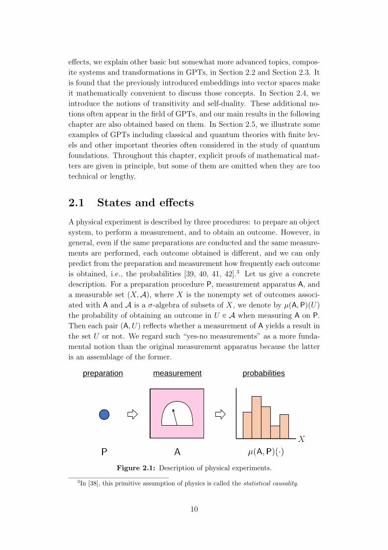
A physical experiment is described by three procedures: to prepare an object
system, to perform a measurement, and to obtain an outcome. However, in
general, even if the same preparations are conducted and the same measure-
ments are performed, each outcome obtained is different, and we can only
predict from the preparation and measurement how frequently each outcome
is obtained, i.e., the probabilities [39, 40, 41, 42].3 Let us give a concrete
description. For a preparation procedure P, measurement apparatus A, and
a measurable set pX,Aq, where X is the nonempty set of outcomes associ-
ated with A and A is a σ-algebra of subsets of X, we denote by µpA,PqpUq
the probability of obtaining an outcome in U P A when measuring A on P.
Then each pair pA, Uq reflects whether a measurement of A yields a result in
the set U or not. We regard such “yes-no measurements” as a more funda-
mental notion than the original measurement apparatus because the latter
is an assemblage of the former.
measurement probabilitiespreparation
Figure 2.1: Description of physical experiments.
3In [38], this primitive assumption of physics is called the statistical causality.
10
In this section, we shall demonstrate how to describe two fundamen-
tal concepts of physics, preparations and measurements, in mathematical
language. As explained above, we focus mainly on yes-no measurements,
and write a yes-no measurement and the probability µpA,PqpUq simply as
M and µpM,Pq respectively. It will be shown that they are reduced to the
notions of states and effects, and are embedded naturally into some vector
space and its dual space respectively. The embedding theorem enables us
to treat abstract concepts of preparations and measurements as mathemat-
ically well-defined objects, which is the very starting point for GPTs. After
their investigations, we will go back to descriptions of general measurement
apparatuses to obtain the notion of observables. This section is mainly in
accord with [30, 31, 41, 43, 44, 45].
2.1.1 Axiomatic description
Let Prep and Meas be the set of all procedures of preparations and yes-no
measurements for some physical experiment respectively. For example, in
the experiment of detecting the spin of an electron, each element of Prep
represents an apparatus that emits an electron, and each element of Meas
represents a value of the meter of some measurement apparatus or the cor-
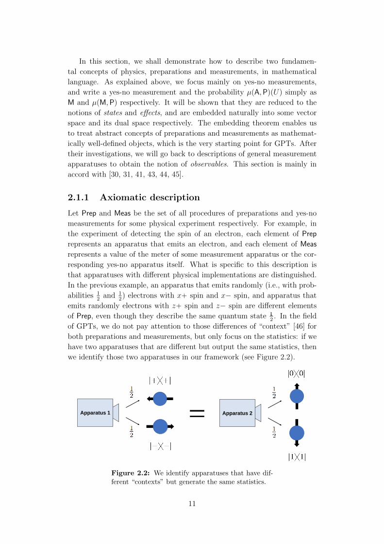
responding yes-no apparatus itself. What is specific to this description is
that apparatuses with different physical implementations are distinguished.
In the previous example, an apparatus that emits randomly (i.e., with prob-
abilities 12
and 12) electrons with x` spin and x´ spin, and apparatus that
emits randomly electrons with z` spin and z´ spin are different elements
of Prep, even though they describe the same quantum state 1
2. In the field
of GPTs, we do not pay attention to those differences of “context” [46] for
both preparations and measurements, but only focus on the statistics: if we
have two apparatuses that are different but output the same statistics, then
we identify those two apparatuses in our framework (see Figure 2.2).
Apparatus 1 Apparatus 2
Figure 2.2: We identify apparatuses that have dif-ferent “contexts” but generate the same statistics.
11
Let us present its mathematical expression. Preparation procedures
P1,P2 P Prep are called operationally equivalent (denoted by P1 „P P2)
if µpM,P1q “ µpM,P2q holds for all M P Meas. In a similar way, measure-
ment procedures M1,M2 P Meas are called operationally equivalent (denoted
by M1 „M M2) if µpM1,Pq “ µpM2,Pq for all P P Prep. The binary rela-
tions „P and „M define equivalence relations, and thus we can introduce
the corresponding quotient sets Ω :“ Prep„P and E :“ Meas„M . These
two sets Ω and E are called the state space and effect space respectively,
and each element of Ω and E are called a state and an effect respectively
[33, 34, 39, 43]. Here, we express those descriptions above as an axiom.
Axiom 1 (Separation principle)
States and effects separate each other. That is, for any distinct ω1, ω2 P Ω,
there exists an effect e P E such that µpe, ω1q ‰ µpe, ω2q, and also, for any
distinct e1, e2 P E, there exists a state ω P Ω such that µpe1, ωq ‰ µpe2, ωq.
We note that in the statement above we regard the function µp¨, ¨q on Measˆ
Prep as on Eˆ Ω in an well-defined way. States and effects are two primitive
notions in GPTs.
Next, we focus on another fundamental concept, probabilistic mixtures. It
is operationally natural to assume that if we can prepare states ω1, ω2, . . . , ωn,
then we can also prepare a state through the probabilistic mixture of ω1, ω2,
. . . , ωn with respective probabilities λ1, λ2, . . . , λn, where λi ě 0 andřni“1 λi “
1.4 We denote the newly introduced state by xλ1, λ2, . . . , λn; ω1, ω2, . . . , ωnyΩ.
The notion of probabilistic mixtures should be considered also for effects,
and we denote the effect obtained through the mixture of effects tejumj“1 Ă E
with a probability weight tσjumj“1 by xσ1, σ2, . . . , σm; e1, e2, . . . , emyE . Then
the nature of probabilistic mixtures motivates us to give the following axiom.
Axiom 2 (Probabilistic mixtures)
For any finite set of states tωiuni“1 Ă Ω and probability weight tλiu
ni“1 (λi ě
0 andř
i λi “ 1), there exists a state xλ1, λ2, . . . , λn; ω1, ω2, . . . , ωnyΩ P Ω
satisfying
µ pe, xλ1, λ2, . . . , λn; ω1, ω2, . . . , ωnyΩq “nÿ
i“1
λiµpe, ωiq (2.1)
for all e P E. Similarly, for any finite set of effects tejumj“1 Ă E and probabil-
ity weight tσjumj“1, there exists an effect xσ1, σ2, . . . , σm; e1, e2, . . . , emyE P E
4From an operational viewpoint, it seems unnatural to consider mixtures with irra-tional ratios because we can only conduct a finite number of experiments. However, inthis thesis, we focus on theories with the completeness assumption (see Mathematicalassumption 1), so at this point admit those irrational mixtures.
12
satisfying
µ pxσ1, σ2, . . . , σm; e1, e2, . . . , emyE , ωq “mÿ
j“1
σjµpej, ωq (2.2)
for all ω P Ω. From Axiom 1, they are uniquely determined.
Axiom 1 and Axiom 2 ensure that, in addition to (2.1), several proper-
ties that probabilistic mixtures should satisfy hold successfully for the state
xλ1, λ2, . . . , λn; ω1, ω2, . . . , ωnyΩ. For example, we can derive easily that
xλ1, λ2, . . . , λn; ω1, ω2, . . . , ωnyΩ “ xλ2, λ1, . . . , λn; ω2, ω1, . . . , ωnyΩ
holds, i.e., the mixture does not depend on the “order” of the states and
probabilities (similar observations also can be obtained for effects).
We require additional conditions for E according to [30, 47, 48]. The first
requirement is that E includes the unit effect u satisfying µpu, ωq “ 1 for all
ω P Ω. In other words, we suppose the existence of a yes-no measurement
apparatus that always outputs “yes”, and this seems to be an operationally
natural condition. We note that such u is unique due to Axiom 1. The
second one is that if e is an element of E , then the complement effect eK
such that µpeK, ωq “ 1 ´ µpe, ωq for all ω P Ω is also an element of E . This
condition comes from an operationally natural intuition that if we admit
a certain yes-no measurement apparatus, then we should also admit the
apparatus constituted by exchanging the “yes” and “no” of the original one.
We remark similarly that such eK is unique. For the complement of the unit
effect u, we sometimes denote it by 0 in this thesis. These conditions are
summarized as follows.
Axiom 3 (Existence of unit and complement effects)
(i) There exists the unit effect u in E such that µpu, ωq “ 1 for all ω P Ω.
(ii) If e P E, then its complement eK P E such that µpeK, ωq “ 1´µpe, ωq for
all ω P Ω.
We note that the effects u and eK in Axiom 3 are consistent with Axiom 2.
Now we can give the definition of a GPT.
Definition 2.1 (Generalized probabilistic theories)
A triple pΩ, E , µq of two sets Ω and E , and a function µ : Ω ˆ E Ñ r0, 1s
satisfying Axiom 1, Axiom 2, and Axiom 3 is called a generalized probabilistic
theory (a GPT for short). The set Ω and its element are called the state space
and a state of the theory, and E and its element are called the effect space
and an effect of the theory respectively.
13
Let us consider infinite countable mixtures for states.5 In the following,
we denote mixtures of two states xλ, 1´ λ; ω1, ω2yΩ simply by xλ; ω1, ω2y. In
order to treat infinite limits, some topological structure should be introduced
into Ω. Here we define a topology on Ω in line with Gudder [43]. We suppose
that if states ω1 and ω2 are “close”, then
xλ; ω11, ω1y “ xλ; ω12, ω2y
with small λ holds for some ω11, ω12 P Ω. That is, the closeness between ω1
and ω2 should be evaluated by
dpω1, ω2q :“ inft0 ă λ ď 1 | xλ; ω11, ω1y “ xλ; ω12, ω2y
for some ω11, ω12 P Ωu.
(2.3)
We note that (2.3) always can be defined since@
12; ω2, ω1
D
“@
12; ω1, ω2
D
holds
due to Axiom 1. We assume that infinite countable mixtures are allowed in
our framework. It is described in the following form.
Mathematical assumption 1 (Completeness)
If d defined in (2.3) satisfies limn,mÑ8 dpωn, ωmq “ 0 for a family of states
tωnu8n“1 Ă Ω, then there exists a unique ω P Ω such that limnÑ8 dpωn, ωq “
0.
There are two things to remark on Mathematical assumption 1. The first one
is about the notion of completeness. In fact, we can prove that the function
d is a metric function on Ω (see Subsection 2.1.2), and thus Mathematical
assumption 1 is equivalent to the requirement that pΩ, dq is a complete metric
space, which especially admits infinite countable mixtures. The other remark
is about the terminology “Mathematical assumption”. In the field of GPTs,
the assumption of closedness or completeness for a state space with respect
to some physically natural topology is a common one [31]. That is, if we can
prepare states that are very “close” to some fixed state, then it is usually
assumed that the fixed state can also be prepared. This seems to be a
natural, but at the same time more artificial assumption than the previous
ones, so in this thesis we regard it as a mathematical assumption rather than
an axiom.
2.1.2 Convex structures and embedding theorems
In the previous section, we presented the primitive descriptions of states
and effects from a physical perspective. We can rephrase them via the
mathematical notion of convex structures [36, 43].
5For infinite countable mixtures of effects, see footnote 20.
14
Definition 2.2
(i) A set S with a map x¨; ¨y such that
1. xλ1, λ2, . . . , λn; s1, s2, . . . , sny defines a unique element of S for any fi-
nite s1, s2, . . . , sn P S and probability weight tλ1, λ2, . . . , λnu (i.e., each
λi ě 0 andřni“1 λi “ 1);
2. xλ1, λ2, . . . , λn; s, s, . . . , sy “ s
is called a convex (pre-)structure. Elements of the form xλ, 1´ λ; s, ty are
denoted simply by xλ; s, ty.
(ii) Let S and T be convex structures. A map F : S Ñ T is called affine if
F pxλ1, λ2, . . . , λn; s1, s2, . . . , snyq
“ xλ1, λ2, . . . , λn;F ps1q, F ps2q, . . . , F psnqy ,(2.4)
and the set of all affine maps from S to T is denoted by Aff pS, T q. If
there exists an affine bijection J : S Ñ T , then S and T are called affinely
isomorphic, and J is called an affine isomorphism.
(iii) Because a convex subset of a vector space is naturally a convex structure
with usual convex combinations6: xλ1, λ2, . . . , λn; s1, s2, . . . , sny “řni“1 λisi,
we can define successfully the set Aff pS,Rq for a convex structure S, and
call its element an affine functional on S. In particular, the set of all f P
Aff pS,Rq such that fpsq P r0, 1s for all s P S is denoted by ES. We regard
Aff pS,Rq as a real vector space in a natural way.
(iv) A convex structure pS, x¨; ¨yq is called a total convex structure if
1. S is equipped with a function d : S ˆ S Ñ R defined as
dps1, s2q :“ inft0 ă λ ď 1 | xλ; s11, s1y “ xλ; s12, s2y
for some s11, s12 P Su,
(2.5)
and for every family tsnun Ă S satisfying limn,mÑ8 dpsn, smq “ 0, there
exists a unique s P S such that limnÑ8 dpsn, sq “ 0;
2. fpsq “ fptq for every f P ES implies s “ t.
Let us consider a GPT with a state space Ω and effect space E . Clearly, Ω
satisfies conditions (i)-1, (i)-2, (iv)-1, and (iv)-2 in Definition 2.2, and thus
is a total convex structure. On the other hand, it is easy to see that the
functional e˝ defined for e P E as e˝ : ω ÞÑ µpe, ωq is an affine functional
6A subset A of a vector space L is called convex if λx ` p1 ´ λqy P A wheneverx, y P A and λ P p0, 1q, and a vector sum
řni“1 λixi for x1, . . . , xn P A is called a convex
combination if tλ1, . . . , λnu is a probability weight. For a more detailed description ofconvex sets, see [49, 50]
15
on Ω due to Axiom 2. Because we are interested only in probabilities, it is
not problematic to identify the effect e representing the associated yes-no
apparatus with the affine functional e˝, and we also call the latter an effect.7
In other words, if we define the map ˝ : e ÞÑ e˝, then it is an injection from
E to EΩ because of Axiom 1, and thus E and E˝ Ă EΩ can be identified
with each other. Moreover, we can observe from Axiom 2 that the notion of
mixtures is represented mathematically as
xσ1, σ2, . . . , σm; e1, e2, . . . , emy˝
E “
mÿ
j“1
σj e˝j , (2.6)
and from Axiom 3 that E˝ includes a special effect u˝ such that u˝pωq “ 1
for all ω P Ω and eK˝ “ u˝ ´ e˝ P E˝ holds whenever e˝ P E˝. We note that
E˝ is a convex subset of the vector space Aff pΩ,Rq due to (2.6). In this way,
we regard the effect space E˝ as a convex subset of EΩ: E˝ Ă EΩ. In this
thesis, we require that the converse inclusion also holds, which is called the
no-restriction hypothesis [26].
Mathematical assumption 2 (No-restriction hypothesis)
Any affine functional e˝ on Ω with e˝pωq P r0, 1s for all ω P Ω is an effect.
That is, E˝ “ EΩ.
The no-restriction hypothesis means that any mathematically valid affine
functional is also physically valid. There is no physical background for this
assumption, and GPTs without assuming it were investigated for example in
[47, 48, 51, 52]. However, in this thesis, we suppose that all theories satisfy
the no-restriction hypothesis based on the fact that it is satisfied both in
classical and quantum theory. Now we can conclude the following.
Proposition 2.3
A GPT is identified with pΩ, EΩq, where Ω is a total convex structure and EΩ
is the set of all affine functionals on it whose values lie in r0, 1s.
Example 2.4 (Examples of convex structures)
(i) Let S be the convex structure of the closed interval r0, 1s of R. If we
consider its elements s1 “ 0 and s2 “ k p0 ă k ď 1q, then an easy calcu-
lation shows dps1, s2q “ 1 ´ 11`k
, which is an increasing function of k. This
observation indicates that the function d is a valid measure to represent how
close two states are. We can also prove that S is a total convex structure.
(ii) Let S “ R, which is naturally a convex structure. We can find easily
that dps1, s2q “ 0 for all s1, s2 P S, and thus this S is not a total convex
structure.
7In [38], e is called an experimental proposition, while the term “effect” (also calledexperimental function) is used for the induced affine functional e˝.
16
The above examples show that under Mathematical assumption 1, the state
space Ω is “closed” and “bounded”, and the function d defined in (2.3) rep-
resents properly the closeness between two states in Ω. In subsequent parts,
we will give the mathematically rigorous verification of these observations.
It is known that a total convex structure can be embedded into a certain
Banach space. In order to show this, we need the following lemma.
Lemma 2.5
Let pS, x¨; ¨yq be a total convex structure with a “metric” d defined in (2.5).
(i) If a family of elements tsnu8n“1 satisfies limnÑ8 dpsn, sq “ 0 with some
s P S, then limnÑ8 fpsnq “ fpsq holds for all f P ES.
(ii) Let pT, x¨; ¨yT q be another total convex structure equipped with a sim-
ilar “metric” dT . For all s1, s2 P S and F P Aff pS, T q, it holds that
dT pF ps1q, F ps2qq ď dps1, s2q. If F is bijective, then dT pF ps1q, F ps2qq “
dps1, s2q.
Proof
(i) Because limnÑ8 dpsn, sq “ 0 holds, there exists N P N for any ε ą 0
such that dpsn, sq ăεε`2
holds whenever n ą N . It implies that there are
λ P p0, εε`2q and t1, t2 P S satisfying xλ; t1, sny “ xλ; t2, sy, which results in
λfpt1q ` p1´ λqfpsnq “ λfpt2q ` p1´ λqfpsq
for f P ES. It follows that
|fpsnq ´ fpsq| “λ
1´ λ|fpt2q ´ fpt1q| ď
2λ
1´ λ,
and thus |fpsnq ´ fpsq| ă ε holds because
2λ
1´ λă
2λ
1´ λ
ˇ
ˇ
ˇ
ˇ
λÑ εε`2
“ ε.
(ii) It holds from the definition of d that
dT pF ps1q, F ps2qq “ inft0 ă λ ď 1 |
xλ; t1, F ps1qyT “ xλ; t2, F ps2qyT , t1, t2 P T u
ď inft0 ă λ ď 1 |
xλ;F psq, F ps1qyT “ xλ;F ps1q, F ps2qyT , s, s1P Su
“ inft0 ă λ ď 1 | F pxλ; s, s1yq “ F pxλ; s1, s2yq, s, s1P Su
ď inft0 ă λ ď 1 | xλ; s, s1y “ xλ; s1, s2y , s, s1P Su
“ dps1, s2q.
If F is bijective, then the two “ď” in the above consideration become ““”,
17
and thus dT pF ps1q, F ps2qq “ dps1, s2q holds. 2
We remember that Aff pS,Rq is a real vector space for a convex structure S.
The set Aff pS,Rq1 :“ tα | α : Aff pS,Rq Ñ R, linearu is naturally a vector
space called the algebraic dual of Aff pS,Rq. Then there is a standard embed-
ding J of S into Aff pS,Rq1 such that each element Jpsq P Aff pS,Rq1 ps P Sqis defined as
rJpsqspfq “ fpsq pf P Aff pS,Rqq. (2.7)
We can prove the following proposition.
Proposition 2.6
Let pS, x¨; ¨yq be a total convex structure with a “metric” d defined in (2.3).
(i) The standard embedding J : S Ñ Aff pS,Rq1 defined via (2.7) is an affine
isomorphism between S and the convex subset JpSq of Aff pS,Rq1.(ii) If there is an affine isomorphism η between S and a convex subset S0
of some real vector space V0 such that aff pS0q does not include the origin 0
of V0, then there is a linear bijection Φ: spanpS0q Ñ spanpJpSqq satisfying
ΦpS0q “ JpSq.8
(iii) pS, dq is a complete metric space.
The claims (i) and (ii) demonstrate that the total convex structure S can be
identified with a convex set in some vector space in an essentially unique way
via the standard embedding J . We note that the functional 0 P Aff pS,Rq1
defined as 0pfq “ 0 for all f P Aff pS,Rq, which is the origin of the vector
space Aff pS,Rq1, does not belong to JpSq because 0 P JpSq contradicts the
existence of the unit effect. On the other hand, the claim (iii) shows that d
is indeed a metric (see Mathematical assumption 1).
Proof (proof of Proposition 2.6)
(i) It is easy to see that J is an affine map from S to Aff pS,Rq1 and JpSq is
a convex set in Aff pS,Rq1. Since S is total (see (iv)-2 in Definition 2.2), for
s, t P S with s ‰ t, there exists an affine functional f P Aff pS,Rq such that
fpsq ‰ fptq, i.e., rJpsqspfq ‰ rJptqspfq. This implies Jpsq ‰ Jptq.
(ii) Let us introduce a subset K :“ třni“1 λixi | λi ě 0, xi P S0, n : finiteu,
i.e., the conic hull of S0 (see Definition 2.7). Then any y P Kzt0u can be
represented as y “ λx with λ ą 0 and x P S0 in a unique way. To see
this, assume that y P Kzt0u satisfies y “ λx “ λ1x1 with λ, λ1 ą 0 and
x, x1 P JpSq. If λ ‰ λ1, then it holds that
0 “ λx´ λ1x1 “ pλ´ λ1q
ˆ
λ
λ´ λ1x´
λ1
λ´ λ1x1˙
.
8For a subset A of a vector space W , its affine hull aff pAq and linear span spanpAq aredefined as aff pAq :“ t
řni“1 λiai | ai P A, λi P R,
ř
i λi “ 1, n: finiteu and spanpAq :“třn
i“1 λiai | ai P A, λi P R, n: finiteu respectively.
18
Because 0 R aff pS0q, the above equation implies λ “ λ1, which is a contra-
diction. Thus we can conclude λ “ λ1 and x “ x1. Now let us construct
the linear bijection Φ from the affine isomorphism η. First, we define an
affine bijection φ0 : S0 Ñ JpSq by φ0 “ J ˝ η´1 (note that J is a bijection
between S and JpSq). From the above consideration, we can extend this φ0
successfully to a bijection φ from K to the conic hull of JpSq: φpyq “ λφ0pxq
for y “ λx with y P K, x P S0, and λ ě 0. It is easy to verify that
φpλy ` µzq “ λφpyq ` µφpzq holds for y, z P K and λ, µ ě 0. Since any
y P spanpS0q such that y “řni“1 λixi with xi P S0, λi P R, and a finite n can
be expressed as y “ u ´ v, where u, v P K, we can consider the extension
of φ to a map Φ from spanpS0q to spanpJpSqq by Φpyq “ φpuq ´ φpvq for
y “ u´v with y P spanpS0q and u, v P K. We note that this Φ is well-defined:
if y “ u1 ´ v1 “ u2 ´ v2 with u1, u2, v1, v2 P K holds, then u1 ` v2 “ u2 ` v1
holds, and thus Φpu1` v2q “ Φpu2` v1q, i.e., Φpu1q`Φpv2q “ Φpu2q`Φpv1q
follows, which implies Φpu1q ´ Φpu2q “ Φpv1q ´ Φpv2q. It is easy to confirm
that Φ: spanpS0q Ñ spanpJpSqq is linear and bijective.
(iii) It is trivial that dps, tq ě 0 and dps, tq “ dpt, sq holds for all s, t P
S. Let dps, tq “ 0. Then there exist a family of positive numbers tλiuiwith limiÑ8 λi “ 0 and families tsiui and ttiui of elements of S such that
xλi; si, sy “ xλi; ti, ty. It follows that
λifpsiq ` p1´ λiqfpsq “ λifptiq ` p1´ λiqfptq
holds for all f P ES. Because 0 ď fpsiq, fptiq ď 1 holds, taking iÑ 8 in the
above equation, we obtain fpsq “ fptq for all f P ES. By the assumption of
totality, we can conclude s “ t. To verify the triangle inequality for d, it is
enough to prove that d1 : JpSqˆ JpSq Ñ R defined on JpSq in a similar way
to d satisfies it. This is because d1pJpsq, Jptqq “ dps, tq holds for all s, t P S
as we have seen in Lemma 2.5. For the evaluation of d1pp, rq ` d1pr, qq with
p, q, r P JpSq, let us assume that λ1, λ2 P p0, 1q satisfy
λ1p1 ` p1´ λ1qp “ λ1r1 ` p1´ λ1qr,
λ2r2 ` p1´ λ2qr “ λ2q1 ` p1´ λ2qq
for p1, q1, r1, r2 P JpSq. We obtain from these equations
λ1p1´ λ2qp1 ` λ2p1´ λ1qr2 ` p1´ λ1qp1´ λ2qp
“ λ2p1´ λ1qq1 ` λ1p1´ λ2qr1 ` p1´ λ1qp1´ λ2qq.
It can be rewritten as
λ0p2 ` p1´ λ0qp “ λ0q2 ` p1´ λ0qq, (2.8)
19
where
λ0 “λ1p1´ λ2q ` λ2p1´ λ1q
λ1p1´ λ2q ` λ2p1´ λ1q ` p1´ λ1qp1´ λ2q“λ1 ` λ2 ´ 2λ1λ2
1´ λ1λ2
and
p2 “λ1p1´ λ2q
λ1p1´ λ2q ` λ2p1´ λ1qp1 `
λ2p1´ λ1q
λ1p1´ λ2q ` λ2p1´ λ1qr2,
q2 “λ2p1´ λ1q
λ1p1´ λ2q ` λ2p1´ λ1qq1 `
λ1p1´ λ2q
λ1p1´ λ2q ` λ2p1´ λ1qr1.
Because λ0 ď λ1 ` λ2, we can see from (2.8) that
d1pp, qq ď d1pp, rq ` d1pr, qq
holds, and thus we can conclude that pS, dq is a metric space. The complete-
ness clearly holds due to (iv)-1 in Definition 2.2. 2
We note that we can prove the same claim as (iii) also for the function d0
defined as
d0ps, tq “dps, tq
1´ dps, tq. (2.9)
In fact, it was shown in [36] that this d0 is a metric on S, and the complete-
ness holds similarly. Before proceeding to the main theorem of this section,
we introduce the notion of convex cones [50, 53, 54].
Definition 2.7
Let L be a vector space and 0 P L be its origin.
(i) A subset C of L is called a cone of vertex 0 if λC Ă C for all λ ą 0. A
cone of vertex x0 is a set of the form x0 ` C, where C is a cone of vertex 0.
In this thesis, the vertex of a cone is always assumed to be 0.
(ii) A cone C Ă L is called
1. convex if it is convex, i.e., satisfies C ` C Ă C;
2. pointed if C X´C “ t0u;
3. generating (or spanning) if spanpCq “ L, i.e., C ´ C “ L.
(iii) The conic hull of a subset A of L is defined as conepAq :“ třni“1 λiai |
λi ě 0, ai P A, n : finiteu. It is easy to see that conepAq is a convex cone.
Let us write conepJpSqq and spanpJpSqq generated by JpSq simply as K and
V respectively. It is easy to see that K is a convex, pointed, and generating
20
cone for V , and thus any v P V is written in the form v “ k`´k´ “ αp´βq,
where k˘ P K, p, q P JpSq, and α, β ě 0. It follows that we can introduce
the following quantity for v P V :
v “ inftα ` β | v “ αp´ βq, α, β ě 0, p, q P JpSqu. (2.10)
Now we can present an embedding theorem for a total convex structure as
follows. We shall omit the proof, but it is given in [43] (see the proofs of
Theorem 4.11 and Theorem 4.12 there).
Theorem 2.8
Let S be a total convex structure, and K and V be the cone and the real
vector space generated by the standard embedding JpSq of S into Aff pS,Rq1
(see (2.7)) respectively.
(i) The function ¨ on V defined in (2.10) is a norm on V satisfying
Jpsq ´ Jptq “ 2d0ps, tq for all s, t P S and Jpsq “ 1 for all s P S. More-
over, pV, ¨ q is a real Banach space, and K is closed.
(ii) Let f P Aff pS,Rq. Then the affine functional f ˝ J´1 : JpSq Ñ R on
JpSq has a unique linear extension f : V Ñ R.
(iii) If we let e : V Ñ R be the unique linear extension of e˝ P ES Ă Aff pS,Rqdescribed in (ii) above, then e is continuous, and thus belongs to the Banach
dual V ˚ :“ tf | f : V Ñ R, linear, bounded (continuous)u of V . In particu-
lar, the linear extension u of the unit effect u˝ such that upJpsqq “ 1 for all
Jpsq P JpSq satisfies u P V ˚.
Let us consider a GPT pΩ, EΩq (see Proposition 2.3). By setting S “ Ω in
Theorem 2.8, we can identify the state space Ω with a convex set Ω :“ JpΩq9
in a Banach space V “ spanpΩq equipped with the norm ¨ in (2.10) called
the base norm, and the effect space EΩ with a subset EΩ :“ te P V ˚ | epωq P
r0, 1s for all ω P Ωu of the Banach dual V ˚. We also call Ω and EΩ the state
space and the effect space of the GPT respectively. In the next part, we give
further explanations about the Banach space V and its Banach dual V ˚.
2.1.3 Ordered Banach spaces
The vector spaces V and V ˚ introduced in the previous part are equipped
with both order and Banach space structures, that is, they are ordered
Banach spaces. In this subsection, we make a brief review of ordered Banach
spaces. Mathematical terms shown in this subsection are according mainly
to [30, 31, 44, 50, 53, 55, 56]. Also, there can be found the technical proofs
of some theorems which we omit. We begin with the definition of an ordered
vector space.
9It will be shown in the following part that Ω is in fact a closed convex set in Vinheriting the closedness of K.
21
Definition 2.9
A real vector space L equipped with a partial ordering10 ď is called an
ordered vector space if it satisfies
(i) x ď y implies x` z ď y ` z for all x, y, z P L;
(ii) x ď y implies λx ď λy for all x, y P L and λ ě 0.
We can prove easily the following (recall Definition 2.7).
Proposition 2.10
Let L be an ordered vector space and ď be its ordering.
(i) L` :“ tx P L | x ě 0u is a convex and pointed cone.
(ii) If pL,ďq is directed, i,e, for every x, y P L there is z P L such that
x ď z, y ď z, then L` in (i) is also generating.
Proof
(i) For x ě 0, it holds clearly that λx ě 0 (λ ě 0), and thus L` is a cone.
Because, for x, y ě 0, both px ě 0 and p1 ´ pqy ě 0 (0 ď p ď 1) hold,
px` p1´ pqy ě 0 follows, which implies L` is convex. The claim that L` is
pointed follows from the observation that x ě 0 and x ď 0 implies x “ 0.
(ii) Because L is directed, for any x P L, there exists z P L such that x ď z
and ´x ď z, equivalently, z´x ě 0 and z`x ě 0 hold. Because 12pz´xq ě 0
and 12pz ` xq ě 0, the expression x “ 1
2pz ` xq ´ 1
2pz ´ xq implies that L` is
generating. 2
Definition 2.11
Let L be an ordered vector space and ď be its ordering.
(i) The cone L` :“ tx P L | x ě 0u is called the positive cone of L.
(ii) For the positive cone L` of L, its order dual cone L3` is defined as
the set of all “positive” functionals on L`, i.e., L3` :“ tf P L1 | fpxq ě
0 for all x P L`u. It is clear that L3` is a convex cone in the algebraic dual
L1 of L and in the subspace L3 :“ L3` ´ L3
` “ spanpL3`q called the order
dual of L. Moreover, we can find that L3` is pointed in L1 and L3 if L` is
generating.
We have proven in Proposition 2.10 that a positive cone can be intro-
duced through an order vector space. Conversely, we can construct an order
structure for a vector space when there is a convex cone.
Proposition 2.12
Let C be a convex and pointed cone in a real vector space L.
(i) If we define a binary relation ď as x ď y ðñ y ´ x P C for x, y P V ,
10A binary relation ď on a set X is called a preorder if it is reflexive, i.e., x ď x px P Xq,and transitive, i.e., x ď y and y ď z implies x ď z px, y, z P Xq. A preorder ď is calleda partial order if it is antisymmetric, i.e., x ď y and y ď x implies x “ y (x, y P X). Weremark that some authors use the term “partial order” to represent a preorder here [57].
22
then the relation ď is a partial ordering, and L is an ordered vector space
with its ordering given by ď.
(ii) The positive cone L` for L defined via the order ď in (i) is identical to
C, i.e., L` “ C.
(iii) If C is in addition generating, then pL,ďq is directed.
Proof
(i) Because C is pointed, x ´ x “ 0 P C, and y ´ x P C and x ´ y P C
imply y ´ x “ 0, i.e., x “ y for x, y P L. Moreover, if y ´ x P C and
z ´ y P C (z, y, z P L), then z ´ x “ pz ´ yq ` py ´ xq P C. Therefore,
we can conclude that ď is a partial ordering. On the other hand, because
y´x “ py` zq´ px` zq (x, y, z P L), x` z ď y` z holds when x ď y. Since
C is a cone, y ´ x P C (x, y P L) implies λpy ´ xq “ λy ´ λx P C (λ ě 0),
i.e., λx ď λy when x ď y.
(ii) The claim L` “ C is trivial since x ě 0 is equivalent to x P C.
(iii) For x, y P L, because C is generating, there exist x1, x2, y1, y2 P C
such that x “ x1 ´ x2 and y “ y1 ´ y2. Defining z “ x1 ` y1, we have
z ´ x “ y1 ` x2 P C and z ´ y “ x1 ` y2 P C, which means that pL,ďq is
directed. 2
It follows from these propositions that a positive cone and a convex and
pointed cone can be identified naturally with each other.
Next, we give descriptions of ordered Banach spaces. An ordered vector
space L is called an ordered Banach space if L is also a Banach space (see [58]
for a review of Banach space). There are two important types of ordered
Banach space in the field of GPTs: base norm Banach spaces and order
unit Banach spaces, which are related with state spaces and effect spaces
respectively. Let us first introduce base norm Banach spaces.
Definition 2.13
Let L be an ordered vector space with its positive cone L`. A convex subset
B Ă L` is called a base of L` if for any x P L` there exists a unique λ ě 0
such that x P λB.
The following lemma is important.
Lemma 2.14
Let L be an ordered vector space with its positive cone L`, and let B be its
base. Then aff pBq does not contain the origin 0 of L.
Proof
Suppose 0 P aff pBq. Then there exist real numbers tλiuni“1 with
řni“1 λi “ 1
and elements txiuni“1 of B such that
řni“1 λixi “ 0. Dividing tλiu
ni“1 into
positive and negative parts, we obtain
ÿ
j
λ`j x`j “
ÿ
k
λ´k x´k ,
23
where tx`j uj and tx´k uk are subsets of txiuni“1, and tλ`j uj and tλ´k uk are
positive numbers satisfyingř
j λ`j ´
ř
k λ´k “ 1. If we suppose K :“
ř
k λ´k ‰
0, then we can rewrite the above equation as
K ` 1
K¨
1
K ` 1
ÿ
j
λ`j x`j “
1
K
ÿ
k
λ´k x´k .
Because y :“ 1K`1
ř
j λ`j x
`j and y1 :“ 1
K
ř
k λ´k x
´k are convex combinations
of elements of B, they belong to B. Then the above equation K`1Ky “ y1
contradicts the uniqueness condition in the definition of the base B, and thus
we obtain K “ 0. It implies 0 P B, but this also contradicts the uniqueness
condition because any positive number λ satisfy λ0 “ 0. 2
By means of this lemma, we can associate a base of a positive cone with a
linear functional in the following way [30, 56].
Proposition 2.15
Let L and L` be an ordered vector space and its positive cone respectively.
The positive cone L` has a base B if and only if there exists a strictly positive
functional eB (i.e., eB P L3 and satisfies eBpxq ą 0 for all nonzero x P L`)
such that
B “ tx P L` | eBpxq “ 1u. (2.11)
Proof
The if part is easy, so we prove the only if part. Let B be a base of L`.
Applying Zorn’s lemma to the set A of all affine sets that include aff pBq
but not t0u, we obtain the maximal affine set H in A. It can be shown [59]
that this H is a hyperplane in L, and thus there exists a linear functional
eB such that eBpxq “ 1 for all x P H. This functional eB is easily found to
be strictly positive because B is a base. 2
We call the functional eB the intensity functional for the base B [38].
Lemma 2.16
Let L be an ordered vector space and L` be its positive cone, and assume
that L` is generating. For a base B Ă L` of L`, the set D :“ convpBY´Bq
is a radial, circled, and convex subset of L.11
Proof
The convexity is clear. It is easy to see 0 P D, and thus D is circled. Because
L` is generating, any x P L can be written as x “ λ`x``λ´x´ with λ˘ ě 0
11A subset U of a vector space L (assumed to be on the field F “ R or C) is radial iffor any x P L there exists λ0 P F such that |λ| ě |λ0| implies x P λU , and is circled ifλU Ă U for any λ with |λ| ď 1 [50].
24
and x` P B, x´ P ´B. Let λ0 “ λ` ` λ´. For λ ě λ0, the vector x can be
rewritten as
x “ λ ¨λ` ` λ´
λ
ˆ
λ`λ` ` λ´
x` `λ´
λ` ` λ´x´
˙
.
Because D is circled, λ``λ´λ
´
λ`λ``λ´
x` `λ´
λ``λ´x´
¯
P D is obtained. It
implies x P λD, and thus D is radial. 2
According to Lemma 2.16, if L` is generating, then the Minkowski functional
of D “ convpB Y´Bq defined as
pDpxq :“ inftλ ą 0 | x P λDu px P Lq (2.12)
is a seminorm on L [50]. It is not difficult to see that, with eB introduced
in Proposition 2.15, the function pD satisfies
pDpxq “ infteBpx`q ` eBpx´q | x “ x` ´ x´, x˘ P L`u px P Lq, (2.13)
or equivalently
pDpxq “ inftα ` β | x “ αb` ´ βb´, α, β ě 0, b˘ P Bu px P Lq (2.14)
since it holds that pDpx`q “ eBpx`q for all x` P L`. Now we can give the
definition of a base norm space.
Definition 2.17
Let L be an ordered vector space with its positive cone L` generating, and
let B be a base of L`. If the function pD defined in (2.12)-(2.14) through
the base B is a norm on L, then pL,Bq is called a base norm space. In this
case, we write pDp¨q as ¨ B and call it the base norm. A base norm space
pL,Bq is called a base norm Banach space if L is complete with respect to
the base norm ¨ B.
Remark 2.18
If we set L “ R2 and L` “ tpu, vq | v ą 0u Y p0, 0q with a base B “ tpu, vq |
v “ 1u, then the function pD satisfies pDppu, 0qq “ 0 for all u P R, and thus
it is not a norm in L. In fact, it can be shown that pD is a norm if and only
if D “ convpB Y´Bq is linearly bounded, i.e., M XD is a bounded subset
of L whenever M is a one-dimensional subspace [56] (in the example, MXD
is not bounded for M “ tpu, 0q | u P Ru).
In this thesis, for a Banach space X, we denote its Banach dual by X˚ “
tf | f : X Ñ R, linear, boundedu. When X is in addition an ordered vector
space (i.e., an ordered Banach space) and X` is its positive cone, we define
25
a subset X˚` of X˚ as X˚
` :“ tf P X˚ | fpxq ě 0 for all x P X`u, and call it
the Banach dual cone for X`. It is verified easily that X˚` is a convex and
closed (in the weak*12 and norm topologies) cone in X˚,13 and is in addition
pointed if X` is generating.
We present miscellaneous facts about base norm Banach spaces.
Proposition 2.19
Let pL,Bq be a base norm Banach space, and L` be the positive cone of L.
For a subset A of L, we denote its norm closure by A.
(i) The intensity functional eB for the base B (see Proposition 2.15) is con-
tinuous, i.e., eB P L˚.
(ii) B is closed if and only if L` is closed.
(iii) The closed unit ball of L is given by D “ convpB Y´Bq.
(iv) The dual norm ¨˚ on the Banach dual L˚ defined as f˚ :“ supt|fpxq| |
xB ď 1u satisfies f˚ “ supt|fpxq| | x P Bu.
(v) L` is a convex, pointed, and generating cone in L, and B is a base of
L` with its intensity functional identical with that of the original base B:
B “ L` X e´1B p1q. Moreover, the base norm induced by B coincides with the
original one by B.
(vi) If L` is closed, then the Banach dual and order dual coincide with each
other: L˚ “ L3.
Proof
(i) Representing x P L as x “ x` ´ x´ (x˘ P L`), we have
|eBpxq| “ |eBpx`q ´ eBpx´q| ď eBpx`q ` eBpx´q.
It implies |eBpxq| ď xB, i.e., eB is bounded.
(ii) Let eB be the intensity functional for B, which is continuous. When L`is closed, its base B “ L` X tx P L | eBpxq “ 1u is also closed. Assume
conversely that B is closed. Since L is complete, for a Cauchy sequence
tαixiui in L` such that αi ě 0 and xi P B, there exists v˚ P L to which tαixiuiconverges. From the continuity of eB, we obtain αi “ eBpαixiq ÝÑ
iÑ8eBpv˚q
(remember that eBpxiq “ 1 holds for every xi P B). If eBpv˚q “ 0, then
αi ÝÑiÑ8
0 holds. Since each αixi is an element of L`, we have αi “ eBpαixiq “
αixiB, and thus αixiB ÝÑiÑ8
0, i.e., v˚ “ limi αixi “ 0. This observation
implies v˚ P L` because L` is pointed and thus 0 P L` (see Proposition
12For a Banach space X and its Banach dual X˚, the weak topology of X often dentedby σpX,X˚q is the weakest topology on X which makes all f P X˚ continuous, and theweak* topology of X˚ often dented by σpX˚, Xq is the weakest topology on X˚ whichmakes all x P X Ă X˚˚ continuous [50, 58].
13Clearly, X˚` satisfies X˚` “Ş
xPX`tf P X˚ | fpxq ě 0u, and thus is weakly* and
norm closed.
26
2.10). If eBpv˚q ‰ 0, then
eBpv˚qxi ´ xjB ď eBpv˚qxi ´ v˚B ` v˚ ´ eBpv˚qxjB
ď eBpv˚qxi ´ αixiB ` αixi ´ v˚B
` v˚ ´ αjxjB ` αjxj ´ eBpv˚qxjB
“ |eBpv˚q ´ αi| ` αixi ´ v˚B
` v˚ ´ αjxjB ` |αj ´ eBpv˚q|.
The last equation converges to 0 as i, j Ñ 8, and thus txiui is a Cauchy
sequence. Because B is closed, txiui converges to x˚ P B. Therefore, we
obtain limi αixi “ eBpv˚qx˚ P L`.
(iii) This claim follows directly from the definition of ¨ B as the Minkowski
functional of D.
(iv) It can be found that
f˚ “ supt|fpxq| | xB ď 1u
“ supt|fpxq| | x P Du
“ supt|fpxq| | x P Du
“ supt|fpxq| | x P Bu.
For the proofs of (v) and (vi), see Proposition 1.40 in [30]. 2
Roughly speaking, the base norm and the intensity functional considered
above correspond to the trace norm and the identity operator in the usual
formulation of quantum theory respectively. In fact, if we let L be the set
LSpHq of all self-adjoint operators on a finite-dimensional Hilbert space H,
then any x P L is decomposed as x “ x` ´ x´ with x˘ ě 0 in the usual
ordering for self-adjoint operators, and thus the trace norm xTr of x is given
via the identity operator 1 by xTr “ Trrx`s`Trrx´s “ Trr1x`s`Trr1x´s,
which corresponds to (2.13).
Let us move to the introduction of order unit Banach spaces.
Definition 2.20
Let L be an ordered vector space equipped with an ordering ď.
(i) L is called Archimedean if x ď 0 whenever there exists y P L such that
nx ď y for all n P N.
(ii) L is called almost Archimedean if x “ 0 whenever there exists y P L such
that ´y ď nx ď y for all n P N.
(iii) A positive element u of L is called an order unit if for any x P L there
exists some n P N such that ´nu ď x ď nu.
It is clear that if L is Archimedean, then it is almost Archimedean. For
a, b P L, we define the order interval ra, bs as ra, bs :“ tx P L | a ď x ď bu.
27
The following lemma is important.
Lemma 2.21
Let L be an ordered vector space with an ordering ď, and let u be an order
unit associated with the ordering ď.
(i) The order interval ∆ :“ r´u, us is a radial, circled, and convex subset of
L.
(ii) The Minkowski functional of ∆ defined as
p∆pxq “ inftλ ą 0 | x P λ∆u px P Lq (2.15)
is a norm on L if and only if L is almost Archimedean.
Proof
It is easy to see that (i) holds due to the definition of the order unit u, and
thus the Minkowski functional p∆ is a seminorm on L. Assume that p∆ is a
norm and x P L satisfies ´y ď nx ď y for all n P N and some y P L. Since
there exists m P N such that ´mu ď y ď mu, we obtain ´mu ď nx ď mu,
or ´mnu ď x ď m
nu for all n P N. Thus inftλ ą 0 | ´λu ď x ď λuu “ 0
holds, and we can conclude x “ 0 because ¨ u is a norm. Conversely,
assume that L is almost Archimedean and x P L satisfies p∆pxq “ 0. Then
´u ď 1λx ď u holds for arbitrary small λ, and thus x “ 0 follows from the
assumption that L is almost Archimedean, which concludes (ii). 2
We can give the definition of an order unit Banach space.
Definition 2.22
Let L be an ordered vector space with an order unit u P L associated with the
ordering of L. pL, uq is called an order unit Banach space if L is Archimedean
and complete with respect to the norm p∆ defined in (2.15). In this case,
we write p∆p¨q as ¨ u, and call it the order unit norm.
We present miscellaneous facts about order unit Banach spaces according
mainly to [30, 55].
Proposition 2.23
Let pL, uq be an order unit Banach space and ď be the ordering of L.
(i) The positive cone L` of L is generating and closed.
(ii) The closed unit ball of L is given by ∆ “ r´u, us.
(iii) If f is a positive functional on L, then f is bounded, and its dual norm
f˚ on the Banach dual L˚ is given by f˚ “ fpuq. Conversely, if a linear
functional f : LÑ R satisfies f˚ “ fpuq, then f is positive.
(iv) If we define Bu :“ tf P L˚` | fpuq “ 1u, then Bu is a base for the
Banach dual cone L˚`.
(v) The Banach dual and order dual coincide with each other: L˚ “ L3.
28
Proof
(i) For x P L, there exists n P N such that ´nu ď x ď nu. Then x “
nu ` px ´ nuq shows x P L` ´ L`, i.e., L` is generating. Let txiui be a
Cauchy sequence in L` and converge to x‹ P L. For any n P N, we have
x‹ ´ xiu ď1n
for sufficiently large i. It implies ´ 1nu ď x‹ ´ xi ď
1nu, and
thus ´nx‹ ď u. Since this holds for all n P N and L is Archimedean, we
obtain ´x‹ ď 0, i.e., x P L`.
(ii) Because ∆ “ r´u, us “ pu ´ L`q X p´u ` L`q and L` is closed, we
can observe that ∆ is closed. Then the definition of ¨ u as the Minkowski
functional of ∆ proves the claim.
(iii) Assume that f is positive. For x P ∆, we have ´fpuq ď fpxq ď
fpuq, i.e., f˚ ď fpuq. The equality clearly holds for x “ u, and thus
we obtain f˚ “ fpuq (in particular, f is bounded). Assume conversely
that f˚ “ fpuq. For x P L` with xu “ 1, we have 0 ď x ď u, or
0 ď u ´ x ď u. It follows that u ´ xu ď 1, and because f˚ “ fpuq, we
obtain |fpuq ´ fpxq| ď fpuq, which implies fpxq ě 0.
(iv) It can be seen from (iii) that every f P L˚` satisfies f˚ “ fpuq, and
thus, when considered as an element of L˚˚ :“ pL˚q˚, the functional u is
strictly positive on L˚`. Then, applying Proposition 2.15, we obtain the
claim.
(v) See Proposition 1.29 in [30]. 2
It can be verified easily that the order unit norm corresponds to the usual
operator norm in the formulation of quantum theory.
Now we can give the most general description of GPTs in terms of base
norm Banach spaces and order unit Banach spaces. We present first of all
a fundamental theorem for our description on a close relationship between
base norm Banach spaces and order unit Banach spaces (see [30, 55, 56] for
the proof).
Theorem 2.24
(i) Let pL,Bq be a base norm Banach space whose positive cone is L`, and
let eB be the intensity functional for B satisfying B “ tx P L` | eBpxq “
1u. Then pL˚, eBq is an order unit Banach space, and L˚` :“ tf P L˚ |
fpxq ě 0 for all x P L`u is its positive cone. Moreover, the order unit norm
coincides with the usual Banach dual norm in L˚.
(ii) Let pL, uq be an order unit Banach space whose positive cone is L`, and
let Bu :“ tf P L˚` | fpuq “ 1u. Then pL˚, Buq is a base norm Banach space,
and L˚` :“ tf P L˚ | fpxq ě 0 for all x P L`u is its positive cone. Moreover,
the base norm coincides with the usual Banach dual norm in L˚, and Bu is
a weakly* compact subset of L˚.
We can also find that the converse of Theorem 2.24 holds (see [30, 56, 60]
for the proof)
29
Theorem 2.25
Let L be a Banach space that has a predual L˚.14
(i) If L is an order unit Banach space with L` its positive cone and u P L`its order unit, then L˚ is a base norm Banach space whose positive cone and
base are given by L˚` “ tx P L˚ | fpxq ě 0 for all f P L`u and B˚u “ tx P
L˚` | upxq “ 1u respectively. Moreover, the base norm coincides with the
original Banach norm in L˚.
(ii) If L is a base norm Banach space with L` its positive cone and B an
weakly* compact base of L`, then there exists e˚B P L˚ such that fpe˚Bq “ 1
for all f P B, and L˚ is an order unit Banach space whose positive cone
and order unit are given by L˚` “ tx P L˚ | fpxq ě 0 for all f P L`u and
e˚B respectively. Moreover, the order unit norm coincides with the original
Banach norm in L˚.
In the next subsection, we interpret these theorems in the language of GPTs
and present the most standard formulation of GPTs based on them.
2.1.4 Standard formulations of GPTs
We adopt Theorem 2.24 (i) to our expression of GPTs. To do this, we
recall that in Subsection 2.1.2 (Theorem 2.8) the state space of a GPT was
shown to be represented as a convex subset Ω of some Banach space V (note
that 0 R Ω by its construction). We presented that the embedding vector
space V is constructed by V “ spanpΩq, and there is a convex, pointed, and
generating cone K in V given by K “ conepΩq. Moreover, we defined a
norm in V by
v “ inftα ` β | v “ αp´ βq, α, β ě 0, p, q P Ωu pv P V q
(see (2.10)), and found that V is a Banach space and K is closed with
respect to the norm. These observations can be interpreted in the language
of ordered Banach spaces. That is, V is a base norm Banach space whose
positive cone and base are given by V` “ K “ conepΩq and Ω respectively.
The positive cone V` is closed and generating, and the base Ω is closed (see
Proposition 2.19 (ii)). On the other hand, it follows from Proposition 2.15
that there exists a strictly positive functional eΩ such that eΩpωq “ 1 for all
ω P Ω. Then Proposition 2.19 (i) and Theorem 2.24 (i) result in that this
eΩ is an element of the Banach dual V ˚, and in fact is an order unit of V ˚
ordered via the Banach dual cone V ˚` . Since V “ spanpΩq, we can find that
the order unit eB coincides with the unit effect u P V ˚ (see Theorem 2.8
(iii)). Overall, we have obtained the following observation.
14Let X be a Banach space. If there exists a Banach space X˚ such that its Banachdual pX˚q
˚ satisfies pX˚q˚ “ X, then X˚ is called a predual of X [44].
30
Theorem 2.26
A GPT is given by pΩ, EΩq, where
1. the state space Ω is a closed base of the closed positive cone V` in a
base norm Banach space V such that V` “ conepΩq and V “ spanpΩq;
2. the effect space EΩ is a subset r0, us “ te P V ˚ | 0 ď e ď uu of the
order unit Banach space V ˚ dual to V with V ˚` :“ tf P V ˚ | fpxq ě
0 for all x P L`u its positive cone and u P V ˚ its order unit determined
by upωq “ 1 for all ω P Ω.
The contents of Theorem 2.26 are the most general formulation of GPTs.
In this thesis, the vector space V in the theorem is called the standard em-
bedding vector space of the state space Ω. We remark that the positive cone
V` represents the set of all “unnormalized” states, which are not necessar-
ily mapped to 1 by the unit effect u, and that EΩ spans V ˚ because V ˚` is
generating. We define another primitive notion of observables based on this
representation.15
Definition 2.27
Let pΩ, EΩq be a GPT. An observable whose outcome space is given by a
measurable space pX,Aq is defined as a normalized effect-valued measure E
on pX,Aq, i.e., E : AÑ EΩ such that
(i) EpXq “ u;
(ii) EpŤ
i Uiq “ř
iEpUiq for any countable family tUiui of pairwise disjoint
sets in A (the sum converges in the weak* topology on V ˚).
When the outcome set X of an observable E is finite, we often describe
it as E “ texuxPX with ex “ Eptxuq representing the yes-no measurement
corresponding to the outcome x P X. We also use the notation E “ teiuli“1
when |X| “ l pl ă 8q, where ei represents the ith yes-no measurement. We
note thatř
xPX ex “ u andřli“1 ei “ u hold. In this thesis, we assume
that observables are composed of a finite number of nonzero effects, and the
trivial observable tuu is not considered.
Although those descriptions above are of the most general form including
theories with dimV “ 8, we are interested only in finite-dimensional cases
in this thesis. We present explicitly this assumption as follows.
Mathematical assumption 3 (Finite dimensionality)
For a GPT pΩ, EΩq, the standard embedding vector space V of Ω is a finite-
dimensional Euclidean space.
15Observables can be introduced also in terms of the abstract description of convexstructures [43], but in this thesis we present the definition of observables after embeddingthem into vector spaces for simplicity.
31
We note that any Hausdorff topological vector space of finite dimension is
isomorphic linearly and topologically to the Euclidean space with the same
dimension, and the norm, weak, and weak* topologies on a Banach space and
its dual are Hausdorff (thus these topologies coincide with each other to be
Euclidean in finite-dimensional cases) [50, 58]. It should be also noted that
a finite-dimensional vector space is isomorphic to its dual. If a GPT satisfies
Mathematical assumption 3, then we call it a finite-dimensional GPT. Let us
develop how we can simplify the formulation of GPTs shown in Theorem 2.26
when dealing with finite-dimensional theories. The following facts derived
for the standard Euclidean topology are useful [30, 50, 61].
Proposition 2.28
Let L “ Rd be a finite-dimensional ordered vector space (in particular, an
ordered Banach space with respect to the Euclidean norm) whose positive
cone L` is generating.
(i) The condition that L` is generating is equivalent to the condition that
L` has an interior point.
(ii) L` is closed if and only if L is Archimedean.
(iii) If L` is closed, then the following statements for e P L˚` are equivalent
(remember that L˚` is defined as L˚` “ tf P L˚ | fpxq ě 0 for all x P L`u,
and the Banach dual L˚ of L is an ordered Banach space with L˚` its positive
cone because L` is generating):
1. e is strictly positive, i.e., epxq ą 0 for all x P L`zt0u;
2. e is an interior point of L˚`;
3. e is an order unit in L˚.
(iv) If L` is closed and B is a base of L`, then B is bounded.
(v) If L` is closed, then L` admits a bounded base, i.e., there exists a
bounded base for L`.
(vi) If L` is closed, then all types of dual L1, L3, and L˚ coincide with each
other.
Proof
In this proof, we denote the ordering of L by ď (thus, x ě 0 if and only if
x P L`).
(i) Let u be an interior point of L`. Then there exists an open ball C
in L such that u ` C Ă L`. For v P C, because C is a ball and thus
´v P C, we have u˘ v ě 0, i.e., ´u ď v ď u. Thus we obtain C Ă r´u, us,
i.e., u is an order unit, which implies that L` is generating (see the proof
of Proposition 2.23 (i)). Assume conversely that L` is generating. It is
not difficult to see that the maximal set tviuki“1 of linearly independent el-
ements in L` is a basis of L (and thus k “ d). Let us consider a subset
32
U :“ tv P L | v “řdi“1 λivi with
řdi“1 |λi| ă 1u of L. Because a map ¨ 1 on
L given by řdi“1 λivi
1 “řdi“1 |λi| defines a norm on L, the above U is an
open subset in L (remember that all norm topologies are equivalent to each
other in finite-dimensional cases). Defining v‹ :“řdi“1 vi P L`, we can see
that for any v “řdi“1 λivi P U , it holds that v‹ ` v “
řdi“1p1 ` λiqvi P L`
because vi P L` and 1 ` λi ą 0. This implies v‹ ` U Ă L`, and thus v‹ is
an interior point of L`.
(ii) Suppose that L` is closed. If x, y P L satisfy nx ď y for all n P N, then
a sequence t 1ny ´ xun in L` converges to ´x P L`, and thus we have x ď 0.
Conversely, suppose that L is Archimedean and consider x P L`, where
L` is the norm closure of L`. Because the interior of L` denoted by
intpL`q is nonempty (see (i)), there exists y P intpL`q, and we can see
that 1n`1
y ` p1 ´ 1n`1qx P intpL`q holds for any n P N [50]. It follows that
y ` nx P intpL`q Ă L`, and thus ´nx ď y for all n P N. Since L is
Archimedean, we obtain x ě 0, which means L` Ă L`.
(iii) (1Ñ2) Let e P L˚ be strictly positive, and consider a closed unit ball
C :“ tx P L | x ď 1u and a unit sphere D :“ tf P L | x “ 1u in
L, where ¨ is the Euclidean norm. Because L` is closed and L “ Rd is
finite-dimensional, S :“ L` X D is a compact subset of L. It implies that
there exists a minimum value M ą 0 for the strictly positive and continu-
ous functional e on S. On the other hand, if we define a closed unit ball
C˚ :“ tf P L˚ | f˚ ď 1u in L˚ with the Banach dual norm ¨ ˚ (which
is equivalent to Euclidean norm in this finite-dimensional case), then, for
f P C˚, we have f˚ “ supyPD |fpyq| [58], and thus ´1 ď fpyq ď 1 holds for
all y P S. It follows that if we take 0 ă ε ă M , then the functional e ` εf
satisfies pe` εfqpyq ą 0 for all y P S. Since this holds for every f P C˚ and
any x P L` can be represented as x “ λy with λ “ x ě 0 and y P S, we
can conclude that e` εC˚ Ă L˚`, i.e., e is an internal point of L˚`.
(2Ñ3) Because e is an interior point of L˚`, there exist α, β ą 0 for every
f P L˚ such that e ` αf P L˚` and e ` βp´fq P L˚`. It can be rewritten as
´ 1αe ď f ď 1
βe, and thus we can conclude that e is an order unit in L˚.
(3Ñ1) Suppose that there exists x0 P L`zt0u such that epx0q “ 0. Since e
is an order unit, for f P L˚, there exists n P N such that ´ne ď f ď ne, i.e.,
fpx0q “ 0. Because this holds for all f P L˚, we obtain x0 “ 0, which is a
contradiction.
(iv) Let eB be the intensity functional for B, which is strictly positive ac-
cording to Proposition 2.15. Since any linear functional is continuous in
a finite dimensional topological vector space (see Theorem 3.4 in [50]), we
obtain eB P L˚`. It follows from (iii) that eB is an order unit in L˚, and
thus, for f P L˚, there exists n P N such that ´neB ď f ď neB. We obtain
|fpxq| ď n for all x P B, and because f P L˚ is arbitrary, we can conclude
that B is bounded.
33
(v) For the unit sphere D in L introduced above, consider T :“ L`XD and
its convex hull T 1 :“ convpT q. Clearly, T 1 does not include 0, and we can find
that T 1 is compact because T is compact (see Theorem 10.2 in [50]). Thus
there exists x0 P T1 such that the continuous norm function ¨ takes its
minimum in T 1. It follows that any x1 P T 1 satisfies x0 ď x0 ´ tpx0 ´ x1q
for 0 ď t ď 1 because x0 ´ tpx0 ´ x1q “ p1 ´ tqx0 ` tx1 P T 1. It can be
rewritten as t2x0´x12´ 2tpx0, x0´x
1qE ě 0, where p¨, ¨qE is the Euclidean
inner product in L “ Rd. Since this holds for all 0 ď t ď 1, it must hold
that px0, x0´x1qE ď 0, that is, any x1 P T 1 satisfies px0, x
1qE ě px0, x0qE ą 0.
On the other hand, any x P L` can be written as x “ xy with y P D (in
particular, y P T 1). Hence we obtain px0, xqE ą 0 for all x P L`zt0u. By
means of the Riesz representation theorem [58], we can identify the inner
product px0, ¨qE as an element f0 P L˚ such that f0pxq “ px0, xqE. This
f0 is a strictly positive functional for L`, and thus defines a base, which is
bounded as shown in (iv).
(vi) As we have seen in (iv) above, any linear functional on L “ Rd is con-
tinuous, and thus we obtain L˚ “ L1 (and L˚` “ L3`). On the other hand, it
follows from (v) above that there are a base B in L and a strictly positive
functional eB P L˚` associated with B. Then (iii) and (i) imply that the
Banach dual cone L˚` generates the Banach dual L˚, and because L˚` “ L3`,
we can conclude the claim (remember that the order dual L3 is given by
L3 “ spanpL3`q). 2
Remark 2.29
The claim (iii)-(vi) in Proposition 2.28 do not necessarily hold when L` is
not closed. To confirm this, let us consider the case where L “ R2 and
L` “ tpx, yq P R2 | y ą 0u Y p0, 0q. It is easy to see that L` defines a
convex, pointed, and generating cone, but we cannot find a bounded base
for this L` or verify L˚ “ L3.
Theorem 2.26 now can be rewritten as follows.
Corollary 2.30
A GPT is given by pΩ, EΩq, where
1. the state space Ω is a compact convex set of some finite-dimensional
Euclidean space V “ RN`1 pN ă 8q such that spanpΩq “ V and
0 R aff pΩq (in particular, dim aff pΩq “ N holds16);
2. the effect space EΩ is a subset r0, us “ te P V ˚ | 0 ď e ď uu of the dual
space V ˚ of V with u P V ˚ satisfying upωq “ 1 for all ω P Ω.17
16For an affine set A of a finite-dimensional vector space L, its dimension dimA isdefined as the dimension of the set A´ a0pa0 P Aq as a vector subspace of L.
17Although the dual space V ˚ of V is isomorphic to RN`1, we do not identify themhere (see Subsection 2.4.2).
34
The mathematical expression given in Corollary 2.30 is the standard for-
mulation of GPTs in this thesis, and all observations on GPTs are based
on this description. We note that order structures similar to the ones de-
scribed in Theorem 2.26 can be introduced for these finite-dimensional V
and V ˚. In fact, in Corollary 2.30, we can verify easily that an order struc-
ture can be introduced for V by a generating cone V` :“ conepΩq, and Ω is
a compact (thus closed) base for V` with which V is a base norm Banach
space. There we can also find that V ˚ can be ordered via a generating cone
V ˚` :“ tf P V ˚ | fpxq ě 0 for all x P L`u, and the functional u, which is
the intensity functional for the base Ω, is an order unit with which V ˚ is an
order unit Banach space.18
Let us further introduce several notions about finite-dimensional GPTs.
For a state space Ω, we can consider its extreme points,19 and denote the
set of all extreme points of Ω by Ωext “ tωexti uiPI , where I is an index
set. Because Ω is a compact convex set in RN`1, thanks to the Krein-
Milman theorem, Ωext is not empty and Ω “ convpΩextq [49, 50, 58]. Similar
arguments also hold for the corresponding effect space EΩ since EΩ “ V ˚` X
pu ´ V ˚`q and Proposition 2.23 (ii) imply EΩ is closed and bounded, i.e.,
compact.20
Definition 2.31
(i) An extreme point of Ω is called a pure state, and a state that is not pure
is called a mixed state.
(ii) An extreme point of EΩ is called a pure effect, and an effect that is not
pure is called a mixed effect.
(iii) An effect e is called indecomposable if e ‰ 0 and a decomposition e “
e1 ` e2, where e1, e2 P EΩ, implies that both e1 and e2 are scalar multiples
of e. We denote the set of all pure and indecomposable effects (shown to be
nonempty [62]) by EextΩ “ teext
j ujPJ , where J is an index set.
It is easy to see that the unit effect u is pure and eK :“ u ´ e P EΩ is
pure whenever e P EΩ is pure. It can be also observed that pure and inde-
composable effects correspond to rank-1 projections in quantum theory (see
Subsection 2.5.2), and that e P EΩ is indecomposable if and only if e is on an
extremal ray of V ˚` .21 We call two GPTs pΩ1, EΩ1q and pΩ2, EΩ2q equivalent if
there exists an affine bijection (affine isomorphism) ψ such that ψpΩ1q “ Ω2.
18A triple pV, V`, uq, where V is a finite-dimensional ordered vector space with a closedpositive cone V` and u P V ˚ is a strictly positive functional on V , is sometimes calledan abstract state space [29] The subset V` X u
´1p1q in this formulation corresponds to astate space in our formulation.
19For a convex subset C in a vector space, x P C is called an extreme point of C ifx “ λy ` p1´ λqz with y, z P C and 0 ă λ ă 1 implies y “ z “ x.
20Therefore, the effect space EΩ is closed under infinite countable mixtures.21A ray P Ă V ˚` is called an extremal ray of V ˚` if x P P and x “ y ` z with y, z P V ˚`
imply y, z P P .
35
In this case, we can find easily that EΩ2 “ EΩ1 ˝ ψ´1, and thus physical pre-
dictions are covariant (equivalent), which can be regarded as a physical ex-
pression of Proposition 2.6 (ii). We remark that the affine isomorphism ψ is
indeed a linear isomorphism on the underlying vector spaces V1 “ spanpΩ1q
and V2 “ spanpΩ2q (see the proof of Proposition 2.6 (ii)). A set of m states
tω1, ω2, ¨ ¨ ¨ , ωmu is called perfectly distinguishable if there exists an observ-
able te1, e2, ¨ ¨ ¨ , emu such that eipωjq “ δij pi, j “ 1, 2, ¨ ¨ ¨ , mq. In general,
we can not identify the state of a system by a single measurement. However,
for perfectly distinguishable states, there exists a measurement by which we
can detect perfectly in which state the system is prepared.
Remark 2.32
There is a physical interpretation for the mathematical assumption of finite
dimensionality. In [22], Hardy assumed that any state is determined by a
finite set of effects named fiducial measurements. If we denote those fiducial
measurements by tefidi u
Ni“0 pN ă 8q, then a state ω can be identified with a
vector
ω “
¨
˚
˚
˚
˝
a0
a1
...
aN
˛
‹
‹
‹
‚
, (2.16)
where the ith row ai represents the probability efidi pωq. It is easy to see that
Hardy’s formulation is consistent with ours: the state space Ω composed
by ω of the form (2.16) is a compact (or closed and bounded) convex set
in RN`1 (by requiring completeness), and the normalization upωq “ 1 for
the unit effect u yields the condition dim aff pΩq “ N . We note that similar
formulations for infinite-dimensional cases are given in [40]. That is, a state
ω is regarded as an element of the product set r0, 1sE with a set of effects
E similarly to (2.16), and the state space is a subset of r0, 1sE which is
compact with respect to the pointwise convergence topology corresponding
to the weak* topology (see also Theorem 2.24 (ii)).
Remark 2.33
In our formulation, effects are constructed from states in the way how a
state space is given first as a closed base of a base norm Banach space and
then effects are given in its dual (see Theorem 2.26 and Corollary 2.30).
On the other hand, as in the operator algebraic formulation of quantum
theory [40, 63, 64, 65], it should be allowed to construct theories starting
with effects. In fact, for a finite-dimensional GPT pΩ, EΩq, if we consider
the set Θ :“ tx P V ˚˚` | xpuq “ 1u in V ˚˚, where V ˚˚ is the double Banach
dual of V or the Banach dual of V ˚, i.e., V ˚˚ “ pV ˚q˚ , then by means of
the canonical identification of V with V ˚˚ it holds that Θ “ Ω. This can
36
be proven in a similar way to Proposition 2.6 (i) by just regarding Ω as S
(an explicit proof is given in [31]). The equation Θ “ Ω holds also in an
infinite-dimensional case22 when Ω is weakly compact, which is identical to
the reflexivity of the underlying base norm Banach space V (Lemma 8.71 in
[68]).
There is also an axiomatic way of deriving our expression of GPTs from
effects. As was proven that states represented by a total convex structure can
be embedded into a base norm Banach space, one can show that an abstract
expression of effects called a convex effect algebra (with some completeness)
can be embedded into an order unit Banach space [69, 70, 71]. Then, due
to Theorem 2.24 and the above argument, we can obtain successfully the
corresponding state space in a base norm Banach space.
2.2 Composite systems
In the previous section, we have presented the mathematical formulation of
single systems in GPTs. Then it is natural to ask how a system composed
of several single systems, a composite system, is described mathematically in
GPTs. This is also motivated by another physical reason that it is in general
difficult to isolate perfectly a system from environments: a composite system
of the target system and its environments emerges naturally [41]. In this
part, we establish the mathematical formulation of composite systems in
GPTs based on that of single systems. We note that we only study theories
for bipartite systems in this thesis. Our description may seem to be only
for limited cases and not general, but it is in fact an essential one also for
multipartite cases,23 and we can develop sufficiently interesting observations
for this simplest scenario.
Let us consider a composite system composed of two single systems char-
acterized by GPTs pΩA, EΩAq and pΩB, EΩBq. By convention, we suppose
that the two subsystems are controlled by Alice and Bob respectively. A
fundamental assumption that is usually assumed implicitly is that the total
system is also expressed by a GPT. In the following, we follow this assump-
tion, and denote the GPT for the total system by pΩAB, EΩABq. Similarly to
the previous section, we write the standard embedding vector spaces of ΩA,
ΩB, and ΩAB as VA, VB, and VAB respectively (thus EΩA is embedded into
22It may be useful to understand the present descriptions from the perspective of theoperator algebraic quantum theory. Consider a concrete von Neumann algebra M asrepresenting observables (for the review of operator algebras, see [63, 66, 67]). Then thesets Ω and Θ given here represent respectively the set of all normal states, which areequivalent to the usual quantum states represented by density operators, and the set ofall states on M. In particular, Ω is a subset of the predual M˚ of M while Θ is a subsetof the Banach dual M˚ of M (see also Theorem 2.24 and Theorem 2.25).
23For the description of multipartite systems, see [29, 31].
37
the dual vector space V ˚A , for example). For the joint system, it is natural to
require that every individual and independent preparation or measurement
by Alice and Bob is a valid preparation or measurement in the bipartite
system respectively. It is also reasonable to assume that if such an inde-
pendent preparation by Alice or Bob is probabilistic with some probability
weight, then the total preparation is also probabilistic with the same prob-
ability weight (similarly for independent measurements). Its mathematical
expression is given as follows [30].
Axiom 4 (Validity of individual preparations and measurements)
There exist biaffine maps24 φ : ΩA ˆ ΩB Ñ ΩAB and ψ : EΩA ˆ EΩB Ñ EΩAB
such that
rψpeA, eBqs pφpωA, ωBqq “ eApωAq ¨ eBpωBq (2.17)
for all ωA P ΩA, ωB P ΩB and eA P EΩA, eB P EΩB . Each φpωA, ωBq and
ψpeA, eBq are called a product state and product effect respectively.
In the assumption, each product state φpωA, ωBq represents the individual
preparation of ωA and ωB by Alice and Bob, and the individual convexity is
reflected via the notion of biaffinity of the map φ (similarly for each product
effect ψpeA, eBq and the map ψ). We also require that if Alice and Bob
measure their respective unit effects uA and uB individually on any joint
state (not necessarily a product state), then the observed probability is 1.
In other words, the unit effect of the total system is ψpuA, uBq.
Axiom 5 (Unit effect of the total system)
The unit effect uAB of the joint system is given by the product effect ψpuA, uBq
of each unit effect uA and uB of Alice and Bob respectively.
Let us give an easy consequence of these axioms according mainly to [30].
Lemma 2.34
Assume Axiom 4 and Axiom 5. There are linear injections Φ: VA b VB Ñ
VAB and Ψ: V ˚A b V˚B Ñ V ˚AB such that
(i) ΦpωA b ωBq “ φpωA, ωBq for all ωA P ΩA and ωB P ΩB;
(ii) ΨpeA b eBq “ ψpeA, eBq for all eA P EΩA and eB P EΩB ;
(iii) uAB “ ΨpuA b uBq.
Proof
Let us first construct a bilinear extension Φ1 on VAˆ VB of the biaffine map
φ on ΩA ˆ ΩB. Due to the assumption of the biaffinity, φpωA, ¨q defines an
24Let X,Y, Z be convex sets. A map f : X ˆ Y Ñ Z is called biaffine if fpx, ¨q is anaffine map from Y to Z for every x P X and fp¨, yq is an affine map from X to Z forevery y P Y .
38
affine map from ΩB to ΩAB for a fixed ωA P ΩA, and it can be extended
(uniquely) to a linear map rφ1pωAqsp¨q from spanpΩBq “ VB to spanpΩABq “
VAB such that rφ1pωAqspωBq “ φpωA, ωBq for all ωB P ΩB (see the proof of
Proposition 2.6 (ii)). In this way, we obtain a map P : ΩA Ñ LpVB, VABq,where LpVB, VABq is the set of all linear operators from VB to VAB. It is
easy to see that P is affine, and thus, similarly to the above argument, it
has a unique linear extension P : VA Ñ LpVB, VABq such that rP pωAqsp¨q “
rφ1pωAqsp¨q for all ωA P ΩA. The bilinear extension Φ1 of φ is now obtained
by Φ1pvA, vBq “ rP pvAqspvBq for vA P VA, vB P VB. Then the existence of
the linear map Φ: VAbVB Ñ VAB satisfying ΦpvAb vBq “ Φ1pvA, vBq for all
vA P VA, vB P VB (in particular (i)) follows immediately from the universal
property of tensor product [72]. The existence of Ψ satisfying (ii) is proved
similarly, and (iii) is an easy consequence of Axiom 5.
The remaining problem is to show the injectivity of Φ. Because ΩA and
ΩB span VA and VB respectively, any vAbvB P VAbVB with vA P VA, vB P VBis expressed as vA b vB P VAB “
ř
i,j aijωiA b ωjB with aij P R and ωiA P
ΩA, ωjB P ΩB. Similarly, any wA b wB P V
˚A b V ˚B with wA P V
˚A , wB P V
˚B is
expressed as wAbwB “ř
k,l bklekAb e
lB with bkl P R and ekA P EΩA , e
lB P EΩB .
Thus we can observe from the linearity of Φ and Ψ that
rΨpwA b wBqspΦpvA b vBqq “ wApvAq ¨ wBpvBq.
Let vAB P VA b VB satisfy ΦpvABq “ 0. Since vAB is expressed by vAB “ř
i viA b v
iB with viA P VA, v
iB P VB, it holds for all wA P V
˚A , wB P V
˚B that
rwA b wBspvABq “ÿ
i
wApviAq ¨ wBpv
iBq “ rΨpwA b wBqspΦpvABqq “ 0.
Because twA b wB | wA P V˚A , wB P V
˚Bu spans V ˚A b V ˚B “ pVA b VBq
˚, we
can conclude vAB “ 0, which means that Φ is injective. The injectivity of Ψ
can be proved similarly. 2
Remark 2.35
It seems to be assumed implicitly in Axiom 4 and Axiom 5 that Alice’s ac-
tions do not influence Bob, and vice versa. For example, there we require
that Alice and Bob can prepare individually their states and effects with-
out influencing each other, or we can see from the biaffinity (bilinearity)
of ψ that the statistics observed by Alice alone are independent of Bob’s
measurements: for any joint state ωAB, the probability of Alice observing
eA P EΩA does not depend on Bob’s observable tf 1 iB ui because it holds that
ÿ
i
rψpeA, f1 iB qspωABq “ rψpeA, uBqspωABq.
In fact, Axiom 4 and Axiom 5 can be rephrased in terms of the so-called
39
no-signaling principle [24, 73, 74],25 or the requirement of causality [26, 27].
There is another important requirement for bipartite systems. We require
that every joint state can be determined by local measurements. This claim
called the tomographic locality for states [22, 24, 75] is described mathemat-
ically as follows.
Axiom 6 (Tomographic locality for states)
If ωAB, ω1AB P ΩAB satisfy rψpeA, eBqspωABq “ rψpeA, eBqspω
1ABq for all eA P
EΩA and eB P EΩB , then ωAB “ ω1AB.
Lemma 2.36
Assume Axiom 4, Axiom 5, and Axiom 6. The linear injections Φ and Ψ
in Lemma 2.34 are also surjective, that is, Φ is a linear bijection between
VA b VB and VAB, and Ψ between V ˚A b V˚B and V ˚AB.
Proof
Suppose that V ˚ABzΨpV˚A b V ˚B q is nonempty, and w1AB P V
˚ABzΨpV
˚A b V ˚B q.
Because w1AB and a basis of ΨpV ˚A b V ˚B q are linearly independent, we can
construct an element v1AB of V ˚˚AB such that v1ABpw1ABq “ 1 and v1ABpwABq “ 0
for all wAB P ΨpV ˚A b V ˚B q. We note that V ˚˚AB “ VAB holds due to the
assumption of finite dimensionality, and thus v1AB above can be regarded
as an element of VAB. It follows that if we define M :“ tvAB P VAB |
wABpvABq “ 0 for all wAB P ΨpV ˚A b V˚B qu, then Mzt0u is nonempty. In the
following, we prove that M “ t0u, which implies V ˚AB “ ΨpV ˚A b V ˚B q. Let
v‹AB P M . For a state ωAB P intpVAB`q, where intpVAB`q is the interior
of the positive cone VAB` of VAB generated by ΩAB (see Proposition 2.28),
we can make ω‹AB :“ ωAB ` εv‹AB belong to VAB` if we take sufficiently
small ε ą 0. Because uAB “ ΨpuA b uBq, it holds from the definition of
M that uABpω‹ABq “ uABpωABq “ 1, i.e., ω‹AB P ΩAB. Moreover, we can
find in a similar way that rΨpeAb eBqspω‹ABq “ rΨpeAb eBqspωABq holds for
all eA P EΩA , eB P EΩB , and thus, from Axiom 6, ω‹AB “ ωAB holds. This
implies v‹AB “ 0, which means M “ t0u and V ˚AB “ ΨpV ˚A b V˚B q. Therefore,
we can conclude Ψ is surjective (i.e., bijective). Then it is easy to derive
dimVAB “ dimVAb VB “ dimVA ¨ dimVB, and the surjectivity (bijectivity)
of Φ follows from this observation. 2
We assume Axiom 4, Axiom 5, and Axiom 6 (thus Lemma 2.36) in this thesis.
Then it does not cause any problem to identify the subsets Φ´1pΩABq and
Ψ´1pEΩABq of VA b VB and V ˚A b V˚B “ pVA b VBq
˚ with the state space and
effect space of the joint system respectively (see the argument above Remark
2.32). We hereafter write Φ´1pΩABq simply as ΩAB, and Ψ´1pEΩABq as EΩAB ,
and work with these expressions of states and effects, where product states
25How the no-signaling principle is formulated in GPTs is explained in detail in [74].
40
and effects are represented as ωA b ωB and eA b eB (ωA P ΩA, ωB P ΩB and
eA P EΩA , eB P EΩB) respectively.
Remark 2.37
One may consider Axiom 5 to be more artificial when compared to the other
axioms. In [30], it was explained that uAB “ uAbuB holds if the tomographic
locality for effects is imposed together with Axiom 4 and Axiom 6.
Let us give more detailed specifications of bipartite systems. For GPTs
pΩA, EΩAq and pΩB, EΩBq of local systems, we define the following classes of
convex sets [76, 77].
Definition 2.38
Let pΩA, EΩAq and pΩB, EΩBq be GPTs.
(i) The convex subset ΩA bmin ΩB of VA b VB defined as
ΩA bmin ΩB :“
#
ÿ
i
piωiA b ω
iB | pi ě 0,
ÿ
i
pi “ 1, ωiA P ΩA, ωiB P ΩB
+
is called the minimal tensor product of ΩA and ΩB. The minimal tensor
product EΩA bmin EΩB of the effect spaces EΩA and EΩB is defined in the
same way.
(ii) The convex subset ΩA bmax ΩB of VA b VB defined as
ΩA bmax ΩB :“ tωAB P VAbVB | peA b eBqpωABq P r0, 1s,
eA P EΩA , eB P EΩB , puA b uBqpωABq “ 1u
is called the maximal tensor product of ΩA and ΩB. The maximal tensor
product EΩA bmax EΩB of the effect spaces EΩA and EΩB is defined in the
same way.
It is verified easily that the minimal and maximal tensor products are dual
to each other in the sense that EΩAbminΩB “ EΩA bmax EΩB and EΩAbmaxΩB “
EΩA bmin EΩB hold. A similar observation can be obtained if we start from
effects (see Remark 2.33). We also note that ΩA bmin ΩB Ă ΩA bmax ΩB
clearly holds.
By means of the axioms introduced so far, we can specify the joint state
space ΩAB in the following way. First, it can be found that ΩAB must include
ΩAbminΩB because product states and probabilistic mixtures are required to
exist. Similarly, the existence of product effects are imposed, and it follows
that ΩAB is included in ΩA bmax ΩB. We have now obtained the following
description for bipartite systems.
41
Theorem 2.39
Let pΩAB, EΩABq be a GPT describing a bipartite system composed of two
subsystems pΩA, EΩAq and pΩB, EΩBq. Then
ΩA bmin ΩB Ă ΩAB Ă ΩA bmax ΩB (2.18)
holds. Dually,
EΩA bmin EΩB Ă EΩAB Ă EΩA bmax EΩB (2.19)
holds.
It can be found that when a bipartite system pΩAB, EΩABq composed of
pΩA, EΩAq and pΩB, EΩBq satisfies both (2.18) and (2.19), then Axiom 4, Ax-
iom 5, and Axiom 6 hold conversely. In fact, Axiom 4 and Axiom 5 clearly
hold, and because any element of V ˚AB can be written as a linear combination
of effects of the form eAb eB (remember that EΩA and EΩB span V ˚A and V ˚Brespectively), Axiom 6 also can be verified.
Definition 2.40
Each element of ΩA bmin ΩB is called a separable state, and an element of
the form ωA b ωB is particularly called a product state. Each element of
ΩA bmax ΩBzΩA bmin ΩB is called an entangled state. Separable effects,
product effects, and entangled effects are defined in the same way.
It should be noted that entangled states exist unless either theory is classical.
More precisely, it was shown in [78] that ΩA bmin ΩB “ ΩA bmin ΩB holds
if and only if either ΩA or ΩB is a simplex (i.e., a classical theory).
Example 2.41 (Quantum theory over a real Hilbert space)
Let K “ Rd (d ă 8) be a finite-dimensional real Hilbert space. We can
consider a GPT whose state space is given by ΩrQTpKq “ tρ P LSpKq | ρ ě0, Trrρs “ 1u with LSpKq the set of all self-adjoint operators on K. The real
quantum theory described by ΩrQTpKq often appears in the field of GPTs
when deriving the standard quantum theory (i.e., complex quantum theory)
from physical principles [22, 51]. It is easy to see that aff pΩrQTpKqq and the
standard embedding vector space V pKq are given by aff pΩrQTpKqq “ tρ PLSpKq | Trrρs “ 1u and V pKq “ LSpKq respectively. We can also observe
that dim aff pΩrQTpKqq “ 12pd2 ` dq ´ 1 and dimV pKq “ 1
2pd2 ` dq hold (in
particular, dimV pKq “ dim aff pΩrQTpKqq ` 1 holds). Suppose in analogy
with the formulation of a finite-dimensional quantum theory over a complex
Hilbert space that the state space of the composite system composed of two
identical state spaces ΩrQTpKq is given by ΩrQTpKbKq “ tρ P LSpKbKq |ρ ě 0, Trrρs “ 1u. Then we can derive
dimVA ¨ dimVB “ r12
`
d2` d
˘
s2, dimVAB “
12
`
d4` d2
˘
,
42
where VA “ VB “ V pKq and VAB “ V pK b Kq are the standard embedding
vector spaces of the individual and total state spaces respectively. The
equations imply dimVA ¨ dimVB ă dimVAB, i.e., VA b VB “ VAB does not
hold. Thus we can conclude that the tomographic locality is not satisfied
in a finite-dimensional quantum theory over a real Hilbert space (it is not
difficult to see that Axiom 4 and Axiom 5 hold in this case).26
2.3 Transformations
In this section, we explain how transformations between systems are formu-
lated in GPTs, which completes our review for basic notions on GPTs. It is
found that not only state changes such as time evolution but also measure-
ments can be described in terms of transformations or their more refined
form channels. We also introduce the notions of compatibility and incom-
patibility for channels, which play a key role in the following chapters.
2.3.1 Channels in GPTs
In quantum theory, transformations of systems are described via the notion
of channels [41, 80]. In this part, we explain how channels are generalized
in GPTs according mainly to [31, 81].
Definition 2.42
Let pΩ1, EΩ1q and pΩ2, EΩ2q be GPTs. An affine map T : Ω1 Ñ Ω2 is called a
channel from Ω1 to Ω2. A linear map T : V1 Ñ V2, where V1 and V2 are the
embedding vector spaces of Ω1 and Ω2 respectively, is equivalently called a
channel from Ω1 to Ω2 if T pΩ1q Ă Ω2 (thus it is positive in the sense that
T ppV1q`q Ă T ppV2q`q27). We denote the set of all channels from Ω1 to Ω2 by
CpΩ1,Ω2q, and denote the set CpΩ1,Ω1q simply by CpΩ1q
A channel T : V1 Ñ V2 in the above definition induces a map T 1 : V ˚2 Ñ V ˚1such that rT 1espωq “ epTωq for all e P EΩ2 and ω P Ω1. In this way, we can
focus on transformations between effects instead of transformations between
states. However, in this thesis, when channels are considered, they always
represent transformations between states, that is, the Schrodinger picture is
adopted although similar arguments can be developed with channels consid-
ered as transformations between effects (the Heisenberg picture).
26We can also eliminate a finite-dimensional quantum theory over a quaternionic Hilbertspace by a similar observation [79].
27It is sometimes more convenient to consider a linear map T : V1 Ñ V2 satisfyingT ppV1q`q Ă T ppV2q`q and u2pT pωqq ď 1 (ω P Ω1), where u2 is the unit effect for Ω2, asrepresenting a transformation of states. Such positive and normalization-nonincreasingmaps in GPTs correspond to the notion of operations in quantum theory [82], althoughoperations in quantum theory are sometimes assumed also to be completely positive [80].
43
It is easy to obtain the following observations.
Proposition 2.43
Let pΩ1, EΩ1q, pΩ2, EΩ2q, and pΩ3, EΩ3q be GPTs.
(i) For T, T 1 P CpΩ1,Ω2q, if we define λT`p1´λqT 1 as rλT`p1´λqT 1spω1q “
λT pω1q ` p1´ λqT1pω1q p0 ď λ ď 1q, then λT ` p1´ λqT 1 P CpΩ1,Ω2q
(ii) If S P CpΩ1,Ω2q and T P CpΩ2,Ω3q, then T ˝ S P CpΩ1,Ω3q.
Let us give several examples of channels.
Example 2.44 (Basic examples of channels)
Let pΩ1, EΩ1q, pΩ2, EΩ2q be GPTs, and V1 and V2 be the standard embedding
vector spaces of Ω1 and Ω2 respectively.
(i) If we define a map idΩ1 : Ω1 Ñ Ω1 by idΩ1pω1q “ ω1 for all ω1 P Ω1, then
idΩ1 P CpΩ1q. We call idΩ1 the identity channel on Ω1.
(ii) Let ω˚ P Ω2. If we define a map Tω˚ : Ω1 Ñ Ω2 by Tω˚pω1q “ ω˚ for all
ω1 P Ω1, then Tω˚ P CpΩ1,Ω2q.
(iii) Consider a bipartite system pΩ12, EΩ12q composed of pΩ1, EΩ1q, pΩ2, EΩ2q.
For the linear maps idΩ1 : V1 Ñ V1 and u2 : V2 Ñ R, where idΩ1 is the identity
channel on Ω1 and u2 is the unit effect on Ω2, we define their tensor product
idΩ1 b u2. Then idΩ1 b u2 as a linear map from V1 b V2 to V1 is a channel
from Ω12 to Ω1, and called the partial trace.
We can demonstrate that even the fundamental notions of states and ob-
servables can be represented in terms of channels. To show this, we need to
define the following convex sets.
Definition 2.45
Let txiun`1i“1 be a set of affinely independent28 vectors in Rd pn ď dq. The
convex set convptxiun`1i“1 q is called an n-dimensional simplex [49]. In partic-
ular, we denote the simplex generated by orthonormal vectors tpiun`1i“1 with
p1 “ p1, 0, . . . , 0q, p2 “ p0, 1, 0, . . . , 0q, . . . simply by ∆n, and call it the n-
dimensinoal standard simplex. It is trivial that any n-dimensional simplex
is isomorphic to ∆n.
Example 2.46 (States, observables, and instruments as channels)
Let pΩ1, EΩ1q, pΩ2, EΩ2q be GPTs, and let us follow similar notations in Def-
inition 2.45 above.
(i) A state ω P Ω1 is equivalent to a channel from ∆1 to Ω1 by the identifi-
cation of ω with a channel Pω : ∆1 Ñ Ω1 defined as Pωpp1q “ ω. Similarly,
we can introduce a conditional preparation channel Ptωiun`1i“1
P Cp∆n,Ω1q
by Ptωiun`1i“1pvq “
řn`1i“1 viωi, where vi is the ith element of the vector v P
Rn`1. The channel Ptωiun`1i“1
represents an apparatus that outputs the states
28Vectors v0, v1, . . . , vn in a vector space V are called affinely independent if thevectors v1 ´ v0, . . . , vn ´ v0 are linearly independent.
44
tωiun`1i“1 according to the proportion determined by a classical input v “
pv1, . . . , vn`1q.
(ii) An observable E “ teiun`1i“1 on Ω1 with pn ` 1q outcomes is equiva-
lent to a channel from Ω1 to ∆n by the identification of E with a channel
ME : Ω1 Ñ ∆n defined as MEpωq “ pe1pωq, . . . , en`1pωqq “řn`1i“1 eipωqpi.
(iii) For a conditional preparation channel Ptωiun`1i“1
P Cp∆n,Ω2q and a mea-
surement channel ME : Ω1 Ñ ∆n, the composition Ptωiun`1i“1˝ME P CpΩ1,Ω2q
is called a measure-and prepare channel. Preparation channels or measure-
ment channels in (i) or (ii) above respectively are examples of measure-and
prepare channels (see [31] for other examples).
(iv) A channel from Ω1 to Ω1 bmin ∆n is called an instrument. It outputs
the measurement outcomes of an observable and the ensemble of the post
measurement states.
Remark 2.47
In this part, we introduce channels in GPTs as positive and normalization-
preserving maps, while in quantum theory channels are defined as trace-
preserving (normalization-preserving) and completely positive maps [41, 80,
83]. The notion of complete positivity can be introduced also in GPTs based
on the above formulation of bipartite systems [31]. However, completely pos-
itive maps do not always correspond to physical processes in GPTs. This
is because, while in quantum theory all completely positive maps are physi-
cally valid transformations in the sense that their physical implementations
exist via the Steinspring’s theorem [84], there is in general not ensured the
existence of such physical implementations in GPTs.
2.3.2 Compatibility and incompatibility for channels
In quantum theory, we cannot always obtain simultaneously statistics for a
pair of observables such as position and momentum, or cannot always dupli-
cate a family of states [20]. These impossibilities are essential ingredients of
quantum theory: for example, without them, the violation of Bell inequality
or the security of quantum cryptography never occurs. Those impossibilities
can be described by the notion of incompatibility in a unified way [21]. In this
part, we demonstrate that the notion of incompatibility can be introduced
successfully also in GPTs.
Definition 2.48
Let pΩ1, EΩ1q, pΩ2, EΩ2q, and pΩ3, EΩ3q be GPTs, and pΩ23, EΩ23q be a GPT
that describes a joint system of pΩ2, EΩ2q and pΩ3, EΩ3q. Channels S P
CpΩ1,Ω2q and T P CpΩ1,Ω3q are called compatible if there exists a chan-
nel R P CpΩ1,Ω23q called a joint channel of S and T such that the marginal
45
actions of R reproduce each action of S and T , that is,
pidΩ2 b u3q ˝R “ S,
pu2 b idΩ3q ˝R “ T,
where idΩ2 b u3 and u2 b idΩ3 are the partial traces in Ω23 (see Example
2.44). If S and T are not compatible, then they are called incompatible
This definition of incompatibility applies to cases when three or more chan-
nels are considered. For incompatibility of observables, we can derive a
simpler expression.
Proposition 2.49
Let pΩ, EΩq be a GPT, and ME and MF be the measurement channels asso-
ciated with observables E “ teiuli“1 and F “ tfju
mj“1 on Ω respectively (see
Example 2.46 (ii)). Then ME and MF are compatible if and only if there
exists an observable (called a joint observable) G “ tgijul,mi“1,j“1 on Ω such
thatmÿ
j“1
gij “ ei,lÿ
i“1
gij “ fj.
Proof
If there exists an observable G “ tgijul,mi“1,j“1 on Ω such that
mÿ
j“1
gij “ ei,lÿ
i“1
gij “ fj,
then it is easy to see that the measurement channel MG P CpΩ,∆l´1 bmin
∆m´1q defined asMGpωq “ pm11pωq, . . . ,mlmpωqq “ř
i,jmijpωqpibpj, where
p1 “ p1, 0, 0, . . .q, p2 “ p0, 1, 0, . . .q, (see Definition 2.45), is a joint channel
of ME and MF . We note that the composite of two simplices is always given
by their minimal tensor product. Conversely, if there exists a joint channel
M P CpΩ,∆l´1 bmin ∆m´1q of ME and MF , then, representing Mpωq P
∆l´1 bmin ∆m´1 as Mpωq “ř
Mpωqijpi b pj (Mpωqij P r0, 1s), we obtainř
jMpωqij “ eipωq andř
iMpωqij “ fjpωq. We can naturally introduce
effects mij : Ω Ñ r0, 1s by mijpωq “ Mpωqij, and it is easy to verify thatř
jmij “ ei andř
imij “ fj (and thusř
i,jmij “ u, i.e., tmijui,j is an
observable). 2
In [85], it was shown that there exists an incompatible pair of observables
in every finite-dimensional GPT unless it is classical. We can present the
existence of another type of incompatibility.
46
Example 2.50 (Generalized no-broadcasting theorem)
Let pΩ, EΩq be a GPT, and let pΩ12, EΩ12q be a GPT describing a composite
system of pΩ1, EΩ1q and pΩ2, EΩ2q, where Ω1 “ Ω2 “ Ω. A set of states
tωiui Ă Ω is called broadcastable if there exists a channel T P CpΩ,Ω12q such
that pidΩ1 b u2qpT pωiqq “ ωi and pu1 b idΩ2qpT pωiqq “ ωi hold for all i. It
was shown in [23, 25] (see also [31]) that tωiui Ă Ω is broadcastable if and
only if it lies in a simplex. In other words, the identity channels idΩ1 and
idΩ2 are compatible if and only if Ω1 “ Ω2 “ Ω is a simplex (i.e., the theory
is classical).
These results on GPTs manifest interesting facts that properties once thought
to be specific to quantum theory are in fact more universal ones.
2.4 Additional notions
So far we have reviewed fundamental notions in GPTs especially focusing
on states and effects. It was shown that states and effects are represented in
terms of ordered Banach spaces, and under the assumption of finite dimen-
sionality, they are reduced to elements of Euclidean spaces. In this part,
based on those descriptions, we develop additional notions on states and
effects that will play significant roles in demonstrating several results of this
thesis. To do this, we follow the notations that have been used so far. That
is, a GPT is given by a pair pΩ, EΩq of a state space and the corresponding
effect space such that Ω Ă V “ RN`1 with spanpΩq “ V and 0 R Ω and
EΩ Ă V ˚. We should also recall that the set of all pure states is denoted by
Ωext, and the set of all pure and indecomposable effects by EextΩ .
2.4.1 Physical equivalence of pure states
It is known that in quantum theory all pure states are physically equivalent
via unitary (and antiunitary) transformations [41]. A similar notion to this
physical equivalence of pure states can be introduced also in GPTs.
Let Ω be a state space. A map T : Ω Ñ Ω is called a state automorphism
on Ω if T is an affine bijection. We denote the set of all state automorphisms
on Ω by GLpΩq, and say that a state ω1 P Ω is physically equivalent to a
state ω2 P Ω if there exists a T P GLpΩq such that Tω1 “ ω2. It was
shown in [45] that the physical equivalence of ω1, ω2 P Ω is equal to the
existence of some unit-preserving affine bijection T 1 : EΩ Ñ EΩ satisfying
epω1q “ T 1peqpω2q for all e P EΩ, which means that ω1 and ω2 have the same
physical contents on measurements. Because any affine map on Ω can be
extended uniquely to a linear map on V , it holds that GLpΩq “ tT : V Ñ
V | T : linear, bijective, T pΩq “ Ωu. It is clear that GLpΩq forms a group,
47
and we can represent the notion of physical equivalence of pure states by
means of the transitive action of GLpΩq on Ωext.
Definition 2.51 (Transitive state space)
A state space Ω is called transitive if GLpΩq acts transitively on Ωext, that
is, for any pair of pure states ωexti , ωext
j P Ωext there exists an affine bijection
Tji P GLpΩq such that ωextj “ Tjiω
exti .
We remark that the equivalence of pure states does not depend on how
the theory is expressed. In fact, when Ω is a transitive state space and
Ω1 :“ ψpΩq is equivalent to Ω with a linear bijection ψ, it is easy to check
that GLpΩ1q “ ψ ˝GLpΩq ˝ ψ´1 and Ω1 is also transitive.
In the remaining of this subsection, we let Ω be a transitive state space.
In a transitive state space, we can introduce successfully the maximally
mixed state as a unique invariant state with respect to every state automor-
phism [86].
Proposition 2.52
For a transitive state space Ω, there exists a unique state ωM P Ω (which we
call the maximally mixed state) such that TωM “ ωM for all T P GLpΩq.
The unique maximally mixed state ωM is given by
ωM “
ż
GLpΩq
Tωext dµpT q,
where ωext is an arbitrary pure state and µ is the normalized two-sided in-
variant Haar measure on GLpΩq.
Note in Proposition 2.52 that the transitivity of Ω guarantees the indepen-
dence of ωM on the choice of ωext. When Ωext is finite and Ωext “ tωexti u
ni“1,
the maximally mixed state ωM has a simpler form
ωM “1
n
nÿ
i“1
ωexti .
We should recall that the action of the linear bijection η :“ 1ωM E
1V on Ω
does not change the theory, where ωME “ pωM , ωMq12E with the standard
Euclidean inner product p¨, ¨qE and 1V is the identity map on V . Since
ηTη´1 “ T holds for all T P GLpΩq, the set GLpΩq is invariant under the
rescaling of Ω by η, i.e., GLpηpΩqq “ GLpΩq. It follows that the unique
maximally mixed state of the rescaled state space ηpΩq is 1ωM E
ωM . In
the remaining of this thesis, when a transitive state space is discussed, we
apply this rescaling and assume that ωME “ 1 holds. This assumption
makes it easy to prove our main theorems in Chapter 3 via Proposition 2.53
introduced in the following.
48
The Haar measure µ on GLpΩq makes it possible for us to construct
a convenient representation of the theory. First of all, we define an inner
product x¨, ¨yGLpΩq on V as
xx, yyGLpΩq :“
ż
GLpΩq
pTx, TyqE dµpT q px, y P V q.
Remark that in this thesis we adopt p¨, ¨qE as the reference inner product of
x¨, ¨yGLpΩq although the following discussion still holds even if it is not p¨, ¨qE.
Thanks to the properties of the Haar measure µ, it holds that
xTx, TyyGLpΩq “ xx, yyGLpΩq@T P GLpΩq,
which proves that any T P GLpΩq to be an orthogonal transformation on V
with respect to the inner product x¨, ¨yGLpΩq. Therefore, together with the
transitivity of Ω, we can see that all pure states of Ω are of equal norm, that
is,
ωexti GLpΩq “ xω
exti , ωext
i y12GLpΩq
“ xTi0ωext0 , Ti0ω
ext0 y
12GLpΩq
“ xωext0 , ωext
0 y12GLpΩq
“ ωext0 GLpΩq
(2.20)
holds for all ωexti P Ωext, where ωext
0 is an arbitrary reference pure state. We
remark that when ωME “ 1, we can obtain from the invariance of ωM for
GLpΩq
ωM2GLpΩq “
ż
GLpΩq
pTωM , TωMqE dµpT q
“
ż
GLpΩq
pωM , ωMqE dµpT q
“ ωM2E
ż
GLpΩq
dµpT q
“ ωM2E,
and thus ωMGLpΩq “ 1 . The next proposition allows us to give a useful
representation of the theory (the proof is given in Appendix A).
Proposition 2.53
For a transitive state space Ω, there exists a basis tvluN`1l“1 of V orthonormal
with respect to the inner product x¨, ¨yGLpΩq such that vN`1 “ ωM and
x P aff pΩq ðñ x “Nÿ
l“1
alvl ` vN`1 “
Nÿ
l“1
alvl ` ωM pa1, ¨ ¨ ¨ , aN P Rq.
49
By employing the representation shown in Proposition 2.53, an arbitrary
x P aff pΩq can be written as a vector form that
x “
ˆ
x
1
˙
with ωM “
ˆ
0
1
˙
, (2.21)
where the vector x is sometimes called the Bloch vector [87, 88] correspond-
ing to x.
2.4.2 Self-duality
In this part, we introduce the notion of self-duality, which also plays an
important role in our work.
Let V` be the positive cone generated by a state space Ω. We define the
internal dual cone of V` relative to an inner product p¨, ¨q on V as V ˚int`p¨,¨q :“
ty P V | px, yq ě 0, @x P V`u, which is isomorphic to the dual cone V ˚`because of the Riesz representation theorem [58].29 The self-duality of V`can be defined as follows.
Definition 2.54 (Self-duality)
V` is called self-dual if there exists an inner product p¨, ¨q on V such that
V` “ V ˚int`p¨,¨q.
We remark similarly to Definition 2.51 that if V` generated by a state space
Ω is self-dual, then the cone V 1` generated by Ω1 :“ ψpΩq with a linear
bijection ψ (i.e. V 1` “ ψpV`q) is also self-dual. In fact, we can confirm that
if V` “ V ˚int`p¨,¨q holds for some inner product p¨, ¨q, then V 1` “ V
1˚int`p¨,¨q1 holds,
where the inner product p¨, ¨q1 is defined as px, yq1 “ pψ´1x, ψ´1yq px, y P V q.
Let us consider the case where Ω is transitive and V` is self-dual with
respect to the inner product x¨, ¨yGLpΩq. Since V` “ V ˚int`x¨,¨yGLpΩq
, we can regard
V` also as the set of unnormalized effects. In particular, every pure state
ωexti P Ωext can be considered as an unnormalized effect, and if we define
ei :“ωexti
ωexti
2GLpΩq
“ωexti
ωext0 2GLpΩq
, (2.22)
then from Cauchy-Schwarz inequality
xei, ωextk yGLpΩq ď eiGLpΩqω
extk GLpΩq “ 1
holds for any pure state ωextk P Ωext (thus ei is indeed an effect). The equality
holds if and only if ωextk is parallel to ei, i.e. ωext
k “ ωexti , and we can also
29In the field of GPTs, effects are often defined as elements of V “ RN`1 through theidentification V ˚ “ V ˚int
`p¨,¨q, and the action of effects on states is represented via the inner
product p¨, ¨q.
50
conclude that an effect is pure and indecomposable if and only if it is of the
form defined as (2.22) together with the fact that effects on the extremal
rays of V ˚int`x¨,¨yGLpΩq
“ V` are indecomposable (for more details see [62]):
ei “ωexti
ωexti
2GLpΩq
“ωexti
ωext0 2GLpΩq
” eexti P Eext
pΩq. (2.23)
When |Ωext| ă 8, it is sufficient for the discussion above that Ω is transitive
and self-dual with respect to an arbitrary inner product.
Proposition 2.55
Let Ω be transitive with |Ωext| ă 8 and V` be self-dual with respect to some
inner product. There exists a linear bijection Ξ: V Ñ V such that Ω1 :“ ΞΩ
is transitive and the generating positive cone V 1` is self-dual with respect to
x¨, ¨yGLpΩ1q, i.e. V1
` “ V1˚int`x¨,¨yGLpΩ1q
.
The proof is given in Appendix B. Proposition 2.55 reveals that if a theory
with finite pure states is transitive and self-dual, then the theory can be
expressed in the way it is self-dual with respect to x¨, ¨yGLpΩq.
2.5 Examples of GPTs
In this section, we present some examples of GPTs with relevant structures
to transitivity or self-duality.
2.5.1 Classical theories with finite levels
Let us denote by ΩCT the state space of a classical system with a finite
level. ΩCT can be represented by means of some finite N P N as the set of
all probability distributions (probability vectors) tp “ pp1, ¨ ¨ ¨ , pN`1qu Ă
V “ RN`1 on some sample space ta1, ¨ ¨ ¨ , aN`1u, i.e., ΩCT is the N -
dimensional standard simplex ∆N . It is easy to justify that the set of all
pure states ΩextCT is given by Ωext
CT “ tpexti u
N`1i“1 , where pext
i is the probability
distribution satisfying ppexti qj “ δij, and the positive cone V` by V` “ tσ “
pσ1, ¨ ¨ ¨ , σN`1q P V | σi ě 0, @iu. Remark that the set
tpexti u
N`1i“1 “ tp1, 0, ¨ ¨ ¨ , 0q, p0, 1, ¨ ¨ ¨ , 0q, ¨ ¨ ¨ , p0, 0, ¨ ¨ ¨ , 1qu
forms a standard orthonormal basis of V . Since any state automorphism
maps pure states to pure states, it can be seen that the set GLpΩCTq of all
state automorphisms on ΩCT is exactly the set of all permutation matrices
with respect to the orthonormal basis tpexti u
N`1i“1 of V . Therefore, ΩCT is a
51
transitive state space, and any T P GLpΩCTq is orthogonal, which results in
xx, yyGLpΩCTq “
ż
GLpΩCTq
pTx, TyqE dµpT q
“
ż
GLpΩCTq
px, yqE dµpT q
“ px, yqE
ż
GLpΩCTq
dµpT q
“ px, yqE. (2.24)
The set of all positive linear functionals on ΩCT can be identified with the
internal dual cone V ˚int`p¨,¨qE
, and every h P V ˚int`p¨,¨qE
can be identified with
h “ phppext1 q, ¨ ¨ ¨ , hppext
N`1qq with all entries nonnegative since
hppexti q “ ph,p
exti qE “ phqi ě 0
holds for all i. Therefore, we can conclude together with (2.24) V` “
V ˚int`p¨,¨qE
“ V ˚int`x¨,¨yGLpΩCTq
. Note that we can find the representation (2.21)
to be valid for this situation by taking a proper basis of V “ RN`1 and
normalization.
2.5.2 Quantum theories with finite levels
The state space of a quantum system with a finite level denoted by ΩQT is
the set of all density operators on N -dimensional Hilbert space H (N ă 8),
that is, ΩQT :“ tρ P LSpHq | ρ ě 0,Trrρs “ 1u, where LSpHq is the set
of all self-adjoint operators on H. The set of all pure states ΩextQT is given
by the rank-1 projections: ΩextQT “ t|ψyxψ| | |ψy P H, xψ|ψy “ 1u. It has
been demonstrated in [89] that with the identity operator 1N on H and the
generators tσiuN2´1i“1 of SUpNq satisfying
σi P LSpHq, Trrσis “ 0, Trrσiσjs “ 2δij, (2.25)
any A P LSpHq can be represented as
A “ c01N `
N2´1ÿ
i“1
ciσi pc0, c1, ¨ ¨ ¨ , cN2´1 P Rq (2.26)
and any B P aff pΩQTq as
B “1
N1N `
N2´1ÿ
i“1
ciσi pc1, ¨ ¨ ¨ , cN2´1 P Rq. (2.27)
52
Since (2.25) implies that t1N , σ1, ¨ ¨ ¨ , σN2´1u forms an orthogonal basis of
LSpHq with respect to the Hilbert-Schmidt inner product p¨, ¨qHS defined by
pX, Y qHS “ TrrX:Y s,
and (2.26) and (2.27) prove dimpLSpHqq “ dimpaff pΩQTqq ` 1, it seems
natural to consider ΩQT to be embedded in V “ LSpHq equipped with
p¨, ¨qHS. Because it holds that
EpΩQTq “ tE P LSpHq | 0 ď TrrEρs ď 1, @ρ P ΩQTu
“ tE P LSpHq | 0 ď E ď 1Nu,
we can see V` “ V ˚int`p¨,¨qHS
“ tA P LSpHq | A ě 0u, and rank-1 projections
are pure and indecomposable effects in quantum theories. We note that
while higher dimensional classical theories are represented by simplices as
shown in the previous example, higher dimensional quantum theories have
more complicated structures [89, 90]: we cannot represent them with higher
dimensional balls just generalizing the three dimensional ball for the qubit
case (the Bloch ball).
On the other hand, it is known that in quantum theory any state auto-
morphism is either a unitary or antiunitary transformation [41], and for any
pair of pure states one can find a unitary operator that links them. Thus,
ΩQT is transitive, and any state automorphism is of the form
ρ ÞÑ UρU : @ρ P ΩQT,
where U is unitary or antiunitary. Considering that
pUXU :, UY U :qHS “ Tr“
UX:U :UY U :‰
“ TrrX:Y s
“ pX, Y qHS
holds for any unitary or antiunitary operator U , we can obtain in a similar
way to (2.24)
xX, Y yGLpΩQTq “ pX, Y qHS. (2.28)
Therefore, we can conclude V` “ V ˚int`p¨,¨qHS
“ V ˚int`x¨,¨yGLpΩQTq
. We remark simi-
larly to the classical cases that we may rewrite (2.27) as (2.21) by taking a
suitable normalization and considering that ωM “ 1NN .
53
2.5.3 Regular polygon theories
If the state space of a GPT is in the shape of a regular polygon with npě 3q
sides, then we call it a regular polygon theory and denote the state space by
Ωn. We set V “ R3 when considering regular polygon theories, and it can
be seen in [91] that the pure states of Ωn are described as
Ωextn “ tωni u
n´1i“0
with
ωni “
¨
˝
rn cosp2πinq
rn sinp2πinq
1
˛
‚, rn “
d
1
cospπnq
(2.29)
when n is finite, and when n “ 8 (the state space Ω8 is a disc),
Ωext8 “ tω8θ uθPr0,2πq
with
ω8θ “
¨
˝
cos θ
sin θ
1
˛
‚. (2.30)
The state space Ω3 represents a classical trit system (the 2-dimensional stan-
dard simplex), while Ω8 represents a qubit system with real coefficients (the
unit disc can be considered as an equatorial plane of the Bloch ball). Regular
polygon theories can be regarded as intermediate theories of those theories.
The state space of the regular polygon theory with n sides (including
n “ 8) defines its positive cone V`, and it is also shown in [91] that the
corresponding internal dual cone V ˚int`p¨,¨qE
Ă R3 is given by the conic hull of
the following extreme effects (in fact, those effects are also indecomposable)
eni “1
2
¨
˚
˝
rn cosp p2i´1qπn
q
rn sinp p2i´1qπn
q
1
˛
‹
‚
, i “ 0, 1, ¨ ¨ ¨ , n´ 1 pn : evenq ;
eni “1
1` r2n
¨
˝
rn cosp2iπnq
rn sinp2iπnq
1
˛
‚, i “ 0, 1, ¨ ¨ ¨ , n´ 1 pn : oddq ;
e8θ “1
2
¨
˝
cos θ
sin θ
1
˛
‚, θ P r0, 2πq pn “ 8q.
(2.31)
54
Moreover, for finite n, we can see that the group GLpΩnq (named the dihe-
dral group) is composed of orthogonal transformations with respect to p¨, ¨qE[92], which also holds for n “ 8. Similar calculations to (2.24) or (2.28)
demonstrate p¨, ¨qE “ x¨, ¨yGLpΩnq for n “ 3, 4, ¨ ¨ ¨ ,8. Therefore, from (2.29)
- (2.31), we can conclude that V` is self-dual, i.e. V` “ V ˚int`p¨,¨qE
“ V ˚int`x¨,¨yGLpΩnq
,
when n is odd or 8, while V` is not identical but only isomorphic to
V ˚int`x¨,¨yGLpΩnq
when n is even (in that case, V` is called weakly self-dual [29, 91]).
Among regular polygon theories, the square theory described by the state
space Ω4 is physically of particular importance, and is often called a gbit
(generalized bit) system [24]. It can be observed that the so-called PR-
box [73] is represented by a pure entangled state of the composite system
Ω4bmaxΩ4 [24], and thus can violate the CHSH inequality maximally in the
sense that it attains the value 4 for that entangled state [91]. The square
theory is also known for its interesting behavior on incompatibility. It was
demonstrated in [93] that a pair of two-outcome observables for Ω4 exhibits
maximal incompatibility, which means that we need maximal noise to make
them compatible (see also Example 3.8).
55
Chapter 3
Preparation uncertainty implies
measurement uncertainty in a
class of GPTs
Since it was propounded by Heisenberg [8], the existence of uncertainty rela-
tions, which is not observed in classical theory, has been regarded as one of
the most significant features of quantum theory. The importance of uncer-
tainty relations lies not only in their conceptual aspects but also in practical
use such as the security proof of quantum key distribution [11, 94]. There
have been researches to capture and formulate the notion of “uncertainty”
in several ways. One of the most outstanding works was given by Robert-
son [95]. There was shown an uncertainty relation in terms of standard
derivation which stated that the probability distributions obtained by the
measurements of a pair of noncommutative observables cannot be simultane-
ously sharp. While this type of uncertainty (called preparation uncertainty)
has been studied also in a more direct way [96, 97, 98] or the entropic way
[99, 100, 101, 102, 103, 104], another type of uncertainty called measurement
uncertainty is known to exist in quantum theory [41]. It describes that when
we consider measuring jointly a pair of noncommutative observables, there
must exist measurement error for the joint measurement, that is, we can only
conduct their approximate joint measurement. There have been researches
on measurement uncertainty with measurement error formulated in terms of
standard derivation [105, 106, 107] or entropy [19]. Their measurement un-
certainty relations were proven by using preparation uncertainty relations.
It implies that there may be a close connection between those two kinds of
uncertainty. From this perspective, in [18], simple inequalities were proven
which demonstrate in a more explicit way than other previous studies that
preparation uncertainty indicates measurement uncertainty and the bound
derived from the former also bounds the latter. The main results of [18] were
56
obtained with preparation uncertainty quantified by overall widths and min-
imum localization error, and measurement uncertainty by error bar widths,
Werner’s measure, and l8 distance [108, 109, 110, 111]. Concerning about
uncertainty, both preparation and measurement uncertainty can be intro-
duced naturally also in GPTs. For example, both types of uncertainty for
GPTs analogical with a qubit system were investigated in [112], and there are
also researches on joint measurability of observables [85, 113, 114, 115, 116],
which are related with measurement uncertainty, in GPTs. It is of inter-
est to give further research on how two types of generalized uncertainty are
related with each other.
In this part, we study the relations between two kinds of uncertainty in
GPTs. We focus on a class of GPTs that are transitive and self-dual in-
cluding finite-dimensional classical and quantum theories, and demonstrate
similar results to [18] in the GPTs: preparation uncertainty relations indicate
measurement uncertainty relations. More precisely, it is proven in a certain
class of GPTs that if a preparation uncertainty relation gives some bound,
then it is also a bound on the corresponding measurement uncertainty rela-
tion with the quantifications of uncertainty in [18] generalized to GPTs. We
also prove its entropic expression by generalizing the quantum results in [19]
to those GPTs. Our results manifest that the close connections between two
kinds of uncertainty exhibited in quantum theory are more universal ones.
We also present, as an illustration, concrete expressions of our uncertainty
relations in regular polygon theories.
This part is organized as follows. In Section 3.1, we introduce measures
that quantify the width of a probability distribution. These measures are
used for considering whether it is possible to localize jointly two probability
distributions obtained by two kinds of measurement on one certain state,
that is, they are used for describing preparation uncertainty. We also in-
troduce measures quantifying measurement error by means of which we can
formulate measurement uncertainty resulting from approximate joint mea-
surements of two incompatible observables. After the introductions of those
quantifications, we present the main theorems and their proofs. In Section
3.2, we demonstrate that similar contents of those theorems can be also
expressed in an entropic way. In Section 3.3, we investigate uncertainty
relations in regular polygon theories.
3.1 Preparation uncertainty and measurement
uncertainty in GPTs
In this section, our main results on the relations between preparation uncer-
tainty and measurement uncertainty are given in GPTs with transitivity and
57
self-duality with respect to x¨, ¨yGLpΩq (see Section 2.4). Measures quantifying
the width of a probability distribution or measurement error are also given
to describe those results. Throughout this section, we consider observables
whose sample spaces are finite metric spaces.
3.1.1 Widths of probability distributions
In this subsection, we give two kinds of measure to quantify how concen-
trated a probability distribution is.
Let A be a finite metric space equipped with a metric function dA, and
OdApa; wq be the ball defined by OdApa; wq :“ tx P A | dApx, aq ď w2u. For
ε P r0, 1s and a probability distribution p on A, we define the overall width
(at confidence level 1´ ε) [18, 108] as
Wεppq :“ inftw ą 0 | Da P A : ppOdApa; wqq ě 1´ εu. (3.1)
We can give another formulation for the width of p. We define the minimum
localization error [18] of p as
LEppq :“ 1´maxaPA
ppaq. (3.2)
Both (3.1) and (3.2) can be applied to probability distributions observed in
physical experiments. Let us consider a GPT with Ω its state space. For
a state ω P Ω and an observable F “ tfauaPA on A, we denote by ωF the
probability distribution obtained by the measurements of F on ω, i.e.
ωF :“ tfapωquaPA.
The overall width and minimum localization error for ωF can be defined as
WεpωFq :“ inftw ą 0 | Da P A :
ÿ
a1POdA pa;wq
fa1pωq ě 1´ εu (3.3)
and
LEpωF q :“ 1´maxaPA
fapωq (3.4)
respectively. Note that as in [18, 108], overall widths can be defined prop-
erly even if the sample spaces of probability distributions are infinite. For
example, overall widths are considered in [108] for probability measures on
R derived from the measurement of position or momentum of a particle.
Those two measures above are used for the mathematical description of
preparation uncertainty relations (PURs). As a simple example, we con-
sider a qubit system with Hilbert space H “ C2. For two projection-valued
measures (PVMs) Z “ t|0yx0| , |1yx1|u and X “ t|`yx`| , |´yx´|u, where
58
t|0y , |1yu and t|`y , |´yu “ t 1?2p|0y ` |1yq, 1?
2p|0y ´ |1yqu are the z-basis and
x-basis of H respectively, it holds from [97, 103] that
LEpρZq ` LEpρXq ě 1´1?
2ą 0 (3.5)
for any state ρ (see also (3.34)). The inequality (3.5) shows that there is
no state ρ which makes both LEpρZq and LEpρXq zero, that is, ρZ and
ρX cannot be localized simultaneously even if the observables are ideal ones
(PVMs). PURs in terms of overall widths were also discussed in [108] for
the position and momentum observables.
3.1.2 Measurement error
In this part, we introduce the concept of measurement error in GPTs, which
derives from joint measurement problems, and describe how to quantify it.
Let us consider a GPT with its state space Ω, and two observables
F “ tfauaPA and G “ tgbubPB on Ω. Although general descriptions of
(in)compatibility was already given in Subsection 2.3.2, here we show the
definition again. We call F and G are compatible or jointly measurable if
there exists a joint observable MFG “ tmFGab upa,bqPAˆB of F and G satisfying
ÿ
bPB
mFGab “ fa for all a P A,
ÿ
aPA
mFGab “ gb for all b P B,
and if F and G are not jointly measurable, then they are called incom-
patible [21, 114]. As was mentioned in Subsection 2.3.2, there exist pairs
of observables that are incompatible in all non-classical GPTs, but we can
nevertheless conduct their approximate joint measurements allowing mea-
surement error. Assume that F and G are incompatible. It is known that
one way to compose their approximate joint measurement is adding some
trivial noise to them. To see this, we consider as a simple example the incom-
patible pair of observables Z “ t|0yx0| , |1yx1|u and X “ t|`yx`| , |´yx´|u in
a qubit system described in the last subsection. It was demonstrated in [117]
that the observables
rZλ : “ λZ ` p1´ λqI
“
"
λ |0yx0| `1´ λ
212, λ |1yx1| `
1´ λ
212
*
,
rXλ : “ λX ` p1´ λqI,
“
"
λ |`yx`| `1´ λ
212, λ |´yx´| `
1´ λ
212
*
(3.6)
59
are jointly measurable for 0 ď λ ď 1?2, where I :“ t122,122u with 12
the identity operator on H “ C2 is a trivial observable. The joint measur-
ablity of (3.6) implies that the addition of trivial noise described by a trivial
observable makes incompatible observables compatible in an approximate
way. In fact, it is observed also in GPTs that adding trivial noise results in
approximate joint measurements of incompatible observables [114, 115, 117].
Because the notion of measurement error derives from the difference be-
tween ideal and approximate observables as discussed above, we have to de-
fine ideal observables in GPTs to quantify measurement error. In this chap-
ter, they are defined in an analogical way with the ones in finite-dimensional
quantum theories, where PVMs are considered to be ideal [41]. If we denote
a PVM by E “ tPaua, then each effect is of the form
Pa “ÿ
ipaq
|ψipaqyxψipaq | .
In particular, every effect is a sum of pure and indecomposable effects, and
we call in a similar way an observable F “ tfauaPA on Ω ideal if each effect
fa satisfies
fa “ÿ
ipaq
eextipaq, or fa “ u´
ÿ
ipaq
eextipaq, (3.7)
where we should recall that the set of all pure and indecomposable effects
is denoted by teexti ui and we do not consider the trivial observable F “ tuu.
It is easy to see that observables defined as (3.7) result in PVMs in finite-
dimensional quantum theories. This type of observable was considered also
in [51].
The introduction of ideal observables makes it possible for us to quantify
measurement error. Consider an ideal observable F “ tfaua and a general
observable rF “ t rfaua, and suppose similarly to the previous subsection that
A is a finite metric space with a metric dA. F may be understood as the
measurement intended to be measured, while rF as a measurement conducted
actually. Taking into consideration the fact that for each nonzero pure effect
there exists at least one state which is mapped to 1 (an “eigenstate” [62]),
we can define for ε P r0, 1s the error bar width of rF relative to F [18, 108] as
Wεp rF , F q “ inftw ą 0 | @a P A, @ω P Ω :
fapωq “ 1 ñÿ
a1POdA pa;wq
rfa1pωq ě 1´ εu. (3.8)
Wεp rF , F q represents the spread of probabilities around the “eigenvalues” of
F observed when the corresponding “eigenstates” of F are measured by rF ,
and thus it can be thought to be one of the quantifications of measurement
60
error. Note that although error bar widths in general (not necessarily finite)
metric spaces were defined in [108], we consider only finite metric spaces
in this chapter, so we employ their convenient forms (3.8) in finite metric
spaces shown in [18]. Another measure is the one given by Werner [111]
as the difference of expectation values of “slowly varying functions” on the
probability distributions obtained when F and rF are measured. It is defined
as
DW p rF , F q :“ supωPΩ
suphPΛ
ˇ
ˇ
ˇpF rhsqpωq ´ pF rhsqpωq
ˇ
ˇ
ˇ, (3.9)
where
Λ :“ th : AÑ R | |hpa1q ´ hpa2q| ď dApa1, a2q,@a1, a2 P Au
is the set of all “slowly varying functions” (called the Lipshitz ball of pA, dAq)
and
F rhs :“ÿ
aPA
hpaqfa
is a map which gives the expectation value of h P Λ when F is measured
on a state ω (similarly for rF rhs). There is known a simple relation between
(3.8) and (3.9).
Proposition 3.1 ([18, 108])
Let pA, dAq be a finite metric space, and F “ tfauaPA and rF “ t rfauaPA be
an ideal and general observable respectively. Then
Wεp rF , F q ď2
εDW pF , F q
holds for ε P p0, 1s.
Proof
Let us define n :“ DW pF ,F qε
for ε P p0, 1s, and consider for a P A a state ω P Ω
satisfying fapωq “ 1. Remember that such state does exist for every a P A
because F is ideal. We also define a function hn on A as
hnpxq :“
#
n´ dApx, aq pdpx, aq ď nq
0 pdpx, aq ą nq.
It can be seen that
|hnpx1q ´ hnpx2q| ď dApx1, x2q
holds for x1, x2 P A, and thus we can obtain from the definition of DW pF , F q
(3.9)ˇ
ˇ
ˇpF rhnsqpωq ´ pF rhnsqpωq
ˇ
ˇ
ˇď DW pF , F q.
61
It results in
ˇ
ˇ
ˇpF rgnsqpωq ´ pF rgnsqpωq
ˇ
ˇ
ˇďDW pF , F q
n“ ε, (3.10)
where we set gn :“ hnn. Since it holds that gnpxq ď χOdA pa; 2nqpxq ď 1 for
all x P A, where χOdA pa; 2nq is the indicator function of the ball OdApa; 2nq “
tx P A | dApx, aq ď nu, and
pF rgnsqpωq “ÿ
xPA
gnpxqfxpωq “ gnpaqfapωq “ 1
because fapωq “ 1, (3.10) can be rewritten as
1´ pF rχOdA pa; 2nqsqpωq ď ε,
that is,ÿ
xPOdA pa; 2nq
rfxpωq ě 1´ ε. (3.11)
(3.11) holds for all a P A and all ω P Ω such that fapωq “ 1, and thus
2n “2
εDW pF , F q ěWεp rF , F q
is concluded (see the definition of Wεp rF , F q (3.8)). 2
On the other hand, there can be introduced a more intuitive quantification
of measurement error called l8 distance [110]:
D8p rF , F q :“ supωPΩ
maxaPA
ˇ
ˇ
ˇ
rfapωq ´ fapωqˇ
ˇ
ˇ. (3.12)
By means of those quantifications of measurement error above, we can
formulate measurement uncertainty relations (MURs). As an illustration,
we again consider the joint measurement problem of incompatible observ-
ables Z and X in a qubit system. Suppose that ĂMZX is an approximate
joint observable of Z and X, and ĂMZ and ĂMX are its marginal observables
corresponding to Z and X respectively. It was proven in [110] that
D8pĂMZ , Zq `D8pĂM
X , Xq ě 1´1?
2ą 0. (3.13)
(3.13) gives a quantitative representation of the incompatibility of Z and
X that D8pĂMZ , Zq and D8pĂM
X , Xq cannot be simultaneously zero, that
is, measurement error must occur when conducting any approximate joint
measurement of Z and X (see [109] for another inequality). MURs for the
position and momentum observables were given in [108] and [111] in terms
62
of (3.8) and (3.9) respectively.
3.1.3 Relations between preparation uncertainty and
measurement uncertainty in a class of GPTs
In the previous subsections, we have introduced several measures to review
two kinds of uncertainty, preparation uncertainty and measurement uncer-
tainty. In this part, we shall manifest as our main results how they are
related with each other in GPTs, which is a generalization of the quantum
ones in [18].
Before demonstrating our main theorems, we confirm the physical set-
tings and mathematical assumptions to state them. In the following, we
focus on a GPT with a state space Ω, and suppose that Ω is transitive and
the positive cone V` is self-dual with respect to x¨, ¨yGLpΩq (see Section 2.4).
While our assumptions may seem curious, it can be observed in [88] that
those two conditions are satisfied simultaneously if the state space is bit-
symmetric. There are also researches where they are derived from certain
conditions possible to be interpreted physically [51, 118]. In addition, we
consider ideal observables F “ tfauaPA and G “ tgbubPB on Ω, whose sample
spaces are finite metric spaces pA, dAq and pB, dBq respectively, and consider
an observable ĂMFG :“ trmFGab upa,bqPAˆB as an approximate joint observable
of F and G, whose marginal observables are given by
ĂMF :“ trmFa ua, rmF
a :“ÿ
bPB
rmFGab ;
ĂMG :“ trmGb ub, rmG
b :“ÿ
aPA
rmFGab .
Remember that, as shown in Subsection 3.1.2, the ideal observable F “ tfauasatisfies
fa “ÿ
ipaq
eextipaq, or fa “ u´
ÿ
ipaq
eextipaq
(3.14)
in terms of the pure and indecomposable effects teexti ui shown in (2.23) (sim-
ilarly for G “ tgbub). The following lemmas are needed to prove our main
results.Lemma 3.2
If Ω is transitive, then the unit effect u P V ˚int`x¨,¨yGLpΩq
Ă V is identical to the
maximally mixed state ωM , i.e. u “ ωM .
Proof
It is an easy consequence of Proposition 2.53. In fact, (2.21) gives
u “ ωM “
ˆ
0
1
˙
.
63
2
Lemma 3.3
If Ω is a transitive state space and its positive cone V` is self-dual with
respect to x¨, ¨yGLpΩq, then for any effect e P EpΩq on Ω it holds that
e
xu, eyGLpΩqP Ω, (3.15)
and for any ideal observable F “ tfauaPA on Ω it holds that
B
fa,fa
xu, fayGLpΩq
F
GLpΩq
“ 1 (3.16)
for all a P A. In particular, each faxu, fayGLpΩq is an “eigenstate” of F .
Proof
In this proof, we denote the inner product x¨, ¨yGLpΩq and the norm ¨ GLpΩq
simply by x¨, ¨y and ¨ respectively.
For any element e P V ˚int`x¨,¨y, the vector exu, ey defines a state because
xu, exu, eyy “ 1 and e P V` due to the the self-duality: V` “ V ˚int`x¨,¨y, which
proves (3.15). To prove (3.16), we focus on the fact that fa in (3.14) is an
effect (thus u ´ fa is also an effect), that is,ř
ipaqeextipaq
is an effect and it
satisfies 0 ď xř
ipaqeextipaq, ωy ď 1 for any state ω P Ω. However, if we act
ř
ipaqeextipaq
on the pure state ωextjpaq
, then (2.23) shows that xeextjpaq, ωext
jpaqy “ 1,
and thus we have
xeextipaq, ωext
jpaqy “ 0 for ipaq ‰ jpaq,
that is,
xeextipaq, eext
jpaqy “ 0 for ipaq ‰ jpaq. (3.17)
Because
xeextipaq, eext
ipaqy “
1
ωext0 2
and xu, eextipaqy “
1
ωext0 2
hold from (2.23), we obtain together with (3.17)
xÿ
ipaq
eextipaq,ÿ
ipaq
eextipaqy “
p#ipaqq
ωext0 2
, xu,ÿ
ipaq
eextipaqy “
p#ipaqq
ωext0 2
,
xu´ÿ
ipaq
eextipaq, u´
ÿ
ipaq
eextipaqy “ 1´
p#ipaqq
ωext0 2
, xu, u´ÿ
ipaq
eextipaqy “ 1´
p#ipaqq
ωext0 2
,
(3.18)
where p#ipaqq is the number of elements of the index set tipaqu and we use
xu, uy “ xu, ωMy “ 1 (Lemma 3.2). Therefore, we can conclude that every
64
effect fa “ř
ipaqeextipaq
or u´ř
ipaqeextipaq
composing F satisfies
B
fa,fa
xu, fay
F
“ 1.
2
Now, we can state our main theorems connecting PURs and MURs.
Similar results to ours were proven [18] for finite-dimensional quantum the-
ories. Because GPTs shown above include those theories, our theorems can
be considered to demonstrate that the relations between PURs and MURs
introduced in [18] are more general ones.
Theorem 3.4
Let Ω be a transitive state space and its positive cone V` be self-dual with
respect to x¨, ¨yGLpΩq, and let pF,Gq be a pair of ideal observables on Ω. For
an arbitrary approximate joint observable ĂMFG of pF,Gq and ε1, ε2 P r0, 1s
satisfying ε1 ` ε2 ď 1, there exists a state ω P Ω such that
Wε1pĂMF , F q ě Wε1`ε2pω
Fq,
Wε2pĂMG, Gq ě Wε1`ε2pω
Gq.
Theorem 3.4 manifests that if one cannot make bothWε1`ε2pωF q andWε1`ε2pω
Gq
vanish, then one also cannot make both Wε1pĂMF , F q and Wε2p
ĂMG, Gq van-
ish. That is, if there exists a PUR, then there also exists a MUR. Moreover,
Theorem 3.4 also demonstrates that bounds for MURs in terms of error bar
widths can be given by ones for PURs described by overall widths.
Proof (Proof of Theorem 3.4)
In this proof, we denote again the inner product x¨, ¨yGLpΩq and the norm
¨ GLpΩq simply by x¨, ¨y and ¨ respectively.
From Lemma 3.3 and the definition of Wε1pĂMF , F q (3.8), for any w1 ě
Wε1pĂMF , F q we have
ÿ
a1POdA pa;w1q
B
rmFa1 ,
faxu, fay
F
ě 1´ ε1,
equivalently,ÿ
b1PB
ÿ
a1POdA pa;w1q
B
rmFGa1b1 ,
faxu, fay
F
ě 1´ ε1
for all a P A. Multiplying both sides by xu, fay “ xωM , faypą 0q (Lemma
3.2) and taking the summation over a yield
ÿ
aPA
ÿ
b1PB
ÿ
a1POdA pa;w1q
@
rmFGa1b1 , fa
D
ě 1´ ε1, (3.19)
65
where we use the relationř
aPAxu, fay “ xu, uy “ xu, ωMy “ 1. Defining a
function χrdA,w1s on Aˆ A such that
χrdA,w1spa, a1q “
$
&
%
1 pdApa, a1q ď
w1
2q
0 pdApa, a1q ą
w1
2q,
it holds that
ÿ
aPA
ÿ
a1POdA pa;w1q
@
rmFGa1b1 , fa
D
“ÿ
pa,a1qPAˆA
χrdA,w1spa, a1q@
rmFGa1b1 , fa
D
“ÿ
a1PA
ÿ
aPOdA pa1;w1q
@
rmFGa1b1 , fa
D
because of the symmetric action of χrdA,w1s on a and a1. Therefore, (3.19)
can be rewritten as
ÿ
a1PA
ÿ
b1PB
ÿ
aPOdA pa1;w1q
@
rmFGa1b1 , fa
D
ě 1´ ε1.
Overall, we obtain
ÿ
a1PA
ÿ
b1PB
ÿ
aPOdA pa1;w1q
xu, rmFGa1b1y
B
fa,rmFGa1b1
xu, rmFGa1b1y
F
ě 1´ ε1. (3.20)
Similar calculations show that for any w2 ěWε2pĂMG, Gq
ÿ
a1PA
ÿ
b1PB
ÿ
bPOdB pb1;w2q
xu, rmFGa1b1y
B
gb,rmFGa1b1
xu, rmFGa1b1y
F
ě 1´ ε2 (3.21)
holds. We obtain from (3.20) and (3.21)
ÿ
a1PA
ÿ
b1PB
xu, rmFGa1b1y
»
–
¨
˝
ÿ
aPOdA pa1;w1q
B
fa,rmFGa1b1
xu, rmFGa1b1y
F
˛
‚
`
¨
˝
ÿ
bPOdB pb1;w2q
B
gb,rmFGa1b1
xu, rmFGa1b1y
F
˛
‚
fi
fl ě 2´ ε1 ´ ε2,
66
which implies that there exists a pa10, b10q P AˆB such that
¨
˝
ÿ
aPOdA pa10;w1q
C
fa,rmFGa10b
10
xu, rmFGa10b
10y
G
˛
‚
`
¨
˝
ÿ
bPOdB pb10;w2q
C
gb,rmFGa10b
10
xu, rmFGa10b
10y
G
˛
‚ě 2´ ε1 ´ ε2
(3.22)
sinceř
a1PA
ř
b1PBxu, rmFGa1b1y “ xu, uy “ 1 and 0 ď xu, rmFG
a1b1y ď 1 for all
pa1, b1q P AˆB. We can see from (3.22) that
ÿ
aPOdA pa10;w1q
C
fa,rmFGa10b
10
xu, rmFGa10b
10y
G
ě 1´ ε1 ´ ε2
`
¨
˝1´ÿ
bPOdB pb10;w2q
C
gb,rmFGa10b
10
xu, rmFGa10b
10y
G
˛
‚
ě 1´ ε1 ´ ε2 (3.23)
holds for an arbitrary w1 ěWε1pĂMF , F q, where we use
ÿ
bPOdB pb10;w2q
C
gb,rmFGa10b
10
xu, rmFGa10b
10y
G
ďÿ
bPB
C
gb,rmFGa10b
10
xu, rmFGa10b
10y
G
“ 1,
and similarly
ÿ
bPOdB pb10;w2q
C
gb,rmFGa10b
10
xu, rmFGa10b
10y
G
ě 1´ ε1 ´ ε2 (3.24)
holds for an arbitrary w2 ěWε2pĂMG, Gq. Because
ω10 :“rmFGa10b
10
xu, rmFGa10b
10y
defines a state ((3.15) in Lemma 3.3), (3.23) and (3.24) together with the
definition of the overall width (3.3) result in
w1 ě Wε1`ε2pω1F0 q,
w2 ě Wε1`ε2pω1G0 q.
These equations hold for any w1 ě Wε1pĂMF , F q and w2 ě Wε2p
ĂMG, Gq, so
67
we finally obtain
Wε1pĂMF , F q ě Wε1`ε2pω
1F0 q
Wε2pĂMG, Gq ě Wε1`ε2pω
1G0 q.
2
The next corollary results immediately from Proposition 3.1. It describes a
similar content to Theorem 3.4 in terms of another measure.Corollary 3.5
Let Ω be a transitive state space and its positive cone V` be self-dual with
respect to x¨, ¨yGLpΩq, and let pF,Gq be a pair of ideal observables on Ω. For
an arbitrary approximate joint observable ĂMFG of pF,Gq and ε1, ε2 P p0, 1s
satisfying ε1 ` ε2 ď 1, there exists a state ω P Ω such that
DW pĂMF , F q ě
ε12Wε1`ε2pω
Fq,
DW pĂMG, Gq ě
ε22Wε1`ε2pω
Gq.
There is also another formulation by means of minimum localization error
and l8 distance.
Theorem 3.6
Let Ω be a transitive state space and its positive cone V` be self-dual with
respect to x¨, ¨yGLpΩq, and let pF,Gq be a pair of ideal observables on Ω. For
an arbitrary approximate joint observable ĂMFG of pF,Gq, there exists a state
ω P Ω such that
D8pĂMF , F q `D8pĂM
G, Gq ě LEpωF q ` LEpωGq.
Proof
We can see from (3.16) in Lemma 3.3 and the definition of the l8 distance
(3.12) that
ˇ
ˇ
ˇ
ˇ
B
fa,fa
xu, fay
F
´
B
rmFa ,
faxu, fay
Fˇ
ˇ
ˇ
ˇ
ď D8pĂMF , F q
holds for all a P A, which can be rewritten as
1´ÿ
bPB
B
rmFGab ,
faxu, fay
F
ď D8pĂMF , F q,
for all a P A. Multiplying both sides by xu, fay and taking the summation
over a, we have
1´ÿ
aPA
ÿ
bPB
@
rmFGab , fa
D
ď D8pĂMF , F q,
68
namely
1´ÿ
a1PA
ÿ
b1PB
xu, rmFGa1b1y
B
fa1 ,rmFGa1b1
xu, rmFGa1b1y
F
ď D8pĂMF , F q (3.25)
In a similar way, we also have
1´ÿ
a1PA
ÿ
b1PB
xu, rmFGa1b1y
B
gb1 ,rmFGa1b1
xu, rmFGa1b1y
F
ď D8pĂMG, Gq. (3.26)
Sinceř
a1PA
ř
b1PBxu, rmFGa1b1y “ 1, (3.25) and (3.26) give
ÿ
a1PA
ÿ
b1PB
xu, rmFGa1b1y
„ˆ
1´
B
fa1 ,rmFGa1b1
xu, rmFGa1b1y
F˙
`
ˆ
1´
B
gb1 ,rmFGa1b1
xu, rmFGa1b1y
F˙
ď D8pĂMF , F q `D8pĂM
G, Gq,
which indicates that there exists a pa10, b10q P AˆB satisfying
˜
1´
C
fa10 ,rmFGa10b
10
xu, rmFGa10b
10y
G¸
`
˜
1´
C
gb10 ,rmFGa10b
10
xu, rmFGa10b
10y
G¸
ď D8pĂMF , F q `D8pĂM
G, Gq. (3.27)
Because
ω10 :“rmFGa10b
10
xu, rmFGa10b
10y
is a state ((3.15) in Lemma 3.3), we can conclude from (3.27) and the defi-
nition of the minimum localization error (3.4) that
LEpω1F0 q ` LEpω
1G0 q ď D8pĂM
F , F q `D8pĂMG, Gq,
which proves the theorem. 2
It is easy to see from the proofs that our theorems can be generalized to the
case where three or more observables are considered.
Remark 3.7
It was claimed in [112] similarly to our theorems that PURs imply MURs
in GPTs. However, the result in [112] was obtained for a pair of binary (i.e.
two-outcome), extreme, sharp, and postprocessing clean [119] observables.
It is known that any effect of a sharp and postprocessing clean observable
is pure and indecomposable, and such observables do not always exist for
a GPT [119, 62]. The only finite-dimensional quantum theory admitting
those observables is a qubit system (remember that pure and indecompos-
able effects correspond to rank-1 projections in finite-dimensional quantum
69
theories). On the other hand, although our GPTs are assumed to be tran-
sitive and self-dual, or regular polygon theories, our theorems are obtained
for more general forms of observables (3.7) always possible to be defined.
Theorem 3.6 (and Theorem 3.12) has an application to evaluate the de-
gree of incompatibility [114, 115, 117] of a GPT.
Example 3.8 (Evaluation of degree of incompatibility)
Suppose that Ω is an arbitrary state space, and F and G are two-outcome
observables on Ω, namely F “ tf0, f1u and G “ tg0, g1u, and consider simi-
larly to (3.6) their “fuzzy” versions
rF λ : “ λF ` p1´ λq!u
2,u
2
)
“
"
λf0 `1´ λ
2u, λf1 `
1´ λ
2u
*
,
rGλ : “ λG` p1´ λq!u
2,u
2
)
“
"
λg0 `1´ λ
2u, λg1 `
1´ λ
2u
* (3.28)
for λ P r0, 1s. It is known that we can find a λF,G ě 12
such that the
distorted observables rF λ and rGλ in (3.28) are jointly measurable for any
λ P r0, λF,Gs, and λopt :“ infF,G λF,G can be thought describing the degree of
incompatibility of the theory. λopt has been calculated in various theories:
for example, λopt “1?2
in finite-dimensional quantum theories [117], and
λopt “12
in the square theory (a regular polygon theory with n “ 4) [93].
To see how Theorem 3.6 contributes to the degree of incompatibility,
we consider the situations in Theorem 3.6 (and Theorem 3.12) with the
marginals ĂMF and ĂMG of the approximate joint observable being rF λ andrGλ in (3.28) for λ P r0, λF,Gs respectively. In this case, we can represent the
measurement error D8p rFλ, F q in a more explicit way:
D8p rFλ, F q “ sup
ωPΩmaxiPt0,1u
ˇ
ˇ
ˇ
ˇ
ˆ
λfi `1´ λ
2u
˙
pωq ´ fipωq
ˇ
ˇ
ˇ
ˇ
“ p1´ λq supωPΩ
maxiPt0,1u
ˇ
ˇ
ˇ
ˇ
fipωq ´1
2
ˇ
ˇ
ˇ
ˇ
“1´ λ
2, (3.29)
where we use the relationˇ
ˇ
ˇ
ˇ
f0pωq ´1
2
ˇ
ˇ
ˇ
ˇ
“
ˇ
ˇ
ˇ
ˇ
pu´ f1qpωq ´1
2
ˇ
ˇ
ˇ
ˇ
“
ˇ
ˇ
ˇ
ˇ
f1pωq ´1
2
ˇ
ˇ
ˇ
ˇ
and the fact that there is an “eigenstate” ωi for each ideal effect fi satisfying
fipωiq “ 1 as we have seen in (3.16) or (3.57). Therefore, we can conclude
from Theorem 3.6 (and Theorem 3.12) that for any λ P r0, λF,Gs and for
70
some state ω0
1´ λ ě
ˆ
1´ maxiPt0,1u
fipω0q
˙
`
ˆ
1´ maxjPt0,1u
gjpω0q
˙
holds, that is,
λF,G ď maxωPΩ
ˆ
maxiPt0,1u
fipωq ` maxjPt0,1u
gjpωq
˙
´ 1 (3.30)
holds, and λopt can be evaluated by taking the infimum of both sides of (3.30)
over all two-outcome observables. We remark that the maximum value in
the right hand side of (3.30) does exist due to the compactness of Ω. The
concrete value of the right hand side of (3.30) for regular polygon theories
will be given in Subsection 3.3.2.
3.2 Entropic uncertainty relations in a class
of GPTs
Entropic uncertainty relations have the advantages of their compatibility
with information theory and independence from the structure of the sample
spaces. They indeed have been applied to the field of quantum informa-
tion in various ways [120]. In this section, we present our main results on
two types of entropic uncertainty in a certain class of GPTs. While our re-
sults reproduce entropic uncertainty relations obtained in finite-dimensional
quantum theories, they indicate that similar relations hold also in a broader
class of physical theories.
3.2.1 Entropic PURs
We continue following the notations in the previous section. Let us consider a
GPT with its state space Ω, and two ideal observables (see (3.7)) F “ tfauaPAand G “ tgbubPB on Ω. Here we do not assume that A and B are metric
spaces but assume that they are finite sets. For the probability distribution
ωF “ tfapωqua obtained in the measurement of F on a state ω P Ω (and
similarly for tgbpωqub), its Shannon entropy is defined as
H`
ωF˘
“ ´ÿ
aPA
fapωq log fapωq. (3.31)
Note that H`
ωF˘
ě 0 and H`
ωF˘
“ 0 if and only if ωF is definite, i.e.
fa˚pωq “ 1 for some a˚ and fapωq “ 0 for a ‰ a˚. If there exists a relation
71
such as
H`
ωF˘
`H`
ωG˘
ě ΓF,G@ω P Ω
with a constant ΓF,G ą 0, then it is called an entropic PUR because it
demonstrates that we cannot prepare a state which makes simultaneously
H`
ωF˘
and H`
ωG˘
vanish, or ωF and ωG definite. One way to obtain an
entropic PUR is to consider the Landau-Pollak-type relation [96, 97, 98]:
maxaPA
fapωq `maxbPB
gbpωq ď γF,G@ω P Ω (3.32)
with a constant γF,G P p0, 2s. Remark that relations of the form (3.32)
always can be found for any pair of observables. It is known [103, 121] that
maxaPA fapωq is related with H`
ωF˘
by
exp“
´H`
ωF˘‰
ď maxaPA
fapωq,
and thus we can observe from (3.32)
exp“
´H`
ωF˘‰
` exp“
´H`
ωG˘‰
ď γF,G.
Considering that
exp“
´H`
ωF˘‰
` exp“
´H`
ωG˘‰
ě 2 exp
«
´H`
ωF˘
´H`
ωG˘
2
ff
holds, we can finally obtain an entropic relation
H`
ωF˘
`H`
ωG˘
ě ´2 logγF,G
2@ω P Ω. (3.33)
If γF,G ă 2, then (3.33) gives an entropic PUR because it indicates that it is
impossible to prepare a state which makes both H`
ωF˘
and H`
ωG˘
zero,
that is, there is no state preparation on which F and G take simultaneously
definite values (note that (3.32) also gives a PUR if γF,G ă 2). In a finite-
dimensional quantum theory with its state space ΩQT, it can be shown that
maxafapωq `max
bgbpωq ď 1`max
a,b| xfa|gby |
@ω P ΩQT, (3.34)
where F “ t|fayxfa|ua and B “ t|gbyxgb|ub are rank-1 PVMs. In that case,
(3.33) can be rewritten as
H`
ωF˘
`H`
ωG˘
ě 2 log2
1`maxa,b| xfa|gby |
@ω P ΩQT, (3.35)
72
which is the entropic PUR proven by Deutsch [102]. There have been studies
to find a better bound [103] or generalization [104] of (3.35).
Remark 3.9
Entropic PURs in quantum theory can be derived also by means of ma-
jorization [122, 123, 124, 125, 126, 127]. This method of majorization can
be also applied to GPTs. To see this, let us introduce probability vectors
fpωq and gpωq defined simply through ωF “ tfapωqua and ωG “ tgbpωqubrespectively. By adding outcomes to either A or B, we can assume without
loss of generality that their cardinalities are equal: |A| “ |B| “ d, and fpωq
and gpωq are d-dimensional vectors. If d-dimensional probability vectors
p “ ppiqi and q “ pqiqi satisfy
kÿ
j“1
pÓj ďkÿ
j“1
qÓj@k “ 1, 2, ¨ ¨ ¨ , d,
where pÓj ’s are obtained thorough ordering the components of p in decreasing
order: tpÓjuj “ tpiui and pÓ1 ě pÓ2 ě pÓ3 ě ¨ ¨ ¨ (similarly for qÓj ’s), then p is
called majorized by q and we write p ă q. For fpωq and gpωq, a relation of
the form
fpωq b gpωq ă r @ω P Ω, (3.36)
where r “ priqi is a d2-dimensional probability vector defined below, was
proven in [123]. The vector r was given by
r “ pR1, R2 ´R1, ¨ ¨ ¨ , Rd ´Rd´1, 0, 0, ¨ ¨ ¨ , 0q
with$
’
&
’
%
Rk “ maxIk
maxωPΩ
ÿ
px,yqPIk
fapωqgbpωq
Ik “ tpa1, b1q, ¨ ¨ ¨ , pak, bkq | pai, biq P AˆB, pai, biq ‰ paj, bjq for i ‰ ju
(thus we can see Rk “ 1 for d ď k ď d2 because F and G are ideal). From
(3.36), we can derive [122]
H`
ωF˘
`H`
ωG˘
ě Hptriuiq@ω P Ω, (3.37)
which gives a similar entropic relation to (3.33). Note that when F and G
are binary, the vector r is completely determined by
R1 “ maxpa,bq
fapωqgbpωq.
73
In [123], R1 was evaluated as
R1 “ maxpa,bq
fapωqgbpωq ďγ2
4
with
γ “ maxpa,bq
pfa ` gbqpωq,
and it was shown that in quantum theory the equality holds:
R1 “ maxpa,bq
fapωqgbpωq “γ2
4.
We will consider in Subsection 3.3.2 similar cases when R1 “γ2
4holds, and
give concrete value of γ.
3.2.2 Entropic MURs
Let Ω be a state space which is transitive and its positive cone V` satisfy
V` “ V ˚int`x¨,¨yGLpΩq
, and we hereafter denote the inner product x¨, ¨yGLpΩq simply
by x¨, ¨y as in the previous section. There can be defined measurement error in
terms of entropy in the identical way with the quantum one by Buscemi et al.
[19]. Let in the GPT E “ texuxPX be an ideal observable and M “ tmxuxPX
be an observable with finite outcome sets X, X. Since
B
ex1 ,ex
xu, exy
F
“ δx1x (3.38)
holds for all x, x1 P X, and
ωM “ u “ÿ
x
ex
“ÿ
x
xu, exyex
xu, exy
(3.39)
holds from Lemma 3.2 and Lemma 3.3, the joint probability distribution
tppx, xqux,x “ txex,mxyux,x “
"
xu, exy
B
exxu, exy
, mx
F*
x,x
(3.40)
is considered to be obtained in the measurement of M on the “eigenstates”
texxu, exyux of E (see (3.38)) with the initial distribution
tppxqux “ txu, exyux . (3.41)
74
According to [19], the conditional entropy
NpM ;Eq : “ HpE|Mq
“ÿ
x
ppxqH ptppx|xquxq
“ÿ
x
xu,mxyH
ˆ"B
ex,mx
xu,mxy
F*
x
˙
(3.42)
calculated via (3.40) describes how inaccurately the actual observable Mcan estimate the input eigenstates of the ideal observable E. In fact, if we
consider measuring M on exxu, exy and estimating the input state from the
output probability distribution
tppx|xqux “
"B
mx,ex
xu, exy
F*
x
by means of a guessing function f : X Ñ X, then the error probability
pferrorpxq is given by
pferrorpxq “ 1´ÿ
x:fpxq“x
ppx|xq “ÿ
x:fpxq‰x
ppx|xq.
When similar procedures are conducted for all x P X with the probability
distribution tppxqux in (3.41), the total error probability pferror is
pferror “ÿ
x
ppxq pferrorpxq “ÿ
xPX
ÿ
x:fpxq‰x
ppx, xq, (3.43)
and it was shown in [19] that
minfpferror Ñ 0 ðñ NpM ;Eq “ HpE|Mq Ñ 0.
We can conclude from the consideration above that the entropic quantity
(3.42) represents the difference between E to be measured ideally and Mmeasured actually, and thus we can define their entropic measurement error
as (3.42).
We are now in the position to derive a similar entropic relation to [19]
with the generalized entropic measurement error (3.42). We continue focus-
ing on a GPT with its state space Ω being transitive and V` being self-dual
with respect to the inner product x¨, ¨yGLpΩq ” x¨, ¨y, that is, V` “ V ˚int`x¨,¨y. Let
F “ tfauaPA and G “ tgbubPB be a pair of ideal observables defined in (3.7),
and consider their approximate joint observable ĂMFG :“ trmFGab upa,bqPAˆB and
75
its marginalsĂMF :“ trmF
a ua, rmFa :“
ÿ
bPB
rmFGab ;
ĂMG :“ trmGb ub, rmG
b :“ÿ
aPA
rmFGab .
as in the previous section. We can prove the following theorem.
Theorem 3.10
Suppose that Ω is a transitive state space with its positive cone V` being
self-dual with respect to x¨, ¨yGLpΩq ” x¨, ¨y, F “ tfaua and G “ tgbub are ideal
observables on Ω, and ĂMFG is an arbitrary approximate joint observable of
pF,Gq with its marginals ĂMF and ĂMG. If there exists a relation
H`
ωF˘
`H`
ωG˘
ě ΓF,G@ω P Ω
with a constant ΓF,G, then it also holds that
NpĂMF ;F q ` NpĂMG;Gq ě ΓF,G.
Proof
Since for every a P A and b P B ωab :“ rmFGabxu, rmaby is a state due to the
self-duality, it holds that
H`
ωFab
˘
`H`
ωGab
˘
ě ΓF,G
for all a P A and b P B. Therefore, taking into consideration that xu, rmFGaby ě
0 for all a, b andř
abxu, rmFGaby “ xu, uy “ xu, ωMy “ 1, we have
ÿ
aPA
ÿ
bPB
xu, rmFGaby“
H`
ωFab
˘
`H`
ωGab
˘‰
ě ΓA,B,
or equivalently (see (3.42))
HpA | ĂMFGq `HpB | ĂMFG
q ě ΓF,G. (3.44)
Note that the conditional entropy HpA | ĂMFGq is obtained through a joint
probability distribution tppa, a, bqua,a,b :“ txfa, rmFGabyu, and we can also ob-
tain HpA | ĂMF q from its marginal distribution tppa, aqua,a “ txfa, rmFa yu.
The quantity
HpA | ĂMFq ´HpA | ĂMFG
q
defined from those two conditional entropies is called the (classical) condi-
tional mutual information, and it is known [128] to be nonnegative:
HpA | ĂMFq ´HpA | ĂMFG
q ě 0.
76
A similar relation holds also for HpG | ĂMFGq and HpG | ĂMGq, and thus,
together with (3.44), we can conclude that
HpF | ĂMFq `HpG | ĂMG
q ě ΓF,G
holds, which proves the theorem. 2
Theorem 3.10 is a generalization of the quantum result [19] to a class of
GPTs. In fact, when we consider a finite-dimensional quantum theory and a
pair of rank-1 PVMs F “ t|fayxfa|ua and G “ t|gbyxgb|ub, our theorem results
in the one in [19] with the quantum bound ΓF,G “ ´2 log maxa,b | xfa|gby |
by Maassen and Uffink [103]. Theorem 3.10 demonstrates that if there is
an entropic PUR, i.e. ΓF,G ą 0, then there is also an entropic MUR which
shows that we cannot make both NpĂMF ;F q and NpĂMG;Gq vanish. It is
again easy to prove that this theorem holds for three or more observables.
Remark 3.11
There is another type of entropic uncertainty relation on successive measure-
ments in quantum theory [129, 130, 131, 132]. With a suitable introduction
of transformations associated with ideal observables, we can derive similar
entropic relations also in GPTs considered above. For an ideal observable
E “ texuxPX , we define the corresponding (Schrodinger) channel ΦE, which
gives the post-measurement states as
ΦE : Ω Ñ Ω: ω ÞÑÿ
x
xex, ωyex
xu, exy(3.45)
in analogy with the channel associated with a rank-1 projective measurement
(Luders measurement [41] for a rank-1 PVM) in quantum theory (remember
(3.38)). Note that this channel is found easily to be a measure-and-prepare
channel (see Example 2.46). In the Heisenberg picture, it becomes
Φ˚E : EΩ Ñ EΩ : e ÞÑÿ
x
B
e,ex
xu, exy
F
ex. (3.46)
Let F “ tfaua and G “ tgbub be ideal observables associated with the
channel defined in (3.45) (or (3.46)). It is easy to see that
H`
ωF˘
`H`
ωG˘
ě ΓF,G@ω P Ω
with
ΓF,G :“ infω
“
H`
ωF˘
`H`
ωG˘‰
holds. We consider measuring successively F and G on a state ω: measur-
ing F first, and then G. The observed statistics are ωF “ tfapωqua and
77
ΦF pωqG “ tgbpΦF pωqqub, and we can derive
H`
ωF˘
`H`
ΦF pωqG˘
ě Γ1F,G (3.47)
with
Γ1F,G : “ infΦF pωq
“
H`
ωF˘
`H`
ΦF pωqG˘‰
(3.48)
“ infΦApωq
“
H`
ΦF pωqF˘
`H`
ΦF pωqG˘‰
(3.49)
because fapωq “ fapΦF pωqq. We can see that Γ1F,G ě ΓF,G holds, and thus
there is more uncertainty in the successive measurement than the individual
measurements of F and G. The entropic relation(3.47) together with (3.48)
can be considered as a generalization of the quantum result [129]. Note
that similarly to [129] we can present another bound for (3.47) in terms of
the joint entropy. In fact, considering that tfaua and tΦ˚F pgbqu are jointly
measurable (!A
gb,fa
xu,fay
E
fa
)
abis the joint observable), that is, the proba-
bility distributions tfapωqua and tgbpΦF pωqqub are obtained from the joint
distribution!A
gb,fa
xu,fay
E
xfa, ωy)
ab, it can be shown [128] that
H`
ωF˘
`H`
ΦF pωqG˘
ě H
ˆ"B
gb,fa
xu, fay
F
xfa, ωy
*
ab
˙
.
It is easy to see that the right hand side is also greater than or equal to ΓF,G.
3.3 Uncertainty relations in regular polygon
theories
In this section, we restrict ourselves to regular polygon theories, and consider
similar situations to the previous sections.
3.3.1 Extensions of previous theorems
Our theorems in Section 3.1 and Section 3.2 have been proven only for a class
of theories such as finite-dimensional classical and quantum theories, and
regular polygon theories with odd sides (see Section 2.5). What is essential
to the proofs of the theorems is that we can see effects as states (the self-
duality), and that every effect of an ideal observable is an “eigenstate” of
itself (Lemma 3.3). In fact, taking those points into consideration, although
it may be a minor generalization, we can demonstrate similar theorems for
even-sided regular polygon theories.
78
Theorem 3.12
Theorem 3.4, Corollary 3.5, Theorem 3.6, and Theorem 3.10 hold for every
regular polygon theory.
Proof
We only need to prove the claim for even-sided regular polygon theories. The
proof is done by confirming that the claim of Lemma 3.3 holds for even-sided
regular polygon theories with modified parametrizations. We again denote
the inner product x¨, ¨yGLpΩnq by x¨, ¨y in this proof.
In the n-sided regular polygon theory with even n, if F “ tfaua is an
ideal observable, then it is of the form
F “ tf0, f1u (3.50)
with
f0 “ eni and f1 “ u´ eni “ eni`n2
(3.51)
for some i (remember that we do not consider the trivial observable F “
tuu). Let us introduce an affine bijection
ψ :“
¨
˝
rn 0 0
0 rn 0
0 0 1
˛
‚ (3.52)
on R3. Because pe, ωqE “ pψ´1peq, ψpωqqE holds for any ω P Ωn and e P
EpΩnq, we can consider an equivalent expression of the theory with ψ pΩnq “:pΩn and ψ´1 pEpΩnqq being its state and effect space respectively (remember
that p¨, ¨qE is the standard Euclidean inner product). The pure states (2.29)
and the extreme effects (2.31) shown in Subsection 2.5.3 are modified as
ωni Ñ ωni :“ ψ pωni q “
¨
˝
r2n cosp2πi
nq
r2n sinp2πi
nq
1
˛
‚; (3.53)
eni Ñ eni :“ ψ´1peni q “
1
2
¨
˚
˝
cosp p2i´1qπn
q
sinp p2i´1qπn
q
1
˛
‹
‚
(3.54)
respectively, and their conic hull (the positive cone and the internal dual
cone) as
V` Ñ pV` :“ ψ pV`q ;
V ˚int`x¨,¨y ÑqV ˚int`x¨,¨y :“ ψ´1
`
V ˚int`x¨,¨y
˘
,
respectively. Note in the equations above that GLpΩnq “ GLppΩnq and
79
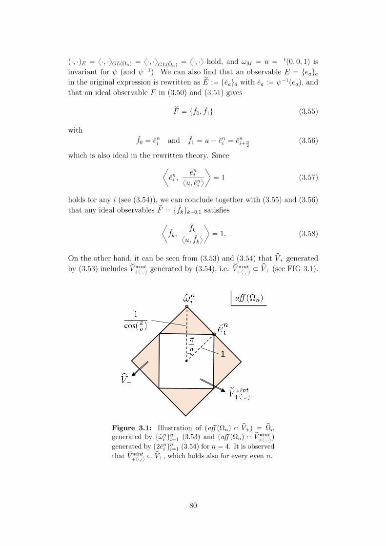
p¨, ¨qE “ x¨, ¨yGLpΩnq “ x¨, ¨yGLppΩnq “ x¨, ¨y hold, and ωM “ u “ tp0, 0, 1q is
invariant for ψ (and ψ´1). We can also find that an observable E “ teauain the original expression is rewritten as qE :“ teaua with ea :“ ψ´1peaq, and
that an ideal observable F in (3.50) and (3.51) gives
qF “ tf0, f1u (3.55)
with
f0 “ eni and f1 “ u´ eni “ eni`n2
(3.56)
which is also ideal in the rewritten theory. Since
B
eni ,eni
xu, eni y
F
“ 1 (3.57)
holds for any i (see (3.54)), we can conclude together with (3.55) and (3.56)
that any ideal observables qF “ tfkuk“0,1 satisfies
B
fk,fk
xu, fky
F
“ 1. (3.58)
On the other hand, it can be seen from (3.53) and (3.54) that pV` generated
by (3.53) includes qV ˚int`x¨,¨y generated by (3.54), i.e. qV ˚int
`x¨,¨y ĂpV` (see FIG 3.1).
1
Figure 3.1: Illustration of paff pΩnq X pV`q “ pΩn
generated by tωni uni“1 (3.53) and paff pΩnq X qV ˚int
`x¨,¨yq
generated by t2eni uni“1 (3.54) for n “ 4. It is observed
that qV ˚int`x¨,¨y Ă
pV`, which holds also for every even n.
80
Therefore,e
xu, eyP pΩn (3.59)
holds for any effect e P qV ˚int`x¨,¨y. It follows from (3.58) and (3.59) that the
claim of Lemma 3.3 holds also for even-sided regular polygon theories in a
rewritten expression (3.53) and (3.54).
We also need to confirm that all of our measures (3.3), (3.4), (3.8), (3.9),
(3.12), (3.31), and (3.42) depend only on probabilities, and thus they are
invariant for the modification above. For example, for a pair of observables
M “ tmaua and F “ tfaua on the original state space Ωn, we can see easily
from (3.4) and (3.12) that
LEpωF q “ 1´maxaPA
fapωq
“ 1´maxaPA
fapωq
“ LEpωqFq
and
D8pM,F q “ supωPΩn
maxaPA
|mapωq ´ fapωq|
“ supωPpΩn
maxaPA
ˇ
ˇmapωq ´ fapωqˇ
ˇ
“ D8p|M, qF q
respectively. It results in that if Theorem 3.6 holds in the modified the-
ory, then it holds also in the original theory. In fact, by virtue of (3.58) and
(3.59) (the “generalized version of Lemma 3.3”), we can repeat the same cal-
culations as in Theorem 3.6, and obtain a similar result to it in the modified
theory. Similar considerations can be adapted also for the other measures,
and it proves Theorem 3.12. 2
3.3.2 Concrete values for Landau-Pollak-type bounds
In this part, we shall concentrate on the Landau-Pollak-type relation (see
(3.34)) for the n-sided regular polygon theory of the form
maxafapωq `max
bgbpωq ď ΓF,Gpnq
@ω P Ωn, (3.60)
where F “ tfaua and G “ tgbub are ideal observables as usual, and show a
concrete calculation for the bound ΓF,Gpnq of uncertainty.
Let us focus on the state space Ωn. Any nontrivial ideal observable is of
the form teni , u ´ eni u (see (2.31)). Note that although teni ui“0,1,2 is also an
81
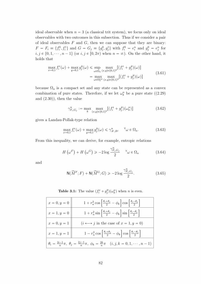
ideal observable when n “ 3 (a classical trit system), we focus only on ideal
observables with two outcomes in this subsection. Thus if we consider a pair
of ideal observables F and G, then we can suppose that they are binary:
F “ Fi ” tf 0i , f
1i u and G “ Gj ” tg0
j , g1j u with f 0
i “ eni and g0j “ enj for
i, j P t0, 1, ¨ ¨ ¨ , n´ 1u (or i, j P r0, 2πq when n “ 8). On the other hand, it
holds that
maxx“0,1
fxi pωq `maxy“0,1
gyj pωq ď supωPΩn
maxpx,yqPt0,1u2
rpfxi ` gyj qpωqs
“ maxωPΩext
n
maxpx,yqPt0,1u2
rpfxi ` gyj qpωqs
(3.61)
because Ωn is a compact set and any state can be represented as a convex
combination of pure states. Therefore, if we let ωnk be a pure state ((2.29)
and (2.30)), then the value
γnFi,Gj :“ maxk
maxpx,yqPt0,1u2
rpfxi ` gyj qpω
nk qs (3.62)
gives a Landau-Pollak-type relation
maxx“0,1
fxi pωq `maxy“0,1
gyj pωq ď γnAi,Bj@ω P Ωn. (3.63)
From this inequality, we can derive, for example, entropic relations
H`
ωF˘
`H`
ωG˘
ě ´2 logγnFi,Gj
2@ω P Ωn (3.64)
and
NpĂMF ;F q ` NpĂMG;Gq ě ´2 logγnFi,Gj
2. (3.65)
Table 3.1: The value pfxi ` gyj qpω
nk q when n is even.
x “ 0, y “ 0 1` r2n cos
”
θi`θj2´ φk
ı
cos”
θi´θj2
ı
x “ 1, y “ 0 1` r2n sin
”
θi`θj2´ φk
ı
sin”
θi´θj2
ı
x “ 0, y “ 1 (iÐÑ j in the case of x “ 1, y “ 0)
x “ 1, y “ 1 1´ r2n cos
”
θi`θj2´ φk
ı
cos”
θi´θj2
ı
θi “2i´1nπ, θj “
2j´1nπ, φk “
2knπ pi, j, k “ 0, 1, ¨ ¨ ¨ , n´ 1q
82
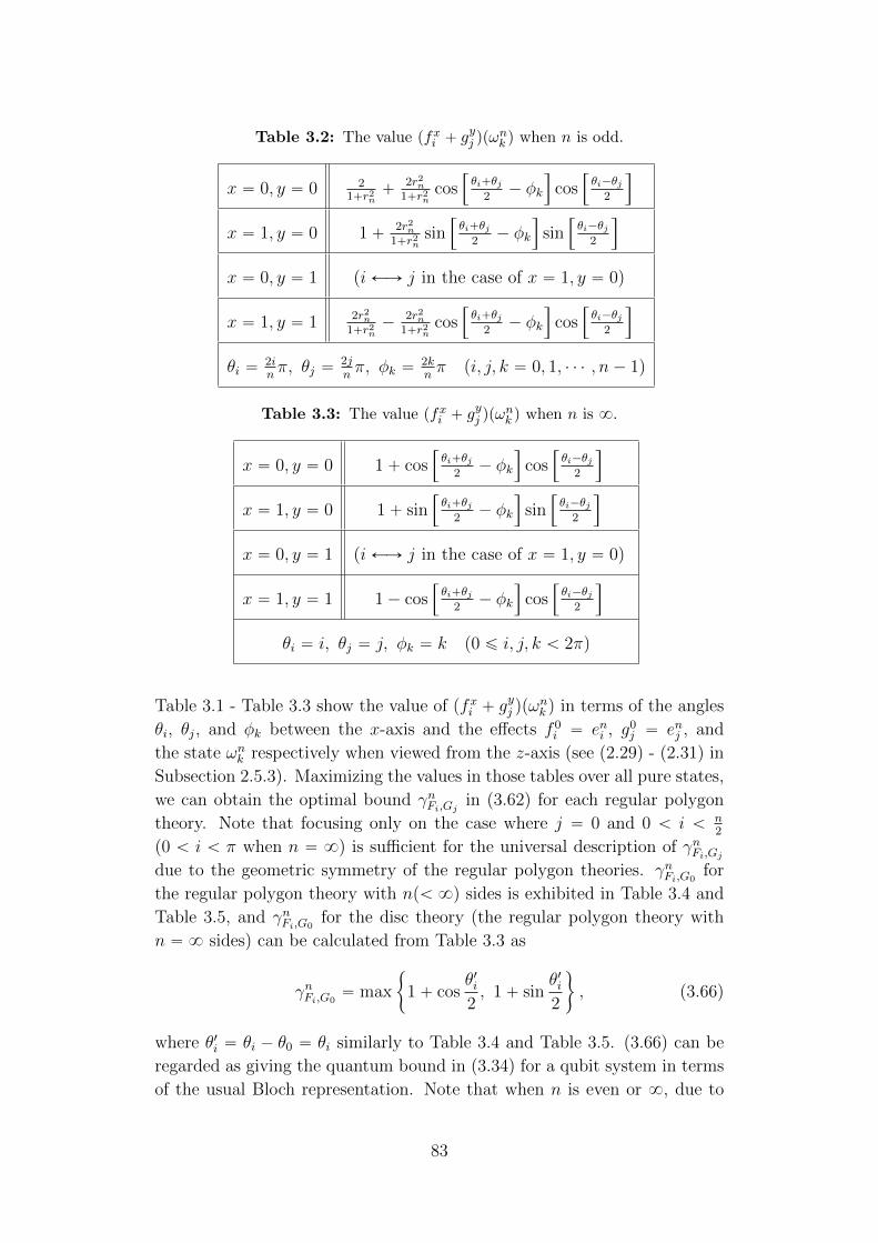
Table 3.2: The value pfxi ` gyj qpω
nk q when n is odd.
x “ 0, y “ 0 21`r2
n`
2r2n
1`r2n
cos”
θi`θj2´ φk
ı
cos”
θi´θj2
ı
x “ 1, y “ 0 1` 2r2n
1`r2n
sin”
θi`θj2´ φk
ı
sin”
θi´θj2
ı
x “ 0, y “ 1 (iÐÑ j in the case of x “ 1, y “ 0)
x “ 1, y “ 1 2r2n
1`r2n´
2r2n
1`r2n
cos”
θi`θj2´ φk
ı
cos”
θi´θj2
ı
θi “2inπ, θj “
2jnπ, φk “
2knπ pi, j, k “ 0, 1, ¨ ¨ ¨ , n´ 1q
Table 3.3: The value pfxi ` gyj qpω
nk q when n is 8.
x “ 0, y “ 0 1` cos”
θi`θj2´ φk
ı
cos”
θi´θj2
ı
x “ 1, y “ 0 1` sin”
θi`θj2´ φk
ı
sin”
θi´θj2
ı
x “ 0, y “ 1 (iÐÑ j in the case of x “ 1, y “ 0)
x “ 1, y “ 1 1´ cos”
θi`θj2´ φk
ı
cos”
θi´θj2
ı
θi “ i, θj “ j, φk “ k p0 ď i, j, k ă 2πq
Table 3.1 - Table 3.3 show the value of pfxi ` gyj qpω
nk q in terms of the angles
θi, θj, and φk between the x-axis and the effects f 0i “ eni , g0
j “ enj , and
the state ωnk respectively when viewed from the z-axis (see (2.29) - (2.31) in
Subsection 2.5.3). Maximizing the values in those tables over all pure states,
we can obtain the optimal bound γnFi,Gj in (3.62) for each regular polygon
theory. Note that focusing only on the case where j “ 0 and 0 ă i ă n2
(0 ă i ă π when n “ 8) is sufficient for the universal description of γnFi,Gjdue to the geometric symmetry of the regular polygon theories. γnFi,G0
for
the regular polygon theory with npă 8q sides is exhibited in Table 3.4 and
Table 3.5, and γnFi,G0for the disc theory (the regular polygon theory with
n “ 8 sides) can be calculated from Table 3.3 as
γnFi,G0“ max
"
1` cosθ1i2, 1` sin
θ1i2
*
, (3.66)
where θ1i “ θi ´ θ0 “ θi similarly to Table 3.4 and Table 3.5. (3.66) can be
regarded as giving the quantum bound in (3.34) for a qubit system in terms
of the usual Bloch representation. Note that when n is even or 8, due to
83
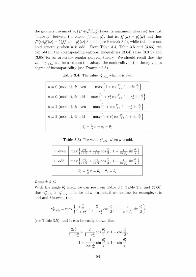
the geometric symmetry, pfxi `gyj qpω
nk q takes its maximum where ωnk lies just
“halfway” between the effects fxi and gyj , that is, fxi pωq “ gyj pωq and thus
fxi pωqgyj pωq “
14pfxi pωq` g
yj pωqq
2 holds (see Remark 3.9), while this does not
hold generally when n is odd. From Table 3.4, Table 3.5 and (3.66), we
can obtain the corresponding entropic inequalities (3.64) (also (3.37)) and
(3.65) for an arbitrary regular polygon theory. We should recall that the
value γnFi,G0can be used also to evaluate the nonlocality of the theory via its
degree of incompatibility (see Example 3.8).
Table 3.4: The value γnFi,G0when n is even.
n ” 0 (mod 4), i: even max!
1` cosθ1i2, 1` sin
θ1i2
)
n ” 0 (mod 4), i: odd max!
1` r2n cos
θ1i2, 1` r2
n sinθ1i2
)
n ” 2 (mod 4), i: even max!
1` cosθ1i2, 1` r2
n sinθ1i2
)
n ” 2 (mod 4), i: odd max!
1` r2n cos
θ1i2, 1` sin
θ1i2
)
θ1i “2inπ “ θi ´ θ0
Table 3.5: The value γnFi,G0when n is odd.
i: even max!
2r2n
1`r2n` 2
1`r2n
cosθ1i2, 1` 1
cos π2n
sinθ1i2
)
i: odd max!
2r2n
1`r2n`
2r2n
1`r2n
cosθ1i2, 1` 1
cos π2n
sinθ1i2
)
θ1i “2inπ “ θi ´ θ0 “ θi
Remark 3.13
With the angle θ1i fixed, we can see from Table 3.4, Table 3.5, and (3.66)
that γnFi,G0ě γ8Fi,G0
holds for all n. In fact, if we assume, for example, n is
odd and i is even, then
γnFi,G0“ max
"
2r2n
1` r2n
`2
1` r2n
cosθ1i2, 1`
1
cos π2n
sinθ1i2
*
(see Table 3.5), and it can be easily shown that
2r2n
1` r2n
`2
1` r2n
cosθ1i2ě 1` cos
θ1i2,
1`1
cos π2n
sinθ1i2ě 1` sin
θ1i2
84
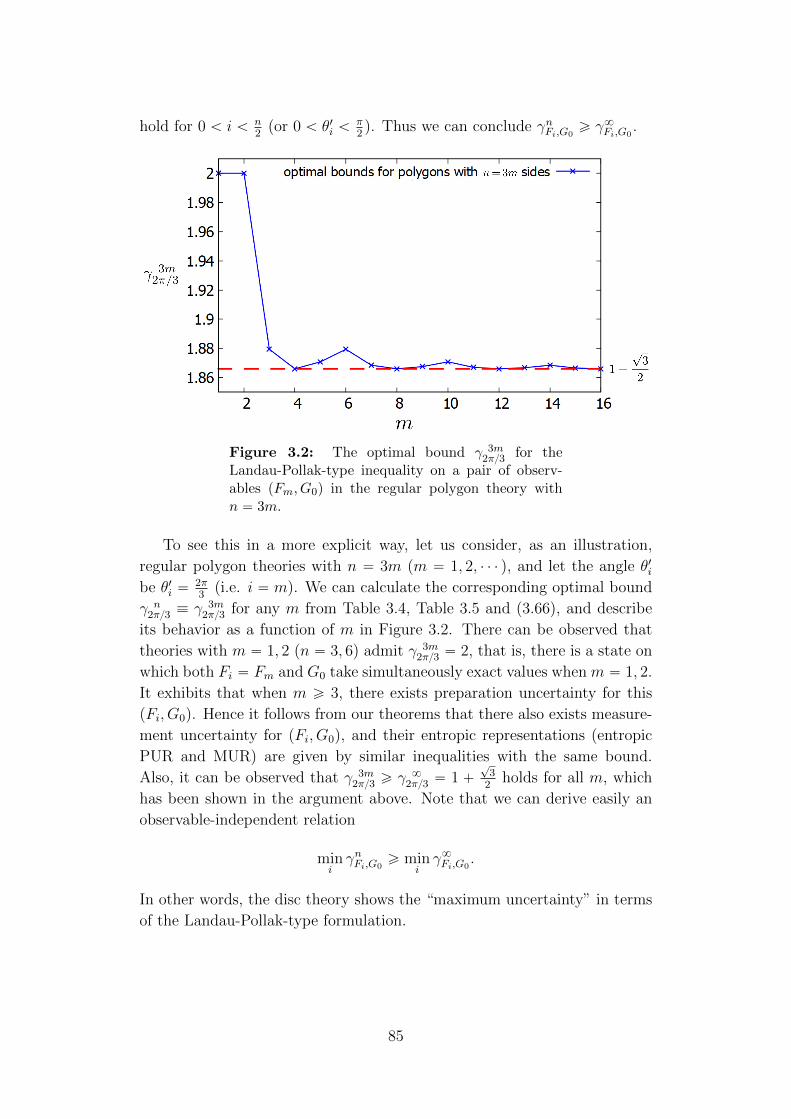
hold for 0 ă i ă n2
(or 0 ă θ1i ăπ2). Thus we can conclude γnFi,G0
ě γ8Fi,G0.
Figure 3.2: The optimal bound γ 3m2π3 for the
Landau-Pollak-type inequality on a pair of observ-ables pFm, G0q in the regular polygon theory withn “ 3m.
To see this in a more explicit way, let us consider, as an illustration,
regular polygon theories with n “ 3m (m “ 1, 2, ¨ ¨ ¨ ), and let the angle θ1ibe θ1i “
2π3
(i.e. i “ m). We can calculate the corresponding optimal bound
γ n2π3 ” γ 3m
2π3 for any m from Table 3.4, Table 3.5 and (3.66), and describe
its behavior as a function of m in Figure 3.2. There can be observed that
theories with m “ 1, 2 (n “ 3, 6) admit γ 3m2π3 “ 2, that is, there is a state on
which both Fi “ Fm and G0 take simultaneously exact values when m “ 1, 2.
It exhibits that when m ě 3, there exists preparation uncertainty for this
pFi, G0q. Hence it follows from our theorems that there also exists measure-
ment uncertainty for pFi, G0q, and their entropic representations (entropic
PUR and MUR) are given by similar inequalities with the same bound.
Also, it can be observed that γ 3m2π3 ě γ 8
2π3 “ 1 `?
32
holds for all m, which
has been shown in the argument above. Note that we can derive easily an
observable-independent relation
miniγnFi,G0
ě miniγ8Fi,G0
.
In other words, the disc theory shows the “maximum uncertainty” in terms
of the Landau-Pollak-type formulation.
85
Chapter 4
Testing incompatibility of
quantum devices with few states
Quantum information processing, including the exciting fields of quantum
communication and quantum computation, is ultimately based on the fact
that there are new types of resources that can be utilized in carefully de-
signed information processing protocols. The best-known feature of quan-
tum information is that quantum systems can be in superposition and en-
tangled states, and these resources lead to applications such as superdense
coding and quantum teleportation. While superposition and entanglement
are attributes of quantum states, quantum measurements have also features
that can power a new type of applications. The best known and most studied
property is the incompatibility of pairs (or collections) of quantum measure-
ments [21]. It is crucial e.g. in the BB84 quantum key distribution protocol
[11] that the used measurements are incompatible.
From the resource perspective, it is important to quantify the incompat-
ibility. There have been several studies on incompatibility robustness, i.e.,
how incompatibility is affected by noise. This is motivated by the fact that
noise is unavoidable in any actual implementation of quantum devices and
similar to other quantum properties (e.g. entanglement), large amount of
noise destroys incompatibility. Earlier studies have mostly focused on quan-
tifying noise [133] and finding those pairs or collections of measurements
that are most robust to certain types of noise [134], or to find conditions
under which all incompatibility is completely erased [135]. In this work,
we introduce quantifications of incompatibility which are motivated by an
operational aspect of testing whether a collection of devices is incompatible
or not. We focus on two integer valued quantifications of incompatibility,
called compatibility dimension and incompatibilility dimension. We formu-
late these concepts for arbitrary collections of devices. Roughly speaking,
the first one quantifies how many states we minimally need to use to detect
incompatibility if we choose the test states carefully, whereas the second
86
one quantifies how many (affinely independent) states we may have to use
if we cannot control their choice. We study some of the basic properties of
these quantifications of incompatibility and we present several examples to
demonstrate their behaviour.
This part is organized as follows. In Section 4.1, we introduce the no-
tion of compatibility and incompatibility dimension, which reflects opera-
tionally how easy it is to detect the incompatibility of quantum devices
considered. We also give brief reviews on related studies recently reported
in [136, 137, 138, 139] for the case of quantum observables, and explain the
interconnections of these studies to ours. In Section 4.2, we show that in-
compatibility dimension is related with the concept of incompatibility witness
[16, 17, 116]. We also derive a useful bound for incompatibility dimension by
means from the relation between them. In Section 4.3, we give a particular
analysis for compatibility and incompatibility dimensions of a pair of mu-
tually unbiased qubit observables. We show that, remarkably, even for the
standard example of noisy orthogonal qubit observables the incompatibil-
ity dimension has a jump in a point where all noise robustness measures are
continuous and indicate nothing special to happen. More precisely, the noise
parameter has a threshold value where the number of needed test states to
reveal incompatibility shifts from 2 to 3. This means that even in this simple
class of incompatible pairs of qubit observables there is a qualitative differ-
ence in the incompatibility of less noisy and more noisy pairs of observables.
An interesting additional fact is that the compatibility dimension of these
pairs of observables does not depend on the noise parameter.
For simplicity and clarity, we will restrict to finite-dimensional Hilbert
spaces and observables with a finite number of outcomes. Our definitions
apply not only to quantum theory but also to any GPT. However, for the
sake of concreteness, we keep the discussion in the realm of quantum theory.
The main definitions work in any GPT without any changes. We expect
that similar findings as the aforementioned result on noisy orthogonal qubit
observables can be made in subsequent studies on other collections of devices.
4.1 (In)compatibility on a subset of states
In this section, we introduce the notion of incompatibility dimension and
compatibility dimension as quantifications of incompatibility. We again men-
tion that we focus on compatibility and incompatibility in quantum theory
in this chapter, but those quantities can be defined naturally also in GPTs.
87
4.1.1 (In)compatibility for quantum devices
We start with presenting explicit descriptions of compatibility and incom-
patibility for quantum observables, although we have already given their
definitions in the general framework of GPTs (see Definition 2.48 and Propo-
sition 2.49). A quantum observable is mathematically described as a positive
operator valued measure (POVM) [80]. A quantum observable with finite
number of outcomes is hence a map x ÞÑ Apxq from the outcome set to the
set of linear operators on a Hilbert space. The compatibility of quantum
observables A1, . . . ,An with outcome sets X1, . . . , Xn means that there ex-
ists an observable G, called joint observable, defined on the product outcome
set X1 ˆ ¨ ¨ ¨ ˆ Xn such that from an outcome px1, . . . , xnq of G, one can
infer outcomes for every A1, . . . ,An by ignoring the other outcomes. More
precisely, the requirement is that
A1px1q “ÿ
x2,...,xn
Gpx1, x2, . . . , xnq,
A2px2q “ÿ
x1,x3...,xn
Gpx1, x2, . . . , xnq,
...
Anpxnq “ÿ
x1,...,xn´1
Gpx1, x2, . . . , xnq.
(4.1)
If A1, . . . ,An are not compatible, then they are called incompatible.
Example 4.1
(Unbiased qubit observables) We recall a standard example to fix the nota-
tion that we will use in later examples. An unbiased qubit observable is a
dichotomic observable with outcomes ˘ and determined by a vector a P R3,
|a| ď 1 via
Aap˘q “ 1
2p1˘ a ¨ σq ,
where a ¨ σ “ a1σ1 ` a2σ2 ` a3σ3 and σi, i “ 1, 2, 3, are the Pauli matrices.
The Euclidean norm |a| of a reflects the noise in Aa; in the extreme case
of |a| “ 1 the operators Aap˘q are projections and the observable is called
sharp. As shown in [140], two unbiased qubit observables Aa and Ab are
compatible if and only if
|a` b| ` |a´ b| ď 2 . (4.2)
There are two extreme cases. Firstly, if Aa is sharp then it is compatible
with some Ab if and only if b “ ra for some ´1 ď r ď 1. Secondly, if
|a| “ 0, then Aap˘q “ 121 and it is called a trivial qubit observable, in which
case it is compatible with all other qubit observables.
88
How can we test if a given family of observables is compatible or incom-
patible? From the operational point of view, the existence of an observable
G satisfying (4.1) is equivalent to the existence of G such that for any state
% the equation
Trr%A1px1qs “ÿ
x2,...,xn
Trr%Gpx1, x2, . . . , xnqs (4.3)
holds. Before contemplating into these questions, we recall that analogous
definitions of quantum compatibility and incompatibility make sense for
other types of quantum devices, in particular, for instruments and chan-
nels [21, 141, 142, 143, 144, 145, 146]. We denote by SpHq the set of all
density operators on a Hilbert space H. The input space of all types of de-
vices must be SpHinq on the same Hilbert space Hin as the devices operate
on a same system. We denote SpHinq simply by S. A device is a completely
positive map and the “type” of the device is characterized by its output
space. Output spaces for the three basic types of devices are:
• observable: P pXq :“ tp “ tppxquxPX | 0 ď ppxq ď 1,ř
x ppxq “ 1u,
• channel: SpHoutq,
• instrument: SpHoutq b P pXq.
In this classification, an observable A is identified with a map % ÞÑ Trr%Apxqs
from SpHinq to P pXq. We limit our investigation to the cases where the
number of outcomes in X is finite and the output Hilbert space Hout is
finite-dimensional. Regarding P pXq Ă SpC|X|q as the set of all diagonal
density operators, we can summarize that quantum devices are normalized
completely positive maps to different type of output spaces.
Devices D1, . . . ,Dn are compatible if there exists a device D that can
simulate D1, . . . ,Dn simultaneously, meaning that by ignoring disjoint parts
of the output of D we get the same actions as D1, . . . ,Dn (see [21]). This
kind of device is called a joint device of D1, . . . ,Dn. The input space of D
is the same as for D1, . . . ,Dn, but the output space is the tensor product
of their output spaces. As an illustration, let Dj : SpHinq Ñ SpHjq pj “
1, . . . , nq be quantum channels. They are compatible iff there exists a channel
D : SpHinq Ñ SpÂn
j“1 Hjq satisfying
D1p%q “ trH2,...,HnDp%q,
D2p%q “ trH1,H3,...,HnDp%q,
...
Dnp%q “ trH1,...,Hn´1Dp%q
89
for all % P SpHinq (see (4.1)). If D1, . . . ,Dn are not compatible, then they are
incompatible. We recall a qubit example to exemplify the general definition.
Example 4.2
(Unbiased qubit observable and partially depolarizing noise) A measurement
of an unbiased qubit observable Aa necessarily disturbs the system. This
trade-off is mathematically described by the compatibility relation between
observables and channels. Let us consider partially depolarizing qubit chan-
nels, which have the form
Γpp%q “ p%` p1´ pq121 (4.4)
for 0 ď p ď 1. A joint device for a channel and observable is an instrument.
Hence, Aa and Γp are compatible if there exists an instrument x ÞÑ Φx such
thatÿ
x
Φxp%q “ Γpp%q and TrrΦxp%qs “ Trr%Aapxqs
for all states % and outcomes x. It has been proven in [144] that Aa and Γpare compatible if and only if
|a| ď1
2
´
1´ p`a
p1´ pqp1` 3pq¯
. (4.5)
This shows that higher is the norm |a|, smaller must p be.
4.1.2 (In)compatibility dimension of devices
To test the incompatibility we should hence check the validity of (4.3) in a
subset of states that spans the whole state space. An obvious question is
then if we really need all those states, or if a smaller number of test states
is enough. Further, does the number of needed test states depend on the
given family of observables? How does noise affect the number of needed
test states? The earlier discussion motivates the following definition, which
is central to our investigation.
Definition 4.3
Let S0 Ă S. Devices D1, . . . ,Dn are S0-compatible if there exist compatible
devices D11, . . . ,D1n of the same type such that
D1jp%q “ Djp%q (4.6)
for all j “ 1, . . . , n and states % P S0. Otherwise, D1, . . . ,Dn are S0-
incompatible.
The definition is obviously interesting only when D1, . . . ,Dn are incompat-
ible in the usual sense, i.e., with respect to the full state space. In that
90
case the definition means that if devices D1, . . . ,Dn are S0-compatible, their
incompatibility cannot be verified by taking test states from S0 only, and
vice versa, if devices D1, . . . ,Dn are S0-incompatible, their actions on S0
cannot be simulated by any collection of compatible devices and therefore
their incompatibility should be able to be observed in some way.
The S0-compatibility depends not only on the size of S0 but also on its
structure. We start with a simple example showing that there exist sets S0
such that an arbitrary family of devices is S0-compatible.
Example 4.4
Any set of devices D1, . . . ,Dn is S0-compatible if S0 “ t%1, . . . , %ku consists
of perfectly distinguishable states. In fact, one may construct a device D1kwhich outputs Dkp%jq after confirming an input state is %j by measuring an
observable that distinguishes the states in S0. It is easy to see that the
devices D11, . . . ,D1n are compatible. The same argument works for devices in
general probabilistic theories and one can use the same reasoning for a subset
S0 that is broadcastable [25]. (We recall that a subset S0 is broadcastable
if there exists a channel B : S Ñ S b S such that the bipartite state Bp%q
has marginals equal to % for all % P S0.) For instance, two qubit states 12
and |0yx0| are broadcastable even though not distinguishable. Any pair of
qubit channels Λ1 and Λ2 is S0-compatible for S0 “ t12, |0yx0|u as we can
define Λ1jp%q “ř1i“0xi|%|iyΛjp|iyxi|q for j “ 1, 2. The channel Λ1j has clearly
the same action as Λj on S0. A joint channel Λ for Λ11 and Λ12 is given as
Λp%q “1ÿ
i“0
xi|%|iyΛ1p|iyxi|q b Λ2p|iyxi|q,
and it is clear that, in fact, Tr2rΛp%qs “ Λ1p%q and Tr1rΛp%qs “ Λ2p%q.
For a subset S0 Ă S, we denote by S0 the intersection of the linear hull
of S0 with S, i.e.,
S0 “ t% P S | % “lÿ
i“1
ci%i for some ci P C and %i P S0u
In this definition we can assume without restriction that ci P R andř
i ci “
1 as they follow from the positivity and unit-trace of states. Since the
condition (4.6) is linear in %, we conclude that devices D1, . . . ,Dn are S0-
compatible if and only if they are S0-compatible. This makes sense: if we
can simulate the action of devices for states in S0, we can simply calculate
the action for all states that are linear combinations of those states. This
observation also shows that a reasonable way to quantify the size of a subset
S0 for the task in question is the number of affinely independent states. We
91
consider the following questions. Given a collection of incompatible devices
D1, . . . ,Dn,
(a) what is the smallest subset S0 such that D1, . . . ,Dn are S0-incompatible?
(b) what is the largest subset S0 such that D1, . . . ,Dn are S0-compatible?
Smallest and largest here mean the number of affinely independent states in
S0. It agrees with the linear dimension of the linear hull of S0, or dimaff S0`
1, where dimaff S0 is the affine dimension of the affine hull aff S0 of S0
[49, 54]. The answer to (a) quantifies how many states we need to use to
detect incompatibility if we choose them carefully, whereas the answer to
(b) quantifies how many (affinely independent) states we may have to use
if we cannot control their choice. Hence for both of these quantities lower
number means more incompatibility in the sense of easier detection. The
precise mathematical definitions read as follows.
Definition 4.5
For a collection of incompatible devices D1, . . . ,Dn, we denote
χincomppD1, . . . ,Dnq “ minS0ĂS
tdimaff S0 ` 1 | D1, . . . ,Dn: S0-incompatibleu
and
χcomppD1, . . . ,Dnq “ maxS0ĂS
tdimaff S0 ` 1 | D1, . . . ,Dn: S0-compatibleu.
We call these numbers the incompatibility dimension and compatibility di-
mension of D1, . . . ,Dn respectively.
From Example 4.4 and the fact that the linear dimension of the linear hull
of S is d2 we conclude that
2 ď χincomppD1, . . . ,Dnq ď d2 (4.7)
and
d ď χcomppD1, . . . ,Dnq ď d2´ 1 . (4.8)
Further, from the definitions of these quantities it directly follows that
χincomppD1, . . . ,Dnq ď χcomppD1, . . . ,Dnq ` 1 . (4.9)
We note that based on their definitions, both χincomp and χcomp are expected
to be smaller for collections of devices that are more incompatible. The
following monotonicity property of χincomp and χcomp under pre-processing
is a basic property that any quantification of incompatibility is expected to
satisfy.
92
Proposition 4.6
Let Λ : S Ñ S be a quantum channel and let rDj be a pre-processing of Dj with
Λ for each j “ 1, . . . , n, i.e., rDjp%q “ DjpΛp%qqq. If rDj’s are incompatible,
then also Dj’s are incompatible and
χincompprD1, . . . , rDnq ě χincomppD1, . . . ,Dnq (4.10)
and
χcompprD1, . . . , rDnq ě χcomppD1, . . . ,Dnq . (4.11)
Proof
Suppose that D1, . . . ,Dn are S0-compatible for some subset S0. Let D1 be
a device that gives devices D11, . . . ,D1n as marginals and these marginals
satisfy (4.6) in S0. Then the pre-processing of D1 with Λ gives rD1, . . . , rDn as
marginals in S0. The claimed inequalities then follow. 2
The post-processing map of a device D depends on type of the device. For
instance, the output set of an observable is P pXq and post-processing is then
described as a stochastic matrix [147]. We formulate and prove the following
monotonicity property of χincomp and χcomp under post-processing only for
observables. The formulation is analogous for other types of devices.
Proposition 4.7
Let rAj be a post-processing of Aj (i.e. rAjpx1q “
ř
x νjpx1, xqAjpxq for some
stochastic matrix νj) for each j “ 1, . . . , n. If rAj’s are S0-incompatible, then
also Aj’s are S0-incompatible and
χincompprA1, . . . , rAnq ě χincomppA1, . . . ,Anq (4.12)
and
χcompprA1, . . . , rAnq ě χcomppA1, . . . ,Anq . (4.13)
Proof
Suppose that A1, . . . ,An are S0-compatible for some subset S0. This means
that there exists an observable G satisfying for all % P S0, any j and xj,
Trr%Ajpxjqs “ÿ
l‰j
ÿ
xl
Trr%Gpx1, . . . , xnqs . (4.14)
We define an observable rG
rGpx11, . . . , x1nq “
ÿ
x1,...,xn
νpx11|x1q ¨ ¨ ¨ νpx1n|xnqGpx1, . . . , xnq,
and it then satisfies
Trr%rAjpx1jqs “
ÿ
l‰j
ÿ
x1l
Trr%rGpx11, . . . , x1nqs (4.15)
93
for all % P S0, any j and x1j. This shows that rA1, . . . , rAn are S0-compatible.
The claimed inequalities then follow. 2
We will now have some examples to demonstrate the values of χincomp and
χcomp in some standard cases.
Example 4.8
Let us consider the identity channel id : SpCdq Ñ SpCdq. It follows from
the definitions that two identity channels are S0-compatible if and only if S0
is a broadcastable set. It is known that a subset of states is broadcastable
only if the states commute with each other [148], and for this reason the
pair of two identity channels is S0-incompatible whenever S0 contains two
noncommuting states. Therefore, we have χincomppid, idq “ 2. On the other
hand, S0 consisting of distinguishable states makes the identity channels S0-
compatible. As S0 consisting of commutative states has at most d affinely
independent states, we conclude that χcomppid, idq “ d.
A comparison of the results of Example 4.8 to the bounds (4.7) and (4.8)
shows that the pair of identity channels has the smallest possible incompat-
ibility and compatibility dimensions. This is quite expectable as that pair is
consider to be the most incompatible pair - any device can be post-processed
from the identity channel. Perhaps surprisingly, the lower bound of χincompcan be attained already with a pair of dichotomic observables; this is shown
in the next example.
Example 4.9
Let P and Q be two noncommuting one-dimensional projections in a d-
dimensional Hilbert space H. We define two dichotomic observables A and
B as
Ap1q “ P ,Ap0q “ 1´ P , Bp1q “ Q ,Bp0q “ 1´Q .
Let us then consider a subset consisting of two states,
S0 “ t%P , %Qu :“ t 1
d´1p1´ P q, 1
d´1p1´Qqu .
We find that the dichotomic observables A and B are S0-incompatible. To
see this, let us make a counter assumption that A and B are S0-compatible,
in which case there exists G such that the marginal condition (4.3) holds for
both observables and for all % P S0. We have Trr%PAp1qs “ 0 and therefore
0 “ Trrp1´ P qGp1, 1qs “ Trrp1´ P qGp1, 0qs.
It follows that Gp1, 1q “ αP and Gp1, 0q “ βP . Further, TrrPAp1qs “
1 and hence α ` β “ 1. In a similar way we obtain Gp1, 1q “ γQ and
94
Gp0, 1q “ δQ with γ ` δ “ 1. It follows that α “ γ “ 0 and β “ δ “ 1.
But Gp1, 0q ` Gp0, 1q “ P ` Q contradicts Gp1, 0q ` Gp0, 1q ď 1. Thus we
conclude χincomppA,Bq “ 2.
For two incompatible sharp qubit observables (Example 4.1) the previous
example gives a concrete subset of two states such that the observables
are incompatible and proves that χincomppAa,Abq “ 2 for such a pair. The
incompatibility dimension for unsharp qubit observables is more complicated
and will be treated in Section 4.3.
Example 4.10
Let us consider two observables A and B. Fix a state %0 P S and define
S0 “ t% P S : Trr%Apxqs “ Trr%0Apxqs @xu .
Then A and B are S0-compatible. To see this, we define an observable G as
Gpx, yq “ Trr%0ApxqsBpyq .
It is then straightforward to verify that (4.3) holds for all % P S0. As a
special instance of this construction, let Aa be a qubit observable and a ‰ 0
(see Example 4.1). We choose S0 “ t% P S | Trr%Aap`qs “ 12u. We then have
S0 “ t12p1`r ¨σq | r ¨a “ 0u and hence dimaff S0 “ 2. Based on the previous
argument, Aa is S0-compatible with any Ab. Therefore, χcomppAa,Abq “ 3
for all incompatible qubit observables Aa and Ab.
4.1.3 Remarks on other formulations of incompatibil-
ity dimension
The notion of S0-compatibility for quantum observables has been introduced
in [136] and in that particular case (i.e. quantum observables) it is equivalent
to Definition 4.3. In the current investigation, our focus is on the largest
or smallest S0 on which devices D1, . . . ,Dn are compatible or incompatible,
and this has some differences to the earlier approaches. In [138], the term
“compatibility dimension” was introduced and for observables A1, . . . ,An on
a d-dimensional Hilbert space H “ Cd: it is given by
RpA1, . . . ,Anq “ maxtr ď d | DV : CrÑ Cd isometry
s.t. V ˚A1V, , . . . , V˚AnV are compatibleu,
Evaluations of RpA1, . . . ,Anq in various cases such as n “ 2 and A1 and
A2 are rank-1 were presented in [138]. To describe it in our notions, let us
denote Cr by K, and define SH and SK as the set of all density operator on
95
H and K respectively. We also introduce SVK as
SVK :“ t% P S | supp% Ă VKu “ V SKV˚Ă SH.
Then we can see that the SK-compatibility of V ˚A1V, , . . . , V˚AnV is equiv-
alent to the SVK-compatibility of A1, . . . ,An. Therefore, if we focus only on
sets of states such as SVK (i.e. states with fixed support), then there is no
essential difference between our compatibility dimension and the previous
one: RpA1, . . . ,Anq “ r iff χcomppA1, . . . ,Anq “ r2. In [138] also the concept
of “strong compatibility dimension” was defined as
RpA1, . . . ,Anq “maxtr ď d | @V : CrÑ Cd isometry
s.t. V ˚A1V, , . . . , V˚AnV are compatibleu.
It is related to our notion of incompatibility dimension. In fact, if we only
admit sets of states such as SVK, then RpA1, . . . ,Anq and χincomppA1, . . . ,Anq
are essentially the same: RpA1, . . . ,Anq “ r iff χincomppA1, . . . ,Anq “ pr`1q2.
Similar notions have been introduced and investigated also in [137, 139].
As in [138], these works focus on quantum observables and on subsets of
states that are lower dimensional subspaces of the original state space.
Therefore, the notions are not directly applicable in GPTs. In [139] in-
compatibility is classified into three types. They are explained exactly in
terms of [138] as
(i) incompressive incompatibility: pA1, . . . ,Anq are SVK-compatible for all Kand V
(ii) fully compressive incompatibility: pA1, . . . ,Anq are SVK-incompatible for
all nontrivial K and V
(iii) partly compressive incompatibility: there is a V and K such that
pA1, . . . ,Anq are SVK-compatible, and some V 1 and K1 such that pA1, . . . ,Anq
are SV 1K1-incompatible.
In [139] concrete constructions of these three types of incompatible observ-
ables were given.
4.2 Incompatibility dimension and incompat-
ibility witness
In this section we show how the notion of incompatibility dimension is related
to the notion of incompatibility witness.
96
4.2.1 Relation between incompatibility dimension and
incompatibility witness for observables
An incompatibility witness is an affine functional ξ defined on n-tuples of
observables such that ξ takes non-negative values on all compatible n-tuples
and a negative value at least for some incompatible n-tuple [16, 17, 116].
Every incompatibility witness ξ is of the form
ξp‘nj“1Ajq “ δ ´ fp‘nj“1Ajq, (4.16)
where δ P R and f is a linear functional on ‘nj“1LspHqmj with LspHq being
the set of all self-adjoint operators on H and mj the number of outcomes of
Aj. It can be written also in the form
ξpA1, . . . ,Anq “ δ ´nÿ
j“1
mjÿ
xj“1
cj,xjTrr%j,xjAjpxjqs, (4.17)
where cj,xj ’s are real numbers, and %j,xj ’s are states. This result has been
proven in [17] for incompatibility witnesses acting on pairs of observables
and the generalization to n-tuples is straightforward. A witness ξ detects the
incompatibility of observables A1, . . . ,An if ξpA1, . . . ,Anq ă 0. The following
proposition gives a simple relation between incompatibility dimension and
incompatibility witness.
Proposition 4.11
Assume that an incompatibility witness ξ has the form (4.17) and it de-
tects the incompatibility of observables A1, . . . ,An. Then A1, . . . ,An are S0-
incompatible for S0 “ t%j,xj | j “ 1, . . . , n, xj “ 1, . . . ,mju.
Proof
Let A1, . . . ,An be S0-compatible. Then we have compatible observablesrA1, . . . , rAn such that Trr%Ajpxjqs “ Trr%rAjpxjqs for all % P S0. This implies
that
ξpA1, . . . ,Anq “ ξprA1, . . . , rAnq ě 0 ,
which contradicts the assumption that ξ detects the incompatibility of ob-
servables A1, . . . ,An. 2
It has been shown in [17] that any incompatible pair of observables is de-
tected by some incompatibility witness of the form (4.17). The proof is
straightforward to generalize to n-tuples of observables, and thus, together
with Proposition 4.11, we can obtain
χincomppA1, . . . ,Anq ď m1 ` ¨ ¨ ¨ `mn. (4.18)
97
That is, the incompatibility dimension of A1, . . . ,An can be evaluated via
their incompatibility witness (we will derive a better upper bound later in
this section). We can further prove the following proposition.
Proposition 4.12
The statements (i) and (ii) for a set of incompatible observables tA1, . . . ,Anu
are equivalent:
(i) χincomppA1, . . . ,Anq ď N
(ii) There exist a family of linearly independent states t%1, . . . , %Nu and real
numbers δ and tcl,j,xjul,j,xj pl “ 1, . . . , N, j “ 1, . . . , n, xj “ 1, . . . ,mjq
such that the incompatibility witness ξ defined by
ξpB1, . . . ,Bnq “ δ ´Nÿ
l“1
nÿ
j“1
mjÿ
xj“1
cl,j,xj trr%lBjpxjqs
detects the incompatibility of tA1, . . . ,Anu.
The claim piq ñ piiq may be regarded as the converse of the previous ar-
gument to obtain (4.18). It manifests that we can find an incompatibility
witness detecting the incompatibility of tA1, . . . ,Anu reflecting their incom-
patibility dimension.
Proof
piiq ñ piq can be proven in the same way as Proposition 4.11. Thus we fo-
cus on proving piq ñ piiq. Suppose that a family of observables tA1, . . . ,Anu
satisfies χincomppA1, . . . ,Anq “ N . Then there exists a family of linearly
independent states t%1, %2, . . . , %Nu in LspHq on which tA1, . . . ,Anu are in-
compatible. We can regard the family tA1, . . . ,Anu as an element of a vector
space L defined as L :“ ‘nj“1LspHqmj , that is, A :“ ‘nj“1Aj P L. For
each l “ 1, . . . , N , j “ 1, . . . , n, and xj “ 1, . . . ,mj, let us define a subset
KpA, %l, j, xjq of L as
KpA, %l, j, xjq :“ tB P L | x%l|BjpxjqyHS “ x%l|AjpxjqyHSu, (4.19)
where x%l|AjpxjqyHS :“ trr%lAjpxjqs is the Hilbert-Schmidt inner product on
LspHq. Note that this inner product can be naturally extended to an inner
product xx¨|¨yy on L:
xxA|Byy “nÿ
j“1
mjÿ
xj“1
xAjpxjq|BjpxjqyHS .
Embedding %l into L by %j,xjl “ ‘ni“1 ‘
miy“1 δijδyxj%l for each j, xj and l, we
98
obtain another representation of (4.19) as
KpA, %l, j, xjq “ tB | xx%j,xl |Byy “ xx%
j,xjl |Ayyu . (4.20)
Thus this set is a hyperplane in L. Note that t%j,xl ul,j,xj is a linearly inde-
pendent set in L. Consider an affine set K :“ XNl“1Xnj“1X
mjxj“1KpA, %l, j, xjq.
Because tA1, . . . ,Anu is incompatible in t%1, ¨ ¨ ¨ , %Nu, it satisfies
K X C “ H, (4.21)
where C :“ tC P L | tC1, . . .Cnu is compatibleu. Thus, by the separating
hyperplane theorem [49], there exists a hyperplane in L which separates
strongly the (closed) convex sets K and C. In the following, we will show
that one of those separating hyperplanes can be constructed from t%j,xl ul,j,xj .
Let us extend a family of linearly independent vectors t%j,xjl ul,j,xj to form
a basis of L. That is, we introduce a basis tvbub“1,...,dimL of L satisfying
tvaua“1,...,Npř
j mjq“ t%
j,xjl ul,j,xj . We introduce its dual basis twbub“1,2,...,dimL
satisfying xxva|wbyy “ δab. Because K can be written as
K “ tB | xx%j,xjl |pB´ Aqyy “ 0, @l, j, xju,
it is represented in terms this (dual) basis as
K “ A`K0,
where K0 is an affine set defined by
K0 : “ tdimLÿ
a“Npř
j mjq`1
cawa | ca P Ru (4.22)
Now we can construct a hyperplane separating K and C. To do this, let
us focus on the convex sets K0 and C 1 :“ C ´ A instead of K and C,
which satisfy K0 X C 1 “ H because of (4.21). We can apply the separating
hyperplane theorem (Theorem 11.2 in [49]) for the affine set K0 and convex
set C 1. There exists a hyperplane H0 in L such that K0 and C 1 are contained
by H0 and one of its associating open half-spaces respectively. That is, there
exists h P L satisfying
H0 “ tB P L | xxB|hyy “ 0u
with K0 Ă H0, and xxC1|hyy ă 0 for all C1 P C 1. Let us examine the vector
h. It satisfies
xxwa|hyy “ 0 for all a “ Npř
jmjq ` 1, . . . , dimL
99
because K0 Ă H0 (see (4.22)). Thus if we write h as h “řdimLa“1 cava, then
we can find that ca “ 0 holds for all a “ Npř
jmjq`1, . . . , dimL. It follows
that
h “
Npř
j mjqÿ
a“1
cava “ÿ
l
ÿ
j
ÿ
xj
cl,j,xj %j,xjl
holds, and the hyperplane H0 can be written as
H0 “ tB P L |ÿ
l
ÿ
j
ÿ
xj
cl,j,xjTrr%lBjpxjqs “ 0u.
Then the hyperplane H 1 :“ A`H0, a translation of H0, of the form
H 1“ tB P L |
ÿ
l
ÿ
j
ÿ
xj
cl,j,xjTrr%lBjpxjqs “ δ1u
contains the original sets K, and satisfy
ÿ
l
ÿ
j
ÿ
xj
cl,j,xjTrr%lCjpxjqs ă δ1
for all C P C. We can displace H 1 slightly in the direction of C to obtain a
hyperplane H defined as
H “ tB P L |ÿ
l
ÿ
j
ÿ
xj
cl,j,xjTrrρlBjpxjqs “ δu,
which (strongly) separates H 1 (in particular K) and C because H 1 is closed
and C is compact (see Corollary 11.4.2 in [49]). The claim now follows as
A P K. 2
4.2.2 An upper bound on the incompatibility dimen-
sion of observables via incompatibility witness
We can give a better upper bound than (4.18) for the incompatibiliy dimen-
sion by slightly modifing the previous argument in [17] on incompatibility
witness.
Proposition 4.13
Let A1, . . . ,An be incompatible observables with m1, . . . ,mn outcomes, re-
spectively. Then
χincomppA1, . . . ,Anq ďnÿ
j“1
mj ´ n` 1.
100
Proof
We continue following the same notations as the proof of Proposition 4.12.
Let us assume that the incompatibility of A1, . . . ,An is detected by an in-
compatibility witness ξ. The functional ξ is of the form
ξpAq “ δ ´ fpAq
with a real number δ and a functional f on L (see (4.16)). Then Riesz
representation theorem shows that the functional f can be represented as
fpAq “nÿ
j“1
mjÿ
xj
xFjpxjq|AjpxjqyHS
with some Fjpxjq P LspHq pj “ 1, . . . , n, xj “ 1, . . . ,mjq. If we define
F 1jpxjq “ Fjpxjq ` εj1, then we find
ξpAq “ δ ` dÿ
j
εj ´nÿ
j“1
mjÿ
xj“1
xF 1jpxjq|AjpxjqyHS.
We choose εj so that
ÿ
xj
trrF 1jpxjqs “ÿ
xj
xF 1jpxjq|1yHS “ 0
holds. The choice of tF 1jpxjquj,xj has still some freedom. Each F 1jpxjq can
be replaced with F 2j pxjq “ F 1jpxjq ` Tj, where Tj P LspHq satisfies trrTjs “
xTj|1yHS “ 0. In fact, it holds that
ÿ
xj
xF 2j pxjq|AjpxjqyHS “ÿ
xj
xF 1jpxjq|AjpxjqyHS `ÿ
xj
xTj|AjpxjqyHS
“ÿ
xj
xF 1jpxjq|AjpxjqyHS ` xTj|1yHS
“ÿ
xj
xF 1jpxjq|AjpxjqyHS.
We choose Tj as mjTj “ ´řmjxj“1 F
1jpxjq which indeed satisfies
mjxTj|1yHS “ ´
mjÿ
xj“1
xF 1jpxjq|1yHS “ 0,
i.e., TrrTjs “ 0, to obtain
ÿ
xj
F 2j pxjq “ 0.
101
We further choose large numbers αj ě 0 so that Gjpxjq :“ F 2j pxjq`αj1 ě 0
for all j and xj. Now we obtain a representation of the witness which is
equivalent to ξ for n-tuples of observables as
ξ˚pAq “ δ ` dÿ
j
pεj ` αjq ´ÿ
j
ÿ
xj
xGjpxjq|AjpxjqyHS,
where positive operators Gjpxjq’s satisfyř
xjGjpxjq “ mjαj1. Defining
density operators %jpxjq by %jpxjq “Gjpxjq
trrGjpxjqs, we obtain yet another repre-
sentation
ξ˚pAq “ δ ` dÿ
j
pεj ` αjq ´ÿ
j
ÿ
xj
trrGjpxjqstrr%jpxjqAjpxjqs
with %jpxjq’s satisfying constraints
ÿ
xj
trrGjpxjqs%jpxjq “ mjαj1. (4.23)
Thus, according to Proposition 4.11, A1, . . . ,An are S0-incompatible with
S0 “ t%jpxjquj,xj . To evaluate dimaff S0, we focus on the condition (4.23).
Introducing parameters pjpxjq :“ trrGjpxjqsdmjαj such thatř
xjpjpxjq “
1, we obtainÿ
xj
pjpxjq%jpxjq “1
d1,
orÿ
xj
pjpxjq%jpxjq “ 0,
where %jpxjq :“ %jpxjq´1d1. It follows that t%jpxjquxj are linearly dependent,
and thus
dimspant%jpxjquxj ď m1 ´ 1.
Similar arguments for the other j’s result in
dimspant%jpxjquj,xj ďÿ
j
pmj ´ 1q “ÿ
j
mj ´ n.
Considering that
dimspant%jpxjquj,xj “ dimaff t%jpxjquj,xj
holds, we can obtain the claim of the proposition. 2
The bound in Proposition 4.13 is not tight in general since the right-hand
side of the inequality can exceed the bound obtained in (4.7). However, for
small n and mj’s, the bound can be tight. In fact, while for n “ 2 and
102
m1 “ m2 “ 2 it gives χincomppA1,A2q ď 3, we will construct an example
which attains this upper bound in the next section.
4.3 (In)compatibility dimension for mutually
unbiased qubit observables
In this section we study the incompatibility dimension of pairs of unbiased
qubit observables introduced in Example 4.1. We concentrate on pairs that
are mutually unbiased, i.e., TrrAap˘qAbp˘qs “ 12 (this terminology orig-
inates from the fact that if the observables are sharp, then the respective
orthonormal bases are mutually unbiased. In the previously written form
the definition makes sense also for unsharp observables [149]). The condition
of mutual unbiasedness is invariant under a global unitary transformation,
hence it is enough to fix the basis x “ p1, 0, 0q, y “ p0, 1, 0q, z “ p0, 0, 1q in
R3 and choose two of these unit vectors. We will study the observables Atx
and Aty, where 0 ď t ď 1. The observables are written explicitly as
Atxp˘q “1
2p1˘ tσ1q , Atyp˘q “
1
2p1˘ tσ2q.
The condition (4.2) shows that Atx and Aty are incompatible if and only if
1?
2 ă t ď 1. The choice of having mutually unbiased observables as well as
using a single noise parameter instead of two is to simplify the calculations.
We have seen in Example 4.10 that χcomppAtx,Atyq “ 3 for all values t
for which the pair is incompatible. We have further seen (discussion after
Example 4.9) that χincomppAx,Ayq “ 2, and from Prop. 4.13 follows that
χincomppAtx,Atyq ď 3 for all 1
?2 ă t ď 1. The remaining question is then
about the exact value of χincomppAtx,Atyq, which can depend on the noise
parameter t and will be in our focus in this section (see Table 4.1).
χincomppAtx,Atyq χcomppA
tx,Atyqt ď 1?
2- -
1?2ă t ă 1
2 or 3(Proposition 4.14)
3(Example 4.10)
t “ 12
(Example 4.9)
Table 4.1: χincomp and χcomp for pAtx,Atyq with0 ď t ď 1. For t ď 1
?2 the observables Atx and
Aty are compatible and χincomp and χcomp are notdefined.
Let us first make a simple observation that follows from Prop. 4.7. Con-
sidering that Asx is obtained as a post-processing of Atx if and only if s ď t,
103
we conclude that
χincomppAsx,Asyq “ 2 ñ χincomppA
tx,Atyq “ 2 for1?
2ă s ď t ,
and
χincomppAs1x,As
1yq “ 3 ñ χincomppA
t1x,At1yq “ 3 for s1 ě t1 ą
1?
2.
Interestingly, there is a threshold value t0 where the value of χincomppAtx,Atyq
changes; this is the content of the following proposition.
Proposition 4.14
There exists 1?
2 ă t0 ă 1 such that χincomppAtx,Atyq “ 3 for 1
?2 ă t ď t0
and χincomppAtx,Atyq “ 2 for t0 ă t ď 1.
The main line of the lengthy proof of Proposition 4.14 is the following.
Defining two subsets L and M of p 1?2, 1s as
L :“ tt | χincomppAtx,Atyq “ 2u, M :“ tt | χincomppA
tx,Atyq “ 3u, (4.24)
we see that
inf L “ supMp“: t10q (4.25)
holds unless L and M are empty. By its definition, the number t10 satisfies
χincomppAtx,Atyq “ 2 for t ą t10, χincomppA
tx,Atyq “ 3 for t ă t10.
Based on the considerations above, the proof of Proposition 4.14 proceeds
as follows. First, in Part 1 - 3 (Subsection 4.3.1 - 4.3.3), we prove that M
is nonempty while L has already been shown to be nonempty as t “ 1 P L.
It will be found that χincomppAtx,Atyq “ 3 for t sufficiently close to 1?
2, and
thus t10 introduced above can be defined successfully. Then we demonstrate
in Part 4 (Subsection 4.3.4) that supM “ maxM , i.e. t10 is equal to t0 in
the claim of Prop. 4.14.
Remark 4.15
In [136] a similar problem to ours was considered. While in that work
the focus was on several affine sets, and a threshold value t0 was given for
each of them by means of their semidefinite programs where observables
tAtx,Aty,Atzu become compatible, we are considereding all affine sets with
dimension 2.
104
4.3.1 Proof of Proposition 4.14 : Part 1
In order to prove that M is nonempty, let us introduce some relevant notions:
D :“ tv | |v| ď 1, vz “ 0u Ă B :“ tv | |v| ď 1u,
SD :“ t%v | v P Du Ă S “ t%v | v P Bu,
where v “ vxx`vyy`vzz P R3, and %v :“ 12p1`v ¨σq. Since SD is a convex
set, we can treat SD almost like a quantum system. In the following, we
will do it without giving precise definitions because they are obvious. For an
observable E on S with effects tEpxqux, we write its restriction to SD as E|Dwith effects tEpxq|Dux, which is an observable on SD. It is easy to obtain
the following Lemma.
Lemma 4.16
The followings are equivalent:
(i) Atx and Aty are incompatible (thus 1?2ă t ď 1).
(ii) Atx and Aty are SD-incompatible.
(iii) Atx|D and Aty|D are incompatible as observables on SD.
Proof
(i) ñ (iii). Suppose that Atx|D and Aty|D are compatible in SD. There exists
an observable M on SD whose marginals coincide with Atx|D and Aty|D. One
can extend this M to the whole S so that it does not depend on z (for
example, one can simply regard its effect c01 ` c1σ1 ` c2σ2 as an effect on
S). Since both Atx|D and Aty|D also do not depend on z, the extension of M
gives a joint observable of Atx and Atx.
(iii) ñ (ii). Suppose that Atx and Aty are SD-compatible. There exists an
observable M on S whose marginals coincide with Atx and Aty in SD. The
restriction of M on SD proves that (iii) is false.
(ii) ñ (i). Suppose that Atx and Aty are compatible, then they are SD-
compatible. 2
This lemma demonstrates that the incompatibility of Atx and Aty means the
incompatibility of Atx|D and Aty|D. We can present further observations.
Lemma 4.17
Let us consider two pure states %r1 and %r2 (r1, r2 P BB, r1 ‰ r2), and a
convex subset S0 of S generated by them: S0 :“ tp%r1`p1´pq%r2 | 0 ď p ď 1u.
We also introduce an affine projection P by P%v “ %Pv, where %v P S with
v “ vxx` vyy` vzz and Pv “ vxx` vyy, and extend it affinely. The affine
hull of S0 is projected to SD as
PS0 :“ tλP%r1 ` p1´ λqP%r2 | λ P Ru X SD. (4.26)
105
If Atx and Aty are S0-incompatible, then their restrictions Atx|D and Aty|Dare PS0-incompatible.
Proof
Suppose that Atx and Aty are S0-incompatible. It implies Pr1 ‰ Pr2, i.e.,
P%r1 ‰ P%r2 (see Example 4.10), and thus PS0 is a segment in SD. If Atx|Dand Aty|D are PS0-compatible, then there exists a joint observable M on SDsuch that its marginals coincide with Atx|D and Aty|D on PS0 Ă SD. This
M can be extended to an observable on S so that the extension does not
depend on z. Because
TrrAtxp˘qP%r1s “ TrrAtxp˘q%r1s,
TrrAtxp˘qP%r2s “ TrrAtxp˘q%r2s
(and their y-counterparts) hold due to the independence of Atxp˘q from
σ3, the marginals of M coincide with Atx and Aty on S0. It results in the
S0-compatibility of Atx and Aty, which is a contradiction. 2
It follows from this lemma that χincomppAtx|D,A
ty|Dq is two when χincomppAtx,Atyq
is two, equivalently χincomppAtx,Atyq is three when χincomppA
tx|D,Aty|Dq is
three (remember that χincomppAtx,Atyq ď 3). In fact, the converse also
holds.
Lemma 4.18
χincomppAtx|D,A
ty|Dq is three when χincomppAtx,Atyq is three.
Proof
Let χincomppAtx,Atyq “ 3. It follows that Atx and Aty are S-compatible for
any line S Ă S. In particular, Atx and Aty are S 1-compatible for any line S 1 in
SD, and thus there is an observable M such that its marginals coincide with
Atx and Aty on S 1. It is easy to see that the marginals of M|D coincide with
Atx|D and Aty|D on S 1, which results in the S 1-compatibility of Atx|D and
Aty|D. Because S 1 is arbitrary, we can conclude χincomppAtx|D,A
ty|Dq “ 3.2
The lemmas above manifest that if Atx and Aty are incompatible, then Atx|Dand Aty|D are also incompatible and
χincomppAtx,Atyq “ χincomppA
tx|D,A
ty|Dq.
Therefore, in the following, we denote Atx|D and Aty|D simply by AtxD and
AtyD respectively, and focus on the quantity χincomppAtxD ,A
tyD q instead of the
original χincomppAtx,Atyq.
Before proceeding to the next step, let us confirm our strategy in the
following parts. In Part 2 (Subsection 4.3.2), we will consider a line (seg-
ment) S1 in SD, and consider for 0 ă t ă 1 all pairs of observables prAt1,rAt2q
106
on SD that coincide with pAtxD ,AtyD q on S1. Then we will investigate the
(in)compatibility of those rAt1 and rAt2 in order to obtain χincomppAtxD ,A
tyD q in
Part 3 (Subsection 4.3.3). It will be shown that when t is sufficiently small,
there exists a compatible pair prAt1,rAt2q for any S1, that is, AtxD and AtyD are
S1-compatible for any line S1. It results in χincomppAtxD ,A
tyD q “ 3, and thus
M ‰ H.
4.3.2 Proof of Proposition 4.14 : Part 2
Let us consider two pure states %r1 and %r2 with r1, r2 P BD (r1 ‰ r2), and a
convex set S1 :“ tp%r1 ` p1´ pq%r2 | 0 ď p ď 1u. We set parameters ϕ1 and
ϕ2 as
r1 “ cosϕ1x` sinϕ1y, (4.27)
r2 “ cosϕ2x` sinϕ2y, (4.28)
where ´π ď ϕ1 ă ϕ2 ă π. By exchanging ˘ properly, without loss of
generality we can assume the line connecting r1 and r2 passes through above
the origin (instead of below). In this case, from geometric consideration, we
have0 ă ϕ2 ´ ϕ1 ď π,
0 ďϕ1 ` ϕ2
2ďπ
2.
(4.29)
Note that when ϕ2 ´ ϕ1 “ π, the states %r1 and %r2 are perfectly distin-
guishable, which results in the S1-compatibility of AtxD and AtyD (see Example
4.4). On the other hand, when ϕ1`ϕ2
2“ 0 or π
2, Trr%AtxD p`qs or Trr%AtyD p`qs
is constant for % P S1 respectively, so AtxD and AtyD are S1-compatible (see
Example 4.10). Thus, instead of (4.29), we hereafter assume
0 ăϕ2 ´ ϕ1
2ăπ
2,
0 ăϕ1 ` ϕ2
2ăπ
2.
(4.30)
Next, we consider a binary observable rAt1 on SD that coincides with AtxD on
S1 Ă SD. There are many possible rAt1, and each rAt1 is determined completely
by its effect rAt1p`q corresponding to the outcome ‘+’ because it is binary.
The effect rAt1p`q is associated with a vector v1 P D defined as
v1 :“ argmaxvPDtrr%vrAt1p`qs. (4.31)
Let us introduce a parameter ξ1 P r´π, πq by
v1 “ cos ξ1x` sin ξ1y, (4.32)
107
and express rAt1p`q as
rAt1p`q “1
2pp1` wpξ1qq1`m1pξ1q ¨ σq , (4.33)
where we set
m1pξ1q “ C1pξ1qv1 with 0 ď C1pξ1q ď 1. (4.34)
Because
Trr%r1AtxD p`qs “ Trr%r1rAt1p`qs,
Trr%r2AtyD p`qs “ Trr%r2rAt1p`qs,
namely1
2`t
2cosϕ1 “
1` w1pξ1q
2`C1pξ1q
2cospϕ1 ´ ξ1q,
1
2`t
2cosϕ2 “
1` w1pξ1q
2`C1pξ1q
2cospϕ2 ´ ξ1q,
(4.35)
hold, we can obtain
C1pξ1q “tpcosϕ1 ´ cosϕ2q
cospϕ1 ´ ξ1q ´ cospϕ2 ´ ξ1q“
t sinϕ0
sinpϕ0 ´ ξ1q, (4.36)
w1pξ1q “ ´t
ˆ
sinpϕ1 ´ ϕ2q
2 sinpϕ1´ϕ2
2q
˙
¨
ˆ
sin ξ1
sinpϕ0 ´ ξ1q
˙
“´t cosψ0 sin ξ1
sinpϕ0 ´ ξ1q, (4.37)
where we set ϕ0 :“ ϕ1`ϕ2
2and ψ0 :“ ϕ2´ϕ1
2(0 ă ϕ0 ă
π2, 0 ă ψ0 ă
π2).
Note that if sinpϕ0 ´ ξ1q “ 0 or cospϕ1 ´ ξ1q ´ cospϕ2 ´ ξ1q “ 0 holds,
then cosϕ1 ´ cosϕ2 “ 0 holds (see (4.36)). It means ϕ0 “ 0, which is
a contradiction, and thus sinpϕ0 ´ ξ1q ‰ 0 (that is, C1pξ1q and w1pξ1q in
(4.36), (4.37) are well-defined). Moreover, because C1pξ1q ě 0, we can see
from (4.36) that sinpϕ0 ´ ξ1q ą 0 holds, which results in
0 ď ξ1 ă ϕ0, (4.38)
or
´π ` ϕ0 ă ξ1 ď 0. (4.39)
In addition, ξ1 is restricted also by the condition that rAt1p˘q are positive.
Since the eigenvalues of rAt1p˘q are 12pp1 ` w1pξ1qq ˘ C1pξ1qq, the restriction
comes from both1` w1pξ1q ` C1pξ1q ď 2,
1` w1pξ1q ´ C1pξ1q ě 0,(4.40)
108
equivalently
1´ w1pξ1q ě C1pξ1q, (4.41)
1` w1pξ1q ě C1pξ1q. (4.42)
When (4.39) (i.e. sin ξ1 ď 0) holds, w1pξ1q ě 0 holds, and thus (4.41) is
sufficient. It is written explicitly as
sin pϕ0 ´ ξ1q ` t sin ξ1 cosψ0 ě t sinϕ0,
or
1
tcos ξ1 `
1
t sinϕ0
pt cosψ0 ´ cosϕ0q sin ξ1 ě 1. (4.43)
In order to investigate (4.43), we adopt a geometric method here while it
can be solved in an analytic way. Let us define
h1pt, ϕ0, ψ0q “1
t sinϕ0
pt cosψ0 ´ cosϕ0q . (4.44)
Then we can rewrite (4.43) as
pcos ξ1, sin ξ1q ¨
„ˆ
1
t, h1
˙
´ pcos ξ1, sin ξ1q
ě 0. (4.45)
In fact, it can be verified easily that`
1t, h1
˘
is the intersection of the line
l1 :“ tλr1 ` p1 ´ λqr2 | λ P Ru and the line x “ 1t
in R2. Considering this
fact, we can find that ξ1 satisfies (4.45) if and only if
ξmin1 pt, ϕ0, ψ0q ď ξ1 ď 0, (4.46)
where ξmin1 pt, ϕ0, ψ0q is determined by the condition
„ˆ
1
t, h1
˙
´ pcos ξmin1 , sin ξmin1 q
K pcos ξmin1 , sin ξmin1 q (4.47)
(see FIG. 4.1). Analytically, it corresponds to the case where the equality
of (4.43) holds:
1
tcos ξmin1 `
1
t sinϕ0
pt cosψ0 ´ cosϕ0q sin ξmin1 “ 1, (4.48)
or
1´ w1pξmin1 q “ C1pξ
min1 q.
109
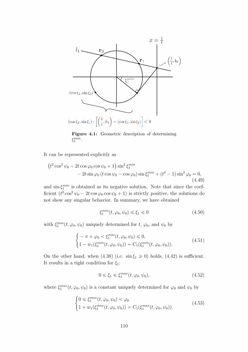
Figure 4.1: Geometric description of determiningξmin1 .
It can be represented explicitly as
`
t2 cos2 ψ0 ´ 2t cosϕ0 cosψ0 ` 1˘
sin2 ξmin1
´ 2t sinϕ0 pt cosψ0 ´ cosϕ0q sin ξmin1 ` pt2 ´ 1q sin2 ϕ0 “ 0,(4.49)
and sin ξmin1 is obtained as its negative solution. Note that since the coef-
ficient pt2 cos2 ψ0 ´ 2t cosϕ0 cosψ0 ` 1q is strictly positive, the solutions do
not show any singular behavior. In summary, we have obtained
ξmin1 pt, ϕ0, ψ0q ď ξ1 ď 0 (4.50)
with ξmin1 pt, ϕ0, ψ0q uniquely determined for t, ϕ0, and ψ0 by
#
´ π ` ϕ0 ă ξmin1 pt, ϕ0, ψ0q ď 0,
1´ w1pξmin1 pt, ϕ0, ψ0qq “ C1pξ
min1 pt, ϕ0, ψ0qq.
(4.51)
On the other hand, when (4.38) (i.e. sin ξ1 ě 0) holds, (4.42) is sufficient.
It results in a tight condition for ξ1:
0 ď ξ1 ď ξmax1 pt, ϕ0, ψ0q, (4.52)
where ξmax1 pt, ϕ0, ψ0q is a constant uniquely determined for ϕ0 and ψ0 by
#
0 ď ξmax1 pt, ϕ0, ψ0q ă ϕ0
1` w1pξmax1 pt, ϕ0, ψ0qq “ C1pξ
max1 pt, ϕ0, ψ0qq.
(4.53)
110
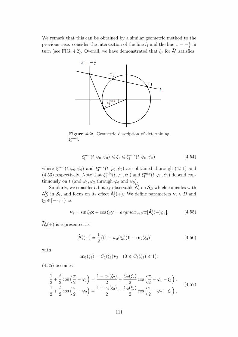
We remark that this can be obtained by a similar geometric method to the
previous case: consider the intersection of the line l1 and the line x “ ´1t
in
turn (see FIG. 4.2). Overall, we have demonstrated that ξ1 for rAt1 satisfies
Figure 4.2: Geometric description of determiningξmax1 .
ξmin1 pt, ϕ0, ψ0q ď ξ1 ď ξmax1 pt, ϕ0, ψ0q, (4.54)
where ξmin1 pt, ϕ0, ψ0q and ξmax1 pt, ϕ0, ψ0q are obtained thorough (4.51) and
(4.53) respectively. Note that ξmin1 pt, ϕ0, ψ0q and ξmax1 pt, ϕ0, ψ0q depend con-
tinuously on t (and ϕ1, ϕ2 through ϕ0 and ψ0).
Similarly, we consider a binary observable rAt2 on SD which coincides with
AtyD in S1, and focus on its effect rAt2p`q. We define parameters v2 P D and
ξ2 P r´π, πq as
v2 “ sin ξ2x` cos ξ2y “ argmaxvPDtrrrAt2p`q%vs. (4.55)
rAt2p`q is represented as
rAt2p`q “1
2pp1` w2pξ2qq1`m2pξ2qq (4.56)
with
m2pξ2q “ C2pξ2qv2 p0 ď C2pξ2q ď 1q.
(4.35) becomes
1
2`t
2cos
´π
2´ ϕ1
¯
“1` x2pξ2q
2`C2pξ2q
2cos
´π
2´ ϕ1 ´ ξ1
¯
,
1
2`t
2cos
´π
2´ ϕ2
¯
“1` x2pξ2q
2`C2pξ2q
2cos
´π
2´ ϕ2 ´ ξ1
¯
,
(4.57)
111
so defining ϕ1 :“ π2´ϕ1 and ϕ2 :“ π
2´ϕ2, we can obtain similarly to (4.36)
and (4.37)
C2pξ2q “t sinϕ0
sinpϕ0 ´ ξ1q, (4.58)
w2pξ2q “´t cosψ0 sin ξ2
sinpϕ0 ´ ξ2q, (4.59)
where ϕ0 :“ ϕ1`ϕ2
2“ π
2´ϕ0. It follows that properties of rAt2 can be obtained
just by replacing ξ1 and ϕ0 exhibited in the argument for rAt1 by ξ2 and ϕ0
respectively. Remark that 0 ă ϕ0 ăπ2
holds similarly to ϕ0, and that the
change ψ0 Ñ ψ0 :“ ϕ2´ϕ1
2“ ´ψ0 does not affect the equations above, so we
dismiss it. From (4.58) and (4.59), we have
ξmin2 pt, ϕ0, ψ0q ď ξ2 ď ξmax2 pt, ϕ0, ψ0q, (4.60)
where
ξmin2 pt, ϕ0, ψ0q “ ξmin1 pt, ϕ0, ψ0q “ ξmin1
´
t,π
2´ ϕ0, ψ0
¯
, (4.61)
and
ξmax2 pt, ϕ0, ψ0q “ ξmax1 pt, ϕ0, ψ0q “ ξmax1
´
t,π
2´ ϕ0, ψ0
¯
, (4.62)
which satisfy
$
&
%
´π
2` ϕ0 ă ξmin2 pt, ϕ0, ψ0q ď 0
1´ w2pξmin2 pt, ϕ0, ψ0qq “ C2pξ
min2 pt, ϕ0, ψ0qq
(4.63)
and$
&
%
0 ď ξmax2 pt, ϕ0, ψ0q ăπ
2´ ϕ0
1` w2pξmax2 pt, ϕ0, ψ0qq “ C2pξ
max2 pt, ϕ0, ψ0qq
(4.64)
respectively.
4.3.3 Proof of Proposition 4.14 : Part 3
In this part, we shall consider the (in)compatibility of the observables rAt1and rAt2 defined in (a) for t close to 1?
2(t „ 1?
2). It is related directly with
the S1-(in)compatibility of AtxD and AtyD as we have shown in the beginning of
this section. Let us examine the behavior of ξmin1 pt, ϕ0, ψ0q for t „ 1?2. We
denote ξmin1 pt “ 1?2, ϕ0, ψ0q and h1pt “
1?2, ϕ0, ψ0q simply by pξmin1 pϕ0, ψ0q
112
and ph1pϕ0, ψ0q respectively. The following lemma is useful.
Lemma 4.19
With ϕ0 fixed, pξmin1 is a strictly decreasing function of ψ0.
Proof
The claim can be observed to hold by a geometric consideration in terms of
FIG. 4.1. In fact, increasing ψ0 with ϕ0 fixed corresponds to moving the line
l1 down with its inclination fixed. The movement makes h1 (or ph1) and hence
ξmin1 (or pξmin1 ) smaller, which proves the claim. Here we show an analytic
proof of this fact. We can see from (4.44) and (4.48) that
?2 cos pξmin1 ` ph1 sin pξmin1 “ 1, (4.65)
i.e.ph1 “
1
sin pξmin1
´
1´?
2 cos pξmin1
¯
holds (note that sin pξmin1 ‰ 0 because sin pξmin1 “ 0 contradicts (4.65)). Then
the claim follows from the observation that
dph1
dpξmin1
“1
psin pξmin1 q2
´?2´ cos pξmin1
¯
ą 0,
and ph1 “1
sinϕ0
`
cosψ0 ´?
2 cosϕ0
˘
is a decreasing function of ψ0. 2
From this lemma, it follows that
pξmin1 pϕ0, ψ0q ă limψ0Ñ`0
pξmin1 pϕ0, ψ0q “: Ξmin1 pϕ0q, (4.66)
and
pξmin2 pϕ0, ψ0q ă Ξmin2 pϕ0q (4.67)
hold for all ϕ0 P p0,π2q and ψ0 P p0,
π2q, where
pξmin2 pϕ0, ψ0q :“ ξmin2
ˆ
t “1?
2, ϕ0, ψ0
˙
´
“ pξmin1
´π
2´ ϕ0, ψ0
¯¯
,
Ξmin2 pϕ0q :“ lim
ψ0Ñ`0
pξmin2 pϕ0, ψ0q
´
“ Ξmin1
´π
2´ ϕ0
¯¯
.
(4.68)
We can prove the following lemma.
Lemma 4.20
Ξmin1 pϕ0q ` Ξmin
2 pϕ0q ď ´π
2
holds for all 0 ă ϕ0 ăπ2.
113
Proof
Let us define
H1pϕ0q :“ limψ0Ñ`0
ph1pϕ0, ψ0q “ limψ0Ñ`0
h1
ˆ
t “1?
2, ϕ0, ψ0
˙
“1
sinϕ0
´
1´?
2 cosϕ0
¯
.
It holds similarly to (4.65) that
?2 cos Ξmin
1 `H1 sin Ξmin1 “ 1. (4.69)
Hence, together with sin2 Ξmin1 ` cos2 Ξmin
1 “ 1, we can obtain
cos Ξmin1 “
1?
2¨
2`H1
a
2H21 ` 2
H21 ` 2
, (4.70)
or its more explicit form
cos Ξmin1 “
1?
2¨
4´ 3?
2 cosϕ0
3´ 2?
2 cosϕ0
. (4.71)
It results in
Ξmin1 pϕ0q “ ´ arccos
ˆ
1?
2¨
4´ 3?
2 cosϕ0
3´ 2?
2 cosϕ0
˙
, (4.72)
where we follow the convention that arccos : r´1, 1s Ñ r0, πs, and thus Ξmin1 P
p´π ` ϕ0, 0s is obtained through ´ arccos : r´1, 1s Ñ r´π, 0s. Because
d
dϕ0
ˆ
1?
2¨
4´ 3?
2 cosϕ0
3´ 2?
2 cosϕ0
˙
“sinϕ0
p3´ 2?
2 cosϕ0q2,
andd
1´
ˆ
1?
2¨
4´ 3?
2 cosϕ0
3´ 2?
2 cosϕ0
˙2
“
d
ˆ
sinϕ0
3´ 2?
2 cosϕ0
˙2
“sinϕ0
3´ 2?
2 cosϕ0
,
we can observe that
dΞmin1
dϕ0
“
ˆ
sinϕ0
3´ 2?
2 cosϕ0
˙´1
¨sinϕ0
p3´ 2?
2 cosϕ0q2“
1
3´ 2?
2 cosϕ0
,
and
d2Ξmin1
dϕ20
“´2?
2 sinϕ0
p3´ 2?
2 cosϕ0q2ă 0, (4.73)
114
which means Ξmin1 is concave. Therefore, for any ϕ0 P p0,
π2q, the concavity
results in
1
2Ξmin
1 pϕ0q `1
2Ξmin
2 pϕ0q “1
2Ξmin
1 pϕ0q `1
2Ξmin
1
´π
2´ ϕ0
¯
ď Ξmin1
ˆ
1
2ϕ0 `
1
2
´π
2´ ϕ0
¯
˙
“ Ξmin1
´π
4
¯
.
Since we can see form (4.72) that Ξmin1
`
π4
˘
“ ´π4,
Ξmin1 pϕ0q ` Ξmin
2 pϕ0q ď ´π
2
holds for any ϕ0 P p0,π2q. 2
According to Lemma 4.19 and Lemma 4.20,
pξmin1 pϕ0, ψ0q `pξmin2 pϕ0, ψ0q ă Ξmin
1 pϕ0q ` Ξmin2 pϕ0q ď ´
π
2,
that is,
ξmin1
ˆ
t “1?
2, ϕ0, ψ0
˙
` ξmin2
ˆ
t “1?
2, ϕ0, ψ0
˙
ă ´π
2
holds for any ϕ0 and ψ0 (i.e. for any ϕ1 and ϕ2). However, we cannot
conclude that
ξmin1 pt, ϕ0, ψ0q ` ξmin2 pt, ϕ0, ψ0q ď ´
π
2(4.74)
holds for t „ 1?2: it may fail when
supϕ0,ψ0
„
ξmin1
ˆ
t “1?
2, ϕ0, ψ0
˙
` ξmin2
ˆ
t “1?
2, ϕ0, ψ0
˙
“ ´π
2.
On the other hand, because we can observe similarly to Lemma 4.19 that
ξmin1 is a strictly decreasing function of ψ0, it is anticipated that (4.74) holds
for t „ 1?2
and for ψ0 sufficiently close to π2. In fact, for ψ0 P r
π4, π
2q, we can
prove the following proposition.
Proposition 4.21
There exists a constant C ă ´π2
such that
pξmin1 pϕ0, ψ0q `pξmin2 pϕ0, ψ0q ă C,
115
i.e.
ξmin1
ˆ
t “1?
2, ϕ0, ψ0
˙
` ξmin2
ˆ
t “1?
2, ϕ0, ψ0
˙
ă C,
holds for all ψ0 P rπ4, π
2q and ϕ0 P p0,
π2q.
Proof
Because
pξmin1 pϕ0, ψ0q `pξmin2 pϕ0, ψ0q “
pξmin1 pϕ0, ψ0q `pξmin1
´π
2´ ϕ0, ψ0
¯
,
we can assume without loss of generality that 0 ă ϕ0 ďπ4. Due to Lemma
4.19, it holds for any ψ0 P rπ4, π
2q that
pξmin1 pϕ0, ψ0q ďpξmin1
´
ϕ0, ψ0 “π
4
¯
,
pξmin1
´π
2´ ϕ0, ψ0
¯
ď pξmin1
´π
2´ ϕ0, ψ0 “
π
4
¯
.(4.75)
Let us denote pξmin1
`
ϕ0, ψ0 “π4
˘
simply by rΞmin1 pϕ0q. In order to investigate
rΞmin1 pϕ0q and rΞmin
1
`
π2´ ϕ0
˘
, we have to recall (4.65). Similarly to (4.69)
and (4.70) in the proof of Lemma 4.20, it results in
cos rΞmin1 “
1?
2¨
2` rH1
b
2 rH21 ` 2
rH21 ` 2
, (4.76)
where
rH1 pϕ0q “ph1
´
ϕ0, ψ0 “π
4
¯
“1
sinϕ0
ˆ
1?
2´?
2 cosϕ0
˙
. (4.77)
Note that in this case we cannot apply a similar method to the one in Lemma
4.20 because rΞmin1 does not have a clear form like (4.72). Alternatively,
we focus on the following monotone relations between rΞmin1 , rH1, and ϕ0
(referring to the proof of Lemma 4.19 may be helpful):
drΞmin1
d rH1
ą 0,d rH1
dϕ0
ą 0
˜
thusdrΞmin
1
dϕ0
ą 0
¸
. (4.78)
From these relations, it can be seen that our restriction 0 ă ϕ0 ďπ4
is
equivalent to the condition rH1 ď 1 ´?
2 since rH1 p0q “ ´8 and rH1
`
π4
˘
“
1 ´?
2. The claim of the proposition can be shown easily when rH1 ď ´1
(or 0 ă ϕ0 ď ϕ˚ :“ arccos 2`?
106
, where rH1pϕ˚q “ ´1). In fact,
116
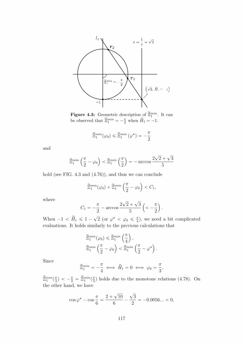
Figure 4.3: Geometric description of rΞmin1 . It can
be observed that rΞmin1 “ ´π2 when rH1 “ ´1.
rΞmin1 pϕ0q ď rΞmin
1 pϕ˚q “ ´π
2
and
rΞmin1
´π
2´ ϕ0
¯
ă rΞmin1
´π
2
¯
“ ´ arccos2?
2`?
3
5
hold (see FIG. 4.3 and (4.76)), and thus we can conclude
rΞmin1 pϕ0q ` rΞmin
1
´π
2´ ϕ0
¯
ă C1,
where
C1 “ ´π
2´ arccos
2?
2`?
3
5
´
ă ´π
2
¯
.
When ´1 ă rH1 ď 1 ´?
2 (or ϕ˚ ă ϕ0 ďπ4), we need a bit complicated
evaluations. It holds similarly to the previous calculations that
rΞmin1 pϕ0q ď rΞmin
1
´π
4
¯
,
rΞmin1
´π
2´ ϕ0
¯
ă rΞmin1
´π
2´ ϕ˚
¯
.
SincerΞmin
1 “ ´π
4ðñ rH1 “ 0 ðñ ϕ0 “
π
3,
rΞmin1 pπ
4q ă ´π
4“ rΞmin
1 pπ3q holds due to the monotone relations (4.78). On
the other hand, we have
cosϕ˚ ´ cosπ
6“
2`?
10
6´
?3
2“ ´0.0056... ă 0,
117
that is,
ϕ˚ ąπ
6.
It follows that π2´ ϕ˚ ă π
3, and thus rΞmin
1
`
π2´ ϕ0
˘
ă ´π4. Therefore, we
can conclude also in this case
rΞmin1 pϕ0q ` rΞmin
1
´π
2´ ϕ0
¯
ă C2,
where
C2 “ rΞmin1
´π
4
¯
` rΞmin1
´π
2´ ϕ˚
¯´
ă ´π
2
¯
.
Overall, we have obtained
rΞmin1 pϕ0, ψ0q ` rΞmin
2 pϕ0, ψ0q ă maxtC1, C2u
´
ă ´π
2
¯
for all ϕ0 P p0,π2q and ψ0 P r
π4, π
2q. 2
By virtue of this proposition, for t sufficiently close to 1?2,
ξmin1 pt, ϕ0, ψ0q ` ξmin2 pt, ϕ0, ψ0q ď ´
π
2
follows from the continuity of ξmin1 and ξmin2 with respect to t when π4ď
ψ0 ăπ2. It means that there always exist ξ‹1 ě ξmin1 and ξ‹2 ě ξmin2 for such t
and for any ϕ1 and ϕ2 satisfying ξ‹1 ` ξ‹2 “ ´
π2. For these ξ‹1 and ξ‹2 , it holds
that v1 “ ´v2, and thus rAt1 and rAt2 are compatible, i.e. AtxD and AtyD are
S1-compatible.
On the other hand, when 0 ă ψ0 ăπ4, it may not hold for t „ 1?
2that
ξmin1 pt, ϕ0, ψ0q ` ξmin2 pt, ϕ0, ψ0q ď ´π2, and thus we cannot apply the same
argument. Nevertheless, we can demonstrate that there exist ξ1 and ξ2 such
that rAt1 and rAt2 are compatible even when 0 ă ψ0 ăπ4. To see this, let us
assume 0 ă ψ0 ăπ4
and apply the necessary and sufficient condition for
(in)compatibility. According to the result proven in [150, 151, 152], rAt1 andrAt2 with (4.33) and (4.56) respectively are compatible if and only if
`
1´ F 21 ´ F
22
˘
ˆ
1´w2
1
F 21
´w2
2
F 22
˙
ď pm1 ¨m2 ´ w1w2q2 (4.79)
holds, where
F1 :“1
2
ˆ
b
p1` w1q2 ´ C2
1 `
b
p1´ w1q2 ´ C2
1
˙
, (4.80)
F2 :“1
2
ˆ
b
p1` w2q2 ´ C2
2 `
b
p1´ w2q2 ´ C2
2
˙
. (4.81)
118
For ξmin1 and ξmin2 , since it holds that
1´ w1pξmin1 q “ C1pξ
min1 q, (4.82)
1´ w2pξmin2 q “ C2pξ
min2 q, (4.83)
they become
F1 “
b
w1pξmin1 q, F2 “
b
w2pξmin2 q. (4.84)
Therefore, (4.79) can be rewritten as
rp1´sinpξmin1 `ξmin2 qqw1pξmin1 qw2pξ
min2 q
´ p1`sinpξmin1 ` ξmin2 qqp1´w1pξmin1 q´w2pξ
min2 qqs
¨“
p1´ w1pξmin1 qqp1´ w2pξ
min2 qqp1´ sinpξmin1 ` ξmin2 qq
‰
ě 0.
(4.85)
If 1 ´ sinpξmin1 ` ξmin2 q “ 0, then (4.85) holds, that is, rAt1 and rAt2 for ξmin1
and ξmin2 respectively are compatible. Therefore, we hereafter assume 1 ´
sinpξmin1 ` ξmin2 q ą 0, and rewrite (4.85) as (note that 0 ă w1pξmin1 q ă 1,
0 ă w2pξmin2 q ă 1)
p1` sinpξmin1 ` ξmin2 qqp1´ w1pξmin1 q ´ w2pξ
min2 qq
ď p1´ sinpξmin1 ` ξmin2 qqw1pξmin1 qw2pξ
min2 q.
(4.86)
In other words, rAt1 and rAt2 with respect to ξmin1 and ξmin2 are incompatible if
and only if
p1` sinpξmin1 ` ξmin2 qqp1´ w1pξmin1 q ´ w2pξ
min2 qq
ą p1´ sinpξmin1 ` ξmin2 qqw1pξmin1 qw2pξ
min2 q
(4.87)
holds. In order to investigate whether (4.87) holds, it is helpful to introduce
a function Z defined as
Zpt, ϕ0, ψ0q :““
1`sinpξmin1 pt, ϕ0, ψ0q`ξmin2 pt, ϕ0, ψ0qq
‰
“
1`w1pξmin1 pt, ϕ0, ψ0qq`w2pξ
min2 pt, ϕ0, ψ0qq
‰
´“
1´ sinpξmin1 pt, ϕ0, ψ0q ` ξmin2 pt, ϕ0, ψ0qq
‰
w1pξmin1 pt, ϕ0, ψ0qqw2pξ
min2 pt, ϕ0, ψ0qq.
(4.88)
Because
p1` sinpξmin1 ` ξmin2 qqp1´ w1pξmin1 q ´ w2pξ
min2 qq
ă p1` sinpξmin1 ` ξmin2 qqp1` w1pξmin1 q ` w2pξ
min2 qq,
119
Zpt, ϕ0, ψ0q ą 0 (4.89)
holds if rAt1 and rAt2 with respect to ξmin1 and ξmin2 are incompatible. Let us
focus on the case where t “ 1?2
(i.e. ξmin1 “ pξmin1 ). If a pair pϕ0, ψ0q satisfies
pξmin1 pϕ0, ψ0q ď ´π2
or pξmin2 pϕ0, ψ0q ď ´π2, then
pξmin1 pϕ0, ψ0q `pξmin2 pϕ0, ψ0q ă C
with
C “ ´π
2` lim
ϕ0Ñπ2´0
ψ0Ñ`0
pξmin1 pϕ0, ψ0q “ ´π
2´ arccos
ˆ
2?
2
3
˙
ă ´π
2
holds due to similar monotone relations to (4.78) between ϕ0, ψ0, and pξmin1
(remember that pξmin2 pϕ0, ψ0q “pξmin1
`
π2´ ϕ0, ψ0
˘
). Therefore, in this case,
we can apply the same argument as Proposition 4.21, which results in the
compatibility of rAt1 and rAt2 for t „ 1?2. On the other hand, let us examine
the case where pϕ0, ψ0q satisfies ψ0 P p0,π4q, and pξmin1 pϕ0, ψ0q ą ´π
2and
pξmin2 pϕ0, ψ0q ą ´π2. Because ψ0 P p0,
π4q, we obtain for general t (see (4.37))
w1pξmin1 q ą ´
t?
2
sin ξmin1
sinpϕ0 ´ ξmin1 qě
t?
2p´ sin ξmin1 q. (4.90)
For t “ 1?2, since
´π
2ă pξmin1 pϕ0, ψ0q ă lim
ϕ0Ñπ2´0
ψ0Ñ`0
pξmin1 pϕ0, ψ0q ,
it gives a bound
w1pξmin1 q ą
1
2sin pξ0, (4.91)
where we define
pξ0 “ ´ limϕ0Ñ
π2´0
ψ0Ñ`0
pξmin1 pϕ0, ψ0q “ arccos
ˆ
2?
2
3
˙
.
Let ε be a positive constant satisfying ε ă 116psin pξ0q
2. Due to the continuity
of sine, there exists a positive constant δ such that sinx P p´1,´1 ` εq
whenever x P`
´π2´ δ,´π
2
˘
. If pϕ0, ψ0q satisfies pξmin1 pϕ0, ψ0q`pξmin2 pϕ0, ψ0q ď
´π2´ δ, then it again leads to the same argument as Proposition 4.21, and
we can see that rAt1 and rAt2 for this pϕ0, ψ0q are compatible. Conversely, if
120
pϕ0, ψ0q satisfies ´π2´ δ ă pξmin1 pϕ0, ψ0q `
pξmin2 pϕ0, ψ0q ă ´π2
(remember
Lemma 4.20), then
´1 ă sinppξmin1 pϕ0, ψ0q `pξmin2 pϕ0, ψ0qq ă ´1` ε
follows from the definition of δ. Therefore, by virtue of (4.88), we have
Z
ˆ
t “1?
2, ϕ0, ψ0
˙
“
”
1` sinppξmin1 pϕ0, ψ0q `pξmin2 pϕ0, ψ0qq
ı
”
1` w1ppξmin1 pϕ0, ψ0qq ` w2p
pξmin2 pϕ0, ψ0qq
ı
´
”
1´ sinppξmin1 pϕ0, ψ0q `pξmin2 pϕ0, ψ0qq
ı
w1ppξmin1 pϕ0, ψ0qqw2p
pξmin2 pϕ0, ψ0qq
ă ε”
1` w1ppξmin1 pϕ0, ψ0qq ` w2p
pξmin2 pϕ0, ψ0qq
ı
´ p2´ εqw1ppξmin1 pϕ0, ψ0qqw2p
pξmin2 pϕ0, ψ0qq
“ ε”
1` w1ppξmin1 pϕ0, ψ0qq
ı ”
1` w2ppξmin1 pϕ0, ψ0qq
ı
´ 2w1ppξmin1 pϕ0, ψ0qqw2p
pξmin2 pϕ0, ψ0qq
ă 4ε´ 2w1ppξmin1 pϕ0, ψ0qqw2p
pξmin2 pϕ0, ψ0qq.
Because
4ε´ 2w1ppξmin1 pϕ0, ψ0qqw2p
pξmin2 pϕ0, ψ0qq ă1
4psin pξ0q
2´
1
2psin pξ0q
2
“ ´1
4psin pξ0q
2,
it follows that
Z
ˆ
t “1?
2, ϕ0, ψ0
˙
ă ´1
4psin pξ0q
2ă 0.
Therefore, for t „ 1?2, it holds that Z pt, ϕ0, ψ0q ď 0, that is, rAt1 and rAt2 with
respect to ξmin1 and ξmin2 are compatible. Overall, we have demonstrated
that when t „ 1?2, there exist compatible observables rAt1 and rAt2 for any line
S1 Ă SD such that they agree with AtxD and AtyD on S1 respectively. That
is, when t „ 1?2, the observables AtxD and AtyD are S1-compatible for any line
S1 Ă SD. Therefore, we can conclude that χincomppAtxD ,A
tyD q “ 3 for t „ 1?
2,
and thus the set M in (4.24) is nonempty.
121
4.3.4 Proof of Proposition 4.14 : Part 4
In this part, we shall show that
t10 :“ inf L “ supM PM,
where L and M are defined in (4.24). In order to prove this, we will see that
if t P L, then t´ δ P L for sufficiently small δ ą 0, that is, t10 R L.
Let us focus again on a system described by a two-dimensional disk
state space SD. It is useful to identify this system with the system of a
quantum bit with real coefficients by replacing tσ1, σ2u with tσ3, σ1u. Then,
defining ED as the set of all effects on SD, we can see that any E P ED can
be expressed as a real-coefficient positive matrix smaller than 1. We also
define ODp2q Ă ED ˆ ED as the set of all binary observables on SD, which
is isomorphic naturally to ED since a binary observable A is completely
specified by its effect Ap`q P ED. With introducing a topology (e.g. norm
topology) on ED, it also can be observed that ODp2q is homeomorphic to ED.
Note that because the system is described by finite-dimensional matrices,
any (natural) topology (norm topology, weak topology, etc.) coincides with
each other. For a pair of states t%r1 , %r2u in SD, and a binary observable
A P ODp2q, we define a set of observables CpA : %r1 , %r2q as the set of all
binary observables rA P ODp2q such that
Trr%r1rAp˘qs “ Trr%r1Ap˘qs,
Trr%r2rAp˘qs “ Trr%r2Ap˘qs.
It can be confirmed easily that CpA : %r1 , %r2q is closed in ODp2q » ED. Let
us denote by ODp4q the set of all observables with four outcomes, which is a
compact (i.e. bounded and closed) subset of E4D. For each M “ tMpx, yqu P
ODp4q, we can introduce a pair of binary observables by
π1pMq “
#
ÿ
y
Mpx, yq
+
x
, π2pMq “
#
ÿ
x
Mpx, yq
+
y
.
Since πj : ODp4q Ñ ODp2q is continuous, the set of all compatible binary
observables denoted by
JMp2, 2q :“ tpπ1pMq, π2pMqq | M P ODp4qu
is compact in ODp2q ˆ ODp2q » ED ˆ ED as well. As we have seen in the
previous part, χincomppAtx,Atyq “ 2 (i.e. χincomppA
txD ,A
tyD q “ 2) if and only if
122
there exists a pair of vectors r1, r2 P BD such that
`
CpAtxD : %r1 , %r2q ˆ CpAtyD : %r1 , %r2q˘
X JMp2 : 2q “ H.
Let us examine concrete representations of the sets. Each effect E P EDis written as E “ 1
2pe01 ` e ¨ σq “ 1
2pe01 ` e1σ1 ` e2σ2q with pe0, eq “
pe0, e1, e2q P R3 satisfying 0 ď e0 ˘ |e| ď 2.
If we consider another effect F “ 12pf01 ` f ¨ σq, the operator norm of
E ´ F is calculated as
E ´ F “1
2p|e0 ´ f0| ` |e´ f |q . (4.92)
We may employ this norm to define a topology on ED and ODp2q » ED. On
the other hand, each state in SD is parameterized as %r1 “ 12p1`x1σ1`y1σ2q,
where r1 “ px1, y1q satisfies |r1| ď 1. For an effect E and a state %r1 , we have
trr%r1Es “ 12pe0`r1 ¨eq. In particular, when considering Atxp˘q “ 1
2p1˘tσ1q,
a binary observable C determined by the effect Cp`q “ 12pc01 ` c ¨ σq “
12pc01` c1σ1 ` c2σ2q satisfies C P CpAtx : %r1 , %r2q if and only if
Trr%r1Atxp`qs “ Trr%r1Cp`qs,
Trr%r2Atxp`qs “ Trr%r2Cp`qs,
i.e.
1` tx1 “ c0 ` r1 ¨ c “ c0 ` x1c1 ` y1c2,
1` tx2 “ c0 ` r2 ¨ c “ c0 ` x2c1 ` y2c2.
hold, where we set r2 “ px2, y2q. The set of their solutions for pc0, cq is
represented as
pc0, cq “ p1, t, 0q ` λ1
ˆ
´x1y2 ´ y1x2
x1 ´ x2
, ´y1 ´ y2
x1 ´ x2
, 1
˙
with λ1 P R. Let us define a vector n P R2 such that
p1,nq ¨ p1, r1q “ p1,nq ¨ p1, r2q “ 0
(i.e. n ¨ r1 “ n ¨ r2 “ ´1). It is easy to see that
ˆ
´x1y2 ´ y1x2
x1 ´ x2
, ´y1 ´ y2
x1 ´ x2
, 1
˙
9p1,nq,
123
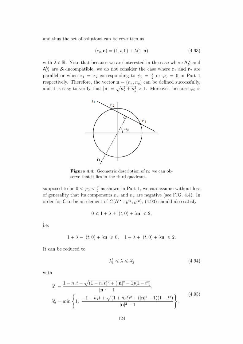
and thus the set of solutions can be rewritten as
pc0, cq “ p1, t, 0q ` λp1,nq (4.93)
with λ P R. Note that because we are interested in the case where AtxD and
AtyD are S1-incompatible, we do not consider the case where r1 and r2 are
parallel or when x1 “ x2 corresponding to ψ0 “π2
or ϕ0 “ 0 in Part 1
respectively. Therefore, the vector n “ pnx, nyq can be defined successfully,
and it is easy to verify that |n| “a
n2x ` n
2y ą 1. Moreover, because ϕ0 is
Figure 4.4: Geometric description of n: we can ob-serve that it lies in the third quadrant.
supposed to be 0 ă ϕ0 ăπ2
as shown in Part 1, we can assume without loss
of generality that its components nx and ny are negative (see FIG. 4.4). In
order for C to be an element of CpAtx : %r1 , %r2q, (4.93) should also satisfy
0 ď 1` λ˘ |pt, 0q ` λn| ď 2,
i.e.
1` λ´ |pt, 0q ` λn| ě 0, 1` λ` |pt, 0q ` λn| ď 2.
It can be reduced to
λt1 ď λ ď λt2 (4.94)
with
λt1 “1´ nxt´
a
p1´ nxtq2 ` p|n|2 ´ 1qp1´ t2q
|n|2 ´ 1,
λt2 “ min
#
1,´1´ nxt`
a
p1` nxtq2 ` p|n|2 ´ 1qp1´ t2q
|n|2 ´ 1
+
,
(4.95)
124
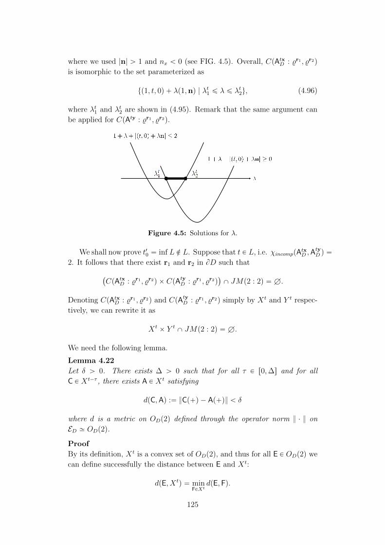
where we used |n| ą 1 and nx ă 0 (see FIG. 4.5). Overall, CpAtxD : %r1 , %r2q
is isomorphic to the set parameterized as
tp1, t, 0q ` λp1,nq | λt1 ď λ ď λt2u, (4.96)
where λt1 and λt2 are shown in (4.95). Remark that the same argument can
be applied for CpAty : %r1 , %r2q.
Figure 4.5: Solutions for λ.
We shall now prove t10 “ inf L R L. Suppose that t P L, i.e. χincomppAtxD ,A
tyD q “
2. It follows that there exist r1 and r2 in BD such that
`
CpAtxD : %r1 , %r2q ˆ CpAtyD : %r1 , %r2q˘
X JMp2 : 2q “ H.
Denoting CpAtxD : %r1 , %r2q and CpAtyD : %r1 , %r2q simply by X t and Y t respec-
tively, we can rewrite it as
X tˆ Y t
X JMp2 : 2q “ H.
We need the following lemma.
Lemma 4.22
Let δ ą 0. There exists ∆ ą 0 such that for all τ P r0,∆s and for all
C P X t´τ , there exists A P X t satisfying
dpC,Aq :“ Cp`q ´ Ap`q ă δ
where d is a metric on ODp2q defined through the operator norm ¨ on
ED » ODp2q.
Proof
By its definition, X t is a convex set of ODp2q, and thus for all E P ODp2q we
can define successfully the distance between E and X t:
dpE, X tq “ min
FPXtdpE,Fq.
125
In particular, for E1 P X t´∆1 Ă ODp2q with ∆1 ą 0 and E1p`q “ 12pe101`e1 ¨σq,
it becomes
dpE1, X tq “ min
FPXtdpE1,Fq “ min
FPXt
1
2p|e10 ´ f0| ` |e´ f |q , (4.97)
where Fp`q “ 12pf01`f ¨σq (see (4.92)). Since, in terms of (4.96), E1 P X t´∆1
and F P X t imply
pe10, e1q “ p1, t´∆1, 0q ` λ1p1,nq
with λt´∆1
1 ď λ1 ď λt´∆1
2 and
pf0, fq “ p1, t, 0q ` λp1,nq
with λt1 ď λ ď λt2 respectively, (4.97) can be rewritten as
2dpE1, X tq “ min
λPrλt1,λt2sp|λ1 ´ λ| ` |p´∆1, 0q ` pλ1 ´ λqn|q .
It follows that
2dpE1, X tq ď ∆1
` minλPrλt1,λ
t2s|λ1 ´ λ|p1` |n|q. (4.98)
Let us evaluate its right hand side. It is easy to see that
minλPrλt1,λ
t2s|λ1 ´ λ| “
$
’
&
’
%
λt1 ´ λ1
pλ1 ă λt1q
0 pλt1 ď λ1 ď λt2q
λ1 ´ λt2 pλ1 ą λt2q
.
Suppose that λ1 ă λt1 holds, for example. In this case, because λt´∆1
1 ď λ1,
we can obtain
λt1 ´ λ1ď λt1 ´ λ
t´∆1
1 .
In a similar way, it can be demonstrated that
supλ1Prλt´∆1
1 ,λt´∆1
2 s
minλPrλt1,λ
t2s|λ1 ´ λ| “ max
!
λt1 ´ λt´∆1
1 , 0, λt´∆1
2 ´ λt2
)
.
By virtue of (4.95), the right hand side converges to 0 as ∆1 Ñ 0, and thus
we can see from (4.98) that
supE1PXt´∆1
dpE1, X tq ÝÑ
∆1Ñ00
126
It results in that there exists ∆ ą 0 such that for all τ P r0,∆s,
supE1PXt´τ
dpE1, X tq ă δ
holds, that is, dpC, X tq ă δ holds for any C P X t´τ . Moreover, because X t is
convex, there exists A P X t satisfying dpC, X tq “ dpC,Aq, which proves the
claim of the lemma. 2
Note that a similar statement also holds for Y t: there exists r∆ ą 0 such
that for all rτ P r0, r∆s and for all D P Y t´rτ , there exists B P Y t satisfying
dpD,Bq ă δ. Let V :“ ODp2q ˆ ODp2qp» ED ˆ EDq and let dV be a product
metric on V defined as
dV ppA,Bq, pC,Dqq “ maxtdpA,Cq, dpB,Dqu.
According to Lemma 4.22 and its Y t-counterpart, if we take ∆0 “ mint∆, r∆upą
0q, then there exists pA,Bq P X t ˆ Y t for all pC,Dq P X t´∆0 ˆ Y t´∆0 such
that dV ppA,Bq, pC,Dqq ă δ. On the other hand, as we have seen, it holds
that
X tˆ Y t
X JMp2 : 2q “ H.
Since X t ˆ Y t and JMp2 : 2q are closed in V , and V is a metric space, we
can apply Urysohn’s Lemma [153]. It follows that there exists a continuous
(in fact uniformly continuous since V is compact) function f : V Ñ r0, 1s
satisfying fpUq “ 0 for any U P X tˆY t and fpW q “ 1 for any W P JMp2 :
2q. The uniform continuity of f implies that for some ε P p0, 1q, there is
δ ą 0 such that
dV ppE1,F1q, pE,Fqq ă δ ñ |f ppE1,F1qq ´ f ppE,Fqq| ă ε (4.99)
holds for any pE,Fq P V . For this δ, we can apply the argument above: we
can take ∆0 ą 0 such that for any pC,Dq P X t´∆0 ˆ Y t´∆0 , there exists
pA,Bq P X t ˆ Y t satisfying dV ppA,Bq, pC,Dqq ă δ. Because fppA,Bqq “ 0,
we have fppC,Dqq ă ε ă 1 (see (4.99)), and thus pC,Dq R JMp2 : 2q . It
indicates that X t´∆0 ˆ Y t´∆0 X JMp2 : 2q “ H, that is, there is ∆0 ą 0 for
any t P L satisfying t´∆0 P L. Therefore, t10 “ inf L R L can be concluded.
127
Chapter 5
Thermodynamical entropy of
mixing in regular polygon
theories
The concept of entropy plays an important role in thermodynamics [154,
155]. It is possible to calculate the thermodynamical entropy of a mixture
of classically different kinds of particles (such as a mixture of nitrogens and
oxygens), and similar ideas were applied by von Neumann to the case where
the system was composed of particles with different quantum internal states
[5]. Similarly to the previous parts, it is expected that generalizing the no-
tion of entropy to GPTs will help us to understand how entropy can affect
our world. In fact, there have been researches which aim to introduce and
investigate the concept of entropy in GPTs from informational perspectives
[62, 156, 157, 158]. In those researches, some kinds of entropy were de-
fined in all theories of GPTs and their information-theoretical properties
were investigated. Meanwhile, there have been also researches referring to
the thermodynamical entropy in terms of the microcanonical or canonical
formulation in GPTs [159, 160], and researches referring to the thermody-
namical entropy of mixing in GPTs [118, 161]. However, in those works,
the entropy was only defined in or applied to some restricted theories of
GPTs with special assumptions such as the existence of a spectral decompo-
sition for any state into perfectly distinguishable pure states. In particular,
it can be found that regular polygon theories do not always satisfy those
assumptions, and thus entropy in regular polygon has never been investi-
gated although they can be regarded as intermediate theories of a classical
trit system and a qubit-like system, where entropy is defined successfully.
It seems natural to ask how entropy of mixing behaves in regular polygon
theories.
In this part, we consider thermodynamical entropy of mixing in regular
128
polygon theories. It is proven that the operationally natural thermody-
namical entropy of a mixture of ideal particles with different internal states
described by a regular polygon theory exists if and only if the state space
of theory is triangle-shaped or disc-shaped, i.e., the theory is either classical
or quantum-like. More precisely, we demonstrate that the thermodynamical
entropy of mixing satisfying conditions imposed in [118], where the concrete
operational construction of the entropy was given as von Neumann did un-
der the assumption of the existence of semipermeable membranes, does not
exist in all the regular polygon theories except for classical and quantum-like
ones.
This part is organized as follows. In Section 5.1, we present a general-
ization of thermodynamically natural entropy of mixing in GPTs. We will
see that the notion of perfect distinguishability plays an important role to
define entropy also in GPTs. Then we demonstrate our main theorem and
its proof in Section 5.2.
5.1 Entropy of mixing in GPTs
In this section, we introduce the thermodynamically consistent definition of
entropy of mixing in GPTs based on the notion of perfect distinguishability.
5.1.1 Perfect distinguishablity for regular polygon the-
ories
We recall that a family of states tωiui is called perfectly distinguishable if
there exists an observable teiui such that eipωjq “ δij. Let us characterize
perfectly distinguishable states in regular polygon theories. We first consider
the regular polygon theory with n sides, where n is an even number greater
than two. Calculating the Euclidean inner product (denoted by p¨, ¨q here)
of pure effects and pure states in Subsection 2.5.3, we obtain
peni , ωni q “
`
eni , ωni´1
˘
“ 1, peni , ωni`n
2´1q “ pe
ni , ω
ni`n
2q “ 0.
These equations indicate that any state in Ωri´1, isn is perfectly distinguishable
from any state in Ωri`n
2´1, i`n
2s
n , where we define
Ωrk´1, ksn “ tω P Ωn | ω “ pωnk´1 ` p1´ pqω
nk , 0 ď p ď 1u,
since the measurement teni , u´ eni u distinguishes perfectly those two states.
For odd n pě 3q, we obtain
peni , ωni q “ 1, peni , ω
ni`n´1
2q “ peni , ω
ni`n`1
2q “ 0.
129
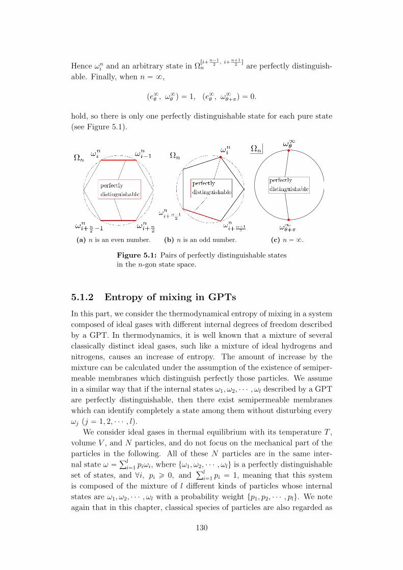
Hence ωni and an arbitrary state in Ωri`n´1
2, i`n`1
2s
n are perfectly distinguish-
able. Finally, when n “ 8,
pe8θ , ω8θ q “ 1, pe8θ , ω
8θ`πq “ 0.
hold, so there is only one perfectly distinguishable state for each pure state
(see Figure 5.1).
(a) n is an even number. (b) n is an odd number. (c) n “ 8.
Figure 5.1: Pairs of perfectly distinguishable statesin the n-gon state space.
5.1.2 Entropy of mixing in GPTs
In this part, we consider the thermodynamical entropy of mixing in a system
composed of ideal gases with different internal degrees of freedom described
by a GPT. In thermodynamics, it is well known that a mixture of several
classically distinct ideal gases, such like a mixture of ideal hydrogens and
nitrogens, causes an increase of entropy. The amount of increase by the
mixture can be calculated under the assumption of the existence of semiper-
meable membranes which distinguish perfectly those particles. We assume
in a similar way that if the internal states ω1, ω2, ¨ ¨ ¨ , ωl described by a GPT
are perfectly distinguishable, then there exist semipermeable membranes
which can identify completely a state among them without disturbing every
ωj pj “ 1, 2, ¨ ¨ ¨ , lq.
We consider ideal gases in thermal equilibrium with its temperature T ,
volume V , and N particles, and do not focus on the mechanical part of the
particles in the following. All of these N particles are in the same inter-
nal state ω “řli“1 piωi, where tω1, ω2, ¨ ¨ ¨ , ωlu is a perfectly distinguishable
set of states, and @i, pi ě 0, andřli“1 pi “ 1, meaning that this system
is composed of the mixture of l different kinds of particles whose internal
states are ω1, ω2, ¨ ¨ ¨ , ωl with a probability weight tp1, p2, ¨ ¨ ¨ , plu. We note
again that in this chapter, classical species of particles are also regarded as
130
the internal states of them. In classical thermodynamics, thermodynamical
entropy is calculated by constructing concrete thermodynamical operations
such as isothermal or adiabatic quasistatic operations. We follow this doc-
trine of thermodynamics also in GPTs that thermodynamical entropy, espe-
cially thermodynamical entropy of mixing, should be operationally-derived
quantity. In fact, as shown in [118], our assumption of the existence of
semipermeable membranes makes it possible to realize concrete thermody-
namical operations to calculate the thermodynamical entropy of mixing of
the system mentioned above in the same way as von Neumann did when the
internal degrees of freedom were quantum [5]. Strictly speaking, it has been
demonstrated operationally in [118] that the thermodynamical entropy of
mixing in the system is
Spωq “lÿ
i“1
piSpωiq ´lÿ
i“1
pi log pi , (5.1)
where Spσq means the per-particle thermodynamical entropy of mixing in
the system which consists of particles in the same state σ, and we set the
Boltzmann constant kB “ 1 (also 0 log 0 “ 0). In the process of deriving
(5.2), the additivity and extensivity of the thermodynamical entropy, and the
continuity of S with respect to states are assumed. The latter one is needed
in order to apply (5.2) to arbitrary states with an arbitrary probability
weight, while its operational derivation has been given only when each piN
is the number of particles in the state ωi and thus each pi is rational. We
impose additional assumption that the entropy of any pure state is equal to
zero, that is, Spσq “ 0 whenever σ is a pure state.
5.2 Main result
Our main result is in the following form.
Theorem 5.1
Consider a system in thermal equilibrium composed of ideal gases whose
internal states are described an element of the state space Ωn of the regular
polygon theory with n sides (n ě 3). The (per-particle) thermodynamical
entropy of mixing S : Ωn Ñ R satisfying
Spωq “lÿ
i“1
piSpωiq ´lÿ
i“1
pi log pi, (5.2)
where tωiui is a family of perfectly distinguishable states, exists if and only
if n “ 3 or 8, that is, the state space is classical or quantum-like.
131
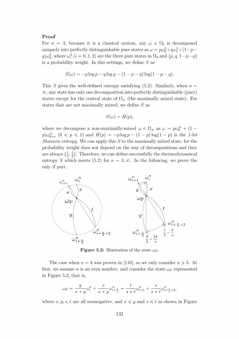
Proof
For n “ 3, because it is a classical system, any ω P Ω3 is decomposed
uniquely into perfectly distinguishable pure states as ω “ pω30`qω
31`p1´p´
qqω32, where ω3
i pi “ 0, 1, 2q are the three pure states in Ω3 and tp, q, 1´p´qu
is a probability weight. In this settings, we define S as
Spωq “ ´p log p´ q log q ´ p1´ p´ qq logp1´ p´ qq.
This S gives the well-defined entropy satisfying (5.2). Similarly, when n “
8, any state has only one decomposition into perfectly distinguishable (pure)
states except for the central state of Ω8 (the maximally mixed state). For
states that are not maximally mixed, we define S as
Spωq “ Hppq,
where we decompose a non-maximally-mixed ω P Ω8 as ω “ pω8θ ` p1 ´
pqω8θ`π p0 ď p ď 1q and Hppq “ ´p log p ´ p1 ´ pq logp1 ´ pq is the 1-bit
Shannon entropy. We can apply this S to the maximally mixed state, for the
probability weight does not depend on the way of decompositions and they
are always t12, 1
2u. Therefore, we can define successfully the thermodynamical
entropy S which meets (5.2) for n “ 3,8. In the following, we prove the
only if part.
Figure 5.2: Illustration of the state ωP.
The case when n “ 4 was proven in [118], so we only consider n ě 5. At
first, we assume n is an even number, and consider the state ωP represented
in Figure 5.2, that is,
ωP “y
x` yωni `
x
x` yωni`n
2“
t
s` tωni`1 `
s
s` tωni`n
2`2,
where x, y, s, t are all nonnegative, and x ď y and s ď t as shown in Figure
132
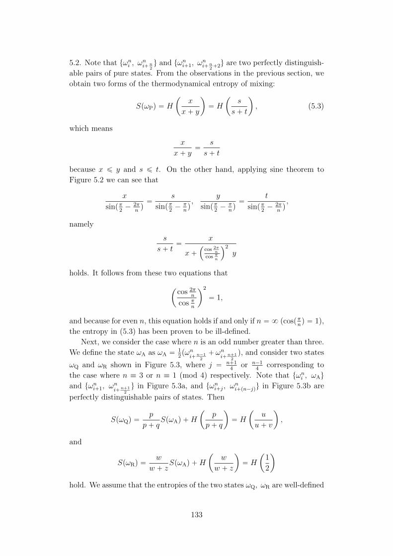
5.2. Note that tωni , ωni`n
2u and tωni`1, ω
ni`n
2`2u are two perfectly distinguish-
able pairs of pure states. From the observations in the previous section, we
obtain two forms of the thermodynamical entropy of mixing:
SpωPq “ H
ˆ
x
x` y
˙
“ H
ˆ
s
s` t
˙
, (5.3)
which means
x
x` y“
s
s` t
because x ď y and s ď t. On the other hand, applying sine theorem to
Figure 5.2 we can see that
x
sinpπ2´ 2π
nq“
s
sinpπ2´ π
nq,
y
sinpπ2´ π
nq“
t
sinpπ2´ 2π
nq,
namely
s
s` t“
x
x`´
cos 2πn
cos πn
¯2
y
holds. It follows from these two equations that
ˆ
cos 2πn
cos πn
˙2
“ 1,
and because for even n, this equation holds if and only if n “ 8 (cospπnq “ 1),
the entropy in (5.3) has been proven to be ill-defined.
Next, we consider the case where n is an odd number greater than three.
We define the state ωA as ωA “12pωn
i`n´12
`ωni`n`1
2
q, and consider two states
ωQ and ωR shown in Figure 5.3, where j “ n`14
or n´14
corresponding to
the case where n ” 3 or n ” 1 (mod 4) respectively. Note that tωni , ωAu
and tωni`1, ωni`n`1
2
u in Figure 5.3a, and tωni`j, ωni`pn´jqu in Figure 5.3b are
perfectly distinguishable pairs of states. Then
SpωQq “p
p` qSpωAq `H
ˆ
p
p` q
˙
“ H
ˆ
u
u` v
˙
,
and
SpωRq “w
w ` zSpωAq `H
ˆ
w
w ` z
˙
“ H
ˆ
1
2
˙
hold. We assume that the entropies of the two states ωQ, ωR are well-defined
133
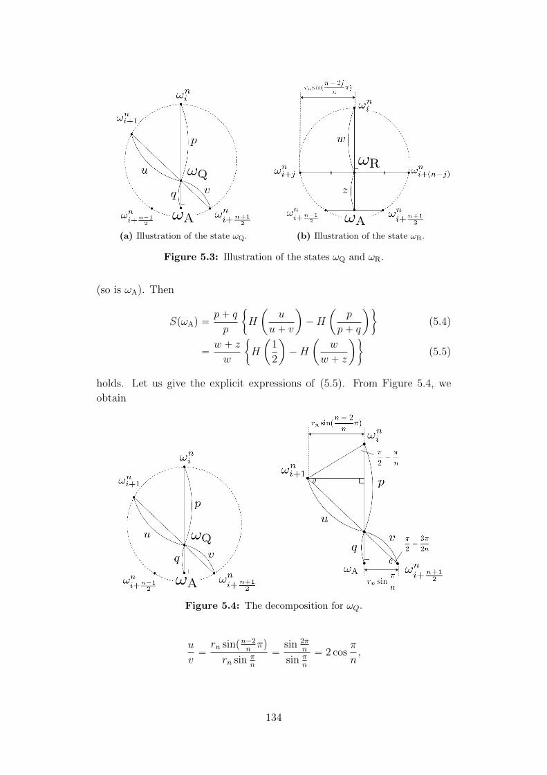
(a) Illustration of the state ωQ. (b) Illustration of the state ωR.
Figure 5.3: Illustration of the states ωQ and ωR.
(so is ωA). Then
SpωAq “p` q
p
"
H
ˆ
u
u` v
˙
´H
ˆ
p
p` q
˙*
(5.4)
“w ` z
w
"
H
ˆ
1
2
˙
´H
ˆ
w
w ` z
˙*
(5.5)
holds. Let us give the explicit expressions of (5.5). From Figure 5.4, we
obtain
Figure 5.4: The decomposition for ωQ.
u
v“rn sinpn´2
nπq
rn sin πn
“sin 2π
n
sin πn
“ 2 cosπ
n,
134
and by sine theorem,
p
sinpπ2´ π
2nq“
u
sinpπ2´ π
nq, q “ v cos
3π
2n
hold. Therefore,
q
p“v
u¨
cos πn¨ cos 3π
2n
cos π2n
“cos 3π
2n
2 cos π2n
“1
2
´
4 cos2 π
2n´ 3
¯
“1
2
´
2 cosπ
n´ 1
¯
.
On the other hand, from Figure 5.3b, we obtain
z
w“
2rn cos2 π2n´ 2rn cos2p
n´2j2n
πq
2rn cos2pn´2j
2nπq
“cos2 π
2n´ sin2 jπ
n
sin2 jπn
for j “n˘ 1
4.
(5.6)
Since
sin2 jπ
n“
1
2
ˆ
1´ cos2jπ
n
˙
“1
2
ˆ
1´ cospn˘ 1qπ
2n
˙
“1
2
´
1˘ sinπ
2n
¯
,
(5.7)
the equation above can be written as
z
w“
2p1` sin π2nqp1´ sin π
2nq ´ p1˘ sin π
2nq
1˘ sin π2n
“ 1¯ 2 sinπ
2n,
where the double sign corresponds to the ones in (5.6) and (5.7), and the
upper and lower sign correspond to the case of n ” 3 and n ” 1 (mod 4)
respectively. Substituting these results to (5.4) and (5.5), we obtain
SpωAq “
ˆ
2 cos πn` 1
2
˙"
H
ˆ
1
2 cos πn` 1
˙
´H
ˆ
2
2 cos πn` 1
˙*
“
´
2¯ 2 sinπ
2n
¯
"
H
ˆ
1
2
˙
´H
ˆ
1
2¯ 2 sin π2n
˙*
.
135
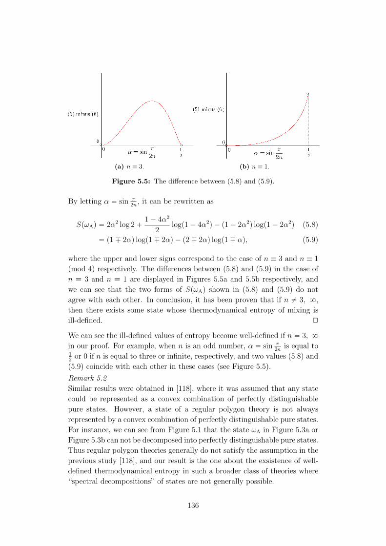
(a) n ” 3. (b) n ” 1.
Figure 5.5: The difference between (5.8) and (5.9).
By letting α “ sin π2n
, it can be rewritten as
SpωAq “ 2α2 log 2`1´ 4α2
2logp1´ 4α2
q ´ p1´ 2α2q logp1´ 2α2
q (5.8)
“ p1¯ 2αq logp1¯ 2αq ´ p2¯ 2αq logp1¯ αq, (5.9)
where the upper and lower signs correspond to the case of n ” 3 and n ” 1
(mod 4) respectively. The differences between (5.8) and (5.9) in the case of
n ” 3 and n ” 1 are displayed in Figures 5.5a and 5.5b respectively, and
we can see that the two forms of SpωAq shown in (5.8) and (5.9) do not
agree with each other. In conclusion, it has been proven that if n ‰ 3, 8,
then there exists some state whose thermodynamical entropy of mixing is
ill-defined. 2
We can see the ill-defined values of entropy become well-defined if n “ 3, 8
in our proof. For example, when n is an odd number, α “ sin π2n
is equal to12
or 0 if n is equal to three or infinite, respectively, and two values (5.8) and
(5.9) coincide with each other in these cases (see Figure 5.5).
Remark 5.2
Similar results were obtained in [118], where it was assumed that any state
could be represented as a convex combination of perfectly distinguishable
pure states. However, a state of a regular polygon theory is not always
represented by a convex combination of perfectly distinguishable pure states.
For instance, we can see from Figure 5.1 that the state ωA in Figure 5.3a or
Figure 5.3b can not be decomposed into perfectly distinguishable pure states.
Thus regular polygon theories generally do not satisfy the assumption in the
previous study [118], and our result is the one about the exsistence of well-
defined thermodynamical entropy in such a broader class of theories where
“spectral decompositions” of states are not generally possible.
136
Chapter 6
Summary
In this thesis, we have studied the notion of uncertainty in quantum the-
ory via convexity. We focused on three expressions of uncertainty: uncer-
tainty relations, incompatibility, and thermodynamical entropy. Our estab-
lishments were based on the idea that to see quantum uncertainty from a
broader point of view makes it possible to understand its essence. In fact,
in each chapter, we considered uncertainty relations and thermodynamical
entropy in a broader class of theories than quantum theory, and investigated
quantum incompatibility, which is a broader notion than uncertainty.
In Chapter 2, we introduced the mathematical framework of GPTs. We
saw that GPTs are constructed by requiring only primitive convexity origi-
nating from probability mixtures, and thus in this sense, they are the most
general description of nature (in particular, broader than quantum theory).
There were proven that GPTs can be expressed mathematically in terms of
ordered Banach spaces, and that it indeed reproduce the usual formulation
of quantum theory.
In Chapter 3, several generalizations of uncertainty relations such as en-
tropic uncertainty relations were considered in a class of GPTs which can
be considered as generalized theories of quantum theory. It was revealed
that similar quantitative relations between preparation and measurement
uncertainty to quantum case hold also in GPTs although only theories with
transitivity and self-duality with respect to a certain inner product were
considered. We also gave concrete calculations of our results for regular
polygon theories. What is also specific to theorems is that they were ob-
tained without considering entanglement or even composite systems while
the quantum results of the previous studies were based on the “ricochet”
property of maximally entangled states. It may be indicated that some
of the characteristics of quantum theory can be obtained without entan-
glement. Future research should reveal the relations between the maximal
entanglement and self-duality, which will be a key to generalizing our theo-
rems to infinite-dimensional cases (remember that the maximally entangled
137
states cannot be defined in infinite-dimensional quantum theories such as
H “ L2pRq). To find information-theoretic applications of our results is also
left for future work.
In Chapter 4, we focused on incompatibility in quantum theory, and
introduced the notions of compatibility and incompatibility dimensions for
collections of quantum devices. They describe the minimum number of
states which are needed to detect incompatibility and the maximum num-
ber of states on which incompatibility vanishes, respectively. We have not
only presented general properties of those quantities but also examined con-
crete behaviors of them for a pair of unbiased qubit observables. We have
proven that even for this simple pair of incompatible observables there exist
two types of incompatibility with different incompatibility dimensions which
cannot be observed if we focus only on robustness of incompatibility under
noise. We expect that it is possible to apply this difference to some quantum
protocols such as quantum cryptography. Future work will be needed to in-
vestigate whether similar results can be obtained for observables in higher
dimensional Hilbert space or other quantum devices. As the definitions ap-
ply to devices in GPTs, an interesting task is further to see how quantum
incompatibility dimension differs from incompatibility dimension in general.
In Chapter 5, we returned to GPTs and considered theremodynamical
entropy in regular polygon theories. We showed that only classical and
quantum-like theories (i.e. the triangle and disc theories respectively) al-
low the operationally natural entropy to be consistent. Further research is
required to reveal if we can obtain the same results in higher dimensional
cases. Moreover, the proof of our main theorem indicates that the entropy
discussed above is defined successfully in other theories where the probabil-
ity coefficients obtained when a state is decomposed into perfectly distin-
guishable states are unique even though the state space is neither classical
nor quantum. This means that we need to impose additional conditions on
the entropy to remove those“unreasonable” theories, which is also a future
problem.
138
Acknowledgments
I would like to, first and foremost, thank my supervisor Takayuki Miyadera.
Since I became his student in 2016, he has taught me many interesting things
on quantum theory to lead me to the study of quantum foundations. Topics
such as quantum uncertainty or incompatibility are examples of those things,
and they are now the main interest of my research. His insightful guidance,
not only as a great researcher but also as a great person, has helped and will
help me a lot in my research and daily life. Nothing in my nine-year college
experience makes me more proud of than being his student and able to learn
from him. I also would like to thank my collaborator Teiko Heinosaari.
I feel very honored to have worked with such a great person and exhibit
our results in my PhD thesis. I cannot miss thanking all members of my
laboratory, especially Kenzo Ogure, Ikko Hamamura, and Kazuki Yamaga,
for their fruitful help in my study. This research has been supported by
JSPS KAKENHI Grant Number JP21J10096, and I also acknowledge the
JSPS Research Fellowship for Young Scientists.
Finally, I would like to express my thanks to my family and friends. I
am grateful to my parents for giving me birth with so good a constitution
that I can stay healthy in everyday life. I also thank my friends for their
encouragement and support. They are all great persons, and examples for
me. I have learned from them what are the most important things in life.
Those things are always within my mind, and are the principles that guide
my life. My deepest gratitude is expressed to my grandparents. The greatest
thing in my life is that they are my grandparents. We live so far that we
cannot often see each other, but I always feel their love supporting and
encouraging me in my daily life. I hope that my accomplishment of this
PhD study will be their pleasure.
139
Appendix
A Proof of Proposition 2.53
In this part, we give a proof of Proposition 2.53. We need the following
proposition, which holds without the assumption of the transitivity of Ω.
Proposition A.1
For a state space Ω, define a linear map PM : V Ñ V by
PMx “
ż
GLpΩq
Tx dµpT q.
Then PM is an orthogonal projection with respect to the inner product x¨, ¨yGLpΩq,
i.e.
PM “ P 2M and xPMx, yyGLpΩq “ xx, PMyyGLpΩq for all x, y P V.
Proof
We denote the inner product x¨, ¨yGLpΩq simply by x¨, ¨y in this proof.
Let VM :“ tx P V | Tx “ x for all T P GLpΩqu be the set of all fixed
points with respect to GLpΩq. Then it is easy to see that PMxM “ xMfor any xM P VM and VM “ ImPM (in particular VM is a subspace of V ).
Therefore,
P 2Mx “ PMpPMxq “ PMx
holds for any x P V , and thus P 2M “ PM . On the other hand, we can observe
xPMx, yy “
ż
GLpΩq
dµpT q pTPMx, TyqE
“
ż
GLpΩq
dµpT q pPMx, TyqE
“
ż
GLpΩq
dµpT q
ˆż
GLpΩq
dµpSqSx, Ty
˙
E
. (A.1)
Let us fix an orthonormal basis twiuN`1i“1 of V compatible with the standard
140
Euclidean inner product of V , i.e.
pwi, wjqE “ δij.
We can consider representing the vectorş
GLpΩqdµpSqSx P V by means of
the orthonormal basis twiui as
ż
GLpΩq
dµpSqSx “ÿ
i
ˆ
wi,
ż
GLpΩq
dµpSqSx
˙
E
wi.
In fact, the “ith-element”´
wi,ş
GLpΩqdµpSqSx
¯
Eis given by (see [162] for
more details)
ˆ
wi,
ż
GLpΩq
dµpSqSx
˙
E
“
ż
GLpΩq
dµpSq pwi, SxqE.
It results inˆż
GLpΩq
dµpSqSx, Ty
˙
E
“ÿ
i
„ż
GLpΩq
dµpSqpwi, SxqE
pwi, T yqE
“
ż
GLpΩq
dµpSq
«
ÿ
i
pSx, wiqEpwi, T yqE
ff
“
ż
GLpΩq
dµpSqpSx, TyqE.
Therefore, we obtain
ż
GLpΩq
dµpT q
ˆż
GLpΩq
dµpSqSx, Ty
˙
E
“
ż
GLpΩq
dµpT q
„ż
GLpΩq
dµpSq pSx, TyqE
“
ż
GLpΩq
dµpSq
„ż
GLpΩq
dµpT q pSx, TyqE
“
ż
GLpΩq
dµpSq
ˆ
Sx,
ż
GLpΩq
dµpT qTy
˙
E
,
where we use Fubini’s theorem for the finite Haar measure µ on GLpΩq. We
can conclude together with (A.1) that
xPMx, yy “ xx, PMyy
holds. 2
Proposition A.1 enables us to give an orthogonal decomposition of a
141
vector x P V such that
x “ p1´ PMqx` PMx, (A.2)
where p1 ´ PMqx P V KM and PMx P VM . When the transitivity of Ω is
assumed, (A.2) is reduced to Proposition 2.53.
Proposition 2.53
For a transitive state space Ω, there exists a basis tvluN`1l“1 of V orthonormal
with respect to the inner product x¨, ¨yGLpΩq such that vN`1 “ ωM and
x P aff pΩq ðñ x “Nÿ
l“1
alvl ` vN`1 “
Nÿ
l“1
alvl ` ωM pa1, ¨ ¨ ¨ , aN P Rq.
Proof
Since we set dimaff pΩq “ N , there exists a set of N linear independent vec-
tors tvluNl“1 Ă raff pΩq´ωM s which forms a basis of the N -dimensional vector
subspace raff pΩq´ωM s Ă V , and we can assume by taking an orthonormal-
ization that they are orthonormal with respect to the inner product x¨, ¨y.
Hence x P aff pΩq if and only if it is represented as
x “Nÿ
l“1
alvl ` ωM pa1, ¨ ¨ ¨ , aN P Rq. (A.3)
Moreover, because of the definition of aff pΩq, for every vl P raff pΩq ´ ωM s
there exist k P N, real numbers tbiuki“1 satisfying
řki“1 bi “ 1, and states
tωiuki“1 such that vl “
řki“1 biωi ´ ωM . By means of Proposition 2.52, we
obtain for all l “ 1, 2, ¨ ¨ ¨ , N
PMvl “kÿ
i“1
biPMωi ´ PMωM
“
kÿ
i“1
biωM ´ ωM “ 0. (A.4)
Therefore, because of Proposition A.1
xωM , vly “ xPMωM , vly
“ xωM , PMvly
“ 0
holds for all l “ 1, 2, ¨ ¨ ¨ , N , and we can conclude together with the unit
norm of ωM that tv1, ¨ ¨ ¨ , vN , ωMu in (A.3) forms an orthonormal basis of
the pN`1q-dimensional vector space V with respect to x¨, ¨y and Proposition
142
2.53 is proven (we can also find that (A.3) corresponds to (A.2)). 2
B Proof of Proposition 2.55
In this part, we prove Proposition 2.55. As we have so far, we let Ω be a
state space, V` be the positive cone generated by Ω, and GLpΩq be the set
of all state automorphisms on Ω in the following.
Lemma B.1
V ˚int`x¨,¨yGLpΩq
is a GLpΩq-invariant set. That is, TV ˚int`x¨,¨yGLpΩq
“ V ˚int`x¨,¨yGLpΩq
for
all T P GLpΩq.
Proof
Let w P V ˚int`x¨,¨yGLpΩq
. It holds that xw, vyGLpΩq ě 0 for all v P V`. Because
any T P GLpΩq is an orthogonal transformation with respect to x¨, ¨yGLpΩq,
we obtain
xTw, vyGLpΩq “ xw, T´1vyGLpΩq ě 0
for all v P V`. Therefore, TV ˚int`x¨,¨yGLpΩq
Ă V ˚int`x¨,¨yGLpΩq
holds, and a similar
argument for T´1 P GLpΩq proves the lemma. 2
Lemma B.2
Let p¨, ¨q be an arbitrary inner product on V . V` is self-dual if and only
if there exists a linear map J : V Ñ V such that J is strictly positive with
respect to p¨, ¨q, i.e. px, Jyq “ pJx, yq for all x, y P V and px, Jxq ą 0 for all
x P V , and JpV`q “ V ˚int`p¨,¨q.
Proof
If part: We introduce an inner product p¨, ¨qJ “ p¨, J ¨q. V˚int`p¨,¨qJ
is written as
V ˚int`p¨,¨qJ“ tv | pv, wqJ ě 0, @w P V`u
“ tv | pv, Jwq ě 0, @w P V`u
“ tv | pJv, wq ě 0, @w P V`u.
Thus v P V ˚int`p¨,¨qJ
is equivalent to Jv P V ˚int`p¨,¨q. It concludes V ˚int
`p¨,¨qJ“ J´1pV ˚int
`p¨,¨qq “
V`.
Only if part: Let V` be self-dual with respect to an inner product x¨, ¨y.
There exists some K : V Ñ V strictly positive with respect to p¨, ¨q such
that x¨, ¨y “ p¨, K¨q. We obtain
V` “ V ˚int`x¨,¨y “ tv| xv, wy ě 0, @w P V`u
“ tv| pv,Kwq ě 0, @w P V`u
“ tv| pKv,wq ě 0, @w P V`u
143
Thus v P V` “ V ˚int`x¨,¨y is equivalent to Kv P V ˚int
`p¨,¨q, i.e. KV` “ V ˚int`p¨,¨q. Define
J “ K. 2
In Lemma B.2, we gave a necessary and sufficient condition for V` with
an inner product p¨, ¨q to be self-dual. The condition was the existence of a
strictly positive map J satisfying JpV`q “ V ˚int`p¨,¨q. This map J may not be
unique. For instance, let us consider a classical system in R2 whose extreme
points are two points p1, 1q and p1,´1q. The positive cone is a “forward
lightcone” V` “ tpx0, x1q| x0 ě 0, x20 ´ x2
1 ě 0u. It is easy to see that
V` “ V ˚int`p¨,¨qE
with the standard Euclidean inner product p¨, ¨qE. However,
if we choose an orthogonal basis tv0, v1u of R2 given by v0 “ p1, 1q and
v1 “ p1,´1q, then every linear map of the form
˜
v0
v1
¸
ÞÑ
˜
λ0v0
λ1v1
¸
for λ0, λ1 ą 0 (which contains “Lorentz transformations” in 1`1 dimension)
is strictly positive and makes V` invariant. Nevertheless, when |Ωext| ă 8,
we can demonstrate that such strictly positive maps are “equivalent” to each
other .
Lemma B.3
Let |Ωext| ă 8. If a linear map J : V Ñ V is strictly positive with respect to
an inner product p¨, ¨q, i.e. px, Jyq “ pJx, yq for all x, y P V and px, Jxq ą 0
for all x P V , and satisfies JpV`q “ V`, then for each ωext P Ωext there exists
µpωextq ą 0 such that Jpωextq “ µpωextqωext.
Proof
Any ωext P Ωext is represented as ωext “ cpωextqw with cpωextq :“ ωext “
pωext, ωextq12 and w satisfying w “ 1. Suppose that there exists a family
tωextk u
Zk“1 “ tcpω
extk qwku
Zk“1 Ă Ωext
such that there is no µpωextk q ą 0 for every k “ 1, 2, ¨ ¨ ¨ , Z satisfying
Jpωextk q “ µpωext
k qωextk , and define W :“ twku
Zk“1. Since J maps each ex-
treme ray of V` to an extreme ray of V`, Jpwkq with wk P W is proportional
to some ωext P Ωext (remember that an extreme ray of V` is the set of positive
scalar multiples of an extreme point of Ω). We can see that Jpwkq is pro-
portional to some wp P W with p ‰ k considering that JpJpwkqq “ µJpwkq
holds if and only if Jpwkq “ µwk holds.
We shall show in the following that there is a wq P W such that Jpwqq R
W despite of the argument above. To prove the claim, let us diagonalize J . It
is written as J “řMn“1 τnRn, where τ1 ą τ2 ą ¨ ¨ ¨ ą τM ą 0 and tRnu
Mn“1 are
orthogonal projections. We choose w1 so that 0 ‰ pw1, R1w1q ě pwk, R1wkq
144
for all wk P W . Although such w1 may not be unique, the following argument
does not depend on the choice. If it happens that pwk, R1wkq “ 0 for all
wk P W , we choose w1 so that 0 ‰ pw1, R2w1q ě pwk, R2wkq for all wk P W .
If still pwk, R2wkq “ 0 for all wk P W , we repeat the argument for R3, R4, ¨ ¨ ¨ .
For simplicity, we assume hereafter that pw1, R1w1q ‰ 0 holds. The general
cases can be treated similarly. Let r1 :“ R1w1R1w1 ‰ 0, then J is written
as
J “ τ1 |r1yxr1| ` τ1pR1 ´ |r1yxr1|q `ÿ
ně2
τnEn “ τ1R0 ` τ1R1 `ÿ
ně2
τnRn,
where we define R0 :“ |r1yxr1|, R1 :“ R1 ´ |r1yxr1| and Rn :“ Rn for n ě 2
satisfying RaRb “ δabRa for a, b “ 0, 1, ¨ ¨ ¨ ,M . Now we consider a vector
Jpw1q
Jpw1q“
τ1R0w1 ` τ1R1w1 `ř
ně2 τnRnw1´
τ 21 pw1, R0w1q ` τ 2
1 pw1, R1w1q `ř
ně2 τ2npw1, Rnw1q
¯12,
which must coincide with some wp P W . Its “R0 -element” can be calculated
asˆ
Jpw1q
Jpw1q, R0
Jpw1q
Jpw1q
˙
“τ 2
1 pw1, R0w1q
τ 21 pw1, R0w1q ` τ 2
1 pw1, R1w1q `ř
ně2 τ2npw1, Rnw1q
“pw1, R0w1q
pw1, R0w1q ` pw1, R1w1q `řMn“2
τ2n
τ21pw1, Rnw1q
. (B.1)
On the other hand, we can obtain that
pw1, R0w1q ` pw1, R1w1q `
Mÿ
n“2
τ 2n
τ 21
pw1, Rnw1q
ă pw1, R0w1q ` pw1, R1w1q `
Mÿ
n“2
pw1, Rnw1q “ 1
because there exists a n ě 2 such that pw1, Rnw1q ‰ 0 (otherwise w1 “
pR0 ` R1qw1 “ R1w1 and thus Jpw1q “ τ1w1 hold, which contradicts w1 P
W ). Therefore, (B.1) results in
ˆ
Jpw1q
Jpw1q, R0
Jpw1q
Jpw1q
˙
ą pw1, R0w1q.
This observation concludes a contradiction to Jpw1qJpw1q “ wp P W
145
because w1 satisfies pw1, R0w1q ě pwk, R0wkq for all wk P W . Overall, we find
that every ωext P Ωext has some µpωextq ą 0 such that Jpωextq “ µpωextqωext.
2
Lemma B.4
Let |Ωext| ă 8, and suppose that linear maps J and K strictly positive
with respect to an inner product p¨, ¨q satisfy JpV`q “ KpV`q “ V ˚int`p¨,¨q (in
particular, V` is self-dual). Then there exists a µpωextq ą 0 for each ωext P
Ωext such that Kpωextq “ µpωextqJpωextq holds.
Proof
As was seen in Lemma B.2, the inner products p¨, ¨qJ :“ p¨, J ¨q and p¨, ¨qK :“
p¨, K¨q satisfy V ˚int`p¨,¨qJ
“ V` and V ˚int`p¨,¨qK
“ V` respectively. Because p¨, ¨qKis represented as p¨, ¨qK “ p¨, L¨qJ with some linear map L strictly positive
with respect to p¨, ¨qJ , we have for arbitrary v, w P V
pv, wqK “ pv,Kwq “ pv, LwqJ “ pv, JLwq,
and thus L “ J´1 ˝K holds. On the other hand, L satisfies
V ˚int`p¨,¨qK“ tv | pv, wqK ě 0, @w P V`u
“ tv | pv, LwqJ ě 0, @w P V`u
“ tv | pLv,wqJ ě 0, @w P V`u “ L´1pV ˚int`p¨,¨qJ
q.
That is, LpV`q “ V` holds. Therefore, we can apply Lemma B.3 to L, and
conclude that
Lpωextq “ µpωext
qωext“ J´1
pKpωextqq,
i.e. Kpωextq “ µpωextqJpωextq holds. 2
Proposition 2.55
Let Ω be transitive with |Ωext| ă 8 and V` be self-dual with respect to some
inner product. There exists a linear bijection Ξ: V Ñ V such that Ω1 :“ ΞΩ
is transitive and the generating positive cone V 1` is self-dual with respect to
x¨, ¨yGLpΩ1q, i.e. V1
` “ V1˚int`x¨,¨yGLpΩ1q
.
Proof
Because of the transitivity of Ω, we can adopt the orthogonal coordinate
system of V introduced in Proposition 2.53. Since V` is self-dual, there
exists a linear map J : V Ñ V strictly positive with respect to x¨, ¨yGLpΩqsuch that JpV`q “ V ˚int
`x¨,¨yGLpΩq(Lemma B.2). We can assume without loss of
generality that J satisfies xωM , JωMyGLpΩq “ 1. Let us introduce
Ω˚ :“ V ˚int`x¨,¨yGLpΩqX rz “ 1s “ tv P V ˚int`x¨,¨yGLpΩq
| xv, ωMyGLpΩq “ 1u,
146
where we identify the “ωM -coordinate” with “z-coordinate” in V and define
rz “ 1s :“ tx P V | xx, ωMyGLpΩq “ 1up“ aff pΩqq (see Proposition 2.53).
Note that since both V ˚int`x¨,¨yGLpΩq
and rz “ 1s are GLpΩq-invariant, Ω˚ is
also GLpΩq-invariant. It is easy to demonstrate that Ω˚ is convex (and
compact), and we denote by Ω˚ext the set of all extreme points of Ω˚. We
can also see that Ω˚ext generates the extreme rays of V ˚int`x¨,¨yGLpΩq
. Because J
satisfying JpV`q “ V ˚int`x¨,¨yGLpΩq
is bijective and maps extreme rays of V` to
extreme rays of V ˚int`x¨,¨yGLpΩq
, it holds that |Ω˚ext| “ |Ωext|. Thus there exists
a bijection f : Ωext Ñ Ω˚ext and βpωextq ą 0 for each ωext P Ωext satisfying
Jpωextq “ βpωextqfpωextq.
For each T P GLpΩq, we introduce JT :“ T´1˝J ˝T . It is easy to see that
JT satisfies JT pV`q “ V ˚int`x¨,¨yGLpΩq
by virtue of Lemma B.1. Furthermore, JT is
shown to be strictly positive with respect to x¨, ¨yGLpΩq because T P GLpΩq is
an orthogonal transformation with respect to x¨, ¨yGLpΩq. Therefore, applying
Lemma B.4 to J and JT , there exists µT : Ωext Ñ Rą0 such that JT pωextq “
µT pωextqJpωextq for ωext P Ωext, that is,
JT pωextq “ µT pω
extqJpωext
q
“ µT pωextqβpωext
qfpωextq
“: βT pωextqfpωext
q,
where we define βT pωextq :“ µT pω
extqβpωextq. We calculate this βT pωextq. It
holds that
JT pωextq “ T´1
˝ JpTωextq
“ T´1pβpTωext
qfpTωextqq
“ βpTωextqT´1fpTωext
q
“ βT pωextqfpωext
q.
This relation shows that T´1fpTωextq is proportional to fpωextq. Considering
that the z-coordinates of fpTωextq and fpωextq are 1 and that T´1 preserves
z-coordinates, we find that T´1fpTωextq “ fpωextq (equivalently, fpTωextq “
Tfpωextq) holds. Consequently, we obtain
JT pωextq “ βpTωext
qfpωextq.
Now we introduce
Jav :“1
|GLpΩq|
ÿ
TPGLpΩq
JT .
We note that |GLpΩq| ă 8 when |Ωext| ă 8 because |GLpΩq| ď |Ωext| !. Jav
147
acts on ωext P Ωext as
Javpωextq “
1
|GLpΩq|
ÿ
TPGLpΩq
βpTωextq ¨ fpωext
q “: Cfpωextq,
where C :“ 1|GLpΩq|
ř
TPGLpΩq βpTωextq is a positive constant which does not
depend on the choice of ωext P Ωext because of the transitivity of Ω. Thus the
map satisfies JavpV`q “ V ˚int`x¨,¨yGLpΩq
since JavpΩextq “ CΩ˚ext, and is strictly
positive with respect to x¨, ¨yGLpΩq since it is a summation of the strictly
positive operators tJT uTPGLpΩq. Moreover, it satisfies
Jav ˝ T “ T ˝ Jav.
for any T P GLpΩq. We thus find that Jav ˝ PM “ PM ˝ Jav holds for the
orthogonal projection PM introduced in Proposition A.1. In fact,
JavpPMxq “1
|GLpΩq|Jav
¨
˝
ÿ
TPGLpΩq
Tx
˛
‚
“1
|GLpΩq|
ÿ
TPGLpΩq
T pJavxq
“ PMpJavxq
holds for all x P V . Therefore, Jav is decomposed into two parts as
Jav “ PM ˝ Jav ˝ PM ` PKM ˝ Jav ˝ P
KM , (B.2)
where PKM “ 1´PM . We note that V KM “ ImPKM “ raff pΩq´ωM s “ RN and
dim VM “ dim ImPM “ 1 hold by virtue of Proposition 2.53. Therefore,
the first part of (B.2) is proportional to 1VM “ 1z “ PM , and because we
set xωM , JωMyGLpΩq “ 1 and thus
xωM , PM ˝ Jav ˝ PMωMyGLpΩq “ xωM , JavωMyGLpΩq
“ xωM , PMJωMyGLpΩq
“ xωM , JωMyGLpΩq
“ 1
“ xωM , PMωMyGLpΩq
holds, it is proven that
PM ˝ Jav ˝ PM “ PM .
Let us examine the second part. Suppose that there exists a nonzero x P V KM
148
such that Tx “ x for all T P GLpΩq. Then PMx “ x ‰ 0 holds, and it
contradicts (A.4). Thus we can find that GLpΩq acts irreducibly on V KM , that
is, only t0u and V KM “ RN itself are invariant subspaces. It concludes that
PKMJavPKM , which commutes with every element in GLpΩq, is proportional to
1V KM“ 1RN “ PKM due to Schur’s lemma. Consequently, we obtain for some
ξ ą 0
Jav “ PM ` ξPKM ,
and thus
JavpV`q “ pPM ` ξPKMqpV`q “ V ˚int`x¨,¨yGLpΩq
. (B.3)
Let us introduce a linear bijection
Ξ :“a
Jav “ PM `a
ξPKM ,
strictly positive with respect to x¨, ¨yGLpΩq, and define Ω1 :“ ΞΩ. It is easy to
check that the positive cone V 1` generated by Ω1 is given by V 1` “ ΞV`, and
GLpΩ1q “ ΞGLpΩqΞ´1 “ GLpΩq (moreover, the unique maximally mixed
state of Ω1 is still ωM). In addition, we can find that
V1˚int`x¨,¨yGLpΩ1q
“ tv | xv, w1yGLpΩq ě 0, @w1 P V 1`u
“ tv | xv,ΞwyGLpΩq ě 0, @w P V`u
“ Ξ´1V ˚int`x¨,¨yGLpΩq.
holds. Since (B.3) can be rewritten as
ΞV` “ Ξ´1V ˚int`x¨,¨yGLpΩq,
we can conclude
V1
` “ V1˚int`x¨,¨yGLpΩ1q
.
2
Remark
In the case of |Ωext| “ 8, there exists a counterexample of Lemma B.3. Let
us consider a state space
Ω “ t tp1,xq “ tp1, x1, x2, x3q P R4
| |x|2 “ x21 ` x
22 ` x
23 ď 1u
(the Bloch ball). Ω defines a corresponding positive cone V` as
V` “ tx P R4| x2
0 ´ |x|2ě 0, x0 ě 0u,
149
which can be identified with a forward light cone of a Minkowski spacetime.
We examine a pure Lorentz transformation Λ defined for λ P R as
Λ “
»
—
—
—
–
coshλ sinhλ 0 0
sinhλ coshλ 0 0
0 0 1 0
0 0 0 1
fi
ffi
ffi
ffi
fl
.
It is easy to prove that this Λ is strictly positive. Since the pure Lorentz
transformation preserves the Minkowski metric, it satisfies ΛpV`q “ V`.
However, Λ transforms an extreme point x “ tp1, 0, 1, 0q to
Λpxq “ tpcoshλ, sinhλ, 1, 0q,
which is not proportional to x. Investigating whether Proposition 2.55 still
holds when |Ωext| “ 8 is a future problem.
150
Bibliography
[1] R. Takakura and T. Miyadera, “Preparation uncertainty implies mea-
surement uncertainty in a class of generalized probabilistic theories,”
Journal of Mathematical Physics, vol. 61, no. 8, p. 082203, 2020.
[2] R. Takakura and T. Miyadera, “Entropic uncertainty relations in
a class of generalized probabilistic theories,” Journal of Physics A:
Mathematical and Theoretical, vol. 54, p. 315302, July 2021.
[3] T. Heinosaari, T. Miyadera, and R. Takakura, “Testing incompatibility
of quantum devices with few states,” Physical Review A, vol. 104,
p. 032228, Sept. 2021.
[4] R. Takakura, “Entropy of mixing exists only for classical and quantum-
like theories among the regular polygon theories,” Journal of Physics
A: Mathematical and Theoretical, vol. 52, p. 465302, Oct. 2019.
[5] J. Von Neumann, Mathematical Foundations of Quantum Mechanics.
Princeton: Princeton University Press, 1955.
[6] L. Hardy and R. Spekkens, “Why physics needs quantum founda-
tions,” Physics in Canada, vol. 66, no. 2, pp. 73–76, 2010.
[7] G. Chiribella and R. W. Spekkens, eds., Quantum Theory: Informa-
tional Foundations and Foils. No. 181 in Fundamental Theories of
Physics, Springer, Dordrecht, 1st ed., 2016.
[8] W. Heisenberg, “Uber den anschaulichen inhalt der quantentheo-
retischen Kinematik und Mechanik,” Zeitschrift fur Physik, vol. 43,
pp. 172–198, Mar. 1927.
[9] A. Einstein, B. Podolsky, and N. Rosen, “Can quantum-mechanical
description of physical reality be considered complete?,” Physical Re-
view, vol. 47, pp. 777–780, May 1935.
[10] J. S. Bell, “On the Einstein Podolsky Rosen paradox,” Physics
Physique Fizika, vol. 1, pp. 195–200, Nov. 1964.
151
[11] C. H. Bennett and G. Brassard, “Quantum cryptography: Public key
distribution and coin tossing,” in International Conference on Com-
puters, Systems & Signal Processing, pp. 175–179, 1984.
[12] A. K. Ekert, “Quantum cryptography based on Bell’s theorem,” Phys-
ical Review Letters, vol. 67, pp. 661–663, Aug. 1991.
[13] P. J. Lahti and S. Bugajski, “Fundamental principles of quantum the-
ory. ii. from a convexity scheme to the DHB theory,” International
Journal of Theoretical Physics, vol. 24, pp. 1051–1080, 1985.
[14] M. Horodecki, P. Horodecki, and R. Horodecki, “Separability of
mixed states: necessary and sufficient conditions,” Physics Letters A,
vol. 223, no. 1, pp. 1–8, 1996.
[15] B. M. Terhal, “Bell inequalities and the separability criterion,” Physics
Letters A, vol. 271, no. 5, pp. 319–326, 2000.
[16] C. Carmeli, T. Heinosaari, T. Miyadera, and A. Toigo, “Witnessing in-
compatibility of quantum channels,” Journal of Mathematical Physics,
vol. 60, no. 12, p. 122202, 2019.
[17] C. Carmeli, T. Heinosaari, and A. Toigo, “Quantum incompatibility
witnesses,” Physical Review Letters, vol. 122, p. 130402, Apr. 2019.
[18] T. Miyadera, “Uncertainty relations for joint localizability and joint
measurability in finite-dimensional systems,” Journal of Mathematical
Physics, vol. 52, no. 7, p. 072105, 2011.
[19] F. Buscemi, M. J. W. Hall, M. Ozawa, and M. M. Wilde, “Noise
and disturbance in quantum measurements: An information-theoretic
approach,” Physical Review Letters, vol. 112, p. 050401, Feb. 2014.
[20] W. K. Wootters and W. H. Zurek, “A single quantum cannot be
cloned,” Nature, vol. 299, pp. 802–803, 1982.
[21] T. Heinosaari, T. Miyadera, and M. Ziman, “An invitation to quantum
incompatibility,” Journal of Physics A: Mathematical and Theoretical,
vol. 49, p. 123001, Feb. 2016.
[22] L. Hardy, “Quantum theory from five reasonable axioms,” 2001,
arXiv:quant-ph/0101012.
[23] H. Barnum, J. Barrett, M. Leifer, and A. Wilce, “Cloning and
broadcasting in generic probabilistic theories,” 2006, arXiv:quant-
ph/0611295.
152
[24] J. Barrett, “Information processing in generalized probabilistic theo-
ries,” Physical Review A, vol. 75, p. 032304, Mar. 2007.
[25] H. Barnum, J. Barrett, M. Leifer, and A. Wilce, “Generalized no-
broadcasting theorem,” Physical Review Letters, vol. 99, p. 240501,
Dec. 2007.
[26] G. Chiribella, G. M. D’Ariano, and P. Perinotti, “Probabilistic theories
with purification,” Physical Review A, vol. 81, p. 062348, June 2010.
[27] G. Chiribella, G. M. D’Ariano, and P. Perinotti, “Informational deriva-
tion of quantum theory,” Physical Review A, vol. 84, p. 012311, July
2011.
[28] L. Masanes and M. P. Muller, “A derivation of quantum theory from
physical requirements,” New Journal of Physics, vol. 13, p. 063001,
June 2011.
[29] H. Barnum, J. Barrett, M. Leifer, and A. Wilce, “Teleportation in
general probabilistic theories,” in Proceedings of Symposia in Applied
Mathematics, vol. 71, pp. 25–48, 2012.
[30] L. Lami, Non-classical correlations in quantum mechanics and beyond.
PhD thesis, Universitat Autonoma de Barcelona, 2017.
[31] M. Plavala, “General probabilistic theories: An introduction,” 2021,
arXiv:2103.07469.
[32] G. W. Mackey, The mathematical foundations of quantum mechanics:
a lecture-note volume. New York ; Amsterdam: W.A. Benjamin, Inc.,
1963.
[33] G. Ludwig, “Versuch einer axiomatischen Grundlegung der Quanten-
mechanik und allgemeinerer physikalischer Theorien,” Zeitschrift fur
Physik, vol. 181, pp. 233–260, 1964.
[34] G. Ludwig, “Attempt of an axiomatic foundation of quantum mechan-
ics and more general theories, ii,” Communications in Mathematical
Physics, vol. 4, pp. 331–348, 1967.
[35] E. B. Davies and J. T. Lewis, “An operational approach to quan-
tum probability,” Communications in Mathematical Physics, vol. 17,
pp. 239–260, Sept. 1970.
[36] S. Gudder, “Convex structures and operational quantum mechanics,”
Communications in Mathematical Physics, vol. 29, no. 3, pp. 249 –
264, 1973.
153
[37] A. Hartkamper and H. Neumann, eds., Foundations of Quantum Me-
chanics and Ordered Linear Spaces: Advanced Study Institute held in
Marburg 1973, vol. 29 of Lecture Notes in Physics. Springer-Verlag
Berlin Heidelberg, 1st ed., 1974.
[38] G. Cassinelli and P. Lahti, “An axiomatic basis for quantum mechan-
ics,” Foundations of Physics, vol. 46, pp. 1341–1373, 2016.
[39] K. Kraus, States, Effects, and Operations: Fundamental Notions of
Quantum Theory, vol. 190 of Lecture Notes in Physics. Springer-Verlag
Berlin Heidelberg, 1st ed., 1983.
[40] H. Araki, Mathematical Theory of Quantum Fields. International Se-
ries of Monographs on Physics, Oxford: Oxford University Press, 1999.
[41] P. Busch, P. J. Lahti, J.-P. Pellonpaa, and K. Ylinen, Quantum Mea-
surement. Theoretical and Mathematical Physics, Springer Interna-
tional Publishing, 2016.
[42] A. S. Holevo, Probabilistic and Statistical Aspects of Quantum Theory,
vol. 1 of North-Holland series in statistics and probability. Amsterdam
; New York: North-Holland Pub. Co., 1982.
[43] S. P. Gudder, Stochastic Methods in Quantum Mechanics. New York:
Dover, 1979.
[44] Y. Kuramochi, “Compact convex structure of measurements and its
applications to simulability, incompatibility, and convex resource the-
ory of continuous-outcome measurements,” 2020, arXiv:2002.03504.
[45] G. Kimura, K. Nuida, and H. Imai, “Physical equivalence of pure
states and derivation of qubit in general probabilistic theories,” 2010,
arXiv:1012.5361.
[46] R. W. Spekkens, “Contextuality for preparations, transformations,
and unsharp measurements,” Physical Review A, vol. 71, p. 052108,
May 2005.
[47] S. N. Filippov, S. Gudder, T. Heinosaari, and L. Leppajarvi, “Oper-
ational restrictions in general probabilistic theories,” Foundations of
Physics, vol. 50, p. 850–876, 2020.
[48] P. Janotta and R. Lal, “Generalized probabilistic theories without the
no-restriction hypothesis,” Physical Review A, vol. 87, p. 052131, May
2013.
154
[49] R. T. Rockafellar, Convex Analysis, vol. 28 of Princeton Mathematical
Series. Princeton University Press, 1970.
[50] H. H. Schaefer, Topological Vector Spaces, vol. 3 of Graduate Texts in
Mathematics. Springer-Verlag New York, 2nd ed., 1999.
[51] H. Barnum, M. P. Muller, and C. Ududec, “Higher-order interference
and single-system postulates characterizing quantum theory,” New
Journal of Physics, vol. 16, p. 123029, Dec. 2014.
[52] A. B. Sainz, Y. Guryanova, A. Acın, and M. Navascues, “Almost-
quantum correlations violate the no-restriction hypothesis,” Physical
Review Letters, vol. 120, p. 200402, May 2018.
[53] N. Bourbaki, Topological Vector Spaces. Elements of Mathematics,
Springer-Verlag Berlin Heidelberg, 2003. Original French edition pub-
lished by Masson, Paris, France, 1981.
[54] S. Boyd and L. Vandenberghe, Convex Optimization. Cambridge Uni-
versity Press, 2004.
[55] E. M. Alfsen, Compact Convex Sets and Boundary Integrals, vol. 57
of Ergebnisse der Mathematik und ihrer Grenzgebiete. Springer-Verlag
Berlin Heidelberg, 1971.
[56] A. J. Ellis, “The Duality of Partially Ordered Normed Linear Spaces,”
Journal of the London Mathematical Society, vol. s1-39, no. 1, pp. 730–
744, 1964.
[57] J. L. Kelley and I. Namioka, Linear Topological Spaces. Springer-
Verlag Berlin Heidelberg, 2nd ed., 1963.
[58] J. B. Conway, A Course in Functional Analysis, vol. 96 of Graduate
Texts in Mathematics. Springer-Verlag New York, 1st ed., 1985.
[59] O. Guler, Foundations of Optimization, vol. 258 of Graduate Texts
in Mathematics book series (GTM, volume 258) Graduate Texts in
Mathematics book series. Springer New York, 1st ed., 2010.
[60] Y. Olubummo and T. A. Cook, “The predual of an order-unit banach
space,” International Journal of Theoretical Physics, vol. 38, pp. 3301–
3303, 1999.
[61] C. D. Aliprantis and R. Tourky, Cones and Duality, vol. 84 of Graduate
Studies in Mathematics. American Mathematica l Society, 2007.
155
[62] G. Kimura, K. Nuida, and H. Imai, “Distinguishability measures and
entropies for general probabilistic theories,” Reports on Mathematical
Physics, vol. 66, no. 2, pp. 175 – 206, 2010.
[63] O. Bratteli and D. W. Robinson, Operator Algebras and Quantum Sta-
tistical Mechanics 1: C*- and W*-Algebras Symmetry Groups Decom-
position of States. Texts and Monographs in Physics, Springer-Verlag
Berlin Heidelberg, 2nd ed., 1987.
[64] R. Haag, Local Quantum Physics. Texts and Monographs in Physics,
Springer-Verlag Berlin Heidelberg, 2nd ed., 1996.
[65] C. J. Fewster and K. Rejzner, “Algebraic quantum field theory – an
introduction,” 2019, arXiv:1904.04051.
[66] M. Takesaki, Theory of Operator Algebras I. New York: Springer,
1st ed.
[67] S. Sakai, C*-Algebras and W*-Algebras. Classics in Mathematics,
Springer-Verlag Berlin Heidelberg, 1st ed., 1998.
[68] E. M. Alfsen and F. W. Shultz, Geometry of State Spaces of Operator
Algebras. Mathematics: Theory & Applications, Boston: Birkhauser,
1st ed., 2003.
[69] E. G. Beltrametti and S. Bugajski, “Effect algebras and statistical
physical theories,” Journal of Mathematical Physics, vol. 38, no. 6,
pp. 3020–3030, 1997.
[70] S. Gudder and S. Pulmannova, “Representation theorem for convex
effect algebras,” Commentationes Mathematicae Universitatis Caroli-
nae, vol. 39, no. 4, pp. 645–659, 1998.
[71] S. Gudder, “Convex structures and effect algebras,” International
Journal of Theoretical Physics, vol. 38, pp. 3179–3187, 1999.
[72] S. Roman, Advanced Linear Algebra, vol. 135 of Graduate Texts in
Mathematics. Springer-Verlag New York, 1st ed., 1992.
[73] S. Popescu and D. Rohrlich, “Quantum nonlocality as an axiom,”
Foundations of Physics, vol. 24, pp. 379–385, 1994.
[74] H. Barnum and A. Wilce, “Post-classical probability theory,” 2012,
arXiv:1205.3833.
[75] L. Hardy, “Reformulating and reconstructing quantum theory,” 2011,
arXiv:1104.2066.
156
[76] A. Hulanicki and R. Phelps, “Some applications of tensor products of
partially-ordered linear spaces,” Journal of Functional Analysis, vol. 2,
no. 2, pp. 177–201, 1968.
[77] A. L. Peressini and D. R. Sherbert, “Ordered topological tensor prod-
ucts,” Proceedings of the London Mathematical Society, vol. s3-19,
no. 1, pp. 177–190, 1969,
[78] G. Aubrun, L. Lami, C. Palazuelos, and M. Plavala, “Entangleability
of cones,” Geometric and Functional Analysis, vol. 31, pp. 181–205,
May 2021.
[79] H. Araki, “On a characterization of the state space of quantum me-
chanics,” Communications in Mathematical Physics, vol. 75, pp. 1–24,
1980.
[80] T. Heinosaari and M. Ziman, The Mathematical Language of Quantum
Theory: From Uncertainty to Entanglement. Cambridge: Cambridge
University Press, 2011.
[81] T. Heinosaari, L. Leppajarvi, and M. Plavala, “No-free-information
principle in general probabilistic theories,” Quantum, vol. 3, p. 157,
July 2019.
[82] R. Haag and D. Kastler, “An algebraic approach to quantum field
theory,” Journal of Mathematical Physics, vol. 5, no. 7, pp. 848–861,
1964.
[83] K. Kraus, “General state changes in quantum theory,” Annals of
Physics, vol. 64, no. 2, pp. 311–335, 1971.
[84] M. Hayashi, S. Ishizaka, A. Kawachi, G. Kimura, and T. Ogawa, Intro-
duction to Quantum Information Science. Graduate Texts in Physics,
Springer-Verlag Berlin Heidelberg, 1st ed., 2015.
[85] M. Plavala, “All measurements in a probabilistic theory are compatible
if and only if the state space is a simplex,” Physical Review A, vol. 94,
p. 042108, Oct. 2016.
[86] E. B. Davies, “Symmetries of compact convex sets,” The Quarterly
Journal of Mathematics, vol. 25, pp. 323–328, Jan. 1974.
[87] M. P. Muller, O. C. O. Dahlsten, and V. Vedral, “Unifying typical en-
tanglement and coin tossing: on randomization in probabilistic theo-
ries,” Communications in Mathematical Physics, vol. 316, pp. 441–487,
2012.
157
[88] M. P. Muller and C. Ududec, “Structure of reversible computation de-
termines the self-duality of quantum theory,” Physical Review Letters,
vol. 108, p. 130401, Mar. 2012.
[89] G. Kimura, “The Bloch vector for n-level systems,” Physics Letters A,
vol. 314, no. 5, pp. 339–349, 2003.
[90] I. Bengtsson, S. Weis, and K. Zyczkowski, Geometry of the Set of
Mixed Quantum States: An Apophatic Approach, pp. 175–197. Basel:
Springer Basel, 2013.
[91] P. Janotta, C. Gogolin, J. Barrett, and N. Brunner, “Limits on non-
local correlations from the structure of the local state space,” New
Journal of Physics, vol. 13, no. 6, p. 063024, 2011.
[92] D. S. Dummit and R. M. Foote, Abstract Algebra. Hoboken, New
Jersey: John Wiley & Sons, Inc., 3rd ed., 2003.
[93] A. Jencova and M. Plavala, “Conditions on the existence of maximally
incompatible two-outcome measurements in general probabilistic the-
ory,” Physical Review A, vol. 96, p. 022113, Aug. 2017.
[94] M. Koashi, “Unconditional security of quantum key distribution and
the uncertainty principle,” Journal of Physics: Conference Series,
vol. 36, pp. 98–102, Apr. 2006.
[95] H. P. Robertson, “The uncertainty principle,” Physical Review, vol. 34,
pp. 163–164, July 1929.
[96] J. B. M. Uffink, Measures of uncertainty and the uncertainty principle.
PhD thesis, University of Utrecht, Utrecht, 1990.
[97] J. I. de Vicente and J. Sanchez-Ruiz, “Separability conditions from
the Landau-Pollak uncertainty relation,” Physical Review A, vol. 71,
p. 052325, May 2005.
[98] T. Miyadera and H. Imai, “Generalized Landau-Pollak uncertainty
relation,” Physical Review A, vol. 76, p. 062108, Dec. 2007.
[99] I. I. Hirschman, “A note on entropy,” American Journal of Mathemat-
ics, vol. 79, no. 1, pp. 152–156, 1957.
[100] W. Beckner, “Inequalities in fourier analysis,” Annals of Mathematics,
vol. 102, no. 1, pp. 159–182, 1975.
[101] I. Bia lynicki-Birula and J. Mycielski, “Uncertainty relations for infor-
mation entropy in wave mechanics,” Communications in Mathematical
Physics, vol. 44, pp. 129–132, June 1975.
158
[102] D. Deutsch, “Uncertainty in quantum measurements,” Physical Review
Letters, vol. 50, pp. 631–633, Feb. 1983.
[103] H. Maassen and J. B. M. Uffink, “Generalized entropic uncertainty
relations,” Physical Review Letters, vol. 60, pp. 1103–1106, Mar. 1988.
[104] M. Krishna and K. R. Parthasarathy, “An entropic uncertainty prin-
ciple for quantum measurements,” Sankhya: The Indian Journal of
Statistics, Series A (1961-2002), vol. 64, no. 3, pp. 842–851, 2002.
[105] E. Arthurs and M. S. Goodman, “Quantum correlations: A general-
ized Heisenberg uncertainty relation,” Physical Review Letters, vol. 60,
pp. 2447–2449, June 1988.
[106] E. Arthurs and J. L. Kelly Jr., “On the simultaneous measurement of a
pair of conjugate observables,” Bell System Technical Journal, vol. 44,
no. 4, pp. 725–729, 1965,
[107] M. Ozawa, “Universally valid reformulation of the Heisenberg uncer-
tainty principle on noise and disturbance in measurement,” Physical
Review A, vol. 67, p. 042105, Apr. 2003.
[108] P. Busch and D. B. Pearson, “Universal joint-measurement uncertainty
relation for error bars,” Journal of Mathematical Physics, vol. 48, no. 8,
p. 082103, 2007,
[109] T. Miyadera and H. Imai, “Heisenberg’s uncertainty principle for
simultaneous measurement of positive-operator-valued measures,”
Physical Review A, vol. 78, p. 052119, Nov. 2008.
[110] P. Busch and T. Heinosaari, “Approximate joint measurements of
qubit observables,” Quantum Information & Computation, vol. 8,
p. 797–818, Sept. 2008.
[111] R. F. Werner, “The uncertainty relation for joint measurement of pos-
tion and momentum,” Quantum Information & Computation, vol. 4,
p. 546–562, Dec. 2004.
[112] D. Saha, M. Oszmaniec, L. Czekaj, M. Horodecki, and R. Horodecki,
“Operational foundations for complementarity and uncertainty rela-
tions,” Physical Review A, vol. 101, p. 052104, May 2020.
[113] M. M. Wolf, D. Perez-Garcia, and C. Fernandez, “Measurements in-
compatible in quantum theory cannot be measured jointly in any other
no-signaling theory,” Physical Review Letters, vol. 103, p. 230402, Dec.
2009.
159
[114] P. Busch, T. Heinosaari, J. Schultz, and N. Stevens, “Comparing the
degrees of incompatibility inherent in probabilistic physical theories,”
Europhysics Letters, vol. 103, p. 10002, July 2013.
[115] N. Stevens and P. Busch, “Steering, incompatibility, and Bell-
inequality violations in a class of probabilistic theories,” Physical Re-
view A, vol. 89, p. 022123, Feb. 2014.
[116] A. Jencova, “Incompatible measurements in a class of general proba-
bilistic theories,” Physical Review A, vol. 98, p. 012133, July 2018.
[117] M. Banik, M. R. Gazi, S. Ghosh, and G. Kar, “Degree of complemen-
tarity determines the nonlocality in quantum mechanics,” Physical
Review A, vol. 87, p. 052125, May 2013.
[118] M. Krumm, H. Barnum, J. Barrett, and M. P. Muller, “Thermody-
namics and the structure of quantum theory,” New Journal of Physics,
vol. 19, no. 4, p. 043025, 2017.
[119] S. N. Filippov, T. Heinosaari, and L. Leppajarvi, “Simulability of ob-
servables in general probabilistic theories,” Physical Review A, vol. 97,
p. 062102, June 2018.
[120] P. J. Coles, M. Berta, M. Tomamichel, and S. Wehner, “Entropic un-
certainty relations and their applications,” Reviews of Modern Physics,
vol. 89, p. 015002, Feb. 2017.
[121] G. H. Hardy, J. E. Littlewood, and G. Polya, Inequalities. Cambridge:
Cambridge University Press, 2nd ed., 1988.
[122] M. H. Partovi, “Majorization formulation of uncertainty in quantum
mechanics,” Physical Review A, vol. 84, p. 052117, Nov. 2011.
[123] S. Friedland, V. Gheorghiu, and G. Gour, “Universal uncertainty re-
lations,” Physical Review Letters, vol. 111, p. 230401, Dec. 2013.
[124] L. Rudnicki, Z. Pucha la, and K. Zyczkowski, “Strong majorization
entropic uncertainty relations,” Physical Review A, vol. 89, p. 052115,
May 2014.
[125] Z. Pucha la, L. Rudnicki, and K. Zyczkowski, “Majorization entropic
uncertainty relations,” Journal of Physics A: Mathematical and The-
oretical, vol. 46, p. 272002, June 2013.
[126] Z. Pucha la, L. Rudnicki, A. Krawiec, and K. Zyczkowski, “Majoriza-
tion uncertainty relations for mixed quantum states,” Journal of
160
Physics A: Mathematical and Theoretical, vol. 51, p. 175306, Apr.
2018.
[127] K. Baek, H. Nha, and W. Son, “Entropic uncertainty relations via
direct-sum majorization relation for generalized measurements,” En-
tropy, vol. 21, no. 3, 2019.
[128] T. M. Cover and J. A. Thomas, Elements of Information Theory.
Hoboken, New Jersey: John Wiley & Sons, Inc., 2nd ed., 2006.
[129] M. Srinivas, “Optimal entropic uncertainty relation for successive
measurements in quantum information theory,” Pramana, vol. 60,
pp. 1137–1152, 2003.
[130] K. Baek, T. Farrow, and W. Son, “Optimized entropic uncertainty
for successive projective measurements,” Physical Review A, vol. 89,
p. 032108, Mar. 2014.
[131] J. Zhang, Y. Zhang, and C.-s. Yu, “Renyi entropy uncertainty rela-
tion for successive projective measurements,” Quantum Information
Processing, vol. 14, pp. 2239–2253, 2015.
[132] A. E. Rastegin, “Entropic uncertainty relations for successive mea-
surements of canonically conjugate observables,” Annalen der Physik,
vol. 528, no. 11-12, pp. 835–844, 2016.
[133] S. Designolle, M. Farkas, and J. Kaniewski, “Incompatibility robust-
ness of quantum measurements: a unified framework,” New Journal
of Physics, vol. 21, p. 113053, Nov. 2019.
[134] T. Heinosaari, J. Schultz, A. Toigo, and M. Ziman, “Maximally in-
compatible quantum observables,” Physics Letters A, vol. 378, no. 24,
pp. 1695–1699, 2014.
[135] T. Heinosaari, J. Kiukas, D. Reitzner, and J. Schultz, “Incompatibility
breaking quantum channels,” Journal of Physics A: Mathematical and
Theoretical, vol. 48, p. 435301, Oct. 2015.
[136] L. Guerini, M. T. Quintino, and L. Aolita, “Distributed sampling,
quantum communication witnesses, and measurement incompatibil-
ity,” Physical Review A, vol. 100, p. 042308, Oct. 2019.
[137] J. Kiukas, “Subspace constraints for joint measurability,” Journal of
Physics: Conference Series, vol. 1638, p. 012003, Oct. 2020.
161
[138] F. Loulidi and I. Nechita, “The compatibility dimension of quan-
tum measurements,” Journal of Mathematical Physics, vol. 62, no. 4,
p. 042205, 2021,
[139] R. Uola, T. Kraft, S. Designolle, N. Miklin, A. Tavakoli, J.-P. Pel-
lonpaa, O. Guhne, and N. Brunner, “Quantum measurement incom-
patibility in subspaces,” Physical Review A, vol. 103, p. 022203, Feb.
2021.
[140] P. Busch, “Unsharp reality and joint measurements for spin observ-
ables,” Physical Review D, vol. 33, pp. 2253–2261, Apr. 1986.
[141] T. Heinosaari, T. Miyadera, and D. Reitzner, “Strongly incompatible
quantum devices,” Foundations of Physics, vol. 44, pp. 34–57, 2014.
[142] E. Haapasalo, “Robustness of incompatibility for quantum devices,”
Journal of Physics A: Mathematical and Theoretical, vol. 48, p. 255303,
June 2015.
[143] T. Heinosaari and T. Miyadera, “Incompatibility of quantum chan-
nels,” Journal of Physics A: Mathematical and Theoretical, vol. 50,
p. 135302, Mar. 2017.
[144] T. Heinosaari, D. Reitzner, T. c. v. Rybar, and M. Ziman, “Incom-
patibility of unbiased qubit observables and pauli channels,” Physical
Review A, vol. 97, p. 022112, Feb. 2018.
[145] Y. Kuramochi, “Quantum incompatibility of channels with general
outcome operator algebras,” Journal of Mathematical Physics, vol. 59,
no. 4, p. 042203, 2018,
[146] E. Haapasalo, “Compatibility of covariant quantum channels with
emphasis on Weyl symmetry,” Annales Henri Poincare, vol. 20,
p. 3163–3195, 2019.
[147] H. Martens and W. M. de Muynck, “Nonideal quantum measure-
ments,” Foundations of Physics, vol. 20, pp. 255–281, 1990.
[148] H. Barnum, C. M. Caves, C. A. Fuchs, R. Jozsa, and B. Schumacher,
“Noncommuting mixed states cannot be broadcast,” Physical Review
Letters, vol. 76, pp. 2818–2821, Apr. 1996.
[149] R. Beneduci, T. J. Bullock, P. Busch, C. Carmeli, T. Heinosaari, and
A. Toigo, “Operational link between mutually unbiased bases and sym-
metric informationally complete positive operator-valued measures,”
Physical Review A, vol. 88, p. 032312, Sept. 2013.
162
[150] P. Stano, D. Reitzner, and T. Heinosaari, “Coexistence of qubit ef-
fects,” Physical Review A, vol. 78, p. 012315, July 2008.
[151] P. Busch and H.-J. Schmidt, “Coexistence of qubit effects,” Quantum
Information Processing, vol. 9, p. 143–169, 2010.
[152] S. Yu, N.-l. Liu, L. Li, and C. H. Oh, “Joint measurement of two
unsharp observables of a qubit,” Physical Review A, vol. 81, p. 062116,
June 2010.
[153] J. L. Kelley, General Topology, vol. 27 of Graduate Texts in Mathe-
matics. Springer-Verlag New York, 1st ed., 1975.
[154] H. B. Callen, Thermodynamics and an Introduction to Thermostatis-
tics. Hoboken, New Jersey: John Wiley & Sons, Inc., 2nd ed., 1985.
[155] M. W. Zemansky and R. H. Dittman, Heat and Thermodynamics. New
York: McGraw-Hill Companies, Inc., 7th ed., 1997.
[156] H. Barnum, J. Barrett, L. O. Clark, M. Leifer, R. Spekkens,
N. Stepanik, A. Wilce, and R. Wilke, “Entropy and information causal-
ity in general probabilistic theories,” New Journal of Physics, vol. 12,
no. 3, p. 033024, 2010.
[157] A. J. Short and S. Wehner, “Entropy in general physical theories,”
New Journal of Physics, vol. 12, p. 033023, Mar. 2010.
[158] G. Kimura, J. Ishiguro, and M. Fukui, “Entropies in general proba-
bilistic theories and their application to the holevo bound,” Physical
Review A, vol. 94, p. 042113, Oct. 2016.
[159] G. Chiribella and C. M. Scandolo, “Microcanonical thermodynamics in
general physical theories,” New Journal of Physics, vol. 19, p. 123043,
Dec. 2017.
[160] G. Chiribella and C. M. Scandolo, “Entanglement as an axiomatic
foundation for statistical mechanics,” 2016, arxiv:1608.04459.
[161] H. Barnum, J. Barrett, M. Krumm, and M. P. Muller, “Entropy, ma-
jorization and thermodynamics in general probabilistic theories,” in
Proceedings of the 12th International Workshop on Quantum Physics
and Logic, Oxford, U.K., July 15-17, 2015, vol. 195, pp. 43–58, Open
Publishing Association, 2015.
[162] G. Kimura and K. Nuida, “On affine maps on non-compact convex
sets and some characterizations of finite-dimensional solid ellipsoids,”
Journal of Geometry and Physics, vol. 86, pp. 1–18, 2014.
163
Related Documents