Convex and network flow optimization for structured sparsity

arX

iv:1

104.

1872

v1 [

mat

h.O

C]

11 A

pr 2

011

Convex and Network Flow Optimization for Structured Sparsity

Julien Mairal ∗† [email protected]

Department of StatisticsUniversity of CaliforniaBerkeley, CA 94720-1776, USARodolphe Jenatton∗ RODOLPHE.JENATTON@INRIA .FR

Guillaume Obozinski GUILLAUME .OBOZINSKI@INRIA .FR

Francis Bach FRANCIS.BACH@INRIA .FR

INRIA - SIERRA TeamLaboratoire d’Informatique de l’Ecole Normale Superieure (INRIA/ENS/CNRS UMR 8548)23, avenue d’Italie 75214 Paris CEDEX 13, France.

AbstractWe consider a class of learning problems regularized by a structured sparsity-inducing norm de-fined as the sum ofℓ2- or ℓ∞-norms over groups of variables. Whereas much effort has been putin developing fast optimization techniques when the groupsare disjoint or embedded in a hierar-chy, we address here the case of general overlapping groups.To this end, we present two differentstrategies: On the one hand, we show that the proximal operator associated with a sum ofℓ∞-norms can be computed exactly in polynomial time by solving aquadratic min-cost flow problem,allowing the use of accelerated proximal gradient methods.On the other hand, we use proximalsplitting techniques, and address an equivalent formulation with non-overlapping groups, but inhigher dimension and with additional constraints. We propose efficient and scalable algorithmsexploiting these two strategies, which are significantly faster than alternative approaches. We illus-trate these methods with several problems such as CUR matrixfactorization, multi-task learningof tree-structured dictionaries, background subtractionin video sequences, image denoising withwavelets, and topographic dictionary learning of natural image patches.Keywords: Convex optimization, proximal methods, sparse coding, structured sparsity, matrixfactorization, network flow optimization, alternating direction method of multipliers.

1. Introduction

Sparse linear models have become a popular framework for dealing with various unsupervised andsupervised tasks in machine learning and signal processing. In such models, linear combinations ofsmall sets of variables are selected to describe the data. Regularization by theℓ1-norm has emergedas a powerful tool for addressing this variable selection problem, relying on both a well-developedtheory (see Tibshirani, 1996; Chen et al., 1999; Mallat, 1999; Bickel et al., 2009; Wainwright,2009, and references therein) and efficient algorithms (Efron et al., 2004; Nesterov, 2007; Beck andTeboulle, 2009; Needell and Tropp, 2009; Combettes and Pesquet, 2010).

The ℓ1-norm primarily encourages sparse solutions, regardless of the potential structural rela-tionships (e.g., spatial, temporal or hierarchical) existing between the variables. Much effort has

∗. Equal contribution.†. Most of this work was performed when affiliated to INRIA, WILLOW project-team.

1

recently been devoted to designing sparsity-inducing regularizations capable of encoding higher-order information about the patterns of non-zero coefficients (Cehver et al., 2008; Jenatton et al.,2009; Jacob et al., 2009; Zhao et al., 2009; He and Carin, 2009; Huang et al., 2009; Baraniuk et al.,2010; Micchelli et al., 2010), with successful applications in bioinformatics (Jacob et al., 2009;Kim and Xing, 2010), topic modeling (Jenatton et al., 2010a,b) and computer vision (Cehver et al.,2008; Huang et al., 2009; Jenatton et al., 2010c). By considering sums of norms of appropriatesubsets, orgroups, of variables, these regularizations control the sparsitypatterns of the solutions.The underlying optimization is usually difficult, in part because it involves nonsmooth components.

Our first strategy uses proximal gradient methods, which have proven to be effective in thiscontext, essentially because of their fast convergence rates and their ability to deal with large prob-lems (Nesterov, 2007; Beck and Teboulle, 2009). They can handle differentiable loss functions withLipschitz-continuous gradient, and we show in this paper how to use them with a regularizationterm composed of a sum ofℓ∞-norms. The second strategy we consider exploits proximal splittingmethods (see Combettes and Pesquet, 2008, 2010; Goldfarg and Ma, 2009; Tomioka et al., 2011,and references therein), which builds upon an equivalent formulation with non-overlapping groups,but in a higher dimensional space and with additional constraints.1 More precisely, we make fourmain contributions:2

• We show that theproximal operatorassociated with the sum ofℓ∞-norms with overlappinggroups can be computed efficiently and exactly by solving aquadratic min-cost flowproblem,thereby establishing a connection with the network flow optimization literature.3 This is themain contribution of the paper, which allows us to use proximal gradient methods in thecontext of structured sparsity.

• We prove that the dual norm of the sum ofℓ∞-norms can also be evaluated efficiently, whichenables us to compute duality gaps for the corresponding optimization problems.

• We present proximal splitting methods for solving structured sparse regularized problems.

• We demonstrate that our methods are relevant for various applications whose practical suc-cess is made possible by our algorithmic tools and efficient implementations. First, we intro-duce a new CUR matrix factorization technique exploiting structured sparse regularization,built upon the links drawn by Bien et al. (2010) between CUR decomposition (Mahoney andDrineas, 2009) and sparse regularization. Then, we illustrate our algorithms with differenttasks: video background subtraction, estimation of hierarchical structures for dictionary learn-ing of natural image patches (Jenatton et al., 2010a,b), wavelet image denoising with a struc-tured sparse prior, and topographic dictionary learning ofnatural image patches (Hyvarinenet al., 2001; Kavukcuoglu et al., 2009; Garrigues and Olshausen, 2010).

1. This class of algorithms for solving structured sparse problems was first suggested to us during a discussion withJean-Christophe Pesquet and Patrick-Louis Combettes. It was also suggested to us later by Ryota Tomioka, whobriefly mentioned the possibility of using such techniques for dealing with structured sparse regularizers in (Tomiokaet al., 2011). It was also used in a related context by Sprechmann et al. (2010) for solving optimization problemswith hierarchical norms.

2. This paper extends a shorter version (Mairal et al., 2010b), by adding new experiments, showing new links withproximal splitting methods and by providing with the full proofs of the optimization results.

3. Interestingly, this is not the first time that network flow optimization tools have been used to solve sparse regularizedproblems with proximal methods. Such a connection was recently established by Chambolle and Darbon (2009) inthe context of total variation regularization.

2

1.1 Notation

Vectors are denoted by bold lower case letters and matrices by upper case ones. We define forq≥ 1theℓq-norm of a vectorx in R

m as‖x‖q , (∑mi=1 |xi |q)1/q, wherexi denotes thei-th coordinate ofx,

and‖x‖∞ , maxi=1,...,m|xi | = limq→∞ ‖x‖q. We also define theℓ0-pseudo-norm as the number ofnonzero elements in a vector:4 ‖x‖0 , #i s.t. xi 6= 0 = limq→0+(∑m

i=1 |xi |q). We consider theFrobenius norm of a matrixX in R

m×n: ‖X‖F , (∑mi=1 ∑n

j=1X2i j )

1/2, whereX i j denotes the entry

of X at row i and columnj. Finally, for a scalary, we denote(y)+ , max(y,0). For an integerp> 0, we denote by 21,...,p the powerset composed of the 2p subsets of1, . . . , p.

The rest of this paper is organized as follows: Section 2 presents structured sparse models andrelated work. Section 3 is devoted to proximal gradient methods, and Section 4 shows how to useproximal splitting methods to address structured sparse optimization problems. Section 5 presentsseveral experiments and applications demonstrating the effectiveness of our approach and Section 6concludes the paper.

2. Structured Sparse Models

In this paper, we are interested in machine learning problems where the solution is not only knownto be sparse beforehand—that is, the solution has only a few non-zero coefficients, but also to formnon-zero patterns with a specific structure. It is indeed possible to encode additional knowledge inthe regularization other than just sparsity. For instance,one may want the non-zero patterns to bestructured in the form of non-overlapping groups (Turlach et al., 2005; Yuan and Lin, 2006; Stojnicet al., 2009; Obozinski et al., 2010), in a tree (Zhao et al., 2009; Bach, 2009; Jenatton et al., 2010a,b),or in overlapping groups (Jenatton et al., 2009; Jacob et al., 2009; Huang et al., 2009; Baraniuk et al.,2010; Cehver et al., 2008; He and Carin, 2009), which is the setting we are interested in here.

As for classical non-structured sparse models, there are basically two lines of research, thateither (A) deal with nonconvex and combinatorial formulations that are in general computationallyintractable and addressed with greedy algorithms or (B) concentrate on convex relaxations solvedwith convex programming methods.

2.1 Nonconvex Approaches

A first approach introduced by Baraniuk et al. (2010) consists in imposing that the sparsity patternof a solution (i.e., its set of non-zero coefficients) is in a predefined subset of groups of variablesG ⊆ 21,...,p. Given this a priori knowledge, a greedy algorithm (Needelland Tropp, 2009) is usedto address the following nonconvex structured sparse decomposition problem

minw∈Rp

12‖y−Xw‖22 s.t. Supp(w) ∈ G and ‖w‖0≤ s,

wheres is a specified sparsity level (number of nonzeros coefficients),y in Rm is an observed signal,

X is a design matrix inRm×p and Supp(w) is the support ofw (set of non-zero entries).In a different approach motivated by the minimum description length principle (see Barron et al.,

1998), Huang et al. (2009) consider a collection of groupsG ⊆ 21,...,p, and define a “coding length”for every group inG , which in turn is used to define a coding length for every pattern in 21,...,p.

4. Note that it would be more proper to write‖x‖00 instead of‖x‖0 to be consistent with the traditional notation‖x‖q.However, for the sake of simplicity, we will keep this notation unchanged in the rest of the paper.

3

Using this tool, they propose a regularization function cl :Rp→ R such that for a vectorw in R

p,cl(w) represents the number of bits that are used for encodingw. The corresponding optimizationproblem is also addressed, also with a greedy procedure:

minw∈Rp

12‖y−Xw‖22 s.t. cl(w)≤ s,

Intuitively, this formulation encourages solutionsw whose sparsity patterns have a small codinglength, meaning in practice that they can be represented by aunion of a small number of groups.Even though they are related, this model is different from the one of Baraniuk et al. (2010).

These two approaches are encoding a priori knowledge on the shape of non-zero patterns thatthe solution of a regularized problem should have. A different point of view consists of modellingthe zero patterns of the solution—that is, define groups of variables that should be encouraged tobe set to zero together. After defining a setG ⊆ 21,...,p of such groups of variables, the followingpenalty can naturally be used as a regularization to induce the desired property

ψ(w), ∑g∈G

ηgδg(w), with δg(w),

1 if there existsj ∈ g such thatw j 6= 0,

0 otherwise,(1)

where theηg’s are positive weights. This regularization was considered by Bach (2010), whoshowed that the convex envelope of such nonconvex functions(more precisely strictly positive,non-increasing submodular functions of Supp(w), see Fujishige, 2005) when restricted on the unitℓ∞-ball, are in fact types of structured sparsity-inducing norms which are the topic of the next sec-tion.

2.2 Convex Approaches with Sparsity-Inducing Norms

In this paper, we are interested in convex regularizations which induce structured sparsity. Gener-ally, we consider the following optimization problem

minw∈Rp

f (w)+λΩ(w), (2)

where f : Rp→ R is a convex function (usually an empirical risk in machine learning and a data-fitting term in signal processing), andΩ : Rp→R is a structured sparsity-inducing norm, defined as

Ω(w) , ∑g∈G

ηg‖wg‖, (3)

whereG ⊆ 21,...,p is a set of groups of variables, the vectorwg in R|g| represents the coefficients

of w indexed byg in G , the scalarsηg are positive weights, and‖.‖ denotes theℓ2- or ℓ∞-norm. Wenow consider different cases

• WhenG is the set of singletons—that isG , 1,2, . . . ,p, and all theηg are equal toone,Ω is theℓ1-norm, which is well known to induce sparsity. This leads forinstance to theLasso (Tibshirani, 1996) or equivalently to basis pursuit (Chen et al., 1999).

• If G is a partition of1, . . . , p, i.e. the groups do not overlap, variables are selected in groupsrather than individually. When the coefficients of the solution are known to be organized in

4

such a way, explicitly encoding the a priori group structurein the regularization can improvethe prediction performance and/or interpretability of thelearned models (Turlach et al., 2005;Yuan and Lin, 2006; Roth and Fischer, 2008; Stojnic et al., 2009; Huang and Zhang, 2010;Obozinski et al., 2010). Such a penalty is commonly called group-Lasso penalty.

• When the groups overlap,Ω is still a norm and sets groups of variables to zero together (Je-natton et al., 2009). The latter setting has first been considered for hierarchies (Zhao et al.,2009; Kim and Xing, 2010; Bach, 2009; Jenatton et al., 2010a,b), and then extended to gen-eral group structures (Jenatton et al., 2009). Solving Eq. (2) in this context is a challengingproblem which is the topic of this paper.

Note that other types of structured-sparsity inducing norms have also been introduced, notably theapproach of Jacob et al. (2009), which penalizes the following quantity

Ω′(w) , minξ=(ξg)g∈G ∈Rp×|G | ∑

g∈Gηg‖ξg‖ s.t. w = ∑

g∈Gξg and ∀g, Supp(ξg)⊆ g.

This penalty, which is also a norm, can be seen as a convex relaxation of the regularization in-troduced by Huang et al. (2009). Dealing with the normΩ′ is relevant, but out of the scope ofthis paper.

2.3 Convex Optimization Methods Proposed in the Literature

Generic approaches to solve Eq. (2) mostly rely on subgradient descent schemes (see Bertsekas,1999), and interior-point methods (Boyd and Vandenberghe,2004). These generic tools do notscale well to large problems and/or do not naturally handle sparsity (the solutions they return mayhave small values but no “true” zeros). These two points prompt the need for dedicated methods.

To the best of our knowledge, only a few recent papers have addressed problem Eq. (2) withdedicated optimization procedures, and in fact, only whenΩ is a linear combination ofℓ2-norms. Inthis setting, a first line of work deals with the non-smoothness ofΩ by expressing the norm as theminimum over a set of smooth functions. At the cost of adding new variables (to describe the set ofsmooth functions), the problem becomes more amenable to optimization. In particular, reweighted-ℓ2 schemes consist of approximating the normΩ by successive quadratic upper bounds (Argyriouet al., 2008; Rakotomamonjy et al., 2008; Jenatton et al., 2010c; Micchelli et al., 2010). It is possibleto show for instance that

Ω(w) = min(zg)g∈G ∈R|G |+

12

∑g∈G

η2g‖wg‖22

zg+zg

.

Plugging the previous relationship into Eq. (2), the optimization can then be performed by alternat-ing between the updates ofw and the additional variables(zg)g∈G .5 When the normΩ is defined as alinear combination ofℓ∞-norms, we are not aware of the existence of such variationalformulations.

Problem (2) has also been addressed with working-set algorithms (Bach, 2009; Jenatton et al.,2009; Schmidt and Murphy, 2010). The main idea of these methods is to solve a sequence of

5. Note that such a scheme is interesting only if the optimization with respect tow is simple, which is typically the casewith the square loss function (Bach et al., 2011). Moreover,for this alternating scheme to be provably convergent, thevariables(zg)g∈G have to be bounded away from zero, resulting in solutions whose entries may have small values,but not “true” zeros.

5

increasingly larger subproblems of (2). Each subproblem consists of an instance of Eq. (2) reducedto a specific subset of variables known as theworking set. As long as some predefined optimalityconditions are not satisfied, the working set is augmented with selected inactive variables (for moredetails, see Bach et al., 2011).

The last approach we would like to mention is that of Chen et al. (2010), who used a smoothingtechnique introduced by Nesterov (2005). A smooth approximation Ωµ of Ω is used, whenΩ isa sum ofℓ2-norms, andµ is a parameter controlling the trade-off between smoothness of Ωµ andquality of the approximation. Then, Eq. (2) is solved with accelerated gradient techniques (Beckand Teboulle, 2009; Nesterov, 2007) butΩµ is substituted to the regularizationΩ. Depending on therequired precision for solving the original problem, this method provides a natural choice for theparameterµ, with a known convergence rate. A drawback is that it requires to choose the precision ofthe optimization beforehand. Moreover, since aℓ1-norm is added to the smoothedΩµ, the solutionsreturned by the algorithm might be sparse but regardless of the structure encoded byΩ. This shouldbe contrasted with other smoothing techniques, e.g., the reweighted-ℓ2 scheme we mentioned above,where the solutions are only approximately sparse.

3. Optimization with Proximal Gradient Methods

We address in this section the problem of solving Eq. (2) under the following assumptions:

• f is differentiable with Lipschitz-continuous gradient.For machine learning problems, thishypothesis holds whenf is for example the square, logistic or multi-class logisticloss (seeShawe-Taylor and Cristianini, 2004).

• Ω is a sum ofℓ∞-norms.Even though theℓ2-norm is sometimes used in the literature (Jenattonet al., 2009), and is in fact used later in Section 4, theℓ∞-norm is piecewise linear, and wetake advantage of this property in this work.

To the best of our knowledge, no dedicated optimization method has been developed for this set-ting. Following Jenatton et al. (2010a,b) who tackled the particular case of hierarchical norms, wepropose to use proximal gradient methods, which we now introduce.

3.1 Proximal Gradient Methods

Proximal methods have drawn increasing attention in the signal processing (e.g., Wright et al.,2009b; Combettes and Pesquet, 2010, and numerous references therein) and the machine learn-ing communities (e.g., Bach et al., 2011, and references therein), especially because of their con-vergence rates (optimal for the class of first-order techniques) and their ability to deal with largenonsmooth convex problems (e.g., Nesterov, 2007; Beck and Teboulle, 2009).

In a nutshell, these methods are iterative procedures that can be seen as a natural extensionof gradient-based techniques when the objective function to minimize has a nonsmooth part. Thesimplest version of this class of methods linearizes at eachiteration the functionf around the currentestimatew0, and this estimate is updated as the (unique by strong convexity) solution of theproximalproblem, defined as follows:

minw∈Rp

f (w0)+ (w−w0)⊤∇ f (w0)+λΩ(w)+

L2‖w−w0‖22.

6

The quadratic term keeps the update in a neighborhood wheref is close to its linear approximation,andL>0 is a parameter which is a upper bound on the Lipschitz constant of ∇ f . This problem canbe equivalently rewritten as:

minw∈Rp

12

∥

∥w0−1L

∇ f (w0)−w∥

∥

22+

λL

Ω(w),

Solvingefficientlyandexactlythis problem is crucial to enjoy the fastest convergence rates of prox-imal methods, i.e., reaching a precision ofO( L

k2 ) in k iterations. In addition, when the nonsmoothtermΩ is not present, the previous proximal problem exactly leadsto the standard gradient updaterule. More generally, we define theproximal operator:

Definition 1 (Proximal Operator)The proximal operator associated with our regularization termλΩ, which we denote by ProxλΩ, isthe function that maps a vectoru ∈ R

p to the unique solution of

minw∈Rp

12‖u−w‖22+λΩ(w). (4)

This operator was initially introduced by Moreau (1962) to generalize the projection operator ontoa convex set. What makes proximal methods appealing to solvesparse decomposition problems isthat this operator can often be computed in closed form. For instance,

• WhenΩ is theℓ1-norm—that isΩ(w) = ‖w‖1— the proximal operator is the well-knownelementwise soft-thresholding operator,

∀ j ∈ 1, . . . , p, u j 7→ sign(u j)(|u j |−λ)+ =

0 if |u j | ≤ λsign(u j)(|u j |−λ) otherwise.

• WhenΩ is a group-Lasso penalty withℓ2-norms—that is,Ω(u) = ∑g∈G ‖ug‖2, with G beinga partition of1, . . . , p, the proximal problem isseparablein every group, and the solutionis a generalization of the soft-thresholding operator to groups of variables:

∀g∈ G ,ug 7→ ug−Π‖.‖2≤λ[ug] =

0 if ‖ug‖2≤ λ‖ug‖2−λ‖ug‖2 ug otherwise,

whereΠ‖.‖2≤λ denotes the orthogonal projection onto the ball of theℓ2-norm of radiusλ.

• WhenΩ is a group-Lasso penalty withℓ∞-norms—that is,Ω(u) = ∑g∈G ‖ug‖∞, the solutionis also a group-thresholding operator:

∀g∈ G , ug 7→ ug−Π‖.‖1≤λ[ug],

whereΠ‖.‖1≤λ denotes the orthogonal projection onto theℓ1-ball of radiusλ, which can besolved inO(p) operations (Brucker, 1984; Maculan and de Paula, 1989). Note that when‖ug‖1≤ λ, we have a group-thresholding effect, withug−Π‖.‖1≤λ[ug] = 0.

7

• WhenΩ is a tree-structured sum ofℓ2- or ℓ∞-norms as introduced by Zhao et al. (2009)—meaning that two groups are either disjoint or one is included in the other, the solution admitsa closed form. Let be a total order onG such that forg1,g2 in G , g1 g2 if and only ifeitherg1 ⊂ g2 or g1∩ g2 = /0.6 Then, if g1 . . . g|G |, and if we define Proxg as (a) theproximal operatorug 7→ Proxληg‖·‖(ug) on the subspace corresponding to groupg and (b) theidentity on the orthogonal, Jenatton et al. (2010a,b) showed that:

ProxλΩ = Proxgm . . .Proxg1, (5)

which can be computed inO(p) operations. It also includes the sparse group Lasso (sum ofgroup-Lasso penalty andℓ1-norm) of Friedman et al. (2010); Sprechmann et al. (2010).

Obtaining closed forms for the case of general overlapping groups is, to the best of our knowl-edge, not possible anymore. The approach we develop in the rest of this paper extends our earlierwork Jenatton et al. (2010a,b) to this setting whenΩ is a weighted sum ofℓ∞-norms.

3.2 Dual of the Proximal Operator

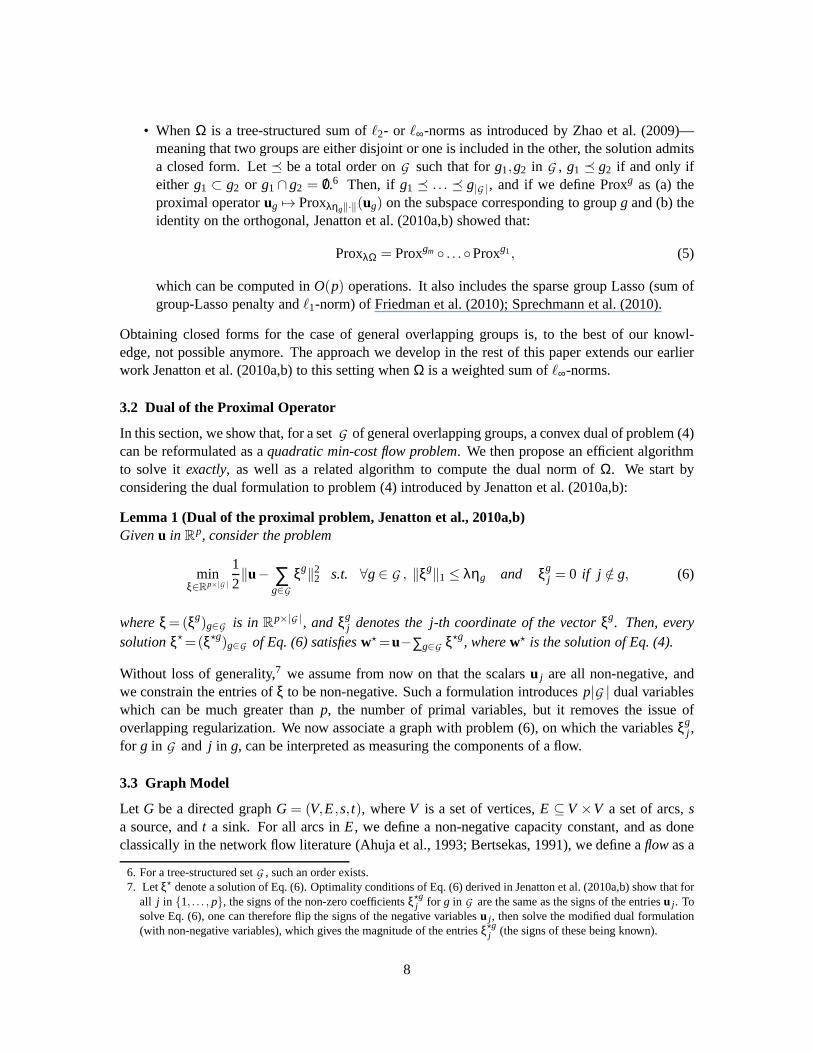
In this section, we show that, for a setG of general overlapping groups, a convex dual of problem (4)can be reformulated as aquadratic min-cost flow problem. We then propose an efficient algorithmto solve it exactly, as well as a related algorithm to compute the dual norm ofΩ. We start byconsidering the dual formulation to problem (4) introducedby Jenatton et al. (2010a,b):

Lemma 1 (Dual of the proximal problem, Jenatton et al., 2010a,b)Givenu in R

p, consider the problem

minξ∈Rp×|G |

12‖u− ∑

g∈Gξg‖22 s.t. ∀g∈ G , ‖ξg‖1≤ ληg and ξg

j = 0 if j /∈ g, (6)

whereξ=(ξg)g∈G is in Rp×|G |, and ξg

j denotes the j-th coordinate of the vectorξg. Then, everysolutionξ⋆=(ξ⋆g)g∈G of Eq. (6) satisfiesw⋆=u−∑g∈G ξ⋆g, wherew⋆ is the solution of Eq. (4).

Without loss of generality,7 we assume from now on that the scalarsu j are all non-negative, andwe constrain the entries ofξ to be non-negative. Such a formulation introducesp|G | dual variableswhich can be much greater thanp, the number of primal variables, but it removes the issue ofoverlapping regularization. We now associate a graph with problem (6), on which the variablesξg

j ,for g in G and j in g, can be interpreted as measuring the components of a flow.

3.3 Graph Model

Let G be a directed graphG = (V,E,s, t), whereV is a set of vertices,E ⊆ V ×V a set of arcs,sa source, andt a sink. For all arcs inE, we define a non-negative capacity constant, and as doneclassically in the network flow literature (Ahuja et al., 1993; Bertsekas, 1991), we define aflowas a

6. For a tree-structured setG , such an order exists.7. Letξ⋆ denote a solution of Eq. (6). Optimality conditions of Eq. (6) derived in Jenatton et al. (2010a,b) show that for

all j in 1, . . . , p, the signs of the non-zero coefficientsξ⋆gj for g in G are the same as the signs of the entriesu j . To

solve Eq. (6), one can therefore flip the signs of the negativevariablesu j , then solve the modified dual formulation(with non-negative variables), which gives the magnitude of the entriesξ⋆g

j (the signs of these being known).

8

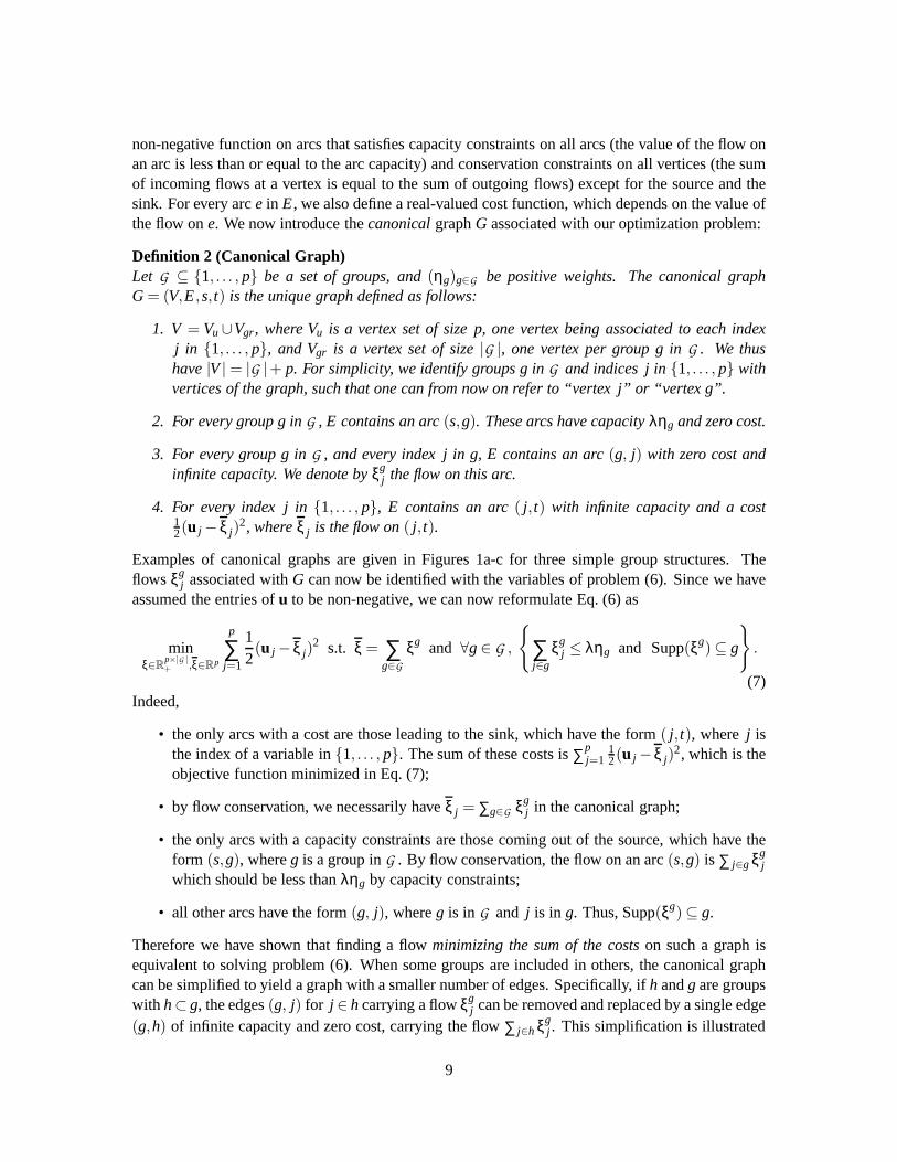
non-negative function on arcs that satisfies capacity constraints on all arcs (the value of the flow onan arc is less than or equal to the arc capacity) and conservation constraints on all vertices (the sumof incoming flows at a vertex is equal to the sum of outgoing flows) except for the source and thesink. For every arce in E, we also define a real-valued cost function, which depends onthe value ofthe flow one. We now introduce thecanonicalgraphG associated with our optimization problem:

Definition 2 (Canonical Graph)Let G ⊆ 1, . . . , p be a set of groups, and(ηg)g∈G be positive weights. The canonical graphG= (V,E,s, t) is the unique graph defined as follows:

1. V = Vu∪Vgr, where Vu is a vertex set of size p, one vertex being associated to each indexj in 1, . . . , p, and Vgr is a vertex set of size|G |, one vertex per group g inG . We thushave|V|= |G |+ p. For simplicity, we identify groups g inG and indices j in1, . . . , p withvertices of the graph, such that one can from now on refer to “vertex j” or “vertex g”.

2. For every group g inG , E contains an arc(s,g). These arcs have capacityληg and zero cost.

3. For every group g inG , and every index j in g, E contains an arc(g, j) with zero cost andinfinite capacity. We denote byξg

j the flow on this arc.

4. For every index j in1, . . . , p, E contains an arc( j, t) with infinite capacity and a cost12(u j −ξ j)

2, whereξ j is the flow on( j, t).

Examples of canonical graphs are given in Figures 1a-c for three simple group structures. Theflows ξg

j associated withG can now be identified with the variables of problem (6). Sincewe haveassumed the entries ofu to be non-negative, we can now reformulate Eq. (6) as

minξ∈Rp×|G |

+ ,ξ∈Rp

p

∑j=1

12(u j −ξ j)

2 s.t. ξ = ∑g∈G

ξg and ∀g∈ G ,

∑j∈g

ξgj ≤ ληg and Supp(ξg)⊆ g

.

(7)Indeed,

• the only arcs with a cost are those leading to the sink, whichhave the form( j, t), where j isthe index of a variable in1, . . . , p. The sum of these costs is∑p

j=112(u j −ξ j)

2, which is theobjective function minimized in Eq. (7);

• by flow conservation, we necessarily haveξ j = ∑g∈G ξgj in the canonical graph;

• the only arcs with a capacity constraints are those coming out of the source, which have theform (s,g), whereg is a group inG . By flow conservation, the flow on an arc(s,g) is ∑ j∈g ξg

jwhich should be less thanληg by capacity constraints;

• all other arcs have the form(g, j), whereg is in G and j is in g. Thus, Supp(ξg)⊆ g.

Therefore we have shown that finding a flowminimizing the sum of the costson such a graph isequivalent to solving problem (6). When some groups are included in others, the canonical graphcan be simplified to yield a graph with a smaller number of edges. Specifically, ifh andg are groupswith h⊂ g, the edges(g, j) for j ∈ h carrying a flowξg

j can be removed and replaced by a single edge(g,h) of infinite capacity and zero cost, carrying the flow∑ j∈h ξg

j . This simplification is illustrated

9

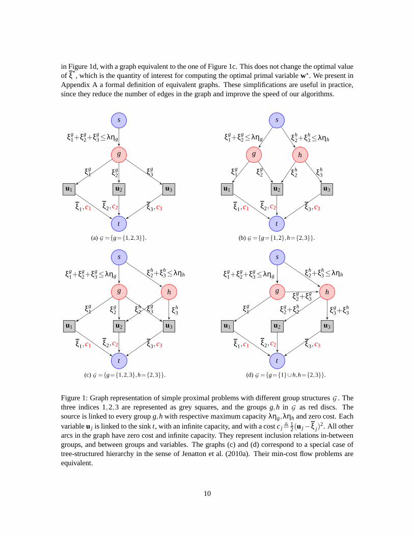
in Figure 1d, with a graph equivalent to the one of Figure 1c. This does not change the optimal valueof ξ

⋆, which is the quantity of interest for computing the optimalprimal variablew⋆. We present in

Appendix A a formal definition of equivalent graphs. These simplifications are useful in practice,since they reduce the number of edges in the graph and improvethe speed of our algorithms.

s

g

ξg1+ξg

2+ξg3≤ληg

u2

ξg2

u1

ξg1

u3

ξg3

t

ξ1,c1 ξ2,c2 ξ3,c3

(a)G =g=1,2,3.

s

g

ξg1+ξg

2≤ληg

h

ξh2+ξh

3≤ληh

u2

ξh2ξg

2

u1

ξg1

u3

ξh3

t

ξ1,c1 ξ2,c2 ξ3,c3

(b) G =g=1,2,h=2,3.

s

g

ξg1+ξg

2+ξg3≤ληg

h

ξh2+ξh

3≤ληh

u2

ξh2ξg

2

u1

ξg1

u3

ξg3 ξh

3

t

ξ1,c1 ξ2,c2 ξ3,c3

(c) G =g=1,2,3,h=2,3.

s

g

ξg1+ξg

2+ξg3≤ληg

h

ξh2+ξh

3≤ληh

ξg2+ξg

3

u2

ξg2+ξh

2

u1

ξg1

u3

ξg3+ξh

3

t

ξ1,c1 ξ2,c2 ξ3,c3

(d) G =g=1∪h,h=2,3.

Figure 1: Graph representation of simple proximal problemswith different group structuresG . Thethree indices 1,2,3 are represented as grey squares, and the groupsg,h in G as red discs. Thesource is linked to every groupg,h with respective maximum capacityληg,ληh and zero cost. Eachvariableu j is linked to the sinkt, with an infinite capacity, and with a costc j ,

12(u j−ξ j)

2. All otherarcs in the graph have zero cost and infinite capacity. They represent inclusion relations in-betweengroups, and between groups and variables. The graphs (c) and(d) correspond to a special case oftree-structured hierarchy in the sense of Jenatton et al. (2010a). Their min-cost flow problems areequivalent.

10

3.4 Computation of the Proximal Operator

Quadratic min-cost flow problems have been well studied in the operations research literature(Hochbaum and Hong, 1995). One of the simplest cases, whereG contains a single group as inFigure 1a, is solved by an orthogonal projection on theℓ1-ball of radiusληg. It has been shown,both in machine learning (Duchi et al., 2008) and operationsresearch (Hochbaum and Hong, 1995;Brucker, 1984), that such a projection can be computed inO(p) operations. When the group struc-ture is a tree as in Figure 1d, strategies developed in the twocommunities are also similar (Jenattonet al., 2010a; Hochbaum and Hong, 1995),8 and solve the problem inO(pd) operations, whered isthe depth of the tree.

The general case of overlapping groups is more difficult. Hochbaum and Hong (1995) haveshown thatquadratic min-cost flow problemscan be reduced to a specificparametric max-flowproblem, for which an efficient algorithm exists (Gallo et al., 1989).9 While this generic approachcould be used to solve Eq. (6), we propose to use Algorithm 1 that also exploits the fact that ourgraphs have non-zero costs only on edges leading to the sink.As shown in Appendix D, it it hasa significantly better performance in practice. This algorithm clearly shares some similarities withexisting approaches in network flow optimization such as thesimplified version of Gallo et al. (1989)presented by Babenko and Goldberg (2006) that uses a divide and conquer strategy. Moreover, anequivalent algorithm exists for minimizing convex functions over polymatroid sets (Groenevelt,1991). This equivalence, a priori non trivial, is uncoveredthrough a representation of structuredsparsity-inducing norms via submodular functions, which was recently proposed by Bach (2010).

Algorithm 1 Computation of the proximal operator for overlapping groups.

input u ∈ Rp, a set of groupsG , positive weights(ηg)g∈G , andλ (regularization parameter).

1: Build the initial graphG0 = (V0,E0,s, t) as explained in Section 3.4.2: Compute the optimal flow:ξ← computeFlow(V0,E0).3: Return: w = u−ξ (optimal solution of the proximal problem).

Function computeFlow(V =Vu∪Vgr,E)

1: Projection step:γ← argminγ ∑ j∈Vu12(u j − γ j)

2 s.t. ∑ j∈Vuγ j ≤ λ∑g∈Vgr

ηg.2: For all nodesj in Vu, setγ j to be the capacity of the arc( j, t).

3: Max-flow step: Update(ξ j) j∈Vu by computing a max-flow on the graph(V,E,s, t).

4: if ∃ j ∈Vu s.t. ξ j 6= γ j then5: Denote by(s,V+) and(V−, t) the two disjoint subsets of(V,s, t) separated by the minimum

(s, t)-cut of the graph, and remove the arcs betweenV+ andV−. Call E+ andE− the tworemaining disjoint subsets ofE corresponding toV+ andV−.

6: (ξ j) j∈V+u← computeFlow(V+,E+).

7: (ξ j) j∈V−u ← computeFlow(V−,E−).8: end if9: Return: (ξ j) j∈Vu.

8. Note however that, while Hochbaum and Hong (1995) only consider a tree-structured sum ofℓ∞-norms, the resultsfrom Jenatton et al. (2010a) also apply for a sum ofℓ2-norms.

9. By definition, a parametric max-flow problem consists in solving, for every value of a parameter, a max-flow problemon a graph whose arc capacities depend on this parameter.

11

The intuition behind our algorithm,computeFlow (see Algorithm 1), is the following: sinceξ =∑g∈G ξg is the only value of interest to compute the solution of the proximal operatorw = u−ξ, the

first step looks for a candidate valueγ for ξ by solving the following relaxed version of problem (7):

argminγ∈Rp

∑j∈Vu

12(u j − γ j)

2 s.t. ∑j∈Vu

γ j ≤ λ ∑g∈Vgr

ηg. (8)

The cost function here is the same as in problem (7), but the constraints are weaker: Any feasi-ble point of problem (7) is also feasible for problem (8). This problem can be solved in lineartime (Brucker, 1984). Its solution, which we denoteγ for simplicity, provides the lower bound‖u− γ‖22/2 for the optimal cost of problem (7).

The second step tries to construct a feasible flow(ξ,ξ), satisfying additional capacity constraintsequal toγ j on arc( j, t), and whose cost matches this lower bound; this latter problem can be castas a max-flow problem (Goldberg and Tarjan, 1986). If such a flow exists, the algorithm returnsξ = γ, the cost of the flow reaches the lower bound, and is thereforeoptimal. If such a flow does notexist, we haveξ 6= γ, the lower bound is not achievable, and we build a minimum(s, t)-cut of thegraph (Ford and Fulkerson, 1956) defining two disjoints setsof nodesV+ andV−; V+ is the part ofthe graph that could potentially have received more flow fromthe source (the arcs betweensandV+

are not saturated), whereasV− could not (all arcs linkings to V− are saturated). At this point, itis possible to show that the value of the optimal min-cost flowon all arcs betweenV+ andV−

is necessary zero. Thus, removing them yields an equivalentoptimization problem, which can bedecomposed into two independent problems of smaller sizes and solved recursively by the calls tocomputeFlow(V+,E+) andcomputeFlow(V−,E−). A formal proof of correctness of Algorithm 1and further details are relegated to Appendix B.

The approach of Hochbaum and Hong (1995); Gallo et al. (1989)which recasts the quadraticmin-cost flow problem as a parametric max-flow is guaranteed to have the same worst-case com-plexity as a single max-flow algorithm. However, we have experimentally observed a significantdiscrepancy between the worst case and empirical complexities for these flow problems, essentiallybecause the empirical cost of each max-flow is significantly smaller than its theoretical cost. Despitethe fact that the worst-case guarantees for our algorithm isweaker than theirs (up to a factor|V|), itis more adapted to the structure of our graphs and has proven to be much faster in our experiments(see Appendix D).10 Some implementation details are also crucial to the efficiency of the algorithm:

• Exploiting maximal connected components: When there exists no arc between two sub-sets ofV, the solution can be obtained by solving two smaller optimization problems cor-responding to the two disjoint subgraphs. It is indeed possible to process them indepen-dently to solve the global min-cost flow problem. To that effect, before calling the functioncomputeFlow(V,E), we look for maximal connected components(V1,E1), . . . ,(VN,EN) andcall sequentially the procedurecomputeFlow(Vi ,Ei) for i in 1, . . . ,N.

• Efficient max-flow algorithm : We have implemented the “push-relabel” algorithm of Gold-berg and Tarjan (1986) to solve our max-flow problems, using classical heuristics that signif-icantly speed it up in practice; see Goldberg and Tarjan (1986) and Cherkassky and Goldberg

10. The best theoretical worst-case complexity of a max-flowis achieved by Goldberg and Tarjan (1986) and isO(

|V||E| log(|V|2/|E|))

. Our algorithm achieves the same worst-case complexity when the cuts are well balanced—that is|V+| ≈ |V−| ≈ |V|/2, but we lose a factor|V| when it is not the case. The practical speed of such algorithms ishowever significantly different than their theoretical worst-case complexities (see Boykov and Kolmogorov, 2004).

12

(1997). We use the so-called “highest-active vertex selection rule, global and gap heuris-tics” (Goldberg and Tarjan, 1986; Cherkassky and Goldberg,1997), which has a worst-casecomplexity ofO(|V|2|E|1/2) for a graph(V,E,s, t). This algorithm leverages the concept ofpre-flowthat relaxes the definition of flow and allows vertices to havea positive excess.

• Using flow warm-restarts: The max-flow steps in our algorithm can be initialized with anyvalid pre-flow, enabling warm-restarts. This is also a key concept in the parametric max-flowalgorithm of Gallo et al. (1989).

• Improved projection step: The first line of the procedurecomputeFlow can be replaced byγ← argminγ ∑ j∈Vu

12(u j− γ j)

2 s.t. ∑ j∈Vuγ j ≤ λ∑g∈Vgr

ηg and|γ j | ≤ λ∑g∋ j ηg. The idea is tobuild a relaxation of Eq. (7) which is closer to the original problem than the one of Eq. (8),but that still can be solved in linear time. The structure of the graph will indeed not allowξ jto be greater thanλ∑g∋ j ηg after the max-flow step. This modified projection step can still becomputed in linear time (Brucker, 1984), and leads to betterperformance.

3.5 Computation of the Dual Norm

The dual normΩ∗ of Ω, defined for any vectorκ in Rp by

Ω∗(κ), maxΩ(z)≤1

z⊤κ,

is a key quantity to study sparsity-inducing regularizations in many respects. For instance, dualnorms are central in working-set algorithms (Jenatton et al., 2009; Bach et al., 2011), and arise aswell when proving theoretical estimation or prediction guarantees (Negahban et al., 2009).

In our context, we use it to monitor the convergence of the proximal method through a dualitygap, hence defining a proper optimality criterion for problem (2). As a brief reminder, the dualitygap of a minimization problem is defined as the difference between the primal and dual objectivefunctions, evaluated for a feasible pair of primal/dual variables (see Section 5.5, Boyd and Van-denberghe, 2004). This gap serves as a certificate of (sub)optimality: if it is equal to zero, thenthe optimum is reached, and provided that strong duality holds, the converse is true as well (seeSection 5.5, Boyd and Vandenberghe, 2004). A description ofthe algorithm we use in the experi-ments (Beck and Teboulle, 2009) along with the integration of the computation of the duality gap isgiven in Appendix C.

We now denote byf ∗ the Fenchel conjugate off (Borwein and Lewis, 2006), defined byf ∗(κ) , supz[z

⊤κ− f (z)]. The duality gap for problem (2) can be derived from standardFenchelduality arguments (Borwein and Lewis, 2006) and it is equal to

f (w)+λΩ(w)+ f ∗(−κ) for w,κ in Rp with Ω∗(κ)≤ λ.

Therefore, evaluating the duality gap requires to compute efficiently Ω∗ in order to find a feasibledual variableκ (the gap is otherwise equal to+∞ and becomes non-informative). This is equivalentto solving another network flow problem, based on the following variational formulation:

Ω∗(κ) = minξ∈Rp×|G |

τ s.t. ∑g∈G

ξg = κ, and∀g∈ G , ‖ξg‖1≤ τηg with ξgj = 0 if j /∈ g. (9)

In the network problem associated with (9), the capacities on the arcs(s,g), g∈ G , are set toτηg,and the capacities on the arcs( j, t), j in 1, . . . , p, are fixed toκ j . Solving problem (9) amounts

13

to finding the smallest value ofτ, such that there exists a flow saturating all the capacitiesκ j on thearcs leading to the sinkt. Equation (9) and Algorithm 2 are proven to be correct in Appendix B.

Algorithm 2 Computation of the dual norm.

input κ ∈Rp, a set of groupsG , positive weights(ηg)g∈G .

1: Build the initial graphG0 = (V0,E0,s, t) as explained in Section 3.5.2: τ← dualNorm(V0,E0).3: Return: τ (value of the dual norm).

Function dualNorm(V =Vu∪Vgr,E)

1: τ←(∑ j∈Vuκ j)/(∑g∈Vgr

ηg) and set the capacities of arcs(s,g) to τηg for all g in Vgr.

2: Max-flow step: Update(ξ j) j∈Vu by computing a max-flow on the graph(V,E,s, t).

3: if ∃ j ∈Vu s.t. ξ j 6= κ j then4: Define(V+,E+) and(V−,E−) as in Algorithm 1, and setτ← dualNorm(V−,E−).5: end if6: Return: τ.

4. Optimization with Splitting Proximal Methods

We now present proximal splitting algorithms (see Combettes and Pesquet, 2008, 2010; Tomiokaet al., 2011, and references therein) for solving Eq. (2). Differentiability of f is not required hereand the regularization function can either be a sum ofℓ2- or ℓ∞-norms. However, we assume that

(A) either f can be writtenf (w) = ∑ni=1 fi(w), where the functionsfi are such that proxγ fi can be

obtained in closed form for allγ > 0 and alli—that is, for allu in Rm, the following problems

admit closed form solutions: minv∈Rm12‖u−v‖22+ γ fi(v).

(B) or f can be writtenf (w) = f (Xw) for all w in Rp, whereX in R

n×p is a design matrix, andone knows how to efficiently compute proxγ f for all γ > 0.

It is easy to show that this condition is satisfied for the square and hinge loss functions, making itpossible to build linear SVMs with a structured sparse regularization. These assumptions are notthe same as the ones of Section 3, and the scope of the problemsaddressed is therefore slightly dif-ferent. Proximal splitting methods seem indeed to offer more flexibility regarding the regularizationfunction, since they can deal with sums ofℓ2-norms.11 However, proximal gradient methods, aspresented in Section 3, enjoy a few advantages over proximalsplitting methods, namely: automaticparameter tuning with line-search schemes (Nesterov, 2007), known convergence rates (Nesterov,2007; Beck and Teboulle, 2009), and ability to provide sparse solutions (approximate solutionsobtained with proximal splitting methods often have small values, but not “true” zeros).

11. We are not aware of any efficient algorithm providing the exact solution of the proximal operator associated to a sumof ℓ2-norms, which would be necessary for using (accelerated) proximal gradient methods. An iterative algorithmcould possibly be used to compute it approximately (e.g., see Jenatton et al., 2010a,b), but such a procedure wouldbe computationally expensive and would require to be able todeal with approximate computations of the proximaloperators (e.g., see Combettes and Pesquet, 2010, and discussions therein). We have chosen not to consider thispossibility in this paper.

14

4.1 Algorithms

We consider a class of algorithms which leverage the conceptof variable splitting (see Combettesand Pesquet, 2010; Bertsekas and Tsitsiklis, 1989; Tomiokaet al., 2011). The key is to introduceadditional variableszg in R

|g|, one for every groupg in G , and equivalently reformulate Eq. (2) as

minw∈Rp

zg∈R|g| for g∈G

f (w)+λ ∑g∈G

ηg‖zg‖ s.t. ∀g∈ G , zg = wg, (10)

The issue of overlapping groups is removed, but new constraints are added, and as in Section 3, themethod introduces additional variables which induce a memory cost ofO(∑g∈G |g|).

To solve this problem, it is possible to use the so-called alternating direction method of multi-pliers (ADMM) (see Combettes and Pesquet, 2010; Bertsekas and Tsitsiklis, 1989; Tomioka et al.,2011).12 It introduces dual variablesνg in R

|g| for all g in G , and defines the augmented Lagrangian:

L(

w,(zg)g∈G ,(νg)g∈G)

, f (w)+ ∑g∈G

[

ληg‖zg‖+νg⊤(zg−wg)+γ2‖zg−wg‖22

]

,

whereγ > 0 is a parameter. It is easy to show that solving Eq. (10) amounts to finding a saddle-point of the augmented Lagrangian.13 The ADMM algorithm finds such a saddle-point by iteratingbetween the minimization ofL with respect to each primal variable, keeping the other onesfixed,and gradient ascent steps with respect to the dual variables. More precisely, it can be summarized as:

1. MinimizeL with respect tow, keeping the other variables fixed.

2. Minimize L with respect to thezg’s, keeping the other variables fixed. The solution can beobtained in closed form: for allg in G , zg← proxληg

γ ‖.‖[wg− 1

γ νg].

3. Take a gradient ascent step onL with respect to theνg’s: νg← νg+ γ(zg−wg).

4. Go back to step 1.

Such a procedure is guaranteed to converge to the desired solution for all value ofγ > 0 (however,tuningγ can greatly influence the convergence speed), but solving efficiently step 1 can be difficult.fTo cope with this issue, we propose two variations exploiting assumptions(A) and(B).

4.1.1 SPLITTING THE LOSSFUNCTION f

We assume condition(A)—that is, we havef (w) = ∑ni=1 fi(w). For example, whenf is the square

loss function f (w) = 12‖y−Xw‖22, whereX in R

n×p is a design matrix andy is in Rn, we would

define for alli in 1, . . . ,n the functions fi : R→ R such thatfi(w) , 12(yi − x⊤i w)2, wherexi is

the i-th row ofX.

12. This method was used in a related context by Sprechmann etal. (2010) for computing the proximal operator associ-ated to hierarchical norms.

13. The augmented Lagrangian is in fact the classical Lagrangian (see Boyd and Vandenberghe, 2004) of the followingoptimization problem which is equivalent to Eq. (10):

minw∈Rp,(zg∈R|g|)g∈G

f (w)+λ ∑g∈G

ηg‖zg‖+ γ2‖zg−wg‖22 s.t. ∀g∈ G , zg = wg.

15

We now introduce new variablesvi in Rp for i = 1, . . . ,n, and replacef (w) in Eq. (10) by

∑ni=1 fi(vi), with the additional constraints thatvi = w. The resulting equivalent optimization prob-

lem can now be tackled using the ADMM algorithm, following the same methodology presentedabove. It is easy to show that every step can be obtained efficiently, as long as one knows how tocompute the proximal operator associated to the functionsfi in closed form. This is in fact the casefor the square and hinge loss functions, wheren is the number of training points. The main problemof this strategy is the possible high memory usage it requires whenn is large.

4.1.2 DEALING WITH THE DESIGN MATRIX

If we assume condition(B), another possibility consists of introducing a new variable v in Rn, such

that one can replace the functionf (w) = f (Xw) by f (v) in Eq. (10) with the additional constraintv = Xw. Using directly the ADMM algorithm to solve the corresponding problem implies addinga termκ⊤(v−Xw)+ γ

2‖v−Xw‖22 to the augmented LagrangianL , whereκ is a new dual vari-able. The minimization ofL with respect tov is now obtained byv← prox1

γ f [Xw−κ], which is

easy to compute according to(B). However, the design matrixX in the quadratic term makes theminimization ofL with respect tow more difficult. To overcome this issue, we adopt a strategypresented by Zhang et al. (2011), which replaces at iteration k the quadratic termγ

2‖v−Xw‖22 in theaugmented Lagrangian by an additional proximity term:γ

2‖v−Xw‖22+γ2‖w−wk‖2Q, wherewk is

the current estimate ofw, and‖w−wk‖2Q = (w−wk)⊤Q(w−wk), whereQ is a symmetric posi-

tive definite matrix. By choosingQ , δI −X⊤X, with δ large enough, minimizingL with respectto w becomes simple, while convergence to the solution is still ensured. More details can be foundin Zhang et al. (2011).

5. Applications and Experiments

In this section, we present various experiments demonstrating the applicability and the benefits ofour methods for solving large-scale sparse and structured regularized problems.

5.1 Speed Benchmark

We consider a structured sparse decomposition problem withoverlapping groups ofℓ∞-norms, andcompare the proximal gradient algorithm FISTA (Beck and Teboulle, 2009) with our proximal op-erator presented in Section 3 (referred to as ProxFlow), twovariants of proximal splitting methods,(ADMM) and (Lin-ADMM) respectively presented in Section 4.1.1 and 4.1.2, and two genericoptimization techniques, namely a subgradient descent (SG) and an interior point method,14 on aregularized linear regression problem. SG, ProxFlow, ADMMand Lin-ADMM are implementedin C++.15 Experiments are run on a single-core 2.8 GHz CPU. We consider a design matrixX inR

n×p built from overcomplete dictionaries of discrete cosine transforms (DCT), which are naturallyorganized on one- or two-dimensional grids and display local correlations. The following familiesof groupsG using this spatial information are thus considered: (1) every contiguous sequence oflength 3 for the one-dimensional case, and (2) every 3×3-square in the two-dimensional setting. Wegenerate vectorsy in R

n according to the linear modely = Xw0+ ε, whereε∼ N (0,0.01‖Xw0‖22).

14. In our simulations, we use the commercial softwareMosek, http://www.mosek.com/15. Our implementation of ProxFlow is available athttp://www.di.ens.fr/willow/SPAMS/.

16

The vectorw0 has about 20% percent nonzero components, randomly selected, while respecting thestructure ofG , and uniformly generated in[−1,1].

In our experiments, the regularization parameterλ is chosen to achieve the same level of spar-sity (20%). For SG, ADMM and Lin-ADMM, some parameters are optimized to provide the low-est value of the objective function after 1000 iterations ofthe respective algorithms. For SG,we take the step size to be equal toa/(k+ b), wherek is the iteration number, and(a,b) arethe pair of parameters selected in10−3, . . . ,10×102,103,104. Note that a step size of theform a/(

√t +b) is also commonly used in subgradient descent algorithms. Inthe context of hier-

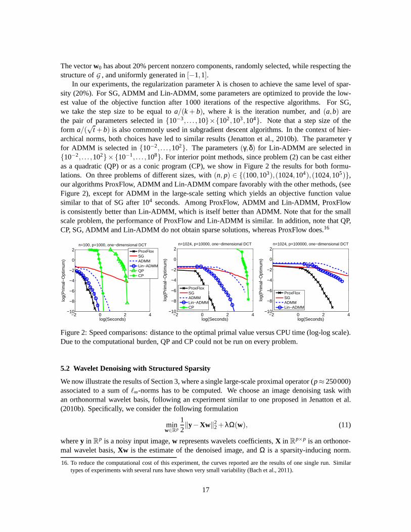
archical norms, both choices have led to similar results (Jenatton et al., 2010b). The parameterγfor ADMM is selected in10−2, . . . ,102. The parameters(γ,δ) for Lin-ADMM are selected in10−2, . . . ,102×10−1, . . . ,108. For interior point methods, since problem (2) can be cast eitheras a quadratic (QP) or as a conic program (CP), we show in Figure 2 the results for both formu-lations. On three problems of different sizes, with(n, p) ∈ (100,103),(1024,104),(1024,105),our algorithms ProxFlow, ADMM and Lin-ADMM compare favorably with the other methods, (seeFigure 2), except for ADMM in the large-scale setting which yields an objective function valuesimilar to that of SG after 104 seconds. Among ProxFlow, ADMM and Lin-ADMM, ProxFlowis consistently better than Lin-ADMM, which is itself better than ADMM. Note that for the smallscale problem, the performance of ProxFlow and Lin-ADMM is similar. In addition, note that QP,CP, SG, ADMM and Lin-ADMM do not obtain sparse solutions, whereas ProxFlow does.16

−2 0 2 4−10

−8

−6

−4

−2

0

2n=100, p=1000, one−dimensional DCT

log(Seconds)

log(

Prim

al−

Opt

imum

)

ProxFloxSGADMMLin−ADMMQPCP

−2 0 2 4−10

−8

−6

−4

−2

0

2n=1024, p=10000, one−dimensional DCT

log(Seconds)

log(

Prim

al−

Opt

imum

)

ProxFloxSGADMMLin−ADMMCP

−2 0 2 4−10

−8

−6

−4

−2

0

2n=1024, p=100000, one−dimensional DCT

log(Seconds)

log(

Prim

al−

Opt

imum

)

ProxFloxSGADMMLin−ADMM

Figure 2: Speed comparisons: distance to the optimal primalvalue versus CPU time (log-log scale).Due to the computational burden, QP and CP could not be run on every problem.

5.2 Wavelet Denoising with Structured Sparsity

We now illustrate the results of Section 3, where a single large-scale proximal operator (p≈ 250000)associated to a sum ofℓ∞-norms has to be computed. We choose an image denoising task withan orthonormal wavelet basis, following an experiment similar to one proposed in Jenatton et al.(2010b). Specifically, we consider the following formulation

minw∈Rp

12‖y−Xw‖22+λΩ(w), (11)

wherey in Rp is a noisy input image,w represents wavelets coefficients,X in R

p×p is an orthonor-mal wavelet basis,Xw is the estimate of the denoised image, andΩ is a sparsity-inducing norm.

16. To reduce the computational cost of this experiment, thecurves reported are the results of one single run. Similartypes of experiments with several runs have shown very smallvariability (Bach et al., 2011).

17

Since here the basis is orthonormal, solving the decomposition problem boils down to computingw⋆ = proxλΩ[X

⊤y]. This make of Algorithm 1 a good candidate to solve it whenΩ is a sum ofℓ∞-norms. We compare the following candidates for the sparsity-inducing normsΩ:

• theℓ1-norm, leading to the wavelet soft-thresholding of Donoho and Johnstone (1995).

• a sum ofℓ∞-norms with a hierarchical group structure adapted to the wavelet coefficients,as proposed in Jenatton et al. (2010b). Considering a natural quad-tree for wavelet coeffi-cients (see Mallat, 1999), this norm takes the form of Eq. (3)with one group per waveletcoefficient that contains the coefficient and all its descendants in the tree. We call this normΩtree.

• a sum ofℓ∞-norms with overlapping groups representing 2×2 spatial neighborhoods in thewavelet domain. This regularization encourages neighboring wavelet coefficients to be setto zero together, which was also exploited in the past in block-thresholding approaches forwavelet denoising (Cai, 1999). We call this normΩgrid.

We consider Daubechies3 wavelets (see Mallat, 1999) for thematrix X, use 12 classical standardtest images,17 and generate noisy versions of them corrupted by a white Gaussian noise of vari-anceσ2. For each image, we test several values ofλ = 2

i4 σ√

log p, with i taken in the range−15,−14, . . . ,15. We then keep the parameterλ giving the best reconstruction error on averageon the 12 images. The factorσ

√log p is a classical heuristic for choosing a reasonable regulariza-

tion parameter (see Mallat, 1999). We provide reconstruction results in terms of PSNR in Table 1.18

Unlike Jenatton et al. (2010b), who set all the weightsηg in Ω equal to one, we tried exponentialweights of the formηg = ρk, with k being the depth of the group in the wavelet tree, andρ is takenin 0.25,0.5,1,2,4. As for λ, the value providing the best reconstruction is kept. The wavelettransforms in our experiments are computed with the matlabPyrTools software.19 Interestingly, weobserve in Table 1 that the results obtained withΩgrid are significantly better than those obtainedwith Ωtree, meaning that encouraging spatial consistency in wavelet coefficients is more effectivethan using a hierarchical coding. We also note that our approach is relatively fast, despite the highdimension of the problem. Solving exactly the proximal problem with Ωgrid for an image withp = 512× 512= 262144 pixels (and therefore approximately the same numberof groups) takesapproximately≈ 4−6 seconds on a single core of a 3.07GHz CPU.

5.3 CUR-like Matrix Factorization

In this experiment, we show how our tools can be used to perform the so-called CUR matrix decom-position (Mahoney and Drineas, 2009). It consists of a low-rank approximation of a data matrixXin R

n×p in the form of a product of three matrices—that is,X ≈CUR. The particularity of the CURdecomposition lies in the fact that the matricesC∈Rn×c andR∈Rr×p are constrained to be respec-tively a subset ofc columns andr rows of the original matrixX. The third matrixU ∈ R

c×r is thengiven byC+XR+, whereA+ denotes a Moore-Penrose generalized inverse of the matrixA (Hornand Johnson, 1990). Such a matrix factorization is particularly appealing when the interpretability

17. These images are used in classical image denoising benchmarks. See Mairal et al. (2009).18. Denoting by MSE the mean-squared-error for images whoseintensities are between 0 and 255, the PSNR is defined

as PSNR= 10log10(2552/MSE) and is measured in dB. A gain of 1dB reduces the MSE by approximately 20%.19. http://www.cns.nyu.edu/∼eero/steerpyr/.

18

PSNR IPSNR vs.ℓ1

σ ℓ1 Ωtree Ωgrid ℓ1 Ωtree Ωgrid

5 35.67 35.98 36.15 0.00± .0 0.31± .18 0.48± .2510 31.00 31.60 31.88 0.00± .0 0.61± .28 0.88± .2825 25.68 26.77 27.07 0.00± .0 1.09± .32 1.38± .2650 22.37 23.84 24.06 0.00± .0 1.47± .34 1.68± .41100 19.64 21.49 21.56 0.00± .0 1.85± .28 1.92± .29

Table 1: PSNR measured for the denoising of 12 standard images when the regularization functionis theℓ1-norm, the tree-structured normΩtree, and the structured normΩgrid, and improvement inPSNR compared to theℓ1-norm (IPSNR). Best results for each level of noise and each wavelet typeare in bold. The reported values are averaged over 5 runs withdifferent noise realizations.

of the results matters (Mahoney and Drineas, 2009). For instance, when studying gene-expressiondatasets, it is easier to gain insight from the selection of actual patients and genes, rather than fromlinear combinations of them.

In Mahoney and Drineas (2009), CUR decompositions are computed by a sampling procedurebased on the singular value decomposition ofX. In a recent work, Bien et al. (2010) have shownthatpartial CUR decompositions, i.e., the selection of either rows or columns ofX, can be obtainedby solving a convex program with a group-Lasso penalty. We propose to extend this approach tothe simultaneous selection of both rows and columns ofX, with the following convex problem:

minW∈Rp×n

12‖X−XWX ‖2F+λrow

n

∑i=1

‖W i‖∞ +λcol

p

∑j=1

‖W j‖∞. (12)

In this formulation, the two sparsity-inducing penalties controlled by the parametersλrow andλcol setto zero some entire rows and columns of the solutions of problem (12). Now, let us denote byWIJ

in R|I|×|J| the submatrix ofW reduced to its nonzero rows and columns, respectively indexed by

I ⊆ 1, . . . , p and J⊆ 1, . . . ,n. We can then readily identify the three components of the CURdecomposition ofX, namely

XWX = CWIJR≈ X.

Problem (12) has a smooth convex data-fitting term and bringsinto play a sparsity-inducing normwith overlapping groups of variables (the rows and the columns of W). As a result, it is a partic-ular instance of problem (2) that can therefore be handled with the optimization tools introducedin this paper. We now compare the performance of the samplingprocedure from Mahoney andDrineas (2009) with our proposed sparsity-based approach.To this end, we consider the four gene-expression datasets9 Tumors, Brain Tumors1, Leukemia1 andSRBCT, with respective dimensions(n, p) ∈ (60,5727),(90,5921),(72,5328),(83,2309).20 In the sequel, the matrixX is normalizedto have unit Frobenius-norm while each of its columns is centered. To begin with, we run our ap-proach21 over a grid of values forλrow andλcol in order to obtain solutions with different sparsitylevels, i.e., ranging from|I| = p and|J| = n down to|I| = |J| = 0. For each pair of values[|I|, |J|],

20. The datasets are freely available athttp://www.gems-system.org/.21. More precisely, since the penalties in problem (12) shrink the coefficients ofW, we follow a two-step procedure: We

first run our approach to determine the sets of nonzero rows and columns, and then computeWIJ = C+XR+.

19

we then apply the sampling procedure from Mahoney and Drineas (2009). Finally, the varianceexplained by the CUR decompositions is reported in Figure 3 for both methods. Since the samplingapproach involves some randomness, we show the average and standard deviation of the resultsbased on five initializations. The conclusions we can draw from the experiments match the ones al-ready reported in Bien et al. (2010) for the partial CUR decomposition. We can indeed see that bothschemes perform similarly. However, our approach has the advantage not to be randomized, whichcan be less disconcerting in the practical perspective of analyzing a single run of the algorithm. Itis finally worth being mentioned that the convex approach we develop here is flexible and can beextended in different ways. For instance, we may imagine addfurther low-rank/sparsity constraintson W thanks to sparsity-promoting convex regularizations.

0

0.2

0.4

0.6

0.8

1

Solutions ordered by increasing explained variance

Exp

lain

ed v

aria

nce

Random CURConvex CUR

0

0.2

0.4

0.6

0.8

1

Solutions ordered by increasing explained variance

Exp

lain

ed v

aria

nce

Random CURConvex CUR

0

0.2

0.4

0.6

0.8

1

Solutions ordered by increasing explained variance

Exp

lain

ed v

aria

nce

Random CURConvex CUR

0

0.2

0.4

0.6

0.8

1

Solutions ordered by increasing explained variance

Exp

lain

ed v

aria

nce

Random CURConvex CUR

Figure 3: Explained variance of the CUR decompositions obtained for our sparsity-based approachand the sampling scheme from Mahoney and Drineas (2009). Forthe latter, we report the averageand standard deviation of the results based on five initializations. From left to right and top tobottom, the curves correspond to the datasets9 Tumors, Brain Tumors1, Leukemia1 andSRBCT.

5.4 Background Subtraction

Following Cehver et al. (2008); Huang et al. (2009), we consider a background subtraction task.Given a sequence of frames from a fixed camera, we try to segment out foreground objects in a newimage. If we denote byy ∈ R

n this image composed ofn pixels, we modely as a sparse linearcombination ofp other imagesX ∈ R

n×p, plus an error terme in Rn, i.e., y ≈ Xw + e for some

20

sparse vectorw in Rp. This approach is reminiscent of Wright et al. (2009a) in thecontext of face

recognition, wheree is further made sparse to deal with small occlusions. The term Xw accountsfor backgroundparts present in bothy andX, while econtains specific, orforeground, objects iny.The resulting optimization problem is given by

minw∈Rp,e∈Rn

12‖y−Xw−e‖22+λ1‖w‖1+λ2‖e‖1+Ω(e), with λ1,λ2≥ 0. (13)

In this formulation, the onlyℓ1-norm penalty does not take into account the fact that neighboringpixels iny are likely to share the same label (background or foreground), which may lead to scatteredpieces of foreground and background regions (Figure 4). We therefore put an additional structuredregularization termΩ one, where the groups inG are all the overlapping 3×3-squares on the image.

This optimization problem can be viewed as an instance of problem (2), with the particulardesign matrix[X, I ] in R

n×(p+n), defined as the columnwise concatenation ofX and the identitymatrix. As a result, we could directly apply the same procedure as the one used in the other ex-periments. Instead, we further exploit the specific structure of problem (13): Notice that for a fixedvectore, the optimization with respect tow is a standard Lasso problem (with the vector of obser-vationsy−e),22 while for w fixed, we simply have a proximal problem associated to the sumof Ωand theℓ1-norm. Alternating between these two simple and computationally inexpensive steps, i.e.,optimizing with respect to one variable while keeping the other one fixed, is guaranteed to convergeto a solution of (13).23 In our simulations, this alternating scheme has led to a significant speed-upcompared to the general procedure.

A dataset with hand-segmented images is used to illustrate the effect ofΩ.24 For simplicity,we use a single regularization parameter, i.e.,λ1 = λ2, chosen to maximize the number of pixelsmatching the ground truth. We considerp= 200 images withn= 57600 pixels (i.e., a resolution of120×160, times 3 for the RGB channels). As shown in Figure 4, adding Ω improves the backgroundsubtraction results for the two tested images, by removing the scattered artifacts due to the lack ofstructural constraints of theℓ1-norm, which encodes neither spatial nor color consistency.

5.5 Topographic Dictionary Learning

Let us consider a setY = [y1, . . . ,yn] inRm×n of nsignals of dimensionm. The problem of dictionary

learning, originally introduced by Olshausen and Field (1996), is a matrix factorization problemwhich aims at representing these signals as linear combinations ofdictionary elementsthat are thecolumns of a matrixX = [x1, . . . ,xp] in R

m×p. More precisely, the dictionaryX is learnedalongwith a matrix ofdecomposition coefficientsW = [w1, . . . ,wn] in R

p×n, so thatyi ≈ Xw i for everysignalyi . Typically, n is large compared tom andp. In this experiment, we consider for instance adatabase ofn= 100000 natural image patches of sizem= 12×12 pixels, for dictionaries of sizep = 400. Adapting the dictionary to specific data has proven to beuseful in many applications,including image restoration (Elad and Aharon, 2006; Mairalet al., 2009), learning image features incomputer vision (Kavukcuoglu et al., 2009). The resulting optimization problem we are interested

22. Since successive frames might not change much, the columns of X exhibit strong correlations. As a result, we usethe LARS algorithm (Efron et al., 2004) whose complexity is independent of the level of correlation inX.

23. More precisely, the convergence is guaranteed since thenon-smooth part in (13) isseparablewith respect tow ande (Tseng, 2001). The result from Bertsekas (1999) may also be applied here, after reformulating (13) as a smoothconvex problem under separable conic constraints.

24. http://research.microsoft.com/en-us/um/people/jckrumm/wallflower/testimages.htm

21

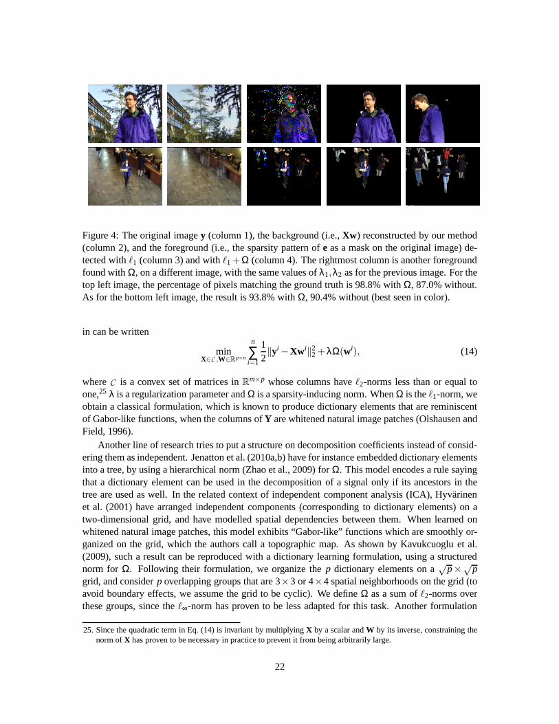
Figure 4: The original imagey (column 1), the background (i.e.,Xw) reconstructed by our method(column 2), and the foreground (i.e., the sparsity pattern of e as a mask on the original image) de-tected withℓ1 (column 3) and withℓ1+Ω (column 4). The rightmost column is another foregroundfound withΩ, on a different image, with the same values ofλ1,λ2 as for the previous image. For thetop left image, the percentage of pixels matching the groundtruth is 98.8% withΩ, 87.0% without.As for the bottom left image, the result is 93.8% withΩ, 90.4% without (best seen in color).

in can be written

minX∈C ,W∈Rp×n

n

∑i=1

12‖yi −Xw i‖22+λΩ(wi), (14)

whereC is a convex set of matrices inRm×p whose columns haveℓ2-norms less than or equal toone,25 λ is a regularization parameter andΩ is a sparsity-inducing norm. WhenΩ is theℓ1-norm, weobtain a classical formulation, which is known to produce dictionary elements that are reminiscentof Gabor-like functions, when the columns ofY are whitened natural image patches (Olshausen andField, 1996).

Another line of research tries to put a structure on decomposition coefficients instead of consid-ering them as independent. Jenatton et al. (2010a,b) have for instance embedded dictionary elementsinto a tree, by using a hierarchical norm (Zhao et al., 2009) for Ω. This model encodes a rule sayingthat a dictionary element can be used in the decomposition ofa signal only if its ancestors in thetree are used as well. In the related context of independent component analysis (ICA), Hyvarinenet al. (2001) have arranged independent components (corresponding to dictionary elements) on atwo-dimensional grid, and have modelled spatial dependencies between them. When learned onwhitened natural image patches, this model exhibits “Gabor-like” functions which are smoothly or-ganized on the grid, which the authors call a topographic map. As shown by Kavukcuoglu et al.(2009), such a result can be reproduced with a dictionary learning formulation, using a structurednorm for Ω. Following their formulation, we organize thep dictionary elements on a

√p×√p

grid, and considerp overlapping groups that are 3×3 or 4×4 spatial neighborhoods on the grid (toavoid boundary effects, we assume the grid to be cyclic). We defineΩ as a sum ofℓ2-norms overthese groups, since theℓ∞-norm has proven to be less adapted for this task. Another formulation

25. Since the quadratic term in Eq. (14) is invariant by multiplying X by a scalar andW by its inverse, constraining thenorm ofX has proven to be necessary in practice to prevent it from being arbitrarily large.

22

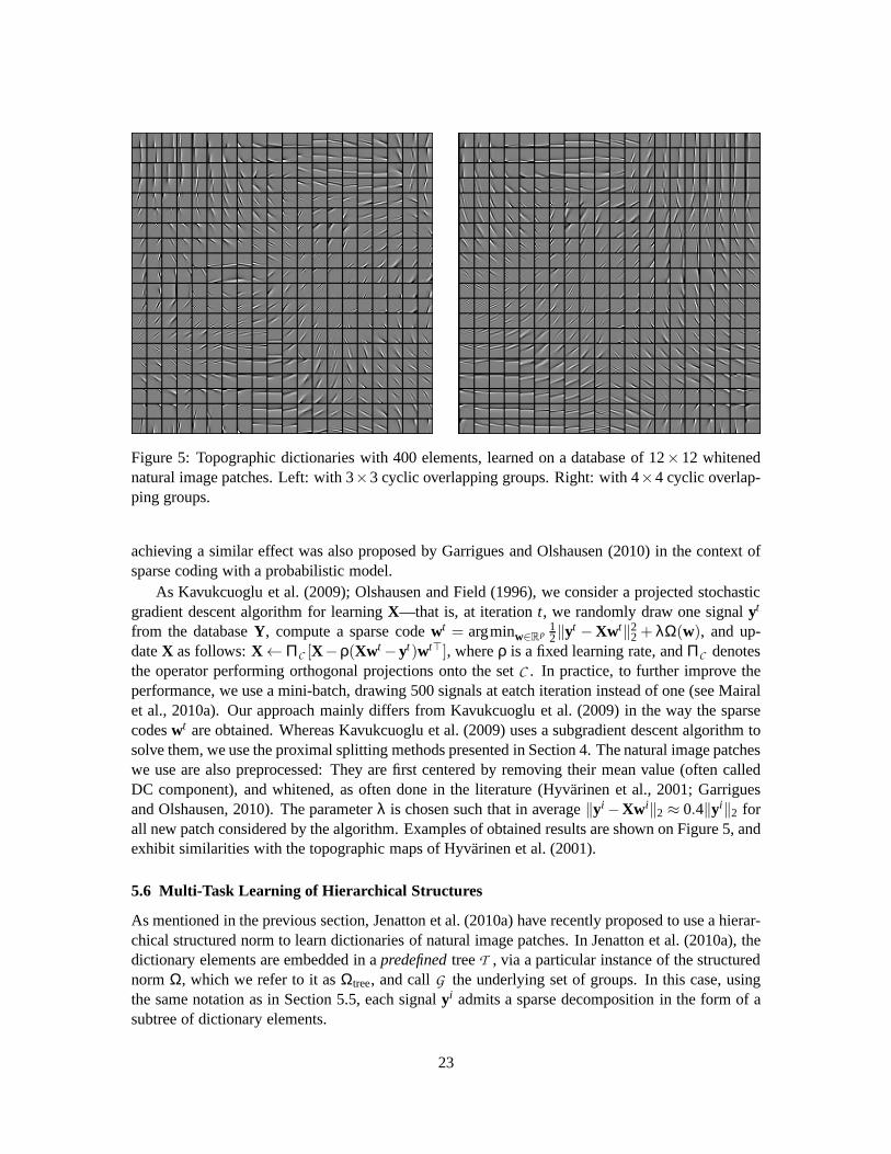
Figure 5: Topographic dictionaries with 400 elements, learned on a database of 12×12 whitenednatural image patches. Left: with 3×3 cyclic overlapping groups. Right: with 4×4 cyclic overlap-ping groups.

achieving a similar effect was also proposed by Garrigues and Olshausen (2010) in the context ofsparse coding with a probabilistic model.

As Kavukcuoglu et al. (2009); Olshausen and Field (1996), weconsider a projected stochasticgradient descent algorithm for learningX—that is, at iterationt, we randomly draw one signalyt

from the databaseY, compute a sparse codewt = argminw∈Rp12‖yt −Xwt‖22 + λΩ(w), and up-

dateX as follows:X← ΠC [X−ρ(Xwt−yt)wt⊤], whereρ is a fixed learning rate, andΠC denotesthe operator performing orthogonal projections onto the set C . In practice, to further improve theperformance, we use a mini-batch, drawing 500 signals at eatch iteration instead of one (see Mairalet al., 2010a). Our approach mainly differs from Kavukcuoglu et al. (2009) in the way the sparsecodeswt are obtained. Whereas Kavukcuoglu et al. (2009) uses a subgradient descent algorithm tosolve them, we use the proximal splitting methods presentedin Section 4. The natural image patcheswe use are also preprocessed: They are first centered by removing their mean value (often calledDC component), and whitened, as often done in the literature(Hyvarinen et al., 2001; Garriguesand Olshausen, 2010). The parameterλ is chosen such that in average‖yi −Xw i‖2 ≈ 0.4‖yi‖2 forall new patch considered by the algorithm. Examples of obtained results are shown on Figure 5, andexhibit similarities with the topographic maps of Hyvarinen et al. (2001).

5.6 Multi-Task Learning of Hierarchical Structures

As mentioned in the previous section, Jenatton et al. (2010a) have recently proposed to use a hierar-chical structured norm to learn dictionaries of natural image patches. In Jenatton et al. (2010a), thedictionary elements are embedded in apredefinedtreeT , via a particular instance of the structurednorm Ω, which we refer to it asΩtree, and callG the underlying set of groups. In this case, usingthe same notation as in Section 5.5, each signalyi admits a sparse decomposition in the form of asubtree of dictionary elements.

23

Inspired by ideas from multi-task learning (Obozinski et al., 2010), we propose to learn thetree structureT by pruning irrelevant parts of a larger initial treeT0. We achieve this by usingan additional regularization termΩjoint across the different decompositions, so that subtrees ofT0

will simultaneouslybe removed for all signalsyi . With the notation from Section 5.5, the approachof Jenatton et al. (2010a) is then extended by the following formulation:

minX∈C ,W∈Rp×n

1n

n

∑i=1

[12‖yi −Xw i‖22+λ1Ωtree(wi)

]

+λ2Ωjoint(W), (15)

whereW , [w1, . . . ,wn] is the matrix of decomposition coefficients inRp×n. The new regularizationterm operates on the rows ofW and is defined asΩjoint(W), ∑g∈G maxi∈1,...,n |wi

g|.26 The overallpenalty onW, which results from the combination ofΩtree andΩjoint, is itself an instance ofΩ withgeneral overlapping groups, as defined in Eq (3).

To address problem (15), we use the same optimization schemeas Jenatton et al. (2010a), i.e.,alternating betweenX andW, fixing one variable while optimizing with respect to the other. Thetask we consider is the denoising of natural image patches, with the same dataset and protocolas Jenatton et al. (2010a). We study whether learning the hierarchy of the dictionary elementsimproves the denoising performance, compared to standard sparse coding (i.e., whenΩtree is theℓ1-norm andλ2 = 0) and the hierarchical dictionary learning of Jenatton et al. (2010a) based onpredefined trees (i.e.,λ2 = 0). The dimensions of the training set — 50000 patches of size8×8 fordictionaries with up top= 400 elements — impose to handle extremely large graphs, with|E| ≈|V| ≈ 4.107. Since problem (15) is too large to be solved exactly sufficiently many times to select theregularization parameters(λ1,λ2) rigorously, we use the following heuristics: we optimize mostlywith the currently pruned tree held fixed (i.e.,λ2 = 0), and only prune the tree (i.e.,λ2 > 0) everyfew steps on a random subset of 10000 patches. We consider thesame hierarchies as in Jenattonet al. (2010a), involving between 30 and 400 dictionary elements. The regularization parameterλ1

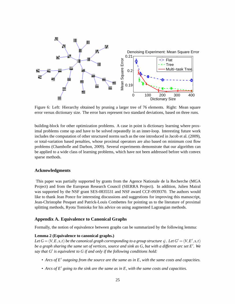
is selected on the validation set of 25000 patches, for both sparse coding (Flat) and hierarchicaldictionary learning (Tree). Starting from the tree giving the best performance (in this case thelargest one, see Figure 6), we solve problem (15) following our heuristics, for increasing valuesof λ2. As shown in Figure 6, there is a regime where our approach performs significantly better thanthe two other compared methods. The standard deviation of the noise is 0.2 (the pixels have valuesin [0,1]); no significant improvements were observed for lower levels of noise. Our experimentsuse the algorithm of Beck and Teboulle (2009) based on our proximal operator, with weightsηg setto 1. We present this algorithm in more details in Appendix C.

6. Conclusion

We have presented new optimization methods for solving sparse structured problems involving sumsof ℓ2- or ℓ∞-norms of any (overlapping) groups of variables. Interestingly, this sheds new light onconnections between sparse methods and the literature of network flow optimization. In particular,the proximal operator for the sum ofℓ∞-norms can be cast as a quadratic min-cost flow problem, forwhich we proposed an efficient and simple algorithm.

In addition to making it possible to resort to accelerated gradient methods, an efficient compu-tation of the proximal operator offers more generally a certain modularity, in that it can be used as a

26. The simplified case whereΩtree and Ωjoint are theℓ1- and mixedℓ1/ℓ2-norms (Yuan and Lin, 2006) correspondsto Sprechmann et al. (2010).

24

0 100 200 300 400

0.19

0.2

0.21Denoising Experiment: Mean Square Error

Dictionary Size

Mea

n S

quar

e E

rror

FlatTreeMulti−task Tree

Figure 6: Left: Hierarchy obtained by pruning a larger tree of 76 elements. Right: Mean squareerror versus dictionary size. The error bars represent two standard deviations, based on three runs.

building-block for other optimization problems. A case in point is dictionary learning where prox-imal problems come up and have to be solved repeatedly in an inner-loop. Interesting future workincludes the computation of other structured norms such as the one introduced in Jacob et al. (2009),or total-variation based penalties, whose proximal operators are also based on minimum cost flowproblems (Chambolle and Darbon, 2009). Several experiments demonstrate that our algorithm canbe applied to a wide class of learning problems, which have not been addressed before with convexsparse methods.

Acknowledgments

This paper was partially supported by grants from the AgenceNationale de la Recherche (MGAProject) and from the European Research Council (SIERRA Project). In addition, Julien Mairalwas supported by the NSF grant SES-0835531 and NSF award CCF-0939370. The authors wouldlike to thank Jean Ponce for interesting discussions and suggestions for improving this manuscript,Jean-Christophe Pesquet and Patrick-Louis Combettes for pointing us to the literature of proximalsplitting methods, Ryota Tomioka for his advice on using augmented Lagrangian methods.

Appendix A. Equivalence to Canonical Graphs

Formally, the notion of equivalence between graphs can be summarized by the following lemma:

Lemma 2 (Equivalence to canonical graphs.)Let G=(V,E,s, t) be the canonical graph corresponding to a group structureG . Let G′=(V,E′,s, t)be a graph sharing the same set of vertices, source and sink asG, but with a different arc set E′. Wesay that G′ is equivalent to G if and only if the following conditions hold:

• Arcs of E′ outgoing from the source are the same as in E, with the same costs and capacities.

• Arcs of E′ going to the sink are the same as in E, with the same costs and capacities.

25

• For every arc(g, j) in E, with (g, j) in Vgr×Vu, there exists a unique path in E′ from g to jwith zero costs and infinite capacities on every arc of the path.

• Conversely, if there exists a path in E′ between a vertex g in Vgr and a vertex j in Vu, thenthere exists an arc(g, j) in E.

Then, the cost of the optimal min-cost flow on G and G′ are the same. Moreover, the values of theoptimal flow on the arcs( j, t), j in Vu, are the same on G and G′.

Proof. We first notice that on bothG andG′, the cost of a flow on the graph only depends on theflow on the arcs( j, t), j in Vu, which we have denoted byξ in E.

We will prove that finding a feasible flowπ on G with a costc(π) is equivalent to finding afeasible flowπ′ onG′ with the same costc(π) = c(π′). We now use the concept ofpath flow, whichis a flow vector inG carrying the same positive value on every arc of a directed path between twonodes ofG. It intuitively corresponds to sending a positive amount offlow along a path of the graph.

According to the definition of graph equivalence introducedin the Lemma, it is easy to showthat there is a bijection between the arcs inE, and the paths inE′ with positive capacities on everyarc. Given now a feasible flowπ in G, we build a feasible flowπ′ on G′ which is asumof pathflows. More precisely, for every arca in E, we consider its equivalent path inE′, with a path flowcarrying the same amount of flow asa. Therefore, each arca′ in E′ has a total amount of flow thatis equal to the sum of the flows carried by the path flows going over a′. It is also easy to show thatthis construction builds a flow onG′ (capacity and conservation constraints are satisfied) and thatthis flow π′ has the same cost asπ, that is,c(π) = c(π′).

Conversely, given a flowπ′ on G′, we use a classical path flow decomposition (see Bertsekas,1991, Proposition 1.1), saying that there exists a decomposition of π′ as a sum of path flows inE′.Using the bijection described above, we know that each path in the previous sums corresponds to aunique arc inE. We now build a flowπ in G, by associating to each path flow in the decompositionof π′, an arc inE carrying the same amount of flow. The flow of every other arc inE is set to zero.It is also easy to show that this builds a valid flow inG that has the same cost asπ′.

Appendix B. Convergence Analysis

We show in this section the correctness of Algorithm 1 for computing the proximal operator, and ofAlgorithm 2 for computing the dual normΩ⋆.

B.1 Computation of the Proximal Operator

We first prove that our algorithm converges and that it finds the optimal solution of the proximalproblem. This requires that we introduce the optimality conditions for problem (6) derived from Je-natton et al. (2010a,b) since our convergence proof essentially checks that these conditions aresatisfied upon termination of the algorithm.

Lemma 3 (Optimality conditions of the problem (6) from Jenatton et al. 2010a,b)The primal-dual variables(w,ξ) are respectively solutions of the primal (4) and dual problems (6) if and only

26

if the dual variableξ is feasible for the problem (6) and

w = u−∑g∈G ξg,

∀g∈ G ,

w⊤g ξgg = ‖wg‖∞‖ξg‖1 and ‖ξg‖1 = ληg,

or wg = 0.

Note that these optimality conditions provide an intuitiveview of our min-cost flow problem.Solving the min-cost flow problem is equivalent to sending the maximum amount of flow in thegraph under the capacity constraints, while respecting therule thatthe flow coming from a group gshould always be directed to the variablesu j with maximum residualu j −∑g∈G ξg

j . This point canbe more formaly seen by noticing that one of the optimality conditions above corresponds to thecase of equality in theℓ1/ℓ∞ Holder inequality.

Before proving the convergence and correctness of our algorithm, we also recall classical prop-erties of the min capacity cuts, which we intensively use in the proofs of this paper. The procedurecomputeFlow of our algorithm finds a minimum(s, t)-cut of a graphG = (V,E,s, t), dividing thesetV into two disjoint partsV+ andV−. V+ is by construction the sets of nodes inV such that thereexists a non-saturating path froms toV, while all the paths froms to V− are saturated. Conversely,arcs fromV+ to t are all saturated, whereas there can be non-saturated arcs fromV− to t. Moreover,the following properties, which are illustrated on Figure 7, hold

• There is no arc going fromV+ to V−. Otherwise the value of the cut would be infinite (arcsinsideV have infinite capacity by construction of our graph).

• There is no flow going fromV− to V+ (see Bertsekas, 1991).

• The cut goes through all arcs going fromV+ to t, and all arcs going froms to V−.

s

g

ξg1+ξg

2<ληg

V+ h

ξh2=ληh

V−

u2

0ξg2

u1

ξg1

u3

ξh3

t

ξ1=γ1 ξ2=γ2 ξ3<γ3

Figure 7: Cut computed by our algorithm.V+=V+u ∪V+

gr , with V+gr =g, V+

u =1,2, andV−=V−u ∪V−gr , with V−gr =h, V−u =3. Arcs going froms to V− are saturated, as well as arcs goingfrom V+ to t. Saturated arcs are in bold. Arcs with zero flow are dotted.

27

Recall that we assume (cf. Section 3.3) that the scalarsu j are all non negative, and that we addnon-negativity constraints onξ. With the optimality conditions of Lemma 3 in hand, we can showour first convergence result.

Proposition 1 (Convergence of Algorithm 1)Algorithm 1 converges in a finite and polynomial number of operations.

Proof. Our algorithm splits recursively the graph into disjoints parts and processes each part recur-sively. The processing of one part requires an orthogonal projection onto anℓ1-ball and a max-flowalgorithm, which can both be computed in polynomial time. Toprove that the procedure converges,it is sufficient to show that when the procedurecomputeFlow is called for a graph(V,E,s, t) andcomputes a cut(V+,V−), then the componentsV+ andV− are both non-empty.

Suppose for instance thatV−= /0. In this case, the capacity of the min-cut is equal to∑ j∈Vuγ j ,

and the value of the max-flow is∑ j∈Vuξ j . Using the classical max-flow/min-cut theorem (Ford and

Fulkerson, 1956), we have equality between these two terms.Since, by definition of bothγ andξ,we have for all j in Vu, ξ j ≤ γ j , we obtain a contradiction with the existence ofj in Vu such that

ξ j 6= γ j .

Conversely, suppose now thatV+= /0. Then, the value of the max-flow is still∑ j∈Vuξ j , and

the value of the min-cut isλ∑g∈Vgrηg. Using again the max-flow/min-cut theorem, we have that

∑ j∈Vuξ j = λ∑g∈Vgr

ηg. Moreover, by definition ofγ, we also have∑ j∈Vuξ j ≤∑ j∈Vu

γ j ≤ λ∑g∈Vgrηg,

leading to a contradiction with the existence ofj in Vu satisfyingξ j 6= γ j . We remind the reader of

the fact that such aj ∈Vu exists since the cut is only computed when the current estimate ξ is notoptimal yet. This proof holds for any graph that is equivalent to the canonical one.

After proving the convergence, we prove that the algorithm is correct with the next proposition.

Proposition 2 (Correctness of Algorithm 1)Algorithm 1 solves the proximal problem of Eq. (4).

Proof. For a group structureG , we first prove the correctness of our algorithm if the graph usedis its associated canonical graph that we denoteG0 = (V0,E0,s, t). We proceed by induction on thenumber of nodes of the graph. The induction hypothesisH (k) is the following:

For all canonical graphs G= (V = Vu ∪Vgr,E,s, t) associated with a group structureGV withweights(ηg)g∈GV such that|V| ≤ k, computeFlow(V,E) solves the following optimization prob-lem:

min(ξg

j ) j∈Vu,g∈Vgr∑j∈Vu

12(u j − ∑

g∈Vgr

ξgj )

2 s.t. ∀g∈Vgr, ∑j∈Vu

ξgj ≤ ληg and ξg

j = 0, ∀ j /∈ g. (16)

SinceGV0 = G , it is sufficient to show thatH (|V0|) to prove the proposition.We initialize the induction byH (2), corresponding to the simplest canonical graph, for which

|Vgr|= |Vu|= 1). Simple algebra shows thatH (2) is indeed correct.We now suppose thatH (k′) is true for allk′ < k and consider a graphG= (V,E,s, t), |V| = k.

The first step of the algorithm computes the variable(γ j) j∈Vu by a projection on theℓ1-ball. This is

28

itself an instance of the dual formulation of Eq. (6) in a simple case, with one group containing allvariables. We can therefore use Lemma 3 to characterize the optimality of (γ j) j∈Vu, which yields

∑ j∈Vu(u j − γ j)γ j =

(

maxj∈Vu |u j − γ j |)

∑ j∈Vuγ j and ∑ j∈Vu

γ j = λ∑g∈Vgrηg,

or u j − γ j = 0, ∀ j ∈Vu.(17)

The algorithm then computes a max-flow, using the scalarsγ j as capacities, and we now have twopossible situations:

1. If ξ j = γ j for all j in Vu, the algorithm stops; we writew j = u j − ξ j for j in Vu, and usingEq. (17), we obtain

∑ j∈Vuw jξ j = (maxj∈Vu |w j |)∑ j∈Vu

ξ j and ∑ j∈Vuξ j = λ∑g∈Vgr

ηg,

or w j = 0, ∀ j ∈Vu.(18)

We can rewrite the condition above as

∑g∈Vgr

∑j∈g

w jξgj = ∑

g∈Vgr

(maxj∈Vu

|w j |)∑j∈Vu

ξgj .

Since all the quantities in the previous sum are positive, this can only hold if for allg∈Vgr,

∑j∈Vu

w jξgj = (max

j∈Vu

|w j |) ∑j∈Vu

ξgj .

Moreover, by definition of the max flow and the optimality conditions, we have

∀g∈Vgr, ∑j∈Vu

ξgj ≤ ληg, and ∑

j∈Vu

ξ j = λ ∑g∈Vgr

ηg,

which leads to∀g∈Vgr, ∑

j∈Vu

ξgj = ληg.

By Lemma 3, we have shown that the problem (16) is solved.

2. Let us now consider the case where there existsj in Vu such thatξ j 6= γ j . The algorithm splitsthe vertex setV into two partsV+ andV−, which we have proven to be non-empty in theproof of Proposition 1. The next step of the algorithm removes all edges betweenV+ andV−

(see Figure 7). Processing(V+,E+) and(V−,E−) independently, it updates the value of theflow matrix ξg

j , j ∈Vu, g∈Vgr, and the corresponding flow vectorξ j , j ∈Vu. As for V, we

denote byV+u ,V+∩Vu, V−u ,V−∩Vu andV+

gr ,V+∩Vgr, V−gr ,V−∩Vgr.

Then, we notice that(V+,E+,s, t) and(V−,E−,s, t) are respective canonical graphs for thegroup structuresGV+ , g∩V+

u | g∈Vgr, andGV− , g∩V−u | g∈Vgr.Writing w j = u j −ξ j for j in Vu, and using the induction hypothesesH (|V+|) andH (|V−|),we now have the following optimality conditions deriving from Lemma 3 applied on Eq. (16)respectively for the graphs(V+,E+) and(V−,E−):

∀g∈V+gr ,g

′ , g∩V+u ,

w⊤g′ξgg′ = ‖wg′‖∞ ∑ j∈g′ξ

gj and ∑ j∈g′ξ

gj = ληg,

or wg′ = 0,(19)

29

and

∀g∈V−gr ,g′ , g∩V−u ,

w⊤g′ξgg′ = ‖wg′‖∞ ∑ j∈g′ξ

gj and ∑ j∈g′ξ

gj = ληg,

or wg′ = 0.(20)

We will now combine Eq. (19) and Eq. (20) into optimality conditions for Eq. (16). We firstnotice thatg∩V+

u = g since there are no arcs betweenV+ andV− in E (see the propertiesof the cuts discussed before this proposition). It is therefore possible to replaceg′ by g inEq. (19). We will show that it is possible to do the same in Eq. (20), so that combining thesetwo equations yield the optimality conditions of Eq. (16).

More precisely, we will show that for allg ∈V−gr and j ∈ g∩V+u , |w j | ≤maxl∈g∩V−u |wl |, in

which caseg′ can be replaced byg in Eq. (20). This result is relatively intuitive:(s,V+) and(V−, t) being an(s, t)-cut, all arcs betweensandV− are saturated, while there are unsaturatedarcs betweensandV+; one therefore expects the residualsu j−ξ j to decrease on theV+ side,while increasing on theV− side. The proof is nonetheless a bit technical.

Let us show first that for allg in V+gr , ‖wg‖∞ ≤ maxj∈Vu |u j − γ j |. We split the setV+ into

disjoint parts:

V++gr , g∈V+

gr s.t. ‖wg‖∞ ≤maxj∈Vu

|u j − γ j |,

V++u , j ∈V+

u s.t. ∃g∈V++gr , j ∈ g,

V+−gr ,V+

gr \V++gr = g∈V+

gr s.t. ‖wg‖∞ > maxj∈Vu

|u j − γ j |,

V+−u ,V+

u \V++u .

As previously, we denoteV+−,V+−u ∪V+−

gr andV++ ,V++u ∪V++

gr . We want to show thatV+−

gr is necessarily empty. We reason by contradiction and assumethatV+−gr 6=∅.

According to the definition of the different sets above, we observe that no arcs are going fromV++ to V+−, that is, for allg in V++

gr , g∩V+−u = ∅. We observe as well that the flow from

V+−gr toV++

u is the null flow, because optimality conditions (19) imply that for a groupg onlynodesj ∈ g such thatw j = ‖wg‖∞ receive some flow, which excludes nodes inV++

u providedV+−

gr 6= ∅; Combining this fact and the inequality∑g∈V+gr

ληg ≥ ∑ j∈V+u

γ j (which is a directconsequence of the minimum(s, t)-cut), we have as well

∑g∈V+−

gr

ληg≥ ∑j∈V+−

u

γ j .

Let j ∈V+−u , if ξ j 6= 0 then for someg∈V+−

gr such thatj receives some flow fromg, whichfrom the optimality conditions (19) impliesw j = ‖wg‖∞; by definition ofV+−

gr , ‖wg‖∞ >

u j − γ j . But since at the optimum,w j = u j − ξ j , this implies thatξ j < γ j , and in turn that

∑ j∈V+−u

ξ j = λ∑g∈V+−gr

ηg. Finally,

λ ∑g∈V+−

gr

ηg = ∑j∈V+−

u ,ξ j 6=0

ξ j < ∑j∈V+−

u

γ j

and this is a contradiction.

30

We now have that for allg in V+gr , ‖wg‖∞ ≤maxj∈Vu |u j− γ j |. The proof showing that for allg

in V−gr , ‖wg‖∞ ≥maxj∈Vu |u j − γ j |, uses the same kind of decomposition forV−, and followsalong similar arguments. We will therefore not detail it.

To summarize, we have shown that for allg ∈ V−gr and j ∈ g∩V+u , |w j | ≤ maxl∈g∩V−u |wl |.

Since there is no flow fromV− to V+, i.e., ξgj = 0 for g in V−gr and j in V+

u , we can now

replace the definition ofg′ in Eq. (20) byg′ , g∩Vu, the combination of Eq. (19) and Eq. (20)gives us optimality conditions for Eq. (16).

The proposition being proved for the canonical graph, we extend it now for an equivalent graphin the sense of Lemma 2. First, we observe that the algorithm gives the same values ofγ for twoequivalent graphs. Then, it is easy to see that the valueξ given by the max-flow, and the chosen(s, t)-cut is the same, which is enough to conclude that the algorithm performs the same steps fortwo equivalent graphs.

B.2 Computation of the Dual Norm Ω⋆

As for the proximal operator, the computation of dual normΩ∗ can itself be shown to solve anothernetwork flow problem, based on the following variational formulation, which extends a previousresult from Jenatton et al. (2009):

Lemma 4 (Dual formulation of the dual-norm Ω⋆.)Let κ ∈ R

p. We have

Ω∗(κ) = minξ∈Rp×|G |,τ∈R

τ s.t. ∑g∈G

ξg = κ, and∀g∈ G , ‖ξg‖1≤ τηg with ξgj = 0 if j /∈ g.

Proof. By definition ofΩ∗(κ), we have

Ω∗(κ), maxΩ(z)≤1

z⊤κ.

By introducing the primal variables(αg)g∈G ∈ R|G |, we can rewrite the previous maximization

problem asΩ∗(κ) = max

∑g∈G ηgαg≤1κ⊤z, s.t. ∀ g∈ G , ‖zg‖∞ ≤ αg,

with the additional|G | conic constraints‖zg‖∞ ≤ αg. This primal problem is convex and satisfiesSlater’s conditions for generalized conic inequalities, which implies that strong duality holds (Boydand Vandenberghe, 2004). We now consider the LagrangianL defined as

L (z,αg,τ,γg,ξ) = κ⊤z+ τ(1−∑g∈G

ηgαg)+ ∑g∈G

(

αg

zg

)⊤(γg

ξgg

)

,

with the dual variablesτ,(γg)g∈G ,ξ ∈ R+×R|G |×Rp×|G | such that for allg∈ G , ξgj = 0 if j /∈ g

and‖ξg‖1 ≤ γg. The dual function is obtained by taking the derivatives ofL with respect to theprimal variablesz and(αg)g∈G and equating them to zero, which leads to

∀ j ∈ 1, . . . , p, κ j +∑g∈G ξgj = 0

∀g∈ G , τηg− γg = 0.

31

After simplifying the Lagrangian and flipping the sign ofξ, the dual problem then reduces to

minξ∈Rp×|G |,τ∈R

τ s.t.

∀ j ∈ 1, . . . , p,κ j =∑g∈G ξgj and ξg

j = 0 if j /∈ g,

∀g∈ G ,‖ξg‖1≤ τηg,

which is the desired result.

We now prove that Algorithm 2 is correct.

Proposition 3 (Convergence and correctness of Algorithm 2)Algorithm 2 computes the value of the dual norm of Eq. (9) in a finite and polynomial number ofoperations.

Proof. The convergence of the algorithm only requires to show that the cardinality ofV in thedifferent calls of the functioncomputeFlow strictly decreases. Similar arguments to those used inthe proof of Proposition 1 can show that each part of the cuts(V+,V−) are both non-empty. Thealgorithm thus requires a finite number of calls to a max-flow algorithm and converges in a finiteand polynomial number of operations.

Let us now prove that the algorithm is correct for a canonicalgraph. We proceed again byinduction on the number of nodes of the graph. More precisely, we consider the induction hypothesisH ′(k) defined as:

for all canonical graphs G= (V,E,s, t) associated with a group structureGV andsuch that|V| ≤ k,dualNormAux(V =Vu∪Vgr,E) solves the following optimization problem:

minξ,τ

τ s.t. ∀ j ∈Vu,κ j = ∑g∈Vgr

ξgj , and∀g∈Vgr, ∑

j∈Vu

ξgj ≤ τηg with ξg

j = 0 if j /∈ g. (21)

We first initialize the induction byH (2) (i.e., with the simplest canonical graph, such that|Vgr| =|Vu|= 1). Simple algebra shows thatH (2) is indeed correct.

We next consider a canonical graphG= (V,E,s, t) such that|V|= k, and suppose thatH ′(k−1)is true. After the max-flow step, we have two possible cases todiscuss:

1. If ξ j = γ j for all j in Vu, the algorithm stops. We know that any scalarτ such that the con-straints of Eq. (21) are all satisfied necessarily verifies∑g∈Vgr

τηg≥∑ j∈Vuκ j . We have indeed

that∑g∈Vgrτηg is the value of an(s, t)-cut in the graph, and∑ j∈Vu

κ j is the value of the max-flow, and the inequality follows from the max-flow/min-cut theorem (Ford and Fulkerson,1956). This gives a lower-bound onτ. Since this bound is reached,τ is necessarily optimal.

2. We now consider the case where there existsj in Vu such thatξ j 6= κ j , meaning that forthe given value ofτ, the constraint set of Eq. (21) is not feasible forξ, and that the value ofτshould necessarily increase. The algorithm splits the vertex setV into two non-empty partsV+

andV− and we remark that there are no arcs going fromV+ toV−, and no flow going fromV−

to V+. Since the arcs going froms to V− are saturated, we have that∑g∈V−grτηg≤ ∑ j∈V−u κ j .

Let us now considerτ⋆ the solution of Eq. (21). Using the induction hypothesisH ′(|V−|), thealgorithm computes a new valueτ′ that solves Eq. (21) when replacingV byV− and this newvalue satisfies the following inequality∑g∈V−gr

τ′ηg≥ ∑ j∈V−u κ j . The value ofτ′ has thereforeincreased and the updated flowξ now satisfies the constraints of Eq. (21) and thereforeτ′≥ τ⋆.Since there are no arcs going fromV+ to V−, τ⋆ is feasible for Eq. (21) when replacingV byV− and we have thatτ⋆ ≥ τ′ and thenτ′ = τ⋆.

32

To prove that the result holds for any equivalent graph, similar arguments to those used in the proofof Proposition 1 can be exploited, showing that the algorithm computes the same values ofτ andsame(s, t)-cuts at each step.

Appendix C. Algorithm FISTA with duality gap

In this section, we describe in details the algorithm FISTA (Beck and Teboulle, 2009) when appliedto solve problem (2), with a duality gap as the stopping criterion. The algorithm, as implemented inthe experiments, is summarized in Algorithm 3.

Without loss of generality, let us assume we are looking for models of the formXw, for somematrixX ∈Rn×p (typically, a linear model whereX is the design matrix composed ofn observationsin R

p). Thus, we can consider the following primal problem

minw∈Rp

f (Xw)+λΩ(w), (22)

in place of problem (2). Based on Fenchel duality arguments (Borwein and Lewis, 2006),

f (Xw)+λΩ(w)+ f ∗(−κ), for w ∈Rp,κ ∈R

n andΩ∗(X⊤κ)≤ λ,

is a duality gap for problem (22), wheref ∗(κ) , supz[z⊤κ− f (z)] is the Fenchel conjugate of

f (Borwein and Lewis, 2006). Given a primal variablew, a good dual candidateκ can be obtainedby looking at the conditions that have to be satisfied by the pair (w,κ) at optimality (Borwein andLewis, 2006). In particular, the dual variableκ is chosen to be

κ =−ρ−1∇f (Xw), with ρ , max

λ−1Ω∗(X⊤∇f (Xw)),1

.

Consequently, computing the duality gap requires evaluating the dual normΩ∗, as explained inAlgorithm 2. We sum up the computation of the duality gap in Algorithm 3. Moreover, we refer tothe proximal operator associated withλΩ as proxλΩ.27

In our experiment, we choose the line-search parameterν to be equal to 1.5.

Appendix D. Speed comparison of Algorithm 1 with parametricmax-flow algorithms

As shown by Hochbaum and Hong (1995), min-cost flow problems,and in particular, the dualproblem of (4), can be reduced to a specificparametric max-flowproblem. We thus compare ourapproach (ProxFlow) with the efficient parametric max-flow algorithm proposed by Gallo et al.(1989) and a simplified version of the latter proposed by Babenko and Goldberg (2006). We referto these two algorithms as GGT and SIMP respectively. The benchmark is established on the samedatasets as those already used in the experimental section of the paper, namely: (1) three datasetsbuilt from overcomplete bases of discrete cosine transforms (DCT), with respectively 104, 105 and106 variables, and (2) images used for the background subtraction task, composed of 57600 pixels.For GGT and SIMP, we use theparaF software which is aC++ parametric max-flow implementation

27. As a brief reminder, it is defined as the function that mapsthe vectoru in Rp to the (unique, by strong convexity)

solution of Eq. (4).

33

Algorithm 3 FISTA procedure to solve problem (22).

1: Inputs: initial w(0) ∈ Rp, Ω, λ > 0, εgap> 0 (precision for the duality gap).

2: Parameters: ν > 1, L0 > 0.3: Outputs: solutionw.4: Initialization : y(1) = w(0), t1 = 1, k= 1.5: while

computeDualityGap(

w(k−1))

> εgap

do6: Find the smallest integersk≥0 such that7: f (prox[λΩ](y(k)))≤ f (y(k))+∆⊤(k)∇ f (y(k))+

L2‖∆(k)‖22,

8: with L , Lkνsk and∆(k) , y(k)−prox[λΩ](y(k)).9: Lk← Lk−1νsk.

10: w(k)← prox[λΩ](y(k)).

11: tk+1← (1+√

1+ t2k)/2.

12: y(k+1)← w(k)+tk−1tk+1

(w(k)−w(k−1)).13: k← k+1.14: end while15: Return: w← w(k−1).

ProcedurecomputeDualityGap(w)

1: κ←−ρ−1∇f (Xw), with ρ , max

λ−1Ω∗(X⊤∇f (Xw)),1

.2: Return: f (Xw)+λΩ(w)+ f ∗(−κ).

available athttp://www.avglab.com/andrew/soft.html. Experiments were conducted on asingle-core 2.33 Ghz.

We report in the following table the average execution time in seconds of each algorithm for 5runs, as well as the statistics of the corresponding problems:

Number of variablesp 10000 100000 1000000 57600

|V| 20000 200000 2000000 57600|E| 110000 500000 11000000 579632

ProxFlow (in sec.) 0.4 3.1 113.0 1.7GGT (in sec.) 2.4 26.0 525.0 16.7SIMP (in sec.) 1.2 13.1 284.0 8.31

Although we provide the speed comparison for a single value of λ (the one used in the correspondingexperiments of the paper), we observed that our approach consistently outperforms GGT and SIMPfor values ofλ corresponding to different regularization regimes.

References

R. K. Ahuja, T. L. Magnanti, and J. Orlin.Network Flows. Prentice Hall, 1993.

A. Argyriou, T. Evgeniou, and M. Pontil. Convex multi-task feature learning.Machine Learning,73(3):243–272, 2008.

34

M. Babenko and A.V. Goldberg. Experimental evaluation of a parametric flow algorithm. Technicalreport, Microsoft Research, 2006. MSR-TR-2006-77.

F. Bach. High-dimensional non-linear variable selection through hierarchical kernel learning. Tech-nical report, arXiv:0909.0844, 2009.

F. Bach. Structured sparsity-inducing norms through submodular functions. InAdvances in NeuralInformation Processing Systems, 2010.

F. Bach, R. Jenatton, J. Mairal, and G. Obozinski. Convex optimization with sparsity-inducingnorms. In S. Sra, S. Nowozin, and S. J. Wright, editors,Optimization for Machine Learning.MIT Press, 2011. To appear.

R. G. Baraniuk, V. Cevher, M. Duarte, and C. Hegde. Model-based compressive sensing.IEEETransactions on Information Theory, 56(4):1982–2001, 2010.

A. Barron, J. Rissanen, and B. Yu. The minimum description length principle in coding and model-ing. IEEE Transactions on Information Theory, 44(6):2743–2760, 1998.

A. Beck and M. Teboulle. A fast iterative shrinkage-thresholding algorithm for linear inverse prob-lems.SIAM Journal on Imaging Sciences, 2(1):183–202, 2009.

D. P. Bertsekas.Linear Network Optimization. MIT Press, 1991.

D. P. Bertsekas.Nonlinear programming. Athena Scientific Belmont, 1999.

D. P. Bertsekas and J. N. Tsitsiklis. Parallel and distributed computation: Numerical Methods. 1989.

P. Bickel, Y. Ritov, and A. Tsybakov. Simultaneous analysisof Lasso and Dantzig selector.Annalsof Statistics, 37(4):1705–1732, 2009.

J. Bien, Y. Xu, and M. W. Mahoney. CUR from a sparse optimization viewpoint. InAdvances inNeural Information Processing Systems, 2010.

J. M. Borwein and A. S. Lewis.Convex analysis and nonlinear optimization: Theory and examples.Springer, 2006.

S. P. Boyd and L. Vandenberghe.Convex Optimization. Cambridge University Press, 2004.

Y. Boykov and V. Kolmogorov. An experimental comparison of min-cut/max-flow algorithms forenergy minimization in vision.IEEE Transactions on Pattern Analysis and Machine Intelligence,26(9):1124–1137, 2004.

P. Brucker. An O(n) algorithm for quadratic knapsack problems. Operations Research Letters, 3:163–166, 1984.

T. T. Cai. Adaptive wavelet estimation: a block thresholding and oracle inequality approach.Annalsof statistics, pages 898–924, 1999.

V. Cehver, M. F. Duarte, C. Hedge, and R. G. Baraniuk. Sparse signal recovery using Markovrandom fields. InAdvances in Neural Information Processing Systems, 2008.

35

A. Chambolle and J. Darbon. On total variation minimizationand surface evolution using parametricmaximal flows.International Journal of Computer Vision, 84(3), 2009.

S. S. Chen, D. L. Donoho, and M. A. Saunders. Atomic decomposition by basis pursuit.SIAMJournal on Scientific Computing, 20:33–61, 1999.

X. Chen, Q. Lin, S. Kim, J. Pena, J. G. Carbonell, and E. P. Xing. An efficient proximal-gradientmethod for single and multi-task regression with structured sparsity. Technical report, 2010.ArXiv:1005.4717v1.

B. V. Cherkassky and A. V. Goldberg. On implementing the push-relabel method for the maximumflow problem.Algorithmica, 19(4):390–410, 1997.

P. L. Combettes and J.-C. Pesquet. Proximal splitting methods in signal processing. InFixed-PointAlgorithms for Inverse Problems in Science and Engineering. Springer, 2010.

P.L. Combettes and J.C. Pesquet. A proximal decomposition method for solving convex variationalinverse problems.Inverse Problems, 24(27), 2008. Art. 065014.

D. L. Donoho and I. M. Johnstone. Adapting to unknown smoothness via wavelet shrinkage.Journalof the American Statistical Association, 90(432):1200–1224, 1995.

J. Duchi, S. Shalev-Shwartz, Y. Singer, and T. Chandra. Efficient projections onto theℓ1-ball forlearning in high dimensions. InProceedings of the International Conference on Machine Learn-ing (ICML), 2008.

B. Efron, T. Hastie, I. Johnstone, and R. Tibshirani. Least angle regression.Annals of Statistics, 32(2):407–499, 2004.

M. Elad and M. Aharon. Image denoising via sparse and redundant representations over learneddictionaries.IEEE Transactions on Image Processing, 54(12):3736–3745, December 2006.

L. R. Ford and D. R. Fulkerson. Maximal flow through a network.Canadian Journal of Mathemat-ics, 8(3):399–404, 1956.

J. Friedman, T. Hastie, and R. Tibshirani. A note on the groupLasso and a sparse group Lasso.Technical report, Preprint arXiv:1001.0736, 2010.

S. Fujishige.Submodular functions and optimization. Elsevier, 2005.

G. Gallo, M. E. Grigoriadis, and R. E. Tarjan. A fast parametric maximum flow algorithm andapplications.SIAM J. Comput., 18:30–55, 1989.

P. Garrigues and B. Olshausen. Group sparse coding with a laplacian scale mixture prior. InAd-vances in Neural Information Processing Systems, 2010.

A. V. Goldberg and R. E. Tarjan. A new approach to the maximum flow problem. InProc. of ACMSymposium on Theory of Computing, pages 136–146, 1986.

D. Goldfarg and S. Ma. Fast multiple splitting algorithms for convex optimization. Technical report,2009. Preprint arXiv:0912.4570v1.

36

H. Groenevelt. Two algorithms for maximizing a separable concave function over a polymatroidfeasible region.Europeran Journal of Operations Research, pages 227–236, 1991.

L. He and L. Carin. Exploiting structure in wavelet-based Bayesian compressive sensing.IEEETransactions on Signal Processing, 57(9):3488–3497, 2009.

D. S. Hochbaum and S. P. Hong. About strongly polynomial timealgorithms for quadratic opti-mization over submodular constraints.Mathematical Programming, 69(1):269–309, 1995.

R. A. Horn and C. R. Johnson.Matrix analysis. Cambridge University Press, 1990.

J. Huang and T. Zhang. The benefit of group sparsity.Annals of Statistics, 38(4):1978–2004, 2010.

J. Huang, Z. Zhang, and D. Metaxas. Learning with structuredsparsity. InProceedings of theInternational Conference on Machine Learning (ICML), 2009.

A. Hyvarinen, P. Hoyer, and M. Inki. Topographic independent component analysis.Neural Com-putation, 13(7):1527–1558, 2001.

L. Jacob, G. Obozinski, and J.-P. Vert. Group Lasso with overlap and graph Lasso. InProceedingsof the International Conference on Machine Learning (ICML), 2009.

R. Jenatton, J-Y. Audibert, and F. Bach. Structured variable selection with sparsity-inducing norms.Technical report, 2009. Preprint arXiv:0904.3523v3.

R. Jenatton, J. Mairal, G. Obozinski, and F. Bach. Proximal methods for sparse hierarchical dic-tionary learning. InProceedings of the International Conference on Machine Learning (ICML),2010a.

R. Jenatton, J. Mairal, G. Obozinski, and F. Bach. Proximal methods for hierarchical sparse coding.2010b. preprint ArXiv:1009.2139v3.

R. Jenatton, G. Obozinski, and F. Bach. Structured sparse principal component analysis. InInter-national Conference on Artificial Intelligence and Statistics (AISTATS), 2010c.

K. Kavukcuoglu, M. Ranzato, R. Fergus, and Y. LeCun. Learning invariant features through to-pographic filter maps. InProceedings of the IEEE Conference on Computer Vision and PatternRecognition (CVPR), 2009.

S. Kim and E. P. Xing. Tree-guided group Lasso for multi-taskregression with structured sparsity.In Proceedings of the International Conference on Machine Learning (ICML), 2010.

N. Maculan and J. R. G. Galdino de Paula. A linear-time median-finding algorithm for projecting avector on the simplex of Rn.Operations Research Letters, 8(4):219–222, 1989.

M. W. Mahoney and P. Drineas. CUR matrix decompositions for improved data analysis.Proceed-ings of the National Academy of Sciences, 106(3):697, 2009.

J. Mairal, F. Bach, J. Ponce, G. Sapiro, and A. Zisserman. Non-local sparse models for imagerestoration. InProceedings of the IEEE International Conference on Computer Vision (ICCV),2009.

37

J. Mairal, F. Bach, J. Ponce, and G. Sapiro. Online learning for matrix factorization and sparsecoding.Journal of Machine Learning Research, 11:19–60, 2010a.

J. Mairal, R. Jenatton, G. Obozinski, and F. Bach. Network flow algorithms for structured sparsity.In Advances in Neural Information Processing Systems, 2010b.

S. Mallat. A Wavelet Tour of Signal Processing, Second Edition. Academic Press, New York,September 1999.

C. A. Micchelli, J. M. Morales, and M. Pontil. A family of penalty functions for structured sparsity.In Advances in Neural Information Processing Systems, 2010.

J. J. Moreau. Fonctions convexes duales et points proximauxdans un espace Hilbertien.C. R. Acad.Sci. Paris Ser. A Math., 255:2897–2899, 1962.

D. Needell and J. A. Tropp. CoSaMP: Iterative signal recovery from incomplete and inaccuratesamples.Applied and Computational Harmonic Analysis, 26(3):301–321, 2009.

S. Negahban, P. Ravikumar, M. J. Wainwright, and B. Yu. A unified framework for high-dimensional analysis of M-estimators with decomposable regularizers. InAdvances in NeuralInformation Processing Systems, 2009.

Y. Nesterov. Smooth minimization of non-smooth functions.Mathematical Programming, 103(1):127–152, 2005.

Y. Nesterov. Gradient methods for minimizing composite objective function. Technical report, Cen-ter for Operations Research and Econometrics (CORE), Catholic University of Louvain, 2007.

G. Obozinski, B. Taskar, and M. I. Jordan. Joint covariate selection and joint subspace selection formultiple classification problems.Stat. Comput., 20(2):231–252, 2010.

B. A. Olshausen and D. J. Field. Emergence of simple-cell receptive field properties by learning asparse code for natural images.Nature, 381:607–609, 1996.

A. Rakotomamonjy, F. Bach, S. Canu, and Y. Grandvalet. SimpleMKL. Journal of Machine Learn-ing Research, 9:2491–2521, 2008.

V. Roth and B. Fischer. The group-Lasso for generalized linear models: uniqueness of solutionsand efficient algorithms. InProceedings of the International Conference on Machine Learning(ICML), 2008.

M. Schmidt and K. Murphy. Convex structure learning in log-linear models: Beyond pairwisepotentials. InProceedings of the International Conference on Artificial Intelligence and Statistics(AISTATS), 2010.

J. Shawe-Taylor and N. Cristianini.Kernel Methods for Pattern Analysis. 2004.

P. Sprechmann, I. Ramirez, G. Sapiro, and Y. C. Eldar. Collaborative hierarchical sparse modeling.Technical report, 2010. Preprint arXiv:1003.0400v1.

38

M. Stojnic, F. Parvaresh, and B. Hassibi. On the reconstruction of block-sparse signals with anoptimal number of measurements.IEEE Transactions on Signal Processing, 57(8):3075–3085,2009.

R. Tibshirani. Regression shrinkage and selection via the Lasso. Journal of the Royal StatisticalSociety: Series B, 58(1):267–288, 1996.

R. Tomioka, T. Suzuki, and M. Sugiyama. Augmented Lagrangian methods for learning, select-ing and combining features. In S. Sra, S. Nowozin, and S. J. Wright, editors,Optimization forMachine Learning. MIT Press, 2011. To appear.

P. Tseng. Convergence of a block coordinate descent method for nondifferentiable minimization.Journal of optimization theory and applications, 109(3):475–494, 2001.

B. A. Turlach, W. N. Venables, and S. J. Wright. Simultaneousvariable selection.Technometrics,47(3):349–363, 2005.

M. J. Wainwright. Sharp thresholds for noisy and high-dimensional recovery of sparsity usingℓ1-constrained quadratic programming (Lasso).IEEE Transactions on Information Theory, 55(5):2183–2202, May 2009.

J. Wright, A. Y. Yang, A. Ganesh, S. S. Sastry, and Y. Ma. Robust face recognition via sparserepresentation.IEEE Transactions on Pattern Analysis and Machine Intelligence, 31(2):210–227, 2009a.

S. Wright, R. Nowak, and M. Figueiredo. Sparse reconstruction by separable approximation.IEEETransactions on Signal Processing, 57(7):2479–2493, 2009b.

M. Yuan and Y. Lin. Model selection and estimation in regression with grouped variables.Journalof the Royal Statistical Society: Series B, 68:49–67, 2006.

X. Zhang, M. Burger, and S. Osher. A unified primal-dual algorithm framework based on Bregmaniteration.Journal of Scientific Computing, 46(1):20–46, 2011.

P. Zhao, G. Rocha, and B. Yu. The composite absolute penalties family for grouped and hierarchicalvariable selection.Annals of Statistics, 37(6A):3468–3497, 2009.

39