Convergent perturbation theory for a q–deformed anharmonic oscillator

arX

iv:m

ath/

9808

024v

1 [

mat

h.Q

A]

5 A

ug 1

998

LMU–TPW–98–11, MPI–PhT–98/62

July 1998

Convergent Perturbation Theory for a q–deformed

Anharmonic Oscillator

R. Dicka, A. Pollok-Narayanana,b∗, H. Steinackera† and J. Wess a,b

aSektion Physik der Ludwig–Maximilians–Universitat

Theresienstr. 37, 80333 Munchen, Germany

bMax–Planck–Institut fur Physik

Fohringer Ring 6, 80805 Munchen, Germany

Abstract: A q–deformed anharmonic oscillator is defined within the framework of

q–deformed quantum mechanics. It is shown that the Rayleigh–Schrodinger perturba-

tion series for the bounded spectrum converges to exact eigenstates and eigenvalues,

for q close to 1. The radius of convergence becomes zero in the undeformed limit.

∗ [email protected]–muenchen.de†[email protected]–muenchen.de

1

1 Introduction

The anharmonic oscillator H = ωa†a + γX4 is a basic quantum mechanical prob-

lem with one particularly interesting feature: its perturbation series diverges, but

nevertheless there exist eigenstates and energies which are smooth as the (positive)

coupling constant γ goes to zero [11, 12, 13]. A similar phenomenon is expected to

occur in many interacting quantum field theories. The anharmonic oscillator can

in fact be considered as a (0 + 1)–dimensional ϕ4 ”field” theory with one degree of

freedom.

In this paper, we study the analog of this model in the framework of q–deformed

quantum mechanics, based on the q–deformed Heisenberg algebra introduced in [5].

In particular, one would like to know how the perturbation theory of the q–deformed

anharmonic oscillator behaves compared to the undeformed case. This is of interest in

view of a possible q–deformation of field theory, which is expected to be less singular

than field theory based on ordinary manifolds, since q–deformation generically puts

physics on a q–lattice [5, 6]. With this motivation, we study the perturbation theory of

the anharmonic oscillator in terms of the q–deformed harmonic oscillator, which was

introduced in [2, 3] and realized in the framework of q–deformed quantum mechanics

in [1].

There is considerable freedom in defining a q–deformed anharmonic oscillator for

q 6= 1. Taking advantage of this freedom, we show that for a suitable definition

of the anharmonic oscillator, the perturbation series converges to exact eigenvalues

and eigenstates for 1 < q < 1.06 with a certain radius of convergence in γ. In the

limit q → 1, the model reduces to the usual anharmonic oscillator, and the radius of

convergence goes to zero. The upper limit on q is not significant.

This paper is organized as follows: In section 2 we review the q-deformed harmonic

oscillator and its spectrum, and calculate the relevant matrix elements. In section 3,

the perturbation series for eigenvalues and eigenstates is discussed. Some estimates

for the matrix elements are given in the Appendix.

2

2 The q-deformed harmonic oscillator

In this section, we give a brief review of the q–deformed harmonic oscillator, and

its realization in terms of a q–deformed Heisenberg algebra. For a more detailed

discussion, see [1] and [5].

The q-deformed Heisenberg algebra is the star–algebra generated by X, P, U with

the relations [5]

q1

2 XP − q−1

2 PX = iU (1)

UX = q−1XU, UP = qPU.

We assume q > 1 to be real. The star structure is such that X and P are hermitian,

and U is unitary:

X = X†, P = P †, U † = U−1. (2)

This algebra has the following (momentum–space) representation [5]:

P |n, σ〉 = σqn|n, σ〉U |n, σ〉 = |n − 1, σ〉

U−1|n, σ〉 = |n + 1, σ〉

X|n, σ〉 = iσq−n

q − q−1(q

1

2 |n − 1, σ〉 − q−1

2 |n + 1, σ〉)

〈n, σ|m, σ′〉 = δn,mδσ,σ′ (3)

with n, m ∈ IN and σ, σ′ = ±1. The completion of these states defines a Hilbert space

H.

The two values of σ describe positive respectively negative momenta. (3) is a

star–representation, i.e. the star is implemented as the adjoint of an operator, and

both X and P have selfadjoint extensions. That is the reason for introducing σ, see

[8].

This is a starting point for studying q–deformed quantum mechanics [14, 15, 9, 5].

In particular, one can define q–deformed creation and anihilation operators as follows:

a = αU−2M + βU−MP (4)

a† = αU2M + βPUM

3

with M ∈ IN , and α, β ∈ C| . They satisfy the Biedenharn–Macfarlane algebra [2, 3]:

aa† − q−2Ma†a = (1 − q−2M)αα = 1 (5)

where we fix α = i√1−q−2M

. The occupation number operator is defined as

n = a†a = αα + ββP 2 + αβ(UM + qMU−M )P. (6)

Now one can write down the following Hamiltonian, which constitutes the q–deformed

harmonic oscillator:

H0 = ωa†a (7)

The spectrum of H0 acting on H consists of a bounded spectrum with eigenvalues

E(0)n = ω[n]M = ω 1−q−2nM

1−q−2M which is 2M–fold degenerate, and an unbounded spec-

trum with eigenvalues ω(q2mME(0)0 + 1−q2mM

1−q−2M ). The 2M ground states of the bounded

spectrum are

|0〉(M)σ,µ =

∞∑

n=−∞

c0

(

−σα

β

)n

q−1

2(Mn2+Mn+2µn)|Mn + µ, σ〉,

0 ≤ µ < M. (8)

The existence of an unbounded spectrum beyond E∞ = ω1−q−2M is clear in view of (5),

since P is an unbounded operator on H. For simplicity, we will only consider M = 1

from now on, and omit the labels µ and M .

So far, β was arbitrary. Requiring that the a, a† are smooth for q → 1 and become

the usual (undeformed) creation and anihilation operators in the limit, one finds [1]

that

α =i√

1 − q−2, β =

i√2mω

(9)

where m is the mass. For this choice, H0 can be interpreted as a q–deformation

of the usual harmonic oscillator, and this will be understood in the following. The

normalized states of the bounded spectrum are

|n〉σ =1

√

[n](a†)n|0〉σ, (10)

where [n] = 1−q−2n

1−q−2 . We define Hb,± ⊂ H to be the closure of the space spanned by

the |n〉±1. As q → 1, Hb,+ becomes the Hilbert space of the usual harmonic oscillator,

4

while the unbounded spectrum disappears at infinity, and the support of the states

with σ = −1 goes to −∞ in the momentum representation. We will thus concentrate

on Hb,+.

The eigenstates of H0 can also be written in terms of the q–deformed Hermite

polynomials, which satisfy (see [10]):

ξH(q)n (ξ) =

√qq2n

2(H

(q)n+1(ξ) + 2q−2[n]H

(q)n−1(ξ)) (11)

Defining ξ =√

mωX, one has

|n〉σ =1√

2n[n]!

H(q)n (ξ)|0〉σ.

Using these Hermite polynomials, it is straightforward to calculate the action of

X on an eigenstate |n〉σ, and it follows in particular that X · Hb,+ ⊂ Hb,+. This will

be important for the perturbation theory below.

Now we turn to the anharmonic oscillator. The undeformed anharmonic oscillator

is defined by H = ωa†a + γX4 for γ > 0, thus one might naively take the same

expression for q > 1, and study its perturbation theory. The relevant matrix elements

can be calculated e.g. using (11), and we find the following results [4]:

〈n|X4|n〉 =(

1

2mω

)2

q8n+6(

[n + 1]([n + 2] + q−4[n + 1] + q−8[n])

+ q−8[n]([n + 1] + q−4[n] + q−8[n − 1]))

〈n + 4|X4|n〉 =(

1

2mω

)2

q8n+14√

[n + 1][n + 2][n + 3][n + 4]

〈n + 2|X4|n〉 =(

1

2mω

)2

q8n+12√

[n + 1][n + 2]

([n + 3] + q−4[n + 2] + q−8[n + 1] + q−12[n]) (12)

They are independent of σ which is suppressed. All other nonvanishing matrix ele-

ments can be obtained from those by hermiticity.

Looking at the powers of q in the matrix elements, one quickly finds that the

perturbation series diverges even faster than in the undeformed case.

However, it is important to realize that there is no reason for considering the same

expression for H as in the undeformed case; the only requirement one has to impose

5

is that H should reduce to the usual anharmonic oscillator as q → 1. Therefore we

might just as well consider the Hamiltonian

H = H0 + γH ′ (13)

with

H ′ =1

2(X4Q5 + Q5X4), where

Q = (1 − a†a(1 − q−2)). (14)

Q satisfies

Q|n〉 = q−2n|n〉. (15)

The matrix elements 〈n|H ′|m〉 can be easily obtained from (12), see Figure 2. As is

shown in the Appendix, they have the following upper bound:

〈n|H ′|m〉 < C(q) := [3]4[2]8q−2nmax+10[nmax]

2 =4q10[3]4[2]8

81(1 − q−2)2(16)

for 1 < q < 1.06, where nmax = ln 32 ln q

. In view of the results of the next section, we

define (13) to be the q–deformed anharmonic oscillator.

3 Perturbation Expansion

We will use the standard Rayleigh-Schrodinger perturbation formulas for the eigen-

states and eigenvalues of

H = H0 + H1 = H0 + γH ′ (17)

in terms of the unperturbed ones, H0|n〉 = E(0)n |n〉:

∆En =∞∑

k=0

E(k)n (∆En, γ) :=

∞∑

k=0

〈n|H1

(

1

E(0)n − H0

Qn (H1 − ∆En)

)k

|n〉

. (18)

6

where Qn = (1 − |n〉〈n|), and

|En〉 = |n〉 +∞∑

k=1

∑

n1,...nknr 6=n

|n1〉(

k∏

j=2〈nj−1|H1 − ∆En|nj〉

)

〈nk|H1|n〉k∏

j=1(E

(0)n − E

(0)nj )

.

(19)

Strictly speaking, we are of course dealing with a degenerate problem (since σ =

±1); however as already explained, X and Q leave Hb,+ invariant, thus the two values

of σ do not interfere, and we can restrict ourselves to the σ = +1 sector. This will be

understood in the following. We will show that these series in fact converge to exact

eigenvalues and eigenstates of the q-deformed anharmonic oscillator, for a certain

range of γ which depends on q.

3.1 Energy Levels

If γ and ∆En are not real, then H1 is understood to act on the right in the above

formulas, so that the matrix elements can be continued analytically in γ and ∆En.

We show first that the sum in (18) is absolutely convergent for |∆En| < ω/5 and

|γ| < γ(q), where γ(q) > 0 provided q > 1, see (22). Thus the rhs of (18) is an

analytic function of ∆En and γ in that domain, which can be solved for ∆En by the

implicit function theorem, defining an analytic function ∆En(γ).

To see that the sum in (18) is (absolutely) convergent for a certain range of ∆En

and γ, we first write E(m)n more explicitely:

E(1)n = 〈n|H1|n〉

E(2)n =

∑

n1n1 6=n

〈n|H1|n1〉〈n1|H1|n〉(E

(0)n − E

(0)n1 )

E(k)n (∆En, γ) =

∑

n1,n2,...,nk−1

nr 6=n

〈n|H1|n1〉(

k−1∏

j=2〈nj−1|H1 − ∆En|nj〉

)

〈nk−1|H1|n〉

(E(0)n − E

(0)nk−1

)(E(0)n − E

(0)nk−2

) . . . (E(0)n − E

(0)n1 )

for k ≥ 3 (20)

7

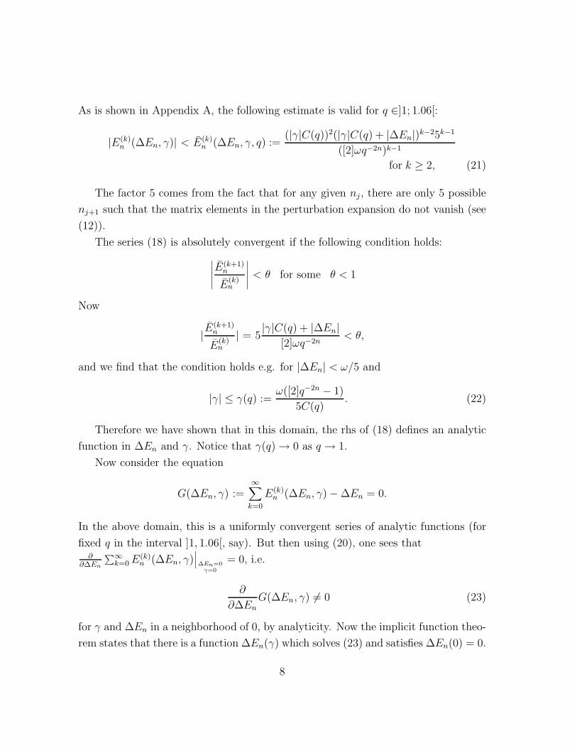
As is shown in Appendix A, the following estimate is valid for q ∈]1; 1.06[:

|E(k)n (∆En, γ)| < E(k)

n (∆En, γ, q) :=(|γ|C(q))2(|γ|C(q) + |∆En|)k−25k−1

([2]ωq−2n)k−1

for k ≥ 2, (21)

The factor 5 comes from the fact that for any given nj , there are only 5 possible

nj+1 such that the matrix elements in the perturbation expansion do not vanish (see

(12)).

The series (18) is absolutely convergent if the following condition holds:

∣

∣

∣

∣

∣

E(k+1)n

E(k)n

∣

∣

∣

∣

∣

< θ for some θ < 1

Now

|E(k+1)n

E(k)n

| = 5|γ|C(q) + |∆En|

[2]ωq−2n< θ,

and we find that the condition holds e.g. for |∆En| < ω/5 and

|γ| ≤ γ(q) :=ω([2]q−2n − 1)

5C(q). (22)

Therefore we have shown that in this domain, the rhs of (18) defines an analytic

function in ∆En and γ. Notice that γ(q) → 0 as q → 1.

Now consider the equation

G(∆En, γ) :=∞∑

k=0

E(k)n (∆En, γ) − ∆En = 0.

In the above domain, this is a uniformly convergent series of analytic functions (for

fixed q in the interval ]1, 1.06[, say). But then using (20), one sees that∂

∂∆En

∑∞k=0 E(k)

n (∆En, γ)∣

∣

∣

∆En=0

γ=0

= 0, i.e.

∂

∂∆En

G(∆En, γ) 6= 0 (23)

for γ and ∆En in a neighborhood of 0, by analyticity. Now the implicit function theo-

rem states that there is a function ∆En(γ) which solves (23) and satisfies ∆En(0) = 0.

8

1.01 1.02 1.03 1.05 1.060.00

0.01

0.02

0.03

0.04

0.05

0.06

0.04

0.03

0.02

0.01

0.05

0.06

-

-

-

-

-

-

1.04

γ (q)

q

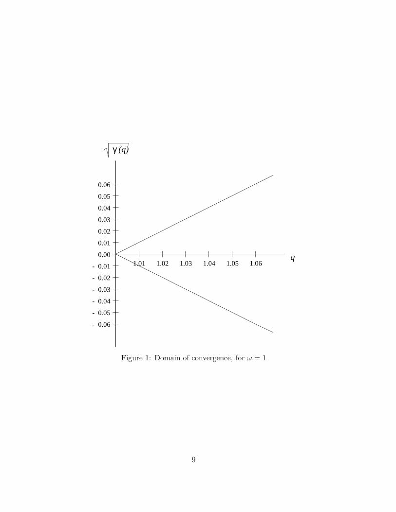
Figure 1: Domain of convergence, for ω = 1

9

Moreover, ∆En(γ) is analytic in a neighborhood of 0, and |∆En| < ω/5 holds auto-

matically if γ is small enough.

The domain of convergence γ(q) is shown in Figure 1 for q ∈]1; 1.06[ and ω = 1. In

particular, γ(q) goes to zero for q → 1, in accordance with the well–known fact that

the perturbation series for the undeformed anharmonic oscillator is divergent [12].

3.2 Eigenstates

In this section, we show that (19) converges in Hb,+ ⊂ H for |γ| < γ(q) and 1 <

q < 1.06, where ∆En = ∆En(γ) is now the perturbed energy found in the previous

section. To do this, we have to show that

∞∑

m=0

|〈m|En〉|2 < ∞, (24)

or more explicitely

〈En|En〉 =∞∑

m=0

|〈m|En〉|2

=∞∑

m=0

∣

∣

∣

∣

∣

δm,n +∞∑

k=1

∑

n1,...nknr 6=n

δm,n1

(

k∏

j=2〈nj−1|H1 − ∆En|nj〉

)

〈nk|H1|n〉k∏

j=1(E

(0)n − E

(0)nj )

∣

∣

∣

∣

∣

2

From the form of the matrix elements (12), we see that the second term is nonzero

only for k ≥ |m−n|4

, therefore

〈En|En〉 ≤ 1 +∞∑

m=0

∑

k≥|m−n|

4

(

(|γ|C(q) + |∆En|)k−1|γ|C(q)5k

([2]q−2nω)k

)2

≤ 1 +∞∑

m=0

(

5|γ|C(q) + |∆En|

[2]q−2nω

)

|m−n|2

∞∑

k=0

(

5|γ|C(q) + |∆En|

[2]q−2nω

)2k

for 1 < q < 1.06. Clearly this converges for γ in the analyticity domain defined

above (such that |∆En| < ω/5 as before), therefore the series (19) converges in Hb,+.

Finally, both H0 and H ′ leave Hb,+ ⊂ H invariant and are bounded operators on

Hb,+ (H ′ is bounded because of (27) and the fact that H ′ acting on |n〉 has no more

10

that 5 nonvanishing components in terms of that basis). Now it follows that |En〉 and

E(0)n + ∆En are indeed eigenstates and eigenvalues of the full anharmonic oscillator.

As already mentioned, it is known [12] that the undeformed anharmonic oscillator

does have nonperturbative eigenstates and energies for γ > 0, which are nevertheless

smooth as γ goes to zero from above. Now the formulas (18) ff. can be analytically

continued in q as well, and one would expect that the above domain of analyticity for

∆En and γ can be extended to include q = 1 and positive real axis of γ. However, at

present we are not able to show this.

Acknowledgements A. P.N. acknowledges with thanks the support from MPI.

Appendix: Matrix elements

Because [n] is an increasing function in n, we have the following estimates:

1

2γ(1 + q−40)q14−2n[n]2 < 〈n + 4|H ′|n〉 <

1

2γ(1 + q−40)q14−2n[n + 4]2

1

2γ(1 + q−20)q12−2n[4]4[n]2 < 〈n + 2|H ′|n〉 <

1

2γ(1 + q−20)q12−2n[4]4[n + 3]2

γq−2n+6[3]4[2]8[n]2 < 〈n|H ′|n〉 < γq−2n+6[3]4[2]8[n + 2]2

(25)

with

[n]i :=1 − q−ni

1 − q−i, [n] =

1 − q−2n

1 − q−2,

See Figure 2 for a plot of 〈n|H ′|n〉.To simplify this, consider the function q−2n[n]2 for n ∈ IR, which takes its maxi-

mum value 481(1−q−2)2

at n = nmax,

nmax :=ln 3

2 ln q. (26)

11

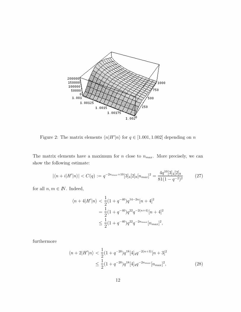
Figure 2: The matrix elements 〈n|H ′|n〉 for q ∈ [1.001, 1.002] depending on n

The matrix elements have a maximum for n close to nmax. More precisely, we can

show the following estimate:

|〈n + i|H ′|n〉| < C(q) := q−2nmax+10[3]4[2]8[nmax]2 =

4q10[3]4[2]881(1 − q−2)2

(27)

for all n, m ∈ IN . Indeed,

〈n + 4|H ′|n〉 <1

2(1 + q−40)q14−2n[n + 4]2

=1

2(1 + q−40)q22q−2(n+4)[n + 4]2

≤ 1

2(1 + q−40)q22q−2nmax [nmax]

2,

furthermore

〈n + 2|H ′|n〉 <1

2(1 + q−20)q18[4]4q

−2(n+3)[n + 3]2

≤ 1

2(1 + q−20)q18[4]4q

−2nmax [nmax]2, (28)

12

and

〈n|H ′|n〉 ≤ q10[3]4[2]8q−2nmax [nmax]

2 = C(q) (29)

Now for 1 ≤ q < 1.06, one has

1 <2q−16[3]4[2]8

1 + q−40(30)

(for i = 4) and

1 <2[3]4[2]8

q12[4]4(1 + q−20)(31)

(for i = 1). Combining these estimates, we obtain (27). Furthermore |E(0)n −E

(0)n±i| ≥

[i]q−2nω, therefore |E(0)nj

− E(0)n | ≥ [2]q−2nω in the denominators of the perturbation

expansion, since i ≥ 2. Now (21) follows, because for any given nj in the perturbation

series, there are at most 5 possible nj+1 such that 〈nj |H ′|nj+1〉 is nonzero; this means

that the number of terms at order k is at most 5k−1.

References

[1] A. Lorek, A. Ruffing, J. Wess, A q-Deformation of the Harmonic Oscillator.

Preprint MPI-PhT/96-26, hep-th/9605161

[2] A.J. Macfarlane, On q–analogues of the quantum harmonic oscillator and quan-

tum group SU(2)q. J. Phys. A 22, 4581 (1989)

[3] L.C. Biedenharn, the quantum group SUq(2) and a q – analogue of the boson

operators. J. Phys. A 22, L873 (1989)

[4] A. Pollok-Narayanan, Storungsrechnung am harmonischen Oszillator in der q–

deformierten Quantenmechanik. Diploma thesis, LMU Munchen, Lehrstuhl Prof.

Wess, Marz 1998

[5] M. Fichtmuller, A. Lorek, J. Wess, q-deformed Phase Space and its Lattice Struc-

ture. hep-th/9511106

13

[6] B.L. Cerchiai, J. Wess, q–deformed Minkowski space based on a q-deformed

Lorentz algebra. To appear in Europ. Journ. of Physics; math.QA/9801104

[7] A. Lorek, J. Wess, Dynamical Symmetries in q-deformed Quantum Mechanics.

Z. Phys. C 67, 671-680 (1994)

[8] A. Hebecker, S. Schreckenberg, J. Schwenk, W. Weich, J. Wess, Representations

of a q-deformed Heisenberg algebra, Z. Phys. C 64, 355-359 (1994)

[9] J. Schwenk, J. Wess, A q-deformed quantum mechanical toy model. Physics Let-

ters B 291, 273-277 (1992)

[10] Ralf Hinterding, q-deformierte Hermite Polynome. Diplomarbeit, LMU

Munchen, Lehrstuhl Prof. J. Wess, April 1997; R. Hinterding, J. Wess, q–

deformed Hermite Polynomials in q–Quantum Mechanics. to appear in Europ.

Phys. Journ. C; math.QA/9803050

[11] C. M. Bender, T. T. Wu, Large Order Behavior of Perturbation Theory. Physical

Review Vol 27, No 7, 461

[12] C. M. Bender, T. T. Wu, anharmonic Oszillator. Phys. Rev. 184, No 5, 1231

(1969)

[13] J.J. Loeffel, A. Martin, B. Simon, A.S. Wightman, Pade approximants and the

anharmonic oscillator. Physics Letters 30 B, 656 (1969)

[14] Joachim Seifert, q-deformierte Ein-Teilchen Quantenmechanik. Dissertation,

LMU Munchen, Lehrstuhl Prof. J. Wess, Juli 1996.

[15] A. Ruffing, Quantensymmetrische Quantentheorie und Gittermodelle fur Oszil-

latorwechselwirkungen. Dissertation, LMU Munchen, Lehrstuhl Prof. J. Wess,

Februar 1996.

14