Controlled Linear Perturbation - Purdue University

Controlled Linear Perturbation

Elisha Sacks, Purdue University

joint work with

Victor Milenkovic, University of Miami

Min-Ho Kyung, University of Ajou

Research supported by a PLM grant and by NSF grantsCCF-0904832 and CCF-0904707.

Controlled Linear Perturbation – p. 1/21

Robustness Problem

Algorithms are expressed in real RAM model.

Input is assumed in general position.

Implementations must use computer arithmetic.

Implementations must handle degenerate input.

Implementations must be fast and accurate.

Controlled Linear Perturbation – p. 2/21

Geometric Predicates

a

c

db

a

c

db

unsafe degenerate

Main interface with real RAM model (also constructions).

Predicate P (x) is true when polynomial f(x) is positive.

Unsafe predicate: |f(x)| near the rounding unit.

Degenerate predicate: f(x) = 0.

Example: b above cd if (d − c) × (b − c) > 0;f(bx, by, cx, cy, dx, dy) = (dx−cx)(by−cy)−(dy−cy)(bx−cx).

Controlled Linear Perturbation – p. 3/21

Exact Computational Geometry

Implement predicates exactly using algebra.

Technical problemsRunning time grows rapidly with algebraic degree.Bit complexity grows rapidly.Degeneracy requires separate, complex algorithm.

Conceptual problemScientific computing is approximate because exactsolutions are impractical and unnecessary.Gold standard is fast algorithms with error bounds.Why should computational geometry be exact?

Controlled Linear Perturbation – p. 4/21

Approximate Computational Geometry

Implement predicates approximately using floating pointarithmetic and numerical solvers.

Advantages:Running time grows modestly with degree.Constant bit complexity.Small constant factors.

Challenge: generate consistent output.

Controlled Linear Perturbation – p. 5/21

Consistency

a

c

db

a

c

db a

c

d

b

unsafe i degenerate i consistent p

An algorithm is consistent when for every input, i, thereexists a perturbed input, p, such that the computedpredicates are correct for p.

The output error is the distance from i to p, ||p − i||.Inconsistent algorithms can crash or output garbage.

Controlled Linear Perturbation – p. 6/21

Perturbation Strategy

1. Derive a safety threshold, e, such that |f(x)| > e infloating point implies safety.

2. Every time a predicate polynomial is evaluated, checkits threshold.

3. If the check fails, perturb the input.

Controlled Linear Perturbation – p. 7/21

CP versus CLP

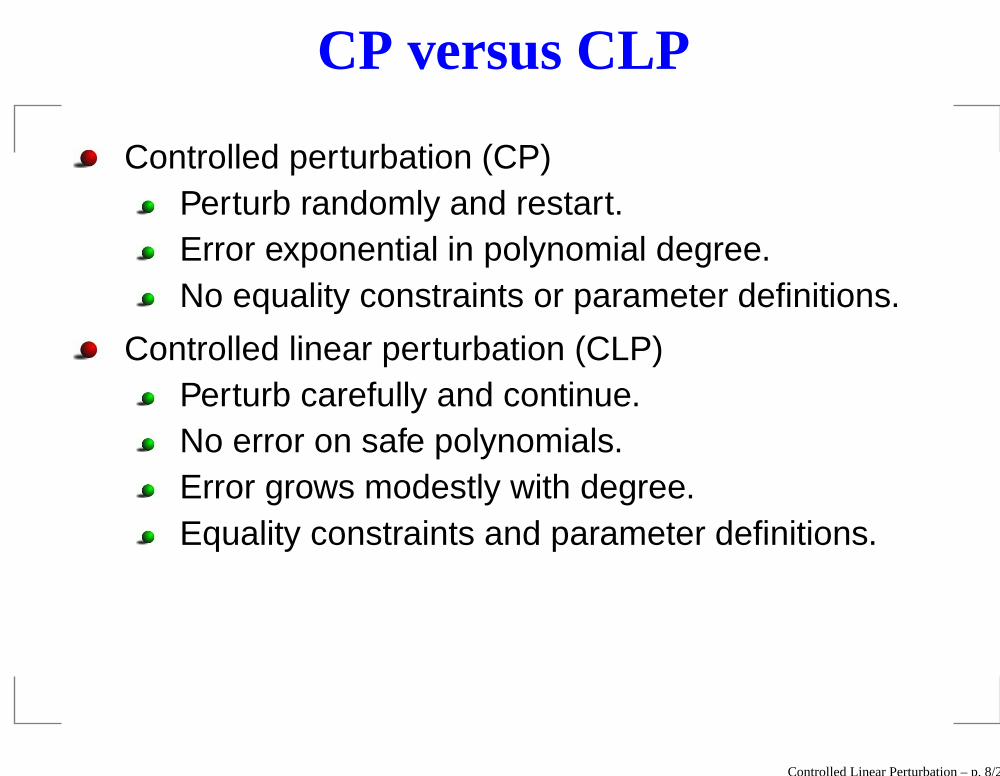
Controlled perturbation (CP)Perturb randomly and restart.Error exponential in polynomial degree.No equality constraints or parameter definitions.

Controlled linear perturbation (CLP)Perturb carefully and continue.No error on safe polynomials.Error grows modestly with degree.Equality constraints and parameter definitions.

Controlled Linear Perturbation – p. 8/21

CLP Strategy

Given: polynomial f(x) with input x = a.

1. If |f(a)| > e, return its sign.

2. Compute p such that |f(p)| > e and likewise forprevious polynomials.

3. Return the sign of f(p).

Controlled Linear Perturbation – p. 9/21

CLP Algorithm

Write p = a + δv with δ ≥ 0 the perturbation size and vthe perturbation direction.

Linearize f(p) ≈ f(a) + δ∇f · v with ∇f the gradient.

Linearization error is negligible because δ is tiny.

Initialize δ = 0, v = 0 and update for each unsafe f .

Best v for sign s is s∇f ignoring prior unsafe fi.

Define u by subtracting ∇fi from ∇f and unitizing.

Update v to v + su; pick s = ±1 with smallerδ = (2se − f(a))/(s∇f · v); update δ.

Prior fi are uneffected by change in v; become saferdue to increase in δ.

Verify signs of f(p) for final p.

Controlled Linear Perturbation – p. 10/21

Sorting Example

Sort x = (0, 0, 0, 1) in increasing order.

Predicate xi < xj has polynomial xj − xi with e = 2µ.

Degenerate for i, j < 4; safe otherwise.

1) Evaluate x2 − x1 with v = (0, 0, 0, 0) and orth = ∅.

∇f = (−1, 1, 0, 0), so u1 =√

0.5(−1, 1, 0, 0).

For s = 1, δ = 2se−f(a)s∇f ·v = 4µ

u1·∇f .

For s = −1, δ = −4µ−u1·∇f .

CLP picks s = 1, δ ≈ 2.8µ, and x1 < x2.

Controlled Linear Perturbation – p. 11/21

Sorting Example Continued

2) Evaluate x3 − x1 with v = u1 and orth = u1.

∇f = (−1, 0, 1, 0), so u2 =√

1/6(−1,−1, 2, 0).

For s = 1, δ < 2.8µ, so CLP picks it and x1 < x3.

3) Evaluate x3 − x2 with v = u1 + u2 ≈ (−1.1, 0.3, 0.8, 0) andorth = u1, u2.

∇f = (0,−1, 1, 0), so u3 = (0, 0, 0, 0).

Only choice is s = 1 with δ ≈ 4µ−0.3+0.8 ≈ 7.7µ and

x1 < x2.

Final order, x1 < x2 < x3, derives from v.

Controlled Linear Perturbation – p. 12/21

Parameter Definitions

er s

c d

esr

c d

full rank rank deficient

Define new parameters, y = b, with equations g(x, y) = 0.

Enforce linearized equations by adding to orth.

Extend v to y by solving gxv + gyw = 0.

Example: e = (y1, y2), b = (3.6,−1.8), equations g(x, y)

(y1 − x1)2 + (y2 − x2)

2 − x23 = 0

(y1 − x4)2 + (y2 − x5)

2 − x26 = 0.

Rank deficient case requires special handling.

Controlled Linear Perturbation – p. 13/21

Singular Predicate Polynomials

Polynomial f is singular when ∇f = 0.

Core CLP fails on near singular unsafe polynomials.

We avoid near singularity by predicate reformulationusing judicious parameter definitions.

Example: point b above line cd with b = c = d.

Define unit vector, u = (d − c)/||d − c||, with equationsu · u − 1 = 0 and u × (d − c) = 0.

Reformulation: u × (b − c) = ux(by − cy) − uy(bx − cx)

Gradient is large: (−uy, ux, uy,−ux, by − cy, cx − bx).

Controlled Linear Perturbation – p. 14/21

Minkowski Sums

Minkowski sum of point sets A and B is the point setA ⊕ B = a + b | a ∈ A, b ∈ B.

Minkowski sums of polyhedra have many applications:packing, path planning, assembly, graphics, solidmodeling, mechanics, simulation.

Prior implementations decompose polyhedra intoconvex pieces.

Complexity is Ω(n4) for input size n; prohibitive.

Approximate algorithms are tricky and slow.

Efficient output sensitive algorithm known for 30 years.

We use CLP to obtain the first robust implementation.

Controlled Linear Perturbation – p. 15/21

Cube + Polyhedron

Controlled Linear Perturbation – p. 16/21

Torus + Polyhedron

Controlled Linear Perturbation – p. 17/21

Cube + Torus

Controlled Linear Perturbation – p. 18/21

Sphere + Helix

Controlled Linear Perturbation – p. 19/21

Results

A, B, and conv the number of triangles in part A, part B,and the convolution, time the running time in seconds, safeand unsafe the number of safe and unsafe predicatepolynomials, and δ the final perturbation size.

A B conv time safe unsafe δ

a 12 32 130 0.1 4e5 5,393 3e-12b 32 2068 4336 5 2.2e6 13,145 8e-10c 12 2068 2946 4.3 1.1e6 15,991 2e-10d 760 4012 40,212 49 27e7 43,752 1e-10

Controlled Linear Perturbation – p. 20/21

Future Work

ResearchAutomated handling of near singular polynomials.Output simplification.

EducationComputational geometry curriculum organizedaround robustness.Computational geometry textbook organizedaround robustness.

ApplicationsPatent.Software library.Robust applications software.

Controlled Linear Perturbation – p. 21/21