Control Theory in TCP Congestion Control and new “FAST” designs. Fernando Paganini and Zhikui Wang UCLA Electrical Engineering July 2002. Collaborators:

Control Theory in TCP Congestion Control and new “FAST” designs.

Fernando Paganini and Zhikui WangUCLA Electrical Engineering

July 2002.

Collaborators: Steven Low, John Doyle, Jiantao Wang (Caltech).

Earlier versions: Sachin Adlakha, Sanjeewa Athuraliya.

Basic fluid-flow models

1 if link uses source

0 otherwise li

l iR

Routing matrix:

1

2 3

2i

3i

1i

1 1 0 0

0 0 1 0

0 1 1 1

R

: Rate of th source: Total rate of th link: Capacity of the th link

i

l

l

x iy lc l

R x y

Feedback mechanism:

Each link has a congestion measure or price .

Each source has access to aggregate price of the links in its path.l

i

T

p

q

q R p

L communication links shared by S source-destination pairs.

4i

Congestion Control Loop

LINKS

SOURCES

R

TR

ROUTING

p

xy

q : link prices

: aggregate link flows

: source rates

: aggregate prices per source

Decentralized control at links and sources.Routing assuming fixed, or varying at much slower time-scale.

Link and Source Controls determine:

• Steady-state properties:– Utilization– Queues– Fairness

• Dynamic properties:– Speed of response– Stability, oscillations.– Sensitivity to noise.

Issues with currently deployed TCP:

• Steady-state properties:– Utilization: (can be affected by dynamics)– Queues (~full with DropTail).– Fairness (dependence on RTT)

• Dynamic properties:– Speed of response: Additive increase is too slow in

large cwnd sizes (high capacity networks). – Stability, oscillations: Multiplicative decrease is too

aggressive in large cwnd. – Sensitivity to noise.

0 1000 2000 3000 4000 5000 6000 7000 8000 9000 100000

100

200

300

400

500

600

700

800Instantaneous queue

time (ms)

Insta

nta

neous q

ueue (

pkts

)

Stability of TCP: ns-2 simulations50 identical FTP sources, single link 9 pkts/ms, RED AQM

Stable case, RTT= 40ms

0 1000 2000 3000 4000 5000 6000 7000 8000 9000 100000

100

200

300

400

500

600

700

800Instantaneous queue

time (10ms)

Insta

nta

neous q

ueue (

pkts

)

Queue

Unstable case, RTT= 200ms

Window

( )(1 ( ))

( )( ) ( )

2i

i ii i

ii

ii w tx

x t qt

t

wq t

dwdt

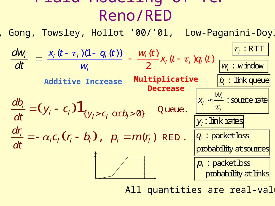
Fluid Modeling of TCP-Reno/RED

RTT

window

: link queue

source rate

packet loss

probability at sources

packet loss probability at links

:

:

:

: link rates

:

:

l

i

i

ii

i

l

i

l

b

w

wx

y

q

p

(Misra, Gong, Towsley, Hollot ’00/’01, Low-Paganini-Doyle ’02)

Additive Increase Multiplicative Decrease

{ or 0} Queue

RED

.

, ( ) .

1i

i

l l

l l l l l l

l l ly c bdb

dt

dr

dt

y c

c r b p m r

All quantities are real-valued.

Stability Analysis of TCP-Reno/RED

• Packet simulations validate both the region and the oscillation frequency at the onset of instability.

• Linearizing around equilibrium we find a stability region: Unstable for large equilibrium windows, which arise with high delay or, strikingly, high capacity!

8 9 10 11 12 13 14 1550

55

60

65

70

75

80

85

90

95

100Round trip propagation delay at critical frequency

capacity (pkts/ms)

dela

y (

ms)

N=40

N=30

N=20

N=20 N=60 Unstable for Large delay Large

capacity Small load

Link capacity

Stability region for the case of N identical sources.

Improving these limitations: • Steady-state properties:

– ECN allows us to decouple feedback from queuing, so in principle we can get high utilization, low delay.

– Resource allocation issue can be addressed if we allow sources to pick a utility function.

– Study this by optimization theory.

• Dynamic properties:– We need to negotiate the appropriate tradeoff between

responding fast to track available bandwidth, but not so fast that everything oscillates: working close to the boundary of linear stability is the best compromise.

– To study this tradeoff: control theory.

Optimization-based approaches (Kelly, Low, …)

• Steady-state properties:– Utilization– Queues– Fairness

• Dynamic properties:– Speed of response– Stability, oscillations.– Sensitivity to noise.

Start from the equilibrium side: • Source utility functions• Characterize social optimum.• Develop decentralized algorithms

Worry about dynamics later: • Stability without delay.• Noise variances• Stability margins to delay.• Speed of response.

Difficulty: hard to arrange for the dynamic tradeoffs,Specially for the wide variety of network scenarios.

Control Theory-Based Approach• Steady-state:

– Utilization– Queues– Fairness

• Dynamic properties:– Speed of response– Stability, oscillations.– Sensitivity to noise.

Look for a scalable (network and delay independent) solution to the dynamic tradeoff (stability vs. speed or response)

To get the other equilibrium property, both approaches can adapt things at a slower time-scale assuming a bound on the RTT:“primal-dual” solutions, similar but with minor differences.

Can also impose one steady-state property:• “Primal” solution (Vinnicombe) gives freedom on utility functions• Our “dual” solution ensures utilization.

Dynamics and the role of delay

• Without delay, nothing would stop us from adapting the sources’ rates arbitrarily fast.

• In the presence of delay, there is a stability problem: e.g., controlling temperature of your shower.

• Special case of general principle in feedback systems: what limits the performance (e.g. speed of response) are characteristics of the open loop (bandwidth, delay).

• In this case, the only impediment is delay. In particular, this sets the time-scale of our response.

Stability/performance tradeoff in presence of delay

( ) ( ) ( )t K t tuy y se K

s

yu

Loop transfer function is

( )s

L ss

Ke

Increase for performance

(fast transients, tracking o .f )

u

K

2K

1

Nyquist plot of ( )L jBut for stability.

2This sets a fundamental limit to speed of time response.

K

Feedback design is about how fast you can respond while remaining stable: the limiting factor comes from the “plant” dynamics. In this problem, from delay. A simple example:

Congestion control loop with delays

LINKSSOURCES

( )fR s source rates:x

: aggregate flows per linky

,( ) ( )fl i i li l

y t x t

( )TbR s: aggregate prices

per sourceq p: link congestion

measures or “prices”

,( ) ( )bi l i li l

q t p t

RTT: , ,f b

i i l i l

, .

if source uses link

0 otherwise ( )

f

i l s

f lii lR s e

Routing/Delay matrix:

Ingredients for scalable stability. Make the feedback gain inversely proportional to RTT.

This must be done at sources, and is already implicit in

window protocols, due to the relation .w

x

Still, other factors contribute to the loop gain. For instance,

the gain tends to scale naturally with the number of sources

sharing a bottleneck, unless some compensation is done.

Difficulty: compe

nsating with decentralized information.

For scalability to delays, the remaining dynamics must

be first order. Roughly, this means we can only put dynamics at

either sources or links (not both), and therefore track on

arbitrary

only

t

e

s

eady-state objective: source's demand curve or link utilization.

“Dual” solution with integrator at links.

SINGLE LINKSOURCES

( )fR s0i

i ii

xx q

( ) ( )fi ii l

y t x t

( )TbR s( ) ( )bi iq t p t

1p y

c

01Loop transfer function: ( ) i i

i i

isxL s

cse

Guarantees steady-state tracking of link utilization.Gain compensation exploits equilibrium rates and capacity. Linear dynamics, single link/multiple sources case:

denotes increments around equilibrium

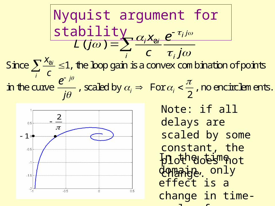
Nyquist argument for stability

0( )j

i i

i i

ixL j

c j

e

0Since 1, the loop gain is a convex combination of points

in the curve , scaled by For , no encirclements.2

i

i j

i i

x

c

j

e

Note: if all delays are scaled by some constant, the plot does not change.

In the time domain, only effect is a change in time-scale of response.

2

1

Extension to arbitrary networks

LINKSSOURCES

( )fR s

( )TbR s

source rates:x

: aggregate flows per linky

: aggregate prices per sourceq p: link prices

( )fy R s x

( )Tbq R s p

0i ii i

i

xx q

M

: number of bottlenecks in source i’s pathiM

1l l

l

p yc

Local analysis around equilibrium. Routing matrices refer here only to bottleneck links.

Stability result Assume the matrix (0)= (0) (involving only

the bottleneck links) is of full row rank, and that . Then the 2

feedback system is locally stable for arbitrary delays and capacities.

Theorem: f b

i

R R R

0

( )

:

Write the loop transfer function ( )

.

( ) is stable, and (0) has positive eigenvalues under the rank assumption. This implies stabi

( ) ( ) ( )

Steps of the proof

Lf

Tb

F s

F s

s

F s F

IL s R s AX M R s

s

T C

lity for small enough 's. Note: integrators at the links!

A perturbation argument preserves stability as long as 1 ( ). This

follows by exploitin ( ) ( ) diagg (as in Johari -Tan '00)jb fR j R j

L j

e

,

which reduces the eigs ( ) to the same region as in the single link case.L j

( )L s

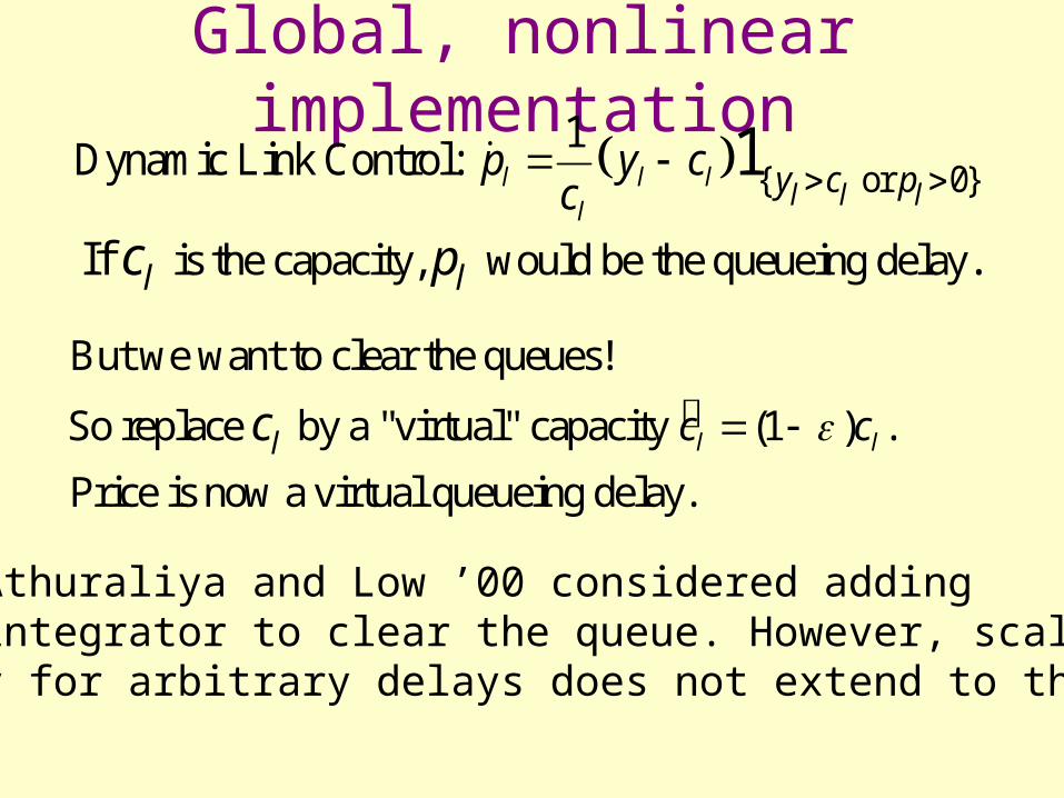
Global, nonlinear implementation { or 0}

1Dynamic Link Control: 1l l l

ll l ly c pp y c

c

is the capacity, would be the queueing delayIf . l lpc

But we want to clear the queues!

So replace by a "virtual" capacity (1 ) .

Price is now a virtual queueing delay. l ll c cc

Remark: Athuraliya and Low ’00 considered adding another integrator to clear the queue. However, scalable stability for arbitrary delays does not extend to that case.

Global, nonlinear implementationStatic control law for sources: linearization requirement is

0 ( , )i i i ii i i i i

i i i

x xx q x q

M q M

“Elasticity” of demand decreases with delay, number of bottlenecks.

max,

Assume known, or take a known upper bound. Initially, fix independently of the operating point. Solving the differential equation:

i i

i i

i

i

i i

qM

M

x x e

This implicitly chooses one utility function, and in particular

would determine issues like fairness.

Properties of the nonlinear laws• Global stability? Validate by

– Flow simulation of differential equations using Matlab. So far, cases of local stability have been global.

– Mathematical proof. Tools which combine delay and nonlinearity are very limited! We have partial results for single link, but with further parameter constraints.

• Equilibrium structure, fairness: Determined by the fixed utility, and possibly very unfair, since exponentials distinguish rates very sharply.

• Objective: allow freedom of choice in utility functions. This calls for source dynamics, which clashes with scalable stability; we can allow it if we only require scalability to “practical” RTTs, and adapt source dynamics slowly.

New solution with fairness tracking

Source control:

'( ) , (slower tracking of fairness).

(faster control of utilization)i

i i

ii i i i i

i m

i iqM

dk U x q

dt

x x e

1Link Control: , 0 virtual queueing delay.l l l l

l

p y c pc

maxi

i i

zk

M M

Equilibrium: '( ) (maximizes ( ) ). (matches virtual capacity).

i i i i i i i

l l

U x q U x q xcy

Can prove local stability under adequate parameter choices(next slide)

Linearized laws and requirements for stability. ( )

i i i

i

i

s zx B q

zBs

A

0

max

1 1, , < .

"( )i i

i ii i i

xB A z

M U x

0RTT, , equilibrium rate2

bound on # of bottlenecks in path

i i i

i

x

M

LINKSSOURCES

( )fR s

( )TbR s

source rates:x

: aggregate flows per linky

: aggregate prices per sourceq

( )fy R s x

( )Tbq R s p

1l l

l

p yc

: link pricesp

virtual capacity.lc

Recap, so far• Our first flow control had scalable stability to

arbitrary delays, plus exact tracking of link utilization.

• We can further assign the equilibrium resource allocation between sources at a slower (universally agreed-on) time-scale (slower than max RTT).

• Packet-implementations:– One approach based on ECN marking to communicate

the price, to be described by Zhikui later.– Alternative (Choe and Low): use queuing delay as

price, modifying TCP Vegas.