Control systems - Frequency domain analysis: Polar Plot

Outline

Control systemsFrequency domain analysis: Polar Plot

V. Sankaranarayanan

V. Sankaranarayanan Frequency domain analysis

Outline

Outline


Polar plot

It is a plot of the magnitude of G(jω) versus the phase angle of G(jω) onpolar coordinates as ω is varied from zero to infinity

In polar plots a positive (negative) phase angle is measured counterclockwise(clockwise) from the positive real axis


Integral and derivative factors


G(jω) = 1jω

= −j 1ω

= 1ω∠−90o

The Polar plot of 1jω

is the negative imaginary axis




The Polar plot of jω is the positive imaginary axis


First order factors

First order factors

G(jω) = 11+jωT

= 1√1+ω2T2

∠−tan−1ωT

G(j0) = 1∠0o, G(j 1T

) = 1√2∠45o

ω −→∞, |G(jω)| −→ 0 and ∠G(jω) −→ −90o

G(s) = X + jY

1

1 + jωT=

1− jωT1 + ω2T 2

G(s) =1

1 + ω2T 2− j

wT

1 + ω2T 2

X =1

1 + ω2T 2Y = −

wT

1 + ω2T 2(X −

1

2

)2

+ Y 2 =

(1

2

)2

So the polar plot is a semi circle.


Plot

G(s) =1

1 + jωT


First order factors

First order factors

G(jω) = 1 + jωT

It is simply the upper half of the straight line passing through point (1, 0) inthe complex plane and parallel to the imaginary axis


Quadratic factors

Quadratic factors

G(jω) = 11+2ζ(j ω

ωn)+(j ω

ωn)2

For ζ > 0

limω→0

G(jω) = 1∠0

limω→∞

G(jω) = 0∠−180

The polar plot of this sinusoidal transfer function starts at 1∠0 and ends at0∠−180 as ω increases from zero to infinity

The high-frequency portion of G(jω) is tangent to the negative real axis.

For the underdamped case ω = ωn, the phase angle is −90

In the polar plot, the frequency point whose distance from the origin ismaximum corresponds to the resonant frequency ωr.



Quadratic factors

Quadratic factors

G(jω) = 1 + 2ζ(j ωωn

) + (j ωωn

)2

=(

1− ω2

ω2n

)+ j

(2ζωωn

)limω→0

G(jω) = 1∠0

limω→∞

G(jω) =∞∠180



Gain Margin and Phase Margin

Gain Margin

The gain margin is the reciprocal of the magnitude |G(jω)| at the frequency atwhich the phase angle is −180o(Phased cross over frequency)

Kg =1

|G(jω)|at∠G = −180o

Phase Margin

The phase margin is the amount of additional phase lag at the gain cross overfrequency required to the verge of instability γ = 180o + φ


Phase and Gain Margin

Nyquist Diagram

Real Axis

Imagin

ary

Axis

−1 −0.8 −0.6 −0.4 −0.2 0 0.2 0.4 0.6 0.8 1−1

−0.8

−0.6

−0.4

−0.2

0

0.2

0.4

0.6

0.8

1

Phase Cross Over at (−0.5,0)

Gain Margin=2

Unit Circle

Gain Cross Over

Phase Margin=44.1


More Example

G(s) =s+ 1

s+ 100

G(jω) =jω + 1

jω + 100

G(j0) = 1100

∠0 G(j∞) = 1∠0

∠G = tan−1 ω − tan−1 ω100

> 0

Nyquist Diagram

Real Axis

Imagin

ary

Axis

−1 −0.8 −0.6 −0.4 −0.2 0 0.2 0.4 0.6 0.8 1−0.5

−0.4

−0.3

−0.2

−0.1

0

0.1

0.2

0.3

0.4

0.5

0 dB

−20 dB

−10 dB

−6 dB−4 dB−2 dB

20 dB

10 dB

6 dB 4 dB 2 dB


More Example

G(s) =s+ 100

s+ 1

G(jω) =jω + 100

jω + 1

G(j0) = 100∠0 G(j∞) = 1∠0∠G = tan−1 ω

100− tan−1 ω < 0

Nyquist Diagram

Real Axis

Imagin

ary

Axis

−20 0 20 40 60 80 100−50

−40

−30

−20

−10

0

10

20

30

40

50

0 dB


Examples

G(s) =s+ 5

(s+ 1)(s+ 10)

G(j0) = 0.5∠0 G(j∞) = 0∠− 90o

−0.5 −0.4 −0.3 −0.2 −0.1 0 0.1 0.2 0.3 0.4 0.5−0.25

−0.2

−0.15

−0.1

−0.05

0

0.05

0.1

0.15

0.2

0.25

0 dB

−20 dB

−10 dB−6 dB−4 dB−2 dB

Nyquist Diagram

Real Axis

Imagin

ary

Axis


Example

G(s) =1

s(sT + 1)

G(jω) =1

jω(jωT + 1)= −

T

1 + ω2T 2− j

1

ω(1 + ω2T 2)

limω→0

G(jω) = −T − j∞ =∞∠− 90o

limω→∞

G(jω) = 0− j0 = 0∠− 180o

Suppose G(s) =1

s(5s+ 1)

−2.5 −2 −1.5 −1 −0.5 0−80

−60

−40

−20

0

20

40

0 dB

−2 dB2 dB

Nyquist Diagram

Real Axis

Imagin

ary

Axis


Example

G(s) =e−s

2s+ 1

G(jω) =e−jω

2jω + 1

Magnitude= 1√4ω2+1

Magnitude decreases with frequency

Phase= −ω − tan−1 4ω Phase is changes with frequency continously.Polar plot starts from 1∠0. Its spiral in nature.

−1 −0.8 −0.6 −0.4 −0.2 0 0.2 0.4 0.6 0.8 1

−0.6

−0.4

−0.2

0

0.2

0.4

0.6

0 dB

−20 dB

−10 dB

−6 dB−4 dB−2 dB

20 dB

10 dB

6 dB

4 dB 2 dB

Nyquist Diagram

Real Axis

Imagin

ary

Axis


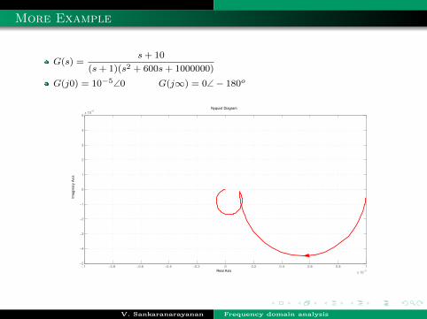
More Example

G(s) =s+ 10

(s+ 1)(s2 + 600s+ 1000000)

G(j0) = 10−5∠0 G(j∞) = 0∠− 180o

−1 −0.8 −0.6 −0.4 −0.2 0 0.2 0.4 0.6 0.8 1

x 10−5

−5

−4

−3

−2

−1

0

1

2

3

4

5x 10

−6Nyquist Diagram

Real Axis

Imagin

ary

Axis


System Type and Polar Plot

G(s) =(s+ z1)(s+ z2) . . . . . . (s+ zm)

sk(s+ p1)(s+ p2) . . . . . . (s+ pn)n > m

Type 0 System:Starting point(ω = 0) isfinite and on real axis.Ending point(ω =∞) isat the origin.

−1 −0.5 0 0.5 1 1.5

−1

−0.5

0

0.5

1

0 dB

−20 dB

−10 dB

−6 dB

−4 dB−2 dB

20 dB

10 dB

6 dB

4 dB

2 dB

Nyquist Diagram

Real Axis

Imagin

ary

Axis



G(s) =(s+ z1)(s+ z2) . . . . . . (s+ zm)

sk(s+ p1)(s+ p2) . . . . . . (s+ pn)n > m

Type 1 System: Atω = 0 the magnitude is0 and phase become−90o.At low frequencypolar plot isasympototic to a lineparallel to imaginaryaxis. At ω =∞magnitude become zero.

−0.1 −0.05 0 0.05 0.1−8

−6

−4

−2

0

2

4

−10 dB−6 dB−4 dB

−2 dB

Nyquist Diagram

Real Axis

Imagin

ary

Axis



G(s) =(s+ z1)(s+ z2) . . . . . . (s+ zm)

sk(s+ p1)(s+ p2) . . . . . . (s+ pn)n > m

Type 2 System: Atω = 0 the magnitude is∞ but angle is −180o.So at lower frequencypolar plot is asymptoticto a line parallel tonegative real axis. Atω =∞ magnitude iszero. −250 −200 −150 −100 −50 0

−3

−2.5

−2

−1.5

−1

−0.5

0

0.5

10 dB

Nyquist Diagram

Real Axis

Imagin

ary

Axis


Control systems - Frequency domain analysis: Polar Plot

Documents