Control-relevant nonlinearity measure and integrated multi-model control Jingjing Du a,* , Tor Arne Johansen b a College of Internet of Things Engineering, Hohai University, Changzhou 213022, China b Department of Engineering Cybernetics, Norwegian University of Science and Technology, NO 7491 Trondheim, Norway Abstract: A control-relevant nonlinearity measure (CRNM) method is proposed based on the gap metric and the gap metric stability margin to measure the nonlinear degree of a system once a linear control strategy is selected. Supported by the CRNM method, an integrated multi-model control framework is developed, in which the multi-model decomposition and local controller design are closely integrated, model redundancy is avoided, computational load is reduced, and dependency on a prior knowledge is reduced. Besides, a 1/δ gap-based weighting method is put forward to combine the local controllers. On one hand, the 1/δ gap-based weighting method has merely one tuning parameter and can be computed off-line; on the other hand, it is sensitive to the tuning parameter, flexible and easy to tune. Two continuous stirred tank reactor (CSTR) systems are investigated. Closed-loop simulations validate the effectiveness and benefits of the proposed integrated multi-model control approach based on CRNM. Keywords: control-relevant nonlinearity measure, gap metric, weighting method, integrated multi-model control, CSTR 1. Introduction Virtually all chemical processes are nonlinear. However, most of them are handled using linear analysis and design techniques because of operating around an equilibrium point, so that the development and implementation of a controller can be largely simplified [1]. Nevertheless, in some important cases, the linearity assumption does not hold and linear controllers are invalid. Then nonlinear controllers are necessary. Therefore, from the perspective of controller design, there is a need for nonlinearity measures, which quantify the nonlinearity extent of a process instead of merely judging a system as linear or nonlinear. Thus we can decide whether a linear controller is adequate for the system or a nonlinear controller is necessary according to the nonlinearity measures. In the past decades, researchers have made extensive studies on nonlinearity measures, and have proposed quite a few definitions and computational methods [1-13]. Most of them are defined as a distance between the nonlinear system and its best linear approximation [2-9]. Although the definitions are intuitive, the general computation of the best linear models and nonlinearity measures are rather complicated [2]. Besides, most of them cannot be used in feedback controller synthesis directly [3]. Recently, the gap metric which was recognized as being more appropriate to measure the distance between two linear systems than a norm-based metric [17-18], has been employed to quantify the nonlinearity level of industrial processes. And several definitions have been developed [13-16]. The nonlinearity measures based on the gap metric are comparatively easier and simpler to compute and apply. And some of them have been used for multi-model decomposition in the multi-model control framework [15, 16]. The multi-model control approaches have been popular in controlling chemical processes

Welcome message from author
This document is posted to help you gain knowledge. Please leave a comment to let me know what you think about it! Share it to your friends and learn new things together.
Transcript

Control-relevant nonlinearity measure and integrated
multi-model control
Jingjing Du a,* , Tor Arne Johansen b a College of Internet of Things Engineering, Hohai University, Changzhou 213022, China b Department of Engineering Cybernetics, Norwegian University of Science and Technology, NO 7491
Trondheim, Norway
Abstract: A control-relevant nonlinearity measure (CRNM) method is proposed based on the gap
metric and the gap metric stability margin to measure the nonlinear degree of a system once a linear
control strategy is selected. Supported by the CRNM method, an integrated multi-model control
framework is developed, in which the multi-model decomposition and local controller design are
closely integrated, model redundancy is avoided, computational load is reduced, and dependency on a
prior knowledge is reduced. Besides, a 1/δ gap-based weighting method is put forward to combine the
local controllers. On one hand, the 1/δ gap-based weighting method has merely one tuning parameter
and can be computed off-line; on the other hand, it is sensitive to the tuning parameter, flexible and
easy to tune. Two continuous stirred tank reactor (CSTR) systems are investigated. Closed-loop
simulations validate the effectiveness and benefits of the proposed integrated multi-model control
approach based on CRNM.
Keywords: control-relevant nonlinearity measure, gap metric, weighting method, integrated
multi-model control, CSTR
1. Introduction
Virtually all chemical processes are nonlinear. However, most of them are handled using
linear analysis and design techniques because of operating around an equilibrium point, so that the
development and implementation of a controller can be largely simplified [1]. Nevertheless, in
some important cases, the linearity assumption does not hold and linear controllers are invalid.
Then nonlinear controllers are necessary. Therefore, from the perspective of controller design,
there is a need for nonlinearity measures, which quantify the nonlinearity extent of a process
instead of merely judging a system as linear or nonlinear. Thus we can decide whether a linear
controller is adequate for the system or a nonlinear controller is necessary according to the
nonlinearity measures. In the past decades, researchers have made extensive studies on
nonlinearity measures, and have proposed quite a few definitions and computational methods
[1-13]. Most of them are defined as a distance between the nonlinear system and its best linear
approximation [2-9]. Although the definitions are intuitive, the general computation of the best
linear models and nonlinearity measures are rather complicated [2]. Besides, most of them cannot
be used in feedback controller synthesis directly [3].
Recently, the gap metric which was recognized as being more appropriate to measure the
distance between two linear systems than a norm-based metric [17-18], has been employed to
quantify the nonlinearity level of industrial processes. And several definitions have been
developed [13-16]. The nonlinearity measures based on the gap metric are comparatively easier
and simpler to compute and apply. And some of them have been used for multi-model
decomposition in the multi-model control framework [15, 16].
The multi-model control approaches have been popular in controlling chemical processes

with wide operating ranges and large set-point changes [19-37]. The key point is to decompose a
nonlinear system into a set of linear subsystems, so that classical linear control strategies can be
easily adopted. Generally, the multi-model control approaches comprise three elements: the
multi-model decomposition (i.e., model bank determination), the local controller design, and the
local controller combination. From an integration perspective, it is necessary to connect the three
elements closely, so that local model redundancy can be avoided to simplify the controller
structure, dependency on previous knowledge can be reduced to make the design procedure more
systematic, computational load can be decreased to make the method more efficient, and
performance of the controller can be raised to make the method more effective. Therefore,
integrated multi-model control methods have been recently put forward [19, 28-30], in which the
model bank determination, the local linear controller design, and the local linear controller
combination are fully or partly integrated. Two integrated multi-model control design frameworks
were proposed in Ref. [19]. One method (Algorithm 2) uses the maximum stability margin (which
is comparatively controller-independent) while the other (Algorithm 1) uses the actual stability
margin of a given controller design. Although Algorithm 2 from Ref. [19] is simpler, it has a
tuning parameter which depends on a priori knowledge. Algorithm 1 from Ref. [19] is more
systematic; however, it is more complicated and involves intensive computation and tests. In Ref.
[20], a weighting method with only one tuning parameter was proposed based on the gap metric,
in which the weights can be computed off-line and kept in a look-up table. Here we call it 1-δ
method for simplicity. It is intuitive and simple compared to traditional methods. Therefore, Ref.
[29] used it to connect the local controller combination with the other two steps to propose an
integrated multi-linear model predictive control method. However, the 1-δ method is not sensitive
to the tuning parameter, which is undesirable.
In this paper, a control-relevant nonlinearity measure (CRNM) method is proposed to
quantify the nonlinearity extent of a process based on the gap metric, which can be used directly in
controller synthesis: It offers guidance for controller design; and it sets up a criterion to assess the
controller’s performance. The proposed CRNM method is then employed to perform model bank
determination and local controller design in a multi-model control framework. Besides, a 1/δ
gap-based weighting method, which has all the advantages of the 1-δ method and is more sensitive
to the tuning parameter, is put forward to combine the local controllers. Thus an improved
integrated multi-model control framework is established based on CRNM, which integrates the
advantages of the algorithms Ref. [19] while overcomes their disadvantages. The proposed
integrated multi-model control approach aims to realize four goals. (a) To select as few linear
models as necessary to design a multi-model controller, so that the model redundancy can be
avoided; (b) to use as little a priori knowledge as possible, so that the method can be systematic
and user-friendly; (c) to reduce computational load as much as possible, so that the method can be
easy to implement; (d) to schedule the local controllers as well as possible so that the global
multi-model controller can be more effective. Two CSTRs are simulated to illustrate the use of the
improved integrated multi-model control approach. Simulation results demonstrate that the
proposed CRNM-based integrated multi-model framework is systematic, efficient and effective,
and performs better than related multi-model control methods [20, 26].
This paper is organized as follows. Related background about the gap metric and the gap
metric stability margin is shortly reviewed in Section 2. In Section 3, a control-relevant
nonlinearity measure method is proposed. Supported by the proposed nonlinearity measure, an

integrated multi-model control approach is proposed in Section 4, which includes a CRNM-based
multi-model decomposition and local controller design procedure and a 1/δ gap-based weighting
method. Closed-loop simulations are present in Section 5 to illustrate the effectiveness of the
proposed approaches, and comparisons have been made with related methods. In Section 6, some
conclusions are made about the paper.
2. Gap metric and gap metric stability margin
Relevant background about the gap metric and the gap metric stability margin is briefly
recalled in this section.
2.1. Gap metric
The gap metric between two linear systems P1 and P2 with their normalized right coprime
factorizations 1
1 1 1P N M and 1
2 2 2P N M , is denoted as δ(P1, P2) and is defined by the
maximum of two directed gaps [17]:
)},(),,(max{:),( 122121 PPPPPP
(1)
where
QN
M
N
MPP
HQ2
2
1
1
21 inf),(
and
QN
M
N
MPP
HQ1
1
2
2
12 inf),(
.
The gap metric between any two linear systems is bounded between 0 and 1. Therefore, the
gap metric is more intuitive than a metric based on norms. Besides, the gap metric offers some
useful information for control system analysis and synthesis. For example, if the gap metric
between two systems is close to 0, then at least one feedback controller can be found to stabilize
both of them; otherwise if the gap is close to 1, it will be difficult of impossible to design a
feedback controller that can stabilize both systems[18].
2.2. Gap metric stability margin
Suppose K is a feedback controller that can stabilize the linear system P, then the gap metric
stability margin of the closed-loop system is defined as [38]:
1
1
1
1
, )()(
KIKPI
P
IPIPKI
K
Ib KP
(2)
where I is the identity matrix. The gap metric stability margin is also called the normalized
coprime stability margin.
Denote the left normalized coprime factors of P as 1P M N , and the Hankel norm as H
.
Then the maximum gap metric stability margin of P is defined as [38]:
1~~
1
)(inf:)(
2
1
1
gstabilizin
H
Kopt
MN
PIPKIK
IPb
(3)
From Eq. (3), it is clear that the maximum stability margin is an intrinsic property of the plant P,
and has nothing to do with the controller. Besides, for the same system P, the maximum stability is
greater than or equal to 𝑏𝑃,𝐾 for any controller K.
The connection between the gap metric and the gap metric stability margin is shown by

Proposition 1.
Proposition 1 [38]: Suppose the feedback system with the pair (𝑃0, 𝐾) is stable. Let 𝒫 ≔
{𝑃: 𝛿(𝑃, 𝑃0) < 𝑟}. Then the feedback system with the pair (𝑃, 𝐾) is also stable for all 𝑃 ∈ 𝒫 if
and only if
𝑏𝑃0,𝐾 ≥ 𝑟 > 𝛿(𝑃, 𝑃0) (4)
Once a nonlinear process is linearized around a set of equilibrium points, the gap metric and
the gap metric stability margin are usable. In this work, we will use the gap metric and the gap
metric stability margin to propose a CRNM method on the basis of Proposition 1. The gap metric
and maximum stability margin of the system are used to define a preliminary nonlinearity measure
NM1 for guidance before a controller is designed, and afterwards the gap metric and actual
stability margin of the closed-loop system are used to define a secondary nonlinearity measure
NM2 to qualify the performance of the controller. If NM2 of the considered system is smaller than
1, it means that the linear controller is capable to stabilize it. Otherwise, we will decompose the
nonlinear system into a set of linear subsystems and design a set of local linear controllers
according to the nonlinearity measure criteria. Thus, the proposed CRNM method tells us whether
the linear controller is capable to stabilize the nonlinear system or not.
Besides, the gap metric is also used for controller combination in the multi-model control of
nonlinear systems by some researchers [20, 21]. In section 4, this work will proposed a 1/δ
gap-based weighting method, which is simpler and more flexible compared to existent weighting
methods.
3. Control-relevant nonlinearity measures based on gap metric and gap metric
stability margin
Consider a nonlinear system represented by Eq. (5):
{�̇� = 𝑓(𝑥, 𝑢)
𝑦 = 𝑔(𝑥, 𝑢) (5)
where nx R is the state vector,
ru R is the control input vector, my R is the output
vector, and f (∙) and g (∙) are nonlinear differentiable functions.
Denote the scheduling variables of system (5) by θ. Generally, θ includes a subset of the
states, inputs and outputs. According to the principles of gain scheduled control design [39], 𝜃
should vary slowly, captures the nonlinearities of the system, characterizes the operating level and
uniquely defines the equilibrium points of system (5).
Denote Ф as the scheduling space of plant (5), and we have . Namely, Ф is the
variation range of θ, also the operating space of plant (5). Then Ф is gridded through the gap
metric based dichotomy method [24]. Suppose n gridding points θ = [θ1, θ2, θi …, θn] are acquired.
Then every gridding point corresponds to an equilibrium point of system (5). The operating point
for θi is denoted as (xo(θi) uo(θi) yo(θi)) := (xoi, uoi, yoi). Then system (5) is linearized about (xoi, uoi,
yoi) and a linearized model Pi is obtained described by:
uDxCy
uBxAx
ii
ii
i = 1, …, n (6)
where oix x x ,
oiu u u , oiy y y ,
x
uxfA oioi
i
),(,
u
uxfB oioi
i
),(

x
uxgC oioi
i
),(, and
u
uxgD oioi
i
),(.
Thus we get n linearized models Pi (i = 1, …, n) to approximate system (5) after gridding and
linearization. Note that for every value of θ, there exists only one equilibrium point, which results
in only one linearized model for every θ.
As is mentioned previously, when a nonlinear system is linearized about a series of
equilibrium points, the gap metric and gap metric stability margin are applicable. Here, we will
use them to define nonlinearity measures in the following subsections.
3.1. Nonlinearity measure based on gap metric and the maximum stability margin
Compute the gap-matrix [25] with all pairs of the n linearized models, and compute their
maximum stability margins according to:
2~~
1)(H
iiiopt MNPb
(7)
where iii NMP
~~ 1 is the left normalized coprime factorization of 𝑃𝑖. Then we get an nn
matrix nnijnnji PPgap ][:)],([ and an 1n vector 11 ][:)]([ noptnioptopt bPbB .
Among the n linearized models, choose the best local linear model P* according to:
))),((max(min::11
*
imninm
m PPPP
(8)
Eq. (8) is called the mix-max principle, which means the biggest gap of the n gaps between P* and
the n linearized models is the smallest in the n linearized models. That is to say, in the n linearized
models, P* is the one that is the nearest to the n linearized models in the min-max sense. Therefore,
P* is the best local linear model.
The biggest gap δmax of the n gaps between P* and the n linearized models is computed
according to:
)(max)(1
*
max i
*
ni,PPP
(9)
Then the preliminary nonlinearity measure over the entire operating range is defined as:
𝑁𝑀1 =𝛿𝑚𝑎𝑥(𝑃
∗)
𝑏𝑜𝑝𝑡(𝑃∗)
(10)
According to Proposition 1, if 𝑁𝑀1 < 1, there exists a linear controller that can theoretically
stabilize nonlinear plant (5) in the whole operating space and the considered system is weakly
nonlinear under the maximum stability criterion. Otherwise the considered system is strongly
nonlinear, and it will be difficult or impossible to get a stabilizing linear controller for it over the
entire operating range.
Because the maximum stability margin of the best local linear model P* has nothing to do
with the controller, therefore, NM1 is a universal measure regardless of control strategies. It can be
computed before a controller is designed, and supplies guidance for the controller design.
3.2. A CRNM based on gap metric and the actual stability margin
The control-relevant nonlinearity measure of system (5), i.e. NM2 over the entire operating
range is defined as:
𝑁𝑀2 =𝛿𝑚𝑎𝑥(𝑃
∗)
KPb
,*
(11)

where K is a linear stabilizing controller designed based on P*. From Proposition 1, we can get
that system (5) under controller K is considered as closed-loop linear if 𝑁𝑀2 < 1 and K satisfies
the desired performance requirements. Otherwise, if a linear controller with both 𝑁𝑀2 < 1 and
acceptable performance cannot be acquired, then system (5) is not possible to be stabilized by the
chosen control strategy, or a nonlinear control method is necessary. Quite a few linear control
techniques can be used to design controllers, such as PID, MPC, LQ, and so on. In this work, H∞
control method is employed to facilitate the comparison between the proposed method and the
methods from Ref.[19] in the following sections.
NM2 can be computed only after the linear controller is designed. It is used to judge whether
the controller is enough for the considered system or not. It is dependent on both the system and
the controller. Therefore, it is a control-relevant nonlinearity measure.
For both NM1 and NM2, the bigger the value is, the more nonlinear the system is. In the next
subsection, the proposed nonlinearity measures are applied to two CSTR processes to demonstrate
their use and effectiveness.
3.3. Case studies
3.3.1. Case 1. An isothermal CSTR (iCSTR)
Consider an iCSTR system with a first-order irreversible reaction, described by the following
equation [26]:
uCCkCdt
dCAAiA
A )( (12)
where CA (mol/l) is the reactant concentration, u (min−1) is the input, CAi (1.0 mol/l) is the feed
concentration, and k (0.028 min−1) is the rate constant.
Fig.1. Static input-output curve of the iCSTR with 19 gridding points
0 0.5 1 1.5 2 2.5 30
0.1
0.2
0.3
0.4
0.5
0.6
0.7
0.8
0.9
1
P10
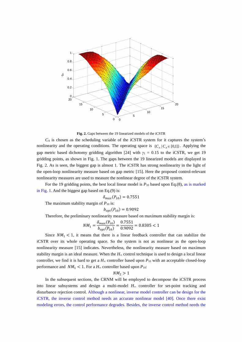
Fig. 2. Gaps between the 19 linearized models of the iCSTR
CA is chosen as the scheduling variable of the iCSTR system for it captures the system’s
nonlinearity and the operating conditions. The operating space is ]}1,0[|{ AA CC . Applying the
gap metric based dichotomy gridding algorithm [24] with γ1 = 0.15 to the iCSTR, we get 19
gridding points, as shown in Fig. 1. The gaps between the 19 linearized models are displayed in
Fig. 2. As is seen, the biggest gap is almost 1. The iCSTR has strong nonlinearity in the light of
the open-loop nonlinearity measure based on gap metric [15]. Here the proposed control-relevant
nonlinearity measures are used to measure the nonlinear degree of the iCSTR system.
For the 19 gridding points, the best local linear model is P10 based upon Eq.(8), as is marked
in Fig. 1. And the biggest gap based on Eq.(9) is:
𝛿𝑚𝑎𝑥(𝑃10) = 0.7551
The maximum stability margin of P10 is:
𝑏𝑜𝑝𝑡(𝑃10) = 0.9092
Therefore, the preliminary nonlinearity measure based on maximum stability margin is:
𝑁𝑀1 =𝛿𝑚𝑎𝑥(P10)
𝑏𝑜𝑝𝑡(P10)=0.7551
0.9092= 0.8305 < 1
Since 𝑁𝑀1 < 1, it means that there is a linear feedback controller that can stabilize the
iCSTR over its whole operating space. So the system is not as nonlinear as the open-loop
nonlinearity measure [15] indicates. Nevertheless, the nonlinearity measure based on maximum
stability margin is an ideal measure. When the H∞ control technique is used to design a local linear
controller, we find it is hard to get a H∞ controller based upon P10 with an acceptable closed-loop
performance and 𝑁𝑀1 < 1. For a H∞ controller based upon P10:
𝑁𝑀2 > 1
In the subsequent sections, the CRNM will be employed to decompose the iCSTR process
into linear subsystems and design a multi-model H∞ controller for set-point tracking and
disturbance rejection control. Although a nonlinear, inverse model controller can be design for the
iCSTR, the inverse control method needs an accurate nonlinear model [40]. Once there exist
modeling errors, the control performance degrades. Besides, the inverse control method needs the
0
5
10
15
20
0
5
10
15
200
0.2
0.4
0.6
0.8
1
δ

nonlinear dynamics to be invertible. It fails when the system exhibits input or output multiplicity,
e.g. Case 2 in this work. Additionally, it may be computationally intensive to get a nonlinear
dynamic inversion [40]. Therefore, the multi-model approach is employed here for its advantages
mentioned previously.
3.3.2. Case 2: An exothermal CSTR (eCSTR)
Consider a benchmark eCSTR process in which an irreversible, first-order reaction takes
place. The eCSTR process is modeled by [27]:
{
�̇�1 = −𝑥1 + 𝐷𝑎(1 − 𝑥1)exp(𝑥2
1+𝑥2 𝛾⁄)
�̇�2 = −𝑥2 + 𝐵𝐷𝑎(1 − 𝑥1)exp(𝑥2
1+𝑥2 𝛾⁄) + 𝛽(𝑢 − 𝑥2)
𝑦 = 𝑥2
(13)
where the state variables x1 and x2 denote the dimensionless reagent conversion and reactor
temperature, respectively. The input variable u represents the dimensionless coolant temperature.
The constants in Eq. (13) are Da = 0.072, γ = 20, B = 8 and β = 0.3, respectively. As shown in Fig.
3, the eCSTR process has strong output multiplicity. Since the output y captures the nonlinearity
of the eCSTR plant, y is chosen as the scheduling variable. Then the operating space is
{ | [0,6]}y y .
The gap metric based gridding algorithm [24] is applied to the eCSTR process with γ1 = 0.15,
and we get 42 steady state points to grid its operating space { | [0,6]}y y , as shown in Fig. 4.
Since the biggest gap is equal to 1, the system exhibits strong open-loop nonlinearity according to
the gap metric based nonlinearity measure [15]. In the following, the proposed CRNM will be
applied to the eCSTR process.
Fig. 3. Static input-output curve of the eCSTR with 42 gridding points
-2 -1.5 -1 -0.5 0 0.5 1 1.5 2 2.5 30
1
2
3
4
5
6
P10

Fig. 4. Gap metrics between the 42 linearized models of the eCSTR.
For the 42 gridding points, the best local linear model is P10 based upon Eq.(8) as marked in
Fig.3. And the biggest gap based upon Eq.(9) is:
𝛿𝑚𝑎𝑥(𝑃10) = 0.7971
The maximum stability margin of P10 is:
𝑏𝑜𝑝𝑡(𝑃10) = 0.7861
Therefore, the preliminary nonlinearity measure based on maximum stability margin for the
eCSTR process is:
𝑁𝑀1 =𝛿𝑚𝑎𝑥(𝑃10)
𝑏𝑜𝑝𝑡(𝑃10)=0.7971
0.7861= 1.014 > 1
Since 𝑁𝑀1 > 1, it is difficult to get a linear controller to stabilize the eCSTR process in the
whole operating space, and 𝑁𝑀2 > 1 for any H∞ controller. In the following, the CRNM will be
used to propose an integrated multi-model control approach for both set-point tracking control and
disturbance rejection control.
Note that although the best local linear model of the eCSTR is also P10 just like the iCSTR,
the two P10 models are totally different. There is no relation between the two models. For example,
if γ1 = 0.13 is used to grid the eCSTR, we will find the best local linear model is P11 which is also
at the point marked by blue hexagram in Fig. 3. In order to make a clear and direct comparison
with the method in Ref.[19] in the following sections, we continue to use γ1 = 0.15 in this work as
in Ref. [19].
4. A CRNM-based integrated multi-model control framework
In this work, we are to propose a CRNM-based integrated multi-model control framework,
which makes full use of the advantages of the two algorithms from Ref. [19], while avoiding their
disadvantages. It means that given a control strategy for local linear controller design, an
appropriate linear model bank for multi-model controller design is acquired systematically with
less computational load and without model redundancy while the local controllers are designed.
Namely, the local model selection is closely integrated with the local controller design. Moreover,
the local stability of the system in every subregion is guaranteed by the corresponding local
controller. Like most multi-model control approaches for nonlinear systems, the global stability of
0
10
2030
40
0
10
20
30
40
0
0.2
0.4
0.6
0.8
1

the nonlinear system cannot be guaranteed. As in Ref. [19], many linear control techniques, such
as H∞, PID, IMC, LQ, and so on, can be used in the proposed multi-model control framework and
H∞ control algorithm is continued to be employed to design local controllers to make the
comparisons in the following sections simple and clear. Moreover, a 1/δ gap-based weighting
algorithm, which is simple, easy and effective to apply, is formulated to combine the local
controllers.
The proposed CRNM-based integrated multi-model control approach which includes a
CRNM-based multi-model decomposition and local controller design algorithm and a gap-based
weighting algorithm, is detailed as follows.
4.1. CRNM-based multi-model decomposition and local controller design
For the nonlinear system (5), the procedure of the CRNM-based multi-model decomposition
and local controller design is summarized as the following algorithm.
4.1.1. Algorithm
Step1: Grid the operating space of system (5) through the gap metric based dichotomy gridding
algorithm [24] and linearize system (5) about the gridding points. Suppose we get n linearized
models Pi (i = 1, …, n).
Step2: Compute the gap-matrix [25] between all pairs of the n linearized models, and get their
maximum stability margins according to Eq. (7). Then we get an nn matrix
nnijnnji PPgap ][:)],([ and an 1n vector 11 ][:)]([ noptnioptopt bPbB .
Step3: Set k = 1, and Nm = 0.
Step4: If k <= n, set l = k and Nm = Nm + 1. Otherwise, go to Step12.
Step5: Choose the best local linear model P* among the kth to lth linearized model according to:
))),((max(min::*
imliklmk
m PPPP
(14)
Step6: Compute the biggest gap δmax between P* and the other linearized models according to:
)(maxmax i
*
lik,PP
(15)
Step7: If 𝑁𝑀1 = 𝛿𝑚𝑎𝑥(𝑃∗)/𝑏𝑜𝑝𝑡(𝑃
∗) < 1, set l = l + 1 and return to Step5; otherwise, go to
Step8.
Step8: Set l = l − 1.
Step9: Design a linear controller K for the best linear model P*. If K satisfies both 𝑁𝑀2 =
𝛿𝑚𝑎𝑥(𝑃∗)/𝑏𝑃,𝑘(𝑃
∗) < 1 and the desired performance requirements, then the l − k + 1 successive
linearized models are classified into one subregion, represented by their local linear model P* and
stabilized by the corresponding controller K. Set k = l + 1, and go back to Step4.
Step10: If an acceptable controller K with 𝑁𝑀2 = 𝛿𝑚𝑎𝑥(𝑃∗)/𝑏𝑃,𝑘(𝑃
∗) < 1 is not found, Set l = l
– 1.
Step11: Re-select P* among the kth to lth linearized model according to
))),((max(min::*
imliklmk
m PPPP
, and re-compute the biggest gap δmax(P*) between P* and the other
linearized models. Go back to Step 9.
Step12: The n linearized models are divided into Nm subregions with Nm local models and Nm
linear controllers.
Finally, the process (5) is decomposed into Nm local models with Nm local linear controllers

which will be combined into a multi-mdoel controller by a 1/δ gap-based weighting method in the
subsequent sections.
Remark 1: Nm is the number of the subregions, i.e., the number of local linear models and
local controllers.
Remark 2: In Step9, the l − k + 1 successive linearized models are classified into one
subregion and represented by P* according to the NM1 criterion.
Remark 3: In the above procedure, NM1 is used to perform the preliminary decomposition;
NM2 is used to perform the final decomposition. The use of NM1 reduces the computational load
greatly; and the use of NM2 makes the decomposition more effective and less dependent on
previous knowledge. Therefore, the above procedure combines the strong points of Algorithm 1 &
Algorithm 2 in Ref. [19].
Remark 4: Just as in Ref. [19], the local model determination and local controller design are
carried out sequentially, making the two steps closely connected with each other. Also, the above
design procedures are somewhat conservative as a result of the conservativeness of Proposition 1.
Local controllers which do not satisfy the CRNM criteria may have better performance.
4.1.2. Case study
In the following, the proposed Algorithm is applied to the above two CSTR processes.
Case 1: The iCSTR
Here, we will apply the proposed CRNM-based multi-model decomposition and local
controller design procedure to the iCSTR process. The detailed procedure is listed step by step as
follows.
S1. For the 19 gridding points, we divide the system preliminarily according to the maximum
stability margin based NM1, getting the result shown in Table 1.
Table 1. Preliminary decomposition for 1st subregion of iCSTR
Subregion Operating point NM1
119 10th 𝑁𝑀1 = 𝛿max (𝑃10)/𝑏𝑜𝑝𝑡(𝑃10)
= 0.7551/0.9092 < 1
S2: On the basis of S1, perform the final decomposition according to the actual stability
margin based NM2, and get the result in Table 2.
Table 2. Final decomposition for 1st subregion of iCSTR
Subregion Operating point NM2
115 8th 𝑁𝑀2 = 𝛿max(𝑃8) 𝑏𝑝𝑘(𝑃8)⁄
= 0.6527 0.7024⁄ < 1
S3: For gridding points 1619, carry out the preliminary decomposition and get Table 3.
Table 3. Preliminary decomposition for 2nd subregion of iCSTR
Subregion Operating point NM1
1619 17th 𝑁𝑀1 = 𝛿max(𝑃17) 𝑏𝑜𝑝𝑡(𝑃17)⁄
= 0.1785/0.9958 < 1
S4: On the basis of S3, perform the final decomposition and get Table 4.
Table 4. Final decomposition for 2nd subregion of iCSTR
Subregion Operating point NM2
1619 17th 𝑁𝑀2 = 𝛿max(𝑃17) 𝑏𝑝𝑘(𝑃17)⁄
= 0.1785/0.1821 < 1

The final decomposition result of the iCSTR process is summarized in Table 5.
Table 5. CRNM-based multi-model decomposition and local controllers of the iCSTR
Subregion 1st 2nd
Linearized models included 115 1619
Operating point of the local
linear model (CA, u)
8th
(0.7734,0.0956)
17th
(0.9281,0.3616)
Local linear model 1236.0
2266.0*
1
s
P 3896.0
07188.0*
2
s
P
subrange 0 ≤ CA ≤ 0.9 0.9 < CA ≤ 1
Local linear controller 009389.027.11
179.1541.921
ss
sK
0007381.08866.0
05.1695.222
ss
sK
NM2 0.6527/0.7024<1 0.1785/0.1821<1
From Table 5, we can see that the system is divided into 2 subregions. The 1st subregion contains
15 linearized models (115), and the local linear model for the 1st subregion is the 8th linearized
model )1236.0/(2266.0*
1 sP , with operating point (CA, u) = (0.7734, 0.0956). The first
subrange is {CA|0≤CA≤0.9}. The local linear H controller 009389.027.11
179.1541.921
ss
sK with
NM2 < 1 is designed. The other column is interpreted in the same way. Note that K1 does not have
an explicit integral action, but it has a pole − 0.0008, which is near the origin. Therefore, K1 has an
approximate integral action, making it proper for tracking control of step changes for the iCSTR
process. So is K2.
The above decomposition result is the same as in Ref. [19]. Namely, the proposed
CRNM-based multi-model decomposition method is as effective as the algorithms from Ref. [19]
in avoiding model redundancy. However, the computational load is much less. Since there is a
tuning parameter ε, Algorithm 2 in Ref. [19] is not as systematical as Algorithm 1 in Ref. [19]. In
the following we therefore only compare the computational load between the proposed method
and Algorithm 1 in Ref. [19].
Using the proposed algorithm in this work, for the 1st subregion, 5 H controllers are
designed and tested, and for the 2nd subregion, 1 H controller is designed and tested. In total, 6
H controllers are designed and tested.
However, in Ref. [19], 14 H controllers are designed and tested for the 1st subregion, and 3
H controllers for the 2nd subregion. In total, 17 H controllers.
The number of controllers that are designed and tested is denoted as “repeat times” for
simplicity in the following. Table 6 shows the computational load of the proposed method and
Algorithm 1 from Ref. [19].
Table 6. Comparison between the CRNM-based method and Algorithm 1 from Ref. [19].
Repeat times CRNM-based method Algorithm 1 from Ref. [19]
1st subregion 5 14
2nd subregion 1 3
Total 6 17
Therefore, the computational load of Algorithm 1 from Ref. [19] is almost three times of the
proposed algorithm for the iCSTR process. So the proposed algorithm reduced computational load

greatly.
Case 2: The eCSTR
As we know from Section 3, the control-relevant nonlinearity measure of the eCSTR process
is strong since NM1 > 1. It is quite difficult to design a single linear controller to stabilize the
eCSTR process over the whole operating range. Therefore, the CRNM-based method is applied to
it to get a multi-model controller.
The detailed decomposition of the eCSTR system is listed as follows:
S1: Perform the preliminary decomposition of the 42 gridding points according to the
maximum stability margin based NM1, and get the following decomposition result in Table 7.
Table 7. Preliminary decomposition for 1st subregion
Subregion Operating point NM1
119 9th 𝑁𝑀1 = 𝛿𝑚𝑎𝑥(𝑃9) 𝑏𝑜𝑝𝑡(𝑃9)⁄
= 0.7922/0.8137 < 1
S2: On the basis of S1, perform the final decomposition of the 1st subregion according to the
actual stability margin based NM2, and get the result in Table 8.
Table 8. Final decomposition for 1st subregion
Subregion Operating point NM1
116 8th 𝑁𝑀2 = 𝛿𝑚𝑎𝑥(𝑃8) 𝑏𝑝𝑘(𝑃8)⁄
= 0.6780/0.6797 < 1
S3: Perform the preliminary decomposition of the 2nd subregion according to the maximum
stability margin based NM1, and get Table 9.
Table 9. Preliminary decomposition for 2nd subregion
Subregion Operating point NM1
1730 25th 𝑁𝑀1 = 𝛿𝑚𝑎𝑥(𝑃25) 𝑏𝑜𝑝𝑡(𝑃25)⁄
= 0.4332/0.4786 < 1
S4: Perform the final decomposition of the 2nd subregion according to the actual stability
margin based NM2, and we get the result as follows in Table 10.
Table 10. Final decomposition for 2nd subregion
Subregion Operating point NM1
1730 25th 𝑁𝑀2 = 𝛿𝑚𝑎𝑥(𝑃25) 𝑏𝑝𝑘(𝑃25)⁄
= 0.4332/0.4432 < 1
S5: Perform the preliminary decomposition of the 3rd subregion according to the maximum
stability margin based NM1, and get Table 11.
Table 11. Preliminary decomposition for 3rd subregion
Subregion Operating point NM1
3142 36th 𝑁𝑀1 = 𝛿𝑚𝑎𝑥(𝑃36) 𝑏𝑜𝑝𝑡(𝑃36)⁄
= 0.5249/0.8471 < 1
S6: Perform the final decomposition of the 3rd subregion according to the actual stability
margin based NM2, and we get the result as follows in Table 12.
Table 12. Final decomposition for 3rd subregion
Subregion Operating point NM1
3142 36th 𝑁𝑀1 = 𝛿𝑚𝑎𝑥(𝑃36) 𝑏𝑝𝑘(𝑃36)⁄
= 0.5249/0.5326 < 1
The decomposition of the eCSTR process is completed. The local models and controllers are

summarized in Table 13.
Table 13. CRNM-based multi-model decomposition and local controllers of the eCSTR
Subregion 1st 2nd 3rd
Linearized
model included 116 1730 3142
Operating point
of local linear
model (x1, x2, u)
8th
(0.2068,1.375, 0.4446)
25th
(0.6077,3.625, -0.4937)
36th
(0.7393,4.5,-0.2149)
Local linear
model 191.0s113.1
3782.03.02
*
1
s
sP
170.0s3649.0
7647.03.02
*
2
s
sP
045.1s195.1
151.13.02
*
3
s
sP
subrange 0 ≤ y≤ 2 2 < y ≤ 4 4 < y ≤ 6
Local linear
controller 0075.027.439.43
785.744.4582.4023
2
1
sss
ssK
619.058.2044.3914.19
528.099.1768.4753.32234
23
2
ssss
sssK
162.07.1614.107
3.1755.2007.16723
2
3
sss
ssK
NM2 0.6780/0.6797<1 0.4332/0.4432<1 0.5249/0.5326<1
Table 13 can be interpreted similarly as Table 5. As displayed in Table 13, the eCSTR is
approximated by 3 local models with no integral elements, and 3 local H controllers are designed
using the CRNM-based integrated multi-model control approach. As to the 3 H controllers in
Table 13, we can also find that they have approximate integral actions, and therefore there are
appropriate for tracking control of step changes, too.
Evidently, the decomposition result is the same as in Ref. [19], which validates that the
proposed CRNM-based multi-model control method is as effective as the methods from Ref. [19]
in selecting local models and designing local controllers. Next, we will compare the computational
load.
Using the proposed method in this work, repeat times are 4 for the first subregion, 1 for the
2nd subregion, and 1 for the 3rd subregion. In total 6 H controllers are designed and tested.
However, in Algorithm 1 of Ref. [19], repeat times are 15 for the 1st subregion, 13 for the 2nd
subregion, and 11 for the 3rd subregion. 39 H controllers are designed and tested in total, more
than 6 times of that using the proposed method as shown in Table 14. Therefore, the proposed
CRNM-based decomposition and local controller design method is much more efficient.
Table 14 Comparison between the CRNM-based method and Algorithm 1 from Ref. [19].
Repeat times CRNM-based method Algorithm 1 in Ref. [19]
1st subregion 4 15
2nd subregion 1 13
3rd subregion 1 11
Total 6 39
In summary, the proposed CRNM-based method can get the same decomposition result as the
algorithms in Ref. [19]. Nevertheless, distinct from Algorithm 1 in Ref. [19], the proposed method
reduces computation largely, so it is more efficient; different from Algorithm 2 in Ref. [19], the
proposed method is independent of a prior knowledge, so it is more systematical. In short, the
proposed method combines the advantages while avoids the disadvantages.
In the next section, a 1/δ gap-based weighing method is proposed to combine the local
controller into a global multi-model controller, which is also according to the gap metric criterion.
4.2. A weighting method based on gap metric
For the nonlinear system described by Eq. (5), at time t, the value of θ is denoted as θt. The
steady state point corresponding to θt is denoted by ),,( ototot yux . Then the linearized model

obtained by linearizing system (5) around ),,( ototot yux is denoted as P(θt):
uDxCy
uBxAx
tt
tt
(16)
where otxxx ,
otuuu , otyyy ,
x
uxfA otot
ot
),(,
u
uxfB otot
ot
),(,
x
uxgC otot
ot
),(, and
u
uxgD otot
ot
),(.
4.2.1. 1/δ weighting method
At time t, nonlinear system (5) is denoted as nPt. Then P(θt) is the linearized model of nPt.
The gap metric between nPt and the local linear system Pi is defined as the gap metric between
P(θt) and Pi, denoted as γi(θt):
))(,()( titi PP , i = 1,…, Nm (17)
Then the weighting function of the ith local linear controller at time t is established as:
𝜑𝑖(𝜃𝑡) =(
1
𝛾𝑖(𝜃𝑡))𝑘𝑤
∑ (1
𝛾𝑗(𝜃𝑡))
𝑘𝑤𝑁𝑚𝑗=1
i = 1,…, Nm (18)
where 𝑘𝑤 ≥ 1 is a tuning parameter. 𝜑𝑖 satisfies ∑ φ𝑖(𝜃𝑡) = 1𝑁𝑚𝑖=1 .
Therefore, the output of the multi-model controller is:
𝑢(𝑡) = ∑ 𝜑𝑖(𝜃𝑡)𝑢𝑖(𝑡)𝑁𝑚𝑖=1 (19)
where ui (t) is the ith local linear controller’s output. According to Eq. (18), a bigger gap will lead
to a smaller weight, and vice versa. The weighting method formed by Eqs.(17)-(18) is called 1/δ
weighting method for simplicity.
For nonlinear system (5), suppose we get three local linear models (P1, P2, P3) by the
proposed CRNM-based Algorithm. Then Fig. 5 shows a graphic interpretation of the 1/δ
weighting method along the system’s transition and static locus. At time instant t, the gaps
between the nonlinear system nPt and local linear model Pi (i = 1, 2, 3) are denoted by γi (i = 1, 2,
3). According to the implication of the gap metric, a big γi indicates that the dynamic behavior of
Pi is far apart from the nonlinear system’s. Therefore, the corresponding controller has a small 𝜑𝑖
and plays a minor role in the multi-model controller, and vice versa. Apparently, the 1/δ weighting
method is more intuitive compared to Gaussian and Trapezoidal functions.
Fig. 5. Illustration of the 1/δ weighting method
Like the 1-δ weighting method from Ref. [20], (a) the proposed weighting functions can be
Steady-state curve
P2
P1 γ1
P3
γ3
γ2
nPt Trajectory
P(θt)

computed off-line and saved as look-up tables since Eqs.(17)-(18) are only dependent on θ but
independent of t. Therefore, online computational load is reduced and the method is more efficient.
(b) There exists merely one tuning parameter in the 1/δ gap-based method regardless of the
number of scheduling variables, whereas the number of parameters for traditional weighting
methods, e.g. Gaussian and Trapezoidal functions, relies on the number of scheduling variables
heavily. Hence the proposed 1/δ gap-based method is comparatively much simpler.
Compared to the weighting method in Ref. [20], the proposed weighting method in this work
is more sensitive to its tuning parameter kw, making it easier to get a proper weight for a local
controller. We will discuss this in the following.
4.2.2. Case studies-comparison between two gap-metric-based weighting methods
In the section, we will show the difference between the 1-δ and 1/δ gap-metric-based
methods by the CSTR processes.
Based on the decomposition results of the two CSTR systems in Section 4.1, we can get the
look-up tables of weights easily. For weights that cannot be found in the tables directly, linear
interpolation is used in this work. Figures of weights will be shown instead of look-up tables for
intuitiveness in the following.
4.2.2.1. The iCSTR
Fig. 6. Weights of two gap-metric-based weighting methods for iCSTR (Solid―weights for the 1st controller,
dash―weights for the 2nd controller)
For the iCSTR, we will make a comparison between the proposed 1/δ weighting method and
the 1-δ weighting method in this section.
Fig. 6 shows a set of weighting functions with different values of tuning parameters (ke and
kw grow from 1 to 20). The upper subplot gives the 1-δ weights of the two local controllers with
different values of ke. The lower subplot depicts the 1/δ weights of the two local controllers with
different values of kw. The solid lines are weights for the 1st local controllers, and the dash lines
0 0.1 0.2 0.3 0.4 0.5 0.6 0.7 0.8 0.9 10
0.2
0.4
0.6
0.8
1
1-δ
gap m
etr
ic b
ased
weig
hting m
eth
od
0 0.1 0.2 0.3 0.4 0.5 0.6 0.7 0.8 0.9 10
0.2
0.4
0.6
0.8
1
CA
1/δ
gap m
etr
ic b
ased
weig
hting m
eth
od
ke=1 k
e=20
kw
=20k
w=1
kw
=6

are for the 2nd local controllers. It is clearly seen that (1)When ke and kw grow bigger and bigger,
the two weighting methods will have the similar weights for each local controller. (2)The variation
ranges of the proposed 1/δ weights are wider than the 1-δ weights. (3)The proposed 1/δ weighting
method is more sensitive to the variation of kw, while the 1-δ method is less sensitive when ke
changes. (4)The proposed 1/δ weights have peaks equal to 1 in their subregions for smaller kw. The
peaks are located at the operating points of local linear models. The ith local controller should
have a weight equal to 1 when the system transits to the ith operating point. It is reasonable that
each curve of the weights should at least have a value equal to 1 regardless of the value of the
tuning parameters. Therefore, the 1/δ weights are more intuitive than the 1-δ weights.
4.2.2.2. The eCSTR
Fig. 7 displays a set of weights for the three local controllers of the eCSTR system when ke
and kw grow from 1 to 50. The upper subplot shows the 1-δ weights of the three local controllers
with different values of ke. The lower subplot shows the 1/δ weights of the three local controllers
with different values of kw. The solid lines are weights for the 1st local controller, the dash lines
are for the 2nd local controller, and the dotted lines are for the 3rd local controller. Obviously, the
1/δ weights have a wider range in its own subregion than 1-δ weights; 1/δ weights have peaks
while 1-δ weights are smoother; the1/δ weights have peak values equal to 1, while the 1-δ
weights have peak smaller than 1. In summary, the 1/δ weights are more flexible and sensitive to
the tuning parameter in their own subregions. Namely, the two weighting methods have the
similar features as in the iCSTR.
From the above experiments, we can get the conclusion that, the proposed 1/δ weighting
method is more sensitive to the tuning parameter, which makes it easier to get a proper weight for
a local controller.
Fig. 7. Weights of two gap-metric-based weighting methods for eCSTR (Solid―weights for the 1st controller,
dash―weights for the 2nd controller, dot―weights for the 3rd controller)
0 1 2 3 4 5 60
0.2
0.4
0.6
0.8
1
1-δ
gap m
etr
ic b
ased
weig
hting m
eth
od
0 1 2 3 4 5 60
0.2
0.4
0.6
0.8
1
y
1/δ
gap m
etr
ic b
ased
weig
hting m
eth
od
ke=1
kw
=50
ke=50
ke=5
kw
=1 kw
=3

5. Closed-loop simulations
In this section, closed-loop simulations of set-point tracking and disturbance rejection control
are displayed for the above two CSTR processes to demonstrate the effectiveness of the proposed
CRNM-based integrated multi-model control approach. For comparison, the 1-δ weighting
method and trapezoidal weighting method from literature are also used to combine multi-model
H∞ controllers.
5.1. Case1: The iCSTR
The proposed 1/δ gap-metric-based weighting functions with kw = 6 shown in Fig. 6 are used
for the iCSTR. For comparison, the 1-δ gap-based weighting functions with ke = 1 shown in Fig. 6
and trapezoidal functions shown in Fig. 8 are also employed to get multi-model H controllers.
Parameters of the trapezoidal and 1-δ weighting functions are well tuned. Then the two local H
controllers from Table 5 are combined into three multi-model H controllers. Note that for the
iCSTR system, there is only one tuning parameter in every gap-based weighting method, while
there are 4 tuning parameters in the trapezoidal weighting method.
Fig. 8. Trapezoidal weighting functions for the iCSTR system (with 4 tuning parameters)
Closed-loop responses of the iCSTR process using three multi-model H controllers are
displayed in Figs. 9 and 10. The one using the 1/δ gap-based weighting method has CAg as its
output and ug as its input; the one using the trapezoidal weighting functions has its output CAT and
input uT; and the one using the 1-δ weighting method has CA0 and u0.
On the whole, the three multi-model controllers have similar performances for set-point
tracking control as shown in Fig. 9. All outputs track the reference signals fast and accurately
without big overshoots or big static errors, and all the inputs vary in the feasible range. Transitions
between the two subregions are also satisfactory: fast, smooth, and no chattering. In order to make
a closer comparison among the three multi-model controllers and the three weighting methods, we
calculate the integrated absolute error (IAE) values: IAEg = 92.1538 < IAE0 = 92.3390 < IAET =
95.8575. Thus, the proposed 1/δ gap-based multi-model H controller is slightly better than the
one using the 1-δ gap-based weighting method, and better than the one using the trapezoidal
0 0.1 0.2 0.3 0.4 0.5 0.6 0.7 0.8 0.9 1-0.2
0
0.2
0.4
0.6
0.8
1
1.2
CA
Tra
pezoid
al w
eig
hting f
unctions
Tf
1
Tf2

weighting method.
Fig. 9. Set-point tracking control of the iCSTR
Disturbance rejection control responses of the iCSTR process using the three multi-model H
controllers are displayed in Fig. 10. When the process is in subregion 2, a disturbance v1 = 0.03
enters the output at time = 90, and leaves at time = 180. During the stay in subregion 1, another
disturbance v2 = 0.1 appears at time = 350 and disappears at time = 430. In both cases, CAg and CA0
return to the reference signal promptly and accurately whenever the disturbance occurs or goes
away. However, CAT is a bit oscillatory when v1 appears, making IAET = 55.0693 significantly
bigger than the other two: IAEg =52.2502 and IAE0= 52.9516. The proposed 1/δ based
multi-model controller is slightly better than the 1-δ based multi-model controller since IAEg <
IAE0, although both the gap-metric-based multi-model controllers have good disturbance rejection
control performances: both react to the disturbances immediately and bring back CA to the
reference signal rapidly and accurately.
0 50 100 150 200 250 300 350 400 450 5000
0.2
0.4
0.6
0.8
1
time/min
CA
0 50 100 150 200 250 300 350 400 450 500-0.5
0
0.5
1
1.5
time/min
u
ug
uT
u0
ref
CAg
CAT
CA0

Fig. 10. Disturbance rejection control of the iCSTR
From the closed-loop responses of the iCSTR system, we can see that the proposed
multi-model controller has a better performance than the other two for both set-point tracking and
disturbance rejection control. Therefore, the CRNM-based integrated multi-model control design
method is effective in selecting local models, designing local controllers, and scheduling local
controllers.
5.2. Case 2 : The eCSTR
For the eCSTR process, the 1/δ gap-based weighting functions with ke=3 shown in Fig. 7 are
used to combine the 3 local H controllers from Table 13 to get a global multi-model H controller.
For comparison, the 1-δ gap-based weighting functions and trapezoidal functions shown in Figs. 7
and 11 are also used to combine the three local H controllers from Table 13. Closed-loop
responses are shown in Figs. 12-13. The output of the 1/δ gap-based closed-loop system is yg with
the control input ug, the output of the 1-δ gap-based system is y0 with its input u0, while the output
of the other system is yT with its input uT.
Note that for the eCSTR systems, there exists merely one tuning parameter in each of the
gap-based weighting methods, while in the trapezoidal functions shown in Fig. 11, there are 8
tuning parameters.
0 50 100 150 200 250 300 350 400 450 5000.4
0.5
0.6
0.7
0.8
0.9
1
time/min
CA
0 50 100 150 200 250 300 350 400 450 500-0.2
0
0.2
0.4
0.6
0.8
time/min
u
ref
CAg
CAT
CA0
ug
uT
u0

Fig.11. Trapezoidal weighting functions for the eCSTR with 8 tuning parameters
Fig. 12. Set-point tracking control of the eCSTR
Fig. 12 shows the set-point tracking control of the three multi-model H controllers for the
eCSTR process. Obviously, all the three outputs follow the reference signal closely as a whole, but
yg is faster than the other two. The IAE values are IAEg = 262.3101, IAET = 321.8751, and IAE0
=
372.9597(ke = 5), respectively. Apparently, IAEg < IAET < IAE0. Therefore, the 1/δ gap metric
based multi-model controller has the best performance among the three controllers, and the
trapezoidal functions based multi-model controller performs better than the 1-δ based multi-model
0 1 2 3 4 5 6-0.2
0
0.2
0.4
0.6
0.8
1
1.2
y
Tra
pezoid
al w
eig
hting f
unctions
Tf1
Tf2
Tf3
0 50 100 150 200 250 3000
1
2
3
4
5
6
time
y
0 50 100 150 200 250 300-3
-2
-1
0
1
2
3
4
time
u
ref
yg
y0
yT
ug
u0
uT

controller for the eCSTR in set-point tracking control regarding to the IAE criterion. Note that the
gap-based weighting methods have much fewer tuning parameters, making them easier to use.
Fig.13. Disturbance rejection control of the eCSTR
When it comes to disturbance rejection control, the proposed multi-model H controller
based on CRNM performs better than the other two as shown in Fig. 13. Obviously, yg is faster
and more accurate in each subregion than y0 and yT. Especially, in the 1st subregion during time =
50 to 100, there is a big static error for yT. Besides, yT has a bigger overshoot when the setpoint
changes to the 3rd subregion. The proposed controller can reject disturbance effectively and bring
the output back to the setpoint quickly, while the other two multi-model H controllers perform
relatively not so well. The IAE values are IAEg = 339.2100, IAET = 418.9340, IAE0
= 397.1170,
respectively.
From the simulation results of the two CSTR systems, it is concluded that:
1) The CRNM-based multi-model decomposition and local control design method is as effective
as the algorithms in Ref. [19], but more efficient and systematic. So linear model redundancy
is largely avoided, computational load is greatly reduced, and dependency on a prior
knowledge is reduced.
2) The proposed 1/δ weighting method is simple and effective. The resulting multi-model
controller can have a performance as good as or even better than traditional weighting
methods with less tuning effort.
3) Compared with the 1-δ weighting method, the 1/δ method is consistently good, but the 1-δ
method is sometimes not as good as traditional methods.
6. Conclusions
A gap-based CRNM method is proposed for quantification of the nonlinearity degree of a
process when a linear control strategy is chosen. If the nonlinearity measures are larger than 1, a
0 20 40 60 80 100 120 140 160 180 2000
2
4
6
8
time
y
0 20 40 60 80 100 120 140 160 180 200-2
-1
0
1
2
3
time
u
ug
uT
u0
ref
yg
yT
y0

nonlinear control algorithm may be needed. Otherwise, the designed linear controller is capable to
stabilize the process over the whole operating space. Supported by the control-relevant
nonlinearity measures, an integrated multi-model control framework is proposed. A bank of local
models and controllers can be selected and designed systematically with little previous knowledge,
with small computational cost, and without model redundancy. A 1/δ gap-based weighting method
is developed for local controller combination. Two CSTR chemical processes are studied and
comparisons have been made among the proposed approaches and other typical methods. It is
demonstrated by the closed-loop simulations that the CRNM-based integrated multi-model control
approach can get an effective model/controller bank, and schedule the local controllers more
effectively.
Acknowledgments
This work is supported by the NSF of China (61104079), NSF of Jiangsu Province
(BK20150854), and by the Fundamental Research Funds for the Central Universities
(2016B15414).
References
[1] M. Guay, P.J. McLellan, D.W. Bacon, Measurement of nonlinearity in Chemical Process
Control Systems: The Steady State Map, The Canadian Journal of Chemical Engineering 73
(1995) 868-882.
[2] T. Schweickhardt, F. Allgower, Linear control of nonlinear systems based on nonlinearity
measures, Journal of Process Control 17 (2007) 273-28.
[3] M. Nikolaou, P. Misra, Linear control of nonlinear process: recent developments and future
directions, Computers and Chemical Engineering 27 (2003) 1043-1059.
[4] A. Helbig, W. Marquardt, F. Allgower, Nonlinearity measures: definition, computation and
applications, Journal of Process Control 10 (2000) 113-123.
[5] T. Schweickhardt, F. Allgower, On system gains, nonlinearity measures, and linear models
for nonlinear systems, IEEE Transactions on Automatic Control 54(1) (2009) 62-78.
[6] K.R. Harris, M.C. Colantonio, A. Palazoglu, On the computation of a nonlinearity measure
using functional expansions, Chemical Engineering Science 55 (2005) 2393-2400.
[7] D. Sun, K. A. Hoo, Nonlinearity measure for a class of SISO nonlinear systems, International
of Journal Control 73 (2000) 29-37.
[8] C.A. Desoer, Y.T. Wang, Foundations of feedback theory for nonlinear dynamical systems,
IEEE Trans. Cir. Syst. 27 (1980) 104-123.
[9] Y. Liu, X.R. Li, Measure of nonlinearity for estimation, IEEE Transactions on Signal
Processing, 63(9) (2015) 2377-2388.
[10] M. Guay, The effect of process nonlinearity on linear controller performance in discrete-time
systems, Computers and Chemical Engineering 30 (2006) 381-391.
[11] S.M. Hosseini, T.A. Johansen, A. Fatehi, Comparison of Nonlinearity Measures based on
Time Series Analysis for Nonlinearity Detection, Modeling, Identification and control 32(4)
(2011 )123-140.
[12] J. Liu, Q. Meng, F. Fang, Minimum variance lower bound ration based nonlinearity measure
for closed loop systems, Journal of Process Control 23 (2013) 1097-1107.
[13] G.T. Tan, M. Huzmezan, K.E. Kwok, Vinicombe metric as a closed-loop nonlinearity

measure, European Control Conference, Cambridge, UK, 2003, 751-756.
[14] W. Tan, H.J. Marquez, T. Chen, J. Liu, Analysis and control of a nonlinear boiler-turbine unit,
Journal of process control 15 (2005) 883-891.
[15] J. Du, C. Song, P. Li, A Gap metric based nonlinearity measure for chemical processes,
Proceedings of the 2009 American Control Conference, St. Louis, MO, US, 2009, 4440-4445.
[16] J. Du, Z. Tong, An improved nonlinearity measure based on gap metric, Proceedings of the
33rd Chinese Control Conference, Nanjing, China, 2014, 1920-1923.
[17] T.T. Georgiou, M.C. Smith, Optimal robustness in the gap metric, IEEE Transactions on
Automatic Control 35 (6) (1990) 673-686.
[18] A.K. El-Sakkary, The gap metric: Robustness of stabilization of feedback systems, IEEE
Transaction on Automatic Control 30 (3) (1985) 240-247.
[19] J. Du, T.A. Johansen, Integrated Multimodel Control of Nonlinear Systems Based on Gap
Metric and Stability Margin, Industrial and Engineering Chemical Research 53(24) (2014)
10206–10215.
[20] J. Du, T.A. Johansen, A gap metric based weighting method for multimodel predictive
control of MIMO nonlinear systems, Journal of Process Control 24 (2014) 1346-1357.
[21] E. Arslan, M.C. Camurdan, A. Palazoglu, Y. Arkun, Multimodel Scheduling Control of
Nonlinear Systems using Gap Metric, Industrial and Engineering Chemical Research 43(2004)
8274-8283.
[22] R. Jeyasenthil, P.S.V. Nataraj, A multiple model gap-metric based approach to nonlinear
quantitative feedback theory, IFAC-PapersOnLine 49-1 (2016) 160-165.
[23] Q. Chi, J. Liang, A multiple model predictive control strategy in the PLS framework, Journal
of Process Control 25 (2015) 129-141.
[24] J. Du, C. Song, Y. Yao, P. Li, Multilinear model decomposition of MIMO nonlinear systems
and its implication for multilinear model-based control, Journal of Process Control 23 (2013)
271-281.
[25] J. Du, C. Song, P. Li, Application of gap metric to model bank determination in multilinear
model approach, Journal of Process Control 19 (2009) 231-240.
[26] W. Tan, H.J. Marquez, T. Chen, J. Liu, Multimodel analysis and controller design for
nonlinear processes, Comput. Chem. Eng. 28 (2004) 2667-2675.
[27] O. Galán, J.A. Romagnoli, A. Palazoglu, Y. Arkun, Gap metric concept and implication for
multilinear model-based controller design, Industrial and Engineering Chemical Research 42
(2003) 2189-2197.
[28] J. Du, C. Song, P. Li, Multimodel control of nonlinear systems: An integrated design
procedure based on gap metric and H∞ loop-shaping, Industrial and Engineering Chemical
Research 51(2012) 3722-3731.
[29] J. Du, T.A. Johansen, Integrated Multilinear Model Predictive Control of Nonlinear Systems
Based on Gap Metric, Industrial and Engineering Chemical Research 54 (22) (2015)
6002–6011.
[30] C. Song, B. Wu, J. Zhao, P. Li, An integrated state space partition and optimal control
method of multi-model for nonlinear systems based on hybrid systems, Journal of Process
Control 25 (2015) 59-69.
[31] C.R. Porfirio, E.A. Neto, D. Odloak, Multi-model predictive control of an industrial C3/C4
splitter. Contr. Eng. Pract. 11 (2003) 764-779.

[32] N.N. Nandola, S. Bhartiya, A multiple model approach for predictive control of nonlinear
hybrid systems, Journal of Process Control 18(2008) 131-148.
[33] M. Kuure-Kinsey, B.Bequette, Multiple Model Predictive Control Strategy for Disturbance
Rejection, Ind. Eng. Chem. Res. 49 (2010) 7983-7989.
[34] M. Garcia, C. Vilas, L. Santos, A. Alonso, A robust multi-model predictive controller for
distributed parameter systems, Journal of Process Control 22 (2012) 60-71.
[35] G. Stojanovski, M. Stankovski, G. Dimirovski, Multiple-model model predictive control for
high consumption industrial furnaces, FACTA UNIVERSITATIS, Series: Automatic Control
and Robotics 9(1) (2010) 131-139.
[36] X. Du, P. Yu, C. Ren, Clustering Multi-model generalized predictive control and its
application in wastewater biological treatment Plant, Journal of Applied Sciences 13 (21)
(2013) 4869-4874.
[37] X. Tao, D. Li, Y. Wang, N. Li, S. Li, Gap-metric-based multiple-model Predictive control
with a polyhedral stability region, Ind. Eng. Chem. Res. 54 (2015) 11319-11329.
[38] K. Zhou, J. Doyle, Essentials of Robust Control, Prentice Hall, Upper Saddle River, New
Jersey, 1999.
[39] W.J. Rugh, J.S. Shamma, Research on gain scheduling, Automatica 36 (2000) 1401-1425.
[40] G.L. Plett, Adaptive inverse control of linear and nonlinear systems using dynamic neural
networks, IEEE Transactions on Neural Networks 14(2) (2003) 360 - 376.
Related Documents