Doctoral Thesis Control Parameter Adaptation in Differential Evolution Adaptace kontroln´ ıch parametr ˚ u v diferenci´ aln´ ı evoluci Author: Ing. Adam Viktorin Branch of study: Engineering Informatics Supervisor: doc. Ing. Roman Šenkeřík, Ph.D. Advisor: doc. Ing. Zuzana Komínková Oplatková, Ph.D. Zlín, 2021

Welcome message from author
This document is posted to help you gain knowledge. Please leave a comment to let me know what you think about it! Share it to your friends and learn new things together.
Transcript

Doctoral Thesis
Control Parameter Adaptation inDifferential Evolution
Adaptace kontrolnıch parametru v diferencialnı evoluci
Author: Ing. Adam ViktorinBranch of study: Engineering InformaticsSupervisor: doc. Ing. Roman Šenkeřík, Ph.D.Advisor: doc. Ing. Zuzana Komínková Oplatková, Ph.D.
Zlín, 2021


At this place, I would like to thank all people that supported me throughout mystudies and also throughout my life in general, whether it was family, friends, orcolleagues. Without them, I would not be able to get this far, and I appreciatethat.A genuine thank you goes to my mentors, colleagues, and most importantly,friends - Alzbeta, Anezka, Zuzana, Michal, Roman, Tomas K. and Tomas T.who helped me countless times with everything, ranging from bureaucracy throughresearch to personal matters.Last but not least, I would like to thank the love of my life, my wife, for "adapt-ing" to my character traits, bearing with me, pushing me forward, and for con-stantly reminding me that I should work on my dissertation when I was "running"away. . . to other projects.
"Correlation does not imply causation."

ABSTRAKT
Tato disertační práce popisuje autorovu výzkumnou aktivitu v oblasti adap-tivních variant algoritmu diferenciální evoluce pro optimalizaci jednokriteriál-ních funkcí definovaných ve spojitém prostoru. První část práce popisuje oblastmatematické optimalizace a její rozdělení do jednotlivých podkategorií podlecharakteristik optimalizované funkce. Tyto charakterisitky jsou: počet optimi-alizačních kritérií, typ vstupu, výpočetní složitost, typ prohledávaného prostoruřešení a počet optimalizovaných parametrů. Zároveň tato sekce zahrnuje popistypického zástupce metaheuristické optimalizace - evoluční výpočetní techniky.Druhá část práce se věnuje variantám algoritmu diferenciální evoluce včetně vari-ant s adaptivními kontrolními parametry. V jedné z podkapitol se autor věnuje idůvodům, proč si vybral algoritmus Success-History based Adaptive DifferentialEvolution jako základ své vědecké práce.V experimentální části práce je navržen nástroj pro analýzu dynamiky populaceevolučních algoritmů, který může být využit jak při tvorbě nových evolučních al-goritmů, tak pro vyhodnocení vlastností algoritmů stávajících a aktuálně použí-vaných. Mimo analýzu dynamiky populace obecně se autor zaměřil i na konkrétníalgoritmy založené na diferenciální evoluci. Navrhl dvě úpravy vnitřní dynamiky- multi–chaotický framework pro výběr rodičů a adaptace kontrolních parametrůs využitím vzdálenosti jedinců. Obě techniky jsou zaměřeny na pomoc s hledánímsprávné rovnováhy mezi prohledáváním prostoru řešení do šířky a do hloubky.Na příkladu moderní verze diferenciální evoluce ve variantě jSO je ukázán přínosimplementace adaptace kontrolních parametrů s využitím vzdálenosti jedinců.Takto upravený algoritmus byl nazván DISH a byl otestován na testovacíchsadách spojených s celosvětovým kongresem evolučních technik - CEC (Congresson Evolutionary Computation). Výsledky ukazují, že využití nové adaptačnístrategie je vhodné především pro úlohy, které optimalizují větší množství vs-tupních parametrů.Praktické využití algoritmu DISH je demonstrováno na příkladu hledání op-timálního rozmístění spaloven odpadu v České republice. Upravený algoritmusDISH poskytuje pro menší instance problému srovnatelné řešení s deterministick-ými metodami. Pro větší instance problému již nejsou deterministické metody
schopny poskytnout řešení v akceptovatelném čase a proto je zde využití meta-heuristického přístupu opodstatněno.Výše zmíněné výsledky ukazují, že i v rámci jednoduchých změn vnitřní dy-namiky algoritmu lze dosáhnout lepší výkonnosti. I proto si autor zvolil jakosvůj budoucí výzkumný směr rozvíjení nástroje pro analýzu vnitřní populačnídynamiky metaheuristických algoritmů.
SUMMARY
This doctoral thesis describes the author’s research in the area of adaptive Dif-ferential Evolution variants for small–scale continuous single–objective optimiza-tion. The first part describes the topic of mathematical optimization and listsvarious problem domains according to the problem characteristics. Namely:number of objectives, input type, computational complexity, type of a searchspace, and problem scale. It also describes the area of metaheuristic optimiza-tion and Evolutionary Computation Techniques.The Differential Evolution algorithm variants and control parameter adaptivityare described in the next part of this work and it also provides the justificationof selecting Success–History based Adaptive Differential Evolution algorithm asa basis for author’s research focus.A novel population dynamic analysis tool is proposed in the experimental part.This tool can be used for the development process of new metaheuristic tech-niques as well as for the analysis of the state-of-the-art methods.The experimental part also provides the proposal of multi–chaotic frameworkfor parent selection for the Differential Evolution based algorithms and Distancebased parameter adaptation, which can be implemented into adaptive variantsof Differential Evolution algorithm to improve the balance between explorationand exploitation. The benefits of using Distance based parameter adaptationare shown on the improved jSO algorithm - DISH. The performance of bothversions (jSO and DISH) is compared on the basis of Congress on EvolutionaryComputation benchmark sets and shows that the DISH variant is more suitable

for optimization problems of a larger scale.The practical use of the DISH algorithm is demonstrated on the operations re-search problem of finding optimal dislocation of waste–to–energy facilities in theCzech Republic. The improved DISH algorithm was able to provide comparablesolutions for smaller instances of the problem and was also able to provide solu-tions for larger instances where traditional solvers failed.Through the above–mentioned results, it can be seen that even simple changesin algorithms’ inner dynamic can lead to significant improvements. Therefore,the research area of adaptive metaheuristics for optimization can benefit fromknowledge gained through thorough algorithm analysis, which is the author’schosen research direction for the future.

TABLE OF CONTENTS
LIST OF FIGURES ......................................................................... 9
LIST OF TABLES............................................................................ 10
LIST OF ABBREVIATIONS........................................................... 13
1 INTRODUCTION ................................................................... 14
1.1 Mathematical optimization .................................................. 15
1.2 Evolutionary computational techniques in optimization ....... 17
2 DISSERTATION GOAL .......................................................... 19
3 CANONICAL DIFFERENTIAL EVOLUTION...................... 21
3.1 Initialization ....................................................................... 22
3.2 Mutation ............................................................................. 22
3.3 Crossover ........................................................................... 22
3.4 Selection ............................................................................ 23
4 DIFFERENTIAL EVOLUTION AND ADAPTIVITY ........... 24
5 SHADE/L–SHADE.................................................................. 35
5.1 Initialization ....................................................................... 35
5.2 Mutation ............................................................................. 35
5.3 Crossover ........................................................................... 36
5.4 Selection ............................................................................ 37
5.5 Update of historical memories............................................. 37
5.6 Linear decrease of the population size ................................ 38
6 PROPOSED METHODS ......................................................... 39
6.1 Population dynamic analysis ................................................ 396.1.1 Cluster analysis ................................................................ 396.1.2 Population diversity........................................................... 42
6.2 Multi–chaotic framework for parent selection................... 436.2.1 Chaotic maps as PRNGs..................................................... 436.2.2 Parent selection ................................................................ 45

6.2.3 Results ........................................................................... 45
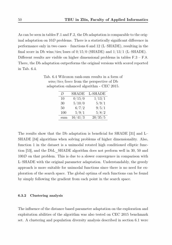
6.3 Distance based parameter adaptation .................................. 496.3.1 Results ........................................................................... 496.3.2 Clustering analysis ............................................................ 50
6.4 DISH ................................................................................... 516.4.1 Initialization .................................................................... 536.4.2 Mutation......................................................................... 546.4.3 Crossover ........................................................................ 556.4.4 Selection ......................................................................... 566.4.5 Linear decrease of the population size .................................... 566.4.6 Update of historical memories .............................................. 576.4.7 Results ........................................................................... 58
7 THE CONTRIBUTION TO SCIENCE AND
PRACTICE .............................................................................. 61
7.1 Population dynamic analysis ................................................ 61
7.2 Distance based parameter adaptation .................................. 62
7.3 Practical applications of DISH ........................................... 627.3.1 Sustainable waste–to–energy facility location ........................... 63
8 DISSERTATION GOAL FULFILLMENT .............................. 68
9 CONCLUSION ........................................................................ 69
REFERENCES ............................................................................... 70
PUBLICATIONS OF THE AUTHOR ........................................... 86
CURRICULUM VITAE...................................................................106
LIST OF APPENDICES..................................................................107

TBU in Zlín, Faculty of Applied Informatics 9
LIST OF FIGURES
6.1 Example of cluster occurrence comparison between SHADEand Db_SHADE algorithms on CEC 2015 benchmark, func-tion 8, 30D. . . . . . . . . . . . . . . . . . . . . . . . . . . . . 42
6.2 Average convergence of SHADE and MC–SHADE algorithmson CEC 2015 benchmark, function 3, 10D. . . . . . . . . . . . 47
6.3 Average convergence of SHADE and MC–SHADE algorithmson CEC 2015 benchmark, function 9, 10D. . . . . . . . . . . . 48
7.1 DR_DISH solution for the sustainable waste–to–energy facilitylocation - 14 regions. . . . . . . . . . . . . . . . . . . . . . . . 65

10 TBU in Zlín, Faculty of Applied Informatics
LIST OF TABLES
4.1 Summary - selected adaptive DE variants and their character-istics. . . . . . . . . . . . . . . . . . . . . . . . . . . . . . . . . 32
6.1 Chaotic maps, generating equations, control parameters andinitial position ranges. . . . . . . . . . . . . . . . . . . . . . . . 44
6.2 CEC 2015 benchmark set results of SHADE and MC–SHADEalgorithms in 10D. . . . . . . . . . . . . . . . . . . . . . . . . . 46
6.3 CEC 2016 competition ranking. . . . . . . . . . . . . . . . . . 48
6.4 Wilcoxon rank-sum results in a form of wins/ties/loses fromthe perspective of Db adaptation enhanced algorithm - CEC2015. . . . . . . . . . . . . . . . . . . . . . . . . . . . . . . . . 50
6.5 Wilcoxon rank-sum results in a form of wins/ties/loses fromthe perspective of DISH - CEC 2015 and CEC 2017. . . . . . . 59
6.6 CEC 2019 competition ranking. *results presented after theoriginal deadline of the competition . . . . . . . . . . . . . . . 60
7.1 DICOPT and DR_DISH solving the sustainable waste–to–energyfacility location. . . . . . . . . . . . . . . . . . . . . . . . . . . 65
E.1 CEC 2016 benchmark set results of MC–SHADE algorithm in10D. . . . . . . . . . . . . . . . . . . . . . . . . . . . . . . . . 113
E.2 CEC 2016 benchmark set results of MC–SHADE algorithm in30D. . . . . . . . . . . . . . . . . . . . . . . . . . . . . . . . . 114
E.3 CEC 2016 benchmark set results of MC–SHADE algorithm in50D. . . . . . . . . . . . . . . . . . . . . . . . . . . . . . . . . 115
E.4 CEC 2016 benchmark set results of MC–SHADE algorithm in100D. . . . . . . . . . . . . . . . . . . . . . . . . . . . . . . . . 116
F.1 CEC 2015 benchmark set results of SHADE and Db_SHADEalgorithms in 10D. . . . . . . . . . . . . . . . . . . . . . . . . . 117
F.2 CEC 2015 benchmark set results of L–SHADE and DbL_SHADEalgorithms in 10D. . . . . . . . . . . . . . . . . . . . . . . . . . 118
F.3 CEC 2015 benchmark set results of SHADE and Db_SHADEalgorithms in 30D. . . . . . . . . . . . . . . . . . . . . . . . . . 119
TBU in Zlín, Faculty of Applied Informatics 11
F.4 CEC 2015 benchmark set results of L–SHADE and DbL_SHADEalgorithms in 30D. . . . . . . . . . . . . . . . . . . . . . . . . . 120
F.5 CEC 2015 benchmark set results of SHADE and Db_SHADEalgorithms in 50D. . . . . . . . . . . . . . . . . . . . . . . . . . 121
F.6 CEC 2015 benchmark set results of L–SHADE and DbL_SHADEalgorithms in 50D. . . . . . . . . . . . . . . . . . . . . . . . . . 122
F.7 CEC 2015 benchmark set results of SHADE and Db_SHADEalgorithms in 100D. . . . . . . . . . . . . . . . . . . . . . . . . 123
F.8 CEC 2015 benchmark set results of L–SHADE and DbL_SHADEalgorithms in 100D. . . . . . . . . . . . . . . . . . . . . . . . . 124
G.1 CEC 2015 benchmark set clustering and population diversityanalysis results of SHADE and Db_SHADE algorithms in 10D. 125
G.2 CEC 2015 benchmark set clustering and population diversityanalysis results of SHADE and Db_SHADE algorithms in 30D. 126
G.3 CEC 2015 benchmark set clustering and population diversityanalysis results of SHADE and Db_SHADE algorithms in 50D. 127
G.4 CEC 2015 benchmark set clustering and population diversityanalysis results of SHADE and Db_SHADE algorithms in 100D.128
G.5 CEC 2015 benchmark set clustering and population diversityanalysis results of L–SHADE and DbL_SHADE algorithms in10D. . . . . . . . . . . . . . . . . . . . . . . . . . . . . . . . . 129
G.6 CEC 2015 benchmark set clustering and population diversityanalysis results of L–SHADE and DbL_SHADE algorithms in30D. . . . . . . . . . . . . . . . . . . . . . . . . . . . . . . . . 130
G.7 CEC 2015 benchmark set clustering and population diversityanalysis results of L–SHADE and DbL_SHADE algorithms in50D. . . . . . . . . . . . . . . . . . . . . . . . . . . . . . . . . 131
G.8 CEC 2015 benchmark set clustering and population diversityanalysis results of L–SHADE and DbL_SHADE algorithms in100D. . . . . . . . . . . . . . . . . . . . . . . . . . . . . . . . . 132
H.1 CEC 2015 benchmark set results of jSO and DISH algorithmsin 10D. . . . . . . . . . . . . . . . . . . . . . . . . . . . . . . . 133

12 TBU in Zlín, Faculty of Applied Informatics
H.2 CEC 2015 benchmark set results of jSO and DISH algorithmsin 30D. . . . . . . . . . . . . . . . . . . . . . . . . . . . . . . . 134
H.3 CEC 2015 benchmark set results of jSO and DISH algorithmsin 50D. . . . . . . . . . . . . . . . . . . . . . . . . . . . . . . . 135
H.4 CEC 2015 benchmark set results of jSO and DISH algorithmsin 100D. . . . . . . . . . . . . . . . . . . . . . . . . . . . . . . 136
H.5 CEC 2017 benchmark set results of jSO and DISH algorithmsin 10D. . . . . . . . . . . . . . . . . . . . . . . . . . . . . . . . 137
H.6 CEC 2017 benchmark set results of jSO and DISH algorithmsin 30D. . . . . . . . . . . . . . . . . . . . . . . . . . . . . . . . 138
H.7 CEC 2017 benchmark set results of jSO and DISH algorithmsin 50D. . . . . . . . . . . . . . . . . . . . . . . . . . . . . . . . 139
H.8 CEC 2017 benchmark set results of jSO and DISH algorithmsin 100D. . . . . . . . . . . . . . . . . . . . . . . . . . . . . . . 140
I.1 CEC 2015 benchmark set clustering and population diversityanalysis results of jSO and DISH algorithms in 10D. . . . . . . 141
I.2 CEC 2015 benchmark set clustering and population diversityanalysis results of jSO and DISH algorithms in 30D. . . . . . . 142
I.3 CEC 2015 benchmark set clustering and population diversityanalysis results of jSO and DISH algorithms in 50D. . . . . . . 143
I.4 CEC 2015 benchmark set clustering and population diversityanalysis results of jSO and DISH algorithms in 100D. . . . . . 144

TBU in Zlín, Faculty of Applied Informatics 13
LIST OF ABBREVIATIONS
AdapSS Adaptive Strategy Selection in DEADE Adaptive DEAI Artificial IntelligenceAIM-dDE Adaptive Invasion–based Model for distributed DEAPTS Adaptive Population Tuning SchemeCDE-b6e6rl Competitive DECEC Congress on Evolutionary ComputationCoDE Composite DECR Crossover rateD DimensionDb Distance based parameter adaptationDBSCAN Density Based Spatial Clustering of Applications with NoiseDE Differential EvolutionDISH Distance based parameter adaptation for Success–History based DEDR_DISH Distance Random DISHECT Evolutionary Computation TechniqueEPSDE DE with Ensemble of Parameters and mutation StrategiesESMDE Evolving Surrogate Model–based DEF Scaling factorFADE Fuzzy Adaptive DEFES Function EvaluationSG GenerationHyDE–DF Hybrid–adaptive DE with Decay FunctioniL–SHADE Improved L–SHADEL-SHADE SHADE with Linear decrease of the population sizeLSHADE_EpSin L–SHADE with Ensemble Sinusoidal parameter adaptationLSHADE–RSP LSHADE with Rank–based Selective Pressure strategyMAXFES MAXimum FESMCO Mean Cluster OccurrenceMC–SHADE SHADE with Multi–Chaotic parent selection frameworkMPD Mean Population DiversityMPEDE Multi–Population based Ensemble of mutation strategies DENFL No Free Lunch theoremNP Population sizePD Population DiversityPRNG Pseudo–Random Number GeneratorSADE Self–Adaptive DESAMODE Seld–Adaptive Multi–Operator DEESDE Self–adaptive DESHADE Success–History based Adaptive DESinDE Sinusoidal DESPS–L–SHADE–EIG L–SHADE with Successful–Parent–Selecting framework and EIGenvector–based crossoverSPSRDEMMS Structured Population Size Reduction DE with Multiple Mutation Strategies
14 TBU in Zlín, Faculty of Applied Informatics
1 INTRODUCTION
Artificial Intelligence (AI) has become a significant part of our everyday lives,even if we do not notice it sometimes. Our commute to work may be optimizedaccording to the current traffic situation with intelligent path planning algo-rithms. Voice assistants in smart devices use AI to understand our speech andcater to our queries. Computer games we play use AI to offer worthy opponents.Virtual keyboards in mobile phones adapt to our style of writing, camera ap-plication is able to adjust its settings according to the current scene and focuson the faces of photographed people. Our emails are automatically filtered andcategorized based on their content with clever algorithms. Antivirus is applyingAI techniques for the detection of malicious software before installation. Adver-tisements we see during internet browsing are based on our search history andbuyer preferences. Automatic text translation is becoming more precise withever more powerful AI techniques. The newest cars are more often than not de-signed by computers. The production and manufacturing can be scheduled andmanaged by AI algorithms. Scanners at airports use AI to detect potentiallydangerous items. Search engines use powerful AI to enhance their performance.Parking gates detect license plates and check whether they should open. Evenelectric toothbrushes use AI to learn user patterns. This work also demonstratesan AI approach to the waste–to–energy facility location problem.The list could be endless, but all of these applications have one thing in common.They build on solid foundations in AI basic research and algorithms that weredeveloped during the last few decades. This dissertation describes the author’scontribution to a specific part of the research field of mathematical optimizationand Evolutionary Computational Techniques (ECTs). This chapter providesa basic introduction into the research area and its subcategories. The secondchapter specifies the main dissertation goal and selected methods for achievingit. Chapters 3, 4 and 5 provide more details about the Differential Evolution(DE) algorithm, control parameter adaptivity and modern adaptive DE vari-ants. Chapter 6 describes methods developed during author’s doctoral studies.Chapters 7 and 8 summarize author’s contribution to the science and practiceand fulfillment of the dissertation goal. And the last chapter contains concluding

TBU in Zlín, Faculty of Applied Informatics 15
remarks with possible future expansion of this work.
1.1 Mathematical optimization
Mathematical optimization is a scientific research area that deals with searchingfor the problem parameter values combination that would yield the best result –objective function value (e.g., minimization of a cost or maximization of a profit).Of course, there are multiple subcategories of optimization tasks that requireappropriate methods for their solving. These categories are divided according to[1] as follows:
• The number of objectives:
– Single–objective optimization – the goal is to optimize one ob-jective.
– Multi–objective optimization – the goal is to simultaneously op-timize two or three objectives.
– Many–objective optimization – the goal is to simultaneously op-timize more than three objectives.
• The input parameter type:
– Discrete/Combinatorial optimization – optimized parametershave a finite number of possible values.
– Continuous/Real–valued/Numerical optimization – optimizedparameters are real–valued.
• The computational complexity of the objective function:
– Expensive optimization – it is computationally expensive to eval-uate the objective function of a single solution.
– Non–expensive optimization – it is computationally inexpensiveto evaluate the objective function of a single solution.
16 TBU in Zlín, Faculty of Applied Informatics
• The search space type:
– Unconstrained optimization – the search space of parameter val-ues is infinite.
– Bound–constrained optimization – the search space is not con-strained; individual parameters have only upper and lower bounds.
– Constrained optimization – the search space is constrained byadditional equalities or inequalities.
• The scale of the problem (number of optimized parameters /dimensionality):
– Small-scale optimization – the dimensionality of the problem isbetween 1 and 100.
– Large-scale optimization – the dimensionality of the problem is inhundreds or thousands.
Optimization algorithms are methods for solving optimization problems and canalso be classified into subcategories. One of the main classifications might be byalgorithms stochasticity into two groups - deterministic and stochastic [2]. De-terministic algorithms follow a rigorous mathematical approach and work withthe mathematical model of the problem to provide the optimal solution. Unfor-tunately, the most complex tasks are unsolvable by deterministic optimizationalgorithms due to the time and computational constraints. Thus, stochastic op-timization algorithms that use randomness in their core are employed. Thesealgorithms can also be titled metaheuristics. Metaheuristics treat optimizationproblems as black boxes - trying to solve optimization tasks using only the in-formation of an input/output combination and learning from that. Due to theirstochastic nature, metaheuristics do not guarantee a finding of the global opti-mum.ECTs form a particular metaheuristic class based on the principle of naturalselection and are described in the next section.
TBU in Zlín, Faculty of Applied Informatics 17
1.2 Evolutionary computational techniques in optimization
ECTs are part of the soft computing field and are based on the Darwinian theoryof evolution [3]. In this sense, ECTs often work with a population of individuals.Those individuals are combined via crossover operator (an analogy with breed-ing), and the resulting individuals are further mutated via mutation operator(analogous to gene mutation) to provide possibly fitter offspring for the nextgeneration. This process is applied to the whole population to provide a newgeneration of solutions to the given optimization task. Thanks to this, ECTscan be used to optimize particularly hard optimization tasks that could not besolved, due to the computational complexity, by traditional deterministic meth-ods.ECTs are often employed for solving complex optimization tasks in various prob-lem domains (e.g., load forecasting in smart grids [4], friction welding [5], un-derwater glider path-planning [6], species distribution modeling [7], large scaleflexible scheduling [8], markerless human motion capture [9] or drug design [10]).The ECT’s goal is to guide a search through a search space of feasible solutionsand to find a satisfactory solution in a reasonable time. The solution mentionedhere is a feature vector of values that correspond to the optimized parametersof the problem. The quality of a single solution (feature vector) is evaluated bythe objective function, where the objective may be either minimization or maxi-mization of the function value. The feature vector, along with its correspondingobjective function value, makes up an individual of ECT. Therefore, the goal ofeach ECT run is to find an individual with a sufficient objective function value.Since ECTs are metaheuristic techniques, there is no guarantee that the foundsolution will be optimal. Each independent run of the evolutionary algorithmcan also provide a different solution, and therefore, algorithms are often runmultiple times.One of the problems while using ECTs is a requirement for a control parametersetting. These parameters can significantly impact the algorithm’s performance,and therefore their correct setting is essential. One of the latest trends in ECTsis to address this problem by adapting the algorithm’s behavior (via adaptingcontrol parameter values) to the given optimization task. With the famous No

18 TBU in Zlín, Faculty of Applied Informatics
Free Lunch (NFL) theorem in mind [11], adaptive algorithms try to overcome theproblem of correct parameter setting by incorporating knowledge of previouslysuccessful values of these parameters into the evolution process in an intelligentway. Thus, the user is no longer obliged to fine–tune these parameters manually.The Differential Evolution (DE) algorithm [12] is one of the main representativesof ECTs and has been thoroughly studied over the last 25 years. Moreover, itsadaptive variants from the last decade show promising results in various problemdomains, and that is why the DE was selected as the author’s research focus.Particularly, this dissertation is focused on the DE algorithm and its adaptivevariants for small–scale continuous single–objective optimization problems witha possible expansion to the area of large–scale optimization.

TBU in Zlín, Faculty of Applied Informatics 19
2 DISSERTATION GOAL
The prevailing trend in the metaheuristic optimization seems to be a constantdevelopment of new techniques without proper justification of their need. Thiswas creditably described by Sörensen in [13]. A similar issue is a vast amountof new versions of existing successful algorithms. In author’s opinion, the mainproblem is not the great volume of variants, but the lack of proper analysis ofimplemented changes and their influence on the algorithm’s behavior. There-fore, the goal of this dissertation is to try and contribute to the scientific area ofmetaheuristic optimization by developing analysis tools which use dataminingtechniques to help with understanding the population dynamic of metaheuristicalgorithms. More specifically, how the control parameter adaptation in Differen-tial Evolution–based algorithms influences the population dynamic and whetherthis information can be used in the development and testing of new ideas.Selected methods to achieve the above stated dissertation goal:
• Analysis – current state–of–the–art methods in adaptive DE field willbe analyzed from the perspective of control parameter adaptation. Whatmechanism decides the direction of the adaptation and whether it is basedon a greedy approach. The effect of the adaptation on exploration/exploitationabilities of the algorithm will be studied.
• Programming – selected state–of–the–art adaptive DE variants will beprogrammed in Java, Wolfram Mathematica, and Python in order to workwith these algorithms and test the proposed modifications.
• Testing – the programmed code will be tested against possible errors andmalfunctions.
• Benchmarking – proposed algorithm variants will be benchmarked onthe basis of CEC benchmark sets of test functions.
• Result evaluation – evaluation of the results will be executed within therules of used benchmark sets. This will create a basis for result comparisonwith the scientific community.

20 TBU in Zlín, Faculty of Applied Informatics
• Result analysis – the statistical analysis of obtained results will be per-formed. Population dynamic analysis will be used to asses the explo-ration/exploitation properties of the proposed framework.
TBU in Zlín, Faculty of Applied Informatics 21
3 CANONICAL DIFFERENTIAL EVOLUTION
The original algorithm of DE was proposed in a technical report in 1995 [12] andpublished in 1997 by Storn and Price [14]. Since its introduction, it is consideredas one of the best performing algorithms for global optimization over continuousspaces. Its key features are simplicity and universality. The original paper [14]proposed DE with only three control parameters – scaling factor F, crossoverrate CR, and population size NP. These three parameters have to be set by theuser, and their correct setting is highly dependable on the optimization task[15, 16].The DE algorithm is initialized with a random population of individuals P, thatrepresent solutions to the optimization problem. In continuous optimization,each individual is composed of a vector x of length D, which is a dimensionality(number of optimized parameters) of the problem and objective function valuef (x ). Each vector component represents a value of the corresponding optimizedparameter.For each individual in a population, three mutually different individuals areselected for mutation, and the resulting mutated vector v is combined with thetarget vector x in the crossover step. The objective function value f (u) of theresulting trial vector u is evaluated and compared to that of the target individualx. When the quality (objective function value) of the trial individual u is better,it is placed into the next generation. Otherwise, the target individual x is placedthere. This step is called selection. The process is repeated until the stoppingcriterion is met (e.g., the maximum number of objective function evaluations, themaximum number of generations, the low bound for diversity between objectivefunction values in population or time restriction).The following sections describe four steps of the DE: initialization, mutation,crossover, and selection.

22 TBU in Zlín, Faculty of Applied Informatics
3.1 Initialization
As aforementioned, the initial population P , of size NP, is randomly generated.For this purpose, the individual vector x i components are generated by Pseudo-Random Number Generator (PRNG) with uniform distribution from the rangewhich is specified for the problem by lower lo and upper up bounds (3.1).
xj,i = U[loj , upj
]for j = 1, . . . , D (3.1)
Where i is the index of a target individual, j is the index of current parameterand D is the dimensionality of the problem.In the initialization phase, a scaling factor value F and crossover value CR hasto be assigned as well. The typical range for F value is (0, 2] and for CR, it is[0, 1].
3.2 Mutation
In the mutation step, three mutually different individuals x r1, x r2, x r3 from apopulation are randomly selected and combined in accordance with the mutationstrategy. The original mutation strategy of canonical DE is "rand/1" and isdepicted in (3.2).
vi = xr1 + F (xr2 − xr3) (3.2)
Where r1 6=r2 6=r3 6=i, F is the scaling factor value and v i is the resulting mutatedvector.
3.3 Crossover
In the crossover step, the mutated vector v i is combined with the target vector x i
and produces a trial vector u i. The binomial crossover (3.3) is used in canonicalDE.

TBU in Zlín, Faculty of Applied Informatics 23
uj,i =
{vj,i if U [0, 1] ≤ CR or j = jrand
xj,i otherwise(3.3)
Where CR is the used crossover rate value and jrand is an index of a parameterthat has to be taken from the mutated vector u i (this ensures the generation ofa vector with at least one component from the mutated vector in order to notpresent objective function with already evaluated solutions).
3.4 Selection
The selection step ensures that the optimization will progress towards bettersolutions because it allows only individuals of better or at least equal objectivefunction value to proceed into the next generation G+1 (3.4).
xi,G+1 =
{ui,G if f (ui,G) ≤ f (xi,G)
xi,G otherwise(3.4)
Where G is the index of the current generation.For easier understanding, the basic concept of the DE algorithm is depicted inthe pseudo–code in Appendix A.
24 TBU in Zlín, Faculty of Applied Informatics
4 DIFFERENTIAL EVOLUTION AND ADAPTIV-ITY
Troublesome fine–tuning of control parameters soon became a problem for re-searchers and practitioners who were trying to accommodate DE for solvingcomplex optimization problems. Therefore, researchers started working on thisproblem by studying DE’s behavior on different types of objective function land-scapes and tried to come up with a simple guide for the setting of control pa-rameter values.In the original technical report by Storn and Price from 1995 [12], authors recom-mend population size NP between 5*D and 10*D, the initial choice of a scalingfactor F = 0.5 and an effective range for F from 0.4 to 1. The initial choice forcrossover rate CR was suggested to 0.1, but for fast convergence 0.9 or 1. In2002, Gamperle et al. [15] tested not only the setting of control parameters butalso the choice of mutation and crossover operators. They suggested populationsize NP between 3*D and 8*D, scaling factor F = 0.6, and crossover rate CRbetween 0.3 and 0.9. Moreover, the authors proposed using "DE/best/2/bin"and "DE/rand/1/bin" variants for the mutation and crossover strategies. In[17], Ronkkonen et al. used a testbed of 25 scalable objective functions to eval-uate the performance of DE, and they recommended scaling factor F = 0.9 asa good first choice and range from 0.4 to 0.95, crossover rate CR from 0 to 0.2for separable functions and 0.9 to 1 for non–separable functions.As can be seen, suggestions from different authors vary and are highly depen-dent on the choice of objective function testbed used in the study. This fact onlysupports the NFL theorem [11], which roughly states that there is no universalalgorithm or algorithm parameter setting, that would solve all the different typesof optimization problems optimally.The solution to these problems may lie in the adaptive behavior of the DE algo-rithm. Since the setting of control parameters and mutation and crossover oper-ators is dependent on the optimized objective function, these variables might beset during the optimization run according to the success of the currently imple-mented settings. Adaptivity in DE is a current trend in the field and has shown

TBU in Zlín, Faculty of Applied Informatics 25
auspicious results right from its beginning around the year 2005. The followingparagraphs present the evolution timeline of selected adaptive DE–based algo-rithms for a continuous single-objective optimization along with their authorsand a short description of each adaptive scheme.
• 2004
– Fuzzy Adaptive DE (FADE) [18] by Liu and Lampinen – usesfuzzy logic controllers to adapt F and CR values.
• 2005
– Self–adaptive DE (SDE) [19] by Omran et al. – self–adaptation ofscaling factor F, which is sampled from a normal distribution N (0.5,0.15) at the beginning, but each individual remembers its scaling fac-tor for future generations. Before mutation, scaling factor F is givenby a recombination of 3 randomly selected values from population.
– Self–Adaptive DE (SaDE) [20] by Qin and Suganthan – this algo-rithm adapts mutation and crossover operators as well as CR valuesduring the optimization run. Mutation and crossover operator com-binations are selected from a pool of strategies according to theirprevious success in generating better offspring (in this version, thepool contained only two strategies). Scaling factor F is sampled froma normal distribution N (0.5, 0.3), and the crossover rate values CRare also sampled from a normal distribution, but with the mean valuedependent on the successful values from previous generations.
• 2006
– jDE [21] by Brest et al. – in this work, authors proposed an algo-rithm with adaptive F and CR values according to two probabilitiesof parameter adjustment – τ1 for scaling factor and τ2 for crossoverrate. These parameters are usually set to 0.1 and thus correspondto the probability of a parameter change of 10%. Furthermore, eachindividual has its combination of F and CR values, that are storedalongside the feature vector.
26 TBU in Zlín, Faculty of Applied Informatics
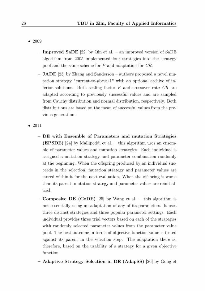
• 2009
– Improved SaDE [22] by Qin et al. – an improved version of SaDEalgorithm from 2005 implemented four strategies into the strategypool and the same scheme for F and adaptation for CR.
– JADE [23] by Zhang and Sanderson – authors proposed a novel mu-tation strategy "current-to-pbest/1" with an optional archive of in-ferior solutions. Both scaling factor F and crossover rate CR areadapted according to previously successful values and are sampledfrom Cauchy distribution and normal distribution, respectively. Bothdistributions are based on the mean of successful values from the pre-vious generation.
• 2011
– DE with Ensemble of Parameters and mutation Strategies(EPSDE) [24] by Mallipeddi et al. – this algorithm uses an ensem-ble of parameter values and mutation strategies. Each individual isassigned a mutation strategy and parameter combination randomlyat the beginning. When the offspring produced by an individual suc-ceeds in the selection, mutation strategy and parameter values arestored within it for the next evaluation. When the offspring is worsethan its parent, mutation strategy and parameter values are reinitial-ized.
– Composite DE (CoDE) [25] by Wang et al. – this algorithm isnot essentially using an adaptation of any of its parameters. It usesthree distinct strategies and three popular parameter settings. Eachindividual provides three trial vectors based on each of the strategieswith randomly selected parameter values from the parameter valuepool. The best outcome in terms of objective function value is testedagainst its parent in the selection step. The adaptation there is,therefore, based on the usability of a strategy for a given objectivefunction.
– Adaptive Strategy Selection in DE (AdapSS) [26] by Gong et
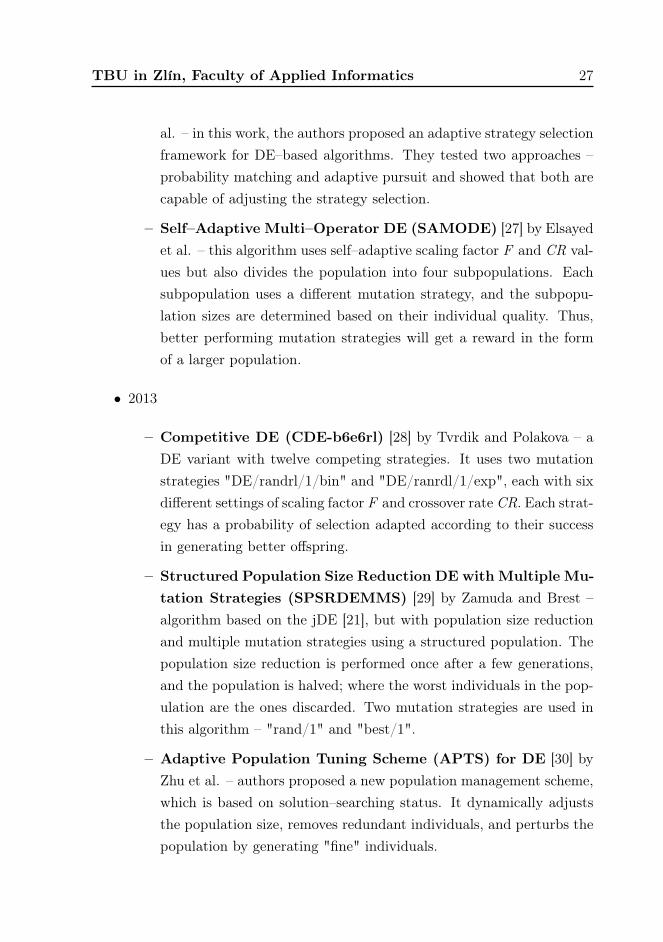
TBU in Zlín, Faculty of Applied Informatics 27
al. – in this work, the authors proposed an adaptive strategy selectionframework for DE–based algorithms. They tested two approaches –probability matching and adaptive pursuit and showed that both arecapable of adjusting the strategy selection.
– Self–Adaptive Multi–Operator DE (SAMODE) [27] by Elsayedet al. – this algorithm uses self–adaptive scaling factor F and CR val-ues but also divides the population into four subpopulations. Eachsubpopulation uses a different mutation strategy, and the subpopu-lation sizes are determined based on their individual quality. Thus,better performing mutation strategies will get a reward in the formof a larger population.
• 2013
– Competitive DE (CDE-b6e6rl) [28] by Tvrdik and Polakova – aDE variant with twelve competing strategies. It uses two mutationstrategies "DE/randrl/1/bin" and "DE/ranrdl/1/exp", each with sixdifferent settings of scaling factor F and crossover rate CR. Each strat-egy has a probability of selection adapted according to their successin generating better offspring.
– Structured Population Size Reduction DE with Multiple Mu-tation Strategies (SPSRDEMMS) [29] by Zamuda and Brest –algorithm based on the jDE [21], but with population size reductionand multiple mutation strategies using a structured population. Thepopulation size reduction is performed once after a few generations,and the population is halved; where the worst individuals in the pop-ulation are the ones discarded. Two mutation strategies are used inthis algorithm – "rand/1" and "best/1".
– Adaptive Population Tuning Scheme (APTS) for DE [30] byZhu et al. – authors proposed a new population management scheme,which is based on solution–searching status. It dynamically adjuststhe population size, removes redundant individuals, and perturbs thepopulation by generating "fine" individuals.

28 TBU in Zlín, Faculty of Applied Informatics
– Success–History based Adaptive DE (SHADE) [31] by Tan-abe and Fukunaga – this algorithm is based on the JADE [23], butimplements historical memories for storing previously successful scal-ing factor F and crossover rate CR values from previous generations.These memories are later used for the generation of F and CR valuesfor each individual.
• 2014
– Adaptive DE (ADE) [32] by Yu et al. – in this work, authorspropose adaptive DE with two–level parameter adaptation. This al-gorithm uses a new strategy, "DE/Lbest/1", which is a variation tothe original "DE/best/1" with multiple sub–populations, each hav-ing its locally best individual. The two–level parameter adaptation isbased on the estimation of optimization state, whether it is exploit-ing or exploring the search space. The scaling factor F and crossoverrate CR are generated on the population level and serve as a base forindividual–level parameter values.
– Adaptive Invasion–based Model for distributed DE (AIM–dDE) [33] by Falco et al. – the adaptive model uses three updatingschemes for setting the scaling factor F and crossover rate CR values.As the name suggests, this adaptive model is suitable for distributedDE, where the network is created from the nodes represented by differ-ent DE strategies. After a predefined number of iterations, importantknowledge is transferred between the connected nodes. In this case,important knowledge consists of better individuals and useful controlparameter values.
– SHADE with Linear decrease of the population size (L–SHADE) [34] - by Tanabe and Fukunaga – authors further improvedtheir SHADE [31] algorithm by implementing linear decrease of thepopulation size. The population is linearly decreased during the opti-mization, and thus, the starting large population provides explorativecapabilities, whereas a smaller population in the later stages of opti-mization promotes the exploitation of the search region.
TBU in Zlín, Faculty of Applied Informatics 29
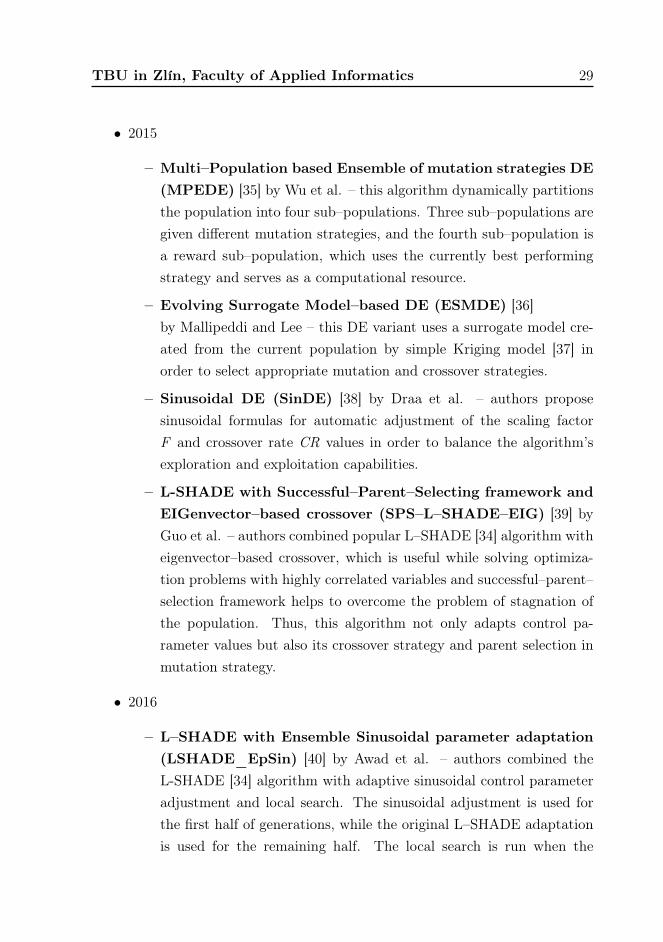
• 2015
– Multi–Population based Ensemble of mutation strategies DE(MPEDE) [35] by Wu et al. – this algorithm dynamically partitionsthe population into four sub–populations. Three sub–populations aregiven different mutation strategies, and the fourth sub–population isa reward sub–population, which uses the currently best performingstrategy and serves as a computational resource.
– Evolving Surrogate Model–based DE (ESMDE) [36]by Mallipeddi and Lee – this DE variant uses a surrogate model cre-ated from the current population by simple Kriging model [37] inorder to select appropriate mutation and crossover strategies.
– Sinusoidal DE (SinDE) [38] by Draa et al. – authors proposesinusoidal formulas for automatic adjustment of the scaling factorF and crossover rate CR values in order to balance the algorithm’sexploration and exploitation capabilities.
– L-SHADE with Successful–Parent–Selecting framework andEIGenvector–based crossover (SPS–L–SHADE–EIG) [39] byGuo et al. – authors combined popular L–SHADE [34] algorithm witheigenvector–based crossover, which is useful while solving optimiza-tion problems with highly correlated variables and successful–parent–selection framework helps to overcome the problem of stagnation ofthe population. Thus, this algorithm not only adapts control pa-rameter values but also its crossover strategy and parent selection inmutation strategy.
• 2016
– L–SHADE with Ensemble Sinusoidal parameter adaptation(LSHADE_EpSin) [40] by Awad et al. – authors combined theL-SHADE [34] algorithm with adaptive sinusoidal control parameteradjustment and local search. The sinusoidal adjustment is used forthe first half of generations, while the original L–SHADE adaptationis used for the remaining half. The local search is run when the
30 TBU in Zlín, Faculty of Applied Informatics
population size NP is equal to or less than 20 for the first time.
– SHADE with Multi–Chaotic parent selection framework(MC–SHADE) [41] by Viktorin et al. – this variant utilizes fivechaotic maps as PRNGs for the selection of parent individuals forthe mutation strategy in SHADE algorithm [31]. The proposed MCframework is suitable for all SHADE–based algorithms.
– LSHADE44 [42] by Polakova et al. – a similar approach as in [28]was proposed for L–SHADE [34] in this work. It is an L–SHADEalgorithm with two different types of mutation and crossover opera-tors combined. The selection of a suitable strategy is based on theprevious success in generating trial offspring.
– Improved L–SHADE (iL–SHADE) [43] by Brest et al. – au-thors propose few tweaks to the original L–SHADE [34] algorithm.The historical memories of scaling factor F and crossover rate CRare initialized to higher values, and one cell of the memory remainsunchanged during the optimization. Large values of F and small CRvalues are not allowed in the early stage of optimization to avoid pre-mature convergence to local optima. There is also a small changeto the mutation strategy "current-to-pbest/1", where the p value iscomputed differently and is based on the optimization stage.
• 2017
– Distance based parameter adaptation (Db) [44] by Viktorinet al. – authors proposed an update to the weighting scheme forSHADE–based [31] algorithms. Instead of the greedy approach, whichcalculates the weights of successful scaling factor F and crossoverrate CR values from the improvement in objective function value,the distance based parameter adaptation promotes exploration of thesearch space by incorporating the distance between the original andtrial individuals as a basis for the weights.
– jSO [45] by Brest et al. – another iteration of iL–SHADE [43], whichuses an updated weighted mutation strategy "current-to-pbest-w/1"
TBU in Zlín, Faculty of Applied Informatics 31
and slightly changes the predefined fixed values of scaling factor Fand crossover rate CR in historical memories.
• 2018
– LSHADE with Rank–based Selective Pressure strategy(LSHADE–RSP) [46] by Stanovov et al. – This algorithm usesan updated mutation strategy from jSO with rank–based selectionof random individuals from the population. The strategy is titled"current-to-pbest/r" and is inspired by ranked selection form geneticalgorithms. It also incorporates the same adaptive scheme for controlparameters as jSO.
– Distance based parameter adaptation for Success–Historybased DE (DISH) [47] by Viktorin et al. – DISH algorithm wascreated by implementing Db adaptation into jSO and led to the im-provement of the algorithm mainly for optimization problems of largerscale.
• 2019
– jDE100 [48] by Brest et al – as the name suggests, it is based on thepreviously mentioned jDE [21] algorithm with few updates. jDE100uses two sub–populations with one–way migration of the best individ-ual. It also introduces new limits for scaling factor F and crossoverrate CR values and utilizes restart strategy if the variance of bestpopulation members in terms of objective function value decreasesunder a specified threshold.
– Hybrid–adaptive DE with Decay Function (HyDE–DF) byLezama et al. – the algorithm incorporates the same adaptive mech-anism for control parameters as it was in jDE, but uses a novel mu-tation strategy titled "target-to-perturbed_best/1". This strategyperturbs the vector of the best individual by a perturbation factortaken from a normal distribution, calculates its difference to a targetvector and gradually decreases the influence of this difference in themutation strategy with algorithm generations. It also implements a

32 TBU in Zlín, Faculty of Applied Informatics
restart strategy if a specified number of successive generations showno improvement in objective function value.
– DISHchain 1e+12 [49] by Zamuda – DISH algorithm with largerpopulation size and a big computational budget designed specificallyfor CEC2019 competition [50].
A quick summary of the algorithms with their characteristics concerning param-eter adaptivity is given in the following Tab. 4.1.
Tab. 4.1 Summary - selected adaptive DE variantsand their characteristics.
Year Algorithm Adaptive CR Adaptive F Adaptive operators(mutation & crossover) Adaptive NP
2004 FADE Fuzzy logic controllers
2005 SDE recombinationSaDE sampling pool of 2 strategies
2006 jDE stochastic change, otherwise retain
2009 Improved SaDE sampling pool of 4 strategiesJADE sampling
2011
EPSDE pool pool of 3 strategiesCoDE best from 3 strategiesAdapSS based on underlying algorithm pool of 4 strategiesSAMODE recombination 4 competing sub–populations
2013
CDE-b6e6rl 12 competing strategiesSPSRDEMMS jDE scheme 2 sub–populations deterministic halving
APTS dynamic adjustmentSHADE sampling with historical memories
2014ADE two–level adaptation sub–populations
AIM–dDE 3 updating schemes distributed populations
L–SHADE SHADE scheme deterministiclinear decrease
2015
MPEDE 3 competeing sub–populations,1 reward
ESMDE surrogate selectionSinDE deterministic sinusoidal change
SPS–L–SHADE–EIG SHADE scheme eigenvector crossover andsuccessful parent selection
deterministiclinear decrease
2016
LSHADE_EpSin SHADE + SinDE scheme deterministiclinear decrease
MC–SHADE SHADE scheme chaos–enhanced parent selection
LSHADE44 SHADE scheme 4 competing strategies deterministiclinear decrease
iL–SHADE updated SHADE scheme deterministiclinear decrease
2017 Db distance based SHADE adaptation
jSO updated iL–SHADE scheme deterministiclinear decrease
2018 LSHADE–RSP jSO scheme current-to-pbest/r mutation deterministiclinear decrease
DISH jSO scheme with Db implementation deterministiclinear decrease
2019jDE100 jDE adaptation with new limits two sub–populations
HyDE–DF jDE adaptation target-to-perturbed_best/1 mutation
DISHchain 1e+12 DISH scheme deterministiclinear decrease
TBU in Zlín, Faculty of Applied Informatics 33
As perceivable, there are a plethora of different variants of adaptive DEs, andthe question is, how to select a suitable algorithm for the problem at hand.Luckily, since 2005, there is an annual competition in numerical optimizationheld within the Congress on Evolutionary Computation (CEC), which providesa benchmark incorporating multiple test functions from various domains. Thebenchmarks are named after the year they were used in the competition, e.g.,CEC2015 benchmark set. These benchmarks also provide a good testbed forresearchers who can easily compare their algorithms with the community. Prac-titioners can also use the competition results as useful guidance when searchingfor a suitable algorithm for their problem.An interesting pattern is visible when observing the results of the CEC com-petition since 2013. In 2013, the SHADE [31] was proposed and sent for thecompetition, where it placed 3rd [51]. The next year, Tanabe and Fukunaga pro-posed L–SHADE [34] and won the CEC2014 competition [52]. In 2015, the com-petition had three different test scenarios - learning-based optimization, expen-sive optimization, and multi–niche optimization. Closest to the original bound–constrained numerical optimization was the learning–based test case [53], whichallowed the competitors to fine–tune the algorithm’s parameters for each prob-lem. This competition was won by SPS–L–SHADE–EIG [39], but there were twoother algorithms based on the L–SHADE [34] – DesPA [54], which ranked 2nd
and LSHADE–ND [55], which shared the 3rd rank with MVMO [56]. In 2016,the competition had four test scenarios, and the single–objective numerical op-timization returned to the set with the same testbed as in 2014 [52]. This time,five out of nine algorithms were based on either SHADE [31], or L–SHADE[34] and the LSHADE_EpSin [40] became the joint winner with UMOEAII[57]. In 2017, algorithms based on L–SHADE [34] ended on 2nd (jSO [45]),3rd (LSHADE_cnEpSin [58]) and 4th place (LSHADE_SPACMA [59]). Andin 2018, 2nd and 3rd places also belonged to L–SHADE–based [34] algorithms -LSHADE–RSP [46] and ELSHADE–SPACMA (not published) respectively. In2019, the CEC competition changed its format and prepared a whole new bench-mark - 100–digit challenge [50], which presented a new approach of evaluatingalgorithms. The goal was to optimize 10 different objective functions in variousdimensions up to the accuracy of 10 decimal digits. If an algorithm was able to
34 TBU in Zlín, Faculty of Applied Informatics
do this at least 25 times out of 50 tries on one function, it got the full score of 10points. Thus, the maximum score was 100 points (10 functions, 10 points each).The total of 18 algorithms were sent for this competition and whole 13 of themwere based on adaptive DE variants [60]. Joined 1st place with 100 points wasobtained by jDE100 [48] (jDE–based) and DISHchain 1e+12 (L–SHADE–based)[49], joined 2nd place with 93 points was obtained by HyDE-DF [61] (jDE–based)and SOMA T3A [62].It is apparent that SHADE [31] and L–SHADE [34] algorithms created an ex-cellent basis to start on when designing an efficient optimization algorithm forsingle–objective bound–constrained numerical optimization, since they are stillcore parts of the best performing algorithms from the latest CEC competitions.Therefore, their selection as a starting point for the author’s research in 2015was continually justified.
TBU in Zlín, Faculty of Applied Informatics 35
5 SHADE/L–SHADE
As aforementioned, the SHADE algorithm was proposed with a self–adaptivemechanism of some of its control parameters to avoid their fine–tuning. Thecontrol parameters in question are scaling factor F and crossover rate CR. It isfair to mention that the SHADE algorithm is based on Zhang and Sanderson’sJADE [23] and shares a lot of its mechanisms. The main difference is in thehistorical memories MF and MCR for successful scaling factor and crossoverrate values with their update mechanism.The following subsections describe individual steps of the SHADE algorithm:initialization, mutation, crossover, selection, and historical memory update.
5.1 Initialization
The initialization of the population P is the same as in the case of canonical DE(3.1). However this step also initializes the historical memories MCR and MF
(5.1).MCR,i = MF,i = 0.5 for i = 1, . . . ,H (5.1)
Where H is a user–defined size of historical memories.Also, the external archive of inferior solutions A has to be initialized. Becauseof no previous inferior solutions, it is initialized empty, A = Ø. And index k forhistorical memory updates is initialized to 1.
5.2 Mutation
Mutation strategy "current–to–pbest/1" was introduced in [23] and it combinesfour mutually different vectors in the creation of the mutated vector v. Therefore,xpbest 6= xr1 6= xr2 6= xi (5.2).
vi = xi + Fi (xpbest − xi) + Fi (xr1 − xr2) (5.2)

36 TBU in Zlín, Faculty of Applied Informatics
Where xpbest is randomly selected individual from the best NP × p individualsin the current population. The p value is randomly generated for each mutationby PRNG with uniform distribution from the range [pmin, 0.2] and pmin =2/NP. Vector xr1 is randomly selected from the current population P. Vectorxr2 is randomly selected from the union of the current population P and externalarchive A. The scaling factor value F i is given by (5.3).
Fi = C [MF,r, 0.1] (5.3)
Where MF,r is a randomly selected value (index r is generated by PRNG fromthe range 1 to H ) from MF memory, and C stands for Cauchy distribution.Therefore the F i value is generated from the Cauchy distribution with locationparameter value MF,r and scale parameter value of 0.1. If the generated valueF i is higher than 1, it is truncated to 1, and if it is less or equal to 0, it isgenerated again by (5.3).
5.3 Crossover
In the crossover step, the trial vector u is created from the mutated v and thetarget x vector. For each vector component, a PRNG with uniform distributionU [0, 1] is used to generate a random value. If this random value is less or equal toa given crossover rate value CRi, the current vector component will be taken froma trial vector. Otherwise, it will be taken from the target vector (5.4). There isalso a safety measure, which ensures that at least one vector component will betaken from the trial vector. This is given by a randomly generated componentindex j rand.
uj,i =
{vj,i if U [0, 1] ≤ CRi or j = jrand
xj,i otherwise(5.4)
Overall, the crossover step is very similar to that of the canonical DE. Theonly difference is, that the crossover rate value CRi is generated from a normaldistribution with a mean parameter value MCR,r selected from the crossoverrate historical memory MCR by the same index r as in the scaling factor case

TBU in Zlín, Faculty of Applied Informatics 37
and standard deviation value of 0.1 (5.5).
CRi = N [MCR,r, 0.1] (5.5)
When the generated CRi value is less than 0, it is replaced by 0, and when it isgreater than 1, it is replaced by 1.
5.4 Selection
There is no change between the selection step of canonical DE and SHADE, andtherefore, the equation (3.4) also applies.
5.5 Update of historical memories
Historical memories MF and MCR are initialized according to (5.1), but theircomponents change during the evolution. These memories serve to hold suc-cessful values of F and CR used in mutation and crossover steps. Successfulregarding producing trial individual better than the target individual. Duringevery single generation, these successful values are stored in their correspondingarrays SF and SCR. After each generation, one cell of MF and MCR memoriesis updated. This cell is given by the index k, which starts at 1 and increases by1 after each generation. When it overflows the memory size H, it is reset to 1.The new value of k -th cell for MF is calculated by (5.6) and for MCR by (5.7).
MF,k =
{meanWL (SF ) if SF 6= ∅
MF,k otherwise(5.6)
MCR,k =
{meanWL (SCR) if SCR 6= ∅
MCR,k otherwise(5.7)
Where meanWL() stands for weighted Lehmer mean (5.8).
38 TBU in Zlín, Faculty of Applied Informatics
meanWL (S) =
∑|S|n=1wn · S2
n∑|S|n=1wn · Sn
(5.8)
Where the weight vector w is given by (5.9) and is based on the improvementin objective function value between trial and target individuals in the currentgeneration G.
wn =abs (f (un,G)− f (xn,G))∑|SCR|
m=1 abs (f (um,G)− f (xm,G))(5.9)
Since both arrays SF and SCR have the same size, it is arbitrary which size willbe used for the upper boundary for m in (5.9).Once again, for easier understanding, the pseudo–code of the SHADE algorithmis depicted in Appendix B.
5.6 Linear decrease of the population size
A linear decrease of the population size was introduced to SHADE in [34] toimprove its performance. The basic idea is to reduce the population size topromote exploitation in later phases of the evolution. Therefore, a new formulato estimate the population size was formed (5.10) and is calculated after eachgeneration. Whenever the new population size NPnew is smaller than currentpopulation size NP, the population is sorted according to the objective functionvalue and the worst NP – NPnew individuals are discarded. Also, the size of anexternal archive is reduced to the NP.
NPnew = round
(NP init −
FES
MAXFES· (NP init −NP f )
)(5.10)
The NP init value is the initial population size, and NPf is the final populationsize. FES and MAXFES are current objective function number evaluationsand the maximum number of objective function evaluations respectively. Thepseudo–code of the L–SHADE algorithm is depicted in Appendix C.
TBU in Zlín, Faculty of Applied Informatics 39
6 PROPOSED METHODS
Previous sections were dedicated to the specification of the author’s selectedscientific area. This section provides a detailed description of proposed analysistools and adaptive frameworks for adaptive DE–based algorithms.
6.1 Population dynamic analysis
The main disadvantage of modern adaptive DE algorithms lies in their suscep-tibility to fast convergence towards local optima. In such a case, the algorithmloses its ability to explore the search space and aims only at the exploitation ofthe currently most promising area. On the other hand, algorithms that mainlyexplore are deemed to fail on complex and rugged objective function landscapes.Therefore, researcher’s frequent goal is to find the optimal balance between theiralgorithm’s exploration and exploitation abilities. The author believes that theexploration/exploitation abilities can be analyzed through studying the pop-ulation dynamic over generations and thus, a new tool for that purpose wasdeveloped.In order to study the speed of population convergence towards the same point inthe search space (part of exploitation), the clustering of the population memberswas proposed. This technique is based on the Density Based Spatial Clusteringof Applications with Noise algorithm (DBSCAN) and is further described in sec-tion 6.1.1 [63]. For the purpose of studying the population exploration abilities,the population diversity metric can be used and is described in section 6.1.2 [64].
6.1.1 Cluster analysis
Datamining technique – the DBSCAN algorithm [63] was selected for the pop-ulation cluster analysis because it conveniently works with inner cluster densityrather than a cluster center. This allows DBSCAN to discover clusters of arbi-trary shapes, which is beneficial for discovering clusters of population members

40 TBU in Zlín, Faculty of Applied Informatics
on complex objective function landscapes.The complete description of the DBSCAN algorithm is available in the originalpaper [63], this section provides only a brief summary.
Glossary:
1. Eps–neighborhood of a point – This denotes an area of the parameterspace, which surrounds point p to the maximum specified distance by Epsparameter.
2. Minimal number of points to form a cluster MinPts – Param-eter, which defines how many points are at least needed in the Eps–neighbourhood to form a cluster.
3. Core points – Points inside of the cluster. These points have at leastMinPts in their Eps–neighborhood.
4. Border points – Points on the border of a cluster. These points donot have MinPts points in their Eps–neighborhood, but are in an Eps–neighborhood of at least one core point.
5. Directly density–reachable points – Point p is directly density–reachableif it is in the Eps–neighbourhood of point q and q is a core point.
6. Density–reachable points – Point p is density–reachable from a corepoint q if there is a chain of core points connecting them.
7. Density–connected points – Point p is density–connected to point q ifthere is a chain of core points connecting them.
8. Cluster – A set of points forms a cluster if all possible tuples are density–connected.
9. Noise – Noise points are points that do not belong to any cluster.
Algorithm:The DBSCAN algorithm starts from an arbitrary point p from the set S. In the

TBU in Zlín, Faculty of Applied Informatics 41
metaheuristic optimizer case, set S is composed of individuals in the population,and their point representations are their parameter values. DBSCAN retrievesall density–reachable points from p, and if the size of this set is bigger than orequal to MinPts, then those points are labeled as a cluster. This is done forall unlabeled points in the set S. Points that do not belong to any cluster arelabeled as noise.For population clustering analysis, the setting of control parameters of the DB-SCAN algorithm is recommended as follows:
1. Set of points S – Individuals in one population form a set of points forclustering analysis. Each point p is given by parameter values of an indi-vidual. Since the goal is to discover spatial clusters in the search space, anindividual’s objective function value is not considered.
2. Eps = 1% of the parameter space – e.g., for the CEC2015 benchmark setwith bounds {-100, 100}D, Eps = 2,
3. MinPts = 4 (minimal number of individuals for mutation for most commonDE schemes),
4. Chebyshev distance [65] – if the distance between any corresponding pa-rameters of two individuals is higher than 1% of the parameter space, theyare not considered as being in the Eps–neighborhood, therefore, cannot bepart of the same cluster.
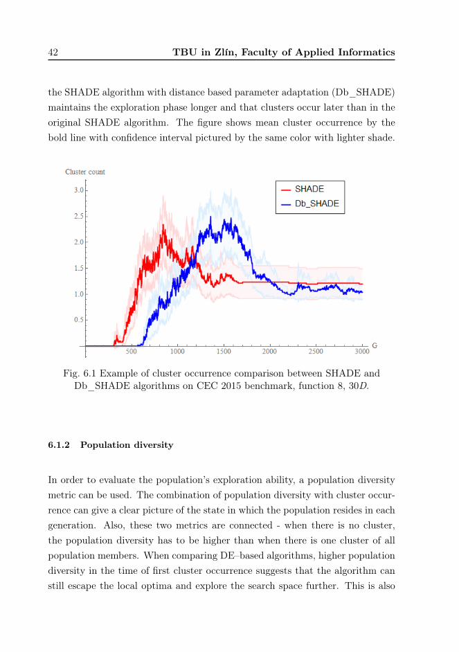
Clustering analysis is used to evaluate algorithms transition from exploration(ideally no clusters) to exploitation phase (clusters occur). In order to evaluatethat, the DBSCAN algorithm is run on each generation of the population duringthe optimization run and the number of clusters and the index of generation oftheir first occurrence is recorded. This gives a metric, which was titled MeanCluster Occurrence (MCO) [66]. This metric represents the average index ofgeneration in which clusters occurred over all algorithm runs on given optimizedfunction.An example of cluster occurrence is shown in Fig. 6.1, where it can be seen that
42 TBU in Zlín, Faculty of Applied Informatics
the SHADE algorithm with distance based parameter adaptation (Db_SHADE)maintains the exploration phase longer and that clusters occur later than in theoriginal SHADE algorithm. The figure shows mean cluster occurrence by thebold line with confidence interval pictured by the same color with lighter shade.
Fig. 6.1 Example of cluster occurrence comparison between SHADE andDb_SHADE algorithms on CEC 2015 benchmark, function 8, 30D.
6.1.2 Population diversity
In order to evaluate the population’s exploration ability, a population diversitymetric can be used. The combination of population diversity with cluster occur-rence can give a clear picture of the state in which the population resides in eachgeneration. Also, these two metrics are connected - when there is no cluster,the population diversity has to be higher than when there is one cluster of allpopulation members. When comparing DE–based algorithms, higher populationdiversity in the time of first cluster occurrence suggests that the algorithm canstill escape the local optima and explore the search space further. This is also

TBU in Zlín, Faculty of Applied Informatics 43
true for many other metaheuristics, not only for the DE.An useful population diversity (PD) metric was proposed in [64]. This metricis based on the square root of the sum of deviations (6.2) of an individual’scomponents from their corresponding means (6.1).
xj =1
NP
NP∑i=1
xj,i (6.1)
PD =
√√√√ 1
NP
NP∑i=1
D∑j=1
(xj,i − xj)2 (6.2)
Where i is the population member iterator and j is the component (dimension)iterator.Mean Population Diversity (MPD) [66] is a proposed metric for computing theaverage population diversity over multiple optimization runs in the moment ofthe first cluster occurrence. This metric should reflect the population’s potentialto explore the search space after its part exploits a locally promising area.
6.2 Multi–chaotic framework for parent selection
The Multi–Chaotic (MC) framework is based on the idea of using chaotic mapsas PRNGs [67]; these generators are used for parent selection with a probabil-ity based on their success in generating better offspring in previous generations.The next subsections describe the whole framework and its use along with ex-perimental results.
6.2.1 Chaotic maps as PRNGs
The chaotic maps are systems generated from a single initial position by simpleequations. Current coordinates of the system are generated from the previousones, consequently creating a system extremely dependent on the initial position.The generated chaotic sequence varies for different initial positions. Therefore,
44 TBU in Zlín, Faculty of Applied Informatics
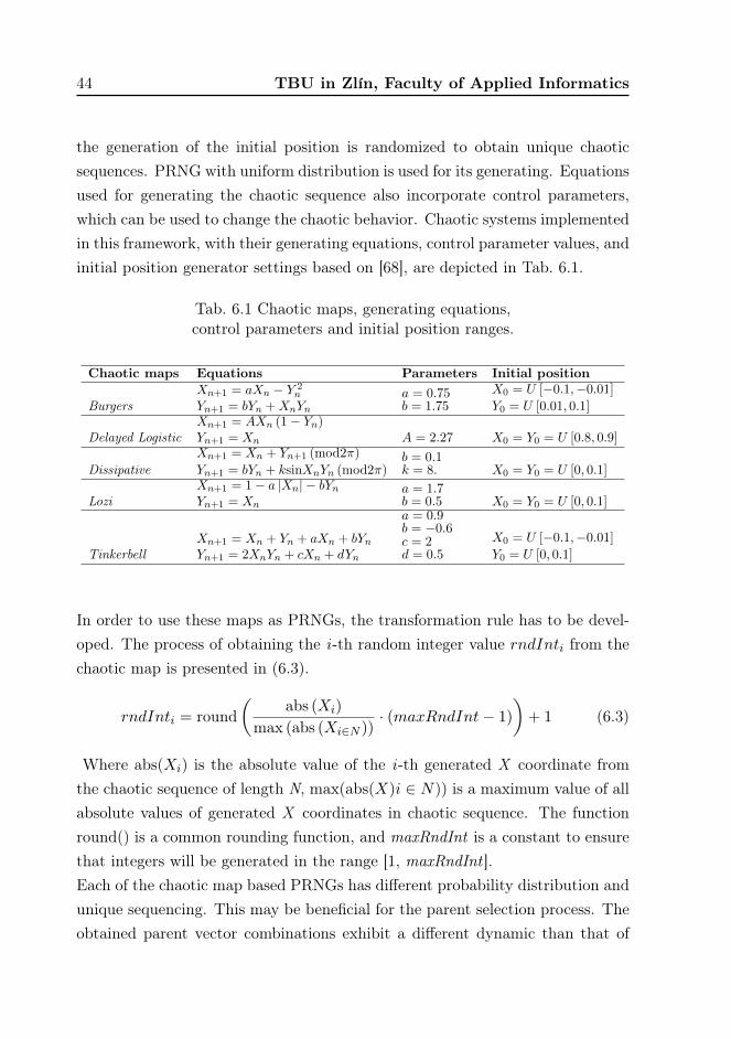
the generation of the initial position is randomized to obtain unique chaoticsequences. PRNG with uniform distribution is used for its generating. Equationsused for generating the chaotic sequence also incorporate control parameters,which can be used to change the chaotic behavior. Chaotic systems implementedin this framework, with their generating equations, control parameter values, andinitial position generator settings based on [68], are depicted in Tab. 6.1.
Tab. 6.1 Chaotic maps, generating equations,control parameters and initial position ranges.
Chaotic maps Equations Parameters Initial position
BurgersXn+1 = aXn − Y 2
n
Yn+1 = bYn +XnYna = 0.75b = 1.75
X0 = U [−0.1,−0.01]Y0 = U [0.01, 0.1]
Delayed LogisticXn+1 = AXn (1− Yn)Yn+1 = Xn A = 2.27 X0 = Y0 = U [0.8, 0.9]
DissipativeXn+1 = Xn + Yn+1 (mod2π)Yn+1 = bYn + ksinXnYn (mod2π)
b = 0.1k = 8. X0 = Y0 = U [0, 0.1]
LoziXn+1 = 1− a |Xn| − bYnYn+1 = Xn
a = 1.7b = 0.5 X0 = Y0 = U [0, 0.1]
TinkerbellXn+1 = Xn + Yn + aXn + bYnYn+1 = 2XnYn + cXn + dYn
a = 0.9b = −0.6c = 2d = 0.5
X0 = U [−0.1,−0.01]Y0 = U [0, 0.1]
In order to use these maps as PRNGs, the transformation rule has to be devel-oped. The process of obtaining the i-th random integer value rndInti from thechaotic map is presented in (6.3).
rndInti = round(
abs (Xi)
max (abs (Xi∈N ))· (maxRndInt− 1)
)+ 1 (6.3)
Where abs(Xi) is the absolute value of the i-th generated X coordinate fromthe chaotic sequence of length N, max(abs(X)i ∈ N)) is a maximum value of allabsolute values of generated X coordinates in chaotic sequence. The functionround() is a common rounding function, and maxRndInt is a constant to ensurethat integers will be generated in the range [1, maxRndInt ].Each of the chaotic map based PRNGs has different probability distribution andunique sequencing. This may be beneficial for the parent selection process. Theobtained parent vector combinations exhibit a different dynamic than that of

TBU in Zlín, Faculty of Applied Informatics 45
parent vector combinations selected by a PRNG with uniform distribution.
6.2.2 Parent selection
MC framework for the parent selection process is based on the ranking selectionof chaotic map based PRNGs. A list of chaotic PRNGs Clist has to be added tothe algorithm and each chaotic PRNG is initialized with the same probabilitypcinit = 1/Csize, where Csize is the size of Clist. For example, for five chaoticPRNGs Csize = 5 and each of them will have the probability of selection pcinit= 1/5 = 0.2 = 20%.For each target vector x i,G in generation G, the chaotic generator PRNGk isselected from the Clist according to its probability pck, where k is the index ofselected chaotic PRNG. This selected generator is then used to replace standardPRNG for the selection of parent vectors, and if the generated trial vector suc-ceeds in the selection, the probabilities are adjusted. There is an upper boundaryfor the probability of selection pcmax = 0.6 = 60%; if the selected chaotic PRNGreaches this probability, then no adjustment takes place. The whole process isdepicted in (6.4).
if f (ui,G) ≤ f (xi,G) and pck < pcmax pcj =
pcj+0.01
1.01 if j = k
pcj1.01 otherwise
otherwise pcj = pcj
(6.4)
6.2.3 Results
This section provides basic statistics of the 51 independent runs of SHADEand MC–SHADE algorithms. Both algorithms use the same setting, and theevaluation is done according to the CEC 2015 benchmark set [53].
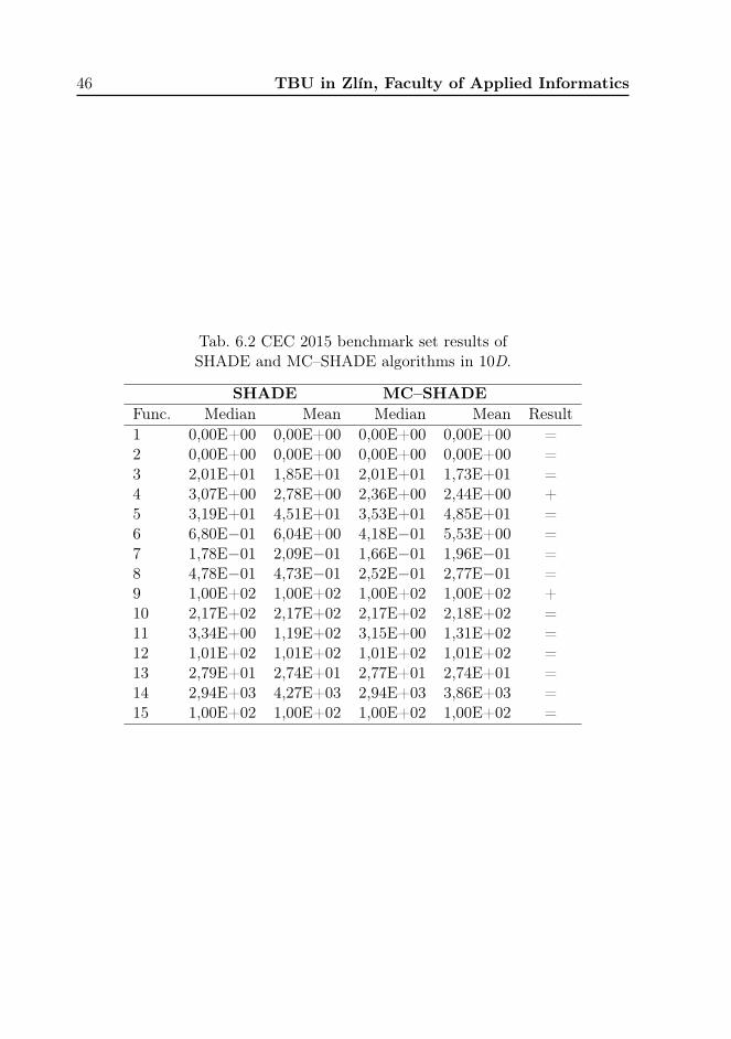
Tab. 6.2 shows median and mean values obtained by SHADE and MC–SHADE
46 TBU in Zlín, Faculty of Applied Informatics
Tab. 6.2 CEC 2015 benchmark set results ofSHADE and MC–SHADE algorithms in 10D.
SHADE MC–SHADEFunc. Median Mean Median Mean Result1 0,00E+00 0,00E+00 0,00E+00 0,00E+00 =2 0,00E+00 0,00E+00 0,00E+00 0,00E+00 =3 2,01E+01 1,85E+01 2,01E+01 1,73E+01 =4 3,07E+00 2,78E+00 2,36E+00 2,44E+00 +5 3,19E+01 4,51E+01 3,53E+01 4,85E+01 =6 6,80E−01 6,04E+00 4,18E−01 5,53E+00 =7 1,78E−01 2,09E−01 1,66E−01 1,96E−01 =8 4,78E−01 4,73E−01 2,52E−01 2,77E−01 =9 1,00E+02 1,00E+02 1,00E+02 1,00E+02 +10 2,17E+02 2,17E+02 2,17E+02 2,18E+02 =11 3,34E+00 1,19E+02 3,15E+00 1,31E+02 =12 1,01E+02 1,01E+02 1,01E+02 1,01E+02 =13 2,79E+01 2,74E+01 2,77E+01 2,74E+01 =14 2,94E+03 4,27E+03 2,94E+03 3,86E+03 =15 1,00E+02 1,00E+02 1,00E+02 1,00E+02 =
TBU in Zlín, Faculty of Applied Informatics 47
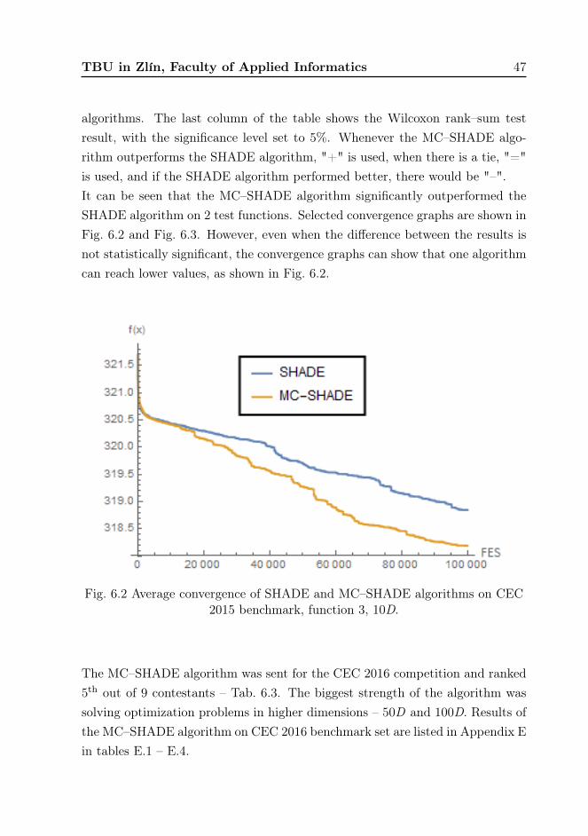
algorithms. The last column of the table shows the Wilcoxon rank–sum testresult, with the significance level set to 5%. Whenever the MC–SHADE algo-rithm outperforms the SHADE algorithm, "+" is used, when there is a tie, "="is used, and if the SHADE algorithm performed better, there would be "–".It can be seen that the MC–SHADE algorithm significantly outperformed theSHADE algorithm on 2 test functions. Selected convergence graphs are shown inFig. 6.2 and Fig. 6.3. However, even when the difference between the results isnot statistically significant, the convergence graphs can show that one algorithmcan reach lower values, as shown in Fig. 6.2.
Fig. 6.2 Average convergence of SHADE and MC–SHADE algorithms on CEC2015 benchmark, function 3, 10D.
The MC–SHADE algorithm was sent for the CEC 2016 competition and ranked5th out of 9 contestants – Tab. 6.3. The biggest strength of the algorithm wassolving optimization problems in higher dimensions – 50D and 100D. Results ofthe MC–SHADE algorithm on CEC 2016 benchmark set are listed in Appendix Ein tables E.1 – E.4.

48 TBU in Zlín, Faculty of Applied Informatics
Fig. 6.3 Average convergence of SHADE and MC–SHADE algorithms on CEC2015 benchmark, function 9, 10D.
Tab. 6.3 CEC 2016 competition ranking.
Algorithm D = 10 D = 30 D = 50 D = 100 Score RankLSHADE_EpSin [40] 1.51E+03 3.18E+03 5.88E+03 3.33E+04 4.38E+04 1UMOEAII [57] 1.44E+03 4.38E+03 1.59E+04 2.96E+04 5.14E+04 2SSEABC [69] 2.11E+03 7.68E+03 1.91E+04 3.06E+04 5.96E+04 3iL–SHADE [43] 1.98E+03 5.32E+03 1.80E+04 2.23E+05 2.49E+05 4MC–SHADE [41] 1.96E+03 1.06E+04 4.55E+04 1.96E+05 2.54E+05 5AEPDJADE [70] 2.17E+03 8.36E+03 4.42E+04 2.77E+05 3.32E+05 6LSHADE44 [42] 1.91E+03 5.97E+03 2.20E+04 3.76E+05 4.06E+05 7SHADE4 [71] 1.83E+03 1.77E+04 1.65E+05 7.79E+05 9.64E+05 8SPMGTLO [72] 8.64E+04 2.28E+06 3.87E+07 1.10E+08 1.51E+08 9
TBU in Zlín, Faculty of Applied Informatics 49
6.3 Distance based parameter adaptation
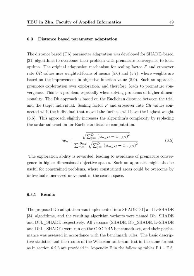
The distance based (Db) parameter adaptation was developed for SHADE–based[31] algorithms to overcome their problem with premature convergence to localoptima. The original adaptation mechanism for scaling factor F and crossoverrate CR values uses weighted forms of means (5.6) and (5.7), where weights arebased on the improvement in objective function value (5.9). Such an approachpromotes exploitation over exploration, and therefore, leads to premature con-vergence. This is a problem, especially when solving problems of higher dimen-sionality. The Db approach is based on the Euclidean distance between the trialand the target individual. Scaling factor F and crossover rate CR values con-nected with the individual that moved the furthest will have the highest weight(6.5). This approach slightly increases the algorithm’s complexity by replacingthe scalar subtraction for Euclidean distance computation.
wn =
√∑Dj=1 (un,j,G − xn,j,G)
2∑|SCR|m=1
√∑Dj=1 (um,j,G − xm,j,G)
2(6.5)
The exploration ability is rewarded, leading to avoidance of premature conver-gence in higher dimensional objective spaces. Such an approach might also beuseful for constrained problems, where constrained areas could be overcome byindividual’s increased movement in the search space.
6.3.1 Results
The proposed Db adaptation was implemented into SHADE [31] and L–SHADE[34] algorithms, and the resulting algorithm variants were named Db_SHADEand DbL_SHADE respectively. All versions (SHADE, Db_SHADE, L–SHADEand DbL_SHADE) were run on the CEC 2015 benchmark set, and their perfor-mance was assessed in accordance with the benchmark rules. The basic descrip-tive statistics and the results of the Wilcoxon rank–sum test in the same formatas in section 6.2.3 are provided in Appendix F in the following tables F.1 – F.8.
50 TBU in Zlín, Faculty of Applied Informatics
As can be seen in tables F.1 and F.2, the Db adaptation is comparable to the orig-inal adaptation on 10D problems. There is a statistically significant difference inperformance only in two cases – functions 6 and 12 (L–SHADE), resulting in thefinal score in Db wins/ties/loses of 0/15/0 (SHADE) and 1/13/1 (L–SHADE).Different results are visible on higher dimensional problems in tables F.3 – F.8.There, the Db adaptation outperforms the original versions with scored reportedin Tab. 6.4.
Tab. 6.4 Wilcoxon rank-sum results in a form ofwins/ties/loses from the perspective of Dbadaptation enhanced algorithm - CEC 2015.
D SHADE L-SHADE10 0/15/0 1/13/130 5/10/0 5/9/150 6/7/2 9/5/1100 5/9/1 5/8/2sum 16/41/3 20/35/5
The results show that the Db adaptation is beneficial for SHADE [31] and L–SHADE [34] algorithms when solving problems of higher dimensionality. Also,function 1 in the dataset is a unimodal rotated high conditioned elliptic func-tion [53], and the DbL_SHADE algorithm does not perform well in 30, 50 and100D on that problem. This is due to a slower convergence in comparison withL–SHADE with the original parameter adaptation. Understandably, the greedyapproach is more suitable for unimodal functions since there is no need for ex-ploration of the search space. The global optima of such functions can be foundby simply following the gradient from each point in the search space.
6.3.2 Clustering analysis
The influence of the distance based parameter adaptation on the exploration andexploitation abilities of the algorithm was also tested on CEC 2015 benchmarkset. A clustering and population diversity analysis described in section 6.1 were
TBU in Zlín, Faculty of Applied Informatics 51
performed and the results are available in Appendix G in tables G.1 – G.4 forSHADE and in tables G.5 – G.8 for L–SHADE.It can be seen that the population’s clustering occurs later for the algorithm vari-ants with distance based parameter adaptation. This is mainly true for higherdimensional settings (30, 50, and 100D). Also, when numbers of cluster occur-rence instances differ between Db and non-Db version, the Db version usuallyclusters in fewer cases. As for the population diversity, the characteristic featureis that when clusters occur in the population, diversity is similar regardless ofthe used adaptation scheme. It is important to note that in Db versions, clus-tering occurs later. Therefore, the population can explore the search space for alonger time, which proves to be beneficial for multimodal and complex objectivefunction landscapes.
6.4 DISH
In the original version of the DE, there were three user–defined control pa-rameters – population size NP, scaling factor F and crossover rate CR. Theseparameters’ values are usually adapted during the optimization in the modernversions of the DE, and DISH is no exception. However, the mutation opera-tor and adaptation mechanisms evolved via several successful algorithms. Theevolution line from DE to DISH is described in the following steps:
1. DE from 1995 by Storn and Price [12].
2. JADE from 2009 [23] – algorithm created by Zhang and Sanderson pro-posed a novel mutation strategy – "current–to–pbest/1" with an optionalarchive of inferior solutions.
3. SHADE from 2013 by Tanabe and Fukunaga [31] – built on the JADEalgorithm with added memories for historically successful F and CR val-ues and new adaptation mechanism for these parameters. This algorithmplaced 3rd in the CEC 2013 competition.
52 TBU in Zlín, Faculty of Applied Informatics
4. The linear decrease of population size was introduced into SHADE andcreated L–SHADE algorithm [34], the winner of the CEC 2014 competition.
5. Improved L–SHADE algorithm titled iL–SHADE [43] was proposed for aCEC 2016 competition by Brest et al. This algorithm introduced changesto the historical memory update system and the initialization of the histor-ical memories. It also proposed a new mechanism for treating F and CRparameters based on the ratio between current and maximum generation(phase of the optimization). This algorithm placed 4th in the CEC 2016competition.
6. Distance based parameter adaptation was proposed for SHADE based al-gorithms by Viktorin et al. in 2017 [73]. This novel adaptation mechanismbased on the distance between solutions instead of the difference betweenobjective function value was presented on SHADE and L–SHADE algo-rithms and shown its superiority over the original.
7. jSO algorithm was proposed by Brest et al. in 2017 [45]. The algo-rithm uses a novel "current–to–pbest–w/1" mutation strategy and slightlychanges fixed values for F and CR parameters. The jSO algorithm was2nd in the CEC 2017 bound constrained competition.
8. DISH algorithm was introduced in 2018 by Viktorin et al. and publishedin 2019 [47]. It incorporates the distance based parameter adaptation intothe jSO algorithm to improve its performance.
The following subsections provide the details of DISH algorithm mechanisms.As a result of the above mentioned evolution some operations (e.g., selection)are equal or similar to those mentioned in the previous sections of this work, butfor the sake of readability, those operations are also described in this section.

TBU in Zlín, Faculty of Applied Informatics 53
6.4.1 Initialization
The initial population P of solutions to the optimized problem is generatedrandomly. The size of the population is determined by the user via NPinit
parameter (initial population size). Each individual solution x is a vector oflength D, which is a dimension of the problem, and each vector componentis generated within its lower lo and upper up bounds by an uniform PRNGU [lo, up] (6.6).
xj,i = U[loj , upj
]for j = 1, . . . , D; i = 1, . . . , NP init (6.6)
Other parameters and variables that have to be set in the initialization phaseare:
1. Final population size - NPf .
2. Stopping criterion - a maximum number of objective function evaluationsMAXFES in the most common case.
3. pmax and pmin parameters for mutation operator. pmax = 0.25 and pmin
= pmax/2 = 0.125
4. External archive A is initialized empty. A = Ø
5. Historical memory size H. H = 5
6. Historical memories for scaling factor M F (6.7) and crossover rate M CR
(6.8).
7. Update historical memory index k. k = 1.
MF,i = 0.5 for i = 1, . . . ,H − 1, MF,H = 0.9 (6.7)
MCR,i = 0.8 for i = 1, . . . ,H − 1, MCR,H = 0.9 (6.8)
54 TBU in Zlín, Faculty of Applied Informatics
The following steps – mutation, crossover, and selection are repeated for eachindividual solution in the generation G, and these generations are repeated untilthe stopping criterion is met.
6.4.2 Mutation
The mutation operator used in DISH is a jSO’s "current–to–pbest–w/1", whichcombines a greedy approach in the first difference and the explorative factor inthe second difference (6.9).
vi = xi + Fw,i (xpBest − xi) + Fi (xr1 − xr2) (6.9)
The v i is the i–th mutated vector created from target vector x i, randomlyselected one of the 100p% best solutions in the population x pBest where p isdetermined by (6.10), a random solution from the population x r1 and randomsolution from the union of the population and external archive x r2. It is alsoimportant to note that all individuals are mutually different - x i 6= x pBest 6= x r1
6= x r2. The differences are scaled by two scaling factor parameters, the scalingfactor Fi (6.11), and the weighted scaling factor Fw,i (6.13).
p = FESratio · (pmax − pmin) + pmin (6.10)
Where FESratio stands for the ratio between the current number of objectivefunction evaluations FES and the maximum number of objective function evalu-ationsMAXFES (FESratio = FES/MAXFES ). Therefore, parameter p increaseslinearly with objective function evaluations.
Fi = C [MF,r, 0.1] (6.11)
The scaling factor value Fi is generated from Cauchy distribution with the lo-cation parameter M F,r and scale parameter value of 0. The index r is randomlygenerated from the range [1, H ]. If the generated value Fi is smaller or equalto 0, it is generated again and if it is higher than 1, it is set to 1. Also, the
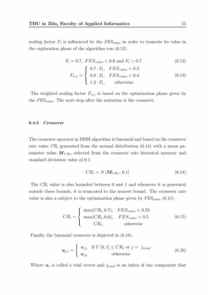
TBU in Zlín, Faculty of Applied Informatics 55
scaling factor Fi is influenced by the FESratio in order to truncate its value inthe exploration phase of the algorithm run (6.12).
Fi = 0.7, FESratio < 0.6 and Fi > 0.7 (6.12)
Fw,i =
0.7 · Fi, FESratio < 0.2
0.8 · Fi, FESratio < 0.4
1.2 · Fi, otherwise
(6.13)
The weighted scaling factor Fw,i is based on the optimization phase given bythe FESratio. The next step after the mutation is the crossover.
6.4.3 Crossover
The crossover operator in DISH algorithm is binomial and based on the crossoverrate value CRi generated from the normal distribution (6.14) with a mean pa-rameter value M CR,r selected from the crossover rate historical memory andstandard deviation value of 0.1.
CRi = N [MCR,r, 0.1] (6.14)
The CRi value is also bounded between 0 and 1 and whenever it is generatedoutside these bounds, it is truncated to the nearest bound. The crossover ratevalue is also a subject to the optimization phase given by FESratio (6.15).
CRi =
max(CRi, 0.7), FESratio < 0.25
max(CRi, 0.6), FESratio < 0.5
CRi, otherwise
(6.15)
Finally, the binomial crossover is depicted in (6.16).
uj,i =
{vj,i if U [0, 1] ≤ CRi or j = jrand
xj,i otherwise(6.16)
Where u i is called a trial vector and jrand is an index of one component that
56 TBU in Zlín, Faculty of Applied Informatics
has to be taken from the mutated vector v i. The jrand index ensures that atleast one vector component of the target vector x i will be replaced. Thus in thefollowing selection step, the tested trial vector will provide new information.
6.4.4 Selection
In the selection step, a quality of the trial solution vector u i is compared to thequality of the original solution vector x i. The quality is given by the objectivefunction value of these solutions. And since the selection operator is elitist, thetrial solution has to have at least equal objective function value as the targetsolution to proceed into the next generation G+1 (6.17).
xi,G+1 =
{ui,G if f (ui,G) ≤ f (xi,G)
xi,G otherwise(6.17)
Where f () depicts the objective function value, and in this case, the objectiveis to minimize it.The mutation, crossover, and selection operators are repeated for each individualsolution in the population, and after the population is exhausted, the algorithmproceeds to the next generation. However, before processing each individual so-lution of the next generation, two essential mechanisms are incorporated into thealgorithm – a linear decrease of the population size and the update of historicalmemories. These two mechanisms are described in the following subsections.
6.4.5 Linear decrease of the population size
The population size is decreased during the algorithm run to provide more timefor exploration in the later phase of optimization. Thus, the smaller populationof individual solutions will have more time to exploit the promising areas of theobjective function landscape.The mechanism used in the DISH algorithm is a linear decrease of populationsize, which uses the information of current objective function evaluations to

TBU in Zlín, Faculty of Applied Informatics 57
shrink the population of solutions. A new population size NPnew is calculatedas follows (6.18).
NPnew = round (NP init − FESratio · (NP init −NP f )) (6.18)
The size of an external archive A is connected to the size of the population, andtherefore, after decreasing the population size, the archive size is reduced as well.Whereas when decreasing the population size, the worst individual solutions arediscarded from the population, in the archive, solutions to discard are selectedrandomly.
6.4.6 Update of historical memories
Historical memories M F and M CR store historically successful values of scalingfactors F and crossover rates CR that were helpful in the production of bettertrial individual solutions. Therefore, these memories have to be updated duringthe optimization in order to store recently used values. After each generation,one cell of both memories is updated, and for that, the algorithm uses indexk to remember, which cell will be updated. The index is initialized to 1, andtherefore, after the first generation, the first memory cell will be updated. Theindex is increased by one after each update, and when it overflows the memorysize H, it starts from 1 again. There is one exception to the update, the last cellof both memories is never updated and still contains values 0.9 for both controlparameters.What will be stored in the k–th cell after the generation G is computed by aweighted Lehmer mean (6.19) of the corresponding generation control parameterarrays SF and SCR. These arrays are filled during the generation by the valuesof control parameters when the trial solution succeeds in the selection step.
meanWL (S) =
∑|S|n=1wn · S2
n∑|S|n=1wn · Sn
(6.19)
The meanWL() stands for weighted Lehmer mean and the computation is equal
58 TBU in Zlín, Faculty of Applied Informatics
for both SF and SCR, therefore, there is no subscript for S in the equation.The k–th memory cells of M F and M CR are then updated according to (6.20)and (6.21).
MF,k =
{meanWL (SF ) if SF 6= ∅ and k 6= H
MF,k otherwise(6.20)
MCR,k =
{meanWL (SCR) if SCR 6= ∅ and k 6= H
MCR,k otherwise(6.21)
The weights for the weighted Lehmer means (6.19) are in the case of the DISHalgorithm computed as depicted in (6.22). This weighting was introduced asthe distance based parameter adaptation [4]. It is titled like that, because inthe original SHADE, L–SHADE, iL–SHADE and jSO algorithms, the weightswere based on the difference between objective function values of trial individualu i and its corresponding target individual x i, whereas in DISH, the weight iscomputed from the Euclidean distance between those two - u i and x i.
wn =
√∑Dj=1 (un,j,G − xn,j,G)
2∑|SCR|m=1
√∑Dj=1 (um,j,G − xm,j,G)
2(6.22)
This approach promotes exploration and tries to avoid the premature conver-gence of the algorithm into local optima.Pseudo–code for the DISH algorithm is available in Appendix D.
6.4.7 Results
Median and mean obtained values on the CEC 2015 benchmark for the compar-ison between jSO and DISH are listed in Appendix H in tables H.1, H.2, H.3and H.4. The algorithm was also tested on CEC 2017 benchmark. Results areavailable in Appendix H in tables H.5, H.6, H.7 and H.8. A quick summary ofthe results in the same format (wins/ties/losses according to Wilcoxon rank–sumtest) as in section 6.3.1 is presented in Table 6.5.

TBU in Zlín, Faculty of Applied Informatics 59
Tab. 6.5 Wilcoxon rank-sum results in a form ofwins/ties/loses from the perspective of DISH -
CEC 2015 and CEC 2017.
D CEC 2015 CEC 201710 0/15/0 0/29/130 3/12/0 3/26/150 7/8/0 14/16/0100 6/7/2 19/10/1sum 16/42/2 36/81/3
Once again, it is perceivable from the results that distance based parameteradaptation is beneficial for higher dimensional problems and the algorithm vari-ant implementing it (DISH) is able to outperform the original algorithm withoutit (jSO).The results of clustering and population diversity analysis on the CEC 2015benchmark set are provided in Appendix I in the following tables I.1, I.2, I.3 andI.4. As it was stated in the previous chapter 6.3, the mean cluster occurrence forthe algorithm variant with distance based parameter adaptation (DISH in thiscase) is mostly higher, therefore clusters emerge later in the optimization phaseand the mean population diversity is similar during that time. This supportsthe initial idea of prolonging the exploration phase of the algorithm.In order to present the algorithm to the scientific community, DISH algorithmwas submitted for the CEC 2019 competition – 100–Digit Challenge [50]. Theresults are presented in Tab. 6.6 [60]. There were two variants in the competi-tion – DISHchain 1e+12 by Zamuda [49] and DISH by Viktorin et al. [47]. Thedifference between these versions was in the larger initial population and morecomputing resources in the case of DISHchain 1e+12. It was shown, that theDISH algorithm is capable of obtaining competitive results and ended on joined1st (DISHchain 1e+12) and 7th place out of 18 contestants.
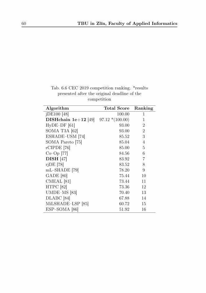
60 TBU in Zlín, Faculty of Applied Informatics
Tab. 6.6 CEC 2019 competition ranking. *resultspresented after the original deadline of the
competition
Algorithm Total Score RankingjDE100 [48] 100.00 1DISHchain 1e+12 [49] 97.12 *(100.00) 1HyDE–DF [61] 93.00 2SOMA T3A [62] 93.00 2ESHADE–USM [74] 85.52 3SOMA Pareto [75] 85.04 4rCIPDE [76] 85.00 5Co–Op [77] 84.56 6DISH [47] 83.92 7rjDE [78] 83.52 8mL–SHADE [79] 78.20 9GADE [80] 75.44 10CMEAL [81] 73.44 11HTPC [82] 73.36 12UMDE–MS [83] 70.40 13DLABC [84] 67.88 14MiLSHADE–LSP [85] 60.72 15ESP–SOMA [86] 51.92 16

TBU in Zlín, Faculty of Applied Informatics 61
7 THE CONTRIBUTION TO SCIENCE ANDPRACTICE
This part focuses on the benefits of proposed techniques in both scientific andapplication fields. Author believes that one of the most important aspects ofdeveloping new heuristic optimization techniques is a proper analysis of their be-haviour and identification of problem domains in which the algorithm performsadequately. Therefore, the population dynamic analysis might be a helpful toolfor researchers, and can determine some of the key features of their evolutionaryalgorithms – described in the next section 7.1. The section 7.2 describes im-plementation possibilities of the proposed distance based parameter adaptationand section 7.3 is devoted to an example of practical application of DISH–basedalgorithm on the problem of sustainable waste–to–energy facility location.
7.1 Population dynamic analysis
As its name suggests, population dynamic analysis is a tool that helps to ana-lyze and understand the collective behavior of the evolutionary algorithm dur-ing the optimization run. This is very important for the development of newideas, mainly in the adaptive evolutionary computation field. Since most of theproposed algorithms in this area aim to balance exploration and exploitationabilities, population dynamic analysis is a great tool to unveil possible issuesand confirm the intended influence of the proposed changes to the evolutionaryalgorithm.The main advantages of using proposed clustering and population diversity anal-ysis can be summarized as follows:
• Optimization phase detection – by combining the information fromcluster and diversity analysis with additional information from the algo-rithm, the exploration, stall, and convergence phases can be detected.
• Premature convergence detection – forming of early clusters in the

62 TBU in Zlín, Faculty of Applied Informatics
population is a good pointer towards premature convergence.
• Sub–optimal computational budget – when clusters are not formedduring the whole optimization run and the population is still evolving, it isa good sign of underestimated computational budget. On the other hand,when clusters are formed, and the population diversity remains the same,it suggests an overestimated computational budget because the algorithmis most likely not going to converge any further.
• Population size advisor – forming of clusters that leave out only a coupleof individuals might call for a larger population size. However, forming ofone large cluster suggests that there are more individuals in the same areathan needed.
• Population management tool – when managing the population sizeduring the optimization run, clustering information can be used to selectpotential candidates for removal and refine the area of new individual gen-eration.
7.2 Distance based parameter adaptation
Distance based parameter adaptation mechanism can be implemented into var-ious evolutionary algorithms that use a greedy approach for any weighted pa-rameter adaptation. Thus, it may be a tool for achieving a longer explorationphase in environments suitable for it. However, it is important to consider theadditional computational complexity when implementing distance based param-eter adaptation. Especially the large-scale optimization and the use of Euclideandistance, may suffer from the curse of dimensionality [87].
7.3 Practical applications of DISH
DISH algorithm can be used for any optimization task with continuous param-eters and can be considered a good choice for problems, which have over 30

TBU in Zlín, Faculty of Applied Informatics 63
optimized parameters since it works best with problems of higher dimensional-ity. One of the real–world applications is described in the next section.
7.3.1 Sustainable waste–to–energy facility location
The problem of waste–to–energy facility location with reduced energy sales andunutilized capacity of plants [88, 89, 90, 91, 92, 93, 94, 95] leads to a mixed–integer non–linear model, which can be solved quite efficiently for small andmedium–sized instances by traditional commercial solvers. However, for largerinstances, the computational complexity becomes an issue. Therefore, a modifiedversion of DISH was proposed and tested in [96].The case study described in the paper deals with finding a location for waste–to–energy facilities in the Czech Republic and the problem can be summarizedas follows:
• Existing waste–to–energy facilities – 4 (locations and capacities: Praha– 310 kt, Brno – 240 kt, Liberec – 96 kt and Plzeň – 95 kt).
• The capacity of Praha and Brno facilities can be extended – oneadditional option for each facility (430 kt Praha and 360 kt Brno).
• Limited number of potential new facility locations – 36.
• Each potential new facility has multiple capacity options – rangingfrom 2 to 27.
• Waste limitation – facilities cannot process more waste than their ca-pacity.
• Waste producers – 206 locations and each of them has to be processedin a facility.
• Transportation cost – based on the traveled distance and the amountof transported waste.
• Gate fee – based on the capacity of the facility.

64 TBU in Zlín, Faculty of Applied Informatics
• Unutilized capacity penalization – non–linear penalization for unusedcapacity of a facility.
In order to use the DISH algorithm for solving mixed–integer non–linear prob-lems, the algorithm had to be slightly adapted and led to the emergence of theDistance Random DISH (DR_DISH) algorithm. DR_DISH algorithm combinesDISH with distance–based clustering–inspired allocation of waste producers towaste–to–energy facilities with a random sequence of producer processing andcan be described in a three–step process [96]:
1. Location – DISH algorithm determines whether or not to build a facility ineach potential location (dimension of the problem is based on the numberof potential new facilities, and each optimized parameter is simplified to abinary decision 1 = build, 0 = do not build).
2. Repeat N –times
(a) Allocation - Randomly iterate through producers and assign themto the nearest existing facility (determined in the first step). If thenearest facility does not have enough capacity (maximum capacity islower than the sum of waste would be), the next nearest facility withadequate capacity is selected.
(b) Capacities - for each waste–to–energy facility a closest larger capac-ity than the sum of its waste is selected.
(c) Evaluation of the solution quality.
3. Out of N solutions, the best is selected and returned.
The DR_DISH algorithm was tested on 14 test cases dealing with instances ofthe problem from the smallest (only one considered region) to the largest (all 14regions of the Czech Republic). The results are provided in Table 7.1, where theconventional solver DICOPT [97] is incorporated as a baseline. An example ofthe proposed solution by DR_DISH algorithm for the whole Czech Republic is

TBU in Zlín, Faculty of Applied Informatics 65
Tab. 7.1 DICOPT and DR_DISH solving thesustainable waste–to–energy facility location.
# of regions [−] Cost [M€] # of facilities [−] Computational time [h:mm:ss]DICOPT DR_DISH DICOPT DR_DISH DICOPT DR_DISH
1 21.0 21.0 1 1 0:00:04 0:01:482 46.3 47.3 5 2 0:00:15 0:03:383 61.6 70.0 4 4 0:00:28 0:05:314 94.5 102.4 9 4 0:01:15 0:08:225 105.5 111.5 6 4 0:01:39 0:09:466 119.7 127.2 10 5 0:10:09 0:12:507 138.5 146.3 10 5 0:02:14 0:14:548 159.8 162.1 12 6 3:55:32 0:17:099 211.0 211.9 14 8 5:54:08 0:22:2110 − 241.9 − 9 − 0:23:4411 − 252.3 − 10 − 0:26:1912 − 268 − 11 − 0:31:5813 − 292.4 − 12 − 0:38:0114 − 301.7 − 12 − 0:40:53
Fig. 7.1 DR_DISH solution for the sustainable waste–to–energy facilitylocation - 14 regions.

66 TBU in Zlín, Faculty of Applied Informatics
shown in Fig. 7.1.As can be seen in Table 7.1, DICOPT solver was able to provide better resultsup to 9 regions. However, the computational complexity became too high for 10and more regions, and the commercial solver was unable to provide a feasible so-lution under given experimental conditions. It is also apparent that DR_DISHprovides solutions that use a smaller number of waste–to–energy facilities withhigher capacity. This is important for the possible real–world implementation ofthe solution since it is easier to guarantee a sufficient waste supply for larger fa-cilities. Therefore, their economic sustainability is easier [96]. Moreover, the per-ception of waste–to–energy facilities amongst the general public is still bad, eventhough the currently used technologies are ensuring clean incineration. Thus,the solution provided by DR_DISH algorithm is more likely to be implementedin practice.Several other approaches worth mentioning were considered during the design ofthe DR_DISH algorithm [96]:
• Small incinerator – locations of facilities determined by DISH, but eachfacility is initialized with the smallest available capacity. Producers areiterated over randomly and processed in the nearest facility with sufficientcapacity. If none of the facilities has sufficient capacity, the nearest onethat can be enlarged to accommodate the waste from the currently eval-uated producer is enlarged. This approach seems to be more viable forsmaller instances (1 – 4 regions with an average improvement of 5.84% incomparison with DR_DISH) but increases the cost for larger instances (5– 14 regions with 3.47% average increase).
• Cost oriented – DISH algorithm solves the sequence of processing pro-ducers. Producers waste is transported to the most cost–effective facilityin terms of transport cost and gate fees. This approach leads to a highernumber of small facilities, but the solution’s cost is increased by 15.5% onaverage in comparison with DR_DISH.
• Heuristic sequence – DISH algorithm solves both – facility location andthe sequence of processing producers. This leads to similar results as for

TBU in Zlín, Faculty of Applied Informatics 67
DR_DISH algorithm (only 0.22% cost increase), but the dimensionality ofthe problem quickly increases and thus is not suitable for larger instances.
• Iterative deterministic approach – This is an approach without heuris-tic. The algorithm starts with all potential facilities. Waste producers areallocated to their nearest facility with sufficient maximum capacity. Thenthe algorithm cyclically tries to remove each facility and reallocate its wasteproducers. This continues while the overall cost decreases. This approachis due to its deterministic nature faster but led to the average increase inthe cost of 5.63%.

68 TBU in Zlín, Faculty of Applied Informatics
8 DISSERTATION GOAL FULFILLMENT
This section describes steps that were taken in order to fulfill the dissertationgoal. This was to investigate current trends in adaptive DE design and utilizedatamining techniques to improve the understanding of the population dynamicand possibly use this information to develop more robust and performance-wisebetter algorithm variants.
• State–of–the–art review – current trends and ideas in the field of adap-tive DE were studied and analyzed for possible deficiencies in the algorithmdesign [98, 99, 100].
• Proposal of novel adaptive DE variants – based on the knowledgegained from the first step, the proposed methods highlight understand-ing of the population dynamic by addressing the problem of prematureconvergence and fast clustering of the population [41, 44].
• Comparison with state of the art methods – proposed methods wereimplemented into the state–of–the–art algorithms (SHADE, L–SHADEand jSO [73, 47]) and compared with their canonical forms on CEC bench-mark sets. The proposed algorithms were also participating in CEC com-petitions in 2016 (5th place) [52] and 2019 (joined 1st, and 7th place) [101].
• Analysis – an analysis of the results [66, 102] was executed to understandthe benefits and drawbacks of the proposed methods. The next step in thisresearch direction is to utilize the analysis findings for the development ofrefined adaptive methods and their implementation.

TBU in Zlín, Faculty of Applied Informatics 69
9 CONCLUSION
This chapter summarizes the results of the doctoral thesis. Methods proposedin this work can be used in both – research and practice.Researchers might find clustering and population diversity analysis useful forbetter understanding of the collective behavior of their evolutionary algorithm’spopulation. Thus, it can help with the development, implementation, and mainlyevaluation of new ideas in the field of adaptive parameter control. Practitionersmay use the analysis results to identify potential problems with incorrect com-putational budget or population size selection.Following the findings of clustering and population diversity analysis of state-of-the-art DE algorithms, a distance based parameter adaptation was proposed.This led to the development of the DISH algorithm, which is a good choice forsingle–objective optimization problems in the continuous domain with a highernumber of optimized parameters. The algorithm is reasonably easy to imple-ment, and its implementation in Java is already available on Github [103]. Itmay also serve for researchers as a baseline for comparison of their proposedalgorithms.As for the distance based parameter adaptation scheme, it is possible to im-plement it into other population–based evolutionary algorithms to affect theirbalance between exploration and exploitation and help with the algorithm’s per-formance aspect.The author would like to utilize the knowledge gained in his doctoral studies anddedicate his future research time and capacity to the development of an anal-ysis framework for continuous single–objective population–based optimizationtechniques. Such a framework should help analyze the behavior of an algorithmduring the optimization phase and serve as a guide for the refinement of devel-oped techniques.The incremental development of new evolutionary algorithms is an ongoing pro-cess that gradually improves the quality of the heuristic optimization field [104].Therefore, in author’s opinion, this type of research should be encouraged, butwith a great emphasis on good research practices.
70 TBU in Zlín, Faculty of Applied Informatics
REFERENCES
[1] Gropp, W. and Moré, J. Optimization Environments and the NEOSServer. Approximation Theory and Optimization, MD Buhmann and A.Iserles, eds, 1997.
[2] Cavazzuti, M. Deterministic Optimization. In Optimiza-tion Methods. : Springer Berlin Heidelberg, September 2012.pp. 77–102. doi: 10.1007/978-3-642-31187-1_4. Available at:<https://doi.org/10.1007/978-3-642-31187-1_4>.
[3] Darwin, C. On the Origin of Species by Means of Natural Selection Orthe Preservation of Favoured Races in the Struggle for Life. H. Milford;Oxford University Press, 1859.
[4] Jesus, D. A. R. and Rivera, W. Application of Evolutionary Algorithmsfor Load Forecasting in Smart Grids. In Proceedings of the InternationalConference on Foundations of Computer Science (FCS), pp. 40–44. TheSteering Committee of The World Congress in Computer Science, Com-puter Engineering and Applied Computing (WorldComp), 2018.
[5] Sathiya, P., Aravindan, S., Haq, A. N. and Paneerselvam, K. Opti-mization of friction welding parameters using evolutionary computationaltechniques. Journal of Materials Processing Technology. 2009, vol. 209,no. 5, pp. 2576 – 2584. ISSN 0924-0136. doi: https://doi.org/10.1016/j.jmatprotec.2008.06.030.
[6] Zamuda, A., Sosa, J. D. H. and Adler, L. Constrained differential evo-lution optimization for underwater glider path planning in sub-mesoscaleeddy sampling. Applied Soft Computing. 2016, vol. 42, pp. 93 – 118. ISSN1568-4946. doi: https://doi.org/10.1016/j.asoc.2016.01.038.
[7] Gobeyn, S., Mouton, A. M., Cord, A. F., Kaim, A., Volk, M.and Goethals, P. L. Evolutionary algorithms for species distribu-tion modelling: A review in the context of machine learning. Ecolog-ical Modelling. 2019, vol. 392, pp. 179 – 195. ISSN 0304-3800. doi:https://doi.org/10.1016/j.ecolmodel.2018.11.013.

TBU in Zlín, Faculty of Applied Informatics 71
[8] Sun, L., Lin, L., Li, H. and Gen, M. Large scale flexible schedulingoptimization by a distributed evolutionary algorithm. Computers & In-dustrial Engineering. 2019, vol. 128, pp. 894 – 904. ISSN 0360-8352. doi:https://doi.org/10.1016/j.cie.2018.09.025.
[9] Yeguas-Bolivar, E., Muñoz-Salinas, R., Medina-Carnicer, R. andCarmona-Poyato, A. Comparing evolutionary algorithms and particlefilters for Markerless Human Motion Capture. Applied Soft Computing.2014, vol. 17, pp. 153 – 166. ISSN 1568-4946. doi: https://doi.org/10.1016/j.asoc.2014.01.007.
[10] Devi, R. V., Sathya, S. S. and Coumar, M. S. Evolutionary algorithmsfor de novo drug design – A survey. Applied Soft Computing. 2015, vol. 27,pp. 543 – 552. ISSN 1568-4946. doi: https://doi.org/10.1016/j.asoc.2014.09.042.
[11] Wolpert, D. H. and Macready, W. G. No Free Lunch Theorems forOptimization. IEEE Transactions on Evolutionary Computation. 1997,vol. 1, no. 1, pp. 67–82.
[12] Price, K. and Storn, R. Differential Evolution-a simple and efficientadaptive scheme for global optimization over continuous space. Technicalreport, Technical Report, International Computer Science Institute, 1995.
[13] Sörensen, K. Metaheuristics—the metaphor exposed. Interna-tional Transactions in Operational Research. 2015, vol. 22, no. 1,pp. 3–18. doi: https://doi.org/10.1111/itor.12001. Available at:<https://onlinelibrary.wiley.com/doi/abs/10.1111/itor.12001>.
[14] Storn, R. and Price, K. Differential Evolution - A Simple andEfficient Heuristic for global Optimization over Continuous Spaces.Journal of Global Optimization. 1997, vol. 11, no. 4, pp. 341–359. ISSN 1573-2916. doi: 10.1023/A:1008202821328. Available at:<https://doi.org/10.1023/A:1008202821328>.

72 TBU in Zlín, Faculty of Applied Informatics
[15] Gämperle, R., Müller, S. D. and Koumoutsakos, P. A parameterstudy for differential evolution. Advances in intelligent systems, fuzzy sys-tems, evolutionary computation. 2002, vol. 10, no. 10, pp. 293–298.
[16] Liu, J. On setting the control parameter of the differential evolutionmethod. In Proceedings of the 8th international conference on soft com-puting (MENDEL 2002), pp. 11–18, 2002.
[17] Ronkkonen, J., Kukkonen, S. and Price, K. Real-Parameter Opti-mization with Differential Evolution. In 2005 IEEE Congress on Evolution-ary Computation. IEEE, 2005. doi: 10.1109/cec.2005.1554725. Availableat: <https://doi.org/10.1109/cec.2005.1554725>.
[18] Liu, J. and Lampinen, J. A Fuzzy Adaptive Differential Evo-lution Algorithm. Soft Computing. 2005, vol. 9, no. 6, pp. 448–462. ISSN 1433-7479. doi: 10.1007/s00500-004-0363-x. Available at:<https://doi.org/10.1007/s00500-004-0363-x>.
[19] Omran, M. G. H., Salman, A. and Engelbrecht, A. P. Self-adaptiveDifferential Evolution. In Computational Intelligence and Security. :Springer Berlin Heidelberg, 2005. pp. 192–199. doi: 10.1007/11596448_28.Available at: <https://doi.org/10.1007/11596448_28>.
[20] Qin, A. and Suganthan, P. Self-adaptive Differential Evolution Algo-rithm for Numerical Optimization. In 2005 IEEE Congress on Evolution-ary Computation. IEEE, 2005. doi: 10.1109/cec.2005.1554904. Availableat: <https://doi.org/10.1109/cec.2005.1554904>.
[21] Brest, J., Greiner, S., Boskovic, B., Mernik, M. and Zumer,V. Self-Adapting Control Parameters in Differential Evolution: AComparative Study on Numerical Benchmark Problems. IEEETransactions on Evolutionary Computation. December 2006, vol. 10,no. 6, pp. 646–657. doi: 10.1109/tevc.2006.872133. Available at:<https://doi.org/10.1109/tevc.2006.872133>.
[22] Qin, A., Huang, V. and Suganthan, P. Differential Evolution Al-gorithm With Strategy Adaptation for Global Numerical Optimization.
TBU in Zlín, Faculty of Applied Informatics 73
IEEE Transactions on Evolutionary Computation. April 2009, vol. 13,no. 2, pp. 398–417. doi: 10.1109/tevc.2008.927706. Available at:<https://doi.org/10.1109/tevc.2008.927706>.
[23] Zhang, J. and Sanderson, A. C. JADE: adaptive differential evolu-tion with optional external archive. IEEE Transactions on evolutionarycomputation. 2009, vol. 13, no. 5, pp. 945–958.
[24] Mallipeddi, R., Suganthan, P., Pan, Q. and Tasgetiren, M. Dif-ferential evolution algorithm with ensemble of parameters and mutationstrategies. Applied Soft Computing. 2011, vol. 11, no. 2, pp. 1679 – 1696.ISSN 1568-4946. doi: https://doi.org/10.1016/j.asoc.2010.04.024. The Im-pact of Soft Computing for the Progress of Artificial Intelligence.
[25] Wang, Y., Cai, Z. and Zhang, Q. Differential Evolution WithComposite Trial Vector Generation Strategies and Control Parame-ters. IEEE Transactions on Evolutionary Computation. February 2011,vol. 15, no. 1, pp. 55–66. doi: 10.1109/tevc.2010.2087271. Available at:<https://doi.org/10.1109/tevc.2010.2087271>.
[26] Gong, W., Fialho, Cai, Z. and Li, H. Adaptive strategy selection in dif-ferential evolution for numerical optimization: An empirical study. Infor-mation Sciences. 2011, vol. 181, no. 24, pp. 5364 – 5386. ISSN 0020-0255.doi: https://doi.org/10.1016/j.ins.2011.07.049.
[27] Elsayed, S. M., Sarker, R. A. and Essam, D. L. Differential evolutionwith multiple strategies for solving CEC2011 real-world numerical opti-mization problems. In 2011 IEEE Congress of Evolutionary Computation(CEC). IEEE, June 2011. doi: 10.1109/cec.2011.5949732. Available at:<https://doi.org/10.1109/cec.2011.5949732>.
[28] Tvrdik, J. and Polakova, R. Competitive differential evolution appliedto CEC 2013 problems. In 2013 IEEE Congress on Evolutionary Com-putation. IEEE, June 2013. doi: 10.1109/cec.2013.6557759. Available at:<https://doi.org/10.1109/cec.2013.6557759>.

74 TBU in Zlín, Faculty of Applied Informatics
[29] Zamuda, A., Brest, J. and Mezura-Montes, E. Structured PopulationSize Reduction Differential Evolution with Multiple Mutation Strategieson CEC 2013 real parameter optimization. In 2013 IEEE Congress on Evo-lutionary Computation. IEEE, June 2013. doi: 10.1109/cec.2013.6557794.Available at: <https://doi.org/10.1109/cec.2013.6557794>.
[30] Zhu, W., Tang, Y., Fang, J. and Zhang, W. Adaptive population tuningscheme for differential evolution. Information Sciences. 2013, vol. 223,pp. 164 – 191. ISSN 0020-0255. doi: https://doi.org/10.1016/j.ins.2012.09.019.
[31] Tanabe, R. and Fukunaga, A. Success-history based parameter adap-tation for Differential Evolution. In 2013 IEEE Congress on EvolutionaryComputation (CEC), pp. 71–78. IEEE, 2013.
[32] Yu, W.-J., Shen, M., Chen, W.-N., Zhan, Z.-H., Gong, Y.-J., Lin, Y.,Liu, O. and Zhang, J. Differential Evolution With Two-Level Parame-ter Adaptation. IEEE Transactions on Cybernetics. July 2014, vol. 44,no. 7, pp. 1080–1099. doi: 10.1109/tcyb.2013.2279211. Available at:<https://doi.org/10.1109/tcyb.2013.2279211>.
[33] Falco, I. D., Cioppa, A. D., Maisto, D., Scafuri, U. and Tarantino,E. An adaptive invasion-based model for distributed Differential Evolution.Information Sciences. 2014, vol. 278, pp. 653 – 672. ISSN 0020-0255. doi:https://doi.org/10.1016/j.ins.2014.03.083.
[34] Tanabe, R. and Fukunaga, A. S. Improving the search performance ofSHADE using linear population size reduction. In 2014 IEEE Congress onEvolutionary Computation (CEC), pp. 1658–1665, 2014.
[35] Wu, G., Mallipeddi, R., Suganthan, P., Wang, R. and Chen, H.Differential evolution with multi-population based ensemble of mutationstrategies. Information Sciences. 2016, vol. 329, pp. 329 – 345. ISSN0020-0255. doi: https://doi.org/10.1016/j.ins.2015.09.009. Special issueon Discovery Science.
TBU in Zlín, Faculty of Applied Informatics 75
[36] Mallipeddi, R. and Lee, M. An evolving surrogate model-based differ-ential evolution algorithm. Applied Soft Computing. 2015, vol. 34, pp. 770– 787. ISSN 1568-4946. doi: https://doi.org/10.1016/j.asoc.2015.06.010.
[37] Díaz-Manríquez, A., Toscano-Pulido, G. and Gómez-Flores, W.On the selection of surrogate models in evolutionary optimization algo-rithms. In 2011 IEEE Congress of Evolutionary Computation (CEC), pp.2155–2162, 2011. doi: 10.1109/CEC.2011.5949881.
[38] Draa, A., Bouzoubia, S. and Boukhalfa, I. A sinusoidal differentialevolution algorithm for numerical optimisation. Applied Soft Computing.2015, vol. 27, pp. 99 – 126. ISSN 1568-4946. doi: https://doi.org/10.1016/j.asoc.2014.11.003.
[39] Guo, S.-M., Tsai, J. S.-H., Yang, C.-C. and Hsu, P.-H. A self-optimization approach for L-SHADE incorporated with eigenvector-basedcrossover and successful-parent-selecting framework on CEC 2015 bench-mark set. In 2015 IEEE congress on evolutionary computation (CEC), pp.1003–1010. IEEE, 2015.
[40] Awad, N. H., Ali, M. Z., Suganthan, P. N. and Reynolds, R. G. Anensemble sinusoidal parameter adaptation incorporated with L-SHADEfor solving CEC2014 benchmark problems. In 2016 IEEE congress onevolutionary computation (CEC), pp. 2958–2965. IEEE, 2016.
[41] Viktorin, A., Pluhacek, M. and Senkerik, R. Success-historybased adaptive differential evolution algorithm with multi-chaoticframework for parent selection performance on CEC2014 benchmarkset. In 2016 IEEE Congress on Evolutionary Computation (CEC).IEEE, July 2016. doi: 10.1109/cec.2016.7744404. Available at:<https://doi.org/10.1109/cec.2016.7744404>.
[42] Polakova, R., Tvrdik, J. and Bujok, P. Evaluating the performanceof L-SHADE with competing strategies on CEC2014 single parameter-operator test suite. In 2016 IEEE Congress on Evolutionary Computation(CEC). IEEE, July 2016. doi: 10.1109/cec.2016.7743921. Available at:<https://doi.org/10.1109/cec.2016.7743921>.
76 TBU in Zlín, Faculty of Applied Informatics
[43] Brest, J., Maučec, M. S. and Bošković, B. iL-SHADE: Improved L-SHADE Algorithm for Single Objective Real-Parameter Optimization. In2016 IEEE World Congress on Computational Intelligence (IEEE WCCI2016), Vancouver, Canada, pp. 1188–1195, 2016.
[44] Viktorin, A., Senkerik, R., Pluhacek, M., Kadavy, T. and Za-
muda, A. Distance based parameter adaptation for differential evolution.In 2017 IEEE Symposium Series on Computational Intelligence (SSCI).IEEE, November 2017. doi: 10.1109/ssci.2017.8280959. Available at:<https://doi.org/10.1109/ssci.2017.8280959>.
[45] Brest, J., Maučec, M. S. and Bošković, B. Single objective real-parameter optimization: algorithm jSO. In 2017 IEEE congress on evolu-tionary computation (CEC), pp. 1311–1318. IEEE, 2017.
[46] Stanovov, V., Akhmedova, S. and Semenkin, E. LSHADE Algorithmwith Rank-Based Selective Pressure Strategy for Solving CEC 2017 Bench-mark Problems. In 2018 IEEE Congress on Evolutionary Computation(CEC). IEEE, July 2018. doi: 10.1109/cec.2018.8477977. Available at:<https://doi.org/10.1109/cec.2018.8477977>.
[47] Viktorin, A., Senkerik, R., Pluhacek, M., Kadavy, T. and Zamuda,A. Distance based parameter adaptation for success-history based differ-ential evolution. Swarm and Evolutionary Computation. 2019, vol. 50,pp. 100462.
[48] Brest, J., Maučec, M. S. and Bošković, B. The 100-Digit Challenge:Algorithm jDE100. In 2019 IEEE Congress on Evolutionary Computation(CEC), pp. 19–26, 2019. doi: 10.1109/CEC.2019.8789904.
[49] Zamuda, A. Function Evaluations Upto 1e+12 and Large Popula-tion Sizes Assessed in Distance-Based Success History Differential Evo-lution for 100-Digit Challenge and Numerical Optimization Scenarios(DISHchain 1e+12): A Competition Entry for "100-Digit Challenge,and Four Other Numerical Optimization Competitions" at the Genetic
TBU in Zlín, Faculty of Applied Informatics 77
and Evolutionary Computation Conference (CECCO) 2019. In Proceed-ings of the Genetic and Evolutionary Computation Conference Compan-ion, GECCO ’19, pp. 11–12, New York, NY, USA, 2019. Associationfor Computing Machinery. doi: 10.1145/3319619.3326751. Available at:<https://doi.org/10.1145/3319619.3326751>. ISBN 9781450367486.
[50] Price, K., Awad, N., Ali, M. and Suganthan, P. Problem definitionsand evaluation criteria for the 100-digit challenge special session and com-petition on single objective numerical optimization. In Technical Report. :Nanyang Technological University, 2018.
[51] Liang, J., Qu, B. and Suganthan, P. Problem definitions and evalua-tion criteria for the CEC 2014 special session and competition on singleobjective real-parameter numerical optimization. Computational Intelli-gence Laboratory, Zhengzhou University, Zhengzhou China and TechnicalReport, Nanyang Technological University, Singapore. 2013, vol. 635.
[52] Liang, J., Qu, B. and Suganthan, P. Problem definitions and evalua-tion criteria for the CEC 2014 special session and competition on singleobjective real-parameter numerical optimization. Computational Intelli-gence Laboratory, Zhengzhou University, Zhengzhou China and TechnicalReport, Nanyang Technological University, Singapore. 2013, vol. 635.
[53] Liang, J., Qu, B., Suganthan, P. and Chen, Q. Problem definitionsand evaluation criteria for the CEC 2015 competition on learning-basedreal-parameter single objective optimization. Technical Report201411A,Computational Intelligence Laboratory, Zhengzhou University, ZhengzhouChina and Technical Report, Nanyang Technological University, Singapore.2014, vol. 29, pp. 625–640.
[54] Awad, N., Ali, M. Z. and Reynolds, R. G. A differential evolutionalgorithm with success-based parameter adaptation for CEC2015 learning-based optimization. In 2015 IEEE Congress on Evolutionary Computation(CEC). IEEE, May 2015. doi: 10.1109/cec.2015.7257012. Available at:<https://doi.org/10.1109/cec.2015.7257012>.

78 TBU in Zlín, Faculty of Applied Informatics
[55] Sallam, K. M., Sarker, R. A., Essam, D. L. and Elsayed, S. M.Neurodynamic differential evolution algorithm and solving CEC2015 com-petition problems. In 2015 IEEE Congress on Evolutionary Computation(CEC). IEEE, May 2015. doi: 10.1109/cec.2015.7257003. Available at:<https://doi.org/10.1109/cec.2015.7257003>.
[56] Rueda, J. L. and Erlich, I. Testing MVMO on learning-based real-parameter single objective benchmark optimization prob-lems. In 2015 IEEE Congress on Evolutionary Computation (CEC).IEEE, May 2015. doi: 10.1109/cec.2015.7257002. Available at:<https://doi.org/10.1109/cec.2015.7257002>.
[57] Elsayed, S., Hamza, N. and Sarker, R. Testing united multi-operator evolutionary algorithms-II on single objective optimization prob-lems. In 2016 IEEE Congress on Evolutionary Computation (CEC).IEEE, July 2016. doi: 10.1109/cec.2016.7744164. Available at:<https://doi.org/10.1109/cec.2016.7744164>.
[58] Awad, N. H., Ali, M. Z. and Suganthan, P. N. Ensemble sinusoidaldifferential covariance matrix adaptation with Euclidean neighborhood forsolving CEC2017 benchmark problems. In 2017 IEEE Congress on Evo-lutionary Computation (CEC), pp. 372–379. IEEE, 2017.
[59] Mohamed, A. W., Hadi, A. A., Fattouh, A. M. and Jambi, K. M.LSHADE with semi-parameter adaptation hybrid with CMA-ES for solv-ing CEC 2017 benchmark problems. In 2017 IEEE Congress on evolution-ary computation (CEC), pp. 145–152. IEEE, 2017.
[60] Price, K., Awad, N., Ali, M. and Suganthan, P. The 2019 100-Digit Challenge on Real-Parameter, Single Objective Optimization: Anal-ysis of Results. Technical report, Technical Report 2019. Available on-line: https:// www.ntu.edu.sg /home /epnsugan /index_files /CEC2019/CEC2019.htm, 2019.
[61] Lezama, F., Soares, J. a., Faia, R. and Vale, Z. Hybrid-Adaptive Dif-ferential Evolution with Decay Function (HyDE-DF) Applied to the 100-Digit Challenge Competition on Single Objective Numerical Optimization.
TBU in Zlín, Faculty of Applied Informatics 79
In Proceedings of the Genetic and Evolutionary Computation ConferenceCompanion, GECCO ’19, pp. 7–8, New York, NY, USA, 2019. Associationfor Computing Machinery. doi: 10.1145/3319619.3326747. Available at:<https://doi.org/10.1145/3319619.3326747>. ISBN 9781450367486.
[62] Diep, Q. B., Zelinka, I., Das, S. and Senkerik, R. SOMA T3A forSolving the 100-Digit Challenge. In Zamuda, A., Das, S., Suganthan,P. N. and Panigrahi, B. K. (Ed.) Swarm, Evolutionary, and MemeticComputing and Fuzzy and Neural Computing, pp. 155–165, Cham, 2020.Springer International Publishing. ISBN 978-3-030-37838-7.
[63] Ester, M., Kriegel, H.-P., Sander, J., Xu, X. and others. A density-based algorithm for discovering clusters in large spatial databases withnoise. In Kdd, vol. 96, pp. 226–231, 1996.
[64] Poláková, R., Tvrdík, J., Bujok, P. and Matoušek, R. Population-size adaptation through diversity-control mechanism for differential evolu-tion. In MENDEL, 22th International Conference on Soft Computing, pp.49–56, 2016.
[65] Deza, M. M. and Deza, E. Encyclopedia of Distances. In Encyclopediaof Distances. : Springer, 2009. pp. 1–583.
[66] Viktorin, A., Senkerik, R., Pluhacek, M. and Kadavy,T. Clustering Analysis of the Population in Db_SHADEAlgorithm. MENDEL. Jun. 2018, vol. 24, no. 1, pp. 9–16. doi: 10.13164/mendel.2018.1.009. Available at:<https://mendel-journal.org/index.php/mendel/article/view/13>.
[67] PLUHACEK, M. Modern methods of development and modification ofevolutionary computational techniques. Doctoral Thesis, Tiomas Bata Uni-versity in Zlín, Faculty of Applied Informatics, Zlín, 2015.
[68] Sprott, J. C. and Sprott, J. C. Chaos and time-series analysis. OxfordUniversity Press, 2003. ISBN 9780198508403.
80 TBU in Zlín, Faculty of Applied Informatics
[69] Yavuz, G., Aydin, D. and Stutzle, T. Self-adaptive search equation-based artificial bee colony algorithm on the CEC 2014 benchmark func-tions. In 2016 IEEE Congress on Evolutionary Computation (CEC).IEEE, July 2016. doi: 10.1109/cec.2016.7743920. Available at:<https://doi.org/10.1109/cec.2016.7743920>.
[70] Yang, M., Guan, J. and Li, C. Differential evolution with auto-enhanced population diversity: The experiments on the CEC'2016competition. In 2016 IEEE Congress on Evolutionary Computation(CEC). IEEE, July 2016. doi: 10.1109/cec.2016.7744402. Available at:<https://doi.org/10.1109/cec.2016.7744402>.
[71] Bujok, P., Tvrdik, J. and Polakova, R. Evaluating the performanceof SHADE with competing strategies on CEC 2014 single-parameter testsuite. In 2016 IEEE Congress on Evolutionary Computation (CEC), pp.5002–5009. IEEE, July 2016. doi: 10.1109/cec.2016.7748322. Available at:<https://doi.org/10.1109/cec.2016.7748322>.
[72] Kommadath, R., Sivadurgaprasad, C. and Kotecha, P. Single phasemulti-group teaching learning algorithm for computationally expensive nu-merical optimization (CEC 2016). In 2016 IEEE Congress on Evolution-ary Computation (CEC). IEEE, July 2016. doi: 10.1109/cec.2016.7744167.Available at: <https://doi.org/10.1109/cec.2016.7744167>.
[73] Viktorin, A., Senkerik, R., Pluhacek, M., Kadavy, T. and Zamuda,A. Distance based parameter adaptation for differential evolution. In 2017IEEE Symposium Series on Computational Intelligence (SSCI), pp. 1–7.IEEE, 2017.
[74] Kumar, A., Misra, R. K., Singh, D. and Das, S. Testing A Multi-Operator based Differential Evolution Algorithm on the 100-Digit Chal-lenge for Single Objective Numerical Optimization. In 2019 IEEE Congresson Evolutionary Computation (CEC), pp. 34–40, 2019. doi: 10.1109/CEC.2019.8789907.
[75] Truong, T. C., Diep, Q. B., Zelinka, I. and Senkerik, R. Pareto-Based Self-organizing Migrating Algorithm Solving 100-Digit Challenge.
TBU in Zlín, Faculty of Applied Informatics 81
In Zamuda, A., Das, S., Suganthan, P. N. and Panigrahi, B. K.(Ed.) Swarm, Evolutionary, and Memetic Computing and Fuzzy and Neu-ral Computing, pp. 13–20, Cham, 2020. Springer International Publishing.ISBN 978-3-030-37838-7.
[76] Zhang, S. X., Shing Chan, W., Tang, K. S. and Yong Zheng, S.Restart based Collective Information Powered Differential Evolution forSolving the 100-Digit Challenge on Single Objective Numerical Optimiza-tion. In 2019 IEEE Congress on Evolutionary Computation (CEC), pp.14–18, 2019. doi: 10.1109/CEC.2019.8790279.
[77] Zhang, G., Shi, Y. and Steed Huang, J. Cooperative OptimizationAlgorithm for the 100-Digit Challenge. In 2019 IEEE Congress on Evolu-tionary Computation (CEC), pp. 376–380, 2019. doi: 10.1109/CEC.2019.8790272.
[78] Alić, A., Berkovič, K., Bošković, B. and Brest, J. Population Sizein Differential Evolution. In Zamuda, A., Das, S., Suganthan, P. N.and Panigrahi, B. K. (Ed.) Swarm, Evolutionary, and Memetic Comput-ing and Fuzzy and Neural Computing, pp. 21–30, Cham, 2020. SpringerInternational Publishing. ISBN 978-3-030-37838-7.
[79] Yeh, J., Chen, T. and Chiang, T. Modified L-SHADE for Single Ob-jective Real-Parameter Optimization. In 2019 IEEE Congress on Evolu-tionary Computation (CEC), pp. 381–386, 2019. doi: 10.1109/CEC.2019.8789991.
[80] Epstein, A., Ergezer, M., Marshall, I. and Shue, W. GADE withFitness-based Opposition and Tidal Mutation for Solving IEEE CEC2019100-Digit Challenge. In 2019 IEEE Congress on Evolutionary Computation(CEC), pp. 395–402, 2019. doi: 10.1109/CEC.2019.8790159.
[81] Bujok, P. and Zamuda, A. Cooperative Model of Evolutionary Algo-rithms Applied to CEC 2019 Single Objective Numerical Optimization. In2019 IEEE Congress on Evolutionary Computation (CEC), pp. 366–371,2019. doi: 10.1109/CEC.2019.8790317.
82 TBU in Zlín, Faculty of Applied Informatics
[82] Xu, P., Luo, W., Lin, X., Qiao, Y. and Zhu, T. Hybrid of PSO andCMA-ES for Global Optimization. In 2019 IEEE Congress on EvolutionaryComputation (CEC), pp. 27–33, 2019. doi: 10.1109/CEC.2019.8789912.
[83] Fu, Y. and Wang, H. A Univariate Marginal Distribution ResamplingDifferential Evolution Algorithm with Multi-Mutation Strategy. In 2019IEEE Congress on Evolutionary Computation (CEC), pp. 1236–1242, 2019.doi: 10.1109/CEC.2019.8790358.
[84] Lu, J., Zhou, X., Ma, Y., Wang, M., Wan, J. and Wang, W. A NovelArtificial Bee Colony Algorithm with Division of Labor for Solving CEC2019 100-Digit Challenge Benchmark Problems. In 2019 IEEE Congresson Evolutionary Computation (CEC), pp. 387–394, 2019. doi: 10.1109/CEC.2019.8790252.
[85] Molina, D. and Herrera, F. Applying Memetic algorithm with Im-proved L-SHADE and Local Search Pool for the 100-digit challenge onSingle Objective Numerical Optimization. In 2019 IEEE Congress on Evo-lutionary Computation (CEC), pp. 7–13, 2019. doi: 10.1109/CEC.2019.8789916.
[86] Kadavy, T., Pluhacek, M., Senkerik, R. and Viktorin, A. TheEnsemble of Strategies and Perturbation Parameter in Self-organizing Mi-grating Algorithm Solving CEC 2019 100-Digit Challenge. In 2019 IEEECongress on Evolutionary Computation (CEC), pp. 372–375, 2019. doi:10.1109/CEC.2019.8790012.
[87] Bellman, R. Dynamic Programming. Dover Books on Com-puter Science Series. Dover Publications, 2003. Available at:<https://books.google.cz/books?id=fyVtp3EMxasC>. ISBN9780486428093.
[88] Šomplák, R., Kudela, J., Smejkalová, V., Nevrlý, V., Pavlas, M.and Hrabec, D. Pricing and advertising strategies in conceptual wastemanagement planning. Journal of Cleaner Production. 2019, vol. 239,pp. 118068. doi: 10.1016/j.jclepro.2019.118068.
TBU in Zlín, Faculty of Applied Informatics 83
[89] Gregor, J., Šomplák, R. and Pavlas, M. Transportation cost as anintegral part of supply chain optimisation in the field of waste management.Chemical Engineering Transactions. 2017, vol. 56, pp. 1927–1932. doi:10.3303/CET1756322.
[90] Alçada-Almeida, L., Coutinho-Rodrigues, J. and Current, J. Amultiobjective modeling approach to locating incinerators. Socio-EconomicPlanning Sciences. 2009, vol. 43, pp. 111–120. doi: 10.1016/j.seps.2008.02.008.
[91] Ferdan, T., Šomplák, R., Zavíralová, L., Pavlas, M. and Frýba, L.A waste-to-energy project: A complex approach towards the assessmentof investment risks. Applied Thermal Engineering. 2015, vol. 89, pp. 1127–1136. doi: 10.1016/j.applthermaleng.2015.04.005.
[92] Ferdan, T., Šomplák and Pavlas, M. Improved feasibility analysisunder volatile conditions: Case of waste-to-energy. Chemical EngineeringTransactions. 2014, vol. 39, pp. 691–696. doi: 10.3303/CET1439116.
[93] Hu, C., Liu, X. and Lu, J. A bi-objective two-stage robust location modelfor waste-to-energy facilities under uncertainty. Decision Support Systems.2017, vol. 99, pp. 37–50. doi: 10.1016/j.dss.2017.05.009.
[94] Kyriakis, E., Psomopoulos, C., Kokkotis, P., Bourtsalas, A. andN., T. A step by step selection method for the location and the sizeof a waste-to-energy facility targeting the maximum output energy andminimization of gate fee. Environmental Science and Pollution Research.2018, vol. 25, pp. 26715–26724. doi: 10.1007/s11356-017-9488-1.
[95] Malinauskaite, J. et al. Municipal solid waste management and waste-to-energy in the context of a circular economy and energy recycling inEurope. Energy. 2017, vol. 141, pp. 2013–2044. doi: 10.1016/j.energy.2017.11.128.
[96] Hrabec, D., Šomplák, R., Nevrlý, V., Viktorin, A., Pluháček, M.and Popela, P. Sustainable waste-to-energy facility location: Influence
84 TBU in Zlín, Faculty of Applied Informatics
of demand on energy sales. Energy. 2020, vol. 207, pp. 118257. ISSN0360-5442. doi: https://doi.org/10.1016/j.energy.2020.118257.
[97] Grossmann, I. E., Viswanathan, J., Vecchietti, A., Raman, R.,Kalvelagen, E. and others. GAMS/DICOPT: A discrete continuousoptimization package. GAMS Corporation Inc. 2002, vol. 37, pp. 55.
[98] Viktorin, A., Senkerik, R., Pluhacek, M. and Kadavy, T. TheInfluence of Archive Size to SHADE. In Silhavy, R., Senkerik, R.,Kominkova Oplatkova, Z., Prokopova, Z. and Silhavy, P. (Ed.)Artificial Intelligence Trends in Intelligent Systems, pp. 517–527, Cham,2017. Springer International Publishing. ISBN 978-3-319-57261-1.
[99] Viktorin, A., Pluhacek, M., Senkerik, R. and Kadavy, T. DetectingPotential Design Weaknesses in SHADE Through Network Feature Analy-sis. In Pisón, F. J., Urraca, R., Quintián, H. and Corchado, E. (Ed.)Hybrid Artificial Intelligent Systems, pp. 662–673, Cham, 2017. SpringerInternational Publishing. ISBN 978-3-319-59650-1.
[100] Viktorin, A., Senkerik, R., Pluhacek, M. and Kadavy,T. Analysing knowledge transfer in SHADE via complex network.Logic Journal of the IGPL. 09 2018, vol. 28, no. 2, pp. 153–170. ISSN 1367-0751. doi: 10.1093/jigpal/jzy042. Available at:<https://doi.org/10.1093/jigpal/jzy042>.
[101] Price, K., Awad, N., Ali, M. and Suganthan, P. Problem definitionsand evaluation criteria for the 100-digit challenge special session and com-petition on single objective numerical optimization. In Technical Report. :Nanyang Technological University, 2018.
[102] Viktorin, A., Senkerik, R., Pluhacek, M. and Kadavy, T. Analyz-ing Control Parameters in DISH. In Rutkowski, L., Scherer, R., Ko-
rytkowski, M., Pedrycz, W., Tadeusiewicz, R. and Zurada, J. M.(Ed.) Artificial Intelligence and Soft Computing, pp. 519–529, Cham, 2019.Springer International Publishing. ISBN 978-3-030-20912-4.

TBU in Zlín, Faculty of Applied Informatics 85
[103] Viktorin, A. TBU–AILab: DISH_java, 2020. Available at:<https://github.com/TBU-AILab/DISH_java>.
[104] Piotrowski, A. P. and Napiorkowski, J. J. Step-by-step improve-ment of JADE and SHADE-based algorithms: Success or failure?Swarm and Evolutionary Computation. 2018, vol. 43, pp. 88 – 108. ISSN2210-6502. doi: https://doi.org/10.1016/j.swevo.2018.03.007. Available at:<http://www.sciencedirect.com/science/article/pii/S2210650217306600>.

86 TBU in Zlín, Faculty of Applied Informatics
PUBLICATIONS OF THE AUTHOR
Journals with IF
[P.1] VIKTORIN, Adam, SENKERIK, Roman, PLUHACEK, Michal, KA-DAVY, Tomas, ZAMUDA, Ales. Distance based parameter adaptationfor Success-History based Differential Evolution. Swarm and Evolution-ary Computation, 2019, 2019, vol. 50, pp. 1-17. ISSN 2210-6502.
[P.2] VIKTORIN, Adam, SENKERIK, Roman, PLUHACEK, Michal, KA-DAVY, Tomas. Analysing knowledge transfer in SHADE via complexnetwork. LOGIC JOURNAL OF THE IGPL, 2020, vol. 28, no. 2, pp.153-170. ISSN 1367-0751.
[P.3] HRABEC, Dusan, SOMPLAK, Radovan, NEVRLY, Vlastimir, VIK-TORIN, Adam, PLUHACEK, Michal, POPELA, Pavel. Sustainablewaste-to-energy facility location: Influence of demand on energy sales.Energy, 2020, vol. 207, pp. 1-15. ISSN 0360-5442.
[P.4] PLUHACEK, Michal, VIKTORIN, Adam, SENKERIK, Roman, KA-DAVY, Tomas, ZELINKA, Ivan. Extended experimental study on PSOwith partial population restart based on complex network analysis.LOGIC JOURNAL OF THE IGPL, 2020, vol. 28, no. 2, pp. 211-225.ISSN 1367-0751.
Journals in Scopus
[P.5] VIKTORIN, Adam, SENKERIK, Roman, PLUHACEK, Michal, KA-DAVY, Tomas. Modified progressive random walk with chaotic PRNG.International Journal of Parallel, Emergent and Distributed Systems,2017, neuveden, neuveden, pp. 1-10. ISSN 1744-5760.
[P.6] VIKTORIN, Adam, SENKERIK, Roman, PLUHACEK, Michal, KA-DAVY, Tomas. Clustering analysis of the population in Db_SHADEalgorithm. Mendel, 2018, vol. 24, no. 1, pp. 9-16. ISSN 1803-3814.
[P.7] SENKERIK, Roman, VIKTORIN, Adam, ZELINKA, Ivan,PLUHACEK, Michal, KADAVY, Tomas, KOMINKOVA
TBU in Zlín, Faculty of Applied Informatics 87
OPLATKOVA, Zuzana, BHATEJA, Vikrant, CHANDRA SATA-PATHY, Suresh. Differential Evolution And Deterministic ChaoticSeries: A Detailed Study. Mendel, 2018, vol. 24, no. 2, pp. 61-68. ISSN1803-3814.
[P.8] PLUHACEK, Michal, ZELINKA, Ivan, SENKERIK, Roman, VIK-TORIN, Adam, KADAVY, Tomas. Particle swarm optimization withdistance based repulsivity. Mendel, 2018, 2018, vol. 24, no. 2, pp. 81-86.ISSN 1803-3814.
Conference papers
[P.9] VIKTORIN, Adam, SENKERIK, Roman, PLUHACEK, Michal. Hy-bridization of Chaotic Systems and Success-History Based Adaptive Dif-ferential Evolution. In HYBRID METAHEURISTICS. Cham : SpringerInternational Publishing Switzerland, 2016, pp. 145-156. ISSN 0302-9743. ISBN 978-3-319-39635-4.
[P.10] VIKTORIN, Adam, SENKERIK, Roman, PLUHACEK, Michal, KA-DAVY, Tomas, ZAMUDA, Ales. Distance Based Parameter Adaptationfor Differential Evolution. In 2017 IEEE Symposium Series on Computa-tional Intelligence (SSCI) Proceedings. New Jersey, Piscataway : IEEE,2017, pp. 2612-2618. ISBN 978-1-5386-2725-9.
[P.11] VIKTORIN, Adam, SENKERIK, Roman, PLUHACEK, Michal, KA-DAVY, Tomas. Analyzing Control Parameters in DISH. In LectureNotes in Computer Science (including subseries Lecture Notes in Artifi-cial Intelligence and Lecture Notes in Bioinformatics). Berlin : SpringerVerlag, 2019, pp. 519-529. ISSN 03029743. ISBN 978-3-030-20911-7.
[P.12] VIKTORIN, Adam, PLUHACEK, Michal, SENKERIK, Roman. Multi-chaotic System Induced Success-History Based Adaptive DifferentialEvolution. In ARTIFICIAL INTELLIGENCE AND SOFT COMPUT-ING, ICAISC 2016. Cham : Springer International Publishing Switzer-land, 2016, pp. 517-527. ISSN 0302-9743. ISBN 978-3-319-39377-3.

88 TBU in Zlín, Faculty of Applied Informatics
[P.13] VIKTORIN, Adam, SENKERIK, Roman, PLUHACEK, Michal. Sim-ulating the Effect of Adaptivity on Randomization. In Proceedings of2016 9th EUROSIM Congress on Modelling and Simulation. New York: IEEE, 2016, pp. 471-476. ISBN 978-1-5090-4119-0.
[P.14] VIKTORIN, Adam, SENKERIK, Roman, PLUHACEK, Michal, KA-DAVY, Tomas, JASEK, Roman. A lightweight SHADE-based algorithmfor global optimization - liteSHADE. In Lecture Notes in Electrical En-gineering. Berlin : Springer Verlag, 2020, pp. 197-206. ISSN 1876-1100.ISBN 978-3-030-14906-2.
[P.15] VIKTORIN, Adam, PLUHACEK, Michal, KOMINKOVAOPLATKOVA, Zuzana, SENKERIK, Roman. Analytical Programmingwith Extended Individuals. In Proceedings - 30th European Conferenceon Modelling and Simulation ECMS 2016. Nottingham : EUROPEANCOUNCIL MODELLING & SIMULATION, SCHOOL COMPUTING& MATHEMATICS, 2016, pp. 237-244. ISBN 978-0-9932440-2-5.
[P.16] VIKTORIN, Adam, PLUHACEK, Michal, SENKERIK, Roman. Syn-thetic objective function to improve the performance of de - Initialstudy. In AIP Conference Proceedings. Maryland : American Instituteof Physics Inc., 2017, pp. nestrankovano. ISSN 0094-243X. ISBN 978-073541538-6.
[P.17] VIKTORIN, Adam, SENKERIK, Roman, PLUHACEK, Michal, KA-DAVY, Tomas. Archive analysis in SHADE. In Lecture Notes in Com-puter Science (including subseries Lecture Notes in Artificial Intelligenceand Lecture Notes in Bioinformatics). Heidelberg : Springer-VerlagBerlin, 2017, pp. 688-699. ISSN 0302-9743. ISBN 978-3-319-59059-2.
[P.18] VIKTORIN, Adam, SENKERIK, Roman, PLUHACEK, Michal, KA-DAVY, Tomas. The Influence of Archive Size to SHADE. In ArtificialIntelligence Trends in Intelligent Systems, CSOC2017, VOL 1 Book Se-ries: Advances in Intelligent Systems and Computing. Cham : SpringerInternational Publishing AG, 2017, pp. 517-527. ISSN 2194-5357. ISBN978-3-319-57260-4.
TBU in Zlín, Faculty of Applied Informatics 89
[P.19] VIKTORIN, Adam, SENKERIK, Roman, PLUHACEK, Michal, KA-DAVY, Tomas. Enhanced archive for SHADE. In Advances in IntelligentSystems and Computing, Volume 837. Berlin : Springer Verlag, 2019,pp. 40-55. ISSN 21945357. ISBN 978-331997887-1.
[P.20] VIKTORIN, Adam, SENKERIK, Roman, PLUHACEK, Michal, KA-DAVY, Tomas. On the prolonged exploration of distance based param-eter adaptation in SHADE. In Lecture Notes in Computer Science (in-cluding subseries Lecture Notes in Artificial Intelligence and LectureNotes in Bioinformatics) Volume 10841. Berlin : Springer Verlag, 2018,pp. 561-571. ISSN 03029743. ISBN 978-331991252-3.
[P.21] VIKTORIN, Adam, SENKERIK, Roman, PLUHACEK, Michal, KA-DAVY, Tomas. Cluster Occurrence in the DbL-SHADE Population. In2018 IEEE Congress on Evolutionary Computation, CEC 2018 - Pro-ceedings. Piscataway, New Jersey : Institute of Electrical and Electron-ics Engineers Inc., 2018, pp. 1-8. ISBN 978-150906017-7.
[P.22] VIKTORIN, Adam, SENKERIK, Roman, PLUHACEK, Michal, KA-DAVY, Tomas. Analysing knowledge transfer in SHADE via complexnetwork. 2018,
[P.23] VIKTORIN, Adam, PLUHACEK, Michal, SENKERIK, Roman. LoziMap Generated Initial Population in Analytical Programming. In Ar-tificial Intelligence Perspectives in Intelligent Systems: Proceedings ofthe 5th computer science on-line conference 2016, vol. 1. Heidelberg :Springer-Verlag Berlin, 2016, pp. 297-306. ISSN 2194-5357. ISBN 978-3-319-33623-7.
[P.24] VIKTORIN, Adam, PLUHACEK, Michal, SENKERIK, Roman.Success-History Based Adaptive Differential Evolution Algorithmwith Multi-Chaotic Framework for Parent Selection Performance onCEC2014 Benchmark Set. In 2016 IEEE Congress on EvolutionaryComputation, CEC 2016. Piscataway, New Jersey : Institute of Elec-trical and Electronics Engineers Inc., 2016, pp. 4797-4803. ISBN 978-1-5090-0622-9.

90 TBU in Zlín, Faculty of Applied Informatics
[P.25] VIKTORIN, Adam, SENKERIK, Roman, PLUHACEK, Michal, KA-DAVY, Tomas. L-SHADE Algorithm with Distance Based Parame-ter Adaptation. In Lecture Notes in Electrical Engineering. Berlin :Springer Verlag, 2017, pp. 69-80. ISSN 1876-1100. ISBN 978-331969813-7.
[P.26] VIKTORIN, Adam, SENKERIK, Roman, PLUHACEK, Michal, KA-DAVY, Tomas. Towards better population sizing for differential evolu-tion through active population analysis with complex network. In Ad-vances in Intelligent Systems and Computing. Berlin : Springer Verlag,2017, pp. 225-235. ISSN 2194-5357. ISBN 978-331961565-3.
[P.27] VIKTORIN, Adam, PLUHACEK, Michal, SENKERIK, Roman, KA-DAVY, Tomas. Detecting potential design weaknesses in shade throughnetwork feature analysis. In Lecture Notes in Computer Science (includ-ing subseries Lecture Notes in Artificial Intelligence and Lecture Notesin Bioinformatics). Heidelberg : Springer-Verlag Berlin, 2017, pp. 662-673. ISSN 0302-9743. ISBN 978-3-319-59649-5.
[P.28] VIKTORIN, Adam, SENKERIK, Roman, PLUHACEK, Michal, KA-DAVY, Tomas. Shade mutation strategy analysis via dynamic simula-tion in complex network. In Proceedings - 31st European Conference onModelling and Simulation, ECMS 2017. Madrid : European Council forModelling and Simulation, 2017, pp. 299-305. ISBN 978-099324404-9.
[P.29] VIKTORIN, Adam, HRABEC, Dusan, PLUHACEK, Michal. Multi-Chaotic Differential Evolution for Vehicle Routing Problem with Profits.In Proceedings - 30th European Conference on Modelling and Simula-tion ECMS 2016. Nottingham : EUROPEAN COUNCIL MODELLING& SIMULATION, SCHOOL COMPUTING & MATHEMATICS, 2016,pp. 245-251. ISBN 978-0-9932440-2-5.
[P.30] VIKTORIN, Adam, PLUHACEK, Michal, SENKERIK, Roman. Net-work Based Linear Population Size Reduction in SHADE. In 20168TH INTERNATIONAL CONFERENCE ON INTELLIGENT NET-

TBU in Zlín, Faculty of Applied Informatics 91
WORKING AND COLLABORATIVE SYSTEMS (INCOS). New York: IEEE, 2016, pp. 86-93. ISSN 2470-9166. ISBN 978-1-5090-4123-7.
[P.31] VIKTORIN, Adam, SENKERIK, Roman, PLUHACEK, Michal, ZA-MUDA, Ales. Steady Success Clusters in Differential Evolution. In 2016IEEE Symposium Series on Computational Intelligence (SSCI) Proceed-ings. Piscataway, New Jersey : Institute of Electrical and ElectronicsEngineers Inc., 2016, pp. 1-8. ISBN 978-1-5090-4240-1.
[P.32] VIKTORIN, Adam, SENKERIK, Roman, PLUHACEK, Michal, KA-DAVY, Tomas. SHADE Algorithm Dynamic Analyzed Through Com-plex Network. In Lecture Notes in Computer Science (including sub-series Lecture Notes in Artificial Intelligence and Lecture Notes in Bioin-formatics). Berlin : Springer Verlag, 2017, pp. 666-677. ISSN 0302-9743.ISBN 978-331962388-7.
[P.33] VIKTORIN, Adam, SENKERIK, Roman, PLUHACEK, Michal, KA-DAVY, Tomas. Addressing Premature Convergence with Distance basedParameter Adaptation in SHADE. In International Conference on Sys-tems, Signals, and Image Processing. Los Alamitors : IEEE ComputerSociety, 2018, pp. nestrankovano. ISSN 21578672. ISBN 978-153866979-2.
[P.34] VIKTORIN, Adam, SENKERIK, Roman, PLUHACEK, Michal, KA-DAVY, Tomas. How distance based parameter adaptation affects pop-ulation diversity. In Lecture Notes in Computer Science (including sub-series Lecture Notes in Artificial Intelligence and Lecture Notes in Bioin-formatics) Volume 10835. Berlin : Springer Verlag, 2018, pp. 307-319.ISSN 03029743. ISBN 978-331991640-8.
[P.35] VIKTORIN, Adam, SENKERIK, Roman, PLUHACEK, Michal,KADAVY, Tomas. COMPARATIVE STUDY OF THE DIS-TANCE/IMPROVEMENT BASED SHADE. In Proceedings - 32nd Eu-ropean Conference on Modelling and Simulation, ECMS 2018. Madrid: European Council for Modelling and Simulation, 2018, pp. 163-169.ISSN 2522-2414. ISBN 978-0-9932440-6-3.
92 TBU in Zlín, Faculty of Applied Informatics
[P.36] VIKTORIN, Adam, SENKERIK, Roman, PLUHACEK, Michal, KA-DAVY, Tomas. Distance vs. Improvement based parameter adaptationin SHADE. In Advances in Intelligent Systems and Computing, Volume764. Berlin : Springer Verlag, 2019, pp. 455-464. ISSN 2194-5357. ISBN978-331991188-5.
[P.37] VIKTORIN, Adam, SENKERIK, Roman, PLUHACEK, Michal, KA-DAVY, Tomas, ZAMUDA, Ales. DISH Algorithm Solving the CEC 2019100-Digit Challenge. In 2019 IEEE Congress on Evolutionary Compu-tation (CEC). Piscataway, New Jersey : Institute of Electrical and Elec-tronics Engineers Inc., 2019, pp. 1-6. ISBN 978-1-72812-153-6.
[P.38] SENKERIK, Roman, VIKTORIN, Adam, PLUHACEK, Michal,JANOSTIK, Jakub, DAVENDRA, Donald. On the influence of differentrandomization and complex network analysis for differential evolution.In 2016 IEEE Congress on Evolutionary Computation, CEC 2016. Pis-cataway, New Jersey : Institute of Electrical and Electronics EngineersInc., 2016, pp. 3346-3353. ISBN 978-1-5090-0622-9.
[P.39] SENKERIK, Roman, ZELINKA, Ivan, PLUHACEK, Michal, VIK-TORIN, Adam, JANOSTIK, Jakub, KOMINKOVA OPLATKOVA,Zuzana. Randomization and Complex Networks for Meta-Heuristic Al-gorithms. In Evolutionary Algorithms, Swarm Dynamics and ComplexNetworks. Heidelberg : Springer-Verlag GmbH, 2018, pp. 177-194. ISBN978-3-662-55661-0.
[P.40] SENKERIK, Roman, KADAVY, Tomas, VIKTORIN, Adam,PLUHACEK, Michal. Ensemble of Strategies and PerturbationParameter Based SOMA for Constrained Technological DesignOptimization Problem. In 2019 IEEE Congress on Evolutionary Com-putation, CEC 2019 - Proceedings. Piscataway, New Jersey : Instituteof Electrical and Electronics Engineers Inc., 2019, pp. 2872-2877. ISBN978-1-72812-153-6.
[P.41] SENKERIK, Roman, VIKTORIN, Adam, KADAVY, Tomas,PLUHACEK, Michal, ZELINKA, Ivan. Insight into adaptive dif-
TBU in Zlín, Faculty of Applied Informatics 93
ferential evolution variants with unconventional randomizationschemes. In Communications in Computer and Information Science.Londyn : Springer Nature, 2020, pp. 177-188. ISSN 1865-0929. ISBN978-3-030-37837-0.
[P.42] SENKERIK, Roman, PLUHACEK, Michal, VIKTORIN, Adam,JANOSTIK, Jakub. On The Application Of Complex Network Anal-ysis For Metaheuristics. In BIOINSPIRED OPTIMIZATION METH-ODS AND THEIR APPLICATIONS: Proceedings of the Seventh In-ternational Conference on Bioinspired Optimization Methods and theirApplications, BIOMA 2016. Ljubljana : Jozef Stefan Institute, 2016,pp. 201-213. ISBN 978-961-264-093-4.
[P.43] SENKERIK, Roman, PLUHACEK, Michal, VIKTORIN, Adam, KA-DAVY, Tomas. On the Randomization of Indices Selection for Differen-tial Evolution. In Artificial Intelligence Trends in Intelligent Systems,CSOC2017, VOL 1 Book Series: Advances in Intelligent Systems andComputing. Cham : Springer International Publishing AG, 2017, pp.537-547. ISSN 2194-5357. ISBN 978-3-319-57260-4.
[P.44] SENKERIK, Roman, VIKTORIN, Adam, PLUHACEK, Michal, KA-DAVY, Tomas, ZELINKA, Ivan. Differential evolution driven analyticprogramming for prediction. In Lecture Notes in Computer Science (in-cluding subseries Lecture Notes in Artificial Intelligence and LectureNotes in Bioinformatics). Heidelberg : Springer-Verlag Berlin, 2017,pp. 676-687. ISSN 0302-9743. ISBN 978-3-319-59059-2.
[P.45] SENKERIK, Roman, VIKTORIN, Adam, PLUHACEK, Michal. Onthe Transforming of the Indices Selection Mechanism inside Differ-ential Evolution into Complex Network. In 2016 8TH INTERNA-TIONAL CONFERENCE ON INTELLIGENT NETWORKING ANDCOLLABORATIVE SYSTEMS (INCOS). New York : IEEE, 2016, pp.186-192. ISSN 2470-9166. ISBN 978-1-5090-4123-7.
[P.46] SENKERIK, Roman, VIKTORIN, Adam, PLUHACEK, Michal, KA-DAVY, Tomas. Population diversity analysis for the chaotic based se-
94 TBU in Zlín, Faculty of Applied Informatics
lection of individuals in differential evolution. In Lecture Notes in Com-puter Science (including subseries Lecture Notes in Artificial Intelligenceand Lecture Notes in Bioinformatics) Volume 10835. Berlin : SpringerVerlag, 2018, pp. 283-294. ISSN 03029743. ISBN 978-331991640-8.
[P.47] SENKERIK, Roman, PLUHACEK, Michal, VIKTORIN, Adam, KA-DAVY, Tomas, JANOSTIK, Jakub, KOMINKOVA OPLATKOVA,Zuzana. A Review On The Simulation of Social Networks Inside Heuris-tic Algorithms. In Proceedings - 32nd European Conference on Mod-elling and Simulation, ECMS 2018. Madrid : European Council forModelling and Simulation, 2018, pp. 176-182. ISSN 2522-2414. ISBN978-0-9932440-6-3.
[P.48] SENKERIK, Roman, PLUHACEK, Michal, ZELINKA, Ivan, VIK-TORIN, Adam, JANOSTIK, Jakub. Extended Study on the Random-ization and Sequencing for the Chaos Embedded Heuristic. In ARTI-FICIAL INTELLIGENCE AND SOFT COMPUTING, ICAISC 2016.Cham : Springer International Publishing Switzerland, 2016, pp. 493-504. ISSN 0302-9743. ISBN 978-3-319-39377-3.
[P.49] SENKERIK, Roman, VIKTORIN, Adam, KADAVY, Tomas,PLUHACEK, Michal, KAZIKOVA, Anezka, DIEP, Quoc Bao,ZELINKA, Ivan. Population Diversity Analysis in Adaptive Differen-tial Evolution Variants with Unconventional Randomization Schemes.In Lecture Notes in Computer Science (including subseries LectureNotes in Artificial Intelligence and Lecture Notes in Bioinformatics).Berlin : Springer Verlag, 2019, pp. 506-518. ISSN 03029743. ISBN978-3-030-20911-7.
[P.50] SENKERIK, Roman, ZELINKA, Ivan, PLUHACEK, Michal, VIK-TORIN, Adam. Study on the development of complex network for evo-lutionary and swarm based algorithms. In Lecture Notes in ComputerScience (including subseries Lecture Notes in Artificial Intelligence andLecture Notes in Bioinformatics). Berlin : Springer Verlag, 2017, pp.151-161. ISSN 0302-9743. ISBN 978-3-319-62427-3.

TBU in Zlín, Faculty of Applied Informatics 95
[P.51] SENKERIK, Roman, PLUHACEK, Michal, VIKTORIN, Adam, KA-DAVY, Tomas, KOMINKOVA OPLATKOVA, Zuzana. Randomizationof individuals selection in differential evolution. In Advances in Intel-ligent Systems and Computing, Volume 837. Berlin : Springer Verlag,2019, pp. 180-191. ISSN 21945357. ISBN 978-331997887-1.
[P.52] SENKERIK, Roman, VIKTORIN, Adam, PLUHACEK, Michal, KA-DAVY, Tomas, KOMINKOVA OPLATKOVA, Zuzana. DifferentialEvolution and Chaotic Series. In International Conference on Systems,Signals, and Image Processing. Los Alamitors : IEEE Computer Soci-ety, 2018, pp. nestrankovano. ISSN 21578672. ISBN 978-153866979-2.
[P.53] SENKERIK, Roman, VIKTORIN, Adam, PLUHACEK, Michal, KA-DAVY, Tomas, ZELINKA, Ivan. How unconventional chaotic pseudo-random generators influence population diversity in differential evolu-tion. In Lecture Notes in Computer Science (including subseries LectureNotes in Artificial Intelligence and Lecture Notes in Bioinformatics) Vol-ume 10841. Berlin : Springer Verlag, 2018, pp. 524-535. ISSN 03029743.ISBN 978-331991252-3.
[P.54] SENKERIK, Roman, PLUHACEK, Michal, VIKTORIN, Adam,KOMINKOVA OPLATKOVA, Zuzana. On The Simulation Of Com-plex Chaotic Dynamics For Chaos Based Optimization. In Proceed-ings - 30th European Conference on Modelling and Simulation ECMS2016. Nottingham : EUROPEAN COUNCIL MODELLING & SIM-ULATION, SCHOOL COMPUTING & MATHEMATICS, 2016, pp.258-264. ISBN 978-0-9932440-2-5.
[P.55] SENKERIK, Roman, VIKTORIN, Adam, PLUHACEK, Michal, KA-DAVY, Tomas, ZELINKA, Ivan. Differential Evolution for ConstrainedIndustrial Optimization. In Lecture Notes in Electrical Engineering.neuveden : Springer Nature, 2018, pp. 123-132. ISSN 18761100. ISBN978-331969813-7.
[P.56] SENKERIK, Roman, VIKTORIN, Adam, PLUHACEK, Michal, KA-DAVY, Tomas, KOMINKOVA OPLATKOVA, Zuzana. On the applica-
96 TBU in Zlín, Faculty of Applied Informatics
bility of random and the best solution driven metaheuristics for analyticprogramming and time series regression. In Advances in Intelligent Sys-tems and Computing, Volume 764. Berlin : Springer Verlag, 2019, pp.489-498. ISSN 2194-5357. ISBN 978-331991188-5.
[P.57] SENKERIK, Roman, PLUHACEK, Michal, ZELINKA, Ivan, VIK-TORIN, Adam. Comparison Of Pso And De In The Task Of OptimalControl Of Chaotic Lozi Map. In Proceedings of the European Mod-elling & Simulation Symposium 2016. Genova : DIME University ofGenoa, 2016, pp. 303-308. ISBN 978-88-97999-76-8.
[P.58] SENKERIK, Roman, VIKTORIN, Adam, PLUHACEK, Michal, KA-DAVY, Tomas, ZELINKA, Ivan. Hybridization of analytic program-ming and differential evolution for time series prediction. In LectureNotes in Computer Science (including subseries Lecture Notes in Ar-tificial Intelligence and Lecture Notes in Bioinformatics). Heidelberg :Springer-Verlag Berlin, 2017, pp. 686-698. ISSN 0302-9743. ISBN 978-3-319-59649-5.
[P.59] SENKERIK, Roman, VIKTORIN, Adam, PLUHACEK, Michal, KA-DAVY, Tomas, KOMINKOVA OPLATKOVA, Zuzana. PerformanceComparison of Differential Evolution Driving Analytic Programmingfor Regression. In 2017 IEEE Symposium Series on Computational In-telligence (SSCI) Proceedings. New Jersey, Piscataway : IEEE, 2017,pp. 2358-2365. ISBN 978-1-5386-2725-9.
[P.60] SENKERIK, Roman, ZELINKA, Ivan, PLUHACEK, Michal, VIK-TORIN, Adam. Comparison of swarm and evolutionary based algo-rithms for the stabilization of chaotic oscillations. In AETA 2016: Re-cent Advances in Electrical Engineering and Related Sciences Book Se-ries: Lecture Notes in Electrical Engineering. Cham : Springer Inter-national Publishing AG, 2017, pp. 63-73. ISSN 1876-1100. ISBN 978-3-319-50903-7.
[P.61] SENKERIK, Roman, VIKTORIN, Adam, PLUHACEK, Michal, KA-DAVY, Tomas. On the Population Diversity for the Chaotic Differen-
TBU in Zlín, Faculty of Applied Informatics 97
tial Evolution. In 2018 IEEE Congress on Evolutionary Computation,CEC 2018 - Proceedings. Piscataway, New Jersey : Institute of Elec-trical and Electronics Engineers Inc., 2018, pp. nestrankovano. ISBN978-150906017-7.
[P.62] SENKERIK, Roman, PLUHACEK, Michal, VIKTORIN, Adam,KOMINKOVA OPLATKOVA, Zuzana, KADAVY, Tomas. Simulationof chaotic dynamics for chaos based optimization-an extended study. InProceedings - 31st European Conference on Modelling and Simulation,ECMS 2017. Madrid : European Council for Modelling and Simulation,2017, pp. 319-325. ISBN 978-099324404-9.
[P.63] SPOLAOR, Simone, GRIBAUDO, Marco, IACONO, Mauro, KA-DAVY, Tomas, KOMINKOVA OPLATKOVA, Zuzana, MAURI, Gi-ancarlo, PILANA, Sabri, SENKERIK, Roman, STOJANOVIC, Natal-ija, TURUNEN, Esko, VIKTORIN, Adam, VITABILE, Salvatore, ZA-MUDA, Ales, NOBILE, Marco Salvatore. Towards Human Cell Sim-ulation. In High-Performance Modelling and Simulation for Big DataApplications. Cham : Springer, 2019, pp. 221-249. ISBN 978-3-030-16271-9.
[P.64] PLUHACEK, Michal, SENKERIK, Roman, VIKTORIN, Adam, KA-DAVY, Tomas. PSO with Attractive Search Space Border Points. InLecture Notes in Computer Science (including subseries Lecture Notesin Artificial Intelligence and Lecture Notes in Bioinformatics). Heidel-berg : Springer-Verlag Berlin, 2017, pp. 665-675. ISSN 0302-9743. ISBN978-3-319-59059-2.
[P.65] PLUHACEK, Michal, SENKERIK, Roman, VIKTORIN, Adam, KA-DAVY, Tomas. Why Simple Population Restart Does Not Work in PSO.In Proceedings of the 2018 IEEE Symposium Series on ComputationalIntelligence, SSCI 2018. Piscataway, New Jersey : Institute of Electri-cal and Electronics Engineers Inc., 2019, pp. 770-776. ISBN 978-1-5386-9276-9.
[P.66] PLUHACEK, Michal, SENKERIK, Roman, VIKTORIN, Adam,

98 TBU in Zlín, Faculty of Applied Informatics
ZELINKA, Ivan. Single Swarm and Simple Multi-Swarm PSO Com-parison. In Proceedings of 2016 9th EUROSIM Congress on Modellingand Simulation. New York : IEEE, 2016, pp. 498-502. ISBN 978-1-5090-4119-0.
[P.67] PLUHACEK, Michal, SENKERIK, Roman, VIKTORIN, Adam, KA-DAVY, Tomas. UNCOVERING COMMUNICATION DENSITY INPSO USING COMPLEX NETWORK. In Proceedings - 31st EuropeanConference on Modelling and Simulation, ECMS 2017. Madrid : Euro-pean Council for Modelling and Simulation, 2017, pp. 306-312. ISBN978-099324404-9.
[P.68] PLUHACEK, Michal, SENKERIK, Roman, VIKTORIN, Adam, KA-DAVY, Tomas. Particle Swarm Optimization with Single Particle Re-pulsivity for Multi-modal Optimization. In Lecture Notes in ComputerScience (including subseries Lecture Notes in Artificial Intelligence andLecture Notes in Bioinformatics) Volume 10841. Berlin : Springer Ver-lag, 2018, pp. 486-494. ISSN 03029743. ISBN 978-331991252-3.
[P.69] PLUHACEK, Michal, SENKERIK, Roman, VIKTORIN, Adam, KA-DAVY, Tomas, ZELINKA, Ivan. A Review of Real-world Applicationsof Particle Swarm Optimization Algorithm. In Lecture Notes in Electri-cal Engineering. neuveden : Springer Nature, 2018, pp. 115-122. ISSN1876-1100. ISBN 978-331969813-7.
[P.70] PLUHACEK, Michal, SENKERIK, Roman, VIKTORIN, Adam, KA-DAVY, Tomas, ZELINKA, Ivan. Chaos Driven PSO with AttractiveSearch Space Border Points. In 2018 IEEE Congress on EvolutionaryComputation, CEC 2018 - Proceedings. Piscataway, New Jersey : Insti-tute of Electrical and Electronics Engineers Inc., 2018, pp. 1147-1152.ISBN 978-150906017-7.
[P.71] PLUHACEK, Michal, SENKERIK, Roman, VIKTORIN, Adam, KA-DAVY, Tomas. Self-Organizing Migrating Algorithm with non-binaryperturbation. In Communications in Computer and Information Sci-
TBU in Zlín, Faculty of Applied Informatics 99
ence. Londyn : Springer Nature, 2020, pp. 43-57. ISSN 1865-0929. ISBN978-3-030-37837-0.
[P.72] PLUHACEK, Michal, SENKERIK, Roman, VIKTORIN, Adam, KA-DAVY, Tomas, ZELINKA, Ivan. PSO with Partial Population RestartBased on Complex Network Analysis. In Lecture Notes in ComputerScience (including subseries Lecture Notes in Artificial Intelligence andLecture Notes in Bioinformatics). Heidelberg : Springer-Verlag Berlin,2017, pp. 183-192. ISSN 0302-9743. ISBN 978-3-319-59649-5.
[P.73] PLUHACEK, Michal, SENKERIK, Roman, VIKTORIN, Adam, KA-DAVY, Tomas. Exploring the Shortest Path in PSO CommunicationNetwork. In 2017 IEEE Symposium Series on Computational Intelli-gence (SSCI) Proceedings. New Jersey, Piscataway : IEEE, 2017, pp.1494-1499. ISBN 978-1-5386-2725-9.
[P.74] PLUHACEK, Michal, SENKERIK, Roman, VIKTORIN, Adam, KA-DAVY, Tomas, ZELINKA, Ivan. USING COMPLEX NETWORK VI-SUALIZATION AND ANALYSIS FOR UNCOVERING THE INNERDYNAMICS OF PSO ALGORITHM. In Mendel. Brno : VUT Brno,2017, pp. 87-94. ISSN 1803-3814.
[P.75] PLUHACEK, Michal, SENKERIK, Roman, VIKTORIN, Adam,ZELINKA, Ivan. Multi-chaotic Approach for Particle Acceleration inPSO. In HYBRID METAHEURISTICS. Cham : Springer InternationalPublishing Switzerland, 2016, pp. 75-86. ISSN 0302-9743. ISBN 978-3-319-39635-4.
[P.76] PLUHACEK, Michal, SENKERIK, Roman, VIKTORIN, Adam. Onthe Impact of Cognitive Factor in PSO – Testing on Selected Functionsfrom CEC 15 Benchmark. In AIP Conference Proceedings. Maryland :American Institute of Physics Inc., 2017, ISSN 0094-243X. ISBN 978-073541538-6.
[P.77] PLUHACEK, Michal, HRDY, Michal, VIKTORIN, Adam, KADAVY,Tomas, SENKERIK, Roman. Spiral extrusion die design using modified
100 TBU in Zlín, Faculty of Applied Informatics
differential evolution algorithm. In Mendel. Brno : Brno University ofTechnology, 2019, pp. 121-130. ISSN 1803-3814.
[P.78] PLUHACEK, Michal, SENKERIK, Roman, VIKTORIN, Adam,ZELINKA, Ivan. Chaos Enhanced Repulsive MC-PSO/DE Hybrid. InARTIFICIAL INTELLIGENCE AND SOFT COMPUTING, ICAISC2016. Cham : Springer International Publishing Switzerland, 2016, pp.466-475. ISSN 0302-9743. ISBN 978-3-319-39377-3.
[P.79] PLUHACEK, Michal, SENKERIK, Roman, VIKTORIN, Adam,JANOSTIK, Jakub, DAVENDRA, Donald. Complex network analy-sis in PSO as an fitness landscape classifier. In 2016 IEEE Congress onEvolutionary Computation, CEC 2016. Piscataway, New Jersey : Insti-tute of Electrical and Electronics Engineers Inc., 2016, pp. 3332-3337.ISBN 978-1-5090-0622-9.
[P.80] PLUHACEK, Michal, KADAVY, Tomas, SENKERIK, Roman, VIK-TORIN, Adam, ZELINKA, Ivan. Comparing Selected PSO Modifica-tions on CEC 15 Benchmark Set. In 2016 IEEE Symposium Series onComputational Intelligence (SSCI) Proceedings. Piscataway, New Jer-sey : Institute of Electrical and Electronics Engineers Inc., 2016, pp."nestrankovano". ISBN 978-1-5090-4240-1.
[P.81] PLUHACEK, Michal, SENKERIK, Roman, JANOSTIK, Jakub, VIK-TORIN, Adam, ZELINKA, Ivan. Study on swarm dynamics convertedinto complex network. In Proceedings - 30th European Conference onModelling and Simulation ECMS 2016. Nottingham : EUROPEANCOUNCIL MODELLING & SIMULATION, SCHOOL COMPUTING& MATHEMATICS, 2016, pp. 252-257. ISBN 978-0-9932440-2-5.
[P.82] PLUHACEK, Michal, SENKERIK, Roman, VIKTORIN, Adam,ZELINKA, Ivan. Creating Complex Networks Using Multi-swarm PSO.In 2016 8TH INTERNATIONAL CONFERENCE ON INTELLIGENTNETWORKING AND COLLABORATIVE SYSTEMS (INCOS). NewYork : IEEE, 2016, pp. 180-185. ISSN 2470-9166. ISBN 978-1-5090-4123-7.
TBU in Zlín, Faculty of Applied Informatics 101
[P.83] PLUHACEK, Michal, SENKERIK, Roman, VIKTORIN, Adam, KA-DAVY, Tomas. How Chaotic Sequences and Generator Sequencing Af-fect the Particle Trajectory in PSO. In 2017 IEEE Symposium Serieson Computational Intelligence (SSCI) Proceedings. New Jersey, Piscat-away : IEEE, 2017, pp. 2570-2577. ISBN 978-1-5386-2725-9.
[P.84] PLUHACEK, Michal, SENKERIK, Roman, VIKTORIN, Adam, KA-DAVY, Tomas. STUDY ON VELOCITY CL AMPING IN PSO USINGCEC‘13 BENCHMARK. In Proceedings - 32nd European Conferenceon Modelling and Simulation, ECMS 2018. Madrid : European Councilfor Modelling and Simulation, 2018, pp. 150-155. ISSN 2522-2414. ISBN978-0-9932440-6-3.
[P.85] PLUHACEK, Michal, SENKERIK, Roman, VIKTORIN, Adam, KA-DAVY, Tomas. Complex Networks in Particle Swarm. In Evolution-ary Algorithms, Swarm Dynamics and Complex Networks. Heidelberg: Springer-Verlag GmbH, 2018, pp. 145-159. ISBN 978-3-662-55661-0.
[P.86] KOMINKOVA OPLATKOVA, Zuzana, VIKTORIN, Adam,SENKERIK, Roman, URBANEK, Tomas. Different Approachesfor constant estimation in analytic programming. In Proceedings -31st European Conference on Modelling and Simulation, ECMS 2017.Madrid : European Council for Modelling and Simulation, 2017, pp.326-332. ISBN 978-099324404-9.
[P.87] KOMINKOVA OPLATKOVA, Zuzana, SENKERIK, Roman, VIK-TORIN, Adam. Differential Evolution and Analytic Programming inthe case of Trigonometric Identities Discovery. In International Confer-ence on Systems, Signals, and Image Processing. Los Alamitors : IEEEComputer Society, 2018, pp. nestrankovano. ISSN 21578672. ISBN 978-153866979-2.
[P.88] KOMINKOVA OPLATKOVA, Zuzana, VIKTORIN, Adam,SENKERIK, Roman. Pseudo Neural Networks via Analytic Pro-gramming with Direct Coding of Constant Estimation. In Proceedings- 32nd European Conference on Modelling and Simulation, ECMS
102 TBU in Zlín, Faculty of Applied Informatics
2018. Madrid : European Council for Modelling and Simulation, 2018,pp. 143-149. ISSN 2522-2414. ISBN 978-0-9932440-6-3.
[P.89] KOMINKOVA OPLATKOVA, Zuzana, VIKTORIN, Adam,SENKERIK, Roman. Comparison of three novelty approaches toconstants (Ks) handling in analytic programming powered by SHADE.In Advances in Intelligent Systems and Computing, Volume 837.Berlin : Springer Verlag, 2019, pp. 134-145. ISSN 21945357. ISBN978-331997887-1.
[P.90] KAZIKOVA, Anezka, PLUHACEK, Michal, VIKTORIN, Adam,SENKERIK, Roman. New Running Technique for the Bison Algorithm.In Lecture Notes in Computer Science (including subseries LectureNotes in Artificial Intelligence and Lecture Notes in Bioinformatics) Vol-ume 10841. Berlin : Springer Verlag, 2018, pp. 417-426. ISSN 03029743.ISBN 978-331991252-3.
[P.91] KAZIKOVA, Anezka, PLUHACEK, Michal, SENKERIK, Roman,VIKTORIN, Adam. Proposal of a new swarm optimization method in-spired in bison behavior. In Advances in Intelligent Systems and Com-puting, Volume 837. Berlin : Springer Verlag, 2019, pp. 146-156. ISSN21945357. ISBN 978-331997887-1.
[P.92] KADAVY, Tomas, PLUHACEK, Michal, SENKERIK, Roman, VIK-TORIN, Adam. On the Performance Significance of Boundary Strate-gies for Firefly Algorithm. In Proceedings of the 2018 IEEE SymposiumSeries on Computational Intelligence, SSCI 2018. Piscataway, New Jer-sey : Institute of Electrical and Electronics Engineers Inc., 2019, pp.765-769. ISBN 978-1-5386-9276-9.
[P.93] KADAVY, Tomas, PLUHACEK, Michal, VIKTORIN, Adam,SENKERIK, Roman. Firework algorithm dynamics simulated and ana-lyzed with the aid of complex network. In Proceedings - 31st EuropeanConference on Modelling and Simulation, ECMS 2017. Madrid : Euro-pean Council for Modelling and Simulation, 2017, pp. 313-318. ISBN978-099324404-9.

TBU in Zlín, Faculty of Applied Informatics 103
[P.94] KADAVY, Tomas, PLUHACEK, Michal, VIKTORIN, Adam,SENKERIK, Roman. Orthogonal Learning Firefly Algorithm. In Lec-ture Notes in Computer Science (including subseries Lecture Notesin Artificial Intelligence and Lecture Notes in Bioinformatics). Berlin: Springer Verlag, 2018, pp. 315-326. ISSN 03029743. ISBN 978-331992638-4.
[P.95] KADAVY, Tomas, PLUHACEK, Michal, VIKTORIN, Adam,SENKERIK, Roman. Comparing border strategies for roaming parti-cles on single and Multi-Swarm PSO. In Artificial Intelligence Trends inIntelligent Systems, CSOC2017, VOL 1 Book Series: Advances in Intel-ligent Systems and Computing. Cham : Springer International Publish-ing AG, 2017, pp. 528-536. ISSN 2194-5357. ISBN 978-3-319-57260-4.
[P.96] KADAVY, Tomas, PLUHACEK, Michal, VIKTORIN, Adam,SENKERIK, Roman. Comparing Boundary Control Methods for FireflyAlgorithm. In Lecture Notes in Computer Science (including subseriesLecture Notes in Artificial Intelligence and Lecture Notes in Bioinfor-matics) Volume 10835. Berlin : Springer Verlag, 2018, pp. 163-173. ISSN03029743. ISBN 978-331991640-8.
[P.97] KADAVY, Tomas, KOVAR, Stanislav, PLUHACEK, Michal, VIK-TORIN, Adam, SENKERIK, Roman. Evolutionary Algorithms Appliedto a Shielding Enclosure Design. In Lecture Notes in Computer Science(including subseries Lecture Notes in Artificial Intelligence and LectureNotes in Bioinformatics). Berlin : Springer Verlag, 2019, pp. 445-455.ISSN 03029743. ISBN 978-3-030-20911-7.
[P.98] KADAVY, Tomas, PLUHACEK, Michal, VIKTORIN, Adam,SENKERIK, Roman. Hypersphere universe boundary method compar-ison on hclpso and PSO. In Lecture Notes in Computer Science (includ-ing subseries Lecture Notes in Artificial Intelligence and Lecture Notesin Bioinformatics). Heidelberg : Springer-Verlag Berlin, 2017, pp. 173-182. ISSN 0302-9743. ISBN 978-3-319-59649-5.
[P.99] KADAVY, Tomas, PLUHACEK, Michal, VIKTORIN, Adam,

104 TBU in Zlín, Faculty of Applied Informatics
SENKERIK, Roman. Multi-swarm Optimization Algorithm Based onFirefly and Particle Swarm Optimization Techniques. In Lecture Notesin Computer Science (including subseries Lecture Notes in Artificial In-telligence and Lecture Notes in Bioinformatics) Volume 10841. Berlin: Springer Verlag, 2018, pp. 405-416. ISSN 03029743. ISBN 978-331991252-3.
[P.100] KADAVY, Tomas, PLUHACEK, Michal, SENKERIK, Roman, VIK-TORIN, Adam. The Ensemble of Strategies and Perturbation Param-eter in Self-organizing Migrating Algorithm Solving CEC 2019 100-Digit Challenge. In 2019 IEEE Congress on Evolutionary Computation(CEC). Piscataway, New Jersey : Institute of Electrical and ElectronicsEngineers Inc., 2019, pp. 372-375. ISBN 978-1-72812-153-6.
[P.101] KADAVY, Tomas, PLUHACEK, Michal, VIKTORIN, Adam,SENKERIK, Roman. Boundary Strategies For Firefly Algorithm Anal-ysed Using CEC‘17 Benchmark. In Proceedings - 32nd European Con-ference on Modelling and Simulation, ECMS 2018. Madrid : EuropeanCouncil for Modelling and Simulation, 2018, pp. 170-175. ISSN 2522-2414. ISBN 978-0-9932440-6-3.
[P.102] KADAVY, Tomas, PLUHACEK, Michal, VIKTORIN, Adam,SENKERIK, Roman. Firefly Algorithm: Enhanced Version with PartialPopulation Restart Using Complex Network Analysis. In Lecture Notesin Electrical Engineering. neuveden : Springer Nature, 2018, pp. 59-68.ISSN 18761100. ISBN 978-331969813-7.
[P.103] KADAVY, Tomas, PLUHACEK, Michal, VIKTORIN, Adam,SENKERIK, Roman. Firefly Algorithm Enhanced by OrthogonalLearning. In Advances in Intelligent Systems and Computing, Volume764. Berlin : Springer Verlag, 2019, pp. 477-488. ISSN 2194-5357. ISBN978-331991188-5.
[P.104] KADAVY, Tomas, PLUHACEK, Michal, VIKTORIN, Adam,SENKERIK, Roman. Dynamic of firework algorithm analyzed with
TBU in Zlín, Faculty of Applied Informatics 105
complex network. In Mendel. Brno : VUT Brno, 2017, pp. 79-86. ISSN1803-3814.
[P.105] KADAVY, Tomas, PLUHACEK, Michal, VIKTORIN, Adam,SENKERIK, Roman. Partial Population Restart of Firefly AlgorithmUsing Complex Network Analysis. In 2017 IEEE Symposium Serieson Computational Intelligence (SSCI) Proceedings. New Jersey, Pis-cataway : IEEE, 2017, pp. 2505-2511. ISBN 978-1-5386-2725-9.
[P.106] KADAVY, Tomas, PLUHACEK, Michal, VIKTORIN, Adam,SENKERIK, Roman. Comparing strategies for search space boundariesviolation in PSO. In Lecture Notes in Computer Science (including sub-series Lecture Notes in Artificial Intelligence and Lecture Notes in Bioin-formatics). Heidelberg : Springer-Verlag Berlin, 2017, pp. 655-664. ISSN0302-9743. ISBN 978-3-319-59059-2.
[P.107] KADAVY, Tomas, PLUHACEK, Michal, SENKERIK, Roman,VIKTORIN, Adam. Introducing Self-Adaptive Parameters to Self-organizing Migrating Algorithm. In 2019 IEEE Congress on Evolution-ary Computation (CEC). Piscataway, New Jersey : Institute of Elec-trical and Electronics Engineers Inc., 2019, pp. 2908-2914. ISBN 978-1-72812-153-6.
[P.108] HRABEC, Dusan, VIKTORIN, Adam, SOMPLAK, Radovan,PLUHACEK, Michal, POPELA, Pavel. A heuristic approach to the fa-cility location problem for waste management: A case study. In Mendel.Brno : Brno University of Technology, 2016, pp. 61-66. ISSN 1803-3814.
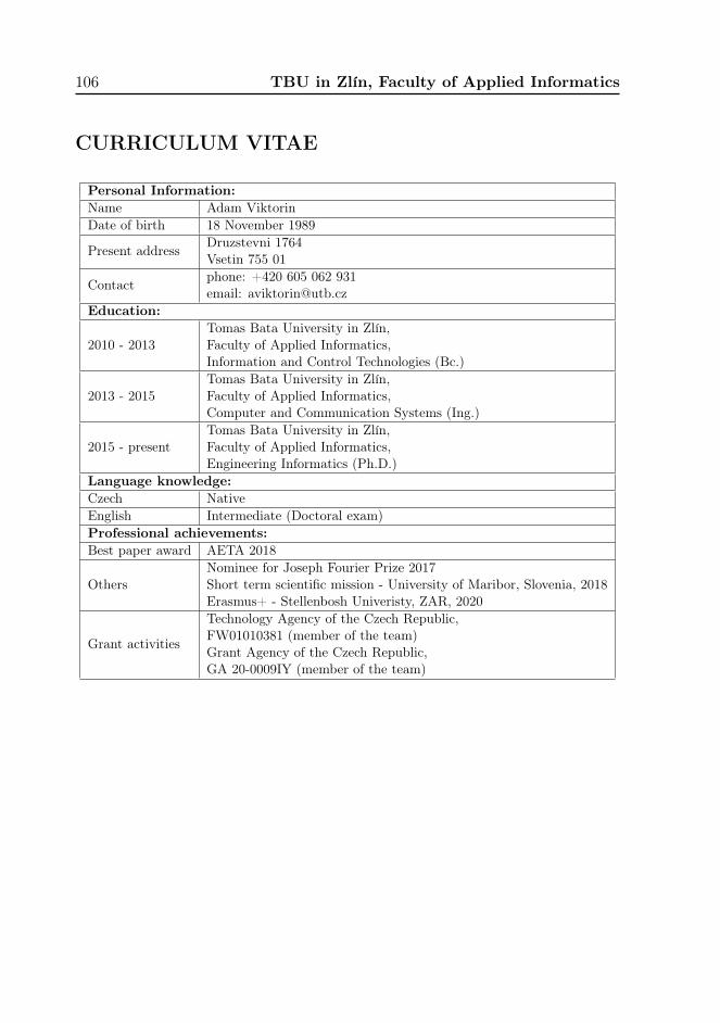
106 TBU in Zlín, Faculty of Applied Informatics
CURRICULUM VITAE
Personal Information:Name Adam ViktorinDate of birth 18 November 1989
Present address Druzstevni 1764Vsetin 755 01
Contact phone: +420 605 062 931email: [email protected]
Education:
2010 - 2013Tomas Bata University in Zlín,Faculty of Applied Informatics,Information and Control Technologies (Bc.)
2013 - 2015Tomas Bata University in Zlín,Faculty of Applied Informatics,Computer and Communication Systems (Ing.)
2015 - presentTomas Bata University in Zlín,Faculty of Applied Informatics,Engineering Informatics (Ph.D.)
Language knowledge:Czech NativeEnglish Intermediate (Doctoral exam)Professional achievements:Best paper award AETA 2018
OthersNominee for Joseph Fourier Prize 2017Short term scientific mission - University of Maribor, Slovenia, 2018Erasmus+ - Stellenbosh Univeristy, ZAR, 2020
Grant activities
Technology Agency of the Czech Republic,FW01010381 (member of the team)Grant Agency of the Czech Republic,GA 20-0009IY (member of the team)

TBU in Zlín, Faculty of Applied Informatics 107
LIST OF APPENDICES
APPENDIX A: DE pseudo–codeAPPENDIX B: SHADE psuedo–codeAPPENDIX C: L–SHADE psuedo–codeAPPENDIX D: DISH psuedo–codeAPPENDIX E: MC–SHADE - Result tablesAPPENDIX F: Distance based parameter adaptation - Result tablesAPPENDIX G: Distance based parameter adaptation - Population analysisAPPENDIX H: DISH - Result tablesAPPENDIX I: DISH - Population analysis

APPENDIX A: DE PSEUDO–CODE
Algorithm 1 DE1: Set NP, CR, F, D and stopping criterion;2: G = 1, xbest = {};3: Randomly initialize (3.1) population P = (x 1,G,. . . ,xNP,G);4: Pnew = {}, x best = best from population P ;5: while stopping criterion not met do6: for i = 1 to NP do7: x i,G = P [i ];8: v i,G by mutation (3.2);9: u i,G by crossover (3.3);10: x i,G+1 by selection (3.4);11: x i,G+1 → Pnew;12: end for13: P = Pnew, Pnew = {}, x best = best from population P ;14: end while15: return x best as the best found solution;
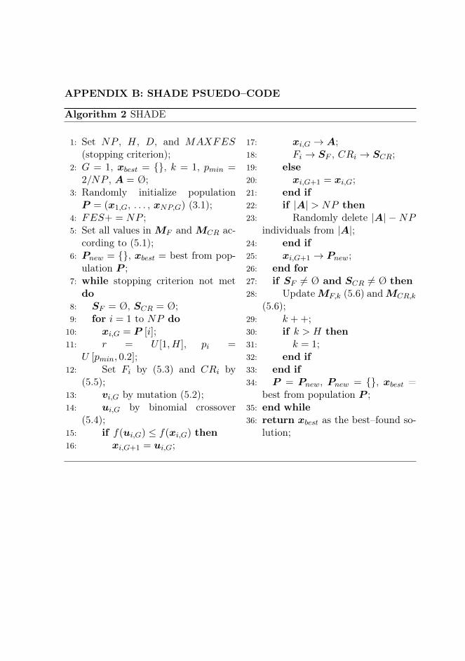
APPENDIX B: SHADE PSUEDO–CODE
Algorithm 2 SHADE
1: Set NP , H, D, and MAXFES(stopping criterion);
2: G = 1, xbest = {}, k = 1, pmin =2/NP , A = Ø;
3: Randomly initialize populationP = (x1,G, . . . , xNP,G) (3.1);
4: FES+ = NP ;5: Set all values in MF and MCR ac-
cording to (5.1);6: Pnew = {}, xbest = best from pop-
ulation P ;7: while stopping criterion not met
do8: SF = Ø, SCR = Ø;9: for i = 1 to NP do10: xi,G = P [i];11: r = U [1, H], pi =
U [pmin, 0.2];12: Set Fi by (5.3) and CRi by
(5.5);13: vi,G by mutation (5.2);14: ui,G by binomial crossover
(5.4);15: if f(ui,G) ≤ f(xi,G) then16: xi,G+1 = ui,G;
17: xi,G → A;18: Fi → SF , CRi → SCR;19: else20: xi,G+1 = xi,G;21: end if22: if |A| > NP then23: Randomly delete |A| − NP
individuals from |A|;24: end if25: xi,G+1 → Pnew;26: end for27: if SF 6= Ø and SCR 6= Ø then28: UpdateMF,k (5.6) andMCR,k
(5.6);29: k ++;30: if k > H then31: k = 1;32: end if33: end if34: P = Pnew, Pnew = {}, xbest =
best from population P ;35: end while36: return xbest as the best–found so-
lution;

APPENDIX C: L–SHADE PSUEDO–CODE
Algorithm 3 L–SHADE
1: Set NP , H, D, and MAXFES(stopping criterion);
2: G = 1, xbest = {}, k = 1, pmin =2/NP , A = Ø;
3: Randomly initialize populationP = (x1,G, . . . , xNP,G) (3.1);
4: FES+ = NP ;5: Set all values in MF and MCR ac-
cording to (5.1);6: Pnew = {}, xbest = best from pop-
ulation P ;7: while stopping criterion not met
do8: SF = Ø, SCR = Ø;9: for i = 1 to NP do10: xi,G = P [i];11: r = U [1, H], pi =
U [pmin, 0.2];12: Set Fi by (5.3) and CRi by
(5.5);13: vi,G by mutation (5.2);14: ui,G by binomial crossover
(5.4);15: if f(ui,G) ≤ f(xi,G) then16: xi,G+1 = ui,G;
17: xi,G → A;18: Fi → SF , CRi → SCR;19: else20: xi,G+1 = xi,G;21: end if22: if |A| > NP then23: Randomly delete |A| − NP
individuals from |A|;24: end if25: xi,G+1 → Pnew;26: end for27: if SF 6= Ø and SCR 6= Ø then28: UpdateMF,k (5.6) andMCR,k
(5.6);29: k ++;30: if k > H then31: k = 1;32: end if33: end if34: P = Pnew, Pnew = {}, xbest =
best from population P ;35: end while36: return xbest as the best–found so-
lution;

APPENDIX D: DISH PSUEDO–CODE
Algorithm 4 DISH1: Set NPinit, NP f , D, and MAXFES (stopping criterion);2: NP = NP init, H = 5, G = 1, xbest = {}, k = 1, pmax = 0.25, pmin = 0.125, A = Ø,
FES = 0;3: Randomly initialize population P = (x1,G, . . . , xNP,G) (6.6);4: FES+ = NP ;5: Set all values in MF to 0.5 and MCR to 0.8;6: Pnew = {}, xbest = best from population P ;7: while stopping criterion not met do8: SF = Ø, SCR = Ø;9: for i = 1 to NP do10: r = U [1, H];11: if r = H then12: MF,r = 0.9;13: MCR,r = 0.9;14: end if15: CRi,G = N(MCR,r, 0.1);16: if CRi,G < 0 then17: CRi,G = 0;18: else if CRi,G > 1 then19: CRi,G = 1;20: end if21: Fi,G = C(MF,r, 0.1);22: while Fi,G ≤ 0 do23: Fi,G = C(MF,r, 0.1);24: end while25: if Fi,G > 1 then26: Fi,G = 1;27: end if28: FESratio = FES/MAXFES;29: if FESratio < 0.6 and Fi,G > 0.7 then30: Fi,G = 0.7;31: end if32: if FESratio < 0.25 then33: CRi,G = max(CRi,G, 0.7);34: else if FESratio < 0.5 then35: CRi,G = max(CRi,G, 0.6);36: end if
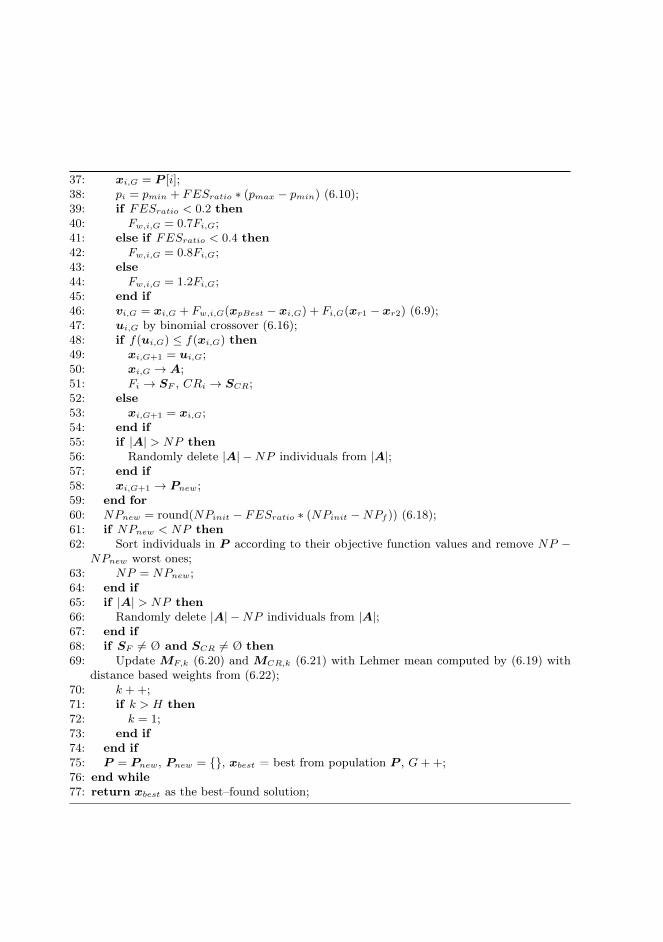
37: xi,G = P [i];38: pi = pmin + FESratio ∗ (pmax − pmin) (6.10);39: if FESratio < 0.2 then40: Fw,i,G = 0.7Fi,G;41: else if FESratio < 0.4 then42: Fw,i,G = 0.8Fi,G;43: else44: Fw,i,G = 1.2Fi,G;45: end if46: vi,G = xi,G + Fw,i,G(xpBest − xi,G) + Fi,G(xr1 − xr2) (6.9);47: ui,G by binomial crossover (6.16);48: if f(ui,G) ≤ f(xi,G) then49: xi,G+1 = ui,G;50: xi,G → A;51: Fi → SF , CRi → SCR;52: else53: xi,G+1 = xi,G;54: end if55: if |A| > NP then56: Randomly delete |A| −NP individuals from |A|;57: end if58: xi,G+1 → Pnew;59: end for60: NPnew = round(NPinit − FESratio ∗ (NPinit −NPf )) (6.18);61: if NPnew < NP then62: Sort individuals in P according to their objective function values and remove NP −
NPnew worst ones;63: NP = NPnew;64: end if65: if |A| > NP then66: Randomly delete |A| −NP individuals from |A|;67: end if68: if SF 6= Ø and SCR 6= Ø then69: Update MF,k (6.20) and MCR,k (6.21) with Lehmer mean computed by (6.19) with
distance based weights from (6.22);70: k ++;71: if k > H then72: k = 1;73: end if74: end if75: P = Pnew, Pnew = {}, xbest = best from population P , G++;76: end while77: return xbest as the best–found solution;

APPENDIX E: MC–SHADE - RESULT TABLES
Tab. E.1 CEC 2016 benchmark set results ofMC–SHADE algorithm in 10D.
Func. Best Worst Median Mean Std1 0.00E+00 0.00E+00 0.00E+00 0.00E+00 0.00E+002 0.00E+00 0.00E+00 0.00E+00 0.00E+00 0.00E+003 0.00E+00 0.00E+00 0.00E+00 0.00E+00 0.00E+004 0.00E+00 3.48E+01 3.48E+01 2.47E+01 1.58E+015 3.74E+00 2.01E+01 2.00E+01 1.54E+01 6.03E+006 0.00E+00 8.95E−01 0.00E+00 3.93E−02 1.77E−017 0.00E+00 3.44E−02 2.35E−03 4.47E−03 5.65E−038 0.00E+00 0.00E+00 0.00E+00 0.00E+00 0.00E+009 1.19E+00 4.90E+00 2.24E+00 2.47E+00 7.93E−0110 0.00E+00 1.87E−01 0.00E+00 2.20E−02 4.11E−0211 1.31E+01 2.72E+02 4.83E+01 6.32E+01 5.18E+0112 9.43E−02 2.66E−01 1.89E−01 1.85E−01 3.75E−0213 5.65E−02 1.12E−01 8.09E−02 8.07E−02 1.36E−0214 5.50E−02 2.18E−01 1.13E−01 1.17E−01 3.91E−0215 2.94E−01 6.97E−01 5.09E−01 4.92E−01 8.61E−0216 8.40E−01 2.21E+00 1.49E+00 1.50E+00 2.47E−0117 0.00E+00 1.21E+02 9.95E−01 9.42E+00 2.85E+0118 7.04E−03 1.36E+00 5.88E−02 1.72E−01 2.42E−0119 9.61E−02 1.04E+00 1.50E−01 2.08E−01 2.08E−0120 7.92E−02 4.41E−01 2.25E−01 2.33E−01 8.23E−0221 4.52E−05 1.13E+00 2.52E−01 2.88E−01 2.84E−0122 7.64E−02 6.83E−01 1.63E−01 1.77E−01 8.84E−0223 3.29E+02 3.29E+02 3.29E+02 3.29E+02 0.00E+0024 1.00E+02 1.11E+02 1.08E+02 1.08E+02 2.12E+0025 1.09E+02 2.01E+02 1.17E+02 1.29E+02 2.85E+0126 1.00E+02 1.00E+02 1.00E+02 1.00E+02 1.73E−0227 1.21E+00 4.00E+02 1.81E+00 6.81E+01 1.37E+0228 3.57E+02 4.95E+02 3.72E+02 4.10E+02 5.30E+0129 1.27E+02 2.25E+02 2.22E+02 2.20E+02 1.33E+0130 4.54E+02 5.97E+02 4.63E+02 4.75E+02 2.44E+01

Tab. E.2 CEC 2016 benchmark set results ofMC–SHADE algorithm in 30D.
Func. Best Worst Median Mean Std1 6.83E−01 1.09E+04 2.09E+03 2.92E+03 2.72E+032 0.00E+00 0.00E+00 0.00E+00 0.00E+00 0.00E+003 0.00E+00 0.00E+00 0.00E+00 0.00E+00 0.00E+004 0.00E+00 3.99E+00 0.00E+00 7.82E−02 5.58E−015 2.01E+01 2.02E+01 2.02E+01 2.02E+01 2.39E−026 0.00E+00 9.15E+00 4.56E−02 1.23E+00 2.37E+007 0.00E+00 1.48E−02 0.00E+00 2.90E−04 2.07E−038 0.00E+00 0.00E+00 0.00E+00 0.00E+00 0.00E+009 1.26E+01 2.65E+01 1.92E+01 1.95E+01 2.95E+0010 0.00E+00 4.16E−02 0.00E+00 1.10E−02 1.46E−0211 1.10E+03 1.94E+03 1.59E+03 1.57E+03 1.91E+0212 1.31E−01 2.73E−01 2.16E−01 2.10E−01 2.98E−0213 1.43E−01 2.74E−01 2.04E−01 2.06E−01 3.00E−0214 1.56E−01 2.85E−01 2.14E−01 2.19E−01 3.59E−0215 1.83E+00 3.71E+00 3.00E+00 3.00E+00 3.91E−0116 7.93E+00 1.03E+01 9.39E+00 9.42E+00 4.43E−0117 4.44E+02 2.15E+03 1.20E+03 1.24E+03 3.93E+0218 2.03E+01 2.25E+02 7.57E+01 7.81E+01 3.68E+0119 2.88E+00 6.96E+00 4.40E+00 4.50E+00 8.29E−0120 2.98E+00 8.12E+01 1.83E+01 1.99E+01 1.27E+0121 1.30E+01 6.90E+02 3.06E+02 3.15E+02 1.58E+0222 2.87E+01 2.97E+02 1.50E+02 1.37E+02 6.64E+0123 3.15E+02 3.15E+02 3.15E+02 3.15E+02 0.00E+0024 2.22E+02 2.36E+02 2.24E+02 2.25E+02 2.02E+0025 2.03E+02 2.09E+02 2.05E+02 2.05E+02 1.80E+0026 1.00E+02 2.00E+02 1.00E+02 1.02E+02 1.40E+0127 3.00E+02 4.38E+02 3.00E+02 3.40E+02 4.76E+0128 6.85E+02 8.63E+02 7.97E+02 8.00E+02 3.02E+0129 5.31E+02 8.22E+02 7.38E+02 7.35E+02 3.86E+0130 5.67E+02 3.47E+03 1.44E+03 1.56E+03 6.43E+02

Tab. E.3 CEC 2016 benchmark set results ofMC–SHADE algorithm in 50D.
Func. Best Worst Median Mean Std1 4.45E+03 7.11E+04 2.03E+04 2.33E+04 1.38E+042 0.00E+00 0.00E+00 0.00E+00 0.00E+00 0.00E+003 0.00E+00 2.26E−02 1.90E−06 1.03E−03 4.05E−034 0.00E+00 9.81E+01 5.00E−04 1.27E+01 2.76E+015 2.02E+01 2.03E+01 2.02E+01 2.02E+01 2.16E−026 7.72E−01 7.92E+00 3.83E+00 3.87E+00 1.84E+007 0.00E+00 1.97E−02 0.00E+00 3.96E−03 5.89E−038 0.00E+00 0.00E+00 0.00E+00 0.00E+00 0.00E+009 3.17E+01 5.75E+01 4.59E+01 4.53E+01 6.96E+0010 0.00E+00 5.00E−02 1.25E−02 1.30E−02 1.34E−0211 2.74E+03 4.28E+03 3.57E+03 3.60E+03 3.89E+0212 1.58E−01 2.64E−01 2.12E−01 2.11E−01 2.24E−0213 2.28E−01 4.89E−01 3.26E−01 3.25E−01 5.30E−0214 2.08E−01 4.68E−01 2.87E−01 2.94E−01 4.28E−0215 5.09E+00 1.07E+01 6.86E+00 6.96E+00 1.01E+0016 1.70E+01 1.84E+01 1.78E+01 1.78E+01 3.57E−0117 1.23E+03 4.51E+03 2.63E+03 2.74E+03 7.89E+0218 7.39E+01 2.69E+02 1.81E+02 1.73E+02 4.41E+0119 6.20E+00 2.91E+01 1.21E+01 1.41E+01 5.57E+0020 1.06E+02 4.46E+02 2.30E+02 2.39E+02 7.43E+0121 8.03E+02 3.29E+03 1.50E+03 1.58E+03 5.66E+0222 1.68E+02 7.00E+02 4.12E+02 4.18E+02 1.33E+0223 3.44E+02 3.44E+02 3.44E+02 3.44E+02 0.00E+0024 2.69E+02 2.79E+02 2.75E+02 2.75E+02 2.29E+0025 2.06E+02 2.26E+02 2.18E+02 2.17E+02 5.59E+0026 1.00E+02 2.00E+02 1.00E+02 1.04E+02 1.95E+0127 3.04E+02 5.56E+02 4.51E+02 4.49E+02 5.02E+0128 1.03E+03 1.28E+03 1.15E+03 1.15E+03 5.71E+0129 7.80E+02 1.11E+03 8.71E+02 8.84E+02 6.52E+0130 8.42E+03 1.18E+04 9.89E+03 9.87E+03 7.70E+02

Tab. E.4 CEC 2016 benchmark set results ofMC–SHADE algorithm in 100D.
Func. Best Worst Median Mean Std1 0.00E+00 0.00E+00 0.00E+00 0.00E+00 0.00E+002 0.00E+00 0.00E+00 0.00E+00 0.00E+00 0.00E+003 0.00E+00 0.00E+00 0.00E+00 0.00E+00 0.00E+004 0.00E+00 3.48E+01 3.48E+01 2.47E+01 1.58E+015 3.74E+00 2.01E+01 2.00E+01 1.54E+01 6.03E+006 0.00E+00 8.95E−01 0.00E+00 3.93E−02 1.77E−017 0.00E+00 3.44E−02 2.35E−03 4.47E−03 5.65E−038 0.00E+00 0.00E+00 0.00E+00 0.00E+00 0.00E+009 1.19E+00 4.90E+00 2.24E+00 2.47E+00 7.93E−0110 0.00E+00 1.87E−01 0.00E+00 2.20E−02 4.11E−0211 1.31E+01 2.72E+02 4.83E+01 6.32E+01 5.18E+0112 9.43E−02 2.66E−01 1.89E−01 1.85E−01 3.75E−0213 5.65E−02 1.12E−01 8.09E−02 8.07E−02 1.36E−0214 5.50E−02 2.18E−01 1.13E−01 1.17E−01 3.91E−0215 2.94E−01 6.97E−01 5.09E−01 4.92E−01 8.61E−0216 8.40E−01 2.21E+00 1.49E+00 1.50E+00 2.47E−0117 0.00E+00 1.21E+02 9.95E−01 9.42E+00 2.85E+0118 7.04E−03 1.36E+00 5.88E−02 1.72E−01 2.42E−0119 9.61E−02 1.04E+00 1.50E−01 2.08E−01 2.08E−0120 7.92E−02 4.41E−01 2.25E−01 2.33E−01 8.23E−0221 4.52E−05 1.13E+00 2.52E−01 2.88E−01 2.84E−0122 7.64E−02 6.83E−01 1.63E−01 1.77E−01 8.84E−0223 3.29E+02 3.29E+02 3.29E+02 3.29E+02 0.00E+0024 1.00E+02 1.11E+02 1.08E+02 1.08E+02 2.12E+0025 1.09E+02 2.01E+02 1.17E+02 1.29E+02 2.85E+0126 1.00E+02 1.00E+02 1.00E+02 1.00E+02 1.73E−0227 1.21E+00 4.00E+02 1.81E+00 6.81E+01 1.37E+0228 3.57E+02 4.95E+02 3.72E+02 4.10E+02 5.30E+0129 1.27E+02 2.25E+02 2.22E+02 2.20E+02 1.33E+0130 4.54E+02 5.97E+02 4.63E+02 4.75E+02 2.44E+01
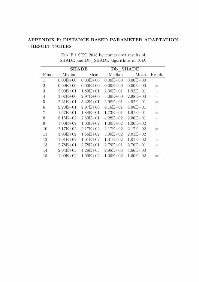
APPENDIX F: DISTANCE BASED PARAMETER ADAPTATION- RESULT TABLES
Tab. F.1 CEC 2015 benchmark set results ofSHADE and Db_SHADE algorithms in 10D.
SHADE Db_SHADEFunc. Median Mean Median Mean Result1 0.00E+00 0.00E+00 0.00E+00 0.00E+00 =2 0.00E+00 0.00E+00 0.00E+00 0.00E+00 =3 2.00E+01 1.89E+01 2.00E+01 1.92E+01 =4 3.07E+00 2.97E+00 3.06E+00 2.98E+00 =5 2.21E+01 3.42E+01 2.98E+01 4.52E+01 =6 2.20E−01 2.97E+00 4.16E−01 8.08E−01 =7 1.67E−01 1.88E−01 1.73E−01 1.91E−01 =8 8.15E−02 2.69E−01 4.28E−02 2.06E−01 =9 1.00E+02 1.00E+02 1.00E+02 1.00E+02 =10 2.17E+02 2.17E+02 2.17E+02 2.17E+02 =11 3.00E+02 1.66E+02 3.00E+02 2.01E+02 =12 1.01E+02 1.01E+02 1.01E+02 1.01E+02 =13 2.78E+01 2.78E+01 2.79E+01 2.76E+01 =14 2.94E+03 4.28E+03 2.98E+03 4.66E+03 =15 1.00E+02 1.00E+02 1.00E+02 1.00E+02 =
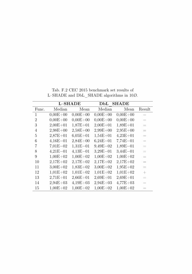
Tab. F.2 CEC 2015 benchmark set results ofL–SHADE and DbL_SHADE algorithms in 10D.
L–SHADE DbL_SHADEFunc. Median Mean Median Mean Result1 0,00E+00 0,00E+00 0,00E+00 0,00E+00 =2 0,00E+00 0,00E+00 0,00E+00 0,00E+00 =3 2,00E+01 1,87E+01 2,00E+01 1,89E+01 =4 2,98E+00 2,58E+00 2,99E+00 2,95E+00 =5 2,87E+01 6,05E+01 1,54E+01 4,23E+01 =6 4,16E−01 2,84E+00 6,24E−01 7,74E−01 −7 7,01E−02 1,31E−01 9,49E−02 1,89E−01 =8 4,21E−01 4,13E−01 3,29E−01 3,44E−01 =9 1,00E+02 1,00E+02 1,00E+02 1,00E+02 =10 2,17E+02 2,17E+02 2,17E+02 2,17E+02 =11 3,00E+02 1,83E+02 3,00E+02 1,95E+02 =12 1,01E+02 1,01E+02 1,01E+02 1,01E+02 +13 2,71E+01 2,66E+01 2,69E+01 2,69E+01 =14 2,94E+03 4,19E+03 2,94E+03 4,77E+03 =15 1,00E+02 1,00E+02 1,00E+02 1,00E+02 =

Tab. F.3 CEC 2015 benchmark set results ofSHADE and Db_SHADE algorithms in 30D.
SHADE Db_SHADEFunc. Median Mean Median Mean Result1 3.73E+01 2.62E+02 2.12E+01 2.42E+02 =2 0.00E+00 0.00E+00 0.00E+00 0.00E+00 =3 2.01E+01 2.01E+01 2.01E+01 2.01E+01 =4 1.41E+01 1.41E+01 1.32E+01 1.31E+01 =5 1.55E+03 1.50E+03 1.54E+03 1.52E+03 =6 5.36E+02 5.73E+02 3.37E+02 3.48E+02 +7 7.17E+00 7.26E+00 6.81E+00 6.74E+00 +8 1.26E+02 1.21E+02 5.27E+01 7.38E+01 +9 1.03E+02 1.03E+02 1.03E+02 1.03E+02 =10 6.27E+02 6.22E+02 5.29E+02 5.32E+02 +11 4.53E+02 4.50E+02 4.10E+02 4.16E+02 +12 1.05E+02 1.05E+02 1.05E+02 1.05E+02 =13 9.52E+01 9.50E+01 9.47E+01 9.50E+01 =14 3.21E+04 3.24E+04 3.22E+04 3.24E+04 =15 1.00E+02 1.00E+02 1.00E+02 1.00E+02 =
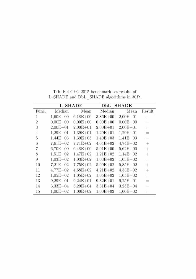
Tab. F.4 CEC 2015 benchmark set results ofL–SHADE and DbL_SHADE algorithms in 30D.
L–SHADE DbL_SHADEFunc. Median Mean Median Mean Result1 1,60E+00 6,18E+00 3,86E+00 2,00E+01 −2 0,00E+00 0,00E+00 0,00E+00 0,00E+00 =3 2,00E+01 2,00E+01 2,00E+01 2,00E+01 =4 1,29E+01 1,39E+01 1,29E+01 1,29E+01 =5 1,44E+03 1,39E+03 1,40E+03 1,41E+03 =6 7,61E+02 7,71E+02 4,64E+02 4,74E+02 +7 6,70E+00 6,48E+00 5,91E+00 5,62E+00 +8 1,51E+02 1,47E+02 1,21E+02 1,14E+02 +9 1,03E+02 1,03E+02 1,03E+02 1,03E+02 =10 7,21E+02 7,75E+02 5,99E+02 5,85E+02 +11 4,77E+02 4,68E+02 4,21E+02 4,33E+02 +12 1,05E+02 1,05E+02 1,05E+02 1,05E+02 =13 9,29E+01 9,24E+01 9,32E+01 9,25E+01 =14 3,33E+04 3,29E+04 3,31E+04 3,25E+04 =15 1,00E+02 1,00E+02 1,00E+02 1,00E+02 =
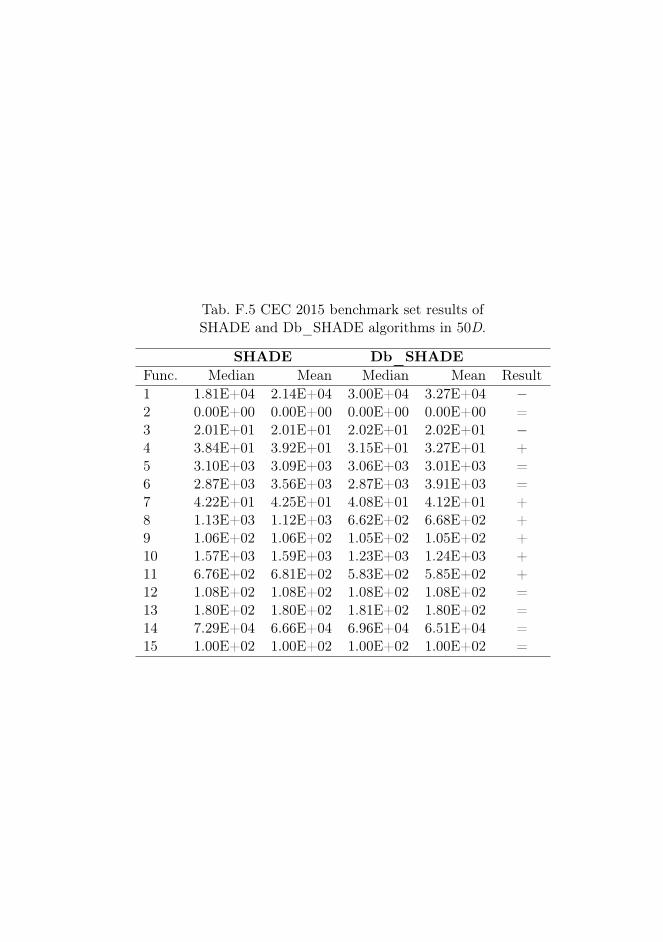
Tab. F.5 CEC 2015 benchmark set results ofSHADE and Db_SHADE algorithms in 50D.
SHADE Db_SHADEFunc. Median Mean Median Mean Result1 1.81E+04 2.14E+04 3.00E+04 3.27E+04 −2 0.00E+00 0.00E+00 0.00E+00 0.00E+00 =3 2.01E+01 2.01E+01 2.02E+01 2.02E+01 −4 3.84E+01 3.92E+01 3.15E+01 3.27E+01 +5 3.10E+03 3.09E+03 3.06E+03 3.01E+03 =6 2.87E+03 3.56E+03 2.87E+03 3.91E+03 =7 4.22E+01 4.25E+01 4.08E+01 4.12E+01 +8 1.13E+03 1.12E+03 6.62E+02 6.68E+02 +9 1.06E+02 1.06E+02 1.05E+02 1.05E+02 +10 1.57E+03 1.59E+03 1.23E+03 1.24E+03 +11 6.76E+02 6.81E+02 5.83E+02 5.85E+02 +12 1.08E+02 1.08E+02 1.08E+02 1.08E+02 =13 1.80E+02 1.80E+02 1.81E+02 1.80E+02 =14 7.29E+04 6.66E+04 6.96E+04 6.51E+04 =15 1.00E+02 1.00E+02 1.00E+02 1.00E+02 =
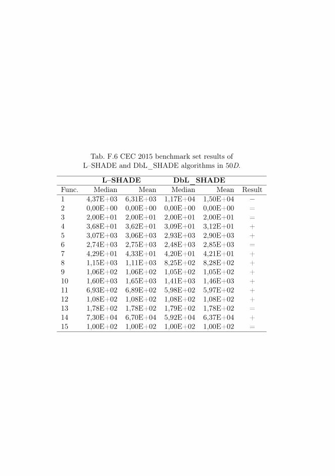
Tab. F.6 CEC 2015 benchmark set results ofL–SHADE and DbL_SHADE algorithms in 50D.
L–SHADE DbL_SHADEFunc. Median Mean Median Mean Result1 4,37E+03 6,31E+03 1,17E+04 1,50E+04 −2 0,00E+00 0,00E+00 0,00E+00 0,00E+00 =3 2,00E+01 2,00E+01 2,00E+01 2,00E+01 =4 3,68E+01 3,62E+01 3,09E+01 3,12E+01 +5 3,07E+03 3,06E+03 2,93E+03 2,90E+03 +6 2,74E+03 2,75E+03 2,48E+03 2,85E+03 =7 4,29E+01 4,33E+01 4,20E+01 4,21E+01 +8 1,15E+03 1,11E+03 8,25E+02 8,28E+02 +9 1,06E+02 1,06E+02 1,05E+02 1,05E+02 +10 1,60E+03 1,65E+03 1,41E+03 1,46E+03 +11 6,93E+02 6,89E+02 5,98E+02 5,97E+02 +12 1,08E+02 1,08E+02 1,08E+02 1,08E+02 +13 1,78E+02 1,78E+02 1,79E+02 1,78E+02 =14 7,30E+04 6,70E+04 5,92E+04 6,37E+04 +15 1,00E+02 1,00E+02 1,00E+02 1,00E+02 =
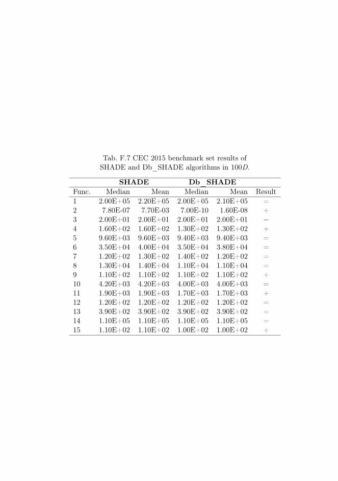
Tab. F.7 CEC 2015 benchmark set results ofSHADE and Db_SHADE algorithms in 100D.
SHADE Db_SHADEFunc. Median Mean Median Mean Result1 2.00E+05 2.20E+05 2.00E+05 2.10E+05 =2 7.80E-07 7.70E-03 7.00E-10 1.60E-08 +3 2.00E+01 2.00E+01 2.00E+01 2.00E+01 −4 1.60E+02 1.60E+02 1.30E+02 1.30E+02 +5 9.60E+03 9.60E+03 9.40E+03 9.40E+03 =6 3.50E+04 4.00E+04 3.50E+04 3.80E+04 =7 1.20E+02 1.30E+02 1.40E+02 1.20E+02 =8 1.30E+04 1.40E+04 1.10E+04 1.10E+04 =9 1.10E+02 1.10E+02 1.10E+02 1.10E+02 +10 4.20E+03 4.20E+03 4.00E+03 4.00E+03 =11 1.90E+03 1.90E+03 1.70E+03 1.70E+03 +12 1.20E+02 1.20E+02 1.20E+02 1.20E+02 =13 3.90E+02 3.90E+02 3.90E+02 3.90E+02 =14 1.10E+05 1.10E+05 1.10E+05 1.10E+05 =15 1.10E+02 1.10E+02 1.00E+02 1.00E+02 +
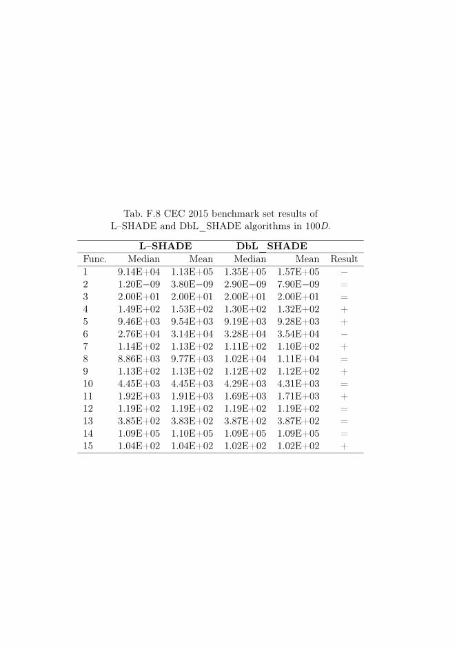
Tab. F.8 CEC 2015 benchmark set results ofL–SHADE and DbL_SHADE algorithms in 100D.
L–SHADE DbL_SHADEFunc. Median Mean Median Mean Result1 9.14E+04 1.13E+05 1.35E+05 1.57E+05 −2 1.20E−09 3.80E−09 2.90E−09 7.90E−09 =3 2.00E+01 2.00E+01 2.00E+01 2.00E+01 =4 1.49E+02 1.53E+02 1.30E+02 1.32E+02 +5 9.46E+03 9.54E+03 9.19E+03 9.28E+03 +6 2.76E+04 3.14E+04 3.28E+04 3.54E+04 −7 1.14E+02 1.13E+02 1.11E+02 1.10E+02 +8 8.86E+03 9.77E+03 1.02E+04 1.11E+04 =9 1.13E+02 1.13E+02 1.12E+02 1.12E+02 +10 4.45E+03 4.45E+03 4.29E+03 4.31E+03 =11 1.92E+03 1.91E+03 1.69E+03 1.71E+03 +12 1.19E+02 1.19E+02 1.19E+02 1.19E+02 =13 3.85E+02 3.83E+02 3.87E+02 3.87E+02 =14 1.09E+05 1.10E+05 1.09E+05 1.09E+05 =15 1.04E+02 1.04E+02 1.02E+02 1.02E+02 +
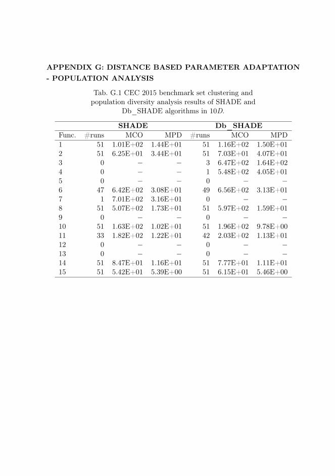
APPENDIX G: DISTANCE BASED PARAMETER ADAPTATION- POPULATION ANALYSIS
Tab. G.1 CEC 2015 benchmark set clustering andpopulation diversity analysis results of SHADE and
Db_SHADE algorithms in 10D.
SHADE Db_SHADEFunc. #runs MCO MPD #runs MCO MPD1 51 1.01E+02 1.44E+01 51 1.16E+02 1.50E+012 51 6.25E+01 3.44E+01 51 7.03E+01 4.07E+013 0 − − 3 6.47E+02 1.64E+024 0 − − 1 5.48E+02 4.05E+015 0 − − 0 − −6 47 6.42E+02 3.08E+01 49 6.56E+02 3.13E+017 1 7.01E+02 3.16E+01 0 − −8 51 5.07E+02 1.73E+01 51 5.97E+02 1.59E+019 0 − − 0 − −10 51 1.63E+02 1.02E+01 51 1.96E+02 9.78E+0011 33 1.82E+02 1.22E+01 42 2.03E+02 1.13E+0112 0 − − 0 − −13 0 − − 0 − −14 51 8.47E+01 1.16E+01 51 7.77E+01 1.11E+0115 51 5.42E+01 5.39E+00 51 6.15E+01 5.46E+00
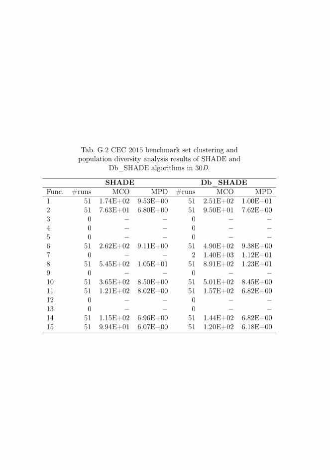
Tab. G.2 CEC 2015 benchmark set clustering andpopulation diversity analysis results of SHADE and
Db_SHADE algorithms in 30D.
SHADE Db_SHADEFunc. #runs MCO MPD #runs MCO MPD1 51 1.74E+02 9.53E+00 51 2.51E+02 1.00E+012 51 7.63E+01 6.80E+00 51 9.50E+01 7.62E+003 0 − − 0 − −4 0 − − 0 − −5 0 − − 0 − −6 51 2.62E+02 9.11E+00 51 4.90E+02 9.38E+007 0 − − 2 1.40E+03 1.12E+018 51 5.45E+02 1.05E+01 51 8.91E+02 1.23E+019 0 − − 0 − −10 51 3.65E+02 8.50E+00 51 5.01E+02 8.45E+0011 51 1.21E+02 8.02E+00 51 1.57E+02 6.82E+0012 0 − − 0 − −13 0 − − 0 − −14 51 1.15E+02 6.96E+00 51 1.44E+02 6.82E+0015 51 9.94E+01 6.07E+00 51 1.20E+02 6.18E+00

Tab. G.3 CEC 2015 benchmark set clustering andpopulation diversity analysis results of SHADE and
Db_SHADE algorithms in 50D.
SHADE Db_SHADEFunc. #runs MCO MPD #runs MCO MPD1 51 2.17E+02 9.70E+00 51 3.05E+02 9.57E+002 51 9.07E+01 7.01E+00 51 1.09E+02 6.94E+003 0 − − 0 − −4 0 − − 0 − −5 0 − − 0 − −6 51 4.72E+02 8.28E+00 51 7.72E+02 8.19E+007 30 4.45E+02 8.95E+00 13 7.71E+02 9.58E+008 50 1.22E+03 1.15E+01 49 1.37E+03 1.14E+019 3 8.21E+02 7.93E+00 0 − −10 51 4.71E+02 7.89E+00 51 5.73E+02 7.89E+0011 51 1.27E+02 7.62E+00 51 1.63E+02 7.62E+0012 0 − − 0 − −13 0 − − 0 − −14 51 1.58E+02 7.30E+00 51 1.98E+02 7.21E+0015 51 1.59E+02 7.25E+00 51 1.72E+02 7.24E+00
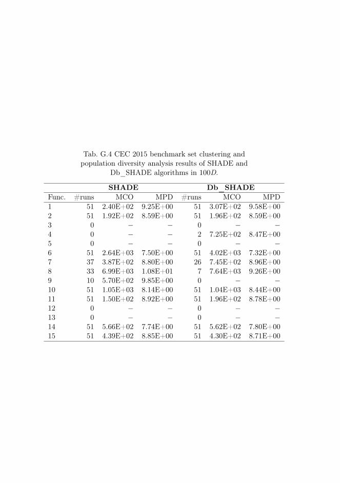
Tab. G.4 CEC 2015 benchmark set clustering andpopulation diversity analysis results of SHADE and
Db_SHADE algorithms in 100D.
SHADE Db_SHADEFunc. #runs MCO MPD #runs MCO MPD1 51 2.40E+02 9.25E+00 51 3.07E+02 9.58E+002 51 1.92E+02 8.59E+00 51 1.96E+02 8.59E+003 0 − − 0 − −4 0 − − 2 7.25E+02 8.47E+005 0 − − 0 − −6 51 2.64E+03 7.50E+00 51 4.02E+03 7.32E+007 37 3.87E+02 8.80E+00 26 7.45E+02 8.96E+008 33 6.99E+03 1.08E+01 7 7.64E+03 9.26E+009 10 5.70E+02 9.85E+00 0 − −10 51 1.05E+03 8.14E+00 51 1.04E+03 8.44E+0011 51 1.50E+02 8.92E+00 51 1.96E+02 8.78E+0012 0 − − 0 − −13 0 − − 0 − −14 51 5.66E+02 7.74E+00 51 5.62E+02 7.80E+0015 51 4.39E+02 8.85E+00 51 4.30E+02 8.71E+00
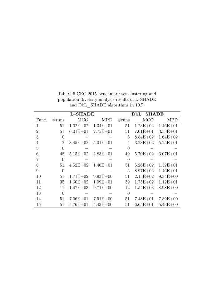
Tab. G.5 CEC 2015 benchmark set clustering andpopulation diversity analysis results of L–SHADE
and DbL_SHADE algorithms in 10D.
L–SHADE DbL_SHADEFunc. #runs MCO MPD #runs MCO MPD1 51 1.02E+02 1.34E+01 51 1.23E+02 1.46E+012 51 6.01E+01 2.75E+01 51 7.01E+01 3.53E+013 0 − − 5 8.84E+02 1.64E+024 2 3.45E+02 5.01E+01 4 3.23E+02 5.25E+015 0 − − 0 − −6 48 5.15E+02 2.83E+01 49 5.70E+02 3.07E+017 0 − − 0 − −8 51 4.52E+02 1.46E+01 51 5.26E+02 1.32E+019 0 − − 2 8.97E+02 1.46E+0110 51 1.71E+02 9.93E+00 51 2.15E+02 9.34E+0011 35 1.60E+02 1.09E+01 39 1.75E+02 1.12E+0112 11 1.47E+03 9.71E+00 12 1.54E+03 8.98E+0013 0 − − 0 − −14 51 7.06E+01 7.51E+00 51 7.48E+01 7.89E+0015 51 5.76E+01 5.43E+00 51 6.65E+01 5.43E+00
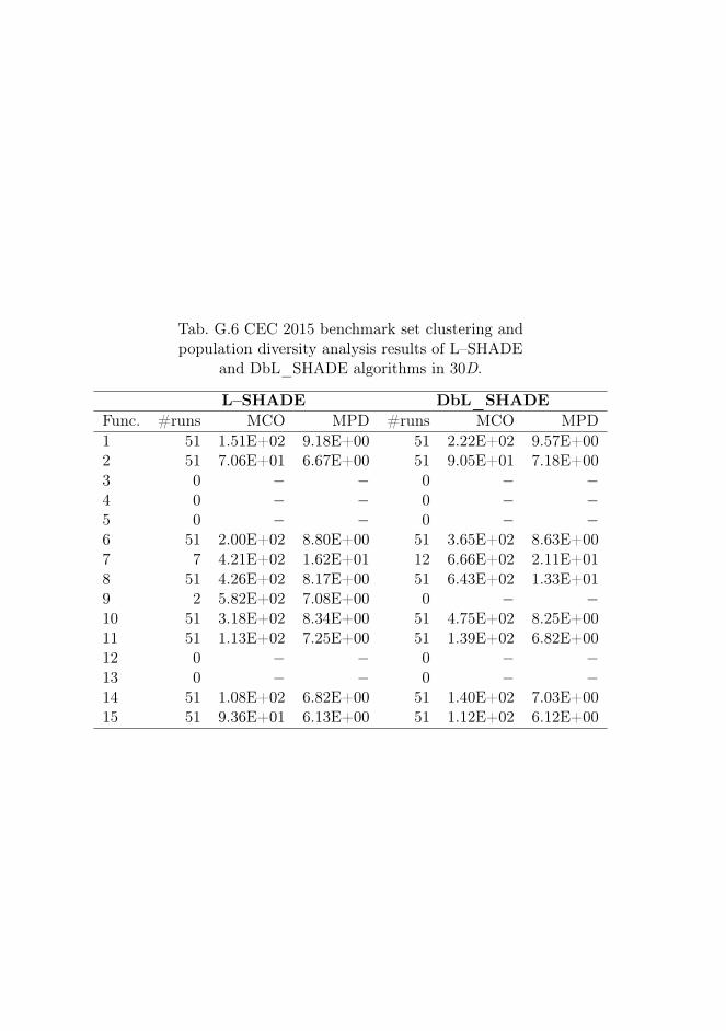
Tab. G.6 CEC 2015 benchmark set clustering andpopulation diversity analysis results of L–SHADE
and DbL_SHADE algorithms in 30D.
L–SHADE DbL_SHADEFunc. #runs MCO MPD #runs MCO MPD1 51 1.51E+02 9.18E+00 51 2.22E+02 9.57E+002 51 7.06E+01 6.67E+00 51 9.05E+01 7.18E+003 0 − − 0 − −4 0 − − 0 − −5 0 − − 0 − −6 51 2.00E+02 8.80E+00 51 3.65E+02 8.63E+007 7 4.21E+02 1.62E+01 12 6.66E+02 2.11E+018 51 4.26E+02 8.17E+00 51 6.43E+02 1.33E+019 2 5.82E+02 7.08E+00 0 − −10 51 3.18E+02 8.34E+00 51 4.75E+02 8.25E+0011 51 1.13E+02 7.25E+00 51 1.39E+02 6.82E+0012 0 − − 0 − −13 0 − − 0 − −14 51 1.08E+02 6.82E+00 51 1.40E+02 7.03E+0015 51 9.36E+01 6.13E+00 51 1.12E+02 6.12E+00
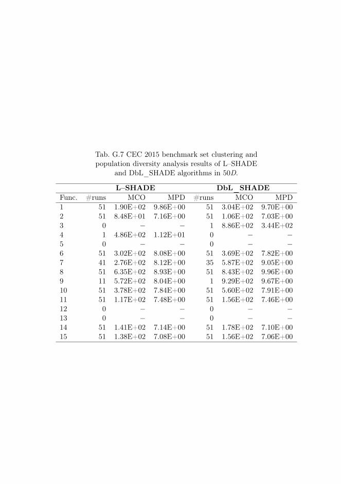
Tab. G.7 CEC 2015 benchmark set clustering andpopulation diversity analysis results of L–SHADE
and DbL_SHADE algorithms in 50D.
L–SHADE DbL_SHADEFunc. #runs MCO MPD #runs MCO MPD1 51 1.90E+02 9.86E+00 51 3.04E+02 9.70E+002 51 8.48E+01 7.16E+00 51 1.06E+02 7.03E+003 0 − − 1 8.86E+02 3.44E+024 1 4.86E+02 1.12E+01 0 − −5 0 − − 0 − −6 51 3.02E+02 8.08E+00 51 3.69E+02 7.82E+007 41 2.76E+02 8.12E+00 35 5.87E+02 9.05E+008 51 6.35E+02 8.93E+00 51 8.43E+02 9.96E+009 11 5.72E+02 8.04E+00 1 9.29E+02 9.67E+0010 51 3.78E+02 7.84E+00 51 5.60E+02 7.91E+0011 51 1.17E+02 7.48E+00 51 1.56E+02 7.46E+0012 0 − − 0 − −13 0 − − 0 − −14 51 1.41E+02 7.14E+00 51 1.78E+02 7.10E+0015 51 1.38E+02 7.08E+00 51 1.56E+02 7.06E+00

Tab. G.8 CEC 2015 benchmark set clustering andpopulation diversity analysis results of L–SHADE
and DbL_SHADE algorithms in 100D.
L–SHADE DbL_SHADEFunc. #runs MCO MPD #runs MCO MPD1 51 1.90E+02 9.47E+00 51 2.79E+02 1.01E+012 51 1.56E+02 8.50E+00 51 1.75E+02 8.57E+003 1 1.48E+03 5.03E+02 1 1.34E+03 5.06E+024 0 − − 1 4.44E+02 8.32E+005 0 − − 0 − −6 51 2.02E+03 8.10E+00 51 3.50E+03 7.28E+007 47 2.62E+02 8.28E+00 45 5.35E+02 8.59E+008 51 4.95E+03 8.18E+00 51 7.19E+03 8.56E+009 7 7.65E+02 9.48E+00 5 7.57E+02 9.81E+0010 51 6.13E+02 7.71E+00 51 8.20E+02 8.10E+0011 51 1.34E+02 8.89E+00 51 1.85E+02 8.72E+0012 0 − − 0 − −13 0 − − 0 − −14 51 3.88E+02 7.53E+00 51 4.34E+02 7.48E+0015 51 3.20E+02 8.60E+00 51 3.39E+02 8.78E+00
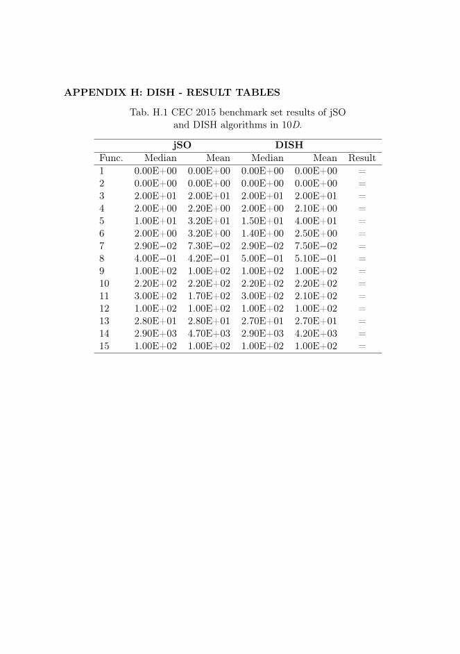
APPENDIX H: DISH - RESULT TABLES
Tab. H.1 CEC 2015 benchmark set results of jSOand DISH algorithms in 10D.
jSO DISHFunc. Median Mean Median Mean Result1 0.00E+00 0.00E+00 0.00E+00 0.00E+00 =2 0.00E+00 0.00E+00 0.00E+00 0.00E+00 =3 2.00E+01 2.00E+01 2.00E+01 2.00E+01 =4 2.00E+00 2.20E+00 2.00E+00 2.10E+00 =5 1.00E+01 3.20E+01 1.50E+01 4.00E+01 =6 2.00E+00 3.20E+00 1.40E+00 2.50E+00 =7 2.90E−02 7.30E−02 2.90E−02 7.50E−02 =8 4.00E−01 4.20E−01 5.00E−01 5.10E−01 =9 1.00E+02 1.00E+02 1.00E+02 1.00E+02 =10 2.20E+02 2.20E+02 2.20E+02 2.20E+02 =11 3.00E+02 1.70E+02 3.00E+02 2.10E+02 =12 1.00E+02 1.00E+02 1.00E+02 1.00E+02 =13 2.80E+01 2.80E+01 2.70E+01 2.70E+01 =14 2.90E+03 4.70E+03 2.90E+03 4.20E+03 =15 1.00E+02 1.00E+02 1.00E+02 1.00E+02 =

Tab. H.2 CEC 2015 benchmark set results of jSOand DISH algorithms in 30D.
jSO DISHFunc. Median Mean Median Mean Result1 8.80E−02 4.30E−01 7.20E−02 6.70E−01 =2 0.00E+00 0.00E+00 0.00E+00 0.00E+00 =3 2.10E+01 2.10E+01 2.10E+01 2.10E+01 =4 1.40E+01 1.40E+01 1.40E+01 1.40E+01 =5 1.50E+03 1.50E+03 1.60E+03 1.50E+03 =6 2.30E+02 2.90E+02 1.80E+02 2.10E+02 +7 2.80E+00 2.90E+00 2.60E+00 2.80E+00 =8 5.10E+01 6.20E+01 3.60E+01 6.30E+01 =9 1.00E+02 1.00E+02 1.00E+02 1.00E+02 +10 5.00E+02 5.00E+02 4.70E+02 4.70E+02 =11 4.40E+02 4.40E+02 4.00E+02 4.20E+02 +12 1.10E+02 1.10E+02 1.10E+02 1.00E+02 =13 9.40E+01 9.40E+01 9.50E+01 9.50E+01 =14 3.10E+04 3.20E+04 3.10E+04 3.20E+04 =15 1.00E+02 1.00E+02 1.00E+02 1.00E+02 =
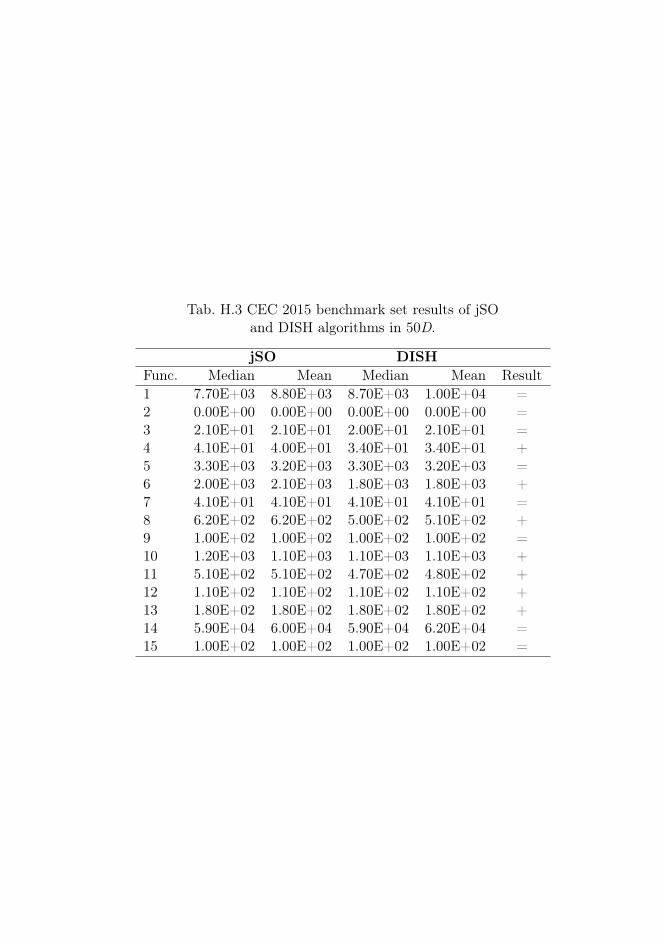
Tab. H.3 CEC 2015 benchmark set results of jSOand DISH algorithms in 50D.
jSO DISHFunc. Median Mean Median Mean Result1 7.70E+03 8.80E+03 8.70E+03 1.00E+04 =2 0.00E+00 0.00E+00 0.00E+00 0.00E+00 =3 2.10E+01 2.10E+01 2.00E+01 2.10E+01 =4 4.10E+01 4.00E+01 3.40E+01 3.40E+01 +5 3.30E+03 3.20E+03 3.30E+03 3.20E+03 =6 2.00E+03 2.10E+03 1.80E+03 1.80E+03 +7 4.10E+01 4.10E+01 4.10E+01 4.10E+01 =8 6.20E+02 6.20E+02 5.00E+02 5.10E+02 +9 1.00E+02 1.00E+02 1.00E+02 1.00E+02 =10 1.20E+03 1.10E+03 1.10E+03 1.10E+03 +11 5.10E+02 5.10E+02 4.70E+02 4.80E+02 +12 1.10E+02 1.10E+02 1.10E+02 1.10E+02 +13 1.80E+02 1.80E+02 1.80E+02 1.80E+02 +14 5.90E+04 6.00E+04 5.90E+04 6.20E+04 =15 1.00E+02 1.00E+02 1.00E+02 1.00E+02 =
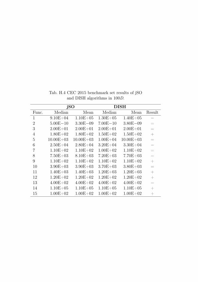
Tab. H.4 CEC 2015 benchmark set results of jSOand DISH algorithms in 100D.
jSO DISHFunc. Median Mean Median Mean Result1 9.10E+04 1.10E+05 1.30E+05 1.40E+05 −2 5.00E−10 3.30E−09 7.00E−10 3.80E−09 =3 2.00E+01 2.00E+01 2.00E+01 2.00E+01 =4 1.80E+02 1.80E+02 1.50E+02 1.50E+02 +5 10.00E+03 10.00E+03 1.00E+04 10.00E+03 =6 2.50E+04 2.80E+04 3.20E+04 3.30E+04 −7 1.10E+02 1.10E+02 1.00E+02 1.10E+02 =8 7.50E+03 8.10E+03 7.20E+03 7.70E+03 =9 1.10E+02 1.10E+02 1.10E+02 1.10E+02 +10 3.90E+03 3.90E+03 3.70E+03 3.80E+03 =11 1.40E+03 1.40E+03 1.20E+03 1.20E+03 +12 1.20E+02 1.20E+02 1.20E+02 1.20E+02 +13 4.00E+02 4.00E+02 4.00E+02 4.00E+02 =14 1.10E+05 1.10E+05 1.10E+05 1.10E+05 +15 1.00E+02 1.00E+02 1.00E+02 1.00E+02 +

Tab. H.5 CEC 2017 benchmark set results of jSOand DISH algorithms in 10D.
jSO DISHFunc. Median Mean Median Mean Result1 0.00E+00 0.00E+00 0.00E+00 0.00E+00 =2 0.00E+00 0.00E+00 0.00E+00 0.00E+00 =3 0.00E+00 0.00E+00 0.00E+00 0.00E+00 =4 0.00E+00 0.00E+00 0.00E+00 0.00E+00 =5 2.00E+00 1.80E+00 2.00E+00 1.80E+00 =6 0.00E+00 0.00E+00 0.00E+00 0.00E+00 =7 1.20E+01 1.20E+01 1.20E+01 1.20E+01 =8 2.00E+00 2.00E+00 2.00E+00 2.00E+00 =9 0.00E+00 0.00E+00 0.00E+00 0.00E+00 =10 1.00E+01 3.60E+01 7.00E+00 4.40E+01 =11 0.00E+00 0.00E+00 0.00E+00 0.00E+00 =12 4.20E-01 2.70E+00 4.20E-01 3.30E-01 =13 4.80E+00 3.00E+00 1.00E+00 2.10E+00 =14 0.00E+00 5.90E-02 0.00E+00 1.20E-01 =15 1.80E-01 2.20E-01 4.50E-01 3.10E-01 -16 5.20E-01 5.70E-01 6.30E-01 5.60E-01 =17 4.00E-01 5.00E-01 3.90E-01 4.40E−01 =18 3.80E−01 3.10E−01 2.70E−01 2.70E−01 =19 0.00E+00 1.10E−02 0.00E+00 9.20E−03 =20 3.10E−01 3.40E−01 3.10E−01 3.40E−01 =21 1.00E+02 1.30E+02 1.00E+02 1.40E+02 =22 1.00E+02 1.00E+02 1.00E+02 1.00E+02 =23 3.00E+02 3.00E+02 3.00E+02 3.00E+02 =24 3.30E+02 3.00E+02 3.30E+02 2.90E+02 =25 4.00E+02 4.10E+02 4.00E+02 4.10E+02 =26 3.00E+02 3.00E+02 3.00E+02 3.00E+02 =27 3.90E+02 3.90E+02 3.90E+02 3.90E+02 =28 3.00E+02 3.40E+02 3.00E+02 3.70E+02 =29 2.30E+02 2.30E+02 2.40E+02 2.40E+02 =30 4.00E+02 4.00E+02 4.00E+02 4.00E+02 =
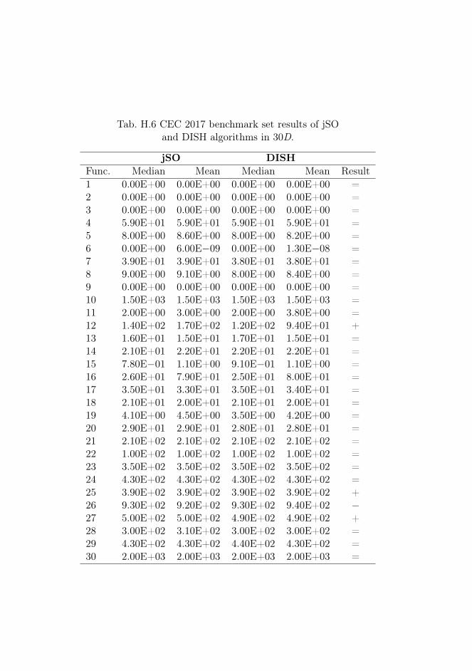
Tab. H.6 CEC 2017 benchmark set results of jSOand DISH algorithms in 30D.
jSO DISHFunc. Median Mean Median Mean Result1 0.00E+00 0.00E+00 0.00E+00 0.00E+00 =2 0.00E+00 0.00E+00 0.00E+00 0.00E+00 =3 0.00E+00 0.00E+00 0.00E+00 0.00E+00 =4 5.90E+01 5.90E+01 5.90E+01 5.90E+01 =5 8.00E+00 8.60E+00 8.00E+00 8.20E+00 =6 0.00E+00 6.00E−09 0.00E+00 1.30E−08 =7 3.90E+01 3.90E+01 3.80E+01 3.80E+01 =8 9.00E+00 9.10E+00 8.00E+00 8.40E+00 =9 0.00E+00 0.00E+00 0.00E+00 0.00E+00 =10 1.50E+03 1.50E+03 1.50E+03 1.50E+03 =11 2.00E+00 3.00E+00 2.00E+00 3.80E+00 =12 1.40E+02 1.70E+02 1.20E+02 9.40E+01 +13 1.60E+01 1.50E+01 1.70E+01 1.50E+01 =14 2.10E+01 2.20E+01 2.20E+01 2.20E+01 =15 7.80E−01 1.10E+00 9.10E−01 1.10E+00 =16 2.60E+01 7.90E+01 2.50E+01 8.00E+01 =17 3.50E+01 3.30E+01 3.50E+01 3.40E+01 =18 2.10E+01 2.00E+01 2.10E+01 2.00E+01 =19 4.10E+00 4.50E+00 3.50E+00 4.20E+00 =20 2.90E+01 2.90E+01 2.80E+01 2.80E+01 =21 2.10E+02 2.10E+02 2.10E+02 2.10E+02 =22 1.00E+02 1.00E+02 1.00E+02 1.00E+02 =23 3.50E+02 3.50E+02 3.50E+02 3.50E+02 =24 4.30E+02 4.30E+02 4.30E+02 4.30E+02 =25 3.90E+02 3.90E+02 3.90E+02 3.90E+02 +26 9.30E+02 9.20E+02 9.30E+02 9.40E+02 −27 5.00E+02 5.00E+02 4.90E+02 4.90E+02 +28 3.00E+02 3.10E+02 3.00E+02 3.00E+02 =29 4.30E+02 4.30E+02 4.40E+02 4.30E+02 =30 2.00E+03 2.00E+03 2.00E+03 2.00E+03 =
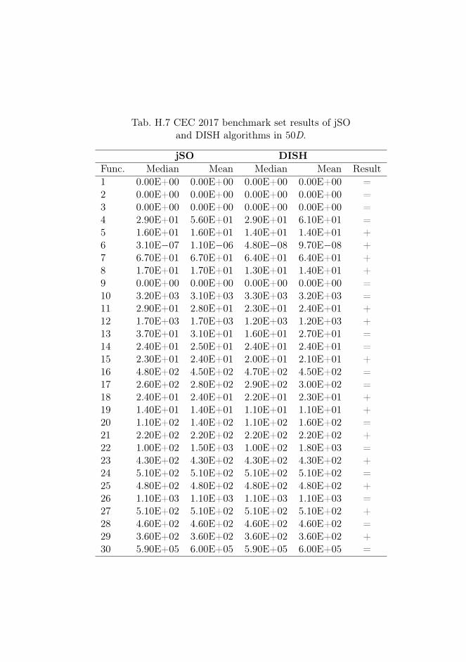
Tab. H.7 CEC 2017 benchmark set results of jSOand DISH algorithms in 50D.
jSO DISHFunc. Median Mean Median Mean Result1 0.00E+00 0.00E+00 0.00E+00 0.00E+00 =2 0.00E+00 0.00E+00 0.00E+00 0.00E+00 =3 0.00E+00 0.00E+00 0.00E+00 0.00E+00 =4 2.90E+01 5.60E+01 2.90E+01 6.10E+01 =5 1.60E+01 1.60E+01 1.40E+01 1.40E+01 +6 3.10E−07 1.10E−06 4.80E−08 9.70E−08 +7 6.70E+01 6.70E+01 6.40E+01 6.40E+01 +8 1.70E+01 1.70E+01 1.30E+01 1.40E+01 +9 0.00E+00 0.00E+00 0.00E+00 0.00E+00 =10 3.20E+03 3.10E+03 3.30E+03 3.20E+03 =11 2.90E+01 2.80E+01 2.30E+01 2.40E+01 +12 1.70E+03 1.70E+03 1.20E+03 1.20E+03 +13 3.70E+01 3.10E+01 1.60E+01 2.70E+01 =14 2.40E+01 2.50E+01 2.40E+01 2.40E+01 =15 2.30E+01 2.40E+01 2.00E+01 2.10E+01 +16 4.80E+02 4.50E+02 4.70E+02 4.50E+02 =17 2.60E+02 2.80E+02 2.90E+02 3.00E+02 =18 2.40E+01 2.40E+01 2.20E+01 2.30E+01 +19 1.40E+01 1.40E+01 1.10E+01 1.10E+01 +20 1.10E+02 1.40E+02 1.10E+02 1.60E+02 =21 2.20E+02 2.20E+02 2.20E+02 2.20E+02 +22 1.00E+02 1.50E+03 1.00E+02 1.80E+03 =23 4.30E+02 4.30E+02 4.30E+02 4.30E+02 +24 5.10E+02 5.10E+02 5.10E+02 5.10E+02 =25 4.80E+02 4.80E+02 4.80E+02 4.80E+02 +26 1.10E+03 1.10E+03 1.10E+03 1.10E+03 =27 5.10E+02 5.10E+02 5.10E+02 5.10E+02 +28 4.60E+02 4.60E+02 4.60E+02 4.60E+02 =29 3.60E+02 3.60E+02 3.60E+02 3.60E+02 +30 5.90E+05 6.00E+05 5.90E+05 6.00E+05 =
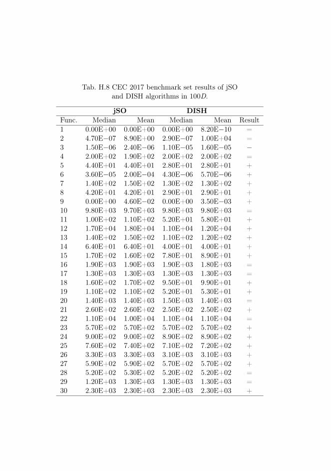
Tab. H.8 CEC 2017 benchmark set results of jSOand DISH algorithms in 100D.
jSO DISHFunc. Median Mean Median Mean Result1 0.00E+00 0.00E+00 0.00E+00 8.20E−10 =2 4.70E−07 8.90E+00 2.90E−07 1.00E+04 =3 1.50E−06 2.40E−06 1.10E−05 1.60E−05 −4 2.00E+02 1.90E+02 2.00E+02 2.00E+02 =5 4.40E+01 4.40E+01 2.80E+01 2.80E+01 +6 3.60E−05 2.00E−04 4.30E−06 5.70E−06 +7 1.40E+02 1.50E+02 1.30E+02 1.30E+02 +8 4.20E+01 4.20E+01 2.90E+01 2.90E+01 +9 0.00E+00 4.60E−02 0.00E+00 3.50E−03 +10 9.80E+03 9.70E+03 9.80E+03 9.80E+03 =11 1.00E+02 1.10E+02 5.20E+01 5.80E+01 +12 1.70E+04 1.80E+04 1.10E+04 1.20E+04 +13 1.40E+02 1.50E+02 1.10E+02 1.20E+02 +14 6.40E+01 6.40E+01 4.00E+01 4.00E+01 +15 1.70E+02 1.60E+02 7.80E+01 8.90E+01 +16 1.90E+03 1.90E+03 1.90E+03 1.80E+03 =17 1.30E+03 1.30E+03 1.30E+03 1.30E+03 =18 1.60E+02 1.70E+02 9.50E+01 9.90E+01 +19 1.10E+02 1.10E+02 5.20E+01 5.30E+01 +20 1.40E+03 1.40E+03 1.50E+03 1.40E+03 =21 2.60E+02 2.60E+02 2.50E+02 2.50E+02 +22 1.10E+04 1.00E+04 1.10E+04 1.10E+04 =23 5.70E+02 5.70E+02 5.70E+02 5.70E+02 +24 9.00E+02 9.00E+02 8.90E+02 8.90E+02 +25 7.60E+02 7.40E+02 7.10E+02 7.20E+02 +26 3.30E+03 3.30E+03 3.10E+03 3.10E+03 +27 5.90E+02 5.90E+02 5.70E+02 5.70E+02 +28 5.20E+02 5.30E+02 5.20E+02 5.20E+02 =29 1.20E+03 1.30E+03 1.30E+03 1.30E+03 =30 2.30E+03 2.30E+03 2.30E+03 2.30E+03 +
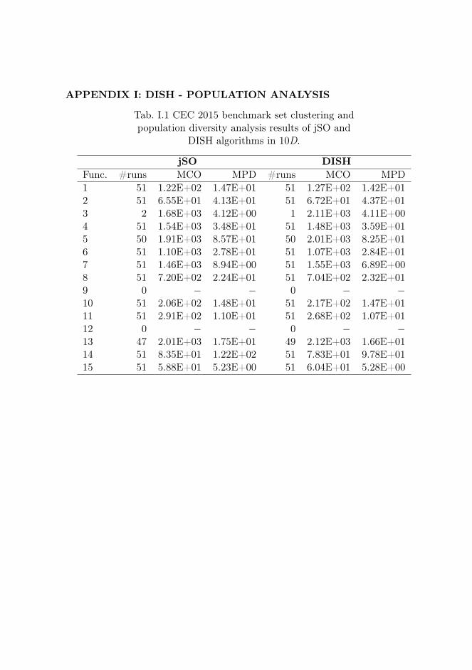
APPENDIX I: DISH - POPULATION ANALYSIS
Tab. I.1 CEC 2015 benchmark set clustering andpopulation diversity analysis results of jSO and
DISH algorithms in 10D.
jSO DISHFunc. #runs MCO MPD #runs MCO MPD1 51 1.22E+02 1.47E+01 51 1.27E+02 1.42E+012 51 6.55E+01 4.13E+01 51 6.72E+01 4.37E+013 2 1.68E+03 4.12E+00 1 2.11E+03 4.11E+004 51 1.54E+03 3.48E+01 51 1.48E+03 3.59E+015 50 1.91E+03 8.57E+01 50 2.01E+03 8.25E+016 51 1.10E+03 2.78E+01 51 1.07E+03 2.84E+017 51 1.46E+03 8.94E+00 51 1.55E+03 6.89E+008 51 7.20E+02 2.24E+01 51 7.04E+02 2.32E+019 0 − − 0 − −10 51 2.06E+02 1.48E+01 51 2.17E+02 1.47E+0111 51 2.91E+02 1.10E+01 51 2.68E+02 1.07E+0112 0 − − 0 − −13 47 2.01E+03 1.75E+01 49 2.12E+03 1.66E+0114 51 8.35E+01 1.22E+02 51 7.83E+01 9.78E+0115 51 5.88E+01 5.23E+00 51 6.04E+01 5.28E+00
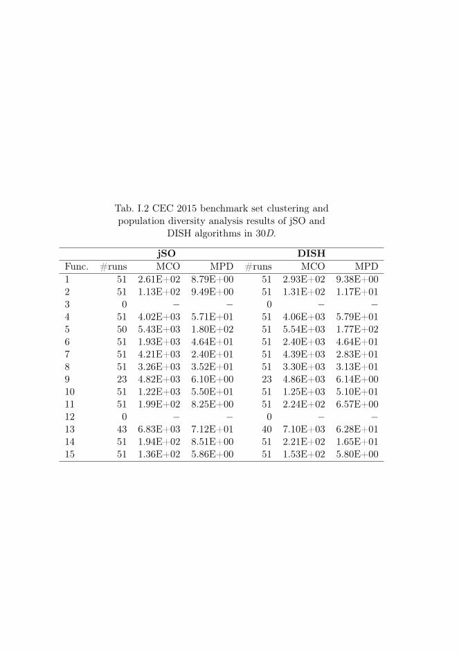
Tab. I.2 CEC 2015 benchmark set clustering andpopulation diversity analysis results of jSO and
DISH algorithms in 30D.
jSO DISHFunc. #runs MCO MPD #runs MCO MPD1 51 2.61E+02 8.79E+00 51 2.93E+02 9.38E+002 51 1.13E+02 9.49E+00 51 1.31E+02 1.17E+013 0 − − 0 − −4 51 4.02E+03 5.71E+01 51 4.06E+03 5.79E+015 50 5.43E+03 1.80E+02 51 5.54E+03 1.77E+026 51 1.93E+03 4.64E+01 51 2.40E+03 4.64E+017 51 4.21E+03 2.40E+01 51 4.39E+03 2.83E+018 51 3.26E+03 3.52E+01 51 3.30E+03 3.13E+019 23 4.82E+03 6.10E+00 23 4.86E+03 6.14E+0010 51 1.22E+03 5.50E+01 51 1.25E+03 5.10E+0111 51 1.99E+02 8.25E+00 51 2.24E+02 6.57E+0012 0 − − 0 − −13 43 6.83E+03 7.12E+01 40 7.10E+03 6.28E+0114 51 1.94E+02 8.51E+00 51 2.21E+02 1.65E+0115 51 1.36E+02 5.86E+00 51 1.53E+02 5.80E+00
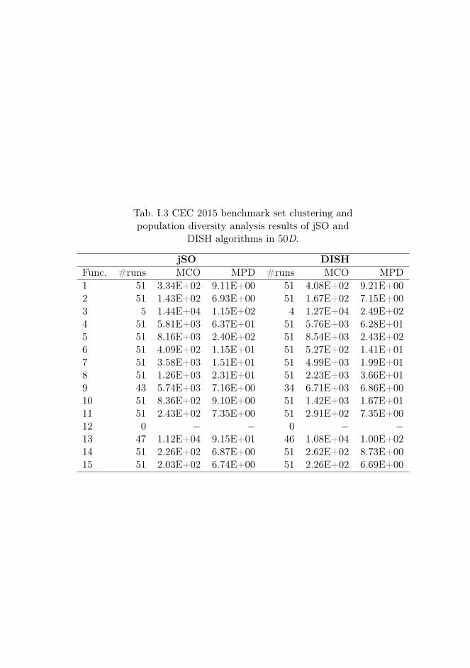
Tab. I.3 CEC 2015 benchmark set clustering andpopulation diversity analysis results of jSO and
DISH algorithms in 50D.
jSO DISHFunc. #runs MCO MPD #runs MCO MPD1 51 3.34E+02 9.11E+00 51 4.08E+02 9.21E+002 51 1.43E+02 6.93E+00 51 1.67E+02 7.15E+003 5 1.44E+04 1.15E+02 4 1.27E+04 2.49E+024 51 5.81E+03 6.37E+01 51 5.76E+03 6.28E+015 51 8.16E+03 2.40E+02 51 8.54E+03 2.43E+026 51 4.09E+02 1.15E+01 51 5.27E+02 1.41E+017 51 3.58E+03 1.51E+01 51 4.99E+03 1.99E+018 51 1.26E+03 2.31E+01 51 2.23E+03 3.66E+019 43 5.74E+03 7.16E+00 34 6.71E+03 6.86E+0010 51 8.36E+02 9.10E+00 51 1.42E+03 1.67E+0111 51 2.43E+02 7.35E+00 51 2.91E+02 7.35E+0012 0 − − 0 − −13 47 1.12E+04 9.15E+01 46 1.08E+04 1.00E+0214 51 2.26E+02 6.87E+00 51 2.62E+02 8.73E+0015 51 2.03E+02 6.74E+00 51 2.26E+02 6.69E+00
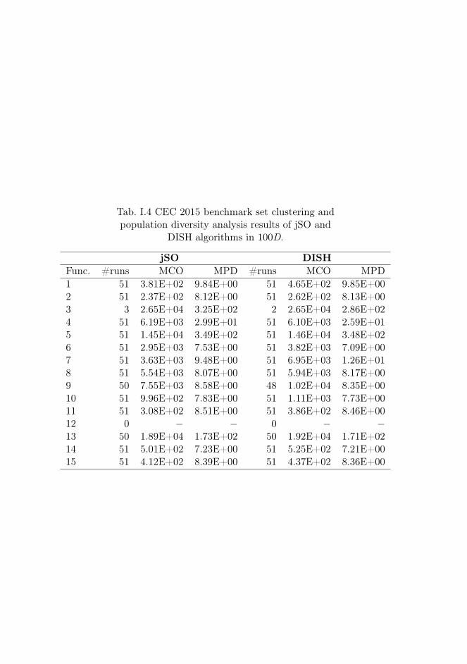
Tab. I.4 CEC 2015 benchmark set clustering andpopulation diversity analysis results of jSO and
DISH algorithms in 100D.
jSO DISHFunc. #runs MCO MPD #runs MCO MPD1 51 3.81E+02 9.84E+00 51 4.65E+02 9.85E+002 51 2.37E+02 8.12E+00 51 2.62E+02 8.13E+003 3 2.65E+04 3.25E+02 2 2.65E+04 2.86E+024 51 6.19E+03 2.99E+01 51 6.10E+03 2.59E+015 51 1.45E+04 3.49E+02 51 1.46E+04 3.48E+026 51 2.95E+03 7.53E+00 51 3.82E+03 7.09E+007 51 3.63E+03 9.48E+00 51 6.95E+03 1.26E+018 51 5.54E+03 8.07E+00 51 5.94E+03 8.17E+009 50 7.55E+03 8.58E+00 48 1.02E+04 8.35E+0010 51 9.96E+02 7.83E+00 51 1.11E+03 7.73E+0011 51 3.08E+02 8.51E+00 51 3.86E+02 8.46E+0012 0 − − 0 − −13 50 1.89E+04 1.73E+02 50 1.92E+04 1.71E+0214 51 5.01E+02 7.23E+00 51 5.25E+02 7.21E+0015 51 4.12E+02 8.39E+00 51 4.37E+02 8.36E+00
Related Documents