1 Control of Motion Compensated Offshore Gangway Offshore Dynamic Systems Lukas Matz Jensen, EN7D January 9, 2018 Aalborg University Esbjerg School of Engineering

Welcome message from author
This document is posted to help you gain knowledge. Please leave a comment to let me know what you think about it! Share it to your friends and learn new things together.
Transcript

1
Control of Motion
Compensated Offshore
Gangway Offshore Dynamic Systems
Lukas Matz Jensen, EN7D
January 9, 2018
Aalborg University Esbjerg
School of Engineering
2
Abstract:
Offshore gangways are commonly used for personnel and equipment transfer during operations at
sea. This can be a difficult and often dangerous task due to rough weathers and waves. To make
offshore transfer operations easier and safer, gangways can be made to compensate for the
disturbances created by wind and waves, to make sure it is always pointed at a desired direction and
angle. The aim of this project is to design the actuation system and a controller specifically for the
pitch rotations of the gangway. These designs must meet a specific set of criterions for both system
and controller. The controller is designed and simulated using MatLab and Simulink software, as
well as an understanding of the hydraulic drive system and controller design in frequency domain.
In this project, a single lag compensator is used with the purpose of reducing at least 90% of
incoming disturbances affecting the system. The controller is simulated in a virtual environment.
This project does however not include experimental testing of the system in use, as the physical
system has not been constructed. The reliance on simulations alone means that the projects results
are still in need of testing for verification purposes.
A satisfying design and analysis of a hydraulic pitch actuation system was made. It was also
concluded that the controller successfully stabilized the gangway pitch system, for the criterions set
for this project. Further work with the project could include a combined controller for movements in
all possible gangway movement angles, including extension and contraction.
3
Preface
This report is written by Lukas Matz Jensen on the topic “Offshore Dynamic Systems”. The chosen
project is: Control of Motion Compensated Offshore Gangway. The report is written in connection
to the 7th semester diploma project, on the energy engineering study at Alborg University Esbjerg
(AAUE), 2017-2018.
The project is carried out to meet curriculum learning objectives. To meet these, it is sought after to
implement knowledge from previous semesters, as well as the knowledge gained during the
internship at SubC Partner. This is applied during theory, system design/analysis and simulations.
Different software has been used during this study to aid in calculations. Among these are MatLab
and Mathcad. Project-relevant calculations and MatLab scripts are included in the appendix.
I would like to thank my supervisors for assisting with the written report and the simulations
conducted. I am also grateful to SubC Partner, for giving me the opportunity to work with the
gangway project and continue with the ideas that originated at them.
4
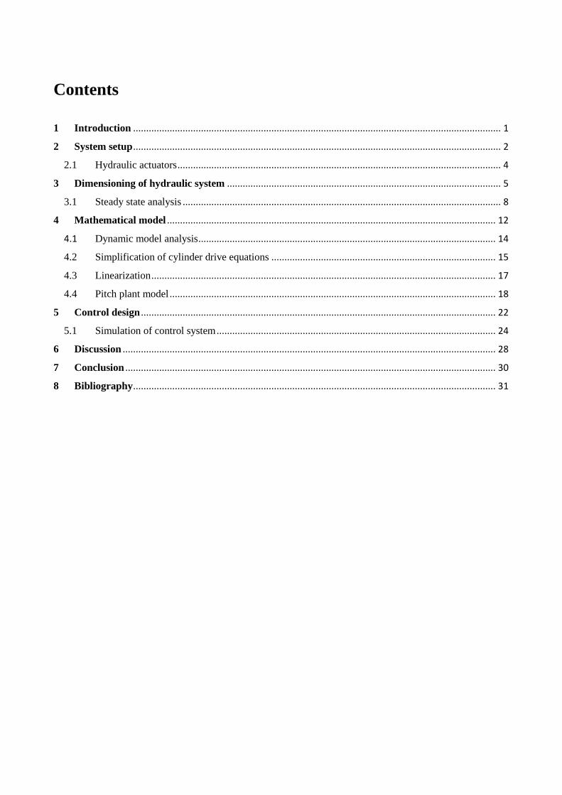
Contents
1 Introduction ............................................................................................................................................. 1
2 System setup ............................................................................................................................................. 2
2.1 Hydraulic actuators ............................................................................................................................ 4
3 Dimensioning of hydraulic system ......................................................................................................... 5
3.1 Steady state analysis .......................................................................................................................... 8
4 Mathematical model .............................................................................................................................. 12
4.1 Dynamic model analysis .................................................................................................................. 14
4.2 Simplification of cylinder drive equations ...................................................................................... 15
4.3 Linearization .................................................................................................................................... 17
4.4 Pitch plant model ............................................................................................................................. 18
5 Control design ........................................................................................................................................ 22
5.1 Simulation of control system ........................................................................................................... 24
6 Discussion ............................................................................................................................................... 28
7 Conclusion .............................................................................................................................................. 30
8 Bibliography ........................................................................................................................................... 31
1
1 Introduction Offshore gangways are broadly used for equipment and personnel transfer at sea. However,
precisely locking the gangway between the vessel on which it is installed and a turbine platform,
can be challenging during offshore operations. Due to heavy influence from wind and waves, it is
desired to create a gangway which compensates for these disturbances. A motion compensated
gangway would allow for safer, easier and more precise transfer of personnel. The motion
compensation is to be active during aiming and while locking the gangway to the Turbine Platform
(TP). After successful connection between vessel and TP, the gangway is set to neutral gear during
personnel transfer.
The problem, which this project aims to solve, is to design a controller which will keep the attitude
of the gangway within a defined margin of error. Disturbances from wind and waves during
operation are the reasons the control design is a challenge. The objective is to keep the pitch attitude
of the gangway stable within defined parameters, using a controller to direct its rotations, as to
reject the disturbances from the offshore environment. More specifically, the goal is to create a
pitch controller which rejects at least 90% of incoming disturbances, without making the system
prone to instability. The full list of criteria for the controller is found and explained during
controller design in chapter 5.
First, the characteristics and motions of the actuators are defined and analyzed to create a
mathematical model describing the system. Hereafter a controller can be designed and simulated in
a virtual environment. Due to the lack of physical testing setup, the results and success of the
project will be based on simulations using MatLab.
The actual process of the gangway system in use would be that a sensor estimates the attitude,
which is compared to a reference attitude to produce an error signal. This error signal is the input to
the controller. The output is a command sent to the drivers, driving the actuators to move at a
correct velocity and direction. It is important to note that the gangway itself has not been fully
designed nor constructed yet. Therefore, any illustrations or assumptions of the gangways practical
use found in this paper, are solely for assistance in overall understanding of the project. These are
not representation of the actual system in use.
Project boundaries
A ship at sea can experience disturbances of up to 24 deg/sec [1]. Personnel transfer at sea with
disturbance at “worst case scenario” of 24 deg/sec is not considered safe and is therefore not a
realistic simulation parameter. This project is aimed at stabilizing the gangway around a reference
point and reject 90% of an incoming disturbance of 8 deg/sec.
For this project, 100% angle accuracy is not critical for success. A minor deviation in attitude angle
will only have a slight effect on the heave motion in the end of the gangway. This is due to the
relatively short length of the gangway being 11,0 meters when fully extended. Furthermore, the

2
gangway must be limited to ±20 degrees of vertical pitch rotation for safety reasons according to
DNV-GL standards [2].
Due to time limitations, the focus of this project will be solely on creating a controller for the pitch
rotations of the gangway system and the design of hydraulic actuators for this Degree of Freedom
(DOF). The reason to focus on this DOF, is also based on the purpose of incorporating a more
thorough implementation of knowledge gained during previous semester lectures. If a controller is
successfully created and simulated for pitch, then future work would allow for the implementation
of yaw, roll, extension and contraction movements of the gangway.
This project is conducted in cooperation with SubC Partner and Aalborg University Esbjerg.
2 System setup Before beginning the theoretical analysis, it is a great help for the overall understanding of the
project, to clearly visualize the gangway system around which the project is centered.
Figure 2.1: CAD-drawing of the offshore extendable gangway without actuators installed [2].
Figure 2.1 shows an illustration of the physical offshore gangway setup. The gangway with 1100 kg
of total mass without onboard personnel, is designed to be installed on the far port or starboard side
of a marine vessel [3]. From here the gangway can be manually steered by an operator, who can
change the reference angles of the gangway by means of an interface, thus commanding the
3
attitude. Without a controller designed for motion compensation, steering the gangway precisely
would be very challenging due to waves influencing vessel movements.
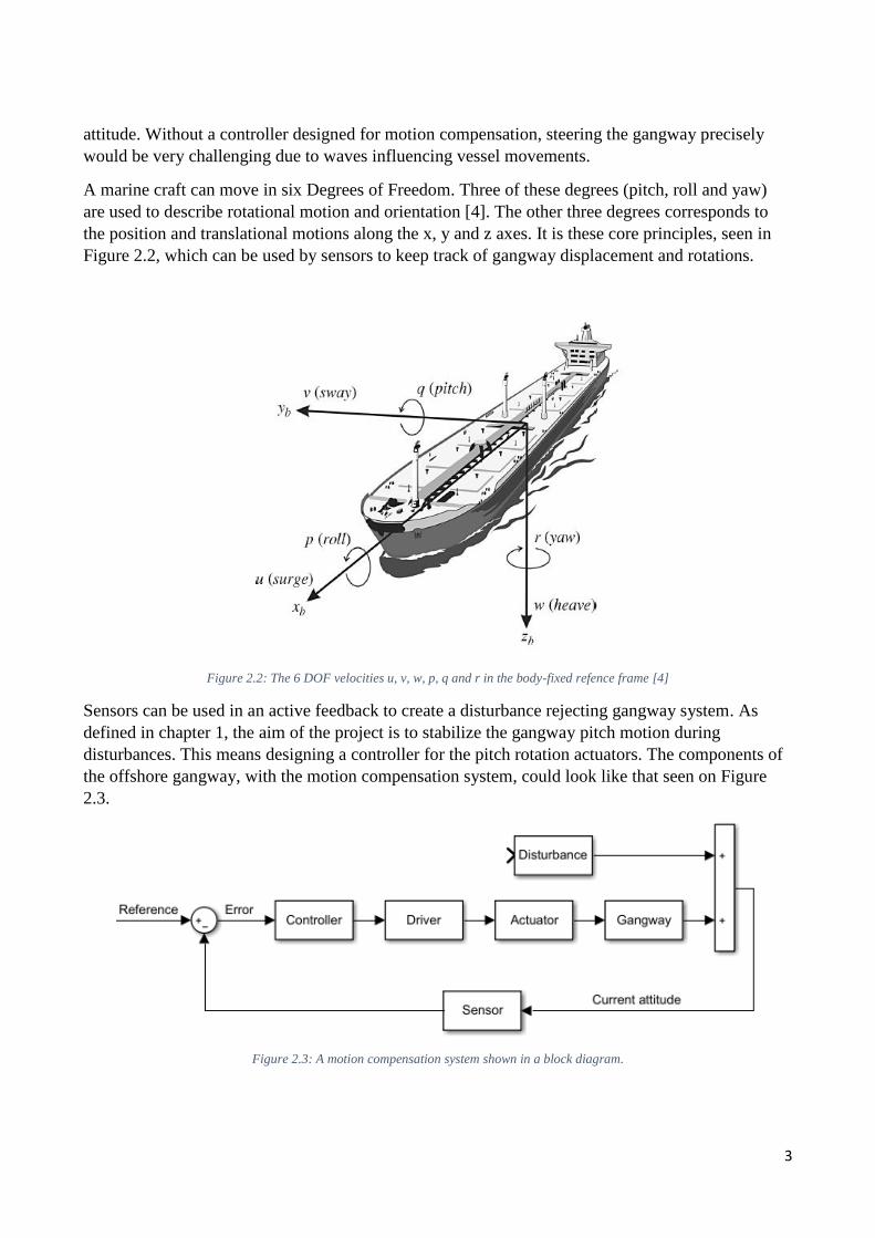
A marine craft can move in six Degrees of Freedom. Three of these degrees (pitch, roll and yaw)
are used to describe rotational motion and orientation [4]. The other three degrees corresponds to
the position and translational motions along the x, y and z axes. It is these core principles, seen in
Figure 2.2, which can be used by sensors to keep track of gangway displacement and rotations.
Figure 2.2: The 6 DOF velocities u, v, w, p, q and r in the body-fixed refence frame [4]
Sensors can be used in an active feedback to create a disturbance rejecting gangway system. As
defined in chapter 1, the aim of the project is to stabilize the gangway pitch motion during
disturbances. This means designing a controller for the pitch rotation actuators. The components of
the offshore gangway, with the motion compensation system, could look like that seen on Figure
2.3.
Figure 2.3: A motion compensation system shown in a block diagram.
4
The results of the project will be based on simulations of the system in MatLab. An in-depth
analysis of the other components, such as drivers and sensors, is therefore redundant, as these have
yet to be specified for the physical system. To successfully model and control the gangway system,
an understanding of the actuators involved with its movements is necessary. Since only the passive
parts of the gangway itself has been fully designed, the motors and actuators of the system is to be
selected and designed. The actuators creating the pitch movements of the gangway are to be two
hydraulic cylinders, which are part of a hydraulic actuation system.
2.1 Hydraulic actuators
The principles behind hydraulics is based on transmitting force and motion through a confined
liquid (usually an oil). In a basic hydraulic system, motion and force is achieved in the actuator by
use of an external pump. A linear actuator consists of a piston inside a cylinder capable of linear
motion. The pump is connected to the cylinder by oil filled hoses. As the pump increases pressure
in the cylinder, the piston is pushed along the axis of the cylinder creating a linear movement and
force.
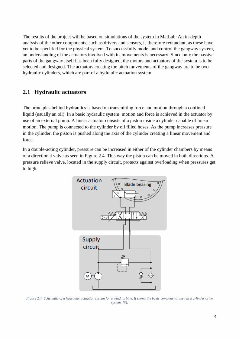
In a double-acting cylinder, pressure can be increased in either of the cylinder chambers by means
of a directional valve as seen in Figure 2.4. This way the piston can be moved in both directions. A
pressure relieve valve, located in the supply circuit, protects against overloading when pressures get
to high.
Figure 2.4: Schematic of a hydraulic actuation system for a wind turbine. It shows the basic components used in a cylinder drive
system. [5].
5
A hydraulic actuator differs from pneumatic actuators in that it can hold a constant force and torque
without the pump supplying more pressure or fluid. This is due to the neigh incompressibility of
fluids compared to the gas medium used in pneumatic systems.
Hydraulic actuators in general have certain advantageous properties, compared to electrical systems
[5]:
• High power density when compared to electrical systems.
• Inherently lubricated and can be more reliable than electrical equivalents under the right
circumstances.
• Operation may commence from rest under full load.
• Smooth adjustment of speed, torque and force is easily achieved.
These advantages make the hydraulic actuator suitable for use in lifting and controlling the
gangway pitch movements. Hydraulic actuators have certain disadvantages as well [5]
• System is sensitive to contamination.
• Prone to leakages and pressure drops.
• Pressure and flow is required to obtain force and motion from a cylinder. Accounting for
pressure drop in a hydraulic system is therefore important.
Fluid leakage, particularly in the spool valve controlling fluid direction, would normally be a
serious consideration when designing a hydraulic system. Leakage will result in in pressure drop
over time. This would cause unwanted movements of the gangway, creating a slow decline in
vertical angle. In this project, the pressure effects of leakage are considered minimal and can be
ignored due to the relatively short active operation time of the gangway. The system only needs be
accurate during the short time it takes, for the operator to lock it into position with the TP.
3 Dimensioning of hydraulic system Before designing the controller, it is first necessary to obtain a mathematical model for the pitch
movement actuators. The plant model consists of a transfer function based on input and output of
the actuator system. The establishment of the mathematical model will be done using an analytical
approach, since no physical system exists yet. The analytical approach is in some aspects inferior to
the experimental approach. This is due to actual physical systems rarely behaving exactly like the
theoretical system describes. An experimental approach would also show any unforeseen system
variations. This must be considered at later stages of project development, if real life
implementations of the controller are planned.
Fully developing the offshore gangway based on the simulations in this report alone and without
further experimental data, is therefore not advised. This chapter will explain the approach of
obtaining a mathematical model for the hydraulic systems.

6
The course of establishing a usable mathematical model for control design is as follows:
• Dimensioning and analysis of the hydraulic actuation system.
• Establishing of non-linear model.
• Linearization of non-linear model using Taylor approximations.
• Design of linear controller.
To derive a mathematical model of the hydraulic system, which controls gangway pitch
movements, a design and analysis of said system is required. Figure 3.1 shows a schematic of the
initial pitch actuation system chosen for the task at hand.
A fixed-displacement pump delivers pressurized fluid to the two hydraulic cylinders. These are used
as actuators to simultaneously lift or lower the offshore gangway. The directional valve acts a
multipurpose component in this system. It is used to direct the flow of oil from the pump to either
the A or B chambers of the cylinders. Thus, the directional valve is used to decide whether an
extending or contracting motion is to be done in the cylinders. The secondary function of the
directional valve in this project, is to regulate the pressure flow rate to the cylinders. This is how the
velocity of the actuators is controlled.
Figure 3.1: Simulink schematic of the designed hydraulic pitch actuation system.

7
The actuators are designed to respond to the offshore scenario described in chapter 1, with a
maximum disturbance of 8 deg/sec. The maximum velocity required of the hydraulic actuators will
be calculated by use of trigonometric equations. This is visualized in the simple illustration on
Figure 3.2.
Figure 3.2: Simplified trigonometric representation of the gangway system seen from the side. The length of the hydraulic actuators
is represented by the letter s.
The length of the two hydraulic rods, at maximum and minimum pitch angles of 110 and 70 degrees
respectively, can be found using Eq. (3.1).
𝑠 = √𝐿12 + ℎ2 − 2 ∗ 𝐿1 ∗ ℎ ∗ 𝑐𝑜𝑠(𝜃) [𝑚] (3. 1)
Here, L1 is the length from gangway start to the point where the hydraulic rod end is attached. 𝜃 is
gangway angle, where a completely horizontal gangway corresponds to 𝜃 = 90° as seen on Figure
3.2. h is the direct vertical height from the bottom of the hydraulic cylinder to gangway start. The
amount of extension or contraction done by the actuators per degree, can then be found using Eq.
(3.2)
∆ℎ𝑦𝑑 = (𝑠𝑚𝑎𝑥 − 𝑠𝑚𝑖𝑛)/(𝜃𝑚𝑎𝑥 − 𝜃𝑚𝑖𝑛) [𝑚
𝑑𝑒𝑔] (3. 2)
Where 𝑠𝑚𝑎𝑥 and 𝑠𝑚𝑖𝑛 are hydraulic rod lengths at 110 and 70 degrees gangway attitude
respectively. Finding the maximum needed velocity of the hydraulic actuators, can now be done
using the following Eq.
𝑣𝑚𝑎𝑥 = 𝜔(∆ℎ𝑦𝑑) [𝑚
𝑠𝑒𝑐] (3. 3)
Here ω is angular velocity of the disturbance. With disturbances of 8 deg/sec and gangway
parameters where
𝐿1 = 3 [𝑚] ℎ = 1.25 [𝑚]
the equation yields a maximum linear actuator velocity, vmax, of 0.16 m/sec.
8
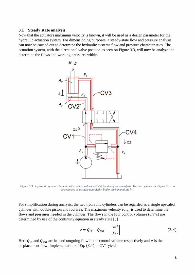
3.1 Steady state analysis
Now that the actuators maximum velocity is known, it will be used as a design parameter for the
hydraulic actuation system. For dimensioning purposes, a steady-state flow and pressure analysis
can now be carried out to determine the hydraulic systems flow and pressure characteristics. The
actuation system, with the directional valve position as seen on Figure 3.3, will now be analyzed to
determine the flows and working pressures within.
Figure 3.3: Hydraulic system schematic with control volumes (CV's) for steady state analysis. The two cylinders in Figure 3.1 can
be regarded as a single upscaled cylinder during analysis [4].
For simplification during analysis, the two hydraulic cylinders can be regarded as a single upscaled
cylinder with double piston and rod area. The maximum velocity 𝑣𝑚𝑎𝑥 is used to determine the
flows and pressures needed in the cylinder. The flows in the four control volumes (CV’s) are
determined by use of the continuity equation in steady state [5]
⩒ = 𝑄𝑖𝑛 − 𝑄𝑜𝑢𝑡 [𝑚3
𝑠𝑒𝑐] (3. 4)
Here 𝑄𝑖𝑛 and 𝑄𝑜𝑢𝑡 are in- and outgoing flow in the control volume respectively and ⩒ is the
displacement flow. Implementation of Eq. (3.4) in CV1 yields
9
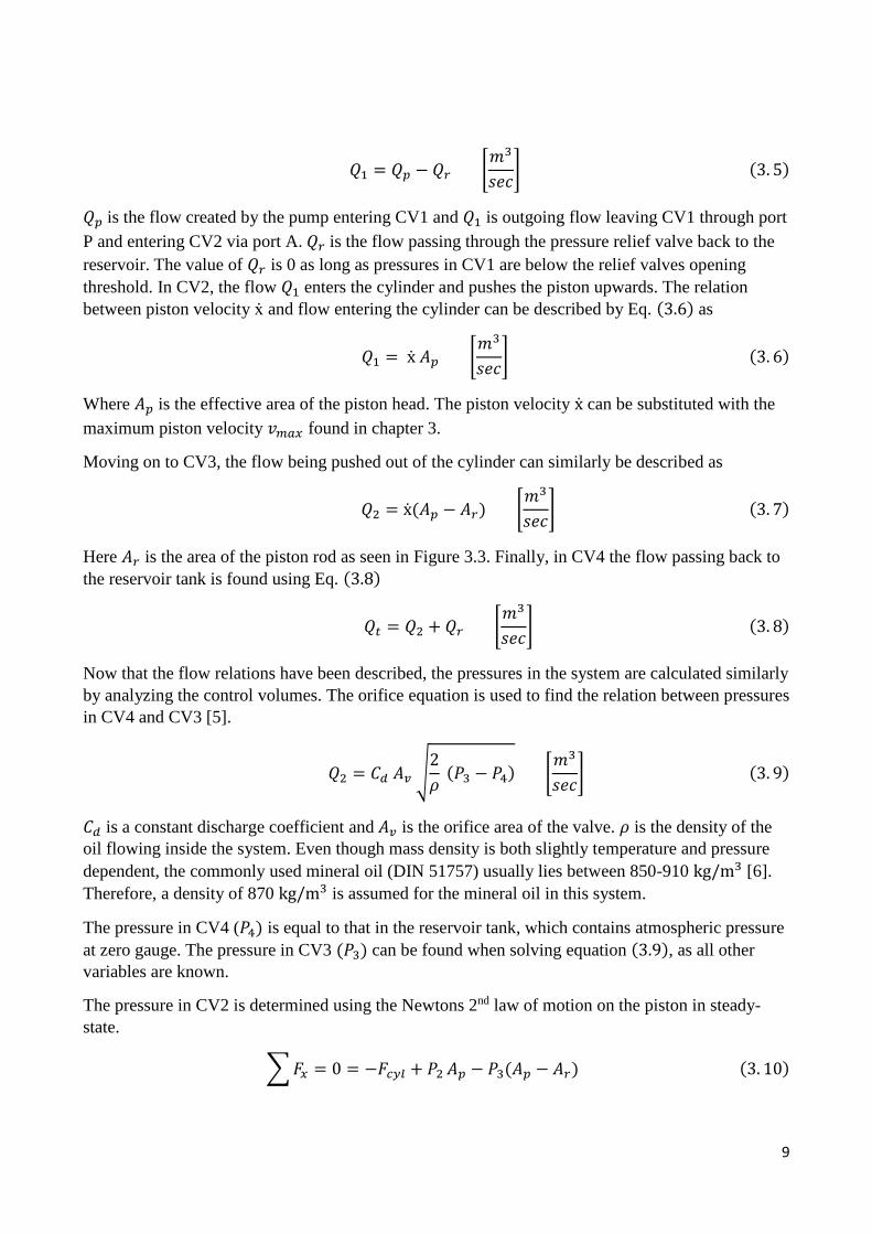
𝑄1 = 𝑄𝑝 − 𝑄𝑟 [𝑚3
𝑠𝑒𝑐] (3. 5)
𝑄𝑝 is the flow created by the pump entering CV1 and 𝑄1 is outgoing flow leaving CV1 through port
P and entering CV2 via port A. 𝑄𝑟 is the flow passing through the pressure relief valve back to the
reservoir. The value of 𝑄𝑟 is 0 as long as pressures in CV1 are below the relief valves opening
threshold. In CV2, the flow 𝑄1 enters the cylinder and pushes the piston upwards. The relation
between piston velocity ẋ and flow entering the cylinder can be described by Eq. (3.6) as
𝑄1 = ẋ 𝐴𝑝 [𝑚3
𝑠𝑒𝑐] (3. 6)
Where 𝐴𝑝 is the effective area of the piston head. The piston velocity ẋ can be substituted with the
maximum piston velocity 𝑣𝑚𝑎𝑥 found in chapter 3.
Moving on to CV3, the flow being pushed out of the cylinder can similarly be described as
𝑄2 = ẋ(𝐴𝑝 − 𝐴𝑟) [𝑚3
𝑠𝑒𝑐] (3. 7)
Here 𝐴𝑟 is the area of the piston rod as seen in Figure 3.3. Finally, in CV4 the flow passing back to
the reservoir tank is found using Eq. (3.8)
𝑄𝑡 = 𝑄2 + 𝑄𝑟 [𝑚3
𝑠𝑒𝑐] (3. 8)
Now that the flow relations have been described, the pressures in the system are calculated similarly
by analyzing the control volumes. The orifice equation is used to find the relation between pressures
in CV4 and CV3 [5].
𝑄2 = 𝐶𝑑 𝐴𝑣 √2
𝜌 (𝑃3 − 𝑃4) [
𝑚3
𝑠𝑒𝑐] (3. 9)
𝐶𝑑 is a constant discharge coefficient and 𝐴𝑣 is the orifice area of the valve. 𝜌 is the density of the
oil flowing inside the system. Even though mass density is both slightly temperature and pressure
dependent, the commonly used mineral oil (DIN 51757) usually lies between 850-910 kg/m3 [6].
Therefore, a density of 870 kg/m3 is assumed for the mineral oil in this system.
The pressure in CV4 (𝑃4) is equal to that in the reservoir tank, which contains atmospheric pressure
at zero gauge. The pressure in CV3 (𝑃3) can be found when solving equation (3.9), as all other
variables are known.
The pressure in CV2 is determined using the Newtons 2nd law of motion on the piston in steady-
state.
∑𝐹𝑥 = 0 = −𝐹𝑐𝑦𝑙 + 𝑃2 𝐴𝑝 − 𝑃3(𝐴𝑝 − 𝐴𝑟) (3. 10)
10
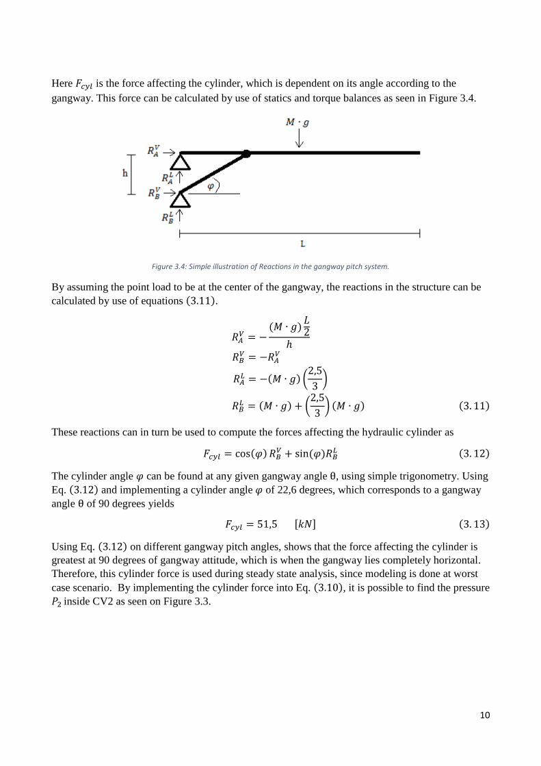
Here 𝐹𝑐𝑦𝑙 is the force affecting the cylinder, which is dependent on its angle according to the
gangway. This force can be calculated by use of statics and torque balances as seen in Figure 3.4.
Figure 3.4: Simple illustration of Reactions in the gangway pitch system.
By assuming the point load to be at the center of the gangway, the reactions in the structure can be
calculated by use of equations (3.11).
𝑅𝐴𝑉 = −
(𝑀 ∙ 𝑔)𝐿2
ℎ 𝑅𝐵𝑉 = −𝑅𝐴
𝑉
𝑅𝐴𝐿 = −(𝑀 ∙ 𝑔) (
2,5
3)
𝑅𝐵𝐿 = (𝑀 ∙ 𝑔) + (
2,5
3) (𝑀 ∙ 𝑔) (3. 11)
These reactions can in turn be used to compute the forces affecting the hydraulic cylinder as
𝐹𝑐𝑦𝑙 = cos(𝜑)𝑅𝐵𝑉 + sin (𝜑)𝑅𝐵
𝐿 (3. 12)
The cylinder angle 𝜑 can be found at any given gangway angle θ, using simple trigonometry. Using
Eq. (3.12) and implementing a cylinder angle 𝜑 of 22,6 degrees, which corresponds to a gangway
angle θ of 90 degrees yields
𝐹𝑐𝑦𝑙 = 51,5 [𝑘𝑁] (3. 13)
Using Eq. (3.12) on different gangway pitch angles, shows that the force affecting the cylinder is
greatest at 90 degrees of gangway attitude, which is when the gangway lies completely horizontal.
Therefore, this cylinder force is used during steady state analysis, since modeling is done at worst
case scenario. By implementing the cylinder force into Eq. (3.10), it is possible to find the pressure
𝑃2 inside CV2 as seen on Figure 3.3.

11
Lastly, the pressure inside CV1 can be found using orifice Eq. (3.9) in the same manner as before,
but substituting with pressure difference between CV1-2.
𝑄1 = 𝐶𝑑 𝐴𝑑 √2
𝜌 (𝑃1 − 𝑃2) [
𝑚3
𝑠𝑒𝑐] (3. 14)
System coefficients can now be calculated when inserting known values and lengths. Listed below
are the known system specifications.
𝑀 = 1100[𝑘𝑔] 𝜌 = 870[𝑘𝑔/𝑚3] 𝐿 = 11[𝑚] ℎ = 1,25[𝑚]
𝐴𝑣 = 15 ∙ 10−6[𝑚2] 𝐴𝑝 = 3,1 ∙ 10−3[𝑚2] 𝐴𝑟 = 10
−3[𝑚2] 𝐶𝑑 = 0.6
The specific value of 𝐶𝑑 has been chosen since it is a commonly assumed spool-valve coefficient
value [5]. The orifice area as well as piston head and rod areas are chosen during system
calculations. Tweaking these values can increases or decreases pressures and flows in the system to
reach desired values for the actuators. In general, smaller sized valves are cheaper, and is therefore
selected as small as possible for this system.
When doing the calculations, it is important to notice that pressures and flows must be in SI units.
For the hydraulic system, the flow calculations using the above stated coefficients yields
𝑄1 = 4,93 ∙ 10−4 [
𝑚3
𝑠]
= 29,58 [𝑙
𝑚𝑖𝑛] (3. 15)
𝑄2 = 3,34 ∙ 10−4 [
𝑚3
𝑠]
= 20,04 [𝑙
𝑚𝑖𝑛] (3. 16)
For system pressures it follows.
𝑃1 = 183,38 [𝑏𝑎𝑟] (3. 17)
𝑃2 = 170,32 [𝑏𝑎𝑟] (3. 18)
𝑃3 = 6,0 [𝑏𝑎𝑟] (3. 19)
𝑃4 = 0 [𝑏𝑎𝑟] (3. 20)
The flows and pressures found for this system are within reasonable magnitudes, compared to
previous work with similar hydraulic systems. These characteristics will be used to create a
dynamic analysis of the cylinder drive system.
12
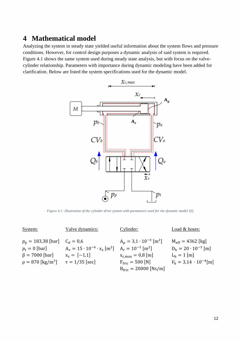
4 Mathematical model Analyzing the system in steady state yielded useful information about the system flows and pressure
conditions. However, for control design purposes a dynamic analysis of said system is required.
Figure 4.1 shows the same system used during steady state analysis, but with focus on the valve-
cylinder relationship. Parameters with importance during dynamic modeling have been added for
clarification. Below are listed the system specifications used for the dynamic model.
Figure 4.1: Illustration of the cylinder drive system with parameters used for the dynamic model [6].
System: Valve dynamics: Cylinder: Load & hoses:
𝑝p = 183,38 [bar]
Cd = 0,6
Ap = 3,1 ∙ 10−3 [m2]
Meff = 4362 [kg]
𝑝t = 0 [bar] Av = 15 ∙ 10−6 ∙ xs [m
2] Ar = 10−3 [m2] Dh = 20 ∙ 10−3 [m]
β = 7000 [bar] xs = [−1,1] xc,max = 0,8 [m] Lh = 1 [m]
ρ = 870 [kg/m3] τ = 1/35 [sec] Ffric = 500 [N] 𝑉h = 3,14 ∙ 10−4[m]
Bfric = 20000 [Ns/m]

13
These parameters are based on assumptions for the system, as well as the values obtained in earlier
chapters. An explanation of the listed coefficients follows.
Fluid stiffness, β, determines the compressibility of a fluid. It is dependent on temperature and
pressure, but is normally in good practice assumed to be between 7000-10000 bar [6].
During dynamic modelling, the orifice area of the directional spool valve Av, is dependent on its
position xs as visualized in Figure 4.2.
Figure 4.2: Directional control valve. Orifice area is dependent on spool position 𝑥𝑠 [5].
The time constant of the system, τ, is set to 1/35 sec. xc,max is found using Eq. (3.1), where it is the
difference between maximum and minimum hydraulic rod length. Ffric is a constant static friction
between piston and cylinder, whereas Bfric is variable according to velocity. The values of the
friction coefficients Ffric and Bfric as well as hose parameters, are all assumptions based on previous
work with, and studies of, similar hydraulic systems [5].
During dynamic analysis the effective mass M, and thus the applied force F, must be related to the
piston of the cylinder, which in turn is related to the length and velocity of the gangway. The
effective mass M can be determined using energy considerations, where the total mass of the
gangway is summed as a point load, positioned at the center of gravity at half the maximum
gangway length.
Figure 4.3: Momentary representation of the hydraulic cylinder rotating the gangway. Its total mass is summed as a payload at half
the gangways total length, LM.

14
For an infinitesimal extraction of the cylinder the effective mass can be computed as
𝑀𝑒𝑓𝑓 = 𝑀(𝐿𝑚
𝐿1 ∙ cos(𝛾))2
[𝑘𝑔] (4. 1)
Where
𝛾 = 𝜃 +𝜋
2− 𝜑 (4. 2)
Here, 𝜃 is the angle of the gangway compared to the horizontal plane, which would be equal to 0 in
the momentary case seen on Figure 4.3. During the dynamic analysis, the model is created after
worst case scenario, which is when the magnitude of the effective mass is highest. The highest 𝑀𝑒𝑓𝑓
value during gangway operation, is achieved when the gangway is at -20 degrees from the
horizontal plane. Therefore, the effective mass 𝑀𝑒𝑓𝑓 is chosen at this point. Eq. (4.1) then yields
𝑀𝑒𝑓𝑓 = 4362 [𝑘𝑔] as listed earlier. Now the dynamic analysis can be carried out, as the required
system dimensions and affecting forces are known.
4.1 Dynamic model analysis One of the most notable differences between steady state and dynamic modeling, is in flow
continuity [5]. Here, the compressibility of the fluid is considered by adding a pressure build-up
flow term to continuity Eq. (3.4), so that
𝑄𝑖𝑛 − 𝑄𝑜𝑢𝑡 = ⩒ +𝑉
𝛽ṗ (4. 3)
If positive, the pressure build-up flow term to the right suggests an increasing flow and if negative,
a decreasing flow. Another difference between dynamic and steady state analysis, lies in the
additions to force Eq. (3.10) where the addition of friction, velocity and acceleration coefficients
yields
𝑀𝑒𝑓𝑓ẍ𝑐 = 𝑃𝑎 𝐴𝑝 − 𝑃𝑏(𝐴𝑝 − 𝐴𝑟) − 𝐹𝑓𝑟𝑖𝑐(ẋ𝑐) − 𝐵𝑓𝑟𝑖𝑐ẋ𝑐 (4. 4)
Here ẍ𝑐 and ẋ𝑐 are acceleration and velocity of the hydraulic piston respectively. 𝑃𝑎 and 𝑃𝑏 are the
pressures on each side of the cylinder. In reality, the contribution of the effective mass 𝑀𝑒𝑓𝑓 would
be dependent on wind, waves and more effecting the gangway during offshore operation. For the
sake of simplifying the model, these affects are disregarded in this project, but could be considered
in future work if they prove to have significant effects on the system.
The orifice equation (3.9) does not change a lot when used in the dynamic analysis. The only
difference is in the orifice area being a function of valve position, as seen in Eq. (4.5) and (4.6).

15
𝑄𝑎 = 𝐶𝑑 𝐴𝑣(𝑥𝑠)√2
𝜌 (𝑃𝑝 − 𝑃𝑎) , 𝑓𝑜𝑟 𝑥𝑠 > 0 (4. 5)
𝑄𝑏 = 𝐶𝑑 𝐴𝑣(𝑥𝑠)√2
𝜌 (𝑃𝑡 − 𝑃𝑏) , 𝑓𝑜𝑟 𝑥𝑠 > 0 (4. 6)
Combined, the equations (4.3), (4.4), (4.5) and (4.6) form a dynamic model description of the
hydraulic system. However, this model is not linear and requires linearization before it is usable for
control design. It is furthermore hard to analyze a higher order model analytically. Through
simplification, the order of the cylinder drive model can be reduced.
4.2 Simplification of cylinder drive equations
For control design purposes it is desired to establish a simplified model description, that captures
the dominant dynamic features of the hydraulic system, while asymmetries are taking into account
[7]. Now that dynamic aspects have been incorporated into the system equations, a simplification of
the cylinder drive seen on Figure 4.1 will be carried out, with the purpose of reducing the order of
the model. Using Eq. (4.3), the continuity equation for positive flow (𝑥𝑠 > 0) can be re-written as
ṗ𝑎 = (𝑄𝑎 − 𝐴𝑃ẋ𝑐)𝛽
𝑉𝑎(𝑥𝑐) (4. 7)
ṗ𝑏 = (𝑄𝑏 + ((𝐴𝑝 − 𝐴𝑟)ẋ𝑐)𝛽
𝑉𝑏(𝑥𝑐)(4. 8)
for CVa and CVb respectively. It is important to note, that the volumes 𝑉a and 𝑉b are the combined
volumes of cylinder and hoses, as seen in Figure 4.1. Similarly, flow Eq. (4.5) and (4.6) for
(𝑥𝑠 > 0) can be simplified as
𝑄𝑎 = 𝐾𝑣(𝑥𝑠)√ (𝑃𝑏 − 𝑃𝑎) (4. 9)
𝑄𝑏 = −𝐾𝑣(𝑥𝑠)√ (𝑃𝑏 − 𝑃𝑡) (4. 10)
Where
𝐾𝑣(𝑥𝑠) = 𝐶𝑑𝐴𝑣(𝑥𝑠)√2
𝜌(4. 11)
For the purpose of creating a simplified model description, a steady state cylinder flow assumption
is made in Eq. (4.12)
𝑄𝑏 = −𝑄𝑎(𝐴𝑝 − 𝐴𝑟)
𝐴𝑃= −𝑄𝑎𝐶𝑅 (4. 12)
16
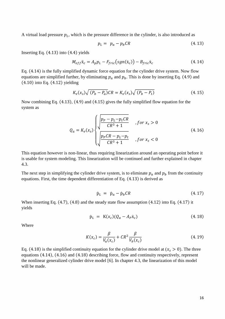
A virtual load pressure 𝑝𝐿, which is the pressure difference in the cylinder, is also introduced as
𝑝𝐿 = 𝑝𝑎 − 𝑝𝑏𝐶𝑅 (4. 13)
Inserting Eq. (4.13) into (4.4) yields
𝑀𝑒𝑓𝑓ẍ𝑐 = 𝐴𝑝𝑝𝐿 − 𝐹𝑓𝑟𝑖𝑐(𝑠𝑔𝑛(ẋ𝑐)) − 𝐵𝑓𝑟𝑖𝑐ẋ𝑐 (4. 14)
Eq. (4.14) is the fully simplified dynamic force equation for the cylinder drive system. Now flow
equations are simplified further, by eliminating 𝑝𝑎 and 𝑝𝑏. This is done by inserting Eq. (4.9) and
(4.10) into Eq. (4.12) yielding
𝐾𝑣(𝑥𝑠)√ (𝑃𝑏 − 𝑃𝑎)𝐶𝑅 = 𝐾𝑣(𝑥𝑠)√ (𝑃𝑏 − 𝑃𝑡) (4. 15)
Now combining Eq. (4.13), (4.9) and (4.15) gives the fully simplified flow equation for the
system as
𝑄𝑎 = 𝐾𝑣(𝑥𝑠)
{
√𝑝𝑃 − 𝑝𝐿−𝑝𝑡𝐶𝑅
𝐶𝑅3 + 1 , 𝑓𝑜𝑟 𝑥𝑠 > 0
√𝑝𝑃𝐶𝑅 − 𝑝𝐿−𝑝𝑡𝐶𝑅3 + 1
, 𝑓𝑜𝑟 𝑥𝑠 < 0
(4. 16)
This equation however is non-linear, thus requiring linearization around an operating point before it
is usable for system modeling. This linearization will be continued and further explained in chapter
4.3.
The next step in simplifying the cylinder drive system, is to eliminate 𝑝𝑎 and 𝑝𝑏 from the continuity
equations. First, the time dependent differentiation of Eq. (4.13) is derived as
ṗ𝐿 = ṗ𝑎 − ṗ𝑏𝐶𝑅 (4. 17)
When inserting Eq. (4.7), (4.8) and the steady state flow assumption (4.12) into Eq. (4.17) it yields
ṗ𝐿 = K(𝑥𝑐)(𝑄𝑎 − 𝐴𝑃ẋ𝑐) (4. 18)
Where
𝐾(𝑥𝑐) =𝛽
𝑉𝑎(𝑥𝑐)+ 𝐶𝑅2
𝛽
𝑉𝑏(𝑥𝑐)(4. 19)
Eq. (4.18) is the simplified continuity equation for the cylinder drive model at (𝑥𝑠 > 0). The three
equations (4.14), (4.16) and (4.18) describing force, flow and continuity respectively, represent
the nonlinear generalized cylinder drive model [6]. In chapter 4.3, the linearization of this model
will be made.

17
4.3 Linearization
The dynamic behavior of hydraulic systems is generally nonlinear, and a linearization of the
nonlinear drive model is therefore necessary. Linearization can be used to find a linear system
around an equilibrium of a nonlinear system. However, the error between the linear and nonlinear
system will gradually increase the further the signal is from the equilibrium point. This is because
the linearization is concerned with the dynamics in a small vicinity around this operating point [6].
This principle is shown graphically on Figure 4.4.
Figure 4.4: The principles of linearization
A linear model is derived based on the generalized non-linear drive model developed in the
previous section. The mathematical equations for the hydraulic system found in chapter 4.2 contain
non-linearities. However, it is only flow Eq. (4.16) that is non-linear.
To compute the linearization, the Taylor series expansion of two variables is used. This is done by
utilizing the first order Taylor approximation [8]
𝑓(𝑥, 𝑦) ≈ 𝑓(𝑥0, 𝑦0) +𝜕𝑓(𝑥, 𝑦)
𝜕𝑥|𝑥0,𝑦0(𝑥 − 𝑥0) +
𝜕𝑓(𝑥, 𝑦)
𝜕𝑦|𝑥0,𝑦0(𝑦 − 𝑦0) (4. 20)
The operating point is established for a certain piston velocity, hence velocity dependent
coefficients can be disregarded [7]. Neglecting the constant terms reduces the Taylor approximation
to that of Eq. (4.21)
∆𝑓(𝑥, 𝑦) ≈𝜕𝑓(𝑥, 𝑦)
𝜕𝑥|𝑥0,𝑦0(𝑥) +
𝜕𝑓(𝑥, 𝑦)
𝜕𝑦|𝑥0,𝑦0(𝑦) (4. 21)
By using Taylor expansion, the valve flow model (4.16) may be established as Eq. (4.22) with
linearization coefficients, (4.23) (4.24) and (3.34).
Qa =𝜕Qa𝜕𝑥𝑠
|𝑥0̅̅̅̅ (𝑥𝑠) +𝜕Qa𝜕𝑝𝐿
|𝑥0̅̅̅̅ (𝑝𝐿) (4. 22)
Where
18
𝜕Qa𝜕𝑥𝑠
|𝑥0̅̅̅̅ = 𝑘𝑞𝑥 =𝜕Kv(𝑥𝑠0)
𝜕𝑥𝑠0∙ √pP − pL0−ptCR
CR3 + 1 (4. 23)
𝜕Qa𝜕𝑝𝐿
|𝑥0̅̅̅̅ = 𝑘𝑞𝑝 = Kv(xs0)1
−𝐶𝑅3 + 1∙
1
2√pP − pL−ptCRCR3 + 1
(4. 24)
Here 𝑥0̅̅ ̅ is the operating point for the linearization given as
𝑥0̅̅ ̅ = [𝑥𝑠0, 𝑥𝑐0, 𝑝𝐿0] (4. 25)
In section 4.4 it will be explained how the operating point is selected, for the model of the projects
pitch cylinder drive.
4.4 Pitch plant model
Now that the linearization is complete, the transfer function for the simplified linear drive model
can be established. To do this, a simple Laplace transformation is carried out for the linearized
model equations based on (4.14), (4.18) and (4.22). The result can be set up as output over input,
in a transfer function between valve position and cylinder piston position as seen in Eq. (4.26).
𝐺(𝑠) =xc(𝑠)
𝑥𝑠(𝑠)=1
𝑠
𝐾(𝑥𝑐0)𝐴𝑝𝑘𝑞𝑥(𝑥𝑠0)
𝑀𝑒𝑓𝑓𝑠2 + (𝐾(𝑥𝑐0)𝑘𝑞𝑝(𝑝𝐿0)𝑀 + 𝐵𝑓𝑟𝑖𝑐)𝑠 + 𝐾(𝑥𝑐0)(𝐴𝑝2 + 𝐵𝑓𝑟𝑖𝑐𝑘𝑞𝑝(𝑝𝐿0))
(4. 26)
The model structure consists of a third order transfer function with a free integrator. Because of this
free integrator, the system can be analyzed analytically as a second order system, where interpreting
parameters like damping ratio and natural frequency is a lot easier, than analyzing a third order
system [6].
For the transfer function seen in Eq. (4.26), the natural frequency can be analyzed as
𝜔 = √𝐾(𝑥𝑐0)(𝐴𝑝
2 + 𝐵𝑓𝑟𝑖𝑐𝑘𝑞𝑝(𝑝𝐿0))
𝑀𝑒𝑓𝑓
(4. 27)
Damping ratio as
𝜁 =1
2
𝐾(𝑥𝑐0)𝑘𝑞𝑝(𝑝𝐿0) + 𝐵𝑓𝑟𝑖𝑐
√𝐾(𝑥𝑐0)𝑀𝑒𝑓𝑓(𝐴𝑝2 + 𝐵𝑓𝑟𝑖𝑐𝑘𝑞𝑝(𝑝𝐿0))
(4. 28)
And the gain as
𝐾𝑔𝑎𝑖𝑛 =𝐴𝑝𝑘𝑞𝑥(𝑥𝑠0)
𝐴𝑝2 + 𝐵𝑓𝑟𝑖𝑐𝑘𝑞𝑝(𝑝𝐿0)
(4. 29)

19
As seen in these equations the natural frequency, damping ratio and gain are dependent on the
operating point [𝑥𝑠0, 𝑥𝑐0, 𝑝𝐿0]. To ensure the model is stable during worst case scenario conditions,
the least stable critical operating point for the cylinder drive system should be chosen.
First, equation (4.27) is utilized to find the critical cylinder position, where system natural
frequency is lowest and thus closest to becoming unstable. By plotting the relation between 𝑥𝑐 and
𝜔, the lowest natural frequency within performance range, is found at a cylinder position of 𝑥𝑐 =
0,48m as seen on Figure 4.5. The cylinder position 𝑥𝑐 = 0,48m is close to the middle of the full
length of the cylinder at 𝑥𝑐,𝑚𝑎𝑥 = 0,8m. Being close to the middle of the cylinder operation
spectrum, makes the linear model more accurate. This is due to the principles seen in Figure 4.4.
Figure 4.5: Natural frequency (omega) at different cylinder positions xc. Lowest frequency is achieved at a cylinder position of
0,48m.
In a similar way as finding the critical cylinder position, equations (4.28) and (4.29) are used to
find a critical operating point that yields a low damping ratio and a high gain for the system. This is
done by solving the equations to find the values for valve position 𝑥𝑠0 and cylinder pressure
difference 𝑝𝐿0, that yields highest gain and lowest damping ratio, without the system becoming
unstable.
20
By doing this and implementing the critical cylinder position of 𝑥𝑐 = 0,48m, a critical operating
point for the hydraulic actuation system can be found as
𝑥0̅̅ ̅ = [𝑥𝑠0, 𝑥𝑐0, 𝑝𝐿0]
𝑥𝑠0 = 0,03 𝑥𝑐0 = 0,48 𝑝𝐿0 = 170 ∙ 105 (4. 30)
Now, implementing the values obtained and listed in section 3.1 and chapter 4, results in the
following transfer function for the hydraulic cylinder drive system.
𝐺(𝑠) =xc(𝑠)
𝑥𝑠(𝑠)=1
𝑠
9,652 ∙ 105
4362𝑠2 + 4775𝑠 + 6,793 ∙ 106(4. 31)
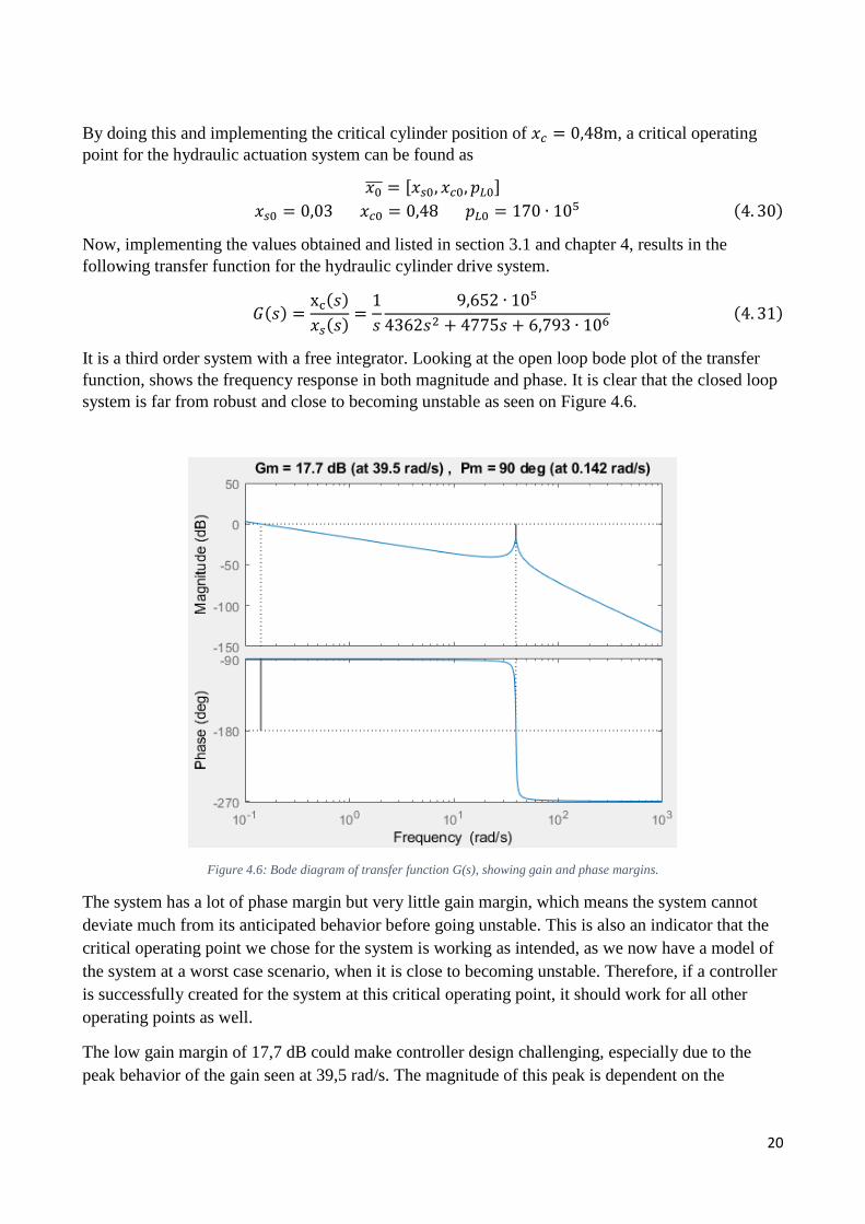
It is a third order system with a free integrator. Looking at the open loop bode plot of the transfer
function, shows the frequency response in both magnitude and phase. It is clear that the closed loop
system is far from robust and close to becoming unstable as seen on Figure 4.6.
Figure 4.6: Bode diagram of transfer function G(s), showing gain and phase margins.
The system has a lot of phase margin but very little gain margin, which means the system cannot
deviate much from its anticipated behavior before going unstable. This is also an indicator that the
critical operating point we chose for the system is working as intended, as we now have a model of
the system at a worst case scenario, when it is close to becoming unstable. Therefore, if a controller
is successfully created for the system at this critical operating point, it should work for all other
operating points as well.
The low gain margin of 17,7 dB could make controller design challenging, especially due to the
peak behavior of the gain seen at 39,5 rad/s. The magnitude of this peak is dependent on the
21
damping ratio, so it makes sense for the peak to be this high, as a very low damping ratio was
chosen for the system during linearization [8]. The low gain margin is somewhat balanced out by
the huge phase margin of 90 degrees, which leaves a lot of room for controller tweaking without the
system going unstable.
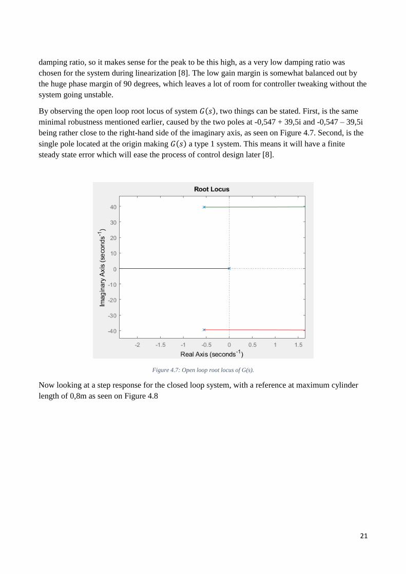
By observing the open loop root locus of system 𝐺(𝑠), two things can be stated. First, is the same
minimal robustness mentioned earlier, caused by the two poles at -0,547 + 39,5i and -0,547 – 39,5i
being rather close to the right-hand side of the imaginary axis, as seen on Figure 4.7. Second, is the
single pole located at the origin making 𝐺(𝑠) a type 1 system. This means it will have a finite
steady state error which will ease the process of control design later [8].
Figure 4.7: Open loop root locus of G(s).
Now looking at a step response for the closed loop system, with a reference at maximum cylinder
length of 0,8m as seen on Figure 4.8

22
Figure 4.8: Step response of G(s) in closed loop.
The plot shows a simulation of the cylinder moving from minimum position up to half the total
cylinder length, corresponding to a gangway pitch rotation of +20 degrees. It can be noted that the
system has zero steady state error but a slow settling time of about 40 seconds. A fast rise and
settling time is not crucial for disturbance rejection, given that the purpose of the gangway is to
rotate according to relatively slow-moving waves. But during offshore operations, time is crucial
and having to wait for a slow-moving gangway is not optimal. Therefore, a faster system is also
sought after during control design.
5 Control design This chapter will cover the control design of the plant found in earlier chapters. Before designing a
controller, it is necessary to sum up the wanted behavior and requirements for the system.
• The controller must reject at least 90% of a disturbance at maximum 8 deg/s corresponding
to 0,14 rad/s.
• A fast settling time below 10 seconds is sought after to make the gangway more responsive.
• System steady state error is to be kept at zero to ensure system precision.
• Overshoot must be kept at zero to make sure system components are not damaged during
operation. This is also for the sake of making the gangway easier to control for the operator.
• It is commonly good practice to keep phase margin above 45 degrees to ensure system
stability. Therefore, a final requirement for the controller is to keep the phase margin above
this minimum threshold.
23
A suitable and simple way to create a robust controller for the hydraulic pitch system, is to use basic
design in frequency domain. Other design methods such as pole placement could also be utilized, as
it is suitable for single-input single-output (SISO) systems as in this project. But this method can be
quite complex and usually a simpler controller is tested beforehand to see if it can suffice.
A less advanced way to control the system, is by use of phase lead and phase lag compensators or a
combination of the two. Both lead and lag compensators consist of a pole and a zero. The difference
between the two, being whether the value of the pole or the zero is largest on the real axis. Lag and
lead compensators can therefore be written as
𝐾(𝑠) = 𝐾𝑠 + 𝑧
𝑠 + 𝑝 𝑤ℎ𝑒𝑟𝑒 {
𝑧 > 𝑝 > 0 𝑓𝑜𝑟 𝑙𝑎𝑔 𝑐𝑜𝑚𝑝𝑒𝑛𝑠𝑎𝑡𝑜𝑟𝑠 𝑝 > 𝑧 > 0 𝑓𝑜𝑟 𝑙𝑒𝑎𝑑 𝑐𝑜𝑚𝑝𝑒𝑛𝑠𝑎𝑡𝑜𝑟𝑠
(5. 1)
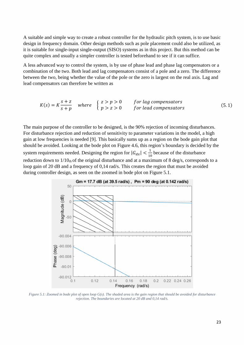
The main purpose of the controller to be designed, is the 90% rejection of incoming disturbances.
For disturbance rejection and reduction of sensitivity to parameter variations in the model, a high
gain at low frequencies is needed [9]. This basically sums up as a region on the bode gain plot that
should be avoided. Looking at the bode plot on Figure 4.6, this region’s boundary is decided by the
system requirements needed. Designing the region for |𝐺𝑑𝑥| <1
10 because of the disturbance
reduction down to 1/10th of the original disturbance and at a maximum of 8 deg/s, corresponds to a
loop gain of 20 dB and a frequency of 0,14 rad/s. This creates the region that must be avoided
during controller design, as seen on the zoomed in bode plot on Figure 5.1.
Figure 5.1: Zoomed in bode plot of open loop G(s). The shaded area is the gain region that should be avoided for disturbance
rejection. The boundaries are located at 20 dB and 0,14 rad/s.
24
To meet the requirements for the controller and avoiding the region seen in the gain plot, the loop
gain at low frequencies must be increased. This is done to reach a steeper slope of the magnitude
around the crossover frequency. Fortunately, lag compensators have this exact characteristic. By
using a lag compensator, the loop gain is increased at low frequencies while the magnitude at high
frequencies remain unchanged. The downside of using a lag compensator is the reduction of phase
at high frequencies, creating a destabilizing effect of the system [9]. Luckily as seen on Figure 4.6,
the phase margin of G(s) is very high at 90 degrees, which is useful when tweaking the lag
compensator to meet the project needs.
5.1 Simulation of control system
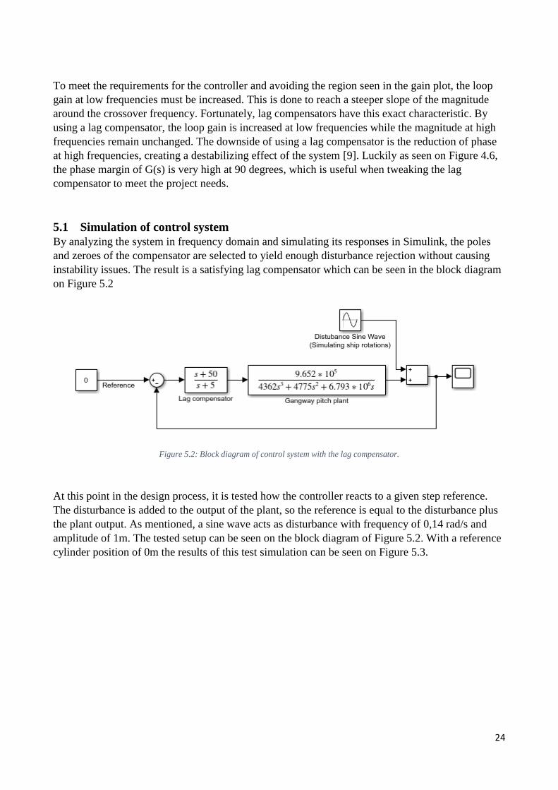
By analyzing the system in frequency domain and simulating its responses in Simulink, the poles
and zeroes of the compensator are selected to yield enough disturbance rejection without causing
instability issues. The result is a satisfying lag compensator which can be seen in the block diagram
on Figure 5.2
Figure 5.2: Block diagram of control system with the lag compensator.
At this point in the design process, it is tested how the controller reacts to a given step reference.
The disturbance is added to the output of the plant, so the reference is equal to the disturbance plus
the plant output. As mentioned, a sine wave acts as disturbance with frequency of 0,14 rad/s and
amplitude of 1m. The tested setup can be seen on the block diagram of Figure 5.2. With a reference
cylinder position of 0m the results of this test simulation can be seen on Figure 5.3.
25
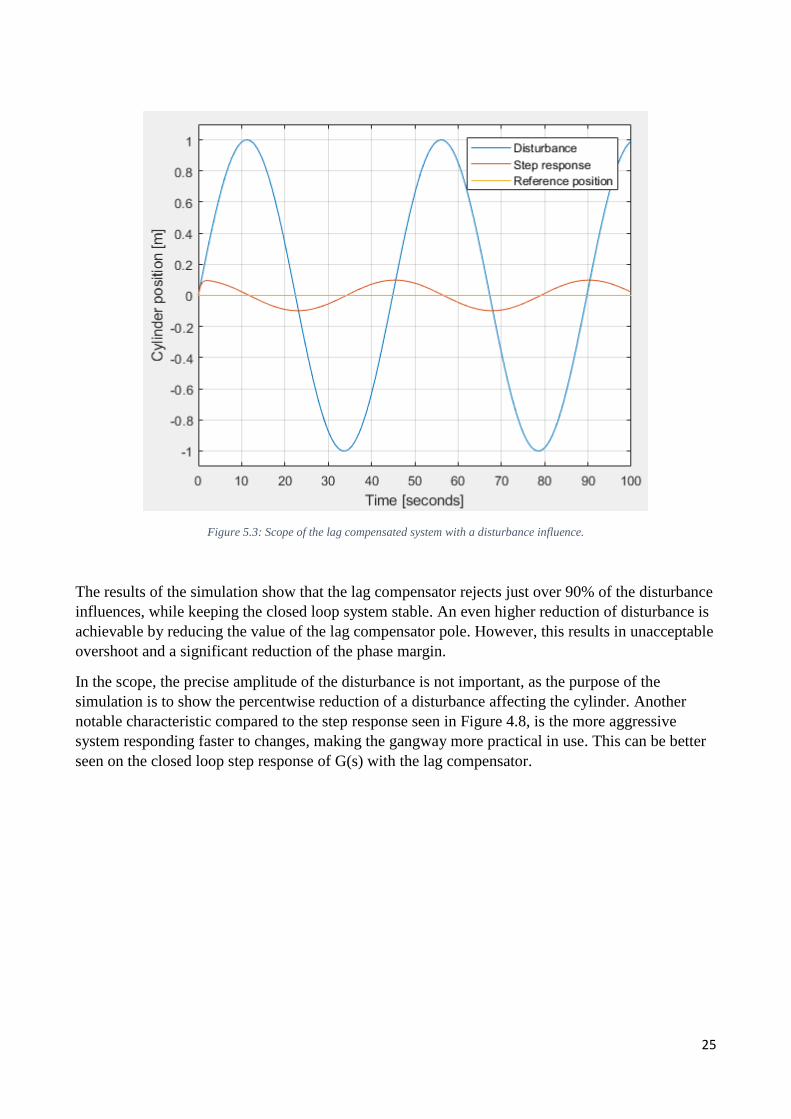
Figure 5.3: Scope of the lag compensated system with a disturbance influence.
The results of the simulation show that the lag compensator rejects just over 90% of the disturbance
influences, while keeping the closed loop system stable. An even higher reduction of disturbance is
achievable by reducing the value of the lag compensator pole. However, this results in unacceptable
overshoot and a significant reduction of the phase margin.
In the scope, the precise amplitude of the disturbance is not important, as the purpose of the
simulation is to show the percentwise reduction of a disturbance affecting the cylinder. Another
notable characteristic compared to the step response seen in Figure 4.8, is the more aggressive
system responding faster to changes, making the gangway more practical in use. This can be better
seen on the closed loop step response of G(s) with the lag compensator.
26
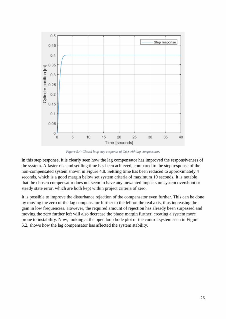
Figure 5.4: Closed loop step response of G(s) with lag compensator.
In this step response, it is clearly seen how the lag compensator has improved the responsiveness of
the system. A faster rise and settling time has been achieved, compared to the step response of the
non-compensated system shown in Figure 4.8. Settling time has been reduced to approximately 4
seconds, which is a good margin below set system criteria of maximum 10 seconds. It is notable
that the chosen compensator does not seem to have any unwanted impacts on system overshoot or
steady state error, which are both kept within project criteria of zero.
It is possible to improve the disturbance rejection of the compensator even further. This can be done
by moving the zero of the lag compensator further to the left on the real axis, thus increasing the
gain in low frequencies. However, the required amount of rejection has already been surpassed and
moving the zero further left will also decrease the phase margin further, creating a system more
prone to instability. Now, looking at the open loop bode plot of the control system seen in Figure
5.2, shows how the lag compensator has affected the system stability.

27
Figure 5.5: Open loop bode plot of the control system, with lag the lag compensator.
The gain margin has been reduced slightly by 1,4 dB but the phase margin has decreased by 13,8
degrees, which still leaves the system with a good amount of margin. Another notable change in the
bode plot is the increase in magnitude of the gain at low frequencies. This creates a steeper slope,
thus avoiding the shaded region shown in Figure 5.1, yielding over 90% disturbance rejection for
the system. The bode plot clearly shows the tradeoff between rejection percentage and system
stability. The lag compensator used here and seen in Figure 5.2, is a satisfying compromise between
system stability and disturbance rejection.
Attempts of creating a combination of lead and lag controllers were made and resulted in a minor
improvement of gain margin for the system. This came at a cost of lower disturbance rejection
percentage however. Thus, a simple lag controller is considered superior for the purpose of this
project. The controller derived in this chapter is purely for simulation purposes. To implement the
controller into a physical testing setup, it would require a rewriting of the block diagram into C
language, which a microprocessor can use to handle the data. If later work proves the need for such
a transformation, it can be done by use of a Simulink shortcut, which eases the rewriting of the
code.
28
6 Discussion Through the report, a design and analysis of the hydraulic actuation system for gangway pitch
rotations has been carried out. Hereafter, a linearized mathematical model has been established and
a controller designed to reject incoming disturbances. It was possible to simulate the control system
response to a disturbance of 0,14 rad/s and achieve stability for the system. The responsiveness of
the system was also improved, as a faster settling time was achieved while the system was kept
within project criteria. However, the final control system’s robustness is still quite low, as seen by
the low gain margin for the open loop system. It is possible that the system robustness could be
improved by further tweaking of the controller or by addition of a lead compensator. Another way
of achieving this could also be by use of a more complex control design method. A higher
robustness would make the system less prone to instability caused by unforeseen system process
variations.
Design methods
During controller design, other methods such as pole placement of full state feedback could have
been used to reach the objective. These methods are more complex however. Full state feedback
uses state space where modeling and design is done in time domain, whereas the lag compensator
used in this project is made in frequency domain. Full state feedback is commonly used for
multiple-input multiple-output (MIMO) systems, where pole placement only works for single-input
single-output (SISO) systems. In this project a SISO system was handled. Using full state feedback
method was therefore not necessary.
The reason then for using a lag compensator instead of pole placement method, was based on the
simplicity and ease of use nature of this control design method. Lead/lag compensators can be seen
as a good starting point before designing other more advanced controllers for a system. Using the
more complex method of pole placement could have yielded a better and more robust controller,
even though the objective was reached with a simpler approach. Another simple method is using
PID control design. However, this method yields a low control over poles and system response.
Experiments
This project has been carried out and evaluated based solely on an analytical approach, with
simulations trying to emulate real world physical responses. This leaves the results of this project in
a state, where verification by means of testing is sought after. When isolated, the pitch movements
of the offshore gangway can be simplified to that of a hydraulic boom crane. Thus, it is possible to
carry out verifying tests of such a system setup found on AAUE campus. However, this would
require a re-dimensioning of the hydraulic system designed in this project, as these were made to
reflect actual gangway dimensions. By use of a physical testing setup, the accuracy of the linear
29
model could be verified, as well as the effectiveness of the controller. This would allow for
improvements of the control system and easier fault detection.
Further work
Even though a satisfying controller has been designed for the pitch rotations of the gangway, further
work could be carried out to create the best possible controller for the system. A sensitivity analysis
would determine how much the cylinder drive system is changeable before becoming unstable. This
could also help clear out system parameter uncertainties such as unforeseen magnitudes of friction,
damping and load.
Furthermore, a higher stability to model uncertainties could possibly be achieved during control
design in the frequency bode analysis. Here, a second region to be avoided at high frequencies,
could have been introduced. This would effectively require the controller to ensure low loop gain at
higher frequencies. Doing this would also make the control system better able to handle possible
sensor measurement noises. However, this was deemed unnecessary for this project due to the lack
of physical sensors. At this point in the project, it would be pure speculation to which amount of
noise would affect the system.
Another possible way to improve the gangway control system, is to examine the possibilities of
testing the linear model controller on the non-linear model. This would ensure the accuracy of the
linearization, by comparing the controller’s response on the two models.
By continuing the work done in this project, it is possible to create an offshore gangway which can
compensate for motions in all other degrees of freedom. Creating a controller for gangway yaw
rotations would first require a new system model derivation and design. This is due to the
movements in this DOF is most likely to be handled by AC motor rotations. The same could be said
for extension and contraction movements of the gangway. However, gangway roll motions could be
controlled by the same hydraulic actuation system used for pitch rotations. This would be by means
of separate motion in the two hydraulic actuators, creating a rolling movement of the gangway.
30
7 Conclusion
Implementing active disturbance rejection in offshore gangways is no new endeavor. In fact, many
products offering motion compensation during offshore operations, are already on the market. The
task of creating a cheaper, smaller scale and easy to use motion compensated gangway, originated
during an internship at SubC Partner in Esbjerg. The preliminary work done during the internship,
was then continued and improved upon in this project.
Following the initial work on the project, it was decided that a narrower, more in-depth analysis and
design of the pitch rotation mechanic was preferred to a wider and more general approach, where all
DOF’s are included. This allowed for better inclusion of theory and methods learned during
previous semester lectures, such as “Offshore Technology and Hydraulic Systems”. This approach
to the project also allowed for more advanced system designs and being more creative with the
gangway pitch actuation system.
The project resulted in a finished theoretical design of the hydraulic actuation system, with its
corresponding linearized mathematical model derived. A satisfying controller was designed in
frequency domain to meet all set criteria for the system. Experimental testing is however still
needed for verification of the system and controller design.
Summarizing the findings of the project:
• A suitable hydraulic cylinder drive system was theoretically designed for gangway pitch
rotations and a linearized model of said system was successfully created.
• Using lead/lag compensator design rules in frequency domain, a controller was made which
satisfies set criteria, by stably reducing over 90% of a disturbance of 8 deg/s.
• The lag compensator introduced significantly improved the responsiveness of the control
system. This reduced settling time to 4 seconds making the gangway system more practical
in use.
• The controller did not introduce a steady state error, nor did it create any unwanted
overshoot, thus staying at zero percent.
• To further improve the design, better testing conditions are required. This includes the
addition of a physical experimental setup for verification and possible improvements of the
drive system and controller.
• Attempts were made to create combination of lead and lag compensators to improve the low
gain margin of the system, thereby effectively increasing its stability. However, these
attempts resulted in failure at reaching the criteria of 90% disturbance rejection.
31
8 Bibliography
[1
] C. Lindquist, E. Hansen, P. Nielsen, L. Jensen and R. Pedersen, "Control of Marine Satellite Tracking
Antenna," Esbjerg, 2016.
[2
]
DNV-GL, "Certification of offshore gangways for personel transfer," December 2015. [Online]. Available:
https://rules.dnvgl.com/docs/pdf/DNVGL/ST/2015-12/DNVGL-ST-0358.pdf. [Accessed 23 November
2017].
[3
]
"Data or graphical materiel granted by SubC Partner". Danmark 2017.
[4
]
T. I. Fossen, Handbook of Marine Craft Hydrodynamics and Motion Control., John Wiley & Sons, 2011.
[5
]
T. O. Andersen and M. R. Hansen, "Fluid Power Circuits, 3rd Edition," Aalborg, June 2007.
[6
]
T. O. Andersen, Fluid Power Systems: Modelling and Analysis, 2nd Edition, Aalborg: Institute of Energy
Technology, 2003.
[7
]
L. Schmidt, " Robust Control of Industrial Hydraulic Cylinder Drives-with Special Reference to Sliding
Mode," [Online]. Available:
https://www.moodle.aau.dk/pluginfile.php/941089/mod_resource/content/0/Generalized_Linear_Mo
del_for_Valve_Dylinder_Drive.pdf. [Accessed 12 December 2017].
[8
]
G. F. Franklin, J. D. Powell and A. Emami-Naeini., Feedback Control of Dynamic Systems. Pearson, 7.
edition, 2015. ISBN 10:1-29-206890-6.
[9
]
M. Soltani, "Basic controller design in frequency domain," 21 February 2017. [Online]. Available:
file:///C:/Users/Lukas/Google%20Drev/Afgangsprojekt/Filer%20og%20læsning/Lead_Lag_Mohsen.pdf.
[Accessed 15 December 2017].
Related Documents