Control of arm movement using population of neurons

Control of Arm Movement Using Population of Neurons

Zoran Nenadic†, Charles H. Anderson‡ and Bijoy Ghosh†

†Department of Systems Science and Mathematics ‡Department of Anatomy & NeurobiologyWashington University Washington UniversitySaint Louis, MO 63130 Saint Louis, MO [email protected] [email protected]@zach.wustl.edu

Abstract

Movements of human arm in a horizontal plane are very stereotyped in the sense thatthe corresponding paths are mainly straight lines and the velocity profiles are “bell-shapedlike” functions. A dynamics of two link model of the human arm has been studied with thegoal of synthesizing the torques which accomplish the desired transfer. For that purposea set of parameters which describes the desired transition (initial position, final position,peak velocity, etc.) is chosen randomly according to a certain distribution. The parametersof the desired trajectory as well as the system variables (angles and angular velocities) areencoded using populations of different number of neurons, usually 100− 150. The underly-ing mathematics including integration, differentiation and other algebraic relationships, hasbeen done at the level of neuronal activity. Finally, the driving torques are generated fromthe corresponding activities using an optimal decoding rule.

1 Introduction

It has been experimentally verified that humans tend to reach from one point in a horizontalplane to another in a stereotyped fashion, that is, the path of a human wrist is primarilya straight line, while the corresponding velocity profile is a bell-shaped function. Moreover,the peak velocity and the distance traveled by a wrist are not independent, i.e. the longer thedistance, the higher the peak velocity, which implies that the total time of transfer remainsfairly constant over different experimental trials, see [1].

2 Mathematical Model

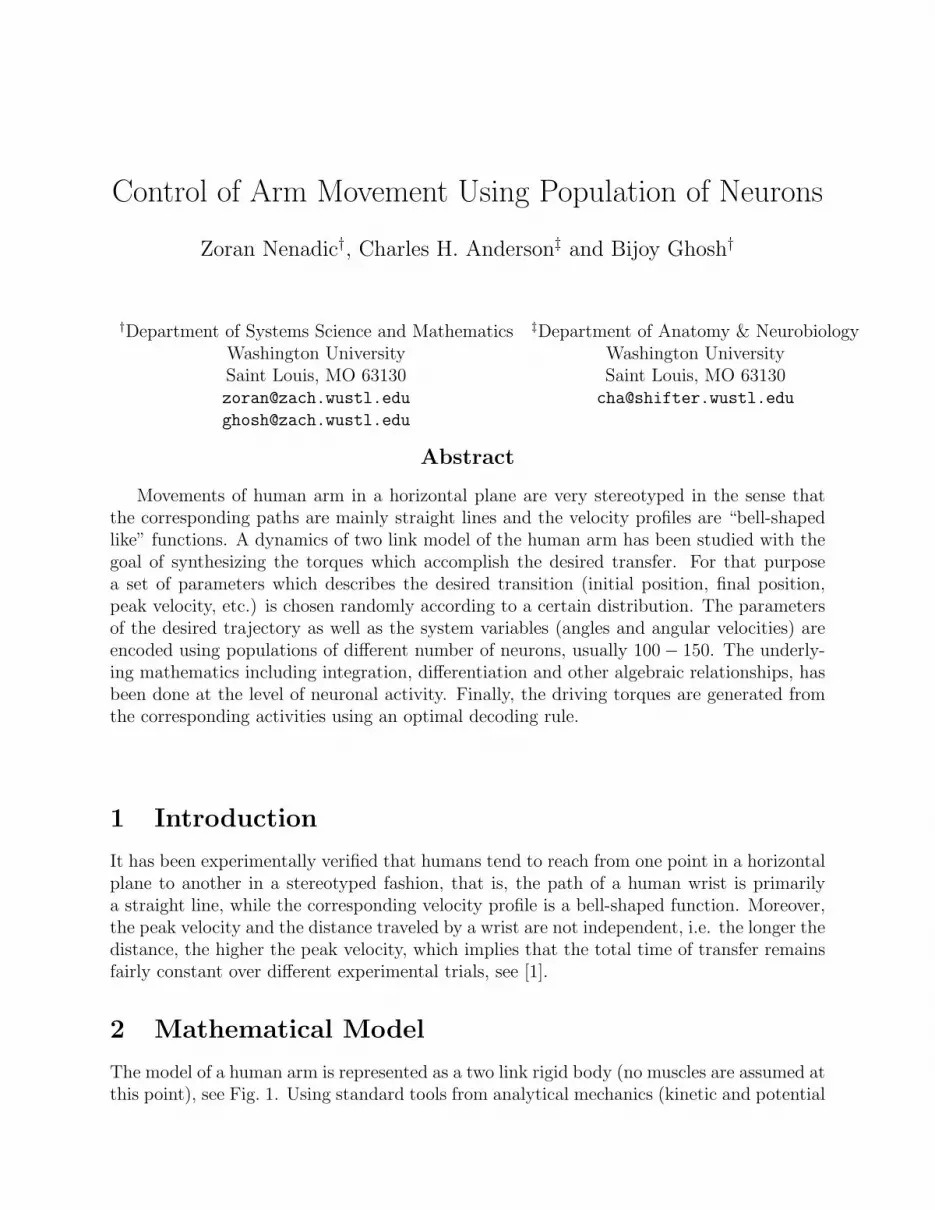
The model of a human arm is represented as a two link rigid body (no muscles are assumed atthis point), see Fig. 1. Using standard tools from analytical mechanics (kinetic and potential

energy, Lagrangian and Lagrange equations of motion) the nonlinear model of the two linksystem has been obtained:

θ

φ

x

y

1

2

Figure 1: Two link system in horizontal plane.

x = f(x) + g(x)u (1)

where x = [θ, φ, θ, φ]T . Equation (1) can be rewritten as:[

x1

x2

]

=[

x3

x4

]

[

x3

x4

]

= −T−1(x)C(x)[

x3

x4

]

+ T−1(x)[

τs

τe

]

(2)

where

T (x) =[

t1 + t2 + 2t3 cos(x2) t2 + t3 cos(x2)t2 + t3 cos(x2) t2

]

represents the inertial matrix, and

C(x) =[

−t3 sin(x2)x4 −t3 sin(x2)(x3 + x4)t3 sin(x2)x3 0

]

is the matrix of Coriolis and centripetal terms. Since the problem is defined in a horizontalplane, there are no gravity forces in the model (2). The friction forces have been neglectedfor this analysis. The terms t1, t2 and t3 are defined as follows:

t1 = m1( l12 )2 + m2l21 + J1 t2 = m2( l1

2 )2 + J2 t3 = m2l1 l22

where mi is the mass of the i− th link, li is its length and Ji represents its moment of inertiawith respect to its center of gravity (i = 1, 2).

3 Control

The vector of external inputs u = [τs, τe]T contains the two torques τs (shoulder) and τe

(elbow), both applied in a horizontal plane, which are to be synthesized by a population ofneurons. The torques are first found analytically using feedback linearization, a procedurefor stabilizing certain class of nonlinear systems, see [2]. This provides an elegant solutioni.e. the synthesized torques depend both on the desired parameters (via desired anglesand desired velocities) and the actual position and velocity, and thus can be viewed as acombination of feedforward/feedback signal. The feedback linearization technique is basedon a local change of coordinates which define so called normal form of the system (2). Letus first define two output equations for the system (2), where y1 and y2 are chosen such thatthe system has defined the vector relative degree r = [r1, r2], see [2]:

y1 = h1(x)(3)

y2 = h2(x)

where h1(x) = x1 and h2(x) = x2. Note that the definition of y1 and y2 is only for the purposeof exact feedback realization, and is chosen arbitrarily. However the choice of the functionsh1(x) and h2(x) is sensible, as x1 = θ and x2 = φ are readily available for measurements(feedback). Thus the system (2) can be rewritten as:

[

x1

x2

]

=[

x3

x4

]

[

x3

x4

]

= −T−1(x)C(x)[

x3

x4

]

+ T−1(x)[

τs

τe

]

(4)

y1 = h1(x)y2 = h2(x)

For this system it is easily found that:

Lg1h1 = 0 Lg2h1 = 0

and

Lg1Lfh1 6= 0 Lg2Lfh1 6= 0

Likewise

Lg1h2 = 0 Lg2h2 = 0

and

Lg1Lfh2 6= 0 Lg2Lfh2 6= 0

where Lfh.= ∂h(x)

∂x f(x) represents the derivative of the vector field h along f . Therefore thesystem (4) has defined vector relative degree r = [2, 2] at some initial point x◦. This, together

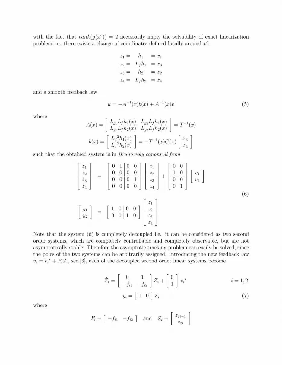
with the fact that rank(g(x◦)) = 2 necessarily imply the solvability of exact linearizationproblem i.e. there exists a change of coordinates defined locally around x◦:

z1 = h1 = x1

z2 = Lfh1 = x3

z3 = h2 = x2

z4 = Lfh2 = x4

and a smooth feedback law

u = −A−1(x)b(x) + A−1(x)v (5)

where

A(x) =[

Lg1Lfh1(x) Lg2Lfh1(x)Lg1Lfh2(x) Lg2Lfh2(x)

]

= T−1(x)

b(x) =[

Lf2h1(x)

Lf2h2(x)

]

= −T−1(x)C(x)[

x3

x4

]

such that the obtained system is in Brunowsky canonical from

z1

z2

z3

z4

=

0 1 0 00 0 0 00 0 0 10 0 0 0

z1

z2

z3

z4

+

0 01 00 00 1

[

v1

v2

]

(6)

[

y1

y2

]

=[

1 0 0 00 0 1 0

]

z1

z2

z3

z4

Note that the system (6) is completely decoupled i.e. it can be considered as two secondorder systems, which are completely controllable and completely observable, but are notasymptotically stable. Therefore the asymptotic tracking problem can easily be solved, sincethe poles of the two systems can be arbitrarily assigned. Introducing the new feedback lawvi = vi

∗ + FiZi, see [3], each of the decoupled second order linear systems become

Zi =[

0 1−fi1 −fi2

]

Zi +[

01

]

vi∗ i = 1, 2

yi =[

1 0]

Zi (7)

where

Fi =[

−fi1 −fi2]

and Zi =[

z2i−1

z2i

]

The second equation of the system (7) can be rewritten by back substitution as

θ = −f11θ − f12θ + v1∗ (8)

for i = 1, and likewiseφ = −f21φ− f22φ + v2

∗ (9)

for i = 2. Thus, v∗1 and v∗2 have to be chosen so that the error differential equation has thefollowing form

ε + fi2ε + fi1ε = 0 (10)

where ε = θd − θ or ε = φd − φ and the subscript d stands for desired. For asymptoticstability, we need fi1, fi2 > 0. From (8), (9) and (10) readily follows

v1∗ = θd + f12θd + f11θd

(11)v2∗ = φd + f22φd + f21φd

Hence, the torque pair which will cause the system (4) to follow the desired trajectoryparameterized by (θd, φd) and the desired velocity profile parameterized by (θd, φd) is givenby

[

τs

τe

]

= C[

θφ

]

+ T[

θd + f12(θd − θ) + f11(θd − θ)φd + f22(φd − φ) + f21(φd − φ)

]

(12)

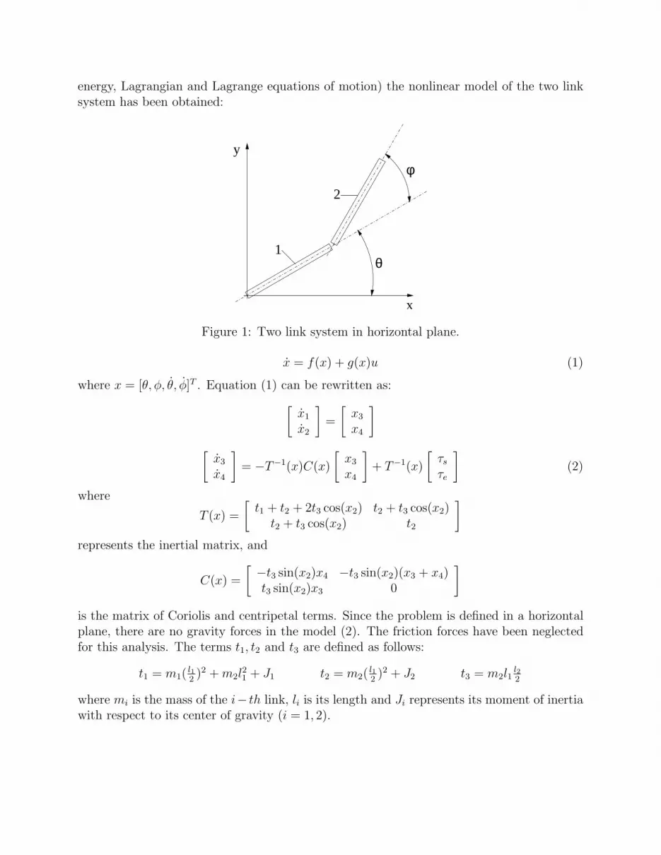
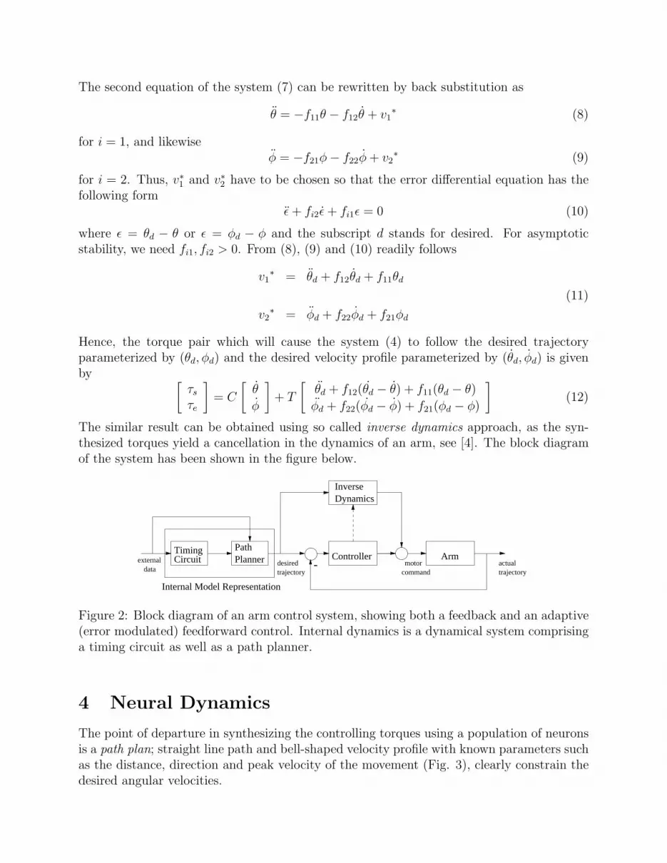
The similar result can be obtained using so called inverse dynamics approach, as the syn-thesized torques yield a cancellation in the dynamics of an arm, see [4]. The block diagramof the system has been shown in the figure below.

desiredtrajectory

Dynamics

-trajectory

Armmotor

commandactual

Inverse

dataexternal

Internal Model Representation

PathControllerPlanner

TimingCircuit

Figure 2: Block diagram of an arm control system, showing both a feedback and an adaptive(error modulated) feedforward control. Internal dynamics is a dynamical system comprisinga timing circuit as well as a path planner.

4 Neural Dynamics

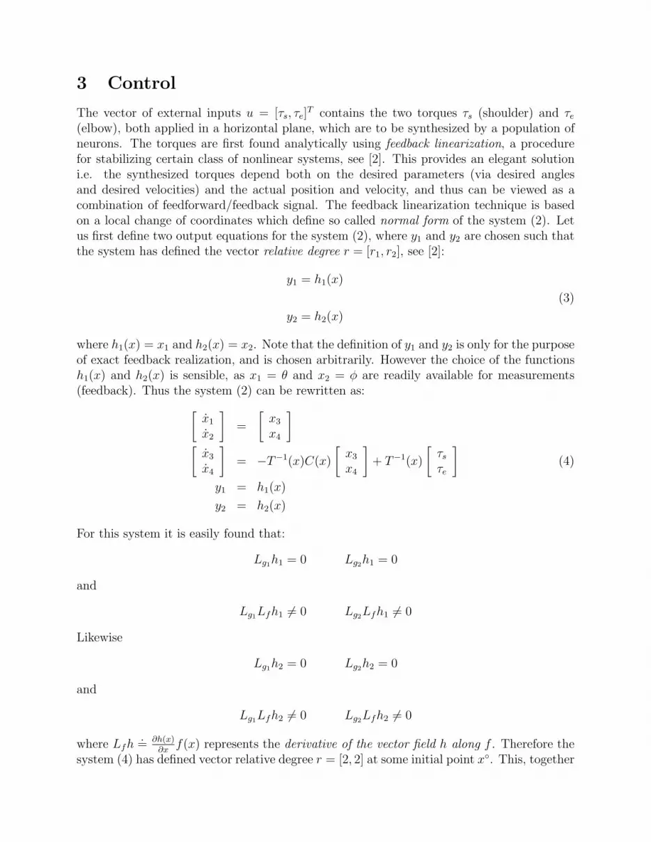
The point of departure in synthesizing the controlling torques using a population of neuronsis a path plan; straight line path and bell-shaped velocity profile with known parameters suchas the distance, direction and peak velocity of the movement (Fig. 3), clearly constrain thedesired angular velocities.

0 T/2 T

Vm

timeve

loci

ty m

agni

tude

Figure 3: The velocity profile plot; Vm– peak velocity, T– total time of transfer.

The initial position of the arm has been randomized by choosing the initial angles from auniform distribution. The final position is also random in the sense that it is determined bya human decision (where we want to reach). The peak velocity is chosen randomly but withhigh correlation to the total distance, which is known once the initial and final position havebeen specified, see Fig. (4). This assumption has a biological relevance; if we want to reachfarther, we do it with higher velocity so that the total reaching time remains fairly constantover different trials. The average time of the transfer is assumed to be 0.5 (sec). Using the

0 0.3 0.6 0.90

1

2

3

4

distance [m]

Vm

[m/s

ec]

Figure 4: Correlation between the peak velocity Vm and the distance.

obvious kinematic relationship, the velocity of the wrist can be expressed as

−→V (t) =

Vm

2(1− cos(

2πtT

))−→rf −−→ri

δ(13)

where −→ri and −→rf are the vectors of the initial and final positions of the arm, δ =‖ −→rf −−→ri ‖,and Vm

2 (1−cos(2πtT )) is a mathematical fit of the bell shaped function described earlier, which

can be thought of as a solution to the second order differential equation

u + ω2u = ω2 (14)

with zero initial conditions, where ω = 2πt/T . The equation (14) is solved using a populationof neurons approach, where the neurons are assumed to be responsible for encoding analog

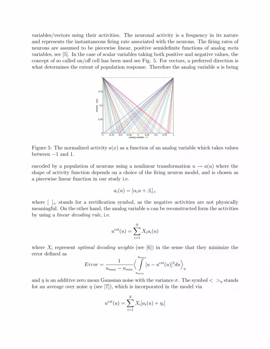
variables/vectors using their activities. The neuronal activity is a frequency in its natureand represents the instantaneous firing rate associated with the neurons. The firing rates ofneurons are assumed to be piecewise linear, positive semidefinite functions of analog metavariables, see [5]. In the case of scalar variables taking both positive and negative values, theconcept of so called on/off cell has been used see Fig. 5. For vectors, a preferred direction iswhat determines the extent of population response. Therefore the analog variable u is being

−1 −0.75 −0.5 −0.25 0 0.25 0.5 0.75 10

0.25

0.5

0.75

1

analog variable − x

activ

ity −

a(x

)

Figure 5: The normalized activity a(x) as a function of an analog variable which takes valuesbetween −1 and 1.

encoded by a population of neurons using a nonlinear transformation u → a(u) where theshape of activity function depends on a choice of the firing neuron model, and is chosen asa piecewise linear function in our study i.e.

ai(u) = [αiu + βi]+

where [ ]+ stands for a rectification symbol, as the negative activities are not physicallymeaningful. On the other hand, the analog variable u can be reconstructed form the activitiesby using a linear decoding rule, i.e.

uest(u) =N

∑

i=1

Xiai(u)

where Xi represent optimal decoding weights (see [6]) in the sense that they minimize theerror defined as

Error =1

umax − umin

⟨

umax∫

umin

[u− uest(u)]2du⟩

η

and η is an additive zero mean Gaussian noise with the variance σ. The symbol < >η standsfor an average over noise η (see [7]), which is incorporated in the model via

uest(u) =N

∑

i=1

Xi[ai(u) + ηi]

where ηi are independent identically distributed random variables ηi ∼ N (0, σ2) and N isthe total number of neurons within a population. Likewise, there is another population ofM neurons which encodes u via a nonlinear transformation i.e.

bj(u) = [γju + δj]+

with the corresponding decoding rule

uest(u) =M

∑

j=1

Yjbj(u)

The differential equation (14) can now be translated at the level of activities

dan(t)dt

= −1τ

an(t)−

[

N∑

i=1

ω(int)ni ai(t) + τ

M∑

j=1

ω(ext)nj bj(t) + βn

]

+

(15)

dbm(t)dt

= −1τ

bm(t)−

[

M∑

j=1

ω(int)mj bj(t) + τ(ω2 − ω2

N∑

i=1

ω(ext)mi ai(t)) + δm

]

+

where the coupling weights for the oscillator (14) are given by

ω(int)ni = αnXi ω(ext)

nj = αnYj ω(int)mj = γmYj ω(ext)

mi = γmXi

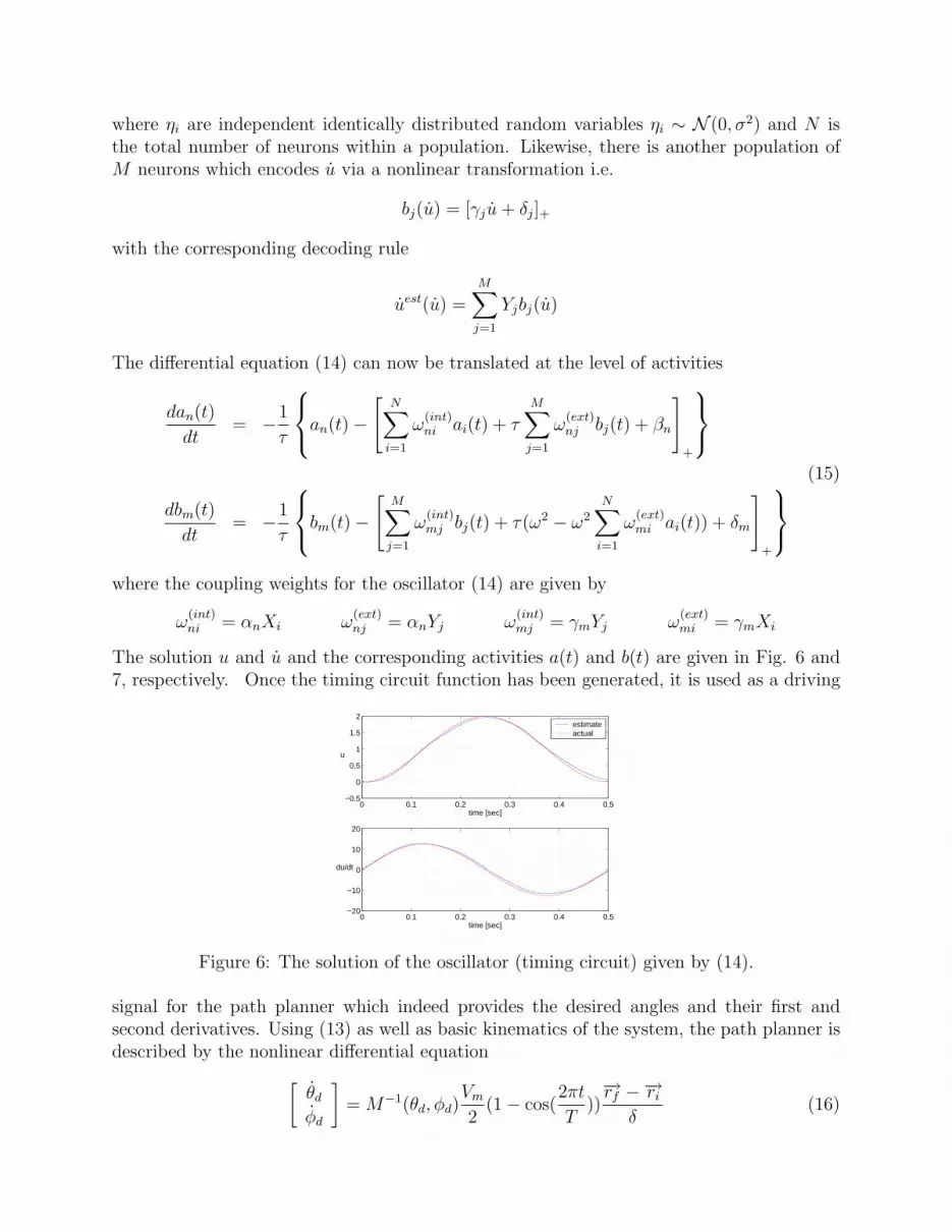
The solution u and u and the corresponding activities a(t) and b(t) are given in Fig. 6 and7, respectively. Once the timing circuit function has been generated, it is used as a driving

0 0.1 0.2 0.3 0.4 0.5−0.5

0

0.5

1

1.5

2

time [sec]

u

estimateactual

0 0.1 0.2 0.3 0.4 0.5−20

−10

0

10

20

time [sec]

du/dt

Figure 6: The solution of the oscillator (timing circuit) given by (14).

signal for the path planner which indeed provides the desired angles and their first andsecond derivatives. Using (13) as well as basic kinematics of the system, the path planner isdescribed by the nonlinear differential equation

[

θd

φd

]

= M−1(θd, φd)Vm

2(1− cos(

2πtT

))−→rf −−→ri

δ(16)

0 0.1 0.2 0.3 0.4 0.50

0.2

0.4

0.6

0.8

1

time [sec]

activ

ity

0 0.1 0.2 0.3 0.4 0.50

0.2

0.4

0.6

0.8

1

time [sec]

activ

ity

Figure 7: The neuronal activities as functions of time. The activities a(u(t)) (left) andb(u(t)) (right).

where

M(θd, φd) =[

−l1 sin(θd)− l2 sin(θd + φd) −l2 sin(θd + φd)l1 cos(θd) + l2 cos(θd + φd) l2 cos(θd + φd)

]

The equation (16) is to be solved by another population of neurons, where −→ri and −→rf areencoded using a rule of preferred direction. This can be thought of as internal dynamics,see [8], and represents a feedforward path in the synthesis of the control torques (Fig. 2).Likewise, the actual position and velocities can be encoded using another populations ofneurons, which comes from the human sensory system and is included in the structure of thetorques as a feedback path. The neuronal activities are often referred to as explicit space,because biologists can make direct measurements on them, see [5]. Finally, the two torquesare encoded by ensembles of neurons, whose activities (firing rates) involve the whole set(vector) of analog variables e.g. the desired and actual angles, desired and actual velocities,etc. The torques are then obtained from the activities using optimal decoding rule, in thesame way it was described earlier. Note that this procedure represents the reconstructionof analog variable/vector as a weighted sum of suitably chosen basis functions, see [6], andwhere the weights are chosen in such a way that the reconstruction error is minimized. Inthis case, the basis functions are actually the neuronal activities, and the desired torques aresimply linear (weighted) combination of these functions.

5 Simulation Results

The procedure described above has been tested by simulations, and the deviations of theactual path from the desired one (straight line) are negligible, see Fig. 8. Also the specifiedvelocity profile and angles have been followed quite accurately, Fig. 9 which is not surprisingas a population of 100−150 neurons does fairly well in terms of the precision of representation.

−0.4 −0.2 0 0.2 0.4 0.6

−0.4

−0.2

0

0.2

0.4

0.6

−0.4 −0.2 0 0.2 0.4 0.6

−0.4

−0.2

0

0.2

0.4

0.6

Figure 8: The initial (left) and final position of the arm together with the path (right).

0 0.1 0.2 0.3 0.4 0.5 0.6 0.70

0.5

1

1.5

2

2.5

3

3.5actual desired

0 0.1 0.2 0.3 0.4 0.50

2

4

θ

0 0.1 0.2 0.3 0.4 0.50

1

2

φ

desiredactual

0 0.1 0.2 0.3 0.4 0.5−10

0

10

dθ/dt

0 0.1 0.2 0.3 0.4 0.5−10

0

10

time [sec]

dφ/dt

Figure 9: The desired and actual velocity profiles (left) and the desired and actual anglesand angular velocities (right).

6 Conclusion

The experimental evidence shows that the movements of human arm in a horizontal planeare very simple. Very often in a task of reaching from one point to another, we use a straightline path and a bell shaped velocity profile. The question of interest is how do we generatethe torques which will make the arm accomplish the desired transfer while following theconstraints imposed on it? In robotics, tracking the desired trajectory is a very standardproblem, which can easily be solved using feedback linearization. This procedure is elegant inthe sense that the generated control (torques) are synthesized through feedforward/feedbacksubsystems, where the feedforward action can be attributed to a specific neural circuitrysuch as the cerebellum. On the other hand, the source of the feedback is yet to be specified,even though there is no doubt about its existence. We assumed it originates from the sensorysystem, and is incorporated in the model with a delayed action, as any other feedback lawwould be. It might be even coming from a visual system, although the delays would be muchhigher in that case. Of course the combination of the two is the most realistic scenario. Thefuture work would be in the direction of making the more realistic model of human arm,using muscles and their dynamics. The activities will then be driving the muscles, which willrespond by exerting forces and torques, consequently. Also, the other types of movementscan be studied, not necessarily in a horizontal plane, which certainly is a harder and morechallenging problem.

References

[1] A. J. Bastian, T. A. Martin, J. G. Keating and W. T. Thach, Cerebellar ataxia: ab-normal control of interaction torques across multiple joints, J. Neurophysiol. 76 (1996)492–509.

[2] Alberto Isidori, Nonlinear Control Systems, Springer-Verlag, 1989.

[3] Bijoy K. Ghosh, Ning Xi and T. J. Tarn, Control in Robotics and Automation, Sensor–Based Integration, Academic Press, 1999.

[4] N. Schweighofer, J. Spoelstra, M. A. Arbib and M. Kawato, Role of the cerebellum inreaching quickly and accurately: II A detailed model of the intermediate cerebellum,European J. Neurosci., in press., 1997.

[5] C. Eliasmith and C. H. Anderson, Developing and applying a toolkit from a generalneurocomputational framework, Neurocomputing. 26-27 (1999) 1013–1018.

[6] C. Eliasmith and C. H. Anderson, Rethinking central pattern generators: a generalapproach, in Proc. 8th Annual Computational Neuroscience 26-27 (1999) 1013–1018.

[7] F. Rieke, D. Warland, R. Steveninck and W. Bialek, Spikes–Exploring the Neural Code,The MIT Press, 1997

[8] E. Nakano, H. Imamizu, R. Osu, Y. Uno, H. Gomi, T. Yoshioka and M. Kawato: Quan-titative examinations of internal representations for arm trajectory planning: minimumcommanded torque change model, J. Neurophysiol. 81 (1999) 2140-2155,.