University of Calgary PRISM: University of Calgary's Digital Repository Graduate Studies The Vault: Electronic Theses and Dissertations 2013-01-25 Control of an Unconventional VTOL UAV for Complex Maneuvers Amiri, Nasibeh Amiri, N. (2013). Control of an Unconventional VTOL UAV for Complex Maneuvers (Unpublished doctoral thesis). University of Calgary, Calgary, AB. doi:10.11575/PRISM/25452 http://hdl.handle.net/11023/462 doctoral thesis University of Calgary graduate students retain copyright ownership and moral rights for their thesis. You may use this material in any way that is permitted by the Copyright Act or through licensing that has been assigned to the document. For uses that are not allowable under copyright legislation or licensing, you are required to seek permission. Downloaded from PRISM: https://prism.ucalgary.ca

Welcome message from author
This document is posted to help you gain knowledge. Please leave a comment to let me know what you think about it! Share it to your friends and learn new things together.
Transcript

University of Calgary
PRISM: University of Calgary's Digital Repository
Graduate Studies The Vault: Electronic Theses and Dissertations
2013-01-25
Control of an Unconventional VTOL UAV for Complex
Maneuvers
Amiri, Nasibeh
Amiri, N. (2013). Control of an Unconventional VTOL UAV for Complex Maneuvers (Unpublished
doctoral thesis). University of Calgary, Calgary, AB. doi:10.11575/PRISM/25452
http://hdl.handle.net/11023/462
doctoral thesis
University of Calgary graduate students retain copyright ownership and moral rights for their
thesis. You may use this material in any way that is permitted by the Copyright Act or through
licensing that has been assigned to the document. For uses that are not allowable under
copyright legislation or licensing, you are required to seek permission.
Downloaded from PRISM: https://prism.ucalgary.ca

UNIVERSITY OF CALGARY
Control of an Unconventional VTOL UAV for Complex Maneuvers
by
Nasibeh Amiri
A THESIS
SUBMITTED TO THE FACULTY OF GRADUATE STUDIES
IN PARTIAL FULFILMENT OF THE REQUIREMENTS FOR THE
DEGREE OF DOCTOR OF PHILOSOPHY
ELECTRICAL AND COMPUTER ENGINEERING
CALGARY, ALBERTA
January, 2013
c© Nasibeh Amiri 2013

Abstract
The increasing potential applications of Unmanned Aerial Vehicles (UAV) provides
the motivations for numerous research to focus on developing fully autonomous and
self guided UAVs with the purpose of controlling UAVs in confined environments.
Current UAVs control systems are not able to offer the precise trajectory regulation
required in autonomous flight technology. These systems fail to control aerial vehi-
cles’ performing complex maneuvers through confined environments because current
UAV designs do not have suitable control mechanisms providing agility and stability
for the required maneuvers. New advances in control theory are required to over-
come these limitations in order to enable aggressive autonomous vehicle maneuvering
while adapting in real time to changes in the operational environment. This thesis
addresses a control problem of an unconventional highly maneuverable Vertical Take-
off and Landing (VTOL) UAV, using tilted ducted fans as flight control mechanism.
The main purpose of this research is to design a nonlinear control methodology that
enables the vehicle to use the full potential of its flying characteristics for independent
control of its six degree-of-freedom, including orientation and position of the UAV.
This thesis investigates maneuvering inside obstructed environments in the presence
of external disturbances such as wind, ground and wall effects. Achieving this goal is
possible due to a revolution in aviation control by introducing Oblique Active Tilting
(OAT) mechanism. Capabilities of OAT system will be fully used in controlling the
UAV to enhance its maneuverability.
ii

Acknowledgments
I would like to gratefully and sincerely thank my supervisor, Dr. Robert Davies,
and my co-supervisor, Dr. Alejandro Ramirez-Serrano, for their continuous support,
generosity in sharing their knowledge and guidance during period of this research.
Besides, I take this opportunity to express my gratitude to all staffs of the Department
of Electrical and Computer Engineering in University of Calgary for providing an
excellent working environment.
I would like to acknowledge and thank all my friends for their love and efforts
and for being the surrogate family which made me feel more at home. Particularly, I
would like to express my gratitude to my very kind friend, Arya Janjani, for his time
and help.
Finally, yet importantly, I would like to thank my lovely parents, sisters, and
brother-in-law whose unwavering love and support kept me motivated throughout
the hardship of this experience. I offer my heartfelt thanks to my beloved Sepehr for
his endless patience, kindness and encouragement when it was most required and his
continued moral support that helped me a lot in completion of this project.
iii

Table of Contents
Abstract . . . . . . . . . . . . . . . . . . . . . . . . . . . . . . . . . . . . . . ii
Acknowledgments . . . . . . . . . . . . . . . . . . . . . . . . . . . . . . . . iii
Table of Contents . . . . . . . . . . . . . . . . . . . . . . . . . . . . . . . . iv
List of Figures . . . . . . . . . . . . . . . . . . . . . . . . . . . . . . . . . . vii
Nomenclature . . . . . . . . . . . . . . . . . . . . . . . . . . . . . . . . . . xi
1 Introduction . . . . . . . . . . . . . . . . . . . . . . . . . . . . . . . . . 51.1 Background of Unmanned Aerial Vehicles . . . . . . . . . . . . . . . 7
1.1.1 Examples of Unmanned Aerial Vehicles . . . . . . . . . . . . 81.2 Introducing the eVader Unmanned Aerial Vehicle . . . . . . . . . . . 101.3 Motivation . . . . . . . . . . . . . . . . . . . . . . . . . . . . . . . . 121.4 General Problem Statement . . . . . . . . . . . . . . . . . . . . . . . 141.5 Thesis Outline . . . . . . . . . . . . . . . . . . . . . . . . . . . . . . 16
2 Literature Review . . . . . . . . . . . . . . . . . . . . . . . . . . . . . . 172.1 Overview of Previous Research on UAV Control . . . . . . . . . . . . 17
2.1.1 Linear Control Techniques of UAV Flight Control . . . . . . . 182.1.2 Nonlinear Control Techniques of UAV Flight Control . . . . . 212.1.3 Control of eVader Vehicle in the Literature . . . . . . . . . . 24
2.2 Objectives and Goals . . . . . . . . . . . . . . . . . . . . . . . . . . 252.3 Definitions . . . . . . . . . . . . . . . . . . . . . . . . . . . . . . . . 282.4 Summary . . . . . . . . . . . . . . . . . . . . . . . . . . . . . . . . . 31
3 Modeling . . . . . . . . . . . . . . . . . . . . . . . . . . . . . . . . . . . 333.1 Introduction . . . . . . . . . . . . . . . . . . . . . . . . . . . . . . . 343.2 Lift-fan OAT Mechanism . . . . . . . . . . . . . . . . . . . . . . . . 35
3.2.1 Special Characteristics of OAT . . . . . . . . . . . . . . . . . 373.2.2 Overview of sOAT and dOAT . . . . . . . . . . . . . . . . . . 40
3.3 Lateral and Longitudinal Rotor Tilting VTOL Modeling . . . . . . . 413.3.1 Translational Dynamics . . . . . . . . . . . . . . . . . . . . . 443.3.2 Ground and wall effects . . . . . . . . . . . . . . . . . . . . . 49
iv

3.3.3 Rotational Dynamics . . . . . . . . . . . . . . . . . . . . . . 493.4 Complete Dynamic Model of The eVader . . . . . . . . . . . . . . . 54
3.4.1 Approximation of Equations of Motion . . . . . . . . . . . . . 563.5 Summary . . . . . . . . . . . . . . . . . . . . . . . . . . . . . . . . . 58
4 Feedback Linearization Control of eVader . . . . . . . . . . . . . . . 604.1 Overview and Background of Feedback Linearization . . . . . . . . . 61
4.1.1 Controllability . . . . . . . . . . . . . . . . . . . . . . . . . . 634.2 Modeling for Control . . . . . . . . . . . . . . . . . . . . . . . . . . . 654.3 eVader’s Feedback Linearization Design . . . . . . . . . . . . . . . . 674.4 Nonlinear Adaptive Control . . . . . . . . . . . . . . . . . . . . . . . 72
4.4.1 Adaptive Control Design for the eVader’s Orientation . . . . 744.4.2 Adaptive Control Design for the eVader’s Position . . . . . . 76
4.5 Stability Analysis . . . . . . . . . . . . . . . . . . . . . . . . . . . . 774.6 Robust Adaptive Feedback Linearization . . . . . . . . . . . . . . . . 784.7 Simulation Results . . . . . . . . . . . . . . . . . . . . . . . . . . . . 794.8 Results and discussion . . . . . . . . . . . . . . . . . . . . . . . . . . 81
5 Integral Backstepping Control of eVader . . . . . . . . . . . . . . . 875.1 Overview and Background of Backstepping Control Technique . . . . 885.2 State-Space Model for Control . . . . . . . . . . . . . . . . . . . . . 905.3 Control System Objective . . . . . . . . . . . . . . . . . . . . . . . . 93
5.3.1 Attitude Control Design . . . . . . . . . . . . . . . . . . . . . 935.3.2 Altitude and Position Controls Design . . . . . . . . . . . . . 97
5.4 Gradient Descent Optimization for Coefficient Tuning . . . . . . . . 985.5 Adaptive Integral Backstepping Control . . . . . . . . . . . . . . . . 995.6 Simulation Results . . . . . . . . . . . . . . . . . . . . . . . . . . . . 1015.7 Summary . . . . . . . . . . . . . . . . . . . . . . . . . . . . . . . . . 105
6 Sliding Mode Control for the eVader . . . . . . . . . . . . . . . . . . 1076.1 Overview of Sliding Mode Control . . . . . . . . . . . . . . . . . . . 108
6.1.1 Sliding Surfaces . . . . . . . . . . . . . . . . . . . . . . . . . 1096.1.2 Chattering . . . . . . . . . . . . . . . . . . . . . . . . . . . . 111
6.2 Modeling for Control . . . . . . . . . . . . . . . . . . . . . . . . . . . 1136.3 Sliding Mode Control based on Backstepping . . . . . . . . . . . . . 117
6.3.1 Controller Design . . . . . . . . . . . . . . . . . . . . . . . . 1176.4 Simulation Results . . . . . . . . . . . . . . . . . . . . . . . . . . . . 1206.5 Summary . . . . . . . . . . . . . . . . . . . . . . . . . . . . . . . . . 123
v

7 Neural Network Nonlinear Function Approximation . . . . . . . . 1307.1 Benefits of Neural Networks . . . . . . . . . . . . . . . . . . . . . . . 1317.2 Problem Statement . . . . . . . . . . . . . . . . . . . . . . . . . . . 134
7.2.1 Function Approximation . . . . . . . . . . . . . . . . . . . . . 1367.3 Feedforward networks . . . . . . . . . . . . . . . . . . . . . . . . . . 1387.4 Overview of Multi-Layer Perceptron . . . . . . . . . . . . . . . . . . 1417.5 Back-Propagation . . . . . . . . . . . . . . . . . . . . . . . . . . . . 1427.6 Training the MLP Neural Network for Actual Control Signal Approx-
imation . . . . . . . . . . . . . . . . . . . . . . . . . . . . . . . . . . 1447.6.1 Generating data for neural network training . . . . . . . . . . 1477.6.2 Training One MLP network . . . . . . . . . . . . . . . . . . . 1487.6.3 Training Six Parallel MLP Networks . . . . . . . . . . . . . . 152
7.7 Summary . . . . . . . . . . . . . . . . . . . . . . . . . . . . . . . . . 162
8 Comprehensive Simulation Scenarios, Results and Discussion . . 1668.1 Scenario #1 . . . . . . . . . . . . . . . . . . . . . . . . . . . . . . . 1688.2 Wind Buffeting (Scenario #3) . . . . . . . . . . . . . . . . . . . . . . 1698.3 Ground Effect (Scenario #12) . . . . . . . . . . . . . . . . . . . . . . 1738.4 Aggressive Maneuver . . . . . . . . . . . . . . . . . . . . . . . . . . . 1778.5 Result Discussion . . . . . . . . . . . . . . . . . . . . . . . . . . . . . 179
9 Conclusion and future work . . . . . . . . . . . . . . . . . . . . . . . 1899.1 Contribution . . . . . . . . . . . . . . . . . . . . . . . . . . . . . . . 1899.2 Future Work . . . . . . . . . . . . . . . . . . . . . . . . . . . . . . . 197
Bibliography . . . . . . . . . . . . . . . . . . . . . . . . . . . . . . . . . . . 200
Appendices
Appendix A . . . . . . . . . . . . . . . . . . . . . . . . . . . . . . . . . . . 212.1 Scope of Scenarios . . . . . . . . . . . . . . . . . . . . . . . . . . . . 212
vi

List of Figures
1.1 Ducted fans of the unconventional highly maneuverable VTOL UAV. 121.2 Fans rotating around longitudinal (y-axis) and lateral (x-aixs) axes. . 12
3.1 Dual-fan VTOL air vehicle having lateral and longitudinal tilting rotorsprototype (eVader). . . . . . . . . . . . . . . . . . . . . . . . . . . . . 36
3.2 Fans tilted longitudinally 90 degrees for high speed forward flight [1]. 373.3 a) Oppositely spinning disks tilted equally towards one another gener-
ating gyroscopic moment τgyro, b) The whole System rotated about yaxis to a new attitude orientation [1]. . . . . . . . . . . . . . . . . . . 39
3.4 Schematic of VTOL aerial vehicle with dual-axis OAT mechanism [1]. 413.5 Schematic of the eVader VTOL with a body fixed frame B and the
inertial frame E. The circular arrows indicate the direction of rotationof each propeller [1]. . . . . . . . . . . . . . . . . . . . . . . . . . . . 43
4.1 Control signals of FL control method in presence of white gaussiannoise with mean = 0 and variance = 0.1 [2]. . . . . . . . . . . . . . . 82
4.2 Regulation of orientation angles of the eVader by FL controller withadditive white noise (φ = 22.5, θ = 15, ψ = 18). . . . . . . . . . . . . 82
4.3 Regulation of position of the evader by FL controller with additivewhite noise (xd = 3, yd = 4, zd = 2). . . . . . . . . . . . . . . . . . . . 82
4.4 Control signals of adaptive FL control method in presence of aerody-namic coefficient uncertainties and unknown mass. . . . . . . . . . . . 83
4.5 Regulation of orientation angles of the eVader by AFL controller (φ =22.5, θ = 15, ψ = 18). . . . . . . . . . . . . . . . . . . . . . . . . . . 83
4.6 Regulation of position of the evader by AFL controller (xd = 3, yd =4, zd = 2). . . . . . . . . . . . . . . . . . . . . . . . . . . . . . . . . . 83
4.7 Parameter estimation of AFL control method (a1 = Jy − Jz, a2 = Jx,a3 = Jz − Jx, a4 = Jy, a5 = Jx − Jy, a6 = Jz, a7 = a8 = a9 = m). . . . 84
4.8 The altitude output of FL and AFL controllers when the mass of thesystems is changed. The FL controller failed to reach the desired alti-tude zd = 2 with almost 0.4 m steady state error. . . . . . . . . . . . 84
5.1 Attitude control of evader’s orientation and the corresponding controlinput signals of IB control method (φ = 10, θ = 35, ψ = 5). . . . . 99
vii

5.2 Position (x, y) stabilization of the eVader and the corresponding controlinput signals of IB control method. . . . . . . . . . . . . . . . . . . . 102
5.3 Autonomous take-off, altitude control in hover and landing of theeVader and the effect of tuning the IB controller gains by GradientDescent algorithm. . . . . . . . . . . . . . . . . . . . . . . . . . . . . 103
5.4 Stabilization of roll, pitch and yaw angles by IB control method (leftfigure) and pitched stability of the eVader at 25 in hover (right figure). 104
6.1 Chattering due to delay in control switching. . . . . . . . . . . . . . . 1126.2 Control input signals of SMC technique for performing pitched hover
scenario (Scenario # 7). . . . . . . . . . . . . . . . . . . . . . . . . . 1246.3 Orientation angles regulation in pitched hover stationary scenario (Sce-
nario # 7). . . . . . . . . . . . . . . . . . . . . . . . . . . . . . . . . 1256.4 Position regulation while stationary at pitched hover scenario (Scenario
# 7). . . . . . . . . . . . . . . . . . . . . . . . . . . . . . . . . . . . . 1256.5 Control input signals of SMC technique in presence of a strong sudden
wind disturbance (unstructured uncertainty, Scenario # 8). . . . . . . 1266.6 Orientation angles and position regulation in hover pitched scenario
with a strong sudden wind disturbance with magnitude 5 (Scenario #8). . . . . . . . . . . . . . . . . . . . . . . . . . . . . . . . . . . . . . 126
6.7 Control input signals of SMC technique when performing Scenario #2 and system parameters (mass and inertia matrix) are varying. . . . 127
6.8 Orientation angles and position regulation with model parameter vari-ations show robustness of SMC technique in presence of structureduncertainties. . . . . . . . . . . . . . . . . . . . . . . . . . . . . . . . 127
6.9 Control input signals of SMC technique while picking up a heavy load(Scenario # 11). . . . . . . . . . . . . . . . . . . . . . . . . . . . . . . 128
6.10 Orientation angles regulation error when the eVader picks up a heavyload (Scenario # 11). . . . . . . . . . . . . . . . . . . . . . . . . . . . 129
6.11 Position regulation error when the eVader picks up a heavy load sce-nario (Scenario # 11). . . . . . . . . . . . . . . . . . . . . . . . . . . 129
7.1 Supervised learning block diagram. . . . . . . . . . . . . . . . . . . . 1337.2 Block diagram of an inverse function approximation system. . . . . . 1387.3 Structure of single-layer feedforward networks. . . . . . . . . . . . . . 1397.4 Structure of multi-layer feedforward neural networks. . . . . . . . . . 1407.5 neuron (1, i), (i = 1, 2, ..., p) in the hidden layer . . . . . . . . . . . . 1437.6 neuron (2, j), (j = 1, 2, ...,m) in the output layer . . . . . . . . . . . . 1437.7 Flowchart of training process in a two-layer perceptron network. This
flowchart does not include the stopping criteria of the training process. 145
viii

7.8 Neural Network Training Performance, Best Validation Performance is0.021463 at epoch 1711. . . . . . . . . . . . . . . . . . . . . . . . . . 150
7.9 Neural Network Training Error for α1. . . . . . . . . . . . . . . . . . 1507.10 Neural Network Training Error for α2. . . . . . . . . . . . . . . . . . 1507.11 Neural Network Training Error for β1. . . . . . . . . . . . . . . . . . 1517.12 Neural Network Training Error for β2. . . . . . . . . . . . . . . . . . 1517.13 Neural Network Training Error for ω1. . . . . . . . . . . . . . . . . . 1517.14 Neural Network Training Error for ω2. . . . . . . . . . . . . . . . . . 1517.15 Neural Network Training Performance to approximate α1 , Best Vali-
dation Performance is 5.0285e-06 at epoch 214. . . . . . . . . . . . . 1537.16 Neural Network Training Error for α1. . . . . . . . . . . . . . . . . . 1547.17 Neural Network Testing Error for α1. . . . . . . . . . . . . . . . . . . 1547.18 Neural Network Training Performance to approximate α2, Best Vali-
dation Performance is 1.3245e-05 at epoch 538. . . . . . . . . . . . . 1557.19 Neural Network Training Error for α2. . . . . . . . . . . . . . . . . . 1557.20 Neural Network Testing Error for α2. . . . . . . . . . . . . . . . . . . 1567.21 Neural Network Training Performance to approximate β1, Best Vali-
dation Performance is 0.065465 at epoch 14. . . . . . . . . . . . . . . 1567.22 Neural Network Training Error for β1. . . . . . . . . . . . . . . . . . 1577.23 Neural Network Testing Error for β1. . . . . . . . . . . . . . . . . . . 1577.24 Neural Network Training Performance to approximate β2, Best Vali-
dation Performance is 0.052288 at epoch 7 . . . . . . . . . . . . . . . 1587.25 Neural Network Training Error for β2 . . . . . . . . . . . . . . . . . . 1587.26 Neural Network Testing Error for β2 . . . . . . . . . . . . . . . . . . 1597.27 Neural Network Training Performance to approximate ω1, Best Vali-
dation Performance is 0.00071265 at epoch 364. . . . . . . . . . . . . 1607.28 Neural Network Training Error for ω1. . . . . . . . . . . . . . . . . . 1607.29 Neural Network Testing Error for ω1. . . . . . . . . . . . . . . . . . . 1617.30 Neural Network Training Performance to approximate ω2, Best Vali-
dation Performance is 0.00016367 at epoch 794 . . . . . . . . . . . . . 1627.31 Neural Network Training Error for ω2 . . . . . . . . . . . . . . . . . . 1637.32 Neural Network Testing Error for ω2 . . . . . . . . . . . . . . . . . . 163
8.1 Control input signals of FL, AFL and SMC controllers for orientationand position regulation in Scenario #1. . . . . . . . . . . . . . . . . . 169
8.2 Attitude outputs of the eVader obtained by applying FL, AFL andSMC controllers in Scenario #1. . . . . . . . . . . . . . . . . . . . . . 170
8.3 Position outputs of the eVader obtained by applying FL, AFL andSMC controllers in Scenario #1. . . . . . . . . . . . . . . . . . . . . . 171
ix

8.4 Control signals of AFL controller without robust modification in pres-ence of wind disturbance. The control signals u1, u2 and u3 go toinfinity and make the eVader unstable. . . . . . . . . . . . . . . . . . 172
8.5 eVader Orientation goes to infinity with AFL controller without robustmodification in presence of wind disturbance. . . . . . . . . . . . . . . 173
8.6 Control signals of RAFL controller, with e-modification, in presence ofwind disturbance. . . . . . . . . . . . . . . . . . . . . . . . . . . . . . 174
8.7 Parameter estimation of RAFL controller with e-modification in pres-ence of wind disturbance. . . . . . . . . . . . . . . . . . . . . . . . . . 175
8.8 eVader orientation with RAFL controller with e-modification in pres-ence of wind disturbance. . . . . . . . . . . . . . . . . . . . . . . . . . 176
8.9 eVader position with RAFL controller with e-modification in presenceof wind disturbance. . . . . . . . . . . . . . . . . . . . . . . . . . . . 177
8.10 Schematic diagram of the eVader which shows z, z0, zcg. . . . . . . . 1788.11 Control signals of AFL with robust modification and SMC control in
presence of ground effect disturbance. . . . . . . . . . . . . . . . . . . 1808.12 Output orientation angles of eVader obtained by applying AFL with
robust modification and SMC control in presence of ground effect dis-turbance. . . . . . . . . . . . . . . . . . . . . . . . . . . . . . . . . . 181
8.13 The Cartesian position output of eVader obtained by applying AFLwith robust modification and SMC control in presence of ground effectdisturbance. . . . . . . . . . . . . . . . . . . . . . . . . . . . . . . . . 182
8.14 Three dimensional position output result obtained by applying RAFLcontrol performing aggressive maneuver. . . . . . . . . . . . . . . . . 183
8.15 Three dimensional position output result obtained by applying SMCcontroller performing aggressive maneuver. . . . . . . . . . . . . . . . 184
8.16 Control signals of RAFL controller in aggressive maneuver scenario. . 1858.17 Control signals of SMC controller in aggressive maneuver scenario. . . 1858.18 Orientation of the eVader performing aggressive maneuver obtained by
applying RAFL controller. . . . . . . . . . . . . . . . . . . . . . . . . 1868.19 Orientation of the eVader performing aggressive maneuver obtained by
applying SMC controller. . . . . . . . . . . . . . . . . . . . . . . . . . 1868.20 Position of the eVader performing aggressive maneuver obtained by
applying RAFL controller. . . . . . . . . . . . . . . . . . . . . . . . . 1878.21 Position of the eVader performing aggressive maneuver obtained by
applying SMC controller. . . . . . . . . . . . . . . . . . . . . . . . . . 1878.22 Orientation tracking error of SMC controller in aggressive maneuver
scenario. . . . . . . . . . . . . . . . . . . . . . . . . . . . . . . . . . . 1888.23 Position tracking error of SMC controller in aggressive maneuver scenario.188
x

Nomenclature
Abbreviations:
AFL Adaptive Feedback LinearizationBP Back PropagationCFD Computational Fluid DynamicCG Center of GravityCMG Control Moment GyroscopeDOF Degree of FreedomdOAT double-axis Oblique Active TiltingFL Feedback LinearizationGE Ground EffectGWE Ground and Wall EffectsIB Integral BacksteppingIMU Inertial Measurement UnitIOL Input Output LinearizationISL Input State LinearizationLQ Linear QuadraticLQR Linear Quadratic RegulatorLP Linear ParameterizableMIMO Multiple Input Multiple OutputMLP Multi Layer PerceptronOAT Oblique Active TiltingOLT Opposed Lateral TiltingPD Proportional DerivativePID Proportional Integral DerivativeRAFL Robust Adaptive Feedback LinearizationSAR Search and RescueSISO Single Input Single OutputSMC Sliding Mode ControlsOAT Single-axis Oblique Active TiltingUAV Unmanned Aerial VehicleUUB Uniformly Ultimately BoundedVTOL Vertical Take-off and Landing
xi

1
List of Terms
Variables:
α1, α2 : Longitudinal tilting angles, rotation of eVader rotor about the vehicle’s
y-axis for right (#1) and left (#2) rotor, respectively
β1, β2 : Lateral tilting angles, rotation of eVader rotor about the vehicle’s x-axis
for right (#1) and left (#2) rotor, respectively
ωi, ω1,
ω2
: Propellers speeds, Rotational velocity of right (#1) and left (#2) rotor,
respectively
φ : Orientation roll angle
θ : Orientation pitch angle
ψ : Orientation yaw angle
r1, r2 : Rotor/disc #1, and #2, respectively
E =
xE, yE, zE
: Right hand inertia frame (earth’s frame)
B =
xB, yB, zB
: Body fixed frame
ζ(t) =
[x(t), y(t), z(t)]T: Position vector of UAV relative to the inertia frame of reference
η(t) =
[φ(t), θ(t), ψ(t)]T: Euler angle vector of UAV relative to the inertia frame of reference E
ζ : Translation velocity vector
η : Rotation velocity vector
Ttot =
[τx, τy, τz]T
: Total torque in Newton-Euler equations applied to the body of vehicle
relative to the body frame B
Ftot : Total force in Newton-Euler equations applied to the body of vehicle
relative to the body fixed frame B
Fgrav : Gravity force
Faero =
[Fax, Fay, Faz]T
: Aerodynamic forces
Fcg : All forces applied to the center of gravity of vehicle’s body relative to
body fixed reference frame B

2
FEcg : All forces applied to the center of gravity of vehicle’s body relative to
inertia reference frame E
FEtot : Total force in Newton-Euler equations applied to the body of vehicle
relative to the inertia frame of reference E
FEaero : Aerodynamic forces relative to inertia reference frame E
Taero =
[Tax, Tay, Taz]T
: Aerodynamic torques relative to inertia reference frame E
Tgyro : Gyroscopic effects of vehicle’s body and propellers
gr(z) : Ground effect function of altitude z
dw(t) : Wind gusts disturbance
τgyro : Gyroscopic pitch moments
τprop : Fan-torque pitch moments
τthrust : Thrust-vectoring pitch moments
τreact : Reactionary moments
τx : Total torque along x-axis
τy : Total torque along y-axis
τz : Total torque along z-axis
ν =
[uv, vv, wv]T
: UAV body linear velocity vector
Ω =
[pv, qv, rv]T
: UAV body angular velocity vector
v : Derivative of UAV body linear velocity vector, Accelerator vector
Ω : Derivative of UAV body angular velocity vector
m : Mass of eVader
J =
diag[Jx, Jy, Jz]
: Vehicle’s body Inertia matrix
Jr : Propeller’s inertia
T1, T2 : Thrust force of right (#1) and left (#2) rotor, respectively
D1, D2 : Drag force of right (#1) and left (#2) rotor, respectively
Q1, Q2 : Net torque applied to right (#1) and left (#2) rotor shaft, respectively
CT : Aerodynamic coefficient in thrust force
CQ : Aerodynamic coefficient in drag force
ρ : Density of air

3
Ar : Rotor blade area
rr : Radius of rotor blade
Rx(βi) : A counterclockwise rotation of a vector through angle βi about the x axis
Ry(αi) : A counterclockwise rotation of a vector through angle αi about the y axis
Rxy(β, α)i : Rotation matrix of vectors in coordinate frame attached to each rotor
about lateral and longitudinal tilting angles
Rx(φ) : A counterclockwise rotation of a vector through angle φ about the x axis
Ry(θ) : A counterclockwise rotation of a vector through angle θ about the y axis
Rz(ψ) : A counterclockwise rotation of a vector through angle ψ about the z axis
Ryxz : Rotation matrix whose Euler angles are φ, θ, ψ with x−y−z convention
cg : Vehicle’s centre of gravity (centre of mass)
O : Aerodynamic venter
lO : Distance from the centre of propeller to the centre of the vehicle (O)
hO : Distance from centre of the vehicle (O) to the centre of gravity (cg)
AGi: Gyroscopic moments
Qi : Propeller torques
di : Translational displacement of the ducts and the vehicles cg
Pi : Reactionary torques
SΩ : Skew-symmetric matrix
Kfax : Friction aerodynamic coefficient along x-axis affects total force
Kfay : Friction aerodynamic coefficient along y-axis affects total force
Kfaz : Friction aerodynamic coefficient along z-axis affects total force
ktax : Friction aerodynamic coefficient along x-axis affects total torque
ktay : Friction aerodynamic coefficient along y-axis affects total torque
ktaz : Friction aerodynamic coefficient along z-axis affects total torque
A : State matrix in linear state-space model
B : Control matrix in linear state-space model
C : Output matrix in linear state-space model
n : System order
x0 : State vector of initial conditions
xd : State vector of desired values
f : Nonlinear function of
g : Nonlinear function of

4
u : Input vector
y2i : Second derivative of ith output yi of a system
req : Relative degree
Γa1 : Positive update gain of the parameter estimation update law in adaptive
control method
eφ1 : Regulation error for φ(t)
eφ2 : Filtered regulation error for φ(t)
eθ1 : Regulation error for θ(t)
eθ2 : Filtered regulation error for θ(t)
eψ1: Regulation error for ψ(t)
eψ2: Filtered regulation error for ψ(t)
d1, ..., d6 : Additive external disturbances
λ1, ..., λ6 : Positive constant gain in integral backstepping control method
χ1, ..., χ6 : Integral of tracking errors
e1, ..., e11 : Roll tracking error
e2 : Angular velocity tracking error corresponding to roll angle
Sφ, Sθ, Sψ : Sliding surfaces of roll, pitch and yaw orientation angles
Sx, Sy, Sz : Sliding surfaces of Euclidean position
eφ, eθ, eψ : Regulation errors of roll, pitch and yaw angles, respectively
ex, ey, ez : Regulation errors of position x, y and z, respectively
V : Lyapunov function
W(1)ik : Connection weight from the kth input to ith neurone in the first layer
W(2)jq : Connection weight from the qth neurone in the first layer to the jth
neurone in the output layer
dref : Neural network desired (reference) output
ek : Error vector of
fu : Estimate of function fu
f−1 : Inverse of function f
yk : Neural network output for kth input point
yj : jth output signal of the second layer of neural network
zi : ith output signal of the first layer of neural network

Chapter 1
Introduction
The use of Unmanned Aerial Vehicles (UAVs) has recently gained extensive interest
due to their diverse potential applications. Different types of UAVs have been uti-
lized in various civil, industrial and military applications such as search and rescue,
weather research and environmental monitoring (e.g., Aerosonde), natural disaster
risk management, pipeline inspection and high altitude military surveillance (e.g.,
MQ-1 Predator). In fact UAVs are becoming more attractive lately as the result of
recent advancements in aerodynamics, propulsion, computers and sensor technology.
However, current UAVs cannot be controlled to navigate autonomously in confined
spaces. Therefore continuous effective improvement is essential in control mecha-
nisms to support and secure multiple tasks being performed with a single airframe
for complex missions in confined spaces.
Current UAVs have different levels of autonomy for operation and control. Some
UAV systems are controlled by an operator through a wireless connection from a
ground control station (remote control). Some systems combine remote control and
computerized automation. Some other systems are capable of semi-autonomous flight
following pre-specified destinations. More sophisticated versions have built-in control
and/or guidance systems to perform low-level human pilot duties such as speed and
flight-path stabilization, and simple scripted navigation functions such as waypoint
following. However only a small group of advanced UAV systems have the ability to
5

6
execute high-level operations in such a way that they can perform only by having
the initial states and desired destinations known. Indeed, from this perspective, early
UAVs are not autonomous at all. In fact, the field of air-vehicle autonomy is a recently
emerging field. Compared to the manufacturing of UAV flight hardware, the market
for autonomous flight technology is fairly immature and undeveloped. Because of
this, autonomy has been and may continue to be the bottleneck for future UAV
developments, and the overall value and rate of expansion of the future UAV market
could be largely driven by advances to be made in the field of autonomy.
Technology development of a fully autonomous UAV, which refers to the technol-
ogy that enables aircrafts to fly with reduced or no human intervention, comprises
the following seven main categories:
1. Task allocation and scheduling: Determining the optimal distribution of tasks
amongst a group of agents, considering different constraints such as time and equip-
ment.
2. Communications: Communication management and coordination between mul-
tiple agents in the presence of imperfect information and missing data.
3. Path planning: Determining an optimal path for vehicle to move while meeting
certain objectives and dealing with constraints, such as obstacles or fuel requirements.
4. Sensor fusion: Combining data from different sensor sources to be used in
vehicle.
5. Trajectory generation (also named motion planning): Determining an optimal
control movement to follow a given path or to go from one position to another.
6. Cooperative tactics: Formulating an optimal algorithm and spatial distribu-
tion of activities between agents in order to maximize chance of success in all given
challenges.
7
7. Trajectory regulation: The specific control mechanisms required to constrain a
vehicle within some deviation from a trajectory.
In the present study the ultimate focus is on developing a control mechanism to
improve trajectory tracking and set point regulation. Thus secure performance is
guaranteed in various possible extreme conditions such as complex agile maneuvers
in confined spaces.
1.1 Background of Unmanned Aerial Vehicles
As briefly discussed in the previous section, the term of UAV refers to aircrafts that
are designed to operate with no human pilot on-board [3]. Consequently, UAVs
have been considered for many applications with the purpose of reducing the human
involvement, and in turn, minimizing mission limitations where human presence is
dangerous, as in a case of searching for people trapped in a fire, or finding sources
of dangerous chemicals at industrial accident sites. Conventional UAVs are typically
classified in two main groups: fixed-wing and rotor crafts. Each of these two types has
advantages and disadvantages depending on the aimed mission and the characteristics
of the environment in which the desired task is to be executed. Conventional fixed-
wing aircrafts are capable of achieving long lasting flights, long distance ranges and
high forward speeds that are not attainable in traditional rotor crafts. However
maneuverability is limited for fixed-wing vehicles. Therefore, they are not suitable for
operations in confined spaces. Conventional fixed-wing aircrafts require a constant
forward speed to generate lift. On the other hand, rotary-wing aircrafts, such as
helicopters, have the advantage of being able to hover and perform Vertical Take Off
and Landing (VTOL) without a need for runways in a limited space. Additionally,

8
rotor crafts have some additional advantages including the ability to fly stationary in
hover, omni-directionality and VTOL capability. However, traditional VTOL vehicles
are usually highly affected by wind and ground effect disturbances. Moreover, their
big rotors decrease maneuverability, causing a limitation in application of rotary-wing
aircrafts in confined spaces. Having rotary-wing aircrafts advantages in mind, from
stability perspective, although fixed-wing aircrafts are generally internally stable [4],
the rotary-wing aircrafts dynamics are naturally unstable without closed-loop control
[5]. This intuitive characteristic makes the control system design more challenging for
rotary-wing UAVs. In what follows and throughout this thesis the term UAV refers
to a rotary-wing UAV.
1.1.1 Examples of Unmanned Aerial Vehicles
The analysis of control methods and the investigation of their performances are fo-
cused on civilian UAV missions in this thesis. Hence, a brief historical development
of the civil UAV sector is presented here. The following UAVs are examples of some
of the more prominent civilian UAV systems that are considered to be operational.
A more complete list of civilian UAVs is presented in [6].
1. AEROSONDE: The AEROSONDE UAV was developed by Aerosonde Pty,
Ltd. of Australia. It was originally designed for meteorological reconnais-
sance and environmental monitoring although it has found additional missions.
AEROSONDEs are currently being operated by NASA Goddard Space Flight
Center for earth science missions.
2. ALTAIR: ALTAIR was built by General Atomics Aeronautical Systems In-
corporated as a high altitude version of the Predator aircraft. It has been

9
designed for increased reliability. It comes with a fault-tolerant flight control
system and triplex avionics. It is operated by General Atomics although NASA
Dryden Flight Research Center maintains an arrangement to conduct Altair
flights.
3. ALTUS I/ALTUS II: The ALTUS aircrafts were developed by General Atom-
ics Aeronautical Systems Incorporated, San Diego, CA, as a civil variant of
the U.S. Air Force Predator. Although ALTUS is similar in appearance with
Predator, it has a slightly longer wingspan and is designed to carry atmospheric
sampling and other instruments for civilian scientific research missions in place
of the military reconnaissance equipment carried by the Predators.
4. CIPRAS: The Office of Naval Research established CIRPAS in the spring of
1996. CIRPAS provides measurements from an array of airborne and ground-
based meteorological, aerosol and cloud particle sensors, and radiation and re-
mote sensors to the scientific community. The data is reduced at the facility
and provided to the user groups as coherent data sets. The measurements are
supported by a ground based calibration facility. CIRPAS conducts payload
integration, reviews flight safety, and provides logistical planning and support
as part of its research and test projects around the world.
5. RMAX: The Yamaha RMAX helicopter has been around since about 1983.
It has been used for both surveillance and crop dusting, and other agricultural
purposes.
6. Quad-rotor: Although the first successful quad-rotors flew in the 1920s
[7], no practical quad-rotor helicopters have been built until recently, largely
10
due to the difficulty of controlling four motors simultaneously with sufficient
bandwidth. Recently, quad-rotor design has become one of the most popular
designs for small UAVs. The dynamic model of the quad-rotor helicopter has
six outputs while it only has four independent inputs. Therefore the quad-rotor
is an under-actuated system and it is not possible to control all its outputs at
the same time.
Due to the fact that new aerial vehicles have no conventional design basis, many
research groups build their own tilt-rotor vehicles according to their desired technical
properties and objectives. Some examples of these tilt-rotor vehicles are large scale
commercial aircrafts like Boeing’s V22 Osprey [8], Bell’s Eagle Eye [9] and smaller
scale vehicles like Arizona State University’s HARVee [10] and Compigne University’s
BIROTAN [11] which consist of two rotors. Some other examples of tilt-rotor vehicles
with quad-rotor configurations are Boeing’s V44 [12] and Chiba University’s QTW
UAV [13]. In fact none of these UAVs can be deployed in confined spaces. The focus
of this research is on developing a control system for an advanced unconventional
VTOL UAV with high maneuverability and capability, named eVader, to provide
secure performance in confined spaces. The eVader is introduced briefly in Section
1.2 and more comprehensively in Chapter 3.
1.2 Introducing the eVader Unmanned Aerial Vehicle
The capability of small UAVs which only need small ground spaces to fly has become
a priority element in the design and development of unmanned vehicles in this modern
era [14]. In this respect, UAVs that are small, autonomous, and have high maneuver-
ability have been considered in recent years. Furthermore the ducted fan configuration

11
has gained more interest (Fig. 1.1). Enclosing the rotors within a frame, ducted fan
rotors, would conclude better rotor protection from breaking during collisions, per-
mit flights in obstacle-dense environments among other aspects beyond the scope of
this thesis such as aerodynamic characteristics. It decreases the risk of damaging
the vehicle, or its surroundings. Moreover, with the helicopters’ limitations in both
flying in closed environments and forward speed, development of alternate VTOL air
vehicles has been increasingly considered by many researchers [15], [16], [17], and [18].
The most popular small helicopter type UAV in the literature is the quad-rotor. Al-
though quad-rotors are small and have diverse advantages over traditional helicopter
designs in the case of small electrically actuated aircraft [8], they do not have high
maneuverability in confined spaces due to their under-actuated property.
The eVader is a novel VTOL UAV which is targeted for operations in confined
spaces. In order to achieve this goal, the vehicle exploits a new mechanism of dual
ducted fans with a lateral and longitudinal rotor tilting mechanism to provide the
agility characteristic needed for missions in confined spaces. The novelty of the design
is the degrees of freedom of the fans which can rotate along both longitudinal and
lateral axes as shown in Fig. 1.2. This mechanism utilizes the inherent gyroscopic
properties of tilting rotors and driving torques of the fans for vehicle pitch control,
and eliminates the need for external control elements or lift devices. The special
characteristics of this new design, which will be discussed in more details in Chapter
3, offer unique capabilities such as inclined hovering, a task which is not theoretically
possible by other type of VTOLs [19]. As a result of the unique characteristics of the
eVader, it is a potential alternative of VTOL for complex maneuvers in urban areas
or inside confined spaces. Throughout present thesis, in order to successfully perform
these missions, an accurate nonlinear model of the vehicle’s dynamics is developed,

12
Figure 1.1: Ducted fans of the unconven-tional highly maneuverable VTOL UAV.
Figure 1.2: Fans rotating around longitu-dinal (y-axis) and lateral (x-aixs) axes.
and control methodologies are designed based on the UAV dynamic model to precisely
track the trajectory (position and orientation) of complex maneuvers.
This research is focused on this kind of VTOL UAV. The weight of the prototype
vehicle, that the simulations of this thesis are based on its parameters, is approxi-
mately 6.5 kg and the fans are 40.64× 25.4 cm. The fans rotational speeds must be
about 6000 rpm to produce enough thrust (equal to the weight of the vehicle) for
hover flight. This 1.7272 m long and 1.1684 m wide aerial vehicle is one of the first
of its kinds among tilt-wing vehicles on that scale range.
1.3 Motivation
As mentioned, the development of fully autonomous and self guided UAVs will re-
sult in minimizing the risk to and the cost of human life. UAVs have been used in
various anti-terrorist and accident-related missions and emergencies, sometimes with
success, but more often just confirming their potential. Although UAVs showed their
potential, they were not completely reliable, accurate and capable of performing the
tasks needed. They were not able to perform diverse tasks in an obstructed unknown
urban environment (e.g., Search and Rescue (SAR) and patrol operations). The main

13
motivation of this work is to deploy UAVs in confined spaces such that they can be
used in operations that may not be possible today such as search for victims in a
collapsed building.
Despite continued research has recently resulted in relative success and consider-
able enhancements in the UAV design, there still remain a number of major challenges
in the mentioned seven fields in Section 1. The main challenges associated with the
UAV controller design that require huge efforts can be listed as follow:
• open loop instability
• High degree of coupling among different state vectors and different variables
• Highly nonlinear behavior
• Diverse sources of noise and disturbances
• Very fast dynamics especially in the case of small model UAVs
Thus, designing a nonlinear control that demonstrates the high performance and ro-
bust stability encounter with significant disturbances is a challenging control problem
for UAVs. In fact, a great amount of innovative work must still be done across a num-
ber of disciplines before the full potential of UAVs would be achieved. A number of
examples of such challenges in the scope of this research interest are:
1. Overcoming the nonlinearity characteristics of UAV flying vehicle such as
open-loop instability and very fast dynamics to achieve a perfect control and
tracking for complex maneuvers.
2. Applying one type of controller for position and orientation trajectory regu-
lation.

14
3. Investigating the effect of changes in aerodynamic of the vehicle on the control
system for UAV Flying in close proximity of solid boundaries (e.g., ground and
walls).
4. Flying autonomously in presence of model inaccuracies (parametric uncer-
tainties), unmodeled dynamics and external disturbances.
5. Flying in confined spaces, which is a challenge for both aerodynamic and
control system design.
6. Performing aggressive maneuvers with agility and stability.
1.4 General Problem Statement
UAVs have been considered for many applications with the purpose of reducing the
human involvement where human presence is dangerous and in turn, reducing mission
limitations. All these applications demand advanced robotics technologies, leading
ultimately to fully autonomous, specialized, and reliable UAVs. In order to achieve
the stated mission, without a need to have an expert pilot, certain levels of auton-
omy are needed for the vehicle to maintain its stability and follow a desired path,
under embedded guidance and control algorithms. The level of autonomy of current
UAV systems, in terms of their control systems for precise trajectory tracking, varies
greatly.
Recent advances in technology, including sensors and micro controllers, now allow
small electrically actuated UAVs and Micro UAVs to be built relatively easily and
cost effectively. These small UAVs, such as small quad-rotors, have completely new
applications and would be able to fly either indoors or outdoors. Indoor flight offers

15
some challenging requirements in terms of size, weight and maneuverability of the
vehicle. Combined indoor and outdoor flying also requires a more advanced on-board
automation system. Inside a building, not much space for maneuvering is available,
but many obstacles exist. Therefore, a very accurate stabilization of the platform,
a highly precise trajectory tracking, and a highly maneuverable UAV are necessary
in order to guarantee a higher degree of autonomy. Certain control systems enable
certain UAVs to operate in cluttered environments, but not for indoor confined spaces
or urban confined environments. A number of other challenges are associated with
small UAV control systems in each of these environments. For instance, wind gusts
in outdoor spaces, the wall effect when flying in close proximity to buildings in urban
areas and the ground effects while flying close to the ground surface, are few examples.
In order to extend the range of current applications of UAVs to areas such as search
and rescue, as well as indoor surveillance, a reliable control methodology and an
agile UAV configuration are required that could facilitate highly complex maneuvers
in confined spaces. To effectively overcome this difficulty, the following problem
statement is formulated in this thesis:
• Develop a control methodology for the new configuration of a small VTOL UAV,
eVader, to successfully maneuver through confined 3D spaces in the presence of
external disturbances such as wind gusts, ground and wall effects and perform
complex tasks such as inclined hover and aggressive maneuvers with agility and
stability.
Motivated by the goal to design a controller which is robust to external distur-
bances and capable of adapting to changes in model parameters as well as sensor
noise, the controller is designed in this thesis for orientation and position regulation

16
and trajectory tracking with capability of independent control of all 6 degrees of free-
dom, including pitch, roll, and yaw angles, and altitude, lateral, and longitudinal
translations.
1.5 Thesis Outline
This thesis is organized as follows: Chapter 2 provides a literature review of the
control techniques and methods that have been studied on UAVs. This chapter also
includes objectives and goals to be addressed in this thesis. Chapter 3 provides
the detailed discussion of the characteristic of the eVader and how it produces the
essential moments, as well as the nonlinear dynamic model of the eVader vehicle. The
following three chapters are focused on the proposed control methodologies and how
these approaches are employed to achieve successful control in various flight scenarios.
This includes a design of feedback linearization, adaptive feedback linearization and
adaptive feedback linearization with robust modification techniques in Chapter 4,
Integral backstepping and adaptive integral backstepping controllers in Chapter 5,
and sliding mode control technique in Chapter 6. Chapter 7 addresses the problem of
approximating the relation between virtual and actual control signals using a neural
network as a nonlinear function approximator. A comprehensive set of simulations
on adverse flight conditions such as windy situations and ground effects, and on
performing aggressive maneuvers are presented in Chapter 8. Finally, Chapter 9
provides a list of contributions and future work of this research.

Chapter 2
Literature Review
Successful implementation of a UAV depends on the level of controllability and flying
capabilities. Throughout the years, different control methods have achieved different
levels of success in controlling UAVs. These methods can be classified in two main
categories: i) linear control and ii) nonlinear control methods. This chapter discusses
these different methods and their limitations.
This chapter starts with a comprehensive survey of works that have been done so
far, related to UAV control, in Section 2.1, followed by the objectives and goals of the
present research in Section 2.2. Definitions of terms used in this thesis to investigate
the problem in hand are introduced in Sections 2.3. The main key points of this
chapter are summarized in Section 2.4.
2.1 Overview of Previous Research on UAV Control
As stated in Chapter 1, UAVs have recently attracted considerable interest for a
wide variety of applications in the civilian world, including monitoring of traffic con-
ditions, recognition and surveillance of vehicles, and search and rescue operations
[20]. In order for a UAV to accomplish its tasks in each of these applications, a
fully autonomous flight system is needed. In addition, fully autonomous flight system
technology requires high-authority control systems, such as position and orientation
control systems and trajectory tracking systems. So far, various control method-
17

18
ologies have been developed for controlling UAVs, ranging from classical linear and
nonlinear techniques to fuzzy control intelligent approaches. However, the fact is that
these techniques have been applied mostly on helicopter type air vehicles.
The existing works can be subdivided into two main categories in term of the
tasks of control systems: the first class addresses the stabilization (regulation) prob-
lem, whereas the second group deals with solving the trajectory tracking issues. In
stabilization problems, a control system, called stabilizer (or a regulator), should be
designed to make the state of the closed-loop system stable around an equilibrium
(operating) point. Example of stabilization task is altitude control of UAVs. In track-
ing control problems, the design objective is to construct a controller, called tracker,
so that the system output tracks a given time-varying trajectory. Making a UAV fly
along a specified path is a tracking control task. In the following sections, some of
these works in the literature on controlling rotary-wing VTOL aircrafts (e.g., heli-
copter and quad-rotor) by linear and nonlinear control approaches for the purpose of
stabilization and trajectory tracking are presented.
2.1.1 Linear Control Techniques of UAV Flight Control
Cranfield University’s Linear Quadratic Regulator (LQR) controller [21], Swiss Fed-
eral Institute of Technology’s Proportional-Integral-Derivative (PID), Linear Quadratic
(LQ) controllers [16] and Lakehead University’s PD2 [22] controller are examples of
the controllers developed on quad-rotors’ linearized dynamic models. The result of
the work of Pounds et. al. shows that linear controls successfully stabilized the pro-
totype X-4 Flyer in the presence of step disturbances [23]. The vehicle uses tuned
plant dynamics with an on-board embedded attitude controller to stabilize flight.
Later the same research group tested a newer Mark II prototype of quad-rotor with

19
a linear single-input single-output (SISO) controller to regulate its attitude without
disturbances [24]. The controller designed by Pounds et. al. stabilized the dominant
decoupled pitch and roll modes, and used a model of disturbance inputs to estimate
the performance of the UAV. The disturbances experienced by the attitude dynamics
were expected to take the form of aerodynamic effects propagated through variations
in the rotor speed. Therefore, the sensitivity model was developed for the motor
speed controller to predict the displacement in position due to a motor speed out-
put disturbance. The desired position variations were in the order of 0.5 m and the
success of the controller to regulate attitude was at low speeds.
The second iteration testbed of the Stanford Testbed of Autonomous Rotorcraft
for Multi-Agent Control (STARMAC-II) quad-rotor prototype achieved free-flight
hovering using PID control [25], where it was noted that wind disturbances caused
the control to fail. In [25], a number of issues were observed in quad-rotor aircrafts,
operating at higher speeds and in the presence of wind disturbances. Hoffman et.
al. in [25] have explored the resulting forces and moments applied to the quad-rotor
related to three aerodynamic effects. The first group of the mentioned effects results
from total thrust variation not only with the power input, but also with the free
stream velocity and the angle of attack in respect to the free stream. This type of
effect would impact altitude control. The second effect results from differing inflow
velocities experienced by the advancing and retreating blades, and it may lead to
blade flapping, which includes roll and pitch moments on the rotor hub as well as a
deflection of the thrust vector. The third group of effects that have been researched
by Hoffman et. al. deals with the interferences caused by the vehicle body in the slip
stream of the rotor. They may result in unsteady attitude-tracking difficulties. The
impact of these type of effects may be significantly reduced by airframe modifications.

20
In summary, according to the result of [25], existing models and control techniques
are inadequate for accurate trajectory tracking at higher speeds and in uncontrolled
(unknown or not-engineered) environments. Later, the same research group worked
on outdoor trajectory tracking [26]. Hoffman et. al in [26] presented a trajectory
tracking algorithm to follow a desired path. The proposed control law in [26] tracks
line segments connected to sequences of waypoints at a desired velocity. The discussed
trajectory tracking algorithm has been experimentally tested to track a path indoors
with 10 cm accuracy and outdoors with 50 cm accuracy. Another prototype called
OS4 achieved autonomous flight where a linear Proportional Derivative (PD) control
maintained stable hover providing robustness to small disturbances [27].
Although, the results of linear control approaches including PD, PD2, PID, LQ
and LQR methods are sufficiently good, either for stabilizing specific operating points
such as hover flight, or small displacements from hover, this stabilization can only
be achieved at low velocities and with small additive aerodynamic disturbances. It
is worth noting here that unstable situations may occur as rotor speed increases and
also in presence of external disturbances such as wind gusts and ground effects. Un-
stable situations makes untethered flight almost impossible for flying vehicles [24].
Moreover, in real conditions the use of a classical linear control is limited to a small
neighbourhood around the operating point. Due to the fact that tracking complex
trajectories involves far away operation from neighbourhood of operating points, per-
forming difficult maneuvers, which require complex trajectory following control, are
not achievable with linear control theory. However, since the goal of this thesis is to
design a controller for the eVader UAV to perform difficult tasks and maneuvers such
as tracking complex trajectories and regulation in presence of external disturbances,
classical linear controllers are not applicable, and nonlinear control approaches are

21
required.
2.1.2 Nonlinear Control Techniques of UAV Flight Control
Nonlinear controls can substantially expand the region of controllable flight angles
compared to linear controls. For instance, Spectrolutions HMX-4 is a tethered quad-
rotor that uses state inputs from a camera fed into a feedback linearization control
without disturbances [28]. In this study, ground and on-board cameras, were used to
estimate the full six degrees of freedom of the helicopter. The pose estimation algo-
rithm is compared through simulation to some other feature based pose estimation
methods and is shown to be less sensitive to feature detection errors. Backstep-
ping controllers have been used to stabilize and perform output tracking control [28].
Nonlinear controls also achieved robustness to impulse disturbances, both in sim-
ulation [29], [30] and using a test-stand experiment [31], [32]. In [33] and [34], a
nested-saturations controller stabilized a Draganfly III in the presence of impulse dis-
turbances, and results were compared to linear feedback controls. An algorithm was
introduced by Hauser et al. to control the VTOL based on an approximate input-
output linearization procedure that achieves bounded tracking [35]. A non-linear
small gain theorem was proposed in [36], for stabilizing a VTOL, which proved the
stability of a controller based on nested saturations. An extension of the algorithm
proposed by Hauser was presented in [37], finding a flat output of the system that was
used for tracking control of the VTOL in the presence of unmodeled dynamics. The
forwarding technique developed in [38] was used in [39] to propose a control algorithm
for the VTOL. This approach leads to a Lyapunov function which ensures asymptotic
stability. Other techniques based on linearization were also proposed in [40]. Marconi
proposed a control algorithm of the VTOL for landing on a ship whose deck oscillates

22
[41]. They designed an internal model-based error feedback dynamic regulator that is
robust with respect to uncertainties. [42] presented an algorithm to stabilize a VTOL
aircraft with a strong input coupling, using a smooth static state feedback. An ap-
proach based on Lyapunov analysis to control the VTOL which can lead to further
developments in nonlinear systems is presented in [43]. The controller has been tested
in numerical simulations, but also in a real-time application. It simplified the tuning
of the controller parameters. [44] proposed control strategy which aims to be both
adaptive to model uncertainty (payloads) as well as robust to disturbances. There is
a summary of UAVs stabilization literature review available in [44]. Reference [45]
provides a review of adaptive intelligent approaches for robust control of a helicopter.
Uncertainties associated with dynamic models lead to a more challenging control
design. Different strategies have been proposed to deal with uncertain quad-rotor
model, such as adaptive control, neural network based control, sliding mode control,
H∞ control and so on. In [46], a direct adaptive control algorithm was designed for
the tracking control of a quad-rotor UAVs roll, pitch, yaw angles, together with alti-
tude while compensating for the model parameter uncertainties. A reference system
corresponding to a virtual UAV, which contains a third order oscillator, was utilized
to track the desired trajectory. In [47], a backstepping based approach was used for
quad-rotor UAV control, while two neural networks were used to approximate the un-
certain aerodynamic components. More literature review for quad-rotor UAV control
can be found in [48].
There are also robust controllers designed for quad-rotor systems. A sliding mode
disturbance observer was presented in [49] to design a robust flight controller for a
quad-rotor vehicle. This controller allowed continuous control, robust to external
disturbance, model uncertainties and actuator failure. Robust adaptive-fuzzy control

23
was applied in [50]. This controller showed a good performance against sinusoidal
wind disturbance. Mokhtari presented robust feedback linearization with a linear
generalized H∞ controller, and the results showed that the overall system was robust
to uncertainties in system parameters and disturbances, when weighting functions
are chosen properly [51]. In [52], a robust dynamic feedback controller of Euler
angles is proposed using estimates of wind parameters. This controller performed well
under wind perturbation and uncertainties in inertia coefficients. In [53], a sliding
mode controller was suggested. Due to the under-actuated property of a quad-rotor
helicopter, they divided a quad-rotor system into two subsystems: a fully-actuated
subsystem and an under-actuated subsystem. Two separate controllers were designed
for these subsystems. A PID controller was applied to the fully actuated subsystem
and a sliding mode controller was designed for the under-actuated subsystem. Because
of the advantage of a sliding mode controller, namely insensitivity to uncertainties, it
robustly stabilized the overall system under parametric uncertainties. A pre-trained
neural network stabilized a Draganfly II quad-rotor in hover without disturbances [54].
Adaptive neural network controls successfully stabilized quad-rotors in simulation
[55], [56].
Most of these methods in prior works have focused on simple trajectories, espe-
cially in case of having uncertainties associated with dynamic model of UAVs. The
simple external disturbances such as impulse signals were studied in most of the pre-
vious works. However, even few studies on sinusoidal wind disturbances have not
achieved the ability of performing complex tasks and executing in confined spaces. In
fact, performing aggressive maneuvers providing agility and stability with rotary-wing
aircrafts have not received much attention in the literature.

24
2.1.3 Control of eVader Vehicle in the Literature
A great deal of research has been done on controlling rotary-wing aerial vehicles such
as helicopters and quad-rotors [57], [46], [58], but controlling VTOLs having a lateral
and longitudinal rotor tilting ability, such as with eVader, is new in the literature.
Previous research on eVader by Gary Gress mainly discussed the eVader mechanism
and the potential of better control responses and independent 6-axis control [59], [1],
[19]. Gress linearized the equation of motion in pitch by assuming small values for
a propeller tilt angle and used a simple linear proportional controller. He investi-
gated the predicted pitch response of the MicroVader UAV to positive control input
(positive angles) of tilt angle for various oblique angles [1]. The feedback propor-
tional controller was applied on the eVader for regulation of the vehicle pitch angle
for different propeller speeds and different longitudinal angles [60].
Although the above-mentioned research by Gress, in eVader control and operation,
investigated the potential of an OAT mechanism to produce sufficient moments to
change the orientation of the UAV, the orientation and position set point regulation
and trajectory tracking of this vehicle to be used as part of an autonomous flight
system, which are the main focus of the present research, were not studied before.
In fact, all the methods presented in Sections 2.1.1 and 2.1.2 have been studied and
applied on helicopter type of UAVs especially on quad-rotor vehicles, but eVader is
still a new subject with lots of room for research and experiment. Hence, this thesis
provides a comprehensive study of different nonlinear control approaches on eVader
aerial vehicles in order to find the best choice of control methodology for this vehicle
in order to implement an autonomous UAV.

25
2.2 Objectives and Goals
In terms of UAV control, most prior works have focused on simple trajectories at
low velocities. Performing complex and aggressive maneuvers providing agility and
stability with rotary-wing aircrafts has not been studied much in literature. Ad-
ditionally, previous treatments of rotary-wing vehicle dynamics have often ignored
known aerodynamic effects of rotor craft vehicles. At slow velocities, such as dur-
ing hovering period, ignoring aerodynamic effects is indeed a reasonable assumption.
However, even at moderate velocities, the impact of the aerodynamic effects resulting
from variation in air speed is significant (e.g., wind gusts). Preliminary results of
the inclusion of aerodynamic phenomena in vehicle and rotor design show promise in
flight tests, although an instability currently occurs as rotor speed increases, making
untethered flight of the vehicle impossible [24]. Although many of the effects have
been discussed in the helicopter literature (e.g, flow simulations of a helicopter in low
speed forward flight in ground effect) [61], [7], [62], their influence on eVader type of
UAV has not been explored.
Considering the shortcomings described above and motivated by the overall ob-
jective of developing an aerial vehicle, capable of performing complex and agile tasks
in confined spaces, this thesis is focused on the following objectives:
1. The first step of every control design is modeling the system in order to
be controlled. The performance of the UAV controller will be dependent on
the availability of a sufficiently accurate vehicle model. Thus, the complete
dynamic model of a VTOL aerial vehicle having a lateral and longitudinal rotor
tilting mechanism (e.g., eVader) is derived based on a first principles approach.
Chapter 3 is devoted to development the complete dynamic model of the eVader.

26
2. The developed 6 Degree of Freedom (DOF) nonlinear dynamic model of the
vehicle in this thesis accounts for various parameters which affect the dynamics
of a flying structure, such as gyroscopic effects and ground effects. The nonlinear
state-space model of the VTOL vehicle under investigation is presented for the
first time in this thesis.
3. There are more advantages associated with the OAT mechanism of eVader
than just stability and controllability in the conventional sense, which have not
been explored yet. Examining these properties by applying a proper choice of
controller to verify the OAT capabilities, is one of the goals of this project. To
achieve this goal, various simulation experiments are tested to investigate the
characteristics of this unique UAV.
4. This project is a comprehensive study on controlling the eVader aerial ve-
hicle with nonlinear control techniques, namely: 1) feedback linearization, 2)
adaptive feedback linearization, 3) adaptive feedback linearizarion with robust
modification (in Chapter 4), 4)integral backstopping, 5) adaptive integral back-
stepping (in Chapter 5), 6) sliding mode approach (in Chapter 6).
5. Along with the presented nonlinear methodologies, another objective of this
thesis is to achieve full six degrees of freedom control including the position
and orientation stabilization and regulation, which is a unique characteristics of
eVader due to the fact that the rotary wing UAVs are usually under-actuated
vehicles, and controlling all six outputs of interest at the same time is impossible.
6. Using the above-mentioned nonlinear control techniques to investigate the
capabilities of the eVader such as performing aggressive and agile maneuvers,

27
maneuvering close to ground and wall surfaces for indoor and outdoor mis-
sions, taking off and landing from sloped surfaces, and tracking an object while
pointing to it that requires the pitched hover capability.
7. Another focus of the present research is to investigate the application of
different control approaches on the eVader to obtain asymptotic stability. Tra-
jectory tracking and set point regulation are desired with complete performance.
For the purpose of this study, complete performance is defined as a performance
that provides the asymptotic stability of the tracking method with structured
(e.g., modelling errors, unmodeled dynamics, sensor noise) and unstructured
uncertainties (e.g., external disturbances).
8. The designed control structure requires achieving both robustness and high
performance in presence of disturbances. The robustness of the flight controller
is defined as its ability to compensate for: 1) external disturbances such as wind
gusts and ground and wall effects, 2) model parameter uncertainties in terms of
changing payload and aerodynamic parameters, and 3) sensor noise for attitude
control signals.
9. Real actuator signals can not be obtained directly as an outcome of a control
algorithm. This problem makes the feasibility of control approaches a difficult
task to investigate. A neural network mapping is utilized to verify the feasibility
issue and to obtain the amount of system inputs including longitudinal and
lateral angles of each duct, and the rotor speeds of each of them.
In summary, the ultimate goal of this project is providing a powerful control
system for a fully autonomous UAV, which would be capable of doing agile and

28
aggressive maneuvers for indoor and outdoor applications. For this purpose, the
focus of this thesis is on the accurate stabilization and precise trajectory tracking
in different flight scenarios with sensor noise, model inaccuracies and unmodeled
dynamics.
2.3 Definitions
A set of fundamental definitions are used for interpretation of a number of terms
to address the problem at hand within this thesis. Some of these definitions are
specifically defined for this thesis.
1. Autonomy: The ability to execute processes or missions using on-board
decision capabilities.
2. Agility: Agility refers to being able to execute controllable maneuvers
under high g forces on complex flight trajectories, very much like piloted fighter
aircrafts do.
3. Aggressive maneuvers: Aggressive maneuverability in this thesis is in
the sense of attitude control: 1) controlling in the whole range of the attitude
angles of the UAV, and 2) tracking a given trajectory at the highest possible
velocity. If aggressive maneuverability in these terms is achieved, the controller
described here executes, in a stable and robust manner: 1) tracking of trajecto-
ries describing curvilinear translational (or horizontal) motion at relatively high
speed and constant altitude, and 2) set-point regulation for fast translational
acceleration/deceleration, hovering, and climb.
4. Asymptotic stability: An equilibrium point 0 is asymptotically stable if it

29
is stable, and if in addition there exists some r > 0 such that ‖x(0)‖ < r implies
that x(t) → 0 as t→ ∞ [63]. Asymptotic stability means that the equilibrium
is stable, and in addition, states started close to 0 actually converge to 0 as
time goes to infinity.
5. Asymptotic tracking: Asymptotic tracking implies that perfect tracking
is asymptotically achieved.
6. Confined environment: Environments with high environment density
measure. In confined environments, the distance between the UAV and obstacles
is usually smaller than in cluttered environments.
7. Exponential stability: An equilibrium point 0 is exponentially stable if
there exist two strictly positive numbers γ and λ such that
∀t > 0, ‖x(t)‖ ≤ γ‖x(0)‖e−λt
in some ball Br around the origin [63]. In other words, it means that the state
vector of an exponentially stable system converges to the origin faster than an
exponential function.
8. Lie derivatives: Let h : Rn → R be a smooth scalar function, and
f : Rn → Rn be a smooth vector field on Rn, then the Lie derivative of h with
respect to f is a scalar function defined by Lf = ∇hf .
9. Lie Bracket: Let f and g be two vector fields on Rn. The Lie bracket of f

30
and g is a third vector field defined by
[f ,g] = ∇gf −∇fg
10. Maneuvering: Maneuver is a tactical move, or series of moves, that
improves or maintains a UAV’s strategic situation in a competitive environment
or avoids a worse situation.
11. Perfect tracking (perfect control): When the closed-loop system is
such that proper initial states imply zero tracking error for all the times, y(t) =
yd(t), ∀t ≥ 0.
12. Relative degree: The number of times the output of a system needs to
be differentiated to generate an explicit relationship between the output y and
the input u.
13. Robustness: The robustness of the flight controller is defined as its ability
to compensate for external disturbances.
14. Reliable control (reliability): The ability of a UAV flight system to
adapt to system or hardware failures is called reliability, which is a key tech-
nology for flying UAVs. Considering that, the most critical system for the
aircraft is the flight control system, having a reliable control is critical. One
approach to improve system reliability is simply to increase the redundancy of
flight systems. This comes with both an initial cost and an on-going weight
penalty. Another approach would be adding on-board intelligence to recognize
and remedy a failure.

31
15. Smooth function: A function that has derivatives of all orders is called a
smooth function.
16. Stability: The equilibrium state x = 0 is said to be stable if, for any
R > 0, there exists r > 0, such that if ‖x(0)‖ < r, then ‖x(t)‖ < R for all
t ≥ 0. Otherwise, the equilibrium point is unstable [63]. Qualitatively, a system
is described as stable if starting the system somewhere near its desired operating
point implies that it will stay around the point ever after.
19. Zero-dynamics (internal dynamics): The zero-dynamics for a nonlinear
system is defined to be the internal dynamics of the system when the system
output is kept at zero by the input.
2.4 Summary
The present study is devoted to developing and discussing a set of perfect control laws
to achieve high maneuverability and high reliability for autonomous flight in highly
cluttered environments. The focus of this research is on a newly built configuration
of small rotary-wing VTOL aerial vehicle with ducted fans, each of which has two
rotors named eVader. A control law needs to be designed to employ the unique fly-
ing capabilities of the eVader UAV using the novel OAT mechanism. By applying
the suggested nonlinear control to the nonlinear dynamics of the eVader, this thesis
pursues the goal of performing aggressive motions such as tracking of trajectories
describing sharp (aggressive) curvilinear translational (or horizontal) motion at rela-
tively high speed, take off and landing from severely sloped surfaces, and stationary
pitched hover, which is not possible in any other manned or unmanned aerial vehicles.
Diverse sources of noise and disturbance plus very fast dynamics, especially in the
32
case of small UAVs such as eVader, adds up to the challenges associated with the
open loop unstable systems (e.g., rotary-wing UAVs). Therefore, a stability problem
should be carefully studied. It is desired to develop a control algorithm that would
simultaneously stabilize the orientation and position of the eVader UAV based on its
nonlinear dynamic model, without making simplification by linearizing the model.
That is to achieve the independent six degrees-of-freedom (DOF) of control which
includes three orientation angles of pitch, roll and yaw and three Cartesian position
variables in 3D space (x, y, z). The model includes frictions due to the aerodynamic
torques, drag forces and gyroscopic effects as well as independent tilting of the right
and left rotors (different tilting angles) and independent (not necessarily the same) ro-
tor speeds. Moreover, motivated by the desire of maintaining stability in the presence
of model uncertainty and external disturbances (such as wind and ground effects gen-
erated by the down wash produced by the vehicle itself), the control strategy is aimed
to be both adaptive to model uncertainties as well as robust to external disturbances.
According to the dynamic model of the vehicle, the resulting control signals from
the output of control methodologies are virtual signals. It is important to note that
actual control signals should be obtainable from virtual control signals, otherwise the
resulting controller would not be a practical design. As a result, another challenge as-
sociated with controlling the eVader is finding the actual control signals corresponding
to actuator signals. Present study takes the advantage of neural network method in
order to calculate actual control signals from virtual control signals by approximating
the mapping relation between virtual and actual control signals of the system.

Chapter 3
Modeling
The first step in designing a control system for a given physical plant (the eVader in
this thesis) is to derive a model that captures the key dynamics of the plant in the
operational range of interest. The presented model in [] by G. Gress was the sOAT
equation of motion for the eVder tilting its propellers by the same angle in the same
but opposite oblique directions. This model only represents the pitching moments
results about the aircraft pitch axis. In this thesis, the highly maneuverable charac-
teristics of the eVader are modeled to represent the autonomous UAV with double
Oblique Active Tilting (dOAT) mechanism for the first time in the literature. This
mechanism allows the vehicle to navigate in confined environments [64], by enabling
the vehicle to respond fast and with agility to obstacles. Following traditional model-
ing approaches, a complete dynamic model of this unconventional UAV is developed
using a Newton-Euler formulation. The dynamic model of the eVader developed in
this research includes reactionary moments, ground effects and aerodynamic friction
effects, and considers the capability of independent movements of each rotor about
both the rotor’s own x-axis and y-axis. When compared to previous models of this
vehicle, the developed new model makes the model more realistic and more reliable
for complex maneuvers. The lateral (β1, β2) and longitudinal (α1, α2) angles, and the
propellers speeds (ω1, ω2) are input signals in the model. The vehicle’s orientation
angles (φ, θ, ψ), the x and y vehicle position, and UAV’s altitude z are the six outputs
33

34
in the model manipulated via α1, α2, β1, β2, ω1 and ω2.
This chapter focuses on a lift-fan dOAT or Opposed Lateral Tilting (OLT) mecha-
nism which is used in the eVader UAV as a control device. The capability of providing
the three required moments for control including pitch, roll, and yaw moments, and
the way in which the dOAT mechanism produces them, are discussed in this chapter.
Moreover, a theoretical analysis of the dOAT vehicle control response is described
3.1 Introduction
The ability of small or medium air vehicles to access and operate in confined and
obstructed environments is required for air mobility to enable aerial transportation
systems and UAV complex mission execution (e.g. search and rescue within collapsed
buildings). Satisfying this condition necessitates VTOL aerial vehicles to be highly
agile, highly maneuverable, and more compact for a given payload, while maintaining
effective vehicle control, which becomes more difficult as the vehicle’s size reduces.
When the moment arms decrease in length, the control of the vehicle requires larger
forces, which conventional control devices (e.g. ailerons) can not provide. To obtain
an effective control for a compact UAV, the vehicle should be able to provide sufficient
moments for control regardless of its dimensions.
A control device that does not rely on moment arms is a gyroscope. It has been
used before in satellites, missile guidance, and space stations [65]. A gyroscope gener-
ates the large moments required to change the attitudes of satellites and space stations
within short time periods [66]. A traditional mechanical Control Moment Gyroscope
(CMG) has been proposed in the literature for attitude stability and control [66],
[67], but weight limitations make it impractical for small aerial vehicles. Along with

35
this, Gary Gress found that utilizing the vehicle’s lift-fans as CMGs offers a powerful
control system with minimal weight and independent of vehicle geometry or scale [1].
He discovered that the tilt rotor-based mechanism can provide hover stability of a
small UAV by using the gyroscopic nature of two tilting rotors [68].
Furthermore, due to the helicopters’ limitations in both close environments and
forward speed, development of alternate VTOL air vehicles has been considered by
many researchers [15], [18], [69]. Therefore, a combination of VTOL capability with
efficient, high-speed cruise flight plus high maneuverable characteristics in tilt-rotor
aircrafts have the potential to revolutionize UAVs. A good example of this type of
VTOL aerial vehicles is VTOL having lateral and longitudinal rotor tilting mecha-
nisms that give them the unique ability to maneuver in confined spaces. This entirely
new system, which uses only the dual lift-fans for control, has been developed recently
[1]. It utilizes the inherent gyroscopic properties and driving torques of the fans for
vehicle pitch control, and it eliminates the need for external control elements or lift
devices.
The system allows for agile and compact VTOL air vehicles by generating pure and
extensive moments rather than just forces. Figure 3.1 shows the University of Calgary
prototype of the eVader UAV that utilizes the dOAT concepts proposed in [68]. From
model simulations verified by several scenarios the dOAT control mechanism has
shown to be very promising.
3.2 Lift-fan OAT Mechanism
In the lift-fan OAT mechanism, unlike other tilt rotor UAVs, propellers can tilt in-
dependently in two directions (lateral and longitudinal with respect to the vehicle’s

36
Figure 3.1: Dual-fan VTOL air vehicle having lateral and longitudinal tilting rotors proto-type (eVader).
frame of reference) providing stability and control in hover mode. This mechanism
provides the required lift and control moments without the need for any helicopter
type cyclic controls. This is unique because most of the UAVs with tilt rotor design
have helicopter type cyclic controls. Cyclic controls are not compact and require rela-
tively slow turning with large diameter rotors which are not desirable for the purpose
of performing aggressive maneuvers, especially when flying in confined spaces. In this
thesis, aggressive maneuver refers to the maneuver with fast changing complex flight
trajectories such as acrobatic maneuvers, like loops and barrel rolls, and cuban eight
maneuvers.
In OAT design, the roll movement is obtained by differential propeller speeds. The
yaw angle can be controlled through differential longitudinal tilting. The gyroscopic
moment issued from opposed lateral tilting, together with the torque generated by
the collective longitudinal tilting, allow to obtain a significant pitching moment. In
the following section, we provide a brief description of how this novel vehicle (Fig.
3.1) operates and how the essential moments are produced.

37
Figure 3.2: Fans tilted longitudinally 90 degrees for high speed forward flight [1].
3.2.1 Special Characteristics of OAT
The OAT design comprises a differential or opposed lateral tilting element for gen-
erating gyroscopic and fan-torque pitching moments, in addition to the collective
longitudinal tilting component, which produces pitch moments from thrust vectors,
as well as forces for controlling horizontal motion. This mechanism can contribute
more than just stability and control in the conventional sense. Using the dual-axis
version makes it possible to have an independent control of all six axes [59].
1. High Speed Flight: Transition to high speed forward flight or airplane
mode is achieved by tilting the fans longitudinally 90 degrees (Fig. 3.2), during
which longitudinal stability is maintained by lateral tilting and by the horizontal
stabilizer at the rear of the aircraft. Because VTOL air vehicles do not require
runways their lifting surface areas need not be as large as those of a conventional
airplane. As a result, there is no need for conventional control surfaces (except the
horizontal stabilizer) and associated dual control system, thereby reducing weight,
complexity, and cost. Furthermore, because the entire wing-halves (fan shrouds) tilt,
and differential longitudinal tilting of the fans generates a gyroscopic rolling moment
(whether in hover or airplane mode), roll rates of the vehicle are substantially higher
than those using a conventional wing with ailerons.

38
2. Gyroscopic pitch moments: Tilting both spinning fans simultaneously to-
wards or away from one another laterally produces gyroscopic moments perpendicular
to their tilt axes in the right angles direction. This moment, τgyro, changes the vehi-
cle’s attitude as illustrated in Fig. 3.3, and this is the moment used to initiate control
and dynamically stabilize the pitch attitude of the developed eVader UAV. Return-
ing the spinning discs to their neutral orientation will stop rotation of the vehicle in
the case of space vehicles, where it will rest at the new attitude. In aerial vehicles,
however, there are aerodynamic and inertial forces which tend to terminate, limit, or
enhance the vehicle’s rotation without returning the fans to neutral.
3. Fan-torque pitch moments: When using lift-fans as CMGs for air vehi-
cle pitch control, there is another pitching moment associated with the fans’ lateral
tilting, which is a fan-torque pitching moment. Unlike the gyroscopic moment, a
fan-torque will remain after the tilting has stopped. Without this moment the fans
would have to be tilting continuously to generate gyroscopic moments in order to
reach a desired pitch angle or to compensate for a pitch disturbance. With the fans’
net torques providing a static pitching moment, these aerial vehicles have the poten-
tial to remain level in hover despite any pitch imbalances. So they have the ability
to pitch while stationary, a particularly advantageous feature allowing direct target-
pointing and VTOL take off and land from sharply inclined surfaces. Till now, only
tandem-rotor helicopters can achieve pitched hover stationary [7].
4. Thrust-vectoring pitch moments: The fan net torque may be insufficient
to provide the static restoration. Therefore, to improve the vehicle’s static stability in
all instances, an additional pitch control moment is obtained by collectively tilting the
fans in the longitudinal direction while simultaneously tilting them laterally. These
improvements all derive from the resulting characteristic of non-vertical thrust vector,

39
Figure 3.3: a) Oppositely spinning disks tilted equally towards one another generatinggyroscopic moment τgyro, b) The whole System rotated about y axis to a new attitudeorientation [1].

40
which also provides more direct horizontal motion control. Therefore, the fans’ tilting
for full and proper pitch control of the UAV will be in oblique direction. Hence the
name of this control method in either of its two executions is single-axis or dual-axis
OAT.
3.2.2 Overview of sOAT and dOAT
1. Single-axis Oblique Active Tilting (sOAT): In the simplest method, called
single-axis OAT or sOAT, the fans or propellers tilt about a fixed and oblique hori-
zontal axis, and the corresponding tilt path lies along a vertical plane oriented at a
fixed angle α from the longitudinal direction. As a result, the rotating disc changes
its lateral and longitudinal tilting following a predefined (fixed) curve. Thus, inde-
pendent lateral and longitudinal disc tilting is not provided. This is due to the fact
that the lateral tilt (β) is coupled with the longitudinal tilt (α). The tilt angle β is
measured along the tilt-path plane, and is zero when the propeller spin axis is verti-
cal. The sOAT mechanism provides full, helicopter-like pitch control of the vehicle.
Moreover, it also improves stability and control in yaw and roll, either by reducing
their high degree of coupling intuitively associated with dual-fan rotor crafts, or by
taking advantage of that coupling. This distinct superiority, together with its sim-
plicity, makes sOAT an exceptional choice of control method for small UAVs (at the
expense of reducing the maneuvering capabilities of the vehicle, e. g. very limited
pitched hover).
2. Dual-axis Oblique Active Tilting (dOAT): In this mechanism the fans
tilt independently about the x and y axis providing lateral (βi) and longitudinal (αi)
tilting angles, respectively (Fig. 3.4). There is much more to be gained by taking
full advantage of the dual-axis OAT capability, like the potential of better control

41
Figure 3.4: Schematic of VTOL aerial vehicle with dual-axis OAT mechanism [1].
response for independent 6-axis control, vertical take offs and landings from severely
sloped terrain, remaining perfectly level in hover, remaining stationary while pitching
and yawing to track a target, and extreme maneuvering in three dimensional space
[59]. The capabilities of dOAT are still an open area of research and exploration. To
investigate these capabilities and verify the characteristics of this control mechanism,
in this thesis, a full model of the dual-fan VTOL aerial vehicle with lateral and
longitudinal tilting rotors is derived, which represents a general dynamic model for
this kind of vehicle and can be used to explore the features of both sOAT and dOAT.
In this thesis, the focus is on dOAT as sOAT is a specific case of dOAT.
3.3 Lateral and Longitudinal Rotor Tilting VTOL Modeling
In this section, the translational and the rotational dynamic equations of the tilt-rotor
aerial vehicle are developed, and a state-space model is suggested for the developed

42
UAV prototype. In this modeling, a general form of the eVader is considered, having a
dOAT ability in which each of its ducts can have independent (different) lateral and
longitudinal angles and different propeller’s speeds that have not been considered
in previous works; see [70] and [1]. Due to the complexity of the vehicle and its
mathematical model, a set of four assumptions are used in this research:
Assumptions
1. The UAV structure is rigid and symmetrical,
2. The centre of mass is fixed below the origin of the body fixed frame B,
3. The propellers are rigid and have a fixed pitch blade, and
4. Thrust and drag forces are proportional to the square of the propeller’s speed.
Let E = xE, yE, zE represent the right hand inertial frame and B = xB, yB, zB
represent the body fixed frame, as can be seen in Fig. 3.5. The eVader is studied
as a vehicle with six Degree of Freedom (DOF). It changes its position along three
coordinate axes, longitudinal x, lateral y and vertical z. Its attitude is described
by three angles, roll φ, pitch θ, and yaw ψ as shown in Fig. 3.5. The Euclidean
position of the UAV with respect to E is represented by ζ(t) = [x(t), y(t), z(t)]T ∈
R3, and the Euler angles of the UAV with respect to E are represented by η(t) =
[φ(t), θ(t), ψ(t)]T ∈ R3 where φ(t) is the roll, θ(t) is the pitch and ψ(t) is the yaw
angle. Rotating the blades around the vehicle’s y axis defines the longitudinal tilting
angle (αi). Considering the right rotor as rotor number one (r1) and the left one as
rotor number two (r2), α1 and α2 are used to refer to the longitudinal angles of r1
(rotor/disc #1) and r2 (rotor/disc #2), respectively. βi, (i = 1, 2 for each rotor) is
the lateral tilting angle, which denotes rotating the blades around the vehicle’s x axis
(Fig. 3.5).
The equations of motion for a rigid body subject to body force Ftot ∈ R3 and

43
Figure 3.5: Schematic of the eVader VTOL with a body fixed frame B and the inertialframe E. The circular arrows indicate the direction of rotation of each propeller [1].
torque Ttot ∈ R3 applied to the center of mass are given by Newton-Euler equations
with respect to the coordinate frame B and can be written as:
mI3×3 0
0 J
V
Ω
+
Ω×mV
Ω× JΩ
=
Ftot
Ttot
where V ∈ R3 is the body linear velocity vector, Ω ∈ R3 is the body angular velocity
vector, m ∈ R specifies the mass, J ∈ R3×3 is the body inertia matrix, and I3×3 is an
identity matrix. A short list of main parameters and effects acting on the eVader is
listed in Table 3.1.

44
Table 3.1: Main physical parameters and effects acting on the eVader VTOL UAV withrespect to the inertial frame E.
Effect Source Symbol used in the modelForces and torques induced The rotation of two propellers FE
tot = Ryxz[Fx, Fy, Fz]on the vehicle Ttot = [τx, τy, τz]
T
Aerodynamic friction UAV motions FEaero = [Fax, Fay, Faz]
T
Taero = [Tax, Tay, Taz]T
Gyroscopic effects Change in the orientation of Tgyro = [Tgx, Tgy, Tgz]T
rigid body and propeller’s plane
Gravity effect Center of mass position Fgrav = [0, 0,−mg]T
External disturbances Ground effect, wind gusts gr(z), dw(t)
3.3.1 Translational Dynamics
In this section, the translational dynamics of motion for eVader are defined. Aerody-
namic forces and moments are derived using a combination of momentum and blade
element theory [7]. The VTOL has one left and one right motor with propellers.
The direction of the thrust can be redirected by tilting the propellers laterally and
longitudinally. A voltage applied to each motor results in a net torque being applied
to the rotor shaft, Qi, which results in a propeller speed, ωi, which in turn results in
a thrust, Ti. In other words, a propeller produces thrust by pushing air in a direction
perpendicular to its plane of rotation. Forward velocity causes a drag force, Di, on
the rotor that acts opposite to the direction of travel. The thrust and drag forces

45
produced by duct/propeller ”i” can be defined below as in [71]:
Ti =12CTρArr
2rω
2i
Di =12CDρArr
2rω
2i
(3.1)
where Ar is the blade area, ρ is the density of air, rr is the radius of the blade, ωi
is the angular velocity of propeller ”i”, and CT > 0 and CD > 0 are aerodynamic
coefficients depending on the blade geometry and the fluid density of the medium
(air in this case). Ti(i = 1, 2) represents the thrust force produced by the right and
left propellers, respectively (see Fig. 3.5). During hover, it can be assumed that the
thrust and drag are proportional to the square of the propellers’ rotational speed.
Thus the thrust and drag forces are given by
Ti ≈ CTω2i
Di ≈ CDω2i
(3.2)
The rotation matrices are comprised of the ducts’ pitch (αi) and roll (βi) manipu-
lation which transform the thrust vectors to the force vectors applied to the vehicle’s
centre of gravity (cg), as it can be seen in (3.6) below using the rotational matrices
Ry(αi) and Rx(βi).
Ry(αi) =
cos(αi) 0 sin(αi)
0 1 0
−sin(αi) 0 cos(αi)
(3.3)

46
Rx(βi) =
1 0 0
0 cos(βi) −sin(βi)
0 sin(βi) cos(βi)
(3.4)
Rxy(β, α)i = Rx(βi)Ry(αi) (3.5)
Rxy(β, α)i =
cos(αi) 0 sin(αi)
sin(βi)sin(αi) cos(βi) −sin(βi)cos(αi)
−cos(βi)sin(αi) sin(βi) cos(βi)cos(αi)
(3.6)
The forces applied to the vehicle’s cg corresponding to the body fixed frame B are
represented by (3.7), in which the thrust vectors (T1, T2) are multiplied by rotation
matrices.
FBcg = Rxy(β, α)1T1e3 +Rxy(β, α)2T2e3
−Rxy(β, α)1D1(e1, e2)−Rxy(β, α)2D2(e1, e2)(3.7)
where e1 = [ 1 0 0 ]T , e2 = [ 0 1 0 ]T and e3 = [ 0 0 1 ]T define the longitudi-
nal, lateral and vertical axes respectively. The drag forces in (3.7) can be considered
as a disturbance in the translational dynamic of the eVader. Therefore, (3.7) can be
written as:
FBcg =
sinα1T1 + sinα2T2
−sinβ1cosα1T1 − sinβ2cosα2T2
cosβ1cosα1T1 + cosβ2cosα2T2
=
Fx
Fy
Fz
(3.8)
It is very important to consider the vehicle’s orientation when calculating the
Cartesian equations of motion. Similar to most aerial vehicles, this type of tilt-rotor
UAV can control its Cartesian position with its attitude. The Cartesian equations of

47
motion can be derived by multiplying the force vector (FBcg) by the rotation matrix
(Ryxz) to give the force vector applied to the inertial frame (E). The rotation matrix
used in our development is in the form Ryxz, with respect to the right-hand convention
using the rotational matrices Ry(θ), Rx(φ), and Rz(ψ). The total force FEtot acting on
the vehicle’s center of gravity is the sum of the lift and drag forces FEcg created by the
rotors, the gravity Fgrav, the aerodynamic forces FEaero, and the ground effect gr(z),
namely:
FEtot = FE
cg + Fgrav + FEaero + gr(z)e3,
FEtot = RyxzF
Bcg + (0, 0,−mg)T +RyxzF
Baero + gr(z)e3.
(3.9)
In forward or sideways flight (horizontal motion), the main rotor downwash is de-
flected by the fuselage, creating a drag force along the x and y axes additional to
the velocity-induced drag force. The aerodynamic friction effect FBaero on the eVader
body during horizontal motion is modeled in body fixed frame based on the model in
[72] as:
FBaero =
−12CDx
Axρx|x| 0 0
0 −12CDy
Ayρy|y| 0
0 0 −12CDz
Azρz|z|
=
−Kfax 0 0
0 −Kfay 0
0 0 −Kfaz
ζ2(t) (3.10)
where CDx, CDy
, CDzrepresent longitudinal drag coefficients in x, y and z direc-
tions respectively, Ax, Ay, Az are the cross-sectional areas of the eVader to the body
fixed axes. In the right hand side of (3.11), the terms −12CDx
Axρ, −12CDy
Ayρ and
−12CDz
Azρ are considered as friction aerodynamic coefficients representing by Kfax,

48
Kfay, Kfaz respectively and ζ(t) is the vehicle’s body linear velocity vector. FEaero
in (3.9) is obtained by multiplying the rotation matrix and the aerodynamic friction
force in body fixed frame as below:
FEaero = Ryxz
−Kfax 0 0
0 −Kfay 0
0 0 −Kfaz
ζ2(t) (3.11)
It is shown in [73] that fuselage drag is negligible in hover and can be omitted from the
hover model. The drag friction coefficients CDx, CDy
, CDzof the eVader are not known
and Faero in translational dynamic of the eVader is considered in simulations of this
research. It can be added to simulations as a disturbance. The term gr(z) represents
the ground effect experienced during landing and flying close to the ground surface.
Computational Fluid Dynamic (CFD) simulation results show that the ground effect
affects the UAV when it is below a certain altitude [74]. This certain level is assumed
to be z0 .
gr(z) =
az(z+zcg)2
− az(z0+zcg)2
0 < z ≤ z0
0 else(3.12)
where az is the ground effect constant and zcg is the z component of the vehicle’s
center of gravity. Due to the fact that it is very difficult to derive the exact equations
for the ground effect, the term gr(z) is usually considered an unknown perturbation
in designing a controller, which requires compensation or adaptation. In this work,
we have used the result of the available CFD research on ducted fans in [75] to model
gr(z). More explanation of ground and wall effects is given in the next section.
49
3.3.2 Ground and wall effects
Ground effects are related to a reduction of the induced airflow velocity. The eVader,
similar to any other aerial vehicle, experiences ground/wall effects (GWE) during
flights in confined spaces. Characterizing these effects on the eVader or similar vehi-
cles, which use more than one fan, is of great complexity as the interaction between
the fans can also affect the aerodynamic performance. However, if the fans are suffi-
ciently far from each other (i.e., > 3rr where rr is the rotor radius), such interactions
can be negligible. The principal need is to find a model of this effect for the eVader
to improve the autonomous take off and landing controllers.
In unconventional UAVs such as the eVader, the rotor can roll and be positioned
at different orientations, or it may operate in proximity to a lateral wall as well as
the ground. In order to have successful autonomous flights in confined spaces, it is
necessary to examine these effects. The effects of solid surfaces (i.e., ground and side
wall) on the performance of one tilting fan of unconventional UAVs, such as eVader,
is computed with CFD analysis in [75]. The interactions between the two fans were
assumed to be negligible as in the eVader prototype the separation between the fans
is larger than 3rr [75]. The result of this investigation is used in Chapter 8, Section
8.3, to model gr(z) in (3.9), based on (8.1) in this study, and added to the model
of the vehicle. The influence of the ground effects in controlling the eVader, while
maneuvering close to the ground is investigated in this thesis in Chapter 8.
3.3.3 Rotational Dynamics
In this section, all the major torques acting on the vehicle in order to drive the angular
acceleration equations of motion are presented. It has been identified that there are

50
four major torques acting on the vehicle that need to be considered when controlling a
VTOL with dOAT: gyroscopic moments, propeller torques, thrust vectoring moments
and reactionary torques.
1. Gyroscopic moments (τ igyro, i = 1, 2): One of the primary torques acting
on the vehicle are the gyroscopic torques created when tilting the ducts. Forcing
propellers to perform laterally in opposite directions will create gyroscopic moments
which are perpendicular to their respective spin and tilt axes. They are created about
a perpendicular axis from the orthogonal axis of rotation of the propeller and the
orthogonal tilt axis. It is worth noting that each duct creates its own torques about
its principle axis, where ωi will be positive or negative depending on the direction of
rotation, and each duct is capable of pitch (αi) and roll (βi) motions. For example,
with the propeller spinning clockwise and positive tilt rotation velocity for αi , there
is a reactionary torque created perpendicular to the orthogonal axis of the spinning
propeller and the tilt axis of βi. These moments are defined by the cross product of
the kinetic moments (Jreωi) of the propellers, where Jre ∈ R3×3 = diag(Jrx , Jry , Jrz) is
the inertia matrix of the spinning part of the fan around tilt axis and the tilt velocity
vector, as below:
τ igyro =
Jrxωi 0 0
0 Jryωi 0
0 0 Jrzωi
×
βi
αi
0
=
−Jrzωiαi
Jrzωiβi
−Jryωiβi + Jrxωiαi
(3.13)
According to the measurements of inertia for the eVader in [1], Jrx , Jry , Jrz can be
considered the same Jrx∼= Jry
∼= Jrz = Jr. Therefore, the gyroscopic moments τ igyro

51
expressed in the rotor frames are:
τ igyro =
−Jrωiαi
Jrωiβi
−Jrωiβi + Jrωiαi
(3.14)
In order to express these gyroscopic moments in the body fixed frame with respect
to the vehicle’s cg, the above equations should be multiplied by the rotational matrices
Rxy(β, α)1 and Rxy(β, α)2, as below:
τgyro = Rxy(β, α)1τ1gyro +Rxy(β, α)2τ
2gyro (3.15)
Rxy(β, α)iτigyro =
−cosαiJrωiαi − sinαiJrωiβi + sinαiJrωiαi
−sinβisinαiJrωiαi + cosβiJrωiβi + sinβicosαiJrωiβi − sinβicosαiJrωiαi
cosβisinαiJrωαi + sinβiJrωiβi − cosβicosαiJrωiβi + cosβisinαiJrωiαi
(3.16)
2. Propeller torques (τ iprop, i = 1, 2): As the blades rotate, they are subject to
drag forces which produce torques around the aerodynamic centre O. These moments
act in opposite direction relative to ωi.
Q1 = (0, 0,−Q1)T
Q2 = (0, 0, Q2)T
(3.17)
The positive quantities Qi can be approximated as Qi ≈ CQω2i [76]. Therefore, these
torques can be written in B as:

52
τprop =2
∑
i=1
Rxy(β, α)iQi =
−sin(α1)Q1 + sin(α2)Q2
sin(β1)cos(α1)Q1 − sin(β2)cos(α2)Q2
−cos(β1)cos(α1)Q1 + cos(β2)cos(α2)Q2
(3.18)
3. Thrust vectoring moments (τ ithrust, i = 1, 2): These torques are derived
based on the thrust vector Ti and the translational displacement of the ducts and
the vehicle’s cg, represented as a vector di. The torques are the cross-product of the
thrust vector, with respect to the vehicle’s cg, and the displacement vector di which
can be defined in B as d1 = (0,−lo, ho)T and d2 = (0, lo, ho)
T .
τthrust = (Rxy(β, α)1T1)× d1 + (Rxy(β, α)2T2)× d2
=
cosβ1cosα1T1lo − sinβ1cosα1T1ho − cosβ2cosα2T2lo − sinβ2cosα2T2ho
−sinα1T1ho − sinα2T2ho
−sinα1T1lo + sinα2T2lo
(3.19)
4. Reactionary torques (τ ireact, i = 1, 2): The reactionary torques are com-
prised of the counter torques experienced by the duct with respect to the vehicle’s cg
and the tilting rotations of the ducts.
τreact = Rxy(β, α)1τ1react +Rxy(β, α)2τ
2react (3.20)

53
τ ireact =
Jpxβi
Jpy αi
0
(3.21)
where Jpe ∈ R3×3 = diag(Jpx), Jpy , Jpz is the propeller group (including the fan and all
its associated rotating components) inertia matrix. According to [1] Jpx∼= Jpy = Jp
and the reactionary moments can be written as:
τ ireact =
Jpβi
Jpαi
0
(3.22)
τreact =
cosα1JP β1 + cosα2Jpβ2
sinβ1 sinα1Jpβ1 + cosβ1Jpα1 + sinβ2sinα2Jpβ2 + cosβ2Jpα2
−cosβ1sinα1Jpβ1 + sinβ1Jpα1 − cosβ2sinα2Jpβ2 + sinβ2Jpα2
(3.23)
Finally, the complete expression of the torque vector, with respect to cg of the
vehicle and expressed in B, is:
Ttot = τgyro + τthrust + τprop − τreact (3.24)
Ttot = [τx, τy, τz]T (3.25)

54
3.4 Complete Dynamic Model of The eVader
The eVader UAV has six Degrees of Freedom (DOF) according to the reference frame
B: three translation velocities v = [v1, v2, v3]T and three rotation velocities Ω =
[Ω1,Ω2,Ω3]T . The relation existing between the velocity vectors (v,Ω) and (ζ , η) is:
ζ = Rtv
Ω = Rrη(3.26)
where Rt and Rr are respectively the transformation velocity matrix and the rotation
velocity matrix between E and B such as:
Rt =
CφCψ SφSθCψ − CφSψ CφSθCψ + SφSψ
CθSψ SφSθSψ + CφCψ CφSθSψ − SφCψ
−Sφ SφCθ CφCθ
(3.27)
and
Rr =
1 0 −Sθ
0 Cφ CθSφ
0 −Sφ CφCθ
(3.28)
where S(.) and C(.) are the respective abbreviations of sin(.) and cos(.).
One can write Rt = RtS(Ω) where S(Ω) denotes the skew symmetric matrix such
that S(Ω)ν = Ω× ν for the vector cross-product × and any vector ν ∈ R3. In other
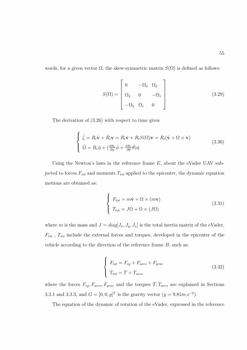
55
words, for a given vector Ω, the skew-symmetric matrix S(Ω) is defined as follows:
S(Ω) =
0 −Ω3 Ω2
Ω3 0 −Ω1
−Ω2 Ω1 0
(3.29)
The derivation of (3.26) with respect to time gives
ζ = Rtv + Rtv = Rtv +RtS(Ω)v = Rt(v + Ω× v)
Ω = Rrη + (∂Rr
∂φφ+ ∂Rr
∂θθ)η
(3.30)
Using the Newton’s laws in the reference frame E, about the eVader UAV sub-
jected to forces Ftot and moments Ttot applied to the epicenter, the dynamic equation
motions are obtained as:
Ftot = mv + Ω× (mv)
Ttot = JΩ + Ω× (JΩ)(3.31)
where m is the mass and J = diag[Jx, Jy, Jz] is the total inertia matrix of the eVader,
Ftot , Ttot include the external forces and torques, developed in the epicenter of the
vehicle according to the direction of the reference frame B, such as:
Ftot = Fcg + Faero + Fgrav
Ttot = T + Taero
(3.32)
where the forces Fcg, Faero, Fgrav and the torques T, Taero are explained in Sections
3.3.1 and 3.3.3, and G = [0, 0, g]T is the gravity vector (g = 9.81m.s−2).
The equation of the dynamic of rotation of the eVader, expressed in the reference

56
frame E, is:
Fcg = mR−1t ζ +mR−1
t G+∆f
T = JRrη + J(∂Rr
∂φφ+ ∂Rr
∂θθ)η +Rrη × JRrη +∆t
(3.33)
In (3.33), Faero and Taero are considered as disturbances ∆f , ∆t, respectively, and it
is assumed that pitch angle satisfy the following inequalities:
−π
2< θ(t) <
π
2(3.34)
so that the inverse of matrix Rr defined in (3.28) exists.
3.4.1 Approximation of Equations of Motion
In this section the simplified dynamic model of the eVader is presented in which the
rate of change of the orientation angles (η) and the body angular velocities (Ω) are
assumed to be approximately equal. This assumption is valid if the perturbations
from hover flight are small. Equation (3.35), outlines Euler’s rigid body motion
equations for the vehicle’s principle angular acceleration roll (φ), pitch(θ) and yaw
(ψ), considering the vehicle’s principle axis of inertia (Jx , Jy and Jz) and the sum of
torques (Ttot = [τx, τy, τz]T ).
Jxφ+ (Jz − Jy)ψθ = τx
Jyθ + (Jx − Jz)φψ = τy
Jzψ + (Jy − Jx)θφ = τz
(3.35)
In order to derive the vehicle’s equations of motion of rotational dynamics, all
torque expressions in (3.16), (3.18), (3.19) and (3.23) are replaced in the right hand

57
side of (3.35) as follow:
Jxφ = ψθ(Jy − Jz)− cosα1Jrω1α1 − sinα1Jrω1β1 + sinα1Jrω1α1
−cosα2Jrω2α2 − sinα2Jrω2β2 + sinα2Jrω2α2
−ho(sinβ1cosα1T1 + sinβ2cosα2T2) + lo(cosβ1cosα1T1 − cosβ2cosα2T2)
−sinα1Q1 + sinα2Q2 + cosα1Jpβ1 + cosα2Jpβ2
Jyθ = φψ(Jz − Jx)− sinβ1sinα1Jrω1α1 + cosβ1Jrω1β1 + sinβ1cosα1(Jrω1β1 − Jrω1α1)
−sinβ2sinα2Jrω2α2 + cosβ2Jrω2β2 + sinβ2cosα2(Jrω2β2 − Jrω2α2)
+sinβ1cosα1Q1 − sinβ2cosα2Q2 − ho(sinα1T1 + sinα2T2)
+sinβ1sinα1Jpβ1 + cosβ1Jpα1 + sinβ2sinα2Jpβ2 + cosβ2Jpα2
Jzψ = θφ(Jx − Jy) + cosβ1sinα1Jrω1α1 + sinβ1Jrω1β1 − cosβ1cosα1(Jrω1β1 − Jrω1α1)
+cosβ2sinα2Jrω2α2 + sinβ2Jrω2β2 − cosβ2cosα2(Jrω2β2 − Jrω2α2)
−cosβ1cosα1Q1 + cosβ2cosα2Q2 − lo(sinα1T1 − sinα2T2)
−cosβ1sinα1Jpβ1 + sinβ1Jpα1 − cosβ2sinα2Jpβ2 + sinβ2Jpα2
(3.36)
Thereby, the dynamic model of the eVader including translational and rotational
dynamics is presented in (3.37), where τx, τy, and τz are specified in (3.36). For the
sake of simplicity, this model is used for designing controllers for the eVader in next
chapters of this thesis. However, the procedure of designing controllers remains the
same for the model presents in Section 3.4.

58
Table 3.2: Parameters of the vehicle.
parameter value parameter valuem 6.5 kg Jr 0.5× 10⁻⁴ kg.m2
g 9.81 m.s−1 Jx 0.013 kg.m2
lo 0.4 m Jy 6× 10⁻³ kg.m2
ho 0.08 m Jz 4× 10⁻⁴ kg.m2
CT 0.01 Jp 3× 10⁻⁴ kg.m2
Jxφ = ψθ(Jy − Jz) + τx
Jyθ = φψ(Jz − Jx) + τy
Jzψ = θφ(Jx − Jy) + τz
mx = CφCψFx + (SφSθCψ − CφSψ)Fy + (CθSθCψ + SφSψ)Fz
my = CθSψFx + (SφSθSψ + CφCψ)Fy + (CφSθSψ − SφCψ)Fz
mz = −SφFx + SφCθFy + CφCθFz −mg + gr(z)
(3.37)
where
Fx = sinα1T1 + sinα2T2
Fy = −sinβ1cosα1T1 − sinβ2cosα2T2
Fz = cosβ1cosα1T1 + cosβ2cosα2T2
Table (3.2) shows the parameters of the eVader that have been used in simulations
of this study. These parameters are based on the measurements in [1] for the eVader.
3.5 Summary
A description of a lift-fan OAT mechanism is presented in this chapter which has the
potential to provide VTOL capability with efficient, and highly maneuverable char-
acteristics in tilt-rotor aircrafts. Moreover, the modeling of a small VTOL UAV with

59
lift-fan OAT system, which is able to perform maneuvers in hover, lateral and forward
flight, is discussed. This UAV has the capability to pitched hover (something that
no other aircraft can execute). It uses the inherent gyroscopic properties and driving
torques of the fans for vehicle pitch control, and eliminates the need for external con-
trol elements or lift devices. Therefore, in order to control this unconventional UAV
for complex missions, a complete dynamic model of it is developed in this chapter,
in which aerodynamic friction effects, ground effects, and reactionary moments are
included. In addition, the lateral and longitudinal tilting angles of eVader vehicle are
not forced to be the same in this model, and each fan rotates independently. In other
words, a dynamic model of dOAT mechanism is developed in this thesis as opposed
to sOAT model which was presented in previous works. There are more advantages
associated with OAT systems, which have not been explored yet. Examining all these
properties, by applying proper choice of nonlinear controller to verify the dOAT ca-
pability, based on the developed nonlinear dynamic model in this chapter, is what is
intended in the following chapters.

Chapter 4
Feedback Linearization Control of eVader
It is well known that a conventional linear control (PID or PD) can stabilize a tradi-
tional VTOL aircraft (e.g., helicopter) in noncritical conditions (e.g., without external
disturbances such as wind gusts) or around a specific operating point [3]. In real con-
ditions the use of a classical linear control is limited to a small neighborhood around
the operating point. However, the goal of this thesis is to design a controller for the
eVader UAV to perform difficult tasks and maneuvers, and follow complex trajectories
in presence of external disturbances. Classical linear controllers are not applicable,
and nonlinear control approaches are required.
Nonlinear control approaches can be divided into two major directions. First,
the ones that employ the use of Lyapunov functions and the second group dealing
with Feedback Linearization (FL). Feedback linearization can be defined as methods
of transforming original system models into equivalent models of a simpler form.
This approach is completely different from conventional (Jacobian) linearization, due
to the fact that FL is achieved by exact state transformation and feedback, rather
than by linear approximations of the system dynamics. The central idea of FL is to
algebraically transform nonlinear system dynamics into (fully or partly) linear ones,
so that linear control techniques can be applied. This chapter is focused on FL, while
Lyapunov-based techniques are investigated in the next chapters (Chapter 5 and 6)
of this thesis.
60

61
Feedback linearization controllers can be directly applied to nonlinear dynamics
without linear approximations of the given system. Although these types of controller
are simple to implement, model uncertainty can cause performance degradation or
instability of the closed-loop system, because it uses inverse system dynamics as part
of the control input to cancel nonlinear terms. One solution to deal with the problem
caused by model uncertainties is adaptive control methods.
In this chapter, the review and background of FL methodologies is discussed in
Section 4.1. In Section 4.2 the dynamic model presented in Chapter 3 for the UAV of
interest (e.g., eVader) is modified for controller design. For this, a state-space model
is developed for the eVader vehicle. Then, in Section 4.3 the feedback linearization
controller is designed to regulate the Cartesian positions (x, y, z) and orientation an-
gles (φ, θ, ψ) to desired values of the UAV. The design of the corresponding adaptive
nonlinear control and robust adaptive control are described in Sections 4.4 and 4.6,
respectively. Then, Section 4.7 presents a number of simulation results of the pro-
posed nonlinear controllers based on FL and adaptive control methodologies. Finally,
Section 4.8 discusses the results and provides a summary of this chapter.
4.1 Overview and Background of Feedback Linearization
The basic idea of FL is first to transform a nonlinear system into a linear system, and
then use the well-known and powerful linear design techniques to complete the control
design. Such concepts are applicable to well-known important classes of nonlinear
systems, namely input-state linearizable or minimum-phase systems, which typically
requires full system state measurement.
One of such mechanisms is the Input-Output Linearization (IOL) technique [77].

62
IOL is a control technique where the output y of the system is differentiated as
many times as required so that the input signal u appears explicitly in the output
equation. The Input-State Linearization (ISL) [77] is a special case of IOL where the
output function leads to a relative degree n. Therefore, if a system is input-output
linearizable with relative degree n, it must be input-state linearizable. If the relative
degree req is less than the system order n, then there will be internal (unobservable)
dynamics in the feedback linearized system. The IOL will be discussed in this thesis.
Due to the under-actuated property of quad-rotors and other helicopter type
UAVs, they are categorized under non-minimum phase nonlinear systems. A non-
minimum phase system has (n−req) internal dynamics, or zero-dynamics, which play
an important role in the stability of the whole dynamics of the system.
These unobservable states may be stable or unstable. However, the stability or
at least controllability of these unobservable states should be addressed to ensure
these states do not cause problems in practice. For such systems with zero-dynamics,
perfect or asymptotic convergent tracking error can not be achieved by FL, which
can only partially linearize the non-minimum phase nonlinear system. Instead, only
small tracking error for the desired trajectories of interest is achievable. There are
some methods to cope with this restriction of FL method for under-actuated systems
[78]. Some of them which have been applied to quad-rotor helicopters are as below:
1. Output-redefinition method: One of the most common approaches for con-
trolling non-minimum phase systems is the output-redefinition method [79]. The
principle of this method is to redefine the output function y1 = h1(x) so that the
resulting zero-dynamic is stable. For example, in the case of quad-rotors, choosing
altitude, pitch, roll, and yaw angles as outputs of the system will introduce unstable
zero-dynamics which will result in drifting the vehicle in the x − y plane [80]. How-

63
ever, by selecting position (x, y, z) and yaw angle as outputs the system will not have
unstable zero-dynamics. From this example, it is observed that FL is able to only
track four out of six specific outputs of quad-rotors and stabilize the other two to
zero.
2. Output-differentiation method: Another practical approximation is using suc-
cessive differentiations of the output [81]. This method neglects the terms containing
the input and keeps differentiating the selected output a number of times equal to the
system order, so that there is no zero-dynamics. Because of the number of differentia-
tions of the system dynamic in this method, it can only be applied to the system if the
coefficient of u values at the intermediate steps are ”small”. Otherwise, because of the
high-order derivative terms arising from the differentiation of the dynamic equations,
FL controllers are quite sensitive to external disturbance or sensor noise. However,
this method provides the opportunity of arbitrarily selecting the desired four outputs
of quad-rotor systems, but differentiation makes this approach noise sensitive.
In this chapter, it is verified that FL is a proper choice of control for the eVader
UAV. This is due to the fact that the system does not have any of the above problems.
In other words, the eVader is a full state-linearizable vehicle and does not have zero-
dynamics.
4.1.1 Controllability
In this section the controllability of the eVader system based on the model of the
vehicle in Section 3.4.1 of Chapter 3 is investigated. The controllability of a linearized
system is investigated based on the following controllability condition: A continuous
time-invariant linear state-space model of the form x = Ax + Bu is controllable if

64
and only if:
rank
[
B AB A2B ... An−1B
]
= n (4.1)
where A ∈ Rn×n is sate matrix and B ∈ Rn×m is control matrix in the linear state-
space model and n is the order of the system.
The controllability condition for linear systems turns into an input-state lineariz-
able condition for single-input nonlinear systems of the form x = f(x) + g(x)u, with
f and g being smooth vector fields. Therefore, based on a theorem 6.2 in [63], if the
vector fields
g, adfg, ..., adn−1f g
are linearly independent, the system is input-state
linearizable. In this expression adfg represents the Lie bracket of the two vector fields
f and g which is defined as:
adfg = ∇gf −∇fg (4.2)
In the Lie bracket adfg, ad stands for ”adjoint”. The concepts of input-state lin-
earization and input-output linearization can be extended for MIMO systems of the
form
x = f(x) +G(x)u
y = h(x)(4.3)
where x is n×1 the state vector, u is the m×1 control input vector of components ui,
y is the m× 1 vector of system outputs of components yi, f and h are smooth vector
fields, and G is a n ×m matrix whose columns are smooth vector fields gi. Input-
output linearization of MIMO systems is obtained by differentiating the outputs yi
until the inputs appear, similarly to the SISO systems. Assume that ri is the smallest

65
integer such that at least one of the inputs appears in y(ri)i , then
y(ri)i = Lrif hi +
m∑
j=1
LgjLri−1f hiuj (4.4)
with LgjLri−1f hi(x) 6= 0 for at least one j. If the partial relative degrees ri, i = 1, ...,m
are all well defined, the system (4.3) is then said to have relative degree (r1, ..., rm)
at x0, and the scalar r = r1 + ...+ rm is called the total relative degree of the system
at point x0 [63].
The vector fields f and gi are formally defined in Section 4.3 throughout the design
development of FL controller for eVader. The investigation of the controllability of
the eVader UAV verified that the system has relative degree (r1 = r2 = r3 = r4 =
r5 = r6 = 2) and the total relative degree (r = r1+ r2+ r3+ r4+ r5+ r6) of its model
is equal to the vehicle’s order (n = 12). Hence, the system is input-state linearizable
and both stabilization and tracking can be achieved for the eVader without any worry
about the stability of the internal dynamics as shown in Section 4.3.
4.2 Modeling for Control
This section presents the state-space model of the eVader UAV suitable for designing
feedback linearization nonlinear control laws. The nonlinear dynamic model (3.37)
developed in Chapter 3 is used to write the system in state-space form x = f(x,u)
with u input vector and x state vector chosen as follows:
x =
[
φ φ θ θ ψ ψ x x y y z z
]T
, (4.5)

66
u =
[
u1 u2 u3 u4 u5 u6
]T
. (4.6)
The expressions for u1, .., u6 are defined in Section 3.4.1 of Chapter 3 as:
u1 = −cosα1Jrω1α1 − sinα1Jrω1β1 + sinα1Jrω1α1
−cosα2Jrω2α2 − sinα2Jrω2β2 + sinα2Jrω2α2
−ho(sinβ1cosα1T1 + sinβ2cosα2T2) + lo(cosβ1cosα1T1 − cosβ2cosα2T2)
−sinα1Q1 + sinα2Q2 + cosα1Jpβ1 + cosα2Jpβ2
u2 = −sinβ1sinα1Jrω1α1 + cosβ1Jrω1β1 + sinβ1cosα1(Jrω1β1 − Jrω1α1)
−sinβ2sinα2Jrω2α2 + cosβ2Jrω2β2 + sinβ2cosα2(Jrω2β2 − Jrω2α2)
+sinβ1cosα1Q1 − sinβ2cosα2Q2 − ho(sinα1T1 + sinα2T2)
+sinβ1sinα1Jpβ1 + cosβ1Jpα1 + sinβ2sinα2Jpβ2 + cosβ2Jpα2
u3 = cosβ1sinα1Jrω1α1 + sinβ1Jrω1β1 − cosβ1cosα1(Jrω1β1 − Jrω1α1)
+cosβ2sinα2Jrω2α2 + sinβ2Jrω2β2 − cosβ2cosα2(Jrω2β2 − Jrω2α2)
−cosβ1cosα1Q1 + cosβ2cosα2Q2 − lo(sinα1T1 − sinα2T2)
−cosβ1sinα1Jpβ1 + sinβ1Jpα1 − cosβ2sinα2Jpβ2 + sinβ2Jpα2
(4.7)

67
u4 = CφCψFx + (SφSθCψ − CφSψ)Fy + (CθSθCψ + SφSψ)Fz
u5 = CθSψFx + (SφSθSψ + CφCψ)Fy + (CφSθSψ − SφCψ)Fz
u6 = −SφFx + SφCθFy + CφCθFz
Fx = sinα1T1 + sinα2T2
Fy = −sinβ1cosα1T1 − sinβ2cosα2T2
Fz = cosβ1cosα1T1 + cosβ2cosα2T2
Therefore the vehicle’s state-space model is given by
f(x,u) =
φ
ψθ(Jy−JzJx
)− ktaxJxφ2 − Jr
JxΩθ + 1
Jxu1
θ
φψ(Jz−JxJy
)− ktayJyθ2 − Jr
JyΩφ+ 1
Jyu2
ψ
θφ(Jx−JyJz
)− ktazJzψ2 + 1
Jzu3
x
−Kfax
mx2 + 1
mu4
y
−Kfay
my2 + 1
mu5
z
−Kfaz
mz2 − g + 1
mu6
(4.8)
4.3 eVader’s Feedback Linearization Design
The feedback linearization technique is based on inner and outer loops of the con-
troller. The input-output linearization-based inner loop uses the full-state feedback
to globally linearize the nonlinear dynamics of selected controlled outputs. Each of

68
the output channels is differentiated sufficiently many times until a control input
component appears in the resulting equation. Using the Lie derivative, the input-
output linearization technique transforms the nonlinear system into a linear and non-
interacting system in the Brunovsky form [63]. The outer controller adopts a classical
polynomial control law for the new input variable of the resulting linear system.
This can be described for the eVader vehicle by linear state-space equations via
the states transformation zl = zl(x) and nonlinear state feedback u = u(x,vl), where
x = (x1, x2, ..., x12)T is the state vector of the nonlinear system, zl = (zl1 , zl2 , ..., zl12)
T
is the state vector and vl = (vl1 , vl2 , vl3 , vl4 , vl5 , vl6)T is the input of the linear system
resulting from the transformation. The transformation of nonlinear form into a linear
and controllable form is given by
zl = Azl + Bvl
y = Czl
(4.9)
where A ∈ R12×12 and B ∈ R12×6 are control and input matrices and C ∈ R6×12 is
the output matrix of the linear system.
The evader’s model can be rewritten from (4.8) as:
x1 = x2, x2 = (x4x6)(Jy−Jz)
Jx− ktax
Jxx22 −
JrJxΩx4 +
u1Jx
x3 = x4, x4 = (x2x6)(Jz−Jx)
Jy− ktay
Jyx24 −
JrJyΩx2 +
u2Jy
x5 = x6, x6 = (x2x4)(Jx−Jy)
Jz− ktaz
Jzx26 +
u3Jz
x7 = x8, x8 = −Kfax
mx28 +
u4m
x9 = x10, x10 = −Kfay
mx210 +
u5m
x11 = x12, x12 = −Kfaz
mx212 − g + u6
m
(4.10)

69
The system model in (4.10) is transformed into an affine nonlinear form given by
(4.11).
x = f(x) +∑6
i=1 giui,
y = h(x),(4.11)
where ui(i = 1, ..., 6) are control variables, y is a 6× 1 output function vector, f and
h are smooth vector fields. The function vectors f(x) ∈ R12, gi ∈ R12 and output
vector y from (4.10) are given by
f(x) =
[
x2 x4x6a1 − a2x22 − a3Ωx4 x4 x2x6a4 − a5x
24 − a6Ωx2 x6 x2x4a7 − a8x
26
x8 −a9x28 x10 −a10x
210 x12 −a11x
212
]T
g1(x) =
[
0 1Jx
0 0 0 0 0 0 0 0 0 0
]T
g2(x) =
[
0 0 0 1Jy
0 0 0 0 0 0 0 0
]T
g3(x) =
[
0 0 0 0 0 1Jz
0 0 0 0 0 0
]T
g4(x) =
[
0 0 0 0 0 0 0 1m
0 0 0 0
]T
g5(x) =
[
0 0 0 0 0 0 0 0 0 1m
0 0
]T
g6(x) =
[
0 0 0 0 0 0 0 0 0 0 0 1m
]T
y(x) =
[
x1 x3 x5 x7 x9 x11
]T
(4.12)
where a1 = Jy−JzJx
, a2 = ktaxJx
, a3 = JrJx, a4 = Jz−Jx
Jy, a5 = ktay
Jy, a6 = Jr
Jy, a7 = Jx−Jy
Jz,
a8 =ktazJz
, a9 =Kfax
m, a10 =
Kfay
mand a11 =
Kfaz
m. The controllability of the system is
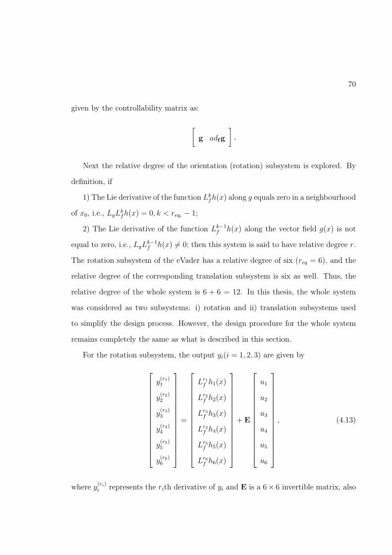
70
given by the controllability matrix as:
[
g adfg
]
,
Next the relative degree of the orientation (rotation) subsystem is explored. By
definition, if
1) The Lie derivative of the function Lkfh(x) along g equals zero in a neighbourhood
of x0, i.e., LgLkfh(x) = 0, k < reqi − 1;
2) The Lie derivative of the function Lk−1f h(x) along the vector field g(x) is not
equal to zero, i.e., LgLk−1f h(x) 6= 0; then this system is said to have relative degree r.
The rotation subsystem of the eVader has a relative degree of six (req = 6), and the
relative degree of the corresponding translation subsystem is six as well. Thus, the
relative degree of the whole system is 6 + 6 = 12. In this thesis, the whole system
was considered as two subsystems: i) rotation and ii) translation subsystems used
to simplify the design process. However, the design procedure for the whole system
remains completely the same as what is described in this section.
For the rotation subsystem, the output yi(i = 1, 2, 3) are given by
y(r1)1
y(r2)2
y(r3)3
y(r4)4
y(r5)5
y(r6)6
=
Lr1f h1(x)
Lr2f h2(x)
Lr3f h3(x)
Lr4f h4(x)
Lr5f h5(x)
Lr6f h6(x)
+ E
u1
u2
u3
u4
u5
u6
, (4.13)
where y(ri)i represents the rith derivative of yi and E is a 6× 6 invertible matrix, also

71
called the decoupling matrix, given by
E(x) =
1Jx
0 0 0 0 0
0 1Jy
0 0 0 0
0 0 1Jz
0 0 0
0 0 0 1m
0 0
0 0 0 0 1m
0
0 0 0 0 0 1m
The linearizing control law u = (x,vl), by which the nonlinear feedback exactly
compensates the system nonlinearities, is defined as
u = E−1
vl1
vl2
vl3
vl4
vl5
vl6
−
L2fh1(x)
L2fh2(x)
L2fh3(x)
L2fh4(x)
L2fh5(x)
L2fh6(x)
. (4.14)
Using the control law defined in (4.14), the following decoupled set of equations
are obtained:
y(ri)i = vli , i = 1, ..., 6. (4.15)
which represents a linear system.
As mentioned above, in this control approach we seek a transformation that trans-
forms the nonlinear system into an equivalent linear system. The main concern in this
type of control is coping with disturbances. Even though the control may have good

72
results around equilibrium points of the system such as in hover, if the system goes
far from equilibrium points by a sudden unexpected disturbances such as wind gusts
or adding a payload, this control would fail to offer perfect control due to the fact that
FL is based on the exact cancellation of nonlinearities, which is, in practice, not often
practically possible. Most likely only the approximations of the model parameters are
available. The suggested approach in such situations is an adaptive nonlinear control
methodology which is discussed and designed for the eVader in the next section. The
basic objective of adaptive control is to maintain consistent performance of a system
in the presence of uncertainty or unknown variation in plant parameters.
4.4 Nonlinear Adaptive Control
The controller designed in the preceding section guarantees that in the presence of
uncertain bounded nonlinearities, the closed-loop state remains bounded. In this sec-
tion, and in the remainder of the thesis, the uncertainties are more specific. They
consist of unknown constant parameters, which appear linearly in the system equa-
tions. In the presence of such parametric uncertainties, we will be able to achieve
both boundedness of the closed-loop states and convergence of the tracking error to
zero.
Many dynamic systems to be controlled have constant or slowly-varying uncertain
parameters. An adaptive control system can thus be regarded as a control system
with on-line parameter estimation. The dynamic behavior of a UAV depends on its
speed, and maneuvering situation. Also if UAV’s mission is to pick up some loads,
it has to manipulate weights, and mass distribution is changing. In addition it is
not reasonable to assume that the inertial parameters of the load and of the UAV

73
are well known and constant. If controllers with constant gains are used and the
load parameters are not accurately known, UAV motion can be either inaccurate or
unstable.
An adaptive controller differs from an ordinary controller in that the controller
parameters are variable, and there is a mechanism for adjusting these parameters
online, based on signals in the system. Many formalisms in nonlinear control can be
used to synthesize mechanism, such as Lyapunov theory, hyperstability theory, and
passivity theory [82]. Lyapunov theory is used in this thesis to design an adaptation
law which would guarantee that the control system remains stable and the tracking
error converges to zero as the parameters are varied.
The controller designed in the previous section employed static feedback, whereas
the controller in this section will, in addition, employ a form of nonlinear integral
feedback. The underlying idea in the design of this dynamic part of feedback is
parameter estimation. The dynamic part of the controller is designed as a parameter
update law with which the static part is continuously adapted to new parameter
estimates, hence its name: Adaptive control law.
Adaptive controllers are dynamic and therefore more complex than the static
controllers designed in Section 4.3. On the other hand, as it is shown in simulations,
an adaptive controller guarantees not only that the plant state x remains bounded,
but also that it tends to a desired constant value (regulation) or asymptotically tracks
a reference signal (tracking),
This section describes an adaptive feedback linearization controller. We define
a suitable feedback control and adaptation rules so that a trajectory of the system
follows desired references under model parameter uncertainty.

74
4.4.1 Adaptive Control Design for the eVader’s Orientation
Because of the presence of unknown parameters in the dynamics of roll angle in (4.8),
an adaptive control input u1(t) needs to be developed to regulate φ(t) to its desired
value φd. Let us consider the regulation error for φ(t) to be defined as:
eφ1 = φ− φd (4.16)
A filtered regulation error system, denoted by eφ2(t) ∈ R can thus be defined as:
eφ2 = ˙eφ1 + eφ1 (4.17)
The time derivative of (4.17) gives the open-loop regulation error.
Jxeφ2 = ψθa1 + a2eφ1 + u1 (4.18)
where unknown constants a1, a2 ∈ R are defined as a1 = Jy − Jz and a2 = Jx. The
control input u1(t) needs to be designed based on the Lyapunov approach, and the
open-loop regulation error system in (4.18), and is given as below:
u1 = −a1ψθ − a2 ˙eφ1 − eφ2 (4.19)
where a1, a2 ∈ R are dynamic estimates for unknown parameters a1, a2. These two
parameters are generated according to the following update laws:
˙a1 = Γa1eφ2ψθ˙a2 = Γa2eφ2 eφ1 (4.20)

75
where Γa1 ,Γa2 ∈ R are some positive update gains. After substituting (4.19) into
(4.8), the closed-loop dynamic is obtained as:
Jxeφ2 = a1ψθ + a2eφ1 − eφ2 (4.21)
where a1 = a1 − a1 and a2 = a2 − a2 are parameter estimation errors.
Following the same approach described above for regulating pitch and yaw angles,
and considering the following four regulation errors and filtered regulation system
error defined as:
eθ1 = θ − θd eθ2 = eθ1 + eθ1 (4.22)
eψ1= ψ − ψd eψ2
= eψ1+ eψ1
(4.23)
the control inputs u2(t) and u3(t) are obtained as
u2 = −a3φψ − a4eθ1 − eθ2 (4.24)
u3 = −a5θφ− a6eψ1− eψ2
(4.25)
where a3 = Jz − Jx, a4 = Jy, a5 = Jx − Jy, and a6 = Jz. The result is the update
laws defined as:˙a3 = Γa3eθ2φψ
˙a4 = Γa4eθ2 eθ1
˙a5 = Γa5eψ2θφ ˙a6 = Γa6eψ2
eψ1
(4.26)

76
4.4.2 Adaptive Control Design for the eVader’s Position
The dynamic equation of the UAV for altitude is given as (Equation (3) in Section
3.4.1):
mz = u6 −mg (4.27)
It is assumed that m in unknown. An adaptive control input u6(t) can be developed
in the same way as developing input signals for controlling orientation angles. After
defining ez1 = z − zd, ez2 = ez1 + ez1 and getting the time derivative of the dynamic
of the altitude error, the open-loop error system is given as
mez2 = −a7g + a7ez1 + u6 (4.28)
where a7 = m is unknown. Having the error dynamic system provided in (4.28), the
control input u6(t) is designed as below
u6 = a7g − a1ez1 − ez2 (4.29)
where a7 is an estimate of unknown parameter a7 which is generated through its
dynamic update law
˙a7 = Γa7(ez2 ez1 − gez2). (4.30)
After substituting (4.29) into (4.27), the closed-loop dynamic is obtained as
mez2 = −a7g + a7ez1 − ez2 (4.31)

77
where a7 is the parameter’s estimation error. The stability of the closed-loop system
(4.31) is proved based on the Lyapunov approach and discussed in the next section
(Section 4.5).
Following the same approach presented above for altitude, the UAV’s longitudinal
and lateral position x(t) and y(t), respectively, are regulated to their desired position
xd and yd by applying u4 and u5.
u4 = −a8ex1 − ex2 ,˙a8 = Γa8 ex1ex2 (4.32)
u5 = −a9ey1 − ey2 ,˙a9 = Γa9 ey1ey2 (4.33)
4.5 Stability Analysis
Theorem 1: The adaptive controller proposed in (4.19) with the updating laws in
(4.20) ensures the boundedness of the closed loop system, and the UAV’s roll angle
φ(t) is regulated to its desired angle φd asymptotically in the sense that
limt→∞eφ1(t) = 0. (4.34)
Proof: To prove the above theorem, a Lyapunov function candidate V1(t) is
chosen as
V1 =1
2e2φ1 +
1
2Jxe
2φ2
+1
2Γ−1a1a21 +
1
2Γ−1a2a22. (4.35)
The time derivative of V1(t) along (4.17), (4.20) and (4.21) is
V1 = −e2φ1 − e2φ2 + eφ1eφ2 . (4.36)

78
By invoking the young’s inequality, V1(t) is restricted to the upper bound
V1 ≤ −1
2e2φ1 −
1
2e2φ2 . (4.37)
Since V1(t) of (4.35) is a non-negative function, we can conclude that V1(t) ∈ L∞,
hence eφ1(t), eφ2(t), a1(t), a2(t) ∈ L∞ and eφ1 , eφ2∈ L∞. We can show that eφ1(t),φ(t),
a1(t), a2(t) ∈ L∞ by utilizing (4.16), (4.17) and (4.20) respectively. It is now easy
to conclude that u1(t), ˙a1(t), ˙a2(t) ∈ L∞ from (4.19) and (4.20). Then (4.18) can be
used to show that eφ2(t) ∈ L∞, which implies that φ(t) ∈ L∞ according to (4.16) and
(4.17). With the above information, Lemma A.3 in [83] is invoked to conclude that
limt→∞eφ1(t) = 0. (4.38)
Thus the UAV’s roll angle φ is regulated to its desired value φd with the control input
of (4.19) and the error reaches zero asymptotically.
4.6 Robust Adaptive Feedback Linearization
The traditional techniques for robust adaptive control include parameter projection
[84], deadzone [84], and e-modification [85]. The e-modification method appears at-
tractive because it requires neither a-priori training on the model (like projection),
nor knowledge of the bounds on disturbances (like deadzone), in order to guaran-
tee uniformly ultimately bounded (UUB) signals. To make the adaptive controller
designed in Sections 4.4.1 and 4.4.2 robust to each bounded approximation error
and wind disturbances, the e-modification term is added to parameter update laws
for ˙a1, ..., ˙a9. The control laws of robust adaptive feedback linearization approach

79
become as follows:
˙a1 = Γa1(eφ2ψθ − ν1‖eφ1‖a1)
˙a2 = Γa2(eφ2 eφ1 − ν2‖eφ2 a2)
˙a3 = Γa3(eθ2φψ − ν3‖eθ2‖a3)
˙a4 = Γa4(eθ2 θ1 − ν4‖eθ2‖a4)
˙a5 = Γa5(eψ2θφ− ν5‖eψ2
‖a5)
˙a6 = Γa6(eψ2ψ1 − ν6‖eψ2
‖a6)
˙a7 = Γa7(ez2 ez1 − gez2 − ν7‖ez2‖a7)
˙a8 = Γa8(ex1ex2 − ν8‖ex2‖a8)
˙a9 = Γa9(ey1ey2 − ν9‖ey2 a9)
(4.39)
In this e-modification term ν1, ..., ν9 are robust modification gains which are positive
constants. The adaptive control laws u1, ..., u6 are the same as in Sections 4.4.1
and 4.4.2. In Chapter 8, the wind disturbance of the form dw(t) = Disturbance
Magnitude(10 + 5sin(2πt)) is added to all states (roll, pitch, yaw, x, y, z) to model
blowing wind in all directions corresponding to vehicle’s frame of reference. The
result of this simulation is presented and discussed in Chapter 8, where comprehensive
simulation scenarios are applied to the eVader UAV.
4.7 Simulation Results
The simulation Scenario #1 is defined as follows: the initial condition is x0 = [0]12×12,
and the desired value is set arbitrarily to xd = [22.5, 0, 15, 0, 18, 0, 3, 0, 4, 0, 2, 0]T .
Table 4.1 shows the results of the FL controller applied on the eVader, designed in
Section 4.3. The parameters of the vehicle that have been used in simulations of
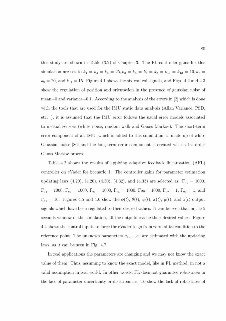
80
this study are shown in Table (3.2) of Chapter 3. The FL controller gains for this
simulation are set to k1 = k3 = k5 = 25, k2 = k4 = k6 = k8 = k10 = k12 = 10, k7 =
k9 = 20, and k11 = 15. Figure 4.1 shows the six control signals, and Figs. 4.2 and 4.3
show the regulation of position and orientation in the presence of gaussian noise of
mean=0 and variance=0.1. According to the analysis of the errors in [2] which is done
with the tools that are used for the IMU static data analysis (Allan Variance, PSD,
etc. ), it is assumed that the IMU error follows the usual error models associated
to inertial sensors (white noise, random walk and Gauss Markov). The short-term
error component of an IMU, which is added to this simulation, is made up of white
Gaussian noise [86] and the long-term error component is created with a 1st order
Gauss-Markov process.
Table 4.2 shows the results of applying adaptive feedback linearization (AFL)
controller on eVader for Scenario 1. The controller gains for parameter estimation
updating laws (4.20), (4.26), (4.30), (4.32), and (4.33) are selected as: Γa1 = 1000,
Γa2 = 1000, Γa3 = 1000, Γa4 = 1000, Γa5 = 1000, Γa6 = 1000, Γa7 = 1, Γa8 = 1, and
Γa9 = 10. Figures 4.5 and 4.6 show the φ(t), θ(t), ψ(t), x(t), y(t), and z(t) output
signals which have been regulated to their desired values. It can be seen that in the 5
seconds window of the simulation, all the outputs reache their desired values. Figure
4.4 shows the control inputs to force the eVader to go from zero initial condition to the
reference point. The unknown parameters a1, ..., a9 are estimated with the updating
laws, as it can be seen in Fig. 4.7.
In real applications the parameters are changing and we may not know the exact
value of them. Thus, assuming to know the exact model, like in FL method, in not a
valid assumption in real world. In other words, FL does not guarantee robustness in
the face of parameter uncertainty or disturbances. To show the lack of robustness of

81
Table 4.1: The result of FL controller for position and orientation regulation simulation
Without Noise With Noisetime(sec) error time(sec) error
Roll φ 2 0.0066 (deg) 2 0.1394 (deg)Pitch θ 2 0.0044 (deg) 2 0.1416 (deg)Yaw ψ 2 0.0053 (deg) 2 0.1407 (deg)Position x 2 0.0156 (m) 2 0.0145 (m)Position y 2 0.0207 (m) 2 0.0197 (m)Altitude z 2 0.0588 (m) 2 0.0602 (m)
Table 4.2: The result of AFL controller for position and orientation regulation simulation
Without Noise With NoiseTime(sec) error Time(sec) error
Roll φ 2 6.7763 (deg) 2 6.7679 (deg)Pitch θ 2 4.3967 (deg) 2 4.4152 (deg)Yaw ψ 2 6.4062 (deg) 2 6.4352 (deg)Position x 2 1.8900 (m) 2 1.8900 (m)Position y 2 1.9013 (m) 2 1.9013 (m)Altitude z 2 0.7438 (m) 2 0.7438 (m)
the FL controller in presence of parameter uncertainty and the effect of variation in
the parameters of the dynamic model, in Scenario # 2, all variables’ initial conditions,
desired values and controller gains are fixed as in Scenario # 1 except the mass of the
eVader. Figure 4.8 shows that the AFL controller adapts itself and reaches a desired
value of altitude, but the FL controller can not make the altitude error zero.
4.8 Results and discussion
Feedback linearization is based on the idea of transforming nonlinear dynamics into
a linear form by using state feedback, with input-state linearization corresponding
to complete linearization and input-output linearization to partial linearization. The
method can be used for both stabilization and tracking control problems.

82
0 0.5 1 1.5 2−1
0
1
2Control Signal u1
time[s]
u1
0 0.5 1 1.5 2−200
0
200
400Control Signal u4
time[s]
u4
0 0.5 1 1.5 2−1
0
1
2Controller u2
time[s]
u2
0 0.5 1 1.5 2−200
0
200
400
600Controller u5
time[s]
u5
0 0.5 1 1.5 2−1
0
1
2Controller u3
time[s]
u3
0 0.5 1 1.5 20
100
200
300Controller u6
time[s]
u6
Figure 4.1: Control signals of FL control method in presence of white gaussian noise withmean = 0 and variance = 0.1 [2].
0 0.2 0.4 0.6 0.8 1 1.2 1.4 1.6 1.8 2−20
0
20
40The roll angle
time[s]
Ro
ll[d
eg
re
e]
0 0.2 0.4 0.6 0.8 1 1.2 1.4 1.6 1.8 2−10
0
10
20The pitch angle
time[s]
Pitch
[de
gre
e]
0 0.2 0.4 0.6 0.8 1 1.2 1.4 1.6 1.8 2−10
0
10
20The yaw angle
time[s]
Ya
w[d
eg
re
e]
Figure 4.2: Regulation of orientation an-gles of the eVader by FL controller withadditive white noise (φ = 22.5, θ =15, ψ = 18).
0 0.2 0.4 0.6 0.8 1 1.2 1.4 1.6 1.8 2−1
0
1
2
3The Cartesian position x
time[s]
x[m
]
system outputdesired x(t)
0 0.2 0.4 0.6 0.8 1 1.2 1.4 1.6 1.8 2−1
0
1
2
3
4The Cartesian position y
time[s]
y[m
]
0 0.2 0.4 0.6 0.8 1 1.2 1.4 1.6 1.8 2−0.5
0
0.5
1
1.5
2The Cartesian position z
time[s]
z[m
]
Figure 4.3: Regulation of position of theevader by FL controller with additivewhite noise (xd = 3, yd = 4, zd = 2).

83
0 0.2 0.4 0.6 0.8 1−4
−2
0
2
4
6Control signal u1
time[s]
u1
0 0.2 0.4 0.6 0.8 1−1000
0
1000
2000
3000Control signal u4
time[s]
u4
0 0.2 0.4 0.6 0.8 1−2
0
2
4Control signal u2
time[s]
u2
0 0.2 0.4 0.6 0.8 1−500
0
500
1000
1500Control signal u5
time[s]
u5
0 0.2 0.4 0.6 0.8 1−0.5
0
0.5
1
1.5
2Control signal u3
time[s]
u3
0 0.1 0.2 0.3 0.4 0.5−1000
−500
0
500
1000Control signal u6
time[s]
u6
Figure 4.4: Control signals of adaptive FL control method in presence of aerodynamiccoefficient uncertainties and unknown mass.
0 0.5 1 1.5 2 2.5 3 3.5 4 4.5 50
5
10
15
20
25The roll angle
time[s]
Ro
ll[d
eg
ree
]
0 0.5 1 1.5 2 2.5 3 3.5 4 4.5 50
5
10
15The pitch angle
time[s]
Pitch
[de
gre
e]
0 0.5 1 1.5 2 2.5 3 3.5 4 4.5 50
5
10
15
20The yaw angle
time[s]
Ya
w[d
eg
ree
]
Figure 4.5: Regulation of orientation an-gles of the eVader by AFL controller (φ =22.5, θ = 15, ψ = 18).
0 0.5 1 1.5 2 2.5 3 3.5 4 4.5 5−1
0
1
2
3The Cartesian position x
time[s]
x [m
]
system outputdesired x(t)
0 0.5 1 1.5 2 2.5 3 3.5 4 4.5 5−1
0
1
2
3
4The Cartesian position y
time[s]
y [m
]
0 0.5 1 1.5 2 2.5 3 3.5 4 4.5 50
0.5
1
1.5
2The altitude z
time[s]
z [m
]
Figure 4.6: Regulation of position of theevader by AFL controller (xd = 3, yd =4, zd = 2).

84
0 1 2 3 4 5−1
0
1
2
3
4
a1
time
a1
0 1 2 3 4 5−10
0
10
20
30
a2
time
a2
0 1 2 3 4 5−1
0
1
2
3
4
a3
time
a3
0 1 2 3 4 5−5
0
5
10
15
a4
time
a4
0 1 2 3 4 5−0.8
−0.6
−0.4
−0.2
0a5
time
a5
0 1 2 3 4 5−1
−0.5
0
0.5
1
a6
time
a6
0 1 2 3 4 5−0.2
0
0.2
0.4
0.6
a7
time
a7
0 1 2 3 4 5−0.2
0
0.2
0.4
0.6
a8
time
a8
0 1 2 3 4 5−0.2
0
0.2
0.4
0.6
a9
time
a9
Figure 4.7: Parameter estimation of AFL control method (a1 = Jy − Jz, a2 = Jx, a3 =Jz − Jx, a4 = Jy, a5 = Jx − Jy, a6 = Jz, a7 = a8 = a9 = m).
0 1 2 3 4 5 60
0.2
0.4
0.6
0.8
1
1.2
1.4
1.6
1.8
2AFL controller
time[s]
Altit
ude
z [m
]
0 1 2 3 4 5 60
0.2
0.4
0.6
0.8
1
1.2
1.4
1.6
1.8
2FL controller
time[s]
Altit
ude
z [m
]
Figure 4.8: The altitude output of FL and AFL controllers when the mass of the systemsis changed. The FL controller failed to reach the desired altitude zd = 2 with almost 0.4 msteady state error.

85
The simulation results obtained show that the proposed controller is able to sta-
bilize the eVader even for relatively critical initial conditions. However, the feedback
linearization method has some important limitations. In feedback linearization an
important assumption is that the model dynamics are perfectly known and can be
canceled entirely. Full state measurement is necessary in implementing the control
law. Many efforts are being made to construct observers for nonlinear systems and to
extend the separation principle to nonlinear systems. Finding convergent observers
for nonlinear systems is difficult. Besides, the lack of a general separation principle,
which would guarantee that the straightforward combination of a stable state feed-
back controller and a stable observer will guarantee the stability of the closed-loop
system, is another difficulty associated to this problem. Moreover, no robustness is
guaranteed in the presence of parameter uncertainty or unmodeled dynamics. This
problem is due to the fact that the exact model of the nonlinear system is not available
in performing feedback linearzation.
Adaptive control based on feedback linearization method has been successfully
developed for eVader. However, adaptive control technique is only applicable for
nonlinear control problems that satisfy the following conditions:
• The nonlinear plant dynamics can be linearly parameterized.
• The full state is measurable.
• Nonlinearities can be canceled stably (i.e., without unstable hidden modes or
dynamics) by the control input if the parameters are known.
However, in next chapters it will be revealed that there are other types of uncertainties
in the eVader dynamic model in addition to the linearly parameterizable nonlineari-

86
ties. For example, there are additive disturbances in control input signal, which make
the adaptive control approach unable to provide asymptotic stability.

Chapter 5
Integral Backstepping Control of eVader
Backstepping is a technique providing a recursive method of designing stabilizing
controls for a class of nonlinear systems that are transformable to a strict feedback
system. Backstepping can force a nonlinear system to behave like a linear system in
a new set of coordinates in the absence of uncertainties. However, backstepping and
other forms of feedback linearization such as IOL and ISL, addressed in the previous
chapter, require cancellations of nonlinearities, even those which are helpful for stabi-
lization and tracking. A major advantage of backstepping over feedback linearization
is that it has the flexibility to avoid cancellations of useful nonlinearities and pursue
the objectives of stabilization and tracking, rather than that of linearization.
In this chapter, an integral backstepping (IB) control technique is proposed to
improve the pitch, yaw, and roll stability of the eVader UAV. The controller is able
to simultaneously stabilize the 6 outputs of the system (i.e., orientation angles and
x, y, z). Position and orientation outputs are regulated to their desired values and all
six of them (φ, θ, ψ, x, y, z) track the desired reference trajectories at the same time.
Thus, unlike backstepping control of VTOL (vertical take off and landing) UAVs such
as quad-rotors, there is no need for inner-loop and outer-loop control. Simulation re-
sults using backstepping verified the potential of the eVader as a small UAV used in
different scenarios such as autonomous take off and landing and tracking time-varying
trajectories in order to maneuver inside obstructed environments. Simulation scenar-
87

88
ios presented in this chapter include attitude and position control, and stabilization
and autonomous take off and landing, which show promising results.
The remainder of this chapter is organized as follows: Section 5.1 discusses the
background of backstepping control technique. The state-space model of the vehicle
for backsteeping design is suggested in Section 5.2, followed by an explanation of the
controller design procedure, first for the vehicle’s attitude and then for its altitude
and position, in Section 5.3. The designed backstepping controller’s gains are tunned
based on gradient descent optimization method in Section 5.4. Simulation results
are also shown. Adaptive backstepping controller design for the eVader dynamic
model with parametric uncertainty is presented in Section 5.5. The conclusion and
discussion are summarized in Section 5.7.
5.1 Overview and Background of Backstepping Control Technique
Backstepping techniques provide an easy method to obtain a control algorithm for
nonlinear systems. Several controllers based on backstepping technique have been
developed for controlling rotary aerial vehicles such as quad-rotors and helicopters
[87], [88]. Madani et. al. designed a full-state backstepping technique based on the
Lyapunov stability theory and backstepping sliding mode control to perform hover
and tracking of desired trajectories [30], [89]. Another controller proposed by Castillo
et. al. used the backstepping technique and saturation functions. Using saturation
function in the control law guaranteed attitude and control inputs boundedness in
the presence of perturbations in the angular displacement [34]. However, this con-
troller was designed for a linear system and can not work properly out of the hover
operation point. Metni et. al. used backstepping techniques to derive an adaptive

89
nonlinear tracking control law for a quad-rotor system, using visual information [90].
This control law uses visual information and defines a desired trajectory by a series of
prerecorded images. The above-mentioned papers, all studied quad-rotor helicopter
control and showed that backstepping control method can effectively deal with the
under-actuated property of quad-rotors. However, due to the under-actuated prop-
erty of quad-rotor UAVs, only four outputs out of six outputs of the system are
controllable independently. For example, the controller can set the quad-rotor tracks
three Cartesian positions (x, y, z) and the yaw angle (ψ) to their desired values and
stabilize the roll (φ) and pitch (θ) angles to zero.
Improvements have been introduced by combining integral action within the con-
trol law, which consequently results in guaranteed asymptotic stability, as well as
steady state errors cancellation due to integral action [88]. The idea of adding in-
tegral action in the backstepping design was first introduced by Kanellakopoulos in
[91] to increase the robustness against external disturbances and model uncertainties.
In this chapter of this thesis, the application of integral backstepping controller pro-
posed in [91] is extended to the eVader UAV for stabilization at hover and trajectory
tracking maneuvers. The goal of using this control method on the eVader is to allow
this vehicle to use the full potential of its flying characteristics, enabled by the OAT
mechanism, in order to maneuver in confined spaces. The backstepping controller
presented in this thesis is a Multi-Input Multi-Output (MIMO) IB controller, which
enables the eVader to track all six outputs of the system including the three Cartesian
positions (x, y, z) and the three orientation angles (φ, θ, ψ). The design methodology
is based on the Lyapunov stability theory. Various simulations on the eVader’s dy-
namic model show that the control law stabilizes the whole system with zero steady
state tracking error.

90
After designing the IB control, the controller gains are tunned by employing a gra-
dient descent technique to avoid trial and error procedure. Optimization-based meth-
ods help to systematically accelerate the multiple-parameter tuning process. With
optimization-based techniques, controller gains are tuned based on optimization of
defined performance indices to improve transient stability, which would enhance the
UAV’s maneuvering performance. That is, the problem of setting nonlinear control
gains is formulated as an optimization problem based on gradient descent optimiza-
tion method including system and control constraints.
5.2 State-Space Model for Control
The state-space form of the model of the targeted OAT mechanism can be written as
in Chapter 3, with the following u input and x state vectors:
x =
[
φ φ θ θ ψ ψ x x y y z z
]T
(5.1)
where:
x1 = φ x7 = x
x2 = x1 = φ x8 = x7 = x
x3 = θ x9 = y
x4 = x3 = θ x10 = x9 = y
x5 = ψ x11 = z
x6 = x5 = ψ x12 = ˙x11 = z
(5.2)
u =
[
u1 u2 u3 u4 u5 u6
]T
(5.3)

91
where
u1 = τx = −cosα1Jrω1α1 − sinα1Jrω1β1 + sinα1Jrω1α1
−cosα2Jrω2α2 − sinα2Jrω2β2 + sinα2Jrω2α2
−ho(sinβ1cosα1T1 + sinβ2cosα2T2) + lo(cosβ1cosα1T1 − cosβ2cosα2T2)
−sinα1Q1 + sinα2Q2 + cosα1Jpβ1 + cosα2Jpβ2
u2 = τy = −sinβ1sinα1Jrω1α1 + cosβ1Jrω1β1 + sinβ1cosα1(Jrω1β1 − Jrω1α1)
−sinβ2sinα2Jrω2α2 + cosβ2Jrω2β2 + sinβ2cosα2(Jrω2β2 − Jrω2α2)
+sinβ1cosα1Q1 − sinβ2cosα2Q2 − ho(sinα1T1 + sinα2T2)
+sinβ1sinα1Jpβ1 + cosβ1Jpα1 + sinβ2sinα2Jpβ2 + cosβ2Jpα2
u3 = τz = −cosβ1sinα1Jrω1α1 + sinβ1Jrω1β1 − cosβ1cosα1(Jrω1β1 − Jrω1α1)
+cosβ2sinα2Jrω2α2 + sinβ2Jrω2β2 − cosβ2cosα2(Jrω2β2 − Jrω2α2)
−cosβ1cosα1Q1 + cosβ2cosα2Q2 − lo(sinα1T1 − sinα2T2)
−cosβ1sinα1Jpβ1 + sinβ1Jpα1 − cosβ2sinα2Jpβ2 + sinβ2Jpα2
(5.4)
and
u4 = CφCψFx + (SφSθCψ − CφSψ)Fy + (CθSθCψ + SφSψ)Fz
u5 = CθSψFx + (SφSθSψ + CφCψ)Fy + (CφSθSψ − SφCψ)Fz
u6 = −SφFx + SφCθFy + CφCθFz
Fx = sinα1T1 + sinα2T2
Fy = −sinβ1cosα1T1 − sinβ2cosα2T2
Fz = cosβ1cosα1T1 + cosβ2cosα2T2
(5.5)
The definition of all parameters and variables used here are the same as the ones
defined in Section 3.3 of Chapter 3. The following state-space expression is obtained

92
for the dynamics of the eVader:
f(x,u) =
φ
ψθa1 − b1φ2 − b2Ωθ + c1u1
θ
φψa2 − b3θ2 − b4Ωφ+ c2u2
ψ
θφa3 − b5ψ2 + c3u3
x
1mu4 − b6x
2
y
1mu5 − b7y
2
z
1mu6 − g − b8z
2
(5.6)
with:
a1 =Jy−Jz
Jxc1 =
1Jx
b1 =ktaxJx
b2 =JrJx
b7 =Kfay
m
a2 =Jz−JxJy
c2 =1Jy
b3 =ktayJy
b4 =JrJy
b8 =Kfaz
m
a3 =Jx−Jy
Jzc3 =
1Jz
b5 =ktazJz
b6 =Kfax
m
(5.7)
It is advantageous to note in the latter system that the orientation angles and their
time derivatives do not depend on the translation components. On the other hand,
translations depend on the UAV’s orientation angles. As a result, one can ideally
imagine the overall system described by (5.6) as integration of two subsystems: i)
the angular rotations, and ii) the linear translations. Thus, to avoid the difficulties of
directly designing a MIMO integral backstepping controller for the entire dynamical
system with six degrees of freedom, the dynamical model of the eVader is divided

93
into two subsystems. Subsequently, the IB method is applied to design the controller
for each of the two subsystems.
5.3 Control System Objective
The main objective of this section is to describe a backstepping controller for the
eVader ensuring that its position x(t), y(t), z(t), and its orientation φ(t), θ(t), ψ(t)
track the desired trajectory φd(t), θd(t), ψd(t), xd(t), yd(t), zd(t) asymptotically. This
is achieved as described in Sections 5.3.1 and 5.3.2.
5.3.1 Attitude Control Design
This section presents the roll control derivation of the UAV, based on IB. The same
approach is applied for pitch and yaw control as well.
Let us consider the first two-state subsystem in (5.6) for the roll control as below:
x1 = x2 = φ
x2 = ψθa1 − b1φ2 − b2Ωθ + c1u1
(5.8)
The first step in IB control design is to consider the tracking-error. The roll
tracking error e1 and its derivative with respect to time are considered first.
e1 = φd − φ
de1dt
= φd − Ωx (5.9)
This definition specifies the control objective, where the recursive methodology
will systematically drive the tracking error to zero. Herein, Lyapunov function (5.10),

94
which is positive definite around the desired position, is used for stabilizing the track-
ing error e1 :
V (e1) =1
2e21, (5.10)
V (e1) = e1(φd − Ωx) (5.11)
If the angular velocity Ωx of the vehicle is considered to be the control input in
(5.3), it would be straightforward to choose Ωx so that exponential convergence for
the system is guaranteed. One example of such selection is :
Ωx = φd + c1e1
where c1 is a positive number that determines the error convergence speed. Thus
the derivative of the Lyapunov function is negative definite and consequently the
error converges exponentially to zero (V = −c1e21 ≤ 0). Hence, e1 = 0 is ultimately
asymptotically stable.
However, the vehicle’s roll angular speed Ωx is not the control input and it is only
a system variable and has its own dynamics. So, a desired behavior is set for it and
it is considered as a virtual control:
Ωxd = c1e1 + φd + λ1χ1 (5.12)
The integral action in the backstepping design is to ensure the convergence of the
tracking error to zero at the steady state, despite the presence of disturbances and
model uncertainties, with c1 and λ1 being positive constants, and χ1 =∫ t
0e1(τ)dτ
being the integral of the roll tracking error. So, the integral term is now introduced
in (5.12). Knowing that Ωx has its own error e2, its dynamics are computed by using

95
(5.12) as follows:
de2dt
= c1(φd − Ωx) + φd + λ1e1 − φ (5.13)
where e2, the vehicle’s roll angular velocity tracking error, is defined by:
e2 = Ωxd − Ωx (5.14)
Therefore, this dynamic error can be compensated by defining the velocity tracking
error and its derivative. Using (5.12) and (5.14) the roll tracking error dynamic is
written as:
de1dt
= −c1e1 − λ1χ1 + e2 (5.15)
By replacing φ in (5.13) by its corresponding expression from model (5.6),the control
input u1 appears in (5.16)
de2dt
= c1(φd − ωx) + φd + λ1e1 − θψa1 + a2φ2 + a3Ωθ − b1u1 (5.16)
Now the augmented Lyapunov function is:
V (e2) =λ12χ21 +
1
2e21 +
1
2e22
The real control input now appeares in (5.16). So, using (5.9), (5.15) and (5.16)
the tracking errors of the position e1, of the angular speed e2, and of the integral
position tracking error χ1 are combined to obtain:
de2dt
= c1(−c1e1 − λ1χ1 + e2) + φd + λ1e1 − θψa1 + a2φ2 + a3Ωθ − τx/Jx (5.17)

96
where τx is the overall rolling torque. The desirable dynamic for the angular speed
tracking error is:
de2dt
= −c2e2 − e1 (5.18)
where c2 is a positive constant which determines the convergence speed of the angular
speed loop. This is achieved if one chooses the control input u1 as:
u1 = + 1b1[(1− c21 + λ1) e1 + (c1 + c2) e2 − c1λ1χ1
+φd − θψa1 + a3Ωθ] (5.19)
Considering the above control signal, the derivative of the Lyapunov function
is semi-negative definite and satisfies V = −c1e21 − c2e
22 ≤ 0. By the definition of
Lyapunov function and its non-positive derivative, the position tracking error e1, the
velocity tracking error e2, and the integral action χ1, are bounded signals. Thus, the
conclusion is the boundedness of all the internal signals in the closed-loop control
system. Thus the derivatives of the error signals, e1 and e2, are bounded as well.
The closed loop system consisting of the vehicle rolling model (5.8), the con-
troller (5.19), and the integral action χ1 has a global uniformly stable equilibrium at
e = [e1, e2]T = 0. This guarantees the global boundedness of the states x1, x2, the
integral action χ1, and the control action u1, and limt→∞e(t) = 0, i.e. subsequently,
limt→∞ [φ(t)− φd(t)] = 0. To find out the proof and read more on Lyapunov global
stability theorem see [63].
Similarly, the corresponding pitch and yaw controls for the eVader UAV are:
u2 = + 1b2[(1− c23 + λ2) e3 + (c3 + c4) e4 − c3λ2χ2
+θd − φψa2
] (5.20)

97
u3 = + 1b3[(1− c25 + λ3) e5 + (c5 + c6) e6 − c5λ3χ3
+ψd − θφa3
] (5.21)
To identify and tune the values of the control law coefficients (c1, c2, c3, c4, c5 and
λ1, λ2, λ3), the gradient descent optimization technique is used.
5.3.2 Altitude and Position Controls Design
Within this thesis, and to find the control law to keep the distance of the UAV from
the ground at a desired value, the altitude tracking error is defined as (ground and
wall fluid flow effects are neglected):
e7 = zd − z (5.22)
The speed tracking error is:
e8 = c7e7 + zd + λ4χ4 − z (5.23)
The control law is then:
u6 = m[
g +(
1− c27 + λ4)
e7 + (c7 + c8) e8 − c7λ4χ4
]
(5.24)
where (c7, c8, λ4) are positive constants.
Position control keeps the vehicle over the desired point. In what follows, the
vehicle’s position is referred to as the (x, y) horizontal position with regard to a
starting point. Horizontal motion is achieved by orienting the thrust vector towards
the desired direction of motion. This is typically done by rotating the vehicle itself in
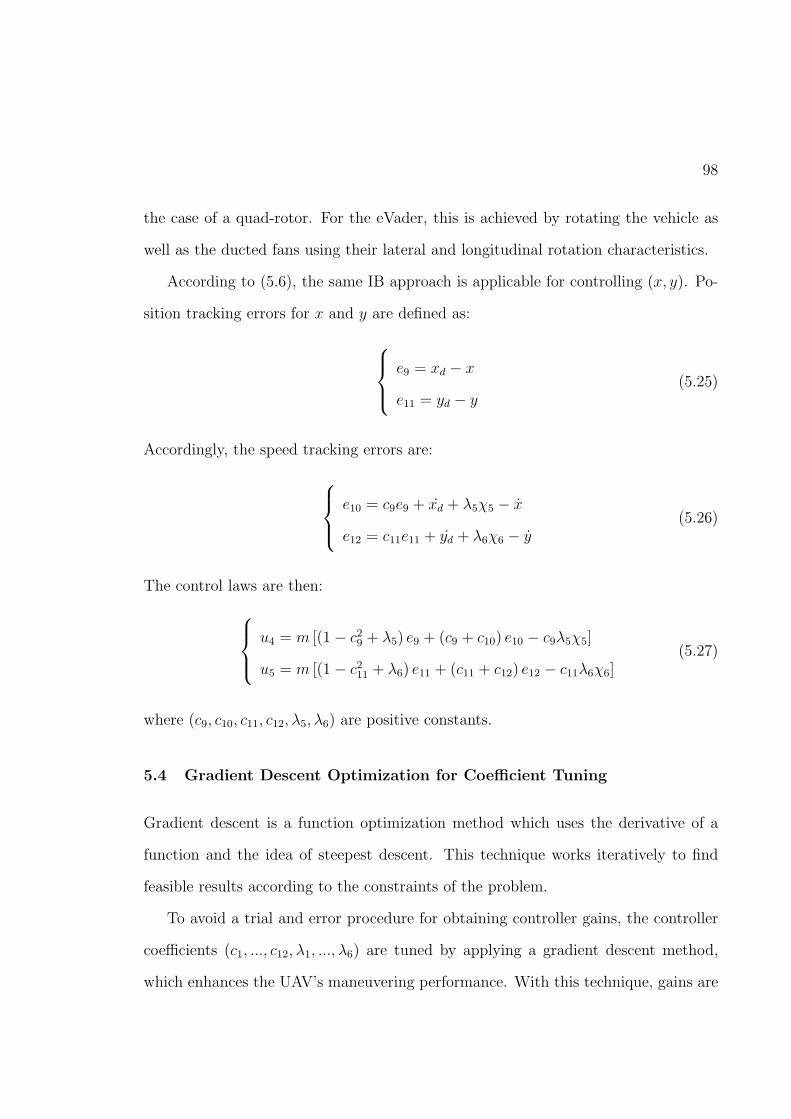
98
the case of a quad-rotor. For the eVader, this is achieved by rotating the vehicle as
well as the ducted fans using their lateral and longitudinal rotation characteristics.
According to (5.6), the same IB approach is applicable for controlling (x, y). Po-
sition tracking errors for x and y are defined as:
e9 = xd − x
e11 = yd − y(5.25)
Accordingly, the speed tracking errors are:
e10 = c9e9 + xd + λ5χ5 − x
e12 = c11e11 + yd + λ6χ6 − y(5.26)
The control laws are then:
u4 = m [(1− c29 + λ5) e9 + (c9 + c10) e10 − c9λ5χ5]
u5 = m [(1− c211 + λ6) e11 + (c11 + c12) e12 − c11λ6χ6](5.27)
where (c9, c10, c11, c12, λ5, λ6) are positive constants.
5.4 Gradient Descent Optimization for Coefficient Tuning
Gradient descent is a function optimization method which uses the derivative of a
function and the idea of steepest descent. This technique works iteratively to find
feasible results according to the constraints of the problem.
To avoid a trial and error procedure for obtaining controller gains, the controller
coefficients (c1, ..., c12, λ1, ..., λ6) are tuned by applying a gradient descent method,
which enhances the UAV’s maneuvering performance. With this technique, gains are

99
Figure 5.1: Attitude control of evader’s orientation and the corresponding control inputsignals of IB control method (φ = 10, θ = 35, ψ = 5).
tuned based on optimization of defined performance indices for improving transient
stability. The problem of setting nonlinear control gains is formulated as an optimiza-
tion problem including system and control constraints. Optimization-based methods
help to systematically accelerate the multiple-parameter tuning process.
5.5 Adaptive Integral Backstepping Control
The task of nonlinear design is much more challenging in the presence of uncertainty.
Backstepping with a general form of bounded uncertainties with unknown bounds is
a key tool used to achieve boundedness without adaptation. When the uncertainty
is in the form of constant but unknown parameters, then a more suitable form of the
backstepping is adaptive backstepping, developed in this section. For example, for
eVader UAV, the value of inertia matrix and the mass of the vehicle are uncertain

100
parameters. As the vehicle is capable of picking up different loads during a given
mission, the total mass of the vehicle may change which is a priori unknown. Adaptive
backstepping approach can help in such situations and thus enable UAVs in general,
and the eVader in particular, to perform more complex missions.
In order to design an adaptive controller for the eVader, the same assumptions
presented in Chapter 4 are considered. That is, the parametric value of inertial
matrix diag(Jx, Jy, Jz), and the mass of the vehicle, m, are unknown. For the sake
of simplifying the controller design, the aerodynamic friction is not considered in the
model for adaptive integral backstopping control design.
The following control law is chosen for adaptive controller:
u1 =1
b1
[
(
1− c21 + λ1)
e1 + (c1 + c2) e2 − c1λ1χ1 + φd − θψa1
]
(5.28)
where a1 is an estimate of a1 = Jy − Jz and b1 is an estimate of b1 = 1Jx. Now,
the update laws for parameter estimates should be derived to complete the adaptive
design. For this purpose, the parameter estimation error signals are defined as:
b1 = b1 − b1 a1 = a1 − a1 (5.29)
In order to obtain the update laws for parameter estimates, the Lyapunov design
approach is utilized. The Lyapunov energy function for the closed-loop system is
chosen as:
V =λ12χ21 +
1
2e21 +
1
2e22 +
1
2γ1a21 +
1
2γ2b22 (5.30)
In the above Lyapunov function, γ1, and γ2 are adaptive gains which are positive
constants, and they determine the convergence speed of the estimates.

101
The rest of the design approach is the same as in Section 4.4.1 in Chapter 4, which
will give the adaptation laws for parameter estimates, a1, b1 as below:
˙a1 = γ1e2θψ
˙b1 = γ2e2
(1− c21 + λ1) e1 + (c1 + c2) e2 − c1λ1χ1 + φd − θψa1
(5.31)
In (5.31), all parameters, c1, c2, λ1, χ1, e1, e2, θ, ψ, and φd are defined to be the same
as in Section 5.3.1.
5.6 Simulation Results
In this section, simulation results for several scenarios are presented in order to observe
the effectiveness of the derived model and the performances of the proposed control
law. We considered the case of stabilization and a trajectory tracking problem. The
following simulations are based on the eVader’s dynamic model presented in Equations
(5.6) and (5.7). In what follows the following UAV parameters from Table 3.2 in
Chapter 4 are used: m = 6.5kg, g = 9.8m/s2, Jr = 0.5×10⁻⁴kg.m2, Jx = 0.013kg.m2,
Jy = 6× 10⁻³kg.m2, Jz = 4× 10⁻⁴kg.m2, l = 0.4m, and h = 0.08m.
In the first simulation, the attitude control is considered. The initial condition
of the orientation angles and their derivatives are at zero. The desired values of the
vehicle orientation were placed at (φd, θd, ψd) = (10, 35, 5). The attitude control
results of the Backstepping approach and the obtained control signals can be seen
in Fig. 5.1. The results of stabilization of x and y position and the related control
signals are shown in Fig. 5.2.
For the purpose of autonomous take off and landing, the vehicle is forced to follow
the squared signal of altitude. The results are depicted in Fig.5.3 for different coeffi-

102
Figure 5.2: Position (x, y) stabilization of the eVader and the corresponding control inputsignals of IB control method.
Table 5.1: The IB controller gains.
c1 = 0.03 c4 = 2 c7 = 1 c10 = 0.05 λ1 = 0.005 λ4 = 0.7c2 = 1.55 c5 = 0.001 c8 = 0.005 c11 = 1.2 λ2 = 1 λ5 = 0.1c3 = 0.001 c6 = 1.5 c9 = 1.4 c12 = 0.05 λ3 = 1 λ6 = 0.1
Table 5.2: The IB controller gains for autonomous take off and landing scenario. In thistable k1 = 1− c211 + λ6, k2 = c11 + c12, k3 = c11λ6.
The blue curve The red curve The green curvek1 = 20.7476 k1 = 47.7377 k1 = 9322k2 = 7.9543 k2 = 8.1071 k2 = 181.5819k3 = 5.1735 k3 = 5.3916 k3 = 115.9134
103
Figure 5.3: Autonomous take-off, altitude control in hover and landing of the eVader andthe effect of tuning the IB controller gains by Gradient Descent algorithm.

104
Figure 5.4: Stabilization of roll, pitch and yaw angles by IB control method (left figure)and pitched stability of the eVader at 25 in hover (right figure).
cients in control law in (5.24). The gradient descent optimization method was used to
apply the desired constraints to the problem and force the output of the IB controller
to track desired trajectories with the error restrictions within an acceptable range
[92]. Therefore, the coefficients of the controller c1, c2, ..., c12, λ1, ...λ6, have been
adjusted by the gradient descent optimization algorithm. Applying the optimization
algorithm improves the controller design by estimating and tuning its parameters.
Different objectives of the optimization technique help improve system performance
and reduce control efforts. For the purpose of automatically tuning and optimiz-
ing controller gains of this thesis work, the rise-time and overshoot constraints were
chosen as objectives. Whenever the optimization solver finds a solution that meets
the design requirements within the parameter bounds, (e.g controller gains must be
positive), the local minimum is found and the optimization process terminates.
The effect of this optimization can be seen in Fig. 5.3. The position initial value

105
is (x(0), y(0), z(0)) = (1, 1, 0) m and the desired value of altitude is fixed at 2 m.
The effect of controller coefficient optimization is illustrated in this figure as well.
The first and second curves in Fig. 5.3 on top are infeasible answers because they
cause the vehicle crash on the ground. The third curve on top in this figure is a
feasible answer obtained from optimization process. The coefficients of control law
(5.24) for this answer are obtained as follows: c7 = 181.58, c8 = 9140.82, and λ4 = 1.
On bottom of Fig. 5.3 all these three curves are shown in the same coordinate to
provide a better sense of comparison. Figure 5.4 shows the stabilization of roll, pitch
and yaw angles. In this simulation the initial values of Euler angles is considered at
(φ0 = 10, θ0 = 35, ψ0 = 5) and the final values are (φ = 0, θ = 25, ψ = 0). The
vehicle becomes stable at 25 pitch angle while is at hover.
5.7 Summary
In this Chapter, an Integral Backstepping control approach was proposed to control
both position and orientation of an eVader. The IB controller is presented based on
the derived dynamic model of this special UAV, which enables us to design 6 control
laws. The controller design is divided to six subsystems, each of which is designed
through similar procedure. The main advantage of the above design method is that
difficulties of designing a controller for the entire system are avoided.
The recursive Lyapunov methodology in the backstepping technique ensures the
system stability, and the integral action increases the system robustness against dis-
turbances and model uncertainties. Furthermore, gradient descent optimization al-
gorithm was applied on controller to find and adjust the coefficients, which makes
the results to be even more promising. As a design tool, backstepping is less restric-
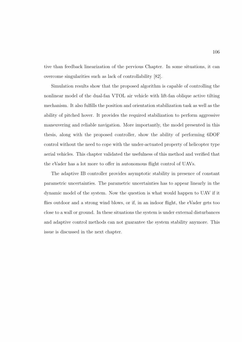
106
tive than feedback linearization of the pervious Chapter. In some situations, it can
overcome singularities such as lack of controllability [82].
Simulation results show that the proposed algorithm is capable of controlling the
nonlinear model of the dual-fan VTOL air vehicle with lift-fan oblique active tilting
mechanism. It also fulfills the position and orientation stabilization task as well as the
ability of pitched hover. It provides the required stabilization to perform aggressive
maneuvering and reliable navigation. More importantly, the model presented in this
thesis, along with the proposed controller, show the ability of performing 6DOF
control without the need to cope with the under-actuated property of helicopter type
aerial vehicles. This chapter validated the usefulness of this method and verified that
the eVader has a lot more to offer in autonomous flight control of UAVs.
The adaptive IB controller provides asymptotic stability in presence of constant
parametric uncertainties. The parametric uncertainties has to appear linearly in the
dynamic model of the system. Now the question is what would happen to UAV if it
flies outdoor and a strong wind blows, or if, in an indoor flight, the eVader gets too
close to a wall or ground. In these situations the system is under external disturbances
and adaptive control methods can not guarantee the system stability anymore. This
issue is discussed in the next chapter.

Chapter 6
Sliding Mode Control for the eVader
The controllers designed in the preceding chapter guarantee that in the presence of
uncertain bounded nonlinearities the closed-loop state remains bounded. Adaptive
control can deal with uncertainties by tuning of the parameters online, but generally
is able to achieve only asymptotical convergence of the tracking error to zero. As it is
mentioned in previous chapters, adaptive control method is based on the assumption
that the structure of the system model is known with unknown slow-varying system
parameters, where the parameters appear linear. But several issues, such as transient
performance, unmodeled dynamics, disturbances such as wind and ground effects,
and not linear parameterizable uncertainties often complicate the adaptive approach
[93], [94].
In this chapter, the focus is on a useful and powerful robust control scheme to deal
with the uncertainties, nonlinearities, and bounded external disturbances using the
sliding mode control (SMC) scheme. These and other uncertainties may come from
unmodeled dynamics, variations in system parameters, or approximations of complex
plant behaviours. In robust control designs, a fixed control law based on a priori
information of the uncertainties is typically designed to compensate for their effects,
107

108
and exponential convergence of the tracking error to a (small) ball centred at the
origin is obtained (see the definition of exponential stability in Chapter 2). Robust
control has some advantages over the adaptive control, such as its ability to deal with
disturbances, quickly-varying parameters, and unmodeled dynamics [63].
Sliding controller design provides a systematic approach to the problem of main-
taining stability and consistent performance despite modelling imprecisions. An
overview of the sliding-mode nonlinear controller and main concepts of SMC de-
sign, such as sliding surface, are introduced in Section 6.1. Section 6.2 represents the
state-space form of the eVader model to facilitate the SMC design. The following
section describes how to design a SMC for the eVader UAV. Section 6.4 then presents
studies of some simulations to investigate the robustness of SMC methodology for
the eVader maneuvers, such as pitched hover maneuvers, while a sudden wind may
be affecting the vehicle’s behavior. The final section of this chapter summarizes the
main concepts of this chapter.
6.1 Overview of Sliding Mode Control
From the control point of view, modelling inaccuracies can be classified into two ma-
jor kinds: i) structured or parametric uncertainties, which correspond to inaccuracies
in the terms included in the model and ii) unstructured uncertainties or unmodeled
dynamics, which correspond to inaccuracies in the system order. Modelling inaccura-
cies has strong effects on nonlinear control systems. Therefore, practical designs must

109
address them explicitly. Two major approaches to dealing with model uncertainty are
robust control and adaptive control. In Chapter 4 of this thesis, adaptive control for
the eVader was employed. In this chapter the focus is on robust control approaches.
The typical structure of a robust controller is composed of a nominal part, similar
to a feedback linearizing or inverse control law, and of additional terms to cope with
model uncertainty. The structure of an adaptive controller is similar, but the differ-
ence is that the model is actually updated during operation, based on the measured
performance. A simple approach to robust control is the so-called sliding control
methodology. ”Perfect” performance can be achieved in the presence of arbitrary
parameter inaccuracies.
6.1.1 Sliding Surfaces
Sliding mode control is a high-speed switched feedback control. It is also known as
variable structure control (VSC) in the literature. The most important task in the
SMC methodology is to design a switched control that drives the plant state to the
switching surface and maintains it on the surface upon interception. A Lyapunov
approach is used to characterize this task. A generalized Lyapunov function, that
characterizes the motion of the state trajectory to the sliding surface, is defined in
terms of the surface. For each chosen switched control structure, one chooses the gains
so that the derivative of this Lyapunov function is negative definite, thus guaranteeing
motion of the state trajectory to the surface. After proper design of the surface, a

110
switched controller is constructed so that the tangent vectors of the state trajectory
point towards the surface such that the state is driven to and maintained on the
sliding surface. Such controllers result in discontinuous closed-loop systems. To be
more precise, the gains in each feedback path switch between two values according
to a rule that depends on the value of the state at each instant. The purpose of
the switching control law is to drive the nonlinear plant’s state trajectory onto a
prespecified (user-chosen) surface in the state-space and to maintain the plant’s state
trajectory on this surface for subsequent time. The surface is called a switching
surface. When the plant state trajectory is ”above” the surface, a feedback path
would have a specific gain and then, a different gain if the trajectory drops below the
surface. This surface defines the rule for proper switching. This surface is also called
a sliding surface (sliding manifold). Ideally, once intercepted, the switched control
maintains the plant’s state trajectory on the surface for all subsequent time, and the
plant’s state trajectory slides along this surface. The motion of the system as it slides
along boundaries of the control structures is called a sliding mode [95].
Intuitively, sliding mode control uses practically infinite gain to force the tra-
jectories of a dynamic system to slide along the restricted sliding mode subspace.
Trajectories from this reduced-order sliding mode have desirable properties (e.g., the
system naturally slides along it until it comes to rest at a desired equilibrium). The
main strength of sliding mode control is its robustness. Because the control can be as
simple as a switching between two states (e.g., on/off ), it does not need to be precise

111
and will not be sensitive to parameter variations that enter into the control chan-
nel. Additionally, because the control law is not a continuous function, the sliding
mode can be reached in finite time (i.e., better than asymptotic behavior). However,
real implementations of sliding mode control approximate the theoretical behavior
of sliding along the surface with a high-frequency and generally non-deterministic
switching control signal that causes the system to ”chatter” in a tight neighborhood
of the sliding surface [96].
In summary, the motion consists of a reaching phase during which trajectories
starting off the manifold S = 0 move toward it and reach it in finite time, followed by
a sliding phase, during which, the motion is confined to the manifold S = 0 and the
dynamics of the system are represented by a reduced-order model with exponentially
stable error dynamics. The S = 0 is called the sliding mode, and the control law
manifold u = −κ(x)sgn(S) is called sliding control mode.
6.1.2 Chattering
It should be noted that the controller is discontinuous at S = 0. Thus, sliding mode
control must be applied with more care than other forms of nonlinear control that
have more moderate control action. In particular, due to the effects of sampling,
switching and delays in the actuators used to implement the controller, and other
imperfections, the hard SMC action can lead to chatter, energy loss, plant damage,
and excitation of unmodeled dynamics [97]. Figure 6.1 shows how delays can cause

112
Figure 6.1: Chattering due to delay in control switching.
chattering. It depicts a trajectory in the region S > 0 heading toward the sliding
manifold S = 0. The trajectory first hits the manifold at a point Pa. In ideal sliding
mode control, the trajectory should start sliding on the manifold from a point Pa.
In reality, there will be a delay between the time the sign of S changes and the time
the control switches. During this delay period, the trajectory crosses the manifold
into the region S < 0. Chattering results in low control accuracy, high heat losses
in electrical power circuits, and high wear of moving mechanical parts. It may also
excite unmodeled high frequency dynamics, which degrade the performance of the
system and may potentially even lead to instability.

113
One commonly used method to eliminate the effects of chattering is to replace the
switching control law by a saturating approximation within boundary layer around
the sliding surface [63], [98], and [99]. Inside the boundary layer, the discontinuous
switching function κsgn(S) is approximated by a continuous function to avoid dis-
continuity of the control signals. Even though the boundary layer design can alleviate
the chattering phenomenon, this approach, however, provides no guarantee of conver-
gence to the sliding mode, and involves a trade-off between chattering and robustness,
and results in the existence of the steady state error.
6.2 Modeling for Control
From Chapter 3, the vehicle’s model can be written in the following form with additive
external disturbances d1, ..., d6.
φ = 1Jx
[
(Jy − Jz)θψ − ktaxφ2 − JrΩθ + u1 + d1
]
θ = 1Jy
[
(Jz − Jx)ψφ− ktayθ2 − JrΩφ+ u2 + d2
]
ψ = 1Jz
[
(Jx − Jy)θφ− ktazψ2 + u3 + d3
]
x = 1m[−Kfaxx
2 + u4 + d4]
y = 1m[−Kfayy
2 + u5 + d5]
z = 1m[−Kfaz z
2 −mg + u6 + d6]
(6.1)

114
Consider the state-space model presented in (6.1), where the vector y = [φ, θ, ψ, x, y, z]T
is the output of interest, the vector u = [u1, u2, u3, u4, u5, u6]T is the control input,
and x = [x1, x2, ..., x12]T is the vehicle’s state vector such as
x = [φ, φ, θ, θ, ψ, ψ, x, x, y, y, z, z]T .
The state-space model can be written in the following closed form:
x = f(x) + b(x)u+ d(x) (6.2)
with f(x), b(x), d(x) defined as follows:

115
f(x) =
x2
a1x4x6 − a2x22 − a3Ωx4
x4
a4x2x6 − a5x24 − a6Ωx2
x6
a7x2x4 − a8x26
x8
−a9x28
x10
−a10x210
x12
−a11x212 − g
12×1
(6.3)
where
a1 =Jy−JzJx
a2 =ktaxJx
a3 =JrJx
a4 =Jz−JxJy
a5 =ktayJy
a6 =JrJy
a7 =Jx−JyJz
a8 =ktazJz
a9 =Kfax
ma10 =
Kfay
ma11 =
Kfaz
m.

116
b(x) =
0 0 0 0 0 0
b1 0 0 0 0 0
0 0 0 0 0 0
0 b2 0 0 0 0
0 0 0 0 0 0
0 0 b3 0 0 0
0 0 0 0 0 0
0 0 0 b4 0 0
0 0 0 0 0 0
0 0 0 0 b4 0
0 0 0 0 0 0
0 0 0 0 0 b4
12×6
(6.4)
where b1 =1Jx, b2 =
1Jy, b3 =
1Jz, and b4 =
1m.
And finally d(x) is defined as:
d(x) =
[
0 d1 0 d2 0 d3 0 d4 0 d5 0 d6
]T
(6.5)
In (6.2) the nonlinear function f(x) is not exactly known, and the control gain b(x)
is of known sign but unknown exact value. f(x) and b(x) are both upper bounded
by known, continuous function of x and external disturbance b(x). The inertia of

117
a mechanical system is only known to a certain accuracy, and friction models only
describe part of the actual friction forces. The control problem is to get the state x
to track a specific time varying state xd in the presence of model imprecision on f(x)
and b(x).
Remark: The disturbance d(x) can describe uncertainties such as inaccurate
torques and lifts of the rotors, the ground effects, wind disturbance, and the bias
between the geometric centre and its centre of gravity.
6.3 Sliding Mode Control based on Backstepping
In this thesis a 2 step approach for the design of the controller is taken. The two
steps are:
1. Defining the sliding mode. This is a surface that is invariant of the controlled
dynamics, where the controlled dynamics are exponentially stable, and where the
system tracks the desired set-point.
2. Defining the control that drives the state to the sliding mode in finite time.
6.3.1 Controller Design
The first step in designing the sliding mode controller is similar to the one used for
the backstepping approach, except Sφ (Surface) as defined in (6.6) is used instead of
e2:
Sφ = λ1e1 + x2 − x1d (6.6)

118
For the second step the following augmented Lyapunov function is considered:
V (e1, Sφ) =1
2(e21 + S2
φ)
The chosen law for the attraction surface is the time derivative of (6.6) satisfying
(SS < 0):
Sφ = −k1sgn(Sφ)− λ1Sφ
= λ1e1 + x2 − x1d
= λ1(x2 − x1d)− x1d + a1x4x6 + b1u1 + d1(t)
(6.7)
As for the backsteppning approach the control u1 is extracted:
u1 =1
b1[−a1x4x6 + x1d − k1sgn(Sφ)− λ21e1 − 2λe1] (6.8)
Using the backstepping approach as a recursive algorithm for the synthesis of
control-law, all the stages of calculation concerning the tracking errors and Lyapunov
functions can be simplified in the following way:
ei =
xi − xid i ∈ 1, 3, 5, 7, 9, 11
λje(i−1) + xi − x(i−1)d i ∈ 2, 4, 6, 8, 10, 12(6.9)

119
with λj > 0,∀j ∈ [1, 6], and
Vi =
12e2i i ∈ 1, 3, 5, 7, 9, 11
12(Vi−1 + e2i ) i ∈ 2, 4, 6, 8, 10, 12
(6.10)
The choice of the sliding surfaces is based upon the synthesized tracking errors
which permitted us the synthesis of stabilizing control laws. Thus, from (6.9) the
dynamic sliding surfaces, Sφ, Sθ, Sψ, Sx, Sy and Sz, are defined as:
Sφ = λ1e1 + e1
Sθ = λ2e3 + e3
Sψ = λ3e5 + e5
Sx = λ4e7 + e7
Sy = λ5e9 + e9
Sz = λ6e11 + e11
(6.11)
As e1 = φ− φd, e3 = θ − θd, e5 = ψ − ψd, e7 = x− xd, e9 = y − yd, and e11 = z − zd,
and for simplicity in notations, the switching surfaces can be rewritten as:

120
Sφ = λ1eφ + eφ
Sθ = λ2eθ + eθ
Sψ = λ3eψ + eψ
Sx = λ4ex + ex
Sy = λ5ey + ey
Sz = λ6ez + ez
(6.12)
To synthesize a stabilizing control law by sliding mode, the necessary sliding con-
dition (SS < 0) must be verified; so the synthesized stabilizing control laws are as
follows:
u1 =1b1
[
−a1x4x6 + φd(t)− 2λ1eφ(t)− λ21eφ(t)− k1sgn(Sφ)]
u2 =1b2
[
−a2x2x6 + θd(t)− 2λ2eθ(t)− λ22eθ(t)− k2sgn(Sθ)]
u3 =1b3
[
−a3x2x4 + ψd(t)− 2λ3eψ(t)− λ23eψ(t)− k3sgn(Sψ)]
u4 =1b4[−a9x
2 + xd(t)− 2λ4ex(t)− λ24ex(t)− k4sgn(Sx)]
u5 =1b4[−a10y
2 + yd(t)− 2λ5ey(t)− λ25ey(t)− k5sgn(Sy)]
u6 =1b4[−a11z
2 − g + zd(t)− 2λ6ez(t)− λ26ez(t)− k6sgn(Sz)]
(6.13)
6.4 Simulation Results
In order to test the developed SMC a number of simulations were tested. Herein,
four of such simulations are presented, which show the performance of the developed

121
SMC. The following four scenarios are presented: 1) pitched hover, 2) pitched hover
under wind disturbances, 3) Scenario # 2 with varying model parameters, and 4)
picking up a load.
1. Pitched hover scenario (Scenario #7): The first simulation is the pitched hover
maneuver, where the vehicle is commanded to hover in a maneuver that no aircraft
known to have performed. In this case study, the system initial condition and the
desired states are chosen as below:
x0 = [22.5, 0, 0, 0, 18, 0, 5, 0, 4, 0, 3, 0]T
xd = [0, 0, 22.5, 0, 0, 0, 0, 0, 0, 0, 3, 0]T
In other words, the controller is commanded to maintain the eVader at the same
altitude at 3 m while pitching its nose from 0 to 22.5, and regulate all other states
to zero. The results are illustrated in Figs. 6.2, 6.3, and 6.4. For this simulation, the
switching functions and controller gains are selected according to Table 6.1. Figure
6.2 shows the six control signals u1, ..., u6. The chattering effect is obviously seen in
this figure. Figure 6.3 shows that the controller is able to regulate the eVader’s roll
and yaw angles to zero, while keeping the vehicle’s pitch angle at 22.5 .
2. Pitched hover windy scenario (unstructured uncertainty, Scenario #8):
The next scenario is the eVader in a pitched hover condition facing a sudden
strong sinusoidal wind disturbance. The initial condition and desired values of states

122
Table 6.1: The SMC controller gains and sliding surfaces
λ1 = 20 Sφ = 20eφ + eφ k1 = 1λ2 = 20 Sθ = 20eθ + eθ k2 = 1λ3 = 20 Sψ = 20eψ + eψ k3 = 1λ4 = 10 Sx = 10ex + ex k4 = 1.5λ5 = 10 Sy = 10ey + ey k5 = 1.5λ6 = 10 Sz = 10ez + ez k6 = 1.5
are the same as previous scenario, and it is assumed that after 1.5 s, the wind blows
for 0.2 s. Wind as an external disturbance is formulated with d1(t) = d2(t) = d3(t) =
d4(t) = d5(t) = d6(t) = 5(10+5sin(2πt)) in eVader model in (6.5). It is also assumed
that wind blows in all directions effects on all states. The results in Figs. 6.5 and 6.6
illustrate the robustness of sliding mode controller in presence of unstructured un-
certainties. This property insures the stability of eVader, while external disturbances
such as wind, ground and wall effects affect the vehicle during its maneuvers.
3. Scenario # 2 with varying model parameter (structured uncertainty): The sim-
ulation scenario # 2 used in Chapter 4, Section 4.7, is simulated again here to verify
the robustness of the designed SMC controller to parameter variations. The scenario
is defined as follows: the initial condition is x0 = [0, 0, 0, 0, 0, 0, 0, 0, 0, 0, 0, 0]T , and
the desired value is xd = [22.5, 0, 15, 0, 18, 0, 3, 0, 4, 0, 2, 0]T . In this simulation the
mass of the eVader is changed with the same amount as in Chapter 4. Moreover,
the inertia matrix of the vehicle is also changed by 20%. Another simulation was
made on the eVader model with mass and inertia matrix uncertainty and the added

123
random noise. This noise can be considered as a measurement noise. The results
were compared with the results of simulation without parameter uncertainty, and
also with the scenario with only the parameter uncertainty but no added noise, in
Table 6.2. As it can be seen easily from this table, after 1 second has passed, the error
for all six outputs are almost zero for all mentioned scenarios. The results in Table
6.2 verify the robustness of the proposed designed controller in presence of struc-
tured (parametric) uncertainty. Figures 6.7 and 6.8 show the control input signals,
the orientation output, and the position output of the eVader, respectively, in this
simulation scenario.
4. Picking-up-a-load scenario (Scenario #11): In this simulation, the eVader is
commanded to pick up a heavy load of 3.5 kg after 1 second into the simulation. It
is assumed that this load adds a sudden disturbance to the pitch (θ) and the pitch
angular velocity (θ) of the vehicle. The results are depicted in Figs. 6.9, 6.10, and
6.11, which show the ability of the controller in handling this situation. The system
pitch returned to a steady state in 0.25 s. The steady state error of altitude is only
4 cm and reached after 0.5 s.
6.5 Summary
A simple approach to robust control is the so-called sliding control methodology. The
aim of a sliding controller is to design a control law to effectively account for parameter
uncertainty, including imprecision on the mass properties or loads, inaccuracies in the

124
Table 6.2: The results of SMC controller for position and orientation regulation simulation(Scenario # 2) in three different conditions: i) the parameters of the dynamic model areknown and do not change, ii) the mass and inertia matrix of the vehicle have uncertaintyand change during the flight, iii) the parameters of the dynamic model have uncertaintyand change plus there is additive white noise due to the sensor measurement noise.
i) Fixed parameters ii) Varying parameters iii) Additive sensor noisetime (sec) error (deg, m) error (deg, m) error (deg, m)
Roll φ 1 0.0089 0.0089 0.0290Pitch θ 1 0.0090 0.0089 0.0379Yaw ψ 1 0.0090 0.009 0.0023Position x 1 0.00003 0.0008 0.0027Position y 1 0.00007 0.0011 0.0033Altitude z 1 0.0003 0.0426 0.0124
0 0.5 1 1.5−5
0
5
10Control Signal u1
time[s]
u1
0 0.5 1 1.5−2000
0
2000
4000Control Signal u4
time[s]
u4
0 0.5 1 1.5−10
0
10Control signal u2
time[s]
u2
0 0.5 1 1.5−2000
0
2000
4000Control signal u5
time[s]
u5
0 0.5 1 1.5−10
0
10Control signal u3
time[s]
u3
0 0.5 1 1.598.0698.08
98.198.1298.14
Control signal u6
time[s]
u6
Figure 6.2: Control input signals of SMC technique for performing pitched hover scenario(Scenario # 7).
125
0 0.1 0.2 0.3 0.4 0.5 0.6 0.7 0.8 0.9 1−10
0
10
20The roll angle
time[s]
Ro
ll[d
eg
re
e]
0 0.1 0.2 0.3 0.4 0.5 0.6 0.7 0.8 0.9 1−20
0
20
40The yaw angle
time[s]
Ya
w[d
eg
re
e]
0 0.1 0.2 0.3 0.4 0.5 0.6 0.7 0.8 0.9 10
10
20The pitch angle
time[s]
Pitch
[de
gre
e]
Figure 6.3: Orientation angles regulationin pitched hover stationary scenario (Sce-nario # 7).
0 0.1 0.2 0.3 0.4 0.5 0.6 0.7 0.8 0.9 10
2
4The Cartesian position x
time[s]
x[m
]
system outputdesired x(t)
0 0.1 0.2 0.3 0.4 0.5 0.6 0.7 0.8 0.9 10
2
4
The Cartesian position y
time[s]
y[m
]
0 0.1 0.2 0.3 0.4 0.5 0.6 0.7 0.8 0.9 13
3
3The Cartesian position z
time[s]z[m
]
Figure 6.4: Position regulation while sta-tionary at pitched hover scenario (Sce-nario # 7).
torque constants of the actuators, friction, and so on.
Although perfect tracking can be achieved in principle in the presence of arbitrary
parameter inaccuracies, such performance is obtained at the cost of extremely high
control activity. The drawback is that this high control activity may excite high
frequency dynamics neglected in the course of modeling. In practice, this corresponds
to modification of control laws by replacing a switching, chattering control law by its
smooth approximation. The switching control laws derived above can be smoothly
interpolated in boundary layers, so as to eliminate chattering, thus leading to a trade-
off between parametric uncertainty and tracking performance.
In this chapter, a robust controller based on SMC methodology was designed for

126
0 0.5 1 1.5 2−20
0
20Control Signal u1
time[s]
u1
0 0.5 1 1.5 2−2000
0
2000
4000Control Signal u4
time[s]
u4
0 0.5 1 1.5 2−40
−20
0
20Control signal u2
time[s]
u2
0 0.5 1 1.5 2−2000
0
2000
4000Control signal u5
time[s]
u50 0.5 1 1.5 2
−20
−10
0
10Control signal u3
time[s]
u3
0 0.5 1 1.5 2−1000
−500
0
500Control signal u6
time[s]u6
Figure 6.5: Control input signals of SMC technique in presence of a strong sudden winddisturbance (unstructured uncertainty, Scenario # 8).
0 0.2 0.4 0.6 0.8 1 1.2 1.4 1.6 1.8 2−10
0
10
20The roll angle
time[s]
Ro
ll[d
eg
re
e]
0 0.2 0.4 0.6 0.8 1 1.2 1.4 1.6 1.8 20
20
40The pitch angle
time[s]
Pitch
[de
gre
e]
0 0.2 0.4 0.6 0.8 1 1.2 1.4 1.6 1.8 2−50
0
50The yaw angle
time[s]
Ya
w[d
eg
re
e]
0 0.2 0.4 0.6 0.8 1 1.2 1.4 1.6 1.8 20
2
4
6The Cartesian position x
time[s]
x[m
]
0 0.2 0.4 0.6 0.8 1 1.2 1.4 1.6 1.8 20
5
10The Cartesian position y
time[s]
y[m
]
0 0.2 0.4 0.6 0.8 1 1.2 1.4 1.6 1.8 22.8
3
3.2The Cartesian position z
time[s]
z[m
]
Figure 6.6: Orientation angles and position regulation in hover pitched scenario with astrong sudden wind disturbance with magnitude 5 (Scenario # 8).

127
0 0.2 0.4 0.6 0.8 1−10
0
10Control Signal u1
time[s]
u1
0 0.1 0.2 0.3 0.4 0.5 0.6 0.7 0.8 0.9 1−500
0
500
1000
1500Control Signal u4
time[s]
u4
0 0.2 0.4 0.6 0.8 1−10
0
10Control signal u2
time[s]
u2
0 0.2 0.4 0.6 0.8 1−1000
0
1000
2000Control signal u5
time[s]
u50 0.2 0.4 0.6 0.8 1
−10
0
10Control signal u3
time[s]
u3
0 0.2 0.4 0.6 0.8 1−1000
0
1000
2000Control signal u6
time[s]u6
Figure 6.7: Control input signals of SMC technique when performing Scenario # 2 andsystem parameters (mass and inertia matrix) are varying.
0 0.05 0.1 0.15 0.2 0.25 0.3 0.35 0.4 0.45 0.50
20
40The roll angle
time[s]
Ro
ll[d
eg
re
e]
0 0.05 0.1 0.15 0.2 0.25 0.3 0.35 0.4 0.45 0.50
10
20The pitch angle
time[s]
Pitch
[de
gre
e]
0 0.05 0.1 0.15 0.2 0.25 0.3 0.35 0.4 0.45 0.50
10
20The yaw angle
time[s]
Ya
w[d
eg
re
e]
0 0.1 0.2 0.3 0.4 0.5 0.6 0.7 0.8 0.9 10
2
4The Cartesian position x
time[s]
x[m
]
0 0.1 0.2 0.3 0.4 0.5 0.6 0.7 0.8 0.9 10
2
4
6The Cartesian position y
time[s]
y[m
]
0 0.1 0.2 0.3 0.4 0.5 0.6 0.7 0.8 0.9 10
1
2The Cartesian position z
time[s]
z[m
]
Figure 6.8: Orientation angles and position regulation with model parameter variationsshow robustness of SMC technique in presence of structured uncertainties.

128
0 0.5 1 1.5−40
−20
0
20Control Signal u1
time[s]
u1
0 0.5 1 1.5−1000
0
1000
2000Control Signal u4
time[s]
u4
0 0.5 1 1.5 2−100
−50
0
50Control signal u2
time[s]
u2
0 0.5 1 1.5−1000
0
1000
2000Control signal u5
time[s]
u50 0.5 1 1.5
−50
0
50Control signal u3
time[s]
u3
0 0.5 1 1.5 260
80
100
120Control signal u6
time[s]u6
Figure 6.9: Control input signals of SMC technique while picking up a heavy load (Scenario# 11).
eVader, which achieves exponential tracking control of a desired trajectory where
the plant dynamics contain uncertainty and bounded non-LP disturbances. Simula-
tion results demonstrate the robustness of the controllers to sensor noise, exogenous
perturbations, parametric uncertainty, and plant nonlinearities, while simultaneously
exhibiting the capability to follow a reference trajectory. However, in order to com-
pensate for uncertainties in the model and external disturbances, large input gains
are required which makes a serious limitation in power-limited systems such as small
UAVs like eVader. Moreover, the chattering phenomena may cause the rotors to
rotate and tilt in a different direction very fast. This may makes using the SMC
impossible for eVader even though it has a robustness property which is necessary for
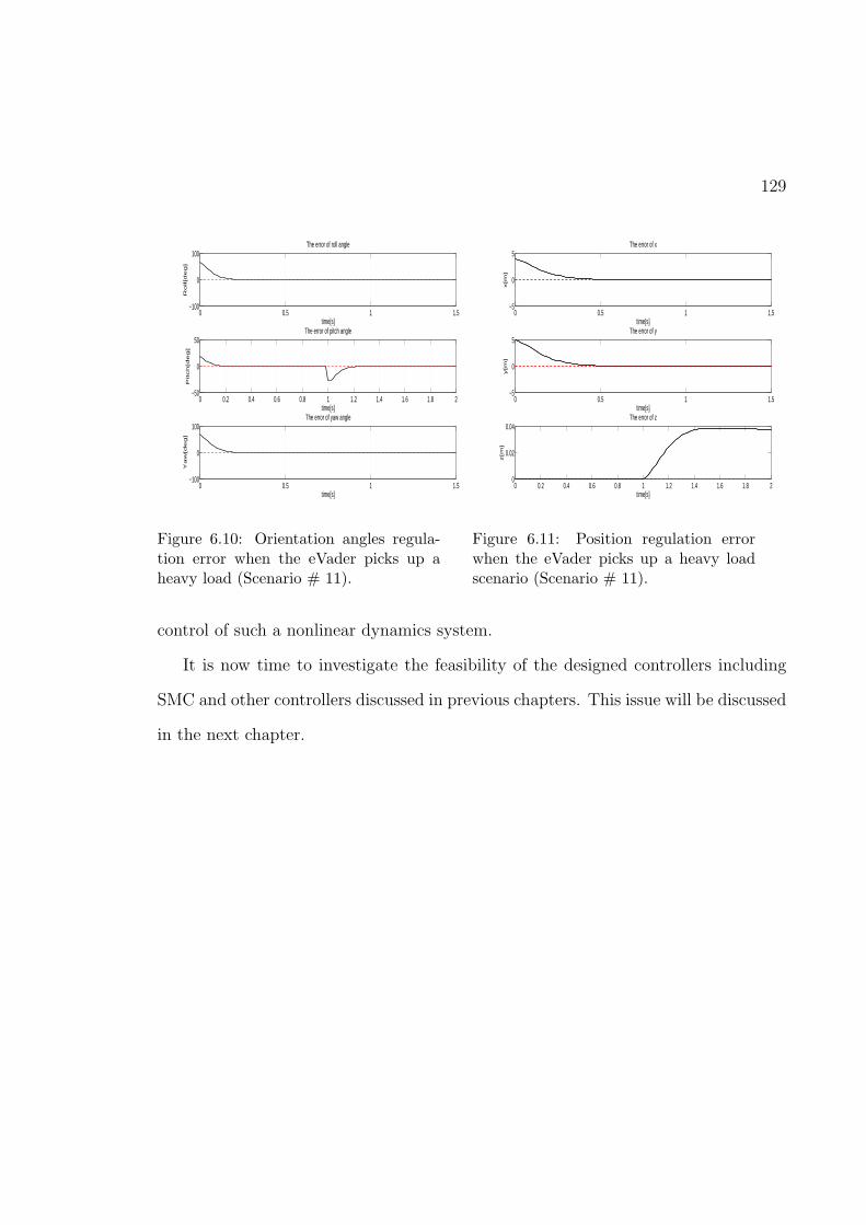
129
0 0.5 1 1.5−100
0
100The error of roll angle
time[s]
Ro
ll[d
eg
]
0 0.2 0.4 0.6 0.8 1 1.2 1.4 1.6 1.8 2−50
0
50The error of pitch angle
time[s]
Pitch
[de
g]
0 0.5 1 1.5−100
0
100The error of yaw angle
time[s]
Ya
w[d
eg
]
Figure 6.10: Orientation angles regula-tion error when the eVader picks up aheavy load (Scenario # 11).
0 0.5 1 1.5−5
0
5The error of x
time[s]
x[m
]
0 0.5 1 1.5−5
0
5The error of y
time[s]
y[m
]
0 0.2 0.4 0.6 0.8 1 1.2 1.4 1.6 1.8 20
0.02
0.04The error of z
time[s]z[m
]
Figure 6.11: Position regulation errorwhen the eVader picks up a heavy loadscenario (Scenario # 11).
control of such a nonlinear dynamics system.
It is now time to investigate the feasibility of the designed controllers including
SMC and other controllers discussed in previous chapters. This issue will be discussed
in the next chapter.

Chapter 7
Neural Network Nonlinear Function Approximation
In previous chapters of this thesis we have derived the dynamic model of eVader UAV
and then designed several control laws to do specific tasks such as regulation to an
arbitrary desired position and orientation, tracking a time varying trajectory in 3D
space, and taking off and landing. All of the designed controllers in previous chapters
are based on six control signals u1, ..., u6, such as six control signals in Equations
(5.3) and (4.8) in Chapters 5 and 4, respectively. However, control signals u1, ..., u6
are not the real actuator signals. They are nonlinear functions of the actual control
signals α1, α2, β1, β2, ω1, ω2, that would be used to actually control the actuators
influencing them. The applicability of previously designed controllers, the eVader
and dOAT mechanism, lies in the existence of a feasible (in range) combination of
longitudinal and lateral angles, and rotor angular speeds, namely α1, α2, β1, β2, ω1, ω2,
to produce the necessary control signals. Thus the question is how to solve equations
of u1, ..., u6 based on α1, α2, β1, β2, ω1, ω2 to obtain actual control signals. Since these
equations do not have a mathematical systematic solution, it is not possible to obtain
the exact values of α1, α2, β1, β2, ω1, ω2. Hence, we proposed to utilize nonlinear
function approximator approaches to find an approximation of these functions in a
130

131
way that by entering the six control signals u1, ..., u6, the function approximator would
give us α1, α2, β1, β2, ω1, ω2 as its outputs. To address this problem, a Multi Layer
Perceptron (MLP) neural network is trained in this thesis as an inverse mapping of the
u1, ..., u6 functions, using supervised learning with back-propagation (BP) algorithm.
By applying this approach, we find an approximation of the actual control signals of
dOAT mechanism, which has not been addressed in the literature before.
The rest of this chapter is organized as follows. The benefits of using neural
networks for the specific problem of this research are first discussed in Section 7.2,
followed by an explanation of feedforward networks in Section 7.3. The MLP networks
are introduced in Section 7.4. Section 7.5 explains the BP learning algorithm. The
application and the results of the MLP neural network with BP learning algorithm
for our specific problem of approximation of the inverse mapping between α1, α2, β1,
β2, ω1, ω2 and u1, ..., u6 is investigated in Section 7.6. Finally, a summary of this
chapter and the main observations and findings of it are discussed in Section 7.7.
7.1 Benefits of Neural Networks
The neural network derives its computing power through, first, its massively par-
allel distributed structure and, second, its ability to learn and therefore generalize.
Generalization refers to the neural network producing reasonable outputs for inputs
not encountered during training (learning). These two information-processing capa-
bilities make it possible for neural networks to solve complex (large-scale) problems

132
that are currently intractable such as the problem of solving the nonlinear functions
of u1, ..., u6 based on six unknown variables α1, α2, β1, β2, ω1, ω2, which does not
have any conventional mathematical solution. The use of neural networks offers the
following useful properties and capabilities:
1. Nonlinearity. A neuron is basically a nonlinear device. Consequently, a neu-
ral network, made up of an interconnection of neurons, is itself nonlinear. Moreover
the nonlinearity is of a special kind in the sense that it is distributed throughout the
network. Nonlinearity is a highly important property, particularly if the underlying
physical mechanism responsible for the generation of an input signal is inherently
nonlinear such as the eVader’s dynamic in the specific problem at hand in this thesis.
2. Input-Output Mapping. A popular concept of learning called supervised
learning (Fig. 7.1) involves the modification of the weights of a neural network by
applying a set of labeled training samples or task examples. Each example consists
of a unique input signal and the corresponding desired response. The network is
presented and an example picked at random from the set, and the weights (free
parameters) of the network are modified so as to minimize the difference between
the desired response and the actual response of the network produced by the input
in accordance with an appropriate statistical criterion. The training of the network
is repeated for many examples in the set until the network reaches a steady state,
where there are no further significant changes in the weights. The previously applied
training examples may be reapplied during the training session but in a different order.

133
Figure 7.1: Supervised learning block diagram.
Thus the network learns from the examples by constructing an input-output mapping
for the problem at hand. Lack of existing systematic mathematical approaches for
the problem of finding actual control signals of UAV flight makes us to think of its
solution as an input-output mapping problem.
3. Adaptivity. Neural networks have a built-in capability to adapt their weights
to changes in the surrounding environment. In particular, a neural network trained to
operate in a specific environment can be easily retrained to deal with minor changes
in the operating environmental conditions. Moreover, when it is operating in a non-
stationary environment (i.e. one whose statistics change with time), a neural network
can be designed to change its weights in real time (adaptive neural network). As a
general rule, it may be said that the more adaptive we make a system in a properly

134
designed fashion, assuming the adaptive system is stable, the more robust its per-
formance will likely be when the system is required to operate in a non-stationary
environment. It should be emphasized, however, that adaptivity does not always
lead to robustness. Indeed, it may do the very opposite. For example, an adaptive
system with short time constants may change rapidly and therefore tend to respond
to spurious disturbances, causing a drastic degradation in system performance.
7.2 Problem Statement
Recalling the equations of u1, ..., u6 from Chapter 3, we have:
u1 = −cosα1Jrω1α1 − sinα1Jrω1β1 + sinα1Jrω1α1
−cosα2Jrω2α2 − sinα2Jrω2β2 + sinα2Jrω2α2
−ho(sinβ1cosα1T1 + sinβ2cosα2T2) + lo(cosβ1cosα1T1 − cosβ2cosα2T2)
−sinα1Q1 + sinα2Q2 + cosα1Jpβ1 + cosα2Jpβ2
u2 = −sinβ1sinα1Jrω1α1 + cosβ1Jrω1β1 + sinβ1cosα1(Jrω1β1 − Jrω1α1)
−sinβ2sinα2Jrω2α2 + cosβ2Jrω2β2 + sinβ2cosα2(Jrω2β2 − Jrω2α2)
+sinβ1cosα1Q1 − sinβ2cosα2Q2 − ho(sinα1T1 + sinα2T2)
+sinβ1sinα1Jpβ1 + cosβ1Jpα1 + sinβ2sinα2Jpβ2 + cosβ2Jpα2
(7.1)

135
u3 = cosβ1sinα1Jrω1α1 + sinβ1Jrω1β1 − cosβ1cosα1(Jrω1β1 − Jrω1α1)
+cosβ2sinα2Jrω2α2 + sinβ2Jrω2β2 − cosβ2cosα2(Jrω2β2 − Jrω2α2)
−cosβ1cosα1Q1 + cosβ2cosα2Q2 − lo(sinα1T1 − sinα2T2)
−cosβ1sinα1Jpβ1 + sinβ1Jpα1 − cosβ2sinα2Jpβ2 + sinβ2Jpα2
u4 = CφCψFx + (SφSθCψ − CφSψ)Fy + (CθSθCψ + SφSψ)Fz
u5 = CθSψFx + (SφSθSψ + CφCψ)Fy + (CφSθSψ − SφCψ)Fz
u6 = −SφFx + SφCθFy + CφCθFz
Fx = sinα1T1 + sinα2T2
Fy = −sinβ1cosα1T1 − sinβ2cosα2T2
Fz = cosβ1cosα1T1 + cosβ2cosα2T2
In order to be able to control the eVader for autonomous flight, based on the
proposed model with six control inputs, the actual control signals, α1, α2, β1, β2, ω1,
ω2, are needed to be obtained. As there are no mathematical systematic approaches to
solve the system of nonlinear equations in (7.1), we are seeking for an approximation
of the six functions in (7.1) so that by giving u1, ..., u6 as an input, the approximation
would give us α1, α2, β1, β2, ω1, ω2. Therefore, we have to find the inverse mapping
between these variables. For this purpose, the neural network is trained as an inverse
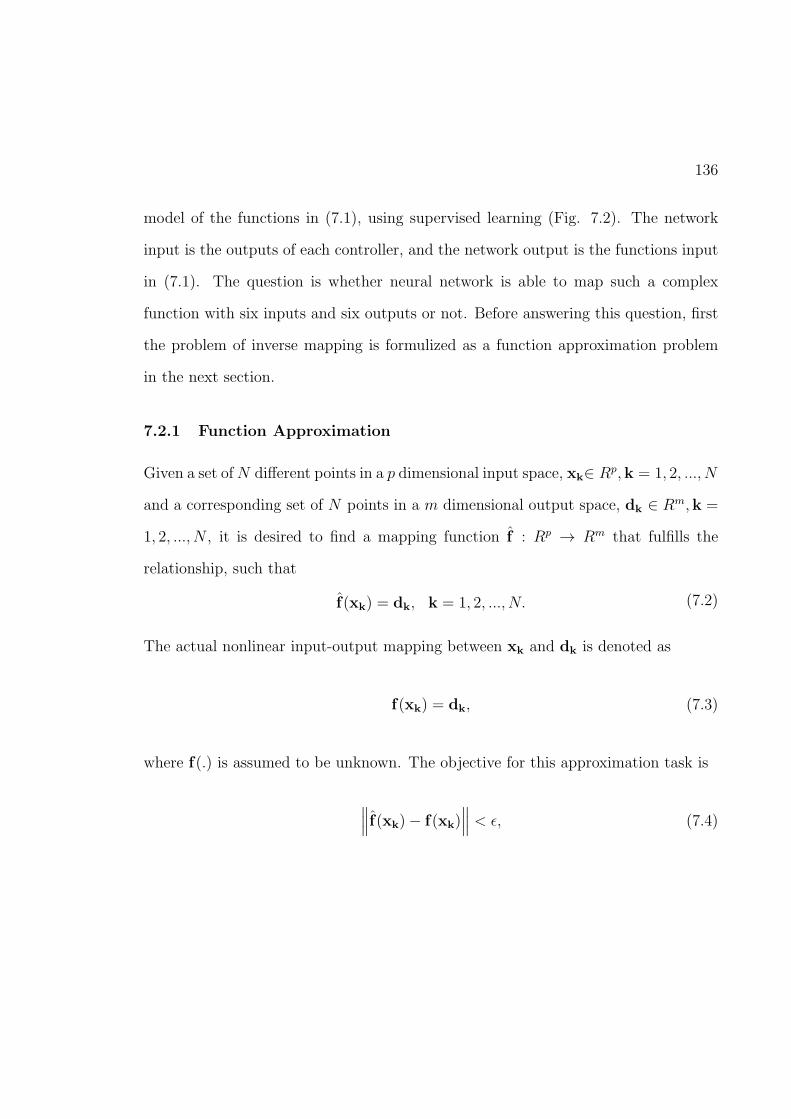
136
model of the functions in (7.1), using supervised learning (Fig. 7.2). The network
input is the outputs of each controller, and the network output is the functions input
in (7.1). The question is whether neural network is able to map such a complex
function with six inputs and six outputs or not. Before answering this question, first
the problem of inverse mapping is formulized as a function approximation problem
in the next section.
7.2.1 Function Approximation
Given a set ofN different points in a p dimensional input space, xk∈ Rp,k = 1, 2, ..., N
and a corresponding set of N points in a m dimensional output space, dk ∈ Rm,k =
1, 2, ..., N , it is desired to find a mapping function f : Rp → Rm that fulfills the
relationship, such that
f(xk) = dk, k = 1, 2, ..., N. (7.2)
The actual nonlinear input-output mapping between xk and dk is denoted as
f(xk) = dk, (7.3)
where f(.) is assumed to be unknown. The objective for this approximation task is
∥
∥
∥f(xk)− f(xk)∥
∥
∥ < ǫ, (7.4)

137
where ǫ is a small positive number. Provided that the size N of the training set is
large enough and the network is equipped with an adequate number of free parameters
(weights), then the approximation error ǫ can be made small enough for the task
(universal approximation theorem [100], [101], [102]).
In this thesis, the ability of a neural network to approximate an unknown input-
output mapping function is used for inverse system identification as its structure is
shown in Fig. 7.2.
Notice that the place of dk and xk have been reversed in the structure of inverse
system identification and dk and xk denote the input vector and desired output of
the unknown inverse system, respectively. Equation (7.5) describes the input-output
relation of an unknown inverse system.
xk = f−1(dk) (7.5)
In the case of Fig. 7.2, yk denotes the output vector of the neural network which
is the vector of actual control signals produced in response to an input vector dk.
The difference between the desired output vector xk (associated with dk) and the
neural network output yk provides the error vector ek. A neural network is utilized
to approximate the inverse function f−1. The error vector ek is used to adjust the
free parameters of the neural network. One of the possibles way to perform the
parameter adjustment is to use an objective function whereby the goal is to adjust

138
Figure 7.2: Block diagram of an inverse function approximation system.
the parameters of the network so as to minimize the objective function. A choice of
objective function is the error function given by:
J(W ) =1
2
m∑
j=1
(dj − yj)T (dj − yj) (7.6)
7.3 Feedforward networks
Neural networks are adaptive nonlinear systems that adjust their parameters auto-
matically in order to minimize a performance criterion. Identification of the neural
models involves learning, which is covered extensively in [103].
There are two different configurations of feedforward networks: i) single-layer
feedforward networks (Fig. 7.3) and ii) multi-layer feedforward networks (Fig. 7.4).

139
Figure 7.3: Structure of single-layer feedforward networks.
Multi-layer feedforward neural networks, or more commonly known as Multi-Layer
Perceptrons (MLP) have very quickly become the most widely encountered neural
networks, particularly within the area of systems and control [104]. Usually, back-
propagation rule or delta learning rule is used to train multi-layer feedforward neural
network. Feedforward networks are widely used in classification [105], and approxi-
mation theory [106], [107].

140
Figure 7.4: Structure of multi-layer feedforward neural networks.

141
7.4 Overview of Multi-Layer Perceptron
In this thesis, MLP network is used, which is very popular in the applied fields as
well as in theoretical research. The reasons for this popularity might be as follows:
• Simplicity.
• Scalability.
• Property to be a general function approximator.
• Adaptivity.
These features make MLP networks a suitable choice of network for inverse function
approximation mapping.
For multi-layer perceptrons, weight learning is most commonly carried out by the
method of back-propagation [108]. In this approach the network outputs are first
compared with a set of desired values for those outputs. The error function (7.6),
on the output layer only, must first be minimized by a best selection of output layer
weights. Once the output layer weights have been selected the weights in the hidden
layer next to the output can be adjusted by employing a linear back-propagation of
error term from the output layer. A full description of back-propagation for both
static and dynamic MLPs can be found in Cichocki and Unbehauen [109]. On the
down side, back-propagation is a nonlinear steepest descent type algorithm, and it
may either converge on local minima or be extremely slow to converge. On the
142
positive side, however, a MLP with only one hidden layer is sufficient to approximate
any continuous function [100].
7.5 Back-Propagation
Back-Propagation (BP) is a specific technique for implementing gradient descent in
weight space for a multilayer feedforward network. The BP algorithm provides a
way to calculate the gradient of the error function efficiently using the chain rule of
differentiation. The error after initial computation in the forward pass is propagated
backward from the output units, layer by layer. This algorithm involves minimization
of an error function in the least mean square, trained by applying gradient descent
method [110]. A general structure of a two-layered feedforward neural network, with
p neurons in the first layer and m neurons in the second layer is depicted in Fig.
7.4. The detailed structure of the input and output neurons are shown in Figs. 7.5
and 7.6. In this thesis, a two-layer linear-output feedforward network (MLP network)
is used. The flowchart of training the MLP network to learn the inverse mapping
between actual control signals (α1, α2, β1, β2, ω1, ω2) and controller control signals
(u1, ..., u6) is shown in Fig. 7.7. This flowchart summarizes the training process in a
two-layer perceptron network. The variables and scripts that are used as superscripts
or subscripts in this flowchart are defined as follows:
• k = 1, 2, ..., n (dimension of input layer), j = 1, 2, ...,m (dimension of output
layer),

143
Figure 7.5: neuron (1, i), (i = 1, 2, ..., p)in the hidden layer
Figure 7.6: neuron (2, j), (j = 1, 2, ...,m)in the output layer
• xk, (k = 1, 2, ..., n) input signal of order n (input layer), xk = [x1x2...xn]T , N
samples of input elements k = 1, 2, ..., N ,
• zi, (i = 1, 2, ..., p) output signal of the first layer (hidden layer), zk = [z1z2...zp]T
the outputs of all neurons in the hidden layer,
• yj, (j = 1, 2, ...,m) output signal of second layer (output layer), yk = [y1y2...ym]T
the output vector of neural network,
• W(1)ik , (i = 1, 2, ..., p), (k = 1, 2, ..., n) the weights corresponding to first layer
neurons, the connection weight from the kth input to ith neuron in first layer,
• W(2)jq , (j = 1, 2, ...,m), (q = 1, 2, ..., p) the connection weight from the qth neuron
in the first layer to the jth neuron in the output layer.

144
In this flowchart a set of N input data xk = [x1, ..., xn] is first presented to the input
layer. The output from this layer are then fed as inputs to the hidden layer and
subsequently the outputs from the hidden layer are fed as weighted inputs (i.e., the
outputs from the hidden layer are multiplied by the weights (W(1)ik xk) to the second
layer which is a output layer in this flowchart. The hidden layer has activation
function of sigmoid. Thus, the accumulative weighted inputs (S(1)i =
∑n
k=0W(1)ik xk)
of all neurons in the hidden layer first go into a sigmoid function (zi = σ(S(1)i )) and are
then fed to the next layer as inputs. Despite the fact that the output layer performs
based on a linear function, the same process as for the hidden layer happens in the
output layer, and the output of this layer (yj =∑p
q=0W(2)jq zq) is the response of neural
network to the input xk. The output of neural network is then compared with the
desired ones and the error goes back to update the weights of output and hidden
layers through BP algorithm as illustrated in Modifications of Weights sections in the
flowchart in Fig. 7.7.
7.6 Training the MLP Neural Network for Actual Control Signal
Approximation
As mentioned before, for approximation or fitting problem, a neural network has to
map between a data set of numeric inputs and a set of numeric targets. A two-
layer feed-forward with sigmoid hidden neurons and linear output neurons is trained,
which based on universal approximation theorem, can fit multi-dimensional mapping
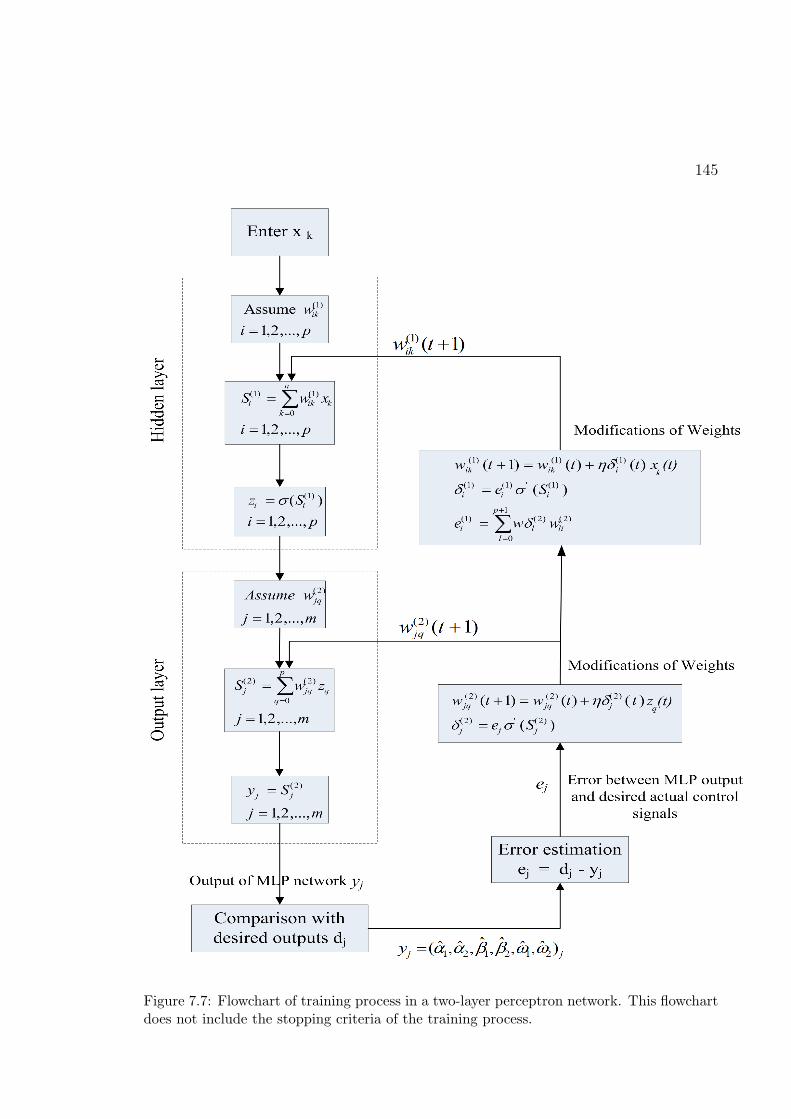
145
Figure 7.7: Flowchart of training process in a two-layer perceptron network. This flowchartdoes not include the stopping criteria of the training process.

146
problems arbitrarily well, given consistent data and enough neurons in its hidden
layer. The network is trained with Levenberg-Marquardt back-propagation algorithm.
Assumptions: We have made some assumptions on variables in (7.1), because
their real values are unknowns. For example, the rate of change of the longitudinal
and lateral angles, (αi, βi), depends on the capability of the mechanical system, and
they are assumed to be constant in training the MLP network. As a result the second
derivatives are considered to be zero. Furthermore, by considering Ti = CTω2i , and
Qi = CQω2i , the values of aerodynamic coefficients CT , CQ are needed for generating
data for neural network training. The list of all of the assumptions for neural network
training is as below:
1. The rates of change of α1, α2 are constant, and are equal to 0.05 rad/s.
2. The rates of change of β1, β2 are constant and are equal to 0.05 rad/s.
3. The second derivatives of α1, α2, β1, β2 are zero.
4. T1 = CTω21, T2 = CTω
22 and CT is assumed to be constant and equal to 0.01.
5. Q1 = CQω21, Q2 = CQω
22 and CQ is assumed to be constant and equal to
0.01.
6. −π/2 ≤ α1 ≤ π/2, −π/2 ≤ α2 ≤ π/2.
7. −π/4 ≤ β1 ≤ π/4, −π/4 ≤ β2 ≤ π/4.

147
8. 600 rad/s ≤ ω1 ≤ 700 rad/s, 600 rad/s ≤ ω2 ≤ 700 rad/s. This angular speed
produces between 573 to 668 rpm, which is enough to maintain the vehicle in
hover [1].
7.6.1 Generating data for neural network training
Considering the above assumptions, a domain range of each variable is divided to 20
equal length segments. All possible combination of the 6 variables α1, α2, β1, β2, ω1,
ω2 are calculated and the 6 controls u1, ..., u6 are generated from (7.1). In order to
approximate the inverse mapping, u1, ..., u6 and α1, α2, β1, β2, ω1, ω2 are entered as
inputs and targets of the neural network approximator, respectively.
• Inputs: 5000 randomly selected samples of 6 variables.
• Targets: 5000 randomly selected samples of 6 variables in the case of training
one MLP network, and 5000 randomly selected samples of 1 variable in the case
of training six parallel MLP networks.
• Randomly divided up the 5000 samples to Training data, Validation data, and
Testing data:
• Training: These 70% of Input data (3500 samples) are presented to the network
during training, and the network is adjusted according to its error.
• Validation: These 50% of the rest of Input data (750 samples) are used to

148
measure network generalization, and to stop training when generalization stops
improving.
• Testing: These 50% of the rest of Input data (750 samples) have no effect on
training and so provide an independent measure of network performance during
and after training. We also test all trained networks with a set of 5000 randomly
selected samples as a test data set.
• Training automatically stops when generalization stops improving, as indicated
by an increase in the mean square error of the validation.
7.6.2 Training One MLP network
As the first approach, one MLP network with 6 inputs and 6 outputs is trained to
estimate all 6 variables α1, α2, β1, β2, ω1, and ω2 with one network. The performance
of the network is measured based on mean squared error (MSE) criteria. Thus, the
best value for the performance of the trained network is zero. Table 7.1 compares
the performance of MLP networks with different number of neurons in their hidden
layer. As it is shown in this table, increasing the number of neurons in a hidden
layer improves the performance of the network, but not significantly (increasing the
number of neurons of the hidden layer from 15 to 50 only results in an improvement
of performance from 0.02 to 0.0177). As a result, the MLP network with one hidden
layer and 15 neurons in its hidden layer is able to approximate the inverse relation

149
Table 7.1: Comparison of the performance and training of the MLP network with 6 inputsand 6 outputs and different number of neurons in hidden layer.
Number of neurons in hidden layer 15 20 30 50Epochs 1717 282 160 21Time 0:18:37 0:11:28 0:03:34 0:00:51Performance 0.02 0.0181 0.0178 0.0177
Table 7.2: MSE and Regression results for a set of test data for MLP network with 6 inputsand 6 outputs and 30 neurons in its hidden layer.
Samples MSE RTraining 3500 1.81527e-2 9.99990e-1Validation 750 2.03653e-2 9.99989e-1Testing 750 2.05127e-2 9.99989e-1
between the output of a controller and α1, α2, β1, β2, ω1, and ω2. However, training
a network with only 15 neurones takes much more time, and if an online training
of the network is desired, this long time may cause harmful effects on the stability
of the system. Therefore, the best choice of network from Table 7.1 is the network
with 30 neurones. Table 7.2 shows the MSE and regression (R) between targets and
approximated values for a network with 30 neurones in its hidden layer. Regression
measures the correlation between outputs and targets. An R value of 1 means a
close relationship, 0 indicates a random relationship. Figures 7.8 to 7.14 shows the
performance, training states, and error histogram of MLP network with 30 neurones.

150
0 200 400 600 800 1000 1200 1400 160010
−2
10−1
100
101
102
1717 Epochs
Me
an
Sq
ua
red
Err
or
(mse
)
TrainValidationTestBest
Figure 7.8: Neural Network Training Performance, Best Validation Performance is 0.021463at epoch 1711.
−0.15 −0.1 −0.05 0 0.05 0.10
200
400
600
800
1000
Errors = Targets − Outputs
In
sta
nce
s
Error Histogram of α1 angle with 20 Bins
TrainValidationTest
Figure 7.9: Neural Network Training Er-ror for α1.
−0.2 −0.15 −0.1 −0.05 0 0.05 0.1 0.150
100
200
300
400
500
600
700
Errors = Targets − Outputs
In
sta
nce
s
Error Histogram of α2 angle with 20 Bins
Figure 7.10: Neural Network TrainingError for α2.

151
−1 −0.8 −0.6 −0.4 −0.2 0 0.2 0.4 0.6 0.8 10
500
1000
1500
2000
2500
Errors = Targets − Outputs
In
sta
nce
s
Error Histogram of β1 angle with 20 Bins
Figure 7.11: Neural Network TrainingError for β1.
−0.8 −0.6 −0.4 −0.2 0 0.2 0.4 0.6 0.8 10
500
1000
1500
2000
Errors = Targets − Outputs
In
sta
nce
s
Error Histogram of β2 angle with 20 Bins
Figure 7.12: Neural Network TrainingError for β2.
−0.3 −0.25 −0.2 −0.15 −0.1 −0.05 0 0.05 0.1 0.150
500
1000
1500
2000
Errors = Targets − Outputs
In
sta
nce
s
Error Histogram of ω1 angle with 20 Bins
Figure 7.13: Neural Network TrainingError for ω1.
−0.5 −0.4 −0.3 −0.2 −0.1 0 0.1 0.2 0.30
200
400
600
800
1000
Errors = Targets − Outputs
Insta
nce
s
Error Histogram of ω2 angle with 20 Bins
Figure 7.14: Neural Network TrainingError for ω2.

152
Table 7.3: Progress report of training 6 neural networks with 6 inputs and 1 output
Training α1 α2 β1 β2 ω1 ω2
Hidden neurones 15 15 15 15 15 15Epoch 214 544 20 13 370 800Time 0:02:16 0:01:42 0:00:03 0:00:09 0:01:02 0:02:14Performance 5.16e-06 1.04e-05 0.0577 0.0480 0.000575 0.000164Gradient 9.51e-06 0.000255 0.00227 0.00234 0.00145 0.0103Mu 0.001 0.0001 0.01 0.1 0.1 0.01
7.6.3 Training Six Parallel MLP Networks
To improve the performance of the approximator and reduce MSE error of training, six
separate MLP networks with six inputs and one output were trained. These networks
are each trained for approximating one of the variables α1, α2, β1, β2, ω1, and ω2.
The progress of each network is shown in Table 7.3. The best training performance
and the regression (R) for the training set of data and a test set of data are shown
in Table 7.4 for all 6 MLP networks. Figures 7.15 to 7.32 show the performance and
error histogram of all trained MLP networks with 15 neurones.

153
Table 7.4: MSE and Regression results for training data and a set of test data for MLPnetworks with 6 inputs and 1 output and 15 neurons in hidden layer
α1 α2 β1 β2 ω1 ω2
Best training 5.0613e-06 1.1154e-05 0.0596 0.486 6.1295e-04 1.6938e-04performance
Regression 0.99998 0.99999 0.87229 0.89587 0.99997 0.99999Best test 4.6070e-06 1.3684e-05 0.0630 0.0525 6.5432e-04 1.9175e-04performance
Regression 0.99998 0.99999 0.86259 0.88848 0.99996 0.99999
0 20 40 60 80 100 120 140 160 180 20010
−6
10−5
10−4
10−3
10−2
10−1
100
214 Epochs
Mea
n S
quar
ed E
rror
(mse
)
TrainValidationTestBest
Figure 7.15: Neural Network Training Performance to approximate α1 , Best ValidationPerformance is 5.0285e-06 at epoch 214.

154
−0.015 −0.01 −0.005 0 0.005 0.01 0.015 0.020
500
1000
1500
2000
Error = Targets − Outputs
Inst
ance
s
Error Histogram with 20 Bins
TrainingValidationTest
Figure 7.16: Neural Network Training Error for α1.
−0.01 −0.008 −0.006 −0.004 −0.002 0 0.002 0.004 0.006 0.008 0.010
50
100
150
200
250
300
Errors = Targets − Outputs
Inst
ance
s
Error Histogram with 20 Bins for a Set of 1000 Test Data
Figure 7.17: Neural Network Testing Error for α1.

155
0 50 100 150 200 250 300 350 400 450 50010
−5
10−4
10−3
10−2
10−1
100
101
544 Epochs
Mea
n Sq
uare
d Er
ror (
mse
)
TrainValidationTestBest
Figure 7.18: Neural Network Training Performance to approximate α2, Best ValidationPerformance is 1.3245e-05 at epoch 538.
−0.02 −0.015 −0.01 −0.005 0 0.005 0.01 0.0150
200
400
600
800
1000
1200
Errors = Targets − Outputs
Inst
ance
s
Error Histogram with 20 Bins
TrainingValidationTest
Figure 7.19: Neural Network Training Error for α2.

156
−0.02 −0.015 −0.01 −0.005 0 0.005 0.01 0.0150
50
100
150
200
250
Errors = Targets − Outputs
Inst
ance
s
Error Histogram with 20 Bins for a Set of 1000 Test Data
Figure 7.20: Neural Network Testing Error for α2.
0 2 4 6 8 10 12 14 16 18 2010
−2
10−1
100
101
20 Epochs
Mea
n S
quar
ed E
rror
(mse
)
TrainValidationTestBest
Figure 7.21: Neural Network Training Performance to approximate β1, Best ValidationPerformance is 0.065465 at epoch 14.

157
−1 −0.8 −0.6 −0.4 −0.2 0 0.2 0.4 0.6 0.8 10
500
1000
1500
2000
2500
3000
Errors = Targets − Outputs
Inst
ance
s
Error Histogram with 20 Bins
TrainingValidationTest
Figure 7.22: Neural Network Training Error for β1.
−0.8 −0.6 −0.4 −0.2 0 0.2 0.4 0.6 0.8 10
100
200
300
400
500
600
700
Errors = Targets − Outputs
Inst
ance
s
Error Histogram with 20 Bins for a Set of 1000 Test Data
Figure 7.23: Neural Network Testing Error for β1.
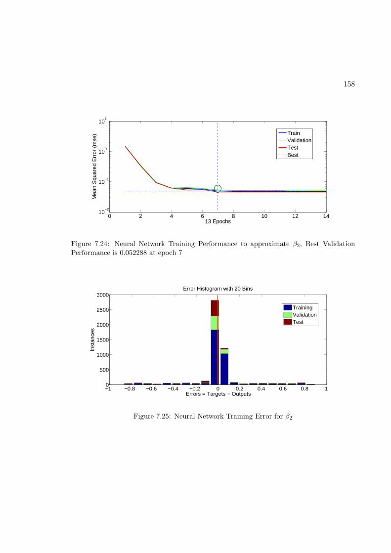
158
0 2 4 6 8 10 12 1410
−2
10−1
100
101
13 Epochs
Mea
n S
quar
ed E
rror
(m
se)
TrainValidationTestBest
Figure 7.24: Neural Network Training Performance to approximate β2, Best ValidationPerformance is 0.052288 at epoch 7
−1 −0.8 −0.6 −0.4 −0.2 0 0.2 0.4 0.6 0.8 10
500
1000
1500
2000
2500
3000
Errors = Targets − Outputs
Inst
ance
s
Error Histogram with 20 Bins
TrainingValidationTest
Figure 7.25: Neural Network Training Error for β2
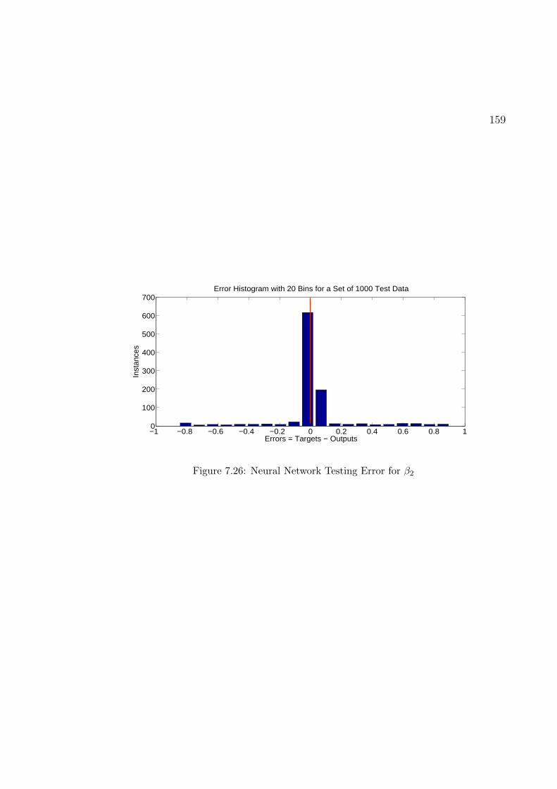
159
−1 −0.8 −0.6 −0.4 −0.2 0 0.2 0.4 0.6 0.8 10
100
200
300
400
500
600
700
Errors = Targets − Outputs
Inst
ance
s
Error Histogram with 20 Bins for a Set of 1000 Test Data
Figure 7.26: Neural Network Testing Error for β2

160
0 50 100 150 200 250 300 35010
−4
10−2
100
102
104
370 Epochs
Mea
n Sq
uare
d Er
ror (
mse
)
TrainValidationTestBest
Figure 7.27: Neural Network Training Performance to approximate ω1, Best ValidationPerformance is 0.00071265 at epoch 364.
−0.2 −0.15 −0.1 −0.05 0 0.05 0.1 0.150
200
400
600
800
1000
1200
Errors = Targets − Outputs
Inst
ance
s
Error Histogram with 20 Bins
TrainingValidationTest
Figure 7.28: Neural Network Training Error for ω1.

161
−0.2 −0.15 −0.1 −0.05 0 0.05 0.1 0.150
50
100
150
200
250
300
Errors = Targets − Outputs
Inst
ance
s
Error Histogram with 20 Bins for a Set of 1000 Test Data
Figure 7.29: Neural Network Testing Error for ω1.
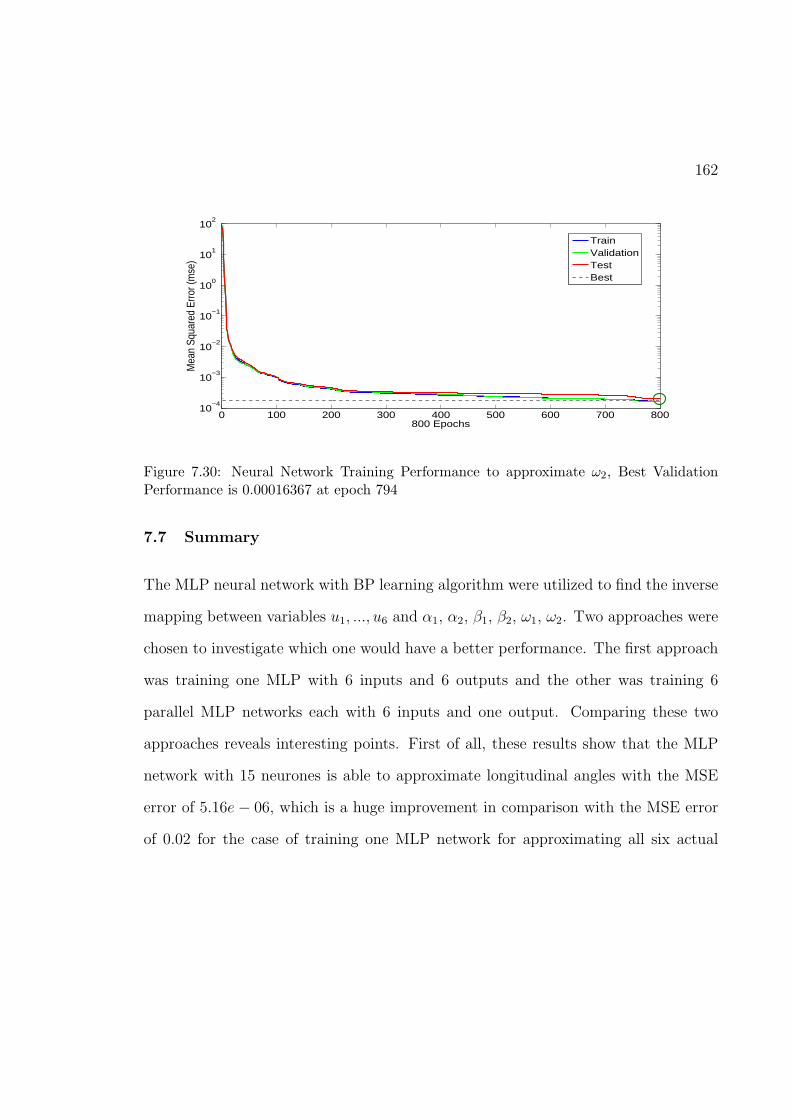
162
0 100 200 300 400 500 600 700 80010
−4
10−3
10−2
10−1
100
101
102
800 Epochs
Mea
n Sq
uare
d Er
ror (
mse
)
TrainValidationTestBest
Figure 7.30: Neural Network Training Performance to approximate ω2, Best ValidationPerformance is 0.00016367 at epoch 794
7.7 Summary
The MLP neural network with BP learning algorithm were utilized to find the inverse
mapping between variables u1, ..., u6 and α1, α2, β1, β2, ω1, ω2. Two approaches were
chosen to investigate which one would have a better performance. The first approach
was training one MLP with 6 inputs and 6 outputs and the other was training 6
parallel MLP networks each with 6 inputs and one output. Comparing these two
approaches reveals interesting points. First of all, these results show that the MLP
network with 15 neurones is able to approximate longitudinal angles with the MSE
error of 5.16e− 06, which is a huge improvement in comparison with the MSE error
of 0.02 for the case of training one MLP network for approximating all six actual
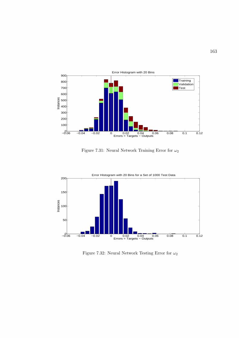
163
−0.06 −0.04 −0.02 0 0.02 0.04 0.06 0.08 0.1 0.120
100
200
300
400
500
600
700
800
900
Errors = Targets − Outputs
Inst
ance
s
Error Histogram with 20 Bins
TrainingValidationTest
Figure 7.31: Neural Network Training Error for ω2
−0.06 −0.04 −0.02 0 0.02 0.04 0.06 0.08 0.1 0.120
50
100
150
200
Errors = Targets − Outputs
Inst
ance
s
Error Histogram with 20 Bins for a Set of 1000 Test Data
Figure 7.32: Neural Network Testing Error for ω2

164
controls. The next important point is concluded by looking through the differences
between the mse errors of each of networks. Actually the performances of all networks
improve except for the case of β1 and β2. The reason lies in the difference between
the domain range of lateral angles β1, β2, and longitudinal angles α1, α2.
Spanning the domain range of each variable is very important for proper training.
It has a direct impact on the performance of the network. Dividing this range results
in a more accurate function approximator and this can be done by separating the
maneuvers from each other. Different maneuvers may span a different part of the
range of longitudinal and lateral angles. Training different networks for each, gives
us a better accuracy. One of the simulations done to support this idea is training a
network when α1 = α2, β1 = β2, and ω1 = ω2, which results in a high performance
of 10−12, which is a significant improvements from the best performance among the
6 parallel networks which is in the range of 10−5.
The function approximator should be trained online because there are pitch, roll
and yaw angles in the equations of u4, u5, and u6. In fact, the variables we estimated
in our simulations are Fx, Fy, and Fz. Otherwise, neural networks should be trained
with collected real data from executing maneuvers. The suggestion of this thesis is
to separate some maneuvers such as vertical flight or taking-off and landing, horizon-
tal flight, transition between these modes, considerable change of roll, pitch, or yaw,
etc, and train a seperate network for each one of them, switching between function
approximators based on the present flight mode. This approach will reduce the es-

165
timation error significantly. Moreover, in online training the network can adapt to
each of these flight modes, but training may take more time. Also, real data should
be collected because we have made lots of assumptions on the rates of changes of
the angles and the aerodynamic coefficients, for which the true values are not known,
and even if these values were to be found by executing some experiments, they would
not be constant during the full flight regime. However, offline training offers the
advantage of providing the approximation of the control signals immediately after
controller outputs come out.

Chapter 8
Comprehensive Simulation Scenarios, Results and Discussion
In this chapter, the previously designed controllers including feedback linearization
(FL), adaptive feedback linearization (AFL), robust adaptive feedback linearization
(RAFL) which is AFL with robust modification term, and sliding mode control
(SMC), are examined on the eVader to perform four different simulation scenarios.
These scenarios are selected to examine the following purposes:
1. Investigating the performance of the above mentioned controllers (FL, AFL,
SCM) on the eVader and comparing their results in terms of the speed of con-
vergence to reach the final desired values (steady state).
2. Study the performance of the eVader with the designed robust controllers
(RAFL and SMC) in an adverse case scenario of wind blowing in all directions
of the vehicle’s frame of reference.
3. Study the performance of the evader with the designed robust controllers
(RAFL and SMC) for landing on the ground in presence of ground effects.
4. Investigating the performance of the eVader following a complex trajectory of
166

167
position and orientation while maneuvering sharp turns and performing sudden
and huge changes in the orientation angles of the vehicle.
A list of all simulation scenarios applied on the eVader throughout this thesis and
their explanations are in . The tag number assigned to each scenarios of this chapter
are based on the list in . One scenario is designed for each of the above purposes for
investigating different aspects of the eVader flight. The following four scenarios are
applied in this chapter: 1) Scenario # 1 (to compare the performance of FL, AFL and
SMC controllers) , 2) wind buffeting, 3) ground effect, and 4) aggressive maneuver.
In order to explain the results, the speed of the vehicle reaching the steady state, the
steady state error, and the stability of the vehicle are considered and the results are
discussed in terms of these criteria.
The rest of this chapter is organized as follows: first, the comparison results of
the three FL, AFL, and SMC controllers are presented in Section 8.1. Next, results
of the AFL and RAFL controls are presented in Section 8.2, as the vehicle undergoes
wind disturbance. The results of the performance comparison of the eVader, when
equipped with RAFL vs. SMC controls, are discussed in Section 8.3. An aggressive
maneuver scenario is examined with SMC and AFL control approaches in Section 8.4.
The final section of this chapter, Section 8.5, explains the observations and findings
of the suitable control approach for the eVader UAV, while performing different tasks
and maneuvers.

168
8.1 Scenario #1
To compare FL, AFL, and SMC in terms of speed of convergence to reach the steady
state, the simulation Scenario #1, without any additive noises or disturbances, was
applied to the eVader nonlinear model. As stated in Appendix A, The initial con-
ditions and desired values of this scenario were chosen as: Initial conditions: x0=
[0, 0, 0, 0, 0, 0, 0, 0, 0, 0, 0, 0]T , and desired states: [φd, φd]T = [22.5, 0]T , [θd, θd]
T =
[15, 0]T , [ψd, ψd]T = [18, 0]T , [xd, xd]
T = [3, 0]T , [yd, yd]T = [4, 0]T , [zd, zd]
T = [2, 0]T .
The result of control signals, and orientation and position outputs are shown in Figs.
8.1 to 8.3. As it is seen in these figures, the fastest controller is SMC and the slowest
one is AFL. SMC reaches the steady state for all six vehicle output states in less
than 0.5 s, while it takes AFL almost 3 s, and FL lies in between of SMC and AFL
controllers. However, considering the chattering effect in SMC control signals which
is seen more clearly in signals of u1, u2, and u3, the best choice of controller in simple
scenarios, assuming there are no model uncertainties and external disturbances, is
the FL control approach. Also, it must be pointed out that the scenario presented
here is not a realistic scenario, as in real world applications, there are always model
uncertainties, imprecision of parameters, and sensor noise.

169
0 0.2 0.4 0.6 0.8 1−5
0
5
10Control Signal u1
u1
0 0.5 1 1.5−1000
0
1000
2000
3000Control Signal u4
u4
0 0.2 0.4 0.6 0.8 1−5
0
5
10Control Signal u2
u2
0 0.5 1 1.5−1000
0
1000
2000
3000
4000Control Signal u5
u50 0.2 0.4 0.6 0.8 1
−2
0
2
4
6
8Control Signal u3
time (s)
u3
0 0.2 0.4 0.6 0.8 1−500
0
500
1000
1500
2000Control Signal u6
time (s)u6
FLAFLSMC
Figure 8.1: Control input signals of FL, AFL and SMC controllers for orientation andposition regulation in Scenario #1.
8.2 Wind Buffeting (Scenario #3)
The purpose of the second test scenario is to study the performance of the eVader
and the proposed controllers in an adverse case scenario of wind blowing strongly in
all directions with respect to the vehicle’s frame of reference. The performances
of the eVader equipped with the AFL controller without robust modification (e-
modification), and the AFL control with robust modification which is indicated here
by RAFL, are compared in the presence of external wind disturbance. Wind blowing
in all directions is a very hard condition for UAVs, and it is rarely addressed by re-
searchers to date. As the focus of this thesis is on controlling the UAV in worst case

170
0 0.5 1 1.5 2 2.5 3 3.5 40
10
20
30The roll angle
Rol
l (de
gree
)
0 0.5 1 1.5 2 2.5 3 3.5 40
5
10
15
20The pitch angle
Pitc
h (d
egre
e)
0 0.5 1 1.5 2 2.5 3 3.5 40
5
10
15
20The yaw angle
time (s)
Yaw
(deg
ree)
FL controlDesired signalAFL controlSMC control
Figure 8.2: Attitude outputs of the eVader obtained by applying FL, AFL and SMC con-trollers in Scenario #1.
scenarios, it was assumed to have the strong external disturbance in all directions.
As a result of this assumption the dw(t), formulated as a sinusoidal signal, is added
to all states.
dw(t) =M [10 + 5sin(2π)t]
In the above equation, M is a disturbance magnitude that has a relation with the
speed of wind. The larger M is related to the stronger wind with more speed.
In this scenario it is expected that the eVader will stay stable at its current posi-
tion (same x, y, and z), while allowing it to change its orientation. Thus, the ini-

171
0 0.5 1 1.5 2 2.5 3 3.5 4 4.5 5−2
0
2
4The Cartesian position x
x (m
)
0 0.5 1 1.5 2 2.5 3 3.5 4 4.5 5−2
0
2
4
6The Cartesian position y
y (m
)
0 0.5 1 1.5 2 2.5 3 3.5 4 4.5 50
1
2
3The Cartesian position z
time (s)
z (m
)
FL outputDesired outputAFL outputSMC output
Figure 8.3: Position outputs of the eVader obtained by applying FL, AFL and SMC con-trollers in Scenario #1.
tial conditions and the desired states are as follows: initial conditions: [φ0, φ0]T =
[22.5, 0]T , [θ0, θ0]T = [15, 0]T , [ψ0, φ]
T = [18, 0]T , [x0, x0]T = [2, 0]T , [y0, y0]
T = [3, 0]T , [z0, z0]T =
[5, 0]T , and desired states: ηd = [0, 0, 0, 0, 0, 0]T , ζd = [3, 0, 4, 0, 2, 0]T .
The simulation results shown in Figs. 8.4 to 8.9, show that although the AFL
control approach without robust modification can handle constant and slow-varying
uncertainties such as model parameters, it is not capable of maintaining the stability
of the UAV in the presence of time-varying external disturbance. On the other hand,
the stability of the eVader is preserved with the RAFL controller (Figs. 8.8 and 8.9),
although there is steady state error, while the wind keeps blowing.

172
0 0.5 1 1.5 2 2.5 3 3.5 4 4.5 50
1
2x 10
215 Control signal u1
time[s]
u1
0 0.5 1 1.5 2 2.5 3 3.5 4 4.5 5−200
−150
−100
−50
0Control signal u4
time[s]u
4
0 0.5 1 1.5 2 2.5 3 3.5 4 4.5 5−6
−4
−2
0
2x 10
215 Control signal u2
time[s]
u2
0 0.5 1 1.5 2 2.5 3 3.5 4 4.5 5−200
−150
−100
−50
0Control signal u5
time[s]
u5
0 0.5 1 1.5 2 2.5 3 3.5 4 4.5 50
1
2
3
4x 10
238 Control signal u3
time[s]
u3
0 0.5 1 1.5 2 2.5 3 3.5 4 4.5 5−40
−20
0
20
40Control signal u6
time[s]
u6
Figure 8.4: Control signals of AFL controller without robust modification in presence ofwind disturbance. The control signals u1, u2 and u3 go to infinity and make the eVaderunstable.

173
0 0.5 1 1.5 2 2.5 3 3.5 4 4.5 5−2
0
2
4
6x 10
213 The roll angle
time[s]
Ro
ll[d
eg
ree
]
0 0.5 1 1.5 2 2.5 3 3.5 4 4.5 5−15
−10
−5
0
5x 10
213 The pitch angle
time[s]
Pitc
h[d
eg
ree
]
0 0.5 1 1.5 2 2.5 3 3.5 4 4.5 50
2
4
6
8
10x 10
236 The yaw angle
time[s]
Ya
w[d
eg
ree
]
Figure 8.5: eVader Orientation goes to infinity with AFL controller without robust modifi-cation in presence of wind disturbance.
8.3 Ground Effect (Scenario #12)
Ground and wall effects are important fluid flow characteristics that aerial vehicles
(e.g., helicopters and other VTOL vehicles) experience. Under ground and wall effects,
it is extremely difficult to control any aerial vehicles. The basic principle of ground
effects is that the closer the rotor’s fan operates to an external surface such as the
ground, said to be in ground effect (GE), the more thrust it produces. In order to
control an aerial vehicle under GE, there is a need to have a representation of such
effects. Previous graduate students working with the eVader UAV in the Autonomous
Reconfigurable Robotic Systems Laboratory at the University of Calgary have studied

174
0 0.5 1 1.5 2 2.5 3 3.5 4 4.5 5−6
−4
−2
0Control signal u1
time[s]
u1
0 0.5 1 1.5 2 2.5 3 3.5 4 4.5 5−200
−150
−100
−50
0Control signal u4
time[s]
u4
0 0.5 1 1.5 2 2.5 3 3.5 4 4.5 5−5
−4
−3
−2
−1Control signal u2
time[s]
u2
0 0.5 1 1.5 2 2.5 3 3.5 4 4.5 5−200
−150
−100
−50
0Control signal u5
time[s]
u5
0 0.5 1 1.5 2 2.5 3 3.5 4 4.5 5−4
−3
−2
−1Control signal u3
time[s]
u3
0 0.5 1 1.5 2 2.5 3 3.5 4 4.5 5−40
−20
0
20
40Control signal u6
time[s]u
6
Figure 8.6: Control signals of RAFL controller, with e-modification, in presence of winddisturbance.
the GE experienced by the eVader. Therefore, to model the GE disturbance and add
such disturbances to the model of the eVader, we used Eq. (8.1), which first presented
and explained in Chapter 3, to represent the GE.
gr(z) =
az(z+zcg)2
− az(z0+zcg)2
0 < z ≤ z0
0 else(8.1)
In (8.1) z is the altitude of the eVader’s rotor with respect to ground, zcg is the altitude
of the vehicle’s centre of gravity, z0 is the hight below which the GE is effective (Fig.
8.10), and az is an unknown constant. The value of az is calculated using the result

175
0 1 2 3 4 5−0.3
−0.2
−0.1
0
0.1
0.2
a1
time
a1
0 1 2 3 4 5−1
0
1
2
3
4
a2
time
a2
0 1 2 3 4 5−0.2
−0.1
0
0.1
0.2
a3
time
a3
0 1 2 3 4 5−2
−1
0
1
2
a4
time
a4
0 1 2 3 4 50
0.2
0.4
0.6
0.8
a5
time
a5
0 1 2 3 4 5−2
−1
0
1
2
a6
time
a6
0 1 2 3 4 50
0.05
0.1
0.15
0.2
0.25
a7
time
a7
0 1 2 3 4 50
0.1
0.2
0.3
0.4
a8
time
a8
0 1 2 3 4 50
0.1
0.2
0.3
0.4
a9
time
a9
Figure 8.7: Parameter estimation of RAFL controller with e-modification in presence ofwind disturbance.
of thrust ratios in constant fan speed, obtained from the CFD (Computational Fluid
Dynamics) simulations for a ducted fan in [75]. The observation made in [75] is that
in constant rotational speed, as the fan gets closer to the ground, the thrust force
increases. The thrust starts to increase at a hight of 1.5-fold rotor diameter. At a
rotor hight of one-half the rotor diameter, the thrust ratio is increased by about 50
percent. This result is compatible with the model in (8.1). Thereby, to calculate the
value of az, Equation (8.1) is solved at point hrr
= 1, with z0 = 1.5, where h is a
fan’s elevation from the ground and rr is the rotor’s radius, which gives a value of
az = 16.7. As a result of the ground effect disturbance, the thrust force on each rotor
of the eVader is increasing as much as modelled in (8.1). To examine the performance

176
0 0.5 1 1.5 2 2.5 3 3.5 4 4.5 50
5
10
15
20
25The roll angle
time[s]
Ro
ll[d
eg
ree
]
0 0.5 1 1.5 2 2.5 3 3.5 4 4.5 50
5
10
15The pitch angle
time[s]
Pitch
[de
gre
e]
0 0.5 1 1.5 2 2.5 3 3.5 4 4.5 50
5
10
15
20The yaw angle
time[s]
Ya
w[d
eg
ree
]
Figure 8.8: eVader orientation with RAFL controller with e-modification in presence ofwind disturbance.
of the designed robust controllers including RAFL and SMC, a landing simulation
scenario was performed in which the initial and final state conditions are as follows:
initial condition: η0 = [45, 0, 30, 0, 20, 0]T , ζ0 = [3, 0, 4, 0, 5, 0]T , and desired states:
xd= [0, 0, 0, 0, 0, 0, 0, 0, 0, 0, 0, 0]T . Thus, the vehicle is commanded to descend from a
height of three meters, while translating and changing its orientation, and land. The
control signal results and position and orientation outputs of the eVader by applying
AFL, with e-modification, and SMC are shown in Figs. 8.11 to 8.13. As it is seen
in Figs. 8.12 and 8.13 the SMC controller is much faster than the RAFL control
technique, as observed in Scenario #1 as well. The AFL controller is also tested in
this scenario, but as in the case of buffeting wind, this controller was not able to

177
0 0.5 1 1.5 2 2.5 3 3.5 4 4.5 52
2.1
2.2
2.3The Cartesian position x
time[s]
x
system outputdesired x(t)
0 0.5 1 1.5 2 2.5 3 3.5 4 4.5 53
3.1
3.2
3.3
3.4The Cartesian position y
time[s]
y
0 0.5 1 1.5 2 2.5 3 3.5 4 4.5 5
4.99
5
5.01
5.02
5.03
5.04The altitude z
time[s]
z
Figure 8.9: eVader position with RAFL controller with e-modification in presence of winddisturbance.
maintain the stability of the eVader when it lands on the ground.
8.4 Aggressive Maneuver
In this thesis, aggressive maneuver refers to maneuvers having a fast changing complex
flight trajectories such as acrobatic maneuvers like loops and barrel rolls, and cuban
eight maneuvers. To produce an aggressive trajectory as a function of time and apply
it to the designed controllers, herein, the Mobius strip equations [111] are used in

178
Figure 8.10: Schematic diagram of the eVader which shows z, z0, zcg.
(8.2) as:
x = [R + rcos(γ)] cos(κ)
y = [R + rcos(γ)] sin(κ)
z = rsin(γ)
(8.2)
with R = 4, r = 3, −π < κ < π, and −π/2 < γ < π/2. Equation (8.2) is used
to provide the 3D Cartesian position of the eVader’s path in this flight scenario.
The vehicle’s orientation reference trajectories are chosen arbitrarily consistent with
a trajectory in Fig. 8.14. Therefore, the roll angle is set to be stable at zero, and
the pitch and yaw angles follow the piecewise constant curves with sharp stepwise
patterns, which vary from 25 to −50 for pitch and from zero degree to 175 for yaw

179
angle (Figures 8.18 and 8.19). Both robust controllers are successful in tracking the
reference trajectories of position and orientation. The RAFL controller reaches to
the desired position trajectory after 4 s (Figure 8.20), while it takes only 0.7 s for
the SMC controller (Figure 8.21). The observations are consistent with the obtained
results in the GE simulation scenario. The 3D position tracking of the aggressive
maneuver for RAFL and SMC controllers are shown in Figs. 8.14 and 8.15. The
control signals of RAFL and SMC controls are shown in Figs. 8.16 and 8.17, the
vehicle’s orientation tracking output by RAFL and SMC shown in Figs. 8.18 and
8.19, the eVader’s position tracking curves shown in Figs. 8.20 and 8.21, and the
eVader’s orientation and position tracking errors by SMC control shown in Figs. 8.22
and 8.23, respectively. A comprehensive discussion of the results is presented in the
next section.
8.5 Result Discussion
This chapter presented and demonstrated the capabilities of the proposed nonlinear
model of the eVader and proposed designed nonlinear control approaches proposed
in Chapters 3 to 6. In this chapter, throughout several simulation scenarios, the
objective of choosing the best controller amongst the designed nonlinear controllers
in this thesis for the eVader is investigated. Because, in this thesis, the eVader is
supposed to perform complex agile maneuvers, a fast response controller is desirable.
The results of simulation Scenario # 1, Figs. 8.1 to 8.3, show the SMC controller is the

180
0 1 2 3 4 5−15
−10
−5
0
5
Control Signal u1
u1
0 1 2 3 4 5−3000
−2000
−1000
0
1000
Control Signal u4
u4
0 1 2 3 4 5−15
−10
−5
0
5Control Signal u2
u2
0 1 2 3 4 5−4000
−2000
0
2000Control Signal u5
u50 1 2 3 4 5
−10
−5
0
5Control Signal u3
time (s)
u3
0 1 2 3 4 5−15000
−10000
−5000
0
5000Control Signal u6
time (s)
u6
AFL control with e−modificationSMC control
Figure 8.11: Control signals of AFL with robust modification and SMC control in presenceof ground effect disturbance.
first one that reaches the desired steady states. However, the undesirable chattering
phenomena observed in Figure 8.1, makes us to consider the second fastest controller,
which is the FL controller. However, as addressed in Chapter 4, the FL controller is
not able to provide asymptotic stability in the presence of model uncertainties. That
means, if there are any variations in the parameters of the model, the FL controller is
no longer able to regulate the system to the desired position and orientation without
steady state errors. The other choice of controller is the AFL one, which is capable
of coping with model uncertainties and parameter variations. The next simulation
of this chapter, testing the performance of eVader under strong windy conditions,
shows that the eVader requires a robust controller to execute stable maneuvers in the

181
0 1 2 3 4 5 6−20
0
20
40
The roll angle
Rol
l (de
gree
)
0 1 2 3 4 5 6−20
0
20
40The pitch angle
Pitc
h (d
egre
e)
0 1 2 3 4 5 6−10
0
10
20The yaw angle
time (s)
Yaw
(deg
ree)
AFL + e−modificationDesired outputSMC control
Figure 8.12: Output orientation angles of eVader obtained by applying AFL with robustmodification and SMC control in presence of ground effect disturbance.
presence of external disturbances, and the adaptive control approach without adding
a robust modification term, is not successful in this condition. Figures 8.4 to 8.5 verify
that the AFL control approach without robust modification is not able to perform
in windy situations. On the other hand, the RAFL is able to maintain the eVader’s
stability while a strong wind is blowing on the vehicle along all directions. The
next two simulation scenarios were made to compare the robust controllers, RAFL,
and SMC. Landing on the ground with GE, and performing Mobius strip maneuver,
with a trajectory including a barrel roll maneuver and a half cuban eight aggressive
maneuvers were considered. The SMC controller shows a better performance than
RAFL when the eVader lands on the ground and there is an external disturbance in

182
0 1 2 3 4 5 6−2
0
2
4The Cartesian position x
x (m
)
0 1 2 3 4 5 6−2
0
2
4
6The Cartesian position y
y (m
)
0 1 2 3 4 5 6−5
0
5
10The Cartesian position z
time (s)
z (m
)
AFL+ e−modificationdesired outputSMC control
Figure 8.13: The Cartesian position output of eVader obtained by applying AFL with robustmodification and SMC control in presence of ground effect disturbance.
thrust forces of the two rotors. It takes some time for adaptive control to adapt to
parameters of the system and this makes it act slower. This delay causes the eVader
to pitch-up to 20 before the vehicle lands on the ground. But, the SMC control
prevents the eVader to pitch up too much and regulate the pitch to zero with only a
small pitch up deviation of 5 (Figure 8.12). The roll and yaw angle deviations caused
by the change of thrust as a result of GE is 4 and 5 for SMC and 17 and 18 for
the RAFL, respectively. In the last scenario of this chapter, the aggressive maneuver,
both SMC and RAFL show great performance following a fast time-varying trajectory
of Mobius strip in three-dimensional space.

183
Figure 8.14: Three dimensional position output result obtained by applying RAFL controlperforming aggressive maneuver.

184
Figure 8.15: Three dimensional position output result obtained by applying SMC controllerperforming aggressive maneuver.

185
0 10 20 30−0.1
0
0.1Control signal u1
time[s]
u1
0 1 2 3−1
0
1x 10
4 Control signal u4
time[s]
u4
0 10 20 30−15−10
−505
Control signal u2
time[s]
u2
0 10 20 30−200
0
200Control signal u5
time[s]
u50 10 20 30
0
10
20Control signal u3
time[s]
u3
0 10 20 3095
100
105Control signal u6
time[s]u6
Figure 8.16: Control signals of RAFL controller in aggressive maneuver scenario.
0 10 20 30−1
0
1Control Signal u1
time[s]
u1
0 1 2 3 4 5−5000
0
5000Control Signal u4
time[s]
u4
0 10 20 30−20
0
20Controller u2
time[s]
u2
0 10 20 30−200
0
200Controller u5
time[s]
u5
0 10 20 30−50
0
50Controller u3
time[s]
u3
0 10 20 3050
100
150Controller u6
time[s]
u6
Figure 8.17: Control signals of SMC controller in aggressive maneuver scenario.

186
0 5 10 15 20 25 30−0.1
0
0.1The roll angle
time[s]
Roll[d
egre
e]
0 5 10 15 20 25 30−50
0
50The pitch angle
time[s]
Pitch
[degr
ee]
0 5 10 15 20 25 300
100
200The yaw angle
time[s]
Yaw[
degr
ee]
Figure 8.18: Orientation of the eVader performing aggressive maneuver obtained by apply-ing RAFL controller.
0 1 2 3 4 5 6 7 8 9 10−0.05
0
0.05The roll angle
time[s]
Roll [
degr
ee]
0 5 10 15 20 25 30−100
0
100The pitch angle
time[s]
Pitch
[deg
ree]
0 5 10 15 20 25 300
100
200The yaw angle
time[s]
Yaw
[degr
ee]
Figure 8.19: Orientation of the eVader performing aggressive maneuver obtained by apply-ing SMC controller.

187
0 5 10 15 20 25 30−10
0
10The Cartesian position x
time[s]
x
system outputdesired x(t)
0 5 10 15 20 25 30−10
0
10The Cartesian position y
time[s]
y
0 5 10 15 20 25 30−5
0
5The altitude z
time[s]
z
Figure 8.20: Position of the eVader performing aggressive maneuver obtained by applyingRAFL controller.
0 5 10 15 20 25 30−10
0
10The Cartesian position x
time [s]
x [m]
system outputdesired trajectory
0 5 10 15 20 25 30−10
0
10The Cartesian position y
time [s]
y [m]
0 5 10 15 20 25 30−5
0
5The Cartesian position z
time [s]
z [m]
Figure 8.21: Position of the eVader performing aggressive maneuver obtained by applyingSMC controller.
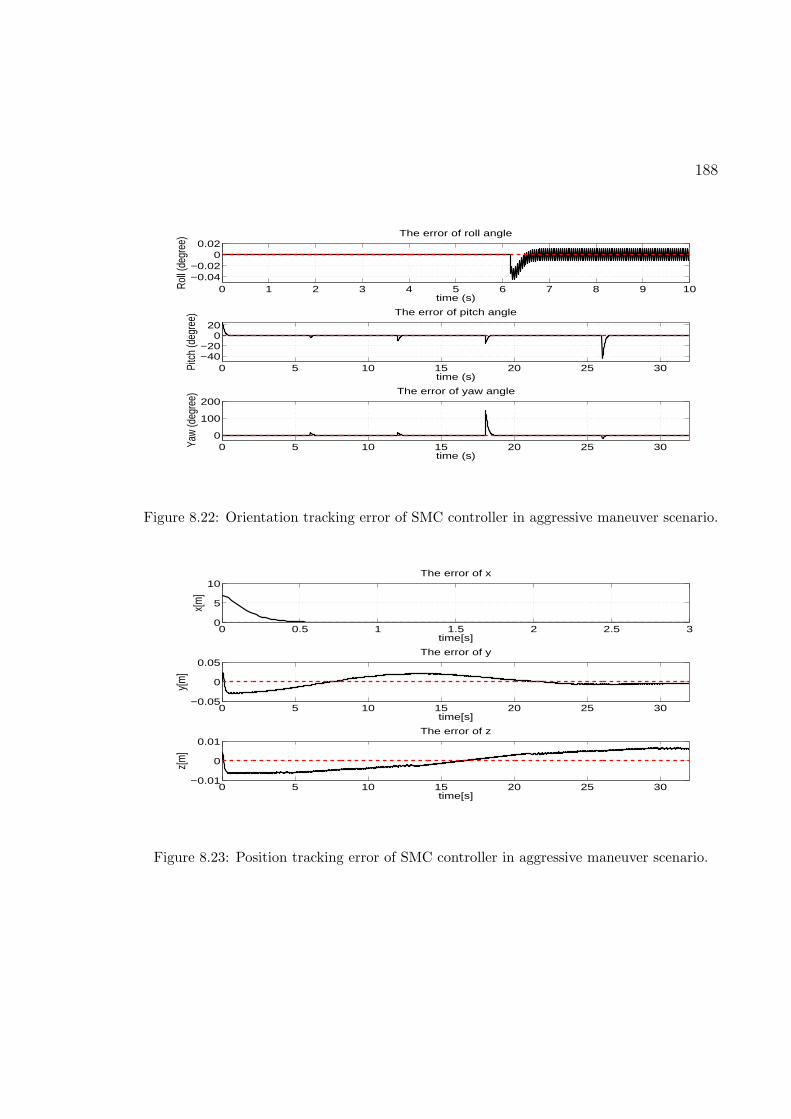
188
0 1 2 3 4 5 6 7 8 9 10−0.04−0.02
00.02
The error of roll angle
time (s)
Roll (
degr
ee)
0 5 10 15 20 25 30−40−20
020
The error of pitch angle
time (s)
Pitc
h (d
egre
e)
0 5 10 15 20 25 300
100
200The error of yaw angle
time (s)
Yaw
(deg
ree)
Figure 8.22: Orientation tracking error of SMC controller in aggressive maneuver scenario.
0 0.5 1 1.5 2 2.5 30
5
10The error of x
time[s]
x[m
]
0 5 10 15 20 25 30−0.05
0
0.05The error of y
time[s]
y[m
]
0 5 10 15 20 25 30−0.01
0
0.01The error of z
time[s]
z[m
]
Figure 8.23: Position tracking error of SMC controller in aggressive maneuver scenario.

Chapter 9
Conclusion and future work
The objective of this work was to control the eVader so that it could be used to its full
potential and perform complex maneuvers, such as following full state trajectories of
aggressive maneuvers, and executing successful landing in presence of ground effects.
Moreover, we tried to control the eVader to execute tasks that other rotary-wing
UAVs are not able to perform, such as pitched hover, which allows the eVader to take
off and land on sloped surfaces. In this thesis, throughout the process of deriving
the nonlinear dynamic model and designing nonlinear controllers to obtain the stated
objectives, we contributed to the literature of small UAVs’ autonomous flight in some
ways. These contributions are listed in the next section.
9.1 Contribution
A set of ten contributions from this thesis were accomplished. These contributions
are listed below:
1. Developing a complete dynamic model of the VTOL UAV with
dOAT mechanism, which includes all torques applyed to the eVader.
189
190
This version of the dynamic model of this vehicle is complete in the sense that
for the first time it takes into account all torques applying on the eVader,
including pitch gyroscopic moments and reactionary torques. In fact, this is the
first model in the literature considering the dOAT mechanism for the eVader,
in which the lateral and longitudinal tilting angles of the eVader vehicle are
different, and each fan rotates and tilts independently. Moreover, the model
also includes air drag, friction aerodynamic forces, and ground effects, which
are typically not included in UAV models for the purpose of control. The main
achievement of developing this model is obtaining the nonlinear model with six
DOF. The developed dynamic model is valid throughout the whole flight range
and covers all flight modes (e.g., hover, pitched hover, following trajectories,
and transition between these modes). Each flight mode can be represented by
a 12-dimensional vector of the initial and final states. The 12 states include
position, linear velocity, pitch, two angles of orientation, and their derivatives.
2. Independent 6 degree-of-freedom control of the UAV.
One of the main advantages of the eVader and its developed nonlinear dynamic
model is that they offer a great property of 6 DOF of control. Usually with
other rotary-wing UAVs such as helicopters and quad-rotors you can only set
4 desired states and stabilize the other 2 states to zero. Independent 6 DOF
control of the eVader enhanced the maneuverability capability of this UAV in

191
such a way that it is able to go from any arbitrary initial state to any arbitrary
final position in 3D space with an arbitrary orientation in the range of (−π, π).
Moreover, performing any possible maneuver within the vehicle’s capabilities in
terms of translations and orientations happens simultaneously, not by having
a sequence of controls in time like what happens in under-actuated vehicles.
For instance, to control a quad-rotor it is only possible to select a set of four
variables to be controlled (e.g., position and yaw angle), and the desired values
of the other two variables (in this case pitch and roll angles) would be forced
by the controller and are not arbitrary. As a result of the independent control
of all outputs of interest, the eVader is able to make difficult tasks and do
maneuvers that other similar UAVs are not able to perform. Maneuvers such
as pitched hover and precisely tracking a desired trajectory and orientation are
now possible.
3. Applying a single type of control technique for full control of the
UAV.
Utilizing single type of control methodology is an original approach as usually
all other UAV control systems combine several control techniques. In each chap-
ter of this thesis on controller design, a single control technique was designed
for all six desirable outputs of the vehicle. Each individual proposed single tech-
nique approach brings simplicity, flexibility and a clearer view of the interaction

192
between the different controllers.
4. Increasing reliability of control system to adapt to real time changes
in aerodynamic parameters and vehicle’s payload.
Due to the fact that the exact model of the nonlinear system is not available in
practice, it is necessary for a reliable controller to be able to adapt to parametric
uncertainties (structured disturbances). Thereby, the designed adaptive con-
troller in this thesis maintained uncertainties in aerodynamic parameters, such
as aerodynamic friction coefficients and the mass of the eVader. The designed
adaptive controller was able to cope with uncertainties in model parameters
and preserved the asymptotic stability of the system under constant external
disturbances and slow-varying parameters, which have not been studied before
for the eVader.
5. Increasing the robustness of the eVader and enabling it to perform
in presence of time-varying disturbances.
The robustness issue of UAVs is very important to be studied as more robust-
ness results in more system reliability in presence of time-varying disturbances.
Although the designed adaptive controller was able to maintain asymptotic
stability of the eVader under constant external disturbances and slow-varying
parameters, it was unable to provide asymptotic stability in presence of time-
varying disturbances such as wind gusts, ground effects and additive distur-

193
bances in control input signal (due to the error of neural network mapping
approximation). In realistic environmental flight conditions, the ground effects
and buffeting wind affect the eVader flight. Thus, the controller is required
to be robust to both unstructured uncertainties as well as structured ones, to
be reliable in practical situations. In order to increase reliability of flight con-
trol system in such situations, two robust controllers were proposed in this
thesis: i) the adaptive control technique with e-modification and ii) the SMC
approach. These controllers both achieved robustness to external unstructured
uncertainties (e.g. unmodeled dynamics) as well as structured model param-
eter uncertainties, both linear and non-linear in parameters. The AFL with
robust modification was designed for the eVader in Chapter 4, and the SMC
control was designed in Chapter 6. Simulation results, in Chapters 4, 6 and
8, demonstrated the robustness of designed controllers to sensor noise, exoge-
nous perturbations, parametric uncertainties, and plant nonlinearities, while
simultaneously exhibiting their capability to follow a reference trajectory.
6. Effectively controling the eVader when operating in the presence
of ground effects.
One of the major external disturbances, which affects the eVader when maneu-
vering in confined spaces is the flow ground effects. This issue was investigated
in this thesis as related to the eVader UAV. The ground effects on the eVader

194
are modeled in this thesis based on the CFD study of ducted fans. Despite
the lack of research in studying UAV flight control under ground effects, the
ground effects should be considered a major concern for applications in confined
spaces. Due to the importance of this issue and to investigate the performance
of the eVader, two robust controllers, RAFL and SMC, were designed to ef-
fectively control the eVader, when operating in the presence of ground effects.
The eVader demonstrated significant results, which have not been obtained and
investigated before.
7. Investigating the eVader performance in presence of buffeting wind
disturbance.
Studies of a constant wind velocity and very small wind gusts have appeared
before in the literature of UAV control. However, the study of buffeting (sinu-
soidal) wind disturbances, which cause a tough scenario for small UAV control,
has not been touched much. In fact, buffeting wind makes UAV control very
difficult because such a disturbance throws off angular and Cartesian estima-
tions. Tough, windy condition for the eVader was investigated in this thesis
for the first time. As presented in Section 8.2, simulation results using the
developed control laws in Chapter 4 and 6 are promising and show robustness
of the proposed control for the eVader flying in windy situations. In addition,
simulation results demonstrate that the eVader with new controller tolerates

195
much higher magnitude of wind (as an external disturbance) than other VTOL
vehicles, without becoming unstable.
8. Enabling the eVader to execute successful aggressive maneuvers
with a single control approach.
Successful performance of aggressive and complex maneuvers by a small eVader
UAV was achieved in this thesis, which was not possible before. Aggressive ma-
neuvers with aerial robots is an area of active research with considerable effort
focusing on strategies for generating sequences of controllers that stabilize the
robot to a desired state. The common approach in the literature for controlling
a complex aggressive maneuver is the Multi Modal control framework and the
hybrid control [112], [113]. In contrast to existing approaches in the literature,
a single controller for maneuver tracking over the full flight envelope, instead
of tracking maneuver mode sequence, was developed in this thesis. With the
proposed controller the eVader is able to handle aggressive maneuver tracking,
similar to such maneuvers with piloted aircrafts.
9. Developing the eVader control system toward flying in confined
environments.
Enabling the eVader to fly in confined environments was listed as one of the
main objectives of this thesis. Although the UAV needs to be equipped with
a navigation system to autonomously fly in high cluttered environments, the

196
key point is to develop a control system that provides high maneuverability and
agility along with maintaining the UAV stability. As results show in Chapter
8, the SMC controller designed for the eVader offers fast response and precise
trajectory tracking ability, which are essential for autonomous fly in confined
spaces. The aggressive maneuver, pitched hover, and ground effects simula-
tions established the efficiency of the proposed SMC and RAFL controllers for
the eVader, performing complex missions required to fly in confined spaces. It
should be mentioned, however, that even thought both SMC and RFAL con-
trollers provide satisfactory responses, due to the faster response of SMC in
comparison with RAFL under the same conditions, SMC is the better choice
for eVader control in such situations.
10. Achieving the estimation of actual control signals by approximat-
ing the nonlinear function relation between virtual control signals in
the model of the vehicle (u1, ..., u6) and the actual controls (α1, α2, β1,
β2, ω1, ω2).
According to the dynamic model of the vehicle, input signals obtained from
the proposed control methodologies are the virtual signals. Therefore, another
challenge associated with controlling the eVader is finding the real actuator
signals and investigating the feasibility of the associated control techniques.
This problem was addressed in this thesis by designing a neural network to

197
match the mapping between the virtual control signals and the real inputs of
the system. Thereby, in other words this thesis provided a good approximation
of the actual six control signals of the eVader dOAT mechanism, which leads to
the feasibility of full controllability. The MLP neural network with BP learning
algorithm was utilized to find the inverse mapping between variables u1, ..., u6
and α1, α2, β1, β2, ω1, ω2. From the results of this thesis work (Chapter 7), it
was observed that spanning the domain range of each variable is very important
for proper training. Spanning the domain range has a direct impact on the
performance of the network. Splitting domain range of each actual control
signal into smaller segments results in a more accurate function approximator.
Hence, dividing the domain range of each variable, may be done by separating
the maneuvers from each other. Different maneuvers may span a different part
of the range of longitudinal and lateral angles. Training specific networks for
each, gives us a better accuracy.
9.2 Future Work
Despite achieving the control of a UAV with dOAT capabilities (which was not pos-
sible before) there are a number of challenges that need to be resolved. Some of the
future tasks that we envision are the next logical steps in controlling highly manoeu-
vrable UAVs, specially the eVader, are listed below:
1. As demonstrated in Chapter 8, in presence of uncertain disturbances such as

198
ground effect and wind, the robust controllers are able to stabilize the system,
but do not achieve the asymptotic stability. Consequently, obtaining asymptotic
stability despite the presence of general uncertain disturbances is left for future
study.
2. Modification of control laws of the robust SMC controller is required to
reduce the observed chattering and the extremely high control activity, which
occurs in SMC technique.
3. The eVader’s rotors (ducts) tilt longitudinally and laterally to perform ma-
neuvers and follow complex flight trajectories. As a result of this tilting, the
mass distribution of the vehicle changes, and consequently the center of mass
of the UAV also changes. This is specially true when heavy ducts are used to
enhance the desired gyroscopic effects, that are used in controlling the vehicle.
However, the developed dynamic model in Chapter 3 is based on the fixed cen-
ter of gravity. Thus, investigating the effect of changing the center of gravity on
dynamics of the system during the flight is another study that needs investiga-
tion. In view of this fact, it is worth to mention again that the eVader requires
an adaptive or robust control law due to the fact that the center of gravity is
changing because of tilting ducted-fans mechanism.
4. Aggressive maneuver tracking trajectories are not simple to obtain. A motion
planning technique should be developed to make the trajectory planning for the

199
vehicle’s desired states as a function of time.
5. Executing experimental tests and performing different flight modes and ma-
neuvers is of great interest to study the proposed controllers in real flight. There-
fore, the proposed controller based on the developed nonlinear model should be
implemented on the prototype of the eVader.
6. As stated in Chapter 7, the neural network function approximator should
be trained on-line because there are pitch, roll and yaw angles in the equations
of control signals, u4, u5, and u6. Another approach for taking into account the
orientation angles is to train the network based on the real data collected by
executing experiments. Therefore, another future study is training the neural
network with real data to approximate the actual mapping between the virtual
and actual control signals.
7. The further step is to develop a fully autonomous and self guided eVader
based on our model, which would need navigation, motion, and path planning
system.

Bibliography
[1] G. R. Gress, “Lift fans as gyroscopes for controlling compact vtol air vehi-
cles: Overview and development status of obliques active tilting,” American
Helicopter Society, 63rd Annual Forum, May 2007.
[2] M. Wis and I. Colomina, “Dynamic dependent imu stochastic modeling for
enhanced ins/gnss navigation,” 5th ESA Workshop on Satellite Navigation
Technologies and European Workshop on GNSS Signals and Signal Processing
(NAVITEC), 2010.
[3] P. Castillo, R. Lozano, and A. Dzul, “Modelling and control of mini-flying
machines,” Springer-Verlag in Advances in Industrial Control, July 2005, iSBN:
1-85233-957-8.
[4] D. P. Raymer, Aircraft Design: A Conceptual Approach. AIAA Education
Series, 2004.
[5] A. Filippone, Flight Performance of Fixed and Rotary Wing Aircraft. Elsevier
Science, 2006.
[6] A. Week and S. Technology, 2005 Aerospace Source Book, 2005.
[7] J. G. Leishman, Principles of Helicopter Aerodynamics. Cambridge University
Press, 2006, second edition.
[8] “Boeing, v-22 osprey,” Available: http://www.boeing.com, 2008, september 13.
200

201
[9] “The bell eagle eye usa,” Available: http://www.bellhelicopter.com, 2008,
september 13.
[10] J. J. Dickeson, D. Miles, O. Cifdaloz, V. L. Wells, and A. A. Rodriguez, “Robust
lpv h gain-scheduled hover-to-cruise conversion for a tilt-wing rotorcraft in the
presence of cg variations,” American Control Conference (ACC2007), pp. 5266
– 5271, 2007, 9-13 July.
[11] I. Kendoul, F.and Fantoni and R. Lorenzo, “Modeling and control of a small
autonomous aircraft having two tilting rotors,” Proceedings of the 44th IEEE
Conference on Decision and Control, and the European Control Conference,
2005, 12-15 December.
[12] D. Snyder, “The quad tiltrotor: Its beginning and evolution,” Proceedings of
the 56th Annual Forum, American Helicopter Society, May 2000.
[13] K. Nonami, “Prospect and recent research & development for civil use au-
tonomous unmanned aircraft as uav and mav,” Journal of System Design and
Dynamics, vol. 1, no. 2, 2007.
[14] D. Murphy and J. Cycon, “Applications for mini vtol uav for law enforce-
ment,” 2nd AIAA: Unmanned Unlimited Systems,Technologies,and Operations-
Aerospace, 2003.
[15] S. Bouabdallah and R. Siegwart, “Full control of a quadrotor,” IEEE Interna-
tional Conference on Intelligent Robots and Systems, pp. 153 –158, 2007.
[16] S. Bouabdallah, A. Noth, and R. Siegwart, “Pid vs lq control techniques applied
to an indoor micro quadrotor,” 2004 IEEE/RSJ International Conference on
Intelligent Robots and Systems (IROS) (IEEE Cat. No.04CH37566), vol. 3, pp.
2451 – 6, 2004.
[17] P. McKerrow, “Modelling the draganflyer four-rotor helicopter,” International
Conference on Robotics and Automation, 2004.
[18] P. Guenard, T. Hamel, and L. Eck, “Control laws for the tele operation of an
unmanned aerial vehicle known as an x4-flyer,” IEEE International Conference
on Intelligent Robots and Systems, pp. 3249 – 3254, Oct. 2006.

202
[19] G. R. Gress, “Vtol air vehicles with high flight speeds and 3d mobility within
helicopter-impenetrable environments,” American Helicopter Society SW Chap-
ter Conference, Next Generation Vertical Lift Technologies, Sept. 2008.
[20] Y. M. Shakernia, T. Koo, and S. S. Sastry, “Landing an unmanned air vehi-
cle: Vision-based motion estimation and nonlinear control,” Asian Journal of
Control 1, no. 3, pp. 128–145, 1999.
[21] I. D. Cowling, O. A. Yakimenko, J. F. Whidborne, and A. K. Cooke, “A pro-
totype of an autonomous controller for a quadrotor uav,” European Control
Conference, 2007, 2-5 July.
[22] A. Tayebi and S. McGilvray, “Attitude stabilization of a four-rotor aerial robot,”
43rd IEEE Conference on Decision and Control, Bahamas, 2004, 14-17 Decem-
ber.
[23] P. Pounds, R. Mahony, P. Hynes, and J. Roberts, “Design of a four-rotor aerial
robot,” Proceedings of the Australasian Conference on Robotics and Automa-
tion, pp. 145–150, 2002.
[24] P. Pounds, R. Mahony, and P. Corke, “Modelling and control of a quad-rotor
robot,” Proceedings of the Australasian Conference on Robotics and Automa-
tion, 2006.
[25] G. Hoffman, H. Huang, S. Waslander, and C. Tomlin, “Quadrotor helicopter
flight dynamics and control:theory and experiment,” Proceedings of the AIAA
Guidance, Navigation & Control Conference, 2007, hilton Head, SC, USA,aIAA
Paper Number 2007-6461.
[26] G. Hoffman, S. Waslander, and C. Tomlin, “Quadrotor helicopter trajectory
tracking control,” Proceedings of the AIAA Guidance, Navigation & Control
Conference, 2008, aIAA Paper Number 2008-7410.
[27] S. Bouabdallah and R. Siegwart, “Field and service robotics,” Springer Tracts
in Advanced Robotics, 2006, ch. Towards intelligent miniature flying robots.

203
[28] E. Altug and C. Taylor, “Vision-based pose estimation and control of a model
helicopter,” Proceedings of the 2004 IEEE International Conference on Mecha-
tronics, Istanbul, Turkey, 2004.
[29] A. Benallegue, A. Mokhtari, and L. Fridman, “Feedback linearization and high
order sliding mode observer for a quadrotor uav,” Proceedings of the 2006 Inter-
national Workshop on Variable Structure Systems, pp. 365–372, Alghero, Italy,
2006.
[30] T. Madani and A. Benalleque, “Control of a quadrotor mini-helicopter via full
state backstepping technique,” Proc. of the 45th IEEE Conference on Decision
and Control, pp. 1515 – 1520, 2006.
[31] T. Madani and A. Benallegue, “Backstepping sliding mode control applied to
a miniature quadrotor flying robot,” Proceedings of the 2006 IEEE Conference
on Industrial Electronics, pp. 700–705, Paris, France, 2006.
[32] ——, “Control of a quadrotor mini-helicopter via full state backstepping tech-
nique,” Proceedings of the 2006 IEEE Conference on Decision & Control, pp.
1515–1520, San Diego, CA, USA, 2006.
[33] D. Lara, A. Sanchez, R. Lozano, and P. Castillo, “Real-time embedded control
system for vtol aircrafts:application to stabilize a quad-rotor helicopter,” Pro-
ceedings of the 2006 IEEE International Conference on Control Applications,
Munich, Germany, 2006.
[34] P. Castillo, P. Albertos, P. Garcia, and R. Lozano, “Simple real-time attitude
stabilization of a quad-rotor aircraft with bounded signals,” Proceedings of the
45th IEEE Conference on Decision and Control, pp. 1533 – 1538, 2006.
[35] J. Hauser, S. Sastry, and G. Meyer, “Nonlinear control design for slightly non-
minimum phase systems: Application to v/stol aircraft,” Automatica, vol. 28,
no. 4, pp. 665 – 679, 1992.
[36] A. R. Teel, “A nonlinear small gain theorem for the analysis of control systems
with saturation,” IEEE Transactions on Automatic Control, vol. 41, no. 9, pp.
1256 – 1270, 1996.

204
[37] P. Martin, S. Devasia, and B. Paden, “A different look at output tracking:
Control of a vtol aircraft,” Automatica, vol. 32, no. 1, pp. 101 – 107, 1996.
[38] F. Mazenc and L. Praly, “Adding integrations, satured controls, and stabi-
lization for feedforward systems,” IEEE Transactions on Automatic Control,
vol. 41, no. 11, pp. 1559 – 1578, 1996.
[39] I. Fantoni and R. Lozano, “Control of nonlinear mechanical systems,” European
Journal of Control, vol. 7, pp. 328 – 348, 2001.
[40] I. Fantoni and R. Lozano, Eds., Non-linear control for underactuated mechan-
ical systems. Springer-Verlag, London, 2001, communications and Control
Engineering Series.
[41] L. Marconi, A. Isidori, and A. Serrani, “Autonomous vertical landig on an
oscillating platform: an internal-model based approach,” Automatica, vol. 38,
pp. 21 – 32, 2002.
[42] R. Olfati-Saber, “Global configuration stabilization for the vtol aircraft with
strong input coupling,” IEEE Transactions on Automatic Control, vol. 41,
no. 11, pp. 1949 – 1952, 2002.
[43] R. Lozanoa, P. Castilloa, and A. Dzulb, “Global configuration stabilization for
the vtol aircraft with strong input coupling,” International Journal of Control,
vol. 77, no. 8, pp. 735 – 740, 2004.
[44] C. Coza, C. Nicol, C. Macnab, and A. Ramirez-Serrano, “Adaptive fuzzy control
for a quadrotor helicopter robust to wind buffeting,” Journal of Intelligent and
Fuzzy Systems, 2010, in press.
[45] C. Nicol, C. Macnab, and A. Ramirez-Serrano, “Robust neural network control
of a quadrotor helicopter,” Canadian Conference on Electrical and Computer
Engineering, CCECE 2008, pp. 1233 – 1238, 2008, niagara Falls, ON, May.
[46] Y. Morel and A. Leonessa, “Direct adaptive tracking control of quadrotor aerial
vehicles,” Proc. of the 2006 Florida Conference on Recent Advances in Robotics,
pp. 1–6, 2006.

205
[47] A. Das, F. Lewis, and S. Subbarao, “Dynamic neural network based robust
backstepping control approach for quadrotors,” Proc. of the 2008 AIAA Guid-
ance, Navigation and Control Conference and Exibit, August 2008.
[48] L. A. J. Toledo, M. Sigut, and J. Felipe, “Stabilization and altitude tracking of
a four-rotor microhelicopter using lifting operators,” IET Control Theory and
Application, vol. 3, no. 4, pp. 452–464, 2009.
[49] L. Besnard, Y. Shtessel, and B. Landrum, “Control of a quadrotor vehicle using
sliding mode disturbance observer,” Proc. of American Control Conference, pp.
5230–5235, July 2007.
[50] C. Coza and C. Macnab, “A new robust adaptive-fuzzy control method applied
to quadrotor helicopter stabilization,” NAFIPS Annual meeting of the North
American Fuzzy Information Society, pp. 454 – 458, 2006.
[51] N. Metni and T. Hamel, “Visual tracking control of aerial robotic systems with
adaptive depth estimation,” International Journal of Control, Automation, and
Systems, vol. 5, no. 1, pp. 51 – 60, 2007.
[52] A. Mokhtari and A. Benallegue, “Dynamic feedback controller of euler angles
and wind parameters estimation for a quadrotor unmanned aerial vehicle,” Pro-
ceedings - IEEE International Conference on Robotics and Automation, vol.
2004, no. 3, pp. 2359 –2366, 2004.
[53] R. Xu and U. Ozquner, “Sliding mode control of a quadrotor helicopter,” Proc.
of the IEEE 45th Conference on Decision & Control, pp. 4957–4962, Dec. 2006.
[54] J. Dunfied, M. Tarbouchi, and G. Labonte, “Neural network based control of a
four rotor helicopter,” Proceedings of the 2004 IEEE International Conference
on Industrial Technology, pp. 1543–1548, Hammamet, Tunisia, 2004.
[55] J. Cesareo Raimundez and A. Fernandez Villaverde, “Adaptive tracking control
for a quad-rotor,” Proceedings of ENOC-2008, Saint Petersburg, Russia, 2008.
[56] T. Dierks and S. Jagannathan, “Neural network output feedback control of
a quadrotor uav,” Proceedings of the 2008 IEEE Conference on Decision and
Control, pp. 3633–3639, Cancun, Mexico, 2008.

206
[57] P. Castillo, R. Lozano, and A. Dzul, “Stabilization of a mini rotorcraft with
four rotors,” IEEE Control Systems Magazine, pp. 45 –55, 2005.
[58] S. Grzonka, G. Grisetti, and W. Burgard, “A fully autonomous indoor quadro-
tor,” IEEE Transactions on Robotics, vol. 28, pp. 90 – 100, 2012.
[59] G. R. Gress, “A dual-fan vtol aircraft using opposed lateral tilting for pitch
control,” American Helicopter Society, 59th Annual Forum, vol. 2, pp. 2201–
2238, May 2003.
[60] N. Amiri, A. R. Serrano, and R. Davies, “Modelling of opposed lateral and lon-
gitudinal tilting dual-fan unmanned aerial vehicle,” 18th IFAC World Congress,
Aug 28-Sep 2, 2011.
[61] T. E. Lee, J. G. Leishman, and M. Ramasamy, “Fluid dynamics of intercting
blade tip vortices with a found plane,” 64th Annual Forum of the American
Helicopter Society, vol. 2, pp. 1231–1248, 2008.
[62] D. A. Griffiths and J. G. Leishman, “A study of dual-rotor interference and
ground effect using a free-vortex wake model,” 58th Annual Forum of the Amer-
ican Helicopter Society, June 2002.
[63] J.-J. E. Slotine and W. Li, Applied Nonlinear Control. Prentice Hall, New
Jersey, 1991.
[64] F. Jansen, “Maneuvering unmanned vehicles through confined 3d environments
using model predictive control,”M.Sc Dissertation in Department of Mechanical
and Manufacturing Engineering, University of Calgary, 2011.
[65] C. M. Roithmayer, “International space station attitude motion associated with
flywheel energy storage,” NASA Langley Research Center, 1999.
[66] K. Lim, J.-Y. Shin, D. Moerder, and E. Cooper, “A new approach to attitude
stability and control for low airspeed vehicles,” Collection of Technical Papers
- AIAA Guidance, Navigation, and Control Conference, vol. 2, pp. 1268 –1283,
2004.

207
[67] K. Lim, J.-Y. Shin, E. Cooper, D. Moerder, T. H. Khong, and M. F. Smith, “An
overview of the nasa flying test platform research,” AIAA Guidance, Navigation
and Control Conference and Exhibit, 2003, aIAA paper 2003-5775.
[68] G. R. Gress, “Using dual propellers as gyroscopes for tilt-prop hover control,”
American Institute of Aeronautics and Astronautics, 2002.
[69] D. Erdos and S. E. Watkins, “Uav autopilot integration and testing,” IEEE
Region 5 Conference, pp. 1–6, 2008.
[70] F. Kendoul, I. Fantoni, and R. Lozano, “Modeling and control of a small au-
tonomous aircraft having two tilting rotors,” IEEE Transactions on Robotics,
vol. 22, no. 6, pp. 1297 – 1302, 2006.
[71] B. W. Mccormick, Aerodynamics, Aeronautics, and Flight Mechanics. John
Wiley and Sons, 1995.
[72] V. Gavrilets, Autonomous Aerobatic Maneuvering of Miniature Helicopters,
May 2003.
[73] M. Barczyk, Nonlinear State Estimation and Modeling of a Helicopter UAV,
2012.
[74] D. A. Griffiths and J. G. Leishman, “Measurements of a rotor flow in ground
effect and visualisation of the brown-out phenomenon,” 64th Annual Forum of
the American Helicopter Society, May 2008.
[75] Z. Hosseini, “Ground/wall effects on a ducted fan for control applications of
highly manoeuvrable vtols operating in confined spaces,” M.Sc Dissertation
in Department of Mechanical and Manufacturing Engineering, University of
Calgary, 2011.
[76] K. P. E. Valavanis, Advances in Unmanned Aerial Vehicles: State of the Art
and the Road to Autonomy. Springer, 2007.
[77] A. Isidori, Nonlinear Control Systems. Springer, 1995, no. v.1.

208
[78] A. Banos, F. Lamnabhi-Lagarrigue, and F. J. Montoyo, Advances in the Control
of Nonlinear Systems. Springer-Verlag London, 2001.
[79] J. K. Hedrick and S. Gopalswamy, “Nonlinear flight control design via slid-
ing methods,” Dept. of Mechanical Engineering, Univ. of California, Berkeley,
1989.
[80] P. James, O. A. Altug, and R. Mahony, “Control of a quadrotor helicopter using
visual feedback,” Proc. of the 2002 IEEE International Conference on Robotics
and Automation, May 2002.
[81] J. E. Hauser, “Approximate tracking for nonlinear systems with application to
flight control,” Doctoral thesis, 1989.
[82] M. Krstic, I. Kanellakopoulos, and P. Kokotovic, Nonlinear and Adaptive Con-
trol Design. John Wiley and Sons, 1995.
[83] M. S. Queiroz, D. M. Dawson, S. P. Nagarkatti, and F. Zhang, Lyapunov-Based
Control of Mechanical Systems (Control Engineering). Birkhuser Boston, 2000.
[84] B. Egardt, Stability of Adaptive Controllers, Springer-Verlag. New York, 1979.
[85] K. Narendra and A. Annaswamy, “A new adaptive law for robust adapta-
tion without persistent excitation,” IEEE Transactions on Automatic Control,
vol. 32, pp. 134 – 145, 1989.
[86] A. Noureldin, J. Armstrong, A. El-Shafie, T. Karamat, D. McGaughey, M. Ko-
renberg, and A. Hussain, “Accuracy enhancement of inertial sensors utilizing
high resolution spectral analysis,” Journal of sensors, 2012.
[87] S. Bouabdallah and R. Siegwart, “Backstepping and sliding-mode techniques
applied to an indoor micro quadrotor,” Proceedings - IEEE International Con-
ference on Robotics and Automation, vol. 2005, pp. 2247 – 2252, 2005.
[88] J. Colorado, A. Barrientos, A. Martinez, B. Lafaverges, and J. Valente, “Mini-
quadrotor attitude control based on hybrid backstepping frenet-serret the-
ory,” 2010 IEEE International Conference on Robotics and Automation (ICRA
2010), pp. 1617 – 1622, 2010.

209
[89] T. Madani and A. Benalleque, “Backstepping sliding mode control applied to
a miniature quadrotor flying robot,” Proc. of IEEE Industrial Electronics, the
32nd Annual Conference, pp. 700 – 705, 2006.
[90] N. Metni and T. Hamel, “Visual tracking control of aerial robotic systems with
adaptive depth estimation,” International Journal of Control, Automation, and
Systems, vol. 5, no. 1, pp. 51 – 60, 2007.
[91] I. Kanellakopoulos and P. Krein, “Integral0action nonlinear control of induction
motors,” 12th IFAC World Congress, 1993.
[92] J. A. Snyman, Practical Mathematical Optimization: An Introduction to Ba-
sic Optimization Theory and Classical and New Gradient-Based Algorithms.
Springer Publishing, 2005.
[93] T. Zhang, S. S. Ge, C. C. Hang, and T. Y. Chai, “Adaptive control of first or-
der systems with nonlinear parametrization,” IEEE Transactions on Automatic
Control, vol. 45, no. 8, pp. 1512–1516, Aug. 2000.
[94] D. E. Miller, “A new approach to model reference adaptive control,” IEEE
Transactions on Automatic Control, vol. 48, no. 5, pp. 743–757, 2003.
[95] A. S. I. Zinober, Ed., Deterministic control of uncertain systems. London:
Peter Peregrinus Press, 1990, iSBN 978-0863411700.
[96] K. D. Young, V. I. Utkin, and U. Ozguner, “A control engineer’s guide to sliding
mode control,” IEEE Transactions on Control Systems Technology, vol. 7, no. 3,
pp. 328–342, 1999.
[97] H. K. Khalil, Ed., Nonlinear Systems (3rd ed). Upper Saddle River, NJ:
Prentice Hall, 2002, iSBN 0-13-067389-7.
[98] C. A. Chen, H. K. Chiang, and J. C. Shen, “Fuzzy sliding mode control of
a magnetic ball suspension system,” International Journal of Fuzzy Systems,
vol. 11, no. 2, pp. 97–106, 2009.

210
[99] Q. L. Hu, Z. D. Wang, and H. J. Gao, “Sliding mode and shaped input vibra-
tion control of flexible systems,” IEEE Transactions on Aerospace and Electric
Systems, vol. 44, no. 2, pp. 503–519, 2008.
[100] G. Cybenko, “Approximation by superpositions of a sigmoidal function,” Math-
ematics of Control Signals, and Systems, vol. 2, no. 4, pp. 303–314, 1989.
[101] K. Hornik, “Approximation capabilities of multilayer feedforward networks,”
Neural Networks, vol. 4, no. 2, pp. 251–257, 1991.
[102] S. Haykin, Neural Networks: A Comprehensive Foundation. Prentice Hall,
1998, vol. 2.
[103] K. J. Hunt, D. Sbarbaro, R. Zbikowski, and P. J. Gawthrop, “Neural networks
for control systems: A survey,” Automatica, vol. 28, no. 6, pp. 1083–1112, 1992.
[104] K. S. Narendra and k. Parthasarathy, “Identification and control of dynamical
systems using neural networks,” IEEE Transactions on Neural Networks, vol. 3,
pp. 4–27, 1990.
[105] Y. Pao, Adaptive Pattern Recognition and Neural Networks. Addison-Wesley,
Reading, Massachusetts, 1989.
[106] P. K. Simpson, Artificial Neural Systems. Pergamon Press, New York, 1989.
[107] R. Hecht-Nielsen, Neurocomputing. Addison-Wesley, Reading, Massachusetts,
1989.
[108] E. Alpaydin, Introduction to Machine Learning. The MIT Press, Cambridge,
Massachusetts, 2010, 2nd ed.
[109] A. Cichocki and R. Unbehauen, Neural networks for optimization and signal
processing. John Wiley and Sons, 1993.
[110] P. J. Webros, The roots of back-propagation. John Wiley and Sons, NY, 1994.
[111] E. A. Jackson, Perspectives of nonlinear dynamics. Cambridge University
Press, 1991.

211
[112] E. Koyuncu, N. K. Ure, and G. Inalhan, “A probabilistic algorithm for mode
based motion planning of agile unmanned air vehicles in complex environ-
ments,” Proceedings of the IFAC World Congress, 2008, korea.
[113] E. Frazzoli, M. A. Dahleh, and E. Feron, “Maneuver based motion planning
for nonlinear systems with symmetries,” IEEE Transactions on Robotics and
Automation, vol. 21, no. 6, pp. 1077–1091, December 2005.

Appendix A
This appendix provides a list of simulation scenarios that applied on the UAV through-
out this research to investigate different aspects of the problem in hand.
.1 Scope of Scenarios
1. Scenario # 1: Moving from the origin to an arbitrary destination with ar-
bitrary orientation which results in a regulation to an arbitrary final states. The
initial conditions are x(0) = [0]12×12, and the desired states are set arbitrarily
to xd = [22.5, 0, 15, 0, 18, 0, 3, 0, 4, 0, 2, 0]T .
2. Scenario # 2: Moving from the origin to an arbitrary destination with
arbitrary orientation while the parameters of the dynamic model of the eVader
is not known completely and the mass of the vehicle changes during the flight
(e.g., as a result of picking up a load).
The initial conditions are x(0) = [0]12×12, and the desired states are set arbi-
trarily to xd = [22.5, 0, 15, 0, 18, 0, 3, 0, 4, 0, 2, 0]T .
3. Scenario # 3: Flight from initial states to final desired states in pres-
ence of wind gusts which is modeled as a sinusoidal disturbance of the form:
dw(t) = 10 + 5sin(2πt); In this scenario the eVader should stay stable at the
same position (same x, y, and z), while changing its orientation. The initial
conditions and the desired states are as follows: initial conditions: [φ0, φ0]T =
[22.5, 0]T , [θ0, θ0]T = [15, 0]T , [ψ0, ψ0]
T = [18, 0]T , [x0, x0]T = [2, 0]T , [y0, y0]
T =
[3, 0]T , [z0, z0]T = [5, 0]T , and desired states: [φd, φd]
T = [0, 0]t, [θd, θd]T =
[0, 0]T , [ψd, ψ]T = [0, 0]T , [xd, xd]
T = [3, 0]T , [yd, yd]T = [4, 0]T , [zd, zd]
T = [2, 0]T .
4. Scenario # 4: Moving from an arbitrary position in 3D space to an arbi-
trary final states which means the evader translate to the desired position and
rotates to the desired orientation. The initial condition of orientation angles
212

213
and position are η(0) = [0, 0, 0]T and ζ(0) = [0, 0, 0]T , respectively, and the
desired states are set arbitrarily to xd = [10, 0, 35, 0, 5, 0, 0, 0, 0, 0, 2, 0]T .
5. Scenario # 5: For the purpose of autonomous take off and landing the
vehicle forced to follow the square signal of altitude. The eVader takes off from
the origin (ζ(0) = [0, 0, 0]T ) to the altitude of 2 m, hover at the same position
for 2 seconds and lands on the ground afterward. The desired value of altitude
is fixed at 2 m.
6. Scenario # 6: Stabilization of roll, pitch and yaw angles. The attitude
initial conditions are set to (φ0 = 10, θ0 = 35, ψ0 = 5) and the final values
are set (φd = 0, θd = 25, ψd = 0). The vehicle should maintain its stability at
hover with 25 pitch angle.
7. Scenario # 7: Stay stable at hover at the same altitude of 3m hight
while pitching the eVader’s nose from 0 to 22.5 and regulate all other states
including roll and yaw angles, position and altitude to zero.
x0 = [22.5, 0, 0, 0, 18, 0, 5, 0, 4, 0, 3, 0]T
xd = [0, 0, 22.5, 0, 0, 0, 0, 0, 0, 0, 3, 0]T
8. Scenario # 8: Pitched hover while wind is blowing, after 1.5 s wind blows
for 0.2 s (a sudden disturbance). The eVader in pitched hover condition facing
with a sudden strong wind disturbance after 1.5 s and wind blows for 0.2 s. It
is also assumed that wind affects the vehicle in all directions according to the
vehicle’s reference frame and has effect on all outputs.
x0 = [22.5, 0, 0, 0, 18, 0, 5, 0, 4, 0, 3, 0]T
xd = [0, 0, 22.5, 0, 0, 0, 0, 0, 0, 0, 3, 0]T
9. Scenario # 9: Flying from the origin to the point ζ(0) = [3, 4, 2]T in
3D space and rotating η(0) = [22.5, 15, 18]T when the parameters of the
eVader dynamic model is varying during the flight. Assuming the mass and

214
the inertia matrix of the vehicle have variations from their priori values. The
initial conditions are x0 = [0, 0, 0, 0, 0, 0, 0, 0, 0, 0, 0, 0]T , the desired values are
xd = [22.5, 0, 15, 0, 18, 0, 3, 0, 4, 0, 2, 0]T .
10. Scenario # 10: White random noise added to the Scenario # 9 to model
noise as a result of measurement errors with mean=0 and variance=0.1. Flying
from the origin to the point ζ(0) = [3, 4, 2]T in 3D space and rotating η(0) =
[22.5, 15, 18]T when the parameters of the eVader dynamic model is varying
during the flight with additive random white noise.
11. Scenario # 11: After 1sec of the flight the eVader picks up a heavy load
of 3.5kg. This load modeled as a sudden disturbance added to θ and θ.
12. Scenario # 12: Landing from altitude of 5 meters to the ground and mov-
ing to the origin in presence of the ground effect disturbance which is modeled
as:
gr(z) =
az(z+zcg)2
− az(z0+zcg)2
0 < z ≤ z0
0 else(1)
During landing the vehicle orientation rotates to zero from its initial condi-
tion. The initial and final states conditions are chosen as follows: initial con-
dition: [φ0, φ0]T = [45, 0]T , [θ0, θ0]
T = [30, 0]T , [ψ0, ψ0]T = [20, 0]T , [x0, x0]
T =
[3, 0]t, [y0, y0]T = [4, 0]T , [z0, z0]
T = [5, 0]T , and desired states:
xd = [0,0,0,0,0,0,0,0,0,0,0,0]T
.
13. Scenario # 13: Performing and aggressive maneuvers which includes
tracking complex trajectories in 3D space with high speed while rotating sharply
as well. To produce an aggressive trajectory as a function of time and apply it
to the proposed controllers, herein, we used the Mobius strip equations [111],
as below:
x = [R + rcos(γ)] cos(κ)
y = [R + rcos(γ)] sin(κ)
z = rsin(γ)
(2)

215
with R = 4, r = 3, −π < κ < π, and −π/2 < γ < π/2. The formula (8.2)
provides a three-dimensional Cartesian position of the eVader path in this flight
scenario. The orientation reference trajectories are chosen arbitrarily consistent
with a trajectory produced by (2). The roll angle is set to be stable at zero
and the pitch and yaw angles follow the piecewise constant curves with sharp
stepwise patterns which varies from 25 to −50 for pitch and from zero degree
to 175 for yaw angle
Related Documents