Control of an electric Propulsion System for a Light Aircraft Final Year Project By EVA MANEUS SALVADOR Tutor: RAMON MANUEL BLASCO-GIMENEZ Escola Tècnica Superior d’Enginyeria del Disseny UNIVERSITAT POLITÈCNICA DE VALÈNCIA Final year Project for the BACHELOR DEGREE IN AEROSPACE ENGINEERING J UNE 2018

Welcome message from author
This document is posted to help you gain knowledge. Please leave a comment to let me know what you think about it! Share it to your friends and learn new things together.
Transcript
Control of an electric Propulsion Systemfor a Light Aircraft
Final Year Project
By
EVA MANEUS SALVADOR
Tutor: RAMON MANUEL BLASCO-GIMENEZ
Escola Tècnica Superior d’Enginyeria del DissenyUNIVERSITAT POLITÈCNICA DE VALÈNCIA
Final year Project for the BACHELOR DEGREE IN AEROSPACE
ENGINEERING
JUNE 2018

SUMMARY
In the future, aviation will most certainly tend to be electric, reason why there exists anincreasing interest in developing electrically propelled aircrafts. An option is to replacetraditional fuel engines with electrical motors where it is available, namely in light aircrafts.
To be able to do so, a design process needs to be followed, which contemplates adapting an electricmotor to suit its new task by designing and testing its control system, specially designed for itsimplementation on the aircraft. Likewise, said modifications will also involve the installation ofbatteries and, lastly, flight testing to prove the performance of the aircraft has not been negativelyaffected, except for the fact the autonomy is reduced substantially in spite of the differences inenergy provision by batteries and by traditional aviation fuels.
Keywords: electric aircraft, control, light aircraft, propulsion
i


AGRAÏMENTS
Estic agraïda al tutor d’aquest treball, Ramón Blasco, per tota l’ajuda rebuda, i als meus pares, sense els quals no haguera pogut fer mai el present projecte.
iii

TABLE OF CONTENTS
Page
List of Tables v
List of Figures vi
1 State of the art 1
2 Objectives of this project 32.1 Objectives . . . . . . . . . . . . . . . . . . . . . . . . . . . . . . . . . . . . . . . . . . . . 3
2.2 Procedure . . . . . . . . . . . . . . . . . . . . . . . . . . . . . . . . . . . . . . . . . . . . 4
3 Propulsion in light aircrafts 73.1 Introduction to propulsion . . . . . . . . . . . . . . . . . . . . . . . . . . . . . . . . . . 7
3.2 Approaches for light aircrafts . . . . . . . . . . . . . . . . . . . . . . . . . . . . . . . . 9
3.2.1 Traditional - Combustion engines and turboprops . . . . . . . . . . . . . . . 9
3.2.2 Modern - Electric . . . . . . . . . . . . . . . . . . . . . . . . . . . . . . . . . . . 12
3.3 General requirements for propulsion . . . . . . . . . . . . . . . . . . . . . . . . . . . . 13
3.4 Electric Aircrafts . . . . . . . . . . . . . . . . . . . . . . . . . . . . . . . . . . . . . . . 17
3.4.1 Electric Motors for propulsion . . . . . . . . . . . . . . . . . . . . . . . . . . . 18
3.4.2 Energy supply and storage . . . . . . . . . . . . . . . . . . . . . . . . . . . . . 19
3.4.3 Safety considerations and redundancy . . . . . . . . . . . . . . . . . . . . . . 20
4 Simulation environment and approach 234.1 Simulink Light Aircraft Model . . . . . . . . . . . . . . . . . . . . . . . . . . . . . . . 23
4.1.1 Environment . . . . . . . . . . . . . . . . . . . . . . . . . . . . . . . . . . . . . 25
4.1.2 Pilot . . . . . . . . . . . . . . . . . . . . . . . . . . . . . . . . . . . . . . . . . . . 25
4.1.3 Vehicle System Model . . . . . . . . . . . . . . . . . . . . . . . . . . . . . . . . 26
4.1.3.1 Avionics . . . . . . . . . . . . . . . . . . . . . . . . . . . . . . . . . . 26
4.1.3.2 Flight Sensors . . . . . . . . . . . . . . . . . . . . . . . . . . . . . . . 26
4.1.3.3 Vehicle . . . . . . . . . . . . . . . . . . . . . . . . . . . . . . . . . . . 27
4.2 Propulsion block layout . . . . . . . . . . . . . . . . . . . . . . . . . . . . . . . . . . . . 28
4.2.1 Propeller . . . . . . . . . . . . . . . . . . . . . . . . . . . . . . . . . . . . . . . . 28
iv
4.2.2 Electric motor . . . . . . . . . . . . . . . . . . . . . . . . . . . . . . . . . . . . . 28
4.2.3 Batteries . . . . . . . . . . . . . . . . . . . . . . . . . . . . . . . . . . . . . . . . 29
5 Propeller design and implementation 315.1 Design of a propeller with JavaProp . . . . . . . . . . . . . . . . . . . . . . . . . . . . 31
5.1.1 Thrust requirements of the Sky Hogg . . . . . . . . . . . . . . . . . . . . . . 32
5.1.2 Working with JavaProp . . . . . . . . . . . . . . . . . . . . . . . . . . . . . . . 33
5.1.3 JavaProp results . . . . . . . . . . . . . . . . . . . . . . . . . . . . . . . . . . . 36
5.2 Implementation of the propeller to the model . . . . . . . . . . . . . . . . . . . . . . 42
6 Propulsion block 456.1 Overview . . . . . . . . . . . . . . . . . . . . . . . . . . . . . . . . . . . . . . . . . . . . 45
6.1.1 Propeller block . . . . . . . . . . . . . . . . . . . . . . . . . . . . . . . . . . . . 46
6.1.2 Power and thrust subsystems . . . . . . . . . . . . . . . . . . . . . . . . . . . 47
6.2 Electric motor block . . . . . . . . . . . . . . . . . . . . . . . . . . . . . . . . . . . . . . 48
6.2.1 Brushless electric motor control . . . . . . . . . . . . . . . . . . . . . . . . . . 48
6.3 Batteries . . . . . . . . . . . . . . . . . . . . . . . . . . . . . . . . . . . . . . . . . . . . 53
7 Performance and results 577.1 Performance during normal use . . . . . . . . . . . . . . . . . . . . . . . . . . . . . . . 57
7.1.1 Levelled flight at constant throttle . . . . . . . . . . . . . . . . . . . . . . . . 57
7.1.2 Climbing and descending flight . . . . . . . . . . . . . . . . . . . . . . . . . . 61
7.2 Performance in event of motor failure . . . . . . . . . . . . . . . . . . . . . . . . . . . 66
8 Conclusions 738.1 Conclusions of the project . . . . . . . . . . . . . . . . . . . . . . . . . . . . . . . . . . 73
8.2 Further studies . . . . . . . . . . . . . . . . . . . . . . . . . . . . . . . . . . . . . . . . 74
A Appendix A 75
Bibliography 77
LIST OF TABLES
TABLE Page
3.1 RICE motor data over the years . . . . . . . . . . . . . . . . . . . . . . . . . . . . . . . . . 14
v
3.2 Characteristics of different electric motors . . . . . . . . . . . . . . . . . . . . . . . . . . 17
3.3 Comparison of specific energy of aviation gasoline and Li-io batteries . . . . . . . . . . 20
5.1 Flight initial conditions . . . . . . . . . . . . . . . . . . . . . . . . . . . . . . . . . . . . . . 32
5.2 Geometric parameters of the blades . . . . . . . . . . . . . . . . . . . . . . . . . . . . . . 34
5.3 Airfoils along the span . . . . . . . . . . . . . . . . . . . . . . . . . . . . . . . . . . . . . . 34
6.1 Specifications of the PI controllers . . . . . . . . . . . . . . . . . . . . . . . . . . . . . . . 52
6.2 Parameters of the simulated brushless AC motor . . . . . . . . . . . . . . . . . . . . . . 53
6.3 Weight values of the Lancair IV-P and the electric motor . . . . . . . . . . . . . . . . . . 54
6.4 Battery characteristics for the SkyHogg . . . . . . . . . . . . . . . . . . . . . . . . . . . . 55
7.1 Description of mission for the levelled flight case . . . . . . . . . . . . . . . . . . . . . . 58
7.2 Description of mission for climbing/descending flight . . . . . . . . . . . . . . . . . . . . 62
7.3 Main points of the motor failure mission . . . . . . . . . . . . . . . . . . . . . . . . . . . 66
A.1 Original SkyHogg model parameters and variables . . . . . . . . . . . . . . . . . . . . . 75
LIST OF FIGURES
FIGURE Page
3.1 Evolution of RICE mass over the decades . . . . . . . . . . . . . . . . . . . . . . . . . . . 10
3.2 Evolution of RICE number of cylinders over the decades . . . . . . . . . . . . . . . . . . 11
3.3 Specific power versus weight over the decades . . . . . . . . . . . . . . . . . . . . . . . . 11
3.4 Halbach magnet array rotor flux distribution . . . . . . . . . . . . . . . . . . . . . . . . . 19
4.1 Diagram of the asbSkyHogg Simulink model . . . . . . . . . . . . . . . . . . . . . . . . . 24
4.2 View of the light aircraft model in Simulink . . . . . . . . . . . . . . . . . . . . . . . . . 25
4.3 Default Autopilot block in asbSkyHogg . . . . . . . . . . . . . . . . . . . . . . . . . . . . 26
4.4 View of the Vehicle block in asbSkyHogg . . . . . . . . . . . . . . . . . . . . . . . . . . . 27
4.5 Default propulsion block in asbSkyHogg . . . . . . . . . . . . . . . . . . . . . . . . . . . . 28
4.6 Flowchart of steps in propulsion block . . . . . . . . . . . . . . . . . . . . . . . . . . . . . 29
5.1 Thrust required for levelled flight . . . . . . . . . . . . . . . . . . . . . . . . . . . . . . . . 33
5.2 Different coefficients obtained with JavaFoil . . . . . . . . . . . . . . . . . . . . . . . . . 35
5.3 Thrust and power at sea level as a function of velocity and propeller angular speed . 37
vi
LIST OF FIGURES
5.4 Thrust at sea level as a function of velocity and angular speed (cuts) . . . . . . . . . . 38
5.5 Power at sea level as a function of velocity and angular speed (cuts) . . . . . . . . . . . 39
5.6 Efficiencies in different altitude and propeller speed conditions . . . . . . . . . . . . . . 40
5.7 Efficiency limits for different altitudes and propeller speeds . . . . . . . . . . . . . . . . 41
5.8 Propeller efficiency limitations . . . . . . . . . . . . . . . . . . . . . . . . . . . . . . . . . 42
5.9 Polynomial adjustment of the thrust and power coefficients . . . . . . . . . . . . . . . . 43
6.1 View of modified propulsion block . . . . . . . . . . . . . . . . . . . . . . . . . . . . . . . . 46
6.2 Propeller subsystem in Simulink . . . . . . . . . . . . . . . . . . . . . . . . . . . . . . . . 47
6.3 Thrust and power subsystems in Simulink . . . . . . . . . . . . . . . . . . . . . . . . . . 48
6.4 Triphasic and biphasic current diagrams . . . . . . . . . . . . . . . . . . . . . . . . . . . 50
6.5 General view of the electric motor simulation . . . . . . . . . . . . . . . . . . . . . . . . 51
6.6 Comparison between the SkyHogg and an aircraft of similar characteristics . . . . . . 54
6.7 View of the inside of the battery block . . . . . . . . . . . . . . . . . . . . . . . . . . . . . 56
7.1 Vertical profile of a levelled flight . . . . . . . . . . . . . . . . . . . . . . . . . . . . . . . . 58
7.2 Power plots in a levelled flight . . . . . . . . . . . . . . . . . . . . . . . . . . . . . . . . . . 59
7.3 Triphasic current and voltage values in the levelled flight case . . . . . . . . . . . . . . 60
7.4 State of charge variation a levelled flight . . . . . . . . . . . . . . . . . . . . . . . . . . . 61
7.5 Vertical profile of the climbs and descents in a flight . . . . . . . . . . . . . . . . . . . . 62
7.6 Throttle and thrust variations during a flight involcing climbs and descents . . . . . . 63
7.7 Velocity and angular speed of the propeller for a flight with climbs and descents . . . 63
7.8 Power used during the climbs and descents in a flight . . . . . . . . . . . . . . . . . . . 64
7.9 Triphasic current and voltage values in the flight with climbs and descents . . . . . . 65
7.10 Battery drainage during the climbs and descents . . . . . . . . . . . . . . . . . . . . . . 65
7.11 Altitude against time in the case of a simulated motor failure . . . . . . . . . . . . . . . 67
7.12 Throttle commands in the case of a simulated motor failure . . . . . . . . . . . . . . . . 67
7.13 Velocity and angular speed of the propeller for a flight with motor failure . . . . . . . 68
7.14 Power consumption in the case of a simulated motor failure . . . . . . . . . . . . . . . . 69
7.15 Thrust as a function of time in a case of motor failure . . . . . . . . . . . . . . . . . . . 70
7.16 State of charge variance in a flight with a motor failure . . . . . . . . . . . . . . . . . . 71
vii


Control of an electric Propulsion Systemfor a Light Aircraft
Final Year Project
By
EVA MANEUS SALVADOR
Tutor: RAMON MANUEL BLASCO-GIMENEZ
REPORT
Escola Tècnica Superior d’Enginyeria del DissenyUNIVERSITAT POLITÈCNICA DE VALÈNCIA
Final year Project for the BACHELOR DEGREE IN AEROSPACE
ENGINEERING
JUNE 2018

CH
AP
TE
R
1STATE OF THE ART
The annual increase of 9% in passenger traffic since the 1960’s [1], linked to spread of
public concern about environmental issues has created the necessity for the aerospace
industry to find solutions to the problem of fossil fuel burning. While attempts to reduce
these emissions have been made by changing the fuel composition [2], there is an increasing
interest in developing electrical propulsion systems.
In the current times, it is possible to find in the market a number of choices to buy an aircraft
with electric motor as its form of propulsion. Nevertheless, it is usual to discover these aircrafts
part from a piston engine version to which slight changes have been made to implement the
electrical motor and its batteries; this means private companies have proven it possible to perform
these substitutions. This project intends to prove this same thing, whilst working in a simulation
environment with a theoretical aircraft.
Analysis of the technologies used in electrical propulsion (batteries and motor) is performed
in subsequent chapters. This project addresses the current state of development of these technolo-
gies as well as its theoretical background to ultimately demonstrate the plausibility of completing
these modifications to light aircrafts in a inexpensive, easy manner.
The fact that the future is coming near fast and it will be greener served as a motivation to
develop this project.
1

CH
AP
TE
R
2OBJECTIVES OF THIS PROJECT
This document has a total of three parts to it, each clearly separated from each other and
with a grade of independence although of course connected at topic level. The connexion
between all the parts is stated in the next paragraphs, as they all obey the same objective
and have ultimately the same purpose.
2.1 Objectives
The present document’s main objective is to design the propulsion system and its control of an
electric powered vehicle and implementing it to a light aircraft model to analyse its performance
and capabilities. In order to be able to do so, an extensive research of the current state of develop-
ment of the technologies used in these type of vehicles was carried out, paying special attention to
the improvements made in the last few years given the relative novelty of this electric propulsion
technology.
The topic is a conjunction of a tool of ever-growing importance in the industry (simulation)
and an emerging technology with a bright future ahead (electric propulsion). The latter gains
importance in the current political and historical situation, where air pollution and its associated
global-scale problems are being addressed by environmentalist organizations and the scientific
community alike, increasing the pressures on the industry to find a solution. A plausible way of
solving the matter has been designing electrical propulsion aircrafts, which, due to the relatively
recent technology being handled, present certain differences with respect to their fossil-fuel
powered counterparts. The aim of this document is to analyse the possibility of implementing an
electric propulsion system to a light aircraft and discussing the matters that should be further
3
CHAPTER 2. OBJECTIVES OF THIS PROJECT
modified, if any, for its performance to match as closely as possible the unmodified model. In
order to achieve this, a simulation program by MathWorks will be used, the infamous Simulink.
This program provides a model of a light aircraft, named the SkyHogg, which will serve as a base
for this project.
The project covers the points of implementing a custom designed propeller, a suitable elec-
tric motor, appropriate batteries and control to all of it. The fact that the project is carried out
as a simulation allows for further elaboration. The aircraft in which the project is based upon
can be modified with appropriate DATCOM files to extend the concept to other light aircrafts,
although this would involve the redesign and tuning of controllers in the simulation and further
studies about aerodynamics, which are outside of the scope of this project.
2.2 Procedure
The procedure followed to develop this project started by investigating the possibilities in the
commercial program Matlab to do an aircraft simulation. Upon finding the complete model of
an aircraft had already been developed in Simulink by Mathworks, the whole project revolved
around it.
Once this has been made clear, here is how the project was structured and the order in which
it was completed:
1. In order to be able to carry out the completion of this project, it was necessary to start off
with an exhaustive bibliographic and literature revision to find the technological limitations
of different components up to the date of starting the project.
2. Nearly simultaneously, the Simulink model and all the documentation about it was studied
to assure a complete understanding of the it for further modifications. It was found little
data exists about the actual aircraft, but the model workspace incorporates a great number
of variables from which information can be extracted.
3. Next, because information from the propeller in the model was not available and it was a
fundamental part from which to extract data that had to be used in the simulation of the
propulsion plant, it was designed from scratch using an on-line tool named JavaProp. The
design was based upon propellers found in light aircrafts available at the moment in the
market.
4. Afterwards, the connections and relations of the propeller with the rest of the propulsion
components were implemented in Simulink to test out its performance. It was an iterative
process and the propeller had to be redesigned a few times until a definitive model was
4
2.2. PROCEDURE
produced. Its performance parameters were studied and graphed for reference and visual
easiness.
5. Once this was all set out, the electric motor control was designed. It started off as a DC
motor control which evolved to be AC. A Simulink block with the actual motor functioning
was provided already made. The batteries were simultaneously designed, and further on
implemented in the simulation.
6. Finally, an analysis of the performance was carried out to prove the viability of the modifi-
cations. Different missions were taken into account and tested, while monitoring various
parameters for the sake of analysis. This allowed to examine the correct working of all the
designed components as well as extracting conclusions about the feasibility of performing
the modification on an actual aircraft of identical characteristics.
5

CH
AP
TE
R
3PROPULSION IN LIGHT AIRCRAFTS
What nowadays falls into the definition of light aircraft is what first allowed humanity to
soar the skies in 1903 for the very first time and has allowed us to do so since then. Of
course, more than a century later many things regarding aviation have changed, but
the focus of this chapter will be on the propulsion aspect, which has probably undergone the most
noticeable changes since that first flight ever.
3.1 Introduction to propulsion
Propelling is the act of pushing or driving an object forward and any machine that produces
thrust, enabling said object to move forward, is a propulsion system. In aviation, Newton’s third
law (action and reaction) is taken advantage from to generate thrust. This is done by accelerating
a gas in the engine, producing a force. [3]
In origin, all propulsion systems take the energy from burning fuel. The principal traditional
airborne propulsion systems would be: gas turbines, propellers, rocket engines, and ramjets.
Gas turbines are by far the type of propulsion system for aircrafts best known by the lay
person. The core of gas turbines is the gas generator, which has the aim to achieve a gas which
has high temperature and pressure. The gas generator is basically formed by the compressor,
combustor and turbine. Air enters through the inlet and is compressed at the compressor before
reaching the combustor, where it is mixed with fuel and burnt, creating hot exhaust gasses. These
gasses enter the turbine, which is coupled to the compressor though a shaft, and power said shaft
to turn the compressor. The exhaust gasses exit the turbine to enter the nozzle, where they are
expanded in order to achieve the highest possible speed at the outlet of the engine.
7
CHAPTER 3. PROPULSION IN LIGHT AIRCRAFTS
Propellers fall in the category known as ‘screw propulsion’ [4], this is: a propeller driven
by a shaft. Different engines serve as different solutions to turn the shaft which results in the
propeller rotating. Two common systems are piston engines and jet engines; the latter system may
be a turboprop or a turboshaft. Piston engines work taking in the surrounding air, mixing it with
fuel and burning it, using the heated gas to move a number of pistons attached to a shaft. Finally,
the shaft causes the propeller to move and ultimately propel the aircraft. Similarly, turboshafts
employ the engine based on a gas generator to power the rotation of the shaft. Alternatively, in
turboprops the gas generator is used to directly drive the propeller [5].
The fundamentals of propellers are based on momentum theory. The propeller acts as a wing,
thus creating lift. The vast majority of thrust is created by the propeller and the exhaust gasses
from the engine provide few thrust [6].
Rocket engines, contrary to the other mentioned propulsion technologies, are non-air-
breathing systems and carry both fuel and oxidizer in the vehicle, allowing the engines to work in
space as well as in the atmosphere. The working principle is both the fuel and oxidizer, known as
propellants, are introduced into the combustion chamber where they are ignited by some system.
The resulting gasses are then accelerated in the nozzle and expelled, driving the vehicle forward
[5].
The ramjet develops thrust through a process similar to the jet engine, but it does not
involve a compressor. The process is as follows: air enters the inlet, is compressed and it goes into
the combustion zone, where fuel is injected, mixed with the air and finally burned. The gases
produced in this combustion are then expelled through the nozzle.
Compression is achieved by the inlet decelerating incoming air, which results in a raise in pres-
sure in the combustion zone. This pressure raise is higher with greater velocity of the incoming
air, which makes the ramjet suitable for supersonic flights but not so at subsonic velocities, where
air at a higher velocity must enter the inlet in order to start the ramjet. However, the combustion
in the ramjet does occur at subsonic velocities [5].
These technologies precede all more recently developed propulsive systems. Advances and
changes have been made, specially regarding fuel-related improvements. The aforementioned
systems, except for the rocket engine, are all air-breathing and work differently at different
altitudes. This determines the actuation of pilots when flying them, to optimize the engine’s
thrust and the fuel consumption.
8

3.2. APPROACHES FOR LIGHT AIRCRAFTS
In the late years, due to the renascence of interest for non-fuel-burning alternatives in
propulsion, propellers are once again gaining importance and popularity, given the reach of
this electrical propulsion technology still has not gone as far as having developed machines
comparable to any of the other mentioned propulsion system and been proven to work all right.
3.2 Approaches for light aircrafts
Light aircrafts are those with a maximum gross take-off weight of no more than 12,500 lb or
5,670 kg [7]. This kind of aircrafts are pushed forward by propellers rotated by some kind of
engine or motor.
Traditionally, this type of aircrafts used to be powered by reciprocating internal combustion
engines, otherwise known as RICE, but recent developments in propulsion technology have
interested companies in incorporating electric propulsion motors to aviation.
Propellers need systems which will be able to turn the shaft at high rates and give the blades
rotatory movement. Due to aerodynamic limitations, such as the appearance of transonic effects
at the tip of the blade, aircrafts using propellers must not go faster than Mach 0.6, which is a
speed lower than typical airliners’. This speed limitation allowed for light aircrafts to continue to
be powered by internal combustion engines even after jet propulsion was invented. In the last
decades, an increase in interest to reduce air pollution has pushed forward the investigation of
electric motors, and the fact light aircrafts did not need as much power as other air transports
made them ideal to try out new powering technologies.
3.2.1 Traditional - Combustion engines and turboprops
The first-ever powered flight, achieved by the Wright brothers in 1903, used a propeller driven
by a 9kW, four-cylinder engine [8]. This accomplishment marked the very start of aviation and
employed reciprocating internal combustion engine, and so did every aircraft designed until jet
engine was invented in the early decades of the twentieth century. RICE technology underwent
multiple changes since the patent of the first reciprocating internal combustion engine was
completed 1876 by Nicolaus Otto [9].
Internal combustion engines are divided into two main categories: spark-ignition (SI) and
compression-ignition (CI). These categories describe whether the ignition of the mixture of fuel
and air in the chamber is started by an external rise in temperature, typically a spark, or by
itself, in a spontaneous manner due to the high temperature [10]. These differences are achieved
by using different fuels: petrol for SI and diesel for CI. The internal working process of a RICE en-
gine describes a cycle which depends on the type of engine: Otto cycle for SI and Diesel cycle for CI.
9
CHAPTER 3. PROPULSION IN LIGHT AIRCRAFTS
RICEs work by intaking air into the combustion chamber, compressing it, adding fuel to create a
mixture and having this mixture ignited (by either method). The expansion of the gasses applies
force to the piston, thus converting chemical energy into usable, mechanical energy.
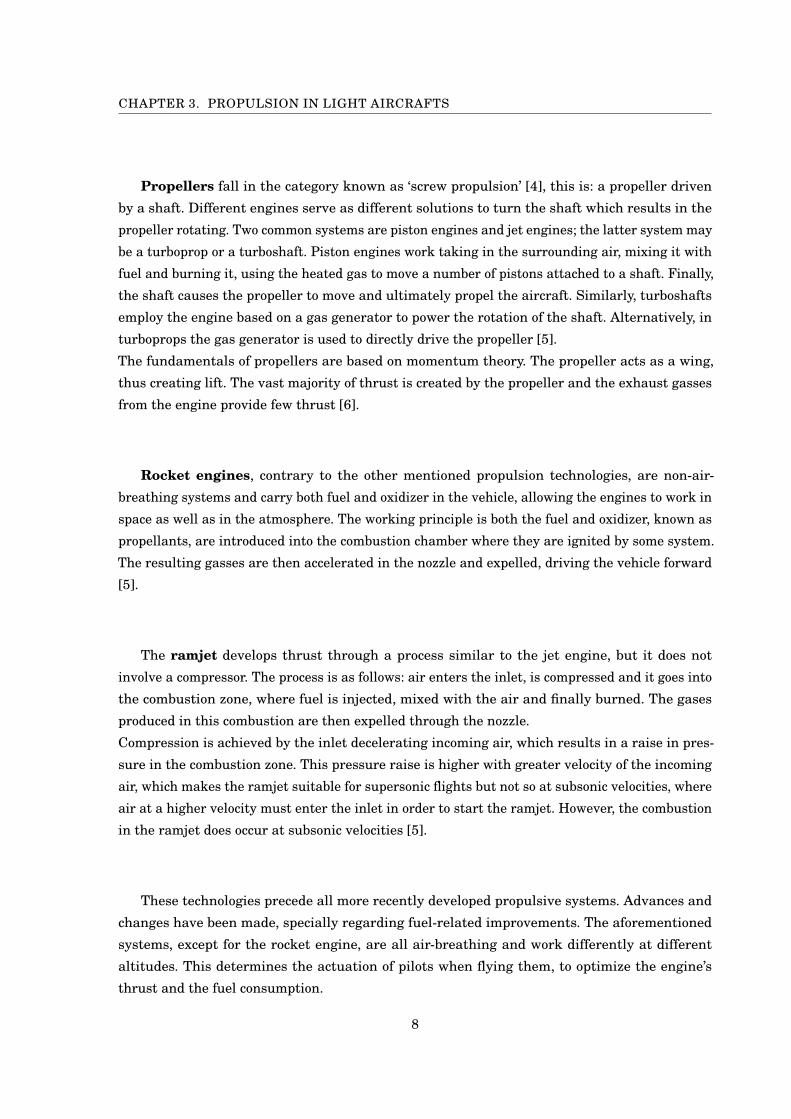
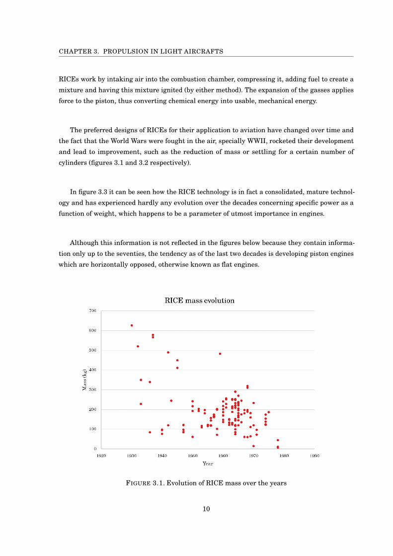
The preferred designs of RICEs for their application to aviation have changed over time and
the fact that the World Wars were fought in the air, specially WWII, rocketed their development
and lead to improvement, such as the reduction of mass or settling for a certain number of
cylinders (figures 3.1 and 3.2 respectively).
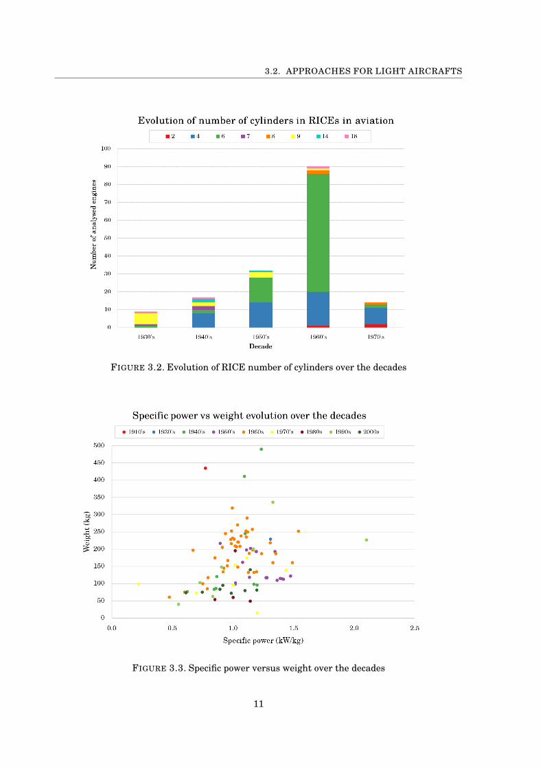
In figure 3.3 it can be seen how the RICE technology is in fact a consolidated, mature technol-
ogy and has experienced hardly any evolution over the decades concerning specific power as a
function of weight, which happens to be a parameter of utmost importance in engines.
Although this information is not reflected in the figures below because they contain informa-
tion only up to the seventies, the tendency as of the last two decades is developing piston engines
which are horizontally opposed, otherwise known as flat engines.
FIGURE 3.1. Evolution of RICE mass over the years
10
3.2. APPROACHES FOR LIGHT AIRCRAFTS
FIGURE 3.2. Evolution of RICE number of cylinders over the decades
FIGURE 3.3. Specific power versus weight over the decades
11
CHAPTER 3. PROPULSION IN LIGHT AIRCRAFTS
On the the topic of traditional means of powering electric aircraft, another technology is
worthy of mentioning: turboprops. The idea of this technology dates back to 1925, but it was
not until 1945 when the first turboprop aircraft flew [8]. This technology basically consists of
a turbojet which drives a shaft with a prop on its end. The turn of the shaft is achieved by the
energy supplied by the expansion of gas. On a side note, the advantages and disadvantages of
the turboprop are the same as for the propeller: speed is limited by compressibility effects at the
blade tips when approaching high velocities [5].
3.2.2 Modern - Electric
Despite being perceived as modern and innovative, electric propulsive motors date back to the
early nineteenth century, where examples of electric motors to power boats or cars can be found
as early as 1838 and 1851, respectively [11]. The development of electric motors was interrupted
because they were dependant on batteries which lacked the necessary energy supply to operate
at a sensible cost [11].
In opposition to internal combustion engines, electric motors convert electrical power into
magnetic power and finally into mechanical power. Hence, electromagnetism acquires utmost
importance in electric motor operation by generating the necessary magnetic forces to produce
motion, whether linear o rotational [12].
Given there are two types of current, direct (DC) and alternating (AC), the consequence
is there are two matching types of electric motors. Whilst there is a reduced number of DC
motor kinds, there exists a great amount of important AC motor types: synchronous, induction,
repulsion... [11]
The kind electric motor to be chosen for a propulsive task depends on a number of factors,
including vehicle limitations, energy source available and expectations such as acceleration,
maximum speed, etcetera [13].
The sort of motor being most widely used actually for light aircraft propulsion is permanent
magnet motor, which falls into the category of brushless motors; more specifically, permanent
magnet brushless DC motors are commonly being used. The main interest of this type of motor is
it allows to control speed and torque while being lightweight and having fewer moving parts [14].
Also, the popularity of the aforementioned kind of motors in propulsive applications is partly
because it is a mature technology and simple to control [13].
12
3.3. GENERAL REQUIREMENTS FOR PROPULSION
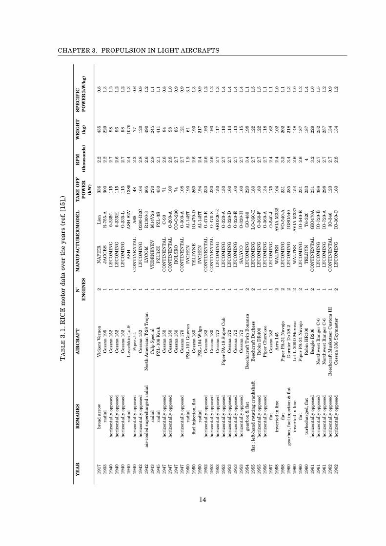
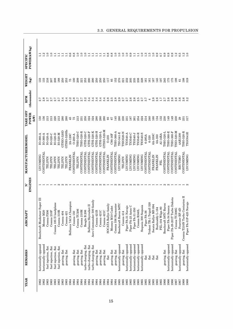
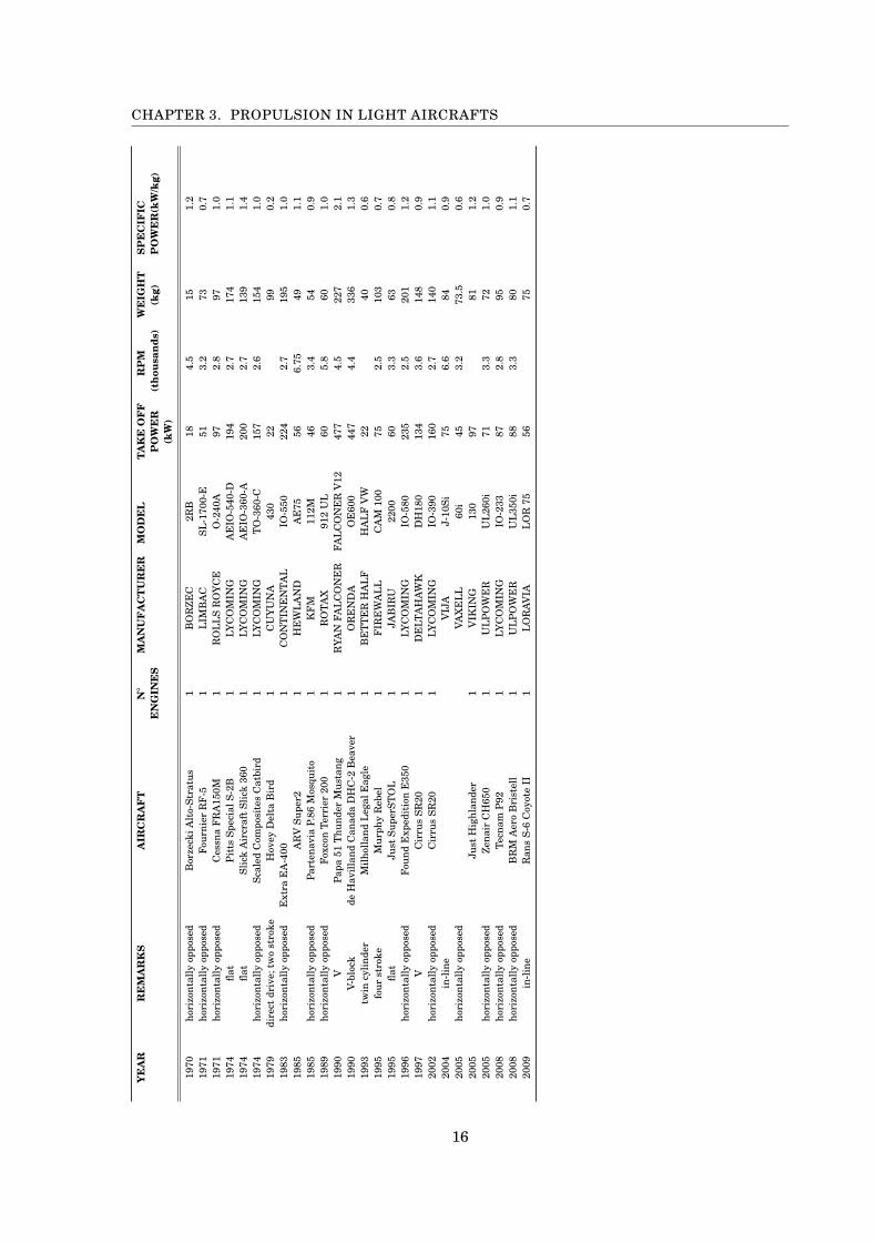
3.3 General requirements for propulsion
To understand what is required from a propulsion system to power light aircrafts, a table with
engine characteristics of a number of light aircrafts has been put together. Table 3.3 shows
relevant data from internal combustion engines and mentions some aircraft in which said engine
was applied. For the sake of comparison, on table 3.2 a collection of electric motor characteristics
was also put together, although because it is a comparison between a fairly old technology versus
a new one, the electric motor table is sparser.
It is easy to notice how the electric options have lower revolution speeds but are comparable
in terms of the specific power and even greater, in some cases, than the traditional reciprocating
engines.
13
CHAPTER 3. PROPULSION IN LIGHT AIRCRAFTS
TA
BL
E3.
1.R
ICE
mot
orda
taov
erth
eye
ars
(ref
.[15
],)
YE
AR
RE
MA
RK
SA
IRC
RA
FT
N
EN
GIN
ES
MA
NU
FA
CT
UR
ER
MO
DE
LTA
KE
OF
FP
OW
ER
(kW
)
RP
M(t
hous
ands
)W
EIG
HT
(kg)
SPE
CIF
ICP
OW
ER
(kW
/kg)
1917
broa
dar
row
Vic
kers
Ver
non
2N
AP
IER
Lio
n33
62.
243
50.
819
33ra
dial
Ces
sna
195
1JA
CO
BS
R-7
55-A
300
2.2
229
1.3
1940
hori
zont
ally
oppo
sed
Ces
sna
152
1LY
CO
MIN
G0-
235C
115
2.7
981.
219
40ho
rizo
ntal
lyop
pose
dC
essn
a15
21
LYC
OM
ING
0-23
5H11
52.
696
1.2
1940
hori
zont
ally
oppo
sed
Ces
sna
152
1LY
CO
MIN
GO
-235
-L11
52.
798
1.2
1940
radi
alL
avoc
hkin
La-
91
ASH
ASH
-82V
1380
2.4
1070
1.3
1940
hori
zont
ally
oppo
sed
Pip
erJ-
41
CO
NT
INE
NT
AL
A65
482.
377
0.6
1942
hori
zont
ally
oppo
sed
Ces
sna
152
1LY
CO
MIN
GO
290-
D2C
104
2.8
120
0.9
1942
air-
cool
edsu
perc
harg
edra
dial
Nor
thA
mer
ican
T-28
Tro
jan
1LY
CO
MR
1300
-360
52.
649
01.
219
43ra
dial
Cul
pSp
ecia
l1
VE
DE
NE
YE
VM
14V
2627
02.
824
51.
119
45ra
dial
PZL
-106
Kru
k1
PZL
RZE
PZL
-3S
450
2.1
411
1.1
1947
hori
zont
ally
oppo
sed
Ces
sna
150
1C
ON
TIN
EN
TA
LC
-90
712.
684
0.8
1947
hori
zont
ally
oppo
sed
Ces
sna
150
1C
ON
TIN
EN
TA
LO
-200
-A10
02.
898
1.0
1947
Ces
sna
150
1R
OL
SRO
CO
-O-2
0074
2.7
860.
919
47ho
rizo
ntal
lyop
pose
dC
essn
a17
01
CO
NT
INE
NT
AL
O-3
00-A
108
2.7
121
0.9
1950
radi
alP
ZL-1
01G
awro
n1
IVC
HE
NA
I-14
RT
190
1.9
613.
119
50fu
elin
ject
ion,
flat
Ces
sna
180
1T
EL
DY
NE
IO-4
70-D
260
2.6
193
1.3
1950
radi
alP
ZL-1
04W
ilga
1IV
CH
EN
AI-
14R
T19
42.
421
70.
919
52ho
rizo
ntal
lyop
pose
dC
essn
a18
21
CO
NT
INE
NT
AL
O-4
70-R
230
2.6
193
1.2
1952
hori
zont
ally
oppo
sed
Ces
sna
180
1C
ON
TIN
EN
TA
LO
-470
-S23
02.
619
31.
219
53ho
rizo
ntal
lyop
pose
dC
essn
a17
21
LYC
OM
ING
AE
O32
0-E
150
2.7
117
1.3
1953
hori
zont
ally
oppo
sed
Pip
erPA
-18
Supe
rC
ub1
LYC
OM
ING
O-3
20-A
150
2.7
110
1.4
1953
hori
zont
ally
oppo
sed
Ces
sna
172
1LY
CO
MIN
GO
-320
-D16
02.
711
41.
419
53ho
rizo
ntal
lyop
pose
dC
essn
a17
21
LYC
OM
ING
O-3
20-E
160
2.7
113
1.4
1953
hori
zont
ally
oppo
sed
Ces
sna
172
1SA
LYC
OO
-320
-H16
02.
711
51.
419
54ge
arbo
x&
flat
Bee
chac
raft
Tw
inB
onan
za2
LYC
OM
ING
GO
-480
220
3.4
198
1.1
1955
flat
;lef
t-ha
ndro
tati
ngcr
anks
haft
Bee
chcr
aft
Duc
hess
2LY
CO
MIN
GL
O-3
60-E
180
2.7
122
1.5
1955
hori
zont
ally
oppo
sed
Rob
inD
R40
01
LYC
OM
ING
O-3
60-F
180
2.7
122
1.5
1956
hori
zont
ally
oppo
sed
Pip
erC
hero
kee
1LY
CO
MIN
GO
-360
-A13
42.
711
81.
119
57fla
tC
essn
a18
21
LYC
OM
ING
O-5
40-J
175
2.4
162
1.1
1958
inve
rted
inlin
eA
ero
145
2W
ALT
ER
AV
IAM
332
104
2.4
102
1.0
1958
flat
Pip
erPA
-31
Nav
ajo
2LY
CO
MIN
GV
O-5
40-A
231
3.2
202
1.1
1960
gear
box,
fuel
inje
ctio
n&
flat
Dor
nier
Do
28-2
2LY
CO
MIN
GIG
SO54
028
53.
421
81.
319
60in
vert
edin
line
Let
L-2
00D
Mor
ava
2W
ALT
ER
AV
IAM
337
154
2.6
148
1.0
1960
flat
Pip
erPA
-31
Nav
ajo
2LY
CO
MIN
GIO
-540
-E23
12.
618
71.
219
60tu
rboc
harg
ed,fl
atR
obin
HR
100
1T
EL
DY
NT
6-32
025
34
187
1.4
1961
hori
zont
ally
oppo
sed
Bea
gle
B20
62
CO
NT
INE
NT
AL
GIO
470A
231
3.2
229
1.0
1961
hori
zont
ally
oppo
sed
Nor
thw
est
Ran
ger
C-6
1LY
CO
MIN
GIO
-720
-B38
82.
725
21.
519
61ho
rizo
ntal
lyop
pose
dN
orth
wes
tR
ange
rC
-61
LYC
OM
ING
IO-7
20-A
298
2.7
257
1.2
1962
hori
zont
ally
oppo
sed
Bee
chcr
aft
Mus
kete
erC
usto
mII
I1
CO
NT
INE
NT
AL
IO-3
4612
32.
713
40.
919
62ho
rizo
ntal
lyop
pose
dC
essn
a33
6Sk
ymas
ter
2LY
CO
MIN
GIO
-360
-C16
02.
813
41.
2
14
3.3. GENERAL REQUIREMENTS FOR PROPULSIONY
EA
RR
EM
AR
KS
AIR
CR
AF
TN
EN
GIN
ES
MA
NU
FA
CT
UR
ER
MO
DE
LTA
KE
OF
FP
OW
ER
(kW
)
RP
M(t
hous
ands
)W
EIG
HT
(kg)
SPE
CIF
ICP
OW
ER
(kW
/kg)
1962
hori
zont
ally
oppo
sed
Bee
chcr
aft
Mus
kete
erSu
per
III
1LY
CO
MIN
GIO
-360
-A15
02.
713
31.
119
62ho
rizo
ntal
lyop
pose
dM
oone
yM
201
CO
NT
INE
NT
AL
IO-3
60-A
156
2.8
133
1.2
1963
fuel
inje
ctio
n,fla
tC
essn
aP
206
1T
EL
DY
NIO
-520
-A21
32.
721
61.
019
63fu
elin
ject
ion,
flat
Ces
sna
210F
1T
EL
DY
NIO
-520
-C21
32.
720
71.
019
63fu
elin
ject
ion,
flat
Ces
sna
185
IIla
ndpl
ane
1T
EL
DY
NIO
-520
-D22
02.
720
81.
119
63fu
elin
ject
ion,
flat
Ces
sna
310R
2T
EL
DY
NIO
-520
-M21
32.
718
81.
119
63ge
arin
g,fla
tC
essn
a40
42
TE
LD
YN
GT
SIO
-520
D28
03.
425
01.
119
63ge
arin
g,fla
tC
essn
a42
12
TE
LD
YN
GT
SIO
-520
Hs
280
3.4
253
1.1
1964
Bel
lanc
a7A
CA
Cha
mpi
on1
FR
AN
KL
IN2A
-120
C45
3.2
750.
619
64ge
arin
g,fla
tC
essn
a15
01
CO
NT
INE
NT
AL
O-2
00-A
752.
810
00.
819
64ge
arin
g,fla
tC
essn
aT
U20
61
TE
LD
YN
TSI
O-5
20-C
213
2.7
209
1.0
1964
gear
ing,
flat
Ces
sna
210M
1C
ON
TIN
EN
TA
LT
SIO
-520
-R23
12.
722
11.
019
64tu
rbo-
char
ging
,flat
Bea
gle
B.2
062
CO
NT
INE
NT
AL
GT
SI-5
20-C
250
3.2
253
1.0
1964
turb
o-ch
argi
ng,fl
atB
ella
nca
Skyr
ocke
tII
1C
ON
TIN
EN
TA
LG
TSI
-520
-F32
43.
429
01.
119
64tu
rbo-
char
ging
,flat
Aer
oC
omm
ande
r50
0fa
mily
2C
ON
TIN
EN
TA
LG
TSI
-520
-K32
43.
429
01.
119
64ge
arin
g,fla
tC
essn
a42
1B2
CO
NT
INE
NT
AL
GT
SI-5
20-H
280
3.4
250
1.1
1964
gear
ing,
flat
Ces
sna
421C
2C
ON
TIN
EN
TA
LG
TSI
-520
-L28
03.
425
01.
119
64ge
arin
g,fla
tC
essn
a42
1C2
CO
NT
INE
NT
AL
GT
SIO
-520
-M28
03.
425
01.
119
64fla
tSO
CA
TA
Ral
lye
fam
ily1
FR
AN
KL
INO
-235
932.
811
70.
819
64ge
arin
g,fla
tM
oone
yM
10C
adet
1C
ON
TIN
EN
TA
LC
90-1
6F67
2.5
850.
819
64ge
arin
g,fla
tC
essn
a33
6Sk
ymas
ter
2C
ON
TIN
EN
TA
LT
SIO
-360
-A14
52.
815
21.
019
65ho
rizo
ntal
lyop
pose
dB
eech
craf
tB
aron
56T
C2
LYC
OM
ING
TIO
-541
-E28
02.
927
01.
019
65ge
arin
g,fla
tC
essn
a41
42
TE
LD
YN
TSI
O52
0-N
230
2.7
221
1.0
1965
hori
zont
ally
oppo
sed
Pip
erPA
-31
Nav
ajo
2LY
CO
MIN
GT
IO54
0-A
231
2.7
232
1.0
1965
hori
zont
ally
oppo
sed
Pip
erPA
-23
Azt
ecC
2LY
CO
MIN
GT
IO54
0-C
187
2.6
205
0.9
1965
hori
zont
ally
oppo
sed
Pip
erPA
-31-
350
2LY
CO
MIN
GT
IO54
0-J
261
2.6
235
1.1
1965
hori
zont
ally
oppo
sed
Ces
sna
R34
0L2
LYC
OM
ING
TIO
540-
R25
42.
523
81.
119
65ho
rizo
ntal
lyop
pose
dSe
quoi
a30
0Se
quoi
a1
LYC
OM
ING
TIO
540-
S22
42.
722
81.
019
65fla
tP
iper
PA-3
61
CO
NT
INE
NT
AL
6-28
5A21
43.
716
11.
319
65fla
tT
ride
ntT
R-1
Tri
gull
320
1C
ON
TIN
EN
TA
L6-
320
240
416
11.
519
65fla
tSo
cata
Ral
lye
MS
894
1F
RA
NK
LIN
6A-3
50C
160
2.8
167
1.0
1965
flat
Bus
hcad
dyL
-164
1F
RA
NK
LIN
6A-3
5013
42.
814
50.
919
65P
ZL-1
04W
ilga
801
PZL
AI-
14R
A13
21.
719
70.
719
66ge
arin
g,fla
tB
eech
craf
t58
TC
Bar
on2
CO
NT
INE
NT
AL
TSI
O-5
20-L
230
2.7
245
0.9
1966
hori
zont
ally
oppo
sed
Pip
erPA
-34
Sene
ca2
CO
NT
INE
NT
AL
TSI
O-3
60-E
149
2.6
175
0.9
1966
hori
zont
ally
oppo
sed
Pip
erPA
-28-
201T
Tur
boD
akot
a1
CO
NT
INE
NT
AL
TSI
O-3
60-F
149
2.6
175
0.9
1967
gear
ing,
flat
Ces
sna
TU
206G
1C
ON
TIN
EN
TA
LT
SIO
-520
-M23
02.
619
81.
219
67ho
rizo
ntal
lyop
pose
dFo
urni
erR
F-4
D1
RE
CT
IMO
4AR
1200
293.
661
0.5
1968
gear
ing,
flat
Ces
sna
T21
0NT
urbo
Cen
turi
onII
1C
ON
TIN
EN
TA
LT
SIO
-520
-R23
12.
619
81.
219
68ho
rizo
ntal
lyop
pose
dP
iper
PA-3
1P-4
25N
avaj
o2
LYC
OM
ING
TIG
O54
1E31
73.
231
91.
0
15
CHAPTER 3. PROPULSION IN LIGHT AIRCRAFTS
YE
AR
RE
MA
RK
SA
IRC
RA
FT
N
EN
GIN
ES
MA
NU
FA
CT
UR
ER
MO
DE
LTA
KE
OF
FP
OW
ER
(kW
)
RP
M(t
hous
ands
)W
EIG
HT
(kg)
SPE
CIF
ICP
OW
ER
(kW
/kg)
1970
hori
zont
ally
oppo
sed
Bor
zeck
iAlt
o-St
ratu
s1
BO
RZE
C2R
B18
4.5
151.
219
71ho
rizo
ntal
lyop
pose
dFo
urni
erR
F-5
1L
IMB
AC
SL-1
700-
E51
3.2
730.
719
71ho
rizo
ntal
lyop
pose
dC
essn
aF
RA
150M
1R
OL
LS
RO
YC
EO
-240
A97
2.8
971.
019
74fla
tP
itts
Spec
ialS
-2B
1LY
CO
MIN
GA
EIO
-540
-D19
42.
717
41.
119
74fla
tSl
ick
Air
craf
tSl
ick
360
1LY
CO
MIN
GA
EIO
-360
-A20
02.
713
91.
419
74ho
rizo
ntal
lyop
pose
dSc
aled
Com
posi
tes
Cat
bird
1LY
CO
MIN
GT
O-3
60-C
157
2.6
154
1.0
1979
dire
ctdr
ive;
two
stro
keH
ovey
Del
taB
ird
1C
UY
UN
A43
022
990.
219
83ho
rizo
ntal
lyop
pose
dE
xtra
EA
-400
1C
ON
TIN
EN
TA
LIO
-550
224
2.7
195
1.0
1985
AR
VSu
per2
1H
EW
LA
ND
AE
7556
6.75
491.
119
85ho
rizo
ntal
lyop
pose
dPa
rten
avia
P.86
Mos
quit
o1
KF
M11
2M46
3.4
540.
919
89ho
rizo
ntal
lyop
pose
dFo
xcon
Terr
ier
200
1R
OT
AX
912
UL
605.
860
1.0
1990
VPa
pa51
Thu
nder
Mus
tang
1R
YAN
FAL
CO
NE
RFA
LC
ON
ER
V12
477
4.5
227
2.1
1990
V-bl
ock
deH
avill
and
Can
ada
DH
C-2
Bea
ver
1O
RE
ND
AO
E60
044
74.
433
61.
319
93tw
incy
linde
rM
ilhol
land
Leg
alE
agle
1B
ET
TE
RH
AL
FH
AL
FV
W22
400.
619
95fo
urst
roke
Mur
phy
Reb
el1
FIR
EW
AL
LC
AM
100
752.
510
30.
719
95fla
tJu
stSu
perS
TO
L1
JAB
IRU
2200
603.
363
0.8
1996
hori
zont
ally
oppo
sed
Foun
dE
xped
itio
nE
350
1LY
CO
MIN
GIO
-580
235
2.5
201
1.2
1997
VC
irru
sSR
201
DE
LTA
HA
WK
DH
180
134
3.6
148
0.9
2002
hori
zont
ally
oppo
sed
Cir
rus
SR20
1LY
CO
MIN
GIO
-390
160
2.7
140
1.1
2004
in-l
ine
VIJ
AJ-
10Si
756.
684
0.9
2005
hori
zont
ally
oppo
sed
VA
XE
LL
60i
453.
273
.50.
620
05Ju
stH
ighl
ande
r1
VIK
ING
130
9781
1.2
2005
hori
zont
ally
oppo
sed
Zena
irC
H65
01
UL
PO
WE
RU
L26
0i71
3.3
721.
020
08ho
rizo
ntal
lyop
pose
dTe
cnam
P92
1LY
CO
MIN
GIO
-233
872.
895
0.9
2008
hori
zont
ally
oppo
sed
BR
MA
ero
Bri
stel
l1
UL
PO
WE
RU
L35
0i88
3.3
801.
120
09in
-lin
eR
ans
S-6
Coy
ote
II1
LO
RA
VIA
LO
R75
5675
0.7
16
3.4. ELECTRIC AIRCRAFTS
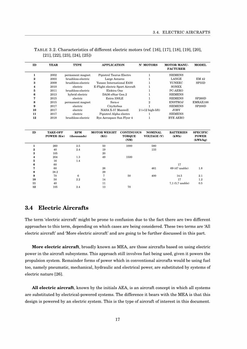
TABLE 3.2. Characteristics of different electric motors (ref. [16], [17], [18], [19], [20],[21], [22], [23], [24], [25])
ID YEAR TYPE APPLICATION N MOTORS MOTOR MANU-FACTURER
MODEL
1 2002 permanent magnet Pipistrel Taurus Electro 1 SIEMENS2 2003 brushless-electric Large Antares 1 LANGE EM 423 2009 brushless-electric Yuneec International E430 1 YUNEEC SP55D4 2010 electric E-Flight electric Sport Aircraft 1 SONEX5 2011 brushless-electric Elektra One 1 PC-AERO6 2013 hybrid electric DA36 eStar Gen.2 1 SIEMENS7 2015 electric Extra 330LE 1 SIEMENS SP260D8 2015 permanent magnet Sora-e 2 ENSTROJ EMRAX1889 2017 electric CityAirbus 1 SIEMENS SP200D
10 2017 electric NASA X-57 Maxwell 2 (+12 high-lift) JOBY11 2017 electric Pipistrel Alpha electro 1 SIEMENS12 2018 brushless-electric Bye Aerospace Sun Flyer 4 1 BYE AERO
ID TAKE-OFFPOWER (Kw)
RPM(thousands)
MOTOR WEIGHT(KG)
CONTINUOUSTORQUE
(NM)
NOMINALVOLTAGE (V)
BATTERIES(kWh)
SPECIFICPOWER(kWh/kg)
1 260 2.5 50 1000 5802 40 2.4 19 1333 105 204 204 1.3 49 15005 16 1.46 60 177 60 26 461 69 (47 usable) 1.88 38.2 299 70 6 7 50 400 14.5 2.1
10 50 2.2 14 17 1.211 40 11 7,1 (5,7 usable) 0.512 105 2.4 13 70
3.4 Electric Aircrafts
The term ‘electric aircraft’ might be prone to confusion due to the fact there are two different
approaches to this term, depending on which cases are being considered. These two terms are ‘All
electric aircraft’ and ‘More electric aircraft’ and are going to be further discussed in this part.
More electric aircraft, broadly known as MEA, are those aircrafts based on using electric
power in the aircraft subsystems. This approach still involves fuel being used, given it powers the
propulsion system. Remainder forms of power which in conventional aircrafts would be using fuel
too, namely pneumatic, mechanical, hydraulic and electrical power, are substituted by systems of
electric nature [26].
All electric aircraft, known by the initials AEA, is an aircraft concept in which all systems
are substituted by electrical-powered systems. The difference it bears with the MEA is that this
design is powered by an electric system. This is the type of aircraft of interest in this document.
17
CHAPTER 3. PROPULSION IN LIGHT AIRCRAFTS
The problematic of these systems arises from the fact the flight safety characteristics still
have to be met. However, the electric aircraft has been proven to present advantages such as
reducing the empty weight of commercial aircrafts by about 10% [27]. In the case of MEA, where
propulsion is still based on fuels, a reduction of similar magnitude in specific fuel consumption
(SFC) has also been proved, among other conveniences [28].
In electric aircrafts, it is noticeable the majority of the electrical system’s weight are electric
cables, generators and motors and even though the losses due to Joule’s law in electrical cables
are smaller than the losses of traditional systems, said energy waste still limits the electrical
system [29] .
3.4.1 Electric Motors for propulsion
Whether or not the electric motors are for airborne applications, there are seven general properties
common to all of this kind of motors [30]:
1. The output of a motor is mostly determined by the cooling arrangement
2. The rated torque is toughly proportional to the rotor volume in motors with comparable
cooling systems
3. Speed is directly proportional to output power per unit volume
4. Large motors have a higher specific torque and are also more efficient than small motors
5. Motor efficiency improves with speed
6. Any voltage may suit a motor without affecting its performance
7. Overloading for short periods of time will not damage most motors
In the case of electric aircrafts, the type of propulsive motor being currently developed for
most prototypes is the permanent magnet motor. They are designed to be specially lightweight
and in many cases are brushless DC motors, which is just another way of saying permanent
magnet excited synchronous motors [13].
The most basic configuration for a brushless DC motor is a triphasic stator winding with
permanent magnets attached to the rotor. The position of the rotor is controlled by transducers
which inform the electronic controller. The controller shifts the DC voltage in the stator windings
and causes the rotor to turn [14]. The magnets used in this kind of motors are usually an alloy of
aluminium, nickel and copper, being known as Alnico alloys, due to their high suitability for the
purpose [31].
18
3.4. ELECTRIC AIRCRAFTS
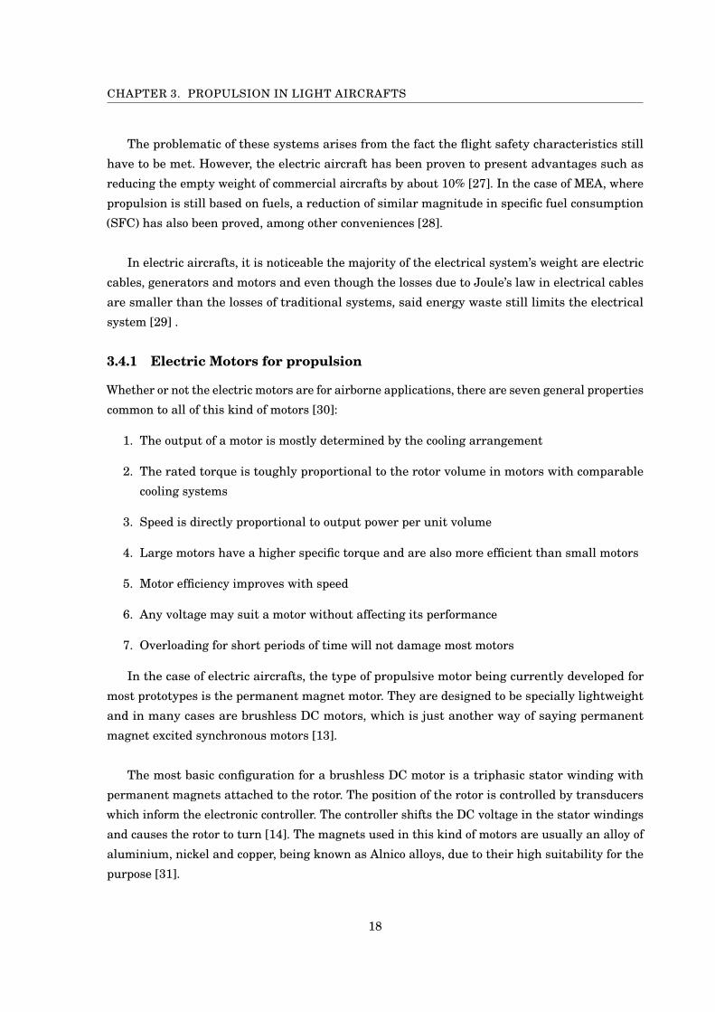
The distribution of the magnets is of great importance to avoid unwanted effects, such as
torque ripple. The Halbach array is an arrangement which combines one radial magnet array
and one azimuthal magnet array. This arrangement focuses the flux to the desired direction and
allows reaching a higher magnetic potential [32]. Implementing a Halbach array to the rotor has
been confirmed to deliver high torque density, better stability [33] and reducing torque ripple due
to near-perfect sinusoidal field distribution [32].
FIGURE 3.4. Halbach magnet array rotor flux distribution (Image from [32])
One of the attractions of brushless motors is they erase the need for rotating contacts and
thus do not have the problems linked to them, such as wearing [14] and because there is no
current circulation in the rotor it does not heat up [13]. To increase reliability and performance,
motors with higher number of phases may be used [34]. However, this involves increasing the
complexity of the motor, which might not be desirable.
3.4.2 Energy supply and storage
Nowadays, three main approaches are considered in electric aircrafts when it comes to energy
supply: either batteries, fuel cells or solar panels.Because the lower power density of the latter
compromise the maximum achievable speed of the aircraft [35] to the present day, manufacturers
do not opt for them, although some projects with solar panels such as Solar Impulse 2 or Sun-
seeker have proven to solar panels to be a feasible technology [36] , [37]. Fuel cells, contrary to
solar panels, resemble batteries but store the fluid outside the battery. Some prototypes such
as SkySpark and ENFICA-FC have flown, but the technology of fuel cells is still not a common
19
CHAPTER 3. PROPULSION IN LIGHT AIRCRAFTS
choice for manufacturers [38], [39].
Focusing on batteries, batteries are devices which transform chemical energy into electrical
energy and vice-versa, depending on whether charging or discharging. The most extended in
use for electrical vehicle applications are Li-ion, given it has been proven to display high energy
density and efficiency when compared to other types of batteries [40] [41]. For airborne propulsion
systems, high energy density batteries are required and lithium based batteries present this
advantage as well as low weight and low cost [31].
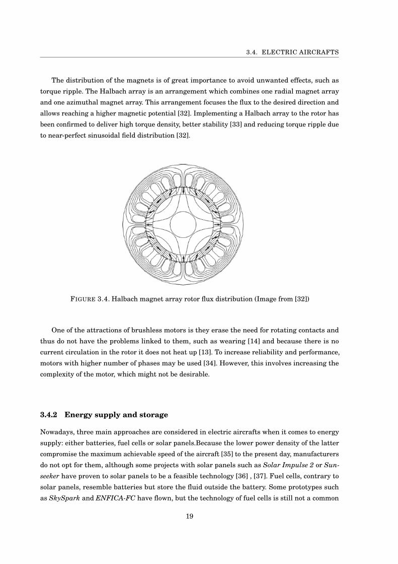
To the present day, the truth is the specific energy of Li-io batteries is nothing comparable to
that of aviation gasoline, as can be observed in table 3.3. Even to the best of their performance,
Li-io batteries of present-day technology are only theoretically capable of reaching 387 Whkg [42].
TABLE 3.3. Comparison of specific energy of aviation gasoline and Li-io batteries (refs.[43], [44], [45], [42], [46])
Energy content
MJ/kg KWh/kg
Aviation gasoline43.7 12.146.4 12.943.5 12.1
Li-io batteries0.36-0.54 0.1-0.15
0.36-0.569 0.1-0.158
This compromises the possible applications of electric light aircrafts to missions where great
autonomy is needed. Because the total energy available on the aircraft will depend on the battery
weight, it is in some cases possible to renounce some payload weight to incorporate more batteries,
thus increasing autonomy
3.4.3 Safety considerations and redundancy
Aircrafts are subject to very strict regulations regarding safety and electric aircrafts are no
exception. Introducing electric propulsion systems introduce new hazards which have to be taken
into account and minimized.
When using brushless DC motors, the main faults that can occur in the machine are short-
circuit due to insulation failure and open-circuit of a winding [34]. For a motor that can continue
to be operative after suffering any of these faults, the motor must necessarily follow a modular
approach treating each phase as a separate module, assuring complete electrical isolation be-
20

3.4. ELECTRIC AIRCRAFTS
tween phases [34].
To assure no malfunctioning will impede the motor to work correctly, two redundant wiring
systems are applied to some prototypes as well as redundant control systems [47]
When implementing brushless motors, given there was a wreck, the motor could still be
excited by its magnets and be dangerous to people nearby due to its high voltage difference in the
terminals [13].
21

CH
AP
TE
R
4SIMULATION ENVIRONMENT AND APPROACH
This chapter presents the model developed by Mathworks on which the whole simulation is
based. The parts other than propulsion system and pilot control are left mostly untouched,
meaning nothing about the aircraft design and functioning will be altered at a big scale.
The modifications performed to the model are closely related to the fact light aircrafts have the
possibility of being adapted to be propelled by electric systems even though they might have
originally been powered by fossil fuel engines.
4.1 Simulink Light Aircraft Model
MATLAB® provides a broad set of utilities related to Aerospace Engineering in its toolbox
‘Aerospace toolbox’. Contained in this package, a complete model of a light aircraft can be found
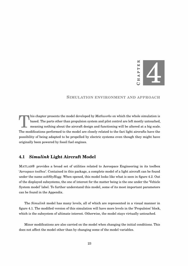
under the name asbSkyHogg. When opened, this model looks like what is seen in figure 4.2. Out
of the displayed subsystems, the one of interest for the matter being is the one under the ‘Vehicle
System model’ label. To further understand this model, some of its most important parameters
can be found in the Appendix.
The Simulink model has many levels, all of which are represented in a visual manner in
figure 4.1. The modified version of this simulation will have more levels in the ‘Propulsion’ block,
which is the subsystem of ultimate interest. Otherwise, the model stays virtually untouched.
Minor modifications are also carried on the model when changing the initial conditions. This
does not affect the model other than by changing some of the model variables.
23

CHAPTER 4. SIMULATION ENVIRONMENT AND APPROACH
Light Aircraft(SkyHogg)
Visualization
Environment
Terrain
Wind Models
Atmospheremodel
Gravitymodel
Vehicle Sys-tem Model
Avionics
Three-axis IMU
Air DataComputer
GuidanceAutopilot
FlightSensors
Vehicle
AirframeActuators
Aerodynamics
3DOF to6DOF
Propulsion
Pilot
FIGURE 4.1. Diagram of the asbSkyHogg Simulink model
24
4.1. SIMULINK LIGHT AIRCRAFT MODEL
FIGURE 4.2. View of the light aircraft model asbSkyHogg in Simulink
4.1.1 Environment
This system contains all necessary information about the surroundings of the aircraft in the
situation in which the simulation will take place. It includes information about the terrain
elevation and shape, the wind behaviour at the specified altitude and it also uses the WGS84
geoid model to define the gravity at the specified coordinates at which the aircraft is situated.
Other than this, the block also includes an atmosphere model to compute the outside temperature,
pressure, air density and speed of sound. The atmosphere model being used in this particular
simulation is the COESA atmosphere model.
4.1.2 Pilot
It is in this block where any human actions that were to be applied to the aircraft to control its
behaviour.
This block has the capability to control the actuators (elevator, rudder and aileron) manually, but
as it will be explained in the paragraphs following, the model does not make it strictly necessary
to control the elevator by hand because it is the autopilot who is in charge of doing so. For this
reason, the inputs for all three actuators are set to zero. On the other hand, this block allows to
control the throttle applied to the motor. For the sake of simplicity, it is set as a constant value
throughout the simulation for the totality of this project.
The final part one is able to control in this system is the altitude command. This is: one is able to
describe the desired vertical movement for the aircraft and the autopilot will follow it closely. The
command is defined as a step, but for the comfort of those who would be flying on the SkyHogg,
the vertical profile of the ascent is of 500 meters every 3 minutes.
25
CHAPTER 4. SIMULATION ENVIRONMENT AND APPROACH
4.1.3 Vehicle System Model
This system contains the totality of the information regarding the vehicle functioning and
geometry. If the aircraft model was to be changed, it is this block which should be modified to
include the essential information which differentiates the functioning of one aircraft to another.
This information can be broken down into three main categories, which happen to be the three
subsystems which the ‘Vehicle System Model’ contains: avionics, vehicle and flight sensors.
4.1.3.1 Avionics
It is inside this block where the Inertial Measurement Unit, indispensable tool to further calculate
the aircraft dynamics, is set. It also includes the air data computer, which takes information from
the aircraft sensors, and the guidance system. The latter combines the information provided by
the other two with the pilot’s commands in order to create a reference signal, in this case for
altitude, which will be of utmost importance in the last block inside this subsystem: the autopilot
block. This block takes the outputs of all three previous blocks (IMU, air data computer and
guidance) as input data. As a result of longitudinal controller which aims to follow the altitude
reference signal created in the ‘Guidance’ subsystem, this autopilot controls the elevator in an
automated way to demand the aircraft to follow the reference as closely as possible.
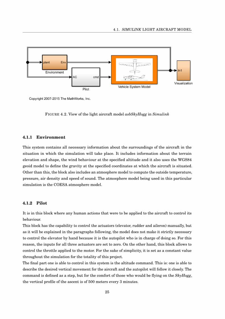
The actual appearance of said ‘Autopilot’ controller is shown in figure 4.3. It is important to note
the controller was tuned for the initial conditions which were predefined for the model and thus
it works best at these conditions.
FIGURE 4.3. Default Autopilot block in asbSkyHogg which controls the elevator position
4.1.3.2 Flight Sensors
This system takes the data from the environment and the aircraft plant conditions (such as
aircraft velocity) and passes it as input to some blocks which act as aircraft sensors, such as Pitot
tubes. It is considerable part of this subsystem remains incomplete and performs no action upon
26
4.1. SIMULINK LIGHT AIRCRAFT MODEL
the input data. It was done this way by the MathWorks developers whom left the transducer and
noise models for its development later on, as it is stated in an annotation inside both blocks.
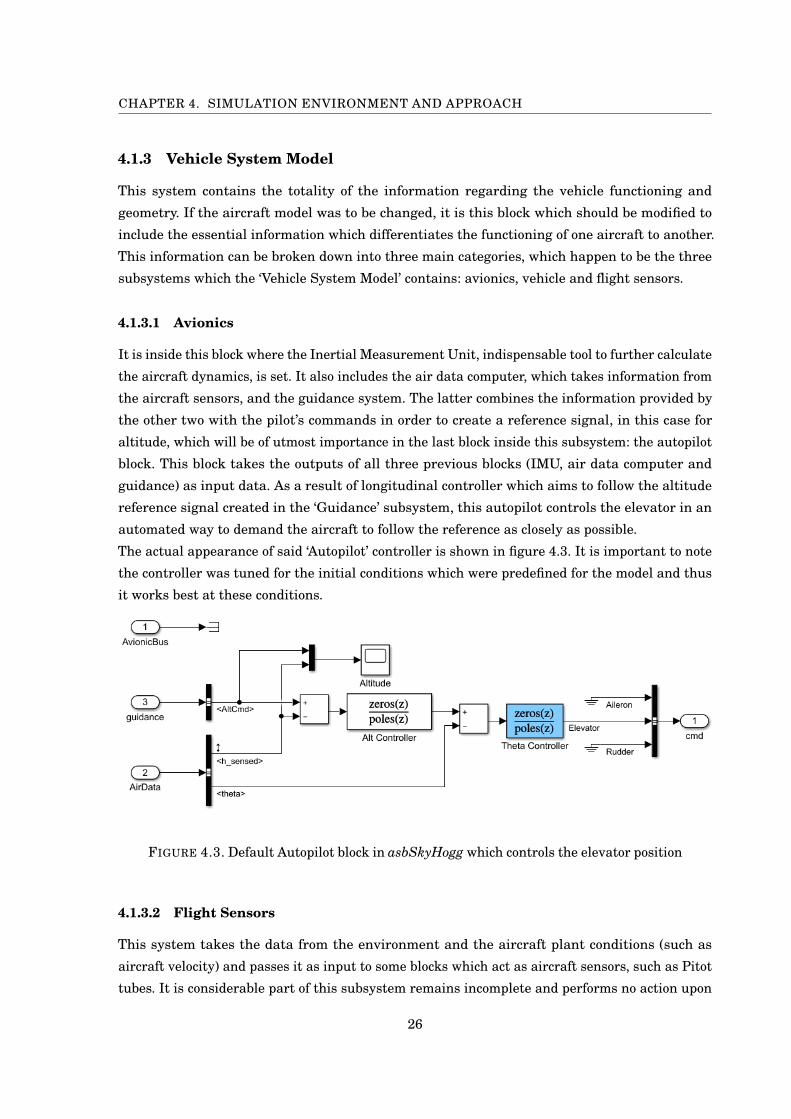
4.1.3.3 Vehicle
This block will be the one suffering modifications throughout this project, as it contains the
propulsion subsystem. The interior of this block is, untouched, what can be seen in figure 4.5. Its
most important component is an input, cmd, coming from the ‘Pilot’ system, which directs the
amount of throttle applied. This throttle leads to a corresponding thrust which is extracted in
the ThrustX block. This thrust is part of the output of the propulsion subsystem, along with the
thrust in Y and Z axes (null thrust) and moments in all three axes (again, null).
Besides the propulsion block, this system also contains other necessary components which
describe the vehicle. The ‘Airframe Actuators’ block uses as input data the information provided
by the ‘Autopilot’ and transmits to the aileron, rudder and elevator the demanded position
commands. The ‘Aerodynamics’ block then uses the data outputted from the ‘Airframes Actuators’
block, alongside with environmental and plant data, to compute the wind in different axes an the
forces and moments being produced by the actuators.
As it is known, the resultant forces and moments on a body are the sum of the forces and moments
acting on said body. The outputs of the ‘Aerodynamics’ and ‘Propulsion’ block are condensed into a
single total force and total moment for the aircraft, which serves as input for the ‘3DOF to 6DOF’
block, that then uses mechanical equations to extract all variables of interest for the aircraft,
namely velocity, longitudinal rotation speed, or body angles.
FIGURE 4.4. View of the Vehicle block in asbSkyHogg with the propulsion block in blue
27
CHAPTER 4. SIMULATION ENVIRONMENT AND APPROACH
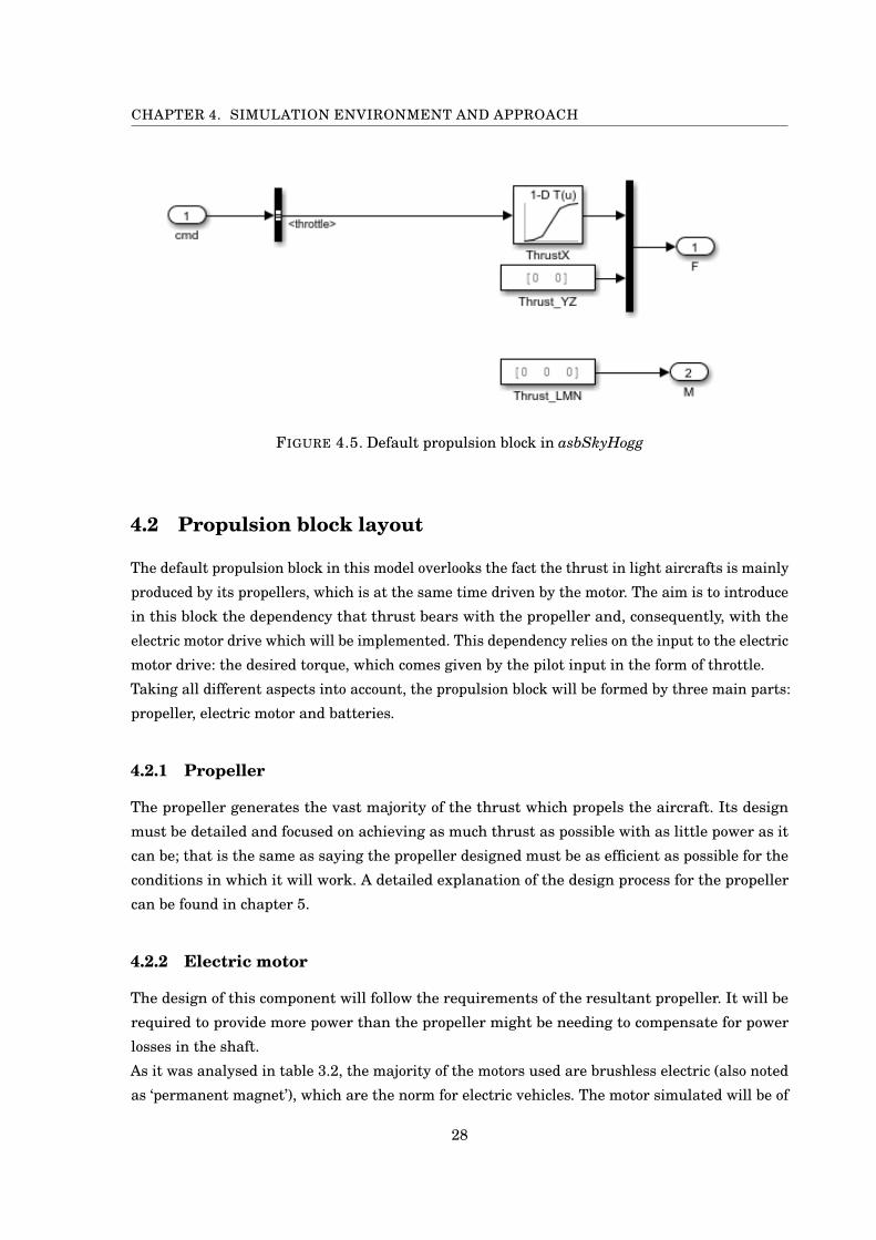
FIGURE 4.5. Default propulsion block in asbSkyHogg
4.2 Propulsion block layout
The default propulsion block in this model overlooks the fact the thrust in light aircrafts is mainly
produced by its propellers, which is at the same time driven by the motor. The aim is to introduce
in this block the dependency that thrust bears with the propeller and, consequently, with the
electric motor drive which will be implemented. This dependency relies on the input to the electric
motor drive: the desired torque, which comes given by the pilot input in the form of throttle.
Taking all different aspects into account, the propulsion block will be formed by three main parts:
propeller, electric motor and batteries.
4.2.1 Propeller
The propeller generates the vast majority of the thrust which propels the aircraft. Its design
must be detailed and focused on achieving as much thrust as possible with as little power as it
can be; that is the same as saying the propeller designed must be as efficient as possible for the
conditions in which it will work. A detailed explanation of the design process for the propeller
can be found in chapter 5.
4.2.2 Electric motor
The design of this component will follow the requirements of the resultant propeller. It will be
required to provide more power than the propeller might be needing to compensate for power
losses in the shaft.
As it was analysed in table 3.2, the majority of the motors used are brushless electric (also noted
as ‘permanent magnet’), which are the norm for electric vehicles. The motor simulated will be of
28
4.2. PROPULSION BLOCK LAYOUT
these characteristics and furthermore will be AC.
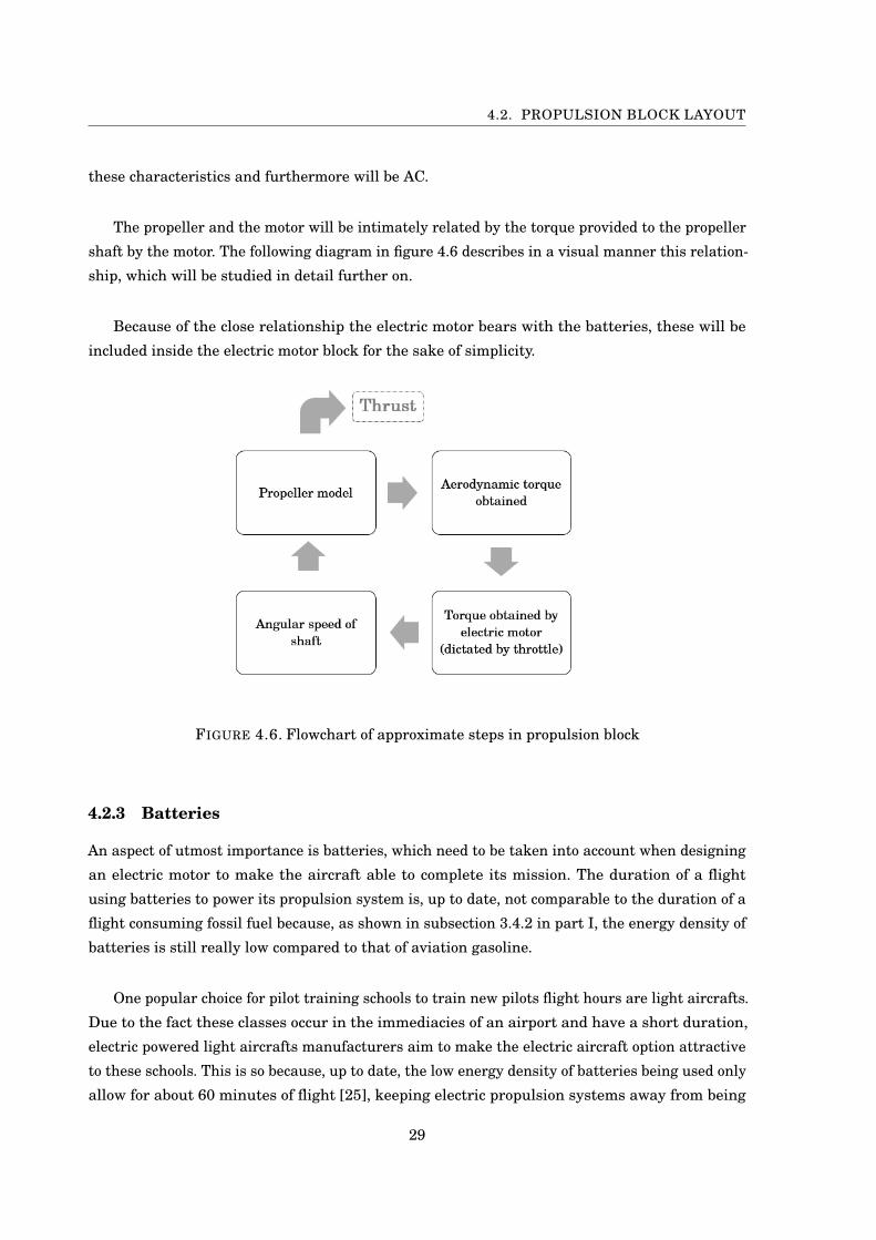
The propeller and the motor will be intimately related by the torque provided to the propeller
shaft by the motor. The following diagram in figure 4.6 describes in a visual manner this relation-
ship, which will be studied in detail further on.
Because of the close relationship the electric motor bears with the batteries, these will be
included inside the electric motor block for the sake of simplicity.
FIGURE 4.6. Flowchart of approximate steps in propulsion block
4.2.3 Batteries
An aspect of utmost importance is batteries, which need to be taken into account when designing
an electric motor to make the aircraft able to complete its mission. The duration of a flight
using batteries to power its propulsion system is, up to date, not comparable to the duration of a
flight consuming fossil fuel because, as shown in subsection 3.4.2 in part I, the energy density of
batteries is still really low compared to that of aviation gasoline.
One popular choice for pilot training schools to train new pilots flight hours are light aircrafts.
Due to the fact these classes occur in the immediacies of an airport and have a short duration,
electric powered light aircrafts manufacturers aim to make the electric aircraft option attractive
to these schools. This is so because, up to date, the low energy density of batteries being used only
allow for about 60 minutes of flight [25], keeping electric propulsion systems away from being
29

CHAPTER 4. SIMULATION ENVIRONMENT AND APPROACH
ubiquitous and applied all types of missions.
A crucial thing to take into account when considering batteries is the weight they add to
the aircraft. While the electric motor actually helps bringing down the total gross weight of the
aircraft, it is the batteries which make it skyrocket. The autonomy of the aircraft will be greatly
limited by the fact there is only a certain amount of battery weight it can carry. A parameter
to be considered when choosing the batteries must be their energy density, as for, as the name
indicates, a bigger energy density will allow a grater energy for the same weight. The matter of
choosing the right batteries is addressed further on in the document.
30
CH
AP
TE
R
5PROPELLER DESIGN AND IMPLEMENTATION
As it has been said, the propeller accounts for the majority of the thrust produced in a
light aircraft. For this reason, its design must be carried out in a careful way and bearing
in mind the characteristics of the SkyHogg and the requirements for the mission.
In this section, the design of the propeller in the program JavaProp, created by Martin Hepperle
and available on-line [48], is described, along with the analysis of the needs of the aircraft and,
ultimately, its limitations.
5.1 Design of a propeller with JavaProp
JavaProp is an inestimably useful tool when it comes to designing propeller blades. It offers a
considerable number of possibilities and configurations for detailed designs. Nevertheless, there
exist some limitations when it comes to employing this application. The way in which this applet
carries out its calculations is based on the blade element theory, working by dividing the propeller
blades into smaller sections. This has the advantage of simplicity and rapidness, although it
implies some downsides and limitations. Quoting the author: "The theory makes no provision for
three dimensional effects, like sweep angle or cross flow. But it is able to find the additional axial
and circumferential velocity added to the incoming flow by each blade segment. This additional
velocity results in an acceleration of the flow and thus thrust. Usually this simplified model works
very well, when the power and thrust loading of the propeller (power per disk area) are relatively
small, as it is the case for most aircraft propellers [48]".
Limitations were acknowledged during the whole process and are commented when necessary,
although as the author stated, mostly the limitations do not have a great influence because of the
31
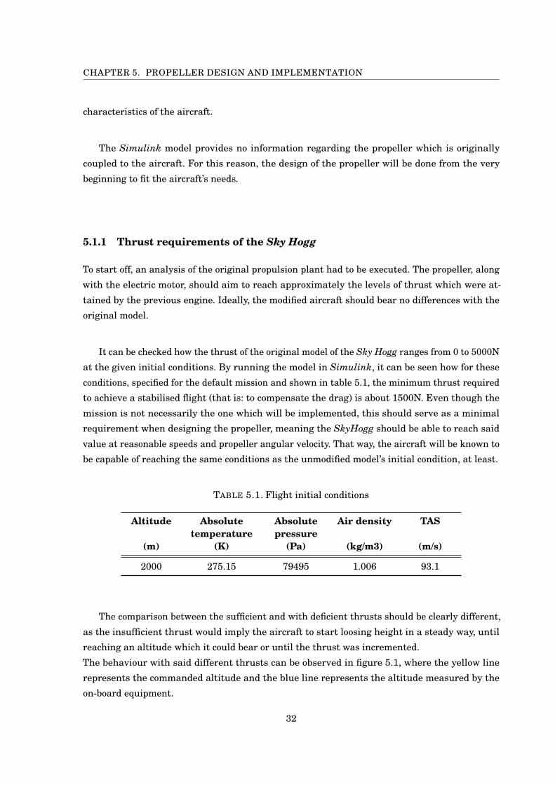
CHAPTER 5. PROPELLER DESIGN AND IMPLEMENTATION
characteristics of the aircraft.
The Simulink model provides no information regarding the propeller which is originally
coupled to the aircraft. For this reason, the design of the propeller will be done from the very
beginning to fit the aircraft’s needs.
5.1.1 Thrust requirements of the Sky Hogg
To start off, an analysis of the original propulsion plant had to be executed. The propeller, along
with the electric motor, should aim to reach approximately the levels of thrust which were at-
tained by the previous engine. Ideally, the modified aircraft should bear no differences with the
original model.
It can be checked how the thrust of the original model of the Sky Hogg ranges from 0 to 5000N
at the given initial conditions. By running the model in Simulink, it can be seen how for these
conditions, specified for the default mission and shown in table 5.1, the minimum thrust required
to achieve a stabilised flight (that is: to compensate the drag) is about 1500N. Even though the
mission is not necessarily the one which will be implemented, this should serve as a minimal
requirement when designing the propeller, meaning the SkyHogg should be able to reach said
value at reasonable speeds and propeller angular velocity. That way, the aircraft will be known to
be capable of reaching the same conditions as the unmodified model’s initial condition, at least.
TABLE 5.1. Flight initial conditions
Altitude Absolutetemperature
Absolutepressure
Air density TAS
(m) (K) (Pa) (kg/m3) (m/s)
2000 275.15 79495 1.006 93.1
The comparison between the sufficient and with deficient thrusts should be clearly different,
as the insufficient thrust would imply the aircraft to start loosing height in a steady way, until
reaching an altitude which it could bear or until the thrust was incremented.
The behaviour with said different thrusts can be observed in figure 5.1, where the yellow line
represents the commanded altitude and the blue line represents the altitude measured by the
on-board equipment.
32
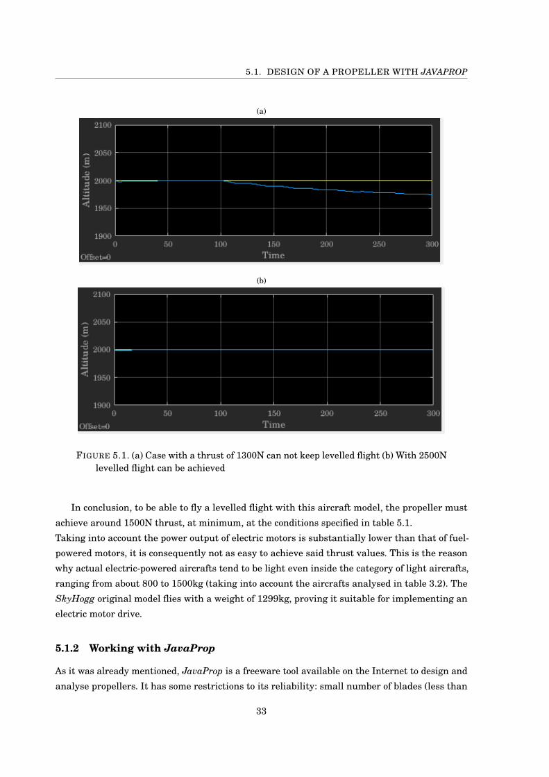
5.1. DESIGN OF A PROPELLER WITH JAVAPROP
(a)
(b)
FIGURE 5.1. (a) Case with a thrust of 1300N can not keep levelled flight (b) With 2500Nlevelled flight can be achieved
In conclusion, to be able to fly a levelled flight with this aircraft model, the propeller must
achieve around 1500N thrust, at minimum, at the conditions specified in table 5.1.
Taking into account the power output of electric motors is substantially lower than that of fuel-
powered motors, it is consequently not as easy to achieve said thrust values. This is the reason
why actual electric-powered aircrafts tend to be light even inside the category of light aircrafts,
ranging from about 800 to 1500kg (taking into account the aircrafts analysed in table 3.2). The
SkyHogg original model flies with a weight of 1299kg, proving it suitable for implementing an
electric motor drive.
5.1.2 Working with JavaProp
As it was already mentioned, JavaProp is a freeware tool available on the Internet to design and
analyse propellers. It has some restrictions to its reliability: small number of blades (less than
33
CHAPTER 5. PROPELLER DESIGN AND IMPLEMENTATION
15) and the propeller loading should not be too high [49].
The application allows to enter some design parameters and test them, modifying the propeller to
fulfil off-design conditions. Therefore, an iterative process was followed, based on trial and error,
to determine the geometry of the blades which would perform well in the simulation conditions.
In table 5.2 some important geometric parameters can be observed, so as to grasp the dimensions
of the actual blade.
TABLE 5.2. Geometric parameters of the blades
N of bladesDiameter Chord
(m) Tip (mm) Root (mm)
4 1.65 50 126.3
The blades have different standard airfoil geometries along the span, which are listed in table
5.3. These airfoils were selected for being common in propeller design and have been proven to
be suitable. The sections of the blade which do not correspond to any of the listed below have
interpolated airfoils, with the interpolation being from the beginning airfoil shape to the ending
as to create a smooth blade surface and shape.
TABLE 5.3. Airfoils along the span
Airfoil
r/R = 0 r/R = 0.35 r/R = 0.65 r/R = 1
MH 112 16.2% MH 114 13% MH 114 13% MH 116 9.8%
Asides from detailed geometry values, JavaProp also provides coefficients for the estimation
of thrust and power. It is important to note the coefficients JavaProp uses differ to those which
are most common in the literature. The definitions for the coefficients employed are exhibited
under these lines and the nomenclature used coincides with the one employed in JavaProp, for
the sake of simplicity.
The traditional coefficients, the ones mostly found as thrust and power coefficient (respec-
tively) in aeronautic literature are as follows:
TC = Tρ2 v2∞ S
PC = Pρ2 v3∞ S
(5.1)
On the other hand, the ones named propeller coefficients by JavaProp are defined as:
34
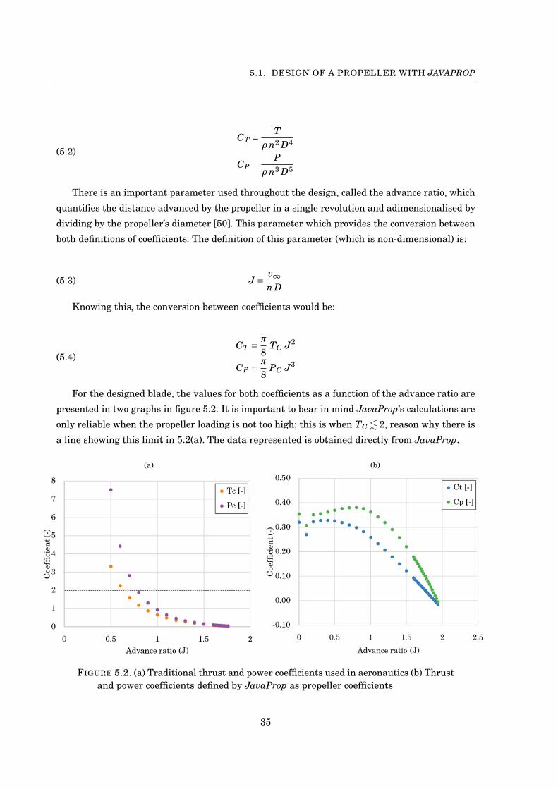
5.1. DESIGN OF A PROPELLER WITH JAVAPROP
CT = Tρ n2 D4
CP = Pρ n3 D5
(5.2)
There is an important parameter used throughout the design, called the advance ratio, which
quantifies the distance advanced by the propeller in a single revolution and adimensionalised by
dividing by the propeller’s diameter [50]. This parameter which provides the conversion between
both definitions of coefficients. The definition of this parameter (which is non-dimensional) is:
(5.3) J = v∞n D
Knowing this, the conversion between coefficients would be:
CT = π
8TC J2
CP = π
8PC J3
(5.4)
For the designed blade, the values for both coefficients as a function of the advance ratio are
presented in two graphs in figure 5.2. It is important to bear in mind JavaProp’s calculations are
only reliable when the propeller loading is not too high; this is when TC . 2, reason why there is
a line showing this limit in 5.2(a). The data represented is obtained directly from JavaProp.
(a) (b)
FIGURE 5.2. (a) Traditional thrust and power coefficients used in aeronautics (b) Thrustand power coefficients defined by JavaProp as propeller coefficients
35
CHAPTER 5. PROPELLER DESIGN AND IMPLEMENTATION
To simplify, the coefficients which will be employed throughout the whole project will be the
JavaProp definition of thrust and power coefficient, that is the coefficients named CT and CP ,
pictured in 5.2(b) and defined in equation 5.2.
This coefficients can be manipulated and used to obtain the thrust and power in different
conditions, as they are defined for a innumerable situations by being characterized as a function
of the advance ratio. As it will be indicated in detail in the next sections, although the coefficient
might be defined for a wide range of advance ratios, not all of them are valid because of the
mentioned problems with high loading. After all, this is just a numerical tool to obtain theoretical
values for thrust and power. This problematic is taken into account in next section and results
are presented and discussed.
5.1.3 JavaProp results
JavaProp provides information in the form of points, due to the fact it works by dividing into
small sections the blade to do its calculations. Once the coefficients have been extracted from the
JavaProp application, it is necessary to work with them in order to visualize the data of interest.
To start off, a polynomial adjustment of the points in figure 5.2 is executed. This polynomial is
further discussed in section 5.2.
Having the polynomial curves of the coefficients, 3D graphs containing the values of thrust
and power in different conditions were done in Matlab, taking into account that results for
high loading are unreliable and thus were not to be included. These surface plots are the visual
representation of the capabilities of the propeller. Anything outside the bounds dictated by the
surface is theoretically not possible for the propeller being questioned.
The plots work with a coloured scale, which turns to hotter colours as the values increase,
which make it easier to identify the wavy shape the surface is doing. Both graphics, thrust and
power, can be seen in figure 5.3. They both refer to the case the aircraft is flying at sea level, that
is, with an air density of ρ = 1.225 kgm3 . If any other altitude was to be studied, it would require
other plots and would bear slightly different results.
36
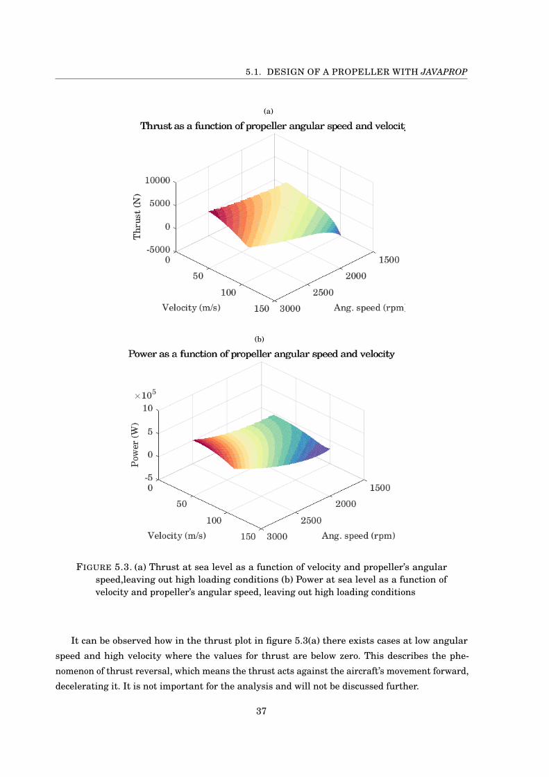
5.1. DESIGN OF A PROPELLER WITH JAVAPROP
(a)
(b)
FIGURE 5.3. (a) Thrust at sea level as a function of velocity and propeller’s angularspeed,leaving out high loading conditions (b) Power at sea level as a function ofvelocity and propeller’s angular speed, leaving out high loading conditions
It can be observed how in the thrust plot in figure 5.3(a) there exists cases at low angular
speed and high velocity where the values for thrust are below zero. This describes the phe-
nomenon of thrust reversal, which means the thrust acts against the aircraft’s movement forward,
decelerating it. It is not important for the analysis and will not be discussed further.
37
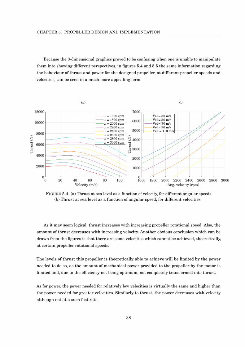
CHAPTER 5. PROPELLER DESIGN AND IMPLEMENTATION
Because the 3-dimensional graphics proved to be confusing when one is unable to manipulate
them into showing different perspectives, in figures 5.4 and 5.5 the same information regarding
the behaviour of thrust and power for the designed propeller, at different propeller speeds and
velocities, can be seen in a much more appealing form.
(a) (b)
FIGURE 5.4. (a) Thrust at sea level as a function of velocity, for different angular speeds(b) Thrust at sea level as a function of angular speed, for different velocities
As it may seem logical, thrust increases with increasing propeller rotational speed. Also, the
amount of thrust decreases with increasing velocity. Another obvious conclusion which can be
drawn from the figures is that there are some velocities which cannot be achieved, theoretically,
at certain propeller rotational speeds.
The levels of thrust this propeller is theoretically able to achieve will be limited by the power
needed to do so, as the amount of mechanical power provided to the propeller by the motor is
limited and, due to the efficiency not being optimum, not completely transformed into thrust.
As for power, the power needed for relatively low velocities is virtually the same and higher than
the power needed for greater velocities. Similarly to thrust, the power decreases with velocity
although not at a such fast rate.
38
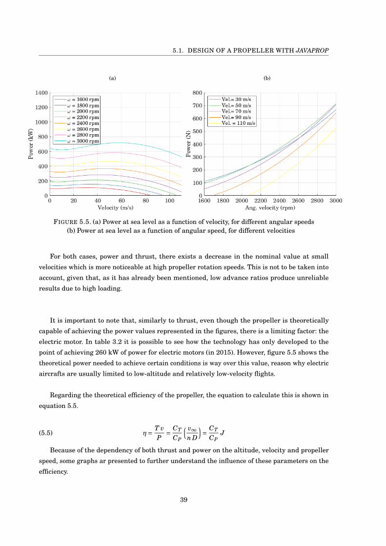
5.1. DESIGN OF A PROPELLER WITH JAVAPROP
(a) (b)
FIGURE 5.5. (a) Power at sea level as a function of velocity, for different angular speeds(b) Power at sea level as a function of angular speed, for different velocities
For both cases, power and thrust, there exists a decrease in the nominal value at small
velocities which is more noticeable at high propeller rotation speeds. This is not to be taken into
account, given that, as it has already been mentioned, low advance ratios produce unreliable
results due to high loading.
It is important to note that, similarly to thrust, even though the propeller is theoretically
capable of achieving the power values represented in the figures, there is a limiting factor: the
electric motor. In table 3.2 it is possible to see how the technology has only developed to the
point of achieving 260 kW of power for electric motors (in 2015). However, figure 5.5 shows the
theoretical power needed to achieve certain conditions is way over this value, reason why electric
aircrafts are usually limited to low-altitude and relatively low-velocity flights.
Regarding the theoretical efficiency of the propeller, the equation to calculate this is shown in
equation 5.5.
(5.5) η= T vP
= CT
CP
( v∞n D
)= CT
CPJ
Because of the dependency of both thrust and power on the altitude, velocity and propeller
speed, some graphs ar presented to further understand the influence of these parameters on the
efficiency.
39
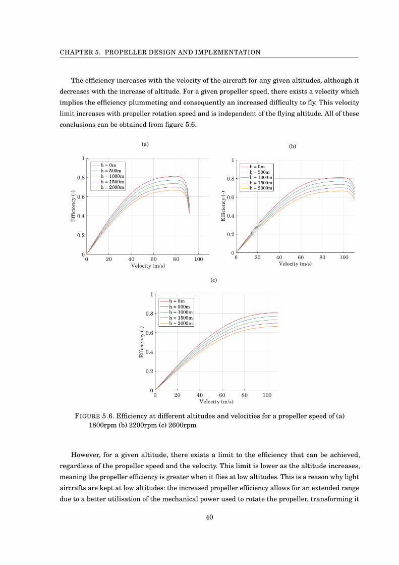
CHAPTER 5. PROPELLER DESIGN AND IMPLEMENTATION
The efficiency increases with the velocity of the aircraft for any given altitudes, although it
decreases with the increase of altitude. For a given propeller speed, there exists a velocity which
implies the efficiency plummeting and consequently an increased difficulty to fly. This velocity
limit increases with propeller rotation speed and is independent of the flying altitude. All of these
conclusions can be obtained from figure 5.6.
(a) (b)
(c)
FIGURE 5.6. Efficiency at different altitudes and velocities for a propeller speed of (a)1800rpm (b) 2200rpm (c) 2600rpm
However, for a given altitude, there exists a limit to the efficiency that can be achieved,
regardless of the propeller speed and the velocity. This limit is lower as the altitude increases,
meaning the propeller efficiency is greater when it flies at low altitudes. This is a reason why light
aircrafts are kept at low altitudes: the increased propeller efficiency allows for an extended range
due to a better utilisation of the mechanical power used to rotate the propeller, transforming it
40
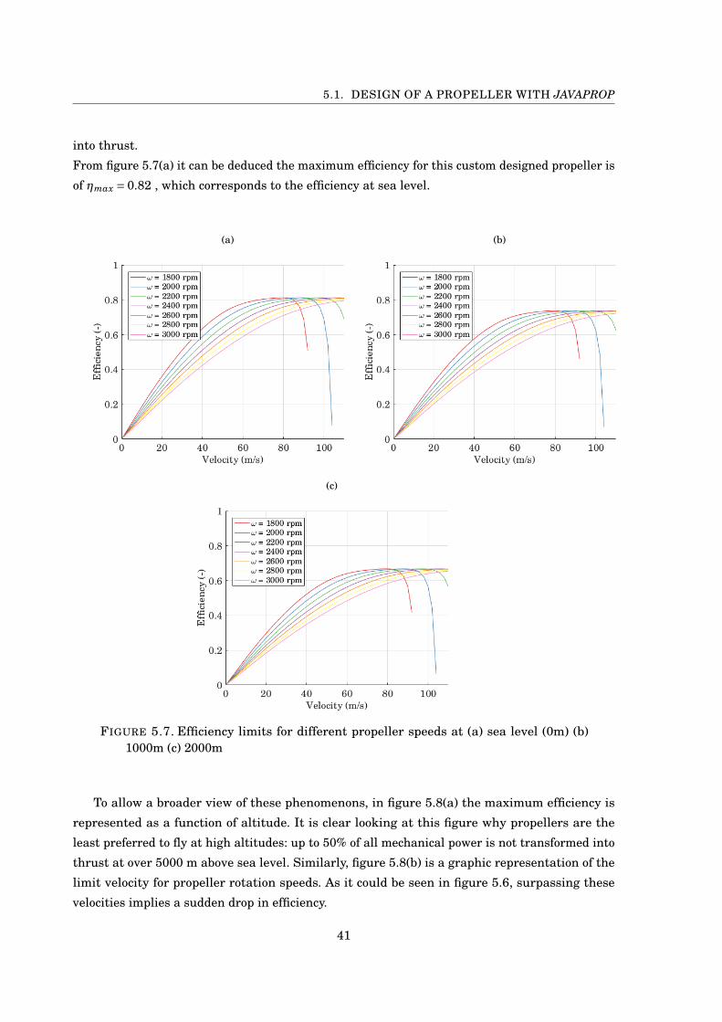
5.1. DESIGN OF A PROPELLER WITH JAVAPROP
into thrust.
From figure 5.7(a) it can be deduced the maximum efficiency for this custom designed propeller is
of ηmax = 0.82 , which corresponds to the efficiency at sea level.
(a) (b)
(c)
FIGURE 5.7. Efficiency limits for different propeller speeds at (a) sea level (0m) (b)1000m (c) 2000m
To allow a broader view of these phenomenons, in figure 5.8(a) the maximum efficiency is
represented as a function of altitude. It is clear looking at this figure why propellers are the
least preferred to fly at high altitudes: up to 50% of all mechanical power is not transformed into
thrust at over 5000 m above sea level. Similarly, figure 5.8(b) is a graphic representation of the
limit velocity for propeller rotation speeds. As it could be seen in figure 5.6, surpassing these
velocities implies a sudden drop in efficiency.
41
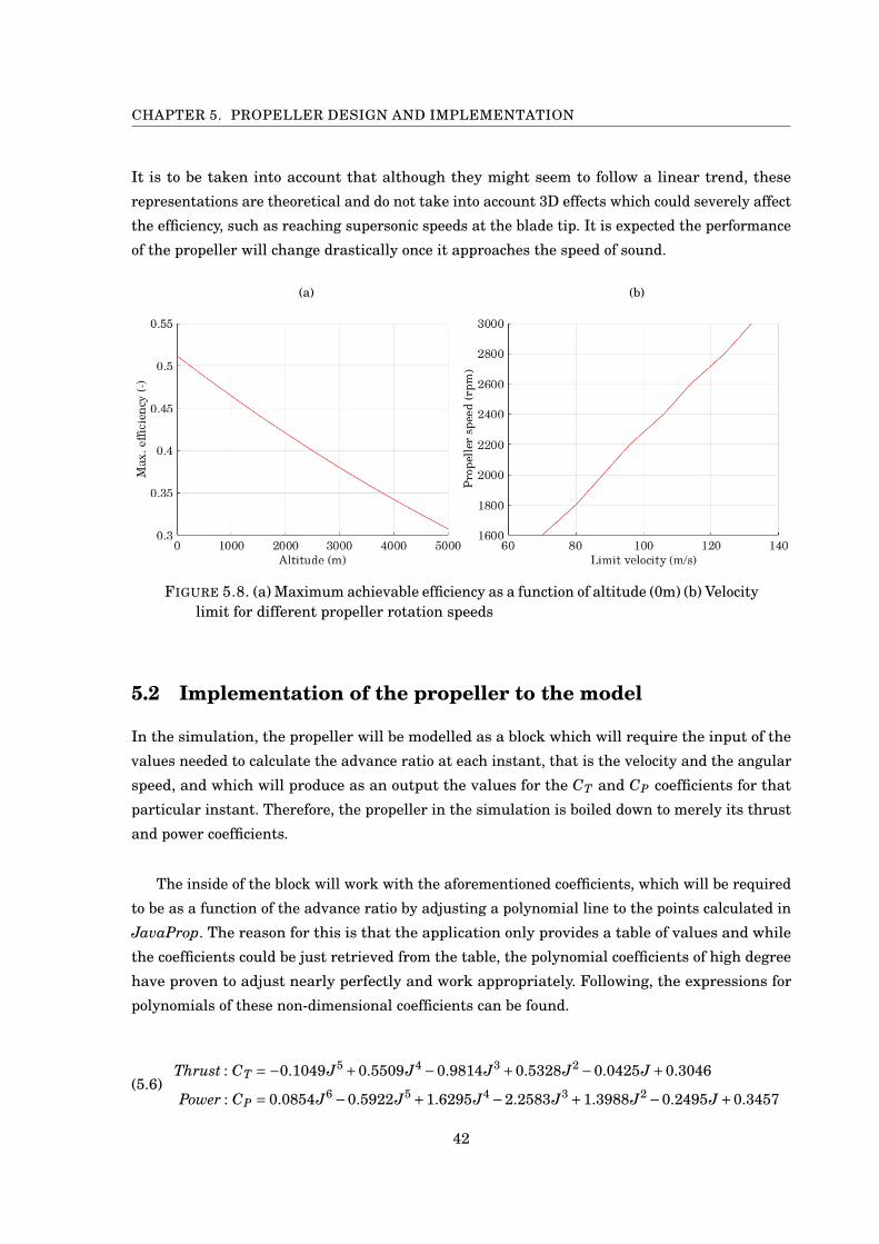
CHAPTER 5. PROPELLER DESIGN AND IMPLEMENTATION
It is to be taken into account that although they might seem to follow a linear trend, these
representations are theoretical and do not take into account 3D effects which could severely affect
the efficiency, such as reaching supersonic speeds at the blade tip. It is expected the performance
of the propeller will change drastically once it approaches the speed of sound.
(a) (b)
FIGURE 5.8. (a) Maximum achievable efficiency as a function of altitude (0m) (b) Velocitylimit for different propeller rotation speeds
5.2 Implementation of the propeller to the model
In the simulation, the propeller will be modelled as a block which will require the input of the
values needed to calculate the advance ratio at each instant, that is the velocity and the angular
speed, and which will produce as an output the values for the CT and CP coefficients for that
particular instant. Therefore, the propeller in the simulation is boiled down to merely its thrust
and power coefficients.
The inside of the block will work with the aforementioned coefficients, which will be required
to be as a function of the advance ratio by adjusting a polynomial line to the points calculated in
JavaProp. The reason for this is that the application only provides a table of values and while
the coefficients could be just retrieved from the table, the polynomial coefficients of high degree
have proven to adjust nearly perfectly and work appropriately. Following, the expressions for
polynomials of these non-dimensional coefficients can be found.
Thrust : CT =−0.1049J5 +0.5509J4 −0.9814J3 +0.5328J2 −0.0425J+0.3046
Power : CP = 0.0854J6 −0.5922J5 +1.6295J4 −2.2583J3 +1.3988J2 −0.2495J+0.3457(5.6)
42
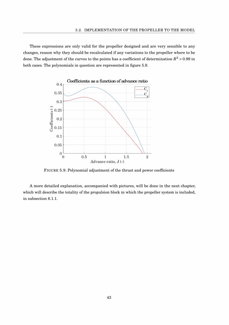
5.2. IMPLEMENTATION OF THE PROPELLER TO THE MODEL
These expressions are only valid for the propeller designed and are very sensible to any
changes, reason why they should be recalculated if any variations to the propeller where to be
done. The adjustment of the curves to the points has a coefficient of determination R2 > 0.99 in
both cases. The polynomials in question are represented in figure 5.9.
FIGURE 5.9. Polynomial adjustment of the thrust and power coefficients
A more detailed explanation, accompanied with pictures, will be done in the next chapter,
which will describe the totality of the propulsion block in which the propeller system is included,
in subsection 6.1.1.
43

CH
AP
TE
R
6PROPULSION BLOCK
This block contains the fundamental modifications applied to the Sky Hogg simulation. In
section 4.2 the original layout was shown, where it could be appreciated how the model
only uses a direct thrust input, ignoring any engine implications. This chapter’s aim is
to describe the totality of the modifications performed on the subsystem to transform it into an
electrically propelled aircraft.
The modification of this propulsion block aims to describe and follow the dictations of the propeller
and motor, adjust to their limitations and deviations, in opposition to the original model where
a thrust as a function of throttle was employed. However, the simplifications considered in the
original model regarding considering thrust forces negligible in Y and Z axes are kept. Likewise,
the moments on all three axes are considered null.
6.1 Overview
As described in section 4.2, there are three main parts to the propulsion block: propeller, electric
motor and batteries. The general distribution of the modified block is as follows in figure 6.1. The
two most important subsystems, propeller and electric motor, are tinted in blue and magenta,
respectively, to improve identification and readability. It can be seen how the outputs of the
propulsion subsystem are the same as in the original model: the thrust and moment in all three
axes.
The inputs to the model are the wind density (obtained from EnvData, environment data), the
velocity, and the pilot commands (throttle); as opposed to the original model, which only had the
latter as an input. The signals entering and exiting blocks carry names which are self-explanatory.
45
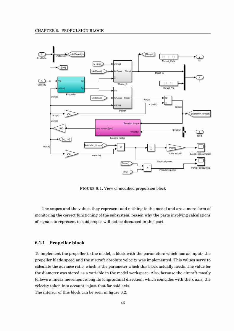
CHAPTER 6. PROPULSION BLOCK
FIGURE 6.1. View of modified propulsion block
The scopes and the values they represent add nothing to the model and are a mere form of
monitoring the correct functioning of the subsystem, reason why the parts involving calculations
of signals to represent in said scopes will not be discussed in this part.
6.1.1 Propeller block
To implement the propeller to the model, a block with the parameters which has as inputs the
propeller blade speed and the aircraft absolute velocity was implemented. This values serve to
calculate the advance ratio, which is the parameter which this block actually needs. The value for
the diameter was stored as a variable in the model workspace. Also, because the aircraft mostly
follows a linear movement along its longitudinal direction, which coincides with the x axis, the
velocity taken into account is just that for said axis.
The interior of this block can be seen in figure 6.2.
46
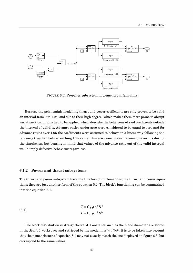
6.1. OVERVIEW
FIGURE 6.2. Propeller subsystem implemented in Simulink
Because the polynomials modelling thrust and power coefficients are only proven to be valid
an interval from 0 to 1.95, and due to their high degree (which makes them more prone to abrupt
variations), conditions had to be applied which describe the behaviour of said coefficients outside
the interval of validity. Advance ratios under zero were considered to be equal to zero and for
advance ratios over 1.95 the coefficients were assumed to behave in a linear way following the
tendency they had before reaching 1.95 value. This was done to avoid anomalous results during
the simulation, but bearing in mind that values of the advance ratio out of the valid interval
would imply defective behaviour regardless.
6.1.2 Power and thrust subsystems
The thrust and power subsystem have the function of implementing the thrust and power equa-
tions; they are just another form of the equation 5.2. The block’s functioning can be summarized
into the equation 6.1.
T = CT ρ n2 D4
P = CP ρ n3 D5(6.1)
The block distribution is straightforward. Constants such as the blade diameter are stored
in the Matlab workspace and retrieved by the model in Simulink. It is to be taken into account
that the nomenclature of equation 6.1 may not exactly match the one displayed on figure 6.3, but
correspond to the same values.
47
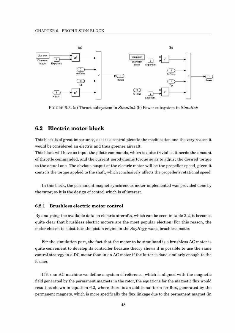
CHAPTER 6. PROPULSION BLOCK
(a) (b)
FIGURE 6.3. (a) Thrust subsystem in Simulink (b) Power subsystem in Simulink
6.2 Electric motor block
This block is of great importance, as it is a central piece to the modification and the very reason it
would be considered an electric and thus greener aircraft.
This block will have as input the pilot’s commands, which is quite trivial as it needs the amount
of throttle commanded, and the current aerodynamic torque so as to adjust the desired torque
to the actual one. The obvious output of the electric motor will be the propeller speed, given it
controls the torque applied to the shaft, which conclusively affects the propeller’s rotational speed.
In this block, the permanent magnet synchronous motor implemented was provided done by
the tutor; so it is the design of control which is of interest.
6.2.1 Brushless electric motor control
By analysing the available data on electric aircrafts, which can be seen in table 3.2, it becomes
quite clear that brushless electric motors are the most popular election. For this reason, the
motor chosen to substitute the piston engine in the SkyHogg was a brushless motor.
For the simulation part, the fact that the motor to be simulated is a brushless AC motor is
quite convenient to develop its controller because theory shows it is possible to use the same
control strategy in a DC motor than in an AC motor if the latter is done similarly enough to the
former.
If for an AC machine we define a system of reference, which is aligned with the magnetic
field generated by the permanent magnets in the rotor, the equations for the magnetic flux would
result as shown in equation 6.2, where there is an additional term for flux, generated by the
permanent magnets, which is more specifically the flux linkage due to the permanent magnet (in
48
6.2. ELECTRIC MOTOR BLOCK
the equation it is highlighted in red). On the other hand, when considering the equations for the
stator, the outcome is similar to the DC case, just with some additional terms which, again, are
due to the permanent magnets.
λd = Ld id+λ0
λq = Lq iq(6.2)
vd = Rs id + dλd
dt−ωrλq
vd = Rs iq +dλq
dt+ωrλd
(6.3)
When plugging in equation 6.2 into equation 6.3 the result is approximately a first order
system, which is comparable to that of the DC case. The electromagnetic force induced by the
permanent magnet is present in the form of the rotor angular speed times the flux, ωrλ0. The
resulting system can be seen in equation 6.4.
vd = Rs id +Lddid
dt−ωrLq iq
vd = Rs iq +Lqdiq
dt+ωrLd id+ωrλ0
(6.4)
The system is missing the torque expression, which is stated in equation 6.5. In order to
allow the control of the torque with this AC machine, a usual approach is to force one of the
currents to be zero, modification which results in a simplification of the torque equation as well
as a simplification of the overall system. With this adaptation, the torque comes as a constant
times a current, which is desirable in order to develop a controller. Said constant is given the
name λm, for the sake of simplicity.
Tm = 23
p(iqλd − idλq)
with iq = 0
Tm = 23
pλd iq =λm iq
(6.5)
It becomes clear that in order to control the torque, the only necessary thing will be to control
the currents. So as to control said currents id and iq, it is necessary to make some assumptions.
In first place, it will be assumed ωr varies at a slow rate, thus making the term ωrλ0 negligible.
Next, a first order linear system will be forced by grouping some terms:
vd =−ωrLq iq +ud
vq =ωrLd id +uq(6.6)
49
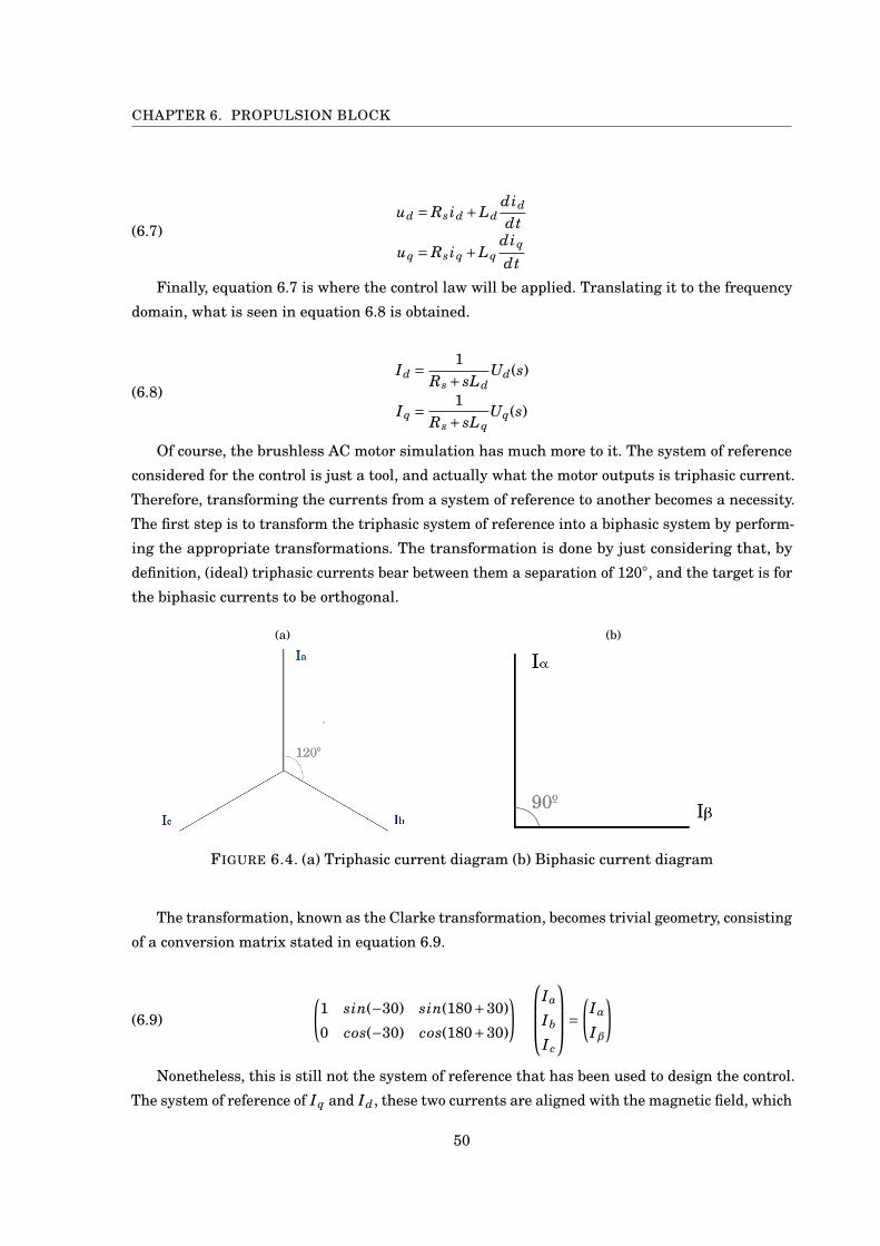
CHAPTER 6. PROPULSION BLOCK
ud = Rs id +Lddid
dt
uq = Rs iq +Lqdiq
dt
(6.7)
Finally, equation 6.7 is where the control law will be applied. Translating it to the frequency
domain, what is seen in equation 6.8 is obtained.
Id = 1Rs + sLd
Ud(s)
Iq = 1Rs + sLq
Uq(s)(6.8)
Of course, the brushless AC motor simulation has much more to it. The system of reference
considered for the control is just a tool, and actually what the motor outputs is triphasic current.
Therefore, transforming the currents from a system of reference to another becomes a necessity.
The first step is to transform the triphasic system of reference into a biphasic system by perform-
ing the appropriate transformations. The transformation is done by just considering that, by
definition, (ideal) triphasic currents bear between them a separation of 120, and the target is for
the biphasic currents to be orthogonal.
(a) (b)
FIGURE 6.4. (a) Triphasic current diagram (b) Biphasic current diagram
The transformation, known as the Clarke transformation, becomes trivial geometry, consisting
of a conversion matrix stated in equation 6.9.
(6.9)
(1 sin(−30) sin(180+30)
0 cos(−30) cos(180+30)
) Ia
Ib
Ic
=(IαIβ
)
Nonetheless, this is still not the system of reference that has been used to design the control.
The system of reference of Iq and Id, these two currents are aligned with the magnetic field, which
50
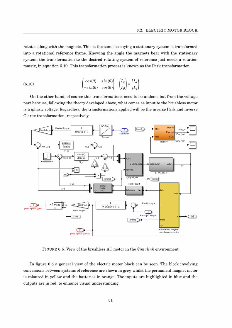
6.2. ELECTRIC MOTOR BLOCK
rotates along with the magnets. This is the same as saying a stationary system is transformed
into a rotational reference frame. Knowing the angle the magnets bear with the stationary
system, the transformation to the desired rotating system of reference just needs a rotation
matrix, in equation 6.10. This transformation process is known as the Park transformation.
(6.10)
(cos(θ) sin(θ)
−sin(θ) cos(θ)
) (IαIβ
)=
(Id
Iq
)
On the other hand, of course this transformations need to be undone, but from the voltage
part because, following the theory developed above, what comes as input to the brushless motor
is triphasic voltage. Regardless, the transformations applied will be the inverse Park and inverse
Clarke transformation, respectively.
FIGURE 6.5. View of the brushless AC motor in the Simulink environment
In figure 6.5 a general view of the electric motor block can be seen. The block involving
conversions between systems of reference are shown in grey, whilst the permanent magnet motor
is coloured in yellow and the batteries in orange. The inputs are highlighted in blue and the
outputs are in red, to enhance visual understanding.
51
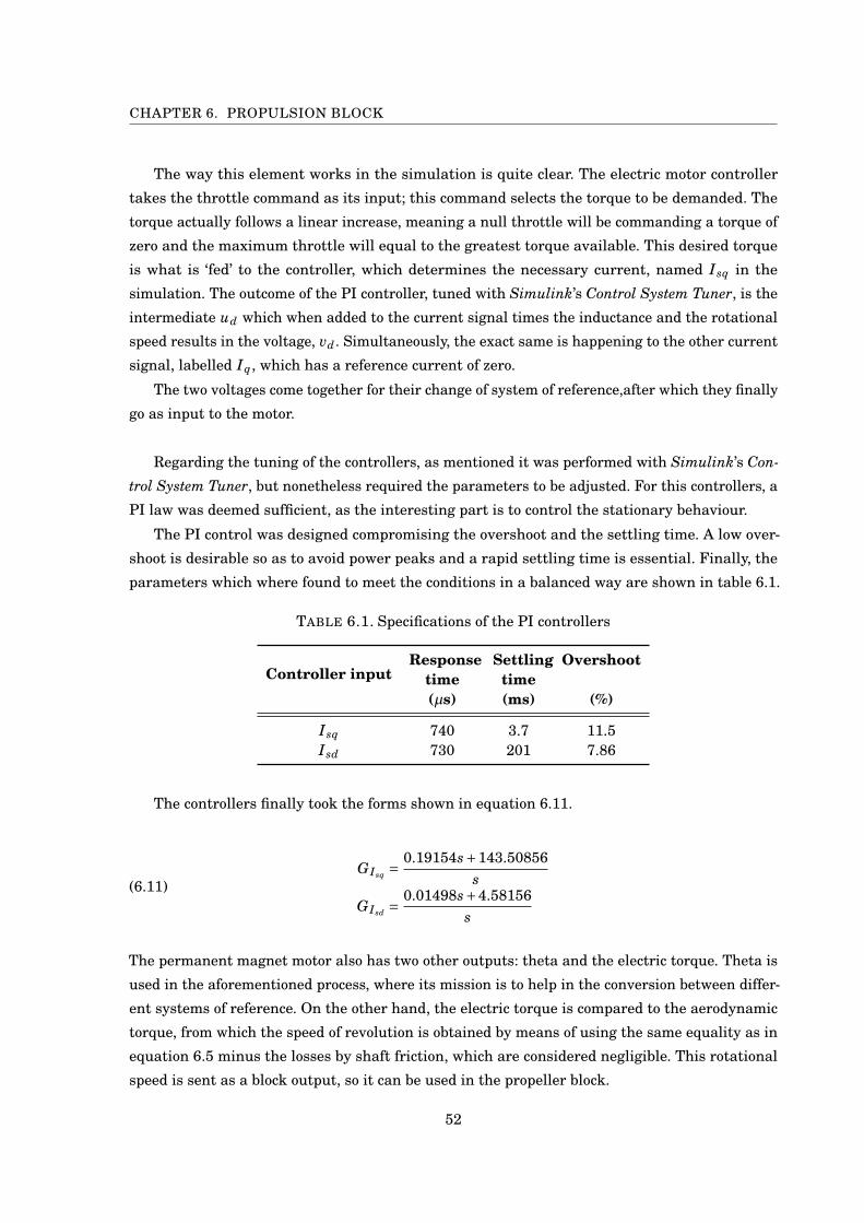
CHAPTER 6. PROPULSION BLOCK
The way this element works in the simulation is quite clear. The electric motor controller
takes the throttle command as its input; this command selects the torque to be demanded. The
torque actually follows a linear increase, meaning a null throttle will be commanding a torque of
zero and the maximum throttle will equal to the greatest torque available. This desired torque
is what is ‘fed’ to the controller, which determines the necessary current, named Isq in the
simulation. The outcome of the PI controller, tuned with Simulink’s Control System Tuner, is the
intermediate ud which when added to the current signal times the inductance and the rotational
speed results in the voltage, vd. Simultaneously, the exact same is happening to the other current
signal, labelled Iq, which has a reference current of zero.
The two voltages come together for their change of system of reference,after which they finally
go as input to the motor.
Regarding the tuning of the controllers, as mentioned it was performed with Simulink’s Con-
trol System Tuner, but nonetheless required the parameters to be adjusted. For this controllers, a
PI law was deemed sufficient, as the interesting part is to control the stationary behaviour.
The PI control was designed compromising the overshoot and the settling time. A low over-
shoot is desirable so as to avoid power peaks and a rapid settling time is essential. Finally, the
parameters which where found to meet the conditions in a balanced way are shown in table 6.1.
TABLE 6.1. Specifications of the PI controllers
Controller inputResponse
timeSettling
timeOvershoot
(µs) (ms) (%)
Isq 740 3.7 11.5Isd 730 201 7.86
The controllers finally took the forms shown in equation 6.11.
G Isq =0.19154s+143.50856
s
G Isd =0.01498s+4.58156
s
(6.11)
The permanent magnet motor also has two other outputs: theta and the electric torque. Theta is
used in the aforementioned process, where its mission is to help in the conversion between differ-
ent systems of reference. On the other hand, the electric torque is compared to the aerodynamic
torque, from which the speed of revolution is obtained by means of using the same equality as in
equation 6.5 minus the losses by shaft friction, which are considered negligible. This rotational
speed is sent as a block output, so it can be used in the propeller block.
52
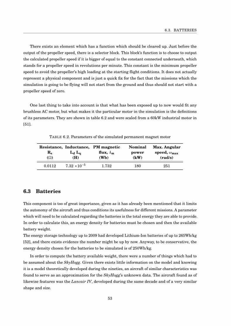
6.3. BATTERIES
There exists an element which has a function which should be cleared up. Just before the
output of the propeller speed, there is a selector block. This block’s function is to choose to output
the calculated propeller speed if it is bigger of equal to the constant connected underneath, which
stands for a propeller speed in revolutions per minute. This constant is the minimum propeller
speed to avoid the propeller’s high loading at the starting flight conditions. It does not actually
represent a physical component and is just a quick fix for the fact that the missions which the
simulation is going to be flying will not start from the ground and thus should not start with a
propeller speed of zero.
One last thing to take into account is that what has been exposed up to now would fit any
brushless AC motor, but what makes it the particular motor in the simulation is the definitions
of its parameters. They are shown in table 6.2 and were scaled from a 60kW industrial motor in
[51].
TABLE 6.2. Parameters of the simulated permanent magnet motor
Resistance,Rs
Inductance,Ld Lq
PM magneticflux, λm
Nominalpower
Max. Angularspeed, ωmax
(Ω) (H) (Wb) (kW) (rad/s)
0.0112 7.32 ×10⁻⁵ 1.732 180 251
6.3 Batteries
This component is too of great importance, given as it has already been mentioned that it limits
the autonomy of the aircraft and thus conditions its usefulness for different missions. A parameter
which will need to be calculated regarding the batteries is the total energy they are able to provide.
In order to calculate this, an energy density for batteries must be chosen and then the available
battery weight.
The energy storage technology up to 2009 had developed Lithium-Ion batteries of up to 265Wh/kg
[52], and there exists evidence the number might be up by now. Anyway, to be conservative, the
energy density chosen for the batteries to be simulated is of 250Wh/kg.
In order to compute the battery available weight, there were a number of things which had to
be assumed about the SkyHogg. Given there exists little information on the model and knowing
it is a model theoretically developed during the nineties, an aircraft of similar characteristics was
found to serve as an approximation for the SkyHogg’s unknown data. The aircraft found as of
likewise features was the Lancair IV, developed during the same decade and of a very similar
shape and size.
53
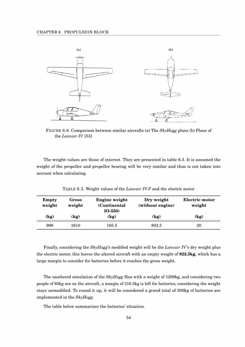
CHAPTER 6. PROPULSION BLOCK
(a) (b)
FIGURE 6.6. Comparison between similar aircrafts (a) The SkyHogg plans (b) Plans ofthe Lancair IV [53]
The weight values are those of interest. They are presented in table 6.3. It is assumed the
weight of the propeller and propeller bearing will be very similar and thus is not taken into
account when calculating.
TABLE 6.3. Weight values of the Lancair IV-P and the electric motor
Emptyweight
Grossweight
Engine weight(Continental
IO-550)
Dry weight(without engine)
Electric motorweight
(kg) (kg) (kg) (kg) (kg)
998 1610 195.5 802.5 20
Finally, considering the SkyHogg’s modified weight will be the Lancair IV ’s dry weight plus
the electric motor, this leaves the altered aircraft with an empty weight of 822.5kg, which has a
large margin to consider for batteries before it reaches the gross weight.
The unaltered simulation of the SkyHogg flies with a weight of 1299kg, and considering two
people of 80kg are on the aircraft, a margin of 316.5kg is left for batteries, considering the weight
stays unmodified. To round it up, it will be considered a grand total of 300kg of batteries are
implemented in the SkyHogg.
The table below summarizes the batteries’ situation.
54
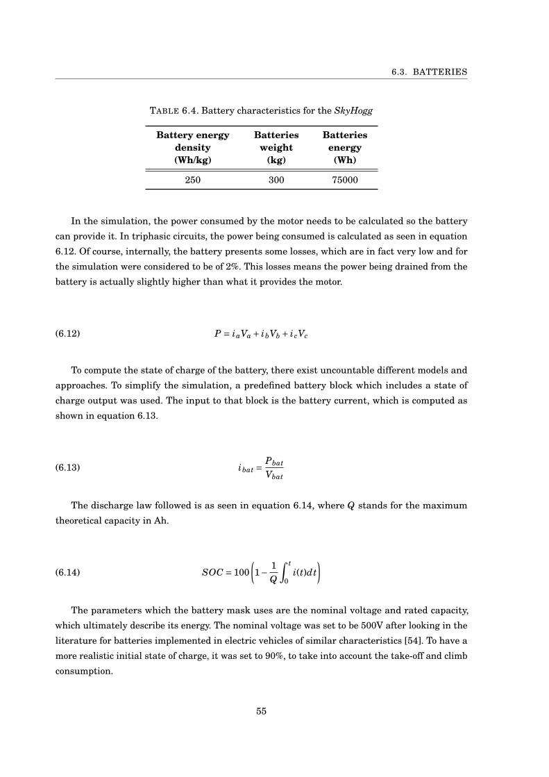
6.3. BATTERIES
TABLE 6.4. Battery characteristics for the SkyHogg
Battery energydensity
Batteriesweight
Batteriesenergy
(Wh/kg) (kg) (Wh)
250 300 75000
In the simulation, the power consumed by the motor needs to be calculated so the battery
can provide it. In triphasic circuits, the power being consumed is calculated as seen in equation
6.12. Of course, internally, the battery presents some losses, which are in fact very low and for
the simulation were considered to be of 2%. This losses means the power being drained from the
battery is actually slightly higher than what it provides the motor.
(6.12) P = iaVa + ibVb + icVc
To compute the state of charge of the battery, there exist uncountable different models and
approaches. To simplify the simulation, a predefined battery block which includes a state of
charge output was used. The input to that block is the battery current, which is computed as
shown in equation 6.13.
(6.13) ibat =Pbat
Vbat
The discharge law followed is as seen in equation 6.14, where Q stands for the maximum
theoretical capacity in Ah.
(6.14) SOC = 100(1− 1
Q
∫ t
0i(t)dt
)
The parameters which the battery mask uses are the nominal voltage and rated capacity,
which ultimately describe its energy. The nominal voltage was set to be 500V after looking in the
literature for batteries implemented in electric vehicles of similar characteristics [54]. To have a
more realistic initial state of charge, it was set to 90%, to take into account the take-off and climb
consumption.
55
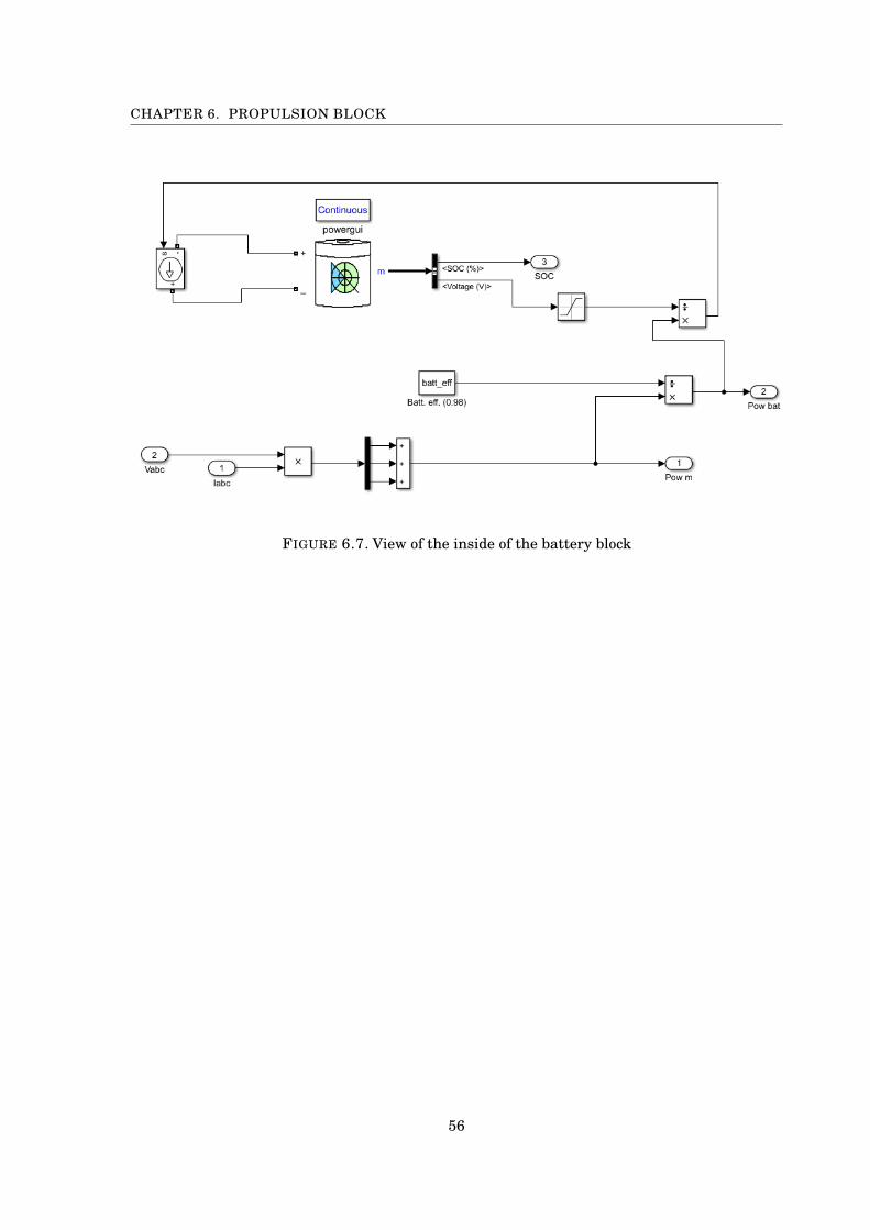
CHAPTER 6. PROPULSION BLOCK
FIGURE 6.7. View of the inside of the battery block
56
CH
AP
TE
R
7PERFORMANCE AND RESULTS
This chapter’s aim is to present the results for tests carried out with the simulation, which
was explained in the above sections. The SkyHogg electric modifications must be tested in
a simulation environment to analyse the feasibility of performing the actual modification.
Basing the viability of the modification upon the fact the aircraft will be used mainly for low
altitude, short flights near the airport, such as for pilot training, missions are designed and tested
based on the premise the flights will be carried out by inexperienced pilots and will only involve
simple manoeuvres.
7.1 Performance during normal use
This first section will test the capability of the modified aircraft to fly casual situations, the type
a light aircraft would fly in normal conditions, as in pilot training lessons.
7.1.1 Levelled flight at constant throttle
This section aims to describe the aircraft’s performance in the simplest type of flight: a levelled,
simple flight. This will draw a picture of the capabilities of the aircraft and will pave the way to
simulating more complicated missions.
For this particular section, the mission will be kept very simple, and it is described in table
7.1. The aim is to look at aircraft parameters, such as power consumed, efficiencies of the motor
and charge of the batteries and extrapolate for longer levelled flights, which also most certainly
happen in real life.
57
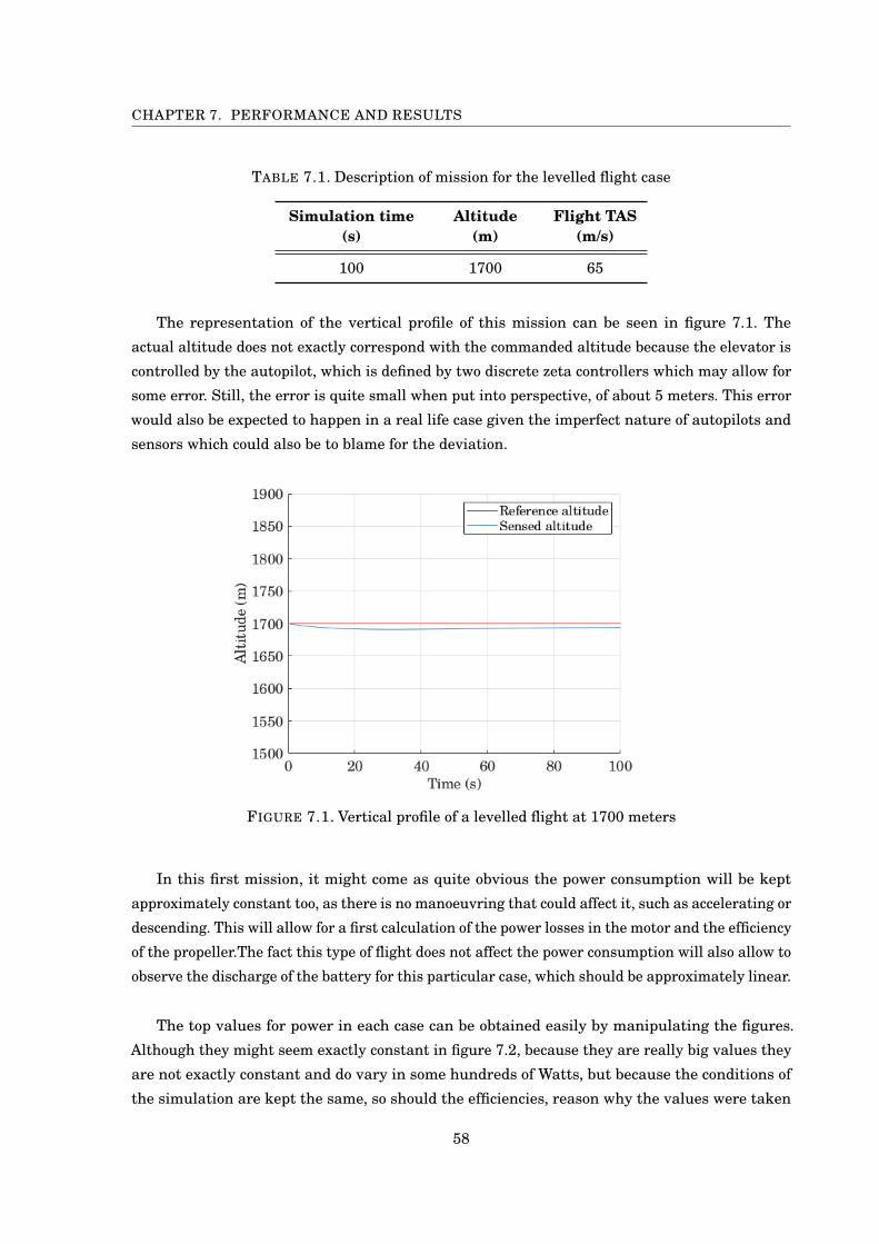
CHAPTER 7. PERFORMANCE AND RESULTS
TABLE 7.1. Description of mission for the levelled flight case
Simulation time Altitude Flight TAS(s) (m) (m/s)
100 1700 65
The representation of the vertical profile of this mission can be seen in figure 7.1. The
actual altitude does not exactly correspond with the commanded altitude because the elevator is
controlled by the autopilot, which is defined by two discrete zeta controllers which may allow for
some error. Still, the error is quite small when put into perspective, of about 5 meters. This error
would also be expected to happen in a real life case given the imperfect nature of autopilots and
sensors which could also be to blame for the deviation.
FIGURE 7.1. Vertical profile of a levelled flight at 1700 meters
In this first mission, it might come as quite obvious the power consumption will be kept
approximately constant too, as there is no manoeuvring that could affect it, such as accelerating or
descending. This will allow for a first calculation of the power losses in the motor and the efficiency
of the propeller.The fact this type of flight does not affect the power consumption will also allow to
observe the discharge of the battery for this particular case, which should be approximately linear.
The top values for power in each case can be obtained easily by manipulating the figures.
Although they might seem exactly constant in figure 7.2, because they are really big values they
are not exactly constant and do vary in some hundreds of Watts, but because the conditions of
the simulation are kept the same, so should the efficiencies, reason why the values were taken
58

7.1. PERFORMANCE DURING NORMAL USE
on some random time. From here it is trivial to obtain the efficiencies; the motor efficiency is
of ηmotor = 0.985 and the efficiency of the propeller for this particular case is ηprop = 0.779. The
motor proves to have a really good efficiency, with <2% of losses.
FIGURE 7.2. Power plots in a levelled flight
The power losses in the motor can be calculated by employing the formula shown in equation
7.1. It uses the root mean square value of the current, which is computed from the peak value of
the intensity.
(7.1) Ploss = 3 Rs i2RMS = 3 Rs
(Imaxp
3
)2
It now seems convenient to analyse the triphasic voltage and current behaviour in the motor
during this levelled flight. As may be expected, there exists at the very start a transition part,
when both the current and voltage start from zero. Again, this is because of the special case of
starting the flight from a dynamic situation in which it is already at an altitude and requires
a starting velocity different to zero. Nevertheless, both parameters reach their final forms in a
reduced amount of time, both reaching the correct peak value for the voltage case or reaching the
right frequency, which applies for both.
Because of the high frequency, in order to be able to observe the behaviour of both parameters,
only the first second of the simulation was plotted in figure 7.3, to improve readability. The
behaviour observed during the second half of the plot is equal to the behaviour obtained during
the rest of the simulated seconds.
59
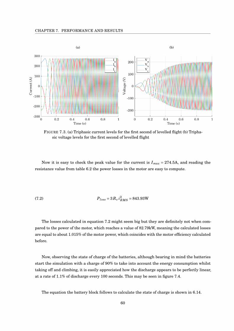
CHAPTER 7. PERFORMANCE AND RESULTS
(a) (b)
FIGURE 7.3. (a) Triphasic current levels for the first second of levelled flight (b) Tripha-sic voltage levels for the first second of levelled flight
Now it is easy to check the peak value for the current is Imax = 274.5A, and reading the
resistance value from table 6.2 the power losses in the motor are easy to compute.
(7.2) Ploss = 3 Rs i2RMS = 843.93W
The losses calculated in equation 7.2 might seem big but they are definitely not when com-
pared to the power of the motor, which reaches a value of 82.79kW, meaning the calculated losses
are equal to about 1.015% of the motor power, which coincides with the motor efficiency calculated
before.
Now, observing the state of charge of the batteries, although bearing in mind the batteries
start the simulation with a charge of 90% to take into account the energy consumption whilst
taking off and climbing, it is easily appreciated how the discharge appears to be perfectly linear,
at a rate of 1.1% of discharge every 100 seconds. This may be seen in figure 7.4.
The equation the battery block follows to calculate the state of charge is shown in 6.14.
60
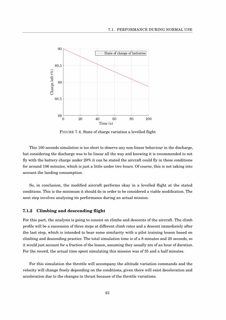
7.1. PERFORMANCE DURING NORMAL USE
FIGURE 7.4. State of charge variation a levelled flight
This 100 seconds simulation is too short to observe any non-linear behaviour in the discharge,
but considering the discharge was to be linear all the way and knowing it is recommended to not
fly with the battery charge under 20% it can be stated the aircraft could fly in these conditions
for around 106 minutes, which is just a little under two hours. Of course, this is not taking into
account the landing consumption.
So, in conclusion, the modified aircraft performs okay in a levelled flight at the stated
conditions. This is the minimum it should do in order to be considered a viable modification. The
next step involves analysing its performance during an actual mission.
7.1.2 Climbing and descending flight
For this part, the analysis is going to consist on climbs and descents of the aircraft. The climb
profile will be a succession of three steps at different climb rates and a descent immediately after
the last step, which is intended to bear some similarity with a pilot training lesson based on
climbing and descending practice. The total simulation time is of a 8 minutes and 20 seconds, so
it would just account for a fraction of the lesson, assuming they usually are of an hour of duration.
For the record, the actual time spent simulating this mission was of 35 and a half minutes.
For this simulation the throttle will accompany the altitude variation commands and the
velocity will change freely depending on the conditions, given there will exist deceleration and
acceleration due to the changes in thrust because of the throttle variations.
61
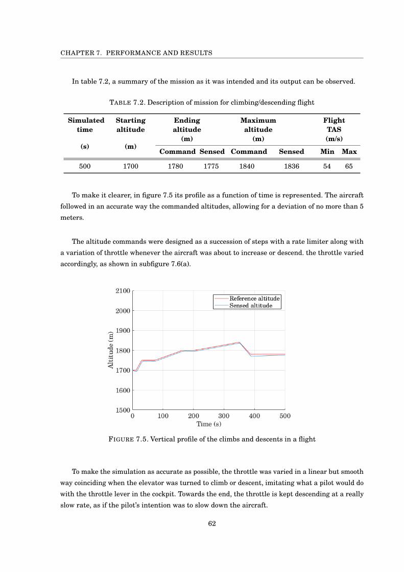
CHAPTER 7. PERFORMANCE AND RESULTS
In table 7.2, a summary of the mission as it was intended and its output can be observed.
TABLE 7.2. Description of mission for climbing/descending flight
Simulatedtime
Startingaltitude
Endingaltitude
Maximumaltitude
FlightTAS
(s) (m)(m) (m) (m/s)
Command Sensed Command Sensed Min Max
500 1700 1780 1775 1840 1836 54 65
To make it clearer, in figure 7.5 its profile as a function of time is represented. The aircraft
followed in an accurate way the commanded altitudes, allowing for a deviation of no more than 5
meters.
The altitude commands were designed as a succession of steps with a rate limiter along with
a variation of throttle whenever the aircraft was about to increase or descend. the throttle varied
accordingly, as shown in subfigure 7.6(a).
FIGURE 7.5. Vertical profile of the climbs and descents in a flight
To make the simulation as accurate as possible, the throttle was varied in a linear but smooth
way coinciding when the elevator was turned to climb or descent, imitating what a pilot would do
with the throttle lever in the cockpit. Towards the end, the throttle is kept descending at a really
slow rate, as if the pilot’s intention was to slow down the aircraft.
62
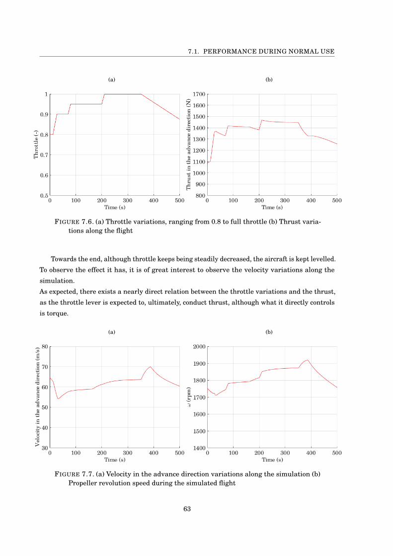
7.1. PERFORMANCE DURING NORMAL USE
(a) (b)
FIGURE 7.6. (a) Throttle variations, ranging from 0.8 to full throttle (b) Thrust varia-tions along the flight
Towards the end, although throttle keeps being steadily decreased, the aircraft is kept levelled.
To observe the effect it has, it is of great interest to observe the velocity variations along the
simulation.
As expected, there exists a nearly direct relation between the throttle variations and the thrust,
as the throttle lever is expected to, ultimately, conduct thrust, although what it directly controls
is torque.
(a) (b)
FIGURE 7.7. (a) Velocity in the advance direction variations along the simulation (b)Propeller revolution speed during the simulated flight
63
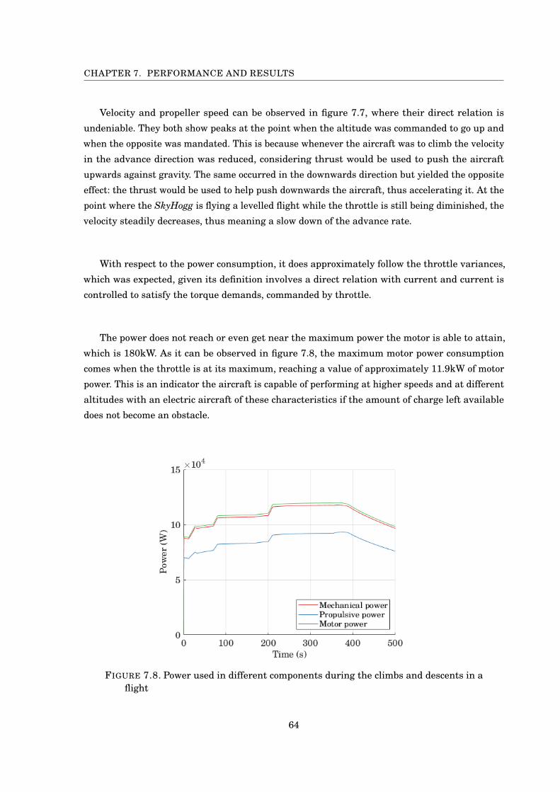
CHAPTER 7. PERFORMANCE AND RESULTS
Velocity and propeller speed can be observed in figure 7.7, where their direct relation is
undeniable. They both show peaks at the point when the altitude was commanded to go up and
when the opposite was mandated. This is because whenever the aircraft was to climb the velocity
in the advance direction was reduced, considering thrust would be used to push the aircraft
upwards against gravity. The same occurred in the downwards direction but yielded the opposite
effect: the thrust would be used to help push downwards the aircraft, thus accelerating it. At the
point where the SkyHogg is flying a levelled flight while the throttle is still being diminished, the
velocity steadily decreases, thus meaning a slow down of the advance rate.
With respect to the power consumption, it does approximately follow the throttle variances,
which was expected, given its definition involves a direct relation with current and current is
controlled to satisfy the torque demands, commanded by throttle.
The power does not reach or even get near the maximum power the motor is able to attain,
which is 180kW. As it can be observed in figure 7.8, the maximum motor power consumption
comes when the throttle is at its maximum, reaching a value of approximately 11.9kW of motor
power. This is an indicator the aircraft is capable of performing at higher speeds and at different
altitudes with an electric aircraft of these characteristics if the amount of charge left available
does not become an obstacle.
FIGURE 7.8. Power used in different components during the climbs and descents in aflight
64
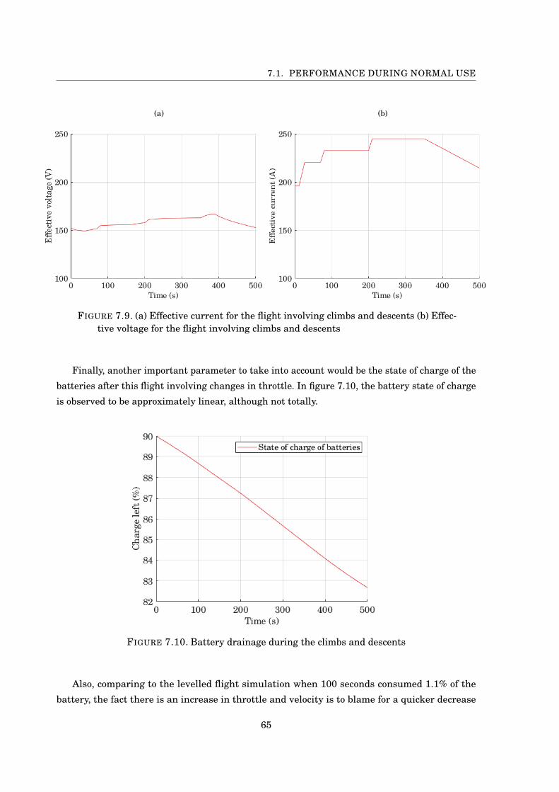
7.1. PERFORMANCE DURING NORMAL USE
(a) (b)
FIGURE 7.9. (a) Effective current for the flight involving climbs and descents (b) Effec-tive voltage for the flight involving climbs and descents
Finally, another important parameter to take into account would be the state of charge of the
batteries after this flight involving changes in throttle. In figure 7.10, the battery state of charge
is observed to be approximately linear, although not totally.
FIGURE 7.10. Battery drainage during the climbs and descents
Also, comparing to the levelled flight simulation when 100 seconds consumed 1.1% of the
battery, the fact there is an increase in throttle and velocity is to blame for a quicker decrease
65
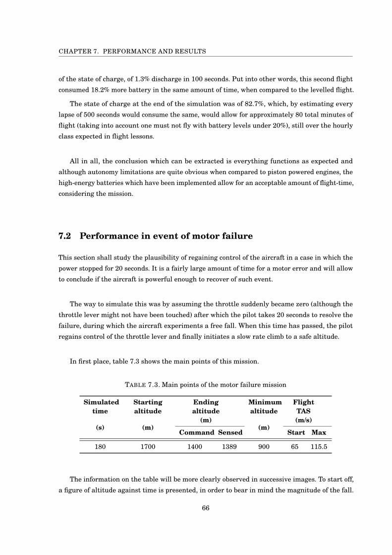
CHAPTER 7. PERFORMANCE AND RESULTS
of the state of charge, of 1.3% discharge in 100 seconds. Put into other words, this second flight
consumed 18.2% more battery in the same amount of time, when compared to the levelled flight.
The state of charge at the end of the simulation was of 82.7%, which, by estimating every
lapse of 500 seconds would consume the same, would allow for approximately 80 total minutes of
flight (taking into account one must not fly with battery levels under 20%), still over the hourly
class expected in flight lessons.
All in all, the conclusion which can be extracted is everything functions as expected and
although autonomy limitations are quite obvious when compared to piston powered engines, the
high-energy batteries which have been implemented allow for an acceptable amount of flight-time,
considering the mission.
7.2 Performance in event of motor failure
This section shall study the plausibility of regaining control of the aircraft in a case in which the
power stopped for 20 seconds. It is a fairly large amount of time for a motor error and will allow
to conclude if the aircraft is powerful enough to recover of such event.
The way to simulate this was by assuming the throttle suddenly became zero (although the
throttle lever might not have been touched) after which the pilot takes 20 seconds to resolve the
failure, during which the aircraft experiments a free fall. When this time has passed, the pilot
regains control of the throttle lever and finally initiates a slow rate climb to a safe altitude.
In first place, table 7.3 shows the main points of this mission.
TABLE 7.3. Main points of the motor failure mission
Simulatedtime
Startingaltitude
Endingaltitude
Minimumaltitude
FlightTAS
(s) (m)(m)
(m)(m/s)
Command Sensed Start Max
180 1700 1400 1389 900 65 115.5
The information on the table will be more clearly observed in successive images. To start off,
a figure of altitude against time is presented, in order to bear in mind the magnitude of the fall.
66
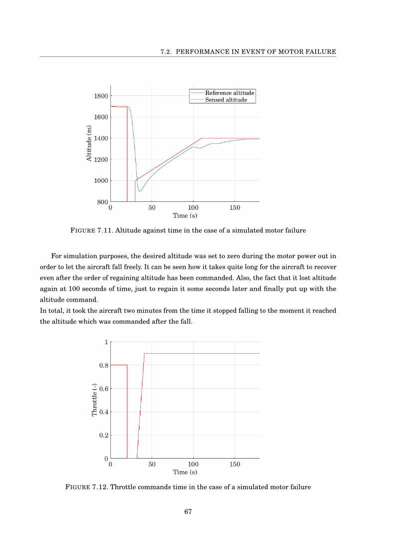
7.2. PERFORMANCE IN EVENT OF MOTOR FAILURE
FIGURE 7.11. Altitude against time in the case of a simulated motor failure
For simulation purposes, the desired altitude was set to zero during the motor power out in
order to let the aircraft fall freely. It can be seen how it takes quite long for the aircraft to recover
even after the order of regaining altitude has been commanded. Also, the fact that it lost altitude
again at 100 seconds of time, just to regain it some seconds later and finally put up with the
altitude command.
In total, it took the aircraft two minutes from the time it stopped falling to the moment it reached
the altitude which was commanded after the fall.
FIGURE 7.12. Throttle commands time in the case of a simulated motor failure
67
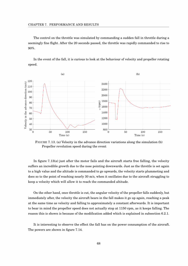
CHAPTER 7. PERFORMANCE AND RESULTS
The control on the throttle was simulated by commanding a sudden fall in throttle during a
seemingly fine flight. After the 20 seconds passed, the throttle was rapidly commanded to rise to
90%.
In the event of the fall, it is curious to look at the behaviour of velocity and propeller rotating
speed.
(a) (b)
FIGURE 7.13. (a) Velocity in the advance direction variations along the simulation (b)Propeller revolution speed during the event
In figure 7.13(a) just after the motor fails and the aircraft starts free falling, the velocity
suffers an incredible growth due to the nose pointing downwards. Just as the throttle is set again
to a high value and the altitude is commanded to go upwards, the velocity starts plummeting and
does so to the point of reaching nearly 30 m/s, when it oscillates due to the aircraft struggling to
keep a velocity which will allow it to reach the commanded altitude.
On the other hand, once throttle is cut, the angular velocity of the propeller falls suddenly, but
immediately after, the velocity the aircraft bears in the fall makes it go up again, reaching a peak
at the same time as velocity and falling to approximately a constant afterwards. It is important
to bear in mind the propeller speed does not actually stop at 1150 rpm, as it keeps falling. The
reason this is shown is because of the modification added which is explained in subsection 6.2.1.
It is interesting to observe the effect the fall has on the power consumption of the aircraft.
The powers are shown in figure 7.14.
68
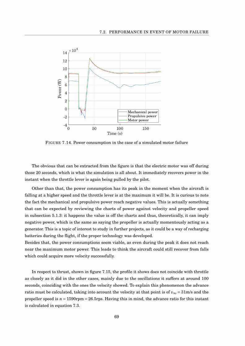
7.2. PERFORMANCE IN EVENT OF MOTOR FAILURE
FIGURE 7.14. Power consumption in the case of a simulated motor failure
The obvious that can be extracted from the figure is that the electric motor was off during
those 20 seconds, which is what the simulation is all about. It immediately recovers power in the
instant when the throttle lever is again being pulled by the pilot.
Other than that, the power consumption has its peak in the moment when the aircraft is
falling at a higher speed and the throttle lever is at the maximum it will be. It is curious to note
the fact the mechanical and propulsive power reach negative values. This is actually something
that can be expected by reviewing the charts of power against velocity and propeller speed
in subsection 5.1.3: it happens the value is off the charts and thus, theoretically, it can imply
negative power, which is the same as saying the propeller is actually momentously acting as a
generator. This is a topic of interest to study in further projects, as it could be a way of recharging
batteries during the flight, if the proper technology was developed.
Besides that, the power consumptions seem viable, as even during the peak it does not reach
near the maximum motor power. This leads to think the aircraft could still recover from falls
which could acquire more velocity successfully.
In respect to thrust, shown in figure 7.15, the profile it shows does not coincide with throttle
as closely as it did in the other cases, mainly due to the oscillations it suffers at around 100
seconds, coinciding with the ones the velocity showed. To explain this phenomenon the advance
ratio must be calculated, taking into account the velocity at that point is of v∞ = 31m/s and the
propeller speed is n = 1590rpm= 26.5rps. Having this in mind, the advance ratio for this instant
is calculated in equation 7.3.
69
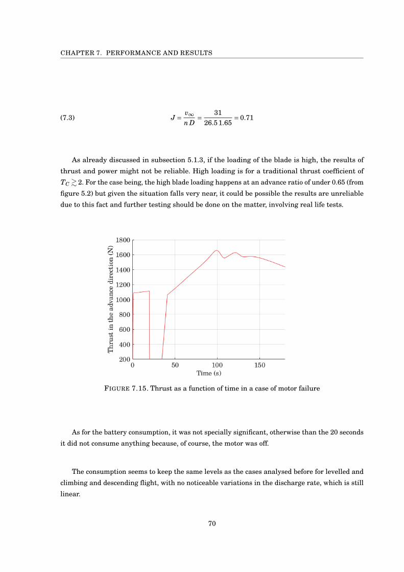
CHAPTER 7. PERFORMANCE AND RESULTS
(7.3) J = v∞n D
= 3126.51.65
= 0.71
As already discussed in subsection 5.1.3, if the loading of the blade is high, the results of
thrust and power might not be reliable. High loading is for a traditional thrust coefficient of
TC & 2. For the case being, the high blade loading happens at an advance ratio of under 0.65 (from
figure 5.2) but given the situation falls very near, it could be possible the results are unreliable
due to this fact and further testing should be done on the matter, involving real life tests.
FIGURE 7.15. Thrust as a function of time in a case of motor failure
As for the battery consumption, it was not specially significant, otherwise than the 20 seconds
it did not consume anything because, of course, the motor was off.
The consumption seems to keep the same levels as the cases analysed before for levelled and
climbing and descending flight, with no noticeable variations in the discharge rate, which is still
linear.
70
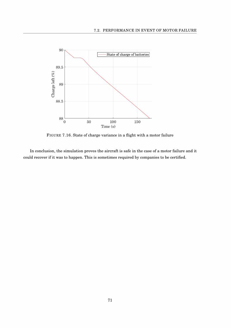
7.2. PERFORMANCE IN EVENT OF MOTOR FAILURE
FIGURE 7.16. State of charge variance in a flight with a motor failure
In conclusion, the simulation proves the aircraft is safe in the case of a motor failure and it
could recover if it was to happen. This is sometimes required by companies to be certified.
71

CH
AP
TE
R
8CONCLUSIONS
This chapter summarizes all the final thoughts on this project; all the conclusions extracted
from the different simulations in different situations as well as any amplification that
could be interesting for future projects to be based on this same topic.
8.1 Conclusions of the project
The project’s conclusions after what was analysed in chapter 7, are that, in effect, the modification
of an aircraft of the same or similar characteristics to the SkyHogg is not only possible but even
desirable in certain situations. However, the desirability of these modifications is conditioned by
the mission the aircraft will have.
At the present moment, electric motors have only reached a portion of the power piston
engines are actually capable of achieving. This limits the climbing speeds and velocities which
the aircrafts are capable of. Furthermore, the most limiting part of the modification corresponds
to batteries. While light aircrafts comparable to the SkyHogg but powered by piston engines are
capable of flying for around 5 hours non-stop with a single fuel replenish, the modified electric
aircraft could only safely fly for little over an hour at a time, and that would greatly depend
on the flight plan. Related to this, another disadvantage the modification bears is, because the
discharge is dependent on the mission and the battery energy is not too elevated, it is limiting
to some missions where constant climbs or variations in velocity are required. Whilst this is
also true for piston engines in the way they consume the fuel, the fact the energy available for
electrical flights is lesser makes it a bigger burden.
73
CHAPTER 8. CONCLUSIONS
On the other hand, the fact the modification is viable and may be useful for determinate
usages is attractive, keeping in mind fuel prices are continuing to grow and air pollution will
force politicians to pass laws on flight time, which will leave electric aircrafts mostly unaffected.
It also brings other advantages such as lower noise, allowing for flights near places where noise
is limited for aviation.
8.2 Further studies
Much remains to be investigated and tried on the topic of the current project. For the time being,
the control applied to the motor could be tested on an actual brushless motor, in order to validate
it. Furthermore, experimenting on a test bench with said motor could be an interesting way of
validating the actual thrust and torque outputs, checking if it follows that commanded by the
throttle lever.
Another interesting project would be studying the possibility of recharging batteries while on
flight, which happens at really high speeds and high propeller velocities.
Moreover, this simulations could be tested at a smaller scale before thinking about imple-
menting them to an actual aircraft, such as trying the control out on a RC aircraft and monitoring
the battery discharge. The final step would be to actually implement the simulated propeller
plant to an actual piston engine light aircraft and perform tests with it.
74
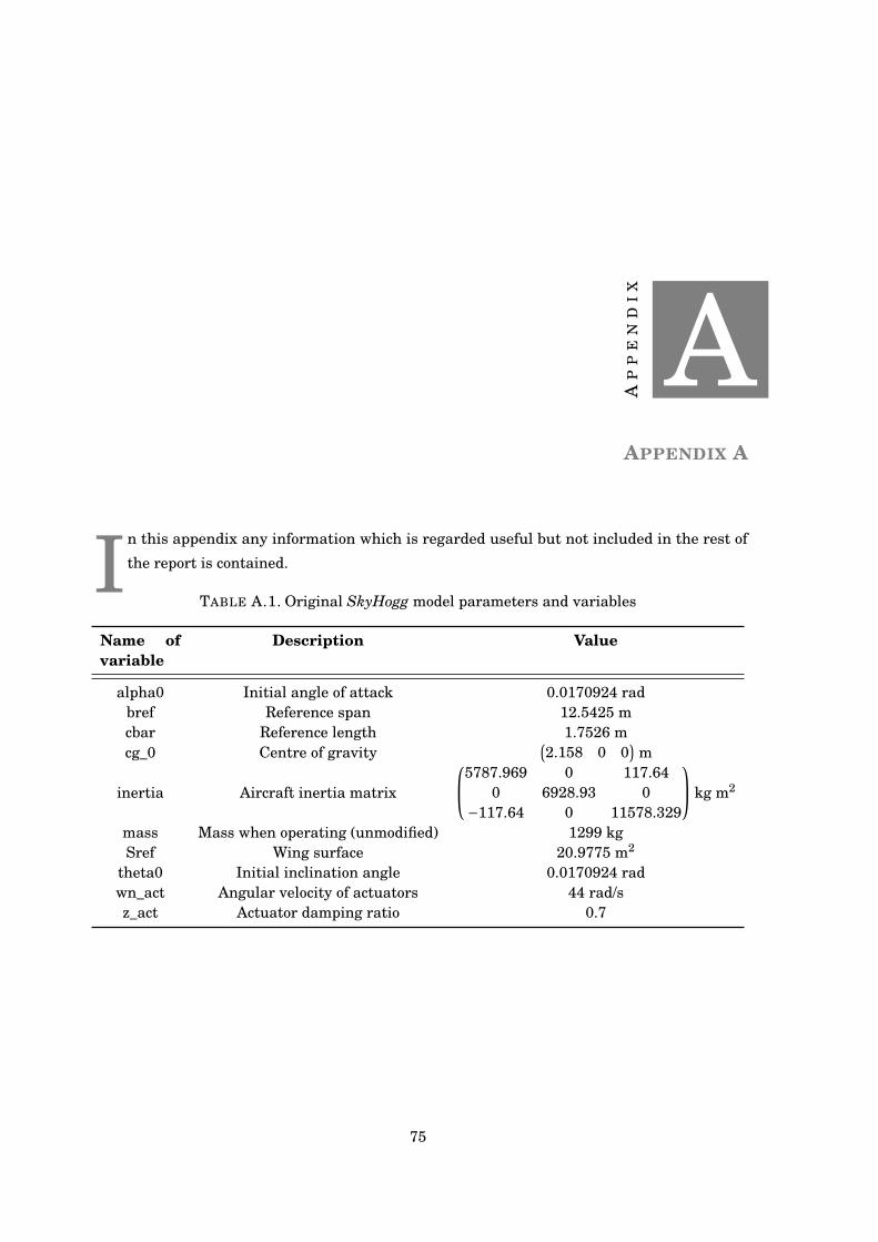
AP
PE
ND
IX
AAPPENDIX A
In this appendix any information which is regarded useful but not included in the rest of
the report is contained.
TABLE A.1. Original SkyHogg model parameters and variables
Name ofvariable
Description Value
alpha0 Initial angle of attack 0.0170924 radbref Reference span 12.5425 mcbar Reference length 1.7526 mcg_0 Centre of gravity
(2.158 0 0
)m
inertia Aircraft inertia matrix
5787.969 0 117.640 6928.93 0
−117.64 0 11578.329
kg m2
mass Mass when operating (unmodified) 1299 kgSref Wing surface 20.9775 m2
theta0 Initial inclination angle 0.0170924 radwn_act Angular velocity of actuators 44 rad/sz_act Actuator damping ratio 0.7
75

BIBLIOGRAPHY
[1] BOGLIETTI, A.; CAVAGNINO, A. ET AL., The safety critical electric machines and drives in
the more electric aircraft: A survey, Proc. 35th IEEE IECON, (2009).
[2] MASIOL, M.; HARRISON, R. M., Aircraft engine exhaust emissions and other airport-related
contributions to ambient air pollution: A review, Atmospheric Environment, 95 (2014).
[3] Begginers guide to propulsion.
https://www.grc.nasa.gov/WWW/k-12/airplane/bgp.html.
Accessed: 2018-04-28.
[4] CARLTON, J., Marine Propellers and Propulsion, Second Edition, Butterworth-Heinemann,
2007.
[5] MATTINGLY, J. D., Elements of Gas Turbine Propulsion, American Institute of Aeronautics
and Astronautics, 2006.
[6] Propeller propulsion.
https://www.grc.nasa.gov/WWW/k-12/airplane/propeller.html.
Accessed: 2018-04-30.
[7] CRANE, D., Dictionary of Aeronautical Terms, third edition, Aviation Supplies & Academics,
1997.
[8] HITCHENS, F. R., Propeller Aerodynamics. The History, Aerodynamics and Operation of
Aircraft Propellers, Andrews UK Limited, 1942.
[9] PAYRI, F.; DESANTES, J. ET AL., Motores de Combustion Interna Alternativos, Editorial
UPV, 2011.
[10] BENSON, R. S.; WHITEHOUSE, N. D., Internal Combustion Engines. A Detailed Introduction
to the Thermodynamics of Spark and Compression Ignition Engines, Their Design and
Development, Pergamon, 1979.
[11] CROCKER, F. B.; ARENDT, M., Electric motors. Their action, control and application, D. Van
Nostrand Company, 1910.
77
BIBLIOGRAPHY
[12] TONG, W., Mechanical Design of Electric Motors, CRC Press, 2014.
[13] EHSANI, M.; GAO, Y. ET AL., Modern electric, hybrid electric, and fuel cell vehicles: funda-
mentals, theory, and design, Power Electronics and Applications Series, CRC Press, 1 ed.,
2004.
[14] TOLIYAT, Handbook of electric motors, 2004.
[15] GUNSTON, B., World Encyclopaedia of Aero Engines: From the Pioneers to the Present Day,
The History Press, 5th ed., 2006.
[16] Electric Aircraft Elektra One.
http://www.aircraft-certification.de/index.php/elektra-one.html.
Accessed: 2018-04-30.
[17] March 24, 2010: E-Flight Electric Sport Aircraft (ESA).
https://www.sonexaircraft.com/e-flight_archive-032410/.
Accessed: 2018-04-30.
[18] Sunflyer: The details.
http://sunflyer.com/specifications/.
Accessed: 2018-04-30.
[19] NASA Armstrong Fact Sheet: NASA X-57 Maxwell.
https://www.nasa.gov/centers/armstrong/news/FactSheets/FS-109.html.
Accessed: 2018-05-01.
[20] P2006T X-57 MAXWELL NASA.
https://www.tecnam.com/innovation/p2006t-x-57-maxwell-nasa/.
Accessed: 2018-05-01.
[21] EASA, Type Certificate Datasheet - EA42 Engines, 2006.
number E.015, issue 01.
[22] EMRAX 188.
http://emrax.com/products/emrax-188/#1482059435741-232ed37a-accc.
Accessed: 2018-05-01.
[23] ACS Aviation Specifications.
https://www.acs-solutions.com.br/index.php/produtos.
Accessed: 2018-05-01.
[24] Taurus Electro Technical Data.
http://www.pipistrel.si/plane/taurus-electro/technical-data.
Accessed: 2018-05-01.
78
BIBLIOGRAPHY
[25] Alpha Electro Technical Data.
http://www.pipistrel.si/plane/alpha-electro/technical-data.
Accessed: 2018-05-01.
[26] ROSERO, J.A.; ORTEGA, J.A. ET AL., Moving towards a more electric aircraft, IEEE
Aerospace and Electronic Systems Magazine, 22 (2007).
[27] HOFFMAN, A.; HANSEN, I. ET AL., Advanced secondary power system for transport aircraft,
NASA Publication Technical Paper, 2463 (1985).
[28] DOYLE, A., More and more electric, Flight International, (1996).
[29] GOHARDANI, A S.; DOULGERIS, G. ET AL., Challenges of future aircraft propulsion: A
review of distributed propulsion technology and its potential application for the all
electric commercial aircraft, Progress in Aerospace Sciences, 95 (2010).
[30] HUGHES, A., Electric Motors and Drives, Newnes, 3rd ed., 2006.
[31] KUMAR, L.; JAIN, S., Electric propulsion system for electric vehicular technology: A review,
Renewable and Sustainable Energy Reviews, 29 (2014).
[32] KRISHNAN, R., Permanent Magnet Synchronous and Brushless DC Motor Drives, Mechanical
Engineering Marcel Dekker, CRC Press, 1st ed., 2009.
[33] PRAVEEN, R. P.; RAVICHANDRAN, M. H. ET AL., A novel slotless halbach-array permanent-
magnet brushless dc motor for spacecraft applications, IEEE Transactions on Industrial
Electronics, 59 (2012).
[34] GOPALARATHNAM, T.; TOLIYAT, H. A. ET AL., Multi-phase fault tolerant brushless dc motor
drives, IEEE IAS Annu. Meeting, 3 (2000).
[35] BIRD, J. J.; LANGELAAN, J. W., Design space exploration for hybrid solar/soaring aircraft,
17th AIAA Aviation Technology, Integration, and Operations Conference, (2017).
[36] Solar Impulse Foundation - Story.
http://aroundtheworld.solarimpulse.com/our-storyl.
Accessed: 2018-05-3.
[37] Sunseeker II - Europe Tour and First Alps Crossing.
http://www.solar-flight.com/projects/sunseeker-ii/.
Accessed: 2018-05-3.
[38] Environmentally Friendly Inter City Aircraft powered by Fuel Cells.
http://www.enfica-fc.polito.it.
Accessed: 2018-05-3.
79
BIBLIOGRAPHY
[39] SkySpark Challenge.
http://www.skyspark.eu/web/ita/index.php.
Accessed: 2018-05-3.
[40] SAVOYE, F.; VENET, P. ET AL., Impact of periodic current pulses on li-ion battery performance,
IEEE Transactions on Industrial Electronics, 59 (2012).
[41] MOTAPON, S. N.; DEISSANT, L. ET AL., A comparative study of energy management schemes
for a fuel-cell hybrid emergency power system of more-electric aircraft, IEEE Transactions
on Industrial Electronics, 61 (2014).
[42] BRUCE, P. G.; FREUNBERGER, S. A. ET AL., Li-O2 and Li-S batteries with high energy
storage, Nature Materials, 11 (2012).
[43] CHEVRON PRODUCTS COMPANY, Aviation Fuels - Technical Review, 2007.
[44] ENERGY INFORMATION AND MODELLING GROUP, New Zealand Energy Data File, 2011.
[45] MCGRAW-HILL, McGraw-Hill concise encyclopedia of science & technology, Mcgraw Hill
Concise Encyclopedia of Science and Technology, McGraw-Hill, 5th ed ed., 2005.
[46] Harding Energy - Lithium batteries.
http://www.hardingenergy.com/lithium/.
Accessed: 2018-05-4.
[47] KORBINIAN PETERMAIER, Electric propulsion components with high power densities for
aviation, 2015.
Transformative Vertical Flight Workshop.
[48] M. HEPPERLE, JavaProp -Design and Analysis of Propellers, 2018.
[49] HEPPERLE, M., JavaProp - Users Guide, 2017.
[50] MIT THERMODYNAMIC NOTES, Performance of Propellers, 2018.
[51] PACAS, M.; WEBER, J., Predictive direct torque control for the pm synchronous machine,
Industrial Electronics, IEEE Transactions, 52 (2005).
[52] GREEN CAR CONGRESS, Panasonic Develops New Higher-Capacity 18650 Li-Ion Cells, 2009.
[53] Lancair Kit Assembly Manual for Lancair IV Fast Build Kit, vol. 1, Lancair International,
1998.
[54] PISTOIA, G.; LIAW, B., Behaviour of Lithium-Ion Batteries in Electric Vehicles: Battery
Health, Performance, Safety, and Cost, Green Energy and Technology, Springer Interna-
tional Publishing, 1 ed., 2018.
80
Control of an electric Propulsion Systemfor a Light Aircraft
Final Year Project
By
EVA MANEUS SALVADOR
Tutor: RAMON MANUEL BLASCO-GIMENEZ
PLANS
Escola Tècnica Superior d’Enginyeria del DissenyUNIVERSITAT POLITÈCNICA DE VALÈNCIA
Final year Project for the BACHELOR DEGREE IN AEROSPACE
ENGINEERING
JUNE 2018

TABLE OF CONTENTS
Page
1 Introduction 1
2 Propeller plans 32.1 Blade geometry . . . . . . . . . . . . . . . . . . . . . . . . . . . . . . . . . . . . . . . . 5
2.2 Clarifications . . . . . . . . . . . . . . . . . . . . . . . . . . . . . . . . . . . . . . . . . . 5
3 Motor wiring plans 73.1 Wire sections . . . . . . . . . . . . . . . . . . . . . . . . . . . . . . . . . . . . . . . . . . 9
3.2 Clarifications . . . . . . . . . . . . . . . . . . . . . . . . . . . . . . . . . . . . . . . . . . 9
i


CH
AP
TE
R
1INTRODUCTION
This document includes the produced plans for the final degree project described in the
‘REPORT’. The plans include the design of the propeller and the wiring of the motor and
the batteries. They include any necessary information for the completion in pages after
the plan.
1


CH
AP
TE
R
2PROPELLER PLANS
Following, the plan in a DIN A3 page is presented. The plan consists of the drawing in the
DIN A3 page as well as the table with detailed specifications on next page. Any necessary
clarifications and explanations are performed on subsequent paragraphs.
3
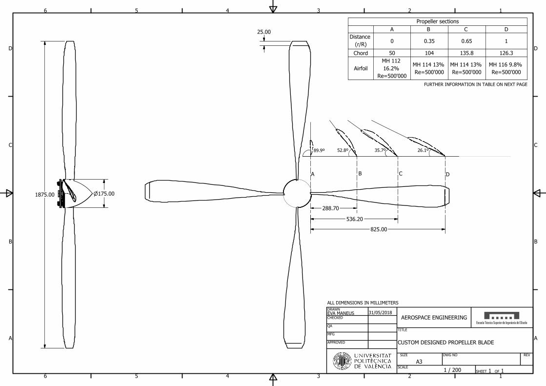
1
1
2
2
3
3
4
4
5
5
6
6
A A
B B
C C
D D
DRAWN
EVA MANEUS
CHECKED
QA
MFG
APPROVED
31/05/2018
AEROSPACE ENGINEERING
TITLE
CUSTOM DESIGNED PROPELLER BLADE
SIZE
A3
SCALE
DWG NO REV
SHEET 1 OF 1
1 / 200
89.9º52.8º 35.7º 26.1º
825.00
D
CB
A
ALL DIMENSIONS IN MILLIMETERS
Propeller sections
A B C D
Distance
(r/R)
0 0.35 0.65 1
Chord 50 104 135.8 126.3
Airfoil
MH 112
16.2%
Re=500'000
MH 114 13%
Re=500'000
MH 114 13%
Re=500'000
MH 116 9.8%
Re=500'000
288.70
536.20
FURTHER INFORMATION IN TABLE ON NEXT PAGE
175.00
1875.00
25.00
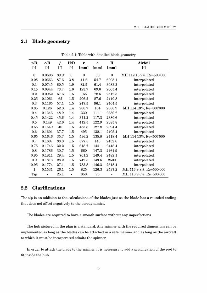
2.1. BLADE GEOMETRY
2.1 Blade geometry
Table 2.1: Table with detailed blade geometry
r/R c/R β H/D r c H Airfoil[-] [-] [] [-] [mm] [mm] [mm] [-]
0 0.0606 89.9 0 0 50 0 MH 112 16.2%, Re=500’0000.05 0.0663 87.6 3.8 41.2 54.7 6208.1 interpolated0.1 0.0745 80.5 1.9 82.5 61.4 3083.3 interpolated
0.15 0.0844 73.7 1.6 123.7 69.6 2665.4 interpolated0.2 0.0952 67.6 1.5 165 78.6 2512.5 interpolated
0.25 0.1061 62 1.5 206.2 87.6 2440.8 interpolated0.3 0.1165 57.1 1.5 247.5 96.1 2404.5 interpolated
0.35 0.126 52.8 1.4 288.7 104 2386.9 MH 114 13%, Re=500’0000.4 0.1346 48.9 1.4 330 111.1 2380.2 interpolated
0.45 0.1422 45.6 1.4 371.2 117.3 2380.6 interpolated0.5 0.149 42.6 1.4 412.5 122.9 2385.8 interpolated
0.55 0.1549 40 1.5 453.8 127.8 2394.4 interpolated0.6 0.1601 37.7 1.5 495 132.1 2405.4 interpolated
0.65 0.1646 35.7 1.5 536.2 135.8 2418.4 MH 114 13%, Re=500’0000.7 0.1697 33.8 1.5 577.5 140 2432.8 interpolated
0.75 0.1746 32.2 1.5 618.7 144.1 2448.4 interpolated0.8 0.1786 30.7 1.5 660 147.3 2464.9 interpolated
0.85 0.1811 29.4 1.5 701.2 149.4 2482.1 interpolated0.9 0.1813 28.2 1.5 742.5 149.6 2500 interpolated
0.95 0.1774 27.1 1.5 783.8 146.3 2518.4 interpolated1 0.1531 26.1 1.5 825 126.3 2537.2 MH 116 9.8%, Re=500’000
Tip - 25.1 - 850 95 - MH 116 9.8%, Re=500’000
2.2 Clarifications
The tip is an addition to the calculations of the blades just so the blade has a rounded ending
that does not affect negatively to the aerodynamics.
The blades are required to have a smooth surface without any imperfections.
The hub pictured in the plan is a standard. Any spinner with the required dimensions can be
implemented as long as the blades can be attached in a safe manner and as long as the aircraft
to which it must be incorporated admits the spinner.
In order to attach the blade to the spinner, it is necessary to add a prolongation of the root to
fit inside the hub.
5

CH
AP
TE
R
3MOTOR WIRING PLANS
In the next pages, the plans and explanations for the installation of the motor control and the
batteries are presented, as well as the alternative battery system to power the electronics
on-board. The calculations for the cable sections involved in the propulsion were performed
and the results are included in a table, along with clarifications on the conditions assumed.
7

CONVERTERDC DC AC
CONTROLLER
BMS
1
1
2
2
3
3
4
4
5
5
6
6
A A
B B
C C
D D
SHEET 1 OF 1
REV
DRAWN
CHECKED
APPROVED
QA
MFG
DWG NOSIZE
SCALE
TITLE
A3
26/06/2018MANEUS, EVA
PERMANENT MAGNET SYNCHRONOUS MOTOR
CONTROL AND CONNECTIONS
3~
MOT
V
+
-
BAT
8
OL A2
OL C1
OL A1
OL B1
OL B2
OL C2
CB A1
B1
DS
2
2
2
OX
SS ENABLE
R
LT ALARM
21
ENCODER
A1
C1
C2
A2
B2
CB A2
CB B1
CB B2
CB C1
CB C2
OHMS
VR LEVER
TO REFRIGERATION
TO MONITOR
..
150
..
150
..
120
..
120
..
120
..
120
..
120
..
120
NO SCALE
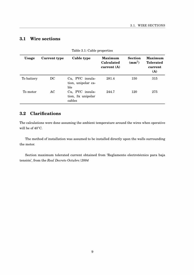
3.1. WIRE SECTIONS
3.1 Wire sections
Table 3.1: Cable properties
Usage Current type Cable type MaximumCalculatedcurrent (A)
Section(mm2)
MaximumToleratedcurrent
(A)
To battery DC Cu, PVC insula-tion, unipolar ca-ble
281.4 150 315
To motor AC Cu, PVC insula-tion, 3x unipolarcables
244.7 120 275
3.2 Clarifications
The calculations were done assuming the ambient temperature around the wires when operative
will be of 40C.
The method of installation was assumed to be installed directly upon the walls surrounding
the motor.
Section maximum tolerated current obtained from ‘Reglamento electrotécnico para baja
tensión’, from the Real Decreto Octubre/2004
9

CONTROLLER
BMS
1
1
2
2
3
3
4
4
5
5
6
6
A A
B B
C C
D D
TITLE
ALTERNATIVE POWER UNIT
SCALE
A3
DWG NOSIZE
25/06/2018
APPROVED
DRAWN
CHECKED
QA
MFG
MANEUS, EVA
SHEET 1 OF 1
REV
V
+
-
BAT
DS
TO COCKPIT INSTRUMENTS
NO SCALE


Control of an electric Propulsion Systemfor a Light Aircraft
Final Year Project
By
EVA MANEUS SALVADOR
Tutor: RAMON MANUEL BLASCO-GIMENEZ
SCHEDULE OF CONDITIONS
Escola Tècnica Superior d’Enginyeria del DissenyUNIVERSITAT POLITÈCNICA DE VALÈNCIA
Final year Project for the BACHELOR DEGREE IN AEROSPACE
ENGINEERING
JUNE 2018

TABLE OF CONTENTS
Page
1 Description of the different works 11.1 Work units . . . . . . . . . . . . . . . . . . . . . . . . . . . . . . . . . . . . . . . . . . . 1
1.1.1 Analysis of requirements and components . . . . . . . . . . . . . . . . . . . . 1
1.1.2 Simulation and testing . . . . . . . . . . . . . . . . . . . . . . . . . . . . . . . 2
2 General conditions 32.1 General provisions . . . . . . . . . . . . . . . . . . . . . . . . . . . . . . . . . . . . . . 3
2.1.1 Documentation on the works contract . . . . . . . . . . . . . . . . . . . . . . 3
2.2 Optional general conditions . . . . . . . . . . . . . . . . . . . . . . . . . . . . . . . . . 4
2.2.1 Functions to develop by the contractor . . . . . . . . . . . . . . . . . . . . . . 4
2.2.2 Functions to develop by the engineering manager . . . . . . . . . . . . . . . 6
2.2.3 Order book . . . . . . . . . . . . . . . . . . . . . . . . . . . . . . . . . . . . . . . 6
2.3 General terms of execution . . . . . . . . . . . . . . . . . . . . . . . . . . . . . . . . . 6
2.3.1 Pace of work . . . . . . . . . . . . . . . . . . . . . . . . . . . . . . . . . . . . . . 6
2.3.2 Order of the works . . . . . . . . . . . . . . . . . . . . . . . . . . . . . . . . . . 7
2.3.3 Extension of the project by unforeseen causes . . . . . . . . . . . . . . . . . . 7
2.3.4 Prorogue due to events of force majeure . . . . . . . . . . . . . . . . . . . . . 7
2.3.5 General conditions of execution of the works . . . . . . . . . . . . . . . . . . 7
2.3.6 Defective works . . . . . . . . . . . . . . . . . . . . . . . . . . . . . . . . . . . . 7
2.3.7 Hidden defects . . . . . . . . . . . . . . . . . . . . . . . . . . . . . . . . . . . . 7
2.3.8 Origin of materials and machinery . . . . . . . . . . . . . . . . . . . . . . . . 8
2.3.9 Defective materials . . . . . . . . . . . . . . . . . . . . . . . . . . . . . . . . . 8
2.3.10 Tests and trials . . . . . . . . . . . . . . . . . . . . . . . . . . . . . . . . . . . . 8
2.3.11 Works without prescriptions . . . . . . . . . . . . . . . . . . . . . . . . . . . . 8
2.3.12 Reception . . . . . . . . . . . . . . . . . . . . . . . . . . . . . . . . . . . . . . . 8
2.3.12.1 Provisional reception . . . . . . . . . . . . . . . . . . . . . . . . . . . 8
2.3.12.2 Final documentation of the works . . . . . . . . . . . . . . . . . . . 9
2.3.12.3 Definitive measurements and provisional validation . . . . . . . . 9
2.3.12.4 Definitive reception . . . . . . . . . . . . . . . . . . . . . . . . . . . 9
i
TABLE OF CONTENTS
2.3.12.5 Extension of the guarantee . . . . . . . . . . . . . . . . . . . . . . . 9
2.3.12.6 Reception of works with a terminated contract . . . . . . . . . . . 9
2.4 General economic conditions . . . . . . . . . . . . . . . . . . . . . . . . . . . . . . . . . 9
2.4.1 General principle . . . . . . . . . . . . . . . . . . . . . . . . . . . . . . . . . . . 9
2.4.2 Prices . . . . . . . . . . . . . . . . . . . . . . . . . . . . . . . . . . . . . . . . . . 10
2.4.2.1 Structure of the pricing . . . . . . . . . . . . . . . . . . . . . . . . . 10
2.4.2.2 Contradictory pricing . . . . . . . . . . . . . . . . . . . . . . . . . . 11
2.4.2.3 Revision of contracted pricing . . . . . . . . . . . . . . . . . . . . . 11
2.4.3 Valuation of the works . . . . . . . . . . . . . . . . . . . . . . . . . . . . . . . . 11
2.4.3.1 Forms of payment . . . . . . . . . . . . . . . . . . . . . . . . . . . . . 11
2.4.3.2 Certificates . . . . . . . . . . . . . . . . . . . . . . . . . . . . . . . . . 12
2.4.3.3 Improvements of the works . . . . . . . . . . . . . . . . . . . . . . . 12
2.4.3.4 Payments . . . . . . . . . . . . . . . . . . . . . . . . . . . . . . . . . . 13
2.4.3.5 Works carried out during the guarantee period . . . . . . . . . . . 13
2.4.4 Penalizations . . . . . . . . . . . . . . . . . . . . . . . . . . . . . . . . . . . . . 13
2.5 General legal conditions . . . . . . . . . . . . . . . . . . . . . . . . . . . . . . . . . . . 13
2.5.1 The contractor . . . . . . . . . . . . . . . . . . . . . . . . . . . . . . . . . . . . 14
2.5.2 The contract . . . . . . . . . . . . . . . . . . . . . . . . . . . . . . . . . . . . . . 15
2.5.3 Arbitration . . . . . . . . . . . . . . . . . . . . . . . . . . . . . . . . . . . . . . . 15
3 Particular conditions 173.1 Group 1: Analysis of requirements and components . . . . . . . . . . . . . . . . . . . 17
3.1.1 Custom propeller design . . . . . . . . . . . . . . . . . . . . . . . . . . . . . . 18
3.1.2 Adequate motor calculation and election . . . . . . . . . . . . . . . . . . . . . 18
3.1.3 Suitable batteries election . . . . . . . . . . . . . . . . . . . . . . . . . . . . . 18
3.2 Group 2: Simulation and testing . . . . . . . . . . . . . . . . . . . . . . . . . . . . . . 18
3.2.1 Controller design . . . . . . . . . . . . . . . . . . . . . . . . . . . . . . . . . . . 19
3.2.2 Mission testing . . . . . . . . . . . . . . . . . . . . . . . . . . . . . . . . . . . . 19
ii
CH
AP
TE
R
1DESCRIPTION OF THE DIFFERENT WORKS
This schedule of conditions describes the different technical, legal and economic aspects
present in this final year project. In this first chapter the different work units will be
stated, with the description in detail being in the next chapters of this document.
1.1 Work units
The work units can be separated into two differentiated groups, with these groups being listed
following:
• Analysis of requirements and components
• Simulation and testing
1.1.1 Analysis of requirements and components
This functional group includes the parts to the project which involve research and design of the
components that will ultimately compose the propulsion system in the modified electrical aircraft.
This group can be broken down into several work units:
• Custom propeller design
• Adequate motor calculation and election
• Suitable batteries
1

CHAPTER 1. DESCRIPTION OF THE DIFFERENT WORKS
1.1.2 Simulation and testing
This functional group connects the components find in the previous group between them to finally
implement the necessary controls to assemble a simulation which can fully function and be ran
to test the whole process is indeed working well.
The different work units to this group are:
• Controller design
• Mission testing
2
CH
AP
TE
R
2GENERAL CONDITIONS
2.1 General provisions
This section has the purpose of regulating the execution of the different project units, stating the
responsibilities of each of the parties involved as well as the relationship between the different
parties. Moreover, the distinct legal aspects of the project, as well as its execution conditions will
be described, including but not limited to the properties of the materials to be employed, the
techniques to use, quality controls and laws and regulations that apply to the project.
2.1.1 Documentation on the works contract
The works contract will include the following documents:
• Conditions set on the contracting document
• Schedule of technical conditions
• The present schedule of general conditions
• Remaining project documentation (report, plans and other documents)
Note the instructions of the project managers will be incorporated to the project as an
interpretation of it. In every document of the above listed the written specifications have to be
held in higher regard than the graphic ones and the dimensioning on the plans shall be put
before the direct scale measurements.
3
CHAPTER 2. GENERAL CONDITIONS
2.2 Optional general conditions
This section describes the relation between the contractor part and the project manager for the
execution of the project units.
2.2.1 Functions to develop by the contractor
It is of the contractor’s responsibility:
• Organize the different parts to the project, develop any necessary construction plans and
authorise the auxiliary and temporary installations for the works.
• Follow and make follow the actual regulations on safety and hygiene in the workplace.
• Serve as the manager to every party involved in the project and likewise coordinate any
intervention of subcontractors.
• Revise and certify the validity of any material used, refusing to use any which are not
subject to the current regulation or the present schedule of conditions.
• Carry the order book and of the project. Make a register of notes done upon it to be applied
on the project.
• Provide the project management with any necessary materials to ease their task.
• Prepare the partial work certifications and the settlement proposal.
• Along with the certificate promotes, prepare the provisional and final reception certificates.
• Subscribe to accident and third-party damage insurances.
• Know the law and verify the project documents. The constructor shall indicate the project
documentation is sufficient for the complete understanding of the project or demand
clarification if otherwise.
• Elaborate the safety and hygiene plan for its approval by the project management.
• Provide offices for plan consulting and for project management tasks. The offices will hold
the work permit, the complete project of execution, the order book the safety and hygiene
plan, the incident book and the insurance documentation.
• The constructor shall communicate the person designated as a deputy, which should assume
the constructor’s functions.
• The works manager, or some attendants, shall be present throughout the working time
and keep company of the engineer or the quantity surveyor and provide precise data for
dimension checking
4
2.2. OPTIONAL GENERAL CONDITIONS
• The contract shall do all that is needed to achieve the good construction and aspect of the
works, even when these are not specifically required, whenever the engineer says so, always
inside the budget limits.
• Any variation that will result in an increment of more than 20 percent on the price of a
work unit or more than 10 percent of the whole budget shall require the redoing of the
project.
• Clarifications, interpretations or modifications of any precept of the schedule of conditions
or any indication on the plans shall be communicated in writing to the constructor, whom
shall return the original papers with a sign on the side of every instruction, order or notice
received.
• The constructor can require from the engineer or the quantity surveyor or technical engineer
whichever instructions or clarifications shall be necessary for the correct execution of the
project. At the same time, solutions for any unaccounted problems throughout the project
shall be provided.
• The contractor complaints against orders or instructions of the project management will
be presented by the engineer, if they are of economic nature, and always following the
corresponding schedule of conditions. Complaints against orders or instructions of tech-
nical nature shall not be taken into account, but the contractor is allowed to expose in a
reasonable manner, although the engineer can limit the answer to an acknowledgement.
• The contractor shall not disallow the engineer, quality surveyor or technical engineer
or designated attendants, neither ask for the designation of other professionals for the
acknowledgements or measurements.
• In the case of unruliness, incompetence or gross negligence that might severely affect the
project execution, the engineer can require the contractor to disallow the workers whom
caused it.
• The contractor can outsource work units attaining the conditions numbered in the schedule
of conditions without it affecting his or her responsibilities as the general contractor of the
project.
• The contractor shall not initiate a work unit without the director’s authorisation.
• The contractor is required to follow the indications in the orders book.
5
CHAPTER 2. GENERAL CONDITIONS
2.2.2 Functions to develop by the engineering manager
The engineering manager is the leading manager of the project execution; ruling the starting, the
pace and the quality of the works. Will assure the complying with the aforementioned and the
safety conditions of the project workers.
The functions reserved for the engineering manager are:
• Compose the supplements or rectifications to the project when necessary.
• Assist the works any time their nature and complexity require so in order to solve the
contingencies produced and hand out necessary instructions.
• Coordinate the intervention on the project of other technicians.
• Approve partial work certificates, expedite and subscribe along with the quality supervisor
or technical engineer the final certificate of the project.
• Pass partial project certificates, the final settlement and counsel the promoter on the
reception ceremony.
• Check on provisional installations, support facilities and safety and hygiene systems in the
workplace.
• Arrange and manage the execution following the project, technical standards and ruling for
a good construction.
• Perform or have disposition of the tests and trials of materials, installations and other
units of work following the control plan as well as any necessary monitoring to assure the
quality matches the project expectations and the applicable technical standards.
• Inform the constructor of the test results and give necessary instructions.
• Plan the quality control and economic control of the works.
2.2.3 Order book
It is mandatory for there to be at the working site a book of orders and incidences, reviewed
by the corresponding professional collegiates, which shall include the order and modifications
applied.
2.3 General terms of execution
2.3.1 Pace of work
The installer or contractor will initiate the works in within the period stated in the schedule
of particular conditions, pacing the works so they are finished within the established partial
6
2.3. GENERAL TERMS OF EXECUTION
periods in order to complete the work in the time limit stated in the contract. The contractor will
communicate the engineer by writing the initiation of the works, at least, three days in advance.
2.3.2 Order of the works
The determination of the order of the works is for the contractor to decide, excepting cases
in which due to technical circumstances it is deemed convenient to be varied by the project
management.
2.3.3 Extension of the project by unforeseen causes
When the works are to be extended, either by unforesen causes or events of force majeure, works
will not be interrupted, being continued according to instructions handed by the engineer whilst
the project is being posed or being processed. The constructor shall carry out any necessary works
of urgent nature, in anticipation, which will be consigned in an additional budget or paid directly.
2.3.4 Prorogue due to events of force majeure
If due to events of force majeure or independently from the constructor’s will to commence the
works could not be initiated, or were suspended, o were not finished within the established period,
a prorogue will be granted to fulfil the contract if the engineer authorises to do so.
2.3.5 General conditions of execution of the works
The works shall be executed strictly following the project guidelines, the modifications to it that
might have been approved and the orders and instructions that are handed in writing under the
engineer, the quality surveyor or the technical engineer’s responsibility.
2.3.6 Defective works
The constructor shall employ material which comply with the general and particular technical
conditions stated in the schedule of conditions and perform the works following what is specified
in said document. Until the definitive reception, the constructor is responsible of execution and of
any defects that might appear from a bad execution. Whenever the engineer, the quality surveyor
or the technical engineer note defects in the works, or materials or machinery which do not fulfil
the required condition, before reception of the work defective parts shall be replaced.
2.3.7 Hidden defects
If the quality surveyor has justified reasons to believe hidden defects exist in the construction,
before the definitive reception the quality surveyor shall require tests and trials deemed appropri-
7
CHAPTER 2. GENERAL CONDITIONS
ate to be performed on the works considered defective. The tests shall be pais by the constructor,
if it exists, and the proprietor, in absence of the former.
2.3.8 Origin of materials and machinery
The constructor shall provide necessary material and machinery of every type on the points
deemed convenient except in cases in which the schedule of conditions states a determinate
provenance. The constructor shall inform the quality surveyor of the suitability and provenance
of the materials and machinery. If the engineer requires so, the constructor will exhibit samples
of the materials.
2.3.9 Defective materials
The engineer, at the request of the quality surveyor, will order the constructor to replace the
defective materials and machinery with others which meet the quality conditions in the present
schedule. If the constructor would not comply, the proprietor would do so, charging the expenses
on the contractor.
2.3.10 Tests and trials
The expenses derived from test and trials are to be paid by the contractor, with the possibility of
those which do not bear enough guarantees to be repeated. The tests for each installation are
specified in the chapter for said installation.
2.3.11 Works without prescriptions
In those works in which no prescriptions exist in the present schedule of conditions nor in the
remaining documentation, the constructor shall follow the instructions dictated by the project
management.
2.3.12 Reception
2.3.12.1 Provisional reception
Three days prior to the completion of the works, the engineer will communicate the proprietor
the proximity of the finalisation date in order to agree upon a date for the provisional reception.
This shall be done with the participation of the proprietor, the quality surveyor, the constructor
and the engineer. A detailed examination of the works shall be performed, and a certificate will
be handed out to each participant, being signed by all of them. From this date, the guarantee
period starts if the works are accepted. Following, the technicians from the project management
will provide with the finalisation of works certificate. If there existed defects, instructions would
8
2.4. GENERAL ECONOMIC CONDITIONS
be handed to righten said defects, setting a time period in which to do so and after which a new
examination will be carried out.
2.3.12.2 Final documentation of the works
The engineer manager will provide he proprietor with the final documentation which shall include
the specifications and contents arranged by the current legislation.
2.3.12.3 Definitive measurements and provisional validation
Once the works are received, the quality surveyor shall perform the definitive measurements in
the presence of the constructor. The necessary certificates shall be handed out in triplicate, which
once the engineer has approved of it and signed will serve for the payment of the proprietor of
the remaining balance minus the deposit quantity.
2.3.12.4 Definitive reception
The works will be verified after the guarantee period, which will be stated in the schedule of
particular conditions and will not be under nine months. The way to proceed will be the same
as for the provisional case. After the guarantee period, the constructor is no longer expected to
repair any damages due to the normal conservation of the works.
2.3.12.5 Extension of the guarantee
If the works do not meet the required conditions the definitive reception shall be postponed
and the engineer shall indicate the constructor the terms in which the necessary works shall
be performed. If these time periods were not followed, the constructor shall lose the amount of
deposit.
2.3.12.6 Reception of works with a terminated contract
In the event of contract termination, the contractor shall take away the tools, support facilities,
etc. Within the term set in the schedule of conditions the workplace shall be left in the adequate
conditions so as the work can be resumed by another company. The finished works shall be
received provisionally and definitively once the guarantee period is over.
2.4 General economic conditions
2.4.1 General principle
This section the economic regulations are described and regulated between the proprietor and the
contractor, as well as the control functions of the project management. Every person intervening
9
CHAPTER 2. GENERAL CONDITIONS
in the work process are in their right of promptly receiving the quantities according to their
actuations as stated in the contract. The proprietor, the contractor and the technicians are
allowed to demand from one another the adequate guarantees to comply with their contractual
obligations regarding payments.
The contractor shall provide the following deposits:
• Cash deposit or bank guarantee of an amount of 10 percent of the total price of the contract,
except if other is stated in the contract.
• Withholding of 5% in the partial certificates or payments being done.
Any penalizations for delays will be covered by the deposit and the repairs will be covered by
the contractor company.
If the contractor refused to complete the necessary work to finish off the project in the conditions
stated in the contract, the engineer in representation of the proprietor will order its finalisation
to another company, paying with the deposit amount, without the actions the proprietor will take
if the deposit does not cover the totality of the works being limiting. The deposit shall be returned
to the contractor within a time period no greater than thirty days after the work finalisation
certificate is signed. The proprietor has the right to demand the contractor proves settlement of
payments and the payment of balance caused by the works.
2.4.2 Prices
2.4.2.1 Structure of the pricing
The calculation of prices comes as a result of adding up the direct and indirect costs, the generated
expenses and the industrial profit.
The direct costs are:
• Labour, with bonuses, charges and social insurances which directly intervene.
• Materials at the prices paid for the project, necessary for the intervention.
• Equipment and safety and hygiene technical systems ofor prevention and protection of
accidents.
• Personnel expenses, fuel and energy derived from machinery functioning and installations
used in the execution of the works.
• Deprecation costs and conservation costs of machinery, installations, systems and equip-
ment.
Indirect costs are:
10
2.4. GENERAL ECONOMIC CONDITIONS
• Costs of installation of offices in the working site, communications, setting warehouses,
workshops, administrative staff affiliated. They are represented as a percentage of direct
and indirect costs.
The industrial benefit:
• The contractor profit is established as a 6 percent of the sum of the aforementioned costs.
Price of physical construction:
• The result of the addition of the aforementioned excepting the industrial profit.
The contractor company price:
• Addition of direct and indirect costs and the industrial profit. VAT expenses are applied to
this amount but it does not form part of it.
2.4.2.2 Contradictory pricing
This phenomenon occurs when the proprietor, via the engineer, introduces units or variations in
quality in some of the planned unit or when it becomes necessary to tackle unforeseen events. The
contractor is required to accept the changes. The pricing will be arranged between the contractor
and the engineer prior to commencing the works.
If the contractor does not claim the prices before signing the contract, it is not allowed to claim
a rise in the prices shown in the budget on which serves as a base for the execution afterwards.
2.4.2.3 Revision of contracted pricing
The revision of prices if the increment of the amounts in the units left to complete are not greater
than 3 percent of the total contract budget is not admissible. If the variation is an increase, a
review will be conducted following the steps stated in the schedule of particular conditions. The
contractor receives a difference which resulting from a variation of the CPI over 3 percent. A
review formula system contemplated in the State Laws of Contract shall be applied.
2.4.3 Valuation of the works
2.4.3.1 Forms of payment
Excepting cases where the opposite is indicated in the schedule of particular conditions, the
payments for the work will be done in one of the following ways:
11
CHAPTER 2. GENERAL CONDITIONS
• A fixed rate, incremented an amount for every work unit, with the invariable amount set
beforehand, varying only the units done and applying to the total work units the fixed
amount.
• Floating rates per work unit, depending on the work conditions and materials employed in
the work, dictated by the engineering manager.
• With lists of day wages and receipt of materials used in the way determined by the schedule
of economic conditions.
• By the work hour, following the conditions stated in the contract.
2.4.3.2 Certificates
On each date specified in the contract or in the schedule of particular conditions, tje contractor
will compose a valued relationship of the works executed during the time periods according to
the measures carried by the quality surveyor.
The executed works will be valued applying to the measurement results the prices stated in
the budget for each of the said works, considering also what is stated in the general schedule of
economic conditions respecting improvements or substitutions of materials.
The contractor may be present when performing the necessary measurements for the elab-
oration of the relationship, similarly, the quality surveyor or the technical engineer will send
the contractor the results of the measurements so as they can be examined and returned signed
or file claims if deemed opportune. The engineer will accept or reject the claims, letting the
contractor know the decision. The contractor is then allowed to claim the proprietor on the
engineer’s settlement.
Parting from the valued relationship, the engineer will complete the certification of the
executed work. This certification will be sent to the proprietor in a time period under a month
after the date referenced in the certificate and will have a status of document which is subject to
variations resulting from the final settlement, without this certificate meaning the approval or
reception of the works mentioned in them.
2.4.3.3 Improvements of the works
In the case the contractor, even with the authorisation of the engineering manager, employs
materials of higher quality, of higher price or works of bigger dimension, the difference in price
will only be paid if the works were completed following the planning.
12
2.5. GENERAL LEGAL CONDITIONS
2.4.3.4 Payments
The payments will be done by the proprietor in the terms previously established and the amounts
will correspond those of the work certificates accepted by the engineering manager.
2.4.3.5 Works carried out during the guarantee period
The payment of this works will be done in the following manner:
• If the works are stated in the project and were not completed in the stated time period
they will be valued with the prices which appear in the budget and paid following what is
established in the project.
• If the works’ finality is a repairing the damages derived from usage, they will be paid the
price of the day previously agreed upon.
• If the purpose of the works is repairing flaws or defects caused by the installation or quality
of the materials, the contractor will be paid no amount.
2.4.4 Penalizations
There exist three types of penalizations, due to a delay in the execution, due to a non-compliance
of the contract and due to a delay in the payments.
• Due to a delay in the completion. The compensation due to unjustified delay in the com-
pletion of the works will be a 10 per thousand of the total amount of the contracted works
for every calendar day delayed after the termination date agreed upon. This quantity will
be deducted and withheld from the deposit. The days lost due to forces majeures such as
strikes, natural disasters or administrative causes.
• Penalisation due to non-compliance with the contract. It will be established in the contract
how the non-compliance or the bad execution of the works is penalised. If the proprietor will
not pay the stated amount within the next month of the period agreed upon, the contractor
will have the right to receive a four and a half percent annually as interest charges. If the
delay is extended to two months after the finalisation of said period, the contractor is in the
right of terminating the contract, and settling the executed works.
2.5 General legal conditions
Both parts agree upon letting conflict managers solve any matters.
13
CHAPTER 2. GENERAL CONDITIONS
2.5.1 The contractor
The contractor is responsible upon the works being executed under the conditions established in
the contract and in the project documents, excluding the report. Therefore, it is mandatory to
undo and redo anything that has been badly done during the works, including cases in which the
units have been already paid. Similarly, it is mandatory to follow what is stated in the Contract
of Employment law and written under the section of accidents at work, family allowances and
social insurance.
The contractor is held accountable for the accidents that might occur due to inexperience or
neglect on the work site and its surrounding. The contractor will be the only accountable and
must take charge of compensations given insurance expenses and safety measures are included
in the price. It is under the contractors responsibility to pay for taxes and excise duties which
must be paid during the time the works are being carried out.
The contractor has the right to produce copies of the plans, budgets, schedule of conditions
and other project documents.
The following will cause the termination of the contract:
1. Death or incapacitation of the contractor.
2. Bankruptcy of the contractor.
3. Alterations made to the contract by:
• Modifications to the project which are deemed as fundamental changes by the engi-
neering manager, and whenever a modification accounts for more than a 40% of the
value of any of the modified project units.
• Modifications made to the work units whenever they account for more than 40% of
the modified units.
4. The suspension of the works once started and the delay of more than three months from
the date of the contract award in the start of the works.
5. Not commencing the works within the time period stated in the contract conditions or the
project.
6. The non-compliance of the conditions of the contract when the causes are negligence or are
damaging of the works.
7. The unjustified abandonment of the works
14
2.5. GENERAL LEGAL CONDITIONS
2.5.2 The contract
The contract is established between the proprietor or developer and the contractor. Various
contract modalities exist:
• Fixed price: An amount for the works is agreed upon and shall not be modified though the
volume of the works varies. It is employed in smaller works.
• Contract per work units
2.5.3 Arbitration
Given the case of litigation or disagreement between the proprietor and the contractor, in first
place the project management will be contacted. If this would not put an end to the dispute, each
part will appoint a surveyor which will act on the behalf of the parts. Ultimately, the dispute
shall be solved in court.
15

CH
AP
TE
R
3PARTICULAR CONDITIONS
This chapter’s purpose is describing the technical conditions to which the project shall be
subject to. This means stating the quality controls, the characteristics of the material and
the tests and trials which will be performed. In order to facilitate the reading of this part,
it has been broken into groups and units which are in a chronological order. To be able to start
a group, it is indispensable all the work units of the group before it have been completed. The
division of the work unit and the groups are stated under these lines:
• Analysis of requirements and components
– Custom propeller design
– Adequate motor calculation and election
– Suitable batteries election
• Simulation and testing
– Controller design
– Mission testing
3.1 Group 1: Analysis of requirements and components
This group will require researching and calculating the appropriate components for the substitu-
tion of the propulsion plant in a light aircraft for an electric propulsion system.
17
CHAPTER 3. PARTICULAR CONDITIONS
3.1.1 Custom propeller design
Based on tests performed upon a simulation of the unmodified aircraft in Simulink, the thrust
requirements are found and used in order to design a propeller in JavaProp. This process requires
iteration and analysis of the data obtained before reaching the final design. The final design
must reach the same orders of magnitude the unmodified aircraft reaches. Data of thrust and
power coefficients must be obtained from JavaProp for its use later on in the simulation. Once
the design is complete, it is transferred to a plan using Autocad and Inventor.
3.1.2 Adequate motor calculation and election
The state of the technology regarding electric motors must be studied in order to choose one
which will be suitable: lightweight, powerful and able to be controlled by current. The parameters
of the chosen motor shall be extracted for their use in the simulations.
3.1.3 Suitable batteries election
For this unit the state of the batteries technology must also be revised looking for modern
improvements. The available battery weight must be calculated taking into account the dry
weight of the aircraft after having the engine retired and selecting an appropriate battery weight
bearing in mind the mission of the aircraft. Approximate calculations of the autonomy must be
done taking into account the discharge of the type of battery. The actual batteries must be chosen
attending:
• Their energy density
• The volume they occupy
• The easiness with which they will fit the aircraft’s available space
3.2 Group 2: Simulation and testing
This second group assumes all of the work unit before it have been completed and are well done.
It will consist on testing the performance of the results obtained in the other group so as to
declare the components are valid and fulfil the expectations. Were the results of the test to come
out negative and the group 1 should be modified and tested again. The outcome of the tests and
simulations could be negative, with this meaning it is not actually possible to perform the desired
modifications upon the aircraft being considered and meeting all the requirements at the same
time. This case would require the expectations to be relaxed or the project to be restarted.
18
3.2. GROUP 2: SIMULATION AND TESTING
3.2.1 Controller design
The controller design first requires all the simulation of the propulsion plant to be set up correctly
in Simulink, including all the parameters obtained from the different parts (propeller, motor
and batteries). Once this is completed and functioning, the control law must be designed so as
to control the torque of the motor with the throttle lever. PI controllers have to be designed to
control the currents. The requirements for these PI controllers are:
• Low settling time
• Little overshoot
• Compromise of the two above
Once the PI designers are completed according to the requirements, the simulation must be
tested and proven to work well.
3.2.2 Mission testing
Some missions will be designed to test the validity of the designed electrical propulsion plant.
This missions will test the following:
• The normal functioning of the simulation, of the control law and the controller, and the
suitability of the installation.
• The possibility of recovering after a problem in the electrical motor involving a free fall,
needed for the certification of the modified aircraft.
• Estimating the autonomy during its normal use and deciding whether it is sufficient.
If any of the tests above would not fulfil the expectations set for the particular modification, a
process of redoing parts of the previous work units shall be started. Again, if several iterations
were performed and the desired results are not achieved, it could be a matter of relaxing
constraints or admitting the inconvenience of the modification for that particular aircraft for the
particular requirements.
19


Control of an electric Propulsion Systemfor a Light Aircraft
Final Year Project
By
EVA MANEUS SALVADOR
Tutor: RAMON MANUEL BLASCO-GIMENEZ
BUDGET
Escola Tècnica Superior d’Enginyeria del DissenyUNIVERSITAT POLITÈCNICA DE VALÈNCIA
Final year Project for the BACHELOR DEGREE IN AEROSPACE
ENGINEERING
JUNE 2018

TABLE OF CONTENTS
Page
1 Introduction 1
2 Break-down of costs 32.1 Cost of labour hours . . . . . . . . . . . . . . . . . . . . . . . . . . . . . . . . . . . . . . 3
2.2 Cost of materials employed . . . . . . . . . . . . . . . . . . . . . . . . . . . . . . . . . 3
2.3 Cost per project part . . . . . . . . . . . . . . . . . . . . . . . . . . . . . . . . . . . . . 4
2.3.1 Estimation of work hours . . . . . . . . . . . . . . . . . . . . . . . . . . . . . . 4
2.3.1.1 Analysis of requirements and components . . . . . . . . . . . . . . 4
2.3.1.2 Simulation and testing . . . . . . . . . . . . . . . . . . . . . . . . . 5
2.3.2 Amounts . . . . . . . . . . . . . . . . . . . . . . . . . . . . . . . . . . . . . . . . 6
2.3.2.1 Analysis of requirements and components . . . . . . . . . . . . . . 6
2.3.2.2 Simulation and testing . . . . . . . . . . . . . . . . . . . . . . . . . 6
3 Partial budget 93.1 Analysis of requirements and components . . . . . . . . . . . . . . . . . . . . . . . . 9
3.2 Simulation and testing . . . . . . . . . . . . . . . . . . . . . . . . . . . . . . . . . . . . 9
4 Costs of material execution, project administration and investment budgets 11
i


CH
AP
TE
R
1INTRODUCTION
This document’s purpose is to provide all necessary information regarding the funding of
the program developed in the ‘REPORT’ of this final year project. This part will include
the costs of analysis and design of the mentioned project, divided into 5 differentiated
project units. These project units, put into two major functional groups are:
• Analysis of requirements and components
– Custom propeller design
– Adequate motor calculation and election
– Suitable batteries
• Simulation and testing
– Controller design
– Mission testing
The estimated costs will be calculated for each of these project units and the overall costs for
each group will be stated. The calculations will include the estimated costs of labour hours as
well as materials and software.
1

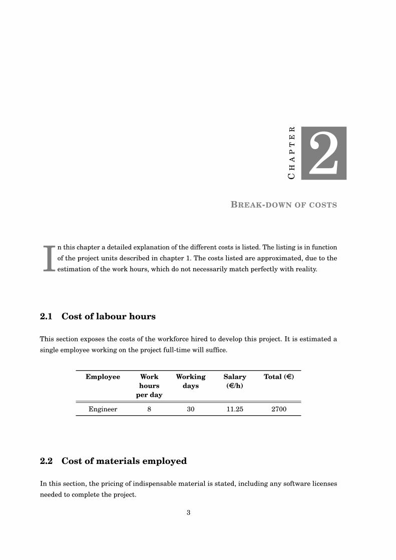
CH
AP
TE
R
2BREAK-DOWN OF COSTS
In this chapter a detailed explanation of the different costs is listed. The listing is in function
of the project units described in chapter 1. The costs listed are approximated, due to the
estimation of the work hours, which do not necessarily match perfectly with reality.
2.1 Cost of labour hours
This section exposes the costs of the workforce hired to develop this project. It is estimated a
single employee working on the project full-time will suffice.
Employee Workhours
per day
Workingdays
Salary(e/h)
Total (e)
Engineer 8 30 11.25 2700
2.2 Cost of materials employed
In this section, the pricing of indispensable material is stated, including any software licenses
needed to complete the project.
3
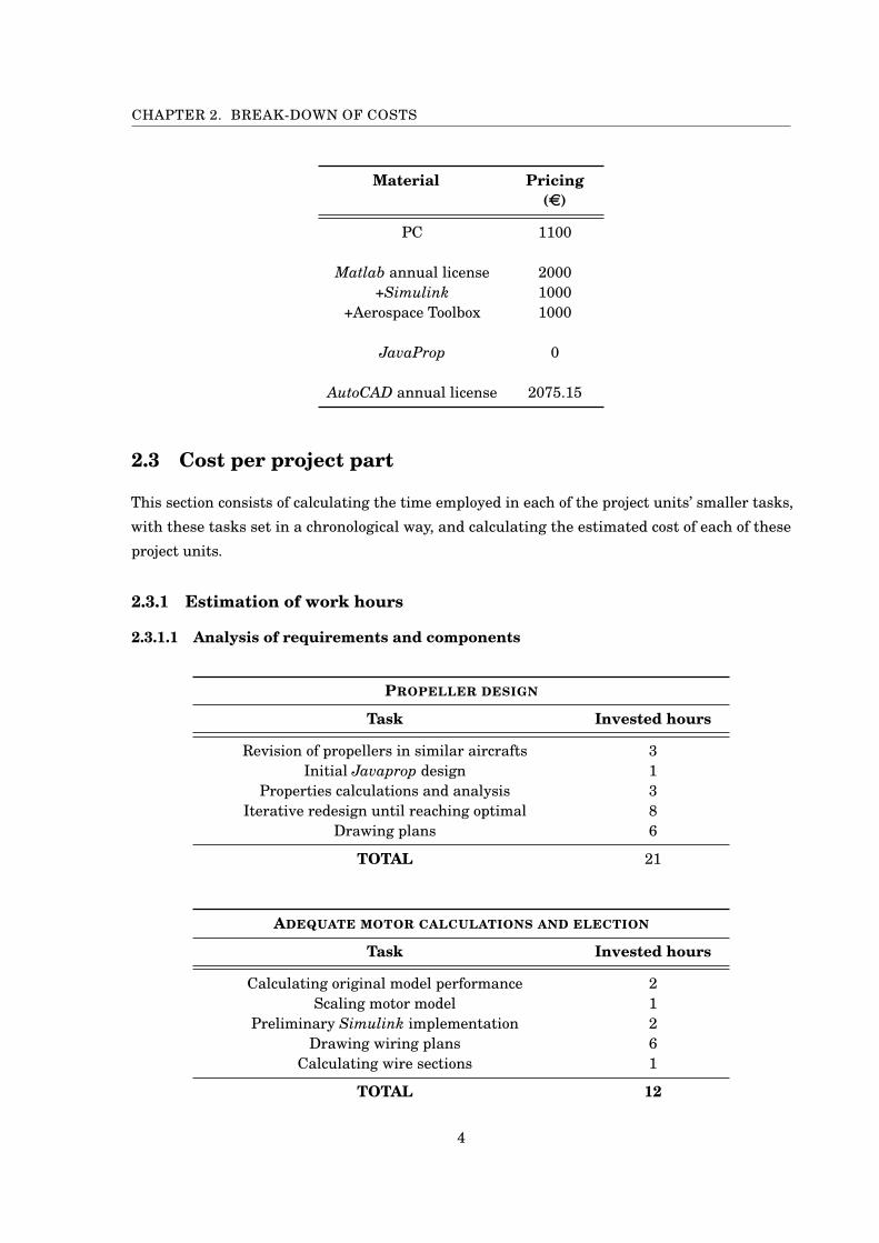
CHAPTER 2. BREAK-DOWN OF COSTS
Material Pricing(e)
PC 1100
Matlab annual license 2000+Simulink 1000
+Aerospace Toolbox 1000
JavaProp 0
AutoCAD annual license 2075.15
2.3 Cost per project part
This section consists of calculating the time employed in each of the project units’ smaller tasks,
with these tasks set in a chronological way, and calculating the estimated cost of each of these
project units.
2.3.1 Estimation of work hours
2.3.1.1 Analysis of requirements and components
PROPELLER DESIGN
Task Invested hours
Revision of propellers in similar aircrafts 3Initial Javaprop design 1
Properties calculations and analysis 3Iterative redesign until reaching optimal 8
Drawing plans 6
TOTAL 21
ADEQUATE MOTOR CALCULATIONS AND ELECTION
Task Invested hours
Calculating original model performance 2Scaling motor model 1
Preliminary Simulink implementation 2Drawing wiring plans 6
Calculating wire sections 1
TOTAL 12
4
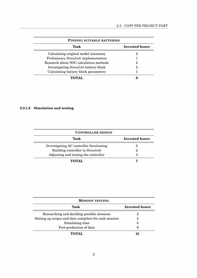
2.3. COST PER PROJECT PART
FINDING SUITABLE BATTERIES
Task Invested hours
Calculating original model autonomy 2Preliminary Simulink implementation 1
Research about SOC calculation methods 2Investigating Simulink battery block 2Calculating battery block parameters 1
TOTAL 9
2.3.1.2 Simulation and testing
CONTROLLER DESIGN
Task Invested hours
Investigating AC controller functioning 2Building controller in Simulink 2
Adjusting and testing the controller 3
TOTAL 7
MISSION TESTING
Task Invested hours
Researching and deciding possible missions 2Setting up scopes and data compilers for each mission 3
Simulating time 8Post-production of data 8
TOTAL 21
5
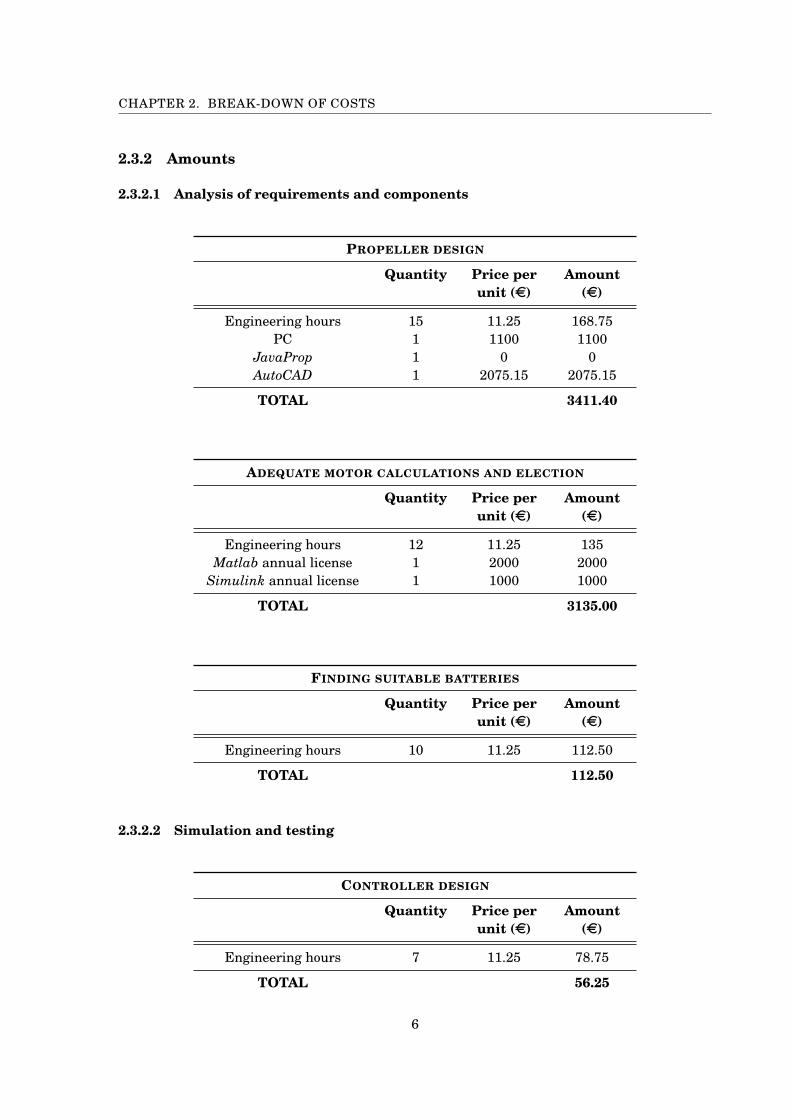
CHAPTER 2. BREAK-DOWN OF COSTS
2.3.2 Amounts
2.3.2.1 Analysis of requirements and components
PROPELLER DESIGN
Quantity Price perunit (e)
Amount(e)
Engineering hours 15 11.25 168.75PC 1 1100 1100
JavaProp 1 0 0AutoCAD 1 2075.15 2075.15
TOTAL 3411.40
ADEQUATE MOTOR CALCULATIONS AND ELECTION
Quantity Price perunit (e)
Amount(e)
Engineering hours 12 11.25 135Matlab annual license 1 2000 2000
Simulink annual license 1 1000 1000
TOTAL 3135.00
FINDING SUITABLE BATTERIES
Quantity Price perunit (e)
Amount(e)
Engineering hours 10 11.25 112.50
TOTAL 112.50
2.3.2.2 Simulation and testing
CONTROLLER DESIGN
Quantity Price perunit (e)
Amount(e)
Engineering hours 7 11.25 78.75
TOTAL 56.25
6

2.3. COST PER PROJECT PART
MISSION TESTING
Quantity Price perunit (e)
Amount(e)
Engineering hours 21 11.25 213.75
TOTAL 213.75
7

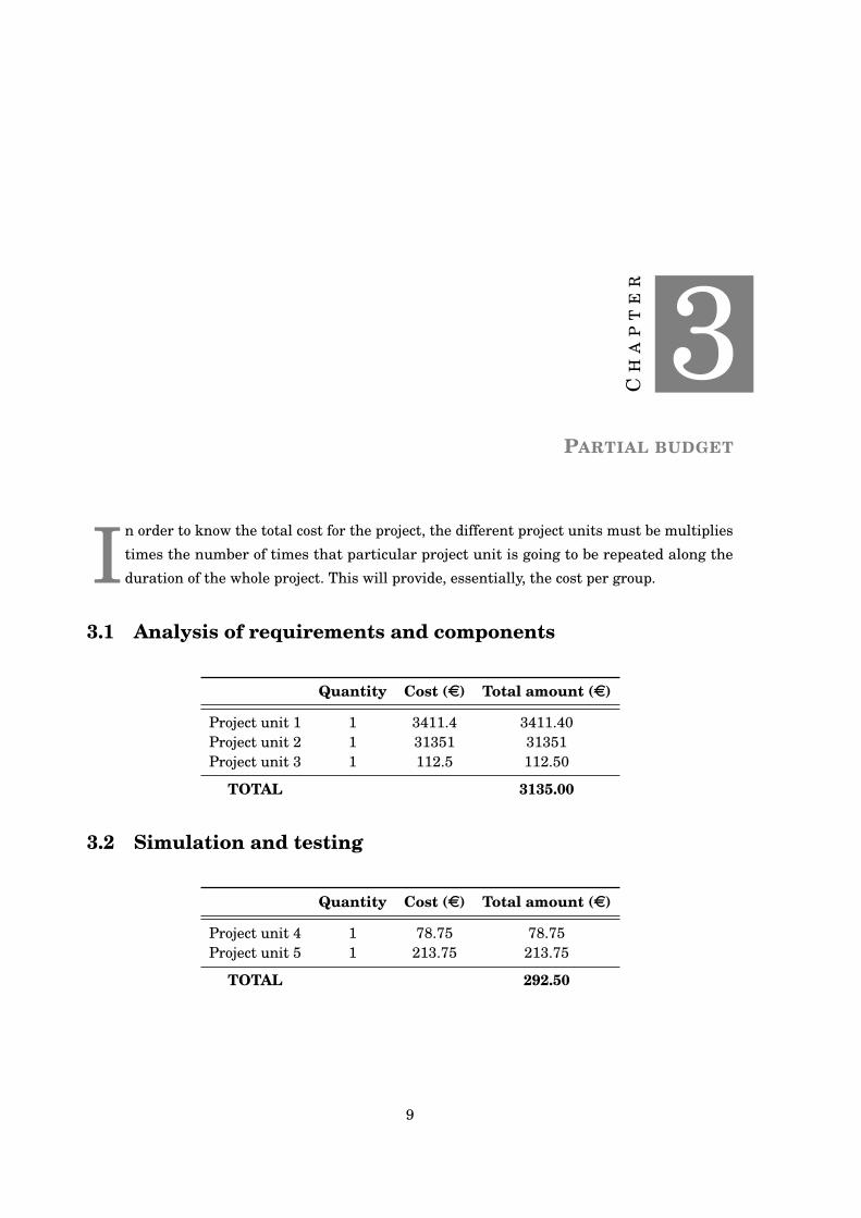
CH
AP
TE
R
3PARTIAL BUDGET
In order to know the total cost for the project, the different project units must be multiplies
times the number of times that particular project unit is going to be repeated along the
duration of the whole project. This will provide, essentially, the cost per group.
3.1 Analysis of requirements and components
Quantity Cost (e) Total amount (e)
Project unit 1 1 3411.4 3411.40Project unit 2 1 31351 31351Project unit 3 1 112.5 112.50
TOTAL 3135.00
3.2 Simulation and testing
Quantity Cost (e) Total amount (e)
Project unit 4 1 78.75 78.75Project unit 5 1 213.75 213.75
TOTAL 292.50
9

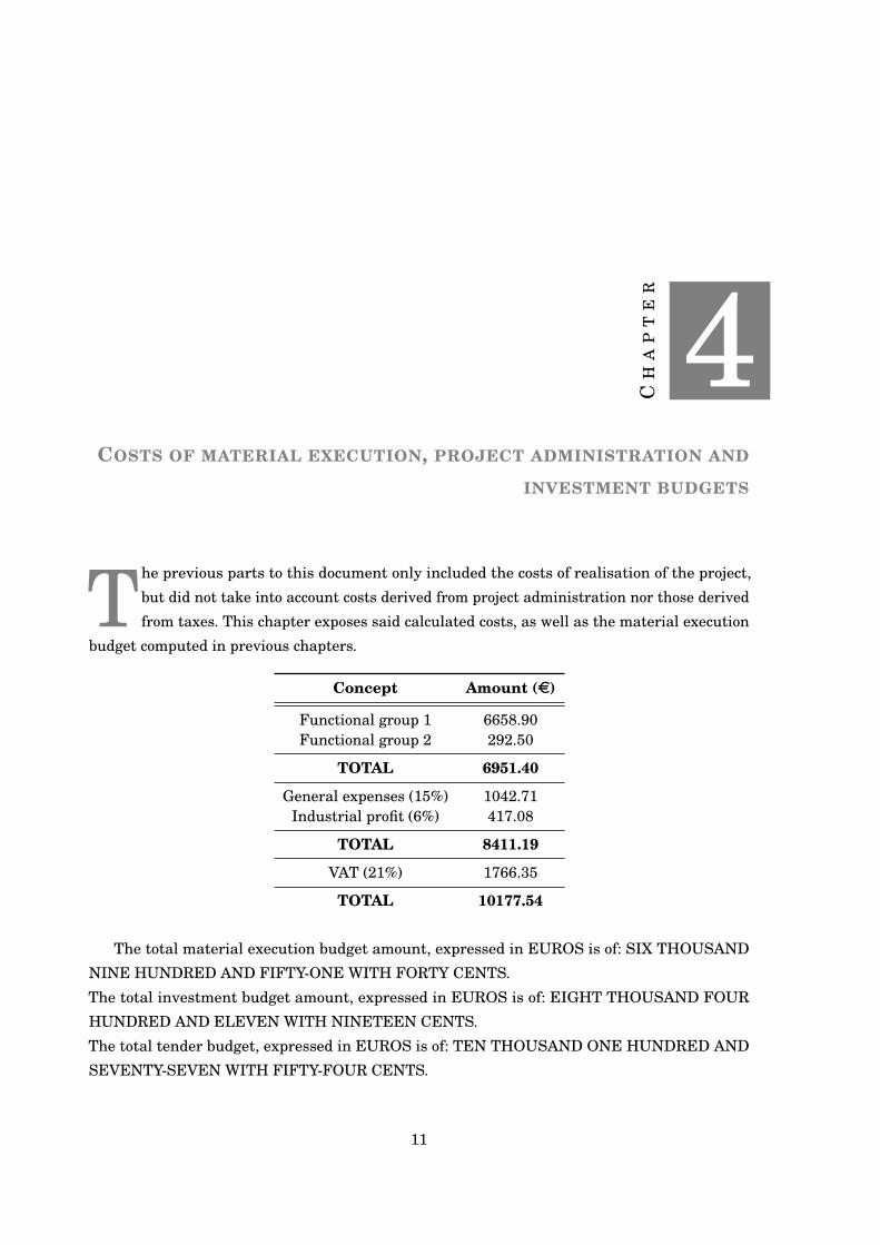
CH
AP
TE
R
4COSTS OF MATERIAL EXECUTION, PROJECT ADMINISTRATION AND
INVESTMENT BUDGETS
The previous parts to this document only included the costs of realisation of the project,
but did not take into account costs derived from project administration nor those derived
from taxes. This chapter exposes said calculated costs, as well as the material execution
budget computed in previous chapters.
Concept Amount (e)
Functional group 1 6658.90Functional group 2 292.50
TOTAL 6951.40
General expenses (15%) 1042.71Industrial profit (6%) 417.08
TOTAL 8411.19
VAT (21%) 1766.35
TOTAL 10177.54
The total material execution budget amount, expressed in EUROS is of: SIX THOUSAND
NINE HUNDRED AND FIFTY-ONE WITH FORTY CENTS.
The total investment budget amount, expressed in EUROS is of: EIGHT THOUSAND FOUR
HUNDRED AND ELEVEN WITH NINETEEN CENTS.
The total tender budget, expressed in EUROS is of: TEN THOUSAND ONE HUNDRED AND
SEVENTY-SEVEN WITH FIFTY-FOUR CENTS.
11
Related Documents