Control Flow Analysis for Brane Calculi

Control Flow Analysis for Brane Calculi

Chiara Bodei1, Andrea Bracciali1 and Davide Chiarugi2

1 Dipartimento di Informatica, Universita di Pisa,Via Pontecorvo, 3 - 56127 Pisa - Italia

{chiara,braccia}@di.unipi.it2 Dipartimento di Scienze Matematiche e Informatiche, Universita di Siena,

Pian dei Mantellini, 4 - 53100 Siena - [email protected]

Abstract

We introduce a Control Flow Analysis for Brane Calculi. This verification technique allows propertiesregarding the behaviour of biological systems to be checked. This is an approximate technique that focusseson the static specification of a system, rather than on its dynamics, striving for effectiveness. Examplesillustrate the approach.

Keywords: Brane calculi, control flow analysis, systems biology

1 Introduction

Systems biology gives computer scientists the opportunity of providing models andformalisms for describing and analysing complex biological systems. In this regard,well established and founded theories and techniques from formal methods offer afertile ground.

The underlying idea is that a biological system can be abstractly modelled asa concurrent system [18]. Several approaches – developed to predict the dynamicbehaviour of the modelled systems – have introduced the idea of performing in silicoexperiments to establish which in vitro experiments are more promising.

The behaviour of a system is usually given in terms of its transition system,whose size can be huge, making its exploration computationally hard. Resortingto static techniques offers the possibility of drastically reducing the computationalcosts, particular high when modelling complex biological systems. The specificationof the system is statically analysed in order to obtain information on the dynamicbehaviour and to check the related dynamic properties, without actually exploringthe whole state space of the associated transition system. The price to be paid is aloss in precision, because usually these techniques can only approximate the actual

Electronic Notes in Theoretical Computer Science 227 (2009) 59–75

1571-0661/$ – see front matter © 2008 Elsevier B.V. All rights reserved.

www.elsevier.com/locate/entcs

doi:10.1016/j.entcs.2008.12.104

http://www.elsevier.com/locate/entcs

behaviour. Static analysis can be exploited for a sort of preliminary screeningof the in silico experiments by efficiently testing different hypothesis and rapidlyidentifying which in vitro experiments worth to be performed. We first introduce aControl Flow Analysis for the version of Brane Calculi [6,7], called MBD and basedon the operations for membrane fusion and splitting. Afterwards, we extend theframework, in order to include also the PEP actions that represent the operationsmodeling endocytosis and exocytosis. The analysis offers predictions on the contentsof membranes: which membranes can be contained in the analysed one and whichactions can affect it. This information offers a basis for studying dynamic properties,by suitably handling the over-approximation the static analysis introduces. Havinga safe over-approximation of the exact behaviour of a system means that all thevalid behaviour are captured. More precisely, all those events that the predictiondoes not include will never happen, while when included, the events can happen,i.e. they are only possible.

We apply our analysis to two simple examples: (1) a model of the infection dueto membrane enveloped viruses, recalling in particular the Semliki Forest Virus [6]and (2) a model of communication via mobile vesicles [19].

The paper follows the tradition initiated by [12,13] and continued with [15,16,3]of applying static techniques and, in particular, Control Flow Analysis to processcalculi used for modelling biological phenomena. Our choice of the Brane calculidepends on the fact they have resulted to be particularly useful for modelling andreasoning about a large class of biological systems, such as the one of the eukaryioticcells that, differently from the prokaryiotes, possess a set of internal membranes.Other applications of static analysis techniques have been proposed, like the Ab-stract Interpretation for BioAmbient in [10]. In a different context, the behaviour ofprocesses is safely approximated and the properties of a fragment of ComputationTree Logic preserved. This makes it possible to address temporal properties andtherefore some kinds of causality.

Among the first formalisms used to investigate biological membranes there arethe P Systems [14], introduces by Paun, which formalize distributed parallel com-putations biologically-inspired: a biological system is seen as a complex hierarchicalstructure of nested membranes inspired by the structure of living cells.

Finally, besides Brane, there are other calculi of interest for our approach, thathave been specifically defined for modelling biological structures such as compart-ments and membranes, e.g. κ-calculus [9], Beta Binders [17] and the Calculus ofLooping Sequences [2].

The rest of the paper is organised as follows. In Section 2 we present the MBDversion of Brane Calculi. We introduce the Control Flow Analysis in Section 3. InSection 4 the analysis is extended in order to also treat the PEP actions. In Section5 the new analysis is applied to a model of infective cycle of the Semliki ForestVirus and to a model of communication via a mobile vesicle. Section 6 presentssome concluding remarks. Proofs of theorems and lemmata presented throughoutthe paper are collected in Appendix A.

C. Bodei et al. / Electronic Notes in Theoretical Computer Science 227 (2009) 59–7560

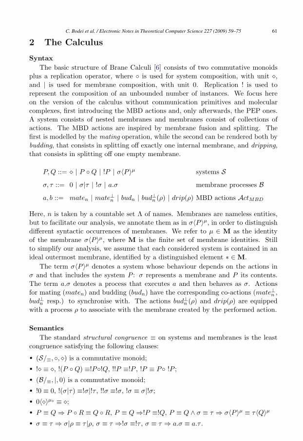
2 The Calculus

SyntaxThe basic structure of Brane Calculi [6] consists of two commutative monoids

plus a replication operator, where ◦ is used for system composition, with unit �,and | is used for membrane composition, with unit 0. Replication ! is used torepresent the composition of an unbounded number of instances. We focus hereon the version of the calculus without communication primitives and molecularcomplexes, first introducing the MBD actions and, only afterwards, the PEP ones.A system consists of nested membranes and membranes consist of collections ofactions. The MBD actions are inspired by membrane fusion and splitting. Thefirst is modelled by the mating operation, while the second can be rendered both bybudding, that consists in splitting off exactly one internal membrane, and dripping,that consists in splitting off one empty membrane.

P,Q ::= � | P ◦ Q | !P | σ〈P 〉μ systems Sσ, τ ::= 0 | σ|τ | !σ | a.σ membrane processes Ba, b ::= maten | mate⊥n | budn | bud⊥n (ρ) | drip(ρ) MBD actions ActMBD

Here, n is taken by a countable set Λ of names. Membranes are nameless entities,but to facilitate our analysis, we annotate them as in σ〈P 〉μ, in order to distinguishdifferent syntactic occurrences of membranes. We refer to μ ∈ M as the identityof the membrane σ〈P 〉μ, where M is the finite set of membrane identities. Stillto simplify our analysis, we assume that each considered system is contained in anideal outermost membrane, identified by a distinguished element ∗ ∈ M.

The term σ〈P 〉μ denotes a system whose behaviour depends on the actions inσ and that includes the system P : σ represents a membrane and P its contents.The term a.σ denotes a process that executes a and then behaves as σ. Actionsfor mating (maten) and budding (budn) have the corresponding co-actions (mate⊥n ,bud⊥n resp.) to synchronise with. The actions bud⊥n (ρ) and drip(ρ) are equippedwith a process ρ to associate with the membrane created by the performed action.

SemanticsThe standard structural congruence ≡ on systems and membranes is the least

congruence satisfying the following clauses:

• (S/≡, ◦, �) is a commutative monoid;• !� ≡ �, !(P ◦ Q) ≡!P◦!Q, !!P ≡!P , !P ≡ P◦ !P ;• (B/≡, |, 0) is a commutative monoid;• !0 ≡ 0, !(σ|τ) ≡!σ|!τ , !!σ ≡!σ, !σ ≡ σ|!σ;• 0〈�〉μ� ≡ �;• P ≡ Q ⇒ P ◦ R ≡ Q ◦ R, P ≡ Q ⇒!P ≡!Q, P ≡ Q ∧ σ ≡ τ ⇒ σ〈P 〉μ ≡ τ〈Q〉μ• σ ≡ τ ⇒ σ|ρ ≡ τ |ρ, σ ≡ τ ⇒!σ ≡!τ , σ ≡ τ ⇒ a.σ ≡ a.τ .

C. Bodei et al. / Electronic Notes in Theoretical Computer Science 227 (2009) 59–75 61

(Par) (Brane) (Struct)P → Q

P ◦ R → Q ◦ R

P → Q

σ〈P 〉μ → σ〈Q〉μP ≡ P ′ ∧ P ′ → Q′ ∧ Q′ ≡ Q

P → Q

(Mate) maten.σ|σ0〈P 〉μP ◦ mate⊥n .τ |τ0〈Q〉μQ → σ|σ0|τ |τ0〈P ◦ Q〉μPQ

where μPQ = MImate(maten, μP , μQ, μ)

and μ identifies the closest membrane surrounding μP and μQ

(Bud) bud⊥n (ρ).τ |τ0〈budn.σ|σ0〈P 〉μP ◦ Q〉μQ → ρ〈σ|σ0〈P 〉μP 〉μR ◦ τ |τ0〈Q〉μQ

where μR = MIbud(budn, μP , μQ, μ)

and μ identifies the closest membrane surrounding μQ

(Drip) drip(ρ).σ|σ0〈P 〉μP → ρ〈〉μR ◦ σ|σ0〈P 〉μP

where μR = MIdrip(drip(ρ), μP , μ)

and μ identifies the closest membrane surrounding μP

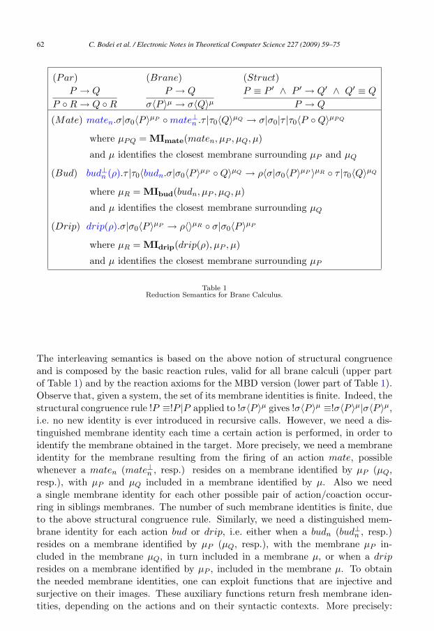
Table 1Reduction Semantics for Brane Calculus.

The interleaving semantics is based on the above notion of structural congruenceand is composed by the basic reaction rules, valid for all brane calculi (upper partof Table 1) and by the reaction axioms for the MBD version (lower part of Table 1).Observe that, given a system, the set of its membrane identities is finite. Indeed, thestructural congruence rule !P ≡!P |P applied to !σ〈P 〉μ gives !σ〈P 〉μ ≡!σ〈P 〉μ|σ〈P 〉μ,i.e. no new identity is ever introduced in recursive calls. However, we need a dis-tinguished membrane identity each time a certain action is performed, in order toidentify the membrane obtained in the target. More precisely, we need a membraneidentity for the membrane resulting from the firing of an action mate, possiblewhenever a maten (mate⊥n , resp.) resides on a membrane identified by μP (μQ,resp.), with μP and μQ included in a membrane identified by μ. Also we needa single membrane identity for each other possible pair of action/coaction occur-ring in siblings membranes. The number of such membrane identities is finite, dueto the above structural congruence rule. Similarly, we need a distinguished mem-brane identity for each action bud or drip, i.e. either when a budn (bud⊥n , resp.)resides on a membrane identified by μP (μQ, resp.), with the membrane μP in-cluded in the membrane μQ, in turn included in a membrane μ, or when a drip

resides on a membrane identified by μP , included in the membrane μ. To obtainthe needed membrane identities, one can exploit functions that are injective andsurjective on their images. These auxiliary functions return fresh membrane iden-tities, depending on the actions and on their syntactic contexts. More precisely:


MImate : ActMBD × M × M × M → M

MIbud : ActMBD × M × M × M → M

MIdrip : ActMBD × M × M → MWe dispense from the actual definition of these functions. We just recall that,given a system, the number of needed membrane identities is finite, as finite are thepossible combinations of actions and contexts. Therefore, we choose M such that,given an action and the identities of the membranes on which the action (and thecorresponding co-action, if any) reside, M includes the membrane identity neededto identify the membrane obtained by firing that action.

3 Control Flow Analysis

We develop a Control Flow Analysis for analysing Brane calculus systems, borrow-ing some ideas from [13]. The aim of the analysis is over-approximating all thepossible behaviour of a Brane system. In particular, our analysis keeps track of thepossible contents of membranes, thus taking care of the possible modifications ofthe containment hierarchy, due to the dynamics. An approximation of the contentsof a membrane or estimate I is defined as

I : M → ℘(M ∪ Act),

where ℘(S) stands for the power-set of the set S and Act is the set of Brane actions.Here, μ′ ∈ I(μ) means that the membrane identified by μ may contain the oneidentified by μ′; a ∈ I(μ) means that the action a may reside on and affect themembrane identified by μ. To validate the correctness of a proposed estimate I,we state a set of clauses operating upon judgements like I |=μ P . This judgementexpresses that when P is enclosed within a membrane identified by μ ∈ M, then Icorrectly captures the behaviour of P , i.e. the estimate is valid also for all the statesQ passed through a computation of P .

Following [13], the analysis is specified in two phases. First, we check that Idescribes the initial process. This is done in Table 2, where the clauses amount to astructural traversal of process syntax. These clauses rely on the following auxiliaryfunction that collects all the actions in a membrane process σ.

Definition 3.1 A : B → Act

• A(0) = ∅;• A(σ|τ) = A(σ) ∪ A(τ);• A(!σ) = A(σ);• A(a.σ) = {a} ∪ A(σ);

Note that the actions collected by A, e.g., in σ = σ0.σ1 are equal to the ones inσ′ = σ0|σ1, witnessing the fact that the analysis is insensitive to the context andintroduces imprecision and approximation.


The clause for membrane system σ〈P 〉μ′checks that whenever a membrane μ′ is

introduced inside a membrane μ, the relative hierarchy position must be reflectedin I, i.e. μ′ ∈ I(μ). Furthermore, the actions in σ that affect the membrane μ′

and that are collected in A(σ), are recorded in I(μ′). Finally, when inspecting thecontent P , the fact that the enclosing membrane is μ′ is recorded, as reflected bythe judgement I |=μ′

P . The rule for � and 0 do not restrict the analysis result,while the rules for parallel composition ◦, and replication ! ensure that the analysisalso holds for the immediate sub-systems, by ensuring their traversal. In particular,the analysis of !P is equal to the one of P . This is another source of imprecision.

Secondly, we check that I also takes into account the dynamics of the processunder consideration; in particular, the dynamics of the containment hierarchy ofmembranes. This is expressed by the closure conditions in the lower part of Table 2that mimic the semantics, by modelling, without exceeding the precision boundariesof the analysis, the semantic preconditions and the consequences of the possibleactions. More precisely, the precondition checks, in terms of I, for the possiblepresence of the redexes necessary for an action to be performed. The conclusionimposes the additional requirements on I, necessary to give a valid prediction of theanalysed action. Consider e.g., the clause for (Mate) (the other clauses are similar).We have to make sure that the precondition requirements are satisfied, i.e. that:

• there exists an occurrence of mate action: maten ∈ I(μP );• there exists an occurrence of the corresponding co-mate action: mate⊥n ∈ I(μQ);• the corresponding membranes must be siblings: μP , μQ ∈ I(μ)

If the precondition requirements are satisfied, then the conclusions of the clauseexpress the consequences of performing the transition mate. In this case, we havethat I must reflect that

• there may exist a membrane μPQ inside μ, with the same father of the membranesμP and μQ: μPQ ∈ I(μ); and that

• the contents of μP and of μQ may also be inside μPQ, and therefore μPQ containsevery membrane that is inside μP or μQ, while each action affecting μP or μQ,affects also μPQ: I(μP ) ∪ I(μQ) ⊆ I(μPQ).

This corresponds to the application of the semantic rule (Mate) that would resultin the fusion of the two membranes.

Example 3.2 We illustrate our analysis on a simple example, taken from [5], ofwhich we report one of the possible steps of computation: the (Mate) one.

(maten|bud⊥m(ρ1))〈budm〈〉μP0 ◦ budo〈〉μP1 〉μP ◦ (mate⊥n |bud⊥o (ρ2))〈〉μQMate−→

(bud⊥m(ρ1)|bud⊥o (ρ2))〈budm〈〉μP0 ◦ budo〈〉μP1 ◦ �〉μPQ

The main entries of the analysis are reported in Table 3, where ∗ identifies the idealoutermost membrane in which the system top-level membranes are. It is easy tocheck that I is a valid estimate, by following the two stages explained above. Thetransition maten is predicted as possible in I, as its precondition requirements are


I |=μ � iff true

I |=μ P ◦ Q iff I |=μ P ∧ I |=μ Q

I |=μ !P iff I |=μ P

I |=μ σ〈P 〉μ′iff μ′ ∈ I(μ) ∧ A(σ) ⊆ I(μ′) ∧ I |=μ′

P

(Mate) maten ∈ I(μP ) ∧ mate⊥n ∈ I(μQ) ∧ μP , μQ ∈ I(μ)

⇒ μPQ ∈ I(μ) ∧ (I(μP ) ∪ I(μQ)) ⊆ I(μPQ)

where μPQ = MImate(maten, μP , μQ, μ)

(Bud) budn ∈ I(μP ) ∧ bud⊥n (ρ) ∈ I(μQ) ∧ μP ∈ I(μQ) ∧ μQ ∈ I(μ)

⇒ A(ρ) ∈ I(μR) ∧ μR ∈ I(μ) ∧ μP ∈ I(μR)

where μR = MIbud(budn, μP , μQ, μ)

(Drip) drip ∈ I(μP ) ∧ μP ∈ I(μ)

⇒ A(ρ) ∈ I(μR) ∧ μR ∈ I(μ)

where μR = MIdrip(drip(ρ), μP , μ)

Table 2Analysis for Brane Processes

μP0 , μP1 ∈ I(μP ), μP , μQ ∈ I(∗) μP0 , μP1 ∈ I(μPQ), μPQ ∈ I(∗)maten ∈ I(μP ) mate⊥n ∈ I(μQ)

budm ∈ I(μP0), bud⊥m(ρ1) ∈ I(μP ) bud⊥m(ρ1) ∈ I(μPQ)

budo ∈ I(μP1), bud⊥o (ρ2) ∈ I(μQ) bud⊥o (ρ2) ∈ I(μPQ)

μP0 ∈ I(μR1), μP0 ∈ I(μ′R1) μP1 ∈ I(μR2)

where μPQ = MImate(maten, μP , μQ, ∗) μR2 = MIbudo(bud0, μP1 , μPQ, ∗)μR1 = MIbudm(budm, μP0 , μP , ∗) μ′

R1 = MIbudm(budm, μP0 , μPQ, ∗)Table 3

Some Entries of the Example Analysis

satisfied: maten ∈ I(μP ) and mate⊥n ∈ I(μQ), and the two membranes are siblings.We can observe that the corresponding conclusion requirements are satisfied aswell, because both I(μP ) and I(μQ) are included in I(μPQ), where μPQ identifiesthe new membrane created by the fusion. Also the transition on budm is initiallypossible and this result is actually predicted by the analysis. Instead, we can observethat the transition on budo cannot be performed in the initial system, because theactions do not reside on two membranes where one is the father of the other. This


is reflected by the analysis; indeed we have that the precondition requirements arenot satisfied: budo ∈ I(μP1), bud⊥o ∈ I(μQ), but μP1 /∈ I(μQ). Nonetheless, thetransition on budo can be performed, after the mate transition (reported above), ascorrectly predicted by the analysis, since budo ∈ I(μP1), with μP1 ∈ I(μPQ) andbud⊥o ∈ I(μPQ). Note that the action budm can be performed in the context inwhich budm ∈ I(μP0), bud⊥m ∈ I(μP ), with μP0 ∈ I(μP ), but also in the one wherebudm ∈ I(μP0), bud⊥m ∈ I(μPQ), with μP0 ∈ I(μPQ). The obtained membranes aretherefore differently identified: μR1 in the first case and μ′

R1in the second.

Semantic CorrectnessOur analysis is semantically correct with respect to the given semantics, i.e. a

valid estimate enjoys the following subject reduction property with respect to thesemantics.

Theorem 3.3 (Subject Reduction)

If P → Q and I |=μ P then also I |=μ Q.

This result depends on the fact that analysis is invariant under the structuralcongruence, as stated below.

Lemma 3.4 (Invariance of Structural Congruence) If P ≡ Q and I |=μ P

then also I |=μ Q.

Existence of the AnalysisWe have previously seen a procedure for verifying whether or not a proposed

estimate I is valid. We now show that for any given P there always is a least choiceof I that is acceptable according to the rules in Table 2, i.e. such that I |=μ P .

Definition 3.5 The set of proposed solutions can be partially ordered by settingI � I ′ iff ∀μ : I(μ) � I ′(μ).

This suffices for making the set of proposed solutions into a complete lattice;using standard notation we write I � I ′ for the binary least upper bound (definedpoint-wise), �E for the greatest lower bound of a set E of proposed estimates (alsodefined pointwise), and ⊥ for the least element.

Definition 3.6 A set E of proposed estimates is a Moore family if and only if itcontains �F for all F ⊆ E (in particular F = ∅ and F = E).

When E is a Moore family it contains a greatest element (�∅) as well as aleast element (�E). The following theorem then guarantees that there always is anestimate satisfying the specification in Table 2.

Theorem 3.7 (Moore Family)

For any system P , the set {I| I |=μ P} is a Moore family.

Currently, our analysis is not implemented, but it can, along the lines of theControl Flow Analysis for BioAmbients [13]. This means that it is possible, givena process, to compute its least estimate.


4 Extension to the PEP Actions

The presented analysis can be extended (see below) in order to deal with thePhago/Exo/Pino (PEP) version of Brane Calculus. These further operations areused to describe endocytosis and exocytosis processes. The first indicates the pro-cess of incorporating external material into a cell, by engulfing it with the cellmembrane, while the second one indicates the reverse process. Endocytosys is ren-dered by two more basic operations: phagocytosis (denoted by phago), that consistsin engulfing just one external membrane, and pinocytosis (denoted by pino), consistsin engulfing zero external membranes; exocytosis is instead denoted by exo. Thedetailed extensions to the syntax follow, while the semantics ones are in Table 4.

a ::= phagon | phago⊥n (ρ) | exon | exo⊥n | pino(ρ) PEP actions ActPEP

MIphago : ActPEP × M × M × M → M

MIpino : ActPEP × M × M → M

(Phago) phagon.σ|σ0〈P 〉μP ◦ phago⊥n (ρ).τ |τ0〈Q〉μQ → τ |τ0〈ρ〈σ|σ0.〈P 〉μP 〉μR ◦ Q〉μQ

where μR = MIphago(phagon, μP , μQ, μ)

and μ identifies the closest membrane surrounding μP and μQ

(Exo) exo⊥n .τ |τ0〈exon.σ|σ0〈P 〉μP ◦ Q〉μQ → P ◦ σ|σ0|τ |τ0〈Q〉μQ

(Pino) pino(ρ).σ|σ0〈P 〉μP → σ|σ0〈ρ〈〉μR ◦ P 〉μP

where μR = MIpino(pino(ρ), μP , μ)

and μ identifies the closest membrane surrounding μP

Table 4Reduction Rules for PEP Actions.

The Control Flow Analysis can be extended by adding the closure conditions inTable 5. Our extended analysis is still semantically correct with respect to the givensemantics and the estimates still form a Moore family, therefore guaranteeing theexistence of a least estimate satisfying the clauses in Tables 2 and 5. The extendedresults are handled and proved in the Appendix.

5 The Analysis at Work

In Brane calculi the dynamics of biological membranes is abstracted by means ofinteractions that lead to modifications of the hierarchy of compartments. ControlFlow Analysis gives information on the possible variations of the containment hier-archy. Both examples presented below show why this information is important, asit offers the basis for qualified predictions about the possible dynamic behaviour.


(Phago) phagon ∈ I(μP ) ∧ phago⊥n (ρ) ∈ I(μQ) ∧ μP , μQ ∈ I(μ)

⇒ A(ρ) ∈ I(μR) ∧ μR ∈ I(μQ) ∧ μP ∈ I(μR)

where μR = MIphago(phagon, μP , μQ, μ)

(Exo) exon ∈ I(μP ) ∧ exo⊥n ∈ I(μQ) ∧ μP ∈ I(μQ) ∧ μQ ∈ I(μ)

⇒ A(σ), A(σ0) ∈ I(μQ) ∧ I(μP ) ⊆ I(μ)

(Pino) pino(ρ) ∈ I(μP ) ∧ μP ∈ I(μ)

⇒ A(ρ) ∈ I(μR) ∧ μR ∈ I(μP )

where μR = MIpino(pino(ρ), μP , μ)

Table 5Closure Rules for PEP Actions

5.1 Viral Infection

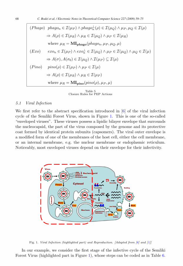
We first refer to the abstract specification introduced in [6] of the viral infectioncycle of the Semliki Forest Virus, shown in Figure 1. This is one of the so-called“enveloped viruses”. These viruses possess a lipidic bilayer envelope that surroundsthe nucleocapsid, the part of the virus composed by the genome and its protectivecoat formed by identical protein subunits (capsomers). The viral outer envelope isa modified form of one of the membranes of the host cell, either the cell membrane,or an internal membrane, e.g. the nuclear membrane or endoplasmic reticulum.Noticeably, most enveloped viruses depend on their envelope for their infectivity.

Fig. 1. Viral Infection (highlighted part) and Reproduction. [Adapted from [6] and [1]]

In our example, we consider the first stage of the infective cycle of the SemlikiForest Virus (highlighted part in Figure 1), whose steps can be coded as in Table 6.


virusdef= phago.exo〈nucap〉μvirus

nucapdef= !bud|X〈vRNA〉μnucap

celldef= membrane〈cytosol〉μmemb

membranedef= !phago⊥(mate)|!exo⊥

cytosoldef= endosome ◦ Z

endosomedef= !mate⊥|!exo⊥〈〉μendo

Table 6Viral Infection System

virus ◦ cell

≡ (phago.exo)〈nucap〉μvirus ◦ (!phago⊥(mate)|!exo⊥)〈cytosol〉μmembphago−→

(!phago⊥(mate)|!exo⊥)〈mate〈exo〈nucap〉μvirus 〉μph ◦ (!mate⊥|!exo⊥)〈〉μendo ◦ Z〉μmemb

mate−→ (!phago⊥(mate)|!exo⊥)〈(!mate⊥|!exo⊥)〈exo〈nucap〉μvirus 〉μph−endo ◦ Z〉μmembexo−→

(!phago⊥(mate)|!exo⊥)〈(!mate⊥|!exo⊥)〈〉μph−endo ◦ nucap ◦ Z〉μmemb ≡membrane〈nucap ◦ cytosol〉μmemb

Table 7Viral Infection Evolution

μnucap ∈ I(μvirus), μendo ∈ I(μmemb), μvirus, μmemb ∈ I(∗)phago, exo ∈ I(μvirus), phago⊥(mate), exo⊥ ∈ I(μmemb)

mate ∈ I(μph), μph ∈ I(μmemb), μvirus ∈ I(μph), I(μph) ∪ I(μendo) ⊆ I(μph−endo)

mate⊥, exo⊥ ∈ I(μendo)

μma ∈ I(μmemb), μvirus ∈ I(μph−endo), mate⊥, exo⊥ ∈ I(μph−endo)

I(μvirus) ⊆ I(μmemb) and in particular μnucap ∈ I(μmemb)

Table 8Viral Infection Analysis Results

We focus only on the first stage, because it lends itself to show how the ControlFlow Analysis predictions could reflect the dynamic modifications of the membraneshierarchy. In addition, striving for simplicity, it does not require further extensionsto the bunch of Brane Calculi primitives used here.

Usually, the Semliki Forest Virus is brought into the cell by phagocytosis, thuswrapped by an additional membrane layer. An endosome compartment is mergedwith the wrapped-up virus. At this point, the virus uses one of its special (viralencoded) membrane protein to trigger the exocytosis process that leads the nakednucleocapsid into the cytosol, ready to continue the infective cycle. By summarising,if the cell gets close to the virus, then it evolves into an infected cell:

virus ◦ cell →∗ membrane〈nucap ◦ cytosol〉μmemb

The complete evolution of the viral infection is reported in Table 7, while the mainanalysis entries are in Table 8. The analysis results allow us to predict the effects ofthe infection. Indeed, the inclusion μnucap ∈ I(μmemb) reflects the fact that, at theend of the shown computation, nucap is inside membrane, together with cytosol.

5.2 Communication via a Mobile Vesicle

In eucaryotic cells a large variety of proteins is targetted to its final destinationvia mobile transport vesicles, i.e. small membrane-enclosed sacs separated fromthe cytosol by a lipidic bilayer. Proteins can be contained in the vesicles (e.g.secretory proteins) or embedded in their membrane, e.g. transmembrane proteins.


Gdef= ωG〈Source ◦ Target〉μG Target

def= !phago⊥n2(exo⊥)|ωTarget〈〉μT

vesicledef= phagon2.exo Source

def= !bud⊥n1(vesicle)|ωSource〈budn1|ωX〈〉μX 〉μS

Table 9Communication via a Mobile Vesicle: Encoding

G = ωG〈!bud⊥n1(phagon2.exo)|ωSource〈budn1|ωX〈〉μX 〉μS

| {z }

Source

◦ Target〉μGbudn1−→

ωG〈!bud⊥n1(vesicle)|ωSource〈〉μS

| {z }

Source∗

◦ vesicle〈ωX〈〉μX 〉μV ◦ Target〉μG ≡

ωG〈Source∗ ◦ phagon2.exo〈ωX〈〉μX 〉μV ◦ !phago⊥n2(exo⊥)|ωTarget〈〉μT 〉μGphagon2−→

ωG〈Source∗ ◦ !phago⊥n2(exo⊥)|ωTarget〈exo⊥〈exo〈ωX〈〉μX 〉μV 〉μE 〉μT 〉μGexo−→

ωG〈Source∗ ◦ !phago⊥n2(exo⊥)|ωTarget〈ωX〈〉μX ◦ 0〈〉μE 〉μT 〉μG ≡ωG〈!bud⊥n1(vesicle)|ωSource〈〉μS ◦ !phago⊥n2(exo⊥) | ωTarget〈ωX〈〉μX 〉μT 〉μG

Table 10Communication via a Mobile Vesicle: Evolution

Through vesicular trafficking, proteins follow routes involving intracellular locations(e.g. endoplasmic reticulum, Golgi apparatus or lysosomes) as well as the plasmamembrane, in the case of endo- and exocytosis.

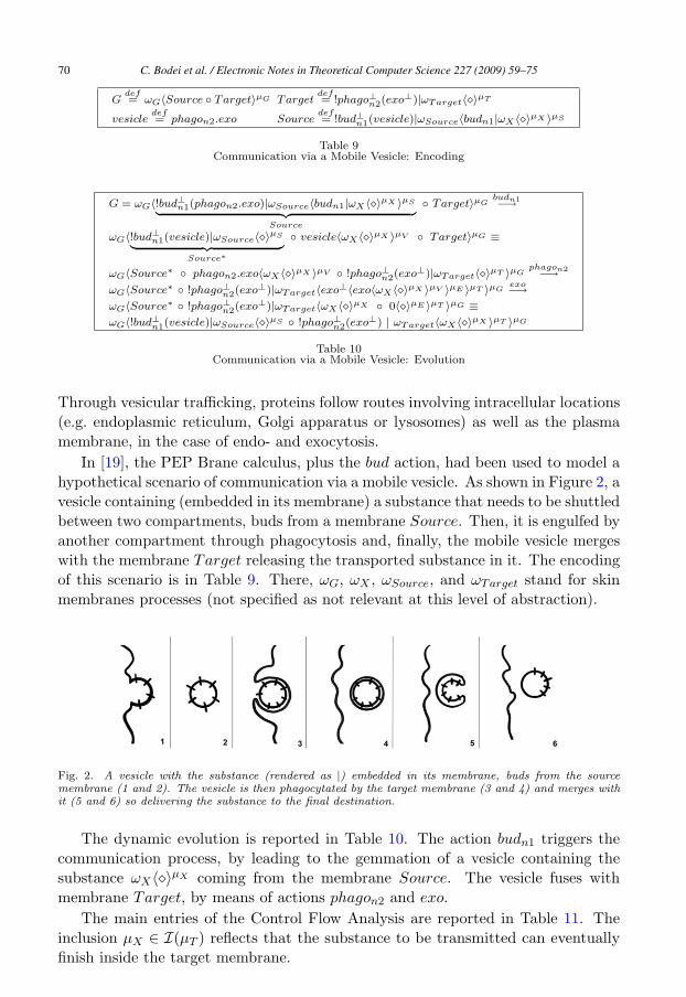
In [19], the PEP Brane calculus, plus the bud action, had been used to model ahypothetical scenario of communication via a mobile vesicle. As shown in Figure 2, avesicle containing (embedded in its membrane) a substance that needs to be shuttledbetween two compartments, buds from a membrane Source. Then, it is engulfed byanother compartment through phagocytosis and, finally, the mobile vesicle mergeswith the membrane Target releasing the transported substance in it. The encodingof this scenario is in Table 9. There, ωG, ωX , ωSource, and ωTarget stand for skinmembranes processes (not specified as not relevant at this level of abstraction).

Fig. 2. A vesicle with the substance (rendered as |) embedded in its membrane, buds from the sourcemembrane (1 and 2). The vesicle is then phagocytated by the target membrane (3 and 4) and merges withit (5 and 6) so delivering the substance to the final destination.

The dynamic evolution is reported in Table 10. The action budn1 triggers thecommunication process, by leading to the gemmation of a vesicle containing thesubstance ωX〈�〉μX coming from the membrane Source. The vesicle fuses withmembrane Target, by means of actions phagon2 and exo.

The main entries of the Control Flow Analysis are reported in Table 11. Theinclusion μX ∈ I(μT ) reflects that the substance to be transmitted can eventuallyfinish inside the target membrane.


μG ∈ I(∗), ωG ∈ I(μG);

bud⊥n1(vesicle), ωSource ∈ I(μS), μS ∈ I(μG)

budn1, ωX ∈ I(μX), μX ∈ I(μS)

phago⊥n2(exo⊥), ωTarget ∈ I(μT ), μT ∈ I(μG)

phagon2, exo ∈ I(μV ), μV ∈ I(μG), μX ∈ I(μV )

exo⊥ ∈ I(μE), μE ∈ I(μT ), μV ∈ I(μE)

I(μV ) ⊆ I(μT ) and, in particular, μX ∈ I(μT )

Table 11Communication via a Mobile Vesicle: Analysis Results

6 Conclusion

We have introduced a Control Flow Analysis for the static approximation of thedynamic behaviour of processes, expressed in the MBD + PEP version of Branecalculi.

Like the ones in [12,13,3], our analysis is context-insensitive and also flow-insensitive and these features affect the analysis precision. Future work regardsthe improvement of our analysis precision, along the lines of [15,16]. Preliminaryresults make us confident that useful information on the behaviour of the analysedsystems can be obtained and used in order to establish biological properties of thesystems under consideration. In particular, the properties that can be expressed asreachability properties of the model. Furthermore, we can obtain information onthe role played by the various elements composing the investigated system. There-fore, it becomes easier to evaluate the behaviour of the whole system when a singleelement is added or removed, following an approach similar to [4].

Acknowledgement

We are grateful to Pierpaolo Degano for his helpful discussions and to the refereesfor their valuable suggestions.

References

[1] B. Alberts, D. Bray, J. Lewis, M. Raff, K. Roberts, and J.D. Watson. “Molecular Biology of the Cell”.Third Edition, Garland.

[2] R. Barbuti, G. Caravagna, A. Maggiolo-Schettini, P. Milazzo, and G. Pardini. The calculus of loopingsequences. In Proc. of SFM’08, Lecture Notes in Computer Science 5016 (2008), 387–423.

[3] C. Bodei. A Control Flow Analysis for Beta-binders with and without Static Compartments. To appearin Theoretical Computer Science (2008), Elsevier.

[4] C. Bodei, A. Bracciali, and D. Chiarugi. On Deducing Causality in Metabolic Networks. In BMCBioinformatics, 9(4) (2008).


[5] N. Busi. Towards a Causal Semantics for Brane Calculi. In What is it About Government thatAmericans Dislike, 1945–1965, University Press, 2007.

[6] L. Cardelli. Brane calculi - interactions of biological membranes. In Proc. of Computational Methodsin Systems Biology (CMSB’04) Lecture Notes in Computer Science 3082 (2005), 257–280, Springer.

[7] L. Cardelli and G. Paun. An universality result for a (mem)brane calculus based on mate/dripoperations. Int. J. Found. Comput. Sci. 17 (1) (2006), 49–68, World Scientific.

[8] V. Danos and J. Krivine. Transactions in RCCS. In Proc. of Conference on Concurrency Theory(CONCUR’05), Lecture Notes in Computer Science 3653 (2005), 398–412, Springer.

[9] V. Danos and Cosimo. Laneve. Graphs for core molecular biology. In Proc. of Computational Methodsin Systems Biology (CMSB’03), Lecture Notes in Computer Science 2602 (2003), 34–46, Springer.

[10] R. Gori, F. Levi. An Analysis for Proving Temporal Properties of Biological Systems. In Proc. ofAPLAS, Lecture Notes in Computer Science 4279 (2006), 234–252.

[11] R. Milner. “Communicating and mobile systems: the π-calculus”. Cambridge University Press, 1999.

[12] F Nielson, H Riis-Nielson, D Schuch-Da-Rosa, and C Priami. Static analysis for systems biology. InProc. of Workshop on Systeomatics - dynamic biological systems informatics, 1–6. Computer SciencePress, 2004.

[13] F. Nielson, H. Riis Nielson, C. Priami, and D. Schuch da Rosa. Control Flow Analysis for BioAmbients.Electronic Notes in Theoretical Computer Science 180(3) (2007), 65–79, Elsevier.

[14] G. Paun. Computing with membranes (P systems): A variant. Int. J. Found. Comput. Sci., 11(1)(2000), 167–181.

[15] H. Pilegaard, F. Nielson, H. R. Nielson. Static analysis of a Model of the LDL degradation pathway.In Proc. of Workshop on Computational Methods in Systems Biology (CMSB’05), 2005.

[16] H. Pilegaard, F. Nielson, H. Riis Nielson. Context Dependent Analysis of BioAmbients. In Proc. ofEmerging Aspects of Abstract Interpretation ’06, 2006.

[17] C. Priami and P. Quaglia. Beta binders for biological interactions. In Proceedings of ComputationalMethods in Systems Biology (CMSB’04), Lecture Notes in Computer Science 3082 (2005), 20–33,Springer.

[18] A. Regev and E. Shapiro. Cellular Abstractions: Cells as Computation, Nature, 419 (2002).

[19] A. Vitale and G. Mauri. Communication via Mobile Vesicles in Brane Calculi. Electronic Notes inTheoretical Computer Science 171 (2) (2007), 187–196, Elsevier.

A Proofs

This appendix restates the lemmata and theorems presented earlier in the paperand gives the proofs of their correctness.

To establish the semantic correctness, the following auxiliary results are needed.

Fact A.1 If I |=μ1 P and I(μ1) ⊆ I(μ2), then I |=μ2 P .

Proof. By structural induction on P . This is straightforward, because the mem-brane identity is only used in recursive calls, to establish a fact like μ ∈ I(μi) ora ∈ I(μi). We show just one case.Case P = σ〈P 〉μ′

. We have that I |=μ1 P is equivalent to μ′ ∈ I(μ1) ∧ A(σ) ∈I(μ′) ∧ I |=μ′

P . Now, μ′ ∈ I(μ1) and I(μ1) ⊆ I(μ2) imply μ′ ∈ I(μ2), and byinduction hypothesis, we have that I |=μ2 P . �

Fact A.2 If σ ≡ τ then A(σ) = A(τ).


Proof. The proof amounts to a straightforward inspection of each of the clausesdefining the structural congruence clauses relative to membranes. We show onlytwo cases, the others are similar.Case σ0|σ1 ≡ σ1|σ0. We have that A(σ0|σ1) = A(σ0) ∪ A(σ1) = A(σ1|σ0).Case σ ≡ τ ⇒ σ|ρ ≡ τ |ρ. We have that A(σ|ρ) = A(σ) ∪ A(ρ). Now, since σ ≡ τ ,we have that A(σ) = A(τ) and therefore A(σ|ρ) = A(τ) ∪ A(ρ), from which therequired A(τ |ρ). �

Lemma A.3 (Invariance of Structural Congruence) If P ≡ Q and I |=μ P

then also I |=μ Q.

Proof. The proof amounts to a straightforward inspection of each of the clausesdefining the structural congruence clauses.Case P0 ◦ P1 ≡ P1 ◦ P0. We have that I |=μ P0 ◦ P1 is equivalent to I |=μ P0 ∧I |=μ P1, that is equivalent to I |=μ P1 ∧ I |=μ P0 and therefore to I |=μ P1 ◦ P0.Case P0 ◦ (P1 ◦P2) ≡ (P0 ◦P1)◦P2. We have that I |=μ P0 ◦ (P1 ◦ P2) is equivalentto I |=μ P0 ∧I |=μ P1 ◦ P2, that is equivalent to I |=μ P0 ∧I |=μ P1 ∧I |=μ P2 and,in turn, to I |=μ P0 ◦ P1 ∧ I |=μ P2, and therefore to I |=μ (P0 ◦ P1) ◦ P2.Case P0 ◦ � ≡ P0. We have that I |=μ P0 ◦ � is equivalent to I |=μ P0 ∧ I |=μ �,that is equivalent to I |=μ P0 ∧ true, and therefore to I |=μ P0.Case !� ≡ �. We have that I |=μ !� is equivalent to I |=μ �.Case !(P0◦P1) ≡!P0◦!P1. We have that I |=μ !(P0 ◦ P1) is equivalent to I |=μ (P0 ◦ P1),that is equivalent to I |=μ P0 ∧ I |=μ P1, that is equivalent to I |=μ !P0 ∧ I |=μ !P1

and therefore to I |=μ !P0◦!P1.Case !!P ≡!P . We have that I |=μ !!P is equivalent to I |=μ !P .Case !P ≡ P◦!P . We have that I |=μ !P is equivalent to I |=μ P , that is equivalentto I |=μ P ∧ I |=μ !P , and therefore to I |=μ P◦!P .Case 0〈�〉μ′ ≡ �. We have that I |=μ 0〈�〉μ′

is equivalent to μ′ ∈ I(μ) ∧ A(0) =∅ ⊆ I(μ′) ∧ I |=μ′ �, that is equivalent to I |=μ′ � ∧ true, that implies true and,in turn, I |=μ �.Case P ≡ Q ⇒ P ◦ R ≡ Q ◦ R. We have that I |=μ P ◦ R is equivalent toI |=μ P ∧ I |=μ R, and from the hypothesis I |=μ P , we have that I |=μ Q. There-fore from I |=μ Q ∧ I |=μ R, we obtain the required I |=μ Q ◦ R.Case P ≡ Q ⇒!P ≡!Q: similar.Case P ≡ Q ∧ σ ≡ τ ⇒ σ〈P 〉μ′ ≡ τ〈Q〉μ′

. We have that I |=μ σ〈P 〉μ′is equivalent

to μ′ ∈ I(μ) ∧ A(σ) ∈ I(μ′) ∧ I |=μ′P . By Fact A.2, A(τ) ∈ I(μ′), and by induc-

tion hypothesis, we have that μ′ ∈ I(μ) ∧ A(τ) ∈ I(μ′) ∧ I |=μ′Q and therefore

I |=μ τ〈Q〉μ′. �

Theorem A.4 (Subject Reduction)

If P → Q and I |=μ P then also I |=μ Q.

Proof. The proof is by induction on P → Q. The proofs for the rules (Par)and (Brane) are straightforward, using the induction hypothesis and the clausesin Table 2. The proof for the (Struct) uses instead the induction hypothesis andLemma A.3. The proofs for the basic actions in the lower part of Table 1 and inTable 4 are straightforward, using the clauses in Tables 2 and 5.


Case (Par). Let P be P0 ◦ P1 and Q be P ′0 ◦ P1. We have to prove that I |=μ Q.

Now I |=μ P is equivalent to I |=μ P0 ∧ I |=μ P1. By induction hypothesis,we have that I |=μ P ′

0, and from I |=μ P ′0 ∧ I |=μ P1 we obtain the required

I |=μ Q.Case (Brane). Let P be σ〈P0〉μ′

and Q be σ〈P ′0〉μ

′. We have to prove that

I |=μ σ〈P ′0〉μ

′. Now I |=μ P is equivalent to μ′ ∈ I(μ) ∧ A(σ) ∈ I(μ′) ∧ I |=μ′

P0.By induction hypothesis, we have that I |=μ P ′

0, and from μ′ ∈ I(μ) ∧ A(σ) ∈I(μ′) ∧ I |=μ′

P ′0 we obtain the required I |=μ Q.

Case (Struct). Let P ≡ P0, with P0 → P1 such that P1 ≡ Q. By Lemma A.3, wehave that I |=μ P0, by induction hypothesis I |=μ P1 and, again by Lemma A.3,I |=μ Q.Case (Mate). Let P be maten.σ|σ0〈P0〉μ0◦mate⊥n .τ |τ0〈P1〉μ1 and Q be σ|σ0|τ |τ0〈P0◦P1〉μ01 . We have that I |=μ P is equivalent to maten ∈ I(μ0) ∧ mate⊥n ∈I(μ1)∧ μ0, μ1 ∈ I(μ) (1) and A(σ) ∈ I(μ0) ∧ A(σ0) ∈ I(μ0) ∧ I |=μ0 P0 ∧ A(τ) ∈I(μ1) ∧ A(τ0) ∈ I(μ1) ∧ I |=μ1 P1. In particular, because of the closure con-ditions, from (1), we have that μ01 ∈ I(μ) ∧ I(μ0) ∪ I(μ1) ⊆ I(μ01). SinceI(μi) ⊆ I(μ01) for i = 0, 1, then, by Fact A.1, we have that A(σ) ∈ I(μ01) ∧ A(σ0) ∈I(μ01)∧I |=μ01 P0 and A(τ) ∈ I(μ01) ∧ A(τ0) ∈ I(μ01) ∧ I |=μ01 P1, and hencethe required I |=μ Q.Case (Bud). Let P be bud⊥n (ρ).τ |τ0〈budn.σ|σ0〈P0〉μ0◦P1〉μ1 and Q be ρ〈σ|σ0〈P0〉μ0〉μR◦τ |τ0〈P1〉μ1 . We have that I |=μ P is equivalent to budn ∈ I(μ0) ∧ bud⊥n (ρ) ∈I(μ1) ∧ μ0 ∈ I(μ1) ∧ μ1 ∈ I(μ) (1) and A(σ) ∈ I(μ0) ∧ A(σ0) ∈ I(μ0) ∧I |=μ0 P0 ∧ A(τ) ∈ I(μ1) ∧ A(τ0) ∈ I(μ1) ∧ I |=μ1 P1. In particular, becauseof the closure conditions, from (1), we have that A(ρ) ∈ I(μR) ∧ μR ∈ I(μ) andμ0 ∈ I(μR), and therefore the required I |=μ Q.Case (Drip). Let P be drip(ρ).σ|σ0〈P0〉μ0 and Q be ρ〈〉μR ◦ σ|σ0〈P0〉μ0 . We havethat I |=μ P is equivalent to drip(ρ) ∈ I(μ0) ∧ μ0 ∈ I(μ) (1) and A(σ) ∈I(μ0) ∧ A(σ0) ∈ I(μ0) ∧ I |=μ0 P0. In particular, because of the closure condi-tions, from (1), we have that A(ρ) ∈ I(μR) ∧ μR ∈ I(μ), and therefore the requiredI |=μ Q.Case (Phago). Let P be phagon.σ|σ0〈P0〉μ0 ◦ phago⊥n (ρ).τ |τ0〈P1〉μ1 and Q beτ |τ0〈ρ〈σ|σ0.〈P0〉μ0〉μR ◦ P1〉μ1 . We have that I |=μ P is equivalent to phagon ∈I(μ0) ∧ phago⊥n (ρ) ∈ I(μ1) ∧ μ0, μ1 ∈ I(μ) (1) and A(σ) ∈ I(μ0) ∧ A(σ0) ∈I(μ0) ∧ I |=μ0 P0 ∧ A(τ) ∈ I(μ1) ∧ A(τ0) ∈ I(μ1) ∧ I |=μ1 P1. In particular,because of the closure conditions, from (1), we have that A(ρ) ∈ I(μR) ∧ μR ∈I(μ1) ∧ μ0 ∈ I(μR), and hence the required I |=μ Q.Case (Exo). Let P be exo⊥n .τ |τ0〈exon.σ|σ0〈P0〉μ0◦P1〉μ1 and let Q be P0◦σ|σ0|τ |τ0〈P1〉μ1 .We have that I |=μ P is equivalent to exon ∈ I(μ0) ∧ exo⊥n ∈ I(μ1) ∧ μ0 ∈I(μ1) ∧ μ1 ∈ I(μ) (1) and A(σ) ∈ I(μ0) ∧ A(σ0) ∈ I(μ0) ∧ I |=μ0 P0 ∧ A(τ) ∈I(μ1) ∧ A(τ0) ∈ I(μ1) ∧ I |=μ1 P1. In particular, because of the closure condi-tions, from (1), we have that A(σ), A(σ0) ∈ I(μ1)∧ I(μ0) ⊆ I(μ). By Fact A.1, wehave that I |=μ P0 and therefore the required I |=μ Q.Case (Pino). Let P be pino(ρ).σ|σ0〈P0〉μ0 and Q be σ|σ0〈ρ〈〉μR ◦ P0〉μ0 . Wehave that I |=μ P is equivalent to pino(ρ) ∈ I(μ0) ∧ μ0 ∈ I(μ) (1) and A(σ) ∈I(μ0) ∧ A(σ0) ∈ I(μ0) ∧ I |=μ0 P0. In particular, because of the closure condi-


tions, from (1), we have that A(ρ) ∈ I(μR)∧μR ∈ I(μ0), and therefore the requiredI |=μ Q.

�

Theorem A.5 (Moore Family)

For any system P , the set {I| I |=μ P} is a Moore family.

Proof. We proceed by structural induction on P . Let E be a set of proposedestimates and let F and Ij such that F ⊆ E = {Ij | j ∈ F}. Next, define I ′ = �FWe have to check that I ′ |=μ′

P . We just consider one case. The others are similar.Case (σ〈P0〉μ′

). Since ∀j ∈ F : Ij |=μ σ〈P0〉μ, then

∀j ∈ F : μ′ ∈ Ij(μ) ∧ A(σ) ∈ Ij(μ′) ∧ Ij |=μ′P

Using the induction hypothesis and the fact that I ′ is obtained in a pointwise way,we then obtain that

μ′ ∈ I ′(μ) ∧ A(σ) ∈ I ′(μ′) ∧ I ′ |=μ′P

thus establishing the required I ′ |=μ σ〈P0〉μ′. �


Control Flow Analysis for Brane Calculi

Documents