Control Engineering Practice

Control Engineering Practice 51 (2016) 13–25

Contents lists available at ScienceDirect

Control Engineering Practice

http://d0967-06

☆InvitFault To

n CorrE-m

stefano.URL

journal homepage: www.elsevier.com/locate/conengprac

Fault tolerant control of a simulated hydroelectric system$

Silvio Simani n, Stefano Alvisi, Mauro VenturiniDipartimento di Ingegneria, Università degli Studi di Ferrara. Via Saragat 1E, 44122 Ferrara, FE, Italy

a r t i c l e i n f o

Article history:Received 31 July 2015Received in revised form14 March 2016Accepted 15 March 2016

Keywords:Fault tolerant controlControl designModelling and identificationAdaptive controlHydraulic system

x.doi.org/10.1016/j.conengprac.2016.03.01061/& 2016 Elsevier Ltd. All rights reserved.

ed paper for the special issue on “Industrial Plerant Control” organised by Peter Fogh Odgaesponding author.ail addresses: [email protected] (S. [email protected] (S. Alvisi), mauro.venturini@un: http://www.silviosimani.it (S. Simani).

a b s t r a c t

This paper analyses the application of two fault tolerant control schemes to a hydroelectric model de-veloped in the Matlab and Simulink environments. The proposed fault tolerant controllers are exploitedfor regulating the speed of the Francis turbine included in the hydraulic system. The nonlinear behaviourof the hydraulic turbine and the inelastic water hammer effects are taken into account in order to de-velop a high-fidelity simulator of this dynamic plant. The first fault tolerant control solution relies on anadaptive control design, which exploits the recursive identification of a linear parametric time-varyingmodel of the monitored system. The second scheme proposed uses the identification of a fuzzy modelthat is exploited for the reconstruction of the fault affecting the system under diagnosis. In this way, thefault estimation and its accommodation is possible. Note that these strategies, which are both based onidentification approaches, are suggested for enhancing the application of the suggested fault tolerantcontrol methodologies. These characteristics of the study represent key issues when on-line im-plementations are considered for a viable application of the proposed fault tolerant control schemes. Thefaults considered in this paper affect the electric servomotor used as a governor, the hydraulic turbinespeed sensor, and the hydraulic turbine system, and are imposed both separately and simultaneously.Moreover, the complete drop of the rotational speed sensor is also analysed. Monte-Carlo simulations arealso used for analysing the most important issues of the proposed schemes in the presence of parametervariations. Moreover, the performances achieved by means of the proposed solutions are compared tothose of a standard PID controller already developed for the considered model. Finally, these strategiesserve to highlight the potential application of the proposed control strategies to real hydraulic systems.

& 2016 Elsevier Ltd. All rights reserved.

1. Introduction

Modern technological and technical processes are based oncomplex control systems that are designed to meet advancedperformance and safety requirements. Conventional feedbackcontrol solutions may lead to unsatisfactory performances, or evento instability, when possible malfunctions in actuators, sensors orother system components are present. To overcome these pro-blems, new strategies to control system design have been pro-posed in order to manage actuator, sensor and component faults,while maintaining desirable stability and performance properties.This class of control design is also known as Fault Tolerant Control(FTC) systems, which have the capability to accommodate thefaults in an automatic way. The closed-loop control system is thusable to manage any malfunctions, while maintaining good control

ractice of Fault Diagnosis andard.

),ife.it (M. Venturini).

properties. The FTC system is based on adaptive strategies or activeFault Detection and Diagnosis (FDD) scheme, i.e. when the faultfunction is estimated and compensated. Regarding the latest issue,many FDD techniques have been developed, see for example thesurvey works (Chen & Patton, 1999; Ding, 2008).

In general, FTC solutions are divided into two strategies,namely Passive Fault Tolerant Control Scheme (PFTCS) and ActiveFault Tolerant Control Scheme (AFTCS), as addressed e.g. in Blanke,Kinnaert, Lunze, and Staroswiecki (2006), Zhang and Jiang (2008),and Noura, Theilliol, Ponsart, and Chamseddine (2009). On onehand, in the case of PFTCS, the designed controllers are definedand designed to be robust with respect to a specific set of pre-sumed faults. This scheme uses neither FDD methods nor con-troller reconfiguration, but it presents limited fault tolerant fea-tures (Zhang & Jiang, 2008). On the other hand, AFTCS reacts ac-tively to the system fault by using a control accommodation ap-proach, so that the stability and the final performance of the entiresystem are maintained. Concerning AFTCS, it was remarked thatrobust and reliable FDD are required (Chen & Patton, 1999; Ding,2008).

FTC solutions can derive from the application of model-basedand model-free designs, as described e.g. in Blanke et al. (2006)

S. Simani et al. / Control Engineering Practice 51 (2016) 13–2514

and Zhang and Jiang (2008). Different FTC methods have beenaddressed in the recent related literature. For example, Kim andKim (2015) proposed stochastic petri nets exploited for designingprocess control system of a continuous casting plant. The work ofSchuh, Zgorzelski, and Lunze (2015) presented deterministic input/output automata applied to a handling system. The paper by Fo-nod et al. (2015) developed a control system to detect, isolate andaccommodate single faults affecting the thruster-based propulsionsystem of an autonomous spacecraft. Ubaid, Daley, and Pope(2015) described a control design procedure through its applica-tion to a laboratory scale slab floor. The study of Li, Liu, and Cao(2015) presented a robust ∞H approach used to solve an optimalstate-feedback-type controller parameter design for a HVDC/ACsystem. The paper by Kiltz, Join, Mboup, and Rudolph (2014) in-troduced a method based on algebraic derivative estimation that isapplied on an example of electromagnetically supported plate.Finally, the work of Blesa, Rotondo, Puig, and Nejjari (2014) usedinterval observers oriented to the design of virtual sensors/ac-tuators for wind turbines.

On the other hand, few works analysed the model-based faulttolerant control problem when applied to hydroelectric plants, asdescribed in Hong, Guangda, and Weiyou (2008), Li et al. (1992),and Wei, Wei-bo, Gen-mao, and Jian-hua (2000). In fact, as amathematical model is needed for the description of the systembehaviour, precise modelling for these processes could be difficultto achieve in practice. There are several works that discuss themodelling of hydroelectric processes with their controller design,as in Mansoor, Jones, Bradley, Aris, and Jones (2000) and Weber,Prillwitz, Hladky, and Asal (2001). These works consider the elasticwater effects, though the nonlinear dynamics are linearised at anoperating point. Other papers (Eker, 2004; Hanmandlu & Goyal,2008; Kishor, Saini, & Singh, 2007) considered different mathe-matical descriptions with the techniques to control the powersystems. Moreover, linear and nonlinear plants with various watercolumn effects and control solutions are also considered. Mah-moud, Dutton, and Denman (2005) and Kishor, Singh, and Ra-ghuvanshi (2006) addressed complex control solutions for hy-draulic processes.

In some cases, it could be impossible to describe the nonlinearsystems in an analytical way; moreover, the system structure withits parameters and measurements can be almost unknown.Therefore, parametric model estimation can represent an alter-native solution for deriving practical models of nonlinear dynamicprocesses systems for control design. Moreover, if nonlinearidentification methods require a detailed knowledge of the modelstructure, fuzzy systems and neural networks can be obtaineddirectly from measured data (Alvisi & Franchini, 2012; Asgari,Venturini, Chen, & Sainudiin, 2014; Nelles, 2001).

This paper proposes two fault-tolerant control approaches forthe adjustment of a hydraulic turbine developed in the ®Matlaband ®Simulink environments. The development of the suggestedsolutions is particularly important from a practical point of view.In fact, the variable demand for electricity and changing conditionsin the power system can lead to different demand of peak energygeneration, with short response time and fast frequency changes.Hydroelectric power systems thus require to operate taking intoaccount different variable load and demand conditions. In general,the operation of hydropower systems can frequently experiencevariations in the flow in both routine operations and abnormalconditions. In particular, turbine operations such as start-up, loadacceptance, load rejection and shutdown can lead to hydraulictransients that can generate large pressure and sub-pressure os-cillations, which must be carefully evaluated to avoid mechanicalfailures in the hydraulic systems. Therefore, the need for accuratesimulation of transient flow in hydroelectric power plants is ob-vious. However, even if the basic technology in a hydraulic process

has not changed much, powerful computers and software now canbe used to provide virtual models and simulators of hydropowersystems.

Therefore, this work proposes a first methodology based on thefuzzy theory, as it represents a suitable method to manage almostunknown situations and uncertain measurements (Babuška, 1998).In this way, instead of using purely nonlinear analytical descrip-tion obtained via the first principle modelling approach, the paperproposes to exploit Takagi–Sugeno (TS) models (Babuška, 1998;Takagi & Sugeno, 1985), whose parameters are estimated via anidentification methodology. In particular, the fuzzy fault tolerantscheme is obtained according to the following stages. The FDDmodel is firstly estimated using the fuzzy identification approach(Babuška, 1998). Secondly, the fault accommodation strategy usesthe estimation of FDD module to compensate for the fault effect.The FDD model is obtained via a proper choice of the fuzzy modelparameters. The Membership Functions (MFs) with their rules arealso derived directly from the data of the monitored system. Thefuzzy modelling and identification scheme is thus able to lead tothe required fault tolerance features. Note that the proposed de-sign approach exploited for the derivation of the fuzzy controllerwas already addressed in Simani and Castaldi (2013), but appliedto a wind turbine system, and without fault tolerance capabilities.

Concerning the traditional controller design, classical linearcontrol schemes, such as the PID solution could not lead to sa-tisfactory behaviour for all operating points of the plant, due tononlinearity, system ageing, environmental conditions, uncertainmeasurements, disturbance and possible faults. Due to this beha-viour, possible solutions could exploit a multiple model approach,or gain-scheduled controllers that are derived to work in fixedoperating points, as described e.g. in Fang, Chen, Dlakavu, andShen (2008). In this case, it was assumed that the model para-meters change slowly compared to the system dynamics, which isgenerally not satisfied. Moreover, classic gain-scheduling strate-gies could guarantee prescribed performance and stability re-quirements at different operating points, but with design proce-dures that sometimes are not direct and straightforward.

Under these considerations, the second FTC approach sug-gested in this paper uses a recursive identification mechanism inconnection with model-based adaptive control design, which wasaddressed e.g. in Bobál, Böhm, Fessl, and Machácek (2005). Notethat this alternative strategy suggested in this paper for theadaptive controller design was already proposed in Simani, Alvisi,and Venturini (2014), but without any fault tolerance properties.Therefore, the controller design problem is proposed here sincethe characteristics of the process under investigation can changeover time. Moreover, in the perspective of the fault tolerant ap-plication, this paper suggests to exploit an adaptive solution basedon a recursive or on-line estimation scheme relying on the on-lineestimation of the controlled process, which is affected by faults.While the time-varying parameters of the plant are identified,which are the result of both disturbance and faults, the time-varying variables of the controller are computed on-line, in orderto maintain fixed control performances.

The efficacy of the suggested FTC strategies are proved on dif-ferent data sequences acquired from the hydraulic system underdiagnosis. Several simulations provide the effectiveness of theproposed regulators also with respect to the baseline PID con-troller proposed in Fang et al. (2008), when both the fault toler-ance and the reference tracking capabilities are considered.Moreover, as it fundamental to analyse the behaviour of the pro-posed control strategies with respect to modelling uncertainties,the suggested verification tool exploits extensive Monte-Carlo si-mulations. In fact, as the hydraulic plant uses a hydraulic turbinerepresented as two-dimensional map, the Monte-Carlo analysisrepresents a viable approach for assessing the performances of the

S. Simani et al. / Control Engineering Practice 51 (2016) 13–25 15

suggested fault tolerant control schemes.The paper has the following structure. Section 2 briefly recalls

the model of the hydraulic system. Section 3 sketches the sug-gested FTC design solutions, which rely on both the fuzzy mod-elling and identification strategy exploited here for obtaining theinput–output description of the considered simulated process andthe FDD module for fault estimation and compensation. The sec-ond adaptive approach is also recalled in Section 3. The obtainedresults are described in Section 4, which shows the simulationsfrom the developed FTC schemes, assessed and compared withrespect to the classic PID regulator. Finally, Section 5 highlights themain achievements of the paper, by suggesting also open problemsand further investigations.

2. Hydraulic system and fault modes

2.1. Hydraulic system model

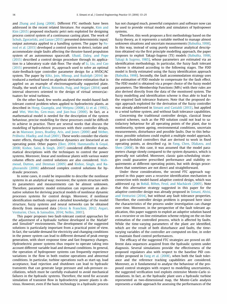
The simulated hydroelectric power plant considered in thiswork is represented in Fig. 1 (Fang et al., 2008; Simani, Alvisi, et al.,2014; Simani, Alvisi, & Venturini, 2015).

It consists of a reservoir with constant water level HR, an up-stream water tunnel with cross-section area A1 and length L1, anupstream surge tank with cross-section area A2, and water levelH2. This is followed by a downstream surge tank with cross-sec-tion area A4 and water level H4, and a downstream tail watertunnel with cross-section area A5 and length L5. Moreover, thepenstock between hydraulic turbine and two surge tanks has across-section area A3 and length L3. T denotes the hydraulic tur-bine. Finally, a tail water lake has constant water level HT.

The expressions (1) and (2) represent the non-dimensionalflow rate and water pressure in terms of the corresponding re-lative deviations:

= +( )

QQ

q11r

= +( )

HH

h12r

where Q is the water flow rate, Qr is the rated flow rate, q is theflow rate relative deviation, whilst H is the water pressure, Hr isthe rated water pressure, and h the water pressure relativedeviation.

According to Fang et al. (2008), with reference to a pressurewater supply system, Newton's second law for a fluid elementinside a tube and the conservation mass law for a control volume,which accounts for water compressibility and tube elasticity, iswritten. Under the assumption that the penstock is short ormedium in length, water and pipeline is considered in-compressible and rigid, respectively. Therefore, (3) considers onlythe inelastic water hammer effect (Fang et al., 2008):

T

HR A , H2 2

AA1 3

L1

AL5

5

A , H44HT

L3

Fig. 1. Layout of the simulated hydropower plant.

= − −( )

hq

T s H3

w f

where s is the derivative operator. Under this assumption, theexpression (3) represents the flow rate deviation and the waterpressure deviation transfer functions for a simple penstock, whereHf is the hydraulic loss and Tw is the water inertia time:

=( )

TL Q

g A H 4w

r

r

depending on the penstock length L, the rated flow rate Qr, thegravity acceleration g, the cross-section area A, and the rated waterpressure Hr. The hydroelectric power plant considered in this workis divided into three sections: the upstream water tunnel, thepenstock and the downstream tail water tunnel.

The upstream water tunnel connects the reservoir to the up-stream surge tank. Since the inlet of upstream water tunnel is inreservoir and the water pressure deviation of the inlet is constantduring hydraulic transients, the transfer function of the flow ratedeviation and the water pressure deviation of the outlet of theupstream water tunnel is expressed in the form:

= − −( )

hq

T s H5

w f1

11 1

The downstream tail water tunnel connects the downstreamsurge tank to the tail water lake. It is assumed that the outlet of thedownstream tail water tunnel is in tailwater lake and the waterpressure deviation of the outlet is constant. Therefore, the transferfunction of flow rate deviation and the water pressure deviation ofthe inlet of downstream tail water tunnel has the form:

= − −( )

hq

T s H6

w f5

55 5

Usually, the water inertia in the draft tube is considered withinthe penstock. Thus, the transfer function of flow rate deviation(the subscript t refers to the turbine) and the water pressure de-viation of the penstock is written as:

= − + ( )h h h h 7t 2 4 3

where:

= − −( )

hq

T s H8

w f3

33 3

The expressions of the surge tanks are derived from the con-tinuity of flow at the two junctions, where the hydraulic losses atorifices of surge tanks are neglected:

= = −

= = −( )

⎧⎨⎪⎪

⎩⎪⎪

A HQ

dhdt

q q q

A HQ

dhdt

q q q9

r

r

r

r

2 22 1 3

4 44 3 5

The surge tank filling time is expressed as:

=( )

TA HQ 10s

r

r

Regarding the Francis turbine in Fig. 1, according to Simani,Alvisi, et al. (2014), the second order polynomial curve (11) relatesthe non-dimensional water flow rate Q Q/ r to the non-dimensionalrotational speed n n/ r . The non-dimensional parameter G (varyingin the range between 0 and 100%) represents the turbine wickedgate opening:

= + + = ( )( )

⎡⎣⎢⎢

⎛⎝⎜

⎞⎠⎟

⎛⎝⎜⎜

⎞⎠⎟⎟

⎤⎦⎥⎥

QQ

G ann

bnn

c f n G,11r r r

1

2

1 1 1

0%

20%

40%

60%

80%

100%

120%

0,00 0,50 1,00 1,50 2,00 2,50

Q/Q

r

n/n r

Wicket gate opening 100%Efficiency = 0%

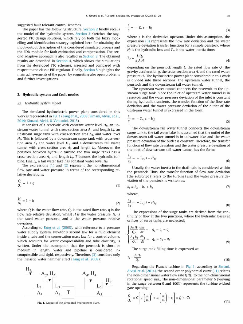
Fig. 2. Non-dimensional water flow rate Q Q/ r vs. non-dimensional rotationalspeed n n/ r .

____1Ts2*s

-Tw1*s-Hf1_______1

-+

du/dtdu/dtTw3

Hf3

1qt -

--++ 1

ht

-+Ts4*s

Tw5*s+Hf5_________1

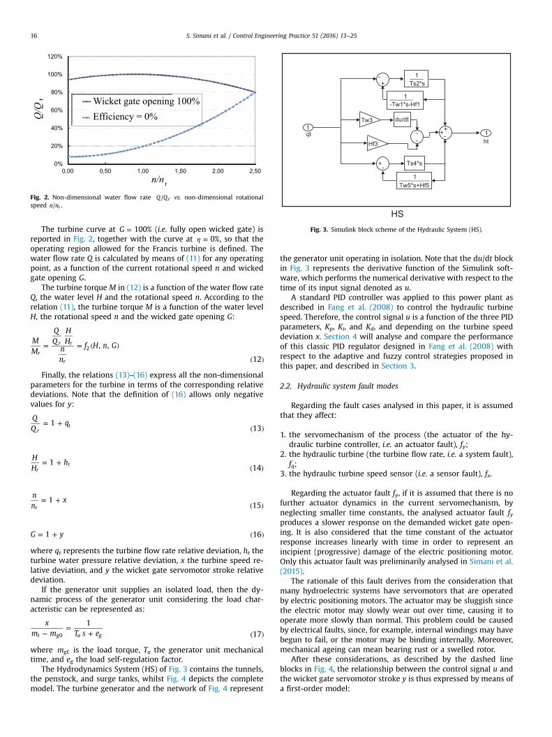
HSFig. 3. Simulink block scheme of the Hydraulic System (HS).

S. Simani et al. / Control Engineering Practice 51 (2016) 13–2516

The turbine curve at =G 100% (i.e. fully open wicked gate) isreported in Fig. 2, together with the curve at η = 0%, so that theoperating region allowed for the Francis turbine is defined. Thewater flow rate Q is calculated by means of (11) for any operatingpoint, as a function of the current rotational speed n and wickedgate opening G.

The turbine torque M in (12) is a function of the water flow rateQ, the water level H and the rotational speed n. According to therelation (11), the turbine torque M is a function of the water levelH, the rotational speed n and the wicked gate opening G:

= = ( )

( )

MM

QQ

HH

nn

f H n G, ,

12r

r r

r

2

Finally, the relations (13)–(16) express all the non-dimensionalparameters for the turbine in terms of the corresponding relativedeviations. Note that the definition of (16) allows only negativevalues for y:

= +( )

QQ

q113r

t

= +( )

HH

h114r

t

= +( )

nn

x115r

= + ( )G y1 16

where qt represents the turbine flow rate relative deviation, ht theturbine water pressure relative deviation, x the turbine speed re-lative deviation, and y the wicket gate servomotor stroke relativedeviation.

If the generator unit supplies an isolated load, then the dy-namic process of the generator unit considering the load char-acteristic can be represented as:

−=

+ ( )x

m m T s e1

17t g a g0

where mg0 is the load torque, Ta the generator unit mechanicaltime, and eg the load self-regulation factor.

The Hydrodynamics System (HS) of Fig. 3 contains the tunnels,the penstock, and surge tanks, whilst Fig. 4 depicts the completemodel. The turbine generator and the network of Fig. 4 represent

the generator unit operating in isolation. Note that the du/dt blockin Fig. 3 represents the derivative function of the Simulink soft-ware, which performs the numerical derivative with respect to thetime of its input signal denoted as u.

A standard PID controller was applied to this power plant asdescribed in Fang et al. (2008) to control the hydraulic turbinespeed. Therefore, the control signal u is a function of the three PIDparameters, Kp, Ki, and Kd, and depending on the turbine speeddeviation x. Section 4 will analyse and compare the performanceof this classic PID regulator designed in Fang et al. (2008) withrespect to the adaptive and fuzzy control strategies proposed inthis paper, and described in Section 3.

2.2. Hydraulic system fault modes

Regarding the fault cases analysed in this paper, it is assumedthat they affect:

1. the servomechanism of the process (the actuator of the hy-draulic turbine controller, i.e. an actuator fault), fy;

2. the hydraulic turbine (the turbine flow rate, i.e. a system fault),fq;

3. the hydraulic turbine speed sensor (i.e. a sensor fault), fx.

Regarding the actuator fault fy, if it is assumed that there is nofurther actuator dynamics in the current servomechanism, byneglecting smaller time constants, the analysed actuator fault fyproduces a slower response on the demanded wicket gate open-ing. It is also considered that the time constant of the actuatorresponse increases linearly with time in order to represent anincipient (progressive) damage of the electric positioning motor.Only this actuator fault was preliminarily analysed in Simani et al.(2015).

The rationale of this fault derives from the consideration thatmany hydroelectric systems have servomotors that are operatedby electric positioning motors. The actuator may be sluggish sincethe electric motor may slowly wear out over time, causing it tooperate more slowly than normal. This problem could be causedby electrical faults, since, for example, internal windings may havebegun to fail, or the motor may be binding internally. Moreover,mechanical ageing can mean bearing rust or a swelled rotor.

After these considerations, as described by the dashed lineblocks in Fig. 4, the relationship between the control signal u andthe wicket gate servomotor stroke y is thus expressed by means ofa first-order model:

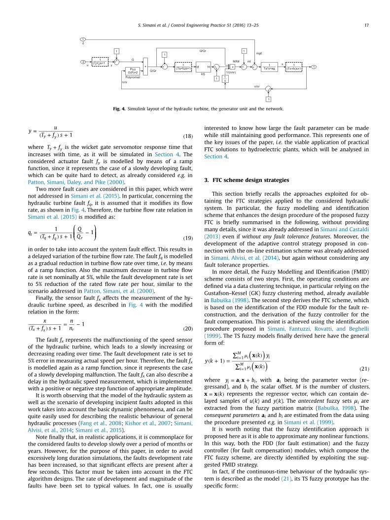
Fig. 4. Simulink layout of the hydraulic turbine, the generator unit and the network.

S. Simani et al. / Control Engineering Practice 51 (2016) 13–25 17

=( + ) + ( )

yu

T f s 1 18y y

where +T fy y is the wicket gate servomotor response time thatincreases with time, as it will be simulated in Section 4. Theconsidered actuator fault fy is modelled by means of a rampfunction, since it represents the case of a slowly developing fault,which can be quite hard to detect, as already considered e.g. inPatton, Simani, Daley, and Pike (2000).

Two more fault cases are considered in this paper, which werenot addressed in Simani et al. (2015). In particular, concerning thehydraulic turbine fault fq, it is assumed that it modifies its flowrate, as shown in Fig. 4. Therefore, the turbine flow rate relation inSimani et al. (2015) is modified as:

=( + ) +

−( )

⎛⎝⎜⎜

⎞⎠⎟⎟q

T f sQQ

11

119

tq q r

in order to take into account the system fault effect. This results ina delayed variation of the turbine flow rate. The fault fq is modelledas a gradual reduction in turbine flow rate over time, i.e. by meansof a ramp function. Also the maximum decrease in turbine flowrate is set nominally at 5%, while the fault development rate is setto 5% reduction of the rated flow rate per hour, similar to thescenario addressed in Patton, Simani, et al. (2000).

Finally, the sensor fault fx affects the measurement of the hy-draulic turbine speed, as described in Fig. 4 with the modifiedrelation in the form:

( + ) += −

( )x

T f snn1

120x x r

The fault fx represents the malfunctioning of the speed sensorof the hydraulic turbine, which leads to a slowly increasing ordecreasing reading over time. The fault development rate is set to5% error in measuring actual speed per hour. Therefore, the fault fxis modelled again as a ramp function, since it represents the caseof a slowly developing malfunction. The fault fx can also describe adelay in the hydraulic speed measurement, which is implementedwith a positive or negative step function of appropriate amplitude.

It is worth observing that the model of the hydraulic system aswell as the scenario of developing incipient faults adopted in thiswork takes into account the basic dynamic phenomena, and can bequite easily used for describing the realistic behaviour of generalhydraulic processes (Fang et al., 2008; Kishor et al., 2007; Simani,Alvisi, et al., 2014; Simani et al., 2015).

Note finally that, in realistic applications, it is commonplace forthe considered faults to develop slowly over a period of months oryears. However, for the purpose of this paper, in order to avoidexcessively long duration simulations, the faults development ratehas been increased, so that significant effects are present after afew seconds. This factor must be taken into account in the FTCalgorithm designs. The rate of development and magnitude of thefaults have been set to typical values. In fact, one is usually

interested to know how large the fault parameter can be madewhile still maintaining good performance. This represents one ofthe key issues of the paper, i.e. the viable application of practicalFTC solutions to hydroelectric plants, which will be analysed inSection 4.

3. FTC scheme design strategies

This section briefly recalls the approaches exploited for ob-taining the FTC strategies applied to the considered hydraulicsystem. In particular, the fuzzy modelling and identificationscheme that enhances the design procedure of the proposed fuzzyFTC is briefly summarised in the following, without providingmany details, since it was already addressed in Simani and Castaldi(2013) even if without any fault tolerance features. Moreover, thedevelopment of the adaptive control strategy proposed in con-nection with the on-line estimation scheme was already addressedin Simani, Alvisi, et al. (2014), but again without considering anyfault tolerance properties.

In more detail, the Fuzzy Modelling and IDentification (FMID)scheme consists of two steps. First, the operating conditions aredefined via a data clustering technique, in particular relying on theGustafson–Kessel (GK) fuzzy clustering method, already availablein Babuška (1998). The second step derives the FTC scheme, whichis based on the identification of the FDD module for the fault re-construction, and the derivation of the fuzzy controller for thefault compensation. This point is achieved using the identificationprocedure proposed in Simani, Fantuzzi, Rovatti, and Beghelli(1999). The TS fuzzy models finally derived here have the generalform of:

( )( )

μ

μ( + ) =

∑ ( )

∑ ( ) ( )

=

=

y kk y

k

x

x1

21

iM

i i

iM

i

1

1

where = +y ba xi i i, with ai being the parameter vector (re-gressand), and bi the scalar offset. M is the number of clusters.

= ( )kx x represents the regressor vector, which can contain de-layed samples of u(k) and y(k). The antecedent fuzzy sets μi areextracted from the fuzzy partition matrix (Babuška, 1998). Theconsequent parameters ai and bi are estimated from the data usingthe procedure presented e.g. in Simani et al. (1999).

It is worth noting that the fuzzy identification approach isproposed here as it is able to approximate any nonlinear functions.In this way, both the FDD (for fault estimation) and the fuzzycontroller (for fault compensation) modules, which compose theFTC fuzzy scheme, are directly identified by exploiting the sug-gested FMID strategy.

In fact, if the continuous-time behaviour of the hydraulic sys-tem is described as the model (21), its TS fuzzy prototype has thespecific form:

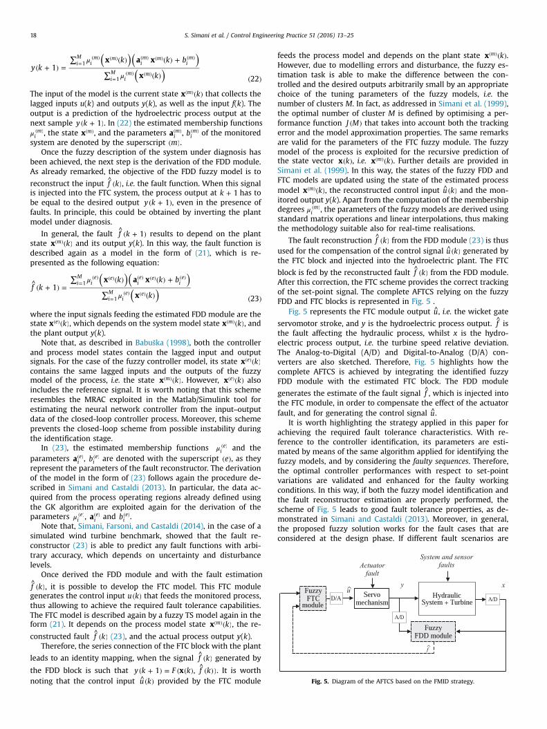
Fig. 5. Diagram of the AFTCS based on the FMID strategy.

S. Simani et al. / Control Engineering Practice 51 (2016) 13–2518

( )( )( )

μ

μ( + ) =

∑ ( ) ( ) +

∑ ( ) ( )

=( ) ( ) ( ) ( ) ( )

=( ) ( )

y kk k b

k

x a x

x1

22

iM

im m

im m

im

iM

im m

1

1

The input of the model is the current state ( )( ) kx m that collects thelagged inputs u(k) and outputs y(k), as well as the input f(k). Theoutput is a prediction of the hydroelectric process output at thenext sample ( + )y k 1 . In (22) the estimated membership functionsμ ( )

im , the state ( )x m , and the parameters ( )ai

m , ( )bim of the monitored

system are denoted by the superscript ( )m .Once the fuzzy description of the system under diagnosis has

been achieved, the next step is the derivation of the FDD module.As already remarked, the objective of the FDD fuzzy model is to

reconstruct the input ^ ( )f k , i.e. the fault function. When this signalis injected into the FTC system, the process output at +k 1 has tobe equal to the desired output ( + )y k 1 , even in the presence offaults. In principle, this could be obtained by inverting the plantmodel under diagnosis.

In general, the fault ^ ( + )f k 1 results to depend on the plantstate ( )( ) kx m and its output y(k). In this way, the fault function isdescribed again as a model in the form of (21), which is re-presented as the following equation:

( )( )( )

μ

μ

^ ( + ) =∑ ( ) ( ) +

∑ ( ) ( )

=( ) ( ) ( ) ( ) ( )

=( ) ( )

f kk k b

k

x a x

x1

23

iM

ie e

ie e

ie

iM

ie e

1

1

where the input signals feeding the estimated FDD module are thestate ( )( ) kx e , which depends on the system model state ( )( ) kx m , andthe plant output y(k).

Note that, as described in Babuška (1998), both the controllerand process model states contain the lagged input and outputsignals. For the case of the fuzzy controller model, its state ( )( ) kx e

contains the same lagged inputs and the outputs of the fuzzymodel of the process, i.e. the state ( )( ) kx m . However, ( )( ) kx e alsoincludes the reference signal. It is worth noting that this schemeresembles the MRAC exploited in the Matlab/Simulink tool forestimating the neural network controller from the input–outputdata of the closed-loop controller process. Moreover, this schemeprevents the closed-loop scheme from possible instability duringthe identification stage.

In (23), the estimated membership functions μ ( )i

e and theparameters ( )ai

e , ( )bie are denoted with the superscript ( )e , as they

represent the parameters of the fault reconstructor. The derivationof the model in the form of (23) follows again the procedure de-scribed in Simani and Castaldi (2013). In particular, the data ac-quired from the process operating regions already defined usingthe GK algorithm are exploited again for the derivation of theparameters μ ( )

ie , ( )ai

e and ( )bie .

Note that, Simani, Farsoni, and Castaldi (2014), in the case of asimulated wind turbine benchmark, showed that the fault re-constructor (23) is able to predict any fault functions with arbi-trary accuracy, which depends on uncertainty and disturbancelevels.

Once derived the FDD module and with the fault estimation^ ( )f k , it is possible to develop the FTC model. This FTC modulegenerates the control input ( )u k that feeds the monitored process,thus allowing to achieve the required fault tolerance capabilities.The FTC model is described again by a fuzzy TS model again in theform (21). It depends on the process model state ( )( ) kx m , the re-

constructed fault ^ ( )f k (23), and the actual process output y(k).Therefore, the series connection of the FTC block with the plant

leads to an identity mapping, when the signal ^ ( )f k generated by

the FDD block is such that ( + ) = ( ( ) ^ ( ))y k F k f kx1 , . It is worthnoting that the control input ^ ( )u k provided by the FTC module

feeds the process model and depends on the plant state ( )( ) kx m .However, due to modelling errors and disturbance, the fuzzy es-timation task is able to make the difference between the con-trolled and the desired outputs arbitrarily small by an appropriatechoice of the tuning parameters of the fuzzy models, i.e. thenumber of clusters M. In fact, as addressed in Simani et al. (1999),the optimal number of cluster M is defined by optimising a per-formance function ( )J M that takes into account both the trackingerror and the model approximation properties. The same remarksare valid for the parameters of the FTC fuzzy module. The fuzzymodel of the process is exploited for the recursive prediction ofthe state vector ( )kx , i.e. ( )( ) kx m . Further details are provided inSimani et al. (1999). In this way, the states of the fuzzy FDD andFTC models are updated using the state of the estimated processmodel ( )( ) kx m , the reconstructed control input ^ ( )u k and the mon-itored output y(k). Apart from the computation of the membershipdegrees μ ( )

im , the parameters of the fuzzy models are derived using

standard matrix operations and linear interpolations, thus makingthe methodology suitable also for real-time realisations.

The fault reconstruction ^ ( )f k from the FDD module (23) is thusused for the compensation of the control signal ^ ( )u k generated bythe FTC block and injected into the hydroelectric plant. The FTC

block is fed by the reconstructed fault ^ ( )f k from the FDD module.After this correction, the FTC scheme provides the correct trackingof the set-point signal. The complete AFTCS relying on the fuzzyFDD and FTC blocks is represented in Fig. 5 .

Fig. 5 represents the FTC module output u, i.e. the wicket gate

servomotor stroke, and y is the hydroelectric process output. f isthe fault affecting the hydraulic process, whilst x is the hydro-electric process output, i.e. the turbine speed relative deviation.The Analog-to-Digital (A/D) and Digital-to-Analog (D/A) con-verters are also sketched. Therefore, Fig. 5 highlights how thecomplete AFTCS is achieved by integrating the identified fuzzyFDD module with the estimated FTC block. The FDD module

generates the estimate of the fault signal f , which is injected intothe FTC module, in order to compensate the effect of the actuatorfault, and for generating the control signal u.

It is worth highlighting the strategy applied in this paper forachieving the required fault tolerance characteristics. With re-ference to the controller identification, its parameters are esti-mated by means of the same algorithm applied for identifying thefuzzy models, and by considering the faulty sequences. Therefore,the optimal controller performances with respect to set-pointvariations are validated and enhanced for the faulty workingconditions. In this way, if both the fuzzy model identification andthe fault reconstructor estimation are properly performed, thescheme of Fig. 5 leads to good fault tolerance properties, as de-monstrated in Simani and Castaldi (2013). Moreover, in general,the proposed fuzzy solution works for the fault cases that areconsidered at the design phase. If different fault scenarios are

S. Simani et al. / Control Engineering Practice 51 (2016) 13–25 19

considered, this situation might require a new fuzzy identificationprocedure.

The remainder of this section recalls the methodology used forobtaining the Linear Parameter Varying (LPV) description of thehydraulic process, which is exploited for the development of theadaptive control strategy. In particular, the on-line estimationscheme exploiting the Least Mean Squares (LMS) with adaptivedirectional forgetting proposed in this work enhances the designprocedure of the suggested adaptive FTC scheme. Note that thisapproach can be seen as a PFTCS. This strategy, which is an im-provement with respect to classical LMS (Ljung, 1999) and LMSwith exponential forgetting (Kulhavý, 1987), was already con-sidered in Simani, Alvisi, et al. (2014) but without any fault toler-ance properties. A different adaptive strategy was presented inSimani and Castaldi (2013) and applied to a wind turbinebenchmark.

Briefly, the LSM with adaptive directional forgetting providesthe on-line estimation of a LPV model of the hydraulic system, i.e.identified model parameters computed at each time step k. Thison-line estimation procedure was implemented in the ®Matlaband ®Simulink environments, as described in Bobal et al. (2005).Once the LPV parameters of the model approximating the beha-viour of the hydraulic process have been computed at each timestep k, the adaptive PI controller is obtained, for example ex-ploiting the Ziegler–Nichols adaptive methodology addressed inBobal et al. (2005), and proposed in Simani, Alvisi, et al. (2014) butwithout fault tolerance capabilities.

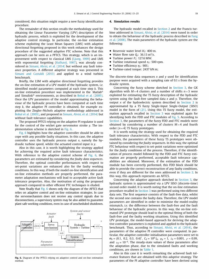
The proposed PFTCS relying on the adaptive PI regulator is usedfor the control of the wicket gate servomotor stroke y. The im-plementation scheme is sketched in Fig. 6.

Fig. 6 highlights how the adaptive controller should be able tocope with any possible faulty situations. In this case, the adaptivecontroller uses the hydraulic process output x, namely the hy-draulic turbine speed, whilst the actuated control input is y.

Also in this case, it is worth highlighting the strategy appliedfor achieving the required active fault tolerance characteristics.With reference to the adaptive control scheme of Fig. 6, theparameters are estimated by considering the faulty data sequences.Therefore, the optimal controller performances with respect toset-point variations are enhanced also for the faulty workingconditions. In this way, if both the model on-line identification andon-line estimation methods are properly performed, the para-meter adaptation mechanisms will lead to acceptable active faulttolerance properties. Also, the motivation of using the proposedapproach compared to other efficient FTC techniques is eluded.

Note finally that Fig. 6 shows only the diagram of the AFTCS thatrelies on adaptive control and on-line estimation strategies. In casethe servomechanism does not receive any control signals due todisconnections, a supervisory system may be also added to guaranteeplant safe working conditions, even in case of unscheduled shutdown.

Fig. 6. Diagram of the PFTCS relying on adaptive control and on-line estimationmethod.

4. Simulation results

The hydraulic model recalled in Section 2 and the Francis tur-bine addressed in Simani, Alvisi, et al. (2014) were tuned in orderto obtain the behaviour of the hydraulic process described in Fanget al. (2008). The main parameters of the hydraulic system are thefollowing:

� Reservoir water level Hr: 400 m.� Water flow rate Qr: 36.13 m /s3 .� Turbine power Pr: 127.6 MW.� Turbine rotational speed nr: 500 rpm.� Turbine efficiency ηr: 90%;� Turbine-rated torque: 2437 kN m;

The discrete-time data sequences x and y used for identificationpurpose were acquired with a sampling rate of 0.1 s from the hy-draulic system.

Concerning the fuzzy scheme sketched in Section 3, the GKalgorithm with M¼4 clusters and a number of shifts n¼3 wereexploited for estimating the TS fuzzy description of the hydraulicsystem using the fault-free sampled data x and y. Therefore, theoutput x of the hydroelectric system described in Section 2 isapproximated by a TS fuzzy Single-Input Single-Output (SISO)model in the form of (21). Using this TS fuzzy model, the esti-mation approach recalled in Section 3 was exploited again foridentifying both the FDD and FTC modules of Fig. 5. According toSection 3, the parameters of the fuzzy FDD and FTC models wereobtained by considering a number of clusters M¼4 and fourthorder (n¼4) TS fuzzy prototypes.

It is worth noting the strategy used for obtaining the requiredfault tolerance characteristics. With respect to the FDD and FTCmodules, the parameters of these fuzzy TS prototypes were ob-tained by considering the faulty sequences. In this way, the optimalFTC behaviour with respect to set-point variations were optimisedfor the faulty conditions of the process. Therefore, if the identifi-cation of process model followed by the FDD and FTC fuzzy esti-mation are properly performed, acceptable fault tolerance cap-abilities are obtained. Moreover, if the estimation of the FDDmodule has been correctly performed, this FDD block should beable to provide the correct reconstruction of any faulty conditions,even if they are different for the ones addressed in Section 2. Inthis way, this approach represents an AFTCS.

Concerning the adaptive approach sketched in Section 3, thehydraulic system is approximated via a LPV SISO (discrete-time)second order model. It is worth noting that the on-line estimationprocedure recalled in Section 3 was performed using two differentdata sets. The first sequence consists of the fault-free data, whilstthe second one contains the faulty data. Therefore, the LPV modelparameters are identified in order to minimise the model-realitymismatch, i.e. the difference between the fault-free and the faultbehaviour of the hydraulic process. In this way, the on-line esti-mated LPV prototype should lead to the optimal fitting of both thefault-free and the faulty working situations. Using this identifiedLPV prototype, the model-based approach for deriving the adap-tive controller parameters is exploited and applied to the hydraulicbenchmark. Thus, according to Simani, Alvisi, et al. (2014), theparameters of the adaptive PI controller were computed. In par-ticular, the adaptive controller initialisation parameters were set toΘ = [ ]0.1, 0.2, 0.3, 0.4 T

0 , =C I1009

4, φ = 10 , λ = 0.0010 , ρ = 0.99,and ν = −100

6. The steady-state values of these parameters afterthe adaptation phase, due to the simulated faults and workingconditions, are shown in Table 1.

Also in this case it is worth remarking the achieved fault tol-erance features that are obtained with this adaptive strategy. Theparameters of the PI adaptive controller have been derived using

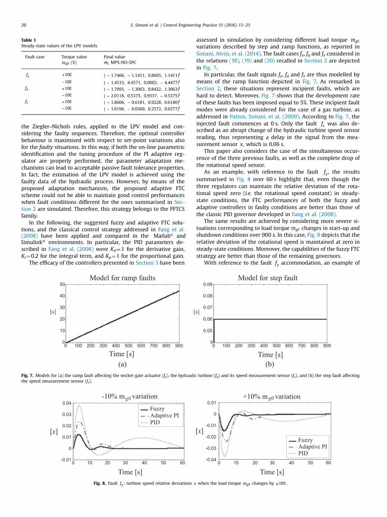
Table 1Steady-state values of the LPV models.

Fault case Torque value Final valuemg0 (%) Θ0 MPS-NO-SPC

fy +100 [ − − ]1.7466, 1.1411, 0.8605, 1.1411 T

−100 [ − − ]1.4533, 4.4571, 0.0002, 4.4477 T

fq +100 [ − − ]1.7095, 1.3063, 0.8422, 1.3063 T

−100 [ − − ]2.0118, 0.5375, 0.9537, 0.5375 T

fx +100 [ − − ]1.8606, 0.6181, 0.9228, 0.6180 T

−100 [ − − ]1.0196, 0.0360, 0.2572, 0.0377 T

S. Simani et al. / Control Engineering Practice 51 (2016) 13–2520

the Ziegler–Nichols rules, applied to the LPV model and con-sidering the faulty sequences. Therefore, the optimal controllerbehaviour is maximised with respect to set-point variations alsofor the faulty situations. In this way, if both the on-line parametricidentification and the tuning procedure of the PI adaptive reg-ulator are properly performed, the parameter adaptation me-chanisms can lead to acceptable passive fault tolerance properties.In fact, the estimation of the LPV model is achieved using thefaulty data of the hydraulic process. However, by means of theproposed adaptation mechanism, the proposed adaptive FTCscheme could not be able to maintain good control performanceswhen fault conditions different for the ones summarised in Sec-tion 2 are simulated. Therefore, this strategy belongs to the PFTCSfamily.

In the following, the suggested fuzzy and adaptive FTC solu-tions, and the classical control strategy addressed in Fang et al.(2008) have been applied and compared in the ®Matlab and

®Simulink environments. In particular, the PID parameters de-scribed in Fang et al. (2008) were Kd¼1 for the derivative gain,Ki¼0.2 for the integral term, and Kp¼1 for the proportional gain.

The efficacy of the controllers presented in Section 3 have been

Time [s]

[s]

Model for ramp faults

0 100 200 300 400 500 600 700 800 9000

10

20

30

40

50

[

)a(Fig. 7. Models for (a) the ramp fault affecting the wicket gate actuator (fy), the hydraulithe speed measurement sensor (fx).

-10% m variationg0

0 10 20 30 40 50 60-0.01

0

0.01

0.02

0.03

0.04

[x]

Time [s]

Fuzzy

PIDAdaptive PI

Fig. 8. Fault fy: turbine speed relative deviations x

assessed in simulation by considering different load torque mg0

variations described by step and ramp functions, as reported inSimani, Alvisi, et al. (2014). The fault cases fy, fq and fx considered inthe relations (18), (19) and (20) recalled in Section 2 are depictedin Fig. 7.

In particular, the fault signals fy, fq and fx are thus modelled bymeans of the ramp function depicted in Fig. 7. As remarked inSection 2, these situations represent incipient faults, which arehard to detect. Moreover, Fig. 7 shows that the development rateof these faults has been imposed equal to 5%. These incipient faultmodes were already considered for the case of a gas turbine, asaddressed in Patton, Simani, et al. (2000). According to Fig. 7, theinjected fault commences at 0 s. Only the fault fx was also de-scribed as an abrupt change of the hydraulic turbine speed sensorreading, thus representing a delay in the signal from the mea-surement sensor x, which is 0.06 s.

This paper also considers the case of the simultaneous occur-rence of the three previous faults, as well as the complete drop ofthe rotational speed sensor.

As an example, with reference to the fault fy, the resultssummarised in Fig. 8 over 60 s highlight that, even though thethree regulators can maintain the relative deviation of the rota-tional speed zero (i.e. the rotational speed constant) in steady-state conditions, the FTC performances of both the fuzzy andadaptive controllers in faulty conditions are better than those ofthe classic PID governor developed in Fang et al. (2008).

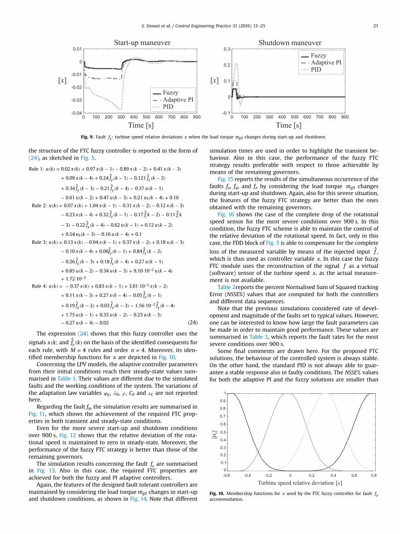
The same results are achieved by considering more severe si-tuations corresponding to load torque mg0 changes in start-up andshutdown conditions over 900 s. In this case, Fig. 9 depicts that therelative deviation of the rotational speed is maintained at zero insteady-state conditions. Moreover, the capabilities of the fuzzy FTCstrategy are better than those of the remaining governors.

With reference to the fault fy accommodation, an example of

Time [s]

s]

Model for step fault

0 100 200 300 400 500 600 700 800 9000

0.05

0.06

0.07

0.08

0.09

)b(c turbine (fq) and its speed measurement sensor (fx), and (b) the step fault affecting

Time [s]0 10 20 30 40 50 60-0.04

-0.03

-0.02

-0.01

0

0.01+10% m variationg0

Fuzzy

PIDAdaptive PI

[x]

when the load torque mg0 changes by ±10%.

Start-up maneuver

Time [s] Time [s]

Shutdown maneuver

0 100 200 300 400 500 600 700 800 900-0.04

-0.03

-0.02

-0.01

0

0.01

0 100 200 300 400 500 600 700 800 900-0.1

0

0.1

0.2

0.3

Fuzzy

PIDAdaptive PI

Fuzzy

PIDAdaptive PI

[x] [x]

Fig. 9. Fault fy: turbine speed relative deviations x when the load torque mg0 changes during start-up and shutdown.

[ ]

Turbine speed relative deviation [x]

0

0.1

0.2

0.3

0.4

0.5

0.6

0.7

0.8

0.9

1

-0.6 -0.4 -0.2 0 0.2 0.4 0.6 0.8

i

Fig. 10. Membership functions for x used by the FTC fuzzy controller for fault fyaccommodation.

S. Simani et al. / Control Engineering Practice 51 (2016) 13–25 21

the structure of the FTC fuzzy controller is reported in the form of(24), as sketched in Fig. 5.

( )

( ) = ( ) + ( − ) − ( − ) + ( − )

+ ( − ) + ^ ( − ) − ^ ( − )

+ ^ ( − ) − ^ ( − ) − ( − )

− ( − ) + ( − ) + ( − ) +

( ) = ( ) + ( − ) − ( − ) − ( − )

− ( − ) + ^ ( − ) − ^ − ) − ^

− ) − ^ ( − ) − ( − ) + ( − )

+ ( − ) − ( − ) +

( ) = ( ) − ( − ) + ( − ) + ( − )

− ( − ) + ^ ( − ) + ^ ( − )

− ^ ( − ) + ^ ( − ) + ( − )

+ ( − ) − ( − ) + · ( − )

+ ·( ) = − ( ) + ( − ) + · ( − )

+ ( − ) + ( − ) − ^ ( − )

+ ^ ( − ) + ^ ( − ) − · ^ ( − )

+ ( − ) + ( − ) − ( − )

− ( − ) −

( (

−

−

−

−

24

u k x k x k x k x k

x k f k f k

f k f k u k

u k u k u k

u k x k x k x k x k

x k f k f k f k

f k u k u k

u k u k

u k x k x k x k x k

x k f k f k

f k f k u k

u k u k u k

u k x k x k x k

x k x k f k

f k f k f k

u k u k u k

u k

Rule 1: 0.02 0.97 1 0.89 2 0.41 3

0.09 4 0.24 1 0.121 2

0.34 3 0.21 4 0.37 1

0.61 2 0.47 3 0.21 4 0.16

Rule 2: 0.07 1.04 1 0.31 2 0.12 3

0.23 4 0.32 1 0.17 2 0.11

3 0.22 4 0.62 1 0.12 2

0.54 3 0.16 4 0.1

Rule 3: 0.13 0.94 1 0.37 2 0.18 3

0.10 4 0.06 1 0.84 2

0.26 3 0.18 4 0.27 1

0.85 2 0.34 3 9.10 10 4

1.72 10

Rule 4: 0.37 0.83 1 3.01 10 2

0.11 3 0.27 4 0.05 1

0.19 2 0.03 3 1.56 10 4

1.75 1 0.35 2 0.23 3

0.27 4 0.02

y y

y y

y

y

y y

y y

y

y y y

5

3

2

2

2

2

The expression (24) shows that this fuzzy controller uses the

signals ( )x k and ^ ( )f ky on the basis of the identified consequents foreach rule, with =M 4 rules and order =n 4. Moreover, its iden-tified membership functions for x are depicted in Fig. 10.

Concerning the LPV models, the adaptive controller parametersfrom their initial conditions reach their steady-state values sum-marised in Table 1. Their values are different due to the simulatedfaults and the working conditions of the system. The variations ofthe adaptation law variables φ0, λ0, ρ, C0 and ν0 are not reportedhere.

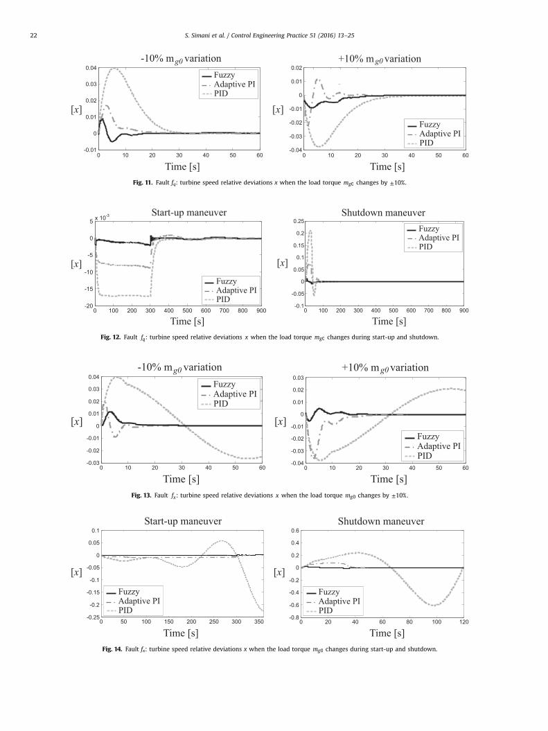
Regarding the fault fq, the simulation results are summarised inFig. 11, which shows the achievement of the required FTC prop-erties in both transient and steady-state conditions.

Even for the more severe start-up and shutdown conditionsover 900 s, Fig. 12 shows that the relative deviation of the rota-tional speed is maintained to zero in steady-state. Moreover, theperformance of the fuzzy FTC strategy is better than those of theremaining governors.

The simulation results concerning the fault fx are summarisedin Fig. 13. Also in this case, the required FTC properties areachieved for both the fuzzy and PI adaptive controllers.

Again, the features of the designed fault tolerant controllers aremaintained by considering the load torque mg0 changes in start-upand shutdown conditions, as shown in Fig. 14. Note that different

simulation times are used in order to highlight the transient be-haviour. Also in this case, the performance of the fuzzy FTCstrategy results preferable with respect to those achievable bymeans of the remaining governors.

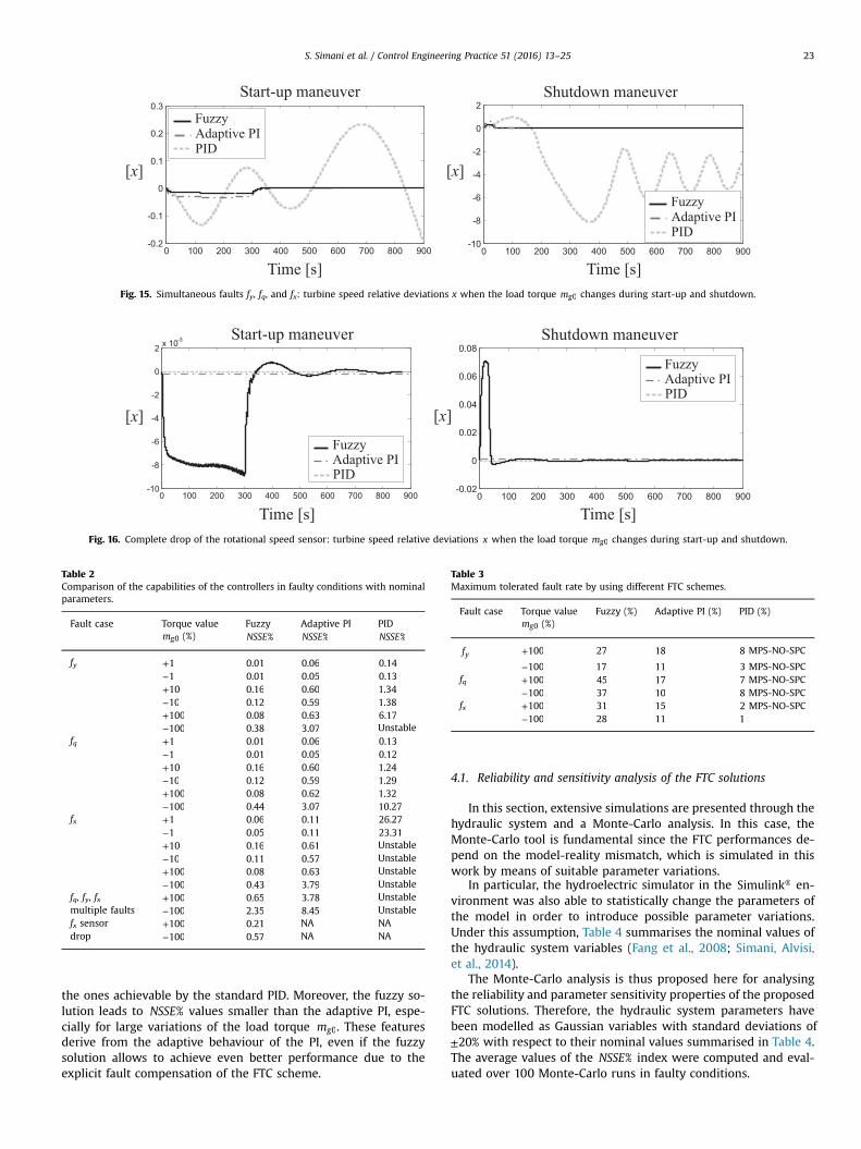
Fig. 15 reports the results of the simultaneous occurrence of thefaults fy, fq, and fx by considering the load torque mg0 changesduring start-up and shutdown. Again, also for this severe situation,the features of the fuzzy FTC strategy are better than the onesobtained with the remaining governors.

Fig. 16 shows the case of the complete drop of the rotationalspeed sensor for the most severe conditions over 900 s. In thiscondition, the fuzzy FTC scheme is able to maintain the control ofthe relative deviation of the rotational speed. In fact, only in thiscase, the FDD block of Fig. 5 is able to compensate for the complete

loss of the measured variable by means of the injected input f ,which is thus used as controller variable x. In this case the fuzzyFTC module uses the reconstruction of the signal f as a virtual(software) sensor of the turbine speed x, as the actual measure-ment is not available.

Table 2reports the percent Normalised Sum of Squared trackingError (NSSE%) values that are computed for both the controllersand different data sequences.

Note that the previous simulations considered rate of devel-opment and magnitude of the faults set to typical values. However,one can be interested to know how large the fault parameters canbe made in order to maintain good performance. These values aresummarised in Table 3, which reports the fault rates for the mostsevere conditions over 900 s.

Some final comments are drawn here. For the proposed FTCsolutions, the behaviour of the controlled system is always stable.On the other hand, the standard PID is not always able to guar-antee a stable response also in faulty conditions. The NSSE% valuesfor both the adaptive PI and the fuzzy solutions are smaller than

Time [s]

-10% m variationg0 +10% m variationg0

Time [s]0 10 20 30 40 50 60

-0.01

0

0.01

0.02

0.03

0.04

0 10 20 30 40 50 60-0.04

-0.03

-0.02

-0.01

0

0.01

0.02Fuzzy

PIDAdaptive PI

Fuzzy

PIDAdaptive PI

[x] [x]

Fig. 11. Fault fq: turbine speed relative deviations x when the load torque mg0 changes by ±10%.

Start-up maneuver

Time [s] Time [s]

Shutdown maneuver

0 100 200 300 400 500 600 700 800 900-20

-15

-10

-5

0

5 x 10

0 100 200 300 400 500 600 700 800 900-0.1

-0.05

0

0.05

0.1

0.15

0.2

0.25

Fuzzy

PIDAdaptive PI

Fuzzy

PIDAdaptive PI

[x] [x]

Fig. 12. Fault fq: turbine speed relative deviations x when the load torque mg0 changes during start-up and shutdown.

Time [s]

-10% m variationg0 +10% m variationg0

Time [s]0 10 20 30 40 50 60

-0.03

-0.02

-0.01

0

0.01

0.02

0.03

0.04

0 10 20 30 40 50 60-0.04

-0.03

-0.02

-0.01

0

0.01

0.02

0.03Fuzzy

PIDAdaptive PI

Fuzzy

PIDAdaptive PI

[x] [x]

Fig. 13. Fault fx: turbine speed relative deviations x when the load torque mg0 changes by ±10%.

Start-up maneuver

Time [s] Time [s]

Shutdown maneuver

0 20 40 60 80 100 120-0.8

-0.6

-0.4

-0.2

0

0.2

0.4

0.6

0 50 100 150 200 250 300 350-0.25

-0.2

-0.15

-0.1

-0.05

0

0.05

0.1

Fuzzy

PIDAdaptive PI

Fuzzy

PIDAdaptive PI

[x] [x]

Fig. 14. Fault fx: turbine speed relative deviations x when the load torque mg0 changes during start-up and shutdown.

S. Simani et al. / Control Engineering Practice 51 (2016) 13–2522

Start-up maneuver

Time [s] Time [s]

Shutdown maneuver

[x] [x]

0 100 200 300 400 500 600 700 800 900-0.2

-0.1

0

0.1

0.2

0.3

0 100 200 300 400 500 600 700 800 900-10

-8

-6

-4

-2

0

2Fuzzy

PIDAdaptive PI

Fuzzy

PIDAdaptive PI

Fig. 15. Simultaneous faults fy, fq, and fx: turbine speed relative deviations x when the load torque mg0 changes during start-up and shutdown.

Start-up maneuver

Time [s] Time [s]

Shutdown maneuver

[x] [x]

0 100 200 300 400 500 600 700 800 900-0.02

0

0.02

0.04

0.06

0.08

0 100 200 300 400 500 600 700 800 900-10

-8

-6

-4

-2

0

2 x 10

Fuzzy

PIDAdaptive PI

Fuzzy

PIDAdaptive PI

Fig. 16. Complete drop of the rotational speed sensor: turbine speed relative deviations x when the load torque mg0 changes during start-up and shutdown.

Table 2Comparison of the capabilities of the controllers in faulty conditions with nominalparameters.

Fault case Torque value Fuzzy Adaptive PI PIDmg0 (%) NSSE% NSSE% NSSE%

fy +1 0.01 0.06 0.14−1 0.01 0.05 0.13+10 0.16 0.60 1.34−10 0.12 0.59 1.38+100 0.08 0.63 6.17−100 0.38 3.07 Unstable

fq +1 0.01 0.06 0.13−1 0.01 0.05 0.12+10 0.16 0.60 1.24−10 0.12 0.59 1.29+100 0.08 0.62 1.32−100 0.44 3.07 10.27

fx +1 0.06 0.11 26.27−1 0.05 0.11 23.31+10 0.16 0.61 Unstable−10 0.11 0.57 Unstable+100 0.08 0.63 Unstable−100 0.43 3.79 Unstable

fq, fy, fx +100 0.65 3.78 Unstablemultiple faults −100 2.35 8.45 Unstablefx sensor +100 0.21 NA NAdrop −100 0.57 NA NA

Table 3Maximum tolerated fault rate by using different FTC schemes.

Fault case Torque value Fuzzy (%) Adaptive PI (%) PID (%)mg0 (%)

fy +100 27 18 8 MPS-NO-SPC

−100 17 11 3 MPS-NO-SPCfq +100 45 17 7 MPS-NO-SPC

−100 37 10 8 MPS-NO-SPCfx +100 31 15 2 MPS-NO-SPC

−100 28 11 1

S. Simani et al. / Control Engineering Practice 51 (2016) 13–25 23

the ones achievable by the standard PID. Moreover, the fuzzy so-lution leads to NSSE% values smaller than the adaptive PI, espe-cially for large variations of the load torque mg0. These featuresderive from the adaptive behaviour of the PI, even if the fuzzysolution allows to achieve even better performance due to theexplicit fault compensation of the FTC scheme.

4.1. Reliability and sensitivity analysis of the FTC solutions

In this section, extensive simulations are presented through thehydraulic system and a Monte-Carlo analysis. In this case, theMonte-Carlo tool is fundamental since the FTC performances de-pend on the model-reality mismatch, which is simulated in thiswork by means of suitable parameter variations.

In particular, the hydroelectric simulator in the ®Simulink en-vironment was also able to statistically change the parameters ofthe model in order to introduce possible parameter variations.Under this assumption, Table 4 summarises the nominal values ofthe hydraulic system variables (Fang et al., 2008; Simani, Alvisi,et al., 2014).

The Monte-Carlo analysis is thus proposed here for analysingthe reliability and parameter sensitivity properties of the proposedFTC solutions. Therefore, the hydraulic system parameters havebeen modelled as Gaussian variables with standard deviations of±20% with respect to their nominal values summarised in Table 4.The average values of the NSSE% index were computed and eval-uated over 100 Monte-Carlo runs in faulty conditions.

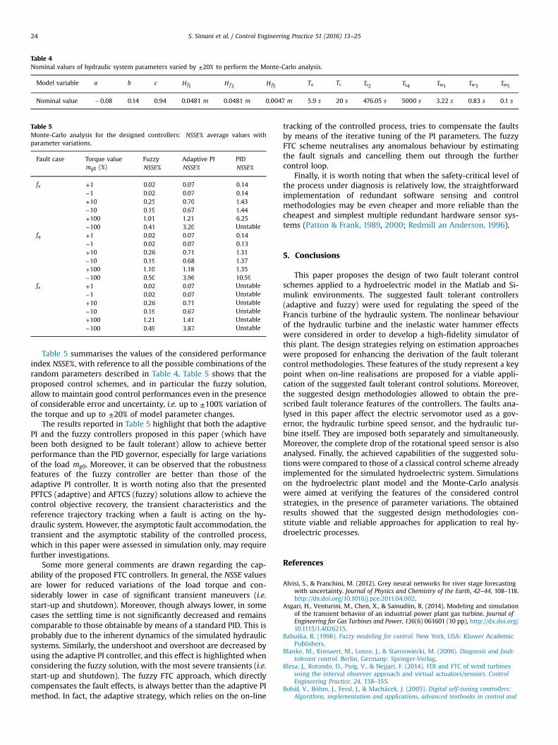
Table 4Nominal values of hydraulic system parameters varied by ±20% to perform the Monte-Carlo analysis.

Model variable a b c H f1 H f3 H f5 Ta Tc Ts2 Ts4 Tw1 Tw3 Tw5

Nominal value �0.08 0.14 0.94 0.0481 m 0.0481 m 0.0047 m 5.9 s 20 s 476.05 s 5000 s 3.22 s 0.83 s 0.1 s

Table 5Monte-Carlo analysis for the designed controllers: NSSE% average values withparameter variations.

Fault case Torque value Fuzzy Adaptive PI PIDmg0 (%) NSSE% NSSE% NSSE%

fy +1 0.02 0.07 0.14−1 0.02 0.07 0.14+10 0.25 0.70 1.43−10 0.19 0.67 1.44+100 1.01 1.21 6.25−100 0.41 3.20 Unstable

fq +1 0.02 0.07 0.14−1 0.02 0.07 0.13+10 0.26 0.71 1.31−10 0.19 0.68 1.37+100 1.10 1.18 1.35−100 0.50 3.96 10.59

fx +1 0.02 0.07 Unstable−1 0.02 0.07 Unstable+10 0.26 0.71 Unstable−10 0.19 0.67 Unstable+100 1.21 1.41 Unstable−100 0.49 3.87 Unstable

S. Simani et al. / Control Engineering Practice 51 (2016) 13–2524

Table 5 summarises the values of the considered performanceindex NSSE%, with reference to all the possible combinations of therandom parameters described in Table 4. Table 5 shows that theproposed control schemes, and in particular the fuzzy solution,allow to maintain good control performances even in the presenceof considerable error and uncertainty, i.e. up to ±100% variation ofthe torque and up to ±20% of model parameter changes.

The results reported in Table 5 highlight that both the adaptivePI and the fuzzy controllers proposed in this paper (which havebeen both designed to be fault tolerant) allow to achieve betterperformance than the PID governor, especially for large variationsof the load mg0. Moreover, it can be observed that the robustnessfeatures of the fuzzy controller are better than those of theadaptive PI controller. It is worth noting also that the presentedPFTCS (adaptive) and AFTCS (fuzzy) solutions allow to achieve thecontrol objective recovery, the transient characteristics and thereference trajectory tracking when a fault is acting on the hy-draulic system. However, the asymptotic fault accommodation, thetransient and the asymptotic stability of the controlled process,which in this paper were assessed in simulation only, may requirefurther investigations.

Some more general comments are drawn regarding the cap-ability of the proposed FTC controllers. In general, the NSSE valuesare lower for reduced variations of the load torque and con-siderably lower in case of significant transient maneuvers (i.e.start-up and shutdown). Moreover, though always lower, in somecases the settling time is not significantly decreased and remainscomparable to those obtainable by means of a standard PID. This isprobably due to the inherent dynamics of the simulated hydraulicsystems. Similarly, the undershoot and overshoot are decreased byusing the adaptive PI controller, and this effect is highlighted whenconsidering the fuzzy solution, with the most severe transients (i.e.start-up and shutdown). The fuzzy FTC approach, which directlycompensates the fault effects, is always better than the adaptive PImethod. In fact, the adaptive strategy, which relies on the on-line

tracking of the controlled process, tries to compensate the faultsby means of the iterative tuning of the PI parameters. The fuzzyFTC scheme neutralises any anomalous behaviour by estimatingthe fault signals and cancelling them out through the furthercontrol loop.

Finally, it is worth noting that when the safety-critical level ofthe process under diagnosis is relatively low, the straightforwardimplementation of redundant software sensing and controlmethodologies may be even cheaper and more reliable than thecheapest and simplest multiple redundant hardware sensor sys-tems (Patton & Frank, 1989, 2000; Redmill an Anderson, 1996).

5. Conclusions

This paper proposes the design of two fault tolerant controlschemes applied to a hydroelectric model in the Matlab and Si-mulink environments. The suggested fault tolerant controllers(adaptive and fuzzy) were used for regulating the speed of theFrancis turbine of the hydraulic system. The nonlinear behaviourof the hydraulic turbine and the inelastic water hammer effectswere considered in order to develop a high-fidelity simulator ofthis plant. The design strategies relying on estimation approacheswere proposed for enhancing the derivation of the fault tolerantcontrol methodologies. These features of the study represent a keypoint when on-line realisations are proposed for a viable appli-cation of the suggested fault tolerant control solutions. Moreover,the suggested design methodologies allowed to obtain the pre-scribed fault tolerance features of the controllers. The faults ana-lysed in this paper affect the electric servomotor used as a gov-ernor, the hydraulic turbine speed sensor, and the hydraulic tur-bine itself. They are imposed both separately and simultaneously.Moreover, the complete drop of the rotational speed sensor is alsoanalysed. Finally, the achieved capabilities of the suggested solu-tions were compared to those of a classical control scheme alreadyimplemented for the simulated hydroelectric system. Simulationson the hydroelectric plant model and the Monte-Carlo analysiswere aimed at verifying the features of the considered controlstrategies, in the presence of parameter variations. The obtainedresults showed that the suggested design methodologies con-stitute viable and reliable approaches for application to real hy-droelectric processes.

References

Alvisi, S., & Franchini, M. (2012). Grey neural networks for river stage forecastingwith uncertainty. Journal of Physics and Chemistry of the Earth, 42–44, 108–118.http://dx.doi.org/10.1016/j.pce.2011.04.002.

Asgari, H., Venturini, M., Chen, X., & Sainudiin, R. (2014). Modeling and simulationof the transient behavior of an industrial power plant gas turbine. Journal ofEngineering for Gas Turbines and Power, 136(6) 061601 (10 pp), http://dx.doi.org/10.1115/1.4026215.

Babuška, R. (1998). Fuzzy modeling for control. New York, USA: Kluwer AcademicPublishers.

Blanke, M., Kinnaert, M., Lunze, J., & Staroswiecki, M. (2006). Diagnosis and fault-tolerant control. Berlin, Germany: Springer-Verlag.

Blesa, J., Rotondo, D., Puig, V., & Nejjari, F. (2014). FDI and FTC of wind turbinesusing the interval observer approach and virtual actuators/sensors. ControlEngineering Practice, 24, 138–155.

Bobál, V., Böhm, J., Fessl, J., & Machácek, J. (2005). Digital self-tuning controllers:Algorithms, implementation and applications, advanced textbooks in control and

S. Simani et al. / Control Engineering Practice 51 (2016) 13–25 25

signal processing (1st ed.). Berlin, Germany: Springer.Chen, J., & Patton, R. J. (1999). Robust model-based fault diagnosis for dynamic sys-

tems. Boston, MA, USA: Kluwer Academic Publishers.Ding, S. X. (2008). Model-based fault diagnosis techniques: Design schemes, algo-

rithms, and tools (1st ed.). Berlin Heidelberg: Springer ISBN: 978-3540763031.Eker, I. (2004). Governors for hydro-turbine speed control in power generation: A

SIMO robust design approach. Energy Conversion and Management, 45(13–14),2207–2221.

Fang, H., Chen, L., Dlakavu, N., & Shen, Z. (2008). Basic modeling and simulation toolfor analysis of hydraulic transients in hydroelectric power plants. IEEE Trans-actions on Energy Conversion, 23(3), 424–434.

Fonod, R., Henry, D., Charbonnel, C., Bornschlegl, E., Losa, D., & Bennani, S. (2015).Robust FDI for fault-tolerant thrust allocation with application to spacecraftrendezvous. Control Engineering Practice, 42, 12–27.

Hanmandlu, M., & Goyal, H. (2008). Proposing a new advanced control techniquefor micro hydro power plants. International Journal of Electrical Power & EnergySystems, 30(4), 272–282.

Hong, Y., Guangda, C., & Weiyou, C. (2008). Uncertain linear system D-domain ro-bust stability fault tolerant control of hydraulic turbine regulator. In The thirdinternational conference on electric utility deregulation and restructuring andpower technologies—DRPT 2008, http://dx.doi.org/10.1109/DRPT.2008.4523818.

Kiltz, L., Join, C., Mboup, M., & Rudolph, J. (2014). Fault-tolerant control based onalgebraic derivative estimation applied on a magnetically supported plate.Control Engineering Practice, 26, 107–115.

Kim, Y., & Kim, C. (2015). Modeling and response time analysis of the level 2 systemfor a continuous steel casting process. Control Engineering Practice 44, 117–125.

Kishor, N., Singh, S., & Raghuvanshi, A. (2006). Dynamic simulations of hydro tur-bine and its state estimation based lq control. Energy Conversion and Manage-ment, 47(18–19), 3119–3137.

Kishor, N., Saini, R., & Singh, S. (2007). A review on hydropower plant models andcontrol. Renewable and Sustainable Energy Reviews, 11(5), 776–796.

Kulhavý, R. (1987). Restricted exponential forgetting in real-time identification.Automatica, 23(9), 589–600.

Li, Z., Ye, L., Wei, S., Malik, O. P., Hope, G. S., & Hancock, G. C. (1992). Fault toleranceaspects of a highly reliable microprocessor-based water turbine governor. IEEETransactions on Energy Conversion, 7(1), 1–7. http://dx.doi.org/10.1109/60.124534.

Li, Y., Liu, F., & Cao, Y. (2015). Delay-dependent wide-area damping control forstability enhancement of HVDC/AC interconnected power systems. ControlEngineering Practice, 37, 43–54.

Ljung, L. (1999). System identification: Theory for the user (2nd ed.). Englewood Cliffs,NJ: Prentice Hall.

Mahmoud, M., Dutton, K., & Denman, M. (2005). Design and simulation of a non-linear fuzzy controller for a hydropower plant. Electric Power Systems Research,73(2), 87–99.

Mansoor, S., Jones, D., Bradley, D., Aris, F., & Jones, G. (2000). Reproducing oscilla-tory behaviour of a hydroelectric power station by computer simulation. Con-trol Engineering Practice, 8(11), 1261–1272.

Nelles, O. (2001). Nonlinear system identification. Berlin Heidelberg, Germany:

Springer-Verlag.Noura, H., Theilliol, D., Ponsart, J.-C., & Chamseddine, A. (2009). Fault-tolerant

control systems: Design and practical applications advances in industrial control(1st ed.). London: Springer.

Patton, R.J., Frank, P.M., & Clark R.N. (Eds.). (1989). Fault diagnosis in dynamic sys-tems, theory and application, control engineering series. London: Prentice Hall,.

Patton, R.J., Frank, P.M., & Clark, R.N. (Eds.). (2000). Issues of Fault diagnosis fordynamic systems. London, UK: Springer-Verlag, London Limited.

Patton, R.J., Simani, S., Daley, S., & Pike, A. (2000). Fault diagnosis of a simulatedmodel of an industrial gas turbine prototype using identification techniques. InThe fourth symposium on fault detection supervision and safety for technicalprocesses, SAFEPROCESS2000 (Vol. 1, pp. 518–524), Budapest, Hungary.

Redmill, F., & Anderson, T. (Eds.). (1996). Safety-critical systems: The convergence ofhigh tech and human factors, 1st ed. Leeds, UK: Springer. ISBN:978-3540760092.

Schuh, M., Zgorzelski, M., & Lunze, J. (2015). Experimental evaluation of an activefault-tolerant control method. Control Engineering Practice, 43, 1–11.

Simani, S., & Castaldi, P. (2013). Data-driven and adaptive control applications to awind turbine benchmark model. Control Engineering Practice, 21(12),1678–1693. http://dx.doi.org/10.1016/j.conengprac.2013.08.009 (Special issueinvited paper). ISSN: 0967-0661. PII: S0967-0661(13)00155-X..

Simani, S., Fantuzzi, C., Rovatti, R., & Beghelli, S. (1999). Parameter identification forpiecewise linear fuzzy models in noisy environment. International Journal ofApproximate Reasoning, 1(22), 149–167.

Simani, S., Alvisi, S., & Venturini, M. (2014). Study of the time response of a simu-lated hydroelectric system. Journal of Physics: Conference Series 570, 1–13. ISSN:1742-6596. http://dx.doi.org/10.1088/1742-6596/570/5/052003.

Simani, S., Farsoni, S., & Castaldi, P. (2014). Fault diagnosis of a wind turbinebenchmark via identified fuzzy models. IEEE Transactions on Industrial Electro-nics, 62(6), 3775–3782. http://dx.doi.org/10.1109/TIE.2014.2364548 (Invitedpaper for the special issue ”Real-time fault diagnosis and fault tolerant control).

Simani, S., Alvisi, S., & Venturini, M. (2015). Data-driven design of a fault tolerantfuzzy controller for a simulated hydroelectric system. In IFAC (Ed.), Proceedingsof the ninth IFAC symposium on fault detection, supervision and safety for technicalprocesses—SAFEPROCESS’15, IFAC, Paris, France (Special session invited paper).

Takagi, T., & Sugeno, M. (1985). Fuzzy identification of systems and its application tomodeling and control. IEEE Transaction on System, Man and Cybernetics, SMC-15(1), 116–132.

Ubaid, U., Daley, S., & Pope, S. A. (2015). Design of remotely located and multi-loopvibration controllers using a sequential loop closing approach. Control En-gineering Practice, 38, 1–10.

Weber, H., Prillwitz, F., Hladky, M., & Asal, H.-P. (2001). Reality oriented simulationmodels of power plants for restoration studies. Control Engineering Practice, 9(7), 805–811.

Wei, L., Wei-bo, L., Gen-mao, W., & Jian-hua, W. (2000). Research on the methods ofdetecting and removing slide valve failure. Journal of Zhejiang University Science,1(1), 56–60.

Zhang, Y., & Jiang, J. (2008). Bibliographical review on reconfigurable fault-tolerantcontrol systems. Annual Reviews in Control, 32, 229–252.