Control Engineering Master Seminar By Hamidreza Azimian A Survey on Visual Object Tracking Algorithms KNT University of Technology Fall 2005 Advisor: Dr. A. Fatehi

Welcome message from author
This document is posted to help you gain knowledge. Please leave a comment to let me know what you think about it! Share it to your friends and learn new things together.
Transcript

Control Engineering Master Seminar
By
Hamidreza Azimian
A Survey on
Visual Object Tracking Algorithms
KNT University of Technology
Fall 2005
Advisor: Dr. A. Fatehi
A Survey in Visual Object Tracking Algorithms
1
Introduction .................................................................................................................... 3 1 KALMAN FILTERING ............................................................................................. 5 2 EXTENDED ALGORITHMS OF KALMAN FILTERING.................................... 14
2.1 Optimal Nonlinear Estimation .......................................................................... 14 2.2 EKF Algorithm ................................................................................................. 15 2.3 Unscented KF versus EKF................................................................................ 15
3 PARTICLE FILTERING.......................................................................................... 21 3.1 Bayesian sequential importance sampling:....................................................... 22 3.2 Selective Re-sampling: ..................................................................................... 25 3.3 Generic Particle Filter Algorithm: .................................................................... 25
4 MULTIPLE-MODEL: A Hybrid Estimation Method .............................................. 27 4.1 Introduction....................................................................................................... 27 4.2 MULTIPLE-MODEL ESTIMATION.............................................................. 29
4.2.1 General Description .................................................................................. 29 4.2.2 Filter Re-initialization and the IMM Algorithm ....................................... 33
4.3 INTRODUCTION TO VSMM ESTIMATION ............................................... 38 4.3.1 Limitations of Fixed Structures ................................................................ 39 4.3.2 When Should a Variable Structure Be Used? ........................................... 41 4.3.3 The Recursive Adaptive Model-Set Approach ......................................... 41
4.4 MODEL-SET ADAPTATION ......................................................................... 43 4.5 VSMM ALGORITHMS ................................................................................... 43
4.5.1 10.6.1 Categories of Variable Structures .................................................. 44 4.5.2 Model-Group Switching Algorithm.......................................................... 46 4.5.3 Likely-Model Set Algorithm..................................................................... 49 4.5.4 Evaluation of MM Algorithms.................................................................. 51
5 CONCLUDING REMARKS.................................................................................... 52
A Survey in Visual Object Tracking Algorithms
2
Abstract- Due to the increasing demand of a faster and more reliable target tracking
ability specifically for some critical applications such as military navigation and
Robotics, using prediction and estimation concepts have been comprehensively studied.
As a result of this demand, old and modern estimation algorithms based on probabilistic
Baysian algorithms have been employed. In the case of visual object tracking much work
has been done to design new algorithms by mixing modern target tracking algorithms
with older object detection algorithms of vision. In this survey the development of target
tracking algorithms has been studied more extensively with providing a few examples of
estimation-based-modified-vision-algorithms. A literature survey is given on the
evolution of the Beysian tracking algorithms such as various types of Kalman filtering,
Particle filtering and finally Multiple-Model.
A Survey in Visual Object Tracking Algorithms
3
INTRODUCTION
The motivation to provide the ability of tracking the moving objects have been supported
by many desired functions in various fields including automation, military navigation and
robotics. It has been a goal of the researchers of the electrical engineering and computer
science for about four decades to achieve such a facility. The functionality of this scheme
has been strongly supported by applications such as "moving target locking", "robot
localization", "radar navigation", and most recently "vision-based control of autonomous
vehicle ". Due to these reasons this field of research has employed experts of different
fields of computer and electrical engineering such as radar and control system experts.
The backbone of the modern target tracking developments is the "Beyesian estimation
algorithms"; to be able to make any prediction we should have much more information
about the probability distribution of the object’s position. Considering a system whose
state variables are the object’s spatial coordination, or probably orientation, with a given
probability distribution function, we can search for a method to calculate the expectation
of the states which is considered as the prediction of those states. This demand was met
and motivated for more research by the "Kalman" filtering, introduced in 1960s. This
method was a suitable and satisfying method until a challenge was born for more robust
method of estimation for nonlinear systems. All the efforts for solving such a problem
was paid off with "Extended Kalman" filtering by Anderson and Moore in 1979. This
method was based on the Taylor series expansion of the nonlinear system while it proved
acceptable for just weakly nonlinear systems with additive noise. A more robust and
powerful estimation method called "Unscented Kalman" filtering was introduced in 1996
by Julier and Uhlmann [7]. It was based on the PDF estimation of the nonlinear system
by deterministic sampling with no system linearization that could make the approach
prone to large errors. Due to this fact it outperformed the EKF.
In parallel with the extensions of the Kalman filtering, some other methods of estimation
were developed. The old "particle Filtering algorithm" which was disregarded due to the
computational complexities in 60s, was restored in 90s. It had superiority to the previous
methods, because it did not require a Gaussian PDF for the states of the system. Another
A Survey in Visual Object Tracking Algorithms
4
algorithm of estimation, developed meanwhile, mainly by Bar-Shalom and Li, flourished
in the early 1990s [17] and was called "Multiple Model". It was based on this fact that
real nonlinear models can be estimated by one or a combination of linear models in
different conditions and a variety of algorithms can be developed to provide robust
switching ability between different models for highly nonlinear system which may switch
between different models very fast. Different versions of Multiple-Model algorithm have
such a strong feature. In the other hand, to achieve a robust and reliable visual object
tracking algorithm, relying just on vision and image processing algorithms, many efforts
have been made during the last few decades. Most of the recent methods are based on
modified segmentation and/or edge detectors such as Canny [1] or optical flow and
correlation [2]. All of these methods had a satisfactory response, but for a more robust
performance of tracking specially in presence of occlusion and/or clutter a more
challenging approach is to predict one step ahead at least.
In this survey we mainly deal with estimation algorithms which are the base for the
modern target tracking. First a short view of the Kalman Filtering is presented since for a
linear model the analytical solution is the Kalman Filter. While this solution is really
novel to linear model problems, it works no good for nonlinear models. Consequently
modified Kalman Filter algorithms, developed during 70s and 80s with much better
performance, are discussed in section 2. But as a more general solution Particle Filters
have been introduced which are suitable for nonlinear and/or non-Gaussian distributed
models. This algorithm is studied in section 3 with more details. This algorithm is
currently being used in a vast quantity. Finally a more descriptive detail is provided for
another family of algorithms based on Bar-Slalom's works flourished in late 80s and early
90s, called Multiple-Model.
A Survey in Visual Object Tracking Algorithms
5
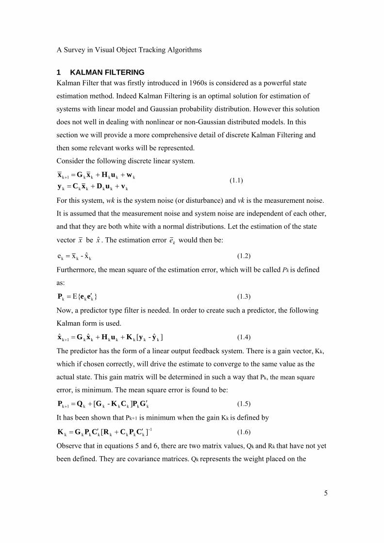
1 KALMAN FILTERING Kalman Filter that was firstly introduced in 1960s is considered as a powerful state
estimation method. Indeed Kalman Filtering is an optimal solution for estimation of
systems with linear model and Gaussian probability distribution. However this solution
does not well in dealing with nonlinear or non-Gaussian distributed models. In this
section we will provide a more comprehensive detail of discrete Kalman Filtering and
then some relevant works will be represented.
Consider the following discrete linear system.
kkkkkk
kkkkk1k
vuDxCywuHxGx
++=++=+ (1.1)
For this system, wk is the system noise (or disturbance) and vk is the measurement noise.
It is assumed that the measurement noise and system noise are independent of each other,
and that they are both white with a normal distributions. Let the estimation of the state
vector x be x̂ . The estimation error ke would then be:
kkk x̂ -x e = (1.2)
Furthermore, the mean square of the estimation error, which will be called Pk is defined
as:
}E{ kkk eeP ′= (1.3)
Now, a predictor type filter is needed. In order to create such a predictor, the following
Kalman form is used.
]ˆ -[ ˆ ˆ kkkkkkk1k yyKuHxGx ++=+ (1.4)
The predictor has the form of a linear output feedback system. There is a gain vector, Kk,
which if chosen correctly, will drive the estimate to converge to the same value as the
actual state. This gain matrix will be determined in such a way that Pk, the mean square
error, is minimum. The mean square error is found to be:
]-[ kkkkkk1k GPCKGQP ′+=+ (1.5)
It has been shown that Pk+1 is minimum when the gain Kk is defined by -1
kkkkkkkk ] [ CPCRCPGK ′+′= (1.6)
Observe that in equations 5 and 6, there are two matrix values, Qk and Rk that have not yet
been defined. They are covariance matrices. Qk represents the weight placed on the
A Survey in Visual Object Tracking Algorithms
6
disturbances in the system model, while Rk weighs the noise that exists in the
measurements. They are defined as:
}E{ kkk wwQ ′= (1.7)
}E{ kkk vvR ′= (1.8)
The covariance matrices act as weighting factors for the disturbances and measurement
noise. It turns out that what is really important is the ratio between these two weight
matrices. If the ratio is large, then the filter is being defined for the case where the
disturbances are larger than the noise in the measurement. When the ratio is low then the
opposite is true.
As described here, the Kalman filter is clearly iterative. The state predictor defined in
equation (1.4), is dependent on the current value of gain matrix. The gain matrix is
dependent on the current mean square error and the next iteration of the mean square
error is dependent on the gain matrix and the current means square error. So the
predictive type Kalman filter algorithm can be defined by the following three equations:
]ˆ - [ ˆ ˆkkkkkkk1k yyKuHxGx ++=+ (1.9)
] [ -1kkkkkkkk CPCRCPGK += (1.10)
]-[ kkkkkk1k GPCKGQP +=+ (1.11)
The gain matrix is computed, followed by the prediction of the state vector at the next
time step. The mean square error is then updated for the next time step and then process
is repeated. To summarize, for a given linear model of a system and two chosen weight matrices,
Qk and Rk, a gain matrix, Kk, can be defined so that the mean square error Pk
is minimum.
The algorithm described above is the common form of the predictive type Kalman filter. If the
state representation of the system, however, is linear time invariant (LTI), then a steady-state
version of the filter can be used. For this type of filter there is only one mean square error matrix
and one gain matrix. The derivation of time invariant form is provided in Ogata. Only the results
will be shown.
If the system is LTI, then the predictor takes the form:
ˆ][ ]ˆ-[ ˆ ˆ
kkk
kkkk 1k
KyHuxKC-Gx CyKHuxGx
++=++=+ (1.12)
The gain matrix, K, is now a function of the mean square error, P. So for chosen Q and
A Survey in Visual Object Tracking Algorithms
7
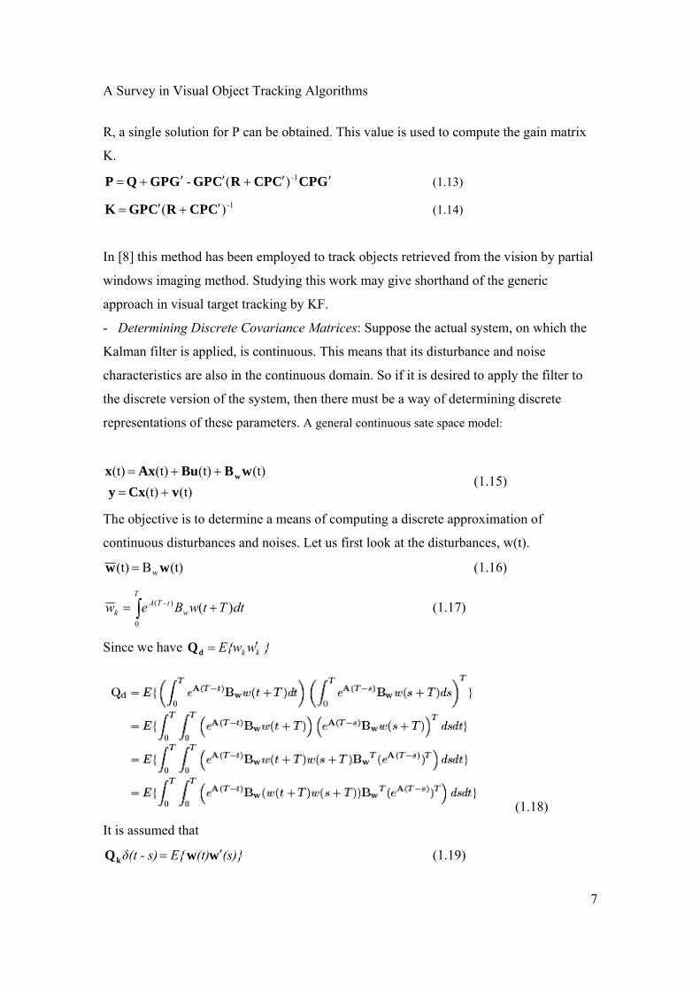
R, a single solution for P can be obtained. This value is used to compute the gain matrix
K.
GCPCCP R CGPGGP QP ′′+′′+= -1)(- (1.13)
)( -1CCP R CGP K ′+′= (1.14)
In [8] this method has been employed to track objects retrieved from the vision by partial
windows imaging method. Studying this work may give shorthand of the generic
approach in visual target tracking by KF.
- Determining Discrete Covariance Matrices: Suppose the actual system, on which the
Kalman filter is applied, is continuous. This means that its disturbance and noise
characteristics are also in the continuous domain. So if it is desired to apply the filter to
the discrete version of the system, then there must be a way of determining discrete
representations of these parameters. A general continuous sate space model:
(t) (t) (t) (t) (t) (t)
vCx ywBBuAxx w
+=++=
(1.15)
The objective is to determine a means of computing a discrete approximation of
continuous disturbances and noises. Let us first look at the disturbances, w(t).
(t)B (t) w ww = (1.16)
∫ += −T
wtTA
k dtTtwBew0
)( )( (1.17)
Since we have }wE{w kk ′=dQ
(1.18)
It is assumed that
(s)}(t)E{ s)-δ(t wwQk ′= (1.19)
A Survey in Visual Object Tracking Algorithms
8
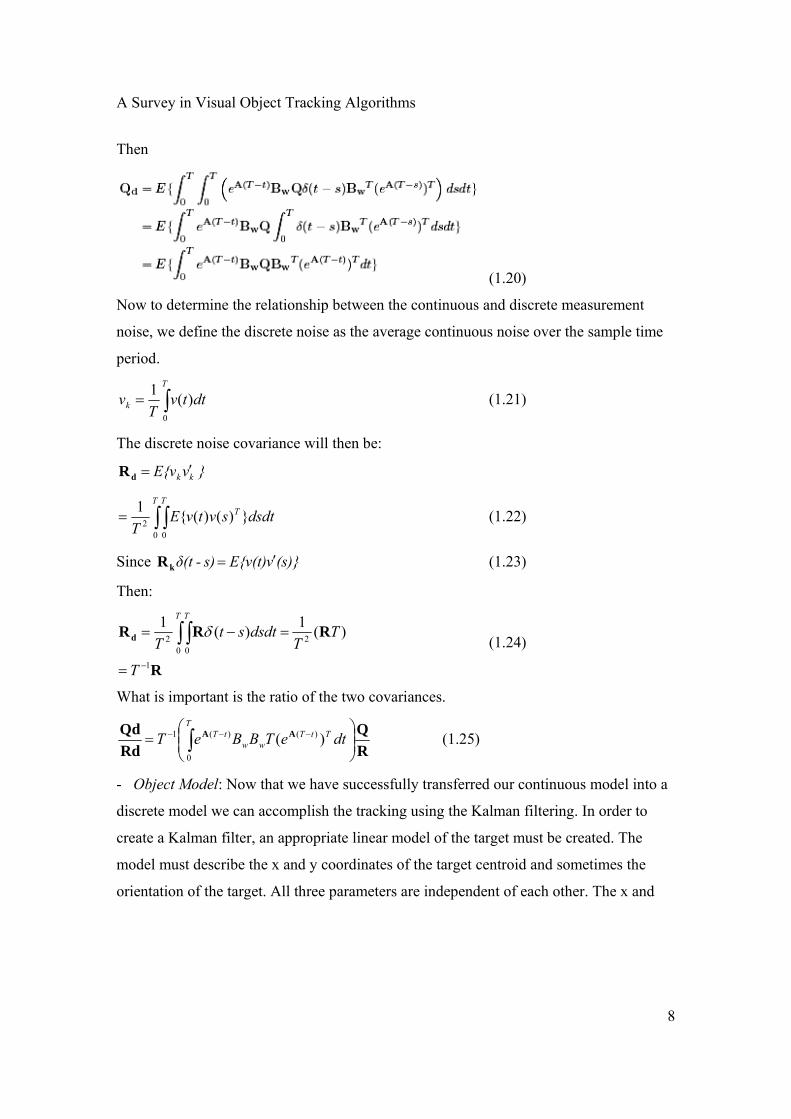
Then
(1.20)
Now to determine the relationship between the continuous and discrete measurement
noise, we define the discrete noise as the average continuous noise over the sample time
period.
∫=T
k dttvT
v0
)(1 (1.21)
The discrete noise covariance will then be:
}vE{v kk ′=dR
∫ ∫=T T
T dsdtsvtvET 0 0
2 })()({1 (1.22)
Since (s)}vE{v(t) s)-δ(t ′=kR (1.23)
Then:
R
RRRd
1
20 0
2 )(1)(1
−=
=−= ∫ ∫T
TT
dsdtstT
T T
δ (1.24)
What is important is the ratio of the two covariances.
RQ
RdQd AA
⎟⎟⎠
⎞⎜⎜⎝
⎛= ∫ −−−
TTtT
wwtT dteTBBeT
0
)()(1 )( (1.25)
- Object Model: Now that we have successfully transferred our continuous model into a
discrete model we can accomplish the tracking using the Kalman filtering. In order to
create a Kalman filter, an appropriate linear model of the target must be created. The
model must describe the x and y coordinates of the target centroid and sometimes the
orientation of the target. All three parameters are independent of each other. The x and
A Survey in Visual Object Tracking Algorithms
9
y models are the same and based on Newton’s second law. The Orientation is based on a
moment equation. As it turns out this description simplifies to a model identical to the
position representations.
For our 2D problem of tracking we have ⎩⎨⎧
==
yy
xx
aFaF
where we have taken pixels as the unit
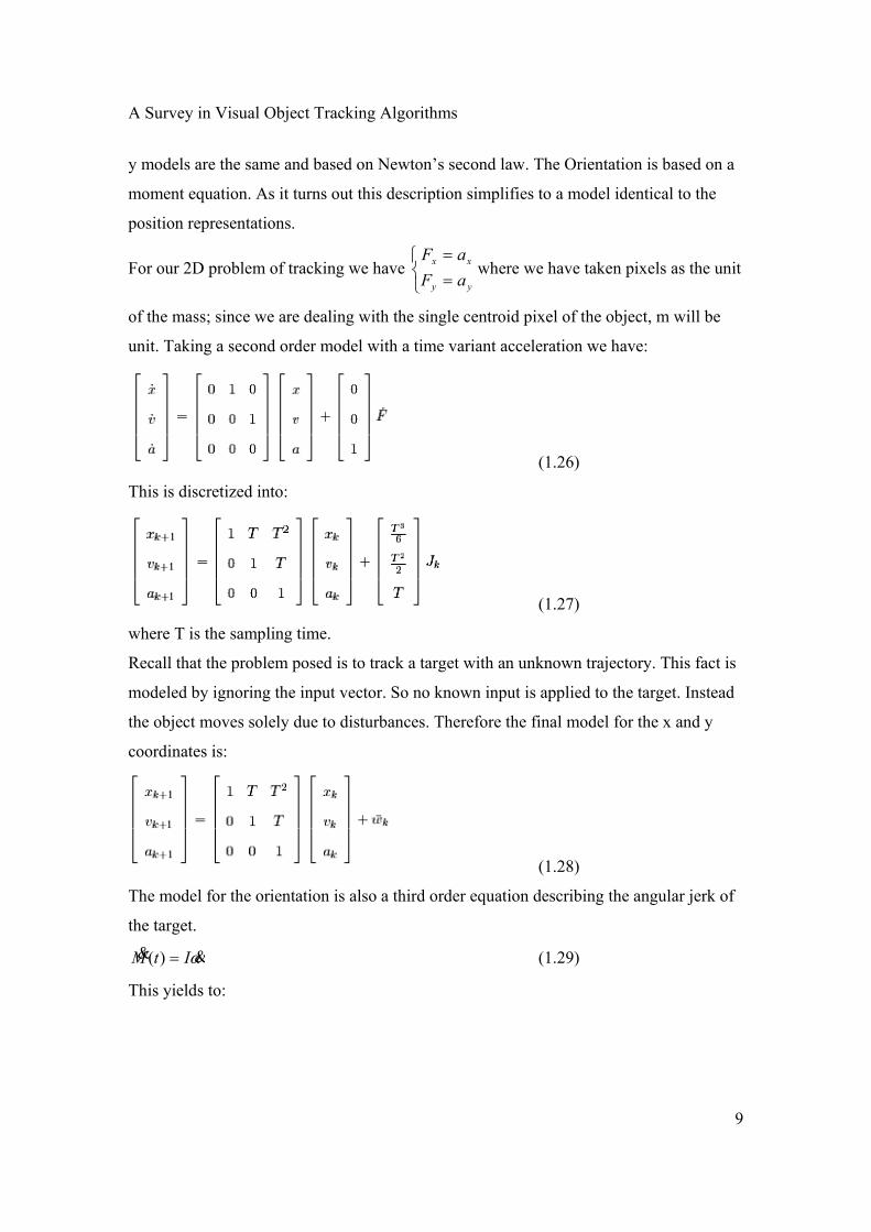
of the mass; since we are dealing with the single centroid pixel of the object, m will be
unit. Taking a second order model with a time variant acceleration we have:
(1.26)
This is discretized into:
(1.27)
where T is the sampling time.
Recall that the problem posed is to track a target with an unknown trajectory. This fact is
modeled by ignoring the input vector. So no known input is applied to the target. Instead
the object moves solely due to disturbances. Therefore the final model for the x and y
coordinates is:
(1.28)
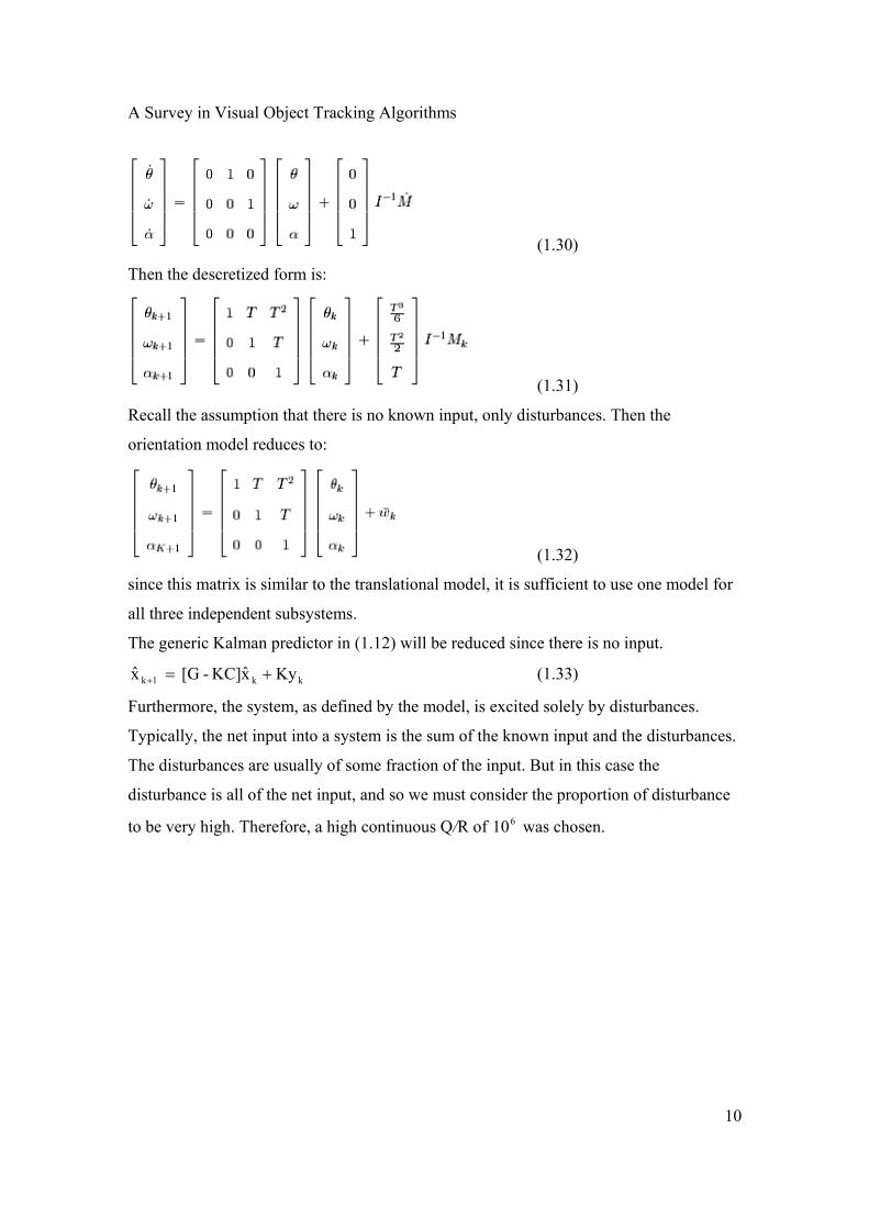
The model for the orientation is also a third order equation describing the angular jerk of
the target.
α&& ItM =)( (1.29)
This yields to:
A Survey in Visual Object Tracking Algorithms
10
(1.30)
Then the descretized form is:
(1.31)
Recall the assumption that there is no known input, only disturbances. Then the
orientation model reduces to:
(1.32)
since this matrix is similar to the translational model, it is sufficient to use one model for
all three independent subsystems.
The generic Kalman predictor in (1.12) will be reduced since there is no input.
Ky x̂KC]-[G x̂ kk 1k +=+ (1.33)
Furthermore, the system, as defined by the model, is excited solely by disturbances.
Typically, the net input into a system is the sum of the known input and the disturbances.
The disturbances are usually of some fraction of the input. But in this case the
disturbance is all of the net input, and so we must consider the proportion of disturbance
to be very high. Therefore, a high continuous Q/R of 610 was chosen.
A Survey in Visual Object Tracking Algorithms
11
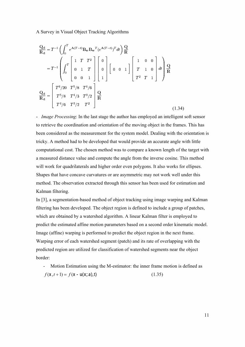
(1.34)
- Image Processing: In the last stage the author has employed an intelligent soft sensor
to retrieve the coordination and orientation of the moving object in the frames. This has
been considered as the measurement for the system model. Dealing with the orientation is
tricky. A method had to be developed that would provide an accurate angle with little
computational cost. The chosen method was to compare a known length of the target with
a measured distance value and compute the angle from the inverse cosine. This method
will work for quadrilaterals and higher order even polygons. It also works for ellipses.
Shapes that have concave curvatures or are asymmetric may not work well under this
method. The observation extracted through this sensor has been used for estimation and
Kalman filtering.
In [3], a segmentation-based method of object tracking using image warping and Kalman
filtering has been developed. The object region is defined to include a group of patches,
which are obtained by a watershed algorithm. A linear Kalman filter is employed to
predict the estimated affine motion parameters based on a second order kinematic model.
Image (affine) warping is performed to predict the object region in the next frame.
Warping error of each watershed segment (patch) and its rate of overlapping with the
predicted region are utilized for classification of watershed segments near the object
border:
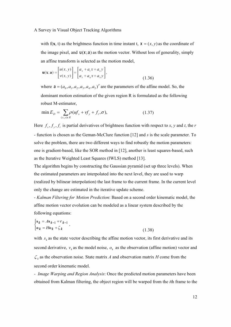
- Motion Estimation using the M-estimator: the inner frame motion is defined as
t)),( ax;u-xx ()1,( ftf =+ (1.35)
A Survey in Visual Object Tracking Algorithms
12
with f(x, t) as the brightness function in time instant t, ),( yx=x as the coordinate of
the image pixel, and );( axu as the motion vector. Without loss of generality, simply
an affine transform is selected as the motion model,
(1.36)
where Taaaaaa ),,,,,( 543210=a are the parameters of the affine model. So, the
dominant motion estimation of the given region R is formulated as the following
robust M-estimator,
,),(min),(∑
∈
++=Ryx
tyxD fvfufE σρ (1.37)
Here tyx fff ,, is partial derivatives of brightness function with respect to x, y and t, the r
- function is chosen as the Geman-McClure function [12] and s is the scale parameter. To
solve the problem, there are two different ways to find robustly the motion parameters:
one is gradient-based, like the SOR method in [12], another is least squares-based, such
as the Iterative Weighted Least Squares (IWLS) method [13].
The algorithm begins by constructing the Gaussian pyramid (set up three levels). When
the estimated parameters are interpolated into the next level, they are used to warp
(realized by bilinear interpolation) the last frame to the current frame. In the current level
only the change are estimated in the iterative update scheme.
- Kalman Filtering for Motion Prediction: Based on a second order kinematic model, the
affine motion vector evolution can be modeled as a linear system described by the
following equations:
(1.38)
with ks as the state vector describing the affine motion vector, its first derivative and its
second derivative, kv as the model noise, ko as the observation (affine motion) vector and
kζ as the observation noise. State matrix A and observation matrix H come from the
second order kinematic model.
- Image Warping and Region Analysis: Once the predicted motion parameters have been
obtained from Kalman filtering, the object region will be warped from the ith frame to the
A Survey in Visual Object Tracking Algorithms
13
(i+1)th frame. Then the warped region is used to determine which watershed segments
enter it according to the following measure: Given that the number of pixels belonging to
the warped template in the sub-region (watershed segment) Ri is Cpi and the number of
all pixels in Ri is Ci , a ratio ri is computed,
iii CCpr /= (1.39)
Based on this measure, we discuss further the classification problem of each subregion in
these following cases:
1) When 0rri ≥ (in this paper r0 = 0.9), classify Ri as part of the final object template;
2) When 01 rrr i <≤ (here r1 = 0.4), another measure as MAE (Mean Absolute Error) of
difference between the warped frame and the current frame is taken into account,
iw
i CtftfM /),()1,(∑ −+= xx (1.40)
where ),( tf w x is the warped image of ),( tf x using the estimated dominant motion
parameters; If the warped error Mi of Ri is smaller enough (less than a given threshold, for
instance, 10), Ri is still regarded as part of the updated template; Otherwise, excluding Ri
out of the object region.
3) When r < r1, R will NOT be included in the updated template.
Finally it has been shown that warping error analysis is efficient to avoid some
misclassification of small regions near the tracked object in the cluttered background.
In this section a general view of the estimation method using Kalman Filter was
presented using two different works accomplished in this field. In the first one a classical
approach was taken with fewer efforts on vision based algorithms. But in the second
work a more extensive part was devoted to the vision based algorithms including
segmentation which guarantees a more robust tracking strength. But tracking power of all
Kalman filter based algorithms is confined to objects with weak maneuver. Maneuvering
objects have got nonlinear models that require other methods of tracking.

A Survey in Visual Object Tracking Algorithms
14
2 EXTENDED ALGORITHMS OF KALMAN FILTERING Unfortunately, tracking objects in real-world environment seldom satisfies Kalman
filter’s requirements. For example, in human tracking, background clutter may resemble
the human face, and in sound source localization, “ghost” sound sources can create
multiple peaks in the generalized cross-correlation function. To make the situation worse,
the system dynamics and observation can be highly non-linear. In order to deal with the
non-linear and/or non-Gaussian reality, two categories of techniques have been
developed in recent years: parametric and non-parametric.
The parametric techniques are based on improvements of the Kalman filter. By
linearizing non-linear functions around the predicted values, extended Kalman filter
(EKF) is proposed to solve non-linear system problems. It is first introduced in control
theory [1] and later on applied in visual tracking. Because of its first-order approximation
of Taylor series expansion, EKF finds only limited success in tracking visual objects. In
recent years, Julier and Uhlmann developed an unscented Kalman filter (UKF) that can
accurately compute the mean and covariance of y = g(x) , where g( ) is an arbitrary
function, up to the second order (third in Gaussion prior) of the Taylor series expansion
of g( ). While UKF is significantly better than EKF in density statistics estimation, it still
assumes a Gaussian parametric form of the posterior, thus cannot handle multi-modal
distributions. In this section we deal with parametric methods in more details.[5]
2.1 Optimal Nonlinear Estimation Consider a system:
1. dynamic equation perturbed by white process noise
2. measurement equation perturbed by white noise
With at least one of these equations nonlinear, the estimation of the system's state
consists of the calculation of PDF conditioned on entire available information. The
numerical implementation of the nonlinear estimator on a set of grid points in the state
space can be very demanding computationally; the memory and computational
requirements are exponential in dimension of state.
A Survey in Visual Object Tracking Algorithms
15
2.2 EKF Algorithm The first approach for estimation of nonlinear systems was Extended Kalman Filter
which was a sub optimal solution. Albeit this algorithm is not an ideal method for our
goal, we will take a look at the concept very concisely.
Let's consider the general form of the nonlinear models as below.
),(),( 11
kkkk
kkkk
hf
wxzvxx
== −−
(2.1)
The covariances of v and w are Q and R respectively. It is a linearization technique based
on a first order Taylor series expansion of the nonlinear system and measurement
functions about the current estimate of the state. This requires both to be differentiable
functions of their vector arguments.
kkkk
kkkk
wxHzvxFx
+=+= −− 11
(2.2)
Where
1|1||
1|1||
1|111|
1|11|
11|
1|
))((
)(
|
|
1|
1|1
−−
−−
−−−−
−−−
−−
−
=
=
−=
−+=
+=
=
=
+=
=
=
−
−−
kkkkkkkk
kkkkkkkkk
Tkkkkkkk
kkkkk
kTkkkk
kkkkkk
mxk
k
mxk
k
mhzmm
mfm
ddhd
df
kk
kk
PHKPPK
FPFQP
SHPK
RHPHSx
H
xF
(2.3)
Higher orders of the EKF are also possible to derive but due to complexity they are not
widespread.[14]
2.3 Unscented KF versus EKF In [7] a new algorithm has been introduced named "Unscented Kalman Filter". This filter
consists of set of points that are deterministically selected from a Gaussian distribution
these points all are propagated through the nonlinearity and the parameters of the
Gaussian approximation are then re-estimated. Using the principle that a set of discretely
A Survey in Visual Object Tracking Algorithms
16
sampled points can be used to parameterize mean and covariance, the estimator yields
performance equivalent to the KF for linear systems yet generalizes elegantly to
nonlinear systems without the linearization steps required by the EKF For some problems
this filter has been shown to give better performance than a standard EKF since it better
approximates the nonlinearity. However, in practice, the use of the EKF has two well-
known drawbacks:
1. Linearization can produce highly unstable filters if the assumption of local linearity is
violated.
2. The derivation of the Jacobian matrices is nontrivial in most applications and often
lead to significant implementation difficulties.
Now the problem will be restated as follow.
kkkkk
kkkkk
hf
wuxzvuxx+=
=
−
−−−
),(),,(
1
111 (2.4)
Now let’s apply KF to this nonlinear problem. It is assumed that the noise vectors v(k)
and w(k), are zero-mean and
jijiEiijiiEiijjiE TTT ,,0)]()([),()]()([),()]()([ ∀=== wvRwwQvv δδ (2.5)
Let )|(ˆ jix be the estimate of x (i) using the observation information up to and including
time j, (j)] z ,, (1) [z Z j …= . The covariance of this estimate is. Given an estimate, the
filter first predicts what the future state of the system will be using the process model.
Ideally, the predicted quantities are given by the expectations
]|)}|1()1()}{|1(ˆ)1([{)|1(]|]),(),(),([[)|1(ˆ
kT
k
kkkkkkEkkkkkkfEkkx
ZxxxxPZvux
+−++−+=+
=+ (2.5)
When f [.] and h [.] are nonlinear, the precise values of these statistics can only be
calculated if the distribution of x (k), condition on Zk, is known. However, this
distribution has no general form and a potentially unbounded number of parameters are
required. In many applications, the distribution of x (k) is approximated so that only a
finite and tractable number of parameters need be propagated. It is conventionally
assumed that the distribution of x (k) is Gaussian for two reasons. First, the distribution is
completely parameterized by just the mean and covariance. Second, given that only the
A Survey in Visual Object Tracking Algorithms
17
first two moments are known, the Gaussian distribution is the least informative. The
problem of applying the Kalman filter to a nonlinear system is the ability to predict the
first two moments of x (k) and z (k). This problem is a specific case of a general problem
to be able to calculate the statistics of a random variable which has undergone a nonlinear
transformation.
Now suppose that x is a random variable with mean x and covariance Px. A second
random variable, y is related to x through the nonlinear function
)(xfy = (2.6)
We wish to calculate the mean of y and covariance Py of y. The statistics of y are
calculated by (i) determining the density function of the transformed distribution and
(ii) evaluating the statistics from that distribution. In some special cases (for example
when f [.] is linear) exact, closed form solutions exist. However, such solutions do not
exist in general and approximate methods must be used. In this paper it is advocate that
the method should yield consistent statistics. Ideally, these should be efficient and
unbiased.
The transformed statistics are consistent if the inequality
0]}}{[{ ≥−−− Ty E yyyyP (2.7)
holds. This condition is extremely important for the validity of the transformation
method. If the statistics are not consistent, the value of Py is under-estimated. If a Kalman
filter uses the inconsistent set of statistics, it will place too much weight on the
information and under estimate the covariance, raising the possibility that the filter will
diverge. By ensuring that the transformation is consistent, the filter is guaranteed to be
consistent as well. However, consistency does not necessarily imply usefulness because
the calculated value of Py might be greatly in excess of the actual mean squared error. It
is desirable that the transformation is efficient - the value of the left hand side of Equation
2.7 should be minimized. Finally, it is desirable that the estimate is unbiased.
To have an unbiased transformation, Taylor series expansion can be used.
(2.8)
A Survey in Visual Object Tracking Algorithms
18
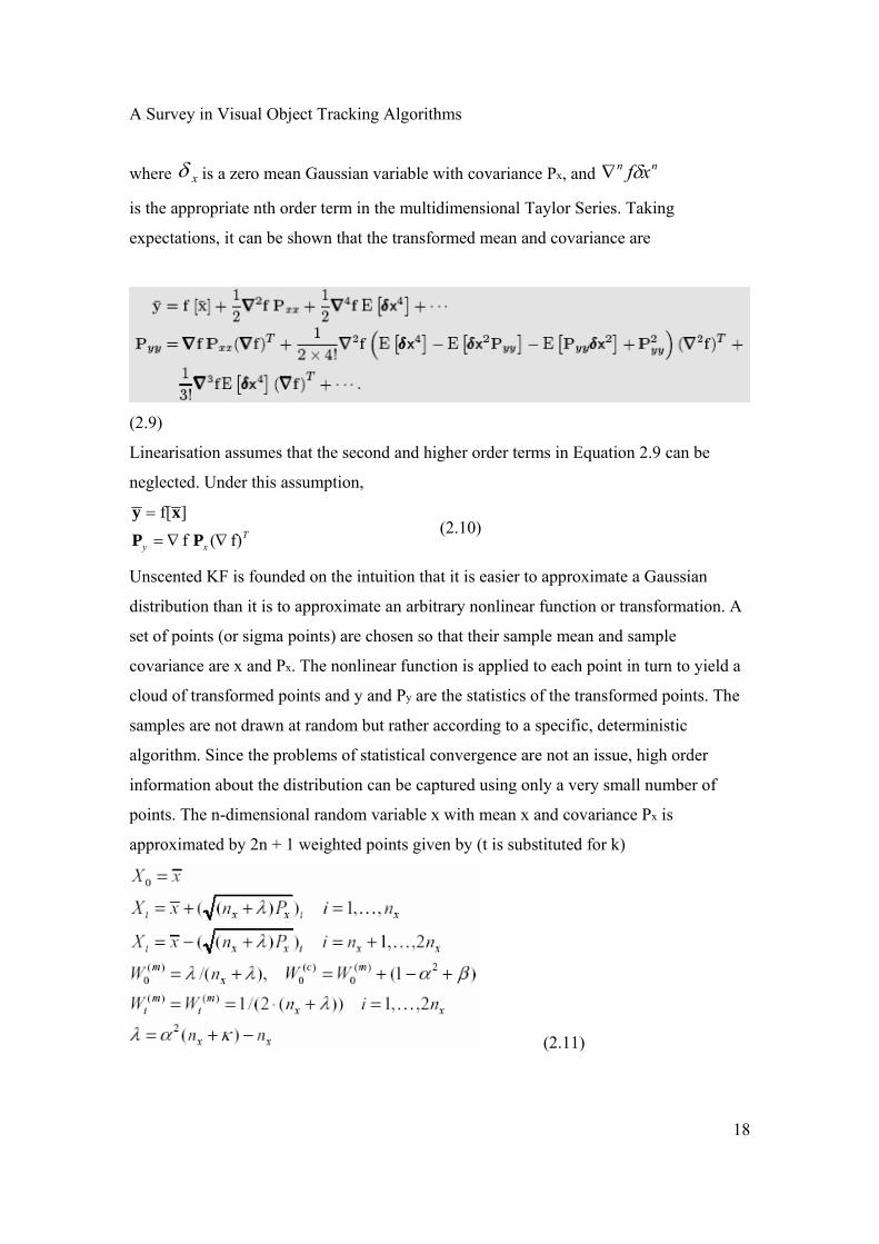
where xδ is a zero mean Gaussian variable with covariance Px, and nn xfδ∇
is the appropriate nth order term in the multidimensional Taylor Series. Taking
expectations, it can be shown that the transformed mean and covariance are
(2.9)
Linearisation assumes that the second and higher order terms in Equation 2.9 can be
neglected. Under this assumption,
Txy f)(f
]f[∇∇=
=
PPxy
(2.10)
Unscented KF is founded on the intuition that it is easier to approximate a Gaussian
distribution than it is to approximate an arbitrary nonlinear function or transformation. A
set of points (or sigma points) are chosen so that their sample mean and sample
covariance are x and Px. The nonlinear function is applied to each point in turn to yield a
cloud of transformed points and y and Py are the statistics of the transformed points. The
samples are not drawn at random but rather according to a specific, deterministic
algorithm. Since the problems of statistical convergence are not an issue, high order
information about the distribution can be captured using only a very small number of
points. The n-dimensional random variable x with mean x and covariance Px is
approximated by 2n + 1 weighted points given by (t is substituted for k)
(2.11)
A Survey in Visual Object Tracking Algorithms
19
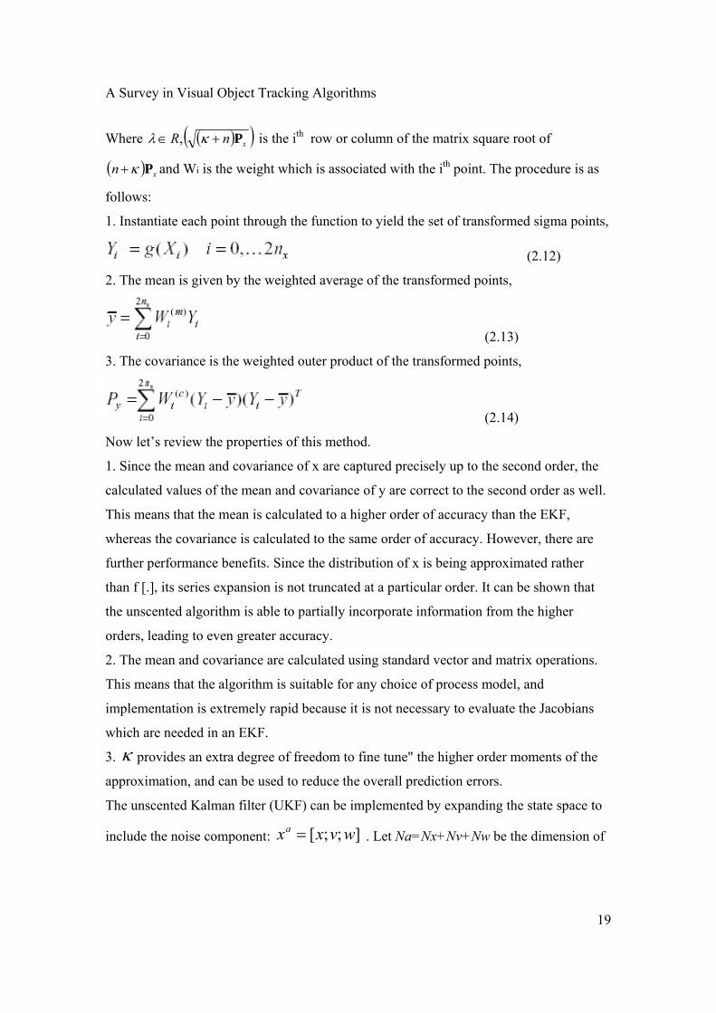
Where ( )( )xnR P+∈ κλ , is the ith row or column of the matrix square root of
( ) xn Pκ+ and Wi is the weight which is associated with the ith point. The procedure is as
follows:
1. Instantiate each point through the function to yield the set of transformed sigma points,
(2.12)
2. The mean is given by the weighted average of the transformed points,
(2.13)
3. The covariance is the weighted outer product of the transformed points,
(2.14)
Now let’s review the properties of this method.
1. Since the mean and covariance of x are captured precisely up to the second order, the
calculated values of the mean and covariance of y are correct to the second order as well.
This means that the mean is calculated to a higher order of accuracy than the EKF,
whereas the covariance is calculated to the same order of accuracy. However, there are
further performance benefits. Since the distribution of x is being approximated rather
than f [.], its series expansion is not truncated at a particular order. It can be shown that
the unscented algorithm is able to partially incorporate information from the higher
orders, leading to even greater accuracy.
2. The mean and covariance are calculated using standard vector and matrix operations.
This means that the algorithm is suitable for any choice of process model, and
implementation is extremely rapid because it is not necessary to evaluate the Jacobians
which are needed in an EKF.
3. κ provides an extra degree of freedom to fine tune" the higher order moments of the
approximation, and can be used to reduce the overall prediction errors.
The unscented Kalman filter (UKF) can be implemented by expanding the state space to
include the noise component: ];;[ wvxxa = . Let Na=Nx+Nv+Nw be the dimension of
A Survey in Visual Object Tracking Algorithms
20
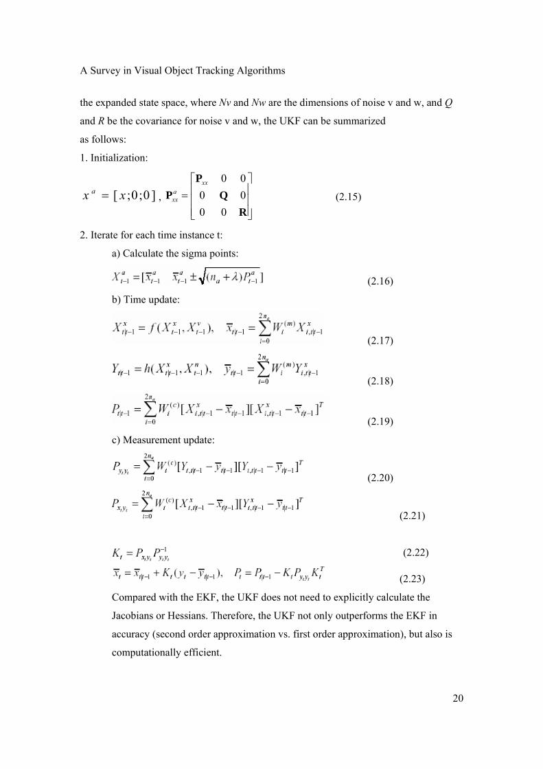
the expanded state space, where Nv and Nw are the dimensions of noise v and w, and Q
and R be the covariance for noise v and w, the UKF can be summarized
as follows:
1. Initialization:
]0;0;[ xx a = , ⎥⎥⎥
⎦
⎤
⎢⎢⎢
⎣
⎡=
RQ
PP
000000xx
axx (2.15)
2. Iterate for each time instance t:
a) Calculate the sigma points:
(2.16)
b) Time update:
(2.17)
(2.18)
(2.19)
c) Measurement update:
(2.20)
(2.21)
(2.22)
(2.23)
Compared with the EKF, the UKF does not need to explicitly calculate the
Jacobians or Hessians. Therefore, the UKF not only outperforms the EKF in
accuracy (second order approximation vs. first order approximation), but also is
computationally efficient.
A Survey in Visual Object Tracking Algorithms
21
3 PARTICLE FILTERING As it was observed, the variant Kalman Filtering methods had a drawback and it was their
Gaussian assumption. A nonlinear Bayesian filtering method called particle filtering,
which had been forgot for a few decades due to its heavy computational demands, has
been re-flourished in the recent decade. Following our foregoing terminology, in this
section we will study Particle Filter as a non-Parametric method. The non-parametric
techniques are based on Monte Carlo simulations. They assume no functional form, but
instead, use a set of random samples (also called particles) to estimate the posteriors.
When the particles are properly placed, weighted, propagated, posteriors can be estimated
sequentially over time. This technique is more popularly known as the particle filters in
recent years. The first appearance of particle filters can be traced back to 1950s. While
almost dormant in the seventies, there is a renaissance of this technique in the early
nineties, due to the massive increases in computing power. However, most of them use
the state transition prior p(xk|xk-1) as the proposal distribution to draw particles from.
Because the state transition does not take into account the most recent observation yk, the
particles drawn from transition prior may have very low likelihood, and their
contributions to the posterior estimation become negligible. This type of particle filters is
prone to be distracted by background clutters. For clarity, in here, this type of filters is
referred as the conventional particle filters. Inside the computer vision community,
particle filters has also enjoyed considerable attention. Following the pioneering work of
CONDENSATION, various improvements and extensions have been proposed for visual
tracking. Because the original CONDENSATION algorithm uses the state transition prior
as its proposal distribution, it belongs to the conventional particle filters. To design better
proposal distributions for CONDENSATION, in general, there are two approaches: the
direct approach and the indirect approach. The indirect approach attacks this problem
indirectly by using an auxiliary tracker to generate the proposal distribution for the main
tracker. The direct approach, on the other hand, addresses this problem directly in its
original space by taking into account the most recent observation. The indirect approach
is adopted in the ICONDENSATION algorithm, where an auxiliary color tracker is used
to generate the proposal distribution for the main contour tracker. While better than the
conventional particle filters, this indirect approach has two major limitations. First, in
A Survey in Visual Object Tracking Algorithms
22
many applications, e.g., audio-based speaker localization, there is simply no easy
auxiliary tracker or sensing modality available. Second, and more importantly, the
auxiliary tracker itself needs a good proposal distribution if it plans to use particle filters,
or it falls back to ad hoc approaches. Merwe et. al. have recently developed the unscented
particle filter (UPF) in the field of filtering theory [15]. Based on this new development, a
direct approach to generate better proposal distributions for audio/visual tracking, has
been introduced [5]. The UPF is a parametric/non-parametric hybrid of UKF and particle
filters. The particle filter part of the UPF provides the general probabilistic framework to
handle nonlinear non-Gaussian systems, and the UKF part of the UPF generates better
proposal distributions by taking into account the most recent observation.
In the pioneering work of CONDENSATION [16], extended factored-sampling is used to
formulate the particle filter framework. Even though easy to follow, it obscures the role
of proposal distributions.
3.1 Bayesian sequential importance sampling: A non-parametric way to represent a distribution is to use particles drawn from the
distribution. For example, we can use the following point-mass approximation to
represent the posterior distribution of x:
(3.1)
where δ is the Dirac delta function, and particles }{ )(:0itx are drawn from p(x0:t|y1:t ). The
approximation converges in distribution when N is sufficiently large [5,17]. This particle-
based distribution estimation is, however, only of theoretical significance. In reality, the
posterior distribution is the one that needs to be estimated, thus not known. Fortunately,
we can instead sample the particles from a known proposal distribution q(x0:t|y1:t ) and
still be able to compute p(x0:t|y1:t ).
Definition 1 [14]: A set of random samples )}(,{ )(:0
)(:0
itt
it xwx drawn from a distribution q
is said to be properly weighted with respect to p if for any integrable function g( ) the
following is true
)()(lim))(( :01 :0:0i
tt
N
ii
ttp xwxgxgE ∑== (3.2)
∑=
=N
itxtt dx
Nyxp i
t1
:0:1:0 )(1)|(ˆ:0
δ
A Survey in Visual Object Tracking Algorithms
23
Furthermore, as N tends to infinity, the posterior distribution p can be approximated by
the properly weighted particles drawn from q:
(3.3)
There are two important points worth emphasizing here. First, the definition says that an
unknown distribution p can be approximated by a set of properly weighted particles
drawn from a known distribution q. Second, the more difficult problem of distribution
estimation is converted to an easier problem of weight estimation. The weights are further
given by:
(3.4)
(3.5)
where the particles )}(,{ )(:0
)(:0
ikk
ik xwx are drawn from the known distribution q. )(~ )(
:0ikk xw
and )( )(:0ikk xw are the unnormalized and normalized importance weights.
In order to propagate the particles )}(,{ )(:0
)(:0
ikk
ik xwx through time, it is beneficial to
develop a recursive calculation of the weights. This can be obtained straightforwardly by
considering the following two facts:
1. Based on the definition of filtering, current states do not depend on future
observations. That is,
(3.6)
2. As used in [15], the state dynamics is a Markov process and the observations are
conditionally independent given the states, i.e.:
(3.7)
Substituting the above two equations into Equation (6), we obtain the recursive estimate
for the importance weights:
∑=
=N
itx
itttt dxxwyxp i
t1
:0:0:1:0 )()()|(ˆ:0
δ
A Survey in Visual Object Tracking Algorithms
24
(3.8)
To summarize, in the sequential importance sampling step, there are two places involving
the proposal distribution. First, particles are drawn from the proposal distribution
(Equation (3.2)). Second, proposal distribution is used to calculate each particle’s
importance weight (i.e., Equation (3.8)).
Choosing the right proposal distribution is one of the most important issues in particle
filter’s design. In reality, there are infinite numbers of choices of the proposal
distribution, as long as its support includes that of the posterior distribution, and it is easy
to sample from. As pointed out in [15], the optimal proposal distribution is the one that
minimizes the variance of the importance weights conditional on x0:t-1 and y1:t. In practice,
however, finding the optimal proposal is very difficult if not impossible.
Instead, the conventional particle filters have chosen to trade the optimality with easy-
implementation by using the transition prior p(xt|xt-1) as the proposal distribution. They
sample from the transition prior and calculate the importance weight as follows:
(3.9)
Although simple to implement, this proposal results in higher Monte Carlo variance and
thus worse performance [15]. Comparing the transition prior p(xt|xt-1) with the general
proposal distribution q(xt|x0:t-1,y1:t), we can easily see that the most recent observation yt
is missing in p(xt| xt-1). This may cause serious deficiency in particle filters, especially
when the likelihood is peaked and the predicted state is near the likelihood’s tail. The
particles generated from the transition prior can therefore easily land on low likelihood
areas thus wasted. To overcome this difficulty, new ways of generating better proposal
distribution will be examined.
A Survey in Visual Object Tracking Algorithms
25
3.2 Selective Re-sampling: Before we continue on discussing design better proposal distributions, we would like to
first present the complete particle-filtering framework in the rest of this section. In
addition to choosing better proposal distributions in the sequential importance sampling
step, another crucial step in designing particle filters is re-sampling. One of the most
important contributions made in the 1990s’ particle-filter renaissance is the introduction
of the re-sampling step by Gordon. Its philosophy is to eliminate particles with low
importance weights and multiply particles with high importance weights, thus improving
the effective particle size.
It can be proven [15] that without re-sampling the variance of the importance weight
increases over time. In practice, this means one of the importance weights tends to one,
while others become zero. That is, the effective particle size reduces from N to almost 1.
This degeneracy phenomenon has been observed in several research fields [15]. In recent
years, the re-sampling step has been adopted in almost all of today’s particle filtering
algorithms. However, cautions must be taken when using the re-sampling step: it should
only be done when the effective particle size is small. The effective particle size S can be
estimated as follows:
(3.10)
The value of S varies between 1 and N. When all the particles are of equal weight 1/N, the
effective particle size is N. When one particle is of weight 1 and the rest are of weight
zero, the effective particle size is 1. It is intuitive that when the weights are comparable to
each other, re-sampling can only reduce the number of distinctive particles [14]. This
suggests that one should not perform the re-sampling step when S is large. On the other
hand, when the weights are much skewed (e.g., near the degeneracy case), many particles
are wasted because of their close-to-zero weight, and the re-sampling step is required to
increase the effective particle size. In practice, a pre-defined threshold ST can be used,
e.g., ST = N/2, to determine if the re-sampling step is needed.
3.3 Generic Particle Filter Algorithm: Here is the complete algorithm:
3.3.1 Sequential importance sampling:
A Survey in Visual Object Tracking Algorithms
26
a). Sample N particles ) (I t x , i = 1, 2, …, N, from the proposal
distribution q(xt|x0:t-1,y1:t). The proposal distribution can be the transition
prior as used in traditional particle filters, or more advanced distributions
discussed in Section 3.
b). Compute the particle weights using Equation (3.8)
c). Normalize the importance weight using Equation (3.5).
3.3.2 Selective re-sampling:
a). Compute the effective particle size S using Equation (3.9).
b). If S < ST, multiple/suppress weighted particles to generate N equal-
weighted particles.
3.3.3 Output:
a). Use Equation (3.2) to compute expectations of g( ). The conditional
mean of xt can be computed with ttt xxg =)( , and conditional covariance
of xt can be computed with Ttttt xxxg =)( . They can be readily used as the
tracking results.
A Survey in Visual Object Tracking Algorithms
27
4 MULTIPLE-MODEL: A Hybrid Estimation Method
4.1 Introduction In the previous sections we provided different estimation algorithms to deal with variety
of systems including linear, nonlinear, with Gaussian and non-Gaussian distribution. As
we saw using Particle filter approach for estimation of nonlinear systems was
computationally exhaustive. In this section we will come up with a simpler, yet novel
method called Multiple Model to deal with nonlinear systems based on [10].
Target tracking is a hybrid estimation problem involving both continuous and discrete
uncertainties. In the prevailing approaches to target tracking, the modeling of the target
motion/dynamics and the sensory system is essential. In these system-oriented
approaches, it is customary to use the continuous-valued process/plant noise and
measurement noise to cover the unknown modeling errors or deviations of the model
from the true system. However, the major challenges of target tracking arise from two
discrete-valued uncertainties: the measurement origin uncertainty and the target motion
uncertainty.
The measurement origin uncertainty refers to the fact that a measurement provided by the
sensory system for target tracking may have originated from an extraneous source,
including clutter, false alarms, and neighboring targets, as well as the target under track.
It may also have originated from countermeasures from the target. This uncertainty is
clearly discrete in nature. It poses the greatest challenge for target tracking. Numerous
techniques have been developed to deal with this uncertainty over the past three decades.
The target motion uncertainty exhibits itself in the situations where a target may undergo
a known or unknown maneuver during an unknown time period. In general, a non-
maneuver motion and different maneuvers can be described only in different motion
models. The use of an incorrect model often leads to unacceptable results. When tracking
a maneuvering target, it is thus crucial to determine reliably and timely the right model to
use.
A major approach to target tracking in the presence of motion uncertainty is the so-called
multiple-model (MM) method, which is probably the most natural approach to hybrid
estimation. It uses a bank of filters based on a set of multiple models that represent/cover
A Survey in Visual Object Tracking Algorithms
28
possible system behavior patterns (e.g., maneuvers) of most interest for the problem
under consideration. These system behavior patterns are referred to as system modes.
The early results of non-interacting (static) MM estimation are valid in principle only for
systems with a time-invariant unknown or uncertain system mode, and are ineffective in
handling such problems as maneuvering target tracking in which the system mode
undergoes frequent transitions. It was not until the development of the highly cost-
effective interacting multiple-model (IMM) estimator that the MM approach became
practical for maneuvering target tracking. Since this development, numerous publications
have appeared reporting successful applications of MM estimation to a variety of target-
tracking problems and the long lists of references therein.
The non-interacting MM estimators and the IMM estimator have a fixed structure (FS) in
the sense that they use a fixed set of models at all times. For a target, many different
maneuvers are possible, and they may not be represented or covered accurately enough
by a small set of models. To achieve good performance within the fixed structure,
therefore, a large filter bank may be necessary. Use of more models and filters is not
necessarily a good solution. First, it increases the computational complexity considerably,
which may arrive at a prohibitive level in many practical situations. Further, even the
optimal use of more models and filters does not guarantee performance improvement.
Thus, there is a dilemma with the fixed structure: to have more models or less? One may
ask the natural question: “Is it necessary to use a fixed set of models?” The answer is
obviously “No.” An MM estimator that does not use a fixed set of models is said to have
a variable structure (VS). One may also ask, “Why is a fixed set of models used?” The
answer is “It is simple.” When simple “solutions” are not good enough, it is natural to
seek for better but usually more complex solutions. In this sense, more and more
researchers are convinced that variable structure is such a better but usually more
complex solution— it is probably the main practical means within the MM approach that
can improve the cost effectiveness substantially for real-world problems where fixed
structures do not work well. (VSMM) estimation for tracking. It covers the relevant
theoretical development and presents several VSMM estimators by way of target-tracking
examples. A good deal of effort is made to present and interpret the results in simple
terms.
A Survey in Visual Object Tracking Algorithms
29
4.2 MULTIPLE-MODEL ESTIMATION
4.2.1 General Description The MM approach is best understood in terms of hybrid systems. A continuous time
hybrid system is described by the following dynamic and measurement equations
(4.1)
t]v(t), s(t), h[x(t), z(t) = (4.2)
and an equation that governs the evolution of s, where x is the base state, which varies
continuously, just like the state of a conventional system; s is the system mode, also
known as the modal state, which has a staircase-type trajectory; that is, it may either
jump or stay unchanged; z is the measurement; and w, v are the process and measurement
noise, respectively. In simple terms, it is said that x is continuous-valued and s is discrete-
valued. Note that the (whole) state ];[ sx=ζ of a hybrid system is hybrid. The set of
modes is often referred to as the mode space and denoted as S.
One of the simplest discrete-time hybrid systems is the following, known as the jump-
linear system:
)(s)w(sG )x(sF x k1-kk1-k1-kk1-kk += (4.3)
)(sv )x(sH z kkkkkk += (4.4)
This system is nonlinear because, for example, x or z does not depend on the state ζ of
the system in a linear fashion. Were the system mode s given, however, the system would
be linear. In fact, s may actually jump at unknown time instants, hence the name. It is
known as a Markovian jump linear system if s is a (homogeneous) Markov chain, that is,
if
kssConstpssssP jiijikjk ,,;}|{ 1 ∀====+ (4.5)
for all time k ( is and js are generic elements in the mode space).
The basic idea of the multiple-model estimation approach is to assume a set of models M
for the hybrid system; run a bank of filters, each based on a unique model in the set; and
the overall estimate is given by a certain combination of the estimates from these filters.
For a Markovian jump linear system, the ith model obeys the following equation:
wG F x kikk
ik1k +=+ x (4.6)
t] w(t),s(t), f[x(t), x(t) =
A Survey in Visual Object Tracking Algorithms
30
ikk
ikk v xH z += (4.7)
Where superscript (i) denotes quantities pertinent to model mi, and the jumps of the
system mode are assumed to have the following transition probabilities
ConstmmP ijik
jk ==
∆
+ π}|{ 1 (4.8)
where ikm denotes the event that model im matches the system mode at time k:
}{ ik
ik msm ==
∆
(4.9)
There is a chaos in the use of the terms mode and model in the literature. To be more
precise, a mode should refer to a (real-world) behavior pattern or a structure of a system
and a model refers to a (mathematical) representation or description of the system at a
certain accuracy level. It is models, not modes, on which an estimator is based. For
example, the behavior pattern of an aircraft while making a coordinated turn is what is
referred to as the mode of coordinated turn. Several mathematical models are available at
different accuracy levels that describe such a mode. Such a distinction between mode and
model is necessary whenever the mismatch between the model and mode is of concern.
The model set M differs in general from the mode space S in two aspects: (i) they have
different number of elements — M usually has significantly fewer elements than S; and
(ii) a model is usually a simplified description of a mode. For example, one may use a
small set of models, such as a non-maneuver model plus two coordinated-turn models
(for right and left turns, respectively) for tracking a target that may undergo various
(complex) maneuver modes.
In the sequel, the following important difference will be maintained: a model is said to be
in effect at k if it is used in the MM estimator at time k, while a mode is said to be in
effect at k if it is the true one at time k. Similarly, a model set is in effect at k if it is used
by the MM estimator at k, whereas a mode set is in effect at k if it is the set of possible
modes at k (it should not contain any impossible mode).
The reason for such definitions will become clear later.
In general, the recursive MM estimation approach involves the following:
- Model-set determination: The performance of an MM estimator depends to a large
degree on the set of models used. The major task in the application of MM estimation lies
in the design of the set M of multiple models. Numerous publications have appeared on
A Survey in Visual Object Tracking Algorithms
31
the ad hoc design of a model set for various specific application problems, in particular
those in maneuvering target tracking. However, relevant theoretical results are limited.
Note that once the set M is determined, the MM method implicitly assumes that the
system modes are represented exactly by the members of M.
- Filter selection: The selection of the recursive filters for each model, sometimes
referred to as the elemental filters, relies on the classical estimation and filtering theory
and the problem at hand. They may be Kalman filters for a jump-linear system, extended
Kalman filters for a problem that is nonlinear even when the mode is given, lattice filters
for adaptive filtering, or the probabilistic data association filters for target tracking in
clutter. Filters based on different models can be of different types.
- Filter re-initialization: Except in the first-generation (static) MM estimators, elemental
recursive filters do not operate independently. The input for a recursive cycle of such a
filter depends on the other filters as well as the output of the same filter from the previous
cycle. This is referred to as re-initialization. It is a natural and important way of
interaction — using the information obtained by other filters. Many schemes are possible
here. Fixed-structure MM algorithms differ from each other primarily in this regard.
- Estimate fusion: The overall estimate is obtained by fusing the estimates from the
elemental filters, each based on a single model in the set M. Three approaches are
available:
Soft decision or no decision: The overall estimate is obtained from all filter-obtained
estimates ikkx |ˆ ; that is, no (hard) decision is made concerning the use of the filter
estimates. This is the mainstream approach in MM estimation fusion. If the conditional
mean of the base state is used as the estimate, such as under the minimum mean-square
error criterion, then the overall estimate is the probabilistically weighted sum of all filter
estimates:
∑== }|{ˆ]|[ˆ ||ki
ki
kkk
kkk zmPxzxEx (4.10)
and the overall covariance is determined accordingly. When some other optimality
criteria are used, the overall estimate may not necessarily be a weighted sum of the filter
estimates.
A Survey in Visual Object Tracking Algorithms
32
Hard decision: The overall estimate is (approximately) determined by the estimates of the
filters based on models that are deemed most likely or at least not unlikely, determined by
a hard decision procedure. In the extreme case where the overall estimate is set to be
equal to the estimate of the single elemental filter based on the most likely model, this
degenerates to the conventional “estimation-after-decision” approach.
Random decision: The overall estimate is approximately determined by a number of
estimates from filters based on some randomly chosen model sequences.
Other approaches to estimate fusion are possible, such as combinations of the above
approaches. Note that MM estimation fusion differs in essence from the decentralized
estimation/track fusion problem in at least two fundamental aspects: (i) one and only one
estimate (but which one is unknown) is assumed to be correct in the MM approach,
whereas more than one estimate may be correct in the track fusion problem, and (ii)
different filters use the same measurements in the MM estimation fusion but different
measurements in track fusion.
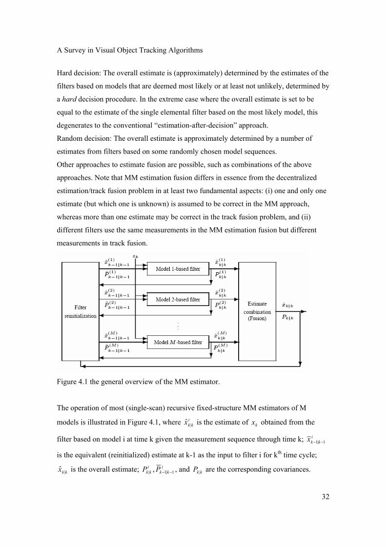
Figure 4.1 the general overview of the MM estimator.
The operation of most (single-scan) recursive fixed-structure MM estimators of M
models is illustrated in Figure 4.1, where ikkx |ˆ is the estimate of kx obtained from the
filter based on model i at time k given the measurement sequence through time k; ikkx 1|1 −−
is the equivalent (reinitialized) estimate at k-1 as the input to filter i for kth time cycle;
kkx |ˆ is the overall estimate; ikk
ikk PP 1|1| , −− , and kkP | are the corresponding covariances.
A Survey in Visual Object Tracking Algorithms
33
The MM approach was initiated by Magill in [47]. The early work only considered
systems with a time-invariant mode that is unknown or uncertain (i.e., s is a nonrandom
constant or a random variable but not a random process). Many applications (or
reinventions) of this MM estimator can be found in the literature under various names,
such as the “static multiple-model (SMM) algorithm”, the “multiple model adaptive
estimator”, the “parallel processing algorithm”, the “filter bank method”, the “partitioned
filter”, the “self-tuning estimator”, and the “modified Gaussian sum adaptive filter”.
These names suggest the structure, features, and capability of this “first-generation” MM
estimator.
In the “first-generation” (SMM) algorithm, individual elemental filters operate
independently without any interaction with one another because it is assumed that the
mode does not jump. Consequently, this method is not effective in handling systems with
frequent mode jumps because it takes a considerable amount of time for the overall
estimate to converge toward the true state because of non-interaction of filters.
Nevertheless, it is effective for some problems involving infrequent mode transitions,
such as some of those for systems subject to faults, as well as problems not involving
mode transitions.
To effectively handle systems with frequent mode jumps, several algorithms have been
developed, such as the generalized pseudo-Bayesian (GPB) estimators and the IMM
estimator. They assume that the system mode is a Markov or semi-Markov process and
thus is allowed to jump between members of a set. They differ from one another (and
from the SMM algorithm) mainly in the filter re-initialization.
4.2.2 Filter Re-initialization and the IMM Algorithm It can be easily shown that the optimal MM estimator has an exponentially increasing
computational complexity because the number of hypotheses (i.e., possible model
sequences) grows exponentially/geometrically with time. This is illustrated in Figure 4.2
for a three-model case. Note that different paths (i.e., model sequences) in Figure 4.2
result in different estimates. More specifically, each of the M recursive elemental filters
at time k has to run 1−kM times, each time starting with a different estimate
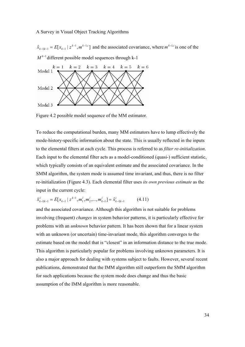
A Survey in Visual Object Tracking Algorithms
34
],|[ˆ ,1111|1
ikkkkk mzxEx −−−−− = and the associated covariance, where ikm ,1− is one of the
1−kM different possible model sequences through k-1
Figure 4.2 possible model sequence of the MM estimator.
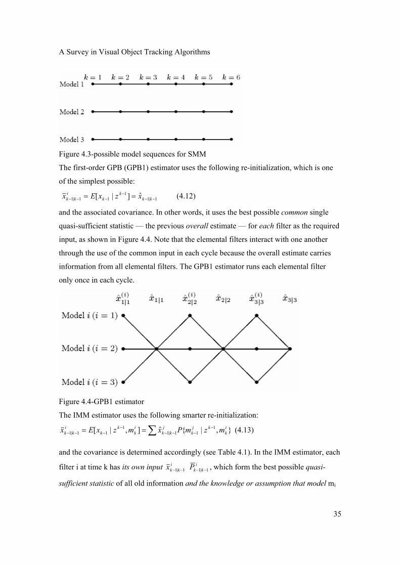
To reduce the computational burden, many MM estimators have to lump effectively the
mode-history-specific information about the state. This is usually reflected in the inputs
to the elemental filters at each cycle. This process is referred to as filter re-initialization.
Each input to the elemental filter acts as a model-conditioned (quasi-) sufficient statistic,
which typically consists of an equivalent estimate and the associated covariance. In the
SMM algorithm, the system mode is assumed time invariant, and thus, there is no filter
re-initialization (Figure 4.3). Each elemental filter uses its own previous estimate as the
input in the current cycle: i
kkik
iikk
ikk xmmmzxEx 1|1121
111|1 ˆ],...,,,|[ −−−
−−−− == (4.11)
and the associated covariance. Although this algorithm is not suitable for problems
involving (frequent) changes in system behavior patterns, it is particularly effective for
problems with an unknown behavior pattern. It has been shown that for a linear system
with an unknown (or uncertain) time-invariant mode, this algorithm converges to the
estimate based on the model that is “closest” in an information distance to the true mode.
This algorithm is particularly popular for problems involving unknown parameters. It is
also a major approach for dealing with systems subject to faults. However, several recent
publications, demonstrated that the IMM algorithm still outperform the SMM algorithm
for such applications because the system mode does change and thus the basic
assumption of the IMM algorithm is more reasonable.
A Survey in Visual Object Tracking Algorithms
35
Figure 4.3-possible model sequences for SMM
The first-order GPB (GPB1) estimator uses the following re-initialization, which is one
of the simplest possible:
1|11
11|1 ˆ]|[ −−−
−−− == kkk
ki
kk xzxEx (4.12)
and the associated covariance. In other words, it uses the best possible common single
quasi-sufficient statistic — the previous overall estimate — for each filter as the required
input, as shown in Figure 4.4. Note that the elemental filters interact with one another
through the use of the common input in each cycle because the overall estimate carries
information from all elemental filters. The GPB1 estimator runs each elemental filter
only once in each cycle.
Figure 4.4-GPB1 estimator
The IMM estimator uses the following smarter re-initialization:
∑ −−−−
−−−− == },|{ˆ],|[ 1
11|11
11|1ik
kjk
jkk
ik
kk
ikk mzmPxmzxEx (4.13)
and the covariance is determined accordingly (see Table 4.1). In the IMM estimator, each
filter i at time k has its own input ikkx 1|1 −− i
kkP 1|1 −− , which form the best possible quasi-
sufficient statistic of all old information and the knowledge or assumption that model mi
A Survey in Visual Object Tracking Algorithms
36
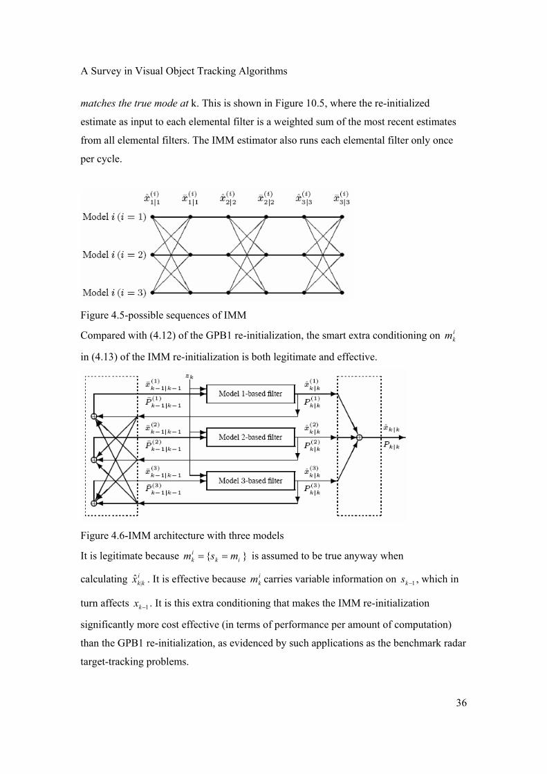
matches the true mode at k. This is shown in Figure 10.5, where the re-initialized
estimate as input to each elemental filter is a weighted sum of the most recent estimates
from all elemental filters. The IMM estimator also runs each elemental filter only once
per cycle.
Figure 4.5-possible sequences of IMM
Compared with (4.12) of the GPB1 re-initialization, the smart extra conditioning on ikm
in (4.13) of the IMM re-initialization is both legitimate and effective.
Figure 4.6-IMM architecture with three models
It is legitimate because }{ ikik msm == is assumed to be true anyway when
calculating ikkx |ˆ . It is effective because i
km carries variable information on 1−ks , which in
turn affects 1−kx . It is this extra conditioning that makes the IMM re-initialization
significantly more cost effective (in terms of performance per amount of computation)
than the GPB1 re-initialization, as evidenced by such applications as the benchmark radar
target-tracking problems.
A Survey in Visual Object Tracking Algorithms
37
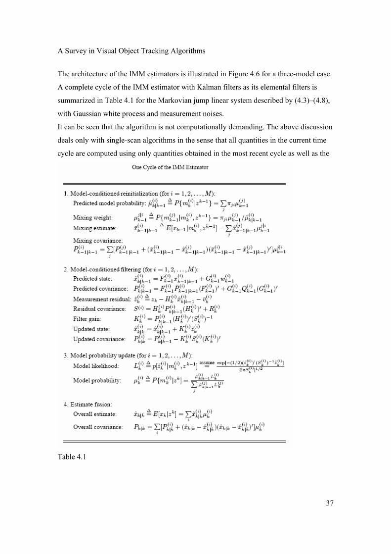
The architecture of the IMM estimators is illustrated in Figure 4.6 for a three-model case.
A complete cycle of the IMM estimator with Kalman filters as its elemental filters is
summarized in Table 4.1 for the Markovian jump linear system described by (4.3)–(4.8),
with Gaussian white process and measurement noises.
It can be seen that the algorithm is not computationally demanding. The above discussion
deals only with single-scan algorithms in the sense that all quantities in the current time
cycle are computed using only quantities obtained in the most recent cycle as well as the
Table 4.1
A Survey in Visual Object Tracking Algorithms
38
current measurements and prior information. Multi-scan estimators can also be used to
improve performance at the cost of more computation.
4.3 INTRODUCTION TO VSMM ESTIMATION Denote by Mk the set of models used at time k by an MM algorithm and by M the total
set of models used; that is, M is the union of all Mk’s. The MM algorithm is said to have
a fixed structure if the model set Mk used is fixed over time (i.e., Mk = M). Otherwise it is
said to have a variable structure. The algorithms described in the last section are of a
fixed structure. Loosely speaking, a fixed structure MM (FSMM) algorithm is one with a
fixed set of models while a variable structure MM (VSMM) algorithm is one with a
variable set of models.
As the outcome of the advances during the past three decades, the state-of-the art FSMM
estimators usually perform quite well for problems that can be handled by the use of a
small set of models. Consequently, they have found a great success in solving many state
estimation problems compounded with structural or parametric uncertainty, particularly
in target tracking. However, when they are applied to solve many real-world problems
(e.g., many practical target-tracking problems), it is often the case that the use of only a
few models is not good enough. Although further development is certainly possible, the
FSMM estimation techniques have arrived at such a stage that great improvement can no
longer be expected. This perception is based on an understanding of the fundamental
limitations of the FSMM approach.
These limitations stem from the following facts:
_ It assumes fundamentally that the system mode at any time can be represented (with a
sufficient accuracy) by one of a fixed set of models that can be determined in advance.
_ The set of possible system modes is not fixed. It depends on the hybrid state of the
system at the previous time.
_ It is shown that use of more models in an FSMM estimator does not necessarily
improve performance; in fact, the performance will deteriorate if too many models are
used.
_ It cannot incorporate certain types of a priori information.
_ Clearly, the amount of computational resource required by an FSMM estimator
increases dramatically with the number of models used.
A Survey in Visual Object Tracking Algorithms
39
These facts are explained next.
4.3.1 Limitations of Fixed Structures Let Sk be the set of possible system modes at time k and let S be the mode space (i.e., the
set of all modes at all times), which is the union of all Sk’s. Fact 1 below is based on the
theoretical result that for a static problem, the MM estimator is optimal only if the model
set used is equal to the mode space.
Fact 1: The “optimal” FSMM estimator (i.e., the one that uses optimally all possible
model sequences formed by the elements of M) is not optimal if the model set Mused
does not match exactly the mode set in effect at any time. Specifically, the “optimal” (in
the sense of having the minimum mean-square error) FSMM estimator is given by1
(4.14)
which in general differs from the optimal estimate ]|[ kk zxE . It is thus clear that the
“optimal” FSMM estimator is not optimal if the model set M is not equal to the mode
space S (i.e., M <> S) or the set Sk of possible modes is actually not fixed. There are
many practical situations in which M <> S, such as the following:
_ The mode space S is too large and a smaller M is used because of limited resources for
processing or computation. This is almost always the case when unknown parameters are
involved.
_ The system modes are too complex and their simplified models are used in M. For
instance, actual target maneuvers are usually far more complex than the commonly used
coordinated-turn or constant-acceleration models, and the like.
_ The mode space S is not known completely.
These situations also reveal the importance of and the difficulty involved in model-set
design for MM estimation.
Fact 2: Use of more models in an FSMM estimator optimally may still degrade
performance. This is shown theoretically in [34, 38]. This fact is closely related with fact
1: The optimal FSMM filter is the one that uses M = Sk for all time k. It follows that
adding more models into M may actually increase the mismatch between M and Sk and
thus lead to performance deterioration.
A Survey in Visual Object Tracking Algorithms
40
Fact 3: The set Sk+1 of possible system modes at any time k + 1 depends in general on the
current hybrid state of the system. This state dependency of the mode set
arises from the fact that a particular system mode may only jump to the system modes for
which the corresponding transition probabilities are not zero. In reality, the mode
transition probabilities are quite often dependent on the base state of the system. For
example, a car (as a ground target) on a closed highway may move only along the
highway, while a car at a four-way intersection may go straight or take a left or right turn.
Similarly, an aircraft approaching a runway from an angle is most likely to take a turn
toward the runway.
The FSMM estimators cannot make use of the above state dependency of the mode set
because the model set M is determined in advance relying only on a priori information,
that is, before any measurement is received in real time, without online information of the
state.
When tracking a car on a closed highway, the inclusion of any maneuver models in the
MM estimator will degrade the performance, while some maneuver models should be
present when the car is at an intersection. Note that intersections of a different type in
general require the use of different model sets for best performance as well as
computational complexity. Similarly, to save the resources for processing and
computation and to enhance performance, it is better not to include many maneuver
models in an MM estimator for tracking a civilian aircraft in an en-route flight. However,
relatively more maneuver models should be present in the MM estimator when the same
aircraft is in a terminal area. These situations exemplify the need to use a variable model
set (i.e., a variable structure) for better performance.
Fact 4: It is difficult or impossible for an FSMM estimator to use many types of a priori
information concerning the system mode. One type of such a priori information is the
knowledge that some system modes are unlikely but not impossible. For example, certain
emergency actions of a target (e.g., a quick evasive maneuver of a civilian aircraft) may
only be triggered by a combination of certain adverse conditions. It would be impossible
for an FSMM estimator to include such information unless it has a single model
representing the combination of the adverse conditions. The presence of such a model,
however, would degrade the estimator’s performance when the target is not in this
A Survey in Visual Object Tracking Algorithms
41
emergency, let alone the potentially dramatic increase in computation because of the need
to cover all such unlikely situations. Another example of such a priori information
involves the transition time and/or jumping magnitude between two consecutive modes;
that is, the time elapse and/or modal distance between two consecutive modes. For
instance, a priori knowledge may be available about the time period for a target of a
particular type to reach certain velocity change and/or the statistical distribution of the
modal jump magnitude.
The limitations of the FSMM estimation have been more or less perceived by those in the
research community. Ad hoc remedies have been proposed for particular applications, but
few theoretical attempts were made to break away from the fixed structure. The
investigation of the adaptive-grid PDA filter, the moving-bank SMM estimators, and the
simplex-directed SMM estimator within the SMM architecture are the only earlier
meaningful efforts along this line known to the author.
4.3.2 When Should a Variable Structure Be Used? In general, a variable structure should be considered if any of the following situations
applies.
_ The mode space is large for the given resources for processing or computation.
_ The set of (most) likely system modes is highly time variant or state dependent.
_ The mode space is not known.
_ Useful but complex a priori information and knowledge about the possible modes is
available.
In general, the more complex the problem is, the more superior the variable structure is to
the fixed structure. A good example of the above situations is the problem of tracking
ground targets.
4.3.3 The Recursive Adaptive Model-Set Approach It has been shown that a key difference between the optimal VSMM and FSMM
estimators is that the former is a probabilistically weighted sum of all estimators based on
admissible mode-set sequences that are mutually exclusive and exhaustive, while the
latter is of all estimators based on possible mode sequences. Although the
probabilistically weighted sum of estimators based on all admissible model-set sequences
A Survey in Visual Object Tracking Algorithms
42
is computationally infeasible, a practical VSMM estimator may make use of the
suggested two-level hierarchical structure: multiple model-set sequences at the higher
level and multiple model sequences at the lower level. For most applications, the higher
level with multiple model-set sequences should be replaced, because of limited
computational resources, by a single (hopefully “best”) model-set sequence. This single
sequence is obtained in practice through model-set adaptation. In other words, the
optimal but infeasible VSMM estimator suggests the use of a recursive MM estimator
based on an adaptive set of models. This is the recursive adaptive model-set (RAMS)
approach (or more precisely, the recursive adaptive digraph (RAD) approach). It will
probably be the prevailing practical approach to VSMM estimation for some years to
come. For example, all the VSMM estimation algorithms and designs developed so far
belong to the RAMS approach. In general, each cycle of a RAMS algorithm using
MMSE optimality criterion has to complete the following two tasks:
_ Model-set adaptation: As the decision component, it determines at each time the model
set to use for the MM estimation, using the a posteriori information contained in the
measurement sequence as well as a priori knowledge. This is unique for VSMM
estimation. Different RAMS algorithms differ from one another primarily with respect to
how the model set adapts. This is discussed in Section 4.4.
_ Model-set (sequence) conditioned estimation: As the estimation component, it provides
the best possible estimates given a model-set sequence, determined by the model-set
adaptation. It consists of the following:
Initialization: Assign initial probabilities to new models and initialize the filters based on
them. This is absent in FSMM estimation.
Re-initialization: Reinitialize filters based on models that remain to be in effect (see
Subsection 4.2.2 for details).
Model-based estimation: Make estimates based on models in the current set assuming
that one and only one of them matches the true mode.
Model-sequence probability calculation: Compute the probability that each model
matches the true mode given the model-set history.
A Survey in Visual Object Tracking Algorithms
43
Estimate fusion: Obtain the overall estimate by fusing all model-based estimates (see
Subsection 4.2.1 for details). Model-set sequence conditioned estimation is the topic of
Section 4.5.
4.4 MODEL-SET ADAPTATION In the RAMS approach, model-set adaptation determines the model set at each time,
rather than a sequence of model sets over a time period. More specifically, it determines
at each time what model set to use for the MM estimation, using the a posteriori
information contained in the measurement sequence as well as the a priori knowledge. It
is probably the most important topic in VSMM estimation. Model-set adaptation can be
decomposed into two functional tasks: (i) determination of candidate sets and (ii)
selection of the best set from the candidate sets.
The selection of the “best” model set from the candidate sets may be formulated well as a
statistical decision problem, in particular a problem of testing statistical hypotheses in the
Neyman-Pearson or sequential test framework.
4.5 VSMM ALGORITHMS As manifested by the great impact of the success of the IMM estimator on the application
of MM estimation techniques, it is fair to say that no matter how promising VSMM
estimation may appear, its ultimate success relies on the development of good practical
VSMM algorithms that can be readily implemented and are general enough to be
applicable to a large class of practical problems. If successful, such development will be a
new milestone in MM estimation.
VSMM estimation has been rapidly gaining momentum since its inception in [18]. Two
VSMM algorithms and several more or less ad hoc have been developed over the past
few years. Several other VSMM algorithms and designs are currently under evaluation or
active development.
The first-generationMM (i.e., SMM) algorithms distinguish among themselves primarily
by the rules for estimate fusion (i.e., how the overall estimate is determined from the
model-based estimates) [18]. The main distinctive features of the second-generation MM
(i.e., interacting MM) algorithms are their filter re-initialization mechanisms (or how the
model sequences are effectively managed). The second generation inherits the estimate
A Survey in Visual Object Tracking Algorithms
44
fusion rule from the first generation. The third-generation (i.e., VSMM) algorithms are
characterized by their variable structures (or model-set adaptation structures); that is, the
determination of the sequence of model sets. As before, the third generation inherits the
second generation’s filter re-initialization mechanism and the first generation’s estimate
fusion rule. It is interesting to note that the development of MM estimation algorithms
has been in the direction from the final product toward the underlying structure through
the internal mechanisms; that is, from the formation of the estimator’s output, to the
management of model sequences, and then to the foundation for generating the model
sequences.
As stated before, model-set adaptation consists of determining candidate sets and
selecting one or more “best” sets from the candidate sets. The selection of the best sets
from a collection of candidate sets is covered in Section 4.4.
The determination of candidate sets is the main task of a particular model-set adaptation
algorithm. In other words, different VSMM algorithms may use the same procedure to
select the best sets from the candidate sets but they differ from one another primarily in
how the candidate sets are determined. Development of good model-set adaptation
algorithms is one of the most important tasks in VSMM estimation.
MM estimation theory, like adaptive filter theory, is believed to eventually develop into
one of a “kit of tools” represented by various VSMM and FSMM estimation algorithms
based on a unified theory.
4.5.1 10.6.1 Categories of Variable Structures The adaptive structure is the most important class of variable structures in which the
variation of the structure is determined by adaptation in real time. Variable structure
includes other non-adaptive structures such as (multiple) predetermined time-varying
structures. The optimal VSMM estimator presented in [19] is such an example. Only
adaptive structures will be considered from now on.
Many adaptive structures are possible. They can be classified into several categories,
which form two broad families, referred to as active model-set and model-set generation
here.
In the active model-set family, the total model-set is finite and can be determined in
advance before any measurement is received. At any given time it uses an active or
A Survey in Visual Object Tracking Algorithms
45
working subset of the total model-set determined by adaptation, hence the name. Its
underlying idea is somewhat similar to that of the active-set method for constrained
optimization problems: At each time some models may be terminated and some may be
activated (rather than generated). Those terminated are usually not maintained.
Model-set switching is one of the simplest classes of active model-set structures in which
the active set is determined by switching among predetermined subsets of the total
model-set. These subsets are the candidate sets for the model-set adaptation problem. The
switching can be soft as well as hard, just like soft and hard decision for the MM estimate
fusion. The key task in this structure is the determination of the decision procedure for
switching (and the collection of model subsets). Such a structure, called model-group
switching algorithm, is presented in Subsection 4.5.2.
Another simple class of active model-set structures can be called likely-model set
structure. Simply put, its active set is formed by deleting the models in the total set that
are unlikely to match the true mode at the given time. To follow the true mode that may
jump, it must have a mechanism of expanding the active model set. There are various
possible ways of expansion (i.e., determination of the candidate sets). Such a structure is
presented in Subsection 4.5.3.
Still another simple class of active model-set structures has a hierarchical architecture.
The active set in this hierarchical model-set structure consists of hierarchical levels of
models. The makeup (i.e., model subset) of a lower level, as a candidate set, is
determined under the guidance of the higher levels. An MM estimator typically operates
at each level, but interactions among levels are generally beneficial. If some models that
form one or more levels are generated (instead of activated) in real time, the
corresponding hierarchical structure may be deemed to belong to the model-set
generation family. Not all hierarchical MM algorithms have an adaptive structure.
In the model-set generation family, new models are generated in real time and thus it is
impossible to specify the total model-set in advance.
It is possible to use one or more adaptive models or elemental filters within an adaptive
structure. This leads to a two-level adaptive structure, meaning that both the models (or
its elemental filters) and the model sets are adaptive. It belongs to the model-set
generation family.
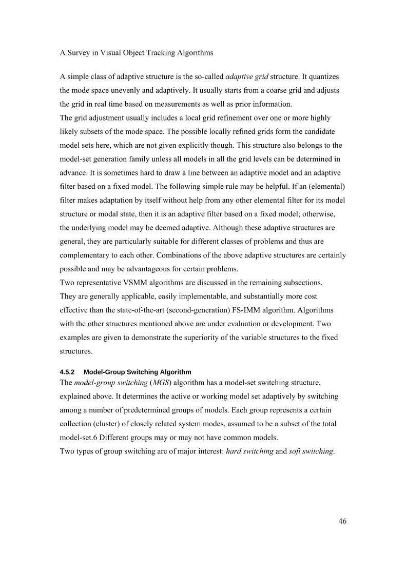
A Survey in Visual Object Tracking Algorithms
46
A simple class of adaptive structure is the so-called adaptive grid structure. It quantizes
the mode space unevenly and adaptively. It usually starts from a coarse grid and adjusts
the grid in real time based on measurements as well as prior information.
The grid adjustment usually includes a local grid refinement over one or more highly
likely subsets of the mode space. The possible locally refined grids form the candidate
model sets here, which are not given explicitly though. This structure also belongs to the
model-set generation family unless all models in all the grid levels can be determined in
advance. It is sometimes hard to draw a line between an adaptive model and an adaptive
filter based on a fixed model. The following simple rule may be helpful. If an (elemental)
filter makes adaptation by itself without help from any other elemental filter for its model
structure or modal state, then it is an adaptive filter based on a fixed model; otherwise,
the underlying model may be deemed adaptive. Although these adaptive structures are
general, they are particularly suitable for different classes of problems and thus are
complementary to each other. Combinations of the above adaptive structures are certainly
possible and may be advantageous for certain problems.
Two representative VSMM algorithms are discussed in the remaining subsections.
They are generally applicable, easily implementable, and substantially more cost
effective than the state-of-the-art (second-generation) FS-IMM algorithm. Algorithms
with the other structures mentioned above are under evaluation or development. Two
examples are given to demonstrate the superiority of the variable structures to the fixed
structures.
4.5.2 Model-Group Switching Algorithm The model-group switching (MGS) algorithm has a model-set switching structure,
explained above. It determines the active or working model set adaptively by switching
among a number of predetermined groups of models. Each group represents a certain
collection (cluster) of closely related system modes, assumed to be a subset of the total
model-set.6 Different groups may or may not have common models.
Two types of group switching are of major interest: hard switching and soft switching.
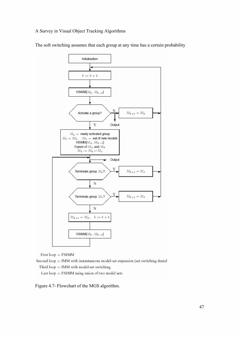
A Survey in Visual Object Tracking Algorithms
47
The soft switching assumes that each group at any time has a certain probability
Figure 4.7- Flowchart of the MGS algorithm.
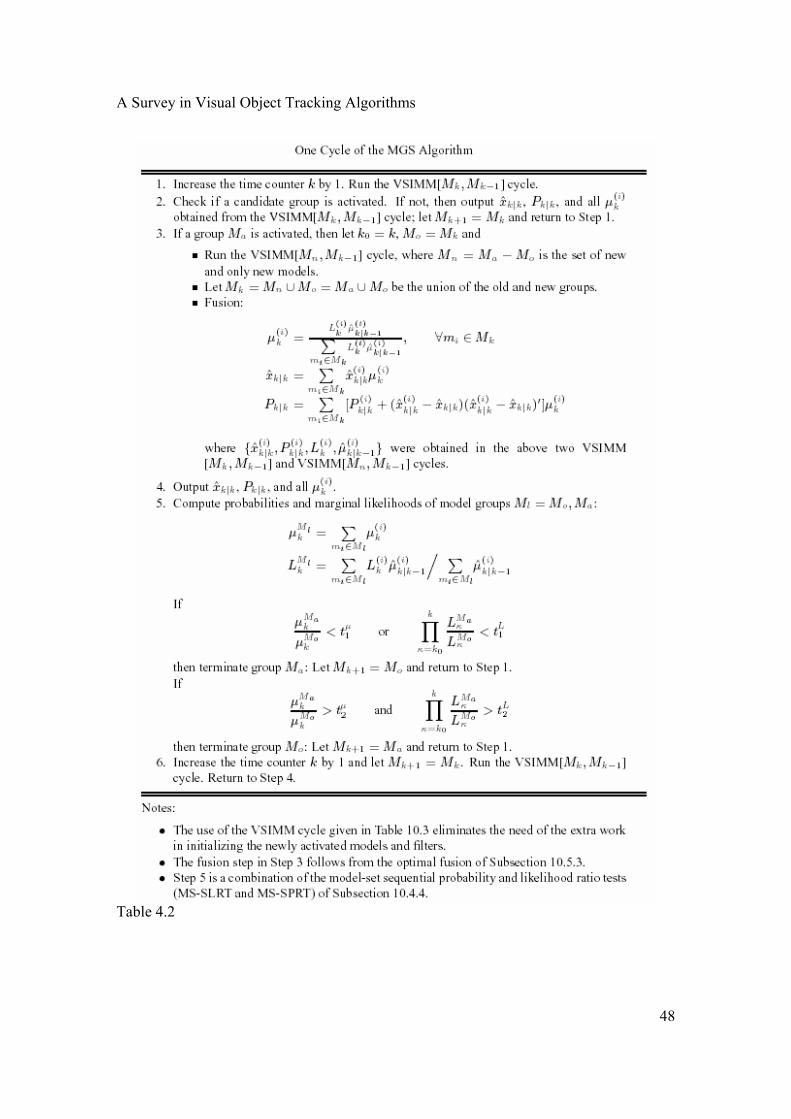
A Survey in Visual Object Tracking Algorithms
48
Table 4.2
A Survey in Visual Object Tracking Algorithms
49
of having a member model matching the true mode and the overall estimate is the
probabilistically weighted sum of all model group-based MM estimates. The MGS
algorithm involves hard switching only. A hard switching is one based on a set of “hard”
rules (i.e., by a hard decision). As such, only one model group is run at a time and thus it
may provide a substantial saving in computation over the FSMM estimator with the total
model-set. The common models in adjacent groups will facilitate group adaptation and
the initialization of newly activated filters. The flowchart and one cycle of the MGS
algorithm are given in Figure 4.7 and Table 4.2, respectively.
A proper initialization of the MGS algorithm relies on a priori information about the
initial true mode. If a priori information indicates that the initial mode is likely to be in a
certain subset of the mode space, then the MGS algorithm should start from the
corresponding model group. In general, one of the following procedures may be used for
initialization without a priori information:
_ Run an FSMM estimator using all models for a few cycles and then choose the group
with the highest probability as the initial one.
_ Calculate all model likelihoods and choose the group having the largest group
likelihood as the initial one.
_ Choose as the initial one the “nominal” model group that represents the nominal system
modes with a mechanism to switch to non-nominal groups.
_ Run several MGS algorithms using the same total model-set but different initial groups
for a few cycles and then choose the one with the highest group likelihood as the initial
group.
4.5.3 Likely-Model Set Algorithm The likely-model set (LMS) algorithm has the likely-model set structure, explained in
Subsection 4.5.1. It uses at any given time a subset of the models in the total set that are
not unlikely to match the true mode at the time.
The key to the implementation of the above idea is the concept of the state dependency of
the mode set, as explained before. In plain terms, it implies that given the current system
mode, the set of possible system modes at the next time is a subset of the mode space,
which is determined by the mode transition law (i.e., the adjacency relations of the
modes). A simple implementation is the following. Classify all models into three
A Survey in Visual Object Tracking Algorithms
50
categories: unlikely, significant, and principal. Then, model-set adaptation can be done as
follows: (i) discard the unlikely ones; (ii) keep the significant ones; and (iii) activate the
models adjacent from the principal ones.
A model mj is adjacent from mi if the transition probability from mi to mj is not zero.
This leads to the following simple LMS algorithm, given for one cycle:
1. Model classification: Identify each model inMk_1 to be unlikely (if its probability is
below t1), principal (if its probability exceeds t2), or significant (if its probability is
between t1 and t2).
2. Model-set adaptation: ObtainMk by deleting all the unlikely models inMk_1 and then
activating all the models adjacent from any principal model ofMk_1.
3. Model-set sequence conditioned estimation: As discussed in Section 4.4.
The unlikely models in Mk_1 can be eliminated by ranking all the models in Mk_1 by
their model probabilities and deleting those whose ratios of model probability to the
largest one are below a certain threshold. This follows from the sequential ranking test of
Subsection 4.3.6. Alternatively, a simpler but less accurate way is to delete all the models
inMk_1 except the K models of the largest probabilities, where K is a constant,
determined from computational considerations. The following combinations of these two
methods may be more reasonable for certain applications.
_ “AND” combination: A model is deleted only if its probability (or probability ratio to
the largest one) is both below the threshold and not among the K largest. This leads to at
least K models that are not deleted.
_ “OR” combination: A model is deleted if its probability (or probability ratio to the
largest one) is either below the threshold or not among the K largest. This leads to at
most K models that are not deleted.
The “AND” combination seems more reasonable in most cases because it guarantees
“performance” and relaxes computation while “OR” combination guarantees computation
and relaxes “performance.”
Table 4.3 gives one cycle of the simple LMS algorithm. with the “AND” logic for the
elimination of the unlikely models. Details and two other more powerful versions of the
LMS algorithm can be found in [42].
A Survey in Visual Object Tracking Algorithms
51
4.5.4 Evaluation of MM Algorithms Various criteria and measures for evaluating MM algorithms are proposed in [40]. The
three most important components of the evaluation of an MM estimator are (i) state
estimation quality (e.g., RMS position and velocity errors), (ii) mode identification
capability (e.g., model probabilities), and (iii) requirements on computational/ processing
resources (e.g., flops and CPU time). These are widely used and well understood. Other
components may include robustness, parallelism, implementability, and so on.
For some applications, such as state estimation with uncertain parameters (e.g., target
accelerations), distance among modes and models can be reasonably defined; that is, the
mode space is a region in a metric space. Some additional criteria and measures are
presented in [40] for such cases, including the following simplified versions for mode
identification capability and mode estimation quality:
_ A correct mode identification (CID) is the event in which the model closest to the true
mode has the highest probability that exceeds a threshold (say, 0.5);
_ An incorrect mode identification (IID is the event in which the model with the highest
probability that exceeds the threshold is not the closest to the true mode;
_ A no mode identification (NID) is the event in which no model has a probability above
the threshold. A comparison of MM estimators in terms of CID, IID, and NID is
meaningful only when they use the same total model-set because these measures do not
account for the relations of the model set to the mode space. For example, it is almost
always the case that a 2-model MM estimator has better CID, IID, and NID than a 100-
model MM estimator for the same problem because these probabilities do not take into
account of how fine the mode space is quantized by the model set. The use of the average
modal distance or mode error does not have this limitation. It is, however, less revealing
and less handy. Also, for some practical problems, it may be hard to define such a
distance or error if different models are characterized by distinct quantities, rather than
different values of the same quantity.
A Survey in Visual Object Tracking Algorithms
52
Table 4.3
5 CONCLUDING REMARKS With investigating all of dominant algorithms which are widely used in the target
tracking field, it is obvious that in most of sophisticated applications such as multiple
A Survey in Visual Object Tracking Algorithms
53
target tracking and maneuvering target tracking in which a complicated time invariant
trajectory is predictable for the target, a compromising approach must be taken so that
while using particle filter or multiple model algorithms, less trouble occurs by
computational demanding algorithms. Due to this bottleneck it seems rational to use one
of the Multiple Model algorithms in dealing with more complicated problems which are
less critical in computational demands. In fact the main superiority of the Multiple Model
to the Particle Filter is that it is fairly less time consuming in the process. In the other
hand this bottleneck compels to use these algorithms only when the other simpler
algorithms such as Kalman Filtering, do not guarantee an acceptable performance.
To sum up, disregarding this bottleneck a much more challenging method , a mixture of
the multiple Model and Particle Filter, can be designed which definitely will show more
robustness in tracking complicated maneuvering targets.
A Survey in Visual Object Tracking Algorithms
54
REFERENCES [1] Pradyumna K. Mishra, P. K. Biswas, Intelligent Target Detection and Tracking of Moving Targets
From Real Time Video Sequences
[2] Richard L. Marks _ Stephen M. Rock, Automatic Object Tracking for an Unmanned
Underwater Vehicle
using Real-Time Image Filtering and Correlation
[3] Yu Huang, Thomas S. Huang, Heinrich Niemann, SEGMENTATION-BASED OBJECT TRACKING
USING IMAGE WARPING AND KALMAN FILTERING
[4] Cody Kwok, Dieter Fox, Map-based Multiple Model Tracking of a Moving Object
[5] Y. Rui, Y. Chen, Better Proposal Distributions: Object Tracking Using Unscented Particle Filter
[6] Mukesh A. Zaveri, S. N. Merchant, Uday B. Desai, Arbitrary Trajectories Tracking using Multiple
Model Based Particle Filtering in Infrared Image Sequence
[7] S. J. Julier, J. K. Uhlmann, A New Extension of the Kalman Filter to Nonlinear Systems
[8] Mikhel E. Hawkins, High Speed Target Tracking Using Kalman Filter and Partial Window Imaging
[9] Derek Stanley Caveney, Multiple Model Techniques in Automotive Estimation and Control
[10] X. Rong Li, Vesselin P. Jilkov, A Survey of Maneuvering Target Tracking—Part V: Multiple-Model
Methods
[11] Y. Bar-Shalom, X. R. Li, Estimation with Applications to Tracking and Navigation, John Wiley &
Sons
[12] Black M, Yacoob Y, “Tracking and recognizing rigid and non-rigid facial motions using local
parametric models of image motion”, ICCV’95, 1995.
[13] Holland P, Welsch R, 'Robust regression using iteratively reweighted least squares', Comm. Statist.
Theor. Methods, 1977.
[14] S. Maskell, N. Gordon, A Tutorial for Particle Filter for Online Nonlinear/Non-Gaussian Bayesian
Tracking, 2001
[15] Merwe, R., Doucet, A., Freitas, N., and Wan, E., The unscented particle filter, Technical Report
CUED/F-INFENG/TR 380, Cambridge University Engineering department, August 2000.
[16] MacCormick, J., and Isard, M., Partitioned sampling, articulated objects, and interface-quality hand
tracking, Proc. ECCV 2000, LNCS 1831.
[17] Li, Bar-Shalom, Performance prediction of the interacting multiple model model algorithms - 1993
[18] Li, X. R., and Y. Bar-Shalom, “Mode-Set Adaptation in Multiple-Model Estimators for Hybrid
Systems,” in Proc. 1992 American Control Conf., Chicago, IL, pp. 1794–1799, June 1992.
[19] Li, X. R., and Y. Bar-Shalom, “Multiple-Model Estimation With Variable Structure,”
IEEE Trans. Automatic Control, Vol. AC-41, pp. 478–493, Apr. 1996.
Related Documents