HAL Id: tel-00942019 https://tel.archives-ouvertes.fr/tel-00942019v1 Submitted on 4 Feb 2014 (v1), last revised 5 Feb 2014 (v2) HAL is a multi-disciplinary open access archive for the deposit and dissemination of sci- entific research documents, whether they are pub- lished or not. The documents may come from teaching and research institutions in France or abroad, or from public or private research centers. L’archive ouverte pluridisciplinaire HAL, est destinée au dépôt et à la diffusion de documents scientifiques de niveau recherche, publiés ou non, émanant des établissements d’enseignement et de recherche français ou étrangers, des laboratoires publics ou privés. Contributions to cooperative localization techniques within mobile wireless bady area networks Jhad Hamie, Denis Benoit, Richard Cédric To cite this version: Jhad Hamie, Denis Benoit, Richard Cédric. Contributions to cooperative localization techniques within mobile wireless bady area networks. Electromagnetism. Université Nice Sophia Antipolis, 2013. English. tel-00942019v1

Welcome message from author
This document is posted to help you gain knowledge. Please leave a comment to let me know what you think about it! Share it to your friends and learn new things together.
Transcript
HAL Id: tel-00942019https://tel.archives-ouvertes.fr/tel-00942019v1
Submitted on 4 Feb 2014 (v1), last revised 5 Feb 2014 (v2)
HAL is a multi-disciplinary open accessarchive for the deposit and dissemination of sci-entific research documents, whether they are pub-lished or not. The documents may come fromteaching and research institutions in France orabroad, or from public or private research centers.
L’archive ouverte pluridisciplinaire HAL, estdestinée au dépôt et à la diffusion de documentsscientifiques de niveau recherche, publiés ou non,émanant des établissements d’enseignement et derecherche français ou étrangers, des laboratoirespublics ou privés.
Contributions to cooperative localization techniqueswithin mobile wireless bady area networks
Jhad Hamie, Denis Benoit, Richard Cédric
To cite this version:Jhad Hamie, Denis Benoit, Richard Cédric. Contributions to cooperative localization techniqueswithin mobile wireless bady area networks. Electromagnetism. Université Nice Sophia Antipolis,2013. English. �tel-00942019v1�
UNIVERSITE DE NICE-SOPHIA ANTIPOLIS - UFR Sciences
Ecole Doctorale en Sciences Fondamentales et Appliquées
THESE
Pour obtenir le titre de :
Docteur en Sciencesde l'UNIVERSITE de Nice-Sophia Antipolis
Spécialté : Physique
Présentée et soutenue par :
Jihad HAMIE
Contributions to CooperativeLocalization Techniques within Mobile
Wireless Body Area Networks
Thèse dirigée par le Professeur Cédric Richard
soutenue le 25 novembre 2013 au CEA-Leti (Minatec), Grenoble, France
Jury :
M. Laurent Clavier Pr. Institut Mines Télécom / Rapporteur
Télécom Lille 1 (Lille)M. Bernard Uguen Pr. Université Rennes 1 (Rennes) Rapporteur
M. Hichem Snoussi Pr. Université de Technologie de Président &
Troyes (Troyes) Examinateur
M. Cédric Richard Pr. Université de Nice - Sophia Directeur de thèse
Antipolis (Nice)M. Benoît Denis Dr.-Eng. CEA-Leti Minatec (Grenoble) CoDirecteur de thèse
M. Jean Schwoerer Dr.-Eng. Orange Labs (Meylan) Examinateur Invité

THESIS
to obtain the
PhD Degree
from the University of Nice - Sophia Antipolis
Specialty : Physics
by
Jihad HAMIE
Contributions to CooperativeLocalization Techniques withinMobile Wireless Body Area
Networks
defended at CEA-Leti Minatec, Grenoble, France
on 2013, November 25th
in front of the evaluation jury :
Reviewers : Pr. Laurent Clavier
Institut Mines Télécom / Télécom Lille 1 (Lille)Pr. Bernard Uguen
Université Rennes 1 (Rennes)President & Examinator : Pr. Hichem Snoussi
Université de Technologie de Troyes (Troyes)Co-Advisors : Pr. Cédric Richard
Université de Nice - Sophia Antipolis (Nice)Dr.-Eng. Benoît Denis
CEA-Leti Minatec (Grenoble)Invited Examinator : Dr.-Eng. Jean Schwoerer
Orange Labs (Meylan)

Abstract
Resumé
Dans le cadre de cette thèse, on se proposait de développer de nouveaux mécan-
ismes de radiolocalisation, permettant de positionner les noeuds de réseaux cor-
porels sans-�l (WBAN) mobiles, en exploitant de manière opportuniste des liens
radio coopératifs bas débit à l'échelle d'un même corps (i.e. coopération intra-
WBAN), entre réseaux distincts (i.e. coopération inter-WBAN), et/ou vis-à-vis
de l'infrastructure environnante. Ces nouvelles fonctions coopératives présentent
un intérêt pour des applications telles que la navigation de groupe ou la capture de
mouvement à large échelle. Ce sujet d'étude, par essence multidisciplinaire, a permis
d'aborder des questions de recherche variées, ayant trait à la modélisation physique
(e.g. modélisation spatio-temporelle des métriques de radiolocalisation en situation
de mobilité, modélisation de la mobilité groupe...), au développement d'algorithmes
adaptés aux observables disponibles (e.g. algorithmes de positionnement coopérat-
ifs et distribués, sélection et ordonnancement des liens/mesures entre les noeuds...),
aux mécanismes d'accès et de mise en réseau (i.e. en support aux mesures coopéra-
tives et au positionnement itératif). Les béné�ces et les limites de certaines de ces
fonctions ont été en partie éprouvés expérimentalement, au moyen de plateformes
radio réelles. Les di�érents développements réalisés tenaient compte, autant que
possible, des contraintes liées aux standards de communication WBAN émergeants
(e.g. Impulse Radio - Ultra Wideband (IR-UWB) IEEE 802.15.6), par exemple en
termes de bande fréquentielle ou de taux d'erreur.
Abstract
Wireless Body Area Networks (WBAN), which have been subject to growing research
interests for the last past years, start covering unprecedented needs in application
�elds such as healthcare, security, sports or entertainment. Even more recently,
such networks have been considered for new opportunistic and stand-alone radiolo-
cation functionalities. Under mesh or quasi-mesh topologies, mobile on-body nodes
can indeed be located within a cooperative fashion, considering peer-to-peer range
measurements based on e.g., Impulse Radio - Ultra Wideband (IR-UWB) Time of
Arrival (TOA) estimates or Narrow-Band (N-B) Received Signal Strength Indicators
(RSSI) at 2.4GHz. This radiolocation add-on is viewed as an important enabling
feature for coarse but opportunistic and large-scale humanMotion Capture (MoCap)
(e.g. as an alternative to costly and geographically restricted acquisition systems)
and/or for robust group navigation applications in practical environments (i.e. un-
der severe non-line of sight conditions).
In this context, the PhD investigations accounted herein aim at exploring new
ii
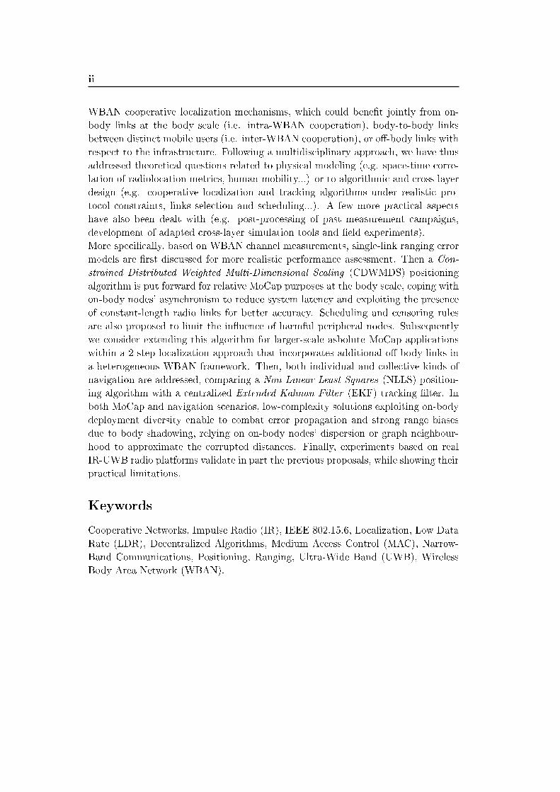
WBAN cooperative localization mechanisms, which could bene�t jointly from on-
body links at the body scale (i.e. intra-WBAN cooperation), body-to-body links
between distinct mobile users (i.e. inter-WBAN cooperation), or o�-body links with
respect to the infrastructure. Following a multidisciplinary approach, we have thus
addressed theoretical questions related to physical modeling (e.g. space-time corre-
lation of radiolocation metrics, human mobility...) or to algorithmic and cross-layer
design (e.g. cooperative localization and tracking algorithms under realistic pro-
tocol constraints, links selection and scheduling...). A few more practical aspects
have also been dealt with (e.g. post-processing of past measurement campaigns,
development of adapted cross-layer simulation tools and �eld experiments).
More speci�cally, based on WBAN channel measurements, single-link ranging error
models are �rst discussed for more realistic performance assessment. Then a Con-
strained Distributed Weighted Multi-Dimensional Scaling (CDWMDS) positioning
algorithm is put forward for relative MoCap purposes at the body scale, coping with
on-body nodes' asynchronism to reduce system latency and exploiting the presence
of constant-length radio links for better accuracy. Scheduling and censoring rules
are also proposed to limit the in�uence of harmful peripheral nodes. Subsequently
we consider extending this algorithm for larger-scale asbolute MoCap applications
within a 2-step localization approach that incorporates additional o�-body links in
a heterogeneous WBAN framework. Then, both individual and collective kinds of
navigation are addressed, comparing a Non Linear Least Squares (NLLS) position-
ing algorithm with a centralized Extended Kalman Filter (EKF) tracking �lter. In
both MoCap and navigation scenarios, low-complexity solutions exploiting on-body
deployment diversity enable to combat error propagation and strong range biases
due to body shadowing, relying on on-body nodes' dispersion or graph neighbour-
hood to approximate the corrupted distances. Finally, experiments based on real
IR-UWB radio platforms validate in part the previous proposals, while showing their
practical limitations.
Keywords
Cooperative Networks, Impulse Radio (IR), IEEE 802.15.6, Localization, Low Data
Rate (LDR), Decentralized Algorithms, Medium Access Control (MAC), Narrow-
Band Communications, Positioning, Ranging, Ultra-Wide Band (UWB), Wireless
Body Area Network (WBAN).

iii
To my friends & my beloved family

Acknowledgment
First of all, I would like to warmly thank Prof. Hichem SNOUSSI for honoring me
by accepting to be the chair-man of my thesis committee. Furthermore, I would
like to address my sincere gratitude to my thesis reviewers Prof. Bernard UGUEN
and Prof. Laurent CLAVIER for their careful reading and review work. My sincere
thanks also goe to the thesis examiner Dr. Jean SCHWOERER for his insightful
participation in my �nal defense committee.
A very special thanks goes out to my advisor Prof. Cedric RICHARD, who
undertook be my supervisor despite his many other academic and professional com-
mitments. His wisdom, knowledge and advice inspired and motivated me.
Foremost, I would like to express my sincere gratitude to my co-advisor Dr.
Benois DENIS for the continuous support of my Ph.D study and research, for his
patience, motivation, enthusiasm, and immense knowledge. His guidance helped me
in all the time of research and writing of this thesis. I could not have imagined
having a better co-advisor and mentor for my Ph.D study.
I thank the head and the people of the DSIS unit at CEA-Leti Minatec, for the
con�dence and interest they have been putting in my work and for hosting me for
3 years in excellent working conditions.
My thoughts also go to my colleagues from the LESC lab, who are good friends
and are always willing to help and give their best suggestions. Many thanks to
Mickael MAMAN for being always there to help me.
I'm also grateful to the members of the CORMORAN project's consortium, for
their precious and insightful comments, and even more globally, to the ANR INFRA
program, which has partly funded the PhD studies accounted herein.
I would also like to thank my parents, my sisters, and elder brother Ali HAMIE.
They were always supporting me and encouraging me with their best wishes. Finally,
I must acknowledge my best friends, Bassem and Abbas for sharing me all the good
and the bad times. I greatly value their friendship and I deeply appreciate their
faith in me.

Contents
1 General Introduction 1
1.1 Location-Based Body-Centric Applications and Needs . . . . . . . . 1
1.2 Enabling On-Body Localization Technologies and Techniques . . . . 6
1.2.1 Optical Systems . . . . . . . . . . . . . . . . . . . . . . . . . 6
1.2.2 Inertial Systems . . . . . . . . . . . . . . . . . . . . . . . . . 6
1.2.3 Magnetic Systems . . . . . . . . . . . . . . . . . . . . . . . . 7
1.2.4 Mechanical Systems . . . . . . . . . . . . . . . . . . . . . . . 7
1.2.5 Ultrasound Systems . . . . . . . . . . . . . . . . . . . . . . . 8
1.2.6 Radio Systems . . . . . . . . . . . . . . . . . . . . . . . . . . 8
1.3 Problem Statement, Open Issues and Personal Contributions . . . . 13
2 State of the Art in Wireless Body Area Networks Localization 21
2.1 Introduction . . . . . . . . . . . . . . . . . . . . . . . . . . . . . . . . 21
2.2 Transmitted Waveforms and Bandplans . . . . . . . . . . . . . . . . 21
2.3 Standardized Channel Models . . . . . . . . . . . . . . . . . . . . . . 22
2.3.1 IEEE 802.15.6 Models . . . . . . . . . . . . . . . . . . . . . . 23
2.3.2 IEEE 802.15.4a Models . . . . . . . . . . . . . . . . . . . . . 25
2.4 Localization Algorithms and Systems . . . . . . . . . . . . . . . . . . 26
2.4.1 Taxonomy of Cooperative Localization Algorithms . . . . . . 27
2.4.2 WBAN Localization Systems . . . . . . . . . . . . . . . . . . 35
2.5 Conclusion . . . . . . . . . . . . . . . . . . . . . . . . . . . . . . . . . 37
3 Single-Link Ranging and Related Error Models 39
3.1 Introduction . . . . . . . . . . . . . . . . . . . . . . . . . . . . . . . . 39
3.2 Empirical Modeling of On-Body Ranging Errors Based on IR-UWB
TOA Estimation . . . . . . . . . . . . . . . . . . . . . . . . . . . . . 40
3.2.1 Single-Link Multipath Channel Model . . . . . . . . . . . . . 40
3.2.2 Path Detection Schemes Enabling TOA Estimation . . . . . . 41
3.2.3 Modeling Methodology . . . . . . . . . . . . . . . . . . . . . . 42
3.2.4 Proposed Conditional Error Models . . . . . . . . . . . . . . . 46
3.3 Theoretical Modeling of O�-body and Body-to-Body Ranging Errors
Based on N-B RSSI Estimation . . . . . . . . . . . . . . . . . . . . . 54
3.4 Theoretical Modeling of O�-body and Body-to-Body Ranging Errors
Based on IR-UWB TOA Estimation . . . . . . . . . . . . . . . . . . 62
3.5 Conclusion . . . . . . . . . . . . . . . . . . . . . . . . . . . . . . . . . 65
4 Localization Algorithms for Individual Motion Capture 69
4.1 Introduction . . . . . . . . . . . . . . . . . . . . . . . . . . . . . . . . 69
4.2 Relative On-Body Localization at the Body Scale . . . . . . . . . . . 71
4.2.1 Relative Localization Algorithms . . . . . . . . . . . . . . . . 71
viii Contents
4.2.2 Medium Access Control For Localization-Enabled WBAN . . 77
4.2.3 Simulations and Results . . . . . . . . . . . . . . . . . . . . . 78
4.3 Large-Scale Absolute On-Body Localization . . . . . . . . . . . . . . 86
4.3.1 Absolute Localization Algorithms . . . . . . . . . . . . . . . . 87
4.3.2 Distance Approximation and Completion Over Neighborhood
Graph . . . . . . . . . . . . . . . . . . . . . . . . . . . . . . . 90
4.3.3 Simulations and Results . . . . . . . . . . . . . . . . . . . . . 91
4.4 Conclusion . . . . . . . . . . . . . . . . . . . . . . . . . . . . . . . . . 95
5 Localization Algorithms for Individual and Collective Navigation 97
5.1 Introduction . . . . . . . . . . . . . . . . . . . . . . . . . . . . . . . . 97
5.2 Individual Navigation . . . . . . . . . . . . . . . . . . . . . . . . . . 98
5.2.1 Classical Approach . . . . . . . . . . . . . . . . . . . . . . . . 98
5.2.2 New Proposal . . . . . . . . . . . . . . . . . . . . . . . . . . . 99
5.3 Collective Navigation . . . . . . . . . . . . . . . . . . . . . . . . . . . 102
5.4 Simulations and Results . . . . . . . . . . . . . . . . . . . . . . . . . 102
5.4.1 Scenario Description . . . . . . . . . . . . . . . . . . . . . . . 102
5.4.2 Simulation Parameters . . . . . . . . . . . . . . . . . . . . . . 103
5.4.3 Simulation Results . . . . . . . . . . . . . . . . . . . . . . . . 104
5.5 Conclusion . . . . . . . . . . . . . . . . . . . . . . . . . . . . . . . . . 109
6 Experiments 111
6.1 Introduction . . . . . . . . . . . . . . . . . . . . . . . . . . . . . . . . 111
6.2 Used Equipment and Experimental Settings . . . . . . . . . . . . . . 112
6.3 Single-Link Ranging Experiments . . . . . . . . . . . . . . . . . . . . 114
6.3.1 Ranging Over On-body Links . . . . . . . . . . . . . . . . . . 114
6.3.2 Ranging Over O�-body Links . . . . . . . . . . . . . . . . . . 119
6.4 Individual Motion Capture Experiments Based on Real Range Mea-
surements . . . . . . . . . . . . . . . . . . . . . . . . . . . . . . . . . 120
6.5 Conclusion . . . . . . . . . . . . . . . . . . . . . . . . . . . . . . . . . 123
7 Conclusions and Perspectives 125
7.1 Conclusions . . . . . . . . . . . . . . . . . . . . . . . . . . . . . . . . 125
7.2 Perspectives . . . . . . . . . . . . . . . . . . . . . . . . . . . . . . . . 128
A Cramer-Rao Lower Bound for the TOA Estimation of UWB Sig-
nals 131
A.1 System Structure . . . . . . . . . . . . . . . . . . . . . . . . . . . . . 131
A.2 CRLB For Single Pulse Systems in AWGN . . . . . . . . . . . . . . . 132
A.3 CRLB For UWB Signal in Multpath Channel . . . . . . . . . . . . . 132
B Adaptive Self-Learning and Detection of On-Body Fixed-Length
Links 133

Contents ix
C Cramer-Rao Lower Bound for Relative On-Body Nodes Position-
ing 135
D Reminder of the Extended Kalman Filter Formulation 137
Bibliography 139

List of Figures
1.1 Typical WBAN deployment for medical and healthcare applications
[1]. . . . . . . . . . . . . . . . . . . . . . . . . . . . . . . . . . . . . . 2
1.2 WBAN integrated in cooperative and heterogeneous networks, as a
core building block of the future daily-life Internet of Things (IoT). . 2
1.3 Cooperative WBANs interacting within their local environment (in-
cluding other WBANs), enabling new site-/context-speci�c applica-
tions for smarter cities/homes and augmented nomadic social net-
working. . . . . . . . . . . . . . . . . . . . . . . . . . . . . . . . . . . 3
1.4 Technical needs and requirements for large-scale individual motion
capture (in low and high precision modes) and group navigation ap-
plications, according to the CORMORAN project (where An: Ankles,
He: Head, Wr: Wrist, To: Torso, Hi: Hips, Lg: Legs, Ba: Back, Sh:
Shoulders, Kn: Knees, Bd: Bends stand for possible sensors' locations). 5
1.5 Example of typical scenario and system deployment for on-body op-
tical tracking (e.g. based on the Infra-Red technology) [2]. . . . . . . 7
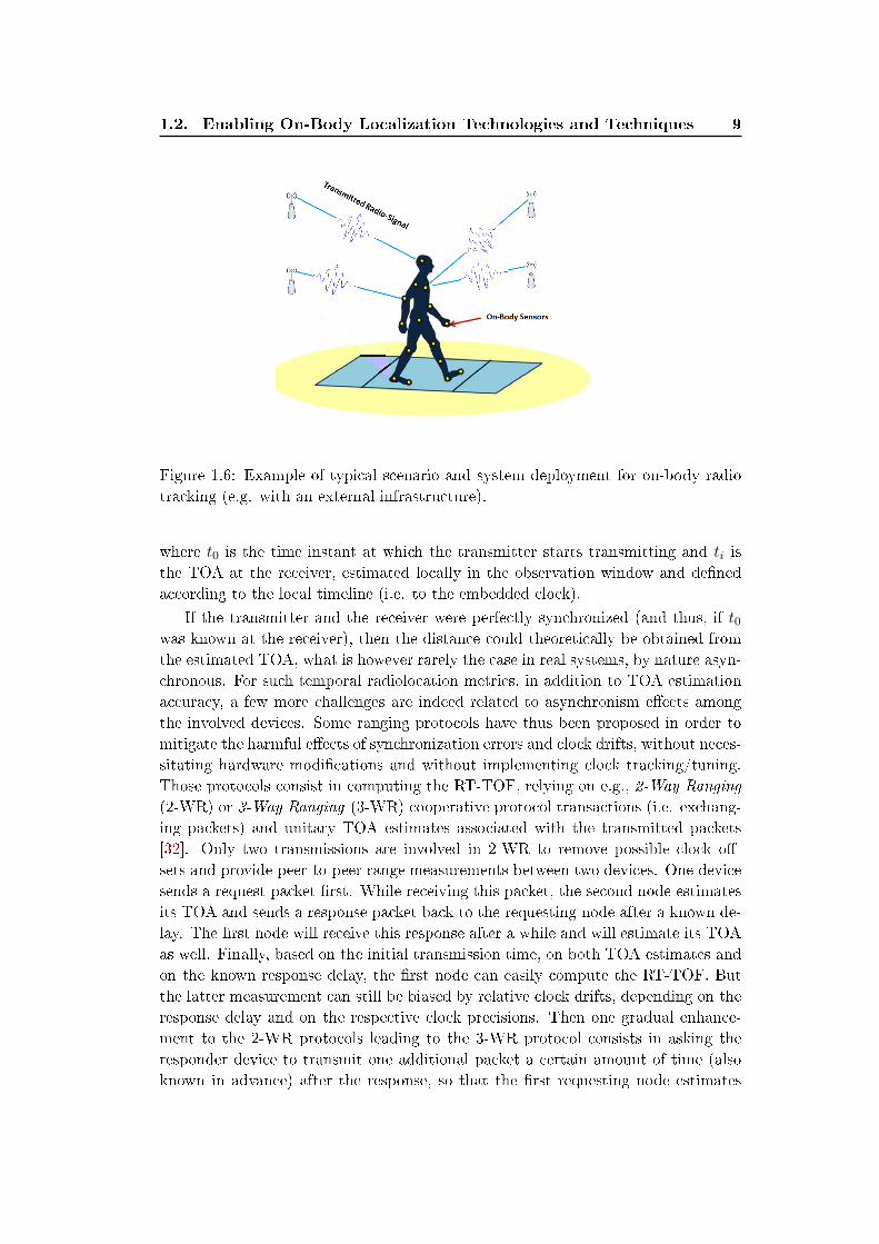
1.6 Example of typical scenario and system deployment for on-body radio
tracking (e.g. with an external infrastructure). . . . . . . . . . . . . . 9
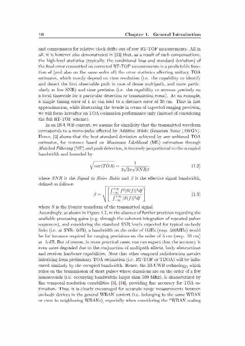
1.7 Best achievable single-link TOA-based ranging standard deviation, as
a function of the e�ective signal bandwidth and signal to noise ratio,
assuming a mono-pulse AWGN scenario [3]. . . . . . . . . . . . . . . 11
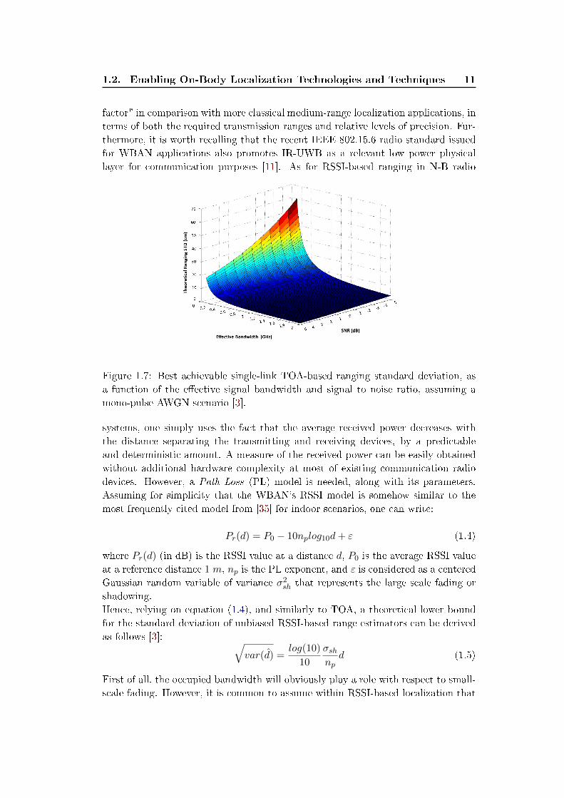
1.8 Best achievable single link RSSI-based ranging standard deviation, as
a function of the actual distance and shadowing parameter (assuming
a path loss exponent equal to 2). . . . . . . . . . . . . . . . . . . . . 13
1.9 Generic cooperative WBAN deployment, with ultra short-range intra-
WBAN links (blue), medium-range inter-WBAN links (magenta),
and large-range o�-body links (orange) for motion capture and navi-
gation purposes. . . . . . . . . . . . . . . . . . . . . . . . . . . . . . 14
1.10 Typical localization scheme in WBAN context. . . . . . . . . . . . . 17
2.1 WBAN frequency bands allocation de�ned by the IEEE 802.15.6 stan-
dard in di�erent countries [4]. . . . . . . . . . . . . . . . . . . . . . . 22
2.2 IEEE 802.15.4a on-body scenarios based on the receiver positions [5]. 26
3.1 Dynamic variations of the power transfer function between the hip
and the wrist under body mobility (standard walk), as a function of
time t. . . . . . . . . . . . . . . . . . . . . . . . . . . . . . . . . . . . 43
3.2 Energy-normalized templates w0(τ,B) used for the generation of syn-
thetic received signals and for correlation-based TOA estimation. . . 43
xii List of Figures
3.3 Equivalent inter-node distance retrieved out of correlation-based
TOA estimation without noise (blue) and �tted reference distance
after averaging with a sliding window and splines interpolation over
the detected NLOS time stamp region (red), for both Hip-Chest (top)
and Hip-Wrist links (bottom). . . . . . . . . . . . . . . . . . . . . . . 46
3.4 Empirical and model-based CDFs of ranging errors with a matched
�lter TOA estimator (i.e. strongest path detection), in both LOS and
NLOS conditions, with SNR(t0) = 5dB, in the band [3.1, 5.1]GHz. . 48
3.5 Mean of ranging errors with a matched �lter TOA estimator (i.e.
strongest path detection), in LOS conditions, as a function of SNR(t0). 48
3.6 Standard deviations of ranging errors σ with a matched �lter TOA es-
timator (i.e. strongest path detection), in LOS and NLOS conditions,
as a function of SNR(t0). . . . . . . . . . . . . . . . . . . . . . . . . 49
3.7 Variation of the false alarm probability for FAP TOA estimation (i.e.
�rst path detection), using a threshold of 10 dB below the global
absolute maximum of the estimated CIR, in LOS conditions, in the
band [3.1, 5.1]GHz, as a function of SNR(t0). . . . . . . . . . . . . . 50
3.8 Mean of ranging errors for FAP TOA estimation (i.e. �rst path de-
tection), in LOS conditions in the band [3.1, 5.1]GHz, as a function
of SNR(t0). . . . . . . . . . . . . . . . . . . . . . . . . . . . . . . . . 51
3.9 Comparison between the variations of the standard deviations of rang-
ing errors σ using a FAP TOA estimator (i.e. �rst path detection
using a threshold of 10 dB below the global absolute maximum of
the estimated CIR) and strongest correlation peak TOA estimator,
in LOS conditions, in the band [3.1, 5.1]GHz, as a function of SNR(t0). 51
3.10 Mean value associated with the Gaussian part of the ranging error
mixture-based model in NLOS conditions, as a function of SNR(t0). 52
3.11 Weight of the Uniform part of the mixture-based ranging error model
in NLOS conditions, as a function of SNR(t0). . . . . . . . . . . . . 52
3.12 Scenario of the on-body measurements campaign carried out in [6],
including four star links. . . . . . . . . . . . . . . . . . . . . . . . . . 55
3.13 Dynamic variation of the power transfer function for 4 on-body links,
in both frequency bands [3.75, 4.25]GHz (top) and [3.75, 4.25]GHz
(bottom). . . . . . . . . . . . . . . . . . . . . . . . . . . . . . . . . . 55
3.14 Best achievable RSSI-based ranging error standard deviation over o�-
body N-B links at 2.45 GHz, as a function of the actual distance
and shadowing parameter, under LOS conditions, where the on-body
device is either placed on heart or hip. . . . . . . . . . . . . . . . . . 58
3.15 Best achievable RSSI-based ranging error standard deviation over o�-
body N-B links at 2.45 GHz, as a function of the actual distance and
shadowing parameter, under NLOS conditions, where the on-body
device is placed on heart. . . . . . . . . . . . . . . . . . . . . . . . . 58
List of Figures xiii
3.16 Best achievable RSSI-based ranging error standard deviation over o�-
body N-B links at 2.45 GHz, as a function of the actual distance and
shadowing parameter, under NLOS conditions, where the on-body
device is placed on hip. . . . . . . . . . . . . . . . . . . . . . . . . . . 60
3.17 Best achievable RSSI-based ranging error standard deviation over
body-to-body N-B links at 2.45 GHz, as a function of the actual
distance and shadowing parameter, under LOS conditions, where the
on-body devices are placed respectively on heart and hip of the two
bodies. . . . . . . . . . . . . . . . . . . . . . . . . . . . . . . . . . . . 60
3.18 Best achievable RSSI-based ranging error standard deviation over
body-to-body N-B links at 2.45 GHz, as a function of the actual
distance and shadowing parameter, under NLOS conditions, where
the on-body devices are placed respectively on heart and hip of the
two bodies. . . . . . . . . . . . . . . . . . . . . . . . . . . . . . . . . 61
3.19 Best achievable RSSI-based ranging error standard deviation over
body-to-body N-B links at 2.45 GHz, as a function of the actual
distance and shadowing parameter, under LOS conditions, where the
on-body devices are placed on the hips of the two bodies. . . . . . . 61
3.20 Best achievable RSSI-based ranging error standard deviation over
body-to-body N-B links at 2.45 GHz, as a function of the actual
distance and shadowing parameter, under NLOS conditions, where
the on-body devices are placed on the hips of two bodies. . . . . . . 62
3.21 UWB o�-body measurement scenario in a typical indoor environment
[7]. . . . . . . . . . . . . . . . . . . . . . . . . . . . . . . . . . . . . . 64
3.22 Best achievable IR-UWB TOA-based ranging error standard devia-
tion as a function of SNR (dB), at di�erent distances between the
transmitter and the receiver in the band [3.1, 5.1]GHz. . . . . . . . . 64
3.23 Best achievable IR-UWB TOA-based ranging error standard devia-
tion as a function of SNR (dB), at di�erent distances between the
transmitter and the receiver in the band [3.75, 4.25]GHz. . . . . . . . 65
4.1 Typical deployment scenario for the relative localization of on-body
wireless nodes (grey circles) with respect to a body-strapped Local
Coordinate System (LCS) de�ned by �xed anchors (red circles). . . . 72
4.2 Beacon-aided TDMA MAC superframe format supporting the local-
ization functionality [8]. . . . . . . . . . . . . . . . . . . . . . . . . . 78
4.3 Peer-to-peer measurement procedure between nodes i and j through
2- and 3-Way ranging protocols, applying TOA estimation for each
received packet. . . . . . . . . . . . . . . . . . . . . . . . . . . . . . . 79
4.4 Snapshot of the biomechanical mobility model based on a piece-wise
cylindrical representation and used for the generation of realistic
inter-node distance measurements under body mobility. . . . . . . . 79
xiv List of Figures
4.5 Relative localization RMSE (m) per on-body node (ID), for var-
ious asynchronous and decentralized positioning algorithms: un-
constrained (DWMDS - blue), constrained (CDWMDS) with self-
calibrated �xed-length ranges (green) and exact �xed-length ranges
(red). . . . . . . . . . . . . . . . . . . . . . . . . . . . . . . . . . . . . 82
4.6 Relative localization RMSE (m) per on-body node with and without
censoring of rapid nodes for σ = 10 cm and a refreshment rate of 30
ms. . . . . . . . . . . . . . . . . . . . . . . . . . . . . . . . . . . . . . 82
4.7 Relative localization RMSE (m) per on-body node with and without
updates scheduling for σ = 10 cm and a refreshment rate of 30 ms. . 83
4.8 Relative localization RMSE (m) per on-body node with and without
forcing measurements symmetry, with σ = 10 cm and a refreshment
rate of 30 ms. . . . . . . . . . . . . . . . . . . . . . . . . . . . . . . . 84
4.9 Comparison of the average RMSE (m) per on-body node with and
without unilateral censoring of nodes 4 and 6, with respect to the-
oretical CRLB with a ranging standard deviation σ = 10 cm, a re-
freshment rate of 30 ms and a PER of 1 %. . . . . . . . . . . . . . . 85
4.10 Average relative localization RMSE (m) over all the on-body nodes
as a function of PER, with σ = 10 cm. . . . . . . . . . . . . . . . . . 85
4.11 Average relative localization RMSE (m) for all the on-body nodes as
a function of the standard deviation of ranging errors, with PER =
0.01. . . . . . . . . . . . . . . . . . . . . . . . . . . . . . . . . . . . . 86
4.12 Typical deployment scenario for the absolute localization of on-body
wireless nodes. . . . . . . . . . . . . . . . . . . . . . . . . . . . . . . 88
4.13 2-step LSIMC approach. . . . . . . . . . . . . . . . . . . . . . . . . . 89
4.14 Example of distance estimation over neighborhood graph (left): the
blue graph represents the initial graph based on the observation
distances and connectivity information. The black graph is recon-
structed based on the calculation of the shortest paths. Example of
reconstructed distance through triangular and linear estimation over
o�-body links (right). . . . . . . . . . . . . . . . . . . . . . . . . . . . 91
4.15 Absolute localization RMSE of estimated locations per on-body node
(ID) with both single- and two-step LSIMC based on TOA, TDOA
and RSSI metrics over o�-body links. . . . . . . . . . . . . . . . . . . 94
4.16 Absolute localization RMSE per on-body node (ID) with two-step
LSIMC based on TOA metrics over o�-body links and distances es-
timation over neighborhood graph. . . . . . . . . . . . . . . . . . . . 94
5.1 Typical WBAN deployment scenario for individual navigation. . . . 99
5.2 Example of classical scheme for individual navigation, based on the
posterior computation of the on-body nodes' centroid. . . . . . . . . 100
5.3 New proposed scheme for individual navigation, where one single
body position is computed, based on intermediary estimated dis-
tances between the on-body centroid and external anchors. . . . . . . 102
List of Figures xv
5.4 Typical WBAN deployment scenario for collective navigation (CGN)
within a group of 3 equipped users. . . . . . . . . . . . . . . . . . . . 103
5.5 Mobility model, including a biomechanical representation based on
piece-wise cylinders and a macroscopic RGPM model, used for the
generation of realistic distance measurements over body-to-body links
in the collective navigation (CGN) scenario. . . . . . . . . . . . . . . 103
5.6 Empirical CDF of the RMSE of estimated on-body nodes' centroid
for a single body, for a NLLS positioning algorithm fed by RSSI-based
and TOA-based range measurements over o�-body link. . . . . . . . 106
5.7 Empirical CDF of the RMSE of estimated on-body nodes' centroid for
a single body, with and without distance reconstruction (i.e. using the
shortest distance over neighborhood graph), for a NLLS positioning
algorithm fed by TOA-based range measurements over o�-body links. 106
5.8 Empirical CDF of the RMSE of estimated on-body nodes' centroid
for a single body, with distance reconstruction, for the classical co-
operative scheme vs. the new proposal (i.e. with a priori known
on-body dispersion), and a NLLS algorithm fed by TOA-based range
measurements over o�-body links. . . . . . . . . . . . . . . . . . . . . 107
5.9 Empirical CDF of the RMSE of estimated on-body nodes' centroid
for a single body and an EKF fed by TOA-based range measurements
over o�-body links. . . . . . . . . . . . . . . . . . . . . . . . . . . . . 107
5.10 Empirical CDF of the RMSE of the RMSE of estimated on-body
nodes' centroids in a group of 3 bodies, for di�erent cooperation sce-
narios and a NLLS algorithm fed by TOA-based range measurements
over o�-body and body-to-body links. . . . . . . . . . . . . . . . . . 108
5.11 CDFs of the RMSE of the estimated centroid location of a group of 3
bodies. Localization is based on the NLLS algorithm and RSS-based
range measurements over inter-body and o�-body links. . . . . . . . 109
6.1 CEA-Leti's IR-UWB LDR-LT ranging-enabled platform (right) with
its package (left). . . . . . . . . . . . . . . . . . . . . . . . . . . . . . 113
6.2 Implemented MAC superframe in the IR-UWB platform [9]. . . . . . 114
6.3 Codamotion tracking system, which considers on-body optical mark-
ers (left) and an external unit (CODA) equipped with 3 cameras [10]. 114
6.4 Experimental Scenario 1: On-body ranging over a static chest-wrist
link in direct LOS visibility. . . . . . . . . . . . . . . . . . . . . . . . 115
6.5 Comparison between measured and real distances over the static
chest-wrist link in Scenario 1. . . . . . . . . . . . . . . . . . . . . . . 115
6.6 Experimental Scenarios 2 (left), 3 (middle) and 4 (right): On-body
ranging over the chest-wrist link in direct LOS visibity, for di�erent
body attitudes. . . . . . . . . . . . . . . . . . . . . . . . . . . . . . . 116
6.7 Comparison between measured and real distances over the chest-wrist
link in Scenario 2. . . . . . . . . . . . . . . . . . . . . . . . . . . . . 117
xvi List of Figures
6.8 Comparison between measured and real distances over the chest-wrist
link in Scenario 3. . . . . . . . . . . . . . . . . . . . . . . . . . . . . 117
6.9 Comparison between measured and real distances over the chest-wrist
link in Scenario 4. . . . . . . . . . . . . . . . . . . . . . . . . . . . . 117
6.10 Experimental Scenario 5: On-body ranging over a static chest-back
link, under systematic NLOS conditions. . . . . . . . . . . . . . . . . 118
6.11 Comparison between measured and real distances over the chest-back
link in Scenario 5. . . . . . . . . . . . . . . . . . . . . . . . . . . . . 118
6.12 Experimental Scenario 6: On-body ranging over a static chest-wrist
link, under systematic NLOS conditions. . . . . . . . . . . . . . . . . 119
6.13 Comparison between measured and real distances over the chest-wrist
link in Scenario 6. . . . . . . . . . . . . . . . . . . . . . . . . . . . . 119
6.14 Comparison between measured and real distances over the chest-
coordinator o�-body link, under systematic LOS conditions. . . . . . 120
6.15 Comparison between measured and real distances over the back-
coordinator o�-body link, under systematic NLOS conditions. . . . . 121
6.16 On-body network deployment scenario for MoCap experiments. . . . 121
6.17 Retained body gestures for considering a quasi-dynamic localization
problem. . . . . . . . . . . . . . . . . . . . . . . . . . . . . . . . . . . 121
6.18 Relative localization average RMSE (m) per on-body node (ID), for
DWMDS and CDWMDS localization algorithms. . . . . . . . . . . . 123
6.19 Absolute localization average RMSE (m) per on-body node (ID),
based on the 2-step localization approach. . . . . . . . . . . . . . . . 123
List of Tables
2.1 UWB PHY allocation de�ned by the IEEE 802.15.6 standard. . . . . 23
2.2 List of the IEEE 802.15.6 scenarios and their description [11]. . . . . 24
3.1 Detailed variation of the standard deviation parameter (in cm) of the
ranging error models, as a function of SNR and B, for both of the
used on-body links under LOS and NLOS conditions. . . . . . . . . . 53
3.2 Semi-analytical models that corresponds to the variation of the stan-
dard deviation parameter (in cm) of the ranging error models, as a
function of SNR and B, for both of the used on-body links under
LOS and NLOS conditions. . . . . . . . . . . . . . . . . . . . . . . . 53
3.3 Path loss model parameters over indoor o�-body N-B links at 2.45
GHz, according to [12]. . . . . . . . . . . . . . . . . . . . . . . . . . . 56
3.4 Mean body shadowing as a function of the body-to-external relative
angle, over o�-body N-B links at 2.45 GHz for a planar monopole
antenna and an on-body device placed on the heart, according to [12]. 57
3.5 Path loss parameters over indoor body-to-body N-B links at 2.45 GHz
for a Tx on the Right Hip (�rst carrying body) and a Rx on the Heart
or the Right Hip (second carrying body), according to [13]. . . . . . 59
4.1 Comparison of the range observations used by DWMDS and CD-
WMDS algorithms. . . . . . . . . . . . . . . . . . . . . . . . . . . . . 75
4.2 TOA-based ranging error parameters over indoor o�-body IR-UWB
links, according to [8]. . . . . . . . . . . . . . . . . . . . . . . . . . . 92
6.1 IR-UWB TOA-based ranging error parameters in Scenarios 2, 3 and 4.116
6.2 IDs, positions and categories of the on-body devices used in MoCap
experiments. . . . . . . . . . . . . . . . . . . . . . . . . . . . . . . . . 122


Acronyms
A-B Aggregate-and-Broadcast
AWGN Additive White Gaussian Noise
BP Belief propagation
BT-LE Bluetooth - Low Energy
B2B Body to Body
CAP Contention Access Period
CDF Cumulative Density Function
CDWMDS Constrained Distributed Weighted Multi-Dimensional Scaling
CFP Contention Free Period
CGN Coordinated Group Navigation
CH Cluster Head
CIR Channel Impulse Response
CM Channel Model
CRLB Cramer-Rao Lower Bound
DBPSK Di�erential Binary Phase Shift Keying
DOA Directions Of Arrival
DWMDS Distributed Weighted Multi-Dimensional Scaling
EEG Electro-Encephalography
EKF Extended Kalman Filter
FAP First Arrival Path
GCS Global Coordinates System
GDOP Geometric Dilution Of Precision
GTS Guaranteed Time Slots
HBC Humand Body Communications
i.i.d. identically independent distributed
IMU Inertial Measurement Unit
INS Inertial Navigation System
IoT Internet of Things
IR-UWB Impulse Radio - Ultra Wideband
KF Kalman Filter
LCS Local Coordinates System
LDR Low Data Rate
LDR-LT Low Data Rate-Location and Tracking
LLS Linear Least Square
LOS Line Of Sight
LSIMC Large Scale Individual Motion Capture
MAC Medium Access Control
MAP Maximum a posteriori
MDS Multidimensional Scaling
MEMS Micro Electro-Mechanical Systems
xx List of Tables
MF Matched Filtering
MMSE Minimum Mean Squared Error
ML Maximum Likelihood
MLL Maximizes the Log-Likelihood
MoCap Motion Capture
MPC Multi Path Components
M2M Mobile to Mobile
N-B Narrow-Band
NBP Non Parametric Belief Propagation
NBP-ST Non Parametric Belief Propagation over Spanning Trees
NGBP Non Parametric Generalized Belief Propagation
NLLS Non Linear Least Squares
NLOS Non Line Of Sight
PC Personal Computer
pdf probability density function
PER Packet Error Rate
PL Path Loss
PRF Pulse Repetition Frequency
QoS Quality of Service
RMSE Root Mean Squared Error
RPGM Reference Point Group Mobility Model
RSSI Received Signal Strength Indicator
RTLS Real Time Location Systems
RT-TOF Round Trip - Time of Flight
SMACOF Scaling by MAjorizing a COnvex Function
SNR Signal to Noise Ratio
SPA Self Positioning Algorithm
SRRC Square-root Raised Cosine
TDMA Time Division Multiple Access
TDOA Time Di�erence of Arrival
TOA Time Of Arrival
TOF Time of Flight
TP-NBP Two Phase - Non Parametric Belief Propagation
TRW-BP Tree-Reweighted Belief Propagation
TS Time Slot
ULP Ultra Low Power
UWB Ultra-Wideband
WBAN Wireless Body Area Network
WLS Weighted Least Squares
WSN Wireless Sensor Network
2-WR 2-Way Ranging
3-WR 3-Way Ranging
Chapter 1
General Introduction
Contents
1.1 Location-Based Body-Centric Applications and Needs . . . 1
1.2 Enabling On-Body Localization Technologies and Techniques 6
1.2.1 Optical Systems . . . . . . . . . . . . . . . . . . . . . . . . . 6
1.2.2 Inertial Systems . . . . . . . . . . . . . . . . . . . . . . . . . 6
1.2.3 Magnetic Systems . . . . . . . . . . . . . . . . . . . . . . . . 7
1.2.4 Mechanical Systems . . . . . . . . . . . . . . . . . . . . . . . 7
1.2.5 Ultrasound Systems . . . . . . . . . . . . . . . . . . . . . . . 8
1.2.6 Radio Systems . . . . . . . . . . . . . . . . . . . . . . . . . . 8
1.3 Problem Statement, Open Issues and Personal Contributions 13
1.1 Location-Based Body-Centric Applications and
Needs
The recent development of sensing and short-range communication integrated tech-
nologies has been disclosing interesting perspectives for mobile, personal and body-
centric applications or services. More particularly, theWireless Body Area Networks
(WBANs), which consist of small and low-power wearable wireless devices, are on
the verge of ful�lling new market needs in a variety of application �elds such as emer-
gency and rescue (e.g. remote posture detection for institutional rescuers or victims),
healthcare (e.g. physiological or activity monitoring, wireless medical actuators and
implants, assistance to medical diagnosis, lab-on-chip chemical analysis), entertain-
ment (e.g. motion capture for gaming or sports analysis), personal communications
and multimedia (e.g. distributed terminals, personal consumer electronics), clothing
applications (e.g. garments with electronic components, smart shoes) [14], [15] (See
Figure 1.1). On the one hand, WBANs rely on emerging radio technologies that
claim Ultra Low Power (ULP) consumption, low complexity, and low cost, such as
Narrow-Band (N-B) solutions at 2.4 GHz based on e.g., Bluetooth - Low Energy
(BT-LE), or Impulse Radio - Ultra Wideband (IR-UWB) solutions, as put forward
in the recent IEEE 802.15.6 standard dedicated to WBAN applications [4], [11].
On the other hand, WBAN nodes usually embed extremely low-power sensors and
actuators based on e.g., Micro Electro-Mechanical Systems (MEMS) or even further
2 Chapter 1. General Introduction
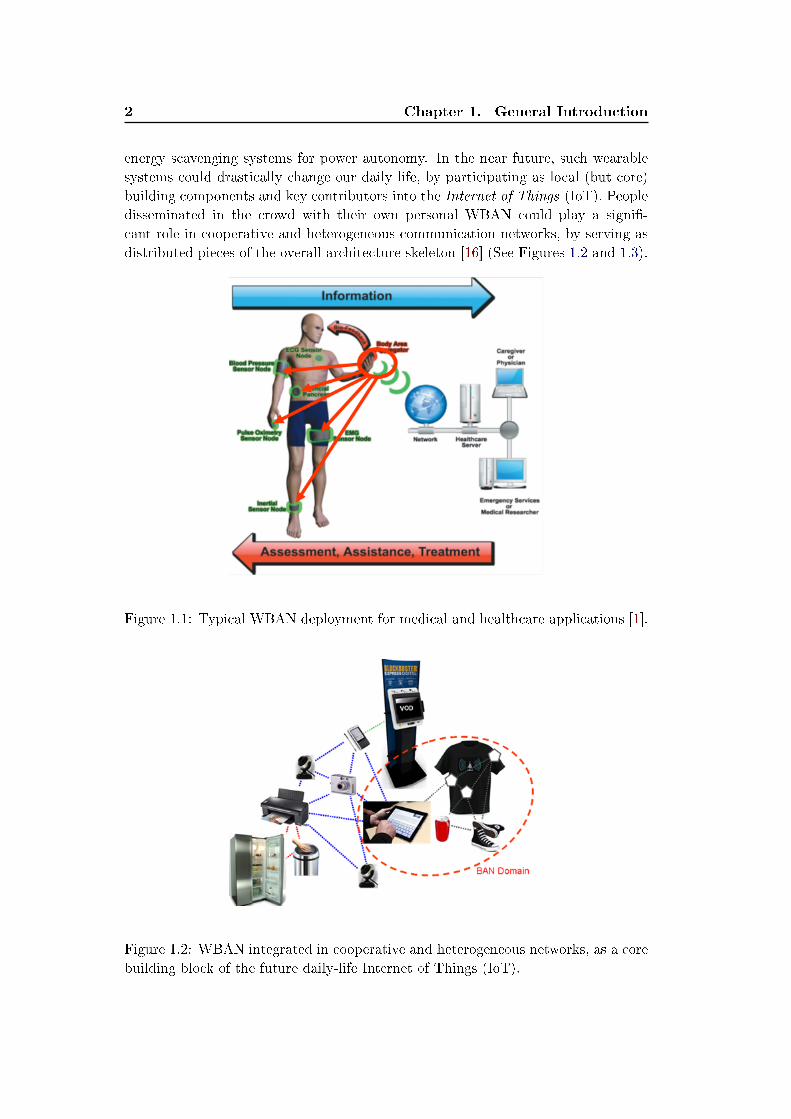
energy scavenging systems for power autonomy. In the near future, such wearable
systems could drastically change our daily life, by participating as local (but core)
building components and key contributors into the Internet of Things (IoT). People
disseminated in the crowd with their own personal WBAN could play a signi�-
cant role in cooperative and heterogeneous communication networks, by serving as
distributed pieces of the overall architecture skeleton [16] (See Figures 1.2 and 1.3).
Figure 1.1: Typical WBAN deployment for medical and healthcare applications [1].
Figure 1.2: WBAN integrated in cooperative and heterogeneous networks, as a core
building block of the future daily-life Internet of Things (IoT).
1.1. Location-Based Body-Centric Applications and Needs 3
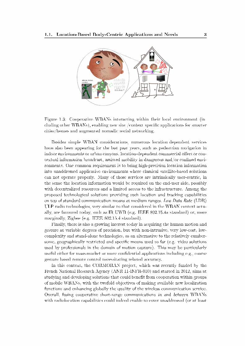
Figure 1.3: Cooperative WBANs interacting within their local environment (in-
cluding other WBANs), enabling new site-/context-speci�c applications for smarter
cities/homes and augmented nomadic social networking.
Besides simple WBAN considerations, numerous location-dependent services
have also been appearing for the last past years, such as pedestrian navigation in
indoor environments or urban canyons, location-dependent commercial o�ers or con-
textual information broadcast, assisted mobility in dangerous and/or con�ned envi-
ronments. One common requirement is to bring high-precision location information
into unaddressed applicative environments where classical satellite-based solutions
can not operate properly. Many of those services are intrinsically user-centric, in
the sense the location information would be required on the end-user side, possibly
with decentralized resources and a limited access to the infrastructure. Among the
proposed technological solutions providing such location and tracking capabilities
on top of standard communication means at medium ranges, Low Data Rate (LDR)
ULP radio technologies, very similar to that considered in the WBAN context actu-
ally, are favoured today, such as IR-UWB (e.g. IEEE 802.15.4a standard) or, more
marginally, Zigbee (e.g. IEEE 802.15.4 standard).
Finally, there is also a growing interest today in acquiring the human motion and
gesture at variable degrees of precision, but with non-intrusive, very low-cost, low-
complexity and stand-alone technologies, as an alternative to the relatively cumber-
some, geographically restricted and speci�c means used so far (e.g. video solutions
used by professionals in the domain of motion capture). This may be particularly
useful either for mass-market or more con�dential applications including e.g., coarse
gesture-based remote control necessitating relaxed accuracy.
In this context, the CORMORAN project, which was recently funded by the
French National Research Agency (ANR 11-INFR-010) and started in 2012, aims at
studying and developing solutions that could bene�t from cooperation within groups
of mobile WBANs, with the twofold objectives of making available new localization
functions and enhancing globally the quality of the wireless communication service.
Overall, fusing cooperative short-range communications in and between WBANs
with radiolocation capabilities could indeed enable to cover unaddressed (or at least
4 Chapter 1. General Introduction
still hardly addressed) applications, such as:
� augmented group navigation (e.g. �re-�ghters progressing in a building on �re
with physiological monitoring and relative position information, coordinated
squads of soldiers on urban battle-�elds);
� low-cost and infrastructure-free tracking of collective systems (e.g. real-time
capture and/or sports analysis);
� nomadic social networking (e.g. sharing personal location-dependent informa-
tion in a decentralized way among authorized members of a given community);
� augmented reality for collective entertainment (e.g. in mobile and interactive
group gaming);
� context-dependent information di�usion (e.g. data broadcast to identi�ed
clusters of people with common interests, needs or locations);
� wireless network optimization (e.g. handover between di�erent radio access
technologies for clusters of people experiencing the same mobility patterns,
optimal data routing under users mobility);
� distant health care, monitoring and rescue systems (e.g. collective launching
or noti�cation of emergency alarms, routine medical treatments at home);
� smart homes and personal multimedia (e.g. house automation, smart HiFi or
eased screen browsing through coarse body capture).
As a preliminary step of the investigations carried out in the frame of COR-
MORAN, the project's partners disseminated a questionnaire to professional en-
tities, identi�ed as possible users and/or integrators of this technology in various
activity domains. The idea was to identify their actual needs and technical re-
quirements, as well as to draw preliminary system speci�cations in terms of e.g.,
sensors/body location precision and refreshment rates, number of sensors/users and
related deployment constraints, typical mobility, operating environments, calibra-
tion needs... The analysis of their feedback con�rms that the most representative
application scenarios could be classi�ed into two main categories, namely the Large
Scale Individual Motion Capture (LSIMC) and the Coordinated Group Navigation
(CGN), as summarized in Figure 1.4.
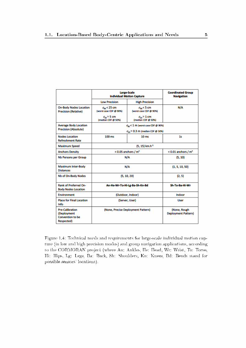
The �rst feature is somehow identical to traditional Motion Capture (MoCap),
which requires a rather high level of accuracy while locating the sensors at the body
scale (most likely at high refreshment rates), but the new aim here is to provide
stand-alone and larger-scale solutions (e.g. extending the service coverage in com-
parison with existing systems, which may be restricted into con�ned areas) with a
limited access to �xed and costly elements of infrastructure around (i.e. �xed access
points, base stations or wireless anchors). Note that depending on the underlying
applications, this motion capture functionality can be intended either as relative on-
body nodes localization (i.e. positioning on-body devices in a local body-strapped
1.1. Location-Based Body-Centric Applications and Needs 5
Figure 1.4: Technical needs and requirements for large-scale individual motion cap-
ture (in low and high precision modes) and group navigation applications, according
to the CORMORAN project (where An: Ankles, He: Head, Wr: Wrist, To: Torso,
Hi: Hips, Lg: Legs, Ba: Back, Sh: Shoulders, Kn: Knees, Bd: Bends stand for
possible sensors' locations).
6 Chapter 1. General Introduction
coordinates system) or absolute on-body localization (i.e. positioning on-body de-
vices in a more global system, external to the carrying body, typically at the building
or �oor scale). The second set of applications, which is not necessarily coupled with
the �rst motion capture functionalities, corresponds to classical pedestrian naviga-
tion applications (i.e. intended in a rather classical way) with relaxed positional
accuracy (most likely at moderate refreshment rates) but within groups of mobile
users, aiming at bene�ting from their collective behaviour.
In the next sub-section, we make a brief overview of enabling on-body localiza-
tion technologies and techniques (including radio solutions) that could �t into this
context, trying to summarize their respective advantages and limitations.
1.2 Enabling On-Body Localization Technologies and
Techniques
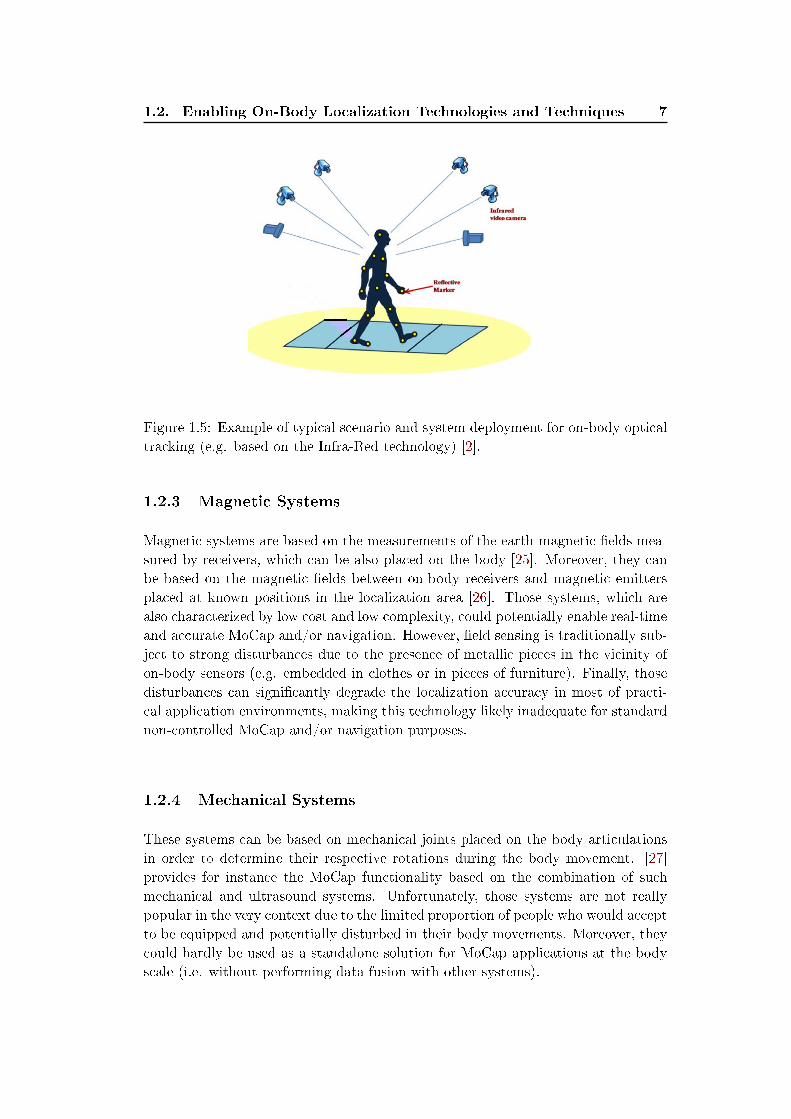
1.2.1 Optical Systems
Most optical systems are based on illuminated and re�ective markers placed on the
body [17], [10]. The localization of any on-body marker necessitates that the lat-
ter is viewed by at least two external cameras, which have known positions and
orientations [18]. Figure 1.5 shows an example of typical operating scenario and
deployment.
Such optical tracking systems are generally characterized by high localization accu-
racy (i.e. with an error of some millimeters) and they are able to support real-time
MoCap and/or navigation applications (i.e. with neglected latency). However, they
have limitations that may prevent from considering them in the very context, such
as cost, complexity or the necessity to operate in geographically restricted and closed
areas (i.e. with the test subject moving in this area). They also su�er from non-
visibility problems, when the markers cannot be viewed by the surrounding cameras
in cases of obstructions and/or obscurity conditions, and thus, the achieved accuracy
can be a�ected accordingly.
1.2.2 Inertial Systems
The most common sensors used within Inertial Measurement Units (IMUs) for the
localization of on-body devices are the accelerometers and the gyroscopes [19]. Those
systems can achieve localization errors of a few centimeters [20], [21], what can be
acceptable for MoCap purposes. They are usually characterized by their low cost
and their relatively low complexity. Besides the interest for those sensors in the
frame of MoCap applications, they have been also considered in Inertial Navigation
Systems (INSs), for instance for pedestrian tracking and dead reckoning, delivering
information related to the displacement amplitude, velocity, or heading [22], [23],
[24]. Unfortunately, the used sensors are usually a�ected by signi�cant drifts over
time [20], which necessitate frequent periodic calibrations.
1.2. Enabling On-Body Localization Technologies and Techniques 7
Figure 1.5: Example of typical scenario and system deployment for on-body optical
tracking (e.g. based on the Infra-Red technology) [2].
1.2.3 Magnetic Systems
Magnetic systems are based on the measurements of the earth-magnetic �elds mea-
sured by receivers, which can be also placed on the body [25]. Moreover, they can
be based on the magnetic �elds between on-body receivers and magnetic emitters
placed at known positions in the localization area [26]. Those systems, which are
also characterized by low cost and low complexity, could potentially enable real-time
and accurate MoCap and/or navigation. However, �eld sensing is traditionally sub-
ject to strong disturbances due to the presence of metallic pieces in the vicinity of
on-body sensors (e.g. embedded in clothes or in pieces of furniture). Finally, those
disturbances can signi�cantly degrade the localization accuracy in most of practi-
cal application environments, making this technology likely inadequate for standard
non-controlled MoCap and/or navigation purposes.
1.2.4 Mechanical Systems
These systems can be based on mechanical joints placed on the body articulations
in order to determine their respective rotations during the body movement. [27]
provides for instance the MoCap functionality based on the combination of such
mechanical and ultrasound systems. Unfortunately, those systems are not really
popular in the very context due to the limited proportion of people who would accept
to be equipped and potentially disturbed in their body movements. Moreover, they
could hardly be used as a standalone solution for MoCap applications at the body
scale (i.e. without performing data fusion with other systems).
8 Chapter 1. General Introduction
1.2.5 Ultrasound Systems
Ultrasound on-body localization systems involve emitters placed on the body and
microphones placed at known positions in the environment [27], [28], relying on the
signal Time of Flight(TOF). However, those systems can be rather strongly a�ected
by the interference caused by ultrasound waves transmitted from di�erent emitters,
in addition to echo e�ects in practical environments [29]. Those factors conduct to
damage dramatically the localization performances. Note that ultrasonic TOF and
inertial measurements can also be combined in the garment of wearable systems
for better robustness in MoCap applications, like in [30], but at the price of much
higher system and processing complexity.
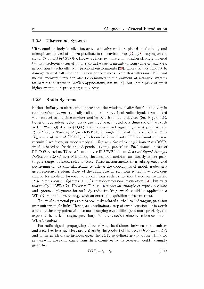
1.2.6 Radio Systems
Rather similarly to ultrasound approaches, the wireless localization functionality in
radiolocation systems typically relies on the analysis of radio signals transmitted
with respect to multiple anchors and/or to other mobile devices (See Figure 1.6).
Location-dependent radio metrics can thus be estimated over these radio links, such
as the Time Of Arrival (TOA) of the transmitted signal or, one step ahead, the
Round Trip - Time of Flight (RT-TOF) through handshake protocols, the Time
Di�erence of Arrival (TDOA), which can be formed out of TOA estimates at syn-
chronized receivers, or more simply the Received Signal Strength Indicator (RSSI),
which is based on the distance-dependent average power loss. For instance, in case of
RT-TOF based on TOA estimation over IR-UWB links or Received Signal Strength
Indicators (RSSI) over N-B links, the measured metrics can directly re�ect peer-
to-peer ranges between radio devices. These measurements then subsequently feed
positioning or tracking algorithms to deliver the coordinates of mobile nodes in a
given reference system. Most of the radiolocation solutions so far have been con-
sidered for medium/large-range applications such as logistics based on asymetric
Real Time Location Systems (RTLS) or indoor personal navigation [31], but very
marginally in WBANs. However, Figure 1.6 shows an example of typical scenario
and system deployment for on-body radio tracking, which could be applied in a
WBAN-oriented context (e.g. with an external acquisition infrastructure).
The �nal positional precision is obviously related to the level of ranging precision
over unitary single links. Hence, as a preliminary step of our discussions, it is worth
assessing the very potential in terms of ranging capabilities (and more precisely, the
expected theoretical ranging precision) of di�erent radio technologies foreseen in our
WBAN context.
For radio signals propagating at celerity c, the distance between a transmitter
and a receiver is straightforwardly given by the product of the Time Of Flight (TOF)
and c. In an ideal synchronous case, the TOF, so de�ned as the elapsed time for
propagating the radio signal from the transmitter to the receiver, would be simply
given by:
TOFi = ti − t0 (1.1)
1.2. Enabling On-Body Localization Technologies and Techniques 9
Figure 1.6: Example of typical scenario and system deployment for on-body radio
tracking (e.g. with an external infrastructure).
where t0 is the time instant at which the transmitter starts transmitting and ti is
the TOA at the receiver, estimated locally in the observation window and de�ned
according to the local timeline (i.e. to the embedded clock).
If the transmitter and the receiver were perfectly synchronized (and thus, if t0was known at the receiver), then the distance could theoretically be obtained from
the estimated TOA, what is however rarely the case in real systems, by nature asyn-
chronous. For such temporal radiolocation metrics, in addition to TOA estimation
accuracy, a few more challenges are indeed related to asynchronism e�ects among
the involved devices. Some ranging protocols have thus been proposed in order to
mitigate the harmful e�ects of synchronization errors and clock drifts, without neces-
sitating hardware modi�cations and without implementing clock tracking/tuning.
Those protocols consist in computing the RT-TOF, relying on e.g., 2-Way Ranging
(2-WR) or 3-Way Ranging (3-WR) cooperative protocol transactions (i.e. exchang-
ing packets) and unitary TOA estimates associated with the transmitted packets
[32]. Only two transmissions are involved in 2-WR to remove possible clock o�-
sets and provide peer-to-peer range measurements between two devices. One device
sends a request packet �rst. While receiving this packet, the second node estimates
its TOA and sends a response packet back to the requesting node after a known de-
lay. The �rst node will receive this response after a while and will estimate its TOA
as well. Finally, based on the initial transmission time, on both TOA estimates and
on the known response delay, the �rst node can easily compute the RT-TOF. But
the latter measurement can still be biased by relative clock drifts, depending on the
response delay and on the respective clock precisions. Then one gradual enhance-
ment to the 2-WR protocols leading to the 3-WR protocol consists in asking the
responder device to transmit one additional packet a certain amount of time (also
known in advance) after the response, so that the �rst requesting node estimates
10 Chapter 1. General Introduction
and compensates for relative clock drifts out of row RT-TOF measurements. All in
all, it is however also demonstrated in [33] that, as a result of such compensations,
the high-level statistics (typically, the conditional bias and standard deviation) of
the �nal error committed on corrected RT-TOF measurements is a predictable func-
tion of (and also on the same order of) the error statistics a�ecting unitary TOA
estimates, which mostly depend on time resolution (i.e. the capability to identify
and detect the �rst observable path in case of dense multipath, and more partic-
ularly at low SNR) and time precision (i.e. the capability to account precisely on
a local timescale for a particular detection or transmission event). As an example,
a simple timing error of 1 ns can lead to a distance error of 30 cm. Thus in �rst
approximation, while illustrating the trends in terms of expected ranging precision,
we will focus hereafter on TOA estimation performance only (instead of considering
the full RT-TOF scheme).
In an IR-UWB context, we assume for simplicity that the transmitted waveform
corresponds to a mono-pulse a�ected by Additive White Gaussian Noise (AWGN).
Hence, [3] shows that the best standard deviation achieved by any unbiased TOA
estimator, for instance based on Maximum Likelihood (ML) estimation through
Matched Filtering (MF) and peak detection, is inversely proportional to the occupied
bandwidth and bounded by√var( ˆTOA) =
1
2√
2π√SNRβ
(1.2)
where SNR is the Signal to Noise Ratio and β is the e�ective signal bandwidth,
de�ned as follows:
β =
√√√√[∫ +∞−∞ f2|S(f)|2df∫ +∞−∞ |S(f)|2df
](1.3)
where S is the Fourier transform of the transmitted signal.
Accordingly, as shown in Figure 1.7, in the absence of further precision regarding the
available processing gains (e.g. through the coherent integration of repeated pulses
sequences), and considering the standard SNR levels expected for typical on-body
links (i.e. at SNR<0dB), a bandwidth on the order of 1GHz (resp. 500MHz) would
be for instance required for ranging precisions on the order of 5 cm (resp. 10 cm)
at -5 dB. But of course, in more practical cases, one can expect that the accuracy is
even more degraded due to the conjunction of multipath e�ects, body obstructions
and receiver hardware capabilities. Note that other temporal radiolocation metrics
inheriting from preliminary TOA estimation (i.e. RT-TOF or TDOA) will be in�u-
enced similarly by the occupied bandwidth. Hence, the IR-UWB technology, which
relies on the transmission of short pulses whose durations are on the order of a few
nanoseconds (i.e. occupying bandwidths larger than 500 MHz), is characterized by
�ne temporal resolution capabilities [3], [34], providing �ne accuracy for TOA es-
timation. Thus, it is clearly encouraged for accurate range measurements between
on-body devices in the general WBAN context (i.e. belonging to the same WBAN
or even to neighboring WBANs), especially when considering the "WBAN scaling
1.2. Enabling On-Body Localization Technologies and Techniques 11
factor" in comparison with more classical medium-range localization applications, in
terms of both the required transmission ranges and relative levels of precision. Fur-
thermore, it is worth recalling that the recent IEEE 802.15.6 radio standard issued
for WBAN applications also promotes IR-UWB as a relevant low power physical
layer for communication purposes [11]. As for RSSI-based ranging in N-B radio
Figure 1.7: Best achievable single-link TOA-based ranging standard deviation, as
a function of the e�ective signal bandwidth and signal to noise ratio, assuming a
mono-pulse AWGN scenario [3].
systems, one simply uses the fact that the average received power decreases with
the distance separating the transmitting and receiving devices, by a predictable
and deterministic amount. A measure of the received power can be easily obtained
without additional hardware complexity at most of existing communication radio
devices. However, a Path Loss (PL) model is needed, along with its parameters.
Assuming for simplicity that the WBAN's RSSI model is somehow similar to the
most frequently cited model from [35] for indoor scenarios, one can write:
Pr(d) = P0 − 10nplog10d+ ε (1.4)
where Pr(d) (in dB) is the RSSI value at a distance d, P0 is the average RSSI value
at a reference distance 1 m, np is the PL exponent, and ε is considered as a centered
Gaussian random variable of variance σ2sh that represents the large scale fading or
shadowing.
Hence, relying on equation (1.4), and similarly to TOA, a theoretical lower bound
for the standard deviation of unbiased RSSI-based range estimators can be derived
as follows [3]: √var(d) =
log(10)
10
σshnp
d (1.5)
First of all, the occupied bandwidth will obviously play a role with respect to small-
scale fading. However, it is common to assume within RSSI-based localization that
12 Chapter 1. General Introduction
those e�ects are somehow averaged (e.g. based on consecutive RSSI measurements
within the channel coherence time over one link). Furthermore, in the classical mod-
eling presented above, the best achievable ranging performance would theoretically
depend on both the channel power parameters (i.e. path loss exponent and shad-
owing deviation) and the distance between the two nodes. But it is adversely well
known in the on-body WBAN context that: (i) the received power is less dependent
on the actual distance than in any other wireless context, (ii) body shadowing is
rather strong (in comparison with the nominal average received power levels), far
dominating (in comparison with other e�ects due to e.g. small-scale fading or dis-
tance) and hardly predictable with no a priori information (e.g. highly variable as
a function of the actual nodes places on the body). Overall, the achievable level
of ranging precision is not only hard to predict or specify a priori over on-body
links, but it is likely insu�cient in comparison with the actual nominal Euclidean
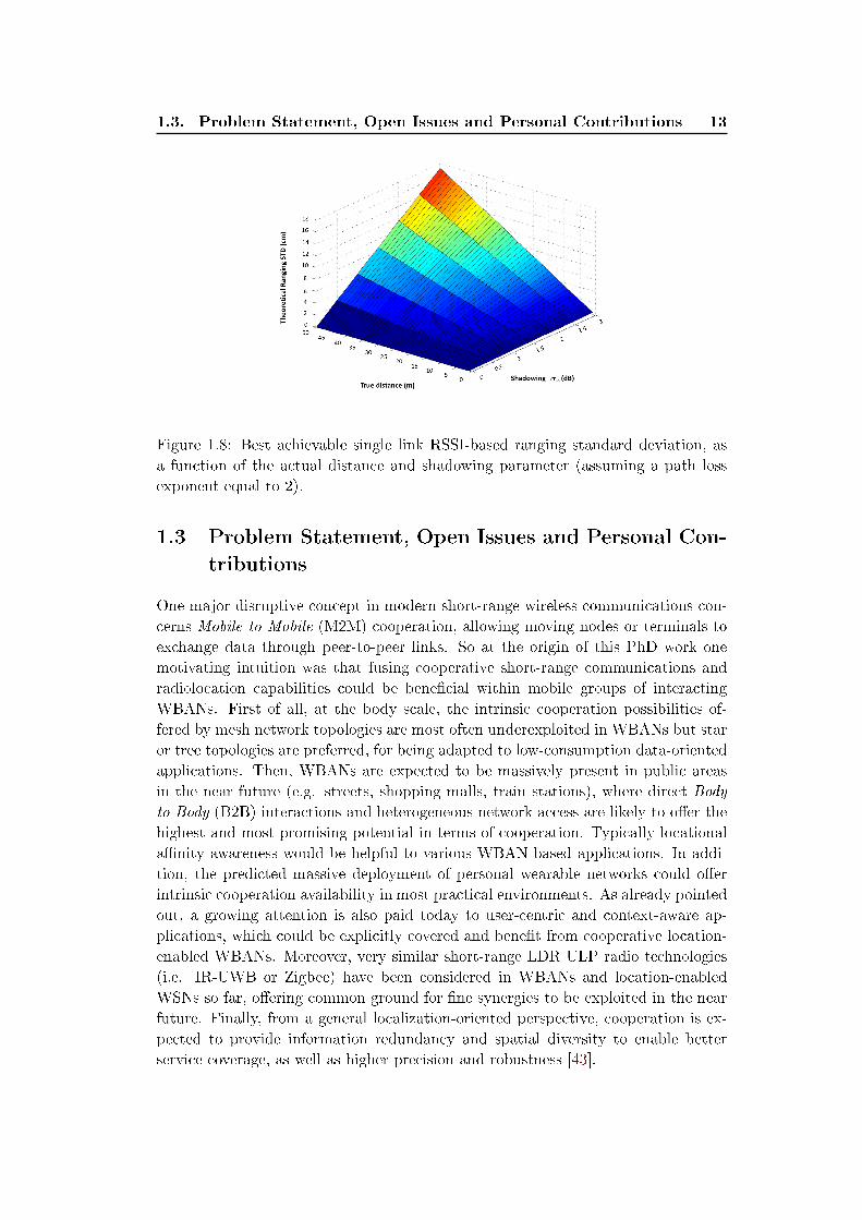
distances to be measured (say, on the order of one meter). Figure 1.8 shows the
variations of this best achievable single-link RSSI-based ranging standard deviation,
as a function of both the actual distance and the shadowing standard deviation,
while assuming a path loss exponent equal to np = 2 for simpli�cation. Hence,
for a given σsh = 2, the lower standard deviation is about 23.03 cm at d = 1 m.
This range of inaccuracy can strongly damage the on-body ranging functionality,
making it hardly compliant (not to say, most likely irrelevant) with MoCap appli-
cations. However, note that RSSI shall still be useful in this on-body context, as
an indirect source of information (e.g. for mitigating ambiguities), but it would be
mostly meaningful over larger-range o�-body and body-to-body links and in case of
relatively low shadowing standard deviation (i.e. in comparison with the path loss
exponent).
The previous trends have also been con�rmed in [36] with joint UWB and N-B ex-
perimentations conducted in a realistic indoor environment (i.e. including typically
radio obstructions and dense multipath) and in a health monitoring context based
on medical WBAN. On this occasion, the ranging performances of both the IEEE
802.15.4 and the IEEE 802.15.4a standards are benchmarked, based respectively on
RT-TOF measurements using integrated UWB prototypes and RSSI measurements
using commercially available standard-compliant components at 2.4GHz.
One way to improve signi�cantly the performance of wireless localization systems
(especially in case of generalized radio obstructions and/or poor geometric dilution
of precision) is to rely on hybrid solutions. For instance, in MoCap applications
or less marginally for navigation applications, inertial measurements have already
been considered on top of IR-UWB TOA in [37], [38], speci�c optimization-based
combinations of TOA in [39], IR-UWB TDOA and AOA in [40] and [41], or even
N-B RSSI �ngerprints in [42]. Nevertheless, those solutions impose the use of too
speci�c settings, system architectures, and fusion strategies. They can not either
comply with a generic and opportunistic WBAN usage, since such wearable networks
do not necessarily include IMUs as on-body sensors depending on the underlying
application. Finally, they are expected to be more expensive and to su�er from
much higher complexity and higher energy consumption.
1.3. Problem Statement, Open Issues and Personal Contributions 13
Figure 1.8: Best achievable single link RSSI-based ranging standard deviation, as
a function of the actual distance and shadowing parameter (assuming a path loss
exponent equal to 2).
1.3 Problem Statement, Open Issues and Personal Con-
tributions
One major disruptive concept in modern short-range wireless communications con-
cerns Mobile to Mobile (M2M) cooperation, allowing moving nodes or terminals to
exchange data through peer-to-peer links. So at the origin of this PhD work one
motivating intuition was that fusing cooperative short-range communications and
radiolocation capabilities could be bene�cial within mobile groups of interacting
WBANs. First of all, at the body scale, the intrinsic cooperation possibilities of-
fered by mesh network topologies are most often underexploited in WBANs but star
or tree topologies are preferred, for being adapted to low-consumption data-oriented
applications. Then, WBANs are expected to be massively present in public areas
in the near future (e.g. streets, shopping malls, train stations), where direct Body
to Body (B2B) interactions and heterogeneous network access are likely to o�er the
highest and most promising potential in terms of cooperation. Typically locational
a�nity awareness would be helpful to various WBAN-based applications. In addi-
tion, the predicted massive deployment of personal wearable networks could o�er
intrinsic cooperation availability in most practical environments. As already pointed
out, a growing attention is also paid today to user-centric and context-aware ap-
plications, which could be explicitly covered and bene�t from cooperative location-
enabled WBANs. Moreover, very similar short-range LDR ULP radio technologies
(i.e. IR-UWB or Zigbee) have been considered in WBANs and location-enabled
WSNs so far, o�ering common ground for �ne synergies to be exploited in the near
future. Finally, from a general localization-oriented perspective, cooperation is ex-
pected to provide information redundancy and spatial diversity to enable better
service coverage, as well as higher precision and robustness [43].
14 Chapter 1. General Introduction
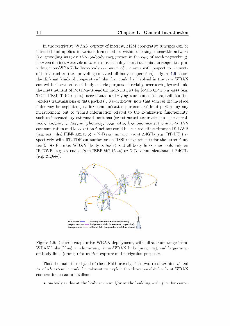
In the restrictive WBAN context of interest, M2M cooperative schemes can be
intended and applied in various forms: either within one single wearable network
(i.e. providing intra-WBAN/on-body cooperation in the case of mesh networking),
between distinct wearable networks at reasonably short transmission range (i.e. pro-
viding inter-WBAN/body-to-body cooperation), or even with respect to elements
of infrastructure (i.e. providing so-called o�-body cooperation). Figure 1.9 shows
the di�erent kinds of cooperative links that could be involved in the very WBAN
context for location-based body-centric purposes. Trivially, over each physical link,
the measurement of location-dependent radio metrics for localization purposes (e.g.
TOF, RSSI, TDOA, etc.) necessitates underlying communication capabilities (i.e.
wireless transmissions of data packets). Nevertheless, note that some of the involved
links may be exploited just for communication purposes, without performing any
measurement but to transit information related to the localization functionality,
such as intermediary estimated positions (or estimated accuracies) in a decentral-
ized embodiment. Assuming heterogeneous network embodiments, the intra-WBAN
communication and localization functions could be ensured either through IR-UWB
(e.g. extended IEEE 802.15.6) or N-B communications at 2.4GHz (e.g. BT-LE) (re-
spectively with RT-TOF estimation or on RSSI measurements for the latter func-
tion). As for inter-WBAN (body-to-body) and o�-body links, one could rely on
IR-UWB (e.g. extended from IEEE 802.15.4a) or N-B communications at 2.4GHz
(e.g. Zigbee).
Figure 1.9: Generic cooperative WBAN deployment, with ultra short-range intra-
WBAN links (blue), medium-range inter-WBAN links (magenta), and large-range
o�-body links (orange) for motion capture and navigation purposes.
Thus the main initial goal of these PhD investigations was to determine if and
to which extent it could be relevant to exploit the three possible levels of WBAN
cooperation so as to localize:
• on-body nodes at the body scale and/or at the building scale (i.e. for coarse
1.3. Problem Statement, Open Issues and Personal Contributions 15
individual MoCap applications);
• carrying bodies belonging to a group at the building scale (i.e. for coordinated
group navigation applications).
Regarding large-scale individual motion capture (LSIMC) needs, both relative or
absolute on-body nodes positioning can be performed, depending on the targeted
use cases.
For relative positioning, we consider a set of wireless devices placed on a body, which
can be classi�ed into two categories. Simple mobile (or blind) nodes with unknown
positions (under arbitrary deployment) must be located relatively to reference an-
chor nodes, which are attached onto the body at known and reproducible positions,
independently of the body attitude and/or direction (e.g. on the chest or on the
back). A set of such anchors can thus de�ne a Cartesian Local Coordinates System
(LCS), which remains time-invariant (i.e. when expressed in the LCS) under body
mobility. The estimated coordinates of the mobile nodes are then expressed into
this LCS. This functionality is also occasionally depicted as Nodes positioning at the
body scale. Possible use cases concern e.g., WBAN optimization through distance-
based packet routing, WBAN self-calibration, raw gesture or posture detection for
animation (e.g. gaming, augmented reality, video post-production), emergency and
rescue alerts (e.g. elderly people or �re�ghters falling down on the �oor), coarse
attitude/body-based remote sensing (e.g. house automation, remote multimedia
browsing and control).
As for absolute on-body nodes positioning, the considered scenario is the same as
the relative one, but the coordinates system used to express the estimated on-body
mobile nodes locations is no more body-strapped but external to the body. In
this framework, one may thus consider as anchor nodes, some �xed elements of
infrastructure (e.g. beacons/landmarks, base stations, access points or gateways)
disseminated at known locations in the environment. Accordingly, the coordinates
of the nodes placed on the body chest or back, which used to be time-invariant in
their LCS, shall now vary in a Global Coordinates System (GCS) under pedestrian
mobility. They directly depend on the body attitude, as well as on the motion di-
rection and/or speed. This sub-scenario may be viewed as a combination of relative
motion capture (i.e. at the body scale) and classical single-user navigation capabili-
ties. Finally, de�ning the on-body nodes locations into a LCS may be still required
here, as an intermediary step of the calculations. Possible use cases concern on-�eld
sports gesture live capture and analysis, physical activity monitoring at home for
non-intrusive and long-term physical rehabilitation or diet assistance.
Like in the LSIMC case, concerning Coordinated Group Navigation (CGN), both
absolute and relative positioning are theoretically possible, although the latter is
seen as less relevant.
For relative positioning, people wearing several on-body wireless sensors and form-
ing a group of mobile users must uniquely localize themselves with respect to their
mates. The inter-body range information is required, that is to say, only the rela-
tive group topology, independently of the actual locations (and orientations) in the
16 Chapter 1. General Introduction
room or in a building. Accordingly, no external anchor nodes would be required
in this embodiment. Possible use cases concern the relative deployment of soldiers
or �re-�ghters, people �nding in nomadic social networks, proximity detection or
collision avoidance in con�ned, blind or dangerous environments (e.g. for security,
collective gaming).
Finally, the absolute positioning of moving bodies forming a group is intended in
a more classical pedestrian navigation sense, where one must retrieve the absolute
coordinates of several users belonging to the same mobile collective entity, with re-
spect to an external GCS. This shall imply the use of �xed and known elements
of infrastructure around. In comparison with other State-of-the-Art navigation so-
lutions, the presence of multiple wearable on-body nodes (i.e. in the WBAN con-
text) is expected to enhance navigation performance by providing spatial diversity
and measurements redundancy (i.e. over o�-body links with respect to the infras-
tructure and/or over inter-WBAN/body-to-body links with respect to other mobile
neighbours), and possibly, further cooperative on-body information exchanges (i.e.
through intra-WBAN links). Without loss of generality, this navigation-oriented
scenario will aim at retrieving mostly the macroscopic positions of the bodies, but
not the on-body nodes' locations in details. Hence, a reference point on the body
shall be chosen to account for this average position (e.g. the geometric center of the
body torso or the barycenter of all the on-body nodes). Possible use cases concern
the absolute deployment of soldiers or �re-�ghters in a given building, the analy-
sis of social mobility patterns and habits in commercial centers, enhanced and/or
augmented personal pedestrian navigation capabilities.
One a priori constraint imposed deliberately to our study is to rely uniquely on
transmitted radio signals that would be anyway present in data-oriented WBAN
contexts, that is to say, with no additional embedded sensors. One more originality
of this work lies in the de�nition of positioning and tracking algorithms that could
be operating:
• in an opportunistic, stand-alone and energy-friendly mode for daily-life and
perennial usage;
• with no or limited geographic restrictions for a truly seamless and large-scale
service coverage (i.e. contrarily to video systems in MoCap and/or GPS in
navigation);
• with limited access to costly elements of infrastructure;
• with reasonably degraded precision in comparison with more accurate tech-
nologies (i.e. as a tolerated drawback).
The block diagram represented in Figure 1.10 shows a generic wireless localiza-
tion scheme adapted to our WBAN context, where one can easily see the critical
impact of both the dynamic propagation channel (i.e. under body mobility) and the
protocol strategy (e.g. in terms of scheduling, response delays...) on the quality and
availability of single-link measurements and in turn, on localization performance.
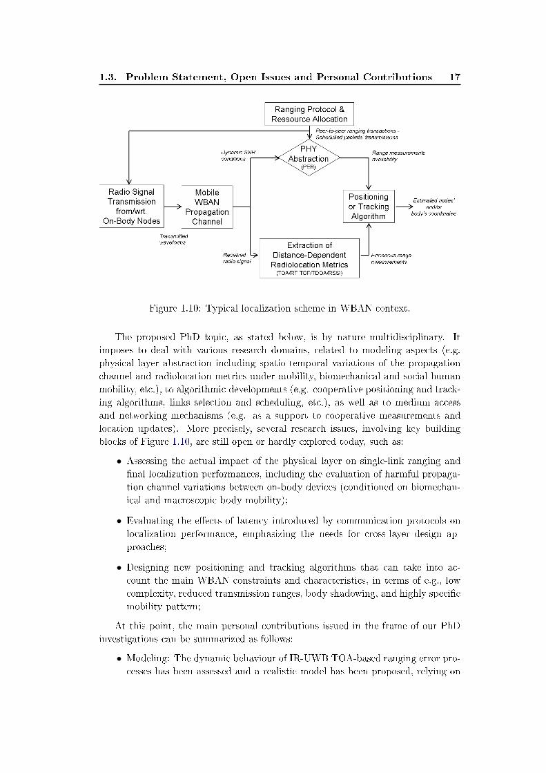
1.3. Problem Statement, Open Issues and Personal Contributions 17
Figure 1.10: Typical localization scheme in WBAN context.
The proposed PhD topic, as stated below, is by nature multidisciplinary. It
imposes to deal with various research domains, related to modeling aspects (e.g.
physical layer abstraction including spatio-temporal variations of the propagation
channel and radiolocation metrics under mobility, biomechanical and social human
mobility, etc.), to algorithmic developments (e.g. cooperative positioning and track-
ing algorithms, links selection and scheduling, etc.), as well as to medium access
and networking mechanisms (e.g. as a support to cooperative measurements and
location updates). More precisely, several research issues, involving key building
blocks of Figure 1.10, are still open or hardly explored today, such as:
• Assessing the actual impact of the physical layer on single-link ranging and
�nal localization performances, including the evaluation of harmful propaga-
tion channel variations between on-body devices (conditioned on biomechan-
ical and macroscopic body mobility);
• Evaluating the e�ects of latency introduced by communication protocols on
localization performance, emphasizing the needs for cross-layer design ap-
proaches;
• Designing new positioning and tracking algorithms that can take into ac-
count the main WBAN constraints and characteristics, in terms of e.g., low
complexity, reduced transmission ranges, body shadowing, and highly speci�c
mobility pattern;
At this point, the main personal contributions issued in the frame of our PhD
investigations can be summarized as follows:
• Modeling: The dynamic behaviour of IR-UWB TOA-based ranging error pro-
cesses has been assessed and a realistic model has been proposed, relying on
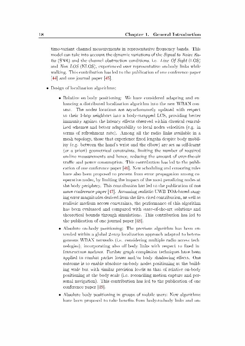
18 Chapter 1. General Introduction
time-variant channel measurements in representative frequency bands. This
model can take into account the dynamic variations of the Signal to Noise Ra-
tio (SNR) and the channel obstruction conditions, i.e. Line Of Sight (LOS)
and Non LOS (NLOS), experienced over representative on-body links while
walking. This contribution has led to the publication of one conference paper
[44] and one journal paper [45].
• Design of localization algorithms:
• Relative on-body positioning: We have considered adapting and en-
hancing a distributed localization algorithm into the new WBAN con-
text. The nodes locations are asynchronously updated with respect
to their 1-hop neighbors into a body-strapped LCS, providing better
immunity against the latency e�ects observed within classical central-
ized schemes and better adaptability to local nodes velocities (e.g. in
terms of refreshment rate). Among all the radio links available in a
mesh topology, those that experience �xed lengths despite body mobil-
ity (e.g. between the hand's wrist and the elbow) are set as self-learnt
(or a priori) geometrical constraints, limiting the number of required
on-line measurements and hence, reducing the amount of over-the-air
tra�c and power consumption. This contribution has led to the publi-
cation of one conference paper [46]. New scheduling and censoring rules
have also been proposed to prevent from error propagation among co-
operative nodes, by limiting the impact of the most penalizing nodes at
the body periphery. This contribution has led to the publication of one
more conference paper [47]. Assuming realistic UWB TOA-based rang-
ing error magnitudes derived from the �rst cited contribution, as well as
realistic medium access constraints, the performance of this algorithm
has been evaluated and compared with state-of-the-art solutions and
theoretical bounds through simulations. This contribution has led to
the publication of one journal paper [48].
• Absolute on-body positioning: The previous algorithm has been ex-
tended within a global 2-step localization approach adapted to hetero-
geneous WBAN networks (i.e. considering multiple radio access tech-
nologies), incorporating also o�-body links with respect to �xed in-
frastructure anchors. Further graph completion techniques have been
applied to combat packet losses and/or body shadowing e�ects. One
outcome is to enable absolute on-body nodes positioning at the build-
ing scale but with similar precision levels as that of relative on-body
positioning at the body scale (i.e. reconciling motion capture and per-
sonal navigation). This contribution has led to the publication of one
conference paper [49].
• Absolute body positioning in groups of mobile users: New algorithms
have been proposed to take bene�ts from body-to-body links and on-
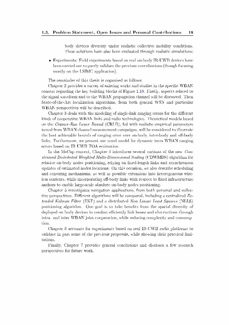
1.3. Problem Statement, Open Issues and Personal Contributions 19
body devices diversity under realistic collective mobility conditions.
These solutions have also been evaluated through realistic simulations;
• Experiments: Field experiments based on real on-body IR-UWB devices have
been carried out to partly validate the previous contributions (though focusing
mostly on the LSIMC application).
The remainder of this thesis is organized as follows.
Chapter 2 provides a survey of existing works and studies in the speci�c WBAN
context regarding the key building blocks of Figure 1.10. Firstly, aspects related to
the signal waveform and to the WBAN propagation channel will be discussed. Then
State-of-the-Art localization algorithms, from both general WSN and particular
WBAN perspectives will be described.
Chapter 3 deals with the modeling of single-link ranging errors for the di�erent
kinds of cooperative WBAN links and radio technologies. Theoretical models based
on the Cramer-Rao Lower Bound (CRLB), fed with realistic empirical parameters
issued from WBAN channel measurement campaigns, will be considered to illustrate
the best achievable bounds of ranging error over on-body, inter-body and o�-body
links. Furthermore, we present our novel model for dynamic intra-WBAN ranging
errors based on IR-UWB TOA estimation.
In the MoCap context, Chapter 4 introduces several variants of the new Con-
strained Distributed Weighted Multi-Dimensional Scaling (CDWMDS) algorithm for
relative on-body nodes positioning, relying on �xed-length links and asynchronous
updates of estimated nodes locations. On this occasion, we also describe scheduling
and censoring mechanisms, as well as possible extensions into heterogeneous wire-
less contexts, while incorporating o�-body links with respect to �xed infrastructure
anchors to enable large-scale absolute on-body nodes positioning.
Chapter 5 investigates navigation applications, from both personal and collec-
tive perspectives. Di�erent algorithms will be compared, including a centralized Ex-
tended Kalman Filter (EKF) and a distributed Non Linear Least Squares (NLLS)
positioning algorithm. One goal is to take bene�ts from the spatial diversity of
deployed on-body devices to combat e�ciently link losses and obstructions through
intra- and inter-WBAN joint cooperation, while reducing complexity and consump-
tion.
Chapter 6 accounts for experiments based on real IR-UWB radio platforms to
validate in part some of the previous proposals, while showing their practical limi-
tations.
Finally, Chapter 7 provides general conclusions and discloses a few research
perspectives for future work.

Chapter 2
State of the Art in Wireless Body
Area Networks Localization
Contents
2.1 Introduction . . . . . . . . . . . . . . . . . . . . . . . . . . . . 21
2.2 Transmitted Waveforms and Bandplans . . . . . . . . . . . . 21
2.3 Standardized Channel Models . . . . . . . . . . . . . . . . . . 22
2.3.1 IEEE 802.15.6 Models . . . . . . . . . . . . . . . . . . . . . . 23
2.3.2 IEEE 802.15.4a Models . . . . . . . . . . . . . . . . . . . . . 25
2.4 Localization Algorithms and Systems . . . . . . . . . . . . . 26
2.4.1 Taxonomy of Cooperative Localization Algorithms . . . . . . 27
2.4.2 WBAN Localization Systems . . . . . . . . . . . . . . . . . . 35
2.5 Conclusion . . . . . . . . . . . . . . . . . . . . . . . . . . . . . 37
2.1 Introduction
In this chapter, we provide a survey of State-of-the-Art contributions directly re-
lated (or at least relevant) to the radio-based localization problem in the WBAN
context. We will account for these works and studies according to the block dia-
gram already presented in the previous chapter, developing each key building block.
Section 2.2 deals with transmitted waveforms and allocated frequency bandplans.
In Section 2.3, aspects related to the WBAN propagation channel will be discussed
from the radiolocation perspective. Then, Section 2.4 will address positioning and
tracking algorithms i) in a general radiolocation context �rst, hence reminding the
main di�erences between centralized/decentralized, cooperative/non-cooperative,
probabilistic/non-probabilistic approaches, and then ii) focusing on existing algo-
rithmic contributions applied into the speci�c frame of WBAN localization. Finally,
Section 2.5 summarizes the chapter.
2.2 Transmitted Waveforms and Bandplans
In November 2007, the IEEE 802.15 Task Group 6, also known as IEEE 802.15.6,
was formed to standardize WBAN, which were not covered by any existing com-
munication standard yet. The work of this group resulted in February 2012 in
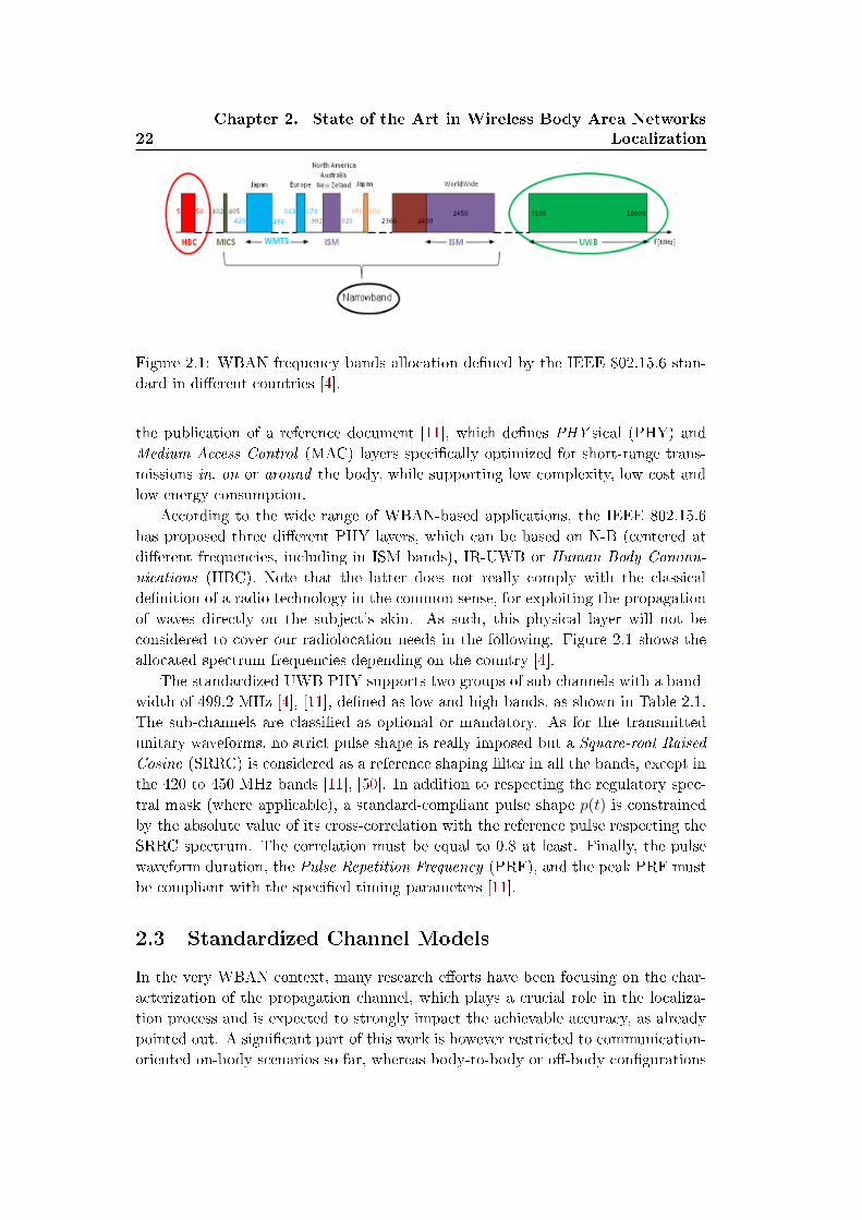
22
Chapter 2. State of the Art in Wireless Body Area Networks
Localization
Figure 2.1: WBAN frequency bands allocation de�ned by the IEEE 802.15.6 stan-
dard in di�erent countries [4].
the publication of a reference document [11], which de�nes PHY sical (PHY) and
Medium Access Control (MAC) layers speci�cally optimized for short-range trans-
missions in, on or around the body, while supporting low complexity, low cost and
low energy consumption.
According to the wide range of WBAN-based applications, the IEEE 802.15.6
has proposed three di�erent PHY layers, which can be based on N-B (centered at
di�erent frequencies, including in ISM bands), IR-UWB or Human Body Commu-
nications (HBC). Note that the latter does not really comply with the classical
de�nition of a radio technology in the common sense, for exploiting the propagation
of waves directly on the subject's skin. As such, this physical layer will not be
considered to cover our radiolocation needs in the following. Figure 2.1 shows the
allocated spectrum frequencies depending on the country [4].
The standardized UWB PHY supports two groups of sub-channels with a band-
width of 499.2 MHz [4], [11], de�ned as low and high bands, as shown in Table 2.1.
The sub-channels are classi�ed as optional or mandatory. As for the transmitted
unitary waveforms, no strict pulse shape is really imposed but a Square-root Raised
Cosine (SRRC) is considered as a reference shaping �lter in all the bands, except in
the 420 to 450 MHz bands [11], [50]. In addition to respecting the regulatory spec-
tral mask (where applicable), a standard-compliant pulse shape p(t) is constrained
by the absolute value of its cross-correlation with the reference pulse respecting the
SRRC spectrum. The correlation must be equal to 0.8 at least. Finally, the pulse
waveform duration, the Pulse Repetition Frequency (PRF), and the peak PRF must
be compliant with the speci�ed timing parameters [11].
2.3 Standardized Channel Models
In the very WBAN context, many research e�orts have been focusing on the char-
acterization of the propagation channel, which plays a crucial role in the localiza-
tion process and is expected to strongly impact the achievable accuracy, as already
pointed out. A signi�cant part of this work is however restricted to communication-
oriented on-body scenarios so far, whereas body-to-body or o�-body con�gurations
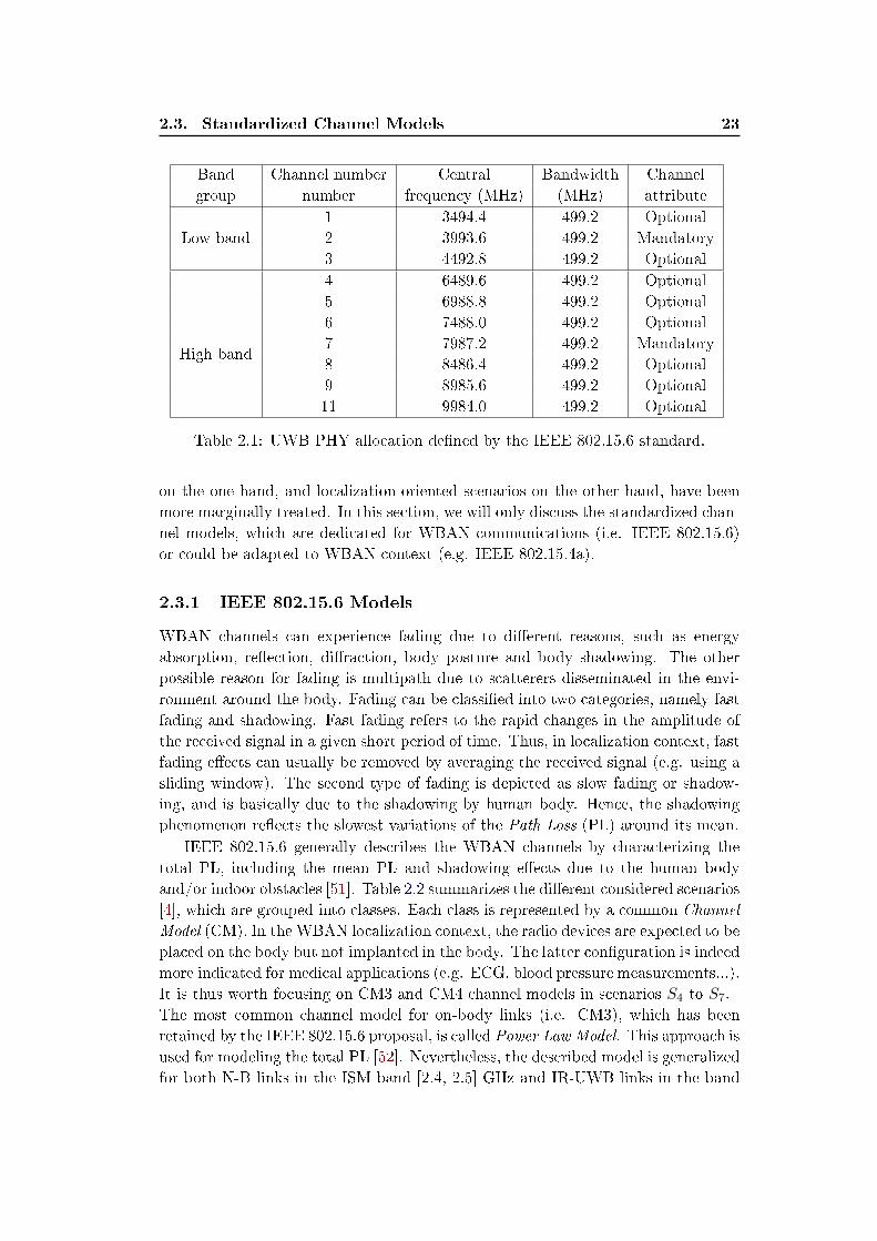
2.3. Standardized Channel Models 23
Band Channel number Central Bandwidth Channel
group number frequency (MHz) (MHz) attribute
Low band
1 3494.4 499.2 Optional
2 3993.6 499.2 Mandatory
3 4492.8 499.2 Optional
High band
4 6489.6 499.2 Optional
5 6988.8 499.2 Optional
6 7488.0 499.2 Optional
7 7987.2 499.2 Mandatory
8 8486.4 499.2 Optional
9 8985.6 499.2 Optional
11 9984.0 499.2 Optional
Table 2.1: UWB PHY allocation de�ned by the IEEE 802.15.6 standard.
on the one hand, and localization-oriented scenarios on the other hand, have been
more marginally treated. In this section, we will only discuss the standardized chan-
nel models, which are dedicated for WBAN communications (i.e. IEEE 802.15.6)
or could be adapted to WBAN context (e.g. IEEE 802.15.4a).
2.3.1 IEEE 802.15.6 Models
WBAN channels can experience fading due to di�erent reasons, such as energy
absorption, re�ection, di�raction, body posture and body shadowing. The other
possible reason for fading is multipath due to scatterers disseminated in the envi-
ronment around the body. Fading can be classi�ed into two categories, namely fast
fading and shadowing. Fast fading refers to the rapid changes in the amplitude of
the received signal in a given short period of time. Thus, in localization context, fast
fading e�ects can usually be removed by averaging the received signal (e.g. using a
sliding window). The second type of fading is depicted as slow fading or shadow-
ing, and is basically due to the shadowing by human body. Hence, the shadowing
phenomenon re�ects the slowest variations of the Path Loss (PL) around its mean.
IEEE 802.15.6 generally describes the WBAN channels by characterizing the
total PL, including the mean PL and shadowing e�ects due to the human body
and/or indoor obstacles [51]. Table 2.2 summarizes the di�erent considered scenarios
[4], which are grouped into classes. Each class is represented by a common Channel
Model (CM). In the WBAN localization context, the radio devices are expected to be
placed on the body but not implanted in the body. The latter con�guration is indeed
more indicated for medical applications (e.g. ECG, blood pressure measurements...).
It is thus worth focusing on CM3 and CM4 channel models in scenarios S4 to S7.
The most common channel model for on-body links (i.e. CM3), which has been
retained by the IEEE 802.15.6 proposal, is called Power Law Model. This approach is
used for modeling the total PL [52]. Nevertheless, the described model is generalized
for both N-B links in the ISM band [2.4, 2.5] GHz and IR-UWB links in the band
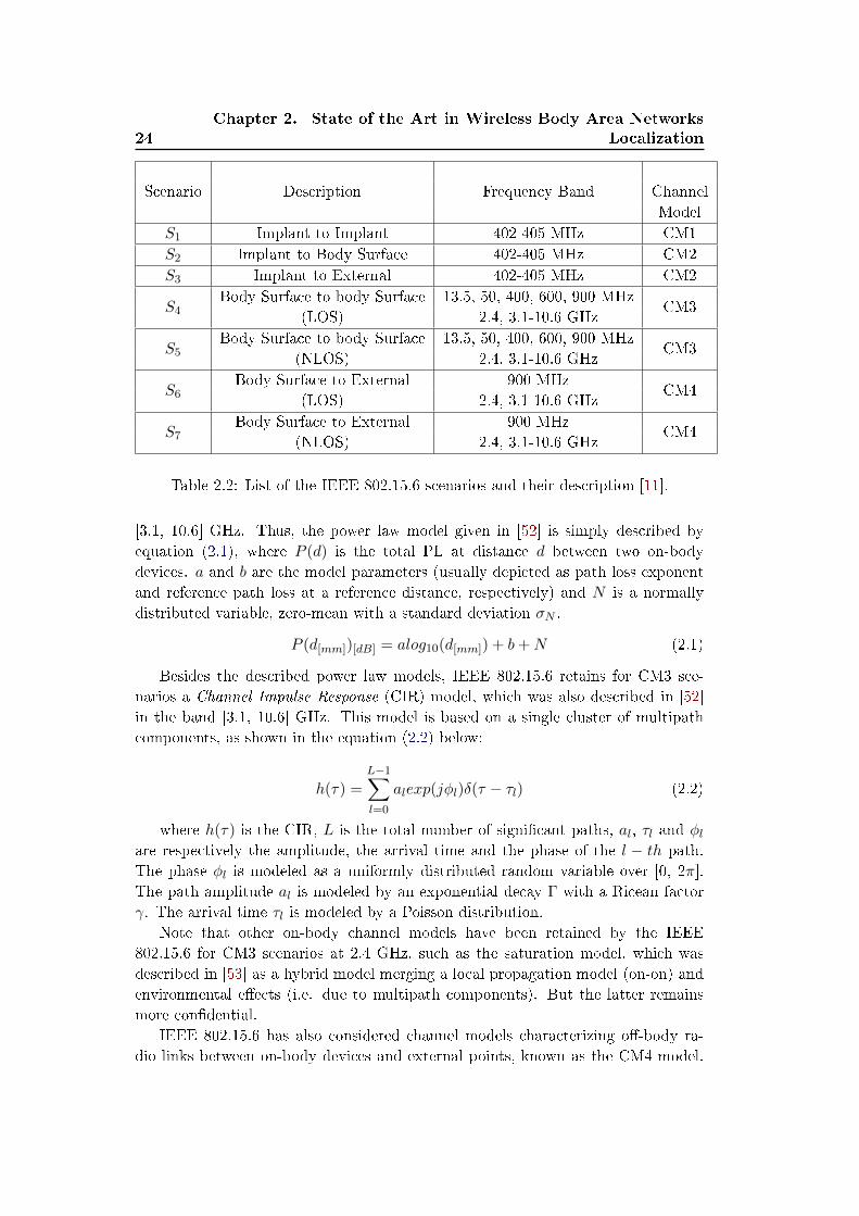
24
Chapter 2. State of the Art in Wireless Body Area Networks
Localization
Scenario Description Frequency Band Channel
Model
S1 Implant to Implant 402-405 MHz CM1
S2 Implant to Body Surface 402-405 MHz CM2
S3 Implant to External 402-405 MHz CM2
S4Body Surface to body Surface 13.5, 50, 400, 600, 900 MHz
CM3(LOS) 2.4, 3.1-10.6 GHz
S5Body Surface to body Surface 13.5, 50, 400, 600, 900 MHz
CM3(NLOS) 2.4, 3.1-10.6 GHz
S6Body Surface to External 900 MHz
CM4(LOS) 2.4, 3.1-10.6 GHz
S7Body Surface to External 900 MHz
CM4(NLOS) 2.4, 3.1-10.6 GHz
Table 2.2: List of the IEEE 802.15.6 scenarios and their description [11].
[3.1, 10.6] GHz. Thus, the power law model given in [52] is simply described by
equation (2.1), where P (d) is the total PL at distance d between two on-body
devices. a and b are the model parameters (usually depicted as path loss exponent
and reference path loss at a reference distance, respectively) and N is a normally
distributed variable, zero-mean with a standard deviation σN .
P (d[mm])[dB] = alog10(d[mm]) + b+N (2.1)
Besides the described power law models, IEEE 802.15.6 retains for CM3 sce-
narios a Channel Impulse Response (CIR) model, which was also described in [52]
in the band [3.1, 10.6] GHz. This model is based on a single cluster of multipath
components, as shown in the equation (2.2) below:
h(τ) =
L−1∑l=0
alexp(jφl)δ(τ − τl) (2.2)
where h(τ) is the CIR, L is the total number of signi�cant paths, al, τl and φlare respectively the amplitude, the arrival time and the phase of the l − th path.
The phase φl is modeled as a uniformly distributed random variable over [0, 2π].
The path amplitude al is modeled by an exponential decay Γ with a Ricean factor
γ. The arrival time τl is modeled by a Poisson distribution.
Note that other on-body channel models have been retained by the IEEE
802.15.6 for CM3 scenarios at 2.4 GHz, such as the saturation model, which was
described in [53] as a hybrid model merging a local propagation model (on-on) and
environmental e�ects (i.e. due to multipath components). But the latter remains
more con�dential.
IEEE 802.15.6 has also considered channel models characterizing o�-body ra-
dio links between on-body devices and external points, known as the CM4 model.
2.3. Standardized Channel Models 25
The normalized received power (i.e. normalized over the maximum value) is rather
modeled by a gamma distribution for standing scenarios, and with a log-normal
distribution for walking scenarios at 2.36 GHz [54]. The described o�-body channel
model also considers characterizing the CIR in the band [3.1, 10.6]GHz. The model
is rather similar to the model described in equation (2.2), but additional ground
e�ects have been considered. Further details on the related measurement set-up
and data analysis can be found in [55].
So far, no model characterizing the body-to-body channels has been standardized
yet. However, various proprietary models have been extracted out of real measure-
ments in some recent works, such as [56], [57], [58] or [13]. All of them have been
focusing on N-B links only.
2.3.2 IEEE 802.15.4a Models
Besides the IEEE 802.15.6 standard, other existing radio standards can ful�ll in
part the new needs of WBANs and localization, though non-explicitly focusing on
WBAN applications and hence, requiring several adaptations at di�erent levels (e.g.
in terms of power consumption, form factor, reliability). Among those standards, the
IEEE 802.15.4a standard can be viewed as an IR-UWB extension of the N-B IEEE
802.15.4 standard [59]. This standard is well known for Wireless Sensor Network
(WSN), and supports peer-to-peer ranging capabilities up to MAC layer. In this
context, some IEEE 802.15.4a channel models could be adapted for characterizing
some WBAN channels, such as o�-body and body-to-body channels. Moreover, the
IEEE 802.15.4a provides a complete description of an on-body channel, which will
be described hereafter.
In [5] an IR-UWB channel model has been characterized for on-body communi-
cations in the band [3, 5]GHz. This model has �nally been extended by the IEEE
802.15.4a standard [60], and declined according to three scenarios depending on the
receiver position (i.e. on the front, the side or the back of the body). Figure 2.2
recalls the three corresponding scenarios. In addition, the mean PL is modeled by
a distance-dependent exponential decay, as shown in equation (2.3) below:
PLdB = γ(d− d0) + PL0,dB (2.3)
where γ = 107dB/m, d is the distance between the transmitter and the receiver
around the perimeter of the body and PL0,dB is the measured PL at the reference
distance d0. Moreover, this model assumes the presence of two clusters of Multi
Path Components (MPC) due to the waves' di�raction around the body and the
re�ection on the ground. The MPC over each cluster are correlated following a
log-normal distribution.
Despite the large number and the variety of the contributions recently issued in
the �eld of WBAN channel characterization and modeling, the available standard-
ized models do not seem totally adapted to our problem, nor uni�ed for a convenient
usage. In our evaluation framework, while assuming single-link radiolocation met-
rics, we will thus either propose brand new localization-oriented models or adapt
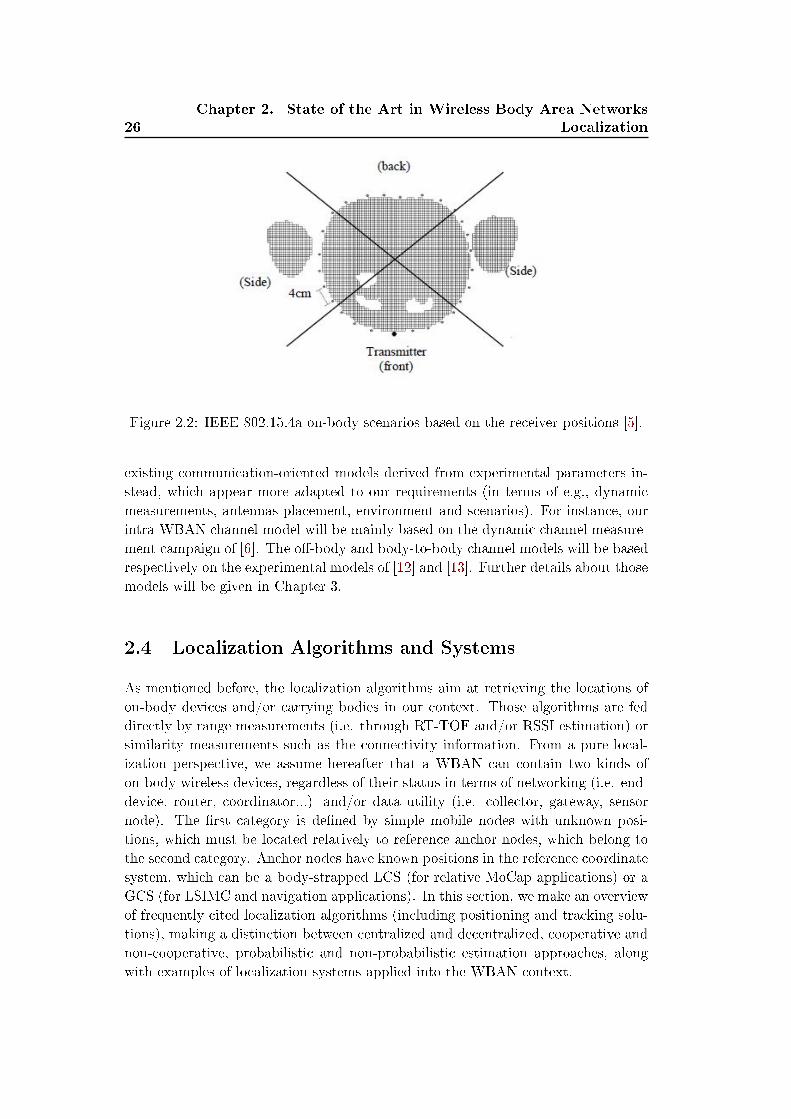
26
Chapter 2. State of the Art in Wireless Body Area Networks
Localization
Figure 2.2: IEEE 802.15.4a on-body scenarios based on the receiver positions [5].
existing communication-oriented models derived from experimental parameters in-
stead, which appear more adapted to our requirements (in terms of e.g., dynamic
measurements, antennas placement, environment and scenarios). For instance, our
intra-WBAN channel model will be mainly based on the dynamic channel measure-
ment campaign of [6]. The o�-body and body-to-body channel models will be based
respectively on the experimental models of [12] and [13]. Further details about those
models will be given in Chapter 3.
2.4 Localization Algorithms and Systems
As mentioned before, the localization algorithms aim at retrieving the locations of
on-body devices and/or carrying bodies in our context. Those algorithms are fed
directly by range measurements (i.e. through RT-TOF and/or RSSI estimation) or
similarity measurements such as the connectivity information. From a pure local-
ization perspective, we assume hereafter that a WBAN can contain two kinds of
on-body wireless devices, regardless of their status in terms of networking (i.e. end-
device, router, coordinator...) and/or data utility (i.e. collector, gateway, sensor
node). The �rst category is de�ned by simple mobile nodes with unknown posi-
tions, which must be located relatively to reference anchor nodes, which belong to
the second category. Anchor nodes have known positions in the reference coordinate
system, which can be a body-strapped LCS (for relative MoCap applications) or a
GCS (for LSIMC and navigation applications). In this section, we make an overview
of frequently cited localization algorithms (including positioning and tracking solu-
tions), making a distinction between centralized and decentralized, cooperative and
non-cooperative, probabilistic and non-probabilistic estimation approaches, along
with examples of localization systems applied into the WBAN context.
2.4. Localization Algorithms and Systems 27
2.4.1 Taxonomy of Cooperative Localization Algorithms
2.4.1.1 Centralized vs. Distributed
Centralized localization approaches consist in collecting all the radiolocation mea-
surements in one single computation center and to proceed with the estimation of
all the blind nodes' coordinates simultaneously. From that perspective, central-
ized approaches are most often seen as fully centralized. Blind nodes can be both
mobile or static nodes with unknown locations. Advantageously, in a body-centric
approach, this computation center could be the WBAN coordinator or on-body
gateway, which is usually endowed with more powerful embedded resources (i.e. in
terms of energy/battery, memory and computational skills) than simple devices.
But the calculi can also be externalized (e.g. hosted in a server) after relaying the
measurement data to the centralized infrastructure through o�-body links. There,
the measurements are jointly processed and the positions for all nodes in the WBAN
are simultaneously determined. Afterwards, the information can be exploited in the
WBAN or sent back to any mobile node. In this approach, accuracy is expected
to be optimal. However, one major drawback is the need for such on-body central
nodes with computational skills and better energy autonomy, what is rather unlikely
and demanding in the WBAN context. Another problem within such centralized
approaches is the latency e�ect (i.e. the time elapsed between the collection of the
required distance measurements and the �nal delivery of all the positions estimates,
possibly while experiencing packet losses), whereas the body gesture and location
can change rapidly during the collection step. Hence, to overcome the previous prob-
lems, decentralized approaches can be favored instead, although their convergence
time may be also problematic.
Such distributed solutions allow each mobile node to localize itself by receiving
information from its neighbors (i.e. anchors and/or mobile nodes). Hence, complex-
ity is also distributed among the mobile nodes in comparison with the centralized
approach, and the latency e�ect described above (i.e. mostly due to the collection
of measurements) can be reduced, provided that the decentralized algorithms does
not necessitate too many iterations to converge properly. In fact, distributed ap-
proaches can bene�t from intrinsic asynchronism (i.e. updating the nodes positions
with di�erent refreshment rates) while localizing the mobile nodes. Accordingly the
positions of the most demanding nodes (e.g. with higher velocity) can be updated
at higher refreshment rates.
In the WBAN context, some centralized algorithms have been considered in
[2], [8], [61], [62], [63]. For both MoCap and navigation purposes, [8] has used
the Non Linear Least Squares (NLLS) algorithm, which consists in minimizing a
global quadratic cost function using the Gradient descent method incorporating
both on-body and o�-body range measurements. [2] and [61] adapt a centralized
classical Multidimensional Scaling (MDS) for on-body MoCap applications and pose
estimation. In [61], the authors introduce additional constraints relying on the prior
knowledge of minimal and maximal feasible distances related to the body dimensions
(and thus some kinds of geographical limitations). In [62] the centralized Maximum
28
Chapter 2. State of the Art in Wireless Body Area Networks
Localization
Likelihood estimator has been considered, introducing other constraints relying on
the actual positions of on-body mobile nodes. However, [8] has also used a variant
of the Linear Least Square (LLS) algorithm, which is somehow decentralized (even
if the term may be debatable) in the sense that blind nodes compute their own
location locally, based primarily on available external anchors or in case of limited
connectivity to external points, based on already positioned on-body devices.
2.4.1.2 Cooperative vs. Non Cooperative
Localization schemes can also be classi�ed into cooperative and non-cooperative cat-
egories. Non-cooperative approaches aim at localizing on-body nodes based on peer-
to-peer range measurements with respect to anchors only [62], [63], [64]. But the
number of anchors (either on-body for the relative Mocap applications, or belonging
to the external infrastructure for the LSIMC and the navigation applications) in the
WBAN context is likely small. One solution to compensate too frequent disconnec-
tion and/or erroneous measurements with respect to those anchors then consists in
allowing peer-to-peer cooperation among mobile nodes. In our WBAN terminology
herein, the term cooperative can refer to two concrete embodiments (possibly im-
plemented simultaneously). On the one hand, intra-WBAN cooperation consists in
exploiting not only radiolocation measurements between blind on-body devices to
be located (either static or mobile) and anchors (either on-body or belonging to the
external infrastructure), but also communication links and/or radiolocation mea-
surements between blind devices. In this case, the latter belong necessarily to the
same WBAN [8], [61]. On the other hand, inter-WBAN cooperation consists in ex-
ploiting radiolocation measurements and/or communication links between on-body
devices that belong to distinct WBAN and bodies, thus exploiting body-to-body
links.
Cooperative approaches can take bene�ts from mesh topologies. But one draw-
back lies in the extra over-the-air tra�c and most often, in their higher complex-
ity, e.g., in terms of synchronization requirements, coordination and/or scheduling
needs, neighborhood discovery and maintenance under mobility. Hence, those two
factors (i.e. complexity and tra�c) represent two research topics that are worth be-
ing investigated to enhance the performance of cooperative localization in WBAN.
A very preliminary comparison between cooperative and and non-cooperative local-
ization schemes in the speci�c context of WBAN has been proposed in [8], showing
that the achieved localization accuracy is better, but the energy consumption and
the over-the-air tra�c (e.g. in terms of the average number of requested superframes
for localizing all the blind nodes in the WBAN) is higher in cooperative schemes
than in non-cooperative schemes.
2.4.1.3 Location Estimators
Consider a WBAN of size m + n nodes, where n is the number of mobile nodes to
be located, and m is the number of anchors with known positions. In the following,
2.4. Localization Algorithms and Systems 29
θt = [X1(t), ... , Xn(t)] is the vector of unknown d-Dimensional (d-D) (i.e. d=2 or
3) coordinates at time t and [Xn+1(t) = Xn+1, ... , Xn+m(t) = Xn+m] is a vector
of known and time-invariant positions of anchors. In our context, note that the
nodes positions can be de�ned either in the body-strapped LCS (e.g. for relative
MoCap) or in a GCS (e.g. for LSIMC and navigation). The pair-wise radiolocation
measurement performed at time t between two devices i and j is depicted by yij(t),
which can be either a scalar value (i.e. TOA, TDOA, TOF, RSSI) or a vector
such as the CIR in rarer localization approaches. Moreover, we consider that the
corresponding observed (erroneous) distance dij(t) can be obtained according to
dij(t) = f(yij(t)), whereas the true and estimated distances between the two devices
at time t are respectively given by dij(t) =√
((Xi(t)−Xj(t))T (Xi(t)−Xj(t)) and
dij(t) =√
((Xi(t)− Xj(t))T (Xi(t)− Xj(t)). Finally d(t) is the vector containing
all the available distances dij(t) at time t
Weighted Least Squares Positioning TheWeighted Least Squares (WLS) algo-
rithm is a non-probabilistic estimator, which does not necessitate prior information
about the distribution of estimated positions. In a cooperative localization context,
the idea is to �nd the latter positions by minimizing a global cost function that incor-
porates quadratic errors between all the pair-wise measurements and their estimates
(conditioned on the current value of the estimated coordinates, set as optimization
variables). In a symetric and/or unidirectional case (i.e. assuming uniquely one
available measurement per pair-wise link), the cost function is as follows:
θt = argminθt
S(θt) (2.4)
where
S(θt) = [∑
1≤i≤n[∑
i≤j≤n+mwij(t)(dij(t)− dij(t))2 + ri(t)||Xi(t)−Xi(t)||2]] (2.5)
where dij(t) denotes the Euclidean distance between nodes i and j, wij(t) is a weight
value, which re�ects the connectivity and the accuracy of the range measurement
between nodes i and j at time t, Xi(t) is a vector with prior information about the
position occupied by node i at time t, while ri(t) quanti�es the reliability of this
prior information. If there is no prior information, then ri(t) = 0, and the WLS cost
function is similar to that of a blind classical NLLS cost function.
The choice of the weights should re�ect the accuracy of the involved observations
and unreliable measurements shall be down-weighted in the cost function. Several
strategies have been adopted for the selection of wij(t) such as exponential decreas-
ing with the measured distance in [65], when the measurement noise variance is
not available. Whenever a model is available, assuming for instance that measure-
ment noise is a Gaussian distributed random process with known standard deviation
σij(t) (e.g. increasing linearly with the true distances in a parametric description
σij(t) = c1dij(t)+c2), then wij(t) can be simply chosen as1
σij(t)(and thus 1
c1dij(t)+c2
or even 1
c1dij(t−1)+c2based on the current measurements or latest estimates) [66].
30
Chapter 2. State of the Art in Wireless Body Area Networks
Localization
This WLS estimator is not (or at least only partly) parametric and thus it is
still very popular in a wide range of localization problems, including in the WBAN
context. One notorious limitation however is that the optimization problem in (2.5)
is non-convex for practical cooperative con�gurations. Accordingly, the solution
can get stuck in a local minimum depending on the starting point and hence, a
relevant global solution may never be reached. A minimum of S(θt) can be computed
using iterative numerical methods initialized at a starting position. Among these
methods, one can cite the Gradient Descent, the Levenberg-Marquardt algorithm
and Scaling by MAjorizing a COnvex Function (SMACOF) [65], [67]. Furthermore,
the partial derivatives of S(θt) with respect to Xi(t) depends only on the neighbors
coordinates and thus, a local cost function can be de�ned at each node, where a local
minimization can be performed. Hence, distributed iterative optimization solutions
have been adopted such as the Distributed Weighted Least-Squares (DWLS) in [68]
or the Distributed Weighted Multi-Dimensional Scaling (DWMDS) in [65], which
implements a more advanced distributed version of SMACOF preventing from the
increase of the cost function at each iteration. The idea still consists for each node
in localizing itself, by minimizing the following cost function:
Xi(t) = argminXi(t)
Si(t) (2.6)
where
Si(t) =n∑
j=1,j 6=iwij(t)(dij(t)− dij(Xi(t), Xj(t)))
2
+
n+m∑j=n+1
2wij(t)(dij(t)− dij(Xi(t), Xj(t)))2 (2.7)
+ri(t)||Xi(t)−Xi(t)||2
In our work, we will adapt this DWMDS algorithm for WBAN localization
purposes. More details will be given in Chapter 4.
Probabilistic Estimators In the localization context, a probabilistic estimator
consists in locating the mobile nodes based on probabilistic assumptions. The latter
can be based on a priori statistical models for the observed measurements condi-
tioned on the mobile positions, like in likelihood functions. These functions can be
not only conditioned on positions but also e.g., on the radio obstruction conditions
over each link (i.e. LOS/NLOS), like in [69] or [70]. But other approaches can be
based also on prior statistical information regarding the occupied positions by the
mobile nodes them-selves. Accordingly, these algorithms are usually more accurate
than simple non-probabilistic estimators like WLS. The probabilistic estimators can
be classi�ed into two categories, namely Bayesian and Non-Bayesian approaches.
Non-Bayesian estimators assume that the mobile positions are treated as unknown
deterministic parameters whereas mobile positions are de�ned as random variables
with known prior distributions in Bayesian estimators.
2.4. Localization Algorithms and Systems 31
Non-Bayesian Positioning In the Non-Bayesian context, positions are
treated as unknown deterministic parameters. One common Non-Bayesian esti-
mator is the Maximum Likelihood (ML) estimator, which operates by maximizing
the likelihood function:
θMLt = argmax
θt
p(y(t)|θt) (2.8)
where the likelihood function p(y(t)|θt) denotes the probability density function (pdf)
of the observation y(t) conditioned upon the variable of interest θt.
It is known from estimation theory [71] that the ML estimator is unbiased and
consistent, i.e. converges asymptotically to the Cramer Rao Lower Bound (CRLB)
at low measurement error variances.
If we assume that the distance observations given by dij(t) = f(yij(t)) provide
su�cient statistics for the estimation of θ and that dij are independent, then the
ML estimator is given by:
θMLt = argmax
θt
p(d(t)|θt) = argmaxθt
∏i
∏j
p(dij(t)|θt) (2.9)
The distance observations are obviously a�ected by ranging errors, which are
most often represented as additive random variables dij(t) = dij(t) + eij(t). In
special cases when the ranging errors are considered as Gaussian identically inde-
pendent distributed (i.i.d.) random variables, the ML estimator simply leads to the
WLS estimator, which equivalently Maximizes the Log-Likelihood (MLL) function,
as follows:
θMLLt = argmax log
θt
(p(d(t)|θt)) = argmaxθt
∑i
∑j
log(p(dij(t)|θt)) (2.10)
One advantage usually put forward with M(L)L is that it can stick with arbi-
trarily complex measurement error behaviours, including multimodal regimes, or
highly speci�c distributions. The counterpart is that the estimator is strongly para-
metric (i.e. with model parameters that necessitate prior calibration) and the un-
derlying optimization problem is even more complex to solve out and sensitive to
initial guesses than in the WLS case, thus making its application rather challenging
in generic WBAN contexts (i.e. regardless of the environment) and under strin-
gent low complexity constraints. Nevertheless, the ML algorithm has already been
considered for on-body localization in a non-cooperative context in [62], but with
rather simpli�ed assumptions regarding the range measurements and with further
constraints on network deployment.
Bayesian Positioning and Tracking In the Bayesian context, the positions
occupied by the mobile nodes are considered as random variables. A Bayesian
estimator thus considers estimating the a posteriori probability distribution from a
32
Chapter 2. State of the Art in Wireless Body Area Networks
Localization
known a priori distribution of the occupied positions. The general Bayes' formula
is given as follows:
p(θt|yt) =p(yt|θt)p(θt)
p(yt)=Likelihood×A priori
Evidence(2.11)
Once the a posteriori distribution is known, the Maximum a posteriori (MAP)
estimator θt maximizes the a posteriori probability distribution [71], as follows:
θMAPt = argmax
θt
p(θt|yt) (2.12)
Another known estimator is the Minimum Mean Squared Error (MMSE) esti-
mator θt, which is calculated as the mean of the a posteriori distribution [71], as
follows:
θMMSEt =
∫θtp(θt|yt)dθt (2.13)
In the dynamic localization context, the nodes positions are somehow correlated
over time. Hence, one can consider tracking �lters, which help to improve localiza-
tion accuracy by exploiting the measurements made at multiple time instants y1:t+1
where the time variable is indexed for simpli�ed notations (i.e. from the past till
the current time step), and thus, by bene�ting also from the spatial consistency
of mobile trajectories. The Bayesian formulation of the tracking �lter conducts to
calculate the a posteriori distribution p(θt+1|y1:t+1) as follows:
p(θt+1|y1:t+1) =p(yt+1|θt+1, y1:t)p(θt+1|y1:t)
p(yt+1|y1:t)(2.14)
Furthermore, the a priori distribution at time t + 1 is calculated from the a
posteriori at time t, using the Chapman-Kolmogorov equation [71]:
p(θt+1|y1:t) =
∫p(θt+1|θt, y1:t)p(θt|y1:t)dθt (2.15)
Thus, the dynamic extensions of the MAP and MMSE estimators are respectively
given by the following equations:
θMAPt+1 = argmax
θt+1
p(θt+1|y1:t+1) (2.16)
θMMSEt+1 =
∫θt+1p(θt+1|y1:t+1)dθt+1 (2.17)
For practicability ans tractability reasons, it is usually assumed that the state
space vector θt to be estimated is issued from a known Markov chain of transi-
tion probability p(θt|θt−1), with a known initial a priori distribution p(θ0). The
observation model is given by:
yt = h(θt) + et (2.18)
2.4. Localization Algorithms and Systems 33
where h is a function relating the observation to the state space vector and et denotes
the observation noise vector, indexing also the time variable to simplify notations.
Assume that the observations are i.i.d. variables at di�erent time instants. Then,
the Chapman-Kolmogorov equation becomes as follows:
p(θt+1|y1:t) =
∫p(θt+1|θt)p(θt|y1:t)dθt (2.19)
If the observations are conditionally independent, then p(yt+1|θt+1, y1:t) =
p(yt+1|θt+1) and the Bayes �lter equation is simpli�ed as follows:
p(θt+1|y1:t+1) =p(yt+1|θt+1)p(θt+1|y1:t)
p(yt+1|y1:t)(2.20)
p(yt+1|y1:t) does not depend on θt+1. Hence, p(yt+1|y1:t) is obtained according to
the following marginalization:
p(yt+1|y1:t) =
∫p(yt+1|θt+1)p(θt+1|y1:t) (2.21)
Once the initial distribution p(θ0) and the transition probability are known (i.e.
in our case, the mobility model), the Bayes �lter computes the a posteriori distri-
bution of θt recursively at any time t. However, due to the non-linearity between
the observation and θt in equation (2.18), equations (2.19) and (2.20) are usually
analytically intractable.
Thus, the particle �lter may be used, which is based on sequential Monte Carlo
methods for approximating numerically the a posteriori densities [72]. In the WSN
localization context, it has been mainly adopted for tracking applications [73], [74],
for instance in vehicular or personal navigation applications. It has been also consid-
ered in the very WBAN context, but still for navigation purposes in indoor environ-
ments [63]. One advantage with the particle �lter is that is can handle non-linear
transitions and arbitrarily complex error densities (on both mobile state and ob-
servation processes). However, for being based on numerical approximations, it is
usually too computationally demanding for low-complexity and real-time applica-
tions like in our WBAN context. It is also highly dependent on the number of used
particles, as well as on speci�c issues like particles cloud degeneracy or impoverish-
ment, which necessitate even more complex mechanisms such as particles resampling
and regularization.
Besides, assuming Gaussian noises and linearized models (i.e. linear state-space
equation and a linear observation model) conducts to the Kalman Filter (KF),
which yields to an tractable solution of the initial Bayesian �lter formulation. But
in typical wireless tracking problems, due to the non-linearity of the function h, the
Extended Kalman Filter (EKF) may be adopted instead, which consists in preserving
the full KF formalism after linearizing locally the incriminated function around the
predicted state. Both KF and EKF are well known and popular in the general
WSN localization context [75], [76], [77], due to their simplicity and practicability
for implementation.
34
Chapter 2. State of the Art in Wireless Body Area Networks
Localization
Overall, as a summary, the particle �lter is a robust Bayesian solution to the
wireless tracking problem in non-linear and non-Gaussian scenarios. But the price
to pay for this �exibility in terms of computational load and energy consumption
tends to prevent from using it in a generic WBAN context. Besides, the complicated
and disparate nature of the body limbs movement during the human motion (i.e.
depending on the on-body node's placement) makes it rather di�cult to maintain
one single state space equation to relay θt+1 and θt, whatever the node. Thus, the
EKF are not really expected to be fully robust and convenient for MoCap applica-
tions. However, they can be more relevant for navigation purposes, where reasonable
assumptions about the macroscopic body movement can be made more easily. More
details about the EKF will be given in Chapter 5, where the individual and group
navigation modes will be investigated.
Graph Inference and Message-Passing Recent research e�orts have been
focusing on iterative, cooperative and decentralized solutions relying on message-
passing, such as Belief propagation (BP) [78], which is one of the well-known graphi-
cal models for inference in statistical physics, arti�cial intelligence, computer vision,
etc. This kind of approaches organizes the global computation of nodes location
beliefs into smaller local computations implying the exchange of packets between
neighbouring mobile nodes. An implicit mapping is thus usually intended between
the physical network topology and a factor-graph representation. Gradual enhance-
ments have been proposed for the last past years in the speci�c WSN cooperative
localization context.
For instance, the Non Parametric Belief Propagation approach (NBP), which
is one famous particle-based approximation of the standard BP has been put for-
ward for non-linear and non-gaussian cases [79]. But one problem with NBP is that
it su�ers from loopy e�ects and error propagation in highly connected networks.
Thus some improved variants have also been proposed, considering e.g., simpli�ca-
tions leading to Non Parametric Generalized Belief Propagation (NGBP) (though
usually still too complex in large-scale networks), ii) NGBP algorithms with pseudo-
junction trees to reduce complexity and improve convergence (e.g. via triangulated
graphs and virtual edges) and iii) Non Parametric Belief Propagation over Spanning
Trees (NBP-ST), where the results of several independent NBP on di�erent span-
ning (loop-free) trees are merged. One step ahead, the over-con�dence of beliefs in
loopy graphs can also be solved out by using Tree-Reweighted Belief Propagation
(TRW-BP), for which the optimal edge appearance probability has been derived
[80]. Another proposal, depicted as the Two Phase - Non Parametric Belief Propa-
gation (TP-NBP) algorithm [81], [82], aims at reducing the amount of transmitted
data while improving the localization error under sparser connectivity. It considers
applying �rst the standard NBP only with respect to 1-hop neighbors for simpli�ca-
tion and then, based on the results of this �rst phase, new countable sets of points
are redrawn to represent each blind node, taking those points as the centers of iden-
ti�ed modes in the beliefs plus a few more points judiciously chosen around. Finally,
2.4. Localization Algorithms and Systems 35
the exact discrete BP is tractable over these points and packets are broadcasted up
to the k-th neighbors.
Alternative but rather similar distributed net-factor approaches rely on net-
message passing. The latter have been tested in the context of UWB cooperative
positioning based on real ranging measurements [43], [83]. One more recent solution
inspired by Mean Field theory is described as the Variational Message Passing
algorithm [84]. It aims at reducing the amount of exchanged information, requiring
only three scalars to account for nodes' locations and beliefs in the transmitted
packets.
Despite promising recent results and a claimed simplicity, all the message-passing
approaches cited above have in common to be more adapted to static and rather
dense networks. Most of them also necessitate several iterations (i.e. packets' ex-
changes) before achieving convergence, what makes then not so relevant in our
WBAN localization context.
2.4.2 WBAN Localization Systems
As regards to precise range estimation based on single-link on-body radio transmis-
sions, preliminary IR-UWB TOA-based ranging results have been provided in [85],
focusing mostly on the e�ect of body-induced pulse distortions with respect to vari-
ous TOF-based ranging algorithms. Those results would have to be extended to cope
with dynamic scenarios (e.g. introducing space-time correlations for TOA estimates
under body mobility), more realistic bandwidths, waveforms and SNR in compli-
ance with upcoming WBAN standards. Other side research activities on single-link
body-to-infrastructure estimation were carried out in [36] in the context of medical
body sensors (e.g. senior health monitoring application), comparing di�erent LDR
radio standards and radiolocation metrics, such as TOA-based IEEE 802.15.4a and
RSSI-based IEEE 802.15.4 ranging. Finally, a �rst-order non-homogeneous Markov
model accounting for the path arrival times in UWBWBANs has been proposed out
of real measurements [86]. However, it is not exploited at all for location-dependent
applications, but uniquely intended for the purpose of simulating realistic WBAN
channels or assessing realistic WBAN communication performances (e.g. through
multipath-combining receiver structures).
Apart from single-link characterization, positioning and tracking schemes have
also been proposed in the WBAN context, enabling either navigation or motion cap-
ture functionalities. For instance, the goal in [87] is to position on-body electrodes
for biomedical applications such as Electro-Encephalography (EEG). The proposed
method relies on a radio transmission technique at low frequency bands to resist
to strong body attenuation and cantilever MEMS micro-antennas, coupled with a
Self Positioning Algorithm (SPA), feeding a LS procedure with relative RSSI-based
range measurements, to infer the coordinates of each electrode in a so-called virtual
coordinate system. However, cooperative measurements are exhaustively included
with no links selection strategies, what is hardly compatible with real-time mobile
WBAN scenarios. Then, only relative positioning is considered, i.e. retrieving only
36
Chapter 2. State of the Art in Wireless Body Area Networks
Localization
inter-nodes distances. Finally, only one-way ranging schemes are considered, making
impractical more precise ranging solutions based on signal RT-TOF estimation (e.g.
with IR-UWB transmissions), as well as cooperative communications (i.e. implying
bilateral data exchanges between mobile nodes). In [88], a technique to improve
indoor body positioning is experimentally evaluated. Starting with the remark that
antenna radiating patterns are not perfectly omni-directional, it is proposed to dis-
tribute several wireless objects on the same body to exploit spatial diversity and
enhance the global precision of the body location. One RSSI-based ranging mea-
surement is then obtained between each on-body object and each available external
anchor. Two subsequent positioning methods are proposed, either averaging all the
RSSI measurements into one single reading for the entire body per link with respect
to an external anchor, or averaging the positions estimated for each on-body object
with respect to external anchors. Even if the solution bene�ts from spatial diversity,
strictly speaking, no inter-WBAN/intra-WBAN cooperative scheme is considered.
In [63], the positioning technique concerns only one single wearable node per body.
In that sense, the invoked WBAN context sounds abusive and body-to-body coop-
eration shall be intended from a very classical and conservative WSN perspective
(i.e. excluding intra-WBAN cooperation and more complex inter-WBAN coopera-
tion involving several links between two bodies). This technique relies on a particle
�lter fed with RSSI measurements collected with respect to anchors or other mo-
bile wearable nodes. In [89], a LS positioning algorithm is put forward, based on
TDOA measurements and one-way transactions between one single wearable node
per body and a set of surrounding synchronized anchors. Like in the previous ref-
erenced work, the WBAN appellation is abusive here and no cooperative scheme is
considered. Moreover, the transmission with respect to surrounding anchors ques-
tions the limited transmission ranges (from on-body transmitters) usually intended
within standardized WBAN applications. In [90], a generic framework is put for-
ward for medical applications. Each WBAN comprises one Cluster Head (CH) node
and several on-body sensors. Only the CH is positioned with respect to a set of
surrounding sensors deployed in the immediate environment, using a particle �lter
fed with Directions Of Arrival (DOA) that are measured at the surrounding sensors.
Here, the radio links between simple nodes and the CH are unexploited for coopera-
tive location purposes and no communication is even possible between simple nodes
in this star network topology. Moreover, one single WBAN can just interact with
the �xed infrastructure, whereas no body-to-body links are supported.
Even more recently, new investigations have been initiated in the �eld of body
motion tracking through WBANs [62]. In the proposed system, mobile agent nodes
equipped with transmitters and placed on the limbs (e.g. on the arms) are tracked
with respect to a set of anchor nodes, which are mounted directly on a �xed part of
the body (e.g. the torso), assuming both synchronous and asynchronous scenarios
between agents and anchors. A geometrically constrained ML positioning algorithm
(i.e. constrained topology resulting from basic bio-mechanical rules) is then con-
sidered to accommodate IR-UWB TOA measurements (potentially with a timing
o�set in the asynchronous case) and retrieve the locations of agent nodes. However,
2.5. Conclusion 37
in this solution, mobile-to-mobile links are not taken into account and inter-WBAN
cooperation is deliberately discarded. As a complementary approach in [8], very
preliminary results have been provided regarding intra-WBAN cooperative location
in a speci�c navigation scenario, integrating realistic protocol and synchronization
constraints. According to this proposal, assuming IR-UWB transmissions and tem-
poral radiolocation metrics, TDOA measurements are performed locally at mobile
wearable nodes with respect to �xed transmitters in the surrounding infrastructure
and peer-to-peer TOA-based range measurements are collected between wearable
mobile nodes to achieve intra-WBAN cooperation. Possible gains are claimed in
terms of service coverage under low tra�c (for several cooperation schemes), while
pointing out obvious needs for more realistic TOA error models (e.g. space-time
correlated and conditioned on body obstructions), more e�cient cooperative link
selection strategies (e.g. based on detected body obstructions), and �nally joint
inter-WBAN cooperation for enhanced group navigation.
None of the previous location algorithms can really handle joint inter/intra-
WBAN cooperation. In most cases, they do not either take into account WBAN
speci�cities, in terms of network topology, body/group mobility, space-time channel
variations and correlations, or standard-compliant protocol exchanges and wave-
forms. Finally, re�ned dynamic TOA-based ranging error models are still required
(e.g. conditioned on body obstructions) to assess more realistic location perfor-
mances.
2.5 Conclusion
In this chapter, we have provided an overview of existing works and recent studies
(explicitly or more indirectly) related to our cooperative WBAN localization prob-
lem. More precisely, we have dealt with key points of the localization system, such
as the transmitted waveforms, the standardized bandplans and the channel models,
the deployment topology and the localization algorithms. For the latter, while pre-
senting possible location estimators, the discussion has been generalized (i.e. not
only from a WBAN perspective, but also into a more classical WSN case).
Regarding the transmitted signal and the channel models �rst, the available
standardized models do not seem fully adapted, nor uni�ed. In the following,
while assuming single-link radiolocation metrics within our evaluation framework,
we will thus either develop a novel localization-oriented model or adapt existing
communication-oriented models derived from experimental parameters instead.
Then it appears that most localization algorithms considered in the WBAN
context so far favor centralized resources and synchronous calculi, which are however
hardly compliant with real-time constraints under realistic human mobility (i.e.
estimating all the unknown nodes' locations simultaneously, after relaying inter-
nodes measurements to a central coordinator). Moreover, they often under-exploit
the available potential of mesh topologies by sticking with non-cooperative links (i.e.
uniquely with respect to �xed anchors). Some of these solutions also necessitate a
38
Chapter 2. State of the Art in Wireless Body Area Networks
Localization
priori parametric models, which may be not really practical, given e.g., the unknown
location-dependent mobility patterns experienced by on-body nodes (i.e. under
non-calibrated and arbitrary deployments). On the contrary, considering that the
DWMDS algorithm is i) distributed and asynchronous, thus adequate for real-time
localization under mobility and adaptable to the local needs of on-body nodes, ii)
non-probabilistic and non-parametric, in the sense no prior statistical information
is absolutely required about the nodes' positions or measurements, we suggest to
adapt and extend this algorithm for the relative MoCap and LSIMC applications in
the following. In parallel, other classical tracking �lters such as the EKF, will be
also adapted for single and group navigation so as to cope with multiple on-body
nodes.
The following chapter will focus on single-link ranging performances and error
models in the cooperative WBAN context, considering the three possible levels of
cooperation and kinds of links (i.e. on-body, body-to-body, o�-body), as well as the
key foreseen technologies.
Chapter 3
Single-Link Ranging and Related
Error Models
Contents
3.1 Introduction . . . . . . . . . . . . . . . . . . . . . . . . . . . . 39
3.2 Empirical Modeling of On-Body Ranging Errors Based on
IR-UWB TOA Estimation . . . . . . . . . . . . . . . . . . . . 40
3.2.1 Single-Link Multipath Channel Model . . . . . . . . . . . . . 40
3.2.2 Path Detection Schemes Enabling TOA Estimation . . . . . . 41
3.2.3 Modeling Methodology . . . . . . . . . . . . . . . . . . . . . . 42
3.2.4 Proposed Conditional Error Models . . . . . . . . . . . . . . 46
3.3 Theoretical Modeling of O�-body and Body-to-Body
Ranging Errors Based on N-B RSSI Estimation . . . . . . . 54
3.4 Theoretical Modeling of O�-body and Body-to-Body
Ranging Errors Based on IR-UWB TOA Estimation . . . . 62
3.5 Conclusion . . . . . . . . . . . . . . . . . . . . . . . . . . . . . 65
3.1 Introduction
Generally speaking, the consideration of realistic ranging error statistics enables a
more solid and fairer assessment of the localization performance (e.g. through realis-
tic simulations) and in some cases, optimal algorithmic design (e.g. through outliers
detection, proper measurement weighting, probabilistic location estimators...). One
major problem in the WBAN context is that such localization-oriented models are
still extremely rare and/or incomplete in the literature but most of them are re-
stricted to on-body channel characterization from a pure communication-oriented
perspective. Besides, in the �eld of cooperative WBAN localization, most of the
algorithmic investigations carried out so far still consider unrealistic and synthetic
TOA-based ranging errors under pedestrian mobility [2], [8], [62], [91], hence biasing
somehow the performance evaluation in comparison with practical operating condi-
tions. In particular, as far as we know, there does not exist any ranging-oriented
parametric model that can really account for dynamic UWB on-body links. Apart
from classical indoor representations (i.e. regardless of the WBAN context), there
is no explicit ranging-oriented model either over o�-body and body-to-body links.
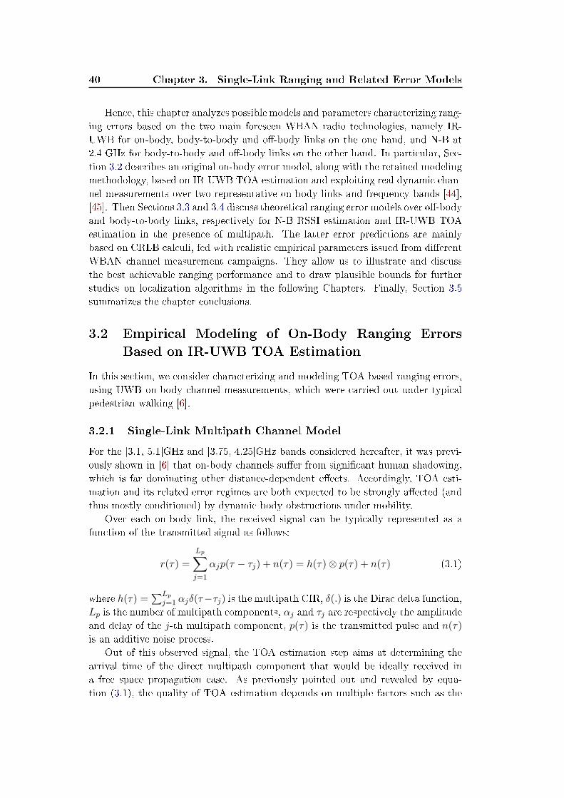
40 Chapter 3. Single-Link Ranging and Related Error Models
Hence, this chapter analyzes possible models and parameters characterizing rang-
ing errors based on the two main foreseen WBAN radio technologies, namely IR-
UWB for on-body, body-to-body and o�-body links on the one hand, and N-B at
2.4 GHz for body-to-body and o�-body links on the other hand. In particular, Sec-
tion 3.2 describes an original on-body error model, along with the retained modeling
methodology, based on IR-UWB TOA estimation and exploiting real dynamic chan-
nel measurements over two representative on-body links and frequency bands [44],
[45]. Then Sections 3.3 and 3.4 discuss theoretical ranging error models over o�-body
and body-to-body links, respectively for N-B RSSI estimation and IR-UWB TOA
estimation in the presence of multipath. The latter error predictions are mainly
based on CRLB calculi, fed with realistic empirical parameters issued from di�erent
WBAN channel measurement campaigns. They allow us to illustrate and discuss
the best achievable ranging performance and to draw plausible bounds for further
studies on localization algorithms in the following Chapters. Finally, Section 3.5
summarizes the chapter conclusions.
3.2 Empirical Modeling of On-Body Ranging Errors
Based on IR-UWB TOA Estimation
In this section, we consider characterizing and modeling TOA-based ranging errors,
using UWB on-body channel measurements, which were carried out under typical
pedestrian walking [6].
3.2.1 Single-Link Multipath Channel Model
For the [3.1, 5.1]GHz and [3.75, 4.25]GHz bands considered hereafter, it was previ-
ously shown in [6] that on-body channels su�er from signi�cant human shadowing,
which is far dominating other distance-dependent e�ects. Accordingly, TOA esti-
mation and its related error regimes are both expected to be strongly a�ected (and
thus mostly conditioned) by dynamic body obstructions under mobility.
Over each on-body link, the received signal can be typically represented as a
function of the transmitted signal as follows:
r(τ) =
Lp∑j=1
αjp(τ − τj) + n(τ) = h(τ)⊗ p(τ) + n(τ) (3.1)
where h(τ) =∑Lp
j=1 αjδ(τ−τj) is the multipath CIR, δ(.) is the Dirac delta function,Lp is the number of multipath components, αj and τj are respectively the amplitude
and delay of the j-th multipath component, p(τ) is the transmitted pulse and n(τ)
is an additive noise process.
Out of this observed signal, the TOA estimation step aims at determining the
arrival time of the direct multipath component that would be ideally received in
a free space propagation case. As previously pointed out and revealed by equa-
tion (3.1), the quality of TOA estimation depends on multiple factors such as the
3.2. Empirical Modeling of On-Body Ranging Errors Based on
IR-UWB TOA Estimation 41
emitted pulse energy (and hence, the received pulse energy) in comparison with the
noise �oor, multipath fading e�ects (and hence, the occupied bandwidth), or signal
obstructions. It is thus possible to generate false alarms due to early noisy realiza-
tions or to miss the direct path due to poor SNR conditions and/or severe NLOS
blockages. The latter phenomena tend to increase the apparent length of the direct
path or they can even cause its absence, leading to overestimated ranges.
3.2.2 Path Detection Schemes Enabling TOA Estimation
3.2.2.1 Strongest Peak Detection
Matched Filtering (MF) usually claims low complexity and low consumption [2],
which are two features particularly suitable for WBAN applications. In our ranging
context, TOA estimates are �rst obtained through strongest peak detection, by look-
ing for the corresponding time shifts that maximizes the cross-correlation function
between the received signal that can be represented as equation (3.1), and a local
template, which theoretically corresponds to the unitary transmitted waveform, as
follows:
c(τ ′) =
∫ +∞
−∞r(τ)p(τ − τ ′) dτ (3.2)
τTOA = argmaxτ ′∈W
|c(τ ′)| (3.3)
where c(τ ′) is the cross correlation function, and τTOA is the estimated TOA in the
temporal observation window W . The estimated distance is d = τTOAv, where v
is the speed of light, assuming that the transmitter and the receiver are somehow
synchronized, e.g. through 2-Way Ranging protocol exchanges (i.e. assuming in �rst
approximation that the TOF is equivalent here to the TOA reading and that the
errors a�ecting TOF measurements are restricted to that a�ecting TOA measure-
ments). It will be seen in the following how to cope in part with the actual timing
uncertainly when characterizing estimation errors out of real channel measurements.
3.2.2.2 First Path Detection
Getting back to the CIR expression in equation (3.1), the propagation delay τj ob-
viously reveals the physical length of the j-th corresponding path. Therefore, under
LOS conditions where a direct path is truly present between the transmitter and
the receiver, the shortest observable propagation delay can be reasonably associated
with the true Euclidean distance. This method, which is depicted hereafter as the
First Arrival Path (FAP) detection scheme, simply consists in preliminarily esti-
mating the CIR out of the received signal r(τ) in equation (3.1), and to associate
the �rst estimated multipath component (i.e. among all the resolved paths) with
the estimated distance between the transmitter and the receiver. Unfortunately,
in NLOS conditions, this FAP may su�er from signi�cant power attenuation that
makes it subject to missed/late detections or early false alarms, thus conducting to
large estimation errors and, more generally speaking, to a higher dispersion of the
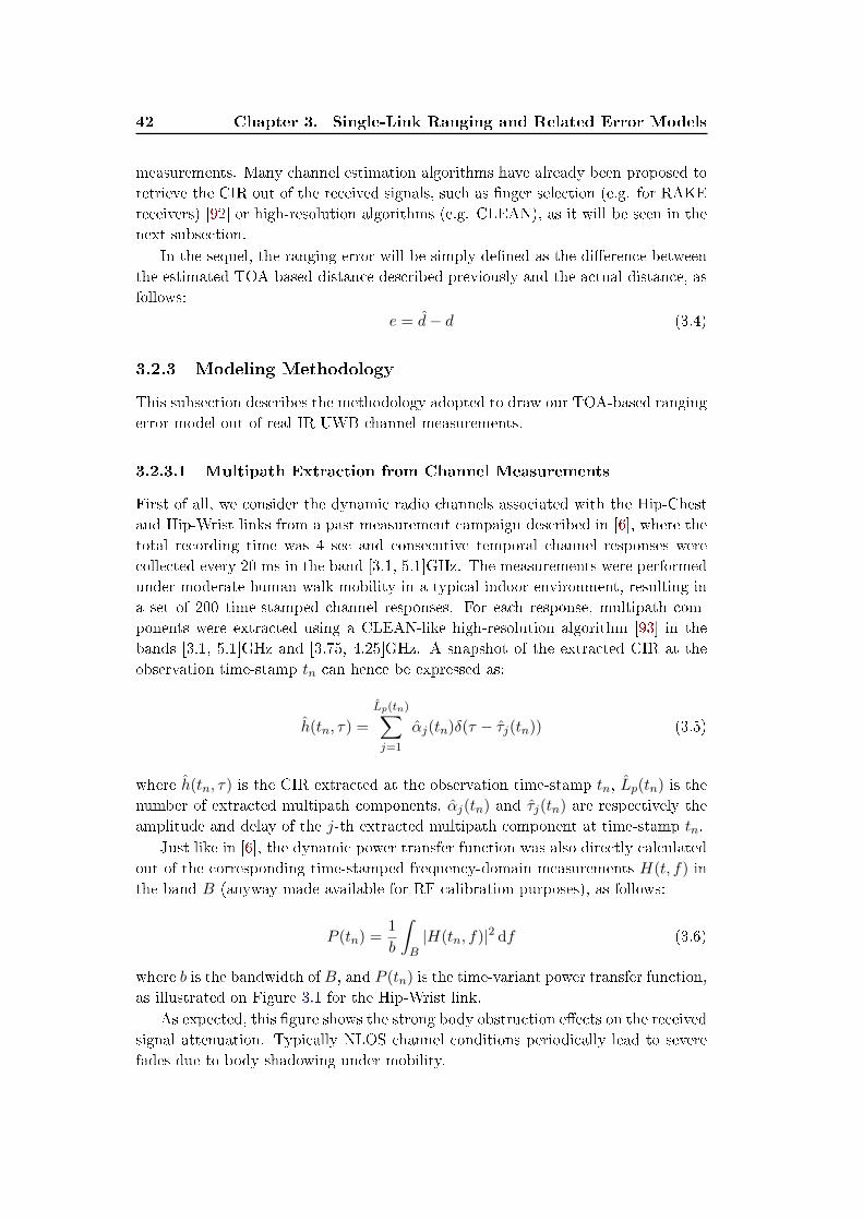
42 Chapter 3. Single-Link Ranging and Related Error Models
measurements. Many channel estimation algorithms have already been proposed to
retrieve the CIR out of the received signals, such as �nger selection (e.g. for RAKE
receivers) [92] or high-resolution algorithms (e.g. CLEAN), as it will be seen in the
next subsection.
In the sequel, the ranging error will be simply de�ned as the di�erence between
the estimated TOA-based distance described previously and the actual distance, as
follows:
e = d− d (3.4)
3.2.3 Modeling Methodology
This subsection describes the methodology adopted to draw our TOA-based ranging
error model out of real IR-UWB channel measurements.
3.2.3.1 Multipath Extraction from Channel Measurements
First of all, we consider the dynamic radio channels associated with the Hip-Chest
and Hip-Wrist links from a past measurement campaign described in [6], where the
total recording time was 4 sec and consecutive temporal channel responses were
collected every 20 ms in the band [3.1, 5.1]GHz. The measurements were performed
under moderate human walk mobility in a typical indoor environment, resulting in
a set of 200 time-stamped channel responses. For each response, multipath com-
ponents were extracted using a CLEAN-like high-resolution algorithm [93] in the
bands [3.1, 5.1]GHz and [3.75, 4.25]GHz. A snapshot of the extracted CIR at the
observation time-stamp tn can hence be expressed as:
h(tn, τ) =
Lp(tn)∑j=1
αj(tn)δ(τ − τj(tn)) (3.5)
where h(tn, τ) is the CIR extracted at the observation time-stamp tn, Lp(tn) is the
number of extracted multipath components, αj(tn) and τj(tn) are respectively the
amplitude and delay of the j-th extracted multipath component at time-stamp tn.
Just like in [6], the dynamic power transfer function was also directly calculated
out of the corresponding time-stamped frequency-domain measurements H(t, f) in
the band B (anyway made available for RF calibration purposes), as follows:
P (tn) =1
b
∫B|H(tn, f)|2 df (3.6)
where b is the bandwidth of B, and P (tn) is the time-variant power transfer function,
as illustrated on Figure 3.1 for the Hip-Wrist link.
As expected, this �gure shows the strong body obstruction e�ects on the received
signal attenuation. Typically NLOS channel conditions periodically lead to severe
fades due to body shadowing under mobility.
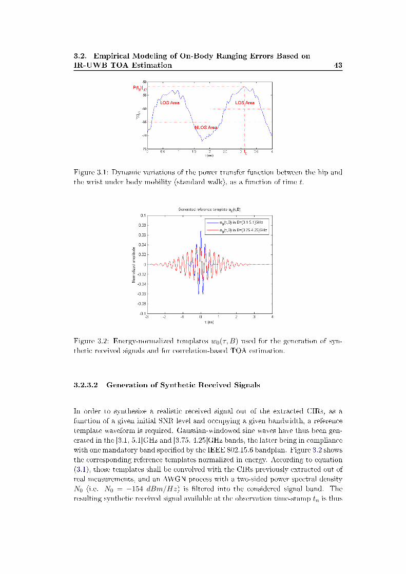
3.2. Empirical Modeling of On-Body Ranging Errors Based on
IR-UWB TOA Estimation 43
Figure 3.1: Dynamic variations of the power transfer function between the hip and
the wrist under body mobility (standard walk), as a function of time t.
Figure 3.2: Energy-normalized templates w0(τ,B) used for the generation of syn-
thetic received signals and for correlation-based TOA estimation.
3.2.3.2 Generation of Synthetic Received Signals
In order to synthesize a realistic received signal out of the extracted CIRs, as a
function of a given initial SNR level and occupying a given bandwidth, a reference
template waveform is required. Gaussian-windowed sine waves have thus been gen-
erated in the [3.1, 5.1]GHz and [3.75, 4.25]GHz bands, the latter being in compliance
with one mandatory band speci�ed by the IEEE 802.15.6 bandplan. Figure 3.2 shows
the corresponding reference templates normalized in energy. According to equation
(3.1), those templates shall be convolved with the CIRs previously extracted out of
real measurements, and an AWGN process with a two-sided power spectral density
N0 (i.e. N0 = −154 dBm/Hz) is �ltered into the considered signal band. The
resulting synthetic received signal available at the observation time-stamp tn is thus
44 Chapter 3. Single-Link Ranging and Related Error Models
given by:
Ws(tn, τ) = h(tn, τ)⊗ w0(τ,B) + n(tn, τ, B)
=
Lp(tn)∑j=1
αj(tn)w0(τ − τj(tn), B) + n(tn, τ, B) (3.7)
where w0(τ,B) is the reference template and n(tn, τ, B) is the band-limited noise
process at the observation time-stamp tn in the occupied band B.
For our simulation needs, in order to enable a dynamic variation of SNR(tn)
and to preserve the natural relative power �uctuations due to body obstructions (as
observed during the measurements campaign), we set and control the SNR values a
priori for an arbitrary reference time stamp (preferably in LOS). In our case, the ref-
erence time t0 is for instance chosen when the received channel exhibits a maximum
of the power transfer function P (t). Imposing a priori the reference value SNR(t0)
(as an input parameter) and given the actual P (tn) (and hence P (t0)) directly avail-
able from measurements at any time-stamp tn, the instantaneous SNR(tn) is then
forced and scaled arti�cially so as to vary realistically over the entire acquisition
duration, as follows:
SNR(t)|dB = SNR(t0)|dB + P (t)|dB − P (t0)|dB (3.8)
where SNR(t) is the re-scaled instantaneous signal energy to noise ratio, SNR(t0)
and P (t0) are respectively the controlled SNR value and power transfer function
at time-stamp t0, and P (t) is the power transfer function at time t. In our study,
SNR(t0) is viewed as an imposed input parameter, which remains constant and
valuable for the whole duration of one walk cycle, and over several noise process
realizations (i.e. over which TOA and ranging statistics will be drawn). Practically,
before applying (3.8) to account for the overall walk duration from the reference
time stamp t0, given the �xed �ltered noise power imposed by B and N0, we re-
scale the synthetic multipath impulse response h(t0, τ) in (3.7) into hr(t0, τ) so
that Ws,r(t0, τ) = hr(t0, τ)⊗w0(τ,B) + n(t0, τ, B) can respect the input parameter
SNR(t0) (and thus, applying the same scaling factor to the useful signal for each
random noise process realization), as follows:
SNR(t0)|lin =
∫[Ws,r(t0, τ
′)− n(t0, τ′, B)]2dτ ′
N0(3.9)
The rationale for parameterizing the error model with SNR(t0) are twofold: i)
we have noticed that the error regime is rather stable over LOS or NLOS portions of
a given walk (i.e. exhibiting approximately the same statistics under relatively small
variations of the instantaneous SNR) but mostly conditioned on body shadowing
and ii) SNR(t0) shall be easier to predict once for all at the beginning of the walk
cycle in localization-oriented simulations (e.g. with classical free-space propagation
models) for being advantageously associated with LOS conditions.
3.2. Empirical Modeling of On-Body Ranging Errors Based on
IR-UWB TOA Estimation 45
3.2.3.3 Emulated TOA Estimates and Conditional Error Regimes
At each observation time-stamp tn, TOA estimates are thus estimated from each
synthesized noisy received signal, using two kinds of estimators. The �rst one con-
sists of a matched �lter, as described in subsection 3.2.2.1, i.e. by looking for the time
shift that maximizes the cross-correlation function between the synthetic received
signal Ws,r(tn, τ) and the reference template w0(τ,B), within a given observation.
In our case, the window has a time length of 5 ns like in [85], [91]. This duration
is su�cient in WBAN applications to observe an arrival time corresponding to the
maximum distance between two synchronized nodes placed on the same body. Thus
we perform �ltering here in terms of excess delay.
The second TOA estimate is based on FAP detection using a CLEAN-like
approach, which can be shortly described for each time stamp tn as follows [94]:
1) Calculate the self-correlation rw0w0(tn, τ) of the template and the cross-
correlation rw0Ws(tn, τ) of the template with the synthesized received signal
Ws(tn, τ).
2) Find the largest correlation peak in rw0Ws(tn, τ), record the normalized amplitude
αk and the relative time delay τk of the correlation peak.
3) Substract rw0w0(tn, τ) scaled by αk from rw0Ws(tn, τ) at the time delay τk.
4) If a stopping criterion (e.g. a minimum threshold on the peak correlation) is not
met, go to step 2. Otherwise, stop.
5) The overall CIR h(tn, τ) is extracted, and the FAP is recorded as the �rst intime
resolved multipath component τ1(tn).
The �rst Hip-Chest link to be considered is always assumed in LOS conditions,
whereas the Hip-Wrist link varies dynamically, leading periodically and alternatively
to LOS and NLOS conditions. In order to classify the obstruction conditions, the
retained method is based on the power transfer function. Relying on the initial
measurements, the channel is considered in LOS (resp. NLOS) conditions whenever
its power transfer function is larger (resp. lower) than -60 dB (resp. -65 dB). The
remaining unspeci�ed time area is considered as a transition zone, with a steep
power transition regime. Alternatively, the channel delay spread, which exhibits
smaller values in LOS and higher values in NLOS conditions, could have been used
to identify the channel obstruction con�gurations.
Finally, during the initial communication-oriented measurement campaign re-
ported in [6], the real distance between nodes was not collected, since measurements
were not carried out for localization purposes. However, in �rst approximation, one
can try to extract this distance out of the measured TOA in time-stamp regions
when the LOS conditions are clearly identi�ed and with SNR(t0) = +∞ for the
synthetic received signals in the largest bandwidth [3.1, 5.1]GHz. Practically, the
�rst Hip-Chest link is considered as �xed and the reference distance extraction was
directly realized by averaging all the TOA measurements issued from MF estima-
tion over the walk cycle to reduce TOA estimation errors appeared during the mul-
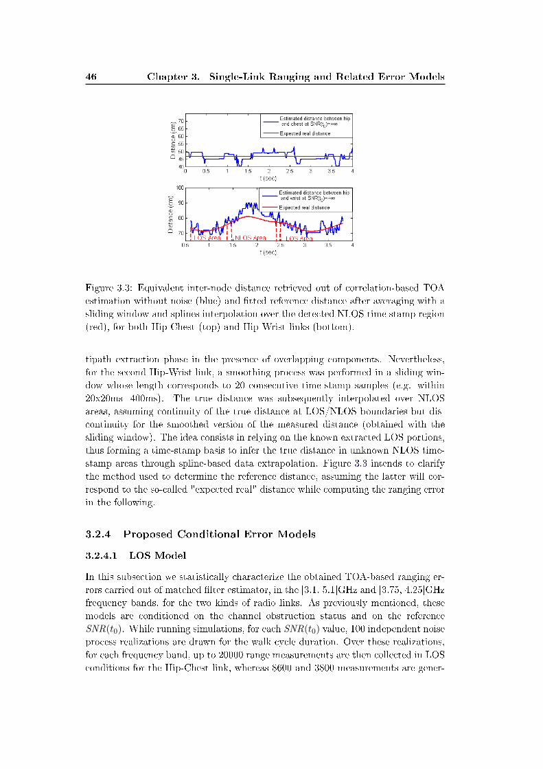
46 Chapter 3. Single-Link Ranging and Related Error Models
Figure 3.3: Equivalent inter-node distance retrieved out of correlation-based TOA
estimation without noise (blue) and �tted reference distance after averaging with a
sliding window and splines interpolation over the detected NLOS time stamp region
(red), for both Hip-Chest (top) and Hip-Wrist links (bottom).
tipath extraction phase in the presence of overlapping components. Nevertheless,
for the second Hip-Wrist link, a smoothing process was performed in a sliding win-
dow whose length corresponds to 20 consecutive time-stamp samples (e.g. within
20x20ms=400ms). The true distance was subsequently interpolated over NLOS
areas, assuming continuity of the true distance at LOS/NLOS boundaries but dis-
continuity for the smoothed version of the measured distance (obtained with the
sliding window). The idea consists in relying on the known extracted LOS portions,
thus forming a time-stamp basis to infer the true distance in unknown NLOS time-
stamp areas through spline-based data extrapolation. Figure 3.3 intends to clarify
the method used to determine the reference distance, assuming the latter will cor-
respond to the so-called "expected real" distance while computing the ranging error
in the following.
3.2.4 Proposed Conditional Error Models
3.2.4.1 LOS Model
In this subsection we statistically characterize the obtained TOA-based ranging er-
rors carried out of matched �lter estimator, in the [3.1, 5.1]GHz and [3.75, 4.25]GHz
frequency bands, for the two kinds of radio links. As previously mentioned, these
models are conditioned on the channel obstruction status and on the reference
SNR(t0). While running simulations, for each SNR(t0) value, 100 independent noise
process realizations are drawn for the walk cycle duration. Over these realizations,
for each frequency band, up to 20000 range measurements are then collected in LOS
conditions for the Hip-Chest link, whereas 8600 and 3800 measurements are gener-
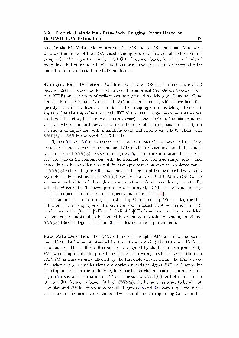
3.2. Empirical Modeling of On-Body Ranging Errors Based on
IR-UWB TOA Estimation 47
ated for the Hip-Wrist link, respectively in LOS and NLOS conditions. Moreover,
we draw the model of the TOA-based ranging errors carried out of FAP detection
using a CLEAN algorithm, in [3.1, 5.1]GHz frequency band, for the two kinds of
radio links, but only under LOS conditions, while the FAP is almost systematically
missed or falsely detected in NLOS conditions.
Strongest Path Detection Conditioned on the LOS case, a side basic Least
Square (LS) �t has been performed between the empirical Cumulative Density Func-
tion (CDF) and a variety of well-known heavy tailed models (e.g. Gaussian, Gen-
eralized Extreme Value, Exponential, Weibull, lognormal...), which have been fre-
quently cited in the literature in the �eld of ranging error modeling. Hence, it
appears that the step-wise empirical CDF of emulated range measurements enjoys
a rather satisfactory �t (in a least squares sense) to the CDF of a Gaussian random
variable, whose standard deviation σ is on the order of the time base period. Figure
3.4 shows examples for both simulation-based and model-based LOS CDFs with
SNR(t0) = 5dB in the band [3.1, 5.1]GHz.
Figures 3.5 and 3.6 show respectively the variations of the mean and standard
deviation of the corresponding Gaussian LOS model for both links and both bands,
as a function of SNR(t0). As seen in Figure 3.5, the mean varies around zero, with
very low values (in comparison with the nominal expected true range value), and
hence, it can be considered as null in �rst approximation over the explored range
of SNR(t0) values. Figure 3.6 shows that the behavior of the standard deviation is
asymptotically constant when SNR(t0) reaches a value of 10 dB. At high SNRs, the
strongest path detected through cross-correlation indeed coincides systematically
with the direct path. The asymptotic error �oor at high SNR thus depends mostly
on the occupied band and center frequency, as discussed in [34].
To summarize, considering the tested Hip-Chest and Hip-Wrist links, the dis-
tribution of the ranging error through correlation-based TOA estimation in LOS
conditions in the [3.1, 5.1]GHz and [3.75, 4.25]GHz bands can be simply modeled
as a centered Gaussian distribution, with a standard deviation depending on B and
SNR(t0) (See the legend of Figure 3.6 for detailed model parameters).
First Path Detection For TOA estimation through FAP detection, the result-
ing pdf can be better represented by a mixture involving Gaussian and Uniform
components. The Uniform distribution is weighted by the false alarm probability
PF , which represents the probability to detect a wrong peak instead of the true
FAP. PF is thus strongly a�ected by the threshold chosen within the FAP detec-
tion scheme (e.g. a smaller threshold obviously leads to higher PF ), and hence, by
the stopping rule in the underlying high-resolution channel estimation algorithm.
Figure 3.7 shows the variation of PF as a function of SNR(t0) for both links in the
[3.1, 5.1]GHz frequency band. At high SNR(t0), the behavior appears to be almost
Gaussian and PF is approximately null. Figures 3.8 and 3.9 show respectively the
variations of the mean and standard deviation of the corresponding Gaussian dis-
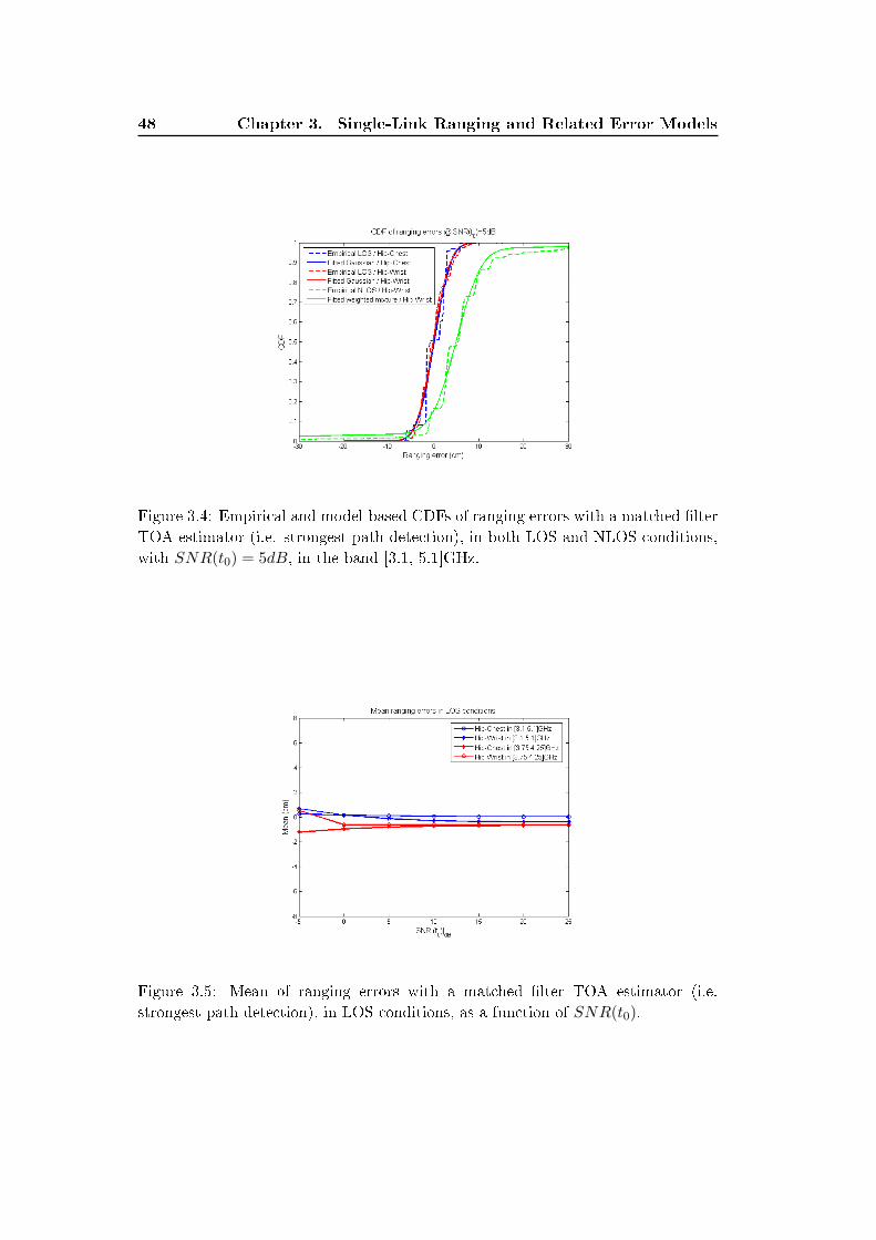
48 Chapter 3. Single-Link Ranging and Related Error Models
Figure 3.4: Empirical and model-based CDFs of ranging errors with a matched �lter
TOA estimator (i.e. strongest path detection), in both LOS and NLOS conditions,
with SNR(t0) = 5dB, in the band [3.1, 5.1]GHz.
Figure 3.5: Mean of ranging errors with a matched �lter TOA estimator (i.e.
strongest path detection), in LOS conditions, as a function of SNR(t0).
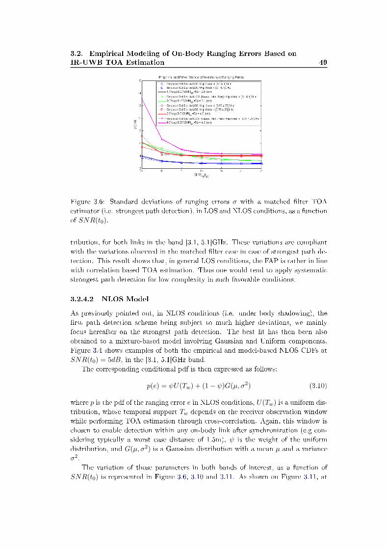
3.2. Empirical Modeling of On-Body Ranging Errors Based on
IR-UWB TOA Estimation 49
Figure 3.6: Standard deviations of ranging errors σ with a matched �lter TOA
estimator (i.e. strongest path detection), in LOS and NLOS conditions, as a function
of SNR(t0).
tribution, for both links in the band [3.1, 5.1]GHz. These variations are compliant
with the variations observed in the matched �lter case in case of strongest path de-
tection. This result shows that, in general LOS conditions, the FAP is rather in line
with correlation-based TOA estimation. Thus one would tend to apply systematic
strongest path detection for low complexity in such favorable conditions.
3.2.4.2 NLOS Model
As previously pointed out, in NLOS conditions (i.e. under body shadowing), the
�rst path detection scheme being subject to much higher deviations, we mainly
focus hereafter on the strongest path detection. The best �t has then been also
obtained to a mixture-based model involving Gaussian and Uniform components.
Figure 3.4 shows examples of both the empirical and model-based NLOS CDFs at
SNR(t0) = 5dB, in the [3.1, 5.1]GHz band.
The corresponding conditional pdf is then expressed as follows:
p(e) = ψU(Tw) + (1− ψ)G(µ, σ2) (3.10)
where p is the pdf of the ranging error e in NLOS conditions, U(Tw) is a uniform dis-
tribution, whose temporal support Tw depends on the receiver observation window
while performing TOA estimation through cross-correlation. Again, this window is
chosen to enable detection within any on-body link after synchronization (e.g con-
sidering typically a worst case distance of 1.5m), ψ is the weight of the uniform
distribution, and G(µ, σ2) is a Gaussian distribution with a mean µ and a variance
σ2.
The variation of those parameters in both bands of interest, as a function of
SNR(t0) is represented in Figure 3.6, 3.10 and 3.11. As shown on Figure 3.11, at
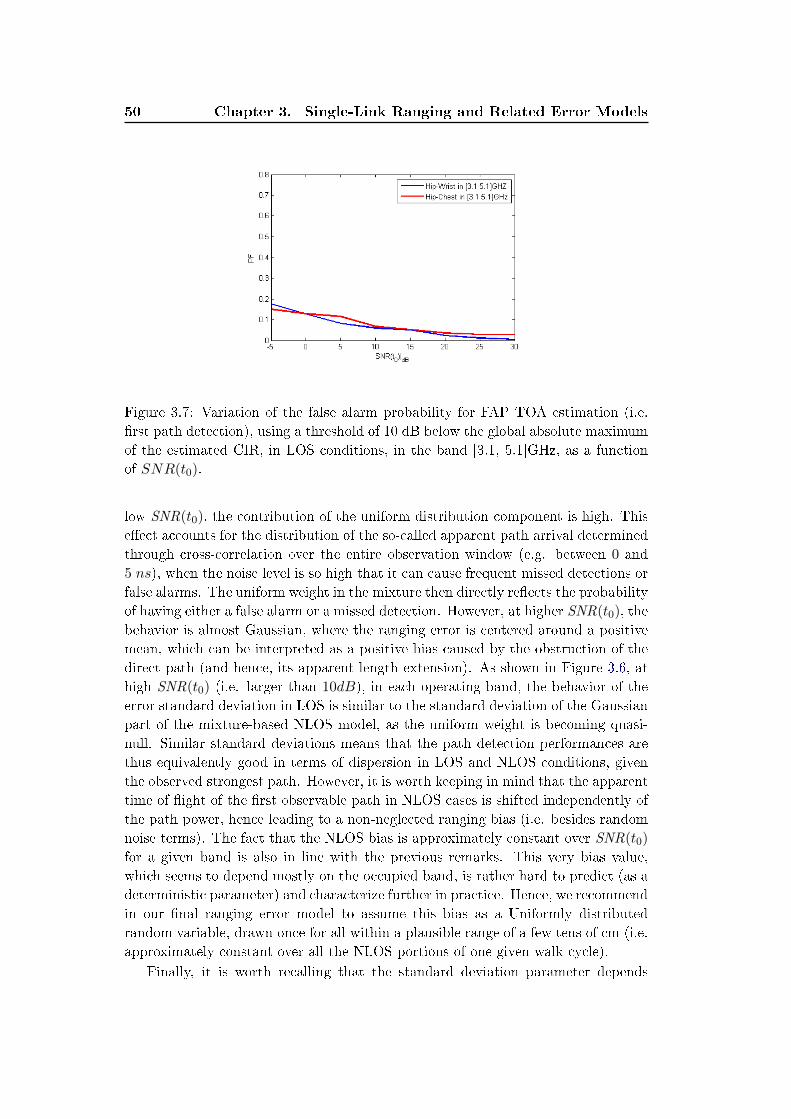
50 Chapter 3. Single-Link Ranging and Related Error Models
Figure 3.7: Variation of the false alarm probability for FAP TOA estimation (i.e.
�rst path detection), using a threshold of 10 dB below the global absolute maximum
of the estimated CIR, in LOS conditions, in the band [3.1, 5.1]GHz, as a function
of SNR(t0).
low SNR(t0), the contribution of the uniform distribution component is high. This
e�ect accounts for the distribution of the so-called apparent path arrival determined
through cross-correlation over the entire observation window (e.g. between 0 and
5 ns), when the noise level is so high that it can cause frequent missed detections or
false alarms. The uniform weight in the mixture then directly re�ects the probability
of having either a false alarm or a missed detection. However, at higher SNR(t0), the
behavior is almost Gaussian, where the ranging error is centered around a positive
mean, which can be interpreted as a positive bias caused by the obstruction of the
direct path (and hence, its apparent length extension). As shown in Figure 3.6, at
high SNR(t0) (i.e. larger than 10dB), in each operating band, the behavior of the
error standard deviation in LOS is similar to the standard deviation of the Gaussian
part of the mixture-based NLOS model, as the uniform weight is becoming quasi-
null. Similar standard deviations means that the path detection performances are
thus equivalently good in terms of dispersion in LOS and NLOS conditions, given
the observed strongest path. However, it is worth keeping in mind that the apparent
time of �ight of the �rst observable path in NLOS cases is shifted independently of
the path power, hence leading to a non-neglected ranging bias (i.e. besides random
noise terms). The fact that the NLOS bias is approximately constant over SNR(t0)
for a given band is also in line with the previous remarks. This very bias value,
which seems to depend mostly on the occupied band, is rather hard to predict (as a
deterministic parameter) and characterize further in practice. Hence, we recommend
in our �nal ranging error model to assume this bias as a Uniformly distributed
random variable, drawn once for all within a plausible range of a few tens of cm (i.e.
approximately constant over all the NLOS portions of one given walk cycle).
Finally, it is worth recalling that the standard deviation parameter depends
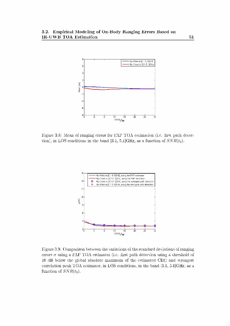
3.2. Empirical Modeling of On-Body Ranging Errors Based on
IR-UWB TOA Estimation 51
Figure 3.8: Mean of ranging errors for FAP TOA estimation (i.e. �rst path detec-
tion), in LOS conditions in the band [3.1, 5.1]GHz, as a function of SNR(t0).
Figure 3.9: Comparison between the variations of the standard deviations of ranging
errors σ using a FAP TOA estimator (i.e. �rst path detection using a threshold of
10 dB below the global absolute maximum of the estimated CIR) and strongest
correlation peak TOA estimator, in LOS conditions, in the band [3.1, 5.1]GHz, as a
function of SNR(t0).
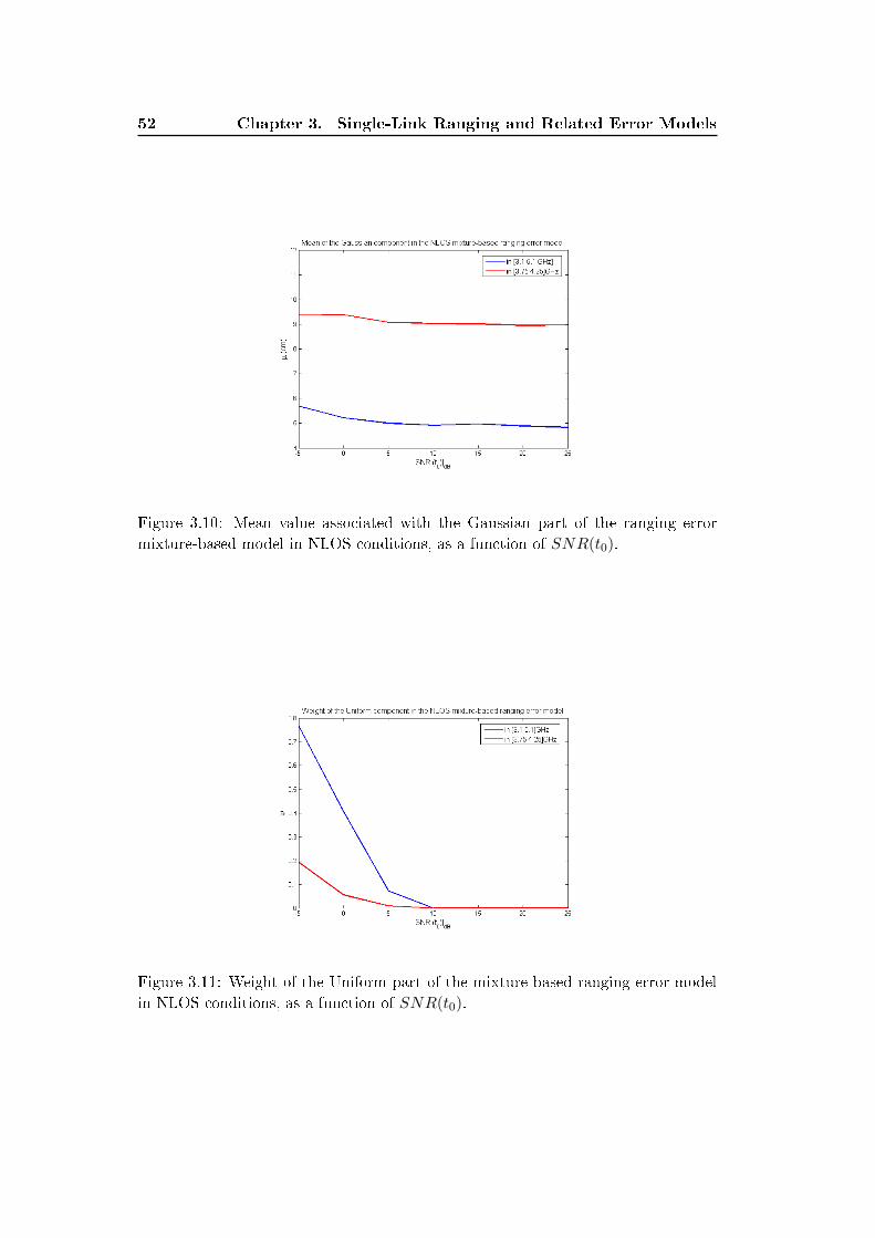
52 Chapter 3. Single-Link Ranging and Related Error Models
Figure 3.10: Mean value associated with the Gaussian part of the ranging error
mixture-based model in NLOS conditions, as a function of SNR(t0).
Figure 3.11: Weight of the Uniform part of the mixture-based ranging error model
in NLOS conditions, as a function of SNR(t0).
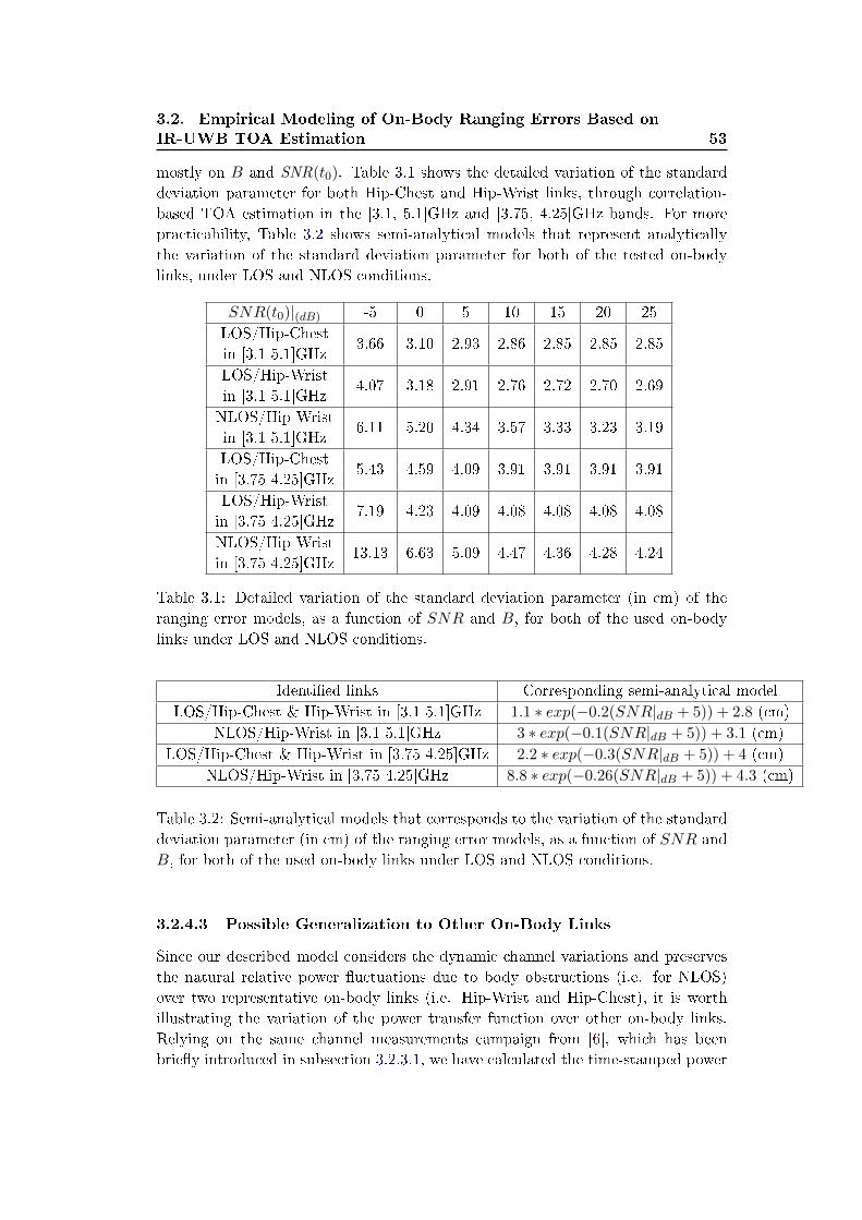
3.2. Empirical Modeling of On-Body Ranging Errors Based on
IR-UWB TOA Estimation 53
mostly on B and SNR(t0). Table 3.1 shows the detailed variation of the standard
deviation parameter for both Hip-Chest and Hip-Wrist links, through correlation-
based TOA estimation in the [3.1, 5.1]GHz and [3.75, 4.25]GHz bands. For more
practicability, Table 3.2 shows semi-analytical models that represent analytically
the variation of the standard deviation parameter for both of the tested on-body
links, under LOS and NLOS conditions.
SNR(t0)|(dB) -5 0 5 10 15 20 25
LOS/Hip-Chest3.66 3.10 2.93 2.86 2.85 2.85 2.85
in [3.1 5.1]GHz
LOS/Hip-Wrist4.07 3.18 2.91 2.76 2.72 2.70 2.69
in [3.1 5.1]GHz
NLOS/Hip-Wrist6.11 5.20 4.34 3.57 3.33 3.23 3.19
in [3.1 5.1]GHz
LOS/Hip-Chest5.43 4.59 4.09 3.91 3.91 3.91 3.91
in [3.75 4.25]GHz
LOS/Hip-Wrist7.19 4.23 4.09 4.08 4.08 4.08 4.08
in [3.75 4.25]GHz
NLOS/Hip-Wrist13.13 6.63 5.09 4.47 4.36 4.28 4.24
in [3.75 4.25]GHz
Table 3.1: Detailed variation of the standard deviation parameter (in cm) of the
ranging error models, as a function of SNR and B, for both of the used on-body
links under LOS and NLOS conditions.
Identi�ed links Corresponding semi-analytical model
LOS/Hip-Chest & Hip-Wrist in [3.1 5.1]GHz 1.1 ∗ exp(−0.2(SNR|dB + 5)) + 2.8 (cm)
NLOS/Hip-Wrist in [3.1 5.1]GHz 3 ∗ exp(−0.1(SNR|dB + 5)) + 3.1 (cm)
LOS/Hip-Chest & Hip-Wrist in [3.75 4.25]GHz 2.2 ∗ exp(−0.3(SNR|dB + 5)) + 4 (cm)
NLOS/Hip-Wrist in [3.75 4.25]GHz 8.8 ∗ exp(−0.26(SNR|dB + 5)) + 4.3 (cm)
Table 3.2: Semi-analytical models that corresponds to the variation of the standard
deviation parameter (in cm) of the ranging error models, as a function of SNR and
B, for both of the used on-body links under LOS and NLOS conditions.
3.2.4.3 Possible Generalization to Other On-Body Links
Since our described model considers the dynamic channel variations and preserves
the natural relative power �uctuations due to body obstructions (i.e. for NLOS)
over two representative on-body links (i.e. Hip-Wrist and Hip-Chest), it is worth
illustrating the variation of the power transfer function over other on-body links.
Relying on the same channel measurements campaign from [6], which has been
brie�y introduced in subsection 3.2.3.1, we have calculated the time-stamped power
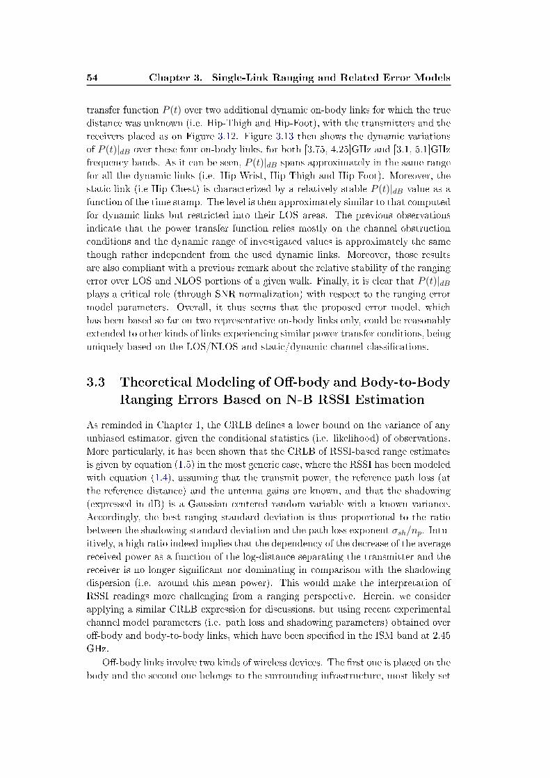
54 Chapter 3. Single-Link Ranging and Related Error Models
transfer function P (t) over two additional dynamic on-body links for which the true
distance was unknown (i.e. Hip-Thigh and Hip-Foot), with the transmitters and the
receivers placed as on Figure 3.12. Figure 3.13 then shows the dynamic variations
of P (t)|dB over these four on-body links, for both [3.75, 4.25]GHz and [3.1, 5.1]GHz
frequency bands. As it can be seen, P (t)|dB spans approximately in the same range
for all the dynamic links (i.e. Hip-Wrist, Hip-Thigh and Hip-Foot). Moreover, the
static link (i.e Hip-Chest) is characterized by a relatively stable P (t)|dB value as a
function of the time stamp. The level is then approximately similar to that computed
for dynamic links but restricted into their LOS areas. The previous observations
indicate that the power transfer function relies mostly on the channel obstruction
conditions and the dynamic range of investigated values is approximately the same
though rather independent from the used dynamic links. Moreover, those results
are also compliant with a previous remark about the relative stability of the ranging
error over LOS and NLOS portions of a given walk. Finally, it is clear that P (t)|dBplays a critical role (through SNR normalization) with respect to the ranging error
model parameters. Overall, it thus seems that the proposed error model, which
has been based so far on two representative on-body links only, could be reasonably
extended to other kinds of links experiencing similar power transfer conditions, being
uniquely based on the LOS/NLOS and static/dynamic channel classi�cations.
3.3 Theoretical Modeling of O�-body and Body-to-Body
Ranging Errors Based on N-B RSSI Estimation
As reminded in Chapter 1, the CRLB de�nes a lower bound on the variance of any
unbiased estimator, given the conditional statistics (i.e. likelihood) of observations.
More particularly, it has been shown that the CRLB of RSSI-based range estimates
is given by equation (1.5) in the most generic case, where the RSSI has been modeled
with equation (1.4), assuming that the transmit power, the reference path loss (at
the reference distance) and the antenna gains are known, and that the shadowing
(expressed in dB) is a Gaussian centered random variable with a known variance.
Accordingly, the best ranging standard deviation is thus proportional to the ratio
between the shadowing standard deviation and the path loss exponent σsh/np. Intu-
itively, a high ratio indeed implies that the dependency of the decrease of the average
received power as a function of the log-distance separating the transmitter and the
receiver is no longer signi�cant nor dominating in comparison with the shadowing
dispersion (i.e. around this mean power). This would make the interpretation of
RSSI readings more challenging from a ranging perspective. Herein, we consider
applying a similar CRLB expression for discussions, but using recent experimental
channel model parameters (i.e. path loss and shadowing parameters) obtained over
o�-body and body-to-body links, which have been speci�ed in the ISM band at 2.45
GHz.
O�-body links involve two kinds of wireless devices. The �rst one is placed on the
body and the second one belongs to the surrounding infrastructure, most likely set
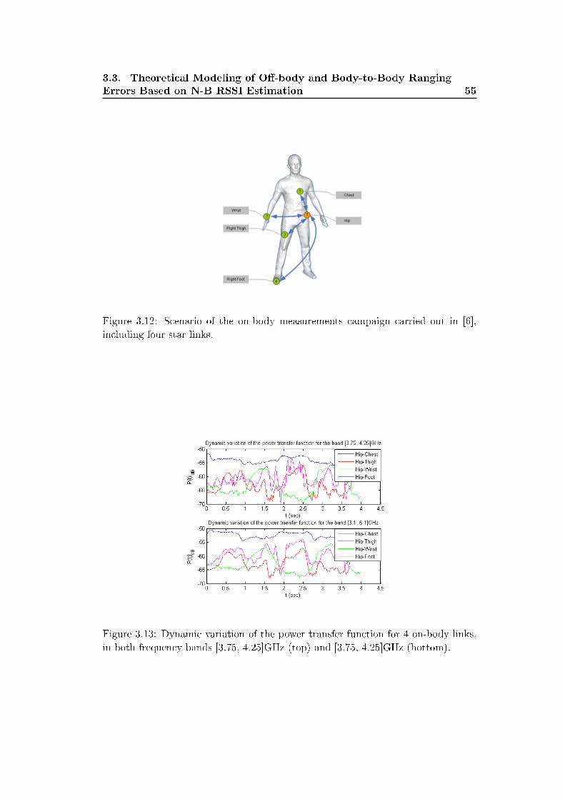
3.3. Theoretical Modeling of O�-body and Body-to-Body Ranging
Errors Based on N-B RSSI Estimation 55
Figure 3.12: Scenario of the on-body measurements campaign carried out in [6],
including four star links.
Figure 3.13: Dynamic variation of the power transfer function for 4 on-body links,
in both frequency bands [3.75, 4.25]GHz (top) and [3.75, 4.25]GHz (bottom).
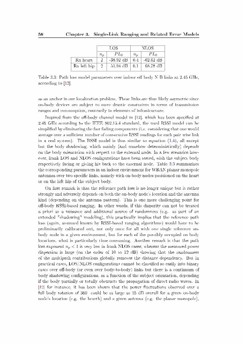
56 Chapter 3. Single-Link Ranging and Related Error Models
LOS NLOS
np PL0 np PL0
Rx heart 2 -38.92 dB 0.4 -62.62 dB
Rx left hip 2 -51.94 dB 0.1 -68.78 dB
Table 3.3: Path loss model parameters over indoor o�-body N-B links at 2.45 GHz,
according to [12].
as an anchor in our localization problem. These links are thus likely asymetric since
on-body devices are subject to more drastic constraints in terms of transmission
ranges and consumption, contrarily to elements of infrastructure.
Inspired from the o�-body channel model in [12], which has been speci�ed at
2.45 GHz according to the IEEE 802.15.4 standard, the used RSSI model can be
simpli�ed by eliminating the fast fading components (i.e. considering that one would
average over a su�cient number of consecutive RSSI readings for each pair-wise link
in a real system). The RSSI model is thus similar to equation (1.4), all except
but the body shadowing, which mainly (and somehow deterministically) depends
on the body orientation with respect to the external node. In a few scenarios how-
ever, frank LOS and NLOS con�gurations have been tested, with the subject body
respectively facing or giving his back to the external node. Table 3.3 summarizes
the corresponding parameters in an indoor environment for WBAN planar monopole
antennas over two speci�c links, namely with on-body nodes positioned on the heart
or on the left hip of the subject body.
On �rst remark is that the reference path loss is no longer unique but it rather
strongly and adversely depends on both the on-body node's location and the antenna
kind (depending on the antenna pattern). This is one more challenging point for
o�-body RSSI-based ranging. In other words, if this disparity can not be treated
a priori as a nuisance and additional source of randomness (e.g. as part of an
extended "shadowing" modeling), this practically implies that the reference path
loss (again, assumed known by RSSI-based ranging algorithms) would have to be
preliminarily calibrated out, not only once for all with one single reference on-
body node in a given environment, but for each of the possibly occupied on-body
locations, what is particularly time consuming. Another remark is that the path
loss exponent np < 1 is very low in frank NLOS cases, whereas the measured power
dispersion is large (on the order of 10 to 12 dB) showing that the randomness
of the multipath contributions globally removes the distance dependency. But in
practical cases, LOS/NLOS con�gurations cannot be classi�ed so easily into binary
cases over o�-body (or even over body-to-body) links but there is a continuum of
body shadowing con�gurations, as a function of the subject orientation, depending
if the body partially or totally obstructs the propagation of direct radio waves. In
[12] for instance, it has been shown that the power �uctuations observed over a
full body rotation of 360 could be as large as 25 dB overall for a given on-body
node's location (e.g. the hearth) and a given antenna (e.g. the planar monopole),
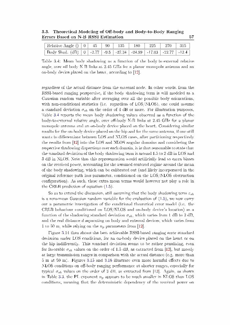
3.3. Theoretical Modeling of O�-body and Body-to-Body Ranging
Errors Based on N-B RSSI Estimation 57
Relative Angle () 0 45 90 135 180 225 270 315
Body Shad. (dB) 0 -2.77 -9.5 -27.34 -24.99 -17.03 -22.77 -12.4
Table 3.4: Mean body shadowing as a function of the body-to-external relative
angle, over o�-body N-B links at 2.45 GHz for a planar monopole antenna and an
on-body device placed on the heart, according to [12].
regardless of the actual distance from the external node. In other words, from the
RSSI-based ranging perspective, if the body shadowing term is still modeled as a
Gaussian random variable after averaging over all the possible body orientations,
with non-conditional statistics (i.e. regardless of LOS/NLOS), one could assume
a standard deviation σsh on the order of 4 dB or more. For illustration purposes,
Table 3.4 reports the mean body shadowing values observed as a function of the
body-to-external relative angle, over o�-body N-B links at 2.45 GHz for a planar
monopole antenna and an on-body device placed on the heart. Considering similar
results for the on-body device placed on the hip and for the same antenna, if one still
wants to di�erentiate between LOS and NLOS cases, after partitioning respectively
the results from [12] into the LOS and NLOS angular domains and considering the
respective shadowing dispersions over each domain, it is thus reasonable to state that
the standard deviation of the body shadowing term is around 1.5 to 2 dB in LOS and
3 dB in NLOS. Note that this representation would arti�cially lead to extra biases
on the received power, accounting for the assumed centered regime around the mean
of the body shadowing, which can be calibrated out (and likely incorporated in the
original reference path loss parameter, conditioned on the LOS/NLOS obstruction
con�guration). As such, these extra mean terms would however not play a role in
the CRLB prediction of equation (1.5).
So as to extend the discussion, still assuming that the body shadowing term εshis a zero-mean Gaussian random variable for the evaluation of (1.5), we now carry
out a parametric investigation of the conditional theoretical error model (i.e. the
CRLB behaviour conditioned on LOS/NLOS and on-body device's location) as a
function of the shadowing standard deviation σsh, which varies from 1 dB to 3 dB,
and the real distance d separating on-body and external devices, which varies from
1 to 50 m, while relying on the np parameters from [12].
Figure 3.14 then shows the best achievable RSSI-based ranging error standard
deviation under LOS conditions, for an on-body device placed on the heart or on
the hip indi�erently. This standard deviation seems to be rather penalizing, even
for favorable σsh values on the order of 1.5 dB, as extracted from [12], but mostly
at large transmission ranges in comparison with the actual distance (e.g. more than
5 m at 50 m). Figures 3.15 and 3.16 illustrate even more harmful e�ects due to
NLOS conditions on o�-body ranging performance at shorter ranges, especially for
typical σsh values on the order of 3 dB, as extracted from [12]. Again, as shown
in Table 3.3, the PL exponent np appears to be much smaller in NLOS than LOS
conditions, meaning that the deterministic dependency of the received power on
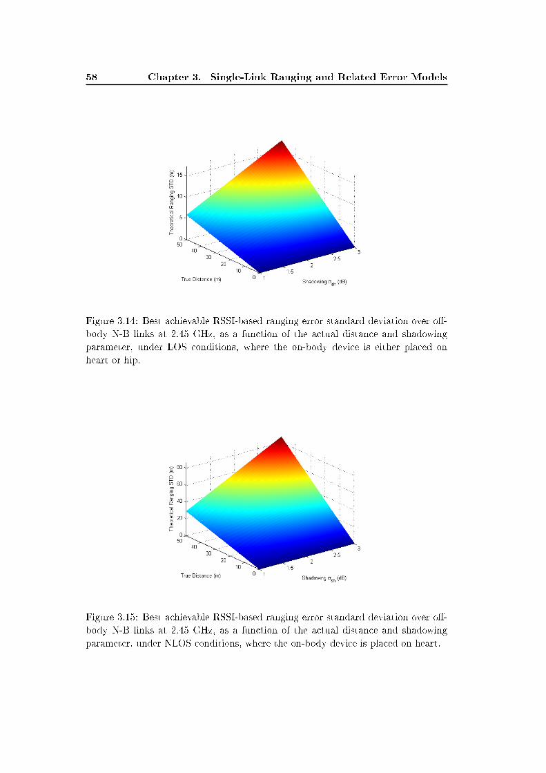
58 Chapter 3. Single-Link Ranging and Related Error Models
Figure 3.14: Best achievable RSSI-based ranging error standard deviation over o�-
body N-B links at 2.45 GHz, as a function of the actual distance and shadowing
parameter, under LOS conditions, where the on-body device is either placed on
heart or hip.
Figure 3.15: Best achievable RSSI-based ranging error standard deviation over o�-
body N-B links at 2.45 GHz, as a function of the actual distance and shadowing
parameter, under NLOS conditions, where the on-body device is placed on heart.
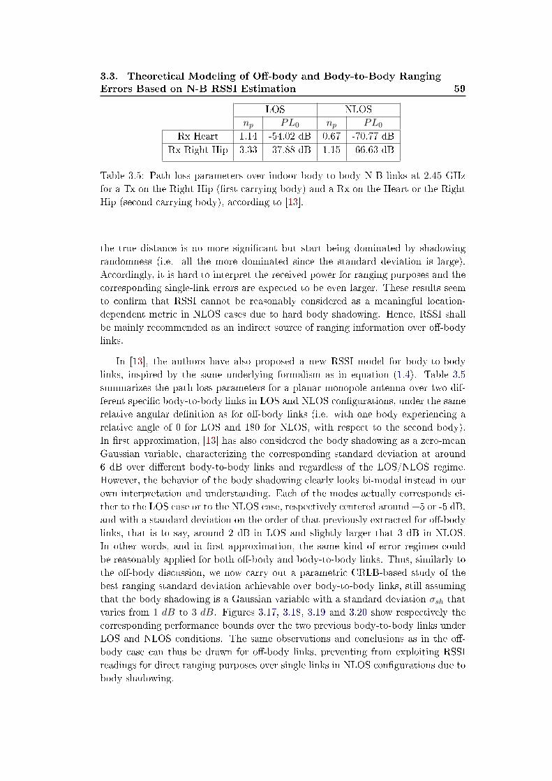
3.3. Theoretical Modeling of O�-body and Body-to-Body Ranging
Errors Based on N-B RSSI Estimation 59
LOS NLOS
np PL0 np PL0
Rx Heart 1.14 -54.02 dB 0.67 -70.77 dB
Rx Right Hip 3.33 -37.88 dB 1.15 -66.63 dB
Table 3.5: Path loss parameters over indoor body-to-body N-B links at 2.45 GHz
for a Tx on the Right Hip (�rst carrying body) and a Rx on the Heart or the Right
Hip (second carrying body), according to [13].
the true distance is no more signi�cant but start being dominated by shadowing
randomness (i.e. all the more dominated since the standard deviation is large).
Accordingly, it is hard to interpret the received power for ranging purposes and the
corresponding single-link errors are expected to be even larger. These results seem
to con�rm that RSSI cannot be reasonably considered as a meaningful location-
dependent metric in NLOS cases due to hard body shadowing. Hence, RSSI shall
be mainly recommended as an indirect source of ranging information over o�-body
links.
In [13], the authors have also proposed a new RSSI model for body-to-body
links, inspired by the same underlying formalism as in equation (1.4). Table 3.5
summarizes the path loss parameters for a planar monopole antenna over two dif-
ferent speci�c body-to-body links in LOS and NLOS con�gurations, under the same
relative angular de�nition as for o�-body links (i.e. with one body experiencing a
relative angle of 0 for LOS and 180 for NLOS, with respect to the second body).
In �rst approximation, [13] has also considered the body shadowing as a zero-mean
Gaussian variable, characterizing the corresponding standard deviation at around
6 dB over di�erent body-to-body links and regardless of the LOS/NLOS regime.
However, the behavior of the body shadowing clearly looks bi-modal instead in our
own interpretation and understanding. Each of the modes actually corresponds ei-
ther to the LOS case or to the NLOS case, respectively centered around +5 or -5 dB,
and with a standard deviation on the order of that previously extracted for o�-body
links, that is to say, around 2 dB in LOS and slightly larger that 3 dB in NLOS.
In other words, and in �rst approximation, the same kind of error regimes could
be reasonably applied for both o�-body and body-to-body links. Thus, similarly to
the o�-body discussion, we now carry out a parametric CRLB-based study of the
best ranging standard deviation achievable over body-to-body links, still assuming
that the body shadowing is a Gaussian variable with a standard deviation σsh that
varies from 1 dB to 3 dB. Figures 3.17, 3.18, 3.19 and 3.20 show respectively the
corresponding performance bounds over the two previous body-to-body links under
LOS and NLOS conditions. The same observations and conclusions as in the o�-
body case can thus be drawn for o�-body links, preventing from exploiting RSSI
readings for direct ranging purposes over single links in NLOS con�gurations due to
body shadowing.
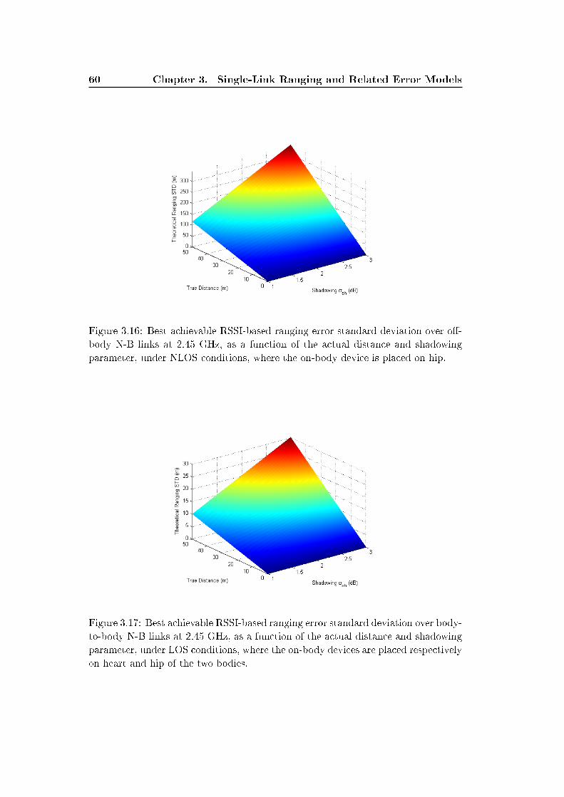
60 Chapter 3. Single-Link Ranging and Related Error Models
Figure 3.16: Best achievable RSSI-based ranging error standard deviation over o�-
body N-B links at 2.45 GHz, as a function of the actual distance and shadowing
parameter, under NLOS conditions, where the on-body device is placed on hip.
Figure 3.17: Best achievable RSSI-based ranging error standard deviation over body-
to-body N-B links at 2.45 GHz, as a function of the actual distance and shadowing
parameter, under LOS conditions, where the on-body devices are placed respectively
on heart and hip of the two bodies.
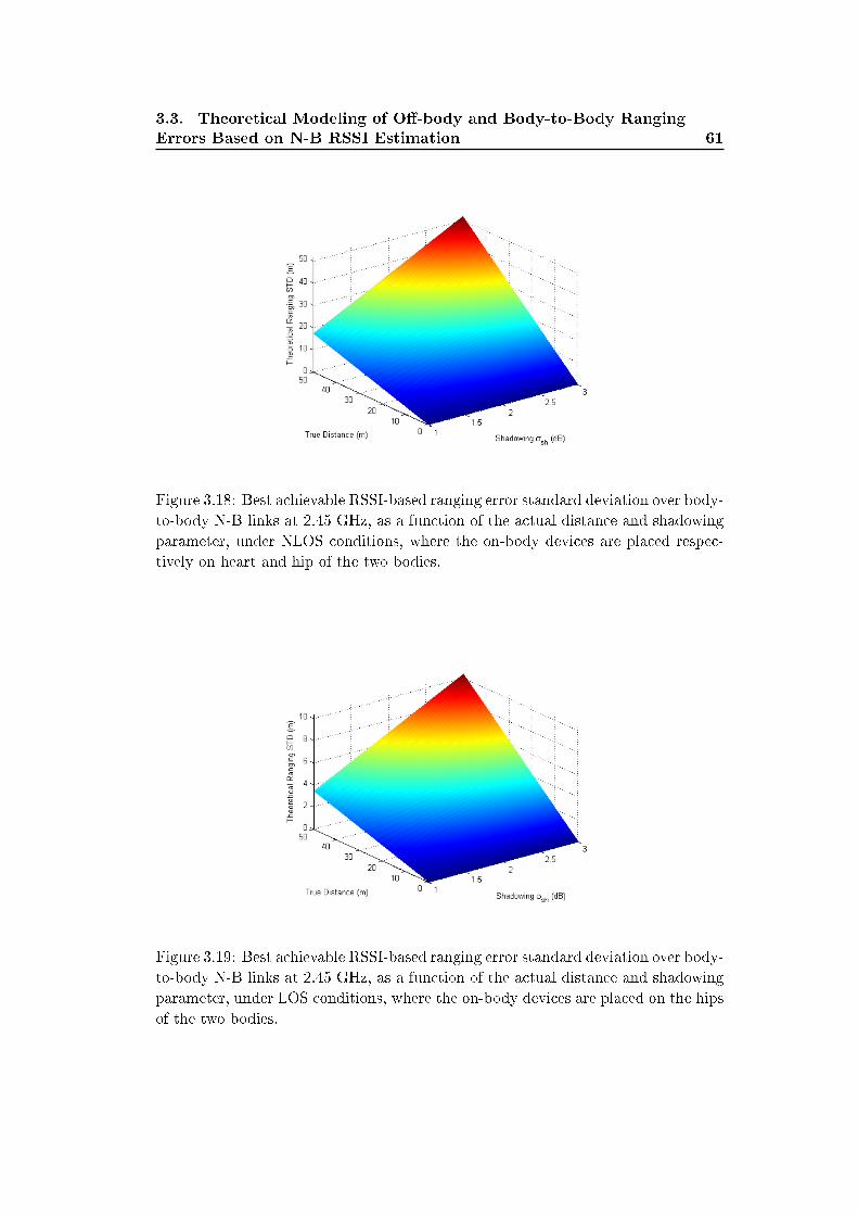
3.3. Theoretical Modeling of O�-body and Body-to-Body Ranging
Errors Based on N-B RSSI Estimation 61
Figure 3.18: Best achievable RSSI-based ranging error standard deviation over body-
to-body N-B links at 2.45 GHz, as a function of the actual distance and shadowing
parameter, under NLOS conditions, where the on-body devices are placed respec-
tively on heart and hip of the two bodies.
Figure 3.19: Best achievable RSSI-based ranging error standard deviation over body-
to-body N-B links at 2.45 GHz, as a function of the actual distance and shadowing
parameter, under LOS conditions, where the on-body devices are placed on the hips
of the two bodies.
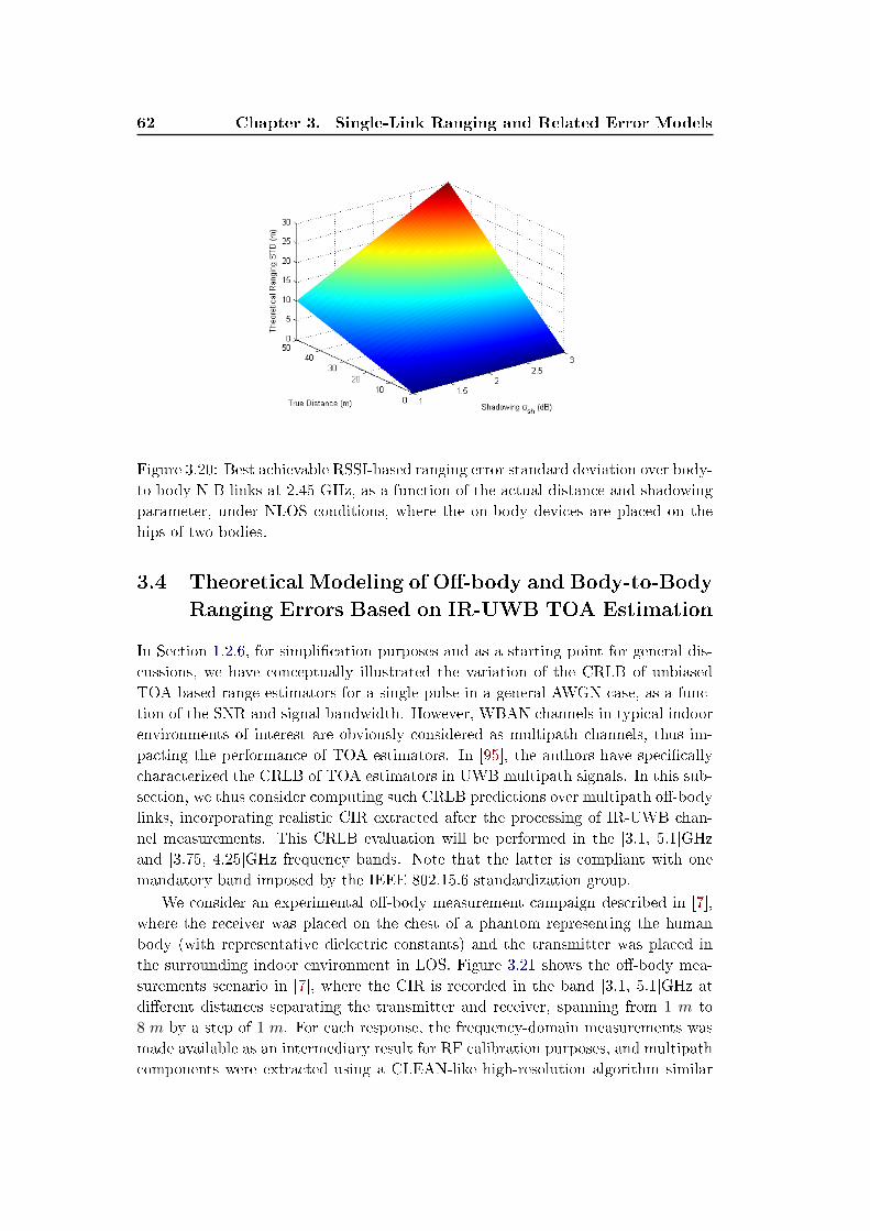
62 Chapter 3. Single-Link Ranging and Related Error Models
Figure 3.20: Best achievable RSSI-based ranging error standard deviation over body-
to-body N-B links at 2.45 GHz, as a function of the actual distance and shadowing
parameter, under NLOS conditions, where the on-body devices are placed on the
hips of two bodies.
3.4 Theoretical Modeling of O�-body and Body-to-Body
Ranging Errors Based on IR-UWB TOA Estimation
In Section 1.2.6, for simpli�cation purposes and as a starting point for general dis-
cussions, we have conceptually illustrated the variation of the CRLB of unbiased
TOA-based range estimators for a single pulse in a general AWGN case, as a func-
tion of the SNR and signal bandwidth. However, WBAN channels in typical indoor
environments of interest are obviously considered as multipath channels, thus im-
pacting the performance of TOA estimators. In [95], the authors have speci�cally
characterized the CRLB of TOA estimators in UWB multipath signals. In this sub-
section, we thus consider computing such CRLB predictions over multipath o�-body
links, incorporating realistic CIR extracted after the processing of IR-UWB chan-
nel measurements. This CRLB evaluation will be performed in the [3.1, 5.1]GHz
and [3.75, 4.25]GHz frequency bands. Note that the latter is compliant with one
mandatory band imposed by the IEEE 802.15.6 standardization group.
We consider an experimental o�-body measurement campaign described in [7],
where the receiver was placed on the chest of a phantom representing the human
body (with representative dielectric constants) and the transmitter was placed in
the surrounding indoor environment in LOS. Figure 3.21 shows the o�-body mea-
surements scenario in [7], where the CIR is recorded in the band [3.1, 5.1]GHz at
di�erent distances separating the transmitter and receiver, spanning from 1 m to
8 m by a step of 1 m. For each response, the frequency-domain measurements was
made available as an intermediary result for RF calibration purposes, and multipath
components were extracted using a CLEAN-like high-resolution algorithm similar
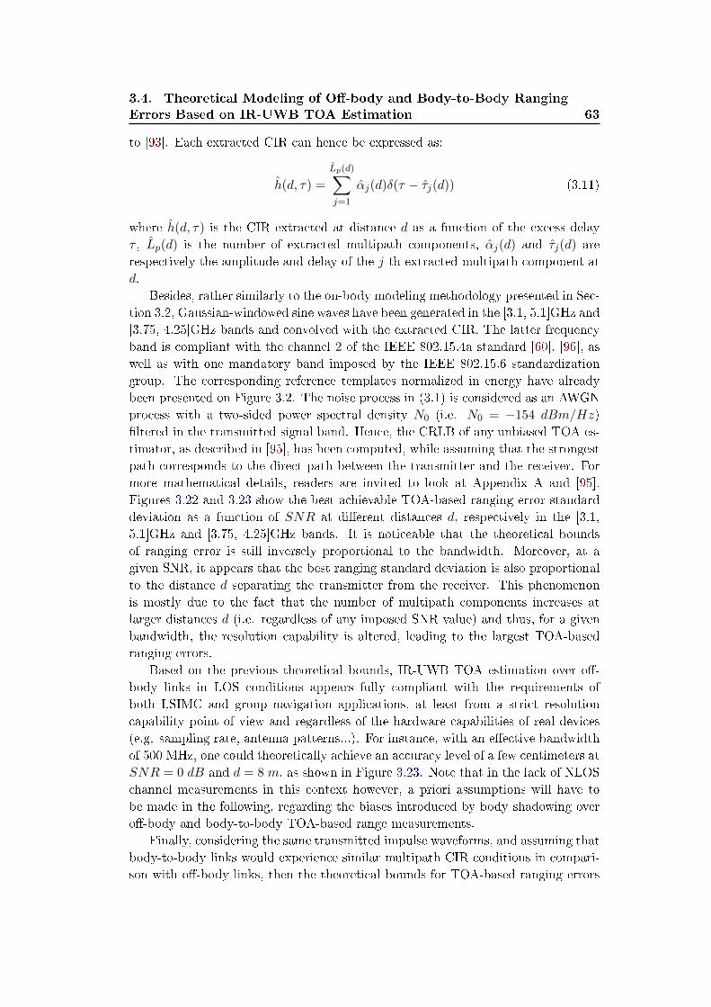
3.4. Theoretical Modeling of O�-body and Body-to-Body Ranging
Errors Based on IR-UWB TOA Estimation 63
to [93]. Each extracted CIR can hence be expressed as:
h(d, τ) =
Lp(d)∑j=1
αj(d)δ(τ − τj(d)) (3.11)
where h(d, τ) is the CIR extracted at distance d as a function of the excess delay
τ , Lp(d) is the number of extracted multipath components, αj(d) and τj(d) are
respectively the amplitude and delay of the j-th extracted multipath component at
d.
Besides, rather similarly to the on-body modeling methodology presented in Sec-
tion 3.2, Gaussian-windowed sine waves have been generated in the [3.1, 5.1]GHz and
[3.75, 4.25]GHz bands and convolved with the extracted CIR. The latter frequency
band is compliant with the channel 2 of the IEEE 802.15.4a standard [60], [96], as
well as with one mandatory band imposed by the IEEE 802.15.6 standardization
group. The corresponding reference templates normalized in energy have already
been presented on Figure 3.2. The noise process in (3.1) is considered as an AWGN
process with a two-sided power spectral density N0 (i.e. N0 = −154 dBm/Hz)
�ltered in the transmitted signal band. Hence, the CRLB of any unbiased TOA es-
timator, as described in [95], has been computed, while assuming that the strongest
path corresponds to the direct path between the transmitter and the receiver. For
more mathematical details, readers are invited to look at Appendix A and [95].
Figures 3.22 and 3.23 show the best achievable TOA-based ranging error standard
deviation as a function of SNR at di�erent distances d, respectively in the [3.1,
5.1]GHz and [3.75, 4.25]GHz bands. It is noticeable that the theoretical bounds
of ranging error is still inversely proportional to the bandwidth. Moreover, at a
given SNR, it appears that the best ranging standard deviation is also proportional
to the distance d separating the transmitter from the receiver. This phenomenon
is mostly due to the fact that the number of multipath components increases at
larger distances d (i.e. regardless of any imposed SNR value) and thus, for a given
bandwidth, the resolution capability is altered, leading to the largest TOA-based
ranging errors.
Based on the previous theoretical bounds, IR-UWB TOA estimation over o�-
body links in LOS conditions appears fully compliant with the requirements of
both LSIMC and group navigation applications, at least from a strict resolution
capability point of view and regardless of the hardware capabilities of real devices
(e.g. sampling rate, antenna patterns...). For instance, with an e�ective bandwidth
of 500 MHz, one could theoretically achieve an accuracy level of a few centimeters at
SNR = 0 dB and d = 8 m, as shown in Figure 3.23. Note that in the lack of NLOS
channel measurements in this context however, a priori assumptions will have to
be made in the following, regarding the biases introduced by body shadowing over
o�-body and body-to-body TOA-based range measurements.
Finally, considering the same transmitted impulse waveforms, and assuming that
body-to-body links would experience similar multipath CIR conditions in compari-
son with o�-body links, then the theoretical bounds for TOA-based ranging errors
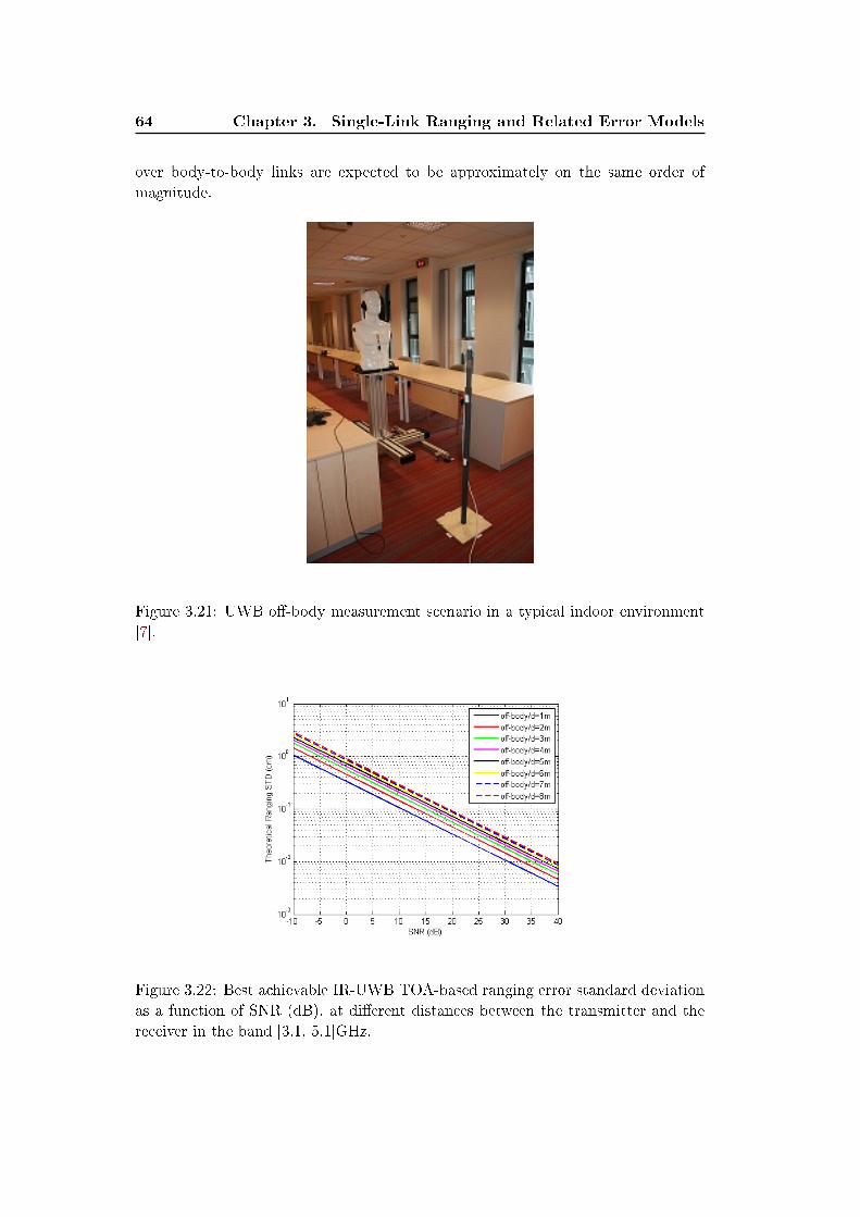
64 Chapter 3. Single-Link Ranging and Related Error Models
over body-to-body links are expected to be approximately on the same order of
magnitude.
Figure 3.21: UWB o�-body measurement scenario in a typical indoor environment
[7].
Figure 3.22: Best achievable IR-UWB TOA-based ranging error standard deviation
as a function of SNR (dB), at di�erent distances between the transmitter and the
receiver in the band [3.1, 5.1]GHz.
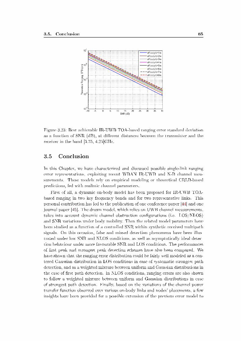
3.5. Conclusion 65
Figure 3.23: Best achievable IR-UWB TOA-based ranging error standard deviation
as a function of SNR (dB), at di�erent distances between the transmitter and the
receiver in the band [3.75, 4.25]GHz.
3.5 Conclusion
In this Chapter, we have characterized and discussed possible single-link ranging
error representations, exploiting recent WBAN IR-UWB and N-B channel mea-
surements. These models rely on empirical modeling or theoretical CRLB-based
predictions, fed with realistic channel parameters.
First of all, a dynamic on-body model has been proposed for IR-UWB TOA-
based ranging in two key frequency bands and for two representative links. This
personal contribution has led to the publication of one conference paper [44] and one
journal paper [45]. The drawn model, which relies on UWB channel measurements,
takes into account dynamic channel obstruction con�gurations (i.e. LOS/NLOS)
and SNR variations under body mobility. Then the related model parameters have
been studied as a function of a controlled SNR within synthetic received multipath
signals. On this occasion, false and missed detection phenomena have been illus-
trated under low SNR and NLOS conditions, as well as asymptotically ideal detec-
tion behaviour under more favourable SNR and LOS conditions. The performances
of �rst peak and strongest peak detection schemes have also been compared. We
have shown that the ranging error distribution could be fairly well modeled as a cen-
tered Gaussian distribution in LOS conditions in case of systematic strongest path
detection, and as a weighted mixture between uniform and Gaussian distributions in
the case of �rst path detection. In NLOS conditions, ranging errors are also shown
to follow a weighted mixture between uniform and Gaussian distributions in case
of strongest path detection. Finally, based on the variations of the channel power
transfer function observed over various on-body links and nodes' placements, a few
insights have been provided for a possible extension of the previous error model to
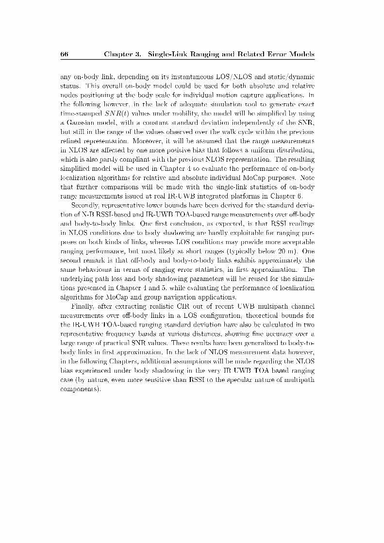
66 Chapter 3. Single-Link Ranging and Related Error Models
any on-body link, depending on its instantaneous LOS/NLOS and static/dynamic
status. This overall on-body model could be used for both absolute and relative
nodes positioning at the body scale for individual motion capture applications. In
the following however, in the lack of adequate simulation tool to generate exact
time-stamped SNR(t) values under mobility, the model will be simpli�ed by using
a Gaussian model, with a constant standard deviation independently of the SNR,
but still in the range of the values observed over the walk cycle within the previous
re�ned representation. Moreover, it will be assumed that the range measurements
in NLOS are a�ected by one more positive bias that follows a uniform distribution,
which is also partly compliant with the previous NLOS representation. The resulting
simpli�ed model will be used in Chapter 4 to evaluate the performance of on-body
localization algorithms for relative and absolute individual MoCap purposes. Note
that further comparisons will be made with the single-link statistics of on-body
range measurements issued at real IR-UWB integrated platforms in Chapter 6.
Secondly, representative lower bounds have been derived for the standard devia-
tion of N-B RSSI-based and IR-UWB TOA-based range measurements over o�-body
and body-to-body links. One �rst conclusion, as expected, is that RSSI readings
in NLOS conditions due to body shadowing are hardly exploitable for ranging pur-
poses on both kinds of links, whereas LOS conditions may provide more acceptable
ranging performance, but most likely at short ranges (typically below 20 m). One
second remark is that o�-body and body-to-body links exhibit approximately the
same behaviours in terms of ranging error statistics, in �rst approximation. The
underlying path loss and body shadowing parameters will be reused for the simula-
tions presented in Chapter 4 and 5, while evaluating the performance of localization
algorithms for MoCap and group navigation applications.
Finally, after extracting realistic CIR out of recent UWB multipath channel
measurements over o�-body links in a LOS con�guration, theoretical bounds for
the IR-UWB TOA-based ranging standard deviation have also be calculated in two
representative frequency bands at various distances, showing �ne accuracy over a
large range of practical SNR values. These results have been generalized to body-to-
body links in �rst approximation. In the lack of NLOS measurement data however,
in the following Chapters, additional assumptions will be made regarding the NLOS
bias experienced under body shadowing in the very IR-UWB TOA-based ranging
case (by nature, even more sensitive than RSSI to the specular nature of multipath
components).

3.5. Conclusion 67
4

Chapter 4
Localization Algorithms for
Individual Motion Capture
Contents
4.1 Introduction . . . . . . . . . . . . . . . . . . . . . . . . . . . . 69
4.2 Relative On-Body Localization at the Body Scale . . . . . . 71
4.2.1 Relative Localization Algorithms . . . . . . . . . . . . . . . . 71
4.2.2 Medium Access Control For Localization-Enabled WBAN . . 77
4.2.3 Simulations and Results . . . . . . . . . . . . . . . . . . . . . 78
4.3 Large-Scale Absolute On-Body Localization . . . . . . . . . 86
4.3.1 Absolute Localization Algorithms . . . . . . . . . . . . . . . . 87
4.3.2 Distance Approximation and Completion Over Neighborhood
Graph . . . . . . . . . . . . . . . . . . . . . . . . . . . . . . . 90
4.3.3 Simulations and Results . . . . . . . . . . . . . . . . . . . . . 91
4.4 Conclusion . . . . . . . . . . . . . . . . . . . . . . . . . . . . . 95
4.1 Introduction
Under mesh or quasi-mesh WBAN topologies (possibly coupled with o�-body links
with respect to the infrastructure), mobile on-body nodes can be localized in a
cooperative fashion out of peer-to-peer range measurements. As seen in Chapter 1,
the enabled individual MoCap applications can be classi�ed according to the two
following categories.
• "Relative On-Body Nodes Positioning" (i.e. relative MoCap): On-body mo-
bile (or blind) nodes are located relatively to reference anchor nodes, which
are attached onto the body at known and reproducible positions (i.e. inde-
pendently of the body attitude and/or direction), forming a Local Coordinate
System (LCS);
• "Absolute On-Body Nodes Positioning" (i.e. LSIMC): The Global Coordi-
nates System (GCS) used to express the estimated on-body nodes' locations
is no longer body-strapped but external to the body. Anchor nodes are �xed
elements of infrastructure disseminated at known locations in the environ-
ment.
70 Chapter 4. Localization Algorithms for Individual Motion Capture
In this new Chapter, we describe and evaluate (through simulations) some local-
ization algorithms adapted to the relative and/or absolute positioning of on-body
nodes.
Section 4.2 deals with relative positioning �rst. A decentralized DWMDS local-
ization algorithm [65], [97] is adapted into the new body sensor network context.
Accordingly, on-body nodes are asynchronously updated with respect to their 1-hop
neighbors in a body-strapped LCS. This approach is expected to provide better
immunity against the latency observed within classical centralized and synchronous
schemes, while enabling adaptability to local nodes velocity (e.g. in terms of re-
freshment rate). The nominal algorithm is fed with all the cooperative peer-to-peer
distance measurements available in our mesh topology. According to one �rst en-
hancement, one incorporates the links that experience �xed lengths despite body
mobility (e.g. between the hand's wrist and the elbow) as geometrical constraints in
the positioning problem, thus leading to a Constrained algorithm (CDWMDS). This
solution tends to limit the number of required on-line measurements and hence, to
reduce over-the-air tra�c and power consumption. Furthermore, while updating the
locations of on-body nodes, the history of the latest estimates is used as prior in-
formation, so as to ease convergence and bene�t from space-time correlation e�ects
under continuous body movements. We also describe additional improvements of
the nominal CDWMDS formulation in this section. One of them consists in applying
unilateral censoring and/or scheduling of the most demanding nodes when updat-
ing estimated positions. Another point is to force the measurements symmetry for
each pair of on-body nodes. The idea is to mitigate the e�ect of outliers or packet
losses, but also to avoid error propagation and divergence issues in the retained
decentralized positioning approach. Then, we apply an existing beacon-aided Time
Division Multiple Access (TDMA) scheme that supports both peer-to-peer rang-
ing and decentralized positioning transactions under real-time constraints. On this
occasion, we make possible a more realistic performance assessment of the algo-
rithm, while accounting for underlying latency issues and investigating the impact
of network connectivity or measurements quality. Finally, we compare our solution
with a more conventional Multidimensional Scaling (MDS) algorithm, which has
been recently considered for MoCap applications in a similar WBAN context [61].
Note that the latter requires that the matrix of measured distances is completed
under partial network connectivity, contrarily to our proposed asynchronous and
decentralized approach.
Secondly, Section 4.3 concerns absolute positioning for LSIMC applications. We
consider combining relative motion capture (i.e. at the body scale) and absolute
single-user navigation (i.e. at the building scale) capabilities within an heteroge-
neous WBAN context. One goal is that o�-body localization procedures could
mutually bene�t from each other, while preserving the �nest precision of relative
localization over large-scale trajectories, contrarily to the �rst cooperative localiza-
tion attempt in [8], where the precision of relative localization at the body scale
was degraded by the introduction of o�-body links. Di�erent options and scenarios
are then compared in terms of location-dependent radio metrics (i.e. TOA, TDOA,
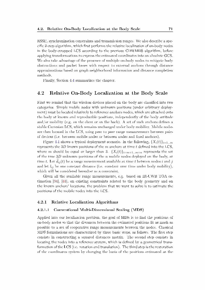
4.2. Relative On-Body Localization at the Body Scale 71
RSSI), synchronization constraints and transmission ranges. We also describe a spe-
ci�c 2-step algorithm, which �rst performs the relative localization of on-body nodes
in the body-strapped LCS according to the previous CDWMDS algorithm, before
applying transformations to express the estimated coordinates into an absolute GCS.
We also take advantage of the presence of multiple on-body nodes to mitigate body
obstructions and packet losses with respect to external anchors through distance
approximations based on graph neighborhood information and distance completion
methods.
Finally, Section 4.4 summarizes the chapter.
4.2 Relative On-Body Localization at the Body Scale
First we remind that the wireless devices placed on the body are classi�ed into two
categories. Simple mobile nodes with unknown positions (under arbitrary deploy-
ment) must be located relatively to reference anchors nodes, which are attached onto
the body at known and reproducible positions, independently of the body attitude
and/or mobility (e.g. on the chest or on the back). A set of such anchors de�nes a
stable Cartesian LCS, which remains unchanged under body mobility. Mobile nodes
are then located in the LCS, using peer-to-peer range measurements between pairs
of devices (i.e. between mobile nodes or between nodes and �xed anchors).
Figure 4.1 shows a typical deployment scenario. In the following, {Xi(t)}i=1...m
represents the 3D known positions of the m anchors at time t de�ned into the LCS,
where m should be equal or larger than 3. {Xi(t)}i=m+1...m+n represents the set
of the true 3D unknown positions of the n mobile nodes deployed on the body, at
time t. Let dij(t) be a range measurement available at time t between nodes i and j
and let lij be one constant distance (i.e. constant over time under body mobility),
which will be considered hereafter as a constraint.
Given all the available range measurements, e.g. based on IR-UWB TOA es-
timation [34], [44], on existing constraints related to the body geometry and on
the known anchors' locations, the problem that we want to solve is to estimate the
positions of the mobile nodes into the LCS.
4.2.1 Relative Localization Algorithms
4.2.1.1 Conventional Multi-Dimensional Scaling (MDS)
Applied into our localization problem, the goal of MDS is to �nd the positions of
on-body nodes so that the distances between the estimated positions �t as much as
possible to a set of cooperative range measurements between the nodes. Classical
MDS formulations are characterized by three basic steps, as follows. The �rst step
consists in constructing a squared distances matrix. The second step consists in
locating the nodes into a reference system, which is de�ned by a geometrical trans-
formation of the LCS (i.e. rotation and translation). The third step is the restoration
of the coordinates system by changing the basis of the positions estimated at the
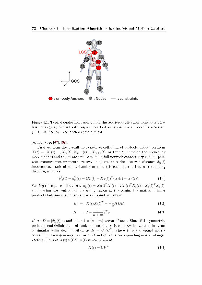
72 Chapter 4. Localization Algorithms for Individual Motion Capture
Figure 4.1: Typical deployment scenario for the relative localization of on-body wire-
less nodes (grey circles) with respect to a body-strapped Local Coordinate System
(LCS) de�ned by �xed anchors (red circles).
second stage [67], [98].
First we form the overall network-level collection of on-body nodes' positions
X(t) = [X1(t), ..., Xm(t), Xm+1(t)..., Xm+n(t)] at time t, including the n on-body
mobile nodes and the m anchors. Assuming full network connectivity (i.e. all pair-
wise distance measurements are available) and that the observed distance δij(t)
between each pair of nodes i and j at time t is equal to the true corresponding
distance, it comes:
δ2ij(t) = d2ij(t) = (Xi(t)−Xj(t))T (Xi(t)−Xj(t)) (4.1)
Writing the squared distance as d2ij(t) = Xi(t)TXi(t)−2Xi(t)
TXj(t)+Xj(t)TXj(t),
and placing the centroid of the con�guration at the origin, the matrix of inner
products between the nodes can be expressed as follows:
B = X(t)X(t)T = −1
2HDH (4.2)
H = I − 1
n+meTe (4.3)
where D = [d2ij(t)]i,j and e is a 1 × (n + m) vector of ones. Since B is symmetric,
positive semi-de�nite and of rank dimensionality, it can now be written in terms
of singular value decomposition as B = UV UT , where V is a diagonal matrix
containing the n+m eigen values of B and U is the corresponding matrix of eigen
vectors. Thus as X(t)X(t)T , X(t) is now given as:
X(t) = UV12 (4.4)
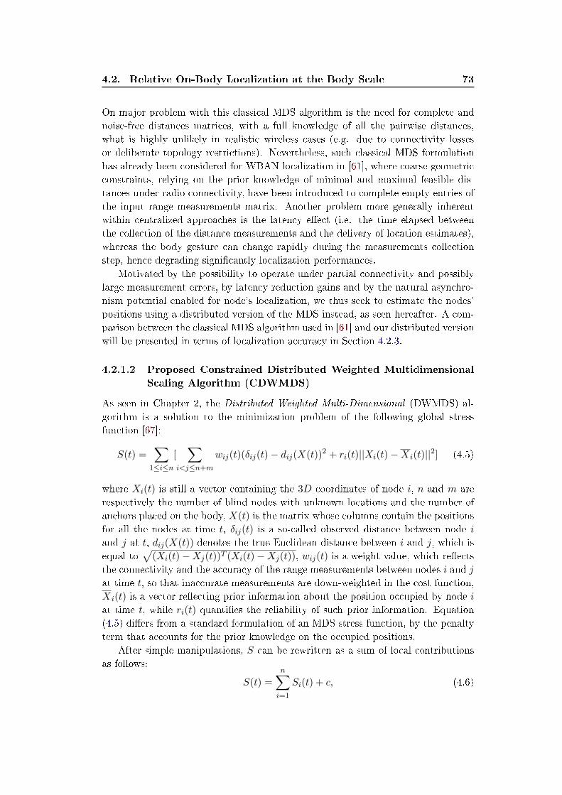
4.2. Relative On-Body Localization at the Body Scale 73
On major problem with this classical MDS algorithm is the need for complete and
noise-free distances matrices, with a full knowledge of all the pairwise distances,
what is highly unlikely in realistic wireless cases (e.g. due to connectivity losses
or deliberate topology restrictions). Nevertheless, such classical MDS formulation
has already been considered for WBAN localization in [61], where coarse geometric
constraints, relying on the prior knowledge of minimal and maximal feasible dis-
tances under radio connectivity, have been introduced to complete empty entries of
the input range measurements matrix. Another problem more generally inherent
within centralized approaches is the latency e�ect (i.e. the time elapsed between
the collection of the distance measurements and the delivery of location estimates),
whereas the body gesture can change rapidly during the measurements collection
step, hence degrading signi�cantly localization performances.
Motivated by the possibility to operate under partial connectivity and possibly
large measurement errors, by latency reduction gains and by the natural asynchro-
nism potential enabled for node's localization, we thus seek to estimate the nodes'
positions using a distributed version of the MDS instead, as seen hereafter. A com-
parison between the classical MDS algorithm used in [61] and our distributed version
will be presented in terms of localization accuracy in Section 4.2.3.
4.2.1.2 Proposed Constrained Distributed Weighted Multidimensional
Scaling Algorithm (CDWMDS)
As seen in Chapter 2, the Distributed Weighted Multi-Dimensional (DWMDS) al-
gorithm is a solution to the minimization problem of the following global stress
function [67]:
S(t) =∑
1≤i≤n[∑
i<j≤n+mwij(t)(δij(t)− dij(X(t))2 + ri(t)||Xi(t)−Xi(t)||2] (4.5)
where Xi(t) is still a vector containing the 3D coordinates of node i, n and m are
respectively the number of blind nodes with unknown locations and the number of
anchors placed on the body, X(t) is the matrix whose columns contain the positions
for all the nodes at time t, δij(t) is a so-called observed distance between node i
and j at t, dij(X(t)) denotes the true Euclidean distance between i and j, which is
equal to√
(Xi(t)−Xj(t))T (Xi(t)−Xj(t)), wij(t) is a weight value, which re�ects
the connectivity and the accuracy of the range measurements between nodes i and j
at time t, so that inaccurate measurements are down-weighted in the cost function,
Xi(t) is a vector re�ecting prior information about the position occupied by node i
at time t, while ri(t) quanti�es the reliability of such prior information. Equation
(4.5) di�ers from a standard formulation of an MDS stress function, by the penalty
term that accounts for the prior knowledge on the occupied positions.
After simple manipulations, S can be rewritten as a sum of local contributions
as follows:
S(t) =
n∑i=1
Si(t) + c, (4.6)
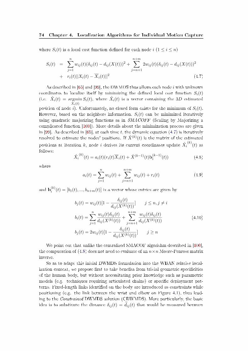
74 Chapter 4. Localization Algorithms for Individual Motion Capture
where Si(t) is a local cost function de�ned for each node i (1 ≤ i ≤ n)
Si(t) =n∑j=1
wij(t)(δij(t)− dij(X(t)))2 +n+m∑j=n+1
2wij(t)(δij(t)− dij(X(t)))2
+ ri(t)||Xi(t)−Xi(t)||2 (4.7)
As described in [65] and [99], the DWMDS thus allows each node i with unknown
coordinates to localize itself by minimizing the de�ned local cost function Si(t)
(i.e. Xi(t) = argminXi(t)
Si(t), where Xi(t) is a vector containing the 3D estimated
position of node i). Unfortunately, no closed form exists for the minimum of Si(t).
However, based on the neighbors information, Si(t) can be minimized iteratively
using quadratic majorizing functions as in SMACOFF (Scaling by Majorizing a
complicated function [100]). More details about the minimization process are given
in [99]. As described in [65], at each time t, the dynamic equation (4.7) is iteratively
resolved to estimate the nodes' positions. If X(k)(t) is the matrix of the estimated
positions at iteration k, node i derives its current coordinates update Xi(k)
(t) as
follows:
Xi(k)
(t) = ai(t)(ri(t)Xi(t) + X(k−1)(t)b(k−1)i (t)) (4.8)
where
ai(t) =n∑j=1
wij(t) +n+m∑j=n+1
wij(t) + ri(t) (4.9)
and b(k)i (t) = [b1(t), ..., bn+m(t)] is a vector whose entries are given by
bj(t) = wij(t)[1−δij(t)
dij(X(k)(t))] j ≤ n, j 6= i
bi(t) =
n∑j=1
wij(t)δij(t)
dij(X(k)(t))+
n+m∑j=n+1
wij(t)δij(t)
dij(X(k)(t))
bj(t) = 2wij(t)[1−δij(t)
dij(X(k)(t))] j ≥ n
(4.10)
We point out that unlike the centralized SMACOF algorithm described in [100],
the computation of (4.8) does not need to evaluate of an n×nMoore-Penrose matrix
inverse.
So as to adapt this initial DWMDS formulation into the WBAN relative local-
ization context, we propose �rst to take bene�ts from trivial geometric speci�cities
of the human body, but without necessitating prior knowledge such as parametric
models (e.g. techniques requiring articulated chains) or speci�c deployment pat-
terns. Fixed-length links identi�ed on the body are introduced as constraints while
positioning (e.g. the link between the wrist and elbow on Figure 4.1), thus lead-
ing to the Constrained DWMDS solution (CDWMDS). More particularly, the basic
idea is to substitute the distance δij(t) = dij(t) that would be measured between
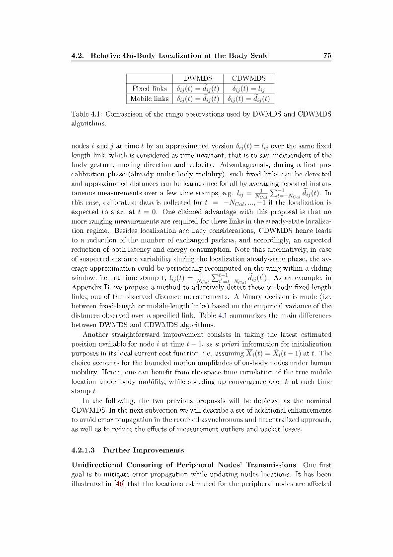
4.2. Relative On-Body Localization at the Body Scale 75
DWMDS CDWMDS
Fixed links δij(t) = dij(t) δij(t) = lij
Mobile links δij(t) = dij(t) δij(t) = dij(t)
Table 4.1: Comparison of the range observations used by DWMDS and CDWMDS
algorithms.
nodes i and j at time t by an approximated version δij(t) = lij over the same �xed
length link, which is considered as time invariant, that is to say, independent of the
body gesture, moving direction and velocity. Advantageously, during a �rst pre-
calibration phase (already under body mobility), such �xed links can be detected
and approximated distances can be learnt once for all by averaging repeated instan-
taneous measurements over a few time stamps, e.g. lij = 1NCal
∑−1t=−NCal
dij(t). In
this case, calibration data is collected for t = −NCal, ...,−1 if the localization is
expected to start at t = 0. One claimed advantage with this proposal is that no
more ranging measurements are required for these links in the steady-state localiza-
tion regime. Besides localization accuracy considerations, CDWMDS hence leads
to a reduction of the number of exchanged packets, and accordingly, an expected
reduction of both latency and energy consumption. Note that alternatively, in case
of suspected distance variability during the localization steady-state phase, the av-
erage approximation could be periodically recomputed on the wing within a sliding
window, i.e. at time stamp t, lij(t) = 1NCal
∑t−1t′=t−NCal
dij(t′). As an example, in
Appendix B, we propose a method to adaptively detect these on-body �xed-length
links, out of the observed distance measurements. A binary decision is made (i.e.
between �xed-length or mobile-length links) based on the empirical variance of the
distances observed over a speci�ed link. Table 4.1 summarizes the main di�erences
between DWMDS and CDWMDS algorithms.
Another straightforward improvement consists in taking the latest estimated
position available for node i at time t− 1, as a priori information for initialization
purposes in its local current cost function, i.e. assuming Xi(t) = Xi(t− 1) at t. The
choice accounts for the bounded motion amplitudes of on-body nodes under human
mobility. Hence, one can bene�t from the space-time correlation of the true mobile
location under body mobility, while speeding up convergence over k at each time
stamp t.
In the following, the two previous proposals will be depicted as the nominal
CDWMDS. In the next subsection we will describe a set of additional enhancements
to avoid error propagation in the retained asynchronous and decentralized approach,
as well as to reduce the e�ects of measurement outliers and packet losses.
4.2.1.3 Further Improvements
Unidirectional Censoring of Peripheral Nodes' Transmissions One �rst
goal is to mitigate error propagation while updating nodes locations. It has been
illustrated in [46] that the locations estimated for the peripheral nodes are a�ected
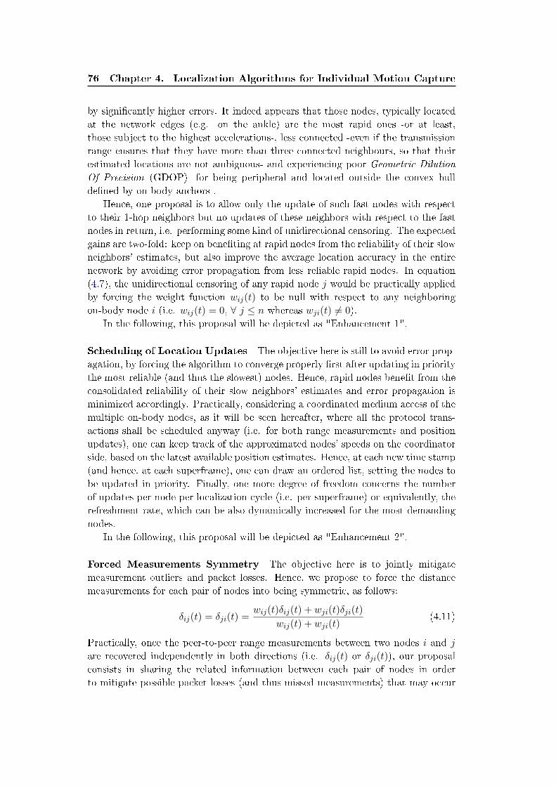
76 Chapter 4. Localization Algorithms for Individual Motion Capture
by signi�cantly higher errors. It indeed appears that those nodes, typically located
at the network edges (e.g. on the ankle) are the most rapid ones -or at least,
those subject to the highest accelerations-, less connected -even if the transmission
range ensures that they have more than three connected neighbours, so that their
estimated locations are not ambiguous- and experiencing poor Geometric Dilution
Of Precision (GDOP) -for being peripheral and located outside the convex hull
de�ned by on-body anchors-.
Hence, one proposal is to allow only the update of such fast nodes with respect
to their 1-hop neighbors but no updates of these neighbors with respect to the fast
nodes in return, i.e. performing some kind of unidirectional censoring. The expected
gains are two-fold: keep on bene�ting at rapid nodes from the reliability of their slow
neighbors' estimates, but also improve the average location accuracy in the entire
network by avoiding error propagation from less reliable rapid nodes. In equation
(4.7), the unidirectional censoring of any rapid node j would be practically applied
by forcing the weight function wij(t) to be null with respect to any neighboring
on-body node i (i.e. wij(t) = 0, ∀ j ≤ n whereas wji(t) 6= 0).
In the following, this proposal will be depicted as "Enhancement 1".
Scheduling of Location Updates The objective here is still to avoid error prop-
agation, by forcing the algorithm to converge properly �rst after updating in priority
the most reliable (and thus the slowest) nodes. Hence, rapid nodes bene�t from the
consolidated reliability of their slow neighbors' estimates and error propagation is
minimized accordingly. Practically, considering a coordinated medium access of the
multiple on-body nodes, as it will be seen hereafter, where all the protocol trans-
actions shall be scheduled anyway (i.e. for both range measurements and position
updates), one can keep track of the approximated nodes' speeds on the coordinator
side, based on the latest available position estimates. Hence, at each new time stamp
(and hence, at each superframe), one can draw an ordered list, setting the nodes to
be updated in priority. Finally, one more degree of freedom concerns the number
of updates per node per localization cycle (i.e. per superframe) or equivalently, the
refreshment rate, which can be also dynamically increased for the most demanding
nodes.
In the following, this proposal will be depicted as "Enhancement 2".
Forced Measurements Symmetry The objective here is to jointly mitigate
measurement outliers and packet losses. Hence, we propose to force the distance
measurements for each pair of nodes into being symmetric, as follows:
δij(t) = δji(t) =wij(t)δij(t) + wji(t)δji(t)
wij(t) + wji(t)(4.11)
Practically, once the peer-to-peer range measurements between two nodes i and j
are recovered independently in both directions (i.e. δij(t) or δji(t)), our proposal
consists in sharing the related information between each pair of nodes in order
to mitigate possible packet losses (and thus missed measurements) that may occur
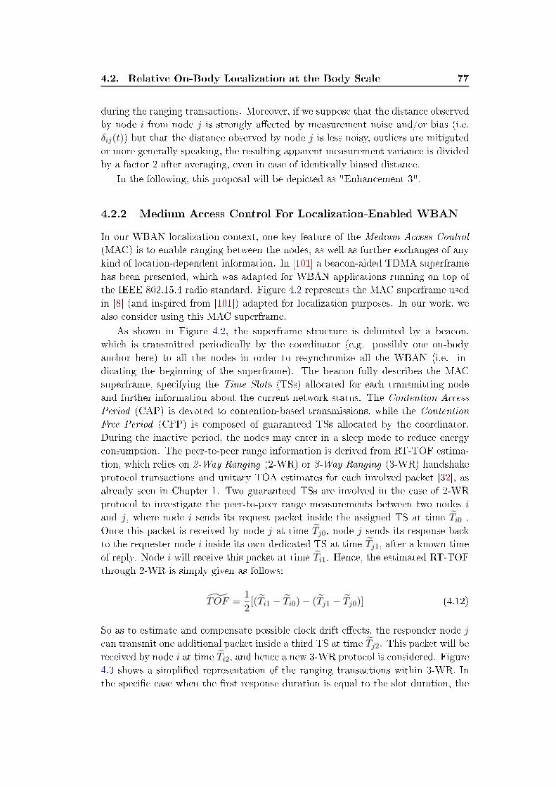
4.2. Relative On-Body Localization at the Body Scale 77
during the ranging transactions. Moreover, if we suppose that the distance observed
by node i from node j is strongly a�ected by measurement noise and/or bias (i.e.
δij(t)) but that the distance observed by node j is less noisy, outliers are mitigated
or more generally speaking, the resulting apparent measurement variance is divided
by a factor 2 after averaging, even in case of identically biased distance.
In the following, this proposal will be depicted as "Enhancement 3".
4.2.2 Medium Access Control For Localization-Enabled WBAN
In our WBAN localization context, one key feature of the Medium Access Control
(MAC) is to enable ranging between the nodes, as well as further exchanges of any
kind of location-dependent information. In [101] a beacon-aided TDMA superframe
has been presented, which was adapted for WBAN applications running on top of
the IEEE 802.15.4 radio standard. Figure 4.2 represents the MAC superframe used
in [8] (and inspired from [101]) adapted for localization purposes. In our work, we
also consider using this MAC superframe.
As shown in Figure 4.2, the superframe structure is delimited by a beacon,
which is transmitted periodically by the coordinator (e.g. possibly one on-body
anchor here) to all the nodes in order to resynchronize all the WBAN (i.e. in-
dicating the beginning of the superframe). The beacon fully describes the MAC
superframe, specifying the Time Slots (TSs) allocated for each transmitting node
and further information about the current network status. The Contention Access
Period (CAP) is devoted to contention-based transmissions, while the Contention
Free Period (CFP) is composed of guaranteed TSs allocated by the coordinator.
During the inactive period, the nodes may enter in a sleep mode to reduce energy
consumption. The peer-to-peer range information is derived from RT-TOF estima-
tion, which relies on 2-Way Ranging (2-WR) or 3-Way Ranging (3-WR) handshake
protocol transactions and unitary TOA estimates for each involved packet [32], as
already seen in Chapter 1. Two guaranteed TSs are involved in the case of 2-WR
protocol to investigate the peer-to-peer range measurements between two nodes i
and j, where node i sends its request packet inside the assigned TS at time Ti0 .
Once this packet is received by node j at time Tj0, node j sends its response back
to the requester node i inside its own dedicated TS at time Tj1, after a known time
of reply. Node i will receive this packet at time Ti1. Hence, the estimated RT-TOF
through 2-WR is simply given as follows:
TOF =1
2[(Ti1 − Ti0)− (Tj1 − Tj0)] (4.12)
So as to estimate and compensate possible clock drift e�ects, the responder node j
can transmit one additional packet inside a third TS at time Tj2. This packet will be
received by node i at time Ti2, and hence a new 3-WR protocol is considered. Figure
4.3 shows a simpli�ed representation of the ranging transactions within 3-WR. In
the speci�c case when the �rst response duration is equal to the slot duration, the
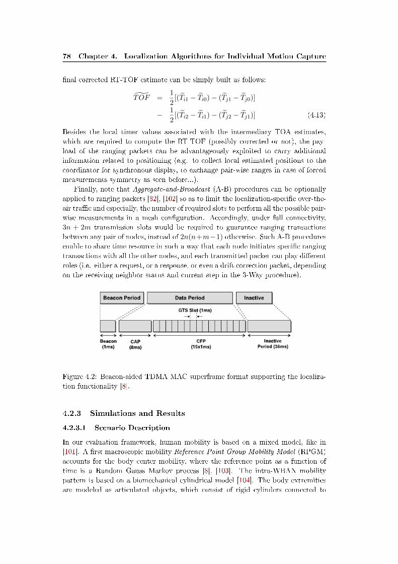
78 Chapter 4. Localization Algorithms for Individual Motion Capture
�nal corrected RT-TOF estimate can be simply built as follows:
TOF =1
2[(Ti1 − Ti0)− (Tj1 − Tj0)]
− 1
2[(Ti2 − Ti1)− (Tj2 − Tj1)] (4.13)
Besides the local timer values associated with the intermediary TOA estimates,
which are required to compute the RT-TOF (possibly corrected or not), the pay-
load of the ranging packets can be advantageously exploited to carry additional
information related to positioning (e.g. to collect local estimated positions to the
coordinator for synchronous display, to exchange pair-wise ranges in case of forced
measurements symmetry as seen before...).
Finally, note that Aggregate-and-Broadcast (A-B) procedures can be optionally
applied to ranging packets [32], [102] so as to limit the localization-speci�c over-the-
air tra�c and especially, the number of required slots to perform all the possible pair-
wise measurements in a mesh con�guration. Accordingly, under full connectivity,
3n + 2m transmission slots would be required to guarantee ranging transactions
between any pair of nodes, instead of 2n(n+m−1) otherwise. Such A-B procedures
enable to share time resource in such a way that each node initiates speci�c ranging
transactions with all the other nodes, and each transmitted packet can play di�erent
roles (i.e. either a request, or a response, or even a drift correction packet, depending
on the receiving neighbor status and current step in the 3-Way procedure).
Figure 4.2: Beacon-aided TDMA MAC superframe format supporting the localiza-
tion functionality [8].
4.2.3 Simulations and Results
4.2.3.1 Scenario Description
In our evaluation framework, human mobility is based on a mixed model, like in
[101]. A �rst macroscopic mobility Reference Point Group Mobility Model (RPGM)
accounts for the body center mobility, where the reference point as a function of
time is a Random Gauss Markov process [8], [103]. The intra-WBAN mobility
pattern is based on a biomechanical cylindrical model [104]. The body extremities
are modeled as articulated objects, which consist of rigid cylinders connected to
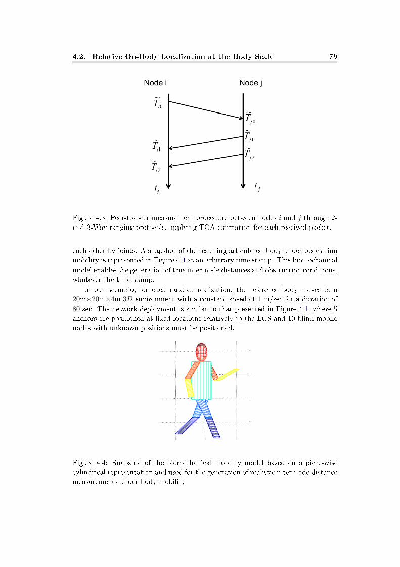
4.2. Relative On-Body Localization at the Body Scale 79
Figure 4.3: Peer-to-peer measurement procedure between nodes i and j through 2-
and 3-Way ranging protocols, applying TOA estimation for each received packet.
each other by joints. A snapshot of the resulting articulated body under pedestrian
mobility is represented in Figure 4.4 at an arbitrary time stamp. This biomechanical
model enables the generation of true inter-node distances and obstruction conditions,
whatever the time stamp.
In our scenario, for each random realization, the reference body moves in a
20m×20m×4m 3D environment with a constant speed of 1 m/sec for a duration of
80 sec. The network deployment is similar to that presented in Figure 4.1, where 5
anchors are positioned at �xed locations relatively to the LCS and 10 blind mobile
nodes with unknown positions must be positioned.
Figure 4.4: Snapshot of the biomechanical mobility model based on a piece-wise
cylindrical representation and used for the generation of realistic inter-node distance
measurements under body mobility.
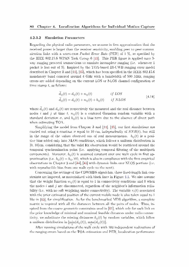
80 Chapter 4. Localization Algorithms for Individual Motion Capture
4.2.3.2 Simulation Parameters
Regarding the physical radio parameters, we assume in �rst approximation that the
received power is larger than the receiver sensitivity, enabling peer-to-peer commu-
nication links with a worst-case Packet Error Rate (PER) of 1 %, as speci�ed by
the IEEE 802.15.6 WPAN Task Group 6 [11]. This PER �gure is applied onto 3-
way ranging protocol transactions to emulate incomplete ranging (i.e. whenever 1
packet is lost out of 3). Inspired by the TOA-based IR-UWB ranging error model
described in Chapter 3 and [44], [45], which has been speci�ed in the IEEE 802.15.6
mandatory band centered around 4 GHz with a bandwidth of 500 MHz, ranging
errors are added depending on the current LOS or NLOS channel con�guration at
time stamp t, as follows:
dij(t) = dij(t) + nij(t) if LOS
dij(t) = dij(t) + nij(t) + bij(t) if NLOS(4.14)
where dij(t) and dij(t) are respectively the measured and the real distance between
nodes i and j at time t, nij(t) is a centered Gaussian random variable with a
standard deviation σ, and bij(t) is a bias term due to the absence of direct path
when estimating TOA.
Simplifying the model from Chapter 3 and [44], [45], our �rst simulations are
carried out using a constant σ equal to 10 cm, independently of SNR(t), but still
in the range of the values observed out of real measurements. bij(t) is a posi-
tive bias added only into NLOS conditions, which follows a uniform distribution in
[0, 10]cm, considering that the valid Rx observation would be restricted around the
temporal synchronization point (i.e. applying temporal �ltering of the multipath
components). Moreover, bij(t) is assumed constant over one walk cycle in �rst ap-
proximation (i.e. bij(t) = bij , ∀t), which is also in compliance with the �rst empiricalobservations in Chapter 3 and [44], [45] with dynamic links over NLOS portions (i.e.
with reproducible bias from one walk cycle to the next).
Concerning the settings of the CDWMDS algorithm, three �xed-length link con-
straints are imposed, as materialized with black lines in Figure 4.1. We also assume
that the weight function wij(t) is equal to 1 in connectivity conditions and 0 when
the nodes i and j are disconnected, regardless of the neighbor's information relia-
bility (i.e. with no soft weighting under connectivity). The variable ri(t) associated
with the prior estimated position of the current mobile node is also taken equal to 1
like in [65], for simpli�cation. As for the benchmarked MDS algorithm, a complete
matrix is required with all the distances between all the pairs of nodes. Thus, in-
spired from the coarse geometric constraints used in [61], which rely for each link on
the prior knowledge of minimal and maximal feasible distances under radio connec-
tivity, we substitute the missing distances δij(t) by random variables, which follow
a uniform distribution in [mint
(dij(t)), maxt
(dij(t))].
After running simulations of the walk cycle with 100 independent realizations of
the ranging errors based on the TOA estimation and PER, localization performance

4.2. Relative On-Body Localization at the Body Scale 81
is assessed in terms of the Root Mean Squared Error (RMSE) per node or average
RMSE (i.e. over all the mobile nodes), while considering di�erent approaches. In a
�rst evaluation, we consider updating the positions with a systematic and regular
refreshment rate of 30 ms, whereas the latency introduced by the exchanged packets
is not taken into account. However, in a second and more realistic approach, we
consider a TDMA MAC superframe similar to that presented in Figure 4.2, where
an Aggregate-and-Broadcast (A-B) procedure is applied to ranging packets to speed
up convergence. Finally, parametric simulation-based studies have also been carried
out in order to assess the performance (over all the on-body nodes) as a function
of the PER and the standard deviation σ of intra-BAN ranging errors in equation
(4.14).
4.2.3.3 Simulation Results
Figure 4.5 shows the RMSE performance per node for the unconstrained DWMDS
and the CDWMDS algorithms. The latter is considered with self-calibrated �xed-
length ranges or exact �xed-length ranges. It is thus rather clear that one can expect
bene�ts from incorporating �xed-length constraints in comparison with the nomi-
nal DWMDS, whatever the considered node. Moreover, no signi�cant degradations
have been observed after self-learning the �xed-length distances (e.g. during a pre-
calibration phase, when each constraint is calculated as the mean of the measured
distances in an observation window of 9 sec) in comparison with a genius-aided intro-
duction of the exact �xed-length distances. Overall, in this case, the average RMSE
(over all the nodes) spans from 26 cm using DWMDS down to 23 cm and 22 cm
using CDWMDS with estimated and true constraints respectively, representing a
relative improvement of 15.4 %.
On Figure 4.6, we compare the RMSE per node of the standard CDWMDS
algorithm (still assuming that any �xed-length constraint is learnt as the mean of
the measured distances in an sliding observation window of 9 sec) with a solution
applying unidirectional censoring of the fastest nodes (i.e. 4 and 6). It is thus
noticeable that such censoring schemes, mitigating error propagation, are globally
e�cient to improve the localization performances of both penalizing and favorable
nodes simultaneously. The average RMSE (i.e. over all the nodes) is for instance
decreased from 23.3 cm down to 19.7 cm, representing one more improvement by
15.4 %.
The e�ect of introducing scheduling in the sequence of location updates is also
illustrated on Figure 4.7. Blue bars represent the localization performance of CD-
WMDS using censoring but random scheduling for the update of nodes' locations,
whereas red bars account for situations when the slowest nodes are updated in pri-
ority and the same fast peripheral nodes (i.e. 4 and 6) are updated later on. The
average RMSE per node then decreases from 19.7 cm down to 17.5 cm, leading to a
11.1 % improvement. Moreover the gain is mainly spectacular for the most poorly
positioned nodes. Note that with such location updates scheduling, the refreshment
rate could be also adjusted depending on the local mobile speed in order to favor
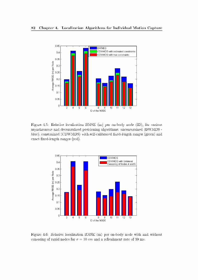
82 Chapter 4. Localization Algorithms for Individual Motion Capture
Figure 4.5: Relative localization RMSE (m) per on-body node (ID), for various
asynchronous and decentralized positioning algorithms: unconstrained (DWMDS -
blue), constrained (CDWMDS) with self-calibrated �xed-length ranges (green) and
exact �xed-length ranges (red).
Figure 4.6: Relative localization RMSE (m) per on-body node with and without
censoring of rapid nodes for σ = 10 cm and a refreshment rate of 30 ms.
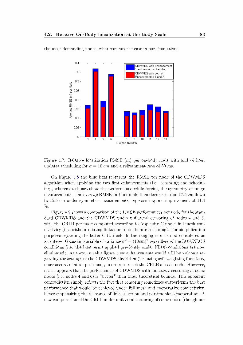
4.2. Relative On-Body Localization at the Body Scale 83
the most demanding nodes, what was not the case in our simulations.
Figure 4.7: Relative localization RMSE (m) per on-body node with and without
updates scheduling for σ = 10 cm and a refreshment rate of 30 ms.
On Figure 4.8 the blue bars represent the RMSE per node of the CDWMDS
algorithm when applying the two �rst enhancements (i.e. censoring and schedul-
ing), whereas red bars show the performance while forcing the symmetry of range
measurements. The average RMSE (m) per node then decreases from 17.5 cm down
to 15.5 cm under symmetric measurements, representing one improvement of 11.4
%.
Figure 4.9 shows a comparison of the RMSE performances per node for the stan-
dard CDWMDS and the CDWMDS under unilateral censoring of nodes 4 and 6,
with the CRLB per node computed according to Appendix C under full mesh con-
nectivity (i.e. without missing links due to deliberate censoring). For simpli�cation
purposes regarding the latter CRLB calculi, the ranging error is now considered as
a centered Gaussian variable of variance σ2 = (10cm)2 regardless of the LOS/NLOS
conditions (i.e. the bias terms applied previously under NLOS conditions are now
eliminated). As shown on this �gure, new enhancements would still be welcome re-
garding the settings of the CDWMDS algorithm (i.e. using soft weighting functions,
more accurate initial positions), in order to reach the CRLB at each node. However,
it also appears that the performance of CDWMDS with unilateral censoring at some
nodes (i.e. nodes 4 and 6) is "better" than those theoretical bounds. This apparent
contradiction simply re�ects the fact that censoring sometimes outperforms the best
performance that would be achieved under full mesh and cooperative connectivity,
hence emphasizing the relevance of links selection and parsimonious cooperation. A
new computation of the CRLB under unilateral censoring of some nodes (though not
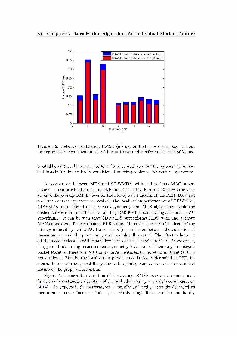
84 Chapter 4. Localization Algorithms for Individual Motion Capture
Figure 4.8: Relative localization RMSE (m) per on-body node with and without
forcing measurements symmetry, with σ = 10 cm and a refreshment rate of 30 ms.
treated herein) would be required for a fairer comparison, but facing possibly numer-
ical instability due to badly conditioned matrix problems, inherent to sparseness.
A comparison between MDS and CDWMDS, with and without MAC super-
frames, is also provided on Figures 4.10 and 4.11. First Figure 4.10 shows the vari-
ation of the average RMSE (over all the nodes) as a function of the PER. Blue, red
and green curves represent respectively the localization performance of CDWMDS,
CDWMDS under forced measurement symmetry and MDS algorithms, while the
dashed curves represent the corresponding RMSE when considering a realistic MAC
superframe. It can be seen that CDWMDS outperforms MDS, with and without
MAC superframe, for each tested PER value. Moreover, the harmful e�ects of the
latency induced by real MAC transactions (in particular between the collection of
measurements and the positioning step) are also illustrated. The e�ect is however
all the more noticeable with centralized approaches, like within MDS. As expected,
it appears that forcing measurements symmetry is also an e�cient way to mitigate
packet losses, outliers or more simply large measurement noise occurrences (even if
not outliers). Finally, the localization performance is slowly degraded as PER in-
creases in our solution, most likely due to the jointly cooperative and decentralized
nature of the proposed algorithm.
Figure 4.11 shows the variation of the average RMSE over all the nodes as a
function of the standard deviation of the on-body ranging errors de�ned in equation
(4.14). As expected, the performance is rapidly and rather strongly degraded as
measurement errors increase. Indeed, the relative single-link errors become hardly
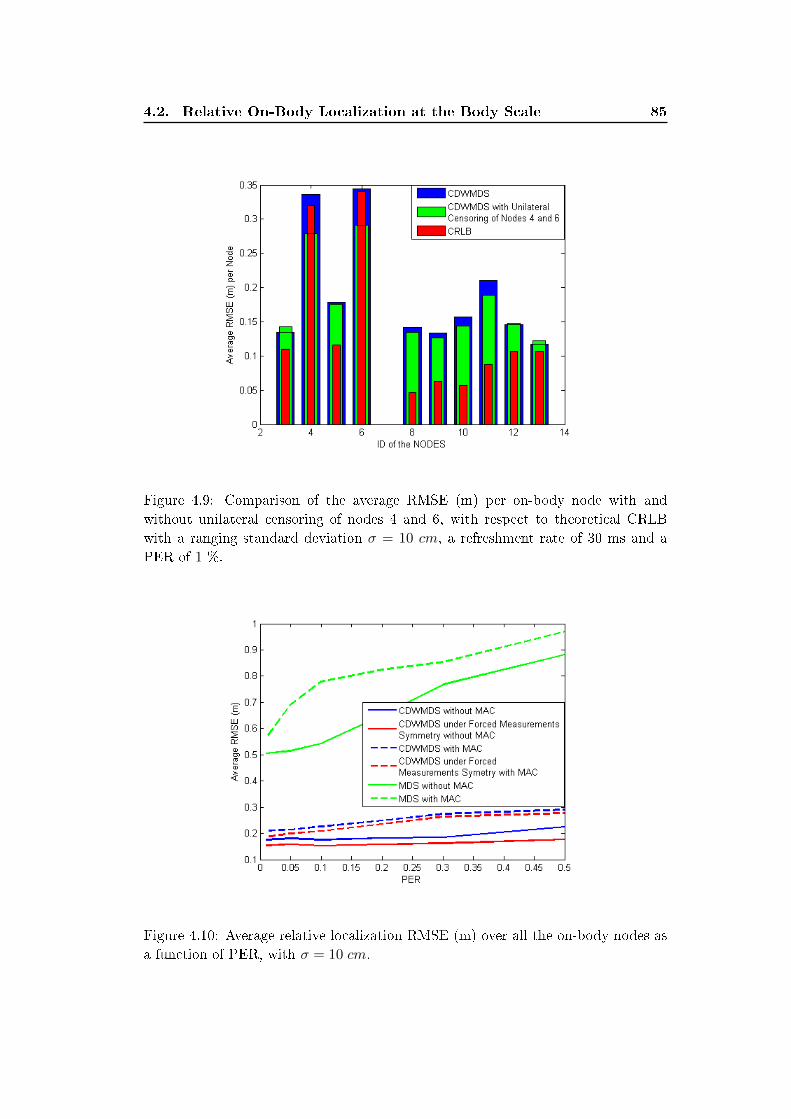
4.2. Relative On-Body Localization at the Body Scale 85
Figure 4.9: Comparison of the average RMSE (m) per on-body node with and
without unilateral censoring of nodes 4 and 6, with respect to theoretical CRLB
with a ranging standard deviation σ = 10 cm, a refreshment rate of 30 ms and a
PER of 1 %.
Figure 4.10: Average relative localization RMSE (m) over all the on-body nodes as
a function of PER, with σ = 10 cm.
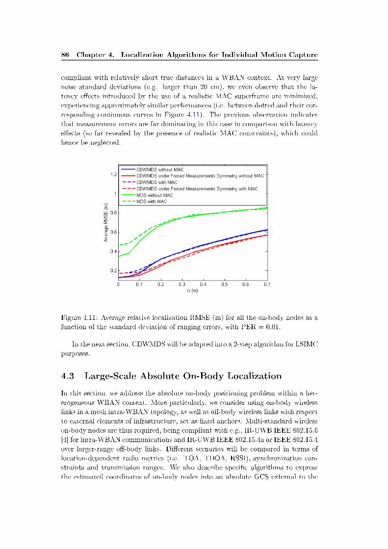
86 Chapter 4. Localization Algorithms for Individual Motion Capture
compliant with relatively short true distances in a WBAN context. At very large
noise standard deviations (e.g. larger than 20 cm), we even observe that the la-
tency e�ects introduced by the use of a realistic MAC superframe are minimized,
experiencing approximately similar performances (i.e. between dotted and their cor-
responding continuous curves in Figure 4.11). The previous observation indicates
that measurement errors are far dominating in this case in comparison with latency
e�ects (so far revealed by the presence of realistic MAC constraints), which could
hence be neglected.
Figure 4.11: Average relative localization RMSE (m) for all the on-body nodes as a
function of the standard deviation of ranging errors, with PER = 0.01.
In the next section, CDWMDS will be adapted into a 2-step algorithm for LSIMC
purposes.
4.3 Large-Scale Absolute On-Body Localization
In this section, we address the absolute on-body positioning problem within a het-
erogeneous WBAN context. More particularly, we consider using on-body wireless
links in a mesh intra-WBAN topology, as well as o�-body wireless links with respect
to external elements of infrastructure, set as �xed anchors. Multi-standard wireless
on-body nodes are thus required, being compliant with e.g., IR-UWB IEEE 802.15.6
[4] for intra-WBAN communications and IR-UWB IEEE 802.15.4a or IEEE 802.15.4
over larger-range o�-body links. Di�erent scenarios will be compared in terms of
location-dependent radio metrics (i.e. TOA, TDOA, RSSI), synchronization con-
straints and transmission ranges. We also describe speci�c algorithms to express
the estimated coordinates of on-body nodes into an absolute GCS external to the
4.3. Large-Scale Absolute On-Body Localization 87
body, as well as to mitigate body obstructions and packet losses.
We �rst assume a set of �xed anchor nodes placed at known positions in the
indoor environment and forming the building infrastructure. These nodes will be
also depicted as infrastructure anchors in the following. A second set of wireless
devices is deployed placed on the pedestrian body. These devices comprise the on-
body mobile nodes and the reference on-body anchors. The latter are attached onto
the body like in the relative localization case and then de�ne a stable Cartesian
LCS, which remains unchanged and time-invariant under body mobility.
Figure 4.12 shows a typical deployment scenario, where the LCS is obviously
in movement and misaligned relatively to an external GCS. In the following,
{Xaci }i=1...Na represents the set of the absolute 3D known positions of the Na �xed
infrastructure anchors expressed in the GCS, where Na should be equal or larger
than 4. {Xai (t)}i=1...n and {Xr
i (t)}i=1...n represent respectively the absolute and
relative 3D unknown positions of the n mobile nodes deployed on the body at time
t, as respectively expressed in the GCS and LCS. Similarly, {Xai (t)}i=n+1...n+m and
{Xri }i=n+1...n+m represent respectively the absolute 3D unknown positions of the m
on-body anchors at time t and their corresponding relative known positions (time-
invariant), where m should be equal or larger than 4. Now let dij(t) be one range
or pseudo-range measurement available at time t between one on-body node i and
a connected node j, j being one on-body node, one on-body anchor or one infras-
tructure anchor, and let lij be a constant distance (i.e. time-invariant over body
mobility whatever the coordinates system), which will be considered as a constraint.
Given all the available measurements {dij(t)}i,j at time t between cooperative
on-body nodes or between on-body nodes and infrastructure anchors, on the known
locations of on-body anchors and infrastructure anchors respectively in the LCS and
GCS, the problem that we want to solve consists in estimating the absolute positions
of the on-body nodes in the GCS.
4.3.1 Absolute Localization Algorithms
4.3.1.1 Proposed 2-Step Approach
The idea here is to start the LSIMC procedure by localizing the on-body nodes
relatively to the LCS, using cooperative peer-to-peer range measurements. As seen
in the previous section, the CDWMDS algorithm is relatively well suited to this
relative positioning problem. It allows each on-body node to estimate its coordinates
Xri (t) into the LCS, by minimizing the local cost function in equation (4.7), which
depends uniquely on its relative neighborhood information. Once the minimization
process is accomplished by all nodes, the set {Xri (t)}i=1...n is available into the LCS.
The second stage consists in converting the relative locations de�ned into the
LCS to absolute locations into the GCS. This transformation of LCS includes a
rotation and a translation. Since on-body anchors are time-invariant in the LCS
under mobility, it is preferable to rely on those nodes to transform the LCS. In 3D
environments, the absolute locations of at least 4 on-body anchors are needed to �nd
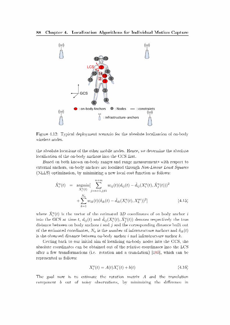
88 Chapter 4. Localization Algorithms for Individual Motion Capture
Figure 4.12: Typical deployment scenario for the absolute localization of on-body
wireless nodes.
the absolute locations of the other mobile nodes. Hence, we determine the absolute
localization of the on-body anchors into the GCS �rst.
Based on both known on-body ranges and range measurements with respect to
external anchors, on-body anchors are localized through Non-Linear Least Squares
(NLLS) optimization, by minimizing a new local cost function as follows:
Xai (t) = argmin
Xai (t)
[n+m∑
j=n+1,j 6=iwij(t)(dij(t)− dij(Xa
i (t), Xaj (t)))2
+
Na∑k=1
wik(t)(δik(t)− dik(Xai (t), Xac
k ))2] (4.15)
where Xai (t) is the vector of the estimated 3D coordinates of on-body anchor i
into the GCS at time t, dij(t) and dij(Xai (t), Xa
j (t)) denotes respectively the true
distance between on-body anchors i and j and the corresponding distance built out
of the estimated coordinates, Na is the number of infrastructure anchors and δik(t)
is the observed distance between on-body anchor i and infrastructure anchor k.
Getting back to our initial aim of localizing on-body nodes into the GCS, the
absolute coordinates can be obtained out of the relative coordinates into the LCS
after a few transformations (i.e. rotation and a translation) [105], which can be
represented as follows:
Xai (t) = A(t)Xr
i (t) + b(t) (4.16)
The goal now is to estimate the rotation matrix A and the translation
component b out of noisy observations, by minimizing the di�erence in
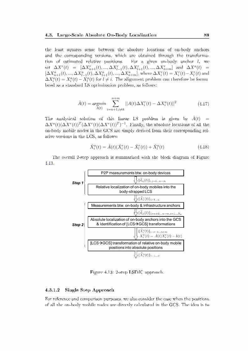
4.3. Large-Scale Absolute On-Body Localization 89
the least squares sense between the absolute locations of on-body anchors
and the corresponding versions, which are obtained through the transforma-
tion of estimated relative positions. For a given on-body anchor l, we
set ∆Xr(t) = [∆Xrn+1(t), ...,∆X
rl−1(t),∆X
rl+1(t), ...,∆X
rn+m] and ∆Xa(t) =
[∆Xan+1(t), ...,∆X
al−1(t),∆X
al+1(t), ...,∆X
an+m], where ∆Xr
i (t) = Xri (t)−Xr
l (t) and
∆Xai (t) = Xa
i (t)−Xal (t) for l 6= i. The alignment problem can therefore be formu-
lated as a standard LS optimization problem, as follows:
A(t) = argminA(t)
n+m∑i=n+1,i 6=k
||A(t)∆Xri (t)−∆Xa
i (t)||2 (4.17)
The analytical solution of this linear LS problem is given by A(t) =
∆Xa(t)(∆Xr(t))T (∆Xr(t)(∆Xr(t))T )−1. Finally, the absolute locations of all the
on-body mobile nodes in the GCS are simply derived from their corresponding rel-
ative versions in the LCS, as follows:
Xai (t) = A(t)(Xr
i (t)− Xrl (t)) + Xa
l (t) (4.18)
The overall 2-step approach is summarized with the block diagram of Figure
4.13.
Figure 4.13: 2-step LSIMC approach.
4.3.1.2 Single Step Approach
For reference and comparison purposes, we also consider the case when the positions
of all the on-body mobile nodes are directly calculated in the GCS. The idea is to
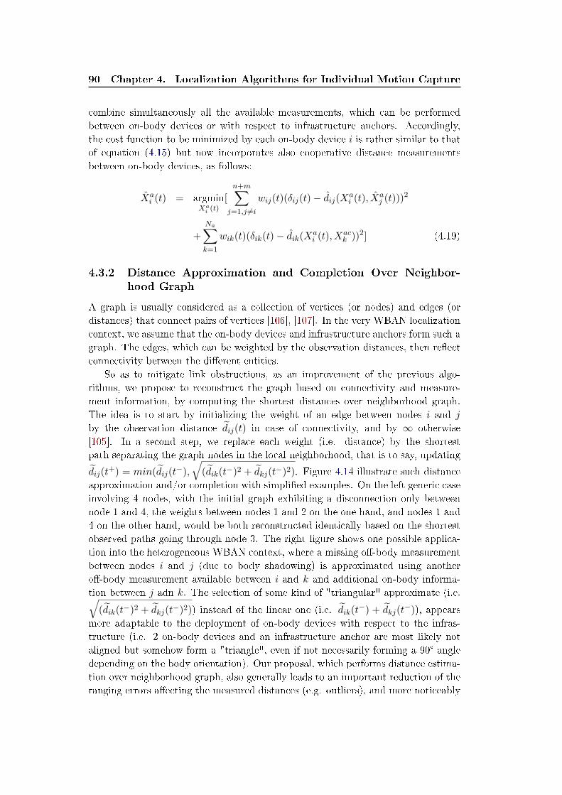
90 Chapter 4. Localization Algorithms for Individual Motion Capture
combine simultaneously all the available measurements, which can be performed
between on-body devices or with respect to infrastructure anchors. Accordingly,
the cost function to be minimized by each on-body device i is rather similar to that
of equation (4.15) but now incorporates also cooperative distance measurements
between on-body devices, as follows:
Xai (t) = argmin
Xai (t)
[n+m∑
j=1,j 6=iwij(t)(δij(t)− dij(Xa
i (t), Xaj (t)))2
+
Na∑k=1
wik(t)(δik(t)− dik(Xai (t), Xac
k ))2] (4.19)
4.3.2 Distance Approximation and Completion Over Neighbor-
hood Graph
A graph is usually considered as a collection of vertices (or nodes) and edges (or
distances) that connect pairs of vertices [106], [107]. In the very WBAN localization
context, we assume that the on-body devices and infrastructure anchors form such a
graph. The edges, which can be weighted by the observation distances, then re�ect
connectivity between the di�erent entities.
So as to mitigate link obstructions, as an improvement of the previous algo-
rithms, we propose to reconstruct the graph based on connectivity and measure-
ment information, by computing the shortest distances over neighborhood graph.
The idea is to start by initializing the weight of an edge between nodes i and j
by the observation distance dij(t) in case of connectivity, and by ∞ otherwise
[105]. In a second step, we replace each weight (i.e. distance) by the shortest
path separating the graph nodes in the local neighborhood, that is to say, updating
dij(t+) = min(dij(t
−),√
(dik(t−)2 + dkj(t−)2). Figure 4.14 illustrate such distance
approximation and/or completion with simpli�ed examples. On the left generic case
involving 4 nodes, with the initial graph exhibiting a disconnection only between
node 1 and 4, the weights between nodes 1 and 2 on the one hand, and nodes 1 and
4 on the other hand, would be both reconstructed identically based on the shortest
observed paths going through node 3. The right �gure shows one possible applica-
tion into the heterogeneous WBAN context, where a missing o�-body measurement
between nodes i and j (due to body shadowing) is approximated using another
o�-body measurement available between i and k and additional on-body informa-
tion between j adn k. The selection of some kind of "triangular" approximate (i.e.√(dik(t−)2 + dkj(t−)2)) instead of the linear one (i.e. dik(t
−) + dkj(t−)), appears
more adaptable to the deployment of on-body devices with respect to the infras-
tructure (i.e. 2 on-body devices and an infrastructure anchor are most likely not
aligned but somehow form a "triangle", even if not necessarily forming a 90° angle
depending on the body orientation). Our proposal, which performs distance estima-
tion over neighborhood graph, also generally leads to an important reduction of the
ranging errors a�ecting the measured distances (e.g. outliers), and more noticeably
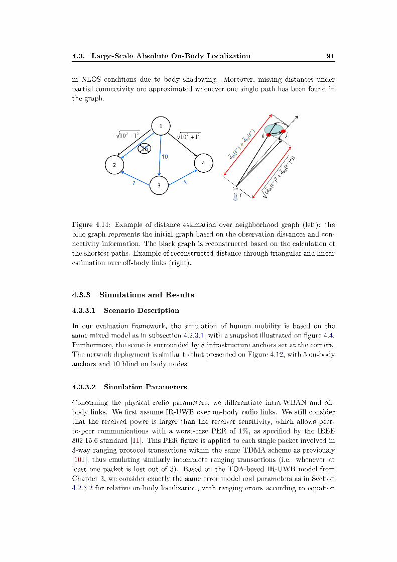
4.3. Large-Scale Absolute On-Body Localization 91
in NLOS conditions due to body shadowing. Moreover, missing distances under
partial connectivity are approximated whenever one single path has been found in
the graph.
Figure 4.14: Example of distance estimation over neighborhood graph (left): the
blue graph represents the initial graph based on the observation distances and con-
nectivity information. The black graph is reconstructed based on the calculation of
the shortest paths. Example of reconstructed distance through triangular and linear
estimation over o�-body links (right).
4.3.3 Simulations and Results
4.3.3.1 Scenario Description
In our evaluation framework, the simulation of human mobility is based on the
same mixed model as in subsection 4.2.3.1, with a snapshot illustrated on �gure 4.4.
Furthermore, the scene is surrounded by 8 infrastructure anchors set at the corners.
The network deployment is similar to that presented on Figure 4.12, with 5 on-body
anchors and 10 blind on-body nodes.
4.3.3.2 Simulation Parameters
Concerning the physical radio parameters, we di�erentiate intra-WBAN and o�-
body links. We �rst assume IR-UWB over on-body radio links. We still consider
that the received power is larger than the receiver sensitivity, which allows peer-
to-peer communications with a worst-case PER of 1%, as speci�ed by the IEEE
802.15.6 standard [11]. This PER �gure is applied to each single packet involved in
3-way ranging protocol transactions within the same TDMA scheme as previously
[101], thus emulating similarly incomplete ranging transactions (i.e. whenever at
least one packet is lost out of 3). Based on the TOA-based IR-UWB model from
Chapter 3, we consider exactly the same error model and parameters as in Section
4.2.3.2 for relative on-body localization, with ranging errors according to equation
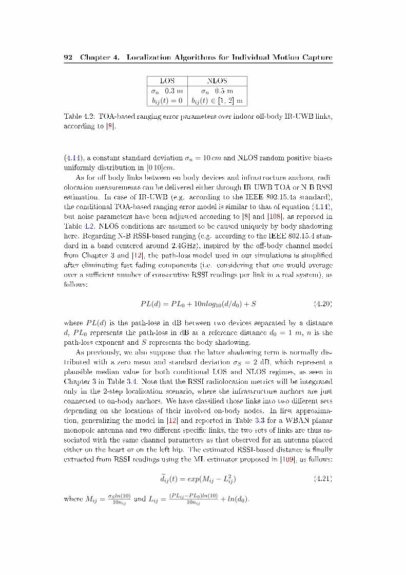
92 Chapter 4. Localization Algorithms for Individual Motion Capture
LOS NLOS
σn=0.3 m σn=0.5 m
bij(t) = 0 bij(t) ∈ [1, 2] m
Table 4.2: TOA-based ranging error parameters over indoor o�-body IR-UWB links,
according to [8].
(4.14), a constant standard deviation σn = 10 cm and NLOS random positive biases
uniformly distribution in [0 10]cm.
As for o�-body links between on-body devices and infrastructure anchors, radi-
olocation measurements can be delivered either through IR-UWB TOA or N-B RSSI
estimation. In case of IR-UWB (e.g. according to the IEEE 802.15.4a standard),
the conditional TOA-based ranging error model is similar to that of equation (4.14),
but noise parameters have been adjusted according to [8] and [108], as reported in
Table 4.2. NLOS conditions are assumed to be caused uniquely by body shadowing
here. Regarding N-B RSSI-based ranging (e.g. according to the IEEE 802.15.4 stan-
dard in a band centered around 2.4GHz), inspired by the o�-body channel model
from Chapter 3 and [12], the path-loss model used in our simulations is simpli�ed
after eliminating fast fading components (i.e. considering that one would average
over a su�cient number of consecutive RSSI readings per link in a real system), as
follows:
PL(d) = PL0 + 10nlog10(d/d0) + S (4.20)
where PL(d) is the path-loss in dB between two devices separated by a distance
d, PL0 represents the path-loss in dB at a reference distance d0 = 1 m, n is the
path-loss exponent and S represents the body shadowing.
As previously, we also suppose that the latter shadowing term is normally dis-
tributed with a zero mean and standard deviation σS = 2 dB, which represent a
plausible median value for both conditional LOS and NLOS regimes, as seen in
Chapter 3 in Table 3.4. Note that the RSSI radiolocation metrics will be integrated
only in the 2-step localization scenario, where the infrastructure anchors are just
connected to on-body anchors. We have classi�ed those links into two di�erent sets
depending on the locations of their involved on-body nodes. In �rst approxima-
tion, generalizing the model in [12] and reported in Table 3.3 for a WBAN planar
monopole antenna and two di�erent speci�c links, the two sets of links are thus as-
sociated with the same channel parameters as that observed for an antenna placed
either on the heart or on the left hip. The estimated RSSI-based distance is �nally
extracted from RSSI readings using the ML estimator proposed in [109], as follows:
dij(t) = exp(Mij − L2ij) (4.21)
where Mij = σS ln(10)10nij
and Lij =(PLij−PL0)ln(10)
10nij+ ln(d0).
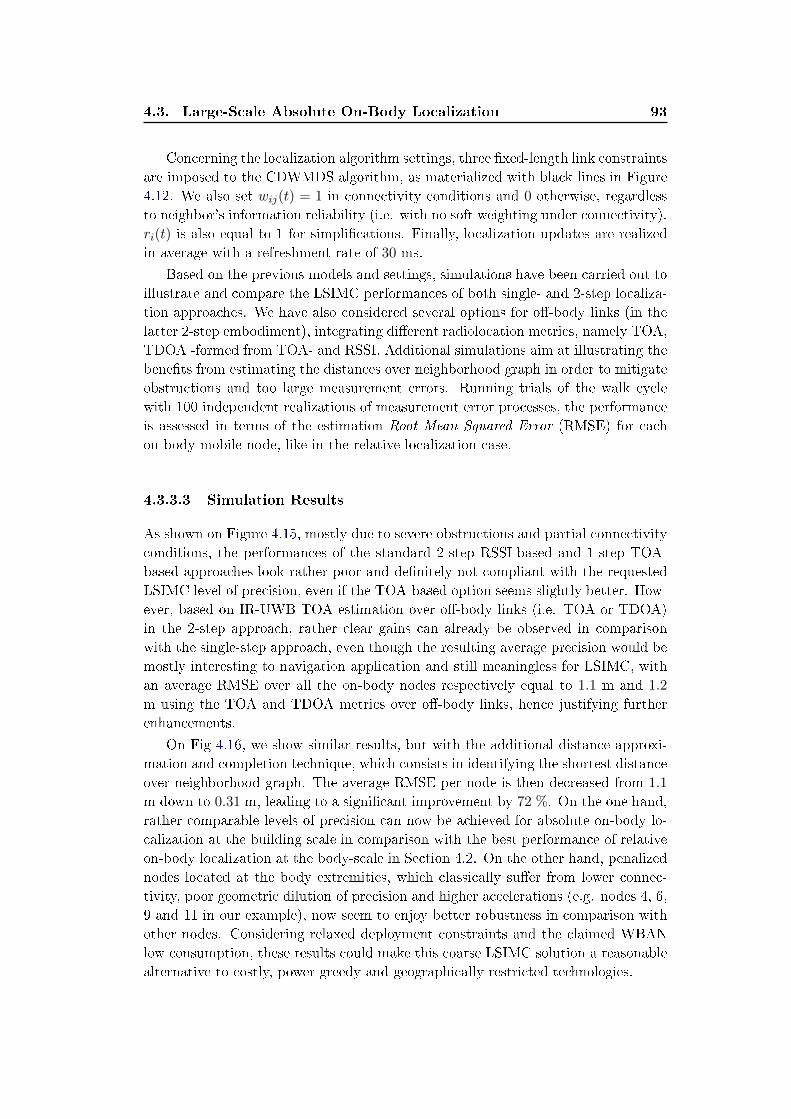
4.3. Large-Scale Absolute On-Body Localization 93
Concerning the localization algorithm settings, three �xed-length link constraints
are imposed to the CDWMDS algorithm, as materialized with black lines in Figure
4.12. We also set wij(t) = 1 in connectivity conditions and 0 otherwise, regardless
to neighbor's information reliability (i.e. with no soft weighting under connectivity).
ri(t) is also equal to 1 for simpli�cations. Finally, localization updates are realized
in average with a refreshment rate of 30 ms.
Based on the previous models and settings, simulations have been carried out to
illustrate and compare the LSIMC performances of both single- and 2-step localiza-
tion approaches. We have also considered several options for o�-body links (in the
latter 2-step embodiment), integrating di�erent radiolocation metrics, namely TOA,
TDOA -formed from TOA- and RSSI. Additional simulations aim at illustrating the
bene�ts from estimating the distances over neighborhood graph in order to mitigate
obstructions and too large measurement errors. Running trials of the walk cycle
with 100 independent realizations of measurement error processes, the performance
is assessed in terms of the estimation Root Mean Squared Error (RMSE) for each
on-body mobile node, like in the relative localization case.
4.3.3.3 Simulation Results
As shown on Figure 4.15, mostly due to severe obstructions and partial connectivity
conditions, the performances of the standard 2-step RSSI-based and 1-step TOA-
based approaches look rather poor and de�nitely not compliant with the requested
LSIMC level of precision, even if the TOA-based option seems slightly better. How-
ever, based on IR-UWB TOA estimation over o�-body links (i.e. TOA or TDOA)
in the 2-step approach, rather clear gains can already be observed in comparison
with the single-step approach, even though the resulting average precision would be
mostly interesting to navigation application and still meaningless for LSIMC, with
an average RMSE over all the on-body nodes respectively equal to 1.1 m and 1.2
m using the TOA and TDOA metrics over o�-body links, hence justifying further
enhancements.
On Fig 4.16, we show similar results, but with the additional distance approxi-
mation and completion technique, which consists in identifying the shortest distance
over neighborhood graph. The average RMSE per node is then decreased from 1.1
m down to 0.31 m, leading to a signi�cant improvement by 72 %. On the one hand,
rather comparable levels of precision can now be achieved for absolute on-body lo-
calization at the building scale in comparison with the best performance of relative
on-body localization at the body-scale in Section 4.2. On the other hand, penalized
nodes located at the body extremities, which classically su�er from lower connec-
tivity, poor geometric dilution of precision and higher accelerations (e.g. nodes 4, 6,
9 and 11 in our example), now seem to enjoy better robustness in comparison with
other nodes. Considering relaxed deployment constraints and the claimed WBAN
low consumption, these results could make this coarse LSIMC solution a reasonable
alternative to costly, power greedy and geographically restricted technologies.
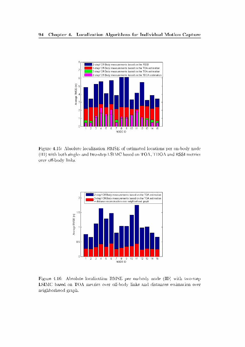
94 Chapter 4. Localization Algorithms for Individual Motion Capture
Figure 4.15: Absolute localization RMSE of estimated locations per on-body node
(ID) with both single- and two-step LSIMC based on TOA, TDOA and RSSI metrics
over o�-body links.
Figure 4.16: Absolute localization RMSE per on-body node (ID) with two-step
LSIMC based on TOA metrics over o�-body links and distances estimation over
neighborhood graph.
4.4. Conclusion 95
4.4 Conclusion
In this Chapter, we have addressed the problem of relative and absolute on-body
localization for individual MoCap purposes.
In Section 4.2, we have dealt with relative body motion capture only. The
corresponding personal contributions have led to the publication of two conference
papers [46], [47] and one journal [48]. A decentralized and cooperative DWMDS al-
gorithm, which can asynchronously estimate unknown on-body nodes locations, has
been adapted in the very context. We have introduced learnt �xed-length geometric
constraints that correspond to time-invariant Euclidean inter-node distances un-
der body mobility. Furthermore, the initial CDWMDS has been enhanced through
scheduling and censoring to mitigate error propagation and harmful e�ects due to
location-dependent node speed disparities. It has been also shown that forcing mea-
surements symmetry could help to mitigate outliers and packet losses. Moreover,
CDWMDS has been proved to outperform with a classical MDS algorithm in terms
of localization accuracy for various PER values and ranging standard deviations
with and without realistic MAC superframe, hence illustrating rather �ne robust-
ness against latency e�ects. However, given the remaining limitations still observed
in terms of achievable precision, which is hardly compliant with high precision Mo-
Cap needs (especially when compared with theoretical bounds at some pathological
nodes), axes of improvement can be identi�ed, such as a judicious coupling with
tracking/smoothing algorithms, better initialization or a soft weighting of the avail-
able measurements.
In Section 4.3, we have addressed the problem of absolute motion capture over
large-scale indoor trajectories in location-enabled heterogeneous wireless body area
networks. The related personal contribution has led to the publication of one con-
ference paper [49]. Two approaches have been presented to estimate the absolute
locations of on-body nodes in a global coordinates system, considering di�erent ra-
diolocation metrics over o�-body links with respect to infrastructure anchors. One
2-step solution relies on preliminary relative localization at the body scale and ap-
plies further transformations through the absolute localization of on-body anchors.
At �rst sight, body shadowing seems very challenging, not to say redhibitory to
achieve precision levels compatible with high-precision MoCap needs. However we
have proposed another algorithm that estimates the shortest path between on-body
and infrastructure anchors over neighborhood graph to compensate for possible ra-
dio obstructions and most penalizing large measurement errors. Thanks to the
latter improvement, approximately the same levels of precision as that obtained for
relative on-body localization could be theoretically achieved over large-scale tra-
jectories. This makes our radio-based solution still attractive for coarse absolute
MoCap applications, even if new improvements are still foreseen, such as the use of
body-to-body cooperation.
The next Chapter will precisely concern cooperative navigation functionalities
in groups of WBANs, relying on such body-to-body links and on-body deployment
diversity. On this occasion, di�erent localization and tracking algorithms will be

96 Chapter 4. Localization Algorithms for Individual Motion Capture
also evaluated and compared.
Chapter 5
Localization Algorithms for
Individual and Collective
Navigation
Contents
5.1 Introduction . . . . . . . . . . . . . . . . . . . . . . . . . . . . 97
5.2 Individual Navigation . . . . . . . . . . . . . . . . . . . . . . . 98
5.2.1 Classical Approach . . . . . . . . . . . . . . . . . . . . . . . . 98
5.2.2 New Proposal . . . . . . . . . . . . . . . . . . . . . . . . . . . 99
5.3 Collective Navigation . . . . . . . . . . . . . . . . . . . . . . . 102
5.4 Simulations and Results . . . . . . . . . . . . . . . . . . . . . 102
5.4.1 Scenario Description . . . . . . . . . . . . . . . . . . . . . . . 102
5.4.2 Simulation Parameters . . . . . . . . . . . . . . . . . . . . . . 103
5.4.3 Simulation Results . . . . . . . . . . . . . . . . . . . . . . . . 104
5.5 Conclusion . . . . . . . . . . . . . . . . . . . . . . . . . . . . . 109
5.1 Introduction
As seen in Chapter 1, in our WBAN context, one can make a distinction between
classical individual navigation on the one hand, where the on-body nodes belong
to one single body, whose "macroscopic" position must be estimated with respect
to a GCS, and collective navigation (CGN) on the other hand, which consists in
retrieving the absolute positions of several mobile users belonging to the same group,
each user wearing his own WBAN. In the �rst case, cooperative on-body and o�-
body links are considered (i.e. just like for LSIMC in the previous Chapter), whereas
additional body-to-body links may be involved in the latter case. In both scenarios,
we assume that �xed and known elements of infrastructure are disseminated in the
environment for absolute localization purposes. In terms of radiolocation metrics
and radio standards, we consider peer-to-peer range measurements through TOA
estimation over IR-UWB links or RSSI estimation over N-B links, like previously.
We also admit various combinations of such cooperative links and measurements,
hence assuming a heterogeneous WBAN context.
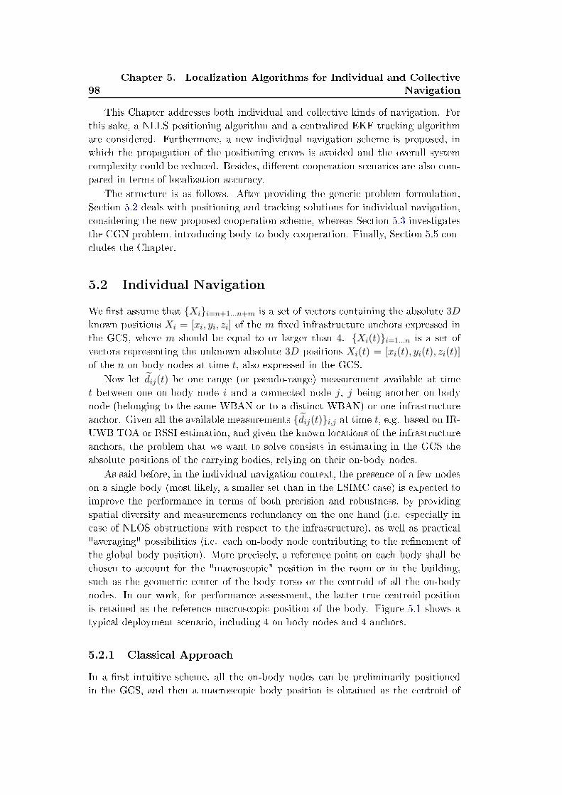
98
Chapter 5. Localization Algorithms for Individual and Collective
Navigation
This Chapter addresses both individual and collective kinds of navigation. For
this sake, a NLLS positioning algorithm and a centralized EKF tracking algorithm
are considered. Furthermore, a new individual navigation scheme is proposed, in
which the propagation of the positioning errors is avoided and the overall system
complexity could be reduced. Besides, di�erent cooperation scenarios are also com-
pared in terms of localization accuracy.
The structure is as follows. After providing the generic problem formulation,
Section 5.2 deals with positioning and tracking solutions for individual navigation,
considering the new proposed cooperation scheme, whereas Section 5.3 investigates
the CGN problem, introducing body-to-body cooperation. Finally, Section 5.5 con-
cludes the Chapter.
5.2 Individual Navigation
We �rst assume that {Xi}i=n+1...n+m is a set of vectors containing the absolute 3D
known positions Xi = [xi, yi, zi] of the m �xed infrastructure anchors expressed in
the GCS, where m should be equal to or larger than 4. {Xi(t)}i=1...n is a set of
vectors representing the unknown absolute 3D positions Xi(t) = [xi(t), yi(t), zi(t)]
of the n on-body nodes at time t, also expressed in the GCS.
Now let dij(t) be one range (or pseudo-range) measurement available at time
t between one on-body node i and a connected node j, j being another on-body
node (belonging to the same WBAN or to a distinct WBAN) or one infrastructure
anchor. Given all the available measurements {dij(t)}i,j at time t, e.g. based on IR-
UWB TOA or RSSI estimation, and given the known locations of the infrastructure
anchors, the problem that we want to solve consists in estimating in the GCS the
absolute positions of the carrying bodies, relying on their on-body nodes.
As said before, in the individual navigation context, the presence of a few nodes
on a single body (most likely, a smaller set than in the LSIMC case) is expected to
improve the performance in terms of both precision and robustness, by providing
spatial diversity and measurements redundancy on the one hand (i.e. especially in
case of NLOS obstructions with respect to the infrastructure), as well as practical
"averaging" possibilities (i.e. each on-body node contributing to the re�nement of
the global body position). More precisely, a reference point on each body shall be
chosen to account for the "macroscopic" position in the room or in the building,
such as the geometric center of the body torso or the centroid of all the on-body
nodes. In our work, for performance assessment, the latter true centroid position
is retained as the reference macroscopic position of the body. Figure 5.1 shows a
typical deployment scenario, including 4 on-body nodes and 4 anchors.
5.2.1 Classical Approach
In a �rst intuitive scheme, all the on-body nodes can be preliminarily positioned
in the GCS, and then a macroscopic body position is obtained as the centroid of
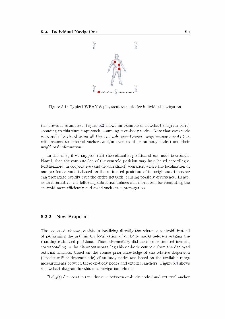
5.2. Individual Navigation 99
Figure 5.1: Typical WBAN deployment scenario for individual navigation.
the previous estimates. Figure 5.2 shows an example of �owchart diagram corre-
sponding to this simple approach, assuming n on-body nodes. Note that each node
is actually localized using all the available peer-to-peer range measurements (i.e.
with respect to external anchors and/or even to other on-body nodes) and their
neighbors' information.
In this case, if we suppose that the estimated position of one node is strongly
biased, then the computation of the centroid position may be a�ected accordingly.
Furthermore, in cooperative (and decentralized) scenarios, where the localization of
one particular node is based on the estimated positions of its neighbors, the error
can propagate rapidly over the entire network, causing possibly divergence. Hence,
as an alternative, the following subsection de�nes a new proposal for computing the
centroid more e�ciently and avoid such error propagation.
5.2.2 New Proposal
The proposed scheme consists in localizing directly the reference centroid, instead
of performing the preliminary localization of on-body nodes before averaging the
resulting estimated positions. Thus intermediary distances are estimated instead,
corresponding to the distances separating this on-body centroid from the deployed
external anchors, based on the coarse prior knowledge of the relative dispersion
("statistical" or deterministic) of on-body nodes and based on the available range
measurements between these on-body nodes and external anchors. Figure 5.3 shows
a �owchart diagram for this new navigation scheme.
If diA(t) denotes the true distance between on-body node i and external anchor

100
Chapter 5. Localization Algorithms for Individual and Collective
Navigation
Figure 5.2: Example of classical scheme for individual navigation, based on the
posterior computation of the on-body nodes' centroid.
A at time t, then
1
n
n∑i=1
d2iA(t) =1
n
n∑i=1
x2i (t)−2xAn
i=n∑i=1
xi(t) + x2A
+1
n
n∑i=1
y2i (t)−2yAn
n∑i=1
yi(t) + y2A
+1
n
n∑i=1
z2i (t)− 2zAn
n∑i=1
zi(t) + z2A (5.1)
Similarly if dbA(t) denotes the true distance between the on-body centroid of coor-
dinates Xb(t) = [xb(t) = 1n
∑ni=1 xi(t), yb(t) = 1
n
∑ni=1 yi(t), zb(t) = 1
n
∑ni=1 zi(t)]
and anchor A, then
d2bA(t) = (1
n
n∑i=1
xi(t))2 − 2xA
n
n∑i=1
xi(t) + x2A
+ (1
n
n∑i=1
yi(t))2 − 2yA
n
n∑i=1
yi(t) + y2A
+ (1
n
n∑i=1
zi(t))2 − 2zA
n
n∑i=1
zi(t) + z2A (5.2)
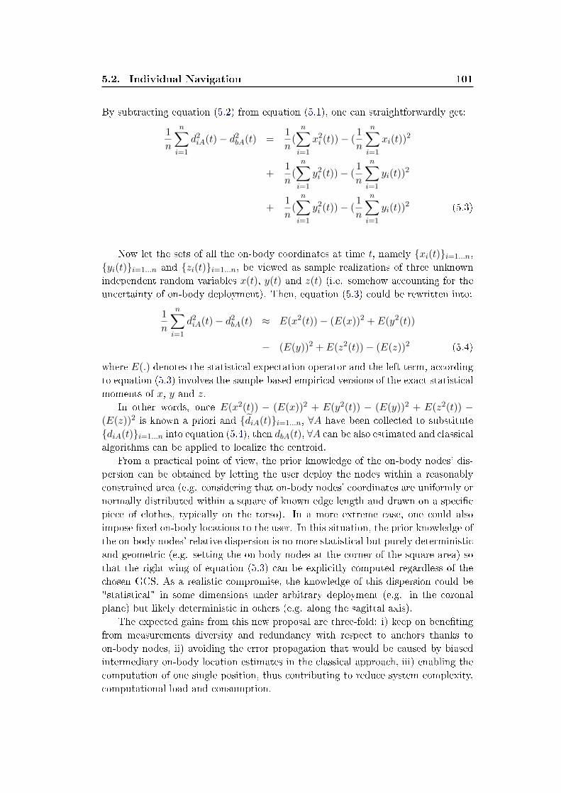
5.2. Individual Navigation 101
By subtracting equation (5.2) from equation (5.1), one can straightforwardly get:
1
n
n∑i=1
d2iA(t)− d2bA(t) =1
n(
n∑i=1
x2i (t))− (1
n
n∑i=1
xi(t))2
+1
n(
n∑i=1
y2i (t))− (1
n
n∑i=1
yi(t))2
+1
n(
n∑i=1
y2i (t))− (1
n
n∑i=1
yi(t))2 (5.3)
Now let the sets of all the on-body coordinates at time t, namely {xi(t)}i=1...n,
{yi(t)}i=1...n and {zi(t)}i=1...n, be viewed as sample realizations of three unknown
independent random variables x(t), y(t) and z(t) (i.e. somehow accounting for the
uncertainty of on-body deployment). Then, equation (5.3) could be rewritten into:
1
n
n∑i=1
d2iA(t)− d2bA(t) ≈ E(x2(t))− (E(x))2 + E(y2(t))
− (E(y))2 + E(z2(t))− (E(z))2 (5.4)
where E(.) denotes the statistical expectation operator and the left term, according
to equation (5.3) involves the sample-based empirical versions of the exact statistical
moments of x, y and z.
In other words, once E(x2(t)) − (E(x))2 + E(y2(t)) − (E(y))2 + E(z2(t)) −(E(z))2 is known a priori and {diA(t)}i=1...n, ∀A have been collected to substitute
{diA(t)}i=1...n into equation (5.4), then dbA(t), ∀A can be also estimated and classical
algorithms can be applied to localize the centroid.
From a practical point of view, the prior knowledge of the on-body nodes' dis-
persion can be obtained by letting the user deploy the nodes within a reasonably
constrained area (e.g. considering that on-body nodes' coordinates are uniformly or
normally distributed within a square of known edge length and drawn on a speci�c
piece of clothes, typically on the torso). In a more extreme case, one could also
impose �xed on-body locations to the user. In this situation, the prior knowledge of
the on-body nodes' relative dispersion is no more statistical but purely deterministic
and geometric (e.g. setting the on-body nodes at the corner of the square area) so
that the right wing of equation (5.3) can be explicitly computed regardless of the
chosen GCS. As a realistic compromise, the knowledge of this dispersion could be
"statistical" in some dimensions under arbitrary deployment (e.g. in the coronal
plane) but likely deterministic in others (e.g. along the sagittal axis).
The expected gains from this new proposal are three-fold: i) keep on bene�ting
from measurements diversity and redundancy with respect to anchors thanks to
on-body nodes, ii) avoiding the error propagation that would be caused by biased
intermediary on-body location estimates in the classical approach, iii) enabling the
computation of one single position, thus contributing to reduce system complexity,
computational load and consumption.

102
Chapter 5. Localization Algorithms for Individual and Collective
Navigation
Figure 5.3: New proposed scheme for individual navigation, where one single body
position is computed, based on intermediary estimated distances between the on-
body centroid and external anchors.
5.3 Collective Navigation
In this application, a few mobile users wearing on-body nodes and forming a group,
must be localized with respect to an external GCS. The localization can then rely on
peer-to-peer range measurements between on-body nodes and infrastructure anchors
over o�-body links, and/or with respect to other on-body nodes on the same or
di�erent bodies (i.e. over on- and body-to-body links). Figure 5.4 shows a typical
deployment with 3 users. Similarly to individual navigation, each user belonging to
the group is tracked by estimating his macroscopic position, for instance de�ned as
the centroid of his deployed on-body nodes.
5.4 Simulations and Results
5.4.1 Scenario Description
In our evaluation framework, a group of 3 persons is de�ned, where each body is
assumed to move randomly and independently from each other (at least in terms
of directions), for simplicity. The human mobility of each user is based on a mixed
model similar to that already presented in Subsection 4.2.3.1. A snapshot of the
resulting animated group is represented on Figure 5.5.
Furthermore, for each random trial, the di�erent bodies move in a 20m× 20m ×4m 3D environment at the constant speed of 1m/sec for an overall duration of
112sec. The scene is surrounded by 4 infrastructure anchors, set at the corners.
The network deployment is similar to that presented on Figure 5.4, where 4 on-
body nodes are placed on each body. All the on-body nodes are indexed from 1 to
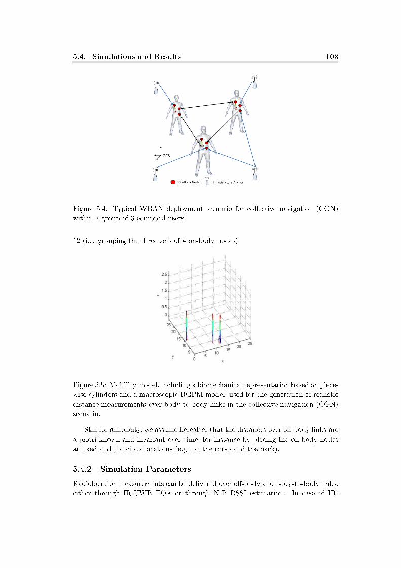
5.4. Simulations and Results 103
Figure 5.4: Typical WBAN deployment scenario for collective navigation (CGN)
within a group of 3 equipped users.
12 (i.e. grouping the three sets of 4 on-body nodes).
Figure 5.5: Mobility model, including a biomechanical representation based on piece-
wise cylinders and a macroscopic RGPM model, used for the generation of realistic
distance measurements over body-to-body links in the collective navigation (CGN)
scenario.
Still for simplicity, we assume hereafter that the distances over on-body links are
a priori known and invariant over time, for instance by placing the on-body nodes
at �xed and judicious locations (e.g. on the torso and the back).
5.4.2 Simulation Parameters
Radiolocation measurements can be delivered over o�-body and body-to-body links,
either through IR-UWB TOA or through N-B RSSI estimation. In case of IR-
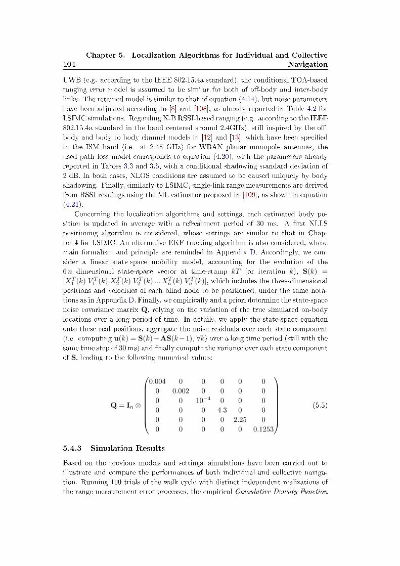
104
Chapter 5. Localization Algorithms for Individual and Collective
Navigation
UWB (e.g. according to the IEEE 802.15.4a standard), the conditional TOA-based
ranging error model is assumed to be similar for both of o�-body and inter-body
links. The retained model is similar to that of equation (4.14), but noise parameters
have been adjusted according to [8] and [108], as already reported in Table 4.2 for
LSIMC simulations. Regarding N-B RSSI-based ranging (e.g. according to the IEEE
802.15.4a standard in the band centered around 2.4GHz), still inspired by the o�-
body and body-to-body channel models in [12] and [13], which have been speci�ed
in the ISM band (i.e. at 2.45 GHz) for WBAN planar monopole antennas, the
used path loss model corresponds to equation (4.20), with the parameters already
reported in Tables 3.3 and 3.5, with a conditional shadowing standard deviation of
2 dB. In both cases, NLOS conditions are assumed to be caused uniquely by body
shadowing. Finally, similarly to LSIMC, single-link range measurements are derived
from RSSI readings using the ML estimator proposed in [109], as shown in equation
(4.21).
Concerning the localization algorithms and settings, each estimated body po-
sition is updated in average with a refreshment period of 30 ms. A �rst NLLS
positioning algorithm is considered, whose settings are similar to that in Chap-
ter 4 for LSIMC. An alternative EKF tracking algorithm is also considered, whose
main formalism and principle are reminded in Appendix D. Accordingly, we con-
sider a linear state-space mobility model, accounting for the evolution of the
6n dimensional state-space vector at time-stamp kT (or iteration k), S(k) =
[XT1 (k) V T
1 (k) XT2 (k) V T
2 (k) ... XTn (k) V T
n (k)], which includes the three-dimensional
positions and velocities of each blind node to be positioned, under the same nota-
tions as in Appendix D. Finally, we empirically and a priori determine the state-space
noise covariance matrix Q, relying on the variation of the true simulated on-body
locations over a long period of time. In details, we apply the state-space equation
onto these real positions, aggregate the noise residuals over each state component
(i.e. computing u(k) = S(k)−AS(k−1), ∀k) over a long time period (still with the
same time step of 30 ms) and �nally compute the variance over each state component
of S, leading to the following numerical values:
Q = In ⊗
0.004 0 0 0 0 0
0 0.002 0 0 0 0
0 0 10−4 0 0 0
0 0 0 4.3 0 0
0 0 0 0 2.25 0
0 0 0 0 0 0.1253
(5.5)
5.4.3 Simulation Results
Based on the previous models and settings, simulations have been carried out to
illustrate and compare the performances of both individual and collective naviga-
tion. Running 100 trials of the walk cycle with distinct independent realizations of
the range measurement error processes, the empirical Cumulative Density Function
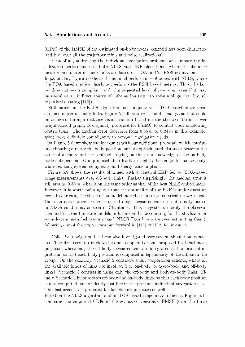
5.4. Simulations and Results 105
(CDF) of the RMSE of the estimated on-body nodes' centroid has been character-
ized (i.e. over all the trajectory trials and noise realizations).
First of all, addressing the individual navigation problem, we compare the lo-
calization performances of both NLLS and EKF algorithms, where the distance
measurements over o�-body links are based on TOA and/or RSSI estimation.
In particular, Figure 5.6 shows the nominal performance obtained with NLLS, where
the TOA-based metrics clearly outperforms the RSSI-based metrics. Thus, the lat-
ter does not seem compliant with the requested level of precision, even if it may
be useful as an indirect source of information (e.g. to solve ambiguities through
hypothesis testing [110]).
Still based on the NLLS algorithm but uniquely with TOA-based range mea-
surements over o�-body links, Figure 5.7 illustrates the additional gains that could
be achieved through distance reconstruction based on the shortest distance over
neighborhood graph, as originally proposed for LSIMC to combat body shadowing
obstructions. The median error decreases from 0.55m to 0.24m in this example,
what looks de�nitely compliant with personal navigation needs.
On Figure 5.8, we show similar results with our additional proposal, which consists
in estimating directly the body position, out of approximated distances between the
external anchors and the centroid, relying on the prior knowledge of the on-body
nodes' dispersion. Our proposal then leads to slightly better performances only,
while reducing system complexity and energy consumption.
Figure 5.9 shows the results obtained with a classical EKF fed by TOA-based
range measurements over o�-body links. Rather surprisingly, the median error is
still around 0.38m, what is on the same order as that of the best NLLS embodiment.
However, it is worth pointing out that the optimality of the EKF is under question
here. In our case, the observation model indeed assumes systematically a zero-mean
Gaussian noise process whereas actual range measurements are notoriously biased
in NLOS conditions, as seen in Chapter 3. This suggests to modify the observa-
tion and/or even the state models in future works, accounting for the stochastic or
semi-deterministic behaviour of such NLOS TOA biases (or even estimating them),
following one of the approaches put forward in [111] or [112] for instance.
Collective navigation has been also investigated over several simulation scenar-
ios. The �rst scenario is viewed as non-cooperative and proposed for benchmark
purposes, where only the o�-body measurements are integrated in the localization
problem, so that each body position is computed independently of the others in the
group. On the contrary, Scenario 2 considers a full cooperation scheme, where all
the available kinds of links are involved (i.e. on-body, body-to-body and o�-body
links). Scenario 3 consists in using only the o�-body and body-to-body links. Fi-
nally, Scenario 4 incorporates o�-body and on-body links, so that each body position
is also computed independently just like in the previous individual navigation case.
This last scenario is proposed for benchmark purposes as well.
Based on the NLLS algorithm and on TOA-based range measurements, Figure 5.10
compares the empirical CDFs of the estimated centroids' RMSE (over the three
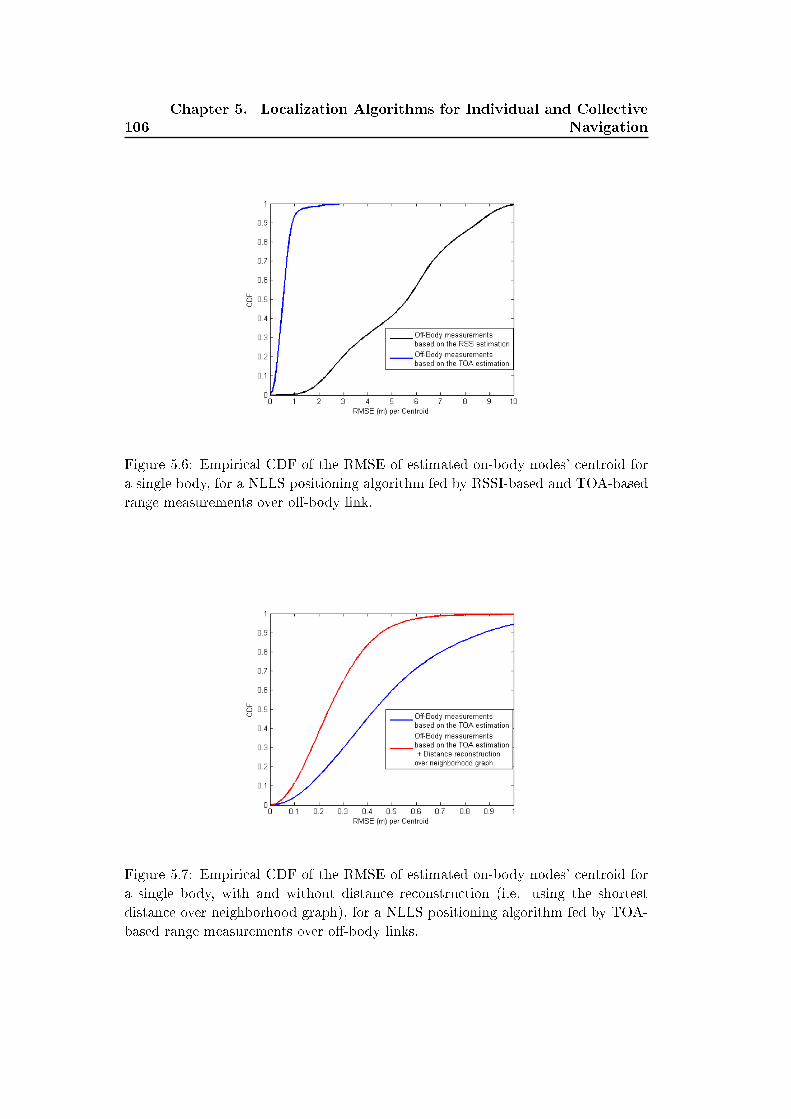
106
Chapter 5. Localization Algorithms for Individual and Collective
Navigation
Figure 5.6: Empirical CDF of the RMSE of estimated on-body nodes' centroid for
a single body, for a NLLS positioning algorithm fed by RSSI-based and TOA-based
range measurements over o�-body link.
Figure 5.7: Empirical CDF of the RMSE of estimated on-body nodes' centroid for
a single body, with and without distance reconstruction (i.e. using the shortest
distance over neighborhood graph), for a NLLS positioning algorithm fed by TOA-
based range measurements over o�-body links.
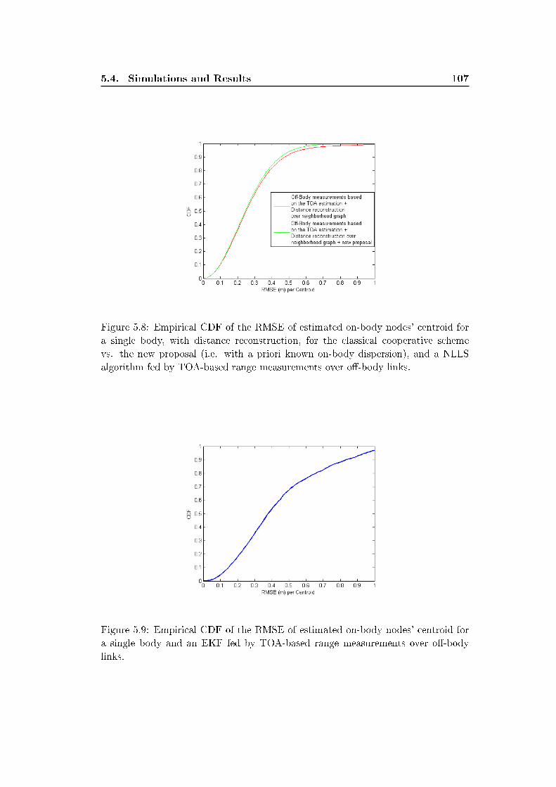
5.4. Simulations and Results 107
Figure 5.8: Empirical CDF of the RMSE of estimated on-body nodes' centroid for
a single body, with distance reconstruction, for the classical cooperative scheme
vs. the new proposal (i.e. with a priori known on-body dispersion), and a NLLS
algorithm fed by TOA-based range measurements over o�-body links.
Figure 5.9: Empirical CDF of the RMSE of estimated on-body nodes' centroid for
a single body and an EKF fed by TOA-based range measurements over o�-body
links.
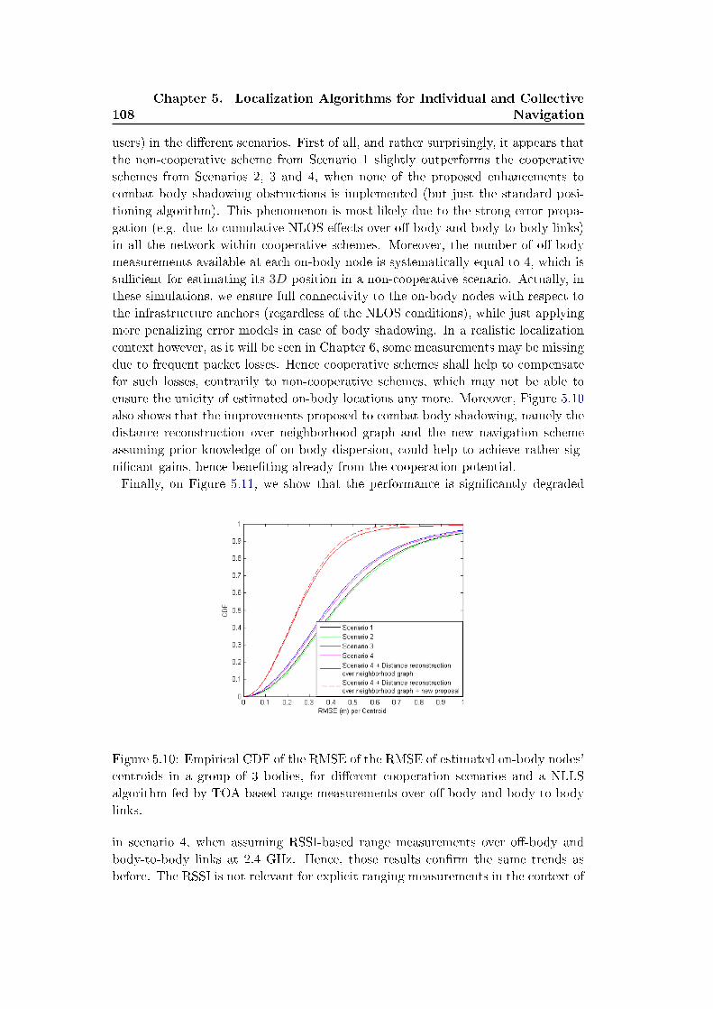
108
Chapter 5. Localization Algorithms for Individual and Collective
Navigation
users) in the di�erent scenarios. First of all, and rather surprisingly, it appears that
the non-cooperative scheme from Scenario 1 slightly outperforms the cooperative
schemes from Scenarios 2, 3 and 4, when none of the proposed enhancements to
combat body shadowing obstructions is implemented (but just the standard posi-
tioning algorithm). This phenomenon is most likely due to the strong error propa-
gation (e.g. due to cumulative NLOS e�ects over o�-body and body-to-body links)
in all the network within cooperative schemes. Moreover, the number of o�-body
measurements available at each on-body node is systematically equal to 4, which is
su�cient for estimating its 3D position in a non-cooperative scenario. Actually, in
these simulations, we ensure full connectivity to the on-body nodes with respect to
the infrastructure anchors (regardless of the NLOS conditions), while just applying
more penalizing error models in case of body shadowing. In a realistic localization
context however, as it will be seen in Chapter 6, some measurements may be missing
due to frequent packet losses. Hence cooperative schemes shall help to compensate
for such losses, contrarily to non-cooperative schemes, which may not be able to
ensure the unicity of estimated on-body locations any more. Moreover, Figure 5.10
also shows that the improvements proposed to combat body shadowing, namely the
distance reconstruction over neighborhood graph and the new navigation scheme
assuming prior knowledge of on-body dispersion, could help to achieve rather sig-
ni�cant gains, hence bene�ting already from the cooperation potential.
Finally, on Figure 5.11, we show that the performance is signi�cantly degraded
Figure 5.10: Empirical CDF of the RMSE of the RMSE of estimated on-body nodes'
centroids in a group of 3 bodies, for di�erent cooperation scenarios and a NLLS
algorithm fed by TOA-based range measurements over o�-body and body-to-body
links.
in scenario 4, when assuming RSSI-based range measurements over o�-body and
body-to-body links at 2.4 GHz. Hence, those results con�rm the same trends as
before. The RSSI is not relevant for explicit ranging measurements in the context of
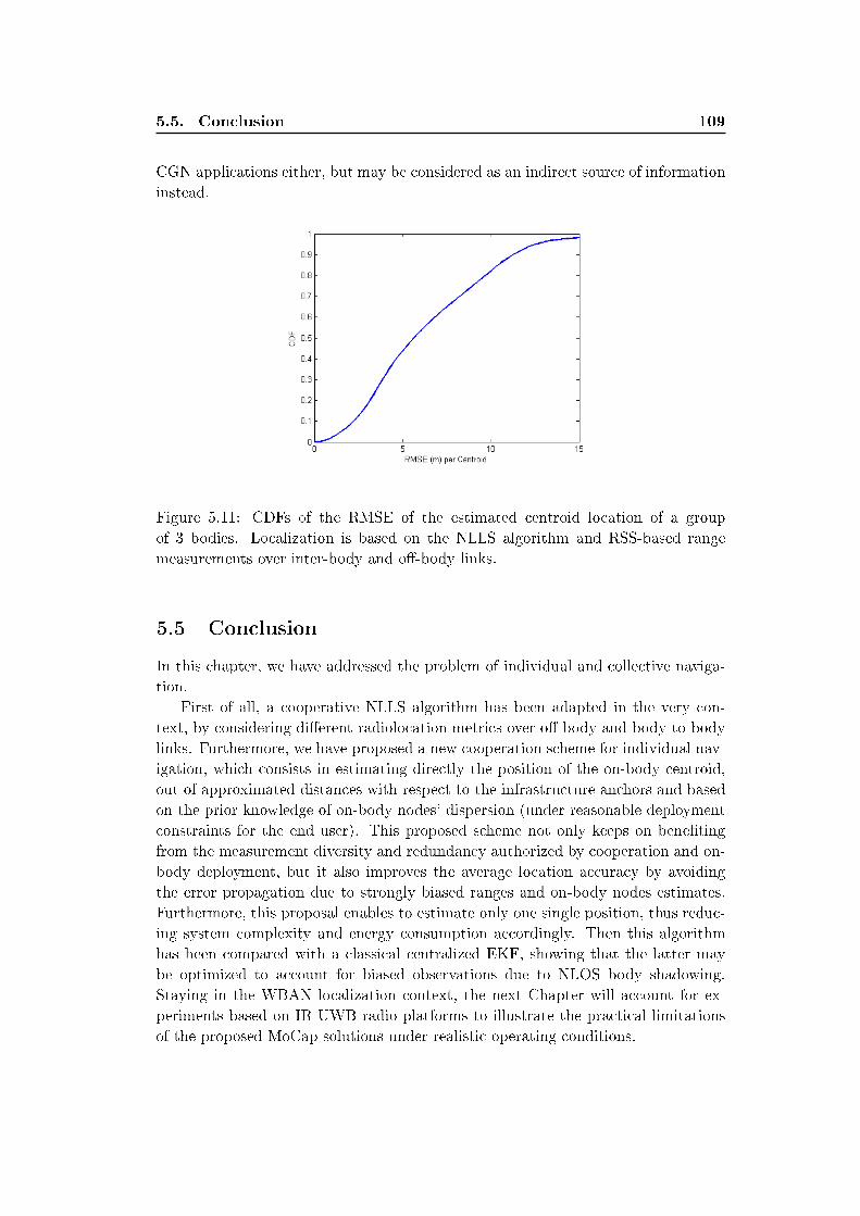
5.5. Conclusion 109
CGN applications either, but may be considered as an indirect source of information
instead.
Figure 5.11: CDFs of the RMSE of the estimated centroid location of a group
of 3 bodies. Localization is based on the NLLS algorithm and RSS-based range
measurements over inter-body and o�-body links.
5.5 Conclusion
In this chapter, we have addressed the problem of individual and collective naviga-
tion.
First of all, a cooperative NLLS algorithm has been adapted in the very con-
text, by considering di�erent radiolocation metrics over o�-body and body-to-body
links. Furthermore, we have proposed a new cooperation scheme for individual nav-
igation, which consists in estimating directly the position of the on-body centroid,
out of approximated distances with respect to the infrastructure anchors and based
on the prior knowledge of on-body nodes' dispersion (under reasonable deployment
constraints for the end user). This proposed scheme not only keeps on bene�ting
from the measurement diversity and redundancy authorized by cooperation and on-
body deployment, but it also improves the average location accuracy by avoiding
the error propagation due to strongly biased ranges and on-body nodes estimates.
Furthermore, this proposal enables to estimate only one single position, thus reduc-
ing system complexity and energy consumption accordingly. Then this algorithm
has been compared with a classical centralized EKF, showing that the latter may
be optimized to account for biased observations due to NLOS body shadowing.
Staying in the WBAN localization context, the next Chapter will account for ex-
periments based on IR-UWB radio platforms to illustrate the practical limitations
of the proposed MoCap solutions under realistic operating conditions.

Chapter 6
Experiments
Contents
6.1 Introduction . . . . . . . . . . . . . . . . . . . . . . . . . . . . 111
6.2 Used Equipment and Experimental Settings . . . . . . . . . 112
6.3 Single-Link Ranging Experiments . . . . . . . . . . . . . . . 114
6.3.1 Ranging Over On-body Links . . . . . . . . . . . . . . . . . . 114
6.3.2 Ranging Over O�-body Links . . . . . . . . . . . . . . . . . . 119
6.4 Individual Motion Capture Experiments Based on Real
Range Measurements . . . . . . . . . . . . . . . . . . . . . . . 120
6.5 Conclusion . . . . . . . . . . . . . . . . . . . . . . . . . . . . . 123
6.1 Introduction
This Chapter accounts for real experiments based on integrated IR-UWB radio
platforms. One goal is to test and partially validate some of the modeling and/or
algorithmic proposals made in Chapters 3 and 4, respectively. Another objective is
to illustrate the practical limitations of the latter developments under real operating
conditions, in comparison with the initial target speci�cations claimed in Chapter
1.
First of all, various data sets of on-body and o�-body range measurements have
been collected for di�erent body gestures and attitudes, so as to verify the mod-
eling hypotheses put forward in Section 3.2 regarding conditional single-link errors
based on IR-UWB TOA estimation. These experiments have been also used for
preliminary calibration purposes (out of raw measurements, from a LS perspective).
Hereafter, the so-called observed range measurements correspond to the calibrated
measurements.
Secondly, IR-UWB devices have been deployed on a reference subject body, with
infrastructure anchors placed in the surrounding indoor environment. In a �rst
step, the intra-WBAN full mesh topology is exploited to collect only on-body range
measurements (including real packet losses due to body shadowing) for relative
MoCap in a body-strapped LCS, applying the CDWMDS algorithm described in
Section 4.2. The second step consists in incorporating additional o�-body links
with respect to infrastructure anchors, in order to enable the absolute positioning
112 Chapter 6. Experiments
of on-body nodes in a GCS external to the body for LSIMC purposes. Hence, the 2-
step localization approach described in Section 4.3 is considered. In both cases, the
obtained experimental results are discussed and compared with simulation-based
results from Sections 4.2.3 and 4.3.3. Unfortunately, due to time constraints, no
group navigation scenarios could be tested experimentally by the time this thesis
has been written.
The remaining part of this Chapter is organized as follows. Section 6.2 brie�y
describes the hardware equipment involved in our measurement campaign, including
IR-UWB LDR platforms and a reference video acquisition system. In Section 6.3, we
evaluate the real ranging errors observed over on-body and o�-body links, in both
LOS and NLOS conditions. Then Section 6.4 investigates relative and absolute
individual MoCap applications, where the involved localization algorithms are fed
with real range measurements. Finally, Section 6.5 draws a few conclusions and
summarizes the main Chapter contributions.
6.2 Used Equipment and Experimental Settings
The used radio platform, which was developed at CEA-Leti, provides a representa-
tive example of integrated IR-UWB Low Data Rate-Location and Tracking (LDR-
LT) device operating in the band [4.25, 4.75]GHz, with a complete protocol stack
from the physical layer up to the localization application layer [113], [114]. Relying
on internal 1 Gsps sampling and 1/1.5 bit quantization on the one hand, as well
as on a Di�erential Binary Phase Shift Keying (DBPSK) modulation on the other
hand, this platform enables data transmissions at the nominal rate of 350 kbps at
up to 40 m in LOS, while performing peer-to-peer ranging through RT-TOF with
clock drift compensation. Regarding unitary TOA estimates, the platform performs
FAP detection. The index of the �rst sample exceeding the threshold is viewed
as the TOA estimate in the local Rx observation window (i.e. direct detection is
performed, but no cross-correlation with a template waveform adapted to the uni-
tary expected pulse). Such detection is enabled within the �ne time resolution of 1
ns, corresponding to the internal sampling capability (i.e. equivalently within the
spatial resolution of 30 cm). The active power consumption, on the order of a few
10s of mW (typically, 10 mW in Tx and 30mW in Rx), is comparable with that of
State-of-the-art technologies foreseen in the WBAN context, such as Bluetooth and
ZigBee, but providing additional unprecedented ranging capabilities [108]. Figure
6.1 shows a picture of this platform in its plastic package.
Besides, fast measurement-oriented software, including simpli�ed MAC and ap-
plications, have also been developed and ported for �exible demonstration purposes.
In particular, the implemented MAC layer enables a beacon-enabled TDMA super-
frame structure, which appears adapted for small-size and coordinated mesh net-
works like in our WBAN context. Figure 6.2 shows the corresponding superframe
structure [9], [115]. The Beacon Period (BP) is entirely speci�ed by the coordinator,
which handles resource allocation and scheduling for the entire network. A slotted

6.2. Used Equipment and Experimental Settings 113
Aloha scheme is used in the Contention Access Period (CAP), in order to authorize
a reduction of the energy consumption [9]. Furthermore, it was chosen to trans-
mit data only during the Contention Free Period (CFP) using Guaranteed Time
Slots (GTS) to prevent from collisions and improve the Quality of Service (QoS).
Hence, in the nominal mode (i.e. in the absence of aggregation and broadcast),
three adjacent GTS are reserved for each peer-to-peer range measurement between
two distinct asyshronous devices, applying 3-Way ranging transactions, as seen in
Chapters 1 and 4. Unfortunately, the implemented MAC su�ers from a few limita-
tions in our speci�c WBAN localization context. One major problem concerns the
refreshment rate that could be achievable for updating the nodes positions, which
is strictly bounded by the superframe periodicity and by the number of available
GTS per superframe. For practicability purposes in our study (but without loss of
generality), the coordinator is external to the body and connected to a Personal
Computer (PC) through a serial port for con�guration and debug. Moreover, an
additional USB link is used as a communication interface between this coordinator
and the PC.
In our investigated scenarios, the TOA-based range measurements issued at IR-
UWB platforms are compared with side reference measurements obtained with the
optical Codamotion tracking system [10], which is able to provide very high localiza-
tion accuracy (i.e. in the order of 0.05 mm). Considering the two levels of precisions,
the Codamotion system will be used to determine the ranging errors. Hence, one
optical marker was placed on each on-body device, in order to de�ne its occupied
position in real-time. Figure 6.3 shows the Codamotion tracking system in action,
where the data �les are fully traceable using legacy �le formats such as ASCII text.
Figure 6.1: CEA-Leti's IR-UWB LDR-LT ranging-enabled platform (right) with its
package (left).
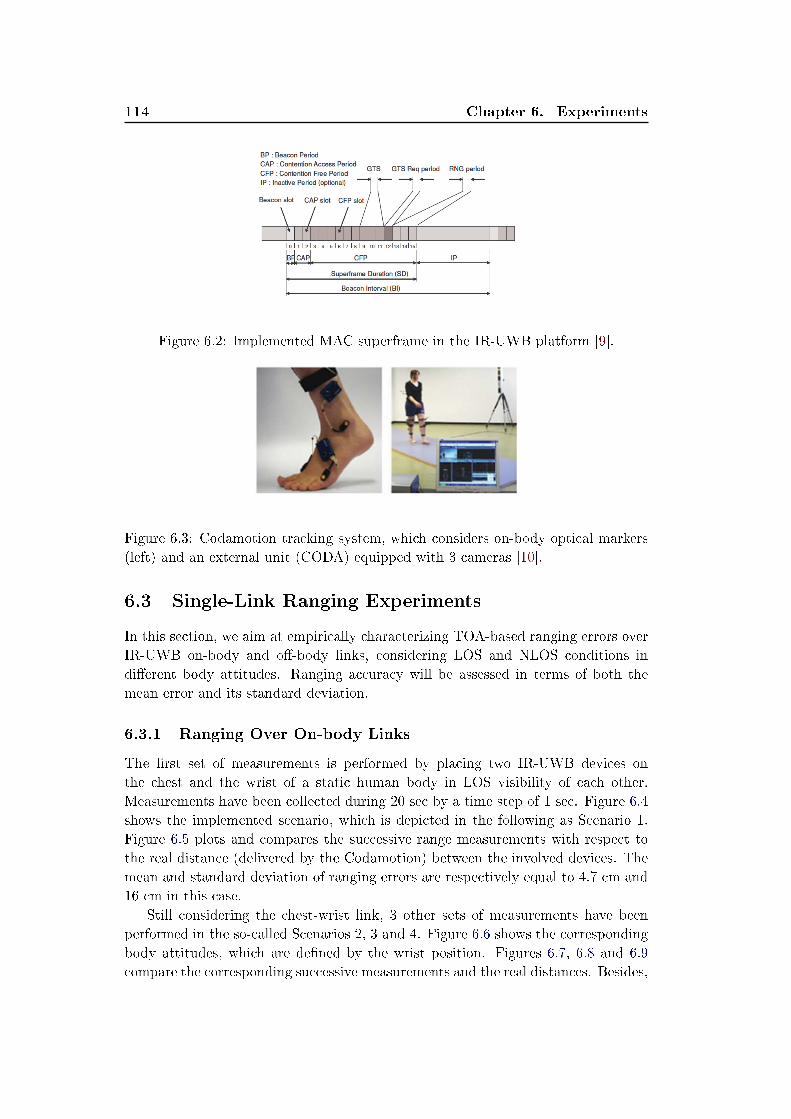
114 Chapter 6. Experiments
Figure 6.2: Implemented MAC superframe in the IR-UWB platform [9].
Figure 6.3: Codamotion tracking system, which considers on-body optical markers
(left) and an external unit (CODA) equipped with 3 cameras [10].
6.3 Single-Link Ranging Experiments
In this section, we aim at empirically characterizing TOA-based ranging errors over
IR-UWB on-body and o�-body links, considering LOS and NLOS conditions in
di�erent body attitudes. Ranging accuracy will be assessed in terms of both the
mean error and its standard deviation.
6.3.1 Ranging Over On-body Links
The �rst set of measurements is performed by placing two IR-UWB devices on
the chest and the wrist of a static human body in LOS visibility of each other.
Measurements have been collected during 20 sec by a time step of 1 sec. Figure 6.4
shows the implemented scenario, which is depicted in the following as Scenario 1.
Figure 6.5 plots and compares the successive range measurements with respect to
the real distance (delivered by the Codamotion) between the involved devices. The
mean and standard deviation of ranging errors are respectively equal to 4.7 cm and
16 cm in this case.
Still considering the chest-wrist link, 3 other sets of measurements have been
performed in the so-called Scenarios 2, 3 and 4. Figure 6.6 shows the corresponding
body attitudes, which are de�ned by the wrist position. Figures 6.7, 6.8 and 6.9
compare the corresponding successive measurements and the real distances. Besides,

6.3. Single-Link Ranging Experiments 115
Figure 6.4: Experimental Scenario 1: On-body ranging over a static chest-wrist link
in direct LOS visibility.
Figure 6.5: Comparison between measured and real distances over the static chest-
wrist link in Scenario 1.
Table 6.1 summarizes the related ranging error parameters (i.e. mean and standard
deviation) for each scenario. The obtained on-body ranging performances in LOS
visibility are in compliance with the results presented in [108] for classical "body-
free" LOS con�gurations at larger ranges in a typical indoor environment, showing
that the standard deviation of ranging errors is below 30 cm. Moreover, the observed
mean error is relatively small in comparison with the standard deviation and even
with the true distance value. Thus, it could be neglected in �rst approximation
over on-body links in direct LOS visibility. Those observations tend to con�rm
the zero-mean Gaussian hypothesis retained in Chapter 3 for IR-UWB TOA-based
on-body measurements in LOS. However, the standard deviation observed with the
real platforms is now larger than the values based on channel measurements (i.e.
previously on the order of 10 cm in favorable SNR conditions) and hence, larger
than the values assumed in the simulations of Chapter 4. This degraded accuracy is
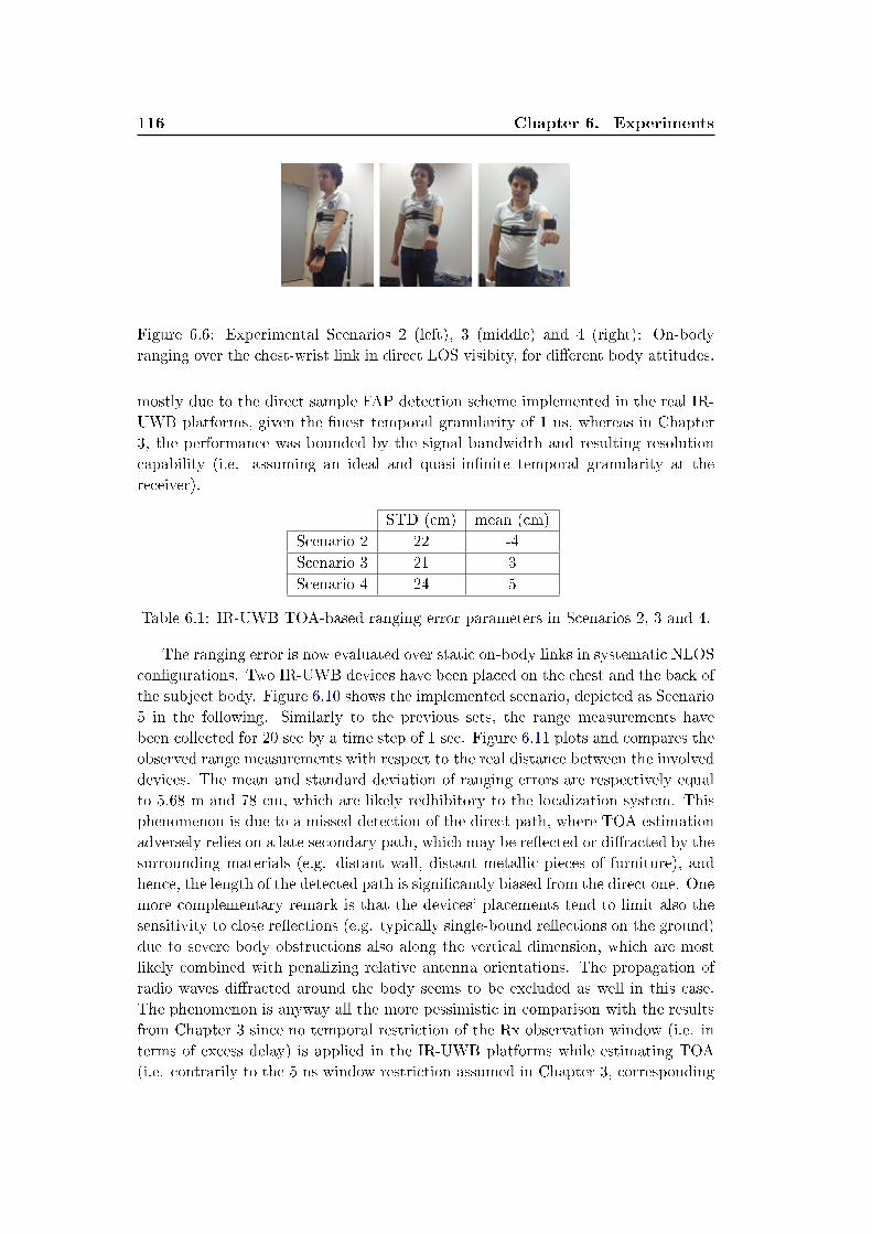
116 Chapter 6. Experiments
Figure 6.6: Experimental Scenarios 2 (left), 3 (middle) and 4 (right): On-body
ranging over the chest-wrist link in direct LOS visibity, for di�erent body attitudes.
mostly due to the direct sample FAP detection scheme implemented in the real IR-
UWB platforms, given the �nest temporal granularity of 1 ns, whereas in Chapter
3, the performance was bounded by the signal bandwidth and resulting resolution
capability (i.e. assuming an ideal and quasi-in�nite temporal granularity at the
receiver).
STD (cm) mean (cm)
Scenario 2 22 -4
Scenario 3 21 3
Scenario 4 24 5
Table 6.1: IR-UWB TOA-based ranging error parameters in Scenarios 2, 3 and 4.
The ranging error is now evaluated over static on-body links in systematic NLOS
con�gurations. Two IR-UWB devices have been placed on the chest and the back of
the subject body. Figure 6.10 shows the implemented scenario, depicted as Scenario
5 in the following. Similarly to the previous sets, the range measurements have
been collected for 20 sec by a time step of 1 sec. Figure 6.11 plots and compares the
observed range measurements with respect to the real distance between the involved
devices. The mean and standard deviation of ranging errors are respectively equal
to 5.68 m and 78 cm, which are likely redhibitory to the localization system. This
phenomenon is due to a missed detection of the direct path, where TOA estimation
adversely relies on a late secondary path, which may be re�ected or di�racted by the
surrounding materials (e.g. distant wall, distant metallic pieces of furniture), and
hence, the length of the detected path is signi�cantly biased from the direct one. One
more complementary remark is that the devices' placements tend to limit also the
sensitivity to close re�ections (e.g. typically single-bound re�ections on the ground)
due to severe body obstructions also along the vertical dimension, which are most
likely combined with penalizing relative antenna orientations. The propagation of
radio waves di�racted around the body seems to be excluded as well in this case.
The phenomenon is anyway all the more pessimistic in comparison with the results
from Chapter 3 since no temporal restriction of the Rx observation window (i.e. in
terms of excess delay) is applied in the IR-UWB platforms while estimating TOA
(i.e. contrarily to the 5 ns window restriction assumed in Chapter 3, corresponding
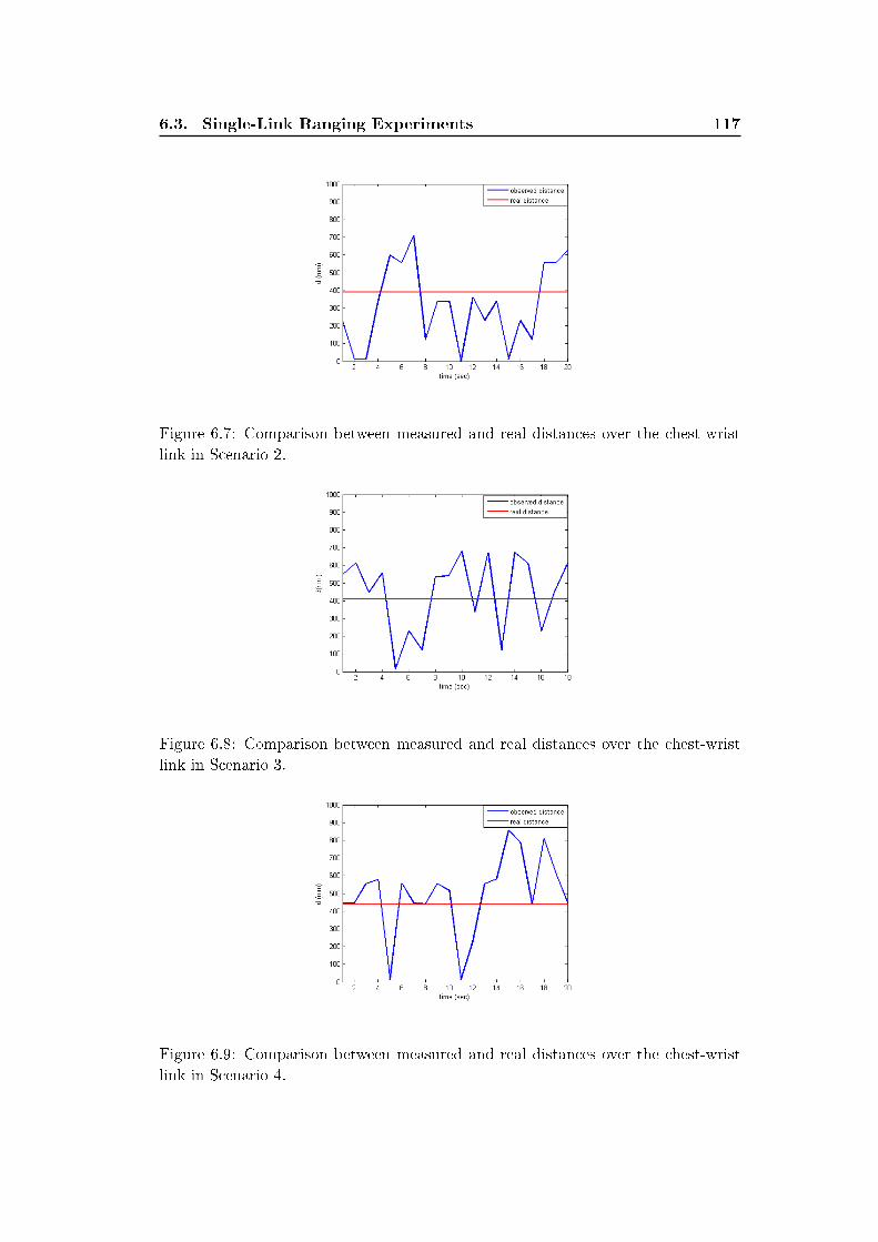
6.3. Single-Link Ranging Experiments 117
Figure 6.7: Comparison between measured and real distances over the chest-wrist
link in Scenario 2.
Figure 6.8: Comparison between measured and real distances over the chest-wrist
link in Scenario 3.
Figure 6.9: Comparison between measured and real distances over the chest-wrist
link in Scenario 4.
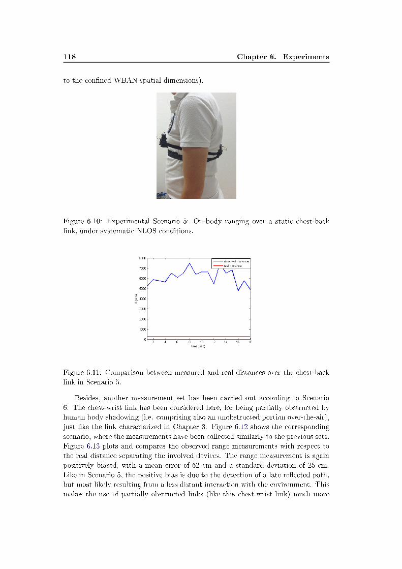
118 Chapter 6. Experiments
to the con�ned WBAN spatial dimensions).
Figure 6.10: Experimental Scenario 5: On-body ranging over a static chest-back
link, under systematic NLOS conditions.
Figure 6.11: Comparison between measured and real distances over the chest-back
link in Scenario 5.
Besides, another measurement set has been carried out according to Scenario
6. The chest-wrist link has been considered here, for being partially obstructed by
human body shadowing (i.e. comprising also an unobstructed portion over-the-air),
just like the link characterized in Chapter 3. Figure 6.12 shows the corresponding
scenario, where the measurements have been collected similarly to the previous sets.
Figure 6.13 plots and compares the observed range measurements with respect to
the real distance separating the involved devices. The range measurement is again
positively biased, with a mean error of 62 cm and a standard deviation of 25 cm.
Like in Scenario 5, the positive bias is due to the detection of a late re�ected path,
but most likely resulting from a less distant interaction with the environment. This
makes the use of partially obstructed links (like this chest-wrist link) much more
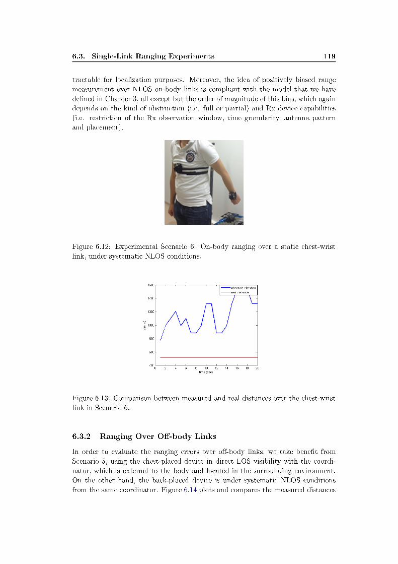
6.3. Single-Link Ranging Experiments 119
tractable for localization purposes. Moreover, the idea of positively biased range
measurement over NLOS on-body links is compliant with the model that we have
de�ned in Chapter 3, all except but the order of magnitude of this bias, which again
depends on the kind of obstruction (i.e. full or partial) and Rx device capabilities
(i.e. restriction of the Rx observation window, time granularity, antenna pattern
and placement).
Figure 6.12: Experimental Scenario 6: On-body ranging over a static chest-wrist
link, under systematic NLOS conditions.
Figure 6.13: Comparison between measured and real distances over the chest-wrist
link in Scenario 6.
6.3.2 Ranging Over O�-body Links
In order to evaluate the ranging errors over o�-body links, we take bene�t from
Scenario 5, using the chest-placed device in direct LOS visibility with the coordi-
nator, which is external to the body and located in the surrounding environment.
On the other hand, the back-placed device is under systematic NLOS conditions
from the same coordinator. Figure 6.14 plots and compares the measured distances
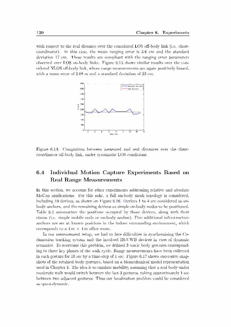
120 Chapter 6. Experiments
with respect to the real distance over the considered LOS o�-body link (i.e. chest-
coordinator). In this case, the mean ranging error is 5.6 cm and the standard
deviation 17 cm. These results are compliant with the ranging error parameters
observed over LOS on-body links. Figure 6.15 shows similar results over the con-
sidered NLOS o�-body link, whose range measurements are again positively biased,
with a mean error of 2.08 m and a standard deviation of 23 cm.
Figure 6.14: Comparison between measured and real distances over the chest-
coordinator o�-body link, under systematic LOS conditions.
6.4 Individual Motion Capture Experiments Based on
Real Range Measurements
In this section, we account for other experiments addressing relative and absolute
MoCap applications. For this sake, a full on-body mesh topology is considered,
including 10 devices, as shown on Figure 6.16. Devices 1 to 4 are considered as on-
body anchors, and the remaining devices as simple on-body nodes to be positioned.
Table 6.2 summarizes the positions occupied by those devices, along with their
status (i.e. simple mobile node or on-body anchor). Five additional infrastructure
anchors are set at known positions in the indoor surrounding environment, which
corresponds to a 4m × 4m o�ce room.
In our measurement setup, we had to face di�culties in synchronizing the Co-
damotion tracking system and the involved IR-UWB devices in case of dynamic
scenarios. To overcome this problem, we de�ned 3 static body gestures correspond-
ing to three key phases of the walk cycle. Range measurements have been collected
in each gesture for 10 sec by a time-step of 1 sec. Figure 6.17 shows successive snap-
shots of the retained body gestures, based on a biomechanical model representation
used in Chapter 4. The idea is to emulate mobility, assuming that a real body under
moderate walk would switch between the last 3 gestures, taking approximately 1 sec
between two adjacent gestures. Thus our localization problem could be considered
as quasi-dynamic.
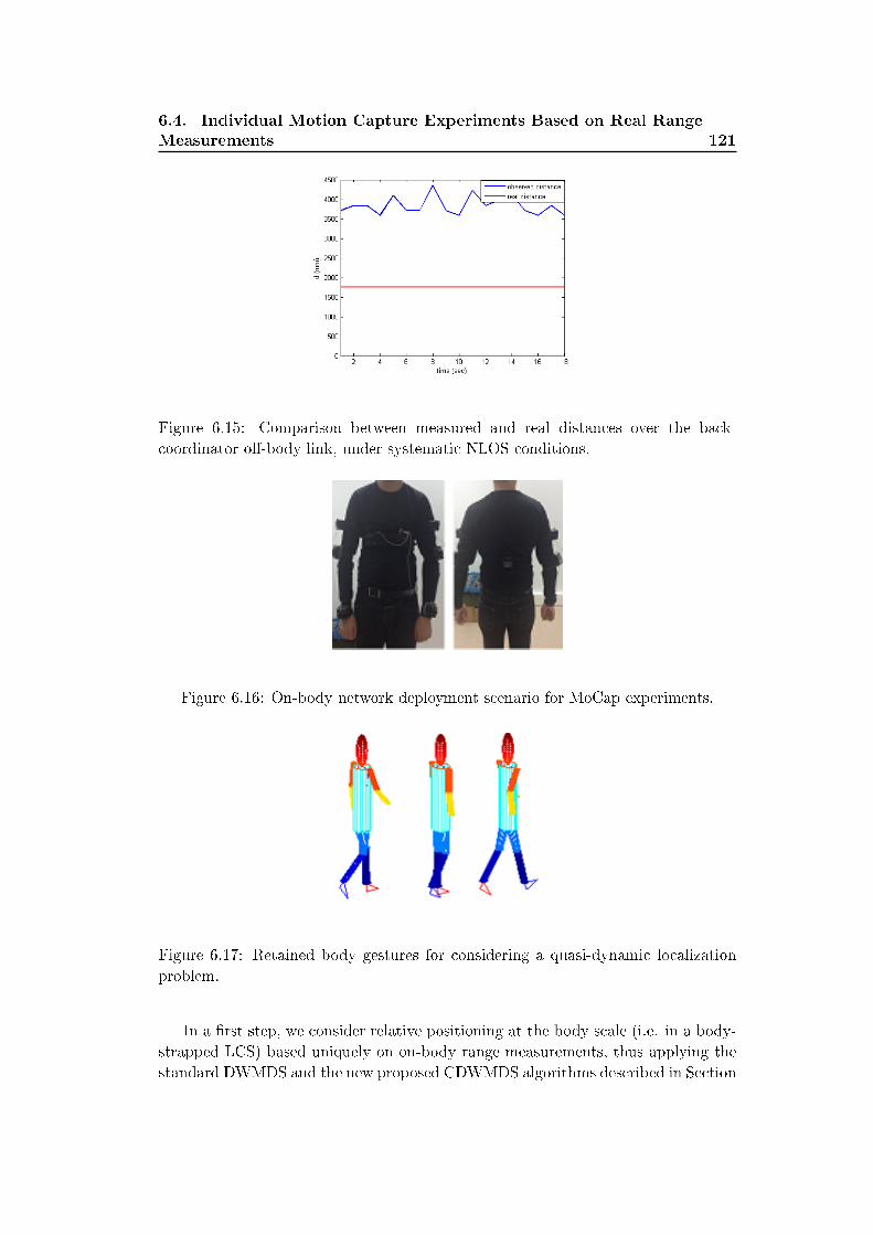
6.4. Individual Motion Capture Experiments Based on Real Range
Measurements 121
Figure 6.15: Comparison between measured and real distances over the back-
coordinator o�-body link, under systematic NLOS conditions.
Figure 6.16: On-body network deployment scenario for MoCap experiments.
Figure 6.17: Retained body gestures for considering a quasi-dynamic localization
problem.
In a �rst step, we consider relative positioning at the body scale (i.e. in a body-
strapped LCS) based uniquely on on-body range measurements, thus applying the
standard DWMDS and the new proposed CDWMDS algorithms described in Section
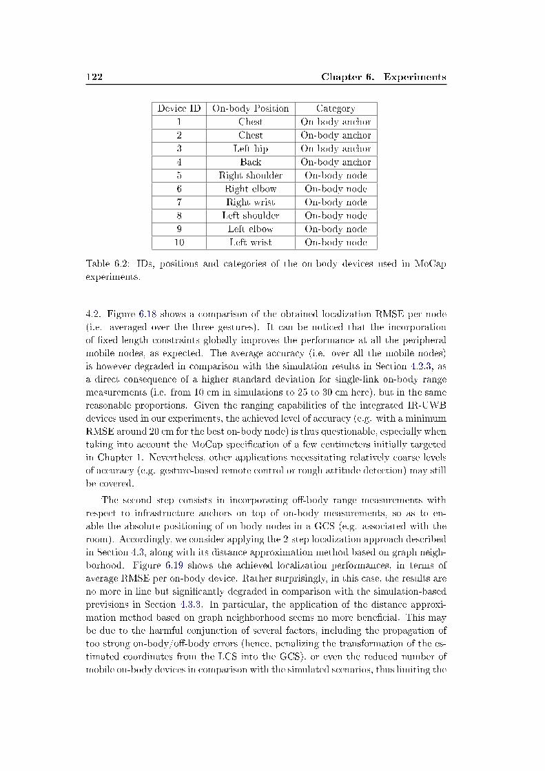
122 Chapter 6. Experiments
Device ID On-body Position Category
1 Chest On-body anchor
2 Chest On-body anchor
3 Left hip On-body anchor
4 Back On-body anchor
5 Right shoulder On-body node
6 Right elbow On-body node
7 Right wrist On-body node
8 Left shoulder On-body node
9 Left elbow On-body node
10 Left wrist On-body node
Table 6.2: IDs, positions and categories of the on-body devices used in MoCap
experiments.
4.2. Figure 6.18 shows a comparison of the obtained localization RMSE per node
(i.e. averaged over the three gestures). It can be noticed that the incorporation
of �xed-length constraints globally improves the performance at all the peripheral
mobile nodes, as expected. The average accuracy (i.e. over all the mobile nodes)
is however degraded in comparison with the simulation results in Section 4.2.3, as
a direct consequence of a higher standard deviation for single-link on-body range
measurements (i.e. from 10 cm in simulations to 25 to 30 cm here), but in the same
reasonable proportions. Given the ranging capabilities of the integrated IR-UWB
devices used in our experiments, the achieved level of accuracy (e.g. with a minimum
RMSE around 20 cm for the best on-body node) is thus questionable, especially when
taking into account the MoCap speci�cation of a few centimeters initially targeted
in Chapter 1. Nevertheless, other applications necessitating relatively coarse levels
of accuracy (e.g. gesture-based remote control or rough attitude detection) may still
be covered.
The second step consists in incorporating o�-body range measurements with
respect to infrastructure anchors on top of on-body measurements, so as to en-
able the absolute positioning of on-body nodes in a GCS (e.g. associated with the
room). Accordingly, we consider applying the 2-step localization approach described
in Section 4.3, along with its distance approximation method based on graph neigh-
borhood. Figure 6.19 shows the achieved localization performances, in terms of
average RMSE per on-body device. Rather surprisingly, in this case, the results are
no more in line but signi�cantly degraded in comparison with the simulation-based
previsions in Section 4.3.3. In particular, the application of the distance approxi-
mation method based on graph neighborhood seems no more bene�cial. This may
be due to the harmful conjunction of several factors, including the propagation of
too strong on-body/o�-body errors (hence, penalizing the transformation of the es-
timated coordinates from the LCS into the GCS), or even the reduced number of
mobile on-body devices in comparison with the simulated scenarios, thus limiting the
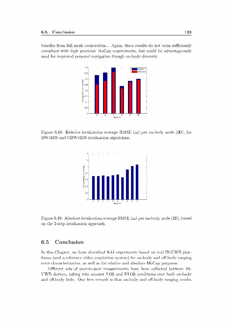
6.5. Conclusion 123
bene�ts from full mesh cooperation... Again, these results do not seem su�ciently
compliant with high precision MoCap requirements, but could be advantageously
used for improved personal navigation though on-body diversity.
Figure 6.18: Relative localization average RMSE (m) per on-body node (ID), for
DWMDS and CDWMDS localization algorithms.
Figure 6.19: Absolute localization average RMSE (m) per on-body node (ID), based
on the 2-step localization approach.
6.5 Conclusion
In this Chapter, we have described �eld experiments based on real IR-UWB plat-
forms (and a reference video acquisition system) for on-body and o�-body ranging
error characterization, as well as for relative and absolute MoCap purposes.
Di�erent sets of peer-to-peer measurements have been collected between IR-
UWB devices, taking into account LOS and NLOS conditions over both on-body
and o�-body links. One �rst remark is that on-body and o�-body ranging results
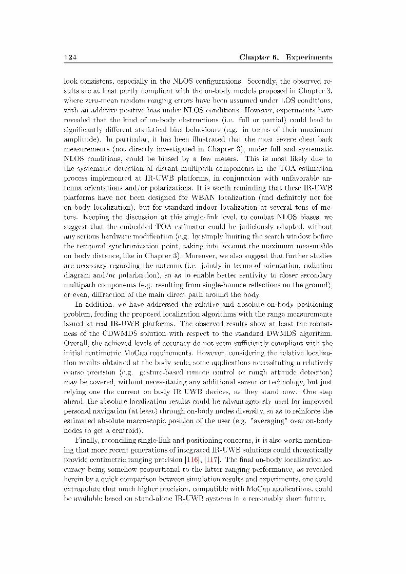
124 Chapter 6. Experiments
look consistent, especially in the NLOS con�gurations. Secondly, the observed re-
sults are at least partly compliant with the on-body models proposed in Chapter 3,
where zero-mean random ranging errors have been assumed under LOS conditions,
with an additive positive bias under NLOS conditions. However, experiments have
revealed that the kind of on-body obstructions (i.e. full or partial) could lead to
signi�cantly di�erent statistical bias behaviours (e.g. in terms of their maximum
amplitude). In particular, it has been illustrated that the most severe chest-back
measurements (not directly investigated in Chapter 3), under full and systematic
NLOS conditions, could be biased by a few meters. This is most likely due to
the systematic detection of distant multipath components in the TOA estimation
process implemented at IR-UWB platforms, in conjunction with unfavorable an-
tenna orientations and/or polarizations. It is worth reminding that these IR-UWB
platforms have not been designed for WBAN localization (and de�nitely not for
on-body localization), but for standard indoor localization at several tens of me-
ters. Keeping the discussion at this single-link level, to combat NLOS biases, we
suggest that the embedded TOA estimator could be judiciously adapted, without
any serious hardware modi�cation (e.g. by simply limiting the search window before
the temporal synchronization point, taking into account the maximum measurable
on-body distance, like in Chapter 3). Moreover, we also suggest that further studies
are necessary regarding the antenna (i.e. jointly in terms of orientation, radiation
diagram and/or polarization), so as to enable better sentivity to closer secondary
multipath components (e.g. resulting from single-bounce re�ections on the ground),
or even, di�raction of the main direct path around the body.
In addition, we have addressed the relative and absolute on-body positioning
problem, feeding the proposed localization algorithms with the range measurements
issued at real IR-UWB platforms. The observed results show at least the robust-
ness of the CDWMDS solution with respect to the standard DWMDS algorithm.
Overall, the achieved levels of accuracy do not seem su�ciently compliant with the
initial centimetric MoCap requirements. However, considering the relative localiza-
tion results obtained at the body scale, some applications necessitating a relatively
coarse precision (e.g. gesture-based remote control or rough attitude detection)
may be covered, without necessitating any additional sensor or technology, but just
relying one the current on-body IR-UWB devices, as they stand now. One step
ahead, the absolute localization results could be advantageously used for improved
personal navigation (at least) through on-body nodes diversity, so as to reinforce the
estimated absolute macroscopic position of the user (e.g. "averaging" over on-body
nodes to get a centroid).
Finally, reconciling single-link and positioning concerns, it is also worth mention-
ing that more recent generations of integrated IR-UWB solutions could theoretically
provide centimetric ranging precision [116], [117]. The �nal on-body localization ac-
curacy being somehow proportional to the latter ranging performance, as revealed
herein by a quick comparison between simulation results and experiments, one could
extrapolate that much higher precision, compatible with MoCap applications, could
be available based on stand-alone IR-UWB systems in a reasonably short future.
Chapter 7
Conclusions and Perspectives
Contents
7.1 Conclusions . . . . . . . . . . . . . . . . . . . . . . . . . . . . . 125
7.2 Perspectives . . . . . . . . . . . . . . . . . . . . . . . . . . . . . 128
7.1 Conclusions
In this PhD dissertation, we have addressed the cooperative localization problem in
WBAN. Various research topics and domains have thus been explored, related to
physical modeling, algorithmic developments, as well as to medium access mecha-
nisms or networking. The main personal contributions issued in the frame of these
PhD investigations can be summarized as follows:
• Modeling: A dynamic on-body model has been proposed for IR-UWB TOA-
based ranging in two key frequency bands and for two representative links.
The drawn model, which relies on UWB channel measurements, takes into ac-
count dynamic channel obstruction con�gurations (i.e. LOS/NLOS) and SNR
variations under body mobility. Then the related model parameters have been
studied as a function of a controlled SNR within synthetic received multipath
signals. On this occasion, false and missed detection phenomena have been
illustrated under low SNR and NLOS conditions, as well as asymptotically
ideal detection behaviour under more favourable SNR and LOS conditions.
The performances of �rst peak and strongest peak detection schemes have
also been compared. We have shown that the ranging error distribution could
be fairly well modeled as a centered Gaussian distribution in LOS conditions
in case of systematic strongest path detection, and as a weighted mixture
between uniform and Gaussian distributions in the case of �rst path detec-
tion. In NLOS conditions, ranging errors are also shown to follow a weighted
mixture between uniform and Gaussian distributions in case of strongest path
detection.
Secondly, representative lower bounds have been derived for the standard
deviation of N-B RSSI-based and IR-UWB TOA-based range measurements
over o�-body and body-to-body links. One �rst conclusion, as expected, is
that RSSI readings in NLOS conditions due to body shadowing are hardly
126 Chapter 7. Conclusions and Perspectives
exploitable for ranging purposes on both kinds of links, whereas LOS condi-
tions may provide more acceptable ranging performance, but most likely at
short ranges (typically below 20 m). One second remark is that o�-body and
body-to-body links exhibit approximately the same behaviours in terms of
ranging error statistics, in �rst approximation.
• Design of localization algorithms:
• Relative on-body positioning for MoCap: A decentralized and coopera-
tive DWMDS algorithm, which can asynchronously estimate unknown
on-body nodes locations, has been adapted. In particular, we have in-
troduced �xed-length geometric constraints (possibly self-learnt) that
correspond to time-invariant Euclidean inter-node distances under body
mobility. This initial CDWMDS has been enhanced through schedul-
ing and censoring mechanisms to mitigate error propagation due to the
location-dependent disparities observed among on-body nodes (e.g. in
terms of connectivity, GDOP and accelerations). It has been also shown
that forcing the symmetry of pair-wise measurements could help to mit-
igate measurement outliers and packet losses. Moreover, CDWMDS
has been proved to outperform a classical MDS algorithm in terms of
localization accuracy for various single-link PER values and ranging
standard deviations even under realistic MAC superframe, hence illus-
trating rather �ne robustness against latency e�ects.
• Absolute on-body positioning for MoCap: Two approaches have been
presented to estimate the absolute locations of on-body nodes in a
global coordinates system, considering di�erent radiolocation metrics
over o�-body links with respect to infrastructure anchors. One 2-step
solution relies on the preliminary relative localization of on-body nodes
at the body scale, before applying further transformations based on the
absolute localization of on-body anchors. At �rst sight, body shadow-
ing seems very challenging, not to say redhibitory, to achieve levels of
precision compatible with high-precision MoCap needs. However we
have proposed another algorithm that estimates the shortest path be-
tween on-body and infrastructure anchors over neighborhood graph to
compensate for possible radio obstructions and penalizing measurement
errors. Thanks to the latter improvement, approximately the same lev-
els of precision as that obtained for relative on-body localization could
be achieved over simulated large-scale trajectories.
• Absolute body centroid positioning for individual and collective naviga-
tion: A cooperative NLLS algorithm has been adapted and compared
with a classical tracking EKF, while considering di�erent radiolocation
metrics over o�-body and body-to-body links. Furthermore, we have
proposed a new cooperation scheme for individual navigation, which
consists in estimating directly the position of the on-body centroid, out
7.1. Conclusions 127
of approximated distances with respect to the infrastructure anchors.
The latter are based on the prior knowledge of on-body nodes' disper-
sion (under reasonable deployment constraints for the end user). This
scheme not only keeps on bene�ting from the measurement diversity
and redundancy authorized by cooperation and on-body deployment,
but it also improves the average localization accuracy by mitigating er-
ror propagation. Finally, only one single position needs to be computed,
thus reducing system complexity and energy consumption accordingly.
• Experiments: Field experiments, based on real IR-UWB platforms (and a ref-
erence video acquisition system) have been described. These measurements
aim at both single-link ranging error characterization and relative/absolute
MoCap evaluation. Due to time constraints, no collective navigation could be
tested however.
On-body and o�-body ranging results look consistent, especially in NLOS con-
�gurations. The observed results are also partly compliant with the originally
proposed on-body models, assuming zero-mean random ranging errors under
LOS conditions and additive positive bias under NLOS conditions. However,
these experiments have also revealed that on-body obstructions could lead
to signi�cantly di�erent bias behaviours, depending whether the obstruction
is full or partial (e.g. chest-back range measurements could be biased by a
few meters). Possible reasons have been pointed out, such as the detection of
late multipath components in the used IR-UWB platforms, which have been
designed for standard indoor localization at several tens of meters (but not
for WBAN applications), or even unfavorable antenna orientations and polar-
izations, which favor neither di�racted path around the body, nor early/close
secondary paths (e.g. single-bounce re�ections on the ground).
Additional experimental scenarios have been considered for relative and ab-
solute on-body positioning, feeding the proposed localization algorithms with
on-body (and o�-body) range measurements from the real IR-UWB platforms.
Signi�cant performance improvements have been noted when applying �xed-
length constraints, even if the achieved accuracy cannot be really compliant
with MoCap requirements at �rst sight. Nevertheless, relying uniquely on
the current on-body IR-UWB devices (i.e. even if not optimized in the very
context), gesture-based remote control or rough attitude detection could be
already covered on the one hand. The absolute localization results could
be also advantageously used for improved individual or collective navigation,
relying on on-body diversity (not shown herein).
Overall, one can conclude that the cooperative localization problem in WBAN,
as initially stated in Chapter 1 for stand-alone and opportunistic MoCap and navi-
gation applications, has been only partly solved out here (especially regarding high
precision MoCap) and numerous points still remain open. On the one hand, prac-
tical experiments and empirical channel-based observations tend to suggest that a
few working hypotheses have been underestimated at the beginning of our PhD
128 Chapter 7. Conclusions and Perspectives
investigations, as well as in our simulations (e.g. body shadowing e�ects on both
ranging errors and packet losses). On the other hand, we believe that the current
state-of-the-art radio capabilities are not yet arrived at their full potential in terms
of single-link precision. Finally, some of our initial proposals detailed above (e.g.
body-constrained decentralized localization, use of on-body diversity...), though non-
de�nitive, may deserve complementary future research e�orts, as seen in the next
subsection.
7.2 Perspectives
After recalling the main PhD contributions and their limitations, we draw hereafter
some related perspectives and possible axes of research for future works:
• Consider coupling the CDWMDS localization algorithm with track-
ing/smoothing algorithms, better initialization policy and/or a soft weighting
of the available single-link measurements in the optimized cost function (e.g.
depending on the link quality, the channel obstruction status or the empiri-
cally observed "instantaneous" PER).
• Enable more e�cient links selection and parsimonious/timely cooperation
over on-body, body-to-body and o�-body links (i.e. relying uniquely on the
most relevant and necessary links), hence improving robustness, while reduc-
ing over-the-air tra�c and latency.
• Design ranging-enabled IR-UWB receivers and impulse detection algorithms,
which could be more suitable into the WBAN localization context. For in-
stance, so as to combat NLOS biases over on-body links due to body shadow-
ing within the current IR-UWB devices (e.g. those used in our experiments),
the embedded TOA estimation procedure could be adapted without changing
the hardware capabilities, by simply limiting the search window (e.g. tak-
ing into account the maximum measurable on-body distance). Regarding the
antenna, optimizations are also expected (i.e. jointly in terms of mastered
orientation, radiation diagram and/or polarization), to enable better sensi-
bility to early/close secondary multipath components, or even, a di�raction
of the direct path around the body. Finally, more recent generations of inte-
grated low-power IR-UWB solutions, which already claim centimetric levels
of ranging precisions, should be considered in the WBAN context to scalably
achieve localization performances compatible with MoCap applications in a
reasonably short future.
• Perform hybrid data fusion to combine IR-UWB radiolocation metrics with
other modalities, such as inertial measurements issued at embedded IMU (e.g.
delivering at least accurate information about the body-limbs orientation).
Such multimodal solutions are likely to o�er the highest and most promising
potential in terms of precision, but additional research e�orts must be made
7.2. Perspectives 129
in terms of algorithmic design and implementation, so as to limit computa-
tional complexity and power consumption, while coping with sychronization
constraints between the two sub-systems.
• Mitigate the e�ects of latency introduced by communication protocols on lo-
calization performance, and thus, emphasizing the needs for cross-layer design
approaches ("by nature").
• Develop more adapted evaluation tools, through semi-deterministic radio
modeling under complex human mobility, for realistic performance assessment
and bene�t from the latest advances in the �eld of WBAN radio propagation
prediction (e.g. di�raction theory applied to dielectric cylinders, deterministic
ray-tracing...) to elaborate even more robust ranging/localization algorithms.

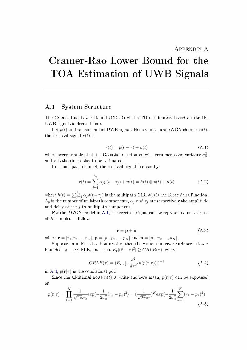
Appendix A
Cramer-Rao Lower Bound for the
TOA Estimation of UWB Signals
A.1 System Structure
The Cramer-Rao Lower Bound (CRLB) of the TOA estimator, based on the IR-
UWB signals is derived here.
Let p(t) be the transmitted UWB signal. Hence, in a pure AWGN channel n(t),
the received signal r(t) is
r(t) = p(t− τ) + n(t) (A.1)
where every sample of n(t) is Gaussian distributed with zero mean and variance σ20,
and τ is the time delay to be estimated.
In a multipath channel, the received signal is given by:
r(t) =
Lp∑j=1
αjp(t− τj) + n(t) = h(t)⊗ p(t) + n(t) (A.2)
where h(t) =∑Lp
j=1 αjδ(t−τj) is the multipath CIR, δ(.) is the Dirac delta function,Lp is the number of multipath components, αj and τj are respectively the amplitude
and delay of the j-th multipath component.
For the AWGN model in A.1, the received signal can be represented as a vector
of K samples as follows:
r = p + n (A.3)
where r = [r1, r2, ..., rK ], p = [p1, p2, ..., pK ] and n = [n1, n2, ..., nK ].
Suppose an unbiased estimator of τ , then the estimation error variance is lower
bounded by the CRLB, and thus, Er|(τ − τ)2| ≥ CRLB(τ), where
CRLB(τ) = (Er|τ [− d2
dτ2ln(p(r|τ))])−1 (A.4)
in A.4, p(r|τ) is the conditional pdf.
Since the additional noise n(t) is white and zero mean, p(r|τ) can be expressed
as
p(r|τ) =
K∏k=1
1√2πσ0
exp(− 1
2σ20(rk − pk)2) = (
1√2πσ0
)Kexp(− 1
2σ20
K∑k=1
(rk − pk)2)
(A.5)
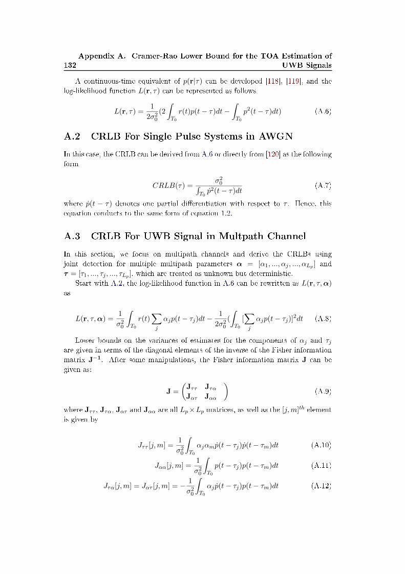
132
Appendix A. Cramer-Rao Lower Bound for the TOA Estimation of
UWB Signals
A continuous-time equivalent of p(r|τ) can be developed [118], [119], and the
log-likelihood function L(r, τ) can be represented as follows
L(r, τ) =1
2σ20(2
∫T0
r(t)p(t− τ)dt−∫T0
p2(t− τ)dt) (A.6)
A.2 CRLB For Single Pulse Systems in AWGN
In this case, the CRLB can be derived from A.6 or directly from [120] as the following
form
CRLB(τ) =σ20∫
T0p2(t− τ)dt
(A.7)
where p(t − τ) denotes one partial di�erentiation with respect to τ . Hence, this
equation conducts to the same form of equation 1.2.
A.3 CRLB For UWB Signal in Multpath Channel
In this section, we focus on multipath channels and derive the CRLBs using
joint detection for multiple multipath parameters α = [α1, ..., αj , ..., αLp ] and
τ = [τ1, ..., τj , ..., τLp ], which are treated as unknown but deterministic.
Start with A.2, the log-likelihood function in A.6 can be rewritten as L(r, τ,α)
as
L(r, τ,α) =1
σ20
∫T0
r(t)∑j
αjp(t− τj)dt−1
2σ20(
∫T0
[∑j
αjp(t− τj)]2dt (A.8)
Lower bounds on the variances of estimates for the components of αj and τjare given in terms of the diagonal elements of the inverse of the Fisher information
matrix J−1. After some manipulations, the Fisher information matrix J can be
given as:
J =
(Jττ JταJατ Jαα
)(A.9)
where Jττ , Jτα, Jατ and Jαα are all Lp×Lp matrices, as well as the [j,m]th element
is given by
Jττ [j,m] =1
σ20
∫T0
αjαmp(t− τj)p(t− τm)dt (A.10)
Jαα[j,m] =1
σ20
∫T0
p(t− τj)p(t− τm)dt (A.11)
Jτα[j,m] = Jατ [j,m] = − 1
σ20
∫T0
αj p(t− τj)p(t− τm)dt (A.12)
Appendix B
Adaptive Self-Learning and
Detection of On-Body
Fixed-Length Links
On-body links can be classi�ed into two categories. The �rst one corresponds to the
mobile links with variable lengths, which are characterized by a distance that varies
over time under body mobility. The second category concerns the �xed-length links,
where the distance is considered as time-invariant under body mobility. Hence, we
formulate the classi�cation/identi�cation issue into a decision problem. For a given
pair of nodes, the �rst hypothesis H0 corresponds to the �xed-length link, whereas
hypothesis H1 corresponds to a variable mobile-length link under mobility.
H0 : Fixed-length link
H1 : Mobile-length link (B.1)
For the considered on-body link between two devices, d = [d(1), d(2), ... , d(N)]
denotes the vector, which contains N consecutive distance measurements, for in-
stance based on IR-UWB TOA or N-B RSSI estimation. Hereafter, a simple new
method is proposed for the detection of the �xed-length links.
The detector is depicted as a variance-based detector. We assume that the
observed distance at time-stamp k can be represented by the following equation:
d(k) = d(k) + n(k) (B.2)
where, d(k) denotes the true distance at time k and n(k) is a random variable, which
represents the ranging error process. For simplicity, we assume that ranging errors
are i.i.d. variables that follow a centered Gaussian distribution, with a variance σ2.
We de�ne two unbiased estimators. The �rst one corresponds to the mean of the
observed distance measurements, denoted by d and represented by equation B.3.
The second one consists in estimating the variance of the observed distance vector,
where the estimated variance ˆvar(d) is given by equation B.4 [121]. This empirical
variance estimator is unbiased and thus, it can be written as a sum of the statistical
variance of the range measurements d seen as r.v., and an additive random variable
e resulting from the estimation process, which is zero-mean with the variance of
(var(d)√
2N−1)2, according to equation B.5.
134
Appendix B. Adaptive Self-Learning and Detection of On-Body
Fixed-Length Links
d ,1
N
N∑i=1
d(i) (B.3)
σ2 ,1
N − 1
N∑i=1
(d(i)− d)2 (B.4)
ˆvar(d) = var(d) + e (B.5)
Under H0, for the �xed-length links, ˆvar(d) is close to σ2 for a su�ciently large
N , whereas it becomes signi�cantly larger than σ2 under mobility. We de�ned
the missed detection probability PM , which represents the probability to detect a
�xed-length link as variable-length one, as follows:
PM = P (Decision = H1|H0) =
∫ +∞
thresholdp(e|H0)de (B.6)
where p(e|H0) denotes the pdf of the variable e, when a �xed-length link is involved.
Once PM is speci�ed a priori, the detection threshold value can be easily calculated,
and thus, a new form of the variance-based detector can be represented in equation
B.7
Decision = H0 if ( ˆvar(d)− σ2) ≤ threshold
Decision = H1 if ( ˆvar(d)− σ2) ≥ threshold (B.7)
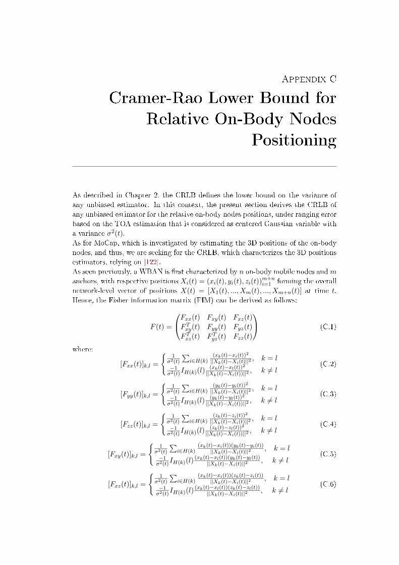
Appendix C
Cramer-Rao Lower Bound for
Relative On-Body Nodes
Positioning
As described in Chapter 2, the CRLB de�nes the lower bound on the variance of
any unbiased estimator. In this context, the present section derives the CRLB of
any unbiased estimator for the relative on-body nodes positions, under ranging error
based on the TOA estimation that is considered as centered Gaussian variable with
a variance σ2(t).
As for MoCap, which is investigated by estimating the 3D positions of the on-body
nodes, and thus, we are seeking for the CRLB, which characterizes the 3D positions
estimators, relying on [122].
As seen previously, a WBAN is �rst characterized by n on-body mobile nodes andm
anchors, with respective positions Xi(t) = (xi(t), yi(t), zi(t))m+ni=1 forming the overall
network-level vector of positions X(t) = [X1(t), ..., Xm(t), ..., Xm+n(t)] at time t.
Hence, the Fisher information matrix (FIM) can be derived as follows:
F (t) =
Fxx(t) Fxy(t) Fxz(t)
F Txy(t) Fyy(t) Fyz(t)
F Txz(t) F Tyz(t) Fzz(t)
(C.1)
where:
[Fxx(t)]k,l =
{1
σ2(t)
∑i∈H(k)
(xk(t)−xi(t))2||Xk(t)−Xi(t)||2 , k = l
−1σ2(t)
IH(k)(l)(xk(t)−xl(t))2||Xk(t)−Xi(t))||2 , k 6= l
(C.2)
[Fyy(t)]k,l =
{1
σ2(t)
∑i∈H(k)
(yk(t)−yi(t))2||Xk(t)−Xi(t)||2 , k = l
−1σ2(t)
IH(k)(l)(yk(t)−yl(t))2||Xk(t)−Xi(t))||2 , k 6= l
(C.3)
[Fzz(t)]k,l =
{1
σ2(t)
∑i∈H(k)
(zk(t)−zi(t))2||Xk(t)−Xi(t)||2 , k = l
−1σ2(t)
IH(k)(l)(zk(t)−zl(t))2||Xk(t)−Xi(t))||2 , k 6= l
(C.4)
[Fxy(t)]k,l =
{1
σ2(t)
∑i∈H(k)
(xk(t)−xi(t))(yk(t)−yi(t))||Xk(t)−Xi(t)||2 , k = l
−1σ2(t)
IH(k)(l)(xk(t)−xl(t))(yk(t)−yl(t))
||Xk(t)−Xi(t)||2 , k 6= l(C.5)
[Fxz(t)]k,l =
{1
σ2(t)
∑i∈H(k)
(xk(t)−xi(t))(zk(t)−zi(t))||Xk(t)−Xi(t)||2 , k = l
−1σ2(t)
IH(k)(l)(xk(t)−xl(t))(zk(t)−zl(t))
||Xk(t)−Xi(t)||2 , k 6= l(C.6)
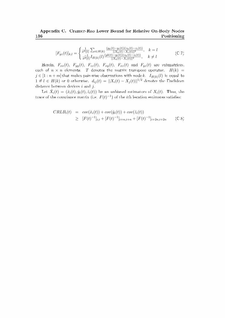
136
Appendix C. Cramer-Rao Lower Bound for Relative On-Body Nodes
Positioning
[Fyz(t)]k,l =
{1
σ2(t)
∑i∈H(k)
(yk(t)−yi(t))(zk(t)−zi(t))||Xk(t)−Xi(t)||2 , k = l
−1σ2(t)
IH(k)(l)(yk(t)−yl(t))(zk(t)−zl(t))
||Xk(t)−Xi(t)||2 , k 6= l(C.7)
Herein, Fxx(t), Fyy(t), Fzz(t), Fxy(t), Fxz(t) and Fyz(t) are submatrices,
each of n × n elements. T denotes the matrix transpose operator. H(k) =
j ∈ [1 : n+m] that makes pair-wise observations with node k. IH(k)(l) is equal to
1 if l ∈ H(k) or 0 otherwise. dij(t) = ||Xi(t) − Xj(t)||1/2 denotes the Euclidean
distance between devices i and j.
Let Xi(t) = (xi(t), yi(t), zi(t)) be an unbiased estimators of Xi(t). Thus, the
trace of the covariance matrix (i.e. F (t)−1) of the ith location estimates satis�es:
CRLBi(t) = cov(xi(t)) + cov(yi(t)) + cov(zi(t))
≥ [F (t)−1]i,i + [F (t)−1]i+n,i+n + [F (t)−1]i+2n,i+2n (C.8)
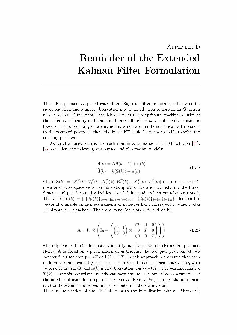
Appendix D
Reminder of the Extended
Kalman Filter Formulation
The KF represents a special case of the Bayesian �lter, requiring a linear state-
space equation and a linear observation model, in addition to zero-mean Gaussian
noise process. Furthermore, the KF conducts to an optimum tracking solution if
the criteria on linearity and Gaussianity are ful�lled. However, if the observation is
based on the direct range measurements, which are highly non linear with respect
to the occupied positions, then, the linear KF could be not reasonable to solve the
tracking problem.
As an alternative solution to such non-linearity issues, the EKF solution [76],
[77] considers the following state-space and observation models:
S(k) = AS(k − 1) + u(k)
d(k) = h(S(k)) + n(k)(D.1)
where S(k) = [XT1 (k) V T
1 (k) XT2 (k) V T
2 (k) ... XTn (k) V T
n (k)] denotes the 6n di-
mensional state-space vector at time-stamp kT or iteration k, including the three-
dimensional positions and velocities of each blind node, which must be positioned.
The vector d(k) = [{{dij(k)}j=n+1:n+m}i=1:n} {{dij(k)}j=1:n}i=1:n}] denotes the
vector of available range measurements of nodes, either with respect to other nodes
or infrastructure anchors. The state transition matrix A is given by:
A = In ⊗
I6 +
(0 1
0 0
)⊗
T 0 0
0 T 0
0 0 T
(D.2)
where Il denotes the l− dimensional identity matrix and ⊗ is the Kronecker product.
Hence, A is based on a priori information bridging the occupied positions at two
consecutive time stamps: kT and (k + 1)T . In this approach, we assume that each
node moves independently of each other. u(k) is the state-space noise vector, with
covariance matrix Q, and n(k) is the observation noise vector with covariance matrix
Σ(k). The noise covariance matrix can vary dynamically over time as a function of
the number of available range measurements. Finally, h(.) denotes the non-linear
relation between the observed measurements and the state vector.
The implementation of the EKF starts with the initialization phase. Afterward,
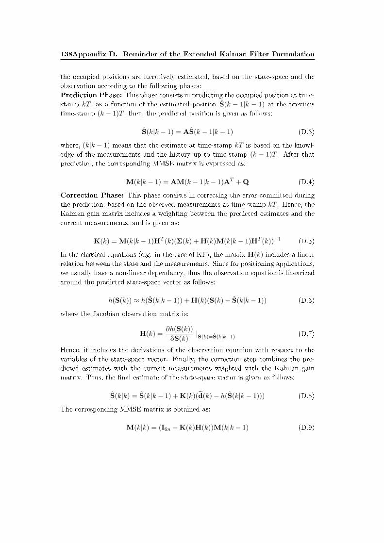
138Appendix D. Reminder of the Extended Kalman Filter Formulation
the occupied positions are iteratively estimated, based on the state-space and the
observation according to the following phases:
Prediction Phase: This phase consists in predicting the occupied position at time-
stamp kT , as a function of the estimated position S(k − 1|k − 1) at the previous
time-stamp (k − 1)T , then, the predicted position is given as follows:
S(k|k − 1) = AS(k − 1|k − 1) (D.3)
where, (k|k − 1) means that the estimate at time-stamp kT is based on the knowl-
edge of the measurements and the history up to time-stamp (k − 1)T . After that
prediction, the corresponding MMSE matrix is expressed as:
M(k|k − 1) = AM(k − 1|k − 1)AT + Q (D.4)
Correction Phase: This phase consists in correcting the error committed during
the prediction, based on the observed measurements at time-stamp kT . Hence, the
Kalman gain matrix includes a weighting between the predicted estimates and the
current measurements, and is given as:
K(k) = M(k|k − 1)HT (k)(Σ(k) + H(k)M(k|k − 1)HT (k))−1 (D.5)
In the classical equations (e.g. in the case of KF), the matrix H(k) includes a linear
relation between the state and the measurements. Since for positioning applications,
we usually have a non-linear dependency, thus the observation equation is linearized
around the predicted state-space vector as follows:
h(S(k)) ≈ h(S(k|k − 1)) + H(k)(S(k)− S(k|k − 1)) (D.6)
where the Jacobian observation matrix is:
H(k) =∂h(S(k))
∂S(k)|S(k)=S(k|k−1) (D.7)
Hence, it includes the derivations of the observation equation with respect to the
variables of the state-space vector. Finally, the correction step combines the pre-
dicted estimates with the current measurements weighted with the Kalman gain
matrix. Thus, the �nal estimate of the state-space vector is given as follows:
S(k|k) = S(k|k − 1) + K(k)(d(k)− h(S(k|k − 1))) (D.8)
The corresponding MMSE matrix is obtained as:
M(k|k) = (I6n −K(k)H(k))M(k|k − 1) (D.9)
Bibliography
[1] M. Hanson, H. Powell, A. Barth, K. Ringgenberg, B. Calhoun, J. Aylor, and
J. Lach. Body area sensor networks: Challenges and opportunities. Computer,
42(1):58�65, 2009. (Cited on pages xi and 2.)
[2] H. Shaban. A novel highly accurate wireless wearable human locomotion track-
ing and gait analysis system via UWB radios. PhD thesis, Virginia Polytechnic
Institute and State University, 2010. (Cited on pages xi, 7, 27, 39 and 41.)
[3] S. Gezici, Zhi Tian, G.B. Giannakis, Hisashi Kobayashi, A.F. Molisch, H.V.
Poor, and Z. Sahinoglu. Localization via ultra-wideband radios: a look at
positioning aspects for future sensor networks. Signal Processing Magazine,
IEEE, 22(4):70�84, 2005. (Cited on pages xi, 10 and 11.)
[4] K. Kyung-Sup, S. Ullah, and N. Ullah. An overview of ieee 802.15.6 stan-
dard. In Applied Sciences in Biomedical and Communication Technologies
(ISABEL), 2010 3rd International Symposium on, pages 1�6, 2010. (Cited on
pages xi, 1, 22, 23 and 86.)
[5] A. Fort, C. Desset, J. Ryckaert, P. De Doncker, L. Van Biesen, and
P. Wambacq. Characterization of the ultra wideband body area propaga-
tion channel. In Ultra-Wideband, 2005. ICU 2005. 2005 IEEE International
Conference on, pages 6�pp, 2005. (Cited on pages xi, 25 and 26.)
[6] R. D'Errico and L. Ouvry. Time-variant ban channel characterization. In
Personal, Indoor and Mobile Radio Communications, 2009 IEEE 20th Inter-
national Symposium on, pages 3000�3004, 2009. (Cited on pages xii, 26, 40,
42, 45, 53 and 55.)
[7] P. Pasquero and R. D'Errico. Joint delay and angle-of-arrival characterization
and modelling of uwb o�-body channels. To be submitted on Antenna and
Propagation, IEEE Transactions. (Cited on pages xiii, 62 and 64.)
[8] E. Ben Hamida, M. Maman, B. Denis, and L. Ouvry. Localization perfor-
mance in wireless body sensor networks with beacon enabled mac and space-
time dependent channel model. In Personal, Indoor and Mobile Radio Com-
munications Workshops (PIMRC Workshops), 2010 IEEE 21st International
Symposium on, pages 128�133, 2010. (Cited on pages xiii, xvii, 27, 28, 37, 39,
70, 77, 78, 92 and 104.)
[9] I. Bucaille, A. Tonnerre, L. Ouvry, and B. Denis. Mac layer design for uwb ldr
systems: Pulsers proposal. In Positioning, Navigation and Communication,
2007. WPNC'07. 4th Workshop on, pages 277�283, 2007. (Cited on pages xv,
112, 113 and 114.)
140 Bibliography
[10] http://www.codamotion.com. (Cited on pages xv, 6, 113 and 114.)
[11] http://www.ieee8012.org/15/pub/TG6.html. (Cited on pages xvii, 1, 11,
22, 24, 80 and 91.)
[12] R. Rosini and R. D'Errico. O�-body channel modelling at 2.45 ghz for two
di�erent antennas. In Antennas and Propagation (EUCAP), 2012 6th Euro-
pean Conference on, pages 3378�3382, 2012. (Cited on pages xvii, 26, 56, 57,
92 and 104.)
[13] R. Rosini, R. d'Errico, and Verdone R. Body-to-body communications: a
measurement-based channel model at 2.45 ghz. In Personal Indoor and Mobile
Radio Communications (PIMRC 2012), pages 1763�1768, 2012. (Cited on
pages xvii, 25, 26, 59 and 104.)
[14] S. Ullah, H. Higgins, B. Braem, B. Latre, C. Blondia, I. Moerman, S. Saleem,
Z. Rahman, and K. Kwak. A comprehensive survey of wireless body area
networks. Journal of Medical Systems, 36(3):1065�1094, 2012. (Cited on
page 1.)
[15] Y. Hovakeemian, K. Naik, and A. Nayak. A survey on dependability in body
area networks. InMedical Information Communication Technology (ISMICT),
2011 5th International Symposium on, pages 10�14, 2011. (Cited on page 1.)
[16] http://www.ee.qub.ac.uk/wireless/interactive.html. (Cited on page 2.)
[17] T.B. Moeslund, A. Hilton, and V. Krager. A survey of advances in vision-based
human motion capture and analysis. Computer Vision and Image Understand-
ing Special Issue on Modeling People - Visionbased understanding of a persons
shape, appearance, movement and behaviour, 104(2-3):90�126, 2006. (Cited on
page 6.)
[18] A. Leardini, L. Chiari, A. Cappozzo, and U. DellaCroce. Human movement
analysis using stereophotogrammetry part 2: instrumental errors. Gait and
Posture, 21(2):197�211, 2005. (Cited on page 6.)
[19] T. Sakaguchi, T. Kanamori, H. Katayose, K. Sato, and S. Inokuchi. Human
motion capture by integrating gyroscopes and accelerometers. In Proceedings
IEEE/SICE/RSJ MFI96, pages 470�475, 1996. (Cited on page 6.)
[20] A. Andreadis, A. Hemery, A. Antonakakis, G. Gourdoglou, P. Mauridis,
D. Christopoulos, and J. Karigiannis. Real-time motion capture technology on
a live theatrical performance with computer generated scenery. In Informatics
(PCI), 2010 14th Panhellenic Conference on, pages 148�152, 2010. (Cited on
page 6.)
[21] S. Aloui, C. Villien, and S. Lesecq. A framework for motion capture system
design using cramer-rao lower bound. In Communications, Computers and
Bibliography 141
Signal Processing (PacRim), 2011 IEEE Paci�c Rim Conference on, pages
79�84, 2011. (Cited on page 6.)
[22] E. Foxlin. Pedestrian tracking with shoe-mounted inertial sensors. Computer
Graphics and Applications, IEEE, 25(6):38�46, 2005. (Cited on page 6.)
[23] Chin-Woo Tan and Sungsu Park. Design of accelerometer-based inertial nav-
igation systems. Instrumentation and Measurement, IEEE Transactions on,
54(6):2520�2530, 2005. (Cited on page 6.)
[24] Lei Fang, P.J. Antsaklis, L.A. Montestruque, M.B. McMickell, M. Lemmon,
Yashan Sun, Hui Fang, I. Koutroulis, M. Haenggi, Min Xie, and Xiaojuan
Xie. Design of a wireless assisted pedestrian dead reckoning system - the
navmote experience. Instrumentation and Measurement, IEEE Transactions
on, 54(6):2342�2358, 2005. (Cited on page 6.)
[25] J.F. OBrien, R.E. Bodenheimer, G.J. Brostow, and J.K. Hodgins. Automatic
joint parameter estimation from magnetic motion capture data. Georgia In-
stitute of Technology, 1999. (Cited on page 7.)
[26] F.H. Raab, E.B. Blood, T.O. Steiner, and H.R. Jones. Magnetic position
and orientation tracking system. Aerospace and Electronic Systems, IEEE
Transactions on, AES-5(2):197�211, 1979. (Cited on page 7.)
[27] Z. Knoll, R. Kiss, and L. Kocsis. Joint kinematics next term and spatial
temporal parameters of gait measured by an ultrasound-based system. Gait
and Posture, 7(26):197�211, 2004. (Cited on pages 7 and 8.)
[28] T. Sato, S. Nakamura, K. Terabayashi, M. Sugimoto, and H. Hashizume. De-
sign and implementation of a robust and real-time ultrasonic motion-capture
system. In Indoor Positioning and Indoor Navigation (IPIN), 2011 Interna-
tional Conference on, pages 1�6, 2011. (Cited on page 8.)
[29] Rim. Bahroun. Localisation de personnes à l'intérieur des batiments par ondes
sismiques. PhD Thesis (in French), Polytechnique de Grenoble, december
2013. (Cited on page 8.)
[30] D. Vlasic, R. Adelsberger, G. Vannucci, J. Barnwell, M. Gross, W. Matusik,
and J. Popovi¢. Practical motion capture in everyday surroundings. ACM
Transactions on Graphics (TOG), 26(3):35, 2007. (Cited on page 8.)
[31] Y. Gu, A. Lo, and I. Niemegeers. A survey of indoor positioning systems
for wireless personal networks. IEEE Communications Survey & Tutorals,
11(1):13�32, 2009. (Cited on page 8.)
[32] M. Maman, B. Denis, M. Pezzin, B. Piaget, and L. Ouvry. Synergetic mac
and higher layers functionalities for uwb ldr-lt wireless networks. In Ultra-
Wideband, 2008. ICUWB 2008. IEEE International Conference on, pages
101�104, 2008. (Cited on pages 9, 77 and 78.)
142 Bibliography
[33] B. Denis. Exploitation des capacités de radiolocalisation des transmissions
ultra-large bande dans les réseaux sans-�l. PhD Thesis (in French), Institut
National des Sciences Appliquées de Rennes, D05-18, 2005. (Cited on page 10.)
[34] Z. Sahinoglu, S. Gezici, and I. Guvenc. Ultra-wideband positioning systems:
Theoretical limits, ranging algorithms, and protocols. Cambridge University
Press Cambridge, U.K., 2008. (Cited on pages 10, 47 and 71.)
[35] T. Rappaport. Wireless communications : Principles and practice. Upper
Saddle River, NJ, USA : Prentice Hall PTR, 2001. (Cited on page 11.)
[36] D. Neirynck, K. Philips, H. De Groot, and J. Espina. Practical comparison of
ranging in ieee 802.15.4 and ieee 802.15.4a medical body sensor networks. In
BodyNets'10, pages 16�22, 2010. (Cited on pages 12 and 35.)
[37] D. Hol, F. Dijkstra, H. Luinge, and T. Schon. Tightly coupled uwb/imu
pose estimation. In Ultra-Wideband, 2009. ICUWB 2009. IEEE International
Conference on, pages 688�692, 2009. (Cited on page 12.)
[38] D. Jourdan, Jr. Deyst, J.J., M.Z. Win, and N. Roy. Monte carlo localization in
dense multipath environments using uwb ranging. In Ultra-Wideband, 2005.
ICU 2005. 2005 IEEE International Conference on, pages 314�319, 2005.
(Cited on page 12.)
[39] J. Youssef, B. Denis, C. Godin, and S. Lesecq. Pedestrian tracking solution
combining an impulse radio handset transmitter with an ankle-mounted iner-
tial measurement unit. International Journal of Navigation and Observation,
2012. (Cited on page 12.)
[40] Sylvain Pittet, Valerie Renaudin, Bertrand Merminod, and Michel Kasser.
Uwb and mems based indoor navigation. The Journal of Navigation,
61(3):369�384, 2008. (Cited on page 12.)
[41] V. Renaudin, B. Merminod, and M. Kasser. Optimal data fusion for pedestrian
navigation based on uwb and mems. In Position, Location and Navigation
Symposium, 2008 IEEE/ION, pages 341�349, 2008. (Cited on page 12.)
[42] F. Evennou and F. Marx. Advanced integration of wi� and inertial navigation
systems for indoor mobile positioning. Eurasip Journal on Applied Signal
Processing, 2006:164�164, 2006. (Cited on page 12.)
[43] H. Wymeersch, J. Lien, and M.Z. Win. Cooperative localization in wireless
networks. Proceedings of the IEEE, 97(2):427�450, 2009. (Cited on pages 13
and 35.)
[44] J. Hamie, B. Denis, R. D'Errico, and C. Richard. Empirical modeling of
intra-ban ranging errors based on ir-uwb toa estimation. In Proceedings of
the 7th International Conference on Body Area Networks, BodyNets'12, pages
139�144, 2012. (Cited on pages 18, 40, 65, 71 and 80.)
Bibliography 143
[45] J. Hamie, B. Denis, R. D'Errico, and C. Richard. On-body toa-based ranging
error model for motion capture applications within wearable uwb networks.
to appear in Journal on Mobile Networks and Applications, 2013. (Cited on
pages 18, 40, 65 and 80.)
[46] J. Hamie, B. Denis, and C. Richard. Constrained decentralized algorithm for
the relative localization of wearable wireless sensor nodes. In Sensors, 2012
IEEE, pages 1�4, 2012. (Cited on pages 18, 75 and 95.)
[47] J. Hamie, B. Denis, and C. Richard. Nodes updates censoring and scheduling
in constrained decentralized positioning for large-scale motion capture based
on wireless body area networks. In Proceedings of the 7th International Con-
ference on Body Area Networks, BodyNets'12, pages 100�105, 2012. (Cited on
pages 18 and 95.)
[48] J. Hamie, B. Denis, and C. Richard. Decentralized positioning algorithm for
relative nodes localization in wireless body area networks. to appear in Journal
on Mobile Networks and Applications, 2013. (Cited on pages 18 and 95.)
[49] J. Hamie, B. Denis, and C. Richard. Joint motion capture and navigation in
heterogeneous body area networks with distance estimation over neighborhood
graph. In Positioning Navigation and Communication (WPNC), 2013 10th
Workshop on, pages 1�6, 2013. (Cited on pages 18 and 95.)
[50] S. Ullah, M. Mohaisen, and M. Alnuem. A review of ieee 802.15.6 mac, phy,
and security speci�cations. International Journal of Distributed Sensor Net-
works, 2013, 2013. (Cited on page 22.)
[51] J. Zhang, D.B. Smith, L.W. Hanlen, D. Minutti, D. Rodda, , and B. Gilbert.
Stability of narrowband dynamic body area channel. Antennas and Wireless
Propagation Letters, IEEE, 8:53�56, 2009. (Cited on page 23.)
[52] K. Takizawa H. Sawada N. Katayama K.Y Yazdandoost T. Kobayashi H.B. Li
T. Aoyagi, J.I. Takada and R. Kohno. Channel models for wearable and im-
plantable wbans-nict. Technical report, IEEE 802.15-08-0416-04-0006, IEEE
802.15 Task Group 6 Document, November 2010. (Cited on pages 23 and 24.)
[53] G. Dolmans, , and A. Fort. Channel models wban-holst centre/imec-nl. Tech-
nical report, IEEE 802.15-08-0418-01-0006, IEEE 802.15 Task Group 6 Docu-
ment, July 2008. (Cited on page 24.)
[54] D. Smith A. Zhang D. Lewis D. Rodda D. Miniutti, L. Hanlen and B. Gilbert.
Narrowband on body to o� body channel characterization for ban. Technical
report, IEEE 802.15-08-0559-00-0006, IEEE 802.15 Task Group 6 Document,
August 2008. (Cited on page 25.)
[55] J. Takada K.Y. Yazdandoost H. Sawada, T. Aoyagi and R. Kohno. Channel
model between body surface and wireless access point for uwb band. Technical
144 Bibliography
report, IEEE 802.15-08-0576-00-0006, IEEE 802.15 Task Group 6 Document,
August 2008. (Cited on page 25.)
[56] S.L. Cotton and W.G. Scanlon. Channel characterization for single-and
multiple-antenna wearable systems used for indoor body-to-body communica-
tions. Antennas and Wireless Propagation, IEEE Transaction on, 57(4):980�
990, 2008. (Cited on page 25.)
[57] G. Koutitas. Multiple human e�ects in body area networks. IEEE Antennas
and Wireless Propagation Letters, IEEE, 9:938�941, 2010. (Cited on page 25.)
[58] Y. Wang, I. Bonev, J. Nielsen, I. Kovacs, and G.F. Pedersen. Characterisa-
tion of the indoor multiantenna body-to-body radio channel. Antennas and
Propagation, IEEE Transactions on, 57(4):972�979, 2009. (Cited on page 25.)
[59] Ieee std 802.15.4-2006, part 15.4: Wireless medium access control (mac) and
physical layer (phy) speci�cations for low-rate wireless personal area networks
(lr-wpans), september 2006. (Cited on page 25.)
[60] Ieee 802.15.4a channel model - �nal report (p802.15-04-0662-04-004a-channel-
model-�nal-report-r1), october 2005. (Cited on pages 25 and 63.)
[61] M. Mhedhbi, M. Laaraiedh, and B. Uguen. Constrained lmds technique for
human motion and gesture estimation. In Positioning Navigation and Com-
munication (WPNC), 2012 9th Workshop on, pages 89�93, 2012. (Cited on
pages 27, 28, 70, 73 and 80.)
[62] Z. Mekonnen, E. Slottke, H. Luecken, C. Steiner, and A. Wittneben. Con-
strained maximum likelihood positioning for uwb based human motion track-
ing. In Indoor Positioning and Indoor Navigation (IPIN), 2010 International
Conference on, pages 1�10, 2010. (Cited on pages 27, 28, 31, 36 and 39.)
[63] H. Ren and L. Meng, M.and Xu. Indoor patient position estimation using
particle �ltering and wireless body area networks. In Engineering in Medicine
and Biology Society, 2007. EMBS 2007. 29th Annual International Conference
of the IEEE, pages 2277�2280, 2007. (Cited on pages 27, 28, 33 and 36.)
[64] W. Cully, S. Cotton, W. Scanlon, and J. McQuiston. Body shadowing miti-
gation using di�erentiated los/nlos channel models for rssi-based monte carlo
personnel localization. In Wireless Communications and Networking Confer-
ence (WCNC), 2012 IEEE, pages 694�698, 2012. (Cited on page 28.)
[65] A. Costa, N. Patwari, and O. Hero. Distributed weighted-multidimensional
scaling for node localization in sensor networks. ACM Trans. Sen. Netw.,
2(1):39�64, 2006. (Cited on pages 29, 30, 70, 74 and 80.)
[66] P. Biswas, T. Lian, T. Wang, and Y. Ye. Semide�nite programming based
algorithms for sensor network localization. ACM Trans. Sen. Netw., 2(2):188�
220, 2006. (Cited on page 29.)
Bibliography 145
[67] AA. Cox, T.and Cox. Multidimensional scaling, volume 88. CRC Press, 2001.
(Cited on pages 30, 72 and 73.)
[68] B. Denis, Liyun He, and L. Ouvry. A �exible distributed maximum log-
likelihood scheme for uwb indoor positioning. In Positioning, Navigation
and Communication, 2007. WPNC'07. 4th Workshop on, pages 77�86, 2007.
(Cited on page 30.)
[69] B. Denis and N. Daniele. Nlos ranging error mitigation in a distributed po-
sitioning algorithm for indoor uwb ad-hoc networks. In Wireless Ad-Hoc
Networks, 2004 International Workshop on, pages 356�360, 2004. (Cited on
page 30.)
[70] G. Destino, D. Macagnano, G. Abreu, B. Denis, and L. Ouvry. Localization
and tracking for ldr-uwb systems. In Mobile and Wireless Communications
Summit, 2007. 16th IST, pages 1�5. IEEE, 2007. (Cited on page 30.)
[71] SM Kay. Fundamentals of statistical signal processing, volume i: Estimation
theory. 1993. (Cited on pages 31 and 32.)
[72] A. Doucet, S. Godsill, and C. Andrieu. On sequential simulation-based methods
for Bayesian �ltering. Department of Engineering, University of Cambridge
UK, 1998. (Cited on page 33.)
[73] F. Gustafsson, F. Gunnarsson, N. Bergman, U. Forssell, J. Jansson, R. Karls-
son, and P. Nordlund. Particle �lters for positioning, navigation, and track-
ing. Signal Processing, IEEE Transactions on, 50(2):425�437, 2002. (Cited on
page 33.)
[74] F. Evennou, F. Marx, and E. Novakov. Map-aided indoor mobile position-
ing system using particle �lter. In Wireless Communications and Networking
Conference, 2005 IEEE, pages 2490�2494, 2005. (Cited on page 33.)
[75] K. Yu and E. Dutkiewicz. Improved kalman �ltering algorithms for mobile
tracking in nlos scenarios. In Wireless Communications and networking Con-
ference (WCNC), 2012 IEEE, pages 2390�2394, 2012. (Cited on page 33.)
[76] X. Yun and E. Bachmann. Design, implementation, and experimental results
of a quaternion-based kalman �lter for human body motion tracking. Robotics,
IEEE Transaction on, 22(6):1216�1277, 2006. (Cited on pages 33 and 137.)
[77] T. Perala and R. Piché. Robust extended kalman �ltering in hybrid posi-
tioning applications. In Positioning, Navigation and Communication, 2007.
WPNC'07. 4th Workshop on, pages 55�63, 2007. (Cited on pages 33 and 137.)
[78] J.S. Yedidia, W.T. Freeman, and Y. Weiss. Understanding belief propagation
and its generalizations. Exploring arti�cial intelligence in the new millennium,
ACM, 97(2):239�269, 2003. (Cited on page 34.)
146 Bibliography
[79] A.T. Ihler, J.W. Fisher, R.L. Moses, and A.S. Willsky. Nonparametric belief
propagation for self-localization of sensor networks. Selected Areas in Com-
munications, IEEE Journal on, 23(4):809�819, 2005. (Cited on page 34.)
[80] V. Savic, H. Wymeersch, F. Penna, and S. Zazo. Optimized edge appearance
probability for cooperative localization based on tree-reweighted nonparamet-
ric belief propagation. In Acoustics, Speech and Signal Processing (ICASSP),
2011 IEEE International Conference on, pages 3028�3031, 2011. (Cited on
page 34.)
[81] H. Noureddine. Signal Processing Techniques for Wireless Cooperative Local-
ization and Tracking. PhD thesis, Telecom Bretagne, 2012. (Cited on page 34.)
[82] H. Noureddine, N. Gresset, D. Castelain, and R. Pyndiah. A new variant of
nonparametric belief propagation for self-localization. In Telecommunications
(ICT), 2010 IEEE 17th International Conference on, pages 822�827, 2010.
(Cited on page 34.)
[83] U. Ferner, H. Wymeersch, and M.Z. Win. Cooperative anchor-less localization
for large dynamic networks. In Ultra-Wideband, 2008. ICUWB 2008. IEEE
International Conference on, pages 181�185, 2008. (Cited on page 35.)
[84] C. Pedersen, T. Pedersen, and B.H. Fleury. A variational message passing
algorithm for sensor self-localization in wireless networks. In Information
Theory Proceedings (ISIT), 2011 IEEE International Symposium on, pages
2158�2162, 2011. (Cited on page 35.)
[85] M. Di Renzo, R. Buehrer, and J. Torres. Pulse shape distortion and rang-
ing accuracy in uwb-based body area networks for full-body motion capture
and gait analysis. In Global Telecommunications Conference, 2007. GLOBE-
COM'07. IEEE, pages 3775�3780, 2007. (Cited on pages 35 and 45.)
[86] A.A. Goulianos and S. Stavrou. Uwb path arrival times in body area networks.
Antennas and Wireless Propagation Letters, IEEE, 6:223�226, 2007. (Cited
on page 35.)
[87] C.P. Figueiredo, N.S. Dias, and P.M. Mendes. 3d localization for biomedical
wireless sensor networks using a microantenna. In Wireless Technology, 2008.
EuWiT 2008. European Conference on, pages 45�48, 2008. (Cited on page 35.)
[88] Cheng Guo, Jing Wang, R.V. Prasad, and M. Jacobsson. Improving the ac-
curacy of person localization with body area sensor networks: An experimen-
tal study. In Consumer Communications and Networking Conference, 2009.
CCNC 2009. 6th IEEE, pages 1�5, 2009. (Cited on page 36.)
[89] L. Cheolhyo, L. Hyung-Soo, and K. Jae-Young. Performance of a one-way
ranging method for wban healthcare services. In Communications and Infor-
mation Technology, 2009. ISCIT 2009. 9th International Symposium on, pages
1460�1463, 2009. (Cited on page 36.)
Bibliography 147
[90] F. Chiti, R. Fantacci, F. Archetti, E. Messina, and D. Toscani. An inte-
grated communications framework for context aware continuous monitoring
with body sensor networks. Selected Areas in Communications, IEEE Journal
on, 27(4):379�386, 2009. (Cited on page 36.)
[91] H. Shaban, M. El-Nasr, and R. Buehrer. Toward a highly accurate ambulatory
system for clinical gait analysis via uwb radios. Information Technology in
Biomedicine, IEEE Transactions on, 14(2):284�291, 2010. (Cited on pages 39
and 45.)
[92] S. Gezici, M. Chiang, H. Poor, and H. Kobayashi. A genetic algorithm based
�nger selection scheme for uwb mmse rake receivers. In Ultra-Wideband, 2005.
ICU 2005. 2005 International conference on, pages 164�169, 2005. (Cited on
page 42.)
[93] B. Denis and J. Keignart. Post-processing framework for enhanced uwb chan-
nel modeling from band-limited measurements. In Ultra Wideband Systems
and Technologies, 2003 IEEE Conference on, pages 260�264, 2003. (Cited on
pages 42 and 63.)
[94] L. Yang. The Applicability of the Tap-Delay Line Channel Model to Ultra
Wideband. PhD thesis, Virginia Polytechnic Institute and State University,
2004. (Cited on page 45.)
[95] J. Zhang, R. Kennedy, and T. Abhayapala. Cramer-rao lower bounds for
the time delay estimation of uwb signals. In Communications, 2004 IEEE
International Conference on, volume 6, pages 3424�3428, 2004. (Cited on
pages 62 and 63.)
[96] L. De Nardis and M. Di Benedetto. Overview of the ieee 802.15. 4/4a standards
for low data rate wireless personal data networks. In Positioning, Navigation
and Communication, 2007. WPNC'07. 4th Workshop on, pages 285�289, 2007.
(Cited on page 63.)
[97] F. Doremani, H. Javadi, and A. Farahi. A new distributed weighted multidi-
mensional scaling algorithm for localization in wireless sensor networks. In-
ternational journal of Computer Science and Engineering Survey, 20(1), 2011.
(Cited on page 70.)
[98] Z. Chen, H. Wei, Q. Wan, S. Ye, and W. Yang. A supplement to multidimen-
sional scaling framework for mobile location: A uni�ed view. signal Processing,
IEEE Transaction on, 57(5):2030�2034, 2009. (Cited on page 72.)
[99] A. Costa, N. Patwari, and O. Hero. Achieving high-accuracy distributed local-
ization in sensor networks. In Acoustics, Speech, and Signal Processing, 2005.
Proceedings. (ICASSP'05). IEEE Conference on, pages iii�641, 2005. (Cited
on page 74.)

148 Bibliography
[100] P. Groenen. The Majorization Approach to Multidimensional Scaling: some
problems and extensions. DSWO Press, Leiden University Leiden, 1993. (Cited
on page 74.)
[101] M. Maman, F. Dehmas, R. D'Errico, and L. Ouvry. Evaluating a tdma mac
for body area networks using a space-time dependant channel model. In Per-
sonal, Indoor and Mobile Radio Communications, 2009 IEEE 20th Interna-
tional Symposium on, pages 2101�2105, 2009. (Cited on pages 77, 78 and 91.)
[102] D. Macagnano, G. Destino, F. Esposito, and G. Abreu. Mac performances for
localization and tracking in wireless sensor networks. In Positioning, Naviga-
tion and Communication, 2007. WPNC'07. 4th Workshop on, pages 297�302,
2007. (Cited on page 78.)
[103] T. Camp, J. Boleng, and V Davies. A survey of mobility models for ad hoc
network research. Wireless Communications and Mobile Computing, 2(5):483�
502, 2002. (Cited on page 78.)
[104] I. Pantazis. Tracking human walking using marg sensors. Technical report,
DTIC Document, 2005. (Cited on page 78.)
[105] C. Wang, J. Chen, Y. Sun, and X. Shen. Wireless sensor networks local-
ization with isomap. In Communications, 2009. ICC'09. IEEE International
Conference on, pages 1�5, 2009. (Cited on pages 88 and 90.)
[106] Béla Bollobás. Extremal Graph Theory. DoverPublications. com, 1978. (Cited
on page 90.)
[107] D. Goldenberg, A. Krishnamurthy, W. Maness, Y. Yang, R. Young, A. Young,
A. Morse, and A. Savvid. Network localization in partially localizable net-
works. In INFOCOM 2005. 24th Annual Joint Conference of the IEEE Com-
puter and Communication Societies. Proceedings IEEE, volume 1, pages 313�
326, 2005. (Cited on page 90.)
[108] M. Pezzin, I. Bucaille, T. Schulze, A. Pato, and L. DeCelis. An open ir-uwb
platform for ldr-lt applications prototyping. In Positioning, Navigation and
Communication, 2009. WPNC 2009. 6th Workshop on, pages 285�293, 2009.
(Cited on pages 92, 104, 112 and 115.)
[109] M. Laaraiedh, S. Avrillon, and B. Uguen. Enhancing positioning accuracy
through direct position estimators based on hybrid rss data fusion. In Vehic-
ular Technology Conference, 2009. VTC Spring 2009. IEEE 69th, pages 1�5,
2009. (Cited on pages 92 and 104.)
[110] N. Amiot, T. Pedersen, M. Laaraiedh, and B. Uguen. A hybrid positioning
method based on hypothesis testing. Wireless Communications Letters, IEEE,
1(4):348�351, 2012. (Cited on page 105.)
Bibliography 149
[111] J. Youssef, B. Denis, C. Godin, and S. Lesecq. Enhanced uwb indoor tracking
through nlos toa biases estimation. In Global Telecommunications Conference,
2008. IEEE GLOBECOM 2008. IEEE, pages 1�5, 2008. (Cited on page 105.)
[112] B. Denis, L. Ouvry, B. Uguen, and F. Tcho�o-Talom. Advanced bayesian
�ltering techniques for uwb tracking systems in indoor environments. In Ultra-
Wideband, 2005. ICU 2005. 2005 IEEE International Conference on, pages
6�pp, 2005. (Cited on page 105.)
[113] D. Lachartre, B. Denis, D. Morche, L. Ouvry, M. Pezzin, B. Piaget, J. Prouvee,
and P Vicent. A 1.1nj/b 802.15.4a-compliant fully integrated uwb transceiver
in 0.13 micrometer cmos. In Solid-State Circuits Conference - Digest of Techni-
cal Papers, 2009. ISSCS 2009. IEEE International, pages 312�313,313a, 2009.
(Cited on page 112.)
[114] M. Pezzin and D. Lachartre. A low power, low data rate impulse radio ultra
wide band transceivers. In Future Network and Mobile Summit, 2010, pages
1�10, 2010. (Cited on page 112.)
[115] B. Denis, M. Maman, and L. Ouvry. On the scheduling of ranging and
distributed positioning upadtes in cooperatives ir-uwb networks. In Ultra-
Wideband, 2009. ICUWB 2009; IEEE International Conference on, pages
370�375, 2009. (Cited on page 112.)
[116] G. Masson, D. Morche, H. Jacquinot, P. Vincent, F. Dehmas, S. Paquelet,
A. Bisiaux, O. Fourquin, J. Gaubert, and S. Bourdel. A 1 nj/b 3.2-to-4.7 ghz
uwb 50 mpulses/s double quadrature receiver for communication and localiza-
tion. In ESSCIRC, 2010 Proceedings of the, pages 502�505, 2010. (Cited on
page 124.)
[117] http://bespoon.com/. (Cited on page 124.)
[118] L. Harry and V. Trees. Detection, estimation, and modulation theory, part i.
Massachussets institute of technology, Jhon Wiley and Sons, 1968. (Cited on
page 132.)
[119] J. Proakis. Intersymbol Interference in Digital Communication Systems. 1995.
(Cited on page 132.)
[120] A. D'Andrea, U. Mengali, and R. Reggianini. The modi�ed cramer-rao bound
and its applications to synchronization problems. Communications, IEEE
Transaction on, 42(234):1391�1399, 1994. (Cited on page 132.)
[121] E. Lehman and G. Casella. Theory of point estimation, volume 31. springer,
1998. (Cited on page 133.)
[122] N. Patwari, A. Hero, M. Perkins, N. Correal, and R. O'dea. Relative location
estimation in wirelsess sensor networks. Signal Processing, IEEE Transaction
on, 51(8):2137�2148, 2003. (Cited on page 135.)

150 Bibliography
Related Documents