HAL Id: tel-01452378 https://tel.archives-ouvertes.fr/tel-01452378v1 Submitted on 1 Feb 2017 (v1), last revised 13 Feb 2017 (v2) HAL is a multi-disciplinary open access archive for the deposit and dissemination of sci- entific research documents, whether they are pub- lished or not. The documents may come from teaching and research institutions in France or abroad, or from public or private research centers. L’archive ouverte pluridisciplinaire HAL, est destinée au dépôt et à la diffusion de documents scientifiques de niveau recherche, publiés ou non, émanant des établissements d’enseignement et de recherche français ou étrangers, des laboratoires publics ou privés. Contribution to Face Analysis from RGB Images and Depth Maps Elhocine Boutellaa To cite this version: Elhocine Boutellaa. Contribution to Face Analysis from RGB Images and Depth Maps. Computer Vision and Pattern Recognition [cs.CV]. Ecole nationale Supérieure en Informatique Alger, 2017. English. tel-01452378v1

Welcome message from author
This document is posted to help you gain knowledge. Please leave a comment to let me know what you think about it! Share it to your friends and learn new things together.
Transcript
HAL Id: tel-01452378https://tel.archives-ouvertes.fr/tel-01452378v1
Submitted on 1 Feb 2017 (v1), last revised 13 Feb 2017 (v2)
HAL is a multi-disciplinary open accessarchive for the deposit and dissemination of sci-entific research documents, whether they are pub-lished or not. The documents may come fromteaching and research institutions in France orabroad, or from public or private research centers.
L’archive ouverte pluridisciplinaire HAL, estdestinée au dépôt et à la diffusion de documentsscientifiques de niveau recherche, publiés ou non,émanant des établissements d’enseignement et derecherche français ou étrangers, des laboratoirespublics ou privés.
Contribution to Face Analysis from RGB Images andDepth Maps
Elhocine Boutellaa
To cite this version:Elhocine Boutellaa. Contribution to Face Analysis from RGB Images and Depth Maps. ComputerVision and Pattern Recognition [cs.CV]. Ecole nationale Supérieure en Informatique Alger, 2017.English. �tel-01452378v1�

Ecole Nationale Superieure d’Informatique
Contribution to Face Analysis from
RGB Images and Depth Maps
Elhocine Boutellaa
A dissertation submitted for the degree of Doctor of Philosophy
Supervisors:
Mr. Samy Ait-Aoudia Prof ESIMr. Abdenour Hadid Prof University of Oulu
Publicly defended on 31/01/2017 before the jury composed of:
Mr. Walid Khaled HIDOUCI Prof ESI PresidentMr. Amar BALLA Prof ESI ExaminerMr. Hamid HADDADOU MCA ESI ExaminerMr. Youcef ZAFFOUNE MCA USTHB ExaminerMr. Samy AIT AOUDIA Prof ESI Thesis Director

Abstract
Automatic human face analysis refers to the processing of facial images by machines inorder to infer useful information, such as identity, gender, ethnicity, mood, etc. Faceanalysis has many interesting applications in security, human computer interaction,social media analysis, etc. Therefore, though face analysis is an well-establishedcomputer vision problem, it is still an active research topic attracting considerableattention from researchers. The research community mainly aims to develop morerobust systems with the ability to fulfill the requirements of current applications.
This thesis contributes to a number of face analysis tasks: face verification andidentification, gender recognition, ethnicity recognition and kinship verification. Facesfrom three different imaging supports i.e. RGB images, depth maps and videos areused throughout the thesis. We present novel approaches and in-depth studies forsolving and improving the face analysis problem.
First, we tackle face verification problem from RGB images. The local binary pat-terns based face verification scheme has been revised through proposing novel efficientrepresentations, which cope with the original approach drawbacks while improvingthe verification performance.
Next, the problems of identity, gender and ethnicity recognition are investigatedfrom both RGB and depth images. The aim is to assess the usefulness low-qualitydepth images, acquired with Microsoft Kinect low-cost sensor, in coping with facialanalysis tasks. The performance of RGB images and depth maps are compared toshow the ability of the latter ones to deal with sever environment illumination cir-cumstances.
Furthermore, the thesis contributes to the problem of kinship verification fromvideos, where the family relationship between two persons is checked by comparingtheir facial attributes. The dynamics of faces are efficiently coded by the means ofspatio-temporal descriptors and deep features. The value of using videos in kinshipproblem is shown by comparing their performance against that of still images.
Throughout the thesis, various benchmark databases are used and extensive exper-iments are carried out to validate our proposed approaches and developed methods.Besides, the results of the proposed approaches are compared against the state of theart, highlighting our contributions and showing improvements. Future directions forthe presented contributions are outlined at end of the thesis.
1


Acknowledgments
This thesis has been carried out within the biometric team, Telecom Laboratory of
Centre de developpement des Technologies Avancees (CDTA), Algiers, Algeria. I
have been working as a research associate within CDTA during the thesis work.
First of all, I express my profound gratitude to my supervisors, Professor Samy
Ait-Aoudia and Professor Abdenour Hadid, for their guidance, support and encour-
agements. I am thankful for their precious advices and fruitful discussions for im-
proving each paper and the thesis. I also acknowledge their patience and help during
the whole thesis work period.
I am grateful to all Biometric team members in CDTA as well as other co-authors
for the fruitful collaboration we established. I acknowledge the help I received and
the exchange I had, which made the work of the thesis easier.
I am thankful for Professor Mohamed Cheriet for hosting me in his research labo-
ratory Synchormedia at Ecole de Technologie Superieure in Montreal Canada for one
month. I am also thankful for Professor Matti Pietikainen for hosting me in Center
for Machine Vision of University of Oulu in Finland for a period of eighteen months.
Both visits had a significant impact on my research. These two research visits have
been funded by CDTA and the Algerian ministry of higher education and scientific
research.
Finally, my deep gratitude is addressed to my parents, family members and friends
for their endless support and encouragement.
3

Abbreviations
AAM active appearance models
ANN artificial neural networks
ASM active shape model
BSIF binarized statistical image features
CNN convolutional neural networks
DET detection error trade-off
DLQP depth local quantized pattern
DPM deformable parts-based model
EER equal error rate
FAR false acceptance rate
FRR false rejection rate
GMM Gaussian mixture model
GPU graphics processing unit
HoG histograms of oriented Gradients
HTER half total error rate
ICA independent component analysis
ICP iterative closest point
LBG Linde-Buzo-Gray
LDA linear discriminant analysis
LLR log likelihood ratio
LBP local binary patterns
LPQ local phase quantization
MAP maximum a posteriori
MLP multi-layer perception
MSE mean squared error
NIR near infrared
NN nearest neighbor
OCLBP over-complete LBP
5

PCA principal component analysis
RBF radial basis function
ROC receiver operating characteristics
ROI regions of interest
SIFT scale invariant feature transform
STFT short-term Fourier transform
SRC sparse representation classifier
SVM support vector machines
TOP three orthogonal planes
UBM universal background model
VQ vector quantization
6


Contents
1 Introduction 19
1.1 Thesis contributions . . . . . . . . . . . . . . . . . . . . . . . . . . . 20
1.2 Thesis organization . . . . . . . . . . . . . . . . . . . . . . . . . . . . 22
2 Background 26
2.1 Face analysis tasks . . . . . . . . . . . . . . . . . . . . . . . . . . . . 26
2.2 Applications and motivation . . . . . . . . . . . . . . . . . . . . . . . 28
2.2.1 Security . . . . . . . . . . . . . . . . . . . . . . . . . . . . . . 28
2.2.2 Social media analysis . . . . . . . . . . . . . . . . . . . . . . . 29
2.2.3 Human computer interaction . . . . . . . . . . . . . . . . . . . 29
2.2.4 Automatic health assessment . . . . . . . . . . . . . . . . . . 29
2.3 Generic face analysis framework . . . . . . . . . . . . . . . . . . . . . 30
2.3.1 Face detection and tracking . . . . . . . . . . . . . . . . . . . 31
2.3.2 Face description . . . . . . . . . . . . . . . . . . . . . . . . . . 33
2.3.3 Face modeling and classification . . . . . . . . . . . . . . . . . 34
2.4 Challenges and remedies . . . . . . . . . . . . . . . . . . . . . . . . . 36
2.4.1 Illumination . . . . . . . . . . . . . . . . . . . . . . . . . . . . 37
2.4.2 Head pose and viewpoint change . . . . . . . . . . . . . . . . 38
2.4.3 Occlusion . . . . . . . . . . . . . . . . . . . . . . . . . . . . . 38
2.5 Summary . . . . . . . . . . . . . . . . . . . . . . . . . . . . . . . . . 39
3 Face verification 41
3.1 Motivations and approach overview . . . . . . . . . . . . . . . . . . . 42
8

3.2 The local binary patterns . . . . . . . . . . . . . . . . . . . . . . . . . 43
3.3 Face representation using LBP . . . . . . . . . . . . . . . . . . . . . . 46
3.4 Face verification using LBP and VQMAP . . . . . . . . . . . . . . . . 48
3.4.1 LBP Quantization . . . . . . . . . . . . . . . . . . . . . . . . 48
3.4.2 VQMAP model . . . . . . . . . . . . . . . . . . . . . . . . . . 50
3.4.3 Face verification system . . . . . . . . . . . . . . . . . . . . . 51
3.5 Face verification using adapted LBP histograms . . . . . . . . . . . . 53
3.6 Experimental analysis . . . . . . . . . . . . . . . . . . . . . . . . . . 55
3.6.1 Databases . . . . . . . . . . . . . . . . . . . . . . . . . . . . . 55
3.6.2 Setup . . . . . . . . . . . . . . . . . . . . . . . . . . . . . . . 57
3.6.3 Results and discussion . . . . . . . . . . . . . . . . . . . . . . 58
3.7 Conclusion . . . . . . . . . . . . . . . . . . . . . . . . . . . . . . . . . 61
4 Face analysis from Kinect data 64
4.1 Kinect sensors . . . . . . . . . . . . . . . . . . . . . . . . . . . . . . . 65
4.2 Review of works using Kinect for face analysis . . . . . . . . . . . . . 67
4.2.1 Face detection and tracking, pose estimation . . . . . . . . . . 67
4.2.2 Face recognition . . . . . . . . . . . . . . . . . . . . . . . . . . 69
4.2.3 Gender and expression recognition . . . . . . . . . . . . . . . 71
4.2.4 Face modeling, reconstruction and animation . . . . . . . . . . 72
4.2.5 Discussion and contribution motivation . . . . . . . . . . . . . 72
4.3 A framework for face analysis from Kinect data . . . . . . . . . . . . 73
4.3.1 Preprocessing . . . . . . . . . . . . . . . . . . . . . . . . . . . 73
4.3.2 Feature extraction . . . . . . . . . . . . . . . . . . . . . . . . 74
4.3.3 Classification . . . . . . . . . . . . . . . . . . . . . . . . . . . 80
4.4 Experiments and results . . . . . . . . . . . . . . . . . . . . . . . . . 81
4.4.1 Databases . . . . . . . . . . . . . . . . . . . . . . . . . . . . . 81
4.4.2 Setup . . . . . . . . . . . . . . . . . . . . . . . . . . . . . . . 83
4.4.3 Experimental results . . . . . . . . . . . . . . . . . . . . . . . 84
4.5 Conclusion . . . . . . . . . . . . . . . . . . . . . . . . . . . . . . . . . 87
9

5 Kinship verification from videos 90
5.1 Background and motivation . . . . . . . . . . . . . . . . . . . . . . . 91
5.2 Video-based kinship verification . . . . . . . . . . . . . . . . . . . . . 92
5.2.1 Approach overview . . . . . . . . . . . . . . . . . . . . . . . . 93
5.2.2 Face detection and tracking . . . . . . . . . . . . . . . . . . . 95
5.2.3 Face description . . . . . . . . . . . . . . . . . . . . . . . . . . 96
5.2.4 Classification . . . . . . . . . . . . . . . . . . . . . . . . . . . 102
5.3 Experiments . . . . . . . . . . . . . . . . . . . . . . . . . . . . . . . . 102
5.3.1 Database and test protocol . . . . . . . . . . . . . . . . . . . . 102
5.3.2 Results and analysis . . . . . . . . . . . . . . . . . . . . . . . 104
5.4 Conclusion . . . . . . . . . . . . . . . . . . . . . . . . . . . . . . . . . 114
6 Summary and future work 116
6.1 Summary . . . . . . . . . . . . . . . . . . . . . . . . . . . . . . . . . 116
6.2 Future directions . . . . . . . . . . . . . . . . . . . . . . . . . . . . . 118
A Vector quantization maximum a posteriori 121
A.1 Modeling VQ as a Gaussian mixture . . . . . . . . . . . . . . . . . . 122
A.2 Defining the prior density . . . . . . . . . . . . . . . . . . . . . . . . 122
A.3 MAP estimates for vector quantization . . . . . . . . . . . . . . . . . 123
10

List of Figures
1-1 Main content of the thesis. . . . . . . . . . . . . . . . . . . . . . . . . 24
2-1 Training phase of face analysis system. . . . . . . . . . . . . . . . . . 31
2-2 Operational phase of face analysis system. . . . . . . . . . . . . . . . 31
2-3 Illustration of face detection. . . . . . . . . . . . . . . . . . . . . . . . 32
2-4 Different strategies for extracting local face features from: a) face grid,
b) face regions, c) face landmarks [69]. . . . . . . . . . . . . . . . . . 35
2-5 Examples of challenging face images. . . . . . . . . . . . . . . . . . . 37
3-1 The basic LBP operator. . . . . . . . . . . . . . . . . . . . . . . . . . 44
3-2 The uniform patterns in LBP8,R configuration [95]. . . . . . . . . . . 45
3-3 Some texture primitives detected by the LBP operator [95]. . . . . . . 46
3-4 Face description using LBP. . . . . . . . . . . . . . . . . . . . . . . . 47
3-5 Face block description: LBP histogram against VQ-LBP codebook.
The histograms are larger and sparse while the codebooks are dense
and compact . . . . . . . . . . . . . . . . . . . . . . . . . . . . . . . . 49
3-6 LBP-face quantization. . . . . . . . . . . . . . . . . . . . . . . . . . . 50
3-7 LBP-VQMAP face verification system. . . . . . . . . . . . . . . . . . 52
3-8 LBP histograms of the same block from three face images of a subject,
taken in the same session, and their adapted histogram. . . . . . . . . 53
3-9 Example of XM2VTS face images of the same person across different
sessions. . . . . . . . . . . . . . . . . . . . . . . . . . . . . . . . . . . 55
3-10 Example of BANCA face images from the three acquisition conditions
: controlled (left), degraded (middle) and adverse (right). . . . . . . . 57
11

3-11 DET curve for baseline LBP, our two approaches (VQMAP and AH)
and their fusion (VQMAP-AH) on BANCA database for the pooled
protocol P. . . . . . . . . . . . . . . . . . . . . . . . . . . . . . . . . . 61
4-1 Comparing face images acquired with Minolta VIVID 910 scanner (left)
against Kinect (right). . . . . . . . . . . . . . . . . . . . . . . . . . . 66
4-2 Examples of 2D cropped image (left) and corresponding 3D face image
(right) obtained with the Microsoft Kinect sensor after preprocessing. 74
4-3 Examples of results after applying the four descriptors to face texture
and depth images. From left to right: the original face image (top:
texture image and bottom: its corresponding depth image) and the
resulting images after the application of LBP, LPQ, HoG and BSIF
descriptors, respectively. . . . . . . . . . . . . . . . . . . . . . . . . . 80
4-4 Face images samples from a subject of the CurtinFaces database. Top:
RGB faces, middle: their corresponding raw depth maps and bottom:
depth cropped face. . . . . . . . . . . . . . . . . . . . . . . . . . . . . 83
4-5 Classification accuracy for identity, gender and ethnicity using RGB
and depth on FaceWarehouse database. . . . . . . . . . . . . . . . . . 86
5-1 Overview of the proposed approach for kinship verification from videos. 94
5-2 Example of face cropping: (left) a frame annotated with the detected
landmarks, and (right) the cropped and aligned face region. . . . . . 95
5-3 Illustration of three orthogonal planes used to extract dynamic textural
face descriptors from a video. . . . . . . . . . . . . . . . . . . . . . . 97
5-4 Division of video into region volumes. . . . . . . . . . . . . . . . . . 98
5-5 Three plan feature vector. . . . . . . . . . . . . . . . . . . . . . . . . 98
5-6 Example of a convolutional neural network. . . . . . . . . . . . . . . 100
5-7 Samples of pair images form UvA-NEMO Smile database for different
kin relations. Positive pairs are combinations of first row with second
row (green rectangles) and negative pairs are combinations of second
row with third row (red rectangles). . . . . . . . . . . . . . . . . . . 103
12

5-8 Comparing deep vs. shallow features on UvA-NEMO Smile database. 107
5-9 Comparing videos vs. still images for kinship verification on UvA-
NEMO Smile database. . . . . . . . . . . . . . . . . . . . . . . . . . . 110
5-10 Performance of our approach against the best state-of-the-art one. . . 112
5-11 Examples of correctly classified positive kin pairs by our approach using
both spatio-temporal features and deep features. . . . . . . . . . . . . 113
5-12 Examples of wrongly classified positive kin pairs by our approach using
both spatio-temporal features and deep features. . . . . . . . . . . . . 113
13
List of Tables
3.1 Partitioning of the XM2VTS database according to the two configura-
tions. . . . . . . . . . . . . . . . . . . . . . . . . . . . . . . . . . . . . 56
3.2 Partitioning of Banca database for MC, UA and P configurations. . . 57
3.3 HTER (%) on XM2VTS database using LPI and LPII protocols for
different configurations of LBP baseline and our proposed methods. . 58
3.4 HTER (%) on BANCA database for MC, UA and P protocols using
different configurations of LBP baseline and our proposed methods. . 60
3.5 HTER (%) for state of the art methods on BANCA database. . . . . 60
4.1 Comparing Kinect and Minolta VIVID 910 3D scanning devices. . . . 67
4.2 Kinect face databases employed in our experiments. . . . . . . . . . . 83
4.3 Mean classification rates (%) and standard deviation using RGB and
depth for face identity classification on FaceWarehouse, IIIT-D and
CurtinFaces databases. . . . . . . . . . . . . . . . . . . . . . . . . . . 84
4.4 Mean classification rates (%) and standard deviation using RGB and
depth for face gender classification on FaceWarehouse, IIIT-D and
CurtinFaces databases. . . . . . . . . . . . . . . . . . . . . . . . . . . 85
4.5 Mean classification rates (%) and standard deviation using RGB and
depth for facial ethicithy classification on FaceWarehouse and Curtin-
Faces database. Results are not provided for IIIT-D database as only
one ethnicity is represented in this database. . . . . . . . . . . . . . . 85
4.6 Summary of reported performance of literature work on face analysis
using Kinect sensor. . . . . . . . . . . . . . . . . . . . . . . . . . . . . 87
14

5.1 VGG-face CNN architecture. . . . . . . . . . . . . . . . . . . . . . . . 101
5.2 Kinship statistics of UvA-NEMO Smile database. . . . . . . . . . . . 103
5.3 Accuracy (in %) of kinship verification using spatio-temporal and deep
features on UvA-NEMO Smile database. . . . . . . . . . . . . . . . . 105
5.4 Comparison of our approach for kinship verification against state of
the art on UvA-NEMO Smile database. . . . . . . . . . . . . . . . . . 111
15


List of publications
This thesis is based on the following publications:
I . E. Boutellaa, F. Harizi, M. Bengherabi, S. Ait-Aoudia, and A. Hadid. Face verification
using local binary patterns and maximum a posteriori vector quantization model. In
Advances in Visual Computing, pages 539-549. Springer, 2013.
II . E. Boutellaa, F. Harizi, M. Bengherabi, S. Ait-Aoudia, and A. Hadid. Face verification
using local binary patterns and generic model adaptation. International Journal of
Biometrics, 7(1):31-44, 2015.
III . E. Boutellaa, M. Bengherabi, S. Ait-Aoudia, and A. Hadid. How much informa-
tion Kinect facial depth data can reveal about identity, gender and ethnicity? In
L. Agapito, M. M. Bronstein, and C. Rother, editors, Computer Vision - ECCV
2014 Workshops, volume 8926 of Lecture Notes in Computer Science, pages 725-736.
Springer International Publishing, 2015.
IV . E. Boutellaa, A. Hadid, M. Bengherabi, and S. Ait-Aoudia. On the use of Kinect
depth data for identity, gender and ethnicity classification from facial images. Pattern
Recognition Letters, 68, Part 2:270-277, 2015.
V . E. Boutellaa, M. Bordallo, S. Ait-Aoudia, X. Feng, and A. Hadid. Kinship Verification
from Videos using Spatio-Temporal Texture Features and Deep Learning, Interna-
tional Conference on Biometrics (ICB), Accepted, 2016.
17


Chapter 1
Introduction
Human face is involved in an impressive variety of different activities. It houses the
majority of our sensory apparatus - eyes, ears, mouth, and nose - allowing the bearer
to see, hear, taste, and smell. Apart from these biological functions, it also provides
a number of signals about our health, emotional state, identity, age, gender, etc.
Humans have an impressive ability to read faces. Indeed, inspecting a person’s face,
one can easily know whether the person is male or female, Asian or Caucasian, happy
or sad, healthy or sick, etc. The aim of automatic face analysis is to make machines
able to perform such tasks.
Machine analysis of faces plays a key role in many emerging applications of com-
puter vision, including biometric recognition systems, human-computer interfaces,
smart environments, visual surveillance, and content-based retrieval of images from
multimedia databases. Due to its many potential applications, automatic face anal-
ysis which includes, e.g., face detection, face recognition, gender classification, age
estimation and facial expression recognition, has become one of the most active top-
ics in computer vision research [69].
Despite of the considerable research advance achieved in the past years in vari-
ous face analysis problems, the topic is still very active attracting attention by re-
searchers from computer vision, pattern recognition and machine learning disciplines.
This interest is not only motivated by the increasing robustness requirements of cur-
rent applications but also by encountered challenges that prevent developing robust
19
systems for real world applications. A widely varied and extremely complicated chal-
lenges limit the development of ideal face analysis systems. On one hand, human
face is inherently a non rigid 3D object which deforms and moves (due, for example,
to expressions and head poses) in complex ways making considerable changes to its
ordinary shape. Other face-internal changes may appear because of some face parts
like hair, mustache and beard as well as change occurring because of age. On the
other hand, various effects external to face, such as garments (e.g., glasses, make up,
hat, mask, scarf, etc.) and environment illumination, significantly affect face analysis
tasks. Finally, combinations of the previously mentioned constraints make the face
analysis task extremely hard to perform.
To overcome the above challenges, face analysis has been studied from different
sensing technologies. While mostly RGB images have been employed, other image
types have also been studied but with less magnitude. For instance, 3D face scans
have been used to overcome the head pose, facial expression and illumination change.
Face videos have also been used in order to take face dynamics into account. On
the other hand, to address these challenges, various feature extraction methods and
classification approaches have been investigated to increase the robustness of face
analysis systems.
The present thesis aims to study some still open issues within face analysis re-
search. A particular emphasis is given to feature extraction and modeling stages. The
contributions are summarized in the following section.
1.1 Thesis contributions
This thesis contributes to different stages of face analysis systems. Various face anal-
ysis tasks (i.e., identity, gender, ethnicity and kinship) are investigated by considering
several imaging technologies (i.e. RGB images, depth images and videos).
The thesis mainly focuses on developing powerful face descriptors and models
which are evaluated on various face analysis tasks. First of all, the successful local
binary patterns (LBP) descriptor is revisited addressing some of its inherent short-
20

comings in face description. Specifically, we propose an efficient and compact LBP-
based face representation using vector quantization maximum a posteriori adaptation
modeling. Additionally, we have proposed an improved version of the original LBP-
histogram representation. To enhance the face description, we build a generic face
using a pool of face images from a background population and derive a specific user
histogram representation by adapting the generic model to each person. The two pro-
posed approaches are evaluated, each one separately as well as their combination, on
the problem of face verification from RGB images. The resets of these investigations
are published in Papers I and II.
Another contribution is concerns the use of novel low-cost depth sensing devices
for face analysis tasks. We have investigated face identification, gender classification
and ethnicity recognition using depth images acquired with Microsoft Kinect sen-
sors. We aimed to study the feasibility and usefulness of employing low resolution
depth images for automatically inferring meaningful face information. For this pur-
pose, we employed four different feature extraction methods (Local Binary Patterns
(LBP), Local Phase Quantization (LPQ), Histogram of Oriented Gradients (HOG)
and Binarized Statistical Image Features (BSIF)) for representing face depth images.
Besides, the performance of depth images has been compared against RGB counter-
parts to analyze the benefits of each type of images. The contributions of this part
of the thesis are published in Papers III and IV.
The thesis contributes also to face analysis from videos where the problem of
kinship verification has been investigated. To account for the dynamics of the face,
face videos are represented by three spatio-temporal descriptors as well as the pow-
erful deep features. Deep features are extracted by an efficient deep convolutional
neural networks architecture. The spatio-temporal features are extensions of LBP,
LPQ and BSIF features to enable describing video sequences in three dimensional
planes. Furthermore, to highlight the importance of using videos for solving kinship
verification problem, we carry out a comparison of videos performance against those
of still images. The contributions of this part of the thesis are published in Paper V.
21

1.2 Thesis organization
The thesis is organized as follows:
• In Chapter 2, we introduce some background and preliminaries. First, we in-
troduce the main face analysis tasks mostly studied in the literature. Next,
potential applications and motivations for the research on face analysis topics
are discussed. Then, we depict the generic scheme for face analysis and ex-
plain the details of each component involved in the global system. The chapter
presents also the challenges related to face image analysis and summarizes some
existing solutions.
• In Chapter 3, we tackle face verification problem using LBP features. Two
face verification approaches are proposed. The first one [19] is based on the
quantization of LBP codes and modeling the resulting vectors by the maxi-
mum a posterior paradigm. The second approach [20] enhances the histogram
representation in LBP-baseline of face recognition. The new histogram rep-
resentation results from weighting a generic face histogram and the targeted
person histogram. Both approaches are further fused to improve the verifica-
tion performance. The evaluation is performed using two publicly available face
databases showing significant improvements.
• In Chapter 4, we study three face analysis tasks, namely identity, gender and
ethnicity recognition, from both RGB and depth images acquired by Microsoft
Kinect sensor. We present the Microsoft Kinect sensor and review its use for
different face analysis tasks [16, 18]. The study of this chapter involves four
different local descriptors. We extend the LBP used for describing faces from
RGB images in Chapter 3, as well as three other descriptors (LPQ,HOG and
BSIF) for describing faces from low resolution depth images. Extensive evalua-
tion and analysis of the proposed approach is performed on four different Kinect
databases. Furthermore, comparisons between results of different features and
image types for the studied problems are discussed.
22

• In Chapter 5, we address the problem of kinship verification from face videos [17].
We first present some analysis of recent works on Kinship verification problem
to identify the important and less investigated issues. Based on this analysis,
we propose an efficient approach to cope with kinship verification problem. The
proposed approach is based on the combination of spatio-temporal features and
the recently widely successful deep features and support vector machines for
classification. Spatio-temporal features are extensions of the features used in
Chapter 4, for RGB and depth images, to describe faces from videos. We exten-
sively evaluate the proposed approach on a kinship video database and compare
our results against state-of-the-art.
• In Chapter 6, we summarize the thesis work, present our conclusions and draw
some future directions.
The main content of the thesis is summarized in Fig. 1-1.
23

ChapterMain topicPublicationImages type Feature extraction ClassifierFace analysis task
Chapter 2
Chapter 3
VerificationNN & VQMAP
Adapted HistogramsPapers I & II
KinshipSpatio-temporal
Deep learning (CNN)Paper V
Chapter 4
KinectEthnicityGender
Paper III & IV
FaceDescription & Analysis
IdentityDepth Maps VideosRGB images
LBP
BSIF LPQ
SVM
Figure 1-1: Main content of the thesis.
24

Chapter 2
Background
In this chapter, we introduce the background information and the notions required
for understanding the thesis. After introducing the main face analysis tasks, we
enumerate their extensive applications which justify the ongoing research interest in
the topic. Next, we present a generic face analysis flow chart and detail its different
components. We also overview the challenges related to face analysis and present the
main remedies proposed by state-of-the-art works. Throughout the sections of the
chapter, a brief survey pointing out the major achievements will be provided.
2.1 Face analysis tasks
A wide rage of information can be automatically inferred from human faces. This
section overviews the main face analysis tasks.
Face recognition [69] is the most researched task and it has a big influence on
other face analysis tasks. As a biometric, a face has many advantages above the
other modalities. Capturing a face image is a non-intrusive process since usually less,
or even no, cooperation of the person is required. Another important reason making
face among the top biometric modalities is the omnipresence of cameras, which fa-
cilitates the face acquisition. Face recognition encompasses two different operational
modes: verification and identification. The former, also known as authentication, is
the process of checking whether a given face corresponds to a claimed identity. In
26

this first mode, a unique matching of the test face against the claimed person face is
needed. On the other hand, face identification refers to finding out whether a probe
face belongs to one person among the population of a face database. In face identi-
fication, the matching of the probe face against the whole database is indispensable.
Though, the first research on automatic face recognition is originated by Woodrow
Bledsoe in 1964 [15], the topic is still today among the most active in computer vision,
pattern recognition and machine learning research communities.
Expression classification [42] is also an important research topic in automatic face
analysis. Facial expressions can reflect different information about the person in-
cluding emotions, mental activities, social interaction and physiological signals. Psy-
chologists identified six prototypic primary facial expressions called basic emotions:
happiness, sadness, fear, disgust, surprise and anger. These expressions are universal
across human ethnicities. Automatic facial expression recognition is accomplished by
the classification of face motion and face deformation into different classes based on
face visual information. The research on facial expression analysis dates back to 1978,
by the pioneer work of Suwa et al. [108], then gained much interest since the 1990s.
Human face holds also a variety of demographic information [125], such as age,
gender and ethnicity. These facial information has been extremely useful in many
fields such as forensics, customer analysis, surveillance, biometrics and video index-
ing. For instance, demographic facial information can help boosting face recognition
algorithms [57]. While face based gender and ethnicity classification are challenging
tasks, age estimation is harder to perform, mainly because age changes with time
while gender and ethnicity remain the same for a given person.
Automatic kinship verification from faces is an emerging task that aims at de-
termining whether two persons have a biological kin relation or not by comparing
their facial attributes. Kinship verification is important for automatically analyzing
the huge amount of photos daily shared on social media. It helps understanding the
family relationships in these photos. Kinship verification is also useful in case of
missing children and elderly people with Alzheimer as well as in kidnapping cases.
Kinship verification can also be used for automatically organizing family albums and
27
generating family trees.
2.2 Applications and motivation
A key issue that motivates the ongoing and growing research on face analysis topics
is the wide range of their important applications. This section gives on overview of
current and potential face analysis applications.
2.2.1 Security
Security is a crucial concern of todays world with cross-countries terrorism threat.
Face plays an important role in establishing security. One of the most important and
worldwide spread applications is biometrics which aims at identifying or authenticat-
ing persons based on their physiological or behavioral traits. Along with fingerprint,
face is the most widely used biometric modality. Face biometrics are used in identity
documents, such as passports, national identity cards, driving licenses, etc. Border
control of immigrants is an other important issue for many countries where face-based
identification is used to prevent illegal immigration. Other applications for face as a
biometric include secure access to buildings, electronic devices, e-commerce services,
etc.
Surveillance is another important security issue where face analysis and recogni-
tion plays an important role. Surveillance cameras are today deployed everywhere
and the automatic analysis of the huge data collected by these cameras is crucial.
For instance, face recognition has been applied to identify the suspects of Boston
Marathon bombings [62] by inspecting the data collected by the surveillance cameras
around the place.
Face analysis finds also important applications in forensics [58] by analyzing ev-
idences collected from crime scenes in order to reconstruct and describe events in a
legal setting. For example, facial sketches created based on eyewitness description
are of great use in law enforcement to help identifying suspects involved in a crime.
Automatic matching of the drawn sketch against criminals databases may accelerate
28

capturing dangerous criminals and hence preventing more crimes.
2.2.2 Social media analysis
Today, social networks are powerful tools that influence many aspects of human life
including culture, economy, politics, etc. Automatic analysis of the huge amount
of daily shared data on social networks is very important for building strategies and
future visions in various fields. Photos and videos of individuals, family, friends, group
of people, etc. are among the most shared types of data in social networks. Therefore,
developing effective automatic face analysis tools for analyzing, understanding and
exploiting these data gained a remarkable attention these last years [115, 27, 44].
2.2.3 Human computer interaction
To make human computer interaction more natural, face [11], gesture and speech
analysis have been extensively considered. Robots that read the facial expression
of the person, deduce the actual emotion and react accordingly have been recently
developed. Moreover, face analysis has been useful for user immersion in virtual
reality and game applications. Fatigue detection by analyzing car drivers face has
been investigated to prevent car accidents.
2.2.4 Automatic health assessment
As human face holds information about the health status of the person, there were
an interest in automatically assessing a person health by analyzing the face. Many
works are inspired by traditional Chinese medicine. Automatic pain detection, which
is useful for elderly people surveillance, has been the subject of many studies [8].
Researchers have also estimated the heart rate from face videos by inspecting the
change in the face color [70].
29

2.3 Generic face analysis framework
We distinguish two different stages in building a face analysis system: the training
stage (Fig. 2-1), where the system is built, tested and optimized, and the operational
stage (Fig. 2-2), where the system is deployed in a targeted environment to fulfill the
desired application.
The process of face analysis starts by capturing the face using a sensor (e.g.,
camera, depth camera). Then, the face needs to be located within the captured image.
This step is called face detection (or localization). In case of video data, the detected
face can be tracked along the video sequence. Once detected, the face region is
segmented from the image and forwarded to the next component. In the preprocessing
step, the face image undergoes a number of treatments in order to enhance it and
to mitigate different artifacts. Usually, this step involves photometric and geometric
normalizations. Next, a feature extraction method is applied to characterize the face
in a distinguishable way. A mathematical model is afterward built for the extracted
descriptors, where the aim is to categorize the descriptors in a specific class depending
on the face analysis task being performed. In the training step, the specific parameters
of each component of the system are optimized on a given database according to
certain performance metric. The output of the training stage are the models and the
optimal parameters for the whole system components.
In the operational stage (Fig.2-2), the system captures new instances of faces
which are submitted to face detection, preprocessing and description components
successively. All these three steps are executed with the optimal parameters obtained
at the training stage. Once the face features are extracted, they are matched to the
trained models and attributed to the most likely class the input face may belong to.
According to the performed face analysis task, the output of the system this time is
the predicted class.
More technical details on the framework components is provided in the following
subsections.
30

Face detection Face
preprocessing Face description
Modeling and
classification
Optimization and parameters tuning
Figure 2-1: Training phase of face analysis system.
Face detection Face
preprocessing Face description Classification
Models
Predicted class
Figure 2-2: Operational phase of face analysis system.
2.3.1 Face detection and tracking
Face detection [126, 124] knew a tremendous progress during the past years thanks to
the availability of in-the-wild data (i.e. faces captured in unconstrained conditions),
collected from the Internet, with its publicly available benchmarking and the devel-
opment of robust computer vision algorithms. The goal of face detection is to predict
whether or not an image contains one or more human faces. The face detection al-
gorithm returns the rectangles indicating the location of each detected face in the
image (see Fig. 2-3). Yang et al [124] categorized the various face detection methods
31

into four groups: i) knowledge-based methods use pre-defined rules based on human
knowledge in order to detect a face; ii) feature invariant approaches aim to find face
structure features that are robust to pose and lighting variations; iii) template match-
ing methods use pre-stored face templates to locate a human face in an image; and
iv) appearance based methods learn face models from a set of representative training
face images which are used for face detection.
Figure 2-3: Illustration of face detection.
The Viola-Jones face detector [114] is considered as the most inspiring method for
face detection. The detector is based on three main ideas that make it powerful and
running in real time. The first concept is the use of integral image or summed area
table algorithm, which quickly and efficiently computes the sum of values in a rectan-
gle, for rapid computation of Haar-like features. The second technique is the classifier
learning with AdaBoost, which is a method for building highly accurate classifier by
combining many weak ones, each with moderate accuracy. Finally, the third idea is
the attentional cascade structure, where sub-windows of the image undergo a series
of weak classifiers that reject the majority of negative sub-windows making the detec-
tion extremely fast. Viola and Jones method made face detection practically feasible
in real-world applications and today it is widely implemented in digital cameras and
photo software.
32

Another important face detection algorithm is the so-called deformable parts-
based model (DPM) or pictorial structures model [43]. DPM qualitatively describes
the visual appearance of an object. Its basic idea is to represent an object by a collec-
tion of parts organized in a deformable configuration. The appearance of each part of
the object is modeled separately and the deformable configuration is represented by
connections between the pairs of parts. One way of implementing DPM is to describe
the pictorial structure of objects via an undirected graph. In the case of face, the set
of graph vertices correspond to facial parts, and the set of edges indicates the connec-
tion between facial parts. The parts may correspond to semantically meaningful facial
landmarks (such as mouth, nose, eyes, etc.) or can be automatically learned through
training examples. The major drawback of DPM models is their high computational
complexity.
In the case of face analysis from video, it is important to keep the trace of a
face, previously located with a face detector in a given frame, along the next frames
until it disappears from the scene. Face tracking algorithms employ both spatial
and motion information in sequences of frames to continuously follow the movements
of previously detected faces. Face tracking algorithms are mainly divided into two
categories. The first one is feature-based tracking, which matches local interest-
points between successive frames and updates the tracking parameters. An example
of this first category is the 3D deformable face tracking [129]. The second category is
appearance-based approach, which tracks faces by matching a statistical model of face
appearance to the image. Examples of this category include 2D Active Appearance
Models (AAM) [31].
2.3.2 Face description
The literature overview reveals a plethora of face descriptors that have been investi-
gated for various face analysis tasks. There are several ways to categorize different
face description approaches [69]. One of the most widely used divisions is to distin-
guish whether the method is based on representing the feature statistics of small local
face patches (i.e. local) or computing features directly from the entire image or video
33

(i.e. global or holistic).
Typical holistic features include subspace methods, which project the data into
a low dimensional space, such as the Eigenfaces [113] and Fisherfaces [12]. The
former approach is based on Principal Component Analysis (PCA), which aims to
represent the data by minimizing its reconstruction error. The PCA seeks a data
representation in the orthogonal directions corresponding to the highest variances.
The principal component axes are defined by the eigenvectors corresponding to the
highest eigenvalues of the covariance matrix of the face data. The face data is pro-
jected into the subspace spanned by these directions. The latter approach is based on
Linear Discriminant Analysis (LDA), which seeks discriminant features subspace by
taking into account the data classes. LDA finds a subspace in which the within class
variability is minimized and the between class variability is maximized. To handle
the nonlinear nature of face data, PCA and LDA have been extended [104, 123] by
applying a nonlinear mapping, using some kernel functions, of the input data to a
new space.
Among the popular and successful state-of-the-art local face descriptors are Scale
Invariant Feature Transform (SIFT) [74], Histograms of oriented Gradients (HoG) [32],
Gabor wavelets [73], Local Binary Patterns (LBP) [88], etc. Generally, these features
characterize the information around a set of points or from face regions (see Fig. 2-4)
then aggregate the features in a vector by the means of some methods such as his-
tograms and bag of features [87]. The local methods have proved to be more effective
in real world conditions given their ability to handle small changes in local face areas.
However, the global methods have been employed to complement the local descriptors
giving a third feature category termed hybrid features.
2.3.3 Face modeling and classification
The classifiers that have been investigated for different face analysis tasks are far
beyond the coverage of this part. However, in this section, we mention the most
commonly used classifiers and face models, especially those which have made a re-
markable advance in face analysis research. Firstly, the nearest neighbor classifier is
34

Figure 2-4: Different strategies for extracting local face features from: a) face grid,b) face regions, c) face landmarks [69].
commonly used for classifying similarities, usually computed with a distance function,
between face feature vectors. The face sample to classify is attributed to the class with
the nearest training samples. Support vector machines (SVM) are also among the
most frequently used classifiers for face analysis. SVM builds optimal separating hy-
perplanes which maximizes the margin between different classes in high dimensional
spaces. Other powerful classification tools are artificial neural networks, which auto-
matically lean different classes based on a brain inspired process. The recent findings
achieved by employing very deep neural network architectures highly impacted face
analysis, thus making impressive advances [110, 107]. Recent face classification trends
include the sparse representation classifier (SRC) [120] which represents a facial image
as a linear combination of training images from the same class. The class of a given
face is recovered by selecting the class corresponding to the smallest reconstruction
error (i.e. sparsest representation).
Regarding models, the aim is to build a face model that is able to capture the face
variations. A typical example is the elastic bunch graph matching approach [119],
where the face is modeled as a graph with nodes are the face landmark points and
edges are labeled with distances. The local regions around the landmarks are de-
scribed with Gabor wavelets. Thus, the face geometry is encoded by the edges while
the texture is encoded by the nodes. In order to account for variations, several face
graphs are stacked so that all Gabor jets describing the same landmark point are
35

assembled together in a bunch. Graphs constructed by different combinations of the
jets result in variations in different faces. A new face is matched by finding the land-
mark points that maximize a graph similarity function. Graph similarity is computed
as the average of the best possible match between the new face and any face stored
within the bunch and normalized with a topographical term which accounts for face
distortion. Another successful face model is the 3D morphable model [14]. A 3D
model, which encodes both face shape and texture, is first constructed from 3D face
scans using computer graphics’ techniques. To account for different face variations,
the morphable model separates intrinsic parameters of the face from extrinsic imag-
ing parameters. In order to match face images, the images are first parameterized in
terms of the morphable model by fitting the model to the face images and similar-
ity between the derived parameters is estimated. Other well established face models
include statistical models such as hidden Markov models [102].
2.4 Challenges and remedies
Face analysis systems are trained with a limited number of face samples captured
under certain conditions while in real life face undergoes huge intrinsic and extrinsic
changes. Fig 2-5 illustrates some challenging face images captured in the wild. It
is practically impossible to cover all the face variations in the training stage making
the face analysis systems fail processing unseen faces with new variations. Further-
more, it has been demonstrated by literature studies [1] that variations (in terms
of illumination, head pose, etc.) in different face images of the same person can be
larger than variation of faces from different persons. Therefore, face analysis perfor-
mance degrades remarkably in adverse environments. This section reviews the main
challenges that hinder face analysis and refers to the main solutions proposed in the
literature.
36

Figure 2-5: Examples of challenging face images.
2.4.1 Illumination
Illumination change in uncontrolled environments is one of the biggest challenges to
face analysis. Even in controlled environments, illumination is still a big challenge to
deal with. Face images are sensitive to the direction of lighting as well as the resultant
pattern of shading that alter informative features and lead to fake contours. Specular
reflections on eyes, teeth and wet skin are also a type of illumination to count for.
Photometric normalization techniques such as histogram equalization and gamma
intensity correction are usually the first preprocessing steps to be applied to face
images in order to compensate for face illumination. Among other literature solu-
tions to the problem of illumination is the development of face descriptors robust
to illumination change. However, the study by [1], which involved several relatively
illumination-insensitive image representations under changes of viewpoint and illumi-
nation, demonstrated that no method is completely sufficient to address the problem.
Some researches resort to other sensing technologies which are less prone to illumi-
37

nation change than intensity images. Therefore, 3D sensors have been used to capture
face range images which describe the depth of the scene objects. An alternative to
3D sensors is to reconstruct the face from 2D images by means of computer vision
techniques and apply synthetic illumination to the 3D face model. Near infrared
(NIR) sensors have also been investigated to overcome the face illumination problem.
Thermal imaging is another sensing technology for handling face illumination change.
Both NIR and thermal images are inherently less sensitive to illumination change how-
ever the former is less efficient in outdoor strong NIR illumination conditions while
the latter is affected by the temperature change and opaque to eye glasses.
2.4.2 Head pose and viewpoint change
3D faces, either collected by 3D scanners or reconstructed from 2D images, are useful
for dealing with head poses and viewpoint changes. Many approaches for head pose
estimation have been proposed in the literature [85]. Once the pose is estimated, the
head can be rotated to a normalized position (very often a frontal pose) and the face
is further analyzed. One can also deal with head pose by either building a face model
from face images of the same individual but with different head orientations [48] or
by building separate view-based models for the same face [93]. The pose can also be
corrected by fitting a 3D morphable model [14] to the image then generating frontal
view of the face. The fitting is achieved based on face landmark correspondence
between the 3D model and the face image. This correspondence requires an automatic
detection of facial points in the 2D images.
2.4.3 Occlusion
Face analysis in uncontrolled situations is very difficult because of uncooperative
users. In face recognition for example, the uncooperative subjects try to fool the
system by intentionally disguising. The face or parts of it may be covered using
sunglasses, scarf, hat, fake face hair, etc. Many researchers attempted to handle
such situations by proposing approaches that are robust to partial face occlusion.
38

Subspace methods have been used to project the face into a new space and discard
the occluded parts. Local face descriptors are shown to be more robust to partial face
occlusion than the holistic approaches. Faces are usually partitioned into small blocks
and each block is modeled separately. Since, the corresponding blocks are matched,
only blocks spanning the occlusion will be affected. The sparse representation [120]
has been found to cope well with occlusions. Some other methods [117] attempted to
reconstruct the occluded face parts, while others (e.g., [84, 111]) detect the occlusion
and use only non-occluded parts for face analysis.
2.5 Summary
In this chapter, we presented an overview of automatic face analysis. We discussed
some exciting applications and attractive motivations for the continuous research in
this topic. The generic face analysis flowchart is depicted and its components are
explained. We have also enumerated a number of practical challenges that restrain
the face analysis problems. Throughout the chapter, the main milestones that marked
the history of face analysis are briefly presented.
The chapter is intended to provide understanding of automatic face analysis con-
cepts pointing out the main state of the art breakthroughs. Literature works, which
are close and directly related to our work, will be presented with technical details in
the corresponding chapters of the thesis.
39


Chapter 3
Face verification
Biometric systems can run into two fundamentally distinct modes: (i) verification (or
authentication) and (ii) recognition (more popularly known as identification). In the
former mode, the system aims to confirm or deny the identity claimed by a person
(one-to-one matching) while in latter mode the system aims to identify an individual
from a database (one-to-many matching). Because of its natural and non-intrusive
interaction, identity verification and recognition using facial information is among
the most active and challenging areas in computer vision research [69]. However,
despite the achieved progress during the recent decades, face biometrics [68] (that is
identifying individuals based on their face information) is still a major area of research.
Particularly, wide range of viewpoints, aging of subjects and complex outdoor lighting
are still challenges in face recognition.
The recent developments in face analysis and recognition have shown that the
local binary patterns (LBP) [88] provide excellent results in representing faces [2, 95].
LBP is a gray-scale invariant texture operator which labels the pixels of an image
by thresholding the neighborhood of each pixel with the value of the center pixel
and considers the result as a binary number. LBP labels can be regarded as local
primitives such as curved edges, spots, flat areas etc. The histogram of the labels can
be then used as a face descriptor. Due to its discriminative power and computational
simplicity, the LBP methodology has attained an established position in face analysis
and has inspired plenty of new research on related methods. In the same context,
41

we present in this chapter a couple of different LBP variants to address the face
verification problem.
The rest of the chapter is organized as follows. Section 3.2 describes the orig-
inal LBP operator and Section 3.3 explains LBP scheme for face recognition. In
Section 3.4, our first proposed approach for efficient and compact LBP representa-
tion overcoming LBP drawbacks (i.e. sparse and unstable histograms) is introduced.
Section 3.5 presents the second proposed approach for robust LBP feature vector
estimation. Experimental evaluation is presented in Section 3.6 and conclusions are
drawn in Section 3.7.
3.1 Motivations and approach overview
The original LBP has some limitations that need to be addressed in order to increase
its robustness and discriminative power and to make the operator suitable for the
needs of different types of problems. The present thesis proposes new solutions that
address inherent problems to the original LBP-based face verification system. One
problem with the LBP method, for instance, is the number of entries in the LBP
histograms as a too small number of bins would fail to provide enough discriminative
information about the face appearance while a too large number of bins may lead to
sparse and unstable histograms. To overcome this drawback, we propose an efficient
and compact LBP representation for face verification. The face is first divided into
several regions from which LBP features are extracted. LBP codes in each region
are then quantified into a low-dimensional feature vector. The face is represented by
concatenating the vectors from all the regions. We generate reliable face model using
vector quantization maximum a posteriori adaptation (VQMAP) method [19]. For
face verification, we use the mean squared error (MSE) to match a test feature vector
to the claimed user model.
Another drawback of the LBP method lays in the feature vector robustness as the
histogram estimation is not always reliable. We tackle this problem by first estimating
a reliable generic feature vector obtained from a pool of users. Face images are divided
42

into equal blocks from which LBP features are extracted and LBP histograms over
blocks are concatenated to form a feature vector [20]. The adapted histogram of a
given block is obtained by weighting its histogram and the generic block one. The
Chi-square (χ2) distance is used to match a probe against the claimed identity model.
To compensate the cohort effect introduced by the generic feature vector, we finally
normalize the obtained score by subtracting the distance between the probe and the
generic feature vectors.
We extensively evaluate our two proposed approaches as well as their fusion on
two publicly available benchmark databases, namely XM2VTS and BANCA. We
compare our obtained results against not only those of the original LBP approach
but also those of other LBP variants, demonstrating very encouraging performance.
3.2 The local binary patterns
The LBP operator has been first introduced in [88] as a texture analysis approach. It is
defined as a gray-scale invariant texture measure, derived from the image appearance
in a local neighborhood of the pixel. It has been shown to be a powerful means
of texture description thanks to its properties in real-world applications, such as
discriminative power, computational simplicity and tolerance against monotonic gray-
scale changes.
The original LBP operator forms labels for the image pixels by thresholding the
3×3 neighborhood of each pixel with the center value and considering the result as a
binary number. Fig. 3-1 shows an example of an LBP calculation. The histogram of
these 28 = 256 different labels can then be used as the image descriptor.
The operator has been extended to use neighborhoods of different sizes. Using a
circular neighborhood and bilinearly interpolating values at non-integer pixel coor-
dinates allow any radius and number of pixels in the neighborhood. The notation
(P,R) is generally used for pixel neighborhoods to refer to P sampling points on a
circle of radius R. The calculation of the LBP codes can be easily done in a single
43

Figure 3-1: The basic LBP operator.
scan through the image. The value of the LBP code of a pixel (xc, yc) is given by:
LBPP,R =P−1∑p=0
s(gp − gc)2p, (3.1)
where gc corresponds to the gray value of the center pixel (xc, yc), gp refers to gray
values of P equally spaced pixels on a circle of radius R, and s defines a thresholding
function as follows:
s(x) =
1, if x ≥ 0;
0, otherwise.(3.2)
Another important extension to the original operator is the definition of the so
called uniform patterns. This extension was inspired by the fact that some binary
patterns occur more commonly in texture images than others. A local binary pattern
is called uniform if the binary pattern contains at most two bitwise transitions from 0
to 1 or vice versa when the bit pattern is traversed circularly. The number of different
44

labels in uniform patterns configuration is reduced to P (P − 1) + 3. For instance, the
58 different uniform patterns in LBP8,R are depicted in Fig. 3-2. In the computation
of the LBP labels, uniform patterns are used so that there is a separate label for each
uniform pattern while all the non-uniform patterns are labeled with a single label.
This yields to the following notation for the LBP operator: LBPu2P,R. The subscript
indicate the use of the operator in a (P,R) neighborhood. Superscript u2 stands for
using only uniform patterns and labeling all remaining patterns with a single label.
Figure 3-2: The uniform patterns in LBP8,R configuration [95].
Each LBP label (or code) can be regarded as a micro-texton. Local primitives
which are codified by these labels include different types of curved edges, spots, flat
45

areas, etc. Fig.3-3 illustrates some of the texture primitives detected by the LBP
operator.
Figure 3-3: Some texture primitives detected by the LBP operator [95].
Since its introduction, LBP gave inspirations to wide range of variants as well as
many new descriptors [55]. Furthermore, LBP has been successful in many computer
vision problems [95, 21]. For instance, face analysis is one of the application where
LBP had a considerable contribution in pushing the state of the art forward. The
following section introduces the LBP-based face representation.
3.3 Face representation using LBP
In LBP-based approaches, an image is generally described using the histogram of the
LBP codes composing the image. This histogram representation does not encompass
the location information. Therefore, this representation is not suitable for face im-
ages as the face is a structured object, where the position of its parts (i.e., eyes, nose,
mouth, etc.) is very important for matching between two facial images. In order
to avoid facial spatial information loss, Ahonen et al.[2] subdivided the face images
into several small blocks. Then, LBP feature is extracted from each block separately,
building a per block local descriptor. The final face descriptor is obtained by com-
bining all the local descriptors from the different blocks. This scheme is illustrated
in Fig. 3-4.
The above face description overcome the limitations of the holistic representations.
Indeed, it has been shown to be more robust to variations in pose and illumination
46

Figure 3-4: Face description using LBP.
than the holistic methods. Moreover, the histogram based face description effectively
represents the face on three different locality levels: i) at pixel-level represented by
the LBP labels forming the histogram bins, ii) regional level represented by the local
histogram, and iii) a global level represented by the concatenation of the regional
histograms.
In this original LBP based face representation and most of its variants, extracted
histograms over different blocks are generally sparse. In other words, most of bins in
the histogram are zero or near to zero, particularly in the case of small face blocks.
Indeed, the number of LBP labels in a block depends on its size. On one hand, large
blocks produce dense histograms that badly represent local face changes. On the other
hand, small blocks are robust to local changes but create unreliable sparse histograms,
as the number of histogram bins exceeds by far the number of LBP patterns in the
block.
Another problem with LBP representation is that the number of bins in the his-
togram is function of the number of neighborhood sampling points P . Therefore, the
number of histogram bins grows considerably when P increases (there are 2P bins in
original LBP and P ∗ (P − 1) + 3 bins in uniform LBP). Hence, small neighborhood
yields in compact but poor representation whereas large neighborhood produces huge
and unreliable feature vectors. This problem is more serious in many LBP variants,
for instance if the face blocks are overlapped, resulting in larger number of local
histograms. Another example where the feature size counts is the multi-scale repre-
47

sentation is adopted [71, 98], in which P and R parameters are varied to generate
diverse representations of the same block, and the resulting histograms are concate-
nated. This representation, known as over-complete LBP (OVLBP) [10], generates a
very high dimensional feature vector.
Besides, inspecting face representation based on LBP reveals the fact that not
all labels are always occurring in some face region. Labels with low occurrences can
be considered as noise, produced by one bit transition in the LBP code, and thus
are useless for characterizing the face region. Therefore, a block can be efficiently
characterized by a more accurate low dimensional vector by discarding such patterns.
The aforementioned shortcomings of the LBP-based face representation lead us to
ask the two following questions. The first question is: Is there a better representation
than the histogram one that better exploits the LBP power? The second question is:
How one can improve the histogram representation in order to overcome its weakness.
In the following sections, we answer these two questions by proposing two approaches
that deal with the raised problems.
3.4 Face verification using LBP and VQMAP
This section introduces our first approach, which answers the first issue in LBP face
representation. We propose an alternative representation instead of the histogram.
Specifically, we apply vector quantization to LBP codes in order to derive a compact
representation. Afterward, we model the resulting face feature vectors by the MAP
paradigm.
3.4.1 LBP Quantization
We apply vector quantification to the LBP codes of each block in the face. This allows
to dynamically obtain a more accurate per face-block feature vector that represents
the face region in a better way, where only significant patters are taken into account.
Patterns of each block in the face are clustered into a fixed number of groups and the
face is represented by resulting codebook. Thus, only relevant LBP labels of a given
48
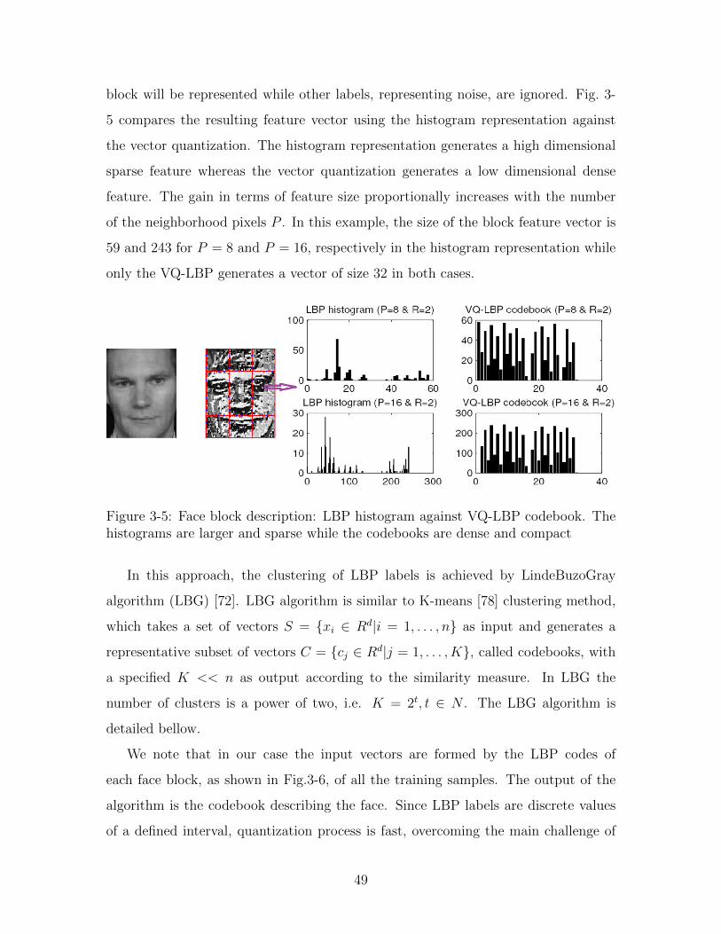
block will be represented while other labels, representing noise, are ignored. Fig. 3-
5 compares the resulting feature vector using the histogram representation against
the vector quantization. The histogram representation generates a high dimensional
sparse feature whereas the vector quantization generates a low dimensional dense
feature. The gain in terms of feature size proportionally increases with the number
of the neighborhood pixels P . In this example, the size of the block feature vector is
59 and 243 for P = 8 and P = 16, respectively in the histogram representation while
only the VQ-LBP generates a vector of size 32 in both cases.
Figure 3-5: Face block description: LBP histogram against VQ-LBP codebook. Thehistograms are larger and sparse while the codebooks are dense and compact
In this approach, the clustering of LBP labels is achieved by LindeBuzoGray
algorithm (LBG) [72]. LBG algorithm is similar to K-means [78] clustering method,
which takes a set of vectors S = {xi ∈ Rd|i = 1, . . . , n} as input and generates a
representative subset of vectors C = {cj ∈ Rd|j = 1, . . . , K}, called codebooks, with
a specified K << n as output according to the similarity measure. In LBG the
number of clusters is a power of two, i.e. K = 2t, t ∈ N . The LBG algorithm is
detailed bellow.
We note that in our case the input vectors are formed by the LBP codes of
each face block, as shown in Fig.3-6, of all the training samples. The output of the
algorithm is the codebook describing the face. Since LBP labels are discrete values
of a defined interval, quantization process is fast, overcoming the main challenge of
49

Algorithm 1 LBG algorithm
1: Input training vectors S = {xi ∈ Rd|i = 1, . . . , n}.2: Initiate a codebook C = {cj ∈ Rd|j = 1, . . . , K}.3: Set D0 = 0 and let k = 0.4: Classify the n training vectors into K clusters according to xi ∈ Sq if ‖xi − cq‖p ≤‖xi − cj‖p for j 6= q.
5: Update cluster centers cj, j = 1, . . . , K by cj = 1|Sj |∑
xi∈Sjxi.
6: Set k ← k + 1 and compute the distortion Dk =∑K
j=1
∑xi∈Sj
‖xi − cq‖p.7: If Dk−1−Dk
Dk> ε (a small number), repeat steps 4 to 6.
8: Output the codebook C = {cj ∈ Rd|j = 1, . . . , K}.
Vector Quantization (VQ) on huge continuous data.
Figure 3-6: LBP-face quantization.
3.4.2 VQMAP model
We model faces by maximum a posteriori vector quantization (VQMAP) which has
the advantage of generating reliable models, especially when only few enrollment faces
per user are available.
VQMAP was first formulated by [51] and applied for speaker verification. It
is a special case of the Gaussian mixture maximum a posteriori method (GMM-
MAP) [99]. In this last model, Gaussian mixtures have three sets of parameters
to be adapted: mean vectors (centroids), covariance matrices, and weights. VQMAP
model is motivated by the fact that accurate models could be obtained by only adapt-
50

ing the mean vectors in the GMM-MAP approach [99]. By reducing the number
of free parameters, the VQMAP model achieves much faster adaptation as well as
simpler implementation. Moreover, the similarity computation for a given probe is
further simplified by replacing the log likelihood ratio (LLR) computation by the
mean squared error (MSE) [51]. Indeed, the speed gain in VQMAP originates mostly
from the replacement of the Gaussian density computations with squared distance
computations, leaving out the exponentiation and additional multiplications [51].
The main issue in the VQ approach is the estimation of the centroids modeling the
face. Let the model parameters noted by θ = (ct1, . . . , ctK)t where ci are the centroids
and K is their number. This estimation has been formulated by MAP. Formally,
MAP seeks the parameters Θ that maximize the posterior probability density function
(pdf):
ΘMAP = arg maxΘ
P (Θ/X)
= arg maxΘ
P (X/Θ)g(Θ),(3.3)
where P (X/Θ) is the likelihood of the training set X = {x1, . . . , xN} given the pa-
rameters Θ and g(Θ) is the prior pdf of the parameters.
The above formulation of VQMAP requires the definition of the likelihood func-
tion P (X/Θ) as well as the prior distribution g(Θ). The likelihood pdf should take
the fact that VQ is non probabilistic model based mean squared error (MSE) into
account. Therefore, the likelihood has been modeled as a Gaussian mixture with
identity covariances and the prior pdf is modeled by the probability of K indepen-
dent Gaussians. The MAP estimates for Vector Quantization is then derived based
on k-means algorithm. The detailed formulation and mathematical development of
the VQMAP model is provided in Appendix A.
3.4.3 Face verification system
The proposed face verification system based on LBP features and VQMAP model
is depicted in Fig. 3-7. In the training stage, a model is generated for each autho-
51

Ve
rifi
ca
tio
n
Tra
inin
g
Models
Score
Computation Test
Face
Train
Faces
Background
Faces
MAP
Adaptation
Vector
Quantization
LBP
Features
LBP
Features
LBP Features
Decision
Figure 3-7: LBP-VQMAP face verification system.
rized user of the system. To generate a user model, a generic face model, called
universal background model (UBM), is first created using a pool of training faces.
After extracting LBP codes from each face, we divide the faces into blocks of equal
size. Then, we run LBG algorithm considering together the set of blocks of the same
position from all training faces. A codebook representing the background model is
obtained. User specific model is then inferred from the global model by applying the
MAP adaptation process using the training faces of the user.
In the verification stage, LBP features are extracted from the probe face F which
is divided into blocks with the size set at the training phase. Then, for each block
of the probe face, the closest UBM vectors are searched. For the face model, nearest
neighbor search is performed on the corresponding adapted vectors only. The match
score S is the difference between the UBM and the target C quantization errors [61]:
S = MSE(F,UBM)−MSE(F,C) (3.4)
52

where:
MSE(X, Y ) =1
|X|∑xi∈X
minyk∈Y||xi − yk||2 (3.5)
where xi and yk are the elements of X and Y , respectively.
The resulting score is compared to the decision threshold set at the training phase
to decide whether to accept the user as authentic or reject him/her as imposter.
3.5 Face verification using adapted LBP histograms
One of the reasons behind the success of LBP methods for face recognition is its sim-
plicity and rapidity. This is mainly due to histogram representation of LBP codes.
However, the histogram estimation may not be accurate in some cases, such as small
changes in the image, lack of training samples or subdivision of low resolution faces
into small boxes. For instance, Fig. 3-8 depicts LBP histogram of the same block (red
box) from three images of a person taken in the same session under the same acqui-
sition conditions. Although the three faces are very similar, at the LBP histogram
level, noticeable differences could be perceived. In this section, we propose an elegant
approach for coping with robust LBP histogram representation.
Figure 3-8: LBP histograms of the same block from three face images of a subject,taken in the same session, and their adapted histogram.
Since faces of different persons share some similarities, it is expected that some
53

LBP codes, which are representative of the face parts (nose, eyes, mouth, etc.), are
common between different faces. Here, we make use of this intuition to enhance
LBP histogram representation. Our proposed approach consists of creating a generic
LBP histogram for each face block computed over the pool of the same region from
several users faces. This generic histogram encloses characteristics from all trained
users. The generic histogram is then adapted to each user. Hence, a face region is
represented by a weighted sum of its LBP histogram and the corresponding generic
histogram:
Hrc (lk) = αHr
w(lk) + (1− α)Hrc (lk) (3.6)
In Eq. 3.6, Hrw denotes the generic histogram of block r. Hr
w is estimated using
the LBP codes from all the blocks of the same position r in the world faces. HrC is
the histogram of the face block r for client c and α ∈ [0, 1] is a weighting factor that
defines the contribution of each component to the final representation. lk is the kth
bin in the histogram.
An example of the adapted histogram is shown in Fig. 3-8. The adapted histogram
catches the important information represented by the highest bins in each of the three
histograms of individual faces. However some extra bins, known as cohort effect, are
introduced by the adaptation. We compensate the cohort effect at the score level.
The feature vector of a given face image is formed by concatenating the different
blocks’ adapted histograms. For each training face of a given user, we generate a
separate feature vector. The score between a training feature vector Hkc and a probe
one Hkp is computed by the χ2 histogram similarity measure. In order to eliminate
the cohort effect introduced by adapting the global model, we normalize the obtained
score by subtracting the similarity between the probe and the generic feature vector
(second term in (3.7)). Thus, the normalized score is given by:
S =∑k
(χ2(Hkp , H
kc )− χ2(Hk
p , Hkw)) (3.7)
54
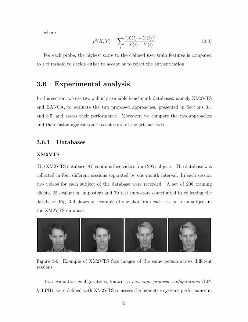
where
χ2(X, Y ) =∑i
(X(i)− Y (i))2
X(i) + Y (i)(3.8)
For each probe, the highest score to the claimed user train features is compared
to a threshold to decide either to accept or to reject the authentication.
3.6 Experimental analysis
In this section, we use two publicly available benchmark databases, namely XM2VTS
and BANCA, to evaluate the two proposed approaches, presented in Sections 3.4
and 3.5, and assess their performance. Moreover, we compare the two approaches
and their fusion against some recent state-of-the-art methods.
3.6.1 Databases
XM2VTS
The XM2VTS database [81] contains face videos from 295 subjects. The database was
collected in four different sessions separated by one month interval. In each session
two videos for each subject of the database were recorded. A set of 200 training
clients, 25 evaluation impostors and 70 test impostors contributed in collecting the
database. Fig. 3-9 shows an example of one shot from each session for a subject in
the XM2VTS database.
Figure 3-9: Example of XM2VTS face images of the same person across differentsessions.
Two evaluation configurations, known as Lausanne protocol configurations (LPI
& LPII), were defined with XM2VTS to assess the biometric systems performance in
55

verification mode. The two configurations are illustrated in Table 3.1. The database
is divided into three subsets: train, evaluation and test. The training data serves for
building clients models. Evaluation subset is used to tune system parameters. Finally,
system performances are estimated on the test subset, using evaluation parameters.
The difference between the two protocols, LPI and LPII, lays in the per-subject
number of face samples in each subset and the session these samples are taken from.
Table 3.1: Partitioning of the XM2VTS database according to the two configurations.
Configuration I Configuration II
Session Shot Clients Imposters Clients Imposters
1 1 Training
Evaluation Test
Training
Evaluation Test
2 Evaluation
2 1 Training
2 Evaluation
3 1 Training
Evaluation 2 Evaluation
4 1
Test Test 2
BANCA
The BANCA database [9] contains 52 users (26 male and 26 female). Faces are col-
lected through 12 different sessions with various acquisition devices of different qual-
ity and in different environment conditions: controlled (high-quality camera, uniform
background, controlled lighting), degraded (web-cam, non-uniform background) and
adverse (high-quality camera, arbitrary conditions). Examples of the three conditions
are shown in Fig. 3-10. For each session, two videos are recorded: a true client access
and an impostor attack.
In the BANCA protocol, seven distinct configurations for the training and testing
policy have been defined. In our experiments, we consider the three configurations
referred as Matched Controlled (MC), Unmatched Adverse (UA) and Pooled Test (P).
As shown in Table 3.2, all of the considered configurations, use the same training
conditions: each client is trained using images from the first recording session of the
controlled scenario. Testing is then performed on images taken from the controlled
56
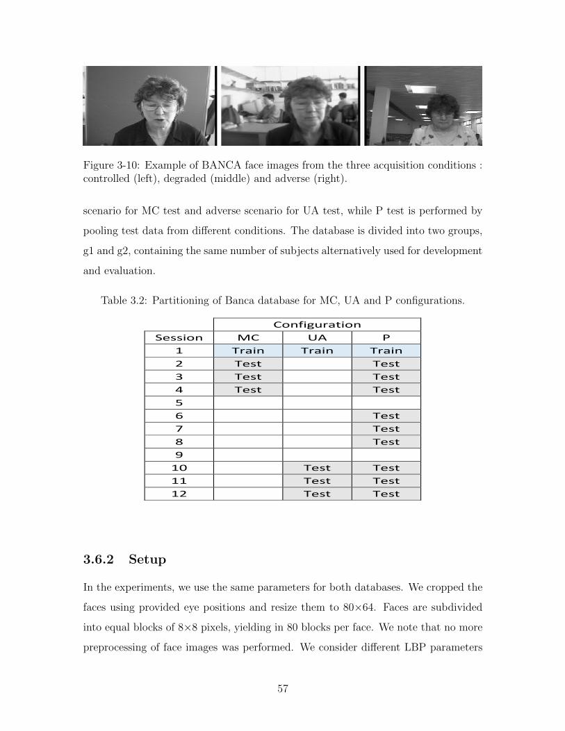
Figure 3-10: Example of BANCA face images from the three acquisition conditions :controlled (left), degraded (middle) and adverse (right).
scenario for MC test and adverse scenario for UA test, while P test is performed by
pooling test data from different conditions. The database is divided into two groups,
g1 and g2, containing the same number of subjects alternatively used for development
and evaluation.
Table 3.2: Partitioning of Banca database for MC, UA and P configurations.
Configuration
Session MC UA P
1 Train Train Train
2 Test Test
3 Test Test
4 Test Test
5
6 Test
7 Test
8 Test
9
10 Test Test
11 Test Test
12 Test Test
3.6.2 Setup
In the experiments, we use the same parameters for both databases. We cropped the
faces using provided eye positions and resize them to 80×64. Faces are subdivided
into equal blocks of 8×8 pixels, yielding in 80 blocks per face. We note that no more
preprocessing of face images was performed. We consider different LBP parameters
57

: (P,R) ∈ {(8, 2), (16, 2), (24, 3)}. Finally, for the sake of comparison, experiments
with similar configuration are also carried out for the baseline LBP approach.
We assess the verification performance by the half total error rate (HTER) which
is the mean of false acceptance rate (FAR) and false rejection rate (FRR) of the
evaluation set :
HTER =FAR(θ) + FRR(θ)
2(3.9)
The threshold θ corresponds to the optimal operating point of the development
set, defined by the minimal equal error rate (EER).
Finally, to compare different systems, we also draw the detection error trade-off
(DET) curve, which plots the FAR vs. FRR and allows comparison at different
operating points with an emphasis around the equal error rate (EER) region.
Table 3.3: HTER (%) on XM2VTS database using LPI and LPII protocols for dif-ferent configurations of LBP baseline and our proposed methods.
Method ParametersProtocol
LPI LPII
LBP Baseline
LBP(8,2)
3.0 2.2
Proposed approach 1: VQMAP 3.0 0.8
Proposed approach 2: AH 1.3 0.5
LBP Baseline
LBP(16,2)
2.9 2.0
Proposed approach 1: VQMAP 2.3 1.1
Proposed approach 2: AH 1.2 0.5
LBP Baseline
LBP(24,3)
3.9 2.9
Proposed approach 1: VQMAP 1.9 1.0
Proposed approach 2: AH 1.3 0.3
3.6.3 Results and discussion
We report in Tables 3.3 and 3.4 the results of the two proposed approaches as well
as those of the baseline LBP system on XM2VTS and BANCA databases. These
58

results clearly show that the two proposed approaches outperform the original LBP
approach in all configurations (i.e. for different parameters and different protocols).
In the VQMAP based approach, the performance gain can be explained by the
fact that not all the information present in the baseline LBP representation is dis-
criminative. Indeed, most of the bins in the baseline LBP histograms are close to zero
and may represent noise. Hence, vector quantization produces discriminative feature
vectors which contain most relevant LBP codes in the face.
In the approach based on the Adapted Histograms (AH), the information from
concatenated generic histograms yields more discriminative feature vectors. The pro-
posed normalization plays also an important role in the achieved results. The error
rate of the approach based on the Adapted Histograms is nearly one-third of that of
the baseline LBP on both databases and for most configurations.
In the experiments on XM2VTS database (Table 3.3), our two proposed ap-
proaches outperform the baseline LBP in all the configurations and for both protocols
LPI and LPII. Moreover, the two approaches show more robustness to different chal-
lenges present in the BANCA database. In fact, they perform better than the baseline
LBP in almost all the configurations (Table 3.4). We also note that the best HTERs
for the considered protocols are obtained by our approaches.
We also performed a score level fusion of the two proposed approaches by first
normalizing the scores using z-norm. Then we used logistic regression to fuse the two
systems. The baseline LBP, our two approaches and their fusion systems are compared
using the DET curve. Fig. 3-11 show the DET curve for the best configuration on the
P protocol of BANCA database including faces from different acquisition conditions
(controlled, degraded and adverse). The effectiveness of the proposed approaches over
the baseline LBP method for different operating points is clearly shown in Fig. 3-11.
Furthermore, the fusion of the two methods enhances the performance, indicating a
relative complementary of the two approaches.
Finally, we compare in Table 3.5 our obtained results against those of some state-
of-the-art counterpart on the challenging BANCA database. These results indicate
that our proposed approaches show competitive results. In the scenario of controlled
59

Table 3.4: HTER (%) on BANCA database for MC, UA and P protocols usingdifferent configurations of LBP baseline and our proposed methods.
Method ParametersProtocol
MC UA P
LBP Baseline
LBP(8,2)
10.5 17.3 25.0
Proposed approach 1: VQMAP 4.0 14.9 16.6
Proposed approach 2: AH 4.2 16.4 12.1
LBP Baseline
LBP(16,2)
10.9 18.5 28.4
Proposed approach 1: VQMAP 3.8 18.8 20.7
Proposed approach 2: AH 3.3 15.8 12.1
LBP Baseline
LBP(24,3)
12.3 25.0 33.3
Proposed approach 1: VQMAP 4.8 18.2 20.4
Proposed approach 2: AH 3.7 17.5 12.6
acquisition conditions (MC) protocols, the best results are given by our adapted LBP
histogram method. Furthermore, the fusion of the two proposed approaches yields
in the best performance for MC, UA and P protocols. It is also worth noting that,
in contrast to the other methods, our proposed approaches also inherit the simplicity
and computational efficiency of the original LBP approach.
Table 3.5: HTER (%) for state of the art methods on BANCA database.
Method Protocol
MC UA P
LBP Baseline [2] 10.5 17.3 25.0
LBP-MAP [100] 7.3 22.1 19.2
LBP-KDE [3] 4.3 18.1 17.6
Weighted LBP-KDE [3] 3.7 15.1 11.6
Proposed approach 1: VQMAP 3.8 14.9 16.6
Proposed approach 2: AH 3.3 15.8 12.1
Fusion VQMAP-AH 3.3 14.4 11.6
60
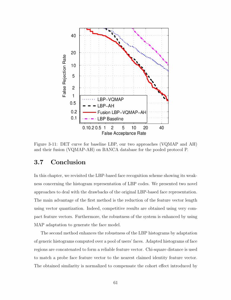
Figure 3-11: DET curve for baseline LBP, our two approaches (VQMAP and AH)and their fusion (VQMAP-AH) on BANCA database for the pooled protocol P.
3.7 Conclusion
In this chapter, we revisited the LBP-based face recognition scheme showing its weak-
ness concerning the histogram representation of LBP codes. We presented two novel
approaches to deal with the drawbacks of the original LBP-based face representation.
The main advantage of the first method is the reduction of the feature vector length
using vector quantization. Indeed, competitive results are obtained using very com-
pact feature vectors. Furthermore, the robustness of the system is enhanced by using
MAP adaptation to generate the face model.
The second method enhances the robustness of the LBP histograms by adaptation
of generic histograms computed over a pool of users’ faces. Adapted histograms of face
regions are concatenated to form a reliable feature vector. Chi-square distance is used
to match a probe face feature vector to the nearest claimed identity feature vector.
The obtained similarity is normalized to compensate the cohort effect introduced by
61

the generic feature vector.
Furthermore, we performed a score level fusion of the two proposed methods
using logistic regression after normalizing scores by z-norm. The fusion yields slightly
enhanced performance. Compared to state-of-the-art, the error rates on XM2VTS
and BANCA databases demonstrated the efficiency of the proposed approaches and
their fusion.
62

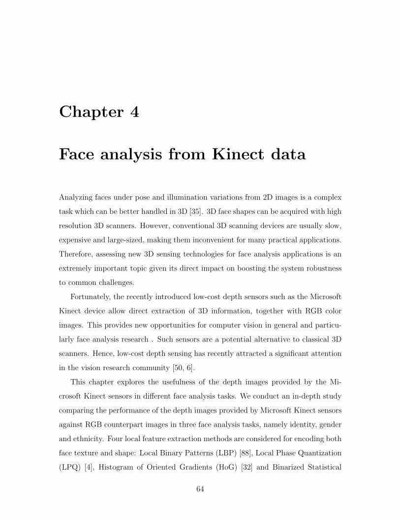
Chapter 4
Face analysis from Kinect data
Analyzing faces under pose and illumination variations from 2D images is a complex
task which can be better handled in 3D [35]. 3D face shapes can be acquired with high
resolution 3D scanners. However, conventional 3D scanning devices are usually slow,
expensive and large-sized, making them inconvenient for many practical applications.
Therefore, assessing new 3D sensing technologies for face analysis applications is an
extremely important topic given its direct impact on boosting the system robustness
to common challenges.
Fortunately, the recently introduced low-cost depth sensors such as the Microsoft
Kinect device allow direct extraction of 3D information, together with RGB color
images. This provides new opportunities for computer vision in general and particu-
larly face analysis research . Such sensors are a potential alternative to classical 3D
scanners. Hence, low-cost depth sensing has recently attracted a significant attention
in the vision research community [50, 6].
This chapter explores the usefulness of the depth images provided by the Mi-
crosoft Kinect sensors in different face analysis tasks. We conduct an in-depth study
comparing the performance of the depth images provided by Microsoft Kinect sensors
against RGB counterpart images in three face analysis tasks, namely identity, gender
and ethnicity. Four local feature extraction methods are considered for encoding both
face texture and shape: Local Binary Patterns (LBP) [88], Local Phase Quantization
(LPQ) [4], Histogram of Oriented Gradients (HoG) [32] and Binarized Statistical
64

Image Features (BSIF) [60]. Extensive experiments are carried out on three pub-
licly available Kinect face databases, namely FaceWarehouse [23], IIIT-D [47] and
CurtinFaces [65].
The chapter is organized as follows. First, the Kinect sensor is briefly introduced
in Section 4.1. Section 4.2 overviews the related literature work devoted to the use of
Kinect depth images for automatic face analysis. Section 4.3 presents our methodol-
ogy for studying the usefulness of Kinect depth images in different face analysis tasks.
Section 4.4 describes the experiments and discusses the obtained results. Section 4.5
provides the conclusions.
4.1 Kinect sensors
The Microsoft Kinect sensor was first introduced in 2009 as a natural user interface
of the Microsoft game console Xbox 360. Kinect captures both conventional RGB
images and depth maps of the scene. The depth-sensing system is licensed from the
PrimeSense Company and the exact technology behind it is still unrevealed. However,
the depth computation is, most probably, based on the structured light principle.
The depth sensing process is composed of an infrared (IR) projector, which emits an
infrared irregular dot distribution, and an IR camera which captures the projected
IR pattern to estimate the depth map. In addition to the RGB and depth sensing
hardware, Kinect provides also an array of four microphones equipped with enhanced
noise suppression capabilities, mainly aimed for voice command in games.
Due to its characteristics, Kinect is a good alternative to expensive high-quality
3D scanners. For instance, a comparison between Kinect and Minotlta VIVID 910,
used for collecting FRGC face database [94], is provided in Table 4.1 and Fig.4-1.
The advantages provided by Kinect in terms of size, weight and price are obvious.
However, on the other hand the quality of the 3D scans is very low compared to that
provided by existing 3D scanners.
The Kinect sensor provides both color and depth videos as 640 × 480 pixel res-
olution at 30 fps. However, the Kinect depth data is very noisy and the distance
65

Figure 4-1: Comparing face images acquired with Minolta VIVID 910 scanner (left)against Kinect (right).
computation of far objects often fails. The maximum distance that can be detected
is 4.5 meters. Recently, a more accurate version of the device, namely Kinect 2, has
been released. The new Kinect has higher color and depth resolution and can sense
far away objects (up to 8 meters) more accurately.
There exist other Kinect-like devices such as Asus Xtion PRO LIVE 1 and Leap
Motion 2. The former is practically similar to Kinect and provides the same function-
alities while the latter is a smaller device intended to track the hand gestures. The
3D sensing technology is being embedded in mobile devices, such as Google Tango 3,
1http://www.asus.com/Multimedia/Xtion_PRO_LIVE/2https://www.leapmotion.com/3https://www.google.com/atap/project-tango/
66

Table 4.1: Comparing Kinect and Minolta VIVID 910 3D scanning devices.
Device Kinect Minolta VIVID 910Size 7.3cm× 28.3cm× 7.28cm 21.3cm× 41.3cm× 27.1cmWeight 564.5 g 11 KgSpeed 0.033s 2.5sPrice < 200 $ > 50K $Color resolution 640× 480 640× 480Depth resolution 320× 240 640× 480Range 0.8 ∼ 4 m 0.6 ∼ 2.5 m
opening new horizons for wider applications. Similarly to Kinect, these devices are
mainly intended for natural user interface applications.
4.2 Review of works using Kinect for face analysis
The facial depth images provided by Kinect-like low-cost sensors are unfortunately
currently of low-resolution and noisy. This can be due, for instance, to missing data
(holes) in some parts of the face, inaccurate depth value computation and limited
distance coverage from the sensor (2 to 4 meters). Despite these challenges, many
researchers have recently explored Kinect depth images for different facial analysis
tasks. The Kinect sensor has been used for face detection and tracking and head
pose estimation as well as for inferring and classifying facial information. The face
recognition problem is the most studied task while there exist few work dealing with
gender and expression recognition. Other use of Kinect includes facial modeling and
animation for games and human-computer interaction applications. In the follow-
ing we review the literature works which utilized Kinect facial images for various
applications.
4.2.1 Face detection and tracking, pose estimation
As a crucial preprocessing step for various face analysis tasks, Kinect has been used
for face detection and segmentation, head pose estimation and normalization and
face tracking. Some work make use of depth maps only while others combine both
67

RGB and depth data. Among the work relying on depth data only, Fanelli et al.[40]
presented a system for real time head localization and head pose estimation. The
authors extended the random regression forest [38] to classify depth image patches
between the head and the rest of the body. Then, a regression is performed in the
continuous spaces of head positions and orientations. Experiments on BIWI Kinect
head pose database [39] demonstrated good performance as well as robustness to
occlusion. In another work, Padeleris et al. [90] rendered auxiliary range images of
the reconstructed head from candidate poses and attempted to find the most similar to
a reference view obtained at initialization. They formulated the head pose estimation
as an optimization problem that quantifies the divergence of the depth measurements
between the rendered views and the reference one. Li et al. [67] performed head
tracking using iterative closest point (ICP) algorithm by registering a dense face
template to depth data captured by Kinect. Niese et al. [86] also fitted a user specific
face model with ICP algorithm to determine the head pose. Cao and Lu [24] detected
and cropped the head from depth images for fatigue detection application. They split
the depth image into different regions, extracted the contour of each region, and then
used ellipse fitting algorithm to fit the contour points. The detected head is the region
with the lowest fitness cost.
On the other hand, combination of color and depth information for face detection
and tracking and head pose estimation has been proven to achieve more robustness
than using the two modalities separately. For instance, in order to accelerate face
detection, Duc et al. [36] used the depth information from the Microsoft Kinect to
estimate the size of the face, thus they limited the range of candidate regions for
face detection. They further applied depth-based skin segmentation by imposing ge-
ometric constraints, which improved the efficiency of finding human skin as well as
reduced the computational cost. Zhang et al. [127] proposed an automatic face seg-
mentation approach employing both color and depth cues. Skin color detection and
depth constraint are used together to provide prior information. Given these pri-
ors, the segmentation is performed by the local spline regression and active learning
framework. Tomari et al. [112] detected and tracked head pose with Kinect for social
68

robots navigation planning. Initially, possible human regions are segmented out and
validated using depth and Hu moment features. Afterward, Haar-like features with
the Adaboost classifier are employed to estimate potential head regions within the
segmented areas. The obtained head regions are post-validated by examining their
dimension and their probability of containing skin. The head pose estimation and
tracking is performed by a boosted-based particle filter. Yang et al. [122] combined
HoG features extracted from Kinect color and depth images for face detection and
head pose estimation. First, they employed nine HoG filters (corresponding to differ-
ent yaw and pitch angle intervals) trained with support vector machines (SVMs) to
achieve a coarse face detection. Then, the detected face location is refined and a feed-
forward multi-layer perception (MLP) network is trained to estimate face orientation.
Jin el al. [59] used both color and depth acquired with Kinect for face detection, facial
region segmentation and head pose estimation. In case of face detection with enough
confidence, the head pose is employed to initialize the parameters of the AAM (active
appearance model) algorithm [37]. The AAM algorithm, which usually uses the three
RGB color channels, is extended to use the face depth information as well. Both face
texture and depth are fitted to a model in order to locate the facial features. The
authors claimed the ability of their approach to detect faces in presence of complex
background and under severe head-pose variations as well as the ability to achieve
more accurate facial landmark labeling compared to the traditional AAM algorithm.
However, no details about the used experimental data and evaluation protocol were
provided.
4.2.2 Face recognition
As stated before, face recognition using Kinect depth images is the most investi-
gated considered among face analysis problems. For instance, Pamplona et al. [91]
addressed continuous authentication problem using 3D faces acquired with Kinect.
Faces are first detected and normalized using ICP. According to its pose, each face
is registered to one of the three positions: frontal, left profile or right profile. HoG
features are extracted and matched to corresponding regions of interest (ROI). This
69

system was evaluated on four 40 minutes long videos with variations in facial expres-
sion, occlusion and pose, where an equal error rate of 0.8% was reported. Li et al.
[66] tackled face recognition under pose, illumination, expression and disguise using
the Kinect sensor. They proposed a preprocessing algorithm that generates a canon-
ical frontal view for both depth map and texture of the face irrespective of its initial
position. To this end, after face registration to a reference model, facial symmetry
is employed to recover missing face parts, fill holes and smooth the face depth data.
Sparse representation classifier (SRC) is used for both depth and texture separately.
Evaluation of this system on CurtinFaces dataset [65] yields in 88.7% recognition rate
using depth data only and 96.7% when face texture and depth are fused. Min et al.
[83] used the PrimeSensor device for real time 3D face identification. To accelerate the
processing and meet the real-time constraint, instead of registration to each gallery
face, a probe face is registered to a few intermediate references (canonical faces) ran-
domly selected from the gallery. Moreover, ICP algorithm was implemented on a
GPU. Good identification results have been reported on a dataset of 20 people with
average speed ranging from 0.04s to 0.38s, depending on the number of the canonical
faces. However, the experimental analysis does not consider severe challenges like
head pose, expression and illumination variations. Goswami et al. [46] proposed a
Kinect based face recognition system, where the HoG descriptor is computed on the
entropy of RGB-D faces and the saliency of RGB. A random decision forest classifier
is used to establish the identity from the concatenation of five HoG descriptors. Ciac-
cio et al. [29] handled the 3D head pose variation problem, by generating different
rotated faces either from the probe or the target. The target consists of one frontal
face per enrolled subject while the probes can be at any pose angle. For recogni-
tion, LBP and covariance matrices are separately used as features and fused after
classification at score level. Experiments on faces with variations in six yaw angles
demonstrated that using the rendered rotated faces from the target frontal face yields
better results than other schemes. Mantecon et al. [80] proposed a face recognition
system using the second version of Kinect which provides higher depth resolution.
Inspired by LBP, they proposed depth local quantized pattern descriptor (DLQP)
70
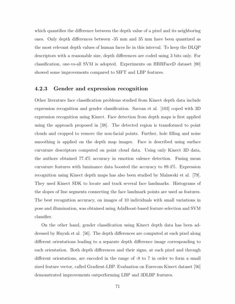
which quantifies the difference between the depth value of a pixel and its neighboring
ones. Only depth differences between -35 mm and 35 mm have been quantized as
the most relevant depth values of human faces lie in this interval. To keep the DLQP
descriptors with a reasonable size, depth differences are coded using 3 bits only. For
classification, one-vs-all SVM is adopted. Experiments on HRRFaceD dataset [80]
showed some improvements compared to SIFT and LBP features.
4.2.3 Gender and expression recognition
Other literature face classification problems studied from Kinect depth data include
expression recognition and gender classification. Savran et al. [103] coped with 3D
expression recognition using Kinect. Face detection from depth maps is first applied
using the approach proposed in [38]. The detected region is transformed to point
clouds and cropped to remove the non-facial points. Further, hole filling and noise
smoothing is applied on the depth map images. Face is described using surface
curvature descriptors computed on point cloud data. Using only Kinect 3D data,
the authors obtained 77.4% accuracy in emotion valence detection. Fusing mean
curvature features with luminance data boosted the accuracy to 89.4%. Expression
recognition using Kinect depth maps has also been studied by Malawski et al. [79].
They used Kinect SDK to locate and track several face landmarks. Histograms of
the slopes of line segments connecting the face landmark points are used as features.
The best recognition accuracy, on images of 10 individuals with small variations in
pose and illumination, was obtained using AdaBoost-based feature selection and SVM
classifier.
On the other hand, gender classification using Kinect depth data has been ad-
dressed by Huynh et al. [56]. The depth differences are computed at each pixel along
different orientations leading to a separate depth difference image corresponding to
each orientation. Both depth differences and their signs, at each pixel and through
different orientations, are encoded in the range of -8 to 7 in order to form a small
sized feature vector, called Gradient-LBP. Evaluation on Eurecom Kinect dataset [56]
demonstrated improvements outperforming LBP and 3DLBP features.
71

4.2.4 Face modeling, reconstruction and animation
In other researches, which are less related to the present thesis, Kinect depth maps
are used for modeling faces [106, 116, 26, 53, 82] for computer graphic applications.
High resolution 3D faces are reconstructed from Kinect low resolution depth data
and used for different applications. Examples of these applications include 3D video
conference [5], personalized avatars [135], real-time facial animation [22, 118], etc.
4.2.5 Discussion and contribution motivation
The analysis of the presented review highlights several remarks on the use of the
depth maps of faces. Mostly, the depth data has been exploited to preprocess the
face and to assist the RGB images based systems. Particularly, depth data has been
used in head pose variation to normalize the face into a reference pose. Depth data
is also helpful for face detection and segmentation especially in illumination variation
situations.
Face description and classification from depth images is less investigated in the
literature. While face recognition is the most relatively tackled problem from depth
data, only a scarce number of research investigated expression and gender recognition
problems. To the best of our knowledge, by the time of the review was being written,
no research investigated the other face analysis problems from Kinect depth data
including age estimation, ethnicity classification, emotion state, etc.
The review also points out the fact that face depth maps maybe either used
solely or combined with RGB channels. However, one notes that there is a lack in
comparing the performance of RGB images against depth maps in order to understand
the benefits of using depth information.
Another important issue concerns the experimental data and evaluation bench-
marks used by the reviewed researches. Most papers make use of private databases
which are generally of small size containing a limited number of subjects and/or lim-
ited number of samples per subject. Moreover, data is often collected in laboratory
environments where real-life challenges are not simulated. Even though few Kinect
72
face databases are made publically available (See our paper [18] for the detailed de-
scription of these databases), the test protocols frequently differ from a paper to
another. All the mentioned concerns make the results biased, incomparable and hard
to reproduce. These issues hinder the advance in this research topics.
Motivated by the previous limitations, we carry out a study of various face analysis
tasks from both RGB images and depth maps. We employ different features to
describe faces from both types of images. The best available Kinect face databases
are used to evaluate the performances of the studied methods. We also compare depth
maps against RGB image in all the study scenarios. The following section provides
the details of the proposed framework for our study.
4.3 A framework for face analysis from Kinect data
To gain insights into the usefulness of the depth images in different face analysis
tasks, we carried out a comprehensive analysis comparing the performance of the
depth images versus RGB counterparts in three face analysis tasks, namely identity,
gender and ethnicity recognition, considering four local feature extraction methods.
Extensive evaluation is performed on three publicly available benchmark databases.
In this Section, we present our experimental framework comprising preprocessing,
feature extraction methods and classifier.
4.3.1 Preprocessing
The depth images acquired by the Kinect sensor usually need to be pre-processed
to overcome the noisy and low quality nature of the images. In our framework, the
depth images are preprocessed as follows. First, the depth maps provided by Kinect
are mapped into real world 3D coordinates. Thus, each pixel is represented by six
values: x, y and z coordinates and the three RGB values. Then, the resulted cloud
of points C is translated so that the nose tip is located at the origin. This is achieved
by subtracting the nose coordinates (xnose, ynose, znose) from the all the points in the
73

cloud:
(xt, yt, zt) = (x, y, z)− (xnose, ynose, znose),∀(x, y, z) ∈ C. (4.1)
The face region is extracted using an ellipsoid centered at the nose tip by discarding
all the points outside the ellipsoid. Then, the face point cloud is smoothed and re-
sampled to a grid of 96× 96. Examples of cropped 2D and 3D face images are shown
in Fig. 4-2. Finally, for the 3D face part, we drop the x and y coordinates and keep
only the z coordinates for describing the face shape.
Figure 4-2: Examples of 2D cropped image (left) and corresponding 3D face image(right) obtained with the Microsoft Kinect sensor after preprocessing.
4.3.2 Feature extraction
After preprocessing, four facial local image descriptors are extracted from the depth
and RGB images. In contrast to global face descriptors which compute features
directly from the entire face image, local face descriptors representing the features in
small local image patches have shown to be more effective in real world conditions [52].
The considered local face descriptors in our experiments are LBP, LPQ, HoG and
BSIF. LBP and HoG are selected for their popularity in computer vision whereas
LPQ and BSIF are recent descriptors which showed very promising results in different
problems [7, 97]. To the best of our knowledge, BSIF has never been used to describe
Kinect depth face data. While, LBP has been presented in the previous chapter, the
description of the three remaining features is given bellow.
74
Local Phase Quantization (LPQ)
LPQ was originally proposed for describing and classifying texture blurred images [89]
then applied to face recognition from blurred images [4]. The LPQ descriptor bases
on the robustness and high insensitivity of the low-frequency phase components to
centrally symmetric blur. Therefore, the descriptor uses the phase information of
short-term Fourier transform (STFT) locally computed on a window around each
pixel of an image. Let Nx be the M2 neighborhoods of the pixel x and let f(x) be
the image function at the bi-dimensional position x. The output of the STFT at the
pixel x is given by:
F (x, u) =∑y∈Nx
f(x− y)e−j2πuT y = W T
u fx, (4.2)
where u indicates the bi-dimensional spatial frequency. In the LPQ descriptor, only
four complex frequencies are considered: u0 = (α, 0), u1 = (α, α), u2 = (0, α), u3 =
(−α,−α) where α is a small scalar frequency (α << 1) ensuring the blur is centrally
symmetric. Hence, each pixel of position x is characterized by a vector Fx:
Fx =[Re{F (x, u0), F (x, u1), F (x, u2), F (x, u3)},
Im{F (x, u0), F (x, u1), F (x, u2), F (x, u3)}],
= Wfx,
(4.3)
where Re{.} and Im{.} denotes the real part and the imaginary part of a complex
number.
In order to derive a binary code for the pixel x , the vector Fx needs to be quan-
tized. To maximize the information preservation by the quantization, the coefficients
should be statistically independent. Therefore, a de-correlation step, based on a
whitening transform, is applied in LPQ before the quantization process. Assuming
that the image function f(x) is a result of a Markov process with the correlation
coefficient between two adjacent pixels is ρ and the variance of each sample is 1, the
75

covariance between two adjacent pixels xi and xj is
σi,j = ρ||xi−xj ||, (4.4)
where ||.|| denotes the L2 norm. Using these information, one computes the covariance
matrix C of the M2 neighborhoods. Hence, the covariance matrix of the transform
coefficient vector Fx can be obtained from:
D = WCW T , (4.5)
for ρ > 0, D is not a diagonal matrix, meaning that the coefficients are correlating.
Assuming Gaussian distribution, independence can be achieved using the following
whitening transform:
Gx = V TFx, (4.6)
where V is an orthonormal matrix derived from the singular value decomposition
(SVD) of the matrix D, that is:
D = UΣV T . (4.7)
Gx is computed for all image positions and subsequently quantized using a simple
scalar quantizer:
qi =
0 if gi < 0
1 otherwise
, (4.8)
where gi is the ith component of Gx. Finally, the resulting binary quantized coeffi-
cients are represented as integer value in [0-255] as follows:
LPQ(x) =8∑i=1
qi2i−1. (4.9)
76

Histogram of Oriented Gradients (HoG)
HoG [32] was initially developed for human detection but later extended and applied
to many other computer vision problems. The basic idea behind HoG is that an
object appearance and shape can be characterized by the distribution of local intensity
gradients or edge directions. To compute the HoG descriptor of a given image I, the
gradients are first obtained at each pixel by computing two 1D derivatives in both
horizontal and vertical directions. This is corresponding to filtering the image with
the two following filters:
Dx =[−1 0 −1
], (4.10)
Dy =
1
0
−1
, (4.11)
thus, the x and y derivatives are obtained by the convolutions:
Ix = I ∗Dx, (4.12)
and
Iy = I ∗Dy. (4.13)
The magnitude and orientation of the gradient are then computed as follows:
|G| =√I2x + I2
y , (4.14)
θ = arctanIyIx. (4.15)
The image is divided into small spatial regions called cells. The magnitudes of
the gradient at each pixel of the cell are accumulated into a histogram according to
77

the gradient direction. This is equivalent to a weighted vote for an orientation-based
histogram, where the weight is the value of the magnitude. In the original work [32],
non-signed orientations have been found to perform better. Therefore, a histogram of
B = 9 bins (orientations) evenly spaced over 0 to 180 degrees was utilized. To prevent
quantization artifacts due to small image changes, each pixel of the cell contributes
to two adjacent bins by a fraction of the magnitude.
In order to cope with local changes of illumination and contrast, four adjacent
cells (2 × 2) are grouped together forming one block. The blocks in an image are
horizontally and vertically overlapped, by two cells in each direction, respectively.
The four-cell histograms of each block are concatenated into a vector v, which is
normalized by its Euclidean norm:
vn =v√‖v‖2 + ε
, (4.16)
where the small positive value ε is added to prevent division by zero.
The final HoG feature vector is formed by concatenating all the normalized block
features of the image. Finally, this feature is normalized again to count for the overall
image contrast.
Binarized Statistical Image Features (BSIF)
BSIF approach [60] is a relatively recent descriptor inspired by LBP. Instead of using
hand-crafted filters, such as in LBP and LPQ, the idea behind BSIF is to automati-
cally learn a fixed set of filters from a small set of natural images. The set of filters
are derived based on statistics of training images. Given an image patch X of size
l× l pixels and a linear filter Wi of the same size, the filter response si is obtained by:
si =∑u,v
Wi(u, v)X(u, v) = wTi x, (4.17)
where wi and x are vectors containing the pixels of Wi and X, respectively. A binary
78

code chain b is obtained by binarizing each response si as follows:
bi =
1, if si ≥ 0
0, otherwise, (4.18)
bi is the ith element of b. In the aim to learn a powerful set of filters Wi, the statistical
independence of the responses si should be maximized. Let W be the matrix of size
n× l2 formed by stacking the n filters wi. Independent filters estimation is achieved
using independent component analysis (ICA). Therefore, one needs to decompose W
into two parts so that the filters responses are rewritten as:
S = Wx = UV x = Uz, (4.19)
where z = V x, and U is a n×n square matrix, and matrix V simultaneously performs
the whitening and dimensionality reduction of training samples x. The randomly
sampled training patches x are first normalized to zero mean and principal component
analysis (PCA) is applied to reduce their dimension to n. Specifically, let C denote
the covariance matrix of samples x and its eigen decomposition is C = BΛBT , the
matrix V is defined as:
V = (Λ−1/2BT )1:n, (4.20)
where Λ contains the eigenvalues of C in descending order, and (.)1:n denotes the first
n rows of the matrix in parenthesis.
Then, given the zero-mean whitened data samples z, one may use standard inde-
pendent component analysis algorithm to estimate an ortHoGonal matrix U which
yields the independent components S of the training data. In other words, since
z = U−1S, the independent components allow to represent the data samples z as a
linear superposition of the basis vectors defined by the columns of U−1. Finally, the
filter matrix W = UV is computed, which can be directly utilized for calculating
BSIF features.
79

Face description
Figure 4-3 depicts examples of results when applying the four selected local descriptors
on face texture and depth images acquired with Kinect sensor for a subject from the
FaceWarehouse database[23]. In our experiments, we extended the BSIF description
method to handle depth images by learning the filters using facial depth images from
the FRGC database [94] as training data. These filters are then used to compute
BSIF features on Kinect depth images. We found this new learning approach yields
in better filters, in terms of performances of face classification, than the original ones.
Figure 4-3: Examples of results after applying the four descriptors to face texture anddepth images. From left to right: the original face image (top: texture image andbottom: its corresponding depth image) and the resulting images after the applicationof LBP, LPQ, HoG and BSIF descriptors, respectively.
To form the face feature vector, for each descriptor, the RGB and depth images
are first divided into several local regions from which local histograms are extracted
and then concatenated into an enhanced feature histogram used for classification.
4.3.3 Classification
The classification of both RGB and depth descriptors is performed using a support
vector machine classifier (SVM). SVM is a supervised classification algorithm that
aims to find the optimal separating hyperplane of the high dimensional training data.
80

This is achieved via maximization of the margins (distance of closest data, regardless
of its class, to the hyperplane). The training feature vectors along with their labels
are input to SVM, which outputs a model able to predict the labels of new unseen
data. In our case, since we are dealing with nonlinear face feature vectors, we opt
for a radial basis function (RBF) kernel. The nonlinear SVM maps the original data
into a new space, using the kernel function, in which classes separation is improved.
4.4 Experiments and results
We analyzed the performance of the four local descriptors (LBP [88], LPQ [4],
BSIF [60] and HoG [32]) presented in Section 4.3.2 on three publicly available Kinect
face databases, FaceWarehouse [23], IIIT-D [47] and Curtinfaces [65], containing both
RGB and depth facial images acquired with Kinect. We report the results for three
different face classification problems: face identification, gender recognition and eth-
nicity classification. We have used the ground truth data whenever it is available
with the database and in case data is not labeled we inferred the needed information
from the face images (e.g, gender). We note that we have been limited to the three
face analysis tasks mainly because of the available data and metha-data nature. For
example, we were unable to perform age estimation because the ages of persons are
not provided. The databases, evaluation methodology and results are provided in the
following.
4.4.1 Databases
FaceWarehouse and IIIT-D databases are selected as these are among the largest
available databases (regarding the number of subjects) while CurtinFaces is the most
challenging Kinect face database (in terms of head pose, illumination and expression).
The three databases are described below.
• The CurtinFaces Kinect Database4 [65] contains over 5000 images of 52
4https://researchdata.ands.org.au/curtinfaces-database/3640
81

subjects in both RGB and depth maps obtained by Kinect sensor. The partic-
ipants consist of 10 females and 42 males. The subjects in the database belong
to three different ethnic groups (Caucasians, Chinese and Indians). The facial
images have various variations in pose, illumination, facial expression as well
as sunglasses and hand disguise. The faces of each subject are acquired under
many combinations of these challenges. For each subject, there are 49 images
under 7 poses and 7 facial expressions, 35 images under 5 illuminations and 7
expressions, and 5 images under disguise (sunglasses and hand). The full set for
each person consists of 97 images. CurtinFaces is among the most challenging
Kinect face databases.
• The FaceWarehouse Database5 [23] comprises 150 individuals aged from
7 to 80. For each subject, the RGB-D face data is captured for the neutral
expression and 19 other expressions. During recording, a guide face mesh for
each specific expression is sequentially shown to the person, who is asked to
imitate the expression and rotate his/her head within a small angle range, while
keeping the expression fixed. For every RGB-D raw data record, a set of facial
feature points on the color image are automatically localized, and manually
adjusted for better accuracy. A template facial mesh is then deformed to fit
the depth data while matching the feature points on the color image to their
corresponding points on the mesh. Based on the 20 fitted meshes of each person,
47 individual-specific expression blendshapes per person are constructed.
• The IIIT-D RGB-D Face Database 6 [46] comprises 106 male and female
subjects. All the subjects are of the same ethnicity (Indian). The number of
images per subject varies between 11 and 254 images. The total number of
images in the database is 4605. The database is captured in two different ses-
sions. The images are captured under normal illumination with some variations
in pose and expression. IIIT-D is the largest Kinect face database in terms of
the number of subjects. Since the images are not segmented, the database can
5http://gaps-zju.org/facewarehouse/6https://research.iiitd.edu.in/groups/iab/facedatabases.html
82

be used for face detection, besides its use for identity and gender recognition.
Table 4.2 outlines the main characteristics of the presented face Kinect databases.
For each database, we report the number of subjects, the number of samples per
subject and the main challenges presented in the database.
Table 4.2: Kinect face databases employed in our experiments.
Database # Subjects # Samples ChallengesFaceWarehouse [23] 150 20 Pose and expressionIIIT-D [46, 47] 106 11-254 Expression and poseCurtinFaces [65] 52 97 Pose, expression, light-
ing and disguise
Examples of the depth and RGB face images for a person from CurtinFaces
database are illustrated in Fig. 4-4.
Figure 4-4: Face images samples from a subject of the CurtinFaces database. Top:RGB faces, middle: their corresponding raw depth maps and bottom: depth croppedface.
4.4.2 Setup
In this section, we provide details about the parameters used in different experiments
and evaluation protocols. First, for each of the four features, as the aim of our study
is not to optimize the performances, we used default parameters with no adjustments.
Uniform LBP patterns are extracted with a radius R = 2 and neighborhood P = 8.
The window size in LPQ is set to 5. HoG features are quantized with 9 bin histograms.
83

The filters used in BSIF are learned from patches of 11 × 11 and coded with 8 bits.
For each feature, histograms are computed from non-overlapped blocks of 16 × 16
pixels, for both RGB and depth images, and concatenated to form the face feature
vector.
For identity recognition, five images per subject are used for training and the rest
for test. In gender and ethnicity classification, 10 subjects7 per class are used to
train the models and the other subjects are used for test. We note that for gender
and ethnicity classification, subjects belonging to train and test subsets are mutually
exclusive in other to avoid the identity bias in classification. Ethnicity evaluation
is performed on FaceWarehouse (Chinese vs. White) and CurtinFaces (Caucasian,
Chinese and Indian) databases only since IIIT-D database includes only one ethnicity.
Finally, the performances are assesses in terms of correct classification rates. For
all the experiments, five-fold cross validation strategy is performed and the mean
classification rate and standard deviation are reported.
4.4.3 Experimental results
Tables 4.3, 4.4 and 4.5 summarize the average accuracy and standard deviation for
the three face analysis problems.
Table 4.3: Mean classification rates (%) and standard deviation using RGB and depthfor face identity classification on FaceWarehouse, IIIT-D and CurtinFaces databases.
MethodDatabase
FaceWarehouse IIIT-D CurtinFacesRGB Depth RGB Depth RGB Depth
LBP 99.6∓0.1 85.3∓0.4 93.8∓1.6 84.4∓1.0 66.2∓0.6 84.0∓1.1LPQ 99.7∓0.1 85.4∓0.4 93.4∓1.4 84.7∓1.8 57.6∓1.0 73.8∓1.1HoG 98.4∓0.4 86.4∓0.6 92.5∓1.5 82.8∓1.3 68.2∓1.0 83.8∓1.0BSIF 99.8∓0.1 88.5∓0.4 91.5∓1.7 77.8∓1.2 72.2∓1.0 77.8∓1.1
The analysis of the results points out that, generally, better performances on the
FaceWarehouse database and IIIT-D database compared to the CurtinFaces database.
7In case the number of subjects for a given class is less than 20, half of the subjects are used fortraining and the other half for testing.
84

Table 4.4: Mean classification rates (%) and standard deviation using RGB and depthfor face gender classification on FaceWarehouse, IIIT-D and CurtinFaces databases.
MethodDatabase
FaceWarehouse IIIT-D CurtinFacesRGB Depth RGB Depth RGB Depth
LBP 74.7∓1.7 77.6∓2.7 87.5∓1.6 76.4∓5.5 86.3∓3.2 84.3∓4.5LPQ 78.4∓2.6 78.8∓1.7 88.0∓2.4 77.4∓4.5 85.3∓3.8 83.5∓3.9HoG 78.6∓2.3 77.5∓1.5 86.1∓2.5 70.1∓3.3 86.8∓2.1 85.0∓4.1BSIF 78.9∓3.0 78.2∓1.7 86.2∓3.2 70.3∓1.9 87.7∓2.6 85.2∓2.5
Table 4.5: Mean classification rates (%) and standard deviation using RGB anddepth for facial ethicithy classification on FaceWarehouse and CurtinFaces database.Results are not provided for IIIT-D database as only one ethnicity is represented inthis database.
MethodDatabase
FaceWarehouse IIIT-D CurtinFacesRGB Depth RGB Depth RGB Depth
LBP 90.6∓4.3 95.3∓1.1 - - 70.5∓3.1 69.4∓3.2LPQ 93.8∓3.9 96.5∓1.0 - - 71.3∓3.0 68.6∓3.0HoG 94.6∓4.0 96.8∓1.6 - - 69.3∓3.3 67.8∓2.4BSIF 96.0∓2.7 98.4∓0.6 - - 74.9∓3.6 70.2∓2.7
CurtinFaces database is indeed more challenging in terms of variations of pose, ex-
pression and illumination.
In overall, the RGB images yield in better performances compared to the depth
images. Nevertheless, the results of the depth images alone are still good and actually
much better than our expectations based on the human perception. It is indeed quite
hard to visually distinguish the subjects using only the depth images. One can also
notice from the results on CurtinFaces database through the three tables that depth
images may compete or even outperform RGB images under challenging illumination
and pose variations. Another important remark is that the difference in classification
accuracy between depth and RGB images is less significant in gender and ethnicity
classification than it is in identity classification. In particular, depth outperforms
RGB in ethnicity classification on FaceWarehouse database. These results point out
the usefulness of Kinect depth images in some face classification problems.
85

Regarding the performance of different features, the four descriptors perform com-
parably across the three databases. However, in most of the cases, the new BSIF
descriptor yields in the best classification rates. Our extensions to BSIF to describe
depth images by learning dedicated depth filters demonstrated interesting results,
making BSIF generally better than the three other descriptors.
Figure 4-5 visually illustrates the obtained results on FaceWarehouse database.
From this figure, one can easily notice that RGB clearly outperforms depth in iden-
tity classification. The performance difference is becoming less significant in gender
classification problem. In ethnicity classification, the depth surprisingly outperforms
the RGB based methods.
Figure 4-5: Classification accuracy for identity, gender and ethnicity using RGB anddepth on FaceWarehouse database.
Our main goal through this work is to compare the performance of Kinect depth
and RGB images in different face analysis tasks. Thus, we did not aim at optimizing
the overall performance using complex methods.
The depth images provided by Kinect sensor are of low quality and noisy thus
requiring a crucial preprocessing before analysis. The outcomes on such images are
highly depending on the preprocessing step and hence cannot be easily generalized or
compared to previously reported results if a different preprocessing is applied. Even
though, for completeness, we summarize in Table 4.6 the performances reported by
other authors in the literature dealing with face analysis tasks on publicly available
86

Kinect face datasets. Again, one cannot fairly compare the different methods since
each method uses different data and/or different evaluation protocols. Furthermore,
most of the reported works combine RGB and depth modalities but omit to report
the performance of each modality separately.
Table 4.6: Summary of reported performance of literature work on face analysis usingKinect sensor.
Method Application Dataset Accuracy
RISE[47] Face recognition III-D 81.0 % (RGB-D)Eurecom 89.0 % (RGB-D)
COV+LBP[29] Face recognition CurtinFaces 84.6% (RGB-D)
Depth+DCS[66] Face recognition CurtinFaces 88.7 % (D)91.1% (RGB)96.7% (RGB-D)
DLQP[80] Face recognition HRRFace 63.95% (D)
G-LBP[56] Gender recognition Eurecom 87.1% (D)
3DLBP[56] Gender recognition Eurecom 85.9% (D)
Curvature [103] Expression recognition SBIA 77.4% (D)84.9% (RGB)89.4% (RGB-D)
As an indication, Li et al. [66] reported a face recognition accuracy of 88.7%
using complex depth preprocessing steps, including symmetric filling of face depth
maps, on CurtinFaces dataset while we achieved 84.0% using simple LBP feature
only. Our performance is comparable to the work of Ciaccio et al. [29] combining
LBP and covariance features on the same dataset. Gender recognition was tackled
by Huynh et. [56] achieving 87.1% accuracy using depth images on Eurecom dataset.
Our experiments on larger and more challenging databases yield better results as can
be noticed from tables. To the best of our knowledge, the ethnicity classification has
not been previously addressed using Kinect data.
4.5 Conclusion
In this chapter, we presented a review on using Kinect depth data for different face
analysis problems. The review of the literature revealed that the recently introduced
consumer low-cost depth sensors have attracted a big interest from researchers work-
87

ing on face analysis tasks. The device was mainly used for face recognition and face
detection, segmentation and tracking as well as head pose estimation and normaliza-
tion. To this end, the depth maps are either considered alone or combined with RGB
channels.
To gain more insight, we presented the first comprehensive study in the litera-
ture exploring the usefulness of the depth information acquired by the low-cost depth
sensor in different face analysis tasks including face identification, gender recogni-
tion and ethnicity classification. We carried out intensive experimental evaluation
with four state-of-the-art local face descriptors on three publicly available Kinect
face databases. While it is difficult to visually distinguish the subjects using only
the depth images, the obtained results confirmed that the depth facial information
alone provides promising classification results beyond the expectations based on the
human perception. Moreover, we found depth maps to perform better than RGB
images under sever illumination, expression and viewpoint changes. Regarding the
best performing methods, the introduced BSIF features derived from a new set of
filters showed interesting results for both RGB and depth images.
88


Chapter 5
Kinship verification from videos
This chapter deals with automatic kinship verification from face videos. Kinship
verification from faces is a challenging task. Indeed, it inherits the research problems
of face verification from images captured in the wild under adverse pose, expression,
illumination and occlusion conditions. In addition, kinship verification should deal
with wider intra-class and inter-class variations, as persons from the same family
may look very different while faces of persons with no kin relation may look similar.
Moreover, automatic kinship verification can face new challenges since a pair of input
images may be from persons of different sex (e.g. brother-sister kin) and/or with a
large age difference (e.g. father-daughter kin).
The published papers and organized competitions (e.g. [76, 75]) dealing with
automatic kinship verification over the past few years showed some promising results.
Typical current best-performing methods combine several face descriptors, apply met-
ric learning approaches and compute Euclidean distances between pairs of features
for kinship verification. One can remark that theses works are based on handcrafted
features extracted from images while kinship verification is less investigated using
deep learning and videos. In the present chapter, we aim to exploit the temporal in-
formation present in face videos, investigating the use of both spatio-temporal shallow
features and deep features describing faces.
This chapter is organized as follows. Section 5.1 briefly overviews the related
work and motivates our approach. The proposed approach for kinship verification
90

from videos is described in Section 5.2. Experiments and analysis are then given in
Section 5.3. In Section 5.4, we give the conclusions.
5.1 Background and motivation
Kinship verification from face is receiving increasing interest by the research commu-
nity. This is mainly motivated by its potential applications, especially in analyzing
daily shared data in social web. The first approaches to tackle kinship verification
were based on low level handcrafted feature extraction and SVM or k-NN classifiers.
For instance, Zhou et al. [132] used a spatial pyramid learning descriptor; Gabor gra-
dient orientation pyramid has been used by Zhou et al. [133]; and Self-similarity of
Weber faces was utilized by Kohli et al. [64]. Several types of face features are then
combined by many researchers and used for verifying the kin relation. For example,
in the second kinship competition [75], all the proposed methods used three or more
descriptors. The best performing method in this competition employed four different
local features (LBP, HOG, over-complete LBP - OCLBP - and Fisher vectors).
On the other hand, different metric learning approaches have been investigated
for tackling the kinship verification problem. Lu et al. [77] learned a distance metric
where the face pairs with a kin relation are pulled close to each other and those without
a kin relation are pushed away. Recently, Zhou et al. [134] applied ensemble similarity
learning for solving the kinship verification problem. They learned an ensemble of
sparse bi-linear similarity bases from kinship data by minimizing the violation of
the kinship constraints between pairs of images and maximizing the diversity of the
similarity bases. Yan et al. [121] and Hu et al. [54] learned multiple distance metrics
based on various features, by simultaneously maximizing the kinship constraint (pairs
with a kinship relation must have a smaller distance than pairs without a kinship
relation) and the correlation of different features.
Motivated by the impressive success of deep learning approaches in various im-
age representation and classification [105] in general and face recognition in partic-
ular [107], Zhang et al. [128] recently proposed a convolution neural network archi-
91

tecture for face-based kinship verification. The proposed architecture is composed
by two convolution max pooling layers followed by a convolution layer then a fully
connected layer. A two-way soft max classifier is used as the final layer to train the
network. The network takes a pair of RGB face images of different persons as an
input, checking the possible kin relations. However, their reported results do not
outperform the shallow methods presented in the FG15 kinship competition on the
same datasets [75]. The reason behind this may be the scarcity of training data, since
deep learning approaches require the availability of enough training samples which is
not the case for available face kinship databases.
While most of the published works cope with kinship problem from images, to
our knowledge the only work that performed kinship from videos was conducted by
Dibeklioglu et al. [34]. The authors combined facial expression dynamics with facial
appearance as features and used SVM for classification.
It appears that most of literature works on kinship verification are mainly based on
shallow handcrafted features and hence are not associated with the recent significant
progress which has been made in machine learning suggesting the use of deep features.
Moreover, the role of facial dynamics in kinship verification is mostly unexplored as
most existing works focus on analyzing still facial images instead of video sequences.
Based on these observations, we propose to approach the problem of kinship verifica-
tion from spatio-temporal point of view and also exploit the recent progress in deep
learning.
5.2 Video-based kinship verification
This section describes our approach for kinship verification from videos. In the fol-
lowing, we first present an overview of the proposed approach, then we provide the
details of each step.
92

5.2.1 Approach overview
Fig. 5-1 depicts an overview of our approach for kinship verification from videos.
Given two face video sequences, to verify their kin relationship, our proposed ap-
proach starts with detecting, cropping and aligning the face images based on facial
landmarks. Then, two types of descriptors are extracted: shallow spatio-temporal
texture features and deep features. As spatio-temporal features, we extract local bi-
nary patterns (LBP) [2], local phase quantization (LPQ) [4] and binarized statistical
image features (BSIF) [60]. These features are all extracted from three orthogonal
planes (TOP) of the videos. Deep features are extracted by convolutional neural
networks (CNNs) [92]. The pairs of features are then combined to be used as inputs
to support vector machines (SVM) for classification. A score level fusion is then per-
formed, to combine all the features’ results, and the issued score is used to decide
whether the two persons in the input videos have a kin relation or not. The details
of the proposed approach are presented in the following sections.
93

Feat
ure
Extr
actio
n
Dee
p Fe
atur
es
Spat
io-T
empo
ral F
eatu
res
CNN
LBPT
OP
LPQ
TOP
BSIF
TOP
Face
Det
ectio
n
&
Alig
nmen
t
Face
Det
ectio
n
&
Alig
nmen
t
Feat
ure
Extr
actio
n
Dee
p fe
atur
es
Spat
io-T
empo
ral F
eatu
res
CNN
LBPT
OP
LPQ
TOP
BSIF
TOP
Kin
Pair
Com
bina
tion
SVM
SVM
SVM
SVM
Kin
/ N
on k
in
Scor
e F
usio
n
Figure 5-1: Overview of the proposed approach for kinship verification from videos.
94

5.2.2 Face detection and tracking
The first step in our proposed approach is to segment the face region from each
video sequence. Therefore, we employed an active shape model (ASM) [30] based
approach. ASM is a statistical model of the shape of an object. It represents an
object by the distribution of a set of points. The model is built based on a set
of training images annotated with landmark points. To detect a new instance of the
object, the ASM iteratively deforms to fit the object in the new image. Therefore, two
steps are alternatively performed to match the model to the new instance: generating
a suggested shape by inspecting the neighborhood of each point and adapting the
suggested shape to the model.
In our case, we detect 68 facial landmarks tracking them along the video. Faces
are then cropped from all the frames of the video and aligned based on the detected
landmarks. Fig. 5-2 illustrates an example of the detected face landmarks in one
frame and the cropped face.
Figure 5-2: Example of face cropping: (left) a frame annotated with the detectedlandmarks, and (right) the cropped and aligned face region.
95

5.2.3 Face description
For describing faces from videos, we use two types of features: texture spatio-temporal
features and deep learning features. These features are introduced hereafter.
Spatio-temporal features
Spatio-temporal texture features have been shown to be efficient for describing faces
in various face analysis tasks, such as face recognition [63] and facial expression clas-
sification [131]. The spatio-temporal textural dynamics of the face in a video are
extracted from three orthogonal planes XY, XT, and YT [96, 130, 7], separately. X
and Y are the horizontal and vertical spatial axes of the video, and T refers to the
time axis. An example of the orthogonal planes at a pixel of the video is given in
Fig. 5-3. This approach characterizes the video sequence in three ways: a stack of
XY planes in axis T, a stack of XT planes in axis Y and a stack of YT planes in
axis X. The XT and YT planes provide information about the space-time transitions
while XY plane represents the spatial information.
96
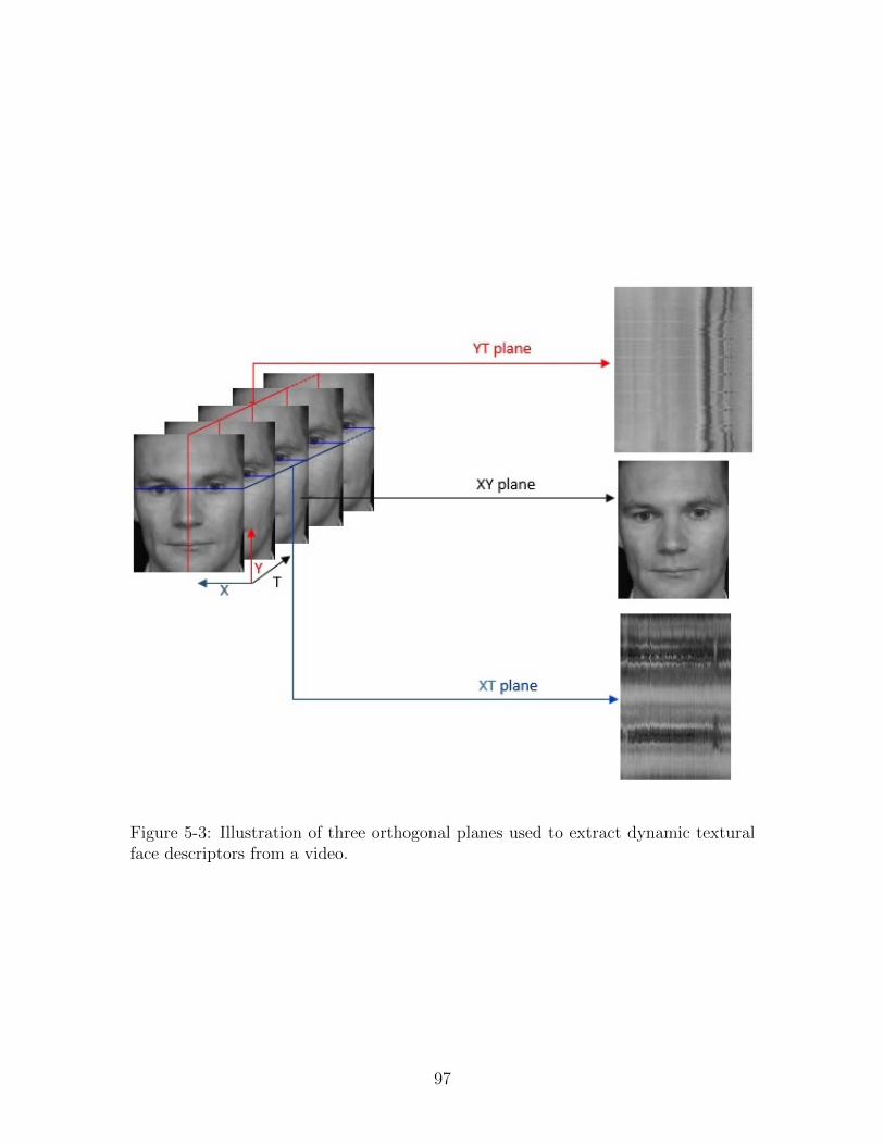
Figure 5-3: Illustration of three orthogonal planes used to extract dynamic texturalface descriptors from a video.
97

The face video is subdivided into smaller volumes (see Fig. 5-4) in order to main-
tain the facial spatial structure. For each region, the texture features of each plane are
summarized in a separate histogram and then the three histograms are concatenated
into a single feature vector (Fig. 5-5). The final face descriptor is composed by the
concatenation of all the regions’ features.
Figure 5-4: Division of video into region volumes.
Figure 5-5: Three plan feature vector.
Three local texture descriptors ( LBP [2], LPQ [4] and BSIF [60]), used in the
previous chapter for still images, are extended here to describe face appearance from
videos. The features are extracted by applying the previous regions three planes strat-
egy. Furthermore, the three features are extracted at multiple scales, to take benefit
of the multi-resolution representation [25], by varying their parameters. Hence, the
98

utilized parameters of LBP are P = {8, 16, 24} and R = {1, 2, 3}; and for LPQ
and BSIF descriptors, the filter sizes were selected as W = {3, 5, 7, 9, 11, 13, 15, 17}.
The feature dimension sizes for the three neighborhoods of LBP are 3540, 14580 and
33300, respectively. For both LPQ and BSIF the feature size is 15360 for each filter.
Deep learning features
Deep neural networks have been recently outperforming the state of the art in various
classification tasks [101]. Particularly, convolutional neural networks (CNNs) demon-
strated impressive performance in object classification in general and face recognition
in particular [110]. Two factors are mainly behind this success of deep learning ap-
proaches. The first one is the abundance of web scale training data. Indeed, the
networks used to beat the state of the art in image detection and classification [101]
are very deep architectures (e.g. Google network (GoogLeNet) has 22 layers [109] )
trained with millions of samples and thousands of classes. The second factor is the
advance made by hardware computation speed, especially GPU, enabling the train-
ing of very deep architectures with billions of parameters. Even though, training of
very deep architectures still require days or even months with the current available
hardware.
The deep learning approaches have many advantages. First, deep neural networks
are scalable models having the capacity to learn highly complex representations of
thousands of categories. Once trained, a deep model stores its knowledge compactly
in learned parameters, making it easy to deploy in any environment. It can then be
easily used for fast prediction of new inputs with no need for storing additional data.
Additionally, deep learning approaches learn to extract discriminative features in con-
trast to hand-engineered feature extractors, such as LBP and its variants. Moreover,
in a deep learning model both feature extraction and classification steps are optimized
at the same time, which is not the case of classical approaches.
In this work, we utilize a convolutional neural network (CNN) for extracting deep
face features. CNNs are hierarchical machine learning models which are able to
learn complex representations of images and signals using vast amounts of training
99

data. Inspired by the human visual system, CNNs progressively extract sophisticated
representation of the input by learning transformations in multiple layers. Fig. 5-6
illustrates an example of a deep CNN. A deep CNN is formed by alternating many
convolutional and subsampling layers. Usually, the top of the network is composed
by one or more fully connected layers and a classification layer.
Figure 5-6: Example of a convolutional neural network.
As stated before, deep neural networks require a huge amount of training data
to learn efficient features, which is not the case for the available kinship databases.
Indeed, our preliminary experiments using a Siamese CNN architecture [28] as well as
deep architecture proposed by a previous work [128] for kinship verification yielded
lower performance than shallow features. An alternative for extracting deep face fea-
tures is to use a pre-trained network. A number of very deep pre-trained architectures
has already been made available by researchers. In our case, we use the VGG-face [92]
network which has been initially trained for face recognition on a reasonably large
dataset of 2.6 million images of 2622 people. This network has been evaluated for
face verification from both pairs of images and videos showing interesting performance
compared against state of the art. This motivated us to use VGG-face network for
extracting deep face features for kinship verification.
The detailed parameters of the VGG-face CNN are provided by Table 5.1. The
input of the network is an RGB face image of size 224 × 224 pixels. The network
is composed of 13 linear convolution layers (conv), each followed by a non-linear
rectification layer (relu). Some of these rectification layers are followed by a non-
linear max pooling layer (mpool). Following are two fully connected layers (fc) both
100

outputting a vector of size 4096. At the top of the initial network are a last fully
connected layer with the size of classes to predict (2622) and a softmax layer for
computing the class posterior probabilities.
To extract deep face features for kinship verification, we input the video frames
one by one to the CNN and collect the feature vector issued by the fully connected
layer fc7 (all the layers of the CNN except the class predictor fc8 layer and the softmax
layer are used). All the frames’ features of a given face video are finally averaged to
obtain the video descriptor.
Table 5.1: VGG-face CNN architecture.
layer 0 1 2 3 4 5 6 7 8 9type input conv relu conv relu mpool conv relu conv reluname conv1 1 relu1 1 conv1 2 relu1 2 pool1 conv2 1 relu2 1 conv2 2 relu2 2support 3 1 3 1 2 3 1 3 1filt dim 3 64 64 128num filts 64 64 128 128stride 1 1 1 1 2 1 1 1 1pad 1 0 1 0 0 1 0 1 0
layer 10 11 12 13 14 15 16 17 18type mpool conv relu conv relu conv relu mpool convname pool2 conv3 1 relu3 1 conv3 2 relu3 2 conv3 3 relu3 3 pool3 conv4 1support 2 3 1 3 1 3 1 2 3filt dim 128 256 256 256num filts 256 256 256 512stride 2 1 1 1 1 1 1 2 1pad 0 1 0 1 0 1 0 0 1
layer 19 20 21 22 23 24 25 26 27 28type relu conv relu conv relu mpool conv relu conv reluname relu4 1 conv4 2 relu4 2 conv4 3 relu4 3 pool4 conv5 1 relu5 1 conv5 2 relu5 2support 1 3 1 3 1 2 3 1 3 1filt dim 512 512 512 512num filts 512 512 512 512stride 1 1 1 1 1 2 1 1 1 1pad 0 1 0 1 0 0 1 0 1 0
layer 29 30 31 32 33 34 35 36 37type conv relu mpool conv relu conv relu conv softmxname conv5 3 relu5 3 pool5 fc6 relu6 fc7 relu7 fc8 probsupport 3 1 2 7 1 1 1 1 1filt dim 512 512 4096 4096num filts 512 4096 4096 2622stride 1 1 2 1 1 1 1 1 1pad 1 0 0 0 0 0 0 0 0
101

5.2.4 Classification
To classify a pair of face features as positive (the two persons have a kinship relation)
or negative (no kinship relation between the two persons), we use a bi-class linear
support vector machine classifier. Before feeding the features and their labels to
the SVM, each pair of features has to be transformed into a single feature vector as
imposed by the classifier. We have examined various ways for combining a pair of
features, such as concatenation and vector distances. We have empirically found that
utilizing the normalized absolute difference shows the best performance. Therefore,
in our work, a pair of feature vectors X = {x1, . . . , xd} and Y = {y1, . . . , yd} is
represented by the vector F = {f1, . . . , fd} where :
fi =∑i
|xi − yi|∑i (xi + yi)
(5.1)
5.3 Experiments
5.3.1 Database and test protocol
To evaluate the proposed approach, we use UvA-NEMO Smile database [33], which
is , to the best of our knowledge, the only available video kinship database. The
database was initially collected for analyzing posed versus spontaneous smiles of sub-
jects. Videos are recorded with a resolution of 1920 × 1080 pixels at a rate of 50
frames per second under controlled illumination conditions. A color chart is placed
on the background of the videos to allow further illumination and color normaliza-
tion. The ages of the subjects in the database vary from 8 to 76 years. Many families
participated in the database collection, allowing its use for evaluation of automatic
kinship from videos. A total of 95 kin relations were identified between 152 subjects in
the database. There are seven different kin relations between pairs of videos: Sister-
Sister (S-S), Brother-Brother (B-B), Sister-Brother (S-B), Mother-Daughter (M-D),
Mother-Son (M-S), Father-Daughter (FD), and Father-Son (F-S). The association of
the videos of persons having kinship relations gives 228 pairs of spontaneous and
102

287 pairs of posed smile videos. The statistics of the database are summarized in
Table 5.2.
Table 5.2: Kinship statistics of UvA-NEMO Smile database.
Spontaneous PosedRelation Subj. # Vid. # Sub. # Vid. #S-S 7 22 9 32B-B 7 15 6 13S-B 12 32 10 34M-D 16 57 20 76M-S 12 36 14 46F-D 9 28 9 30F-S 12 38 19 56All 75 228 87 287
S-S B-B S-B M-D M-S F-D F-S
Figure 5-7: Samples of pair images form UvA-NEMO Smile database for differentkin relations. Positive pairs are combinations of first row with second row (greenrectangles) and negative pairs are combinations of second row with third row (redrectangles).
Following [34], we randomly generate negative kinship pairs corresponding to each
positive pair. Therefore, for each positive pair we associate the first video with an-
other video of a person within the same kin subset while ensuring there is no relation
between the two subjects. Examples of the positive pairs and the generated negative
pairs are illustrated by Fig. 5-7. For all the experiments, we perform a per-relationship
evaluation and report the average accuracy (rate of correctly classified pairs) of spon-
taneous and posed videos. The accuracy for the whole database, obtained by pooling
all the relations, is also provided. Since the number of pairs of each relation is small,
103
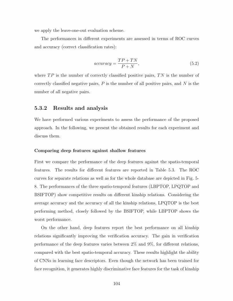
we apply the leave-one-out evaluation scheme.
The performances in different experiments are assessed in terms of ROC curves
and accuracy (correct classification rates):
accuracy =TP + TN
P +N, (5.2)
where TP is the number of correctly classified positive pairs, TN is the number of
correctly classified negative pairs, P is the number of all positive pairs, and N is the
number of all negative pairs.
5.3.2 Results and analysis
We have performed various experiments to assess the performance of the proposed
approach. In the following, we present the obtained results for each experiment and
discuss them.
Comparing deep features against shallow features
First we compare the performance of the deep features against the spatio-temporal
features. The results for different features are reported in Table 5.3. The ROC
curves for separate relations as well as for the whole database are depicted in Fig. 5-
8. The performances of the three spatio-temporal features (LBPTOP, LPQTOP and
BSIFTOP) show competitive results on different kinship relations. Considering the
average accuracy and the accuracy of all the kinship relations, LPQTOP is the best
performing method, closely followed by the BSIFTOP, while LBPTOP shows the
worst performance.
On the other hand, deep features report the best performance on all kinship
relations significantly improving the verification accuracy. The gain in verification
performance of the deep features varies between 2% and 9%, for different relations,
compared with the best spatio-temporal accuracy. These results highlight the ability
of CNNs in learning face descriptors. Even though the network has been trained for
face recognition, it generates highly discriminative face features for the task of kinship
104

Table 5.3: Accuracy (in %) of kinship verification using spatio-temporal and deepfeatures on UvA-NEMO Smile database.
Method S-S B-B S-B M-D M-S F-D F-S Mean AllBSIFTOP 75.07 83.46 71.23 82.46 72.37 81.67 79.84 78.01 75.83LPQTOP 69.67 78.21 82.54 71.71 83.30 78.57 83.91 78.27 76.02LBPTOP 80.47 77.31 70.50 78.29 72.37 84.40 71.50 76.41 72.82
DeepFeat 88.92 92.82 88.47 90.24 85.69 89.70 92.69 89.79 88.16
verification.
105

0 0.2 0.4 0.6 0.8 10
0.1
0.2
0.3
0.4
0.5
0.6
0.7
0.8
0.9
1
1. LBPTOP2. LPQTOP3. BSIFTOP4. DeepFeat
(a) Sister-Sister
0 0.2 0.4 0.6 0.8 10
0.1
0.2
0.3
0.4
0.5
0.6
0.7
0.8
0.9
1
1. LBPTOP2. LPQTOP3. BSIFTOP4. DeepFeat
(b) Brother-Brother
0 0.2 0.4 0.6 0.8 10
0.1
0.2
0.3
0.4
0.5
0.6
0.7
0.8
0.9
1
1. LBPTOP2. LPQTOP3. BSIFTOP4. DeepFeat
(c) Sister-Brother
0 0.2 0.4 0.6 0.8 10
0.1
0.2
0.3
0.4
0.5
0.6
0.7
0.8
0.9
1
1. LBPTOP2. LPQTOP3. BSIFTOP4. DeepFeat
(d) Mother-Daughter
106
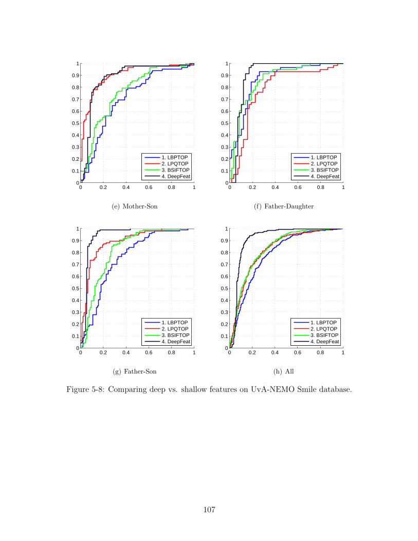
0 0.2 0.4 0.6 0.8 10
0.1
0.2
0.3
0.4
0.5
0.6
0.7
0.8
0.9
1
1. LBPTOP2. LPQTOP3. BSIFTOP4. DeepFeat
(e) Mother-Son
0 0.2 0.4 0.6 0.8 10
0.1
0.2
0.3
0.4
0.5
0.6
0.7
0.8
0.9
1
1. LBPTOP2. LPQTOP3. BSIFTOP4. DeepFeat
(f) Father-Daughter
0 0.2 0.4 0.6 0.8 10
0.1
0.2
0.3
0.4
0.5
0.6
0.7
0.8
0.9
1
1. LBPTOP2. LPQTOP3. BSIFTOP4. DeepFeat
(g) Father-Son
0 0.2 0.4 0.6 0.8 10
0.1
0.2
0.3
0.4
0.5
0.6
0.7
0.8
0.9
1
1. LBPTOP2. LPQTOP3. BSIFTOP4. DeepFeat
(h) All
Figure 5-8: Comparing deep vs. shallow features on UvA-NEMO Smile database.
107
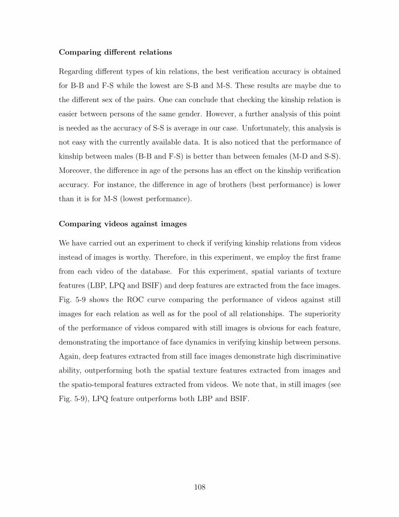
Comparing different relations
Regarding different types of kin relations, the best verification accuracy is obtained
for B-B and F-S while the lowest are S-B and M-S. These results are maybe due to
the different sex of the pairs. One can conclude that checking the kinship relation is
easier between persons of the same gender. However, a further analysis of this point
is needed as the accuracy of S-S is average in our case. Unfortunately, this analysis is
not easy with the currently available data. It is also noticed that the performance of
kinship between males (B-B and F-S) is better than between females (M-D and S-S).
Moreover, the difference in age of the persons has an effect on the kinship verification
accuracy. For instance, the difference in age of brothers (best performance) is lower
than it is for M-S (lowest performance).
Comparing videos against images
We have carried out an experiment to check if verifying kinship relations from videos
instead of images is worthy. Therefore, in this experiment, we employ the first frame
from each video of the database. For this experiment, spatial variants of texture
features (LBP, LPQ and BSIF) and deep features are extracted from the face images.
Fig. 5-9 shows the ROC curve comparing the performance of videos against still
images for each relation as well as for the pool of all relationships. The superiority
of the performance of videos compared with still images is obvious for each feature,
demonstrating the importance of face dynamics in verifying kinship between persons.
Again, deep features extracted from still face images demonstrate high discriminative
ability, outperforming both the spatial texture features extracted from images and
the spatio-temporal features extracted from videos. We note that, in still images (see
Fig. 5-9), LPQ feature outperforms both LBP and BSIF.
108

0 0.2 0.4 0.6 0.8 10
0.1
0.2
0.3
0.4
0.5
0.6
0.7
0.8
0.9
1
1. LBPTOP2. LPQTOP3. BSIFTOP4. DeepFeat Video5. LBP6. LPQ7. BSIF8. DeepFeat Image
(a) Sister-Sister
0 0.2 0.4 0.6 0.8 10
0.1
0.2
0.3
0.4
0.5
0.6
0.7
0.8
0.9
1
1. LBPTOP2. LPQTOP3. BSIFTOP4. DeepFeat Video5. LBP6. LPQ7. BSIF8. DeepFeat Image
(b) Brother-Brother
0 0.2 0.4 0.6 0.8 10
0.1
0.2
0.3
0.4
0.5
0.6
0.7
0.8
0.9
1
1. LBPTOP2. LPQTOP3. BSIFTOP4. DeepFeat Video5. LBP6. LPQ7. BSIF8. DeepFeat Image
(c) Sister-Brother
0 0.2 0.4 0.6 0.8 10
0.1
0.2
0.3
0.4
0.5
0.6
0.7
0.8
0.9
1
1. LBPTOP2. LPQTOP3. BSIFTOP4. DeepFeat Video5. LBP6. LPQ7. BSIF8. DeepFeat Image
(d) Mother-Daughter
109
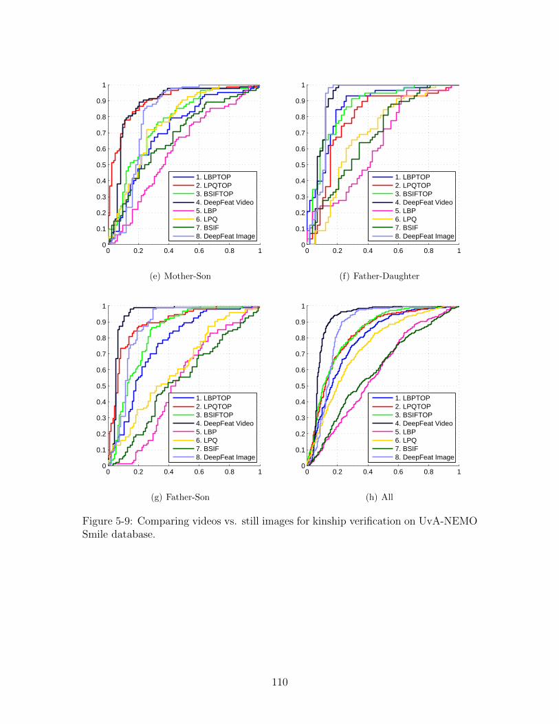
0 0.2 0.4 0.6 0.8 10
0.1
0.2
0.3
0.4
0.5
0.6
0.7
0.8
0.9
1
1. LBPTOP2. LPQTOP3. BSIFTOP4. DeepFeat Video5. LBP6. LPQ7. BSIF8. DeepFeat Image
(e) Mother-Son
0 0.2 0.4 0.6 0.8 10
0.1
0.2
0.3
0.4
0.5
0.6
0.7
0.8
0.9
1
1. LBPTOP2. LPQTOP3. BSIFTOP4. DeepFeat Video5. LBP6. LPQ7. BSIF8. DeepFeat Image
(f) Father-Daughter
0 0.2 0.4 0.6 0.8 10
0.1
0.2
0.3
0.4
0.5
0.6
0.7
0.8
0.9
1
1. LBPTOP2. LPQTOP3. BSIFTOP4. DeepFeat Video5. LBP6. LPQ7. BSIF8. DeepFeat Image
(g) Father-Son
0 0.2 0.4 0.6 0.8 10
0.1
0.2
0.3
0.4
0.5
0.6
0.7
0.8
0.9
1
1. LBPTOP2. LPQTOP3. BSIFTOP4. DeepFeat Video5. LBP6. LPQ7. BSIF8. DeepFeat Image
(h) All
Figure 5-9: Comparing videos vs. still images for kinship verification on UvA-NEMOSmile database.
110

Table 5.4: Comparison of our approach for kinship verification against state of theart on UvA-NEMO Smile database.
Method S-S B-B S-B M-D M-S F-D F-S Mean AllFang et al. [41] 61.36 56.67 56.25 56.14 55.56 57.14 55.26 56.91 53.51Guo & Wang [49] 65.91 56.67 60.94 58.77 62.50 67.86 55.26 61.13 56.14Zhou et al. [133] 63.64 70.00 60.94 57.02 56.94 66.07 60.53 62.16 58.55Dibeklioglu et al. [34] 75.00 70.00 68.75 67.54 75.00 75.00 78.95 72.89 67.11
Our DeepFeat 88.92 92.82 88.47 90.24 85.69 89.70 92.69 89.79 88.16Our Deep+Shallow 88.93 94.74 90.07 91.23 90.49 93.10 88.30 90.98 88.93
Feature fusion
We have fused spatio-temporal features and deep features to check their complemen-
tarity. For simplicity, we have opted for a simple sum at the score-level to perform the
fusion. Table 5.4 shows a comparison of the fusion results with the previous works.
Overall, the fusion enhanced the verification accuracy by a significant margin. The
effect is more evident in the relationships depicted by different sex and higher age
variation, such as M-S (improved by 4.8%) and F-D (improved by 3.4%).
Comparison against state of the art
Comparing our results against the state-of-the-art ones demonstrates considerable
improvements in all the kinship subsets as shown in Table 5.4. For better illustration
we depict in Fig. 5-10 the performance of our approach the best one from the state of
the art [34]. Depending on the relation type, the improvement in verification accuracy
of our approach compared with the best performing method by Dibeklioglu et al. [34]
ranges from 9% to 23%. The average accuracy of all the kin relations has been
improved by over 18%.
111

Figure 5-10: Performance of our approach against the best state-of-the-art one.
Classification examples
Finally, in Fig.5-11 and Fig.5-12 we provide some examples of positive pairs correctly
classified and positive pairs wrongly classified by our fusion approach, respectively.
112

S-S B-B S-B M-D M-S F-D F-S
Figure 5-11: Examples of correctly classified positive kin pairs by our approach usingboth spatio-temporal features and deep features.
S-S B-B S-B M-D M-S F-D F-S
Figure 5-12: Examples of wrongly classified positive kin pairs by our approach usingboth spatio-temporal features and deep features.
113

5.4 Conclusion
In this chapter, we have investigated the kinship verification problem from face video
sequences. Faces are described using both spatio-temporal features and deep learned
features. Experimental evaluation has been performed on the kinship part of UvA-
NEMO Smile video database. Our study demonstrates the high efficiency of deep
features in describing faces for inferring kinship relations. Further fusion of spatio-
temporal features and deep features exhibited interesting improvements in verification
accuracy. We have also shown the out-performance of videos against still images in
kinship verification. Furthermore, comparison of our approach against the previous
similar work indicates significant improvements in verification accuracy.
Using a CNN pre-trained for face recognition, we obtained improved results for
kinship verification demonstrating the generalization ability of deep features to similar
tasks. Even though the deep features results in our work are very promising, these
features are extracted in a frame basis way. Employing a video deep architecture
would lead into better results. However, the scarcity of kinship videos prevented us
from opting to a such solution.
114


Chapter 6
Summary and future work
This thesis investigated several face analysis tasks, namely face verification and iden-
tification, gender recognition, ethnicity classification and kinship verification, from
RGB images depth maps and videos. In this chapter, the thesis contributions are
summarized and perspectives are elaborated.
6.1 Summary
In the first part of the thesis, we have proposed two novel approaches for improving
face description and modeling based on local binary patterns. Both approaches are
evaluated on face authentication problem showing interesting enhancements in terms
of verification performance. The two proposed approaches share the same intuition
of reinforcing a user-specific model by making use of generic face model, exploiting
the shared similarities of human faces, which is adapted to each person specificity.
The first method is theoretically well established. A compact feature vector is auto-
matically selected from face region’s LBP codes by clustering each region codes of a
pool of background faces. The maximum a posteriori paradigm is employed to infer
a specific model for a given person. The second approach keeps the simplicity of
histogram representation, which is strengthened via a new improved estimation. A
face model is estimated as weighted sum of a generic model and the person specific
model. We have fused both approaches yielding in further improvements compared
116

to the LBP-baseline as well as similar previous works.
The 3D facial scans have been shown to outperform RGB images in face analysis
under adversarial illumination, head pose and expression conditions. However, high
resolution 3D scanners, given their cost, size and scan speed, are impractical for de-
ployment of face analysis applications. The recent advance in 3D sensing technology
provides very promising alternatives to old scanners. The thesis contributes in this
scope by the use of facial depth maps, captured with Microsoft Kinect, which are
of low resolution but of low cost and rendered at video rates. Moreover, Kinect like
sensors are today being miniaturized and integrated in portable devises, opening new
perspectives for using such depth images in many exiting applications. Motivated by
these benefits, we conducted an in-depth study on three databases involving four dif-
ferent descriptors to compare depth maps against RGB images for three face analysis
tasks. While humans are unable to infer any useful information from the kinect noisy
depth images, we showed that machines are successful in predicting identity, gen-
der and ethnicity from such images. Moreover, we demonstrated that Kinect depth
images outperform their RGB counterparts under sever illumination, expression and
head pose challenges.
The thesis contributed to automatic face-based kinship verification, which is a
relatively new and challenging research problem in computer vision. While most of
the existing works extract shallow handcrafted features from still face images, we
approached this problem from spatio-temporal point of view and explored the use of
both shallow texture features and deep features for characterizing faces. Promising
results, especially those of deep features, are obtained. Our experiments also showed
the superiority of using videos over still images, hence pointing out the important
role of facial dynamics for kinship verification. Furthermore, the fusion of the two
types of features (i.e. shallow spatio-temporal texture features and deep features)
yielded significant performance improvements compared to state-of-the-art methods.
Our experiments also pointed out the impact of gender and wide age differences on
the problem of kinship verification.
To sum up, since efficient face description is a key step in the face analysis system,
117

in this thesis, we mainly focused on employing efficient local texture features for de-
scribing faces. We first extracted these features from still images, which we have later
extended to depth maps and videos. In the last part of the thesis, we have considered
the promising deep features, which exhibited remarkable performance improvements.
Moreover, efficient face modeling approaches have also been developed by the first
part of the thesis. All our contributions have been validated through extensive eval-
uation on publicly available face databases and fairly compared against state of the
art.
6.2 Future directions
The work presented in this thesis opens up some perspectives and suggests some
future research directions which are elaborated hereafter:
Firstly, though limited to some specific face analysis problems, the work of the
present thesis can easily be extended to handle other similar face analysis tasks, such
as age estimation, expression recognition, pain detection, etc.
Our proposed VQMAP face model generates a compact and efficient represen-
tation instead of a high dimensional LBP feature vector. It is worth to apply the
proposed model to other LBP variants and LBP-like features which generate higher
size features, especially those involving multi-resolution and over complete represen-
tations. Furthermore, it is of interest to investigate other metrics in both clustering
and matching steps in the VQMAP model. For instance, as Hamming distance is
more appropriate for binary series matching, it would yield further performance im-
provements, given the binary nature of LBP codes. We note also that our histogram
adaptation approach is directly applicable to all other histogram-based image descrip-
tors.
Regarding face analysis from 3D scans, even though a number of face databases
acquired with Kinect has already been made available for research purposes (see our
paper [18] for a detailed description of the available Kinect face databases), most
of these databases are small-sized and collected in controlled environments. Be-
118

sides, there is no standard evaluation protocol associated with the publicly available
datasets. Thus, each published paper designs its own evaluation methodology making
it difficult to fairly compare various research results. Therefore, it is crucial to define
standard evaluation protocols for each database.
Besides, the depth sensing is being developed and improved rapidly. Actually,
a new version of Kinect (named Kinect 2), with enhanced depth sensing providing
better quality depth maps, has been recently released by Microsoft. Google has also
recently integrated a depth sensor in its Tango mobile devices. To the best of our
knowledge, there is only one small publicly available Kinect 2 depth face database
(HRRFaceD [80]) while no depth face database acquired with mobile devices exists.
Thus, collecting new datasets with the latest versions of RGB-D sensors considering
real world challenges and defining standard evaluation protocols is a key issue to be
considered by the research community. Another promising research path is exploring
3D videos (i.e. 4D data) by analyzing faces from spatio-temporal depth data.
The lack of databases is also noticed for kinship problem. In this thesis, because
of training data scarcity, we have been constrained to use a CNN pre-trained (for
face recognition), in our experiments. Even though the deep features we extracted
gave are very promising results, these features are extracted in a frame basis way.
Employing a video deep architecture would lead into better results. However, deep
learning approaches require the availability of huge training data, which is not the
current case for Kinship. Therefore, further work includes the collection of a large
kinship video database encompassing real world challenges to enable learning deep
video features.
119


Appendix A
Vector quantization maximum a
posteriori
This appendix presents the vector quantization maximum a posteriori (VQ-MAP) [51]
model. We provide the formulation and detail mathematical development of the
model.
The goal of vector quantization is to estimate the parameter vector, denoted as
Θ = (ct1, . . . , ctK)t, which models the data. Here, ci are the centroids and K is the
model size, which is a trade-off between the representation accuracy and the data
model size.
The maximum a posteriori modeling paradigm, irrespective of the actual model
in question, is formulated as a way to seek Θ that maximizes the posterior probability
density function (pdf). Formally:
ΘMAP = arg maxΘ
P (Θ/X)
= arg maxΘ
P (X/Θ)g(Θ),(A.1)
where P (X/Θ) is the likelihood of the training set X = {x1, . . . , xN} given the pa-
rameters Θ, and g(Θ) is the prior pdf of the parameters. Three subproblems need to
be solved so that a maximization algorithm can be derived:
• The likelihood function P (X/Θ) needs to be defined in terms of vector quanti-
121

zation;
• An appropriate prior distribution g(Θ) needs to be defined;
• The prior distribution contains its own set of parameters, which also needs to
be estimated.
In the following, these points are addressed and the maximization algorithm is
derived.
A.1 Modeling VQ as a Gaussian mixture
For the VQ-MAP algorithm, one must formulate Equation (A.1) in the vector quan-
tization framework. Since VQ is not a parametric probabilistic model, one needs to
specify a likelihood pdf that corresponds to the mean squared error (MSE), which
defines the VQ model. The likelihood P (X/Θ) can be modeled as a Gaussian mixture
as in [13]. The density of the kth component is defined as:
p(x/ck,Σk) =1
2πεexp
{− 1
2ε‖x− ck‖2
}, (A.2)
where Σk = Iε, and ε is constant. It is shown in [13] that with this model, the EM
algorithm reduces to k-means algorithm and that component prior weights πk do not
play any role in the algorithm. The weights just reflect the proportion of the data
vectors in a given cluster.
A.2 Defining the prior density
When selecting the appropriate prior density g(Θ), a good choice would be the con-
jugate prior of the p(x/ck,Σk) as in [13]. Prior distribution is called a conjugate prior
if its algebraic form is the same as the resulting posterior distribution. The conjugate
prior of a multivariate Gaussian with a known covariance matrix is a multivariate
122

Gaussian. Therefore the prior of the component k is modeled as:
p(ck/µk, Σk) = Bk exp
{−1
2(ck − µk)tΣk
−1(ck − µk)
}, (A.3)
where Σk is the covariance matrix of the prior distribution, and
Bk =1
(2π)D/2∣∣∣Σk
∣∣∣1/2 . (A.4)
Assuming independence between the parameters of the individual mixture com-
ponents, as was done in [45], the prior model can be written as:
g(Θ) ∝K∏k=1
g(ck/µk, Σk). (A.5)
A.3 MAP estimates for vector quantization
In order to maximize the posterior pdf in Equation (A.1), one needs to jointly de-
termine the observation posteriors and the model parameters of each component.
Unfortunately, the maximization cannot be performed directly [45]. Instead, locally
optimal solution can be obtained by EM algorithm [13] for the Gaussian mixture mod-
els and by k-means algorithm for the vector quantization models. Both algorithms
work essentially in a similar manner:
1. find observation posteriors (E-step);
2. given the posteriors, re-estimate the parameters (M-step).
In k-means, the observation posteriors correspond to hard partitioning of the
dataset. In the M-step, the parameters are maximized by calculating new centroid
estimates. Now the corresponding steps need to be defined in the new framework so
that MAP parameters can be optimized.
Interestingly, the term g(Θ) affects the maximization of the posterior distribution
only in the M-step [13]. Optimal Θ with respect to observation posteriors can then
123

be calculated by maximizing the following auxiliary function [45]:
R(Θ, Θ) = Q(Θ, Θ) + log(Θ), (A.6)
where Θ are the parameters estimated in the previous iteration, and Θ are the pa-
rameters to be estimated. The function Q is the expectation of the complete-data log
likelihood [13] and can be expressed as:
Q(Θ, Θ) =N∑i=1
K∑j=1
γik {lnπk + ln p(x/ck,Σk)} , (A.7)
where πk is the prior weight of the component k, and γik is the posterior probability
of the observation i for the component k. By letting ε → 0 in Equation (A.2), the
complete-data log likelihood function becomes the MSE [13]:
Q(Θ, Θ) = −1
2
N∑i=1
K∑j=1
rik ‖xi − ck‖2 . (A.8)
The values of rik form a binary matrix, where
rik =
1, if k = arg minj ‖xi − cj‖ ;
0, otherwise.
(A.9)
In vector quantization literature, MSE describes the distortion when observations
xi are encoded as their nearest centroids cj.
By substituting (A.5) and (A.8) into (A.6), one arrives at a new auxiliary function
form:
R(Θ, Θ) = −N∑i=1
K∑j=1
rik ‖xi − ck‖2 −K∑k=1
(ck − µtk)Σk
−1(ck − µk). (A.10)
ck needs to be found such for each component that minimizes the above equation.
The µk and Σk are the prior parameters for the component k, and they are selected
from a previously trained universal background model as in [99]. However, in the
124

VQ model, covariance matrices (variance parameters) are not recorded as a part of
the UBM. Therefore, for all components the covariances are set to Σk = I. This is
motivated by the model assumptions in Equation (A.2). Now, R(Θ, Θ) can be written
as:
R(Θ, Θ) = r11 ‖x1 − c1‖2 + . . .+ rNK ‖xN − cK‖2 + ‖c1 − µ1‖2 + . . .+ ‖cK − µK‖2 .
(A.11)
Now, let Sk = {x1, . . . , x|Sk|} denotes the set of training vectors that are mapped
to ck. Rk denotes the terms of R(Θ, Θ) that contain centroid ck:
Rk = ‖x1 − ck‖2 + . . .+∥∥x|Sk| − ck
∥∥2+ ‖ck − µk‖2
= 2|Sk| 〈xk, ck〉+ |Sk| ‖ck‖2 ‖ck − µk‖2
= 2|Sk| 〈xk, ck〉+ (|Sk|+ 1) ‖ck‖2 + 2 〈ck, µk〉 ,
(A.12)
where |Sk| is the number of vectors mapped to centroid ck, and xk is the average of
all vectors in the same cluster. Taking the gradient with respect to ck from Equa-
tion (A.12), the centroid re-estimation formula for the M-step as is obtained:
ck =|Sk||Sk|+ 1
xk +1
|Sk|+ 1µk. (A.13)
125


Bibliography
[1] Y. Adini, Y. Moses, and S. Ullman. Face recognition: the problem of compensatingfor changes in illumination direction. IEEE Transactions on Pattern Analysis andMachine Intelligence, 19(7):721–732, Jul 1997.
[2] T. Ahonen, A. Hadid, and M. Pietikainen. Face description with local binary patterns:Application to face recognition. IEEE Transactions on Pattern Analysis and MachineIntelligence, 28(12):2037–2041, 2006.
[3] T. Ahonen and M. Pietikainen. Pixelwise local binary pattern models of faces usingkernel density estimation. In M. Tistarelli and M. Nixon, editors, Advances in Bio-metrics, volume 5558 of Lecture Notes in Computer Science, pages 52–61. SpringerBerlin Heidelberg, 2009.
[4] T. Ahonen, E. Rahtu, V. Ojansivu, and J. Heikkila. Recognition of blurred facesusing local phase quantization. In International Conference on Pattern Recognition(ICPR), pages 1–4, Dec 2008.
[5] P. Anasosalu, D. Thomas, and A. Sugimoto. Compact and accurate 3D face modelingusing an RGB-D camera: Let’s open the door to 3D video conference. In InternationalConference on Computer Vision Workshops (ICCVW), pages 67–74, Dec 2013.
[6] M. Andersen, T. Jensen, P. Lisouski, A. Hansen, T. Gregersen, and P. Ahrendt.Kinect depth sensor evaluation for computer vision applications. Technical report,Department of Engineering, Aarhus University, Denmark, 2012.
[7] S. Arashloo and J. Kittler. Dynamic texture recognition using multiscale binarizedstatistical image features. IEEE Transactions on Multimedia, 16(8):2099–2109, Dec2014.
[8] A. B. Ashraf, S. Lucey, J. F. Cohn, T. Chen, Z. Ambadar, K. M. Prkachin, and P. E.Solomon. The painful face pain expression recognition using active appearance mod-els. Image and Vision Computing, 27(12):1788 – 1796, 2009. Visual and multimodalanalysis of human spontaneous behaviour:.
[9] E. Bailly-Bailliere, S. Bengio, F. Bimbot, M. Hamouz, J. Kittler, J. Mariethoz,J. Matas, K. Messer, V. Popovici, F. Poree, B. Ruiz, and J.-P. Thiran. The bancadatabase and evaluation protocol. In J. Kittler and M. Nixon, editors, Audio- andVideo-Based Biometric Person Authentication, volume 2688 of Lecture Notes in Com-puter Science, pages 625–638. Springer Berlin Heidelberg, 2003.
127

[10] O. Barkan, J. Weill, L. Wolf, and H. Aronowitz. Fast high dimensional vector mul-tiplication face recognition. In IEEE International Conference on Computer Vision(ICCV), pages 1960–1967, Dec 2013.
[11] M. S. Bartlett, G. Littlewort, I. Fasel, and J. R. Movellan. Real time face detection andfacial expression recognition: Development and applications to human computer in-teraction. In Computer Vision and Pattern Recognition Workshop, 2003. CVPRW’03.Conference on, volume 5, pages 53–53. IEEE, 2003.
[12] P. N. Belhumeur, J. P. Hespanha, and D. J. Kriegman. Eigenfaces vs. fisherfaces:recognition using class specific linear projection. IEEE Transactions on Pattern Anal-ysis and Machine Intelligence, 19(7):711–720, Jul 1997.
[13] C. M. Bishop. Pattern Recognition and Machine Learning (Information Science andStatistics). Springer-Verlag New York, Inc., Secaucus, NJ, USA, 2006.
[14] V. Blanz and T. Vetter. Face recognition based on fitting a 3D morphable model.IEEE Transactions on Pattern Analysis and Machine Intelligence, 25(9):1063–1074,Sept 2003.
[15] W. W. Bledsoe. The model method in facial recognition. Technical report, PanoramicResearch, Inc., Palo Alto, California, 1964.
[16] E. Boutellaa, M. Bengherabi, S. Ait-Aoudia, and A. Hadid. How much informa-tion kinect facial depth data can reveal about identity, gender and ethnicity? InL. Agapito, M. M. Bronstein, and C. Rother, editors, Computer Vision - ECCV2014 Workshops, volume 8926 of Lecture Notes in Computer Science, pages 725–736.Springer International Publishing, 2015.
[17] E. Boutellaa, M. Bordallo, S. Ait-Aoudia, X. Feng, and A. Hadid. Kinship verificationfrom videos using spatio-temporal texture features and deep learning. In internationalconference on biometrics (ICB). IEEE, 2016. Accepted.
[18] E. Boutellaa, A. Hadid, M. Bengherabi, and S. Ait-Aoudia. On the use of kinectdepth data for identity, gender and ethnicity classification from facial images. PatternRecognition Letters, 68, Part 2:270 – 277, 2015. Special Issue on Soft Biometrics.
[19] E. Boutellaa, F. Harizi, M. Bengherabi, S. Ait-Aoudia, and A. Hadid. Face verificationusing local binary patterns and maximum a posteriori vector quantization model. InAdvances in Visual Computing, pages 539–549. Springer, 2013.
[20] E. Boutellaa, F. Harizi, M. Bengherabi, S. Ait-Aoudia, and A. Hadid. Face verificationusing local binary patterns and generic model adaptation. International Journal ofBiometrics, 7(1):31–44, 2015.
[21] S. Brahnam, L. Jain, L. Nanni, and A. Lumini, editors. Local Binary Patterns: NewVariants and Applications. Spinger, 2014.
[22] C. Cao, Y. Weng, S. Lin, and K. Zhou. 3D shape regression for real-time facialanimation. ACM Transactions on Graphics, 32(4):41:1–41:10, July 2013.
128

[23] C. Cao, Y. Weng, S. Zhou, Y. Tong, and K. Zhou. Facewarehouse: A 3D facialexpression database for visual computing. IEEE Transactions on Visualization andComputer Graphics, 20(3):413–425, March 2014.
[24] Y. Cao and B.-L. Lu. Real-time head detection with kinect for driving fatigue detec-tion. In M. Lee, A. Hirose, Z.-G. Hou, and R. Kil, editors, Neural Information Pro-cessing, volume 8228 of Lecture Notes in Computer Science, pages 600–607. SpringerBerlin Heidelberg, 2013.
[25] C. H. Chan, M. Tahir, J. Kittler, and M. Pietikainen. Multiscale local phase quan-tization for robust component-based face recognition using kernel fusion of multi-ple descriptors. IEEE Transactions onPattern Analysis and Machine Intelligence,35(5):1164–1177, May 2013.
[26] Y.-L. Chen, H.-T. Wu, F. Shi, X. Tong, and J. Chai. Accurate and robust 3D facialcapture using a single RGB-D camera. In International Conference on ComputerVision (ICCV), pages 3615–3622, Dec 2013.
[27] Y.-Y. Chen, W. H. Hsu, and H.-Y. M. Liao. Discovering informative social subgraphsand predicting pairwise relationships from group photos. In Proceedings of the 20thACM International Conference on Multimedia, MM ’12, pages 669–678, New York,NY, USA, 2012. ACM.
[28] S. Chopra, R. Hadsell, and Y. LeCun. Learning a similarity metric discriminatively,with application to face verification. In IEEE Computer Society Conference on Com-puter Vision and Pattern Recognition, volume 1, pages 539–546 vol. 1, June 2005.
[29] C. Ciaccio, L. Wen, and G. Guo. Face recognition robust to head pose changesbased on the RGB-D sensor. In International Conference on Biometrics: Theory,Applications and Systems (BTAS), pages 1–6, Sept 2013.
[30] T. Cootes, C. Taylor, D. Cooper, and J. Graham. Active shape models-their trainingand application. Computer Vision and Image Understanding, 61(1):38 – 59, 1995.
[31] T. F. Cootes, G. J. Edwards, and C. J. Taylor. Active appearance models. InH. Burkhardt and B. Neumann, editors, European Conference on Computer Vision,pages 484–498, Berlin, Heidelberg, 1998. Springer Berlin Heidelberg.
[32] N. Dalal and B. Triggs. Histograms of oriented gradients for human detection. InConference on Computer Vision and Pattern Recognition, volume 1, pages 886–893vol. 1, June 2005.
[33] H. Dibeklioglu, A. Salah, and T. Gevers. Are you really smiling at me? spontaneousversus posed enjoyment smiles. In A. Fitzgibbon, S. Lazebnik, P. Perona, Y. Sato,and C. Schmid, editors, Computer Vision ECCV 2012, volume 7574 of Lecture Notesin Computer Science, pages 525–538. Springer Berlin Heidelberg, 2012.
[34] H. Dibeklioglu, A. Salah, and T. Gevers. Like father, like son: Facial expressiondynamics for kinship verification. In IEEE International Conference on ComputerVision (ICCV), pages 1497–1504, Dec 2013.
129

[35] H. Drira, B. Ben Amor, A. Srivastava, M. Daoudi, and R. Slama. 3D face recognitionunder expressions, occlusions, and pose variations. IEEE Transactions on PatternAnalysis and Machine Intelligence, 35(9):2270–2283, Sept 2013.
[36] M. V. Duc, A. Masselli, and A. Zell. Real time face detection using geometric con-straints, navigation and depth-based skin segmentation on mobile robots. In Inter-national Symposium on Robotic and Sensors Environments (ROSE), pages 180–185,Nov 2012.
[37] G. Edwards, C. Taylor, and T. Cootes. Interpreting face images using active appear-ance models. In International Conference on Automatic Face and Gesture Recognition,pages 300–305, Apr 1998.
[38] G. Fanelli, M. Dantone, J. Gall, A. Fossati, and L. Van Gool. Random forests for realtime 3D face analysis. International Journal of Computer Vision, 101(3):437–458,February 2013.
[39] G. Fanelli, J. Gall, and L. Van Gool. Real time 3D head pose estimation: Recentachievements and future challenges. In International Symposium on CommunicationsControl and Signal Processing (ISCCSP), pages 1–4, May 2012.
[40] G. Fanelli, T. Weise, J. Gall, and L. Gool. Real time head pose estimation from con-sumer depth cameras. In Pattern Recognition, volume 6835, pages 101–110. SpringerBerlin Heidelberg, 2011.
[41] R. Fang, K. Tang, N. Snavely, and T. Chen. Towards computational models of kinshipverification. In IEEE International Conference on Image Processing (ICIP), pages1577–1580, Sept 2010.
[42] B. Fasel and J. Luettin. Automatic facial expression analysis: a survey. PatternRecognition, 36(1):259 – 275, 2003.
[43] P. F. Felzenszwalb and D. P. Huttenlocher. Pictorial structures for object recognition.International Journal of Computer Vision, 61(1):55–79, 2005.
[44] A. Gallagher and T. Chen. Understanding images of groups of people. In IEEEConference on Computer Vision and Pattern Recognition, pages 256–263. IEEE, 2009.
[45] J. Gauvain and C.-H. Lee. Maximum a posteriori estimation for multivariate gaussianmixture observations of markov chains. IEEE Transactions on Speech and AudioProcessing, 2(2):291–298, Apr 1994.
[46] G. Goswami, S. Bharadwaj, M. Vatsa, and R. Singh. On RGB-D face recognitionusing kinect. In International Conference on Biometrics: Theory, Applications andSystems (BTAS), pages 1–6, Sept 2013.
[47] G. Goswami, M. Vatsa, and R. Singh. RGB-D face recognition with textureand attribute features. IEEE Transactions on Information Forensics and Security,9(10):1629–1640, Oct 2014.
130

[48] D. B. Graham and N. M. Allinson. Face recognition from unfamiliar views: subspacemethods and pose dependency. In Proceedings. Third IEEE International Conferenceon Automatic Face and Gesture Recognition, pages 348–353, Apr 1998.
[49] G. Guo and X. Wang. Kinship measurement on salient facial features. IEEE Trans-actions on Instrumentation and Measurement, 61(8):2322–2325, Aug 2012.
[50] J. Han, L. Shao, D. Xu, and J. Shotton. Enhanced computer vision with microsoftkinect sensor: A review. IEEE Transactions on Cybernetics, 43(5):1318–1334, Oct2013.
[51] V. Hautamaki, T. Kinnunen, I. Karkkainen, J. Saastamoinen, M. Tuononen, andP. Franti. Maximum a posteriori adaptation of the centroid model for speaker verifi-cation. IEEE Signal Processing Letters, 15:162–165, 2008.
[52] B. Heisele, P. Ho, J. Wu, and T. Poggio. Face recognition: component-based versusglobal approaches. Computer Vision and Image Understanding, 91(12):6 – 21, 2003.Special Issue on Face Recognition.
[53] M. Hernandez, J. Choi, and G. Medioni. Laser scan quality 3D face modeling usinga low-cost depth camera. In Proceedings of the 20th European Signal ProcessingConference (EUSIPCO), pages 1995–1999, Aug 2012.
[54] J. Hu, J. Lu, J. Yuan, and Y.-P. Tan. Large margin multi-metric learning for faceand kinship verification in the wild. In Computer Vision–ACCV 2014, pages 252–267.Springer, 2015.
[55] D. Huang, C. Shan, M. Ardabilian, Y. Wang, and L. Chen. Local binary patternsand its application to facial image analysis: a survey. IEEE Transactions on Systems,Man, and Cybernetics, Part C: Applications and Reviews, 41(6):765–781, 2011.
[56] T. Huynh, R. Min, and J.-L. Dugelay. An efficient LBP-based descriptor for facialdepth images applied to gender recognition using RGB-D face data. In J.-I. Parkand J. Kim, editors, Computer Vision Workshops (ACCVW), volume 7728 of LectureNotes in Computer Science, pages 133–145. Springer Berlin Heidelberg, 2013.
[57] A. K. Jain, S. C. Dass, K. Nandakumar, and K. N. Soft biometric traits for per-sonal recognition systems. In Proceedings of International Conference on BiometricAuthentication, pages 731–738, 2004.
[58] A. K. Jain and A. Ross. Bridging the gap: from biometrics to forensics. PhilosophicalTransactions of the Royal Society of London B: Biological Sciences, 370(1674), 2015.
[59] Q. Jin, J. Zhao, and Y. Zhang. Facial feature extraction with a depth AAM algorithm.In International Conference on Fuzzy Systems and Knowledge Discovery (FSKD),pages 1792–1796, May 2012.
[60] J. Kannala and E. Rahtu. BSIF: Binarized statistical image features. In InternationalConference on Pattern Recognition (ICPR), pages 1363–1366, 2012.
131

[61] T. Kinnunen, J. Saastamoinen, V. Hautamaki, M. Vinni, and P. Franti. Comparingmaximum a posteriori vector quantization and gaussian mixture models in speakerverification. In IEEE International Conference on Acoustics, Speech and Signal, pages4229–4232, 2009.
[62] J. C. Klontz and A. K. Jain. A case study on unconstrained facial recognition using theboston marathon bombings suspects. Technical Report MSU-CSE-13-4, Departmentof Computer Science, Michigan State University, East Lansing, Michigan, May 2013.
[63] S. Koelstra, M. Pantic, and I. Y. Patras. A dynamic texture-based approach torecognition of facial actions and their temporal models. IEEE Transactions on PatternAnalysis and Machine Intelligence, 32(11):1940–1954, 2010.
[64] N. Kohli, R. Singh, and M. Vatsa. Self-similarity representation of weber faces forkinship classification. In IEEE Fifth International Conference on Biometrics: Theory,Applications and Systems (BTAS), pages 245–250, Sept 2012.
[65] B. Li, W. Liu, S. An, and A. Krishna. Tensor based robust color face recognition.In International Conference on Pattern Recognition (ICPR), pages 1719–1722, Nov2012.
[66] B. Li, A. Mian, W. Liu, and A. Krishna. Using kinect for face recognition undervarying poses, expressions, illumination and disguise. In Workshop on Applicationsof Computer Vision (WACV), pages 186–192, Jan 2013.
[67] S. Li, K. Ngan, and L. Sheng. A head pose tracking system using RGB-D camera. InM. Chen, B. Leibe, and B. Neumann, editors, Computer Vision Systems, volume 7963of Lecture Notes in Computer Science, pages 153–162. Springer Berlin Heidelberg,2013.
[68] S. Z. Li and A. K. Jain, editors. Encyclopedia of Biometrics. Springer, USA, 2009.
[69] S. Z. Li and A. K. Jain, editors. Handbook of Face Recognition, 2nd Edition. Springer-Verlag London, 2011.
[70] X. Li, J. Chen, G. Zhao, and M. Pietikinen. Remote heart rate measurement fromface videos under realistic situations. In 2014 IEEE Conference on Computer Visionand Pattern Recognition, pages 4264–4271, June 2014.
[71] S. Liao, X. Zhu, Z. Lei, L. Zhang, and S. Li. Learning multi-scale block local binarypatterns for face recognition. In S.-W. Lee and S. Li, editors, Advances in Biometrics,volume 4642 of Lecture Notes in Computer Science, pages 828–837. Springer BerlinHeidelberg, 2007.
[72] Y. Linde, A. Buzo, and R. Gray. An algorithm for vector quantizer design. IEEETransactions on Communications, 28(1):84–95, 1980.
[73] C. Liu and H. Wechsler. Gabor feature based classification using the enhanced fisherlinear discriminant model for face recognition. IEEE Transactions on Image process-ing, 11(4):467–476, 2002.
132
[74] D. G. Lowe. Distinctive image features from scale-invariant keypoints. InternationalJournal of Computer Vision, 60(2):91–110, 2004.
[75] J. Lu, J. Hu, V. Liong, X. Zhou, A. Bottino, I. Ul Islam, T. Figueiredo Vieira, X. Qin,X. Tan, S. Chen, S. Mahpod, Y. Keller, L. Zheng, K. Idrissi, C. Garcia, S. Duffner,A. Baskurt, M. Castrillon-Santana, and J. Lorenzo-Navarro. The FG 2015 kinshipverification in the wild evaluation. In IEEE International Conference and Workshopson Automatic Face and Gesture Recognition, volume 1, pages 1–7, May 2015.
[76] J. Lu, J. Hu, X. Zhou, J. Zhou, M. Castrillon-Santana, J. Lorenzo-Navarro, L. Kou,Y. Shang, A. Bottino, and T. Figuieiredo Vieira. Kinship verification in the wild:The first kinship verification competition. In IEEE International Joint Conferenceon Biometrics (IJCB), pages 1–6. IEEE, 2014.
[77] J. Lu, X. Zhou, Y.-P. Tan, Y. Shang, and J. Zhou. Neighborhood repulsed metriclearning for kinship verification. IEEE Transactions on Pattern Analysis and MachineIntelligence, 36(2):331–345, 2014.
[78] J. MacQueen. Some methods for classification and analysis of multivariate observa-tions. In Fifth Berkeley Symp. on Math. Statist. and Prob., volume 1, pages 1281–297.Univ. of Calif. Press, 1967.
[79] F. Malawski, B. Kwolek, and S. Sako. Using kinect for facial expression recognitionunder varying poses and illumination. In D. Slezak, G. Schaefer, S. Vuong, and Y.-S.Kim, editors, Active Media Technology, volume 8610 of Lecture Notes in ComputerScience, pages 395–406. Springer International Publishing, 2014.
[80] T. Mantecon, C. Del-Bianco, F. Jaureguizar, and N. Garcia. Depth-based face recog-nition using local quantized patterns adapted for range data. In IEEE InternationalConference on Image Processing (ICIP), pages 293–297, Oct 2014.
[81] K. Messer, J. Matas, J. Kittler, and K. Jonsson. XM2VTSDB: The extended M2VTSdatabase. In In Second International Conference on Audio and Video-based BiometricPerson Authentication, pages 72–77, 1999.
[82] G. Meyer and M. Do. Real-time 3D face modeling with a commodity depth camera.In International Conference on Multimedia and Expo Workshops (ICMEW), pages1–4, July 2013.
[83] R. Min, J. Choi, G. Medioni, and J. Dugelay. Real-time 3D face identification froma depth camera. In International Conference on Pattern Recognition (ICPR), pages1739–1742, Nov 2012.
[84] R. Min, A. Hadid, and J. L. Dugelay. Improving the recognition of faces occludedby facial accessories. In IEEE International Conference on Automatic Face GestureRecognition and Workshops (FG 2011), pages 442–447, March 2011.
[85] E. Murphy-Chutorian and M. M. Trivedi. Head pose estimation in computer vision: Asurvey. IEEE Transactions on Pattern Analysis and Machine Intelligence, 31(4):607–626, April 2009.
133

[86] R. Niese, P. Werner, and A. Al-Hamadi. Accurate, fast and robust realtime face poseestimation using kinect camera. In International Conference on Systems, Man, andCybernetics (SMC), pages 487–490, Oct 2013.
[87] E. Nowak, F. Jurie, and B. Triggs. Sampling strategies for bag-of-features imageclassification. In Computer Vision–ECCV 2006, pages 490–503. Springer, 2006.
[88] T. Ojala, M. Pietikainen, and T. Maenpaa. Multiresolution gray-scale and rotationinvariant texture classification with local binary patterns. IEEE Transactions onPattern Analysis and Machine Intelligence, 24(7):971–987, 2002.
[89] V. Ojansivu and J. Heikkil. Blur insensitive texture classification using local phasequantization. In A. Elmoataz, O. Lezoray, F. Nouboud, and D. Mammass, editors,Image and Signal Processing, volume 5099 of Lecture Notes in Computer Science,pages 236–243. Springer Berlin Heidelberg, 2008.
[90] P. Padeleris, X. Zabulis, and A. Argyros. Head pose estimation on depth data basedon particle swarm optimization. In Conference on Computer Vision and PatternRecognition Workshops (CVPRW), pages 42–49, June 2012.
[91] M. Pamplona Segundo, S. Sarkar, D. Goldgof, L. Silva, and O. Bellon. Continuous3D face authentication using RGB-D cameras. In Conference on Computer Visionand Pattern Recognition Workshops (CVPRW), pages 64–69, June 2013.
[92] O. M. Parkhi, A. Vedaldi, and A. Zisserman. Deep face recognition. In BritishMachine Vision Conference, 2015. 1(3), p.6.
[93] A. Pentland, B. Moghaddam, and T. Starner. View-based and modular eigenspacesfor face recognition. In IEEE Computer Society Conference on Computer Vision andPattern Recognition, pages 84–91, Jun 1994.
[94] P. Phillips, P. Flynn, T. Scruggs, K. Bowyer, J. Chang, K. Hoffman, J. Marques,J. Min, and W. Worek. Overview of the face recognition grand challenge. In Confer-ence on Computer Vision and Pattern Recognition (CVPR), volume 1, pages 947–954vol. 1, 2005.
[95] M. Pietikainen, A. Hadid, G. Zhao, and T. Ahonen. Computer Vision Using LocalBinary Patterns. Springer-Verlag London, 2011.
[96] J. Pivrinta, E. Rahtu, and J. Heikkil. Volume local phase quantization for blur-insensitive dynamic texture classification. In A. Heyden and F. Kahl, editors, ImageAnalysis, volume 6688 of Lecture Notes in Computer Science, pages 360–369. SpringerBerlin Heidelberg, 2011.
[97] A. Rattani, C. Chen, and A. Ross. Evaluation of texture descriptors for automatedgender estimation from fingerprints. In L. Agapito, M. M. Bronstein, and C. Rother,editors, Computer Vision - ECCV 2014 Workshops, volume 8926 of Lecture Notes inComputer Science, pages 764–777. Springer International Publishing, 2015.
134

[98] X.-M. Ren, X.-F. Wang, and Y. Zhao. An efficient multi-scale overlapped blockLBP approach for leaf image recognition. In D.-S. Huang, J. Ma, K.-H. Jo, andM. Gromiha, editors, Intelligent Computing Theories and Applications, volume 7390of Lecture Notes in Computer Science, pages 237–243. Springer Berlin Heidelberg,2012.
[99] D. A. Reynolds, T. F. Quatieri, and R. B. Dunn. Speaker verification using adaptedgaussian mixture models. Digital Signal Processing, 10(1-3):19–41, 2000.
[100] Y. Rodriguez and S. Marcel. Face authentication using adapted local binary patternhistograms. In A. Leonardis, H. Bischof, and A. Pinz, editors, Computer Vision ECCV2006, volume 3954 of Lecture Notes in Computer Science, pages 321–332. SpringerBerlin Heidelberg, 2006.
[101] O. Russakovsky, J. Deng, H. Su, J. Krause, S. Satheesh, S. Ma, Z. Huang, A. Karpa-thy, A. Khosla, M. Bernstein, A. C. Berg, and L. Fei-Fei. ImageNet Large ScaleVisual Recognition Challenge. International Journal of Computer Vision (IJCV),115(3):211–252, 2015.
[102] F. S. Samaria and A. C. Harter. Parameterisation of a stochastic model for humanface identification. In Applications of Computer Vision, 1994., Proceedings of theSecond IEEE Workshop on, pages 138–142, Dec 1994.
[103] A. Savran, R. Gur, and R. Verma. Automatic detection of emotion valence on facesusing consumer depth cameras. In International Conference on Computer VisionWorkshops (ICCVW), pages 75–82, Dec 2013.
[104] B. Schlkopf, A. Smola, E. Smola, and K.-R. Muller. Nonlinear component analysis asa kernel eigenvalue problem. Neural Computation, 10:1299–1319, 1998.
[105] K. Simonyan and A. Zisserman. Very deep convolutional networks for large-scaleimage recognition. CoRR, abs/1409.1556, 2014.
[106] Q. Sun, Y. Tang, P. Hu, and J. Peng. Kinect-based automatic 3D high-resolutionface modeling. In International Conference on Image Analysis and Signal Processing(IASP), pages 1–4, Nov 2012.
[107] Y. Sun, X. Wang, and X. Tang. Deep learning face representation from predicting10,000 classes. In Proceedings of the 2014 IEEE Conference on Computer Vision andPattern Recognition, CVPR ’14, pages 1891–1898, Washington, DC, USA, 2014. IEEEComputer Society.
[108] M. Suwa, N. Sugie, and K. Fujimora. preliminary note on pattern recognition ofhuman emotional expression. In Proceedings of the Fourth International Joint Con-ference on Pattern Recognition, pages 408–410, 1978.
[109] C. Szegedy, W. Liu, Y. Jia, P. Sermanet, S. Reed, D. Anguelov, D. Erhan, V. Van-houcke, and A. Rabinovich. Going deeper with convolutions. CoRR, abs/1409.4842,2014.
135
[110] Y. Taigman, M. Yang, M. Ranzato, and L. Wolf. Deepface: Closing the gap to human-level performance in face verification. In IEEE Conference on Computer Vision andPattern Recognition (CVPR), pages 1701–1708, June 2014.
[111] X. Tan, S. Chen, Z. H. Zhou, and J. Liu. Face recognition under occlusions and variantexpressions with partial similarity. IEEE Transactions on Information Forensics andSecurity, 4(2):217–230, June 2009.
[112] R. Tomari, Y. Kobayashi, and Y. Kuno. Multi-view head detection and trackingwith long range capability for social navigation planning. In International Conferenceon Advances in Visual Computing - Volume Part II, ISVC, pages 418–427, Berlin,Heidelberg, 2011. Springer-Verlag.
[113] M. Turk and A. Pentland. Eigenfaces for recognition. J. Cognitive Neuroscience,3(1):71–86, Jan. 1991.
[114] P. Viola and M. Jones. Rapid object detection using a boosted cascade of simplefeatures. In Computer Vision and Pattern Recognition, 2001. CVPR 2001. Proceed-ings of the 2001 IEEE Computer Society Conference on, volume 1, pages I–511–I–518vol.1, 2001.
[115] G. Wang, A. Gallagher, J. Luo, and D. Forsyth. Seeing people in social context: Rec-ognizing people and social relationships. In K. Daniilidis, P. Maragos, and N. Paragios,editors, European Conference on Computer Vision, pages 169–182. Springer BerlinHeidelberg, Berlin, Heidelberg, 2010.
[116] K. Wang, X. Wang, Z. Pan, and K. Liu. A two-stage framework for 3D face recon-struction from RGB-D images. IEEE Transactions on Pattern Analysis and MachineIntelligence, 36(8):1493–1504, Aug 2014.
[117] Z. M. Wang and J. H. Tao. Reconstruction of partially occluded face by fast re-cursive pca. In International Conference on Computational Intelligence and SecurityWorkshops, pages 304–307, Dec 2007.
[118] T. Weise, S. Bouaziz, H. Li, and M. Pauly. Realtime performance-based facial ani-mation. ACM Transactions on Graphics, 30(4):77:1–77:10, July 2011.
[119] L. Wiskott, J. M. Fellous, N. Kuiger, and C. von der Malsburg. Face recognition byelastic bunch graph matching. IEEE Transactions on Pattern Analysis and MachineIntelligence, 19(7):775–779, Jul 1997.
[120] J. Wright, A. Y. Yang, A. Ganesh, S. S. Sastry, and Y. Ma. Robust face recogni-tion via sparse representation. IEEE Transactions on Pattern Analysis and MachineIntelligence, 31(2):210–227, Feb 2009.
[121] H. Yan, J. Lu, W. Deng, and X. Zhou. Discriminative multimetric learning for kinshipverification. IEEE Transactions on Information Forensics and Security, 9(7):1169–1178, July 2014.
[122] J. Yang, W. Liang, and Y. Jia. Face pose estimation with combined 2D and 3D hogfeatures. In International Conference on Pattern Recognition (ICPR), pages 2492–2495, Nov 2012.
136

[123] M. H. Yang. Kernel eigenfaces vs. kernel fisherfaces: Face recognition using kernelmethods. In Fifth IEEE International Conference on Automatic Face and GestureRecognition, pages 215–220, May 2002.
[124] M.-H. Yang, D. J. Kriegman, and N. Ahuja. Detecting faces in images: a survey.IEEE Transactions on Pattern Analysis and Machine Intelligence, 24(1):34–58, Jan2002.
[125] Z. Yang and H. Ai. Demographic classification with local binary patterns. In S.-W. Leeand S. Z. Li, editors, Advances in Biometrics: International Conference, ICB 2007,Seoul, Korea, August 27-29, 2007. Proceedings, pages 464–473, Berlin, Heidelberg,2007. Springer Berlin Heidelberg.
[126] S. Zafeiriou, C. Zhang, and Z. Zhang. A survey on face detection in the wild: Past,present and future. Computer Vision and Image Understanding, 138:1 – 24, 2015.
[127] J. Zhang, H. Wang, S. Liu, F. Davoine, C. Pan, and S. Xiang. Active learningbased automatic face segmentation for kinect video. In International Conference onAcoustics, Speech and Signal Processing (ICASSP), pages 1816–1820, May 2013.
[128] K. Zhang, Y. Huang, C. Song, H. Wu, and L. Wang. Kinship verification with deepconvolutional neural networks. In Proceedings of the British Machine Vision Confer-ence (BMVC), pages 148.1–148.12. BMVA Press, September 2015.
[129] W. Zhang, Q. Wang, and X. Tang. Real time feature based 3-D deformable facetracking. In European Conference on Computer Computer Vision - ECCV, pages720–732, 2008.
[130] G. Zhao and M. Pietikainen. Dynamic texture recognition using local binary patternswith an application to facial expressions. IEEE Transactions on Pattern Analysis andMachine Intelligence, 29(6):915–928, June 2007.
[131] G. Zhao and M. Pietikainen. Boosted multi-resolution spatiotemporal descriptors forfacial expression recognition. Pattern recognition letters, 30(12):1117–1127, 2009.
[132] X. Zhou, J. Hu, J. Lu, Y. Shang, and Y. Guan. Kinship verification from facialimages under uncontrolled conditions. In Proceedings of the 19th ACM InternationalConference on Multimedia, MM ’11, pages 953–956, New York, NY, USA, 2011. ACM.
[133] X. Zhou, J. Lu, J. Hu, and Y. Shang. Gabor-based gradient orientation pyramidfor kinship verification under uncontrolled environments. In Proceedings of the 20thACM International Conference on Multimedia, MM ’12, pages 725–728, New York,NY, USA, 2012. ACM.
[134] X. Zhou, Y. Shang, H. Yan, and G. Guo. Ensemble similarity learning for kinshipverification from facial images in the wild. Information Fusion, pages –, 2015.
[135] M. Zollhofer, M. Martinek, G. Greiner, M. Stamminger, and J. Sußmuth. Automaticreconstruction of personalized avatars from 3D face scans. Journal of Visualizationand Computer Animation, 22(2-3):195–202, 2011.
137
Related Documents