contribution of rutgers university to the new jersey economy

CONTRIBUTION OF

RUTGERS UNIVERSITY

TO THE NEW JERSEY

ECONOMY

Will Irving, Michael L. Lahr

Acknowledgements

The authors are grateful for data and other assistance from:

Peter J. McDonough, Jr., Rutgers Department of External Affairs

Henry Velez and Kevin Kimberlin, Rutgers University Facilities and Capital Planning

J. Michael Gower, Executive Vice President for Finance and Administration, Rutgers

University

Kim Manning, Vice President, University Communications and Marketing

Jeanne Weber, Cindy Paul, and Joanne Dus-Zastrow, Rutgers University Office of Creative

Services

David Zimmerman and Tatiana Litvin-Vechnyak, Rutgers University Office of Research

Commercialization

Margaret Brennan-Tonetta and Lucas Marxen, Rutgers University Office of Research and

Economic Development

Robert Heffernan and Tina Grycenkov, Rutgers University Office of Institutional Research

and Academic Planning

Steve Andreassen, Rutgers Biomedical and Health Sciences

James W. Hughes and Sharon Fortin , Edward J. Bloustein School of Planning and Public

Policy

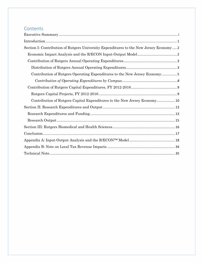
Contents Executive Summary .................................................................................................................................. i

Introduction ............................................................................................................................................... 1

Section I: Contribution of Rutgers University Expenditures to the New Jersey Economy ..... 2

Economic Impact Analysis and the R/ECON Input-Output Model ........................................... 2

Contribution of Rutgers Annual Operating Expenditures .......................................................... 3

Distribution of Rutgers Annual Operating Expenditures ....................................................... 3

Contribution of Rutgers Operating Expenditures to the New Jersey Economy ................. 5

Contribution of Operating Expenditures by Campus ............................................................ 8

Contribution of Rutgers Capital Expenditures, FY 2012-2016 .................................................. 9

Rutgers Capital Projects, FY 2012-2016 ..................................................................................... 9

Contribution of Rutgers Capital Expenditures to the New Jersey Economy .................... 10

Section II: Research Expenditures and Output ............................................................................... 13

Research Expenditures and Funding ............................................................................................. 13

Research Output ................................................................................................................................. 15

Section III: Rutgers Biomedical and Health Sciences .................................................................... 16

Conclusion ................................................................................................................................................ 17

Appendix A: Input-Output Analysis and the R/ECON™ Model .................................................. 18

Appendix B: Note on Local Tax Revenue Impacts .......................................................................... 34

Technical Note ......................................................................................................................................... 35

i

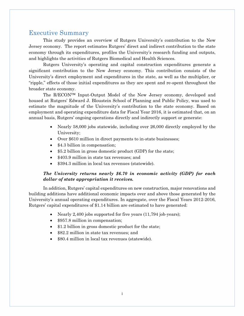
Executive Summary This study provides an overview of Rutgers University’s contribution to the New

Jersey economy. The report estimates Rutgers’ direct and indirect contribution to the state

economy through its expenditures, profiles the University’s research funding and outputs,

and highlights the activities of Rutgers Biomedical and Health Sciences.

Rutgers University’s operating and capital construction expenditures generate a

significant contribution to the New Jersey economy. This contribution consists of the

University’s direct employment and expenditures in the state, as well as the multiplier, or

“ripple,” effects of those initial expenditures as they are spent and re-spent throughout the

broader state economy.

The R/ECON™ Input-Output Model of the New Jersey economy, developed and

housed at Rutgers’ Edward J. Bloustein School of Planning and Public Policy, was used to

estimate the magnitude of the University’s contribution to the state economy. Based on

employment and operating expenditure data for Fiscal Year 2016, it is estimated that, on an

annual basis, Rutgers’ ongoing operations directly and indirectly support or generate:

Nearly 58,000 jobs statewide, including over 26,000 directly employed by the

University;

Over $610 million in direct payments to in-state businesses;

$4.3 billion in compensation;

$5.2 billion in gross domestic product (GDP) for the state;

$403.9 million in state tax revenues; and

$394.3 million in local tax revenues (statewide).

The University returns nearly $6.70 in economic activity (GDP) for each

dollar of state appropriation it receives.

In addition, Rutgers’ capital expenditures on new construction, major renovations and

building additions have additional economic impacts over and above those generated by the

University’s annual operating expenditures. In aggregate, over the Fiscal Years 2012-2016,

Rutgers’ capital expenditures of $1.14 billion are estimated to have generated:

Nearly 2,400 jobs supported for five years (11,794 job-years);

$957.8 million in compensation;

$1.2 billion in gross domestic product for the state;

$82.2 million in state tax revenues; and

$80.4 million in local tax revenues (statewide).

1

Introduction

This study, conducted on behalf of the Rutgers University President’s Office,

estimates the contribution of the University’s operating and capital expenditures to the New

Jersey economy. Rutgers’ ongoing operations and capital construction are carried out in

support of the three core elements of the University’s mission: education, research and

service. In fulfilling these core functions, each year Rutgers spends significant amounts on

its ongoing operations, including salaries for faculty and staff, purchases of material,

equipment and services, and investments in long-term capital assets such as academic

buildings and other facilities. In aggregate, these expenditures and their multiplier effects

comprise a significant contribution to the New Jersey economy. The main purpose of this

report is to estimate the size of this contribution.

In addition to the immediate and ongoing contribution of Rutgers to the New Jersey

economy via its operating and capital expenditures, the University generates significant

longer-term and broader economic impacts associated with its research output and

educational functions. For example, Rutgers’ research output includes numerous patents,

licensed technologies and other products that generate revenue for the University while

contributing to economic growth in a number of industries, and Rutgers Biomedical and

Health Sciences makes significant contributions to development and provision of medical

treatments through clinical trials, provision of care through free clinics and other activities.

This study is divided into three sections. Section I estimates the contribution of

Rutgers’ operating and capital expenditures to the New Jersey economy. The section includes

a breakdown of the University’s expenditures, a description of the methodology and economic

model used in the analysis, and estimates of the University’s contribution to the state

economy. Section II provides an overview of the University’s research funding sources and

outputs. Section III highlights the work of Rutgers Biomedical and Health Sciences.

2

Section I: Contribution of Rutgers University Expenditures to

the New Jersey Economy

Expenditures on operations and capital projects at all of Rutgers’ campuses and

facilities support further employment and business expenditures throughout the state

economy. Economic impact analysis provides a method to measure the size of this

contribution.

Economic Impact Analysis and the R/ECON Input-Output Model

The R/ECON™ Input-Output Model developed and maintained at Rutgers

University’s Edward J. Bloustein School of Planning and Public Policy is used to estimate

the economic impacts of various types of expenditures or investments, in terms of

employment, gross domestic product, compensation (i.e., income) and tax revenues.1 The

model consists of 383 individual sectors of the New Jersey economy and measures the effect

of changes in expenditures in one industry on economic activity in all other industries. Thus,

the expenditures made on labor, materials, equipment, third-party services and other inputs

for ongoing operations or one-time capital projects have both direct economic effects as

those expenditures become incomes and revenues for workers and businesses, and

subsequent indirect effects as those workers and businesses, in turn, spend those dollars

on other goods and services. 2 These expenditures on consumer goods, business investment

expenditures, and other items in turn become income for other workers and businesses. This

income gets further spent, and so on.

The R/ECON™ Input-Output model estimates both the direct economic effects of the

initial expenditures (in terms of jobs and income) and the indirect (also known as

multiplier or “ripple”) effects (in additional jobs and income) of the subsequent economic

activity that occurs following the initial expenditures. The model also estimates the gross

domestic product for New Jersey and the tax revenues generated by the combined direct and

indirect new economic activity caused by the initial business expenditures and the re-

spending of those dollars through the economy.

In addition, embodied in the model are estimates – known as regional purchase

coefficients, or RPCs – of the share of local (i.e., in-state) demand for labor and material that

can be met by in-state supply. That is, based on historical inter-industry relationships, the

1 A detailed description of input-output analysis and the R/ECON™ Input-Output Model is provided

in Appendix A. 2 Input-output models divide impacts into three categories – direct effects, indirect effects, and induced

effects. A direct effect is the change in purchases due to a change in economic activity. An indirect effect

is the change in the purchases of suppliers to those economic activities directly experiencing change.

An induced effect is the change in consumer spending that is generated by changes in labor income

within the region as a result of the direct and indirect effects of the economic activity. For ease of

presentation, this report includes both indirect and induced effects in the category of indirect effects.

3

model can estimate the portion of the project expenditures that are made on labor, material

and services produced in New Jersey. Similarly, these inter-industry relationships also

capture the portion of indirect expenditures (i.e., spending of the business revenues and

personal incomes initially generated by the project expenditures) that remain in the state.

Those initial expenditures and indirect impacts that spill out of the state are referred to as

economic “leakage.” Leakages include payments to social security, income taxes, personal

savings, and payments for goods and services sourced outside of New Jersey. Estimates of

“leakage” associated with project expenditures can be further refined based on specific project

information regarding the expected sourcing of labor, materials or other services.

Capital expenditures on construction and renovation are one-time outlays that

generate one-time economic impacts. That is, the economic multiplier that result from the

initial construction expenditures occur only once, as or shortly after the initial outlays are

made. These impacts, in terms of employment, income, output (GDP), and tax revenues, do

not continue once the capital construction project expenditures cease.

In contrast, the impacts of ongoing operational spending are assumed to be

recurring, as long as expenditure levels are maintained at the same or similar levels from

year to year.

Contribution of Rutgers Annual Operating Expenditures

Distribution of Rutgers Annual Operating Expenditures

Rutgers’ annual operating expenditures contribute both directly and indirectly to the

state economy. In Fiscal Year 2016, these expenditures totaled just over $3.5 billion.3 The

distribution of these direct expenditures drives the modeling of Rutgers’ contribution to the

state economy.

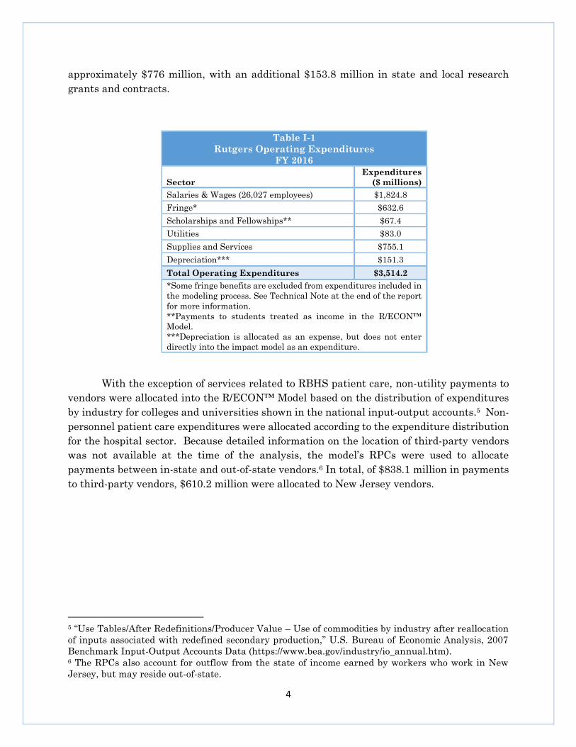
In FY 2016, Rutgers employed 26,027 total full- and part-time faculty and staff,

including teaching and graduate assistants, with a total of $1.8 billion in salaries and wages

(Table I-1).4 Expenditures also included payments of $838.1 million to outside vendors,

including $83 million in payments for utilities, and $67.4 million in scholarship and

fellowship payments. For comparison, Rutgers’ total state appropriation for FY 2016

(including operating budget funds and fringe benefits paid directly by the state) was

3 FY 2016 data on University payroll, payments for products and services from third-party vendors

and other expenditures were obtained from the Rutgers University Financial Statements. 4 Employment is as of November 1, 2015. Some forms of direct aid to student accounts (e.g., tuition

remission and housing costs) are treated as fringe benefits, and together with depreciation expense,

were excluded from the model analysis. Input-output analysis tracks the flow of dollars spent through

the economy, but does not capture the value of non-cash flows such as depreciation and direct aid to

student accounts for tuition, housing or other costs. See Technical Note at the end of this report for

additional information.

4

approximately $776 million, with an additional $153.8 million in state and local research

grants and contracts.

With the exception of services related to RBHS patient care, non-utility payments to

vendors were allocated into the R/ECON™ Model based on the distribution of expenditures

by industry for colleges and universities shown in the national input-output accounts.5 Non-

personnel patient care expenditures were allocated according to the expenditure distribution

for the hospital sector. Because detailed information on the location of third-party vendors

was not available at the time of the analysis, the model’s RPCs were used to allocate

payments between in-state and out-of-state vendors.6 In total, of $838.1 million in payments

to third-party vendors, $610.2 million were allocated to New Jersey vendors.

5 “Use Tables/After Redefinitions/Producer Value – Use of commodities by industry after reallocation

of inputs associated with redefined secondary production,” U.S. Bureau of Economic Analysis, 2007

Benchmark Input-Output Accounts Data (https://www.bea.gov/industry/io_annual.htm). 6 The RPCs also account for outflow from the state of income earned by workers who work in New

Jersey, but may reside out-of-state.

Table I-1

Rutgers Operating Expenditures

FY 2016

Sector

Expenditures

($ millions)

Salaries & Wages (26,027 employees) $1,824.8

Fringe* $632.6

Scholarships and Fellowships** $67.4

Utilities $83.0

Supplies and Services $755.1

Depreciation*** $151.3

Total Operating Expenditures $3,514.2

*Some fringe benefits are excluded from expenditures included in

the modeling process. See Technical Note at the end of the report

for more information.

**Payments to students treated as income in the R/ECON™

Model.

***Depreciation is allocated as an expense, but does not enter

directly into the impact model as an expenditure.

5

Contribution of Rutgers Operating Expenditures to the New Jersey Economy

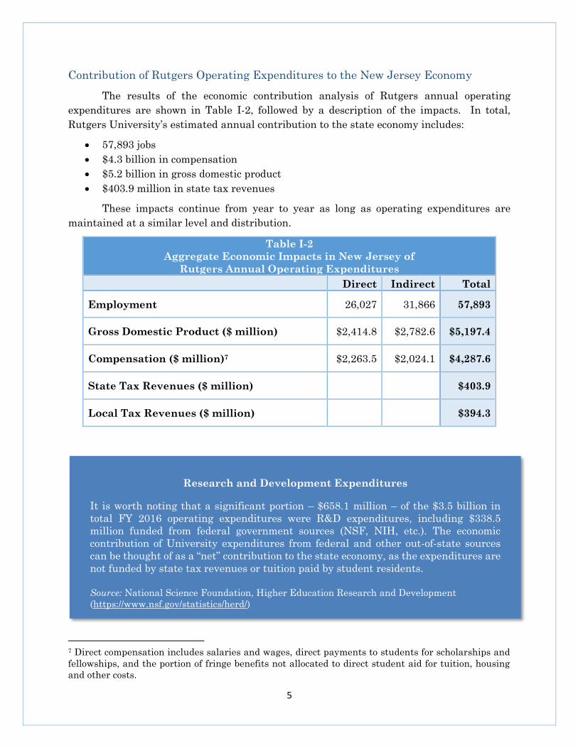
The results of the economic contribution analysis of Rutgers annual operating

expenditures are shown in Table I-2, followed by a description of the impacts. In total,

Rutgers University’s estimated annual contribution to the state economy includes:

57,893 jobs

$4.3 billion in compensation

$5.2 billion in gross domestic product

$403.9 million in state tax revenues

These impacts continue from year to year as long as operating expenditures are

maintained at a similar level and distribution.

Table I-2

Aggregate Economic Impacts in New Jersey of

Rutgers Annual Operating Expenditures

Direct Indirect Total

Employment 26,027 31,866 57,893

Gross Domestic Product ($ million) $2,414.8 $2,782.6 $5,197.4

Compensation ($ million)7 $2,263.5 $2,024.1 $4,287.6

State Tax Revenues ($ million) $403.9

Local Tax Revenues ($ million) $394.3

7 Direct compensation includes salaries and wages, direct payments to students for scholarships and

fellowships, and the portion of fringe benefits not allocated to direct student aid for tuition, housing

and other costs.

Research and Development Expenditures

It is worth noting that a significant portion – $658.1 million – of the $3.5 billion in

total FY 2016 operating expenditures were R&D expenditures, including $338.5

million funded from federal government sources (NSF, NIH, etc.). The economic

contribution of University expenditures from federal and other out-of-state sources

can be thought of as a “net” contribution to the state economy, as the expenditures are

not funded by state tax revenues or tuition paid by student residents.

Source: National Science Foundation, Higher Education Research and Development

(https://www.nsf.gov/statistics/herd/)

6

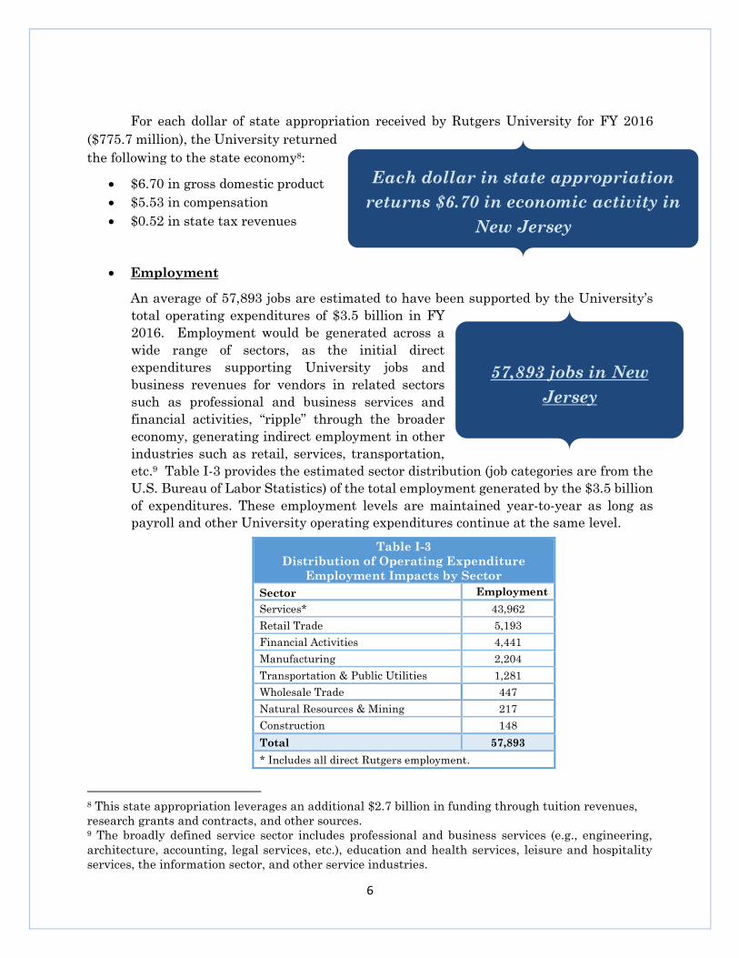
For each dollar of state appropriation received by Rutgers University for FY 2016

($775.7 million), the University returned

the following to the state economy8:

$6.70 in gross domestic product

$5.53 in compensation

$0.52 in state tax revenues

Employment

An average of 57,893 jobs are estimated to have been supported by the University’s

total operating expenditures of $3.5 billion in FY

2016. Employment would be generated across a

wide range of sectors, as the initial direct

expenditures supporting University jobs and

business revenues for vendors in related sectors

such as professional and business services and

financial activities, “ripple” through the broader

economy, generating indirect employment in other

industries such as retail, services, transportation,

etc.9 Table I-3 provides the estimated sector distribution (job categories are from the

U.S. Bureau of Labor Statistics) of the total employment generated by the $3.5 billion

of expenditures. These employment levels are maintained year-to-year as long as

payroll and other University operating expenditures continue at the same level.

8 This state appropriation leverages an additional $2.7 billion in funding through tuition revenues,

research grants and contracts, and other sources. 9 The broadly defined service sector includes professional and business services (e.g., engineering,

architecture, accounting, legal services, etc.), education and health services, leisure and hospitality

services, the information sector, and other service industries.

Table I-3

Distribution of Operating Expenditure

Employment Impacts by Sector

Sector Employment

Services* 43,962

Retail Trade 5,193

Financial Activities 4,441

Manufacturing 2,204

Transportation & Public Utilities 1,281

Wholesale Trade 447

Natural Resources & Mining 217

Construction 148

Total 57,893

* Includes all direct Rutgers employment.

57,893 jobs in New

Jersey

Each dollar in state appropriation

returns $6.70 in economic activity in

New Jersey

7

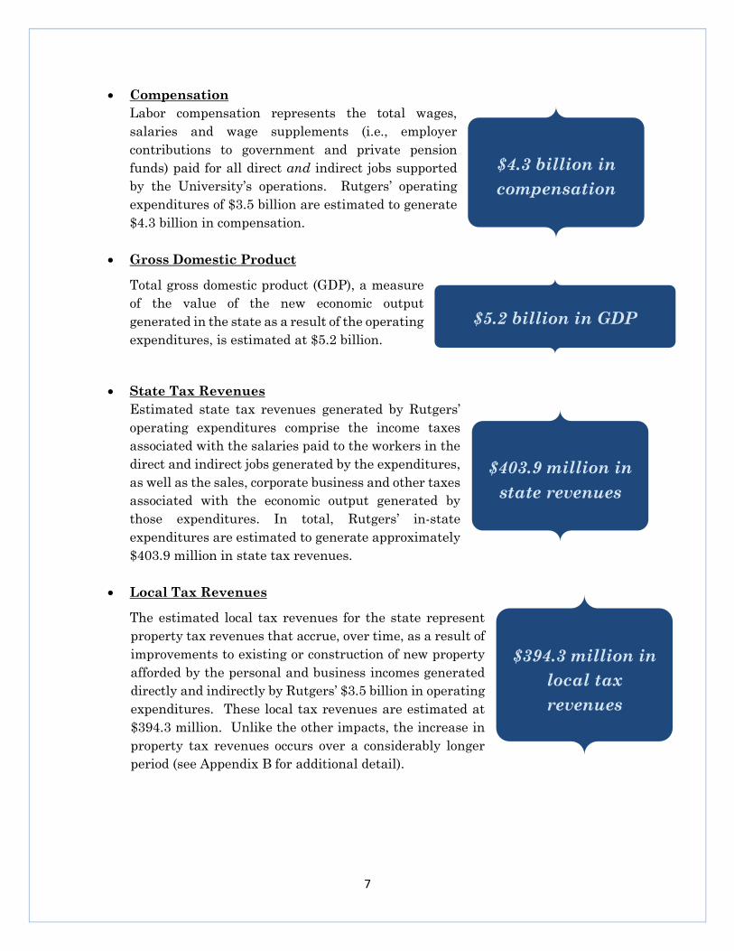
Compensation

Labor compensation represents the total wages,

salaries and wage supplements (i.e., employer

contributions to government and private pension

funds) paid for all direct and indirect jobs supported

by the University’s operations. Rutgers’ operating

expenditures of $3.5 billion are estimated to generate

$4.3 billion in compensation.

Gross Domestic Product

Total gross domestic product (GDP), a measure

of the value of the new economic output

generated in the state as a result of the operating

expenditures, is estimated at $5.2 billion.

State Tax Revenues

Estimated state tax revenues generated by Rutgers’

operating expenditures comprise the income taxes

associated with the salaries paid to the workers in the

direct and indirect jobs generated by the expenditures,

as well as the sales, corporate business and other taxes

associated with the economic output generated by

those expenditures. In total, Rutgers’ in-state

expenditures are estimated to generate approximately

$403.9 million in state tax revenues.

Local Tax Revenues

The estimated local tax revenues for the state represent

property tax revenues that accrue, over time, as a result of

improvements to existing or construction of new property

afforded by the personal and business incomes generated

directly and indirectly by Rutgers’ $3.5 billion in operating

expenditures. These local tax revenues are estimated at

$394.3 million. Unlike the other impacts, the increase in

property tax revenues occurs over a considerably longer

period (see Appendix B for additional detail).

$5.2 billion in GDP

$403.9 million in

state revenues

$394.3 million in

local tax

revenues

$4.3 billion in

compensation

8

Contribution of Operating Expenditures by Campus

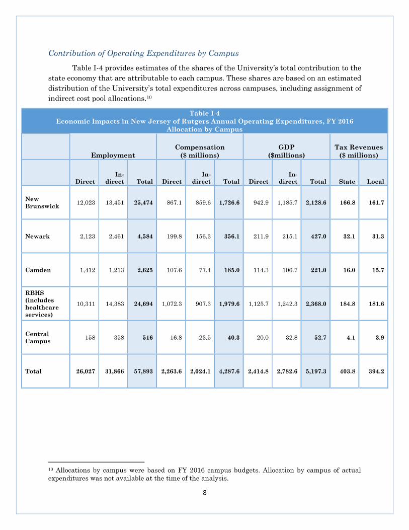
Table I-4 provides estimates of the shares of the University’s total contribution to the

state economy that are attributable to each campus. These shares are based on an estimated

distribution of the University’s total expenditures across campuses, including assignment of

indirect cost pool allocations.10

Table I-4

Economic Impacts in New Jersey of Rutgers Annual Operating Expenditures, FY 2016

Allocation by Campus

Employment

Compensation

($ millions)

GDP

($millions)

Tax Revenues

($ millions)

Direct

In-

direct Total Direct

In-

direct Total Direct

In-

direct Total State Local

New

Brunswick 12,023 13,451 25,474 867.1 859.6 1,726.6 942.9 1,185.7 2,128.6 166.8 161.7

Newark 2,123 2,461 4,584 199.8 156.3 356.1 211.9 215.1 427.0 32.1 31.3

Camden 1,412 1,213 2,625 107.6 77.4 185.0 114.3 106.7 221.0 16.0 15.7

RBHS

(includes

healthcare

services)

10,311 14,383 24,694 1,072.3 907.3 1,979.6 1,125.7 1,242.3 2,368.0 184.8 181.6

Central

Campus 158 358 516 16.8 23.5 40.3 20.0 32.8 52.7 4.1 3.9

Total 26,027 31,866 57,893 2,263.6 2,024.1 4,287.6 2,414.8 2,782.6 5,197.3 403.8 394.2

10 Allocations by campus were based on FY 2016 campus budgets. Allocation by campus of actual

expenditures was not available at the time of the analysis.

9

Contribution of Rutgers Capital Expenditures, FY 2012-2016

Rutgers Capital Projects, FY 2012-2016

The capital expenditures included in this analysis comprise a wide range of

construction and renovation activities at all the University campuses over the last five fiscal

years. These include significant new structures and improvements to student housing,

classroom and laboratory facilities, administrative buildings, recreational and athletic

facilities and other campus buildings and infrastructure, as well as smaller renovations such

as roof and elevator replacements. The period analyzed includes all or part of the construction

activity for major projects including the Chemistry and Chemical Biology Building on Busch

Campus, the Residential Honors College, academic building and Lot 8 Housing facility on

College Avenue, the Business School facility on Livingston Campus, the Life Sciences

Building in Newark and the Nursing and Science Building in Camden. In all, capital

spending over the five-year period totaled nearly $1.14 billion.

Capital expenditures on construction and renovation are distributed across expense

categories such as labor, equipment, material such as girders, cement and masonry, design

and engineering services and other cost items. The distribution of these project expenditures

differs across project types (e.g., new construction versus renovation, housing versus

classrooms, infrastructure projects, etc.). Projects were classified into a range of types,

including multifamily residential structures (i.e., dormitories), educational and vocational

structures, and nonresidential maintenance and repair.

10

Contribution of Rutgers Capital Expenditures to the New Jersey Economy

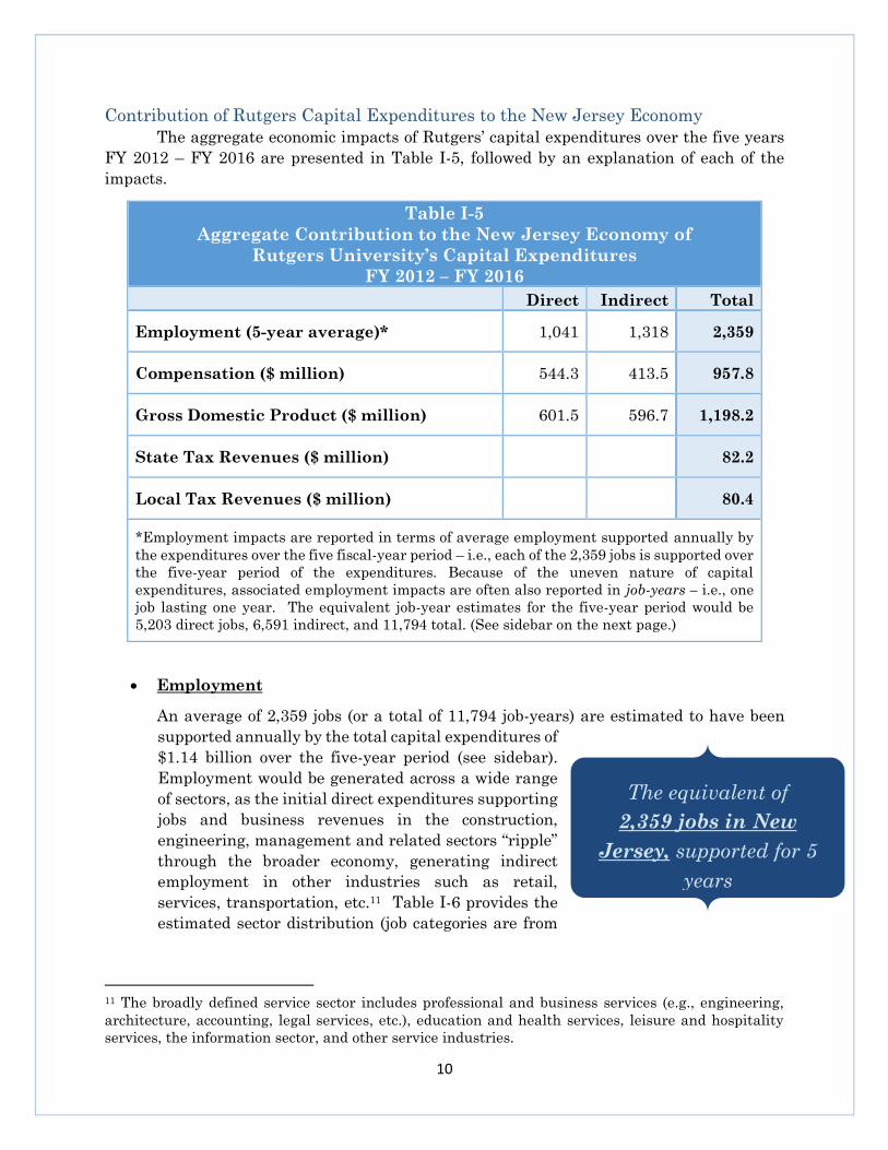
The aggregate economic impacts of Rutgers’ capital expenditures over the five years

FY 2012 – FY 2016 are presented in Table I-5, followed by an explanation of each of the

impacts.

Table I-5

Aggregate Contribution to the New Jersey Economy of

Rutgers University’s Capital Expenditures

FY 2012 – FY 2016

Direct Indirect Total

Employment (5-year average)* 1,041 1,318 2,359

Compensation ($ million) 544.3 413.5 957.8

Gross Domestic Product ($ million) 601.5 596.7 1,198.2

State Tax Revenues ($ million) 82.2

Local Tax Revenues ($ million) 80.4

*Employment impacts are reported in terms of average employment supported annually by

the expenditures over the five fiscal-year period – i.e., each of the 2,359 jobs is supported over

the five-year period of the expenditures. Because of the uneven nature of capital

expenditures, associated employment impacts are often also reported in job-years – i.e., one

job lasting one year. The equivalent job-year estimates for the five-year period would be

5,203 direct jobs, 6,591 indirect, and 11,794 total. (See sidebar on the next page.)

Employment

An average of 2,359 jobs (or a total of 11,794 job-years) are estimated to have been

supported annually by the total capital expenditures of

$1.14 billion over the five-year period (see sidebar).

Employment would be generated across a wide range

of sectors, as the initial direct expenditures supporting

jobs and business revenues in the construction,

engineering, management and related sectors “ripple”

through the broader economy, generating indirect

employment in other industries such as retail,

services, transportation, etc.11 Table I-6 provides the

estimated sector distribution (job categories are from

11 The broadly defined service sector includes professional and business services (e.g., engineering,

architecture, accounting, legal services, etc.), education and health services, leisure and hospitality

services, the information sector, and other service industries.

The equivalent of

2,359 jobs in New

Jersey, supported for 5

years

11

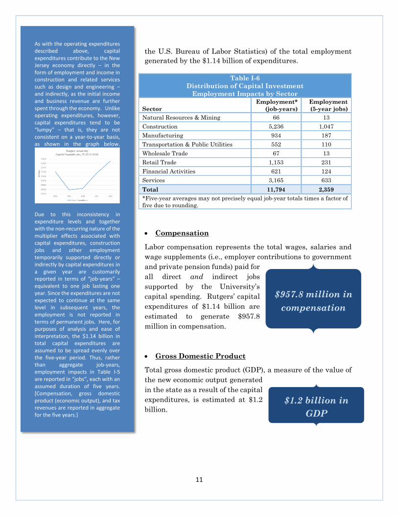
the U.S. Bureau of Labor Statistics) of the total employment

generated by the $1.14 billion of expenditures.

Compensation

Labor compensation represents the total wages, salaries and

wage supplements (i.e., employer contributions to government

and private pension funds) paid for

all direct and indirect jobs

supported by the University’s

capital spending. Rutgers’ capital

expenditures of $1.14 billion are

estimated to generate $957.8

million in compensation.

Gross Domestic Product

Total gross domestic product (GDP), a measure of the value of

the new economic output generated

in the state as a result of the capital

expenditures, is estimated at $1.2

billion.

Table I-6

Distribution of Capital Investment

Employment Impacts by Sector

Sector

Employment*

(job-years)

Employment

(5-year jobs)

Natural Resources & Mining 66 13

Construction 5,236 1,047

Manufacturing 934 187

Transportation & Public Utilities 552 110

Wholesale Trade 67 13

Retail Trade 1,153 231

Financial Activities 621 124

Services 3,165 633

Total 11,794 2,359

*Five-year averages may not precisely equal job-year totals times a factor of

five due to rounding.

$957.8 million in

compensation

$1.2 billion in

GDP

As with the operating expenditures described above, capital expenditures contribute to the New Jersey economy directly – in the form of employment and income in construction and related services such as design and engineering – and indirectly, as the initial income and business revenue are further spent through the economy. Unlike operating expenditures, however, capital expenditures tend to be “lumpy” – that is, they are not consistent on a year-to-year basis, as shown in the graph below.

Due to this inconsistency in expenditure levels and together with the non-recurring nature of the multiplier effects associated with capital expenditures, construction jobs and other employment temporarily supported directly or indirectly by capital expenditures in a given year are customarily reported in terms of “job-years” – equivalent to one job lasting one year. Since the expenditures are not expected to continue at the same level in subsequent years, the employment is not reported in terms of permanent jobs. Here, for purposes of analysis and ease of interpretation, the $1.14 billion in total capital expenditures are assumed to be spread evenly over the five-year period. Thus, rather than aggregate job-years, employment impacts in Table I-5 are reported in “jobs”, each with an assumed duration of five years. [Compensation, gross domestic product (economic output), and tax revenues are reported in aggregate for the five years.]

12

State Tax Revenues

Estimated state tax revenues generated by Rutgers’ capital

expenditures comprise the income taxes associated with the

salaries paid to the workers in the direct and indirect jobs

generated by the construction activity, as well as the sales,

corporate business and other state taxes associated with the

economic output generated by those expenditures. In total,

the capital expenditures are estimated to generate

approximately $82.2 million in state tax revenues.

Local Tax Revenues

The estimated local tax revenues for the state represent property tax revenues that

accrue, over time, as a result of improvements to existing

or construction of new property afforded by the personal

and business incomes generated directly and indirectly by

the construction expenditures. These local tax revenues

are estimated at $80.4 million. Unlike the other impacts,

the increase in property tax revenues occurs over a

considerably longer period (see Appendix B for additional

detail).

$82.2 million in

state tax

revenues

$80.4 million in

local tax

revenues

13

Section II: Research Expenditures and Output

Research Expenditures and Funding

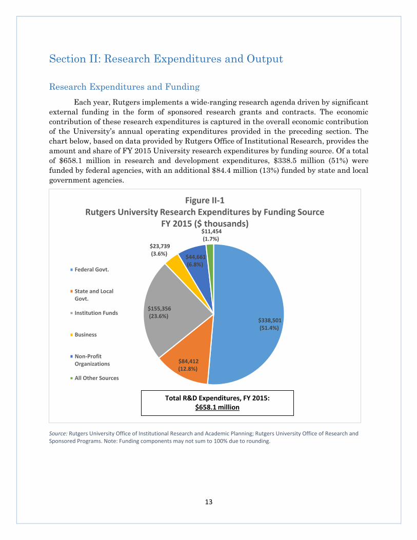
Each year, Rutgers implements a wide-ranging research agenda driven by significant

external funding in the form of sponsored research grants and contracts. The economic

contribution of these research expenditures is captured in the overall economic contribution

of the University’s annual operating expenditures provided in the preceding section. The

chart below, based on data provided by Rutgers Office of Institutional Research, provides the

amount and share of FY 2015 University research expenditures by funding source. Of a total

of $658.1 million in research and development expenditures, $338.5 million (51%) were

funded by federal agencies, with an additional $84.4 million (13%) funded by state and local

government agencies.

Source: Rutgers University Office of Institutional Research and Academic Planning; Rutgers University Office of Research and Sponsored Programs. Note: Funding components may not sum to 100% due to rounding.

$338,501 (51.4%)

$84,412 (12.8%)

$155,356 (23.6%)

$23,739 (3.6%)

$44,661 (6.8%)

$11,454 (1.7%)

Figure II-1Rutgers University Research Expenditures by Funding Source

FY 2015 ($ thousands)

Federal Govt.

State and LocalGovt.

Institution Funds

Business

Non-ProfitOrganizations

All Other Sources

Total R&D Expenditures, FY 2015:$658.1 million

14

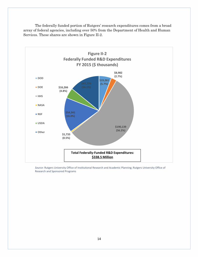
The federally funded portion of Rutgers’ research expenditures comes from a broad

array of federal agencies, including over 50% from the Department of Health and Human

Services. These shares are shown in Figure II-2.

Source: Rutgers University Office of Institutional Research and Academic Planning; Rutgers University Office of Research and Sponsored Programs

$19,261(5.7%)

$8,982(2.7%)

$190,139(56.2%)

$1,733(0.5%)

$54,341(16.0%)

$16,266(4.8%)

$47,779(14.1%)

Figure II-2Federally Funded R&D Expenditures

FY 2015 ($ thousands)

DOD

DOE

HHS

NASA

NSF

USDA

Other

Total Federally-Funded R&D Expenditures: $338.5 Million

15

Research Output

Each year, Rutgers research activity generates important outputs that benefit the

University and the state economy through commercialization and licensing of new

technologies and the creation of spinoff companies that create further jobs and economic

activity in the state. Indicators of this activity include:

Patents, Disclosures and License Agreements

In FY 2015 and FY 2016, Rutgers researchers disclosed 352 inventions, the University

entered into 182 license agreements, and Rutgers was granted 309 total patents for

technologies developed at the University. :

82 U.S. patents in FY 2015

94 U.S. patents in FY 2016

65 foreign patents in FY 2015

68 foreign patents in FY 2016

184 disclosures in FY 2015

168 disclosures in FY 2016

25 exclusive license agreements in FY 2015

35 exclusive license agreements in FY 2016

50 non-exclusive license agreements in FY 2015

72 non-exclusive license agreements in FY 2016

License Revenue

Rutgers patents and licensing agreements generated a total of $31.5 million in royalty

income for the University in FY 2015 and FY 2016 combined.

Spinoff Companies

Rutgers technologies have resulted in the creation of 119 startups to date, including

39 currently active companies in New Jersey. Thirteen startups have been created since FY

2015, with new technologies generating new opportunities for economic activity and growth

in the state:

Maverick Vascular Technologies,

Inc. - 2015

Visikol, Inc. (restart of Phytosis,

LLC) - 2016

Elucid Bioimaging , Inc. - 2015 Z53 Therapeutics, LLC - 2016

Polymer Therapeutics, LLC -2015 SubUAS, LLC - 2017

PolyCore Therapeutics, LLC. - 2016 OptoVibronex, LLC - 2017

XPEED Turbine Technology, LLC. -

2016 Aerial Technologies, Inc. - 2017

Virbio, Inc. - 2016 CeraMaxx, LLC - 2017

NewCo (Mega Hill option) - 2017

16

Section III: Rutgers Biomedical and Health Sciences

Rutgers Biomedical and Health Sciences brings together eight schools and five

research and treatment centers and institutes, as well as affiliations with clinical partners

throughout New Jersey. This broad instructional, research and clinical capacity presents

significant opportunity for clinical trials, patient care, and other activities that generate

economic and other benefits for the University and the state. In FY 2016, RBHS:

Conducted 350 clinical trials

Provided $12.6 million in low-cost and no-cost services to low-income patients through

its clinics

Employed more than 1,300 healthcare professionals

Spent over $684 million in patient care-related expenditures

17

Conclusion

In implementing its core missions of education, research and service, Rutgers

University also makes a significant contribution to the state economy through its operations

and capital investments. The University’s expenditures on the personnel, goods and services

necessary to fulfill its core missions ripple through the state economy, generating additional

economic activity in the form of employment, income, gross domestic product and tax

revenues for state and local governments. This report has estimated the size of that

contribution, including the effects of Rutgers’ operating expenditures, which are estimated

to support, on an ongoing annual basis:

Nearly 58,000 jobs statewide, including over 26,000 directly employed by the

University;

Over $610 million in direct payments to in-state businesses;

$4.3 billion in compensation;

$5.2 billion in gross domestic product for the state;

$403.9 million in state tax revenues; and

$394.3 million in local tax revenues (statewide).

The report also estimated the contribution of Rutgers’ capital expenditures for FY 2012 – FY

2016, which include:

Nearly 2,400 jobs supported for five years (11,794 job-years);

$957.8 million in compensation;

$1.2 billion in gross domestic product for the state;

$82.2 million in state tax revenues; and

$80.4 million in local tax revenues (statewide).

A significant portion of Rutgers’ operating expenditures are externally funded by

sponsored research grants and contracts. Over half of the University’s $638 million in

externally sponsored research funding in FY 2016 was federally financed. This funding drives

significant research output in the form of patents, invention disclosures, and licensed

technologies that generate royalty income and lead to start-up companies which bring further

economic activity to the state.

Rutgers Biomedical and Health Sciences brings important research and clinical

capacity to the University. With its eight schools and multiple centers and institutes, RBHS

educates future healthcare professionals, pursues innovative medical research that brings

significant federal research funding to the state, conducts hundreds of clinical trials and

provides clinical care to the community through its clinics and affiliated practices.

18

Appendix A: Input-Output Analysis and the R/ECON™ Model

This appendix discusses the history and application of input-output analysis and

details the input-output model, called the R/ECON™ I-O model, developed by Rutgers

University. This model offers significant advantages in detailing the total economic effects of

an activity (such as historic rehabilitation and heritage tourism), including multiplier effects.

Estimating Multipliers

The fundamental issue determining the size of the multiplier effect is the “openness”

of regional economies. Regions that are more “open” are those that import their required

inputs from other regions. Imports can be thought of as substitutes for local production. Thus,

the more a region depends on imported goods and services instead of its own production, the

more economic activity leaks away from the local economy. Businessmen noted this

phenomenon and formed local chambers of commerce with the explicit goal of stopping such

leakage by instituting a “buy local” policy among their membership. In addition, during the

1970s, as an import invasion was under way, businessmen and union leaders announced a

“buy American” policy in the hope of regaining ground lost to international economic

competition. Therefore, one of the main goals of regional economic multiplier research has

been to discover better ways to estimate the leakage of purchases out of a region or, relatedly,

to determine the region’s level of self-sufficiency.

The earliest attempts to systematize the procedure for estimating multiplier effects

used the economic base model, still in use in many econometric models today. This approach

assumes that all economic activities in a region can be divided into two categories: “basic”

activities that produce exclusively for export, and region-serving or “local” activities that

produce strictly for internal regional consumption. Since this approach is simpler but similar

to the approach used by regional input-output analysis, let us explain briefly how multiplier

effects are estimated using the economic base approach.

If we let x be export employment, l be local employment, and t be total employment, then

t = x + l

For simplification, we create the ratio a as

a = l/t

so that l = at

then substituting into the first equation, we obtain

t = x + at

By bringing all of the terms with t to one side of the equation, we get

t - at = x or t (1-a) = x

Solving for t, we get t = x/(1-a)

19

Thus, if we know the amount of export-oriented employment, x, and the ratio of local

to total employment, a, we can readily calculate total employment by applying the economic

base multiplier, 1/(1-a), which is embedded in the above formula. Thus, if 40 percent of all

regional employment is used to produce exports, the regional multiplier would be 2.5. The

assumption behind this multiplier is that all remaining regional employment is required to

support the export employment. Thus, the 2.5 can be decomposed into two parts the direct

effect of the exports, which is always 1.0, and the indirect and induced effects, which is the

remainder—in this case 1.5. Hence, the multiplier can be read as telling us that for each

export-oriented job another 1.5 jobs are needed to support it.

This notion of the multiplier has been extended so that x is understood to represent

an economic change demanded by an organization or institution outside of an economy—so-

called final demand. Such changes can be those effected by government, households, or even

by an outside firm. Changes in the economy can therefore be calculated by a minor alteration

in the multiplier formula:

t = x/(1-a)

The high level of industry aggregation and the rigidity of the economic assumptions

that permit the application of the economic base multiplier have caused this approach to be

subject to extensive criticism. Most of the discussion has focused on the estimation of the

parameter a. Estimating this parameter requires that one be able to distinguish those parts

of the economy that produce for local consumption from those that do not. Indeed, virtually

all industries, even services, sell to customers both inside and outside the region. As a result,

regional economists devised an approach by which to measure the degree to which each

industry is involved in the nonbase activities of the region, better known as the industry’s

regional purchase coefficient (r). Thus, they expanded the above formulations by calculating

for each i industry

li = r idi

and xi = ti - r idi

given that di is the total regional demand for industry i’s product. Given the above formulae

and data on regional demands by industry, one can calculate an accurate traditional

aggregate economic base parameter by the following:

a = l/t = li/ti

Although accurate, this approach only facilitates the calculation of an aggregate

multiplier for the entire region. That is, we cannot determine from this approach what the

effects are on the various sectors of an economy. This is despite the fact that one must

painstakingly calculate the regional demand as well as the degree to which each industry is

involved in nonbase activity in the region.

20

As a result, a different approach to multiplier estimation that takes advantage of

detailed demand and trade data was developed. This approach is called input-output

analysis.

Regional Input-Output Analysis: A Brief History

The basic framework for input-output analysis originated nearly 250 years ago when

François Quesenay published Tableau Economique in 1758. Quesenay’s “tableau” graphically

and numerically portrayed the relationships between sales and purchases of the various

industries of an economy. More than a century later, his description was adapted by Leon

Walras, who advanced input-output modeling by providing a concise theoretical formulation

of an economic system (including consumer purchases and the economic representation of

“technology”).

It was not until the twentieth century, however, that economists advanced and tested

Walras’s work. Wassily Leontief greatly simplified Walras’s theoretical formulation by

applying the Nobel prize–winning assumptions that both technology and trading patterns

were fixed over time. These two assumptions meant that the pattern of flows among

industries in an area could be considered stable. These assumptions permitted Walras’s

formulation to use data from a single time period, which generated a great reduction in data

requirements.

Although Leontief won the Nobel Prize in 1973, he first used his approach in 1936

when he developed a model of the 1919 and 1929 U.S. economies to estimate the effects of

the end of World War I on national employment. Recognition of his work in terms of its wider

acceptance and use meant development of a standardized procedure for compiling the

requisite data (today’s national economic census of industries) and enhanced capability for

calculations (i.e., the computer).

The federal government immediately recognized the importance of Leontief’s

development and has been publishing input-output tables of the U.S. economy since 1939.

The most recently published tables are those for 2007. Other nations followed suit. Indeed,

the United Nations maintains a bank of tables from most member nations with a uniform

accounting scheme.

21

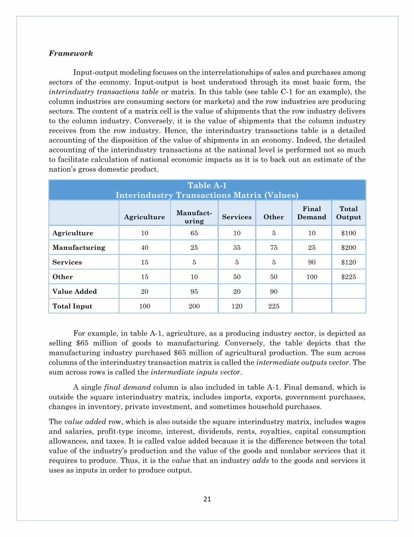
Framework

Input-output modeling focuses on the interrelationships of sales and purchases among

sectors of the economy. Input-output is best understood through its most basic form, the

interindustry transactions table or matrix. In this table (see table C-1 for an example), the

column industries are consuming sectors (or markets) and the row industries are producing

sectors. The content of a matrix cell is the value of shipments that the row industry delivers

to the column industry. Conversely, it is the value of shipments that the column industry

receives from the row industry. Hence, the interindustry transactions table is a detailed

accounting of the disposition of the value of shipments in an economy. Indeed, the detailed

accounting of the interindustry transactions at the national level is performed not so much

to facilitate calculation of national economic impacts as it is to back out an estimate of the

nation’s gross domestic product.

Table A-1

Interindustry Transactions Matrix (Values)

Agriculture

Manufact-

uring

Services

Other

Final

Demand

Total

Output

Agriculture 10 65 10 5 10 $100

Manufacturing 40 25 35 75 25 $200

Services 15 5 5 5 90 $120

Other 15 10 50 50 100 $225

Value Added 20 95 20 90

Total Input 100 200 120 225

For example, in table A-1, agriculture, as a producing industry sector, is depicted as

selling $65 million of goods to manufacturing. Conversely, the table depicts that the

manufacturing industry purchased $65 million of agricultural production. The sum across

columns of the interindustry transaction matrix is called the intermediate outputs vector. The

sum across rows is called the intermediate inputs vector.

A single final demand column is also included in table A-1. Final demand, which is

outside the square interindustry matrix, includes imports, exports, government purchases,

changes in inventory, private investment, and sometimes household purchases.

The value added row, which is also outside the square interindustry matrix, includes wages

and salaries, profit-type income, interest, dividends, rents, royalties, capital consumption

allowances, and taxes. It is called value added because it is the difference between the total

value of the industry’s production and the value of the goods and nonlabor services that it

requires to produce. Thus, it is the value that an industry adds to the goods and services it

uses as inputs in order to produce output.

22

The value added row measures each industry’s contribution to wealth accumulation.

In a national model, therefore, its sum is better known as the gross domestic product (GDP).

At the state level, this is known as the gross state product—a series produced by the U.S.

Bureau of Economic Analysis and published in the Regional Economic Information System.

Below the state level, it is known simply as the regional equivalent of the GDP—the gross

regional product.

Input-output economic impact modelers now tend to include the household industry

within the square interindustry matrix. In this case, the “consuming industry” is the

household itself. Its spending is extracted from the final demand column and is appended as

a separate column in the interindustry matrix. To maintain a balance, the income of

households must be appended as a row. The main income of households is labor income,

which is extracted from the value-added row. Modelers tend not to include other sources of

household income in the household industry’s row. This is not because such income is not

attributed to households but rather because much of this other income derives from sources

outside of the economy that is being modeled.

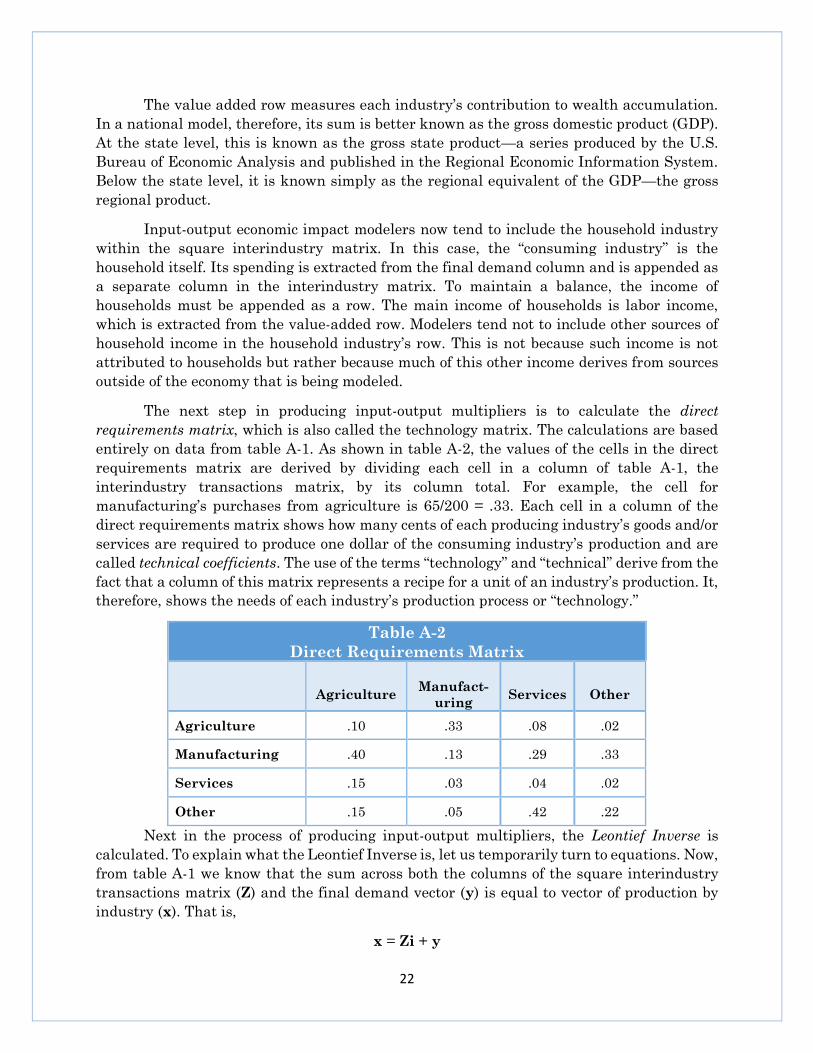
The next step in producing input-output multipliers is to calculate the direct

requirements matrix, which is also called the technology matrix. The calculations are based

entirely on data from table A-1. As shown in table A-2, the values of the cells in the direct

requirements matrix are derived by dividing each cell in a column of table A-1, the

interindustry transactions matrix, by its column total. For example, the cell for

manufacturing’s purchases from agriculture is 65/200 = .33. Each cell in a column of the

direct requirements matrix shows how many cents of each producing industry’s goods and/or

services are required to produce one dollar of the consuming industry’s production and are

called technical coefficients. The use of the terms “technology” and “technical” derive from the

fact that a column of this matrix represents a recipe for a unit of an industry’s production. It,

therefore, shows the needs of each industry’s production process or “technology.”

Table A-2

Direct Requirements Matrix

Agriculture

Manufact-

uring

Services

Other

Agriculture .10 .33 .08 .02

Manufacturing .40 .13 .29 .33

Services .15 .03 .04 .02

Other .15 .05 .42 .22

Next in the process of producing input-output multipliers, the Leontief Inverse is

calculated. To explain what the Leontief Inverse is, let us temporarily turn to equations. Now,

from table A-1 we know that the sum across both the columns of the square interindustry

transactions matrix (Z) and the final demand vector (y) is equal to vector of production by

industry (x). That is,

x = Zi + y

23

where i is a summation vector of ones. Now, we calculate the direct requirements matrix (A)

by dividing the interindustry transactions matrix by the production vector or

A = ZX-1

where X-1 is a square matrix with inverse of each element in the vector x on the diagonal

and the rest of the elements equal to zero. Rearranging the above equation yields

Z = AX

where X is a square matrix with the elements of the vector x on the diagonal and zeros

elsewhere. Thus,

x = (AX)i + y

or, alternatively,

x = Ax + y

solving this equation for x yields

x = (I-A)-1 y

Total = Total * Final

Output Requirements Demand

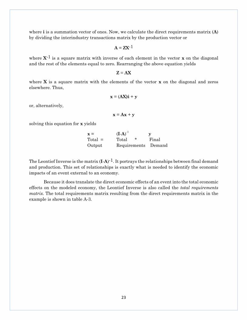
The Leontief Inverse is the matrix (I-A)-1. It portrays the relationships between final demand

and production. This set of relationships is exactly what is needed to identify the economic

impacts of an event external to an economy.

Because it does translate the direct economic effects of an event into the total economic

effects on the modeled economy, the Leontief Inverse is also called the total requirements

matrix. The total requirements matrix resulting from the direct requirements matrix in the

example is shown in table A-3.

24

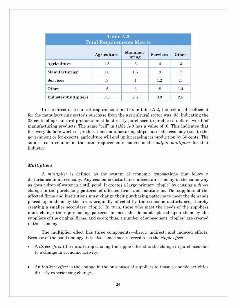
Table A-3

Total Requirements Matrix

Agriculture

Manufact-

uring

Services

Other

Agriculture 1.5 .6 .4 .3

Manufacturing 1.0 1.6 .9 .7

Services .3 .1 1.2 .1

Other .5 .3 .8 1.4

Industry Multipliers .33 2.6 3.3 2.5

In the direct or technical requirements matrix in table A-2, the technical coefficient

for the manufacturing sector’s purchase from the agricultural sector was .33, indicating the

33 cents of agricultural products must be directly purchased to produce a dollar’s worth of

manufacturing products. The same “cell” in table A-3 has a value of .6. This indicates that

for every dollar’s worth of product that manufacturing ships out of the economy (i.e., to the

government or for export), agriculture will end up increasing its production by 60 cents. The

sum of each column in the total requirements matrix is the output multiplier for that

industry.

Multipliers

A multiplier is defined as the system of economic transactions that follow a

disturbance in an economy. Any economic disturbance affects an economy in the same way

as does a drop of water in a still pond. It creates a large primary “ripple” by causing a direct

change in the purchasing patterns of affected firms and institutions. The suppliers of the

affected firms and institutions must change their purchasing patterns to meet the demands

placed upon them by the firms originally affected by the economic disturbance, thereby

creating a smaller secondary “ripple.” In turn, those who meet the needs of the suppliers

must change their purchasing patterns to meet the demands placed upon them by the

suppliers of the original firms, and so on; thus, a number of subsequent “ripples” are created

in the economy.

The multiplier effect has three components—direct, indirect, and induced effects.

Because of the pond analogy, it is also sometimes referred to as the ripple effect.

A direct effect (the initial drop causing the ripple effects) is the change in purchases due

to a change in economic activity.

An indirect effect is the change in the purchases of suppliers to those economic activities

directly experiencing change.

25

An induced effect is the change in consumer spending that is generated by changes in

labor income within the region as a result of the direct and indirect effects of the economic

activity. Including households as a column and row in the interindustry matrix allows

this effect to be captured.

Extending the Leontief Inverse to pertain not only to relationships between total

production and final demand of the economy but also to changes in each permits its

multipliers to be applied to many types of economic impacts. Indeed, in impact analysis the

Leontief Inverse lends itself to the drop-in-a-pond analogy discussed earlier. This is because

the Leontief Inverse multiplied by a change in final demand can be estimated by a power

series. That is,

(I-A)-1 y = y + A y + A(A y) + A(A(A y)) + A(A(A(A y))) + ...

Assuming that y—the change in final demand—is the “drop in the pond,” then

succeeding terms are the ripples. Each “ripple” term is calculated as the previous “pond

disturbance” multiplied by the direct requirements matrix. Thus, since each element in the

direct requirements matrix is less than one, each ripple term is smaller than its predecessor.

Indeed, it has been shown that after calculating about seven of these ripple terms that the

power series approximation of impacts very closely estimates those produced by the Leontief

Inverse directly.

In impacts analysis practice, y is a single column of expenditures with the same

number of elements as there are rows or columns in the direct or technical requirements

matrix. This set of elements is called an impact vector. This term is used because it is the

vector of numbers that is used to estimate the economic impacts of the investment.

There are two types of changes in investments, and consequently economic impacts,

generally associated with projects—one-time impacts and recurring impacts. One-time

impacts are impacts that are attributable to an expenditure that occurs once over a limited

period of time. For example, the impacts resulting from the construction of a project are one-

time impacts. Recurring impacts are impacts that continue permanently as a result of new

or expanded ongoing expenditures. The ongoing operation of a new train station, for example,

generates recurring impacts to the economy. Examples of changes in economic activity are

investments in the preservation of old homes, tourist expenditures, or the expenditures

required to run a historical site. Such activities are considered changes in final demand and

can be either positive or negative. When the activity is not made in an industry, it is generally

not well represented by the input-output model. Nonetheless, the activity can be represented

by a special set of elements that are similar to a column of the transactions matrix. This set

of elements is called an economic disturbance or impact vector. The latter term is used

because it is the vector of numbers that is used to estimate the impacts. In this study, the

impact vector is estimated by multiplying one or more economic translators by a dollar figure

that represents an investment in one or more projects. The term translator is derived from

26

the fact that such a vector translates a dollar amount of an activity into its constituent

purchases by industry.

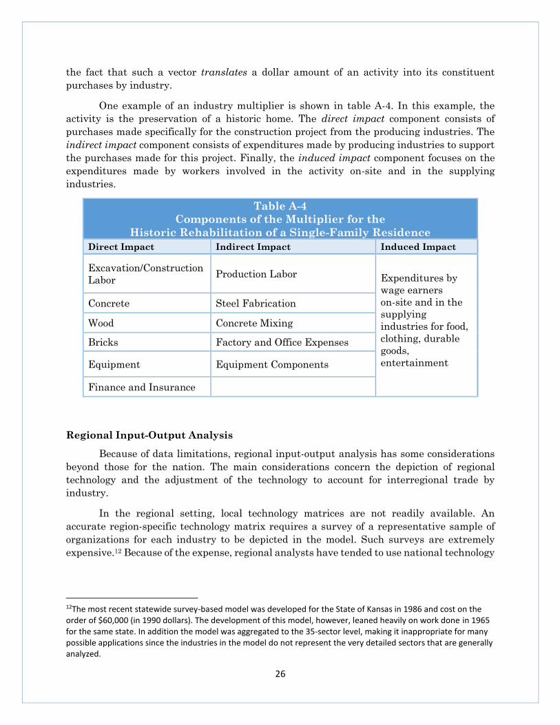
One example of an industry multiplier is shown in table A-4. In this example, the

activity is the preservation of a historic home. The direct impact component consists of

purchases made specifically for the construction project from the producing industries. The

indirect impact component consists of expenditures made by producing industries to support

the purchases made for this project. Finally, the induced impact component focuses on the

expenditures made by workers involved in the activity on-site and in the supplying

industries.

Table A-4

Components of the Multiplier for the

Historic Rehabilitation of a Single-Family Residence

Direct Impact Indirect Impact Induced Impact

Excavation/Construction

Labor Production Labor Expenditures by

wage earners

on-site and in the

supplying

industries for food,

clothing, durable

goods,

entertainment

Concrete Steel Fabrication

Wood Concrete Mixing

Bricks Factory and Office Expenses

Equipment Equipment Components

Finance and Insurance

Regional Input-Output Analysis

Because of data limitations, regional input-output analysis has some considerations

beyond those for the nation. The main considerations concern the depiction of regional

technology and the adjustment of the technology to account for interregional trade by

industry.

In the regional setting, local technology matrices are not readily available. An

accurate region-specific technology matrix requires a survey of a representative sample of

organizations for each industry to be depicted in the model. Such surveys are extremely

expensive.12 Because of the expense, regional analysts have tended to use national technology

12The most recent statewide survey-based model was developed for the State of Kansas in 1986 and cost on the order of $60,000 (in 1990 dollars). The development of this model, however, leaned heavily on work done in 1965 for the same state. In addition the model was aggregated to the 35-sector level, making it inappropriate for many possible applications since the industries in the model do not represent the very detailed sectors that are generally analyzed.

27

as a surrogate for regional technology. This substitution does not affect the accuracy of the

model as long as local industry technology does not vary widely from the nation’s average.13

Even when local technology varies widely from the nation’s average for one or more

industries, model accuracy may not be affected much. This is because interregional trade may

mitigate the error that would be induced by the technology. That is, in estimating economic

impacts via a regional input-output model, national technology must be regionalized by a

vector of regional purchase coefficients,14 r, in the following manner:

(I-rA)-1 ry

or

ry + rA (ry) + rA(rA (ry)) + rA(rA(rA (ry))) + ...

where the vector-matrix product rA is an estimate of the region’s direct requirements matrix.

Thus, if national technology coefficients—which vary widely from their local equivalents—

are multiplied by small RPCs, the error transferred to the direct requirements matrices will

be relatively small. Indeed, since most manufacturing industries have small RPCs and since

technology differences tend to arise due to substitution in the use of manufactured goods,

technology differences have generally been found to be minor source error in economic impact

measurement. Instead, RPCs and their measurement error due to industry aggregation have

been the focus of research on regional input-output model accuracy.

13Only recently have researchers studied the validity of this assumption. They have found that large urban areas may have technology in some manufacturing industries that differs in a statistically significant way from the national average. As will be discussed in a subsequent paragraph, such differences may be unimportant after accounting for trade patterns. 14A regional purchase coefficient (RPC) for an industry is the proportion of the region’s demand for a good or service that is fulfilled by local production. Thus, each industry’s RPC varies between zero (0) and one (1), with one implying that all local demand is fulfilled by local suppliers. As a general rule, agriculture, mining, and manufacturing industries tend to have low RPCs, and both service and construction industries tend to have high RPCs.

28

A Comparison of Three Major Regional Economic Impact Models

In the United States there are three major vendors of regional input-output models.

They are U.S. Bureau of Economic Analysis’s (BEA) RIMS II multipliers, Minnesota IMPLAN

Group Inc.’s (MIG) IMPLAN Pro model, and CUPR’s own RECON™ I–O model. CUPR has

had the privilege of using them all. (R/ECON™ I–O builds from the PC I–O model produced

by the Regional Science Research Corporation (RSRC).)

Although the three systems have important similarities, there are also significant

differences that should be considered before deciding which system to use in a particular

study. This document compares the features of the three systems. Further discussion can be

found in Brucker, Hastings, and Latham’s article in the Summer 1987 issue of The Review of

Regional Studies entitled “Regional Input-Output Analysis: A Comparison of Five Ready-

Made Model Systems.” Since that date, CUPR and MIG have added a significant number of

new features to PC I–O (now, R/ECON™ I–O) and IMPLAN, respectively.

Model Accuracy

RIMS II, IMPLAN, and RECON™ I–O all employ input-output (I–O) models for

estimating impacts. All three regionalize the U.S. national I–O technology coefficients table

at the highest levels of disaggregation. Since aggregation of sectors has been shown to be an

important source of error in the calculation of impact multipliers, the retention of maximum

industrial detail in these regional systems is a positive feature that they share. The systems

diverge in their regionalization approaches, however. The difference is in the manner that

they estimate regional purchase coefficients (RPCs), which are used to regionalize the

technology matrix. An RPC is the proportion of the region’s demand for a good or service that

is fulfilled by the region’s own producers rather than by imports from producers in other

areas. Thus, it expresses the proportion of the purchases of the good or service that do not

leak out of the region, but rather feed back to its economy, with corresponding multiplier

effects. Thus, the accuracy of the RPC is crucial to the accuracy of a regional I–O model, since

the regional multiplier effects of a sector vary directly with its RPC.

The techniques for estimating the RPCs used by CUPR and MIG in their models are

theoretically more appealing than the location quotient (LQ) approach used in RIMS II. This

is because the former two allow for crosshauling of a good or service among regions and the

latter does not. Since crosshauling of the same general class of goods or services among

regions is quite common, the CUPR-MIG approach should provide better estimates of

regional imports and exports. Statistical results reported in Stevens, Treyz, and Lahr (1989)

confirm that LQ methods tend to overestimate RPCs. By extension, inaccurate RPCs may

lead to inaccurately estimated impact estimates.

Further, the estimating equation used by CUPR to produce RPCs should be more

accurate than that used by MIG. The difference between the two approaches is that MIG

estimates RPCs at a more aggregated level (two-digit SICs, or about 86 industries) and

applies them at a disaggregate level (over 500 industries). CUPR both estimates and applies

the RPCs at the most detailed industry level. The application of aggregate RPCs can induce

as much as 50 percent error in impact estimates (Lahr and Stevens, 2002).

29

Although both RECON™ I–O and IMPLAN use an RPC-estimating technique that is

theoretically sound and update it using the most recent economic data, some practitioners

question their accuracy. The reasons for doing so are three-fold. First, the observations

currently used to estimate their implemented RPCs are based on 20-years old trade

relationships—the Commodity Transportation Survey (CTS) from the 1977 Census of

Transportation. Second, the CTS observations are at the state level. Therefore, RPC’s

estimated for substate areas are extrapolated. Hence, there is the potential that RPCs for

counties and metropolitan areas are not as accurate as might be expected. Third, the observed

CTS RPCs are only for shipments of goods. The interstate provision of services is unmeasured

by the CTS. IMPLAN replies on relationships from the 1977 U.S. Multiregional Input-Output

Model that are not clearly documented. RECON™ I–O relies on the same econometric

relationships that it does for manufacturing industries but employs expert judgment to

construct weight/value ratios (a critical variable in the RPC-estimating equation) for the

nonmanufacturing industries.

The fact that BEA creates the RIMS II multipliers gives it the advantage of being

constructed from the full set of the most recent regional earnings data available. BEA is the

main federal government purveyor of employment and earnings data by detailed industry. It

therefore has access to the fully disclosed and disaggregated versions of these data. The other

two model systems rely on older data from County Business Patterns and Bureau of Labor

Statistic’s ES202 forms, which have been “improved” by filling-in for any industries that have

disclosure problems (this occurs when three or fewer firms exist in an industry or a region).

Model Flexibility

For the typical user, the most apparent differences among the three modeling systems

are the level of flexibility they enable and the type of results that they yield. R/ECON™ I–O

allows the user to make changes in individual cells of the 383-by-383 technology matrix as

well as in the 11 383-sector vectors of region-specific data that are used to produce the

regionalized model. The 11 sectors are: output, demand, employment per unit output, labor

income per unit output, total value added per unit of output, taxes per unit of output (state

and local), nontax value added per unit output, administrative and auxiliary output per unit

output, household consumption per unit of labor income, and the RPCs. The PC I–O model

tends to be simple to use. Its User’s Guide is straightforward and concise, providing

instruction about the proper implementation of the model as well as the interpretation of the

model’s results.

The software for IMPLAN Pro is Windows-based, and its User’s Guide is more

formalized. Of the three modeling systems, it is the most user-friendly. The Windows

orientation has enabled MIG to provide many more options in IMPLAN without increasing

the complexity of use. Like R/ECON™ I–O, IMPLAN’s regional data on RPCs, output, labor

compensation, industry average margins, and employment can be revised. It does not have

complete information on tax revenues other than those from indirect business taxes (excise

and sales taxes), and those cannot be altered. Also like R/ECON™, IMPLAN allows users to

modify the cells of the 538-by-538 technology matrix. It also permits the user to change and

30

apply price deflators so that dollar figures can be updated from the default year, which may

be as many as four years prior to the current year. The plethora of options, which are

advantageous to the advanced user, can be extremely confusing to the novice. Although

default values are provided for most of the options, the accompanying documentation does

not clearly point out which items should get the most attention. Further, the calculations

needed to make any requisite changes can be more complex than those needed for the

R/ECON™ I–O model. Much of the documentation for the model dwells on technical issues

regarding the guts of the model. For example, while one can aggregate the 538-sector impacts

to the one- and two-digit SIC level, the current documentation does not discuss that

possibility. Instead, the user is advised by the Users Guide to produce an aggregate model to

achieve this end. Such a model, as was discussed earlier, is likely to be error ridden.

For a region, RIMS II typically delivers a set of 38-by-471 tables of multipliers for

output, earnings, and employment; supplementary multipliers for taxes are available at

additional cost. Although the model’s documentation is generally excellent, use of RIMS II

alone will not provide proper estimates of a region’s economic impacts from a change in

regional demand. This is because no RPC estimates are supplied with the model. For

example, in order to estimate the impacts of rehabilitation, one not only needs to be able to

convert the engineering cost estimates into demands for labor as well as for materials and

services by industry, but must also be able to estimate the percentage of the labor income,

materials, and services which will be provided by the region’s households and industries (the

RPCs for the demanded goods and services). In most cases, such percentages are difficult to

ascertain; however, they are provided in the R/ECON™ I–O and IMPLAN models with simple

triggering of an option. Further, it is impossible to change any of the model’s parameters if

superior data are known. This model ought not to be used for evaluating any project or event

where superior data are available or where the evaluation is for a change in regional demand

(a construction project or an event) as opposed to a change in regional supply (the operation

of a new establishment).

31

Model Results

Detailed total economic impacts for about 400 industries can be calculated for jobs,

labor income, and output from R/ECON™ I–O and IMPLAN only. These two modeling

systems can also provide total impacts as well as impacts at the one- and two-digit industry

levels. RIMS II provides total impacts and impacts on only 38 industries for these same three

measures. Only the manual for R/ECON™ I–O warns about the problems of interpreting and

comparing multipliers and any measures of output, also known as the value of shipments.

As an alternative to the conventional measures and their multipliers, R/ECON™ I–O

and IMPLAN provide results on a measure known as “value added.” It is the region’s

contribution to the nation’s gross domestic product (GDP) and consists of labor income,

nonmonetary labor compensation, proprietors’ income, profit-type income, dividends,

interest, rents, capital consumption allowances, and taxes paid. It is, thus, the region’s

production of wealth and is the single best economic measure of the total economic impacts

of an economic disturbance.

In addition to impacts in terms of jobs, employee compensation, output, and value

added, IMPLAN provides information on impacts in terms of personal income, proprietor

income, other property-type income, and indirect business taxes. R/ECON™ I–O breaks out

impacts into taxes collected by the local, state, and federal governments. It also provides the

jobs impacts in terms of either about 90 or 400 occupations at the users request. It goes a

step further by also providing a return-on-investment-type multiplier measure, which

compares the total impacts on all of the main measures to the total original expenditure that

caused the impacts. Although these latter can be readily calculated by the user using results

of the other two modeling systems, they are rarely used in impact analysis despite their

obvious value.

In terms of the format of the results, both R/ECON™ I–O and IMPLAN are flexible.

On request, they print the results directly or into a file (Excel® 4.0, Lotus 123®, Word® 6.0,

tab delimited, or ASCII text). It can also permit previewing of the results on the computer’s

monitor. Both now offer the option of printing out the job impacts in either or both levels of

occupational detail.

RSRC Equation

The equation currently used by RSRC in estimating RPCs is reported in Treyz and

Stevens (1985). In this paper, the authors show that they estimated the RPC from the 1977

CTS data by estimating the demands for an industry’s production of goods or services that

are fulfilled by local suppliers (LS) as

LS = De(-1/x)

and where for a given industry

x = k Z1a1Z2

a2 Pj Zjaj and D is its total local demand.

Since for a given industry RPC = LS/D then

32

ln{-1/[ln (lnLS/ lnD)]} = ln k + a1 lnZ1 + a2 lnZ2 + Sj ajlnZj

which was the equation that was estimated for each industry.

This odd nonlinear form not only yielded high correlations between the estimated and

actual values of the RPCs, it also assured that the RPC value ranges strictly between 0 and

1. The results of the empirical implementation of this equation are shown in Treyz and

Stevens (1985, table 1). The table shows that total local industry demand (Z1), the

supply/demand ratio (Z2), the weight/value ratio of the good (Z3), the region’s size in square

miles (Z4), and the region’s average establishment size in terms of employees for the industry

compared to the nation’s (Z5) are the variables that influence the value of the RPC across all

regions and industries. The latter of these maintain the least leverage on RPC values.

Because the CTS data are at the state level only, it is important for the purposes of

this study that the local industry demand, the supply/demand ratio, and the region’s size in

square miles are included in the equation. They allow the equation to extrapolate the

estimation of RPCs for areas smaller than states. It should also be noted here that the CTS

data only cover manufactured goods. Thus, although calculated effectively making them

equal to unity via the above equation, RPC estimates for services drop on the weight/value

ratios. A very high weight/value ratio like this forces the industry to meet this demand

through local production. Hence, it is no surprise that a region’s RPC for this sector is often

very high (0.89). Similarly, hotels and motels tend to be used by visitors from outside the

area. Thus, a weight/value ratio on the order of that for industry production would be

expected. Hence, an RPC for this sector is often about 0.25.

The accuracy of CUPR’s estimating approach is exemplified best by this last example.

Ordinary location quotient approaches would show hotel and motel services serving local

residents. Similarly, IMPLAN RPCs are built from data that combine this industry with

eating and drinking establishments (among others). The results of such aggregation process

is an RPC that represents neither industry (a value of about 0.50) but which is applied to

both. In the end, not only is the CUPR’s RPC-estimating approach the most sound, but it is

also widely acknowledged by researchers in the field as being state of the art.

33

Advantages and Limitations of Input-Output Analysis

Input-output modeling is one of the most accepted means for estimating economic

impacts. This is because it provides a concise and accurate means for articulating the

interrelationships among industries. The models can be quite detailed. For example, the

current U.S. model currently has more than 500 industries representing many six-digit North

American Industrial Classification System (NAICS) codes. The R/ECON™ model used in this

study has 383 sectors. Further, the industry detail of input-output models provides not only

a consistent and systematic approach but also more accurately assesses multiplier effects of

changes in economic activity. Research has shown that results from more aggregated

economic models can have as much as 50 percent error inherent in them. Such large errors

are generally attributed to poor estimation of regional trade flows resulting from the

aggregation process.

Input-output models also can be set up to capture the flows among economic regions.

For example, the model used in this study can calculate impacts for a county, as well as a

metropolitan area or a state economy.

The limitations of input-output modeling should also be recognized. The approach

makes several key assumptions. First, the input-output model approach assumes that there

are no economies of scale to production in an industry; that is, the proportion of inputs used

in an industry’s production process does not change regardless of the level of production. This

assumption will not work if the technology matrix depicts an economy of a recessional

economy (e.g., 1982) and the analyst is attempting to model activity in a peak economic year

(e.g., 1989). In a recession year, the labor-to-output ratio tends to be excessive because firms

are generally reluctant to lay off workers when they believe an economic turnaround is about

to occur.

A less-restrictive assumption of the input-output approach is that technology is not

permitted to change over time. It is less restrictive because the technology matrix in the

United States is updated frequently and, in general, production technology does not radically

change over short periods.

Finally, the technical coefficients used in most regional models are based on the

assumption that production processes are spatially invariant and are well represented by the

nation’s average technology. In a region as large and diverse as New Jersey, this assumption

is likely to hold true.

34

Appendix B: Note on Local Tax Revenue Impacts

The estimated local tax revenues for the state estimated in this analysis represent

property tax revenues that accrue, over time, as a result of improvements to existing or

construction of new property. This activity is afforded by the personal and business incomes

generated directly and indirectly by the construction expenditures.

Local tax revenues result from the expenditures generated from the income for

workers and revenues for business.15 The personal incomes and in business revenues are, in

part, used to pay property taxes and to improve properties (both residential and commercial).

Thus, households and businesses that benefit from the operating and capital expenditures

acquire and/or improve residential and commercial properties or alternatively are able to pay

rents that include associated property taxes.

Historical New Jersey fiscal and economic data are used to measure the relationship

between business revenues and the amount of commercial property tax revenues collected,

and between household incomes and the amount of residential property tax revenues

collected.16 Given both household income and business revenues associated with the

construction expenditures, the R/ECON™ Input-Output Model invokes the known statistical

relation of local property tax revenues to both household income and business revenues in

order to estimate the addition to local tax revenues attributable to the expenditures.

15 For businesses, the revenue increase is measured in terms of value-added, and it is the change in

value added in the business sector that is the basis for the estimated change in property tax revenues. 16 For the entire state, approximately 76% of total local property tax revenues are attributable to

residential property; with approximately 21% derived primarily from commercial and industrial

property.

35

Technical Note

Total University expenditures for FY 2016 were obtained from the FY 2016 Rutgers

Financial Statements, Operating Expenses by Natural Classification.17 The sum of the wages

and salaries and fringe benefits reported therein totaled approximately $2.46 billion,

compared to $2.0 billion in the Statements of Cash Flows.18 Based on information in the

Financial Statements $261.3 million of this discrepancy was assumed to be accounted for in

the allocation of direct tuition and housing aid to student accounts in the form of fringe

benefits, and was excluded from the economic model.19 Depreciation expense of $151.3 million

was also excluded from the model. Approximately $67.45 million in scholarship and

fellowship funds paid out to students was treated as income (i.e., salaries and wages).

Approximately $83 million was allocated to payments for utilities, as indicated in the

Statement of Cash Flows, with the remainder of the $838.1 million in supplies and services

expenses allocated across a range of industries based on the vector for colleges and

universities in the national input-output accounts. Thus, with the exclusion of depreciation

expense and direct aid to student accounts, a total of $3.1 billion of the $3.51 billion in total

operating expenses reported in the FY 2016 Financial Statements were allocated into the

model.

The $3.1 billion in expenditures were allocated across Rutgers campuses based on the

FY 2016 budgets for individual campuses (allocation by campus of actual expenditures was

not available).20 Allocations were first based on the Direct Expenses for each campus, and the

division of those expenses between personnel and non-personnel. To this initial allocation

were added the campuses’ shares of sponsored research and programs (assigned to personnel

and non-personnel based on the Natural Expenses by Functional Classification in the FY

2016 Financial Statements21). Finally, based on allocations by Cost Center for Central

Campus in the FY 2016 Budget Summaries, shares of the $547 million in indirect costs

attributed to Central Campus were assigned to each campus. All shares were aggregated into

personnel and non-personnel categories, then used to distribute FY 2016 total expenditures

across campuses and across accounting classifications within each campus.

17 Annual Financial Report of Rutgers, The State University of New Jersey, FY 2016, p. 16. 18 Ibid., p. 22. 19 Ibid., p. 13. 20 FY 2016 Operating Budget Summaries were used for Rutgers’ New Brunswick, Newark and Camden

campuses, as well as RBHS and the central administration (http://budgetfacts.rutgers.edu/). 21 Annual Financial Report, p. 51.