i CONTRIBUTION OF INERT WASTE IN DETERIORATING URBAN AMBIENT AIR QUALITY by Khalid Iqbal (2010-NUST-TfrPhD-ENV-58) Institute of Environmental Sciences & Engineering (IESE) School of Civil and Environmental Engineering (SCEE) National University of Sciences & Technology (NUST) Islamabad, Pakistan (44000) (2016)

Welcome message from author
This document is posted to help you gain knowledge. Please leave a comment to let me know what you think about it! Share it to your friends and learn new things together.
Transcript

i
CONTRIBUTION OF INERT WASTE IN
DETERIORATING URBAN AMBIENT AIR QUALITY
by
Khalid Iqbal
(2010-NUST-TfrPhD-ENV-58)
Institute of Environmental Sciences & Engineering (IESE)
School of Civil and Environmental Engineering (SCEE)
National University of Sciences & Technology (NUST)
Islamabad, Pakistan (44000)
(2016)

ii
CONTRIBUTION OF INERT WASTE IN
DETERIORATING URBAN AMBIENT AIR QUALITY
by
Khalid Iqbal
(2010-NUST-TfrPhD-ENV-58)
A thesis submitted in partial
fulfillment of the requirements for
the degree of
Doctor of Philosophy
in
Environmental Engineering
Institute of Environmental Sciences & Engineering (IESE)
School of Civil and Environmental Engineering (SCEE)
National University of Sciences & Technology (NUST)
Islamabad, Pakistan (44000)
(2016)

iii
APPROVAL SHEET
Certified that the contents and form of thesis titled “Contribution of Construction
Inert Waste in Deteriorating Urban Ambient Air Quality” submitted by Mr. Khalid
Iqbal have been found satisfactory for the requirement of the degree.
Supervisor: _______________
Professor (Dr. Muhammad Anwar Baig)
Member: _______________
Associate Professor (Dr. Sher Jamal Khan)
Member: _______________ Associate Professor (Dr. Muhammad Arshad)
External Examiner: _______________ Name: Dr Nawazish Ali
Designation: Principal Engineer
Department: DD&CE-in C’sB & GHQ,
Rawalpindi
iv
DEDICATION
This work is dedicated to my beloved parents and rest of the members of my
family and friends! It is their support and love that enabled to complete this task.

v
DECLARATION
I hereby declare that this dissertation is the outcome of my own efforts and has not
been published anywhere else before. The matter quoted in the text has been
properly referred and acknowledged.
______________ Khalid Iqbal
(2010-NUST-TfrPhD-ENV-58)

vi
ACKNOWLEDGEMENTS
Islam prohibits all sorts of mischief in the land. Allah says, “That if anyone slew a
person –unless it be for murder or for spreading mischief in the land – it would be
as if he slew the whole people.” - (Maida: 32)
Many Islamic experts pointed out that types of mischief include tree felling and all
types of pollution, including solid waste, in view of the fact that they cause death.
The Prophet (P. B. U. H) prohibited causing damage and inflicting it on others. He
said, “No harm and no inflicting harm”, and “who caused harm, Allah shall inflict
harm on him,” - Narrated by Ibne Majja and Abu Dawud.
I would like to express the deepest appreciation to my committee chair, Professor
Dr Muhammad Anwar Baig, Head of Department of Environmental Sciences,
IESE, SCEE, NUST, who has the attitude and the substance of a genius: he
continually and convincingly conveyed a spirit of adventure in regard to research
and scholarship, and an excitement in regard to teaching. Without his guidance and
persistent help this dissertation would not have been possible.
I would like to thank my committee members, Dr Sher Jamal Khan, Dr
Muhammad Arshad and Dr Nawazish Ali, whose work demonstrated to me that
concern for global affairs supported by an “engagement” in comparative literature
and modern technology should always transcend academia and provide a quest for
our times.
May Allah bestow strength and contentment to all these splendid celebrities !
(Aamin)!
Khalid Iqbal

vii
TABLE OF CONTENTS
APPROVAL SHEET............................................................................................... iii
DEDICATION ........................................................................................................ iv
DECLARATION .......................................................................................................v
ACKNOWLEDGEMENTS ..................................................................................... vi
TABLE OF CONTENTS ....................................................................................... vii
LIST OF ABBREVIATIONS / ACRONYMS ....................................................... xii
LIST OF TABLES ................................................................................................ xiii
LIST OF THE FIGURES..................................................................................... xiv
ABSTRACT .............................................................................................................. 1
Chapter 1 .................................................................................................................. 4
1. INTRODUCTION ........................................................................................... 4
1.1. CONSTRUCTION INDUSTRY ............................................................4
1.1.1. Role of Construction Activities..............................................................5
1.1.2. Global Situation of Construction Industry and Employment ....................5
1.1.3. Economic Impact of Construction Sector in Pakistan ..............................6
1.1.4. Construction Waste...............................................................................6
1.1.5. Economic Aspects of Construction Waste Materials................................7
1.1.6. Construction Waste Generation .............................................................9
1.1.7. Impacts on Environment and Human Health...........................................9
1.2. PROBLEM STATEMENT..................................................................11
1.2.1. Assessment of Construction Waste Generation .....................................11
1.2.2. Physico-chemical Characteristics of SPM.............................................12
1.2.3. Prediction of SPM Concentration at Varying Distances .........................13
1.3. OBJECTIVES ....................................................................................14
1.4. BENEFITS OF THE STUDY..............................................................15
1.5. SCOPE OF WORK ............................................................................16
1.5.1. Quantitative and Qualitative Assessment of Construction Waste ............16
Chapter 2 ................................................................................................................ 17
2. REVIEW OF THE LITERATURE .............................................................. 17
2.1. CONSTRUCTION WASTE CHARACTERIZATION..........................17
2.1.1. Construction Waste Generation ...........................................................17
2.1.2. Types of Construction Waste...............................................................20

viii
2.1.3. Composition of Construction Waste.....................................................21
2.1.4. Reasons and Sources of Construction Waste.........................................22
2.2. SPM CHARACTERIZATION ............................................................23
2.2.1. Methods for Particulate Matter Sampling .............................................23
2.2.2. Concentration of Suspended Particulate Matter .....................................26
2.2.3. Composition of Suspended Particulate Matter.......................................29
2.3. ATMOSPHERIC DISPERSION MODELS..........................................31
2.3.1. Gaussian Air Pollutant Dispersion Equation .........................................32
2.3.2. Briggs Plume Rise Equations...............................................................34
2.3.3. Other advanced atmospheric pollution dispersion models ......................35
2.3.3.1. ADMS 3 ............................................................................................35
2.3.3.2. AERMOD..........................................................................................35
2.3.3.3. DISPERSION21 .................................................................................36
2.3.3.4. ISC3 ..................................................................................................36
2.3.3.5. Operational Street Pollution Model (IOSPM) .......................................36
2.4. STATISTICAL MODELS ..................................................................37
Chapter 3 ................................................................................................................ 41
3. MATERIALS AND METHODS .................................................................. 41
3.1. CONSTRUCTION WASTE MATERIAL ............................................42
3.2. PREDICTION OF SPM CHARACTERISTICS....................................43
3.2.1. Site Selection .....................................................................................43
3.2.2. Time and Duration of Samples Collection ............................................44
3.2.3. Fine Inert Sample Collection ...............................................................44
3.2.4. Particulate Matter Sampling ................................................................45
3.2.5. Physicochemical Analysis of Inert Material ..........................................45
3.2.6. pH and Electrical Conductivity ............................................................47
3.2.7. Metals Analysis of Inert Material.........................................................47
3.2.8. Ions Analysis in Inert Material.............................................................50
3.3. Physicochemical Analysis of Suspended Particulate Matter ...................51
3.3.1. pH and electrical conductivity .............................................................51
3.3.2. Trace Metals Analysis in Particulate Matter..........................................52
3.3.3. Ions Analysis in Particulate Matter ......................................................52
3.4. Statistical Analysis .............................................................................52
3.4.1. Dependent and independent variables...................................................54
3.4.2. Statistical Data Treatment ...................................................................54
3.4.3. Confirmatory Tests .............................................................................54

ix
3.4.4. Regression Models .............................................................................55
3.4.5. Validation of the Models .....................................................................55
3.5. SPM MONITORING AT METRO PROJECT SITE .............................55
3.6. PREDICTION OF SPM CONCENTRATION AT VARYING DISTANCES ......................................................................................................57
3.6.1. Site Selection .....................................................................................57
3.6.2. Time and Duration of SPM Samples Collection ....................................58
3.6.2.1. Lahore City ........................................................................................58
3.6.2.2. Gujrat City .........................................................................................58
3.6.2.3. Kharian City.......................................................................................58
3.6.3. Particulate Matter Monitoring..............................................................59
3.6.3.1. Meteorological data ............................................................................60
3.6.4. Particulate Matter Comparison ............................................................60
3.6.5. Statistical Analysis .............................................................................60
3.6.5.1. Dependent and independent variables...................................................61
3.6.5.2. Statistical data treatment .....................................................................61
3.6.5.3. Confirmatory tests ..............................................................................61
3.6.6. Regression Models .............................................................................62
3.6.7. Validation of the Models .....................................................................62
Chapter 4 ................................................................................................................ 63
4. RESULTS AND DISCUSSION.................................................................... 63
4.1. CONSTRUCTION WASTE ASSESSMENT .......................................63
4.2. PREDICTION OF SPM CHARACTERISTICS....................................75
4.2.1. Correlations Analysis ..........................................................................76
4.2.2. Linear Regression Analysis: ................................................................76
4.2.3. Data Normality Tests: .........................................................................84
4.2.4. Statistical Regression-Based Models ....................................................84
4.2.5. Validity of the models.........................................................................88
4.3. SPM MONITORING AT RAWALPINDI ISLAMABAD METRO PROJECT SITE ..................................................................................................90
4.4. COMPARISON OF THE SUSPENDED PARTICULATE MATTER CONCENTRATIONS .........................................................................................91
4.4.1. Lahore City ........................................................................................91
4.4.2. Gujrat City .........................................................................................95
4.4.3. Kharian City..................................................................................... 103
4.5. STATISTICAL MODELS FOR PREDICTION OF PM CONCENTRATIONS AT VARYING DISTANCES .......................................... 108

x
4.5.1. Correlation Analysis ......................................................................... 108
4.5.2. Linear Regression Analysis ............................................................... 114
4.5.3. Data Normality Tests: ....................................................................... 116
4.5.4. Statistical Regression-Based Models .................................................. 116
4.5.5. Validity of the models....................................................................... 119
4.6. GEOGRAPHICAL BOUNDARIES................................................... 120
4.7. LIMITATIONS ................................................................................ 121
Chapter 5 .............................................................................................................. 122
5. CONCLUSIONS AND RECOMMENDATIONS ...................................... 122
5.1. CONCLUSIONS .............................................................................. 122
5.2. RECOMMENDATIONS .................................................................. 123
Chapter 6 .............................................................................................................. 125
6. REFERENCES ........................................................................................... 125
APPENDIX............................................................................................................ 147
LIST OF PUBLICATIONS .................................................................................... 147
ANNEXURE - I...................................................................................................... 148
ANNEXURE – II.................................................................................................... 151
ANNEXURE – III .................................................................................................. 152
ANNEXURE – IV .................................................................................................. 153
ANNEXURE VI ..................................................................................................... 155
ANNEXURE – VII ................................................................................................. 156
ANNEXURE – VIII................................................................................................ 157
ANNEXURE – IX .................................................................................................. 158
ANNEXURE - X .................................................................................................... 159
ANNEXURE - XI ................................................................................................... 160
ANNEXURE – XII ................................................................................................. 161
ANNEXURE – XIII................................................................................................ 162
ANNEXURE – XIV ................................................................................................ 163
ANNEXURE – XV ................................................................................................. 164
ANNEXURE – XVII............................................................................................... 166
ANNEXURE – XVIII ............................................................................................. 167
ANNEXURE – XIX ................................................................................................ 168
ANNEXURE – XX ................................................................................................. 169
ANNEXURE – XXI ................................................................................................ 170

xi
ANNEXURE – XXII............................................................................................... 171
ANNEXURE – XXIII ............................................................................................. 172
ANNEXURE – XXIV.............................................................................................. 173
ANNEXURE – XXV ............................................................................................... 174
ANNEXURE – XXVI.............................................................................................. 175
ANNEXURE – XXVII ............................................................................................ 176
ANNEXURE – XXVIII ........................................................................................... 177
ANNEXURE – XXIX.............................................................................................. 178
ANNEXURE – XXX ............................................................................................... 179

xii
LIST OF ABBREVIATIONS / ACRONYMS
ADS Asian Dust Storm
ANOVA Analysis of Variance
C&D Construction and Demolition Waste
DETR Department of Environment Transport and the Regions
EC Electrical Conductivity
EPA Environmental Protection Agency
EWC European Waste Catalog
ICW Inert Construction Waste
ISO International Organization of Standardization
MSW Municipal Solid Waste
NEQS National Environmental Quality Standards
PAK-EPA Pakistan Environmental Protection Agency
pH Power of Hydrogen
PM Particular matter
POP Plaster of Paris
SPM Suspended particular matter
SPSS Statistical Package for Social Sciences
T&V Theft and vandalism
UK United Kingdom
US EPA United States Environmental Protection Agency
US United States
WGR Waste Generation Rate

xiii
LIST OF TABLES
Table 2-1: Particulate matter concentration in various Asian cities ....................... 27
Table 4-1: Quantitative assessment of cutting waste at construction sites ............. 65
Table 4-2: Quantitative assessment of Theft & Vandalism Waste at construction sites........................................................................................................ 67
Table 4-3: Quantitative assessment of Transit Waste at construction sites ............ 69
Table 4-4: Quantitative assessment of Applications Waste at construction sites ... 71
Table 4-5: Overall mean percentage of waste categories on construction sites...... 73
Table 4-6: Reasons and source identification for each kind of waste..................... 74
Table 4-7: Pearson correlation (two tailed) between various physico-chemical characteristics of inert material and particulate matter ......................... 75
Table 4-8: Regression analysis (ANOVA) of physico-chemical characteristics .... 81
Table 4-9: Statistical Regression-based models (y = a + b.x) for determination of
various ................................................................................................... 87
Table 4-10: Validation of the regression based models by comparing estimated and actual values at a new construction site ................................................ 89
Table 4-11: Pearson correlations (two tailed) between concentrations of ............ 109
Table 4-12: Regression analysis (ANOVA) of particulate matter concentrations 115
Table 4-13: Statistical regression-based models (y = a + b.x) for determination of particulate matter................................................................................. 118
Table 4-14: Validation of the regression based models by comparing estimated and
actual values at a new construction site .............................................. 120

xiv
LIST OF THE FIGURES
Figure 3-1: Pattern for inert material sampling from ground at the construction site ............................................................................................................. 46
Figure 4-1: Percentage of respondents in the survey .............................................. 63
Figure 4-2: Percentage of educational qualification of the respondents ................. 66
Figure 4-3: Comparison of physico-chemical characteristics of fine inert
construction waste and suspended particulate matter.......................... 78
Figure 4-4: Relationship between pH value of SPM and construction................... 79
Figure 4-5: Relationship between electrical conductivity of SPM and .................. 79
Figure 4-6: Relationship between concentration of Al observed in the inert waste dumped and SPM collected samples ................................................... 80
Figure 4-7: Relationship between concentration of Ca observed in the inert waste dumped and SPM collected samples ................................................... 80
Figure 4-8: Relationship between concentration of Ni observed in the inert waste dumped and SPM collected samples ................................................... 81
Figure 4-9: Relationship between concentration of Fe observed in the inert waste
dumped and SPM collected samples ................................................... 82
Figure 4-10: Relationship between concentration of Zn observed in the inert waste
dumped and SPM collected samples ................................................... 82
Figure 4-11: Relationship between concentration of SO4-2 observed in the inert waste dumped and SPM collected samples ......................................... 83
Figure 4-12: Relationship between concentration of NO3-1 observed in the inert waste dumped and SPM collected samples ......................................... 83
Figure 4-13: Relationship between concentration of Cl-1 observed in the inert waste dumped and SPM collected samples ......................................... 84
Figure 4-14: Comparison of SPM Concentrations at five Metro Project Sites....... 90
Figure 4-15: Comparison of SPM concentrations at varying distances at Lahore construction site during 01-07 January 2014....................................... 92
Figure 4-16: Comparison of PM10 concentrations at Lahore construction site at varying distances during 01-07 January 2014 ..................................... 92
Figure 4-17: Comparison of PM2.5 concentrations at Lahore construction site at
varying distances during 01-07 January 2014 ..................................... 93
Figure 4-18: Comparison of SPM concentrations at Lahore construction site at
varying distances during 11-17 June 2014 .......................................... 93
Figure 4-19: Comparison of PM10 concentrations at Lahore construction site at varying distances during 11-17 June 2014 .......................................... 94

xv
Figure 4-20: Comparison of PM2.5 concentrations at Lahore construction site at
varying distances during 11-17 June 2014 .......................................... 94
Figure 4-21: Comparison of SPM concentrations at Gujrat construction site at varying distances during 19-25 May 2015 .......................................... 96
Figure 4-22: Comparison of PM10 concentrations at Gujrat construction site at varying distances during 19-25 May 2015 .......................................... 97
Figure 4-23: Comparison of PM2.5 concentrations at Gujrat construction site at varying distances during 19-25 May 2015 .......................................... 97
Figure 4-24: Comparison of SPM concentrations Gujrat construction site at varying
distances during 13-19 June 2015 ....................................................... 98
Figure 4-25: Comparison of PM10 concentrations at Gujrat construction site at
varying distances during 13-19 June 2015 .......................................... 99
Figure 4-26: Comparison of PM2.5 concentrations at Gujrat construction site at varying distances during 13-19 June 2015 .......................................... 99
Figure 4-27: Comparison of SPM concentrations at Gujrat construction site at varying distances during 18-24 August 2015 .................................... 100
Figure 4-28: Comparison of PM10 concentrations at Gujrat construction site at varying distances during 18-24 August 2015 .................................... 100
Figure 4-29: Comparison of PM2.5 concentrations Gujrat construction site at
varying distances during 18-24 August 2015 .................................... 101
Figure 4-30: Comparison of SPM concentrations at Kharian construction site at
varying distances during 26 May to 01 June 2015 ............................ 103
Figure 4-31: Comparison of PM10 concentrations at Kharian construction site at varying distances during 26 May to 01 June 2015 ............................ 104
Figure 4-32: Comparison of PM2.5 concentrations at Kharian construction site at varying distances during 26 May to 01 June 2015 ............................ 104
Figure 4-33: Comparison of SPM concentrations at Kharian construction site at varying distances during 17-23 November 2015............................... 105
Figure 4-34: Comparison of PM10 concentrations at Kharian construction site at
varying distances during 17-23s November 2015 ............................. 106
Figure 4-35: Comparison of PM2.5 concentrations at Kharian construction site at
varying distances during 17-23 November 2015............................... 106
Figure 4-36: Regression curve between SPM Conc at 3 m and 8 m distance from the source ........................................................................................... 110
Figure 4-37: Regression curve between SPM Conc at 3 m and 13 m distance from the source ........................................................................................... 110
Figure 4-38: Regression curve between SPM Conc at 3 m and 18 m distance from the source ........................................................................................... 111
Figure 4-39: Regression curve between PM10 Conc at 3 m and 8 m distance from
the source ........................................................................................... 111

xvi
Figure 4-40: Regression curve between PM10 Conc at 3 m and 13 m distance from
the source ........................................................................................... 112
Figure 4-41: Regression curve between PM10 Conc at 3 m and 18 m distance from the source ........................................................................................... 112
Figure 4-42: Regression curve between PM2.5 Conc at 3 m and 8 m distance from the source ........................................................................................... 113
Figure 4-43: Regression curve between PM2.5 Conc at 3 m and 13 m distance from the source ........................................................................................... 113
Figure 4-44: Regression curve between PM2.5 Conc at 3 m and 18 m distance from
the source ........................................................................................... 114

1
ABSTRACT
Developing countries are exhaustively involved in construction activities as visible
from their budgets and ground realities. This involves all sorts of earth material
resources from soil, rocks to cables and aluminum channels for building a
structure. During such activities, a large amount of construction material is wasted.
This waste not only creates hindrance in solid waste management, but gives ugly
look and chokes open drains, while particulate matter (PM) is also generated which
causes life-threatening health effects. Therefore, waste and PM are imperative to be
monitored in any country in order to improve air quality of its cities. Generally
monitoring of suspended particulate matter (SPM) needs sophisticated and costly
equipment, highly trained manpower and expensive resources including continuous
supply of energy, which the countries like Pakistan lacks. In order to overcome
such issues, a study aiming at simple, less expensive and cost effective method to
assess the amount of construction waste material generated and resulting SPM
based on physio-chemical analysis of waste material was conducted. This has been
achieved by the estimation of physico-chemical characteristics of SPM only by
determining the same characteristics of fine inert material and the prediction of
SPM, PM10 and PM2.5 concentration away from the source of construction waste
generation. In order to carry on, a structured questionnaire was distributed among
800 stakeholders, including civil engineers, architects, quantity surveyors and
contractors from large, medium and small cities namely: Lahore, Gujranwala,
Sialkot, Gujrat and Kharian, were approached for the assessment of construction
waste. For monitoring physico-chemical analysis of left over waste material and its
contribution in local air quality from four construction projects/sites in Lahore,

2
Gujrat, Kharian and Rawalpindi/Islamabad (construction of Metero Bus mega
project) was investigated during various seasons (2013 – 2015) and at different
construction stages of the project. In order to accomplish the objectives, a total of
168 samples including 84 samples of fine inert material and similar number of
samples of corresponding SPM, were collected from the selected construction site
in Lahore whereas, a total of 1764 samples, 147 of each SPM, PM10 and PM2.5 at 3,
8, 13 and 18m distance from the source of generation at other three construction
sites. Analysis included pH, electrical conductivity trace metals (Al, Ca, Ni, Fe &
Zn) and ions (SO4-2, NO3
- & Cl-) of fine inert material and corresponding PM
which were used in developing regression-based statistical models to estimate
physico-chemical characteristics of SPM.
The study concluded that construction materials wastage accounted for an average
of 9.88% due to poor transportation, error in calculations/cutting, improper storage,
over ordering and poor material handling. The PM concentration was observed
well beyond the permissible limits (NEQS) at all construction sites, except the sites
where recommended measures like watering were being adopted to control the PM
generation. The statistical analysis showed highly significant correlation and
regression between (i) all the physico-chemical parameters of fine inert material
and corresponding PM, and (ii) concentrations of SPM, PM10 and PM2.5 at 3, 8, 13
and 18m at all construction sites, and the linear regression model has been
proposed and tested to estimate physico-chemical characteristics of SPM from the
corresponding characteristics of fine inert material. The residual error percentage
difference of less than 20% in case of estimation of physico-chemical

3
characteristics and less than 10% in case of estimation of concentration at varying
distances from source of generation signifies the reliability of proposed model.

4
Chapter 1
1. INTRODUCTION
Ambient air quality refers to the quality of outdoor air, measured near
ground level, away from direct sources of pollution in our surrounding
environment; while inert waste is defined as the waste which is neither biologically
or chemically reactive and will not decompose. Sand and, concrete, blocks, bricks,
ceramics, pipes, gravel, sand, soil and stones are included in it.
According to an estimate, 90% of the construction waste is the inert waste,
which, at constructions sites, mainly contributes in the generation of the particulate
matter - one of the major constituents of the ambient air pollution (EPD HK, 2015).
Therefore, it can be concluded that construction industry and processes
significantly contribute in generation of particulate matter in the ambient air (Ingrid
et al., 2014).
1.1. CONSTRUCTION INDUSTRY
Construction in any country is a complex sector of the economy, which
involves a broad range of stakeholders and has wide ranging linkages with other
areas of activity such as manufacturing and the use of materials, energy, finance,
labor and equipment (Hillebrandt, 1985).
Construction is a process of making and developing buildings,
infrastructure and all related activities are combined termed as construction
industry. As an industry, it comprises six to nine percent of the gross domestic
product (GDP) of developed countries (Chitkara, 1998). Building construction is
generally categorized into residential and non-residential

5
(commercial/institutional), while infrastructure is usually called heavy/highway,
which includes bridges, highways, large public works, dams and water/wastewater
and utility distribution, which also includes power generation, refineries, mills and
manufacturing plants (Halpin and Bolivar, 2010). All type of construction is an
important activity in terms of infrastructure and economic development, but is
believed to be environmentally unfriendly due to generation of construction waste
during various phases (Foo et al., 2013; Babatunde and Olusola, 2012).
1.1.1. Role of Construction Activities
The construction activities have a key role in socioeconomic development
of any country with great significance to the attainment of national socioeconomic
development goals of providing infrastructure, sanctuary and employment.
Besides, the industry creates considerable employment and supply a growth
stimulus to other sectors through backward and forward linkages. Therefore, it is
essential that this vital activity is nurtured for the healthy growth of the economy
(Khan, 2008).
1.1.2. Global Situation of Construction Industry and Employment
Globally, construction industry is looked upon as one of the largest
fragmented industries. An estimate of annual global construction output is closer to
US $ 8.2 trillion in 2013 (HIS Economics, 2013). The construction industry is also
a prime source of employment generation offering job opportunities to millions of
unskilled, semi-skilled and skilled workforce. Total construction output worldwide
was estimated at just over $3,000 billion in 1998. Output is heavily concentrated
(77 per cent) in the high income countries (Western Europe, North America, Japan

6
and Australasia). The contribution of low and middle income countries was only 23
% of total world construction output (ILO Geneva, 2001).
1.1.3. Economic Impact of Construction Sector in Pakistan
As indicated in Pakistan Economic Survey of 2015, the contribution of
construction in industrial sector is above 12 %, while it contributes 2.4 % in the
GDP. The sector offers employment opportunities to more than seven percent of
the labor force. This subsector is believed to be one of the potential apparatus of
the industries. The construction sector has recorded a growth of 7.05 % in 2015-16
against the growth of 7.25 % last year (2014-15). The seven plus growth in this
subsector is owing to speedy and quick execution of work on various projects,
enhanced investment in small-scaled construction and brisk accomplishment of
development schemes and other projects of federal and provincial governments in
Pakistan (Pakistan Economic Survey, 2015)
1.1.4. Construction Waste
The construction waste is the material wasted in any construction process
(Li and Zhang, 2013), which may typically be defined as the difference between
the construction materials ordered and applied in real at any construction site. All
the construction processes generate the construction waste, which is the mixture
bricks or blocks, concrete or crushed stones, sand, cement, wood, metals and others
(Bakshan et al., 2015).
Around 25%-30% of the total waste generated in the European Union (EU)
comprises of construction and demolition waste (CDW), which is produced due to
construction or total or partial demolition of buildings and civil infrastructure. It
consists mainly of concrete, bricks, gypsum, wood, glass, metals, plastic, solvents,

7
asbestos and excavated soil. Materials produced from land levelling are regarded as
construction and demolition waste in some countries (EC, 2016).
The European Waste Catalog (EWC) defines construction waste into eight
categories such as tiles, bricks, concrete and ceramics; glass, wood and plastic;
bituminous mixtures, coal tar and tarred products; dredging spoil, metals, soil and
stones; insulation materials and asbestos-containing materials; etc. However, the
“Directive 2008/98/EC of the European Parliament and of the Council of 19
November 2008 on Waste” excludes “uncontaminated soil and other naturally
occurring material excavated in the course of construction activities where it is
certain that the material will be used for the purposes of construction in its natural
state on the site from which it was excavated.”
In Hong Kong, the construction waste is divided into inert and non-inert
construction waste (non-ICW) (Lu et al., 2015).
1.1.5. Economic Aspects of Construction Waste Materials
In most parts of the world, construction industry consumes huge amount of
natural resources and often generates large quantities of construction waste (Jain,
2012). Activities like construction, renovation or demolition of structures generate
a mixture of inert and non- inert materials which are particularly defined as
construction wastes. Statistical data shows, construction and demolition (C&D)
debris frequently makes up 10–30% of the waste received at many landfill sites
around the world (Fishbein, 1998). Pakistani construction industry is one among
the largest as far as economic spending, amount of raw materials and natural
resources consumed, quantity of products and materials manufactured, employment
created and environmental impacts etc. Due to growth in construction industry, it

8
seems appropriate to develop linkage between construction and demolition (C&D)
waste generation and the national and global economic growth related issues. At
present, there is lack of awareness about resource-efficient construction practices
and techniques (Jain, 2012).
The environment and economy related benefits from waste minimization
and recycling are mammoth, as it will benefit both the environment and the
industry in terms of cost savings and waste management (Muniraja et al., 2015;
Kamran et al., 2015; Chaudhry and Batool, 2014; Noman et al., 2014; Gutherie et
al., 1999).
Least priority to waste minimization and management systems results in
generation of enormous amount of material waste every year, which is not only
detrimental at environmental level but also in economic terms as waste materials
have their specific economic values before getting mishandled. It is economically
workable to do significant cost savings from the whole process (Jain, 2012) and
adoption at large scale can significantly save huge amount of money.
The undue wastage of construction materials and low awareness about
waste reduction are common in the construction sites. In most European countries,
it has been cost effectively feasible to recycle up to 80–90% of the total amount of
construction waste with easy-to-implement and control recycling technologies
(Lauritzen, 1998). Considering enormous increase in amount of waste generation
owing to the growth in construction industry can lead to wastage of materials
which has its economic value. Currently, existence of regional and national
policies, laws and regulations governing reuse and recycle principles for C&D
waste lacks in Pakistan.

9
1.1.6. Construction Waste Generation
Quantity and composition of construction waste keep on changing due to
dynamic nature of construction activities (Pinto and Agopyan, 1994) and hence
cannot be exactly measured with varying construction methods and practices and
specificity and phases of the project (Kern et al., 2015). However, various studes
have been carried out for determination of waste generated during various projects
and phases of construction.
1.1.7. Impacts on Environment and Human Health
Being important source of pollution locally and globally (Pinto and
Agopayan, 1994), construction activities and waste material cause serious
environmental disruption and pollution (Bakshan et al., 2015; Wang et al., 2014;
Nugroho et al., 2013; Fatima et al., 2012; Karim et al., 2010; Esin and Cosgun,
2007) and inflict negative impacts of direct and indirect nature on environment
(Cho et al 2010; Tam and Tam, 2008).
The construction waste not only causes problem in solid waste
management, but also give ugly look, besides causing water and soil pollution
(Ahmad et al., 2011) and threatening sustainable development in developed and
developing states (Li and Zhang, 2013).
In developing and under-developed countries, like Pakistan, usually the
construction material i.e., sand, clay, crushed stone and bricks etc, is not only
placed openly in front of and/or around the construction sites at roads and streets
during the whole construction process, but also the waste generated during the
construction is not removed from the scene after the completion of the
construction.

10
Due to sweeping, wind blowing, traffic flow and other mechanical
disturbances, a part of fine inert makes suspended particular matter (SPM) of
varying sizes in the air. Rest of the large-sized inert waste erodes with the passage
of time and more and more fine inert is produced, resulting in increased particulate
matter in the ambient air around.
Furthermore, during rains, a part of inert waste deposits on roads and
around, dries and transforms into particulate matter due to traffic and other
mechanical disturbances. Several epidemiological studies have also demonstrated
that PM exposure, carrying various metals within, is responsible for life-
threatening and serious health effects causing occurrence of acute respiratory
infections, lung cancer, and chronic respiratory and cardiovascular diseases (King
et al., 2016; Challoner et al., 2015; Beelen et al. 2014; Assimakopoulos et al. 2013;
Heinrich et al 2013; Xu et al., 2012; WHO, 2006; WHO, 2005; Sorensen et al.,
2003; Chiaverini 2002).
The health impacts of PM emissions are not restricted to the construction
site, as fine particles (smaller than 2.5 µm in diameter) can travel further than
coarser dust (particulate matter of 2.5-10 µm in diameter) and hence can affect the
health of people living and working in the surrounding and far away (Ahmad and
Aziz, 2012; Resende, 2007).
Each year, over two million deaths are estimated to occur globally as a
direct consequence of air pollution through damage to the lungs and the respiratory
system (Shah et al., 2013; Ahmad et al., 2011; Shabbir and Ahmad, 2010). Among
these, about 2.1 and 0.47 million are caused by fine particulate matter (PM) and
ozone, respectively (Shah et al., 2013; Chuang et al., 2011).
11
Moreover, increased mass of SPM in the ambient air reduces visibility and
creates hindrances in managing rest of the MSW around.
1.2. PROBLEM STATEMENT
1.2.1. Assessment of Construction Waste Generation
The construction waste, actually, contributes a major part of waste in each
country. But, in under-developed and developing countries, unfortunately,
awareness to construction waste, being not priority, is very poor (Nugroho et al.,
2013). Though, this is not considered as good solution, but construction waste in
developed countries like the US, Australia, Germany and Finland, is disposed of by
dumping at landfills (Bakshan et al., 2015; Nagapan et al., 2012; Faniran and
Caban, 1998). Due to this option, a shortage of waste dumping yards and exhaust
of landfill spaces have become a major issues in a number of countries. This
situation has forced the researchers to find out an alternate and efficient waste
management system. Surplus construction material, which is one of the major
causes of construction waste generation, also increases cost of the project
significantly, which can be lowered by reducing construction waste by 5%, which
could save up to £130 million in the UK (Ajayi et al., 2015).
The need for environmental protection led to the development of guidelines
and regulations to improve the management of construction waste with the goal of
reducing the amount of waste. In many nations, solid waste management plan is a
legislative requirement for construction activities.
Therefore, for a sustainable-built environment, raising the awareness and
designing and implementing plans for management and minimization of waste has
become essential (Li and Zhang, 2013). The first step in designing and

12
implementing such plans and programs is to estimate and categorize the quantity
and composition of construction waste generated. Information about quantification
and classification, in fact, provides the actual amount of the waste and hence help
in making the adequate decision for the minimization and ultimately the
sustainable management (Wu et al., 2014; Jalali, 2007).
In nutshell, minimization of construction waste and management have
become a serious and challenging environmental issue in the developing cities all
over the world today and hence more and more research is needed in this area to
combat the issue (Laurent et. al., 2014).
The enormous amount of construction activity, at the growth rate of 2.4 %,
has produced a large amount of inert waste over the past two decades in Pakistan.
Hence, a wide range of pollutants, in the form of PM of varying sizes, carrying
different metals, continuously enter the urban environment during construction
activities (Waheed et al., 2012).
1.2.2. Physico-chemical Characteristics of SPM
Keeping in view all these significances, advance research needs to be
performed to expose the pollution impact on the environment during construction
activities. In this connection, determination of concentration and other physico-
chemical characteristics of the fine inert on ground and particulate matter generated
due to this fine inert waste at and around construction sites are imperative to
monitor and control the atmospheric quality of the cities.
The determination of physico-chemical characteristics of fine inert/dust/soil
is technically easy and comparatively inexpensive owing to readily available
equipment and trained manpower. But, on the other hand, air pollution monitoring

13
for determination of physical and chemical characteristics, needs not only
sophisticated and expensive equipment but also highly trained manpower and
costly resources, including continuous supply of energy, which the countries like
Pakistan lack and suffering acute shortage. Keeping in view all these issues and
problems, there has been need to develop any mechanism to estimate physical and
chemical characteristics of particulate matter (PM) only by determining the
physico-chemical characteristics of inert/dust/soil at the construction sites.
Therefore, this study aims at determining the physic-chemical characteristics of the
inert material/dust/soil and the corresponding particulate matter and finding
correlation between both by regression analysis to estimate physico-chemical
characteristics of particulate matter (PM) only by determining characteristics of
inert material/dust/soil at any construction site.
1.2.3. Prediction of SPM Concentration at Varying Distances
PM generated at the construction sites is not restricted to the construction
site. Fine particles (particularly smaller than 2.5 µm in diameter) travel further in
the air than coarser dust (particulate matter of 2.5-10 µm in diameter), and hence
can also affect the health of people living and working far away (Resende 2007).
Particles less than 10 μm (PM10) reach tracheobronchial and alveolar regions of the
respiratory tract and hence have been of prime interest for epidemiology studies.
PM10 comprises of organic carbon, elemental carbon, sulfate, nitrate, and metals.
Coarse particles (2.5–10 μm and PM10-2.5) are formed by mechanical grinding and
re-suspension of solid material and are composed of crustal elements, metals from
suspended road dust, and organic debris. These variations suggest that PM2.5 and
PM10-2.5 may differ in their impacts on human health (Adar et al., 2014).

14
Therefore, there has been a need to determine the phyico-chemical
characteristics of suspended particulate matter at the varying distances from the
construction site. Again, due to lack of resources, equipment, shortage of energy in
the country and other constraints monitoring and characterization of suspended
particulate matter at varying distances is a difficult process. Hence, keeping in view
all the issues and problems, there has also again been a need to develop any
mechanism to estimate concentration particulate matter (PM) of different sizes at
the varying distances from the construction site only by determining the
concentration at the source of generation at the construction sites.
1.3. OBJECTIVES
The objectives of the study are:
Quantifying and classifying the construction waste in order to make
this data a tool for waste minimization, environmental protection in
terms of air pollution, particularly emission of suspended particulate
matter, and reducing the project cost
Identification of sources and determining the contribution of inert
waste in generation of suspended particulate matter (SPM)
Developing correlation between physico-chemical characteristics of
the inert material/dust/soil and the corresponding SPM by regression
analysis to estimate characteristics of SPM only by characteristics of
inert material/dust/soil
Developing mechanism to estimate concentration of suspended
particulate matter at the varying distances from the construction site

15
only by determining the SPM concentration at the source of generation
at the construction sites
Providing baseline information for managing the construction waste,
establishing national environmental quality standards and making
guidelines for passersby and workers at construction site
1.4. BENEFITS OF THE STUDY
Quantification and classification of the construction waste will help in
assessing the wastage of construction material and overcasting in the
construction project, which will ultimately help in designing strategies
for waste minimization, reducing the cost of the construction projects
and designing solid waste management system
Model/Mechanism developed for determining physico-chemical
characteristics of suspended particulate matter at the construction site
and at the varying distances from the construction sites from the
characteristics of inert material/soil/dust at the construction site will
make the monitoring possible with limited time, energy resources,
equipment and trained manpower .
The study will be a part of efforts to monitor and control the
atmospheric quality of our cities with a view to study the impacts of
rapid and unplanned urbanization.
The correlations determined and statistical model developed will help
monitoring PM in air and help in developing inert waste disposal
National Environmental Quality Standards (NEQS), besides making
guidelines for passersby and workers at construction site

16
1.5. SCOPE OF WORK
1.5.1. Quantitative and Qualitative Assessment of Construction Waste
The study was conducted in various cities of Punjab Province of Pakistan at
construction sites through questionnaires as far as quantification and classification
is concerned.
1.5.2. Physico-chemical Characteristics of Fine Inert Waste and SPM
For monitoring physico-chemical characteristics of fine inert waste and
suspended particulate matter and developing statistical models for estimating
physico-chemical characteristics of suspended particulate matter at the construction
site from the characteristics of inert material/soil/dust, data was collected from a
construction site at Model Town Link Road in Lahore, the metropolitan city of
Punjab, Pakistan.
1.5.3. Monitoring and Estimation of SPM Conc at Varying Distances
Data for monitoring concentration of suspended particulate matter at the
varying distances from the source of generation at construction sites was collected
at construction sites in Lahore, the metropolitan city of Punjab, Pakistan; Gujrat, a
district headquarters in Punjab; and Kharian city, a subdivision in District Gujrat.
1.5.4. Monitoring of SPM at Mega Project
Data for monitoring concentration of suspended particulate matter
generated at the mega project site, samples were collected at five locations of
Rawalpindi Islamabad Metro Bus Project site.
So, a big, medium and small urban construction locality were selected for
conducting the aforesaid study.

17
Chapter 2
2. REVIEW OF THE LITERATURE
A lot of efforts are being exercised to determine and study construction
waste quantification and classification, physico-chemical characterization of
particulate matter in the ambient air and estimation and prediction of various
factors and features (dependent) by determining other correlated factors and
characters with the help of statistical models, including correlation, simple linear
regression.
2.1. CONSTRUCTION WASTE CHARACTERIZATION
The review on relevant research papers and articles on construction waste
provide basis of understanding to various concepts. Construction waste
characterization includes quantity, types, composition and reasons and resources of
construction waste.
2.1.1. Construction Waste Generation
The construction waste is not a priority in many developing states due to
poor awareness to construction waste. The construction waste contributes in a
major part of waste in every country. The waste is important for the construction
manager to manage a site space and also for an environmentalist to manage.
Therefore, the quantity of waste is pivotal to handle the construction waste
problems (Nugroho et al., 2013).
Construction waste quantification needs to be done early in the project, but
it is difficult to exactly determine the quantity of construction waste at the
construction site (Mahayuddin and Zaharuddin, 2013).

18
The construction waste generation trend varies from developed to the
developing and underdeveloped countries (Chen and Chang, 2000). There are
many factors that contribute in construction waste amount. The total waste
generated in any state, region or country is also affected by the economic
conditions, local regulations, major disasters and weather (Foo et al., 2013).
Construction waste accounts for a substantial share of 25-30% of total solid
waste generated worldwide (Kern et al., 2015; Rodríguez et al., 2015). Globally,
building waste production of 2-3 billion tonne per year is estimated (Shirvastava
and Chini, 2008). As per statistical data available, construction and demolition
waste around the world frequently makes 10 to 30% of the waste at many landfill
sites (Rodríguez et al., 2015; Begum et al. 2005). The construction process in the
European Union generates 530 million tones waste annually (European
Commission, 2011) and produces about 33% of the total waste stream (Rodríguez
et al., 2015; Eurostat 2010).
A high amount of construction waste, up to 30%, is generated during
construction activities (Kern et al., 2015; Rodríguez et al., 2015; Lau et al., 2008).
A study by Sandler and Swingle (2006) revealed approximately 136 million tons of
building-related construction and demolition debris generation each year in the US.
In the Netherlands, nearly 1-10% of the amount purchased is wasted for each
building material. In UK, around 70 million tons of C&D materials and soil ended
up every year (DETR, 2000).The construction waste contributed 16-44 % of the
total solid waste generated every year in Australia (McDonald and Smithers, 1998;
Bell, 1998).

19
Other countries like Finland and Germany, the construction wastes
contribute as much as 15% to the landfills (Faniran and Caban, 1998). In China,
construction activities contribute for nearly 40% of the total municipal solid waste
generated every year (Wang et al., 2008; Dong et al., 2001). According to another
study, the construction activities generate solid waste 30-40% of the total solid
waste generated per year in China. In Hong Kong, contribution of construction
waste has been reported to be 38% (Hong Kong Polytechnic and the Hong Kong
Construction Association Ltd, 1993); while other studies have reported
construction waste in the range of 30- 40% (Wong et al., 2005) and 15-27% (Tam
et al., 2007). In 2007, total construction waste produced was reported to be
4,656,037 tons, which accounts for 61% of the total waste (7,669,097 tons)
generated that year (CDM, 2010). In two separate studies, the waste produced at
construction sites in Brazil have been reported to be almost 28% (Formoso et al.,
2002) and 20-30% of the total weight of materials on site. These results quite
matches with results of the studies conducted in other countries, like Germany,
Netherlands, Australia, the United Kingdom and China etc (Bossink and Brouwers,
1996).
The construction waste generated is about 175,000 tonnes annually in
Kuching and almost 100,000 tonnes in Samarahan in Malaysia (The Star, 2006). In
India, construction waste accounts for above 25% of the total solid waste of 48
million tonne generated per year (TIFAC Report, 2000). Hamassaki and Neto
(1994) concluded that about 25% of construction material is wasted during various
construction activities.

20
A series of surveys conducted by Wakade and Sawant (2010) shows that
the quantity of construction waste generated is 5.8 million tons annually in the city
of Mumbai, India. In Kuwait, construction work generates about 45 kg/m2,
whereas, the demolition work produces waste at an average rate of 1.5 ton/m2 : at
the rate of 1.45 ton/m2 for residential; and at the rate of 1.75 ton/m2 for industry.
As many as 30% of the total solid waste generated in Pakistan is estimated
to be comprising of construction and demolition waste.
2.1.2. Types of Construction Waste
Construction is responsible for generating a variety of wastes. Ekanayake
and Ofori (2000) categorized construction waste into three major classes as
material, labour and machinery waste. Construction material waste can also be
categorized as cutting waste, application waste, transit waste and theft and
vandalism (Muhweziet al., 2012). The waste can also be classified into
construction, demolition, civil work and renovation work waste (Li et al., 2005).
In yet another classification, contractions waste have been divided into
three major categories: (1) inert (soil, sand, rocks, concrete, aggregates, plaster,
bricks, masonry blocks, glass, and tiles), (2) non- inert (, wood, paper, drywall,
gypsum, metals, plastic, cardboard, packaging), and (3) hazardous (flammable
materials like paint and corrosive materials such as acids and bases, explosive
materials that undergo violent or chemical reaction when exposed to air or water)
(Bakshan et al., 2015).
Construction waste is also grouped into physical and non-physical waste.
Physical waste is defined as the losses during construction activities or materials
damaged that cannot be repaired or used. On the other hand, non-physical wastes is

21
related to cost overrun and delay in construction projects (Nagapan, 2012). This
can be interpreted as losses of money and time and not physical (Foo et al., 2013).
Structure and finishing waste have been defined for new building
construction (Skoyles and Skoyles, 1987).
2.1.3. Composition of Construction Waste
The composition of construction waste is also required to be determined in
the start of the project, but exact composition of the construction waste is difficult
to be calculated (Mahayuddin and Zaharuddin, 2013). The composition of
construction waste tends to vary from country to country owing to their own
construction techniques and material (Chen and Chang, 2000)
The construction is responsible for producing a number of waste
components including papers, wood, metal, brick, material packaging, concrete,
drywall, roofing, organic material, plastics, cardboard and others (Astrup et al.,
2014; Nagapan et al., 2013; Lau et al. 2008). Among many, the typical components
of construction waste include wood, concrete, drywall, metals, roofing and brick
(Tang & Larsen 2004; US EPA, 1998).
A study conducted on 30 construction sites reveals wastage of 12.32%
(concrete), 9.62% (metal), 6.54% (brick), 0.43% (plastic), 69.10% (wood) and 2%
(others) as major waste generated (Faridah et al., 2004).
In another study the concrete was estimated to be the largest part of the
construction waste. Further, Tam et al. (2007) and Li et al. (2005) concluded that
the concrete is the one of the major sources of construction waste at a construction
project. Pinto and Agopyan (1994) stated that rubbish (40-50%), wood waste (20-
30%) and miscellaneous (20-30%) composes the construction waste.

22
2.1.4. Reasons and Sources of Construction Waste
Waste production on construction sites have been reported owing to poor or
multiple handling, inadequate storage and protection, over-ordering of materials,
poor site control, lack of training, bad stock control and damage to materials during
delivery (WRAP, 2007; DETR, 2000; cited in Swinburne et.al., 2010).The building
material surplus is the biggest contributor to construction waste generation
(Mahayuddin and Zaharuddin, 2013). Moreover, reasons and sources of waste are
also found in faulty design, poor material handling, lack of planning, inappropriate
procurement, mishandling and other processes.
Attitude and behavior of labour, material management and design
coordination (Al-Sari et al.2012; Chen et al., 2002; Teo and Loosemore, 2001),
region, structural and functional type, building above ground, height underground
and total floor area (Huang et al., 2011) and project size, construction method,
building type, human error, technical problem and material storage method,
(Mokhtar et al., 2011) are a few other factors that influence construction waste
generation.
Furthermore, lack of experience and inadequate planning (Wan et al., 2009;
Nazech et al., 2008; Osmani et al., 2008), mistakes and errors in design (Wang et
al., 2008; Osmani et al., 2008) frequent design changes (Faniran and Caban, 2007)
and inadequate monitoring and control (Wan et al., 2009; Osmani et al., 2008) are
yet another reasons responsible for generation of construction waste. Sources of
construction waste are also classified into five groups which include design,
material procurement, material handling, operations and residual (Gavilan and
Bernold, 1994). The design changes and the variability in the number of drawings,

23
along with the redesigning and material alteration, are the major construction waste
sources (Esin and Cosgun, 2007). The modification generates about 92 % of waste,
while interior modification causes approximately 70% of total waste. Floor, kitchen
components and exterior door often undergo modification different from the initial
design (Esin and Cosgun, 2007).
Likewise, external factors like theft and vandalism and other key
stakeholders such as vendors, developers, architects, owners, designers and
contractors influence waste generation in their capacities.
2.2. SPM CHARACTERIZATION
Suspended particulate matter is material suspended in the air, and it can
include soil, road dust, soot, smoke, and liquid droplets. SPM can come directly
from sources like vehicles, ships, aircraft, unpaved roads, and wood burning.
Larger particles, those with a diameter larger than 2.5 µm (PM2.5), typically come
from unpaved roads and windblown dust, but finer particles, those smaller than
PM2.5, typically come from combustion sources: vehicles, ships, etc.
2.2.1. Methods for Particulate Matter Sampling
The sampling of particulate matter can be carried out by different types of
equipment.
For identification and characterization of particulate matter concentrations
at construction jobsites, Ingrid et al. (2014) used MiniVol Portable Air Sampler
which has been jointly developed by the US Environmental Protection Agency (US
EPA) and the Lane Regional Air Pollution Authority for portable air pollution
sampling technology. Airmetrics (Springfield, OR, USA) manufactures the
MiniVol™ TAS, which samples ambient air at 5 L/min for particulate matter

24
(PM10, PM2.5 and TSP). Lightweight and portable, the MiniVol™ TAS is ideal for
remote areas or locations where no permanent site has been established.
Martínez et al. (2014) collected samples with a high volume Andersen equipment
using quartz fiber filters for studying dispersion of atmospheric coarse particulate
matter in the San Luis Potosí, an urban area of Mexico. A total of 188 samples
were randomly collected at 24-hour running time within the period from May 2003
to April 2004. The filters were stabilized before and after sampling at 23 ± 2 ºC and
40 ± 5% relative humidity.
Respirable Dust Sampler was used to collect suspended particulate matter
(SPM) and respirable particulate matter (RPM) from the open atmosphere, while
Dust Trak was used for PM concentrations for PM1, PM2.5,PM10 (RPM) and
suspended particulate matter (SPM) in order to study pollution due to particulate
matter from mining activities in India. The relevant meteorological data, that
include wind speed, humidity, were also collected (Gautam et al., 2012).
For estimation of suspended particulate matter (SPM) and respirable particulate
matter (RPM) in ambient air due to mining in Manavalakurichi, South West Coast
of Tamilnadu, India, High Volume Air Sampler, Ecotech model AAS217BL with
flow rate of 1.1 m3/min and special grade glass micro-fibre filter, Whatmann EPM
2000 was used for 8 hour duration monitoring. SPM and RPM were analysed
gravimetrically (Mini and Manjunatha, 2014).
The Partisol® model 2300 4-channel speciation samplers (Thermo Fisher
Scientific Inc., USA) were used to collect air through an inlet (at a flow rate of 16.7
LPM) that removes particles with aerodynamic diameters greater than 10.0 μm; the
remaining particles are collected on the filter.
25
Teflon filters (Whatman Grade PTFE Filters of 47 mm diameter) were used
for collection and measurement of mass concentration of PM10 gravimetrically
following the standard operating procedures (USEPA 1998). Meteorological
parameters (temperature, relative humidity, wind speed, and wind direction) were
also recorded during the monitoring periods (Behera et al., 2011).
Pandey et al. (2014) collected SPM for eight hour from 09:00 to 17:00 h by
drawing air at a flow rate of 1.1 m3/min through Whatman glass Fiber filter (20.4
cm× 25.4 cm) using a high volume sampler (Model APM 415, Envirotech, India)
for assessment of air pollution around coal mining area near Jharkhand, India. The
difference of weight of filter before and after sampling was used to calculate PM10
concentration and SPM concentration was calculated by adding the concentration
of particulate collected through hopper. Eight hourly Monitoring of PM1.0 and
PM2.5 was also done by portable aerosol Spectrometer Model 1.109, Grimm
Technology Inc., USA.
In a study to measure particulate matter, “The Casella” (particulate
sampling system instrument), in compliance with ISO-9096 and BS-3405, was
used. Cellulosic filter media, with pore size <10 micron, were used in the
instrument, for retention of PM10 for definite time intervals (Mumtaz et al., 2014).
For spatial, temporal and size distribution of particulate matter and its
chemical constituents in Faisalabad, Pakistan, Ambient PM of different size
fractions (TSP, PM10, PM4, PM2.5) was monitored with a MicroDust Pro Real Time
Aerosol Monitor (model HB3275-07, Casella CEL, UK) on a 6-h average basis at
each sampling site. This instrument has a detection range of 0.001-2500 mg m–3
with a resolution 0.001 mg m–3 (Javed et al., 2015).

26
Singh and Perwez (2015) collected SPM samples on 24 hourly basis at 14
selected discrete receptors once a week in the study area during three seasons for
one year (post-monsoon, winter and summer seasons). The samples were collected
by resipirable dust sampler (Envirotech APM 460 NL) (flow rate of 1.1 m3 min–1).
In a study for determining the distribution of respirable suspended particulate
matter in ambient air in Joda-Barbil region in Odisha, India, air quality parameters
like suspended particulate matter (SPM) and respirable suspended particulate
matter (RSPM) were measured using High Volume Air Sampler (Make:
Envirotech, Model: APM-460) maintaining an average flow rate of more than
1.1m3/min, (Glass Fiber Filter Paper) and Electronic Balance adopting Gravimetric
method. Sampling was conducted on 24 hourly basis at each station during the
study period (Panda et al., 2011).
Characterization of suspended particulate matter primarily accounts for
concentration and composition of suspended particulate matter.
2.2.2. Concentration of Suspended Particulate Matter
The rapid infrastructural growth and urbanization have resulted in
generation of a large amount suspended particulate matter in the air over the past
two decades in Pakistan (Tahir et al., 2015). Hence, a wide range of pollutants in
particulate matter has continuously entered the urban environment (Waheed et al.,
2012).
Concentration of suspended particulate matter reported in various cities and
countries are as under:

27
Table 2-1: Particulate matter concentration in various Asian cities
City/
Country
TSP
(μgm−3)
PM2.5
(μgm−3)
PM10
(μgm−3)
PM10 -2.5
(μgm−3) Reference
Karachi 668 - - - Parekh et al.,
(2001)
Islamabad 691 - - - Parekh et al.,
(2001)
Medit cities - 40 - 76 Shaka and
Saliba (2004)
Kanpur,
India - 25–200 45–589 -
Sharma and
Shaily (2005)
Lahore 996 - 368 - Ghauri et al.,
(2007)
Quetta 778 - 298 - Ghauri et al.,
(2007)
Karachi 410 - 302 - Ghauri et al.,
(2007)
Kolkata, India
- - 68-280 - Karar and
Gupta (2007)
Cincinnati - 7-48 - - Martet al.,
(2004)
Zurich, SL - - 24–25 - Minguillón et
al., (2012)
A study was carried out for determining the suspended particulate matter
concentrations in ambient air of ten locations. The locations were selectd around
the mining and mineral separation activity in Manavalakurichi, southwest coast of
Tamil Nadu, India. The study period was from January 2014 to June 2014. The
results showed that SPM varied from 80.2 µg/m3 to 173.0 µg/m3 within permissible
limit of 200 µg/m3 (Mini and Manjunatha, 2014).

28
In another study, conducted at a mountainous rural site of Tamdao,
Vietnam shoed higher PM2.5 levels during dry season. The average reading was
found to be 51 µg/m3, followed by the transitional season, 33 µg/m3, and the lowest
in wet season, 25 µg/m3 (Co et al., 2014).
Another study was carried out at three different construction site phases, of
earthworks, superstructure and finishing in Salvador, Bahia, Brazil. The results of
the study showed the highest TSP concentrations with average concentrations of
462.25 µg/m3, 483.12 µg/m3 and 212.31 µg/m3, at various points (Ingrid et al.,
2014).
In Birmingham (the UK), Coimbra (Portugal) and Lahore (Pakistan), a
comparative receptor modeling study, for airborne particulate pollutants, was
conducted. In the cities of Birmingham and Coimbra, samples of only PM10, while
in Lahore, total suspended particulates (TSP) were collected. A high concentration
of TSP in Lahore was indicated. Large differences among the cities were observed
with soil dust. It was estimated to contribute 62% of TSP in Lahore, but much less
contribution was estimated in case of the cities of Birmingham and Coimbra
(Harrison et al. 1997).
In another study, for monitoring of PM2.5 and PM10 in the city of Lahore
from 12 January 2007 to 19 January 2008, showed ambient aerosol characterized
with organic carbon (OC), elemental carbon (EC), sulfate, nitrate, chloride,
ammonium, sodium, calcium, and potassium, and organic species. The
concentration of PM2.5 and PM10 was recorded as 194±94 μg m−3 and 336 ± 135 μg
m−3, respectively (Stone et al., 2010).

29
2.2.3. Composition of Suspended Particulate Matter
Composition of suspended particulate matter varies in different studies
conducted in various parts of the world. Concentration of metal contents in the PM
in Islamabad was reported to be calcium as 4.531 μg m−3, sodium 3.905 μg m−3,
iron 2.464 μg m−3, zinc 2.311 μg m−3, potassium 2.086 μg m−3, magnesium 0.962
μg m−3, copper 0.306 μg m−3, antimony 0.157 μg m−3, lead 0.144 μg m−3 and
strontium 0.101 μg m−3 (Shah and Shaheen, 2008). In the Midwestern United
States, average urban levels of Fe, Pb and Zn ranged from 0.04–0.07 μg m−3,
0.001–0.005 μg m−3, and 0.006–0.011 μg m−3, while average rural concentrations
were 0.03–0.04 μg m−3, 0.002 μg m−3, and 0.006 μg m−3, respectively, in the fine
particulate matter (PM2.5) (Kundu and Elizabeth, 2014). Analyzing the chemical
data of the PM10 elements like Cl, Ca, Si, Al, Fe and Na have been reported at a
residential building construction site in Salvador, Bahia, Brazil (Araújo et al 2014).
Average concentrations for different trace metals in PM10 at various locations in
Dhanbad Region, Jharkhand, India were found to be Fe at 8.5 μg/m3, followed by
Cu (1.43 μg/m3, ), Zn (0.60 μg3), Mn (0.39 μg/m3), Cr (0.28 μg/m3), Cd (0.050
μg/m3), Pb (0.24 μg/m3) and Ni (0.0096 μg/m3). On the average, the decreasing
elemental concentration trend was: Fe>Cu>Zn>Mn>Cr> Cd>Pb>Ni (Dubey et al.,
2012). Ten of the eleven metals listed as EPA air toxics (Mn, Cr, Sb, Ni, Pb, As,
Co, Cd, Se, and Be) were detected North Carolina interstate in each PM size
fraction (Hays et al 2011).
In the city of Thessaloniki, Greece, crustal elements, such as Ca, Si, Fe, Al
were the most abundant, followed by elements related to anthropogenic processes
(K, S and Zn) (Terzi et al 2010). In Madurai city, India, industrial areas had the

30
highest concentrations of heavy metals such as Fe, Zn and Cr and also the SO 4-2
ions, traffic areas with relatively higher traffic densities in the city endured highest
concentrations of Cd and the NO−3 ion. (Bhaskar et al 2009).
In Taipei, mineral dust in PM10 was estimated to be 80% during Asian Dust
Storm (ADS) episodes and 15% in non-ADS periods (Hu et al., (2004)
Chemical characterization of PM2.5 measured at Ohio shows sulfate ion to be the
largest component, showing strong seasonal variations with max concentration
during the summer (John et al. 2000).
In the Cincinnati, the PM2.5 concentration was reported as 38.2% in case of
iron and 68.7% for nickel (Martuzevicius et al., 2004).
In Kuwait, high trace metal concentrations were observed in the sequence of PM10
>; PM2.5 >; PM1.0 respectively (Bu-Olayan and Thomas, 2010).
Analysis of PM2.5 chemical components in North Carolina organic matter as
the most abundant component of PM2.5 (45–50% of total mass), sulfate as major
soluble ion (30%), followed by ammonia and nitrate (7–11% and 6–9%,
respectively).
At all sites, ammonia combined mainly with sulfate, except in winter, when
sulfate was relatively low, while nitrate was found high. Examining correlations
between PM2.5 and its major chemical components showed that total PM2.5 was
well correlated with sulfate, ammonia and organic carbon. The ammonia correlated
much better with sulfate than nitrate.
For both rural and urban sites, sulfate had a maximum mass concentration
in summer and a minimum in winter. On the other hand nitrate displayed a vice
versa trend. A low mass ratio of nitrate to sulfate was seen at all sites, which

31
suggests that stationary source emissions were more important than the vehicle
emissions in the studied areas. The equivalent ratio of ammonia to the sum of
sulfate and nitrate is < 1 (Viney et al., 2006).
2.3. ATMOSPHERIC DISPERSION MODELS
Atmospheric dispersion models are computer–programmed mathematical
simulations for prediction of air pollutants dispersion.
These models estimate the downwind ambient concentration of air
pollutants or toxins emitted from various sources by solving the mathematical
equations and algorithms.
Moreover, with changes in emission sources, these models can also be used to
estimate future concentrations.
These are the most useful for pollutants that are dispersed over large
distances. The regression models are also used for pollutants with a very high
spatio-temporal variability.
For governmental agencies, which are responsible of environmental
protection and air quality management, these dispersion models are very important
as far as determination of existing or proposed industrial facilities for compliance
of the National Environmental Quality Standards of various countries.
A major and significant application of a roadway dispersion model that
resulted from such research was applied to the Spadina Expressway of Canada in
1971 (Fensterstock et al., 1971).
For planning of accidental chemical releases, these models are also used by
public safety responders and personnel of the emergency management services.

32
The dispersion models vary depending on the mathematics used to develop
the model, but all require the input of data that may include:
Meteorological conditions: wind speed and direction, atmospheric turbulence,
ambient air temperature, inversion, cloud cover and solar radiation
Concentration or quantity of pollutant and temperature of the material
Other parameters: height, source location, source type and exit velocity an
temperature and mass flow rate
The location, height and width of any obstructions (such as buildings or other
structures) in the path of the emitted gaseous plume
A post and pre-processor module for the input of meteorological is included
in many dispersion modeling programs for graphing the output data and/or plotting
the area impacted by the air pollutants on maps.
The isopleths, showing areas of minimal to high concentrations may also
include in plots of areas impacted, which usually define areas of the highest health
risk.
Moreover, for the public and responders, these isopleths plots are useful in
determining protective actions.
2.3.1. Gaussian Air Pollutant Dispersion Equation
The history of air pollution dispersion dates back to the 1930s and earlier.
Bosanquet and Pearson (1936) derived one of the early air pollutant plume
dispersion equations.

33
This equation neither assumed Gaussian distribution nor did it include any
effect of ground reflection of the pollutant plume.
Sir Graham Sutton derived an air pollutant plume dispersion equation in
1947. For the vertical and crosswind dispersion of the plume, this equation
included the assumption of Gaussian distribution. It also included the effect of
ground reflection of the plume (Sutton, 1947).
Today, there was a huge growth in employing air pollutant plume
dispersion calculations between the late 1960s, with the beginning of stringent
environmental control regulations.

34
A number of computer programs, for calculation of dispersion of air
pollutant emissions, were established meanwhile, which were termed "air
dispersion models". The complete equation, for Gaussian Dispersion Modeling of
Continuous, Buoyant Air Pollution Plumes, was the basis for most of those models
(Beychok, 2005; Turner, 1994).
2.3.2. Briggs Plume Rise Equations
He = Hs + ΔH
This equation needs the input of H, which is the pollutant plume's centerline
height above ground level. The H is the sum of Hs and ΔH. Hs is the actual physical
height of the pollutant plume's emission source point, while ΔH is the plume rise
due the plume's buoyancy.
To determine ΔH, many models used "the Briggs equations." Briggs first
published his plume rise observations and comparisons in 1965 (Briggs, 1965).
At a symposium, in 1968, sponsored by a Dutch organization, CONCAWE,
Briggs compared many of the plume rise models.
Same year, Briggs also wrote the section of the publication edited by Slade
(Slade, 1968), describing the comparative analyses of plume rise models. In 1969,
that was followed by his classical critical review of the entire plume rise literature,
proposing a set of plume rise equations. These equations have become widely
known as "the Briggs equations". Briggs, subsequently, modified his 1969 plume
rise equations in 1971 and 1972 (Briggs, 1968, 1969, 1971, 1972).
35
2.3.3. Other advanced atmospheric pollution dispersion models
2.3.3.1. ADMS 3
The ADMS 3 (Atmospheric Dispersion Modeling System) is one among
advanced model for atmospheric pollution dispersion. This model estimates
concentrations emitted from point, line, volume and area sources, besides
intermittently from point sources (US EPA, 2016). It was developed by Cambridge
Environmental Research Consultants (CERC) of the UK in collaboration with the
UK Meteorological Office, National Power plc (now INNOGY Holdings plc) and
the University of Surrey. The first version of ADMS was released in 1993. The
version of the ADMS model discussed on this page is version 3 and was released in
February 1999. It runs on Microsoft Windows. The current release, ADMS 5
Service Pack 1, was released in April 2013 with a number of additional features
(CERC, 2016).
2.3.3.2. AERMOD
The AERMOD is an integrated system. This atmospheric dispersion system
includes three modules (Brode, 2006):
A dispersion model meant for short-range (up to 50 kilometers) dispersion of
air pollutant emissions from stationary industrial sources.
A meteorological data preprocessor (AERMET), which accepts surface
meteorological data, upper air soundings, and optionally, data from on-site
instrument towers.
A terrain preprocessor (AERMAP), with major purpose is to provide a physical
relationship between terrain features and the behavior of air pollution plumes.

36
AERMOD also includes PRIME (Plume Rise Model Enhancements) (US
EPA, 2016) which is an algorithm for modeling the effects of downwash
created by the pollution plume flowing over nearby buildings.
2.3.3.3. DISPERSION21
DISPERSION21, also called DISPERSION 2.1, is model developed by the
air quality research unit at Swedish Meteorological and Hydrological Institute
(SMHI), located in Norrköping (Turner, 1994).
The model is widely used in Sweden by local and regional environmental
agencies, various industrial users, consultant services offered by SMHI and for
educational purposes (Beychok, 2005).
2.3.3.4. ISC3
ISC3 (Industrial Source Complex) model is a popular steady-state Gaussian
plume model which can be used to assess pollutant concentrations from a wide
variety of sources associated with an industrial complex. This model can account
for point, area, line, and volume sources; settling and dry deposition of particles;
downwash; separation of point sources and limited terrain adjustment. ISC3
operates in both long-term and short-term modes. The screening version of ISC3 is
SCREEN3 (Beychok, 2005; Turner, 1994).
2.3.3.5. Operational Street Pollution Model (IOSPM)
The OSPM is a model developed for simulating the dispersion of air
pollutants in the street canyons. This model was was developed by the National
Environmental Research Institute of Denmark, Department of Atmospheric
Environment, Aarhus University (Beychok, 2005). As a result of re-organisation at
Aarhus University the model has been maintained by the Department of

37
Environmental Science at Aarhus University. For about 20 years, OSPM has been
used in many countries for studying traffic pollution, performing analyses of field
campaign measurements, studying efficiency of pollution abatement strategies,
carrying out exposure assessments and as reference in comparisons to other
models. OSPM is generally considered as state-of-the-art in practical street
pollution modeling (Turner, 1994)
2.4. STATISTICAL MODELS
Although any statistical models have not been used for estimating physico-
chemical characteristics of suspended particulate matter, but simple linear and
multiple regressions have been used for estimating dependent variables and
parameters by several academic studies all over the world.
Kern et al (2015) developed a statistical model for determination of waste
generated at the construction of high-rise buildings mainly by guessing the
influence of design and production system. They used multiple regressions for
estimating the amount of waste at the construction site. The resultant model
produced dependent (amount of waste generated) and independent variables,
associated with design and production system. Consequently, the regression model,
resulted in an adjusted R2 value of 0.694, which predicts approximately 69% of the
factors involved in the generation of waste in similar constructions.
Later, Kolmogorov–Smirnov and Shapiro–Wilk statistical tests were used
with the dependent variable (Y) in order to see whether multiple linear regression
would be suitable or not for the purpose. This process was later followed by the
hypothesis of data normality of the dependent variable.

38
Yilmaz and Kaynar (2011) developed regression models for predicting
swell potential of clayey soils in Turkey. They used of RBF and MLP functions of
ANN (artificial neural networks), ANFIS (adaptive neuro-fuzzy inference system)
for prediction of S% (swell percent) of soil, and compared with the traditional
statistical model of MR (multiple regression). However, it was found that the
constructed RBF exhibited a high performance than MLP, ANFIS and MR for
predicting S%.
Based on 43 Japanese cases as the training dataset, Dong et al (2011)
developed logistic regression model, a widely used statistical approach, for
quantitative prediction of the stability and failure probability of a landslide dam in
Taiwan. The study utilized the logistic regression method and the jack-knife
technique to identify the important geomorphic variables, including peak flow (or
catchment area), dam height, width and length in sequence, affecting the stability
of landslide dams and evaluated failure probability of a landslide dam. Together
with an estimation of the impact of an outburst flood from a landslide-dammed
lake, the failure probability of the landslide dam predicted by the proposed logistic
regression model could be useful for evaluating the related risk (Dong et al., 2011).
Nguyen et al (2011), using three very different genres of data
simultaneously, i.e, blogs, telephone conversations, and online forum posts and
developed linear regression to predict the age of a text’s author with correlation
(0.74) as well as mean absolute error between 4.1 and 6.8 years as complementary
and useful measures.
Naseem et al (2010) adopted a novel approach of face reading and
recognition by formulating a pattern in terms of linear regression. They used a

39
fundamental concept that patterns from a single-object class lie on a linear
subspace and developed a linear model representing a probe image as a linear
combination of class-specific galleries.
Mrode and Thompson (2005) predicted animal breeding values using linear
models. Kamruzzaman et al (2012) introduced non-destructive prediction and
visualization of chemical composition in lamb meat using NIR hyper-spectral
imaging and multivariate regression. They acquired hyperspectral images for lamb
samples originated from different breeds and different muscles and extracted mean
spectra of the samples from the hyperspectral images. Accordingly, they built
multivariate calibration models by using partial least squares (PLS) regression for
predicting water, fat and protein contents. The models had good prediction abilities
for these chemical constituents with determination coefficient (R2p) of 0.88, 0.88
and 0.63 with standard error of prediction (SEP) of 0.51%, 0.40% and 0.34%,
respectively. The results obtained from this study clearly revealed that NIR
hyperspectral imaging in tandem with PLSR modeling can be used for the non-
destructive prediction of chemical compositions in lamb meat for the meat industry
(Mrode and Thompson, 2005).
Cosby et al (1984) examined 1448 soil samples in an evaluation of the
usefulness of qualitative descriptors as predictors of soil behavior and used ana lysis
of variance and multiple linear regression techniques to derive quantitative
expressions for the moments of the parameters as functions of the particle size
distributions (percent sand, silt, and clay content) of soils and based upon
discriminate analysis, suggested that the co-variation of these parameters can be
used to construct a classification scheme based on the behavior of soils which is

40
analogous to the textural classification scheme based on the sand, silt, and clay
content of soils.
Air quality was predicted by outdoor air characteristics by two modelling
techniques, the Personal-exposure Activity Location Model (PALM), to predict
outdoor air quality at a particular building, and Artificial Neural Networks, to
model the indoor/outdoor relationship of the building (Challoner et al., 2015).

41
Chapter 3
3. MATERIALS AND METHODS
The quantification and classification of construction waste material was
planned with the help of questionnaires to be distributed among construction
stakeholders in various districts of Punjab Province of Pakistan, while monitoring
of (i) physico-chemical characteristics of fine inert construction material and
suspended particulate matter for developing statistical model to estimate physico-
chemical characteristics of suspended particulate matter, and (ii) monitoring of
concentrations of SPM, PM10 and PM2.5 at the distance of 3, 8, 13 and 18m from
the source of generation of particulate matter for estimation of concentration of
different sizes of suspended particulate matter at varying distances from source of
generation was planned to be conducted in mega, medium and small cities.
Further, for monitoring of suspended particulate matter at mega project in big city,
five sites of Rawalpindi-Islamabad Metrobus Project were selected for sampling.
Samples were to be taken for consecutive seven days (one week) from 2013
to 2015 from various sites in different seasons in dry and sunny weeks.
The methodology followed for quantification and classification of
construction waste, characterization of physico-chemical characteristics of inert
construction waste material at the construction site and concentration of various
sized of suspended particulate matter at the varying distances from the construction
site and consequently developing statistical model have been explained below.

42
3.1. CONSTRUCTION WASTE MATERIAL
Methodologies adopted for determining data for quantifying and classifying
waste generation rates are diverse and usually include: direct observation by the
researchers; analyzing records of contractors; survey via telephone and
questionnaire; on-site weighing and sorting the waste materials; data acquiring
through employees of construction companies; and tape measurement and truck
load records. Most of the studies investigated WGRs by differentiating material
waste, while others investigated waste by treating the waste stream as a whole. All
the studies derived a general rate in terms of percentage (%), volume (m3) or
quantity (tons). This research study adopted (Howard, 1970 cited in Muhwezi
et.al., 2012) classification of construction materials waste, i.e. cutting waste,
application waste, transit waste and theft and vandalism. Cutting waste includes
reinforcement bars, roof carcass, roofing sheets, false ceiling, wires and cables and
pipes; Theft and Vandalism waste includes cement, sand, clay, crushed stone,
wood/timber, wires and cables, pipes, wood preservatives and reinforcement bars;
Transit wastes includes blocks and bricks, window glazing, prefabricated windows,
tiles and ceramic sanitary appliances; while application waste includes paint,
mortar, concrete and POP/POP ceiling.
For this study, data were collected through structured questionnaire
(Annexure I). The questionnaires were distributed among civil engineers,
architects, quantity surveyors and contractors, hailing from various districts of
Punjab province of Pakistan. As many as 800 copies of the questionnaire were
administered to construction professionals, contractors and other stakeholders
involved at design and construction activities in the study area. 200 questionnaires

43
were distributed among each group of professional (200 x 4 = 800). A total of 411
copies collected were found suitable for the analysis. The data collected were
presented in tables and analyzed using frequency distribution, summation,
percentage and mean representations. Along with other details such as educational
qualification and experience in the relevant field, the respondents were mainly
asked to score their judgments about various categories and sub-categories on
percentage of ten construction wastage classes as: 00-05%, 5.1-10%, 10.1-15%,
15.1-20%, 20.1-25%, 25.1-30%, 30.1-35%, 35.1-40%, 40.1-45% and 45.1-50%,
besides reasons of wastages. The score of each class of wastage [frequency (f)] was
multiplied by the mean (x) of each class and summation of fx was divided by the
total numbers of responses (questionnaires) i.e. 411, to calculate mean (%) of each
construction material in all four categories of wastes. Mean wastages (%) of all
four types of wastes was calculated by taking mean of all constituents in each and
every category of the waste. Similarly, reasons of wastage were de termined by
calculating percentages of responses. The same methodology was adopted by
Babatunde and Olusola (2012). Moreover, respondents were also asked to give
reason of each sub-category of the waste in the questionnaire. The respondents
were also asked to recommend the maximum percentage of wastage of
construction material in the construction project.
3.2. PREDICTION OF SPM CHARACTERISTICS
3.2.1. Site Selection
For this study, under-construction plaza having one acre plot size, at the
Model Town Link Road, Lahore, was selected (Annex II-A). From this site
collection of samples of fine inert at ground and particulate matter in the

44
surrounding/ambient air for determining correlation/statistical
regression/relationship between physicochemical characteristics of fine inert waste
and particulate matter in the corresponding air.
3.2.2. Time and Duration of Samples Collection
Samples of both the fine inert and the particulate matter in the air generated
from the fine inert were collected for four weeks: 04-10 June 2013 (Week 1), 19-25
October 2013 (Week 2), 25-31 December 2013 (Week 3) and 08-14 February 2014
(Week 4). On each day of the sampling week, three samples each in the morning,
noon/afternoon and evening were collected 24 hour/8 hourly basis. In total, 21
samples of inert fine material and as many samples (21) of corresponding
particulate matter in the air were collected at the construction site during each
week. As a whole, 84 samples of inert fine material and the same number of
samples of particulate matter were collected from the construction site for
developing relationship between physicochemical characteristics of fine inert
material and particulate matter in the air. Samples were collected on calm days
with wind speed < 10 km/hr. Samples of both fine inert and PM were collected for
four weeks covering all four seasons and various stages of construction
(earthworks, superstructure and finishing).
3.2.3. Fine Inert Sample Collection
Samples of fine inert material/waste were taken with stainless steel utensil
from the top surface (0-6 inches) using the pattern as shown in the Figure 1. All the
five subsamples were then mixed and grind to make a composite sample of at least
200 grams. The samples were preserved in the polyethylene bags.

45
3.2.4. Particulate Matter Sampling
For monitoring of particulate matter, the Casella Particulate Sampling
System (CEL-712 Microdust Pro Real- time Dust Monitor/Instrument, the UK),
was used, after making the modifications recommended by its manufacturers under
iso-kinetic conditions (Annex-II-B). The instrument was designed to comply with
BS 3405 and ISO-9096 for compliance monitoring,
From the ambient air, the monitor sucks particulate matter at the rate
monitored by a calibrated volume-measuring standard gauge. On the scale
calibrated in liters and fractions thereof, the volume of the ambient air drawn is
indicated. With the help of a stopwatch, which provides measurements in seconds
with high precision and accuracy, the total time of ambient air inlet was noted.
Quantitative special filter media was used as the surface to retain the
particulate quantitatively during a definite interval of time. To prevent the escaping
of fugitive ambient particulate matter being monitored and to ensure the accuracy
of measurement, the filter media is placed in the special port with leak-proof
assembly.
After monitored interval of time, the pre-weighted filter media is weighed
with analytical balance measuring up to 0.01µg. The difference is the weight of the
PM measured during a definite interval of time. The weight of the PM obtained by
this way is further calculated into the units of µg/m3 (Szybist et al., 2007).
3.2.5. Physicochemical Analysis of Inert Material
Physico-chemical characterization is the characterization of the properties
relating to both physical and chemical behaviour of a substance. Among many

46
others, these properties include pH, electrical conductivity, boiling point, freezing
point, size, shape and chemical composition of the substance (Akhtar et al., 2014).
Using the standards methods, samples of both inert fine material collected
from ground and particulate matter in the air surrounding/ambient air were
analyzed for pH, electrical conductivity (EC) five trace metals including aluminum
(Al), calcium (Ca), nickel (Ni), iron (Fe) and zinc (Zn) and three ions i.e. sulphate
(SO4-2), nitrate (NO3-) and chloride (Cl-).
The physico-chemical properties chosen for this study included pH and
electrical conductivity (EC) and concentrations of metals including Aluminum
(Al), Calcium (Ca), Nickel (Ni), Iron (Fe) and Zinc (Zn) and a few ions like sulfate
(SO42−), nitrate (NO3−) and chloride (Cl−) keeping in view the possibility of
prevalence at construction site and their impacts on human health. The pH and
electrical conductivity affect human skin and cause regulatory and auto-regulatory
physiological dysfunctioning and disorder of human body resulting in many
medical complexities and issues, while the metals and ions in particulate matter
affect respiratory system, cardiovascular system, cause cancer, genotoxicity,
neurotoxicity, immunotoxicity, affect eyes, liver, pancreases and glucose
metabolism (Nejadkoorki, 2015).
Figure 3-1: Pattern for inert material sampling from ground at the construction site

47
3.2.6. pH and Electrical Conductivity
First 50 gram of inert material/soil/dust was dissolved in de- ionized water
to make slurry with the ratio of 1:1. The pH and electrical conductivity (µs/cm)
was measured using hand-held pH meter (HANNA Instruments Model # HI 9812,
USA) and EC meter (HANNA Instruments Model # HI 9812, USA), respectively
(Annex III-A) (GTM, 2015).
The meter can operate well at the temperature range of 0-50°C. HI 9812-5
is the complete, versatile and splash-proof portable combination meter. The
instrument provides measurements for pH, EC, TDS and temperature ranges,
which are easily selectable through a keypad on the front panel.
Conductivity measurements are automatically compensated for temperature
changes with a built- in temperature sensor. The temperature coefficient is fixed at
2%/°C.
This meter, HI 9812-5, is a pH/EC/TDS meter designed for simplicity of
use in taking pH, µS/cm, ppm and temperature measurements. The pH measuring
range of the meter is 0-14, while EC measuring range is 1990 μS/cm.
3.2.7. Metals Analysis of Inert Material
Inert waste samples were analyzed in Atomic Absorption
Spectrophotometer (Perkin Elmer 1210, USA) (Annex III-B) for concentrations (of
aluminum (Al), calcium (Ca), nickel (Ni), iron (Fe) and zinc (Zn), following the
method of US-EPA (Compendium Method IO-3.2) (CFR Part 50, 2008).
The main principle of atomic absorption spectroscopy is that atoms of
different elements absorb and re-emit light in different ways. In this
characterization technique, an extremely light-sensitive device called a photometer

48
measures how much light passes through a material and how much is absorbed to
identify the elements present.
Different elements absorb different wavelengths of light. These absorbed
light waves excite the electrons of an element’s atoms, causing them to jump up to
higher energy levels around the nucleus of the atom. In atomic absorption
spectroscopy, a beam source emitting a set of known wavelengths or a continuous
spectrum is shined up a thin sample or a solution. As the different wavelengths of
light pass through the sample, they encounter different elements that either absorb
or pass along the light, depending on the characteristic wavelength of the sample
atoms. Opposite to the beam source, a sensitive electronic detector of light
measures the amplitude or intensity of different wavelengths of light after they pass
through the sample. Regions of the spectrum with decreased intensity indicate the
absorption of specific wavelengths. These specific wavelengths correspond to
specific atoms, which can be identified by comparing these absent wavelengths
with the elemental spectra listed in a table or electronic database.
For reducing interferences caused by organic matter and converting
associated metals into their free form, the samples were digested. The
concentrations of heavy metals were determined by running the samples on Atomic
Absorption Spectrophotometer.
The samples were digested by using nitric acid (HNO3) and hydrochloric
acid (HCl) digestion. The nitric acid is used to digest the samples more effectively
for both flame photometry and electro-thermal atomic absorption
spectrophotometry. Sometimes, there is need to add perchloric acid, hydrocholic
acid or sulphuric acid for complete digestion. For metals determination, in short,

49
the combination of the abovementioned two acids is the best option to digest the
samples.
3.2.7.1. Nitric Acid (HNO3) and Hydrochloric Acid (HCl) Digestion
The samples collected were burnt in muffle furnace at 500oC to get its ash.
Three milliliter of concentrated nitric acid and one milliliter of hydrocholic acid in
3:1 (aqua regia) was added. The beakers were placed on hot plates by covering
with watch glasses at the temperature of 90oC for the period of about one hour.
During heating, it was ensured that sample did not boil and bottom of the beaker
was not allowed to go dry.
Samples were allowed to cool at room temperature, followed by addition of
10 ml of de- ionized (DI) water. The samples were filtered through 0.45 micron
millipore filter in order to remove any insoluble material to avoid any blockage or
malfunctioning of nebulizer. Later, the filtrates were transferred to 50 ml
volumetric flasks and volume was adjusted with DI water.
3.2.7.2. Standards Preparation
Standard solutions of (Al), calcium (Ca), nickel (Ni), iron (Fe) and zinc
(Zn) were prepared to determine the concentration of metals in the samples to draw
the calibration curves for respective metals. The standards and samples were
analyzed on Atomic Absorption Spectrophotometer (Perkin 1210 AA).
3.2.7.3. Atomic Absorption Spectroscopy
In this technique, sample solution is aspirated into flame and sample
element is converted into atomic vapors. The flame contains atoms of that element.
Some of them are thermally excited by the flame, but most remain in ground state.
Then ground state atoms are capable of absorbing radiant energy of their own

50
specific resonance wavelength. The radiation of specific resonance wavelength is
given off by a specific line source as hollow cathode lamp, of element to be
analyzed.
Analytical grade chemicals were used in all this work.
3.2.8. Ions Analysis in Inert Material
The ions were determined using HACH Spectrophotometer DR 2010, USA
(Annex IV). 50 gram of inert material was dissolved in 100 ml of water and filtered
through ordinary filter. The filtrate was processed in HACH Spectrophotometer
DR 2010 for determination of concentrations of sulphate (SO4-2), nitrate (NO-
3) and
chloride (Cl-) ions (APHA, 2005).
Specifications of the instrument are as under:
i. Wavelength Range: 400 - 900 nm
ii. Wavelength Resolution: 1nm
iii. Source Lamp: Halogen Tungsten
iv. Detector: Silicon Photodiode, UV enhanced
v. Data Readout: 4-digit LCD, 1.5-cm Character Height
3.2.8.1. Determination of sulfate ion
After selecting the wavelength to 450nm, the contents of one Sulfa Ver 4
Sulfate reagent powder pillow was added to the sample cell filled with 25ml of
sample and swirled to dissolve. After giving the reaction time of five minutes,
another sample cell was filled with 25ml of blank sample and reading was adjusted
to 0 mg/L (SO4-2). Finally, the prepared sample cell was pit into the cell holder for
reading of sulfate ions concentration in mg/L.

51
3.2.8.2. Determination of nitrate ion
After calibration and selecting the wavelength to 500nm, the contents of
one Nitra Ver 5 Nitrate reagent powder pillow was added to the sample cell filled
with 25ml of sample and then swirled to dissolve. After giving the reaction time of
five minutes, an amber color was developed. This indicated presence of nitrate.
The reading was adjusted to 0 mg/L (NO3-) after another sample cell was filled
with 25ml of blank sample. The reading was recorded for nitrate ions of in mg/L
after prepared sample cell was placed into the cell holder.
3.2.8.3. Determination of chloride ion
Similarly, after calibration, selecting the wavelength to 455nm, filling the sample
cell with 25ml of sample, adding the contents reagent powder pillow and giving the
reaction time of five minutes, filling another sample cell with 25ml of blank
sample, adjusting the reading adjusted to 0 mg/L (NO3-), the reading was noted for
Nitrate ions concentration in mg/L.
3.3. Physicochemical Analysis of Suspended Particulate Matter
The same physico-chemical characteristics, as that of inert soil/material,
were determined using the standards methods.
3.3.1. pH and electrical conductivity
The suspended particulate matter collected was dissolved in de- ionized
water to make slurry with the ratio of 1:1. The pH and electrical conductivity
(µS/cm) was measured by dipping the probes of the hand-held pH meter (HANNA
Instruments Model # HI 9812) and EC meter (HANNA Instruments Model # HI
9812), respectively (GTM, 2015) (Annex III-A).

52
3.3.2. Trace Metals Analysis in Particulate Matter
The filter paper with suspended particulate matter was burnt at 700oC for 15
minutes. Later, one gram of ash was dissolved and digested in 4 ml of aqua regia in
light heat for the period of one hour. 10 ml of water was added and filtered through
0.45 micron millipore filter. The filtrate was then analyzed in Atomic Absorption
Spectrophotometer (PerkinElmer 1210) for concentrations of aluminum (Al),
calcium (Ca), nickel (Ni), iron (Fe) and zinc (Zn), following the method of US-
EPA (Compendium Method IO-3.2) (CFR Part 50, 2008) as described in the
Section 3.2.7 above in this dissertation (Annex III-B).
3.3.3. Ions Analysis in Particulate Matter
For determination of ions, 50 gram of inert material was dissolved in 100
ml of water and filtered through ordinary filter. The filtrate was processed in
HACH Spectrophotometer DR 2010 for determination of concentrations of
sulphate (SO4-2), nitrate (NO3
-) and chloride (Cl-) ions (APHA, 2005) as described
in Section 3.2.8 above in this dissertation (Annex IV).
All analyses were done in EPA/EPD Certified Apex Environment
Laboratory Lahore and the University of Gujrat, Gujrat.
3.4. Statistical Analysis
To address the research question and achieve the objective of the study,
correlation and statistical linear regression analysis was done with SPSS 16
Statistical Package (software).
SPSS 16 Statistics is a widely used software package for statistical analysis.
The software name originally stood for Statistical Package for the Social Sciences
(SPSS). It is also used by market researchers, health researchers, survey

53
companies, government, education researchers, marketing organizations, data
miners, and others. In addition to statistical analysis, data management and data
documentation are features of the base software.
Statistics included in the base software are:
Descriptive statistics: Frequencies, Descriptives
Bivariate statistics: Means, ANOVA, Correlation
Prediction for numerical outcomes: Linear regression
The SPSS was used to predict/estimate values of response variables
(dependent variables: physico-chemical characteristics of suspended particulate
matter in the air) through explanatory variables (independent variable: physico-
chemical characteristics of inert matter/material/waste at ground), or assesses the
effects of the explanatory variables as predictor of response variables (Stevenson,
2001). Enter method of linear regression analysis was used.
In correlation analysis, correlation coefficient (r) is estimated, which ranges
between -1 and +1 and quantifies the direction and strength of the linear
association between the two or more variables. The correlation between two
variables can be positive (i.e., higher levels of one variable are associated with
higher levels of the other) or negative (i.e., higher levels of one variable are
associated with lower levels of the other). The sign of the correlation coefficient
indicates the direction of the association, while magnitude of the correlation
coefficient indicates the strength of the association. Estimation or prediction of
future values is not possible through correlation analysis.
Correlation quantifies the degree to which two variables are related, but
does not fit a line through the data points. On the other hand, simple linear

54
regression finds the best line that predicts one variable from another. From
correlation an index describing the linear relationship between two variables can be
obtained; while in regression the relationship between the variables can be
predicted and can be used to predict dependent variable from the independent
variable.
3.4.1. Dependent and independent variables
Values of pH and electrical conductivity and concentrations of aluminum
(Al), calcium (Ca), nickel (Ni), iron (Fe) and zinc (Zn) metals and sulphate (SO4-2),
nitrate (NO3-) and chloride (Cl-) ions in the particulate matter were taken as
dependent variables, while the values of pH and electrical conductivity and
concentrations of metals and ions mentioned above in the inert matter/waste were
taken as independent variables.
3.4.2. Statistical Data Treatment
The next step of the study consisted of treatment of data collected using
linear regression in order to identify the relationship between the dependent
variable Y (physico-chemical characteristics of suspended particulate matter) and
the independent variables X (physico-chemical characteristics of inert matter). All
analyses were made using the SPSS 16 Statistical Package for correlations and
regression analysis for calculating regression coefficients, including regression
constants and slopes for dependent variables against the predictor (independent
variables).
3.4.3. Confirmatory Tests
Before developing regression models for prediction of dependent variables,
in addition to significance of the regression, a test of the hypothesis of data

55
normality of the dependent variable was also conducted to check whether simple
linear regression can be used for prediction or not.
3.4.4. Regression Models
After regression analysis, regression equations, using constants and slopes,
were developed for determining pH and EC, concentrations of five trace metals and
three ions in the particulate matter from the corresponding values/concentration of
the inert material of waste.
3.4.5. Validation of the Models
Physico-chemical characteristics on both inert material and particulate
matter were determined at a new construction site .Moreover, the
values/concentrations of physico-chemical characteristics in the inert waste were
estimated by using model established with help of regression analysis. The
estimated and actual values/concentrations were compared. The percentage
differences of actual/established and estimated values of the physicochemical
characteristics of suspended particulate matter were calculated to test the validity
of the results.
3.5. SPM MONITORING AT METRO PROJECT SITE
Suspended particulate matter monitoring was done at five construction sites
of the Metro Bus Project of the twin cities. The construction sites selected are as
under (Annex V & VI):
i. Site 1: IJP Road-Tipu Sultan Road Junction, Islamabad
ii. Site 2: IJP Road- 9th Ave Junction, Islamabad
iii. Site 3: 9th Ave - Itwar/Pesh Morr, Islamabad
iv. Site 4: Pak Secretariat, Islamabad

56
v. Site 5: Benazir Bhutto Hospital, Murree Road, Rawalpindi
Suspended particulate matter samples were collected with High Volume Air
Sampler HV 500 F SIBATA-Japan (Annex VII & VIII-A). This open faced
equipment is designed for suction flow rate of 500 L/min for measuring the dust
pollution during the work environment and to carry along. It also has constant flow
rate system and is loaded cumulative flow rate and timer. Other specifications
include suction pressure of -160hPa (500 L/min), ability to go back to the operating
state before power failure if anything happens, temperature range 0-40 degree
Celsius, and weight of 8.5 kg.
The conditioning of the filter papers [Corporation 110 mm Glass Fiber TSP
Filters] (Annex VII-B) was done at room temperature of 20 degree Celsius with the
humidity of 50% for the period of 24 hours before sampling. Each filter paper was
numbered and weighed. After sample collection, conditioning of the filter papers
were done at 20 degree Celsius with 50% relative humidity for the period of 48
hours. Later the filter papers were weighed and concentration of the particulate
matter was calculated with the volume of air sucked.
C = m/(Q x T)) (equation 3.1)
Where:
C= particulate concentration (mass/volume);
m= net mass collected on the filter or substrate (mass);
Q= volumetric flow rate of the sampler (volume/time);
T= duration of sampling (time).
Samples were collected for the following three different weeks during
different season.

57
i. Week 1: 06-12 July 2014
ii. Week 2: 02-08 January 2015
iii. Week 3: 09-15 April 2015
Concentrations of suspended particulate matter during three weeks periods
were compared with each other and the NEQS set by the PAK-EPA to determine
the contribution of inert waste and particulate matter generated during the
construction process in the twin cities.
3.6. PREDICTION OF SPM CONCENTRATION AT
VARYING DISTANCES
3.6.1. Site Selection
Three construction sites:
(i) An under-construction one acre plaza, at Model Town Link Road, Lahore, the
metropolitan city and the provincial capital of the Punjab Province of Pakistan
(Annex II-A),
(ii) half acre under-construction plaza at Rehman Shaheed Road, Gujrat, District
Gujrat of Province Punjab (Annex VIII-B), and,
(iii) another ¾ acre under-construction plaza at President Fazal Elahi Road,
Kharian City, a sub-division in District Gujrat of Punjab Province of Pakistan
(Annex IX-A), were selected for collecting samples of suspended particulate matter
in the surrounding/ambient air for determining concentrations at varying distances
from the construction site along the roads in front of construction sites.

58
3.6.2. Time and Duration of SPM Samples Collection
Samples of SPM, PM10 and SPM2.5 at all construction sites were collected
from three (3) meters, eight (8) meters, 13 meters and 18 meters away from the
source of particulate matter generation as per following details:
3.6.2.1. Lahore City
Samples were collected for two weeks, once in the winter from 01-07
January 2014 (Week 1) and once in the summer season from 11-17 June 2014
(Week 2).
3.6.2.2. Gujrat City
Samples were collected during various seasons for the period of three
weeks from 19-25 May 2015, 13-19 June 2015 and 18-24 August 2015.
3.6.2.3. Kharian City
Samples were taken for two weeks, for seven consecutive days during each
week, in different seasons, once in the summer from 26 May 2015 to 01 June 2015
and once in the winter from 17-23 November 2015.
Samples from all sites were collected on calm days with wind speed < 10
km/hr. Samples of both fine inert and PM were collected for four weeks covering
different seasons and various stages of construction (earthworks, superstructure and
finishing).
After completion of the construction, traffic frequency and concentration of
SPM, PM10 and PM2.5 for the period of one week from 11 October 2016 to 17
October 2016 for finding correlation between traffic frequency and concentration
of particulate matter of various sizes.
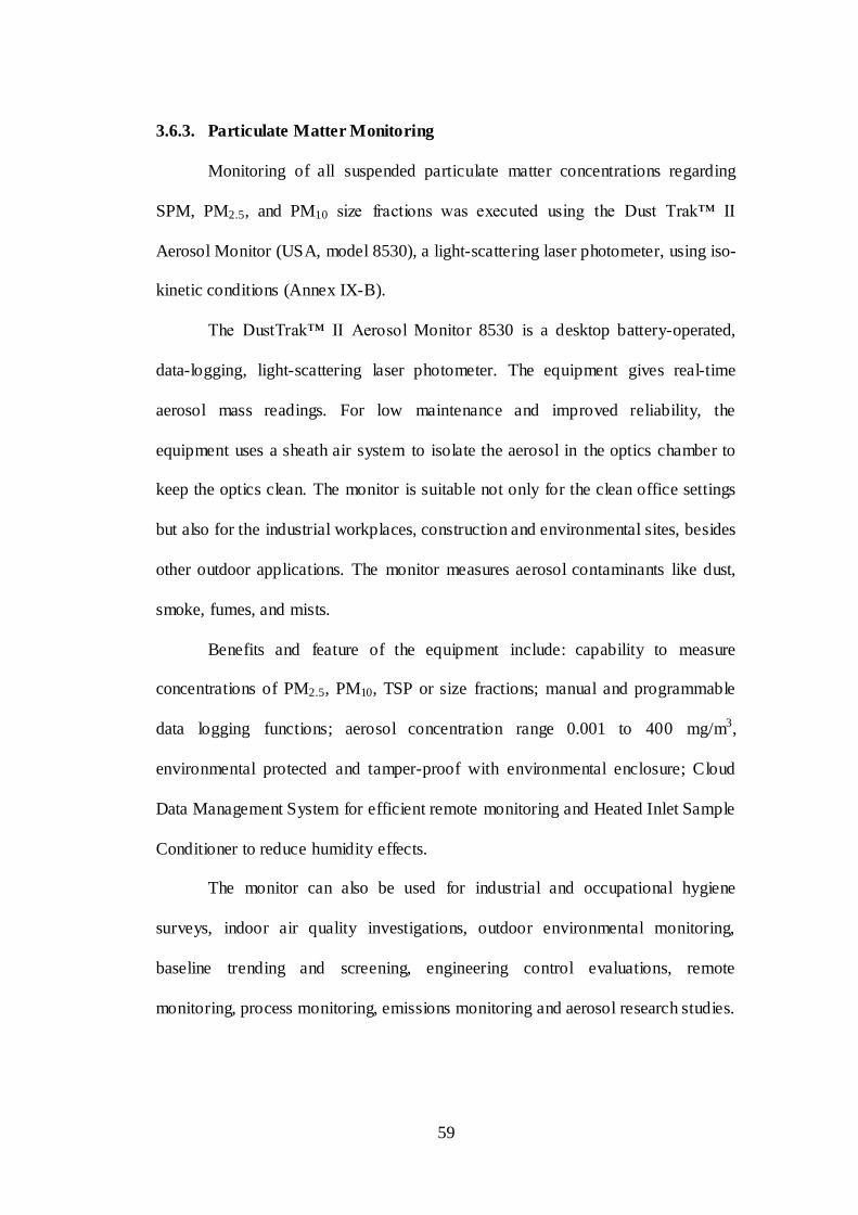
59
3.6.3. Particulate Matter Monitoring
Monitoring of all suspended particulate matter concentrations regarding
SPM, PM2.5, and PM10 size fractions was executed using the Dust Trak™ II
Aerosol Monitor (USA, model 8530), a light-scattering laser photometer, using iso-
kinetic conditions (Annex IX-B).
The DustTrak™ II Aerosol Monitor 8530 is a desktop battery-operated,
data-logging, light-scattering laser photometer. The equipment gives real-time
aerosol mass readings. For low maintenance and improved reliability, the
equipment uses a sheath air system to isolate the aerosol in the optics chamber to
keep the optics clean. The monitor is suitable not only for the clean office settings
but also for the industrial workplaces, construction and environmental sites, besides
other outdoor applications. The monitor measures aerosol contaminants like dust,
smoke, fumes, and mists.
Benefits and feature of the equipment include: capability to measure
concentrations of PM2.5, PM10, TSP or size fractions; manual and programmable
data logging functions; aerosol concentration range 0.001 to 400 mg/m3,
environmental protected and tamper-proof with environmental enclosure; Cloud
Data Management System for efficient remote monitoring and Heated Inlet Sample
Conditioner to reduce humidity effects.
The monitor can also be used for industrial and occupational hygiene
surveys, indoor air quality investigations, outdoor environmental monitoring,
baseline trending and screening, engineering control evaluations, remote
monitoring, process monitoring, emissions monitoring and aerosol research studies.

60
SPM monitoring was carried out at all the specified sampling points using
iso-kinetic conditions. Monitoring was carried out thrice during each day – once in
the morning, once at noon and once in the afternoon, in bright sunny days with
calm wind velocity conditions ideal for PM monitoring/air pollution monitoring at
the height of four feet.
3.6.3.1. Meteorological data
The meteorological data, including temperature, humidity, wind speed,
rainfall and atmospheric pressure, were also recorded during sampling of SPM,
PM10 and PM2.5 from all sites of Lahore, Gujrat and Kharian and
Islamabad/Rawalpindi during all fourteen (14) weeks (Annex XX to XXVII).
3.6.4. Particulate Matter Comparison
Concentrations of SPM, PM2.5, and PM10 at the distances of 3, 8, 13 and
18m at each construction site and during the each week were compared not only
with each other but also the National Environmental Quality Standards (NEQS) of
the Pakistan Environmental Protection Agency (Pak-EPA).
3.6.5. Statistical Analysis
To address the research question and achieve the objective of the study,
correlation and statistical linear regression analysis was done with SPSS 16
Statistical Package (software) to predict/estimate concentration of response
variables (dependent variables: concentrations of SPM, PM2.5 and PM10 at 8, 13
and 18 m from the source of generation of particulate matter ) through explanatory
variables (independent variable: concentrations of SPM, PM2.5 and PM10.0 at 8m
from the source of generation of particulate matter), or assesses the explanatory

61
variables as predictor of response variables (Stevenson, 2001). Enter method of
linear regression analysis was used.
3.6.5.1. Dependent and independent variables
Concentrations of SPM, PM2.5, and PM10 at 8, 13 and 18 m from the source
of generation of particulate matter were taken as dependent variables, while the
concentrations of SPM, PM2.5, and PM10 at 3 m from the source of generation of
particulate matter were taken as independent variables. For monitoring particulate
matter in the air, it is standard to take air samples/PM samples at the distance of
three meters from the source of generation of particulate matter. As monitoring
particulate matter in the air from 3 meters from the source of generation is the
standard, hence three meters was taken as the independent variable.
3.6.5.2. Statistical data treatment
The next step of the study consisted of treatment of data collected using
linear regression in order to identify the relationship between the dependent
variable Y (Concentrations of SPM, PM2.5, and PM10 at 8, 13 and 18 m from the
source of generation of particulate matter) and the independent variables X
(concentrations of SPM, PM2.5, and PM10 at 3 m from the source of generation of
particulate matter). All analyses were done using the SPSS 16 Statistical Package
for correlations and regression analysis for calculating regression coefficients,
including regression constants and slopes for dependent variables against the
predictor (independent variables).
3.6.5.3. Confirmatory tests
Before developing regression models for prediction of dependent variables,
in addition to significance of the regression, a test of the hypothesis of data

62
normality of the dependent variable was also conducted to check whether simple
linear regression can be used for prediction or not (Annex X to XIX).
3.6.6. Regression Models
After regression analysis, regression equations, using constants and slopes,
were developed for determining concentrations of SPM, PM2.5, and PM10 at 8, 13
and 18 m from the source of generation of particulate matter from the
corresponding concentration of SPM, PM2.5, and PM10 at 3 m distance from the
source of generation of particulate matter.
3.6.7. Validation of the Models
Concentrations of SPM, PM2.5, and PM10 from 3, 8, 13 and 18 m were
determined at new construction site in Jhelum City. Moreover, concentrations of
SPM, PM2.5, and PM10 at 8, 13 and 18 m were estimated by using determined
concentrations of particulate matters at 3m from the source of generation and
models established with help of regression analysis. The estimated and actual
concentrations were compared. The percentage differences of actual/determined
and estimated values of the concentrations were calculated to test the validity of the
results.

63
Chapter 4
4. RESULTS AND DISCUSSION
Based upon the data, samples and analysis conducted as per material and
methods in the previous chapter, results obtained have been described as under:
4.1. CONSTRUCTION WASTE ASSESSMENT
The average years of professional experience of respondents were
approximately five years. So, it can be concluded that the respondents were
suitable and have acquired adequate relevant experience of the construction
industry. Therefore, based on this ascertain, the information provided by these
respondents was considered reliable and dependable.
Figure 4-1: Percentage of respondents in the survey
Figure 4-1 demonstrates 35.52% respondents were civil engineers, 23.36% were
architects, 21.65% were quantity surveyors and 19.46 % were contractors. Based
on this information, it can be stated that civil engineers, followed by contractors,
played a major role in this study. As far as academic qualification of respondents is

64
concerned, 56.45% were bachelors and 18.49% was masters’ degree holders
(Figure 4-2). Hence, it can be deduced that most of the respondents were highly
educated and information provided by them were reliable. Table 4.1 exhibits the
quantitative assessment of cutting waste generated on construction sites. The table
shows that pipes had highest percentage of wastages (12%), followed by false
ceiling (11.44%). On the other hand, wires and cables and roofing sheets have the
least percentage wastages (7.67% and 8.73%). Table 4-6 shows that error in
calculation/cutting and poor material handling/operations are the main reasons
behind this high percentage (Gavilan and Bernold, 1994; Skoyles and Skoyles,
1987). However, in another study in Nigeria, wastage of reinforcement bars was
found to be highest (19.03%), followed by wires and cables (17.26%) and roofing
sheets and pipes (both 15.70%). Poor and multiple handling of tools, and
inadequate training of the construction workers to handle sophisticated
equipment were stated to be reason of wastage (Babatunde and Olusola, 2012;
(Gavilan and Bernold, 1994). Almost same wastage due to cutting (10%) was
reported by Katz and Baum (2011).

65
Table 4-1: Quantitative assessment of cutting waste at construction sites
Class
Interval
Mean
(x)
No of Responses against each Types of Cutting Waste [Frequency (f)]
Reinforcement bars
Roof carcass
Roofing sheets
False Ceiling
Wires and cables
Pipes
00-05% 2.5 137 103 135 90 119 51
5.1-10% 7.5 109 133 123 121 190 90
10.1-15% 12.5 46 80 71 85 75 153
15.1-20% 17.5 75 55 81 51 23 85
20.1-25% 22.5 23 26 1 38 4 30
25.1-30% 27.5 10 11 0 17 0 2
30.1-35% 32.5 9 2 0 9 0 0
35.1-40% 37.5 2 1 0 0 0 0
Sum fx 4207.50 4207.50 3587.50 4702.50 3152.50 4932.50
Mean (%) 10.24 10.24 8.73 11.44 7.67 12.00

66
Table 4-2 shows quantitative assessment of Theft and Vandalism (T&V)
during construction. The table indicates that Wood/Timber have highest percentage
of wastages of 16.78 %, followed by sand and cement with percentage of 16.03 and
13.80%, respectively; while wood preservatives and pipes have the least percentage
wastages of 8.90% and 10.65%, respectively. The main reason for this wastage was
found to be improper storage as indicated in Table 4-6. Same reason was stated in
another study carried out in Malaysia (Skoyles and Skoyles, 1987). Contrary to
this, Babatunde and Olusola (2012) reported that reinforcement bars, timber and
cement had the highest percentage of wastages (18.64%, 18.64% and 18.44%,
respectively), due to workers’ poor or no educational level and poverty in Nigeria.
Figure 4-2: Percentage of educational qualification of the respondents
Table 4-3 reveals that blocks & bricks, tiles and window glazing have the
highest percentage of wastages of 13.61%, 10.19% and 6.79%, respectively, in the
category of Transit Waste. Out of all constituents of the Transit Waste in this study,
blocks and bricks, tiles and ceramic appliances contribute in the generation of
suspended particulate matter in the surrounding air.
Bachelors
56% Masters
19%
Below
Bachelors
25%
Educational Qualification
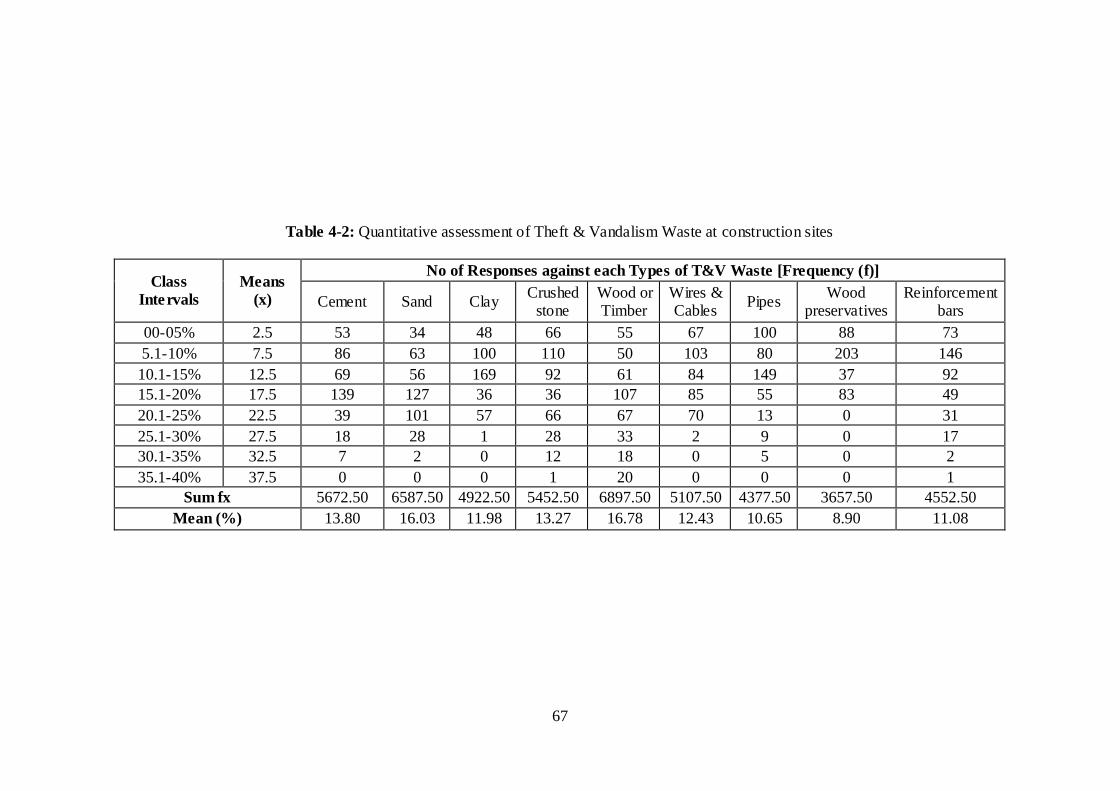
67
Table 4-2: Quantitative assessment of Theft & Vandalism Waste at construction sites
Class
Intervals
Means
(x)
No of Responses against each Types of T&V Waste [Frequency (f)]
Cement Sand Clay Crushed
stone Wood or Timber
Wires & Cables
Pipes Wood
preservatives Reinforcement
bars
00-05% 2.5 53 34 48 66 55 67 100 88 73
5.1-10% 7.5 86 63 100 110 50 103 80 203 146
10.1-15% 12.5 69 56 169 92 61 84 149 37 92
15.1-20% 17.5 139 127 36 36 107 85 55 83 49
20.1-25% 22.5 39 101 57 66 67 70 13 0 31
25.1-30% 27.5 18 28 1 28 33 2 9 0 17
30.1-35% 32.5 7 2 0 12 18 0 5 0 2
35.1-40% 37.5 0 0 0 1 20 0 0 0 1
Sum fx 5672.50 6587.50 4922.50 5452.50 6897.50 5107.50 4377.50 3657.50 4552.50
Mean (%) 13.80 16.03 11.98 13.27 16.78 12.43 10.65 8.90 11.08

68
Out of all constituents of theft and vandalism waste of our study, cement,
sand, clay and crushed stone produce fine inert waste, which ultimately generate
suspended particulate matter in the surrounding air.
While ceramic sanitary appliances and prefabricated windows have the least
percentage of wastages with 5.41% and 5.63%. As against this study, a survey,
conducted by Babatunde and Solomon Olusola (2012), indicated tiles, window
glazing and ceramic sanitary with highest wastage of 21.38%, 14.73% and 14.72%,
respectively, while prefabricated windows and blocks/bricks with least percentage
wastages of 11.58% and 14.15%, respectively. The reason was reported to be
deplorable road network in Nigeria.
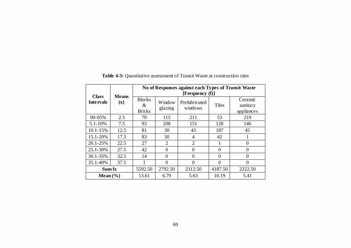
69
Table 4-3: Quantitative assessment of Transit Waste at construction sites
Class
Intervals
Means
(x)
No of Responses against each Types of Transit Waste
[Frequency (f)]
Blocks &
Bricks
Window glazing
Prefabricated windows
Tiles Ceramic sanitary
appliances
00-05% 2.5 70 115 211 53 219
5.1-10% 7.5 93 208 151 128 146
10.1-15% 12.5 81 30 43 187 45
15.1-20% 17.5 83 30 4 42 1
20.1-25% 22.5 27 2 2 1 0
25.1-30% 27.5 42 0 0 0 0
30.1-35% 32.5 14 0 0 0 0
35.1-40% 37.5 1 0 0 0 0
Sum fx 5592.50 2792.50 2312.50 4187.50 2222.50
Mean (%) 13.61 6.79 5.63 10.19 5.41

70
Table 4-4 describes that mortar has the highest percentage of wastage of
9.73%, followed by paint with wastage of 8.36%, whereas, application of
POP/POP ceiling and concrete has the least percentage of wastages of 7.20% and
8.25%, respectively, among the application waste. Reason behind this wastage was
found to be over ordering and improper storage as shown in Table 4-6. Same
results were given by Skoyles and Skoyles (1987) in their study conducted in
Malaysia. Whereas, in another study conducted in Nigeria, wastage of the POP
ceiling was reported as highest (15.70%), followed by wastage of mortar (14.91%),
concrete (14.13%) and paint (12.95%), respectively. The reason was stated as
multiple handling of tools, and inadequate training of the workers to handle
sophisticated equipment (Babatunde and Olusola, 2012).
Among application waste, mortar, concrete and POP contribute in produce
fine inert waste, which ultimately generate suspended particulate matter in the
surrounding air.
Table 4-5 represents the overall mean percentage of waste categories on
construction sites. The table demonstrates that theft and vandalism has the highest
average wastage of 12.77% followed by cutting waste with 10.05 % wastage.
Transit waste and application waste have least overall average wastage of 8.32%
and 8.39%, respectively. All the respondents were of the view that overall mean
percentage of waste at any construction project should not be more than five
percent.
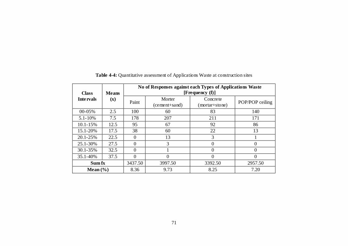
71
Table 4-4: Quantitative assessment of Applications Waste at construction sites
Class
Intervals
Means
(x)
No of Responses against each Types of Applications Waste
[Frequency (f)]
Paint Morter
(cement+sand)
Concrete
(mortar+stone) POP/POP ceiling
00-05% 2.5 100 60 83 140
5.1-10% 7.5 178 207 211 171
10.1-15% 12.5 95 67 92 86
15.1-20% 17.5 38 60 22 13
20.1-25% 22.5 0 13 3 1
25.1-30% 27.5 0 3 0 0
30.1-35% 32.5 0 1 0 0
35.1-40% 37.5 0 0 0 0
Sum fx 3437.50 3997.50 3392.50 2957.50
Mean (%) 8.36 9.73 8.25 7.20

72
Earlier, a study conducted in Nigeria, concluded that theft and vandalism
waste had the highest average level of 16.58% followed by cutting waste
with 15.44%. Application waste and transit waste had the least overall
average wastage of 14.16 % and 14.89% respectively (Babatunde and Olusola,
2012).
In this study, the total means wastage was calculated as 9.88%, which is in
accordance with the findings of Shen et al. (2005), who reported wastage rate as
equivalent to 1–10% of the purchased construction materials and much less than
the reported by Yahya and Boussabaine (2006), who found out wastage of about
25% of construction materials during construction activities. The wastage rate in
Nigerian and the UK construction industry were reported as high as 15.32%
(Babatunde and Olusola, 2012) and 10–15% (McGrath and Anderson, 2000),
respectively. In another study, surprisingly, 30% of the weight of total construction
materials on site has been reported in the UK.
From business and financial viewpoint, the cost of construction waste
revealed in this study is too high. Reducing wastage to 5% or less may certainly
help in saving billions in case of mega projects and millions in case of small or
medium sized construction projects.
Table 4-6 shows that 62.77% respondents believe that the reason for cutting
waste is error in calculations and cutting while 24.09% were of the view that poor
material handling/operations are the main reasons as stated by Gavilan and Bernold
(1994) and Skoyles and Skoyles (1987) in their findings. Improper storage was
declared as the major source of theft and vandalism waste by 69.34% respondents.

73
Table 4-5: Overall mean percentage of waste categories on construction sites
Waste Types Mean Wastage (%)
Cutting waste 10.05
T & V Waste 12.77
Transit waste 8.32
Application Waste 7.39
Total Waste 9.88
Similarly 78.35% construction stakeholders opined transportation as main
cause of transit waste. Therefore, it can be concluded that careful calculations and
proper material handling can lead to reduction is cutting waste. Similarly, theft and
vandalism waste can be reduced by proper storage of the construction material.
However, respondents indicated multiple reasons for wastage of application waste
including over ordering (60.58%), improper storage (14.36%), poor planning
(14.11%) and poor material handling/operations (10.95%)
In general, it may be deduced that all the construction materials have higher
percentage wastages due to poor and multiple handling of tools, and inadequate
training of the construction workers to handle sophisticated equipment. Theft and
vandalism was supposed to be very common among poor, unskilled and
uneducated workers.

74
Table 4-6: Reasons and source identification for each kind of waste
Sources/reasons of
wastage
Cutting
waste (%)
T&V
Waste (%)
Transit
waste (%)
Application
Waste (%)
Faulty or fancy design 13.14 - - -
Improper storage - 69.34 - 14.36
Over ordering - 24.57 14.84 60.58
Error in calculations/cutting 62.77 - - -
Poor material handling/operations
24.09 6.08 - 10.95
Poor planning - - 6.81 14.11
Transportation - - 78.35 -

75
4.2. PREDICTION OF SPM CHARACTERISTICS
The results of the statistical analysis are presented in five parts – (1)
comparison of the average values and concentration of physico-chemical
characteristics of inert waste material and that of suspended particulate matter
(Figure 4-3), (2) two tailed Pearson correlations of physico-chemical characteristics
of inert waste to the corresponding physico-chemical characteristics of suspended
particulate matter at 0.01 level (Table 4-7), (3) analysis of variance (ANOVA) of
regression analysis (Table 4-8), (4) simple linear regression curves with R2 values
(Figure 4-4 to 4-13), and (5) statistical models for determining values and
concentrations of physico-chemical characteristics (y) of suspended particulate
matter in the air with determined values/concentrations of physico-chemical
characteristics of inert matter at new location (x), regression constant (a) and value
of slope (b) of the regression curve, at any new locations (Table 4-9).
Concentration of sulfate in SPM is higher than that of the inert matter. The reason
may be due to additional contribution of the sulfate from any other source in air,
especially diesel fuel used in the public transport.
Table 4-7: Pearson correlation (two tailed) between various physico-chemical
characteristics of inert material and particulate matter
S No Characteristics
(Inert vs PM) Correlation P value
Significance
at 0.01 level
1 pH 0.778
0.00
Sig
nif
ican
t
2 EC 0.494
3 Al 0.708
4 Ca 0.792
5 Ni 0.757
6 Fe 0.813
7 Zn 0.945
8 SO4-2 - 0.485
9 NO3-1 0.592
10 Cl-1 0.830

76
4.2.1. Correlations Analysis
Table 4-7 exhibits two-tailed Pearson correlations between
values/concentrations of physic-chemical characteristics of inert material at ground
and suspended particulate material in the surrounding/ambient air. The P values
(0.000 in all cases) show that all the correlations were highly significant at 0.01
level. The correlation ranges from highest 0.945 to lowest 0.484. The highest
correlation was found in case of Zn (0.945), followed Cl-1 (0.830) and Fe (0.813),
whereas, lowest correlation was determined in case of SO4-2 (0.485), followed by
electrical conductivity (0.494) and NO3- (0.592). All the correlations were positive,
except that of sulfate’s. The negative correlation of sulfate is surprising and needs
further investigation for digging out the reason behind this unanticipated
behaviour. However, possible reasons of low correlations for SO4-2 and NO3
- might
be due to the effect and contribution of some other sources, e.g. road traffic
emissions.
4.2.2. Linear Regression Analysis:
Coefficient of determination (R2) is an important concept in regression
analysis and is believed to be one of the parameters to verify and confirm the
efficiency and validity of regression model for estimation purpose. The maximum
R2 value is found in case of Zn (0.892) followed by Cl− (0.688), while SO42−,
followed by electrical conductivity, exhibit the minimum value of R2 as 0.235 and
0.244, respectively. Usually it is considered that higher the value of R2, the better
the model will fit the data and greater will be the explanatory power of the
regression. But only R2 is insufficient to decide about the goodness of fit of model.
Smaller R2 value always does not mean model is not good for estimation. In such

77
cases, R2 is interpreted with ANOVA significance for proper model interpretation.
In this study, R2 value for SO42− and electrical conductivity are only 24%, but their
ANOVA results are significant and hence only 24% explained variation cannot be
neglected and can be considered for estimation of the dependent variables.
Table 4-8 exhibits summary of analysis of variance (ANOVA) of simple
linear regression showing R2 values, F values, P values and significance at 0.01
level. These values shows that R2 values of all physico-chemical characteristics
were significant at 0.01 level. Figures 4-4 to 4-13 illustrate linear regression curves
between determined/observed values/concentrations of physico-chemical
characteristics of inert material (independent variable: along x-axis) and
corresponding characteristics of suspended particulate matter (depended variable:
along y-axis). All the curves/graphs, except Figure 4-9, demonstrated that
values/concentrations of physico-chemical characteristics of suspended particulate
matter decreased as compared to values/concentrations of physico-chemical
characteristics of inert material. However, in case of Figure 4-9, concentration of
sulfate in SPM (dependent variable) increased as compared to concentration of
sulfate in inert matter (independent variable). Nonetheless, the extent of increase or
decrease depends upon slope of the corresponding regression line/curve.
The meteorological data during all four weeks of sample collection have
been show in Annex XX, XXI-A and XXII-A. As the wind velocity was calm
during all days of the four weeks, therefore, there was no effect of wind velocity
and direction on the dispersion of particulate matter. It is pertinent to mention that
there was no rain during all days of four weeks during which the samples were
taken and hence effect of wind and rain is negligible.

78
Figure 4-3: Comparison of physico-chemical characteristics of fine inert construction waste and suspended particulate matter
0.0 50.0 100.0 150.0
pH [inert]
pH [PM]
EC (µS/cm) [inert]
EC (µS/cm) [PM]
Al ( µg/g) [inert]
Al (µg/g) [PM]
Ca (µg/g) [inert]
Ca (µg/g) [PM]
Ni (µg/g) [inert]
Ni (µg/g) [PM]
Fe (µg/g) [inert]
Fe (µg/g) [PM]
Zn (µg/g) [inert]
Zn (µg/g) [PM]
Sulfate (mg/l) [inert]
Sulfate (mg/l) [PM]
Nitrate (mg/l) [inert]
Nitrate (mg/l) [PM]
Chloride (mg/l) [inert]
Chloride (mg/l) [PM]
Week 4
Week 3
Week 2
Week 1

79
Figure 4-4: Relationship between pH value of SPM and construction
waste dumped on ground
Figure 4-5: Relationship between electrical conductivity of SPM and
construction waste dumped on ground

80
Figure 4-6: Relationship between concentration of Al observed in the inert waste
dumped and SPM collected samples
Figure 4-7: Relationship between concentration of Ca observed in the inert waste
dumped and SPM collected samples

81
Table 4-8: Regression analysis (ANOVA) of physico-chemical characteristics
S No Characteristics R2 P value Significance
at 0.01 level
1 pH 0.606
0.0
00
Sig
nifican
t 2 EC 0.244
3 Al 0.501
4 Ca 0.627
5 Ni 0.572
6 Fe 0.660
7 Zn 0.892
8 SO4-2 0.235
9 NO3-1 0.351
10 Cl-1 0.688
Figure 4-8: Relationship between concentration of Ni observed in the inert waste
dumped and SPM collected samples

82
Figure 4-9: Relationship between concentration of Fe observed in the inert waste
dumped and SPM collected samples
Figure 4-10: Relationship between concentration of Zn observed in the inert waste
dumped and SPM collected samples

83
Figure 4-11: Relationship between concentration of SO4
-2 observed in the inert waste dumped and SPM collected samples
Figure 4-12: Relationship between concentration of NO3
-1 observed in the inert waste dumped and SPM collected samples

84
Figure 4-13: Relationship between concentration of Cl-1 observed in the inert
waste dumped and SPM collected samples 4.2.3. Data Normality Tests:
Though, regression analyses of all the characteristics were found
significant, but before developing regression models for prediction of dependent
variables, data normality test of the dependent variable were also conducted to
check whether simple linear regression can be used for prediction of dependent
variable or not.
Data normality test of all dependent variable have been shown in the
Annexure X to XIX. After confirmation of the normality of the dependent
variables, regression based models were established.
4.2.4. Statistical Regression-Based Models
Table 4-9 exhibits simple linear regression-based models [Y = a + b (x)]
developed for determining the values and concentrations of each physico-chemical

85
characteristics in suspended particulate matter (dependent variables) at any other
construction site, by determining only the values and concentrations of
corresponding physico-chemical characteristics of inert material (independent
variables) at the new site.
In the model [Y = a + b (x)], Y is value/concentration of physico-chemical
characteristics of suspended particulate matter (dependent variable: to be estimated
at new location), a and b are the values of constant and slope of regression
line/curve (both determined for each and every physico-chemical characteristics in
regression analysis), and x is the value/concentration of physico-chemical
characteristics of inert material (independent variable) determined at the new
location.
The constant/intercept itself and alone doesn’t tell anything about the
relationship between predictor and response (independent and dependent variable).
The negative value of constant in case of pH, Al, Ca and Zn is simply indicating
that the fitted line is passing through x-axis. The intercept/constant is like a matter
of extrapolation and extrapolation towards base/x-axis is a meaningless
extrapolation.
For example, if house prices are modeled in terms of size of rooms. If you
use the raw data, the intercept is a rather meaningless extrapolation – the price of a
zero-roomed house; you are extrapolating beyond the observed data! Further, in
case, there is no fine inert, the models will not be applicable. So there is no
justification in stating that ‘the constant b is the level of ambient air pollutant in
case there is no emission from a construction site (inert = 0)’. So, keeping in view
86
all above arguments, it is not justified to say that the value of constant represents
the background/ambient air concentration.
Therefore, at any new construction site, employing the statistical regression
models given in Table 4-9, values/concentrations of pH and EC and concentrations
of aluminum (Al), calcium (Ca), nickel (Ni), iron (Fe) and zinc (Zn) metals and
sulfate (SO4-2), nitrate (NO3
-) and chloride (Cl-) ions in suspended particulate
matter in air can be estimated only by determining the corresponding
values/concentrations of pH and EC and concentrations of a luminum (Al), calcium
(Ca), nickel (Ni), iron (Fe) and zinc (Zn) metals and sulfate (SO4-2), nitrate (NO3
-)
and chloride (Cl-1) ions in the inert matter on ground at any construction site.

87
Table 4-9: Statistical Regression-based models (y = a + b.x) for determination of various physico-chemical characteristics of particulate matter
S No Characteristics Unit Constant
(a)
Slope
(b)
Statistical model for
dependent variable in
particulate matter
[y = a + b(x)]
1 pH - -1.264 1.136* Y= -1.264 + 1.136 (x)
2 EC (µS/cm) 73.014 0.323* Y= 73.014 + 0.323 (x)
3 Al (µg/g) -3.120 0.996* Y = -3.120 + 0.996 (x)
4 Ca (µg/g) -9.270 0.977* Y= -9.270 + 0.977 (x)
5 Ni (µg/g) 2.031 0.825* Y= 2.031 + 0.825 (x)
6 Fe (µg/g) 30.430 0.881* Y= 30.430+ 0.881 (x)
7 Zn (µg/g) -8.291 0.883* Y= -8.291 + 0.883 (x)
8 SO4-2 (mg/l) 41.574 -0.532* Y= 41.574 + -0.532 (x)
9 NO3- (mg/l) 3.695 0.593* Y= 3.695 + 0.593 (x)
10 Cl- (mg/l) 6.889 0.810* Y= 6.889 + 0.810 (x) *Significant at 0.01 level

88
4.2.5. Validity of the models
At a new construction site at Model Town Link Road Lahore, Pakistan,
physico-chemical characteristics on both inert material and particulate matter were
determined. Moreover, the values/concentrations of physico-chemical
characteristics in the inert waste were estimated by using model established with
help of regression based models.
The estimated and actual values/concentrations were compared in the Table
4-10. The same type of comparison was adopted by Kern at al. (2015) in their
study in which they estimated construction waste generation by linear regression
analysis. The percentage difference varied from -16.3 in case of NO3-1 to 19.8 in
case of Al. The minimum difference was found in case of pH (3.8%), followed by
Ca (-4.3%), Fe (8.6%) and Cl-1 (-9.1%).
However, all the differences were less than 20%, which underlines the
reliability of the statistical models established for estimating phyico-chemical
characteristics.

89
Table 4-10: Validation of the regression based models by comparing estimated and actual values at a new construction site
S No Characteristics Unit Independent
variable (x)
Dependent
variable
(Y)
(estimated)
Dependent
variable
(Y)
(actual)
% Difference
1 pH - 7.6 7.3696 7.1 3.8
2 EC (µS/cm) 145 119.849 135 -11.2
3 Al (µg/g) 22.5 19.29 16.1 19.8
4 Ca (µg/g) 81 69.867 73 -4.3
5 Ni (µg/g) 11.5 11.5185 12.7 -9.3
6 Fe (µg/g) 180 189.01 174 8.6
7 Zn (µg/g) 60.7 45.3071 40.7 11.3
8 SO4-2 (mg/l) 31 25.082 29 -13.5
9 NO3-1 (mg/l) 22 16.741 20 -16.3
10 Cl-1 (mg/l) 24.7 26.896 29.6 -9.1

90
4.3. SPM MONITORING AT RAWALPINDI ISLAMABAD
METRO PROJECT SITE
Figure 4-14 illustrates concentration of suspended particulate matter (SPM)
the Rawalpindi Islamabad Metro Project Site (Annex V & VI) during three weeks,
ie. 06-12 July 2014, 02-08 January 2015 and 09-15 April 2015.
Figure 4-14: Comparison of SPM Concentrations at five Metro Project Sites
The figure shows that maximum concentration of suspended particulate
matter was found at IJP-Tipu Sultan Road Junction, Islamabad, followed by
Benazir Bhutto Hospital, Rawalpindi, during all three weeks. Whereas, minimum
concentration of suspended particulate matter was found at Pakistan Secretariat,
Islamabad. However, it was observed that at all project sites, concentration of
suspended particulate matter was well beyond permissible limits of 500
microgram/m3 set by the PAK-EPA.
The meteorological data during all three weeks of sample collection have
been shown in Annex XXIII to XXIV. As, during all days of the three weeks, the
Conc
(mg/m
3)

91
wind velocity was calm, therefore, there was no effect of wind velocity and
direction on the dispersion of particulate matter. Further, there was no rain during
all days of three weeks and hence there was no effect of rain on particulate matter
generation and dispersion.
4.4. COMPARISON OF THE SUSPENDED PARTICULATE
MATTER CONCENTRATIONS
4.4.1. Lahore City
Figures 4-15 to 4-17 depict comparative analysis of concentrations of
suspended particulate matter (SPM), PM10 and PM2.5 at the construction site in
Lahore during the week starting from 01-07 January 2014 (Week 1), while figures
4-18 to 4-20 exhibit concentrations of suspended particulate matter (SPM), PM10
and PM2.5 during the week from 11-17 June 2014 (Week 2) at the distances of 3, 8,
13 and 18m.
During the week from 01-07 January 2014, concentration of SPM remained
below the permissible limits of 500 µg/m3 as per NEQS set by the PAK-EPA.
However, during the week from 01-07 January 2014, concentration of PM10
exhibited the random response, some days below and some days above the
permissible limits of 150 µg/m3 as per NEQS set by the PAK-EPA. This trend
might be due to high rise building in proximity of the monitor.
In case of PM2.5, the concentration, like SPM, also remained below the
permissible limits of 35 µg/m3 as per NEQS set by the PAK-EPA.

92
Figure 4-15: Comparison of SPM concentrations at varying distances at Lahore construction site during 01-07 January 2014
Figure 4-16: Comparison of PM10 concentrations at Lahore construction site at
varying distances during 01-07 January 2014
0
100
200
300
400
500
600
Wednesday
01/01/2014
Thursday
02/01/2014
Friday
03/01/2014
Saturday
04/01/2014
Sunday
05/01/2014
Monday
06/01/2014
Tuesday
07/01/2014
Co
ncen
tra
tio
n (
µg
/m3)
SPM
3m
8m
13m
18m
0
50
100
150
200
250
Wednesday
01/01/2014
Thursday
02/01/2014
Friday
03/01/2014
Saturday
04/01/2014
Sunday
05/01/2014
Monday
06/01/2014
Tuesday
07/01/2014
Co
ncen
tra
tio
n (
µg
/m3)
PM10 3m
8m
13m
18m

93
Figure 4-17: Comparison of PM2.5 concentrations at Lahore construction site at
varying distances during 01-07 January 2014
Figure 4-18: Comparison of SPM concentrations at Lahore construction site at varying distances during 11-17 June 2014
0
5
10
15
20
25
30
35
40
Wednesday
01/01/2014
Thursday
02/01/2014
Friday
03/01/2014
Saturday
04/01/2014
Sunday
05/01/2014
Monday
06/01/2014
Tuesday
07/01/2014
Co
ncen
tra
tio
n (
µg
/m3)
PM2.5
3m
8m
13m
18m
100
200
300
400
500
600
Wednesday
11/06/2014
Thursday
12/06/2014
Friday
13/06/2014
Saturday
14/06/2014
Sunday
15/06/2014
Monday
16/06/2014
Tuesday
17/06/2014
Co
ncen
tra
tio
n (
µg
/m3)
SPM
3m
8m
13m
18m

94
Figure 4-19: Comparison of PM10 concentrations at Lahore construction site at varying distances during 11-17 June 2014
Figure 4-20: Comparison of PM2.5 concentrations at Lahore construction site at
varying distances during 11-17 June 2014
0
50
100
150
200
Wednesday
11/06/2014
Thursday
12/06/2014
Friday
13/06/2014
Saturday
14/06/2014
Sunday
15/06/2014
Monday
16/06/2014
Tuesday
17/06/2014
Co
ncen
tra
tio
n (
µg
/m3)
PM10
3m
8m
13m
18m
5
10
15
20
25
30
35
40
Wednesday
11/06/2014
Thursday
12/06/2014
Friday
13/06/2014
Saturday
14/06/2014
Sunday
15/06/2014
Monday
16/06/2014
Tuesday
17/06/2014
Co
ncen
tra
tio
n (
µg
/m3)
PM2.5
3m
8m
13m
18m

95
Similarly, during the week from 11-17 June 2014, concentration of SPM
was recorded below the NEQS set by the PAK-EPA. During the same week,
concentration of PM10 showed the random and mixed response due to random
activity and mechanical disturbance.
However, during the week from 11-17 June 2014, concentration of PM2.5
was also found below the NEQS set by the PAK-EPA.
The meteorological data during all two weeks of sample collection have
been shown in Annex XXI-B and XXII-B. The calm wind velocity during all days
of the two weeks, caused no effect of wind velocity and direction on the dispersion
of particulate matter. Further, as the samples were taken from the one-way wide
urban roadside, at both side of which, there were high rising buildings, plazas and
towers etc, therefore, there was no tunnel effect of the wind as well. Hence, the
dispersion and movement of the particulate matter were only in the direction
towards which the traffic was flowing. It is pertinent to mention that there was no
rain during all days of two weeks during which the samples were taken and hence
there was no effect of rain on particulate matter generation and dispersion.
4.4.2. Gujrat City
Figures 4-21 to 4-29 demonstrate comparison of concentrations of SPM,
PM10 and PM2.5 at the construction site in Gujrat during the week from 19-25 May
2015, 13-19 June 2015 and 18-24 August 2015 at the distances of 3, 8, 13 and 18m
from the source of generation of particulate matters.

96
Figure 4-21: Comparison of SPM concentrations at Gujrat construction site at varying distances during 19-25 May 2015
The concentration of SPM and PM10 was observed beyond the permissible
limits of 500 µg/m3 and 150 µg/m3 during the week 19-25 May 2015, at 3m, 8m,
13m and 18 m distances from the source of generation of particulate matter, with
the exception of concentration of SPM at 18 m distance on Friday. On Friday and
Saturday, the concentration was below the permissible limit due to less activities
and traffic due to Friday prayers and weekly leave in the city. Though, being a
metropolitan city, the mechanical disturbance at and around the construction site in
Lahore was more as compared construction site in Gujrat, the suspended particulate
matter generation was less is Lahore than Gujrat owing to watering at construction
site, covering of fine inert material with plastic sheets and construction activities
during the night time when other mechanical disturbances were less.
400
450
500
550
600
650
700
750
800
Tuesday
19/05/2015
Wednesday
20/05/2016
Thursday
21/05/2015
Friday
22/05/2015
Saturday
23/05/2015
Sunday
24/05/2015
Monday
25/05/2015
Co
ncen
tra
tio
n (
µg
/m3)
SPM
3m
8m
13m
18m

97
Figure 4-22: Comparison of PM10 concentrations at Gujrat construction site at varying distances during 19-25 May 2015
Figure 4-23: Comparison of PM2.5 concentrations at Gujrat construction site at
varying distances during 19-25 May 2015
100
150
200
250
300
350
400
450
500
Tuesday
19/05/2015
Wednesday
20/05/2016
Thursday
21/05/2015
Friday
22/05/2015
Saturday
23/05/2015
Sunday
24/05/2015
Monday
25/05/2015
Co
ncen
tra
tio
n (
µg
/m3)
PM10 3m
8m
13m
18m
0
10
20
30
40
50
60
70
80
Tuesday
19/05/2015
Wednesday
20/05/2016
Thursday
21/05/2015
Friday
22/05/2015
Saturday
23/05/2015
Sunday
24/05/2015
Monday
25/05/2015
Co
ncen
tra
tio
n (
µg
/m3)
PM2.5
3m
8m
13m
18m

98
In case of PM2.5, the concentration was beyond the PAK-EPA NEQS limits
at 3m and 8 m distances, while, as the particulate matter travels ahead, it settles and
concentration went below the permissible limits of 35 µg/m3 at the distance of 13m
and 18 m from the source of generation. During the week 13-19 May 2015, the
concentration of SPM was observed beyond the permissible limits of 500 µg/m3 at
3m and 8m distance, while at the distance of 18 m distance, concentration was
within permissible limit of PAK-EPA. At the distance of 13 m, the concentration of
SPM was random while comparing with standard. During the same week,
concentrations of PM10 at all distances from the source were beyond the standard
limit of 150 µg/m3. As far as PM2.5 is concerned, concentration at distance of 3m
was beyond the PAK-EPA permissible limit of 35 µg/m3, but as it travels farther to
8, 13 and 18 m from the source, the concentration decreased to the permissible
limit due to settlement and dispersion of the particulate matter.
Figure 4-24: Comparison of SPM concentrations Gujrat construction site at
varying distances during 13-19 June 2015
300
400
500
600
700
Saturday
13/06/2015
Sunday
14/06/2015
Monday
15/06/2015
Tuesday
16/06/2015
Wednesday
17/06/2015
Thursday
18/06/2015
Friday
19/06/2015
Co
ncen
tra
tio
n (
µg
/m3)
SPM
3m
8m
13m
18m

99
Figure 4-25: Comparison of PM10 concentrations at Gujrat construction site at varying distances during 13-19 June 2015
Figure 4-26: Comparison of PM2.5 concentrations at Gujrat construction site at varying distances during 13-19 June 2015
100
150
200
250
300
350
400
Saturday
13/06/2015
Sunday
14/06/2015
Monday
15/06/2015
Tuesday
16/06/2015
Wednesday
17/06/2015
Thursday
18/06/2015
Friday
19/06/2015
Co
ncen
tra
tio
n (
µg
/m3)
PM10
3m
8m
13m
18m
0
10
20
30
40
50
60
70
Saturday
13/06/2015
Sunday
14/06/2015
Monday
15/06/2015
Tuesday
16/06/2015
Wednesday
17/06/2015
Thursday
18/06/2015
Friday
19/06/2015
Co
ncen
tra
tio
n (
µg
/m3)
PM2.5 3m
8m
13m
18m
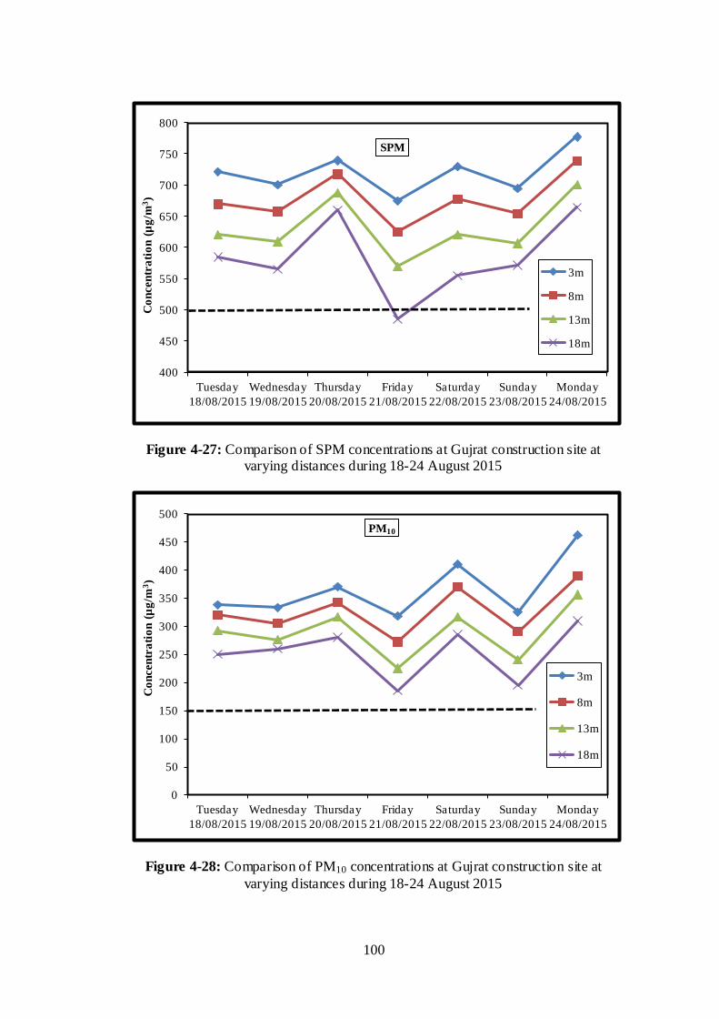
100
Figure 4-27: Comparison of SPM concentrations at Gujrat construction site at varying distances during 18-24 August 2015
Figure 4-28: Comparison of PM10 concentrations at Gujrat construction site at
varying distances during 18-24 August 2015
400
450
500
550
600
650
700
750
800
Tuesday
18/08/2015
Wednesday
19/08/2015
Thursday
20/08/2015
Friday
21/08/2015
Saturday
22/08/2015
Sunday
23/08/2015
Monday
24/08/2015
Co
ncen
tra
tio
n (
µg
/m3)
SPM
3m
8m
13m
18m
0
50
100
150
200
250
300
350
400
450
500
Tuesday
18/08/2015
Wednesday
19/08/2015
Thursday
20/08/2015
Friday
21/08/2015
Saturday
22/08/2015
Sunday
23/08/2015
Monday
24/08/2015
Co
ncen
tra
tio
n (
µg
/m3)
PM10
3m
8m
13m
18m

101
Figure 4-29: Comparison of PM2.5 concentrations Gujrat construction site at varying distances during 18-24 August 2015
Figures 4-27 to 4-29 exhibit the concentration of SPM, PM10 and PM2.5, at
the varying distances of 3, 8, 13 and 18m from the source of generation of
particulate matter during the period from 18 August to 24 August 2015 at the
construction site in Gujrat.
The concentrations of all sizes of particulate matter were found above the
permissible limits of 500 microgram/m3, 150 microgram/m3 and 35 microgram/m3,
in case of SPM, PM10 and PM2.5, respectively, with the exception of concentration
of PM2.5 at the distance of 18m, where it was found below the standard limit of 35
microgram/m3.
As shown in Fig 4-15, SPM in Lahore site was recorded high on Saturdays
and reaches lowest on Sundays. This might be due to late closing of market and
people staying outside for late hours on Saturday night and very little showing up
and late coming out on Sundays. Similar trend was observed in Fig 4-18 in June
0
10
20
30
40
50
60
70
80
90
Tuesday
18/08/2015
Wednesday
19/08/2015
Thursday
20/08/2015
Friday
21/08/2015
Saturday
22/08/2015
Sunday
23/08/2015
Monday
24/08/2015
Co
ncen
tra
tio
n (
µg
/m3)
PM2.5
3m
8m
13m
18m

102
2014. However mixed trend was observed in case of PM10, but the concentration
was touching the maximum permissible levels on few days of week.
Different trend was observed in Gujrat city (Fig 4-22 – 4-24) where roads
are not much wider and traffic is low on Fridays and Sundays due to two local
holidays (offices and schools remain closed on Sunday and markets are mostly
closed on Fridays). Concentration of both PM10 and PM2.5 were noticed above the
NEQS. Here, local traffic and local wind (calm) might be affecting dispersion of
dust. Moreover, environmental practices are not strictly practiced in Gujrat as
compared to Lahore city, where water spray on dust is commonly observed due to
EPD monitoring.
The meteorological data recorded during all three weeks of sample
collection have been shown in Annex XXV to XXVI. As the wind velocity was
calm during all days of the three weeks, therefore, there was no effect of wind
velocity and direction on the dispersion of particulate matter.
Further, as the samples were taken from the wide one-way urban roadside,
at both side of which, there were high rising buildings, plazas and towers etc,
therefore, there was no tunnel effect of the wind as well.
Hence, the dispersion and movement of the particulate matter were in the
direction towards which the traffic was flowing. It is pertinent to mention that there
was no rain during all days of three weeks during which the samples were taken
and hence there was no effect of rain on particulate matter generation and
dispersion.
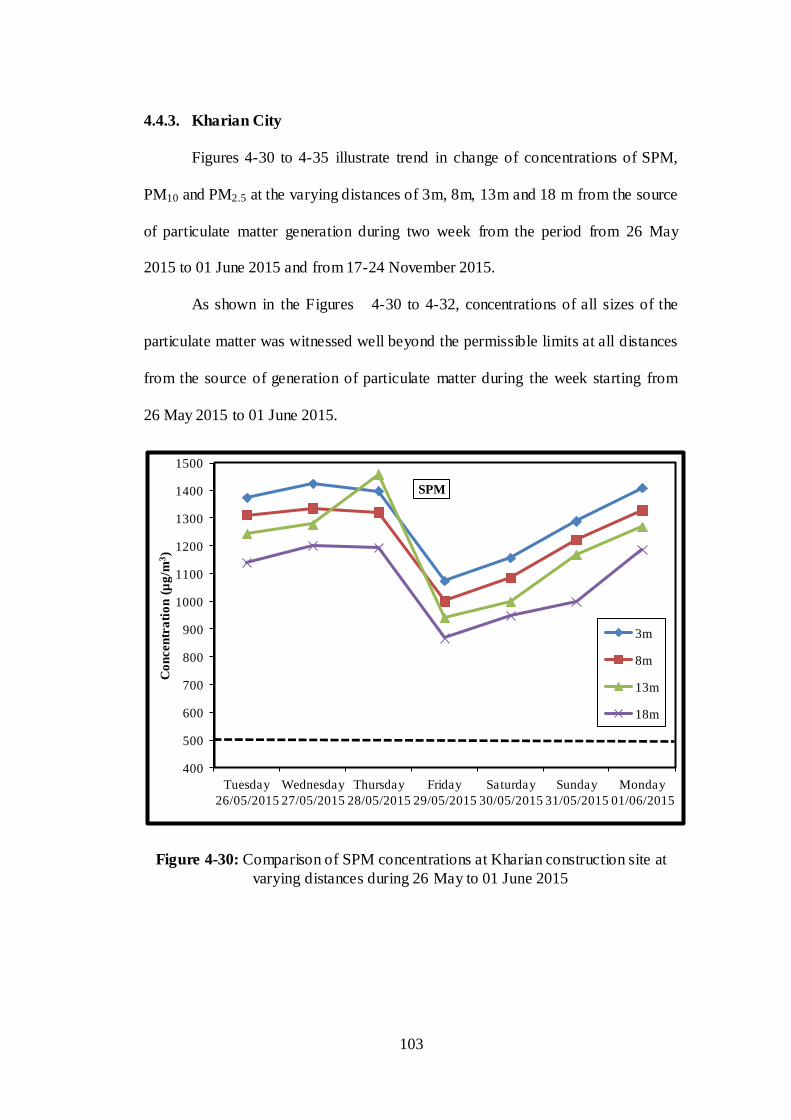
103
4.4.3. Kharian City
Figures 4-30 to 4-35 illustrate trend in change of concentrations of SPM,
PM10 and PM2.5 at the varying distances of 3m, 8m, 13m and 18 m from the source
of particulate matter generation during two week from the period from 26 May
2015 to 01 June 2015 and from 17-24 November 2015.
As shown in the Figures 4-30 to 4-32, concentrations of all sizes of the
particulate matter was witnessed well beyond the permissible limits at all distances
from the source of generation of particulate matter during the week starting from
26 May 2015 to 01 June 2015.
Figure 4-30: Comparison of SPM concentrations at Kharian construction site at
varying distances during 26 May to 01 June 2015
400
500
600
700
800
900
1000
1100
1200
1300
1400
1500
Tuesday
26/05/2015
Wednesday
27/05/2015
Thursday
28/05/2015
Friday
29/05/2015
Saturday
30/05/2015
Sunday
31/05/2015
Monday
01/06/2015
Co
ncen
tra
tio
n (
µg
/m3)
SPM
3m
8m
13m
18m

104
Figure 4-31: Comparison of PM10 concentrations at Kharian construction site at varying distances during 26 May to 01 June 2015
Figure 4-32: Comparison of PM2.5 concentrations at Kharian construction site at varying distances during 26 May to 01 June 2015
0
100
200
300
400
500
600
700
800
900
1000
Tuesday
26/05/2015
Wednesday
27/05/2015
Thursday
28/05/2015
Friday
29/05/2015
Saturday
30/05/2015
Sunday
31/05/2015
Monday
01/06/2015
Co
ncen
tra
tio
n (
µg
/m3)
PM10
3m
8m
13m
18m
0
35
70
105
140
175
210
245
Tuesday
26/05/2015
Wednesday
27/05/2015
Thursday
28/05/2015
Friday
29/05/2015
Saturday
30/05/2015
Sunday
31/05/2015
Monday
01/06/2015
Co
ncen
tra
tio
n (
µg
/m3)
PM2.5
3m
8m
13m
18m

105
Figures 4-33 to 4-35 explain the concentrations SPM, PM10 and PM2.5 at the
distance of 3m, 8m, 13m and 18m from the source of generation of particulate
matter during the week 17-24 November 2015 in Kharian.
From the figures mentioned above, it has been observed that concentration
of SPM remained beyond the permissible limits at all four points from the source
of generation of particulate matter, except for Friday. However, in case of PM10
and PM2.5, the concentration was found random, sometimes above and sometimes
below the NEQS limits set by the PAK-EPA.
It was observed that concentrations of all sizes of particulate matter remain
less on Friday, Saturday and Sunday due to less activity and mechanical
disturbance owing to Friday prayers and weekends.
Figure 4-33: Comparison of SPM concentrations at Kharian construction site at
varying distances during 17-23 November 2015
200
300
400
500
600
700
800
900
Tuesday
17/11/2015
Wednesday
18/11/2015
Thursday
19/11/2015
Friday
20/11/2015
Saturday
21/11/2015
Sunday
22/11/2015
Monday
23/11/2015
Co
ncen
tra
tio
n (
µg
/m3)
SPM
3m
8m
13m
18m

106
Figure 4-34: Comparison of PM10 concentrations at Kharian construction site at varying distances during 17-23s November 2015
Figure 4-35: Comparison of PM2.5 concentrations at Kharian construction site at
varying distances during 17-23 November 2015
0
50
100
150
200
250
300
350
400
450
Tuesday
17/11/2015
Wednesday
18/11/2015
Thursday
19/11/2015
Friday
20/11/2015
Saturday
21/11/2015
Sunday
22/11/2015
Monday
23/11/2015
Co
ncen
tra
tio
n (
µg
/m3)
PM10 3m
8m
13m
18m
0
10
20
30
40
50
60
70
80
90
Tuesday
17/11/2015
Wednesday
18/11/2015
Thursday
19/11/2015
Friday
20/11/2015
Saturday
21/11/2015
Sunday
22/11/2015
Monday
23/11/2015
Co
ncen
tra
tio
n (
µg
/m3)
PM2.5
3m
8m
13m
18m

107
As no preventive measures were taken to control suspended particulate
matter generation at the construction site in Kharian city as compared to
construction site in Lahore, therefore particulate matter at construction site in
Kharian was higher as compared to the construction site in Lahore, where measures
were adopted to suppress the generation of particulate matter. Being a smaller city
than Gujrat, particulate matter generation at the construction site in Kharian was
less as compared to Gujrat, owing to less mechanical disturbance and traffic flow
in Kharian. Though, being a metropolitan city, the mechanical disturbance at and
around the construction site in Lahore was more as compared construction site in
Gujrat, but the suspended particulate matter generation was less is Lahore than
Gujrat owing to watering at construction site, covering of fine inert material with
plastic sheets and construction activities during the night time when other
mechanical disturbances were less.
In Annex XXVII, the meteorological data recorded during all two weeks of
sample collection have been shown. As the wind velocity was calm during all days
of the two weeks, therefore, there was no effect of wind velocity and direction on
the dispersion of particulate matter. Further, as the samples were taken from the
wide urban roadside, at both side of which, there were high rising buildings, plazas
and towers, therefore, there was no tunnel effect of the wind as well. Hence, the
dispersion and movement of the particulate matter were in the direction towards
which the traffic was flowing. It is pertinent to mention that there was no rain
during all days of four weeks during which the samples were taken and hence there
was no effect of rain on particulate matter generation and dispersion.

108
4.5. STATISTICAL MODELS FOR PREDICTION OF PM
CONCENTRATIONS AT VARYING DISTANCES
The results of the statistical analysis are presented in four parts – (1) two
tailed Pearson correlations between concentrations of SPM, PM10 and PM2.5 at the
distance of 3, 8, 13 and 18 m from the source of generation of particulate matter at
0.01 level at all construction sites during all weeks. (Table 4-11), (2) simple linear
regression curves with R2 values (Fig 4-36 to 4-44), and (3) analysis of variance
(ANOVA) of regression analysis (Table 4-12) and (4) statistical models for
determining concentrations of SPM, PM10 and PM2.5 at 8m, 13m and 18m (y) with
determined concentrations of SPM, PM10 and PM2.5 at 3m distance from the source
of particulate generation. at new location (x), regression constant (a) and value of
slope (b) of the regression curve, at any new locations (Table 4-13).
4.5.1. Correlation Analysis
Table 4-11 demonstrates two-tailed Pearson correlations between
concentrations of SPM, PM10 and PM2.5 at varying distances of 3, 8, 13 and 18m
from the source generation of particulate matter generation at all construction sites
during all weeks.

109
Table 4-11: Pearson correlations (two tailed) between concentrations of particulate matter at varying distances
3 m 8 m 13 m 18 m
Particulate
Matter Correlations P value Correlations P value Correlations P value
SPM 0.998 0.000 0.994 0.000 0.995 0.000
PM10 0.992 0.000 0.986 0.000 0.978 0.000
PM2.5 0.996 0.000 0.989 0.000 0.978 0.000

110
Figure 4-36: Regression line between SPM Conc at 3 m and 8 m
distance from the source
Figure 4-37: Regression line between SPM Conc at 3 m and 13 m
distance from the source

111
Figure 4-38: Regression line between SPM Conc at 3 m and 18 m
distance from the source
Figure 4-39: Regression line between PM10 Conc at 3 m and 8 m
distance from the source

112
Figure 4-40: Regression line between PM10 Conc at 3 m and 13 m
distance from the source
Figure 4-41: Regression line between PM10 Conc at 3 m and 18 m
distance from the source

113
Figure 4-42: Regression line between PM2.5 Conc at 3 m and 8 m
distance from the source
Figure 4-43: Regression line between PM2.5 Conc at 3 m and 13 m
distance from the source

114
Figure 4-44: Regression line between PM2.5 Conc at 3 m and 18 m
distance from the source
The P values (0.000 in all cases) show that all the correlations were highly
significant at 0.01 level. The correlation ranges from highest 0.998 (in case of
correlations between SPM at 3 m and 8 m distance) to lowest 0.978 (in case of both
PM 10 at 3m and 18 m, and PM2.5 at 3m and 18 m). All the correlation values were
positive.
4.5.2. Linear Regression Analysis
Figures 4-39 to 4-47 exhibit linear regression curves between
concentrations of SPM, PM10 and PM2.5 at 3m distance from the source of
generation of particulate matter (independent variable: along x-axis) and
concentrations of SPM, PM10 and PM2.5 at 8, 13 and 18m distance from the source
of generation (depended variable: along y-axis).

115
Table 4-12: Regression analysis (ANOVA) of particulate matter concentrations
S No Regression between R2 F value P value Significance
at 0.01 level
1 SPM (3m) & SPM (8m) 0.997 4.14 x 10⁴
0.0
00
Sig
nifican
t 2 SPM (3m) & SPM (13m) 0.988 1.19 x 10⁴
3 SPM (3m) & SPM (18m) 0.989 1.32 x 10⁴
4 PM10 (3m) & PM10 (8m) 0.984 9.106 x 10³
5 PM10 (3m) & PM10 (13m) 0.972 5.015 x 10³
6 PM10 (3m) & PM10 (18m) 0.957 3.228 x 10³
7 PM2.5 (3m) & PM2.5 (8m) 0.993 2.04 x 10³
8 PM2.5 (3m) & PM2.5 (13m) 0.978 6.373 x 10³
9 PM2.5 (3m) & PM2.5 (18m) 0.956 3.153 x 10³
116
4.5.3. Data Normality Tests:
Though, regression analyses of all the concentrations were found
significant, but before developing regression models for prediction of dependent
variables, data normality test of the dependent variable were also conducted to
check whether simple linear regression can be used for prediction of dependent
variable or not. Data normality tests of the dependent variable have been shown in
Annexure VII to XI. After confirmation of the normality of the dependent
variables, regression based models were established.
4.5.4. Statistical Regression-Based Models
Table 4-13 exhibits simple linear regression-based models [Y = a + b (x)],
developed for determining the concentrations of SPM, PM10 and PM2.5 at the
distance of 8m, 13m and 18 m (dependent variables) at any other construction site,
by determining only the concentrations of SPM, PM10 and PM2.5 at the distance of
3m from the source of generation of particulate matter.
In the model [Y = a + b (x)], Y is concentration of SPM, PM10 and PM2.5 at
the distance of 8, 13and 18 m (dependent variable: to be estimated at new location),
(a) and (b) are the values of constant and slope of regression line/curve (both
determined for corresponding concentration of SPM, PM10 and PM2.5, and (x) is the
concentration of SPM, PM10 and PM2.5 at the distance of 3m from the source of
generation of particulate matter (independent variable) determined at the new
location.
Therefore, at any new construction site/location, employing the statistical
regression models given in Table 4-12, concentrations of SPM, PM10 and PM2.5 at
the distance of 8, 13 and 18 m can be estimated/calculated only by determining the

117
concentrations of SPM, PM10 and PM2.5 at the distance of 3 m. Moreover,
concentration of SPM, PM10 and PM2.5 can also be interpolated at any distance
from the source of generation with the help of these models.

118
Table 4-13: Statistical regression-based models (y = a + b.x) for determination of particulate matter concentrations at varying distances from source of generation
S No Concentration to
be determined
Concentration
to be estimated Unit
Constant
(a)
Slope
(b)
Statistical model for dependent
variable in particulate matter
[y = a + b(x)]
1 SPM (3m) SPM (8m) (µg/m3 -22.724 0.963* Y= -22.724 + 0.963 (x)
2 SPM (3m) SPM (13m) (µg/m3 -77.273 0.976* Y= -77.273 + 0.976 (x)
3 SPM (3m) SPM (18m) (µg/m3 -75.693 0.892* Y = -75.693 + 0.892 (x)
4 PM10 (3m) PM10 (8m) (µg/m3 -12.423 0.937* Y= -12.423 + 0.937 (x)
5 PM10 (3m) PM10 (13m) (µg/m3 -19.159 0.854* Y= -19.159 + 0.854 (x)
6 PM10 (3m) PM10 (18m) (µg/m3 -35.951 0.795* Y= -35.951 + 0.795 (x)
7 PM2.5 (3m) PM2.5 (8m) (µg/m3 -3.788 0.884* Y= -3.788 + 0.884 (x)
8 PM2.5 (3m) PM2.5 (13m) (µg/m3 -8.465 0.821* Y= -8.465 + -0.821 (x)
9 PM2.5 (3m) PM2.5 (18m) (µg/m3 -11.033 0.734* Y= -11.033 + 0.734 (x)
*Significant at 0.01 level
119
4.5.5. Validity of the models
At a new construction site in District Jhelum, Pakistan, concentrations of
SPM, PM10 and PM2.5 were determined at 3m, 8m, 13 and 18 m from the source of
generation of particulate matter.
Moreover, concentrations of particulate matter at 8, 13 and 18 m were also
estimated by using models established with the help of regression analysis. The
estimated and actual concentrations were compared in the Table 4-14 (Kern at al.,
2015).
The percentage difference varied from -8.6 (in case of concentration of
PM2.5 at 8m distance from source of generation of particulate matter) to 7.5 when
concentration of PM2.5 was estimated at 18 m distance.
The minimum difference was found in case of concentration of SPM at 8 m
distance (1.5%), followed by concentration of SPM at 13 m (2.7%) and
concentration of SPM at 18 m (3.5%). Whereas maximum difference was found in
case of concentration of PM2.5 at 8 m (-8.6%), followed by concentration of
PM2.5 at 18 m (7.5%) and concentration of PM10 at 13 m (6.9%).
However, all the differences were less than 10%, which underlines the
reliability of the statistical models established for estimating concentrations of
different sizes of particulate matters at varying distances from the source of
generation at the construction site.

120
Table 4-14: Validation of the regression based models by comparing estimated and
actual values at a new construction site
Sr No Particulate
Matter
Distance
(m)
Concentration
(µg/m3) %
Difference Actual Estimated
1
SPM
3 678 - -
2 8 621 630 1.5
3 13 569 584 2.7
4 18 511 529 3.5
5
PM10
3 324 - -
6 8 274 291 6.3
7 13 241 258 6.9
8 18 231 222 -4.1
9
PM2.5
3 119 - -
10 8 111 101 -8.6
11 13 85 89 5.0
12 18 71 76 7.5
4.6. GEOGRAPHICAL BOUNDARIES
In one way or the other, a growing number of studies justifiably put
emphasize on the importance of regionalization. Results of the studies may change
from region to region depending upon the various factors involved in the studies
affecting the results. As far as this study is concerned, the basic idea of estimating
physico-chemical characteristics of suspended particulate matter from the physico-
chemical characteristics of the corresponding soil or fine inert material is logical
and rationale and assumed to be workable worldwide. However, generation of
particulate matter and its physico-chemical characteristics greatly depends upon
local inert material and environment and metrological and climatic conditions.
Therefore, specific regression-based models need to be developed for various
geographical areas in different parts of the world having its own and distinctive
environmental, meteorological and climatic conditions.

121
4.7. LIMITATIONS
These models are applicable in dry periods only when there is no rainfall.
Obviously, when there will be rainfall, no particulate matter will be generated from
the fine inert material even if there is a massive mechanical disturbance at the
construction site. Secondly, it will pertinent to mention here that particulate matter
monitoring is recommended only in dry and sunny days/weeks only. As these
models are developed primarily for estimating physico-chemical characteristics as
part of particulate matter monitoring, hence there is no question to apply these
models in the rainy days and during wet periods. The urban geometry around the
site will also cast impact on the results as it would affect the wind flow.

122
Chapter 5
5. CONCLUSIONS AND RECOMMENDATIONS
5.1. CONCLUSIONS
i. This study identified four major types of construction waste generation,
which includes cutting (10.05%), theft and vandalism 12.77%), transit (8.32%)
and application wastes (7.39%). The study finally concluded that construction
materials wastage accounted for an average of 9.88% at the construction sites in
Punjab province of Pakistan.
ii. The main reasons behind wastage were found to be poor
transportation/network of transportation, error in calculations/cutting, improper
storage, over ordering and poor material handling.
iii. Monitoring of suspended particulate matter generation at construction sites
of small and mega projects in various small and big cities indicated that the
SPM was well beyond the permissible limits of PAK-EPA’s NEQS due to
construction activities, digging and other mechanical disturbances. However, the
particulate matter generation was within permissible limits at those sites where
preventive measures, like watering at construction sites and covering of fine
construction material, were taken to control the generation of particulate matter.
iv. Significant correlation and regression was found at 0.01 level between all
corresponding physico-chemical characteristics of fine inert material and
suspended particulate matter in the ambient/surrounding air. Data normality test
of all the dependent variable and finally the validity of the simple linear
regression based models by comparing the actual and estimated values of

123
dependent variables (with difference less than 20%) indicate that statistical
regression model can be used for estimation and prediction of physico-chemical
characteristics of the suspended particulate matter (dependent variable) by using
the physico-chemical characteristics of fine inert material at any other/new
construction site.
v. Significant correlation and regression was found at 0.01 level between
corresponding concentrations of SPM, PM10 and PM2.5 from 3m, 8m, 13m and
18m from source of generation of particulate matter. Data normality test of all
the dependent variable was performed and actual and estimated values of
dependent variables (with difference less than 10%) were also compared. All the
above indicators show that statistical regression models can be used for
estimation and prediction of concentrations of SPM, PM10 and PM2.5 at 8m, 13m
and 18m, (dependent variable) only by determining the concentrations of of
SPM, PM10 and PM2.5 at 3m distance from the source of generation of
particulate matters. at any other/new construction site.
5.2. RECOMMENDATIONS
i. The study recommends reducing wastage to as low as possible (5% or less)
by strict cheek on identified reasons of construction wastage to minimize
environmental hazards and reduce the costs of projects and make solid waste
management systems manageable.
ii. Improvement in transportation/network of transportation, training of
workers for precision in calculations/cutting, development of proper storage
facilities, control on over ordering and careful construction material handling are
recommended to reduce the wastage of construction material.

124
iii. Watering at the construction and covering with plastic sheets of fine
construction material is recommended to control generation of particulate matter
due to mechanical disturbance at the construction sites.
iv. Instead of placing at open spaces at roads and streets around and in front of
construction site, the construction material should be stored properly in covered
and walled area.
v. Regression-based models developed for estimating physico-chemical
characteristics of suspended particulate matter are recommended to be applied as
easier and low costing method for monitoring ambient air quality at the
construction site in order determine characteristics of suspended particulate
matter.
vi. Regression-based models developed for predicting concentration of
different sizes are also recommended to be applied for determin ing the distance
from the source of generation where suspended particulate matter would be
below the permissible limits. The same should be conveyed to passersby so that
they could stand at the safer place from the construction site.
vii. The relationship between other physico-chemical characteristics of fine
inert material and that of suspended particulate matter is recommended to
develop statistical models to estimate other characteristics of suspended
particulate matter from the fine inert.
viii. It is also recommended to estimate physico-chemical characteristics of
suspended particulate matter at varying distances from the source of generation.
ix. Regression based models are recommended to be tested/validated at more
constructions sites
125
Chapter 6
6. REFERENCES
Adar, S.D., Paola, A. F., Nicholas, C. and Jennifer, L. P. (2014). Ambient coarse
particulate matter and human health: A systematic review and meta-analysis.
Curr Environ Health Rep., 1(3): 258–274.
Ahmad, S.S. , Aziz, N. (2013). Spatial and temporal analysis of ground level ozone
and nitrogen dioxide concentration across the twin cities of Pakistan.
Environmental Monitoring and Assessment, 185(4): 3133-3147.
Ahmad, S.S., Patrick, B, Lisa E. and Rabia, S. (2011). Monitoring nitrogen dioxide
levels in urban areas in Rawalpindi, Pakistan. Water, Air, & Soil Pollution,
220(1): 141–150
Ajayi, S.O., Lukumon, O.O., Muhammad, B., Olugbenga, O.A., Hafiz, A.A.,
Hakeem, A.O. and Kadirim, K.O. (2015). Waste effectiveness of the
construction industry: Understanding the impediments and requisites for
improvements. Resources, Conservation and Recycling, 102: 101–112.
Akolkar, A. B. (2001). Management of municipal solid waste in India - Status and
options: An overview, In: Proceedings of the Asia Pacific Regional Workshop
on Sustainable Waste.
Al-Sari, M.I., Al-Khatib, I.A., Avraamides, M. and Fatta-Kassinos, D. (2012). A
study on the attitudes and behavioural influence of construction waste
management in occupied Palestinian territory. Waste Manage. Res. 30(2): 122–
136.
Ângulo, S. C. (2005). Caracterização de Agregados de Resíduos de Construção e
DemoliçãoReciclados e aInfluência de suas Características no

126
ComportamentoMecânico dos Concretos. 149 f, Tese (Doutoradoem
Engenharia Civil) – Escola Politécnica. Universidade de São Paulo, São Paulo.
Anink, D., Mak, J. and Boonstra, C. (1996). Handbook of sustainable building: An
environmental preference method for selection of materials for use in
construction and refurbishment. James and James, London.
APE, (2001). The current and potential use of urban organic waste in Karachi - A
market analysis for composted municipal solid wastes. Unpublished Final
Report, Association for Protection of the Environment (APE), Karachi.
Assimakopoulos, M.N., Dounis, A., Spanou, A., Santamouris, M. (3013). Indoor
air quality in a metropolitan area metro using fuzzy logic assessment system.
Sci. Total. Environ., 449: 461–469.
Astrup, T.F., Tonini, D., Turconi, R. and Boldrin, A. (2014). Life cycle assessment
of thermal waste-to-energy technologies: Review and recommendations. Waste
Management, 37: 104-115.
Babatunde. and Olusola. (2012). Quantitative assessment of construction materials
wastage in the Nigerian construction sites. Journal of Emerging Trends in
Economics and Management Sciences (JETEMS), 3(3): 238-241.
Baek, C., Park, S., Suzuki, M. and Lee, S., (2013). Life cycle carbon dioxide
assessment tool for buildings in the schematic design phase. Energy Build., 61:
275–287.
Bakshan, A., SrourI, Chehab, G. and El-Fadel, M. (2015). A field based
methodology for estimating waste generation rates at various stages of
construction projects. Resources Conservation and Recycling, 100: 70–80.

127
Beelen, R., Stafoggia, M., Raaschou-Nielsen, O., Andersen, Z.J., Xun, W.W.,
Katsouyanni, K., Dimakopoulou, K., Brunekreef, B., Weinmayr, G., Hoffmann,
B. et al. (2014). Long-term exposure to air pollution and cardiovascular
mortality: Analysis of 22 European cohorts. Epidemiology, 25(3): 368–378.
Begum, R. A., Satari, S.K. and Pereira, J.J. (2010). Waste generation and
recycling: comparison of conventional and industrialized building systems.
Am. J. Environ. Sci., 6, 383-388.
Begum, R.A., Siwar, C., Pereira, J.J. and Jaafar, A.H., (2006). A benefit-cost
analysis on the economic feasibility of construction waste minimization: The
case of Malaysia. Resources, Conservation and Recycling, 48(1): 86-98.
Behera, S. N., Mukesh, S., Onkar, D. and Shukla, S. P. (2014). GIS-based emission
inventory, dispersion modeling, and assessment for source contributions of
particulate matter in an urban environment. Water Air Soil Pollut, 218:423–
436.
Bell, N. (1998). Waste Minimization and Resource Recovery. The Environmental
Design Guide, Gen 21 (2). Royal Australian Institute of Architects, Canberra.
Beychok, M.R. (2005). Fundamentals of Stack Gas Dispersion (4th ed.). Self-
published. ISBN 0-9644588-0-2. www.air-dispersion.com
Bhaskar, B.V, Rajasekhar, R.V., Muthusubramanian, P. and Amit, P. (2009). Ionic
and heavy metal composition of respirable particulate in Madurai, India.
Environmental Monitoring and Assessment. 164(1): 323-336.
Bosanquet, C.H. and Pearson, J.L. (1936). The spread of smoke and gases from
chimneys, Trans. Faraday Soc., 32:1249.

128
Bossink, B.A.G. and Brouwers, H..J.H. (1996). Construction waste: Quantification
and source evaluation. Journal of Construction Engineering and Management,
ASCE, 122(1): 55-60.
Briggs, G.A. (1965). A plume rise model compared with observations. JAPCA,
15(9): 433–438.
Briggs, G.A. (1968). CONCAWE meeting: discussion of the comparative
consequences of different plume rise formulas, Atmos. Envir., 2: 228–232.
Briggs, G.A. (1971). Some recent analyses of plume rise observation, Proc. Second
Int’l. Clean Air Congress, Academic Press, New York.
Briggs, G.A. (1972). Discussion: chimney plumes in neutral and stable
surroundings. Atmos. Envir., 6(7): 507–510.
Briggs, G.A., (1969). Plume Rise. USAEC Critical Review Series.
Brode, R.W. (2006). AERMOD Technical Forum, EPA R/S/L Modelers
Workshop, San Diego, California.
Buty, D., Caneill, J.Y. and Carissimo, B. (1988). Simulation numerique de la
couche limite atmospherique en terrain complexe au moyen d'un modele
mesometeorologique non hydrostatique: le code MERCURE, J. Theor. Appl.
Mech., 7: 35-62.
C.D.M. (2010). Waste Characterization Study, Department of Environment, City of
Chicago, Illinois, United States.
Canepa, E. and Builtjes, P.J.H. (2001). Methodology of model testing and
application to dispersion simulation above complex terrain. Int. J. Environ.
Pollut., 16(1-6): 101-115.

129
Canepa, E., Dallorto, L. and Ratto, C.F. (2000). About the plume rise description in
the dispersion code SAFE_AIR. Int. J. Environ. Pollut., 14(1-6): 235-245.
Canepa, E., Modesti, F. and Ratto, C.F. (2000). Evaluation of the SAFE_AIR code
against air pollution field and laboratory experiments. Atmos. Environ., 34(28):
4805-4818.
Cavallaro, M., Canepa, E. and Georgieva, E. (2007). The SAFE_AIR II dispersion
model: description and statistical evaluation of its dispersion module against
wind tunnel data from area sources. Ecolog. Model., 202(3): 547-558.
Challoner, A., Pilla, F., Gill, L. (2015). Prediction of indoor air exposure from
outdoor air quality using an artificial neural network model for inner city
commercial buildings. Int. J. Environ. Res. Public Health, 12(12):15233-53.
Chaudhry, M.N. and Batool, S. A. (2014). Assessment of key parameters in
municipal solid waste management: a prerequisite for sustainability.
International Journal of Sustainable Development & World Ecology Volume
21( 6): 519-525
Chen, H. W. and Chang, N. B. (2000). Prediction analysis of solid waste generation
based on grey fuzzy dynamic modeling. Resources, Conservation and
Recycling, 29(1-2): 1-18.
Chen, Z., Li, H. and Wong, C.T.C. (2002). An application of bar-code system for
reducing construction wastes, Automation in Construction 11: 521–533.
Chitkara, K. K. (1998). Construction Project Management, New Delhi: Tata
McGraw-Hill Education, p. 4, ISBN 9780074620625, retrieved May 16, 2015
Cho, Y.K., Alaskar, S., Bode, T.A. (2010). BIM—Integrated sustainable material
and renewable energy simulation. In Construction Research Congress.

130
Innovation for Reshaping Construction Practice. Ruwanpura, J., Mohamed, Y.,
Lee, S., Eds.; American Society of Civil Engineers: Banff Alberta, AL, Canada,
(2010): 288–297.
Chuang, K.J., Yan, Y.H., Chiu, S.Y. and Cheng, T.J. (2011). Long-term air
pollution exposure and risk factors for cardiovascular diseases among the
elderly in Taiwan. Occup. Environ. Med., 68: 64–8.
Co, H.X., Nghiem, T.D., Nguyen, T. K., Nguyen, T.H., Nguyen, H.P. and Hoang,
A. L. (2014). Levels and composition of ambient particulate matter at a
mountainous rural site in Northern Vietnam. Aerosol and Air Quality Research,
14: 1917–1928.
Community Multi-scale Air Quality Model, Research in Action, US EPA. Epa.gov.
2010-11-17.
Conseil International du Bâtiment, CIB. (2011). Agenda XXI on Sustainable
Construction.
Cosby, B. J., Hornberger, G. M., Clapp, R. B., and Ginn, T. R. (1984). A statistical
exploration of the relationships of soil moisture characteristics to the physical
properties of soils. Water Resources Research. 20(6): 682-690.
DETR (Department of the Environment, Transport and the Regions). (1999). Away
with waste: a draft waste strategy for England and Wales, parts 1 and 2. UK:
Department of Environment Transport and the Regions.
DETR (Department of the Environment, Transport and the Regions). (2000).
Building a Better Quality of Life – A Strategy for More Sustainable
Construction. DETR, London.

131
Directive 2008/98/EC of the European Parliament and of the Council of 19
November 2008. http://eur- lex.europa.eu/legal-
content/EN/TXT/?uri=CELEX:32008L0098
Dockery, D.W., Pope, C.A., Xu, X.P., Spengler, J.D., Ware, J.H., Fay, M.E.,
Ferris, B.G. and Speizer, F.E. (1993). An associated between air pollution and
mortality in 6 United States Cities. N Engl J Med. 329:1753–1759.
Dong, J.T., Yu, H. T., Chien, C.C., , Jyh, L.L. and Yii, W. P. (2011). Logistic
regression model for predicting the failure probability of a landslide dam.
Engineering Geology, 117: 52–61.
Dong, S.S., Tong, K.W. and Wu, Y.P. (2001). Municipal solid waste management
in China: using commercial management to solve a growing problem. Utilities
Policy 10: 7–11.
Dubey, B, Asim, K. P. and Gurdeep, S. (2012). Trace metal composition of
airborne particulate matter in the coal mining and non–mining areas of
Dhanbad Region, Jharkhand, India. Atmospheric Pollution Research, 3(2): 238-
246.
Ekanayake, L.L. and Ofori, G. (2000). Construction material waste source
evaluation. Proceedings: Strategies for a Sustainable Built Environment,
Pretoria.
Ekanayake, L.L. and Ofori, G. (2004). Building waste assessment score: design-
based tool. Building and Environment, 39: 851–861.
Environmental Protection Department, Government of Hong Kong (EPD HK).
(2015). http://www.epd.gov.hk/epd/misc/cdm/introduction.htm

132
Esin, T. and Cosgun, N., (2007). A study conducted to reduce construction waste
generation in Turkey. Building and Environment 42 (4): 1667–1674.
European Commission, 2016.
http://ec.europa.eu/environment/waste/construction_demolition.htm
European Commission. (2011) .Service Contract on Management of Construction
and Demolition WasteeSR1. Available from:
http://ec.europa.eu/environment/waste/pdf/2011_CW_Report.pdf18/07/2013
Faniran, O.O. and Caban, G. (1998). Minimizing waste on construction project
sites, Engineering Construction and Architectural Management Journal. 5(2):
182–8.
Faridah, A.H.A., Hasmanie, A.H. and Hasnain, M.I. (2004). A study on
construction and demolition waste from buildings in Seberang Perai.
Proceeding of 3rd National Conference in Civil Engineering, Copthorne
Orchid, Tanjung Bungah, Malaysia.
Fatima, S. A., Chaudhry, M. N. and Batool, S. A. (2012). Evaluation and
assessment of recyclables in households of Samanabad Town, Lahore,
Pakistan. Nature Environment and Pollution Technology, 11(3): 361-368.
Fehr, M., and Santos, F. C. (2009). Landfill diversion: Moving from sanitary to
economic targets. Cities 26: 280–286.
Fensterstock, J. C., Kurtzwega, J. A. and Ozolins, G. (1971). Reduction of air
pollution potential through environmental planning. Journal of the Air Pollution
Control Association, 21(7): 395-399.

133
Fishbein, B. (1998). Building for Future: Strategies to reduce construction and
demolition waste in municipal projects. Retrieved 1998, from
www.informinc.org/cdreport.html
Foo, L.C., Ismail, A.R., Asmi, A., Nagapan, S. and Khalid, K.I. (2013).
Classification and quantification of construction waste at housing project site.
International Journal of Zero Waste Generation, 1(1):1-4.
Formoso, T.C., Soibelman, M.L., Cesare, C.D. and Isatto, E.L. (2002). Material
waste in building industry: main causes and prevention. J. Constr. Eng.
Manage. ASCE, 128 (4): 316-325.
Gautam, S., Basanta, K. P. and Aditya, K. P. (2012). Pollution due to particulate
matter from mining activities. Reciklaža i održivi razvoj, 5: 53 – 58.
Gavilan, R. M. and Bernold L. E. (1994). Source evaluation of solid waste in
building construction. Journal of Construction Engineering & Management
120(3): 536-552.
Gutherie, P., Woolveridge, A., and Patel, V. (1999). Waste minimization in
construction: Site Guide. London: Construction Industry Research and
Information Association.
Halpin, D. W. and Bolivar A. (2010). Construction Management (4 ed.), Hoboken,
NJ: John Wiley & Sons, p. 9, ISBN 9780470447239, retrieved May 16, 2015.
Hamassaki, L.T. and Neto, C.S., (1994). Technical and economic aspects of
construction/demolition waste utilization. Sustainable construction.
Proceedings on 1st Conference of CIB TG 16, C. J. Kibert, ed., Ctr. for
Construction and Environment, Gainesville, Fla., pp. 395-403.

134
Harrison, R.M., Smith, D.J.T., Pio, C.A. and Castro, L.M. (1997). Comparative
receptor modeling study of airborne particulate pollutants in Birmingham
(United Kingdom), Coimbra (Portugal) and Lahore (Pakistan). Atmospheric
Environment, 31: 3309–3321.
Heinrich, J., Thiering, E., Rzehak, P., Krämer, U., Hochadel, M., Rauchfuss, K.M.,
Gehring, U. and Wichmann, H.E. (2013). Long-term exposure to NO2 and
PM10 and all-cause and cause-specific mortality in a prospective cohort of
women. Occup. Environ. Med., 70: 179–186.
Hillebrand, P. (1985). Analysis of the British Construction Industry, Macmillan,
London.
Hong Kong Polytechnic and the Hong Kong Construction Association Ltd,
Reduction of Construction Waste: Final Report, Hong Kong, (1993).
http://www.cerc.co.uk/environmental-software/ADMS-model.html.
https://www3.epa.gov/scram001/7thconf/iscprime/tekpapr1.pdf.
https://www3.epa.gov/scram001/dispersion_alt.htm#adms3.
https://www3.epa.gov/scram001/guidance/guide/appw_03.pdf.
Huang, R.Y., Yeh, L.H., Chen, H.H., Lin, J.D., Chen, P.F., Sung, P.H. and Yau,
J.T. (2011). Estimation of construction waste generation and management in
Taiwan, Advanced Materials Research, 243–249: 6292–6295.
IHS Economics. (2013). Global Construction Outlook: Executive Outlook. 4rth
Quarter.
ILO Geneva (2001). The construction industry in the twenty first century: Its
image, employment prospects and skill requirements, International Labor
Office Geneva.

135
Ingrid, P. S. Araújo., Dayana, B. Costa, and Rita, J. B. de Moraes. (2014).
Identification and Characterization of Particulate Matter Concentrations at
Construction Jobsites. Sustainability, 6 (11): 7666-7688,
Jain, M. (2012). Economic Aspects of Construction Waste Materials in terms of
cost savings – A case of Indian construction Industry. International Journal of
Scientific and Research Publications, 2(10):1-7 .
Jalali, S., (2007). Quantification of Construction Waste Amount. 6th International
Technical Conference of Waste, Viseu, Portugal, October.
Javed, W., Anthony, S. W., Ghulam, M., Hamaad, R. A. and Basra, S. M. A.
(2015). Spatial, temporal and size distribution of particulate matter and its
chemical constituents in Faisalabad, Pakistan. Atmósfera, 28 (2): 99-116.
Kamran, A., Chaudhry, M. N. and Batool, S. A. (2015). Role of the informal sector
in recycling waste in Eastern Lahore. Pol. J. Environ. Stud., 24(2): 537-543.
Kamruzzaman, M., Gamal, E., Da-Wen, S., and Paul, A. (2012). Non-destructive
prediction and visualization of chemical composition in lamb meat using NIR
hyperspectral imaging and multivariate regression. Innovative Food Science
and Emerging Technologies, 16: 218–226.
Karim, S., Chaudhry, M.N., Ahmed, K., and Batool, A. (2010). Impacts of solid
waste leachate on groundwater and surface water quality. J. Chem. Soc. Pak
32(5): 606-612.
Kartam, N., Mutairi, N., Al-Ghusain, I. and Al-Humoud, J. (2004). Environmental
management of construction and demolition waste in Kuwait. Waste
Management, 24: 1049–1059.

136
Katz, A. and Baum, H. (2011). A novel methodology to estimate the evolution of
construction waste in construction sites. Journal of Waste Management Vol. 31:
353 – 358.
Kazi, N. M. (1999). Citizens Guide for Dhaka - Capacity Building for Primary
Collection in Solid Waste, Environment and Development Associates (EDA)
and Water, Engineering and Development Centre (WEDC), Dhaka.
Kern, A.P., Dias, M.F., Kulakowski, M.P., and Gomes, L.P. (2015). Waste
generated in high-rise buildings construction: A quantification model based on
statistical multiple regression. Waste Management, 39: 35–44.
Khan, R.A. (2008). Role of construction sector in economic growth: Empirical
evidence from Pakistan economy. First International Conference on
Construction in Developing Countries (ICCIDC–I) “Advancing and Integrating
Construction Education, Research & Practice” August 4-5, 2008, Karachi,,
Pakistan.
Ki, H. K., Ehsanul, K. and Shamin, K. (2015). A review on the human health
impact of airborne particulate matter. Environment International, 74: 136–143.
King, E.A., Bourdeau, E.P., Zheng, X.Y.K. and F. Pilla. (2016). A combined
assessment of air and noise pollution on the High Line, New York City.
Transportation Research Part D: Transport and Environment, 42: 91–103.
Kundua, S. and Elizabeth, A. (2014). Composition and sources of fine particulate
matter across urban and rural sites in the Midwestern United States. Environ
Sci Process Impacts, 16 (6): 1360–1370.

137
Lau, H., Whyte, A., and Law, P.L. (2008). Composition and characteristics of
construction waste generated by residential housing project. International
Journal of Environment Resources, 2(3): 261-268.
Laurent, A., Bakas, I., Clavreul, J., Bernstad, A., Niero, M., Gentil, E., Hauschild,
M.Z. and Christensen, T.H., (2014). Review of LCA studies of solid waste
management systems – Part I: lessons learned and perspectives. Waste
Manage., 34: 573–588.
Lauritzen, E. (1998). Emergency Construction Waste Management. Safety Science
30(1-2): 45-53.
Li, H., Chen, Z. and Yong, L. (2005). Application of integrated GPS and GIS
technology for reducing construction waste and improving construction
efficiency. Journal of Automation in Construction, 14: 323 – 331.
Li, Y. and Zhang, X. (2013). Web-based construction waste estimation system for
building construction projects. Automation in Construction 35: 142–156.
Lu, W., Chen, X., Daniel, C.W., and Wang, H.H. (2015). Analysis of the
construction waste management performance in Hong Kong: the public and
private sectors compared using big data. Journal of Cleaner Production xxx.:
112(1): 521-531.
Mahayuddin, S.A., and Zaharuddin, W.A.Z.W. (2013). Quantification of Waste in
Conventional Construction. International Journal of Environmental Science and
Development, 4(3): 296-299.
Martínez, L. F. P., Carbajal, N., Campos-Ramos, A., Aragón-Piña, A. and García,
A. R. (2014). Dispersion of atmospheric coarse particulate matter in the San
Luis Potosí, Mexico, urban area. Atmosfera, 27(1) 5–19.

138
McDonald, B. and Smithers, M. (1998). Implementing a waste management plan
during the construction phase of a project, a case study. Journal of Construction
Management and Economics, 16: 71-78.
McGrath, C., and Anderson, M. (2000). Waste Minimizing on a Construction Site.
Building Research Establishment Digest No. 447.
Michael, D., Haysa, S., Choa, R., Baldaufa, J. and Schauerc, M. (2011). Particle
size distributions of metal and non-metal elements in an urban near-highway
environment. Atmospheric Environment, 45(4): 925–934.
Minguillón, M. C, Querol, X., Baltensperger, U. and Prévôt, A.S.H. (2012). Fine
and coarse PM composition and sources in rural and urban sites in Switzerland:
Local or regional pollution. Science of the Total Environment, 427-428: 191–
202.
Mini, K. and Manjunatha B. M. (2014). Estimation of suspended particulate matter
(SPM), respirable particulate matter (RPM) and 232 Thorium concentration
variations in ambient air due to Beach Placer Mining in Manavalakurichi,
South West Coast of Tamilnadu, India. International Journal of Innovative
Research in Science, Engineering and Technology. 3( 6): 13793-13801.
Mokhtar, S.N., Mahmood, N.Z., Hassan, C.R.C., Masudi, A.F. and Sulaiman,
N.M., (2011). Factors that contribute to the generation of construction waste at
sites. Adv. Mater. Res., 163–167: 4501–4507.
Mrode, R.A. and Thompson. (2005). Linear models for the prediction of Animal
Breeding Values (2nd Edition). CABI Publishing, CAB International,
Wallingford, Oxfordshire OX10, UK.

139
Muhwezi, L., Chamuriho, L.M., and Lema, N.M., (2012). An investigation into
materials wastes on building construction projects in Kampala-Uganda.
Scholarly Journal of Engineering Research, 1(1), 11-18.
Mumtaz, M. W., Hamid, M., Farooq, A. and Nazamid, S. (2014). RSM based
optimization of chemical and enzymatic transesterification of palm oil:
biodiesel production and assessment of exhaust emission levels. The Scientific
World Journal, 2014: 1-11.
Muniraj, I. K., Siva, K. U., Zhenhu, H., Liwen, X. and Xinmin, Z. (2015).
Microbial lipid production from renewable and waste materials for second-
generation biodiesel feedstock. Environmental Technology Reviews. 4(1): 1-
16.
Nagapan, S., Rahman, I. A., and Asmi A. (2012). Factors contributing to physical
and non-physical waste generation in construction industry. International
Journal of Advances in Applied Sciences, 1(1): 1-10.
Nagapan, S., Rahman, I.A., Asmi, A., and Adnan, N.F. (2013). Study of site's
construction waste in BatuPahat, Johor, Procedia Engineering. 53: 99–103.
Naseem, I., Roberto, T. and Mohammed, B. (2010). Linear regression for face
recognition. IEEE, Transactions on pattern analysis and machine intelligence,
32(11): 2106-2112.
Nejadkoorki, F. (2015). Current Air Quality Issues, Intech Publishers.
Nguyen, D, Noah, A. and Carolyn, P. (2001). Author age prediction from text
using linear regression. Proceedings of the ACL Workshop on Language
Technology for Cultural Heritage, Social Sciences, and Humanities
(LATECH), 115-123.

140
Noman, M., Batool, S.A. and Chaudhary, M. N. (2013). Economic and
employment potential in textile waste management of Faisalabad. Waste
Manag. Res. 31(5):485-93.
Nugroho, A., Tanit, T., and Takano, S. (2013). Measurement of the construction
waste volume based on digital images. International Journal of Civil &
Environmental Engineering IJCEE-IJENS, 13(02): 35-41.
Nugroho, S., Rahman, I.A., Asmi, A. (2012). Factors contributing to physical and
non-physical waste generation in construction industry, International Journal of
Advances in Applied Sciences.1 (1): 1-10.
Pakistan Economic Survey. (2015). Ministry of Finance, Government of Pakistan,
Islamabad, Pakistan.
Panda, K. K., Akhila, K. S., Rahas, B. P., and Meikap, B.C. (2011). Distribution of
respirable suspended particulate matter in ambient air and its impact on human
health and remedial measures in Joda-Barbil region in Odisha. South African
Journal of Chemical Engineering, 18 (1): 18-29.
Pandey, B., Madhoolika, A. and,Siddharth, S. (2014). Assessment of air pollution
around coal mining area: emphasizing on spatial distributions, seasonal
variations and heavy metals, using cluster and principal component analysis.
Atmospheric Pollution Research, 5: 79-86.
Pinto, T. and Agopyan, V. (1994). Construction wastes as raw materials for low-
cost construction products, Sustainable construction (Proc. 1st Conf. of CIB TG
16), C. J.Kibert, ed., Ctr. For Constr. And Envir., Gainesville, Fla: 335-342.

141
Poon, C.S., Yu, A.T.W., Wong, S.W., and Cheung, E. (2004). Management of
construction waste in public housing projects in Hong Kong. Journal of
Construction Management and Economics, 22: 675-689.
Querol, X., Alastuey, A., Rodriguez, S., Plana, F., Ruiz, C.R., Cots, N., et al.
(2010). PM10 and PM2.5 source apportionment in the Barcelona Metropolitan
area, Catalonia, Spain. Atmos. Environ., 35:6407–19.
Reddrop, A. and Ryan, C. (1997). Housing Construction Waste, Vol. 2. Canberra:
Commonwealth Department of Industry, Science and Tourism.
Resende, F. (2007). Atmospheric Pollution Emission of Particulate Matter.
Evaluation and Control at Construction Sites of Buildings. Master’s
Dissertation, University of São Paulo, São Paulo, Brazil, (2007): 232.
Rodríguez, G., Medina, C., Alegre, F.J., Asensio, E., and de Rojas, M.I.S. (2015).
Assessment of construction and demolition waste plant management in Spain:
in pursuit of sustainability and eco-efficiency. Journal of Cleaner Production,
90: 16-24.
Roeland, C. J., Jianmin, C. and Yunjie, H. (2014). The impact of nonlocal
ammonia on submicron particulate matter and visibility degradation in Urban
Shanghai. Advances in Meteorology. Vol 2014, Article ID 534675, 12 pages.
Sandler, K., and Swingle, P., (2006). OSWER Innovations Pilot: Building
Deconstruction and Reuse.<http://www.epa.gov/oswer/>.
Shabbir, R. and Ahmad, S.S. (2010). Monitoring urban transport air pollution and
energy demand in Rawalpindi and Islamabad using leap model. Energy, 35(5):
2323–2332.

142
Shah, A.S.V., Langrish, J.P., Nair, H., McAllister, D.A., Hunter, A.L., Donaldson,
K. et al. (2013). Global association of air pollution and heart failure: a
systematic review and meta-analysis. The Lancet, 382, 1039–48.
Shen, L.Y., Wu, Y.Z., Chan, E.H.W., and Hao, J.L., (2005). Application of system
dynamics for assessment of sustainable performance of construction projects. J.
Zhejiang Univ. Sci. A 6 (4): 339–349.
Singh, G. and Perwez, A. (2015). Air quality impact assessment with respect to
suspended particulate matters in iron ore mining region of Goa. The Ecosean,
Special issue, VIII: 311-318.
Skoyles, E, R.; Skoyles, J. R. (1987) Waste Prevention on Sites. Mitchell
Publishing London.
Slade, D.H. (1968). Meteorology and atomic energy 1968, Air Resources
Laboratory, U.S. Dept. of Commerce.
Stevenson, W.J. (2001). Estatística aplicada à administração. Harbra, São Paulo.
Stone, E., Schauer, J., Quraishi, T. and Mahmood, A. (2010). Chemical
characterization and source apportionment of fine and coarse particulate matter
in Lahore, Pakistan. Atmospheric Environment, 44:1062–1070.
Sutton, O.G. (1947). The problem of diffusion in the lower atmosphere, QJRMS,
73(317-318): 257-281.
Swinburne, J., Udeaja, C.E., and Tait, N. (2010). Measuring material wastage on
construction sites: a case study of local authority highway projects, Built and
Natural Environment Research Papers, 3(1): 31-41..
Tah, J.H.M. and Abanda, H.F. (2011). Sustainable building technology knowledge
representation: Using Semantic Web techniques. Adv. Eng. Inf., 25: 547–558.
143
Tahir, A. A., Adnan, M., Qaisar, M., Ahmad, S.S. and Zahid, U. (2015). Impact of
rapid urbanization on microclimate of urban areas of Pakistan. Air Quality,
Atmosphere & Health, 8(3): 299–306.
Tam, V.W.Y. and Tam, C.M. (2008). Waste reduction through incentives: a case
study. Building Research and Information, 36(1): 37–43.
Tam, V.W.Y., Tam, C.M., Zeng, S.X., and Ng, W.C.Y., (2007). Towards adoption
of prefabrication in construction. Build. Environ., 42 (10): 3642-3654.
Tang, H.H., and Larsen, I.B., (2004). Managing Construction Waste – A Sarawak
Experience, DANIDA / Sarawak Government UEMS Project, Natural
Resources and Environmental Board (NREB), Sarawak & Danish International
Development Agency (DANIDA).
Teo, M.M.M., and Loosemore, M. (2001). A theory of waste behaviour in the
construction industry. Constr. Manage. Econom., 19 (7): 741–751.
Terzi, E., George, A., Aikaterini, B., Nikolaos, M., Kostas, N. and Constantini, S.
(2010). Chemical composition and mass closure of ambient PM10 at urban sites.
Atmospheric Environment 44: 2231-2239.
The Star Online, Manyin: Recycle wood and construction waste
http://thestar.com.my/news/story.asp?file=/2006/10/3/southneast/15505469&se
c=southneast.
TIFAC, Ed. (2000). Utilization of waste from construction industry. Department of
Science & Technology, New Delhi, India.
Turner, D.B., (1994). Workbook of atmospheric dispersion estimates: an
introduction to dispersion modeling (2nd ed.). CRC Press. ISBN 1-56670-023-
X. www.crcpress.com

144
U.S. Environmental Protection Agency (EPA). Waste Wise Update: Building For
the Future; (2002). Available from
http://www.epa.gov/wastewise/pubs/wwupda16.pdf.
UNEP, (2001). State of the environment (2001),
http://www.eapap.unep.org/reports/soe/.
United States Environmental Protection Agency (US EPA). (1998).
Characterization of building-related construction and demolition debris in the
United States, Report No. EPA530-R-98-010, U.S. Environmental Protection
Agency Municipal and Industrial Solid Waste Division Office of Solid Waste.
Viney P. A., Binyu W. and Daniel Q. T. (2006). Characterization of major
chemical components of fine particulate matter in North Carolina. Air & Waste
Manage. Assoc., 56:1099 –1107. 2006
Waheed, S., Siddique, N., Arif, M., Daud, M. and Markwitz, A. (2012). Size-
fractionated airborne particulate matter characterization of a residential area
near Islamabad airport by IBA methods. J. Radioanal. Nucl. Chem., 293:279–
287.
Wakade, A.S., and Sawant, P.H. (2010). Use of recycled concrete aggregate in sub
base and base course layers for road pavements. Dissertation report of MTech
degree, submitted to Mumbai University, India.
Walhi, J., (2001). A long way to zero waste management, In: Proceedings of the
Waste-Not-Asia Conference, Taiwan, 25-30 July (2001), Global Alliance for
Incinerator Alternatives (GAIA).

145
Wang, J. Y., Kang, X.P. and Tam, V.W.Y., (2008). An investigation of
construction wastes: an empirical study in Shenzhen. Journal of Engineering,
Design and Technology, 6 (3), 227–236.
Wang, J., Li, Z., and Tam, V.W. (2014). Critical factors in effective construction
waste minimization at the design stage: a Shenzhen case study, China. Resour.
Conserv. Recycl., 82:1–7.
Wang, J.Y., Kang, X.P., Shen, L.Y. and Tan, Y.E. (2004). Research on
management measures for reducing construction waste. Architecture
Technology, 35(10):732–4.
WCED (World Commission on Environment and Development). (1987). Our
common future. UK: Oxford University Press: 1–23.
WHO air quality guidelines for particulate matter, ozone, nitrogen dioxide and
sulfur dioxide (Global update 2005): Summary of Risk Assessment.
Wong, S.H,L., Tam, W.C.K., Yim, A.H.L., and I.P, N.H.Y., (2006). Monitoring of
Solid Waste in Hong Kong. Waste Statistics for 2005, Environmental
Protection Department, Hong Kong, China.
World Bank, (2001). The Philippines Environment Monitor (2001), The World
Bank.
World Health Organization (WHO). (2013). Health effects of particulate matter.
Policy implications for countries in eastern Europe, Caucasus and central Asia.
Copenhagen: WHO Regional Office for Europe; 2013
[http://www.euro.who.int/__data/assets/pdf_file/0006/189051/Health-effects-
of-particulate-matter- final-Eng.pdf].
146
World Health Organization Report. (2006). Health risks of particulate matter from
long-range transboundary air pollution. WHO Regional Office for Europe,
Scherfigsvej 8, DK-2100 Copenhagen Ø, Denmark.
Wu, Z., Ann, T.W., Shen, L., and Liu, G., (2014). Waste Management. Waste
Management, 34: 1683–1692.
Xu, L., Xiaoqiu, C., Jinsheng, C., Fuwang, Z., Chi, H., Ke, D., Yang, W. (2014).
Characterization of PM10 atmospheric aerosol at urban and urban background
sites in Fuzhou city, China. Environ. Sci. Pollut. Res., 19:1443–1453.
Yahya, K.A., and Boussabaine, H., (2006). Eco-costing of construction waste.
Manage Environ QualInt J, 17: 6-19.
Yilmaz, I. and Kaynar, O. (2011). Multiple Regression, ANN (RBF, MLP) and
ANFIS models for prediction of swell potential of clayey soils. Expert Systems
with Applications, 38 (2011): 5958–5966.

147
APPENDIX
LIST OF PUBLICATIONS
i. Iqbal, K. and Baig, M.A. (2015). Source identification, classification and
quantification of construction waste material. Proceedings of International
Conference on Waste Management and Environment 2015: Paradigm
Transformation in Waste Management towards Green Environment, 20th-22nd
August 2015, Kuala Lumpur, Malaysia. pp: 150-165.
ii. Iqbal, K. and Baig, M.A. (2016). Quantitative and qualitative estimation of
construction waste material in Punjab Province of Pakistan. American-Eurasian
Journal of Agricultural and Environmental Sciences, 16(4): 770-779.
iii. Iqbal, K., Baig, M.A. and Khan, S. J (2017). Estimation of physico-
chemical characteristics of suspended particulate matter (SPM) at construction
sites: A statistical regression-based model. Accepted for Publication in Journal of
the Chemical Society of Pakistan (JCSP), 39 (2).
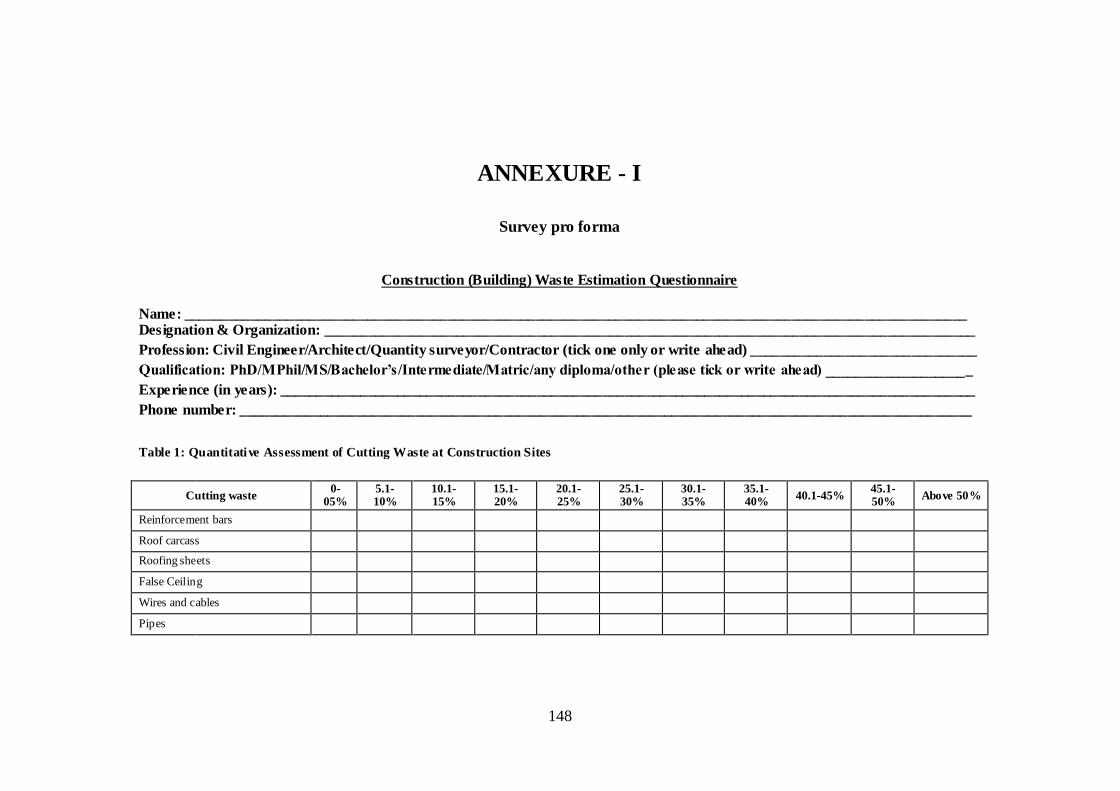
148
ANNEXURE - I
Survey pro forma
Construction (Building) Waste Estimation Questionnaire
Name: ___________________________________________________________________________________________________________ Designation & Organization: _________________________________________________________________________________________
Profession: Civil Engineer/Architect/Quantity surveyor/Contractor (tick one only or write ahead) _______________________________
Qualification: PhD/MPhil/MS/Bachelor’s/Intermediate/Matric/any diploma/other (please tick or write ahead) ____________________
Experience (in years): _______________________________________________________________________________________________
Phone number: ____________________________________________________________________________________________________
Table 1: Quantitative Assessment of Cutting Waste at Construction Sites
Cutting waste
0-05%
5.1-10%
10.1-15%
15.1-20%
20.1-25%
25.1-30%
30.1-35%
35.1-40%
40.1-45% 45.1-50%
Above 50%
Reinforcement bars
Roof carcass
Roofing sheets
False Ceiling
Wires and cables
Pipes

149
Table 2: Quantitative Assessment of Theft and Vandalism (T&V) Waste at Construction Sites
T & V Waste
0-
05%
5.1-
10%
10.1-
15%
15.1-
20%
20.1-
25%
25.1-
30%
30.1-
35%
35.1-
40% 40.1-45%
45.1-
50% Above 50%
Cement
Sand
Clay
Crushed stone
Wood/Timber
Wires and cables
Pipes
Wood preservatives
Reinforcement bars
Table 3: Quantitative Assessment of Transit Waste at Construction Sites
Transit waste
0-
05%
5.1-
10%
10.1-
15%
15.1-
20%
20.1-
25%
25.1-
30%
30.1-
35%
35.1-
40% 40.1-45%
45.1-
50% Above 50%
Blocks & Bricks
Window glazing
Prefabricated windows
Tiles
Ceramic sanitary appliances

150
Table 4: Quantitative Assessment of Applications Waste at Construction Sites
Application Waste
0-
05%
5.1-
10%
10.1-
15%
15.1-
20%
20.1-
25%
25.1-
30%
30.1-
35%
35.1-
40% 40.1-45%
45.1-
50% Above 50%
Paint
Mortar (cement + sand)
Concrete (cement + sand +
crushed stone)
POP Ceiling
Table 5: Source Identi fication (tick only one for each kind of waste)
Sources/reasons of wastage Cutting waste T & V Waste Transit waste Application Waste
Faulty or fancy design
Improper storage
Over ordering
Error in calculations/cutting
Poor material handling/operations
Poor planning
Transportation
In case of any confusion while filing up the questionnaire, please contact 0343-6206591

151
ANNEXURE – II
A: Construction site at Model Town Link Road Lahore
B: Casella Particulate Sampling System at Construction site at Model Town Link Road Lahore

152
ANNEXURE – III
A: HANNA Instruments Model # HI 9812 for measuring pH and electrical conductivity of samples
B: AAS (Perkin Elmer 1210) for determining concentrations of
Al, Ca, Ni, Fe and Zn samples

153
ANNEXURE – IV
HACH Spectrophotometer DR/2010 for determination of ions in dust samples

154
ANNEXURE V
A: Rawalpindi Islamabad Metrobus Project Layout
B: Rawalpindi Islamabad Metrobus Project Layout- Rawalpindi Area
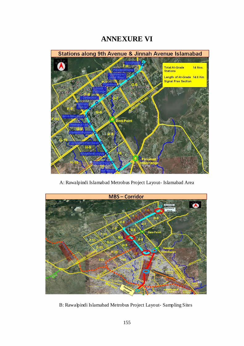
155
ANNEXURE VI
A: Rawalpindi Islamabad Metrobus Project Layout- Islamabad Area
B: Rawalpindi Islamabad Metrobus Project Layout- Sampling Sites

156
ANNEXURE – VII
A: Collecting SPM sample with High Volume Sampler Sibata HV 500F at
Rawalpindi Islamabad Metrobus Project
B: Particulate matter collected at filter paper

157
ANNEXURE – VIII
A: High Volume Sampler Sibata HV 500F installed at Rawalpindi Islamabad Metrobus Project Site
B: Construction site at Rehman Shaheed Road, Gujrat, for collecting samples of
SPM, PM10 and PM2.5 at varying distances from source of generation

158
ANNEXURE – IX
A: Construction site at Fazal Elahi Road (Gulyana Road), Kharian, for collecting samples of SPM. PM10 and PM2.5 at varying distances
B: DustTrak™ II Aerosol Monitor 8530 used for collection of
SPM, PM10, PM2.5 samples

159
ANNEXURE - X
Data Normality Tests of Physico-Chemical Characteristics
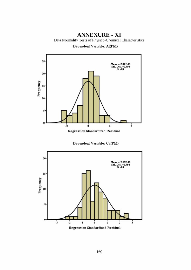
160
ANNEXURE - XI Data Normality Tests of Physico-Chemical Characteristics

161
ANNEXURE – XII Data Normality Tests of Physico-Chemical Characteristics

162
ANNEXURE – XIII Data Normality Tests of Physico-Chemical Characteristics
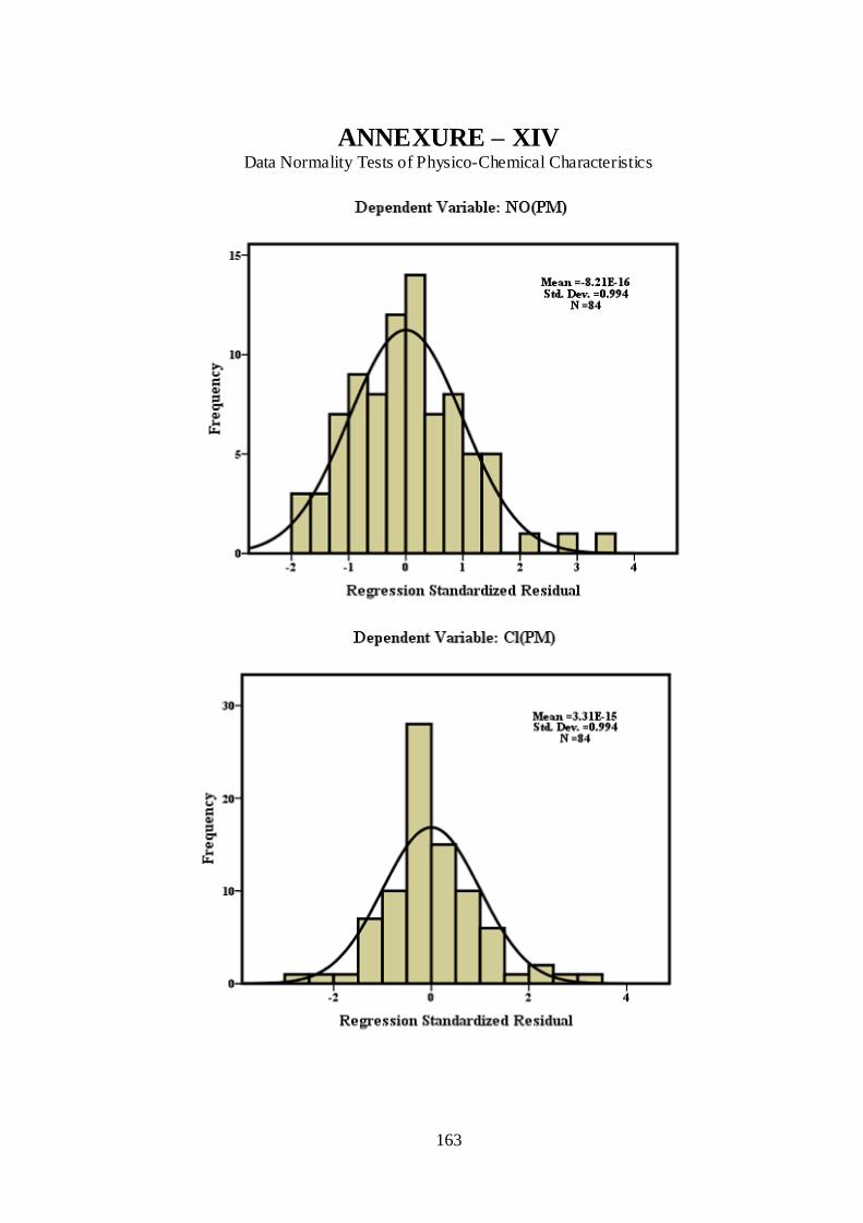
163
ANNEXURE – XIV Data Normality Tests of Physico-Chemical Characteristics

164
ANNEXURE – XV Data Normality Tests of Particulate Matter at Various Distances from Source

165
ANNEXURE – XVI Data Normality Tests of Particulate Matter at Various Distances from Source

166
ANNEXURE – XVII Data Normality Tests of Particulate Matter at Various Distances from Source

167
ANNEXURE – XVIII Data Normality Tests of Particulate Matter at Various Distances from Source

168
ANNEXURE – XIX Data Normality Tests of Particulate Matter at Various Distances from Source
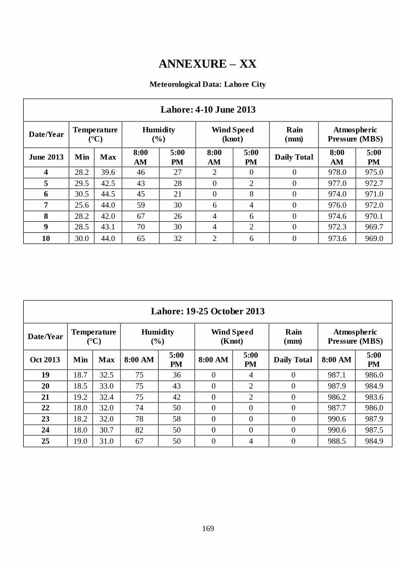
169
ANNEXURE – XX
Meteorological Data: Lahore City
Lahore: 4-10 June 2013
Date/Year Temperature
(°C)
Humidity
(%)
Wind Speed
(knot)
Rain
(mm)
Atmospheric
Pressure (MBS)
June 2013 Min Max 8:00
AM
5:00
PM
8:00
AM
5:00
PM Daily Total
8:00
AM
5:00
PM
4 28.2 39.6 46 27 2 0 0 978.0 975.0
5 29.5 42.5 43 28 0 2 0 977.0 972.7
6 30.5 44.5 45 21 0 8 0 974.0 971.0
7 25.6 44.0 59 30 6 4 0 976.0 972.0
8 28.2 42.0 67 26 4 6 0 974.6 970.1
9 28.5 43.1 70 30 4 2 0 972.3 969.7
10 30.0 44.0 65 32 2 6 0 973.6 969.0
Lahore: 19-25 October 2013
Date/Year Temperature
(°C)
Humidity
(%)
Wind Speed
(Knot)
Rain
(mm)
Atmospheric
Pressure (MBS)
Oct 2013 Min Max 8:00 AM 5:00
PM 8:00 AM
5:00
PM Daily Total 8:00 AM
5:00
PM
19 18.7 32.5 75 36 0 4 0 987.1 986.0
20 18.5 33.0 75 43 0 2 0 987.9 984.9
21 19.2 32.4 75 42 0 2 0 986.2 983.6
22 18.0 32.0 74 50 0 0 0 987.7 986.0
23 18.2 32.0 78 58 0 0 0 990.6 987.9
24 18.0 30.7 82 50 0 0 0 990.6 987.5
25 19.0 31.0 67 50 0 4 0 988.5 984.9

170
ANNEXURE – XXI
Meteorological Data: Lahore City
Lahore: 25-31 December 2013 - A
Date/Year Temperature
(°C)
Humidity
(%)
Wind Speed
(Knot)
Rain
(mm)
Atmospheric
Pressure (MBS)
Dec 2013 Min Max 8:00 AM 5:00
PM 8:00 AM
5:00
PM Daily Total 8:00 AM
5:00
PM
25 5.5 19.5 73 36 0 4 0 996.0 993.8
26 4.5 19.7 71 40 0 0 0 995.0 992.5
27 3.5 19.7 84 55 0 0 0 993.4 992.7
28 3.0 17.2 84 46 0 0 0 994.1 992.6
29 2.3 18.2 84 41 0 0 0 993.8 992.1
30 2.4 18.2 84 49 0 0 0 992.6 990.4
31 2.5 17.5 80 81 0 4 0 992.6 995.5
Lahore: 01-07 January 2014 - B
Date/Year Temperature
(°C)
Humidity
(%)
Wind Speed
(Knot)
Rain
(mm)
Atmospheric
Pressure (MBS)
Jan 2014 Min Max 8:00 AM 5:00
PM 8:00 AM
5:00
PM Daily Total 8:00 AM
5:00
PM
1 3.5 14.8 78 53 4 4 0 997.7 996.3
2 2.5 16.2 70 43 0 2 0 995.5 993.7
3 2.6 19.0 84 36 0 4 0 993.1 990.9
4 2.5 20.5 84 51 0 0 0 992.3 990.4
5 2.5 19.3 84 47 0 0 0 990.8 987.9
6 3.1 19.0 84 48 0 4 0 990.6 992.4
7 3.0 19.5 72 52 0 0 0 992.6 991.5

171
ANNEXURE – XXII
Meteorological Data: Lahore City
Lahore: 8-14 February 2014 - A
Date/Year Temperature
(°C)
Humidity
(%)
Wind Speed
(Knot)
Rain
(mm)
Atmospheric
Pressure (MBS)
Feb 2014 Min Max 8:00 AM 5:00
PM 8:00 AM
5:00
PM Daily Total 8:00 AM
5:00
PM
8 6.2 16.0 93 56 0 4 0 987.0 985.5
9 5.8 19.0 73 41 0 4 0 986.4 985.3
10 6.2 19.4 75 49 0 0 0 986.3 985.2
11 6.5 19.6 86 50 0 4 0 987.9 988.4
12 6.5 19.5 87 39 4 6 0 988.8 987.5
13 5.5 20.6 67 40 0 4 0 987.9 985.8
14 5.7 21.5 87 61 4 6 0 988.4 984.5
Lahore: 11-17 June 2014 - B
Date/Year Temperature
(°C)
Humidity
(%)
Wind Speed
(Knot)
Rain
(mm)
Atmospheric
Pressure (MBS)
June 2014 Min Max 8:00
AM
5:00
PM
8:00
AM
5:00
PM Daily Total
8:00
AM
5:00
PM
11 30.0 45.7 37 21 4 6 0 972.7 970.1
12 26.0 42.8 43 33 0 6 0 973.8 971.4
13 27.0 42.0 48 36 8 6 0 973.6 970.6
14 27.4 40.0 58 33 4 6 0 972.7 969.7
15 29.5 41.3 59 36 0 4 0 973.7 970.9
16 31.0 42.4 49 31 6 6 0 972.7 969.3
17 30.0 43.3 55 29 0 6 0 971.8 968.8
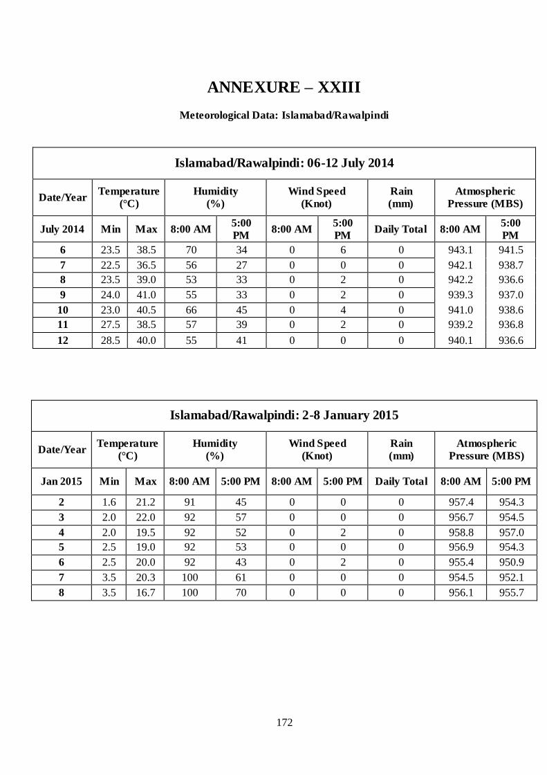
172
ANNEXURE – XXIII
Meteorological Data: Islamabad/Rawalpindi
Islamabad/Rawalpindi: 06-12 July 2014
Date/Year Temperature
(°C)
Humidity
(%)
Wind Speed
(Knot)
Rain
(mm)
Atmospheric
Pressure (MBS)
July 2014 Min Max 8:00 AM 5:00
PM 8:00 AM
5:00
PM Daily Total 8:00 AM
5:00
PM
6 23.5 38.5 70 34 0 6 0 943.1 941.5
7 22.5 36.5 56 27 0 0 0 942.1 938.7
8 23.5 39.0 53 33 0 2 0 942.2 936.6
9 24.0 41.0 55 33 0 2 0 939.3 937.0
10 23.0 40.5 66 45 0 4 0 941.0 938.6
11 27.5 38.5 57 39 0 2 0 939.2 936.8
12 28.5 40.0 55 41 0 0 0 940.1 936.6
Islamabad/Rawalpindi: 2-8 January 2015
Date/Year Temperature
(°C)
Humidity
(%)
Wind Speed
(Knot)
Rain
(mm)
Atmospheric
Pressure (MBS)
Jan 2015 Min Max 8:00 AM 5:00 PM 8:00 AM 5:00 PM Daily Total 8:00 AM 5:00 PM
2 1.6 21.2 91 45 0 0 0 957.4 954.3
3 2.0 22.0 92 57 0 0 0 956.7 954.5
4 2.0 19.5 92 52 0 2 0 958.8 957.0
5 2.5 19.0 92 53 0 0 0 956.9 954.3
6 2.5 20.0 92 43 0 2 0 955.4 950.9
7 3.5 20.3 100 61 0 0 0 954.5 952.1
8 3.5 16.7 100 70 0 0 0 956.1 955.7
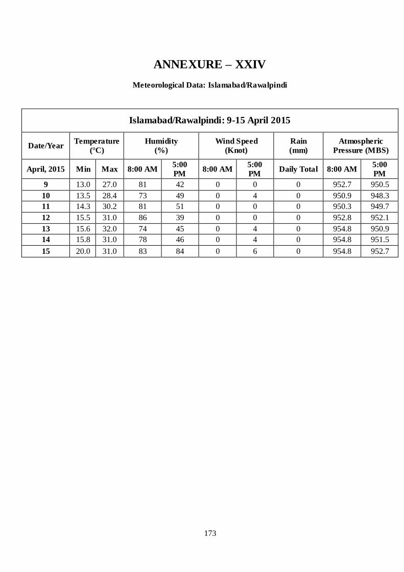
173
ANNEXURE – XXIV
Meteorological Data: Islamabad/Rawalpindi
Islamabad/Rawalpindi: 9-15 April 2015
Date/Year Temperature
(°C)
Humidity
(%)
Wind Speed
(Knot)
Rain
(mm)
Atmospheric
Pressure (MBS)
April, 2015 Min Max 8:00 AM 5:00
PM 8:00 AM
5:00
PM Daily Total 8:00 AM
5:00
PM
9 13.0 27.0 81 42 0 0 0 952.7 950.5
10 13.5 28.4 73 49 0 4 0 950.9 948.3
11 14.3 30.2 81 51 0 0 0 950.3 949.7
12 15.5 31.0 86 39 0 0 0 952.8 952.1
13 15.6 32.0 74 45 0 4 0 954.8 950.9
14 15.8 31.0 78 46 0 4 0 954.8 951.5
15 20.0 31.0 83 84 0 6 0 954.8 952.7

174
ANNEXURE – XXV
Meteorological Data: Gujrat City
Gujrat: 19-25 May 2015
Date/Year Temperature
(°C)
Humidity
(%)
Wind Speed
(Knot)
Rain
(mm)
May 2015 Min Max 8:00 AM 5:00 PM 8:00 AM 5:00 PM Daily Total
19 21.5 36.0 64 26 4 4 0.0
20 22.0 38.5 60 21 2 4 0.0
21 20.5 38.5 47 19 0 4 0.0
22 21.0 40.5 52 24 0 6 0.0
23 22.5 41.5 38 20 0 2 0.0
24 23.0 40.5 28 18 0 8 0.0
25 23.0 39.0 48 19 0 4 0.0
Gujrat: 13-19 June 2015
Date/Year Temperature
(°C)
Humidity
(%)
Wind Speed
(Knot)
Rain
(mm)
June 2015 Min Max 8:00 AM 5:00 PM 8:00 AM 5:00 PM Daily Total
13 24.0 40.5 61 43 4 6 0
14 23.0 35.0 66 39 6 6 0
15 22.0 35.5 67 54 4 2 0
16 22.5 34.0 58 31 2 4 0
17 24.0 39.5 59 24 0 4 0
18 24.5 41.0 49 26 6 6 0
19 26.0 42.0 36 32 6 8 0

175
ANNEXURE – XXVI
Meteorological Data: Gujrat City
Gujrat: 18-24 August 2015
Date/Year Temperature
(°C)
Humidity
(%)
Wind Speed
(Knot)
Rain
(mm)
Aug 2015 Min Max 8:00 AM 5:00 PM 8:00 AM 5:00 PM Daily Total
18 25.0 36.5 72 65 4 4 0.0
19 24.5 36.0 77 65 4 6 0.0
20 25.0 34.5 85 60 4 6 0.0
21 22.5 36.0 84 75 4 4 0.0
22 22.5 32.0 77 61 2 4 0.0
23 24.0 33.0 81 73 4 6 0.0
24 23.0 34.5 88 54 2 4 0.0

176
ANNEXURE – XXVII
Meteorological Data: Kharian City
Kharian: 26 May-01June 2015
Date/Year Temperature
(°C)
Humidity
(%)
Wind Speed
(Knot)
Rain
(mm)
May/June,
2015 Min Max 8:00 AM
5:00
PM 8:00 AM
5:00
PM Daily Total
26 21.5 36.0 64 26 4 4 0.0
27 22.0 38.5 60 21 2 4 0.0
28 20.5 38.5 47 19 0 4 0.0
29 21.0 40.5 52 24 0 6 0.0
30 22.5 41.5 38 20 0 2 0.0
31 23.0 40.5 28 18 0 8 0.0
1 23.0 39.0 48 19 0 4 0.0
Kharian: 17-24 November 2015
Date/Year Temperature
(°C)
Humidity
(%)
Wind Speed
(Knot)
Rain
(mm)
Nov, 2015 Min Max 8:00 AM 5:00 PM 8:00 AM 5:00 PM Daily Total
17 24.0 40.5 61 43 4 6 0
18 23.0 35.0 66 39 6 6 0
19 22.0 35.5 67 54 4 2 0
20 22.5 34.0 58 31 2 4 0
21 24.0 39.5 59 24 0 4 0
22 24.5 41.0 49 26 6 6 0
23 26.0 42.0 36 32 6 8 0

177
ANNEXURE – XXVIII
Measuring pH and electrical conductivity in the Laboratory

178
ANNEXURE – XXIX
Construction site at Rehman Shaheed Road, Gujrat City for sampling of SPM,
PM10 and PM2.5 at varying distances
Construction site at Fazal Elahi Road Kharian for sampling of SPM, PM10 and
PM2.5 at varying distances

179
ANNEXURE – XXX
Construction site at Model Town Link Road Lahore for sampling
of SPM, PM10 and PM2.5 at varying distances
Related Documents