Contract Structure, Risk Sharing, and Investment Choice Greg Fischer London School of Economics November 2012 Abstract Few micronance-funded businesses grow beyond subsistence entrepreneur- ship. This paper considers one possible explanation: that the structure of existing micronance contracts may discourage risky but high-expected return investments. To explore this possibility, I develop a theory that unies mod- els of investment choice, informal risk sharing, and formal nancial contracts. I then test the predictions of this theory using a series of experiments with clients of a large micronance institution in India. The experiments conrm the theoretical predictions that joint liability creates two potential ine¢ ciencies. First, borrowers free-ride on their partners, making risky investments without compensating partners for this risk. Second, the addition of peer-monitoring overcompensates, leading to sharp reductions in risk-taking and protability. Equity-like nancing, in which partners share both the benets and risks of more protable projects, overcomes both of these ine¢ ciencies and merits fur- ther testing in the eld. Keywords: investment choice, informal insurance, risk sharing, contract design, micronance, experiment. JEL Classication Codes: O12, D81, C91, C92, G21 Contact information: [email protected]. I would like to thank Esther Duo, Abhijit Banerjee, and Antoinette Schoar for advice and encouragement throughout this research. I am indebted to Shamanthy Ganeshan who provided outstanding research assistance. Daron Acemoglu, Oriana Bandiera, Tim Besley, Gharad Bryan, Robin Burgess, David Cesarini, Sylvain Chassang, Raymond Guiteras, Gerard Padr i Miquel, Rob Townsend, Tom Wilkening, and various seminar participants generously contributed many useful comments and advice. I am also grateful to the editor and three anonymous referees for providing thoughtful comments. In Chennai, the Centre for Micro Finance and the management and employees of Mahasemam Trust deserve many thanks. I gratefully acknowledge the nancial support of the Russell Sage Foundation, the George and Obie Shultz Fund, the National Science Foundations Graduate Research Fellowship, and the Economic and Social Research Councils First Grants Scheme.

Welcome message from author
This document is posted to help you gain knowledge. Please leave a comment to let me know what you think about it! Share it to your friends and learn new things together.
Transcript
Contract Structure, Risk Sharing, and InvestmentChoice
Greg Fischer∗
London School of Economics
November 2012
Abstract
Few microfinance-funded businesses grow beyond subsistence entrepreneur-ship. This paper considers one possible explanation: that the structure ofexisting microfinance contracts may discourage risky but high-expected returninvestments. To explore this possibility, I develop a theory that unifies mod-els of investment choice, informal risk sharing, and formal financial contracts.I then test the predictions of this theory using a series of experiments withclients of a large microfinance institution in India. The experiments confirmthe theoretical predictions that joint liability creates two potential ineffi ciencies.First, borrowers free-ride on their partners, making risky investments withoutcompensating partners for this risk. Second, the addition of peer-monitoringovercompensates, leading to sharp reductions in risk-taking and profitability.Equity-like financing, in which partners share both the benefits and risks ofmore profitable projects, overcomes both of these ineffi ciencies and merits fur-ther testing in the field.Keywords: investment choice, informal insurance, risk sharing, contract
design, microfinance, experiment.JEL Classification Codes: O12, D81, C91, C92, G21
∗Contact information: [email protected]. I would like to thank Esther Duflo, Abhijit Banerjee,and Antoinette Schoar for advice and encouragement throughout this research. I am indebtedto Shamanthy Ganeshan who provided outstanding research assistance. Daron Acemoglu, OrianaBandiera, Tim Besley, Gharad Bryan, Robin Burgess, David Cesarini, Sylvain Chassang, RaymondGuiteras, Gerard Padró i Miquel, Rob Townsend, Tom Wilkening, and various seminar participantsgenerously contributed many useful comments and advice. I am also grateful to the editor and threeanonymous referees for providing thoughtful comments. In Chennai, the Centre for Micro Financeand the management and employees of Mahasemam Trust deserve many thanks. I gratefullyacknowledge the financial support of the Russell Sage Foundation, the George and Obie ShultzFund, the National Science Foundation’s Graduate Research Fellowship, and the Economic andSocial Research Council’s First Grants Scheme.

1 Introduction
In 2005, designated the “International Year of Microcredit”by the United Nations,
microfinance institutions around the world issued approximately 110 million loans
with an average size of $340. The following year, Muhammad Yunus and Grameen
Bank received the Nobel Peace Prize for their efforts to eliminate poverty through mi-
crocredit. But while the provision of small, uncollateralized loans to poor borrowers in
poor countries may help alleviate poverty, there is little evidence that microfinance-
funded businesses grow beyond subsistence entrepreneurship. Few hire employees
outside their immediate families, formalize, or generate sustained capital growth.
This paper considers one possible explanation for this phenomenon: the structure
of existing microfinance contracts themselves may discourage risky but high-expected
return investments. Typical microfinance contracts produce a tension between mecha-
nisms that tend to reduce risk-taking, such as peer monitoring, and those that tend to
encourage risk-taking, such as risk-pooling. Much of the theoretical literature has fo-
cused on joint liability, a common feature in most microfinance programs, as a means
to induce peer monitoring and mitigate ex ante moral hazard over investment choice
(e.g., Stiglitz 1990, Varian 1990, Armendariz and Morduch 2005, Conning 2005). Un-
der joint liability, small groups of borrowers are responsible for one another’s loans.
If one member fails to repay, all members suffer the default consequences.
While this mechanism has been widely credited with making it possible, indeed
profitable, to lend to poor borrowers in poor countries, a growing literature critically
explores the relative merits of joint versus individual liability.1 There have long
been suspicions that peer monitoring may overcompensate and produce too little risk
relative to the social optimum (Banerjee, Besley, and Guinnane 1994). In particular,
joint liability compels an individual to bear the cost of her partner’s project when it
fails but does not mandate a compensating transfer upon success. This creates an
1When all decisions are taken cooperatively (Ghatak and Guinnane 1999) or when binding exante side contracts are feasible (Rai and Sjöström 2004) these mechanisms are identical; however,joint liability lending is most prevalent in settings where binding, complete contracts are not feasible.Madajewicz (2003, 2004) compares individual and group lending directly, focusing on monitoringcosts and the relationship between available loan size and borrower wealth, but this basic comparisonis diffi cult to make empirically. In practice, variation in loan types is likely the product of selectionon unobserved characteristics by either the borrower or the lender. Giné and Karlan (2011) overcomethis limitation with a large, natural field experiment that randomly assigned individuals into jointand individual liability loan contracts. They find no impact of joint liability on repayment ratesand some evidence that individual liability centers generated fewer dropouts and more new clients.
1
incentive to discourage risk-taking by others and thus joint liability may blunt the
entrepreneurial tendencies of borrowers.
At the same time, joint liability induces risk-pooling– not only does the threat of
common default induce income transfers to members suffering negative shocks, but
the repeated interactions of microfinance borrowers are a natural environment for
the emergence of informal risk sharing. This risk-pooling may increase borrowers’
willingness to take risk themselves. Moreover, the ability to share risk informally
allows borrowers whose risky projects succeed to compensate their partners for the
implicit insurance provided by joint liability. In doing so, it can mitigate the incen-
tives to discourage risk-taking. It is therefore critical to evaluate formal contracts in
an environment where informal risk sharing is possible.
To shed light on how microfinance contracts affect investment choices, this paper
develops a theoretical framework that unifies models of investment choice, informal
risk-sharing with limited commitment, and formal financial contracts in order to
illustrate a range of theoretical effects and motivate a series of empirical tests. It
then implements a corresponding experiment with actual microfinance clients in India.
The theoretical framework builds on a simple model of informal risk-sharing in
the spirit of Coate and Ravallion (1993) and Ligon, Thomas, and Worrall (2002).2
In this model, two risk-averse individuals receive a series of income draws subject
to idiosyncratic shocks. In the absence of formal insurance and savings, they enter
into an informal risk-sharing arrangement that is sustained by the expectation of
future reciprocity. I enrich this model by endogenizing the income process, allowing
agents to optimize their investment choices in response to the insurance environment.
Contrary to much of the static investment choice literature in microfinance, in this
model risky projects generate higher expected returns than safe projects, reflecting
the natural assumption that individuals must be compensated for additional risk with
additional returns.3 On this framework I then overlay formal financial contracts. I
2An extensive empirical literature documents the importance of informal insurance arrangementsas a risk management tool for those who lack access to formal insurance markets (e.g., Townsend1994, Udry 1994, Foster and Rosenzweig 2001, Fafchamps and Lund 2003, Fernando 2006). Taken asa whole, the empirical evidence suggests that informal risk coping strategies do not achieve full riskpooling even though in some cases they perform remarkably well. This paper adds to an emergingexperimental literature (Barr and Genicot 2008, Robinson 2008, Charness and Genicot 2009) thatuses the precise control possible in an experimental setting to understand how such mechanismswork in practice.
3Following Stiglitz (1990), most theoretical work in microfinance has assumed that riskier invest-ments represent at best a mean-preserving spread of the safer choice and often generated a lower
2
consider in turn individual liability, joint liability, and an equity-like contract in which
all investment returns are shared equally.
The model illustrates two opposing influences of joint liability on investment
choice. Mandatory transfers from one’s partner encourage greater risk-taking by
partially insuring against default. Risk-taking borrowers may compensate their part-
ners for this insurance with increased transfers when risky projects succeed, or they
may “free-ride,”forcing their partners to insure against default without compensating
transfers. The parallel need to provide this insurance counters the risk-encouragement
effect of receiving it, and relatively risk-averse individuals may elect safer investments
to avoid joint default should their partners’projects fail.
The theoretical analysis also produces two important supporting results. First, it
demonstrates that joint liability contracts may crowd out informal insurance. By ef-
fectively mandating income transfers to assist loan repayment, joint liability eases the
sting of punishment and can make cooperation harder to sustain. Second, informal
insurance tends to increase risk-taking. Contrary to standard risk-sharing models,
this has the surprising implication that we may find more informal insurance among
risk-tolerant individuals whose willingness to take riskier investments expands their
scope for cooperation.
While these models offer useful insights, in the context of repeated interactions
they produce a multiplicity of equilibria, and theory alone can provide only partial
guidance regarding the likely consequences of informal insurance and formal contracts
for investment behavior. To shed further light on these questions, I conducted a series
of experiments with actual microfinance clients in India. The experiments capture the
key elements of the theoretical framework and the microfinance investment decisions
it represents. Based on extensive piloting, I designed the games to be easily un-
derstood by typical microfinance clients– project choices and payoffs were presented
visually, all randomizing devices used common items and familiar mechanisms (e.g.,
guessing which of an experimenter’s hands held a colored stone), and game money
was physical– and confirmed understanding at numerous points throughout the ex-
periment. Individuals were matched in pairs that dissolved at the end of each round
with a 25% probability in order to simulate a discrete-time, infinite-horizon model
with discounting. In each round, subjects could use the proceeds of a “loan”to invest
expected return. Examples include Morduch (1999), Ghatak and Guinnane (1999), and de Aghionand Gollier (2000).
3

in one of several projects that varied according to risk and expected returns. Returns
were determined through a simple randomizing device, after which individuals could
engage in informal risk-sharing by transferring income to their partners. In order to
play in future rounds, subjects needed to repay their loans according to the terms of
a formal financial contract, which I varied across treatments.
I considered five contracts: autarky, individual liability, joint liability, joint lia-
bility with a project approval requirement, and an equity-like contract in which all
income was shared equally. Much of the microfinance literature assumes a local
information advantage; therefore, to test the role of information, I conducted each
of the treatments under both perfect monitoring, where all actions and outcomes
were observable, and imperfect public monitoring, where individuals observed only
whether their partner earned suffi cient income to repay her loan. At the end of the
experiment, one period was randomly selected for cash payment.4
A laboratory-like experiment allows precise manipulation of contracts, informa-
tion, and investment returns to a degree that would be impractical for a natural field
experiment. Moreover, even in carefully constructed field experiments, low periodic-
ity, long lags to outcome realization, fungibility of investment funds and measurement
issues associated with micro-business data complicate the use of investment choice as
an outcome variable.5 An experiment overcomes each of these challenges. While
the use of an experiment entails a trade-off between control and realism, I attempted
to maximize external validity with meaningful payoffs of up to one week’s reported
income, subjects drawn from actual microfinance clients, and an experimental de-
sign that closely simulates the underlying theory. This approach builds on Giné,
Jakiela, Karlan, and Morduch (2009), which pioneered the use of laboratory exper-
iments with a relevant subject pool in order to unpack the effects of various design
features in microfinance contracts.
The core experimental result is that joint liability produced significant free-riding.
Risk-tolerant individuals, as measured in a benchmarking risk experiment, took signif-
icantly greater risk under joint liability with imperfect monitoring. Yet the transfers
4As described in Charness and Genicot (2009), this payment structure prevents individuals fromself-insuring income risk across rounds. The utility maximization problem of the experiment corre-sponds to that of the theoretical model.
5Giné and Karlan (2011), for example, were able to randomize across joint and individual loancontracts with a partner bank in the Philippines. They find no difference in default rates and fasterexpansion of the client base under individual liability but are unable to evaluate investment behavior.
4
they made when successful did not increase with the riskiness of their investments
or the expected default burden they placed on their partners. Increased risk-taking
was not evident under joint liability with perfect monitoring, and when individuals
were given explicit approval rights over their partners’investment choices, risk-taking
fell below that observed in autarky. Together, these results indicate that increased
risk-taking was not the product of cooperative insurance. They also suggest that
peer monitoring mechanisms, as embodied in explicit project approval rights, not
only prevent ex ante moral hazard but more generally discourage risky investments,
irrespective of whether or not such risks are effi cient. This may in part explain why
we see little evidence that microfinance-funded businesses grow beyond subsistence
entrepreneurship. It may also help us reconcile some of the anecdotal evidence on
the limits of joint liability and the increasing willingness of microfinance institutions
to consider contracts other than joint liability.6
The equity-like contract increased risk-taking and expected returns relative to
other contracts while at the same time producing the lowest default rates. Increased
risk was almost always hedged across borrowers, with the worst possible joint outcome
still suffi cient for loan repayment. These results are encouraging and suggest that
equity-like contracts merit further exploration in the field.
It is worth emphasizing that both the theory and experiment abstract from effort,
willful default, partner selection, and savings. This is not meant to imply that any of
these factors is unimportant.7 Instead, the purpose is to isolate the elements of risk-
sharing, investment choice, and formal contracts and to explore their implications.
The rest of this paper is organized as follows. Section 2 develops the model
of informal risk-sharing with formal financial contracts and endogenous investment
6In 2002, Grameen Bank in Bangladesh introduced the Grameen Generalized System, typicallyreferred to as Grameen II, which, among other features, formally eliminates joint financial liability.BancoSol, a large and well-known Bolivian microfinance institution, has moved much of its portfolioto individual loans. For anecdotal evidence on the limits of joint liability see, for example, Woolcock(1999) and Montgomery (1996).
7The theory of strategic default on microfinance contracts is explored in Besley and Coate (1995)and Armendariz (1999), while Armendariz and Morduch (2005) and Laffont and Rey (2003) bothtreat moral hazard over effort in detail. To the best of my knowledge, neither area has seen carefulempirical work in the context of microfinance. Similarly, the empirical implications of savings forinformal risk sharing arrangements remain poorly understood. Bulow and Rogoff’s (1989) model ofsovereign debt implies that certain savings technologies can unravel relational contracts, includinginformal insurance. Ligon, Thomas, and Worrall (2000) consider a simple storage technologyand find that the ability to self-insure can crowd out informal transfers, with ambiguous welfareimplications.
5

choice. Proofs are contained in Appendix B, unless otherwise noted. Section 3
describes the experimental design, and Section 4 presents the experimental results.
Section 5 concludes.
2 AModel of Investment Choice and Risk Sharing
The primary aim of this section is to illustrate important theoretical effects of formal
financial contracts and informal risk-sharing arrangements on investment choices and
to motivate a series of empirical tests. While the theoretical setting is distilled to
just those elements necessary to frame the informal risk-sharing and investment choice
problem, the economic environment remains quite complex. Multiple equilibria, is-
sues of equilibrium selection, and the importance of assumptions about the structure
of information and beliefs limit the ability to make general propositions. However,
restrictions to the particular economic environment modeled in the experiment will
allow some concrete empirical predictions derived from theory and numerical simu-
lations and, where such predictions are not sharp, to frame the theoretical effects
influencing behavior.
2.1 Overview of the Economic Environment
Consider a world where two individuals make periodic investments that are funded by
outside financing. Each period, they each allocate their investment between a safe
project that generates a small positive return with certainty or a risky investment
that may fail but compensates for this risk by offering a higher expected return.
Formal financial contracts govern individuals’ability to borrow and hence their
investment opportunities. These formal financial contracts specify the availability of
borrowing as a function of past outcomes, repayment terms, and the feasible range
of income transfers between agents. Their terms are set by a third party before the
start of the game and are constant throughout the game.8 The analysis considers four
principle types of formal financial contracts: autarky, individual liability, joint liabil-
ity and quasi-equity, which is equivalent to joint liability with third-party enforced
equal sharing of all income. The individual and joint liability contracts capture
8This maps to the experimental setting where formal financial contracts are the key dimensionof experimental variation and exogenously imposed for each game.
6
key elements of micro-lending contracts that exist in practice. The other two are
counterfactual and provide benchmarks for risk-sharing arrangements, with practical
implications discussed more fully in Section 4. All four are described in more detail
below.
Individuals are risk averse, but they cannot save and lack access to formal insur-
ance. In order to maximize utility they therefore enter into an informal risk-sharing
arrangement that may extend beyond any sharing rules specified in the formal con-
tract. This informal arrangement is not legally enforceable and must therefore be
self-enforcing: an individual will transfer no more than the discounted value of what
she expects to get out of the relationship in the future.
Throughout, I consider two monitoring environments: perfect monitoring, where
all investment choices and income realizations are observable, and imperfect public
monitoring, where each player observes only her own actions and income realizations
as well as the transfers made by her partner.
2.2 The Economic Environment
I model the economic environment described above using a discrete-time, infinite-
horizon economy with two agents indexed by i ∈ {A,B} and preferences
E0∞∑t=0
δtui(ci,t)
at time t = 0, where E0 is the expectation at time t = 0, δ ∈ (0, 1) is the discount
factor, ci,t ≥ 0 denotes the consumption of agent i at time t, and ui represents agent
i’s per-period von Neumann-Morgenstern utility function, which is assumed to be
nicely behaved: u′i(c) > 0, u′′i (c) < 0 ∀c > 0 and limc→0 u′i(c) = ∞. In the notation
that follows, I suppress the time and agent indicators where not required for clarity.
This remainder of this section describes the three components of the game struc-
ture: the stage game, the dynamic game, and formal financial contracts.
Stage Game. The stage game depends on a state variable, {DA, DB}, that indi-cates the amount of borrowing available to each agent and evolves according to a
deterministic transition function that is set by the formal financial contract as de-
scribed below. In every stage game, player i chooses an action ai = (αi, τ i), which
7

specifies an investment allocation and transfer. These actions are played in steps 2
and 4 of the stage game, respectively. Each stage game proceeds as follows:
1. Players begin the stage game with a formal financial contract in place. Each
individual has zero wealth and access to a loan Di, where the amount of this
loan is specified by the formal financial contract, described below. In describing
the stage game, I will proceed by considering the case in which Di = D for both
players.
2. From her total capital, Di, each individual allocates a share αi ∈ [0, 1] to a
risky investment that with probability π returns R for each unit allocated and
0 otherwise. The remainder, 1 − αi, she allocates to a safe investment that
returns S ∈ [1, Rπ) with certainty. Denote by θi ∈ {h, l} individual i’s staterealization. When the risky project succeeds (θi = h), individual i’s total income
is yhi (αi, Di) = {αiR + (1− αi)S}Di. When the risky project fails (θi = l), her
income is yli(αi, Di) = {(1 − αi)S}Di. Note that π is fixed: the probability of
success is identical and independent across players and periods.
3. The state of nature is realized and each individual receives her income, yi.
Denote by θ = (θA, θB) the state of nature, such that for any state θ, (yA, yB) =
(yθAA , yθBB ). For notational simplicity I write the four states of nature as Θ =
{hh, hl, lh, ll}.9
4. Each individual chooses to transfer an amount τ i ∈ T fi ≡ [τ i, τ i] to her partner,
where the feasible range is specified by the formal financial contract and any
transfers above τ i are voluntary. Income after transfers is yi = yi − (τ i − τ−i).
5. Loan repayment is determined mechanically: Pi = min(Di, yi). There is no
willful default.
6. Agents consume. Because agents cannot save, the specified loan repayment
uniquely determines consumption for the period: ci = yi − (τ i − τ−i)− Pi.
Dynamics. Consider an infinite repetition of the stage game where preferences
and discounting are as described above. Players’ access to loans in step 1 of the
stage game, {DA,t, DB,t}, is given by a deterministic transition function that is set9These states occur with probability π2, π(1− π), π(1− π), and (1− π)2, respectively.
8
by the formal contract, detailed below. As with actual microfinance contracts, an
individual’s ability to borrow in the current period is a function of past borrowing
and repayment.
Let ai,t = (αi,t, τ i,t) denote the action played by player i and θt ∈ Θ denote
the state of nature realized in period t. In games of imperfect public monitoring,
each player observes only her own actions and income realizations as well as the
transfers made by her partner. Player i’s private history up to period t is given
by hti ≡ {ai,t′ , τ−i,t′ , θi,t′}t−1t′=0; h0i is the empty set. Agents have observed more when
choosing their transfer in step 4 of the stage game than when choosing the preceding
investment: player i’interim private history in period t, hti, is the concatenation of
hti and {αi,t, θi,t}. For each t ≥ 0, H ti is the set of all h
ti; define H
ti analogously.
Based on the history of observed transfers, agents form beliefs, µ(·), about the fullhistory of investment choices and income realizations. In games of perfect monitoring,
all investment choices and income realizations are observable, and a public history
ht ≡ {ai,t′ , a−i,t′ , θt′}t−1t′=0 is a list of t action profiles identifying the actions played and
the state of nature in periods 0 through t− 1. The interim public history in period
t, ht, is the concatenation of ht and {αi,t, α−i,t, θt}. With h0 equal to the empty set,for each t ≥ 0, H t is the set of all ht; define H t analogously. Let Hi =
⋃∞t=0H
ti and
define Hi, H, and H analogously.
Formal Financial Contracts. I consider the above game under four different for-
mal financial contracts. Each game begins with a formal contract in place that spec-
ifies three rules, which are fixed throughout each game: (1) a deterministic transition
function that determines the availability of borrowing (Di,t) based on prior period re-
payment (Pi,t−1 and P−i,t−1) and borrowing (Di,t−1 and D−i,t−1); (2) a feasible range
of transfers, T fi ≡ [τ i, τ i], from each individual as a function of each individual’s in-
come, yi and y−i; and (3) loan repayment (Pi) as a function of income after transfers,
yi. For all contracts, both individuals begin with access to a loan: DA,0 = DB,0 = D.
I also normalize the interest rate on all loans to zero and exclude the possibility of
willful default or ex post moral hazard– an individual will always repay if she has
suffi cient funds– in order to focus on investment choice and risk-sharing behavior:
Pi = min(Di, yi).
Under autarky, an individual can borrow in the subsequent period if and only if
she repays her own loan in the current one: Di,t+1 = D if and only if Pi,t = Di,t = D.
9
Individuals cannot make income transfers: T fi = {0}.Under individual liability, an individual can borrow in the subsequent period if
and only if she repays her own loan in the current one: Di,t+1 = D if and only if
Pi,t = Di,t = D. Individuals can make voluntary income transfers: T fi = [0, yi].
Under joint liability, an individual can only borrow in the subsequent period if
both she and her partner repaid their loans in the current period: Di,t+1 = D if and
only if Pi,t = Di,t = D for i ∈ {A,B}. If either individual has insuffi cient funds torepay her loan, her partner must help if she can. Additional voluntary transfers are
possible: T fi = [max(min(yi −Di, D−i, y−i), 0), yi].
Under the equity contract, as with joint liability, an individual can only borrow
in the subsequent period if both she and her partner repaid their loans in the current
period. Individuals must share their income equally before any voluntary transfers:
T fi = [12yi, yi].
2.3 Strategies and Equilibria
Strategies and Restrictions. A pure strategy for player i, σi, is a mapping from
all possible histories into the set of actions, Ai, with typical element ai. There are
two components to an action: an investment choice, αi, and a transfer, τ i. Strategies
map from H t into investment choices and from H t into transfers in games of perfect
monitoring and from H ti and H t
i in games of imperfect public monitoring. Ui(σ)
is i’s expected, discounted utility of strategy σ, where the expectation is taken over
histories. In addition to the standard requirements for a perfect Bayesian equilibrium,
I will consider equilibria whose strategies exhibit certain properties.
First, as is standard in the literature on informal insurance, the informal risk-
sharing arrangement is supported by trigger strategy punishments. If either party
reneges on the informal insurance arrangement, both members revert to the mini-
mum transfer profile, i.e., they exit the informal insurance arrangement in perpetuity
and make only those transfers required by the formal contract. Note that I assume
no direct punishment; the only consequence for reneging on the informal risk-sharing
arrangement is exclusion from further informal insurance possibilities. Second, im-
mediately subsequent transfers are the only future actions conditioned on investment
choices. This precludes, for example, both punishment based on prior investment
10
choices and using investment choices to punish.10
Third, I restrict attention to strategies where, outside any punishment phase,
transfers are only a function of current income realizations. Whenever the same
income, (yA, yB), is realized, the same transfers are made.11 ,12
To summarize, for each player there is an equilibrium-path investment level, αe,
and a punishment-path investment level, αp. Deviations from these investment lev-
els have no implications for continuation play. For each player, there is also an
equilibrium-path transfer rule that gives period-t transfers as a function of period-t
realized incomes only– in particular, transfers are not a function of period-t invest-
ment levels– and a punishment-path transfer that prescribes the minimum transfer
profile allowed by the financial contract in each period.
Informal Insurance Arrangements. An informal insurance arrangement, T (αA, αB),
specifies the net transfer from A to B for any state of nature θ given individuals’al-
locations to the risky asset (αA, αB). Since individuals are risk averse and πR > S,
in autarky both individuals will allocate an amount αi ∈ (0, 1] to the risky asset.
Because αi > 0, there exist at least two states of the world where the autarkic ratios
of marginal utilities differ, and individuals will have an incentive to share risk. I
10Based on pilot results, I choose to restrict attention to equilibria that do not condition oninvestment choices as this appears to more accurately reflect participants’behavior. Participantsdescribed their partners’behavior as untrustworthy, unfair, or non-cooperative when they failed tomake certain transfers conditional on their outcome and not based on their investment choices. Thosemaking risky investments were described as non-cooperative only if they failed to make significanttransfers when their investments succeeded.11Ligon, Thomas, and Worrall (2002) demonstrate that conditioning current transfers on the past
history of transfers, what they call the dynamic limited commitment model, increases the scope forinsurance. Adding a debt-like component to transfers, which they model as an evolution of thePareto weight in favor of the transferring partner, can relax her incentive compatibility constraint.In any period, the debt repayment element from an individual who has received transfers in the pastcan more than offset the static risk-sharing (insurance) component. This could lead to misleadingconclusions about the extent of informal insurance in any single period after the first; however, inexpectation, the dynamic model simply expands the equilibrium set. The model in which transfersare only a function of current income realizations, what Ligon, Thomas and Worrall refer to asthe static limited commitment model, therefore represents a conservative and analytically tractableframework in which to interpret experimental results where transfer behavior is averaged over allobservations.12In the empirical analysis, I restrict attention to transfers generating effi cient payoff vectors in
which the Pareto weight is equal to the ratio of marginal utilities in autarky. This restriction impliesthat if both individuals make the investment allocation that would be optimal in autarky, regardlessof their risk preferences, transfers occur only when one project succeeds and one project fails (stateshl and lh).
11
assume individuals can enter into an informal risk-sharing arrangement supported by
the expectation of future reciprocity. Conditional on individuals’allocations to the
risky asset, the vector Ti = (τhhi , τhli , τ
lhi , τ
lli ) specifies the transfer from i to −i in each
state of the world, and the vector T = TA−TB fully specifies the transfer arrangement.The minimum transfer profile describes the transfer vector in which individuals make
only those transfers required by the formal financial contract. Note that although
individuals may choose not to make any voluntary (informal) transfers, they are still
subject to the transfer requirements, if any, of the formal financial contract.13
With the restrictions on strategies described above, incentive compatibility re-
quires that in any state of the world the discounted future value of remaining in the
informal insurance arrangement must be at least as large as the potential one-shot
gain from deviation, i.e.,
u(yθi − τ θi + τ θ−i) ≥ u(yθi )− δ(
Vi(α, T )
1− δ Pr[Ri|α, T ]− Vi(α
p, 0)
1− δ Pr[Ri|αp, 0]
), (1)
where Pr[Ri|α, T ] is the probability that individual i meets the repayment terms of
her formal financial contract (as described above) conditional on investment choice
α and transfer arrangement T ; VA(αp, 0) = πu(yh(αp, D)) + (1 − π)u(yl(αp, D)),
A’s expected per-period autarkic utility; VA(α, T ) = π2u(yh(α,D) − τhh) + π(1 −π)u(yh(α,D)−τhl)+π(1−π)u(yl(α,D)−τ lh)+(1−π)2u(yl(α,D)−τ ll), A’s expectedper-period utility with investment choice α and transfer arrangement T ; and B’s
utility is defined analogously.
When formal contracts specify a minimum transfer τ θ in state θ, I modify the
constraint accordingly:
u(yθi−τ θi+τ θ−i) ≥ u(yθi−τ θi+τ θ−i)−δ(
Vi(α, T )
1− δ Pr[Ri|α, T ]− Vi(α
p, T )
1− δ Pr[Ri|αp, T ]
), (2)
where T = (τhh, τhl, τ lh, τ ll), the minimum transfer profile.
Definition 1 (Implementability) For an investment allocation (αA, αB), a trans-
fer arrangement, T , is implementable if and only if it satisfies both agents’incentive13In the case of individual liability, the minimum transfer profile is analogous to reversion to
autarky. I choose an alternative designation here to avoid confusion with the autarky contract andto highlight the fact that in the joint liability and equity contracts even agents who exit the informalinsurance arrangement may still be required to make transfers in certain states.
12
compatibility constraints in all states, i.e., (2) holds for i ∈ {A,B} and ∀θ.
Equilibrium. I will concentrate on perfect Bayesian equilibria with the restrictions
described above. In games of perfect monitoring, the set of relevant histories is the
set of all h ∈ H ∪ H; in games of imperfect public monitoring, this is the set of allh ∈ Hi ∪ Hi. I define a restricted perfect Bayesian equilibrium (RPBE) as a strategy
profile σ∗ and beliefs µ(·) such that for all players i, all relevant histories h, and allalternative strategies σ
′i (i) the incorporated transfer profiles are implementable, (ii)
Ui(σ∗i |h, µ(h)
)≥ Ui
(σ′i, σ∗−i|h, µ(h)
), i.e., investment choices and transfer profiles are
optimal conditional on beliefs, (iii) beliefs are updated according to Bayes’rule where
applicable, and (iv) the immediately subsequent transfers are the only future actions
conditioned on investment choices. As described above, this restricts attention to
equilibria in which, outside any punishment phase, transfers are only a function of
current income realizations.
In games of perfect monitoring, where investment choices and income are ob-
servable, these equilibria simplify to subgame perfect equilibria as is standard in
the theoretical literature on informal insurance. Following previous literature, I will
concentrate on payoff vectors that are Pareto effi cient within the set of equilibrium
payoffs.14 That is, individuals’strategies and beliefs must constitute an RPBE and
solve maxα,T UA(σ) + λUB(σ), where λ is the Pareto weight placed on B.
2.4 The Impact of Contracts and Monitoring on Informal
Risk-Sharing
The following two sections develop predictions generated by the preceding model.
This section explores the effects of monitoring and contracts on informal risk-sharing,
and Section 2.5 concerns risk-taking decisions. They provide a framework for inter-
preting the experimental results presented in sections 4.1 and 4.2, respectively. This
section divides the discussion of informal risk-sharing into two branches. First, I
examine the role of monitoring. Much of the literature on microfinance discusses the
importance of peer monitoring and local information,15 and the experimental setting
14Of course, we could observe transfers inside the frontier. The empirical setting allows me to testthe practical applicability of this convention, and Section 4.1 describes the results of these tests.15Among the numerous examples are Banerjee, Besley, and Guinnane (1994), Stiglitz (1990),
Wydick (1999), Chowdhury (2005), Conning (2005), Armendariz (1999), and Madajewicz (2004).
13

was designed to test their importance by evaluating each contract with and without
perfect monitoring. Second, I examine the role of financial contracts themselves,
focusing on the differences between individual and joint liability.
Monitoring. Standard models of informal insurance assume perfect monitoring;
however, in practice, even when agents know one another well, this assumption is
unlikely to hold. A full characterization of the equilibria that are Pareto effi cient
under imperfect monitoring is sensitive to a number of assumptions. I will consider
symmetric equilibria, in the sense that punishment takes the form of reversion to
the minimum transfer profile, which punishes both parties. The result is ineffi ciency.
Since mutual punishments are ineffi cient and this punishment occurs with positive
probability, the set of sustainable transfer arrangements is bounded away from the
perfect-monitoring frontier.16
With imperfect public monitoring, at the time of making her transfer an individual
knows only her own private history. Her partner’s income is never revealed. Under
a cooperative transfer regime, she chooses a pure strategy T′i = (τhi , τ
li), where the
superscript denotes her own outcome. Her partner does likewise. We can assess the
effect of imperfect public monitoring by determining if the transfer profiles, T′A and T
′B,
that would implement a constrained effi cient equilibrium under perfect monitoring,
T ∗, are themselves implementable under imperfect public monitoring.17 If τh > τ l
is to be incentive compatible, an individual who transfers τ l must be punished with
some positive probability p. Because of imperfect monitoring, punishment cannot
be conditioned on income realization. This leads to the following prediction, which
section B.2 discusses in more detail:
Prediction 1 (monitoring and informal insurance) Fix the Pareto weight, λ.Then the RPBE with perfect monitoring features transfers at least as large as the
RPBE with imperfect monitoring. If the incentive compatibility constraint is binding
in the RPBE with perfect monitoring, i.e., the transfer arrangement does not achieve
16This intuition is consistent with the work of Green and Porter (1984). Radner, Myerson, andMaskin (1986) study a model of partnership games in which every equilibrium (symmetric and not)is ineffi cient, while Fudenberg, Levine, and Maskin (1994) identify conditions under which thereexist approximately effi cient equilibria.17Note that only strategies T = (τhh, τhl, τ lh, τ ll) where τhl+ τ lh = τhh+ τ ll are replicable under
limited information.
14
full insurance, then transfers in the RPBE with perfect monitoring are strictly larger
than those in the RPBE with imperfect monitoring.
Formal Financial Contracts. I now turn to the effect of joint liability on informal
insurance. Joint liability will affect the set of informal insurance arrangements that
are consistent with an RPBE through its effect on the implementability constraint in
equation (2). When neither party takes default risk, joint liability does not require
transfers in any state of nature and will not affect the set of implementable trans-
fers. However, when both agents have the potential for default and the transfers
required by joint liability improve both individuals’expected utility from the min-
imum transfer profile, V (αp, T ), the scope for punishment by exiting the informal
insurance arrangement is reduced. In those states where transfers are not required
by the contract, this will tighten the incentive compatibility constraint in (2) and re-
duce the maximum implementable transfers. The effect in states where transfers are
required is more nuanced, with the reduced scope for punishment offset by a smaller
gain from immediate deviation as well as the direct effect of the mandatory transfer
itself. Similar offsetting effects occur when only one individual takes default risk.
In this case, the risk-taking individual’s utility increases relative to individual liabil-
ity without voluntary transfers– she benefits from the mandatory insurance of joint
liability– reducing her willingness to make informal transfers. The reverse holds for
her partner, and the net effect is ambiguous. For games of perfect monitoring, these
effects are summarized in the following prediction, which is discussed in more detail
in Section B.2.
Prediction 2 (joint liability and informal insurance) Fix the Pareto weight, λ,and consider a game of perfect monitoring and an RPBE under individual liability
(T= 0) in which the transfer profile, T , implements a constrained effi cient RPBE.
The addition of joint liability (T 6= 0) exerts four opposing effects on the transfer
profile, T ′, that implements a constrained effi cient RPBE: (i) by mandating trans-
fers from one’s partner (∃θ s.t. τ−i > 0), joint liability increases an agent’s utility
from the non-cooperative (punishment) equilibrium. This reduces the scope for pun-
ishment and therefore reduces the agent’s maximum incentive compatible transfers;
(ii) by mandating transfers to one’s partner (∃θ s.t. τ i > 0), joint liability reduces
an agent’s utility from the non-cooperative equilibrium and hence increases the max-
imum incentive compatible transfers; (iii) when transfers are required joint liability
15

reduces the scope for immediate deviation (if τ i > 0 then u(yi−τ i+τ−i) > u(yi)) and
therefore increases the maximum incentive compatible transfers; (iv) in states of the
world where transfers are required for debt repayment, joint liability can mechanically
increase transfers. The net effect of these forces depends on the specific parameters
and individual preferences.
To motivate further the empirical tests, we can solve numerically for specific pa-
rameter values relevant to the empirical setting in order to describe the payoff vectors
that are Pareto effi cient in the set of equilibrium payoffs.18 The incentive compatibil-
ity constraints in (1) and (2) describe a set of constrained-effi cient risk transfers with
each point determined by the relative weight assigned to each agent by the social
planner. As a benchmark, I selected a single point on this frontier using a Pareto
weight, λ, equal to the ratio of marginal utilities in state hh under autarky.19 A clear
pattern emerges from the numerical simulations. For the parameter values used in
the experiment, joint liability generally crowds out informal insurance when at least
one individual takes default risk. For example, consider two individuals with con-
stant relative risk aversion, u(c) = c(1−ρ)/(1−ρ), and risk aversion parameters of 0.52
and 0.39 who allocate 0.375 and 0.625 to the risky asset, respectively.20 Individual li-
ability supports a transfer from the individual taking more risk of approximately 30%
18See Section 3 for a detailed description of the experimental setting. It maps closely to theenvironment with parameter values S = 1, R = 3, D = 1, δ = 0.75, and π = 0.5; however, asexplained therein, subjects were presented with eight discrete investment choices rather than thecontinuous allocation problem described here.19I set λ = λ0 ≡ u
′
A(αA(R − S) + S − D)/u′B(αB(R − S) + S − D), where αA and αB are theactual investment choices made by each agent. If this weight did not admit a non-zero, individually-rational transfer arrangement irrespective of the incentive compatibility constraints, I set λ to theclosest value of λ that would. Specifically, there exists a feasible set of Pareto weights, [λ, λ], forwhich a non-zero, individually-rational, implementable transfer arrangement may exist. If λ0 > λthen I set λ = λ, and if λ0 < λ, I set λ = λ. From this starting point of a transfer vector thatachieves full insurance with a Pareto weight of λ , I numerically searched for the transfer vector thatwould implement a constrained effi cient RPBE. See Section 4.1 for a discussion of the empiricalimplications of the choice of starting weights.To determine the range of λ, I solve argmaxT VA(αA, T ) s.t. VB(αB , T ) ≥ VB(αB , T ), that is,
for agents’ actual investment choices, the transfer arrangement that maximizes A’s utility whilesatisfying B’s participation constraint. The solution is a transfer arrangement that achieves fullinsurance with a constant ratio of marginal utilities in all states of nature θ: u
′
A(yθA−D−τθ)/u
′
B(yθB−
D + τθ) ≡ λ. Similarly, I define λ as the ratio of marginal utilities that obtains from the transferarrangement that maximizes B’s utility while satisfying A’s participation constraint.20This corresponds to benchmark risk allocations of D and E in the experiment and corresponding
investment choices of C and E. The vector of maximum incentive compatible transfer based onPareto weights as described in the text is (−54.4, 22.0,−98.8, 0). No informal transfers are incentivecompatible under joint liability.
16

of her income when both projects succeed and 55% when only her project does. In
exchange, when her project fails she receives approximately 16% of her partner’s in-
come, which both generates positive consumption and prevents default. In contrast,
under joint liability, no informal transfers are incentive compatible. The partner
taking default risk can rely on mandatory transfers and thus has no need to make
compensating transfers when her project succeeds. The chief exception to this pat-
tern of crowding out occurs when one partner is particularly risk averse.21 In this
case, the utility cost of inducing suffi cient transfers from her to prevent default under
individual liability is very high. Intuitively, the risk-averse partner does not want
to be exposed to additional risk through an informal insurance arrangement. Under
joint liability, the mandatory transfer requirement binds and transfers are larger than
under individual liability.
2.5 The Impact of Contracts and Monitoring on Risk-Taking
I now turn to the effect of formal and informal insurance on individuals’allocation
to the risky asset. Intuitively, informal insurance exerts two effects on risk-taking de-
cisions. First, transfers from individuals with successful projects to partners whose
projects fail increase agents’allocation to the risky asset. Second, pooling of in-
come moves each agent’s optimal investment choice to a point between their autarkic
choices; this effect increases the optimal allocation to the risky asset for the more risk-
averse agent and reduces the allocation for the more risk tolerant. While, the general
effect of informal insurance on risk-taking depends on parameter values, preferences
and Pareto weights, these two factors lead to the following prediction.
Prediction 3 (informal insurance and risk taking) Fix the Pareto weight, λ,and consider a transfer arrangement T that implements an RPBE. If transfers are
made only when exactly one risky project succeeds (T = (0, τhl, τ lh, 0); τhl, τ lh > 0)
then both individuals’allocations to the risky asset are greater than under the RPBE
without transfers, T = (0, 0, 0, 0). If the transfer arrangement achieves full insurance
(u′(yθA− τ θ)/u
′(yθB + τ θ) = λ, a constant, for all θ), then the less risk-tolerant partner
will unambiguously allocate more to the risky asset than she would in an equilibrium
without informal transfers;however, the difference in the investment allocation by the
more risk-tolerant partner is indeterminate.
21This corresponds to benchmark risk choices A or B, equivalent to ρ > 1.
17

Section B.2 discusses this prediction in more detail. Note that the first part of the
prediction leads to the corollary that in any equilibrium that includes a symmetric
insurance arrangement, both parties will allocate more to the risky asset than they
would in an equilibrium without transfers. This would include as a special case
the equity contract when both parties make the same investment. For asymmetric
arrangements, both of the aforementioned effects cause the more risk-averse partner
to allocate more to the risky asset than in an equilibrium without transfers, while
they exert opposing effects on the more risk-tolerant partner’s decision. With full
insurance, restricting the Pareto weight to be equal to the ratio of marginal utilities in
autarky is suffi cient to ensure that total risk-taking increases.22 Note, however, that
if the Pareto weight is suffi ciently skewed towards the utility of the less risk-tolerant
agent, total risk-taking by the pair can fall. For example, consider the following
environment: S = 1, R = 3, D = 1, δ = 0.75, and π = 0.5. When individuals A
and B have CRRA risk aversion parameters of 0.2 and 2.5, their autarkic allocations
to the risky asset are 0.91 and 0.10, respectively. With full insurance and equal
Pareto weights, the optimal total allocation to the risky asset increases to 1.22. The
allocation that maximizes B’s utility subject to meeting A’s participation constraint,
that is, an allocation that puts all of the decision weight on the less risk-tolerant
individual, sees only 0.78 allocated to the risky asset.
The interaction between informal insurance and investment choice can produce
surprising results. In contrast to standard models of informal insurance with exoge-
nous income processes, a model with endogenous investment choice has the interesting
feature that more risk-tolerant individuals may engage in greater risk sharing. Con-
sider the environment described above. The maximum sustainable insurance transfer
is realized for individuals with ρ = 0.55 who select α∗ = 0.42. They transfer, 0.82 or
65% of the full risk-sharing amount in states lh and hl. More risk-tolerant individuals
are too impatient to support additional transfers, while more risk-averse individuals
allocate a lower share to the risky asset. In the experimental setting described in
Section 3, the optimal investment choice for two individuals with ρ = 0.4 generates
22While there is intuitive appeal to extending the results to arrangements where full insuranceis not achieved, the conclusion is not maintained without additional assumptions on the method ofequilibrium selection. As discussed in the appendix, starting from autarkic investment allocations,transfers from the less risk-tolerant partner in state hh and from the more risk-tolerant partner inll will increase total risk taking; however, the direction of transfers in these states depends itself onthe investment choices made by both individuals.
18

a payoff (yh, yl) of (160, 40) and supports a maximum transfer of 42, or 70% of the
full insurance transfer. For individuals with ρ = 0.6, the optimal investment choice
generates a payoff of (140, 50) and supports a maximum transfer of 26 or 59% of full
insurance. Table 2 details the maximum sustainable transfer for all symmetric choice
pairs and a range of risk aversion indices, and Table 3 demonstrates the interaction
between informal insurance and investment choice, with more cooperative informal
insurance supporting increased risk-taking.
Turning to formal contracts, joint liability exerts three influences on project choice:
free-riding, risk mitigation, and debt distortion. Figure 2 illustrates these effects,
plotting individual B’s best response function for αB with respect to αA in the envi-
ronment S = 1, R = 3, D = 1, δ = 0.75, and π = 0.5 where ρB = 0.4. The dashed
line shows α∗B(αA) under individual liability with no informal insurance. Because
there is no strategic interaction in this setting, B’s best response is constant. Under
joint liability with no informal insurance, three distinct effects are evident. First,
for low values of αA, B takes greater risk, “free-riding”on the effective default insur-
ance provided by A. As αA rises, αB returns to its level under individual liability;
however, once αA > 0.5, B must make transfers to A to prevent default when A’s
project is unsuccessful. As a consequence, B reduces her own risk-taking. Once A’s
risk-taking is suffi ciently large (here, αA ≈ 0.9) the cost of providing default insurance
is too great (B’s payoff after transfers is states hl and, particularly, ll, is too low);
the usual distortionary effects of debt with limited liability take over; and B’s best
response is to allocate all of her capital to the risky asset.
Taken together, these factors imply that when insurance is required by joint liabil-
ity, an individual’s risk-taking may increase or decrease relative to autarky. Consider
the following numerical example. Two individuals with CRRA utility and risk aver-
sion parameter ρ = 0.5 are in an environment with S = 1, R = 3, D = 1, δ = 0.9,
and π = 0.5. In autarky, each individual’s optimal allocation to the risky asset, α∗,
is 0.25. Now consider the situation in which they are paired under joint liability
and no informal insurance. There are now three Nash equilibria to the stage game:
(0, 1), (1, 0) and (0.25, 0.25). The first two equilibria demonstrate the free riding and
risk mitigation effects of joint liability. In response to increased risk-taking by their
partners, individuals may reduce their own investment in the risky asset relative to
autarky. This example also leads to the following prediction:
19
Prediction 4 (joint liability and risk taking) Fix the Pareto weight, λ, and con-sider RPBE with no voluntary transfers under both individual (T = 0) and joint li-
ability (T =T ). If neither partner would take default risk under individual liability,
i.e., (1 − αi)S ≥ 1 for i ∈ {A,B}, then the total allocation to the risky asset byboth individuals (αA + αB) is weakly greater under joint liability than under individ-
ual liability. However, if either partner optimally takes default risk under individual
liability, the difference in the total allocation to the risky asset is indeterminate.
Intuitively, if neither partner would take default risk in autarky, the need for any
risk mitigation is limited to the amount that one’s partner increases her risk-taking
and the total impact is unambiguously non-negative. When at least one individual
would take default risk in autarky, the problem does not admit a clean analytical
solution; however, numerical simulations allow us to characterize how risk-taking
responds to joint liability in different regions of the parameter space. For most of the
empirically relevant values, total risk-taking weakly increases. However, there are
three regions where total risk-taking can fall when moving from individual liability to
joint liability with only those transfers required for debt repayment. In all cases, at
least one individual optimally chooses to take maximal risk in autarky. First, when
there is a large difference in risk aversion, the desire to prevent joint default can push
the more risk-averse party to reduce her allocation to the risky asset. Second, when
δ is suffi ciently large and S is less than 2, such that no single individual’s allocation
to the safe asset would be suffi cient to repay both loans, a relatively risk-tolerant
individual may reduce her own allocation to the risky asset because the possibility of
transfers from her partner reduces her own utility cost to preventing default. Third,
when the probability of success, π, and the relative return to the risky asset, R/S,
are both suffi ciently close to 1, i.e., the risky asset is not too risky, even relatively
risk-averse individuals will allocate their entire investment to the risky asset under
autarky for δ suffi ciently low. For intermediate values of δ, the possibility to guarantee
repayment and hence future borrowing by reducing risk-taking can lead both parties
to reduce their allocation to the risky asset.
Finally, I discuss the effect of approval rights on risk-taking. Joint liability con-
tracts may confer explicit approval rights over a partner’s project choice. These
approval rights may be exogenous and absolute (Stiglitz 1990) or enforceable through
social sanctions. While explicitly modeling such approval rights is beyond the scope
of this model, they are practically important and, as described in Section 3, can be
20

carefully studied in the experimental setting. It is therefore useful to frame the theo-
retical forces influencing their potential effects on investment choices. On one hand,
approval rights provide an additional punishment mechanism, which can extend the
set of equilibrium payoffs. On the other hand, when insurance is imperfect, approval
rights may be used directly to curtail a partner’s risk-taking when it reduces one’s
own utility. Observed behavior will depend on which equilibria is expected in the
risk-sharing game. We can make the following conjecture.
Prediction 5 (approval rights) For transfer arrangements suffi ciently close to theminimum transfer profile, own payoffs under joint liability are decreasing in one’s
partner’s risk-taking and approval rights will likely reduce risk-taking.
The reasoning behind this prediction is at the core of the free-riding problem: the
risk-taking partner benefits from the mandatory transfers required by joint liability
and does not compensate her partner for this insurance. Her partner may use approval
rights to prevent risk-taking because she is jointly responsible for failure but does not
share the gains from success.
3 Experimental Design and Procedures
3.1 Basic Structure
This section describes a series of experiments designed to simulate the economic envi-
ronment described in Section 2. Subjects were recruited from the clients of Mahase-
mam, a large microfinance institution in urban Chennai, a city of seven million people
in southeastern India. All were women, and their mean reported daily income was
approximately Rs. 55 or $1.22 at then-current exchange rates. Participants earned
an average of Rs. 81 per session, including a Rs. 30 show-up fee, and experimental
winnings ranged from Rs. 0 to Rs. 250.
Mahasemam organizes its clients into groups of 35 to 50 women called kendras.
These kendras meet weekly for approximately one hour with a bank field offi cer
to conduct loan repayment activities. To recruit individuals for the experiment, I
attended these meetings and introduced the experiment. Those interested in partici-
pating were given invitations for a specific experimental session occurring within the
following week and told that they would receive Rs. 30 for showing up on time.
21

At the start of each session, individuals played an investment game to benchmark
their risk preferences. Subjects were given a choice between eight lotteries, each of
which yielded either a high or low payoff with probability 0.5. Panel A of Table 4
summarizes the eight choices.23 Payoffs in the benchmarking game ranged from Rs.
40 with certainty for choice A to an equal probability of Rs. 120 or Rs. 0 for choice
H.
The body of the session then consisted of two to five games, each comprising an
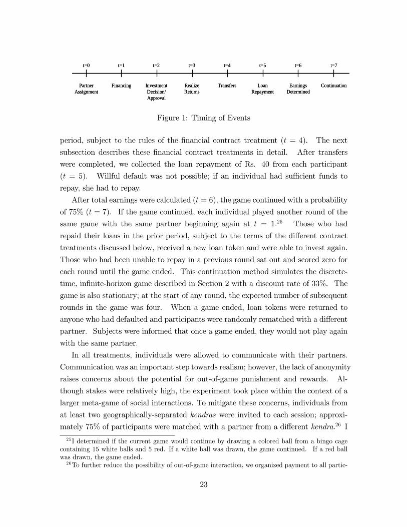
uncertain number of rounds. Figure 1 summarizes timing for each round of the stage
game. At the start of each game, individuals were publicly and randomly matched
with one other participant (t = 0 in Figure 1) and endowed with a token worth Rs.
40 (t = 1), which was described as a loan that could be used to invest in a project
but which needed to be repaid at the end of each round. Each subject then used the
token to indicate her choice from a menu of eight investment lotteries (t = 2), after
which we collected their tokens. Because many subjects were illiterate, I illustrated
the choices graphically as shown in Figure A1. These lotteries were designed to elicit
subjects’ risk preferences and were ranked according to risk and return. Payoffs
ranged from Rs. 80 with certainty for choice A to an equal probability of Rs. 280
or 0 for choice H; the other choices were distributed between these two.24 Because
expected profits increase monotonically with risk, they serve as a proxy for risk-taking
in the discussion below.
We then determined returns for each individual’s project and paid this income in
physical game money (t = 3). Pilot studies suggested that participants understood
the game more clearly and payoffs were more salient when the game money was
physical and translated one-for-one to rupees. After individuals received their income,
they could transfer to their partners any amount up to their total earnings for the
23To determine investment success, subjects played a game where a researcher randomly andsecretly placed a black stone in one hand and a white stone in the other. Subjects then picked ahand and earned the amount shown in the color of the stone that they picked (figure A1). Nearlyall subjects played a similar game as children in which one player hides a single object, usuallya coin or stone, in one of her hands. If the other player guesses the correct hand, they win theobject and are allowed to hide the object in her hands. In Tamil, the game is known as eitherkandupidi vilayaattu, which translates roughly as “the find-it game,”or kallu vilayaattu, “the stonegame.” Subjects’ experience with games similar to the experiment’s randomizing device providessome confidence that the probabilities of the game are reasonably well understood.24The granularity of choices entailed a trade-off between feasibility (both subjects’comprehen-
sion and experimental logistics) and mapping as closely as possible to the theoretical framework ofcontinuous choices. Piloting suggested a practical maximum of eight choices.
22
PartnerAssignment
RealizeReturns
InvestmentDecision/Approval
Transfers LoanRepayment
EarningsDetermined
ContinuationFinancing
t=0 t=2t=1 t=4t=3 t=7t=6t=5
PartnerAssignment
RealizeReturns
InvestmentDecision/Approval
Transfers LoanRepayment
EarningsDetermined
ContinuationFinancing
t=0 t=2t=1 t=4t=3 t=7t=6t=5
Figure 1: Timing of Events
period, subject to the rules of the financial contract treatment (t = 4). The next
subsection describes these financial contract treatments in detail. After transfers
were completed, we collected the loan repayment of Rs. 40 from each participant
(t = 5). Willful default was not possible; if an individual had suffi cient funds to
repay, she had to repay.
After total earnings were calculated (t = 6), the game continued with a probability
of 75% (t = 7). If the game continued, each individual played another round of the
same game with the same partner beginning again at t = 1.25 Those who had
repaid their loans in the prior period, subject to the terms of the different contract
treatments discussed below, received a new loan token and were able to invest again.
Those who had been unable to repay in a previous round sat out and scored zero for
each round until the game ended. This continuation method simulates the discrete-
time, infinite-horizon game described in Section 2 with a discount rate of 33%. The
game is also stationary; at the start of any round, the expected number of subsequent
rounds in the game was four. When a game ended, loan tokens were returned to
anyone who had defaulted and participants were randomly rematched with a different
partner. Subjects were informed that once a game ended, they would not play again
with the same partner.
In all treatments, individuals were allowed to communicate with their partners.
Communication was an important step towards realism; however, the lack of anonymity
raises concerns about the potential for out-of-game punishment and rewards. Al-
though stakes were relatively high, the experiment took place within the context of a
larger meta-game of social interactions. To mitigate these concerns, individuals from
at least two geographically-separated kendras were invited to each session; approxi-
mately 75% of participants were matched with a partner from a different kendra.26 I
25I determined if the current game would continue by drawing a colored ball from a bingo cagecontaining 15 white balls and 5 red. If a white ball was drawn, the game continued. If a red ballwas drawn, the game ended.26To further reduce the possibility of out-of-game interaction, we organized payment to all partic-
23
included within-kendra matches to test the effect of these linkages, and all results are
reported for both outside- and within-kendra pairs.
At the start of each game, we verbally explained the rules to all subjects and
confirmed understanding through a short quiz and a practice round. The Appendix
provides an example of the verbal instructions, translated from the Tamil. At the
end of each session, subjects completed a survey covering their occupations and bor-
rowing and repayment experience. The survey also included three trust and fairness
questions from the General Social Survey (GSS) and a version of the self-reported
risk-taking questions from the German Socioeconomic Panel (SOEP).27 I then paid
each subject privately and confidentially for only one period drawn at random for each
individual at the end of the session. This is a key design feature. If every round were
included for payoff, individuals could partially self-insure income risk across rounds
(Charness and Genicot 2009).
3.2 Financial Contract Treatments
Using the basic game structure described above, I considered five contract treatments:
autarky, individual liability, joint liability, joint liability with approval rights, and
equity. Each required loan repayment of Rs. 40 per borrower and included dynamic
incentives– subjects failing to meet contractual repayment requirements were unable
to borrow in future rounds and earned zero for each remaining round of the game. The
ipants according to kendra so members of each group could leave the lab at different times. Whilekendras were geographically separated, it was possible that individuals from different kendras couldmeet up outside the game, particularly at their local microfinance branches. However, discussionswith participants and Mahasemam lending offi cers suggested that such occurrences would be rare.For two sessions, numbers 6 and 8 as described in Table 5, all participants were from a single kendra.Results are robust to excluding these sessions.27The three GSS questions are the same as those used by Giné, Jakiela, Karlan, and Morduch
(2009) and Cassar, Crowley, and Wydick (2007). Back-translated from the Tamil, they are: (1)“Generally speaking, would you say that people can be trusted or that you can’t be too careful indealing with people?”; (2) “Do you think most people would try to take advantage of you if they gota chance, or would they try to be fair?”; and (3) “Would you say that most of the time people tryto be helpful, or that they are mostly just looking out for themselves?” Dohmen, Falk, Huffman,Schupp, Sunde, and Wagner (2006) demonstrates the effectiveness of self-reported questions aboutone’s willingness to take risks in specific areas (e.g., financial matters or driving) at predicting riskybehaviors in those areas. Based on this finding, I asked the following question: “How do you seeyourself? As it relates to your business, are you a person who is fully prepared to take risks or doyou try to avoid taking risks? Please tick a box on the scale where 0 means ‘unwilling to take risks’and 10 means ‘fully prepared to take risks.’” Subject were unaccustomed to abstract, self-evaluationquestions and had diffi culty answering.
24
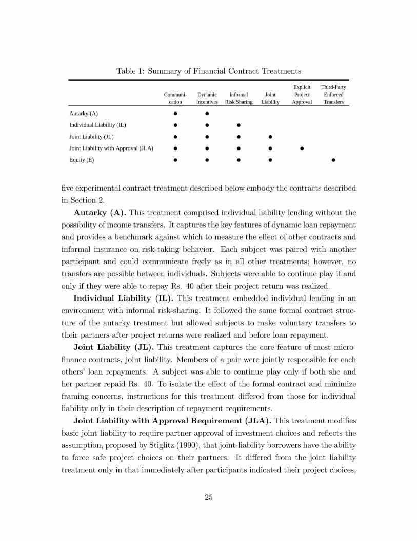
Table 1: Summary of Financial Contract Treatments
Explicit ThirdPartyCommuni Dynamic Informal Joint Project Enforced
cation Incentives Risk Sharing Liability Approval Transfers
Autarky (A) � �
Individual Liability (IL) � � �
Joint Liability (JL) � � � �
Joint Liability with Approval (JLA) � � � � �
Equity (E) � � � � �
five experimental contract treatment described below embody the contracts described
in Section 2.
Autarky (A). This treatment comprised individual liability lending without thepossibility of income transfers. It captures the key features of dynamic loan repayment
and provides a benchmark against which to measure the effect of other contracts and
informal insurance on risk-taking behavior. Each subject was paired with another
participant and could communicate freely as in all other treatments; however, no
transfers are possible between individuals. Subjects were able to continue play if and
only if they were able to repay Rs. 40 after their project return was realized.
Individual Liability (IL). This treatment embedded individual lending in anenvironment with informal risk-sharing. It followed the same formal contract struc-
ture of the autarky treatment but allowed subjects to make voluntary transfers to
their partners after project returns were realized and before loan repayment.
Joint Liability (JL). This treatment captures the core feature of most micro-finance contracts, joint liability. Members of a pair were jointly responsible for each
others’loan repayments. A subject was able to continue play only if both she and
her partner repaid Rs. 40. To isolate the effect of the formal contract and minimize
framing concerns, instructions for this treatment differed from those for individual
liability only in their description of repayment requirements.
Joint Liability with Approval Requirement (JLA). This treatment modifiesbasic joint liability to require partner approval of investment choices and reflects the
assumption, proposed by Stiglitz (1990), that joint-liability borrowers have the ability
to force safe project choices on their partners. It differed from the joint liability
treatment only in that immediately after participants indicated their project choices,
25
we asked their partner if they approved of the choice. A subject whose partner
did not approve her choice was automatically assigned choice A, the riskless option.
Note that under the imperfect monitoring treatment, approval rights also remove any
uncertainty about one’s partner’s investment choice.
Equity (E). In this treatment I enforced an equal division of all income therebyeliminating the commitment problem and the implementability constraint it places
on insurance transfers. Participants were able to make additional transfers, and the
game was otherwise identical to the joint liability treatment.
3.3 Monitoring Treatments
All of the financial contract treatments except for autarky were played under two mon-
itoring regimes: perfect and imperfect public monitoring. As described in Section 2.4,
much of the literature on microfinance discusses the importance of peer monitoring
and local information, and these treatments were designed to see how monitoring
affects performance under different contracts. In all treatments, we seated mem-
bers of a pair together and allowed them to communicate freely. Under perfectmonitoring, all actions and outcomes were observable. Under imperfect publicmonitoring, we separated partners with a physical divider that allowed communica-tion but prevented them from seeing each other’s investment choices and outcomes.
After investment outcomes were realized, we informed each participant if her partner
had suffi cient income to repay her own loan. Transfer amounts were observed only
after the transfer was completed.28
4 Experimental Results
In total, I have 3,443 observations from 450 participant-sessions, representing 256
unique subjects. All sessions were run between March 2007 and May 2007 at a tem-
porary experimental economic laboratory in Chennai, India. I conducted 24 sessions,
averaging two hours each, excluding time spent paying subjects. As summarized
in Table 5, the number of participants per session ranged from 8 and 24, depending
on show-ups. The mean was 18.75. Participants were invited to attend multiple
28Using physical game money, each player placed her transfer in a bowl behind the physical divider.Experimental assistants then swapped the bowls simultaneously. Unobservability was successfullyenforced with the threat of financial punishment and dismissal from the experiment.
26

sessions, and the number of sessions per participants ranged from 1 to 6, with a mean
of 1.75. Summary statistics appear in Table 6.
In the subsections that follow, I separate the experimental results into two cat-
egories. Section 4.1 describes the effect of contracts and monitoring on informal
risk-sharing. Section 4.2 concerns risk-taking and project choice.
4.1 The Impact of Contracts and Monitoring on Informal
Risk-Sharing
RESULT 1. Actual informal insurance transfers fall well short of full risk-sharing and
the maximum implementable informal insurance arrangement with perfect monitoring.
On average, transfers achieve only 14% of full risk-sharing and approximately 30% of
the maximum implementable transfer.
As discussed in Section 2, existing models of informal insurance with limited com-
mitment, including this one, do not make unique predictions for observed transfers.
The dynamic game setting admits a multiplicity of equilibria that always includes
the minimum transfer profile, i.e., no voluntary transfers. However there is a natural
tendency to focus on payoff vectors that are Pareto effi cient in the set of equilibrium
payoffs, which places an upper bound on the performance of informal insurance and
may also represent the outcome of focal strategies (Coate and Ravallion 1993). I
calculate the transfers that would implement the effi cient payoff vector using numeri-
cal simulations based on individuals’CRRA risk-aversion parameters estimated from
the benchmarking risk experiments, actual project choices for each subject pair, and
a static transfer arrangement.29 These experimental results find observed transfers
well below those achieved by either full risk-sharing or those required for constrained
effi ciency.
29This describes a set of transfer vectors with each vector determined by the relative weightassigned to each agent by the social planner. As a benchmark, I selected a single transfer vector usinga Pareto weight, λ, equal to the ratio of marginal utilities in state hh under autarky. If this weight didnot admit a non-zero, individually-rational transfer arrangement (e.g., one agent preferred autarkyto any transfer arrangement based on the starting weight), I searched numerically and selectedthe weight closest to this initial value for which a non-zero transfer arrangement was individuallyrational. In general, performance relative to the constrained-effi cient transfer arrangement shouldbe interpreted with caution. When incentive compatibility constraints are binding or agents havedifferent preferences, expected transfers are not independent of the Pareto weight. However, inthe current setting, where the probability of any state is symmetric and independent of the Paretoweight, the results are robust to calculating the benchmark transfer vector based on any weightsatisfying both agents’participation constraints, provided such a weight exists.
27
Columns 1 and 2 of Table 7 summarize net transfers from the partner with higher
income under individual liability, joint liability and joint liability with approval.
Columns 3 and 4 report the same information conditional on exactly one project
in the pair succeeding. This corresponds to states hl and lh, where the direction
of transfers is independent from assumptions about Pareto weights. If risk-sharing
were complete, these transfers would equal one-half of the difference between payoffs;
however, in each case transfers are well below the full risk-sharing benchmark. Joint
liability with perfect monitoring generates the highest net transfers, 5.3, but this is
only 27% of the full risk-sharing amount of 19.6. These shortfalls arise along both
the extensive and intensive margins. For individual and joint liability contracts with
perfect monitoring, either individual made a transfer in only 50% of all rounds. Under
imperfect public monitoring, the probability of any transfer fell to 30%. Furthermore,
when transfers were made, they tended to remain well below the full risk-sharing
benchmark. Again, joint liability with perfect monitoring produces the largest net
transfers relative to full insurance, but conditional on any transfer being made they
still average only 43% of the full insurance amount. While transfers occur more often
under joint liability with approval– in 72% of all rounds with perfect monitoring and
47% without– net transfers were smaller than those in other contracts.
This result may explain why we see semi-formal risk-sharing mechanisms, such as
the state-contingent loans used for risk smoothing in northern Nigeria (Udry 1994);
highlights the importance of equilibrium selection; and casts doubt on constrained
effi ciency as the focal selection criteria for informal risk-sharing equilibria. The pre-
ponderance of empirical research on informal insurance with limited commitment
suggests that actual transfers fall short of full insurance.30 While this can in part be
explained by implementability constraints imposed by limited commitment (Ligon,
Thomas, and Worrall 2002), these experimental results suggest that actual informal
insurance may settle on an equilibrium with payoffs well below what would be con-
strained effi cient. One possible explanation, consistent with the results from Char-
ness and Genicot (2009), is that effi ciency may be easier to obtain when there is
an obvious focal strategy. In their experiment, transfers were close to theoretically
predicted amounts when subjects had identical and perfectly negatively correlated
30See, for example, Townsend’s (1994) study of risk and insurance in the ICRISAT villages; Udry’s(1994) work on informal credit markets as insurance in northern Nigeria; and Fafchamps and Lund’s(2003) study of quasi-credit in the Philippines.
28
income processes; however, with heterogeneity, actual transfers were substantially
below predicted levels and close to those I observed.31 Exploring alternative selec-
tion criteria, such as risk-dominance in the sense of Harsanyi and Selten (1988), offers
a promising avenue for future research.
Although informal insurance consistently fell short of the theoretical maximum,
formal contracts and information greatly influence risk-sharing behavior. The next
result highlights the importance of monitoring.
RESULT 2. Informal insurance is substantially larger under perfect monitoring than
when monitoring is imperfect. On average, transfers under perfect monitoring are
60% larger than those when monitoring is imperfect.
As shown in Prediction 1, we expect cooperation will be harder to sustain when
monitoring is imperfect. In practice, this effect is large and economically significant.
Net transfers under both individual and joint liability with imperfect monitoring are
roughly half what they are under perfect monitoring. This result is evident in Figure
4 and the summary statistics presented in Table 7. Table 8 reports the results from
the cell-means regression
τ it = α +∑
jβjTj + εit, (3)
where τ it is the transfer made by individual i in round t, and Tj is a indicator for the
contract and monitoring treatment. In all contracts, perfect monitoring generated
substantially larger transfers than imperfect monitoring. The percentage difference
was largest under individual liability, where mean transfers increase from 2.42 to
5.83, or 140%, and is substantial in all contracts. As shown in columns 1 through 4
of Table 7, perfect monitoring more than doubles observed net transfers as a percent-
age of the benchmark constrained effi cient transfer for both the individual and joint
liability contracts. Wilcoxon rank-sum tests reject equivalence at any conventional
significance level (p < 0.0001) for all contracts. Columns 5 through 12 of Table 7
detail transfer behavior for outside and within-kendra pairs. Surprisingly, while net
transfers are higher when individuals are paired with someone from their same kendra,
31There is some suggestive evidence that transfers may be higher as a percentage of the constrainedPareto maximum under both individual and joint liability when both parties pick the same project;however, this evidence is not robust. Transfers as a percentage of full risk-sharing are approximatelyequivalent for both symmetric and non-symmetric investment choices (approximately 20% underindividual liability and 30% under joint liability). There is no evidence that when both parties havethe same baseline risk preferences transfers are larger as a share of the constrained-effi cient transferor full insurance.
29
the differences are not statistically significant, and transfers as a percentage of full
insurance or those necessary to implement the effi cient payoff vector are comparable
in both groups.
I now turn to a specific form of cooperation: transfers made when both members of
a pair have suffi cient income to repay their loans. These “upside”transfers represent
pure insurance.
RESULT 3. Upside risk-sharing is greater under joint liability, increasing by 40%
under perfect monitoring and more than doubling under imperfect monitoring.
We would expect that joint liability and the threat of common punishment would
induce loan repayment assistance when one party lacked suffi cient funds to repay and
the other was able to cover the shortfall. However, as shown in Prediction 2, the
impact of joint liability contracts on “upside”transfers, i.e., transfers excluding loan
repayment assistance and thus representing pure insurance, is theoretically ambigu-
ous. There is substantial overlap in the set of sustainable equilibrium transfers in all
contract treatments. For example, the minimum transfer profile, no transfers beyond
what is contractually required, is an equilibrium strategy under any formal contract.
In practice, joint liability substantially increases observed upside risk-sharing.
Table 9 shows the results from the cell-mean regression of upside transfers, i.e.,
transfers excluding loan repayment assistance, made by individuals in each contract
setting when their investments are successful. Upside transfers under joint liability
are 3.85 (120%) and 2.94 (40%) larger than transfers under individual liability with
imperfect and perfect monitoring. These differences are significant at the 1%- and 5%-
levels. Much of this difference is driven by risk-tolerant individuals, whose transfers
increase by 6.32 (228%) and 6.03 (132%) under joint liability. That risk-tolerant
individuals increase their total transfers when successful under joint liability with
imperfect monitoring may be expected given that, as discussed in Result 6, they also
take significantly greater risk. As a consequence, their total payoff when successful
is larger and they have more to share. They also accrue a greater debt by requiring
assistance when their projects fail. However, risk-tolerant individuals’transfers as a
percentage of the full risk-sharing amount also increase from 9.7% under individual
liability to 17.5% under joint liability. They also increase their upside transfers under
perfect monitoring, which did not increase their risk-taking. With perfect monitoring,
risk-tolerant individuals’net transfers as a percentage of full risk-sharing increase from
25.7% to 47.5%.
30

Joint liability also appears to increase upside transfers made by risk-averse indi-
viduals, although this effect is more modest. When monitoring is imperfect, their
transfers increase by 101% from 3.33 to 6.69, and this difference is significant at the
5%-level. With perfect monitoring, the increase is smaller (12%) and insignificant, al-
though this is from a relatively high base of 6.28 under individual liability with perfect
monitoring. While theory predicts such a response for relatively risk-tolerant indi-
viduals making high-risk investments, the effect was broadly distributed and suggests
the possibility of a behavioral response.32
It is tempting to interpret increased upside transfers by individuals taking greater
risk as compensation for the default insurance their partners provide, but several other
factors call this interpretation into question. Joint liability increases upside transfers
even for those not taking additional risk. Moreover, when monitoring is imperfect,
transfers do not appear to increase with the amount of risk imposed. Panel A of Figure
5 shows mean transfers made at each payoff level. Note that transfers at payoff levels
of 180 and above, each of which resulted from investments with potential default
costs, do not differ from those made at a payoff of 160, the result of a successful
investment in project D, which has no default risk. Transfers are flat above 160, even
though the potential cost of default increases with the potential gain.
RESULT 4. Informal insurance transfers are treated like debt; cumulative net trans-
fers received to date are a strong predictor of net transfers made in the current period.
The model presented in Section 2 solved for mutual insurance arrangements with
a restriction to stationary transfers, that is, whenever the same state occurs, the same
net transfer is made independent of past histories. As Kocherlakota (1996) and Ligon,
Thomas, and Worrall (2002) demonstrate, a dynamic limited commitment model may
improve welfare relative to the stationary model by promising additional future pay-
ments to relax incentive compatibility constraints on transfers in the current period.
In practice, such dynamic transfer schemes may be implemented through informal
loans as described in Eswaran and Kotwal (1989), Udry (1994) and Fafchamps and
32The economics literature has largely focused on importance of social capital in supporting lend-ing arrangements. See, for instance, Karlan (2007), Abbink, Irlenbusch, and Renner (2006), andCassar, Crowley, and Wydick (2007). Two notable exceptions are Ahlin and Townsend’s (2007)work in Thailand and Wydick’s (1999) in Guatemala, both of which find that social ties can lowerrepayment rates. However, sociological and anthropological case studies explore the possibil-ity that microfinance and group lending in particular may affect social cohesion (e.g., Lont andHospes 2004, Fernando 2006, Montgomery 1996).
31

Lund (2003).
I test formally for this effect by regressing transfers in each round after the first on
payoffs, cumulative net transfers, and the first period transfers of both individuals:
τ it = αi + β1yit + β2y−it + γ
t−1∑t′=1
(τ it′ − τ−it′) + εit, (4)
where τ it is the transfer made by individual i in round t, yit is individual i’s income
in round t, and individual fixed effects, αi, are included to capture subjects’predis-
position towards making transfers. If transfers are treated as debt to be repaid, we
expect γ < 0.
As shown in panel A of Table 10, the coeffi cient on cumulative net transfers made
is consistently negative– ranging from −0.120 to −0.302– and significant at the 1%-
level. These results imply, for example, that under joint liability with imperfect
monitoring we would expect an individual who received the same payoffas her partner
and had previously received Rs. 20 of net transfers to make a net transfer of Rs. 5.
4.2 The Impact of Contracts and Monitoring on Risk-Taking
I now turn to the effect of contracts and monitoring on risk-taking behavior. As de-
scribed above, expected profits serve as a proxy for risk-taking and increase monoton-
ically from 40 for the riskless choice, A, to 140 for the riskiest choice, H. Panel B of
Table 4 describes each of the eight project choices.
Figure 3 summarizes risk-taking levels relative to autarky across the contract and
monitoring treatments. The illustrated values are calculated from the simple cell-
means regression
yit = α +∑
jβjTj + εit, (5)
where yit is the expected profit of individual i’s project choice in round t, and Tj is
an indicator for the contract and monitoring treatment. Table 11 presents the full
results from this estimation.
RESULT 5. Informal insurance does not increase risk-taking.
As shown in the discussion of Prediction 3, constrained-effi cient informal insurance
32

should increase total risk-taking.33 ,34 However, observed insurance fell well short what
would be required for constrained effi ciency, and the effect on risk-taking remains an
empirical question.
Comparing investment choices in the individual liability treatment to those under
autarky provides an immediate test of this response; the individual liability treat-
ment differed from autarky only in that subjects were able to engage in informal
risk-sharing. As is evident from Figure 3, the availability of informal insurance had
little effect on individuals’ risk-taking behavior. Neither of the individual liability
coeffi cients from the estimation of (5) are significant as shown in panel A of Table
11. We can reject at the 5%-level increases of 1.2% and 3.2% in the imperfect and
perfect monitoring treatments.
Given the relatively low levels of informal risk-sharing actually observed, this
outcome is perhaps not surprising. While the experiments were designed such that
the maximum implementable informal risk-sharing arrangement would increase the
optimal contract choice by at least one class (e.g., the optimal contract pair for two
individuals with CRRA utility and ρ of 0.5 would move from the pair {B,B}, withindividual payoffs of 100 or 70 in autarky, to {C,C}, with individual payoffs of 140 or50 under individual liability with informal insurance), the realized levels of informal
insurance support only a small increase in risk-taking.
The availability of informal insurance may also have made risk more salient and
thus discouraged risk-taking. While communication was allowed in all treatments,
participants in autarky treatment rarely spoke to one another. Under individual
liability with informal insurance, participants often discussed their project choices
and occasionally made contingent transfer plans. These discussions typically focused
on what would happen in the event of a bad outcome and, by making this state more
salient, may have discouraged risk-taking.
33As shown in section 2.5, this prediction does not necessarily hold if individuals differ substantiallyin their risk aversion and the Pareto weight is heavily skewed towards the more risk-averse agent.Based on preferences calculated from benchmark risk choices, such a reduction would only be possiblein 1.4% of all observations. Observed transfers in these observations are not consistent with a Paretoweight that substantially favors the more risk-averse agent.34Using the parameters of the experimental setting, I calculated individuals’optimal investment
choices under autarky and with informal insurance that achieves a payoff vector that is Paretoeffi cient in the equilibrium set. The numerical results imply that constrained-effi cient insuranceshould increase risk-taking, as measured by the expected profit of individuals’project choices, bybetween Rs. 5 and Rs. 10, or 10% to 20%.
33

RESULT 6. With imperfect monitoring, joint liability increases aggregate risk-taking
as more risk-tolerant individuals take significantly greater risk, relying on their part-
ners to insure against default. Those taking additional risk do not compensate their
partners for this insurance but instead free-ride on the mandatory transfer require-
ment. However, this behavior is sensitive to the monitoring environment. Under
perfect monitoring, joint liability marginally reduces risk-taking relative to individual
liability.
As described in Prediction 4 theory does not make sharp predictions for the effect
of joint liability on investment choice. On one hand, risk-pooling and mandatory
transfers from one’s partner encourage risk-taking. On the other hand, the threat of
joint default may induce risk mitigation and reduce risk-taking. Which effect dom-
inates in practice depends on the risk tolerance of both partners, other parameter
values, and the selected equilibrium of the dynamic game. In light of the relatively
larger amount of informal insurance observed in joint liability relative to individual
liability, particularly under perfect monitoring, we would expect greater risk-taking
under joint liability. Under joint liability with imperfect monitoring, we would expect
a more modest increase in risk-taking if individuals are behaving cooperatively; how-
ever, if cooperation breaks down, the free-riding effect described in Section 2 would
dominate.
In the experiment under perfect monitoring, joint liability marginally reduces
risk-taking relative to individual liability. Expected profits fall by 2.8% (1.43). This
result, shown in panel B of Table 11, is consistent with the finding that increased com-
munication between partners tends to decrease risk-taking, but it is not statistically
significant. Under imperfect monitoring, the effect is reversed. Joint liability in-
creases risk-taking by 3.7% (1.88; p = 0.012) relative to individual liability. However
in neither case is the Wilcoxon rank-sum test significant; p = 0.204 and p = 0.121.
Within the joint liability contract, the effect of monitoring on risk-taking is pro-
nounced. Imperfect monitoring increases risk-taking by 4.3% (2.17; p = 0.009) rela-
tive to joint liability with perfect monitoring, and the Wilcoxon rank-sum test easily
rejects equivalence (p = 0.001). Large differences in behavior across risk types drives
this increase. Risk-averse individuals respond little to joint liability regardless of the
monitoring structure, while more risk-tolerant individuals take significantly greater
risk when monitoring is imperfect.
I divide subjects into risk categories based on their choices in the risk benchmark-
34
ing games. Approximately 70% of subjects picked one of the safe choices, A through
D, and are categorized as “risk averse.”The remaining 30% picked choices E through
H and are categorized as “risk tolerant.”This division corresponds to a coeffi cient of
risk aversion of 0.44 for individuals with CRRA utility and a wealth of zero.
When monitoring is perfect, joint liability does not appear to affect the investment
choices of risk-averse individuals. In fact, as shown in column 5 of Table 12, they take
less risk than in autarky and their project choices are statistically indistinguishable
from those of risk-averse individuals. This is consistent with Giné, Jakiela, Karlan,
and Morduch’s (2009) finding that participants who tend to take risks reduce their
risk-taking when their partners make safer choices.
When monitoring is imperfect, risk-tolerant individuals increase their risk-taking
under the simple joint liability contract. As can be seen in column 1, panel C of Table
12, the mean expected return for risk-tolerant individuals increases by 26% (1.2σ)
from 51.3 under individual liability to 64.7 under joint liability. A nonparametric
Wilcoxon rank test show this difference is significant at any conventional level (p <
0.0001).35 Evidence of compensatory transfers is mixed. As discussed above, risk-
tolerant individuals do make larger transfers under joint liability, but two facts call
into question the intent of these transfers. First, as can be seen in panel B of Table
9, this increase appears in both perfect and imperfect monitoring, while increased
risk-taking is only evident when monitoring is imperfect. Second, as shown in Figure
5, there is no discernible difference in transfers by risky individuals who chose projects
just below the potential threshold for default (projects C and D) and those who forced
their partners to insure against default (projects E, F, G and H). One interpretation
of this result is that risk-tolerant individuals increase transfers under joint liability
to compensate their partners for the option value of default insurance even if their
investment choices render this insurance moot. Further experimentation would be
useful to test this hypothesis.
The results in columns 3 and 7 of Table 12 demonstrate a stark difference in the
behavior of pairs from the same kendra. While joint liability with imperfect moni-
toring still induces risk-tolerant types to increase their allocation to the risky asset,
this increase is substantially less than when matched with a partner from a different
35This result is robust to moving the definition of “risk tolerant”up or down one risk class. Afully non-parametric specification for the effect of benchmarked investment choice on risk-takingunder joint liability with limited information shows noticeable break between those who elected a“safe”choice in the benchmarking rounds and those who did not.
35
kendra (6.26 vs. 16.20). This effectively eliminates the free-riding phenomenon wit-
nessed in outside-kendra pairs. Under perfect monitoring, risk-tolerant types actually
reduce their allocation to the risky asset. While there are a number of factors that
could be driving this behavior, it is consistent with the fact that for within-kendra
pairs informal insurance under joint liability with perfect monitoring generates trans-
fers closer to those required for constrained effi ciency and the observation, discussed
in Prediction 3, that income pooling pushes each agent’s optimal choice to a point
between their autarkic choices.36
When cooperation breaks down, we expect individuals to take action to discourage
free-riding. The next result shows that explicit approval rights are used ex ante to
reduce risk-taking.
RESULT 7. Explicit approval rights are used to curtail risk-taking under joint liability.
Consistent with Prediction 5, panel C of Table 11 confirms that approval rights are
used to prevent risk-taking ex ante, particularly when monitoring is imperfect. When
monitoring is imperfect, risk-taking in the JLA contract is 6.3% lower than in autarky
and 8.3% lower than under joint liability without explicit approval. Both differences
are significant at greater than the 1%-level. This effect is concentrated among risk-
tolerant individuals, for whom expected profits fall 22% from 63.8 to 49.9. Risk-averse
individuals also reduce their risk relative to individual or joint liability, but the effect
is more modest and only borderline significant.
As expected, joint liability creates two potential ineffi ciencies: free-riding when
the enforcement mechanisms necessary to sustain cooperation are weak and excessive
caution when these mechanisms are strong. The next result turns to one possible
solution: equity-like contracts under which full risk-sharing is enforced by a third-
party.
RESULT 8. Equity increases expected returns relative to other contracts while pro-
ducing the lowest default rates. Under imperfect monitoring, expected profits are 5%
larger than under individual liability and 10% larger than under joint liability with
approval rights. While expected profits are only slightly larger than under joint lia-
bility, the increased willingness to take risk is distributed across individuals and not
the result of risk-tolerant individuals free-riding on their partners.
36Statistical tests of whether changes in risk allocation depend on the risk preferences of one’spartner require a very thin parsing of the data and are inconclusive.
36
Third-party enforcement of equal income distribution overcomes much of the com-
mitment problem associated with informal risk-sharing arrangements. When part-
ners have identical preferences, it achieves full insurance. As such, and in line with
Prediction 3, we would expect equity-like contracts to encourage greater risk-taking
than under autarky or contracts where limited commitment reduces the sustainable
amount of insurance.
This result can be seen in Figure 3 and the summary of expected profits by contract
type in Table 11. Formal statistical evidence is provided by the regression described
in (5). Tests for the equivalence of the equity treatment dummy coeffi cients against
those for individual, joint liability, and joint liability with approval are each significant
at better than the 5%-level. Wilcoxon tests reject equivalence at better than the 1%-
level in each case. While statistically significant and practically meaningful, the
differences in risk-taking between equity and individual liability or autarky are less
than we would expect. Numerical simulations based on benchmarked risk-taking
behavior predict expected profits under the equity contract should increase by 10% to
20% relative to autarky. Actual expected profits increase by 2% to 5%, approximately
0.10 to 0.25 standard deviations. Relative to joint liability with approval rights, the
increase in expected profits from equity contracts is more than twice as large, 5%
under perfect monitoring and 10% under imperfect public monitoring.
Panel C of Table 6 reports default rates for each contract, ranging from a high of
4.8% in autarky to 0% under equity. The low default rates are consistent with the
reported rates of most microfinance institutions– Mahasemam itself reports client
defaults of less than 1%– but since the terms of default were set by the experiment, I
focus on relative performance across the contract treatments.37 Default rates follow
the pattern we would expect. Adding informal transfers (moving from autarky to the
individual liability treatment) reduces default rates by two percentage points from
4.83% to 2.80%. Moving from individual to joint liability further reduces default rates
to 1.35%, or 1.51% when approval rights are explicit. Finally, equity generated no
defaults as increased risk was almost always hedged across borrowers, with the worst
possible joint outcome still suffi cient for loan repayment. Each of the differences in
default rates is significant at the 5%-level.
While these experiments abstracted from key challenges for implementing equity
contracts, including moral hazard over effort and costly state verification, the results
37Low levels of reported default suggest that willful default is not prevalent.
37
are encouraging. Innovative financial contracts may encourage substantial increases
in the expected returns of microfinance-funded projects. However, further research is
required to understand why observed risk-taking under the equity contract remained
below what would be predicted based on individuals’benchmarked risk preferences.
Based on the results of this experiment, exploration of how social factors influence
decisions under uncertainty could provide important information on how to most
effectively move from the lab to equity-like contracts in the field.
5 Conclusion
This paper has developed a theory of risk-taking and informal insurance in the pres-
ence of formal financial contracts designed to answer the questions: How do microfi-
nance borrowers choose among risky projects? How do they share risk? How do formal
financial contracts affect these behaviors? And can the structure of formal financial
contracts themselves explain in part the limited growth observed in microfinance-
funded businesses? To shed further light on these questions, it examined the results
of a lab experiment that captured the key elements of the theory using actual micro-
finance clients in India as subjects. Theory-based experimentation allows us to test
generalizable effects of financial contracts and to delineate mechanisms that would be
challenging to identify in a full field setting.
The experiment uncovered a number of interesting results. First, informal insur-
ance falls well short of not only the full risk-sharing benchmark but also the con-
strained optimal insurance arrangement predicted by theory. This calls into question
the use of constrained effi ciency as the focal equilibrium selection criteria for informal
sharing arrangements. Exploring alternative selection criteria, such as risk-dominance
in the sense of Harsanyi and Selten (1988) and Carlsson and van Damme (1993), offers
a promising avenue for future research.
Second, joint liability encouraged informal insurance. Upside income transfers,
those not required for loan repayment, were almost twice as large under joint lia-
bility as under individual lending. This result cannot be explained as compensation
for default insurance– increased transfers are evident even among those who did not
take additional risk. Joint liability may have increased the perceived social connec-
tion to one’s partner, thus moving the equilibrium insurance arrangement towards
constrained effi ciency. Or joint liability may have provided a coordination device
38
that facilitated implementation of cooperative transfer arrangements. A definitive
explanation is beyond the scope of the available experimental evidence, and further
research is necessary to distinguish social effects, coordination devices, and other
explanations.
Third, the core result supports the motivating conjecture: the structure of existing
microfinance contracts themselves may discourage risky but high-expected return
investments. When monitoring was imperfect, joint liability produced significant free-
riding. Risk-tolerant individuals took substantially greater risk without compensating
their partners for the added insurance burden. Granting approval rights, some form
of which likely exist in practice, eliminated free-riding but also reduced risk-taking
below levels in autarky. The strength of this effect suggests that peer monitoring may
not only reduce ex ante moral hazard but also discourage risk-taking more generally,
regardless of effi ciency. Taken together, these findings provide one explanation for
the lack of demonstrable growth in microfinance-funded enterprises.
Finally, equity increased risk-taking and expected returns relative to other finan-
cial contracts, although these increases were less than half what theory would predict
for optimal behavior. At the same time, equity also generated the lowest default
rates. While there are significant hurdles to implementing such contracts in practice
and further research is required to understand deviations from predicted risk-taking
behavior, these results are encouraging and suggest that equity-like contracts merit
further exploration in the field.
39

References
Abbink, K., B. Irlenbusch, and E. Renner (2006): “Group Size and Social Tiesin Microfinance Institutions,”Economic Inquiry, 44(4), 614—628.
Ahlin, C., and R. M. Townsend (2007): “Using Repayment Data to Test acrossModels of Joint Liability Lending,”Economic Journal, 117(517), F11—F51.
Armendariz, B. (1999): “On the Design of a Credit Agreement with Peer Moni-toring,”Journal of Development Economics, 60(1), 79—104.
Armendariz, B., and J. Morduch (2005): The Economics of Microfinance. Cam-bridge, MA: MIT Press.
Banerjee, A. V., T. Besley, and T. W. Guinnane (1994): “Thy Neighbor’sKeeper: The Design of a Credit Cooperative with Theory and a Test,”QuarterlyJournal of Economics, 109(2), 491—515.
Barr, A., and G. Genicot (2008): “Risk Sharing, Commitment and Information:An Experimental Analysis,”Discussion paper, The Centre for the Study of AfricanEconomies Working Paper Series Paper 278.
Besley, T., and S. Coate (1995): “Group Lending, Repayment Incentives andSocial Collateral,”Journal of Development Economics, 46(1), 1—18.
Bulow, J., and K. Rogoff (1989): “Sovereign Debt: Is to Forgive to Forget?,”American Economic Review, 79(1), 43—50.
Carlsson, H., and E. van Damme (1993): “Global Games and Equilibrium Se-lection,”Econometrica, 61(5), 989—1018.
Cassar, A., L. Crowley, and B. Wydick (2007): “The Effect of Social Capitalon Group Loan Repayment: Evidence from Field Experiments,”Economic Journal,117(517), F85—F106.
Charness, G., and G. Genicot (2009): “Informal Risk Sharing in an Infinite-Horizon Experiment,”The Economic Journal, 119(537), 796—825.
Chowdhury, P. R. (2005): “Group-Lending: Sequential Financing, Lender Moni-toring and Joint Liability,”Journal of Development Economics, 77(2), 415—439.
Coate, S., and M. Ravallion (1993): “Reciprococity Without Commitment:Characterization and Performance of Informal Insurance Arrangements,”Journalof Development Economics, 40, 1—24.
40
Conning, J. (2005): “Monitoring by Peers or by Delegates? Joint Liability Loansand Moral Hazard,” Hunter College Department of Economics Working Papers:407.
de Aghion, B., and C. Gollier (2000): “Peer Group Formation in an AdverseSelection Model,”Economic Journal, 110(465), 632—643.
Dohmen, T. J., A. Falk, D. Huffman, J. Schupp, U. Sunde, and G. G.Wagner (2006): “Individual Risk Attitudes: New Evidence from a Large, Repre-sentative, Experimentally-Validated Survey,”Discussion paper, IZA.
Eswaran, M., and A. Kotwal (1989): “Credit as Insurance in AgrarianEconomies,”Journal of Development Economics, 31(1), 37—53.
Fafchamps, M., and S. Lund (2003): “Risk-sharing Networks in Rural Philip-pines,”Journal of Development Economics, 71(2), 261—287.
Fernando, J. L. (ed.) (2006): Microfinance: Perils and Prospects. London, NewYork: Routledge.
Foster, A. D., and M. R. Rosenzweig (2001): “Imperfect Commitment, Al-truism, and the Family: Evidence from Transfer Behavior in Low-Income RuralAreas,”Review of Economics and Statistics, 83(3), 389—407.
Fudenberg, D., D. I. Levine, and E. Maskin (1994): “The Folk Theorem withImperfect Public Information,”Econometrica, 62(5), 997—1039.
Ghatak, M., and T. W. Guinnane (1999): “The Economics of Lending withJoint Liability: Theory and Practice,”Journal of Development Economics, 60(1),195—228.
Giné, X., P. Jakiela, D. S. Karlan, and J. Morduch (2009): “MicrofinanceGames,”American Economic Journal: Applied Economics.
Giné, X., and D. S. Karlan (2011): “Group versus Individual Liability: LongTerm Evidence from Philippine Microcredit Lending Groups,”Discussion paper,Yale mimeo.
Green, E. J., and R. H. Porter (1984): “Noncooperative Collusion under Imper-fect Price Information,”Econometrica, 52(1), 87—100.
Harsanyi, J. C., and R. Selten (1988): A General Theory of Equilibrium Selectionin Games. Cambridge, MA, London: MIT Press.
Karlan, D. S. (2007): “Social Connections and Group Banking,”Economic Journal,117(517), F52—84.
41
Kocherlakota, N. (1996): “Implications of Effi cient Risk Sharing without Com-mitment,”Review of Economic Studies, 63, 595—610.
Laffont, J.-J., and P. Rey (2003): “Moral Hazard, Collusion and Group Lend-ing,”IDEI Working Papers, Institut d’Economie Industrielle (IDEI), Toulouse.
Ligon, E., J. P. Thomas, and T.Worrall (2000): “Mutual Insurance, IndividualSavings, and Limited Commitment,”Review of Economic Dynamics, 3(2), 216—246.
(2002): “Informal Insurance Arrangements with Limited Commitment: The-ory and Evidence from Village Economies,”Review of Economic Studies, 69(1),209—244.
Lont, H., and O. Hospes (eds.) (2004): Livelihood and Microfinance: Anthropo-logical and Sociological Perspectives on Savings and Debt. Delft: Eburon.
Madajewicz, M. (2003): “Does the Credit Contract Matter? The Impact of Lend-ing Programs on Poverty in Bangladesh,”Columbia University working paper.
(2004): “Joint-Liability Contracts Versus Individual-Liability Contracts,”Columbia University working paper.
Montgomery, R. (1996): “Disciplining or Protecting the Poor? Avoiding the SocialCosts of Peer Pressure in Micro-credit Schemes,”Journal of International Devel-opment, 8(2), 289—305.
Morduch, J. (1999): “The Microfinance Promise,”Journal of Economic Literature,37(4), 1569—1614.
Radner, R., R. Myerson, and E. Maskin (1986): “An Example of a RepeatedPartnership Game with Discounting and with Uniformly Ineffi cient Equilibria,”Review of Economic Studies, 53(1), 59—69.
Rai, A. S., and T. Sjöström (2004): “Is Grameen Lending Effi cient? RepaymentIncentives and Insurance in Village Economies,”Review of Economic Studies, 71(1),217—234.
Robinson, J. (2008): “Limited Insurance Within the Household: Evidence from aField Experiment in Western Kenya,”University of California Santa Cruz mimeo.
Stiglitz, J. E. (1990): “Peer Monitoring and Credit Markets,”World Bank Eco-nomic Review, 4(3), 351—366.
Townsend, R. (1994): “Risk and Insurance in Village India,”Econometrica, 62(4),539—591.
42

Udry, C. (1994): “Risk and Insurance in a Rural Credit Market: An EmpiricalInvestigation in Northern Nigeria,”Review of Economic Studies, 61(3), 495—526.
Varian, H. R. (1990): “Monitoring Agents with Other Agents,”Journal of Institu-tional and Theoretical Economics, 146(1), 153—174.
Woolcock, M. J. V. (1999): “Learning from Failures in Microfinance: What Un-successful Cases Tell Us About How Group-based Programs Work,” AmericanJournal of Economics and Sociology, 58(1), 17—42.
Wydick, B. (1999): “Can Social Cohesion Be Harnessed to Repair Market Failures?Evidence from Group Lending in Guatemala,”Economic Journal, 109(457), 463—475.
43
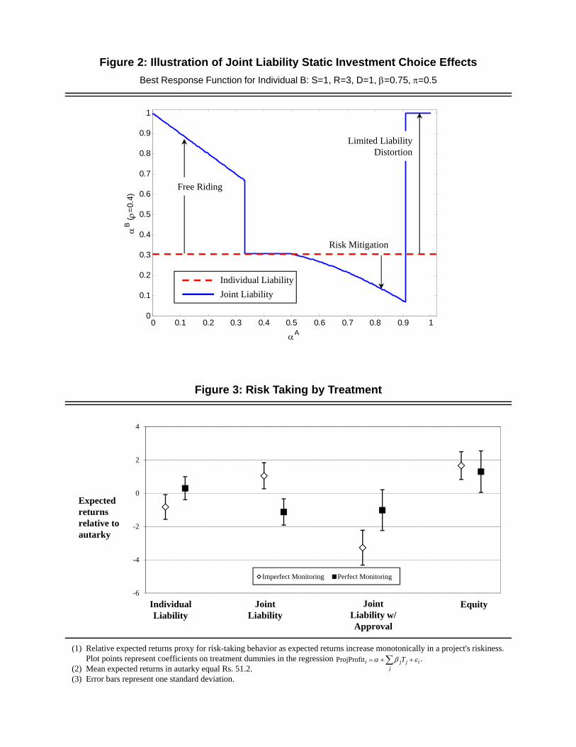
-6
-4
-2
0
2
4
Imperfect Monitoring Perfect Monitoring
JointLiability w/Approval
IndividualLiability
JointLiability
Equity
Expected returns relative to autarky
Relative expected returns proxy for risk-taking behavior as expected returns increase monotonically in a project's riskiness. Plot points represent coefficients on treatment dummies in the regression .Mean expected returns in autarky equal Rs. 51.2.Error bars represent one standard deviation.
0 0.1 0.2 0.3 0.4 0.5 0.6 0.7 0.8 0.9 10
0.1
0.2
0.3
0.4
0.5
0.6
0.7
0.8
0.9
1
A
B (=
0.4)
Free Riding
Risk Mitigation
Limited Liability Distortion
Individual Liability
Joint Liability
Figure 2: Illustration of Joint Liability Static Investment Choice Effects
Best Response Function for Individual B: S=1, R=3, D=1, =0.75, =0.5
Figure 3: Risk Taking by Treatment
(1)
(2)(3)
ProjProfiti j j ij
T
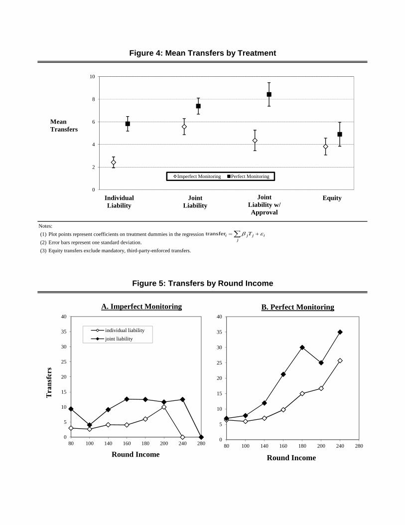
Notes:
(1) Plot points represent coefficients on treatment dummies in the regression
(2) Error bars represent one standard deviation.
(3) Equity transfers exclude mandatory, third-party-enforced transfers.
Figure 4: Mean Transfers by Treatment
Figure 5: Transfers by Round Income
0
2
4
6
8
10
Imperfect Monitoring Perfect Monitoring
IndividualLiability
JointLiability
JointLiability w/Approval
Equity
MeanTransfers
0
5
10
15
20
25
30
35
40
80 100 140 160 180 200 240 280
Round Income
A. Imperfect Monitoring
individual liability
joint liability
0
5
10
15
20
25
30
35
40
80 100 140 160 180 200 240 280
Round Income
B. Perfect Monitoring
transferi j j ij
T
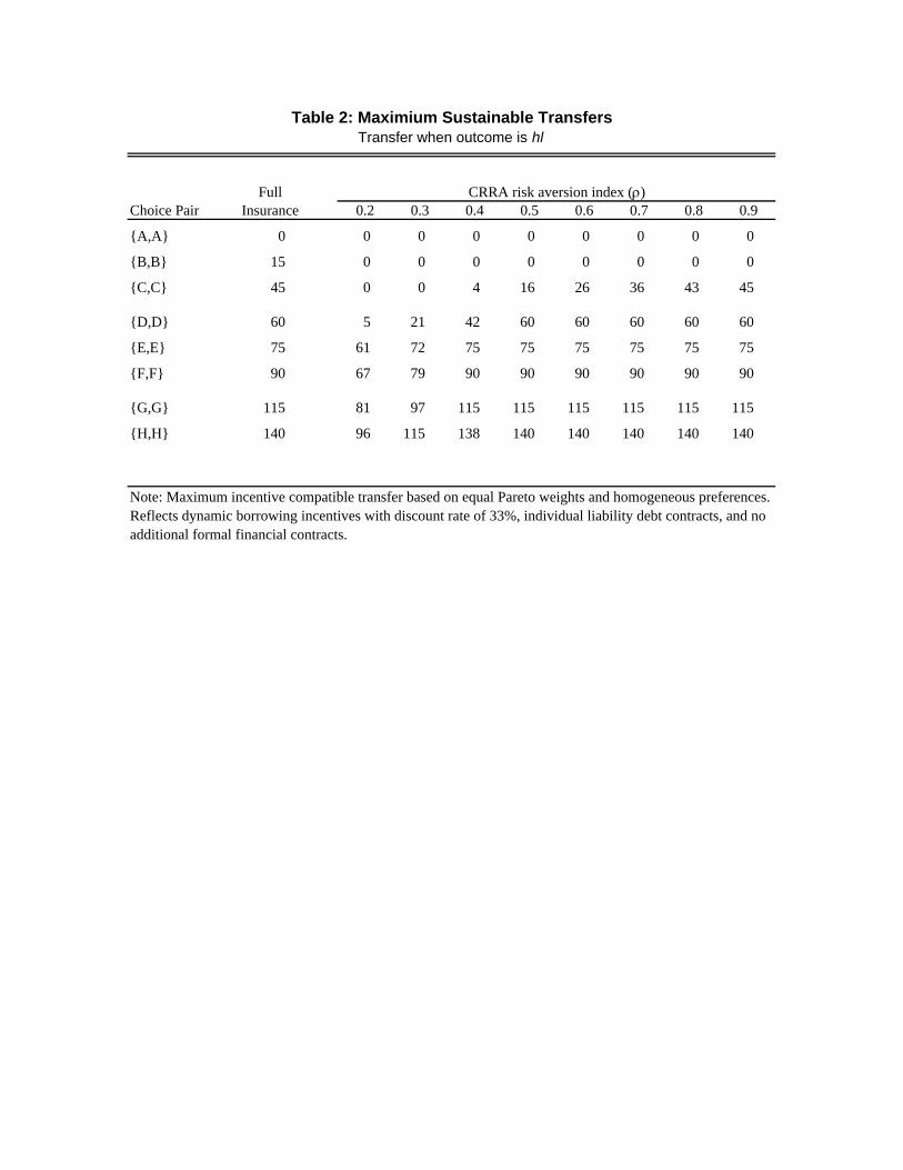
FullChoice Pair Insurance 0.2 0.3 0.4 0.5 0.6 0.7 0.8 0.9
{A,A} 0 0 0 0 0 0 0 0 0
{B,B} 15 0 0 0 0 0 0 0 0
{C,C} 45 0 0 4 16 26 36 43 45
{D,D} 60 5 21 42 60 60 60 60 60
{E,E} 75 61 72 75 75 75 75 75 75
{F,F} 90 67 79 90 90 90 90 90 90
{G,G} 115 81 97 115 115 115 115 115 115
{H,H} 140 96 115 138 140 140 140 140 140
Note: Maximum incentive compatible transfer based on equal Pareto weights and homogeneous preferences. Reflects dynamic borrowing incentives with discount rate of 33%, individual liability debt contracts, and no additional formal financial contracts.
Table 2: Maximium Sustainable TransfersTransfer when outcome is hl
CRRA risk aversion index ()

A. AUTARKY
Choice Pair 0.2 0.3 0.4 0.5 0.6 0.7 0.8 0.9
{A,A} 23.9 18.9 15.2 12.6 10.9 10.1 10.5 14.5
{B,B} 26.0 20.3 16.1 13.2 11.3 10.3 10.6 14.6
{C,C} 28.8 21.5 16.5 13.2 11.0 10.0 10.2 14.2
{D,D} 28.8 20.4 14.7 11.0 8.5 7.0 6.5 8.1
{E,E} 13.0 9.1 6.5 4.7 3.6 2.9 2.7 3.3
{F,F} 14.5 10.0 7.0 5.1 3.8 3.1 2.8 3.3
{G,G} 17.3 11.7 8.0 5.7 4.2 3.3 2.9 3.4
{H,H} 20.1 13.2 8.9 6.2 4.5 3.5 3.0 3.5
B. FULL INSURANCE
Choice Pair 0.2 0.3 0.4 0.5 0.6 0.7 0.8 0.9
{A,A} 23.9 18.9 15.2 12.6 10.9 10.1 10.5 14.5
{B,B} 26.2 20.4 16.2 13.3 11.4 10.4 10.7 14.6
{C,C} 29.8 22.6 17.5 14.0 11.7 10.5 10.7 14.6
{D,D} 30.9 22.7 17.1 13.2 10.7 9.2 8.9 11.6
{E,E} 19.4 14.1 10.4 8.0 6.4 5.4 5.2 6.7
{F,F} 21.0 15.1 11.1 8.4 6.6 5.6 5.3 6.7
{G,G} 24.9 17.5 12.6 9.3 7.2 5.9 5.5 6.9
{H,H} 28.5 19.7 13.9 10.1 7.7 6.3 5.7 7.0
C. MAXIMUM SUSTAINABLE TRANSFERS
Choice Pair 0.2 0.3 0.4 0.5 0.6 0.7 0.8 0.9
{A,A} 23.9 18.9 15.2 12.6 10.9 10.1 10.5 14.5
{B,B} 26.0 20.3 16.1 13.2 11.3 10.3 10.6 14.6
{C,C} 28.8 21.5 16.7 13.7 11.6 10.5 10.7 14.6
{D,D} 29.5 22.1 17.0 13.2 10.7 9.2 8.9 11.6
{E,E} 19.3 14.1 10.4 8.0 6.4 5.4 5.2 6.7
{F,F} 20.9 15.1 11.1 8.4 6.6 5.6 5.3 6.7
{G,G} 24.7 17.4 12.6 9.3 7.2 5.9 5.5 6.9
{H,H} 28.3 19.6 13.9 10.1 7.7 6.3 5.7 7.0
Note: Bold and boxed amount represents maximum per period utility along column. Maximum incentive compatible
transfer based on equal Pareto weights and homogeneous preferences. Reflects dynamic borrowing incentives with
discount rate of 33%, individual liability debt contracts, and no additional formal contracts. Full insurance reflects equal
sharing of all income.
CRRA risk aversion index ()
Table 3: Average Per Period Utility for Different Transfer Regimes
CRRA risk aversion index ()
CRRA risk aversion index ()
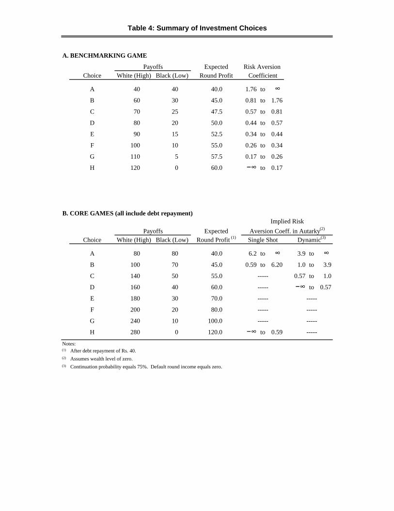
A. BENCHMARKING GAME
ExpectedChoice White (High) Black (Low) Round Profit
A 40 40 40.0 1.76 to ∞
B 60 30 45.0 0.81 to 1.76
C 70 25 47.5 0.57 to 0.81
D 80 20 50.0 0.44 to 0.57
E 90 15 52.5 0.34 to 0.44
F 100 10 55.0 0.26 to 0.34
G 110 5 57.5 0.17 to 0.26
H 120 0 60.0 −∞ to 0.17
B. CORE GAMES (all include debt repayment)
ExpectedChoice White (High) Black (Low) Round Profit (1)
A 80 80 40.0 6.2 to ∞ 3.9 to ∞
B 100 70 45.0 0.59 to 6.20 1.0 to 3.9
C 140 50 55.0 0.57 to 1.0
D 160 40 60.0 −∞ to 0.57
E 180 30 70.0
F 200 20 80.0
G 240 10 100.0
H 280 0 120.0 −∞ to 0.59
Notes:(1) After debt repayment of Rs. 40.(2) Assumes wealth level of zero.(3) Continuation probability equals 75%. Default round income equals zero.
-----
-----
-----
-----
Table 4: Summary of Investment Choices
-----
-----
Single Shot
-----
-----
-----
Dynamic(3)
Implied Risk
Aversion Coeff. in Autarky(2)
Payoffs
Payoffs
Risk Aversion Coefficient

A. SESSION SUMMARY
Session Date Rounds ParticipantsParticipants in larger kendra
1 11/30/2006 5 24 12
2 11/30/2006 9 23 12
3 11/30/2006 12 16 9
4 11/30/2006 7 20 11
5 11/30/2006 6 14 7
6 11/30/2006 11 8 8
7 11/30/2006 9 22 12
8 11/30/2006 12 10 10
9 11/30/2006 7 21 11
10 11/30/2006 9 21 11
11 11/30/2006 7 20 10
12 11/30/2006 10 18 10
13 11/30/2006 12 15 10
14 11/30/2006 11 20 10
15 11/30/2006 10 20 10
16 11/30/2006 15 20 11
17 11/30/2006 11 17 10
18 11/30/2006 14 17 10
19 11/30/2006 11 23 12
20 11/30/2006 10 24 12
21 11/30/2006 11 17 10
22 11/30/2006 9 20 10
23 11/30/2006 10 20 10
24 11/30/2006 13 20 10
B. OBSERVATION COUNTS BY GAME
Game Perfect Imperfect TotalBenchmarking -- -- 341 Autarky -- -- 768 Individual liability 420 520 940 Joint Liability 352 336 688 Joint liability with partner approval 172 110 282 Equity 318 106 424
Monitoring
Table 5: Session Detail
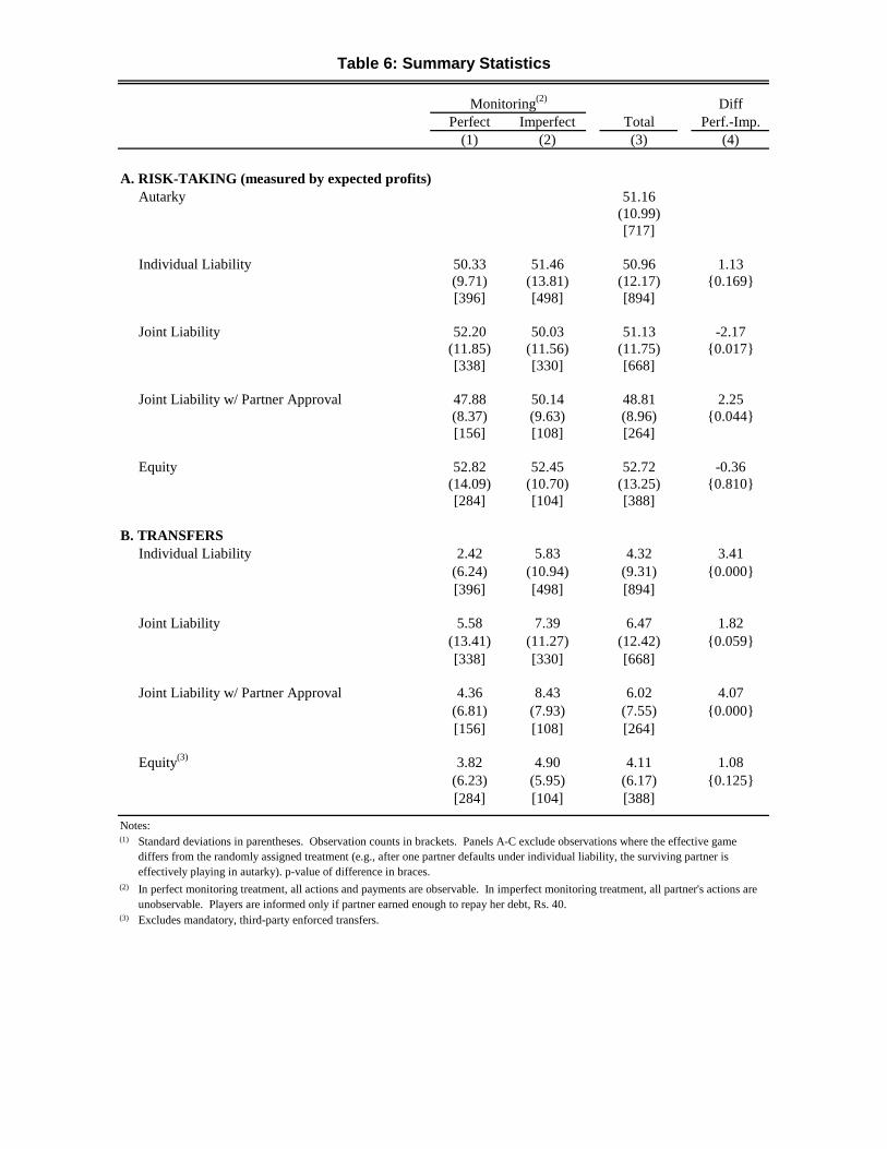
DiffPerfect Imperfect Total Perf.-Imp.
(1) (2) (3) (4)
A. RISK-TAKING (measured by expected profits)Autarky 51.16
(10.99)[717]
Individual Liability 50.33 51.46 50.96 1.13(9.71) (13.81) (12.17) {0.169}[396] [498] [894]
Joint Liability 52.20 50.03 51.13 -2.17(11.85) (11.56) (11.75) {0.017}[338] [330] [668]
Joint Liability w/ Partner Approval 47.88 50.14 48.81 2.25(8.37) (9.63) (8.96) {0.044}[156] [108] [264]
Equity 52.82 52.45 52.72 -0.36(14.09) (10.70) (13.25) {0.810}[284] [104] [388]
B. TRANSFERSIndividual Liability 2.42 5.83 4.32 3.41
(6.24) (10.94) (9.31) {0.000}[396] [498] [894]
Joint Liability 5.58 7.39 6.47 1.82(13.41) (11.27) (12.42) {0.059}[338] [330] [668]
Joint Liability w/ Partner Approval 4.36 8.43 6.02 4.07(6.81) (7.93) (7.55) {0.000}[156] [108] [264]
Equity(3) 3.82 4.90 4.11 1.08(6.23) (5.95) (6.17) {0.125}[284] [104] [388]
Notes:(1)
(2)
(3)
In perfect monitoring treatment, all actions and payments are observable. In imperfect monitoring treatment, all partner's actions are unobservable. Players are informed only if partner earned enough to repay her debt, Rs. 40.
Table 6: Summary Statistics
Monitoring(2)
Excludes mandatory, third-party enforced transfers.
Standard deviations in parentheses. Observation counts in brackets. Panels A-C exclude observations where the effective game differs from the randomly assigned treatment (e.g., after one partner defaults under individual liability, the surviving partner is effectively playing in autarky). p-value of difference in braces.
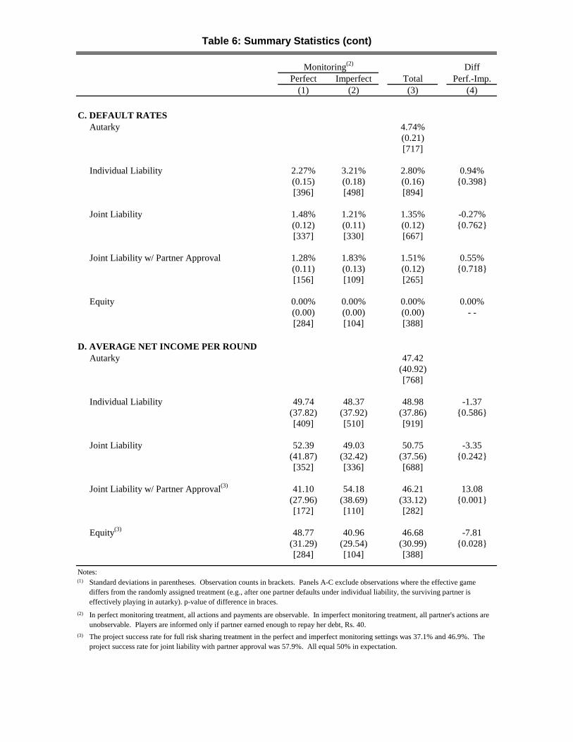
DiffPerfect Imperfect Total Perf.-Imp.
(1) (2) (3) (4)
C. DEFAULT RATESAutarky 4.74%
(0.21)[717]
Individual Liability 2.27% 3.21% 2.80% 0.94%(0.15) (0.18) (0.16) {0.398}[396] [498] [894]
Joint Liability 1.48% 1.21% 1.35% -0.27%(0.12) (0.11) (0.12) {0.762}[337] [330] [667]
Joint Liability w/ Partner Approval 1.28% 1.83% 1.51% 0.55%(0.11) (0.13) (0.12) {0.718}[156] [109] [265]
Equity 0.00% 0.00% 0.00% 0.00%(0.00) (0.00) (0.00) - -[284] [104] [388]
D. AVERAGE NET INCOME PER ROUNDAutarky 47.42
(40.92)[768]
Individual Liability 49.74 48.37 48.98 -1.37(37.82) (37.92) (37.86) {0.586}[409] [510] [919]
Joint Liability 52.39 49.03 50.75 -3.35(41.87) (32.42) (37.56) {0.242}[352] [336] [688]
Joint Liability w/ Partner Approval(3) 41.10 54.18 46.21 13.08(27.96) (38.69) (33.12) {0.001}[172] [110] [282]
Equity(3) 48.77 40.96 46.68 -7.81(31.29) (29.54) (30.99) {0.028}[284] [104] [388]
Notes:(1)
(2)
(3)
In perfect monitoring treatment, all actions and payments are observable. In imperfect monitoring treatment, all partner's actions are unobservable. Players are informed only if partner earned enough to repay her debt, Rs. 40.
The project success rate for full risk sharing treatment in the perfect and imperfect monitoring settings was 37.1% and 46.9%. The project success rate for joint liability with partner approval was 57.9%. All equal 50% in expectation.
Table 6: Summary Statistics (cont)
Monitoring(2)
Standard deviations in parentheses. Observation counts in brackets. Panels A-C exclude observations where the effective game differs from the randomly assigned treatment (e.g., after one partner defaults under individual liability, the surviving partner is effectively playing in autarky). p-value of difference in braces.
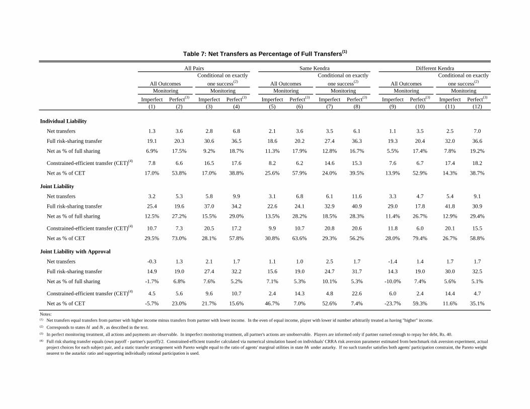
Imperfect Perfect(3) Imperfect Perfect(3) Imperfect Perfect(3) Imperfect Perfect(3) Imperfect Perfect(3) Imperfect Perfect(3)
(1) (2) (3) (4) (5) (6) (7) (8) (9) (10) (11) (12)
Individual Liability
Net transfers 1.3 3.6 2.8 6.8 2.1 3.6 3.5 6.1 1.1 3.5 2.5 7.0
Full risk-sharing transfer 19.1 20.3 30.6 36.5 18.6 20.2 27.4 36.3 19.3 20.4 32.0 36.6
Net as % of full sharing 6.9% 17.5% 9.2% 18.7% 11.3% 17.9% 12.8% 16.7% 5.5% 17.4% 7.8% 19.2%
Constrained-efficient transfer (CET)(4) 7.8 6.6 16.5 17.6 8.2 6.2 14.6 15.3 7.6 6.7 17.4 18.2
Net as % of CET 17.0% 53.8% 17.0% 38.8% 25.6% 57.9% 24.0% 39.5% 13.9% 52.9% 14.3% 38.7%
Joint Liability
Net transfers 3.2 5.3 5.8 9.9 3.1 6.8 6.1 11.6 3.3 4.7 5.4 9.1
Full risk-sharing transfer 25.4 19.6 37.0 34.2 22.6 24.1 32.9 40.9 29.0 17.8 41.8 30.9
Net as % of full sharing 12.5% 27.2% 15.5% 29.0% 13.5% 28.2% 18.5% 28.3% 11.4% 26.7% 12.9% 29.4%
Constrained-efficient transfer (CET)(4) 10.7 7.3 20.5 17.2 9.9 10.7 20.8 20.6 11.8 6.0 20.1 15.5
Net as % of CET 29.5% 73.0% 28.1% 57.8% 30.8% 63.6% 29.3% 56.2% 28.0% 79.4% 26.7% 58.8%
Joint Liability with Approval
Net transfers -0.3 1.3 2.1 1.7 1.1 1.0 2.5 1.7 -1.4 1.4 1.7 1.7
Full risk-sharing transfer 14.9 19.0 27.4 32.2 15.6 19.0 24.7 31.7 14.3 19.0 30.0 32.5
Net as % of full sharing -1.7% 6.8% 7.6% 5.2% 7.1% 5.3% 10.1% 5.3% -10.0% 7.4% 5.6% 5.1%
Constrained-efficient transfer (CET)(4) 4.5 5.6 9.6 10.7 2.4 14.3 4.8 22.6 6.0 2.4 14.4 4.7
Net as % of CET -5.7% 23.0% 21.7% 15.6% 46.7% 7.0% 52.6% 7.4% -23.7% 59.3% 11.6% 35.1%
Notes:(1)
(2)
(3)
(4)
Table 7: Net Transfers as Percentage of Full Transfers(1)
Net transfers equal transfers from partner with higher income minus transfers from partner with lower income. In the even of equal income, player with lower id number arbitrarily treated as having "higher" income.
In perfect monitoring treatment, all actions and payments are observable. In imperfect monitoring treatment, all partner's actions are unobservable. Players are informed only if partner earned enough to repay her debt, Rs. 40.
Conditional on exactly
one success(2)
Monitoring Monitoring
Full risk sharing transfer equals (own payoff - partner's payoff)/2. Constrained-efficient transfer calculated via numerical simulation based on individuals' CRRA risk aversion parameter estimated from benchmark risk aversion experiment, actual project choices for each subject pair, and a static transfer arrangement with Pareto weight equal to the ratio of agents' marginal utilities in state hh under autarky. If no such transfer satisfies both agents' participation constraint, the Pareto weight nearest to the autarkic ratio and supporting individually rational participation is used.
Corresponds to states hl and lh , as described in the text.
Same Kendra Different Kendra
Monitoring
Conditional on exactly
one success(2)All OutcomesMonitoring
All Pairs
All Outcomes
Conditional on exactly
one success(2)
Monitoring MonitoringAll Outcomes
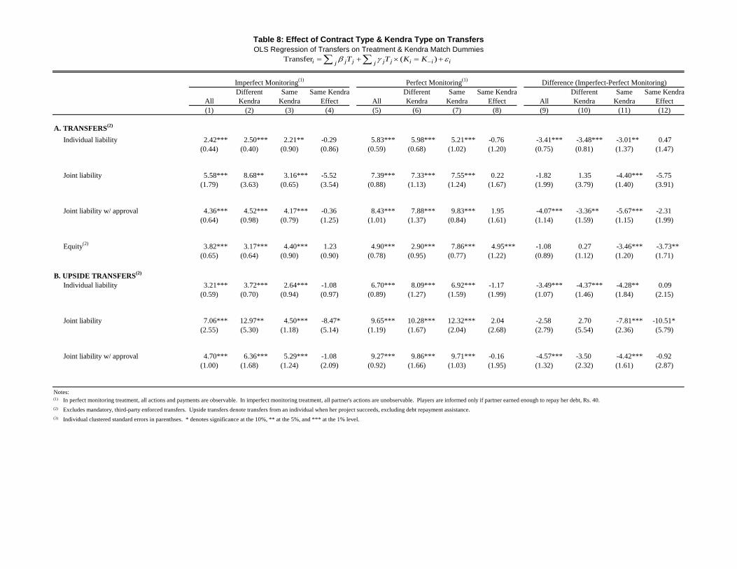
Different Same Same Kendra Different Same Same Kendra Different Same Same KendraAll Kendra Kendra Effect All Kendra Kendra Effect All Kendra Kendra Effect(1) (2) (3) (4) (5) (6) (7) (8) (9) (10) (11) (12)
A. TRANSFERS(2)
Individual liability 2.42*** 2.50*** 2.21** -0.29 5.83*** 5.98*** 5.21*** -0.76 -3.41*** -3.48*** -3.01** 0.47 (0.44) (0.40) (0.90) (0.86) (0.59) (0.68) (1.02) (1.20) (0.75) (0.81) (1.37) (1.47)
Joint liability 5.58*** 8.68** 3.16*** -5.52 7.39*** 7.33*** 7.55*** 0.22 -1.82 1.35 -4.40*** -5.75 (1.79) (3.63) (0.65) (3.54) (0.88) (1.13) (1.24) (1.67) (1.99) (3.79) (1.40) (3.91)
Joint liability w/ approval 4.36*** 4.52*** 4.17*** -0.36 8.43*** 7.88*** 9.83*** 1.95 -4.07*** -3.36** -5.67*** -2.31 (0.64) (0.98) (0.79) (1.25) (1.01) (1.37) (0.84) (1.61) (1.14) (1.59) (1.15) (1.99)
Equity(2) 3.82*** 3.17*** 4.40*** 1.23 4.90*** 2.90*** 7.86*** 4.95*** -1.08 0.27 -3.46*** -3.73** (0.65) (0.64) (0.90) (0.90) (0.78) (0.95) (0.77) (1.22) (0.89) (1.12) (1.20) (1.71)
B. UPSIDE TRANSFERS(2)
Individual liability 3.21*** 3.72*** 2.64*** -1.08 6.70*** 8.09*** 6.92*** -1.17 -3.49*** -4.37*** -4.28** 0.09 (0.59) (0.70) (0.94) (0.97) (0.89) (1.27) (1.59) (1.99) (1.07) (1.46) (1.84) (2.15)
Joint liability 7.06*** 12.97** 4.50*** -8.47* 9.65*** 10.28*** 12.32*** 2.04 -2.58 2.70 -7.81*** -10.51* (2.55) (5.30) (1.18) (5.14) (1.19) (1.67) (2.04) (2.68) (2.79) (5.54) (2.36) (5.79)
Joint liability w/ approval 4.70*** 6.36*** 5.29*** -1.08 9.27*** 9.86*** 9.71*** -0.16 -4.57*** -3.50 -4.42*** -0.92 (1.00) (1.68) (1.24) (2.09) (0.92) (1.66) (1.03) (1.95) (1.32) (2.32) (1.61) (2.87)
Notes:(1)
(2) Excludes mandatory, third-party enforced transfers. Upside transfers denote transfers from an individual when her project succeeds, excluding debt repayment assistance.(3)
Table 8: Effect of Contract Type & Kendra Type on TransfersOLS Regression of Transfers on Treatment & Kendra Match Dummies
Individual clustered standard errors in parenthses. * denotes significance at the 10%, ** at the 5%, and *** at the 1% level.
Imperfect Monitoring(1)
In perfect monitoring treatment, all actions and payments are observable. In imperfect monitoring treatment, all partner's actions are unobservable. Players are informed only if partner earned enough to repay her debt, Rs. 40.
Difference (Imperfect-Perfect Monitoring)Perfect Monitoring(1)
Transfer ( )i j j j j i i ij jT T K K

Imperfect Perfect DifferenceMonitoring Monitoring Imp-Per
(1) (2) (3)
A. ALL
Individual liability 3.21 6.70 -3.49***(0.35) (0.85) (0.92)
Joint liability 7.06 9.65 -2.58 (0.82) (2.59) (2.72)
Joint liability w/ approval 4.70 9.27 -4.57***(0.35) (1.37) (1.41)
Difference: Joint - Individual 3.85*** 2.94 (0.90) (2.53)
B. RISK TOLERANT SUBJECTS
Individual liability 2.77 4.59 -1.82 (0.81) (0.92) (1.23)
Joint liability 9.09 10.63 -1.53 (4.97) (4.10) (6.44)
Joint liability w/ approval 6.36 9.50 -3.14 (2.06) (0.29) (2.08)
Difference: Joint - Individual 6.32 6.03 (4.84) (4.18)
C. RISK AVERSE SUBJECTSIndividual liability 3.33 6.28 -2.95*
(0.29) (1.74) (1.77)
Joint liability 6.69 7.05 -0.36 (0.98) (3.22) (3.37)
Joint liability w/ approval 4.20 10.14 -5.94***(0.32) (0.82) (0.88)
Difference: Joint - Individual 3.36*** 0.77 (1.07) (3.45)
Notes:(1)
(2)
(3) Risk tolerant and risk averse classifications based on benchmark risk experiments
Table 9: Effect of Contract Type & Monitoring on Upside SharingTransfers When Project Suceeds, Excluding Debt Repayment Assistance
In perfect monitoring treatment, all actions and payments are observable. In imperfect monitoring treatment, all partner's actions are unobservable. Players are informed only if partner earned enough to repay her debt, Rs. 40.
Standard errors clustered at the session level in parentheses. * Denotes significance at the 10%-level, ** at the 5%-level, and *** at the 1% level.
UpsideTransferi j j ijT
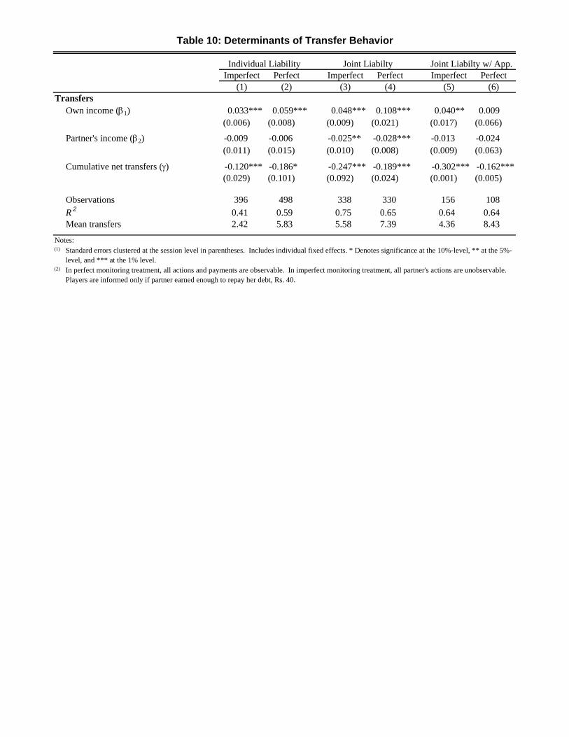
Imperfect Perfect Imperfect Perfect Imperfect Perfect(1) (2) (3) (4) (5) (6)
TransfersOwn income (1) 0.033*** 0.059*** 0.048*** 0.108*** 0.040** 0.009
(0.006) (0.008) (0.009) (0.021) (0.017) (0.066)
Partner's income (2) -0.009 -0.006 -0.025** -0.028*** -0.013 -0.024 (0.011) (0.015) (0.010) (0.008) (0.009) (0.063)
Cumulative net transfers () -0.120*** -0.186* -0.247*** -0.189*** -0.302*** -0.162***(0.029) (0.101) (0.092) (0.024) (0.001) (0.005)
Observations 396 498 338 330 156 108
R 2 0.41 0.59 0.75 0.65 0.64 0.64 Mean transfers 2.42 5.83 5.58 7.39 4.36 8.43
Notes:(1)
(2) In perfect monitoring treatment, all actions and payments are observable. In imperfect monitoring treatment, all partner's actions are unobservable. Players are informed only if partner earned enough to repay her debt, Rs. 40.
Table 10: Determinants of Transfer Behavior
Individual Liability Joint Liabilty Joint Liabilty w/ App.
Standard errors clustered at the session level in parentheses. Includes individual fixed effects. * Denotes significance at the 10%-level, ** at the 5%-level, and *** at the 1% level.

Imperfect Perfect DifferenceMonitoring Monitoring Imp-Per
(1) (2) (3)
A. COEFFICIENT ESTIMATES
Individual liability -0.83 0.30 -1.13 (0.94) (1.18) (1.22)
Joint liability 1.05 -1.13 2.17***(0.83) (1.17) (0.76)
Joint liability w/ approval -3.27*** -1.02 -2.25* (1.03) (1.55) (1.39)
Equity 1.66 1.29 0.36 (2.86) (1.28) (1.81)
B. TREATMENT EFFECTS RELATIVE TO JOINT LIABILITY
Individual -1.88*** 1.43 (0.69) (1.40)
Joint liability w/ approval -4.32*** 0.11 (0.73) (1.40)
Equity 0.61 2.42***(2.58) (0.85)
C. TREATMENT EFFECTS RELATIVE TO JOINT LIABILITY w/ APPROVAL
Individual 2.44*** 1.32 (0.46) (1.93)
Equity 4.93** 2.31 (2.40) (1.52)
Notes:(1)
(2)
Table 11: Effect of Contract Type & Monitoring on Risk TakingOLS Regression of Expected Profits on Treatment Dummies
Omitted Category: autkary; Mean expected profits: 51.2
In perfect monitoring treatment, all actions and payments are observable. In imperfect monitoring treatment, all partner's actions are unobservable. Players are informed only if partner earned enough to repay her debt, Rs. 40.
Standard errors clustered at the session level in parentheses. * Denotes significance at the 10%-level, ** at the 5%-level, and *** at the 1% level.
ProjProfiti j j ijT
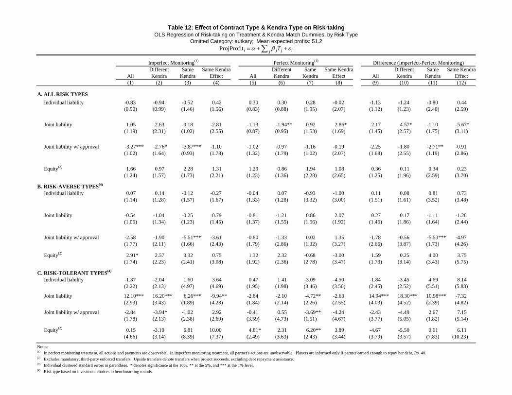
Different Same Same Kendra Different Same Same Kendra Different Same Same KendraAll Kendra Kendra Effect All Kendra Kendra Effect All Kendra Kendra Effect(1) (2) (3) (4) (5) (6) (7) (8) (9) (10) (11) (12)
A. ALL RISK TYPES
Individual liability -0.83 -0.94 -0.52 0.42 0.30 0.30 0.28 -0.02 -1.13 -1.24 -0.80 0.44 (0.90) (0.99) (1.46) (1.56) (0.83) (0.88) (1.95) (2.07) (1.12) (1.23) (2.40) (2.59)
Joint liability 1.05 2.63 -0.18 -2.81 -1.13 -1.94** 0.92 2.86* 2.17 4.57* -1.10 -5.67* (1.19) (2.31) (1.02) (2.55) (0.87) (0.95) (1.53) (1.69) (1.45) (2.57) (1.75) (3.11)
Joint liability w/ approval -3.27*** -2.76* -3.87*** -1.10 -1.02 -0.97 -1.16 -0.19 -2.25 -1.80 -2.71** -0.91 (1.02) (1.64) (0.93) (1.78) (1.32) (1.79) (1.02) (2.07) (1.68) (2.55) (1.19) (2.86)
Equity(2) 1.66 0.97 2.28 1.31 1.29 0.86 1.94 1.08 0.36 0.11 0.34 0.23 (1.24) (1.57) (1.73) (2.21) (1.23) (1.36) (2.28) (2.65) (1.25) (1.96) (2.59) (3.70)
B. RISK-AVERSE TYPES(4)
Individual liability 0.07 0.14 -0.12 -0.27 -0.04 0.07 -0.93 -1.00 0.11 0.08 0.81 0.73 (1.14) (1.28) (1.57) (1.67) (1.33) (1.28) (3.32) (3.00) (1.51) (1.61) (3.52) (3.48)
Joint liability -0.54 -1.04 -0.25 0.79 -0.81 -1.21 0.86 2.07 0.27 0.17 -1.11 -1.28 (1.06) (1.34) (1.23) (1.45) (1.37) (1.55) (1.56) (1.92) (1.46) (1.86) (1.64) (2.44)
Joint liability w/ approval -2.58 -1.90 -5.51*** -3.61 -0.80 -1.33 0.02 1.35 -1.78 -0.56 -5.53*** -4.97 (1.77) (2.11) (1.66) (2.43) (1.79) (2.86) (1.32) (3.27) (2.66) (3.87) (1.73) (4.26)
Equity(2) 2.91* 2.57 3.32 0.75 1.32 2.32 -0.68 -3.00 1.59 0.25 4.00 3.75 (1.74) (2.23) (2.41) (3.08) (1.92) (2.36) (2.78) (3.47) (1.73) (3.14) (3.43) (5.75)
C. RISK-TOLERANT TYPES(4)
Individual liability -1.37 -2.04 1.60 3.64 0.47 1.41 -3.09 -4.50 -1.84 -3.45 4.69 8.14 (2.22) (2.13) (4.97) (4.69) (1.95) (1.98) (3.46) (3.50) (2.45) (2.52) (5.51) (5.83)
Joint liability 12.10*** 16.20*** 6.26*** -9.94** -2.84 -2.10 -4.72** -2.63 14.94*** 18.30*** 10.98*** -7.32 (2.93) (3.43) (1.89) (4.28) (1.84) (2.14) (2.26) (2.55) (4.03) (4.52) (2.39) (4.82)
Joint liability w/ approval -2.84 -3.94* -1.02 2.92 -0.41 0.55 -3.69** -4.24 -2.43 -4.49 2.67 7.15 (1.78) (2.13) (2.38) (2.69) (3.59) (4.73) (1.51) (4.67) (3.77) (5.05) (1.82) (5.14)
Equity(2) 0.15 -3.19 6.81 10.00 4.81* 2.31 6.20** 3.89 -4.67 -5.50 0.61 6.11 (4.66) (3.14) (8.39) (7.37) (2.49) (3.63) (2.43) (3.44) (3.79) (3.57) (7.83) (10.23)
Notes:(1)
(2) Excludes mandatory, third-party enforced transfers. Upside transfers denote transfers when project succeeds, excluding debt repayment assistance.(3)
(4) Risk type based on investment choices in benchmarking rounds.
Table 12: Effect of Contract Type & Kendra Type on Risk-takingOLS Regression of Risk-taking on Treatment & Kendra Match Dummies, by Risk Type
In perfect monitoring treatment, all actions and payments are observable. In imperfect monitoring treatment, all partner's actions are unobservable. Players are informed only if partner earned enough to repay her debt, Rs. 40.
Omitted Category: autkary; Mean expected profits: 51.2
Individual clustered standard errors in parenthses. * denotes significance at the 10%, ** at the 5%, and *** at the 1% level.
Imperfect Monitoring(1) Perfect Monitoring(1) Difference (Imperfect-Perfect Monitoring)
ProjProfiti j j ijT

A Sample Instructions
The following instructions are for the joint liability game with imperfect monitoring.Detailed instructions for other treatments are available on request.
INSTRUCTIONS
Good afternoon everyone and thank you for agreeing to participate in our study.We are conducting a study of how microfinance clients make investments and sharerisk. Instead of asking you a lot of questions, what we’d like to do is have youplay some games with us. The games are simple. You don’t need any special skills.They’re probably like games you played before. You don’t need to know how to read.There are no “right”or “wrong”answers. We just want to understand how you makechoices and what sorts of investment you prefer.Here is how the game works. You will play games where the amount of money
you win is based on picking a colored stone. Display large 100/10 payoff sheet. Oneof us will hold a stone in each hand. One stone is white. The other is black. Showstones. We will mix the stones up and you will pick a hand. No one will know whichstone is in which hand, so the color you get is based on chance.If you pick the white stone you will win the amount shown in white. If you pick
the black stone you will win the amount shown in black.Play practice round and administer oral test to confirm understanding. Distribute
project choice sheets and tokens (carom coins).We will give you choices about which game you want to play. Look at the sheet
in front of you. It describes eight games. The color on the page tells you how muchyou win for each color stone. If you play game “B”how much do you win if you pickthe white stone? How much for the black?You can pick which game you want to play by placing a carom coin on your choice.
For example, if you wanted to play the first game you would put your black caromcoin over the “A”. Demonstrate. And if you wanted to play [the fifth game], you putyour coin over the “E”.The choice is yours. There are no right or wrong answers. It’s only about which
choice you prefer.You can discuss your choices with the other person at your table, but do not speak
with anyone else. Also, while you may talk with the person at your table, you maynot look at her choices or score sheet. The first time you look at your partner’s sheet,we will deduct Rs. 20 from your score. If you peek a second time, we will have toask you to leave the study.We will play several rounds today. At the end of the day we will put the number
for each round you play in this blue bucket. Suppose you play three rounds. Wewill put the numbers 1, 2, and 3 in the bucket and you will pick a number from thebucket without looking. We will pay you in rupees for every point you scored in just
58

that round. Remember, you will only be paid in rupees for one of the rounds thatyou play today. Demonstrate example. Remember, every round counts but you willonly be paid in rupees for one of the rounds. At the end of the day, you will be paidindividually and privately. No one will see exactly how much you earn.Administer second test of understanding.In this game you will play with a partner. You will use a white carom coin to
mark your choices. When you make your choice, we will take your white coin. Afteryou play the stone matching game, we will pay you in chips. The white chips areworth Rs. 5 and the red chips are worth Rs. 20. At the end of each round, you mustrepay your loan of Rs. 40. You and your partner are responsible for each other’sloans. So to get your white coin back, you both must repay your loan. You may notlook at your partner’s score sheet or see how much she wins. However, after we playthe stone matching game, we will tell you whether your partner made enough to payher loan back.After you play the stone matching game and receiving your chips, you can choose
to give some of your earnings to your partner. You can discuss these transfers withyour partner. You do not have to make any transfers. However, you are responsiblefor both your loan and your partner’s loan and will be able to continue playing thegame only if both of you can repay your loan of Rs.40.If you wish to make any transfers, put any chips you wish to transfer to your
partner in the bowl in front of you. Do not hand chips directly to her or place themin her bowl. Only place the chips you wish to transfer in the bowl in front of you.This is important because we need to keep track in order to pay you the correctamount at the end of the day. We will then collect your loan repayment.Your earnings for the round will be equal to the total amount of chips that you
have after any transfers you make to your partner and after you repay your loan. Ifeither you or your partner are unable to repay your loan, you will both earn zero forthe round and will not receive your white coin.At the end of each round, we will pick a ball from this cage. There are 20 balls in
the cage: 15 are white and 5 are red. If the ball is white, you will play another roundof the same game with the same partner. If you do not have your white coin, you willhave to sit out and will score zero for the round. If the ball is red, this game willstop and we will play a new game. Everyone will start with a new white coin and bematched with a new partner. After the red ball is pulled from the cage, you will notplay with the same partner again for the remainder of the day. At any time, you canexpect the game to last four more rounds but we will play until a red ball appears.If you have any questions at any time, please raise your hand and one of us will
come and assist you.Administer final test of understanding.Play practice round.
59

B Proofs and Derivations
B.1 Autarkic Investment Choice
In autarky (individual liability with no informal transfers), an individual’s single-period investment choice problem solves
maxαU(α,D) = πu[yh(α,D)−D] + (1− π)u[max{yl(α)−D, 0}]. (6)
Because of the discontinuity created by limited liability, this problem does not havea “nice”closed form solution for α∗, the optimal allocation to the risky investment.With the constant relative risk aversion utility function, u(c) = c(1−ρ)/(1 − ρ), thefirst order condition for an interior maximum is:
α∗INT =(z − 1)[S(1 +D)−D]
[(z − 1)S +R](1 +D), (7)
where
z =
[π(R− S)
(1− π)S
]1/ρ.
Accounting for the discontinuity created by limited liability, the optimal allocation is
α∗ =
{α∗INT , if EU(α∗INT ) > EU(1)1, otherwise
. 38
In the dynamic problem, individuals solve
maxαV (α,Dt) = E{U(α) + δV (α,Dt)},
which is equivalent to the solution of
maxα
U(α,Dt)
1− δ Pr[R|α],
where Pr[R|α] is the probability that the individual meets the repayment terms ofthe individual liability loan conditional on investment choice α.
B.2 Discussion of Predictions
As described in Section 2.3, note that λ represents the Pareto weight placed on agentB.38In this formulation of the model with limited liability, it is never optimal for an individual to
choose α ∈(S(1+D)−DS(1+D) , 1
).
60

Definition 2 (relative marginal utility) For any state of nature θ ∈ {hh, hl, lh, ll}and transfer arrangement T = {τ θ}S, let κθ(T ) = u
′(yθA − τ θ)/u
′(yθB + τ θ).
Where not required for clarity, I will drop the argument and refer to κθ(T ) simplyas κθ. Note that the first-best insurance arrangement involves full income pooling,κθ = λ, a constant, ∀θ. Under individual liability with no transfers (T = 0), theautarky treatment, the first-order conditions for optimal investment allocation requireπ(R− S)u′(yhi ) = (1− π)Su′(yli), which implies that κ
hh(0) = κll(0).Lemma 1 places some structure on the relative marginal utilities, κθ, generated
by any transfer arrangement generating a payoff vector that is constrained effi cientin the set of equilibrium payoffs.
Lemma 1 (properties of κ) For any transfer arrangement, T = (τhh, τhl, τ lh, τ ll),generating a payoff vector that is constrained effi cient in the set of equilibrium payoffs:
1. κhl ≤ κlh;
2. If κhl = λ, then κhh = λ. Similarly, if κlh = λ, then κll = λ;
3. If there exist θ and θ′ such that κθ > κθ′then κhl < κlh.
Note that this implies that an individual is weakly better off when her projectsucceeds and her partner’s fails than when her project fails and her partner’s succeeds.
Proof. For the first part of the lemma, suppose κhl > κlh. This implies thatu′A(y
hlA −τhl)
u′B(yhlB +τ
hl)>
u′A(ylhA −τ lh)
u′B(ylhB +τ
lh). But since yhli > ylhi , there exists a τ ∈ (τ lh, τhl) such
that T ′ = (τhh, τ ,−τ , τ ll) satisfies the incentive compatibility constraints for bothagents and u′A(y
hlA −τ)
u′B(yhlB +τ)
=u′A(y
lhA +τ)
u′B(ylhB −τ)
. This transfer arrangement increases expected utilityfor both agents, a violation of Pareto optimality. For the second part, supposeκhl = κ > κhh. This implies that A’s incentive compatibility constraint does notbind in hh. Therefore, there exists T ′′ = (τhh + dτ , τhl − dτ πu′(yhhB +τhh)
(1−π)u′(yhlB +τhl), τ lh, τ ll)
that satisfies the incentive compatibility constraints and leaves B’s expected utilityunchanged. But κhl > κhh implies that VA(α, T ′′) > VA(α, T ), a violation of Paretooptimality. A similar argument shows that κlh = λ implies κll = λ. The third partof the lemma follows immediately.
Lemma 2 (transfers when exactly one project succeeds) For any non-zerotransfer arrangement, transfers will be made in states where one risky project suc-ceeds and the other fails, θ ∈ {hl, lh}, and the agent whose project succeeds will makea transfer to the agent whose project fails. That is, if T 6= 0, then τhl > 0 > τ lh.
61
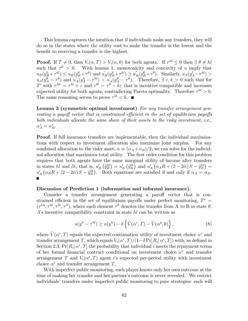
This lemma captures the intuition that if individuals make any transfers, they willdo so in the states where the utility cost to make the transfer is the lowest and thebenefit to receiving a transfer is the highest.
Proof. If T 6= 0, then Vi(α, T ) > Vi(α, 0) for both agents. If τhl ≤ 0 then ∃ θ 6= hlsuch that τ θ > 0. With lemma 1, monotonicity and concavity of u imply thatuB(yhB+τhl) ≤ uB(yθB+τ θ) and u
′B(yhB+τhl) ≥ u
′B(yθB+τ θ). Similarly, uA(ylA−τhl) >
uA(yθA − τ θ) and u′A(yhA − τhl) < u
′A(yθA − τ θ). Therefore, ∃ ε, k > 0 such that for
T ′ with τhl′ = τhl + ε and τ θ′ = τ θ − kε that is incentive compatible and increasesexpected utility for both agents, contradicting Pareto optimality. Therefore τhl > 0.The same reasoning serves to prove τ lh < 0.
Lemma 3 (symmetric optimal investment) For any transfer arrangement gen-erating a payoff vector that is constrained effi cient in the set of equilibrium payoffsboth individuals allocate the same share of their assets to the risky investment, i.e.,α∗A = α∗B.
Proof. If full insurance transfers are implementable, then the individual maximiza-tions with respect to investment allocation also maximize joint surplus. For anycombined allocation to the risky asset, α ≡ (αA+αB)/2, we can solve for the individ-ual allocation that maximizes total utility. The first order condition for this problemrequires that both agents have the same marginal utility of income after transfersin states hl and lh, that is, u′B
(yhlB)
= u′B(ylhB)and u′A
(αAR + (2− 2α)S − yhlB
)=
u′A(αBR + (2− 2α)S − ylhB
). Both equations are satisfied if and only if αA = αB.
Discussion of Prediction 1 (information and informal insurance).Consider a transfer arrangement generating a payoff vector that is con-
strained effi cient in the set of equilibrium payoffs under perfect monitoring, T ∗ =(τhh, τhl, τ lh, τ ll), where each element τ θ denotes the transfer from A to B in state θ.A’s incentive compatibility constraint in state hl can be written as
u(yh − τhl) ≥ u(yh)− δ{V (αe, T )− V (αp, 0)
}, (8)
where V (αe, T ) equals the expected continuation utility of investment choice αe andtransfer arrangement T , which equals Vi(αe, T )/(1−δ Pr[Ri|αe, T ]) with, as defined inSection 2.3, Pr[Ri|αe, T ] the probability that individual i meets the repayment termsof her formal financial contract conditional on investment choice αe and transferarrangement T and Vi(αe, T ) agent i’s expected per-period utility with investmentchoice αe and transfer arrangement T .With imperfect public monitoring, each player knows only her own outcome at the
time of making her transfer and her partner’s outcome is never revealed. We restrictindividuals’transfers under imperfect public monitoring to pure strategies: each will
62
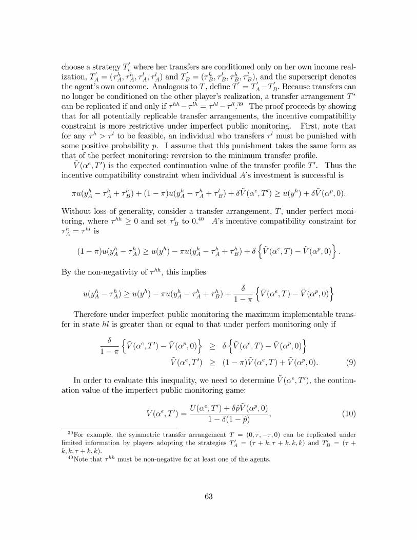
choose a strategy T′i where her transfers are conditioned only on her own income real-
ization, T′A = (τhA, τ
hA, τ
lA, τ
lA) and T
′B = (τhB, τ
lB, τ
hB, τ
lB), and the superscript denotes
the agent’s own outcome. Analogous to T , define T′= T
′A−T
′B. Because transfers can
no longer be conditioned on the other player’s realization, a transfer arrangement T ∗
can be replicated if and only if τhh−τ lh = τhl−τ ll.39 The proof proceeds by showingthat for all potentially replicable transfer arrangements, the incentive compatibilityconstraint is more restrictive under imperfect public monitoring. First, note thatfor any τh > τ l to be feasible, an individual who transfers τ l must be punished withsome positive probability p. I assume that this punishment takes the same form asthat of the perfect monitoring: reversion to the minimum transfer profile.
V (αe, T ′) is the expected continuation value of the transfer profile T ′. Thus theincentive compatibility constraint when individual A’s investment is successful is
πu(yhA − τhA + τhB) + (1− π)u(yhA − τhA + τ lB) + δV (αe, T ′) ≥ u(yh) + δV (αp, 0).
Without loss of generality, consider a transfer arrangement, T , under perfect moni-toring, where τhh ≥ 0 and set τ lB to 0.40 A’s incentive compatibility constraint forτhA = τhl is
(1− π)u(yhA − τhA) ≥ u(yh)− πu(yhA − τhA + τhB) + δ{V (αe, T )− V (αp, 0)
}.
By the non-negativity of τhh, this implies
u(yhA − τhA) ≥ u(yh)− πu(yhA − τhA + τhB) +δ
1− π
{V (αe, T )− V (αp, 0)
}Therefore under imperfect public monitoring the maximum implementable trans-
fer in state hl is greater than or equal to that under perfect monitoring only if
δ
1− π
{V (αe, T ′)− V (αp, 0)
}≥ δ
{V (αe, T )− V (αp, 0)
}V (αe, T ′) ≥ (1− π)V (αe, T ) + V (αp, 0). (9)
In order to evaluate this inequality, we need to determine V (αe, T ′), the continu-ation value of the imperfect public monitoring game:
V (αe, T ′) =U(αe, T ′) + δpV (αp, 0)
1− δ(1− p) , (10)
39For example, the symmetric transfer arrangement T = (0, τ ,−τ , 0) can be replicated underlimited information by players adopting the strategies T ′A = (τ + k, τ + k, k, k) and T ′B = (τ +k, k, τ + k, k).40Note that τhh must be non-negative for at least one of the agents.
63

where p is the probability that either player receives the low draw (and thereforemakes the low transfer) and is punished, and U(αe, T
′) is the per-period expected
utility of investment choice αe and transfer arrangement T ′. The probability that agiven player has the low draw and is punished is (1−π)p, therefore the probability thatboth players avoid punishment is (1−p+πp)2 and p = 1− (1−p+πp)2. Combiningequations (9) and (10) provides the condition that the maximum sustainable transferunder imperfect public monitoring is greater than or equal to that under perfectmonitoring only if
U(αe, T ′) + δpV (αp, 0)
1− δ(1− p) ≥ (1− π)U(αe, T ′)
1− δ + πV (αp, 0) (11)
(1− δ)V (αp, 0) ≥ U(αe, T ′)
However, note that for any positive transfer to be feasible, U(αe, T ′) > (1 −δ)V (αp, 0), that is, in expectation the transfer arrangement must generate at least asmuch utility as the minimum transfer profile. Equation (11) implies an immediatecontradiction, therefore transfers under the imperfect public monitoring are weaklyless than those under perfect monitoring and strictly so if transfers are positive andthe incentive compatibility constraint is binding under perfect monitoring.
Discussion of Prediction 2 (joint liability and informal insurance). Thisprediction describes the four effects of joint liability (mandatory transfers) on themaximum incentive compatible insurance arrangement. For illustration, first, con-sider the case where individual A does not take default risk but her partner does.Here, VA(α, T ) under joint liability is strictly less than VA(α, 0) under individual lia-bility. She must occasionally make but never receives such transfers. This relaxesher incentive compatibility constraint in (2) relative to (1). Furthermore, in stateswhere transfers are contractually required (hl and ll), required transfers reduce thescope for deviation, u(yθA − τ θ). For any T , her incentive compatibility constraintsare relaxed and she will be willing to make weakly greater transfers in each state ofthe world. However, the situation is reversed for her partner. For her, VB(α, T )under joint liability is greater than VB(α, 0) under individual liability. Since τ θ ≥ 0for all θ and the incentive compatibility constraint in (2) unambiguously tightens.The net effect is ambiguous.Now, suppose both individuals take default risk. For expositional simplicity, I
restrict attention to investment allocations where total income is insuffi cient to repayboth loans in states hl and lh, however, the results extend with minor modificationsto cases where this does not hold. Here, VA(α, T ) under joint liability is greater than
VA(α, 0) under individual liability if πuA(yhA)+(1−π)uA(yhA−τ)1−δ(2π−π2) >
uA(yhA)
1−δπ , which simplifies
to uA(yhA−τ)
uA(yhA)
> 1−2πδ1−δπ .When the required transfers are relatively low, the probability of
success is high, and the discount factor (and hence the value of being able to repay andreborrow) is high, the expected utility of making only those transfers required by joint
64

liability exceeds that of autarky. If this condition holds for both individuals, jointliability reduces the maximum incentive compatible transfer in state hh. Turningto transfers in states hl and lh, we must account for the fact that the mandatorytransfer limits the scope for deviation. Here, VA(α, T ) under joint liability is greater
than VA(α, 0) under individual liability if uA(yhA−τ)
uA(yhA)
> 1+d−4δπ−3δ2π+δπ2+4δ2π2(1−δπ)(1+δ(1−3π+π2) .While the
precise criteria offers little insight, the implications are similar to those above, but theparameter space over which the maximum implementable transfers are smaller underjoint liability than under individual liability is further restricted. In all states, thenet effect of joint liability on the set of implementable informal insurance transfersdepends on the parameter values.
Discussion of Prediction 3 (informal insurance and risk taking).For the first part of the prediction– if transfers are made only when exactly one
risky project succeeds, then both individuals’allocations to the risky asset are greaterthan under an RPBE without transfers– note first that from lemma 2, τhl > 0 > τ lh.Without loss of generality consider individual A’s investment choice problem. Inautarky, the optimal investment choice requires π(R − S)u′(α∗(R − S) + S) − (1 −π)Su′((1−α∗)S) = 0. For any transfer arrangement, T = (0, τhl, τ lh, 0), the first ordercondition for optimality evaluated at α∗(0) is π2(R−S)u′(α(R−S)+S−τhh)+π(1−π){(R−S)u′(α(R−S)+S−τhl)−Su′((1−α)S−τ lh)}−(1−π)2Su′((1−α)S−τ ll) > 0.Therefore α∗(T ) > α∗(0).For the second part of the prediction, assume ρA ≤ ρB, that is, B is weakly more
risk averse than A. From lemma 3 we know that if T achieves full insurance, thenα∗A(T ) = α∗B(T ). Full insurance requires that κθ = λ ∀θ, therefore τ ll > 0 > τhh.Intuitively, the more risk-tolerant party, A, is insuring her partner by making transfersin the jointly low state (ll) and receiving payment in the jointly high state (hh). Asabove, I evaluate each individual’s first-order condition for optimal investment at theautarkic optimum. For individual B, the partial of each term evaluated at αB(0) ispositive, therefore B will unambiguously allocate more to the risky asset for an RPBEwith T 6= 0 than for one with T = 0. For agent A, however, the effect of transfersin states hl and lh is positive, but the effect of τhh and τ ll is negative, tending toreduce A’s optimal allocation to the risky asset relative to autarky. The relative sizeof these effects depends on the parameters and the net impact is ambiguous.Finally, I show that the combined effect of full insurance is to increase total risk-
taking. Following lemma 3, if insurance is complete, then both agents allocate thesame amount to the risky asset. If their combined allocation to the risky asset isunchanged, then α∗i (T ) = (α∗A(0) + α∗B(0))/2 ≡ α(0). This implies that total incomein states hh and ll is the same as in autarky and total income is the same in stateshl and lh. Full insurance requires κθ = λ ∀θ, which implies that (i) yhhi ≥ yhli =ylhi ≥ ylli ∀i and (ii) (R − S)πu
′i(y
hhi ) = S(1 − π)u
′i(y
lli ), i.e., transfers in states
hh and ll recover the autarkic distribution of income. Now we can evaluate thefirst-order condition for optimal investment at α∗i (T ) = α(0), which I rewrite as
65
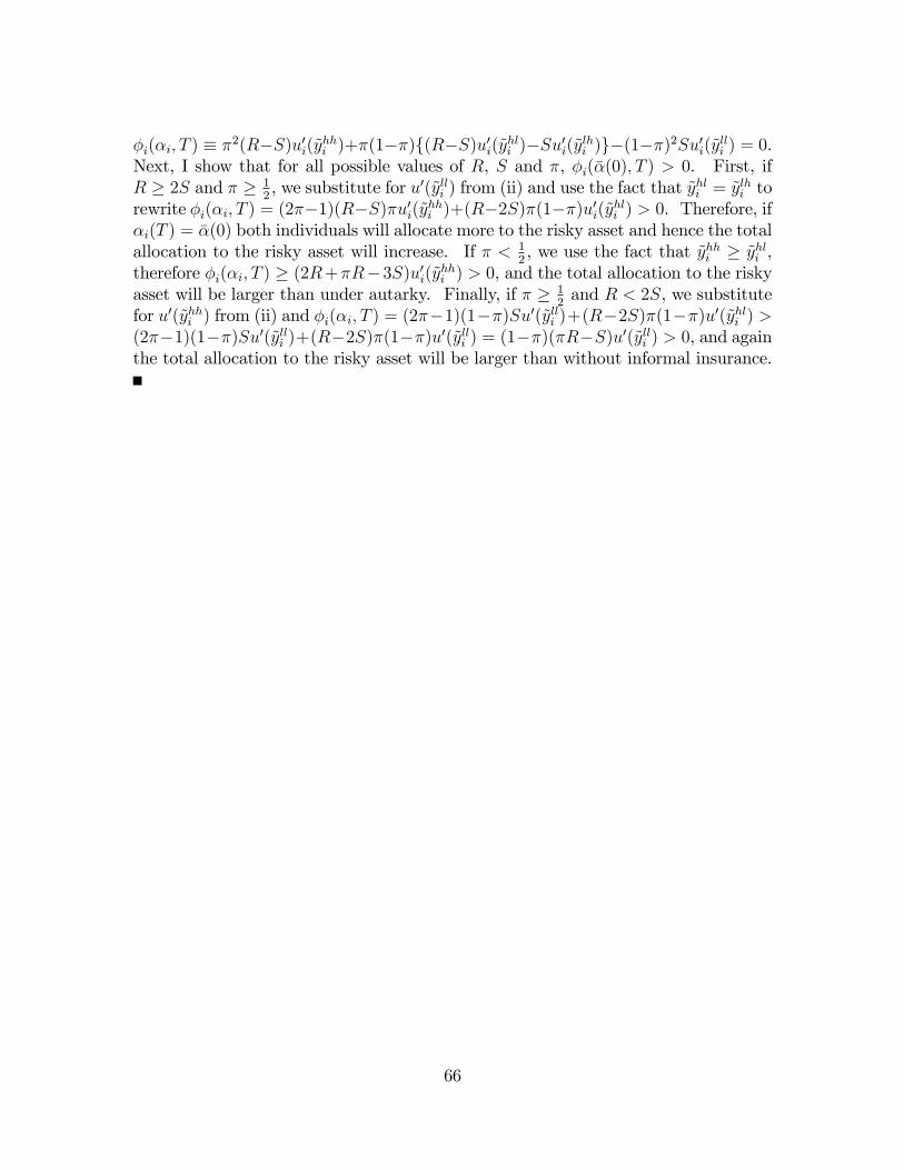
φi(αi, T ) ≡ π2(R−S)u′i(yhhi )+π(1−π){(R−S)u′i(y
hli )−Su′i(ylhi )}−(1−π)2Su′i(y
lli ) = 0.
Next, I show that for all possible values of R, S and π, φi(α(0), T ) > 0. First, ifR ≥ 2S and π ≥ 1
2, we substitute for u′(ylli ) from (ii) and use the fact that yhli = ylhi to
rewrite φi(αi, T ) = (2π−1)(R−S)πu′i(yhhi )+(R−2S)π(1−π)u′i(y
hli ) > 0. Therefore, if
αi(T ) = α(0) both individuals will allocate more to the risky asset and hence the totalallocation to the risky asset will increase. If π < 1
2, we use the fact that yhhi ≥ yhli ,
therefore φi(αi, T ) ≥ (2R+πR−3S)u′i(yhhi ) > 0, and the total allocation to the risky
asset will be larger than under autarky. Finally, if π ≥ 12and R < 2S, we substitute
for u′(yhhi ) from (ii) and φi(αi, T ) = (2π−1)(1−π)Su′(ylli )+(R−2S)π(1−π)u′(yhli ) >(2π−1)(1−π)Su′(ylli )+(R−2S)π(1−π)u′(ylli ) = (1−π)(πR−S)u′(ylli ) > 0, and againthe total allocation to the risky asset will be larger than without informal insurance.
66
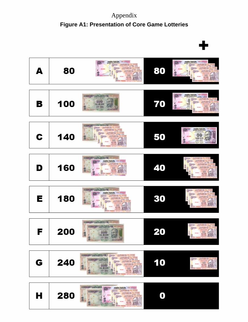
AppendixFigure A1: Presentation of Core Game Lotteries
Related Documents