Contour line construction for a new rectangular facility in an existing layout with rectangular departments by Hari Kelachankuttu, Rajan Batta, Rakesh Nagi ∗ Department of Industrial Engineering, 342 Bell Hall University at Buffalo (SUNY), Buffalo, NY 14260 May 2003 Revised April 2004 Abstract In a recent paper, Savas, Batta and Nagi [12] consider the optimal placement of a finite-sized facility in the presence of arbitrarily-shaped barriers under rectilinear travel. Their model applies to a layout context, since barriers can be thought to be existing departments and the finite-sized facility can be viewed as the new department to be placed. In a layout situation, the existing and new departments are typically rectangular in shape. This is a special case of the Savas et al. paper. However the resultant optimal placement may be infeasible due to practical constraints like aisle locations, electrical connections, etc. Hence there is a need for the development of contour lines, i.e. lines of equal objective function value. With these contour lines constructed, one can place the new facility in the best manner. This paper deals with the problem of constructing contour lines in this context. This contribution can also be viewed as the finite-size extension of the contour line result of Francis [3]. Keywords: Contour Line, Facility Layout, Facility Location. ∗ Author for correspondence: nagi@buffalo.edu

Welcome message from author
This document is posted to help you gain knowledge. Please leave a comment to let me know what you think about it! Share it to your friends and learn new things together.
Transcript

Contour line construction for a new rectangular facility in an existing
layout with rectangular departments
by
Hari Kelachankuttu, Rajan Batta, Rakesh Nagi∗
Department of Industrial Engineering, 342 Bell HallUniversity at Buffalo (SUNY), Buffalo, NY 14260
May 2003Revised April 2004
Abstract
In a recent paper, Savas, Batta and Nagi [12] consider the optimal placement of a finite-sized
facility in the presence of arbitrarily-shaped barriers under rectilinear travel. Their model applies
to a layout context, since barriers can be thought to be existing departments and the finite-sized
facility can be viewed as the new department to be placed. In a layout situation, the existing and
new departments are typically rectangular in shape. This is a special case of the Savas et al. paper.
However the resultant optimal placement may be infeasible due to practical constraints like aisle
locations, electrical connections, etc. Hence there is a need for the development of contour lines,
i.e. lines of equal objective function value. With these contour lines constructed, one can place the
new facility in the best manner. This paper deals with the problem of constructing contour lines
in this context. This contribution can also be viewed as the finite-size extension of the contour
line result of Francis [3].
Keywords: Contour Line, Facility Layout, Facility Location.
∗Author for correspondence: [email protected]

1 Introduction
According to Francis, McGinnis and White [4] and Bindschedler and Moore [2], a facilities layout
problem may arise because of a change in the design of the product, the addition or deletion of a
product from a company’s product line, a significant increase or decrease in the demand for a product,
changes in the design of the process, etc. Sometimes the layout has to be redesigned to include a new
facility such as a single machine, cell or a department. Placement of a new facility in the presence
of existing facilities can be considered as a “restricted layout problem” since in a plant layout the
existing facilities will act as barriers where travel and new facility placement are not permitted.
The facilities location literature discusses problems in which restrictions are imposed upon where
facilities can be placed (Hamacher [5], Nickel [10], Hamacher and Schobel [6] and Klamroth [7]).
Recognizing the practical relevance of facility size consideration, Savas et al. [12] consider the optimal
placement of a finite-sized facility in the presence of arbitrarily-shaped barriers with the median
objective and rectilinear distance metric. In a layout context, barriers may be thought of as existing
facilities which are usually rectangular. Therefore a special case of their model in which the barriers
and the facility are assumed to be rectangular, may be applied to a layout problem where a new
rectangular facility has to be optimally placed in the presence of other rectangular facilities. In a
layout context, the optimal site may not be always suitable for facility placement. For example the
optimal site may pose concerns due to sharp corners, jogs or narrowing of material handling aisles.
Hence there is a need to find a nearby location that is usable. Contour lines, that are lines of equal
objective function value, help to evaluate the costs of locations other than optimal sites. They help to
find the next best solution for an existing layout problem, when the new facility cannot be placed at
its intended optimal location. Francis [3] has considered this problem in the context where facilities
are points. The finite-area case is more appropriate for facilities layout.
The remainder of this paper is organized as follows. In Section 2, we describe and define the
problem. In Section 3, we briefly visit the grid construction procedure of Larson and Sadiq [8] and
the Equal Travel Time Line concept of Batta, Ghose and Palekar [1]. We then illustrate some new
properties of Equal Travel Time Lines in Section 4. Section 5 illustrates the contour line construction
procedure which is followed by a numerical example in Section 6. Section 7 describes the complexity
of our solution procedure. Conclusions and directions for future research are presented in Section 8.
1

2 Problem Definition
We are given a finite number of rectangular existing facilities (EFs) in a 2D plane in which a rectan-
gular new facility (NF) has to be placed. We assume that the NF is oriented with its sides parallel to
the X and Y axes, and one of the four possible orientations is chosen. The procedure can be repeated
for the remaining three orientations. Each EF is characterized by its four corner vertices and has one
or more I/O points on its boundary. These EFs are labeled EF1, . . . ,EFm. Material flow between the
NF and the EFs takes place through a single I/O point X located on the NF boundary. Let (x, y)
represent the coordinates of the I/O point of the NF, D be the set of all EF I/O points, and S be the
rectangular space representing the shop floor area. Let d(i, j : X) be the shortest feasible rectilinear
distance between I/O points i and j (i, j ∈ D ∪ X) given that X is located at (x, y). Here the
term feasible implies a path that does not penetrate the interior of the NF or EFs, which serve as
impenetrable barriers to travel.
There are two types of material flows in the problem. One is the flow between the EFs and the NF
and the other is the flow between all pairs of EFs. All flows takes place through a shortest feasible
rectilinear distance path. In computing the distance, we permit travel on a EF or NF boundary
but not inside. It certainly makes good sense to recognize that the placement of the NF may block
shortest path movements between pairs of EF I/O points, as Fig. 1 illustrates. The same is true for
movement between X and an EF I/O point. At the NF position in Fig. 1, the NF interferes with the
flow between I/O points 1-3 and 1-X.
EF3
EF4EF 2
EF1
��������������������������������������������������������
��������������������������������������������������������
������������������������������������������������������������
������������������������������������������������������������
���������������������������������������������
���������������������������������������������
������������������������������������������������������
������������������������������������������������������
������
������
������������������������
�������
����������
���������������
����
����
Shop floor, S
I/O points
1 2
4
5 6
3Path 1−3
Path 1−X
NF
X
Figure 1: Example to illustrate that NF placement can affect the flow distance between a pair of EFsI/O points and between the NF I/O point and an EF I/O point
The NF needs to be placed such that: (a) the NF does not intersect the union of the interiors of
2
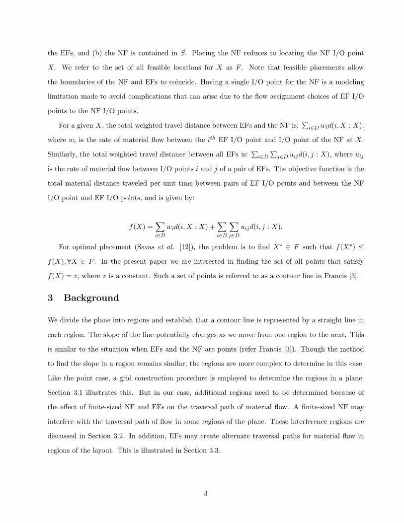
the EFs, and (b) the NF is contained in S. Placing the NF reduces to locating the NF I/O point
X. We refer to the set of all feasible locations for X as F . Note that feasible placements allow
the boundaries of the NF and EFs to coincide. Having a single I/O point for the NF is a modeling
limitation made to avoid complications that can arise due to the flow assignment choices of EF I/O
points to the NF I/O points.
For a given X, the total weighted travel distance between EFs and the NF is:∑
i∈D wid(i,X : X),
where wi is the rate of material flow between the ith EF I/O point and I/O point of the NF at X.
Similarly, the total weighted travel distance between all EFs is:∑
i∈D
∑j∈D uijd(i, j : X), where uij
is the rate of material flow between I/O points i and j of a pair of EFs. The objective function is the
total material distance traveled per unit time between pairs of EF I/O points and between the NF
I/O point and EF I/O points, and is given by:
f(X) =∑i∈D
wid(i,X : X) +∑i∈D
∑j∈D
uijd(i, j : X).
For optimal placement (Savas et al. [12]), the problem is to find X∗ ∈ F such that f(X∗) ≤f(X),∀X ∈ F . In the present paper we are interested in finding the set of all points that satisfy
f(X) = z, where z is a constant. Such a set of points is referred to as a contour line in Francis [3].
3 Background
We divide the plane into regions and establish that a contour line is represented by a straight line in
each region. The slope of the line potentially changes as we move from one region to the next. This
is similar to the situation when EFs and the NF are points (refer Francis [3]). Though the method
to find the slope in a region remains similar, the regions are more complex to determine in this case.
Like the point case, a grid construction procedure is employed to determine the regions in a plane.
Section 3.1 illustrates this. But in our case, additional regions need to be determined because of
the effect of finite-sized NF and EFs on the traversal path of material flow. A finite-sized NF may
interfere with the traversal path of flow in some regions of the plane. These interference regions are
discussed in Section 3.2. In addition, EFs may create alternate traversal paths for material flow in
regions of the layout. This is illustrated in Section 3.3.
3

3.1 Grid construction and cell formation
If the EFs and NF are points, the grid is obtained by drawing horizontal and vertical lines through each
EF. When the EFs have finite dimensions, Larson and Sadiq’s approach [8] is needed. Specializing
their approach for rectangular EFs, the grid can be constructed by drawing horizontal and vertical
traversal lines from all the corners and the I/O points of the EFs, with each line terminating at
the first EF encountered or at an edge of S. Figure 2 illustrates the grid lines constructed. Let Lh
denote the set of horizontal traversal lines and Lv denote the set of vertical traversal lines. Also, let
L = Lh⋃
Lv be the set of all EF traversal lines. The EFs and L divide the region S −⋃mi=1 EFi into
a number of cells. A cell is defined as a closed region in the grid that is not an EF. Cells have the
property that a shortest feasible rectilinear path from an EF I/O point to a point located in the cell
is passes through one of the cell corners (see Larson and Sadiq [8]), and that the length of this path is
concave over the cell. Since we consider rectangular EFs, all the cells formed will also be rectangular.
When a finite-sized NF is placed, a new set of traversal lines passing through its corners and I/O
point are introduced. This new set of lines are referred to as NF traversal lines, L′(X), when the NF
I/O point is located at X.
��������������������������������������������������������
��������������������������������������������������������
������������������������������������������������
������������������������������������������������
������������������������������������
������������������������������������
������������������������������������
������������������������������������
����������������������������������������������
����������������������������
1 2
5
4
3
6
NF traversal lines EF Traversal lines
EF3
EF4EF2EF1
NF
X
Figure 2: EF and NF traversal lines
3.2 Interference sets Q
If a rectangular NF is fully-contained in a cell, the shortest feasible rectilinear path from its I/O
point to an EF I/O point is still concave. In fact, the distance function is identical to that of a
point NF located at X. However, when the rectangular NF intersects one or more EF traversal lines,
distance measurement from its I/O point to an EF I/O point can be affected. The disruption can be
4

characterized provided the NF intersects a distinct set of grid lines as X is varied. This forms the
motivation of interference sets. An interference set Q is a set of placements X obtained by moving
the NF such that the NF intersects a distinct set of grid lines (Savas et al. [12]). More precisely,
for a set of grid lines S ⊂ L, QS is a closed region whose boundary is composed from two types of
segments: (a) locations X such that the NF boundary intersects with some EF boundary, and/or
(b) locations X such that some grid line(s) in set S coincide with some NF traversal line(s). An
example for the formation of sets Q is illustrated in Fig. 3. Consider a NF being moved around a cell
such that the NF intersects the subset of the traversal lines {hi, hi+1, vj}. As illustrated, Qhi, Qhi+1
,
Qhi,vj, Qvj and Qhi+1,vj
are the sets of X locations such that the NF intersects the sets of traversal
lines {hi}, {hi+1}, {hi, vj}, {vj} and {hi+1, vj} respectively. It is noted that each intersection set Qis rectangular and mutually exclusive. Qhi,vj
is shaded for ease of visualization (while the others are
defined by their corners). For example, point 6 of Qhi,vjis generated when grid line hi is coincident
with NF traversal line h′1 and grid line vj is coincident with NF traversal line v′2.
Qv,h
j i
= 1−2−5−6
i+1
i
1
Q
= 7−8−11−12
h
2 3
6
9
1
j+1j
h
Q
h i
v, hj i+1
= 2−3−4−5
Q
7 8
45
12 11 10
i+1
vv
= 8−9−10−11
v v
Q h
h
vj
= 6−5−8−7
1 2
Xh
2h
NF
Figure 3: Interference Sets Q
3.3 Equal travel time lines
As stated in Section 3.1, a shortest feasible rectilinear path from an EF I/O point to a point NF
inside a cell passes through the corner of the cell. In other words, for a fixed NF location within a
cell C, X ∈ C, the EF I/O points may be “assigned” to the nearest corners of the cell for the purpose
of shortest distance measurement. However for any EF I/O point i, the assignment of the cell corner
may change upon moving the NF within the cell. This results in the creation of an Equal Travel Time
5
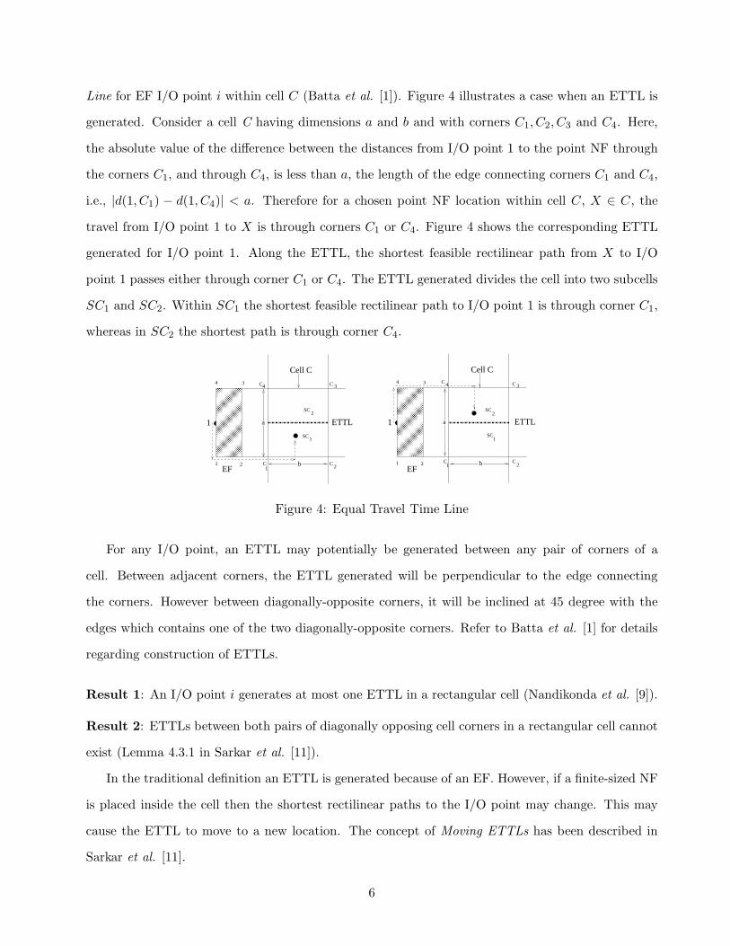
Line for EF I/O point i within cell C (Batta et al. [1]). Figure 4 illustrates a case when an ETTL is
generated. Consider a cell C having dimensions a and b and with corners C1, C2, C3 and C4. Here,
the absolute value of the difference between the distances from I/O point 1 to the point NF through
the corners C1, and through C4, is less than a, the length of the edge connecting corners C1 and C4,
i.e., |d(1, C1) − d(1, C4)| < a. Therefore for a chosen point NF location within cell C, X ∈ C, the
travel from I/O point 1 to X is through corners C1 or C4. Figure 4 shows the corresponding ETTL
generated for I/O point 1. Along the ETTL, the shortest feasible rectilinear path from X to I/O
point 1 passes either through corner C1 or C4. The ETTL generated divides the cell into two subcells
SC1 and SC2. Within SC1 the shortest feasible rectilinear path to I/O point 1 is through corner C1,
whereas in SC2 the shortest path is through corner C4.
����������������������������������������
����������������������������������������
�������������������������������������������������������
�������������������������������������������������������
4 3
1 a
1 2
Cell C
C4 3
1 a
1 2
Cell C
b
ETTL ETTL
SC
b
C
CC C C
CC
11 22
33 44
SC SC
SC
1 1
2 2
EF EF
Figure 4: Equal Travel Time Line
For any I/O point, an ETTL may potentially be generated between any pair of corners of a
cell. Between adjacent corners, the ETTL generated will be perpendicular to the edge connecting
the corners. However between diagonally-opposite corners, it will be inclined at 45 degree with the
edges which contains one of the two diagonally-opposite corners. Refer to Batta et al. [1] for details
regarding construction of ETTLs.
Result 1: An I/O point i generates at most one ETTL in a rectangular cell (Nandikonda et al. [9]).
Result 2: ETTLs between both pairs of diagonally opposing cell corners in a rectangular cell cannot
exist (Lemma 4.3.1 in Sarkar et al. [11]).
In the traditional definition an ETTL is generated because of an EF. However, if a finite-sized NF
is placed inside the cell then the shortest rectilinear paths to the I/O point may change. This may
cause the ETTL to move to a new location. The concept of Moving ETTLs has been described in
Sarkar et al. [11].
6
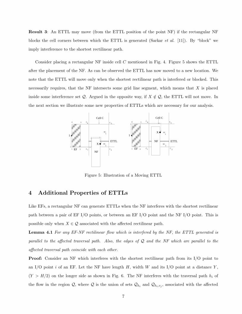
Result 3: An ETTL may move (from the ETTL position of the point NF) if the rectangular NF
blocks the cell corners between which the ETTL is generated (Sarkar et al. [11]). By “block” we
imply interference to the shortest rectilinear path.
Consider placing a rectangular NF inside cell C mentioned in Fig. 4. Figure 5 shows the ETTL
after the placement of the NF. As can be observed the ETTL has now moved to a new location. We
note that the ETTL will move only when the shortest rectilinear path is interfered or blocked. This
necessarily requires, that the NF intersects some grid line segment, which means that X is placed
inside some interference set Q. Argued in the opposite way, if X /∈ Q, the ETTL will not move. In
the next section we illustrate some new properties of ETTLs which are necessary for our analysis.
����������������������������������������
����������������������������������������
�������������������������������������������������������
�������������������������������������������������������
4 3
1
1 2
4 3
1
1 2
Cell C
ETTL ETTL
Cell C
SC
SC
NF
NFSC
SC
C
C C
C C
C1 2
22
11
334C
1
4
C2
EFEF
X
X
Figure 5: Illustration of a Moving ETTL
4 Additional Properties of ETTLs
Like EFs, a rectangular NF can generate ETTLs when the NF interferes with the shortest rectilinear
path between a pair of EF I/O points, or between an EF I/O point and the NF I/O point. This is
possible only when X ∈ Q associated with the affected rectilinear path.
Lemma 4.1 For any EF-NF rectilinear flow which is interfered by the NF, the ETTL generated is
parallel to the affected traversal path. Also, the edges of Q and the NF which are parallel to the
affected traversal path coincide with each other.
Proof: Consider an NF which interferes with the shortest rectilinear path from its I/O point to
an I/O point i of an EF. Let the NF have length H, width W and its I/O point at a distance Y ,
(Y > H/2) on the longer side as shown in Fig. 6. The NF interferes with the traversal path hi of
the flow in the region Q, where Q is the union of sets Qhiand Qhi,vj
, associated with the affected
7

traversal path hi. Let X be such that the edges of Q and the NF which are parallel to the traversal
path hi coincide with each other. At this position the distance traveled along the path i− 1− 2−X
is Y +H −Y + const = H + const and along i− 4− 3−X is H −Y +Y + const = H + const. This is
illustrated in Fig. 6a. Therefore at this position the flow from i−X can occur through corners 1− 2
or 4− 3 of the NF. This remains true for any position along a line through this point and parallel to
the affected traversal path. Therefore the ETTL generated will be parallel to the affected traversal
path and the edges of Q and the NF which are parallel to the affected traversal path coincide with
each other. The ETTL generated divides the region Q into Q1 and Q2. Inside Q1 the flow is through
corners 4− 3 of the NF whereas inside Q2 the flow is through corners 1− 2. �
H Y
W
���������������������������� ����������������������������������������������������������������������������������������������
(a)
X
i j
1 2
4 3
Y
H−Y
H−Y
Y ETTL
h
v
i−X
3
i jY−H/2
H−Y
H/2
i−j
4
21
ETTL
h
v
X
ii
j j
Q2
Q1
Q2
Q1
NF (b)
X
Figure 6: Illustrations for Lemmas 4.1 and 4.2
Lemma 4.2 For rectilinear flow between a pair of EF I/O points which is interfered with by an NF,
the ETTL generated will be at the center of the region Q associated with the affected traversal path
and parallel to the path.
Proof: Suppose that the NF interferes with the shortest rectilinear path between I/O points i and
j. The NF interferes with the traversal path hi of the flow in the region Q, where Q is the union
of sets Qhiand Qhi,vj
, associated with the affected traversal path hi. Consider the NF being placed
at the center of Q. Since X is not at the center (Y > H/2), the center of Q will be offset from the
traveral path by (Y − H/2). At this position the distance travelled along the path i − 1 − 2 − j is
2∗H/2+const = H +const and along i−4−3−j is 2∗(H−Y +Y −H/2)+const = H +const. This
is illustrated in Fig. 6b. Therefore at this position the flow from i− j can occur through corners 1−2
8
or 4 − 3 of the NF. This remains true for any position along a line through this point and parallel
to the affected traversal path. The line divides the region Q into Q1 and Q2. Inside Q1 the flow is
through corners 4− 3 of the NF whereas inside Q2 the flow is through corners 1− 2. Therefore the
ETTL generated will be at the center of the region Q associated with the affected traversal path and
parallel to it. �
In summary the different types of ETTLs that can be generated are as follows:
• Region inside Q
– ETTLs due to an EF I/O point for flow between the EF I/O point and X (Section 3.3).
– ETTLs due to the NF for flow between an EF I/O point and X (Lemma 4.1).
– ETTLs due to the NF for flow between a pair of EF I/O points (Lemma 4.2).
• Region outside Q (i.e., NF fully contained in a cell)
– ETTLs due to an EF I/O point for flow between the EF I/O point and X. In this case
the finite size of the facility will not cause the ETTL to move from the original point NF
case.
We illustrate these types of ETTLs using the example shown in Fig. 7. There are two EF I/O
points, i and j. As illustrated, i generates an ETTL for flow between i−X inside the cell. The NF
also generates ETTLs for flow between i−X and i− j. Inside the region abcd the flow from i−X is
through the upper corners m− n of the EF1. Inside dclk it is through the lower corners p− o of the
EF2. Inside dclk the flow is through either corners q − r or corners t− s of the NF. Inside efgh the
flow is through the lower corners t− s of the NF. However inside hglk it is through the upper corners
q − r of the NF. Armed with the above results we can proceed with constructing contour lines.
5 Contour Line Construction
For the function f(X) the contour line of value z is represented as L(z) where L(z) = {X ∈ F : f(X) = z}.A contour set whose boundary is a contour line is the set of all points having values of f(X) ≤ z.
Francis [3] has shown that for point-sized NF and EFs, the contour line is continuous, with the cor-
responding contour set being convex. However the finite sizes of the NF and the EFs may present
complications as given below:
9

2
1
3
1
2
3j
������������������������
������������������������
������������������������
������������������������
bm va
c
fe
Q
hi
g
d
l
NF
k
u
q
n
x w
EF
j
r
p o st
ETTL due to EF for flow between i−NF
2
1
ETTL due to NF for flow between i−NF
ETTL due to NF for flow between i−j
EF1iX
Figure 7: Different types of ETTLs
1. Contour lines may be intercepted by an EF and hence could be disconnected.
2. The finite-sized NF may interfere with the traversal path of flow between facilities in the region Qassociated with the affected traversal path. Therefore points inside Q may have an objective function
value higher than that of the nearby points. This can make the contour line disconnected.
In the case of point NF and point EFs, if one starts with a location X of objective function value
z, then the slope in the cell to which X belongs will cause the contour line to be incident on some
adjacent cells and the process can be repeated until the contour is closed. In our case, the contour
line and set for a particular value z can only be constructed after evaluating all the cells, at least
implicitly, to identify those cells which contain an X such that f(X) = z. Let Sz denote the set of
cells which contain an X such that f(X) = z. The NF may interfere with the material flow in some
cells while in others it may not. In those cells where the NF interferes with the flow it does so only
in the region Q associated with the affected traversal path. Therefore the set Sz may be classified
as shown in Fig. 8. In our analysis, we consider the objective function and the method to calculate
the slope of the contour line in each of them separately. We start by illustrating our methodology
through a numerical example where an NF has to be placed in a shop floor having two EF I/O points,
i and j. The weights of the flow between facilities are as shown in Fig. 9. We then present a general
procedure to construct the contour line for a given problem instance.
5.1 Identification of cells
Inside a cell, the candidate points for the minima of the objective function of a point NF are the
corners of the cell. Let zip represent the objective function value of a point-sized NF located at the
10
zSSet of cells Q
interferencesCells with
QOutside
interferencesCells with no
Figure 8: Classification of cells
54
��������������������
��������������������
�������������������������
�������������������������
10
1
= 1/4
i
6
78111213
14
j
9
2 3
= 1 u
u = 1 = 3/4 w
w
2311
1
ij
ji
i
80
14
18
28
3626
NF
EFj
2EF
Figure 9: Numerical Example
ith corner of a cell, where i = 1, 2, 3, 4. In a cell if the minimum value of zp, i.e. mini
{zip
}, is greater
than z then no point can be found inside the cell with value z since the placement of a rectangular
NF will only increase the objective function value. If the NF is not interfering with any flow then it
may be considered as a point inside the cell. Then values of zip at the corners may be used to identify
cells which contain the objective function value z. However if the NF interferes with the flow at any
of the corners and mini
{zip
}is less than z, then a point with value less than z may or may not be
present in these cells. The presence of such a point depends on the effect of the NF on the material
flow. Based on the above observations we present an algorithm to determine the set of candidate
cells, Sz, which contain contour line segments of value z.
11

Algorithm for determining the set of cells Sz:
Input: Set of cells from the grid construction procedure of Section 3.1
Initialize: Sz=∅For each cell C:
If mini
{zip
}≤ z
If no interferences
If maxi
{zip
}≥ z
Sz ← Sz ∪ C
Else
Sz ← Sz ∪ C
Output: Set of cells Sz
Applying this algorithm to the numerical example, for z = 35, the set of cells is
S35 = {1, 2, 3, 9, 10, 11, 12, 13, 14}.
5.2 Objective function
In this section we analyze the objective function and illustrate the method to calculate slope of the
line in each of the classifications of set Sz.
5.2.1 Cells with no interferences
Consider a cell C where an NF does not interfere with any of the material flow. Consider a shortest
feasible rectilinear path from an I/O point i to the NF as illustrated in Fig. 10. The NF does not
affect the length of the path from I/O point i to the NF, and hence, the NF may be considered as
a point inside the cell. For a point NF, irrespective of its position inside cell C the total weighted
travel distance between a pair of EF I/O points will be a constant. However the total weighted travel
distance between EF I/O points and X will vary. The EF I/O points may be assigned to appropriate
corners of the cell. It has to be noted that even though there is no effect of the NF inside the cell,
an EF could generate an ETTL as defined in Section 3.3. Therefore the assignment of the EF I/O
points may vary inside the cell.
Let w1, w2, w3, w4 be the weights of the I/O points assigned to the corresponding corner of a
cell/subcell for the purpose of shortest distance measurement. Note that corners are numbered from
12

i
Cell C
i
w
Cell C
(b)(a)
1 2
3
w
ww4
Figure 10: Cell with no interferences
the lower left corner and moving counterclockwise. The objective function may be written as:
f(x, y) = w1(x− xmin) + w2(xmax − x) + w3(xmax − x) + w4(x− xmin) + w1(y − ymin) + w2(y −ymin) + w3(ymax − y) + w4(ymax − y) + const,
where (xmin, ymin), (xmax, ymin), (xmax, ymax), (xmin, ymax) are the corners of the cell/subcell. As can
be observed the objective function is linear in x and y. Therefore the part of the contour line inside
this cell/subcell will be a line segment of the following functional form:
y = x{−w1+w4−w3−w2
w1+w2−w3−w4
}+ const.
The coefficient of x yields the slope of the contour line where the numerator is the difference
between the sum of the weights of the I/O points served through corners 1 and 4, and the sum of
the weights of the I/O points served through corners 2 and 3; and the denominator is the difference
between the sum of the weights of the I/O points served through corners 1 and 2, and the sum of the
weights of the I/O points served through corners 3 and 4. This is similar to the results for point-sized
NF and EFs as defined in Francis [3].
In the numerical example, cells 1, 2, 3, 11, 12, 13 and 14 of the set S35 have no interferences due to
the NF. Inside cell 14, I/O points i and j generate ETTLs for flow to X. Therefore the assignment
of the I/O points i and j to cell corners varies inside cell 14. However the NF may be considered as
a point inside these and the slope may be found using the results for a point NF inside a subcell.
5.2.2 Inside Q
Consider cells 9 and 10 in the numerical example where the NF interferes with the traversal path hi
of the flow between i−X and i− j.
13
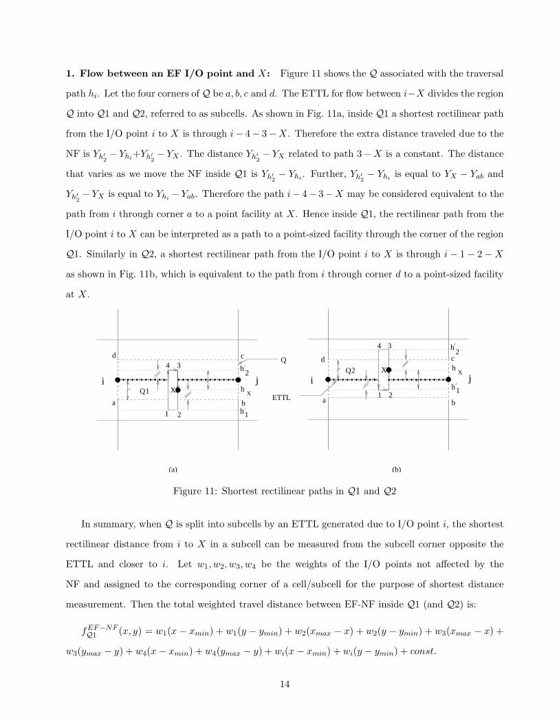
1. Flow between an EF I/O point and X: Figure 11 shows the Q associated with the traversal
path hi. Let the four corners of Q be a, b, c and d. The ETTL for flow between i−X divides the region
Q into Q1 and Q2, referred to as subcells. As shown in Fig. 11a, inside Q1 a shortest rectilinear path
from the I/O point i to X is through i− 4− 3−X. Therefore the extra distance traveled due to the
NF is Yh′2− Yhi
+Yh′2− YX . The distance Yh′
2− YX related to path 3−X is a constant. The distance
that varies as we move the NF inside Q1 is Yh′2− Yhi
. Further, Yh′2− Yhi
is equal to YX − Yab and
Yh′2− YX is equal to Yhi
− Yab. Therefore the path i− 4− 3−X may be considered equivalent to the
path from i through corner a to a point facility at X. Hence inside Q1, the rectilinear path from the
I/O point i to X can be interpreted as a path to a point-sized facility through the corner of the region
Q1. Similarly in Q2, a shortest rectilinear path from the I/O point i to X is through i − 1 − 2 −X
as shown in Fig. 11b, which is equivalent to the path from i through corner d to a point-sized facility
at X.
(b)
4 3
1
(a)
a
4 3
21
Q2
c
ji j
b
d
b
cd
a
i
2
Q
ETTLQ1
h2
h1
1
h2
h
hX
hX
X
X
Figure 11: Shortest rectilinear paths in Q1 and Q2
In summary, when Q is split into subcells by an ETTL generated due to I/O point i, the shortest
rectilinear distance from i to X in a subcell can be measured from the subcell corner opposite the
ETTL and closer to i. Let w1, w2, w3, w4 be the weights of the I/O points not affected by the
NF and assigned to the corresponding corner of a cell/subcell for the purpose of shortest distance
measurement. Then the total weighted travel distance between EF-NF inside Q1 (and Q2) is:
fEF−NFQ1 (x, y) = w1(x− xmin) + w1(y − ymin) + w2(xmax − x) + w2(y − ymin) + w3(xmax − x) +
w3(ymax − y) + w4(x− xmin) + w4(ymax − y) + wi(x− xmin) + wi(y − ymin) + const.
14
= x(w1 + wi + w4 − w3 − w2) + y(w1 + wi + w2 − w3 − w4) + const.
fEF−NFQ2 (x, y) = w1(x− xmin) + w1(y − ymin) + w2(xmax − x) + w2(y − ymin) + w3(xmax − x) +
w3(ymax − y) + w4(x− xmin) + w4(ymax − y) + wi(x− xmin) + wi(ymax − y) + const.
= x(w1 + wi + w4 − w3 − w2) + y(w1 + w2 − w3 − w4 −wi) + const.
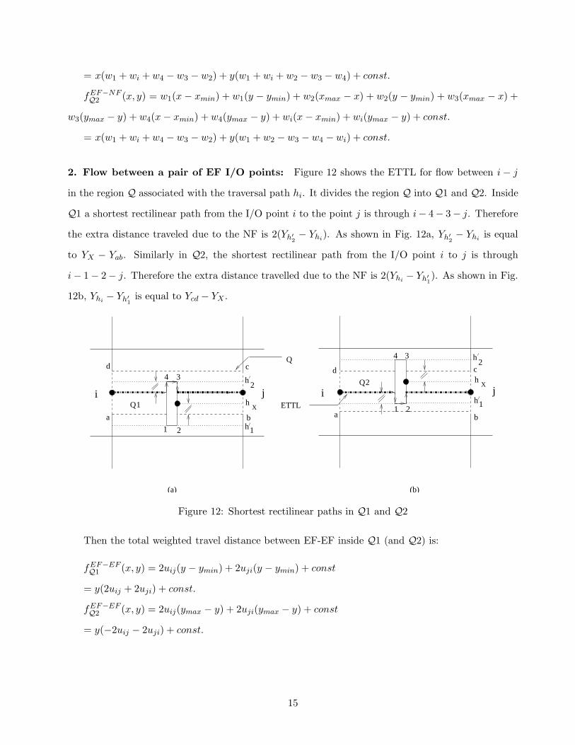
2. Flow between a pair of EF I/O points: Figure 12 shows the ETTL for flow between i− j
in the region Q associated with the traversal path hi. It divides the region Q into Q1 and Q2. Inside
Q1 a shortest rectilinear path from the I/O point i to the point j is through i− 4− 3− j. Therefore
the extra distance traveled due to the NF is 2(Yh′2− Yhi
). As shown in Fig. 12a, Yh′2− Yhi
is equal
to YX − Yab. Similarly in Q2, the shortest rectilinear path from the I/O point i to j is through
i− 1− 2− j. Therefore the extra distance travelled due to the NF is 2(Yhi− Yh′
1). As shown in Fig.
12b, Yhi− Yh′
1is equal to Ycd − YX .
(b)
4 3
1
(a)
a
4 3
21
Q1
Q2
c
ji j
b
d
b
cd
a
i
2
Q
ETTL
h2
h1
h2
h1
hX
hX
Figure 12: Shortest rectilinear paths in Q1 and Q2
Then the total weighted travel distance between EF-EF inside Q1 (and Q2) is:
fEF−EFQ1 (x, y) = 2uij(y − ymin) + 2uji(y − ymin) + const
= y(2uij + 2uji) + const.
fEF−EFQ2 (x, y) = 2uij(ymax − y) + 2uji(ymax − y) + const
= y(−2uij − 2uji) + const.
15
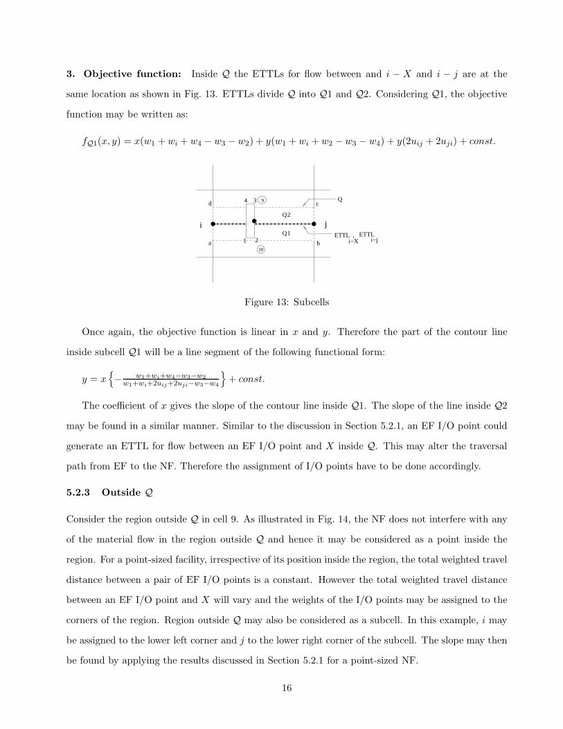
3. Objective function: Inside Q the ETTLs for flow between and i − X and i − j are at the
same location as shown in Fig. 13. ETTLs divide Q into Q1 and Q2. Considering Q1, the objective
function may be written as:
fQ1(x, y) = x(w1 + wi + w4 − w3 − w2) + y(w1 + wi + w2 − w3 − w4) + y(2uij + 2uji) + const.
4 3
1 2a
c
i
d
b
j
9
10
ETTL ,
Q
Q2
Q1i−X
ETTLi−j
Figure 13: Subcells
Once again, the objective function is linear in x and y. Therefore the part of the contour line
inside subcell Q1 will be a line segment of the following functional form:
y = x{− w1+wi+w4−w3−w2
w1+wi+2uij+2uji−w3−w4
}+ const.
The coefficient of x gives the slope of the contour line inside Q1. The slope of the line inside Q2
may be found in a similar manner. Similar to the discussion in Section 5.2.1, an EF I/O point could
generate an ETTL for flow between an EF I/O point and X inside Q. This may alter the traversal
path from EF to the NF. Therefore the assignment of I/O points have to be done accordingly.
5.2.3 Outside Q
Consider the region outside Q in cell 9. As illustrated in Fig. 14, the NF does not interfere with any
of the material flow in the region outside Q and hence it may be considered as a point inside the
region. For a point-sized facility, irrespective of its position inside the region, the total weighted travel
distance between a pair of EF I/O points is a constant. However the total weighted travel distance
between an EF I/O point and X will vary and the weights of the I/O points may be assigned to the
corners of the region. Region outside Q may also be considered as a subcell. In this example, i may
be assigned to the lower left corner and j to the lower right corner of the subcell. The slope may then
be found by applying the results discussed in Section 5.2.1 for a point-sized NF.
16

4 3
1 2
9 9
i j i j
Q d c
bab
cd
a
QOutside
Figure 14: Outside Q
5.3 Contour line construction method
We summarize the contour line construction procedure as follows:
Consider starting at a feasible point X ∈ F which has an objective function value of z.
1. Draw the EF traversal lines and form the grid.
2. Identify the the cell C which contains X.
3. Identify the the subcells in cell C.
(a) Identify ETTLs formed due to EF I/O points, for flow between EF I/O points and X in
cell C and determine its subcells. Note that the NF is finite-sized and could cause the
ETTL to move from the point NF case (Result 3).
(b) Identify the interference sets Qs, where the NF interferes with any of the material flows.
Identify the ETTLs formed, due to the NF for material flow between a pair of EF I/O
points or an EF I/O point and X, inside cell C and hence determine the subcells.
4. For cell C and its subcells, assign weights of the unaffected EF I/O point to X material flow
to the appropriate cell corner. For affected material flow between a pair of EF I/O points and
between an EF I/O point and X, assign weights to the corner opposite to the corresponding
ETTL and nearest to the EF (Section 5.2.2).
5. For cell C and its subcells, the slope of the contour line is determined as follows:
(a) From step 4, let,
17

wi be the sum of the weights of the material flow between EF I/O points and X assigned
to corner i,
uvj and uhkbe the sum of the weights of the material flow between pairs of EF I/O points
affected along the vertical and horizontal path(s),
let 1, 2, 3, 4 be the corners of the cell/subcell starting from the lower left corner and moving
anticlockwise, then,
a = (w1 + w4 + 2uv1 + 2uv4)− (w2 + w3 + 2uv2 + 2uv3), and
b = (w1 + w2 + 2uh1 + 2uh2)− (w3 + w4 + 2uh3 + 2uh4)
(b) Slope of the contour line = −ab
6. Proceed to construct the contour line that passes through X, using the slope computed in Step
5. If this line terminates (in either direction) at the boundary of an adjacent cell/subcell, it
identifies a point in this adjacent cell/subcell that has an objective function value of z. In this
case, recompute the slope using Step 5 and then proceed to draw the continuation of this contour
line. It is also possible that the line terminates at the boundary of the feasible region F . In this
case, examine cells in set Sz (determined using the algorithm of Section 5.1) through which this
contour line has not yet passed, and attempt to find a new starting point that has objective
function value z. To do this one can take advantage of the fact that inside a cell/subcell the
assignment of EF I/O points to the corners of the cell/subcell remains unchanged. Hence the
determination of a point of objective function value z can be set up as a linear program with
no objective, and with constraints that limits the location of X to be within the cell/subcell as
well as a constraint that specifies that the objective function value for the chosen X is z. If this
linear program is infeasible, the cell/subcell contains no point with objective function value z.
Otherwise, it returns one such point. The procedure is then restarted with this new location
and its associated cell C ′.
6 Numerical Example
Figure 15 shows the contour lines constructed for z =31, 35, 41 and 43 using the above procedure.
As can be observed the contour lines for z = 31 and 35 are intercepted by the EFs making them
disconnected.
18

35
43
35
NF
28
14
18
0 8 11 23 26 36
Infeasible Regiion
35
41
43
41
35
31
31
31
35 35
41
43
43
41
������������������������
������������������������
��������������������
��������������������
jEFiEF
Figure 15: Contour lines
7 Solution Complexity
Our solution methodology proceeds in two steps. First the number of cells in which objective function
value z is potentially present has to be identified using the algorithm of Section 5.1. Each EF generates
2 horizontal and 2 vertical traversal lines from its boundaries. Hence if there are m EFs, 2m horizontal
and 2m vertical lines will be produced. Similarly n I/O points can generate at most n horizontal and
n vertical lines. Hence the maximum number of cells generated is O(m2 + n2).
The contour line is then constructed by calculating the slope of the line in each of the identified
cells. Here the complexity depends on the number of subcells generated inside each cell. Result 2 states
that ETTLs between diagonally-opposite corners for rectangular EFs are not possible. Nandikonda
et al. [9] have shown that an I/O point of an EF will generate at most one ETTL. Hence n I/O points
of EFs can generate n ETTLs, in the worst case generating O(n2) subcells per cell. In addition to
this, subcells may be generated due to ETTLs for material flow between a pair of EF I/O points and
between an EF I/O point and X. If, in a cell, the NF interferes the material flow with k (k ≤ n)
EF I/O points, then the maximum number of ETTLs formed inside the cell for flow between EF I/O
points and X will be k. Additionally the flow between k I/O points and the rest of the I/O points
may be affected by the NF. This can generate a maximum of k(n− k) ETTLs for the flows between
19
pairs of EF I/O points. In addition to the ETTLs the boundaries of Qs will also divide the cell into
subcells. Hence the number of subcells that can be generated inside a cell is O(n2). Therefore the
total number of subcells that can be generated is O(m2n2 + n4), which is polynomially bound.
8 Conclusions
In summary, this paper addresses the contour line construction procedure for a finite-sized rectangular
new facility to be placed in a layout having other existing rectangular facilities. Optimal placement
of a finite-sized new facility in the presence of other facilities has been studied by Savas et al. [12].
However due to other considerations the optimal site may not be always suitable for placement of the
new facility. This necessitates the new facility to be placed at alternate locations and provides the
motivation for this paper. Contour lines helps to place the I/O point of the new facility at locations
other than the optimal site with characterized increase in the objective function value. To draw the
contour lines, we divide the plane into regions and formulate a method to calculate the slope of the
contour line in each of these regions. Our work can be viewed as an extension to the work by Francis
[3] who developed the contour line procedure for locating a point NF in the presence of point EFs.
Francis [3] also use the concept of dividing the plane into regions and calculating the slope of the
contour line in each of those regions. This work is applicable for a facilities location problem. To
extend this to a layout context we have to assume finite size for the new facility and the presence
of other finite-sized existing facilities. However, the finite size of the new facility and the presence
of other facilities makes the problem complex to solve since travel is not permitted in these regions
and the rectilinear metric gets destroyed. By a systematic division of the plane into subregions where
the slope of the line remains constant, we develop a procedure for constructing layout contour lines.
Unlike the location case, layout contour lines are non-convex and disconnected. Complexity analysis
establishes that the methodology developed is polynomially bound.
Acknowledgment
This work is supported by the National Science Foundation via grant number DMI–0300370. The
authors would like to thank the two anonymous referees for their constructive comments. These
comments helped strengthen the paper significantly.
20
References
[1] R. Batta, A. Ghose, and U. Palekar. Locating facilities on the manhattan metric with arbitrarily
shaped barriers and convex forbidden regions. Transportation Science, 23(1):26–36, 1989.
[2] A.E. Bindschedler and J.M. Moore. Optimum location of new machines in existing plant layouts.
Journal of Industrial Engineering, 12:41–48, 1961.
[3] R. L. Francis. Note on the optimum location of new machines in existing plant layouts. Journal
of Industrial Engineering, 14(2):57–59, January-February 1963.
[4] R. L. Francis, L. F. McGinnis, and J. A. White. Facility Layout and Location: An Analytical
Approach. Prentice Hall, Englewood Cliffs, NJ, 1992.
[5] H. W. Hamacher. Verfahren der Planaren Standortplanurg. (Methods for Planar Location Plan-
ning). Viewag Verlag, 1995.
[6] H. W. Hamacher and A. Schobel. A note on center problems with forbidden polyhedra. Letters
of Operations Research, 20:165–169, 1997.
[7] K. Klamroth. Single Facility Location Problems with Barriers. Habilitation thesis, University of
Kaiserslautern, Germany, 2000.
[8] R.C. Larson and G. Sadiq. Facility locations with the manhattan metric in the presence of
barriers to travel. Operations Research, 31(4):652–669, January 1983.
[9] P. Nandikonda, R. Batta, and R. Nagi. Locating a 1-center on a manhattan plane with “arbi-
trarily” shaped barriers. Annals of Operations Research, 123:157–172, 2003.
[10] S. Nickel. Discretization of planar location problems. Shaker Verlag, Aachen, 1995.
[11] A. Sarkar, R. Batta, and R. Nagi. Placing a finite size facility with a center objective on a
rectilinear plane with barriers. European Journal of Operational Research, submitted 2003.
[12] S. Savas, R. Batta, and R. Nagi. Finite-size facility placement in the presence of barriers to
rectilinear travel. Operations Research, 50(6):1018–1031, November-December 2002.
21
Related Documents