Contour Detection and Hierarchical Image …malik/papers/arbelaezMFM-pami...Contour Detection and Hierarchical Image Segmentation ... ing machine generated contours to human ground-truth

1

Contour Detection andHierarchical Image Segmentation

Pablo Arbelaez, Member, IEEE, Michael Maire, Member, IEEE,Charless Fowlkes, Member, IEEE, and Jitendra Malik, Fellow, IEEE.

Abstract—This paper investigates two fundamental problems in computer vision: contour detection and image segmentation. Wepresent state-of-the-art algorithms for both of these tasks. Our contour detector combines multiple local cues into a globalizationframework based on spectral clustering. Our segmentation algorithm consists of generic machinery for transforming the output ofany contour detector into a hierarchical region tree. In this manner, we reduce the problem of image segmentation to that of contourdetection. Extensive experimental evaluation demonstrates that both our contour detection and segmentation methods significantlyoutperform competing algorithms. The automatically generated hierarchical segmentations can be interactively refined by user-specified annotations. Computation at multiple image resolutions provides a means of coupling our system to recognition applications.

�

1 INTRODUCTION

This paper presents a unified approach to contour de-tection and image segmentation. Contributions include:

• A high performance contour detector, combininglocal and global image information.

• A method to transform any contour signal into a hi-erarchy of regions while preserving contour quality.

• Extensive quantitative evaluation and the release ofa new annotated dataset.

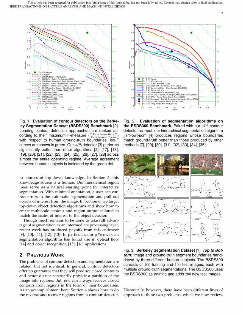
Figures 1 and 2 summarize our main results. Thetwo Figures represent the evaluation of multiple con-tour detection (Figure 1) and image segmentation (Fig-ure 2) algorithms on the Berkeley Segmentation Dataset(BSDS300) [1], using the precision-recall framework in-troduced in [2]. This benchmark operates by compar-ing machine generated contours to human ground-truthdata (Figure 3) and allows evaluation of segmentationsin the same framework by regarding region boundariesas contours.

Especially noteworthy in Figure 1 is the contour de-tector gPb, which compares favorably with other leadingtechniques, providing equal or better precision for mostchoices of recall. In Figure 2, gPb-owt-ucm providesuniversally better performance than alternative segmen-tation algorithms. We introduced the gPb and gPb-owt-ucm algorithms in [3] and [4], respectively. This paperoffers comprehensive versions of these algorithms, mo-tivation behind their design, and additional experimentswhich support our basic claims.

We begin with a review of the extensive literature oncontour detection and image segmentation in Section 2.

• P. Arbelaez and J. Malik are with the Department of Electrical Engineeringand Computer Science, University of California at Berkeley, Berkeley, CA94720. E-mail: {arbelaez,malik}@eecs.berkeley.edu

• M. Maire is with the Department of Electrical Engineering, CaliforniaInstitute of Technology, Pasadena, CA 91125. E-mail: [email protected]

• C. Fowlkes is with the Department of Computer Science, University ofCalifornia at Irvine, Irvine, CA 92697. E-mail: [email protected]

Section 3 covers the development of the gPb contourdetector. We couple multiscale local brightness, color,and texture cues to a powerful globalization frameworkusing spectral clustering. The local cues, computed byapplying oriented gradient operators at every locationin the image, define an affinity matrix representing thesimilarity between pixels. From this matrix, we derivea generalized eigenproblem and solve for a fixed num-ber of eigenvectors which encode contour information.Using a classifier to recombine this signal with the localcues, we obtain a large improvement over alternativeglobalization schemes built on top of similar cues.

To produce high-quality image segmentations, we linkthis contour detector with a generic grouping algorithmdescribed in Section 4 and consisting of two steps. First,we introduce a new image transformation called theOriented Watershed Transform for constructing a set ofinitial regions from an oriented contour signal. Second,using an agglomerative clustering procedure, we formthese regions into a hierarchy which can be representedby an Ultrametric Contour Map, the real-valued imageobtained by weighting each boundary by its scale ofdisappearance. We provide experiments on the BSDS300as well as the BSDS500, a superset newly released here.

Although the precision-recall framework [2] has foundwidespread use for evaluating contour detectors, con-siderable effort has also gone into developing metricsto directly measure the quality of regions produced bysegmentation algorithms. Noteworthy examples includethe Probabilistic Rand Index, introduced in this contextby [5], the Variation of Information [6], [7], and theSegmentation Covering criteria used in the PASCALchallenge [8]. We consider all of these metrics anddemonstrate that gPb-owt-ucm delivers an across-the-board improvement over existing algorithms.

Sections 5 and 6 explore ways of connecting ourpurely bottom-up contour and segmentation machinery

Digital Object Indentifier 10.1109/TPAMI.2010.161 0162-8828/10/$26.00 © 2010 IEEE

IEEE TRANSACTIONS ON PATTERN ANALYSIS AND MACHINE INTELLIGENCEThis article has been accepted for publication in a future issue of this journal, but has not been fully edited. Content may change prior to final publication.

2

0 0.1 0.2 0.3 0.4 0.5 0.6 0.7 0.8 0.9 10

0.1

0.2

0.3

0.4

0.5

0.6

0.7

0.8

0.9

1

0.1

0.2

0.3

0.4

0.5

0.6

0.7

0.8

0.9

iso−F

Recall

Pre

cisi

on

[F = 0.79] Human[F = 0.70] gPb[F = 0.68] Multiscale − Ren (2008)[F = 0.66] BEL − Dollar, Tu, Belongie (2006)[F = 0.66] Mairal, Leordeanu, Bach, Herbert, Ponce (2008)[F = 0.65] Min Cover − Felzenszwalb, McAllester (2006)[F = 0.65] Pb − Martin, Fowlkes, Malik (2004)[F = 0.64] Untangling Cycles − Zhu, Song, Shi (2007)[F = 0.64] CRF − Ren, Fowlkes, Malik (2005)[F = 0.58] Canny (1986)[F = 0.56] Perona, Malik (1990)[F = 0.50] Hildreth, Marr (1980)[F = 0.48] Prewitt (1970)[F = 0.48] Sobel (1968)[F = 0.47] Roberts (1965)

Fig. 1. Evaluation of contour detectors on the Berke-ley Segmentation Dataset (BSDS300) Benchmark [2].Leading contour detection approaches are ranked ac-cording to their maximum F-measure ( 2·Precision·Recall

Precision+Recall )with respect to human ground-truth boundaries. Iso-Fcurves are shown in green. Our gPb detector [3] performssignificantly better than other algorithms [2], [17], [18],[19], [20], [21], [22], [23], [24], [25], [26], [27], [28] acrossalmost the entire operating regime. Average agreementbetween human subjects is indicated by the green dot.

to sources of top-down knowledge. In Section 5, thisknowledge source is a human. Our hierarchical regiontrees serve as a natural starting point for interactivesegmentation. With minimal annotation, a user can cor-rect errors in the automatic segmentation and pull outobjects of interest from the image. In Section 6, we targettop-down object detection algorithms and show how tocreate multiscale contour and region output tailored tomatch the scales of interest to the object detector.

Though much remains to be done to take full advan-tage of segmentation as an intermediate processing layer,recent work has produced payoffs from this endeavor[9], [10], [11], [12], [13]. In particular, our gPb-owt-ucmsegmentation algorithm has found use in optical flow[14] and object recognition [15], [16] applications.

2 PREVIOUS WORK

The problems of contour detection and segmentation arerelated, but not identical. In general, contour detectorsoffer no guarantee that they will produce closed contoursand hence do not necessarily provide a partition of theimage into regions. But, one can always recover closedcontours from regions in the form of their boundaries.As an accomplishment here, Section 4 shows how to dothe reverse and recover regions from a contour detector.

0 0.1 0.2 0.3 0.4 0.5 0.6 0.7 0.8 0.9 10

0.1

0.2

0.3

0.4

0.5

0.6

0.7

0.8

0.9

1

0.1

0.2

0.3

0.4

0.5

0.6

0.7

0.8

0.9

iso−F

Recall

Pre

cisi

on

[F = 0.79] Human[F = 0.71] gPb−owt−ucm[F = 0.67] UCM − Arbelaez (2006)[F = 0.63] Mean Shift − Comaniciu, Meer (2002)[F = 0.62] Normalized Cuts − Cour, Benezit, Shi (2005)[F = 0.58] Canny−owt−ucm[F = 0.58] Felzenszwalb, Huttenlocher (2004)[F = 0.58] Av. Diss. − Bertelli, Sumengen, Manjunath, Gibou (2008)[F = 0.56] SWA − Alpert, Galun, Basri, Brandt (2007)[F = 0.55] ChanVese − Bertelli, Sumengen, Manjunath, Gibou (2008)[F = 0.55] Donoser, Urschler, Hirzer, Bischof (2009)[F = 0.53] Yang, Wright, Ma, Sastry (2007)

Fig. 2. Evaluation of segmentation algorithms onthe BSDS300 Benchmark. Paired with our gPb contourdetector as input, our hierarchical segmentation algorithmgPb-owt-ucm [4] produces regions whose boundariesmatch ground-truth better than those produced by othermethods [7], [29], [30], [31], [32], [33], [34], [35].

Fig. 3. Berkeley Segmentation Dataset [1]. Top to Bot-tom: Image and ground-truth segment boundaries hand-drawn by three different human subjects. The BSDS300consists of 200 training and 100 test images, each withmultiple ground-truth segmentations. The BSDS500 usesthe BSDS300 as training and adds 200 new test images.

Historically, however, there have been different lines ofapproach to these two problems, which we now review.


3

2.1 Contours

Early approaches to contour detection aim at quantifyingthe presence of a boundary at a given image locationthrough local measurements. The Roberts [17], Sobel[18], and Prewitt [19] operators detect edges by convolv-ing a grayscale image with local derivative filters. Marrand Hildreth [20] use zero crossings of the Laplacian ofGaussian operator. The Canny detector [22] also modelsedges as sharp discontinuities in the brightness chan-nel, adding non-maximum suppression and hysteresisthresholding steps. A richer description can be obtainedby considering the response of the image to a family offilters of different scales and orientations. An exampleis the Oriented Energy approach [21], [36], [37], whichuses quadrature pairs of even and odd symmetric filters.Lindeberg [38] proposes a filter-based method with anautomatic scale selection mechanism.

More recent local approaches take into account colorand texture information and make use of learning tech-niques for cue combination [2], [26], [27]. Martin et al.[2] define gradient operators for brightness, color, andtexture channels, and use them as input to a logisticregression classifier for predicting edge strength. Ratherthan rely on such hand-crafted features, Dollar et al. [27]propose a Boosted Edge Learning (BEL) algorithm whichattempts to learn an edge classifier in the form of aprobabilistic boosting tree [39] from thousands of simplefeatures computed on image patches. An advantage ofthis approach is that it may be possible to handle cuessuch as parallelism and completion in the initial classi-fication stage. Mairal et al. [26] create both generic andclass-specific edge detectors by learning discriminativesparse representations of local image patches. For eachclass, they learn a discriminative dictionary and use thereconstruction error obtained with each dictionary asfeature input to a final classifier.

The large range of scales at which objects may ap-pear in the image remains a concern for these modernlocal approaches. Ren [28] finds benefit in combininginformation from multiple scales of the local operatorsdeveloped by [2]. Additional localization and relativecontrast cues, defined in terms of the multiscale detectoroutput, are fed to the boundary classifier. For each scale,the localization cue captures the distance from a pixelto the nearest peak response. The relative contrast cuenormalizes each pixel in terms of the local neighborhood.

An orthogonal line of work in contour detection fo-cuses primarily on another level of processing, globaliza-tion, that utilizes local detector output. The simplest suchalgorithms link together high-gradient edge fragmentsin order to identify extended, smooth contours [40],[41], [42]. More advanced globalization stages are thedistinguishing characteristics of several of the recenthigh-performance methods benchmarked in Figure 1,including our own, which share as a common featuretheir use of the local edge detection operators of [2].

Ren et al. [23] use the Conditional Random Fields

(CRF) framework to enforce curvilinear continuity ofcontours. They compute a constrained Delaunay triangu-lation (CDT) on top of locally detected contours, yieldinga graph consisting of the detected contours along withthe new “completion” edges introduced by the trian-gulation. The CDT is scale-invariant and tends to fillshort gaps in the detected contours. By associating arandom variable with each contour and each completionedge, they define a CRF with edge potentials in termsof detector response and vertex potentials in terms ofjunction type and continuation smoothness. They useloopy belief propagation [43] to compute expectations.

Felzenszwalb and McAllester [25] use a different strat-egy for extracting salient smooth curves from the outputof a local contour detector. They consider the set ofshort oriented line segments that connect pixels in theimage to their neighboring pixels. Each such segment iseither part of a curve or is a background segment. Theyassume curves are drawn from a Markov process, theprior distribution on curves favors few per scene, anddetector responses are conditionally independent giventhe labeling of line segments. Finding the optimal linesegment labeling then translates into a general weightedmin-cover problem in which the elements being coveredare the line segments themselves and the objects cover-ing them are drawn from the set of all possible curvesand all possible background line segments. Since thisproblem is NP-hard, an approximate solution is foundusing a greedy “cost per pixel” heuristic.

Zhu et al. [24] also start with the output of [2] andcreate a weighted edgel graph, where the weights mea-sure directed collinearity between neighboring edgels.They propose detecting closed topological cycles in thisgraph by considering the complex eigenvectors of thenormalized random walk matrix. This procedure extractsboth closed contours and smooth curves, as edgel chainsare allowed to loop back at their termination points.

2.2 Regions

A broad family of approaches to segmentation involveintegrating features such as brightness, color, or tex-ture over local image patches and then clustering thosefeatures based on, e.g., fitting mixture models [7], [44],mode-finding [34], or graph partitioning [32], [45], [46],[47]. Three algorithms in this category appear to bethe most widely used as sources of image segments inrecent applications, due to a combination of reasonableperformance and publicly available implementations.

The graph based region merging algorithm advocatedby Felzenszwalb and Huttenlocher (Felz-Hutt) [32] at-tempts to partition image pixels into components suchthat the resulting segmentation is neither too coarse nortoo fine. Given a graph in which pixels are nodes andedge weights measure the dissimilarity between nodes(e.g. color differences), each node is initially placed inits own component. Define the internal difference of acomponent Int(R) as the largest weight in the minimum


4

spanning tree of R. Considering edges in non-decreasingorder by weight, each step of the algorithm mergescomponents R1 and R2 connected by the current edge ifthe edge weight is less than:

min(Int(R1) + τ(R1), Int(R2) + τ(R2)) (1)

where τ(R) = k/|R|. k is a scale parameter that can beused to set a preference for component size.

The Mean Shift algorithm [34] offers an alternativeclustering framework. Here, pixels are represented inthe joint spatial-range domain by concatenating theirspatial coordinates and color values into a single vector.Applying mean shift filtering in this domain yields aconvergence point for each pixel. Regions are formed bygrouping together all pixels whose convergence pointsare closer than hs in the spatial domain and hr in therange domain, where hs and hr are respective bandwidthparameters. Additional merging can also be performedto enforce a constraint on minimum region area.

Spectral graph theory [48], and in particular the Nor-malized Cuts criterion [45], [46], provides a way ofintegrating global image information into the groupingprocess. In this framework, given an affinity matrix Wwhose entries encode the similarity between pixels, onedefines diagonal matrix Dii =

∑j Wij and solves for the

generalized eigenvectors of the linear system:

(D −W )v = λDv (2)

Traditionally, after this step, K-means clustering isapplied to obtain a segmentation into regions. This ap-proach often breaks uniform regions where the eigenvec-tors have smooth gradients. One solution is to reweightthe affinity matrix [47]; others have proposed alternativegraph partitioning formulations [49], [50], [51].

A recent variant of Normalized Cuts for image seg-mentation is the Multiscale Normalized Cuts (NCuts)approach of Cour et al. [33]. The fact that W mustbe sparse, in order to avoid a prohibitively expensivecomputation, limits the naive implementation to usingonly local pixel affinities. Cour et al. solve this limitationby computing sparse affinity matrices at multiple scales,setting up cross-scale constraints, and deriving a neweigenproblem for this constrained multiscale cut.

Sharon et al. [52] propose an alternative to improvethe computational efficiency of Normalized Cuts. Thisapproach, inspired by algebraic multigrid, iterativelycoarsens the original graph by selecting a subset of nodessuch that each variable on the fine level is stronglycoupled to one on the coarse level. The same mergingstrategy is adopted in [31], where the strong coupling ofa subset S of the graph nodes V is formalized as:∑

j∈S pij∑j∈V pij

> ψ ∀i ∈ V − S (3)

where ψ is a constant and pij the probability of mergingi and j, estimated from brightness and texture similarity.

Many approaches to image segmentation fall into adifferent category than those covered so far, relying on

the formulation of the problem in a variational frame-work. An example is the model proposed by Mumfordand Shah [53], where the segmentation of an observedimage u0 is given by the minimization of the functional:

F(u, C) =∫

Ω

(u− u0)2dx + μ

∫Ω\C

|∇(u)|2dx + ν|C| (4)

where u is piecewise smooth in Ω\C and μ, ν are weight-ing parameters. Theoretical properties of this model canbe found in, e.g. [53], [54]. Several algorithms have beendeveloped to minimize the energy (4) or its simplifiedversion, where u is piecewise constant in Ω\C. Koepfleret al. [55] proposed a region merging method for thispurpose. Chan and Vese [56], [57] follow a differentapproach, expressing (4) in the level set formalism ofOsher and Sethian [58], [59]. Bertelli et al. [30] extendthis approach to more general cost functions based onpairwise pixel similarities. Recently, Pock et al. [60] pro-posed to solve a convex relaxation of (4), thus obtainingrobustness to initialization. Donoser et al. [29] subdividethe problem into several figure/ground segmentations,each initialized using low-level saliency and solved byminimizing an energy based on Total Variation.

2.3 BenchmarksThough much of the extensive literature on contourdetection predates its development, the BSDS [2] hassince found wide acceptance as a benchmark for this task[23], [24], [25], [26], [27], [28], [35], [61]. The standard forevaluating segmentations algorithms is less clear.

One option is to regard the segment boundariesas contours and evaluate them as such. However, amethodology that directly measures the quality of thesegments is also desirable. Some types of errors, e.g. amissing pixel in the boundary between two regions, maynot be reflected in the boundary benchmark, but canhave substantial consequences for segmentation quality,e.g. incorrectly merging large regions. One might arguethat the boundary benchmark favors contour detectorsover segmentation methods, since the former are notburdened with the constraint of producing closed curves.We therefore also consider various region-based metrics.

2.3.1 Variation of InformationThe Variation of Information metric was introduced forthe purpose of clustering comparison [6]. It measures thedistance between two segmentations in terms of theiraverage conditional entropy given by:

V I(S, S′) = H(S) + H(S′)− 2I(S, S′) (5)

where H and I represent respectively the entropies andmutual information between two clusterings of data Sand S′. In our case, these clusterings are test and ground-truth segmentations. Although V I possesses some inter-esting theoretical properties [6], its perceptual meaningand applicability in the presence of several ground-truthsegmentations remains unclear.


5

2.3.2 Rand IndexOriginally, the Rand Index [62] was introduced for gen-eral clustering evaluation. It operates by comparing thecompatibility of assignments between pairs of elementsin the clusters. The Rand Index between test and ground-truth segmentations S and G is given by the sum of thenumber of pairs of pixels that have the same label inS and G and those that have different labels in bothsegmentations, divided by the total number of pairs ofpixels. Variants of the Rand Index have been proposed[5], [7] for dealing with the case of multiple ground-truthsegmentations. Given a set of ground-truth segmenta-tions {Gk}, the Probabilistic Rand Index is defined as:

PRI(S, {Gk}) =1T

∑i<j

[cijpij + (1− cij)(1− pij)] (6)

where cij is the event that pixels i and j have the samelabel and pij its probability. T is the total number ofpixel pairs. Using the sample mean to estimate pij , (6)amounts to averaging the Rand Index among differentground-truth segmentations. The PRI has been reportedto suffer from a small dynamic range [5], [7], and itsvalues across images and algorithms are often similar.In [5], this drawback is addressed by normalization withan empirical estimation of its expected value.

2.3.3 Segmentation CoveringThe overlap between two regions R and R′, defined as:

O(R,R′) =|R ∩R′||R ∪R′| (7)

has been used for the evaluation of the pixel-wise clas-sification task in recognition [8], [11]. We define thecovering of a segmentation S by a segmentation S′ as:

C(S′ → S) =1N

∑R∈S

|R| · maxR′∈S′

O(R,R′) (8)

where N denotes the total number of pixels in the image.Similarly, the covering of a machine segmentation S by

a family of ground-truth segmentations {Gi} is definedby first covering S separately with each human segmen-tation Gi, and then averaging over the different humans.To achieve perfect covering the machine segmentationmust explain all of the human data. We can then definetwo quality descriptors for regions: the covering of S by{Gi} and the covering of {Gi} by S.

3 CONTOUR DETECTION

As a starting point for contour detection, we considerthe work of Martin et al. [2], who define a functionPb(x, y, θ) that predicts the posterior probability of aboundary with orientation θ at each image pixel (x, y)by measuring the difference in local image brightness,color, and texture channels. In this section, we reviewthese cues, introduce our own multiscale version of thePb detector, and describe the new globalization methodwe run on top of this multiscale local detector.

0 0.5 1

Upper Half−Disc Histogram

0 0.5 1

Lower Half−Disc Histogram

Fig. 4. Oriented gradient of histograms. Given anintensity image, consider a circular disc centered at eachpixel and split by a diameter at angle θ. We computehistograms of intensity values in each half-disc and outputthe χ2 distance between them as the gradient magnitude.The blue and red distributions shown in the middle panelare the histograms of the pixel brightness values in theblue and red regions, respectively, in the left image. Theright panel shows an example result for a disc of radius5 pixels at orientation θ = π

4 after applying a second-order Savitzky-Golay smoothing filter to the raw histogramdifference output. Note that the left panel displays a largerdisc (radius 50 pixels) for illustrative purposes.

3.1 Brightness, Color, Texture GradientsThe basic building block of the Pb contour detector isthe computation of an oriented gradient signal G(x, y, θ)from an intensity image I . This computation proceedsby placing a circular disc at location (x, y) split into twohalf-discs by a diameter at angle θ. For each half-disc, wehistogram the intensity values of the pixels of I coveredby it. The gradient magnitude G at location (x, y) isdefined by the χ2 distance between the two half-dischistograms g and h:

χ2(g, h) =12

∑i

(g(i)− h(i))2

g(i) + h(i)(9)

We then apply second-order Savitzky-Golay filtering[63] to enhance local maxima and smooth out multipledetection peaks in the direction orthogonal to θ. This isequivalent to fitting a cylindrical parabola, whose axisis orientated along direction θ, to a local 2D windowsurrounding each pixel and replacing the response at thepixel with that estimated by the fit.

Figure 4 shows an example. This computation is moti-vated by the intuition that contours correspond to imagediscontinuities and histograms provide a robust mech-anism for modeling the content of an image region. Astrong oriented gradient response means a pixel is likelyto lie on the boundary between two distinct regions.

The Pb detector combines the oriented gradient sig-nals obtained from transforming an input image intofour separate feature channels and processing each chan-nel independently. The first three correspond to thechannels of the CIE Lab colorspace, which we refer to


6

Fig. 5. Filters for creating textons. We use 8 orientedeven- and odd-symmetric Gaussian derivative filters anda center-surround (difference of Gaussians) filter.

as the brightness, color a, and color b channels. Forgrayscale images, the brightness channel is the imageitself and no color channels are used.

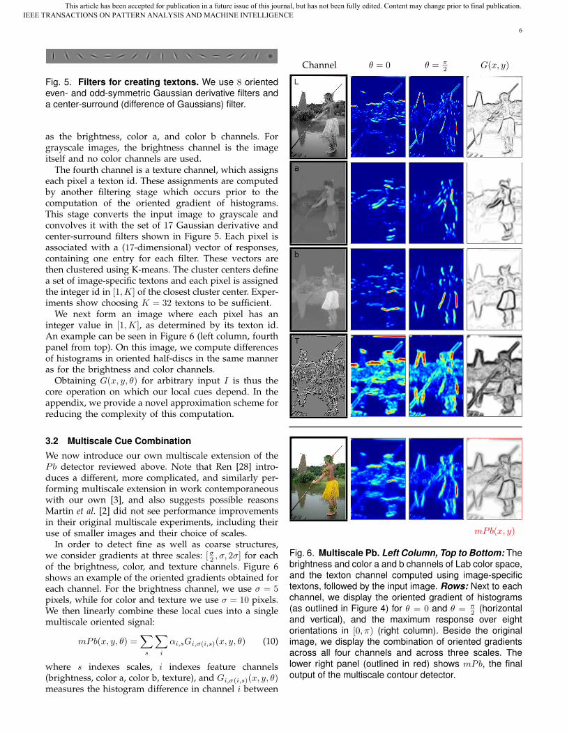
The fourth channel is a texture channel, which assignseach pixel a texton id. These assignments are computedby another filtering stage which occurs prior to thecomputation of the oriented gradient of histograms.This stage converts the input image to grayscale andconvolves it with the set of 17 Gaussian derivative andcenter-surround filters shown in Figure 5. Each pixel isassociated with a (17-dimensional) vector of responses,containing one entry for each filter. These vectors arethen clustered using K-means. The cluster centers definea set of image-specific textons and each pixel is assignedthe integer id in [1, K] of the closest cluster center. Exper-iments show choosing K = 32 textons to be sufficient.

We next form an image where each pixel has aninteger value in [1, K], as determined by its texton id.An example can be seen in Figure 6 (left column, fourthpanel from top). On this image, we compute differencesof histograms in oriented half-discs in the same manneras for the brightness and color channels.

Obtaining G(x, y, θ) for arbitrary input I is thus thecore operation on which our local cues depend. In theappendix, we provide a novel approximation scheme forreducing the complexity of this computation.

3.2 Multiscale Cue Combination

We now introduce our own multiscale extension of thePb detector reviewed above. Note that Ren [28] intro-duces a different, more complicated, and similarly per-forming multiscale extension in work contemporaneouswith our own [3], and also suggests possible reasonsMartin et al. [2] did not see performance improvementsin their original multiscale experiments, including theiruse of smaller images and their choice of scales.

In order to detect fine as well as coarse structures,we consider gradients at three scales: [σ

2 , σ, 2σ] for eachof the brightness, color, and texture channels. Figure 6shows an example of the oriented gradients obtained foreach channel. For the brightness channel, we use σ = 5pixels, while for color and texture we use σ = 10 pixels.We then linearly combine these local cues into a singlemultiscale oriented signal:

mPb(x, y, θ) =∑

s

∑i

αi,sGi,σ(i,s)(x, y, θ) (10)

where s indexes scales, i indexes feature channels(brightness, color a, color b, texture), and Gi,σ(i,s)(x, y, θ)measures the histogram difference in channel i between

Channel θ = 0 θ = π2 G(x, y)

mPb(x, y)

Fig. 6. Multiscale Pb. Left Column, Top to Bottom: Thebrightness and color a and b channels of Lab color space,and the texton channel computed using image-specifictextons, followed by the input image. Rows: Next to eachchannel, we display the oriented gradient of histograms(as outlined in Figure 4) for θ = 0 and θ = π

2 (horizontaland vertical), and the maximum response over eightorientations in [0, π) (right column). Beside the originalimage, we display the combination of oriented gradientsacross all four channels and across three scales. Thelower right panel (outlined in red) shows mPb, the finaloutput of the multiscale contour detector.


7

Fig. 7. Spectral Pb. Left: Image. Middle Left: The thinned non-max suppressed multiscale Pb signal defines a sparseaffinity matrix connecting pixels within a fixed radius. Pixels i and j have a low affinity as a strong boundary separatesthem, whereas i and k have high affinity. Middle: First four generalized eigenvectors resulting from spectral clustering.Middle Right: Partitioning the image by running K-means clustering on the eigenvectors erroneously breaks smoothregions. Right: Instead, we compute gradients of the eigenvectors, transforming them back into a contour signal.

Fig. 8. Eigenvectors carry contour information. Left: Image and maximum response of spectral Pb overorientations, sPb(x, y) = maxθ{sPb(x, y, θ)}. Right Top: First four generalized eigenvectors, v1, ...,v4, used increating sPb. Right Bottom: Maximum gradient response over orientations, maxθ{∇θvk(x, y)}, for each eigenvector.

two halves of a disc of radius σ(i, s) centered at (x, y) anddivided by a diameter at angle θ. The parameters αi,s

weight the relative contribution of each gradient signal.In our experiments, we sample θ at eight equally spacedorientations in the interval [0, π). Taking the maximumresponse over orientations yields a measure of boundarystrength at each pixel:

mPb(x, y) = maxθ{mPb(x, y, θ)} (11)

An optional non-maximum suppression step [22] pro-duces thinned, real-valued contours.

In contrast to [2] and [28] which use a logistic regres-sion classifier to combine cues, we learn the weights αi,s

by gradient ascent on the F-measure using the trainingimages and corresponding ground-truth of the BSDS.

3.3 Globalization

Spectral clustering lies at the heart of our globalizationmachinery. The key element differentiating the algorithmdescribed in this section from other approaches [45], [47]

is the “soft” manner in which we use the eigenvectorsobtained from spectral partitioning.

As input to the spectral clustering stage, we constructa sparse symmetric affinity matrix W using the interven-ing contour cue [49], [64], [65], the maximal value of mPbalong a line connecting two pixels. We connect all pixelsi and j within a fixed radius r with affinity:

Wij = exp(−max

p∈ij{mPb(p)}/ρ

)(12)

where ij is the line segment connecting i and j and ρ isa constant. We set r = 5 pixels and ρ = 0.1.

In order to introduce global information, we defineDii =

∑j Wij and solve for the generalized eigenvectors

{v0,v1, ...,vn} of the system (D − W )v = λDv (2),corresponding to the n+1 smallest eigenvalues 0 = λ0 ≤λ1 ≤ ... ≤ λn. Figure 7 displays an example with foureigenvectors. In practice, we use n = 16.

At this point, the standard Normalized Cuts approachassociates with each pixel a length n descriptor formedfrom entries of the n eigenvectors and uses a clustering


8

Tg

Thr

esho

lded

Pbg

Thr

esho

lded

gP

bgP

bT

Fig. 9. Benefits of globalization. When compared with the local detector Pb, our detector gPb reduces clutter andcompletes contours. The thresholds shown correspond to the points of maximal F-measure on the curves in Figure 1.

algorithm such as K-means to create a hard partition ofthe image. Unfortunately, this can lead to an incorrectsegmentation as large uniform regions in which theeigenvectors vary smoothly are broken up. Figure 7shows an example for which such gradual variationin the eigenvectors across the sky region results in anincorrect partition.

To circumvent this difficulty, we observe that theeigenvectors themselves carry contour information.Treating each eigenvector vk as an image, we convolvewith Gaussian directional derivative filters at multipleorientations θ, obtaining oriented signals {∇θvk(x, y)}.Taking derivatives in this manner ignores the smoothvariations that previously lead to errors. The informationfrom different eigenvectors is then combined to providethe “spectral” component of our boundary detector:

sPb(x, y, θ) =n∑

k=1

1√λk

· ∇θvk(x, y) (13)

where the weighting by 1/√

λk is motivated by thephysical interpretation of the generalized eigenvalueproblem as a mass-spring system [66]. Figures 7 and 8present examples of the eigenvectors, their directionalderivatives, and the resulting sPb signal.

The signals mPb and sPb convey different informa-tion, as the former fires at all the edges while the latterextracts only the most salient curves in the image. Wefound that a simple linear combination is enough to ben-efit from both behaviors. Our final globalized probabilityof boundary is then written as a weighted sum of local

0 0.1 0.2 0.3 0.4 0.5 0.6 0.7 0.8 0.9 10

0.1

0.2

0.3

0.4

0.5

0.6

0.7

0.8

0.9

1

0.1

0.2

0.3

0.4

0.5

0.6

0.7

0.8

0.9

iso−F

Recall

Pre

cisi

on

[F = 0.79] Human[F = 0.70] gPb[F = 0.68] sPb[F = 0.67] mPb[F = 0.65] Pb − Martin, Fowlkes, Malik (2004)

Fig. 10. Globalization improves contour detection.The spectral Pb detector (sPb), derived from the eigen-vectors of a spectral partitioning algorithm, improves theprecision of the local multiscale Pb signal (mPb) usedas input. Global Pb (gPb), a learned combination of thetwo, provides uniformly better performance. Also note thebenefit of using multiple scales (mPb) over single scalePb. Results shown on the BSDS300.


9

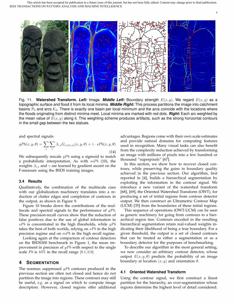
Fig. 11. Watershed Transform. Left: Image. Middle Left: Boundary strength E(x, y). We regard E(x, y) as atopographic surface and flood it from its local minima. Middle Right: This process partitions the image into catchmentbasins P0 and arcs K0. There is exactly one basin per local minimum and the arcs coincide with the locations wherethe floods originating from distinct minima meet. Local minima are marked with red dots. Right: Each arc weighted bythe mean value of E(x, y) along it. This weighting scheme produces artifacts, such as the strong horizontal contoursin the small gap between the two statues.

and spectral signals:

gPb(x, y, θ) =∑

s

∑i

βi,sGi,σ(i,s)(x, y, θ) + γ · sPb(x, y, θ)

(14)We subsequently rescale gPb using a sigmoid to matcha probabilistic interpretation. As with mPb (10), theweights βi,s and γ are learned by gradient ascent on theF-measure using the BSDS training images.

3.4 ResultsQualitatively, the combination of the multiscale cueswith our globalization machinery translates into a re-duction of clutter edges and completion of contours inthe output, as shown in Figure 9.

Figure 10 breaks down the contributions of the mul-tiscale and spectral signals to the performance of gPb.These precision-recall curves show that the reduction offalse positives due to the use of global information insPb is concentrated in the high thresholds, while gPbtakes the best of both worlds, relying on sPb in the highprecision regime and on mPb in the high recall regime.

Looking again at the comparison of contour detectorson the BSDS300 benchmark in Figure 1, the mean im-provement in precision of gPb with respect to the singlescale Pb is 10% in the recall range [0.1, 0.9].

4 SEGMENTATION

The nonmax suppressed gPb contours produced in theprevious section are often not closed and hence do notpartition the image into regions. These contours may stillbe useful, e.g. as a signal on which to compute imagedescriptors. However, closed regions offer additional

advantages. Regions come with their own scale estimatesand provide natural domains for computing featuresused in recognition. Many visual tasks can also benefitfrom the complexity reduction achieved by transformingan image with millions of pixels into a few hundred orthousand “superpixels” [67].

In this section, we show how to recover closed con-tours, while preserving the gains in boundary qualityachieved in the previous section. Our algorithm, firstreported in [4], builds a hierarchical segmentation byexploiting the information in the contour signal. Weintroduce a new variant of the watershed transform[68], [69], the Oriented Watershed Transform (OWT), forproducing a set of initial regions from contour detectoroutput. We then construct an Ultrametric Contour Map(UCM) [35] from the boundaries of these initial regions.

This sequence of operations (OWT-UCM) can be seenas generic machinery for going from contours to a hier-archical region tree. Contours encoded in the resultinghierarchical segmentation retain real-valued weights in-dicating their likelihood of being a true boundary. For agiven threshold, the output is a set of closed contoursthat can be treated as either a segmentation or as aboundary detector for the purposes of benchmarking.

To describe our algorithm in the most general setting,we now consider an arbitrary contour detector, whoseoutput E(x, y, θ) predicts the probability of an imageboundary at location (x, y) and orientation θ.

4.1 Oriented Watershed TransformUsing the contour signal, we first construct a finestpartition for the hierarchy, an over-segmentation whoseregions determine the highest level of detail considered.


10

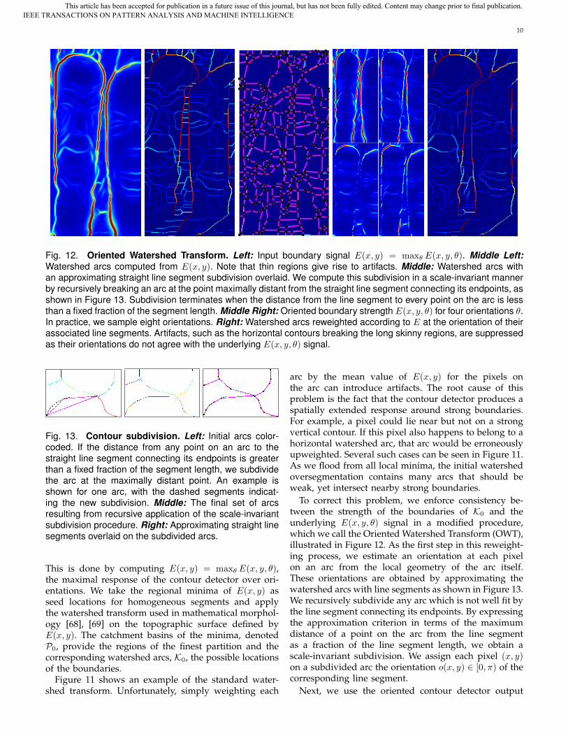
Fig. 12. Oriented Watershed Transform. Left: Input boundary signal E(x, y) = maxθ E(x, y, θ). Middle Left:Watershed arcs computed from E(x, y). Note that thin regions give rise to artifacts. Middle: Watershed arcs withan approximating straight line segment subdivision overlaid. We compute this subdivision in a scale-invariant mannerby recursively breaking an arc at the point maximally distant from the straight line segment connecting its endpoints, asshown in Figure 13. Subdivision terminates when the distance from the line segment to every point on the arc is lessthan a fixed fraction of the segment length. Middle Right: Oriented boundary strength E(x, y, θ) for four orientations θ.In practice, we sample eight orientations. Right: Watershed arcs reweighted according to E at the orientation of theirassociated line segments. Artifacts, such as the horizontal contours breaking the long skinny regions, are suppressedas their orientations do not agree with the underlying E(x, y, θ) signal.

Fig. 13. Contour subdivision. Left: Initial arcs color-coded. If the distance from any point on an arc to thestraight line segment connecting its endpoints is greaterthan a fixed fraction of the segment length, we subdividethe arc at the maximally distant point. An example isshown for one arc, with the dashed segments indicat-ing the new subdivision. Middle: The final set of arcsresulting from recursive application of the scale-invariantsubdivision procedure. Right: Approximating straight linesegments overlaid on the subdivided arcs.

This is done by computing E(x, y) = maxθ E(x, y, θ),the maximal response of the contour detector over ori-entations. We take the regional minima of E(x, y) asseed locations for homogeneous segments and applythe watershed transform used in mathematical morphol-ogy [68], [69] on the topographic surface defined byE(x, y). The catchment basins of the minima, denotedP0, provide the regions of the finest partition and thecorresponding watershed arcs, K0, the possible locationsof the boundaries.

Figure 11 shows an example of the standard water-shed transform. Unfortunately, simply weighting each

arc by the mean value of E(x, y) for the pixels onthe arc can introduce artifacts. The root cause of thisproblem is the fact that the contour detector produces aspatially extended response around strong boundaries.For example, a pixel could lie near but not on a strongvertical contour. If this pixel also happens to belong to ahorizontal watershed arc, that arc would be erroneouslyupweighted. Several such cases can be seen in Figure 11.As we flood from all local minima, the initial watershedoversegmentation contains many arcs that should beweak, yet intersect nearby strong boundaries.

To correct this problem, we enforce consistency be-tween the strength of the boundaries of K0 and theunderlying E(x, y, θ) signal in a modified procedure,which we call the Oriented Watershed Transform (OWT),illustrated in Figure 12. As the first step in this reweight-ing process, we estimate an orientation at each pixelon an arc from the local geometry of the arc itself.These orientations are obtained by approximating thewatershed arcs with line segments as shown in Figure 13.We recursively subdivide any arc which is not well fit bythe line segment connecting its endpoints. By expressingthe approximation criterion in terms of the maximumdistance of a point on the arc from the line segmentas a fraction of the line segment length, we obtain ascale-invariant subdivision. We assign each pixel (x, y)on a subdivided arc the orientation o(x, y) ∈ [0, π) of thecorresponding line segment.

Next, we use the oriented contour detector output


11

Fig. 14. Hierarchical segmentation from contours. Far Left: Image. Left: Maximal response of contour detectorgPb over orientations. Middle Left: Weighted contours resulting from the Oriented Watershed Transform - UltrametricContour Map (OWT-UCM) algorithm using gPb as input. This single weighted image encodes the entire hierarchicalsegmentation. By construction, applying any threshold to it is guaranteed to yield a set of closed contours (the oneswith weights above the threshold), which in turn define a segmentation. Moreover, the segmentations are nested.Increasing the threshold is equivalent to removing contours and merging the regions they separated. Middle Right:The initial oversegmentation corresponding to the finest level of the UCM, with regions represented by their meancolor. Right and Far Right: Contours and corresponding segmentation obtained by thresholding the UCM at level 0.5.

E(x, y, θ), to assign each arc pixel (x, y) a boundarystrength of E(x, y, o(x, y)). We quantize o(x, y) in thesame manner as θ, so this operation is a simple lookup.Finally, each original arc in K0 is assigned weight equalto average boundary strength of the pixels it contains.Comparing the middle left and far right panels of Fig-ure 12 shows this reweighting scheme removes artifacts.

4.2 Ultrametric Contour Map

Contours have the advantage that it is fairly straightfor-ward to represent uncertainty in the presence of a trueunderlying contour, i.e. by associating a binary randomvariable to it. One can interpret the boundary strengthassigned to an arc by the Oriented Watershed Transform(OWT) of the previous section as an estimate of theprobability of that arc being a true contour.

It is not immediately obvious how to represent un-certainty about a segmentation. One possibility, whichwe exploit here, is the Ultrametric Contour Map (UCM)[35] which defines a duality between closed, non-self-intersecting weighted contours and a hierarchy of re-gions. The base level of this hierarchy respects evenweak contours and is thus an oversegmentation of theimage. Upper levels of the hierarchy respect only strongcontours, resulting in an under-segmentation. Movingbetween levels offers a continuous trade-off betweenthese extremes. This shift in representation from a singlesegmentation to a nested collection of segmentationsfrees later processing stages to use information frommultiple levels or select a level based on additionalknowledge.

Our hierarchy is constructed by a greedy graph-basedregion merging algorithm. We define an initial graphG = (P0,K0, W (K0)), where the nodes are the regionsP0, the links are the arcs K0 separating adjacent regions,and the weights W (K0) are a measure of dissimilarity

between regions. The algorithm proceeds by sorting thelinks by similarity and iteratively merging the mostsimilar regions. Specifically:

1) Select minimum weight contour:C∗ = argminC∈K0

W (C).2) Let R1, R2 ∈ P0 be the regions separated by C∗.3) Set R = R1 ∪R2, and update:P0 ← P0\{R1, R2} ∪ {R} and K0 ← K0\{C∗}.

4) Stop if K0 is empty.Otherwise, update weights W (K0) and repeat.

This process produces a tree of regions, where the leavesare the initial elements of P0, the root is the entire image,and the regions are ordered by the inclusion relation.

We define dissimilarity between two adjacent regionsas the average strength of their common boundary inK0, with weights W (K0) initialized by the OWT. Since atevery step of the algorithm all remaining contours musthave strength greater than or equal to those previouslyremoved, the weight of the contour currently beingremoved cannot decrease during the merging process.Hence, the constructed region tree has the structure ofan indexed hierarchy and can be described by a den-drogram, where the height H(R) of each region R is thevalue of the dissimilarity at which it first appears. Statedequivalently, H(R) = W (C) where C is the contourwhose removal formed R. The hierarchy also yields ametric on P0×P0, with the distance between two regionsgiven by the height of the smallest containing segment:

D(R1, R2) = min{H(R) : R1, R2 ⊆ R} (15)

This distance satisfies the ultrametric property:

D(R1, R2) ≤ max(D(R1, R), D(R,R2)) (16)

since if R is merged with R1 before R2, then D(R1, R2) =D(R,R2), or if R is merged with R2 before R1, thenD(R1, R2) = D(R1, R). As a consequence, the whole


12

hierarchy can be represented as an Ultrametric ContourMap (UCM) [35], the real-valued image obtained byweighting each boundary by its scale of disappearance.

Figure 14 presents an example of our method. TheUCM is a weighted contour image that, by construction,has the remarkable property of producing a set of closedcurves for any threshold. Conversely, it is a convenientrepresentation of the region tree since the segmentationat a scale k can be easily retrieved by thresholding theUCM at level k. Since our notion of scale is the averagecontour strength, the UCM values reflect the contrastbetween neighboring regions.

4.3 ResultsWhile the OWT-UCM algorithm can use any source ofcontours for the input E(x, y, θ) signal (e.g. the Cannyedge detector before thresholding), we obtain best re-sults by employing the gPb detector [3] introduced inSection 3. We report experiments using both gPb as wellas the baseline Canny detector, and refer to the resultingsegmentation algorithms as gPb-owt-ucm and Canny-owt-ucm, respectively.

Figures 15 and 16 illustrate results of gPb-owt-ucmon images from the BSDS500. Since the OWT-UCMalgorithm produces hierarchical region trees, obtaining asingle segmentation as output involves a choice of scale.One possibility is to use a fixed threshold for all imagesin the dataset, calibrated to provide optimal performanceon the training set. We refer to this as the optimal datasetscale (ODS). We also evaluate performance when theoptimal threshold is selected by an oracle on a per-imagebasis. With this choice of optimal image scale (OIS), onenaturally obtains even better segmentations.

4.4 EvaluationTo provide a basis of comparison for the OWT-UCMalgorithm, we make use of the region merging (Felz-Hutt) [32], Mean Shift [34], Multiscale NCuts [33], andSWA [31] segmentation methods reviewed in Section 2.2.We evaluate each method using the boundary-basedprecision-recall framework of [2], as well as the Variationof Information, Probabilistic Rand Index, and segmentcovering criteria discussed in Section 2.3. The BSDSserves as ground-truth for both the boundary and regionquality measures, since the human-drawn boundariesare closed and hence are also segmentations.

4.4.1 Boundary QualityRemember that the evaluation methodology developedby [2] measures detector performance in terms of preci-sion, the fraction of true positives, and recall, the fractionof ground-truth boundary pixels detected. The global F-measure, or harmonic mean of precision and recall at theoptimal detector threshold, provides a summary score.

In our experiments, we report three different quanti-ties for an algorithm: the best F-measure on the datasetfor a fixed scale (ODS), the aggregate F-measure on the

BSDS300 BSDS500ODS OIS AP ODS OIS AP

Human 0.79 0.79 − 0.80 0.80 −gPb-owt-ucm 0.71 0.74 0.73 0.73 0.76 0.73[34] Mean Shift 0.63 0.66 0.54 0.64 0.68 0.56[33] NCuts 0.62 0.66 0.43 0.64 0.68 0.45Canny-owt-ucm 0.58 0.63 0.58 0.60 0.64 0.58[32] Felz-Hutt 0.58 0.62 0.53 0.61 0.64 0.56[31] SWA 0.56 0.59 0.54 − − −gPb 0.70 0.72 0.66 0.71 0.74 0.65Canny 0.58 0.62 0.58 0.60 0.63 0.58

TABLE 1. Boundary benchmarks on the BSDS. Resultsfor six different segmentation methods (upper table) andtwo contour detectors (lower table) are given. Shown arethe F-measures when choosing an optimal scale for theentire dataset (ODS) or per image (OIS), as well as theaverage precision (AP). Figures 1, 2, and 17 show the fullprecision-recall curves for these algorithms.

BSDS300Covering PRI VI

ODS OIS Best ODS OIS ODS OISHuman 0.73 0.73 − 0.87 0.87 1.16 1.16gPb-owt-ucm 0.59 0.65 0.75 0.81 0.85 1.65 1.47[34] Mean Shift 0.54 0.58 0.66 0.78 0.80 1.83 1.63[32] Felz-Hutt 0.51 0.58 0.68 0.77 0.82 2.15 1.79Canny-owt-ucm 0.48 0.56 0.66 0.77 0.82 2.11 1.81[33] NCuts 0.44 0.53 0.66 0.75 0.79 2.18 1.84[31] SWA 0.47 0.55 0.66 0.75 0.80 2.06 1.75[29] Total Var. 0.57 − − 0.78 − 1.81 −[70] T+B Encode 0.54 − − 0.78 − 1.86 −[30] Av. Diss. 0.47 − − 0.76 − 2.62 −[30] ChanVese 0.49 − − 0.75 − 2.54 −

BSDS500Covering PRI VI

ODS OIS Best ODS OIS ODS OISHuman 0.72 0.72 − 0.88 0.88 1.17 1.17gPb-owt-ucm 0.59 0.65 0.74 0.83 0.86 1.69 1.48[34] Mean Shift 0.54 0.58 0.66 0.79 0.81 1.85 1.64[32] Felz-Hutt 0.52 0.57 0.69 0.80 0.82 2.21 1.87Canny-owt-ucm 0.49 0.55 0.66 0.79 0.83 2.19 1.89[33] NCuts 0.45 0.53 0.67 0.78 0.80 2.23 1.89

TABLE 2. Region benchmarks on the BSDS. For eachsegmentation method, the leftmost three columns reportthe score of the covering of ground-truth segments ac-cording to optimal dataset scale (ODS), optimal imagescale (OIS), or Best covering criteria. The rightmostfour columns compare the segmentation methods againstground-truth using the Probabilistic Rand Index (PRI) andVariation of Information (VI) benchmarks, respectively.

dataset for the best scale in each image (OIS), and theaverage precision (AP) on the full recall range (equiva-lently, the area under the precision-recall curve). Table 1shows these quantities for the BSDS. Figures 2 and 17display the full precision-recall curves on the BSDS300and BSDS500 datasets, respectively. We find retrainingon the BSDS500 to be unnecessary and use the sameparameters learned on the BSDS300. Figure 18 presentsside by side comparisons of segmentation algorithms.

Of particular note in Figure 17 are pairs of curvescorresponding to contour detector output and regionsproduced by running the OWT-UCM algorithm on thatoutput. The similarity in quality within each pair shows


13

Fig. 15. Hierarchical segmentation results on the BSDS500. From Left to Right: Image, Ultrametric Contour Map(UCM) produced by gPb-owt-ucm, and segmentations obtained by thresholding at the optimal dataset scale (ODS)and optimal image scale (OIS). All images are from the test set.


14

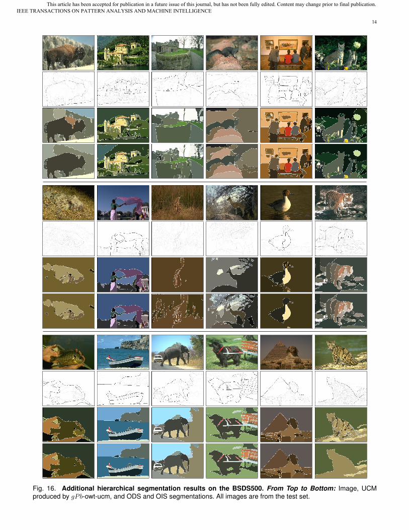
Fig. 16. Additional hierarchical segmentation results on the BSDS500. From Top to Bottom: Image, UCMproduced by gPb-owt-ucm, and ODS and OIS segmentations. All images are from the test set.


15

0 0.1 0.2 0.3 0.4 0.5 0.6 0.7 0.8 0.9 10

0.1

0.2

0.3

0.4

0.5

0.6

0.7

0.8

0.9

1

0.1

0.2

0.3

0.4

0.5

0.6

0.7

0.8

0.9

iso−F

Recall

Pre

cisi

on

[F = 0.80] Human[F = 0.73] gPb−owt−ucm[F = 0.71] gPb[F = 0.64] Mean Shift − Comaniciu, Meer (2002)[F = 0.64] Normalized Cuts − Cour, Benezit, Shi (2005)[F = 0.61] Felzenszwalb, Huttenlocher (2004)[F = 0.60] Canny[F = 0.60] Canny−owt−ucm

Fig. 17. Boundary benchmark on the BSDS500. Com-paring boundaries to human ground-truth allows us toevaluate contour detectors [3], [22] (dotted lines) and seg-mentation algorithms [4], [32], [33], [34] (solid lines) in thesame framework. Performance is consistent when goingfrom the BSDS300 (Figures 1 and 2) to the BSDS500(above). Furthermore, the OWT-UCM algorithm pre-serves contour detector quality. For both gPb andCanny, comparing the resulting segment boundaries tothe original contours shows that our OWT-UCM algorithmconstructs hierarchical segmentations from contours with-out losing performance on the boundary benchmark.

that we can convert contours into hierarchical segmen-tations without loss of boundary precision or recall.

4.4.2 Region QualityTable 2 presents region benchmarks on the BSDS. For afamily of machine segmentations {Si}, associated withdifferent scales of a hierarchical algorithm or differentsets of parameters, we report three scores for the cov-ering of the ground-truth by segments in {Si}. Thesecorrespond to selecting covering regions from the seg-mentation at a universal fixed scale (ODS), a fixed scaleper image (OIS), or from any level of the hierarchy orcollection {Si} (Best). We also report the ProbabilisticRand Index and Variation of Information benchmarks.Figure 19 shows these two measures as a function ofscale in our hierarchical output.

While the relative ranking of segmentation algorithmsremains fairly consistent across different benchmark cri-teria, the boundary benchmark (Table 1 and Figure 17)appears most capable of discriminating performance.

4.4.3 Additional DatasetsWe concentrated experiments on the BSDS because it isthe most complete dataset available for our purposes,

Fig. 18. Pairwise comparison of segmentation algo-rithms on the BSDS300. The coordinates of the red dotsare the boundary benchmark scores (F-measures) at theoptimal image scale for each of the two methods com-pared on single images. Boxed totals indicate the numberof images where one algorithm is better. For example, thetop-left shows gPb-owt-ucm outscores NCuts on 99/100images. When comparing with SWA, we further restrictthe output of the second method to match the number ofregions produced by SWA. All differences are statisticallysignificant except between NCuts and Mean Shift.

0 0.1 0.2 0.3 0.4 0.5 0.6 0.7 0.8 0.9 10

0.1

0.2

0.3

0.4

0.5

0.6

0.7

0.8

0.9

1

Scale

Pro

babi

listic

Ran

d In

dex

gPb−owt−ucmCanny−owt−ucm

0 0.1 0.2 0.3 0.4 0.5 0.6 0.7 0.8 0.9 11

2

3

4

5

6

7

8

9

10

Scale

Var

iatio

n of

Info

rmat

ion

gPb−owt−ucmCanny−owt−ucm

Fig. 19. Evaluating regions on the BSDS300. Con-tour detector influence on segmentation quality is evidentwhen benchmarking the regions of the resulting hierarchi-cal segmentation. Left: Probabilistic Rand Index. Right:Variation of Information.

MSRC PASCAL 2008ODS OIS Best ODS OIS Best

gPb-owt-ucm 0.66 0.75 0.78 0.45 0.58 0.61Canny-owt-ucm 0.57 0.68 0.72 0.40 0.53 0.55

TABLE 3. Region benchmarks on MSRC and PASCAL2008. Shown are scores for the segment covering criteria.

has been used in several publications, and has the advan-tage of providing multiple human-labeled segmentationsper image. Table 3 reports the comparison betweenCanny-owt-ucm and gPb-owt-ucm on two other publiclyavailable datasets:


16

Fig. 20. Interactive segmentation. Left: Image. Middle: UCM produced by gPb-owt-ucm (grayscale) with additionaluser annotations (color dots and lines). Right: The region hierarchy defined by the UCM allows us to automaticallypropagate annotations to unlabeled segments, resulting in the desired labeling of the image with minimal user effort.

• MSRC [71]The MSRC object recognition database is composedof 591 natural images with objects belonging to21 classes. We evaluate performance using theground-truth object instance labeling of [11], whichis cleaner and more precise than the original data.

• PASCAL 2008 [8]We use the train and validation sets of the segmen-tation task on the 2008 PASCAL segmentation chal-lenge, composed of 1023 images. This is one of themost difficult and varied datasets for recognition.We evaluate performance with respect to the objectinstance labels provided. Note that only objectsbelonging to the 20 categories of the challenge arelabeled, and 76% of all pixels are unlabeled.

4.4.4 SummaryThe gPb-owt-ucm segmentation algorithm offers the bestperformance on every dataset and for every benchmarkcriterion we tested. In addition, it is straight-forward,fast, has no parameters to tune, and, as discussed inthe following sections, can be adapted for use with top-down knowledge sources.

5 INTERACTIVE SEGMENTATION

Until now, we have only discussed fully automatic imagesegmentation. Human assisted segmentation is relevantfor many applications, and recent approaches rely on thegraph-cuts formalism [72], [73], [74] or other energy min-imization procedure [75] to extract foreground regions.

For example, [72] cast the task of determining binaryforeground/background pixel assignments in terms ofa cost function with both unary and pairwise poten-tials. The unary potentials encode agreement with es-timated foreground or background region models andthe pairwise potentials bias neighboring pixels not sep-arated by a strong boundary to have the same label.

They transform this system into an equivalent minimumcut/maximum flow graph partitioning problem throughthe addition of a source node representing the fore-ground and a sink node representing the background.Edge weights between pixel nodes are defined by thepairwise potentials, while the weights between pixelnodes and the source and sink nodes are determined bythe unary potentials. User-specified hard labeling con-straints are enforced by connecting a pixel to the sourceor sink with sufficiently large weight. The minimum cutof the resulting graph can be computed efficiently andproduces a cost-optimizing assignment.

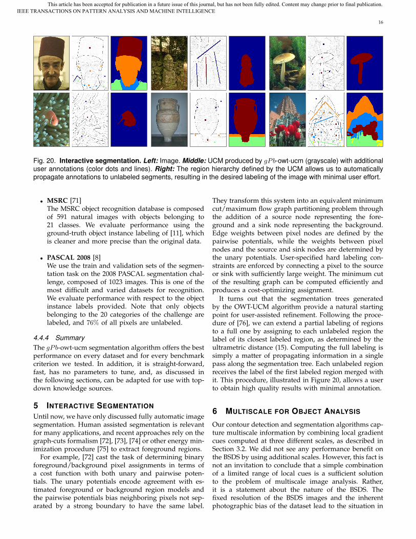
It turns out that the segmentation trees generatedby the OWT-UCM algorithm provide a natural startingpoint for user-assisted refinement. Following the proce-dure of [76], we can extend a partial labeling of regionsto a full one by assigning to each unlabeled region thelabel of its closest labeled region, as determined by theultrametric distance (15). Computing the full labeling issimply a matter of propagating information in a singlepass along the segmentation tree. Each unlabeled regionreceives the label of the first labeled region merged withit. This procedure, illustrated in Figure 20, allows a userto obtain high quality results with minimal annotation.

6 MULTISCALE FOR OBJECT ANALYSIS

Our contour detection and segmentation algorithms cap-ture multiscale information by combining local gradientcues computed at three different scales, as described inSection 3.2. We did not see any performance benefit onthe BSDS by using additional scales. However, this fact isnot an invitation to conclude that a simple combinationof a limited range of local cues is a sufficient solutionto the problem of multiscale image analysis. Rather,it is a statement about the nature of the BSDS. Thefixed resolution of the BSDS images and the inherentphotographic bias of the dataset lead to the situation in


17

Fig. 21. Multiscale segmentation for object detection. Top: Images from the PASCAL 2008 dataset, with objectsoutlined at ground-truth locations. Detailed Views: For each window, we show the boundaries obtained by running theentire gPb-owt-ucm segmentation algorithm at multiple scales. Scale increases by factors of 2 moving from left to right(and top to bottom for the blue window). The total scale range is thus larger than the three scales used internally foreach segmentation. Highlighted Views: The highlighted scale best captures the target object’s boundaries. Note thelink between this scale and the absolute size of the object in the image. For example, the small sailboat (red outline) iscorrectly segmented only at the finest scale. In other cases (e.g. parrot, magenta outline), bounding contours appearacross several scales, but informative internal contours are scale sensitive. A window-based object detector couldlearn and exploit an optimal coupling between object size and segmentation scale.

which a small range of scales captures the boundarieshumans find important.

Dealing with the full variety one expects in highresolution images of complex scenes requires more thana naive weighted average of signals across the scalerange. Such an average would blur information, result-ing in good performance for medium-scale contours,but poor detection of both fine-scale and large-scalecontours. Adaptively selecting the appropriate scale ateach location in the image is desirable, but it is unclearhow to estimate this robustly using only bottom-up cues.

For some applications, in particular object detection,we can instead use a top-down process to guide scaleselection. Suppose we wish to apply a classifier to de-termine whether a subwindow of the image containsan instance of a given object category. We need onlyreport a positive answer when the object completely fillsthe subwindow, as the detector will be run on a set of

windows densely sampled from the image. Thus, weknow the size of the object we are looking for in eachwindow and hence the scale at which contours belongingto the object would appear. Varying the contour scalewith the window size produces the best input signal forthe object detector. Note that this procedure does notprevent the object detector itself from using multiscaleinformation, but rather provides the correct central scale.

As each segmentation internally uses gradients atthree scales, [σ

2 , σ, 2σ], by stepping by a factor of 2 inscale between segmentations, we can reuse shared localcues. The globalization stage (sPb signal) can optionallybe customized for each window by computing it usingonly a limited surrounding image region. This strategy,used here, results in more work overall (a larger numberof simpler globalization problems), which can be miti-gated by not sampling sPb as densely as one sampleswindows.


18

Figure 21 shows an example using images from thePASCAL dataset. Bounding boxes displayed are slightlylarger than each object to give some context. Multiscalesegmentation shows promise for detecting fine-scale ob-jects in scenes as well as making salient details availabletogether with large-scale boundaries.

APPENDIXEFFICIENT COMPUTATION

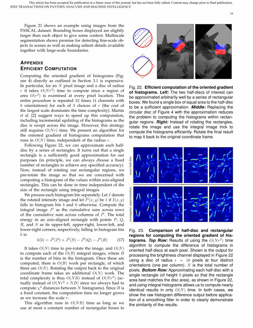
Computing the oriented gradient of histograms (Fig-ure 4) directly as outlined in Section 3.1 is expensive.In particular, for an N pixel image and a disc of radiusr it takes O(Nr2) time to compute since a region ofarea O(r2) is examined at every pixel location. Thisentire procedure is repeated 32 times (4 channels with8 orientations) for each of 3 choices of r (the cost ofthe largest scale dominates the time complexity). Martinet al. [2] suggest ways to speed up this computation,including incremental updating of the histograms as thedisc is swept across the image. However, this strategystill requires O(Nr) time. We present an algorithm forthe oriented gradient of histograms computation thatruns in O(N) time, independent of the radius r.

Following Figure 22, we can approximate each half-disc by a series of rectangles. It turns out that a singlerectangle is a sufficiently good approximation for ourpurposes (in principle, we can always choose a fixednumber of rectangles to achieve any specified accuracy).Now, instead of rotating our rectangular regions, wepre-rotate the image so that we are concerned withcomputing a histogram of the values within axis-alignedrectangles. This can be done in time independent of thesize of the rectangle using integral images.

We process each histogram bin separately. Let I denotethe rotated intensity image and let Ib(x, y) be 1 if I(x, y)falls in histogram bin b and 0 otherwise. Compute theintegral image Jb as the cumulative sum across rowsof the cumulative sum across columns of Ib. The totalenergy in an axis-aligned rectangle with points P , Q,R, and S as its upper-left, upper-right, lower-left, andlower-right corners, respectively, falling in histogram binb is:

h(b) = Jb(P ) + Jb(S)− Jb(Q)− Jb(R) (17)

It takes O(N) time to pre-rotate the image, and O(N)to compute each of the O(B) integral images, where Bis the number of bins in the histogram. Once these arecomputed, there is O(B) work per rectangle, of whichthere are O(N). Rotating the output back to the originalcoordinate frame takes an additional O(N) work. Thetotal complexity is thus O(NB) instead of O(Nr2) (ac-tually instead of O(Nr2 + NB) since we always had tocompute χ2 distances between N histograms). Since B isa fixed constant, the computation time no longer growsas we increase the scale r.

This algorithm runs in O(NB) time as long as weuse at most a constant number of rectangular boxes to

Fig. 22. Efficient computation of the oriented gradientof histograms. Left: The two half-discs of interest canbe approximated arbitrarily well by a series of rectangularboxes. We found a single box of equal area to the half-discto be a sufficient approximation. Middle: Replacing thecircular disc of Figure 4 with the approximation reducesthe problem to computing the histograms within rectan-gular regions. Right: Instead of rotating the rectangles,rotate the image and use the integral image trick tocompute the histograms efficiently. Rotate the final resultto map it back to the original coordinate frame.

exac

tha

lf-d

isc

gpp

rect

angu

lar

appr

oxim

atio

n

Fig. 23. Comparison of half-disc and rectangularregions for computing the oriented gradient of his-tograms. Top Row: Results of using the O(Nr2) timealgorithm to compute the difference of histograms inoriented half-discs at each pixel. Shown is the output forprocessing the brightness channel displayed in Figure 22using a disc of radius r = 10 pixels at four distinctorientations (one per column). N is the total number ofpixels. Bottom Row: Approximating each half-disc with asingle rectangle (of height 9 pixels so that the rectanglearea best matches the disc area), as shown in Figure 22,and using integral histograms allows us to compute nearlyidentical results in only O(N) time. In both cases, weshow the raw histogram difference output before applica-tion of a smoothing filter in order to clearly demonstratethe similarity of the results.


19

approximate each half-disc. For an intuition as to whya single rectangle turns out to be sufficient, look againat the overlap of the rectangle with the half disc in thelower left of Figure 22. The majority of the pixels used informing the histogram lie within both the rectangle andthe disc, and those pixels that differ are far from thecenter of the disc (the pixel at which we are computingthe gradient). Thus, we are only slightly changing theshape of the region we use for context around each pixel.Figure 23 shows that the result using the single rectangleapproximation is visually indistinguishable from thatusing the original half-disc.

Note that the same image rotation technique can beused for computing convolutions with any orientedseparable filter, such as the oriented Gaussian derivativefilters used for textons (Figure 5) or the second-orderSavitzky-Golay filters used for spatial smoothing of ouroriented gradient output. Rotating the image, convolvingwith two 1D filters, and inverting the rotation is moreefficient than convolving with a rotated 2D filter. More-over, in this case, no approximation is required as theseoperations are equivalent up to the numerical accuracyof the interpolation done when rotating the image. Thismeans that all of the filtering performed as part of thelocal cue computation can be done in O(Nr) time insteadof O(Nr2) time where here r = max(w, h) and w and hare the width and height of the 2D filter matrix. For larger, the computation time can be further reduced by usingthe Fast Fourier Transform to calculate the convolution.

The entire local cue computation is also easily paral-lelized. The image can be partitioned into overlappingsubimages to be processed in parallel. In addition, the96 intermediate results (3 scales of 4 channels with 8orientations) can all be computed in parallel as they areindependent subproblems. Catanzaro et al. [77] have cre-ated a parallel GPU implementation of our gPb contourdetector. They also exploit the integral histogram trickintroduced here, with the single rectangle approxima-tion, while replicating our precision-recall performancecurve on the BSDS benchmark. The speed improvementsdue to both the reduction in computational complexityand parallelization make our gPb contour detector andgPb-owt-ucm segmentation algorithm practical tools.

REFERENCES

[1] D. Martin, C. Fowlkes, D. Tal, and J. Malik, “A database of humansegmented natural images and its application to evaluating seg-mentation algorithms and measuring ecological statistics,” ICCV,2001.

[2] D. Martin, C. Fowlkes, and J. Malik, “Learning to detect naturalimage boundaries using local brightness, color and texture cues,”PAMI, 2004.

[3] M. Maire, P. Arbelaez, C. Fowlkes, and J. Malik, “Using contoursto detect and localize junctions in natural images,” CVPR, 2008.

[4] P. Arbelaez, M. Maire, C. Fowlkes, and J. Malik, “From contoursto regions: An empirical evaluation,” CVPR, 2009.

[5] R. Unnikrishnan, C. Pantofaru, and M. Hebert, “Toward objectiveevaluation of image segmentation algorithms,” PAMI, 2007.

[6] M. Meila, “Comparing clusterings: An axiomatic view,” ICML,2005.

[7] A. Y. Yang, J. Wright, Y. Ma, and S. S. Sastry, “Unsupervisedsegmentation of natural images via lossy data compression,”CVIU, 2008.

[8] M. Everingham, L. van Gool, C. Williams, J. Winn, and A. Zisser-man, “PASCAL 2008 Results,” http://www.pascal-network.org/challenges/VOC/voc2008/workshop/index.html, 2008.

[9] D. Hoiem, A. A. Efros, and M. Hebert, “Geometric context froma single image,” ICCV, 2005.

[10] A. Rabinovich, A. Vedaldi, C. Galleguillos, E. Wiewiora, andS. Belongie, “Objects in context,” ICCV, 2007.

[11] T. Malisiewicz and A. A. Efros, “Improving spatial support forobjects via multiple segmentations,” BMVC, 2007.

[12] N. Ahuja and S. Todorovic, “Connected segmentation tree: A jointrepresentation of region layout and hierarchy,” CVPR, 2008.

[13] A. Saxena, S. H. Chung, and A. Y. Ng, “3-d depth reconstructionfrom a single still image,” IJCV, 2008.

[14] T. Brox, C. Bregler, and J. Malik, “Large displacement opticalflow,” CVPR, 2009.

[15] C. Gu, J. Lim, P. Arbelaez, and J. Malik, “Recognition usingregions,” CVPR, 2009.

[16] J. Lim, P. Arbelaez, C. Gu, and J. Malik, “Context by regionancestry,” ICCV, 2009.

[17] L. G. Roberts, “Machine perception of three-dimensional solids,”In Optical and Electro-Optical Information Processing, J. T. Tippett etal. Eds. Cambridge, MA: MIT Press, 1965.

[18] R. O. Duda and P. E. Hart, Pattern Classification and Scene Analysis.New York: Wiley, 1973.

[19] J. M. S. Prewitt, “Object enhancement and extraction,” In PictureProcessing and Psychopictorics, B. Lipkin and A. Rosenfeld. Eds.Academic Press, New York, 1970.

[20] D. C. Marr and E. Hildreth, “Theory of edge detection,” Proceed-ings of the Royal Society of London, 1980.

[21] P. Perona and J. Malik, “Detecting and localizing edges composedof steps, peaks and roofs,” ICCV, 1990.

[22] J. Canny, “A computational approach to edge detection,” PAMI,1986.

[23] X. Ren, C. Fowlkes, and J. Malik, “Scale-invariant contour com-pletion using conditional random fields,” ICCV, 2005.

[24] Q. Zhu, G. Song, and J. Shi, “Untangling cycles for contourgrouping,” ICCV, 2007.

[25] P. Felzenszwalb and D. McAllester, “A min-cover approach forfinding salient curves,” POCV, 2006.

[26] J. Mairal, M. Leordeanu, F. Bach, M. Hebert, and J. Ponce, “Dis-criminative sparse image models for class-specific edge detectionand image interpretation,” ECCV, 2008.

[27] P. Dollar, Z. Tu, and S. Belongie, “Supervised learning of edgesand object boundaries,” CVPR, 2006.

[28] X. Ren, “Multi-scale improves boundary detection in naturalimages,” ECCV, 2008.

[29] M. Donoser, M. Urschler, M. Hirzer, and H. Bischof, “Saliencydriven total variational segmentation,” ICCV, 2009.

[30] L. Bertelli, B. Sumengen, B. Manjunath, and F. Gibou, “A varia-tional framework for multi-region pairwise similarity-based im-age segmentation,” PAMI, 2008.

[31] S. Alpert, M. Galun, R. Basri, and A. Brandt, “Image segmentationby probabilistic bottom-up aggregation and cue integration,”CVPR, 2007.

[32] P. Felzenszwalb and D. Huttenlocher, “Efficient graph-based im-age segmentation,” IJCV, 2004.

[33] T. Cour, F. Benezit, and J. Shi, “Spectral segmentation withmultiscale graph decomposition.” CVPR, 2005.

[34] D. Comaniciu and P. Meer, “Mean shift: A robust approachtoward feature space analysis,” PAMI, 2002.

[35] P. Arbelaez, “Boundary extraction in natural images using ultra-metric contour maps,” POCV, 2006.

[36] M. C. Morrone and R. Owens, “Feature detection from localenergy,” Pattern Recognition Letters, 1987.

[37] W. T. Freeman and E. H. Adelson, “The design and use ofsteerable filters,” PAMI, 1991.

[38] T. Lindeberg, “Edge detection and ridge detection with automaticscale selection,” IJCV, 1998.

[39] Z. Tu, “Probabilistic boosting-tree: Learning discriminative mod-els for classification, recognition, and clustering,” ICCV, 2005.

[40] P. Parent and S. W. Zucker, “Trace inference, curvature consis-tency, and curve detection,” PAMI, 1989.

[41] L. R. Williams and D. W. Jacobs, “Stochastic completion fields: Aneural model of illusory contour shape and salience,” ICCV, 1995.


20

[42] J. Elder and S. Zucker, “Computing contour closures,” ECCV,1996.

[43] Y. Weiss, “Correctness of local probability propagation in graph-ical models with loops,” Neural Computation, 2000.

[44] S. Belongie, C. Carson, H. Greenspan, and J. Malik, “Color andtexture-based image segmentation using EM and its applicationto content-based image retrieval,” ICCV, pp. 675–682, 1998.

[45] J. Shi and J. Malik, “Normalized cuts and image segmentation,”PAMI, 2000.

[46] J. Malik, S. Belongie, T. Leung, and J. Shi, “Contour and textureanalysis for image segmentation,” IJCV, 2001.

[47] D. Tolliver and G. L. Miller, “Graph partitioning by spectralrounding: Applications in image segmentation and clustering,”CVPR, 2006.

[48] F. R. K. Chung, Spectral Graph Theory. American MathematicalSociety, 1997.

[49] C. Fowlkes and J. Malik, “How much does globalization helpsegmentation?” UC Berkeley, Tech. Rep. CSD-04-1340, 2004.

[50] S. Wang, T. Kubota, J. M. Siskind, and J. Wang, “Salient closedboundary extraction with ratio contour,” PAMI, 2005.

[51] S. X. Yu, “Segmentation induced by scale invariance,” CVPR, 2005.[52] E. Sharon, M. Galun, D. Sharon, R. Basri, and A. Brandt, “Hier-

archy and adaptivity in segmenting visual scenes,” Nature, vol.442, pp. 810–813, 2006.

[53] D. Mumford and J. Shah, “Optimal approximations by piecewisesmooth functions, and associated variational problems,” Commu-nications on Pure and Applied Mathematics, pp. 577–684, 1989.

[54] J. M. Morel and S. Solimini, Variational Methods in Image Segmen-tation. Birkhauser, 1995.

[55] G. Koepfler, C. Lopez, and J. Morel, “A multiscale algorithmfor image segmentation by variational method,” SIAM Journal onNumerical Analysis, 1994.

[56] T. Chan and L. Vese, “Active contours without edges,” IP, 2001.[57] L. Vese and T. Chan, “A multiphase level set framework for image

segmentation using the mumford and shah model,” IJCV, 2002.[58] S. Osher and J. Sethian, “Fronts propagation with curvature

dependent speed: Algorithms based on Hamilton-Jacobi formu-lations,” Journal of Computational Physics, 1988.

[59] J. A. Sethian, Level Set Methods and Fast Marching Methods. Cam-bridge University Press, 1999.

[60] T. Pock, D. Cremers, H. Bischof, and A. Chambolle, “An algorithmfor minimizing the piecewise smooth mumford-shah functional,”ICCV, 2009.

[61] F. J. Estrada and A. D. Jepson, “Benchmarking image segmenta-tion algorithms,” IJCV, 2009.

[62] W. M. Rand, “Objective criteria for the evaluation of clusteringmethods,” Journal of the American Statistical Association, vol. 66,pp. 846–850, 1971.

[63] A. Savitzky and M. J. E. Golay, “Smoothing and differentiation ofdata by simplified least squares procedures,” Analytical Chemistry,1964.

[64] C. Fowlkes, D. Martin, and J. Malik, “Learning affinity functionsfor image segmentation: Combining patch-based and gradient-based approaches,” CVPR, 2003.

[65] T. Leung and J. Malik, “Contour continuity in region-based imagesegmentation,” ECCV, 1998.

[66] S. Belongie and J. Malik, “Finding boundaries in natural images: Anew method using point descriptors and area completion,” ECCV,1998.

[67] X. Ren and J. Malik, “Learning a classification model for segmen-tation,” ICCV, 2003.

[68] S. Beucher and F. Meyer, Mathematical Morphology in Image Pro-cessing. Marcel Dekker, 1992, ch. 12.

[69] L. Najman and M. Schmitt, “Geodesic saliency of watershedcontours and hierarchical segmentation,” PAMI, 1996.

[70] S. Rao, H. Mobahi, A. Yang, S. Sastry, and Y. Ma, “Natural imagesegmentation with adaptive texture and boundary encoding,”ACCV, 2009.

[71] J. Shotton, J. Winn, C. Rother, and A. Criminisi, “Textonboost:Joint appearance, shape and context modeling for multi-classobject recognition and segmentation,” ECCV, 2006.

[72] Y. Boykov and M.-P. Jolly, “Interactive graph cuts for optimalboundary & region segmentation of objects in n-d images.” ICCV,2001.

[73] C. Rother, V. Kolmogorov, and A. Blake, ““Grabcut”: Interactiveforeground extraction using iterated graph cuts,” SIGGRAPH,2004.

[74] Y. Li, J. Sun, C.-K. Tang, and H.-Y. Shum, “Lazy snapping,”SIGGRAPH, 2004.

[75] S. Bagon, O. Boiman, and M. Irani, “What is a good imagesegment? A unified approach to segment extraction,” ECCV, 2008.

[76] P. Arbelaez and L. Cohen, “Constrained image segmentation fromhierarchical boundaries,” CVPR, 2008.

[77] B. Catanzaro, B.-Y. Su, N. Sundaram, Y. Lee, M. Murphy, andK. Keutzer, “Efficient, high-quality image contour detection,”ICCV, 2009.

Pablo Arbelaez received a PhD with honors inApplied Mathematics from the Universite ParisDauphine in 2005. He is a Postdoctoral Scholarwith the Computer Vision group at UC Berkeleysince 2007. His research interests are in com-puter vision, where he has worked on a num-ber of problems, including perceptual grouping,object recognition and the analysis of biologicalimages.

Michael Maire received a BS with honors fromthe California Institute of Technology in 2003 anda PhD in Computer Science from the Universityof California, Berkeley in 2009. He is currentlya Postdoctoral Scholar in the Department ofElectrical Engineering at Caltech. His researchinterests are in computer vision as well as its usein biological image and video analysis.

Charless Fowlkes received a BS with honorsfrom Caltech in 2000 and a PhD in ComputerScience from the University of California, Berke-ley in 2005, where his research was supportedby a US National Science Foundation GraduateResearch Fellowship. He is currently an Assis-tant Professor in the Department of ComputerScience at the University of California, Irvine. Hisresearch interests are in computer and humanvision, and in applications to biological imageanalysis.Jitendra Malik was born in Mathura, India in1960. He received the B.Tech degree in Elec-trical Engineering from Indian Institute of Tech-nology, Kanpur in 1980 and the PhD degree inComputer Science from Stanford University in1985. In January 1986, he joined the universityof California at Berkeley, where he is currentlythe Arthur J. Chick Professor in the ComputerScience Division, Department of Electrical Engi-neering and Computer Sciences. He is also onthe faculty of the Cognitive Science and Vision

Science groups. During 2002-2004 he served as the Chair of theComputer Science Division and during 2004-2006 as the DepartmentChair of EECS. He serves on the advisory board of Microsoft ResearchIndia, and on the Governing Body of IIIT Bangalore.

His current research interests are in computer vision, computationalmodeling of human vision and analysis of biological images. His workhas spanned a range of topics in vision including image segmentation,perceptual grouping, texture, stereopsis and object recognition with ap-plications to image based modeling and rendering in computer graphics,intelligent vehicle highway systems, and biological image analysis. Hehas authored or co-authored more than a hundred and fifty researchpapers on these topics, and graduated twenty-five PhD students whooccupy prominent places in academia and industry. According to GoogleScholar, four of his papers have received more than a thousand cita-tions.

He received the gold medal for the best graduating student in Elec-trical Engineering from IIT Kanpur in 1980 and a Presidential YoungInvestigator Award in 1989. At UC Berkeley, he was selected for theDiane S. McEntyre Award for Excellence in Teaching in 2000, a MillerResearch Professorship in 2001, and appointed to be the Arthur J. ChickProfessor in 2002. He received the Distinguished Alumnus Award fromIIT Kanpur in 2008. He was awarded the Longuet-Higgins Prize for acontribution that has stood the test of time twice, in 2007 and in 2008.He is a fellow of the IEEE and the ACM.


Contour Detection and Hierarchical Image …malik/papers/arbelaezMFM-pami...Contour Detection and Hierarchical Image Segmentation ... ing machine generated contours to human ground-truth

Documents