Continuum-mechanical, Anisotropic Flow model for polar ice masses, based on an anisotropic Flow Enhancement factor

Continuum-mechanical, Anisotropic Flowmodel for polar ice masses, based on ananisotropic Flow Enhancement factor

Luca Placidi∗

Department of Structural and Geotechnical Engineering, “Sapienza”,

University of Rome, Via Eudossiana 18, I-00184 Rome, Italy

Smart Materials and Structures Laboratory,

c/o Fondazione “Tullio Levi-Civita”,

Palazzo Caetani (Ala Nord), I-04012 Cisterna di Latina, Italy

Ralf GreveHakime Seddik

Institute of Low Temperature Science, Hokkaido University,

Kita-19, Nishi-8, Kita-ku, Sapporo 060-0819, Japan

Sergio H. Faria

GZG, Department of Crystallography, University of Gottingen,

Goldschmidtstraße 1, D-37077 Gottingen, Germany

Abstract

Cont. Mech. Thermodyn. 22 (3), 221–237 (2010). doi: 10.1007/s00161-009-0126-0Authors’ version; original publication available at www.springerlink.com

A complete theoretical presentation of the Continuum-mechanical, AnisotropicFlow model, based on an anisotropic Flow Enhancement factor (CAFFE model) isgiven. The CAFFE model is an application of the theory of mixtures with continuousdiversity for the case of large polar ice masses in which induced anisotropy occurs.The anisotropic response of the polycrystalline ice is described by a generalizationof Glen’s flow law, based on a scalar anisotropic enhancement factor. The enhance-ment factor depends on the orientation mass density, which is closely related to theorientation distribution function and describes the distribution of grain orientations(fabric). Fabric evolution is governed by the orientation mass balance, which dependson four distinct effects, interpreted as local rigid body rotation, grain rotation, ro-tation recrystallization (polygonization) and grain boundary migration (migrationrecrystallization), respectively. It is proven that the flow law of the CAFFE model istruly anisotropic despite the collinearity between the stress deviator and stretchingtensors.

∗E-mail: [email protected]

1

arX

iv:0

903.

0688

v5 [

phys

ics.

geo-

ph]

19

Mar

201

0

1 Introduction

In order to study the mechanical behaviour of large polar ice masses, we use the methodof continuum mechanics. Generally, ice is treated as an incompressible, isotropic andextremely viscous non-Newtonian fluid, and Glen’s flow law (Glen 1955, Nye 1952) isused as a constitutive equation. However, for thick polar ice masses anisotropic behaviouroccurs, and therefore, Glen’s flow law must be changed. Many efforts have been undertakento deal with this problem (e.g. Hutter 1983, Budd and Jacka 1989, Jacka and Budd 1989,Azuma 1995, Staroszczyk and Morland 2001, Morland and Staroszczyk 2003, Placidi et al.2006, Gagliardini et al. 2009). In this paper we will present a continuum-mechanical model,which is based on earlier work by Faria (2001, 2006a,b), Placidi (2004, 2005), Placidiet al. (2004), Placidi and Hutter (2006a,b). The model is referred to as the Continuum-mechanical, Anisotropic Flow model, based on an anisotropic Flow Enhancement factor,or “CAFFE model” for short.

The macroscopic anisotropy of polar ice is due to its microstructure. Ice is a polycrys-talline material made of a vast number of crystallites (grains), the mechanical behaviourof which is extremely anisotropic (Jacka and Budd 1989). A single ice crystal shows trans-versely isotropic behaviour, and its c-axis (optical axis) defines the privileged direction(Boehler 1987). Slide along basal planes, orthogonal to the c-axis, is easier than slidealong other crystallographic planes, and since the study by McConnel (1891) it has beencommon to refer to this as the deck-of-cards behaviour of ice. However, the transition fromthe mechanics of a single crystal to that of a huge polycrystal entails the complication ofdifferent deformation mechanisms, and the selection of these mechanisms in different sit-uations. A continuum approach is deemed appropriate in order to deal with this problemin a manageable fashion. We choose the approach of describing the polycrystalline ice as amixture (Truesdell 1957a,b), the species of which are the grains characterized by a certainorientation (Faria et al. 2006). The orientations of the crystallites, i.e., the unit vectorsparallel to the c-axes, belong to a continuous space, so that the ice is considered a Mixturewith Continuous Diversity (MCD) (Faria 2001).

In the MCD theory, equations are defined at the species level (“microscopic”) and at themixture level (“macroscopic”). However, the “microscopic” equations do not govern theevolution of single crystallites, the dynamics of which is hidden in the theory. The objectiveof the mixture approach is to predict the polycrystalline behaviour only. In other words, theCAFFE model is a macroscopic model, and the microstructure is taken into account onlyphenomenologically, without going down to the actual microscopic level. The same holdsfor classical continuum mechanics: we know that matter is discontinuous, spaces betweenparticles (atoms, molecules, etc.) are empty and the molecular structures have stronginfluences on the mechanical behaviour. However, the microstructural characteristics arenot resolved in detail; instead, constitutive equations for a continuous body are postulatedthat are in accordance with experimental data and general principles like determinism,objectivity and the Second Law of Thermodynamics. In the same way, in a MCD, thebehaviour of a single species is important for the mixture dynamics, but single speciesdynamics does not correspond to any measurable quantity.

The general set of equations for polycrystalline ice modelled as a MCD was developedby Faria (2001, 2006a), Faria et al. (2006), Faria (2006b), Placidi and Hutter (2006b), andrestrictions of the constitutive equations due to the Second Law of Thermodynamics were

2

given by these authors. Placidi (2004, 2005), Placidi and Hutter (2006a) suggested explicitforms for the constitutive relations. In this study, we present the CAFFE model as animproved version of these previous formulations. After defining the notation (Section 2),we derive in Section 3 in a rational way the set of CAFFE equations, while taking carethat the following requirements are satisfied:

• All fundamental principles of classical continuum mechanics must be fulfilled.

• The model must be sufficiently simple to allow numerical implementation in currentflow models for polar ice masses.

• The parameters of the model must in principle be measurable by either laboratoryexperiments or field observations.

In Section 3.1, we define the orientation mass density, and in Section 3.2 we deal withthe general mass balance that governs its evolution. In Section 3.3, we characterize theconstitutive quantities introduced in Section 3.2 in order to describe grain rotation, localrigid body rotation, grain boundary migration (or migration recrystallization) and polygo-nization (or rotation recrystallization). In Sections 3.4 and 3.5, we present an anisotropicgeneralization of Glen’s flow law based on a scalar anisotropic enhancement factor. It issimilar to that by Placidi and Hutter (2006a), but simpler and consistent with the SecondLaw of Thermodynamics.

Section 4 is devoted to the analysis of the anisotropic properties of the CAFFE flow law.We note the collinearity between the stretching and the stress deviator tensors and showthat collinearity and isotropy do not share any fundamental concepts, in the sense thatnon-collinear, isotropic flow laws as well as collinear, anisotropic flow laws are possible (e.g.Liu 2002, Faria 2008). A discussion of the advantages and disadvantages of collinearity inan anisotropic flow law terminates Section 4.

Some examples for the constitutive relations introduced in Section 3.3 are provided inthe appendix (Section A).

2 Notation

For a general fieldA, the star superscriptA∗ denotes an orientational dependenceA∗ (x, t,n),where t is the time, x the position vector and n the orientation (unit vector parallel to thec-axis) in the present configuration. Otherwise the field A (x, t) is supposed to be indepen-dent of n. It is implicitly assumed that for a given position x all possible orientations nare defined. The gradient (∇) and divergence (∇·) operators are applied, as usual, to thespace variable x, while the orientational gradient (∇∗) and divergence (∇∗·) operators areapplied to the orientational variable n. For arbitrary scalars A∗ and vectors A∗, we define

∇A∗ =∂A∗

∂x, ∇∗A∗ =

∂A∗

∂n−(∂A∗

∂n· n)

n , (1)

∇ ·A∗ = tr [∇A∗] = tr

[∂A∗

∂x

], ∇∗ ·A∗ = tr

[∂A∗

∂n−(∂A∗

∂n· n)

n

]. (2)

3

An immediate consequence of Eq. (1)2 is ∇∗A∗ ·n = 0. We also note that the explicit formof the orientational gradient operator in spherical coordinates is

∇∗A∗ = e1

[cos θ cosϕ

∂A∗

∂θ− sinϕ

sin θ

∂A∗

∂ϕ

]

+ e2

[cos θ sinϕ

∂A∗

∂θ+

cosϕ

sin θ

∂A∗

∂ϕ

]+ e3

[− sin θ

∂A∗

∂θ

], (3)

where {e1, e2, e3} is a fixed orthonormal basis on which we project vectors and tensors,and θ and ϕ are the zenith and azimuth angle, respectively. The orientation n can beparameterized as follows,

n =

sin θ cosϕsin θ sinϕ

cos θ

= sin θ cosϕ e1 + sin θ sinϕ e2 + cos θ e3 . (4)

3 CAFFE model

3.1 Orientation mass density, orientation distribution function

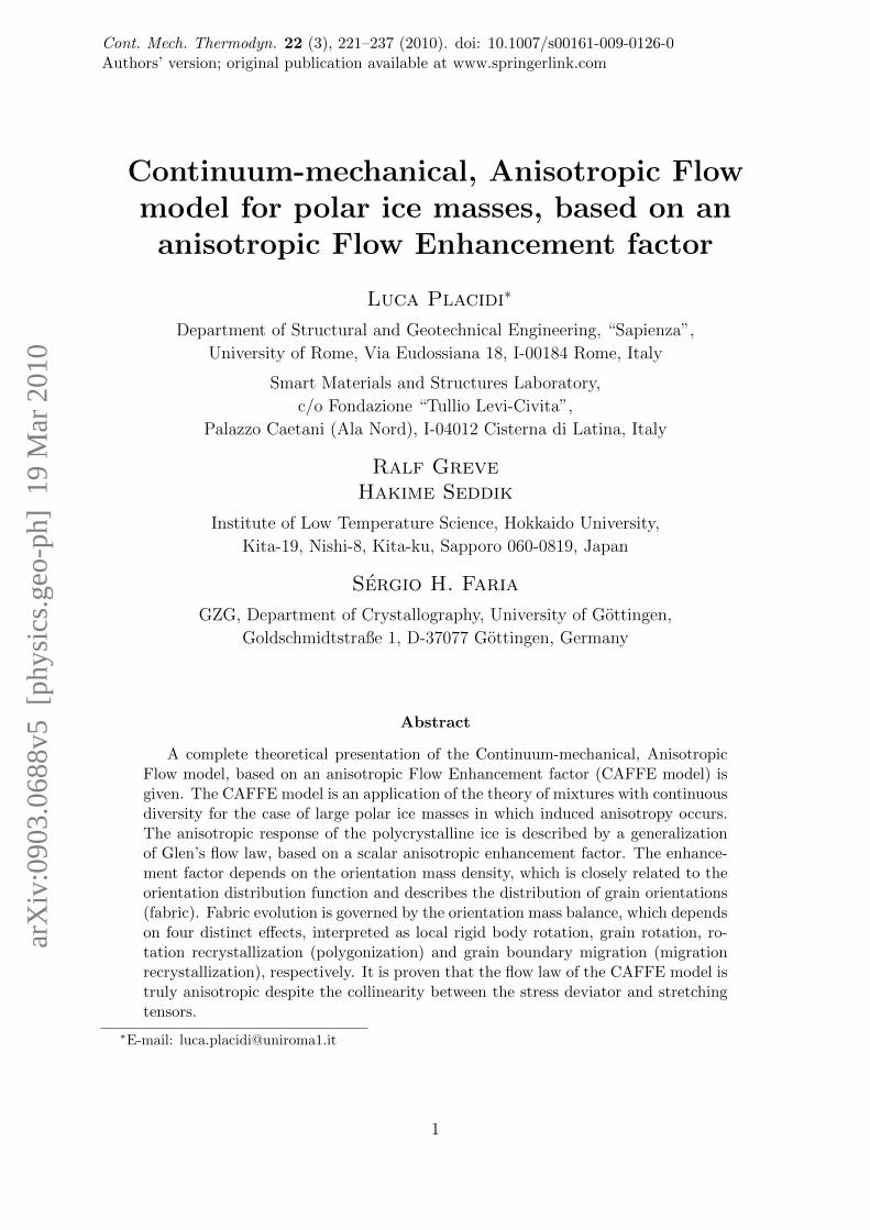
In the CAFFE model, each point of the continuous body is interpreted as a representativevolume element of the polycrystal that encloses a large number of crystallites with theirown orientations. Each orientation is represented by a unit vector n ∈ S2 (where S2

denotes the unit sphere) parallel to the c-axis (Fig. 1a).

n n

uu

(b)(a)

Figure 1: (a) Each point of the unit sphere S2 represents a particular orientation n. Theorientation transition rate u∗ is orthogonal to n. Panel (b) shows a projection on the planespanned by u∗ and n. The anticlockwise direction of the rotation corresponds to a spinvelocity s∗ pointing out of the plane.

35

Figure 1: (a) Each point of the unit sphere S2 represents a particular orientation n. Theorientation transition rate u∗ is orthogonal to n. Panel (b) shows a projection on the planespanned by u∗ and n. The anticlockwise direction of the rotation corresponds to a spinvelocity s∗ pointing out of the plane.

In the MCD framework, distributions of continuous species parameters (like the ori-entation) are expressed in terms of associated mass densities. This means that for everytime t and position x an orientation mass density %∗ (x, t,n) is defined such that, whenintegrated over S2, the usual mass density of the polycrystal % (x, t) results,

% (x, t) =∫S2%∗ (x, t,n) d2n , (5)

where d2n (= sin θ dθ dϕ in spherical coordinates) is the solid angle increment on theunit sphere S2. The orientation mass density %∗, as stated in Eq. (5), has the following

4

physical meaning: the product %∗(x, t,n) d2n is the mass fraction of crystallites withorientations directed towards n within the solid angle d2n. Therefore, the quantity %∗/%can be interpreted as the analogue of the usual orientation distribution function (ODF)(e.g. Rashid 1992, Placidi and Hutter 2004), which is also used in the context of liquidcrystals (e.g. Blenk et al. 1992, Papenfuss 2000) or in mesoscopic damage mechanics (e.g.Massart et al. 2004, Papenfuss and Van 2008). However, we remark that in the glaciologicalcommunity, the ODF usually describes the relative number, and not the mass fraction, ofgrains with a certain orientation.

3.2 Orientation mass balance

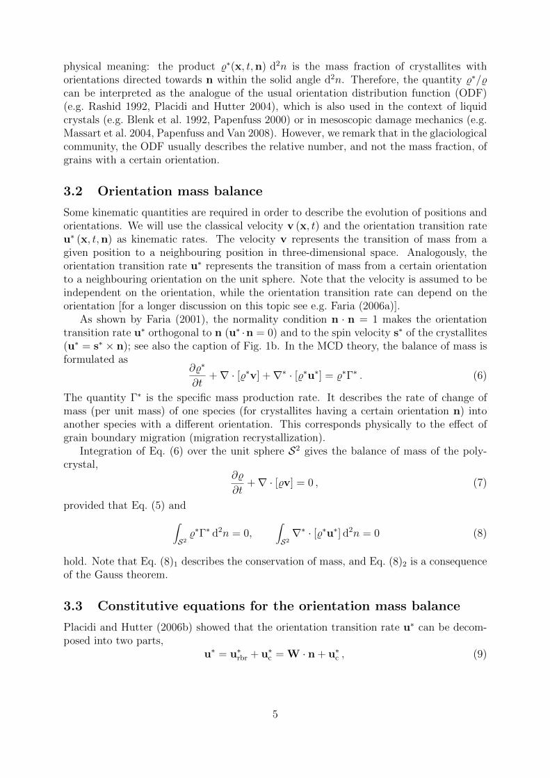
Some kinematic quantities are required in order to describe the evolution of positions andorientations. We will use the classical velocity v (x, t) and the orientation transition rateu∗ (x, t,n) as kinematic rates. The velocity v represents the transition of mass from agiven position to a neighbouring position in three-dimensional space. Analogously, theorientation transition rate u∗ represents the transition of mass from a certain orientationto a neighbouring orientation on the unit sphere. Note that the velocity is assumed to beindependent on the orientation, while the orientation transition rate can depend on theorientation [for a longer discussion on this topic see e.g. Faria (2006a)].

As shown by Faria (2001), the normality condition n · n = 1 makes the orientationtransition rate u∗ orthogonal to n (u∗ ·n = 0) and to the spin velocity s∗ of the crystallites(u∗ = s∗ × n); see also the caption of Fig. 1b. In the MCD theory, the balance of mass isformulated as

∂%∗

∂t+∇ · [%∗v] +∇∗ · [%∗u∗] = %∗Γ∗ . (6)

The quantity Γ∗ is the specific mass production rate. It describes the rate of change ofmass (per unit mass) of one species (for crystallites having a certain orientation n) intoanother species with a different orientation. This corresponds physically to the effect ofgrain boundary migration (migration recrystallization).

Integration of Eq. (6) over the unit sphere S2 gives the balance of mass of the poly-crystal,

∂%

∂t+∇ · [%v] = 0 , (7)

provided that Eq. (5) and∫S2%∗Γ∗ d2n = 0,

∫S2∇∗ · [%∗u∗] d2n = 0 (8)

hold. Note that Eq. (8)1 describes the conservation of mass, and Eq. (8)2 is a consequenceof the Gauss theorem.

3.3 Constitutive equations for the orientation mass balance

Placidi and Hutter (2006b) showed that the orientation transition rate u∗ can be decom-posed into two parts,

u∗ = u∗rbr + u∗c = W · n + u∗c , (9)

5

where u∗rbr = W · n is the contribution of the local rigid body rotation of the polycrystal,W = Skw L is the skew-symmetric part of the velocity gradient L = ∇v and u∗c is a vectorto be constitutively prescribed. For the latter, we introduce phenomenologically a furtherdecomposition,

u∗c = u∗gr +q∗

%∗, (10)

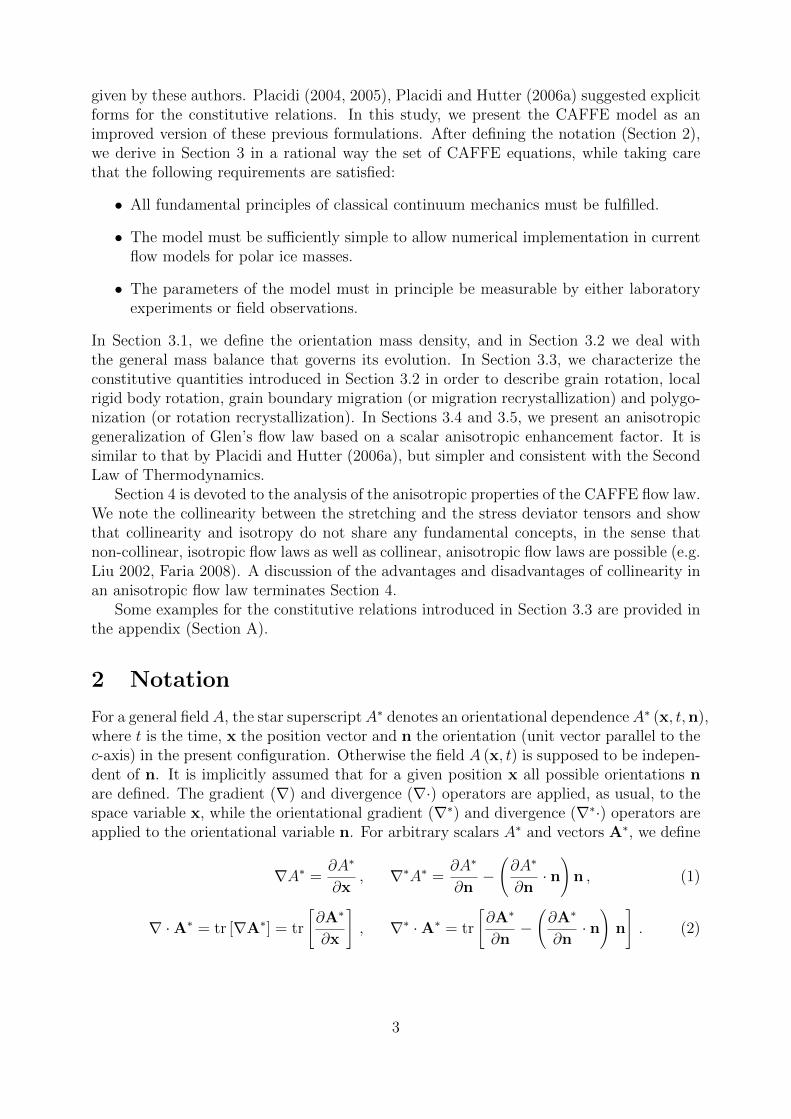
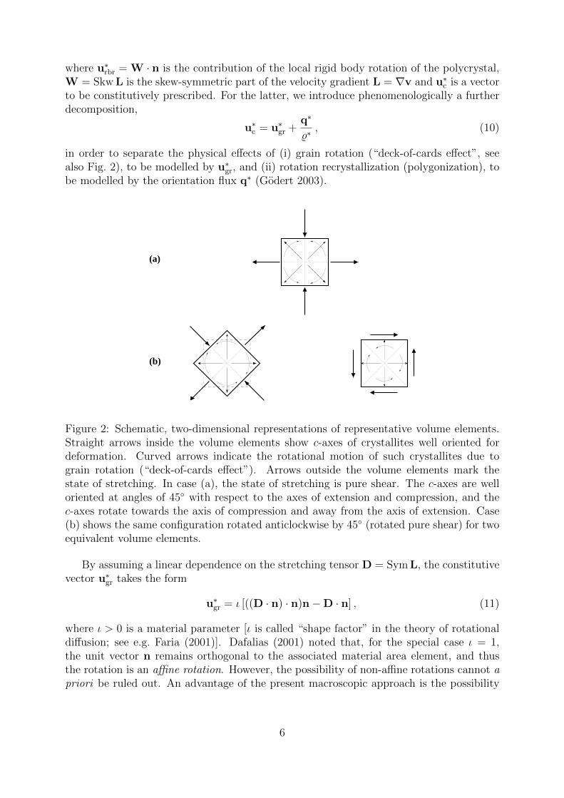
in order to separate the physical effects of (i) grain rotation (“deck-of-cards effect”, seealso Fig. 2), to be modelled by u∗gr, and (ii) rotation recrystallization (polygonization), tobe modelled by the orientation flux q∗ (Godert 2003).

(a)

(b)

Figure 2: Schematic, two-dimensional representations of representative volume elements.Straight arrows inside the volume elements show c-axes of crystallites well oriented fordeformation. Curved arrows indicate the rotational motion of such crystallites due tograin rotation (“deck-of-cards effect”). Arrows outside the volume elements mark thestate of stretching. In case (a), the state of stretching is pure shear. The c-axes are welloriented at angles of 45◦ with respect to the axes of extension and compression, and thec-axes rotate towards the axis of compression and away from the axis of extension. Case(b) shows the same configuration rotated anticlockwise by 45◦ (rotated pure shear) for twoequivalent volume elements.

36

Figure 2: Schematic, two-dimensional representations of representative volume elements.Straight arrows inside the volume elements show c-axes of crystallites well oriented fordeformation. Curved arrows indicate the rotational motion of such crystallites due tograin rotation (“deck-of-cards effect”). Arrows outside the volume elements mark thestate of stretching. In case (a), the state of stretching is pure shear. The c-axes are welloriented at angles of 45◦ with respect to the axes of extension and compression, and thec-axes rotate towards the axis of compression and away from the axis of extension. Case(b) shows the same configuration rotated anticlockwise by 45◦ (rotated pure shear) for twoequivalent volume elements.

By assuming a linear dependence on the stretching tensor D = Sym L, the constitutivevector u∗gr takes the form

u∗gr = ι [((D · n) · n)n−D · n] , (11)

where ι > 0 is a material parameter [ι is called “shape factor” in the theory of rotationaldiffusion; see e.g. Faria (2001)]. Dafalias (2001) noted that, for the special case ι = 1,the unit vector n remains orthogonal to the associated material area element, and thusthe rotation is an affine rotation. However, the possibility of non-affine rotations cannot apriori be ruled out. An advantage of the present macroscopic approach is the possibility

6

to parameterize ι without any conflicts with “microscopic” assumptions. [As a contrastingexample, the model by Staroszczyk and Morland (2001) is also a macroscopic model, butit is restricted to affine rotations.] In fact, Placidi (2004) showed that the fabrics in theupper 2000 m of the GRIP ice core in central Greenland can be best explained by thevalue ι ≈ 0.4. A study on the EPICA ice core in Dronning Maud Land, East Antarctica,provided a best fit between modelled and measured fabrics for ι = 0.6 (Seddik et al. 2008).

The constitutive equations (9) and (11) are not new in the literature and not specificto ice (e.g. Larson 1988, Blenk et al. 1992, Larson 1999, Papenfuss 2000, Dafalias 2001,and references therein). They were derived by Placidi (2004) within the MCD framework.We remark that, even though the unit vector n specifying the orientation of the crystals isunique, Eq. (11) is not the most general case. In fact, Dafalias (2001) discussed the case ofnon-affine rotations. More generally, Faria (2001) and Placidi and Hutter (2006b) derivedthe thermodynamically consistent class of these constitutive equations.

Following the argumentation by Godert (2003), the orientation flux (which is supposedto describe rotation recrystallization) is modelled as a diffusive process,

q∗ = −λ∇∗[ρ∗H∗] , (12)

where the parameter λ > 0 is the orientation diffusivity, andH∗ is an orientation-dependent“hardness” function. However, recent results by Durand et al. (2008) suggest that rotationrecrystallization is an isotropic process not affected by the orientation. In this case, thechoice

H∗ ≡ 1 (13)

is indicated, which renders Eq. (12) equivalent to Fick’s laws of diffusion on the unit sphere.We remark that in the MCD theory the hardness function is called the chemical potentialfor the given species. It is a constitutive quantity that depends at least on the OMD %∗.Consequently, it is possible to show by applying the chain rule that often an equivalent ofFick’s law results even when H∗ is not a constant (e.g. Faria 2001).

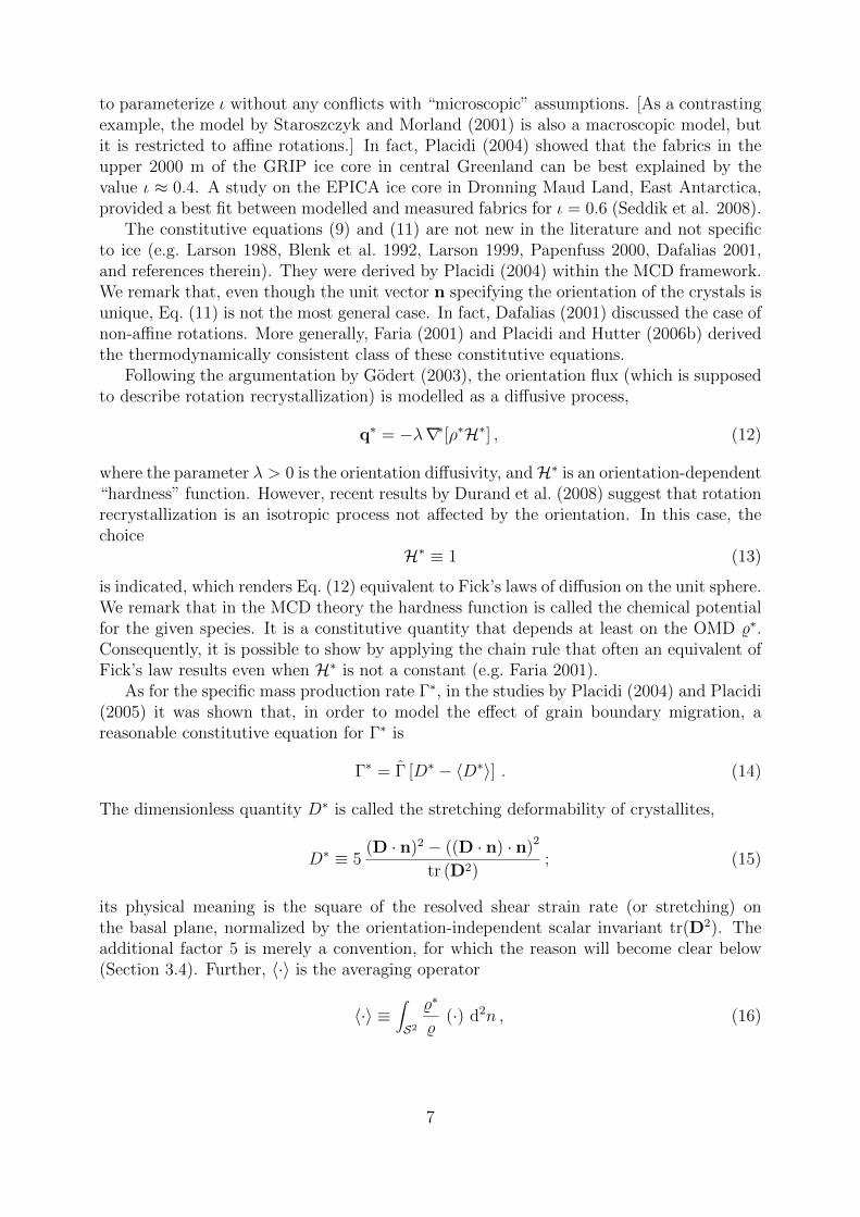
As for the specific mass production rate Γ∗, in the studies by Placidi (2004) and Placidi(2005) it was shown that, in order to model the effect of grain boundary migration, areasonable constitutive equation for Γ∗ is

Γ∗ = Γ [D∗ − 〈D∗〉] . (14)

The dimensionless quantity D∗ is called the stretching deformability of crystallites,

D∗ ≡ 5(D · n)2 − ((D · n) · n)2

tr (D2); (15)

its physical meaning is the square of the resolved shear strain rate (or stretching) onthe basal plane, normalized by the orientation-independent scalar invariant tr(D2). Theadditional factor 5 is merely a convention, for which the reason will become clear below(Section 3.4). Further, 〈·〉 is the averaging operator

〈·〉 ≡∫S2%∗

%(·) d2n , (16)

7

and Γ is a constitutive parameter (see Fig. 3). The conservation of mass expressed byEq. (8)1 is compatible with Eqs. (14)–(16), and they are also compatible with the ratio-nal constitutive theory developed by Placidi and Hutter (2006b). Provided that Γ > 0,Eqs. (14)–(16) have the effect that Γ∗ is greater than zero when the stretching deformabil-ity D∗ is high, and Γ∗ is less than zero when the stretching deformability D∗ is low. Thismeans that crystallites well-oriented for deformation will be enlarged (e.g. Kamb 1972).Since ice crystallites deform essentially by basal shearing, the resolved shear rate (whichis proportional to the orientation dependence of D∗) is related to the rate of accumulationof deformation energy in the material, which drives dynamic recrystallization.

D*

Γ*

0D*

Figure 3: Specific mass production rate Γ∗ according to Eq. (14).

The first contribution in Eq. (9), u∗rbr, is thermodynamically reversible, because thereis no energy dissipation associated with local rigid body rotations. The second contribu-tion, u∗c, has been split up in Eq. (10) into u∗gr and q∗. The grain-rotation part, u∗gr, isthermodynamically irreversible because it is linearly dependent on the stretching tensorD, see Eq. (11), which by definition must vanish for any reversible process in a viscousfluid (e.g., Hutter 1983, Muller 1985, Faria 2001). The rotation-recrystallization part, q∗,is thermodynamically irreversible because of the diffusive nature of the process as specifiedin Eq. (12). The specific mass production rate Γ∗ is also thermodynamically irreversible,because grain growth and recrystallization are thermally activated, irreversible processes[see also the discussion by Faria et al. (2006, Sect. 3c)]. Note that, besides the physicalinterpretation, the thermodynamic reversibility or irreversibility of these terms can also beinvestigated by exploiting the Second Law of Thermodynamics (Faria 2006a, Placidi andHutter 2006b).

A problem is that it is not possible at the moment to constrain the values of the twoparameters Γ and λ in a reasonable fashion. Determining these parameters by experimentsis very difficult, because the relevant time scales are far too large and the strain rates fartoo low to be reproduced in the laboratory. Deformation experiments, even if conductedover a period of years, inevitably end up by activating non-natural deformation and re-crystallization mechanisms. The only promising way out of this is to measure the fabrics(c-axis distributions) and the changes in grain stereology (sizes and shapes) in naturalpolar ice and fit Γ and λ to these observations. The situation is complicated further by thefact that a functional dependence of these parameters on temperature and/or dislocationdensity should be considered (cf. Faria 2006a,b). This requires further attention.

Some examples for the orientation transition rate (grain rotation) and the orientationproduction rate (recrystallization) under different deformation regimes are given in theappendix (Section A).

8

3.4 Anisotropic flow law

The anisotropic flow law presented by Placidi and Hutter (2006a) has been modified inorder to make it simpler and compatible with the Second Law of Thermodynamics,

D = A E(S)

(tr(S2)

2

)(n−1)/2S , (17)

where A and n are the same rate factor and stress exponent, respectively, as in the isotropicGlen flow law, S is the stress deviator defined by

S = t−(

tr t

3

)I (18)

(i.e., the deviatoric part of the Cauchy stress tensor t) and I is the identity tensor. Further,S ∈ [0, 5/2] is the positive scalar

S = 〈S∗〉 =∫S2%∗

%S∗ d2n , (19)

and S∗ is the analogue of D∗,

S∗ ≡ 5(S · n)2 − ((S · n) · n)2

tr(S2), (20)

which can also be written in terms of the Cauchy stress tensor as

S∗ = 5((t · n)× n)2

tr(t2)> 0 . (21)

We call S∗ the stress deformability of crystallites and S the stress deformability of thepolycrystal. In the literature, the scalar (t · n)2 − ((t · n) · n)2 = (S · n)2 − ((S · n) · n)2

has been identified with the square of the resolved stress on the basal plane, so that thestress deformability of crystallites, Eq. (20), can also be called the normalized square ofthe resolved stress on the basal plane. As for the stress exponent, it is often chosen asn = 3 (e.g. Paterson 1994), but we will keep it general in the following.

For a thermodynamicist it may appear strange to formulate a constitutive equation interms of the stretching tensor and not in terms of the stress deviator. However, there is noinconsistency in this formulation. From the theoretical point of view the stress is indeedthe constitutive property and the strain rate (stretching) is the variable, but whether wechoose this or the inverse relation is just a matter of taste or custom. In the glaciologicalcommunity the inverse form is most commonly used; in the book by Hutter (1983) thehistorical reason for this is given.

Our new formulation of the flow law is not only compatible with the Second Law ofThermodynamics (Placidi and Hutter 2006b), but Eq. (17) is much more flexible than

the previous Placidi–Hutter formulation. The mechanical non-linearity (tr(S2)/2)(n−1)/2

and the anisotropic part E(S) are now nicely separated, so that the choice of the stressexponent is not limited to n = 3 any more, and the new formulation is not even restrictedto a power law.

9

In Section 3.5 we will show that, due to Eq. (17), the two quantities D∗ and S∗ definedin Eqs. (15) and (20) are identical,

S∗ = D∗ , (22)

so that we will simply call them the species (or “crystallite”) deformability. In the sameway, the positive scalars S and D will be called the polycrystal deformability,

S = 〈S∗〉 = 〈D∗〉 = D . (23)

Both the crystal and polycrystal deformabilities can only assume values in the range fromzero to 5/2,

S∗ = D∗ ∈ [0, 52] , S = D ∈ [0, 5

2] . (24)

The proof (which is laborious and shall not be detailed here) involves to insert Eq. (4) inEqs. (15) and (16), and study the maxima and minima of the deformabilities D∗ and Dfor general stretching tensors D as functions of the zenith angle θ and the azimuth angleφ. Taking into account that for a randomly distributed OMD (isotropic fabric)

%∗ =%

4π⇒ S = D = 1 (25)

holds, the function E(S) is demanded to be monotone, of class C1[0, 5/2] and has thefixed points

E(0) = Emin , E(1) = 1 , E(52) = Emax , (26)

where Emin < 1 and Emax > 1 are the minimum and the maximum enhancement factors.This means that if the polycrystal deformability S is highest (S = 5/2), the flow law (17)gives the maximum stretching, if the polycrystal deformability S is lowest (S = 0), theflow law (17) gives the minimum stretching, and if the polycrystal deformability is thesame as for the isotropic case (S = 1), the flow law (17) reproduces the classical Glen flowlaw.

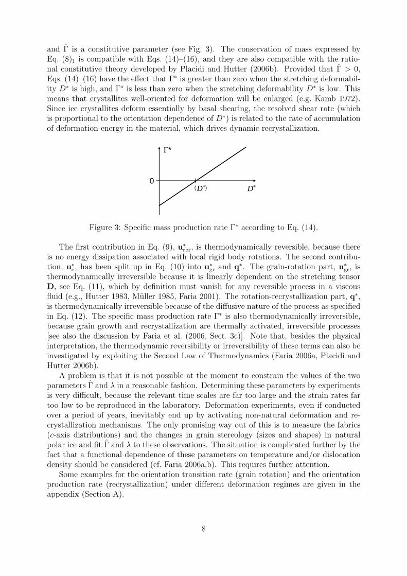
As for the detailed functional form of the anisotropic enhancement factor E(S), someexperimental data suggest that the enhancement factor depends on the “averaged Schmidfactor” to the fourth power (Azuma 1995, Miyamoto 1999). Since the polycrystal deforma-bility S of the CAFFE model is related to the square of the averaged Schmidt factor, itis reasonable to assume a dependency of E on S2. However, this does not allow to fulfillEq. (26) for arbitrary choices of the parameters Emin and Emax. Hence the function E(S) ischosen to depend on S2 in the interval [1, 5/2] [in which the experiments by Azuma (1995)and Miyamoto (1999) have been carried out] only, and for the interval [0, 1] a dependencyon Sτ is introduced. The exponent τ is adjusted such that the function is continuouslydifferentiable at S = 1. This yields

E (S) =

(1− Emin)Sτ + Emin , τ =

8

21

(Emax − 1

1− Emin

), S ∈ [0, 1] ,

4S2 (Emax − 1) + 25− 4Emax

21, S ∈

[1, 5

2

].

(27)

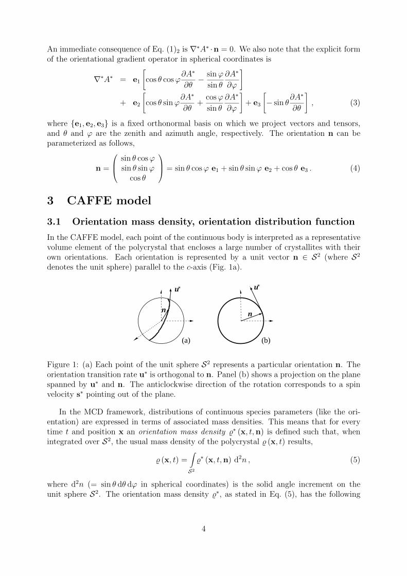
Several investigations (e.g. Russell-Head and Budd 1979, Pimienta et al. 1987, Budd andJacka 1989) indicate that the parameter Emax (maximum softening) is∼ 10. The parameterEmin (maximum hardening) can be realistically chosen between 0 and ∼ 0.1, a non-zerovalue serving mainly the purpose of avoiding numerical problems. The function (27) isshown in Fig. 4.

10

0 0.5 1 1.5 2 2.50123456789

10

DeformabilityE

nhan

cem

ent f

acto

r Emax

= 10

Emin

= 0.1

Figure 4: Anisotropic enhancement factor E(S) as a function of the deformability S ac-cording to Eq. (27), for Emax = 10 and Emin = 0.1.

3.5 Inversion of the anisotropic flow law

The anisotropic flow law (17) can be inverted analytically as long as the power-law formis retained. From Eq. (17) we find

tr(D2)

2= A2 E2(S)

(tr(S2)

2

)n−1tr(S2)

2, (28)

and thustr(S2)

2= A−2/n E−2/n(S)

(tr(D2)

2

)1/n

. (29)

Inserting this result in Eq. (17) and solving for S yields

S = A−1/n E−1/n(S)

(tr(D2)

2

)−(1−1/n)/2D . (30)

In order to complete the inversion, we must prove Eqs. (22) and (23). By writingEq. (17) in short as D = S/(2η) (where η is the shear viscosity of the flow law), we obtainfor the crystalline deformability S∗

S∗ = 5(S · n)2 − ((S · n) · n)2

tr(S2)

= 5(2ηD · n)2 − ((2ηD · n) · n)2

tr[(2ηD)2]

= 5(D · n)2 − ((D · n) · n)2

tr(D2)= D∗ , (31)

so that Eq. (22) is proven. By applying the averaging operator (16) to this result, we findimmediately

S = D , (32)

11

which is the assertion of Eq. (23). Hence, we can replace S by D in Eq. (30), which yieldsthe inverted anisotropic flow law

S = A−1/n E−1/n(D)

(tr(D2)

2

)−(1−1/n)/2D . (33)

4 On the anisotropy of the CAFFE flow law

In Sections 3.4 and 3.5 we have given the generalization of Glen’s flow law considered inthe CAFFE model. The anisotropy of the CAFFE flow law has recently been analyzedmathematically by Faria (2008) through the derivation of the symmetry group of theCAFFE model. In this section, we prove in a more direct way that the CAFFE flow isanisotropic despite the collinearity between the tensors S and D, and give examples inorder to justify this choice.

4.1 CAFFE anisotropy in the context of material theory

In the context of constitutive theory, the definition of isotropy states that any rotationof the body in question does not alter its material response. Mathematically speaking,this means invariance of the material functions (or functionals) to arbitrary orthogonaltransformations P of an undistorted configuration κ (e.g. Liu 2002, p. 86), so that thesymmetry group G of the material contains the entire group of orthogonal transformationsO(3) [G ⊇ O(3)]. Anisotropy is the logical opposite: for at least one orthogonal transfor-mation the invariance does not hold, so that the symmetry group does not contain theentire group of orthogonal transformations [G 6⊇ O(3)].

By construction, the anisotropy of the CAFFE flow law (17) must be contained in theenhancement factor E(S) via the polycrystal deformability S. So let us assume that, atthe initial time t = 0, the initial configuration κt=0 is given by an unloaded ice specimenwith the OMD %∗(x,n, 0). At t = 0+, it is subjected to the stress S, and, according toEqs. (19) and (20), the resulting polycrystal deformability is

S =5

% tr(S2)

∫S2%∗(n)

[(S · n)2 − ((S · n) · n)2

]d2n , (34)

where, for simplicity of notation and in the rest of this session, we will omit the dependenceof OMD on position and time. Now let us consider a second initial configuration κt=0

rotated by a proper orthogonal tensor P with respect to κt=0. The rotated orientationsare given by

n = P · n (35)

(Fig. 5). The OMD follows the rotation, so that

%∗(n) = %∗(n)(35)⇒ %∗(n) = %∗(PT · n) . (36)

At t = 0+, the rotated configuration is subjected to the stress S, which is supposed to bethe same as before,

S = S (37)

12

(Fig. 5). The polycrystal deformability with respect to the rotated configuration is then

S(34)=

5

% tr(S2)

∫S2%∗(n)

[(S · n)2 − ((S · n) · n)2

]d2n

(36), (37)=

5

% tr(S2)

∫S2%∗(PT · n)

[(S · n)2 − ((S · n) · n)2

]d2n . (38)

Let us change the name of the integration variable in the last integral of Eq. (38) from nto n,

S =5

% tr(S2)

∫S2%∗(PT · n)

[(S · n)2 − ((S · n) · n)2

]d2n . (39)

This is the same as the polycrystal deformability with respect to κt=0 [Eq. (34)] for arbitrarytransformations P ∈ O(3) if and only if %∗(n) = const = %/(4π). In this case, the flowlaw (17) is isotropic. For the general case of a non-constant OMD, the deformabilities(34) and (39) are not equal for arbitrary transformations P, so that the flow law (17) isanisotropic, QED. From a mathematical point of view, Eqs. (34) and (39) make clear thatthe symmetry group G of the material defined by the anisotropic CAFFE flow law includesthe invariance group of orthogonal transformations that keep the orientation mass density%∗ unchanged (e.g. Faria 2008).

Figure 5: Anisotropy of the CAFFE flow law: If the same stress (S = S) is applied to tworotated initial configurations (κt=0, κt=0), the responses S and S are different in general.

4.2 Anisotropic behavior for simple shear

Let us illustrate the anisotropic behavior of the CAFFE flow law by a simple example. Forthe vertical single maximum fabric

%∗(x,n, t) = %(x, t) δ(n− e3) (40)

and the simple shear deformation

L =

0 0 γ0 0 00 0 0

⇒ D =

0 0 γ2

0 0 0γ2

0 0

, (41)

13

we find

%∗

%= δ(n− e3) , S =

0 0 τ0 0 0τ 0 0

, S∗(e3) =5

2⇒ S =

5

2. (42)

Thus, the x-z component of the flow law (17) yields

γ = 2AE(52) τn = 2AEmaxτ

n , (43)

where the explicit definition of the function E(S) [Eq. (27)] has been used.Now we rotate the sample around the direction e2 by 45◦ and keep the experimental

apparatus fixed [apply the same stress in the sense of Eq. (37)]. In this case, the OMDchanges as follows,

%∗ = % δ(n− e13), e13 =

1√2

01√2

, (44)

while the state of stress (42)2 is unchanged. The species deformability is equal to zero forthe orientation e13,

S∗(e13) = 0 ⇒ S = 0 . (45)

It follows that the stretching tensor evaluated with the flow law (17) yields the shear rate

γ = 2AE(0) τn = 2AEminτn . (46)

Since Emin � Emax, the shear rate of Eq. (46) is much smaller than that of Eq. (43). Inother words, the material response of the ice specimen has changed considerably due to the45◦ rotation of its initial configuration. This fulfills clearly the criterion for an anisotropicmaterial.

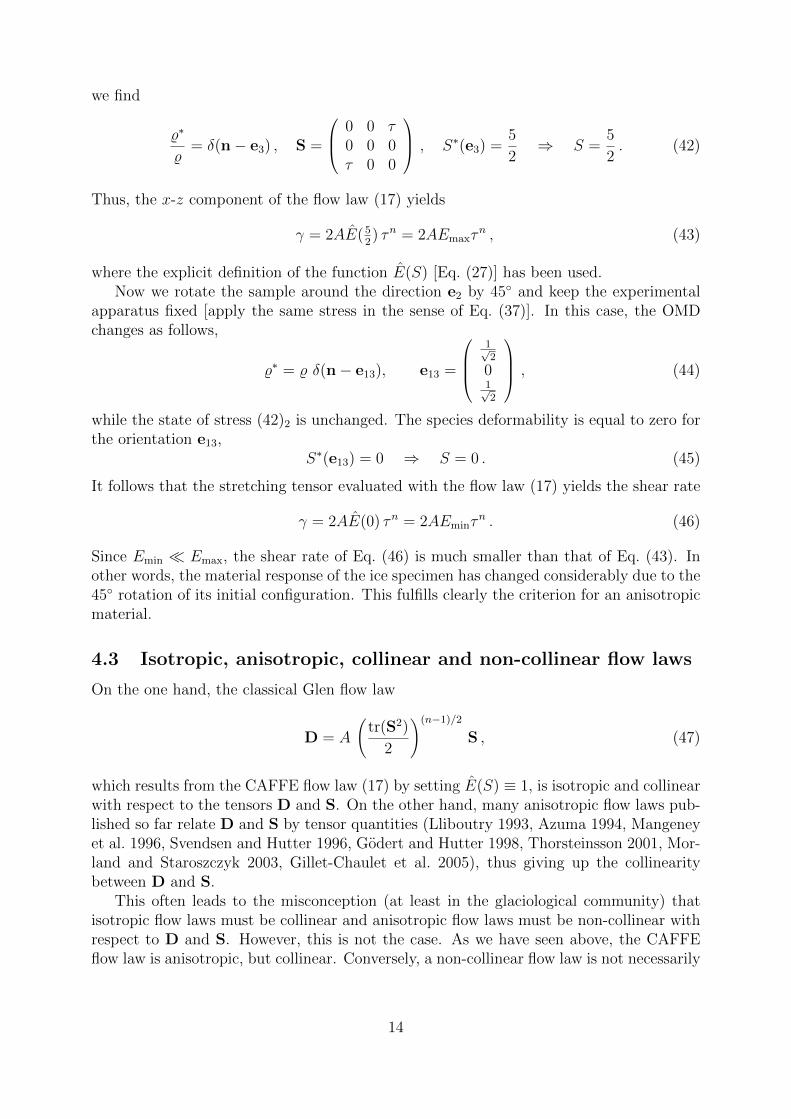
4.3 Isotropic, anisotropic, collinear and non-collinear flow laws

On the one hand, the classical Glen flow law

D = A

(tr(S2)

2

)(n−1)/2S , (47)

which results from the CAFFE flow law (17) by setting E(S) ≡ 1, is isotropic and collinearwith respect to the tensors D and S. On the other hand, many anisotropic flow laws pub-lished so far relate D and S by tensor quantities (Lliboutry 1993, Azuma 1994, Mangeneyet al. 1996, Svendsen and Hutter 1996, Godert and Hutter 1998, Thorsteinsson 2001, Mor-land and Staroszczyk 2003, Gillet-Chaulet et al. 2005), thus giving up the collinearitybetween D and S.

This often leads to the misconception (at least in the glaciological community) thatisotropic flow laws must be collinear and anisotropic flow laws must be non-collinear withrespect to D and S. However, this is not the case. As we have seen above, the CAFFEflow law is anisotropic, but collinear. Conversely, a non-collinear flow law is not necessarily

14

anisotropic. An example is the general Reiner-Rivlin flow law for isotropic viscous fluids(e.g. Liu 2002, p. 109). For the incompressible case, it reads

S = α1D + α2

(D2 − tr (D2)

3I

), (48)

where α1 and α2 are material parameters. Provided that α2 6= 0, this flow law is evidentlynon-collinear. So we highlight that isotropy/anisotropy and collinearity/non-collinearityare two entirely different concepts, and all four possible combinations can be realized.

The disadvantage of using a collinear anisotropic flow law is that, for a given fabricand a given state of stretching, we select a single viscosity of the polycrystal that is thesame for every components of the stress deviator. However, in reality, for complex statesof stretching (superposition of compression and shear etc.) different directions will showdifferent degrees of softening or hardening. This shortcoming is a tribute to the simpleformulation with a scalar enhancement factor, which allows to set up the flow law withonly two well-known parameters (Emin, Emax).

5 Conclusion

We have presented a constitutive model for the dynamics of large polar ice masses. ThisCAFFE model consists of an anisotropic generalization of Glen’s flow law based on a scalarenhancement factor, and a fabric evolution equation based on an orientation mass balance.The latter arises from the framework of Mixtures with Continuous Diversity and uses theorientation mass density as the variable which describes the anisotropic fabric. Threeconstitutive quantities have been introduced, namely the orientation transition rate due tograin rotation, the orientation flux and the specific mass production rate. They have beenlinked to the physical processes of grain rotation, rotation recrystallization (polygonization)and grain boundary migration (migration recrystallization), respectively. The anisotropyof the CAFFE flow law has been proven, and in that context it has been emphasized thatisotropy/anisotropy and collinearity/non-collinearity (between the stress and stretchingtensors) must be clearly separated. Some applications of the CAFFE model to simpledeformation states have been discussed (in the appendix), for which analytical solutionscould be obtained, and which could easily be checked for their physical plausibility andconsistency with observations.

Due to its relative simplicity, the CAFFE model is suitable for implementation in ice-flow models. This has already been done by Seddik et al. (2008) for a one-dimensionalmodel of the site of the EPICA ice core at Kohnen Station in Dronning Maud Land, EastAntarctica (EPICA Community Members 2006), and by Seddik (2008) and Seddik et al.(2009) for the three-dimensional, full-Stokes model Elmer/Ice in order to simulate the iceflow in the vicinity within 100 km around the Dome Fuji drill site (Motoyama 2007) incentral East Antarctica.

Acknowledgements

The authors would like to thank Kolumban Hutter and Leslie W. Morland for many productivediscussions. Comments of the scientific editor Wolfgang Muller and an anonymous reviewer

15

helped considerably to improve the structure and clarity of the manuscript. This work wassupported by a Grant-in-Aid for Creative Scientific Research (No. 14GS0202) from the JapaneseMinistry of Education, Culture, Sports, Science and Technology, by a Grant-in-Aid for ScientificResearch (No. 18340135) from the Japan Society for the Promotion of Science, and by a grant(Nr. FA 840/1-1) from the Priority Program SPP-1158 of the Deutsche Forschungsgemeinschaft(DFG).

A Examples for the evolution of the orientation mass

density

A.1 Evolution due to grain rotation

The deck-of-cards deformation mechanism (grain rotation) implies that the c-axis of a crystallitein the polycrystalline aggregate rotates towards the axes of compression and away from that ofextension. This is illustrated graphically in Fig. 2 for the case of rotated pure shear (simpleshear) and described mathematically by Eq. (11), provided that the constitutive parameter ι ispositive. Equation (11) fulfills the principle of material frame indifference. Thus, if the rulesfor compression and for extension are satisfied, then the rules for simple shear are a directconsequence. Here we give some simple examples in which this can explicitly be seen.

We use a Cartesian frame of reference for which the orientation n of the c-axis is parameterizedby Eq. (4). For uniaxial vertical compression (transversely isotropic horizontal extension), thestretching tensor is

D =

ε2 0 00 ε

2 00 0 −ε

=1

2ε e1 e1 +

1

2ε e2 e2 − ε e3 e3 , (49)

where ε > 0 holds. From Eqs. (4), (11) and (49) we derive the explicit form of the orientationtransition rate due to grain rotation,

u∗gr = −3

4ι ε sin 2θ

cosϕ cos θsinϕ cos θ− sin θ

= −3

4ι ε sin 2θ (cosϕ cos θ e1 + sinϕ cos θ e2 − sin θ e3) . (50)

The direction of u∗gr is coherent with the rules of Fig. 2a (see also Fig. 1b): The third componentu∗gr · e3 is positive when θ < π/2 and negative when θ > π/2. If the crystallites are in the planespanned by e1 and e3 (ϕ = 0), Eq. (50) simplifies to

ϕ = 0 ⇒ u∗gr =3

4ι ε sin 2θ

− cos θ0

sin θ

, (51)

and if they are in the plane spanned by e2 and e3 (ϕ = π/2), we find

ϕ =π

2⇒ u∗gr =

3

4ι ε sin 2θ

0− cos θsin θ

. (52)

16

It is worth noting that the norm of u∗gr which results from Eqs. (50), (51) or (52) shows theexplicit dependence on the Schmidt factor sin 2θ that Azuma and Higashi (1985) recognizedexperimentally. The presence of the Schmidt factor guarantees that crystallites with verticaland horizontal orientations do not rotate, while those at orientations 45◦ off the vertical showmaximum rotation.

If the uniaxial compression is along the first (e1) instead of the third (e3) axis of the frameof reference, the orientation transition rate due to grain rotation takes the form

D =

−ε 0 00 ε

2 00 0 ε

2

⇒ u∗gr = ι ε

sin θ cosϕ+B (θ, ϕ) sin θ cosϕ−1

2 sin θ sinϕ+B (θ, ϕ) sin θ sinϕ−1

2 cos θ +B (θ, ϕ) cos θ

, (53)

where

B (θ, ϕ) ≡ − sin θ cosϕ sin θ cosϕ+1

2sin θ sinϕ sin θ sinϕ+

1

2cos θ cos θ . (54)

The difference to Eq. (50) arises only because the spherical coordinate system, which underliesthe representation of the unit vector n in Eq. (4), is more convenient for the vertical compression(49) than for the horizontal compression (53)1.

For a planar elongation (or pure shear) state of deformation,

D =

ε 0 00 0 00 0 −ε

= ε e1 e1 − ε e3 e3 , (55)

the orientation transition rate due to grain rotation results from Eqs. (4), (11) and (55) as

u∗gr = ι ε

(−1 + sin θ cosϕ sin θ cosϕ− cos θ cos θ) sin θ cosϕ0

sin θ sin θ (1 + cosϕ cosϕ) cos θ

, (56)

which, in the plane spanned by e1 and e3, is

ϕ = 0 ⇒ u∗gr = ι ε sin 2θ

− cos θ0

sin θ

. (57)

This is larger by the factor 4/3 compared to the orientation transition rate of Eq. (51)2. Thereason for this difference is that the component D22 does not contribute to grain rotation in theplane spanned by e1 and e3, which makes the orientation transition rate in the case of Eq. (57)(where D22 = 0) faster than in the case of Eq. (51) (where D22 = ε/2).

For the simple shear situation of Eq. (41), which is illustrated in Fig. 2b, we find for theorientation transition rate due to grain rotation

u∗gr = ιγ

2

cos θ (2 sin2 θ cos2 ϕ− 1)12 sin θ sin 2θ sin 2ϕsin θ cosϕ cos 2θ

, (58)

which, in the plane spanned by e1 and e3, gives

ϕ = 0 ⇒ u∗gr = ιγ

2cos 2θ

− cos θ0

sin θ

. (59)

The direction of u∗gr is once more consistent with the rules of Fig. 2b (see also Fig. 1b). Forinstance, for crystallites oriented upward within θ < π/4 and a positive shear rate γ > 0, thecomponent of u∗gr along e1 is negative.

17

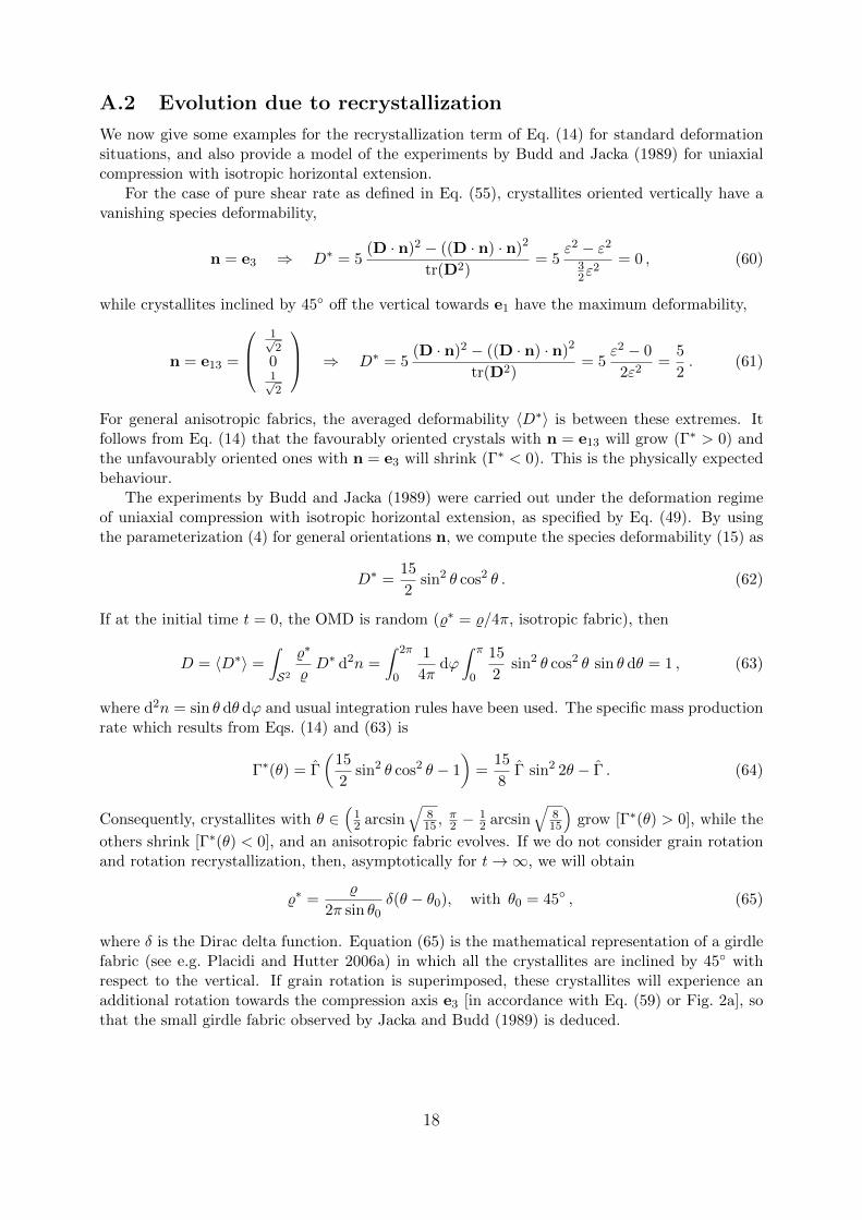
A.2 Evolution due to recrystallization

We now give some examples for the recrystallization term of Eq. (14) for standard deformationsituations, and also provide a model of the experiments by Budd and Jacka (1989) for uniaxialcompression with isotropic horizontal extension.

For the case of pure shear rate as defined in Eq. (55), crystallites oriented vertically have avanishing species deformability,

n = e3 ⇒ D∗ = 5(D · n)2 − ((D · n) · n)2

tr(D2)= 5

ε2 − ε232ε

2= 0 , (60)

while crystallites inclined by 45◦ off the vertical towards e1 have the maximum deformability,

n = e13 =

1√2

01√2

⇒ D∗ = 5(D · n)2 − ((D · n) · n)2

tr(D2)= 5

ε2 − 0

2ε2=

5

2. (61)

For general anisotropic fabrics, the averaged deformability 〈D∗〉 is between these extremes. Itfollows from Eq. (14) that the favourably oriented crystals with n = e13 will grow (Γ∗ > 0) andthe unfavourably oriented ones with n = e3 will shrink (Γ∗ < 0). This is the physically expectedbehaviour.

The experiments by Budd and Jacka (1989) were carried out under the deformation regimeof uniaxial compression with isotropic horizontal extension, as specified by Eq. (49). By usingthe parameterization (4) for general orientations n, we compute the species deformability (15) as

D∗ =15

2sin2 θ cos2 θ . (62)

If at the initial time t = 0, the OMD is random (%∗ = %/4π, isotropic fabric), then

D = 〈D∗〉 =

∫S2%∗

%D∗ d2n =

∫ 2π

0

1

4πdϕ

∫ π

0

15

2sin2 θ cos2 θ sin θ dθ = 1 , (63)

where d2n = sin θ dθ dϕ and usual integration rules have been used. The specific mass productionrate which results from Eqs. (14) and (63) is

Γ∗(θ) = Γ

(15

2sin2 θ cos2 θ − 1

)=

15

8Γ sin2 2θ − Γ . (64)

Consequently, crystallites with θ ∈(12 arcsin

√815 ,

π2 − 1

2 arcsin√

815

)grow [Γ∗(θ) > 0], while the

others shrink [Γ∗(θ) < 0], and an anisotropic fabric evolves. If we do not consider grain rotationand rotation recrystallization, then, asymptotically for t→∞, we will obtain

%∗ =%

2π sin θ0δ(θ − θ0), with θ0 = 45◦ , (65)

where δ is the Dirac delta function. Equation (65) is the mathematical representation of a girdlefabric (see e.g. Placidi and Hutter 2006a) in which all the crystallites are inclined by 45◦ withrespect to the vertical. If grain rotation is superimposed, these crystallites will experience anadditional rotation towards the compression axis e3 [in accordance with Eq. (59) or Fig. 2a], sothat the small girdle fabric observed by Jacka and Budd (1989) is deduced.

18

Another interesting example is the rotated pure shear (simple shear) regime of Eq. (41) forgeneral orientations n represented by Eq. (4). The crystal deformability is computed for this caseas

D∗ =5

2

[cos2 ϕ sin2 θ + cos2 θ (1− 4 cos2 ϕ sin2 θ)

]. (66)

If at the initial time t = 0, the OMD is random (%∗ = %/4π, isotropic fabric), then, analogue toEqs. (63) and (64), we find

D = 1 (67)

and

Γ∗(θ, ϕ) =5

2Γ[cos2 ϕ sin2 θ + cos2 θ (1− 4 cos2 ϕ sin2 θ)

]− Γ . (68)

For times t > 0, an anisotropic fabric evolves, because crystallites oriented near n = e1 (θ ≈ π/2and ϕ ≈ 0) or n = e3 (θ ≈ 0) grow and the others shrink. Hence, without local rigid bodyrotation, grain rotation and rotation recrystallization, asymptotically for t → ∞ we will obtainthe two-maxima fabric

%∗ =1

2δ (n− e1) +

1

2δ (n− e3) . (69)

If grain rotation and rigid body rotation are superimposed, the fabric reported by Kamb (1972)results.

References

Azuma, N. 1994. A flow law for anisotropic ice and its application to ice sheets. Earth Planet.Sci. Lett., 128 (3-4), 601–614.

Azuma, N. 1995. A flow law for anisotropic polycrystalline ice under uniaxial compressive defor-mation. Cold Reg. Sci. Technol., 23 (2), 137–147.

Azuma, N. and A. Higashi. 1985. Formation processes of ice fabric patterns in ice sheets. Ann.Glaciol., 6, 130–134.

Blenk, S., H. Ehrentraut and W. Muschik. 1992. Macroscopic constitutive equations for liquidcrystals induced by their mesoscopic orientation distribution. Int. J. Eng. Sci., 30, 1127–1143.

Boehler, J. P. 1987. Applications of Tensor Functions in Solid Mechanics. Springer, New York.

Budd, W. F. and T. H. Jacka. 1989. A review of ice rheology for ice sheet modelling. Cold Reg.Sci. Technol., 16 (2), 107–144.

Dafalias, Y. F. 2001. Orientation distribution function in non-affine rotations. J. Mech. Phys.Solids, 49, 2493–2516.

Durand, G., A. Persson, D. Samyn and A. Svensson. 2008. Relation between neighbouring grainsin the upper part of the NorthGRIP ice core – implications for rotation recrystallization. EarthPlanet. Sci. Lett., 265 (3), 666–671. doi:10.1016/j.epsl.2007.11.002.

EPICA Community Members. 2006. One-to-one coupling of glacial climate variability in Green-land and Antarctica. Nature, 444 (7116), 195–198. doi:10.1038/nature05301.

Faria, S. H. 2001. Mixtures with continuous diversity: general theory and application to polymersolutions. Cont. Mech. Thermodyn., 13, 91–120.

19

Faria, S. H. 2006a. Creep and recrystallization of large polycrystalline masses. I. General contin-uum theory. Proc. R. Soc. A, 462 (2069), 1493–1514. doi:10.1098/rspa.2005.1610.

Faria, S. H. 2006b. Creep and recrystallization of large polycrystalline masses. III. Continuumtheory of ice sheets. Proc. R. Soc. A, 462 (2073), 2797–2816. doi:10.1098/rspa.2006.1698.

Faria, S. H. 2008. The symmetry group of the CAFFE model. J. Glaciol., 54 (187), 643–645.

Faria, S. H., G. M. Kremer and K. Hutter. 2006. Creep and recrystallization of large polycrys-talline masses. II. Constitutive theory for crystalline media with transversely isotropic grains.Proc. R. Soc. A, 462 (2070), 1699–1720. doi:10.1098/rspa.2005.1635.

Gagliardini, O., F. Gillet-Chaulet and M. Montagnat. 2009. A review of anisotropic polar icemodels: from crystal to ice-sheet flow models. In: T. Hondoh (Ed.), Physics of Ice CoreRecords Vol. 2. Yoshioka Publishing, Kyoto, Japan. In press.

Gillet-Chaulet, F., O. Gagliardini, J. Meyssonnier, M. Montagnat and O. Castelnau. 2005. Auser-friendly anisotropic flow law for ice-sheet modelling. J. Glaciol., 51 (172), 3–14.

Glen, J. W. 1955. The creep of polycrystalline ice. Proc. R. Soc. Lond. A, 228, 519–538.

Godert, G. 2003. A mesoscopic approach for modelling texture evolution of polar ice includingrecrystallization phenomena. Ann. Glaciol., 37, 23–28.

Godert, G. and K. Hutter. 1998. Induced anisotropy in large ice shields: theory and its homoge-nization. Cont. Mech. Thermodyn., 10 (5), 293–318.

Hutter, K. 1983. Theoretical Glaciology; Material Science of Ice and the Mechanics of Glaciersand Ice Sheets. D. Reidel Publishing Company, Dordrecht, The Netherlands.

Jacka, T. H. and W. F. Budd. 1989. Isotropic and anisotropic flow relations for ice dynamics.Ann. Glaciol., 12, 81–84.

Kamb, B. 1972. Experimental recrystallization of ice under stress. In: H. C. Heard, I. Y. Borg,N. L. Carter and C. B. Raileigh (Eds.), Flow and Fracture of Rocks, pp. 211–241. AmericanGeophysical Union, Washington DC.

Larson, R. G. 1988. Constitutive equations for polymer melts and solutions. Butterworths seriesin chemical Engineering, Boston.

Larson, R. G. 1999. The structure and rheology of complex fluids. Oxford University press.

Liu, I.-S. 2002. Continuum Mechanics. Springer, Berlin etc.

Lliboutry, L. 1993. Anisotropic, transversely isotropic nonlinear viscosity of rock ice and rheo-logical parameters inferred from homogenization. Int. J. Plast., 9, 619–632.

Mangeney, A., F. Califano and O. Castelnau. 1996. Isothermal flow of an anisotropic ice sheetin the vicinity of an ice divide. J. Geophys. Res., 101 (B12), 28189–28204.

Massart, T. J., R. H. J. Peerlings and M. G. D. Geers. 2004. Mesoscopic modeling of failureand damage-induced anisotropy in brick masonry. European Journal of Mechanics - A/Solids,23 (5), 719–735. doi:10.1016/j.euromechsol.2004.05.003.

20

McConnel, J. C. 1891. On the plasticity of an ice crystal. Proc. R. Soc. Lond. A, 49, 323–343.

Miyamoto, A. 1999. Mechanical properties and crystal textures of Greenland deep ice cores.Doctoral thesis, Hokkaido University, Sapporo, Japan.

Morland, L. W. and R. Staroszczyk. 2003. Stress and strain-rate formulations for fabric evolutionin polar ice. Cont. Mech. Thermodyn., 15 (1), 55–71.

Motoyama, H. 2007. The second deep ice coring project at Dome Fuji, Antarctica. Sci. Drill., 5,41–43. doi:10.2204/iodp.sd.5.05.2007.

Muller, I. 1985. Thermodynamics. Pitman Advanced Publishing Program, Boston.

Nye, J. F. 1952. The distribution of stress and velocity in glaciers and ice sheets. Proc. R. Soc.Lond. A, 239, 113–133.

Papenfuss, C. 2000. Theory of liquid crystals as an example of mesoscopic continuum mechanics.Comput. Mater. Sci., 19, 4552.

Papenfuss, C. and P. Van. 2008. Scalar, vectorial, and tensorial damage parameters from themesoscopic background. Proceedings of the Estonian Academy of Sciences, 57 (3), 132–141.

Paterson, W. S. B. 1994. The Physics of Glaciers. Pergamon Press, Oxford etc., 3rd ed.

Pimienta, P., P. Duval and V. Y. Lipenkov. 1987. Mechanical behaviour of anisotropic polar ice.In: E. D. Waddington and J. S. Walder (Eds.), The Physical Basis of Ice Sheet Modelling,IAHS Publication No. 170, pp. 57–66. IAHS Press, Wallingford, UK.

Placidi, L. 2004. Thermodynamically consistent formulation of induced anisotropy in polarice accounting for grain-rotation, grain-size evolution and recrystallization. Doctoral the-sis, Department of Mechanics, Darmstadt University of Technology, Germany. URL http:

//elib.tu-darmstadt.de/diss/000614/.

Placidi, L. 2005. Microstructured continua treated by the theory of mixtures. Doctoral thesis,University of Rome “La Sapienza”, Italy.

Placidi, L., S. H. Faria and K. Hutter. 2004. On the role of grain growth, recrystallization andpolygonization in a continuum theory for anisotropic ice sheets. Ann. Glaciol., 39, 49–52.

Placidi, L. and K. Hutter. 2004. Characteristics of orientation and grain-size distributions. In:Proceedings of the 21st International Congress of Theoretical and Applied Mechanics. Warsaw,Poland.

Placidi, L. and K. Hutter. 2006a. An anisotropic flow law for incompressible polycrystallinematerials. Z. angew. Math. Phys., 57, 160–181. doi:10.1007/s00033-005-0008-7.

Placidi, L. and K. Hutter. 2006b. Thermodynamics of polycrystalline materials treated by thetheory of mixtures with continuous diversity. Cont. Mech. Thermodyn., 17 (6), 409–451. doi:10.1007/s00161-005-0006-1.

Placidi, L., K. Hutter and S. H. Faria. 2006. A critical review of the mechanics of polycrystallinepolar ice. GAMM-Mitt., 29 (1), 80–117.

21

Rashid, M. M. 1992. Texture evolution and plastic response of two-dimensional polycrystals. J.Mech. Phys. Solids, 40, 1009–1029.

Russell-Head, D. S. and W. F. Budd. 1979. Ice sheet flow properties derived from borehole shearmeasurements combined with ice core studies. J. Glaciol., 24 (90), 117–130.

Seddik, H. 2008. A full-Stokes finite-element model for the vicinity of Dome Fuji with flow-inducedanisotropy and fabric evolution. Doctoral thesis, Graduate School of Environmental Science,Hokkaido University, Sapporo, Japan. URL http://hdl.handle.net/2115/34136.

Seddik, H., R. Greve, L. Placidi, I. Hamann and O. Gagliardini. 2008. Application of a continuum-mechanical model for the flow of anisotropic polar ice to the EDML core, Antarctica. J.Glaciol., 54 (187), 631–642.

Seddik, H., R. Greve, T. Zwinger and L. Placidi. 2009. A full-Stokes ice flow model for the vicinityof Dome Fuji, Antarctica, with induced anisotropy and fabric evolution. The CryosphereDiscuss., 3 (1), 1–31.

Staroszczyk, R. and L. W. Morland. 2001. Strengthening and weakening of induced anisotropyin polar ice. Proc. R. Soc. Lond. A, 457 (2014), 2419–2440.

Svendsen, B. and K. Hutter. 1996. A continuum approach for modelling induced anisotropy inglaciers and ice sheets. Ann. Glaciol., 23, 262–269.

Thorsteinsson, T. 2001. An analytical approach to deformation of anisotropic ice-crystal aggre-gates. J. Glaciol., 47 (158), 507–516.

Truesdell, C. 1957a. Sulle basi della termomeccanica. Nota I. Rendiconnti Accademia dei Lincei,8/22, 33–38.

Truesdell, C. 1957b. Sulle basi della termomeccanica. Nota II. Rendiconnti Accademia dei Lincei,8/22, 158–166.

22