Continuous detection and prediction of grasp states and kinematics from primate motor, premotor, and parietal cortex Dissertation for the award of the degree “Doctor rerum naturalium” of the Georg-August-Universität Göttingen within the doctoral program Theoretical and Computational Neuroscience of the Georg-August University School of Science (GAUSS) submitted by Veera Katharina Menz from Hünfeld, Germany Göttingen, 2015

Welcome message from author
This document is posted to help you gain knowledge. Please leave a comment to let me know what you think about it! Share it to your friends and learn new things together.
Transcript
Continuous detection and prediction of
grasp states and kinematics from primate
motor, premotor, and parietal cortex
Dissertation
for the award of the degree
“Doctor rerum naturalium”
of the Georg-August-Universität Göttingen
within the doctoral program Theoretical and Computational Neuroscience
of the Georg-August University School of Science (GAUSS)
submitted by
Veera Katharina Menz
from Hünfeld, Germany
Göttingen, 2015

ii
Thesis Committee
Prof. Dr. Hansjörg Scherberger Research Group Neurobiology German Primate Center Kellnerweg 4 37077 Göttingen Prof. Dr. Fred Wolf Theoretical Neurophysics Max Planck Institute for Dynamics and Self-Organization Am Faßberg 17 37077 Göttingen Prof. Dr. Alexander Gail Cognitive Neuroscience Laboratory German Primate Center Kellnerweg 4 37077 Göttingen
Members of the Examination Board
Referee: Prof. Dr. Florentin Wörgötter Department of Computational Neuroscience Drittes Physikalisches Institut/BCCN Georg-August Universität Friedrich-Hund-Platz 1 37077 Göttingen
2nd Referee: Prof. Dr. Julia Fischer Kognitive Ethologie German Primate Center Kellnerweg 4 37077 Göttingen
3rd Referee: Dr. Igor Kagan Decision and Awareness Group German Primate Center Kellnerweg 4 37077 Göttingen
Date of oral examination: April 29, 2015

iii
Herewith I declare that I have written this thesis independently and with no
other aids and sources than quoted.
Göttingen, February 27, 2015 Veera Katharina Menz


v
Acknowledgements
Although it is my name that is written in front of this thesis, a work like this is never the product of
only one person. In fact, it is the connections between many people that make such a project
possible; I am just one part of this big network of people. Each person in this network contributed in
one way or another to the realization of this work and I want to take the opportunity here to mention
those people who wove this net together with me.
First of all, there was of course Hans, my supervisor, who gave me, as a mathematician, the
opportunity to dive into this strange, yet fascinating world of monkeys and brains. Throughout this
project he gave me the freedom to take my own decisions, directed me when it was necessary, and
always was there with help and support, regardless of the issue.
Then, there was Stefan, who agreed to show and explain to me all kinds of things about monkey
training and recording, and who let me work with him when I was new in the lab and needed to
learn. Only thanks to Hans and Stefan, who had the confidence in me to realize this project and who
gave me the data so that I could do it, I was able to take on this project.
Furthermore, there was my thesis committee consisting of Hans, Prof. Fred Wolf, and Prof.
Alexander Gail, which were very supportive towards me, be it by means of scientific criticism or
the friendly atmosphere of our meetings.
Apart from this scientific part of the net, there were many other connections to people, friends
and family, which were equally important for this project, because they were important to me. The
first ones to mention here are of course my present and former colleagues from the Neurobiology
Lab who are at least as much friends to me as they are colleagues: Ricarda and Natalie, with whom
I could always laugh and cry, Andres, Anja, Ben, Matthias, Sabine, Stefan, Wei-an, Yves, as well as
Tanya and Sebastian, who empathized from across the ocean, and the Movie-Nighters Jeroen and
Janine, Rijk, Josey, and Jonathan, who always provided a good start to the week. You guys made
work a good place to be!

vi
Then, there were Antonio, Caio, Clio, and Valeska from the befriended labs, with whom I could
make and experience awesome art, be it music, movies, books, design, tv, or acting; all the
awesome people I played theatre with; and my Flamenco girls. All these people supported me
indirectly in my work by being there for me and backing me in all my other important projects that I
had apart from work. You made me feel that I belong here.
The people who proof read parts of my thesis, Annabelle, Janine, Jonathan.
My friends from Köln and home, Annabelle, Martina, Sebi, Tina, and Anne, who gave me
advise or distracted me or supported me in any other necessary way.
My parents, who supported my decisions, gave me love, advice, and helping hands.
And of course Jonathan, who was always there, always supportive, always understanding,
always showing me that it’s gonna be alright.
Thanks to all of you.
vii
Table of Contents
Chapter I - Introduction ................................................................................................................... 1
1. Introduction ................................................................................................................................. 3
1.1. Cortical mechanisms involved in the planning and execution of grasping .......................... 4
1.1.1. Dorsal and ventral stream .............................................................................................. 5
1.1.2. Area AIP in the parietal cortex ...................................................................................... 6
1.1.3. Area F5 in the premotor cortex ..................................................................................... 9
1.1.4. Primary motor cortex M1 ............................................................................................ 11
1.1.5. The fronto-parietal grasping network .......................................................................... 13
1.2. Neuroprosthetics................................................................................................................. 15
1.2.1. Limitations and restrictions of previous decoding studies .......................................... 17
1.3. Motivation and overview of thesis ..................................................................................... 20
Chapter II - Kinematic decoding ................................................................................................... 23
2. Materials and Methods .............................................................................................................. 25
2.1. Basic procedures ................................................................................................................ 25
2.2. Experimental setup ............................................................................................................. 26
2.3. Behavioural paradigm ........................................................................................................ 28
2.4. Signal procedures and imaging .......................................................................................... 28
2.5. Hand kinematics ................................................................................................................. 30
2.6. Neural recordings ............................................................................................................... 31
2.7. Decoding ............................................................................................................................ 31
2.7.1. Decoding algorithm ..................................................................................................... 31
2.7.2. Decoding procedure .................................................................................................... 32
2.7.3. Variation of decoding parameters ............................................................................... 33
2.7.4. Evaluation of decoding performance .......................................................................... 34
2.7.5. Chance decoding performance .................................................................................... 35
3. Results ....................................................................................................................................... 37
3.1. Kinematic and neuronal data .............................................................................................. 37
3.2. Decoding of 27 DOF .......................................................................................................... 38
3.3. Decoding performance of different areas ........................................................................... 41
3.4. Influence of number of units on decoding performance .................................................... 44
3.5. Decoding performance of proximal and distal movements ................................................ 46
3.6. Optimal decoding parameters ............................................................................................. 48
4. Discussion ................................................................................................................................. 51
viii
4.1. Movement reconstruction with primary and premotor cortex ............................................ 51
4.2. Movement reconstruction with parietal cortex ................................................................... 55
4.3. Influence of unit number on decoding performance .......................................................... 57
4.4. Reconstruction of proximal and distal joints ...................................................................... 58
4.5. Optimal decoding parameters and their network implications ........................................... 60
4.6. Conclusion .......................................................................................................................... 65
Chapter III - State decoding ........................................................................................................... 67
5. Materials and Methods .............................................................................................................. 69
5.1. Decoding algorithm ............................................................................................................ 69
5.2. Decoding procedure ........................................................................................................... 71
5.3. Variation of decoding parameters ...................................................................................... 72
5.4. Evaluation of decoding performance ................................................................................. 72
5.5. Accuracy of movement onset prediction ............................................................................ 73
5.6. Chance level performance .................................................................................................. 74
6. Results ....................................................................................................................................... 77
6.1. State detection performance of different areas ................................................................... 77
6.2. Detection performance for individual states ...................................................................... 79
6.3. Resting state detection during passive resting phases and active hold epochs ................... 81
6.4. Decoding of movement onset ............................................................................................. 83
6.5. Optimal decoding parameters ............................................................................................. 86
7. Discussion ................................................................................................................................. 89
7.1. State reconstruction with primary and premotor cortex ..................................................... 89
7.2. State reconstruction with parietal cortex ............................................................................ 91
7.3. Reconstruction of individual states .................................................................................... 92
7.4. Active and passive resting .................................................................................................. 94
7.5. Decoding of movement onset ............................................................................................. 96
7.6. Optimal decoding parameters ............................................................................................. 98
7.7. Conclusion .......................................................................................................................... 99
Chapter IV - Conclusions ............................................................................................................ 101
8. Conclusions and Outlook ........................................................................................................ 103
9. Summary ................................................................................................................................. 107
References ................................................................................................................................... 109
Abbreviations .............................................................................................................................. 121
Curriculum Vitae ......................................................................................................................... 123

ix


Chapter I - Introduction

1. Introduction
3
1. Introduction
Manipulation of objects and interaction with our environment by means of our hands is an essential
part of our everyday lives. How much we actually rely on the use of our hands becomes most
apparent when we lose the ability to perform hand and arm movements. Consequently, it comes as
no surprise that the recovery of exactly these functions ranges as number one on the list of abilities
which are wished to be regained by affected people (Anderson 2004). Hand and arm functions are
essential to fulfil our physical and emotional needs as well as to establish and maintain an
independent and self-directed life and are thus a significant contributor to the quality of life.
In order to restore the skill of everyday hand movements in patients who have lost this function
due to spinal cord injuries, loss of limbs or other motor diseases, the development of
neuroprostheses has come more and more into focus. The goal of these devices is the translation of
neural activity arising during attempted movement generation into an output for controlling an
external actuator like a robot hand as a hand and arm replacement.
However, grasping is a highly evolved behaviour, and the underlying mechanisms both on the
mechanical and brain level are highly complex. The generation of movement and especially of
finger kinematics is distributed across many areas within the cortex and subcortical structures.
Besides the actual control of muscles to perform a movement, these areas code a variety of other
aspects involved in the planning and execution of hand movements, such as features of the
environment in which the action is going to take place in, features about the object the action is
directed at, internal states like current hand position, muscle fatigue or motivational states,
mechanical restrictions of the environment and the body, knowledge and expectations about the
action to be performed, etc. All of these aspects need to be brought together in order to generate a
movement plan which then can be executed.
Also on the mechanical level, the human hand shows a lot of complexity. Almost 40 muscles are
engaged in the movement of the hand, acting to both extend and flex as well as stabilizing
1. Introduction
4
individual joints (Lemon 1999, Raos et al 2006). In conjunction with several proximal muscles, the
human hand and wrist are able to exhibit a total number of 27 degrees of freedom (DOF) (Lin et al
2000, Rehg and Kanade 1994). So far, neuroprosthetic devices have only been able to reproduce a
fraction of this number.
This thesis is devoted to addressing this and other problems which are faced in the development
of neuroprosthetics. However, before describing these challenges in more detail, I will first give an
overview of the cortical mechanisms involved in the planning and execution of grasps (section 1.1).
We will focus particularly on three different areas in the neocortex (M1, F5, and AIP, sections
1.1.2-1.1.4), which play important roles in this process, and describe their particular contributions to
the planning and execution of hand movements (section 1.1.5).
Following, I will give an introduction to the state of the art of neuroprosthetics restoring hand
and arm movements (section 1.2). Strengths and achievements of this technology are discussed, but
also problems which have not been solved yet are addressed (section 1.2.1). Finally, I will delineate
which of the current problems I will address in this thesis and give an outline of the structure of the
thesis (section 1.3).
1.1. Cortical mechanisms involved in the planning and execution of grasping
Although the generation of hand and arm movements seems trivial to us while we perform hundreds
of them every day, they involve a highly complex network of brain areas and computations carried
out in those areas.
Imagine for example the mundane action of picking up a cup of coffee from the table. In order to
bring the hand to the cup and grasp it, a visuomotor transformation needs to be performed in the
brain in order to convert visual information about the object to be grasped or manipulated into a
movement plan which then can be executed. We will now follow the processing of visual
information through the brain and its transformation into a movement.
1. Introduction
5
1.1.1. Dorsal and ventral stream. First, the gaze fixates onto the cup so that the image of the cup
and its environment falls onto the retina. From there, information about the image is forwarded via
the optic tract, through the lateral geniculate nucleus to primary visual cortex (V1) where features
like the orientation of edges are detected (Hubel and Wiesel 1968). From there, information is
forwarded into two major processing pathways, the ventral (temporal) and the dorsal (parietal)
stream. These pathways are hierarchically organized: information from lower visual areas (early on
within the stream) is projected to higher ones and this way integrated there into representations of
more complex and abstract features (e.g. information of orientation of individual edges is combined
into the representation of a geometric shape).
The two pathways differ from each other in terms of information they code: whereas the ventral
pathway is concerned with object recognition (what do I see? a cup with delicious coffee!) and thus
associated with perception, the dorsal pathway deals with information relevant to action generation,
like the location or shape of the object to be grasped (where is the object? on the table in front me!
what shape does it have? it is a cylinder with a circular extension on the right side!) (Goodale and
Milner 1992, Norman 2002).
The significance of these two pathways and the information they code becomes apparent in the
following two patient cases, described by Goodale et al (1994) and Goodale et al (1991), in which
either of the streams was disrupted: in the first case, patient DF suffering from a lesion from a
bilateral damage in the ventrolateral occipital region interrupting the ventral visual pathway, was
not able to visually discriminate irregularly shaped objects, but could shape her hand according to
the respective objects in order to grasp them with her fingers. In contrast, patient RV who suffered
from a lesion of the occipitoparietal cortex disrupting the dorsal visual pathway, was able to
visually discriminate the objects, however could not grasp those objects properly. In the following,
1. Introduction
6
we will therefore focus on the latter of the two pathways, the dorsal stream, in our journey of
tracing the generation of hand movement through the brain.
The dorsal pathway extends to the posterior parietal cortex (PPC) which contains several brain
areas involved in the planning of movement: neurons in the lateral intraparietal area (LIP) become
active during planning of saccadic eye movements (Andersen et al 1990b, Gnadt and Andersen
1988, Pesaran et al 2002), the parietal reach region (PRR) (medial and posterior to LIP; Snyder et al
1997) has been shown to be modulated during planning of reaching movements as well as to be
tuned to the direction of reaches (Batista and Andersen 2001, Snyder et al 1997), and the medial
intraparietal sulcus (MIP) (part of PRR; Musallam et al 2004) has been shown to encode the
location of a reach target in an eye-centred reference frame (Pesaran et al 2006). The anterior
intraparietal area (AIP) has been found to be specialized for the visual guidance of hand movements
(Gallese et al 1994, Murata et al 2000, Sakata et al 1995) and forms the fronto-parietal grasping
network, together with area F5 in the premotor cortex and primary motor cortex (M1) (Jeannerod et
al 1995). Therefore, in the following three chapters, we will take a closer look at areas AIP, F5, and
M1 and their contributions to the generation of grasping movements. Afterward, we will summarize
the major points and shed more light on the fronto-parietal grasping network itself (section 1.1.5).
1.1.2. Area AIP in the parietal cortex. Area AIP plays an important role in the visuomotor
transformation for grasping. It receives input from the caudal intraparietal area (CIP) (Borra et al
2008, Sakata et al 1999, Sakata et al 1995) which has been shown to be involved in the integration
of information about texture and gradient signals of a stimulus in order to produce a representation
of surface orientation in 3D space (Sakata et al 1997, Sakata et al 1999, Tsutsui et al 2001, Tsutsui
et al 2002), as well as from areas PG and PFG (Borra et al 2008). PG and PFG, located in the
rostral part of area 7a and the caudal part of 7b, have been shown to be involved in the execution of
goal-directed hand and mouth movements (Fogassi and Luppino 2005). Information about eye
1. Introduction
7
movements is sent to AIP from the rostral part of LIP (Andersen et al 1990a, Borra et al 2008) as
well as from the ventral part of the frontal eye field (FEF) (Borra et al 2008). Furthermore, AIP
shows strong reciprocal connections to the secondary somatosensory area (SII) (Borra et al 2008), a
higher order somatosensory area involved in tactile object exploration and recognition as well as in
expectation of a tactile stimulus (Carlsson et al 2000, Reed et al 2004).
Although the ventral and dorsal visual streams are considered as separate pathways encoding
different aspects of visual information (see section 1.1.1), there is also evidence that areas within
the streams communicate with each other across the two pathways. AIP is one of these brain
regions (Borra et al 2008), suggesting that AIP receives information about object recognition and
discrimination and at the same time contributes to the representation of 3D objects and surfaces in
the inferotemporal cortex (Janssen et al 2001). In addition, AIP is reciprocally connected with area
12 (Borra et al 2008, Schwartz and Goldman‐Rakic 1984) and area 46 (Borra et al 2008, Petrides
and Pandya 1984, Schwartz and Goldman‐Rakic 1984) in the prefrontal cortex. Wilson et al (1993)
showed that area 12 acts as a working memory for keeping a representation of spatial stimuli.
In conclusion, as an area integrating information about eye position, object surface information,
expected tactile sensation, object meaning, goal-directed hand movements, and with access to the
representation of objects in the working memory, AIP seems to play a significant role in the
generation of hand movements. Indeed, inactivation and lesions of area AIP in monkeys or humans
resulted in deficits of hand preshaping and mismatch of hand orientation when grasping an object
(Binkofski et al 1998, Faugier-Grimaud et al 1978, Gallese et al 1994).
Murata et al (2000) and Sakata et al (1995) studied the response of single units recorded in
macaque area AIP while monkeys performed a delayed reach and grasp task in which different
objects were presented to the animals one at a time. After a short delay period, the monkeys reached
to the object and grasped it. The grasping was either performed in light or in dark. In addition, in a
1. Introduction
8
separate task condition, the monkeys only fixated on the presented object without performing the
motor action.
Depending on their response throughout the different task conditions, Murata, Sakata and
colleagues assigned neurons in AIP into five different categories: the first class of cells consisted of
“object-type visual-motor” neurons that responded to the presentation of objects regardless of
subsequent movement or not, and that were also active during movement execution. However,
activity was decreased if the movement was performed in the dark compared to movement
performed in the light (Baumann et al 2009, Lehmann and Scherberger 2013, Townsend et al
2011). The same effect of illumination was also present in the activity of the second class of
neurons, the “nonobject-type visual-motor” cells, however the response during presentation of the
object was only present if a movement followed. Neurons of the third and fourth class, the “object-
type” and “nonobject-type visual-dominant” cells, respectively, showed activity during movement
execution only if the movement was performed in the light. “Object-type visual-dominant” neurons
did not require a subsequent motor execution to become active during object presentation whereas
“nonobject-type visual-dominant” cells did. According to Borra et al (2008), the visual response of
these four neuron types could be driven by projections from the lateral superior temporal sulcus
(lSTS). Last but not least, the neurons of the fifth category, the “motor-dominant” cells, were active
during movement execution and did not exhibit any difference in activity if the movement was
performed in the light or in the dark. Together with the “object-type visual-motor” neurons, these
cells were the most common ones.
Furthermore, neurons in AIP have been shown to be selective in their response for object shape
(Murata et al 2000, Sakata et al 1995, Schaffelhofer et al 2015), object size (Murata et al 2000,
Schaffelhofer et al 2015), and object orientation (Baumann et al 2009, Murata et al 2000).
However, not only visual features of objects to be grasped were found to be encoded in AIP, but
also aspects of the performed hand action like grip types and target position in space (Baumann et
1. Introduction
9
al 2009, Jeannerod et al 1995, Lehmann and Scherberger 2013, Murata et al 2000, Sakata et al
1995).
Based on these findings, it has been suggested that activity in AIP could already reflect a motor
plan based on visual and somatosensory information (Borra et al 2008, Debowy et al 2001, Murata
et al 2000) instead of solely extracting visual cues relevant for grasping.
Information is then projected from AIP to area F5 in the premotor cortex where a pattern of hand
movements or grip type is selected. The chosen action command is sent back to AIP as an efference
copy where it can be compared to spatial features of the object and the initial motor plan and be
upgraded if necessary (Borra et al 2008, Murata et al 2000, Sakata et al 1995).
1.1.3. Area F5 in the premotor cortex. Area F5 is located rostrally in the ventral premotor cortex
(PMv) and as already mentioned above, is strongly connected with area AIP in a reciprocal way
(Borra et al 2008, Gerbella et al 2011, Luppino et al 1999). Similarly to area AIP (as described in
the previous section 1.1.2), F5 receives input from areas PFG, SII, and area 12 (Gerbella et al 2011)
providing F5 with information about the goal of a hand action (Fogassi and Luppino 2005), the
tactile expectation of a stimulus (Carlsson et al 2000, Reed et al 2004), and access to upheld
information about spatial stimuli (Wilson et al 1993), respectively. Furthermore, area 46v in the
prefrontal cortex coding goals of a motor action (Mushiake et al 2006, Saito et al 2005) is
projecting to F5 and area GrFO in the granular postarcuate cortex has been suggested to convey
motivational information to F5 (Gerbella et al 2011). Connections from area F6/pre-SMA in the
medial rostral premotor cortex provide F5 with higher order aspects of motor control (Gerbella et al
2011) like temporal sequencing of a motor action (Rizzolatti and Luppino 2001, Saito et al 2005).
F5 can be divided into three anatomically distinct parts: the first part lying in the posterior (and
dorsal) part of the postarcuate bank (F5p), the second one in the anterior (and ventral) part of the
postarcuate bank (F5a), and the third located on the postarcuate convexity cortex (F5c). The three
1. Introduction
10
parts are strongly interconnected (Belmalih et al 2009, Gerbella et al 2011, Rizzolatti and Luppino
2001).
The different parts of F5 also show functional differences: cells in the convexity become active,
when the subject is observing someone else’s hand actions (“mirror” neurons), whereas cells in the
bank of F5 respond to the presentation of 3D objects and while the subject is grasping an object
(“canonical” neurons) (Rizzolatti and Fadiga 1998). More precisely, “canonical” neurons have been
shown to code the goal of an action rather than the individual components comprising an action.
Examples are “Grasping-with-the-hand neurons”, “Holding neurons” or “Tearing neurons”
(Rizzolatti et al 1988). These neurons have also been shown to exhibit selectivity for different grip
types and hand shapes involved in a hand action (Fluet et al 2010, Lehmann and Scherberger 2013,
Raos et al 2006, Rizzolatti et al 1988, Rizzolatti and Fadiga 1998, Schaffelhofer et al 2015).
Furthermore, wrist orientation has been found to be coded as part of the hand configuration in F5
neurons (Kakei et al 1999, 2001, Raos et al 2006).
Raos et al (2006) and Murata et al (1997) recorded grasping neurons in macaque brains while
animals performed a delayed grasping task and examined the responses of the cells more
thoroughly. Similarly to the experiment performed by Murata et al (2000) and Sakata et al (1995)
with which the activity of AIP neurons was investigated (see section 1.1.2), animals were trained to
grasp different objects that were presented in front of them either in the light or in the dark. In
addition, in a separate task condition, the animals were only required to observe the presented
object without grasping it.
Based on these experiments, Raos, Murata, and colleagues grouped the neurons into “motor” and
“visoumotor” cells: both neuron types were active during movement execution. However
“visuomotor” cells also responded before movement onset while the object was presented to the
animal regardless if an actual movement was following or not (Murata et al 1997), whereas “motor”
neurons only discharged during movement execution. Interestingly, “visoumotor” cells showed
1. Introduction
11
tuning towards certain objects. However, the selectivity did not appear to correspond to visual
features of the object as was observed in AIP, but rather to the type of grip used to grasp the object
(Raos et al 2006, Schaffelhofer et al 2015).
According to Raos et al (2006), the number of recorded “motor” and “visuomotor” cells in F5
was about the same. Compared to AIP, the amount of motor-dominant cells was higher in F5
(Murata et al 2000).
Based on these findings, it has been concluded that sensorimotor information projected from the
parietal cortex to F5 is integrated with higher order motor information in order to select an action
plan, motor pattern, or grip type (Belmalih et al 2009, Fluet et al 2010, Gerbella et al 2011, Kakei et
al 2001, Murata et al 1997, Raos et al 2006, Rizzolatti et al 1988, Rizzolatti et al 1987, Stark et al
2007). This information is then forwarded to the hand field in primary motor cortex (Borra et al
2010, Dum and Strick 2005, Matelli et al 1986, Muakkassa and Strick 1979), layers of the superior
colliculus, sectors of the mesencephalic, pontine, the bulbar reticular formation, and hand muscle
motoneurons in the spinal cord (Borra et al 2010, Dum and Strick 1991, Galea and Darian-Smith
1994, He et al 1993) as well as back to area AIP as already mentioned above (Borra et al 2008,
Murata et al 2000, Sakata et al 1995).
In conclusion, area F5 plays an important role for movement generation. Patient studies in which
recovery of independent finger movement impairments due to a lesion in M1 or its corticospinal
projections could be attributed to F5, support the notion that this area is highly involved in the
generation of hand movements (Fridman et al 2004, Nudo 2007). Indeed, studies in which area F5
was inactivated confirm that the ability to shape the hand in order to grasp an object was severely
impaired (Fogassi et al 2001).
1.1.4. Primary motor cortex M1. Area M1 is located rostral to the central sulcus and is
somatotopically organized: experiments conducted as early as 1870 demonstrated that electrical
1. Introduction
12
stimulation of the motor cortex was able to elicit muscle twitches and movements in different parts
of the contralateral side of the body. Which exact region was excited was determined by the
location of stimulation within the motor cortex – stimulation from medial to lateral in M1 elicited
movements in the lower body parts up to the trunk, to the head and the face. Conversely, patients
with lesions in primary motor cortex experience a complete loss of the ability to perform voluntary
movements with the respective contralateral body part (Kandel et al 2000). For example, differently
to the inactivation of ventral premotor cortex, where the ability of proper hand shaping to perform
grasp is impaired, a lesion of the M1 hand and digit area results in the inability to perform
independent finger movements or finger movements at all (Fulton 1949, Travis 1955).
M1’s hand area receives its strongest input from area F5 to which it is reciprocally connected
(Dum and Strick 2005, Matelli et al 1986, Muakkassa and Strick 1979) and the neurons located
there have been subject to extensive studies in the past. They have been found to be modulated by
various aspects of motor actions like joint angles and muscle activation (Bennett and Lemon 1996,
Holdefer and Miller 2002, Morrow and Miller 2003, Rathelot and Strick 2006, Thach 1978, Umilta
et al 2007) together with more abstract kinematic features like movement direction (Ashe and
Georgopoulos 1994, Georgopoulos et al 1986, Kakei et al 1999, Thach 1978), position of the wrist
(Ashe and Georgopoulos 1994, Kakei et al 1999, 2001, Thach 1978), and force (Ashe 1997, Cheney
and Fetz 1980, Taira et al 1996).
Contrary to area F5, where elevated activity is present already in pre-movement periods, cells in
M1 only become active shortly before movement onset and during movement execution.
Furthermore, M1 neurons are modulated by different motor components of a performed action, i.e.
they exhibit different activity patterns for reaching, grasping, holding and releasing an object,
whereas units in F5 show a continuous tuning throughout the entire movement execution (Umilta et
al 2007). In conclusion, while F5 seems to represent an action plan or grip type as already described
1. Introduction
13
above (section 1.1.3), cells in M1 seem to code individual steps of movement execution in order to
realise the movement plan or hand shape.
Information is then projected from M1 via the pyramidal tract to motor neurons and interneurons
in the spinal cord. Interneurons are interposed to motor neurons which then in turn innervate
respective muscle fibres in order to execute a movement (Bennett and Lemon 1996, Dum and Strick
1991, Holdefer and Miller 2002, Morrow and Miller 2003, Rathelot and Strick 2009). Rathelot and
Strick (2009) discovered that area M1 can be partitioned into two subdivisions with different
influences on motor output based on their connections to the spinal cord: one part (termed “old” M1
and located in the rostral region of M1) contains cells that contact spinal interneurons and is
therefore considered to have a mainly indirect influence on motor commands. In contrast, neurons
making direct, monosynaptic connections with motoneurons in the spinal cord (CM cells) are
almost exclusively located in the caudal region of M1 (termed “new” M1). It has been suggested
that the latter type of cells is necessary for primates to execute highly developed muscle activity
patterns like precision grips (Rathelot and Strick 2009).
1.1.5. The fronto-parietal grasping network. In 1998, Fagg and Arbib proposed a computational
model to describe the cortical involvement in grasping, termed the FARS model (Fagg 1996, Fagg
and Arbib 1998). Based on previous findings (Jeannerod et al 1995), this model attempted to depict
the roles of areas AIP and F5 and their contribution to the generation of grasping movements.
According to the FARS model, visual input is projected via the dorsal stream to area AIP in
which visual dominant neurons extract 3D features of the object to be grasped. Then, specific,
grasping relevant features (object affordances) are selected by visuomotor cells and forwarded to
visuomotor neurons in area F5. According to Fagg and Arbib (1998), multiple visual descriptions
are delivered by AIP in order to provide a selection of possibilities of how an object may be
grasped. Coming back to our example of the coffee mug, the cup may be grasped for example with
1. Introduction
14
all fingers clasped around the cup’s body or only with thumb and index finger held at the cup’s
handle. The most appropriate choice depends on different aspects, such as the goal of the action (is
the cup to be moved on the table or to be brought to the mouth for drinking, etc.) or external factors
(is the cup empty or filled, is the content hot or cold, etc.). All these aspects are brought together in
area F5 which receives input from prefrontal and premotor cortex like areas as F6 and area 24 (see
section 1.1.3 for a more detailed description) including for example the meaning of the object to be
grasped which is delivered to the prefrontal cortex by the inferotemporal lobe (IT) (ventral stream).
Visuomotor cells in F5 choose one of the grasping prototypes provided by AIP that satisfies the
requirements best. Motor neurons in F5 then dissect this prototype into temporally segmented
sequences which are forwarded to M1 and the spinal cord. In M1, movement execution is initiated
and detailed execution information is projected to the spinal cord (Fagg 1996, Fagg and Arbib 1998,
Rizzolatti and Luppino 2001). In addition, F5 sends information about motor prototypes to motor
dominant neurons in area AIP where it is stored in a working-memory-like fashion and can be
compared to the affordances of the object.
The computational implementation of the FARS model and its comparison to actual observed
data was able to rectify the general layout of the model. Based on later studies and observations,
modifications have been suggested to it: since area AIP exhibits stronger connections to the
prefrontal cortex than F5, additionally to receiving projections directly from IT, it has been
proposed that the appropriate object description is not chosen in F5, but instead already selected in
AIP and forwarded to area F5 where it is translated into the respective motor prototype by
visuomotor neurons (Rizzolatti and Luppino 2001).
In conclusion, together with the hand area of M1, areas F5 and AIP form the fronto-parietal
grasping circuit in which visual information is utilized and transformed into a grasping plan
(visuomotor transformation) which then can be executed by projections to the spinal cord to
adequately innervate muscles in the arm and hand. Finally, after briefly looking at our cup filled
1. Introduction
15
with hot coffee, we stretch our arm and grasp it to reward ourselves after this long and complex
journey through the brain.
1.2. Neuroprosthetics
In order to translate neural activity into a motor command to control a robot hand or another
actuator, two different approaches have been pursued depending on the medical condition of the
subject causing the motor impairment. In the case of remaining functioning nerves in the peripheral
nervous system (e.g. in a stump of an arm or the trunk), neural activity formerly activating muscles
in the hand and arm can be recorded from the peripheral nerves and used to control a prosthetic,
robotic limb (Raspopovic et al 2014, Rossini et al 2010). However, in patients in which the
communication between the central and peripheral nervous system is interrupted (e.g. due to a
spinal cord injury), peripheral activity cannot be accessed. Instead, neural activity is recorded
directly from the brain.
Reading activity from the brain can be done in multiple ways: the least invasive method to
record neural activity are electroencephalogram (EEG) recordings carried out by scalp electrodes
attached to the skull by means of a head cap. Although 3D arm position in space (Bradberry et al
2010, Kim et al 2014) has been successfully predicted from EEG signals, the method also contains
several disadvantages: depending on the parameters to be decoded, the neural signals originally
encoding these parameters might not be accessible to the EEG electrodes or the recorded neural
signals might be disturbed by brain activity encoding unrelated parameters (Kim et al 2014).
Therefore, brain activity unrelated to the actual parameters to be predicted often has to be used for
prediction instead (Hochberg and Donoghue 2006). Consequently, the patient needs to learn to
modulate his or her brain activity accordingly (Hochberg and Donoghue 2006), which in some
cases requires extensive training (Neumann and Kubler 2003, Wolpaw and McFarland 2004).
Furthermore, since the information transfer of EEG signals is limited (Hochberg and Donoghue
1. Introduction
16
2006, Lal et al 2005), the complexity of the output into which the EEG activity is to be translated, is
limited as well. Naturalistic hand movements that are composed of a high number of degrees of
freedom and show a high kinematic variability can therefore not be predicted accurately by means
of EEG signals (Bradberry et al 2010).
Electrocorticographic (ECoG) recordings obtained by an electrode grid placed on top of the
cortex underneath the dura mater deliver a volume-averaged neural signal similarly to EEG, but
have a much higher spectral and spatial resolution (Hochberg and Donoghue 2006, Liu et al 2010).
The ability to decode hand and finger movements from ECoG signals is subject to ongoing
research. For example, patients with temporally implanted subdural electrode arrays due to other,
unrelated medical reasons were instructed to perform individual finger movements. Researchers
were able to read out from the brain activity when fingers were moved and could distinguish which
finger was moved (Kubanek et al 2009, Liu et al 2010). In other studies, movements performed
with a joystick or reaches to lift a cup were successfully detected (Pistohl et al 2013, Wang et al
2012) or grip types to grasp a cup were decoded (Pistohl et al 2012).
However, in none of the mentioned studies has the detected or decoded movement been
translated into an actual movement of a robot arm so far. Instead, this has been realised with neural
activity recorded by electrode arrays implanted into the cortex. With this method, action potentials
from individual cells can be picked up and activity from multiple, up to several hundred neurons
can be recorded simultaneously (Maynard et al 1997, Williams et al 1999). This technique provides
the highest spatial and temporal resolution compared to the recording methods described above. As
a consequence, the “original” neural signal from areas involved in the generation of arm and hand
movements can be utilized to control a prosthetic limb, ideally similarly as a healthy person would
use his or her brain activity to move the arm and hand. Furthermore, the control signal for prosthetic
control is separated (at least to a certain extent) from brain activity involved in other tasks of motor
control like talking or looking around. Therefore, these tasks can be carried out by the subject at the
1. Introduction
17
same time as moving the prosthetic without affecting the control of the artificial limb (Hochberg
and Donoghue 2006).
First successful studies have been conducted with monkeys in which neural activity was
translated into movements of a virtual or robot arm. The animals were able to perform reaching
movements without using their own limbs or even managed to perform self-feeding actions
(Velliste et al 2008, Wessberg et al 2000).
Recently, this method was also transferred to human patients. Chadwick et al (2011) recorded
spiking activity in the arm area of primary motor cortex of a tetraplegic person which was translated
into arm movements in a virtual environment. The movements were restricted to elbow and
shoulder joints in the horizontal plane (2 DOF in total) with which the subject performed reaches to
virtual objects.
In a study conducted by Hochberg et al (2012), two tetraplegic participants were able to control
the arm endpoint position of a robot arm to perform reaches towards an object and grasp it. These
movements included 4 DOF in total. The number of parameters controlled by neural activity was
increased in study carried out by Collinger et al (2013) in which a tetraplegic patient performed
reaching, grasping and manipulative movements with a robot arm. A total number of 7 DOF were
controlled by the patient and allowed more natural and flexible actions with the neuroprosthesis.
1.2.1. Limitations and restrictions of previous decoding studies. In the electrophysiological
decoding studies described above, four major problems arise which need to be addressed in order to
develop more natural and robust neuroprosthetics in the future.
First, as already described above, the number of DOF decoded from or controlled by neural
signals remained relatively low. Human online control achieved 7 DOF (Collinger et al 2013) and
only one monkey study so far was able to predict an almost full description of hand and arm
movements offline continuously over time: there, 18 DOF of the hand and fingers were decoded
1. Introduction
18
together with 7 other wrist and arm joints. Additionally, arm endpoint position and grasp aperture
was reconstructed (Vargas-Irwin et al 2010). However, the human hand and wrist alone exhibits a
total number of 27 DOF (Lin et al 2000, Rehg and Kanade 1994). A neuroprosthetic needs to offer
the possibility of a variety of hand and arm movements to achieve versatile and natural hand
movements.
Second, most of the decoding studies with humans and monkeys so far have focused on utilizing
neural activity from M1 (Ben Hamed et al 2007, Carmena et al 2003, Chadwick et al 2011,
Collinger et al 2013, Hochberg et al 2012, Vargas-Irwin et al 2010, Velliste et al 2008) and
premotor cortex or F5 for their predictions (Aggarwal et al 2013, Bansal et al 2012). Most of the
studies recording from primary motor cortex used activity from the rostral part of M1. However, as
already mentioned in section 1.1.4, neurons in this area of M1 might only have an indirect influence
on motor control as opposed to cells in the caudal region with direct connections to motoneurons in
the spinal cord (Rathelot and Strick 2009). Higher decoding performance might therefore be
achieved if activity from the latter part of M1 was used for decoding.
Furthermore, other areas than M1 and F5 might have the potential to be suited for prediction of
hand and arm movements. As described in section 1.1.2, area AIP in the parietal cortex is also
highly involved in the generation of hand and arm movements and has been found to carry motor
related information. Nevertheless, so far only very few studies investigated the suitability of AIP for
decoding of grasping kinematics: Townsend et al (2011) as well as Lehmann and Scherberger
(2013) were able to decode two different grip types with an accuracy of ~70% and 75% (averaged),
respectively. However, the result was considerably lower than for decoding from area F5
(performance: >90%). A similar result was obtained by Schaffelhofer et al (2015) who predicted 20
different grip types with both F5 and AIP and obtained higher decoding accuracy with F5 than with
AIP. In contrast, decoding the grip type together with object position in space or object orientation
could be performed with higher accuracy with AIP than F5 (Lehmann and Scherberger 2013,
1. Introduction
19
Townsend et al 2011). However, all of these studies only decoded grip types and hand shape
categories from activity in AIP. A prediction of continuous kinematics is still lacking. So far, only
signals from the posterior part of parietal cortex (PPC) like the parietal reach region (PRR) and area
5d have been used for predicting hand positions in 3D space (Hauschild et al 2012, Wessberg et al
2000).
The third problem concerns the decoding scheme of the neuroprosthesis. All decoding studies
mentioned above used a continuous kinematic decoding scheme, i.e. a motor output was
continuously decoded and translated into robot movement over time. However, in phases of resting
or no movement many decoding algorithms still have been found to produce a noisy, jittering output
resulting in a slight tremble of the hand. Furthermore, it might be advantageous to the patient to be
able to turn the prostheses on or off depending on whether the patient wants to engage in a motor
action or not. Therefore, it has been suggested to combine the continuous kinematic decoding with a
state decoder working in parallel monitoring the cognitive state the patient is in (Achtman et al
2007, Darmanjian et al 2003, Ethier et al 2011, Hudson and Burdick 2007, Kemere et al 2008).
Depending on the predicted state, the robotic arm could be turned on or off or switched into other
configurations needed to perform a specific task.
In monkeys, state decoding has already begun to be explored. Typically, either different epochs
related to the specific course of a behavioural task have been decoded (Achtman et al 2007,
Aggarwal et al 2013, Kemere et al 2008), or more general behavioural states like “movement” or
“no movement” (Aggarwal et al 2008, Ethier et al 2011, Lebedev et al 2008, Velliste et al 2014).
Again, all these studies recorded activity from motor and premotor cortex to make state predictions.
In parietal cortex, only area PRR has been used to decode behavioural categories during reaching
movements (Hudson and Burdick 2007, Hwang and Andersen 2009, Shenoy et al 2003); no
comparable investigation has been conducted with area AIP so far.
1. Introduction
20
The fourth and final point concerns the feedback the patient receives from the prosthetic. By
visually inspecting the decoded hand actions, errors can be counteracted by the patient and control
can be maintained. However, without tactile feedback the ability to perform natural movements is
greatly diminished (Flanagan and Wing 1993, Johansson and Westling 1984, Johansson and
Flanagan 2009). Currently, methods to deliver haptic information from the prosthesis back to the
brain are being investigated in monkeys (O'Doherty et al 2009, O'Doherty et al 2011) but at the
moment any elicited haptic sensations still remain far from natural experience.
1.3. Motivation and overview of thesis
This thesis aims to address the first three points described in the previous section. To do so, we
recorded spiking activity simultaneously from the three areas AIP, F5, and M1 which are involved
in the fronto-parietal grasping network (see section 1.1). The electrode arrays located in the hand
area of M1 were placed into the anterior bank of the central sulcus ("new" M1, Rathelot and Strick
2009) to be able to record from CM cells.
Using a delayed grasping task which aimed to elicit a variety of different hand and finger
movements, we decoded 27 DOF of reaching and grasping kinematics from the recorded spiking
activity. To our knowledge, this is the most complete decoding of finger, wrist, and arm joints so
far. Furthermore, we predicted two different behavioural states, resting and movement, with activity
from the three brain areas. For the first time, decoding could be carried out with simultaneously
recorded spiking activity from areas M1, F5, and AIP. This provided the unique opportunity to
investigate the areas’ suitability for decoding and their information content with respect to grasping
kinematics comparatively.
Due to the two different types of decodings carried out in this study, this thesis is divided into
two major chapters: in the first part (chapter II), the continuous decoding of 27 DOF of the hand
and arm is presented. It is composed of a section describing the materials and methods (section 2), a
1. Introduction
21
section in which the results are illustrated (section 3) as well as a section in which the results are
interpreted and discussed in the context of previous research findings (section 4). The results
presented in this chapter have also been submitted for publication (Menz et al 2015) and are
currently under review.
The second part, chapter III, consists of the materials and methods (section 5), results (section
6), and discussion (section 7) of the state decoding. Finally, in chapter IV, section 8, the results of
both individual decodings are brought together and an outlook towards future research is given
based on the findings presented in this thesis. A summary of all the findings of this study is
presented at the end of this thesis in section 9.

Chapter II - Kinematic decoding

2. Materials and Methods of kinematic decoding
25
2. Materials and Methods
In the following sections, the basic procedures, experimental setup, behavioural paradigm, signal
procedures and imaging, recording of the hand kinematics, neural recordings, and the decoding are
described.
Animal training (as described in section 2.1), neural and kinematic recordings during
experimental sessions (as described in sections 2.2 and 2.3) were performed by Stefan Schaffelhofer
and were partly assisted by me. The processing of the kinematic and neural data (except for the
principal component analysis shown in figure 1 (e), as well as the filtering of neural signals and
spike sorting as described in section 2.6, which was also carried out by Stefan Schaffelhofer), the
implementation of decoding algorithms and procedures, the decodings (both kinematic decodings as
described in this chapter and state decodings as described in chapter III), performance evaluations
of decodings and all further analyses were performed by me.
Furthermore, although the results presented in section 3 and parts of the discussion in section 4
were submitted for publication (Menz et al 2015), they were entirely written by me.
2.1. Basic procedures
For decoding hand movements, two purpose-bread macaque monkeys (Macaca mulatta, animal Z:
female, 7.0 kg; animal M: male, 10.5 kg) were trained to grasp a wide range of different objects
while wearing an instrumented glove (Schaffelhofer and Scherberger 2012). After training was
accomplished, both animals were implanted with head holders on the skull and with microelectrode
arrays in cortical areas AIP, F5, and M1. In the following recording sessions, spiking activity was
recorded from these electrodes together with the kinematics of the primate hand.
Animal care and all experimental procedures were conducted in accordance with German and
European law and were in agreement with the Guidelines for the Care and Use of mammals in
Neuroscience and Behavioral Research (National Research Council 2003).
2. Materials and Methods of kinematic decoding
26
2.2. Experimental setup
During training and experimental sessions the animals were sitting upright in a customized animal
chair with their head fixed. In order to protect the instrumented glove, we constrained the passive
(non-grasping) hand with a plastic tube that encompassed the forearm in a natural posture. A
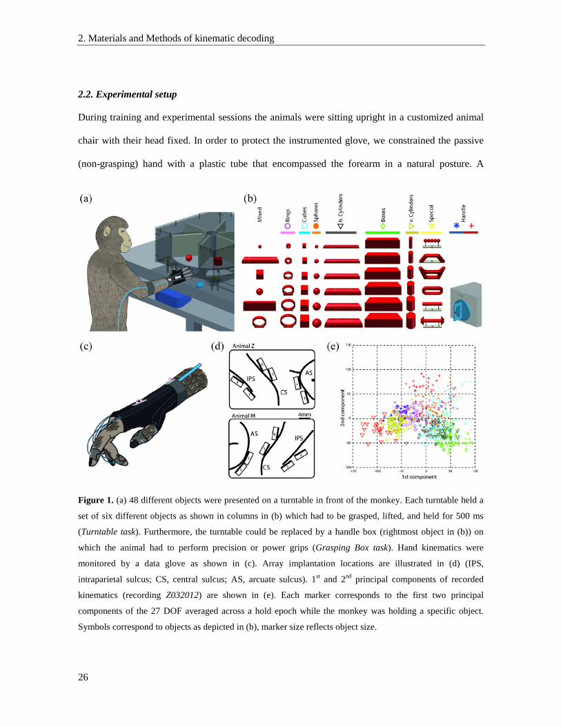
Figure 1. (a) 48 different objects were presented on a turntable in front of the monkey. Each turntable held a
set of six different objects as shown in columns in (b) which had to be grasped, lifted, and held for 500 ms
(Turntable task). Furthermore, the turntable could be replaced by a handle box (rightmost object in (b)) on
which the animal had to perform precision or power grips (Grasping Box task). Hand kinematics were
monitored by a data glove as shown in (c). Array implantation locations are illustrated in (d) (IPS,
intraparietal sulcus; CS, central sulcus; AS, arcuate sulcus). 1st and 2nd principal components of recorded
kinematics (recording Z032012) are shown in (e). Each marker corresponds to the first two principal
components of the 27 DOF averaged across a hold epoch while the monkey was holding a specific object.
Symbols correspond to objects as depicted in (b), marker size reflects object size.
2. Materials and Methods of kinematic decoding
27
capacitive switch at the side of the active (performing) hand allowed detecting the animal’s hand
position at rest. All graspable objects (figure 1 (b)) were placed at a distance of ~25 cm in front of
the animal at chest level. We used a PC-controlled turntable (figure 1 (a)) to pseudo randomly
present the objects. Light barriers on top of the ceiling and a step motor ensured precise object
positioning. Additional light barriers beneath the turntable detected when the monkey lifted the
displayed object.
Eight exchangeable turntables allowed presentation of a total of 48 objects. To obtain a high
variation of hand kinematics, we designed the objects to have different shape and size (figure 1 (b))
including rings (outer diameter: 10 mm, 20 mm, 30 mm, 40 mm, 50 mm, 60 mm), cubes (length:
15 mm, 20 mm, 25 mm, 30 mm, 35 mm, 40 mm), spheres (diameter: 15 mm, 20 mm, 25 mm,
30 mm, 35 mm, 40 mm), cylinders (length: 140 mm; diameter: 15 mm, 20 mm, 25 mm, 30 mm,
35 mm, 40 mm), and bars (length: 140 mm; height 50 mm; depth: 15 mm, 20 mm, 25 mm, 30 mm,
35 mm, 40 mm). Furthermore, a mixed turntable was used, holding mid-sized objects of various
shapes for fast exchange (sphere 15 mm, horizontal cylinder 30 mm, cube 30 mm, bar 10 mm, ring
50 mm), as well as a special turntable that contained objects of abstract forms (figure 1 (b)). All
objects had a uniform weight of 120 g, independent of their size and shape.
In addition to these 48 objects, we also trained the monkeys to grasp a handle object in two
different ways, either with a precision grip (using thumb and index finger) or with a power grip
(enclosure of handle using all digits). These grip types were detected by sensors in cavities the
middle of the handle and a light barrier behind the handle, respectively.
Eye position was measured with an optical eye tracker (ISCAN, Woburn, MA, USA), and hand
kinematics were recorded by a custom-made hand tracking device (Schaffelhofer and Scherberger
2012; see section 2.5.). To avoid interference with the electro-magnetic based hand tracker, no
ferromagnetic materials were used in the experimental setup, including animal chair, table and
manipulanda (Kirsch et al 2006, Raab et al 1979). All task relevant behavioural parameters (eye
2. Materials and Methods of kinematic decoding
28
position, stimulus presentation, switch activation) were controlled by custom-written behavioural
control software that was implemented in LabView (National Instruments).
2.3. Behavioural paradigm
Monkeys were trained to perform grasping actions in the dark in order to observe motor signals in
the absence of visual information. To realize this approach, a delayed grasping paradigm (Turntable
task) was implemented (Schaffelhofer et al 2015): monkeys initialized a trial by pressing a
capacitive switch in front of them. This action turned on a red LED that the animals had to fixate.
After fixating for 500-800 ms, a target object located next to the fixation LED was illuminated for
700 ms (cue epoch), followed by a waiting period in the dark (planning epoch, 500-1000 ms) in
which the animals had to withhold movement execution but continue to fixate until the fixation
LED blinked (“go” signal). Then, the animals grasped the object and held it up for 500 ms (hold
epoch).
Grasp movements performed on the handle (Grasping Box task, see figure 1 (b) “Handle”) were
executed with the same paradigm with the exception that one of two additional LEDs instructed the
monkeys during cue period to perform either a precision grip (yellow LED) or a power grip (green
LED).
Incorrect trials were aborted immediately; correct trials were rewarded with juice.
2.4. Signal procedures and imaging
Prior to surgery, we performed a 3D anatomical MRI scan of the animal’s skull and brain to locate
anatomical landmarks (Townsend et al 2011). For this, the animal was sedated (10 mg/kg ketamine
and 0.5 mg/kg xylazine, i.m.), placed in the scanner (GE Signa HD or Siemens TrioTim; 1.5 Tesla)
in a prone position, and T1-weighted images were acquired (iso-voxel size: 0.7 mm3).
2. Materials and Methods of kinematic decoding
29
Then, in an initial procedure, a head post (titanium cylinder; diameter 18 mm) was implanted on
top of the skull (approximate stereotaxic position: midline, 40mm anterior, 20° forward tilted) and
secured with bone cement (Refobacin Plus, BioMed, Berlin) and orthopedic bone screws (Synthes,
Switzerland). After recovery from this procedure and subsequent training with head fixation, each
animal was implanted in a second procedure with six floating microelectrode arrays (FMAs;
MicroProbes for Life Science, Gaithersburg, MD, USA). Specifically, two FMAs were inserted in
each area AIP, F5, and M1 (see figure 1 (d)). FMAs consisted of 32 non-moveable monopolar
platinum-iridium electrodes (impedance: 300-600 kΩ at 1 kHz) as well as two ground and two
reference electrodes per array (impedance < 10 kΩ). Electrode lengths ranged between 1.5 and
7.1 mm and were configured as in Townsend et al (2011).
Electrode array implantation locations are depicted in figure 1 (d). In both animals the lateral
array in AIP was located at the end of the intraparietal sulcus at level of PF, whereas the medial
array was placed more posteriorly and medially at the level of PFG (Borra et al 2008). In area F5,
the lateral array was positioned approximately in area F5a (Belmalih et al 2009, Borra et al 2010),
whereas the medial array was located in F5p in animal Z and at the border of F5a and F5p in animal
M. Finally, both arrays in M1 were positioned in the hand area of M1 (anterior bank of the central
sulcus at the level of the spur of the arcuate sulcus and medial to it) (Rathelot and Strick 2009).
All surgical procedures were performed under aseptic conditions and general anaesthesia (e.g.
induction with 10 mg/kg ketamine, i.m., and 0.05 mg/kg atropine, s.c., followed by intubation,
1-2% isofluorane, and analgesia with 0.01 mg/kg buprenorphene, s.c.). Heart and respiration rate,
electrocardiogram, oxygen saturation, and body temperature were monitored continuously.
Systemic antibiotics and analgesics were administered for several days after each surgery. To
prevent brain swelling while the dura was open, the animal was mildly hyperventilated (end-tidal
CO2 < 30 mmHg) and mannitol kept at hand. Animals were allowed to recover for at least 2 weeks
before behavioural training or recording experiments recommenced.
2. Materials and Methods of kinematic decoding
30
2.5. Hand kinematics
To monitor the animal’s movements, an instrumented glove for small primates was used that
allowed recording the animal’s finger, hand and arm movements in 27 DOF (Schaffelhofer and
Scherberger 2012). The glove was equipped with 7 electro-magnetic sensor coils that enabled hand
and arm movement tracking at a temporal resolution of 100 Hz without depending on light or sight
to a camera (figure 1 (c)). In this way, finger movements could be tracked continuously even when
the sensors were behind or below objects. The method has been described in detail in Schaffelhofer
and Scherberger (2012). In short, the technique exploits the anatomical constraints of the primate
hand and the 3D position and orientation information of the sensors located at the fingertips, the
hand’s dorsum and the lower forearm.
Recorded 3D positions of the finger, hand, and arm joints were compared to the animal’s
anatomy. Rarely occurring errors (e.g. due to short freezing of the kinematic tracking) were set to
NaN. Then, each joint angle was calculated for every recorded time step and afterward linearly
resampled to exactly 100 Hz. This way, also recorded and previously added NaNs were eliminated
by linear interpolation.
Specifically, the following 27 joint angles were extracted: spread (extension/flexion),
carpometacarpal (CMC), metacarpophalangeal (MCP), and interphalangeal (IP) joint of the thumb;
spread (adduction/abduction), metacarpophalangeal (MCP), proximal interphalangeal (PIP), and
distal interphalangeal (DIP) joint of index, middle, ring, and little finger; radial/ulnar deviation
(yaw), flexion/extension (pitch), and pronation/supination (roll) of the wrist; flexion/extension of
the elbow; as well as adduction/abduction (yaw), flexion/extension (pitch), and lateral/medial
rotation (roll) of the shoulder.
Furthermore, the speed of every DOF at each time sample was calculated and added to the
kinematics. This resulted in a 54xT-matrix with T as the total number of samples. Note, that only
2. Materials and Methods of kinematic decoding
31
data recorded while the monkey was exposed to the handle or turntable task was used and
concatenated into one matrix, including both correctly and incorrectly performed trials, reward
epochs, as well as the time between trials (inter-trial intervals). Data recorded while turntables or
the Grasping Box were exchanged by the experimenter were not included.
For illustration purposes, the 27 DOF were averaged during the hold epoch of each successful
trial of recording Z032012, and a principal component analysis was performed. The first two
principal components of the kinematics of each trial are illustrated in figure 1 (e), demonstrating
that we were able to cover a wide range of hand configurations together with sampling very small
differences in hand kinematics.
2.6. Neural recordings
Extracellular signals were simultaneously recorded from six FMAs (6 x 32 channels) that were
permanently implanted into area AIP, F5, and M1 (two arrays in each area). Raw signals were
sampled at a rate of 24 kHz with a resolution of 16 bit, and stored to disk together with the
behavioural and the kinematic data using a RZ2 Biosignal Processor (Tucker Davis Technologies,
FL, USA). Offline, the raw data was bandpass filtered (0.3-7 kHz) and spikes were detected
(threshold: > 3.5 standard deviation). Spike sorting was performed with WaveClus (Quiroga et al
2004) for automatic sorting and OfflineSorter (Plexon TX, USA) for subsequent manual inspection
and revision. Only single and multiunits were considered for further analyses.
2.7. Decoding
2.7.1. Decoding algorithm. For offline prediction of the hand and arm kinematics, we employed a
Kalman filter (Kalman 1960) as described in Wu et al. (2006, 2004). A Kalman filter assumes a
linear relationship between the kinematics at time instant k and the following time instant k+1 (step
size: 10 ms), as well as between the kinematics and the neural data at time k:
2. Materials and Methods of kinematic decoding
32
xk+1 = Axk + wk,
zk = Hxk + qk.
Here, xk+1 is the 54x1-vector of the 27 angles and their velocities at time k+1, A a 54x54-matrix
relating the kinematics of one time step to the following one, zk a vector of length N containing the
neural data at time k where N denotes the total number of recorded units, H a Nx54-matrix relating
the kinematics at time k to the corresponding neural information at time k, and wk and qk noise terms
that are assumed to be normally distributed with zero mean, i.e. wk ~ N(0,W) and qk ~ N(0,Q), with
W ∈ℝ54×54 and Q ∈ℝN×N covariance matrices.
2.7.2. Decoding procedure. For decoding a complete recording session, we used 7-fold cross-
validation. For this, the recording session was divided into seven data sets of equal length and
composition: each task type (i.e. Grasping Box task and data from each turntable) was divided into
seven parts of equal length and these parts were randomly attributed to the seven sets, so that
eventually each set contained data of each turntable and the Grasping Box task.
To decode the kinematics of the i-th of the seven sets, the parameters of the Kalman filter,
namely A, H, W, and Q, were calculated by using the neural and kinematic data of the remaining six
sets (decoder training). Then, the kinematic data of the i-th set (27 DOF and their respective
velocities) were iteratively predicted by the Kalman filter. The initial value of each DOF (and
velocity) was randomly set within the observed range of the respective DOF/velocity during the
recording (interval between the smallest and highest value). For each subsequent time step, the
Kalman filter first calculated an a-priori estimation of the kinematics based on the kinematic state of
the previous time step. Then, an update of this prediction based on the corresponding neural activity
was performed (a-posteriori estimation) (Welch and Bishop 2006).
2. Materials and Methods of kinematic decoding
33
This procedure was carried out for each of the seven data sets, hence leading to the decoding of
the entire recording session. The decoding procedure was implemented in a custom-written
software in Matlab (MathWorks Inc., Natick, MA, USA).
2.7.3. Variation of decoding parameters. The neural data used for decoding was varied in the
following way in order to systematically investigate the impact on decoding performance:
(1) For each unit, spike times were binned in specific time intervals, i.e. the number of occurring
spikes in a specific time bin was counted. Since the kinematic data was predicted by the
Kalman filter with a frequency of 100 Hz, the bins for counting the spikes were shifted in
time steps of 10 ms which resulted in overlapping bins if the window length was larger than
10 ms. To test the impact of bin length on the decoding performance, it was systematically
varied.
(2) In addition to bin length, we tested whether the introduction of a time lag (gap) between the
time series of the kinematics and the series of spike counts would lead to changes in
decoding performance. We therefore systematically varied gap length (using both positive
and negative values). Using a gap length g < 0 and a bin length b > 0 translated into
predicting the kinematics at time point tk with the spike count in the time window
[tk+g-b tk+g] in the a-posteriori step of the Kalman filter, meaning that neural activity
preceded the kinematics. Positive gap lengths where the neural data used for decoding
succeeded the kinematic prediction were tested as well. A positive gap length g > 0 and bin
length b > 0 would then take the spikes in the time window [tk+g tk+g+b] into account. For
the purpose of clarity, we used the notation g = -0, b > 0 to refer to the time window [tk-b tk]
and g = (+)0, b > 0 for the time window [tk tk+b] of spike counting.
2. Materials and Methods of kinematic decoding
34
For each recording and area/combination of areas, we tested different combinations of bin and gap
lengths, ranging from 0 to ±180 sec for gaps and 10–250 ms for bin lengths, and evaluated them
with respect to their decoding performance.
2.7.4. Evaluation of decoding performance. To assess decoding performance, we calculated both
Pearson’s correlation coefficient (CC) and the relative root mean squared error (rRMSE) for each
DOF across the entire decoded recording session to compare the measured trajectory of a joint
angle with the decoded trajectory as predicted by the Kalman filter.
CC was defined as
CC = �∑ (𝑥𝑘 − �̅�)(𝑥�𝑘 − �̅��)𝑁𝑘=1 � ⋅ ��∑ (𝑥𝑘 − �̅�)2 ∙𝑁
𝑘=1 ∑ (𝑥�𝑘 − �̅��)2𝑁𝑘=1 �
−1
,
where N is the total number of samples, 𝑥𝑘 and 𝑥�𝑘 denote the true and decoded DOF at time k,
respectively, and �̅� and �̅�� are the means across all N samples of the true and decoded DOF,
respectively.
rRMSE was determined by calculating the root mean squared error (RMSE)
RMSE =�1N
� (xk-x�k)2N
k=1
for each DOF and then normalizing it by the range of the respective DOF:
rRMSE = RMSE/(d95 - d5),
where d5 and d95 are the 5th and 95th percentile of all recorded data samples of the respective DOF.
The normalization allowed us to compare prediction errors of joint angles that differed in their
operational range.
For each neuronal dataset we determined the optimal gap and bin length combination that
maximized CC and minimized rRMSE. Most of the times, the optimal combinations matched for
CC and rRMSE. Both CC and rRMSE are important measures for performance, however, a
2. Materials and Methods of kinematic decoding
35
trajectory prediction that captures the movement shape with an offset bias might have a high CC,
but will also have a high rRMSE. In cases where the optimal parameter combination did not match
for CC and rRMSE, we therefore favoured the parameter combination yielding better rRMSE,
which generally also had a high CC. The optimal parameter combination was selected to evaluate
the information content that can be utilized by the Kalman filter to predict continuous movements.
2.7.5. Chance decoding performance. Since the Kalman filter used the previous kinematic state as
the first part of its prediction (a-priori estimation), in case of very regular movement, the filter
might be able to already achieve a high performance simply by utilizing the regularity of the
oscillatory kinematics, i.e. without having to rely on the neural information at all. In such a case, a
high decoding performance might then be falsely attributed to the neural data. To avoid such an
effect, we included both correct and incorrect trials (where the kinematics often did not follow the
typical temporal structure of the correct trials) in the decoding.
Furthermore, we calculated a chance level performance to get an estimation of how much the
filter was utilizing potentially encoded information in the neural data to predict the continuous
kinematics, as opposed to relying solely on the inherent kinematic information. For this, we
removed any potential task-relevant information contained in the spike train population by applying
the following random shift method: We shifted the spike sequence of each unit individually by a
random gap length of at least 20 sec in either positive or negative time direction. Neural data that
was shifted beyond the end or the beginning of the kinematic data was circularly reinserted at the
beginning or end, respectively. This way, we destroyed any potential relationship between the
kinematics of the limb and spike sequence, while keeping the inherent temporal structure of the
spike sequence intact. Importantly, we used different randomly determined gap lengths for each
unit, thus destroying also any potential correlations in the neuronal population. Using this
2. Materials and Methods of kinematic decoding
36
temporally reshuffled neural data, we carried out decodings and calculated the performance
measures, CC and rRMSE, from which we determined the chance level performance as follows:
By repeating this surrogate method ten times, we established the probability distribution of CC
and rRMSE during chance performance for each area and recording session. To test if the CC or
rRMSE obtained from the respective standard decoding differed significantly from chance, we
compared the respective CC or rRMSE value to the median of the chance probability distribution by
means of a two-sided sign test. If p < 0.05, we considered the performance of the standard decoding
to be significantly different from chance.
When comparing the mean performance across all ten recording sessions to chance (as in the
analysis of decoding performance for proximal and distal groups of joints, figure 6), a chance
distribution across recording sessions was composed out of the means of the chance distributions of
each recording. Then, a two-sided sign test was performed to determine whether the median of that
chance distribution differed significantly from the mean performance of the standard decoding
across all ten recording sessions.
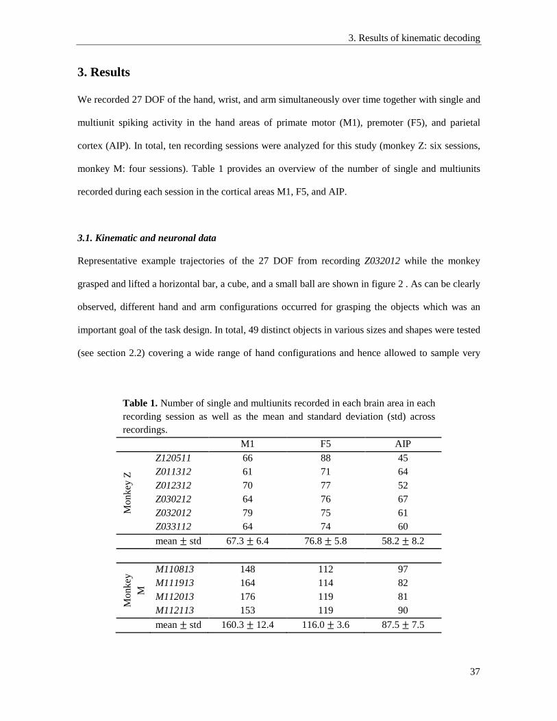
3. Results of kinematic decoding
37
3. Results
We recorded 27 DOF of the hand, wrist, and arm simultaneously over time together with single and
multiunit spiking activity in the hand areas of primate motor (M1), premoter (F5), and parietal
cortex (AIP). In total, ten recording sessions were analyzed for this study (monkey Z: six sessions,
monkey M: four sessions). Table 1 provides an overview of the number of single and multiunits
recorded during each session in the cortical areas M1, F5, and AIP.
3.1. Kinematic and neuronal data
Representative example trajectories of the 27 DOF from recording Z032012 while the monkey
grasped and lifted a horizontal bar, a cube, and a small ball are shown in figure 2 . As can be clearly
observed, different hand and arm configurations occurred for grasping the objects which was an
important goal of the task design. In total, 49 distinct objects in various sizes and shapes were tested
(see section 2.2) covering a wide range of hand configurations and hence allowed to sample very
Table 1. Number of single and multiunits recorded in each brain area in each recording session as well as the mean and standard deviation (std) across recordings. M1 F5 AIP
Mon
key
Z
Z120511 66 88 45 Z011312 61 71 64 Z012312 70 77 52 Z030212 64 76 67 Z032012 79 75 61 Z033112 64 74 60
mean ± std 67.3 ± 6.4 76.8 ± 5.8 58.2 ± 8.2
Mon
key
M
M110813 148 112 97 M111913 164 114 82 M112013 176 119 81 M112113 153 119 90
mean ± std 160.3 ± 12.4 116.0 ± 3.6 87.5 ± 7.5
3. Results of kinematic decoding
38
small differences in hand kinematics (see also figure 1 (e) in Materials and Methods).
In addition to the kinematic data, neural activity of the recorded units is shown at the bottom of
figure 2 (rasterplot). As expected, units in M1 displayed a clear modulation of firing rate during
movement execution, whereas they exhibited a decreased activity during periods with no
movement. An increase of spiking activity was also observed during movement periods for units in
F5 and AIP. The extent however was smaller than in M1 and was smallest in AIP. In contrast, AIP
showed a higher firing rate during periods where the object was presented to the monkey and while
the animal was planning the movement. A similar behaviour could be observed for F5 although the
planning activity was decreased compared to AIP. Such activity patterns have been reported
previously for single units in M1 (Bansal et al 2011, Poliakov and Schieber 1999, Umilta et al
2007, Vargas-Irwin et al 2010), F5 (Fluet et al 2010, Lehmann and Scherberger 2013, Murata et al
1997, Raos et al 2006, Rizzolatti et al 1988, Umilta et al 2007), and AIP (Baumann et al 2009,
Lehmann and Scherberger 2013, Murata et al 2000, Townsend et al 2011), hence confirming the
validity of the observed patterns within these areas.
3.2. Decoding of 27 DOF
Since a clear relationship between neural activity and kinematics could be observed, we decoded
27 DOF of the hand, wrist and arm continuously over time using single unit activity from areas M1,
F5, and AIP. Figure 3 shows example trajectories from recording Z032012 of hand, wrist and
shoulder joints over a time course of 80 sec while the monkey was lifting objects of the mixed
Figure 2. Joint angle kinematics of all recorded 27 DOF of recording Z032012 during 3 trials. Hand, wrist,
and arm DOF are shown while the monkey grasped a horizontal bar, a cube, and a small ball (objects on top).
Task epochs are marked by black vertical lines and labelled (“C”, cue; “P”, planning; “G”, “go” signal; “H”,
hold epoch). Simultaneously recorded neural activity from M1, F5, and AIP is presented as a rasterplot below.
Each unit is represented by one row of dots, and each dot represents the occurrence of a spike. Colour code
indicates the firing rate of a unit in Hz.
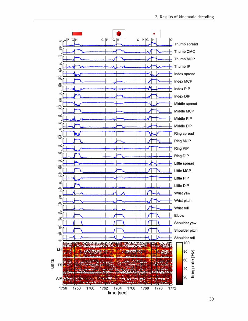
3. Results of kinematic decoding
39
3. Results of kinematic decoding
40
turntable. Both the true and the predicted joint angles are shown. Decodings were performed with
either single units from area M1 (figure 3 (a)), F5 (figure 3 (b)), or AIP (figure 3 (c)). For all three
areas, the estimated trajectory followed the real one accurately: the timing of both movement onset
and termination were captured in a very precise way. The movement amplitude seemed to be
reproduced best when decoding with data from area M1 and was slightly diminished when
predicting from areas F5 or AIP, respectively. Furthermore, in time periods without movement
(inter-trial intervals) the predicted trajecory contained more jittering when decoding from AIP than
when decoding with M1 or F5.
tdiv = 1761.5 sec (marked with a pink triangle on top) is one of the time instants when the data
was divided in order to carry out the 7-fold cross-validation: here the Kalman filter was re-trained
and decoding was restarted with new initial values within the range of the respective DOF (see
section 2.7.2 in Materials and Methods). This led to discontinuities in most curves, since the
decoding trajectory was placed far off the actual trajectory at this time instant. However, the
Kalman filter managed to bring the trajectory back close to the true amplitude within 300-400 ms,
hence illustrating the power of the algorithm.
Figure 3. Examples of real and decoded trajectories of four example DOF (thumb MCP, index DIP, wrist
yaw, and shoulder roll) are shown over a duration of 80 sec (recording Z032012). Blue lines: recorded
trajectories, red lines: decoded kinematics using neural activity from (a) area M1 (bin length 10 ms, gap
length -50 ms, 79 single units), (b) area F5 (bin length 10 ms, gap length -30 ms, 75 single units), and (c) area
AIP (bin length 10 ms, gap length -10 ms, 61 single units). Decoding performance (CC and rRMSE) during
these 80 sec is indicated separately for each trajectory. Pink triangle: time point when data was divided for
7-fold cross-validation, leading to brief (re-)initialization errors in the decoded trajectories. Decoding
performance across the entire recording session and across all 27 DOF are shown in (d) for CC and (e) for
rRMSE for individual areas or combinations thereof. Orange lines and errorbars in (d)-(e) indicate chance
level and standard deviation (see section 2.7.5 in Materials and Methods).
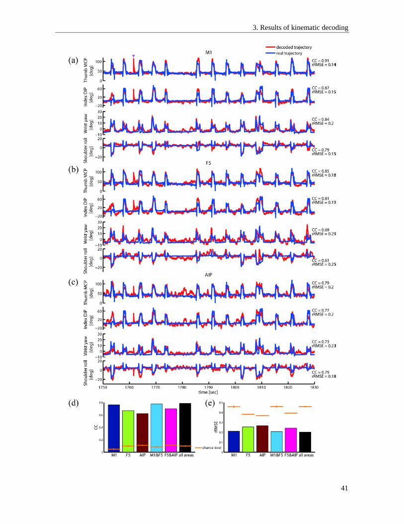
3. Results of kinematic decoding
41
3. Results of kinematic decoding
42
3.3. Decoding performance of different areas
To quantify the decoding performance of the different areas more precisely, we calculated the CC
and rRMSE for each DOF over the entire recording session (Z032012) and averaged the CCs across
all 27 DOF (figure 3 (d)-(e)). As expected, decoding with neural signals from area M1 yielded the
best decoding performance in comparison to decoding from F5 or AIP. However, there was no
significant difference in mean between M1 and F5, neither for CC nor rRMSE (one-way ANOVA
and Tukey-Kramer multicomparison test, p > 0.05). The similar CC shows that the actual
movement could be captured similarly precisely when decoding from M1 or F5. Still, predictions
made with F5 did not seem to capture the amplitude of the movement as well as when decoding
with M1, and there was more noise during resting phases (see also figure 3 (a)-(b)), which was
reflected in a higher rRMSE for F5. AIP yielded good performance values as well which did not
differ significantly from those obtained with area F5. However, when comparing AIP and M1, a
significant difference was found in the mean correlation coefficients (p < 0.05).
In addition to predicting from one brain area alone, we also decoded with pairs of areas
(AIP&F5 and M1&F5) and with all three areas combined to investigate if the decoding performance
could be improved by combining information from different brain areas. Decoding from M1 and F5
in combination increased the mean CC and decreased the mean rRMSE slightly, but not
significantly in comparison to decoding with M1 alone. Similarly, there was no significant
improvement when decoding from F5 and AIP in combination compared to decoding from F5
alone. As expected, decoding performance was best when all three areas were used for decoding.
However, there was no significant improvement in comparison to using only data from M1.
We were curious to evaluate to which extent the decoding performance could be attributed to
movement information contained in a brain area as opposed to information inherent in the
kinematics themselves. In other words, we wanted to determine a decoding performance based on
neural information that did not contain any meaningful information with respect to movement. If
3. Results of kinematic decoding
43
the resulting decoding accuracy was comparable to the performance presented in bars in
figure 3 (d)-(e), the performance must have been obtained by the Kalman filter solely relying on the
information within the kinematics (a-priori estimation, see section 2.7.2 in Materials and Methods).
In contrast, if the decoding performance was significantly lower when using meaningless spiking
activity, additional movement information must have been present in the brain areas which the
decoder was able to translate into kinematic predictions in order to yield the accuracy in figure 3
(d)-(e). Therefore, we performed simulated decodings with randomly reshuffled spiking activity in
which neural information is unrelated to movement kinematics to determine a chance level
performance, (random shift method, see section 2.7.5 in Materials and Methods for further
explanation). This method was repeated ten times for each neuronal dataset (area or combination of
areas), and CC and rRMSE were calculated for each DOF and then averaged across all 27 DOF.
Mean and standard deviation (across ten repetitions) are shown in figure 3 (d)-(e) (orange lines).
Clearly, decoding with the original neural data significantly outperformed chance performance both
in terms of CC and rRMSE (two-sided sign test, see section 2.7.5 in Materials and Methods,
p < 0.002). This demonstrated that significant movement information was present in these brain
areas that the decoder was able to translate into accurate movement predictions.
Figure 4 illustrates the combined results across all recording sessions (six sessions for monkey
Z, four sessions for monkey M; see also table 1). Overall, they confirm the findings of the example
recording shown in figure 3 (d)-(e). When decoding with neural activity from a single area, M1
yielded best results, followed by F5 and AIP, all differing significantly from each other in their
accuracies (one-way ANOVA and Tukey-Kramer multicomparison analysis; p < 0.05). Combining
two or three areas for decoding improved the decoding performance only slightly (but not
significantly) compared to using only the better performing single area.
Finally, we also compared the performances between monkeys for each area. There were no
differences in means or variances for M1 and F5 (two-sample t-test, p > 0.10, and Bartlett’s test,
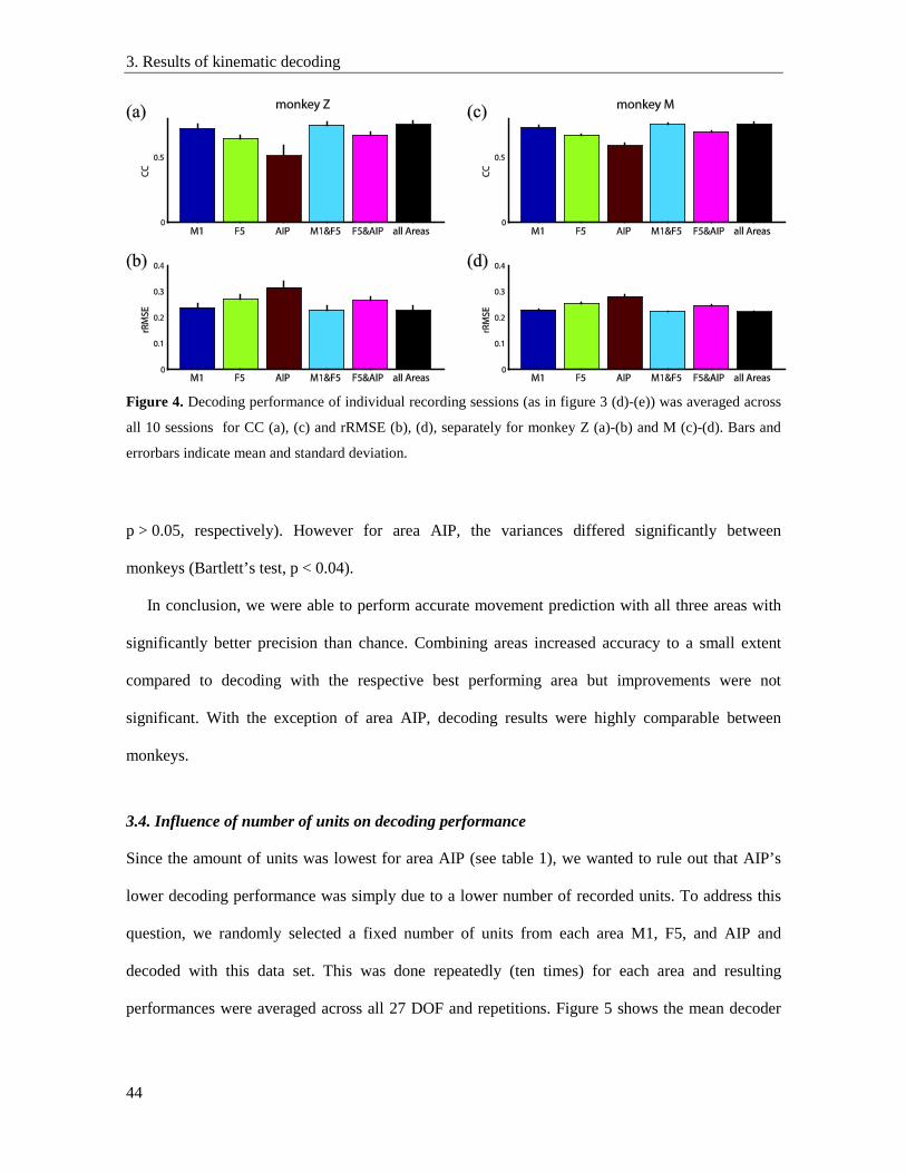
3. Results of kinematic decoding
44
p > 0.05, respectively). However for area AIP, the variances differed significantly between
monkeys (Bartlett’s test, p < 0.04).
In conclusion, we were able to perform accurate movement prediction with all three areas with
significantly better precision than chance. Combining areas increased accuracy to a small extent
compared to decoding with the respective best performing area but improvements were not
significant. With the exception of area AIP, decoding results were highly comparable between
monkeys.
3.4. Influence of number of units on decoding performance
Since the amount of units was lowest for area AIP (see table 1), we wanted to rule out that AIP’s
lower decoding performance was simply due to a lower number of recorded units. To address this
question, we randomly selected a fixed number of units from each area M1, F5, and AIP and
decoded with this data set. This was done repeatedly (ten times) for each area and resulting
performances were averaged across all 27 DOF and repetitions. Figure 5 shows the mean decoder
Figure 4. Decoding performance of individual recording sessions (as in figure 3 (d)-(e)) was averaged across
all 10 sessions for CC (a), (c) and rRMSE (b), (d), separately for monkey Z (a)-(b) and M (c)-(d). Bars and
errorbars indicate mean and standard deviation.
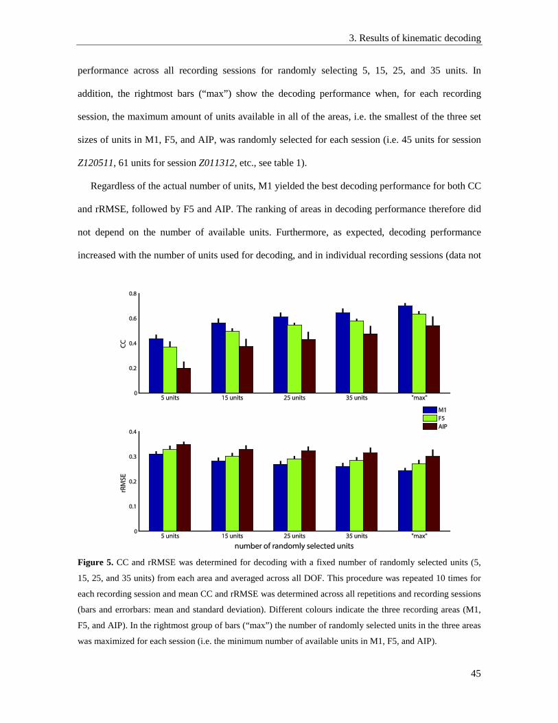
3. Results of kinematic decoding
45
performance across all recording sessions for randomly selecting 5, 15, 25, and 35 units. In
addition, the rightmost bars (“max”) show the decoding performance when, for each recording
session, the maximum amount of units available in all of the areas, i.e. the smallest of the three set
sizes of units in M1, F5, and AIP, was randomly selected for each session (i.e. 45 units for session
Z120511, 61 units for session Z011312, etc., see table 1).
Regardless of the actual number of units, M1 yielded the best decoding performance for both CC
and rRMSE, followed by F5 and AIP. The ranking of areas in decoding performance therefore did
not depend on the number of available units. Furthermore, as expected, decoding performance
increased with the number of units used for decoding, and in individual recording sessions (data not
Figure 5. CC and rRMSE was determined for decoding with a fixed number of randomly selected units (5,
15, 25, and 35 units) from each area and averaged across all DOF. This procedure was repeated 10 times for
each recording session and mean CC and rRMSE was determined across all repetitions and recording sessions
(bars and errorbars: mean and standard deviation). Different colours indicate the three recording areas (M1,
F5, and AIP). In the rightmost group of bars (“max”) the number of randomly selected units in the three areas
was maximized for each session (i.e. the minimum number of available units in M1, F5, and AIP).
3. Results of kinematic decoding
46
shown) the standard deviation of CC and rRMSE decreased with growing number of units, hence
demonstrating that results became more consistent.
Remarkably, performance already lay above chance when choosing only a small number of
single units (like five). For each recording, we compared the distribution of performance levels
obtained by ten repetitions of the random selection of five units with the distribution of chance
levels obtained by ten repetitions of the random shift method obtained by using all available units in
an area (Mann-Whitney U-test): when using M1 for decoding, the performances (both CC and
rRMSE) differed significantly from chance for all ten recording sessions (p < 0.001). For F5, there
was a significant performance difference to chance in 9 and 10 of 10 recordings for CC and rRMSE,
respectively (p < 0.05). For area AIP, decoding with five units was able to yield a significantly
better performance than chance level in eight out of ten recordings for CC (p < 0.05) and in all
recordings for rRMSE (p < 0.05).
Thus we can conclude that all areas carry substantial amount of information about hand and arm
kinematics which enabled kinematic prediction that was better than chance already with a small
number of units. Decoding accuracy improved monotonically with increasing number of units used
for decoding whereas the ranking of areas in decoding performance was independent of the amount
of recorded units.
3.5. Decoding performance of proximal and distal movements
Decoding performance for different groups of joints was compared in figure 6. Although the
electrode arrays were carefully placed in the hand area of motor, premotor, and parietal cortex,
decoding of elbow and shoulder joints (“arm joints” in figure 6) generally performed best for all
areas. Decoding performance was significantly higher than for all other groups of DOF except for
wrist angles when decoding with AIP and using rRMSE for judgement (one-way ANOVA and
Tukey-Kramer multicomparison analysis, p < 0.05). The high decoding accuracy is likely due to the
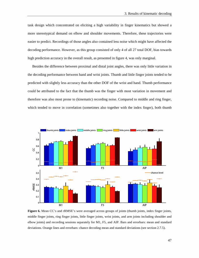
3. Results of kinematic decoding
47
task design which concentrated on eliciting a high variability in finger kinematics but showed a
more stereotypical demand on elbow and shoulder movements. Therefore, these trajectories were
easier to predict. Recordings of those angles also contained less noise which might have affected the
decoding performance. However, as this group consisted of only 4 of all 27 total DOF, bias towards
high prediction accuracy in the overall result, as presented in figure 4, was only marginal.
Besides the difference between proximal and distal joint angles, there was only little variation in
the decoding performance between hand and wrist joints. Thumb and little finger joints tended to be
predicted with slightly less accuracy than the other DOF of the wrist and hand. Thumb performance
could be attributed to the fact that the thumb was the finger with most variation in movement and
therefore was also most prone to (kinematic) recording noise. Compared to middle and ring finger,
which tended to move in correlation (sometimes also together with the index finger), both thumb
Figure 6. Mean CC’s and rRMSE’s were averaged across groups of joints (thumb joints, index finger joints,
middle finger joints, ring finger joints, little finger joints, wrist joints, and arm joints including shoulder and
elbow joints) and recording sessions separately for M1, F5, and AIP. Bars and errorbars: mean and standard
deviations. Orange lines and errorbars: chance decoding mean and standard deviations (see section 2.7.5).
3. Results of kinematic decoding
48
and small finger movements were more independent. When grasping, the little finger often did not
clasp the object as the other fingers did, but was positioned more loosely next to the object. It
therefore exhibited, similarly to the thumb, a movement pattern with higher variation across the
tested grip types.
In addition, figure 6 shows the respective chance performance levels. As it is clearly visible,
decoding performance of all joint groups was significantly better than chance level (two-sided sign
test, see section 2.7.5 in Materials and Methods, p < 0.002).
3.6. Optimal decoding parameters
As mentioned above, different parameter combinations (varying gap and bin lengths) were tested
for decoding and evaluated in terms of CC and rRMSE. Bin lengths of 10-250 ms were
systematically combined with gap lengths ranging from 0 to ±180 sec and the best combination
with respect to CC and rRMSE was determined. This procedure was repeated for all recording
sessions and areas. In 95% of these optimal combinations a bin length of 10 ms was the best
duration for counting spikes. Gap lengths, however, varied more strongly between areas and
recordings. Figure 7 (a)-(b) illustrates the decoding performance of M1, F5, and AIP as a function
of gap lengths while bin length was kept constant at 10 ms. Furthermore, the cumulative
distribution of optimal gap lengths (across recording sessions) for each area is provided in
figure 7 (c)-(d).
For area M1, the gap lengths yielding the best decoding performance for each recording
clustered around durations from -70 to 10 ms. A two-sided sign test showed that the median of these
gap lengths (-10 ms) was not significantly different from zero for CC (p = 0.07), but was for
rRMSE (median: -50 ms, p = 0.04). For area F5, the optimal gap lengths were shifted more into the
negative range, indicating that neural data used for decoding preceded the kinematic prediction: for
both CC and rRMSE, the median (-40 ms for CC, -60 ms for rRMSE) was significantly different
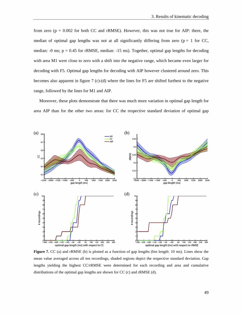
3. Results of kinematic decoding
49
from zero (p = 0.002 for both CC and rRMSE). However, this was not true for AIP: there, the
median of optimal gap lengths was not at all significantly differing from zero (p = 1 for CC,
median: -0 ms; p = 0.45 for rRMSE, median: -15 ms). Together, optimal gap lengths for decoding
with area M1 were close to zero with a shift into the negative range, which became even larger for
decoding with F5. Optimal gap lengths for decoding with AIP however clustered around zero. This
becomes also apparent in figure 7 (c)-(d) where the lines for F5 are shifted furthest to the negative
range, followed by the lines for M1 and AIP.
Moreover, these plots demonstrate that there was much more variation in optimal gap length for
area AIP than for the other two areas: for CC the respective standard deviation of optimal gap
Figure 7. CC (a) and rRMSE (b) is plotted as a function of gap lengths (bin length: 10 ms). Lines show the
mean value averaged across all ten recordings, shaded regions depict the respective standard deviation. Gap
lengths yielding the highest CC/rRMSE were determined for each recording and area and cumulative
distributions of the optimal gap lengths are shown for CC (c) and rRMSE (d).
3. Results of kinematic decoding
50
length distributions were 30.62 ms (M1), 29.83 ms (F5), and 83.11 ms (AIP). This difference was
significant (non-parametric Levene’s test, p < 0.03). Similar results were observed for rRMSE with
standard deviations of 37.06 ms (M1), 38.89 ms (F5), and 452.86 ms (AIP), also significantly
different (non-parametric Levene’s test, p < 0.01).
Furthermore, when decoding with data from AIP, a second, but smaller peak in performance
appeared for gap lengths around -1700 ms (figure 7 (a)-(b)). The ranking of the three areas in terms
of decoding performance was reversed for these long gap lengths. Contrary to AIP, the
performances for F5 and M1 improved steadily the closer the neural data used for decoding lay in
time compared to the kinematics to be predicted. For gap lengths longer than
approximately -600 ms, F5 still yielded higher decoding accuracy than M1. For positive gap
lengths, decoding performance monotonically decreased and there was no second peak in either
area.
In conclusion, while consistently observing a bin length of 10 ms as optimal throughout areas, the
impact of specific gap lengths on decoding performance varied largely. Consequently, the gap
lengths yielding highest decoding performance differed to a great extent for M1, F5, and AIP.
4. Discussion of kinematic decoding
51
4. Discussion
Our goal was to investigate the possibility of decoding complete hand, wrist, and arm movements
(represented by 27 DOF) from single and multiunit activity in the hand areas of motor (M1),
premotor (F5), and parietal cortex (AIP) in a comparative way. To our knowledge, this is the first
study that combines and compares these three grasping areas for prediction of versatile, continuous
hand kinematics. Simultaneous recordings of population activity from three areas by multi-electrode
arrays gave us the possibility to examine differences between these areas and evaluate the
information content with respect to hand and arm kinematics in these areas.
Our task design required the monkey to grasp a high number of distinct objects of different sizes
and shapes. Our goal was to elicit versatile hand and finger movements to investigate the
information content in each of the brain areas by means of decoding naturalistic grasping
movements with a high number of dimensionalities. Brochier et al (2004) demonstrated with a
similar, smaller set of objects that for each of them distinctive patterns of EMG activity in shoulder,
arm, hand, and digit muscles and thus different kinds of hand movements and configurations were
elicited. By including similar and more objects in our study, we hoped to achieve distinctive and
various hand movements and shapes. The PCA analysis of the performed kinematics in each trial
demonstrated that we succeeded in covering a wide range of hand configurations while also
sampling small differences in hand kinematics (see figure 1 in Materials and Methods).
4.1. Movement reconstruction with primary and premotor cortex
Continuous trajectories of 27 joint angles could be reconstructed accurately over time by using
single and multiunit activity from M1, F5, or AIP. However, decoding performance varied between
the areas. Highest performance was achieved when using M1 for decoding, followed by F5
(figures 3 and 4). These results were very consistent between monkeys.
4. Discussion of kinematic decoding
52
It is known that various parameters regarding hand and arm movements such as joint and muscle
representations, wrist position, and grasp configurations are encoded in both M1 (Ashe 1997, Ashe
and Georgopoulos 1994, Georgopoulos et al 1986, Kakei et al 1999, Rathelot and Strick 2006,
Taira et al 1996, Thach 1978, Umilta et al 2007) and F5 (Fluet et al 2010, Kakei et al 2001, Raos et
al 2006, Rizzolatti et al 1988). Furthermore, F5 has strong projections to the digit area of M1 (Borra
et al 2010, Dum and Strick 2005, Matelli et al 1986, Muakkassa and Strick 1979) as well as direct
connections to motoneurons in the spinal cord (Galea and Darian-Smith 1994, He et al 1993). F5
has therefore been considered to operate – to some extent – at the same hierarchical level as M1
(Dum and Strick 2005). Based on these findings, it is not surprising that both M1 and F5 were able
to predict joint kinematics in a precise way (figures 3 and 4). Resting epochs were reconstructed
better with activity from M1 than when using F5. This might be connected to the fact that contrary
to units in M1, a group of neurons in F5 already responded to object representation as shown
previously (Lehmann and Scherberger 2013, Murata et al 1997, Raos et al 2006) which might have
mistakenly been interpreted by the decoder as movement information.
The suitability of areas M1 and F5 for decoding of continuous arm and hand kinematics has
previously been investigated (Aggarwal et al 2013, Bansal et al 2012, Ben Hamed et al 2007,
Carmena et al 2003, Vargas-Irwin et al 2010). However, different decoding algorithms, task types
and parameters for decoding (such as bin and gap lengths) were employed which makes it difficult
to compare these results to ours. Furthermore, the number of decoded DOF was much lower in most
of these studies. However, the three following studies were closest related to ours: first, Aggarwal et
al (2013) trained two monkeys to grasp four different objects in different locations in front of them
and decoded 18 DOF (15 DOF of the hand and three DOF of the wrist) additionally to the hand
endpoint position with a Kalman filter. For prediction, they used single and multiunit activity
simultaneously recorded from M1, dorsal premotor cortex (PMd), and ventral premotor cortex
(PMv). Very similarly to our results, they obtained a CC of 0.76 (averaged across all sessions and
4. Discussion of kinematic decoding
53
DOF) when combining both M1 and F5 for decoding which fits very well with our respective CC of
0.75 when averaging across monkeys (figure 4 (a), (c)). When decoding kinematics with brain areas
separately, both their and our studies came to similar conclusions as well: decoding with area M1
produced a higher CC than when using activity from premotor cortex and combining both areas
barely improved the decoding performance compared to using only M1 (Aggarwal et al 2013).
Second and third, Vargas-Irwin et al (2010) and Bansal et al (2012) trained two monkeys to
grasp six to nine different objects that swung on a string in front of the animals. Vargas-Irwin and
colleagues recorded single unit activity from the hand regions of M1 and decoded 25 DOF (3 DOF
of the shoulder, 1 elbow DOF, 3 wrist DOF, 18 hand DOF) with a linear state-space model. Their
mean CC across all these decoded joint angles reached a value of 0.72 which corresponds to our CC
of 0.72 for kinematic reconstruction with M1 averaged across all sessions.
Bansal and colleagues additionally recorded from PMv (F4/F5 boundary) but reconstructed only
eight kinematic DOF (3D hand position, 3D velocity, aperture and speed of the hand) with a
Kalman filter. In their study, no significant difference in decoding accuracy between M1 and PMv
was observed and the average CC (across brain areas) had a value of 0.66 (Bansal et al 2012).
Note that all three studies included circumstances not present in our study that might have
influenced the decoding performance in the positive direction: first, in all three studies, the number
of objects used for grasping was substantially lower than in our task. It is therefore likely, that we
were able to elicit more versatile grasping kinematics and finger configurations. However, more
variance in the kinematics will increase the difficulty for precise decoding and is therefore likely to
affect the decoding performance in a negative way.
Second, Aggarwal and colleagues only decoded time periods from cue onset to beginning of
holding the object during correct trials. No other epochs of the task or inter-trial intervals were
considered and incorrect trials were discarded. In contrast, in our study all occurring movement and
resting kinematics were included. We deliberately chose to do so in order to mimic a more natural
4. Discussion of kinematic decoding
54
behaviour, where also unexpected movements could occur in addition to the ones demanded by the
task design. Again, this introduced variance in the kinematics in our study and increased the
difficulty for precise decoding.
Third, in Bansal et al’s study the decoding was performed using only a specific subset of units.
The units were selected by a greedy selection algorithm aiming to improve the CC. Bansal and
colleagues showed in their paper that this method indeed outperformed an average selection
approach (Bansal et al 2012). Similarly, Vargas-Irwin and colleagues chose a subset of units for
decoding that was selected by a greedy selection algorithm evaluating the correlation between firing
rate and kinematics. Moreover, each DOF was decoded separately enabling the selection the most
suitable subset of units for each DOF individually. Additionally, the optimal time lag between each
unit and a specific DOF was determined. In our study none of these optimization steps were carried
out, only a general optimal bin and gap length was selected for an entire neuronal population.
Evaluation of unit contribution to kinematic features was left to the automated training of the
Kalman filter. Despite all these points, our decoding accuracy was the same, or even higher, than
reported in those studies.
On the one hand, this might be contributed to the mathematical power of the Kalman filter. On
the other hand, our decoding results might have benefited from the fact that our M1 electrodes were
located in the anterior bank of the central sulcus (“new” M1) as opposed to the surface anterior to
the central sulcus (“old” M1) where Aggarwal’s and Bansal’s arrays were placed. Rathelot and
Strick (2009) demonstrated that units in the “old” M1 project to spinal interneurons and therefore
might only have an indirect influence on motor execution. In contrast, cells in the “new” M1 part
were found to make monosynaptic connections with motoneurons in the spinal cord (and were
hence termed cortico-motoneuronal cells, in short CM cells). It has been suggested that these cells
enable primates to execute highly developed muscle activity patterns (Rathelot and Strick 2009).
Information coded by these cells therefore might contain a more direct motor control signal than the
4. Discussion of kinematic decoding
55
information encoded in cells in the rostral region of M1 and might therefore be particularly
beneficial for the decoding of hand kinematics.
4.2. Movement reconstruction with parietal cortex
Decoding with AIP yielded the lowest decoding performance even though it was significantly
above chance (figures 3 and 4), suggesting that AIP carries substantial information about movement
kinematics that can be decoded. The signals in AIP do not necessarily have to be movement
commands, but could also represent other information related to movement execution like object
features relevant for grasping. However, the temporal characteristics of movement appeared to be
precisely captured by AIP, which supports the notion that motor related information in AIP is not
exclusively categorical information, like visual features, but also includes temporal aspects of
movement execution.
Predicted trajectories during resting periods often showed undesired jittering when decoding
from AIP. This might be accounted for by the fact that AIP responded to the visual presentation of
objects and therefore exhibited higher activity already much before the actual movement execution
(Baumann et al 2009, Lehmann and Scherberger 2013, Murata et al 2000, Sakata et al 1995,
Townsend et al 2011). This visual activity could have affected the decoder and might have caused
noisy movement residuals during periods of resting.
To our knowledge, this is the first study investigating area AIP as a potential brain region for
continuous decoding of versatile hand and finger movements. Previously, other areas in the parietal
cortex have been subject of decoding studies, mostly with emphasis on arm and reaching
movements: the parietal reach region (PRR), area 5d (Hauschild et al 2012) and posterior parietal
cortex (PPC) (Wessberg et al 2000) have been used for prediction of hand position in 3D space.
Hauschild et al (2012) obtained respective CC values that were very close to ours when decoding
from AIP (figure 4), whereas Wessberg et al (2000) reported that PPC and M1 performed equally
4. Discussion of kinematic decoding
56
well and were only outperformed in accuracy when decoding from PMd. Carmena et al (2003)
predicted 2D cursor position elicited by hand manipulations of a vertical pole from neuronal firing
rates in the medial intraparietal area in PPC and compared them to trajectories reconstructed from
other brain areas, such as M1 and PMd. Similarly to our results, they found M1 to deliver the best
decoding results (same CC as in our results) followed by PMd and PPC. However, the decoding
performance of cursor position predicted from PMd and PPC did not reach the performance levels
we were able to obtain for prediction of 27 joint angles of the arm and the hand with areas F5 and
AIP, respectively.
Other studies focusing directly on areas AIP and F5 for decoding only predicted categorical
variables like grip types: Lehmann and Scherberger (2013), Schaffelhofer et al (2015) as well as
Townsend et al (2011) found that F5 was better suited for decoding of grip types than AIP.
Furthermore, Townsend and colleagues were able to observe that decoding from combined activity
of F5 and AIP did not increase decoding performance significantly in comparison to F5 alone. Both
points correspond well with our results (figures 3 and 4). The fact that decoding performance did
not improve when neural activities from F5 and AIP were combined suggests that AIP largely
shares its kinematics-related information with area F5.
Another point we noticed in our results was that the decoding performance of AIP was not as
consistent between monkeys as it was for M1 and F5. Monkey Z showed a higher variability in
prediction accuracy than monkey M when decoding from AIP. One reason could be that two more
recording sessions were used for monkey Z (six sessions) which were spread over a longer time
duration (3.5 months) than for monkey M (four sessions in one month). However, this difference in
recording numbers and periods did not seem to affect the decoding performance of M1 and F5 as
much. Also, high variability in decoding performance could not be observed in monkey M for any
of the three tested areas. Therefore we suspect that the observed prediction variance for AIP in
monkey Z could have been associated with the array implanted in AIP in that monkey. For example,
4. Discussion of kinematic decoding
57
the array could have changed its position over time. An indication for this could be the number of
units recorded in AIP in each session (see table 1) and its variability from session to session. As we
were able to observe in the random neuron selection procedure (figure 5) and others have shown
before with neuron dropping analyses (Aggarwal et al 2013, Bansal et al 2012), decoding accuracy
increases with number of neurons and saturates after a certain amount of units. Therefore changes in
number of recorded units do not affect the decoding performance largely as long as the overall
number of neurons stays on a high level. This was the case for both monkeys for M1 and F5 as well
as in AIP for monkey M (see table 1). However, for lower numbers of recorded units as in area AIP
in monkey Z, the effect of a small change in unit number on decoding performance is bigger and
thus might have introduced a higher variability between decodings.
4.3. Influence of unit number on decoding performance
We demonstrated that differences in decoding performance between AIP, F5, and M1 did not
primarily depend on the number of neurons available for decoding, but strongly reflected the type of
information encoded in these areas (figure 5).
Furthermore, we found that already a very small number of randomly selected single units raised
decoding accuracy above chance. As suggested previously (Vargas-Irwin et al 2010), neurons in
M1 and F5 do not seem to be reflect a specific kinematic variable but instead carry information
about a broader range of movement parameters, which would allow reasonable movement
reconstruction even with a few neurons. This seemed to hold true also for units in AIP.
Neuron dropping analyses in previous studies suggested that only a limited amount of units is
necessary for making accurate predictions of hand and arm movements: Ben Hamed et al (2007)
concluded that 30-40 neurons from M1 were enough to discriminate finger movements and Vargas-
Irwin et al (2010) found 10-30 cells from primary motor cortex to be enough to decode continuous
joint kinematics. However, as already mentioned above (section 4.1), Vargas-Irwin and colleagues
4. Discussion of kinematic decoding
58
had selected neurons according to their decoding performance. Thus, the subset of aforementioned
10-30 neurons contained only cells that were optimally suited for movement prediction. A random
selection of units as performed in our study therefore most likely requires a higher number of units
to provide a comparable amount of information to the decoder and achieve a similarly high
decoding accuracy. Indeed, a random selection of 35 units produced an average decoding
performance of ≈ 90% of the accuracy obtained when using all available units for prediction.
4.4. Reconstruction of proximal and distal joints
Although the task demanded a wide variety of finger movements and hand configurations, no
substantial difference was found between decoding finger and wrist joints (figure 6). However, a
slight tendency towards a higher decoding performance for index, middle, and ring finger was
observed. These fingers showed higher synergies in their movements. Since the Kalman filter used
combined state information of all DOF for predicting a single joint (a priori estimate), more
information was available for joints moving in a correlated fashion and therefore the algorithm
could predict such DOF more accurately. In contrast, thumb movements were more independent
from the other fingers and showed more variation and were therefore harder to predict by the
decoder. Furthermore, the little finger was not actively used for grasping in many conditions and
played a rather subordinated role. The finger tended to be moved along with the other fingers but
often did not clasp the object properly as the other fingers did. Since it was used more passively, its
movement intention might have been underrepresented in the brain activity, which might explain
the slightly reduced decoding performance. For a few objects like the ones from the “special”
turntable (see figure 1 (b) in Materials and Methods) where the grasp was mainly carried out with
fingers 2-4 (similarly to the “spherical power grasp” described in Cutkosky and Wright (1986)), this
was also true for the thumb.
4. Discussion of kinematic decoding
59
In contrast, shoulder and elbow movements were predicted with significantly higher accuracy.
Since our task was designed to focus on eliciting dexterous grasping kinematics, arm movements
were more stereotypical than those of finger and wrist kinematics. Therefore, they also might have
been less prone to noise in the kinematic tracking. This might have facilitated the prediction of
shoulder and elbow movements. Nevertheless, by including incorrect trials that were often aborted
in the middle or contained unexpected movements (due to the monkey moving its arm away from
the object instead of towards it, or executing no movement at all), we tried to prevent the
occurrence of a stereotypical temporal structure in the kinematics. However, since we recorded
from highly trained animals, the number of incorrect trials was generally low.
In conclusion, although the arrays were carefully placed in the hand areas of primary, premotor,
and parietal cortex, both distal and proximal joints could be predicted with high accuracy. This
finding is supported by the observation of Vargas-Irwin et al (2010) that individual neurons in
primary motor cortex encode information about both proximal and distal kinematics. McKiernan et
al (1998) showed that a large portion of CM cells have muscle fields in both distal and proximal
muscles. Since we recorded in the “new” part of M1 (Rathelot and Strick 2009), it is likely that our
recorded population contained a considerable portion of such cells. Furthermore, neurons in both F5
and M1 have been found to be tuned not only to hand kinematics but also to different wrist postures
although the percentages of tuned units was lower in F5 than in area M1 (Kakei et al 1999, 2001).
In F5, the wrist orientation seems to be encoded as an additional feature of the grip configuration
(Raos et al 2006) and populations of units tuned to reaching movements have been identified in
both F5 and AIP (Lehmann and Scherberger 2013, Rizzolatti et al 1988).
Moreover, our results go hand in hand with the finding that also on the mechanical level
proximal and distal kinematics can hardly be disentangled (Jeannerod 1988, Lemon 1999): Stark et
al (2007) measured EMG activity during reach and grasp movements in shoulder, elbow, wrist, and
4. Discussion of kinematic decoding
60
extrinsic digit muscles and found that distal muscle activity cannot be exclusively related to either
reaching or grasping movements, respectively, but are rather biomechanically dependent.
4.5. Optimal decoding parameters and their network implications
In our study, a bin length of 10 ms yielded the highest decoding performance in 95% of the tested
data sets, regardless of which brain area was used for prediction. Previous decoding studies used bin
lengths of 100-150 ms, however without explaining their choice (Aggarwal et al 2013, Bansal et al
2012, Vargas-Irwin et al 2010). Long time windows will likely include the time point when
information content is highest, but they also act like low-pass filters. In contrast, with a short
window, changes in firing rate can be detected with higher temporal precision, which is
advantageous especially for brain areas with lower tuning strength, like AIP. However, it is also
crucial to combine the bin length with an adequate time lag to find the optimal relation between
brain activity and actual movement execution. Indeed, we found the time point from which data was
used for decoding to show high impact on decoding performance and the optimal time lag varied
considerably for the three areas (figure 7).
When decoding from M1, we found the highest amount of information being present when
neural data preceded the hand kinematics by 0-50 ms. Previous studies investigating the temporal
lag between neural activity in primary motor cortex and movement execution reported a wide range
of gap lengths both supporting and opposing our results:
Ashe and Georgopoulos (1994) decoded different movement parameters like direction, position,
velocity, and acceleration of reaching movements to instantaneous single unit activity in primary
motor cortex using a multiple linear regression method. They varied the time lag from 0 up to
±200 ms systematically for each individual unit and described the median optimal time lag
as -90 ms, although the distribution of optimal time lags of all cells covered the entire tested range
of gap lengths. However, it is noteworthy to mention that contrary to our study, only time periods
4. Discussion of kinematic decoding
61
during onset of target (i.e. immediately before movement onset) and 500 ms after reaching the
target were decoded. These time periods did not include incorrect trials, inter-trial intervals or any
other phases in which movement was withheld and/or planned.
A similarly broad result was obtained by Paninski et al (2004) who used a center-out-task to
investigate M1 cells. They evaluated different time lags with respect to mutual information between
firing rate and position in 2D space and obtained a heterogeneous range of optimal gap lengths
(spanning the entire range of ±1 sec). In contrast, Humphrey et al (1970) correlated spike
frequencies of M1 cells to wrist movements and exerted force and reported a very specific time lag
of -100 ms to yield the highest correlation.
Morrow and Miller (2003) decoded muscle activity from neurons in primary motor cortex by
means of linear regression. 15 out of 50 recorded units were randomly selected for decoding and
different delays were systematically tested for the respective subset of units with respect to their
decoding performance. This method was repeated 50 times and a delay of -50 ms was determined to
yield the highest decoding performance. In addition, they reported the CC of the decoding
depending on the different tested gap lengths. Their findings are comparable to our results (figure 7
(a)) with small differences: their peak performance exceeded ours and dropped faster the more the
gap lengths deviated from the optimal one, until levelling off at a time lag of around ±250 ms to a
CC of approximately 0.6. In contrast to our study however, they predicted only four distal muscles
(i.e. four DOF of the hand only instead of a complete kinematic representation of both the hand and
the arm as in our study) which showed very stereotypical behaviour since the monkey was only
required to perform one type of grip. Therefore, a higher decoding accuracy was probably achieved.
The faster drop of decoding accuracy for time lags around the optimal length could either be due to
the fact that Morrow and colleagues used a different decoding algorithm than we did or that
sequentially recorded neuronal activity was used for decoding (or both). Additional information
encoded in the coherence or phase synchrony within the neuronal population (Averbeck and Lee
4. Discussion of kinematic decoding
62
2004) was therefore not contained in their data. In our study however, this information was
available to the decoder due to simultaneous array recordings and might have helped to maintain a
relatively high decoding performance for gap lengths around the optimal ones. For a time gap of
around ±500 ms however, their decoding performance is comparable to ours. Unfortunately, no
longer time gaps were tested in their study.
A similar optimal time lag as presented by Morrow and Miller (2003) was reported by Cheney
and Fetz (1980) who investigated CM cells in precentral cortex and their relationship to EMG
activation of forearm muscles. They found an average latency of -60 to -70 ms prior to EMG
activation for most of the units; however the whole range of time lags from -200 ms to +80 ms with
respect to EMG activity onset was present in the investigated sample of units. In contrast,
McKiernan et al (1998), determining the latency between spikes of CM cells in primary motor
cortex and the onset of muscle activity of elbow, wrist, digit, and intrinsic hand muscles, reported
an onset of postspike effects around 8 ms and a peak of around 11 ms after neuronal activity.
Similar results were obtained by Fetz and Cheney (1980), Kasser and Cheney (1985), as well as by
Lemon et al (1986).
Our results fit well in this broad range of temporal relationships. Since we did not test for an
optimal time lag for each recorded unit individually, but sought for a gap length accounting for the
neural signal as a population, our result represents more an average across the population. We were
recording in the anterior bank of the central sulcus, therefore it is very likely that our neuronal
population contained CM cells which have direct projections to motoneurons in the spinal cord
(Rathelot and Strick 2009). This might explain why we found a tendency towards shorter gap
lengths as described by McKiernan et al (1998) to yield higher decoding accuracy in contrast to the
other studies mentioned above which recorded almost exclusively from the “old” part (Rathelot and
Strick 2009) of M1.
4. Discussion of kinematic decoding
63
Optimal time gaps for F5 exhibited the same temporal order as M1 (namely neural activity
preceding movement), but were longer than for M1. This indicates that information about grasping
is present earlier in F5 than in primary motor cortex. Furthermore, F5 yielded higher decoding
accuracies compared to M1 if neural activity preceding the movement with long time lags was used.
However, for very short gap lengths (i.e. close to movement execution and during movement
execution), M1 exceeded F5 in prediction strength (figure 7 (a)-(b)). These findings go hand in
hand with the results of Schaffelhofer et al (2015) who found (using the same task design as
described in our study) that grip type classification during planning epoch yielded higher decoding
accuracy when using activity from F5 for prediction than when using M1, whereas during the hold
epoch (i.e. during movement execution) M1 was better suited for decoding. Furthermore, these
findings are supported by a study conducted by Umilta et al (2007) in which F5 units showed
grasp/object related tuning earlier than units in M1. The preference index (PI), indicating the degree
of selectivity for a certain object, was higher in F5 during periods immediately before and at the
beginning of the movement, whereas peak selectivity in M1 occurred during grasping execution and
holding of an object.
Furthermore, our time lag results are in line with the fronto-parietal grasp network hypothesis
(Jeannerod et al 1995 and section 1.1.5), which states that visual information about an object to be
grasped is projected from AIP to F5, where a grip type is selected. Grip type information is then
forwarded to both M1 and the spinal cord. Neurons in M1 translate the grip type into a motor
command which is projected to the spinal cord as well. According to this idea, the temporal peak of
neural information with respect to grasping should be found in F5 earlier than in M1, which goes
hand in hand with our results.
However, the role of AIP in this process seems to be more intricate. Decoding performance
peaked for gap lengths close to zero and optimal gap lengths showed a much higher variance than
when decoding with M1 or F5. Additionally, we found a smaller peak in decoding performance for
4. Discussion of kinematic decoding
64
time lags around -1700 ms preceding movement. It is very unlikely that in natural grasping
movements, AIP represents movement intentions more than 1.5 sec before execution. Instead, this
second peak could be caused by the visual task instruction: the object is illuminated approximately
1.5 sec before movement onset (variable time duration due to a variable length of the planning
epoch), which is known to cause a visual activation in AIP (Sakata et al 1995, Schaffelhofer et al
2015). Furthermore, Schaffelhofer et al (2015) showed that object information (and to a less extent
grip type) could be decoded from single and multiunit activity during the cue epoch of the task.
Clearly, object features and hand configurations were coupled in our task; therefore cue information
could have been used by the decoder for movement prediction. However, an object can be grasped
in different ways. Therefore, visual information could only be used as a rough guideline for the
prediction of individual movement kinematics. Accordingly, decoding performance was lower for
these long gap lengths compared to the accuracy peak when decoding with very short time lags.
Previous studies testing the temporal delay between activity in parietal cortex and movement
found similar short durations for optimal time lags: the study by Ashe and Georgopoulos (1994)
described above did not only test single unit activity in primary motor cortex, but also in the arm
area of area 5. They obtained a median optimal time lag of +30 ms (neuronal activity following
movement), although again the distribution of time lags of all investigated cells covered the entire
tested time range from -200 to +200 ms. In contrast to M1, where 50% of the units showed an
optimal gap length between -200 and approximately -100 ms, 50% of the units from the arm region
in area 5 showed highest performance for time lags between approximately 20 to 200 ms. A
different result was reported by Hauschild et al (2012) who evaluated time lags from -45 to -125 ms
for prediction of arm endpoint position in 3D space from spiking activity in PRR and area 5d and
found a gap length of ≈ -80 ms to be optimal (with a bin length of 90 ms).
The closest experimental result to our findings was reported by Mulliken et al (2008) who
performed a center-out-task with and without obstacles and recorded individual PPC neurons.
4. Discussion of kinematic decoding
65
Based on mutual information, Mulliken and colleagues determined the optimal time lag between
neural activity and movement angle for neurons which exhibited tuning to this movement
parameter. The distribution of optimal time lags had a median ± interquartile range of 0 ± 90 ms and
-30 ± 90 ms for the center-out task with and without obstacles, respectively (lags were tested
approximately between ±180 ms), showing again a wide spread across the entire tested gap length
range. The authors argued that a motor command in PPC would require at least 90 ms to be
translated into movement. Furthermore, a proprioceptive feedback would take at least 30-90 ms to
reach PPC. Thus, the authors concluded that the information in parietal cortex at time lags close to
zero could encode a forward estimate of movement and neurons in PPC were therefore not only
involved in movement planning, but also in movement control by utilizing an efference copy from
premotor and motor cortices and projections to and from the cerebellum (Mulliken et al 2008). The
same is likely the case for AIP. It has been suggested that so-called motor neurons in AIP could
represent a copy of the motor plan in F5 in order to compare it to the visual object properties.
Depending on the result, a positive or negative feedback could be sent to the premotor cortex in
order to facilitate or modify the motor command (Murata et al 2000, Sakata et al 1997, Sakata et al
1999, Sakata et al 1995). Our results are compatible with this hypothesis.
4.6. Conclusion
We were able to show for the first time that high-dimensional reaching and grasping movements
could be decoded continuously over time with high precision not only from areas M1 and F5 but
also from area AIP in the parietal cortex. Although the decoding performance from AIP was inferior
to that from motor and premotor cortex, our results support the idea that AIP not only encodes
categorical visual information, as shown previously by other studies, but that AIP also contains
temporal movement information, at least to some extent. However, kinematic information in AIP
seems to be redundant to movement intentions encoded in area F5.


Chapter III - State decoding

5. Materials and Methods of state decoding
69
In this chapter the decoding of two different behavioural states, resting and movement, from neural
activity in areas M1, F5, and AIP is be presented. The chapter is structured in the following way: In
section 5, we will describe the respective materials and methods, which are followed by the
presentation of the results (section 6). In the end, the results will be discussed put into the greater
scientific context (section 7).
5. Materials and Methods
The basic procedures, experimental setup, behavioural paradigm, signal procedure, imaging,
kinematic and neural recordings were identical for state decoding as described in chapter II,
sections 2.1-2.6. Methods and analyses that differed from the kinematic decoding such as decoding
algorithm, decoding procedure, variation of decoding parameters, evaluation of decoding
performance, and chance decoding performance are described below.
5.1. Decoding algorithm
In addition to the prediction of continuous kinematics, we performed a separate decoding to classify
kinematic states. For this, we employed a weighted Support Vector Machine (wSVM) (Huang and
Du 2005) to distinguish between movement and resting states based on neural activity.
A Support Vector Machine (SVM) is a binary, linear classification algorithm which constructs a
hyperplane between two populations of vectors corresponding to two different classes (decoder
training). The hyperplane can be described by points p satisfying
w⋅p - b = 0
with w normal vector of the plane and b‖w‖ offset of the hyperplane from the origin along w. To
separate the two populations of data samples, the plane is required to fulfil w⋅xi - b ≥ 1 for all data
points xi belonging to class one and w⋅xi - b ≤ ‐1 for all data points xi belonging to class two. For
5. Materials and Methods of state decoding
70
data sets, in which these requirements cannot be fulfilled because the two populations are not
cleanly separated, a non-negative slack variable 𝜉𝑖 can be introduced. In this way, the requirements
become w⋅xi - b ≥ 1 ‐ 𝜉𝑖 and w⋅xi - b ≤ ‐1+ 𝜉𝑖 for data points xi belonging to the two classes,
respectively (Cortes and Vapnik 1995). In our decoding, we chose this “soft margin” approach. By
means of quadratic programming methods, the variables w, b, and 𝜉𝑖 can be optimized with subject
to the described requirements while at the same time maximizing the distance between the
hyperplane to the data points of the two populations (Platt 1999).
By mapping the vectors into a (higher dimensional) feature space with an appropriate kernel, the
construction of the hyperplane can be carried out even for data points which are not linearly
separable in the input space (Cortes and Vapnik 1995, Smola and Schölkopf 2004). For our
decoding, we used a radial basis function kernel (RBF) defined by
K �xi, xj� = e -γ� xi − xj�2,
with xi and xj data points, and γ free parameter, γ > 0 (Chang et al 2010, Hsu et al 2003).
After the hyperplane has been determined, the class of a given test vector x can then be decoded
by simply calculating on which side of the hyperplane the vector is located, i.e. if w⋅x - b greater or
smaller than zero.
However, the standard SVM has been found to produce a prediction bias toward the class with
the larger training sample size (Chew et al 2000). In our study, due to the task design,
approximately two thirds of the neural data corresponds to resting as opposed to movement. Thus,
to avoid the aforementioned bias, a weighted SVM was used for state prediction since it
compensates for uneven sizes of training samples and minimizes misclassification errors (Huang
and Du 2005).
5. Materials and Methods of state decoding
71
5.2. Decoding procedure
The kinematic data was prepared for state decoding by calculating the speed of each kinematic
dimension and smoothing each of the velocities with a Gaussian kernel (width: σ = 0.05 sec). Next,
each data sample of a DOF was classified as either movement and marked with “1” if the absolute
speed exceeded an empirically set threshold of 0.9 °/sec, or as resting and marked with “0” if
otherwise. This yielded a kinematic state information vector for each individual DOF. To obtain a
general kinematic state information vector, a time sample was classified as movement if more than a
third of the individual movement vectors displayed a “1” at that time instant, otherwise it was
classified as resting. This threshold was empirically determined. In a last step, very short sequences
of movement or resting were deleted by reversing the state class if the sequence was shorter than
nine time samples (i.e. shorter than 90 ms).
This way, the neural activity of each time step was assigned to a state of either resting or
movement. Using both the neural activity and the kinematic state information, a wSVM was trained
and employed to predict the kinematic state of the entire recording session by means of a 7-fold
cross-validation as already described in the Methods and Materials section of the Kalman filter (see
section 2.7.2). However, in contrast to the Kalman filter decoding, state decoding was not
performed with a sampling rate of 100 Hz but with a rate of 20 Hz. Since the computational load for
training the SVM is much higher than for the Kalman filter, computational time was saved using
only every fifth time sample of the training data to calibrate the SVM. Similarly, prediction of the
kinematic states was also performed only every 50 ms.
The decoding procedure was implemented with custom-written software in Matlab (MathWorks
Inc., Natick, MA, USA) using the c-code library LIBSVM for Support Vector Machines (Chang
and Lin 2011).
5. Materials and Methods of state decoding
72
5.3. Variation of decoding parameters
Similar to the decoding of continuous kinematics, we varied parameters of the neural data such as
bin length and gap length to test the impact on state prediction accuracy. At the same time, we
optimised two SVM parameters with respect to decoding accuracy, which needed to be chosen by
the experimenter prior to training of the algorithm, namely the regularization parameter C (Cortes
and Vapnik 1995, Smola and Schölkopf 2004) and the free parameter γ of the RBF kernel (see
section 5.1). We fixed the bin and gap length to specific initial values based on previous decoding
results and tested combinations of exponentially growing sequences of C and γ for decoding
(typically C = 20, 21, 23, …, 29 and γ = 2-2, 2-1, …, 22 following Hsu et al (2003)). The combination
of C and γ yielding the highest decoding accuracy was determined and kept fixed. Then, various
combinations of bin and gap lengths were tested (similarly as described in section 2.7.3) ranging
from -1000 to 200 ms for gap lengths and 10-1400 ms for bin lengths (same notation as in section
2.7.3). Now, the best combination of bin and gap lengths was determined and kept fixed while again
different combinations of C and γ were tested as described before. After that, keeping the resulting
optimal combination of C and γ, again bin and gap lengths were optimised. This process was
repeated iteratively until either none of the parameters were modified any more or decoding
accuracy only changed marginally from one iteration to the next. The resulting set of four
parameters was then considered as the optimal parameter combination.
5.4. Evaluation of decoding performance
To measure decoding performance, the accuracy was calculated as percent of correctly decoded
samples:
percent of correctly decoded samples = # correctly predicted samples# total testing samples
⋅100 % .
5. Materials and Methods of state decoding
73
“# of total testing samples” referred to either the total number of predicted samples in a decoding
(as in figure 10) or the total number of decoded samples in specific kinematic classes (as in figure
11) or trial/inter-trial epochs (as in figure 12).
5.5. Accuracy of movement onset prediction
To assess how precisely movement onset was detected by the decoder, we defined a window wi
centered around each true movement onset at time toni , with i = 1,…,Non and Non number of
movement onsets in a recording, i.e. wi = [toni - 400 ms, ton
i + 400 ms]. Each sample within a
window was checked for its state information so that for each window wi a respective state
information vector si = [si1, si
2, …, siN] could be created, si
n ∈ {0, 1} state information, n = 1,…,N, and
N = 17 number of samples in wi (N = 17 because the sample of movement onset is added to two
times the number of samples in a 400 ms window corresponding to eight samples each). Then, an
averaged state information vector s̅ = [s̅1, s�2, …, s̅N] across all windows in a recording was
calculated with s�n = 1Non
∑ sinNon
i=1 , n = 1,…,N. The parameters s�n represented the probability of
movement occurring relative to movement onset. By definition, s�9, representing the likelihood at
the time instant in which movement onsets took place, had a 100% probability to belong to the
movement state, whereas the time sample directly before had a 0% probability of movement.
The probability of movement depending on the time relative to movement onset was then
averaged across recordings and the mean values were fitted by a logistic curve with a vertical offset
p(t) = a1 + e-b(t-c) + d , (1)
with p probability of movement, t time relative to movement onset, and four fitting parameters a, b,
c, and d, .
Next, the probability of decoded movement in a 800 ms time window around each true
movement onset was determined in the predicted data sets separately for each area used for
5. Materials and Methods of state decoding
74
decoding in the same way as described above. Again, a logistic curve was fitted. The fit parameters
b and c in equation (1), describing the slope and the horizontal shift of the respective functions,
were analysed to assess the accuracy of movement onset prediction compared to true movement
onset.
5.6. Chance level performance
In contrast to kinematic decoding with the Kalman filter, state prediction with the wSVM does not
infer any information from the temporal structure in the data since the wSVM is not an iterative
algorithm. Instead, each data sample is an independent vector in the input space and its
classification does not depend on previous predictions. To assess chance level accuracy, it is
therefore legitimate to assign the given distribution of states randomly to the neural data to create
“meaningless” neural data.
In a decoding based on a data set like that, one could imagine a classifier that matches the
frequency distribution of the states in the training data in its prediction. Average chance level
decoding accuracy can then be calculated as the percentage of correctly classified samples in the
following way:
Be s the total number of samples, pR and pM the probability in the true data set for a sample to
belong to the resting or movement state, respectively (i.e. s = s⋅pR+ s⋅pM). The number of correctly
classified samples will then (on average) be the sum of number of samples belonging to movement
that are correctly classified as movement and the number of samples belonging to resting that are
correctly classified as resting. The number of samples belonging to movement is s⋅pM and since the
decoder has learned the distribution of classes, it will (on average) classify these samples as
movement with a probability of pM, assuming the classifier is an unbiased estimator. Therefore, the
number of correctly classified samples will be s⋅pM⋅pM. The same is true for the number of
correctly classified resting samples, namely s⋅pR⋅pR. The total proportion of correctly classified
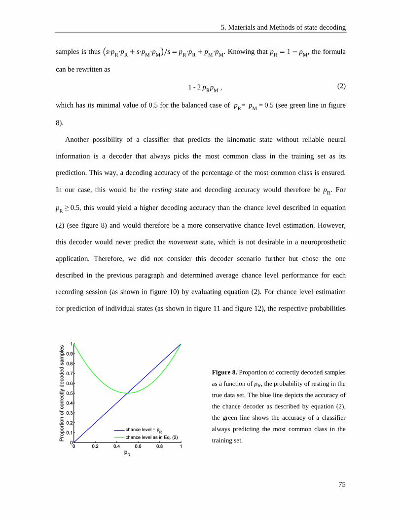
5. Materials and Methods of state decoding
75
samples is thus �s⋅pR⋅pR + s⋅pM⋅pM�/s = pR⋅pR + pM⋅pM. Knowing that pR = 1 − pM, the formula
can be rewritten as
1 - 2 pRpM , (2)
which has its minimal value of 0.5 for the balanced case of pR= pM = 0.5 (see green line in figure
8).
Another possibility of a classifier that predicts the kinematic state without reliable neural
information is a decoder that always picks the most common class in the training set as its
prediction. This way, a decoding accuracy of the percentage of the most common class is ensured.
In our case, this would be the resting state and decoding accuracy would therefore be pR. For
pR ≥ 0.5, this would yield a higher decoding accuracy than the chance level described in equation
(2) (see figure 8) and would therefore be a more conservative chance level estimation. However,
this decoder would never predict the movement state, which is not desirable in a neuroprosthetic
application. Therefore, we did not consider this decoder scenario further but chose the one
described in the previous paragraph and determined average chance level performance for each
recording session (as shown in figure 10) by evaluating equation (2). For chance level estimation
for prediction of individual states (as shown in figure 11 and figure 12), the respective probabilities
Figure 8. Proportion of correctly decoded samples
as a function of pR, the probability of resting in the
true data set. The blue line depicts the accuracy of
the chance decoder as described by equation (2),
the green line shows the accuracy of a classifier
always predicting the most common class in the
training set.
5. Materials and Methods of state decoding
76
of a class (i.e. pR and pM, respectively, in figure 11 for example) were used.

6. Results of state decoding
77
6. Results
In figure 3 (a)-(c) in chapter II, section 3.2, four example trajectories of the 27 decoded DOF were
illustrated. As already described before, the Kalman filter was able to predict movement kinematics
accurately with spiking activity from each of the three areas. However, during resting phases
between trials and during fixation, cue, and planning epochs, the prediction of the Kalman filter did
not exactly match the original trajectories. Instead, the decoded DOF exhibited jittering and
undesired movement.
To address this problem, we performed a separate continuous prediction of the kinematic state,
namely movement or resting states to distinguish between phases with and without movement. If
information about the condition of the movement could be inferred from the neural data in addition
to actual kinematic movement trajectories, this could enable the kinematic decoder to adjust its
prediction during states of resting to prevent undesired movement by either pausing the decoding of
the joint trajectories or overwriting its prediction with a desired stationary value.
6.1. State detection performance of different areas
Figure 9 illustrates state predictions from recording M110813 over a time course of 55 sec. The
trajectory of the index MCP joint is shown additionally as a reference to indicate when the monkey
was resting or performing a movement. Decodings were carried out with units from either area M1
(figure 9 (a)), F5 (figure 9 (b)), or AIP (figure 9 (c)). For all three areas, the state prediction agreed
largely with the trajectory: Each time the monkey reached to an object to grasp it, the decoder
classified the state as movement. Even during phases after the monkey had lifted the object and held
it for a few hundred milliseconds the decoder often detected the resting state. When decoding with
AIP however, the classifier sometimes assigned the movement state to periods where the monkey
was clearly resting. Furthermore, the onset of movement was not always detected exactly on time
but showed a short delay.
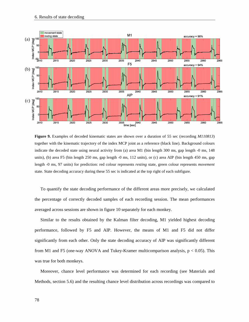
6. Results of state decoding
78
Figure 9. Examples of decoded kinematic states are shown over a duration of 55 sec (recording M110813)
together with the kinematic trajectory of the index MCP joint as a reference (black line). Background colours
indicate the decoded state using neural activity from (a) area M1 (bin length 300 ms, gap length -0 ms, 148
units), (b) area F5 (bin length 250 ms, gap length -0 ms, 112 units), or (c) area AIP (bin length 450 ms, gap
length -0 ms, 97 units) for prediction: red colour represents resting state, green colour represents movement
state. State decoding accuracy during these 55 sec is indicated at the top right of each subfigure.
To quantify the state decoding performance of the different areas more precisely, we calculated
the percentage of correctly decoded samples of each recording session. The mean performances
averaged across sessions are shown in figure 10 separately for each monkey.
Similar to the results obtained by the Kalman filter decoding, M1 yielded highest decoding
performance, followed by F5 and AIP. However, the means of M1 and F5 did not differ
significantly from each other. Only the state decoding accuracy of AIP was significantly different
from M1 and F5 (one-way ANOVA and Tukey-Kramer multicomparison analysis, p < 0.05). This
was true for both monkeys.
Moreover, chance level performance was determined for each recording (see Materials and
Methods, section 5.6) and the resulting chance level distribution across recordings was compared to
(a)
(b)
(c)
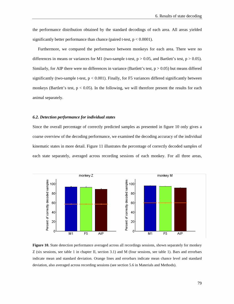
6. Results of state decoding
79
the performance distribution obtained by the standard decodings of each area. All areas yielded
significantly better performance than chance (paired t-test, p < 0.0001).
Furthermore, we compared the performance between monkeys for each area. There were no
differences in means or variances for M1 (two-sample t-test, p > 0.05, and Bartlett’s test, p > 0.05).
Similarly, for AIP there were no differences in variance (Bartlett’s test, p > 0.05) but means differed
significantly (two-sample t-test, p < 0.001). Finally, for F5 variances differed significantly between
monkeys (Bartlett’s test, p < 0.05). In the following, we will therefore present the results for each
animal separately.
6.2. Detection performance for individual states
Since the overall percentage of correctly predicted samples as presented in figure 10 only gives a
coarse overview of the decoding performance, we examined the decoding accuracy of the individual
kinematic states in more detail. Figure 11 illustrates the percentage of correctly decoded samples of
each state separately, averaged across recording sessions of each monkey. For all three areas,
Figure 10. State detection performance averaged across all recordings sessions, shown separately for monkey
Z (six sessions, see table 1 in chapter II, section 3.1) and M (four sessions, see table 1). Bars and errorbars
indicate mean and standard deviation. Orange lines and errorbars indicate mean chance level and standard
deviation, also averaged across recording sessions (see section 5.6 in Materials and Methods).
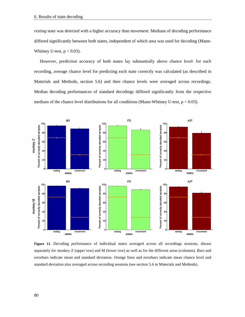
6. Results of state decoding
80
resting state was detected with a higher accuracy than movement. Medians of decoding performance
differed significantly between both states, independent of which area was used for decoding (Mann-
Whitney U-test, p < 0.03).
However, prediction accuracy of both states lay substantially above chance level: for each
recording, average chance level for predicting each state correctly was calculated (as described in
Materials and Methods, section 5.6) and then chance levels were averaged across recordings.
Median decoding performances of standard decodings differed significantly from the respective
medians of the chance level distributions for all conditions (Mann-Whitney U-test, p < 0.03).
Figure 11. Decoding performance of individual states averaged across all recordings sessions, shown
separately for monkey Z (upper row) and M (lower row) as well as for the different areas (columns). Bars and
errorbars indicate mean and standard deviation. Orange lines and errorbars indicate mean chance level and
standard deviation also averaged across recording sessions (see section 5.6 in Materials and Methods).
6. Results of state decoding
81
Comparing different brain areas for decoding yielded very similar results as already obtained for
the overall decoding performance in figure 10: mean decoding accuracy for both resting and
movement state did not differ significantly between M1 and F5, as well as not between F5 and AIP.
However, there was a significant difference between AIP and M1, except for resting state detection
in monkey Z, where medians did differ significantly between F5 and AIP (Kruskal-Wallis test and
Tukey-Kramer multicomparison test, p < 0.05).
Finally, we compared individual state detection accuracy between monkeys: Median
performances did not differ significantly between animals (Mann-Whitney U-test, p > 0.05) except
for resting state prediction decoded from F5 and AIP where means were significantly different
(p < 0.05).
In conclusion, we were able to predict two separate kinematic states with single and multiunit
activity from either of the three tested brain areas. Performance ranking of the areas corresponded to
the ranking obtained for the continuous kinematic decoding with the Kalman filter except for the
fact that the differences between M1 and F5 were non-significant.
6.3. Resting state detection during passive resting phases and active hold epochs
Since the movement and resting state was defined based on a velocity threshold, the resting state
included on the one hand passive waiting phases between trials as well as during fixation, cue, and
planning epochs, and on the other hand phases during hold epochs where the monkey was holding
the grasped object without moving its hand and arm. Although kinematically similar, these phases
might be different in terms of neural coding. Whereas the monkey is passively resting its hand
while waiting for the go signal to perform its next movement, it is actively engaged by tensing
muscles in the arm and hand while holding an object. In the following, we will therefore distinguish
these two different categories of resting by the terms passive and active resting.
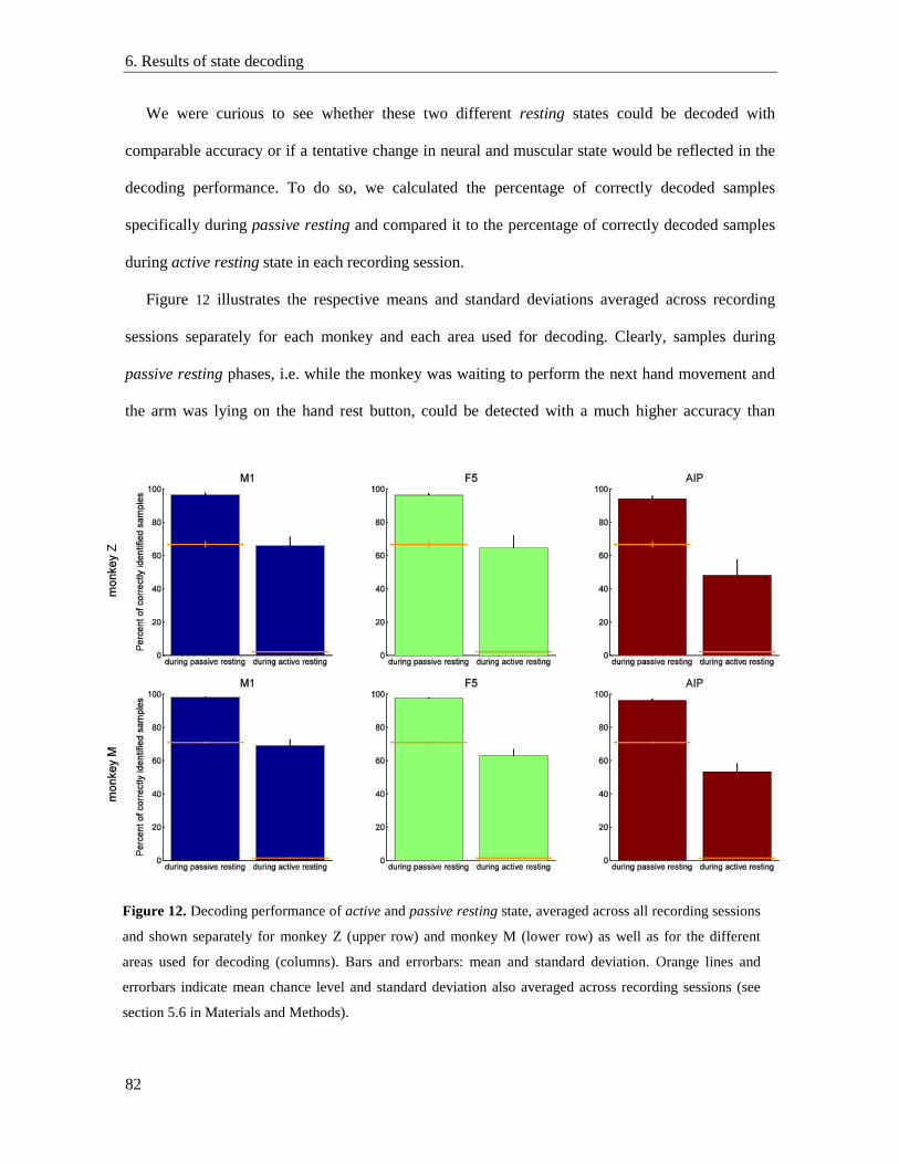
6. Results of state decoding
82
We were curious to see whether these two different resting states could be decoded with
comparable accuracy or if a tentative change in neural and muscular state would be reflected in the
decoding performance. To do so, we calculated the percentage of correctly decoded samples
specifically during passive resting and compared it to the percentage of correctly decoded samples
during active resting state in each recording session.
Figure 12 illustrates the respective means and standard deviations averaged across recording
sessions separately for each monkey and each area used for decoding. Clearly, samples during
passive resting phases, i.e. while the monkey was waiting to perform the next hand movement and
the arm was lying on the hand rest button, could be detected with a much higher accuracy than
Figure 12. Decoding performance of active and passive resting state, averaged across all recording sessions
and shown separately for monkey Z (upper row) and monkey M (lower row) as well as for the different
areas used for decoding (columns). Bars and errorbars: mean and standard deviation. Orange lines and
errorbars indicate mean chance level and standard deviation also averaged across recording sessions (see
section 5.6 in Materials and Methods).
6. Results of state decoding
83
samples during hold phases (active resting). Medians differed significantly in both monkeys and
independent from which area was used for decoding (Mann-Whitney U-test, p < 0.03).
The performances of the three areas did not differ from the previous results: when comparing the
decoding accuracy of passive resting among the areas, there was no significant difference in means
between M1 and F5, but AIP was differing significantly from both M1 and F5 (Kruskal-Wallis test
and Tukey-Kramer multicomparison test, p < 0.05). The same was true when comparing the
accuracy of predicting active resting between areas.
All decoding performances were significantly better than their respective chance level: again, for
each recording, chance level for predicting active or passive resting were separately calculated (see
section 5.6) and averaged across recordings. Median decoding performances of standard decodings
differed significantly from the respective medians of the chance level distributions (Mann-Whitney
U-test, p < 0.03). This was true for both passive and active resting.
Finally, decoding results were compared between monkeys: there were no significant differences
in the median decoding accuracies between monkeys for any conditions (Mann-Whitney U-test,
p > 0.05).
6.4. Decoding of movement onset
For a neuroprosthetic application, it is not only important to correctly distinguish between
movement and resting phases but to catch the timing of movement onset precisely. As described in
Materials and Methods (see section 5.5), we calculated the probability of true and decoded
movement around each actual movement onset. Figure 13 shows the mean probabilities together
with their standard deviations averaged across recordings. The results were fitted with logistic
curves which are shown in addition.
As expected, there was a stepwise transition from resting to movement in the real data (figure 13
(a), (e)): by definition, since movement always started at t = 0 ms, the probability of movement was
6. Results of state decoding
84
at a 100% level for this time point, whereas the preceding time sample at t = -50 ms had a
probability of 0%. For the decoded data sets however, the transition happened much more
smoothly. The fit parameter b (see equation (1) in section 5.5 in Materials and Methods) describing
the slope of the fitted function (larger values of b correspond to steeper graphs) decreased
drastically from 3.5 and 1.8 in the actual data set (for monkeys Z and M, respectively) to 0.05 and
0.07 when decoding with M1 (figure 13 (b), (f)), 0.03 and 0.05 when decoding with F5
(figure 13 (c), (g)), and 0.02 and 0.02 when decoding when AIP (figure 13 (d), (h)). The
decreasing values also indicate that decoding with M1 showed the most precise transition from
resting to movement, whereas in state reconstruction with F5 and AIP more samples both before
and after movement onset were incorrectly classified.
Next, we looked at the average time of movement onset prediction represented by the fit
parameter c. Unfortunately, in the fit of the true data, this parameter cannot account for true
movement onset: since we used discrete time samples with a sampling rate of 20 Hz for fitting the
sigmoidal function, any number between -50 and 0 ms would have been a legitimate fitting value
for c. Therefore, the actual value of c in the fit of the true data is meaningless to us.
This holds true to a certain extent also for c in the fitted functions of the decoded data.
Nevertheless, we found that c, when decoding with either M1 or F5, also fell within this time
window of -50 to 0 ms suggesting that movement onset could be captured on average within the
precision of 50 ms (c = -15.5 ms and -16.0 ms when decoding from M1, c = -10.4 ms and -6.4 ms
when decoding from F5, for monkey Z and M, respectively). In contrast, when decoding with AIP,
we obtained values of c = 13.4 ms and 41.9 ms for monkey Z and M, respectively, suggesting that
Figure 13. Probability of true and decoded movement states in a 800 ms time window around each actual
movement onset (see Materials and Methods, section 5.5). Dots illustrate mean probability of true (a), (e) and
predicted (b)-(d), (f)-(h) movement averaged across recordings, separately for monkey Z (a)-(d) and monkey
M (e)-(h) whereas shaded regions show standard deviations. Red lines depict the respective fits.
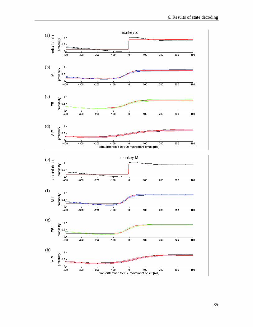
6. Results of state decoding
85
(a)
(b)
(c)
(d)
(e)
(f)
(g)
(h)
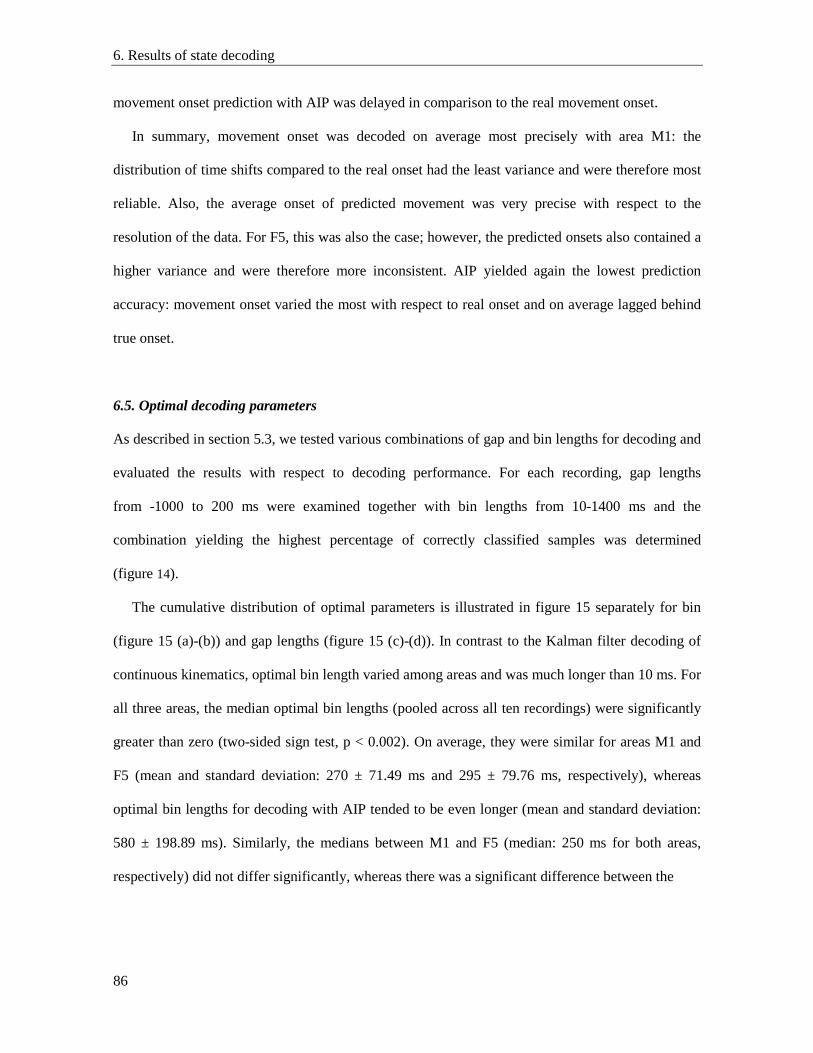
6. Results of state decoding
86
movement onset prediction with AIP was delayed in comparison to the real movement onset.
In summary, movement onset was decoded on average most precisely with area M1: the
distribution of time shifts compared to the real onset had the least variance and were therefore most
reliable. Also, the average onset of predicted movement was very precise with respect to the
resolution of the data. For F5, this was also the case; however, the predicted onsets also contained a
higher variance and were therefore more inconsistent. AIP yielded again the lowest prediction
accuracy: movement onset varied the most with respect to real onset and on average lagged behind
true onset.
6.5. Optimal decoding parameters
As described in section 5.3, we tested various combinations of gap and bin lengths for decoding and
evaluated the results with respect to decoding performance. For each recording, gap lengths
from -1000 to 200 ms were examined together with bin lengths from 10-1400 ms and the
combination yielding the highest percentage of correctly classified samples was determined
(figure 14).
The cumulative distribution of optimal parameters is illustrated in figure 15 separately for bin
(figure 15 (a)-(b)) and gap lengths (figure 15 (c)-(d)). In contrast to the Kalman filter decoding of
continuous kinematics, optimal bin length varied among areas and was much longer than 10 ms. For
all three areas, the median optimal bin lengths (pooled across all ten recordings) were significantly
greater than zero (two-sided sign test, p < 0.002). On average, they were similar for areas M1 and
F5 (mean and standard deviation: 270 ± 71.49 ms and 295 ± 79.76 ms, respectively), whereas
optimal bin lengths for decoding with AIP tended to be even longer (mean and standard deviation:
580 ± 198.89 ms). Similarly, the medians between M1 and F5 (median: 250 ms for both areas,
respectively) did not differ significantly, whereas there was a significant difference between the
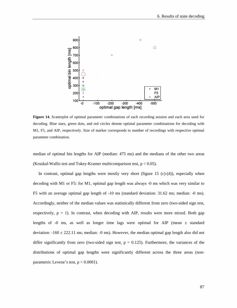
6. Results of state decoding
87
median of optimal bin lengths for AIP (median: 475 ms) and the medians of the other two areas
(Kruskal-Wallis test and Tukey-Kramer multicomparison test, p < 0.05).
In contrast, optimal gap lengths were mostly very short (figure 15 (c)-(d)), especially when
decoding with M1 or F5: for M1, optimal gap length was always -0 ms which was very similar to
F5 with an average optimal gap length of -10 ms (standard deviation: 31.62 ms; median: -0 ms).
Accordingly, neither of the median values was statistically different from zero (two-sided sign test,
respectively, p = 1). In contrast, when decoding with AIP, results were more mixed. Both gap
lengths of -0 ms, as well as longer time lags were optimal for AIP (mean ± standard
deviation: -160 ± 222.11 ms; median: -0 ms). However, the median optimal gap length also did not
differ significantly from zero (two-sided sign test, p = 0.125). Furthermore, the variances of the
distributions of optimal gap lengths were significantly different across the three areas (non-
parametric Levene’s test, p < 0.0001).
Figure 14. Scatterplot of optimal parameter combinations of each recording session and each area used for
decoding. Blue stars, green dots, and red circles denote optimal parameter combinations for decoding with
M1, F5, and AIP, respectively. Size of marker corresponds to number of recordings with respective optimal
parameter combination.
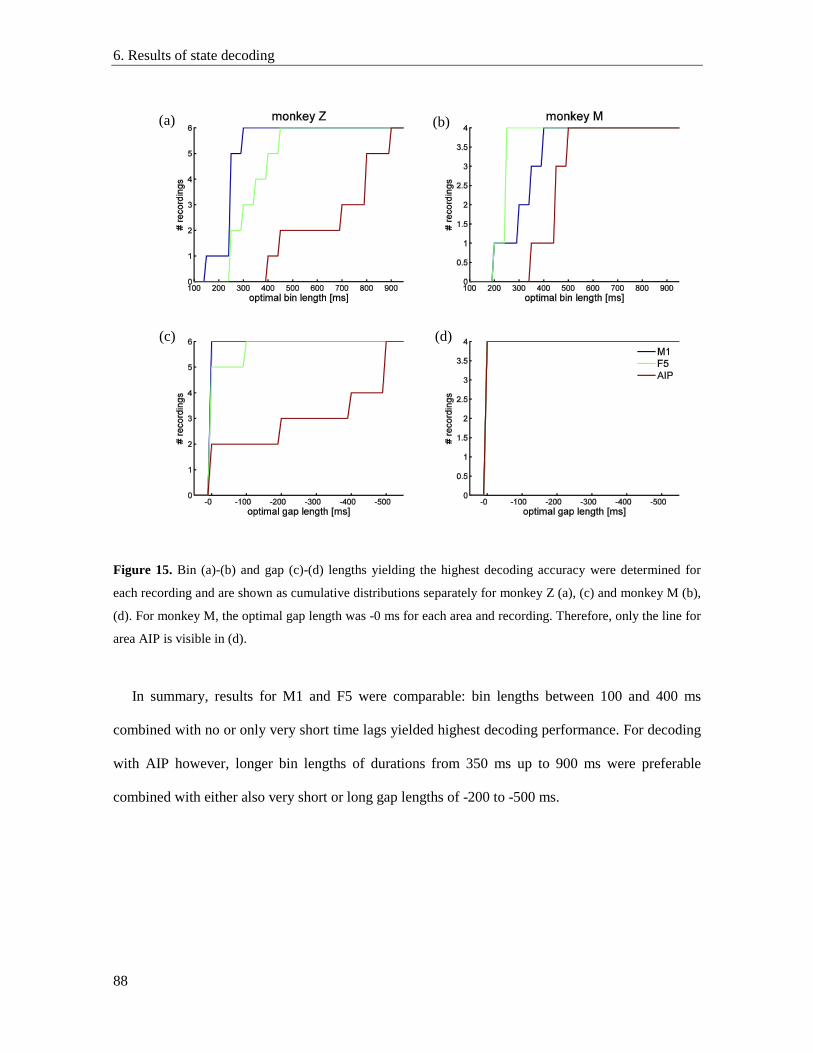
6. Results of state decoding
88
Figure 15. Bin (a)-(b) and gap (c)-(d) lengths yielding the highest decoding accuracy were determined for
each recording and are shown as cumulative distributions separately for monkey Z (a), (c) and monkey M (b),
(d). For monkey M, the optimal gap length was -0 ms for each area and recording. Therefore, only the line for
area AIP is visible in (d).
In summary, results for M1 and F5 were comparable: bin lengths between 100 and 400 ms
combined with no or only very short time lags yielded highest decoding performance. For decoding
with AIP however, longer bin lengths of durations from 350 ms up to 900 ms were preferable
combined with either also very short or long gap lengths of -200 to -500 ms.
(a) (b)
(c) (d)
7. Discussion of state decoding
89
7. Discussion
In addition to decoding 27 joint angles continuously over time, we predicted two different
kinematic conditions (resting and movement) describing the state of the kinematics from single unit
activity in M1, F5, and AIP. To our knowledge, this is the first study testing not only motor and
premotor areas for state prediction, but also area AIP in the parietal cortex.
In short, we found that all three areas were well suited for state decoding. M1 and F5 yielded
very similar results whereas prediction accuracy with activity from AIP was most often
significantly lower. However, all areas exceeded chance level by far.
7.1. State reconstruction with primary and premotor cortex
Compared to Kalman filter decoding of 27 joint angles, we found very similar results for the
prediction of states for the three different areas: we obtained best decoding performance with neural
activity from M1, followed by F5 and AIP. All three areas were able to predict the state with high
accuracy (figure 10), which was significantly better than chance level. Comparing the reconstructed
state with actual trajectories (figure 9) confirmed that the predicted states matched the monkey’s
behaviour well. However, in contrast to the Kalman filter decoding, the differences in prediction
accuracy were smaller between the three areas and were never significant between F5 and M1.
Previously, the motor and premotor cortices have been subject to investigations of their
suitability for decoding kinematic and task-related categories. A variety of decoding algorithms
have been employed to detect kinematic states (Aggarwal et al 2008, Darmanjian et al 2003, Ethier
et al 2011, Lebedev et al 2008, Velliste et al 2014) or different kinds of trial epochs (Achtman et al
2007, Aggarwal et al 2013). However, in a neuroprosthetic application, detection of specific trial
epochs will keep the patient restricted to a limited amount of motor actions within the respective
task scheme, whereas the detection of kinematic states as resting or movement will provide the
freedom of more natural and general ways to perform movements. To put this into practice, we
7. Discussion of state decoding
90
aimed to detect kinematic categories not only during correct trials but also during inter-trial periods
and error trials.
So far, only one other study followed the same approach recently: Velliste et al (2014)
distinguished between idle and active neural states during both trials and inter-trial intervals. In
contrast to our definition of resting and movement state, their idle state corresponded only to our
passive resting state, whereas our active resting state belonged to their active neural state. By
utilizing a linear discriminant analysis (LDA) they were able to predict these states from spikes in
M1 with a precision of approximately 98%. This was slightly higher than our average decoding
performance of 94% when decoding from M1 (figure 10) and might be due to their different
definition of states (see also discussion in section 7.4). Another study that decoded states only
during correct trials used a more similar definition to our classification of kinematic states: Ethier et
al (2011) set a velocity threshold to define data samples recorded during a centre-out reaching task
performed with a cursor on a screen as resting or movement and achieved a prediction accuracy of
approximately 90% when decoding from M1. There, LDA was used for state classification as well.
Other studies were only able to produce lower performances than the ones mentioned above or
presented in this study: Aggarwal et al (2008) decoded resting and movement state of individual
finger movements with a gating classifier (committee of neural networks) from neural activity in
M1 and achieved an accuracy of about 85%. However, they only used sequentially recorded units
for decoding which might have been disadvantageous compared to our simultaneous recordings
from multiple arrays, in which additional information might have been encoded in the coherence or
phase synchrony within the neuronal population (Averbeck and Lee 2004). Furthermore, their
classifier might have been inferior to our wSVM method. This might also be the reason why
Darmanjian et al (2003) only achieved a performance of approximately 80% when predicting
stationary and moving states from M1 with a hidden Markov model. SVMs have been shown to
outperform hidden Markov models in some cases (Miao et al 2007, Wissel et al 2013).
7. Discussion of state decoding
91
Aggarwal et al (2013) did not only decode from M1, but also included single and multiunit
activity from premotor cortex (PM) into the data set for prediction of four different kinematic states
during correct trials of a reach and grasp task. With LDA, they were only able to achieve a
performance of about 70%. However, none of their states included our passive resting condition,
since the monkey never placed its hand in a resting position during the task. Instead, as baseline
state, the monkey had to actively pull a lever to initiate a trial before performing a reach and grasp
to another object. This made their baseline state more comparable to our active resting state. The
other states of their task (reaction, move, hold) also corresponded more to our active resting or
movement state. As we showed in figure 11, active resting state was more difficult to distinguish
from movement than passive resting, which could explain why Aggarwal and colleagues had more
difficulty with distinguishing their four states with their decoder.
When comparing decoding performance separately for M1 and PM, Aggarwal and colleagues
found that detection of states was more accurate with M1 than with PM. However, the difference
was only significant for baseline state. These findings correspond well with our results where M1
performed insignificantly better in prediction than F5.
Lebedev et al (2008) also compared kinematic state prediction from spiking activity of M1 and
PMd. Their two states of button press and release were comparable to the definition of our passive
resting and movement, respectively. They predicted a value corresponding to the probability of a
state and compared it to the true occurrence of states. By doing so, similarly to our results, they
obtained a higher decoding performance for M1 (CC ≈ 0.93) than for PMd (CC ≈ 0.87).
7.2. State reconstruction with parietal cortex
So far, this is the first study to investigate AIP as a potential area for detection of kinematic states as
well as to compare the resulting decoding performance to other areas. Previously, only PRR in the
parietal cortex encoding reaching movements has been subject to this analysis: Hudson and Burdick
7. Discussion of state decoding
92
(2007) decoded baseline and reach state with hidden Markov models from single and multiunits in
PRR while a monkey was performing a delayed centre-out reaching task. Again, baseline state
consisted of an active hand positioning over a centre target, which made it similar to our active
resting state. Furthermore, Hudson and Burdick only demanded the decoding of reach state
between go signal and beginning of hold phase during correctly performed trials in order to classify
the prediction as successful. No attention was paid to the actual duration of predicted reach states as
long as it stayed within the described interval. Furthermore, no comparison was made to the length
of actual reaching movements. This way, they were able to decode with almost 80% accuracy.
Assessment of the performance with our methods would most likely have yielded a substantially
lower accuracy.
Shenoy et al (2003) also predicted the onset of movement during a delayed centre-out reaching
task from activity in PRR. Similarly as in Hudson’s and Burdick’s study, all possible kinematic
states again corresponded to either our active resting or movement state. There was no condition in
their task comparable to our passive resting state. In approximately 85% of the trials, their decoder
issued a movement command within the allowed time slot, however, again there was no direct
comparison to actual movements.
In conclusion, we were able to show that not only motor and premotor areas are suited to predict
kinematics states during reaching and grasping movements, but also area AIP in the parietal cortex
seems to be an appropriate candidate. Although performance was inferior to the ones obtained by
M1 or F5, it was still substantially higher than results reported previously in any other study
utilizing signals from parietal cortex for state prediction.
7.3. Reconstruction of individual states
For all three areas, resting state could be predicted more accurately than movement (figure 11). It is
known that standard SVMs show a classification bias towards the category with the larger data set,
7. Discussion of state decoding
93
resulting in a classification bias towards that class (Chew et al 2000): since the upper limit of the
classification error rate of a class is inversely proportionally related to its size (Huang and Du
2005), data sets with larger sizes will show a smaller classification error. To prevent this from
happening in our decoding where resting state made up approximately two thirds of the data set, we
employed a weighted SVM instead (Huang and Du 2005) to counter a potential bias towards that
class (see also section 5.1 in Materials and Methods). In short, a weighted SVM introduces two
different penalty parameters C for the two different classes (instead of one constant value for all
training samples as in the standard SVM). Their values are set to the inverse ratio of the respective
training class size. This way, the influence of data set size can be cancelled resulting in the same
upper limit of classification error rate for each class. As a consequence, the boundary (hyperplane)
separating the training samples of both classes is chosen in a way that more samples belonging to
the smaller class are correctly assigned to their respective class (compared to the non-weighted
SVM), with the potential risk of a higher misclassification of the samples of the opposite, now less
important category. However, even with this modification, we still observed a prediction bias
towards resting state.
Other studies in which resting and movement states were predicted did not find a bias towards
one of the states (Darmanjian et al 2003, Ethier et al 2011, Velliste et al 2014). However, the two
different states seemed to be more equally distributed within the data sets in at least two of the
studies (Darmanjian et al 2003, Velliste et al 2014), which might be a reason why a bias did not
occur. Furthermore, different algorithms were used for decoding (LDA and a hidden Markov
model). The influence of decoding algorithm on the decoding performance of specific states needs
to be tested in more detail in the future.
In a neuroprosthetic application, a potential bias of the wSVM could be accounted for from the
theoretical side by adjusting the penalty parameters of both states even further as part of the training
7. Discussion of state decoding
94
step. This would modify the bias within the decoder and make the algorithm more sensitive towards
the movement state (Huang and Du 2005).
Another way of sensitizing the decoder for movement state, which was not tested here, could be
to decrease the velocity threshold determining which data sample is classified as movement in the
training data. This way, more samples during transition periods from resting to movement and vice
versa would be defined as movement and could produce a “counter-bias” in the training step
towards movement. However, this could also lead to a misclassification of resting samples that were
classified correctly before. The impact of this trade-off needs to be tested further in the future.
Moreover, our definition of resting and movement might have influenced the decoding
performance of each state. As described in Materials and Methods (section 5.2), we first determined
a kinematic information vector for each DOF by assigning each data sample to one of the two
categories based on the respective velocity at a time instant. Then, a general kinematic information
vector was constructed out of the individual ones by defining a time sample as movement if at least
one third of the individual kinematic information vectors were categorized as movement at that
time. This way, we classified samples with less than nine joints displaying movement as a general
resting sample. The neural state for these samples however might have been (at least to some
extent) a movement state. Thus, the decoder might have learned that some data samples are to be
classified as resting although their neural state represented movement. In the decoding step, actual
movement samples therefore might have been incorrectly classified as resting which, thus decreased
the prediction accuracy of the movement state.
7.4. Active and passive resting
Although kinematically similar (i.e. velocity below a certain threshold), we found that there were
differences in prediction accuracy within the resting state category: Phases in which the monkey
was waiting to perform the next movement could be decoded with higher precision (passive resting)
7. Discussion of state decoding
95
than phases in which the monkey held its hand and arm still while holding the grasped object
(active resting). A reason for the lower precision during hold epochs could be that these phases of
no movement were much shorter and embedded within a movement. Since our criterion to
distinguish resting and movement was based on an empirically set velocity threshold, the state in
transition phases from movement to no movement and vice versa is highly dependent on the defined
threshold. Subsequently, this would impact the prediction accuracy within these phases (cf. above,
section 7.3). Previous studies classifying resting and movement states also found transition periods
from one state to the other to be the phases exhibiting the most prediction errors (Ethier et al 2011).
Another possibility for the difference in decoding accuracy could be that the actual neural state
differed between periods of relaxed resting and periods of still hand position during a movement
(Darmanjian et al 2003, Velliste et al 2014). Velliste et al (2014) recently showed that the neural
activity of M1 between passive and active resting exhibited different tuning models and thus
differed significantly. During active resting, the activity pattern of the recorded units resembled the
pattern during movement state instead of the one during passive resting. This suggests that a
division of data samples into resting and movement based on a mere velocity threshold without
taking muscle activation into account (as in our study and several previous studies (Achtman et al
2007, Aggarwal et al 2013, Ethier et al 2011, Shenoy et al 2003)) does not necessarily reflect the
actual difference in neural coding. Velliste and colleagues therefore divided their neural activity
into idle (during passive resting) and active (during active resting and movement) state instead.
Since the amount of passive resting was much higher in our data than active resting, the decoder
probably associated resting state to a large extent with the neural tuning during passive resting and
therefore classified phases in which the monkey was holding the object (active resting) to the
opposite state, namely movement. In our definition of resting and movement states this resulted in
low prediction accuracy during holding. However, if we had considered idle and active state as the
7. Discussion of state decoding
96
two different kinematic categories, the decoding performance might have been higher during hold
phases.
In a neuroprosthetic application (where state and continuous kinematic prediction is combined)
in which detection of resting state would mean overwriting any kinematic prediction with zero
velocity, it might be even more desirable to keep the controlled actuator within an active (i.e. “on”
state) state while the patient is engaged in an action even during phases of zero velocity (imagine
for example holding a cup still while pouring coffee into it). This might help to improve the feeling
of control over the prosthetic. A prosthetic that switched between resting and movement (i.e.
switched “off” and “on”) during movement execution could confuse the patient and worsen the
control. In contrast, during phases of relaxed resting (for example while watching tv) in which the
prosthetic is not needed, it might be helpful to turn the prosthetic “off” by putting it into a resting
state. This way the patient is not required be constantly engaged in prosthetic control to keep the
arm and hand still.
7.5. Decoding of movement onset
Prediction of movement onset was on average very precise and close to the actual movement onset:
whereas decoded onsets obtained with activity from F5 and M1 lay very close to the actual
movement onset (within the resolution accuracy of the data), predicted onsets with AIP came
slightly after real onsets. When looking at the variance of delay between real and decoded onsets,
M1 performed better than F5, whereas decoding from AIP delivered the most variability in onset
detection.
To our knowledge, this study compares the precision with which a decoder predicts movement
onset for the first time comparatively for areas M1, F5, and AIP. The accuracy of state transition
prediction has in general been barely described in the literature for any of the three areas. In the
study of Aggarwal et al (2013), four different epochs of a behavioural reach and grasp task were
7. Discussion of state decoding
97
decoded from single and multiunit activity recorded in M1 and PM with LDA. To assess the latency
of state transition prediction, the following method was employed: being in the current correct state,
the decoder needed to have predicted the correct following state at least three out of five times.
Only then, a transition into the next state was carried out. Furthermore, only transitions into the
subsequent epoch (following the order as defined by the task) were allowed to take place. Most
comparable to our transition from resting to movement (i.e. movement onset) was their transition
from reaction state to move. There, Aggarwal and colleagues obtained an average delay of predicted
transition of about 75 ms for M1, and 75 and 50 ms for PM for two monkeys, respectively. Since
we did not impose any restrictions on the transition from resting to movement, as opposed to
Aggarwal and colleagues, our transitioning times are much shorter and appear earlier.
In contrast, Kemere et al (2008) predicted transitions from planning to movement around 150 ms
after an instructed go signal, which was 100 ms before actual movement onset. They decoded with
spiking activity from caudal dorsal premotor cortex while the monkey was performing a reaching
task. Here, a hidden Markov model was utilized for decoding.
The precision of transition prediction depends highly on the definition of when a respective
prediction is allowed to occur. If a certain degree of certainty needs to be achieved as in Aggarwal
and colleagues’ study (where a subsequent state had to be predicted for a specific number of times
before a state transition was allowed to happen), longer delays are likely to be introduced. In
contrast, if the emphasis is laid on precision of onset prediction, an approach as presented in our
study might be more appropriate.
Certainly, the selected decoding algorithm also plays a role in the precision of movement onset
prediction. A decoder that takes into account the history of states for its prediction (like a hidden
Markov model (Eddy 1996, Rabiner 1989)) might produce a different time lag than a predictor that
treats each data sample independently (like an SVM (Huang and Du 2005)). However, the impact of
decoding algorithm on performance needs to be further investigated in the future.
7. Discussion of state decoding
98
7.6. Optimal decoding parameters
Optimal bin and gap lengths overlapped to a great extent for M1 and F5: windows with a length of
up to 450 ms directly preceding the kinematic state sample to be predicted yielded highest decoding
accuracies. On average, bin lengths were slightly longer for F5 than for M1. In contrast, when
decoding with AIP, optimal parameter combinations showed much more variation. On the one
hand, bin lengths of 350 to 400 ms directly preceding the kinematic state produced highest decoding
accuracies, on the other hand bin lengths of 700-900 ms with times lags of -200 to -500 ms were
optimal.
To our knowledge, no study so far has systematically reported the impact of bin and gap lengths
on state decoding performance. Typically in decoding studies, the gap length was set to zero and a
bin length preceding the time instant to be decoded was chosen without further justification or
explanation. The bin lengths used for decoding with M1 ranged from 30 ms (Velliste et al 2014) up
to 100 ms (Aggarwal et al 2008, Aggarwal et al 2013, Darmanjian et al 2003) and 500 ms (Ethier et
al 2011) to predict kinematic or behavioural states. Contrary to our findings where bin lengths of
slightly longer duration where optimal for F5 than for M1, most studies decoding from M1 and PM
used the same parameters for both areas (Aggarwal et al 2013, Lebedev et al 2008). For state
prediction from activity recorded in PM, we find bin lengths of 100-500 ms (Achtman et al 2007,
Aggarwal et al 2013, Lebedev et al 2008) in the literature, for decoding with activity from parietal
cortex (PRR) we find a bin of 250 ms (Shenoy et al 2003). These values correspond roughly with
our findings, however we cannot decide if these values truly correspond to optimal bin lengths (and
thus contradict or support our findings) or if they were chosen based on other, non-reported reasons.
However, the bin and gap lengths found to be optimal for state decoding differ from the ones
found for the Kalman filter decoding in chapter II, section 3. There, highest prediction
performances were obtained for very short bins (10 ms) preceding the kinematics in combination

7. Discussion of state decoding
99
with different gap lengths. Since the Kalman filter decoded continuous kinematics, where fast
changes occurring in short time windows needed to be predicted, instantaneous monitoring of firing
rates was important. This justifies the necessity of very short time windows. However for decoding
kinematic states, which are categorical variables, small changes in neural activity were less
important and therefore did not need to be strictly monitored by the decoder. Instead, categorical
changes in neural patterns are better reflected in longer time intervals and thus longer bin lengths
improved discrimination of kinematic states over short ones.
In general, our findings correspond to the general framework of the fronto-parietal network
hypothesis (Jeannerod et al 1995 and section 1.1.5): visual information about the object to be
grasped is first present in AIP, forwarded to F5 where a grip type is selected, which is then
projected to M1. There, a motor command is issued and sent to the spinal cord. The optimal bin
length, representing at what time most information with respect to the kinematic state is encoded in
an area, follows this order for the three tested areas: bin lengths were longest for AIP, then F5, and
shortest for M1. According to earlier studies and as discussed in section 4.5, AIP receives an
efference copy from premotor and motor cortices, which can serve as a tool for the online control of
movement (Mulliken et al 2008). This could explain why we did not only find bins to be optimal
for AIP that were longer than the ones for M1 and F5, but we also obtained bin lengths that were
similar to the ones for M1 and F5.
7.7. Conclusion
Although we included both correct and incorrect trials as well as inter-trial intervals and did not
restrict the decoder to any given structure of the task, we were able to achieve higher decoding
accuracy with activity from AIP, F5, and M1 than most of the previous comparable studies could.
Furthermore, our decoding paradigm allowed for unexpected and thus more natural behaviour (by
including incorrect trials and inter-trial intervals) and it may therefore contribute towards the
7. Discussion of state decoding
100
development of neuroprosthetics that are not only usable in artificial lab conditions, but also in an
everyday environment.
Contrary to our classification of resting and movement states based on a velocity threshold,
further improvement of prediction performance might be achieved by classifying data samples into
categories based on the active or passive engagement of the subject.
Moreover, the impact of decoding algorithms on prediction accuracy is not entirely clear at this
stage. After the identification of the behavioural states that can be distinguished best based on their
neural activity, the contribution of decoding algorithms to the accuracy of prediction should be
assessed more precisely in the future.
Our results fit well into the framework of the fronto-parietal network hypothesis. For the first
time, we were able to show the suitability of area AIP for predicting kinematic states and to put the
respective decoding performance into context by comparing it to different cortical areas like motor
and premotor cortex, which have already been accepted broadly as potential candidates for
kinematic decoding (Schaffelhofer et al 2015). These findings contribute to the development and
realization of future neuroprosthetic applications by providing information about the contribution of
different cortical areas to motor coding as well as by providing information about their suitability
for prediction of kinematic and behavioural states.

Chapter IV - Conclusions

8. Conclusions and Outlook
103
8. Conclusions and Outlook
In this study, we were able to show for the first time that continuous decoding of hand, wrist, and
arm kinematics over time was possible not only from areas M1 and F5, but also from parietal area
AIP. Furthermore, our study presents the most complete decoding of finger, wrist, and arm joints so
far. In addition, we not only predicted continuous movement, but were also able to detect in which
behavioural state the animal was in. More precisely, we were able to decode resting and movement
states with high precision from spiking activity in all three areas.
However, in this study we only tested the feasibility of both kinematic and state prediction
separately. The next step would be the combination of decoding methods into one decoder, in which
both state and kinematic prediction run in parallel and are able to influence each other.
The need for a combined decoder has already been expressed earlier by several researchers
(Achtman et al 2007, Darmanjian et al 2003, Ethier et al 2011, Hudson and Burdick 2007, Kemere
et al 2008). Since cortical activity patterns have been shown to be dependent on the cognitive state
of the subject (Kemere et al 2008, Velliste et al 2014), it might be advantageous to detect those
states in order to adjust the kinematic decoder to these changes and prevent or counteract false
movement predictions.
Indeed, previous studies have shown that combined decoders have the potential to deliver
predictions with higher accuracies than kinematic decoders without state detection: Aggarwal et al
(2013) improved their decoding of 18 joint angles of the hand and wrist with a Kalman filter using
from M1 and PM when they combined it with a state predictor detecting four different states of the
behavioural task. However, the increase in performance was small and only observed if more than
approximately 45 units were used for decoding.
In contrast, Ethier et al (2011) achieved a significant increase of decoding performance when
they combined their prediction of 2D velocity of arm movements from activity in M1 with a state
classifier detecting resting or movement. Similarly, Velliste et al (2014) combined a Laplace
8. Conclusions and Outlook
104
Gaussian Filter decoding of 3D position, 3D velocity, and speed of the arm endpoint of a monkey
performing reaching movements with an LDA detecting idle and active neural states with activity
from M1. This way, they increased their prediction accuracy significantly compared to only using
the Laplace Gaussian Filter for decoding. Also Darmanjian et al (2003) were able to improve their
prediction of 3D arm position from M1 when they combined their kinematic decoder with a hidden
markov Model for state detection.
However, the question of how to combine state and kinematic decoding is not trivial and offers
many possible answers. If resting and movement states are detected by a state decoder to prevent
unwanted movement predictions during phases of posture, a simple low-pass filtering during
detected resting state could avoid noisy jittering in the kinematic prediction. Ethier et al (2011)
tested this method for decoding 2D velocity from M1 in a centre-out reaching task using Wiener
cascade model and an LDA for prediction. However, no significant increase of decoding
performance was achieved this way. Instead, this was accomplished when two separate movement
decoders were built with training data consisting of kinematics during either movement or resting
state. In the decoding step, movement prediction was performed by switching between the two
movement decoders based on the classification of the state decoder. The latter approach has also
been successfully realized in combination with other state decoding algorithms like a hidden
Markov model (Darmanjian et al 2003).
An additional way to combine decoders could be such that the kinematic prediction is stopped
(kinematic output is kept constant or decoded velocity is overwritten with zero) if the state classifier
detects a resting state (Velliste et al 2014, Wood et al 2005) or a corresponding task epoch
(Aggarwal et al 2013).
Furthermore, the combination of a kinematic decoder with a state detector also offers the
possibility to switch between different motor action patterns: whereas standard kinematic
movement prediction is carried out during movement state, the kinematic decoding could pause
8. Conclusions and Outlook
105
when a second behavioural or cognitive state is detected. Then, the prosthesis could perform a
predefined grasp, a click (if the movement is performed on a virtual platform like a computer or
smartphone), or another predefined action customized to the patient’s needs. Moreover, the number
of possible states could be increased to offer more flexibility in automated actions to be carried out.
These and other possibilities will have to be explored in the future. Our results contribute to the
basic understanding about how well different brain areas in the fronto-parietal grasping network are
suited for neuroprosthetic applications and how different types of decodings can be carried out with
signals from these areas. In the future, these findings can contribute to the development and
exploration of sophisticated types of neuroprostheses.

9. Summary
107
9. Summary
In this study, we performed two different kinds of decodings: first, we investigated the possibility of
decoding complete hand, wrist, and arm movements that were represented by 27 DOF from single
and multiunit activity in the hand areas of motor (M1), premotor (F5), and parietal cortex (AIP) in a
comparative way. Second, we performed a detection of kinematic states, namely resting and
movement, from the spiking activity in the same three cortical areas. To mimic more natural
behaviour in which also unexpected movements could occur, we decoded both correct and error
trials as well as inter-trial intervals and did not restrict the decoders to any given structure of the
task.
To our knowledge, this is the first study that combines and compares areas M1, F5, and AIP for
prediction of versatile, continuous hand kinematics as well as detection of respective behavioural
states. Simultaneous recordings of population activity from the three areas by multi-electrode arrays
gave us the possibility to examine the differences between the areas and evaluate the information
content with respect to hand and arm kinematics in these areas.
We found that continuous trajectories of 27 joint angles could be reconstructed accurately over
time by using single and multiunit activity from M1, F5, or AIP. The highest performance was
achieved when using M1 for decoding, followed by F5 and area AIP. The same order of decoding
accuracy was also true for the detection of kinematic states. All three areas were able to predict both
joint angles and kinematic states significantly better than chance level. Furthermore, performances
were similar to or even higher than reported in previous studies.
When combining activity from two or more areas for decoding of 27 joint angles, no significant
increase of decoding performance was achieved. Furthermore, the differences in decoding
performance between the three areas did not primarily depend on the number of neurons available
for decoding, but strongly reflected the type of information encoded in these areas. No substantial
9. Summary
108
difference was found between decoding finger and wrist joints, whereas shoulder and arm
movements were predicted with significantly higher accuracy.
For the decoding of joint angles, we found neural data from very short time bins preceding the
kinematics to be suited best for decoding. However, the bin needed to be combined with an
adequate time lag to find the optimal relation between brain activity and movement execution.
These optimal gap lengths differed substantially between areas. Shorter gap lengths were ideal
when decoding from M1, whereas optimal time gaps for F5 were longer than for M1, indicating that
information about grasping is present earlier in F5 than in primary motor cortex. When decoding
from area AIP, best decoding performance was obtained for gap lengths close to zero (with neural
activity preceding kinematics) supporting the idea that AIP could represent a copy of the motor plan
in F5 in order to compare it to the visual properties. All these findings are in line with the fronto-
parietal grasp network hypothesis (Jeannerod et al 1995). Similar results were obtained for the
decoding of kinematic states, however, optimal bin lengths were longer than when predicting 27
joint angles.
Resting state could be detected with higher accuracy than movement. In addition, there was a
difference in decoding accuracy between passive resting, when the monkey was waiting to perform
the next movement, and active resting, when the animal held its hand still while holding the object:
passive resting was detected by the classifier with higher precision than active resting.
Nevertheless, movement onset was on average detected very precisely and the time lag between
true and predicted movement onset lay within the resolution accuracy of the data when decoding
from M1 and F5. When AIP was used for classification, movement onsets were detected shortly
after real movement beginnings.
In conclusion, we found that all three areas were suited for decoding of both high-dimensional
kinematics and kinematic states. Our findings contribute to the development of more sophisticated
neuroprosthetics that will operate in a natural and intuitive way.
References
109
References
Achtman N, Afshar A, Santhanam G, Byron M Y, Ryu S I and Shenoy K V (2007) Free-paced
high-performance brain–computer interfaces J Neural Eng 4 336-347
Aggarwal V, Acharya S, Tenore F, Shin H C, Etienne-Cummings R, Schieber M H and Thakor N V
(2008) Asynchronous decoding of dexterous finger movements using M1 neurons IEEE
Trans Neural Syst Rehabil Eng 16 3-14
Aggarwal V, Mollazadeh M, Davidson A G, Schieber M H and Thakor N V (2013) State-based
decoding of hand and finger kinematics using neuronal ensemble and LFP activity during
dexterous reach-to-grasp movements J Neurophysiol 109 3067-3081
Andersen R, Asanuma C, Essick G and Siegel R (1990a) Corticocortical connections of
anatomically and physiologically defined subdivisions within the inferior parietal lobule J
Comp Neurol 296 65-113
Andersen R A, Bracewell R M, Barash S, Gnadt J W and Fogassi L (1990b) Eye position effects on
visual, memory, and saccade-related activity in areas LIP and 7a of macaque J Neurosci 10
1176-1196
Anderson K D (2004) Targeting recovery: priorities of the spinal cord-injured population J
Neurotrauma 21 1371-1383
Ashe J (1997) Force and the motor cortex Behav Brain Res 87 255-269
Ashe J and Georgopoulos A P (1994) Movement parameters and neural activity in motor cortex and
area 5 Cereb Cortex 4 590-600
Averbeck B B and Lee D (2004) Coding and transmission of information by neural ensembles
Trends Neurosci 27 225-230
Bansal A K, Truccolo W, Vargas-Irwin C E and Donoghue J P (2012) Decoding 3D reach and
grasp from hybrid signals in motor and premotor cortices: spikes, multiunit activity, and
local field potentials J Neurophysiol 107 1337-1355
Bansal A K, Vargas-Irwin C E, Truccolo W and Donoghue J P (2011) Relationships among low-
frequency local field potentials, spiking activity, and three-dimensional reach and grasp
kinematics in primary motor and ventral premotor cortices J Neurophysiol 105 1603-1619
Batista A P and Andersen R A (2001) The parietal reach region codes the next planned movement
in a sequential reach task J Neurophysiol 85 539-544
Baumann M A, Fluet M C and Scherberger H (2009) Context-specific grasp movement
representation in the macaque anterior intraparietal area J Neurosci 29 6436-6448
References
110
Belmalih A, Borra E, Contini M, Gerbella M, Rozzi S and Luppino G (2009) Multimodal
architectonic subdivision of the rostral part (area F5) of the macaque ventral premotor
cortex J Comp Neurol 512 183-217
Ben Hamed S, Schieber M H and Pouget A (2007) Decoding M1 neurons during multiple finger
movements J Neurophysiol 98 327-333
Bennett K M and Lemon R N (1996) Corticomotoneuronal contribution to the fractionation of
muscle activity during precision grip in the monkey J Neurophysiol 75 1826-1842
Binkofski F, Dohle C, Posse S, Stephan K, Hefter H, Seitz R and Freund H (1998) Human anterior
intraparietal area subserves prehension A combined lesion and functional MRI activation
study Neurology 50 1253-1259
Borra E, Belmalih A, Calzavara R, Gerbella M, Murata A, Rozzi S and Luppino G (2008) Cortical
connections of the macaque anterior intraparietal (AIP) area Cereb Cortex 18 1094-1111
Borra E, Belmalih A, Gerbella M, Rozzi S and Luppino G (2010) Projections of the hand field of
the macaque ventral premotor area F5 to the brainstem and spinal cord J Comp Neurol 518
2570-2591
Bradberry T J, Gentili R J and Contreras-Vidal J L (2010) Reconstructing three-dimensional hand
movements from noninvasive electroencephalographic signals J Neurosci 30 3432-3437
Brochier T, Spinks R L, Umilta M A and Lemon R N (2004) Patterns of muscle activity underlying
object-specific grasp by the macaque monkey J Neurophysiol 92 1770-1782
Carlsson K, Petrovic P, Skare S, Petersson K M and Ingvar M (2000) Tickling expectations: neural
processing in anticipation of a sensory stimulus J Cognitive Neurosci 12 691-703
Carmena J M, Lebedev M A, Crist R E, O'Doherty J E, Santucci D M, Dimitrov D F, Patil P G,
Henriquez C S and Nicolelis M A (2003) Learning to control a brain-machine interface for
reaching and grasping by primates PLoS Biol 1 E42
Chadwick E K, Blana D, Simeral J D, Lambrecht J, Kim S P, Cornwell A S, Taylor D M, Hochberg
L R, Donoghue J P and Kirsch R F (2011) Continuous neuronal ensemble control of
simulated arm reaching by a human with tetraplegia J Neural Eng 8 034003
Chang C-C and Lin C-J (2011) LIBSVM: A library for support vector machines ACM Trans Intell
Syst Technol 2 27:21-27:27
Chang Y-W, Hsieh C-J, Chang K-W, Ringgaard M and Lin C-J (2010) Training and testing low-
degree polynomial data mappings via linear SVM JMLR 11 1471-1490
Cheney P D and Fetz E E (1980) Functional classes of primate corticomotoneuronal cells and their
relation to active force J Neurophysiol 44 773-791
References
111
Chew H-G, Crisp D J, Bogner R E and Lim C-C (2000) Target detection in radar imagery using
support vector machines with training size biasing Proceedings of the 6th international
conference on Control, Automation, Robotics and Vision Singapore
Collinger J L, Wodlinger B, Downey J E, Wang W, Tyler-Kabara E C, Weber D J, McMorland A J,
Velliste M, Boninger M L and Schwartz A B (2013) High-performance neuroprosthetic
control by an individual with tetraplegia Lancet 381 557-564
Cortes C and Vapnik V (1995) Support-vector networks Mach Learn 20 273-297
Cutkosky M R and Wright P (1986) Modeling manufacturing grips and correlations with the design
of robotic hands Proceedings of the IEEE International Conference on Robotics and
Automation 1533-1539
Darmanjian S, Kim S P, Nechyba M C, Morrison S, Principe J, Wessberg J and Nicolelis M A
(2003) Bimodal brain-machine interface for motor control of robotic prosthetic Proceedings
of the IEEE/RSJ International Conference on Intelligent Robots and Systems (IROS) Las
Vegas, Nevada 3612-3617
Debowy D J, Ghosh S, Ro J Y and Gardner E P (2001) Comparison of neuronal firing rates in
somatosensory and posterior parietal cortex during prehension Exp Brain Res 137 269-291
Dum R P and Strick P L (1991) The origin of corticospinal projections from the premotor areas in
the frontal lobe J Neurosci 11 667-689
Dum R P and Strick P L (2005) Frontal lobe inputs to the digit representations of the motor areas on
the lateral surface of the hemisphere J Neurosci 25 1375-1386
Eddy S R (1996) Hidden markov models Curr Opin Struc Biol 6 361-365
Ethier C, Sachs N A and Miller L E (2011) Continuous state-dependent decoders for brain machine
interfaces 5th International IEEE/EMBS Conference on Neural Engineering (NER) Cancun,
Mexico 473-477
Fagg A H (1996) A computational model of the cortical mechanisms involved in primate grasping.
Ph.D. Dissertation, University of Southern California, Computer Science Department.
Fagg A H and Arbib M A (1998) Modeling parietal-premotor interactions in primate control of
grasping Neural Netw 11 1277-1303
Faugier-Grimaud S, Frenois C and Stein D G (1978) Effects of posterior parietal lesions on visually
guided behavior in monkeys Neuropsychologia 16 151-168
Fetz E E and Cheney P D (1980) Postspike facilitation of forelimb muscle activity by primate
corticomotoneuronal cells J Neurophysiol 44 751-772
References
112
Flanagan J R and Wing A M (1993) Modulation of grip force with load force during point-to-point
arm movements Exp Brain Res 95 131-143
Fluet M C, Baumann M A and Scherberger H (2010) Context-specific grasp movement
representation in macaque ventral premotor cortex J Neurosci 30 15175-15184
Fogassi L, Gallese V, Buccino G, Craighero L, Fadiga L and Rizzolatti G (2001) Cortical
mechanism for the visual guidance of hand grasping movements in the monkey: A
reversible inactivation study Brain 124 571-586
Fogassi L and Luppino G (2005) Motor functions of the parietal lobe Curr Opin Neurobiol 15 626-
631
Fridman E A, Hanakawa T, Chung M, Hummel F, Leiguarda R C and Cohen L G (2004)
Reorganization of the human ipsilesional premotor cortex after stroke Brain 127 747-758
Fulton J F (1949) Physiology of the nervous system. University of Michigan: Oxford University
Press.
Galea M P and Darian-Smith I (1994) Multiple corticospinal neuron populations in the macaque
monkey are specified by their unique cortical origins, spinal terminations, and connections
Cereb Cortex 4 166-194
Gallese V, Murata A, Kaseda M, Niki N and Sakata H (1994) Deficit of hand preshaping after
muscimol injection in monkey parietal cortex Neuroreport 5 1525-1529
Georgopoulos A P, Schwartz A B and Kettner R E (1986) Neuronal population coding of
movement direction Science 233 1416-1419
Gerbella M, Belmalih A, Borra E, Rozzi S and Luppino G (2011) Cortical connections of the
anterior (F5a) subdivision of the macaque ventral premotor area F5 Brain Struct Funct 216
43-65
Gnadt J W and Andersen R A (1988) Memory related motor planning activity in posterior parietal
cortex of macaque Exp Brain Res 70 216-220
Goodale M A, Meenan J P, Bulthoff H H, Nicolle D A, Murphy K J and Racicot C I (1994)
Separate neural pathways for the visual analysis of object shape in perception and
prehension Curr Biol 4 604-610
Goodale M A and Milner A D (1992) Separate visual pathways for perception and action Trends
Neurosci 15 20-25
Goodale M A, Milner A D, Jakobson L S and Carey D P (1991) A Neurological Dissociation
between Perceiving Objects and Grasping Them Nature 349 154-156
References
113
Hauschild M, Mulliken G H, Fineman I, Loeb G E and Andersen R A (2012) Cognitive signals for
brain-machine interfaces in posterior parietal cortex include continuous 3D trajectory
commands Proc Natl Acad Sci U S A 109 17075-17080
He S Q, Dum R P and Strick P L (1993) Topographic organization of corticospinal projections from
the frontal lobe: motor areas on the lateral surface of the hemisphere J Neurosci 13 952-980
Hochberg L R, Bacher D, Jarosiewicz B, Masse N Y, Simeral J D, Vogel J, Haddadin S, Liu J, Cash
S S, van der Smagt P and Donoghue J P (2012) Reach and grasp by people with tetraplegia
using a neurally controlled robotic arm Nature 485 372-375
Hochberg L R and Donoghue J P (2006) Sensors for brain-computer interfaces IEEE Eng Med Biol
Mag 25 32-38
Holdefer R N and Miller L E (2002) Primary motor cortical neurons encode functional muscle
synergies Exp Brain Res 146 233-243
Hsu C-W, Chang C-C and Lin C-J (2003) A practical guide to support vector classification.
Technical report, National Taiwan University, Taipei 106, Taiwan, Department of
Computer Science.
Huang Y-M and Du S-X (2005) Weighted support vector machine for classification with uneven
training class sizes Proceedings of the 4th International Conference on Machine Learning
and Cybernetics Guangzhou, China 4365-4367
Hubel D H and Wiesel T N (1968) Receptive fields and functional architecture of monkey striate
cortex J Physiol 195 215-243
Hudson N and Burdick J W (2007) Learning hybrid system models for supervisory decoding of
discrete state, with applications to the parietal reach region 3rd International IEEE/EMBS
Conference on Neural Engineering Kohala Coast, Hawaii, USA 587-592
Humphrey D R, Schmidt E M and Thompson W D (1970) Predicting measures of motor
performance from multiple cortical spike trains Science 170 758-762
Hwang E J and Andersen R A (2009) Brain control of movement execution onset using local field
potentials in posterior parietal cortex J Neurosci 29 14363-14370
Janssen P, Vogels R, Liu Y and Orban G A (2001) Macaque inferior temporal neurons are selective
for three-dimensional boundaries and surfaces J Neurosci 21 9419-9429
Jeannerod M (1988) The neural and behavioural organization of goal-directed movements. New
York: Oxford University Press.
Jeannerod M, Arbib M A, Rizzolatti G and Sakata H (1995) Grasping objects: the cortical
mechanisms of visuomotor transformation Trends Neurosci 18 314-320
References
114
Johansson R and Westling G (1984) Roles of glabrous skin receptors and sensorimotor memory in
automatic control of precision grip when lifting rougher or more slippery objects Exp Brain
Res 56 550-564
Johansson R S and Flanagan J R (2009) Coding and use of tactile signals from the fingertips in
object manipulation tasks Nat Rev Neurosci 10 345-359
Kakei S, Hoffman D S and Strick P L (1999) Muscle and movement representations in the primary
motor cortex Science 285 2136-2139
Kakei S, Hoffman D S and Strick P L (2001) Direction of action is represented in the ventral
premotor cortex Nat Neurosci 4 1020-1025
Kalman R E (1960) A new approach to linear filtering and prediction problems J Basic Eng-T
ASME 82 35-45
Kandel E R, Schwartz J H and Jessell T M (2000) Principles of neural science. New York:
McGraw-Hill.
Kasser R J and Cheney P D (1985) Characteristics of corticomotoneuronal postspike facilitation and
reciprocal suppression of EMG activity in the monkey J Neurophysiol 53 959-978
Kemere C, Santhanam G, Byron M Y, Afshar A, Ryu S I, Meng T H and Shenoy K V (2008)
Detecting neural-state transitions using hidden Markov models for motor cortical prostheses
J Neurophysiol 100 2441-2452
Kim J H, Bießmann F and Lee S W (2014) Decoding Three-Dimensional Trajectory of Executed
and Imagined Arm Movements from Electroencephalogram Signals IEEE Trans Neural
Syst Rehabil Eng PP 1
Kirsch S R, Schilling C and Brunner G (2006) Assessment of metallic distortions of a
electromagnetic tracking system P Soc Photo-Opt Ins 6141 J1410-J1410
Kubanek J, Miller K, Ojemann J, Wolpaw J and Schalk G (2009) Decoding flexion of individual
fingers using electrocorticographic signals in humans J Neural Eng 6 066001
Lal T N, Hinterberger T, Widman G, Schröder M, Hill J, Rosenstiel W, Elger C, Schölkopf B and
Birbaumer N (2005) Methods towards invasive human brain computer interfaces. In:
Advances in Neural Information Processing Systems. Cambridge, MA: MIT Press. Saul L
K, Weiss Y and Bottou L Eds.
Lebedev M A, O'Doherty J E and Nicolelis M A (2008) Decoding of temporal intervals from
cortical ensemble activity J Neurophysiol 99 166-186
Lehmann S J and Scherberger H (2013) Reach and gaze representations in macaque parietal and
premotor grasp areas J Neurosci 33 7038-7049
References
115
Lemon R N (1999) Neural control of dexterity: what has been achieved? Exp Brain Res 128 6-12
Lemon R N, Mantel G W and Muir R B (1986) Corticospinal facilitation of hand muscles during
voluntary movement in the conscious monkey J Physiol 381 497-527
Lin J, Wu Y and Huang T S (2000) Modeling the constraints of human hand motion IEEE WHM
121-126
Liu Y, Sharma M, Gaona C M, Breshears J, Roland J, Freudenburg Z, Weinberger K Q and
Leuthardt E (2010) Decoding Ipsilateral Finger Movements from ECoG Signals in Humans
Adv Neur In 23 1468-1476
Luppino G, Murata A, Govoni P and Matelli M (1999) Largely segregated parietofrontal
connections linking rostral intraparietal cortex (areas AIP and VIP) and the ventral
premotor cortex (areas F5 and F4) Exp Brain Res 128 181-187
Matelli M, Camarda R, Glickstein M and Rizzolatti G (1986) Afferent and efferent projections of
the inferior area 6 in the macaque monkey J Comp Neurol 251 281-298
Maynard E M, Nordhausen C T and Normann R A (1997) The Utah intracortical electrode array: a
recording structure for potential brain-computer interfaces Electroencephalogr Clin
Neurophysiol 102 228-239
McKiernan B J, Marcario J K, Karrer J H and Cheney P D (1998) Corticomotoneuronal postspike
effects in shoulder, elbow, wrist, digit, and intrinsic hand muscles during a reach and
prehension task J Neurophysiol 80 1961-1980
Menz V K, Schaffelhofer S and Scherberger H (2015) Representation of continuous hand and arm
movements in macaque areas M1, F5, and AIP: a comparative decoding study J Neural Eng
(subm.)
Miao Q, Huang H-Z and Fan X (2007) A comparison study of support vector machines and hidden
Markov models in machinery condition monitoring J Mech Sci Technol 21 607-615
Morrow M M and Miller L E (2003) Prediction of muscle activity by populations of sequentially
recorded primary motor cortex neurons J Neurophysiol 89 2279-2288
Muakkassa K F and Strick P L (1979) Frontal lobe inputs to primate motor cortex: evidence for four
somatotopically organized ‘premotor’ areas Brain Res 177 176-182
Mulliken G H, Musallam S and Andersen R A (2008) Forward estimation of movement state in
posterior parietal cortex Proc Natl Acad Sci U S A 105 8170-8177
Murata A, Fadiga L, Fogassi L, Gallese V, Raos V and Rizzolatti G (1997) Object representation in
the ventral premotor cortex (area F5) of the monkey J Neurophysiol 78 2226-2230
References
116
Murata A, Gallese V, Luppino G, Kaseda M and Sakata H (2000) Selectivity for the shape, size,
and orientation of objects for grasping in neurons of monkey parietal area AIP J
Neurophysiol 83 2580-2601
Musallam S, Corneil B D, Greger B, Scherberger H and Andersen R A (2004) Cognitive control
signals for neural prosthetics Science 305 258-262
Mushiake H, Saito N, Sakamoto K, Itoyama Y and Tanji J (2006) Activity in the lateral prefrontal
cortex reflects multiple steps of future events in action plans Neuron 50 631-641
National Research Council (2003) Guidelines for the care and use of mammals in neuroscience and
behavioral research. Washington, D.C.: National Academies Press.
Neumann N and Kubler A (2003) Training locked-in patients: A challenge for the use of brain-
computer interfaces IEEE Trans Neural Syst Rehabil Eng 11 169-172
Norman J (2002) Two visual systems and two theories of perception: An attempt to reconcile the
constructivist and ecological approaches Behav Brain Sci 25 73-144
Nudo R J (2007) Postinfarct cortical plasticity and behavioral recovery Stroke 38 840-845
O'Doherty J E, Lebedev M A, Hanson T L, Fitzsimmons N A and Nicolelis M A (2009) A brain-
machine interface instructed by direct intracortical microstimulation Front Integr Neurosci
3 20
O'Doherty J E, Lebedev M A, Ifft P J, Zhuang K Z, Shokur S, Bleuler H and Nicolelis M A (2011)
Active tactile exploration using a brain-machine-brain interface Nature 479 228-231
Paninski L, Fellows M R, Hatsopoulos N G and Donoghue J P (2004) Spatiotemporal tuning of
motor cortical neurons for hand position and velocity J Neurophysiol 91 515-532
Pesaran B, Nelson M J and Andersen R A (2006) Dorsal premotor neurons encode the relative
position of the hand, eye, and goal during reach planning Neuron 51 125-134
Pesaran B, Pezaris J S, Sahani M, Mitra P P and Andersen R A (2002) Temporal structure in
neuronal activity during working memory in macaque parietal cortex Nat Neurosci 5 805-
811
Petrides M and Pandya D N (1984) Projections to the frontal cortex from the posterior parietal
region in the rhesus monkey J Comp Neurol 228 105-116
Pistohl T, Schmidt T S, Ball T, Schulze-Bonhage A, Aertsen A and Mehring C (2013) Grasp
detection from human ECoG during natural reach-to-grasp movements PLoS One 8 e54658
Pistohl T, Schulze-Bonhage A, Aertsen A, Mehring C and Ball T (2012) Decoding natural grasp
types from human ECoG Neuroimage 59 248-260
References
117
Platt J (1999) Fast training of support vector machines using sequential minimal optimization. In:
Advances in kernel methods—support vector learning. Cambridge, MA: MIT Press.
Schölkopf B, Burges C J C and Smola A J Eds.
Poliakov A V and Schieber M H (1999) Limited functional grouping of neurons in the motor cortex
hand area during individuated finger movements: A cluster analysis J Neurophysiol 82
3488-3505
Quiroga R Q, Nadasdy Z and Ben-Shaul Y (2004) Unsupervised spike detection and sorting with
wavelets and superparamagnetic clustering Neural Comput 16 1661-1687
Raab F H, Blood E B, Steiner T O and Jones H R (1979) Magnetic position and orientation tracking
system IEEE T Aero Elec Sys 15 709-718
Rabiner L (1989) A tutorial on hidden Markov models and selected applications in speech
recognition Proc IEEE 77 257-286
Raos V, Umilta M A, Murata A, Fogassi L and Gallese V (2006) Functional properties of grasping-
related neurons in the ventral premotor area F5 of the macaque monkey J Neurophysiol 95
709-729
Raspopovic S, Capogrosso M, Petrini F M, Bonizzato M, Rigosa J, Di Pino G, Carpaneto J,
Controzzi M, Boretius T and Fernandez E (2014) Restoring natural sensory feedback in
real-time bidirectional hand prostheses Sci Transl Med 6 222ra219
Rathelot J A and Strick P L (2006) Muscle representation in the macaque motor cortex: an
anatomical perspective Proc Natl Acad Sci U S A 103 8257-8262
Rathelot J A and Strick P L (2009) Subdivisions of primary motor cortex based on cortico-
motoneuronal cells Proc Natl Acad Sci U S A 106 918-923
Reed C L, Shoham S and Halgren E (2004) Neural substrates of tactile object recognition: an fMRI
study Hum Brain Mapp 21 236-246
Rehg J M and Kanade T (1994) Visual tracking of high dof articulated structures: an application to
human hand tracking 3rd European Conference on Computer Vision Stockholm, Sweden
35-46
Rizzolatti G, Camarda R, Fogassi L, Gentilucci M, Luppino G and Matelli M (1988) Functional
organization of inferior area 6 in the macaque monkey. II. Area F5 and the control of distal
movements Exp Brain Res 71 491-507
Rizzolatti G and Fadiga L (1998) Grasping Objects and Grasping Action Meanings: the Dual Role
of Monkey Rostroventral Premotor Cortex (Area F5). In: Sensory Guidance of Movement.
Chichester: Wiley. Novartis Foundation Symposium 218
References
118
Rizzolatti G, Gentilucci M, Fogassi L, Luppino G, Matelli M and Ponzoni-Maggi S (1987) Neurons
related to goal-directed motor acts in inferior area 6 of the macaque monkey Exp Brain Res
67 220-224
Rizzolatti G and Luppino G (2001) The cortical motor system Neuron 31 889-901
Rossini P M, Micera S, Benvenuto A, Carpaneto J, Cavallo G, Citi L, Cipriani C, Denaro L, Denaro
V and Di Pino G (2010) Double nerve intraneural interface implant on a human amputee
for robotic hand control Clin Neurophysiol 121 777-783
Saito N, Mushiake H, Sakamoto K, Itoyama Y and Tanji J (2005) Representation of immediate and
final behavioral goals in the monkey prefrontal cortex during an instructed delay period
Cereb Cortex 15 1535-1546
Sakata H, Taira M, Kusunoki M, Murata A and Tanaka Y (1997) The TINS Lecture. The parietal
association cortex in depth perception and visual control of hand action Trends Neurosci 20
350-357
Sakata H, Taira M, Kusunoki M, Murata A, Tsutsui K, Tanaka Y, Shein W N and Miyashita Y
(1999) Neural representation of three-dimensional features of manipulation objects with
stereopsis Exp Brain Res 128 160-169
Sakata H, Taira M, Murata A and Mine S (1995) Neural mechanisms of visual guidance of hand
action in the parietal cortex of the monkey Cereb Cortex 5 429-438
Schaffelhofer S, Agudelo-Toro A and Scherberger H (2015) Decoding a wide range of hand
configurations from macaque Motor, Premotor, and Parietal Cortices J Neurosci 35 1068-
1081
Schaffelhofer S and Scherberger H (2012) A new method of accurate hand- and arm-tracking for
small primates J Neural Eng 9 026025
Schwartz M L and Goldman‐Rakic P S (1984) Callosal and intrahemispheric connectivity of the
prefrontal association cortex in rhesus monkey: relation between intraparietal and principal
sulcal cortex J Comp Neurol 226 403-420
Shenoy K V, Meeker D, Cao S, Kureshi S A, Pesaran B, Buneo C A, Batista A P, Mitra P P,
Burdick J W and Andersen R A (2003) Neural prosthetic control signals from plan activity
Neuroreport 14 591-596
Smola A J and Schölkopf B (2004) A tutorial on support vector regression Stat Comput 14 199-222
Snyder L, Batista A and Andersen R (1997) Coding of intention in the posterior parietal cortex
Nature 386 167-170
References
119
Stark E, Asher I and Abeles M (2007) Encoding of reach and grasp by single neurons in premotor
cortex is independent of recording site J Neurophysiol 97 3351-3364
Taira M, Boline J, Smyrnis N, Georgopoulos A P and Ashe J (1996) On the relations between
single cell activity in the motor cortex and the direction and magnitude of three-
dimensional static isometric force Exp Brain Res 109 367-376
Thach W T (1978) Correlation of neural discharge with pattern and force of muscular activity, joint
position, and direction of intended next movement in motor cortex and cerebellum J
Neurophysiol 41 654-676
Townsend B R, Subasi E and Scherberger H (2011) Grasp movement decoding from premotor and
parietal cortex J Neurosci 31 14386-14398
Travis A M (1955) Neurological deficiencies after ablation of the precentral motor area in Macaca
mulatta Brain 78 155-173
Tsutsui K-I, Jiang M, Yara K, Sakata H and Taira M (2001) Integration of Perspective and
Disparity Cues in Surface-Orientation–Selective Neurons of Area CIP J Neurophysiol 86
2856-2867
Tsutsui K-I, Sakata H, Naganuma T and Taira M (2002) Neural correlates for perception of 3D
surface orientation from texture gradient Science 298 409-412
Umilta M A, Brochier T, Spinks R L and Lemon R N (2007) Simultaneous recording of macaque
premotor and primary motor cortex neuronal populations reveals different functional
contributions to visuomotor grasp J Neurophysiol 98 488-501
Vargas-Irwin C E, Shakhnarovich G, Yadollahpour P, Mislow J M, Black M J and Donoghue J P
(2010) Decoding complete reach and grasp actions from local primary motor cortex
populations J Neurosci 30 9659-9669
Velliste M, Kennedy S D, Schwartz A B, Whitford A S, Sohn J W and McMorland A J (2014)
Motor cortical correlates of arm resting in the context of a reaching task and implications
for prosthetic control J Neurosci 34 6011-6022
Velliste M, Perel S, Spalding M C, Whitford A S and Schwartz A B (2008) Cortical control of a
prosthetic arm for self-feeding Nature 453 1098-1101
Wang Z, Gunduz A, Brunner P, Ritaccio A L, Ji Q and Schalk G (2012) Decoding onset and
direction of movements using Electrocorticographic (ECoG) signals in humans Front
Neuroeng 5 15
Welch G and Bishop G (2006) An Introduction to the Kalman Filter. Chapel Hill, NC: University of
North Carolina.
References
120
Wessberg J, Stambaugh C R, Kralik J D, Beck P D, Laubach M, Chapin J K, Kim J, Biggs S J,
Srinivasan M A and Nicolelis M A (2000) Real-time prediction of hand trajectory by
ensembles of cortical neurons in primates Nature 408 361-365
Williams J C, Rennaker R L and Kipke D R (1999) Long-term neural recording characteristics of
wire microelectrode arrays implanted in cerebral cortex Brain Res Protoc 4 303-313
Wilson F A, Scalaidhe S P and Goldman-Rakic P S (1993) Dissociation of object and spatial
processing domains in primate prefrontal cortex Science 260 1955-1958
Wissel T, Pfeiffer T, Frysch R, Knight R T, Chang E F, Hinrichs H, Rieger J W and Rose G (2013)
Hidden Markov model and support vector machine based decoding of finger movements
using electrocorticography J Neural Eng 10 056020
Wolpaw J R and McFarland D J (2004) Control of a two-dimensional movement signal by a
noninvasive brain-computer interface in humans Proc Natl Acad Sci U S A 101 17849-
17854
Wood F, Donoghue J P and Black M J (2005) Inferring attentional state and kinematics from motor
cortical firing rates Proceedings of the 2005 IEEE Engineering in Medicine and Biology
27th Annual Conference Shangai, China 149-152
Wu W, Gao Y, Bienenstock E, Donoghue J P and Black M J (2006) Bayesian population decoding
of motor cortical activity using a Kalman filter Neural Comput 18 80-118
Wu W, Shaikhouni A, Donoghue J P and Black M J (2004) Closed-loop neural control of cursor
motion using a Kalman filter Proceedings of th 26th Annual International Conference of
the IEEE EMBS San Francisco, CA, USA 4126-4129
Abbreviations
121
Abbreviations
AIP anterior intraparietal area
AS arcuate sulcus
CIP caudal intraparietal sulcus
CS central sulcus
DLPF dorsolateral prefrontal cortex
DO dorsal opercular area
DOF degree of freedom
DP dorsal prelunate area
ECoG electrocorticogram
EEG electroencephalogram
F1 primary motor cortex (M1)
F5 rostral part of ventral premotor area
F5a anterior (and ventral) part of the postarcuate bank in F5
F5c postarcuate convexity in F5
F5p posterior (and dorsal) part of the postarcuate bank in F5
FEF frontal eye field
GrF granular frontal area
IAS inferior arcuate sulcus
IFS inferior frontal sulcus
IPD inferior precentral dimple
IPS intraparietal sulcus
IT inferotemporal lobe
LDA linear discriminant analysis
LGN lateral geniculate nucleus
Abbreviations
122
LIP lateral intraparietal area
LS lateral sulcus / lunate sulcus
lSTS lateral superior temporal sulcus
M1 primary motor cortex
MIP medial intraparietal sulcus
MT middle temporal area
PM premotor cortex
PMd dorsal premotor cortex
PMv ventral premotor cortex
PPC posterior parietal cortex
PRR parietal reach region
PS principle sulcus
S spur of the arcuate sulcus
SII secondary somatosensory area
SAS superior arcuate sulcus
SMA supplementary motor area
STS superior temporal sulcus
SVM Support Vector Machine
V1 primary visual cortex
VIP ventral intraparietal area
wSVM weighted Support Vector Machine
123
Curriculum Vitae Personal information Name Veera Katharina Menz Affiliation Research Group Primate Neurobiology
German Primate Center Kellnerweg 4, 37077 Göttingen
Phone +49 551 3851 484 Email [email protected]
Date of birth August 20, 1984
Place of birth Hünfeld, Germany
Education 2011 – present PhD student at the Research Group Primate Neurobiology, German
Primate Center, Göttingen, Germany Title of PhD thesis: “Continuous detection and prediction of grasp states
and kinematics from primate motor, premotor, and parietal cortex” Participant of the GGNB doctoral program "Theoretical and Computational Neuroscience" (PTCN), thesis committee:
• Prof. Dr. Hansjörg Scherberger (German Primate Center)
• Prof. Dr. Fred Wolf (Max Planck Institute for Dynamics and Self-Organization)
• Prof. Dr. Alexander Gail (German Primate Center)
2004 – 2010 Studies of mathematics with physics as second subject (Diplom: 1,0), Mathematical Institute, University of Cologne, Germany
Title of diploma thesis: “Modelling of Synaptic STDP and Analysis in a Two-Neuron Model”
1995 – 2004 Wigbertschule Hünfeld, Abitur (1,6) Languages German Native speaker Finnish Second mother tongue English Excellent Latin Latin proficiency certificate
124
Professional Experience 2010 – 2011 Research Assistant, Research Group of Prof. Dr. Tassilo Küpper,
Mathematical Institute, University of Cologne 2009 – 2010 Undergraduate Assistant, Research Group of Prof. Dr. Tassilo Küpper,
Mathematical Institute, University of Cologne Teaching Experience 2012 – 2013 Supervision Master Thesis “Principal component analysis for Kalman filter
decoding of grasping movements from area AIP, F5, and M1” 2012 Supervision lab rotation “Systemic Neurobiology”: “The influence of spike
sorting on decoding of grasping movements with a Kalman Filter from area AIP, F5 and M1”
2012 Teaching assistant, “Motor Systems” lecture and seminar 2010 – 2011 Tutor of mathematics students Certificates Mar 2012 “Scientific integrity & the responsible conduct of research”, German
Primate Center, Göttingen Feb 2012 40-hours course in Laboratory Animal Science according to the
recommendations of the FELASA (Category B) May 2011 Communication training “Sag's klar” for scientists, organized by the Klaus
Tschira Stiftung Publications Menz VK*, Schaffelhofer S*, and Scherberger H (2015): Representation of continuous hand and arm movements in macaque areas M1, F5, and AIP: a comparative decoding study. J Neur Eng (submitted) Menz VK, Schaffelhofer S, and Scherberger H (2012): Decoding of reach and grasp kinematics from primate premotor, motor, and parietal cortex. Front Comput Neurosci Conference Abstract: Bernstein Conference 2012. doi: 10.3389/conf.fncom.2012.55.00111 Menz VK, Popovych S, and Küpper T (2012): Modelling of Synaptic STDP and Analysis in a Two-Neuron Model. Discontinuity, Nonlinearity and Complexity, 1(2): 147-159. Programming skills Microsoft Office, LaTeX, Matlab, Maple, basic knowledge in C++, Photoshop, Adobe Illustrator and Gimp
125
Talks Sep 2011 “Modelling of Synaptic STDP and Analysis in a Two-Neuron Model”,
Minisymposium “Modellierung und Analyse neuraler Netzwerke zum Verständnis sensorischer Reizverarbeitungsstörungen”, Annual Meeting of the Society of German Mathematicians DMV, Cologne, Germany
Jan 2011 “Modelling of Synaptic STDP and Analysis in a Two-Neuron Model”, Max Planck Institute for Dynamics and Self-Organization, Göttingen, Germany
Nov 2010 “Modelling of Synaptic STDP and Analysis in a Two-Neuron Model”, German Primate Center, Göttingen, Germany Nov 2009 “Modelling of Synaptic STDP and Analysis in a Two-Neuron Model”, School of Engineering, Computing and Mathematics, University of Exeter,
UK Conferences Sep 2014 Bernstein Conference on Computational Neuroscience, Göttingen,
Germany with poster presentation “Continuous detection and prediction of complete hand and arm kinematics from primate motor, premotor, and parietal cortex”
Mar 2014 7th Primate Neurobiology Meeting, Tübingen, Germany with poster presentation “Detection and predition of continuous hand and arm kinematics from primate motor, premotor, and parietal cortex”
Dec 2013 GGNB Science Day, Göttingen, Germany with poster presentation „Detection and decoding of continuous hand and arm movements from primate motor, premotor, and parietal cortex“
Nov 2013 Annual Meeting of the Society for Neuroscience, San Diego, CA with poster presentation “Decoding of movement states and continuous kinematics of hand and arm motions from primate motor, premotor and parietal cortex”
Mar 2013 10th Meeting of the German Neuroscience Society, Göttingen, Germany with poster presentation “Decoding continuous reach and grasp movements from primate premotor, motor, and parietal cortex”
Mar 2013 6th Primate Neurobiology Meeting, Göttingen, Germany with poster presentation “Decoding continuous reach and grasp movements from primate premotor, motor, and parietal cortex”
Oct 2012 Annual Meeting of the Society for Neuroscience, New Orleans, LA with poster presentation “Decoding of reach and grasp kinematics from primate premotor, motor, and parietal cortex”
Sep 2012 Bernstein Conference on Computational Neuroscience, Munich, Germany with poster presentation “Decoding of reach and grasp kinematics from primate premotor, motor, and parietal cortex”
126
Sep 2012 BCCN/BFNT SAB-Meeting, Göttingen, Germany with poster presentation “Decoding of reach and grasp kinematics from primate premotor, motor, and parietal cortex”
Mar 2012 5th Primate Neurobiology Meeting, Tübingen, Germany Sep 2011 Annual Meeting of the Society of German Mathematicians DMV, Cologne, Germany Mar 2011 9th Meeting of the German Neuroscience Society, Göttingen, Germany Mar 2011 4th Primate Neurobiology Meeting, Göttingen, Germany Nov 2009 “Mathematische Analyse nichtlinearer Phänomene” Meeting,
Oberwolfach, Germany Workshops Mar 2013 Excellence Workshop “Towards Long-Term Cortical Neurointerfaces”,
Delmenhorst, Germany with poster presentation “Decoding continuous reach and grasp movements from primate premotor, motor, and parietal cortex”
Apr 2012 “Nonlinear Dynamics and Applications”, Mathematical Institute, University of Cologne, Cologne, Germany
Göttingen, February 27, 2015
Katharina Menz
Related Documents