Continental Hydrologic Intercomparison Project, Phase 1: A ...

1. Introduction and BackgroundThe Earth has a finite amount of freshwater resources and managing these is an important part of sustain-able and equitable development. Over the 20th century, water withdrawals increased seven-fold, creating economic, social, and ecological stress (Gleick, 2000). With growing water demand, it is increasingly im-portant to understand the physical processes of the hydrologic cycle to successfully manage current water resources and plan for future needs (Gleick, 2003). The drivers of the hydrologic system are far more com-plex than only the processes considered at the individual catchment level and it is imperative to understand quantity, location, and fluxes of water over continental scales (Oki & Kanae, 2006; Stewart, 2015). Obtaining a clear understanding of large-scale hydrologic processes is essential to global water resources management (Barthel,  2014; Eagleson,  1986) and recognizing the wider implications and patterns of the water cycle over larger regions can help us manage resources and better understand processes at the watershed scale (Savenije & Van der Zaag, 2008). In addition, it is important to approach the study of the hydrologic states and fluxes at large scales in an integrated manner and consider interactions between subsurface, land-sur-face, and energy balance processes (Maxwell et al., 2015).

Effective water management depends on tools to aid forecasting and decision making, beyond what is achievable with observations alone (e.g., Kroepsch, 2018; Naabil et al., 2017; Vörösmarty et al., 2000). Al-though there are a variety of approaches to effectively aid management of water resources at continental scales, this study focuses on numerical experiments. Hydrologic models are capable of providing compre-hensive information about the quantity and movement of water, supplementing data, and helping to pro-vide broader knowledge of processes across continental scales (Baroni et al., 2019; Devia et al., 2015; Fatichi

Abstract High-resolution, coupled, process-based hydrology models, in which subsurface, land-surface, and energy budget processes are represented, have been applied at the basin-scale to ask a wide range of water science questions. Recently, these models have been developed at continental scales with applications in operational flood forecasting, hydrologic prediction, and process representation. As use of large-scale model configurations increases, it is exceedingly important to have a common method for performance evaluation and validation, particularly given challenges associated with accurately representing large domains. Here, we present phase 1 of a comparison project for continental-scale, high-resolution, processed-based hydrologic models entitled the Continental Hydrologic Intercomparison Project (CHIP). The first phase of CHIP is based on past Earth System Model intercomparisons and comprised of a two-model proof of concept comparing the ParFlow-CONUS hydrologic model, version 1.0 and a NOAA US National Water Model configuration of WRF-Hydro, version 1.2. The objectives of CHIP phase 1 are: (a) describe model physics and components, (b) design an experiment to ensure a fair comparison, and (b) assess simulated streamflow with observations to better understand model bias. To our knowledge, this is the first comparison of continental-scale, high-resolution, physics-based models which incorporate lateral subsurface flow. This model intercomparison is an initial step toward a continued effort to unravel process, parameter, and formulation differences in current large-scale hydrologic models and to engage the hydrology community in improving hydrology model configuration and process representation.

TIJERINA ET AL.

© 2021. The Authors.This is an open access article under the terms of the Creative Commons Attribution-NonCommercial License, which permits use, distribution and reproduction in any medium, provided the original work is properly cited and is not used for commercial purposes.

Continental Hydrologic Intercomparison Project, Phase 1: A Large-Scale Hydrologic Model Comparison Over the Continental United StatesDanielle Tijerina1 , Laura Condon2 , Katelyn FitzGerald3 , Aubrey Dugger3 , Mary Michael O’Neill4, Kevin Sampson3 , David Gochis3 , and Reed Maxwell1

1Princeton University, Princeton, NJ, USA, 2University of Arizona, Tucson, AZ, USA, 3National Center for Atmospheric Research, Boulder, CO, USA, 4NASA, College Park, MD, USA

Key Points:• We conduct a proof of concept

intercomparison of two continental-scale, high-resolution hydrologic models to evaluate model biases and simulated streamflow

• Both models tend to better simulate streamflow in the eastern US and have more variable performance in the western US

• Model intercomparisons help the hydrologic community identify model biases and inform areas for improvement

Supporting Information:Supporting Information may be found in the online version of this article.

Correspondence to:D. Tijerina and R. Maxwell,[email protected];[email protected]

Citation:Tijerina, D., Condon, L., FitzGerald, K., Dugger, A., O’Neill, M. M., Sampson, K., et al. (2021). Continental hydrologic intercomparison project, phase 1: A large-scale hydrologic model comparison over the continental United States. Water Resources Research, 57, e2020WR028931. https://doi.org/10.1029/2020WR028931

Received 29 SEP 2020Accepted 6 JUN 2021

10.1029/2020WR028931RESEARCH ARTICLE

1 of 27

Water Resources Research

et al., 2016), however, models are by no means perfect and the community strives for continual improve-ment (Beven & Cloke, 2012).

Existing large-scale hydrologic models have advanced through collaboration within the hydrologic com-munity and with other geoscience disciplines, taking influence from the global and regional models in the climate (e.g., Gent et al., 2011), meteorology (e.g., Dimego et al., 2017), earth system (e.g., Kay et al., 2015), and operational flood forecasting (e.g., Cloke & Pappenberger, 2009; Emerton et al., 2016) communities. Over many decades, these disciplines have worked to simulate hydrologic cycle processes like precipitation, soil moisture, and land surface fluxes using global circulation models, land surface models, and Earth sys-tem models (Eagleson, 1986), as well as improved hydrologic process representation within these models (Clark et al., 2015). These codes are able to conduct simulations over large scales, but typically have very coarse resolution—for global models, on the order of 20–100 km (Wood et al., 2011). This level of detail may be sufficient for atmospheric properties but is too coarse to accurately represent heterogeneities of the terrestrial water cycle (Bierkens, 2015; Bierkens et al., 2014; Wood et al., 2011). Presented as a Grand Chal-lenge to Hydrology, the development of hyper-resolution models—those with resolutions of 1 km globally and <100 m at regional scales—means greater detail in hydrologic parameters (Wood et al., 2011). At these finer resolutions, the heterogeneities that play such an important role in determining the behavior of the hydrologic cycle are more accurately characterized (Bierkens et al., 2014; Shrestha et al., 2015). However, large-scale models still ignore many important small-scale heterogenietes and addressing how to resolve this problem remains an important topic of on-going work in continental-scale modeling (Maxwell & Con-don, 2016). While resolution is an important factor, it is not the only key to better hydrologic prediction, which is discussed later in this study.

Here, we present the results from the first phase of a model intercomparison over the continental United States focused on continental-scale, high-resolution, physics-based models which incorporate lateral sub-surface flow—the Continental Hydrologic Intercomparison Project (CHIP). The construction of CHIP is based on previous model intercomparisons in hydrology and other earth system modeling disciplines and is designed to be an evolving, multiphase evaluation process. In implementing the initial phase of CHIP, we put forth an initial comparison structure for improving model process representation, increasing un-derstanding of the implications of physics configurations in large-scale simulations, and acknowledging collaboration with the hydrologic community to use and improve CHIP as an actively growing component of continental scale modeling efforts. The main objectives of the first phase of CHIP are to document and inventory physical, hyper-resolution, continental-scale models, and analyze their ability to simulate stream-flow to unravel the causes of model performance and differences between the models.

1.1. Development of Comparison Methodology

Past model intercomparisons have examined a range of questions leading to a more complete understand-ing of physical processes, model parameterizations, and simulation performance. These inquiries include how models compare to each other and observations, how to improve models and build confidence in simulation results to increase user communities, and how assessments of model physics, meteorological forcing, and input datasets can lead to simulation improvements (e.g., Boone et al., 2009; Clark et al., 2015; Eyring et al., 2016; Gates, 1992; Henderson-Sellers et al., 1993; Kollet et al., 2017; Meehl et al., 1997; Smith et al., 2004). Considering this range of potential comparison goals, the focus of the first phase of CHIP is to assess general model performance and identify biases.

Examples of hydrology model comparisons include inventorying global scale models (Bierkens, 2015), eval-uating at the catchment and regional scale (Fry et al., 2014; Goodrich & Woolhiser, 1991; Koch et al., 2016; Perra et al., 2018), and focusing on physics formulations (Kollet et al., 2017). Large-scale comparisons have taken place outside of hydrology such as the Coupled Model Intercomparison Project (CMIP), comparing coupled climate models and the Earth's response to change (e.g., Eyring et al., 2016; Meehl et al., 1997, 2000), land surface model (LSM) intercomparison over West Africa to understand land-atmosphere feedbacks (Boone et al., 2009), and studies based on North American Land Data Assimilation System (NLDAS) mete-orological forcing product used in various LSMs to assess surface water and energy fluxes (Xia et al., 2012) and simulated water balance (Cai et al., 2014).

TIJERINA ET AL.

10.1029/2020WR028931

2 of 27

Water Resources Research

The motivation for this study is rooted in the challenges of evaluating and comparing newly developed hydrology models over large spatial areas, particularly given challenges associated with accurately rep-resenting large domains. Modeling standards and benchmarks are emerging (Kollet et al., 2017; Maxwell et al., 2014; Reed et al., 2004; Smith et al., 2004, 2012), but these have not been specifically directed toward large domain models. To our knowledge, a comparison of physically based, high-resolution, fully coupled hydrology models over continental scales has not been completed prior. This type of comparison remains difficult because of differences in model formulation and lack of proper verification (e.g., analytical solu-tions for coupled model physics (Konikow & Bredehoeft, 1992)) and comprehensive measurements at large scales (Famiglietti & Rodell, 2013). In addition, simulations used for comparison typically require use of high-performance computing infrastructure, which is not always available.

With these challenges in mind, we look to specific elements of past model intercomparisons in the land surface modeling, climate, and hydrology disciplines to guide the development of CHIP. The Project for Intercomparison of Land Surface Parameterization Schemes (PILPS) outlined an intercomparison of land surface schemes with a multiphase science plan (Henderson-Sellers et al., 1993, 1995), first using synthetic forcing (Pitman et al., 1999; Yang et al., 1995) and later running models with observational meteorologi-cal forcings (Bowling et al., 2003; Qu et al., 1998; Schlosser et al., 2000; Wood et al., 1998). The Integrated Hydrologic Model Intercomparison Project (IH-MIP) initiated an intercomparison of variably saturated groundwater-surface water system models with a two-model proof of concept (Sulis et al., 2010), subse-quently adding other models in later studies (Kollet et al., 2017; Maxwell et al., 2014). The CMIP, a global coupled climate model intercomparison project run by the World Climate Research Program, began the extensive multiphase intercomparison initiative by documenting simulation errors with comparison to ob-servations and beginning with an assessment of the ability of models to simulate one process, sea surface temperature (Meehl et al., 1997).

Adopting aspects of previous intercomparison methodologies, CHIP begins with a proof of concept com-parison of two models (e.g., Sulis et al., 2010) and an assessment of one variable (e.g., Meehl et al., 1997), with anticipated expansion in later phases (e.g., Henderson-Sellers et al., 1995). The first phase of CHIP has three objectives: (a) describe model physics and components, (b) design an experiment to ensure fair comparison, and (c) assess the ability of models to simulate streamflow compared to USGS observations in an effort to understand model bias.

It is important to note that this study focuses on comparing coupled and integrated, physical models. The goal of these models is to concurrently represent the terrestrial hydrologic and energy cycles (Kollet et al., 2017; Maxwell et al., 2014), using physical equations to simulate and couple subsurface, land surface, and energy budget processes simultaneously, offering comprehensive information about a range of hydrologic process-es (Barthel & Banzhaf, 2016; Bixio et al., 2002; Brunner & Simmons, 2012; Camporese et al., 2010; Kollet & Maxwell, 2006; Wood et al., 2011). The concept of integrated, physics-based models was introduced in the late 1960s (Crawford & Linsley, 1966; Freeze & Harlan, 1969) and these models have since become more computationally efficient with improved solvers and parallel computing (Kollet et al., 2010). Integrated, process-based hydrologic models have successfully simulated catchment scales at high spatial resolutions, up to 10 m (e.g., Pribulick et al., 2016; Senatore et al., 2015; Yucel et al., 2015). Advances in computational resources like scientific computing infrastructure and parallel computing techniques (Kollet et al., 2010; Maxwell, 2013) enable increased computational complexity and improved process representation through use of high-resolution, physical models at regional and continental scales. Examples of applications of such large-scale models include: Keune et al. (2016) analyzing how groundwater representations affect land surface-atmosphere feedbacks over Europe during the 2003 heat wave; Condon and Maxwell (2019b) un-raveling the impact of long-term groundwater storage declines on simulated surface water behavior across the United States; Kollet et al. (2018) implementing an integrated hydrologic research model for developing an operational forecasting workflow over Europe; and the operational use of the NOAA National Water Model for hydrologic prediction over the United States and improved flood forecasting (https://water.noaa.gov/about/nwm). With the increasing use of and access to coupled, hyper-resolution, physics-based mode-ling approaches over continental domains, comparison and evaluation of these codes becomes increasingly important, especially considering the potential scientific and societal implications of these applications.

TIJERINA ET AL.

10.1029/2020WR028931

3 of 27

Water Resources Research

Here, we compare two physically based hydrologic models that have successfully simulated process-es at continental scales and at high spatial and temporal resolutions—the CONUS configuration of Par-Flow-CLM (PF-CONUS) version 1.0 and the National Water Model version 1.2 configuration of WRF-Hydro (WRF-Hydro.NWM). The comparison takes place over most of the contiguous United States and is based off Maxwell and Condon (2016) and the initial PF-CONUS simulation. The Maxwell and Condon (2016) experiment design was chosen because of a clear, proven workflow, and readily available validation data. The experiment has been organized with as many similar input components as possible to limit the number of differing variables during the experiment. For instance, even if models differ in certain physics aspects (a focus of intercomparison), keeping certain properties controlled in both models—like meteorological forcing, temporal resolution, and aggregation methods—limits inconsistencies between them.

As a large-scale model intercomparison proof of concept, PF-CONUS and WRF-Hydro.NWM are used here because of their similar qualities that make a comparison reasonable: both codes represent the water cy-cle in an integrated manner, simulate components from the subsurface to the tree canopy, are distributed with lateral flow, possess parallel computing capabilities, and are considered hyper-resolution for continen-tal-scales. In addition, PF-CONUS and WRF-Hydro.NWM can both be run without calibration, a unique attribute these models share and few hydrological models have in common. Both PF-CONUS and WRF-Hy-dro.NWM have a straightforward implementation (e.g., the ability to use the same forcing for both mod-els), are community supported and open-source codes, and provide model user support—for example, both ParFlow and WRF-Hydro codes have active GitHub code repositories, regularly updated model manuals, and community model trainings. Finally, validation efforts have taken place for both PF-CONUS (Maxwell & Condon, 2016; Maxwell et al., 2015; O’Neill et al., 2020) and WRF-Hydro.NWM (Salamanca et al., 2018; Salas et al., 2018; https://www.ncl.ucar.edu/Applications/ESMF.shtml) for a range of hydrologic compo-nents, giving us confidence in their ability to simulate process over continental scales.

The main research question for this work is how do model biases contribute to the simulated streamflow over the United States with the two, continental scale, hyper-resolution, physics-based, distributed hydro-logic models we have available? To limit the scope of this work, we provide an initial proof-of-concept comparison of large-scale, process-based hydrology models and have focused only on streamflow analysis, based on the initial PF-CONUS v1.0 study (Maxwell & Condon, 2016). Although verification of other hydro-logic components has been previously completed individually for both PF-CONUS and WRF-Hydro.NWM, we focus on streamflow because it is a spatially integrated quantity. Streamflow is the result of variations in climatic (e.g., precipitation, temperature, and evapotranspiration), physiographic (e.g., topography and soil structure), and human factors (Riggs & Harvey, 1990), therefore using it as a comparison variable for this study provides an evaluation of an averaging of different processes occurring in the entire upstream sub-catchment. We expect the comparison of additional hydrologic processes to be a major component of future iterations of CHIP.

2. Description of Model Components and PhysicsThe first objective of CHIP phase 1 is to describe model physics and the specific configurations used in the intercomparison. In the interest of brevity, we identify the most pertinent physical process, includ-ing subsurface configuration, surface and energy fluxes, and characterization of streamflow routing. Both ParFlow-CLM and WRF-Hydro codes represent similar physical processes in the hydrologic cycle, albeit in different ways. The following descriptions outline some of these main differences in model configura-tion, physical process representation, and how models characterize water storage and movement. A general physics description is given for both models, followed by a detailed account of the specific configurations used in this experiment.

2.1. National Water Model v1.2 Configuration of WRF-Hydro Processes

The National Center for Atmospheric Research’s Weather Research and Forecasting hydrological extension package, or WRF-Hydro (Gochis et al., 2015) was developed as a mechanism to couple terrestrial hydrologi-cal model components to the atmospheric Weather Research Forecasting Model and has evolved to support a range of standalone and coupled modeling applications. WRF-Hydro offers a parallelized structure with

TIJERINA ET AL.

10.1029/2020WR028931

4 of 27

Water Resources Research

multiphysics options for representing subsurface flow, baseflow processes, surface overland flow, channel routing, and snow processes (Yucel et al., 2015). WRF-Hydro solves the Boussinesq equation for saturated subsurface lateral flow, adding exfiltration from fully saturated cells to infiltration excess from the LSM (Gochis et al., 2015). In this way, the surface interacts with the subsurface and both contribute to overland flow and channel routing. In addition, capabilities exist for simple lake and reservoir routing scheme op-tions, but the configuration of WRF-Hydro.NWM here was run without reservoirs. The current surface water representation in the National Water Model implementation does not include overbank flow, and water flows one-way only into channels and lakes. For subsurface processes, soil layers with a depth of two meters are uniform in composition and water table depth is determined according to the depth to water of the layer nearest the surface, simplifying representation of variably saturated soils. Also, baseflow is depicted using a conceptual storage-discharge bucket model for each catchment (Gochis et al., 2015; Sen-atore et al., 2015). Further information on WRF-Hydro.NWM input datasets and parameters can be found in Salas et al. (2018). Although the primary application of the National Water Model within the National Weather Service is operational flood forecasting, the operational use of WRF-Hydro will not be addressed in this paper.

2.2. ParFlow-CONUS v1.0 Processes

ParFlow (PARallel Flow) (Ashby & Falgout, 1996; Jones & Woodward, 2001; Kollet & Maxwell, 2006) is an integrated, parallel model platform that simultaneously solves three-dimensional saturated and variably saturated groundwater flow, coupled with overland flow (Kollet & Maxwell, 2008). Especially important for this methodology, is the terrain following grid formulation that allows the structured grid to follow topog-raphy (Maxwell, 2013). As a result of solving variably saturated groundwater flow with three-dimensional Richards’ equation, ParFlow is able to simulate lateral groundwater flow and replicate a realistic water table that can fluctuate spatially and temporally. With such a complicated subsurface representation, it can take a long time for the groundwater to reach a steady-state and it is a difficult and computationally expensive problem to solve (Maxwell et al., 2014). Overland flow is represented by the kinematic wave equation in two dimensions, removing the acceleration and pressure terms from the momentum equation and simplifying this process. In addition, lakes are not considered in this analysis (Maxwell et al., 2015). Finally, although the continental scale configuration of ParFlow, PF-CONUS, characterizes the subsurface to a depth of 102 m in this simulation, the deepest layer with a 100 m depth has the same geologic properties throughout each grid cell, giving way to a vertically homogeneous deep subsurface (Maxwell & Condon, 2016). Further information on PF-CONUS input datasets can be found in Maxwell et al. (2015).

2.3. PF-CONUS and WRF-Hydro.NWM Configuration Comparison

While there are many different physics options available for both ParFlow and WRF-Hydro, in this inter-comparison each model has a specific configuration. Table 1 provides details of the primary model assump-tions and configurations used in this experiment for the CONUS domain. Some differences are highlighted here, a significant one being that each model is coupled to a different LSM. WRF-Hydro.NWM is coupled to the Noah-Multiparameterization Land Surface Model (Noah-MP) (Niu et al., 2011) and PF-CONUS is cou-pled to the Community Land Model (CLM) (Oleson et al., 2010). While it is true that both models employ partial differential equations to represent physical processes, both LSMs are based on physical principles and accepted parameterizations. There is undoubtedly room for improvement and comparison of these parameterizations between LSMs, however, this is not the focus of this study.

Another main difference is spatial grid resolution. PF-CONUS maintains one structured resolution for both the hydrologic and land surface model, generating results at 1 km lateral resolution. WRF-Hydro.NWM has a structured, multiresolution grid with Noah-MP at 1 km lateral resolution and the terrain routing processes at 250 m lateral resolution. In addition, both models have different stream network configurations. Surface and subsurface integration in PF-CONUS results in groundwater convergence with overlaying topography, allowing streams to form naturally (Maxwell et al., 2015). A vectorized stream network based upon the National Hydrography Data set Plus (NHDPlus) v2 data set (McKay et al., 2012) overlays the WRF-Hydro.NWM domain and the Muskingum-Cunge method defines the channel routing processes within the net-work. When considering model calibration, both models can be used without calibration once data and

TIJERINA ET AL.

10.1029/2020WR028931

5 of 27

Water Resources Research

forcings are defined, a distinct feature for hydrological models. In this study, PF-CONUS V1.0 has not been calibrated to any extent, but work has been completed to calibrate portions of WRF-Hydro.NWM, primarily for its application outside of this study as an operational model. For a more complete description of each model, see the WRF-Hydro model technical description and user's guide, version 5.0 (Gochis et al., 2018) and the ParFlow User's Manual (Maxwell et al., 2014; Kuffour et al., 2020).

3. Experiment DesignThe second objective of CHIP is to design an experiment to ensure, to the extent possible, that simulations result in a viable and objective comparison. The following section introduces model uncertainties and po-tential biases, which are further analyzed in conjunction with the intercomparison results in Section 4. The section goes on to describe the modeling domain structure for each code, meteorological forcing inputs and time period chosen, observational data sets used to assess simulated streamflow, and evaluation metrics used for performance evaluation.

3.1. Model Uncertainties, Assumptions, and Potential Biases

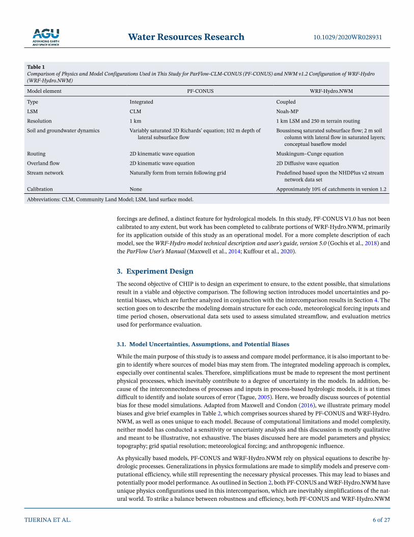
While the main purpose of this study is to assess and compare model performance, it is also important to be-gin to identify where sources of model bias may stem from. The integrated modeling approach is complex, especially over continental scales. Therefore, simplifications must be made to represent the most pertinent physical processes, which inevitably contribute to a degree of uncertainty in the models. In addition, be-cause of the interconnectedness of processes and inputs in process-based hydrologic models, it is at times difficult to identify and isolate sources of error (Tague, 2005). Here, we broadly discuss sources of potential bias for these model simulations. Adapted from Maxwell and Condon (2016), we illustrate primary model biases and give brief examples in Table 2, which comprises sources shared by PF-CONUS and WRF-Hydro.NWM, as well as ones unique to each model. Because of computational limitations and model complexity, neither model has conducted a sensitivity or uncertainty analysis and this discussion is mostly qualitative and meant to be illustrative, not exhaustive. The biases discussed here are model parameters and physics; topography; grid spatial resolution; meteorological forcing; and anthropogenic influence.

As physically based models, PF-CONUS and WRF-Hydro.NWM rely on physical equations to describe hy-drologic processes. Generalizations in physics formulations are made to simplify models and preserve com-putational efficiency, while still representing the necessary physical processes. This may lead to biases and potentially poor model performance. As outlined in Section 2, both PF-CONUS and WRF-Hydro.NWM have unique physics configurations used in this intercomparison, which are inevitably simplifications of the nat-ural world. To strike a balance between robustness and efficiency, both PF-CONUS and WRF-Hydro.NWM

TIJERINA ET AL.

10.1029/2020WR028931

6 of 27

Model element PF-CONUS WRF-Hydro.NWM

Type Integrated Coupled

LSM CLM Noah-MP

Resolution 1 km 1 km LSM and 250 m terrain routing

Soil and groundwater dynamics Variably saturated 3D Richards’ equation; 102 m depth of lateral subsurface flow

Boussinesq saturated subsurface flow; 2 m soil column with lateral flow in saturated layers; conceptual baseflow model

Routing 2D kinematic wave equation Muskingum–Cunge equation

Overland flow 2D kinematic wave equation 2D Diffusive wave equation

Stream network Naturally form from terrain following grid Predefined based upon the NHDPlus v2 stream network data set

Calibration None Approximately 10% of catchments in version 1.2

Abbreviations: CLM, Community Land Model; LSM, land surface model.

Table 1 Comparison of Physics and Model Configurations Used in This Study for ParFlow-CLM-CONUS (PF-CONUS) and NWM v1.2 Configuration of WRF-Hydro (WRF-Hydro.NWM)

Water Resources Research

use more computationally efficient and simplified versions of equations to represent various physical pro-cesses. Each simplification of a physical process within the models presents the possibility of attributing to or propagating model error throughout simulations. The extent to which it is reasonable to simplify models has been debated in the literature (e.g., Beven, 2002; Brunner & Simmons, 2012) and this is partially because error associated with these simplifications is hard to quantify. Conversely, even when it appears that these physically based models are performing well, it is important that we consider if we are “getting the right answers for the right reasons” (Kirchner, 2006) and that the physics are, in fact, sufficiently representing the natural processes being modeled. This is particularly important in modeling continental domains be-cause there remains uncertainty as to whether or not the physics suitable at the microscale perspective is adequate to properly represent the same processes at larger scales (Hrachowitz & Clark, 2017; Peters-Lidard et al., 2017). Considering model physics of PF-CONUS and WRF-Hydro.NWM, we expect the largest im-pacts on the results of CHIP to be the variation in groundwater representation and differences in areas with more groundwater interactions, the significant difference in stream routing and the stream density within grid cells, and the influence of complex topography on model components.

Parameterization presents another area of model uncertainty. With increased model complexity, such as large-domain models, parameterization becomes a problem because of the increasing number of unknown parameters and reliance on hard to measure inputs (Kumar et al., 2013). PF-CONUS and WRF-Hydro.NWM are physically based models, eliminating the dependency on high amounts of parameterization. However, they require parameter estimation for certain model inputs and physical properties such as subsurface hy-drologic conductivity, Manning's roughness coefficient in channels, and land cover and vegetation types. Moreover, these parameters are reliant on accurate data. The uncertainty in national-scale datasets and the challenges of gathering data over continental scales can exacerbate parameter uncertainty in continental- scale models (Fatichi et al., 2016). These data are subject to different collection methods, documentation, or availability of data collected, resulting in necessary parameter estimations for both models. There also exists uncertainty from small-scale heterogeneities and whether or not an effective parameter exists at the given model resolution. The extent to which small-scale heterogeneities influences large-scale processes is addressed in Maxwell and Condon (2016). The study indicates that there is evidence of small-scale heter-ogeneities impacting partitioning relationships in ParFlow. However, Meyerhoff & Maxwell, 2011 and Gil-bert et al., 2016 found for excess saturation, small-scale heterogeneity averages out and runoff is adequately

TIJERINA ET AL.

10.1029/2020WR028931

7 of 27

Bias Category PF-CONUS WRF-Hydro.NWM

Model Physics & Parameters Kinematic wave equation in streams results in no represented upstream propagation

Simplified exponential baseflow model and shallow subsurface depth

One-way flow into channels with no over-bank flowUncertainty and discontinuity in large spatial data sets* (e.g., hydraulic conductivity in PF-CONUS) Analytically derived initial values of groundwater

bucket model parameters

Topography & Resolution River network not defined and routing of pooled surface water occurs within 1 km grid cells

Predefined NHDPlus2 vector river network

Stream network mapping Coarse resolution may ignore heterogeneities*

Watershed drainage area DEM downscaled resolution*

Spatial Heterogeneity and Uncertainty Heterogeneity exists at all scales, not represented below grid resolution*

Vertically homogeneous soil and subsurface layers*

Meteorological Forcing Bias in temperature affects ET and snow*

Bias in precipitation affects flow volume and timing*

Anthropogenic Influence Influence of dams*

Groundwater pumping*

Urban areas not explicitly modeled*

*Applies to both PF-CONUS and WRF-Hydro.NWM.

Table 2 Potential Biases Affecting PF-CONUS and WRF-Hydro.NWM Model Performance and Examples of Bias Sources for Each Model

Water Resources Research

simulated. While this is certainly an area that requires more study for continental-scale modeling, in-depth study of effective parameters in PF-CONUS and WRF-Hydro.NWM is beyond the scope of this paper. How-ever, the ability to upscale parameters is an undeniably significant component in making large-scale hydro-logic models possible.

Bias can also be a result of model grid resolution and topography. Although both PF-CONUS and WRF-Hy-dro.NWM are considered high resolution for the domain extent, spatial discretization may affect the mod-els’ ability to represent parameter and input heterogeneities and any heterogeneity existing below model grid resolution will be ignored. For example, because of the way in which streams form and water is routed according to topography in PF-CONUS, coarser resolution can lead to discrepancies in stream location and affect overland flow routing of surface water across 1 km grid cells (Maxwell et al., 2015). In addition, dis-crepancies in topography and hillside characteristics can affect hydrologic response because of frequent loss of topographic relief with decrease in resolution and the influence of relief on other processes such as rate of flow, evapotranspiration rates, or soil moisture (Tague, 2005), particularly at resolutions used in the mod-els in this study (Shrestha et al., 2015). Topographic processing from the digital elevation model data set also may result in errors in drainage area, which can affect flow volume when water is incorrectly accumulated in a drainage basin or routed to an improper basin. In the simulations here, even with high-resolution grid discretization at the continental scale, models will exclude fine-scale heterogeneities.

Meteorological forcing is a fundamental element contributing to the accuracy of hydrologic modeling and accurate forcing remains a challenge to the large-scale hydrology modeling community (Bierkens, 2015). Forcing provides hydrology models quantities like precipitation, temperature, wind speed, and incoming so-lar radiation—all of which have an effect on simulated components related to streamflow (Cosgrove, 2003). Therefore, some performance errors in PF-CONUS and WRF-Hydro.NWM may be a result of meteoro-logical forcing biases, in our case, the use of NLDAS-2. There are well-documented temperature and pre-cipitation biases in the NLDAS-2 meteorological forcing product (O'Neill et al., 2020; Pan et al., 2003; Xia et al., 2012) which can especially influence evapotranspiration, snowmelt, and streamflow. In addition, Pan et al. (2003) and Sheffield et al., (2003) found that when the NLDAS-2 forcing product was used in various land surface models, snow cover, and SWE were consistently underestimated, particularly in high elevation regions. Schreiner-McGraw and Ajami (2021) found that mountain water budget partitioning is most sensi-tive toward the total volume of snowmelt, which is influenced by both temperature and precipitation biases in forcing. It follows that if there is bias in meteorological forcing, such as early snowmelt, it may result in streamflow timing and volume errors in regions where streamflow is dominated by snowmelt.

It is well established in the literature that our water resources are affected by human influence and that human activities alter the dynamics of natural systems (e.g., Brown et al., 2013; Gleick, 2000; Haddeland et al., 2014; Vörösmarty et al., 2000). Some studies have included anthropogenic factors into their models and studies (Ferguson & Maxwell, 2012; García-Leoz et al., 2018; Gleeson et al., 2012; Keune et al., 2018; Naabil et al., 2017), but the results presented from CHIP Phase 1 simulate predevelopment conditions and exclude anthropogenic influences, following Maxwell and Condon (2016). Therefore, the configurations of PF-CONUS and WRF-Hydro.NWM compared here do not contain representations of anthropogenic influ-ences like reservoirs and dams, irrigation, groundwater pumping, and urban development. Because neither model configuration in this study incorporates these aspects of human influences on hydrology, biases will be present as a result of excluding these activities. Water management affects surface water runoff volume and timing because of regulation from dams and consumptive use. In addition, it is known that groundwa-ter levels affect surface water amounts (Condon & Maxwell, 2019b; Langhoff et al., 2006; Tran et al., 2020), so groundwater pumping may affect the total volume of surface water flow.

3.2. Comparison Domain

This comparison of PF-CONUS and WRF-Hydro.NWM is based on the Maxwell and Condon (2016) do-main setup involving the initial PF-CONUS simulation over most of the contiguous US. This first version of PF-CONUS consisted of a rectangular domain centered over most of the US and incorporates eight major river basins (Figure 1). It covers an area of nearly 6.3 million km2 and has a depth of 102 m divided into five layers (0.1, 0.3, 0.6, 1.0, and 100 m; Maxwell & Condon, 2016). The rectangular domain was used as a PF-CONUS proof of concept, designed to eliminate the need to implement coastal boundary conditions.

TIJERINA ET AL.

10.1029/2020WR028931

8 of 27

Water Resources Research

PF-CONUS v2.0, currently in development, will extend to the US coasts and match the current National Water Model domain. The WRF-Hydro.NWM domain encompasses all of the conterminous US and parts of Mexico and Canada within the NHDPlus network. It extends to the coastlines and has a vertical depth of 2 m, made up of four layers (0.1, 0.3, 0.6, and 1.0 m). As previously stated, both model configurations in this study simulated predevelopment conditions without representation of anthropogenic influence, with the exception of an urban land cover classification existing in both LSMs. For this study, we conduct a WRF-Hy-dro simulation over the NWM v1.2 CONUS domain and compare it within the rectangular domain with the previously run simulation of PF-CONUS v1.0 (Maxwell & Condon, 2016). Because of the significant computational expense required, the WRF-Hydro.NWM simulation was run on the NCAR Computational Information Systems Laboratory Cheyenne high-performance supercomputer and PF-CONUS was run pre-viously on the NCAR Yellowstone high-performance supercomputer.

The PF-CONUS and WRF-Hydro.NWM simulations were run for one year. We use water year 1985 (Octo-ber 1, 1984–September 30, 1985) for the comparison because it is the most climatologically average water year in the reconstructed time period (Maxwell & Condon, 2016). Both models used same hourly WY1985 NLDAS-2 historical meteorological forcing at a 1/8° spatial resolution (Cosgrove, 2003; Mitchell, 2004; Xia et al., 2012) spatially downscaled to the 1 km grid using bilinear interpolation with no bias correction (e.g., Latombe et  al.,  2018; Liu et  al.,  2019; https://www.ncl.ucar.edu/Applications/ESMF.shtml). Models pro-duced results at hourly temporal resolution.

3.3. Streamflow Validation Data and Metrics

As an initial comparison, in this study we evaluate the models' ability to simulate streamflow. Streamflow can be sensitive to slope variations (Condon & Maxwell, 2019a) and inaccuracies in drainage area, top-ographic relief, and temperature and precipitation biases in meteorological forcing (O'Neill et al., 2020), which can result in flux errors that propagate downstream. However, streamflow is a beneficial quantity to compare performance between PF-CONUS and WRF-Hydro.NWM because (a) the spatiotemporal avail-ability of data for the specified time period and reliability of observations, (b) as an integrated quantity,

TIJERINA ET AL.

10.1029/2020WR028931

9 of 27

Figure 1. The comparison extent and USGS streamflow gage locations used for validation, including 2200 total gages, with 376 being reference gages.

Water Resources Research

streamflow can indicate and distinguish between different types of bias; and (c) the ability to simulate streamflow has implications and applications beyond this comparison.

Model simulation results are compared with a subset of streamflow observation gages (Figure 1) from Max-well and Condon (2016). Although Maxwell and Condon (2016) compared ParFlow simulated runoff at 3050 US Geological Survey (USGS) streamflow gages, we sought to compare gages with direct spatial align-ment between PF-CONUS and WRF-Hydro.NWM. The discrepancies in gage locations stems from differ-ences in stream network representation within the models. Because we are comparing streams on a grid and streams within a vector network, not every gage in the NHDPlus vector network had the same coordinates as the grid square identified to contain that same gage in PF-CONUS, so these observations were not includ-ed in the comparison. Accordingly, our comparison consists of 2200 USGS streamflow gages from WY1985 with coordinates that matched within the boundary of the PF-CONUS domain (Falcone et al., 2010).

To address the CHIP goal of assessing simulated streamflow and characterizing model bias, we evaluat-ed a variety of metrics. Nash-Sutcliffe efficiency (NSE) is widely used as a standard metric for evaluating model performance and predictive skill, but may be overly sensitive to outliers and extreme events (Legates & McCabe, 1999) and makes it difficult to distinguish different types of bias (Maxwell & Condon, 2016). Kling-Gupta efficiency (KGE) addresses some of the limitations of NSE and uses multiple objectives with the goal of preventing overfitting to a certain aspect of a hydrograph (Gupta et al., 2009; Pool et al., 2018). It also facilitates analysis and can distinguish the relative importance of different components in the context of hydrological modeling (Gupta et  al.,  2009), which makes it particularly useful for model calibration. However, KGE assumes data normality, linearity, and the absence of outliers (Pool et al., 2018) and stream-flow timeseries tend to be skewed with non-normal distributions (Yue et al., 2002). The Pearson correlation coefficient is another widely used metric because of its ability to detect linear correlation and covariance (Legates & McCabe, 1999). While this is useful, it is limited in recognizing nonlinear correlations and may be susceptible to sensitivity to extreme values (Pool et al., 2018).

The analysis here focuses on parsing out different types of model bias and two central, widely applied metrics were combined to assess agreement of aggregated daily mean streamflow magnitude and timing to USGS observed values. Relative flow bias evaluates how well the models capture total flow volume and is given as

1 1

1

bias ,n n

i ii i

nii

S O

O (1)

where Si are simulated flows and Oi are observed flows on day i for n days of simulation. Relative bias is useful because it quantifies the magnitude of error and the direction of bias (e.g., either over or under pre-dicting streamflow) and can be used as an absolute value to be mapped as a spatial quantity. Absolute bias is used to analyze flow magnitude accuracy and we set a threshold of bias lower than one as low bias, with 0 being ideal. Gupta et al., 1999 found that relative bias performs more variably in dryer years, but because water year 1985 is climatically average, this is not a limitation in this study. The Spearman's rho (rs) nonpar-ametric rank correlation coefficient detects monotonic trends in shape in timeseries. Given as

1s 2

61 ,

1

nii d

rn n

(2)

where d is the difference in independent ranking for simulated and observed values for day i and n is the number of values in each time series. Spearman's rho is particularly effective for nonlinear and non-nor-mally distributed data like hydrologic time series (Yue et al., 2002) and is used here to quantify the corre-lation between modeled and observed flow shape as an indication of flow timing. We use a threshold of Spearman's rho greater than 0.5 as good shape, with 1 being optimal rs. The overall evaluation approach using relative bias and Spearman's rho is aligned with the goals of the study, namely, to assess the simulated streamflow of both models and to distinguish different types of model biases in those results.

Both relative bias and Spearman's rho are calculated for the entire water year from daily averaged flow, consistent with the temporal resolution of the available USGS streamflow observations. From these two

TIJERINA ET AL.

10.1029/2020WR028931

10 of 27

Water Resources Research

metrics, four Streamflow Performance Categories (SPCs) were created, combining relative flow and Spear-man's rho to visualize flow magnitude and shape together with the categories being (a) good shape and low bias, (b) poor shape and low bias, (c) good shape and high bias, and (d) poor shape and high bias. Utilizing SPC as a composite metric allows for model results to be classified such that, at each gage location, perfor-mance can be identified as having a timing or magnitude error. Categories are displayed for each model in a single Condon Diagram (Maxwell & Condon, 2016) and spatially to catalog general and regional differences in model performance. It should be noted that the thresholds identified for relative bias and Spearman's rho that define the SPC are not intended for critical analysis of the models for the purpose of WY1985 stream-flow prediction. Instead, we use these determinations to broadly describe model performance and begin to parse sources of model bias to understand strengths and weaknesses in both simulations.

4. Results and DiscussionThe third objective of CHIP Phase 1 is to assess the ability of models to simulate streamflow compared with USGS observed flow. The goals of this objective are to describe model performance with regard to simulated streamflow results and identify areas of bias and potential sources of model error, as described in Section 3.1. We use the SPCs and identify how model performance may be a result of various biases to bet-ter understand the reasons behind discrepancies in modeled and observed streamflow. We address overall simulated streamflow performance, spatial patterns, and how differences in performance between models may indicate types of bias.

4.1. Model Streamflow Performance

To evaluate model performance with respect to streamflow timing and magnitude, absolute relative flow bias and Spearman's rho were calculated individually for each gage location and then plotted together in Condon Diagrams (Maxwell & Condon, 2016). In Figure 2, the four SPCs are plotted as a composite metric showing model performance at each gage with respect to relative bias and Spearman's rho thresholds. In this way, we are able to assess both flow volume and shape and understand how model performance is

TIJERINA ET AL.

10.1029/2020WR028931

11 of 27

Figure 2. Condon diagrams comparing streamflow performance for (a) PF-CONUS and (b) WRF-Hydro.NWM. Lines show thresholds for good shape (Spearman's rho) and low bias (absolute relative flow bias). The points are as follows: green are ‘good shape, low bias,’ purple are ‘bad shape, low bias,’ blue are ‘good shape, high bias,’ and red are ‘bad shape, high bias’.

Water Resources Research

distributed between categories at each gage. The four quadrants symbolize good shape and low bias (green), poor shape and low bias (purple), good shape and high bias (blue), and poor shape and high bias (red).

From this combined comparison, we see that both models generally capture magnitude, with just over 80% of gages for each model having low bias for total flow (green and purple points in Figure 2). WRF-Hydro.NWM more accurately depicts flow timing with 74% of gages having good shape, compared with 66% of gages for PF-CONUS (green and blue points in Figure 2). Both models have 9% of gages that perform poorly in both metrics (red points in Figure 2). Furthermore, more than half of gages for both models exhibit rela-tively favorable performance for both streamflow volume and timing considering the thresholds set (green points in Figure 2). These results show that, largely, both models are able to simulate streamflow at gage location in comparison with observations.

Spatially plotting the streamflow metrics over the model domain reveals regional patterns in simulation re-sults. Figure 3 shows relative bias and Spearman's rho mapped separately for PF-CONUS and WRF-Hydro.NWM and Figure 4 maps the four SPCs for the two models. When comparing the spatial distribution of the streamflow categories (Figure 4), PF-CONUS and WRF-Hydro.NWM both perform well in the eastern part of the domain, with an overwhelming amount of the gages there having low bias and good shape. Similarly, both models have consistently poor performance throughout the Great Plains where the major-ity of gages with red SPC are located, indicating inadequate model performance for both magnitude and shape. The western portion of the domain is where the most distinct differences in streamflow simulations between models are seen. Generally, WRF-Hydro.NWM performs well within the given metric thresholds (green in Figure 4b), but tends to over-predict flow volume (Figure 3c) with 28% of gages with a relative bias greater than 0.5, compared with only 4% of gages less than −0.5 relative bias. One reason for this is that the NWM v1.2 configuration of WRF-Hydro and utilization of the NHD-Plus streamflow network does not allow for losses from the groundwater buckets or channel. The buckets attenuate flow, but all outflow goes to the channel. Conversely, particularly in the intermountain west, PF-CONUS slightly under-predicts flow volume (Figure 3a) with 16% of gages with relative flow bias less than −0.5, compared with 0.27% with relative flow bias greater than 0.5. Also, PF-CONUS has significantly lower Spearman's rho values than WRF-Hydro.NWM (Figure  3b). This pattern is reinforced in the PF-CONUS SPC map (Figure  4a)

TIJERINA ET AL.

10.1029/2020WR028931

12 of 27

Figure 3. Relative annual flow bias (a and c) and Spearman's rho (b and d) for PF-CONUS and WRF-Hydro.NWM, respectively, for all 2200 gages in the domain.

Water Resources Research

where most of the western US is purple indicating acceptable flow volume, but inadequate shape for the simulation.

Further spatial analysis is accomplished when identifying gages where PF-CONUS and WRF-Hydro.NWM have the same SPC. Figure 5a shows the gage locations that have common SPC (yellow points) and different SPC (gray points). Out of the 2200 gage locations, 1376 gages (62%) had the same SPC designation between the two models. Using only those locations with common SPC, Figures 5b–5e depict maps of where mod-els have the same category. Nearly half of the total gages have a common SPC of low bias and good shape

TIJERINA ET AL.

10.1029/2020WR028931

13 of 27

Figure 4. Streamflow Performance Category maps for (a) PF-CONUS and (b) WRF-Hydro.NWM for all 2,200 streamflow gages in the domain.

Water Resources Research

TIJERINA ET AL.

10.1029/2020WR028931

14 of 27

Figure 5. The top map depicts gages where PF-CONUS and WRF-Hydro.NWM have common (yellow) and different (gray) Streamflow Performance Category in the domain (a). Maps below show where models have the same Streamflow Performance Category with low bias, good shape (b), high bias, good shape (c), low bias, poor shape (d), and high bias, poor shape (e).

Water Resources Research

(Figure 5b), most of which are in the eastern portion of the domain. 2.2% of total gages have high bias and good shape (Figure 5c), 9% of total gages have a low bias and poor shape (Figure 5d), and 3.9% have high bias and poor shape. Considering that for the gages with common SPC to both PF-CONUS and WRF-Hydro.NWM only have 6.1% of total gages with high bias (blue and red gages), compared with 12.9% with poor shape (purple and red gages), results indicate that both models have greater success simulating flow volume than they do capturing timing.

Overall, results of the comparison show that PF-CONUS and WRF-Hydro.NWM have similar performance with regard to depicting streamflow volume, which is indicated in the similar results for relative bias when compared with observed (Figure 3). The largest discrepancy between the models was the difference in tem-poral pattern of flow. PF-CONUS displayed less favorable results regarding shape, having 11% fewer gages in the acceptable range of Spearman's rho values than WRF-Hydro.NWM (Figure 2). On the whole, both PF-CONUS and WRF-Hydro.NWM generally agree with observed flow at over half of the gage locations used in the evaluation. Neither model had more than 10% of gages with poor SPC and both models had more than 54% of gages with acceptable streamflow category (Figure 2).

4.2. Potential Sources of Model Bias in Results

With knowledge of the potential biases affecting model results (Section 3.1), combined with an analysis of simulated streamflow using the SPCs, we can begin to parse out general sources of bias and what model error may be attributed to. First, where both PF-CONUS and WRF-Hydro.NWM perform well and have a common SPC of low bias and good shape (Figure 5b), we expect that meteorological forcing inputs have low bias and are not generating errors in streamflow because this would affect both models. Also, we infer that respective model physics are satisfactory and models are solving physical equations as expected. It is important to consider here if in fact we are “getting the right answers for the right reasons,” (Kirchner, 2006) but this is difficult to characterize, particularly at continental scales where details such as a match to an in-dividual gage can be obfuscated. Where both models have poorer SPC (Figures 5c–5e), physics formulation may be the source of error, but is more likely attributable to factors that would have an identical effect on each model, such as contributing biases from meteorological forcing and exclusion of anthropogenic influ-ence in simulations. For example, it is evident from Figure 5e that most of the gages with high bias and poor shape are located in the Great Plains region, suggesting that the models’ poorest performance is at gages in the central part of the domain subject to large quantities of groundwater abstraction and irrigation, or gages downstream of these areas (Condon & Maxwell, 2019b; Herbert & Döll, 2019).

Although areas of agreement can help identify what common factors are contributing to error, we can also gather information about certain bias qualities when looking at where models disagree and have uncom-mon SPC. Figures 6a and 6b maps the 824 gage locations for PF-CONUS and WRF-Hydro.NWM where the models SPC differ from each other. To better understand patterns of disagreement, Figures 6c–6f identify where models have either volume or shape discrepancies, separating gages where one model has accept-able performance and the other has either poor shape or high bias. The reasoning here is that, because models have differing error in simulated streamflow, the bias is related to a factor that affects each model individually. Therefore, aspects like meteorological forcing or anthropogenic influence are presumed not to be a source of bias at these gages. However, we cannot completely rule out physics as a source of error at these gages because contrasting model physics can potentially produce different performance errors in each model.

Figures 6c and 6d indicates where models differ from each other in flow shape. Figure 6c shows gages where PF-CONUS has green SPC and WRF-Hydro.NWM has purple SPC (low bias and poor shape) and Figure 6d shows the opposite case at gages where WRF-Hydro.NWM has green SPC and PF-CONUS has purple SPC. Figure 6c indicates that WRF-Hydro.NWM has poorer timing than PF-CONUS along the mid-reach of the Missouri River and at a small cluster in the east near the Appalachian Mountain region. PF-CONUS has comparatively poorer timing in the Rocky Mountain region, with almost all gages with poor shape being in the western portion of the domain (Figure 6d). In these gages where models differ in shape, biases are likely a result of snow physics, topographic relief and downscaled resolution, or stream network errors. This is explored further in Section 4.4.

TIJERINA ET AL.

10.1029/2020WR028931

15 of 27

Water Resources Research

Figures  6e and  6f show similar comparisons, but with volume discrepancies. In Figure  6e, PF-CONUS had green SPC and WRF-Hydro.NWM had blue SPC with high bias and good shape and with the opposite case in Figure 6f where WRF-Hydro.NWM has green SPC and PF-CONUS has blue SPC. It is evident that PF-CONUS has comparatively more gages with high flow bias, primarily in the eastern portion of the do-main and the Great Plains area. These gages in this region with volume discrepancies may indicate where models are seeing the influence of differing groundwater configurations or partitioning bias. The relative spatial patterns for where WRF-Hydro.NWM has high flow bias are less evident because high biased gages are distributed across the domain, with smaller concentrations of high biased gages in the southwestern and midwestern US. It should be noted, that at these gage locations with volume discrepancies, both PF-CONUS (Figure 6f) and WRF-Hydro.NWM (Figure 6e) overpredict flow magnitude at every gage. At gages in which models differ in total flow volume, biases are likely a result of model physics, partitioning discrepancies,

TIJERINA ET AL.

10.1029/2020WR028931

16 of 27

Figure 6. Maps of gages where PF-CONUS (a) and WRF-Hydro.NWM (b) Streamflow Performance Categories differ from each other. The maps below show which of these gages have streamflow shape or volume discrepancies—gages where PF-CONUS has acceptable (green) performance and WRF-Hydro.NWM has poor shape (c) or high bias (e); and gages where WRF-Hydro.NWM has acceptable performance and PF-CONUS has poor shape (d) or high bias (f).

Water Resources Research

model parameters, and/or stream loss (e.g., PF-CONUS allows for streams to lose water from channels to groundwater, or channels to overbank flow, but WRF-Hydro.NWM version 1.2 does not have this capability activated).

4.3. Identifying Biases From Anthropogenic Influence

Both of the hydrologic simulations compared here are predevelopment and so exclude urban hydrology, groundwater extraction, and surface water management. Therefore, identifying how human activities, and the omission of them from these simulations, affects modeled streamflow can be difficult. It may be reason-able that model error in the gages that differ in SPC shown in Figure 6, are not a result of human influence. We determine this because if there were an anthropogenic influence affecting model performance, it would likely present similar types of bias in both PF-CONUS and WRF-Hydro.NWM simulations, perhaps with differing responses to groundwater abstraction or irrigation given the distinctions in surface water-ground-water interactions by physical governing equations in the two models.

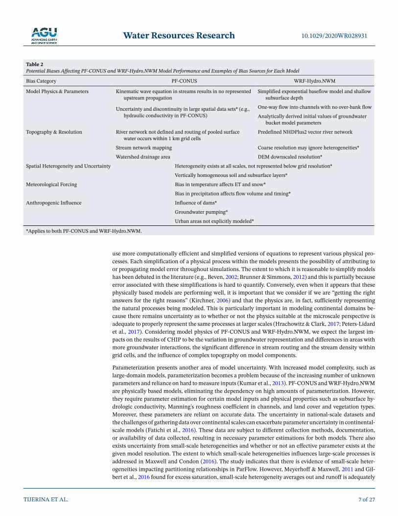
To remove locations where anthropogenic influence may be the cause of model error, we identify and ana-lyze streamflow performance at USGS Reference Gages. Reference gages are within watersheds in the USGS Geospatial Attributes of Gages for Evaluating Streamflow, version 2 data set (GAGES-II) that have been identified based on criteria that they are the least-disturbed by human influence within the GAGES-II net-work (Falcone et al., 2010). With evaluation of model simulation results at reference gages, we can analyze how models perform in watersheds with natural streamflow and absence of human activities, effectively isolating areas where physics or forcing may be the driving factor for model bias. Out of the 2200 gages used in the analysis, 376 of them are classified as reference gages. Figure 7 shows model SPC at reference gages for PF-CONUS (Figure 7a) and WRF-Hydro.NWM (Figure 7b), as well as the reference gages that share a common SPC between the two models (Figures 7c–7f). A total of 209 reference gages, or 55.6% of total reference gages, have common green SPC for both models, showing mostly good performance in sim-ulating streamflow shape and magnitude at gages without human influence (Figure 7c). At these locations, we make the same bias assumptions as with the total gages in common—that physics and forcing are not contributing to error. The reference gage analysis is revealing when both models agree in SPC at a gage but have poorer performance (Figures 7d–7f). Analyzing the reference gages where models agree but do poorly, we have the same analysis as in Figures 5c–5e, but have effectively removed the human influence. There-fore, considering the general bias categories presented in Table 2, we assume that because the model biases are not a result of anthropogenic factors, error must be a result of either the NLDAS-2 forcing product or model physics. In addition, because the models have the same type of error at these locations, we can also deduce that the individual model properties, such as parameters or river network representation, likely do not contribute to error.

Even though the reference gages with common, poorer performance (Figures 7d–7f) only make up 7% of the total reference gages, these locations remain important in parsing out multiple types of bias. The challenge remains that discrete biases are not always identifiable because they contribute simultaneously to model error. An avenue for future work exists to use this same analysis, but to address how meteorological forcing biases and the methodology of statistical downscaling affect model performance. This type of analysis may effectively isolate the areas where physics formulation may be the cause of bias and why and how model physics, and the particular options selected for each model in their respective configurations, ultimately effects streamflow performance. Conversely, Figure 8 shows a similar analysis as in Figures 6a and 6b, but at reference gages with differing SPC for PF-CONUS and WRF-Hydro.NWM. Comparable conclusions can be reached—that contributing error at these gages has to do with individual model components. In using reference gages, there is even more certainty that at these locations with differing SPC that performance error is not a result of anthropogenic influence.

In using reference gages as a proxy for identifying anthropogenic biases it should be noted that errors in the data may be present. Uncertainties exist in the national-scale GIS data used to compile these reference gage data. The reference gages may not account for the influence of groundwater pumping nearby to gages, making some human influence in the reference gages potentially unidentifiable with this data. More specif-ically, the two common reference gages with a high bias and poor shape SPC in Figure 7f may be anomalous and unrepresentative toward the goal of removing human influence. Although the Ute Creek gage near

TIJERINA ET AL.

10.1029/2020WR028931

17 of 27

Water Resources Research

Logan, New Mexico is classified as a reference gage, NWIS documentation states that the river is diverted for irrigation a few hundred acres upstream of the station and the river has no flow most days (https://wa-terdata.usgs.gov/nwis/uv?site_no=07226500). Similarly, NWIS documentation states that data before 2007 at Beaver Creek gage at Cedar Bluffs, Kansas may be erroneous even if they have been flagged as approved (https://waterdata.usgs.gov/ks/nwis/uv/?site_no=06846500). The rivers at both gages are intermittent and

TIJERINA ET AL.

10.1029/2020WR028931

18 of 27

Figure 7. The six maps show performance at USGS reference gages. The top two panels depict Streamflow Performance Categories at all 376 reference gages for PF-CONUS (a) and WRF-Hydro.NWM (b). The bottom four panels show reference gages where models have common Streamflow Performance Category with low bias, good shape (c), high bias, good shape (d), low bias, poor shape (e), and high bias, poor shape (f).

Water Resources Research

low discharge, and streamflow may be difficult to simulate at these locations given the resolutions used in continental-scale modeling.

4.4. Discussion of Spatial Distribution of Model Bias

Considering the biases that contribute to model error, some conclusions about regional differences in model performance can be made. Spatial representation of SPC (Figure 4) shows that PF-CONUS and WRF-Hy-dro.NWM have overall acceptable performance in the eastern portion of the domain and the poorest per-formance in the central and western portions. These differences in regional performance for both PF-CO-NUS and WRF-Hydro.NWM are partially a result of the water availability and its controlling factors. For

TIJERINA ET AL.

10.1029/2020WR028931

19 of 27

Figure 8. Reference gage locations where SPC differs for (a) PF-CONUS and (b) WRF-Hydro.NWM.

Water Resources Research

example, in the arid western part of the US which is generally water-limited, precipitation is the main control of water availability (Miralles et al., 2016). With the models being dependent on accurate precipi-tation representation, the inadequate model performance in the west, particularly the poorer streamflow timing in the Rocky Mountains for PF-CONUS, may be largely a result of NLDAS-2 meteorological forcing biases in temperature and precipitation. These results are corroborated with the NLDAS-2 temperature, precipitation, and SWE biases described previously in Section 4.2 (Pan et al., 2003; Sheffield et al., 2003; Xia et al., 2012).

In addition, these model biases in the mountainous west are partially a result of complex topography. Previ-ous evaluation of biases specific to PF-CONUS outlined in Maxwell and Condon (2016) concluded this to be true and Condon & Maxwell, 2019a addressed new methods of topographic processing of digital elevation models to improve the representation of drainage networks in model domains. Complex topography also contributes to inaccuracies in meteorological forcing—the timing error in the models in the western, high elevation region of the domain is consistent with the correlation between NLDAS-2 biases and complex topography (Maxwell & Condon, 2016; Sheffield et al., 2003).

The western domain discrepancies are corroborated in Figure 8, where models differ in SPC at reference gages. PF-CONUS has poor timing for nearly all reference gages in the western part of the domain, com-pared with generally favorable performance from WRF-Hydro.NWM. Because human influence has been removed and because of the documented biases in NLDAS-2 forcing over mountains, one may expect these differences to be a result of forcing. However, because the models use the same forcing, yet have varying types of error, these gages exemplify biases in physics configuration between the models.

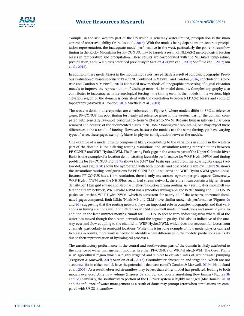
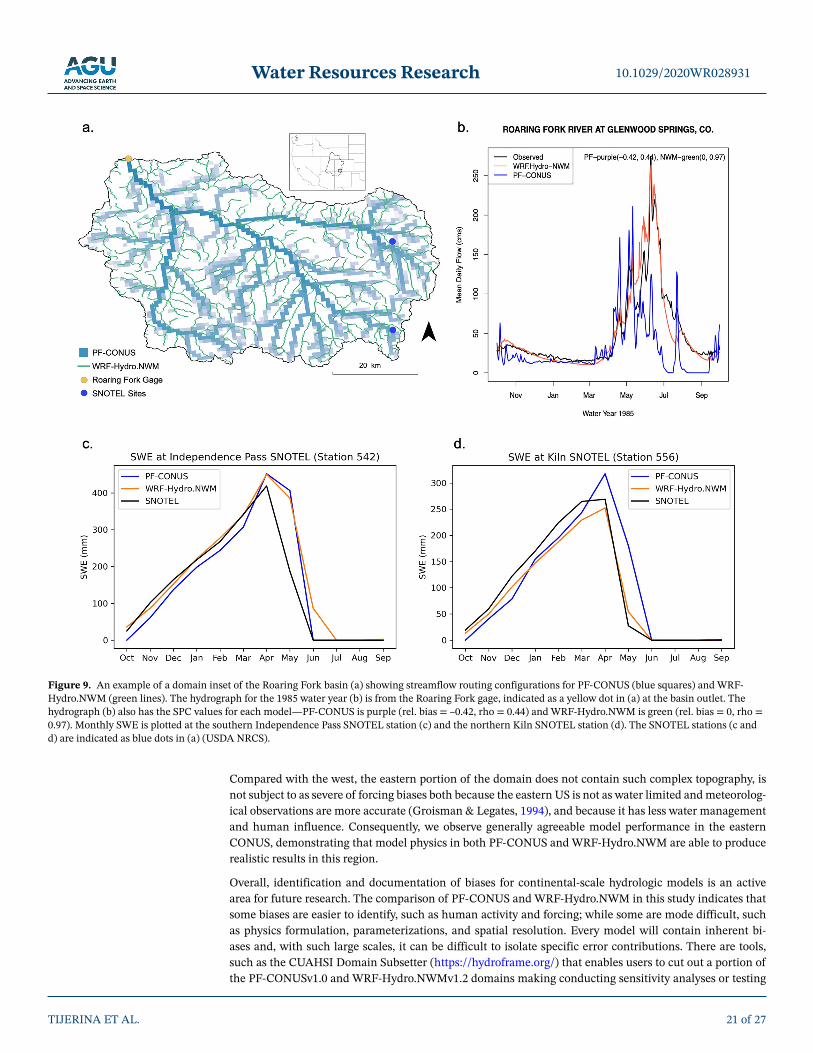
One example of a model physics component likely contributing to the variations in runoff in the western part of the domain is the differing routing resolutions and streamflow routing representations between PF-CONUS and WRF-Hydro.NWM. The Roaring Fork gage in the western part of the Upper Colorado River Basin is one example of a location demonstrating favorable performance for WRF-Hydro.NWM and timing problems for PF-CONUS. Figure 9a shows the 3,767 km2 basin upstream from the Roaring Fork gage (yel-low dot) and Figure 9b shows the hydrograph with both models’ and observed streamflow. Figure 9a shows the streamflow routing configurations for PF-CONUS (blue squares) and WRF-Hydro.NWM (green lines). Because PF-CONUS has a 1 km resolution, there is only one stream segment per grid square. Conversely, WRF-Hydro-NWM uses the NHDPlus vectorized stream network, therefore it can contain a higher stream density per 1 km grid square and also has higher-resolution terrain routing. As a result, after snowmelt en-ters the stream network, WRF-Hydro.NWM has a smoother hydrograph and better timing and PF-CONUS peaks earlier than WRF-Hydro.NWM, which is consistent for nearly all of the western, snowmelt-domi-nated gages compared. Both LSMs (Noah-MP and CLM) have similar snowmelt performance (Figures 9c and 9d), suggesting that the routing network plays an important role in complex topography and that vari-ations in timing are not a result of differences in LSM snowmelt model formulations and snow physics. In addition, in the later summer months, runoff for PF-CONUS goes to zero, indicating areas where all of the water has moved though the stream network and the segments go dry. This also is indicative of the one-way overland flow coupling to the channel in WRF-Hydro.NWM, which does not account for losses from channels, particularly in semi-arid locations. While this is just one example of how model physics can lead to biases in results, more work is needed to identify where differences in the models’ predictions are likely due to their representation of hydrological processes.

The unsatisfactory performance in the central and southwestern part of the domain is likely attributed to the absence of water management modules in either PF-CONUS or WRF-Hydro.NWM. The Great Plains is an agricultural region which is highly irrigated and subject to elevated rates of groundwater pumping (Ferguson & Maxwell, 2012; Scanlon et al., 2012). Groundwater abstraction and irrigation, which are not accounted for in either model, have the potential to decrease runoff (Condon & Maxwell, 2019b; Haddeland et al., 2006). As a result, observed streamflow may be less than either model has predicted, leading to both models over-predicting flow volume (Figures 3a and 3c) and poorly simulating flow timing (Figures 3b and 3d). Similarly, the southwestern portion of the US river system is highly managed (MacDonald, 2010) and the influence of water management as a result of dams may prompt error when simulations are com-pared with USGS streamflow.

TIJERINA ET AL.

10.1029/2020WR028931

20 of 27

Water Resources Research

Compared with the west, the eastern portion of the domain does not contain such complex topography, is not subject to as severe of forcing biases both because the eastern US is not as water limited and meteorolog-ical observations are more accurate (Groisman & Legates, 1994), and because it has less water management and human influence. Consequently, we observe generally agreeable model performance in the eastern CONUS, demonstrating that model physics in both PF-CONUS and WRF-Hydro.NWM are able to produce realistic results in this region.

Overall, identification and documentation of biases for continental-scale hydrologic models is an active area for future research. The comparison of PF-CONUS and WRF-Hydro.NWM in this study indicates that some biases are easier to identify, such as human activity and forcing; while some are mode difficult, such as physics formulation, parameterizations, and spatial resolution. Every model will contain inherent bi-ases and, with such large scales, it can be difficult to isolate specific error contributions. There are tools, such as the CUAHSI Domain Subsetter (https://hydroframe.org/) that enables users to cut out a portion of the PF-CONUSv1.0 and WRF-Hydro.NWMv1.2 domains making conducting sensitivity analyses or testing

TIJERINA ET AL.

10.1029/2020WR028931

21 of 27

Figure 9. An example of a domain inset of the Roaring Fork basin (a) showing streamflow routing configurations for PF-CONUS (blue squares) and WRF-Hydro.NWM (green lines). The hydrograph for the 1985 water year (b) is from the Roaring Fork gage, indicated as a yellow dot in (a) at the basin outlet. The hydrograph (b) also has the SPC values for each model—PF-CONUS is purple (rel. bias = –0.42, rho = 0.44) and WRF-Hydro.NWM is green (rel. bias = 0, rho = 0.97). Monthly SWE is plotted at the southern Independence Pass SNOTEL station (c) and the northern Kiln SNOTEL station (d). The SNOTEL stations (c and d) are indicated as blue dots in (a) (USDA NRCS).

Water Resources Research

different model configurations simpler, with the ability to run multiple simulations quickly. The Domain Subsetter can also enable longer term simulations using the same continental-scale modeling inputs as PF-CONUS and WRF-Hydro.NWM (e.g., Tran et al., 2020). In addition, Raney et al. (2019) developed the Dockerized Job Scheduler, a Docker container and parameterization tool to allow users to run the Nation-al Water Model under different settings (https://github.com/aaraney/NWM-Dockerized-Job-Scheduler). Tools like these can help aid in identifying model errors and eventually lead to improvements in model development for both PF-CONUS and WRF-Hydro.NWM.

5. ConclusionsThis article presents the Continental Hydrologic Intercomparison Project, a proof of concept intercom-parison for large-scale, high-resolution, hydrologic models. We demonstrated an evaluation of two pro-cessed-based, hydrologic models over the majority of the contiguous United States: ParFlow-CONUS v1.0 and the National Water Model v1.2 configuration of WRF-Hydro. The proof-of-concept comparison be-tween PF-CONUS and WRF-Hydro.NWM addressed the three main elements of the CHIP methodology: describing model physics and components, designing an experiment to ensure reasonable comparison, and analyzing the ability of models to simulate streamflow and discussing potential model bias. This is the first study to provide an objective analysis comparing performance of two high-resolution, large-scale, pro-cessed-based hydrology models.

Considering the results of CHIP and discussion of model biases in the simulations of PF-CONUS and WRF-Hydro.NWM, the following are recommendations for model improvement and further work:

1. Continued assessment of input parameter scaling and heterogeneity, as well as assembling continen-tal-scale data sets that are more consistent.

2. Enhancement of topographic processing and improvement of topographic representation, especially over complex topography.

3. Evaluation and further comparison of the LSMs in each model (Noah-MP and CLM).4. Analyze how meteorological forcing biases impact simulation results, as well as efforts toward reducing

previously documented temperature and precipitation biases in forcing products.5. Bearing in mind the regional differences of streamflow performance discussed, establish a focused effort

to study regional model behavior using tools like the CUAHSI Subsetter in HydroFrame (https://hydrof-rame.org/subset-data-and-run-models/).

6. Further assessment of the impacts of human activity affecting model results and incorporation of an-thropogenic influence into continental scale models.

7. Continued community collaboration for model development. This point is not as much a recommen-dation, but rather acknowledgment and encouragement of the community effort that drives the overall development and improvement of continental-scale modeling.

CHIP, comparing PF-CONUS and WRF-Hydro.NWM, provided an initial comparison of large-scale models over the continental United States. Our aim is that future iterations of CHIP will evaluate additional hydro-logic variables and model components, as well as conduct in-depth analyses of the contribution of model biases to simulations. Understanding performance advantages and disadvantages in these types of models will help hydrologists improve upon model configurations and process representations, making advances in hydrologic modeling. As use and development of large-scale models becomes more common, a defined standard of comparison and evaluation methodology can ensure that these and other newly developed con-tinental-scale models continue to improve.

Furthermore, not only is it important to expand our knowledge of model performance, but just as essential, is that the hydrologic community come together to evaluate large-scale models in a consistent and repro-ducible manner. As observed in previous model intercomparisons, effectively comparing models requires cooperation within the given discipline and participation and engagement of the broader modeling com-munity. The CHIP comparison provides hydrology modelers a template for methodology and analysis (e.g., use of the same meteorological forcing, an initial evaluation of modeled streamflow using the composite SPC) on which to present comparisons of large-scale models, eventually furthering model development and improvement. With continued efforts to use and improve the methods here for future comparisons, the

TIJERINA ET AL.

10.1029/2020WR028931

22 of 27

Water Resources Research

Continental Hydrologic Intercomparison Project can become a comprehensive and cooperative evaluation template, establishing a cohesive and reproducible methodology for comparing and validating continen-tal-scale models.

Data Availability StatementThe codes for ParFlow-CLM and WRF-Hydro are publicly available and open source. ParFlow source code and manual are available at https://github.com/parflow/parflow and the WRF-Hydro.NWM source code is available at https://github.com/NCAR/wrf_hydro_nwm_public and WRF-Hydro documentation is on the project website at https://ral.ucar.edu/projects/wrf_hydro/technical-description-user-guide. USGS gage data was downloaded from the USGS Water Data for the Nation web portal at https://waterdata.usgs.gov/nwis. NLDAS-2 meteorological forcing data is available on the NASA GES DISC EarthData website at https://disc.gsfc.nasa.gov/datasets?keywords=NLDAS. Data used in the comparison, including raw WRF-Hydro.NWM streamflow outputs from the 1985 simulation run for this study, aggregated streamflow data for PF-CONUS and WRF-Hydro.NWM, USGS gage metadata, calculated statistics, and R scripts con-taining the code for statistical analysis and reproducing figures, can be found on CUAHSI HydroShare at https://doi.org/10.4211/hs.18f8a253b0d54094a75d675eed30ad6d.

ReferencesAshby, S. F., & Falgout, R. D. (1996). A parallel multigrid preconditioned conjugate gradient algorithm for groundwater flow simulations.

Nuclear Science & Engineering, 124(1), 145–159. https://doi.org/10.13182/NSE96-A24230Baroni, G., Schalge, B., Rakovec, O., Kumar, R., Schüler, L., Samaniego, L., et al. (2019). A comprehensive distributed hydrological mode-

ling intercomparison to support process representation and data collection strategies. Water Resources Research, 55, 990–1010. https://doi.org/10.1029/2018WR023941

Barthel, R. (2014). HESS opinions “Integration of groundwater and surface water research: An interdisciplinary problem?” Hydrology and Earth System Sciences, 18(7), 2615–2628. https://doi.org/10.5194/hess-18-2615-2014

Barthel, R., & Banzhaf, S. (2016). Groundwater and Surface Water Interaction at the Regional-scale—A Review with Focus on Regional Integrated Models. Water Resources Management, 30(1), 1–32. https://doi.org/10.1007/s11269-015-1163-z

Beven, K. (2002). Towards an alternative blueprint for a physically based digitally simulated hydrologic response modelling system. Hydro-logical Processes, 16(2), 189–206. https://doi.org/10.1002/hyp.343

Beven, K. J., & Cloke, H. L. (2012). Comment on “Hyperresolution global land surface modeling: Meeting a grand challenge for monitoring Earth's terrestrial water” by Eric F. Wood et al. Water Resources Research, 48, W01801. https://doi.org/10.1029/2011wr010982

Bierkens, M. F. P. (2015). Global hydrology 2015: State, trends, and directions. Water Resources Research, 51(7), 4923–4947. https://doi.org/10.1002/2015WR017173.Received

Bierkens, M. F. P., Bell, V. A., Burek, P., Chaney, N., Condon, L. E., David, C. H., et al. (2014). Hyper-resolution global hydrological model-ling: What is next?: “Everywhere and locally relevant” M. F. P. Bierkens et al. Invited Commentary. Hydrological Processes, 29, 310–320. https://doi.org/10.1002/hyp.10391

Bixio, A. C., Gambolati, G., Paniconi, C., Putti, M., Shestopalov, V. M., Bublias, V. N., et al. (2002). Modeling groundwater-surface water interactions including effects of morphogenetic depressions in the Chernobyl exclusion zone. Environmental Geology, 42(2–3), 162–177. https://doi.org/10.1007/s00254-001-0486-7

Boone, A., De Rosnay, P., Balsamo, G., Beljaars, A., Chopin, F., Decharme, B., et al. (2009). The AMMA land surface model intercompar-ison project (ALMIP). Bulletin of the American Meteorological Society, 90(12), 1865–1880. https://doi.org/10.1175/2009BAMS2786.1

Bowling, L. C., Lettenmaier, D. P., Nijssen, B., Graham, L. P., Clark, D. B., El Maayar, M., et al. (2003). Simulation of high-latitude hydro-logical processes in the Torne-Kalix basin: PILPS Phase 2(e) 1: Experiment description and summary intercomparisons. Global and Planetary Change, 38(1–2), 1–30. https://doi.org/10.1016/S0921-8181(03)00003-1

Brown, T. C., Foti, R., & Ramirez, J. A. (2013). Projected freshwater withdrawals in the United States under a changing climate. Water Resources Research, 49, 1259–1276. https://doi.org/10.1002/wrcr.20076

Brunner, P., & Simmons, C. T. (2012). HydroGeoSphere: A fully integrated, physically based hydrological model. Ground Water, 50(2), 170–176. https://doi.org/10.1111/j.1745-6584.2011.00882.x

Cai, X., Yang, Z.-L., Xia, Y., Huang, M., Wei, H., Leung, L. R., & Ek, M. B. (2014). Assessment of simulated water balance from Noah, No-ah-MP, CLM, and VIC over CONUS using the NLDAS test bed. Journal of Geophysical Research: Atmospheres, 119, 13751–13770. https://doi.org/10.1002/2013JD020225.Received10.1002/2014jd022113

Camporese, M., Paniconi, C., Putti, M., & Orlandini, S. (2010). Surface-subsurface flow modeling with path-based runoff routing, bound-ary condition-based coupling, and assimilation of multisource observation data. Water Resources Research, 46, W02512. https://doi.org/10.1029/2008WR007536

Clark, M. P., Fan, Y., Lawrence, D. M., Adam, J. C., Bolster, D., Gochis, D. J., et al. (2015). Improving the representation of hydrologic pro-cesses in Earth System Models. Water Resources Research, 51, 5929–5956. https://doi.org/10.1002/2015WR017096

Cloke, H. L., & Pappenberger, F. (2009). Ensemble flood forecasting: A review. Journal of Hydrology, 375(3–4), 613–626. https://doi.org/10.1016/j.jhydrol.2009.06.005

Condon, L. E., & Maxwell, R. M. (2019a). Modified priority flood and global slope enforcement algorithm for topographic processing in physically based hydrologic modeling applications. Computers & Geosciences, 126, 73–83. https://doi.org/10.1016/j.cageo.2019.01.020

Condon, L. E., & Maxwell, R. M. (2019b). Simulating the sensitivity of evapotranspiration and streamflow to large-scale groundwater depletion. Science Advances, 5(6), eaav4574. https://doi.org/10.1126/sciadv.aav4574

TIJERINA ET AL.

10.1029/2020WR028931

23 of 27

AcknowledgmentsThis work was supported by the U.S. Department of Energy Office of Science, Offices of Advanced Scientific Computing Research and Biological and Environmental Sciences IDEAS project and the U.S. National Science Foundation, Office of Advanced Cyber-infrastructure Award CSSI: 1835903. The authors acknowledge high-per-formance computing support from Cheyenne (doi:10.5065/D6RX99HX) provided by NCAR's Computational and Information Systems Laboratory, sponsored by the National Science Foundation. Additional funding was provided from the American Associ-ation of University Women, Selected Professions Fellowship.

Water Resources Research

Cosgrove, B. A., Lohmann, D., Mitchell, K. E., Houser, P. R., Wood, E. F., Schaake, J. C., et al. (2003). Real-time and retrospective forcing in the North American Land Data Assimilation System (NLDAS) project. Journal of Geophysical Research, 108(D22), 8842. https://doi.org/10.1029/2002JD003118

Crawford, N. H., & Linsley, R. K. (1966). Digital simulation in hydrology: Stanford watershed model IV. In Contemporary Hydrology. Stanford University. Deparyment of Civil Engineering.

Devia, G. K., Ganasri, B. P., & Dwarakish, G. S. (2015). A review on hydrological models. Aquatic Procedia, 4, 1001–1007. https://doi.org/10.1016/j.aqpro.2015.02.126

Dimego, G. J., Schwartz, C. S., Dudhia, J., Romine, G. S., Chen, F., Grell, G. A., et al. (2017). The weather research and forecasting mod-el: overview, system efforts, and future directions. Bulletin of the American Meteorological Society, 98(8), 1717–1737. https://doi.org/10.1175/bams-d-15-00308.1

Eagleson, P. S. (1986). The emergence of global-scale hydrology. Water Resources Research, 22(9), 6S–14S. https://doi.org/10.1029/WR022i09Sp0006S

Emerton, R. E., Stephens, E. M., Pappenberger, F., Pagano, T. C., Weerts, A. H., Wood, A. W., et al. (2016). Continental and global scale flood forecasting systems. WIREs Water, 3(3), 391–418. https://doi.org/10.1002/wat2.1137

Eyring, V., Bony, S., Meehl, G. A., Senior, C. A., Stevens, B., Stouffer, R. J., & Taylor, K. E. (2016). Overview of the Coupled Model Inter-comparison Project Phase 6 (CMIP6) experimental design and organization. Geoscientific Model Development, 9, 1937–1958. https://doi.org/10.5194/gmd-9-1937-2016

Falcone, J. A., Carlisle, D. M., Wolock, D. M., & Meador, M. R. (2010). GAGES: A stream gage database for evaluating natural and altered flow conditions in the conterminous United States. Ecology, 91(2), 621. https://doi.org/10.1890/09-0889.1

Famiglietti, J. S., & Rodell, M. (2013). Water in the balance. Science, 340(6138), 1300–1301. https://doi.org/10.1017/CBO9781107415324. 00410.1126/science.1236460

Fatichi, S., Vivoni, E. R., Ogden, F. L., Ivanov, V. Y., Mirus, B., Gochis, D., et al. (2016). An overview of current applications, challeng-es, and future trends in distributed process-based models in hydrology. Journal of Hydrology, 537, 45–60. https://doi.org/10.1016/j.jhydrol.2016.03.026

Ferguson, I. M., & Maxwell, R. M. (2012). Human impacts on terrestrial hydrology: Climate change versus pumping and irrigation. Envi-ronmental Research Letters, 7(4), 044022. https://doi.org/10.1088/1748-9326/7/4/044022

Freeze, R. A., & Harlan, R. L. (1969). Blueprint for a physically-based, digitally-simulated hydrologic response model. Journal of Hydrology, 9, 237–258. https://doi.org/10.1016/0022-1694(69)90020-1

Fry, L. M., Gronewold, A. D., Fortin, V., Buan, S., Clites, A. H., Luukkonen, C., et al. (2014). The great lakes runoff intercomparison project phase 1: Lake Michigan (GRIP-M). Journal of Hydrology, 519, 3448–3465. https://doi.org/10.1016/j.jhydrol.2014.07.021

García-Leoz, V., Villegas, J. C., Suescún, D., Flórez, C. P., Merino-Martín, L., Betancur, T., & León, J. D. (2018). Land cover effects on water balance partitioning in the Colombian Andes: Improved water availability in early stages of natural vegetation recovery. Regional Envi-ronmental Change, 18(4), 1117–1129. https://doi.org/10.1007/s10113-017-1249-7

Gates, W. L. (1992). AMIP: The atmospheric model intercomparison project. Bulletin of the American Meteorological Society, 73(12), 1962–1970. https://doi.org/10.1175/1520-0477(1992)073<1962:atamip>2.0.co;2

Gent, P. R., Danabasoglu, G., Donner, L. J., Vertenstein, M., Yang, Z.-L., Rasch, P. J., et al. (2011). The community climate system model version 4. Journal of Climate, 24(19), 4973–4991. https://doi.org/10.1175/2011jcli4083.1

Gilbert, J. M., Jefferson, J. L., Constantine, P. G., & Maxwell, R. M. (2016). Global spatial sensitivity of runoff to subsurface permeability using the active subspace method. Advances in Water Resources, 92, 30–42. https://doi.org/10.1016/j.advwatres.2016.03.020

Gleeson, T., Wada, Y., Bierkens, M. F. P., & Van Beek, L. P. H. (2012). Water balance of global aquifers revealed by groundwater footprint. Nature, 488(7410), 197–200. https://doi.org/10.1038/nature11295

Gleick, P. H. (2000). The changing water paradigm—A look at twenty-first century water resources development. Water International, 25(1), 127–138. https://doi.org/10.1080/02508060008686804

Gleick, P. H. (2003). Global freshwater resources: Soft-Path Solutions for the 21st Century. Science, 302(5650), 1524–1528. https://doi.org/10.1126/science.1089967

Gochis, D. J., Barlage, M., Dugger, A., FitzGerald, K., Karsten, L., McAllister, M., et al. (2018). The WRF-Hydro modeling system technical description, (Version 5.0). NCAR Technical Note. Retrieved from https://ral.ucar.edu/sites/default/files/public/WRFHydroV5Technical-Description.pdf

Gochis, D. J., Yu, W., & Yates, D. N. (2015). The WRF-Hydro model technical description and user's guide, version 3.0. NCAR technical docu-ment. Retrieved from http://www.ral.ucar.edu/projects/wrf_hydro/

Goodrich, D. C., & Woolhiser, D. (1991). Catchment Hydrology. In Contributions in hydrology. U.S. National Report to International Union of Geodesy and Geophysics 1987–1990 (pp. 202–209). https://doi.org/10.1002/rog.1991.29.s1.202

Groisman, P., & Legates, D. (1994). The accuracy of United States precipitation data. Bulletin of the American Meteorological Society, 75(2), 215–227. https://doi.org/10.1175/1520-0477(1994)0752.0.CO

Gupta, H. V., Kling, H., Yilmaz, K. K., & Martinez, G. F. (2009). Decomposition of the mean squared error and NSE performance criteria: Implications for improving hydrological modelling. Journal of Hydrology, 377(1–2), 80–91. https://doi.org/10.1016/j.jhydrol.2009.08.003

Gupta, H. V., Sorooshian, S., & Yapo, P. O. (1999). Status of automatic calibration for hydrologic models: Comparison with multilevel expert calibration. Journal of Hydrologic Engineering, 4(2), 135–143. https://doi.org/10.1061/(asce)1084-0699(1999)4:2(135)

Haddeland, I., Heinke, J., Biemans, H., Eisner, S., Flörke, M., Hanasaki, N., et al. (2014). Global water resources affected by human inter-ventions and climate change. Proceedings of the National Academy of Sciences of the United States of America, 111(9), 3251–3256. https://doi.org/10.1073/pnas.1222475110

Haddeland, I., Lettenmaier, D. P., & Skaugen, T. (2006). Effects of irrigation on the water and energy balances of the Colorado and Mekong river basins. Journal of Hydrology, 324(1–4), 210–223. https://doi.org/10.1016/j.jhydrol.2005.09.028

Henderson-Sellers, A., Pitman, A. J., Love, P. K., Irannejad, P., & Chen, T. H. (1995). The project for intercomparison of land surface parameterization Schemes (PILPS): Phases 2 and 3. Bulletin of the American Meteorological Society, 76(4), 489–503. https://doi.org/10.1175/1520-0477(1995)076<0489:tpfiol>2.0.co;2

Henderson-Sellers, A., Yang, Z.-L., & Dickinson, R. E. (1993). The project for intercomparison of land-surface parameterization schemes. Bulletin of the American Meteorological Society, 74(7), 1335–1349. https://doi.org/10.1175/1520-0477(1993)074<1335:tpfiol>2.0.co;2

Herbert, C., & Döll, P. (2019). Global assessment of current and future groundwater stress with a focus on transboundary aquifers. Water Resources Research, 55, 4760–4784. https://doi.org/10.1029/2018WR023321

Hrachowitz, M., & Clark, M. P. (2017). HESS Opinions: The complementary merits of competing modelling philosophies in hydrology. Hydrology and Earth System Sciences, 21(8), 3953–3973. https://doi.org/10.5194/hess-21-3953-2017

TIJERINA ET AL.

10.1029/2020WR028931

24 of 27

Water Resources Research

Jones, J. E., & Woodward, C. S. (2001). Newton-Krylov-multigrid solvers for large-scale, highly heterogeneous, variably saturated flow problems. Advances in Water Resources, 24(7), 763–774. https://doi.org/10.1016/S0309-1708(00)00075-0

Kay, J. E., Deser, C., Phillips, A., Mai, A., Hannay, C., Strand, G., et al. (2015). The community earth system model (CESM) large ensemble project : A community resource for studying climate change in the presence of internal climate variability. Bulletin of the American Meteorological Society, 96(8), 1333–1349. https://doi.org/10.1175/BAMS-D-13-00255.1

Keune, J., Gasper, F., Goergen, K., Hense, A., Shrestha, P., Sulis, M., & Kollet, S. (2016). Studying the influence of groundwater representa-tions on land surface-atmosphere feedbacks during the European heat wave in 2003. Journal of Geophysical Research: Atmospheres, 121(22), 13301–13313. https://doi.org/10.1002/2016JD025426

Keune, J., Sulis, M., Kollet, S., Siebert, S., & Wada, Y. (2018). Human water use impacts on the strength of the continental sink for atmos-pheric water. Geophysical Research Letters, 45, 4068–4076. https://doi.org/10.1029/2018GL077621

Kirchner, J. W. (2006). Getting the right answers for the right reasons: Linking measurements, analyses, and models to advance the science of hydrology. Water Resources Research, 42, W03S04. https://doi.org/10.1029/2005WR004362

Koch, J., Cornelissen, T., Fang, Z., Bogena, H., Diekkrüger, B., Kollet, S., & Stisen, S. (2016). Inter-comparison of three distributed hydro-logical models with respect to seasonal variability of soil moisture patterns at a small forested catchment. Journal of Hydrology, 533, 234–249. https://doi.org/10.1016/j.jhydrol.2015.12.002

Kollet, S., Gasper, F., Brdar, S., Goergen, K., Hendricks-Franssen, H. J., Keune, J., et al. (2018). Introduction of an experimental terrestrial forecasting/monitoring system at regional to continental scales based on the terrestrial systems modeling platform (v1.1.0). Water, 10(11), 1697. https://doi.org/10.3390/w10111697

Kollet, S. J., & Maxwell, R. M. (2006). Integrated surface-groundwater flow modeling: A free-surface overland flow boundary condition in a parallel groundwater flow model. Advances in Water Resources, 29(7), 945–958. https://doi.org/10.1016/j.advwatres.2005.08.006

Kollet, S. J., & Maxwell, R. M. (2008). Capturing the influence of groundwater dynamics on land surface processes using an integrated, distributed watershed model. Water Resources Research, 44, W02402. https://doi.org/10.1029/2007WR006004

Kollet, S. J., Maxwell, R. M., Woodward, C. S., Smith, S., Vanderborght, J., Vereecken, H., & Simmer, C. (2010). Proof of concept of regional scale hydrologic simulations at hydrologic resolution utilizing massively parallel computer resources. Water Resources Research, 46, W04201. https://doi.org/10.1029/2009WR008730

Kollet, S. J., Sulis, M., Maxwell, R. M., Paniconi, C., Putti, M., Bertoldi, G., et al. (2017). The integrated hydrologic model intercomparison project, IH-MIP2: A second set of benchmark results to diagnose integrated hydrology and feedbacks. Water Resources Research, 53, 867–890. https://doi.org/10.1002/2016WR019191

Konikow, L. F., & Bredehoeft, J. D. (1992). Ground-water models cannot be validated. Advances in Water Resources, 15(1), 75–83. https://doi.org/10.1016/0309-1708(92)90033-X

Kroepsch, A. C. (2018). Groundwater modeling and governance: Contesting and building (sub)Surface Worlds in Colorado's Northern San Juan basin. Engaging Science, Technology, and Society, 4(1), 43–66. https://doi.org/10.17351/ests2018.208

Kuffour, B., Engdahl, N., Woodward, C., Condon, L., Kollet, S., & Maxwell, R. (2020). Simulating coupled surface-subsurface flows with ParFlow v3.5.0: Capabilities, applications, and ongoing developmentof an open-source, massively parallel, integrated hydrologic model. Geoscientific Model Development Discussions, 13, 1373–1397. https://doi.org/10.5194/gmd-2019-19010.5194/gmd-13-1373-2020

Kumar, R., Samaniego, L., & Attinger, S. (2013). Implications of distributed hydrologic model parameterization on water fluxes at multiple scales and locations. Water Resources Research, 49, 360–379. https://doi.org/10.1029/2012WR012195

Langhoff, J. H., Rasmussen, K. R., & Christensen, S. (2006). Quantification and regionalization of groundwater-surface water interaction along an alluvial stream. Journal of Hydrology, 320(3–4), 342–358. https://doi.org/10.1016/j.jhydrol.2005.07.040

Latombe, G., Burke, A., Vrac, M., Levavasseur, G., Dumas, C., Kageyama, M., & Ramstein, G. (2018). Comparison of spatial downscaling methods of general circulation model results to study climate variability during the Last Glacial Maximum. Geoscientific Model Devel-opment, 11(7), 2563–2579. https://doi.org/10.5194/gmd-11-2563-2018

Legates, D. R., & McCabe, G. J. (1999). Evaluating the use of “goodness-of-fit” measures in hydrologic and hydroclimatic model validation. Water Resources Research, 35(1), 233–241. https://doi.org/10.1029/1998WR900018

Liu, Y., Feng, J., Yang, Z., Hu, Y., & Li, J. (2019). Gridded statistical downscaling based on interpolation of parameters and predictor loca-tions for summer daily precipitation in North China. Journal of Applied Meteorology and Climatology, 58(10), 2295–2311. https://doi.org/10.1175/jamc-d-18-0231.1

MacDonald, G. M. (2010). Water, climate change, and sustainability in the southwest. Proceedings of the National Academy of Sciences, 107(50), 21256–21262. https://doi.org/10.1073/pnas.0909651107

Maxwell, R., & Condon, L. (2016). Connections between groundwater flow and transpiration partitioning. Science, 353(6297), 377–380. https://doi.org/10.1126/science.aaf7891

Maxwell, R. M. (2013). A terrain-following grid transform and preconditioner for parallel, large-scale, integrated hydrologic modeling. Advances in Water Resources, 53, 109–117. https://doi.org/10.1016/j.advwatres.2012.10.001

Maxwell, R. M., Condon, L. E., & Kollet, S. J. (2015). A high-resolution simulation of groundwater and surface water over most of the continental US with the integrated hydrologic model ParFlow v3. Geoscientific Model Development, 8, 923–937. https://doi.org/10.5194/gmd-8-923-2015

Maxwell, R. M., Putti, M., Meyerhoff, S., Delfs, J.-O., Ferguson, I. M., Ivanov, V., et al. (2014). Surface-subsurface model intercomparison: A first set of benchmark results to diagnose integrated hydrology and feedbacks. Water Resources Research, 50, 1531–1549. https://doi.org/10.1002/2013WR013725.Received

McKay, L., Bondelid, T., Dewald, T., Johnston, C., Moore, R., & Rea, A. (2012). NHDPlus version 2: User guide. US Environmental Protection Agency.

Meehl, G. A., Boer, G. J., Covey, C., Latif, M., & Stouffer, R. J. (1997). Intercomparison makes for a better climate model. Eos, 78(41), 445. https://doi.org/10.1029/97eo00276

Meehl, G. A., Boer, G. J., Covey, C., Latif, M., & Stouffer, R. J. (2000). The coupled model intercomparison project (CMIP). Bulletin of the American Meteorological Society, 81(2), 313–318. https://doi.org/10.1175/1520-0477(2000)081<0313:tcmipc>2.3.co;2

Meyerhoff, S. B., & Maxwell, R. M. (2011). Quantifying the effects of subsurface heterogeneity on hillslope runoff using a stochastic ap-proach. Hydrogeology Journal, 19(8), 1515–1530. https://doi.org/10.1007/s10040-011-0753-y

Miralles, D. G., Nieto, R., McDowell, N. G., Dorigo, W. A., Verhoest, N. E. C., Liu, Y. Y., et al. (2016). Contribution of water-limited ecore-gions to their own supply of rainfall. Environmental Research Letters, 11(12), 124007. https://doi.org/10.1088/1748-9326/11/12/124007

Mitchell, K. E. (2004). The multi-institution North American Land Data Assimilation System (NLDAS): Utilizing multiple GCIP products and partners in a continental distributed hydrological modeling system. Journal of Geophysical Research, 109, D07S90. https://doi.org/10.1029/2003JD003823

TIJERINA ET AL.

10.1029/2020WR028931

25 of 27

Water Resources Research

Naabil, E., Lamptey, B. L., Arnault, J., Kunstmann, H., & Olufayo, A. (2017). Water resources management using the WRF-Hydro model-ling system: Case-study of the Tono dam in West Africa. Journal of Hydrology: Regional Studies, 12, 196–209. https://doi.org/10.1016/j.ejrh.2017.05.010

Niu, G. Y., Yang, Z. L., Mitchell, K. E., Chen, F., Ek, M. B., Barlage, M., et al. (2011). The community Noah land surface model with mul-tiparameterization options (Noah-MP): 1. Model description and evaluation with local-scale measurements. Journal of Geophysical Research, 116(12), 1–19. https://doi.org/10.1029/2010JD015139

Oki, T., & Kanae, S. (2006). Global hydrological cycles and water resources. Freshwater Resources, 313, 1068–1072. https://doi.org/10.1126/science.1128845

Oleson, K. W., Lawrence, D. M., Gordon, B., Flanner, M. G., Kluzek, E., Peter, J., et al. (2010). Technical description of version 4.0 of the Community Land Model (CLM). NCAR/TN-503+STR NCAR Technical Note. University Corporation for Atmospheric Research. https://doi.org/10.5065/D6RR1W7M

O’Neill, M., Tijerina, D., Condon, L., & Maxwell, R. (2020). Assessment of the ParFlow-CLM CONUS 1.0 integrated hydrologic model: Evaluation of hyper-resolution water balance components across the contiguous United States. Geoscientific Model Development, 1–50. https://doi.org/10.5194/gmd-2020-364

Pan, M., Sheffield, J., Wood, E. F., Mitchell, K. E., Houser, P. R., Schaake, J. C., et al. (2003). Snow process modeling in the North American Land Data Assimilation System (NLDAS): 2. Evaluation of model simulated snow water equivalent. Journal of Geophysical Research, 108(D22), 8850. https://doi.org/10.1029/2003JD003994

Perra, E., Piras, M., Deidda, R., Paniconi, C., Mascaro, G., Vivoni, E. R., et al. (2018). Multimodel assessment of climate change-induced hydrologic impacts for a Mediterranean catchment. Hydrology and Earth System Sciences, 22(7), 4125–4143. https://doi.org/10.5194/hess-22-4125-2018

Peters-Lidard, C. D., Clark, M., Samaniego, L., Verhoest, N. E. C., van Emmerik, T., Uijlenhoet, R., et al. (2017). Scaling, Similarity, and the Fourth Paradigm for Hydrology. Hydrology and Earth System Sciences, 1–21. https://doi.org/10.5194/hess-2016-695

Pitman, A. J., Henderson-Sellers, A., Desborough, C. E., Yang, Z. L., Abramopoulos, F., Boone, A., et al. (1999). Key results and implications from phase 1(c) of the project for intercomparison of land-surface parametrization schemes. Climate Dynamics, 15(9), 673–684. https://doi.org/10.1007/s003820050309

Pool, S., Vis, M., & Seibert, J. (2018). Evaluating model performance: Towards a non-parametric variant of the Kling-Gupta efficiency. Hydrological Sciences Journal, 63(13–14), 1941–1953. https://doi.org/10.1080/02626667.2018.1552002

Pribulick, C. E., Foster, L. M., Bearup, L. A., Navarre-Sitchler, A. K., Williams, K. H., Carroll, R. W. H., & Maxwell, R. M. (2016). Contrasting the hydrologic response due to land cover and climate change in a mountain headwaters system. Ecohydrology, 9(8), 1431–1438. https://doi.org/10.1002/eco.1779

Qu, W., Henderson-Sellers, A., Pitman, A. J., Chen, T. H., Abramopoulos, F., Boone, A., et al. (1998). Sensitivity of latent heat flux from PILPS land-surface schemes to perturbations of surface air temperature. Journal of the Atmospheric Sciences, 55(11), 1909–1927. https://doi.org/10.1175/1520-0469(1998)055<1909:SOLHFF>2.0.CO;2

Raney, A., Maghami, I., & Feng, Y. (2019). National water model Dockerized job scheduler: A reproducible framework to gener-ate parameter-based NWM ensemble. National Water Model Innovators Program Summer Institute. https://doi.org/10.4211/hs.096e7badabb44c9f8c29751098f83afa

Reed, S., Koren, V., Smith, M., Zhang, Z., Moreda, F., Seo, D. J., & DMIP Participants. (2004). Overall distributed model intercomparison project results. Journal of Hydrology, 298(1–4), 27–60. https://doi.org/10.1016/j.jhydrol.2004.03.031

Riggs, H. C., & Harvey, K. D. (1990). Temporal and spatial variability of streamflow. In M. G. Wolman, & H. C. Riggs (Eds.), Temporal and spatial variability of streamflow. Surface water hydrology (Vol. 1, pp. 81–96). Geological Society of America. https://doi.org/10.1130/dnag-gna-o1.81

Salamanca, F., Zhang, Y., Barlage, M., Chen, F., Mahalov, A., & Miao, S. (2018). Evaluation of the WRF-urban modeling system coupled to Noah and Noah-MP land surface models over a semiarid urban environment. Journal of Geophysical Research: Atmospheres, 123(5), 2387–2408. https://doi.org/10.1002/2018JD028377

Salas, F. R., Somos-Valenzuela, M. A., Dugger, A., Maidment, D. R., Gochis, D. J., David, C. H., et al. (2018). Towards real-time continental scale streamflow simulation in continuous and discrete space. Journal of the American Water Resources Association, 54(1), 7–27. https://doi.org/10.1111/1752-1688.12586

Savenije, H. H. G., & Van der Zaag, P. (2008). Integrated water resources management: Concepts and issues. Physics and Chemistry of the Earth, 33(5), 290–297. https://doi.org/10.1016/j.pce.2008.02.003

Scanlon, B. R., Faunt, C. C., Longuevergne, L., Reedy, R. C., Alley, W. M., McGuire, V. L., & McMahon, P. B. (2012). Groundwater deple-tion and sustainability of irrigation in the US high plains and central valley. Proceedings of the National Academy of Sciences, 109(24), 9320–9325. https://doi.org/10.1073/pnas.1200311109

Schlosser, C. A., Slater, A. G., Robock, A., Pitman, A. J., Vinnikov, K. Y., Henderson-Sellers, A., et al. (2000). Simulations of a boreal grass-land hydrology at Valdai, Russia: PILPS phase 2(d). Monthly Weather Review, 128(2), 301–321. https://doi.org/10.1175/1520-0493(2000)128<0301:soabgh>2.0.co;2

Schreiner-McGraw, A., & Ajami, H. (2021). Combined impacts of uncertainty in precipitation and air temperature on simulated mountain system recharge from an integrated hydrologic model. Hydrology and Earth System Sciences, 1–30. https://doi.org/10.5194/hess-2020-558

Senatore, A., Mendicino, G., Gochis, D. J., Yu, W., Yates, D. N., & Kunstmann, H. (2015). Fully coupled atmosphere-hydrology simulations for the central Mediterranean: Impact of enhanced hydrological parameterization for short and long time scales. Journal of Advances in Modeling Earth Systems, 7(4), 1693–1715. https://doi.org/10.1002/2015MS000510

Sheffield, J., Pan, M., Wood, E. F., Mitchell, K. E., Houser, P. R., Schaake, J. C., et al. (2003). Snow process modeling in the North Ameri-can Land Data Assimilation System (NLDAS): 1. Evaluation of model-simulated snow cover extent. Journal of Geophysical Research, 108(D22), 8849. https://doi.org/10.1029/2002JD003274

Shrestha, P., Sulis, M., Simmer, C., & Kollet, S. (2015). Impacts of grid resolution on surface energy fluxes simulated with an integrated surface-groundwater flow model. Hydrology and Earth System Sciences, 19(10), 4317–4326. https://doi.org/10.5194/hess-19-4317-2015

Smith, M. B., Koren, V., Reed, S., Zhang, Z., Zhang, Y., Moreda, F., et al. (2012). The distributed model intercomparison project - Phase 2: Motivation and design of the Oklahoma experiments. Journal of Hydrology, 418–419, 3–16. https://doi.org/10.1016/j.jhydrol.2011.08.055

Smith, M. B., Seo, D. J., Koren, V. I., Reed, S. M., Zhang, Z., Duan, Q., et al. (2004). The distributed model intercomparison project (DMIP): Motivation and experiment design. Journal of Hydrology, 298(1–4), 4–26. https://doi.org/10.1016/j.jhydrol.2004.03.040

Stewart, B. (2015). Measuring what we manage—The importance of hydrological data to water resources management. Proceedings of the International Association of Hydrological Sciences, 366, 80–85. https://doi.org/10.5194/piahs-366-80-2015

TIJERINA ET AL.

10.1029/2020WR028931

26 of 27

Water Resources Research

Sulis, M., Meyerhoff, S. B., Paniconi, C., Maxwell, R. M., Putti, M., & Kollet, S. J. (2010). A comparison of two physics-based numerical models for simulating surface water-groundwater interactions. Advances in Water Resources, 33(4), 456–467. https://doi.org/10.1016/j.advwatres.2010.01.010

Tague, C. (2005). Heterogeneity in hydrologic processes: A terrestrial hydrologic modeling perspective. In G. Lovett, C. Jones, M. Turner, & K. Weathers (Eds.), Ecosystem Function in Heterogeneous Landscapes (pp. 119–136). New York: Springer Science.

Tran, H., Zhang, J., Cohard, J. M., Condon, L. E., & Maxwell, R. M. (2020). Simulating groundwater-streamflow connections in the upper Colorado River basin. Groundwater, 58(3), 392–405. https://doi.org/10.1111/gwat.13000

Vörösmarty, C. J., Green, P., Salisbury, J., & Lammers, R. B. (2000). Global water resources: Vulnerability from climate change and popula-tion growth. Science, 289(5477), 284–288. https://doi.org/10.1126/science.289.5477.284

Wood, E. F., Lettenmaier, D. P., Liang, X., Lohmann, D., Boone, A., Chang, S., et al. (1998). The project for intercomparison of land-surface parameterization schemes (PILPS) phase 2(c) Red-Arkansas River basin experiment: 1. Experiment description and summary intercom-parisons. Global and Planetary Change, 19(1–4), 115–135. https://doi.org/10.1016/S0921-8181(98)00044-7

Wood, E. F., Roundy, J. K., Troy, T. J., Van Beek, L. P. H., Bierkens, M. F. P., Blyth, E., et al. (2011). Hyperresolution global land sur-face modeling: Meeting a grand challenge for monitoring Earth's terrestrial water. Water Resources Research, 47, W05301. https://doi.org/10.1029/2010WR010090

Xia, Y., Mitchell, K., Ek, M., Cosgrove, B., Sheffield, J., Luo, L., et al. (2012). Continental-scale water and energy flux analysis and validation for North American Land Data Assimilation System project phase 2 (NLDAS-2): 2. Validation of model-simulated streamflow. Journal of Geophysical Research, 117, D03110. https://doi.org/10.1029/2011JD016051

Yang, Z. L., Dickinson, R. E., Henderson-Selles, A., & Pitman, A. J. (1995). Preliminary study of spin-up processes in land surface models with the first stage data of project for intercomparison of land surface parameterization schemes phase 1(a). Journal of Geophysical Research, 100(D8), 16553. https://doi.org/10.1029/95jd01076

Yucel, I., Onen, A., Yilmaz, K. K., & Gochis, D. J. (2015). Calibration and evaluation of a flood forecasting system: Utility of numerical weather prediction model, data assimilation and satellite-based rainfall. Journal of Hydrology, 523, 49–66. https://doi.org/10.1016/j.jhydrol.2015.01.042

Yue, S., Pilon, P., & Cavadias, G. (2002). Power of the Mann-Kendall and Spearman's rho tests for detecting monotonic trends in hydrolog-ical series. Journal of Hydrology, 259(1–4), 254–271. https://doi.org/10.1016/S0022-1694(01)00594-7

TIJERINA ET AL.

10.1029/2020WR028931

27 of 27