Contentslistsavailableat ScienceDirect Journal of ...inside.mines.edu/~pamartin/ref-paps/R131_JCAMw.pdf · m is that they are eigenfunctions of the basic hypersingular operator. This

Journal of Computational and Applied Mathematics 269 (2014) 118–131

Contents lists available at ScienceDirect

Journal of Computational and AppliedMathematics

journal homepage: www.elsevier.com/locate/cam

Hypersingular integral equations over a disc: Convergence ofa spectral method and connection with Tranter’s method

Leandro Farina a,b, P.A. Martin c,∗, Victor Péron d

a Instituto de Matemática, Universidade Federal do Rio Grande do Sul, Porto Alegre, RS, Brazil1

b BCAM—Basque Center for Applied Mathematics, Bilbao, Basque Country, Spainc Department of Applied Mathematics and Statistics, Colorado School of Mines, Golden, CO 80401, USAd Université de Pau et des Pays de l’Adour, MAGIQUE3D, INRIA-Bordeaux Sud Ouest, LMA, 64013 Pau cedex, France

a r t i c l e i n f o

Article history:

Received 27 August 2013Received in revised form 21 March 2014

Keywords:

Hypersingular integral equationsSpectral methodGalerkin methodTranter’s methodJacobi polynomialsScreen problems

a b s t r a c t

Two-dimensional hypersingular equations over a disc are considered. A spectral methodis developed, using Fourier series in the azimuthal direction and orthogonal polynomialsin the radial direction. The method is proved to be convergent. Then, Tranter’s methodis discussed. This method was devised in the 1950s to solve certain pairs of dual integralequations. It is shown that this method is also convergent because it leads to the samealgebraic system as the spectral method.

© 2014 Elsevier B.V. All rights reserved.

1. Introduction

Two-dimensional boundary-value problems involving a Neumann-type boundary condition on a thin plate or crackcan often be reduced to one-dimensional hypersingular integral equations. Examples are potential flow past a rigid plate,acoustic scattering by a hard strip, water-wave interaction with thin impermeable barriers [1], and stress fields aroundcracks [2]; for many additional references, see [3] and [4, Section 6.7.1]. The basic equation encountered takes the form

×∫ 1

−1

1

(x − t)2+ K(x, t)

v(t) dt = f (x) for − 1 < x < 1, (1)

supplemented by two boundary conditions, which we take to be v(−1) = v(1) = 0. Here, v is the unknown function, fis prescribed and the kernel K is known. The cross on the integral sign indicates that it is to be interpreted as a two-sidedfinite-part integral of order two: if g ′ is Hölder continuous (g ∈ C1,α),

×∫ b

a

g(t)

(x − t)2dt = lim

ε→0

∫ x−ε

a

g(t)

(x − t)2dt +

∫ b

x+ε

g(t)

(x − t)2dt −

2g(x)

ε

. (2)

Assuming that f is sufficiently smooth, the solution v has square-root zeros at the end-points. This suggests that wewrite

v(x) = w(x) u(x) with w(x) =√

1 − x2.

∗ Corresponding author. Tel.: +1 303 273 3895.E-mail addresses: [email protected] (L. Farina), [email protected] (P.A. Martin), [email protected] (V. Péron).

1 Permanent address.

http://dx.doi.org/10.1016/j.cam.2014.03.0140377-0427/© 2014 Elsevier B.V. All rights reserved.

L. Farina et al. / Journal of Computational and Applied Mathematics 269 (2014) 118–131 119

Then, we expand u using a set of orthogonal polynomials; a good choice is to use Chebyshev polynomials of the second kind,Un, defined by [5, 18.5.2]

Un(cos θ) =sin(n + 1)θ

sin θ, n = 0, 1, 2, . . . .

This is a good choice because of the formula

1

π×∫ 1

−1

w(t)

(x − t)2Un(t) dt = −(n + 1)Un(x). (3)

Thus, we approximate u by

uN(x) =N∑

n=0

anUn(x),

substitute into (1) and evaluate the hypersingular integral analytically, using (3). To find the coefficients a0, a1, . . . , aN , onecan use a collocation method or a Galerkin method. These methods have been used by many authors, and they are knownto be very effective. Convergence results are also available; see, for example, [6,7] and [8, Section 7.9].

In this paper, we generalize some of these results to two-dimensional hypersingular integral equations. Thus, rather thanintegrating over a finite interval, we now integrate over a circular disc. Such equations arise, for example, in the scattering ofacoustic waves by a hard disc; this particular application is described in the Appendix. We develop an appropriate spectral(Galerkin) method, using Fourier expansions in the azimuthal direction and Jacobi polynomials in the radial direction. TheHilbert-space arguments used by Golberg are generalized and a convergence theorem is proved by using tensor-producttechniques. Our results are proved in weighted L2 spaces. It may be possible to obtain results in other spaces, but we havenot pursued this. For some results in this direction, see [9]. There is also work by Stephan and his collaborators on Galerkinboundary element methods for hypersingular integral equations over open flat domains; see, for example, [10] and thereview [11].

Next, we discuss Tranter’s method, a method for solving certain pairs of dual integral equation. This method involves afree parameter (denoted by µ in Section 7). In fact, this freedom is illusory: it should be chosen to that the physical fieldshave the correct behaviour near the edge of the circular disc. Once this choice is made, we find that our spectral method andTranter’s method lead to exactly the same linear system of algebraic equations: thus, Tranter’s method is also convergent.

The spectral method and Tranter’s method have been used extensively to obtain numerical results; references are givenin Section 8. Both methods have been found to converge: we prove that here. We also illustrate the convergence of thespectral method with numerical results for an axisymmetric problem (Section 6). In order to have a concrete example, wehave given a detailed study of acoustic scattering by a thin sound-hard screen in the Appendix.

2. The hypersingular integral equation

Let x and y be Cartesian coordinates. Let r and θ be polar coordinates, so that x = r cos θ and y = r sin θ . The unit disc is

D = (r, θ) : 0 ≤ r < 1, − π < θ ≤ π.Then, we consider the following hypersingular integral equation

1

4π×∫

D

w(ρ)

R3u(ρ, ϕ) dA +

∫

D

K(ρ, ϕ; r, θ) u(ρ, ϕ)w(ρ) dA = f (r, θ), (4)

for (r, θ) ∈ D, where dA = ρ dρ dϕ. Here, u is to be found, f is known, K(ρ, ϕ; r, θ) is a known weakly-singular kernel, and,as before,

w(ρ) =√

1 − ρ2. (5)

Also, R is the distance between two points, (r, θ) and (ρ, ϕ), on the disc,

R =√

r2 + ρ2 − 2rρ cos(θ − ϕ).

The hypersingular integral in (4) can be defined in several equivalent ways. Thus, if g is smooth enough (g ∈ C1,α), onenatural definition in the context of boundary-value problems is

×∫

D

g(ρ, ϕ)dA

R3= lim

z→0

∂

∂z

∫

D

g(ρ, ϕ)

limζ→0

∂

∂ζ

(

1√

R2 + (z − ζ )2

)

dA;

another is

×∫

D

g(ρ, ϕ)dA

R3= ∇2

2

∫

D

g(ρ, ϕ)dA

R, (6)

120 L. Farina et al. / Journal of Computational and Applied Mathematics 269 (2014) 118–131

where ∇22 in the two-dimensional Laplacian; and another (cf. (2)) is

×∫

D

g(ρ, ϕ)dA

R3= lim

ε→0

∫

D\Dε

g(ρ, ϕ)dA

R3−

2πg(r, θ)

ε

,

where Dε is a small disc of radius ε centred at the singular point, (r, θ).We are going to discuss the convergence of a Galerkin method for solving (4). In this method, described in Section 4,

we use a Fourier series in θ with the coefficients expanded in terms of Jacobi polynomials. Application of such a method toproblems inwhichwaterwaves interact with plane circular discs has been carried out [12]. IfD is replaced by amore generalplane domain, Ω , the spectral method can still be used, if we first conformally map Ω onto a circular disc. For a descriptionof this extended method see [13]. If the disc is nonplanar, it is still possible to use a similar Fourier expansion method[14,15], in conjunction with a boundary perturbation method [16].

3. Fredholm theory

Our objective in this section is to show that a Fredholm theory exists for (4). To do this, wewill use a procedure analogousto the one given by Golberg [6].

Define functions Eσm(θ) as follows: Ee

0 = 1, Eo0 = 0, Ee

m(θ) =√2 cosmθ , Eo

m(θ) =√2 sinmθ ,m = 0, 1, 2, . . . , where the

superscripts e and o indicate even and odd functions of θ , respectively. These functions are orthogonal:∫ π

−π

Eσm(θ)Eν

n (θ) dθ = 2πδmnδσν . (7)

In the radial direction, we are going to expand using

Φnm(ρ) = cmρnw(ρ) P (n,1/2)

m (1 − 2ρ2), with cm =m!

Γ (m + 32 )

, (8)

where P(α,β)n is a Jacobi polynomial [5, Section 18.3] and cm has been inserted for later algebraic convenience. The function

Φnm(ρ) is proportional to Pn

2m+n+1(w(ρ)) and to ρnCn+1/22m+1 (w(ρ)), where Pm

n is an associated Legendre function and Cλn is a

Gegenbauer polynomial.As the Jacobi polynomials are orthogonal, so too are the functions Φn

m:

∫ 1

0Φn

m(ρ)Φnk (ρ)

ρ dρ

w(ρ)= hn

mδkm, (9)

where

hnm =

(m + n)!m!(4m + 2n + 3)Γ (m + n + 3

2 ) Γ (m + 32 )

. (10)

Next, we define functions of two variables over the unit disc D by

Ψ nσm (r, θ) = An

m

Φnm(r)

w(r)Eσn (θ). (11)

We choose the constants Anm so that the set of functions Ψ nσ

m (m, n = 0, 1, 2, . . ., σ = e, o) is orthonormal with respect to

the weight w(ρ) =√

1 − ρ2. Thus, using (7) and (9),∫

D

Ψ nσm (ρ, ϕ) Ψ n′σ ′

m′ (ρ, ϕ)w(ρ) dA = 2π(

Anm

)2hnmδmm′ δnn′ δσσ ′ .

Hence we take 2π(Anm)2hn

m = 1.We define the inner product of two functions, f and g , both defined on D, by

〈f , g〉 =∫

D

f (ρ, ϕ) g∗(ρ, ϕ)w(ρ) dA, (12)

where the ∗ denotes complex conjugation. Thus,

〈Ψ nσm , Ψ n′σ ′

m′ 〉 = δmm′ δnn′ δσσ ′ . (13)

Then we define a weighted L2 space by

L2w = spanΨ nσm , m, n = 0, 1, 2, . . . , σ = e, o, (14)


where the overline denotes closure. Then L2w , with the inner product (12), is a Hilbert space. We also define a norm on L2w by‖f ‖ =

√〈f , f 〉.

For any f ∈ L2w , we have its generalized Fourier series,

f =∑

m,n,σ

〈f , Ψ nσm 〉 Ψ nσ

m (15)

where the sum is over the ranges given in (14).The main reason for introducing the functions Ψ nσ

m is that they are eigenfunctions of the basic hypersingular operator.This stems from the following fact. Suppose that v and p are related by

1

4π×∫

D

v

R3dA = p(r, θ), (r, θ) ∈ D.

Writing

v(r, θ) = Φnm(r) Eσ

n (θ) and p(r, θ) = Cnm

Φnm(r)

√1 − r2

Eσn (θ),

the coefficient Cnm is given by

Cnm = −

Γ (m + n + 32 ) Γ (m + 3

2 )

(m + n)!m!. (16)

Therefore, if we write v = wΨ nσm , we obtain

1

4π×∫

D

w

R3Ψ nσ

m dA = CnmΨ nσ

m . (17)

These results are implicit in Krenk’s papers [17,18] and explicit in [13].We remark that (17) is the two-dimensional analogueof (3).

We note that hnm and Cn

m, defined by (10) and (16), respectively, are related by

hnmCn

m = −1

4m + 2n + 3. (18)

As Γ ( 32 ) = 1

2

√π , we have C0

0 = − 14π . Then

Cn+1m

Cnm

=m + n + 3

2

m + n + 1> 1

and, similarly, Cnm+1/C

nm > 1. Thus, as |Cn

m| is an increasing function of bothm and n, we infer that

|Cnm| ≥ π/4, m, n = 0, 1, 2, . . . . (19)

This bound will be used later.

3.1. The dominant equation

Suppose that K ≡ 0. Thus (4) reduces to the dominant equation

Hu = f , (20)

where the hypersingular operator H : V → L2w is defined on the space

V =

u ∈ L2w

∣

∣

∑

m,n,σ

〈u, Ψ nσm 〉2

(

Cnm

)2< ∞

by

(Hu)(r, θ) =1

4π×∫

D

w(ρ)

R3u(ρ, ϕ) dA.

Substituting

u =∑

m,n,σ

〈u, Ψ nσm 〉Ψ nσ

m (21)


and (15) into (20), we have

1

4π×∫

D

w(ρ)

R3

∑

m,n,σ

〈u, Ψ nσm 〉Ψ nσ

m (ρ, ϕ) dA =1

4π

∑

m,n,σ

〈u, Ψ nσm 〉 ×

∫

D

w(ρ)

R3Ψ nσ

m (ρ, ϕ) dA

=∑

m,n,σ

〈u, Ψ nσm 〉Cn

mΨ nσm =

∑

m,n,σ

〈f , Ψ nσm 〉Ψ nσ

m ,

where we have used (17). Thus

〈u, Ψ nσm 〉 =

(

Cnm

)−1 〈f , Ψ nσm 〉.

Since f ∈ L2w , we have

‖f ‖2 =∑

m,n,σ

〈f , Ψ nσm 〉2 < ∞.

Then,

‖u‖2 =∫

D

|u|2w dA =∑

m,n,σ

〈f , Ψ nσm 〉2

(

Cnm

)2≤

16

π2

∑

m,n,σ

〈f , Ψ nσm 〉2 =

16

π2‖f ‖2, (22)

where we have used the bound (19). Thus, we see that H−1 : L2w → V , given by

H−1u =∑

m,n,σ

〈u, Ψ nσm 〉

Cnm

Ψ nσm , (23)

is a bounded right inverse for H . From (23) it follows that the nullspace of H−1 is equal to 0, and therefore for every f ∈ L2w ,(20) has a unique solution u ∈ V .

3.2. The general equation

Now suppose that K(ρ, ϕ; r, θ) 6≡ 0. Thus, we consider (4), written as

Hu + Ku = f , (24)

where f ∈ L2w and the integral operator K : V → L2w is defined by

(Ku)(r, θ) =∫

D

K(ρ, ϕ; r, θ) u(ρ, ϕ)w(ρ) dA. (25)

If (24) has a solution u ∈ V , then Ku ∈ L2w , so that the right-hand side of Hu = f − Ku is also in L2w . Thus

u + H−1Ku = H−1f . (26)

Solving (24) is equivalent to solving (26), an equation of the second kind.Since K(ρ, ϕ; r, θ) is weakly singular, K is a compact operator on V , and the boundedness of H−1 implies that H−1K is

compact also. Thus the solvability of (24) can be determined from the classical Fredholm theory. In particular, (26) has aunique solution if and only if the nullspace of I + H−1K is equal to 0. We assume that this condition holds, and this showsthat (24) has a unique solution u ∈ V for every f ∈ L2w .

4. The spectral method

Now we consider an approximation to u. First we define the space VN ⊂ V as

VN = spanΨ nσm , m = 0, 1, . . . ,N1, n = 0, 1, . . . ,N2, σ = e, o,

where N is the dimension of VN . We look for approximate solutions of (24), uN ∈ VN . Then uN can be expressed as a linearcombination of functions Ψ nσ

m . For brevity, we write

uN =N∑

m,n,σ

anσm Ψ nσm ≡

N1∑

m=0

N2∑

n=0

∑

σ=e,o

anσm Ψ nσm . (27)

Define the residual RN by RN = (H + K)uN − f . Thus, from (27),

RN =N∑

m,n,σ

anσm (H + K)Ψ nσm − f =

N∑

m,n,σ

anσm(

CnmΨ nσ

m + KΨ nσm

)

− f ,


using (17). To determine the coefficients anσm , we impose the condition

〈RN , Ψ nσm 〉 = 0, m = 0, 1, . . . ,N1, n = 0, 1, . . . ,N2, σ = e, o, (28)

which generates

N∑

m,n,σ

anσm(

Cnm〈Ψ nσ

m , Ψ kνl 〉 + 〈KΨ nσ

m , Ψ kνl 〉)

= 〈f , Ψ kνl 〉,

l = 0, 1, . . . ,N1,k = 0, 1, . . . ,N2,ν = e, o.

Using (13), we obtain

Ckl a

kνl +

N∑

m,n,σ

〈KΨ nσm , Ψ kν

l 〉anσm = 〈f , Ψ kνl 〉,

l = 0, 1, . . . ,N1,k = 0, 1, . . . ,N2,ν = e, o.

(29)

The spectral method for solving (4) consists of solving Eq. (29), which in turn can be seen as a linear system for thecoefficients anσm , followed by use of (27). We will show that this method converges in mean.

To do this, we introduce orthogonal projection operators PN : L2w → VN , defined by

PN f =N∑

m,n,σ

〈f , Ψ nσm 〉Ψ nσ

m .

We will write N → ∞ as a shorthand for N1 → ∞ and N2 → ∞. Evidently, ‖PN f − f ‖ → 0 as N → ∞ (Parseval).From (28), we have PNRN = 0, giving

PNHuN + PNKuN = PN f . (30)

By construction, HuN is in VN whence PNHuN = HuN . Thus (30) simplifies to

HuN + PNKuN = PN f , (31)

which is in the form of equations treated in the book by Golberg and Chen [8, Section 4.14.2]. Thenwe can appeal to a generalresult [8, Theorem 4.42] and deduce that uN → u as N → ∞, where u solves (24).

5. Special cases of the spectral method

In many applications, the kernel K(ρ, ϕ; r, θ) is an even function of ϕ − θ and so it can be expanded as

K(ρ, ϕ; r, θ) =∞∑

n=0

ǫnKn(ρ, r) cos n(ϕ − θ) =∑

n,σ

Kn(ρ, r)Eσn (ϕ)Eσ

n (θ), (32)

where∑

n,σ ≡∑∞

n=0

∑

σ=e,o, ǫ0 = 1 and ǫn = 1 for n ≥ 1. Then

(KΨ nσm )(r, θ) = 2πAn

mEσn (θ)

∫ 1

0Kn(ρ, r)Φn

m(ρ) ρ dρ,

using (7), (11) and (25). Integrating again gives

〈KΨ nσm , Ψ kν

l 〉 = (2π)2AnmA

nl δnkδσν I

nml

where

Inml =∫ 1

0

∫ 1

0Kn(ρ, r)Φn

m(ρ)Φnl (r) ρr dr dρ. (33)

Thus, the linear system (29) becomes

Ckl a

kνl + (2π)2Ak

l

N1∑

m=0

IkmlAkma

kνm = 〈f , Ψ kν

l 〉, l = 0, 1, . . . ,N1, (34)

for each k = 0, 1, . . . ,N2 and ν = e, o: the system (29) has decoupled into many smaller systems.Suppose, now, that

Kn(ρ, r) = Kn(r, ρ) =1

4π

∫ ∞

0p(κ)Jn(κρ)Jn(κr) dκ (35)


for some function p, where Jn is a Bessel function; see (A.10) for such a representation in the context of acoustic scattering.Then

Inml =1

4π

∫ ∞

0p(κ)Jn

l Jnm dκ,

where

Jnm(κ) =

∫ 1

0Jn(κr)Φ

nm(r)r dr =

2

κ√

πjn+2m+1(κ) (36)

and jn(x) =√

π/(2x)Jn+1/2(x) is a spherical Bessel function. (The integral has been evaluated using Tranter’s integral; see(58).) Then, multiply (34) by hk

l Akl , use 2πhk

l (Akl )

2 = 1 and (18), and define Akνl = akνl Ak

l . The result is

Akνl

2k + 4l + 3−

2

π

N1∑

m=0

Akνm

∫ ∞

0

p(κ)

κ2jk+2l+1(κ)jk+2m+1(κ) dκ = −hk

l Akl 〈f , Ψ kν

l 〉, (37)

where the constants on the right-hand side are given explicitly by

hkl A

kl 〈f , Ψ kν

l 〉 =1

2π

∫

D

f (ρ, ϕ)Φkl (ρ)Eν

l (ϕ) dA. (38)

It turns out that exactly the same system, (37), arises when Tranter’s method is used to solve a related pair of dual integralequations. This approach is described in Section 7.

6. Numerical examples

The spectral method can be readily implemented. For a specific example, we apply it to a simple but non-trivialaxisymmetric problem, described in Section 6.1. The numerical results are then given in Section 6.2.

6.1. An example

Let us consider a simple axisymmetric problem, with a symmetric separable kernel. Thus

K(ρ, ϕ; r, θ) = Q (ρ)Q (r) and f (r, θ) = f0(r)

for some functions Q and f0. Then, from (34), there is just one non-trivial system to solve, that with k = 0 and ν = e,

C0l a

Nl + (2π)2A0

l

N∑

m=0

I0mlA0ma

Nm = 〈f , Ψ 0e

l 〉, l = 0, 1, . . . ,N, (39)

where N = N1 and we have written aNm ≡ a0em to emphasize the dependence on N . The separability of K implies that we cansolve (39) explicitly, because, from (33),

I0ml = QmQl with Qm =∫ 1

0Q (r)Φ0

m(r)r dr.

Thus, from (39),

C0l a

Nl = 〈f , Ψ 0e

l 〉 − (2π)2A0l QlSN , l = 0, 1, . . . ,N, (40)

where

SN =N∑

m=0

A0mQma

Nm

is easily determined: multiply (40) by A0l Ql/C

0l and sum over l to give

SN = FN/(1 − TN) (41)

where

TN = 2πN∑

m=0

(4m + 3)Q 2m, FN = −

N∑

m=0

(4m + 3)Qm

∫ 1

0f0(r)Φ

0m(r)r dr

and we have used (38) together with relations between C0m, A

0m and h0

m.


Having determined aNl by solving (39), we have

uN =N∑

l=0

aNl Ψ 0el and u =

∞∑

l=0

alΨ0el ,

where al solves (39) with N = ∞. Thus

C0l al = 〈f , Ψ 0e

l 〉 − (2π)2A0l QlS∞, l = 0, 1, . . . , (42)

where S∞ is defined by (41) with N = ∞. Hence

‖u − uN‖2 =N∑

l=0

(al − aNl )2 +∞∑

l=N+1

(al)2. (43)

Also, subtracting (40) from (42) gives

al − aNl = (2π)2(A0l /C

0l )Ql(SN − S∞), l = 0, 1, . . . ,N. (44)

For a specific example, let us chooseQ (r) = λJ0(ζ r) and f0(r) = J0(ζ r), where λ and ζ are constants. ThenQm = λJ0m(ζ ),

〈f , Ψ 0em 〉 = 2πA0

mJ0m(ζ ), TN = −2πλFN and

FN = −λ

N∑

m=0

(4m + 3)

J0m(ζ )

2 = −4λ

πζ 2

N∑

m=0

(4m + 3)j22m+1(ζ ),

with J0l defined by (36). In the limit as N → ∞, we have

F∞ = −2λ

πζ 2

(

1 −sin 2ζ

2ζ

)

,

using [5, 10.60.12 and 10.60.13]. From (40) and (42), we obtain

C0ma

Nm = 2πA0

m(1 − 2πλSN)J0m(ζ ) and C0

mam = 2πA0m(1 − 2πλS∞)J0

m(ζ ). (45)

For (44), we want

SN − S∞ =FN − F∞

(1 + 2πλFN)(1 + 2πλF∞),

which decays rapidly to zero as N increases. Eq. (43) reduces to

‖u − uN‖2 = −2π(2πλ)2(SN − S∞)2N∑

l=0

4l + 3

C0l

J0l (ζ )

2

− 2π(1 − 2πλS∞)2∞∑

l=N+1

4l + 3

C0l

J0l (ζ )

2, (46)

using 2π(A0l )

2/C0l = −(4l + 3). The coefficients C0

l are given by (16), and they are negative.We can estimate the second term on the right-hand side of (46) since, using (19), we have∣

∣

∣

∣

∣

∞∑

l=N+1

4l + 3

C0l

J0l (ζ )

2

∣

∣

∣

∣

∣

≤4

π

∞∑

l=N+1

(4l + 3)

J0l (ζ )

2 =4

λπ(FN − F∞).

6.2. Numerical results

To illustrate the numerical implementation, a Matlab script for solving (39) was written. We present numerical resultsfor different choices of f (the right-hand side) and Q (the function determining the kernel K ), for the simple axisymmetricproblems considered in Section 6.1.

First, let us consider the case ofQ (r) = J0(r) and f0(r) = J0(r) (i.e.,λ = ζ = 1), forwhich an analytical solutionwas givenin Section 6.1. The numerical results show that the quantity S∞ − SN is as small as 5.2009 × 10−4 for N = 0 and convergesnumerically to 1.1102 × 10−16 for N = 3. Analogously, the first term on the right hand side of (46) is 2.9597 × 10−5 forN = 0 and 1.3500 × 10−30 for N = 3.

In Table 1, the coefficients aNm are shown forN = 5, 10, 30. It is seen that each sequence (aNm)m decays to zero very rapidlyand the stability and the fast convergence of the spectral method are apparent. The same characteristics are observed forother choices of f and Q . For instance, for f0(r) = Q (r) = J0(4r), the coefficients are shown in Table 2.

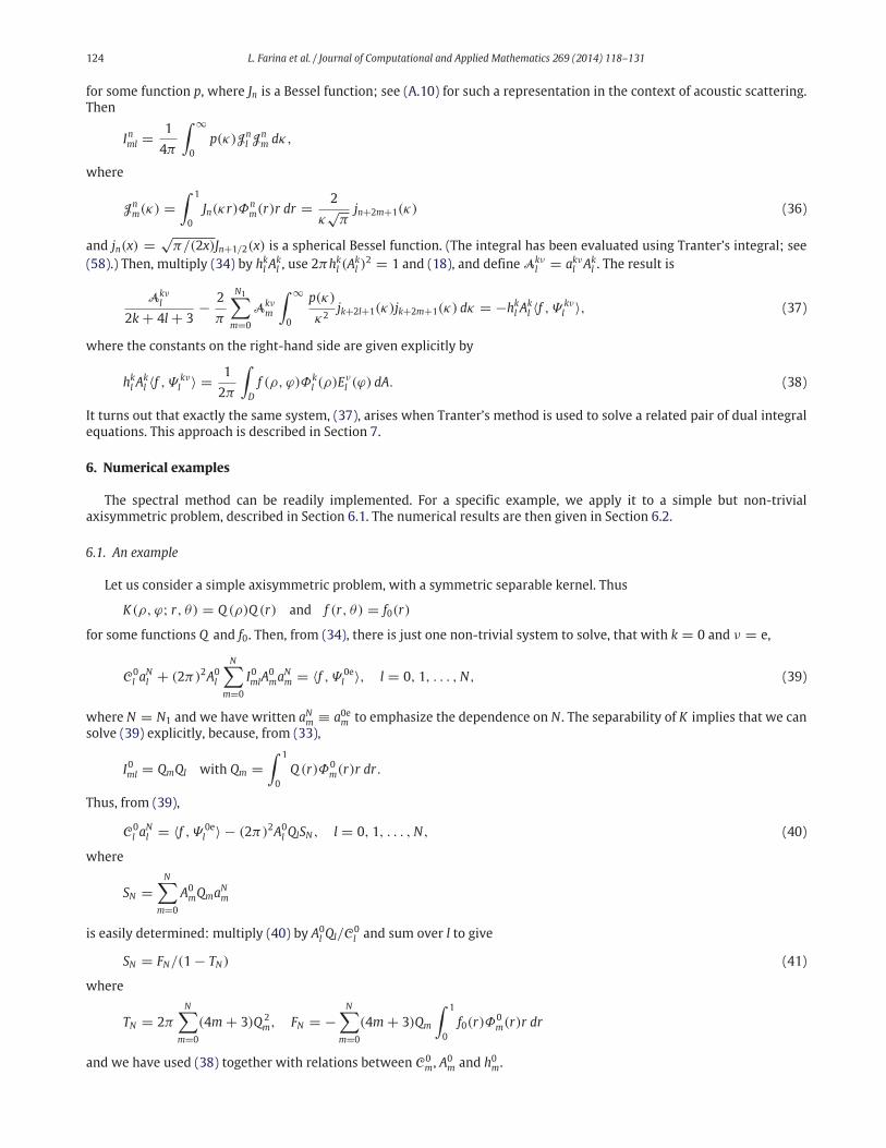
In Fig. 1, we can see, graphically, the decay of a15m for other cases involving Bessel functions. An oscillatory behaviour ofaNm occurred when Q is singular at the edge of the disc, Q (ρ) = 1/(5[ρ − 1]) + J0(ρ), with f0(ρ) = J0(ρ), see Fig. 2.


Table 1

The coefficients aNm for N = 5, 10, 30 when f = J0(ρ) and Q = J0(ρ).

m a5m a10m a30m

0 1.409196726786439 1.409196726786439 1.4091967267864401 0.042915968733271 0.042915968733271 0.0429159687332712 0.000442308257273 0.000442308257273 0.0004423082572733 0.000002291112648 0.000002291112648 0.0000022911126484 0.000000007136162 0.000000007136162 0.0000000071361625 0.000000000014834 0.000000000014834 0.0000000000148346 0.000000000000022 0.0000000000000227 0.000000000000000 0.000000000000000

Table 2

The coefficients aNm for N = 5, 10, 30 when f = J0(4ρ) and Q = J0(4ρ).

m a5m a10m a30m

0 −0.205479259329904 −0.205479259330105 −0.2054792593301051 −0.413133494237696 −0.413133494238101 −0.4131334942381012 −0.093555808001548 −0.093555808001639 −0.0935558080016393 −0.009020467889063 −0.009020467889072 −0.0090204678890724 −0.000491797018978 −0.000491797018978 −0.0004917970189785 −0.000017365405743 −0.000017365405743 −0.0000173654057436 −0.000000430856651 −0.0000004308566517 −0.000000007935952 −0.0000000079359528 −0.000000000112917 −0.0000000001129179 −0.000000000001279 −0.000000000001279

10 −0.000000000000012 −0.00000000000001211 −0.000000000000000

Fig. 1. The coefficients a15m for the case f = ρ, Q = J4(2ρ) (solid line) and for f = J0(ρ), Q = J2(4ρ) (dashed line).

7. Dual integral equations and Tranter’s method

Boundary value problems that lead to the hypersingular integral equation (4) can often be treated by reduction to a pairof dual integral equations for an auxiliary function B. These equations have the form

1

4π2

∫∫

κ(1 + h(κ))B e−i(ξx+ηy) dξ dη = g(x, y), (x, y) ∈ D, (47)∫∫

B e−i(ξx+ηy) dξ dη = 0, (x, y) ∈ D′, (48)


Fig. 2. The coefficients a15m for the case f = J0(ρ), Q = 1/(5[ρ − 1]) + J0(ρ).

where D is the unit disc in the xy-plane and D′ is the rest of that plane. The double integrals are over the whole ξη-plane,κ =

√

ξ 2 + η2 and h(κ) is a given function satisfying h(κ) → 0 as κ → ∞. For acoustic scattering by a hard disc,h(κ) = (γ /κ) − 1 with γ (κ) defined by (A.3).

Expand B and g in Fourier series,

B(ξ , η) = 2π∑

n,σ

in Bσn (κ)Eσ

n (β), g(x, y) =∑

n,σ

gσn (r)Eσ

n (θ),

where we have introduced polar coordinates, defined by

x = r cos θ, y = r sin θ, ξ = κ cosβ, η = κ sinβ. (49)

Then, using the expansion [5, 10.12.3]

e±i(ξx+ηy) =∞∑

n=0

ǫn(±i)nJn(κr) cos n(θ − β) =∑

n,σ

(±i)nJn(κr)Eσn (θ)Eσ

n (β), (50)

we can integrate with respect to β . The result is∫ ∞

0Bσn (κ)Jn(κr)(1 + h(κ))κ2 dκ = gσ

n (r), 0 ≤ r < 1, (51)

∫ ∞

0Bσn (κ)Jn(κr)κ dκ = 0, r > 1, (52)

with separate pairs of dual integral equations for each pair, n and σ .These equations are amenable to Tranter’s method [19]. Thus, write

Bσn (κ) = κ−µ

∞∑

m=0

αnσm Jn+2m+µ(κ), (53)

where µ is a positive parameter and the coefficients αnσm are to be found. The expansion (53) ensures that (52) is satisfied

automatically (use [5, 10.22.56]) whereas (51) becomes

∞∑

m=0

αnσm

∫ ∞

0(1 + h(κ))κ2−µJn+2m+µ(κ)Jn(κr) dκ = gσ

n (r), 0 ≤ r < 1. (54)

Multiply this equation by rn+1(1 − r2)µ−1Fl(n + µ, n + 1, r2) and integrate over 0 < r < 1. Here, Fm(a, c, x) =2F1(−m,m + a; c; x) is the notation for Jacobi polynomials used by some authors [20, p. 83], including Tranter [19,21];specifically, from (8) and [5, 18.5.7],

Φnm(r) = rn

√

1 − r2(n + m)!

n! Γ (m + 32 )

Fm(n + 3/2, n + 1, r2).


To effect the integration, we use Tranter’s integral [19,21],

21−µΓ (n + m + 1)

Γ (n + 1)Γ (m + µ)

∫ 1

0xn+1Fm(n + µ, n + 1, x2)

Jn(ξx)

(1 − x2)1−µdx = ξ−µJn+2m+µ(ξ), (55)

with n > −1 and µ > 0. Thus, (54) gives

∞∑

m=0

αnσm

∫ ∞

0(1 + h(κ))κ2−2µJn+2m+µ(κ)Jn+2l+µ(κ) dκ = E(n, l, µ), (56)

where the constants on the right-hand side are given by

E(n, l, µ) =21−µ(n + l)!n! Γ (l + µ)

∫ 1

0rn+1(1 − r2)µ−1Fl(n + µ, n + 1, r2) gσ

n (r) dr.

Now, how should we select µ? Tranter [19, p. 319] observes that the system (56) can be solved explicitly if the term(1 + h)κ2−2µ in the integrand is replaced by κ−1, and then suggests that the difference between these two terms should bemade ‘fairly small’, if possible, by the choice of µ. (There is a similar suggestion in Tranter’s book [21, p. 116] and in Duffy’sbook [22, p. 248].) If we interpret Tranter’s prescription as meaning in the limit κ → ∞, we find that µ = 3

2 . With thischoice, (56) reduces to

∞∑

m=0

αnσm

∫ ∞

0(1 + h(κ))jn+2m+1(κ)jn+2l+1(κ) dκ =

π

2E(n, l, 3/2)

=π

2

2−1/2(n + l)!n! Γ (l + 3

2 )

∫ 1

0rn+1

√

1 − r2Fl(n + 3/2, n + 1, r2)gσn (r) dr

=π

2√2

∫ 1

0Φn

l (r)gσn (r) r dr, (57)

where jn is a spherical Bessel function, and (55) gives∫ 1

0Φn

m(x) Jn(ξx)x dx =2

ξ√

πjn+2m+1(ξ). (58)

Then, as the spherical Bessel functions are orthogonal in the following sense [5, 10.22.55],∫ ∞

0jn+2m+1(κ)jn+2l+1(κ) dκ =

πδlm

2(2n + 4l + 3), (59)

the system (57) becomes

αnσl

2n + 4l + 3+

2

π

∞∑

m=0

αnσm

∫ ∞

0h(κ)jn+2m+1(κ)jn+2l+1(κ) dκ =

1√2

∫ 1

0Φn

l (r)gσn (r) dr.

This system is the same as (37). As the spectral method leading to (37) has been shown to be convergent, we infer thattruncated forms of Tranter’s method are convergent.

Notice the choiceµ = 32 madewith Tranter’smethod. This choice is not arbitrary. Indeed,with any particular application,

the quantity B can be related to a physical quantity, v, a quantity that has a known behaviour near the edge of the disc, D.This behaviour is enforced by the correct choice forµ. Similar remarks can bemadewhen Tranter’s method is used for otherboundary value problems, such as acoustic scattering by a sound-soft disc (Dirichlet condition).

8. Conclusion

We have shown that two apparently different numerical methods are convergent. The first is a spectral method forsolving two-dimensional hypersingular integral equations over a disc. The unknown function is expanded in a tensor-product manner, with trigonometric functions of the angular variable and orthogonal polynomials in the radial variable.The second method, Tranter’s method, is older and arises when the underlying boundary value problem is reduced to dualintegral equations instead of a hypersingular integral equation. In this method, a different unknown function is expandedin a series of Bessel functions of various orders (a Neumann series). Although the two methods appear to be unrelated, theyare not: they both lead to the same linear algebraic system.

Both methods have been used in the literature to generate numerical results for a variety of physical problems involvingdiscs. For the spectral method, see [23,12,14,15] and [24, Section 5.2]. For Tranter’s method, see [25–27] and [22, p. 251].The observed convergence accords with our theoretical analysis. It would be useful to estimate the rate of convergence, butwe have not done that yet. Extensions to systems of integral equations may also be feasible; certainly, there are relevantnumerical results in the literature obtained using variants of the spectral method [23,24] and of Tranter’s method [28,26,27,29]. Again, numerical convergence has been observed but the algorithms have not been analysed.


Acknowledgement

LF and VP acknowledge support from EU project FP7-295217-HPC-GA.

Appendix. An example: acoustic scattering by a hard screen

Consider a flat, sound-hard screen, Ω , in the plane z = 0. There is an incident field, uin, and the problem is to computethe scattered field, u. Thus, we seek a bounded solution of (∇2 + k2)u = 0, satisfying the Sommerfeld radiation conditionat infinity and the boundary condition

∂u

∂z= gin on both sides of Ω , (A.1)

where gin(x, y) = −∂uin/∂z evaluated at z = 0. It can be shown that the solution must be an odd function of z, so theproblem can be reduced to one in the half-space z > 0.

Derivation of a hypersingular integral equation using Fourier transforms

Take the Fourier transform of (∇2 + k2)u = 0 with respect to x and y, with, for example,

U(ξ , η, z) = F u =∫∫

u(x, y, z) ei(ξx+ηy) dx dy;

the integration is over the whole xy-plane. Then, with κ2 = ξ 2 + η2, and writing, for example U ′ = ∂U/∂z, we obtainU ′′ + (k2 − κ2)U = 0. Hence,

U(ξ , η, z) = B(ξ , η) e−γ z, z > 0, (A.2)

for some function B, where

γ = (κ2 − k2)1/2 =

√

κ2 − k2, |κ| > k,

−i√

k2 − κ2, |κ| < k;(A.3)

thus, Re γ ≥ 0 and the branch has been chosen so that the radiation condition is satisfied with a time dependence of e−iωt .We have a screen, Ω , in the xy-plane. The rest of the xy-plane is denoted by Ω ′. As we have split the problem into two

half-space problems, we must also impose continuity of u across Ω ′. Thus, let

v(x, y) = u(x, y, 0+) − u(x, y, 0−);this gives the discontinuity in u across the plane z = 0. Hence v(x, y) = 0 for (x, y) ∈ Ω ′. We regard v on Ω as our basicunknown. Its Fourier transform is

V (ξ , η) =∫

Ω

v(x, y) ei(ξx+ηy) dx dy = 2B = 2U(ξ , η, 0). (A.4)

We obtain an integral equation by inverting, u = F −1U , and imposing (A.1),

1

4π2

∫∫

U ′(ξ , η, 0) e−i(ξx+ηy) dξ dη = gin(x, y), (x, y) ∈ Ω, (A.5)

where U is given by (A.2). Symbolically, we have

F −1 γF v = −2gin. (A.6)

This integral equation holds for flat screens Ω of any shape.If Ω had been sound-soft, with a Dirichlet boundary condition on Ω instead of (A.1), we would have obtained

F −1

γ −1F uz

= g, (A.7)

an equation for the normal derivative of u on Ω , uz(x, y), where g is known from the boundary condition. We remark thatPenzel [9] has given a detailed analysis of a Galerkin method for (A.7), with expansion functions similar to our Ψ nσ

m , and hementions that similar methods apply to (A.6).

Returning to (A.6), this equation can be written as a hypersingular integral equation, as follows. Let L = ∇22 + k2, where

∇22 is the two-dimensional Laplacian with respect to x and y. We have Lei(ξx+ηy) = −γ 2ei(ξx+ηy). Thus

F −1 γF v = −LF −1

γ −1F v

.


Then, changing the order of integration (which is now permissible), we obtain

(F −1γ −1F v)(x, y) =∫

Ω

M(x − x′, y − y′)v(x′, y′) dA′ (A.8)

where dA′ = dx′ dy′ and

M(x, y) =∫∫

1

4π2γe−i(ξx+ηy) dξ dη =

1

2π

∫ ∞

0

κ

γJ0(κr) dκ =

eikr

2πr. (A.9)

To evaluateM , we used polar coordinates, (49), eiκx =∑∞

n=0 ǫninJn(κr) cos nθ and [30, 6.554 (2) and (3)]. Thus, (A.6) becomes

L

∫

Ω

eikR

4πRv(x′, y′) dA′ = gin(x, y), (x, y) ∈ Ω,

with R = (x − x′)2 + (y − y′)21/2. We have

L

(

eikR

R

)

= ∇22

(

1

R

)

+ ∇22

(

eikR − 1

R

)

+ k2eikR

R

= ∇22

(

1

R

)

+(1 − ikR)eikR − 1

R3,

where the last term is O(R−1) as R → 0. Hence, using (6), we see that v solves a hypersingular integral equation of theform (4).

The hypersingular part does not depend on k. Thus, if we write γ = κ + (γ − κ), (A.6) becomes

−F −1 κF v − F −1 (γ − κ)F v = 2gin

and a calculation similar to that leading to (A.8) with (A.9) gives

−F −1 κF v = ∇22F −1

κ−1F v

= ∇22

∫

Ω

v dA′

2πR.

Thus, we have

1

4π×∫

Ω

v

R3dA′ + (KΩv)(x, y) = gin(x, y), (x, y) ∈ Ω

where

(KΩv)(x, y) = −1

2

(

F −1 (γ − κ)F v)

(x, y) =∫

Ω

K(x − x′, y − y′)v(x′, y′) dA′

and

K(X, Y ) =1

8π2

∫∫

(κ − γ )e−i(ξX+ηY ) dξ dη =1

4π

∫ ∞

0κ(κ − γ )J0(κR) dκ. (A.10)

Using the addition theorem [4, Theorem 2.10], [5, 10.23.7],

J0(κR) =∑

n,σ

Jn(κr)Jn(κρ)Eσn (θ)Eσ

n (ϕ),

we can write K ≡ K in the form (32) with the representation (35) and p(κ) = κ(κ − γ ).Adopting a similar procedure for the sound-soft problem,we find that (A.7) can bewritten as a Fredholm integral equation

of the first kind over Ω with a weakly-singular kernel.

Use of the free-space Green’s function

There are well-known integral representations for scattering by bounded obstacles of finite volume, and these can bespecialized for a flat screen [4, Section 6.7]. For a sound-hard screen, we obtain

u(x, y, z) =∫

Ω

v(x′, y′)

limz′→0

∂

∂z ′

(

eikR

4πR

)

dA′,

where R2 = (x − x′)2 + (y − y′)2 + (z − z ′)2. This representation makes use of the free-space Green’s function, eikR/R,and so the radiation condition is satisfied. On the screen (where z = 0), we can use (A.1), giving precisely the same integralequation, (4), as obtained above.

The main virtue of the Fourier-transform derivation is that it does not require access to the free-space Green’s function.On the other hand, Green’s function techniques can be used for non-flat screens.


Dual integral equations

Instead of working with a physical unknown such as v, we can use B(ξ , η) = U(ξ , η, 0), and then impose (A.1) on Ω andv = 0 on Ω ′. This gives a pair of dual integral equations for B:

1

4π2

∫∫

γ B e−i(ξx+ηy) dξ dη = −gin(x, y), (x, y) ∈ Ω, (A.11)

1

4π2

∫∫

B e−i(ξx+ηy) dξ dη = 0, (x, y) ∈ Ω ′. (A.12)

These are in the form of (47) and (48) with h(κ) = (γ /κ) − 1 = O(κ−2) as κ → ∞.

References

[1] N.F. Parsons, P.A. Martin, Trapping of water waves by submerged plates using hypersingular integral equations, J. Fluid Mech. 284 (1995) 359–375.[2] P.A. Martin, Perturbed cracks in two dimensions: an integral equation approach, Int. J. Fract. 104 (2000) 315–325.[3] G. Monegato, Definitions, properties and applications of finite-part integrals, J. Comput. Appl. Math. 229 (2009) 425–439.[4] P.A. Martin, Multiple Scattering, Cambridge University Press, Cambridge, 2006.[5] NIST digital library of mathematical functions, http://dlmf.nist.gov/.[6] M.A. Golberg, The convergence of several algorithms for solving integral equations with finite-part integrals, J. Integral Equations 5 (1983) 329–340.[7] V.J. Ervin, E.P. Stephan, Collocation with Chebyshev polynomials for a hypersingular integral equation on an interval, J. Comput. Appl. Math. 43 (1992)

221–229.[8] M.A. Golberg, C.S. Chen, Discrete Projection Methods for Integral Equations, Computational Mechanics Publications, Southampton, 1997.[9] F. Penzel, On the solution of integral equations on the circular disk by use of orthogonal polynomials, in: S. Samko, A. Lebre, A.F. dos Santos (Eds.),

Factorization, Singular Operators and Related Problems, Kluwer, Dordrecht, 2003, pp. 205–217.[10] N. Heuer, M.E. Mellado, E.P. Stephan, A p-adaptive algorithm for the BEMwith the hypersingular operator on the plane screen, Int. J. Numer. Methods

Eng. 53 (2002) 85–104.[11] E.P. Stephan, The hp-version of BEM—fast convergence, adaptivity and efficient preconditioning, J. Comput. Math. 27 (2009) 348–359.[12] L. Farina, P.A. Martin, Scattering of water waves by a submerged disc using a hypersingular integral equation, Appl. Ocean Res. 20 (1998) 121–134;

Appl. Ocean Res. 21 (1999) 157–158 (erratum).[13] P.A. Martin, Mapping flat cracks onto penny-shaped cracks, with applications to somewhat circular tensile cracks, Quart. Appl. Math. 54 (1996)

663–675.[14] J.S. Ziebell, L. Farina, Water wave radiation by a submerged rough disc, Wave Motion 49 (2012) 34–49.[15] L. Farina, J.S. Ziebell, Solutions of hypersingular integral equations over circular domains by a spectral method, in: J. Brandts, S. Korotov, M. Křížek,

J. Šístek, T. Vejchodský (Eds.), Applications of Mathematics 2013, In Honor of the 70th Birthday of Karel Segeth, Institute of Mathematics, Academy ofSciences of the Czech Republic, Prague, 2013, pp. 51–66.

[16] P.A. Martin, On potential flow past wrinkled discs, Proc. Roy. Soc. A 454 (1998) 2209–2221.[17] S. Krenk, A circular crack under asymmetric loads and some related integral equations, J. Appl. Mech. 46 (1979) 821–826.[18] S. Krenk, Some integral relations of Hankel transform type and applications to elasticity theory, Integral Equations Operator Theory 5 (1982) 548–561.[19] C.J. Tranter, A further note on dual integral equations and an application to the diffraction of electromagnetic waves, Quart. J. Mech. Appl. Math. 7

(1954) 317–325.[20] W. Magnus, F. Oberhettinger, Formulas and Theorems for the Functions of Mathematical Physics, Chelsea, New York, 1949.[21] C.J. Tranter, Integral Transforms in Mathematical Physics, third ed., Methuen, London, 1966.[22] D.G. Duffy, Mixed Boundary Value Problems, Chapman & Hall/CRC, Boca Raton, 2008.[23] S. Krenk, H. Schmidt, Elastic wave scattering by a circular crack, Philos. Trans. R. Soc. A 308 (1982) 167–198.[24] A. Boström, Review of hypersingular integral equation method for crack scattering and application to modeling of ultrasonic nondestructive

evaluation, Appl. Mech. Rev. 56 (2003) 383–405.[25] W. Zhang, H.A. Stone, Oscillatory motions of circular disks and nearly spherical particles in viscous flows, J. Fluid Mech. 367 (1998) 329–358.[26] A.M.J. Davis, R.J. Nagem, Effect of viscosity on acoustic diffraction by a circular disk, J. Acoust. Soc. Am. 115 (2004) 2738–2748.[27] J.D. Sherwood, Resistance coefficients for Stokes flow around a disk with a Navier slip condition, Phys. Fluids 24 (2012) 093103.[28] A.M.J. Davis, S.G. Llewellyn Smith, Tangential oscillations of a circular disk in a viscous stratified fluid, J. Fluid Mech. 656 (2010) 342–359.[29] J.P. Tanzosh, H.A. Stone, Transverse motion of a disk through a rotating viscous fluid, J. Fluid Mech. 301 (1995) 295–324.[30] I.S. Gradshteyn, I.M. Ryzhik, Table of Integrals, Series, and Products, fifth ed., Academic Press, San Diego, 1994.

Contentslistsavailableat ScienceDirect Journal of ...inside.mines.edu/~pamartin/ref-paps/R131_JCAMw.pdf · m is that they are eigenfunctions of the basic hypersingular operator. This

Documents