Contents · matrix de–ned by KPSW satis–es the above requirement and can be obtained from the (assumed) known (or pre-estimated) cointegrating relations. KPSW choose to give a

University of York

Department of Economics

PhD Course 2006

VAR ANALYSIS IN MACROECONOMICS

Lecturer: Professor Mike Wickens

Lecture 5

Macroeconomic Fluctuations:

Keynesian, RBC and DSGE Models

Contents

1. Blanchard SVAR model

2. Blanchard and Quah VAR model

3. King, Plosser, Stock and Watson VMA model

4. RBC models and the VAR model

(i) General theoretical considerations

(ii) Cooley and Dwyer model

(iii) Using a VAR to calibrate a DSGE model

5. Fiscal policy using a VAR

(i) Fiscal shocks

(ii) Fiscal sustainablility

6. Open economy VAR models

(i) General theoretical considerations

0

(ii) A sticky-price monetary model with a �oating exchange rate

(iii) Garrett, Lee, Pesaran and Shin model

(iv) DSGE models

(v) The sustainability of the current account using a VAR

1

VARs have been widely used to study business cycle �uctuations in macroeconomics. We

consider some of the principal investigations.

The aim in most of these papers is either to uncover key features of the macroeconomy or, in

the case of RBC and DSGE models, to use the data to learn how best to formulate the model. The

latter often address the issue: if the predictions of these models are inconsistent with the data, or

require the model parameters to take implausible values, how can the models be re-formulated so

that its predictions match the data.?

1 Blanchard SVAR model (AER 1989)

Blanchard proposed a Keynesian model of the macroeconomy and used a structural VAR.

Model

AD : y = c12es + ed

OL : u = a21y + es

PS : p = a34w + a31y + c32es + ep

WS : w = a43p+ a42u+ c42es + ew

MR : m = a51y + a52u+ a53p+ a54w + em

where y =log GDP, u =unemployment rate, p =log price level, w =log wage rate,

m =log M1.

The AD equation is the aggregate demand function, OL is Okun�s law, the remaining equations

are the price, the wage and the money rule

2

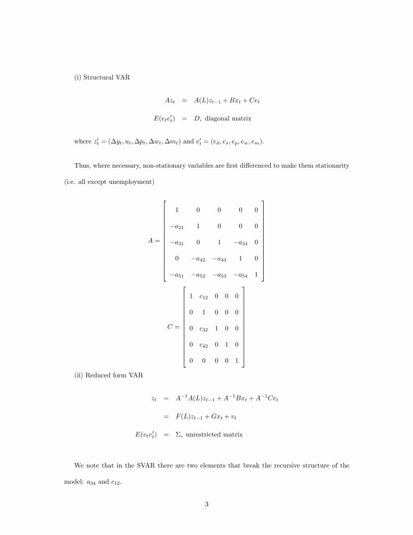
(i) Structural VAR

Azt = A(L)zt�1 +Bxt + Cet

E(ete0t) = D; diagonal matrix

where z0t = (�yt; ut;�pt;�wt;�mt) and e0t = (ed; es; ep; ew; em):

Thus, where necessary, non-stationary variables are �rst di¤erenced to make them stationarity

(i.e. all except unemployment)

A =

2666666666666664

1 0 0 0 0

�a21 1 0 0 0

�a31 0 1 �a34 0

0 �a42 �a43 1 0

�a51 �a52 �a53 �a54 1

3777777777777775

C =

2666666666666664

1 c12 0 0 0

0 1 0 0 0

0 c32 1 0 0

0 c42 0 1 0

0 0 0 0 1

3777777777777775(ii) Reduced form VAR

zt = A�1A(L)zt�1 +A�1Bxt +A

�1Cet

= F (L)zt�1 +Gxt + vt

E(vtv0t) = �; unrestricted matrix

We note that in the SVAR there are two elements that break the recursive structure of the

model: a34 and c12:

3

Given c12 and either a34 or a43 the SVAR is just identi�ed. In the absence of this knowledge

it is necessary to use structural estimation and not OLS.

Main empirical conclusions

(i) relations between the real variables and relations between the nominal variables are stronger

than across real and nominal variables

(ii) Estimates are broadly consistent with the Keynesian model. The main exception is the

strong unemployment e¤ect (supply shock) in the aggregate demand function.

(iii) Demand shocks explain most of the short-run �uctuations in output, prices and wages

(iv) Supply shocks dominate in the medium to long term.

(v) The main problem is that unemployment seems to strongly Granger-cause output, instead

of the other way round.

4

2 Blanchard and Quah VAR model (AER 1989)

The aim here is to use long-run restrictions to identify the di¤erence between demand and supply

shocks. Blanchard and Quah postulate the following Keynesian model:

yt = mt � pt + �at

yt = nt + at

pt = wt � at

wt = wjfEt�1nt =_ng

ut =_n� nt

�mt = edt

�at = est

Notes:

(i) at = productivity shock

(ii) Wages are chosen one period in advance so as to achieve full employment.

(iii) The disturbances edt and est are iid with zero mean and constant variances.

The system can be re-written as

�yt = �edt + ��est + est

ut = �edt � �est

Thus, yt is I(1) and ut is I(0).

The model implies that demand shocks have no long run e¤ect on output, and the impulse

response function of output to demand shocks is zero for all lags- i.e. there is only a contempora-

neous e¤ect.

5

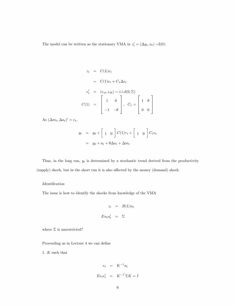
The model can be written as the stationary VMA in z0t = (�yt; ut) �I(0):

zt = C(L)et

= C(1)et + C1�et

e0t = (est; edt) � i:i:d(0;�)

C(1) =

2664 1 0

�1 ��

3775 ; C1 =

2664 1 �

0 0

3775As (�mt;�at)

0 = et,

yt = y0 +

�1 0

�C(1)� t +

�1 0

�C1et

= y0 + at + ��at +�mt

Thus, in the long run, yt is determined by a stochastic trend derived from the productivity

(supply) shock, but in the short run it is also a¤ected by the money (demand) shock.

Identi�cation

The issue is how to identify the shocks from knowledge of the VMA

zt = B(L)ut

Eutu0t = �

where � is unrestricted?

Proceeding as in Lecture 4 we can de�ne

1. K such that

et = K�1ut

Eete0t = K�10�K = I

6

2. C(L) such that

C(L) = B(L)K

Hence

�zt = B(L)KK�1ut

= C(L)et

We now have orthogonal shocks

K has n2 = 4 elements and the restriction K�10�K = I provides n(n+1)2 = 3 of these.

3. Now impose the long-run restriction that the demand shock has no long-run e¤ect on yt:

Thus

C(1)12 = 0

This implies that C(1) and K are de�ned to satisfy the restriction

C(1)12 = B(1)11K21 +B(1)12K22 = 0

This is the 4th restriction required to identify K:

Estimation

How do we estimate the VMA?

Answer we estimate the VAR

A(L)zt = ut

In principle we need to invert the VAR to get the VMA

zt = A(L)�1ut = B(L)ut

In practice we do NOT need to take the last step as we only need estimates of C(1) and � in

order to construct K, and we can use

C(1) = A(1)�1

7

Note: Blanchard and Quah do something slightly di¤erent.

Main empirical conclusions: (Figs 1 and 2)

(i) Output:

Supply shock: Output is permanently (and positively) a¤ected by a positive supply shock.

The full e¤ect takes about

2 years and is slow to take e¤ect.

Demand shock: output responds quickly but the e¤ect disappears after about 5 years.

(ii) Unemployment:

Supply shock: Unemployment increases in the short run, before falling after about 2 years.

The e¤ect disappears after about 4 years. B & Q interpret the behaviour in the short run to price

and wage rigidities: a productivity shock raises real wages and hence increases unemployment.

Could also argue that there is capital-labour substitution.

Demand shock: Causes unemployment to fall in the short run due to increased demand.

Comment

The evidence on the impulse response function of output to the demand shock is not strictly

consistent with the theoretical model, nor are the two IRFs for unemployment. One might expect

the supply shock to reduce unemployment even in the short run. The theoretical modelalso says

that the e¤ects should be instantaneous and not distributed over time. But this was only a stylised

model.

8

3 King, Plosser, Stock andWatson VMAmodel (AER 1991)

The aim here is to use a VMA and to identify the common stochastic trends using information

about long-run relations among the variables obtained from cointegrating regressions.

Model

Long-run relations

m� p = �yy � �ii

c� y = �1(i��p)

v � y = �2(i��p)

v =investment.

These equations were estimated by �dynamic�OLS (using 5 leads and lags of di¤erences in

each of the variables). This is a way of exploiting the super-consistency property of cointegrating

regressions to eliminate the e¤ects of dynamics. This is Stock and Watson�s recommendation but

is hardly ever used.

De�ne z0 = (y; c; v;m�p; i;�p) � I(1): Thus it is assumed that p;m � I(2) and m�p � I(1):

Identi�cation

Consider the VMA

�zt = �+ C(L)et

= �+ C(1)et + C�(L)�et

= �+ �0et + C�(L)�et

Eete0t = �

9

As there are 3 long-run relations and 6 non-stationary variables, there are 3 stochastic trends.

The problem now is to construct and �:

If, for example, we start with the CVAR

�zt = Azt�1 + et

= ��0zt�1 + et

and the associated VMA is

�zt = C(1)et + C�(L)�et

= �0et + C�(L)�et

Then using �� t = et we can write

zt = z0 + �0� t + C

�(L)et

Since �0zt � I(0);

�0zt = �0z0 + (�0 )�0� t + �

0C�(L)et � I(0)

But this can only be true if the term in � t is eliminated as it is I(1): Thus should be

constructed so that

�0 = 0

i.e. must be orthogonal to �0:

Although the matrix � must then be chosen so that 0� = C(1); this does not uniquely de�ne

�:

The matrix de�ned by KPSW satis�es the above requirement and can be obtained from the

(assumed) known (or pre-estimated) cointegrating relations. KPSW choose � to give a recursive

10

structure to the stochastic trends. Thus

=

26666666666666666664

1 0 0

1 0 �1

1 0 �2

�y ��i ��i

0 1 1

0 1 0

37777777777777777775

; � =

26666666666666666664

1 �12 �13

0 1 �23

0 0 1

0 0 0

0 0 0

0 0 0

37777777777777777775 is known, but � require estimation.

Note that if we let �� t = et then the stochastic trends �t = �0� t are formed from cumulating

the �rst three elements of et: Hence from ��t = �0�� t = �0et

��1t = e1t

��2t = �12e1t + e2t

��3t = �13e1t + �23e2t + e3t

and the stochastic trends have a recursive structure.

It is also assumed that � can be partitioned conformably with e0t = (e1t; e2t; e3tje4t; e5t; e6t)

� =

2664 �11 0

0 �22

3775 �11 is diagonal

Thus, as part of the recursive structure, the stochastic trends are constrained to be uncorre-

lated.

11

It follows that the long-run structure of the model is

yt = �1t

�pt = �12�1t + �2t

it = �13�1t + �23�2t + �3t

ct = yt + �1(it ��pt)

vt = yt + �2(it ��pt)

mt � pt = �yyt � �iit

Hence

�1 is the �real balanced growth�shock - i.e. output (supply?) shock

�2 is the �neutral in�ation�shock - i.e. price (nominal?) shock

�3 is the �real interest rate�shock - demand shock?

Main empirical conclusions (Fig 4)

(i) The output shock has a large permanent e¤ect on output, consumption and investment. In

the case of investment this is initially negative.

(ii) The in�ation shock has little e¤ect on output and consumption. Investment is a¤ected in

the short run but not the long run.

(iii) The real interest rate shock has no long run e¤ects, but in the short run all three variables

increase.

(iv) KPSW conclude that US data are not consistent with the view that a single permanent

shock is the dominant source of business-cycle �uctuations.

(v) and that contrary to Monetarist thought in�ation shocks have little e¤ect on real variables

even in the short run.

Comment on the KPSW model

12

It is not clear that the restrictions imposed are consistent with the data. In particular, is it

really correct to restrict � in this way?

Levtchenkova, Pagan and Robertson (J. of Econ Surveys, 1998) argue that the shocks do not

have the structure assumed by KPSW. They suggest that a better way to proceed would be

construct and � by directly by exploiting the long-run structural information.

13

4 RBC and VAR models

4.1 Ellen McGrattan (Fed Res. Bank of Minn QR 1994)

She summarizes the typical RBC methodology and its �ndings to that date very clearly.

The original Kydland-Prescott analysis attempts to explain business cycles as being due to

technology shocks. The KP model can account for some features of the data but not others.

Features captured:

(i) cyclical variability of output

(ii) the lower variability of consumption than income

(iii) higher variability of investment

Features not captured:

(i) the variability of consumption is too low

(ii) the variability of hours worked is too low

(iii) the variability of investment is too low

(iv) the correlation between hours worked and productivity is far too high.

See Charts 1-3 and Table 1

Hansen (1985) tries to improve the performance of the model by altering the labour supply

structure. He argues that employment is indivisible: individuals work either a set number of hours

or none. This enables the model to better capture the variability of hours worked, but still has a

too high correlation between hours and productivity. (see Table 1).

McGrattan argues that the standard RBC model omits �scal shocks. Her results suggest that in

response to changes in tax rates to �nance government expenditures households substitute between

taxable and non-taxable activities thereby altering the variability of consumption, investment,

14

hours worked and productivity. The result is a lower correlation of hours worked and productivity.

(see Tables 2 and 3).

(i) General theoretical issues

There is a huge literature on RBCmodels. Notable papers are Prescott (FRBMQR 1986), King,

Plosser & Rebelo (JME 1988), Kydland and Prescott (FRBMQR 1990), McGrattan (FRBMQR

1994), Campbell (JME 1994), Cooley and Dwyer (J.Ectcs 1998).

The classical problem is that the economy is seeking to choose consumption C; labour L and

capital K to maximise

Et

1Xs=0

�sU(Ct+s)

where � = 11+� subject to a budget constraint (the national income identity), a production function

and a capital accumulation equation:

Yt = Ct + It

Yt = F (At;Kt; Lt)

�Kt+1 = It � �Kt

or, just to the combined constraint,

F (At;Kt; Lt) = Kt+1 + Ct � (1� �)Kt

The main agenda of the RBC literature became to show how it is that productivity shocks

(i.e. shocks to At) are the main cause of business cycle �uctuations.

Rather than work in such generality it is convenient to consider speci�c functional forms. We

assume a Cobb-Douglas production

Yt = AtK�t L

1��t

15

with labour growing at the constant rate n, implying that

Lt = (1 + n)tL0

and where log productivity is a random walk about a constant rate of long-run growth �

At = (1 + �)tZt

lnZt = zt; �zt = et � i:i:d(0; !2)

The only shock to this economy is et and this gets propagated throughout the economy.

In order to obtain the solution to the model, �rst we re-de�ne all variables in terms of deviations

about their long-run growth paths. In equilibrium, the balanced growth rate for the economy is

� = n+ �1�� .

We can treat technical progress in this model as labour augmenting, hence we re-write the

production function as

yt = Ztk�t

where

yt =Yt

L#t=

Yt

[(1 + �)1

1�� ]tLt=

Yt(1 + �)tL0

kt =Kt

L#t=

Kt

[(1 + �)1

1�� ]tLt

=Kt

(1 + �)tL0

L#t = (1 + �)t

1��Lt = [(1 + �)1

1��]t(1 + n)tL0 = (1 + �)

tL0

where we have used the approximation

[(1 + �)1

1��]t(1 + n)t ' (1 + �)t

� ' n+�

1� �

The national income identity is now

yt = ct + it

16

where

ct =Ct

L#t=

Ct(1 + �)tL0

it =It

L#t=

It(1 + �)tL0

and the capital accumulation equation can be written as

�Kt+1 = It � �Kt

Kt+1

L#t+1

L#t+1

L#t=

It

L#t+ (1� �)Kt

L#t

(1 + �)kt+1 = it + (1� �)kt

sinceL#t+1

L#t= 1 + �:

Finally, we assume that the utility function is

U(Ct) =Ct

1��

1� �

=[(1 + �)tct]

1��

1� �

The problem facing the economy can now be formulated in terms of maximising the value function

Vt = U(Ct) + �Et(Vt+1)

=[(1 + �)tct]

1��

1� � + �Et(Vt+1)

subject to

Ztk�t = ct + (1 + �)kt+1 � (1� �)kt

The �rst-order conditions for this stochastic dynamic programming problem are

@Vt@ct

= (1 + �)(1��)tc��t + �Et[@Vt+1@ct+1

� @ct+1@ct

] = 0

17

We note that

Vt+1 = U(Ct+1) + �Et+1(Vt+2)

hence,

@Vt+1@ct+1

= (1 + �)(1��)(t+1)c��t+1

To evaluate @ct+1@ct

we re-express it as

@ct+1@ct

=

@ct+1@kt+1@ct@kt+1

and then use the budget constraints for periods t and t+1 to evaluate numerator and denominator.

This gives

@ct+1@ct

=�Zt+1k

��1t+1 + 1� �

�(1 + �)

Hence

@Vt@ct

= (1 + �)(1��)tc��t � �Et[(1 + �)(1��)(t+1)c��t+1 ��Zt+1k

��1t+1 + 1� �1 + �

]

= (1 + �)(1��)tfc��t � �Et[(1 + �)��c��t+1(�Zt+1k��1t+1 + 1� �)]g = 0

implying the Euler equation

Et

��[(1 + �)

ct+1ct]��(�Zt+1k

��1t+1 + 1� �)

�= 1

In evaluating the Euler equation we should take account of the conditional covariance terms

involving ct+1; kt+1 and Zt+1 - particularly covt(ct+1; kt+1) because we can ignore those involving

Zt+1 as it is predicted to be Zt in every future period - but instead, for convenience, we shall omit

them. This is equivalent to assuming certainty equivalence or, in a decentralised economy, that

there is a real risk-free interest rate.

Steady-state solution

In equilibrium �ct+1 = �kt+1 = 0 and Zt = 1 for each time period. Hence we can drop the

time subscript in the steady state to obtain

�(1 + �)��[�k��1 + 1� �] = 1

18

implying that in equilibrium

k '�� + � + �(n+ �

1�� )

�

� �11��

Although kt is constant in equilibrium, the capital stock per capita of the economy, Kt

Lt, is growing

through time. As kt = Kt

[(1+�)1

1�� ]tLt; the optimal path for capital per capita is

(� + � + �(n+ �

1�a )

�)�11�� [(1 + �)

11�� ]t

and hence grows at approximately the rate �1�� :

Optimal per capita growth rates

The optimal growth rate of per capita output YtLt is determined from that of yt =Yt

[(1+�)1

1�� ]tLt

.

As yt = k�t and �kt+1 = 0; it follows that �yt+1 = 0 too. Thus, the growth rate of YtLtis also

approximately �1�� : The optimal growth rate of consumption per capita

CtLt

can be obtained

from the condition that �ct+1 = 0 and ct = Ct

[(1+�)1

1�� ]tLt

: Thus the growth rate of CtLt is also

approximately �1�� :

Optimal total growth rates

The optimal growth rates of total output, total capital and total consumption are obtained by

taking into account population growth. Adding on the growth rate of the population, we obtain

their common rate of growth � = n+ �1�� . As the growth rates of output, capital and consumption

are the same, the optimal solution is a balanced growth path.

Short-run dynamics

We consider short-run deviations about the logarithm of the growth path. The model reduces

to two equations: the Euler equation and the budget constraint. We need to take logarithmic

approximations of each based on the Taylor series approximation

f(xt) ' f(x�t ) + f0(x�t )

�@xt@ lnxt

�x�t

[lnxt � lnx�t ]

' f(x�t ) + f0(x�t )x

�t [lnxt � lnx�t ]

19

Leaving out the intercept, and using certainty equivalence in which Et lnZt+1 = lnZt = zt;

the Euler equation can be shown to approximately satisfy

Et� ln ct+1 = �(� +� + �

�)(1� �)Et ln kt+1 + (� +

� + �

�)zt

The log-linearized budget constraint is

ln kt+1 = �[� + �(� � 2)] ln ct + (1 + � + ��) ln kt

+� + � + (� � �)�

�zt

These two equations can be written as the system2664 1 + � + �� �[� + �(� � 2)]

0 1

37752664 ln kt

ln ct

3775 =

2664 1 0

(� + �+�� )(1� �) 1

3775Et2664 ln kt+1

ln ct+1

3775

�

2664 �+�+(���)��

� + �+��

3775 ztWe note that each equation involves zt which is I(1): This implies that neither the linearized

Euler equation nor the budget constraint give a cointegrating relation. This is despite the fact

that along the steady-state growth path the ratio of consumption to capital is constant. Although

the ratio of consumption to capital is expected to be constant, in practice, future shocks cause it

to be non-stationary.

The general form of the solution is

Bxt = CEtxt+1 +Dzt

xt = B�1CEtxt+1 +B�1zt

The roots of the matrix A = B�1C determine the type of solution: roots < 1 in absolute value

are stable, and those greater than 1 are unstable. These can be obtained from the determinental

equation

jAj � (trA)L+ L2 = 0

20

In this example there are two roots. If we set L = 1 in the equation then there are three cases

(i) jAj � (trA) + 1 > 0 implies both roots are either stable or unstable.

(ii) jAj � (trA) + 1 < 0 implies a saddlepath solution (one root is stable and the other is

unstable).

(iii) jAj � (trA) + 1 = 0 then at least one root is 1:

It can be shown that

jAj � (trA) + 1 = �[� + �(� � 2)](� + �+�

� )(1� �)1 + � + ��

< 0

if � � 2; a su¢ cient but not necessary condition. The short-run dynamics about the steady-state

growth path therefore follow a saddlepath.

Solving the unstable root forwards and noting that Etzt+s = zt implies that the general solution

is the VAR

xt = Qxt�1 +Rzt

where the error term is I(1). Since the vector xt is not cointegrated, we must take �rst di¤erences.

This gives the stationary VAR

�xt = Q�xt�1 +Ret

or, in terms of the original variables,2664 � ln Kt

Lt

� ln CtLt

3775 = constant + Q

2664 � ln Kt�1Lt�1

� ln Ct�1Lt�1

3775+RetIt is important to note that there is only one disturbance term in this VAR and this drives

both ln Kt

Ltand ln CtLt . This is because there is only one shock in the orginal model, a productivity

shock. This is characteristic of RBC models. As the joint distribution of ln Kt

Ltand ln CtLt is not

degenerate, there is obviously a need to identify and introduce an additional shock. Sometimes

this is assumed to be a shock to U(Ct); i.e. a preference shock.

21

In the literature it is common to assume that the productivity shock is a stationary autore-

gression, eg Campbell (1994). This raises the issue of what makes real variables non-stationary.

It seems likely that productivity and money supply shocks are two key sources of real and

nominal non-stationarities.

22

4.2 Cooley and Dwyer (J. of Ectcs 1998)

C&D compare the Blanchard and Quah (1989) results, which are widely regarded as issuing a

strong challenge to RBC theory despite the inconsistencies between the theory and the evidence,

with three RBC/DSGE models.

Their argument is that the B&Q methodology is based on atheoretical assumptions and the

B&Q results are not capable of being produced by RBC/DSGE models based on �a lot of economic

theory�.

They consider three di¤erent versions of the RBC/DSGE model.

(a) Their second model has one shock: a technology shock.

It is an RBC model in which the aim is to maximise

E��t(ln ct �Ah t )

subject to

ct + it � yt

kt+1 = it + (1� �)kt

yt = k�t (eatht)

1��

�at = g + �(L)"t

�(L) = �0 + �1L+ �2L2 + �1L

4 + �0L4

�0 < �1 < �2; �(1) = 1

This model is calibrated.

Data is generated from the model for di¤erent samples of random errors.

Impulse response functions are calculated and the average IRF is plotted in Fig 4.

23

This is compared with the IRF based on using the B&Q procedure for actual data.

The calibrated IRFs are remarkably similar to the B&Q IRFs even to the extent of producing

an even larger sized demand shock when in theory none exists.

This raises doubts about what the B&Q method is really measuring.

(b) The third model has two shocks: a technology and a preference shock. The model is

E��t(ln ct �Ah t ez1t)

z1t = �1(L)"1t

subject to

ct + it � yt

kt+1 = it + (1� �)kt

yt = ez2tk1��t h�t

�z2t = �2(L)"2t

where the roots of �1(L) and �2(L) are assumed to lie outside the unit circle.

The solution takes the form

lnht = �11z1t + �12z2t + �13 ln kt

ln yt = �21z1t + �22z2t + �23 ln kt

ln kt+1 = �31z1t + �32z2t + �33 ln kt

It is possible to eliminate capital from the model using the last equation which can be written

ln kt =�31z1t�1 + �32z2t�1

(1� �33L)

24

to obtain a VAR in � lnht and � ln yt :

� lnht = �33� lnht + �11�z1t + (�13�31 � �11�33)�z1t�1

+�12�z2t + (�13�32 � �12�33)�z2t�1

� ln yt = �33� ln yt + �21�z1t + (�23�31 � �21�33)�z1t�1

+�22�z2t + (�23�32 � �22�33)�z2t�1

It is in �rst di¤erences because the technology shock z2t is I(1).

The model can also be written

(1� �33L)

2664 � lnht

� ln yt

3775 = B(L)

2664 �"1t

"2t

3775This may be compared with the equivalent B&Q model (using hours instead of unemployment)

A(L)

2664 lnht

� ln yt

3775 =2664 "dt

"st

3775This shows that

(i) the equation in lnht involves an I(1) variable and hence lnht must be I(1) and not I(0) as

in B&Q:

(ii) the model has a VARMA structure and not a VAR structure

This will a¤ect the estimated IRFs from the B&Q model which will be biased.

(iii) the shocks "dt and "st do not match the distinction found in the theoretical model which

implies that the shocks in the VAR are functions of both technology and preference shocks.

(iv) the theoretical model implies that both "dt and "st have permanent e¤ects on both vari-

ables.

(v) the true technology shock has a permanent e¤ect on lnht:

(vi) the preference shock does not have a permanent e¤ect on ln yt - as in B&Q - but this does

not require any restrictions of the sort imposed by B&Q to produce it.

25

4.3 Using a VAR to calibrate a DSGE model

Rotemberg and Woodford (NBER Macroeconomics Annual 1997), Christiano, Eichenbaum and

Evans (NBER 2001) and Smets and Wouter (ECB WP 2001)

1. formulate a DSGE model

2. Construct and estimate a VAR based on the variables in the DSGE

3. Calibrate the DSGE to the impulse response functions obtained from the VAR

They can then carry out policy analysis using the calibrated DSGE model.

The calibration chooses the DSGE parameters � to minimise the distance function

[vec(IRFV AR)� vec(IRFDSGEM (�))]0W�1[vec(IRFV AR)� vec(IRFDSGEM (�))]

where W is a diagonal weighting matrix of the di¤erent IRFs and time periods that has the

variances of the VAR IRFs on the leading diagonal.

26

5 Fiscal policy using a VAR

We consider two issues

(a) The e¤ects of �scal shocks (government spending and taxation shocks) on GDP

(b) The sustainability of the current �scal stance.

5.1 Fiscal shocks

We consider the paper by Blanchard and Perotti (1999)

Their basic model is an SVAR in three variables taxes, government spending and GDP.

A(L)zt = et

where

z0t = (lnTt; lnGt; lnYt).

- all variables in the VAR are logarithms, real and in per capita terms.

- all are I(1) variables.

- the data are either de-trended

- or cointegration is assumed between lnTt and lnGt

- the cointegrating relation is assumed to be lnTt � lnGt

- the data are quarterly

It is assumed that "0t = ("Tt ; "

Gt ; "

Yt ) are uncorrelated tax, spending and output shocks.

The identi�cation scheme relating "t to et is de�ned as266666641 0 �a1

0 1 b1

�c1 �c2 1

37777775

26666664eTt

eGt

eYt

37777775 =266666641 a2 0

b2 1 0

0 0 1

37777775

26666664"Tt

"Gt

"Yt

3777777527

All of the parameters are assumed known and replaced by prior estimates. It is assumed that

b1 = 0 and either a2 = 0 or b2 = 0.

If, for example, b2 = 0 then

"t =

266666641 a2 0

0 1 0

0 0 1

37777775

�1 266666641 0 �a1

0 1 0

�c1 �c2 1

37777775 et

=

266666641 �a2 �a1

0 1 0

�c1 �c2 1

37777775 et= Qet

As a result

A(L)zt = et = Q�1"t

QA(L)zt = "t

A�(L)zt = "t

In other words, we can re-write the original VAR as a new VAR in zt which has uncorrelated

errors and a di¤erent dynamic structure. It is now straightforward to obtain the impulse response

functions.

Main �ndings

(i) The spending shock "Gt has a strong positive e¤ect on both GDP and taxes

(ii) The tax shock "Tt has a strong negative e¤ect on GDP but does not a¤ect spending.

5.2 Fiscal sustainability

Fiscal sustainablity concerns the evolution of btyt and whether it remains �nite or explodes.

28

The �scal stance is said to be sustainable if btyt is �nite and if �nancial markets are willing to

hold the level of debt that emerges. The current �scal de�cit can then be sustained inde�nitely

without the government incurring unsupportable debt obligations.

If the current �scal stance is not sustainable, then a change of policy will be required at some

point to make it sustainable.

Univariate and multivariate models, as well as cointegration analysis, have been used to try to

determine �scal sustainability.

The key condition that lies at the centre of this analysis is the present-value (or inter-temporal)

government budget constraint (PVGBC). Fiscal policy is said to be sustainable if the PVGBC is

satis�ed. This has been tested in a number of ways.

5.2.1 The government budget constraint (GBC)

Three ways of writing the GBC

1. The nominal GBC

Ptgt + (1 +Rt)Bt�1 = Bt +�Mt + PtTt

gt is real government expenditure including real transfers to households

Tt is total real taxes

Mt is the stock of outside nominal, non-interest bearing money at the start of period t

Bt is the nominal value of government bonds issued by the end of period t

Rt is the average interest rate on bonds issued at the end of period t� 1

RtBt�1 is total interest payments made in period t

29

2. The real GBC

gt + (1 + rt)bt�1 = Tt + bt +mt �1

1 + �tmt�1

�t =�PtPt�1

is the rate of in�ation

bt is the real stock of government debt

mt is the real stock of money

rt is the real rate of interest de�ned by

1 + rt =1 +Rt1 + �t

rt ' Rt � �t

3. The real GBC as a proportion of GDP

gtyt+

1 +Rt(1 + �t)(1 + t)

bt�1yt�1

=Ttyt+btyt+mt

yt� 1

(1 + �t)(1 + t)

mt�1yt�1

yt is real GDP

Ptyt is nominal GDP

t is the rate of growth of GDP

Ttytis the average tax rate

5.2.2 Four de�cits

1. Total nominal government de�cit (or public sector borrowing requirement, PSBR)

PtDt = Ptgt +RtBt�1 � PtTt ��Mt

2. The real government de�cit as a proportion of GDP Dt

yt

Dt

yt=

gtyt+

Rt(1 + �t)(1 + t)

bt�1yt�1

� Ttyt� mt

yt+

1

(1 + �t)(1 + t)

mt�1yt�1

=btyt� 1

(1 + �t)(1 + t)

bt�1yt�1

30

The right-hand side shows the net borrowing required to fund the de�cit expressed as a pro-

portion of GDP.

3. Nominal primary de�cit Ptdt (the total de�cit less debt interest payments)

Ptdt = PtDt �RtBt�1

4. The ratio of the primary de�cit to GDP dtyt

dtyt

=Dt

yt� Rt(1 + �t)(1 + t)

bt�1yt�1

=gtyt� Ttyt� mt

yt+

1

(1 + �t)(1 + t)

mt�1yt�1

=btyt� 1 +Rt(1 + �t)(1 + t)

bt�1yt�1

5.2.3 The evolution of the debt-GDP ratio

(i) In terms of the primary de�cit

This is described by a non-linear di¤erence equation that may be stable or unstable.

btyt= (1 + �t)

bt�1yt�1

+dtyt

where �t is real interest rate adjusted for economic growth

1 + �t =1 +Rt

(1 + �t)(1 + t)

�t ' Rt � �t � t = rt � t

(ii) In terms of the total de�cit

Concerned with the evolution of btyt over timecan also be written in terms of the total de�cit

btyt=

1

(1 + �t)(1 + t)

bt�1yt�1

+Dt

yt

For positive in�ation and growth this is a stable di¤erence equation

31

5.2.4 Existing tests

The literature on �scal sustainability distinguishes between two cases concerning the discount rate

�t

(i) �t (and hence Rt;�t and t) constant

(ii) �t time varying.

Constant discount rate If

1 + � =1 +R

(1 + �)(1 + )

� ' R� � �

btytevolves according to the di¤erence equation

btyt= (1 + �)

bt�1yt�1

+dtyt

Case1: � < 0 (stable case)

Have

1 +R

(1 + �)(1 + )< 1

As btyt evolves according to a stable di¤erence equation it can be solved backwards by successive

substitution

Et(bt+nyt+n

) = (1 + �)n btyt+n�1Xs=0

(1 + �)n�s

Et(dt+syt+s

)

Conditions for �scal sustainability

limn!1

(1 + �)n btyt

= 0

limn!1

Et(bt+nyt+n

) = limn!1

nXs=1

(1 + �)n�s

Et(dt+syt+s

)

32

The evolution of the debt-GDP ratio depends on that of dtyt

Suppose that dtyt may be stochastic but is expected to grow at the rate �, then

Et(dt+syt+s

) = (1 + �)s dtyt

and

limn!1

Et(bt+nyt+n

) = limn!1

nXs=1

(1 + �)n�s

(1 + �)s dtyt

= limn!1

(1 + �)

�(1 + �)n � (1 + �)n

�� �

�dtyt

Hence

(i) If �; � < 0

limn!1

Et(bt+nyt+n

) = 0

(ii) If � = 0

limn!1

Et(bt+nyt+n

) = �1�

dtyt

(iii) If � > 0

limn!1

Et(bt+nyt+n

)!1

Conclusions

1. The debt-GDP ratio will remain �nite and positive if the ratio of the primary surplus to

GDP (�dtyt) does not explode

2. If � < 0 then dtytis a stationary I(0) process and the expected, or long-run value of the

debt-GDP ratio is zero thereby satisfying �scal sustainability

3. If � = 0 then

(i) dtyt is a non-stationary I(1) process, and hencebtytwill also be I(1).

(ii) btytand dt

ytwill be cointegrated with cointegrating vector (1; 1� )

33

(iii) Fiscal policy is therefore sustainable provided btytdoes not grow over time

i.e. there is no drift.

Case 2: � > 0 (unstable case)

This is the usual case that is considered in the literature.

We now have

0 <(1 + �)(1 + )

1 +R< 1

Hence btytevolves as an unstable di¤erence equation.

This must be solved forwards, not backwards as follows:

btyt

=1

1 + �Et(

bt+1yt+1

� dt+1yt+1

)

= (1 + �)�n

Et(bt+nyt+n

)�nXs=1

(1 + �)�sEt(

dt+syt+s

)

Conditions for �scal sustainability

limn!1

(1 + �)�n

Et(bt+nyt+n

) = 0

btyt

=1Xs=1

(1 + �)�sEt(

�dt+syt+s

)

The RHS is the expected present value of current and future primary surpluses expressed as a

proportion of GDP

This condition implies that current and future surpluses will be su¢ cient to pay-o¤ current

debt.

If dtyt is expected to evolve as before

btyt

=1Xs=1

(1 + �)�s(1 + �)s(

�dtyt)

=1 + �

�� � (�dtyt) if � 1 < � < �; � > 0

34

Provided that the current level of the debt-GDP ratio does not exceed the right-hand side,

�scal policy is sustainable and the debt-GDP ratio will grow at the rate �, the same rate as �dtyt.

If �dtyt is stationary then �1 < � < 0 and btytwill also be stationary, thereby satifsying �scal

sustainability.

If � = 0, so that �dtyt is I(1) then we obtain the same condition as in the stable case, namely

btyt=1

�(�dtyt)

Implies that btytwill be I(1) and cointegrated with �dt

yt.

Comments on the rationale for existing empirical tests for �scal

sustainability

1. Hamilton and Flavin (1986)

Test the transversality condition by testing H0 : A0 = 0 in

btyt= A0 (1 + �)

�t �1Xs=1

(1 + �)�sEt(

dt+syt+s

)

Note H&F use real debt and the real primary de�cit

2. Trehan and Walsh (1988) and Hakkio and Rush (1991)

Use a cointegration test for �scal sustainability

If btyt anddtytor (bt and dt) have unit roots and are cointegrated with cointegrating vector (�; 1)

then �scal policy is sustainable

Or, if government expenditures and revenues are I(1), then the cointegrating vector with debt

must be (�; 1;�1).

Note: if the cointegrating relation between debt and the primary de�cit is

dtyt+ �

btyt= ut

35

where ut is I(0) then

(1 + �)btyt= (1 + �)

bt�1yt�1

+ ut

and btythas a unit root i¤ � = �.

Time-varying discount rate Assuming that the compound discount rate over an s-period

horizon satis�es

�t;s = �si=1

1

1 + �t+i� 1 for all s � 1

we solve the GBC forwards to obtain

btyt= Et[(�

ns=1

1

1 + �t+s)bt+nyt+n

]� Et[nXs=1

(�si=11

1 + �t+i)dt+syt+s

]

Conditions for �scal sustainability

limn!1

Et[(�ns=1

1

1 + �t+s)bt+nyt+n

] = 0

btyt

= Et[1Xs=1

(�si=11

1 + �t+i)(�dt+syt+s

)]

Again implies the present value of current and future primary surpluses must be su¢ cient

to o¤set current debt liabilities with the di¤erence that the discount rate is compounded from

time-varying rates.

Tests for �scal sustainability

Use an alternative representation of GBC

De�ne

xt = �t;nbtyt

zt = �t;ndtyt

36

The GBC is now

�xt = zt

Conditions for �scal sustainability

limn!1

Et(xt+n) = 0

xt = � limn!1

Et[nXs=1

zt+s]

1. Wilcox (1989)

Shows that �scal sustainability is satis�ed if xt is a zero-mean stationary process

2. Wickens and Uctum (2000)

Prove a more general and useful result that does not require xt to be stationary. They show

that �scal sustainability is satis�ed if zt is a zero-mean stationary process. It then follows that xt

will be an I(1) process.

3. Trehan and Walsh (1991)

Argue that �scal policy is sustainable with a variable discount rate if the total de�cit is sta-

tionary.

It can be shown that this result follows directly from the representation

btyt=

1

(1 + �t)(1 + t)

bt�1yt�1

+Dt

yt

as for �t; t > 0 this is a stable di¤erence equation implying thatbtytis �nite (and stationary)

if Dt+s

yt+sis stationary.

5.3 Stability and Growth Pact (SGP)

Maastricht conditions

37

btyt< 0:6 and

Dt

yt< 0:03

For constant �t and t and constantbtytand Dt

ytat these maximum values

b

y=

(1 + �)(1 + )

(1 + �)(1 + )� 1D

y

' 1

� +

D

y

Hence

� + 'Dy

by

=0:03

0:6� 5%

Some implications

1. The nominal rate of growth must not be less than 5%

2. If nominal growth were lower than 5% then debt would rise above 0:6 even if the de�cit

limit were satis�ed. But this may still be sustainable.

3. If the de�cit were above 3% then the sustainability of debt at 60% simply requires nominal

growth to be the appropriate number greater than 5%.

5.4 Assessment

1. These measures of �scal sustainability are of limited practicality

- it is necessary to forecast future de�cits, in�ation, growth and interest rates in order to

compute the present value of expected future de�cits

- may sometimes be possible to use o¢ cial forecasts as in Wickens and Uctum (2000)

- or may need to construct forecasts

38

- could use a structural economic model but this has the disadvantage of embodying prior

information that may prove contentious and di¢ cult for outsiders to replicate

- could use a VAR. This has the merit of being easily understood and replicable.

2. The time horizon in these tests is so distant that the tests provide an ine¤ective

constraint on �scal policy in the short run

- therefore follow Uctum and Wickens (2000) and examine �scal sustainability over a �nite

time horizon.

3. A government running persistent, and even large de�cits, may simply claim

that they

expect, or will generate, o¤setting surpluses at some point in the future

- it is therefore desirable to be able to evaluate �scal sustainability under alternative policies

- problem is how to do this.

4. IGBC is a non-linear function of the policy instruments interest rates and taxes

- therefore recast the analysis of �scal sustainability using a log-linear approximation

5. Need a measure of the departure from �scal sustainability instead of a test

statistic

- construct an index based on the ratio of the present value of the forecast �scal surplus to

the current level of debt.

Taken together, we believe these changes to standard practice constitute a considerable ad-

vance. Moreover, as the whole procedure can easily by automated, it has the potential to become

a standard desciptive statistic for the �scal stance.

39

5.5 A log-linear approach to �scal sustainability

5.5.1 The log-linearized GBC

As the primary de�cit can take negative values, it is necessary to write the GBC in terms of total

expenditures gt and total revenues vt both of which are strictly positive

btyt=gtyt� vtyt+ (1 + �t)bt�1

where

vtyt=Ttyt+mt

yt� 1

(1 + �t)(1 + t)

mt�1yt�1

The steady-state solution to the GBC

�b

y= �g

y+v

y

If h(xt) = exp[lnxt] then a �rst-order Taylor series approximation about lnx is

h(xt) = x[1 + (lnxt � lnx)]

De�ning

f(xt) = exp [lnbtyt]� exp [ln gt

yt]+ exp [ln

vtyt]� exp [ln (1 + �t) + ln

bt�1yt�1

] = 0

a log-linear approximation to the GBC is given by

lnbtyt

' c+g

blngtyt� v

blnvtyt+ (1 + �) ln(1 + �t) + (1 + �)ln

bt�1yt�1

c = �� ln by� g

blng

y+v

blnv

y� (1 + �) ln(1 + �)

Assuming that � > 0, we solve the equation forwards to obtain

lnbtyt

= (1 + �)�n

Et(lnbt+nyt+n

) +

nXs=1

(1 + �)�sEt(kt+s)

kt = �c� g

blngtyt+v

blnvtyt� (1 + �) ln(1 + �t)

40

kt is the logarithmic equivalent of the primary surplus

The conditions for �scal sustainability

limn!1

(1 + �)�n

Et(lnbt+nyt+n

) = 0

lnbtyt

=

1Xs=1

(1 + �)�sEt(kt+s)

Hence

- ln btyt(and hence bt

yt) remains �nite and stationary if kt is stationary.

- This could happen if each term of kt is stationary, or I(1) but cointegrated with the

approporiate contegrating vector

- Or, if kt and each component of kt are I(1) then, if they also cointegrated with cointegrating

vector given by the coe¢ cients in the de�nition of c, then �scal sustainability is still satis�ed

5.5.2 An index of sustainability for a �nite time horizon

For a �nite time horizon we need a di¤erent approach to �scal sustainability from one that depends

on considerations of stationarity and non-stationarity

We propose an index of sustainability that is a generalization of that proposed by Buiter (1985)

and Blanchard (1990)

Their indices are based on a comparison of the current debt-GDP ratio and that n periods

ahead with given �xed values of the de�cit and discount rate.

Our generalization allows the de�cit and discount rate to be time-varying and endogenous, and

the target level of the debt-GDP ratio to be a choice variable.

The IGBC for a �nite time horizon of n periods shows what level of bt+nyt+nis expected to occur

given btytand future values of kt

41

If we replace Et[lnbt+nyt+n

] by a target level ln( bt+nyt+n)� we obtain

lnbtyt

Q (1 + �)�nln(

bt+nyt+n

)� +nXs=1

(1 + �)�sEt(kt+s)

Actual Q Target + Fiscal stance

Consider the following measure of �scal sustainability which compares the LHS and RHS

FS(t; n) = (1 + �)�nln(

bt+nyt+n

)� +nXs=1

(1 + �)�sEt(kt+s)� ln

btyt

FS(t; n) = 0 Debt-GDP ratio is forecast to be on target over the horizon

FS(t; n) > 0 Debt-GDP ratio is forecast to be below target (fall)

FS(t; n) < 0 Debt-GDP ratio is forecast to be above target (increase) - current �scal stance is not sustainable.

Our proposed index of �scal sustainability is

FSI(t; n) = expFS(t; n)

=Kt;n

bt=yt

where

lnKt;n = (1 + �)�nln(

bt+nyt+n

)� +nXs=1

(1 + �)�sEt(kt+s)

FSI(t; n) = 1 Debt-GDP ratio is forecast to be constant over the horizon

FSI(t; n) > 1 Debt-GDP ratio is forecast to be below target

FS(t; n) < 1 Debt-GDP ratio is forecast to be above target - current �scal stance is not sustainable.

How to choose ln( bt+nyt+n)�?

- like Buiter and Blanchard assume that the aim is a constant debt-GDP ratio over the

42

planning horizon.

- this eliminates ( bt+nyt+n)� from the index

Now get the index to be calculated in the paper:

lnbtyt

Q 1

1� (1 + �)�nnXs=1

(1 + �)�sEt(kt+s)

FS(t; n) =1

1� (1 + �)�nnXs=1

(1 + �)�sEt(kt+s)� ln

btyt

FSI(t; n) =Kt;n

bt=yt

lnKt;n =1

1� (1 + �)�nnXs=1

(1 + �)�sEt(kt+s)

5.5.3 Forecasting the �scal variables

We obtain forecasts of the vector

zt =

�lnbtyt; ln

gtyt; ln

vtyt; ln (1 + �t) ; ln(1 + t); ln (1 + �t)

�using the VAR

zt = A0 +

pXi=1

Aizt�i + et

et � i:i:d:[0;�]

zt may be I(0) or I(1)

n�period ahead forecasts may be obtained using the companion form

Zt = B0 +BZt�1 + ut:

43

where Z0t=[z0t; z

0t�1; :::; zt�p+1], u

0t=[e

0t;0; :::;0], B

00 = [A

00; 0; :::; 0] and

B = A1 A2 : : Ap�1

0 I 0 : :

0 : I 0 :

: : : : :

: : 0 I 0

The forecast of Zt+n is

Et[Zt+s] =s�1Xi=0

BiB0 +BsZt

Expressing kt as the following linear function of zt

kt = �c+ �0zt

and de�ning the selection matrix S =[I;0;0; ::;0] such that

zt= SZt

we obtain

FS(t; n) =1

1� (1 + �)�nnXs=1

f(1 + �)�s [�c+ �0S(s�1Xi=0

BiB0 +BsZt)]g � ln

btyt

� an + b0nZt

44

5.6 Evaluating �scal sustainability under alternative policy rules

We are interested in assessing whether a change in policy is consistent with �scal sustainability.

And we wish to carry out the analysis using the same VAR.

We now write the VAR as

zt = A(L)zt�1 + et

A0 = 0; A(L) =

pXi=1

AiLi

zt�s = Lszt

z0t = (z01t; z02t)

e0t = (e01t; e02t)

z2t is a set of policy instruments to be determined by new rules that can be expressed as linear

functions of zt, and its lagged values. We wish to form a new VAR based on replacing the old

equations for z2t.

We cannot simply substitute the new equations for the old as this would also alter the cor-

relation structure of the disturbances of the VAR model. If the VAR equations for the policy

instruments are changed then the correlation structure of the VAR errors will change too. Only

if the original errors were uncorrelated would there be no problem.

We therefore seek a way of replacing the equation for the policy instruments so that the

correlation structure of the VAR errors is una¤ected.

This can be accomplished by transforming the VAR equations for z1t into a VAR that is

conditional on the current value of the policy instrument.

45

We de�ne "t, the component of e1t that is uncorrelated with e2t, by

e1t = "t +Ge2t

E("te2t) = 0

In e¤ect we are applying the block Choleski decomposition

et =

2664 e1t

e2t

3775 =2664 I G

0 I

37752664 "t

e2t

3775where G is derived from �, the covariance matrix of the VAR errors:

� = E[ete0t]

=

2664 I G

0 I

37752664 �"" 0

0 �22

37752664 I 0

G0 I

3775

=

2664 �"" +G�22G0 G�22

�22G0 �22

3775where E["t"0t] = �"". Hence,

G = �12��122

G can easily be estimated from the covariance matrix of VAR residuals.

Denoting

H =

2664 I G

0 I

3775we pre-multiply the VAR by

H�1 =

2664 I �G

0 I

3775with the result that the disturbances associated with z1t are uncorrelated with those of z2t

H�1zt = H�1A(L)zt�1 +H�1et

46

Partitioning A(L) conformably,

z1t = [A11(L)�GA21(L)]z1;t�1 +Gz2t + [A12(L)�GA22(L)]z2;t�1 + "t

z2t = A21(L)z1;t�1 +A22(L)z2;t�1 + e2t

We now replace the equation for z2t by the new policy rule. Suppose this takes the general

form

Fz1t + z2t = A�21(L)z1;t�1 +A�22(L)z2t + e

�2t

A Taylor rule for in�ation, for example, is non-stochastic and has no lagged dynamics, and so

A�21(L), A�22(L) and e

�2t

would all be zero.

The complete model is now2664 I �G

F I

37752664 z1t

z2t

3775 =2664 I �G

0 I

37752664 A11(L) A12(L)

A�21(L) A�22(L)

37752664 z1;t�1

z2;t�1

3775+2664 "t

e�2t

3775

We can re-write this as a new VAR that can be used for policy analysis, called a PVAR.

2664 z1t

z2t

3775 =

2664 I �G

F I

3775�1 2664 I �G

0 I

37752664 A11(L) A12(L)

A�21(L) A�22(L)

37752664 z1;t�1

z2;t�1

3775

+

2664 I �G

F I

3775�1 2664 "t

e�2t

3775

We note that the response of z1t to "t in the PVAR must take account of the fact that we have

carried out a transformation of the disturbances. Thus in the original VAR

@z1t@"t

= I

47

but in the new VAR

@z1t@"t

= I � F (I + FG)�1G

We also note that now z2t will in general respond to "t.

Application to �scal sustainability

Simply construct the PVAR and then calculate FSI(t; n) as before.

Consider imposing a Taylor rule. The policy instrument for this is the short rate rst, not Rt

the e¤ective rate on total government debt.

Total debt consists of bonds of di¤erent maturities and so the e¤ective rate of return is an

implicit weighted average of rates on each maturity, weighted by the number of bonds issued

at each maturity.

We therefore include rst in the VAR

We also include the nominal long rate rlt to help forecast Rt and to better capture the monetary

transmission mechanism.

As a result, we modify the de�nition of zt to be

zt =

�lnbtyt; ln

gtyt; ln

vtyt; ln (1 + �t) ; ln(1 + t); ln (1 + �t) ; ln (1 + rlt) ; ln (1 + rst)

�

48

6 Open economy VAR models

6.1 General theoretical considerations

A central issue for monetary policy is how to determine the nominal anchor for an economy.

Historically, this has been achieved in several di¤erent ways, depending in part on whether the

economy is essentially a closed or open economy.

1. Gold standard (prior to WWII)

Link money supply to gold holdings

Depends on how closely �at money is backed by gold

In�ation depends on national gold holding

2. Bretton Woods

An exchange rate targeting scheme

Link currency to the US dollar

US dollar on the gold standard

In�ation equal to US in�ation

What happens if US in�ation is unacceptable?

3. Floating exchange rates

(i) use money supply targeting

- direct control of money base as an instrument

- money as an intermediate target, interest rate is the instrument

(ii) use in�ation targeting

- with the interest rate as the instrument

- discretion v. rules

49

(ii) Exchange rate target

- ECU

- dollar standard

- currency board

4. Monetary Union

EMU + �oating exchange rate

The key implications of this are:

1. What is the instrument: MS or i?

2. Is the instrument exogenous due to pure discretion, or determined by a rule?

3. How should the instrument be treated in the VAR?

- as a VAR variable?

- as an exogenous variable

- as a separate equation?

4. When the exchange rate is �exible

- how important is the exchange rate channel in the transmission mechanism from the monetary

instrument to in�ation?

- ought the exchange rate be included as a variable in the VAR?

6.2 A sticky-price monetary model with a �oating exchange rate

The monetary model of the exchange rate is

1. PPP

p#t = st + p�t

2. Money demand

mt = pt + yt � �it

50

3. UIP

it = i�t + Et[�st+1]

where money (mt), output (yt), the foreign price level (p�t ) - all logs -and the foreign interest

rate (i�t ) are treated as exogenous.

The monetary model treats the domestic price level (pt) as perfectly �exible, but modern

monetary analysis assumes that prices are sticky. The Calvo model and the Taylor model predict

that prices are determined by a forward-looking model of the form

�pt = �(p#t � pt�1) + �Et[�pt+1]

where p#t = target price level.

If we assume that the target price level in the long run satis�es PPP then

p#t = st + p�t

and hence the PPP equation is replaced by

�pt = � (st + p�t � pt�1) + �Et[�pt+1]

The solution of the model and the speci�cation of a VAR depends on how monetary policy is

conducted:

- whether mt or it is the policy instrument

- and whether a rule is used.

(i) If mt is the policy instrument then the solution is obtained from

51

�Et[pt+1] + (1 + �)pt � (1� �)pt�1 � �st = �p�t

pt � �Et[st+1] + �st = mt � yt + �i�t

Assuming that it and i�t are I(1), this would suggest a CVAR in (pt; st; yt;mt; p�t ; i

�t ) with three

CVs

pt � p�t � st

it � i�t

mt � pt � yt � �it

If it and i�t are I(0) there would be only two CVs

pt � p�t � st

mt � pt � yt

(ii) If it is the policy instrument then the solution is obtained from

�Et[pt+1] + (1 + �)pt � (1� �)pt�1 � �st = �p�t

it � Et[st+1] + st = i�t

This would suggest a CVAR in (pt; st; p�t ; i�t ) with two CVs

pt � p�t � st

it � i�t

or,if it and i�t are I(0), just the one CV, the PPP relation.

52

6.3 Garratt, Lee, Pesaran and Shin (EJ 2002)

They utilise restrictions on the cointegrating vectors to construct a quarterly model for the UK.

GLPS formulate an economic model consisting of the following equations:

PPP, UIP, Production function, Money demand,and stock-�ow relations.

They express the log-linearized long-run structure as:

PPP : pt � p�t � et = a10 + a11t+ �18(p�t � pot ) + "1;t+1

UIP : rt � r�t = a20 + "2;t+1

PF : yt � y�t = a30 + "3;t+1

BOP : pt � p�t � et = a40 + a41t+ �43rt + �45yt + �48(p�t � pot ) + "4;t+1

MM : ht � yt = a50 + a51t+ �53rt + �55yt + "5;t+1

An asterisk denotes the foreign equivalent, po is the oil price, r is the nominal interest rate. The

PF relation takes the domestic and foreign log production functions and assumes that domestic

productivity di¤ers from foreign productivity by a stationary random variable.

This set up implies that the non-stationarity is being transmitted by foreign variables.

The BOP equation appears not to be identi�ed in the long run as it can be formed by a linear

combination of the PPP and BOP equations. In the estimation, KLPS alter this speci�cation

slightly. It transpires that this removes this identi�cation problem.

The model is a CVAR in zt = (pt � pot ; et; rt; r�t ; yt; y�t ; ht � yt; p�t � pot )0

with two exogenous variables t and �(p�t � pot )

�zt = ��[�0zt�1 � a0 � a1t] + �(L)�zt�1 + �(p�t � pot ) + ut

53

�0 =

2666666666666664

1 �1 0 0 0 0 0 �(1 + �18)

0 0 1 �1 0 0 0 0

0 0 0 0 1 �1 0 0

1 �1 ��43 0 ��45 0 0 �(1 + �48)

0 0 ��53 0 ��55 0 1 0

3777777777777775The model is estimated by FIML and takes account of the restrictions to �:

Thus the model contains 8 I(1) variables and 5 long-run relations.

It is natural to think of there being 5 endogenous variables (pt � pot ; et; rt; yt; ht � yt) and 3

exogenous variables (r�t ; y�t ; p

�t � pot ); but GLPS do not make this distinction.

GLPS then focus on an impulse response function analysis of the e¤ects of the shocks on �0zt

. This gives the speed of the return to long-run equilibrium of each variable

This is a¤ected by how fast all of the variables in the long-relation react, and not just one

variable in the long-run relation such as the variable normalised.

6.4 DSGE models

Modern open economy macro is based increasingly upon the use of DSGE models with monop-

olistically competitive goods markets which deliver real exchange rate e¤ects in forward-looking

aggregate demand functions, prices dependent on marginal cost (and through this output) and

price stickiness. Examples are Gali and Monacelli (2000), Devereux and Engel (2001) and Smets

and Wouters (2002).

Smets and Wouters examine the implications of imperfect exchange rate pass-through to do-

mestic prices for optimal monetary policy in the euro zone. The analysis is based on an open

economy DSGEM. This is then log-linearised, calibrated and simulated.

54

The simulation requires the calibration of the processes generating the shocks. They use an

unrestricted VAR with exogenous variables.

- there are 6 endogenous variables: real GDP, net trade, in�ation, short interest rate, real

e¤ective exchange rate and import price in�ation

- and 3 exogenous variables: US short rate, US real GDP and US in�ation.

They identify the shocks using a Choleski decomposition with this ordering.

They claim to be able to examine the e¤ects of 5 shocks: to money, the exchange rate, pro-

ductivity, foreign demand, exchange rate risk premium.

The conclusions reached from the model simulations are:

1. Import prices exhibit the same degree of price stickiness as domestic prices as a result

exchange rate pass-through is imperfect.

2. The imperfect pass-through reduces the e¤ectiveness of the exchange rate channel in sta-

bilising domestic in�ation.

3. This implies that monetary policy would need to be very active to work viw the exchnage

rate

4. It is therefore better to aim monetary policy in the EU directly at domestic in�ation.

6.5 The sustainability of the current account using a VAR

Another perennial open economy question is whether or not current policy leads to a sustainable

current account position. If not this could ultimately undermine monetary policy. We therefore

examine the sustainability of a country�s economic position by examining its balance of payments

(BOP).

The problem is analagous to the sustainability of �scal policy which was analysed by examining

the government�s budget constraint. Thus the BOP replaces the GBC in the analysis.

55

6.5.1 The balance of payments

The balance of payments written in nominal terms is

CAt = Ptxt � StP �t xmt +R�tStB�t �RtBFt = St�B�t+1 ��BFt+1

where

B�t = domestic nominal holding of foreign assets expressed in foreign currency

BFt = foreign holding of domestic assets expressed in domestic currency

Ft = StB�t �BFt = net asset position expressed in domestic currency

CAt = current account balance expressed in nominal domestic currency terms

The BOP in real terms is obtained by de�ating by the domestic price level, Pt. This can be

written in the following equivalent ways

xt �StP

�t

Ptxmt + (1 +R

�t )St

B�tPt� (1 +Rt)

BFtPt

=StPtB�t+1 �

BFt+1Pt

xt �StP

�t

Ptxmt + (1 +R

�t )StP

�t

Pt

B�tP �t

� (1 +Rt)BFtPt

=Pt+1Pt

StSt+1

P �t+1St+1

Pt+1

B�t+1P �t+1

xt �Qtxmt + (1 +R�t )Qtb�t � (1 +Rt)bFt = (1 + �t+1)

�Qt+1b

�t+1

1 + �st+1� bFt+1

�xt �Qtxmt + (1 +R�t )ft � (Rt �R�t )bFt =

�1 + �t+11 + �st+1

��ft+1 ��st+1bFt+1

�where Qt =

StP�t

Pt= real exchange rate, �t+1 =

Pt+1Pt

� 1 = in�ation rate and ft = FtPt= Qtb

�t � bFt ,

with lower-case letters denotes the real equivalent.

The balance of payments can also be expressed as a proportion of GDP by dividing by real

domestic GDP, yt, to obtain

xt �Qtxmtyt

+ (1 +R�t )ftyt� (Rt �R�t )

bFtyt=

�(1 + �t+1)(1 + t+1)

1 + �st+1

��ft+1yt+1

��st+1bFt+1yt+1

�(1)

where t is the rate of growth of GDP. This can be simpli�ed and written as a di¤erence equation

in ftyt:

56

� tyt+ (1 +R�t )

ftyt=

�(1 + �t+1)(1 + t+1)

1 + �st+1

�ft+1yt+1

(2)

where

� tyt=xt �Qtxmt

yt� (Rt �R�t )

bFtyt+

�(1 + �t+1)(1 + t+1)

1 + �st+1

��st+1

bFt+1yt+1

; (3)

can be interpreted as the �primary�current account surplus expressed as a proportion of GDP.

This is analagous to the primary government de�cit.

We note that if uncovered parity holds ex-post and the exchange rate is constant, or if there

is foreign holding of domestic assets, then � t is just the trade balance. The two additional terms

on the right-hand side of equation (3) occur if these conditions do not hold. The �rst is excess

interest payments to foreign holders of domestic debt due to domestic exceeding foreign interest

rates. The second captures the cost of a revaluation of real foreign holdings of domestic assets

due to a depreciation of the exchange rate; the higher is the domestic nominal rate of growth, the

greater is this cost.

6.5.2 Current account sustainability

Current account sustainability involves the existence of a solution for ftytfrom equation (2). First

we consider the case where �t, t, R�t and �st are constant, taking the values �, , R

� and �s = 0.

We also assume that R = R�, i.e. that UIP holds in the long run. Hence equation (2) becomes

ftyt=(1 + �)(1 + )

1 +R�ft+1yt+1

� 1

1 +R�xt �Qtxmt

yt(4)

The solution for ftyt now depends on whether (1+�)(1+ ) is greater or less than 1+R�: Under

long-run UIP this is approximately equivalent to whether � + is greater or less than R. This is

the same condition that arises in the analysis of the sustainability of �scal policy.

If R < �+ then (4) is a stable di¤erence equation. In this case the ratio of net assets to GDP

remain �nite whether the trade balance is positive or negative. A trade de�cit would therefore

57

be sustainable. We therefore focus on the unstable case where R > � + and solve equation (4)

forwards to obtain

ftyt=

�(1 + �)(1 + )

1 +R

�nft+nyt+n

� 1

1 +R

nXi=0

�(1 + �)(1 + )

1 +R

�iEt

�xt+i �Qt+ixmt+i

yt+i

�Taking limits as n!1 gives the transversality condition

limn!1

�(1 + �)(1 + )

1 +R

�nEt(

ft+nyt+n

) = 0 (5)

If this holds then we obtain the inter-temporal or present-value balance of payments condition

expressed as a proportion of GDP:

�ftyt� 1

1 +R

1Xi=0

�(1 + �)(1 + )

1 +R

�iEt

�xt+i �Qt+ixmt+i

yt+i

�This can be interpreted as follows. If the economy has a negative net asset position (i.e.

if ftyt< 0), then it needs the present value of current and expected future real trade surpluses

xt+i�Qt+ixmt+i

yt+ias a proportion of GDP to be positive and large enough to pay-o¤ net debt.

In the special case where the real trade surplus is constant and positive (i.e. x�Qxmy > 0) a

simple connection emerges between net indebtedness and the long-run real trade surplus that is

required to sustain a given level of net indebtedness:

�fy� 1

R� (� + )x�Qxm

y(6)

To �nd the implication of this analysis for the current account, we note that in the long run

the real current account is the real trade balance plus real net interest earnings, hence

CA

Py=x�Qxm

y+R

f

y

Substituting for x�Qxmy from equation (6) gives

(�CAPy

) � (� + )(�fy)

58

It follows that it is possible to have a permanent and sustainable current account de�cit (CA < 0)

- even if fy < 0 - provided that the current account de�cit does not exceed the right-hand side.

The higher the rate of growth of nominal GDP, the more likely that a permanent current account

de�cit can be sustained without increasing a country�s net indebtedness.

6.5.3 Dynamic e¢ ciency

Dynamic e¢ ciency requires that in the long run economic agents (households, government or the

economy) aim to exactly consume their assets. If their spending plans are not su¢ cient to use up

their assets then they are said to be dynamically ine¢ cient. Unless they have a bequest motive,

they should raise consumption. If the economy has a positive net foreign asset position then it

follows that it should run a long-run trade de�cit su¢ cient to run down its assets. Thus the

economy should ensure that for f > 0 it has a trade de�cit but that this does not exceed the

left-hand side of

[R� (� + )]fy� Qxm � x

y> 0

It would clearly be a mistake to have a positive net asset position and a trade balance or surplus.

6.5.4 The long-run equilibrium real exchange rate

The long-run equilibrium real exchange rate must satisfy equation (6). Hence, it is

Q � x+ [R� (� + )]fxm

This equilibrium real exchange rate requires neither a long-run real trade balance nor a long-run

current account balance. It may therefore be contrasted with the popular FEER, the fundamental

e¤ective exchange rate. This is not based on the notion of current sustainability, but on long-run

current account balance; the FEER is analagous to requiring a balanced government budget in the

long run. Our analysis has shown that in the long run it is possible to have a both a permanent

59

trade and current account de�cit. Put another way, long-run current account balance is su¢ cient,

but not necessary, for current account sustainability.

6.5.5 Econometric tests of current account sustainability

We now suggest some tests of current account sustainability. These are closely related to well-

known tests of �scal sustainablility. Suppose that the trade balance as a proportion of GDP is

stochastic and is expected to grow at the rate �, then

Et

�xt+i �Qt+ixmt+i

yt+i

�= (1 + �)

i

�xt �Qtxmt

yt

�, � 2 < � � 0 (7)

It follows that

�ftyt

� 1

1 +R

1Xi=0

�(1 + �)(1 + ) (1 + �)

1 +R

�i�xt �Qtxmt

yt

�(8)

� 1

R� (� + + �)xt �Qtxmt

ytif R > � + + �

We consider two cases: where xt�Qtxmt

ytis stationary and where it is non-stationary.

(i) xt�Qtxmt

ytstationary

In this case �2 < � < 0 and so ftytwill also be stationary and the current account position is

sustainable.

(ii) xt�Qtxmt

ytis non-stationary

If � = 0 then xt�Qtxmt

ytis I(1). It then follows that in the long run

�ftyt=

1

R� (� + )xt �Qtxmt

yt(9)

Hence, ftytwill be I(1) and will be cointegrated with xt�Qtx

mt

yt, the above equation de�ning the

cointegrating relation. It follows that if ftyt andxt�Qtx

mt

ytare I(1) and cointegrated with cointe-

grating vector (R� �� ; 1) then the current account position is sustainable. To see this we note

that if the cointegrating relation between ftytand xt�Qtx

mt

ytis

xt �Qtxmtyt

+ �ftyt= ut

60

where ut is I(0) then, from equation (4),

(1 + �)ftyt= (1 +R� � � )ft�1

yt�1+ ut

It follows that ftythas a unit root if � = R� � � .

6.5.6 Current account sustainability with a time-varying discount rate

The above analysis of current account sustainability has assumed for convenience that UIP holds

at each period of time and that in�ation, growth, interest rates and the nominal exchange rate

are constant. In practice, of course, none of these assumptions will hold. The correct no-arbitrage

equation for foreign exchange will usually involve a time-varying risk premium and in�ation,

growth, interest rates and the exchange rate will be time-varying. To analyse the general case,

we therefore revert to the original balance of payments equations (2) and 3). We also de�ne the

time-varying discount rate

1 + �t+1 =(1 + �t+1)(1 + t+1)

(1 +R�t )(1 + �st+1)(10)

We may now write the balance of payments as

1

1 +R�t

� tyt+ftyt=

1

1 + �t+1

ft+1yt+1

(11)

This may be solved forwards to obtain

ftyt= Et[(�

ni=1

1

1 + �t+i)ft+nyt+n

]� Et[nXi=1

(�ij=11

1 + �t+j)

1

1 +R�t+i

� t+iyt+i

]

if

�t;i = �ij=1

1

1 + �t+j� 1 for all i � 1

Hence current account sustainability requires that the transversality condition

limn!1

Et[(�ni=1

1

1 + �t+i)ft+nyt+n

] = 0 (12)

61

holds. This implies that

�ftyt

= Et[1Xi=1

(�ij=11

1 + �t+j)

1

1 +R�t+i

� t+iyt+i

] (13)

In other words, the present value of the trade surplus (adjusted for foreign holdings of domestic

debt) current must be su¢ cient to o¤set current net debt liabilities.

In order to analyse sustainability further we de�ne the variables

xt = �t;n(�ft)yt

zt = �t;n1

1 +R�t

� tyt

We may now re-write equation (11) as

�xt = zt

Current account sustainability now requires the transversality condition

limn!1

Et(xt+n) = 0

and implies that

xt = � limn!1

Et[nXi=1

zt+i]

It follows that current account sustainability is satis�ed if xt is a zero-mean stationary process.1

However, current account sustainability is also satis�ed if zt is a zero-mean stationary process. In

this case the adjusted trade de�cit is stationary.2 It then follows that xt will be an I(1) process.3

6.5.7 A log-linear approach to current account sustainability

The log-linearized balance of payments

1 This result is analagous to that of Wilcox (1989) for �scal sustainability.

2 This result is analagous to that of Trehan and Walsh (1991) for �scal sustainability.

3 This result is analagous to that of Wickens and Uctum (2000) for sustainability.

62

The �rst step is to log-linearize the balance of payments. This must be carried out term by

term in order to ensure that all terms are positive. We therefore start by writing the balance of

payments as a proportion of GDP as

xtyt�Qt

xmtyt+ (1 +R�t )St

b�tyt� (1 +Rt)

bFtyt= (1 + �t+1)(1 + t+1)[St

b�t+1yt+1

�bFt+1yt+1

]

We now approximate this about the steady-state solution which we assume exists, and in which

we assume that all variables are constant. We also assume that in the long run trade is in balance

so that xy = Qxm

y and UIP holds so that R = R�. The steady-state solution of the balance of

payments is then approximately

x

y�Qx

m

y+ (R� � � )[S b

�

y� bF

y] = 0

Given long-run trade balance this implies that either R = �+ or that S b�

y =bF

y ; we assume the

latter.

Writing each term zt in the balance of payments as exp[ln zt], the balance of payments may be

re-written as

0 = exp [lnxtyt]� exp [lnQt

xmtyt]+ exp [ln(1 +R�t )St

b�tyt]� exp [ln(1 +Rt)

bFtyt]

� exp[ln(1 + �t+1)(1 + t+1)Stb�t+1yt+1

] + exp[ln(1 + �t+1)(1 + t+1)bFt+1yt+1

]

Noting that a �rst-order Taylor series approximation of exp[ln zt] about ln z is

exp[ln zt] = z[1 + (ln zt � ln z)]

a log-linear approximation to the balance of payments is given by

0 =x

y[ ln

xtyt� lnQt

xmtyt]+(1 +R)S

b�

y[ln(1 +R�t )St

b�tyt� ln(1 +Rt)

bFtyt]

�(1 + �)(1 + )S b�

y[lnSt

b�t+1yt+1

� lnbFt+1yt+1

]

63

This can be re-written as a di¤erence equation in the logarithmic equivalent of the net asset

position ln at = lnStb�tyt� ln b

Ft

yt= ln

Stb�t

bFt:

ln at =(1 + �)(1 + )

1 +Rln at+1 �

x

(1 +R)Sb�[ ln

xtyt� lnQt

xmtyt] + (Rt �R�t )

� (1 + �)(1 + )1 +R

� lnSt+1 (14)

Although the change in the exchange rate appears as a separate term in this equation, in�ation

and growth do not. This is due to taking the approximation about a zero long-term net asset

position. A corollary is that time-varying in�ation and growth rates only a¤ect the balance of

payments when there is a non-zero long-run net asset position.

Assuming once more that R > � + , equation (14) is an unstable di¤erence equation and so

must be solved forwards. The solution is

ln at =

�(1 + �)(1 + )

1 +R

�nEt(ln at+n) +

n�1Xi=0

�(1 + �)(1 + )

1 +R

�iEt(kt+s) (15)

kt = � x

(1 +R)Sb�[ ln

xtyt� lnQt

xmtyt]+(Rt �R�t )�

(1 + �)(1 + )

1 +R� lnSt+1 (16)

where kt is, in e¤ect, proportional to the logarithmic equivalent of the trade balance adjusted for

an interest di¤erential and changes in the exchange rate. We note that if R = �+ then the last

two terms are approximately Rt �R�t�Et� lnSt+1, which is zero if UIP holds and is otherwise the

FOREX risk premium. Thus the adjustment is required if the FOREX risk premium is non-zero.

And if there is a non-zero net asset position in the long run, then further adjustment would be

needed to take account of in�ation and growth.4

The transversality condition is

limn!1

�(1 + �)(1 + )

1 +R

�nEt(ln at+n) = 0 (17)

4 In this case kt becomes

kt = � x

(1 +R)Sb�[ ln

xt

yt� lnQ

t

xmtyt]+(Rt �R�t )�

(1 + �)(1 + )

1 +R� lnSt+1

�(S b�

y� bF

y)(�t+1 + t+1)

This ignores the e¤ect of a non-zero net asset position on the interest di¤erential and on ln at.

64

which implies that

ln at =1Xi=0

�(1 + �)(1 + )

1 +R

�iEt(kt+s) (18)

If kt is stationary then ln at, and hence at, remains �nite and stationary. This may occur due

to the individual terms of kt being stationary, or due to some being I(1) but being cointegrated

with the appropriate contegrating vector.

Testing current account sustainability

This can be done in a similar way to testing for �scal sustainability. First construct a VAR to

forecast future values of kt. This requires a VAR in zt = (ln at, lnxt, lnxmt , ln yt, lnQt, Rt, R�t ).

65