Contents 1 Introduction 4 2 Equations, Diagrams, and other Tools 5 2.1 How Diagrams Explain Economic Laws ................ 6 2.2 How Equations Explain Economic Laws ............... 10 2.3 How Equations are Related to Diagrams ............... 12 2.4 Discovering Economic Laws with Regression Analysis ........ 13 2.5 Different Ways to Calculate Quantitative Change .......... 14 2.6 Videos, Simulations, and other Internet Resources .......... 15 2.7 End of Chapter Questions ....................... 17 3 Markets 18 3.1 Competitive Markets ......................... 19 3.2 Monopoly Markets ........................... 20 3.3 Oligopoly Markets ........................... 21 3.4 Other Market Types .......................... 22 3.5 Videos, Simulations, and other Internet Resources .......... 23 3.6 End of Chapter Questions ....................... 24 4 Introduction to the Demand Concept 25 4.1 Determinants of Demand ....................... 26 4.2 Relationship between Demanded Quantity and Price ......... 27 4.3 Demand Curve ............................ 28 4.4 Shifts of the Demand Curve ..................... 29 4.5 Demand Equation .......................... 30 4.6 Change of the Demand Equation .................. 31 4.7 Videos, Simulations, and other Internet Resources .......... 32 4.8 End of Chapter Questions ....................... 34 5 Introduction to the Supply Concept 35 5.1 Determinants of Supply ........................ 36 5.2 Supplied Quantity and Price ..................... 37 5.3 Supply Curve ............................. 38 5.4 Shifts of the Supply Curve ...................... 39 1

Welcome message from author
This document is posted to help you gain knowledge. Please leave a comment to let me know what you think about it! Share it to your friends and learn new things together.
Transcript

Contents
1 Introduction 4
2 Equations, Diagrams, and other Tools 52.1 How Diagrams Explain Economic Laws . . . . . . . . . . . . . . . . 62.2 How Equations Explain Economic Laws . . . . . . . . . . . . . . . 102.3 How Equations are Related to Diagrams . . . . . . . . . . . . . . . 122.4 Discovering Economic Laws with Regression Analysis . . . . . . . . 132.5 Different Ways to Calculate Quantitative Change . . . . . . . . . . 142.6 Videos, Simulations, and other Internet Resources . . . . . . . . . . 152.7 End of Chapter Questions . . . . . . . . . . . . . . . . . . . . . . . 17
3 Markets 183.1 Competitive Markets . . . . . . . . . . . . . . . . . . . . . . . . . 193.2 Monopoly Markets . . . . . . . . . . . . . . . . . . . . . . . . . . . 203.3 Oligopoly Markets . . . . . . . . . . . . . . . . . . . . . . . . . . . 213.4 Other Market Types . . . . . . . . . . . . . . . . . . . . . . . . . . 223.5 Videos, Simulations, and other Internet Resources . . . . . . . . . . 233.6 End of Chapter Questions . . . . . . . . . . . . . . . . . . . . . . . 24
4 Introduction to the Demand Concept 254.1 Determinants of Demand . . . . . . . . . . . . . . . . . . . . . . . 264.2 Relationship between Demanded Quantity and Price . . . . . . . . . 274.3 Demand Curve . . . . . . . . . . . . . . . . . . . . . . . . . . . . 284.4 Shifts of the Demand Curve . . . . . . . . . . . . . . . . . . . . . 294.5 Demand Equation . . . . . . . . . . . . . . . . . . . . . . . . . . 304.6 Change of the Demand Equation . . . . . . . . . . . . . . . . . . 314.7 Videos, Simulations, and other Internet Resources . . . . . . . . . . 324.8 End of Chapter Questions . . . . . . . . . . . . . . . . . . . . . . . 34
5 Introduction to the Supply Concept 355.1 Determinants of Supply . . . . . . . . . . . . . . . . . . . . . . . . 365.2 Supplied Quantity and Price . . . . . . . . . . . . . . . . . . . . . 375.3 Supply Curve . . . . . . . . . . . . . . . . . . . . . . . . . . . . . 385.4 Shifts of the Supply Curve . . . . . . . . . . . . . . . . . . . . . . 39
1

CONTENTS 2
5.5 The Supply Equation . . . . . . . . . . . . . . . . . . . . . . . . . 405.6 Change of the Supply Equation . . . . . . . . . . . . . . . . . . . . 415.7 Videos, Simulations, and other Internet Resources . . . . . . . . . . 425.8 End of Chapter Questions . . . . . . . . . . . . . . . . . . . . . . . 44
6 Aggregating Individuals’ and Firms’ Demand and Supply 456.1 Aggregating Individuals’ and Firms’ Demand and Supply Curves . . 466.2 The Effect of Market Entrance and Exit on Market Demand and
Supply Curve . . . . . . . . . . . . . . . . . . . . . . . . . . . . . 476.3 Aggregating Individuals’ and Firms’ Demand and Supply Equations 486.4 The Effect of Market Entrance and Exit on Market Demand and
Supply Equations . . . . . . . . . . . . . . . . . . . . . . . . . . . 496.5 Videos, Simulations, and other Internet Resources . . . . . . . . . . 50
7 Equilibrium Concept and Economic Analysis 517.1 Finding an Equilibrium in a Demand and Supply Diagram . . . . . . 527.2 Effects of Shifting Demand and Supply Curves on the Equilibrium . 537.3 Calculating Equilibrium Price and Quantity . . . . . . . . . . . . . 54
7.3.1 Calculating Equilibrium Price and Quantity from Demandand Supply Equations . . . . . . . . . . . . . . . . . . . . . 54
7.4 Calculating Changes of Equilibrium Price and Quantity . . . . . . . 557.5 Videos, Simulations, and other Internet Resources . . . . . . . . . . 567.6 End of Chapter Questions . . . . . . . . . . . . . . . . . . . . . . . 58
8 Economic Analysis Using the Demand-Supply Concept 59
9 Elasticity 609.1 Elasticity - Definition, Measurement, and Differences with Slope . . 619.2 Price Elasticity . . . . . . . . . . . . . . . . . . . . . . . . . . . . . 62
9.2.1 Price Elasticity of Demand . . . . . . . . . . . . . . . . . . 629.2.2 Price Elasticity of Supply . . . . . . . . . . . . . . . . . . . 629.2.3 How Price Elasticity Impacts Price and Quantity Changes . . 62
9.3 Income Elasticity of Demand . . . . . . . . . . . . . . . . . . . . . 639.3.1 Definition . . . . . . . . . . . . . . . . . . . . . . . . . . . 639.3.2 Normal and Inferior Goods . . . . . . . . . . . . . . . . . . 63
9.4 Cross Price Elasticity of Demand . . . . . . . . . . . . . . . . . . . 649.4.1 Definition . . . . . . . . . . . . . . . . . . . . . . . . . . . 649.4.2 Substitutes and Complements . . . . . . . . . . . . . . . . 64
9.5 Videos, Simulations, and other Internet Resources . . . . . . . . . . 659.6 End of Chapter Questions . . . . . . . . . . . . . . . . . . . . . . . 74
10 Measuring Welfare 7510.1 Consumer Surplus Concept . . . . . . . . . . . . . . . . . . . . . . 7610.2 Producer Surplus Concept . . . . . . . . . . . . . . . . . . . . . . . 7710.3 Measuring Welfare in a Competitive Market . . . . . . . . . . . . . 7810.4 Short Comings of the Consumer-Producer Surplus Concept . . . . . 79

CONTENTS 3
10.5 Videos, Simulations, and other Internet Resources . . . . . . . . . . 8010.6 End of Chapter Questions . . . . . . . . . . . . . . . . . . . . . . . 81
11 Government Interventions 8211.1 Price Controls . . . . . . . . . . . . . . . . . . . . . . . . . . . . . 8311.2 Effect of Taxation on Equilibrium Price and Quantity . . . . . . . . 8711.3 Consumers’ and Producers’ Tax Burden . . . . . . . . . . . . . . . 9111.4 Welfare Effects of a Tax . . . . . . . . . . . . . . . . . . . . . . . . 95
11.4.1 Dead-Weight Loss and the Laffer Curve . . . . . . . . . . . 9811.5 Videos, Simulations, and other Internet Resources . . . . . . . . . . 10011.6 End of Chapter Questions . . . . . . . . . . . . . . . . . . . . . . . 101
12 Deriving Individual Demand from Preferences 102
13 Deriving Firm Supply from Cost of Production 10313.1 Types of Cost . . . . . . . . . . . . . . . . . . . . . . . . . . . . . 10413.2 Graphical Representation of Cost Types . . . . . . . . . . . . . . . 10513.3 Optimal Production Quantity in a Competitive Market . . . . . . . 10613.4 Deriving the Short Run Supply Curve for a Competitive Market . . . 10713.5 Deriving the Long Run Supply Curve for a Competitive Market . . . 10813.6 Videos, Simulations, and other Internet Resources . . . . . . . . . . 10913.7 End of Chapter Questions . . . . . . . . . . . . . . . . . . . . . . . 110
14 Monopoly 11114.1 Profit Maximizing . . . . . . . . . . . . . . . . . . . . . . . . . . . 112
14.1.1 Conditions for a Profit Maximum . . . . . . . . . . . . . . . 11214.1.2 Deriving the Monopolist’s Profit Maximum in a Market Di-
agram . . . . . . . . . . . . . . . . . . . . . . . . . . . . . 11214.2 Welfare Effects . . . . . . . . . . . . . . . . . . . . . . . . . . . . . 11314.3 Monopolistic Competition . . . . . . . . . . . . . . . . . . . . . . . 11414.4 Price Discrimination . . . . . . . . . . . . . . . . . . . . . . . . . . 11514.5 Videos, Simulations, and other Internet Resources . . . . . . . . . . 11614.6 End of Chapter Questions . . . . . . . . . . . . . . . . . . . . . . . 117
15 Oligopoly 11815.1 Profit Maximization in a Duopoly . . . . . . . . . . . . . . . . . . . 11915.2 A Game Theory Approach . . . . . . . . . . . . . . . . . . . . . . . 12015.3 Videos, Simulations, and other Internet Resources . . . . . . . . . . 12115.4 End of Chapter Questions . . . . . . . . . . . . . . . . . . . . . . . 122
Chapter 1
Introduction
Author: Author@@@
Chapter IntroductionHere comes the content
4

Chapter 2
Equations, Diagrams, andother Tools
Author: Carsten Lange
Chapter Introduction
� keep it short
� write in the “you will learn” style to ensure consistency in the book
� list what the reader will learn with references to the sections.
� emphasize the keywords for the learning goals (see Chapter Government In-terventions Intro for examples)
This chapter will introduce tools and techniques that help to analyze economicproblems. These tools and techniques are used throughout the book. You will learnhow graphs in diagrams as well as equations can represent economic laws. Youwill see that a function in a diagram is just another representation of an economiclaw and you will learn how empirical data can be used to derive an economiclaw resulting in either a graph or an equation. Since economic variables changeover time, it is also important to measure the change of an economic variable suchas income. Change of an economic variable can be calculated in various ways andthe most common ways to calculate change are covered in this Chapter. Thisincludes absolute change of an economic variable, relative (percentage) changeof an economic variable, and the so called midpoint formula as a way to measurepercentage change.
5

CHAPTER 2. EQUATIONS, DIAGRAMS, AND OTHER TOOLS 6
2.1 How Diagrams Explain Economic Laws
Author: Carsten Lange
Topics that need to be covered because other chapters or sections might buildon them:
� Explain that an economic law can be presented in a diagram
� Show how to use a diagram
� Explain that the argument always has to start at one specific axis and is notreversible
� Interpret the slope economically
Terms that need to be introduced since other chapters or sections might use them:
� independent and dependent variable
� direction of causality
A graph in a diagram can be used to represent an economic law. This is bestexplained by an example that uses a well known fact in economics:
The higher the income1 of a person is, the more the person consumes.
If Figure 2.1 represents the law that connects income with consumption for a personnamed Anne, then we can find out for each of Anne’s potential incomes what herconsumption would be.
If Anne had an income of $60,000, how can we find how much she wouldconsume according to the income-consumption law presented by the graph? Wefirst find an income of $60,000 at the income axis (horizontal axis) and then movestraight up (this ensures that income does not change) until we reach the graph,which presents the economic behavior/law we are interested in.2 From the pointon the graph we move horizontally (this ensures that the consumption level doesnot change) to the left to find the answer Anne’s consumption at the vertical axis:labeled Consumption: Anne would consume for $50,000, if she had an income of$60,000. The same way we could find out consumption levels for all incomes coveredby the graph. E.g., an income of $160,000 would create consumption for $130,000.
The arrows in Figure 2.1 suggest that we start at the horizontal axes. Whichraises the question, if it is import at which axis we start our argumentation. Theanswer is yes! Since the axis we start and the axis we end determines the directionof causation. Here the income (at the horizontal axis) causes the consumptionlevel (at the vertical axis) and not the other way around! Wouldn’t it be nice, if a
11It would be more precise to use the disposable income, which is income minus tax, but fornow we want to keep things simple and just talk about a persons income in general.
2This sounds trivial since there is only one graph, but in economics we often use diagramswith more than one graph and then it is important to use the correct graph that represents theeconomic law we are interested in.

CHAPTER 2. EQUATIONS, DIAGRAMS, AND OTHER TOOLS 7
Figure 2.1: The Relation Between Income and Consumption for a Specific Consumer(with numbered axes)
higher consumption automatically leads to a higher income, but this unfortunatelyonly happens in our dreams. Consequently, in our example we have to start at thehorizontal axis because income causes consumption and not the other way around.Most of the times the variable that causes the other variable (independent variable;here: income) is shown at the horizontal axis and the variable that is caused bythe independent variable (dependent variable; here: consumption) is shown at thevertical axis. Unfortunately, economists do not always follow this rule and we willsee already in Chapters 4 and 5 exceptions of this rule when the demand and supplydiagrams are discussed.
At this point it should be clear that the diagram in Figure 2.1 is very useful todescribe Anne’s consumption behavior as we can choose any income and find outhow much Anne would consume. However, in economics diagrams similar to theone shown in Figure 2.2 are more common. This diagram is essentially the sameas the one in Figure 2.1 except that it does not show numbers ($-amounts) at theaxis. You might ask, what is a diagram good for, if it does not have numbers at theaxis? Let’s give the diagram in Figure 2.2 a chance to tell its story. We start sameway as we started we started in Figure 2.1 by choosing an income level of interest.We choose the income level that is labeled Y0. Although the horizontal axis inFigure 2.2 does not show $-amounts we know that a $-amount would be assignedto Y0, if there were numbers. As before we move straight up starting at Y0untilwe reach the graph and then we move horizontally to the left until we reach thevertical axis at a point C0. Again, if there were numbers, a consumption $-amounthad been assigned to C0. Therefore, we can summarize that if Anne had an income
CHAPTER 2. EQUATIONS, DIAGRAMS, AND OTHER TOOLS 8
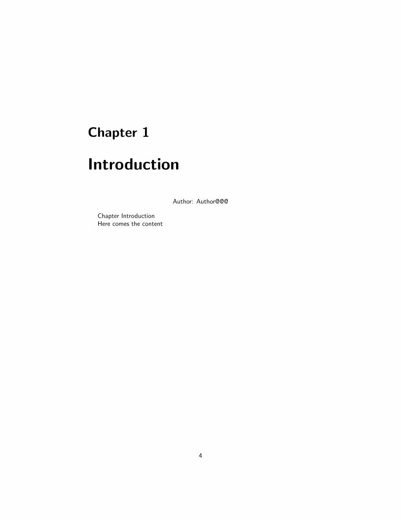
Figure 2.2: The Relation Between Income and Consumption for a Specific Consumer(without numbered axes)
of Y0(dollars) she would consume C0(dollars). We admit that this information isnot very useful. But it becomes useful, if we look at another potential income ofAnne, the income that is represented by Y1. We again go straight up to the graphand then move horizontally to the left until we reach the vertical axis at point C1.Analog to the income/consumption pair labeled with a Y0/C0, we can now saythat if Anne has an income of Y1she will consume C1. Although not obvious, thisprovides valuable information and here is why:
The $-amount behind Y1 must be higher than the one behind Y0. This isbecause Y1is further to the right than Y0and consequently represents a higher income(remember: on the horizontal axis of a diagram we find the large numbers towardsthe right while we find the small numbers to the left). Now we know that an increasein income from Y0to Y1will lead to a change in consumption from C0to C1. We alsoknow that the dollar amount behind C1is bigger than the one behind C0, becauseC1is located higher on the vertical axis than C0(larger numbers are further up onthe vertical axis than lower ones). If we summarize what we found so far, we getan important result about Anne’s behavior.
If Anne’s income increases (from Y0 to Y1), then Anne’s consumptionwill increase (fromC0to C1).

CHAPTER 2. EQUATIONS, DIAGRAMS, AND OTHER TOOLS 9
Now not having numbers at the axis in Figure2.2 becomes an advantage rather thana disadvantage. Because the economic law stated above is not based on specific$-amounts, we can generalize the law and state that any increase in Anne’s incomewill lead to an increase in Anne’s consumption. If we now add the assumption thatAnne is a typical person (we will call this later an representative economic agent)we can state the law derived from Figure 2.2 more general:
If an economic agent’s income increases, then we assume that her/hisconsumption will increase.
Thus the diagram in Figure 2.2 represents an economic law from which we believeit is true. The law shows the behavior of consumers, when income changes. If wecombine the graph in this diagram with other graphs, we can combine assumptionsabout economic agents and then draw conclusions on how this affects economicvariables. We will do this in Chapter 7 when we analyze how demand and supplybehavior (each represented by one graph) together can determine the price in amarket.

CHAPTER 2. EQUATIONS, DIAGRAMS, AND OTHER TOOLS 10
2.2 How Equations Explain Economic Laws
Author: Carsten Lange
Topics that need to be covered because other chapters or sections might buildon them:
� equation expresses an economic law
� interpret the slope parameter economically
Terms that need to be introduced since other chapters or sections might use them:
� specific equations
� general equations
Instead of expressing Anne’s behavior in a diagram we can also use an equation.As there were two types of diagrams in Section 2.1, we can distinguish two typesof equations — specific equations and general equations. Similar to the diagramtypes the first equation type uses numbers, while the second one is more generaland uses parameters instead. The equation
Ci = 0.8Yi + 2000 (2:1)
shows Anne’s consumption behavior in the same way as Figure 2.1 did. We canchoose potential incomes for Anne and find out Anne’s consumption level. Forexample, if Anne had an income of $60,000, her consumption would be:
Ci = 0.8 60, 000 + 2000 = 50, 000
This is the same consumption level we derived for an income of $60,000 whenusing Figure 2.1 and this is not only true for an income of $60,000. It is also truefor any income we choose. Let’s try an income of $160,000.
Ci = 0.8 160, 000 + 2000 = 130, 000
Again, the results derived from equation (2:1) match the results derived fromFigure 2.1. This is because the equation and the graph both describe Anne’s be-havior. In fact we can derive the graph from the equation and vice versa (seeSection 2.3). This means a graph and an equation can express the same law. It isjust as using another language to describe the same fact. However, as we usuallydo not have enough information to express an economic behavior exactly by using adiagram with numbered axes, we do not usually have enough information to expresseconomic behavior with a specific equation such as equation (2:1). Instead we usea more generalized type of equation. For example:
Ci = mYi + b withm > 0 (2:2)

CHAPTER 2. EQUATIONS, DIAGRAMS, AND OTHER TOOLS 11
What can we derive from this equation? First, we can see that the consumptionlevel is determined by the sum of two parts. The first part (mYi) is influencedby the income, while the second part is not. In fact the second part (b) showsthe influence of all other factors on consumption – except income. The influenceof these factors combined can either be positive or negative. Therefore b also canbe positive or negative. Although in most cases we do not know what the exactaccumulated influence of all these factors on consumption is, we assume it is atleast constant. This is called the ceteris paribus condition. Ceteris paribus isLatin and means everything else equal. Note, that it says everything else ratherthan everything. This raises the question, what is allowed to change and whatneeds to be held equal? The answer is that the variables we analyze are allowed tochange, while everything else is not allowed to change. Otherwise, the law that wederived would not hold anymore. In our case income and consumption are allowedto change while everything else is held equal/constant including the parameters man b in equation (2:2).
In Section (2.1) we were able to derive an economic law from the generalizeddiagram (no numbers at the axis) and we can derive exactly the same economic lawfrom equation (2:2). We look at both parts that determine consumption (mYiandb). Obviously, the second part (b) cannot help us a lot, since we do not even knowif it is positive or negative. But the first part (mYi) can help. If we look carefullyat mYi we can see that every income $-amount we use will be multiplied with thesame positive number. Consequently, if income increases, a larger number will bemultiplied with m and the first part of the equation (mYi) becomes bigger. Sincethe second part does not change the right hand side of equation (2:2) becomesbigger meaning that consumption (Ci) which is determined by the right hand sideof equation (2:2) becomes bigger. In short:
If an economic agent’s income increases, then we assume that her/hisconsumption will increase.
Again, the generalized form of the equation and the generalized form of the diagramexpress the same economic behavior. Again, the diagram uses just a different way(a different language if you like) to express the same behavior than the equation.
In order to find out how an economic variable on the right hand side of abehavioral equation influences the variable that is explained, we can use the followingshortened procedure: Look at the parameter (m in our case) in front of the variablewhose influence you want to analyze (Yi in our case). Then find out if the parameteris positive or negative. If it is negative it means, whenever the analyzed variableincreases, the variable on the left hand side of the equation will decrease. If itis positive (like in our case), whenever the analyzed variable increases, so will thevariable on the left hand side of the equation.

CHAPTER 2. EQUATIONS, DIAGRAMS, AND OTHER TOOLS 12
2.3 How Equations are Related to Diagrams
Author: @@@Author
Topics that need to be covered because other chapters or sections might buildon them:
� transform an equation into a diagram
� transform a diagram into an equation
Terms that need to be introduced since other chapters or sections might use them:Here comes the content

CHAPTER 2. EQUATIONS, DIAGRAMS, AND OTHER TOOLS 13
2.4 Discovering Economic Laws with Regression Anal-ysis
Author: @@@Author
Topics that need to be covered because other chapters or sections might buildon them:
� regression line derived from a diagram by eye-balling (mention that OLS cando the same but better). The underlying math will not be explained
� explain how a regression line in a diagram can be transformed into a regressionfunction
� explain how a regression function with 3 independent variables can be trans-formed into one with 1 independent variable using c.p. assumption
Terms that need to be introduced since other chapters or sections might use them:
� regression line
� regression function
�
Here comes the content
CHAPTER 2. EQUATIONS, DIAGRAMS, AND OTHER TOOLS 14
2.5 Different Ways to Calculate Quantitative Change
Author: @@@Author
Topics that need to be covered because other chapters or sections might buildon them:
� difference between absolute change and relative change of an economic vari-able
� using the traditional way to calculate percentage or relative change
� using the midpoint formula to calculate percentage or relative change
� equivalence of expressing percentage change as 5% or as 0.05
Terms that need to be introduced since other chapters or sections might use them:
� absolute change
� relative change
� percentage change
� midpoint formula
Here comes the content

CHAPTER 2. EQUATIONS, DIAGRAMS, AND OTHER TOOLS 15
2.6 Videos, Simulations, and other Internet Resources
This section will be automatically generated from a database and Instructors canlater pick which content they liek to be included.
Links to Videos, Simulations, audio files, possibly to Wikipedia for keyterms willbe ordered by subsection and then by type
Instructional Videos
Each video covers a selected concept of content.
For Section: 2.1 How Diagrams Explain Economic Laws
How to use a Diagram that has no Numbered Axisby Carsten Lange
Shows how an economic law or behavior can be displayed in a diagram. It also usesan example on how to use such a diagram.Click here to start ID:2 Click here to rate
How to use a Diagram that has a Numbered Axisby Carsten Lange
Shows how an economic law or behavior can be displayed in a diagram. It also usesan example on how to use such a diagram.Click here to start ID:3 Click here to rate
Short Videos
Short videos provide students with five minutes videos about key techniques andconcepts. In order to keep the videos short, only the most important aspects are cov-ered. However, the topics covered are techniques and concepts that many studentsstruggle with.
Diagrams and Economic Laws, Part 2by Carsten Lange
The video explains how to work with a diagram such as a demand diagram. It alsopoints out why each graph in a in a diagram represents an economic law. Part 2covers diagrams without numbered axis. This type of diagram is very comon ineconomics and many students struggle with its interpretation.Click here to start ID:28 Click here to rate

CHAPTER 2. EQUATIONS, DIAGRAMS, AND OTHER TOOLS 16
Diagrams and Economic Laws, Part 1by Carsten Lange
The video explains how to work with a diagram such as a demand diagram. It alsopoints out why each graph in a in a diagram represents an economic law. Part 1covers diagrams with numbered axis.Click here to start ID:29 Click here to rate

CHAPTER 2. EQUATIONS, DIAGRAMS, AND OTHER TOOLS 17
2.7 End of Chapter Questions
Author: @@@Author
End of Chapter Questions are not part of the first edition.In the second edition they will be generated from a database depending on the
instructors choice.

Chapter 3
Markets
Author: @@@Author
Topics that need to be covered because other chapters or sections might buildon them:
� explain the concept of a market in general
� importance and functions of markets
Then give a brief overview of the Chapter:
� keep it short
� write in the “you will learn” style to ensure consistency in the book
� list what the reader will learn with references to the sections.
� emphasize the keywords for the learning goals (see Chapter Government In-terventions Intro for examples)
Here comes content
18

CHAPTER 3. MARKETS 19
3.1 Competitive Markets
Author:
Topics that need to be covered because other chapters or sections might buildon them:
� general description of a competitive market
� criteria for a competitive market together with reasons why they are important
� explanation why both suppliers and consumers are price takers
Topics that should not be covered here because they are covered in another chapter:
� theory of competitive markets
Here comes content

CHAPTER 3. MARKETS 20
3.2 Monopoly Markets
Author: @@@Author
Topics that need to be covered because other chapters or sections might buildon them:
� general description of a monopoly market
� criterion for a monopoly market
� a monopolist can set the price or the quantity but not both
Topics that should not be covered here because they are covered in another chapter:
� theory of monopoly
Here comes content
CHAPTER 3. MARKETS 21
3.3 Oligopoly Markets
Author: @@@Author
Topics that need to be covered because other chapters or sections might buildon them:
� general description of a oligopoly market
� criterion for a oligopoly market
Topics that should not be covered here because they are covered in another chapter:
� theory of oligopoly
Here comes content

CHAPTER 3. MARKETS 22
3.4 Other Market Types
Author: Author@@@Author
Topics that need to be covered because other chapters or sections might buildon them:
� general description and criteria for other market forms such as
• monopsony
• imperfect competition
• monopolistic competition
Topics that should not be covered here because they are covered in another chapter:
� theories for the above covered markets
Here comes content

CHAPTER 3. MARKETS 23
3.5 Videos, Simulations, and other Internet Resources
Author: @@@Author
This section will be automatically generated from a database and Instructorscan later pick which content they liek to be included.
Links to Videos, Simulations, audio files, possibly to Wikipedia for keyterms willbe ordered by subsection and then by type
Key Terms to Remember
Find an explanation of important key terms on the Internet.
For Section: 3 Markets
Introduction to Marketsby Wikipedia
Gives a basic definition of a market.Click here to start ID:1 Click here to rate
Instructional Videos
Each video covers a selected concept of content.
For Section: ?? Competitive Markets
Introduction to the Analysis of Marketsby Carsten Lange
Defines markets and their functions and explains simplifying assumptions commonlymade in market analysis.Click here to start ID:4 Click here to rate
Price Determinationby Carsten Lange
Explains why price must be jointly explained by supply and demand and gives anexample for how prices are determined in a competitive market.Click here to start ID:6 Click here to rate

CHAPTER 3. MARKETS 24
3.6 End of Chapter Questions
Author: @@@Author
End of Chapter Questions are not part of the first edition.In the second edition they will be generated from a database depending on the
instructors choice.

Chapter 4
Introduction to the DemandConcept
Author: Carsten Lange
Topics that need to be covered because other chapters or sections might buildon them:
� .What is demand
� Demand vs. Demanded Quantity
� Individual demand vs. Market demand (just the basics, it will be covered inmore detail later)
Topics that should not be covered here because they are covered in another chapter:
� Derive Market demand from Individual demand wll be covered in anotherChapter
Terms that need to be introduced since other chapters or sections might use them:
� Demand
� Demanded quantity
� Individual Demand
� market demand
Here comes content
25

CHAPTER 4. INTRODUCTION TO THE DEMAND CONCEPT 26
4.1 Determinants of Demand
Author: @@@Author
Concepts to be covered:
� Price (short because there is a section for price)
� Income, Wealth, Price of another good
� Difficulty to how to deal with so many determinants
Concepts that need not to be covered because they are covered elsewhere:
� Price (just briefly reiterate)
Here comes the content
CHAPTER 4. INTRODUCTION TO THE DEMAND CONCEPT 27
4.2 Relationship between Demanded Quantity andPrice
Author: @@@Author
Concepts to cover:
� If all demand determinants except price are assumed to be constant, thenonly price will influence the demanded quantity
� all other demand determinants are assumed to be constant does no mean theyare actually constant.
� c.p. condition
� Demanded Quantity vs. Price (reiterate)
� Law of demand (verbally)
� Demand function
� Demand schedule
� Demand/Price Diagram
Concepts that need not to be covered because they are covered elsewhere:
� Shifting Curves
� How to work with demand curve
Here comes the content

CHAPTER 4. INTRODUCTION TO THE DEMAND CONCEPT 28
4.3 Demand Curve
Author: @@@Author
Topics that need to be covered because other chapters or sections might buildon them:
� .How the demand curve assigns demanded quantity to prices
� Direction of the argument goes always from Price to quantity demanded neverthe other way. Argument always starts at the price axis
� Independent vs. dependent variable
� Demand curve represents demand behavio and thus “Demand”
Topics that should not be covered here because they are covered in another chapter:
� .
Terms that need to be introduced since other chapters or sections might use them:
� .Demand curve
� Independent vs. dependent variable
� direction of causality
Here comes content

CHAPTER 4. INTRODUCTION TO THE DEMAND CONCEPT 29
4.4 Shifts of the Demand Curve
Author: @@@Author
Topics that need to be covered because other chapters or sections might buildon them:
� .Demad curve was constructed under the assumption that all other demanddeterminants are constant, if one of them changes the demand curve is notvalid anymore.
� When will the new demand curve shift to the right and when to the left
� Most times parallel shifts are assumed for simplicity but the curve does nothave to shift parallel
Topics that should not be covered here because they are covered in another chapter:
� .demand equation
Terms that need to be introduced since other chapters or sections might use them:
� .Demand curve shifts
Here comes content
CHAPTER 4. INTRODUCTION TO THE DEMAND CONCEPT 30
4.5 Demand Equation
Author: @@@Author
Topics that need to be covered because other chapters or sections might buildon them:
� .Express Demanded quantity as function of multiple variables.
� Show that if all other variables other than the price are constant, their influ-ence collapse to constant
� Show that if one (or more) of the variables that were assumed to be constantchanges the constant changes. Thus the curve shifts
Topics that should not be covered here because they are covered in another chapter:
� .
Terms that need to be introduced since other chapters or sections might use them:
� .Constant
� Demand Function
Here comes content

CHAPTER 4. INTRODUCTION TO THE DEMAND CONCEPT 31
4.6 Change of the Demand Equation
Author: @@@Author
This section will likely be very short. The content is covered in its own sectionto give instructors later the ability to omit the section
Topics that need to be covered because other chapters or sections might buildon them:
� Express the demand equation with multi variables
� Show that if a variable that is supposed to be constant changes than theconstant of the demand-price equation will change
� Mention that positive changes of the constant will shift the related demandcurve to the right and vice versa.
Topics that should not be covered here because they are covered in another chapter:
� .First derivative (will be verbally covered in Elasticity Chapter)
Terms that need to be introduced since other chapters or sections might use them:
� .Constant
Here comes the content

CHAPTER 4. INTRODUCTION TO THE DEMAND CONCEPT 32
4.7 Videos, Simulations, and other Internet Resources
This section will be automatically generated from a database and Instructors canlater pick which content they like to be included.
Links to Videos, Simulations, audio files, possibly to Wikipedia for keyterms willbe ordered by subsection and then by type
Instructional Videos
Each video covers a selected concept of content.
For Section: 4.1 Determinants of Demand
Individual Demand Basicsby Carsten Lange
Covers the basic determinants of demand and explains normal versus inferior andsubstitute versus complementary goods.Click here to start ID:7 Click here to rate
For Section: 4.2 Relationship between Demanded Quantity and Price
Quantity Demanded and Individual’s Responses to Priceby Carsten Lange
Defines ”quanty demanded” and explains how individual’s demand responds to price.Click here to start ID:8 Click here to rate
For Section: 4.3 Demand Curve
Demand Curve Derivation Basicsby Carsten Lange
Covers the derivation of a demand curve using a class experiment for coke demandat varying price levels.Click here to start ID:5 Click here to rate

CHAPTER 4. INTRODUCTION TO THE DEMAND CONCEPT 33
The Law of Demandby Carsten Lange
Explains the law of demand as the inverse relationship between price and quantityand show how this is reflected in a downward-sloping demand curve.Click here to start ID:9 Click here to rate
For Section: 4.4 Shifts of the Demand Curve
Shifts in the Demand Curveby Carsten Lange
Explains shifts in demand versus changes in quantity demanded and differentiatesbetween direct and indirect determinants of demand.Click here to start ID:12 Click here to rate
CHAPTER 4. INTRODUCTION TO THE DEMAND CONCEPT 34
4.8 End of Chapter Questions
Author: @@@Author
End of Chapter Questions are not part of the first edition.In the second edition they will be generated from a database depending on the
instructors choice.

Chapter 5
Introduction to the SupplyConcept
Author: Author@@@
Topics that need to be covered because other chapters or sections might buildon them:
� .What is supply
� supply vs. supplied Quantity
� Firm supply vs. market supply (just the basics, it will be covered in moredetail later)
Topics that should not be covered here because they are covered in another chapter:
� Derive Market supply from Individual supply will be covered in another Chap-ter
Terms that need to be introduced since other chapters or sections might use them:
� supply
� supplied quantity
� firm supply
� market supply
Here comes content
35

CHAPTER 5. INTRODUCTION TO THE SUPPLY CONCEPT 36
5.1 Determinants of Supply
Author: @@@Author
Concepts to be covered:
� Price (short because there is a section for price)
� Cost (labor, material, tax levied to the product)
� Difficulty to how to deal with so many determinants
Concepts that need not to be covered because they are covered elsewhere:
� Price (just briefly reiterate)
Here comes the content

CHAPTER 5. INTRODUCTION TO THE SUPPLY CONCEPT 37
5.2 Supplied Quantity and Price
Author: @@@Author
Concepts to cover:
� If all supply determinants except price are assumed to be constant, then onlyprice will influence the supplied quantity
� all other supply determinants are assumed to be constant does no mean theyare actually constant.
� c.p. condition
� Supplied Quantity vs. Price (reiterate)
� Law of supply (verbally; explain why higher prices increase supply)
� Supply function
� Supply schedule
� Supply/Price Diagram
Concepts that need not to be covered because they are covered elsewhere:
� Shifting Curves
� How to work with supply curve
Here comes the content

CHAPTER 5. INTRODUCTION TO THE SUPPLY CONCEPT 38
5.3 Supply Curve
Author: @@@Author
Topics that need to be covered because other chapters or sections might buildon them:
� .How the supply curve assigns supplied quantity to prices
� Direction of the argument goes always from Price to quantity supplied; neverthe other way. Argument always starts at the price axis
� Independent vs. dependent variable
� Supply curve represents supply behavior and thus “Supply”
Topics that should not be covered here because they are covered in another chapter:
� .
Terms that need to be introduced since other chapters or sections might use them:
� .Supply curve
� Independent vs. dependent variable
� direction of causality
Here comes the content

CHAPTER 5. INTRODUCTION TO THE SUPPLY CONCEPT 39
5.4 Shifts of the Supply Curve
Author: @@@Author
Topics that need to be covered because other chapters or sections might buildon them:
� .Demad curve was constructed under the assumption that all other supplydeterminants are constant, if one of them changes the supply curve is notvalid anymore.
� When will the new supply curve shift to the right and when to the left
� Most times parallel shifts are assumed for simplicity but the curve does nothave to shift parallel
Topics that should not be covered here because they are covered in another chapter:
� .supply equation
Terms that need to be introduced since other chapters or sections might use them:
� .Supply curve shifts
Here comes the content

CHAPTER 5. INTRODUCTION TO THE SUPPLY CONCEPT 40
5.5 The Supply Equation
Author: @@@Author
Topics that need to be covered because other chapters or sections might buildon them:
� .Express supplied quantity as function of multiple variables.
� Show that if all other variables other than the price are constant, their influ-ence collapse to constant
� Show that if one (or more) of the variables that were assumed to be constantchanges the constant changes. Thus the curve shifts
Topics that should not be covered here because they are covered in another chapter:
� .
Terms that need to be introduced since other chapters or sections might use them:
� .Constant
� Supply Function
Here comes the content
CHAPTER 5. INTRODUCTION TO THE SUPPLY CONCEPT 41
5.6 Change of the Supply Equation
Author: @@@Author
This section will likely be very short. The content is covered in its own sectionto give instructors later the ability to omit the section
Topics that need to be covered because other chapters or sections might buildon them:
� Express the supply equation with multi variables
� Show that if a variable that is supposed to be constant changes than theconstant of the supply-price equation will change
� Mention that positive changes of the constant will shift the related supplycurve to the right and vice versa.
Topics that should not be covered here because they are covered in another chapter:
� .First derivative (will be verbally covered in Elasticity Chapter)
Terms that need to be introduced since other chapters or sections might use them:
� .Constant
Here comes the content

CHAPTER 5. INTRODUCTION TO THE SUPPLY CONCEPT 42
5.7 Videos, Simulations, and other Internet Resources
This section will be automatically generated from a database and Instructors canlater pick which content they like to be included.
Links to Videos, Simulations, audio files, possibly to Wikipedia for keyterms willbe ordered by subsection and then by type
Instructional Videos
Each video covers a selected concept of content.
For Section: 5.1 Determinants of Supply
Basic Determinants of Supplyby Carsten Lange
Gives an overview of direct and indirect determinants of supply (price, cost, etc).Click here to start ID:13 Click here to rate
For Section: 5.2 Supplied Quantity and Price
The Law of Supplyby Carsten Lange
Explains the law of supply and individual rationale in choosing quantity supplied.Also covers derivation of individual and market supply curves.Click here to start ID:14 Click here to rate
For Section: 5.3 Supply Curve
Quantitative Approach to Deriving Market Supplyby Carsten Lange
Explains how to derive market supply from individual supply curves using a quanti-tative example in Excel.Click here to start ID:15 Click here to rate
For Section: 5.4 Shifts of the Supply Curve

CHAPTER 5. INTRODUCTION TO THE SUPPLY CONCEPT 43
Shifts in the Supply Curveby Carsten Lange
Reviews the determinants of supply, lists shifters of supply, and explains how to usesupply if the price changes.Click here to start ID:16 Click here to rate
Short Videos
Short videos provide students with five minutes videos about key techniques andconcepts. In order to keep the videos short, only the most important aspects are cov-ered. However, the topics covered are techniques and concepts that many studentsstruggle with.
For Section: 5.2 Supplied Quantity and Price
The Law of Suppy - Why does a price increase increases production?by Carsten Lange
The video explains in an intuitive way, why costs are crucial to explain that priceincreases for a good usually leads to more production in a market. This is alsorefered to as the Law of Supply.Click here to start ID:30 Click here to rate

CHAPTER 5. INTRODUCTION TO THE SUPPLY CONCEPT 44
5.8 End of Chapter Questions
Author: @@@Author
End of Chapter Questions are not part of the first edition.In the second edition they will be generated from a database depending on the
instructors choice.

Chapter 6
Aggregating Individuals’ andFirms’ Demand and Supply
Author: @@@Author
Topics to be covered here.Here comes the content
45
CHAPTER 6. AGGREGATING INDIVIDUALS’ AND FIRMS’ DEMAND AND SUPPLY 46
6.1 Aggregating Individuals’ and Firms’ Demand andSupply Curves
Author: @@@Author
Insert topics to be covered here.Here comes content
CHAPTER 6. AGGREGATING INDIVIDUALS’ AND FIRMS’ DEMAND AND SUPPLY 47
6.2 The Effect of Market Entrance and Exit on Mar-ket Demand and Supply Curve
Author: @@@Author
Insert topics to be covered here.Here comes content

CHAPTER 6. AGGREGATING INDIVIDUALS’ AND FIRMS’ DEMAND AND SUPPLY 48
6.3 Aggregating Individuals’ and Firms’ Demand andSupply Equations
Author: @@@Author
Insert topics to be covered here.Here comes content

CHAPTER 6. AGGREGATING INDIVIDUALS’ AND FIRMS’ DEMAND AND SUPPLY 49
6.4 The Effect of Market Entrance and Exit on Mar-ket Demand and Supply Equations
Author: @@@Author
Insert topics to be covered here.Here comes content
CHAPTER 6. AGGREGATING INDIVIDUALS’ AND FIRMS’ DEMAND AND SUPPLY 50
6.5 Videos, Simulations, and other Internet Resources
This section will be automatically generated from a database and Instructors canlater pick which content they like to be included.
Links to Videos, Simulations, audio files, possibly to Wikipedia for keyterms willbe ordered by subsection and then by type
Instructional Videos
Each video covers a selected concept of content.
For Section: 6.1 Aggregating Individuals’ and Firms’ Demand and Supply Curves
Deriving a Market Demand Curveby Carsten Lange
Walks through an empirical approach (classroom example) to deriving market de-mand from individual demand, using Excel.Click here to start ID:11 Click here to rate
Market Demandby Carsten Lange
Covers differentiation between individual and market demand, how to aggregateindividual demand into market demand, and how to derive a demand schedule fromsample data.Click here to start ID:10 Click here to rate

Chapter 7
Equilibrium Concept andEconomic Analysis
Author: @@@Author
Insert topics to be covered here.Here comes the content
51
CHAPTER 7. EQUILIBRIUM CONCEPT AND ECONOMIC ANALYSIS 52
7.1 Finding an Equilibrium in a Demand and SupplyDiagram
Author: @@@Author
Insert topics to be covered here.Here comes content

CHAPTER 7. EQUILIBRIUM CONCEPT AND ECONOMIC ANALYSIS 53
7.2 Effects of Shifting Demand and Supply Curveson the Equilibrium
Author: @@@Author
Insert topics to be covered here.Here comes content
CHAPTER 7. EQUILIBRIUM CONCEPT AND ECONOMIC ANALYSIS 54
7.3 Calculating Equilibrium Price and Quantity
Author: Author@@@
7.3.1 Calculating Equilibrium Price and Quantity from De-mand and Supply Equations
Here comes content
CHAPTER 7. EQUILIBRIUM CONCEPT AND ECONOMIC ANALYSIS 55
7.4 Calculating Changes of Equilibrium Price andQuantity
Author: @@@Author
Calculating Change of Equilibrium Price and Quantity When Equation Parame-ters Change
Here comes content
CHAPTER 7. EQUILIBRIUM CONCEPT AND ECONOMIC ANALYSIS 56
7.5 Videos, Simulations, and other Internet Resources
This section will be automatically generated from a database and Instructors canlater pick which content they like to be included.
Links to Videos, Simulations, audio files, possibly to Wikipedia for keyterms willbe ordered by subsection and then by type
Instructional Videos
Each video covers a selected concept of content.
For Section: 7.1 Finding an Equilibrium in a Demand and Supply Diagram
Market Equilibriumby Carsten Lange
Covers how prices are determined at equilibrium price and quantity, as well as theadaptation (”invisible hand”) process.Click here to start ID:17 Click here to rate
For Section: 7.2 Effects of Shifting Demand and Supply Curves on the Equilibrium
Market Equilibrium in Changing Market Conditionsby Carsten Lange
Uses the supply and demand diagram to analyze changes in market conditionsutilizing a ”five-step” approach.Click here to start ID:18 Click here to rate
Short Videos
Short videos provide students with five minutes videos about key techniques andconcepts. In order to keep the videos short, only the most important aspects are cov-ered. However, the topics covered are techniques and concepts that many studentsstruggle with.
For Section: 7.1 Finding an Equilibrium in a Demand and Supply Diagram

CHAPTER 7. EQUILIBRIUM CONCEPT AND ECONOMIC ANALYSIS 57
Finding Demanded and Supplied Quantities in a Market Equilibrium Diagram, Part 1by Carsten Lange
The video helpd students to find demanded and supplied quantities simultaneouslyfor a given price in a market diagram. This skill is important for many applicationsincluding price ceilings and floors as well as stability analysis of an equilibrium. Thevideo provides a step by step approach to find and compare supplied and demandedquantities. Part 1 uses a diagram with numbered axis.Click here to start ID:31 Click here to rate
Equilibrium and Stability - Why can we be so sure that most markets reach the equilibrium price and quantity?by Carsten Lange
The videos shows briefly how stuents can find an equilibrium in a diagram. After-wards, two examples are used to show that markets tend to reach the equilibrium.This is important to understand, because performing analysis with demand and sup-ply diagrams becomes much easier when we can assume that a market reaches itsequilibrium by itself.Click here to start ID:33 Click here to rate
CHAPTER 7. EQUILIBRIUM CONCEPT AND ECONOMIC ANALYSIS 58
7.6 End of Chapter Questions
Author: @@@AuthorAuthor
Insert topics to be covered here.Here comes contentCurrently not determined how to deal with those. Maybe through an external
Database.

Chapter 8
Economic Analysis Using theDemand-Supply Concept
Author: @@@Author
This Chapter will show in the setting of a competitive market how the concepts ofdemand, supply, and equilibrium can be used to solve real world problems.Although in the real world no market is perfectly competitive, many markets are atleast similar to competitive markets. This means that what we derive here for aperfectly competitive market can be applied in the real world to markets that aremostly competitive. Chapters ?? and ?? will later show, how the results change ifwe analyze markets that are more similar to monopolistic or oligopolistic markets.
59

Chapter 9
Elasticity
Author: @@@Author
Give a brief overview of the Chapter:
� keep it short
� write in the “you will learn” style to ensure consistency in the book
� list what the reader will learn with references to the sections.
� emphasize the keywords for the learning goals (see Chapter Government In-terventions Intro for examples)
Here comes the content
60
CHAPTER 9. ELASTICITY 61
9.1 Elasticity - Definition, Measurement, and Dif-ferences with Slope
Author: @@@Author
� Show how elasticity is measured in general
� introduce mid point formula
� difference between slope and elasticity
� introduce: elastic, inelastic, perfectly inelastic, perfectly elastic
Here comes the content

CHAPTER 9. ELASTICITY 62
9.2 Price Elasticity
Author: @@@Author
Short introduction
9.2.1 Price Elasticity of Demand
� Meaning of price elasticity of demand
� Definition of price elasticity of demand
� How to calculate price elasticity o demand
� Why is price elasticity of demand always negative
Here comes the content
9.2.2 Price Elasticity of Supply
� Meaning of price elasticity of supply
� Definition of price elasticity of supply
� How to calculate price elasticity o supply
� Why is price elasticity of demand always positive
Here comes the content
9.2.3 How Price Elasticity Impacts Price and Quantity Changes
Use diferent market diagrams to show how a given shock leads to bigger and smallermovementent in price depnding on the elasticity of demand and supply
Here comes the content
CHAPTER 9. ELASTICITY 63
9.3 Income Elasticity of Demand
Author: @@@Author
Possibly a brief introduction or leave empty
9.3.1 Definition
� Definition of income elasticity
� How income elasticity is calculated (use midpoint formula rather than calculusformula)
Here comes the content
9.3.2 Normal and Inferior Goods
� Verbal explanation and definition of inferior and normal goods
� show why inferior goods have a negative and normal goods have a positiveincome elasticity
� why are income elasticities important in real world
Here comes the content

CHAPTER 9. ELASTICITY 64
9.4 Cross Price Elasticity of Demand
Author: @@@Author
Short Intro
9.4.1 Definition
� Meaning of price cross price elasticity of demand
� Definition of price cross price elasticity of demand
� How to calculate cross price price elasticity of demand (midpoint formula)
Here comes the content
9.4.2 Substitutes and Complements
� Introduce Substitute and Complements
� Why is price cross price elasticity of demand always negative for complements
� Why is price cross price elasticity of demand always positive for substitutes
� Discuss a price change of a complement and its effects on demand, equilibriumprice of the other good using a market diagram
� Discuss a price change of a substitute and its effects on demand, equilibriumprice of the other good using a market diagram
Here comes the content

CHAPTER 9. ELASTICITY 65
9.5 Videos, Simulations, and other Internet Resources
This section will be automatically generated from a database and Instructors canlater pick which content they like to be included.
Links to Videos, Simulations, audio files, possibly to Wikipedia for keyterms willbe ordered by subsection and then by type
Instructional Videos
Each video covers a selected concept of content.
For Section: 9 Elasticity
Elasticity and Its Applicationby Carsten Lange
Defines price elasticity and differentiates between elastic and inelastic goods.Click here to start ID:24 Click here to rate
For Section: 9.2 Price Elasticity
Price Elasticity of Demandby Carsten Lange
Explains why price elasticity of demand is always negative and shows how to measureprice elasticity when quantity demanded changes, both quantitatively and diagra-matically. Also shows under which circumstances price elasticity is low or high andgives some important ranges for elasticity of demand.Click here to start ID:25 Click here to rate

CHAPTER 9. ELASTICITY 66
Price Elasticity of Demandby Carsten Lange
Explains why price elasticity of demand is always negative and shows how to measureprice elasticity when quantity demanded changes, both quantitatively and diagra-matically. Also shows under which circumstances price elasticity is low or high andgives some important ranges for elasticity of demand.Click here to start ID:25 Click here to rate
Price Elasticity and Revenuesby Carsten Lange
Explains the interrelation between price elasticity and revenues when quantity ischanged.Click here to start ID:26 Click here to rate
Price Elasticity and Revenuesby Carsten Lange
Explains the interrelation between price elasticity and revenues when quantity ischanged.Click here to start ID:26 Click here to rate
Price Elasticity and Revenuesby Carsten Lange
Explains the interrelation between price elasticity and revenues when quantity ischanged.Click here to start ID:26 Click here to rate
Price Elasticity and Revenuesby Carsten Lange
Explains the interrelation between price elasticity and revenues when quantity ischanged.Click here to start ID:26 Click here to rate
CHAPTER 9. ELASTICITY 67
Price Elasticity of Supplyby Carsten Lange
Defines price elasticity of supply and gives some circumstances under which it maybe low or high. Cross-price and income elasticityClick here to start ID:27 Click here to rate
Price Elasticity of Supplyby Carsten Lange
Defines price elasticity of supply and gives some circumstances under which it maybe low or high. Cross-price and income elasticityClick here to start ID:27 Click here to rate
Price Elasticity of Supplyby Carsten Lange
Defines price elasticity of supply and gives some circumstances under which it maybe low or high. Cross-price and income elasticityClick here to start ID:27 Click here to rate
Price Elasticity of Supplyby Carsten Lange
Defines price elasticity of supply and gives some circumstances under which it maybe low or high. Cross-price and income elasticityClick here to start ID:27 Click here to rate
Price Elasticity and Revenuesby Carsten Lange
Explains the interrelation between price elasticity and revenues when quantity ischanged.Click here to start ID:26 Click here to rate
Price Elasticity and Revenuesby Carsten Lange
Explains the interrelation between price elasticity and revenues when quantity ischanged.Click here to start ID:26 Click here to rate
Price Elasticity and Revenuesby Carsten Lange
Explains the interrelation between price elasticity and revenues when quantity ischanged.Click here to start ID:26 Click here to rate

CHAPTER 9. ELASTICITY 68
Price Elasticity and Revenuesby Carsten Lange
Explains the interrelation between price elasticity and revenues when quantity ischanged.Click here to start ID:26 Click here to rate
Price Elasticity of Demandby Carsten Lange
Explains why price elasticity of demand is always negative and shows how to measureprice elasticity when quantity demanded changes, both quantitatively and diagra-matically. Also shows under which circumstances price elasticity is low or high andgives some important ranges for elasticity of demand.Click here to start ID:25 Click here to rate

CHAPTER 9. ELASTICITY 69
Price Elasticity of Supplyby Carsten Lange
Defines price elasticity of supply and gives some circumstances under which it maybe low or high. Cross-price and income elasticityClick here to start ID:27 Click here to rate
Price Elasticity of Supplyby Carsten Lange
Defines price elasticity of supply and gives some circumstances under which it maybe low or high. Cross-price and income elasticityClick here to start ID:27 Click here to rate
Price Elasticity of Supplyby Carsten Lange
Defines price elasticity of supply and gives some circumstances under which it maybe low or high. Cross-price and income elasticityClick here to start ID:27 Click here to rate
Price Elasticity of Supplyby Carsten Lange
Defines price elasticity of supply and gives some circumstances under which it maybe low or high. Cross-price and income elasticityClick here to start ID:27 Click here to rate
Price Elasticity of Supplyby Carsten Lange
Defines price elasticity of supply and gives some circumstances under which it maybe low or high. Cross-price and income elasticityClick here to start ID:27 Click here to rate
Price Elasticity of Supplyby Carsten Lange
Defines price elasticity of supply and gives some circumstances under which it maybe low or high. Cross-price and income elasticityClick here to start ID:27 Click here to rate
Price Elasticity of Supplyby Carsten Lange
Defines price elasticity of supply and gives some circumstances under which it maybe low or high. Cross-price and income elasticityClick here to start ID:27 Click here to rate

CHAPTER 9. ELASTICITY 70
Price Elasticity of Supplyby Carsten Lange
Defines price elasticity of supply and gives some circumstances under which it maybe low or high. Cross-price and income elasticityClick here to start ID:27 Click here to rate
Price Elasticity and Revenuesby Carsten Lange
Explains the interrelation between price elasticity and revenues when quantity ischanged.Click here to start ID:26 Click here to rate
Price Elasticity and Revenuesby Carsten Lange
Explains the interrelation between price elasticity and revenues when quantity ischanged.Click here to start ID:26 Click here to rate
Price Elasticity and Revenuesby Carsten Lange
Explains the interrelation between price elasticity and revenues when quantity ischanged.Click here to start ID:26 Click here to rate
Price Elasticity and Revenuesby Carsten Lange
Explains the interrelation between price elasticity and revenues when quantity ischanged.Click here to start ID:26 Click here to rate
Price Elasticity of Demandby Carsten Lange
Explains why price elasticity of demand is always negative and shows how to measureprice elasticity when quantity demanded changes, both quantitatively and diagra-matically. Also shows under which circumstances price elasticity is low or high andgives some important ranges for elasticity of demand.Click here to start ID:25 Click here to rate
CHAPTER 9. ELASTICITY 71
Price Elasticity of Demandby Carsten Lange
Explains why price elasticity of demand is always negative and shows how to measureprice elasticity when quantity demanded changes, both quantitatively and diagra-matically. Also shows under which circumstances price elasticity is low or high andgives some important ranges for elasticity of demand.Click here to start ID:25 Click here to rate
Price Elasticity and Revenuesby Carsten Lange
Explains the interrelation between price elasticity and revenues when quantity ischanged.Click here to start ID:26 Click here to rate
Price Elasticity and Revenuesby Carsten Lange
Explains the interrelation between price elasticity and revenues when quantity ischanged.Click here to start ID:26 Click here to rate
Price Elasticity and Revenuesby Carsten Lange
Explains the interrelation between price elasticity and revenues when quantity ischanged.Click here to start ID:26 Click here to rate
CHAPTER 9. ELASTICITY 72
Price Elasticity and Revenuesby Carsten Lange
Explains the interrelation between price elasticity and revenues when quantity ischanged.Click here to start ID:26 Click here to rate
Price Elasticity of Supplyby Carsten Lange
Defines price elasticity of supply and gives some circumstances under which it maybe low or high. Cross-price and income elasticityClick here to start ID:27 Click here to rate
Price Elasticity of Supplyby Carsten Lange
Defines price elasticity of supply and gives some circumstances under which it maybe low or high. Cross-price and income elasticityClick here to start ID:27 Click here to rate
Price Elasticity of Supplyby Carsten Lange
Defines price elasticity of supply and gives some circumstances under which it maybe low or high. Cross-price and income elasticityClick here to start ID:27 Click here to rate
Price Elasticity of Supplyby Carsten Lange
Defines price elasticity of supply and gives some circumstances under which it maybe low or high. Cross-price and income elasticityClick here to start ID:27 Click here to rate
Price Elasticity of Demandby Carsten Lange
Explains why price elasticity of demand is always negative and shows how to measureprice elasticity when quantity demanded changes, both quantitatively and diagra-matically. Also shows under which circumstances price elasticity is low or high andgives some important ranges for elasticity of demand.Click here to start ID:25 Click here to rate
CHAPTER 9. ELASTICITY 73
Price Elasticity of Demandby Carsten Lange
Explains why price elasticity of demand is always negative and shows how to measureprice elasticity when quantity demanded changes, both quantitatively and diagra-matically. Also shows under which circumstances price elasticity is low or high andgives some important ranges for elasticity of demand.Click here to start ID:25 Click here to rate
Short Videos
Short videos provide students with five minutes videos about key techniques andconcepts. In order to keep the videos short, only the most important aspects are cov-ered. However, the topics covered are techniques and concepts that many studentsstruggle with.
For Section: 9.1 Measuring Slope vs. Elasticity
Calculating Percentage Change - Traditional Formula vs. Midpoint Formulaby Carsten Lange
The video demonstrates the shortcomings of calculating percentage change with thetraditional fomula taught in highschool. Then it introduces the midpoint formula forcalculating percentage change as an alternative that overcomes these shortcomings.Click here to start ID:35 Click here to rate

CHAPTER 9. ELASTICITY 74
9.6 End of Chapter Questions
Author: @@@Author
End of Chapter Questions are not part of the first edition.In the second edition they will be generated from a database depending on the
instructors choice.

Chapter 10
Measuring Welfare
Author: @@@Author
Insert topics to be covered here.Here comes the content
75

CHAPTER 10. MEASURING WELFARE 76
10.1 Consumer Surplus Concept
Author: @@@Author
Insert topics to be covered here.Here comes content

CHAPTER 10. MEASURING WELFARE 77
10.2 Producer Surplus Concept
Author: @@@Author
Insert topics to be covered here.Here comes content
CHAPTER 10. MEASURING WELFARE 78
10.3 Measuring Welfare in a Competitive Market
Author: @@@Author
Insert topics to be covered here.Here comes content

CHAPTER 10. MEASURING WELFARE 79
10.4 Short Comings of the Consumer-Producer Sur-plus Concept
Author: @@@Author
Insert topics to be covered here.Here comes content
CHAPTER 10. MEASURING WELFARE 80
10.5 Videos, Simulations, and other Internet Re-sources
Author: @@@Author
This section will be automatically generated from a database and Instructorscan later pick which content they like to be included.
Links to Videos, Simulations, audio files, possibly to Wikipedia for key termswill be ordered by subsection and then by type
Here comes content

CHAPTER 10. MEASURING WELFARE 81
10.6 End of Chapter Questions
Author: @@@Author
End of Chapter Questions are not part of the first edition.In the second edition they will be generated from a database depending on the
instructors choice.

Chapter 11
Government Interventions
Author: Craig Kerr
Chapter IntroductionIn previous chapters, we have observed that perfectly competitive markets maxi-
mize total welfare without any outside influence from governments. In this chapter,we will look at how perfectly competitive markets are affected by two tools govern-ments have at their disposal, price controls and taxes. By the end of the chapter,the reader should understand:
1. How price controls affect welfare and the allocation of goods and servicesin competitive markets (see Section 11.1).
2. How taxes affect welfare and the allocation of goods and services in com-petitive markets (see Sections 11.2 and 11.4)..
3. That it does not matter whether producers or consumers are taxed whenconsidering the tax burden, welfare, or the allocation of goods and services incompetitive markets (see Section 11.3).
4. What determines how the tax burden is shared between consumers andproducers (see Section 11.3).
82

CHAPTER 11. GOVERNMENT INTERVENTIONS 83
11.1 Price Controls
Author: Craig Kerr
� Explain ceiling
� Explain floor
� Explain binding and not-binding ceiling (floor)
� Show consequences in market diagram for binding ceiling. Excess demand.Explain social consequences such as waste and black markets
� Show consequences in market diagram for binding floor. Excess supply. Ex-plain social consequences such as waste and over-production
� Welfare consequences can be covered but don’t have too.
The prices of gasoline vary widely over time. During periods of rising gasolineprices, it is common to see news reporters interviewing disgruntled consumers atthe pump. Invariably, at least one consumer suggests that the government shouldput a cap on gasoline prices. Would such a limit really help consumers? How woulda price ceiling effect the allocation of gasoline?
price ceilling - maximum price that may be legally charged.Suppose the market for gasoline is perfectly competitive and can be described
by the equations
P = 6 −QD
and
P = 2QS
where quantity is in millions of gallons. If the federal government put a $5 priceceiling on gasoline, how much gasoline would be demanded? How much gasolinewould be supplied? What would the price be?
Figure 11.1 depicts the market for gasoline. The equilibrium price is $4 a gallonand the equilibrium quantity is 2 million gallons. Therefore, when the governmentdeclares charging over $5 to be illegal, nothing there is no change as the price isalready below $5. This is what is known as a non-binding price ceiling becausethe constraint of P ≤ $5 does not bind any agent’s behavior.
What happens when the price ceiling is set below equilibrium price at $3? As youcan see in Figure 11.2, the price ceiling is now binding as it changes the behavior ofsome consumers and producers. Producers are only willing to sell 1.5 million gallonsat a price of $3 whereas consumers now wish to purchase 3 million gallons. Theprice ceiling has created a 1.5 million gallon shortage (excess demand). Not onlyare consumers not able to purchase the 3 million gallons they desire at the currentprice, they cannot even purchase the 2 million they were previously consuming.

CHAPTER 11. GOVERNMENT INTERVENTIONS 84
S
D
1 2 2.5 6Q
4
5
6
P
Figure 11.1: Non-Binding Ceiling
D
S
1.5 2 3 6Q
4
3
6
P
Figure 11.2: Binding Ceiling

CHAPTER 11. GOVERNMENT INTERVENTIONS 85
D
S
7.5 20Q
5
1012.5
P
Figure 11.3: Non-binding Price Floor
A binding price ceiling results in a shortage of goods and services. In reality,this can lead to black markets or secondary markets. Any consumer that is able topurcahse gasoline for $3 may buy as much as he can and resell it to his neighbor for$4 making a $1 a gallon profit. Without a price ceiling, no neighbor would purchasegasoline for a price higher than market price. However, with a binding price ceilingmany consumers are unable to purchase gasoline in the market due to the shortageand may have to purchase gasoline on secondary markets at higher prices.
A government can also declare a legal minimum on prices. This is called a pricefloor. An example of a price floor in labor services in the minimum wage. Justlike a price ceiling, a price floor can be binding or non-binding. Suppose the marketfor unskilled labor is perfectly competitive in a city and can be described by theequations
P = 20 −QD
and
P = 5 + QS
where quantity is in thousands of workers and the price is the hourly wage.If the federal government imposed a $10 minimum wage, it would not bind as the
equilibrium wage (price of labor services) is $12.50 as seen in Figure 11.3. Since allconsumers of labor services (employers) are paying $12.50, the federal governmentdeclaring that all employers must pay at least $10 will not change anything asemployers already are.
However, if a minimum wage of $15 were imposed, the price floor would bindand result in a shortage as observed in Figure 11.4. Since a $15 minimum wageis more than what employers are currently paying, there will be employers who arenot willing or able to pay minimum wage and quantity demanded decreases to 5.
CHAPTER 11. GOVERNMENT INTERVENTIONS 86
5 7.5 10 20Q
5
1512.5
P
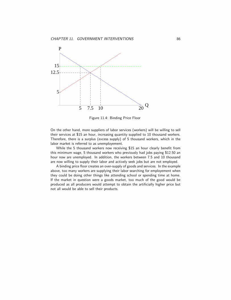
Figure 11.4: Binding Price Floor
On the other hand, more suppliers of labor services (workers) will be willing to selltheir services at $15 an hour, increasing quantity supplied to 10 thousand workers.Therefore, there is a surplus (excess supply) of 5 thousand workers, which in thelabor market is referred to as unemployement.
While the 5 thousand workers now receiving $15 an hour clearly benefit fromthis minimum wage, 5 thousand workers who previously had jobs paying $12.50 anhour now are unemployed. In addition, the workers between 7.5 and 10 thousandare now willing to supply their labor and actively seek jobs but are not employed.
A binding price floor creates an over-supply of goods and services. In the exampleabove, too many workers are supplying their labor searching for employement whenthey could be doing other things like attending school or spending time at home.If the market in question were a goods market, too much of the good would beproduced as all producers would attempt to obtain the artificially higher price butnot all would be able to sell their products.

CHAPTER 11. GOVERNMENT INTERVENTIONS 87
11.2 Effect of Taxation on Equilibrium Price andQuantity
Author: Craig Kerr
What needs to be covered
� What is a tax
� Function of a tax: raise funds for the government and/or redistribute in-come/wealth
� Price based taxes and quantity based taxes (including a statement that thesection only covers quantity based taxes - if this is correct.
� examples for tax on consumers and tax on producers, showing what happensin regards of equilibrium quantity and price
What should not be covered, because it is covered in the following sections
� Quantifying welfare effects with CS and PS (verbal coverage is OK in theissection.
� Price consumers pay and producers receive
In this world nothing can be said to be certain, except death and taxes.- Benjamin Franklin
Most governments impose taxes on their constituents. When a recent college grad-uate receives his first paycheck, he may find that the federal government takesaround 17.5% of his wages!1 With the money he has left after paying taxes, he willmake additional small payments to the government every time he purchases goodsor services through sales tax. If he uses a portion of his earnings to purchase stocksand/or bonds, he will again pay taxes if he sells the asset at a profit.
Taxes are practically unnavoidable payments made to governmets for the purposeof funding the services they provide or to redistribute wealth among the population.The money collected by governments are used to pave roads, employ police andfiremen, maintain parks, and provide many other public goods. The tax you areprobably most familiar with is the sales tax, which is a percentage of the price paidfor a good or service.
In this chapter, we will consider a tax on the quantity of goods or servicespurchased. The federal gasoline tax is an example of a quantity tax. In 2014, everygallon of gasoline was taxed $0.184. The amount of the tax does not change withthe price, only the quantity purchased.
Let us look at how the federal gasonline tax effects the market for gasoline. Wewill assume that the market is perfectly competitive and, for ease of calculation,that the tax is $2 a gallon. Although the consumer sees the tax in the price at the
1Assuming a salary of $55,000 in 2014 for a single filer.
CHAPTER 11. GOVERNMENT INTERVENTIONS 88
pump, the gas station owner is the one who actually pays the tax to the government.How does the tax affect the owner’s behavior?
Suppose the market for gasoline is perfectly competitive and can be describedby the supply and demand equations
P = 1 +1
5QS
P = 8 − 1
5QD,
which are displayed in Figure 11.5 by the solid lines and quantity is in millions ofgallons. The supply curve has an intercept at $1, meaning that the price of gasolinemust be at least $1 before any gas station will supply a positive amount of gasoline.If the gas stations must now pay $2 to the government for every gallon the sell,they would only be willing to sell gasoline for an extra $2 a gallon. That is, gasstations must now receive at least $1 + $2 = $3 per gallon before they are willingto supply a positive amount of gasoline.
This increase in the minimum willingness to accept means that the supply curvewill shift up by $2 at every quantity. Mathematically, this means we add $2 tothe right hand side of our supply eqution. Note that we do this when the supplyequation is solved in terms of P . If our supply equation was in terms of Q and weadded 2, we would be adding a quantity of 2, which is not a dollar amount.
The equation for supply with a tax of $2 per gallon is then
P = 2 + 1 +1
5QS
P = 3 +1
5QS
and the new equilibrium price with the tax is $5.50. The introduction of a tax onproducers causes supply to shift left (or up), which results in a shortage (excesssupply) of 10 million gallons of gasonline . This puts upward pressure on price untilthe market reaches a new equilibrium at $5.50 a gallon.
Notice that the price did not increase by the amount of the tax as we mightinitially expect. This is due to the Law of Demand. Since the price of gasonlineincreases with a tax, quantity demanded decreases, here from 17.5 million to 12.5million gallons. Therefore, when a government introduces a quantity tax in a com-petitive market, the equilibrium price will increase and the equilibrium quantity willdecrease. Since the government receives $2 per gallon and 12.5 million gallons aresold, the tax revenue collected by the government is $25 million.
In the example above, we looked at a quantity tax on producers. But what if thegovernmnet decided to tax consumers of gasonline instead? That is, what if everytime you purchased gasoline, it was your responsibility to send the governmnet acheck for $2 for every gallon you purchased? How would this change theequilibrium quantity and price in the gasoline market?

CHAPTER 11. GOVERNMENT INTERVENTIONS 89
ST
S
D
7.5 12.5 17.5 40Q
1
3
4.55.5
8
P
Figure 11.5: Gasoline in CA
First note that the price-intercept of the demand curve is at $8 implying thatconsumers will start to demand positive amounts of gasoline once the price is below$8. If consumers have to pay $2 to the governmnet for every gallon they purchase,then the total price paid for gasoline is the price they pay at the pump plus the $2tax. Therefore, since no consumer demands any gasonline unless the price is lessthan $8 total, the price at the pump must now be below $6.
Mathematically, we can represent the consumers’ demand with the tax by sub-tracting the $2 tax from their demand curve since they are willing to pay $2 lessper gallon at the pump. The demand curve with the tax is then
P = 8 − 2 − 1
5QD
P = 6 − 1
5QD.
Figure 11.6 displays the effect of taxing consumers. The equilibrium quantityis the same as before, 12.5 million gallons. However, the equilibrium price is now$3.50. When a tax on gasoline is introduced, demand decreases as each consumeris willing to purchase less for any given price because they now have an additionalcost of paying $2 to the government not included in the price. This creates a surplus(excess supply) of 10 million gallons putting downward pressure on price until thenew equilibrium is reached at $3.50.
Regardless of who is taxed, equilibrium quantity falls when a tax is introduced.Here we can see another use for taxes, to discourage behavior. It is well knownthat the production and use of gasonline is harmful to the environment. One way agovernmnet can reduce the amount of gasonline people use is to tax its sale. Thisis the main argument behind so-called “sin taxes” on cigarettes and alcohol.

CHAPTER 11. GOVERNMENT INTERVENTIONS 90
S
DDT
7.5 12.5 17.5 30 40Q
1
3.54.5
6
8
P
Figure 11.6: Gasoline in CA
CHAPTER 11. GOVERNMENT INTERVENTIONS 91
11.3 Consumers’ and Producers’ Tax Burden
Author: Craig Kerr
� For consumer tax
• equilibrium price
• price consumers pay
• price producers get
• tax wedge
� For producer tax
• equilibrium price
• price consumers pay
• price producers get
• tax wedge
� Show that it does not mater if tax is levied on consumers or producers
Topics that are covered in other sections:
� welfare effects
In the previous section, we saw that the equilibrium price of gasoline did notchange by the full amount of the tax regardless of whether consumers or producerswere taxed. When producers were taxed $2 a gallon, the price increased by $1.When consumers were taxed, the price decreased by $1. In both cases, producersand consumers shared the burden of a tax.
Figure 11.7 represents the market for gasoline for when producers are taxed $2.Note that the supply curve shifts by the amount of the tax ($2) but the equilibriumprice only increase by half the amount (from $4.50 to $5.50). This new equilibriumprice is paid by consumers and is therefore called the buyer’s price. Every consumerthat is still purchasing gasoline is now paying $1 more than they otherwise wouldhave without the tax even though it is the producers who are being taxed. Thus,the consumer tax burden is $1.
With a $2 tax on producers of gasoline, the equilibrium market price is $5.50 butproducers only keep $3.50 after taxes are paid. This after-tax dollar amount is whatwe call the sellers’ price and it appears on the graph where the new equilibriumquantity meets supply curve without the tax. The seller’s price is $1 less than theywould receive if there were no taxes on gasoline. We therefore say that the producertax burden is also $1.
What are the prices paid by consumers and producers when the tax is insteadlevied on consumers? Does the tax burden shift toward consumers in this case? Fig-ure 11.8 displays the graph for when consumers are taxed $2 per gallon of gasoline.In this case, the new equilibrium price is $3.50. Since producers do not pay the tax,
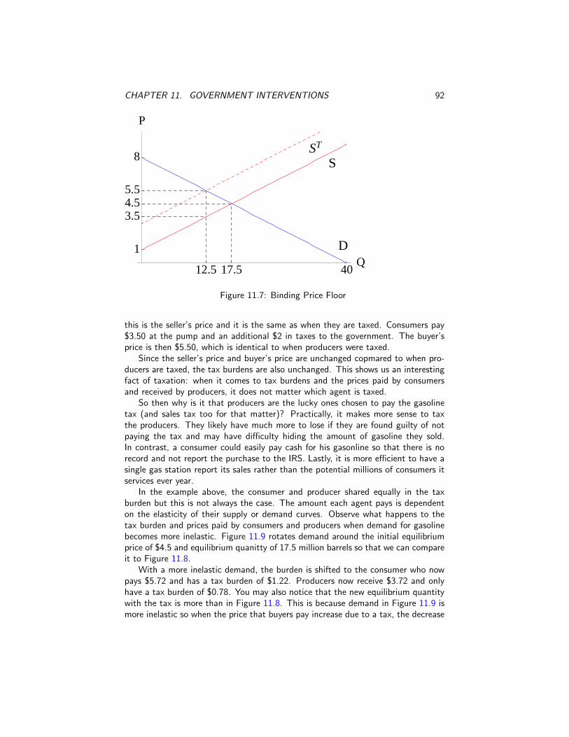
CHAPTER 11. GOVERNMENT INTERVENTIONS 92
ST
S
D
12.5 17.5 40Q
1
3.54.55.5
8
P
Figure 11.7: Binding Price Floor
this is the seller’s price and it is the same as when they are taxed. Consumers pay$3.50 at the pump and an additional $2 in taxes to the government. The buyer’sprice is then $5.50, which is identical to when producers were taxed.
Since the seller’s price and buyer’s price are unchanged copmared to when pro-ducers are taxed, the tax burdens are also unchanged. This shows us an interestingfact of taxation: when it comes to tax burdens and the prices paid by consumersand received by producers, it does not matter which agent is taxed.
So then why is it that producers are the lucky ones chosen to pay the gasolinetax (and sales tax too for that matter)? Practically, it makes more sense to taxthe producers. They likely have much more to lose if they are found guilty of notpaying the tax and may have difficulty hiding the amount of gasoline they sold.In contrast, a consumer could easily pay cash for his gasonline so that there is norecord and not report the purchase to the IRS. Lastly, it is more efficient to have asingle gas station report its sales rather than the potential millions of consumers itservices ever year.
In the example above, the consumer and producer shared equally in the taxburden but this is not always the case. The amount each agent pays is dependenton the elasticity of their supply or demand curves. Observe what happens to thetax burden and prices paid by consumers and producers when demand for gasolinebecomes more inelastic. Figure 11.9 rotates demand around the initial equilibriumprice of $4.5 and equilibrium quanitty of 17.5 million barrels so that we can compareit to Figure 11.8.
With a more inelastic demand, the burden is shifted to the consumer who nowpays $5.72 and has a tax burden of $1.22. Producers now receive $3.72 and onlyhave a tax burden of $0.78. You may also notice that the new equilibrium quantitywith the tax is more than in Figure 11.8. This is because demand in Figure 11.9 ismore inelastic so when the price that buyers pay increase due to a tax, the decrease

CHAPTER 11. GOVERNMENT INTERVENTIONS 93
S
DDT
12.5 17.5 40Q
1
3.54.55.5
8
P
Figure 11.8: Tax on Consumer
in their quantity demanded is relatively smaller. This is also why they have more ofthe burden; prices at the pump decrease with the decrease in demand. If demanddecreases less, the price will also decrease less. In general, the more elastic (inelastic)consumers or producers are, the less (more) of the tax burden they will bear.

CHAPTER 11. GOVERNMENT INTERVENTIONS 94
S
DDT
13.6 17.5 31.8Q
1
3.724.5
5.72
10P
Figure 11.9: Tax on Consumer with Inelastic Demand

CHAPTER 11. GOVERNMENT INTERVENTIONS 95
11.4 Welfare Effects of a Tax
Author: Craig Kerr
� show changes in welfare in diagram, when tax is introduced and show deadweight loss
� introduce term dead weight loss and excess burden
� discuss which products are best suited for taxation and show the role ofelasticity for DWL/EB
� maybe: discuss the strategy of the second best
In previous sections, we saw how taxes decrease equilibrium quantity and drivea wedge between the price that consumers pay and the price that producers receive.As you might have guessed, this causes a loss of welfare in aggregate for bothgroups. Figure 11.10 displays the market for gasoline when a $2 tax is applied.
A
B
C
D
E
F
S
D
12.5 17.5 40Q
1
3.5
4.5
5.5
8
P
Figure 11.10: Gasoline in CA
Without a tax on gasoline, consumers have a surplus equal to the area below thedemand curve and above the price (Consumer Surplus = A+B+E). When a $2 taxis introduced, consumers will pay $5.50 in total per gallon and only purchase 12.5million gallons regardless of whether producers or consumers are taxed. Consumersurplus will then be equal to Area A.
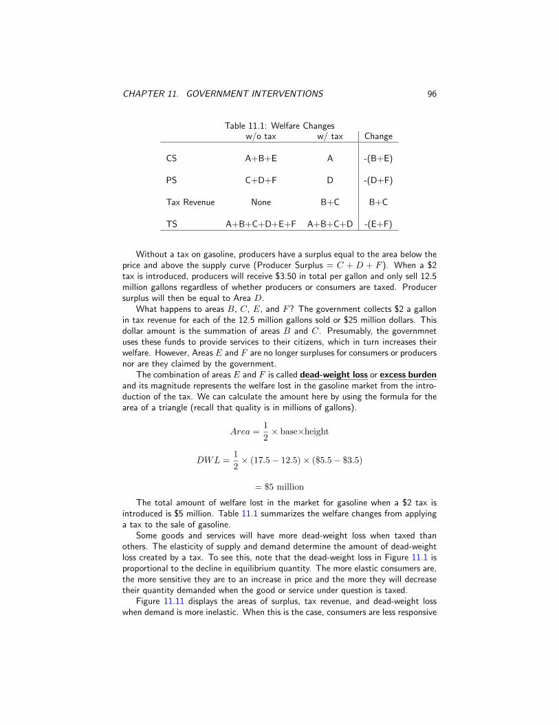
CHAPTER 11. GOVERNMENT INTERVENTIONS 96
Table 11.1: Welfare Changesw/o tax w/ tax Change
CS A+B+E A -(B+E)
PS C+D+F D -(D+F)
Tax Revenue None B+C B+C
TS A+B+C+D+E+F A+B+C+D -(E+F)
Without a tax on gasoline, producers have a surplus equal to the area below theprice and above the supply curve (Producer Surplus = C + D + F ). When a $2tax is introduced, producers will receive $3.50 in total per gallon and only sell 12.5million gallons regardless of whether producers or consumers are taxed. Producersurplus will then be equal to Area D.
What happens to areas B, C, E, and F? The government collects $2 a gallonin tax revenue for each of the 12.5 million gallons sold or $25 million dollars. Thisdollar amount is the summation of areas B and C. Presumably, the governmnetuses these funds to provide services to their citizens, which in turn increases theirwelfare. However, Areas E and F are no longer surpluses for consumers or producersnor are they claimed by the government.
The combination of areas E and F is called dead-weight loss or excess burdenand its magnitude represents the welfare lost in the gasoline market from the intro-duction of the tax. We can calculate the amount here by using the formula for thearea of a triangle (recall that quality is in millions of gallons).
Area =1
2× base×height
DWL =1
2× (17.5 − 12.5) × ($5.5 − $3.5)
= $5 million
The total amount of welfare lost in the market for gasoline when a $2 tax isintroduced is $5 million. Table 11.1 summarizes the welfare changes from applyinga tax to the sale of gasoline.
Some goods and services will have more dead-weight loss when taxed thanothers. The elasticity of supply and demand determine the amount of dead-weightloss created by a tax. To see this, note that the dead-weight loss in Figure 11.1 isproportional to the decline in equilibrium quantity. The more elastic consumers are,the more sensitive they are to an increase in price and the more they will decreasetheir quantity demanded when the good or service under question is taxed.
Figure 11.11 displays the areas of surplus, tax revenue, and dead-weight losswhen demand is more inelastic. When this is the case, consumers are less responsive
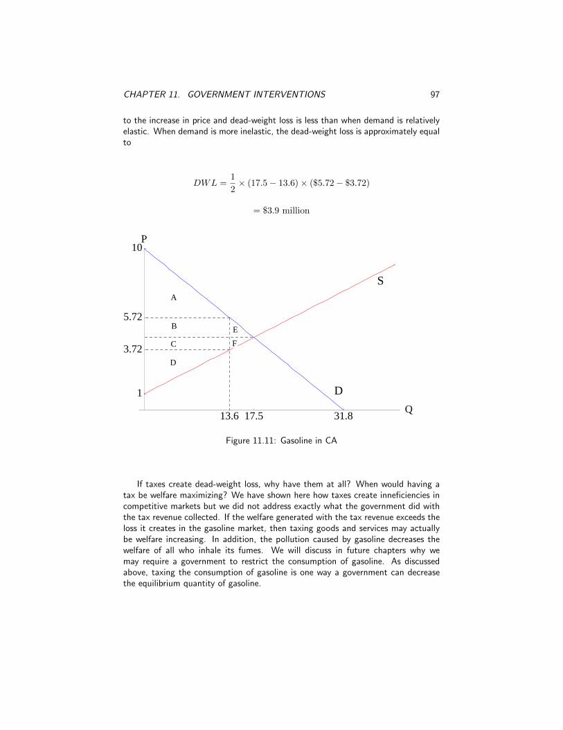
CHAPTER 11. GOVERNMENT INTERVENTIONS 97
to the increase in price and dead-weight loss is less than when demand is relativelyelastic. When demand is more inelastic, the dead-weight loss is approximately equalto
DWL =1
2× (17.5 − 13.6) × ($5.72 − $3.72)
= $3.9 million
S
D
E
D
B
C
A
F
13.6 17.5 31.8Q
1
3.72
5.72
10P
Figure 11.11: Gasoline in CA
If taxes create dead-weight loss, why have them at all? When would having atax be welfare maximizing? We have shown here how taxes create inneficiencies incompetitive markets but we did not address exactly what the government did withthe tax revenue collected. If the welfare generated with the tax revenue exceeds theloss it creates in the gasoline market, then taxing goods and services may actuallybe welfare increasing. In addition, the pollution caused by gasoline decreases thewelfare of all who inhale its fumes. We will discuss in future chapters why wemay require a government to restrict the consumption of gasoline. As discussedabove, taxing the consumption of gasoline is one way a government can decreasethe equilibrium quantity of gasoline.
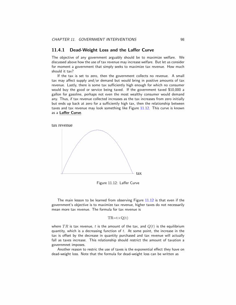
CHAPTER 11. GOVERNMENT INTERVENTIONS 98
11.4.1 Dead-Weight Loss and the Laffer Curve
The objective of any government arguably should be to maximize welfare. Wediscussed above how the use of tax revenue may increase welfare. But let us considerfor moment a government that simply seeks to maximize tax revenue. How muchshould it tax?
If the tax is set to zero, then the government collects no revenue. A smalltax may affect supply and/or demand but would bring in positive amounts of taxrevenue. Lastly, there is some tax sufficiently high enough for which no consumerwould buy the good or service being taxed. If the government taxed $10,000 agallon for gasoline, perhaps not even the most wealthy consumer would demandany. Thus, if tax revenue collected increases as the tax increases from zero initiallybut ends up back at zero for a sufficiently high tax, then the relationship betweentaxes and tax revenue may look something like Figure 11.12. This curve is knownas a Laffer Curve.
tax
tax revenue
Figure 11.12: Laffer Curve
The main lesson to be learned from observing Figure 11.12 is that even if thegovernment’s objective is to maximize tax revenue, higher taxes do not necessarilymean more tax revenue. The formula for tax revenue is
TR=t×Q(t)
where TR is tax revenue, t is the amount of the tax, and Q(t) is the equilibriumquantity, which is a decreasing function of t. At some point, the increase in thetax is offset by the decrease in quantity purchased and tax revenue will actuallyfall as taxes increase. This relationship should restrict the amount of taxation agovernmnet imposes.
Another reason to restric the use of taxes is the exponential effect they have ondead-weight loss. Note that the formula for dead-weight loss can be written as

CHAPTER 11. GOVERNMENT INTERVENTIONS 99
DWL =1
2× t×∆Q
since the base of the triangle in Figure 11.10 is the amount of the tax and the heightis the change in quantity. From this equation, we observe that if the governmnetdoubles some tax, we would replace t with 2t. Note that if the amount of the taxincreases, then so does the change in quantity. Thus, a doubling of taxes will morethan double the deadweight loss. That is, dead-weight loss increases exponentiallywith the amount of a tax. The relationship is described in Figure 11.13.
tax
DWL
Figure 11.13: DWL from tax

CHAPTER 11. GOVERNMENT INTERVENTIONS 100
11.5 Videos, Simulations, and other Internet Re-sources
Author: @@@Author
This section will be automatically generated from a database and Instructorscan later pick which content they like to be included.
Links to Videos, Simulations, audio files, possibly to Wikipedia for key termswill be ordered by subsection and then by type
Here comes content
CHAPTER 11. GOVERNMENT INTERVENTIONS 101
11.6 End of Chapter Questions
Author: @@@Author
End of Chapter Questions are not part of the first edition.In the second edition they will be generated from a database depending on the
instructors choice.

Chapter 12
Deriving Individual Demandfrom Preferences
Author: @@@Author
Insert topics to be covered here.This Chapter will not be part of the first edition. It will be added for the second
edition.
102

Chapter 13
Deriving Firm Supply fromCost of Production
Author: @@@Author
Insert topics to be covered here.Here comes the content
103

CHAPTER 13. DERIVING FIRM SUPPLY FROM COST OF PRODUCTION 104
13.1 Types of Cost
Author: @@@Author
� Explain each cost type briefly
� distinguish between average (per unit) costs and overal/total cost
� add table that gives an overview about different costs and how they arecalculated.
Here comes content
CHAPTER 13. DERIVING FIRM SUPPLY FROM COST OF PRODUCTION 105
13.2 Graphical Representation of Cost Types
Author: @@@Author
� Include a graph that has average fix cost, average variable cost, and margianlcost
� explain U shape, the fact that MC intersect in AVC’s and ATC’s minumumas well as other properties of graphs.
Here comes content

CHAPTER 13. DERIVING FIRM SUPPLY FROM COST OF PRODUCTION 106
13.3 Optimal Production Quantity in a CompetitiveMarket
Author: @@@Author
Emphasize individual firmderive opt productionexplain final market exit conditionsexplain temporary market exit conditionsHere comes content

CHAPTER 13. DERIVING FIRM SUPPLY FROM COST OF PRODUCTION 107
13.4 Deriving the Short Run Supply Curve for aCompetitive Market
Author: @@@Author
Derive Supply CurveHere comes content

CHAPTER 13. DERIVING FIRM SUPPLY FROM COST OF PRODUCTION 108
13.5 Deriving the Long Run Supply Curve for aCompetitive Market
Author: @@@Author
Derive Supply CurveHere comes content

CHAPTER 13. DERIVING FIRM SUPPLY FROM COST OF PRODUCTION 109
13.6 Videos, Simulations, and other Internet Re-sources
Author: @@@Author
This section will be automatically generated from a database and Instructorscan later pick which content they like to be included.
Links to Videos, Simulations, audio files, possibly to Wikipedia for key termswill be ordered by subsection and then by type
Here comes content

CHAPTER 13. DERIVING FIRM SUPPLY FROM COST OF PRODUCTION 110
13.7 End of Chapter Questions
Author: @@@Author
End of Chapter Questions are not part of the first edition.In the second edition they will be generated from a database depending on the
instructors choice.

Chapter 14
Monopoly
Author: @@@Author
� explain briefly what a monopoly is (refer for more details to the ChapterMarkets, Section Monopoly)
� discuss briefly why monopoly requires market entrance barriers
� explain some of the barriers including local monopolies for utility companies
Then give a brief overview of the Chapter:
� keep it short
� write in the “you will learn” style to ensure consistency in the book
� list what the reader will learn with references to the sections.
� emphasize the keywords for the learning goals (see Chapter Government In-terventions Intro for examples)
Here comes the content
111

CHAPTER 14. MONOPOLY 112
14.1 Profit Maximizing
Author: @@@Author
� in order to maximize profit a monopolist can try to find an optimal price. Thenthe demand in the market determines the quantity he can sell and thereforehis production
� in order to maximize profit a monopolist can try to find an optimal quantityhe produces. Then the demand in the market determines the price whichgenerate enough demand to sell, what has been produced
� a monopolist cannot set the price and quantity simultaneously
� here it is assumed that the monopolist try to finds first the profit maximizingquantity and then determines the price depending on the market demand thatensures that the produced quantity can be sold
Here comes content
14.1.1 Conditions for a Profit Maximum
Author: @@@Author
� explain why MC=MR
� MR can be split in positve Quantity effect (one extra unit produced increasesrevenue by the prce it is sold) and a negative Price Effect (in order to sell oneextra unit the monopolist had to lower the price for all units)
Here comes content
14.1.2 Deriving the Monopolist’s Profit Maximum in a MarketDiagram
Author: @@@Author
� explain demand curve, MC curve, MR revenue curve, Average Total Costcurve
� use diagram to derive optimal quantity and price
� show profit in diagram using the Avg Total Cost curve
Here comes content

CHAPTER 14. MONOPOLY 113
14.2 Welfare Effects
Author: @@@Author
� compare monopoly outcome with competitive market outcome in diagram
� show that a monopolist produces less and therefore can charge a higher price
� show that monopolist makes profit while competitive market does not generateprofit
� show welfare effects using consumer an producer surplus
� show excess burden of a monopoly with consumer producer surplus concept
Here comes content

CHAPTER 14. MONOPOLY 114
14.3 Monopolistic Competition
Author: @@@Author
If time is short. This section can be delivered in 2015.
� cover and explain monopolistic competition
� show differences between monopolistic competition and monopoly
� can but does not have to be done verbally
� explain why monopolistic competition is more realistic
Here comes content

CHAPTER 14. MONOPOLY 115
14.4 Price Discrimination
Author: @@@Author
� explain price discrimination in general
� explain price discrimination in regards of:
• different prices depending on different demand groups (e.g. studentdiscount)
• different prices depending on purchased quantity
• different prices for each consumer (monopolist collects full consumersurplus)
Here comes content
CHAPTER 14. MONOPOLY 116
14.5 Videos, Simulations, and other Internet Re-sources
This section will be automatically generated from a database and Instructors canlater pick which content they like to be included.
Links to Videos, Simulations, audio files, possibly to Wikipedia for key termswill be ordered by subsection and then by type
Instructional Videos
Each video covers a selected concept of content.
For Section: 14 Monopoly
Introduction to Monopoly Marketsby Carsten Lange
Defines a monopoly and explains barriers to entry.Click here to start ID:20 Click here to rate
For Section: 14.1 Profit Maximizing
Monopoly Profit Maximizationby Carsten Lange
Gives a general overview of how monopolies maximize profit and how their profitchanges as their output changes.Click here to start ID:21 Click here to rate
Monopolistic Output Determination (Diagramatically)by Carsten Lange
Covers how to find the profit-maximizing level of output using a monopolist’s supplyand demand diagram.Click here to start ID:23 Click here to rate
Calculating Monopoly Profitby Carsten Lange
Explains how to find the profit-maximizing level of output in a monopoly marketand how to calculate profit at this output level. Also explains the monopolist’smarginal revenue curve as it relates to profit determination.Click here to start ID:22 Click here to rate

CHAPTER 14. MONOPOLY 117
14.6 End of Chapter Questions
Author: @@@Author
End of Chapter Questions are not part of the first edition.In the second edition they will be generated from a database depending on the
instructors choice.

Chapter 15
Oligopoly
Author: @@@Author
Insert topics to be covered here.Here comes the content
118

CHAPTER 15. OLIGOPOLY 119
15.1 Profit Maximization in a Duopoly
Author: @@@Author
Insert topics to be covered here.Here comes content

CHAPTER 15. OLIGOPOLY 120
15.2 A Game Theory Approach
Author: @@@Author
Insert topics to be covered here.Here comes content

CHAPTER 15. OLIGOPOLY 121
15.3 Videos, Simulations, and other Internet Re-sources
Author: @@@Author
This section will be automatically generated from a database and Instructorscan later pick which content they like to be included.
Links to Videos, Simulations, audio files, possibly to Wikipedia for key termswill be ordered by subsection and then by type
Here comes content

CHAPTER 15. OLIGOPOLY 122
15.4 End of Chapter Questions
Author: @@@Author
End of Chapter Questions are not part of the first edition.In the second edition they will be generated from a database depending on the
instructors choice.
Related Documents