Contamination of Stainless Steel Components with Stable Caesium and Strontium Isotopes A thesis submitted to The University of Manchester for the degree of Masters of Philosophy in the Faculty of Engineering and Physical Sciences 2012 Amy Louise Taylor-Underhill School of Materials

Welcome message from author
This document is posted to help you gain knowledge. Please leave a comment to let me know what you think about it! Share it to your friends and learn new things together.
Transcript

Contamination of Stainless Steel Components with Stable Caesium and Strontium Isotopes
A thesis submitted to The University of Manchester for the degree of Masters of Philosophy
in the Faculty of Engineering and Physical Sciences
2012
Amy Louise Taylor-Underhill
School of Materials

2
Table of Contents 1. Introduction .......................................................................................................... 11 1.1 Aims & Objectives ..................................................................................................... 13
2. Literature Review................................................................................................ 14 2.1. Austenitic Stainless Steel....................................................................................... 14 2.2. The passive layer...................................................................................................... 15 2.3. Contamination Processes ...................................................................................... 21 2.4. Chemistry of Caesium and Strontium in the Nuclear Fuel Cycle .............. 23 2.5. Caesium and Strontium Contamination ........................................................... 25 2.5.1. Caesium and strontium interactions with iron oxides ............................ 33 2.6. Decontamination techniques for Stainless Steel ........................................... 36 2.6.1. Chemical Decontamination ............................................................................... 36 2.6.2. Mechanical Decontamination........................................................................... 39
2.6.3. Alternative Techniques…………………………...……………...…………………..…. 41 3. Experimental......................................................................................................... 43 3.1. Materials and Composition................................................................................... 45 3.1.1. Material and Surface Preparation................................................................... 45 3.1.2. Etching Procedure................................................................................................ 48 3.2. Characterisation methods..................................................................................... 48 3.2.1. Laser profilometry method............................................................................... 48 3.3. Contamination methods ........................................................................................ 54 3.3.1. High temperature contamination method................................................... 55 3.3.2. Aqueous Contamination..................................................................................... 56 3.3.2.1. Solutions Preparation Procedure................................................................ 56 3.3.2.2. Coupon Sampling Procedure......................................................................... 58 3.3.2.3. Solution pH measurement ............................................................................. 58
4. Results & Discussion........................................................................................... 59 4.1. Surface Imaging ........................................................................................................ 60 4.2. Roughness Parameters .......................................................................................... 64 4.2.1. Discussion of the Roughness Parameters .................................................... 68 4.3. Caesium and Strontium Contamination ........................................................... 71 4.3.1. Caesium contamination...................................................................................... 71 4.3.1.1. 4M Nitric Acid (environment A)................................................................... 72 4.3.1.2. Neutral Bicarbonate (environment B)....................................................... 76 4.3.1.3. Caesium carbonate (environment C) …….…………………………………..… 76 4.3.1.4. pH 11 sodium hydroxide (environment D) ............................................. 81 4.3.1.5. High temperature (environment E)............................................................ 83 4.3.1.6. Caesium Contamination Discussion ........................................................... 86 4.3.1.6.2. Effects of time on caesium contamination ............................................ 89 4.3.1.6.3. Effects of pH on caesium contamination................................................ 90 4.3.1.6.4. Comparison of caesium contamination techniques........................... 90 4.3.2. Strontium contamination results.................................................................... 92 4.3.2.1. 4M Nitric Acid (environment A)................................................................... 92 4.3.2.2. Bicarbonate (environment B)....................................................................... 95 4.3.2.3. pH 11 sodium hydroxide (environment D) ............................................. 96 4.3.2.4. High temperature (environment E)..........................................................100 4.3.2.5. Strontium Contamination Discussion ......................................................102 4.3.2.5.1. Contamination as a function of cold work ..........................................102 4.3.2.5.2. Contamination as a function of time .....................................................103 4.3.2.5.3. The effect of pH on contamination ........................................................104 4.3.2.5.4. The effects of pH deviation on strontium contamination..............105 4.3.2.5.5. Comparison of strontium contamination techniques .....................107

3
5. Possible further work and improvements ................................................109
6. Conclusions..........................................................................................................111
7. References............................................................................................................112 Word Count: 19,630

4
List of Tables Table 1. Chemical Composition Requirements ........................................................... 14 Table 2. Chemical Decontamination Techniques ....................................................... 37 Table 3. Mechanical Techniques for Decontamination of Components ……….40 Table 4. Alternative Techniques for Decontamination ........................................... 41 Table 5. Comparison of surface analysis techniques…………………………..……...44 Table 6. AISI 304H coupons prepared and their environments ......................... 45 Table 7. Chemical Composition Requirements ........................................................... 45 Table 8. Depth of AISI 304H stainless steel strips ..................................................... 46 Table 9. Sample names according to steel conditions and environments ...... 47 Table 10. High temperature paste contamination of samples ............................. 51 Table 11. High temperature paste contamination of samples ............................. 55 Table 12. R-‐values of the investigated stainless steel coupons…………………...64

5
List of Figures Figure 1. Diagram illustrating the redox reaction involved in passivation of iron ................................................................................................................................................. 15 Figure 2. a) Simplified diagram showing the Stern (Outer Helmholtz) layer and Diffuse Layer and b) the oxide layer in more detail, ε is an estimate dielectric constant of the water molecules .................................................................. 17 Figure 3. A schematic representation of the potential drop over a metal/passive film/ environment system. ΔΦI/II and ΔΦII/III represent the interfacial potential drops and DFII corresponds to the dielectric drop over the oxide layer .......................................................................................................................... 18 Figure 4. Schematic illustration of transport and deposition mechanisms of dust particles and fission products in helium ducts ................................................. 26 Figure 5. Grain boundary penetration of Cr-‐51 in normal and in Cs-‐preloaded steel 1.4970 ................................................................................................................................ 30 Figure 6. Relative adsorption of strontium on hematite, as a function of pH………………………………………………………………………………………..………………….34 Figure 7. Illustration of the as received and cold rolled strips ............................ 46 Figure 8. Illustration of the coupons used in the experimental set ………........ 47 Figure 9. Diagram to show how the Ra and Rq are calculated ............................ 50 Figure 10. Diagram to show how the Rz values are calculated ........................... 50 Figure 11. Illustration of the GDOES sputtering and emission processes…………………………………………………………………………………………......... 51 Figure 12. Trapezoids under a strontium curve ........................................................ 53 Figure 13. How the area of a trapezoid is calculated ............................................... 54 Figure 14. As received AISI 304H stainless steel SEM micrograph a) at x 500 and b) at 750 x magnification (backscattered electrons) ...................................... 60 Figure 15. 5% cold rolled AISI 304H stainless steel SEM micrograph a) at x 500 and b) at 750 x magnification (backscattered electrons) ............................. 62 Figure 16. 30% cold rolled AISI 304H stainless steel SEM micrograph a) at x 500 and b) at 750 x magnification (backscattered electrons) ............................. 63 Figure 17. a) Laser profilometry R-‐values of all coupons along the x-‐axis.................................................................................................................................................. 66

6
Figure 17. b) Laser profilometry R-‐values of all coupons along the y-‐axis………………………………………………………………………………….…………………..….67 Figure 18. GDOES sputtering data depth profiles of a) as received control sample (A0p1) exposed to nitric acid and b) as received sample (A0Csp1) exposed to nitric acid and caesium. ................................................................................. 73 Figure 19. 5% cold rolled sample (A5Csp1) exposed to nitric acid and caesium; and 30% cold rolled sample (A30Csp1) exposed to nitric acid and caesium GDOES sputtering data depth profiles ......................................................... 75 Figure 20. GDOES sputtering depth profiles of the control sample (B0p1) without Cs, and as received sample (B0Csp1) exposed to Cs and sodium bicarbonate ................................................................................................................................ 77 Figure 21. GDOES sputtering data depth profile of 30% cold rolled sample (B30Csp1) exposed to sodium bicarbonate and caesium ...................................... 78 Figure 22. GDOES sputtering data depth profiles of a) as received sample (C0Csp1) exposed to caesium carbonate, b) as received second sample (C0Csp2) exposed to caesium carbonate ...................................................................... 79 Figure 23. a) GDOES sputtering profile of 5% cold rolled sample (C5Csp1) exposed to caesium carbonate, b) GDOES sputtering data depth profile of second 5% cold rolled sample (C5Csp2) exposed to caesium carbonate........ 80 Figure 24. GDOES sputtering data profile of 30% cold rolled sample (C30Csp1) exposed to caesium carbonate.................................................................... 81 Figure 25. GDOES sputtering data depth profile of the as received control sample (D0p1) exposed to sodium hydroxide ............................................................ 82 Figure 26. GDOES sputtering data profiles of as received sample (D0Csp1) and 30% cold rolled sample (D30Csp1) exposed to Cs and sodium hydroxide..................................................................................................................................... 83 Figure 27. GDOES sputtering data profiles of 30% cold rolled samples, E30Csp1 and E30Csp2, exposed to caesium carbonate paste and high temperatures ............................................................................................................................. 85 Figure 28. A GDOES depth profile of Type 304 stainless steel ............................ 86 Figure 29. Caesium contamination as a function of cold work using integrals from C0Csp1, C5Csp1 and C30Csp1 ................................................................................ 88 Figure 30. The effect of exposure time on caesium contamination.................... 89 Figure 31. Graph showing the effect of pH on caesium contamination using integrals from A5Csp1, C0Csp1, C0Csp2, C5Csp1, C5Csp2 and C30Csp1 ….... 90

7
Figure 32. Comparison of caesium peaks for different contamination techniques ....................................................................................................................................91 Figure 33. GDOES sputtering data profile of the as received sample (A0p1) exposed to nitric acid ............................................................................................................. 93 Figure 34. GDOES sputtering data profiles of the as received sample (A0Srp1) and 30% cold rolled sample (A30Srp1) both exposed to nitric acid and strontium .................................................................................................................................... 94 Figure 35. GDOES sputtering data profile of the control sample (B0p1) without strontium ................................................................................................................... 95 Figure 36. As received (B0Srp1) and 30% cold rolled (B30Srp1) samples (exposed to sodium bicarbonate and strontium) GDOES sputtering data profiles ......................................................................................................................................... 96 Figure 37. Control sample (D0p1) exposed to sodium hydroxide GDOES sputtering data profile .......................................................................................................... 97 Figure 38. GDOES sputtering data profiles of as received sample (D0Srp1) and 30% cold rolled sample (D30Srp1) exposed to sodium hydroxide and strontium .................................................................................................................................... 98 Figure 39. GDOES sputtering data profiles of 30% cold rolled samples (D30Srp3 and D30Srp4) exposed to sodium hydroxide and strontium……………………………………………………………………………………………..... 99 Figure 40. GDOES sputtering data profile of 30% cold rolled etched sample (D30Sre1) exposed to Sr and sodium hydroxide .................................................... 100 Figure 41. GDOES sputtering data profiles of 30% cold rolled samples (E30Srp1 and E30Srp2) exposed to strontium carbonate paste and high temperatures .......................................................................................................................... 101 Figure 42. Strontium contamination as a function of cold work from samples D0Srp1 and D30Srp3 .......................................................................................................... 102 Figure 43. Relationship between the exposure time and the amount of strontium contamination on D30Srp3 coupon...……………………..…………….... 104 Figure 44. The relationship between pH and strontium contamination using integrals from A30Srp1, B0Srp1, B30Srp1, D0Srp1 and D30Srp1-‐4.……….. 105 Figure 45. The effect of pH deviation on strontium contamination using D30Srp1 integrals…………….……………………………………..……………..……………...106 Figure 46. Comparison of strontium contamination techniques…………….....108

8
Abstract The University of Manchester Amy Louise Taylor-Underhill Masters of Philosophy in the Faculty of Engineering and Physical Sciences Contamination of Stainless Steel Components with Stable Caesium and Strontium Isotopes 2012 This M.Phil. thesis investigates the effects of the environment on caesium (Cs) and strontium (Sr) contamination of as received and cold rolled Type 304H stainless steel. Stable (non radioactive) isotopes were used in the experiments, to simulate surface contamination of components in the nuclear industry through radioactive counterparts. The contamination was monitored using Glow Discharge Optical Emission Spectroscopy (GDOES). The parameters of time, pH and cold work were investigated to determine the most favourable contamination conditions. The effect of pH using acidic, neutral and alkaline environments were investigated for both caesium and strontium. A slight increase of Cs contamination was observed on Type 304H coupons as the pH increased, mainly observed in the Cs carbonate environments, and an exponential increase in Sr contamination on the Type 304H coupons was observed as the pH increased. A number of coupons were cold rolled to a deformation of 5% and 30%, and compared to as received samples to investigate the effect cold work on Cs and Sr contamination. There was a small effect on caesium contamination, increasing slightly with an increase in strain. However, no trend was observed between Sr contamination and cold work. It was concluded from this study that Sr contaminates Type 304H steel more readily than Cs. It was found that Sr penetrated further into the bulk of the steel and did not desorb with a change in pH. The most promising environment for strontium contamination was a strontium / sodium hydroxide solution. The most promising environment for Cs contamination was using Cs carbonate.

9
Declaration No portion of the work referred to in this thesis has been submitted in support of an application for another degree or qualification of this or any other university or other institute of learning.

10
Copyright Statement
i. The author of this thesis (including any appendices and/or schedules to this thesis) owns certain copyright or related rights in it (the “Copyright”) and s/he has given The University of Manchester certain rights to use such copyright, including for administrative purposes.
ii. Copies of this thesis, either in full or in extracts and whether in hard or
electronic copy, may be made only in accordance with the Copyright, Designs and Patents Act 1988 (as amended) and regulations issued under it or, where appropriate, in accordance with licensing agreements which the University has from time to time. This page must form part of any copies made.
iii. The ownership of certain Copyright, patents, designs, trade marks and
other intellectual property (the “Intellectual Property”) and any reproductions of copyright works in the thesis, for example graphs and tables (“Reproductions”), which may be described in this thesis, may not be owned by the author and may be owned by third parties. Such Intellectual Property and Reproductions cannot and must not be made available for use without the prior written permission of the owner(s) of the relevant Intellectual Property and/or Reproductions.
iv. Further information on the conditions under which disclosure,
publication and commercialisation of this thesis, the Copyright and any Intellectual Property and/or Reproductions described in it may take place is available in the University IP policy (see http://documents.manchester.ac.uk/DocuInfo.aspx?DocID=487), in any relevant Thesis restriction declarations deposited in the University Library, The University Library’s regulations (see http://www.manchester.ac.uk/library/aboutus/regulations) and in the University’s policy on Presentation of Theses.

11
1. Introduction
The title of this project originates from the problems the Nuclear Industry
confronts when decommissioning facilities containing stainless steel components.
The process of decommissioning is the final stage in the life-cycle of a nuclear
facility [1]. Cost-effective decontamination of the structural materials used in a
nuclear facility can greatly reduce highly radioactive components for storage or
disposal.
The Nuclear Industry in the UK is currently in the process of decommissioning the
majority of their facilities and are experiencing widespread and varied problems.
This is due to the unpredictability of the timescale of operations and radioactive
contamination [1]. One of the major problems is plate-out, a phenomenon not fully
understood, which involves radionuclide contamination of components. The
definition of plate-out is the ‘Deposition of radioactive solids, colloids, or ions
suspended in aqueous liquid onto the surface of a material holding the liquid.’ A
large amount of plate-out contamination is believed to be only weakly bound to the
surface [2]. The Plate Out Factor, POF, which is the activity of the empty
reprocessing plant after the commissioning stage divided by the activity of the
liquor passed through the plant is calculated to 40 for the reprocessing plants in the
UK, showing that the radioactivity of the internal surfaces of the plant is much
higher than the radioactivity of the original liquor [3]. The empty steel vessel is
therefore classed after decommissioning as high-level waste (HLW) and the
radioactivity is too high for manual dismantling. The steel would need to be
decontaminated in a cost-effective way, for example, to reduce radioactivity for

12
manual dismantling, minimise secondary waste, reduce worker dose and increase
man access [3].
The fission products caesium-137 and strontium-90 contribute to a high amount of
the radioactivity experienced in spent nuclear fuel [4, 5]. These isotopes make an
important contribution to the POF of the steel and are the major waste hazard for
the first 400 years. They are present in relatively large quantities as the fission
products from spent nuclear fuel and make a significant contribution to the overall
activity [3]. These nuclides are known to contaminate steel and stainless steels in
reprocessing plant and storage ponds where the cladding, which prevents the
leaching, is either removed or damaged [6]. Caesium and strontium contribute
largely to the heat generated from the spent fuel since they are the most abundant,
and contribute the most radioactivity of the mid-length half-life radionuclides [7].
It has been estimated that caesium-137 and strontium-90 contribute 4.5 billion and
3 billion curies respectively to the total 12 billion curies of radioactivity seen in
spent nuclear reactor fuel in the US [8].

13
1.1 Aims & Objectives
This project is focusing on the mechanism of caesium and strontium contamination
in AISI type 304H stainless steel, by using the non-radioactive (stable) isotopes
Cs-133 and Sr-89 to simulate the behaviour of caesium-137 and strontium-90. The
aims of this project were as follows:
To determine an effective method of caesium and strontium contamination
on the stainless steel surface from aqueous and high temperature
environments;
To investigate the effect of pH on caesium and strontium contamination by
replicating exposure conditions in a spent fuel pond and under reprocessing
environments;
To determine whether cold deformation of the stainless steel can encourage
contamination of these radionuclides.
The findings of this project aim to give a greater understanding of the extent the
radionuclides penetrate stainless steel. This information could be used to develop
effective decontamination techniques so that these steel components could be
recycled or released without potential radiation risks.

14
2. Literature Review
2.1. Austenitic Stainless Steel
Austenitic stainless steel contains iron, nickel and chromium, plus small amounts
of additional minor constituents. The quantities and types of metal are carefully
selected for desired properties and purpose of the alloy [9]. AISI 304 stainless steel
is a standard grade of austenitic steel containing 16-30% chromium, 8-25% nickel
and <0.15% carbon. The name austenitic refers to the microstructure the steel
adopts with these constituents.
Compositional variations of bulk AISI 304(L) are detailed in table 1, the amount
of minor elements incorporated varying slightly between each grade.
Table 1. Chemical Composition Requirements, wt.-% [9] Type
C Mn P S Si Cr Ni
304 0.08 2.00 0.045 0.030 0.75 18.0-20.0 8.0-10.5 304L 0.030 2.00 0.045 0.030 0.75 18.0-20.0 8.0-12.0 304H 0.10 2.00 0.045 0.030 0.75 18.0-20.0 8.0-10.5
The H and L in table 1 refer to a high or low amount of carbon, respectively. The
main difference in the properties of these two grades is that the tensile and yield
strength of 304H is greater than that of 304L [10]. The passivity in high
temperature environments is affected by the carbon content of the steel, and the
carbide precipitation behaviour at grain boundaries

15
2.2. The passive layer
Iron and chromium can both form oxide films to protect the bulk from corrosion.
They exhibit passivity in certain environments and the alloying of these elements
result in stainless steel forming a passive oxide film that protects the bulk from
corrosion [11]. This passive oxide layer can be a few nanometres thick and only
develops if there is sufficient oxygen available. Figure 1 shows the transfer of
electrons involved in the growth of the passive layer, ie the film grows by outward
diffusion of iron. A reduction/oxidation (redox) reaction is the basis of passivation
of the steel, but this may also cause corrosion. In certain environments, the passive
layer can be broken down, and if unable to repair itself, the surface is classed as
active and will corrode [11-13]. The stability of the passive layer depends entirely
on the anodic or cathodic redox reactions and if the oxidized or reduced species is
soluble in the electrolyte [11].
Figure 1. Diagram illustrating the redox reaction involved in passivation of
iron [11]

16
The passive film on stainless steel typically comprises of three layers. The layer
closest to the surface contains nickel ferrite (NiFe2O4), the central layer contains
iron and chromium oxides (including chromium ferrite FeCr2O4). The iron and
chromium oxides closer to the steel have the lowest oxygen content, such as FeO
[14]. Closer to the oxide/water interface, the oxides formed include iron
oxyhydroxides, which are only formed in an oxygen-rich environment [14]. The
monolayer formed on top of the oxide is known as the Inner Helmholtz layer and
comprises of hydroxides, strongly bound cations and adhered water molecules [6,
13-15]. The Stern layer, also known as the Outer Helmholtz layer, is comprised of
hydrated ions that are non-specifically adsorbed [15]. Further out, the diffuse layer
is where attracted species reside and the ions in this layer act as a counter charge to
the other layers [15]. A simplified diagram of these layers and a diagram showing
the discrete layers are illustrated in figure 2. The molecules and ions in the diffuse
layer are attracted to the oxide layer only and are not adsorbed in any way. The
diffuse layer can prevent colloids and other large molecules to penetrate further to
the oxide layer. The stern and diffuse layer are dependant on the solution, any
aqueous anions or cations present would be attracted to the surface and adsorbed
[13, 15]. The total amount of charge in the diffuse layer relates to the pH
dependence of the metal/oxide surface [15].

17
a)
b)
Figure 2. a) Simplified diagram showing the Stern (Outer Helmholtz) layer
and Diffuse Layer and b) the oxide layer in more detail, ε is an estimate
dielectric constant of the water molecules [15]

18
The surface potential is the electric charge over the metal/oxide/environment. This
is shown in the schematic diagram in figure 3. The surface potential depends on
the degree of protonation of hydroxyl groups and the extent of adsorption of ions
[15]. The amphoteric nature of the oxide layer means that the charge is positive in
low pH solutions and negative in high pH. The anions and cations in solution also
contributes to the overall surface potential [11]. The point of zero charge (pzc) is
the pH value where the net surface charge is zero and heavily depends on the
composition of the passive layer [16].
Figure 3. A schematic representation of the potential drop over a
metal/passive film/ environment system. ΔΦI/II and ΔΦII/III represent the
interfacial potential drops and ΔΦII corresponds to the dielectric drop over
the oxide layer [11]
Dilute nitric acid is an oxidising medium that is used to passivate stainless steel
[17]. The flow of electrons from the metal to the nitric acid causes the redox
reaction seen in figure 1, and the oxide layer thickens, mainly comprising of
chromium oxides. This is a partial anodic process, oxidising the iron, chromium
and nickel in the steel. If hot concentrated (>8M) nitric acid is used as the medium,

19
the insoluble chromium oxide in the passive layer is oxidised to the soluble
chromate (Cr6+) ion, resulting in the steel being in its transpassive state [17].
The chromium in the passive layer becomes soluble in alkaline environments, so
the layer becomes enriched in iron oxides [18]. The hydroxyl groups present on
the stern layer are deprotonated in this kind of environment. The dissolution rate of
the passive film is slower in higher pH environments, so the film is thicker [18,
19]. At pH 11, the nickel that is contained in the passive film becomes further
enriched, confirming that the composition of the alloy plays an important role in
the prevention of corrosion [20].
Drogowska et al [21] investigated electro-oxidation of AISI 304 stainless steel in
bicarbonate solutions. It was found that at low potentials, AISI 304 behaves like a
chromium-rich metallic phase and the dissolution of iron is hindered by the
formation of chromium oxides, remaining passive [21]. The study concluded that
at most surface potentials and concentrations, the steel remained passive.
However, it was discovered at the surface potential of 0.4V (versus a standard
calomel electrode), dissolution of the film occurred intermittently due to oxidation
of the chromium [20-22]. In neutral or slightly alkaline solutions, a chromium-rich
oxide layer was found on the steel and only became oxidized at high potentials.
The passivity was found to be independent of bicarbonate concentration below a
potential of 0.4V, but it was found that the anodic current increase was a linear
function of bicarbonate concentration [21].
A higher amount of nickel in the steel leads to austenite stability and so dictates
the amount of plastic deformation [23]. Austenitic steel is plastically deformed

20
through the movement of dislocations and high dislocation densities are often
observed [23, 24]. One way of achieving this is through cold rolling the steel.
Cold rolling of a sample can cause an increase in the iron oxide in the passive
layer and therefore a change in film chemistry due to the heat of surface friction
[25]. There have been studies confirming an increase in the thickness of the layer
that is proportional to the reduction in depth [25]. It is important to note that the
oxide layer is frequently formed during manufacture and that the presence of the
grain boundaries weakens this layer. The dislocations and defects can encourage
corrosion and sensitisation due to the pathways along which chromium diffusion
rate is faster [26, 27]. Cold rolling causes changes in grain size and shape,
microstructure, grain boundary substructure and dislocation density [24].

21
2.3. Contamination Processes
Within this section, the various interactions between aqueous solution and the steel
are described to achieve an understanding of contamination processes. Adsorption
at a solid/liquid interface is the basis of surface-chemical reactions. It influences
the distribution of substances between the aqueous and solid phase and the
reactivity of the surface [16]. The process of adsorption has already taken place
with the passive layer: the adsorption of water molecules, ions or hydroxides
forming the stern layer [15].
Weak electrostatic interactions do not involve a chemical bond and can be
removed easily from the surface [28]. These are attracted by van der Waals
interaction, hydrogen bonds or electrostatic interactions. These ions or molecules
are in the Outer Helmholtz layer, attracted to the surface potential of the oxide
layer [16]. This is classed as physisorption. The contaminant can also be
chemically bonded to the outer surface of the oxide layer and would be easier to
remove by breaking the bond to the oxide, rather than removing the oxide itself
[28]. This is known as chemisorption. This is the basis of the Inner Helmholtz
layer, where anions, cations and other molecules are chemically bonded to the iron
and chromium oxides [16]. Langmuir developed an adsorption isotherm that
applies to chemisorbed species, but is less valid for physisorbed species [28]. This
is based on the theory that there are a number of available sites on a surface where
chemisorption can take place. This is at a ratio of one absorbant to one site [28].
The Langmuir isotherm would apply to the Inner Helmholtz layer, it presumes all
of the bonding sites are uniform in energy [28]. The amount of surface charge that
can accumulate is restricted by the number of adsorption sites on the oxide layer

22
[16], as stated by Langmuir. The adsorption of Mn+ to the oxide layer increases the
surface charge and the point of zero charge is increased as a result.
It has been suggested that contaminants, for example strontium, will be
precipitated in pure oxide layers if the solution is highly concentrated,
incorporated within the layer as it forms within the solution. This will occur if the
amount of contaminant ion is higher than the amount of iron [14, 28]. The
contaminant could also be substituted for iron or chromium within the oxide film
that forms on the corroding steel. The stability of the incorporated contaminant
structure dictates the ease of removal of the contaminant [14, 28].

23
2.4. Chemistry of Caesium and Strontium in the Nuclear Fuel Cycle
Caesium and strontium are produced by nuclear fission within the reactor and are
usually contained within the cladding of the nuclear fuel. Caesium-137 is volatile
and can reside within the fuel metal lattice as gas bubbles or as a solid solution.
The volatility of caesium is due to the low boiling point of this element, lowest of
all metals other than mercury. As the temperature rises, the gas bubbles grow in
size and migrate out of the lattice. Caesium may reside in the gap between the
cladding and the fuel [29]. If the cladding is damaged, then caesium would be
released into the local atmosphere of the fuel rod, then transported through the
reactor core and primary system. Results from the Argon National Laboratory
found that caesium is only present in ionic form up to 1499.850C (1775K), whereas
strontium forms strontium oxide [29].
In a light water reactor primary circuit under severe accident conditions, caesium
can react in a number of ways. Caesium forms caesium iodide and hydroxide from
overheated fuel in a light water reactor. Caesium iodide can further react with
boric acid to form caesium borate and hydrogen iodide. Caesium hydroxide reacts
with stainless steel to form isolated caesium cations that are incorporated in the
chromial lattice in the oxide layer [29]. The release of strontium depends on the
degree of zircaloy oxidation and reactions of strontium with steam.
Caesium and strontium contamination also occurs within the reprocessing and
spent fuel pond environments [29]. The fuel cladding, which keeps the fission
products contained, is removed in the reprocessing environment. The spent fuel
pond is where the used fuel is stored to cool before reprocessing. The spent fuel
emits a large amount of heat and the pond has a cooling system to avoid a fuel fire,

24
which would occur if the fuel reaches a temperature of 8000C. Caesium would be
released as a gas if this occurred [8]. The fuel rods are kept at ca. pH 11 in aqueous
sodium hydroxide in these spent fuel ponds [30]. This is to maintain the required
pH. Caesium and strontium are found if the fuel cladding is damaged, causing
leaching of these contaminants into the aqueous environment. Strontium hydroxide
and caesium hydroxide would be formed in this environment, along with hydrated
ionic caesium [6]. Magnesium hydroxide would also be found in this environment
from the corrosion of the Magnox fuel cladding, as well as carbonate species due
to the absorption of carbon dioxide from the atmosphere.
The process of reprocessing nuclear fuel involves the removal and dissolving of
the spent fuel and recovering the uranium and plutonium that have not undergone
fission. The PUREX (Plutonium Uranium Reduction Extraction) process is the
most common extraction process for reprocessing [31]. This uses nitric acid as the
aqueous medium and tributyl phosphate (TBP) as the organic phase. The uranium
and plutonium form complexes with the TBP, leaving the fission products within
the aqueous (nitric acid) phase. Caesium and strontium would form nitrates,
nitrites and oxides in this kind of environment [31]. It has been suggested that they
could also be released as radioactive gaseous effluents [29].
25
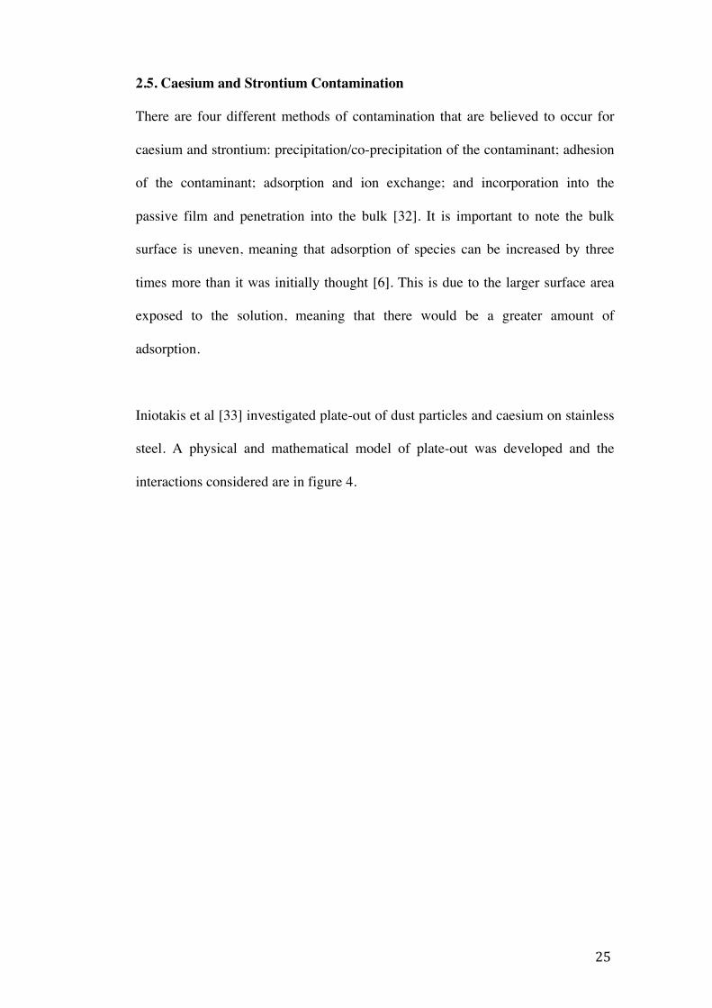
2.5. Caesium and Strontium Contamination
There are four different methods of contamination that are believed to occur for
caesium and strontium: precipitation/co-precipitation of the contaminant; adhesion
of the contaminant; adsorption and ion exchange; and incorporation into the
passive film and penetration into the bulk [32]. It is important to note the bulk
surface is uneven, meaning that adsorption of species can be increased by three
times more than it was initially thought [6]. This is due to the larger surface area
exposed to the solution, meaning that there would be a greater amount of
adsorption.
Iniotakis et al [33] investigated plate-out of dust particles and caesium on stainless
steel. A physical and mathematical model of plate-out was developed and the
interactions considered are in figure 4.

26
Figure 4. Schematic illustration of transport and deposition mechanisms of
dust particles and fission products in helium ducts [33]
Iniotakis et al ran experiments on AISI 316 and 347 stainless steels [33]. These
were preloaded with caesium-137 and measured with γ-spectroscopy. The samples
were then decontaminated with 2M nitric acid, deionised water and ultrasonically
cleaned. These were successful in decontamination. The theoretical calculations
confirmed the experimental results. It was postulated that the presence of an oxide
layer on the steel prevented penetration of caesium into the bulk metal [33].
Adeleye et al conducted a study about the kinetics of contamination of stainless
steel by caesium-134 and caesium-137 [13]. They postulated that the optimum pH
value for caesium plate-out was pH 10 and the variation of the grade of austenitic

27
stainless steel did not have a significant effect on the amount of contamination.
Contamination of caesium occurred in weakly acidic solutions (from pH 2)
through to alkaline environments. Adeleye stated that the plate-out reached a
steady state value ten days after commissioning of the plant, meaning that this is
believed to be a rapid process [13].
Type 304L stainless steel was also contaminated with a mixture of radioactive and
stable nuclides of caesium. This was done by immersion of steel coupons in three
different pH solutions and concentrations of between 3.01E-9 and 3.01E-5M. A
spike of active caesium with a specific activity was added to each solution. This
was carried out to reduce the radiological risk posed by using the radionuclide
alone. The samples were immersed in the solution for a week and, when removed
and dried, the activity was measured with a Ge-Li detector [34]. All other steel
surfaces were coated in Araldite to ensure that there would be no adsorption on the
other surfaces. However, it has also been reported that ions in solution will adhere
to glass and plastic surfaces, so it is likely that caesium may have adhered to the
Araldite used in this experiment [35].
Kadar et al investigated various iron oxides to determine the likely environments
for transuranic, uranium and fission product contamination. The pzc determined
for the various iron oxides in the passive film of stainless steels and these values
ranged between 4.2-8.8 [36]. It was discussed in the study that pH values lower
than the pzc would result in the passive film being positively charged, repelling the
cations in solution. Kadar et al suggested that cation adsorption would occur in
weakly acidic solutions as well as higher pH values [36]. The experimental results
found at pH values below the pzc, meaning that the passive layer had an overall

28
positive charge, absorption of caesium occurred on a Type 321 stainless steel tube,
whereas it was not found on the canister made from the same grade [37].
Interactions between the caesium ion and composition of the oxide layer was
suggested to be attributed to the contamination and the morphology of the steel
samples [37].
Takeuchi et al investigated the adhesion of radionuclides onto stainless steel in a
nitric acid environment [32]. A mixture of radionuclides, including Cs-134 and Cs-
137, was obtained by dissolving “Joyo Mark-II Fuel” with the uranium and
plutonium removed. A 304ULC (Ultra Low Carbon) stainless steel disk was
polished and subsequently immersed in this solution for 180 days at 400C. The
coupon was then decontaminated with distilled water, 3M nitric acid and
supersonic cleaning in a 3M nitric acid solution. The contamination was measured
by γ-ray spectroscopy. It was suggested that the caesium radioisotopes did not
contaminate the stainless steel easily and that contamination further into the bulk
was a result of corrosion [32].
Taylor investigated the interactions of radionuclides and colloids on stainless steel
pipe surfaces in static and turbulent flows. Taylor postulated that dissolved carbon
dioxide is always present in aqueous solutions and caesium will slowly form
caesium carbonate, coming out of solution and depositing on the steel passive
layer. He reported that there would be a slow build-up on the steel surface of
caesium, initially ionic caesium and then caesium carbonate [6]. This is unlikely
since caesium is in the hydrated ion form in aqueous solutions. There has been
suggestion that caesium diffuses through the passive layer via grain boundaries [6,
30], although Taylor implies that at low temperatures (374K) this will be a very

29
slow process. Taylor [6] discussed only caesium, ruthenium and cobalt in this
paper, but it has implications for strontium. He also suggested that there exists an
optimum pH for plate out and that electrostatic force initially, and then Van der
Waals forces play a part in attraction and adsorption respectively [6]. Taylor [6]
discussed that once a molecule has occupied a site on this layer, no other molecule
or ion can attach on top of it. However, this “monolayer” will constantly be
renewed with particle collisions [6].
An investigation of caesium adsorptions on zirconium and stainless steel was
analysed using Electrochemical Quartz Crystal Microbalance (EQCM). This
method is based on a mass-change generated frequency shift measurement on a
piezoelectric quartz crystal. The mass change was caused by ion adsorption. The
solution used contained 8g/L boric acid and 5mg/L potassium hydroxide, based on
the composition of the primary cooling water. It was found that a presence of a
monolayer of the contaminant on the passive layer and this was selective for the
grade of stainless steel of metal tested [38].
Investigations by Matzke et al [39, 40] have been carried out to confirm that
caesium diffusion occurs via the grain boundaries. The presence of caesium within
the steel was found to enhance chromium mobility through the grain boundaries,
as shown in figure 5. Ion bombardment was the method of caesium contamination
and they found that the passive layer does not prevent caesium penetration. At low
oxygen potentials, it was found that caesium diffusion was very slow. The rate at
which the diffusion occurs depends on the amount of defects present in the steel
[39, 40].

30
Figure 5. Grain boundary penetration of Cr-51 in normal and in Cs-
preloaded steel 1.4970 [40]
Sahai et al [41] reported that strontium contamination on a variety of minerals was
directly proportional to an increase in pH. The amount of contamination varied,
but a general trend was observed [41]. The reasoning behind investigating

31
strontium contamination was because strontium was more mobile in soils than
other hazardous radionuclides [41].
Rouppert et al [42, 43] investigated the contamination and decontamination of
stainless steel with caesium. It was postulated that radionuclides change from a
fixed to removable form on the steel depending on the environment conditions.
The rearrangement of the chemical system is caused by environmental and process
strains. It was implied that diffusion through the grain boundaries is very slow at
<2000C, according to Fick’s equation [42]. It was suggested that the adsorption of
cesium would occur by ion exchange. The hydroxyl groups on the oxide layer are
lewis acids and the hydrogen would be replaced by the metal ion. This process is
highly dependant on the pH of the system [42]. Type 304L steel coupons were
sealed in metallic boxes containing 100mg of CsOH. The boxes were heated to
8500C for 1 day and Fourier Transform IR spectroscopy was used to determine
chemical forms of the hydroxyl groups on the oxide layer. This would indicate if
chemisorption would have taken place [42]. The FTIR results indicated that
physisorption and chemisorption had taken place. The contaminated coupons were
then exposed for a month at ambient temperature to pH 2 nitric acid, pH 12 NaOH
and distilled water. It was found that the amount of chemisorbed caesium had
reduced in each environment [42]. The following equations were used to describe
the reactions taking place:
1) CsOH <==> Cs+ + OH- Disassociation of Cs in water
2) CrOO- + H+ <==> CrOOH Acidic behaviour of metal hydroxyl
group
3) CrOOCs +H+ <===> CrOOH + Cs+ Desorption of Cs

32
An increase in acidity displaces the equilibria of equations 2 and 3 to the right,
according to Le Chatelier’s principle [42]. In reverse, an increase in alkalinity
would displace the equilibria in 2 and 3 to the left.
Woodhouse investigated contamination of pond furniture and focused on caesium
and strontium contamination on mild and stainless steel surfaces [30]. Woodhouse
aimed to achieve stable and radioactive caesium and strontium contamination.
Stable caesium contamination was investigated at pH 12. The solution contained
carbonate-free sodium hydroxide and a ribbon of magnesium to simulate the fuel
pond environment. Different concentrations of caesium were used (60, 120, 240
and 360ppm), as was different compounds (CsOH, CsCl and CsNO3) and the
solutions were incubated at different temperatures (200C and 500C). The
contamination was measured with XPS. It was found that the temperature, caesium
compound and pH (12 and 14) did not influence caesium contamination [30].
Woodhouse stated that his experimental findings showed that strontium had a
higher affinity for stainless steel than caesium. This was confirmed by results that
he had obtained. TOF-SIMS was used to determine the spatial resolution of
caesium and strontium adsorption. This method confirmed that caesium adsorbed
onto the grain boundaries. It was found that strontium initially contaminated the
steel on the grains, and then was found on the grain boundaries deeper into the
oxide layer. This indicated that the radionuclides contaminated the steel in
different areas [30].

33
2.5.1. Caesium and strontium interactions with iron oxides
It has been found that the adsorption of caesium and strontium on iron oxides
depend on different parameters for each radionuclide. It has been postulated that
caesium adsorption involves ion exchange. The caesium cation replaces sodium,
potassium, magnesium and calcium on the surface. The substrate is found to be the
most important factor in caesium contamination, since caesium does not adsorb
well onto iron oxides [44]. It also competes with other cations, for example
strontium, for the absorption sites. Caesium adsorption is reported not to be pH
dependant, it relies on the surface charge of the substrate [45].
Music et al investigated the influences of pH on the adsorption of caesium and
strontium to hydrous iron oxides [45]. A pH increase from 8.5 to 9.0 caused a
decrease in the adsorbed caesium due to the competition for the adsorption sites by
sodium. Strontium contamination was found to be heavily pH dependant, as shown
in figure 6.

34
Figure 6. Relative adsorption of strontium on hematite, as a function of pH
[45]
The contamination on the hydrous iron oxides were analysed using X-ray
diffraction and Mossbauer spectrometry. The adsorption of strontium caused a
release of H+, either one or two released per strontium adsorbed [45]. This acidic
hydrogen release was interpreted as ion exchange, the strontium replacing the
hydrogen on the hydroxyl group. This is shown in the equation below. It was
found that an increase of 1 pH unit would cause considerable strontium adsorption
[45].
Fe(OH)2 + Sr2+ <==> Fe(O-)2Sr + 2H+

35
Steele [2, 14] conducted studies into the computer modeling of the iron oxides
found in the passive layer of stainless steels [2, 14]. It was found that after removal
of weakly bound contamination, the steel was still contaminated and the iron
oxides proved difficult to remove. This is due to the formation of the metal oxide
layers bound to the steel surface or passive layers, or formed on the corroding steel
over many years of use [2]. Decontamination techniques like the Ferrox process
utilize the iron oxides ability to encapsulate contaminants by adsorption or
incorporation into the bulk. The conversion of iron oxides into more stable phases
can affect their ability to retain or release contaminants [2]. Strontium was one of
the radionuclides investigated in the latter study. It was found that strontium was
most likely to contaminate chromite (FeCr2O4). The calculated stability of the
structures containing a strontium impurity confirm that these were more stable
than those containing cobalt, uranium and lanthanum [14].

36
2.6. Decontamination techniques for Stainless Steel
2.6.1. Chemical Decontamination
There are many different chemicals that can be used to decontaminate nuclear
components. These are mainly for non-porous surfaces and are circulated through
the system. The application of chemical decontamination depends on a number of
factors:
Shape and dimensions of system to be decontaminated;
Type and nature of the chemical reagent;
Type of material and contamination;
Availability of process equipment;
History of operation;
Exposure to workers and safety/environmental issues
Time and cost;
Quantity of secondary waste;
Effectiveness of previous chemical decontamination.
Chemical reagents are divided into two sub-groups: mild chemicals (detergents,
complexing agents and dilute acids or alkalis) and aggressive chemicals
(concentrated acids or alkalis and corrosive agents [46].
Mild chemical decontamination is used when the base material needs to be
recovered. The main advantages of these reagents are that they have low corrosion
rates and the secondary waste is easily treated. These chemicals do not have high
decontamination factors and require long contact times. Using other mild chemical
reagents in a number of stages or increasing the temperature can improve these.
There may also be a risk of recontamination [46].

37
Aggressive chemical reagents are used commonly in a multistep process with
rinses in between each step. They decontaminate by corroding the surface. Their
advantages are high decontamination factors (10-100) and short exposure times.
An added disadvantage is the treatment of the spent reagent and the hazards posed
by the operator handling such hazardous chemicals. Additional ventilation will
also be needed [46].
For chemical decontamination procedures, good contact with the contaminated
surface must be proven as well as drainage and storage of the contaminated
medium. Care must also be taken so as to avoid the recontamination of the surface
as the chemical solution becomes saturated [46].
In the table below is a list of chemical techniques used in the nuclear industry.
Table 2. Chemical decontamination techniques [47] Chemical Techniques Material/surface Strong mineral acids Carbon steel, stainless steel, Inconel, metals
and Metallic oxides
Acid salts Metal surfaces Organic acids Metals, metallic oxides and plastics
Bases and alkaline salts Carbon steel Complexing agents Metals
Bleaching Organic materials from metals Detergents and surfactants Organic materials from metals, plastics and
concrete Organic solvents Organic materials from metals, plastics and
concrete Multiphase treatment processes Carbon steel, stainless steel, Inconel,
Zircaloy Foam decontamination Porous and non-porous surfaces
Chemical gels Porous and non-porous surfaces Decontamination by pastes Carbon steel, stainless steel
Decontamination by chemical fog Carbon steel, stainless steel

38
Strong mineral acids are used to dissolve the oxide layer and lower the pH of the
solutions to increase solubility or ion exchange of the metal ions. These have good
decontamination factors, ranging from 2-20 [46]. The decontaminaion factor is the
activity of the vessel before the decontamination process divided by the activity of
the vessel after the decontamination process. The acids used for stainless steel are:
Sulphuric acid. This is used as an oxidising agent and has been proven to
have some degree of success.
Fluoroboric acid. This acid attacks nearly every metallic oxide and metal
surface. It has been implied that thin layers of the contaminated steel can
be removed without substantial damage to the steel.
Fluoronitric acid. This acid is used for rapid decontamination of stainless
steel.
Acid salts such as sodium phosphates, sodium sulphate, sodium fluoride and
ammonium citrate, can be used in the place of acids or combined to give more
effective decontamination [47].
Organic acids like formic acid, citric acid and oxalic peroxide are mainly used
during plant operation, but can also be used for decommissioning. These can form
a complex with the contaminants and can be used as part of a multistep process.
Complexing agents include organic acids and acid salts, but also EDTA (Ethylene-
diamine-tetra-acetic acid). These form stable complexes with metal ions to prevent
recontamination and encourage them into solution.
Bleach, detergents and surfactants and organic solvents are all used to remove
grease, chemical agents (bleaching), and organic materials. These are used across
other industries for the same applications [47].

39
Multiphase treatment processes used a variety of methods to achieve a higher
decontamination factor (or more effective decontamination). These can range from
a decontamination factor of 15-50 [47]. Redox agents change the oxidation state of
the oxide layer, rendering it soluble. An example of this is using an alkaline
permanganate in the first stage, a strongly oxidising solution which converts the
chromium ions in the oxide layer to soluble chromates. This is then followed by an
acid stage (oxalic acid, EDTA, sulphuric acid, sulphamic acid, etc) to ensure
complexing of the dissolved metal ions from within the oxide layer. The main
problems associated with this technique are the undesired corrosion of the steel
and the very hazardous chemical effluent [46].
Foam decontamination is used for complex shapes of steels. The foams act as a
carrier for chemical decontamination agents and have low volumes of waste. They
are easy to apply and this can be done remotely or manually. Pastes are widely
used for stainless steel surfaces and consist of a carrier, a filler and an acid or a
mixture of acids as the active decontaminant. There are also versions that contain
an abrasive that improves effectiveness [47].
2.6.2. Mechanical Decontamination
Mechanical decontamination methods can be described as two separate processes:
surface cleaning and surface removal. This method can be used alongside or before
chemical decontamination. Mechanical decontamination techniques can be used on
any surface with good results achieved. On porous surfaces, this method is the
only option [46]. The selection of this technique, as with chemical

40
decontamination, depends on a number of factors that are the same for any
technique. As mentioned above, the selected method may need to be repeated to
meet acceptance criteria.
Surface cleaning techniques are used when contamination is limited to the surface
of the material. This may be adsorbed dust or molecules. This kind of technique
produces liquid waste that needs to be treated. Sometimes this technique is used
after surface removal [46]. The disadvantage to this technique is that there may be
a production of air borne dusts that would pose a threat to worker safety. Also, the
area to be worked upon needs to be free of cracks and corners so that the
equipment can easily access the area.
Table 3. Mechanical techniques for decontamination of components [47] Mechanical techniques Material
Flushing with water Large areas Dusting/vacuuming/wiping/
scrubbing Concrete & other surfaces
Strippable coating Large non-porous surfaces, Easily accessible
Abrasive cleaning Metal & concrete surfaces, hand tools Sponge blasting Paints, protective coatings, rust, metals
CO2 blasting Plastics, ceramics, composites, Stainless steel, carbon steel, concrete, paints
High pressure liquid nitrogen Blasting
Metals, concrete
Wet ice blasting Coatings, Concrete surface High pressure and ultra high pressure water jets
Inaccessible surfaces, structural steel And cell interiors
Mechanical decontamination techniques can be used on stainless steel in a variety
of ways. This includes:
Flushing with water,

41
Dusting/vacuuming/wiping/scrubbing-this is normally carried out as a
pretreatment and is a useful procedure to get rid of large quantities dust,
aerosols and particles.
Strippable coating. Strippable coatings have been used in many practical
applications. This involves the application of the polymer and
decontaminant mixture to a surface and the polymer is removed after
setting.
Abrasive cleaning-this uses abrasive material and is used to remove
smeared or fixed contamination. This can be a wet or dry procedure.
Sponge blasting. The sponges consist of water-based urethane and they
create a scrubbing effect when they are blasted onto a surface.
CO2 blasting is another version of blasting that involves carbon dioxide
pellets as the cleaning medium. This method cannot be used for brittle or
soft materials.
High pressure liquid nitrogen blasting shoots grit at the contaminated
surface using a liquid nitrogen jet. The liquid nitrogen makes the surface
brittle and aids in decontamination.
High pressure water jets.
2.6.3. Alternative Techniques
These techniques have also been developed as another option to mechanical or
chemical contamination.
Table 4. Alternative Techniques for Decontamination [47] Techniques Material
Electropolishing Conductive surfaces Ultrasonic cleaning Small objects with loosely
Adsorbed contamination Melting Metal

42
Electropolishing is a technique that is the opposite of electroplating. It is an anodic
dissolution method of a controlled amount of the surface of the material. This only
works with conductive materials, so long as there are no protective surface
coatings. The equipment is relatively cheap and it is a simple procedure. It
produces a smooth polished surface that is difficult to recontaminate, it removes
practically all radionuclides and the secondary waste is relatively low. Currently,
electropolishing takes place in a tank, which means that the contaminated material
needs to be removed from the plant and immersed. Another disadvantage is that
hidden parts are not well treated [46]. The electropolishing technique involves a
range of electrodes and uses citric acid, ammonium nitrate or nitric acid
electrolytes at temperatures between 25-50C. The duration of this cycle is about 30
mins [46].
Melting is a type of decontamination that uses slightly contaminated scrap metal to
decontaminate the steel, but this is only decontaminate volatile contaminants (Cs-
137) or radionuclides that concentrate in the slag (Pu). The radioactivity of the
molten steel can be measured and this treatment is seen as waste reduction, since
the molten steel will be decontaminated. This treatment solves a problem with
inaccessible surfaces and is regarded as a final step in decontamination [46]. It has
also been mentioned that an electroslag remelting process uses a copper mold to
collect the decontaminated steel, detailing a different twist on this process [48].

43
3. Experimental
The aim of the experiments is to investigate the parameters of cold work applied to
the stainless steel coupon, solution pH and exposure time and their influence on
caesium and strontium contamination. This follows on from the previous
investigations by Woodhouse [30].
Cold rolling of stainless steel has been carried out to confirm whether the plastic
deformation of a sample can encourage contamination. The aim of this method
was to expose type 304H stainless steel with varying strain to caesium or strontium
in three different pH environments. The stainless steel coupons required a varying
amount of plastic deformation (as received, 5% and 30% cold rolled) with a large
polished surface. This deformation was to mimic the strain applied to the stainless
steel in the structure of the reprocessing plants and ponds. It was expected that the
plastic deformation in the structural steel would have been greater than 30%, but
the strain applied initially should have given an indication on whether it had an
effect on contamination. The surfaces of the coupons were examined using laser
profilometry and microscopy. One coupon was etched to confirm Woodhouse’s
findings that strontium contamination occurs via the grain boundaries.
Aqueous environments simulating the acidic conditions in reprocessing plant,
neutral environments and the mildly caustic spent pool pond were examined to
confirm the preferential environment for contamination of caesium and strontium.
All solutions were incubated at 500C. Further investigations using high
temperature paste were carried out to determine the most effective method of
contamination. All of the coupons were analysed using Glow Discharge Optical

44
Emission Spectroscopy (GDOES). The data was examined to determine whether
contamination occurred and the composition of the passive layer. The GDOES
data will be compared to previous studies.
Other analytical techniques could have been used to analyse the steel surface, for
example: SIMS, XPS and AES. Each of these techniques has advantages and
disadvantages. These are detailed in table 5.
Table 5. Comparison of surface analysis techniques [49] Analytical method Advantages Disadvantages GDOES Up to 100µm depth, good
quantification, fast analysis time.
10µg/g detection limit, 5mm analysis area.
XPS Easily acquired chemical information.
1µm depth analysis, preferential sputtering changes surface, 0.1 at % detection.
AES Local depth profiling, 100nm analysis area,
1µm depth analysis, 0.1 at % detection.
SIMS 0.1µg/g detection limit, trace analysis, surface sensitive
1µm depth analysis, poor quantification, interference.
GDOES was chosen as the analytical technique to be used because it has a fast
analysis time, gives a representation of the bulk material and the data is easily
interpreted. This technique would ideally be used in conjunction with another
analytical technique.
Table 6 details the number of stainless steel coupons prepared, the amount of cold
work (CW), the contaminant the coupon was exposed to and the contamination
environment.

45
3.1. Materials and Composition
The composition of AISI 304H stainless steel is detailed in table 7.
Table 7. Chemical Composition Requirements, % [9] Constituent C Mn P S Si Cr Ni 304H 0.04-
0.10 2.00 0.045 0.030 0.75 18.0-20.0 8.0-10.5
3.1.1. Material and Surface Preparation
Three long strips of as received AISI304H stainless steel were cut off the main
plate along the rolling direction. These strips are shown in figure 7. The strips
were approximately 30mm in width and 300mm in length. One strip was not cold
rolled for comparison (as received), one required a 5% reduction in depth and one
required a 30% depth reduction. A MRB Marshall Richards Barco machine was
used to cold roll the two strips and, each reduction was carried out by a multi-pass
process. The original depth of the strips (table 8) was 13.00 ±0.3mm. Table 8 gives
Table 6. AISI 304H coupons prepared and their environments As received & polished
coupon (0..p) 5% CW
& polished coupon (5..p)
30% CW & polished coupon
(30..p)
30% CW & etched coupon (30..e)
Cs Sr
Blank Cs Cs Sr Sr
4M Nitric Acid solution
(A)
1 1 1 1 1 1 0
pH 7 solution (B)
1 1 1 0 1 1 0
Carbonate solution (C)
2 0 0 2 1 0 0
NaOH solution (D)
1 1 1 0 1 4 1
High temperature method (E)
0 0 0 0 2 2 0

46
the final thicknesses of the strips with typical error after deformation. The
thickness measurements were carried out using a calibrated caliper and an average
of five measurements was taken, the absolute error of the measurements recorded.
Table 8. Depth of AISI 304H stainless steel strips As received 5% cold rolled 30% cold rolled Average depth (5 measurements)
13.00mm 12.3mm 9.03mm
Min/max value (±mm)
0.3 0.2 0.2
Figure 7. Illustration of the as received and cold rolled strips
All three strips were cut into 10 equally sized coupons, with approximate
dimensions of 30mm by 30mm by variable depth (figure 8), using a Brillant 250H
cutting machine. The coupon dimensions are illustrated in figure 8. The coupons
were then ground on one surface using a Saphir 330 machine with silicon carbide
grinding paper, successively using p200, p400, p800 and p1200 paper at 250-
300rpm with water as a lubricant. At each stage the sample was reground after
rotation at 90 degrees.

47
Figure 8. Illustration of the coupons used in the experimental set
All of the samples were then washed with deionised water and dried thoroughly.
The samples were polished to 0.25 micron diamond paste finish. Between each
polishing the samples were rinsed in water and dried in hot air. The purpose of
polishing was to reduce the roughness of the samples. The prepared surface of the
coupon was checked for scratches using an optical microscope. Table 9 shows the
sample number allocated for each coupon according to cold work, environment
and contaminant.
Table 9. Sample names according to steel conditions and environments As received polished
coupon (0..p) 5% cold-rolled polished coupon (5..p)
30% cold rolled polished coupon (30..p)
30% cold rolled etched coupon (30..e)
Cs Sr
Blank
Cs Cs Sr Sr
4M Nitric Acid solution (A)
A0Csp1 A0Srp1
A0p1 A5Csp1 A30Csp1 A30Srp1 ----
pH 7 solution (B)
B0Csp1 B0Srp1 B0p1 ---- B30Csp1 B30Srp1 ----
Carbonate solution (C)
C0Csp1 C0Csp2
---- ---- C5Csp1 C5Csp2
C30Csp1 ---- ----
NaOH solution (D)
D0Csp1 D0Srp1
D0p1 ---- D30Csp1 D30Srp1 D30Srp2 D30Srp3 D30Srp4
D30Sre1
High temperature method (E)
---- ---- ---- ---- E30Csp1 E30Csp2
E30Srp1 E30Srp2
----

48
3.1.2. Etching Procedure
One 30% cold rolled sample (D30Sre1) was etched to determine if an increase in
the amount of strontium contamination would be observed if the grain boundaries
were more defined. The sample was electrochemically etched in 10% w/w oxalic
acid [50]. The coupon was submerged using tongs into a shallow beaker of oxalic
acid at room temperature in a well-ventilated area. A direct current was applied at
1 A/cm2 of steel surface for 90 seconds: i.e. a total current of 9A was applied. The
steel cathode was attached to the side of the beaker, in contact with the oxalic acid,
and the polished coupon was the anode. After etching, the coupon was extracted
using tongs and rinsed with hot water and acetone to remove all of the oxalic acid
[50]. The etched coupon was checked using an optical microscope to confirm that
the grain boundaries could be seen clearly throughout the sample. Examples of
etched samples can be seen in section 4.1.
3.2. Characterisation methods
3.2.1. Laser profilometry method
The surface roughness of the coupons were measured with laser profilometry to
ensure that they would be sufficiently flat for GDOES analysis. This was carried
out using the Nanofocus µ-scan surface profilo-meter. The 30mm x 30mm
polished surface of each coupon was examined. The frequency of the laser was
800Hz, scan speed was 8 mm/s, working distance was 20mm and the resolution on
the x-axis was 10 microns and 70 microns on the y-axis. The coupons were wiped
clean before analysis using fibre-free tissue. One set of samples, however, was
stored for 7 days before this analysis was carried out. This caused surface
contamination by dust particles.

49
The laser position on the coupon was calibrated to ensure the optimum working
distance. A 3D profile of the sample was obtained and roughness parameters
extracted. High R-values would result in uneven sputtering GDOES profiles. The
average roughness (Ra), the mean roughness depth (Rz) and the root mean
roughness squared (Rq) was obtained for the x and y-axes of each coupon.
The parameters that will be examined are the values that give the indication of the
roughness of each coupon. These parameters are the Ra, Rq and Rz. The Ra value
(figure 9) is the arithmetic average of the absolute values of the roughness profile
of a surface. A total of approximately 2500 roughness profile coordinate
measurements were made for the x-axis and 350 for the y-axis on the coupons in
this experimental set.
The Rz and Rq roughness values (figures 10 and 9) represent the mean of a
number of roughness depths of a number of successive lengths (l), and the root
mean square average of the roughness profile coordinates respectively. The valleys
and peaks of the roughness measurements influence the Rz and Rq values more
than the Ra value [51]. Below are the equations showing how the values are
calculated:
Rz = 1/n (Rz1 + Rz2 + Rz3 + Rz4 + Rz5….etc.)

50
Figure 9. Diagram to show how the Ra and Rq values are calculated [51]
Figure 10. Diagram to show how the Rz values are calculated [51]
3.2.2. Glow Discharge Optical Emission Spectroscopy (GDOES)
GDOES is used as an analysis tool to determine if contamination has occurred at
the stainless steel surfaces. This analysis method analyses any solid material by
sputtering the surface and causing excitation of the atoms on the surface of the
material.
Low-pressure argon gas is passed through an electric current and if the potential is
high enough a plasma is created. [52]. The generated positive ions in this plasma
are attracted to the negative electrode and knock atoms off the surface of that
electrode [53]. This sputter process results in an emission of secondary electrons,

51
which are then attracted to the positive pole (anode) and collide with more argon
atoms on the way.
When the sputtered atoms enter the plasma, they are excited by the collisions of
the electrons or excited argon atoms [52]. A simplified diagram of the sputtering
and emission processes can be seen in figure 11. These sputtered atoms then de-
excite, producing the “glow”. By measuring the wavelength, the numbers of each
type of atom from the cathode can be measured [52, 53]. The detection limits for
GDOES are given in table 10. Iron is not included since it is the main component
of the steel.
Table 10. GDOES Detection Limits [54] Element Detection Limit Nickel 5-10ppm Chromium 5-10ppm Oxygen 100ppm Caesium 20,000ppm (0.02%) Strontium 20ppm
Figure 11. Illustration of the GDOES sputtering and emission processes [53]

52
Elemental depth distributions were examined by GD OES analysis, where a GD-
Profiler 2 (Horiba Jobin Yvon) operating in the rf-mode at 13.56 MHz was
employed. A 4 mm diameter copper anode and high purity argon gas was used.
The emission responses from the excited sputtered elements were detected with a
polychromator of focal length of 500 mm with 30 optical windows. The emission
lines used were 130.21 nm for oxygen, 371.99 nm for iron, 425.43 nm for
chromium, 341.47 nm for nickel, 403.44 nm for manganese and 156.14 nm for
carbon. The caesium response was recorded using a monochromator adjusted to a
line at 455.52 nm. The elemental depth profiling was carried out at argon pressure
of 700 Pa and a power of 35 W, with a data acquisition time of 0.02 s.
Prior to each depth profiling, pre-sputtering of a monocrystalline silicon wafer was
undertaken to clean the GD source [55]. Quantum XP software was used to sort
and manipulate the data sets. The analysis process is repeated on a different area of
the sample at each time-point to give a representative indication of contamination
[53].
The trapezoidal rule was used to calculate each integral. Figure 12 gives an
indication of how the integrals were calculated. The area of each trapezoid is
calculated and the sum of all of these gives a quantification of the curve. The
trapezoidal rule calculates the area under a curve by separating the x-axis into
discrete units. This gives an approximation for the area under the curve. For this
set of data, the smallest amount was 0.02 seconds of sputtering time. The total
distance on the x-axis was maximum 0.5 seconds from the start of the curve and
250 corresponding y-values were obtained. The first value was taken 0.02 seconds

53
before the peak occurred. The maximum background intensity was subtracted from
the strontium or caesium peak intensities.
Figure 12. Trapezoids under a strontium curve
The area for one trapezoid= dx x ((y1 + y2)/2), where dx is 0.02, y1 is the first
point on the y axis for x1 and y2 is the corresponding y-value for x2 (shown in
figure 13). A total of 250 values was obtained, each corresponding to the area of
the respective trapezoid. The sum of all of these values was the area under the
curve (integral).

54
Figure 13. How the area of a trapezoid is calculated
3.3. Contamination methods
Two contamination methods were used to achieve considerable caesium and
strontium contamination. These were:
• High temperature contamination, where a coupon was exposed to a
concentrated paste of caesium carbonate or strontium nitrate and incubated
at 3500C for 7 days;
• Aqueous contamination, which involved exposing the steel coupon to a
reaction solution of caesium nitrate, caesium carbonate or strontium nitrate
and the solution was kept at constant temperature.
The high temperature contamination was used to demonstrate the effect of high
temperature on contamination using a highly concentrated paste of the
contaminant. The aqueous procedure was used to simulate the nitric acid aqueous
environment seen in reprocessing plants and the alkaline environment seen in
spent fuel storage ponds. The neutral environment is examined to discover if
contamination occurs in this environment. These experiments gave an indication to
the environments that would experience the largest amount of caesium or
strontium contamination.
55
3.3.1. High temperature contamination method
The aim of these tests was to achieve Cs and Sr contamination on the coupon
without exposure to an aqueous environment. The coupons were cleaned in
deionised water using an ultrasonic water bath for 30 minutes. The coupons were
immersed and removed using tongs holding the sides of the sample. After
extraction, the coupons were left to air dry. Table 11 summarises the samples used
in this experiment.
Table 11. High temperature paste contamination of samples Caesium carbonate Strontium nitrate E30Csp1 E30Srp1 E30Csp2 E30Srp2
A few drops of deionised water was added to a few spatulas of a powder, either
caesium carbonate or anhydrous strontium nitrate. These were mixed with a
paintbrush until a thick paste was observed. The paste was spread over the
polished surface of the sample until a layer of approximately 5mm was achieved.
The samples were then incubated in a temperature calibrated oven at 3500C for 7
days. After the coupons were carefully removed from the oven and cooled, the
samples were then rinsed in water until all of the paste residue was removed. Each
individual coupon was immersed in a beaker of DI water for 30 minutes after the
initial rinse. The addition and removal of the coupon was done using plastic coated
tongs, holding the coupon on the sides. Strontium nitrate is hygroscopic and it was
observed that the residue was encouraging condensation during the drying
procedure. These samples were then left to air dry and taken for GDOES analysis.

56
3.3.2. Aqueous Contamination
The environments examined in this experimental set are 4M nitric acid, NaHCO3
Cs2CO3 and 0.01M NaOH. The desired concentration of caesium and strontium
was 1000ppm (7.52mM and 11.4mM respectively for each contaminant). Previous
studies have used 0.1 mol/l concentrations of caesium-133 for contamination of
stainless steel [32]. It was decided to have a larger concentration of contaminants
than what is found on plant to achieve a considerable amount of contamination.
The concentration of caesium in the Cs2CO3 solution was 18mM to achieve a pH
value of 11. The steel coupons detailed in table 8 were cleaned in the ultrasonic
bath for 30 minutes, extracted using tongs and left to air dry before immersion in
the reaction solutions.
3.3.2.1. Solutions Preparation Procedure
Concentrated (15.86M) HNO3 was at first diluted with de-ionised water to achieve
a 3.97M nitric acid solution. Either Cs2CO3 or Sr(NO3)2 (both ACS grade) was
then added to this solution to obtain a final concentration of 1000ppm of either Cs
or Sr. The prepared solutions were then poured into reaction jars, and clean plastic
coated tongs were used to place the sample coupons into the solutions. The jars
were then sealed tightly and incubated in the water bath at 500C. The reaction jars
were constructed of coated glass, which was chemical and heat resistant. The top
of the jar had a specially developed screw thread that prevented leakages and
contamination with the lid tightly sealed. The only exchange of carbon dioxide that
took place was within the air space of the sealed jar.
A 10mM NaHCO3 solution was prepared with deionised water. Either CsNO3 or
Sr(NO3)2 (both ACS grade) was then added to this solution to obtain a final

57
concentration of 1000ppm of either Cs or Sr. The prepared solutions were then
poured into reaction jars, and clean plastic coated tongs were used to place the
sample coupons into the solutions. The pH was adjusted to between 7-7.5 using a
Pasteur pipette containing 0.001M NaOH or 0.015M nitric acid. The pH was
measured using a calibrated pH probe. The jars were then sealed tightly and
incubated in the water bath at 500C.
A Cs2CO3 solution was prepared with deionised water to achieve a final
concentration of 18mM. The prepared solutions were then poured into reaction
jars, and clean plastic coated tongs were used to place the sample coupons into the
solutions. The pH was checked to ensure the value was close to 11. The pH was
measured using a calibrated pH probe. The jars were then sealed tightly and
incubated in the water bath at 500C.
A 0.001M NaOH solution was first prepared by the addition of deionised water to
0.1mol of anhydrous NaOH pellets. Either CsNO3 or Sr(NO3)2 (both ACS grade)
was then added to this solution to obtain a final concentration of respectively
1000ppm of either Cs or Sr. The prepared solutions were then poured into reaction
jars, and clean plastic coated tongs were used to place the sample coupons into the
solutions. The pH was checked to ensure the value was 11. The pH was measured
using a calibrated pH probe. The jars were then sealed tightly and incubated in the
water bath at 500C.

58
3.3.2.2. Coupon Sampling Procedure
Polished coupon samples were exposed for 1, 5, 9 and 16 weeks. At each time-
point the coupons were extracted and immediately analysed by GDOES to
determine the extent of contamination at that particular time. Following exposure
the steel coupons were extracted from the reaction solutions with clean plastic
coated tongs. The lid was removed immediately before removal of the coupon to
reduce the exposure of the reaction mixture to air. When the coupon was removed,
the lid was replaced on the jar and screwed tightly to again prevent exposure to air
that would cause a pH deviation.
The coupons were initially rinsed with de-ionised water for 30 seconds and then
submerged in a beaker of DI water for 30 minutes. This was carried out to dissolve
any possible salt residue from the surface. The coupons were extracted from the
water using tongs, holding the coupon on its sides. The sample was left to dry in
air and taken for GDOES analysis. After GDOES, the samples were immersed
back in the correct reaction solutions using tongs.
3.3.2.3. Solution pH measurement
The pH of the neutral, carbonate and sodium hydroxide solutions were monitored
on a weekly basis to ensure the pH remained relatively constant. Before each
measurement, the pH probe was cleaned and calibrated using pH 7 and 10.19
calibration solutions. Another buffer solution of pH 9 was measured and used as a
standard. Aliquots of each of the solutions were taken using disposable syringes.
The lids of the vessels were removed immediately before and secured after each
aliquot was taken. An average of the three measurements was recorded.

59
4. Results & Discussion
Section 4.1 and 4.2 summarise examinations of the surface of the coupons using
electron microscopy and laser profilometry. Electron microscopy was used to
determine the changes in microstructure with cold work and the possible effects
that this would have on contamination. The steel samples for electron-microscopy
have all been etched with 10 wt.% oxalic acid to aid the visibility of the grains.
Laser profilometry was performed to acquire a 3D profile of the steel coupon.
From this information, the roughness values can be calculated. Section 4.3 then
discusses all GDOES results, to identify potential routes to simulate Sr and Cs
contamination.
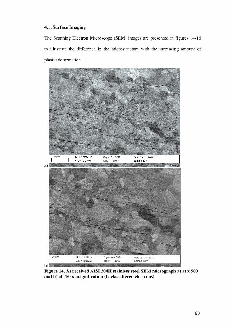
60
4.1. Surface Imaging
The Scanning Electron Microscope (SEM) images are presented in figures 14-16
to illustrate the difference in the microstructure with the increasing amount of
plastic deformation.
a)
b) Figure 14. As received AISI 304H stainless steel SEM micrograph a) at x 500 and b) at 750 x magnification (backscattered electrons)

61
It can be seen from the micrographs that the microstructure changes with the
amount of cold rolling performed on the sample. Figure 14 also shows that the as
received steel contains a lot of stringers, indicating this was from the
manufacturing process. This would imply that the orientation of those has arisen
from the rolling process during manufacture. The black lines seen in the image are
possibly ferrite or MnS sulphide inclusions. The grains are polygonal, indicating
recrystallised material conditions, with grain sizes varying from typically 20µm by
10µm to 120µm by 90µm.

62
a)
b) Figure 15. 5% cold rolled AISI 304H stainless steel SEM micrograph a) at x 500 and b) at 750 x magnification (backscattered electrons)
In figures 15 and 16, the grains are progressively harder to distinguish and black
spots can be seen. The black spots are most likely precipitated phases or particles
of dust. In figure 15, the grain sizes vary from 10µm by 10µm to 140µm by 90µm.
This implies that the grains change in size and become more elongated when cold
rolled at a 5% reduction.

63
a)
b) Figure 16. 30% cold rolled AISI 304H stainless steel SEM micrograph a) at x 500 and b) at 750 x magnification (backscattered electrons)
At a 30% depth reduction (figure 16), the grain size varies from ca. 10µm x 5µm
to 120µm x 80µm. This suggests that further elongation and changes in
microstructure occurs at a 30% reduction. In figure 16, the black spots observed

64
are similar to those seen in figure 15. These could either be from carbides or other
particles/second phases.
4.2. Roughness Parameters
The roughness values are important in ensuring that the sample roughness is
sufficiently low for GDOES analysis. Table 12 shows the roughness values
obtained with the nanoscan laser profilometer. The roughness of a surface is
defined as closely spaced irregularities on the surface, possibly from cutting and
grinding procedures [51].
Table 12. R-values of the investigated stainless steel coupons Sample Ra value
x-axis Rz value x-axis
Rq value x-axis
Ra value y-axis
Rz value y-axis
Rq value y-axis
A0p1 0.406 1.634 0.755 0.164 0.706 0.237 B0p1 0.500 2.053 0.871 0.044 0.180 0.055 D0p1 1.697 7.630 2.299 1.398 5.638 1.799 A0Csp1 1.519 7.127 1.989 1.508 6.056 2.114 A30Csp1 1.641 7.489 2.263 1.858 7.642 2.299 A0Srp1 0.916 4.317 1.138 1.445 5.838 1.856 A30Srp1 1.064 4.648 1.413 1.218 4.896 1.531 B0Csp1 1.063 5.221 1.619 1.534 6.242 1.990 B30Csp1 0.341 1.331 0.517 0.047 0.194 0.060 B0Srp1 1.528 6.912 1.932 1.569 6.330 2.036 B30Srp1 3.975 20.434 5.072 2.201 9.251 2.813 D0Csp1 3.543 18.307 12.467 2.930 13.183 8.492 D30Csp1 2.778 14.087 3.517 3.373 14.217 4.548 D0Srp1 1.175 5.340 1.462 1.376 5.719 1.737 D30Srp1 2.524 14.377 4.595 1.472 6.702 2.089 D30Srp2 5.067 26.123 8.163 4.322 17.701 5.968 D30Srp3 4.863 25.088 6.191 6.902 30.695 12.865 D30Srp4 1.221 6.059 1.576 1.706 6.787 2.138 D30Sre1 2.552 11.701 3.128 1.899 7.583 2.435 E30Srp1 9.944 61.317 14.031 8.044 40.743 11.961 E30Srp2 2.043 8.978 2.570 1.082 4.379 1.323 E30Csp1 3.635 17.607 5.093 2.230 9.903 4.068 E30Csp2 1.297 5.840 1.640 0.863 3.507 1.092

65
Figure 17 shows the Ra, Rq and Rz values for the x-axis (a) and y-axis (b) in
graphical form for comparison. The high Rz and Rq values seen for B30Srp1,
D30Srp1, D30Srp2, D30Srp3, D30Sre1, E30Srp1 and E30Csp1 indicate that there
were possibly some dust particles/contaminations present on the surface.
Ultrasonic cleaning of the samples before laser profilometry would have ensured
all of the particles would have been removed from the coupon surface. This was
only realized after GDOES analysis and so the results that were obtained from the
samples that had large parameters (relatively high surface roughness) should be
treated with caution. Examples of samples that had high surface roughness
measurements are B30Srp1, D30Srp1, D30Srp2, D30Srp3, D30Sre1, E30Srp1 and
E30Csp1.

66
a)
Figure 17. a) Laser profilometry R-values of all coupons along the x-axis

67
b)
Figure 17. b) Laser profilometry R-values of all coupons along the the y-axis
68
The value that has been observed to vary the most from table 12 and figure 17 is
the Rz value, which is the mean roughness depth. This value would be large if
particles of dust were present on the surface, since this would increase the absolute
height difference measured. It can be seen from figure 9 that the Rq values
represent a larger range of the roughness profile than the Ra value, which is
generally expected, since Rq is based on the absolute sum of the height variations.
This explains the range of Rq values, the coupons with dust contamination having
far larger values. The presence of contaminations on the surface would give a
larger difference between the minimum and maximum roughness profile, the Ra,
Rq and Rz all being increased as a result. In figure 17 it is clear which coupons
have contamination.
4.2.1. Discussion of the Roughness Parameters
The roughness measurements were inconsistent with the examination of the
coupons after the polishing procedure. GDOES is sensitive to the surface
roughness and the coupons, in general, would need to be “flat” for GDOES
analysis. If the sample were slanted, the sample would not attach properly to the o-
ring of the GDOES, posing a problem for maintaining the vacuum needed for
sputtering. The presence of scratches or a rough sample would cause uneven
sputtering and a deformed surface profile [56]. For example, the caesium
carbonate samples (sample codes C0Csp1, C0Csp2, C5Csp1, C5Csp2 & C30Csp1)
had a number of scratches, and the GDOES profiles seem slightly distorted due to
uneven sputtering. This can be seen in figures 22-24. Both samples E30Srp1 and
D30Srp3 have got high R-values and examination of the GDOES data reveals that
there is a small amount of deformation in comparison to other samples within the

69
same exposure conditions. However, E30Srp1 and E30Srp2 both experienced
deformation and it is unclear whether this was caused by an uneven surface (for
E30Srp1) or the exposure conditions. D30Srp3 experienced a small amount of
deformation, indicating this could be due to the uneven surface, but the steel/oxide
interface can still be established.
As discussed in section 2.2, the surface layer of Type 304 stainless steel is a few
nanometres thick. The roughness parameters are expressed as micrometres,
meaning that a Ra value of a few micrometres would be greater than the thickness
of the surface layer itself. This would have a detrimental effect on the depth profile
and the detection of caesium and strontium contamination, resulting in total
degradation of the depth profiles [57].
The surface roughness measurements (Ra, Rq and Rz) would be expected to be
less than 1 for the surface to be flat, which is the required roughness for a sample
analysed by GDOES [56-58]. This would be an essential parameter to consider
with contamination. Microscopically flat samples can be achieved by
electropolishing, giving an accuracy of interfaces within a few nanometres [57].
Etched samples, that have ridges and cavities of up to 1 micron diameter, can give
deformed profiles [57]. Examination of Figure 40 in section 4.3.2.3 confirms that
roughness measurements greater than 1 micron give deformed depth profiles. This
would mean the integrals taken from under the deformed peaks would not be
accurate, although it is sufficient to give a rough indication.
Greater care should have been taken during the preparation of these samples. This
includes inspection of the samples under a microscope to ensure there are no

70
visible scratches, more time taken to thoroughly prepare the surface and ultrasonic
cleaning of the samples before laser profilometry to ensure removal of particles
from the surface,

71
4.3. Caesium and Strontium Contamination
In this section, caesium and strontium contamination will be examined separately.
Firstly, the GDOES data sputtering profiles for each contaminant will be examined
to determine the influence of the environment on the passive layer of the coupon
and to determine where within the steel the contamination has occurred. A
comparison between the blank and the contaminated coupons will also be
investigated to discover whether the presence of the contaminant changes the
composition of the surface layer. Then the area under curve (integral) calculated
from each environment will be examined to determine the amount of
contamination against the experimental parameters of time, pH and cold work. The
effect of pH deviation on strontium contamination will also be examined. Lastly, a
comparison of contamination techniques will be made to determine the most
effective technique for contaminating stainless steel surfaces with stable Cs and Sr
isotopes.
4.3.1. Caesium contamination
GDOES is useful for determination of where the contamination occurs but is
sensitive to the steel sample surface roughness. In this section, the GDOES
sputtering data is examined for each contamination environment in turn to
determine the change in the steel surface and upon cesium contamination. Then the
integrals of the peaks observed in the sputtering data will be examined against the
parameters of cold work, pH and time to discover any correlation. Cs
contamination was quantified using the area under the peak (integrals).

72
4.3.1.1. 4M Nitric Acid (environment A)
It was discussed earlier that nitric acid is used to passivate stainless steel, generally
causing an enrichment in chromium in the passive layer. Figure 18 shows the
reference coupon exposed to 4M nitric acid only (A0p1) and a large chromium
peak is observed initially, suggesting the passivation of the coupon. On both A0p1
and A0Csp1, the carbon peak occurs initially, which shows the contamination of
carbon on the outermost of the surface. A small presence of carbon is seen in the
profile due to the carbon content of the steel. There was no detectable Cs
contamination on the A0Csp1 sample exposed to the nitric acid environment.

73
a)
b)
Figure 18. GDOES sputtering data depth profiles of a) as received control sample (A0p1) exposed to nitric acid and b) as received sample (A0Csp1) exposed to nitric acid and caesium.
Figure 19 shows the sputtering profiles of cold rolled samples in Cs-containing
solutions A5Csp1 and A30Csp2. It can be observed that the A5Csp1 sputtering

74
profile of carbon skewed, possibly due to the scratches on the surface causing
uneven sputtering. This “smears” the C-peak over a longer analysis time/depth.
The peaks seen for the A5Csp1 data set can still be quantified since the uneven
sputtering still can detect the amount of atoms in the passive layer. However, this
experimental set also experienced excessive evaporation due to a problem with
sealing the container. pH measurements were recorded in parallel, which indicated
a pH shift from 0 to ca. 4.5. Precipitation of a white crystalline substance was also
observed. The contamination results seen in this experimental set may have been
caused by the observed changes in the system, and need to be labeled as
inconclusive for this sample set.
A5Csp1 shows a Fe peak before the Cr peak occurs. This would suggest the
removal of Cr from the surface. There was also no Cs contamination observed in
the nitric acid environment.

75
Figure 19. 5% cold rolled sample (A5Csp1) exposed to nitric acid and caesium; and 30% cold rolled sample (A30Csp1) exposed to nitric acid and caesium GDOES sputtering data depth profiles

76
4.3.1.2. Neutral Bicarbonate (environment B)
The GDOES profiles of the samples exposed to the neutral bicarbonate
environment can be seen in figure 20. B0p1 was a control sample, and the solution
did not contain any caesium or strontium, only the neutral bicarbonate solution.
Interestingly, the surface is found to have an uppermost layer of iron and oxide,
and the presence of chromium increase further into the passive layer. The distance
between the chromium and iron suggests that the chromium oxide layer is not as
thick as the layer seen on A0p1 in figure 18. Additionally, there was no presence
of a caesium peak in the Cs-containing solution shown with the B0Csp1 data set.

77
Figure 20. GDOES sputtering depth profiles of the control sample (B0p1) without Cs, and as received sample (B0Csp1) exposed to Cs and sodium bicarbonate
In figure 21, it is observed that the GDOES sputtering profile is similar to the
B0Csp1 profile in figure 20. The application of 30% cold work did not encourage
cesium contamination for the B30Csp1 data set.

78
Figure 21. GDOES sputtering data depth profile of 30% cold rolled sample (B30Csp1) exposed to sodium bicarbonate and caesium
4.3.1.3. Caesium carbonate (environment C)
Peaks observed in our studies occurred after initial sputtering indicating that
caesium contamination was within the passive layer and the caesium did not
penetrate further into the bulk of the steel. C0Csp1 indicated the presence of a
small Cs peak. The uneven appearance of this peak observed in figure 22 is due to
the “smearing” of the profile. The carbon content of the steel would also give
evidence to the presence of carbon deeper within the bulk of the steel. These
samples contained scratches and a shift of the GDOES sputtering profiles was
observed. This can be seen in figures 22 and 23.

79
a)
b)
Figure 22. GDOES sputtering data depth profiles of a) as received sample (C0Csp1) exposed to caesium carbonate, b) as received second sample (C0Csp2) exposed to caesium carbonate
Figure 23 shows the effect of a small deformation on the GDOES profiles in
C5Csp1 and C5Csp2. A small caesium peak can be observed in C5Csp1, with the
caesium profile shown in pink. The caesium peak occurs near the surface of the
passive layer, confirming that caesium does not penetrate into the bulk. However,

80
the second control sample C5Csp2 does not show the same Cs enrichment peak,
but the profile is skewed due to the surface scratches and roughness.
a)
b)
Figure 23. a) GDOES sputtering profile of 5% cold rolled sample (C5Csp1) exposed to caesium carbonate, b) GDOES sputtering data depth profile of second 5% cold rolled sample (C5Csp2) exposed to caesium carbonate

81
A caesium peak is also observed in figure 24 in the 30% deformed sample in the
carbonate environment. This profile seemed to be clearer in comparison to the
other profiles seen in figures 22 and 23. The passive layer has a similar
composition to the bicarbonate environment, a presence of iron oxides on the outer
surface of the passive layer and chromium oxides further towards the oxide/steel
interface. The Cs peak is again seen at the outer Fe-containing layer.
Figure 24. GDOES sputtering data profile of 30% cold rolled sample (C30Csp1) exposed to caesium carbonate
4.3.1.4. pH 11 sodium hydroxide (environment D)
The sodium hydroxide environment was expected to exhibit high contamination
results for caesium reported in previous studies [13]. Figure 25 shows the sodium
hydroxide blank coupon that does not contain any caesium or strontium. This
profile mirrors the profile of B0p1 seen in figure 20. The composition of the
passive layer from examination of the GDOES profile suggests the presence of
carbon compounds in the outermost layer, with iron and oxides in the outer layer

82
and chromium oxides deeper within the passive layer. The presence of nickel is
seen just below the oxide/steel interface.
Figure 25. GDOES sputtering data depth profile of the as received control sample (D0p1) exposed to sodium hydroxide
The GDOES sputtering profiles observed in figure 26 show no presence of cesium
after exposure of coupons to the sodium hydroxide environment. D30Csp1
exhibits a larger chromium peak than the undeformed D0Csp1 sample, with a
slight dip in the chromium, nickel and iron profiles suggesting a change in
sputtering rate. The reason for this is not known. However, no Cs was found in this
layer.

83
Figure 26. GDOES sputtering data profiles of as received sample (D0Csp1) and 30% cold rolled sample (D30Csp1) exposed to Cs and sodium hydroxide
4.3.1.5. High temperature (environment E)
The high temperature environment experiments were carried out to determine
whether caesium contamination could be achieved easily without exposure to an
aqueous environment. As demonstrated in figure 27, no caesium contamination

84
peak was observed. It was expected that there would be a high amount of caesium
contamination on the sputtering profiles, indicating that an aqueous caesium
carbonate environment is more promising to achieve Cs contamination on stainless
steel surfaces. The sputtering profile of E30Csp2 demonstrates deformation,
possibly due to scratches/contaminants on the surface.

85
Figure 27. GDOES sputtering data profiles of 30% cold rolled samples, E30Csp1 and E30Csp2, exposed to caesium carbonate paste and high temperatures

86
4.3.1.6. Caesium Contamination Discussion
In this section the surface layer compositions and contamination results will be
discussed. Results from samples C0Csp1, C5Csp1 and C30Csp1 indicated the
presence of a small iron peaks, located just ahead of the chromium peak. The Cs
peaks in the raw GDOES sputtering data occurred within the surface layer,
although the oxide/steel interface is difficult to determine in these profiles [57].
Additionally, the results of ACs5p1, C0Csp1, C5Csp1, C5Csp2 and C30Csp1 had
surface scratches, and therefore need to be treated with caution. Caesium
contamination was mainly observed in strained samples C5Csp1 and C30Csp1;
and examination of these profiles suggests the presence of caesium in the top
surface layer. No caesium was observed further into the bulk.
Figure 28. A GDOES depth profile of Type 304 stainless steel [58]
Figure 28 shows a typical surface GDOES profile of a Type 304 stainless steel
[58]. The oxide/steel interface is determined by the signal intensity at the point of

87
the rising iron signal that is half the height of the maximum steady value, signified
by the solid black line on figure 28. [58]. The composition of the surface layer in
each of the aqueous environments was found to show similar results. The 4M
nitric acid solution yielded coupons whose outer surface layers were enriched in
chromium, with iron further towards the bulk and nickel oxides close to the
oxide/steel interface. This finding confirmed previous studies into passive surface
layer formation of AISI 304 stainless steel by nitric acid at variable concentrations
[17].
The neutral, carbonate and sodium hydroxide solutions all had similar surface
layer profiles. It was stated in previous studies that the chromium within the
passive layer is soluble in more alkaline environments, meaning that the surface
layers becomes enriched in iron oxides [18]. It cannot be confirmed that the
passive layer is thicker upon cold rolling as discussed in a previous study [25], as
this was not evident from the GDOES sputtering profiles in figures 20-26. It was
suggested that the presence of chromium oxides would prevent iron oxide
dissolution in certain environments [20-22].
The peaks observed in the raw GDOES depth profile are exponentially modified
Gaussian in shape and occur after the initial carbon peak that is seen at the stern
layer. Woodhouse postulated that caesium diffused into the steel through the grain
boundaries [30], but this finding was not supported by our results. If this were the
case, a Cs signal “tail” would have been observed in the GDOES depth profile
showing caesium penetration into the bulk. The size of the caesium atom would
mean that it would be less likely than strontium to penetrate the bulk via the grain
boundaries, due to the size of its atomic radius being much larger than strontium.

88
4.3.1.6.1. Effects of cold work on Cs contamination
C0Csp1, C5Csp1 and C30Csp1 are examined to determine the effect of cold work
on caesium contamination. Figure 29 is a graph summarising the areas under the
caesium peaks from the GDOES sputtering profiles as a function of cold work. All
three coupons were exposed to caesium carbonate, which was found to be the most
promising environment.
Figure 29. Caesium contamination as a function of cold work using integrals from C0Csp1, C5Csp1 and C30Csp1
The effect of cold work on the steel seemed to have some effect on caesium
contamination. However, the differences between C0Csp1 and C30Csp1 coupons
show generally more contamination in samples with 30% cold work, but this trend
cannot be confirmed for the 5% cold worked samples, which is seen for sample
C5Csp1. Large variations of the Cs peaks was observed, which only allows to
make assumptions on the basis of the mean values, which show a general trend.
0 0.05 0.1 0.15 0.2 0.25 0.3 0.35 0.4
0% 10% 20% 30% 40%
Integral of Cs peak
Amount of cold work

89
4.3.1.6.2. Effects of time on caesium contamination
Figure 30 shows the relationship between caesium contamination and the time the
steel coupon was exposed to the reaction solution. The pH of this system
(C30Csp1) was kept constant. The caesium contamination for C30Csp1 seemed to
fall over the period of 16 weeks. This graph also confirms that the plate-out of
caesium onto the steel surface is a rapid process, agreeing with the literature [13].
Figure 30. The effect of exposure time on caesium contamination
These results indicate that either caesium is weakly bound to the steel surface [6],
and adsorption and desorption of caesium can occur readily. The removal of the
sample out of the solution for analysis and the drying and rinsing procedures have
contributed to this observation. These coupons were rinsed with water for 30
seconds, and then immersed in the water for 30 minutes. This could remove
weakly bound material. Any residual caesium contamination would desorb from
the surface layer, giving a false value for caesium contamination.
0
0.1
0.2
0.3
0.4
0.5
0.6
0 2 4 6 8 10 12 14 16 18
Integral of Cs peak
Number of weeks

90
4.3.1.6.3. Effects of pH on caesium contamination
The areas under the caesium peaks observed points were plotted on a graph against
the pH of the system. This can be seen in figure 31. There is a slight increase in
caesium contamination as the pH value increases. However, this would be
expected to increase exponentially if there was a positive correlation between the
increase in pH and caesium contamination. Music et al, for example, postulated
that caesium contamination was not pH dependant and the adsorption of caesium
was not favourable on iron oxides [45]. Figure 31 indicates a slight increase of the
Cs peak with pH, but the data sets also show large variations, in particular with the
higher pH solutions. The standard variation at pH 12 gave 0.134, whereas at pH 9
gave 0.04 and at pH 3 gave 0.07.
Figure 31. Graph showing the effect of pH on caesium contamination using integrals from A5Csp1, C0Csp1, C0Csp2, C5Csp1, C5Csp2 and C30Csp1
4.3.1.6.4. Comparison of caesium contamination techniques
In this section, the effectiveness of the contamination techniques for caesium are
discussed. Figure 32 shows the systems that were not successful for caesium
contamination, the sodium hydroxide solution (D30Csp1) and the high
0 0.05 0.1 0.15 0.2 0.25 0.3 0.35 0.4
0 2 4 6 8 10 12
Integral of Cs peak
pH

91
temperature environment (E30Csp1), indicating that these environments were least
likely to result in surface Cs contamination. The most successful technique was the
caesium carbonate aqueous solution (C30Csp1).
Figure 32. Comparison of caesium peaks for different contamination techniques
The high temperature experiments were expected to yield large integrals due to the
concentration of Cs on the surface, promoting enhanced diffusion into the bulk.
The surface layer has a negative charge in alkaline environments and should
generally attract the Cs ion. The difficulty of achieving caesium contamination
was experienced in previous studies [30, 32], however the adsorption of caesium
did occur in the carbonate environment. The presence of sodium ions in the
hydroxide solutions could explain the absence of caesium contamination in these
environments [44, 45]. The size of the sodium ion is smaller than caesium so
experiences higher mobility through the diffuse layer. The charge density of the
sodium ion is higher than caesium, meaning that the electrostatic attraction is
greater. Langmuir stated there are adsorption sites on the passive layer [28] and the
sodium ion will be in competition with caesium for those sites. GDOES analysis
did not include a sodium profile.
0 0.1 0.2 0.3 0.4
D30Csp1
E30Csp1
C30Csp1
Integral of Cs peak
Contamination techniques

92
4.3.2. Strontium contamination results
Strontium contamination of the stainless steel was observed using GDOES
analysis. The GDOES sputtering profiles are examined to determine the
composition of the passive layer and where strontium contamination occurs. This
analysis also provides information on how deep the contaminant penetrated into
the bulk. Next, the relationship between the variables of pH, exposure time, cold
work on the strontium contamination was investigated. Strontium contamination
was quantified using the area under the peak (integrals).
4.3.2.1. 4M Nitric Acid (environment A)
Figure 33 shows the GDOES sputtering profile of the blank coupon, which did not
contain any strontium. A large chromium peak is again observed, indicating an
enrichment of chromium oxide in the outer surface layer. The initial peak of
carbon is observed in all profiles. This is due to carbon (possibly, a hydrocarbon
layer) contamination of the surface and the stern layer. Figure 34 shows the nitric
acid solution with Sr contaminant. The absence of strontium peaks in the stainless
steel in figure 34 confirms that no Sr contamination occurred in this experimental
set-up.

93
Figure 33. GDOES sputtering data profile of the as received sample (A0p1) exposed to nitric acid

94
Figure 34. GDOES sputtering data profiles of the as received sample (A0Srp1) and 30% cold rolled sample (A30Srp1) both exposed to nitric acid and strontium

95
4.3.2.2. Bicarbonate (environment B)
The bicarbonate blank solution did not contain any strontium and is illustrated in
figure 35. It can be clearly seen from this profile that the iron profile increases
before the chromium profile, differing from the nitric acid exposure in figure 33.
Figure 35. GDOES sputtering data profile of the control sample (B0p1) without strontium
Figure 36 shows the GDOES sputtering profiles of the as received (B0Srp1) and
30% strained (B30Srp1) sample. These profiles have a strontium peak that seemed
to occur inside the passive layer, possibly closer to the oxide/bulk steel interface.
The initial contamination could have been attributed to Sr precipitation, with the Sr
ions penetrating into the passive layer. The composition of the surface layer seems
to differ between these profiles, B0Srp1 having a layer of iron with oxygen on the
outermost of the surface layer, and then the chromium appears deeper within the
layer. An example of one of these iron-chromium oxides is chromite (FeCr2O4).
This indicates that in neutral environment strontium remains in the surface layer,
since no penetration into the steel was observed.

96
Figure 36. As received (B0Srp1) and 30% cold rolled (B30Srp1) samples (exposed to sodium bicarbonate and strontium) GDOES sputtering data profiles
4.3.2.3. pH 11 sodium hydroxide (environment D)
The sodium hydroxide aqueous environment was expected to yield high strontium
contamination [30]. Figure 37 shows the control sample (D0p1) exposed to sodium
hydroxide solution without strontium. Sr peaks can be clearly seen in the GDOES

97
sputtering data in figure 38 and the changes in the passive layer compared to
neutral environment are also observed. It is evident in figure 38 that there has been
considerable strontium contamination. Strontium can be seen throughout the
passive layer, reaching the maximum amount of contamination at the oxide/steel
interface. The “tails” observed on the profiles even suggests that strontium may
have penetrated into the bulk of the steel. Upon examination of the profiles, there
is no difference in the amount of contamination between D0Srp1 (as received) and
D30Srp1 (30% cold rolled). However, these systems unfortunately also
experienced pH deviations. The pH fell from pH 11 to pH 6 over the space of 3
weeks. It is suspected that this was due to the absorption of carbon dioxide, the
vessels not tightly sealed enough to prevent the carbon dioxide exchange.
Figure 37. Control sample (D0p1) exposed to sodium hydroxide GDOES sputtering data profile
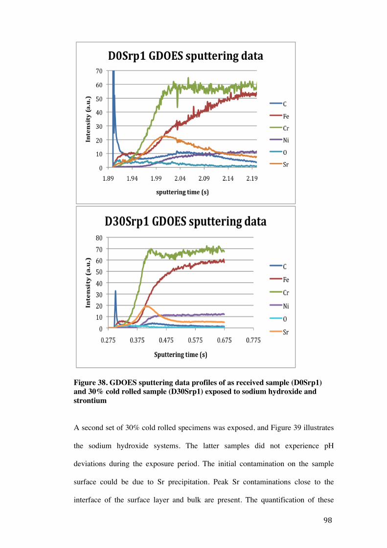
98
Figure 38. GDOES sputtering data profiles of as received sample (D0Srp1) and 30% cold rolled sample (D30Srp1) exposed to sodium hydroxide and strontium
A second set of 30% cold rolled specimens was exposed, and Figure 39 illustrates
the sodium hydroxide systems. The latter samples did not experience pH
deviations during the exposure period. The initial contamination on the sample
surface could be due to Sr precipitation. Peak Sr contaminations close to the
interface of the surface layer and bulk are present. The quantification of these

99
peaks in comparison to the profiles seen in figure 38 will be discussed in section
4.3.2.5.
Figure 39. GDOES sputtering data profiles of 30% cold rolled samples (D30Srp3 and D30Srp4) exposed to sodium hydroxide and strontium
Figure 40 shows the GDOES profile for the coupon that was etched with 10%
oxalic acid to induce an intergranularly corroded surface. This sample was

100
immersed in sodium hydroxide at pH 11 with strontium as a contaminant. The
comparison between figure 40 and figure 39 is that the strontium peak is not as
large, nor does it penetrate into the bulk in the etched sample (D30Sre1). The
surface layer does seem to differ, with an apparent enrichment in chromium.
However, the surface quality of the etched sample caused the profiles to be
“smeared” into the bulk, making a more quantitative comparison difficult.
Figure 40. GDOES sputtering data profile of 30% cold rolled etched sample (D30Sre1) exposed to Sr and sodium hydroxide
4.3.2.4. High temperature (environment E)
The high temperature experiments were carried out to achieve a uniform strontium
contamination without exposure to an aqueous environment. The GDOES profiles
can be seen in figure 41. It is evident from the profiles that strontium
contamination was achieved, with the strontium possibly penetrating into the bulk
of the steel, inline with oxygen and carbon. The presence of oxygen and carbon in

101
the bulk is most likely due to the formation of a surface during furnace exposure at
3500C, encouraging the diffusion of different components.
Figure 41. GDOES sputtering data profiles of 30% cold rolled samples (E30Srp1 and E30Srp2) exposed to strontium carbonate paste and high temperatures

102
4.3.2.5. Strontium Contamination Discussion
Most strontium contamination experiments yielded some significant peaks, which
are quantified in this section and discussed against the parameters of cold work,
pH, time and pH deviation. A quantitative comparison of the area under the
measured Sr peaks will also be discussed.
4.3.2.5.1. Contamination as a function of cold work
Figure 42 is an indication of the amount of strontium contamination seen with
increasing cold work on the stainless steel coupons. The data show some
variations, and the mean contamination seems not to increase with cold work. The
integrals for the contamination on the D0Srp1 coupon indicated contaminations
from a minimum of 0.3 to a maximum of 6.2, with a standard deviation of 2.26.
The contamination of cold worked samples appears more uniform, the integrals
ranging between a minimum of 1.6 and a maximum of 4.2, giving a standard
deviation of 1.04.
Figure 42. Strontium contamination as a function of cold work from samples D0Srp1 and D30Srp3
0
1
2
3
4
5
6
7
0% 5% 10% 15% 20% 25% 30% 35%
Integral of Sr peak
Depth reduction

103
The raw data from the depth profiles revealed a large peak in the oxide layer in
both D0Srp1 and D30Srp3 and a steady tail from the peak, indicating initial
precipitation of strontium on the surface, then penetration of strontium into the
bulk of the steel. Steele [2, 14] proposed that diffusion into the bulk would take
place through the grain boundaries as well as diffusion through the interstitials and
vacancies of the steel. The activation energy required for this process is
temperature dependant and at 500C this should be sufficient to overcome the
energy barrier. Woodhouse found that strontium penetrated the bulk through the
grain boundaries [30].
4.3.2.5.2. Contamination as a function of time
It can be seen in figure 43 that the data has reached a steady value, indicating rapid
contamination after only 1 week of exposure. D30Srp3 was chosen to examine
because the pH did not fluctuate in that system. All other experimental parameters
were constant to make a judgment on the affect of time.

104
Figure 43. Relationship between the exposure time and the amount of strontium contamination on D30Srp3 coupon
Strontium contamination seemed to have reached a steady value after only 1 week
exposure, increasing only very little over the space of 3 weeks. This confirms a
previous investigation that plate-out is a rapid process, reaching a maximum
amount of contamination over a short period [6, 13]. The later investigations
reported plate-out after only 10 days exposure.
4.3.2.5.3. The effect of pH on contamination
An increase in contamination correlating with an increase in pH has been reported
in previous work, and was therefore expected in this set of results [14, 45]. Figures
44 and 45 show the integrals of strontium contamination in variable pH values.
Figure 44 shows an exponential increase in contamination in higher pH values, in
particular in the regime in excess of the neutral environment. The environments
examined for this graph included B0Srp1, B30Srp1, D0Srp1 and D30Srp1-4 and
integrals were taken from the week 1 measurement, before the pH fluctuation had
0
1
2
3
4
5
6
7
0 0.5 1 1.5 2 2.5 3 3.5 4 4.5
Integral of Sr peak
Number of weeks

105
taken place (see section 4.3.2.5.4.). At pH 7, the contamination is relatively
uniform, the range being 0.05-1.12. At a higher pH the contamination varies
between a minimum of 1.61 and a maximum of 6.22 with a standard deviation of
these data of 1.47, indicating that the contamination varies across and between the
sample surfaces.
Figure 44. The relationship between pH and strontium contamination using integrals from A30Srp1, B0Srp1, B30Srp1, D0Srp1 and D30Srp1-4
It can be also seen in figure 39 that strontium is detected throughout the oxide
layer, peaking at the same point as there is a rise in the chromium profile. This
indicates that the strontium is incorporated into the surface layer/interface, after
the initial precipitation on the surface. The “tail” observed on the strontium profile
shows that it has possibly penetrated into the bulk.
4.3.2.5.4. The effects of pH deviation on strontium contamination
The following environments experienced fluctuations in pH: B0Srp1, B30Srp1,
D0Srp1, D30Srp1. The amount of strontium contamination was expected to
0
1
2
3
4
5
6
7
0 2 4 6 8 10 12
Integral of Sr peak
pH

106
decrease with decreasing pH value, analogue to observations of different exposure
regimes. Figure 45 shows the effect of pH fluctuation on the contamination of
strontium.
Figure 45. The effect of pH deviation on strontium contamination using D30Srp1 integrals
Figure 45 gives an indication of the influence of pH fluctuation on strontium
contamination. The integrals of strontium contamination after the pH drop show
that the contamination showed larger variations. The GDOES depth profiles at the
lower pH values were similar to that illustrated in figure 39. This would imply that
the strontium incorporated into the bulk does not desorb easily and that
decontamination of strontium would be difficult (Steele [2]).
The reactions 1-3 below show the equlibria encountered by carbon dioxide in
aqueous systems. The adsorption of CO2 from the environment caused the
bicarbonate and hydroxide solutions B0Srp1, B30Srp1, D0Srp1 and D30Srp1 to
experience pH drifts.
0 0.5 1
1.5 2
2.5 3
3.5 4
4.5
0 2 4 6 8 10 12
Integral of Sr peak
pH

107
(1) Sr 2+ (aq) + CO2 (aq) + H20 H2CO3 (aq) + Sr 2+ (aq)
(2) Sr 2+ (aq) + H2CO3 (aq) H+ (aq) + Sr(HCO3)2 (aq)
(3) Sr 2+ (aq) + H2O + HCO3- (aq) SrCO3 (aq) + H+ (aq)
In equation (1), carbonic acid, H2CO3, is classed as a weak acid and this can make
the pH measurements fall in neutral or alkaline solutions. Carbon dioxide is
absorbed by the aqueous solution and this results in the generation of carbonic
acid. The carbonic acid is unstable and so the equilibrium lies to the hydrogen ions
and bicarbonate (equation 2).
The carbonate ion is present in strongly alkaline solutions. As carbon dioxide is
absorbed, the pH can fall and bicarbonate is formed (equation 3), since the
bicarbonate ion is weakly alkaline.
4.3.2.5.5. Comparison of strontium contamination techniques
Figure 46 is a graph to illustrate the different environments and techniques for
contaminating Type 304H stainless steel with stable strontium. The integral of the
area under the curve of each technique was used for comparison. In figure 46
E30Srp2 was the high temperature experiment.

108
Figure 46. Comparison of strontium contamination techniques
0 1 2 3 4 5 6
D30Sre1
E30Srp2
D30Srp4
Integral of Sr peak
Contamination technique

109
5. Possible further work and improvements
The results of this study have revealed some interesting results about
contamination of Type 304H stainless steel with stable Cs and Sr compounds.
There are a number of further experiments that are suggested to get a greater
understanding of caesium and strontium contamination. These are:
Experiments involving strontium carbonate. Following the success of
contaminating steel with strontium in alkaline environments, strontium
carbonate solution may yield higher amounts of contamination, eliminating
the sodium ion competition for adsorption sites.
Repeating the caesium carbonate experiments with reducing the
experimental variables in this system. It is suggested that caesium
bicarbonate could be used for a pH 7 environment.
Investigating caesium and strontium contamination as a function of heat.
This would be expected to yield higher contamination of both caesium and
strontium.
Changing the degree of cold deformation of the steel, as well as
investigation into other grades of austenitic stainless steels.
Ultrasonic cleaning of the steel coupons before laser profilometry;
Investigating where the contamination occurs on a microstructure scale, for
example by EBSD.
Analysis of the solutions after contamination to confirm the mass balance
of the materials.
Variation of the concentration of Cs/Sr, ranging from ppb concentrations to
ppm.

110
Controlled variation of the solution chemistry, including a study of
exclusion and inclusion of carbonate.

111
6. Conclusions
The following conclusions can be made from the work carried out in this M.Phil
thesis:
Stable strontium contaminations were more pronounced than stable Cs
contamination on Type 304 stainless steel surfaces.
Strontium was found to penetrate into the steel substrate and does not
desorb with a change in pH.
The etched sample did not exhibit a higher amount of Sr contamination.
The high temperature experiments were not successful in contaminating
Type 304 stainless steel with Cs, but did achieve Sr contamination.
It was more difficult for contaminating stainless steel surfaces with
Caesium, and the most promising method was by using Cs carbonate
solutions, eliminating the competition from other alkali ions.
Caesium contamination increased slightly with increased cold deformation
and solution pH.

112
7. References 1. Rahman, A.A., Decommissioning and radioactive waste management.
2008, Dunbeath: Boca Raton Fla. : Whittles ; CRC Press. xiii, 448. 2. Steele, H., Steel Decontamination. Nexia Solutions, 2005. 3. Ojovan, M.I., Lee, W. E., An introduction to nuclear waste
immobilisation. 2005, Amsterdam ; London: Elsevier. xviii, 315. 4. IAEA, Further Analysis of Extended Storage of Spent Fuel. 1997. 5. Gephart, R.E., A short history of waste management at the Hanford Site.
Physics and Chemistry of the Earth, 2010. 35: p. 298-‐306. 6. Taylor, J.B., A theoretical analysis of the deposition of radioactive ions,
particles and colloids from aqueous liquid onto a stainless steel surface. Thesis, 1990.
7. Wilson, P.D., The nuclear fuel cycle : from ore to wastes. Oxford science publications. 1996, Oxford: Oxford University Press. xix, 323 p.
8. Alvarez, R., Spent Nuclear Fuel Pools in the US:Reducing the Deadly Risks of Storage. http://www.ips-‐dc.org.
9. West, A.R., Basic solid state chemistry. 1999, Chichester: Wiley. xvi, 480.
10. ASTM, Standard Specification for Chromium and Chromium-Nickel Stainless Steel Plate, Sheet, and Strip for Pressure Vessels and for General Applications. 2002 (A240).
11. Schmuki, P., From Bacon to barriers: a review on the passivity of metals and alloys. Journal of Solid State Electrochemistry, 2002. 6: p. 145-‐164.
12. Okamoto, G., Passive film of 18-8 stainless steel structure and its function. Corrosion Science, 1973. 13: p. 471-‐489.
13. Adeleye, S., White, D., Taylor, J.,, Kinetics of Contamination of Stainless Steel in contact with Radioactive Solutions at Ambient Temperatures. Journal of Radioanalytical and Nuclear Chemistry, 1995. 189(1): p. 65-‐70.
14. Steele, H., Chemical Modelling of Steel Surface Contamination. Nexia Solutions, 2006.
15. Nilsson, A., L.G.M. Pettersson, and J.K. N©*rskov, Chemical bonding at surfaces and interfaces. 2008, Amsterdam ; Oxford: Elsevier. xii, 520 p.
16. Stumm, W. and J.J. Morgan, Aquatic chemistry : chemical equilibria and rates in natural waters. 3rd ed. 1996, New York ; Chichester: Wiley. xvi, 1022 p.
17. Fauvet, P., Balbaud, F., Robin, R., Corrosion mechanisms of austenitic stainless steels in nitric media used in reprocessing plants. Journal of Nuclear Materials, 2008. 375: p. 52-‐64.
18. Olsson, C.-‐O.A., Landolt, D., Passive films on stainless steels-chemistry, structure and growth. Electrochimica Acta, 2003. 48: p. 1093-‐1104.
19. Marshall, P.I., Burstein, G.T., The Effects of pH on the Repassivation of 304L Stainless Steel. Corrosion Science, 1983. 23(11): p. 1219-‐1228.
20. Addari, D., Elsener, B., Rossi, A., Electrochemistry and surface chemistry of stainless steels in alkaline media simulating concrete pore solutions. Electrochimica Acta, 2008. 53: p. 8078-‐8086.
21. Drogowska, M., Menard, H., Brossard, L., Electrooxidation of stainless steel AISI 304 in carbonate aqueous solution at pH 8. Journal of Applied Electrochemistry, 1996. 26: p. 217-‐225.

113
22. Drogowska, M., Menard, H., Brossard, L., Pitting of AISI 304 stainless steel in bicarbonate and chloride solutions. Journal of Applied Electrochemistry, 1997. 27: p. 169-‐177.
23. Hadji, M., Badji, R., Microstructure and Mechanical Properties of Austenitic Stainless Steels After Cold Rolling. Journal of Materials Engineering and Performance, 2002. 11(2): p. 145-‐151.
24. Ravi Kumar, B., Mahato, B., Singh, R., Influence of Cold-Worked Structure on Electrochemical Properties of Austenitic Stainless Steels. Metallurgical and Materials Transactions A, 2007. 38A: p. 2085-‐2094.
25. Houmard, M., Berthome, G., Boulange L., Joud, J.C., Surface physico-chemistry study of an austenitic stainless steel: Effect of simple cold rolling treatment on surface contamination. Corrosion Science, 2007. 49: p. 2602-‐2611.
26. Domankova, M., Marek, P., Moravcik, R., The effect of cold work on the sensitisation of austenitic stainless steels. Materials and Technology, 2007. 41(3): p. 131-‐134.
27. Grabke, H.J., Muller-‐Lorenz, E.M., Strauss, S., Pippel, E., Woltersdorf, J., Effects of Grain Size, Cold Working, and Surface Finish on the Metal-Dusting Resistance of Steels. Oxidation of Metals, 1998. 50(314).
28. Dabrowski, A., Adsorption-from theory to practice. Advances in Colloid and Interface Science, 2001. 93: p. 135-‐224.
29. Ajlouni, A.W., Almasa'efah, Y.S., Abdelsalam, M., Nuclear Fission Products: From Source to Environment. Journal of Environmental Science and Technology, 2010. 3(4): p. 182-‐194.
30. Woodhouse, G.J., Decontamination of Pond Furniture used in the Nuclear Power Industry. Thesis, 2008.
31. Sood, D.D., Patil, S.K., Chemistry of Nuclear Fuel Reprocessing: Current Status. Journal of Radioanalytical and Nuclear Chemistry, 1996. 203(2): p. 547-‐573.
32. Takeuchi, M., Nagai, T., Takeda, S., Koizumi, T., Aoshima, A., Adhesive Property of Radionuclides on Material Surface in High Level Radioactive Liquid Waste. Journal of Nuclear Science and Technology, 2000. 37(1): p. 107-‐109.
33. Iniotakis, N., Malinowski, J., Gottaut, H., Munchow, K., Results from Plate-Out Investigations. www.iaea.org/inisnkm/nkm/aws/htgr/abstracts/abst_iwggcr2_4.html.
34. Adeleye S., W.D., Taylor J.,, Ambient temperature contamination of process piping and the effects of pretreatment. Nuclear Technology, 1996. 113(1): p. 46-‐53.
35. Eichholz, G.G., Nagel, A. E., Hughes, R. B., Adsorption of Ions in Dilute Aqueous Solution on Glass and Plastic Surfaces. Journal of Analytical Chemistry, 1965. 37(7): p. 863-‐868.
36. Kadar, P., Varga, K., Nemeth, Z., Vajda, N., Pinter, T., Schunk, J., Accumulation of uranium, transuranium and fission products on stainless steel surfaces. I. A comprehensive view of the experimental parameters influencing the extent and character of the contamination. Journal of Radioanalytical and Nuclear Chemistry, 2010. 284: p. 303-‐308.

114
37. Kadar, P., Varga, K., Baja, B., Nemeth, Z., Vajda, N., Stefanka, Zs. Kover, L., Cserny, I., Toth, J., Pinter, T., Schunk, J., Accumulation of uranium, transuranium and fission products on stainless steel surfaces II. Sorption studies in a laboratory model system. Journal of Radioanalytical and Nuclear Chemistry, 2011. 288: p. 943-‐954.
38. Repanszki, R., Adsorption of fission products on stainless steel and zirconium. Adsorption, 2007. 13: p. 201-‐207.
39. Matzke, H.J., Study of the diffusion of Cesium in stainless steel using ion beams. Journal of Nuclear Materials, 1977. 64: p. 130-‐138.
40. Matzke, H.J., Diffusion of Cesium in Stainless Steel and Possible Implications for Chromium Depletion and Mobility. Journal of Nuclear Science and Technology, 1983. 20(3): p. 237-‐245.
41. Sahai, N., Carroll, S.A., Roberts, S., O'Day, P.A., X-Ray Adsorption Spectroscopy of Strontium (II) Coordination II. Sorption and Precipitation at Kaolinite, Amorphous Silica, and Goethite Surfaces. Journal of Colloid and Interface Science, 2000. 222: p. 198-‐212.
42. Rouppert, F., Rivoallan, A., Largeron, C., An Investigation of Chemical Equilibria involving Cesium metal oxides and hydroxides on stainless steel. In-situ study of the contaminant adsorption modes using Fourier Transform IR Spectroscopy. WM'00 Conference, 2000.
43. Rouppert, F., Rivoallan, A., Largeron, C., Reliability and Consistancy of Surface Contamination Methods. WM'02 Conference, 2002.
44. Cornell, R.M., Adsorption of Cesium on Minerals: A Review. Journal of Radioanalytical and Nuclear Chemistry, 1993. 171(2): p. 483-‐500.
45. Music, S., Ristic, M., Adsorption of Trace Elements or Radionuclides on Hydrous Iron Oxides. Journal of Radioanalytical and Nuclear Chemistry, 1988. 120(2): p. 289-‐304.
46. IAEA, Methods for the Minimization of Radioactive Waste From Decontamination and Decommissioning of Nuclear Facilities.
47. IAEA, State of the Art Technology for Decontamination and Dismantling of Nuclear Facilities. 1999.
48. Pal, U.B., Electroslag Remelting (ESR) Slags for Removal of Radioactive Oxide Contaminants from Stainless Steel. 1999.
49. Oswald, S., Baunack, S., Comparison of depth profiling techniques using ion sputtering from the practical point of view. Thin Solid Films, 2003. 425: p. 9-‐19.
50. ASTM, Standard Practices for Detecting Susceptibility to Intergranular Attack in Austenitic Stainless Steel. 2002 (A262).
51. http://www.bcmac.com/pdf_files/surface%20finish%20101.pdf. 52. Payling, R., D.G. Jones, and A. Bengtson, Glow discharge optical emission
spectrometry. 1997, Chichester: J. Wiley. xli, 846 p. 53. HoribaJobinYvon, User manual GD-profiler 2. 54. email from Patrick Chapon at Horiba Jobin Yvon. 2012. 55. Molchan, I.S., Thompson, G.E., Skeldon, P., Trigoulet, N., Chapon, P. et
al, The concept of plasma cleaning in glow discharge spectroscopy. Journal of Analytical Atomic Spectrometry, 2009. 24: p. 734-‐741.
56. Trigoulet, N., Hashimoto, T., Molchan, I.S., Skeldon, P., Thompson, G.E., Tempez, A., Chapon, P., Surface topography effects on glow discharge analysis. Surface and Interface Analysis, 2010. 42: p. 328-‐333.

115
57. Shimizu, K., Brown, G.M., Habazaki, H., Kobayashi, K., Skeldon, P., Thompson, G.E., Influence of Surface Roughness on the Depth Resolution of GDOES Depth Profiling Analysis. Surface and Interface Analysis, 1999. 27: p. 153-‐156.
58. Shimizu, K., Habazaki, H., Skeldon, P., Thompson, G.E., Wood, G.C., GDOES depth profiling analysis of the air-formed oxide film on a sputter-deposited Type 304 stainless steel. 2000. 29: p. 743-‐746.
Related Documents