UNIVERSITÉ PARIS DESCARTES école doctorale de sciences mathématiques de paris centre THÈSE DE DOCTORAT en vue de l’obtention du grade de Docteur de l’Université Paris Descartes Discipline : Mathématiques présentée par Kevin KUOCH Processus de contact avec ralentissements aléatoires transition de phase et limites hydrodynamiques Contact process with random slowdowns phase transition and hydrodynamic limits sous la direction d’Ellen SAADA soutenue publiquement le 28 novembre 2014 devant le jury composé de M. Thierry Bodineau CNRS - École Polytechnique Rapporteur M. Thomas Mountford École Polytechnique Fédérale de Lausanne Rapporteur M. Mustapha Mourragui Université de Rouen Examinateur M. Frank Redig Technische Universiteit Delft Examinateur M. Rinaldo Schinazi University of Colorado Colorado Springs Examinateur Mme Ellen Saada CNRS - Université Paris Descartes Directrice

Welcome message from author
This document is posted to help you gain knowledge. Please leave a comment to let me know what you think about it! Share it to your friends and learn new things together.
Transcript
UNIVERSITÉ PARIS DESCARTESécole doctorale de sciences mathématiques de paris centre
THÈSE DE DOCTORATen vue de l’obtention du grade de
Docteur de l’Université Paris DescartesDiscipline : Mathématiques
présentée parKevin KUOCH
Processus de contact avecralentissements aléatoires
transition de phase et limites hydrodynamiques
Contact process with random slowdownsphase transition and hydrodynamic limits
sous la direction d’Ellen SAADA
soutenue publiquement le 28 novembre 2014 devant le jury composé de
M. Thierry Bodineau CNRS - École Polytechnique RapporteurM. Thomas Mountford École Polytechnique Fédérale de Lausanne RapporteurM. Mustapha Mourragui Université de Rouen ExaminateurM. Frank Redig Technische Universiteit Delft ExaminateurM. Rinaldo Schinazi University of Colorado Colorado Springs ExaminateurMme Ellen Saada CNRS - Université Paris Descartes Directrice


À mes parents,
À ma grande soeur,

.
RemerciementsL’exercice des remerciements... loin d’être aussi facile que je ne l’imaginais, tant
l’écosystème de la recherche est riche, tant les proches omniprésents sont nombreux. Ily a certainement des oublis et je prie les personnes concernées de m’en excuser.
Mes premiers mots vont naturellement à ma directrice de thèse, Ellen Saada, enversqui j’exprime ma plus profonde gratitude. Non seulement elle a été -incroyablement-patiente et humaine mais elle a su me mettre sur le chemin -malgré tous mes possiblesdéboires- avec les encouragements nécessaires. C’est une chance et un immense honneurd’avoir pu travailler avec elle, je ne serai que toujours friand de ses critiques et conseilstant ils sont chers et avisés.
À ceux qui me font l’honneur de composer le jury. Je remercie chaleureusement Ri-naldo Schinazi, pour avoir initié ce modèle mathématique et pour les discussions (malgréle décalage horaire) que nous avons pu partager. Il a su attiser ma curiosité et être unesource d’inspiration considérable. Je tiens également à remercier Mustapha Mourragui,sa disponibilité, les innombrables aller-retours entre Paris et Rouen mais par dessustout, sa convivialité et ses mots d’encouragement ont été d’un grand apport. Rapporterune thèse est loin d’être une part de gâteau. Je tiens à remercier Thierry Bodineau etThomas Mountford d’avoir accepté de rapporter cette thèse, pour l’attention et les com-mentaires prodigués à ce manuscrit. J’aimerais aussi remercier Frank Redig de prendrepart à ce jury et pour son chaleureux accueil aux Pays-Bas.
Ayant été le premier à avoir mis un article entre mes mains, j’aimerais remercierAmaury Lambert pour m’avoir initié à cette voie mais aussi pour s’être montré dispo-nible et m’avoir conforté dans des choix.
D’autre part, le long de mes études, j’ai eu la chance d’avoir pu suivre des personnesqui m’ont fait avancer jusque là aujourd’hui, en particulier, j’aimerais remercier JeanBertoin, Marc Yor et Olivier Zindy, pour avoir été d’une notable attention et des sourcesd’inspiration.
Après ces années passées à Paris Descartes. Je remercie Annie Raoult, pour le soinqu’elle a porté au laboratoire. La terrasse étant sujette à beaucoup de pauses et dediscussions : Merci à l’équipe de Probabilités, pour leur accueil et leurs conseils ; Mercià Joan Glaunès pour sa sympathie et les parties de tennis ; Merci également à AvnerBar-Hen, à Mikael Falconnet pour leur gentillesse.
Aux équipes administrative et informatique pour leurs aides diverses et variées :Merci à Marie-Hélène Gbaguidi toujours avec sourire et à l’écoute, Vincent Delos, Isa-belle Valéro, Christophe Castellani, Thierry Raedersdorff, Azedine Mani, Arnaud Meu-nier.
À l’équipe de biomathématiques qui m’a confié trois années d’enseignement. Je re-mercie profondément Simone Bénazeth pour son accueil et sa gentillesse. Merci éga-lement à Chantal Guihenneuc-Jouyaux, Ioannis Nicolis, Patrick Deschamps, VirginieLasserre.
Merci aux doctorants et jeunes docteurs que j’ai pu voir ou qui me voient passer,ces ambiances de travail ou de non-travail, je vous les dois : Merci à Gaëlle C. (je t’en
i

prie pour les chaussures de mariage) ; Léon T. ; Mariella D. ; Christophe D. ; RebeccaB. ; Charlotte D. ; Charlotte L. ; Jean R. ; Gwennaëlle M. ; Anne-Claire E.
Having recently landed in the Netherlands, I’d like to deeply thank Aernout vanEnter and Daniel Valesin for their kindness and for taking care of my comfy arrival inGroningen.
Somehow I have had the chance to visit incredible places along past years and totake part in seminars, conferences and other events. I am very grateful to every personand institution that made it possible.
Trois années, c’est long. Certain(e)s ont dû entendre cette phrase à maintes repriseset je n’écrirais certainement pas ces mots si vous n’aviez pas été là. Il serait trop longd’exprimer à chacun(e) de vous mes sentiments et ma gratitude, vous les connaissezprobablement déjà.
Mes plus doux remerciements à mes ami(e)s de très longue date (plus de la moitiéde mes 25ans quand même !) : Mathieu J. et nos pinardises ; Guillaume de M. (vilainmerle) ; Timothée de G. (bulle) ; Jerôme T. et ses pin’s ; Marine L. ; Louis M. ; Hélènede R. ; Guillaume L. (qui a osé suivre un de mes cours...) ; Mathieu B. ; Anne-Félice P.et ses bonjoirs ; Marine H. ; Nicolas I. ; Clémentine d’A. ; Hervé de S-P. ; Theodora B. ;Loup L. ; Bastien L. ; ce qui ne peut être évité, il faut parfois l’embrasser, à la mémoired’Alexandre Z. pour ce qu’il a été et ce qu’il laisse derrière lui.
Je remercie chaleureusement Alex K. pour le plaisir de partager des discussions etmoments aussi saugrenus qu’improbables avec lui.
Il est temps de retourner mes tendres remerciements à mon cher Daniel Kious (ehon y est arrivé finalement !), et à sa Famille pour leurs chaleureux accueils.
Merci à Samuel R. pour toutes nos inlassables conversations (et dégustations dewhisky), j’espère qu’il nous en reste encore plein devant nous - j’attends avec impatiencemon t-shirt Cyclop. Merci à Mario M. qui, sans conteste, fait le meilleur tiramisu que jeconnaisse. Merci à Raphaël L-R. pour entre autres ses conseils et son humour.
Merci à Pierre-Alban D. pour son soutien et être un si bon accolyte de fortune ;Merci à David B. non seulement pour avoir révolutionné le port du cardigan ; Merci àDiane T. et ses prestations de danse contemporaine ; Merci à Julie L. pour prendre soinde mes dents (j’attends toujours mon prochain rdv).
Merci aussi à Alicia H. et son rire détonant ; à Justyna S. pour sa gentillesse et sonattention.
Enfin, et de tout mon cœur, je remercie mes parents et ma grande sœur, pourl’exemple qu’ils sont, pour toute la joie qu’ils me procurent, pour tout leur amour dontje suis -ô combien- insatiable.
Groningen, le 8 Novembre 2014.
ii

“Would you tell me, please, which way I ought to go from here ?”“That depends a good deal on where you want to get to,” said the Cat.“I don’t much care where—” said Alice.“Then it doesn’t matter which way you go,” said the Cat.“—so long as I get somewhere,” Alice added as an explanation.“Oh, you’re sure to do that," said the Cat, “if you only walk long enough.”
– Lewis Carroll, Alice in Wonderland, Chapter VI.
iii

iv

RésuméDans cette thèse, on étudie un système de particules en interaction qui généralise un
processus de contact, évoluant en environnement aléatoire. Le processus de contact peutêtre interprété comme un modèle de propagation d’une population ou d’une infection.La motivation de ce modèle provient de la biologie évolutive et de l’écologie comporte-mentale via la technique du mâle stérile, il s’agit de contrôler une population d’insectesen y introduisant des individus stérilisés de la même espèce : la progéniture d’une fe-melle et d’un individu stérile n’atteignant pas de maturité sexuelle, la population se voitréduite jusqu’à potentiellement s’éteindre.
Pour comprendre ce phénomène, on construit un modèle stochastique spatial surun réseau dans lequel la population suit un processus de contact dont le taux de crois-sance est ralenti en présence d’individus stériles, qui forment un environnement aléatoiredynamique.
Une première partie de ce document explore la construction et les propriétés duprocessus sur le réseau Zd. On obtient des conditions de monotonie afin d’étudier lasurvie ou la mort du processus. On exhibe l’existence et l’unicité d’une transition dephase en fonction du taux d’introduction des individus stériles. D’autre part, lorsqued “ 1 et cette fois en fixant l’environnement aléatoire initialement, on exhibe de nouvellesconditions de survie et de mort du processus qui permettent d’expliciter des bornesnumériques pour la transition de phase.
Une seconde partie concerne le comportement macroscopique du processus en étu-diant sa limite hydrodynamique lorsque l’évolution microscopique est plus complexe.On ajoute aux naissances et aux morts des déplacements de particules. Dans un pre-mier temps sur le tore de dimension d, on obtient à la limite un système d’équationsde réaction-diffusion. Dans un second temps, on étudie le système en volume infini surZd, et en volume fini, dans un cylindre dont le bord est en contact avec des réservoirsstochastiques de densités différentes. Ceci modélise des phénomènes migratoires avecl’extérieur du domaine que l’on superpose à l’évolution. À la limite on obtient un sys-tème d’équations de réaction-diffusion, auquel s’ajoutent des conditions de Dirichlet auxbords en présence de réservoirs.
Mots-clefs. système de particules en interaction, modèle stochastique spatial, pro-cessus de contact, milieu aléatoire, attractivité, percolation, transition de phase, limitehydrodynamique, réservoirs.
v

vi

AbstractIn this thesis, we study an interacting particle system that generalizes a contact
process, evolving in a random environment. The contact process can be interpretedas a spread of a population or an infection. The motivation of this model arises frombehavioural ecology and evolutionary biology via the sterile insect technique ; its aim isto control a population by releasing sterile individuals of the same species : the progenyof a female and a sterile male does not reach sexual maturity, so that the population isreduced or potentially dies out.
To understand this phenomenon, we construct a stochastic spatial model on a lat-tice in which the evolution of the population is governed by a contact process whosegrowth rate is slowed down in presence of sterile individuals, shaping a dynamic randomenvironment.
A first part of this document investigates the construction and the properties of theprocess on the lattice Zd. One obtains monotonicity conditions in order to study thesurvival or the extinction of the process. We exhibit the existence and uniqueness ofa phase transition with respect to the release rate. On the other hand, when d “ 1and now fixing initially the random environment, we get further survival and extinctionconditions which yield explicit numerical bounds on the phase transition.
A second part concerns the macroscopic behaviour of the process by studying its hy-drodynamic limit when the microscopic evolution is more intricate. We add movementsof particles to births and deaths. First on the d-dimensional torus, we derive a systemof reaction-diffusion equations as a limit. Then, we study the system in infinite volumein Zd, and in a bounded cylinder whose boundaries are in contact with stochastic reser-voirs at different densities. As a limit, we obtain a non-linear system, with additionallyDirichlet boundary conditions in bounded domain.
Keywords. interacting particle system, spatial stochastic model, contact process, ran-dom environment, attractiveness, percolation, phase transition, hydrodynamic limit, re-servoirs.
vii

viii
Contents1 Introduction 1
1.1 Interacting Particle Systems . . . . . . . . . . . . . . . . . . . . . . . . . 21.2 A short story of the contact process . . . . . . . . . . . . . . . . . . . . . 61.3 Hydrodynamic limits . . . . . . . . . . . . . . . . . . . . . . . . . . . . . 101.4 From life and nature . . . . . . . . . . . . . . . . . . . . . . . . . . . . . 121.5 The generalized contact process . . . . . . . . . . . . . . . . . . . . . . . 15
2 Phase transition on Zd 212.1 Introduction . . . . . . . . . . . . . . . . . . . . . . . . . . . . . . . . . . 212.2 Settings and results . . . . . . . . . . . . . . . . . . . . . . . . . . . . . . 222.3 Graphical construction . . . . . . . . . . . . . . . . . . . . . . . . . . . . 282.4 Attractiveness and stochastic order . . . . . . . . . . . . . . . . . . . . . 312.5 Phase transition . . . . . . . . . . . . . . . . . . . . . . . . . . . . . . . . 472.6 The critical process dies out . . . . . . . . . . . . . . . . . . . . . . . . . 542.7 The mean-field model . . . . . . . . . . . . . . . . . . . . . . . . . . . . . 65
3 Survival and extinction conditions in quenched environment 693.1 Introduction . . . . . . . . . . . . . . . . . . . . . . . . . . . . . . . . . . 693.2 Settings and results . . . . . . . . . . . . . . . . . . . . . . . . . . . . . . 703.3 Random growth on vertices . . . . . . . . . . . . . . . . . . . . . . . . . 723.4 Random growth on oriented edges . . . . . . . . . . . . . . . . . . . . . . 763.5 Numerical bounds on the transitional phase . . . . . . . . . . . . . . . . 79
4 Hydrodynamic limit on the torus 814.1 Introduction . . . . . . . . . . . . . . . . . . . . . . . . . . . . . . . . . . 814.2 Notations and Results . . . . . . . . . . . . . . . . . . . . . . . . . . . . 824.3 The hydrodynamic limit . . . . . . . . . . . . . . . . . . . . . . . . . . . 864.4 Proof of the replacement lemma . . . . . . . . . . . . . . . . . . . . . . . 964.A Construction of an auxiliary process . . . . . . . . . . . . . . . . . . . . . 1024.B Properties of measures . . . . . . . . . . . . . . . . . . . . . . . . . . . . 1074.C Quadratic variations computations . . . . . . . . . . . . . . . . . . . . . 1104.D Topology of the Skorohod space . . . . . . . . . . . . . . . . . . . . . . . 113
5 Hydrodynamic limits of a generalized contact process with stochasticreservoirs or in infinite volume 1155.1 Introduction . . . . . . . . . . . . . . . . . . . . . . . . . . . . . . . . . . 1165.2 Notation and Results . . . . . . . . . . . . . . . . . . . . . . . . . . . . . 1185.3 Proof of the specific entropy (Theorem 5.2.1) . . . . . . . . . . . . . . . . 1305.4 Hydrodynamics in a bounded domain . . . . . . . . . . . . . . . . . . . . 1375.5 Empirical currents . . . . . . . . . . . . . . . . . . . . . . . . . . . . . . 1465.6 Hydrodynamics in infinite volume . . . . . . . . . . . . . . . . . . . . . . 1485.7 Uniqueness of weak solutions . . . . . . . . . . . . . . . . . . . . . . . . . 1495.A Changes of variables formulas . . . . . . . . . . . . . . . . . . . . . . . . 155
ix

Contents
5.B Quadratic variations computations . . . . . . . . . . . . . . . . . . . . . 1575.C Estimates in bounded domain . . . . . . . . . . . . . . . . . . . . . . . . 160
Perspectives 163
References 169
x

1Introduction
Contents1.1 Interacting Particle Systems . . . . . . . . . . . . . . . . . 2
1.1.1 The setup . . . . . . . . . . . . . . . . . . . . . . . . . . . . . 21.1.2 Invariant measures . . . . . . . . . . . . . . . . . . . . . . . . 41.1.3 Coupling and stochastic order . . . . . . . . . . . . . . . . . . 5
1.2 A short story of the contact process . . . . . . . . . . . . 61.2.1 Construction of the process . . . . . . . . . . . . . . . . . . . 61.2.2 Upper invariant measure and duality . . . . . . . . . . . . . . 81.2.3 Survival and extinction . . . . . . . . . . . . . . . . . . . . . 9
1.3 Hydrodynamic limits . . . . . . . . . . . . . . . . . . . . . 111.4 From life and nature . . . . . . . . . . . . . . . . . . . . . 12
1.4.1 The sterile insect technique . . . . . . . . . . . . . . . . . . . 121.4.2 Time to unleash the mozzies ? . . . . . . . . . . . . . . . . . . 131.4.3 Past mathematical models . . . . . . . . . . . . . . . . . . . . 14
1.5 The generalized contact process . . . . . . . . . . . . . . . 151.5.1 Phase transition in dynamic random environment . . . . . . . 171.5.2 Survival and extinction in quenched environment . . . . . . . 181.5.3 Hydrodynamic limit in a bounded domain . . . . . . . . . . . 181.5.4 Hydrodynamic limits with stochastic reservoirs or in infinite
volume . . . . . . . . . . . . . . . . . . . . . . . . . . . . . . 18
This thesis examines two different aspects of a generalized contact process. In amicroscopic scale, we study survival or extinction of the process with respect to varyingparameters. Then, we go to a macroscopic scale and establish hydrodynamic limits,where in the dynamics of the underlying process we add displacements of particles andfurther on migratory phenomena.
In this chapter, we introduce some general settings we shall make use of, first oninteracting particle systems in Section 1.1 and then on the contact process in Section1.2. After what, in Section 1.4, we develop shortly the big picture of the sterile insecttechnique. In Section 1.5, we describe a generalized contact process and our results thatlead to an understanding of this competition model.
1

Chapter 1. Introduction
1.1 Interacting Particle SystemsInteracting particle systems are a class of Markov processes that arose in the early
seventies due to pioneering works by F. Spitzer [70, 71] and R.L. Dobrushin [16]. Theyhave provided a framework that describes the space-time evolution of an infinity ofindistinguishable particles governed by a strong random and local interaction.
This particular class of stochastic processes comes up in various areas of applications :physics, biology, computer science, economics and sociology,... that dictate the natureof the randomness of the processes.
1.1.1 The setupAs a preparation, one first reviews some necessary background theory about inter-
acting particle systems. For further contents on the topic, one refers the reader to T.M.Liggett’s books [58, 57].
State spaces are of the form Ω “ F S, where F is discrete and finite, S is a countableset of sites. Note that Ω is compact in the product topology. A configuration ζ P Ω isdescribed by the state of each site x of the graph S, given at time t by ζtpxq P F . Foreach ζ P Ω and T Ă S, the local dynamics of the system is depicted by a collectionof transition measures cT pζ, dαq, assumed to be finite and positive on F T . Assumefurther that the mapping ζ ÞÑ cT pζ, dαq is continuous from Ω to the space of finitemeasures on F T with the topology of weak convergence. If ζ is the current configuration,a transition of state or flip involving the coordinates in T occurs at rate cT pζ, F T q andcT pζ, dαqcT pζ, F
T q is the distribution of the resulted configuration restricted to T .We will use the notation Pζ for the distribution of the process pζtqtě0 starting from
the initial configuration ζ, and Eζ will denote the corresponding expectation. The infi-nitesimal description of a process ζ P Ω is given by its generator L, a linear unboun-ded operator defined on an appropriate dense domain DpΩq of the space of functionsf : Ω Ñ R. For any cylinder function f , i.e. that depends only on finitely many coordi-nates, L is defined by
Lfpζq “ÿ
T
ż
ΩcT pζ, dαq
`
fpζαq ´ fpζq˘
, (1.1.1)
where ζα is obtained from ζ only by flipping the coordinates in T , that is, for α P F T ,
ζα “
"
ζpxq if x R T,αpxq if x P T.
The series converges provided that cT p., .q satisfies natural summability conditions.Let CpΩq be the space of continuous real-valued functions on Ω equipped with the
uniform norm. All the processes we consider here have the Feller property (i.e. strongMarkov processes whose transition measures are weakly continuous in the initial state)so that the semigroup St of the process on CpΩq is well defined :
2

1.1. Interacting Particle Systems
Theorem 1.1.1. Suppose tSt, t ą 0u is a Markov semigroup on CpΩq. Then there existsa unique Markov process tP ζ , ζ P Ωu such that
Stfpζq “ Eζfpζtqfor all f P CpΩq, ζ P Ω and t ě 0.
The link binding the infinitesimal description of the process (generator) to the time-evolution of the process (semigroup) is given by the Hille-Yosida theory set in the Banachspace CpΩq.Theorem 1.1.2 (Hille-Yosida). There is a one-to-one correspondence between Markovgenerators on CpΩq and Markov semigroups on CpΩq. This correspondence is given by
1. DpΩq “"
f P CpΩq : limtÓ0
Stf ´ f
texists
*
, and
Lf “ limtÓ0
Stf ´ f
t, f P DpΩq.
2. for t ě 0,Stf “ lim
nÑ8pf ´
t
nLfq´n, f P CpΩq.
Relying on the Hille-Yosida theory, the following result states sufficient conditionsfor the existence of an infinite particle system.Theorem 1.1.3 (T.M. Liggett (1972)). Assume that
supxPS
ÿ
TQx
sup´
cT pζ, FTq : ζ P Ω
¯
ă 8
andsupxPS
ÿ
TQx
ÿ
u‰x
sup´
cT pζ1, dαq ´ cT pζ2, dαqT : ζ1pyq “ ζ2pyq for all y ‰ u¯
ă 8
where ¨ T stands for the total variation norm of a measure on F T . Then the closureL of L defined in (1.1.1) is the generator of a Feller Markov process pζtqtě0 on Ω. Inparticular, if f is a cylinder function then,
Lf “ limtÑ0
Stf ´ f
t,
LStf “ StLfand uptq “ Stf is the unique solution to the evolution equation
Btuptq “ Luptq, up0q “ f. (1.1.2)Let P be the set of probability measures on Ω equipped with the topology of weak
convergence, i.e.
µn Ñ µ in P if and only ifż
Ωfdµn Ñ
ż
Ωfdµ
for all f P CpΩq. Note that the compactness of Ω implies the compactness of P in thisinduced topology.
3

Chapter 1. Introduction
1.1.2 Invariant measuresStudy of interacting particle systems involves use of their invariant measures and
ideally, convergence to them. If µ is a probability measure on Ω, the distribution of ζtwith initial distribution µ is denoted by µSt and is defined by
ż
ΩfdpµStq “
ż
ΩStfdµ, f P CpΩq.
By the Riesz Representation theorem, this relation defines uniquely µSt. The measureµ is invariant with respect to the process if µSt “ µ for all t ą 0. Denote by I the setof all invariant measures. Furthermore,
Theorem 1.1.4 (Proposition 1.8 [58]). i. µ P I if and only ifż
ΩLfdµ “ 0, for all cylinder functions f.
ii. I is compact, convex and non-empty.iii. I is the closed convex hull of its extreme points.iv. Let µ P P. If µ :“ lim
tÑ8µSt exists, then µ P I.
Remark that a process always has at least one invariant measure. This measuremight satisfy a symmetry property called reversibility that allows simpler computationsor even, further results. A probability measure µ on Ω is reversible for the process if
ż
ΩfStgdµ “
ż
ΩgStfdµ, for all f, g P CpΩq
or equivalently,ż
ΩfLgdµ “
ż
ΩgLfdµ, for all cylinder functions f, g.
1.1.3 Coupling and stochastic orderA coupling is a construction of two (or even more) stochastic processes on a common
probability space. To make use of this powerful tool, we will deal with several topics thatare closely connected with coupling such as stochastic order relations between proba-bility measures, monotone processes and correlation inequalities. These useful relationsallow us to compare processes, so that one can deduce properties from one to anotherby domino effect.
Assuming that F is totally ordered, the state space Ω is a partially ordered set, withpartial order given by
ζ ď ζ 1 if for all x P S, ζpxq ď ζ 1pxq, (1.1.3)
4

1.1. Interacting Particle Systems
where this last inequality refers to the order on F . A function f P CpΩq is increasing if
ζ ď ζ 1 ñ fpζq ď fpζ 1q.
This leads naturally to define the stochastic order between two probability measures µ1and µ2 on Ω, that is, µ2 is stochastically larger than µ1, written µ1 ď µ2 if :
ż
Ωfdµ1 ď
ż
Ωfdµ2 for any increasing function f on Ω.
A necessary and sufficient condition for a semigroup, acting on measures, to preservethe ordering on Ω is given by
Theorem 1.1.5 (Theorem 2.2 [57]). For a Feller process on Ω with semigroup St, thefollowing two statements are equivalent :
a. If f is an increasing function on Ω then Stf is an increasing function of Ω for allt ě 0.
b. If µ1 ď µ2 then µ1St ď µ2St for all t ě 0.
Stochastic order between two particle systems pζtqtě0 and pζ 1tqtě0 is given by theexistence of a coupled process pζt, ζ 1tqtě0 on the probability space Ω ˆ Ω that preservesthe order between their initial configurations, that is, if ζ0 ď ζ 10 then ζt ď ζ 1t a.s. for allt ą 0. Such a coupling is said to be increasing and ζ 1t is said to be stochastically largerthan ζt. When pζtqtě0 and pζ 1tqtě0 are two copies of the same process, we say the processis attractive.
The following result gives the connection between coupling and stochastic order.
Theorem 1.1.6 (Theorem 2.4 [58]). Let µ1 and µ2 be probability measures on Ω. Thenµ2 is stochastically larger than µ1 if and only if there exists a coupling pζ, ζ 1q such that ζhas distribution µ1, ζ 1 has distribution µ2 and ζ ď ζ 1 almost surely, that is, there existsa measure ν on Ω such that
νtpζ, ζ 1q : ζ P Au “ µ1pAq
νtpζ, ζ 1q : ζ 1 P Au “ µ2pAq
νtpζ, ζ 1q : ζ ď ζ 1u “ 1
Furthermore, we will consider different types of stochastic processes :
pξtqtě0 (basic) contact processpξt, ωtqtě0 contact process in dynamic random environmentpηtqtě0 multitype contact process
5

Chapter 1. Introduction
1.2 A short story of the contact processIntroduced by T.E. Harris in 1974 [39], the contact process on the graph S with
growth rate λ1 is an interacting particle system pξtqtě0 on t0, 1uS, whose dynamics isgiven by the following transition measure : the involved sets T are singletons T “ txuand,
cT pξ, dαq “
"
λ1n1px, ξqδt1u if ξpxq “ 0,δt0u if ξpxq “ 1, (1.2.1)
where nipx, ξq “ř
yPS:|y´x|“11tξpyq “ 1u stands for the number of neighbours of site x
that are in state i. Here | ¨ | refers to the maximum norm : |x| “ max1ďjďd
|xj|, for x P Rd.Denote by Pλ1 the law of the contact process with growth rate λ1.
It is usually interpreted as the spread of a population, an infection or a rumour.Regarded as an infection, infected sites (in state 1) become healthy spontaneously aftera unit exponential time while healthy sites (state 0) become infected at some rate, pro-portional to the number of their infected neighbours.
General theory about the contact process is finely exposed by T.M Liggett [58] forresults from 1974 to 1985, [57] for results after 1985 and by R. Durrett [18] as well.
1.2.1 Construction of the processLet A be a subset of S. Define ξAt as the process starting from the initial configuration
ξ0 “ 1A. Configurations ξ P t0, 1uS are commonly identified with subsets of S via
ΞAt “ tx P S : ξAt pxq “ 1u,
regarded as the set of occupied sites at time t. When A “ t0u, we will omit the exponent.As a consequence of Theorem 1.1.3, the transition measure cT pξ, dαq uniquely defines aMarkov process, so that the infinitesimal generator of the contact process is defined forany cylinder function f on t0, 1uS by
L1fpξq “ÿ
xPS
ż
ΩcT pξ, dαqrfpξ
αq ´ fpξqs (1.2.2)
Graphical representation The graphical construction of the contact process is dueto T.E. Harris [40]. The idea is to construct a percolation structure on which to definethe process, lending itself to the use of the theory of percolation (see G. Grimmett [33]).To carry out this representation, for each pair px, yq P S2 that are joined by an edge inS, let tT x,yn , n ě 1u be the arrival times of independent rate λ1 Poisson processes and foreach x P S, let tDx
n, n ě 1u be the arrival times of independent rate 1 Poisson processes.
6
1.2. A short story of the contact process
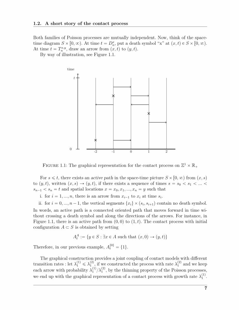
Both families of Poisson processes are mutually independent. Now, think of the space-time diagram S ˆ r0,8q. At time t “ Dx
n, put a death symbol “x” at px, tq P S ˆ r0,8q.At time t “ T x,yn , draw an arrow from px, tq to py, tq.
By way of illustration, see Figure 1.1.
-2 -1 0 1 2
time
0
t
Figure 1.1: The graphical representation for the contact process on Z1 ˆ R`
For s ď t, there exists an active path in the space-time picture Sˆr0,8q from px, sqto py, tq, written px, sq Ñ py, tq, if there exists a sequence of times s “ s0 ă s1 ă ... ăsn´1 ă sn “ t and spatial locations x “ x0, x1, ..., xn “ y such that
i. for i “ 1, ..., n, there is an arrow from xi´1 to xi at time si.ii. for i “ 0, ..., n´ 1, the vertical segments txiuˆ psi, si`1q contain no death symbol.
In words, an active path is a connected oriented path that moves forward in time wi-thout crossing a death symbol and along the directions of the arrows. For instance, inFigure 1.1, there is an active path from p0, 0q to p1, tq. The contact process with initialconfiguration A Ă S is obtained by setting
AAt :“ ty P S : Dx P A such that px, 0q Ñ py, tqu
Therefore, in our previous example, At0ut “ t1u.
The graphical construction provides a joint coupling of contact models with differenttransition rates : let λp1q1 ď λ
p2q1 , if we constructed the process with rate λp2q1 and we keep
each arrow with probability λp1q1 λp2q1 , by the thinning property of the Poisson processes,
we end up with the graphical representation of a contact process with growth rate λp1q1 .
7
Chapter 1. Introduction
Thus, one has a non-decreasing growth with respect to λ1. On the other hand, it alsoprovides a monotone coupling :
A Ă B ñ AAt Ă ABt ,
Therefore, the contact process is attractive and it also follows from the graphical construc-tion that the contact process is additive (see D. Griffeath [32]) :
AAYBt “ AAt Y ABt .
1.2.2 Upper invariant measure and dualitySince the partial order on Ω defined in (1.1.3) induces one on the set of probability
measures on Ω, there will be a lowest and largest element on I with respect to thispartial order.
If 0 denotes the configuration identically equal to 0, since 0 is an absorbing statethen δ0 is called the lower invariant measure for the contact process. The upper invariantmeasure can be constructed using attractiveness : choose the initial configuration as thebiggest possible one, i.e. starting from Ξ0 “ S, and let µt be the distribution of ξt, sothat µ0 “ δ1. Then µt ď µ0. By attractiveness and applying the Markov property, wehave µt`s ď µt for all s ą 0. Therefore, t ÞÑ µt is decreasing and in particular, for everyincreasing function f on Ω, the map t ÞÑ
ş
Ω fdµt is decreasing as well. Since PpΩq iscompact for the weak topology, the limiting distribution
µ :“ limtÑ8
µt
exists and is the upper invariant measure of the process. It is invariant as a limitingmeasure for the Markov process by Theorem 1.1.4. In particular, the measure µ haspositive correlations.
Correlation inequalities will be crucial property in Section 2.6 where we will work inarbitrary large but finite spaces. A probability measure µ on Ω has positive correlationsif
ż
Ωfgdµ ě
ż
Ωfdµ
ż
Ωgdµ,
for all increasing functions f, g on Ω. A sufficient condition for a measure to have positivecorrelations is given by the following result.
Theorem 1.2.1 (C. Fortuin, P. Kasteleyn and J. Ginibre [29]). Suppose S is finite. Letµ be a probability measure on Ω such that for all ζ, ζ 1 P X
µ1pmaxpζ, ζ 1qqµ2pminpζ, ζ 1qq ě µ1pζqµ2pζ1q
Then µ has positive correlations.
8

1.2. A short story of the contact process
One essential property satisfied by the contact process is that it is self-dual [34,Proposition 6.5], that is, the dual process is again a contact process. For A,B Ă S,
Pλ1pΞAt XB ‰ Hq “ Pλ1pΞB
t X A ‰ Hq (1.2.3)
This property allows us to link an equality relation between survival probability anddensity of 1’s under the upper invariant measure. Indeed, since tΞt0ut`1 X S ‰ Hu Ă
tΞt0ut X S ‰ Hu for all t ě 0, t ÞÑ tΞt0ut X S ‰ Hu is non-increasing,
limtÑ8
Pλ1pΞt0ut X S ‰ Hq “ Pλ1p@t ě 0, Ξt0ut ‰ Hq
By self-duality, applying (1.2.3) with A “ t0u and B “ S, one obtains
Pλ1pΞt0ut X S ‰ Hq “ Pλ1pΞS
t X t0u ‰ Hq.
The right-hand side is Pλ1pΞSt p0q “ 1q, and by weak convergence of µ0 to µ, one has
limtÑ8
Pλ1pΞSt p0q “ 1q “ µtξ : ξp0q “ 1u
where µ stands for the upper invariant measure of pξtqtě0. By translation invariance ofµ,
limtÑ8
Pλ1pΞt0ut X S ‰ Hq “ lim
tÑ8Pλ1pξ
St p0q “ 1q “ µtξ : ξpxq “ 1u (1.2.4)
1.2.3 Survival and extinctionA key feature of the contact process lies in the fact its growth does not evolve spon-
taneously but depends on some neighbourhood. In words, the configuration 0 is a trapand a natural question is whether the individuals survive, that is, if there is infinitelyoften a site in state 1. The main feature of the contact process is that it exhibits a phasetransition in the following way.
Define the survival event of the process by t@t ě 0, Ξt ‰ Hu with the initialconfiguration ξ0 “ 1t0u. The contact process is said to die out if
Pλ1p@t ě 0, Ξt ‰ Hq “ 0
and to survive strongly ifPλ1p limtÑ8 ξtp0q “ 1q ą 0.
The process is said to survive weakly if it survives but not strongly, that is,
Pλ1p@t ě 0, Ξt ‰ Hq ą 0.
Using these definitions and monotonicity, we are now ready to define the two followingcritical values :
λc “ inftλ1 : Pλ1p@t ě 0 Ξt ‰ Hq ą 0u (1.2.5)
9

Chapter 1. Introduction
andλs “ inftλ1 : Pλ1p limtÑ8 ξtp0q “ 1q ą 0u. (1.2.6)
for which, the process
dies out if λ1 ă λcsurvives weakly if λc ă λ1 ă λs
survives strongly if λ1 ą λs
Sincet limtÑ8
ξtp0q “ 1u Ă t@t ě 0 Ξt ‰ Hu,
if the process survives weakly then it survives strongly thus λc ď λs.On the d´dimensional integer lattice Zd, one of the most important results about
the contact process is the existence and uniqueness of a critical value λc “ λs.
Theorem 1.2.2 (T.E. Harris [39]). There exists a critical value λc P p0,8q such thatthe contact process survives if λ1 ą λc and dies out if λ1 ă λc, i.e.
Pλ1p@t ě 0, Ξt ‰ Hq “ 0 if λ1 ă λc,
Pλ1p@t ě 0, Ξt ‰ Hq ą 0 if λ1 ą λc.
After having been an open question during about fifteen years, the critical behaviourhas been given by
Theorem 1.2.3 (C. Bezuidenhout and G.R. Grimmett [5]). The critical contact processdies out, that is,
Pλcp@t ě 0, Ξt ‰ Hq “ 0.
R. Holley and T.M. Liggett [41] proved λc ď 2 in the one-dimensional case. Animproved upper bound 1.942 was given by T.M. Liggett [54]. More generally, one hasfor the general case d ě 1,
p2d´ 1q´1ď λc ď 2d´1,
see N. Konno [47] for further information on bounds of the contact process.
1.3 Hydrodynamic limitsHydrodynamic limits are a device that arose in statistical physics to derive deter-
ministic macroscopic evolution laws assuming the underlying microscopic dynamics arestochastic.
By way of illustration, consider the evolution of a system constituted of a largenumber of components (such as a fluid), one can examine and characterize the equi-librium states of the system through macroscopic quantities (such as temperature orpressure). Now, investigating the fluid in a volume which is small macroscopically but
10

1.3. Hydrodynamic limits
large microscopically, the system is close to an equilibrium state and characterized bysome spatial parameter. As the local equilibrium picture should evolve in a smooth way,at some time t the system is close to a new equilibrium state now characterized by aparameter depending on space and time. This space-time parameter evolves smoothlyin time according to a partial differential equation, the hydrodynamic equation.
To take the limit from the microscopic to the macroscopic system, we need to in-troduce a suitable space-time scaling. Consider a microscopic space SN embedded ina corresponding macroscopic space S (e.g. SN “ pZNZqd and S “ pRZqd) so eachmicroscopic vertex x P SN is associated to a macroscopic vertex xN P S. Therefore,distance between particles converges to zero. Besides, we renormalize the time by linkinga microscopic time t to a macroscopic time tθpNq (e.g. θpNq “ N2), since more time isneeded in the macroscopic scale to observe movements of particles.
To investigate the hydrodynamic behaviour of interacting particle systems we shallprove that starting from a sequence of measures associated to some initial density profileρ0, in the following sense
limNÑ8
µN
˜
ˇ
ˇ
ˇ
1Nd
ÿ
xPSN
GpxNqηpxq ´
ż
S
Gpuqρ0puqduˇ
ˇ
ˇą δ
¸
“ 0 (1.3.1)
for any δ ą 0 and continuous function G : S Ñ R, then at some renormalized timetθpNq, we obtain a state StθpNqµN associated to a new density profile ρtp¨q that is aweak solution of a partial differential equation. That is,
limNÑ8
µN
˜
ˇ
ˇ
ˇ
1Nd
ÿ
xPSN
GpxNqηtθpNqpxq ´
ż
S
Gpuqρtpuqduˇ
ˇ
ˇą δ
¸
“ 0. (1.3.2)
In other words, the sequence of measures µN integrates the density ρt at the macroscopicpoint u P S in the same way than an equilibrium measure of density γpuq does.
Since we shall work in a fixed space as N increases, we will examine the time-evolution of the empirical measures associated to the interacting particle system : for aconfiguration η P Ω, define the empirical measure πNpηq on S associated to η by
πNpηq “ N´dÿ
xPSN
ηpxqδxN , (1.3.3)
where δx represents the Dirac measure concentrated on x. This way, we can express(1.3.2) in terms of the empirical density, by integrating G with respect to πN . Sincethere is a one-to-one correspondence between a configuration η and empirical measureπNpηq, the measure πNt inherits the Markov property.
The goal to derive the hydrodynamic limits is to prove the empirical measure πNtconverges in probability to an absolutely continuous measure ρpt, uqdu where ρtpuq isthe solution of a partial differential equation with initial condition ρ0.
Monographs dealing with hydrodynamic limits include A. De Masi and E. Presutti[15], H. Spohn [72] C. Kipnis and C. Landim [42].
11

Chapter 1. Introduction
1.4 From life and natureDuring the last decades, a better understanding of biological phenomena has arisen
the need to study stochastic spatial processes. Authors such as R. Durrett, R. Schinazi,or J. Schweinsberg have deemed the relation of interacting particle systems to biological,ecological and medical frameworks. A quick interesting overview may be found in jointpapers of R. Durrett with the biologist S. Levin [21, 22], and [20].
In this document, the biological phenomenon we are concerned is the so-called Sterileinsect technique (SIT). Due to entomologists R.C. Bushland and E.F. Knipling’s works[46] in the fifties, it is a pest control method whereby sterile individuals of the popula-tion to either regulate or eradicate are released. While sterile males compete with wildmales, they eventually mate with (wild) females preventing the apparition of progenies.By repeated releases, we should be able to cause a variety of outcomes ranging fromreduction to extinction.
1.4.1 The sterile insect techniqueIn the thirties and forties, the idea of designing a gene that actively spreads through
a pest population without conveying some fitness advantage had arisen independentlyby A. S. Serebrovskii (Moscow State University), F. L. Vanderplank (Bristol Zoo andTanzania Research Department) and E. F. Knipling (United States Department of Agri-culture). Serebrovskii and Vanderplank both sought to achieve pest control through par-tial sterility that occurs when different species or genetic strains were hybridized (usingchromosomal translocations or crossing) : competition between two interbreeding strainsdoesn’t favour the fitter group, involving the genetic property called under-dominancewhich can actually cause the strain with greater fitness to die out.
Discovery and first success story. Discovery of induced mutagenesis by 1946 No-bel Prize H.J. Muller conducted Bushland and Knipling to use ionizing radiation in thesterilization process to get rid of the new world screw-worm fly (Cochliomyia hominivo-rax).
After successful eradication programs carried out in Curaçao and Florida in the latefifties, the technique was applied during the next decades to eradicate the screw-wormfrom the USA, Mexico, and Central America to Panama, until it has been declared afly-free area.
The big picture. Food safety, quality and biodiversity have required demands atnational and international levels for the development and introduction of area-wide(and biological approaches) for integrated management of pest control.
Fruit flies are a major interference in the marketing of fruit and vegetable commo-dities, preventing therefore important economic developments. The Mediterranean fruit
12

1.4. From life and nature
fly (medfly) is a notorious insect pest threatening multi-million commodities exporttrade throughout the world.
In the seventies, a first large-scale program stopped the invasion of the medfly fromCentral America. Eradication from Mexico and maintaining the country free of this pestat an annual cost of US$ 8 million, has protected fruit and vegetable export markets ofclose to US$ 1 billion a year.
In Japan, the SIT was employed in the eighties and nineties to eradicate the melonfly in Okinawa and south-western islands, permitting access for fruits and vegetablesproduced in these islands to the main markets in the mainland. A program with Peruoperates in Argentina, northern Chile and southern Peru. Chilean fruits have enteredthe US market for exports estimated to up to US$ 500 million per year.
More recently, the SIT is increasingly applied with eradication programs of fruitflies ongoing in Middle-East (Israel, Jordan, Palestine), South Africa, and Thailand ; inpreparation in Brazil, Portugal, Spain, and Tunisia.
Economic benefits have been confirmed so that for medflies and other fruit flies, thecurrent worldwide production capacity of sterile individuals has reached several billiona week.
Future trends. Lauded for its attributes in terms of economics, environment andsafety, the technique has successfully been able to get rid of populations threateninglivestocks, fruits, vegetables, and crops. But besides economic reasons to involve SIT,public health issues have induced governments to request supports from InternationalAtomic Energy Agency (IAEA) and Food and Agriculture Organization of the UnitedNations (FAO) for SIT initiatives to stem vector-borne diseases.
1.4.2 Time to unleash the mozzies ?Thinking about the deadliest animal in the world, mosquitoes would not hit our
minds. But one estimates about 1 million people per year die from mosquito-bornediseases, such as malaria, dengue fever, etc ... [Source : World health organization].
Urbanisation, globalisation and climate change have accelerated the spread and in-creased the number of outbreaks of new mosquito-borne diseases, such as the dengue.
Considered as the fastest growing disease, dengue fever is currently not cured byany vaccine or effective antiviral drug, meaning that mosquito control is the only viableoption to control the disease at short notice. The SIT has the potential to reduce thetargeted mosquitoes population to a level below which the disease is not transmitted.A first trial using sterile mosquitoes was conducted in El Salvador in the seventies,where 4.4 million sterile individuals were released in a 15 square km area over 22 weeks,eradicating successfully the targeted population. Going on a much larger area, totalsuppress of the population failed due to an immigration of local mosquitoes into thetrial area.
13

Chapter 1. Introduction
Figure 1.2: Average number of dengue cases in most highly endemic countries as re-ported to WHO 2004-2010.
Being the highest endemic country of dengue, the brazilian government is highlyconcerned by the expansion of the dengue fever. According to pilot-scale releases in thestate of Bahia started in june 2013, releases of genetically modified mosquitoes resultedin a 96% reduction of the wild population in the target area after 6 months- levelmaintained for a further 7 months using continued releases, at reduced rates, to avoidre-infestation.
The National Technical Commission for Biosecurity (CTNBio) in Brazil recentlyapproved (april 2014) the commercial release of genetically modified mosquitoes in abid to curb outbreaks of dengue fever. As of july 2014, the research program in the stateof Bahia is waiting for an approval granted by the Brazilian Health Surveillance Agency(ANVISA) to ensue a scaling-up of the program. [Source : Comissão Técnica Nacionalde Biossegurança (CTNBio), Agência Nacional de Vigilância Sanitária (ANVISA).]
1.4.3 Past mathematical modelsEven if models of population dynamics are typically posed as difference or differential
equations, such as predator-prey systems (whose Nicholson-Bailey and Lotka-Volterramodels are the work horses), stochastic models give additional information on the expec-ted variability of the resulting control. Some of them were developed by Kojima (1971),Bogyo (1975), Costello and Taylor (1975), Taylor (1976) and Kimanani and Odhiambo(1993), and they confirmed the former results of Knipling (1955) [46] and others thatused deterministic models.
As a former model, Knipling (1955, 1959) derived a simple numerical model foresha-
14
1.5. The generalized contact process
dowing most future modelling developments. The key feature of Knipling’s models, andfound in most of all subsequent models, is the ratio of fertile males to all males in thepopulation. Simply modifying a geometric growth model,
Ft`1 “ λpWtpS `WtqqFt
where Ft and Wt is the population size of females and wild males at time t, λ is thegrowth rate per generation, R is the release rate of sterile individuals each generation.This yields an unstable positive equilibrium for F when R “ R˚, where R˚ “ F pλ´ 1qdenotes the critical release rate, so that if R ą R˚ then the population collapses whileif R ă R˚ then the population will increase indefinitely.
The question of the competitive ability of males was modelled amongst others byBerryman (1967), Bogyo et al. (1971), Berryman et al. (1973), Ito (1977), and Barclay(1982) all showing that the critical release rate increases as the competitive ability ofsterilized individuals decreases.
For a general overview of the technique, we refer the reader to [27].
1.5 The generalized contact processIn the further chapters, one constructs a contact process in random environment to
lead a better understanding of this ecological phenomenon. Fix growth parameters λ1,λ2 and release rate r.
One introduces the contact process in dynamic random environment (CP-DRE) onthe graph S with parameters set pλ1, λ2, rq as an interacting particle system pξt, ωtqtě0 P
pt0, 1u ˆ t0, 1uqS that evolves through the following dynamics. The environment partpωtqtě0 evolves independently according to
0 Ñ 1 at rate r, 1 Ñ 0 at rate 1, (1.5.1)
while the contact process part evolves at x P S according to
0 Ñ 1 at rateř
y:y´x“1
´
λ1ξpyqp1´ ωpyqq ` λ2ξpyqωpyq¯
,
1 Ñ 0 at rate 1.(1.5.2)
As we shall see, the most interesting case corresponds to λ2 ď λc ă λ1, where λc denotesthe critical value of the (basic) contact process. In words, the CP-DRE depicts a basiccontact process whose growth rate is either subcritical or supercritical according to atime-evolving random environment which is parametrized by a rate r.
In our framework, one understands the environment as the space-time evolution ofthe sterile population released at rate r while the contact process stands for the wildpopulation. When mixed up on a site, a competition between the two species occurs,
15
Chapter 1. Introduction
slowing down the growth of the wild individuals to a subcritical rate λ2, if not, the wildindividuals perform a supercritical contact process. Each individual dies spontaneouslyat rate 1.
In a traditional overview, the contact process part describes the spread of an infec-tion, so that the environment is thought of as being an immune response, attemptingto slow down the expansion of the infection.
We also make use of a different but equivalent outlook of this process, that is, oneconstructs a (single) multitype contact process pηtqtě0 on t0, 1, 2, 3uS, where each of thesevalues corresponds to a possible combination of values taken by the process pξt, ωtqtě0.This way, a site x of S is empty if in state 0, occupied by type-1 individuals if in state1, by type-2 individuals if in state 2 and occupied by both types simultaneously if instate 3.
It is important to underline that a site is occupied by a type of individuals and notas usual, by the number of individuals present standing on. We shall therefore ratherthink of a multicolour system.
Biologically speaking, one interprets the type-1 individuals as being the wild in-dividuals and the type-2 as being the sterile individuals. Sites in state 3 containingboth types represent sites where competition occurs. We say that sites in state 1 or 3constitute the wild population.
Furthermore, in the multitype outlook we consider two kinds of action for the type-2individuals that are reducing the growth rate in sites in state 3. In a so-called asymmetriccase, type-2 individuals prevent births from occurring in sites they are standing on. Callit symmetric otherwise. Common transition rates for both cases at site x are given by
0 Ñ 1 at rate λ1n1px, ηq ` λ2n3px, ηq 1 Ñ 0 at rate 10 Ñ 2 at rate r 2 Ñ 0 at rate 11 Ñ 3 at rate r 3 Ñ 1 at rate 1
3 Ñ 2 at rate 1
(1.5.3)
in which one adds the following transition in the symmetric case
2 Ñ 3 at rate λ1n1px, ηq ` λ2n3px, ηq. (1.5.4)
As competition occurs in sites in state 3, growth rate λ2 has to be lower than growth rateλ1 of sites in state 1 where only type-1 individuals live. One thus makes the hypothesis :
λ2 ă λ1. (1.5.5)
Here, since the presence of type-2 individuals dictate the growth rate of type-1 indi-viduals, to even inhibit births in the asymmetric case, the type-2 individuals shape adynamic random environment for the type-1 individuals.
16

1.5. The generalized contact process
Both outlooks of the process are linked by the following relations :
ηpxq “ 0 Ø p1´ ξpxqqp1´ ωpxqq “ 1ηpxq “ 1 Ø ξpxqp1´ ωpxqq “ 1ηpxq “ 2 Ø p1´ ξpxqqωpxq “ 1ηpxq “ 3 Ø ξpxqωpxq “ 1
In a microscopic scale, we examine survival and extinction conditions for the popula-tion, after what, taking the hydrodynamic limit, we study the behaviour of the densitiesof each type of population at a macroscopic scale.
1.5.1 Phase transition in dynamic random environmentSet S as the d-dimensional integer lattice Zd, d ě 1. In Chapter 2, one investigates
how the release rate affects the behaviour of the process.First, we point out general properties of the system, such as necessary and sufficient
conditions for the process to be monotone, then, only sufficient conditions to be in linewith the construction of the process. The tricky part to prove these conditions lies inthe definition of an order on the state space t0, 1, 2, 3uZd , since a value on a given sitedoes not correspond to the number of particles but a type. This is the interest of thenext result.
Proposition. The symmetric multitype process is monotone, in the sense that, one canconstruct on a same probability space two symmetric multitype processes pηp1qt qtě0 andpηp2qt qtě0 with respective parameters pλp1q1 , λ
p1q2 , rp1qq and pλp2q1 , λ
p2q2 , rp2qq, such that
ηp1q0 ď η
p2q0 ùñ η
p1qt ď η
p2qt a.s. for all t ě 0 (1.5.6)
if and only if both parameters sets satisfy
1. λp1q2 ď λp1q1 ,
2. λp2q2 ď λp2q1 ,
3. λp1q1 ď λp2q1 ,
4. λp1q2 ď λp2q2 ,
5. rp1q ě rp2q
6. λp1q1 ď 1,7. λp1q2 ď 1,8. rp1q ě 1.
Essentials of SIT concern the control of the population by releasing sterile indivi-duals, the question we address now is for which values of r does the wild populationsurvive or die out ? For this, we prove the existence and uniqueness of a phase transitionwith respect to the release rate r for fixed growth rates λ1 and λ2. The most interestingcases are discussed in the following results :
Theorem. Suppose λ2 ď λc ă λ1 fixed. Consider the symmetric multitype process.There exists a unique critical value rc P p0,8q such that the wild population survives ifr ă rc and dies out if r ě rc.
Theorem. Suppose λc ă λ1 fixed. Consider the asymmetric multitype process. Thereexists a unique critical value sc P p0,8q such that the wild population survives if r ă scand dies out if r ě sc.
17

Chapter 1. Introduction
This actually confirms the former conclusions done by Knipling (1955) in a determi-nistic model mentioned in Section 1.4.
Proofs strongly rely on the use of graphical representations and comparison withpercolation processes that introduced M. Bramson and R. Durrett [11]. Using dynamicrenormalization techniques from G. Grimmett et al. [2, 35], we are in particular able todescribe the behaviour of the critical process. As a consequence, this allows us to discussthe competitive ability of the sterile individuals which was biologically exhibited (asmentioned in Section 1.4) : one shows the critical value increases as the competitivenessof the sterilized population decreases or as the fitness of the wild population increases.
We end up this chapter by considering the associated mean-field equations. Thisshows us a dynamical system featuring the densities of each type of individuals. There,we can explicit equilibria and mainly explicit numerical bounds on the transitional phase.We shall derive a rigorous proof of the convergence of the empirical densities to thesemacroscopic equations in Chapters 4 and 5.
1.5.2 Survival and extinction in quenched environmentIn the previous chapter, we were unable to get a hand on bounds for the critical rate.
Most of the arguments made use of theory of percolation, misfit to explicit criteria forthe survival and extinction events. A way to come to this end is to consider the processpξt, ωqtě0 by restricting the random environment to be initially fixed and setting S “ Z.
Using former results obtained by T.M. Liggett [52, 53], one obtains in Chapter 3several survival and extinction conditions for the process. In that way, we consider twokinds of growth rates in Z : one where the rates depend on the edges and one where therates depend on the vertices. This yields numerical bounds on the transitional phase forthe process to survive or die out.
After having investigated the behaviour of each type of individuals in a microscopicscale, we now turn into the study of the system in a macroscopic scale. When themicroscopic evolution is more intricate, by a suitable scaling in time and space, weinvestigate the convergence of the empirical densities of each type of population.
1.5.3 Hydrodynamic limit in a bounded domain
In Chapter 4, set S “ Td the d-dimensional torus, and assume the microscopic dy-namics is driven by the asymmetric multitype process pηtqtě0 along with a diffusionprocess, modelling the migrations of the individuals. The diffusion process we considerhere is a stirring process that exchanges two neighbouring occupation variables. Resul-ting with a reaction-diffusion process, we prove the convergence of the time-evolutionof the empirical densities to the weak solution of a reaction-diffusion system.
18

1.5. The generalized contact process
1.5.4 Hydrodynamic limits with stochastic reservoirs or in in-finite volume
One of the recurring reasons why the SIT fails, comes from an unexpected immi-gration in the system that prevents to maintain the pest population at a low level afterregular releases. Such migrations with the external of the targeted area suggests themicroscopic system is likely to be in non-equilibrium states.
In Chapter 5, one considers the microscopic time-evolution to be driven by the CP-DRE along with a rapid-stirring process. We consider a bounded cylinder connected tostochastic reservoirs at its boundaries with different densities in a stationary regime,creating and annihilating individuals. Such reservoirs create a flow through the systemthat put it in a nonequilibrium state, as dynamics within the bulk is no more reversible.Jointly with M. Mourragui and E. Saada, we establish the limiting equations given bya non-linear reaction-diffusion system with Dirichlet boundary conditions and a law oflarge numbers for the empirical currents. In a second step, we derive the hydrodynamiclimit of the CP-DRE with rapid-stirring in infinite volume Zd.
19

Chapter 1. Introduction
20

2Phase transition on the
d-dimensional integer latticeContents
2.1 Introduction . . . . . . . . . . . . . . . . . . . . . . . . . . 212.2 Settings and results . . . . . . . . . . . . . . . . . . . . . 22
2.2.1 The model . . . . . . . . . . . . . . . . . . . . . . . . . . . . 222.2.2 Necessary and sufficient conditions for attractiveness . . . . . 252.2.3 Oriented percolation . . . . . . . . . . . . . . . . . . . . . . . 26
2.3 Graphical construction . . . . . . . . . . . . . . . . . . . . 282.4 Attractiveness and stochastic order . . . . . . . . . . . . . 312.5 Phase transition . . . . . . . . . . . . . . . . . . . . . . . 47
2.5.1 Behaviour of the critical value with varying growth rates . . . 482.5.2 Subcritical case . . . . . . . . . . . . . . . . . . . . . . . . . . 492.5.3 Supercritical case . . . . . . . . . . . . . . . . . . . . . . . . . 52
2.6 The critical process dies out . . . . . . . . . . . . . . . . . 542.6.1 Local characterization of the survival event . . . . . . . . . . 552.6.2 Extinction of the critical case . . . . . . . . . . . . . . . . . . 64
2.7 The mean-field model . . . . . . . . . . . . . . . . . . . . 652.7.1 Asymmetric multitype process . . . . . . . . . . . . . . . . . 652.7.2 Symmetric multitype process . . . . . . . . . . . . . . . . . . 66
2.1 IntroductionThe Sterile insect technique concerns the control of a population by releasing sterile
individuals of the same species, leading to a competition with the wild individuals tothe reproduction. When a match with sterile individuals occurs, offsprings reach neitherthe adult phase nor sexual maturity, reducing the next generation.
This chapter is an attempt to understand the behaviour of the wild population withrespect to the release of the competitive sterile individuals in this model. Following issues
21

Chapter 2. Phase transition on Zd
corresponding to biology and ecology, a wide class of multi-type contact processes hasemerged. Relevant questions are to identify the mechanisms involving survival, existenceor coexistence of species ; such questions have been topics of works such as the grass-bushes-tree model by R. Durrett and G. Swindle [26], a 2-type contact process by C.Neuhauser [65], a 3-type model by R. Durrett and C. Neuhauser [23] for the spread ofa plant disease.
The populations we consider are composed of wild males whereby sterile males arereleased at rate r to curb their development. We investigate the survival of the wildones whose growth rate is time-evolving and randomly determined depending on thedynamics of the sterile individuals.
In Section 2.2, we describe the model and introduce some preliminary results aboutstochastic order and percolation. Then, we build graphically the particle system throughHarris’ graphical representation in Section 2.3. After exhibiting necessary and sufficientconditions for monotonicity properties in Section 2.4, we prove the existence and uni-queness of a phase transition with respect to the release rate in Sections 2.5 and 2.6.
2.2 Settings and results
2.2.1 The modelOn the state space Ω “ F S, where F “ t0, 1, 2, 3u and S “ Zd, the multitype contact
process is an interacting particle system pηtqtě0 whose configuration at time t is ηt P Ω,that is, for all x P Zd, ηtpxq P F represents the state of site x at time t. Two sites x andy are nearest neighbours on Zd if x ´ y “ 1, also written x „ y, and nipx, ηtq standsfor the number of nearest neighbours of x in state i, i “ 1, 3.
One understands the model as follows : at time t, a site x in Zd is empty if in state0, occupied by type-1 individuals if in state 1, by type-2 individuals if in state 2 and byboth type-1 and type-2 individuals if in state 3.
Note that we only consider the type of individuals standing on each site and nottheir number. Moreover, we assume no limit on the number of female individuals, whichis biologically a reasonable assumption (see Chapter 1).
Type-2 individuals act in two possible ways, they will reduce the growth rate ofthe type-1 individuals within sites in state 3. There, a competition occurs, so that thegrowth rate λ2 shall be lower than the regular growth rate λ1 in type-1 population wherestand only wild individuals. Our basic assumption is thus,
λ2 ă λ1. (2.2.1)
Furthermore, in a so-called asymmetric case, type-2 individuals will stem births on sitesthey occupy.
Since we deal with the evolution of a population modelled by a particle system, wewill often mingle the terms “individuals” and “particles”.
22
2.2. Settings and results
The multitype contact process. Common transitions to both cases are the follo-wing : individuals on a site in state 1 (resp. 3) gives birth to type-1 individuals at rateλ1 (resp. λ2) on one of its 2d nearest neighbour sites, if empty. A type-2 individual isdropped independently and spontaneously at rate r on any site in Zd. Each type dies atrate 1, deaths are mutually independent. In the so-called symmetric case, births occurson sites in state 2 as well.
Transition rates in x for a current configuration η that are common to both casesare :
0 Ñ 1 at rate λ1n1px, ηq ` λ2n3px, ηq 1 Ñ 0 at rate 10 Ñ 2 at rate r 2 Ñ 0 at rate 11 Ñ 3 at rate r 3 Ñ 1 at rate 1
3 Ñ 2 at rate 1
(2.2.2)
to which one adds the following transition in the symmetric case
2 Ñ 3 at rate λ1n1px, ηq ` λ2n3px, ηq. (2.2.3)
Therefore, the evolution of type-2 individuals occurs whatever the evolution of type-1 individuals is. Since type-2 individuals dictate the growth rate and even inhibit birthsin the asymmetric case, the type-2 individuals shape a dynamic random environmentfor the type-1 individuals.
In both cases, if η P Ω and x P Zd, denote by ηix P Ω, i P t0, 1, 2, 3u, the configurationobtained from η after a flip of x to state i :
η ÝÑ ηix at rate cpx, η, iq, where @u P Zd, ηixpuq “"
ηpuq if u ‰ xi if u “ x
(2.2.4)
Let L be the infinitesimal generator of pηtqtě0, then for any cylinder function f on Ω :
Lfpηq “ÿ
xPZd
3ÿ
i“0cpx, η, iq
`
fpηixq ´ fpηq˘
(2.2.5)
with infinitesimal transition rates, common to both cases,
cpx, η, 0q “ 1 if ηpxq P t1, 2u
cpx, η, 1q “"
λ1n1px, ηq ` λ2n3px, ηq if ηpxq “ 01 if ηpxq “ 3
cpx, η, 2q “"
r if ηpxq “ 01 if ηpxq “ 3
cpx, η, 3q “ r if ηpxq “ 1
(2.2.6)
23
Chapter 2. Phase transition on Zd
and add the following rate in the symmetric case :
cpx, η, 3q “ λ1n1px, ηq ` λ2n3px, ηq if ηpxq “ 2.
Notice that all rates satisfy for all i P F ,
cpx, η, iq ě 0, supx,η
cpx, η, iq ă 8, (2.2.7)
supxPZd
ř
uPZdsupη|cpx, ηu, iq ´ cpx, η, iq| ă 8. (2.2.8)
Under these mild conditions, by Theorem 1.1.3 there exists a unique Markov processassociated to the generator (2.2.5). Denote by pηAt qtě0 the process starting from A, i.e.such that η0 “ 1A, in other words η0 corresponds to the configuration containing sites instate 1 in A and empty otherwise. We care about the evolution of the wild population,i.e. individuals contained in sites in state 1 and 3. Define
HAt “ tx P Zd : ηAt pxq P t1, 3uu, (2.2.9)
as the set of sites containing the wild population at time t ě 0. Note that since η0 “ t0u,Ht0u0 “ tx P Zd : ηt0u0 pxq “ 1u.
Denote by Pλ1,λ2,r the distribution of pηt0ut qtě0 with parameters pλ1, λ2, rq. For fixedλ1 and λ2, simplify by Pr.
Definition 2.2.1. The process pηtqtě0 with initial configuration η0 “ 1t0u, survives if
Pλ1,λ2,rp@t ě 0, Ht0ut ‰ Hq ą 0 (2.2.10)
and dies out ifPλ1,λ2,rpDt ě 0, Ht0u
t “ Hq “ 1. (2.2.11)
Define the critical value according to the parameter r by
rc “ rcpλ1, λ2q :“ inftr ą 0 : PrpDt ě 0, Ht0ut “ Hq “ 1u (2.2.12)
Indeed, the class t0, 2u is a trap : as soon as Ht “ H, the wild population is extinctwhile sterile individuals are constantly dropped along the time.
Recall λc stands for the critical value of the basic contact process. The purpose ofthis chapter is to settle the following results.
We begin by a first set of conditions for the process to survive or die out, whenλ2 ă λ1 are both smaller or larger than λc :
Proposition 2.2.1. Suppose λ2 ă λ1 ď λc. For all r ě 0, both symmetric and asym-metric multitype processes with parameters pλ1, λ2, rq die out.
24

2.2. Settings and results
Proposition 2.2.2. Suppose λc ă λ2 ă λ1. For all r ě 0, the symmetric multitypeprocess with parameters pλ1, λ2, rq survives.
The most interesting cases are given by
Theorem 2.2.1. Suppose λ2 ă λc ă λ1. Consider the symmetric multitype process.There exists a unique critical value rc P p0,8q such that if r ă rc, then the processsurvives and if r ą rc, then the process dies out.
Theorem 2.2.2. Suppose λc ă λ1 and λ2 ă λ1. Consider the asymmetric multitypeprocess. There exists a unique critical value sc P p0,8q such that if r ă sc, then theprocess survives and if r ą sc, then the process dies out.
In both cases, one has
Theorem 2.2.3. The critical multitype process dies out.
The next two subsections are setting preliminaries to prove these results.
2.2.2 Necessary and sufficient conditions for attractivenessWe saw in Chapter 1 the stochastic order between two processes is related to the
total order defined on the set of values taken by both processes, here on F “ t0, 1, 2, 3u.In a biological context, setting an order between types of individuals does not make anysense, but mathematically it allows us to construct a monotone model and to comparedifferent dynamics as well. This is the purpose of Section 2.4, using Theorem 2.2.4below. Elements of F can be understood as species of respective types A, B, C and D.A process can be made attractive by reordering its space of values. Subsequently, denoteby A the state 2, by B the state 0, by C the state 3 and by D the state 1, ordered by
A ă B “ A` 1 ă C “ B ` 1 ă D “ C ` 1. (2.2.13)
Extending conditions obtained by T. Gobron and E. Saada [31] for conservative particlesystems, D. Borrello [10] has settled necessary and sufficient conditions to non conser-vative dynamics to determine stochastic order between two processes. Particularly, [10,section 2.2.2] deals with multitype contact processes corresponding to our framework.We will see that this order is actually the only possible one that preserves the stochasticorder.
Let x, y P Zd be two neighbouring sites and α, β P F , rewrite the transition rates ofpηtqtě0 with notations of [10], for k P t1, 2u, as‚ R0,k
α,β the growth rate of a type-1 individual in y such that ηpyq “ β, dependingonly on the value of ηpxq “ α. The state in y flips from β to β ` k.
‚ P kβ the jump rate of a site from state ηpyq “ β to state β ` k, depending only on
the value of ηpyq.
25
Chapter 2. Phase transition on Zd
‚ P´kα the jump rate of a site from state ηpxq “ α to state α´k for k ď α, dependingonly on the value of ηpxq.
Next, defineΠ0,kα,β :“ R0,k
α,β ` Pkβ and Π´k,0α,β :“ P´kα . (2.2.14)
Theorem 2.2.4. [10, Theorem 2.4] For all pα, βq P F 2, pγ, δq P F 2 such that pα, βq ďpγ, δq (coordinate-wise, in the sense that α ď γ and β ď δ), h1 ě 0, j1 ě 0, an interactingparticle systems pAtqtě0 with transition rates pR0,k
α,β, P`kβ , P´kα q is stochastically larger
than an interacting particle system pBtqtě0 with transition rates p rR0,kα,β,
rP`kβ , rP´kα q if andonly if
iqÿ
kąδ´β`j1
rΠ0,kα,β ď
ÿ
ląj1
Π0,lγ,δ and iiq
ÿ
kąh1
rΠ´k,0α,β ěÿ
ląγ´α`h1
Π´l,0γ,δ (2.2.15)
One has for the asymmetric multitype process pηtqtě0, with the order (2.2.13), thefollowing rates.
R0,2D,B “ λ1, R0,2
C,B “ λ2,P 1A “ P 1
C “ 1,P´1B “ P´1
D “ r,P´2C “ P´2
D “ 1,
(2.2.16)
to which, one adds the following rates if we consider the symmetric multitype process.
R0,2D,A “ λ1, R0,2
C,A “ λ2. (2.2.17)
Similarly, for a basic contact process with growth rate λ1 on t0, 1uZd , one has
rR0,2D,B “ λ1, rP´2
D “ 1. (2.2.18)
It will be also useful to consider a basic contact process with growth rate λ2, defined ont2, 3uZd , with rates
rR0,2C,A “ λ2, rP´2
C “ 1. (2.2.19)
2.2.3 Oriented percolationIn the following, we give a brief description presented by R. Durrett [19] about orien-
ted percolation and the comparison theorem, and their correspondence with interactingparticle systems. The first application of this technique was done by M. Bramson andR. Durrett [11] for spin systems.
Construction. Here is a description of an oriented (site) percolation process withparameter p. Consider the bi-dimensional even lattice
L “ tpx, nq P Z2 : x` n is even, n ě 0u.
26

2.2. Settings and results
From L, construct an oriented graph by drawing successively an oriented bond frompx, nq to px` 1, n` 1q and one from px, nq to px´ 1, n` 1q. Let tωpx, nq, px, nq P Lu berandom variables taking their values in t0, 1u that indicate whether a site of L is open(1) or closed (0). We define their distribution in what follows.
There is an (oriented) open path from px, nq to py,mq, denoted by px,mq Ñ py, nq, ifthere exists a sequence of points x “ xn, ..., xm “ y such that pxk, kq P L, |xk´xk`1| “ 1for n ď k ď m ´ 1 and ωpxk, kq “ 1 for n ď k ď m. Since in our further setup, ourconstructions will set dependencies between the ωpx, nq’s, we say that the ωpx, nq’s areM -dependent with density at least 1´γ, for positiveM and γ, if whenever pxk, nkq1ďkďIis a finite sequence such that pxi, niq ´ pxj, njq8 ąM for i ‰ j then
P pωpxi, niq “ 0 for 1 ď i ď |I|q ď γI .
Oriented percolation is understood as a mimic of the crossing of fluids through someporous materials along a given direction, as a flow of water in a porous rock. Therefore,open sites are understood as air spaces the fluid can reach and turning them into wetsites if reached. Varying the microscopic porosity of the spaces (given by the distributionof ω), percolation processes exhibit a macroscopic phase transition from a permeablepercolating regime to an impermeable non-percolating regime.
Given an initial condition W0 Ă 2Z “ tx P Z : px, 0q P Lu, we introduce the processof wet sites at time n ě 0 by
Wn :“ ty : px, 0q Ñ py, nq for some x P W0u
Let W 0n be the process starting from W 0
0 “ t0u and defineC0 :“ tpy, nq : p0, 0q Ñ py, nqu
as the set of points reached by the origin p0, 0q through an oriented open path. It isalso called the connected open component or cluster from the origin. When the latter isinfinite, that is, t|C0| “ 8u, we say that percolation occurs.
A natural question is whether percolation occurs or not. The following result showsthat if the density of open sites is high enough then percolation occurs with positiveprobability :Theorem 2.2.5 (R. Durrett [18]). If γ ď 6´4p2M`1q2, then
P p|C0| ă 8q ď 120Percolation processes that will arise areM -dependent but since most of the literature
concerns percolation with independent random variables, next theorem tells us how aM -dependent process stochastically dominates the measure of a 0-dependent percolation.Let πp be the product measure of an independent percolation process with density p,i.e. with cylinder probabilities
πppω : ωpx, nq “ 1 @px, nq P G; ωpx, nq “ 0 @px, nq P Hq “ p|G|p1´ pq|H|.where G,H are finite subsets of L. We have in our setup,
27
Chapter 2. Phase transition on Zd
Theorem 2.2.6 (Liggett, Schonmann and Stacey [59]). Let µ be a 1-dependent Ber-noulli distribution. If
µpωpx, nq “ 1q ě 1´ p1´?pq2 a.s.
for all px, nq P L with p ě 14, then µ ě πp.
So far, the link between an interacting particle system and a percolation process isstill missing, this is the point of what follows.
Comparison theorem. The next result gives general conditions guaranteeing a pro-cess to dominate an oriented percolation.
(H) Comparison Assumptions. Let be pξtqtě0 a translation invariant finiterange process such that ξt P F Zd , constructed from a graphical representation. Givenpositive integers L, T , k0 and j0, define for pm,nq P L, space-time regions
Rm,n “ p2mLe1, nT q ``
r´k0L, k0Lsdˆ r0, j0T s
˘
(2.2.20)
where pe1, ..., edq stands for the canonical basis in Rd. Let M :“ maxpk0, j0q, the regionsRm,n and Rm1,n1 are disjoint if pm,nq ´ pm1, n1q8 ąM .
Let H be collection of configurations determined by the values of ξ in r´L,Lsd. Wedeclare pm,nq P L to be wet if ξnT P τ2mLe1H, where τLe1 stands for the translation byL in the direction e1.
Suppose, for all pm,nq P L, there exists a good event Gm,n depending only on thegraphical representation of the particle system in Rm,n such that P pGm,nq ě 1 ´ θ(θ ą 0) and so that if pm,nq is wet, then on Gm,n, pm` 1, n` 1q and pm´ 1, n` 1q doas well, that is,
ξpn`1qT P τ2pm´1qLe1H and ξpn`1qT P τ2pm`1qLe1H.
Let Xn “ tm : pm,nq P L, ξnT P τ2mLe1Hu be the set of wet sites at time t. Then,
Theorem 2.2.7. [19, Theorem 4.3] If the comparison assumptions (H) hold, then onecan define random variables ωpx, nq so that for all n ě 0, Xn dominates anM-dependentoriented percolation with initial configuration W0 “ X0 and density at least 1 ´ γ, thatis,
Wn Ă Xn for all n.
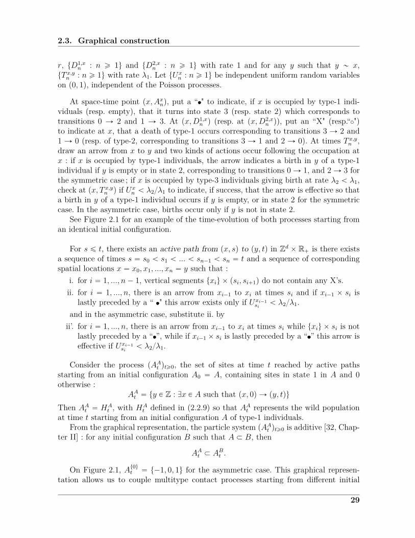
2.3 Graphical constructionIn parallel to the analytical construction provided by the Hille-Yosida theorem 1.1.2,
the multitype contact process can be constructed from a collection of independent Pois-son processes [38]. Think of the diagram Zd ˆR`. For each x P Zd, consider the arrivaltimes of mutually independent families of Poisson processes : tAxn : n ě 1u with rate
28
2.3. Graphical construction
r, tD1,xn : n ě 1u and tD2,x
n : n ě 1u with rate 1 and for any y such that y „ x,tT x,yn : n ě 1u with rate λ1. Let tUx
n : n ě 1u be independent uniform random variableson p0, 1q, independent of the Poisson processes.
At space-time point px,Axnq, put a “ " to indicate, if x is occupied by type-1 indi-viduals (resp. empty), that it turns into state 3 (resp. state 2) which corresponds totransitions 0 Ñ 2 and 1 Ñ 3. At px,D1,x
n q (resp. at px,D2,xn q), put an “X" (resp.“ ")
to indicate at x, that a death of type-1 occurs corresponding to transitions 3 Ñ 2 and1 Ñ 0 (resp. of type-2, corresponding to transitions 3 Ñ 1 and 2 Ñ 0). At times T x,yn ,draw an arrow from x to y and two kinds of actions occur following the occupation atx : if x is occupied by type-1 individuals, the arrow indicates a birth in y of a type-1individual if y is empty or in state 2, corresponding to transitions 0 Ñ 1, and 2 Ñ 3 forthe symmetric case ; if x is occupied by type-3 individuals giving birth at rate λ2 ă λ1,check at px, T x,yn q if Ux
n ă λ2λ1 to indicate, if success, that the arrow is effective so thata birth in y of a type-1 individual occurs if y is empty, or in state 2 for the symmetriccase. In the asymmetric case, births occur only if y is not in state 2.
See Figure 2.1 for an example of the time-evolution of both processes starting froman identical initial configuration.
For s ď t, there exists an active path from px, sq to py, tq in Zd ˆ R` is there existsa sequence of times s “ s0 ă s1 ă ... ă sn´1 ă sn “ t and a sequence of correspondingspatial locations x “ x0, x1, ..., xn “ y such that :
i. for i “ 1, ..., n´ 1, vertical segments txiu ˆ psi, si`1q do not contain any X’s.ii. for i “ 1, ..., n, there is an arrow from xi´1 to xi at times si and if xi´1 ˆ si is
lastly preceded by a “ " this arrow exists only if Uxi´1si
ă λ2λ1.and in the asymmetric case, substitute ii. byii’. for i “ 1, ..., n, there is an arrow from xi´1 to xi at times si while txiu ˆ si is not
lastly preceded by a “ ”, while if xi´1 ˆ si is lastly preceded by a “ ” this arrow iseffective if Uxi´1
siă λ2λ1.
Consider the process pAAt qtě0, the set of sites at time t reached by active pathsstarting from an initial configuration A0 “ A, containing sites in state 1 in A and 0otherwise :
AAt “ ty P Z : Dx P A such that px, 0q Ñ py, tqu
Then AAt “ HAt , with HA
t defined in (2.2.9) so that AAt represents the wild populationat time t starting from an initial configuration A of type-1 individuals.
From the graphical representation, the particle system pAAt qtě0 is additive [32, Chap-ter II] : for any initial configuration B such that A Ă B, then
AAt Ă ABt .
On Figure 2.1, At0ut “ t´1, 0, 1u for the asymmetric case. This graphical represen-tation allows us to couple multitype contact processes starting from different initial
29

Chapter 2. Phase transition on Zd
-2 -1 0 1 2
time
t
Figure 2.1: Graphical representation in the space-time picture Z ˆ R`. Starting fromη0 “ 1t0u, following the arrows, if U0
1 ăλ2λ1
and U02 ă
λ2λ1, the wild population occupies
at time t the set Ht “ t´1, 0, 1u in the asymmetric case and the set Ht “ t´2,´1, 0, 1uin the symmetric case.
30

2.4. Attractiveness and stochastic order
configurations by imposing the evolution to obey to the same Poisson processes. Otherkinds of couplings would be possible through the analytical construction of the processas we will see later. By way of illustration, At1ut “ H and A
t0,1ut “ t´1, 0, 1u in the
asymmetric case, At1ut “ t2u and At0,1ut “ t´2,´1, 0, 1, 2u in the symmetric case. Moregenerally, graphical representations allow to couple processes with different dynamics aswell, we investigate this question furthermore thereafter.
2.4 Attractiveness and stochastic order
Recall pηtqtě0 denotes the multitype contact process with parameters (λ1, λ2, r) andpξtqtě0 denotes the basic contact process with growth rate λ1. Most of the proofs belowrely on the construction of a markovian coupled process.
We defined a partial order on F Zd between two configurations ηp1q and ηp2q by (1.1.3)and (2.2.13). Here we shall settle necessary and sufficient conditions, then only sufficient,to obtain several properties of stochastic order with which we will work. We beginwith the symmetric multitype contact process since it contains the transitions of theasymmetric one and of the basic contact process.
Proposition 2.4.1. The symmetric multitype process is monotone, in the sense that,one can construct on a same probability space two symmetric multitype processes pηp1qt qtě0
and pηp2qt qtě0 with respective parameters pλp1q1 , λp1q2 , rp1qq and pλp2q1 , λ
p2q2 , rp2qq, such that
ηp1q0 ď η
p2q0 ùñ η
p1qt ď η
p2qt a.s. for all t ě 0 (2.4.1)
if and only if all parameters satisfy
1. λp1q2 ď λp1q1 ,
2. λp2q2 ď λp2q1 ,
3. λp1q1 ď λp2q1 ,
4. λp1q2 ď λp2q2 ,
5. rp1q ě rp2q
6. λp1q1 ď 1,7. λp1q2 ď 1,8. rp1q ě 1.
Remark conditions 1. and 2. are the assumptions made from the construction of theprocess, see (2.2.1).
Proof of Proposition 2.4.1. Let pηp1qt qtě0 and pηp2qt qtě0 be two symmetric processes withparameters pλp1q1 , λ
p1q2 , rp1qq and pλp2q1 , λ
p2q2 , rp2qq respectively. Apply Theorem 2.2.4 with
j1, h1 P t0, 1u (one can check they are the only non trivial possible values). Necessary andsufficient conditions on the rates for pηp2qt qtě0 to be stochastically larger than pηp1qt qtě0are given by relations (2.2.15) with pα, βq ď pγ, δq, that is,
ÿ
kąδ´β`j1
Π0,k,p1qα,β,p1q ď
ÿ
ląj1
Π0,l,p2qγ,δ and
ÿ
kąh1
Π´k,0,p1qα,β ěÿ
ląγ´α`h1
Π´l,0,p2qγ,δ
31
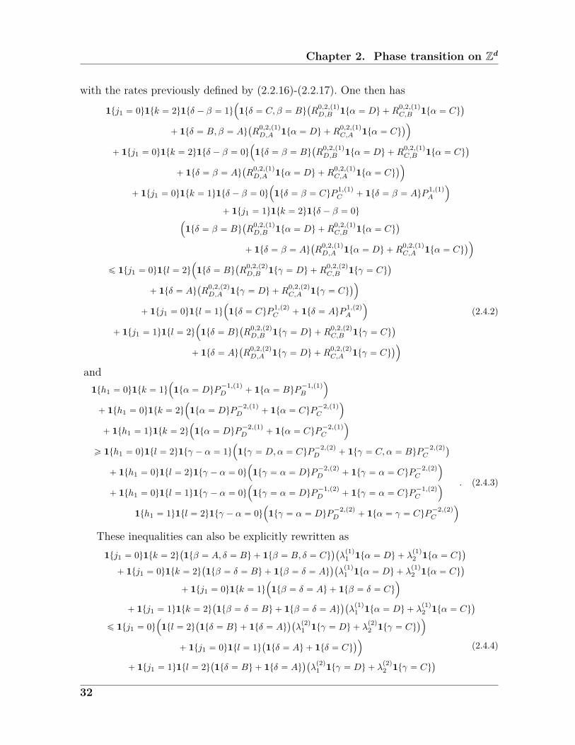
Chapter 2. Phase transition on Zd
with the rates previously defined by (2.2.16)-(2.2.17). One then has
1tj1 “ 0u1tk “ 2u1tδ ´ β “ 1u´
1tδ “ C, β “ Bu`
R0,2,p1qD,B 1tα “ Du `R
0,2,p1qC,B 1tα “ Cu
˘
` 1tδ “ B, β “ Au`
R0,2,p1qD,A 1tα “ Du `R
0,2,p1qC,A 1tα “ Cu
˘
¯
` 1tj1 “ 0u1tk “ 2u1tδ ´ β “ 0u´
1tδ “ β “ Bu`
R0,2,p1qD,B 1tα “ Du `R
0,2,p1qC,B 1tα “ Cu
˘
` 1tδ “ β “ Au`
R0,2,p1qD,A 1tα “ Du `R
0,2,p1qC,A 1tα “ Cu
˘
¯
` 1tj1 “ 0u1tk “ 1u1tδ ´ β “ 0u´
1tδ “ β “ CuP1,p1qC ` 1tδ “ β “ AuP
1,p1qA
¯
` 1tj1 “ 1u1tk “ 2u1tδ ´ β “ 0u´
1tδ “ β “ Bu`
R0,2,p1qD,B 1tα “ Du `R
0,2,p1qC,B 1tα “ Cu
˘
` 1tδ “ β “ Au`
R0,2,p1qD,A 1tα “ Du `R
0,2,p1qC,A 1tα “ Cu
˘
¯
ď 1tj1 “ 0u1tl “ 2u´
1tδ “ Bu`
R0,2,p2qD,B 1tγ “ Du `R
0,2,p2qC,B 1tγ “ Cu
˘
` 1tδ “ Au`
R0,2,p2qD,A 1tγ “ Du `R
0,2,p2qC,A 1tγ “ Cu
˘
¯
` 1tj1 “ 0u1tl “ 1u´
1tδ “ CuP1,p2qC ` 1tδ “ AuP
1,p2qA
¯
` 1tj1 “ 1u1tl “ 2u´
1tδ “ Bu`
R0,2,p2qD,B 1tγ “ Du `R
0,2,p2qC,B 1tγ “ Cu
˘
` 1tδ “ Au`
R0,2,p2qD,A 1tγ “ Du `R
0,2,p2qC,A 1tγ “ Cu
˘
¯
(2.4.2)
and1th1 “ 0u1tk “ 1u
´
1tα “ DuP´1,p1qD ` 1tα “ BuP
´1,p1qB
¯
` 1th1 “ 0u1tk “ 2u´
1tα “ DuP´2,p1qD ` 1tα “ CuP
´2,p1qC
¯
` 1th1 “ 1u1tk “ 2u´
1tα “ DuP´2,p1qD ` 1tα “ CuP
´2,p1qC
¯
ě 1th1 “ 0u1tl “ 2u1tγ ´ α “ 1u´
1tγ “ D,α “ CuP´2,p2qD ` 1tγ “ C,α “ BuP
´2,p2qC
˘
` 1th1 “ 0u1tl “ 2u1tγ ´ α “ 0u´
1tγ “ α “ DuP´2,p2qD ` 1tγ “ α “ CuP
´2,p2qC
¯
` 1th1 “ 0u1tl “ 1u1tγ ´ α “ 0u´
1tγ “ α “ DuP´1,p2qD ` 1tγ “ α “ CuP
´1,p2qC
¯
1th1 “ 1u1tl “ 2u1tγ ´ α “ 0u´
1tγ “ α “ DuP´2,p2qD ` 1tα “ γ “ CuP
´2,p2qC
¯
. (2.4.3)
These inequalities can also be explicitly rewritten as1tj1 “ 0u1tk “ 2u
`
1tβ “ A, δ “ Bu ` 1tβ “ B, δ “ Cu˘`
λp1q1 1tα “ Du ` λ
p1q2 1tα “ Cu
˘
` 1tj1 “ 0u1tk “ 2u`
1tβ “ δ “ Bu ` 1tβ “ δ “ Au˘`
λp1q1 1tα “ Du ` λ
p1q2 1tα “ Cu
˘
` 1tj1 “ 0u1tk “ 1u´
1tβ “ δ “ Au ` 1tβ “ δ “ Cu¯
` 1tj1 “ 1u1tk “ 2u`
1tβ “ δ “ Bu ` 1tβ “ δ “ Au˘`
λp1q1 1tα “ Du ` λ
p1q2 1tα “ Cu
˘
ď 1tj1 “ 0u´
1tl “ 2u`
1tδ “ Bu ` 1tδ “ Au˘`
λp2q1 1tγ “ Du ` λ
p2q2 1tγ “ Cu
˘
¯
` 1tj1 “ 0u1tl “ 1u`
1tδ “ Au ` 1tδ “ Cu˘
¯
` 1tj1 “ 1u1tl “ 2u`
1tδ “ Bu ` 1tδ “ Au˘`
λp2q1 1tγ “ Du ` λ
p2q2 1tγ “ Cu
˘
(2.4.4)
32

2.4. Attractiveness and stochastic order
and
1th1 “ 0u`
1tk “ 1urp1qp1tα “ Bu ` 1tα “ Du˘
` 1th1 “ 0u1tk “ 2u`
1tα “ Cu ` 1tα “ Du˘
` 1th1 “ 1u1tk “ 2up1tα “ Cu ` 1tα “ Duq
ě 1th1 “ 0u1tl “ 2u1tγ “ 1` αu´
1tγ “ Cu ` 1tγ “ Du¯
` 1th1 “ 0u1tl “ 2u1tγ “ αu`
1tγ “ Cu ` 1tγ “ Du˘
` 1th1 “ 0u1tl “ 1u1tγ “ αurp2qp1tγ “ Bu ` 1tγ “ Duq
` 1th1 “ 1u1tγ “ αu1tl “ 2up1tγ “ Cu ` 1tγ “ Duq.
(2.4.5)
All different possible scenarios provide the following necessary conditions :
(I) j1 P t0, 1u, δ “ β P tA,Bu in (2.4.4) give
(i) α “ C, γ “ D : λp1q2 ď λp2q1 . This is a consequence of conditions 1. and 3. or
2. and 4.(ii) α “ γ “ C : λp1q2 ď λ
p2q2 stated by condition 4.
(iii) α “ γ “ D : λp1q1 ď λp2q1 stated by condition 3.
(II) j1 “ 0, β “ B, δ “ 1` β “ C in (2.4.4) give
(i) α “ D : λp1q1 ď 1 stated by condition 6.
(ii) α “ C : λp1q2 ď 1 stated by condition 7.
(III) h1 “ 0, γ “ α P tB,Du in (2.4.5) give rp1q ě rp2q stated by condition 5.(IV) h1 “ 0,α “ B, γ “ 1` α “ C in (2.4.5) give rp1q ě 1 stated by condition 8.
while in other scenarios, one retrieves redundantly the above conditions or tautologicalinequalities such as “1 ě 0". Finally, one obtained the necessary conditions stated from1. to 8.
Now, we construct a coupled process pηp1qt , ηp2qt qtě0 on Ω ˆ Ω such that ηp1q0 ď η
p2q0 .
According to the given order (2.2.13) on F , as ηp1q0 ď ηp2q0 :
n1px, ηp1q0 q ` n3px, η
p1q0 q ď n1px, η
p2q0 q ` n3px, η
p2q0 q.
We saw that it is possible to construct the coupled process either through generatorsor through a graphical representation, via a collection of independent Poisson processeswhose rates are given by the parameters of the processes. The coupling of two processeson a graphical construction is provided by coupling the Poisson processes related tobirths and releases.
In what follows, we construct the coupling through generators. The three followingtables depict the infinitesimal transitions of the coupled process.
33

Chapter 2. Phase transition on Zd
transition rate
p0, 0q ÝÑ
$
’
’
&
’
’
%
p1, 1qp0, 1qp2, 2qp2, 0q
λp1q1 n1px, η
p1qq ` λp1q2 n3px, η
p1qq
λp2q1 n1px, η
p2qq ´ λp1q1 n1px, η
p1qq ` λp2q2 n3px, η
p2qq ´ λp1q2 n3px, η
p1qq
rp2q
rp1q ´ rp2q
p1, 1q ÝÑ
$
&
%
p0, 0qp3, 3qp3, 1q
1rp2q
rp1q ´ rp2q
p2, 2q ÝÑ
$
&
%
p3, 3qp2, 3qp0, 0q
λp1q1 n1px, η
p1qq ` λp1q2 n3px, η
p1qq
λp2q1 n1px, η
p2qq ´ λp1q1 n1px, η
p1qq ` λp2q2 n3px, η
p2qq ´ λp1q2 n3px, η
p1qq1
p3, 3q ÝÑ"
p1, 1qp2, 2q
11
p2, 0q ÝÑ
$
’
’
&
’
’
%
p3, 1qp2, 1qp0, 0qp2, 2q
λp1q1 n1px, η
p1qq ` λp1q2 n3px, η
p1qq
λp2q1 n1px, η
p2qq ´ λp1q1 n1px, η
p1qq ` λp2q2 n3px, η
p2qq ´ λp1q2 n3px, η
p1qq1rp2q
p2, 3q ÝÑ
$
&
%
p3, 3qp0, 1qp2, 2q
λp1q1 n1px, η
p1qq ` λp1q2 n3px, η
p1qq11
p2, 1q ÝÑ
$
’
’
&
’
’
%
p3, 1qp2, 0qp0, 1qp2, 3q
λp1q1 n1px, η
p1qq ` λp1q2 n3px, η
p1qq11rp2q
p3, 1q ÝÑ
$
&
%
p2, 0qp1, 1qp3, 3q
11rp2q
p0, 1q ÝÑ
$
’
’
&
’
’
%
p2, 3qp1, 1qp2, 1qp0, 0q
rp2q
λp1q1 n1px, η
p1qq ` λp1q2 n3px, η
p1qq
rp1q ´ rp2q
1
Table 2.1
transition rate
p0, 3q ÝÑ
$
’
’
&
’
’
%
p1, 1qp0, 1qp2, 2qp2, 3q
λp1q1 n1px, η
p1qq ` λp1q2 n3px, η
p1qq
p1´ λp1q1 qn1px, ηp1qq ` p1´ λp1q2 qn3px, η
p1qq1
rp1q ´ 1
Table 2.2
34
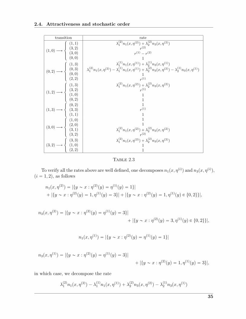
2.4. Attractiveness and stochastic order
transition rate
p1, 0q ÝÑ
$
’
’
&
’
’
%
p1, 1qp3, 2qp3, 0qp0, 0q
λp2q1 n1px, η
p2qq ` λp2q2 n3px, η
p2qq
rp2q
rp1q ´ rp2q
1
p0, 2q ÝÑ
$
’
’
&
’
’
%
p1, 3qp0, 3qp0, 0qp2, 2q
λp1q1 n1px, η
p1qq ` λp1q2 n3px, η
p1qq
λp2q1 n1px, η
p2qq ´ λp1q1 n1px, η
p1qq ` λp2q2 n3px, η
p2qq ´ λp1q2 n3px, η
p1qq1rp1q
p1, 2q ÝÑ
$
’
’
&
’
’
%
p1, 3qp3, 2qp1, 0qp0, 2q
λp2q1 n1px, η
p2qq ` λp2q2 n3px, η
p2qq
rp1q
11
p1, 3q ÝÑ
$
&
%
p0, 2qp3, 3qp1, 1q
1rp1q
1
p3, 0q ÝÑ
$
’
’
&
’
’
%
p1, 0qp2, 0qp3, 1qp3, 2q
11
λp2q1 n1px, η
p2qq ` λp2q2 n3px, η
p2qq
rp2q
p3, 2q ÝÑ
$
&
%
p3, 3qp1, 0qp2, 2q
λp2q1 n1px, η
p2qq ` λp2q2 n3px, η
p2qq11
Table 2.3
To verify all the rates above are well defined, one decomposes n1px, ηpiqq and n3px, η
piqq,pi “ 1, 2q, as follows
n1px, ηp2qq “ |ty „ x : ηp2qpyq “ ηp1qpyq “ 1u|
` |ty „ x : ηp2qpyq “ 1, ηp1qpyq “ 3u| ` |ty „ x : ηp2qpyq “ 1, ηp1qpyq P t0, 2uu|,
n3px, ηp2qq “ |ty „ x : ηp2qpyq “ ηp1qpyq “ 3u|
` |ty „ x : ηp2qpyq “ 3, ηp1qpyq P t0, 2uu|,
n1px, ηp1qq “ |ty „ x : ηp2qpyq “ ηp1qpyq “ 1u|
n3px, ηp1qq “ |ty „ x : ηp2qpyq “ ηp1qpyq “ 3u|
` |ty „ x : ηp2qpyq “ 1, ηp1qpyq “ 3u|,
in which case, we decompose the rate
λp2q1 n1px, η
p2qq ´ λ
p1q1 n1px, η
p1qq ` λ
p2q2 n3px, η
p2qq ´ λ
p1q2 n3px, η
p1qq
35
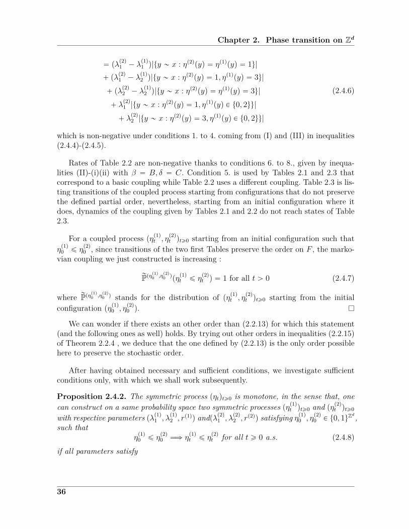
Chapter 2. Phase transition on Zd
“ pλp2q1 ´ λ
p1q1 q|ty „ x : ηp2qpyq “ ηp1qpyq “ 1u|
` pλp2q1 ´ λ
p1q2 q|ty „ x : ηp2qpyq “ 1, ηp1qpyq “ 3u|
` pλp2q2 ´ λ
p1q2 q|ty „ x : ηp2qpyq “ ηp1qpyq “ 3u|
` λp2q1 |ty „ x : ηp2qpyq “ 1, ηp1qpyq P t0, 2uu|` λ
p2q2 |ty „ x : ηp2qpyq “ 3, ηp1qpyq P t0, 2uu|
(2.4.6)
which is non-negative under conditions 1. to 4. coming from (I) and (III) in inequalities(2.4.4)-(2.4.5).
Rates of Table 2.2 are non-negative thanks to conditions 6. to 8., given by inequa-lities (II)-(i)(ii) with β “ B, δ “ C. Condition 5. is used by Tables 2.1 and 2.3 thatcorrespond to a basic coupling while Table 2.2 uses a different coupling. Table 2.3 is lis-ting transitions of the coupled process starting from configurations that do not preservethe defined partial order, nevertheless, starting from an initial configuration where itdoes, dynamics of the coupling given by Tables 2.1 and 2.2 do not reach states of Table2.3.
For a coupled process pηp1qt , ηp2qt qtě0 starting from an initial configuration such that
ηp1q0 ď η
p2q0 , since transitions of the two first Tables preserve the order on F , the marko-
vian coupling we just constructed is increasing :
rPpηp1q0 ,η
p2q0 qpηp1qt ď η
p2qt q “ 1 for all t ą 0 (2.4.7)
where rPpηp1q0 ,η
p2q0 q stands for the distribution of pηp1qt , η
p2qt qtě0 starting from the initial
configuration pηp1q0 , ηp2q0 q.
We can wonder if there exists an other order than (2.2.13) for which this statement(and the following ones as well) holds. By trying out other orders in inequalities (2.2.15)of Theorem 2.2.4 , we deduce that the one defined by (2.2.13) is the only order possiblehere to preserve the stochastic order.
After having obtained necessary and sufficient conditions, we investigate sufficientconditions only, with which we shall work subsequently.
Proposition 2.4.2. The symmetric process pηtqtě0 is monotone, in the sense that, onecan construct on a same probability space two symmetric processes pηp1qt qtě0 and pηp2qt qtě0
with respective parameters pλp1q1 , λp1q2 , rp1qq andpλp2q1 , λ
p2q2 , rp2qq satisfying ηp1q0 , η
p2q0 P t0, 1uZd,
such thatηp1q0 ď η
p2q0 ùñ η
p1qt ď η
p2qt for all t ě 0 a.s. (2.4.8)
if all parameters satisfy
36

2.4. Attractiveness and stochastic order
1. λp1q2 ď λp1q1 ,
2. λp2q2 ď λp2q1 ,
3. λp1q1 ď λp2q1 ,
4. λp1q2 ď λp2q2 ,
5. rp1q ě rp2q
Proof. Given our initial conditions, possible states for the coupled process keep layingin Table 2.1 of Proposition 2.4.1 and the coupled process does not reach any state ofTables 2.2 and 2.3. One can therefore omit conditions 4. to 6. of the previous Proposition2.4.1 and transition rates from the couple p0, 3q can be defined through a basic couplingeven if it does not preserve the order :
transition rate
p0, 3q ÝÑ
$
’
’
&
’
’
%
p1, 3qp0, 1qp0, 2qp2, 3q
λp1q1 n1px, η
p1qq ` λp1q2 n3px, η
p1qq11rp1q
Table 2.4
in which case, Table 2.4 substitutes Table 2.2.
Remark 2.4.1. In view of the proof of Proposition 2.4.2, one can actually relax theadmissible initial conditions : it is enough to assume ηp1q0 and ηp2q0 satisfying ηp1q0 ď η
p2q0
and for all x P Zd, pηp1q0 pxq, ηp2q0 pxqq ‰ p0, 3q. In particular one could start from η
p1q0 “
ηp2q0 .
Since Tables 2.1, 2.4 and 2.3 correspond to a basic coupling, to construct such pro-cesses on a same probability space via the graphical representation, one define fromSection 1.2 mutually independent Poisson processes : tT x,yn , n ě 1u with rate λ
p2q1 ,
tD1,xn , n ě 1u with rate 1, tD2,x
n , n ě 1u with rate 1 and independent uniform ran-dom variables tUx,y
n , n ě 1u on p0, 1q, independent of the Poisson processes. Indeed,after conditions 1 to 5 of Proposition 2.4.2, the growth rate λp2q1 is the largest one. Ateach time t “ T x,yn a birth might occur and the uniform random variables determineif it occurs or not. For instance, if ηp1qt pxq is in state 3 and ηp1qt pyq is in state 0, then abirth in y for ηp1qt occurs if Ux,y
n ă λp1q2 λ
p2q1 ; if ηp2qt pxq is in state 3 and ηp2qt pyq is in state
0, then a birth in y for the process ηp2qt occurs if Ux,yn ă λ
p2q2 λ
p2q1 . Since λp1q2 ď λ
p2q2 , as
soon as Ux,yn P pλ
p1q2 λ
p2q1 , λ
p2q2 λ
p2q1 s an arrow used by the process ηp2qt is not used by the
process ηp1qt .
If pηp1qt qtě0 and pηp2qt qtě0 differ by at most one parameter, one deduces from Proposi-tion 2.4.2 several monotonicity properties :
Corollary 2.4.1. Suppose ηp1q0 , η
p2q0 P t0, 1uZd. Then for the processes pηp1qt qtě0 and
pηp2qt qtě0 with parameters pλp1q1 , λ
p1q2 , rp1qq and pλp2q1 , λ
p2q2 , rp2qq respectively, one has
(i) Attractiveness : if pλp1q1 , λp1q2 , rp1qq “ pλ
p2q1 , λ
p2q2 , rp2qq , then ηp1q0 ď η
p2q0 ùñ η
p1qt ď η
p2qt
a.s., for all t ě 0.
37
Chapter 2. Phase transition on Zd
(ii) Increase w.r.t. λ1 : if pηp1qt qtě0 and pηp2qt qtě0 have respective parameters pλp1q1 , λ2, rq
and pλp2q1 , λ2, rq such that λ2 ď λp1q1 ď λ
p2q1 , then ηp1q0 ď η
p2q0 ùñ η
p1qt ď η
p2qt a.s., for
all t ě 0.(iii) Increase w.r.t. λ2 : if pηp1qt qtě0 and pηp2qt qtě0 have respective parameters pλ1, λ
p1q2 , rq
and pλ1, λp2q2 , rq such that λp1q2 ď λ
p2q2 ď λ1, then ηp1q0 ď η
p2q0 ùñ η
p1qt ď η
p2qt a.s., for
all t ě 0.(iv) Decrease w.r.t. r : if pηp1qt qtě0 and pηp2qt qtě0 have respective parameters pλ1, λ2, r
p1qq
and pλ1, λ2, rp2qq such that rp1q ě rp2q with λ2 ă λ1, then ηp1q0 ď η
p2q0 ùñ η
p1qt ď η
p2qt
a.s., for all t ě 0.
A consequence related to Corollary (2.4.1)-(iv) is the non-increase of the survivalprobability with respect to the release rate r for fixed λ1, λ2 :
Corollary 2.4.2. Suppose λ2 and λ1 fixed. If pηtqtě0 has initial configuration η0 “ 1t0u,the mapping
r ÞÝÑ Prp@t ě 0, Ht ‰ Hq
is a non-increasing function.
Proof. Indeed if pηp1qt qtě0 and pηp2qt qtě0 are two processes such that ηp1q0 , ηp2q0 P t0, 1uZd
and with respective parameters pλ1, λ2, rp1qq and pλ1, λ2, r
p2qq such that rp1q ď rp2q, thenaccording to Corollary 2.4.1,
Hp2q0 Ă H
p1q0 ùñ H
p2qt Ă H
p1qt ,
for all t ě 0.
One defined the asymmetric process as a particular case of the symmetric processwhere the transition from state 2 to state 3 does not occur. One can thus, in a similarway to Propositions 2.4.1 and 2.4.2, obtain necessary and sufficient conditions, then,only sufficient conditions, for the monotonicity of the asymmetric process.
Proposition 2.4.3. The asymmetric process pηtqtě0 is monotone in the sense that,conditions
1. λp1q2 ď λp1q1 ,
2. λp2q2 ď λp2q1 ,
3. λp1q1 ď λp2q1 ,
4. λp1q2 ď λp2q2 ,
5. rp1q ě rp2q,
are sufficient to construct on a same probability space two asymmetric process pηp1qt qtě0
and pηp2qt qtě0 with respective parameters pλp1q1 , λp1q2 , rp1qq and pλp2q1 , λ
p2q2 , rp2qq and with ini-
tial condition ηp1q0 , ηp2q0 P t0, 1uZd, such that
ηp1q0 ď η
p2q0 ùñ η
p1qt ď η
p2qt a.s., for all t ě 0. (2.4.9)
38
2.4. Attractiveness and stochastic order
Proof. As in the proof of Proposition 2.4.2, one applies Theorem 2.2.4 with j1, h1 P
t0, 1u to two asymmetric processes pηp1qt qtě0 and pηp2qt qtě0 with respective parameterspλp1q1 , λ
p1q2 , rp1qq and pλp2q1 , λ
p2q2 , rp2qq. Using relations (2.4.2)-(2.4.3) with the corresponding
rates of both processes given by (2.2.16), with pα, βq ď pγ, δq, one has
1tj1 “ 0u˜
1tk “ 2u´
1tβ “ δ “ Bu`
λp1q1 1tα “ Du ` λ
p1q2 1tα “ Cu
˘
¯
` 1tk “ 1u´
1tβ “ δ “ Au ` 1tβ “ δ “ Cu¯
¸
` 1tj1 “ 0u1tk “ 2u´
1tβ “ B, δ “ Cu`
λp1q1 1tα “ Du ` λ
p1q2 1tα “ Cu
˘
¯
` 1tj1 “ 1u1tk “ 2u´
1tβ “ δ “ Bu`
λp1q1 1tα “ Du ` λ
p1q2 1tα “ Cu
˘
¯
ď 1tj1 “ 0u´
1tl “ 2u1tδ “ Bu`
λp2q1 1tγ “ Du ` λ
p2q2 1tγ “ Cu
˘
` 1tl “ 1u`
1tδ “ Au ` 1tδ “ Cu˘
¯
` 1tj1 “ 1u´
1tl “ 2u1tδ “ Bu`
λp2q1 1tγ “ Du ` λ
p2q2 1tγ “ Cu
˘
(2.4.10)
while the second relation leaves (2.4.5) unchanged. One deduces the following necessaryconditions :(I) j1 P t0, 1u, δ “ β “ B in (2.4.10) give
(i) α “ γ “ C, β “ B, δ “ C : λp1q2 ď λp2q2 stated by condition 4.
(ii) α “ C, γ “ D : λp1q2 ď λp2q1 stated by conditions 1. and 3.
(iii) α “ γ “ D : λp1q1 ď λp2q1 stated by condition 3.
(II) j1 “ 0, β “ B, δ “ 1` β “ C in (2.4.10) give(i) α “ D : λp1q1 ď 1.(ii) α “ C : λp1q2 ď 1.
The relation (2.4.5) staying unchanged, one has(III) h1 “ 0, γ “ α P tB,Du in (2.4.5) give rp1q ě rp2q stated by condition 5.(IV) h1 “ 0,α “ B, γ “ 1` α “ C in (2.4.5) give rp1q ě 1.The obtained necessary conditions are
1. λp1q2 ď λp1q1 ,
2. λp2q2 ď λp2q1 ,
3. λp1q1 ď λp2q1 ,
4. λp1q2 ď λp2q2 ,
5. rp1q ě rp2q
6. λp1q1 ď 1,7. λp1q2 ď 1,8. rp1q ě 1.
As for Proposition 2.4.1, these conditions allow us to construct an increasing marko-vian coupling. As in Proposition 2.4.2, given our initial configurations, state p0, 3q is notpossible for the coupled process. One can thus dispense conditions 6 to 8. and sufficientconditions to settle an increasing markovian coupling as in Proposition 2.4.2 are givenby
39

Chapter 2. Phase transition on Zd
1. λp1q2 ď λp1q1 ,
2. λp2q2 ď λp2q1 ,
3. λp1q1 ď λp2q1 ,
4. λp1q2 ď λp2q2 ,
5. rp1q ě rp2q
Details of the dynamics of the coupled process pηp1qt , ηp2qt qtě0 are summarized in the
following tables.
transition rate
p0, 0q ÝÑ
$
’
’
&
’
’
%
p1, 1qp0, 1qp2, 2qp2, 0q
λp1q1 n1px, η
p1qq ` λp1q2 n3px, η
p1qq
λp2q1 n1px, η
p2qq ´ λp1q1 n1px, η
p1qq ` λp2q2 n3px, η
p2qq ´ λp1q2 n3px, η
p1qq
rp2q
rp1q ´ rp2q
p1, 1q ÝÑ
$
&
%
p0, 0qp3, 3qp3, 1q
1rp2q
rp1q ´ rp2q
p2, 2q ÝÑ p0, 0q 1
p3, 3q ÝÑ"
p1, 1qp2, 2q
11
p2, 0q ÝÑ
$
&
%
p2, 1qp0, 0qp2, 2q
λp2q1 n1px, η
p2qq ` λp2q2 n3px, η
p2qq1rp2q
p2, 3q ÝÑ"
p0, 1qp2, 2q
11
p2, 1q ÝÑ
$
&
%
p2, 0qp0, 1qp2, 3q
11rp2q
p3, 1q ÝÑ
$
&
%
p2, 0qp1, 1qp3, 3q
11rp2q
p0, 1q ÝÑ
$
’
’
&
’
’
%
p2, 3qp1, 1qp2, 1qp0, 0q
rp2q
λp1q1 n1px, η
p1qq ` λp1q2 n3px, η
p1qq
rp1q ´ rp2q
1
Table 2.5
transition rate
p0, 3q ÝÑ
$
’
’
&
’
’
%
p1, 3qp0, 1qp0, 2qp2, 3q
λp1q1 n1px, η
p1qq ` λp1q2 n3px, η
p1qq11rp1q
Table 2.6
40
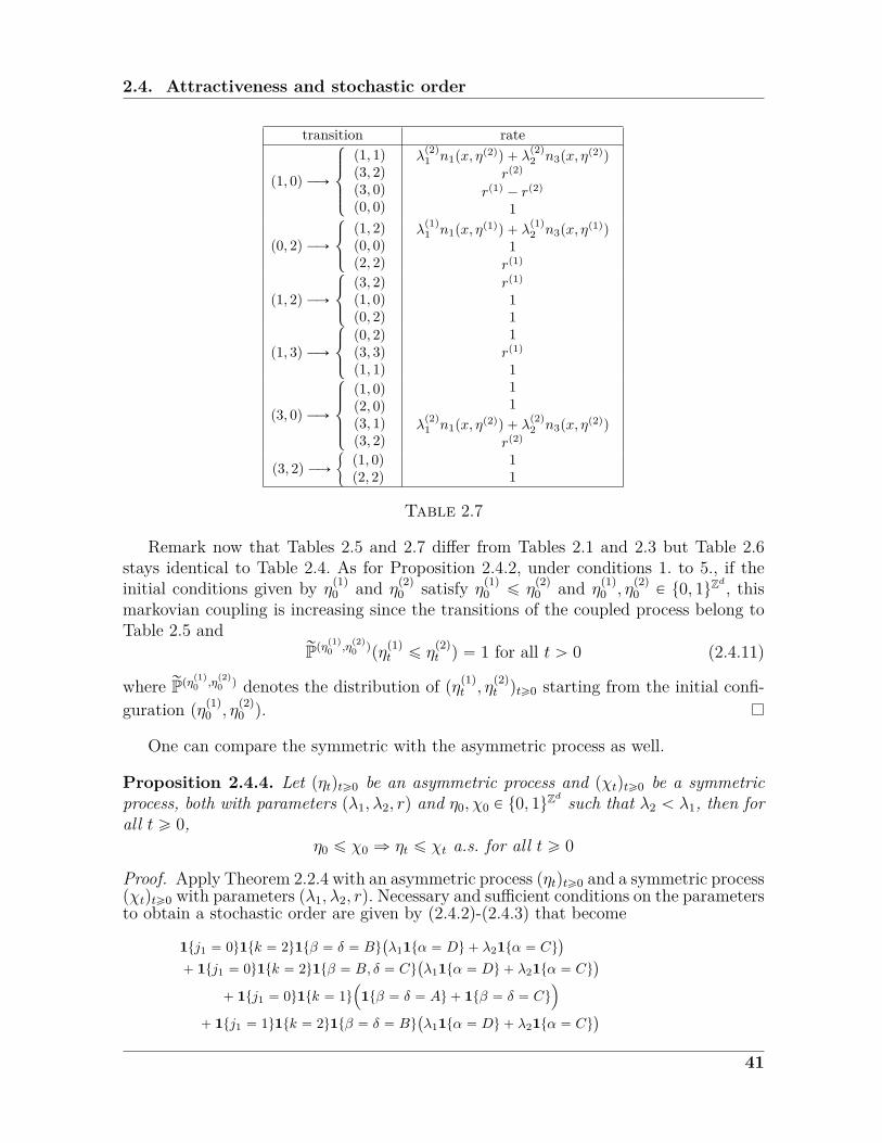
2.4. Attractiveness and stochastic order
transition rate
p1, 0q ÝÑ
$
’
’
&
’
’
%
p1, 1qp3, 2qp3, 0qp0, 0q
λp2q1 n1px, η
p2qq ` λp2q2 n3px, η
p2qq
rp2q
rp1q ´ rp2q
1
p0, 2q ÝÑ
$
&
%
p1, 2qp0, 0qp2, 2q
λp1q1 n1px, η
p1qq ` λp1q2 n3px, η
p1qq1rp1q
p1, 2q ÝÑ
$
&
%
p3, 2qp1, 0qp0, 2q
rp1q
11
p1, 3q ÝÑ
$
&
%
p0, 2qp3, 3qp1, 1q
1rp1q
1
p3, 0q ÝÑ
$
’
’
&
’
’
%
p1, 0qp2, 0qp3, 1qp3, 2q
11
λp2q1 n1px, η
p2qq ` λp2q2 n3px, η
p2qq
rp2q
p3, 2q ÝÑ"
p1, 0qp2, 2q
11
Table 2.7
Remark now that Tables 2.5 and 2.7 differ from Tables 2.1 and 2.3 but Table 2.6stays identical to Table 2.4. As for Proposition 2.4.2, under conditions 1. to 5., if theinitial conditions given by ηp1q0 and η
p2q0 satisfy ηp1q0 ď η
p2q0 and η
p1q0 , η
p2q0 P t0, 1uZd , this
markovian coupling is increasing since the transitions of the coupled process belong toTable 2.5 and
rPpηp1q0 ,η
p2q0 qpηp1qt ď η
p2qt q “ 1 for all t ą 0 (2.4.11)
where rPpηp1q0 ,η
p2q0 q denotes the distribution of pηp1qt , η
p2qt qtě0 starting from the initial confi-
guration pηp1q0 , ηp2q0 q.
One can compare the symmetric with the asymmetric process as well.
Proposition 2.4.4. Let pηtqtě0 be an asymmetric process and pχtqtě0 be a symmetricprocess, both with parameters pλ1, λ2, rq and η0, χ0 P t0, 1uZ
d such that λ2 ă λ1, then forall t ě 0,
η0 ď χ0 ñ ηt ď χt a.s. for all t ě 0
Proof. Apply Theorem 2.2.4 with an asymmetric process pηtqtě0 and a symmetric processpχtqtě0 with parameters pλ1, λ2, rq. Necessary and sufficient conditions on the parametersto obtain a stochastic order are given by (2.4.2)-(2.4.3) that become
1tj1 “ 0u1tk “ 2u1tβ “ δ “ Bu`
λ11tα “ Du ` λ21tα “ Cu˘
` 1tj1 “ 0u1tk “ 2u1tβ “ B, δ “ Cu`
λ11tα “ Du ` λ21tα “ Cu˘
` 1tj1 “ 0u1tk “ 1u´
1tβ “ δ “ Au ` 1tβ “ δ “ Cu¯
` 1tj1 “ 1u1tk “ 2u1tβ “ δ “ Bu`
λ11tα “ Du ` λ21tα “ Cu˘
41
Chapter 2. Phase transition on Zd
ď 1tj1 “ 0u´
1tl “ 2u`
1tδ “ Bu ` 1tδ “ Au˘`
λ11tγ “ Du ` λ21tγ “ Cu˘
` 1tl “ 1u`
1tδ “ Au ` 1tδ “ Cu˘
¯
` 1tj1 “ 1u1tl “ 2u`
1tδ “ Bu ` 1tδ “ Au˘`
λ11tγ “ Du ` λ21tγ “ Cu˘
(2.4.12)
and
1th1 “ 0u´
1tk “ 1urp1tα “ Bu ` 1tα “ Duq ` 1tk “ 2up1tα “ Cu
` 1tα “ Duq¯
` 1th1 “ 1u´
1tk “ 2up1tα “ Cu ` 1tα “ Duq¯
ě 1th1 “ 0u1tγ “ αu´
1tl “ 1urp1tγ “ Bu ` 1tγ “ Duq
` 1tl “ 2up1tγ “ Cu ` 1tγ “ Duq¯
` 1th1 “ 0u1tγ “ 1` αu´
1tl “ 2up1tγ “ Cu ` 1tγ “ Duq¯
` 1th1 “ 1u1tγ “ αu´
1tl “ 2up1tγ “ Cu ` 1tγ “ Duq¯
(2.4.13)
These equations exhibit the following necessary conditions :
(I) j1 P t0, 1u, δ “ β “ B,α “ C, γ “ D in (2.4.12) give : λ2 ď λ1
(II) h1 “ 0, α “ B, γ “ 1` α “ C in (2.4.13) give r ě 1
As previously, condition r ě 1 is necessary to construct an increasing markovian coupledprocess in a general framework, but if one restricts the initial conditions to satisfyη0 ď χ0 and η0, χ0 P t0, 1uZ
d , condition λ2 ď λ1 is sufficient and the coupled process canbe constructed through the following transitions :
42

2.4. Attractiveness and stochastic order
transition rate
p0, 0q ÝÑ
$
&
%
p1, 1qp0, 1qp2, 2q
λ1n1px, ηq ` λ2n3px, ηqλ1pn1px, χq ´ n1px, ηqq ` λ2n3px, χq ´ n3px, ηqq
r
p1, 1q ÝÑ"
p0, 0qp3, 3q
1r
p2, 2q ÝÑ"
p0, 0qp2, 3q
1λ1n1px, χq ` λ2n3px, χq
p3, 3q ÝÑ"
p1, 1qp2, 2q
11
p2, 0q ÝÑ
$
&
%
p2, 1qp0, 0qp2, 2q
λ1n1px, χq ` λ2n3px, χq1r
p2, 3q ÝÑ"
p0, 1qp2, 2q
11
p2, 1q ÝÑ
$
&
%
p2, 0qp0, 1qp2, 3q
11r
p3, 1q ÝÑ
$
&
%
p2, 0qp1, 1qp3, 3q
11r
p0, 1q ÝÑ
$
&
%
p2, 3qp1, 1qp0, 0q
rλ1n1px, ηq ` λ2n3px, ηq
1
Table 2.8
transition rate
p0, 3q ÝÑ
$
’
’
&
’
’
%
p2, 3qp1, 3qp0, 1qp0, 2q
rλ1n1px, ηq ` λ2n3px, ηq
11
Table 2.9
43

Chapter 2. Phase transition on Zd
transition rate
p1, 0q ÝÑ
$
&
%
p1, 1qp3, 2qp0, 0q
λ1n1px, χq ` λ2n3px, χqr1
p0, 2q ÝÑ
$
’
’
&
’
’
%
p1, 3qp0, 3qp0, 0qp2, 2q
λ1n1px, ηq ` λ2n3px, ηqλ1n1px, χq ` λ2n3px, χq
1r
p1, 2q ÝÑ
$
&
%
p3, 2qp0, 0qp1, 3q
r1
λ1n1px, χq ` λ2n3px, χq
p1, 3q ÝÑ"
p0, 2qp3, 3q
1r
p3, 0q ÝÑ
$
’
’
&
’
’
%
p1, 0qp2, 0qp3, 1qp3, 2q
11
λ1n1px, χq ` λ2n3px, χqr
Table 2.10
As in (2.4.6), the second rate in Table 2.8 is positive. Starting from an initial confi-guration such that η0 ď χ0 and η0, χ0 P t0, 1uZ
d , the coupled process does not reach anyconfiguration of Tables 2.9 and 2.10. Condition λ2 ď λ1 is sufficient to obtain
ηt ď χt a.s., for all t ě 0.
Finally, one settles two comparisons between a basic contact process and a multitypeprocess.
Proposition 2.4.5. Let pξtqtě0 be a basic contact process on t0, 1uZd with growth rateλ1 and let pχtqtě0 be a symmetric multitype process with parameters pλ1, λ2, rq such thatλ2 ă λ1. Then,
χ0 ď ξ0 ñ χt ď ξt a.s. for all t ě 0Proof. Consider the basic contact process pξtqtě0 viewed as a symmetric multitype pro-cess with parameters pλp2q1 , λ
p2q2 , rp2qq with λ
p2q1 “ λ1, λp2q2 “ 0, rp2q “ 0. Values A and
C do not exist for the process ξt, retrieving the proof of Proposition 2.4.1, relations(2.4.2)-(2.4.3) become
1tj1 “ 0u1tk “ 2u1tβ “ δ “ Bu`
λ11tα “ Du ` λ21tα “ Cu˘
¯
` 1tj1 “ 0u1tk “ 2u´
1tβ “ A, δ “ Bu`
λ11tα “ Du ` λ21tα “ Cu˘
` 1tj1 “ 1u1tk “ 2u1tβ “ δ “ Bu`
λ11tα “ Du ` λ21tα “ Cu˘
ď`
1tj1 “ 0u ` 1tj1 “ 1u˘
1tl “ 2u1tδ “ Buλ11tγ “ Du(2.4.14)
44

2.4. Attractiveness and stochastic order
and1th1 “ 0u
´
1tk “ 1urp1tα “ Bu ` 1tα “ Duq ` 1tk “ 2up1tα “ Cu
` 1tα “ Duq¯
` 1th1 “ 1u1tk “ 2up1tα “ Cu ` 1tα “ Duq
ě 1th1 “ 0u1tγ “ αu1tl “ 2u1tγ “ Du
` 1th1 “ 0u1tγ “ 1` αu1tl “ 2u1tγ “ Du
` 1th1 “ 1u1tγ “ αu1tl “ 2u1tγ “ Du
(2.4.15)
that exhibit the following necessary condition : j1 P t0, 1u, β “ δ “ B, α “ C, γ “ D in(2.4.14) give λ2 ď λ1. While relation (2.4.15) does not give further condition. Conditionλ2 ď λ1 is sufficient and allows us to construct the following coupling.
transition rate
p0, 0q ÝÑ
$
&
%
p2, 0qp1, 1qp0, 1q
rλ1n1px, χq ` λ2n3px, χq
λ1pn1px, ξq ´ n1px, χqq ´ λ2n3px, χq
p1, 1q ÝÑ"
p0, 0qp3, 1q
1r
p2, 0q ÝÑ
$
&
%
p3, 1qp2, 1qp0, 0q
λ1n1px, χq ` λ2n3px, χqλ1pn1px, ξq ´ n1px, χqq ´ λ2n3px, χq
1
p2, 1q ÝÑ
$
&
%
p2, 0qp0, 1qp3, 1q
11
λ1n1px, χq ` λ2n3px, χq
p3, 1q ÝÑ"
p2, 0qp1, 1q
11
p0, 1q ÝÑ
$
&
%
p1, 1qp2, 1qp0, 0q
λ1n1px, χq ` λ2n3px, χqr1
p1, 0q ÝÑ
$
&
%
p1, 1qp3, 0qp0, 0q
λ1n1px, χq ` λ2n3px, χqr1
p3, 0q ÝÑ
$
&
%
p2, 0qp1, 0qp3, 1q
11
λ1n1px, ξq
Table 2.11For all x P Zd, one has if χ ď ξ
n1px, χq “ |ty „ x : χpyq “ ξpyq “ 1u| (2.4.16)n3px, χq “ |ty „ x : χpyq “ 3, ξpyq “ 1u| (2.4.17)n1px, ξq “ |ty „ x : χpyq “ ξpyq “ 1u| ` |ty „ x : χpyq “ 3, ξpyq “ 1u|
` |ty „ x : χpyq P t0, 2u, ξpyq “ 1u| (2.4.18)
45

Chapter 2. Phase transition on Zd
Therefore, under condition condition λ2 ď λ1
λ1pn1px, ξq ´ n1px, χqq ´ λ2n3px, χq
“ pλ1 ´ λ2qn3px, χq ` λ1|ty „ x : χpyq P t0, 2u, ξpyq “ 1u|
is non-negative, andχ0 ď ξ0 ñ χt ď ξt a.s.,
for all t ě 0.
For next proposition, prξtqtě0 is a basic contact process on t2, 3uZd whose dynamicsis given by the following transitions in x P Zd
2 Ñ 3 at rate λ2n3px, rξq, 3 Ñ 2 at rate 1 (2.4.19)
Proposition 2.4.6. Let pηtqtě0 be a symmetric multitype process with parameters pλ1, λ2, rqsuch that λ2 ď λ1. Then
rξ0 ď η0 ñ rξt ď ηt a.s., for all t ě 0.
Proof. Use once again Theorem 2.2.4 to obtain necessary and sufficient conditions fora stochastic order. For the process prξtqtě0, values B and D are not reached and ratesare given by (2.2.19). Necessary and sufficient conditions on the parameters are givenby relations (2.4.2)-(2.4.3) applied to rates (2.4.19) i.e. (2.2.19), (2.2.16) and (2.2.17),
`
1tj1 “ 0u ` 1tj1 “ 1u˘
1tk “ 2u1tβ “ δ “ Auλ21tα “ Cu
` 1tj1 “ 0u1tk “ 2u1tδ “ B, β “ Auλ21tα “ Cu
ď 1tj1 “ 0u´
1tl “ 2u`
1tδ “ Bu ` 1tδ “ Au˘`
λ11tγ “ Du ` λ21tγ “ Cu˘
` 1tl “ 1u1tδ “ Au¯
` 1tj1 “ 1u1tl “ 2u`
1tδ “ Bu ` 1tδ “ Au˘`
λ11tγ “ Du ` λ21tγ “ Cu˘
(2.4.20)
and
1th1 “ 0u1tk “ 2u1tα “ Cu ` 1th1 “ 1u1tk “ 2u1tα “ Cu
ě 1th1 “ 0u1tγ “ αu1tl “ 2u1tγ “ Cu
` 1th1 “ 0u1tγ “ 1` αu1tl “ 2u1tγ “ Du
` 1th1 “ 1u1tγ “ αu1tl “ 2u1tγ “ Cu
(2.4.21)
exhibiting the following conditions : j1 P t0, 1u, β “ δ “ A, α “ C, γ “ D in (2.4.20)give λ2 ď λ1. Inequality (2.4.21) gives no condition on the rates and condition λ2 ď λ1
is sufficient to construct the coupled process prξt, ηtqtě0 via the following dynamics :
46
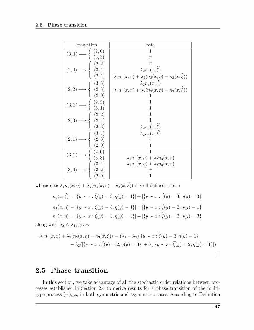
2.5. Phase transition
transition rate
p3, 1q ÝÑ"
p2, 0qp3, 3q
1r
p2, 0q ÝÑ
$
&
%
p2, 2qp3, 1qp2, 1q
r
λ2n3px, rξq
λ1n1px, ηq ` λ2pn3px, ηq ´ n3px, rξqq
p2, 2q ÝÑ
$
&
%
p3, 3qp2, 3qp2, 0q
λ2n3px, rξq
λ1n1px, ηq ` λ2pn3px, ηq ´ n3px, rξqq1
p3, 3q ÝÑ"
p2, 2qp3, 1q
11
p2, 3q ÝÑ
$
&
%
p2, 2qp2, 1qp3, 3q
11
λ2n3px, rξq
p2, 1q ÝÑ
$
&
%
p3, 1qp2, 3qp2, 0q
λ2n3px, rξqr1
p3, 2q ÝÑ"
p2, 0qp3, 3q
1λ1n1px, ηq ` λ2n3px, ηq
p3, 0q ÝÑ
$
&
%
p3, 1qp3, 2qp2, 0q
λ1n1px, ηq ` λ2n3px, ηqr1
whose rate λ1n1px, ηq ` λ2pn3px, ηq ´ n3px, rξqq is well defined : since
n3px, rξq “ |ty „ x : rξpyq “ 3, ηpyq “ 1u| ` |ty „ x : rξpyq “ 3, ηpyq “ 3u|
n1px, ηq “ |ty „ x : rξpyq “ 3, ηpyq “ 1u| ` |ty „ x : rξpyq “ 2, ηpyq “ 1u|
n3px, ηq “ |ty „ x : rξpyq “ 3, ηpyq “ 3u| ` |ty „ x : rξpyq “ 2, ηpyq “ 3u|along with λ2 ď λ1, gives
λ1n1px, ηq ` λ2pn3px, ηq ´ n3px, rξqq “ pλ1 ´ λ2q|ty „ x : rξpyq “ 3, ηpyq “ 1u|` λ2p|ty „ x : rξpyq “ 2, ηpyq “ 3u| ` λ1|ty „ x : rξpyq “ 2, ηpyq “ 1u|q
2.5 Phase transitionIn this section, we take advantage of all the stochastic order relations between pro-
cesses established in Section 2.4 to derive results for a phase transition of the multi-type process pηtqtě0, in both symmetric and asymmetric cases. According to Definition
47

Chapter 2. Phase transition on Zd
2.2.1, we assume the multitype process to have initial configuration η0 “ 1t0u and noteηt “ η
t0ut .
As announced in Section 2.2, we first deal with the cases where λ2 ă λ1 are bothsmaller or larger than λc.
Proof of Proposition 2.2.1. Let pξtqtě0 be a basic contact process with growth rate λ1and let pηtqtě0 be a symmetric multitype process with parameters pλ1, λ2, rq such thatη0 ď ξ0. By Proposition 2.4.5, pξtqtě0 is stochastically larger than pηtqtě0. Since λ1 ď λc,pξtqtě0 is subcritical, thus, the symmetric multitype process dies out.
The extinction of the asymmetric multitype process is a consequence of the extinctionof the symmetric process and Proposition 2.4.4.
Proof of Proposition 2.2.2. Let prξtqtě0 be a basic contact process with growth rate λ2 ont2, 3uZd and let pηtqtě0 be a symmetric multitype process with parameters pλ1, λ2, rq. ByProposition 2.4.6, pξtqtě0 is stochastically lower than pηtqtě0. Since λ2 ą λc, the processprξtqtě0 is supercritical and therefore, the symmetric multitype process survives.
We now turn to Theorems 2.2.1 and 2.2.2, for which we shall prove :
Theorem 2.5.1. Assume λ2 ă λc ă λ1 fixed. Let pηtqtě0 be the symmetric multitypeprocess. Then,(i) there exists r0 P p0,8q such that if r ă r0 then the process pηtqtě0 survives.(ii) there exists r1 P p0,8q such that if r ą r1 then the process pηtqtě0 dies out.
Theorem 2.5.2. Assume λc ă λ1 and λ2 ă λ1 fixed. Let pηtqtě0 be the asymmetricmultitype process. Then,(i) there exists s0 P p0,8q such that if r ă s0 then the process pηtqtě0 survives.(ii) there exists s1 P p0,8q such that if r ą s1 then the process pηtqtě0 dies out.
These results imply Theorems 2.2.1 and 2.2.2, that is, the existence of a uniquephase transition with a critical value rc (resp. sc) defined in (2.2.12). Indeed, relyingon Theorems 2.5.1 and 2.5.2, by monotonicity given by Corollary 2.4.2 one has r0 “ r1(resp. s0 “ s1).
We shall prove both theorems in Subsections 2.5.2 and 2.5.3. One concludes for thecritical case by proving Theorem 2.2.3 in Subsection 2.6.
Before that, subsection 2.5.1 deals with consequences of Theorems 2.5.1 and 2.5.2along with monotonicity results of Section 2.4.
2.5.1 Behaviour of the critical value with varying growth ratesSuppose the existence of the critical value rc guaranteed in virtue of Theorems 2.5.1
and 2.5.2, one investigates the behaviour of rc when growth rates λ1 and λ2 are moving.One manages to prove monotonicity between growth rates and the release rate, in thesense that, the more competitive the species is (i.e. the higher the parameter λ2 is) or
48
2.5. Phase transition
the fittest the species is (i.e. the higher the parameter λ1 is), the higher the release rateis (i.e. the higher the critical value rc is) :
Proposition 2.5.1. For j “ 1, 2, the function λj ÞÝÑ rcpλjq is non-increasing.
Proof. We consider j “ 2 as the case j “ 1 is similar. Let pηtqtě0 and pη1tqtě0 be twomultitype processes with respective parameters pλ1, λ2, rq and pλ1, λ
12, rq. By Theorems
2.5.1 and 2.5.2, existence and uniqueness of the critical values rc and r1c associated tothose processes are guaranteed. We now show that if λ2 ă λ12, then rc ď r1c.
By contradiction, suppose rc ą r1c. Let r be fixed be such that rc ą r ą r1c. Sinceλ2 ă λ12, by Corollary 2.4.1-(iii), if η0 “ η10 then ηt ď η1t a.s. By Theorem 2.2.3 andCorollary 2.4.1,
Prp@t ě 0, H 1t ‰ Hq ď Pr1cp@t ě 0, H 1
t ‰ Hq “ 0
But since r ă rc, the process pηtqtě0 survives : Prp@t ě 0, Ht ‰ Hq ą 0. This contradictsηt ď η1t a.s., hence rc ď r1c.
2.5.2 Subcritical caseThe following proof relies on a comparison of the multitype process with an oriented
percolation process on the even grid L. Then we show that for the associated open sites,percolation occurs thanks to results we presented in Section 2.2.3.
We follow arguments used by N. Konno, R. Schinazi and H. Tanemura [48] in thecase of a spatial epidemic model.
Proof of Theorem 2.5.1 (i). To simplify notations, choose d “ 1 but the proof remainsthe same for any d ě 2. Introduce the following space-time regions,
B “ p´4L, 4Lq ˆ r0, T s, Bm,n “ p2mLe1, nT q ` BI “ r´L,Ls, Im “ 2mLe1 ` I
for positive integers L, T to be chosen later, where pe1, ..., edq denotes the canonical basisof Rd. Notice they correspond to the boxes introduced in (2.2.20) with j0 “ 1, k0 “ 4.
Consider the process pηm,nt qtě0 restricted to the region Bm,n, that is, constructed fromthe graphical representation where only arrival times of the Poisson processes occurringwithin Bm,n are taken into account. Therefore, a birth on a site x P Bm,n from some sitey only occurs if y P Bm,n. By Proposition 2.4.2 and Remark 2.4.1, one has
ηm,nt ď ηtˇ
ˇ
Bm,n, (2.5.1)
for all t ą 0 if ηm,n0 “ η0ˇ
ˇ
Bm,n.
Let k “ t?Lu and define C “ r´k, ks. One declares pm,nq P L to be wet if for any
configuration at time nT such that there is a translate of C full with 1’s in Im with Im
49
Chapter 2. Phase transition on Zd
containing only 0’s and 1’s, the process restricted to Bm,n is such that at time pn` 1qTthere are a translate of C in Im´1 and a translate of C in Im`1, both full of 1’s, withIm´1 and Im`1 containing only 0’s and 1’s.
Let us show that the probability of a site pm,nq P L to be wet can be made arbitrarilyclose to 1 for L and T chosen sufficiently large. By translation invariance, it is enoughto deal with the case pm,nq “ p0, 0q.
Suppose I contains only 0’s and 1’s as well as the translate of C full of 1’s and setr “ 0 in B, that is, no more type-2 individuals arrive in the box B after time 0.
If type-2 individuals are present on the base p´4L,´LqYpL, 4Lqˆt0u, the probabilityof the event E they all die by time T 2 is at least
´
1´ expp´T 2q¯6L
which is larger than 1´ ε for T and L chosen large enough. On E, the process restrictedto the box B is now from time T 2 a supercritical contact process pξm,nt qtěT 2 withdistribution rPpξm,nt P ¨q. But we have to make sure that at time T 2, there are stillenough 1’s for ξm,nT 2 , for this we use the following result. Define τp`q “ inftt ą 0 :Ξr´`,`st
ˇ
ˇ
ˇ
r´`,`s“ Hu, the hitting time of the trap state 0 of the contact process starting
from r´`, `s and restricted to r´`, `s ˆ r0, T 2s. T. Mountford [62] proved that
rPpτp`q ď expp`qq ď expp´`q for ` large enough (2.5.2)
Partition C into M “ t?ku boxes, each of them being a translate of r0,M s. From each
of these M boxes, say box j ďM run a supercritical contact process denoted by pζjt qtě0which coincides with the restriction of ξm,nt to this box. Therefore for each x in this boxJ , as in 2.5.1, ζjT 2pxq ď ξm,nT 2 pxq for all x P Bm,n. Then for the union of these j boxes(j ď M), the probability there is at least M 1’s within C by time T 2 is after (2.5.2),with T such that exppMq ď T 2, at least
rPpτpMq ě T 2qM ě rPpτpMq ě exppMqqM ě p1´ expp´MqqM (2.5.3)
which can be made larger than 1´ ε, for M , i.e. L, large enough.
A result of R. Durrett and R. Schinazi [25] shows that for a contact process pξtqtě0,for any A Ă Z, except for a set with exponentially small probability, either ΞA
t “ H, orξAt “ ξZt on a linearly time growing set r´αt, αts : there exists α ą 0 such that for allA Ă Z, there exist positive constants C, γ such that
rPpΞAt ‰ H, ξ
At pxq ‰ ξZt pxqq ď C expp´γtq (2.5.4)
where x P A` αt.We applied this result with A Ă C which correspond to the numbers of 1’s in the
box. We just proved that |A| ą |M |. Moreover according to Proposition 2.6.1, one can
50

2.5. Phase transition
choose k, and so L, large enough so that this supercritical contact process ξAt startingfrom at least M 1’s survives at time T 2 with probability close to 1, hence ξAt ‰ H
and (2.5.4) is valid. In this situation, taking T 2 “ 9Lp2αq with L large enough, theprocess pξm,nt qtě0 starting from at least M 1’s in r´L,Ls at time T 2 will be coupledwith a process ξZt on r´3L, 3Ls with probability at least 1 ´ ε at time T . Hence, since3L ą αT 2 ą 2L, by time T the contact process ξAt started inside r´L,Ls has notreached the boundary of r´4L, 4Ls with probability close to 1. Then, the process ξm,nt
and the contact process ξAt are the same with probability 1´ ε in r´4L, 4Ls ; this way,the coupling of pξm,nt qtě0 with pξZt qtě0 works so far with probability 1 ´ ε if L is largeenough.
Since the distribution of pξZt qtě0 is stochastically larger than the upper invariantmeasure ν (see Chapter 1 Section 1.1.2) of the contact process, on the survival event, νloads a positive density ρ of 1’s. Since ν is ergodic (see Chapter 1 Section 1.1.2),
limLÑ8
12L` 1
´Lÿ
x“´3L1tηpxq “ 1u “ ρ ν -a.e.
In other words, as soon as L is large enough, under ν there are at least k 1’s in anyinterval of length 2L`1 with ν-probability at least 1´ε. Since we obtained that pξm,nt qtě0is coupled to pξZt qtě0 by time T with probability at least 1´2ε, for L large enough, thereare at least k 1’s in r´3L,´Ls at time T with probability at least 1´ 2ε and similarly,at least k 1’s at time t in rL, 3Ls with probability at least 1 ´ 2ε as well for pξm,nt qtě0.Consequently,
rPpp0, 0q wetq ą 1´ 4ε, if r “ 0. (2.5.5)
Since B is a finite space-time region, for fixed L, T , one can pick r0 ą 0 small enoughso that the arrival times of a rate r Poisson process, such that r ă r0, in B occurs withprobability at most ε. Let AL,T prq be the first arrival time of a rate r Poisson processin r´2L, 2Ls ˆ r0, T s.
Prpp0, 0q wetq ě Prpp0, 0q wet, AL,T prq ą T qPrpAL,T prq ą T q
ě p1´ 4εqe´rp4L`1qT
ě 1´ 6ε
as soon as the exponent of the exponential is close to 0, i.e. by choosing r small enough.See Figure 2.2 for an illustration.Now construct a percolation process by defining the good event Gm,n “ tpm,nq wetu.
Notice that Gm,n depends only on the process constructed in Bm,n, and for pa, bq PL, events Gm,n and Ga,b are independent if pm,nq and pa, bq are not neighbours. Theevents tGm,n, pm,nq P Lu are thus 1-dependent. By the comparison theorem 2.2.7, theprocess pηm,nt qtě0 restricted to regions Bm,n is stochastically larger than a 1-dependentpercolation process with probability 1´ ε.
By Lemma 2.2.5, one can choose ε small enough so that percolation occurs in the1-dependent percolation process with density 1´ ε.
51
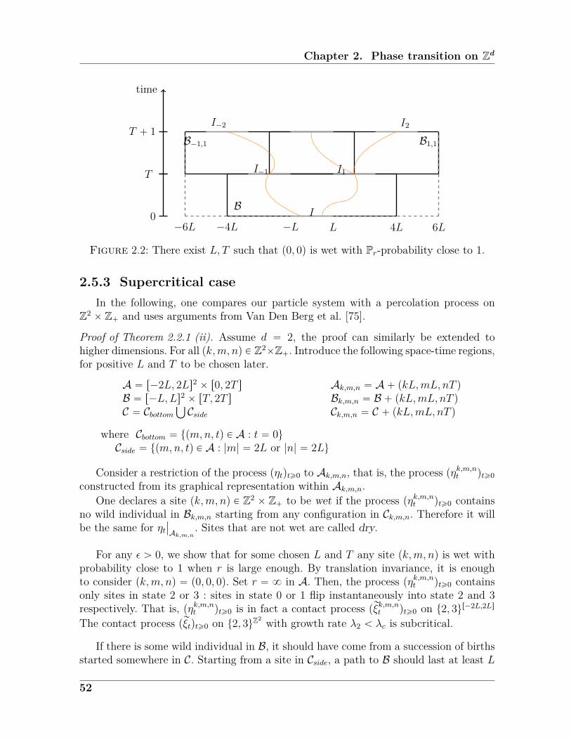
Chapter 2. Phase transition on Zd
time
0
T
T ` 1
I
I1I´1
I2I´2
L´L 4L´4L´6L 6L
B
B´1,1 B1,1
Figure 2.2: There exist L, T such that p0, 0q is wet with Pr-probability close to 1.
2.5.3 Supercritical caseIn the following, one compares our particle system with a percolation process on
Z2 ˆ Z` and uses arguments from Van Den Berg et al. [75].
Proof of Theorem 2.2.1 (ii). Assume d “ 2, the proof can similarly be extended tohigher dimensions. For all pk,m, nq P Z2ˆZ`. Introduce the following space-time regions,for positive L and T to be chosen later.
A “ r´2L, 2Ls2 ˆ r0, 2T s Ak,m,n “ A` pkL,mL, nT qB “ r´L,Ls2 ˆ rT, 2T s Bk,m,n “ B ` pkL,mL, nT qC “ Cbottom
Ť
Cside Ck,m,n “ C ` pkL,mL, nT q
where Cbottom “ tpm,n, tq P A : t “ 0uCside “ tpm,n, tq P A : |m| “ 2L or |n| “ 2Lu
Consider a restriction of the process pηtqtě0 to Ak,m,n, that is, the process pηk,m,nt qtě0constructed from its graphical representation within Ak,m,n.
One declares a site pk,m, nq P Z2 ˆ Z` to be wet if the process pηk,m,nt qtě0 containsno wild individual in Bk,m,n starting from any configuration in Ck,m,n. Therefore it willbe the same for ηt
ˇ
ˇ
Ak,m,n. Sites that are not wet are called dry.
For any ε ą 0, we show that for some chosen L and T any site pk,m, nq is wet withprobability close to 1 when r is large enough. By translation invariance, it is enoughto consider pk,m, nq “ p0, 0, 0q. Set r “ 8 in A. Then, the process pηk,m,nt qtě0 containsonly sites in state 2 or 3 : sites in state 0 or 1 flip instantaneously into state 2 and 3respectively. That is, pηk,m,nt qtě0 is in fact a contact process prξk,m,nt qtě0 on t2, 3ur´2L,2Ls
The contact process prξtqtě0 on t2, 3uZ2 with growth rate λ2 ă λc is subcritical.
If there is some wild individual in B, it should have come from a succession of birthsstarted somewhere in C. Starting from a site in Cside, a path to B should last at least L
52

2.5. Phase transition
sites ; according to C. Bezuidenhout and G. Grimmett [6] there exists such a path withprobability at most C expp´γLq, for some positive constants C, γ. Hence,
PpDpx, tq P Cside ˆ r0, 2T s : px, tq Ñ Bq ď 4`
2T ˆ p4L` 1q˘
C expp´γLq
Similarly, starting from the base Cbottom, there exists a path lasting at least T sites withprobability
PpDpx, tq P Cbottom : px, tq Ñ Bq ď p4L` 1q2C expp´γT q
Consequently if r “ 8,
Ppp0, 0, 0q wet q ě 1´ 4`
2Lˆ p4L` 1q˘
Ce´γL ´ p4L` 1q2Ce´γT ě 1´ ε2,
for L and T large enough.Since A is a finite space-time region, one can pick r large enough so that with
probability at least 1 ´ ε2, an exponential clock with parameters r rings before anyother so that there are no type-1 individuals in A with probability close to 1 :
Prpk,m, nq wetq ě 1´ ε
for r large enough.
To construct a percolation process on Z2 ˆ Z`, one puts an oriented arrow frompk,m, nq to px, y, zq if n ď z and if Ak,m,nXAx,y,z ‰ H. The eventGk,m,n “ tpk,m, nq wetudepends only on the graphical construction of the process within Ak,m,n, furthermore,for all pk,m, nq P Z2 ˆ Z`, there is a finite number of sites px, y, zq P Z2 ˆ Z` suchthat Ak,m,nXAx,y,z ‰ H. The percolation process is dependent but of finite range. Theexistence of a path of wild individuals for the particle system corresponds to a path ofdry sites for the percolation and we proved that dry paths are unlikely.
Let us show that for all sites, there exists a finite random time after which there isno more wild individuals remaining. Follow the construction given by van den Berg etal. [75].
Since the percolation is of finite range, there exists some positive constant Cpdqsuch that if the distance between two sites is at least Cpdq then they are mutually in-dependent. For any x P Z2, define Tx “ suptt : ηtpxq P t1, 3uu the last time where xis occupied by a wild individual. By translation invariance, deal with the case x “ p0, 0q.
Let K ą 0, suppose T0 ą TK, there exists some m P Z` such that p0, 0,mq is theend of a dry path starting from px, y, 0q with px, yq P Z2. The number of paths of length` is at most δ`. Moreover, a self-avoiding path of length ` contains at most ν` mutuallyindependent sites (i.e. whose in-between distance is at least Cpdq), ν ą 0. Hence,
PpT0 ą TKq ďÿ
měK´1
ÿ
`ěm
δ``
1´ Pppk,m, nq wet q˘ν` (2.5.6)
53

Chapter 2. Phase transition on Zd
For r large enough,the right-hand side tends to 0 when K goes to infinity. That is,T0 is almost surely finite and the region A ˆ rTx,8q is wild individuals-free. For thepercolation process, this means there is an infinite path of wet sites, hence the processpηtqtě0 dies out.
To sum up, we just showed there exist r0 and r1 such that r0 ď rc ď r1, for r ď r0the process survives and for r ě r1 the process dies out.
This proves the existence of a phase transition for the symmetric multitype process.The proof of Theorem 2.5.1-(i) only uses that contact process with growth rate λ1 issupercritical, this is also true to show the existence of s0 in Theorem 2.5.2-(i). By Pro-position 2.4.4, the asymmetric multitype process dies out as soon as the symmetric onedoes, existence of s1 in Theorem 2.5.2-(ii) is then immediately guaranteed by Theorem2.5.1-(ii). Though, one can remark that conditions of Theorem 2.5.2 are milder : onecan actually show the existence of s1 in a neater way. Indeed, retrieving briefly the proofof the supercritical case : assume λ2 ą λc : with the lack of the transition "2 Ñ 3" inthe asymmetric case and choosing first r “ 8, one notices for the subcritical contactprocess on t2, 3uZ2 , there are no possible paths of wild individuals created by the 3’sfrom the boundary Ck,m,n up to extinction, but this occurs exponentially fast (see C.Bezuidenhout and G. Grimmett [6]).
2.6 The critical process dies outIn this section, we prove Theorem 2.2.3 : the critical multi-type contact process dies
out. i.e. PrcpHt ‰ H @t ě 0q “ 0. Recall pηtqtě0 stands for the multitype process,starting from the initial configuration η0 “ 1t0u.
One follows closely the arguments used by C. Bezuidenhout and G. Grimmett [5],well-exposed by T.M. Liggett [57, Chapter I.2]. We shall use both presentations.
The dynamic renormalization construction sees the time-evolution of the process ina suitable chosen scaling : space-time is divided into finite space-time regions. So far,this looks heavily like the comparison with oriented percolation we defined in Section2.2. But here, instead of fixing every region initially, the idea is rather to determinetheir positions according to the past random position in the construction, along withthe evolution of the process.
Let us sketch the contents of the proof.
Outline. The first step consists to observe that if the process survives in an arbitrarylarge box, then it reaches its boundaries densely. We shall estimate these densities ateach side of a space-time region.
This way, one can repeat this step by running the process in an other adjacent boxstarting from the boundary of the previous one and so on, conditionally on the factthat the starting configuration is dense enough. This is the second step. In connection
54

2.6. The critical process dies out
with the proofs of Theorems 2.5.2 and 2.5.1 where we looked after having translationsof occupied finite intervals at a given fixed time, here we look after having translationsof the densities in some space-time slab.
Now, knowing that at each stage, one can construct overall a path of adjacent boxeswherein the process survives and reaches the boundaries densely, it remains to comparethe process with an oriented percolation process to extend the arguments to infinitespace and time. As before, compare a space-time box to a vertex in the even latticeof an oriented percolation so that one declare a vertex to be wet if some good eventassociated to the box is a success. Conclude thanks to results about percolation theory,recalled in Section 2.2.
2.6.1 Local characterization of the survival eventWe saw under specific hypothesis on r, the multi-type contact process survives with
positive probability. Supposing it survives, one exhibits here several properties of growthsatisfied by the process restricted to an arbitrary large box. Such results have beenproved for the basic contact process by C. Bezuidenhout and G. Grimmett [5], thanksto techniques of dynamic renormalization introduced by G. Grimmett et al. [35, 2].
First note the arguments developed by [5] rely on elementary properties of the contactprocess making them robust. They are also valid for the multitype process because thelatter satisfies the following properties we have exhibited in previous sections :(A) contact process-like dynamics : one retrieves the growth rate λ1 or λ2 of a basic
contact process, even if it is determined randomly. We will make use of the moresuitable one depending on the situation.
(B) attractiveness, by Section 2.4.(C) correlation inequalities : using correlation inequalities such as FKG inequality
1.2.1.Note that the use of (C) is possible because we shall work in finite space-time regionsin the following. Such techniques have been several times exploited to study criticalprocesses, including works by O. Garet and R. Marchand [30] for a branching randomwalk, J. Steif and M. Warfheimer [74] for a randomly evolving contact process.
Covering of an arbitrary large boxProposition 2.6.1. Suppose pηtqtě0 survives, then
limnÑ8
PrpH r´n,nsd
t ‰ H @tq “ 1. (2.6.1)
Proof. By attractiveness of the process pηtqtě0 (see Corollary 2.4.1), if A,B Ă Zd aresuch that A Ă B then
PrpHBt ‰ H @t ě 0q ě PrpHA
t ‰ H @t ě 0q ą 0.
Since we assumed pηtqtě0 survives, limAÒZd
PrpHAt ‰ H @tq “ 1.
55

Chapter 2. Phase transition on Zd
Consider, for L ě 1 and A Ă Zd, the truncated process pLηAt qtě0 defined as theprocess pηtqtě0 starting from the initial configuration η0 “ 1A constructed from the gra-phical representation in p´L,Lqdˆr0, ts. Denote by pLHA
t qtě0 the associated set of sitesoccupied by wild individuals at time t.
The next two results show that sites occupied by wild individuals are dense in someorthant of the top of a box of size p´L,Lqd ˆ r0, T s. Following estimates are analogousto the ones we did previously in the proof of Theorem 2.5.1, Subsection 2.5.2, one provesby (A) and (B) of pηtqtě0 that
Proposition 2.6.2. Let n ě 1 and N ě 1, then
limtÑ8
limLÑ8
Prp|LH r´n,nsd
t | ě Nq “ PrpH r´n,nsd
t ‰ H @t ą 0q (2.6.2)
Proof. Since H r´n,nsd
t “Ť
Lě0LHt
r´n,nsd , for any fixed t, by monotonicity (see Corollary
2.4.1),limLÑ8
Prp|LH r´n,nsd
t | ě Nq “ Prp|H r´n,nsd
t | ě Nq. (2.6.3)
It is thus enough to show
limtÑ8
Prp|H r´n,nsd
t | ě Nq “ PrpH r´n,nsd
t ‰ H @t ą 0q.
On the other hand, for an initial configuration constituted of p2n ` 1qd wild indivi-duals, the probability that these p2n ` 1qd wild individuals die before any birth is atleast the probability the maximum of p2n ` 1qd independent exponential clocks withparameter 1 is smaller than the minimum of 2dp2n`1qd independent exponential clockswith parameter λ2, since λ2 ă λ1. That is,
PrpH r´n,nsd
t “ H for some t|Fsq ě
” 11` 2dλ2|H
r´n,nsds |
ı|Hr´n,nsd
s |
where Ft “ σpηr´n,nsd
s , s ď tq is the sigma-algebra generated by the graphical represen-tation of the process pηr´n,ns
d
t qtě0 until time t.
Define F8 “Ş
sě0σpFsq, since tH r´n,nsd
t “ H for some tu is a tail-event with respect
to F8, and 1tH r´n,nsd
t “ H for some tu is Pr-integrable, by the martingale convergencetheorem, Lévy’s zero–one law gives
limsÑ8
Er1tH r´n,nsd
t “ H for some tu|Fss “ 1tH r´n,nsd
t “ H for some tu a.s.
Therefore,limtÑ8
|Hr´n,nsd
t | “ 8 a.s. ontH r´n,nsd
s ‰ H @s ě 0u, (2.6.4)
56
2.6. The critical process dies out
and by (2.6.3) and (2.6.4),
limtÑ8
Prp|H r´n,nsd
t | ě N,H r´n,nsd
s ‰ H @s ą 0q “ PrpH r´n,nsd
t ‰ H @t ě 0q
Using FKG inequality (C), one shows that the truncated process contains a largenumber of occupied sites in some orthant of Rd. For this, define the 2d orthants of Rd :for u “ pu1, ..., udq P t´,`u
d,
Ou :“ tx “ px1, ..., xdq P Rd : sgnpxiq “ ui, 1 ď i ď du.
By symmetry and reflexion with respect to the time axis, without loss of generality onecan only consider the positive orthant i.e. when sgnpxiq “ ` for any 1 ď i ď d that wedenote by
O` :“ tx “ px1, ..., xdq P Rd : sgnpxiq “ `, 1 ď i ď du.
Proposition 2.6.3. Fix n ě 1, N ě 1 and L ě n,
Prp|LH r´n,nsd
t XO`| ď Nq2
d
ď Prp|LH r´n,nsd
t | ď 2dNq (2.6.5)
Proof. Along this proof, make us of (A) since we retrieve a basic contact process, sothat one use the suitable growth rate depending on the ongoing estimate. First, remarkthat
|LHr´n,nsd
t | “ÿ
uPt´,`ud
|LHr´n,nsd
t XOu|.
All t|LH r´n,nsd
t XOu|, u P t´,`udu are independent, identically distributed and positivelycorrelated by monotonicity : increasing with respect to growth rate Poisson processand decreasing with respect to death and release rates Poisson processes, using (B) byCorollary 2.4.1. So that by FKG inequality, for all u P t´,`ud :
˜
Prˆ
|LHr´n,nsd
t XO`| ď N
˙
¸2d
“ź
uPt´,`ud
Prˆ
|LHr´n,nsd
t XOu| ď N
˙
ď Prˆ
č
uPt´,`ud
´
|LHr´n,nsd
t XOu| ď N
¯
˙
ď Prˆ
ÿ
uPt´,`ud
|LHtr´n,nsd
XOu| ď 2dN
˙
ď Prˆ
|LHr´n,nsd
t | ď 2dN˙
.
57

Chapter 2. Phase transition on Zd
By Propositions 2.6.2 and 2.6.3, for any ε ą 0, there exist L and t sufficiently largesuch that
Prp|LH r´n,nsd
t XOud | ě Nq ą 1´ ε2d .
Before going on space-time conditions, consider the lateral parts of the box p´L,Lqd ˆr0, T s. For this, define
SpL, T q :“ tpx, tq P Zd ˆ r0, T s : |x|8 “ Lu,
the boundary of the box p´L,Lqd ˆ r0, T s and define LH :“Ť
tě0 LHt ˆ ttu. For anyA Ă Zd, let NA
S pL, T q be the cardinal of the set
tpx, tq P SpL, T q X LHA : px1, s1q, px2, s2q P SpL, T q X LH
A such that |s1 ´ s2| ě 1u.
Proposition 2.6.4. Let pLjqjě1 and pTjqjě1 be two increasing sequences of integers.For any integers M,N, n,
limjÑ8
PrpN r´n,nsdpLj, Tjq ďMqPrp|LjH
r´n,nsd
Tjď Nq
ď PrpH r´n,nsd
t “ H for some tq (2.6.6)
Proof. Let FL,T be the sigma-algebra generated by the Poisson processes of the graphicalrepresentation of the process pηtqtě0 in p´L,Lqdˆr0, T s. For each site of LH r´n,nsd
T , thereis a probability at least
p1` 2dλ1q´1
that a site does not give birth (exponential clock with parameter 1 associated to adeath ringing before an exponential clock associated to a birth). By independance ofthe Poisson processes, the probability that none of x P LHT
r´n,nsd contributes to thesurvival of the process is at least
´
p1` 2dλ1q´1¯|LH
r´n,nsd
T |
.
For the lateral parts of p´L,Lqdˆr0, T s, consider now a segment txuˆ r0, T s, where|x|8 “ L, and define px, t1q, ..., px, tjq a maximal set of 1-sparse time-wise points of thesegment in SpL, T q X r´n, nsd i.e. such that for any points px, tiq and px, tjq in this set,then |ti ´ tj| ě 1. Fix j ě 1, the segment
I “jď
k“1txu ˆ ptk ´ 1, tk ` 1q.
is of Lebesgue-measure at least 2j. There is no arrow in the graphical representationstarting from a site of I with probability at least
´
e´2jλ1¯2d
.
58

2.6. The critical process dies out
For each interval of length y in txu ˆ r0, T qzI, the event no arrow occurs or an arrowoccuring is preceded by a death or a slowdown symbol, occurs with probability at least
11` 2dλ1
.
Consequently, no points of txu ˆ r0, T s contributes to the survival of the process withprobability at least
e´4djλ1´ 1
2dλ1
¯j
.
Counting the contribution of all such x,
PrpH r´n,nsd
t “ H for some t|FL,T q ě e´4dkλ1´ 1
1` 2dλ1
¯k
a.s. (2.6.7)
on the event tN r´n,nsd
S pL, T q ` |LHr´n,nsd
T | ď ku.
Then, consider two increasing sequences pTjqjě0, pLjqjě0 and integers M,N , define
Hj :“ tN r´n,nsd
S pLj, Tjq ` |LHr´n,nsd
Tj| ďM `Nu.
If G “ tH r´n,nsd
t “ H for some tu, by the martingale convergence theorem,
limjÑ8
PrpG|FLj ,Tjq “ 1G a.s.
From (2.6.7), for all j ě 0, on Hj, PrpG|FLj ,Tjq is bounded below by some positive formand thus, lim
jÑ8Hj Ă G. That is,
limjÑ8
PrpHjq ď Prp limjÑ8
Hjq ď PrpGq.
Furthermore, by FKG inequality (C),
PrpN r´n,nsdpL, T q ` |LH
r´n,nsd
T | ďM `Nq
ě PrpN r´n,nsd
S pL, T q ďM, |LHr´n,nsd
T | ď Nq
ě PrpN r´n,nsd
S pL, T q ďMqPrp|LH r´n,nsd
T | ď Nq
this concludes the proof.
As for the top of the box (Proposition 2.6.3), one can control the number of occupiedsites on the lateral parts of the box p´L,Lqdˆr0, T s. For this, introduce for i “ 1, ..., d2dand u P t´,`ud, the 2d sides of the box by
Sui pL, T q :“ tpx, tq P Zd ˆ r0, T s, xi “ uiL, sgnpxjq “ uj pj ‰ iqu
59

Chapter 2. Phase transition on Zd
and NAi pL, T q the cardinal of the set
tpx, tq P Sui pL, T q X LHA : px1, s1q, px2, s2q P SpL, T q X LH
A such that |s1 ´ s2| ě 1u.
By symmetry and reflexion with respect to the time axis, it is enough to look only atthe positive coordinates :
S`pL, T q :“ Sp`,...,`q1 pL, T q “ tpx, tq P Zd ˆ r0, T s, x1 “ L, xj ě 0 pj ‰ iqu.
Proposition 2.6.5. For any integers M,L, T and n ă L,
PrpN r´n,nsd
` pL, T q ďMqd2dď PrpN r´n,nsd
S pL, T q ďMd2dq
Proof. Remark that tN r´n,nsd
i pL, T q, 1 ď i ď d2du are identically distributed and positi-vely correlated. Moreover,
Nr´n,nsd
S pL, T q ďd2dÿ
i“1Nr´n,nsd
i pL, T q.
So, as for Proposition 2.6.4, one has by FKG inequality,
PrpN r´n,nsd
` pL, T q ďMqd2d“
d2dź
i“1PrpN r´n,nsd
i pL, T q ďMq
ď Prpd2dč
i“1Nr´n,nsd
i pL, T q ďMq
ď PrpN r´n,nsd
S pL, T q ďMd2dq.
Space-time conditions
Proposition 2.6.6. Suppose pηtqtě0 survives. For any ε6 ą 0, there exist integersn, L, T ą 0 such that
Prˆ
L`2nHr´n,nsd
T`1 Ą x` r´n, nsd for some x P r0, Lqd˙
ą 1´ ε6 (2.6.8)
and
Prˆ
L`2nHr´n,nsd
t`1 Ą x` r´n, nsd for some
px, tq P tL` nu ˆ r0, Lqd´1ˆ r0, T q
˙
ą 1´ ε6 (2.6.9)
60

2.6. The critical process dies out
Proof. Fix δ ą 0. By Proposition 2.6.1, choose n such that
PrpH r´n,nsd
t ‰ H @t ě 0q ą 1´ δ2
Let N be sufficiently large so that N points in Zd contain at least N 1 points which arep2n` 1q-sparse in L8-distance. Choose now N 1 sufficiently large so that
”
1´ Prpn`1Ht0ut Ą r´n, nsdq
ıN 1
ď δ.
Likewise, choose M sufficiently large so that M points in Zd contain at least M 1
points which are p2n` 1q-sparse. Choose now M 1 sufficiently large so that”
1´ Pr`
n`1Ht0u1 Ą r0, 2ns ˆ r´n, nsd´1˘
ıM 1
ď δ.
Fix n, L,N , the map t ÞÑ Prp|LH r´n,nsd
t | ě 2dNq is continuous and limnÑ8
Prp|LH r´n,nsd
t | ą
2dNq “ 0, by Proposition 2.6.2, there exist two increasing sequences Lj Ò 8 and Tj Ò 8such that for all j ě 1,
Prp|LjHr´n,nsd
Tj| ą 2dNq “ 1´ δ.
Using Proposition 2.6.4, there exists some j0 for which,
PrpN r´n,nsd
S pLj0 , Tj0q ąMd2dq ą 1´ δ.
Considering L “ Lj0 and T “ Tj0 , applying Propositions 2.6.3 and 2.6.5, one has
Prp|LH r´n,nsd
T X r0, Lqd| ą 2dNq ě 1´ δ12d
andPrpN r´n,nsd
S pL, T q ąMd2dq ą 1´ δ1d2d .
In other words, because the Poisson processes used in the graphical representation areindependent in different space-time regions,
Prˆ
L`2nHr´n,nsd
T`1 Ą x` r´n, nsd for some x P r0, Lqd˙
ě p1´ δ1d2dqp1´ δq
and
Prˆ
L`2nHr´n,nsd
T`1 Ą x` r´n, nsd for some
px, tq P tL` nu ˆ r0, Lqd´1ˆ r0, T q
˙
ě p1´ δ12dqp1´ δq.
Conclude by choosing δ such that p1´δ12dqp1´δq ě 1´ε and p1´δ1d2dqp1´δq ě 1´ε.
61

Chapter 2. Phase transition on Zd
Proposition 2.6.7. Suppose (2.6.8)-(2.6.9) are satisfied. Then, for any ε7 “ ε7pε6q ą 0,there exist n, L, T such that
Pr`
2L`3nHr´n,nsd
t Ą x` r´n, nsd for somepx, tq P rL` n, 2L` ns ˆ r0, 2Lqd´1
ˆ rT, 2T s˘
ą 1´ ε7. (2.6.10)
Proof. For any ε7 ą 0, choose n, L and T as in (2.6.8)-(2.6.9), by Proposition (2.6.6).With (2.6.9), with Pr´probability at least 1´ε6, there exists px, tq P tL`nuˆr0, Lqd´1ˆ
r0, T q such that L`2nHr´n,nsd
t`1 Ą x` r´n, nsd.
By the Markov property and (2.6.8), starting from T`1, with Pr´probability at least1´ε6, there exists some y such that y´x P r0, Lqd satisfying L`2nH
r´n,nsd
T`1 Ą y`r´n, nsd.Consequently,
Pr`
2L`3nHr´n,nsd
t Ą x` r´n, nsd for somepx, tq P rL` n, 2L` ns ˆ r0, 2Lqd´1
ˆ rT ` 1, 2pT ` 1qs˘
ě p1´ ε6qd.
The next result links the previous estimates with a percolation process.
Block constructions The following two constructions rely on the geometry of theboxes only, proofs are similar to the ones of [5, Lemma 18] and [5, Lemma 19] respecti-vely. They allow us to position the successive boxes adjacently and well centred.
Proposition 2.6.8. Suppose pηtqtě0 survives. For any ε8 “ ε8pε7q ą 0 and fix k P N,there exist integers n, a, b such that n ă a for which : for all px, sq P r´a, asdˆr0, bs, withPr´probability at least 1´ ε8, there exists a translate py, tq ` r´n, nsd ˆ t0u satisfying :
i. py, tq P ra, 3as ˆ r´a, asd´1 ˆ r5b, 6bs.ii. From px, sq` r´n, nsdˆt0u, there exist active paths reaching any points of py, tq`r´n, nsd ˆ t0u lying within the region
r´5a, 5asd ˆ r0, 6bs.
The idea is to repeat sufficiently enough the Proposition 2.6.7 in order to translatethe center px, sq of a box to the center py, tq of another box, so that if the first box isoccupied, then the second one is as well and so on [see Figure 2.3].
Proof. Choose n, L, T as in Proposition 2.6.7 . Define a “ 2L ` n and b “ 2T . Onecan thus construct boxes as following : noting one needs to recentre within the boxpy, tq P ra, 3as ˆ r´a, asd´1 ˆ r5b, 6bs :(1) for 2 ď i ď d, for some current centre pz, rq such that zi ě 0 or zi ă 0, it suffices
to move it in the opposite direction. Since a ě 2L, the ith coordinate does notleave out of r´a, as.
62

2.6. The critical process dies out
(2) Move the spatial coordinate to reach ra, 3as. Since it always moves by at least2L` n and 2L` n ě 2a, it reaches ra, 3as in at most four steps.
(3) Move the time coordinate to reach 5b. As it moves between T and 2T , it reaches5b after four to ten steps. As b “ 2T , it does not overcross 6b by 10 steps.
As each step depend only of Poisson processes within the region r´5a, 5asd by disjointtime intervals, by Proposition 2.6.7, this construction succeeds with probability at leastp1´ ε7q10 “: 1´ ε8.
Iterating k times the previous result, one obtains (see Figure 2.3) :
Proposition 2.6.9. Suppose pηtqtě0 survives. For any ε9 “ ε9pε8q ą 0 and k P N fixed,there exist δ ą 0, and integers n, a, b such that n ă a for which : For all px, sq P r´a, asdˆr0, bs, with Pr´probability at least p1´ε9qk, there exists a translated py, tq`r´n, nsdˆt0usuch that :
i. py, tq P p2ka` r´a, asq ˆ r´a, asd´1 ˆ p5kb` r0, bsq.ii. From px, sq ` r´n, nsdˆ t0u, there exist active paths reaching any point of py, tq `r´n, nsd ˆ t0u lying within the region
R “
k´1ď
j“0p2ja` r´5a, 5asq ˆ r´5a, 5asd´1
ˆ p5jb` r0, 6bsq.
Comparison with oriented percolation For p, q P Z such that q ě 0 and p ` q iseven, define
vp,q :“ r´a, asd ˆ r0, bs ` pp2kaed ˆ q5kbqand
S “ď
qě0 p`q even
´
T ` pp2kaed ˆ q5kbq¯
,
where T “ r´a, asd´1 ˆ!
pxd, tq P Z ˆ R` : 0 ď t ď p5k ` 1qb, ´5a ˘ atb ď xd ď
5a˘atb)
. Here, S is a cross shaped nesting of successive boxes (as in Figure 2.3) usingreflections and symmetries. Similarly to [5, Lemma 21], one has
Theorem 2.6.1. If pηtqtě0 survives, there exist integers n, a such that
Prpηr´n,nsd
t survives in Zˆ r´5a, 5asd´1ˆ r0,8qq ą 0
Proof. Adapting the proof of [5, Lemma 21], fix δ ą 0 and ε ą 0 such that 1 ´ ε ą1 ´ δ. Choose n, a, b as in Proposition 2.6.9. Construct random variables tZnpiq “pInpiq, Pnpiqq : n ě 0, i ě 0u, where Inpiq P t0, 1u and Pnpiq P Zd ˆ r0,8q such thatPnpiq is undefined if Inpiq “ 0. Fix Z0p0q “ p1, 0q.
For defined random variables tZnpiq : n ď N, i ě 0u, construct recursively ZN`1piq “pIN`1piq, PN`1piqq as follows.
63
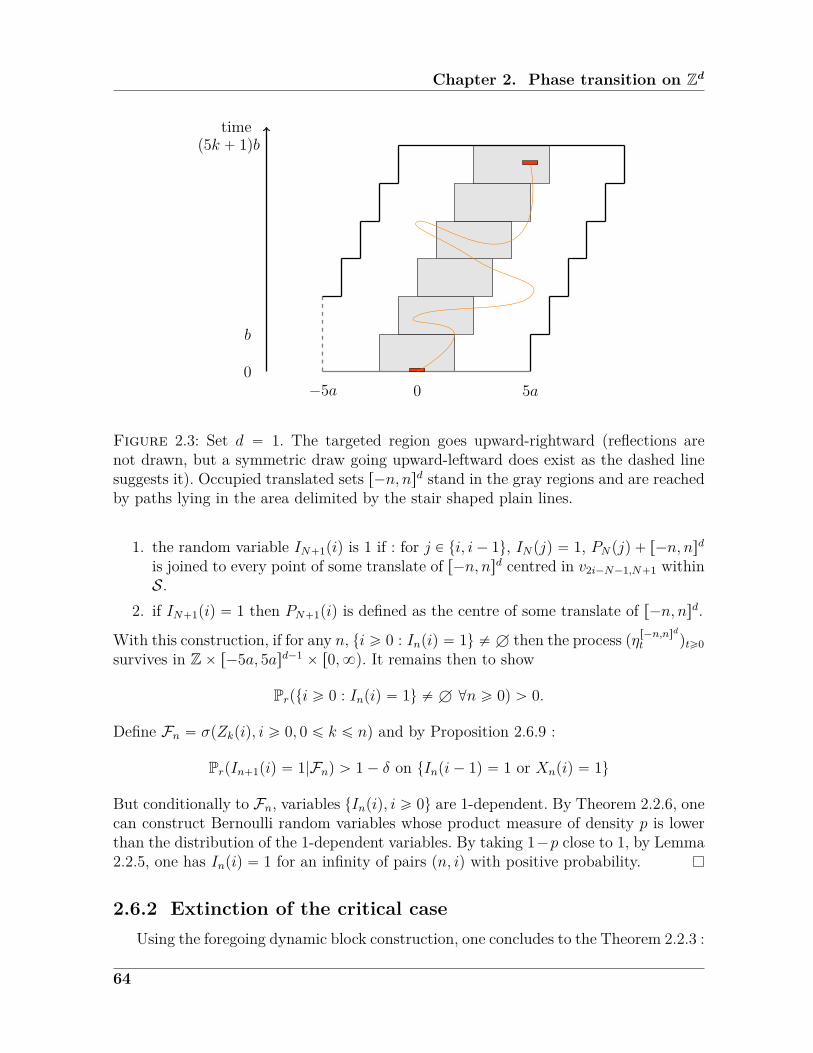
Chapter 2. Phase transition on Zd
0
b
p5k ` 1qbtime
0´5a 5a
Figure 2.3: Set d “ 1. The targeted region goes upward-rightward (reflections arenot drawn, but a symmetric draw going upward-leftward does exist as the dashed linesuggests it). Occupied translated sets r´n, nsd stand in the gray regions and are reachedby paths lying in the area delimited by the stair shaped plain lines.
1. the random variable IN`1piq is 1 if : for j P ti, i´ 1u, INpjq “ 1, PNpjq ` r´n, nsdis joined to every point of some translate of r´n, nsd centred in v2i´N´1,N`1 withinS.
2. if IN`1piq “ 1 then PN`1piq is defined as the centre of some translate of r´n, nsd.
With this construction, if for any n, ti ě 0 : Inpiq “ 1u ‰ H then the process pηr´n,nsd
t qtě0survives in Zˆ r´5a, 5asd´1 ˆ r0,8q. It remains then to show
Prpti ě 0 : Inpiq “ 1u ‰ H @n ě 0q ą 0.
Define Fn “ σpZkpiq, i ě 0, 0 ď k ď nq and by Proposition 2.6.9 :
PrpIn`1piq “ 1|Fnq ą 1´ δ on tInpi´ 1q “ 1 or Xnpiq “ 1u
But conditionally to Fn, variables tInpiq, i ě 0u are 1-dependent. By Theorem 2.2.6, onecan construct Bernoulli random variables whose product measure of density p is lowerthan the distribution of the 1-dependent variables. By taking 1´p close to 1, by Lemma2.2.5, one has Inpiq “ 1 for an infinity of pairs pn, iq with positive probability.
2.6.2 Extinction of the critical caseUsing the foregoing dynamic block construction, one concludes to the Theorem 2.2.3 :
64

2.7. The mean-field model
Proof of Theorem 2.2.3. Let r ą 0 be such that the process pηtqtě0 survives. In the blockconstructions established in Propositions 2.6.8 and 2.6.9, each event depends only onthe graphical representation of the process in each box p2ja`r´5a, 5asqˆr´5a, 5asd´1ˆ
p5jb ` r0, 6bsq, for j ě 0. Then, Propositions 2.6.8 and 2.6.9 are preserved with Pr`δ-probability for some δ ą 0. From Theorem 2.6.1, the process pηqtě0 survives in r ` δ.But since r`δ ď rc, then r ă rc. That is, whenever the process survives, r stands belowrc : the critical process dies out.
2.7 The mean-field modelConsider in this section the mean-field model associated to the multitype process,
both symmetric and asymmetric. This is a deterministic and non-spatial process whereall individuals are mixed up, leading to study the densities of each type of particlesoverall.
Mean-field models give rise to differential systems and are interesting to compare sto-chastic behaviours, as previously studied, with corresponding deterministic behaviours.We investigate here the equilibria of these differential systems, first in the asymme-tric model, and in the symmetric model then. Since existence of such equilibria yieldsthe existence of a critical value, we survey the mean-field equations in order to exhibitconditions on the parameter r to deduce bounds on the critical value rc.
Subsequently, let ui be the density of type-i individuals for i “ 1, 2, 3. Overall, onehas u1`u2`u3 “ 1´u0. Furthermore, in connection with the definition of wild and sterileindividuals, we consider as well v1, resp. v2, the density of the wild individuals (type-1and type-3 individuals), resp. the sterile individuals (type-2 and type-3 individuals), andthe density of empty sites v0 “ u0. Relations between the u-system and the v-systemare described by
$
&
%
u1 “ 1´ v0 ´ v2u2 “ 1´ v0 ´ v1u3 “ v0 ` v1 ` v2 ´ 1
. (2.7.1)
Since we consider densities, both systems satisfy
ui P r0, 1s for i “ 0, 1, 2, 3, vi P r0, 1s for i “ 0, 1, 2. (2.7.2)
2.7.1 Asymmetric multitype processAssuming total mixing, the mean-field model associated to the asymmetric multitype
process is given by :$
&
%
u11 “ 2dpλ1u1 ` λ2u3qu0 ` u3 ´ pr ` 1qu1u12 “ ru0 ` u3 ´ u2u13 “ ru1 ´ 2u3
. (2.7.3)
65

Chapter 2. Phase transition on Zd
This system admits two equilibria :
pu1, u2, u3q “´
0, r
r ` 1 , 0¯
,
´ 1r ` 1´
r ` 24dλ1 ` 2dλ2r
,r
r ` 1´r
2
´ 1r ` 1´
r ` 24dλ1 ` 2dλ2r
¯
,r
2pr ` 1q´rpr ` 2q
2p4dλ1 ` 2dλ2rq
¯
.
Note that the first equilibrium gives pu1, u2, u3q “´
0, rr`1 , 0
¯
which puts a positivedensity on the sterile individuals and none on the others, which corresponds to theextinction of the process.
$
’
’
&
’
’
%
v10 “ ´2d´
pλ2 ´ λ1qv0 ` λ2v1 ` pλ2 ´ λ1qv1 ` λ1 ´ λ2
¯
v0 ´ pr ` 2qv0 ´ v1 ´ v2 ` 2
v11 “ 2d´
pλ2 ´ λ1qv0 ` λ2v1 ` pλ2 ´ λ1qv2 ` λ1 ´ λ2
¯
v0 ´ v1
v12 “ rp1´ v2q ´ v2(2.7.4)
This system gives rise to an equilibrium :
pv0, v1, v2q “´ 2` r
4dλ1r ` 2dλ2r,r ` 2
2pr ` 1q ´pr ` 2q2
2p4dλ1 ` 2dλ2rq,
r
r ` 1
¯
.
In particular, by checking conditions (2.7.2), one highlights a condition : the density v1is non-negative as soon as
4dλ1 ` 2dλ2r ą pr ` 1qpr ` 2q.
which gives the following condition
r ă2dλ2 ´ 3`
a
p2dλ2 ´ 3q2 ´ 8p1´ 2dλ1q
2 (2.7.5)
This indicates a lower bound for the phase transition.
2.7.2 Symmetric multitype processThe mean-field equations associated to the symmetric multitype process are :
$
&
%
u11 “ 2dpλ1u1 ` λ2u3qu0 ` u3 ´ pr ` 1qu1u12 “ ru0 ` u3 ´ u2 ´ 2dpλ1u1 ` λ2u3qu2u13 “ ru1 ` 2dpλ1u1 ` λ2u3qu2 ´ 2u3
(2.7.6)
As previously, this system admits one trivial equilibrium :
pu1, u2, u3q “´
0, r
r ` 1 , 0¯
66
2.7. The mean-field model
retrieving once again a situation related to the extinction of the process, by a posi-tive density of sterile individuals and none of the wild ones. We derive the non-trivialequilibrium thanks to the corresponding v-system :$
’
’
&
’
’
%
v10 “ ´2d´
pλ2 ´ λ1qv0 ` λ2v1 ` pλ2 ´ λ1qv1 ` λ1 ´ λ2
¯
v0 ´ pr ` 2qv0 ´ v1v2 ` 2
v11 “ 2d´
pλ2 ´ λ1qv0 ` λ2v1 ` pλ2 ´ λ1qv2 ` λ1 ´ λ2
¯
qp1´ v1q ´ v1
v12 “ rp1´ v2q ´ v2(2.7.7)
Let us determine the non-trivial equilibrium. Last line of (2.7.7) gives already v2 “r
r ` 1 . Using relations of (2.7.1) in (2.7.7), according to v11 “ 0, an equilibrium pv0, v1, v2q
satisfies in particularv1 “ 2dpλ1u1 ` λ2u3qp1´ v1q (2.7.8)
checking v1 cannot be equal to 1, one then hasv1
1´ v1“ 2dpλ1u1 ` λ2u3q (2.7.9)
andv1 ‰ 1. (2.7.10)
On the other hand, from the u-system (2.7.6) with relations (2.7.1) and using condition(2.7.10),
u11 “ 0 ô v1v0
1´ v1` p2` rqv0 ` v1 ´
r ` 2r ` 1 “ 0
u12 “ 0 ô pr ` 2qv0 ` v1 ´r ` 2r ` 1 `
v0v1
1´ v1
u13 “ 0 ô p1´ v1q2` p1´ v1qp
1r ` 1 ´ pr ` 1qv0q ´ v0 “ 0
By solving the last line with respect to p1´ v1q, one has
1´ v1 “ pr ` 1qv0 or 1´ v1 “ ´1
r ` 1 .
To deduce the value of v1, we investigate both possibilities. Using (2.7.9)
1. if 1´ v1 “ ´1
r ` 1 , But since this value is negative, necessarily 1´ v1 ‰ ´1
r ` 1 .
2. if 1´ v1 “ pr ` 1qv0, using (2.7.9) v0 solves
2dpλ1 ` λ2rqpr ` 1qv20 ´ p2dλ1 ` 2dλ2r ` r ` 1qv0 ` 1 “ 0.
This impliesv0 “
1r ` 1 or v0 “
12dλ1 ` 2dλ2r
.
67

Chapter 2. Phase transition on Zd
(a) if v0 “1r`1 , then by relations (2.7.1),
u1 “ 0, u3 “ 1, v2 “ 1` u2,
which is a contradiction.(b) if v0 “
12dλ1 ` 2dλ2r
, then
v1 “r ` 1
2dpλ1 ` λ2rq, v2 “
r
r ` 1 .
Verifying this v-system to be a set of densities by condition 2.7.2, one case highlightsa condition on r : v1 ď 1 if and only if rp1 ´ 2dλ2q ď 2dλ1 ´ 1. In the case whereλ2 ď 1p2dq, then one has the condition
r ď2dλ1 ´ 11´ 2dλ2
. (2.7.11)
Consequently, a non-trivial equilibrium of 2.7.7 is given by
pv0, v1, v2q “´ 1
2dλ1 ` 2dλ2r,
r ` 12dλ1 ` 2dλ2r
,r
r ` 1
¯
(2.7.12)
To put in a nutshell, this survey of equilibria associated to both mean-field models, insymmetric and asymmetric case, gave us the bounds (2.7.5) and (2.7.11) for the phasetransition.
We will turn into a rigorous proof of the convergence of the empirical densities tothese reaction-diffusion systems. This is dealt with the hydrodynamic limits in Chapters4 and 5.
68

3Survival and extinction conditions
in quenched environmentContents
3.1 Introduction . . . . . . . . . . . . . . . . . . . . . . . . . . 693.2 Settings and results . . . . . . . . . . . . . . . . . . . . . 70
3.2.1 Preliminaries . . . . . . . . . . . . . . . . . . . . . . . . . . . 703.2.2 The model . . . . . . . . . . . . . . . . . . . . . . . . . . . . 72
3.3 Random growth on vertices . . . . . . . . . . . . . . . . . 723.3.1 Extinction conditions . . . . . . . . . . . . . . . . . . . . . . 733.3.2 Survival conditions . . . . . . . . . . . . . . . . . . . . . . . . 76
3.4 Random growth on oriented edges . . . . . . . . . . . . . 763.4.1 Extinction conditions . . . . . . . . . . . . . . . . . . . . . . 773.4.2 Survival conditions . . . . . . . . . . . . . . . . . . . . . . . . 78
3.5 Numerical bounds on the transitional phase . . . . . . . . 793.5.1 Back to the basic contact process . . . . . . . . . . . . . . . . 793.5.2 The transitional phase . . . . . . . . . . . . . . . . . . . . . . 80
3.1 IntroductionOne considers here the unidimensional contact process on Z, either in an inhomo-
geneous (deterministic) environment, or in a quenched random environment where thegrowth parameter takes two possible values depending on the environment. Previouslyin Chapter 2, we investigated the contact process in a dynamic random environment,for which we exhibited a phase transition. Nevertheless, through the use of percolationtheory, we were not able to explicit rigorous numerical bounds on the phase transition,but we are now.
Here, we are concerned by two kinds of quenched random environment on Z : in thefirst case, growth rates are randomly chosen according to each vertex ; in the secondcase, growth rates are chosen randomly on each oriented edges.
69

Chapter 3. In quenched environment
The contact process in random environment has already been studied in many waysto understand how a random rate affects the behaviour of the process. In an unidimen-sional case, M. Bramson, R. Durrett and R. Schonmann [12] exhibited an intermediaryphase where the process survives without growing linearly. In higher dimensions, N.Madras, R. Schinazi and R. Schonmann [60] showed there exist choices of a randomdeath rate for which the critical contact process survives. Several survival and extinc-tion conditions have been given successively by T.M. Liggett [52, 53], C. Newman andS. Volchan [66] in dimension 1 and E. Andjel [1], A. Klein [45] in higher dimensions.
We will rely on [52, 53] whose model and results are described in Section 3.2 beforetaking advantage of them by illustrating them in our framework. We expose our resultswhen growth rates are depending on vertices in Section 3.3 and depending on edges inSection 3.4. To conclude the chapter, we obtain by the two previous sections a list ofnumerical bounds in Section 3.5
3.2 Settings and results
3.2.1 PreliminariesThe contact process in random environment introduced by T.M. Liggett [52, 53] is
a Markov process pχtqtě0 on t0, 1uZ whose transitions at each site x P Z are given by
0 Ñ 1 at rate ρpxqχpx` 1q ` λpxqχpx´ 1q1 Ñ 0 at rate δpxq (3.2.1)
where the family t`
δpxq, ρpxq, λpxq˘
, x P Zu stands for the random environment whichis an ergodic stationary process. See Figure 3.1. If t
`
δpxq, ρpxq, λpxq˘
, x P Zu is chosendeterministic, hence inhomogeneous, we will refer to it as the inhomogeneous contactprocess.
k ´ 2 k ´ 1 k k ` 1 k ` 2
λpk ` 2q
ρpk ` 1q
λpk ` 1q
ρpkq
λpkq
ρpk ´ 1q
λpk ´ 1q
ρpk ´ 2q
Figure 3.1: Quenched random environment
Definition 3.2.1. Let ω be the random environment. For almost-every realization ofω, the process pχtqtě0 survives if
Pωp@t ě 0, Xt ‰ Hq ą 0
70

3.2. Settings and results
and dies out ifPωp@t ě 0, Xt ‰ Hq “ 0.
T.M. Liggett [52, 53] settled survival and extinction conditions for such a process,among which :
Theorem 3.2.1 (T.M. Liggett [52]). 1. The inhomogeneous contact process dies outif for all n ě 0,
ÿ
kěn
kź
j“n
ρpjq
δpj ` 1q ă 8 andÿ
kďn
nź
j“k
λpjq
δpj ´ 1q ă 8.
2. The contact process in random environment dies out if
E log ρp0q ă E log δp0q and E log λp0q ă E log δp0q.
3. Suppose the random vector tpδpkq, ρpkq, λpkqq, k P Zu i.i.d. The contact process inrandom environment dies out if
E´
ρpkqδpkq´1¯
ă 1
andEδpkq´1
´
1´ E´
δpkqλpkq´1¯¯
ă Eλpkq´1´
1´ E´
ρpkqδpkq´1¯¯
.
Theorem 3.2.2 (T.M. Liggett [53]). The contact process in random environment sur-vives if the two following series converge,
ÿ
jě0E
˜
1λpj ` 1q
jź
k“1
δpkq´
λpkq ` ρpk ´ 1q ` δpkq¯
λpkqρpk ´ 1q
¸
,
ÿ
jě0E
˜
1ρpj ´ 1q
jź
k“1
δpk ´ 1q´
λpkq ` ρpk ´ 1q ` δpk ´ 1q¯
λpkqρpk ´ 1q
¸
.
Furthermore, if tpδpkq, ρpkq, λpkqq, k P Zu is i.i.d., then the contact process in randomenvironment survives if
Eδpλ` ρ` δq
λρă 1.
Adaptating the results above of T.M. Liggett [52, 53], one is able to exhibit extinctionand survival conditions leading us to explicit numerical bounds on the phase transitionof the contact process in quenched random environment.
71

Chapter 3. In quenched environment
3.2.2 The modelOur framework is the following. One describes the environment as a configuration
over the sites of Z. Let p P p0, 1q, define a random environment ω P t0, 1uZ where eachsite x P Z is free (0) with probability 1 ´ p or slowed-down (1) with probability p,independently of any other site.
The contact process in random environment we consider here is a contact processpχtqtě0 with state space t0, 1uZ and quenched environment ω. Let λ1 and λ2 be growthparameters such that
λ2 ď λc ă λ1, (3.2.2)
where λc stands for the critical growth rate of the basic contact process on t0, 1uZ.Recall from previous chapter that some release rate r was curbing the expansion of asupercritical contact process with λ1 ą λc to a subcritical rate λ2 ď λc. Subsequently,for r P p0,8q,
p “ rpr ` 1q (3.2.3)
stands for (in connection with the previous chapter) the probability a site is sloweddown (corresponding to the minimum of two exponential clocks with parameters r and1). Deaths occur at rate 1.
The process pχtqtě0 is still monotone according to Chapter 2 Section 2.4.
Denote by Pωλ1,λ2,r the distribution of pχtqtě0 with parameters pλ1, λ2, rq and envi-ronment ω. For fixed parameters λ1 and λ2 satisfying λ2 ď λc ă λ1, simplify by Pωr . Forany A Ă Z, define XA
t :“ tx P Z : χAt pxq “ 1u, where χAt denotes the process at time tstarted from the initial configuration χ0 “ 1A. If A “ t0u, simplify by Xt ” X
t0ut .
Consider subsequently two kinds of random environment : one depending of thevertices and one depending on the edges of the graph.
3.3 Random growth on verticesConsider the dynamics where growth rates are affected to vertices. If λvpkq is the
growth rate from site k P Z : a birth at site k occurs at rate λvpk´1q if k´1 is occupiedplus at rate λvpk ` 1q if k ` 1 is occupied, where
λvpkq “ λ1p1´ ωpkqq ` λ2ωpkq (3.3.1)
See Figure 3.2.Based on the notations of Section 3.2, one has
λpk ` 1q “ ρpk ´ 1q “ λvpkq
and λvpkq “ ρvpkq for all k P Z.
72

3.3. Random growth on vertices
k ´ 2 k ´ 1 k k ` 1 k ` 2
λvpk ` 1q
λvpk ` 2q
λvpkq
λvpk ` 1q
λvpk ´ 1q
λvpkq
λvpk ´ 2q
λvpk ´ 1q
Figure 3.2: Random environment on vertices
3.3.1 Extinction conditionsTheorem 3.2.1-(1) can be rewritten as follows.
Theorem 3.3.1. Assume that ω is a fixed environment. The inhomogeneous contactprocess pχtqtě0 dies out if for all n P Z,
ÿ
kěn
kź
j“n
λvpj ` 1q ă 8 andÿ
kďn
nź
j“k
λvpj ´ 1q ă 8. (3.3.2)
where for j P Z, λvpjq is defined by (3.3.1).
Proof. Introduce a modified version pαtqtě0 of the process pχtqtě0 where a death at sitex P Z occurs uniquely if αpx ´ 1q “ 0 or αpx ` 1q “ 0, while births occur at the samerate than pχtqtě0 :
0 Ñ 1 at rateÿ
y:|y´x|“1
´
λ1p1´ ωpyqq ` λ2ωpyq¯
αpyq (3.3.3)
1 Ñ 0 at rate 1tn0px, αq ą 0u (3.3.4)
where n0px, αq “ř
y:|y´x|“11tαpyq “ 0u stands for the number of neighbours of site x
that are in state 0. This way, if initially the set tx P Z : α0pxq “ 0u is a non-emptyinterval then for all t ą 0, tx P Z : αtpxq “ 0u is still an interval of Z until it potentiallydisappears in case αt is identically equal to 1 on Z. In the non-empty case, consideringtimes at which a flip occurs, each end of this interval moves respectively as a birth anddeath chain : the rightmost zero evolves according to
k Ñ k ` 1 at rate 1 and k Ñ k ´ 1 at rate λvpk ` 1q
and the leftmost zero evolves according to
k Ñ k ` 1 at rate λvpk ´ 1q and k Ñ k ´ 1 at rate 1
For m, ` P Z such that m ă 0 ă `, consider the initial condition
α0pxq “
"
0 if m ď x ď `,1 otherwise.
73
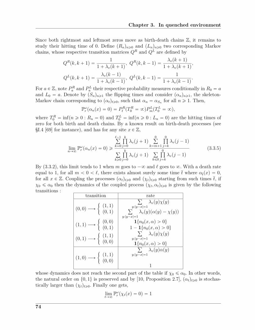
Chapter 3. In quenched environment
Since both rightmost and leftmost zeros move as birth-death chains Z, it remains tostudy their hitting time of 0. Define pRnqně0 and pLnqně0 two corresponding Markovchains, whose respective transition matrices QR and QL are defined by
QRpk, k ` 1q “ 1
1` λvpk ` 1q , QRpk, k ´ 1q “ λvpk ` 1q
1` λvpk ` 1q ,
QLpk, k ` 1q “ λvpk ´ 1q
1` λvpk ´ 1q , QLpk, k ´ 1q “ 1
1` λvpk ´ 1q .
For a P Z, note PRa and PL
a their respective probability measures conditionally in R0 “ aand L0 “ a. Denote by pSnqně1 the flipping times and consider pαnqně1, the skeleton-Markov chain corresponding to pαtqtě0, such that αn “ αSn for all n ě 1. Then,
Pωr pαnpxq “ 0q “ PR` pT
R0 “ 8qP
LmpT
L0 “ 8q,
where TR0 “ infpn ě 0 : Rn “ 0q and TL0 “ infpn ě 0 : Ln “ 0q are the hitting times ofzero for both birth and death chains. By a known result on birth-death processes (see§I.4 [69] for instance), and has for any site x P Z,
limnÑ8
Pωr pαnpxq “ 0q ě
`´1ř
k“0
kś
j“0λvpj ` 1q
ř
kě0
kś
j“0λvpj ` 1q
0ř
k“m`1
0ś
j“k
λvpj ´ 1q
ř
kď0
0ś
j“k
λvpj ´ 1q(3.3.5)
By (3.3.2), this limit tends to 1 when m goes to ´8 and ` goes to 8. With a death rateequal to 1, for all m ă 0 ă `, there exists almost surely some time t where αtpxq “ 0,for all x P Z. Coupling the processes pαtqtě0 and pχtqtě0 starting from such times t, ifχ0 ď α0 then the dynamics of the coupled process pχt, αtqtě0 is given by the followingtransitions :
transition rate
p0, 0q ÝÑ"
p1, 1qp0, 1q
ř
y:|y´x|“1λvpyqχpyq
ř
y:|y´x|“1λvpyqpαpyq ´ χpyqq
p1, 1q ÝÑ"
p0, 0qp0, 1q
1tn0px, αq ą 0u1´ 1tn0px, αq ą 0u
p0, 1q ÝÑ"
p1, 1qp0, 0q
ř
y:|y´x|“1λvpyqχpyq
1tn0px, αq ą 0u
p1, 0q ÝÑ"
p1, 1qp0, 0q
ř
y:|y´x|“1λvpyqαpyq
1whose dynamics does not reach the second part of the table if χ0 ď α0. In other words,the natural order on t0, 1u is preserved and by [10, Proposition 2.7], pαtqtě0 is stochas-tically larger than pχtqtě0. Finally one gets,
limtÑ8
Pωr pχtpxq “ 0q “ 1
74

3.3. Random growth on vertices
for all x P Z.
If the family tωpkq, k P Zu is random and i.i.d. then the family tλvpkq, k P Zu is i.i.d.as well, one deduces the following criterion from Theorem 3.2.1-(2).
Corollary 3.3.1. The process in random environment pχtqtě0 dies out if
Eωr log λvp0q ă 0.
that is, if λ2 ă 1 and r ą ´ log λ2 log λ1.
Proof. By the ergodic theorem,
limkÑ8
1k
kÿ
j“0log λvpjq “ Eωr log λvp0q.
Denote by ak “kś
j“0λvpjq the general term of series (3.3.2). Since Eωr log λvp0q ă 0,
limkÑ8
1k
log ak ă ´b,
for some positive b. That is, limkÑ8
log ak ă limkÑ8
p´bkq, written log ak „k8 ´bk, andÿ
kě0ak “
ÿ
kě0expplog akq „k8
ÿ
kě0expp´bkq.
Therefore, assumptions (3.3.2) are satisfied as soon as Eωr log λvp0q ă 0.
Applying this result to our dynamics given by (3.3.1),
Eωr log λvp0q “ p log λ2 ` p1´ pq log λ1 ă 0 (3.3.6)
i.e. p ą log λ1plog λ1 ´ log λ2q. Since p ă 1, this implies
λ2 ă 1. (3.3.7)
By (3.2.3) and (3.3.1),
Eωr`
log λvp0q˘
“r log λ2 ` log λ1
r ` 1 ,
one has under (3.3.7) the following extinction criterion from (3.3.6)
r ą ´log λ1
log λ2. (3.3.8)
Since we assumed λ1 ą λc, the right-hand side is positive and (3.3.8) is an upper boundon the transitional phase with respect to λ1 and λ2 for the extinction of the process.
75
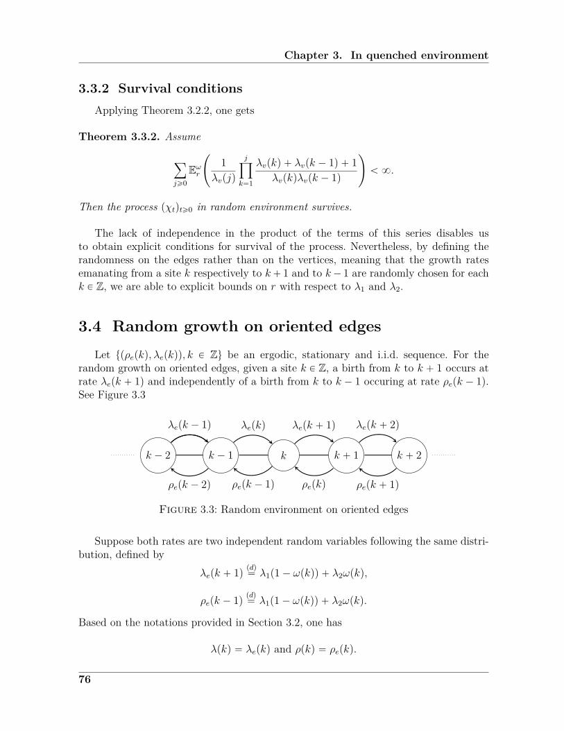
Chapter 3. In quenched environment
3.3.2 Survival conditionsApplying Theorem 3.2.2, one gets
Theorem 3.3.2. Assume
ÿ
jě0Eωr
˜
1λvpjq
jź
k“1
λvpkq ` λvpk ´ 1q ` 1λvpkqλvpk ´ 1q
¸
ă 8.
Then the process pχtqtě0 in random environment survives.
The lack of independence in the product of the terms of this series disables usto obtain explicit conditions for survival of the process. Nevertheless, by defining therandomness on the edges rather than on the vertices, meaning that the growth ratesemanating from a site k respectively to k` 1 and to k´ 1 are randomly chosen for eachk P Z, we are able to explicit bounds on r with respect to λ1 and λ2.
3.4 Random growth on oriented edges
Let tpρepkq, λepkqq, k P Zu be an ergodic, stationary and i.i.d. sequence. For therandom growth on oriented edges, given a site k P Z, a birth from k to k ` 1 occurs atrate λepk ` 1q and independently of a birth from k to k ´ 1 occuring at rate ρepk ´ 1q.See Figure 3.3
k ´ 2 k ´ 1 k k ` 1 k ` 2
λepk ` 2q
ρepk ` 1q
λepk ` 1q
ρepkq
λepkq
ρepk ´ 1q
λepk ´ 1q
ρepk ´ 2q
Figure 3.3: Random environment on oriented edges
Suppose both rates are two independent random variables following the same distri-bution, defined by
λepk ` 1q pdq“ λ1p1´ ωpkqq ` λ2ωpkq,
ρepk ´ 1q pdq“ λ1p1´ ωpkqq ` λ2ωpkq.
Based on the notations provided in Section 3.2, one has
λpkq “ λepkq and ρpkq “ ρepkq.
76
3.4. Random growth on oriented edges
3.4.1 Extinction conditionsTheorem 3.2.1 permits to obtain the following criteria.
Theorem 3.4.1. The process in random environment dies out if the two followingassertions are satisfied.
i.Eωr λepkq ă 1,
ii.1´ Eωr
1λepkq
ă Eωr1
λepkq
´
1´ Eωr λepkq¯
.
that is, if λ2 ă 1 and r ą λ1 ´ 11´ λ2
.
Proof. Computing the expectation of the growth rates, conditions on r for the processto die out are given by :
(i) can be rewritten using (3.2.3)
λ1p1´ pq ` λ2p ă 1 ô rp1´ λ2q ą λ1 ´ 1,
therefore, as λ1 ´ 1 ą 0 since λ1 ą λc ą 1, one has again
λ2 ă 1 (3.4.1)
and the conditionr ą
λ1 ´ 11´ λ2
(3.4.2)
On the other hand, piiq is
Aprq “ 2r2 1´ λ2
λ2` r
´2´ λ2
λ1`
2´ λ1
λ2´ 2
¯
` 21´ λ1
λ1ą 0.
The roots of the polynomial are real since its corresponding discriminant ∆ is non-negative,
∆ “1
λ21λ
22pλ1 ´ λ2q
2´
pλ1 ` λ2 ´ 2q2 ` 4λ1λ2
¯
Roots are therefore given by
δ˘ “pλ1 ` λ2 ´ 2qpλ1 ` λ2q ˘ pλ1 ´ λ2q
a
pλ1 ` λ2 ´ 2q2 ` 4λ1λ2
4λ1p1´ λ2q
Consequently, the process in random environment survives as soon as r satisfies
pr ´ δ`qpr ´ δ´q ą 0
Since λ2 ă 1 and λ1 ą 1, one has δ`δ´ “p1´ λ1qλ2
p1´ λ2qλ1ă 0. Both roots δ´ and δ` are of
opposite sign and Aprq ą 0 ifr ą δ`, (3.4.3)
(because δ´ ă 0). Notice condition 3.4.2 implies that r ą δ`.
77
Chapter 3. In quenched environment
3.4.2 Survival conditionsApplying Theorem 3.2.2 to our case where the sequence tρpkq, λpkq, k P Zu is i.i.d.,
we getTheorem 3.4.2. The process in random environment survives if for all j ě 0,
Eωr´ 1λepj ` 1q
¯´
Eωrλepkq ` ρepk ´ 1q ` 1
λepkqρepk ´ 1q
¯j
ă 1
that is, if λ2 ă 1`?
2 ă λ1 and r ăλ2
´
λ1 ´?
2´ 1¯
λ1
´
λ2 ´?
2´ 1¯ .
Proof. The (geometric) series converges as soon as
Eωrλep0q ` ρep0q ` 1
λep0qρep0qă 1,
that is, if
2Eωr1
λepkq` Eωr
1λepkqρepk ´ 1q
“2λ1 ` 1λ2
1p1´ pq2 ` 2λ1 ` λ2 ` 1
λ1λ2pp1´ pq ` 2λ2 ` 1
λ22
p2
smaller than 1 i.e. using (3.2.3) if,
Aprq :“ r2”
λ21p2λ2 ` 1q ´ λ2
1λ22
ı
` rλ1λ2
”
2pλ1 ` λ2 ` 1q ´ 2λ1λ2
ı
`
”
λ22p2λ1 ` 1q ´ λ2
1λ22
ı
ă 0. (3.4.4)
The associated discriminant is ∆ “ 8λ21λ
22pλ1 ´ λ2q
2. And the roots of Aprq are
δA´ “´λ2
´
λ1 `?
2´ 1¯
λ1
´
λ2 `?
2´ 1¯ ă 0
and
δA` “´λ2
´
λ1 ´?
2´ 1¯
λ1
´
λ2 ´?
2´ 1¯ ,
which is positive ifλ1 ą 1`
?2, (3.4.5)
and λ2 ă 1`?
2, this last condition is cleared by the assumption (3.2.2), as λ2 ă λc ď1`
?2. In this case, the process survives if r is such that
r ă δA`. (3.4.6)
78

3.5. Numerical bounds on the transitional phase
3.5 Numerical bounds on the transitional phase
3.5.1 Back to the basic contact processAssume r “ 0, then for all x P Z, ωpxq “ 0 a.s. and λepxq “ ρepxq “ λ1. We thus
recover the one-dimensional basic contact process with growth rate λ1. In this case, ourestimates lead to the following bound for λc.
Corollary 3.5.1. For the one-dimensional basic contact process,
λc ď 1`?
2.
Proof. According to (3.4.4) in the proof of Theorem 3.4.2, the process survives if λ21 ´
2λ1 ´ 1 ą 0, that is, ifλ1 ą 1`
?2.
Recall on Z, λc P r1.539, 1.942s. This bound is quite rough but its advantage is thatwe derived it simply. Consequently, one first deduces a bound on the critical value λc ofthe one-dimensional basic contact process : λc ď 1`
?2 » 2.41.
3.5.2 The phase transitionFrom results obtained in the previous section, one gets the following numerical
bounds for a phase transition. By choosing parameters λ1 and λ2 satisfying (3.4.1),condition (3.4.2) from Theorem 3.4.1 gives us lower bounds on the phase transition.Moreover, by choosing parameters λ2 and λ1 satisfying (3.4.5), condition (3.4.6) fromTheorem 3.4.2 gives us upper bounds.
λ1 λ2 transitional phase1000 0.2 r0.07, 1249s100 0.2 r0.07, 124s10 0.2 r0.044, 11.25s2 0.2 r0, 1.25s
λ1 λ2 transitional phase1000 0.8 r0.49, 4995q100 0.8 r0.48, 495q10 0.8 r0.36, 45s2 0.8 p0, 5s
λ1 λ2 transitional phase1000 1.4 r1.37,8q100 1.4 r1.34,8q10 1.4 r1.04,8q2 1.4 R`
Remark that the necessary condition λ2 ă 1 disables us to conclude to an upperbound for values of λ2. In a similar way, condition (3.4.5) of Theorem 3.4.2 imposes λ1to be larger than 1`
?2, disabling us to find an explicit lower bound on the transitional
phase in such cases.
79

Chapter 3. In quenched environment
80

4Hydrodynamic limit on the
d-dimensional torusContents
4.1 Introduction . . . . . . . . . . . . . . . . . . . . . . . . . . 824.2 Notations and Results . . . . . . . . . . . . . . . . . . . . 82
4.2.1 The model . . . . . . . . . . . . . . . . . . . . . . . . . . . . 824.2.2 Hydrodynamics for the reaction-diffusion process . . . . . . . 85
4.3 The hydrodynamic limit . . . . . . . . . . . . . . . . . . . 864.3.1 Tightness . . . . . . . . . . . . . . . . . . . . . . . . . . . . . 874.3.2 Replacement lemma . . . . . . . . . . . . . . . . . . . . . . . 894.3.3 Identification of limit points . . . . . . . . . . . . . . . . . . . 934.3.4 Uniqueness of weak solutions . . . . . . . . . . . . . . . . . . 95
4.4 Proof of the replacement lemma . . . . . . . . . . . . . . 964.4.1 One block estimate . . . . . . . . . . . . . . . . . . . . . . . . 974.4.2 Equivalence of ensembles . . . . . . . . . . . . . . . . . . . . 994.4.3 Two blocks estimate . . . . . . . . . . . . . . . . . . . . . . . 100
4.A Construction of an auxiliary process . . . . . . . . . . . . 1024.B Properties of measures . . . . . . . . . . . . . . . . . . . . 1074.C Quadratic variations computations . . . . . . . . . . . . . 1104.D Topology of the Skorohod space . . . . . . . . . . . . . . . 113
4.1 IntroductionIn this chapter, one derives the hydrodynamic limit on the d-dimensional torus of
the asymmetric multitype contact process defined in Chapter 1.The work here is is based on the entropy method due to M. Z. Guo, G. C. Papani-
colaou and S. R. S. Varadhan [37] to prove the hydrodynamic behaviour of a large classof interacting particle systems through the investigation of the time-evolution of the en-tropy and arguments by C. Kipnis, S. Olla and S.R.S Varadhan [43], using martingalestechniques.
81
Chapter 4. Hydrodynamic limit on the torus
This chapter is a preliminary to the next one, it introduces many involved quantitiesand we detail here classical computations that appear in both chapters. It is organizedas follows. We begin by describing the model and the main result in Section 4.2, which issubsequently proved in Section 4.3, while classical proofs concerning the block estimatesare proved in Section 4.4.
In the Appendix 4.A, we deal with a construction of an auxiliary process, a trick in-troduced by M. Mourragui [63], in case of unbounded rates. Whereafter, we expose somelengthy computations surrounding the reference measure (Appendix 4.B) and reminderson the Skorohod topology (Appendix 4.D).
4.2 Notations and ResultsLet TdN “ pZNZqd be the d´dimensional discrete microscopic torus t0, ..., N ´ 1ud
and Td “ pRZqd be the corresponding macroscopic torus r0, 1qd.
4.2.1 The model
Define EN “ t0, 1, 2, 3uTdN . The model we investigate is a reaction-diffusion process
pηtqtě0 given by the generatorLN :“ LN,R,D “ N2LD
N ` LRN , (4.2.1)
where N2LDN stands for the generator of a rapid-stirring process, defined for any function
f on EN byN2LD
Nfpηq “ N2ÿ
x,yPTdNx´y“1
´
fpηx,yq ´ fpηq¯
, (4.2.2)
here, x “ max1ďjďd
|xj| denotes the max norm for x P Zd, and η P EN , ηx,y is theconfiguration obtained from η by exchanging the occupation variables ηpxq and ηpyq oftwo neighbouring sites x, y P TdN , that is,
ηx,ypzq “
$
&
%
ηpxq if z “ y,ηpyq if z “ x,ηpzq if z ‰ x, y,
and LRN is the generator of the asymmetric CP-DRE defined in Chapter 2, which is given
for any cylinder function f on EN by
LRNfpηq “
3ÿ
i“0cpx, η, iq
´
fpηixq ´ fpηq¯
(4.2.3)
with η P EN , ηix is the configuration obtained from η by flipping the state of site x intothe state i P t0, 1, 2, 3u, that is,
ηixpzq “
"
i if z “ x,ηpzq if z ‰ x.
82
4.2. Notations and Results
while the rate function c is defined by
cpx, η, 0q “ 1 if ηpxq P t1, 2u,
cpx, η, 1q “
$
’
&
’
%
βpx, ηq :“ λ1ř
yPTdNy´x“1
η1pyq ` λ2ř
yPTdNy´x“1
η3pyq if ηpxq “ 0,
1 if ηpxq “ 3,
cpx, η, 2q “"
r if ηpxq “ 0,1 if ηpxq “ 3,
cpx, η, 3q “ r if ηpxq “ 1.
(4.2.4)
Since the conserved quantities for the generator LDN concern the total number of particles
of each type i P t1, 2, 3u, one defines the product measure νNpψon EN by
νNpψpηq :“
ź
xPTdN
1Z
pψ
exp˜
3ÿ
i“0rψi1tηpxq “ ius
¸
(4.2.5)
where Zpψ “
3ř
i“0exppψiq is the normalization constant, for pψ “ pψ0, ψ1, ψ2, ψ3q such that
ψ0, ψ1, ψ2, ψ3 P R are parameters. Because of a high use of indicator functions, we shallsimplify the notation by
ηipxq “ 1tηpxq “ iu,
for x P TdN and i “ 1, 2, 3.
As usual, we parametrize the measure by the conserved quantities (see for instance R.Marra and M. Mourragui [61]). By a change of variables (see Appendix 4.B for details),given parameters ρ1, ρ2, ρ3 such that ρi ě 0 and ρ1`ρ2`ρ3 ď 1, one defines the productmeasure for pρ “ pρ1, ρ2, ρ3q by
νNpρ p¨q “ νNΨpρ1,ρ2,ρ3qp¨q and ρ0 “ 1´ ρ1 ´ ρ2 ´ ρ3. (4.2.6)
where Ψ is a bijection from R3` to p0, 1q3 given by (4.B.3). The measures tνN
pρ , pρ P r0, 1s3uare invariant [see Lemma 4.B.1] with respect to the rapid-stirring process with generatorN2LD
N , and they are parametrized by the densities :"
ENνpρrηkpxqs “ νN
pρ pηpxq “ kq “ ρk, 1 ď k ď 3,νNpρ pηpxq “ 0q “ 1´ ρ1 ´ ρ2 ´ ρ3.
For any function φ on EN , denote by rφppρq the expectation of φ with respect to νNpρ :
rφppρq “ ENνpρrφpηqs. (4.2.7)
83

Chapter 4. Hydrodynamic limit on the torus
To do changes of variables, it will be more convenient to write the measures as follows :
νNpρ pηq “ exp
!3ÿ
j“0
ÿ
xPTdN
%jηjpxq)
(4.2.8)
with %j “ log ρj (4.2.9)
Since conserved quantities are densities of three types of particles, we need to workwith three dimensional vectors whose i-th component is associated to the type i. Thesevectors will be distinguished with a hat. For any configuration η, define the empiricalmeasure of type i on EN by
πN,ipηq “1Nd
ÿ
xPTdN
ηipxqδ xN, (4.2.10)
where δ xNpdyq stands for the Dirac measure at xN . And note for pηsqsPr0,T s,
pπNt pηq :“ pπN,1t , πN,2t , πN,3t qpηq, (4.2.11)
where πN,it pηq “ πN,ipηtq. Let Cn,mpr0, T s ˆ Td;Rq be the set of functions n times conti-nuously differentiable in time and m times continuously differentiable in space. For anyfunction Gi P C1,2pr0, T s ˆ Td;Rq, denote the integral of Gi,t with respect to πN,it by
xπN,it , Gi,ty “1Nd
ÿ
xPTdN
Gi,tpxNqηipxq. (4.2.12)
For any function pGt “ pG1,t, G2,t, G3,tq P C1,2pr0, T s ˆ Td;R3q, define the integral of pGt
with respect to pπNt by
xpπt, pGty “
3ÿ
i“1xπN,it , Gi,ty.
4.2.2 Hydrodynamics for the reaction-diffusion processLet M1
` be the subset of M of all positive measures absolutely continuous withrespect to the Lebesgue measure with positive density bounded by 1 :
M1` “
π P M : πpduq “ ρpuqdu and 0 ď ρpuq ď 1 a.e.(
.
Fix T ą 0. Let Dpr0, T s, pM1`q
3q be the set of right-continuous with left limitstrajectories with values in pM1
`q3, endowed with the Skorohod topology and equipped
with its Borel σ´ algebra.For any probability measure µ on EN , denote by PNµN the probability measure on
Dpr0, T s, ENq of the process pηtqtPr0,T s with generator LN and by ENµN the correspondingexpectation. Consider QN
µ “ PNµN ˝ ppπNq´1 the law of the process`
pπNt pηtq˘
tPr0,T s.
84
4.2. Notations and Results
Fix T ą 0. A sequence of probability measures is associated to a density profilepγ “ pγ1, γ2, γ3q : Td Ñ r0, 1s3 if for any δ ą 0 and any function pG P C1pTd,R3q,
limNÑ8
µN!ˇ
ˇ
ˇxpπNpηq, pGp¨qy ´ xpγp¨q, pGp¨qy
ˇ
ˇ
ˇą δ
)
“ 0 , (4.2.13)
Denote by pρ “ pρ1, ρ2, ρ3q : r0, T s ˆ Td Ñ r0, 1s3 a typical macroscopic trajectory.We shall show that the macroscopic time-evolution of empirical density pπN is given bya reaction-diffusion system
#
Btpρ “ ∆pρ ` pRppρq in Td ˆ p0, T q,pρ0p¨q “ pγp¨q in Td,
(4.2.14)
where pR “ pR1,R2,R3q : r0, 1s3 Ñ R3 is defined by$
’
&
’
%
R1pρ1, ρ2, ρ3q “ 2dpλ1ρ1 ` λ2ρ3qρ0 ` ρ3 ´ ρ1pr ` 1q ,R2pρ1, ρ2, ρ3q “ rρ0 ` ρ3 ´ ρ2 ,
R3pρ1, ρ2, ρ3q “ rρ1 ´ 2ρ3 ,
(4.2.15)
with ρ0 “ 1´ ρ1´ ρ2´ ρ3. A weak solution pρp¨, ¨q : r0, T s ˆTd Ñ R3 of (4.2.14) satisfiesthe following assertions :(S1) For any i P t1, 2, 3u, ρi P L2 `r0, T s ˆ Td
˘
.(S2) For any function pGpt, uq “ pGtpuq “ pG1,tpuq, G2,tpuq, G3,tpuqq in C1,2`r0, T s ˆ
Td;R3˘, one has
xpρT , pGT y ´ xpρ0, pG0y
“
ż T
0ds xpρs, pBs `∆q pGsy `
ż T
0ds xpRppρsq, pGsy, (4.2.16)
here for pG, pH P C1,2pr0, T sˆTd;R3q, x pGp¨q, pHp¨qy stands for the usual inner product
of L2pTdq : x pG, pHy “3ř
i“1
ż
TdGipuqHipuqdu.
The rest of this chapter is devoted to prove the following result.
Theorem 4.2.1. Let pγ : Td Ñ r0, 1s3 be an initial continuous profile and pµNqNě1 be asequence of probability measures with µN a probability measure on EN for each N asso-ciated to pγ. The sequence of random measures ppπNt qNě1 converges weakly in probabilityas N goes to infinity to the absolutely continuous measure pπtpduq “ pρpt, uqdu whosedensity pρpt, uq “ pρ1, ρ2, ρ2qpt, uq is the unique weak solution of the reaction-diffusionsystem (4.2.14). That is, for any t P r0, T s, any δ ą 0 and any function pG P CpTd,R3q
limNÑ8
PNµN!ˇ
ˇ
ˇxpπNpηtq, pGp¨qy ´ xpρtp¨q, pGp¨qy
ˇ
ˇ
ˇą δ
)
“ 0 .
85

Chapter 4. Hydrodynamic limit on the torus
4.3 The hydrodynamic limit
For any function pG “ pG1, G2, G3q P C1,2pr0, T s ˆ Td;R3q, by Dynkin’s formula
MN,it “ xπN,it , Gi,ty ´ xπ
N,i0 , Gi,0y ´
tż
0
LNxπN,is , Gi,syds´
ż t
0xπN,is , BsGi,syds (4.3.1)
is a QNµN´martingale with respect to the σ´algebra Ft “ σpηs, s ď tq.
To derive the hydrodynamic behaviour of the reaction-diffusion process, one needsto prove that the above martingale vanishes as N goes to infinity. To this purpose, applythe generator LN to the function η Ñ ηipxq so that the integral part of MN,i
t is depictedas follows.
N2LDNxπ
N,it , Gi,ty “
N2
Nd
ÿ
xPTdN
dÿ
j“1Gi,tpxNq
´
ηi,tpx` ejq ` ηi,tpx´ ejq ´ 2ηi,tpxq¯
“ xπN,it ,∆NGi,tp¨qy,
where ∆NGi,tpxNq “ N2dÿ
j“1pGi,tppx` ejqNq `Gi,tppx´ ejqNq ´ 2Gi,tpxNqq is the
discrete laplacian in dimension d and pe1, ..., edq is the canonical basis of Rd. And com-puting LR
Nηipxq for each i gives
LRNη1pxq “
ÿ
xPTdN
˜
λ1ÿ
y:y´x“1η1pyq ` λ2
ÿ
y:y´x“1η3pyq
¸
η0pxq ` η3pxq ´ pr ` 1qη1pxq,
(4.3.2)LRNη2pxq “ rη2pxq ` η3pxq ´ η2pxq, (4.3.3)
LRNη3pxq “ rη1pxq ´ 2η3pxq, (4.3.4)
so that we deduce
LRNxπ
N,1t , G1,ty “
1Nd
ÿ
xPTdN
G1,tpxNq
˜
λ1ÿ
y:y´x“1η1,tpyq ` λ2
ÿ
y:y´x“1η3,tpyq
¸
η0,tpxq
` xπN,3t , G1,ty ´ pr ` 1qxπN,1t , G1,ty,
LRNxπ
N,2t , G2,ty “ rxπN,0t , G2,ty ` xπ
N,3t , G2,ty ´ xπ
N,2t , G2,ty
,LRNxπ
N,3t , G3,ty “ rxπN,1t , G3,ty ´ 2xπN,3t , G3,ty. (4.3.5)
Thus, to close the equations we need to replace the local function of η which isthe term in LR
Nη1pxq by a functional of the empirical densities given by pπNt definedin (4.2.11). This is the purpose of the replacement lemma and the blocks estimates,exposed in Sections 4.3.2 and 4.4.
86

4.3. The hydrodynamic limit
Next, we need to characterize all the limit points of the sequence pQNµN qNě1 : their
existence comes from by the tightness of the sequence of measures, it is proved in Section4.3.1, then, the identification and uniqueness of the limit points as weak solutions of(4.2.14) conclude the proof in Sections 4.3.3 and 4.3.4.
4.3.1 TightnessExistence of limit points is guaranteed by the following lemma.
Lemma 4.3.1 (Tightness). The sequence pQNµ qNě1 is tight and all its limit points Q˚µ
satisfyQ˚µ
´
pπ : 0 ď pπtpuq ď 1, pπtpuq “ pπtpuqdu, t P r0, T s¯
“ 1. (4.3.6)
Proof. By Proposition 4.D.4, it is enough to show tightness for the real-valued processtxpπt, pGy, t P r0, T su for all functions pG P C2pTd;R3q. By Prohorov’s theorem 4.D.1, toget the tightness of txpπt, pGy, t P r0, T su in Dpr0, T s,R3q with the uniform topology, oneneeds to check the two following assertions :(i) boundedness :
limmÑ8
limNÑ8
QNµN
´
suptPr0,T s
|xpπt, pGy| ě m¯
“ 0. (4.3.7)
(ii) equicontinuity :
limδÑ0
limNÑ8
QNµN
´
sup|t´s|ďδ
|xpπt, pGy ´ xpπs, pGy| ą ε¯
“ 0, for any ε ą 0. (4.3.8)
The limit (4.3.7) is immediate since for each t P r0, T s and 1 ď i ď 3, the total massof πN,it is bounded by 1. To prove (4.3.8), it is enough to show for the martingale MN,i
t
defined in (4.3.1) that
limδÑ0
limNÑ8
QNµN
´
sup|t´s|ďδ
|MN,it ´MN,i
s | ą ε¯
“ 0, for any ε ą 0 (4.3.9)
and
limδÑ0
limNÑ8
QNµN
´
sup0ďt´sďδ
ˇ
ˇ
ˇ
ż t
s
LNxπN,ir , Giydr
ˇ
ˇ
ˇą ε
¯
“ 0, for any ε ą 0. (4.3.10)
To prove (4.3.9), one shows the quadratic variation xMN,iyt of the martingale MN,it
converges to zero as N goes to 8. Note that since pG is not time-dependent, the timederivative of pG is null in the expression (4.3.1). By the Doob-Meyer decomposition,
xMN,iyt “
ż t
0
!
LNxπN,is , Giy
2´ 2xπN,is , GiyLNxπ
N,is , Giy
)
ds. (4.3.11)
87
Chapter 4. Hydrodynamic limit on the torus
We postpone the detailed computations to Appendix 4.C. By Lemma 4.C.1, one has
N2ż t
0
#
LDNxπ
N,is , Giy
2´ 2xπN,is , GiyLD
NxπN,is , Giy
+
ds ď CpGqtN´d
ż t
0
!
LRNxπ
N,is , Giy
2´ 2xπN,is , GiyLR
NxπN,is , Giy
)
ds ď Cpλ1, λ2, rqtGi22N
´d
where Cpλ1, λ2, rq stands for the supremum of the bounded rates since all involved ratesin factor in (4.C.6) are positive. Therefore, combining both estimates,
xMN,iyt ď
`
Cpλ1, λ2, rqGi22 ` CpGq
˘
t
Nd, (4.3.12)
which converges to zero as N Ñ 8, one deduces (4.3.9) by using Doob’s martingaleinequality.
To prove (4.3.10), on one hand,ˇ
ˇN2LDNxπ
N,it , Giy
ˇ
ˇ “ˇ
ˇxπN,it ,∆NGiyˇ
ˇ ď ∆Gi1,
where ∆G stands for the Laplace operator ∆G “dř
j“1B2ejG when Bej is the first derivative
in the j-th direction. On the other hand, since all rates (4.2.4) are bounded, by (4.3.5),ˇ
ˇLRNxπ
N,it , Giy
ˇ
ˇ ď Cpλ1, λ2, rqGi1.
To show that pπt is absolutely continuous, remark that for any function pG P CpTd,R3q,
suptPr0,T s
|xpπNt ,pGy| ď pG8.
Hence, since pπ¨ ÞÑ suptPr0,T s
|xpπt, pGy| is continuous with respect to the Skorohod topology,
any limit point satisfies by Portmanteau theorem,
suptPr0,T s
|xpπt, pGy| ď pG1
that is, any limit point is supported on trajectories such that pπt is absolutely continuouswith respect to the Lebesgue measure for all t P r0, T s.
4.3.2 Replacement lemmaFor any positive integer k and x P TdN , denote by ηki pt, xq the empirical density of
type´i particles given by
ηki pt, xq “1
p2k ` 1qdÿ
yPTdNy´xďk
ηi,tpyq, (4.3.13)
88

4.3. The hydrodynamic limit
and define the vector ppηkt qpxq “ pηk1 , ηk2 , η
k3qpt, xq. We now deal with replacing local
functions of η by functions of the empirical density within a macroscopic box, in otherwords, for any cylinder function φ and the function rφp¨q defined by (4.2.7), one showsfor any continuous function G and ε ą 0 the following replacement lemma,
Proposition 4.3.1. For all a ą 0,
limεÑ0
limNÑ8
1Nd
logPNµN
¨
˝
1Nd
ż
ÿ
xPT dN
τxVεNpηtqdt ě a
˛
‚“ ´8,
where Vkpηq :“
ˇ
ˇ
ˇ
ˇ
ˇ
1p2k ` 1qd
ř
yďk
τyφpηq ´ rφppηkp0qq
ˇ
ˇ
ˇ
ˇ
ˇ
.
Proof. For any γ ą 0, by Markov’s inequality,
PNνNpρ
¨
˝
1Nd
ż
ÿ
xPTdN
τxVεNpηtqdt ě a
˛
‚ď expp´γNdaq ¨ENνNpρ
»
–exp
¨
˝γ
Tż
0
ÿ
xPTdN
τxVεNpηtqdt
˛
‚
fi
fl .
Introduce in L2pνNpρ q the operator
AN,γ :“ 12pLN ` pLNq
‹q ` γ
ÿ
xPTdN
τxVεN (4.3.14)
where pLNq‹ is the adjoint of LN in L2pνNpρ q.
Fix T ą 0, by Feynman-Kac formula (see [42, Appendix 1.7]), for all t P r0, T s, theunique solution of the differential equation
$
&
%
Btupt, ηq “12pLN ` pLNq
˚qupt, ηq ` γř
xPTdN
τxVεNupt, ηq
up0, ηq “ 1(4.3.15)
is given by upt, ηq “ ENνNpρ
»
–up0, ηq exp
¨
˝
Tż
0
γÿ
xPTdN
τxVεNpηsqds
˛
‚
fi
fl.
By the spectral decomposition of the auto-adjoint operator AN,γ,
λεNpγq “ supu“1
xAN,γu, uy (4.3.16)
is the largest eigenvalue of the operator AN,γ, so that
ENνNpρ
»
–exp
¨
˝
Tż
0
γÿ
xPTdN
τxVεNpηsqds
˛
‚
fi
fl ď exppTλεNpγqq
89

Chapter 4. Hydrodynamic limit on the torus
hence, 1Nd
logPNνNpρ
¨
˝
1Nd
ż T
0
ÿ
xPTdN
τxVεNpηsqds ě a
˛
‚ď1
2NdTλεNpγq ´ γa.
It thus remains to show for all γ ą 0,
limεÑ0
limNÑ8
λεNpγq
Nd“ 0, (4.3.17)
in which case one would have for all γ ą 0,
limεÑ0
limNÑ8
1Nd
logPNνNpρ
¨
˝
1Nd
ż T
0
ÿ
xPTdN
τxVεNpηsqds ě a
˛
‚ď ´γa
and conclusion will follow by letting γ go to infinity. By Rayleigh-Ritz variational for-mula,
λεNpγq “ supfNPL2pνN
pρq
fN L2“1
¨
˝
ż
γÿ
xPTdN
τxVεNpηqpfNq2pηqdνN
pρ pηq ` xLNfN , fNy
˛
‚
“ supfNPL2pνN
pρq
fN L2“1
˜
ż
γÿ
xPTdN
τxVεNpηqpfNq2pηqdνN
pρ pηq `N2xLD
NfN , fNy ` xLR
NfN , fNy
¸
Estimate the reaction part as follows.
xLRNf
N , fNy “ÿ
xPTdN
3ÿ
i“0
ż
cpx, η, iqfNpηq´
fNpηixq ´ fNpηq
¯
dνNpρ pηq
“ÿ
xPTdN
3ÿ
i“0
ż
cpx, η, iqfNpηqfNpηixqdνNpρ pηq ´
ÿ
xPTdN
3ÿ
i“0
ż
cpx, η, iqfNpηq2dνN
pρ pηq
ďÿ
xPTdN
3ÿ
i“0
ż
cpx, η, iq´
fNpηq2`
14f
Npηixq
2¯
dνNpρ pηq ´
ÿ
xPTdN
3ÿ
i“0
ż
cpx, η, iqfNpηq2dνN
pρ pηq
where we used the inequality AB ď12aA
2 `a
2B2 for A,B, a ą 0 with a “ 2. Use
formulas of changes of variables given by Lemma 4.B.2 to bound the first sum by theL2-norm of fN and the fact that fN is a density with respect to νN
pρ to bound the secondintegral :
xLRNf
N , fNy ďCpλ1, λ2, rq
4ÿ
xPTdN
3ÿ
i“0
ÿ
j‰i
ż
fNpηixq2ηjpxqdν
Npρ pηq
90
4.3. The hydrodynamic limit
“Cpλ1, λ2, rq
4ÿ
xPTdN
3ÿ
i“0
ÿ
j‰i
ż
ρjρifNpηq
2ηipxqdν
Npρ pηq
ď CppρqCpλ1, λ2, rq
4 Nd
Hence,
1Nd
λεNpγq “ supfNPL2pνN
pρq
fN L2“1
˜
1Nd
ż
γÿ
xPTdN
τxVεNpfNq2pηqdνN
pρ pηq `N2´dxLD
NfN , fNy
¸
` C0
for some positive constant C0 “ CppρqCpλ1, λ2, rq4. By reversibility of the measure withrespect to the generator LD
N , DDNp|f
N |q ď DDNpf
Nq and one can take the supremumover functions f in L2pνN
pρ q such that fL2pνNpρ“ 1 to the supremum over non-negative
functions f in L2pνNpρ q such that
?fL2pνN
pρ“ 1. Recall νN
pρ is reversible with respect tothe generator LD
N but not LRN . Going back to the upper bound of λεNpγq,
1Nd
λεNpγq ď supfNě0,fNPL2pνN
pρq
?fN
L2“1
˜
1Nd
ż
γÿ
xPTdN
τxVεNfNpηqdνN
pρ pηq `N2´dxLD
N
a
fN ,a
fNy
¸
` C0
ď supfNě0,fNPL2pνN
pρq
?fN
L2“1
˜
ż 1Nd
γÿ
xPTdN
τxVεNfNpηqdνN
pρ pηq ´N2´dDD
NpfNq
¸
` C0,
whereDDNpf
Nq “
ÿ
x,yPTdNx´y“1
ż
´
a
fNpηx,yq ´a
fNpηq¯2dνN
pρ pηq
is the Dirichlet form associated to the generator of stirring. Since φ is bounded, thereexists some positive constant C such that
ÿ
xPTdN
VεNpηq ď CNd,
one can thus restrict the supremum over functions fN satisfying
DDNpf
Nq ď CNd´2
To get (4.3.17), it remains to show for all positive C,
limεÑ0
limNÑ8
supfNPAN
1Nd
ż
ÿ
xPTdN
τxVεNpηqfNpηqdνN
pρ pηq “ 0, (4.3.18)
91

Chapter 4. Hydrodynamic limit on the torus
where
AN :“!
fN P L2pνN
pρ q : fN ě 0, a
fNL2 “ 1,DDNpf
Nq ď CNd´2
)
This limit will follow from the blocks estimates. On one hand, the one block estimateensures the average of local functions in some large microscopic boxes can be replaced bytheir mean with respect to the grand-canonical measure parametrized by the particlesdensity in these boxes. While the two blocks estimate ensures the particles density overlarge microscopic boxes and over small macroscopic boxes is very close. Let us first statethe block estimates, we postpone their proofs to the next section.Lemma 4.3.2 (One block estimate).
limkÑ8
limNÑ8
supfN :DD
N pfN qďCNd´2
1Nd
ż
ÿ
xPTdN
τx
ˇ
ˇ
ˇ
ˇ
ˇ
1p2k ` 1qd
ÿ
yďk
´
τyφpηq ´ rφppηkp0qq¯
ˇ
ˇ
ˇ
ˇ
ˇ
fNpηqdνNpρ pηq “ 0. (4.3.19)
Lemma 4.3.3 (Two blocks estimate). For i P t0, 1, 2, 3u,
limkÑ8
limεÑ0
limNÑ8
suphďεN
supfN :DD
N pfN qďCNd´2
1Nd
ż
ÿ
xPT dN
ˇ
ˇηki px` hq ´ ηεNi pxq
ˇ
ˇ fNpηqdνNpρ pηq “ 0. (4.3.20)
Let us prove that the limit (4.3.18) is a consequence of these two previous lemmas.
1Nd
ż
ÿ
xPTdN
τxVεNpηqfNpηqdνN
pρ pηq
“1Nd
ż
ÿ
xPTdN
τx
ˇ
ˇ
ˇ
ˇ
ˇ
1p2εN ` 1qd
ÿ
yďεN
τyφpηq ´ rφppηεNp0qq
ˇ
ˇ
ˇ
ˇ
ˇ
fNpηqdνNpρ pηq
ď1Nd
ż
ÿ
xPTdN
τx
ˇ
ˇ
ˇ
ˇ
ˇ
1p2εN ` 1qd
ÿ
yďεN
˜
τyφpηq ´1
p2k ` 1qdÿ
z´yďk
τzφpηq
¸ˇ
ˇ
ˇ
ˇ
ˇ
fNpηqdνNpρ pηq
(4.3.21)
`1Nd
ż
ÿ
xPTdN
τx
ˇ
ˇ
ˇ
ˇ
ˇ
1p2εN ` 1qd
ÿ
yďεN
˜
1p2k ` 1qd
ÿ
z´yďk
τzφpηq ´ rφppηkpyqq
¸ˇ
ˇ
ˇ
ˇ
ˇ
fNpηqdνNpρ pηq
(4.3.22)
`1Nd
ż
ÿ
xPTdN
τx
ˇ
ˇ
ˇ
ˇ
ˇ
1p2εN ` 1qd
ÿ
yďεN
rφppηkpyqq ´ rφppηεNp0qq
ˇ
ˇ
ˇ
ˇ
ˇ
fNpηqdνNpρ pηq. (4.3.23)
92

4.3. The hydrodynamic limit
The first expression (4.3.21) of the right-hand side can be decomposed into boxes ofsize p2k ` 1qd so that,
ż
ˇ
ˇ
ˇ
ˇ
ˇ
1p2εN ` 1qd
ÿ
yďεN
˜
τyφpηq ´1
p2k ` 1qdÿ
z´yďk
τzφpηq
¸ˇ
ˇ
ˇ
ˇ
ˇ
fNpηqdνNpρ pηq
“
ż
ˇ
ˇ
ˇ
ˇ
ˇ
1p2εN ` 1qd
ÿ
yďεN
˜
τyφpηq ´1
p2k ` 1qdÿ
zďk
τy`zφpηq
¸ˇ
ˇ
ˇ
ˇ
ˇ
fNpηqdνNpρ pηq
“
ż
ˇ
ˇ
ˇ
ˇ
ˇ
1p2k ` 1qd
ÿ
zďk
˜
1p2εN ` 1qd
ÿ
yďεN
τyφpηq
´1
p2εN ` 1qdÿ
yďεN
τy`zφpηq
¸ˇ
ˇ
ˇ
ˇ
ˇ
fNpηqdνNpρ pηq
ďp2k ` 1qdp2εN ` 1qφ8,
which tends to zero when N goes to infinity. The second and third expressions (4.3.22)and (4.3.23) tend to zero as well as a consequence of the blocks estimates by translationinvariance of νN
pρ .
4.3.3 Identification of limit points
Now we show that any limit point of the sequence pQNµN qNě1 is concentrated on
trajectories that are weak solutions of the reaction-diffusion system (4.2.14). For this,we come back to the martingale MN,i
t defined in (4.3.1), which satisfies (4.3.9).We focus on the case i “ 1 since it is the only one for which we need to use the
replacement lemma. Define
B1ε ppπ
Nt q “ xπ
N,1t , G1,ty ´ xπ
N,10 , G1,0y ´
tż
0
xπN,1s , BsG1,syds´
tż
0
xπN,1s ,∆NG1,syds
´
tż
0
xπN,3s , G1,syds`
tż
0
pr ` 1qxπN,1s , G1,syds
´
tż
0
1Nd
ÿ
xPTdN
G1,spxNq2dλ1xπN,1s , ιεp¨ ´ xNqyxπ
N,0s , ιεp¨ ´ xNqyds
´1Nd
tż
0
ÿ
xPTdN
G1,spxNq2dλ2xπN,3s , ιεp¨ ´ xNqyxπ
N,0s , ιεp¨ ´ xNqyds.
93

Chapter 4. Hydrodynamic limit on the torus
For any a ą 0, by Doob’s inequality,
limεÑ0
limNÑ8
PNµNˆ
sup0ďtďT
ˇ
ˇ
ˇMN,1
t
ˇ
ˇ
ˇą a
˙
“ 0
To close the equation, replace the local function LRNη1pxq appearing inMN,1
t by a functionof the empirical density thanks to the Replacement lemma 4.3.1. Here φ is a localfunction given by
τxφpηq “
˜
λ1ÿ
y:y´x“1η1pyq ` λ2
ÿ
y:y´x“1η3pyq
¸
η0pxq. (4.3.24)
The occupation variables ηipxq are of mean ηεNi under the measure νNpηεN . Let ιε “
1p2εqd1tr´ε, εsdu be the approximation of the identity and remark that
ηεNi pxq “p2εNqd
p2εN ` 1qd xπN,i, ιεp¨ ´ xNqy. (4.3.25)
So that, one has by Proposition 4.3.1 and expression (4.3.25) :
limεÑ0
limNÑ8
QNµN
´
sup0ďtďT
ˇ
ˇ
ˇB1ε ppπ
Nt q
ˇ
ˇ
ˇą a
¯
“ 0.
If Q˚µ is a limit point of the sequence pQNµN qNě1, the mapping pπ ÞÝÑ B1
ε ppπT q iscontinuous in Skorohod topology, taking the limit as N goes to infinity,
limεÑ0
Q˚µ
˜ˇ
ˇ
ˇ
ˇ
ˇ
xπ1T , G1,T y ´ xπ
10, G1,0y ´
Tż
0
xπ1s , BsG1,syds´
Tż
0
xπ1s ,∆G1,syds
´
Tż
0
xπ3s , G1,syds`
Tż
0
pr ` 1q ă π1s , G1,syds´
Tż
0
ż
Td
!
G1,spuq2dλ1`
π1s ˚ ιε
˘`
π0s ˚ ιε
˘
)
ds du
´
Tż
0
ż
Td
!
G1,spuq2dλ2`
π3s ˚ ιε
˘`
π0s ˚ ιε
˘
)
ds du
ˇ
ˇ
ˇ
ˇ
ˇ
ą a
¸
“ 0.
In virtue of Lemma 4.3.1, all limit points are absolutely continuous with respect to theLebesgue measure on Td, that is, if pπs “ pρps, uqdu, then for all i P t0, 1, 2, 3u, pπit ˚ ιεqpuqconverges in L2pTdq to ρipt, uq as ε goes to 0. Hence,
Q˚µ´ˇ
ˇ
ˇxπ1
T , G1,T y ´ xπ10, G1,0y ´
Tż
0
xπ1s , BsG1,syds´
Tż
0
xπ1s ,∆G1,syds
94
4.3. The hydrodynamic limit
´
ż T
0ds
ż
Tddu xR1ppπ
1sq, G1,spuqy
ˇ
ˇ
ˇą a
¯
“ 0
For i “ 2, 3, the martingales MN,it do not provide local functions of η so that one
has immediately the following limits.
Q˚µ´ˇ
ˇ
ˇxπiT , Gi,T p¨qy ´ xπ
i0, Gi,0¨qy ´
Tż
0
Bsxπis, Gi,sp¨qyds´
Tż
0
xπis,∆Gi,sp¨qyds
´
ż T
0ds
ż
Tddu xRippπ
isq, Gi,spuqy
ˇ
ˇ
ˇą a
¯
“ 0
Finally, any limit point is concentrated on trajectories pπtpduq “ pρpt, uqdu which areweak solutions of (4.2.14).
4.3.4 Uniqueness of weak solutionsFollowing the uniqueness of weak solutions of non-linear parabolic equations done in
[42, Appendix 2.4], one has
Proposition 4.3.2. There exists a unique weak solution to the reaction-diffusion system(4.2.14) satisfying (S1) and (S2).
Proof. For each z P Zd, introduce ψz : Td Ñ C defined by
ψzpuq “ exp´
p2πiqpz.uq¯
(4.3.26)
where pz.uq denotes the usual inner product in Rd. The set tψz : z P Zdu forms anorthonormal basis of L2pTdq so that any function f P L2pTdq can be rewritten as : f “ÿ
zPZdxψz, fyψz, with x., .y standing for the inner product of L2pTdq. For any f, g P L2pTdq,
one hasż
Tdfpuqgpuqdu “
ÿ
zPZdxψz, fyxψz, gy.
Consider now two such solutions of (4.2.14) pρp1q and pρp2q starting from an initialprofile pγ. Note pm the difference pρp1q ´ pρp2q and introduce Ri
M : r0, T s Ñ R the function
RiMptq “
ÿ
zPZd
M
p1` a|z|2qpM ` a|z|αqxψz,mipt, ¨qyxψz,mipt, ¨qy..
Since pρpjq, j “ 1, 2, satisfies (S1), RiMptq converges as M Ñ 8 and as aÑ 0 to
Riptq :“
ÿ
zPZdxψz,mipt, ¨qyxψz,mipt, ¨qy.
95

Chapter 4. Hydrodynamic limit on the torus
which is equal to mipt, ¨q2L2Td by (4.3.26). By an integration by parts, note that
xψz, Bejfy “ ´2πizjxψz, fy, for any function f P C1pTdq. Now, differentiate RiMptq,
BtRiMptq “ 2
ÿ
zPZd
M
p1` a|z|2qpM ` a|z|αqxψz,mipt, ¨qyxψz, Btmipt, ¨qy
“ ´8π2ÿ
zPZd
M |z|2
p1` a|z|2qpM ` a|z|αqxψz,mipt, ¨qyxψz,mipt, ¨qy
`ÿ
zPZd
M
p1` a|z|2qpM ` a|z|αqxψz,mipt, ¨qyxψz,Rippρ
p1qq ´Rippρ
p2qqy
ď ´8π2ÿ
zPZd
M
p1` a|z|2qpM ` a|z|αqxψz,mipt, ¨qyxψz,mipt, ¨qy
`ÿ
zPZd
M
p1` a|z|2qpM ` a|z|αqxψz,mipt, ¨qyxψz,Rippρ
p1qq ´Rippρ
p2qqy
where we used that |z|2 ě 1 for all z ‰ 0. Then, integrating along the time and takingthe limit as M Ñ 8 and aÑ 0,
Riptq ď Ri
p0q ´ 8π2ż t
0Ripsqds`
ż t
0
ˇ
ˇxmips, ¨q,Rippρ
p1qq ´Rippρ
p2qqyˇ
ˇds.
Then, notice that pR is Lipschitz,
|Rippρp1qq ´Rippρ
p2qq| ď Cpλ1, λ2, rq
3ÿ
i“1|mi|, for all i “ 1, 2, 3.
Therefore,
3ÿ
i“1mipt, ¨q
2L2pTdq ď
3ÿ
i“1mip0, ¨q2L2pTdq ` 3
`
´ 8π2` Cpλ1, λ2, rq
˘
3ÿ
i“1
ż t
0mips, ¨q
2L2pTdqds
and one concludes the proof by Gronwall’s inequality.
4.4 Proof of the replacement lemmaOne follows the well-reviewed proofs provided by C. Kipnis and C. Landim [42, Chap.
5], originally introduced by [37].
4.4.1 One block estimateProof of Lemma 4.3.2. Note that Vkpηq depends only on configurations η through theoccupation variables tηpxq, |x| ď ku. Therefore, one can project any probability density
96
4.4. Proof of the replacement lemma
fN on a space of configurations independent of N . Let fNpηq “ 1Nd
ř
xPTdN
τxfNpηq. By
translation invariance of the measure νNpρ ,
1Nd
ż
ÿ
xPTdN
τxVkpηqfNpηqdνNpρ pηq “
ż
VkpηqfNpηqdνNpρ pηq
For Λk :“ tx P TdN , |x| ď ku, define Ek :“ FΛk . Now, denote by νkpρ the product
measure νNpρ restricted to Ek and for any probability density fN , denote by fk the
conditional expectation of fN with respect to the σ´algebra σpηpxq, x P Λkq, i.e. for allη P Ek
fkpηq “1
νkpρ pηq
ż
1tη1, η1pxq “ ηpxq x P ΛkufNpη1qdνN
pρ pη1q
it is thus enough to show :
limkÑ8
limNÑ8
supfN :fNďDDN pfN qďCNd´2
ż
Vkpηqfkpηqdνkpρ pηq “ 0
By convexity of the Dirichlet forms, if DDk denotes the Dirichlet form, associated to
the stirring process, defined over the set of densities fk : Λk Ñ R`, then
DDk pfkq ď CpkqN´dDD
NpfNq ď CpkqN´dDD
NpfNq, (4.4.1)
so that DDk pfkq ď C 1pkqN´2. Therefore, it remains to show
limkÑ8
limNÑ8
supfk:DD
kpfkqďC1pkqN´2
ż
Vkpηqfkpηqdνkpρ pηq “ 0
By compactness of the level set of DDk and lower semi-continuity of Dirichlet forms,
limNÑ8
supfk:DD
kpfkqďC1pkqN´2
ż
Vkpηqfkpηqdνkpρ pηq ď sup
DDkpfkq“0
ż
Vkpηqfkpηqdνkpρ pηq.
Now, it is about to show
limkÑ8
supfk:DD
kpfkq“0
ż
Vkpηqfkpηqdνkpρ pηq “ 0.
A probability density fk, whose associated Dirichlet form is null, is constant over eachhyperplane with a fixed number of type-i particles for all i. The set of measures tfkνk
pρ :DDk pfkq “ 0u is convex, we can restrict ourselves to its extremal elements which are
uniform over the configurations with a fixed number of particles of each type i pi “1, 2, 3q. For any vector p` “ p`1, `2, `3q P pr0, p2k ` 1qds X Ndq3 such that `1 ` `2 `
97
Chapter 4. Hydrodynamic limit on the torus
`3 “ p2k ` 1qd ´ `0, denote by mkp`the measure νk
pρ conditioned on the hyperplanetη : p2k ` 1qdpηkp0q “ p`u,
mkp`p¨q “ νk
pρ
`
¨ |p2k ` 1qdpηkp0q “ p`˘
(4.4.2)
Note this measure does not depend on pρ. It remains to show
limkÑ8
supp`
ż
ˇ
ˇ
ˇ
1p2k ` 1qd
ÿ
yďk
τyφpηq ´ rφ´
p`
p2k ` 1qd¯ˇ
ˇ
ˇdmk
p`pηq “ 0. (4.4.3)
Now fix a positive integer p increasing to infinity after k and decompose the set Λk
in cubes of length p2p ` 1q. Consider the set A “ tp2p ` 1qx, x P ZduŞ
Λk´p and listits elements by A “ tx1, ..., xqu such that x` ď xj for ` ď j. Let B` “ x` ` Λp if1 ď ` ď q. Note that B`
Ş
Bj “ H if ` ‰ j andqŤ
`“1B` Ă Λk. Define B0 “ Λkz
qŤ
`“1B`
so that |B0| ď Cpkd´1 by construction, for some positive constant C. This way, theintegral (4.4.3) is bounded by
qÿ
i“1
|B`|
|Λk|
ż
ˇ
ˇ
ˇ
1|B`|
ÿ
yPB`
τyφpηq ´ rφ´
p`
p2k ` 1qd¯ˇ
ˇ
ˇdmk
p`pηq
But |B0| ď Cpkd´1 and occupation variables ηipxq have mean `ip2k ` 1qd under mkp`,
qÿ
`“1
|Λp|
|Λk|
ż
ˇ
ˇ
ˇ
1|Λp|
ÿ
yPB`
τyφpηq ´ rφ´
p`
p2k ` 1qd¯ˇ
ˇ
ˇdmk
p`pηq `Oppkq
Moreover, the distribution of the occupation variables tpξ, ωqpyq, y P B`u do not dependon `, this sum is hence equal to
ż
ˇ
ˇ
ˇ
1p2p` 1qd
ÿ
yďp
τyφpηq ´ rφ´
p`
p2k ` 1qd¯ˇ
ˇ
ˇdmk
p`pηq `Oppkq
By the equivalence of ensembles (see next Lemma 4.4.1), letting k go to infinity andp`p2k ` 1qd tend to pρ, this integral converges to
ż
ˇ
ˇ
ˇ
1p2p` 1qd
ÿ
yďp
τyφpηq ´ rφ`
pρ˘
ˇ
ˇ
ˇdν
pρpηq (4.4.4)
As p goes to infinity, since νpρ is product, by the law of large numbers this integral
converges uniformly to 0 on every compact subset of R`.
98
4.4. Proof of the replacement lemma
4.4.2 Equivalence of ensemblesTo prove the closeness between the grand-canonical and the canonical measures, we
derive the so-called equivalence of ensembles.
Lemma 4.4.1 (Equivalence of ensembles). For every bounded function f : t0, 1, 2, 3uTd ÑR,
limkÑ8
supp`
ˇ
ˇmkp`pfq ´ νk
p`p2k`1qdpfqˇ
ˇ “ 0
Proof of the equivalence of ensembles. For any m P N, let px1, ..., xmq P pΛkqm and let
mi “mř
j“1ηipxjq. Denote by Ii the set of sites that are in state i P t1, 2, 3u, i.e. Ii “
txj, j “ 1, ...,m : ηipxjq “ 1u, so that |Ii| “ mi.Consider `0 “ p2k ` 1qd ´ `1 ´ `2 ´ `3 and m0 “ m´m1 ´m2 ´m3. First, compute
νkpρ
˜
η1pxjq “ 1, xj P I1 ; η2pxjq “ 1, xj P I2 ; η3pxjq “ 1, xj P I3 ;
ÿ
Λkz3Ť
i“1Ii
η1pxq “ `1 ´m1 ;ÿ
Λkz3Ť
i“1Ii
η2pxq “ `2 ´m2 ;ÿ
Λkz3Ť
i“1Ii
η3pxq “ `3 ´m3
¸
“
`
p2k ` 1qd ´m˘
!p`0 ´m0q!p`1 ´m1q!p`2 ´m2q!p`3 ´m3q!
p%0q`0p%1q
`1p%2q`2p%3q
`3
by the expression of the measure νNpρ given in (4.2.8) and
νkpρ
˜
ÿ
xPΛk
η1pxq “ `1 ;ÿ
xPΛk
η2pxq “ `2 ;ÿ
xPΛk
η3pxq “ `3
¸
“p2k ` 1qd`0!`1!`2!`3!p%0q
`0p%1q`1p%2q
`2p%3q`3
Consequently, the canonical measure is given by
mkp`
´
η1pxjq “ 1, xj P I1 ; η2pxjq “ 1, xj P I2 ; η3pxjq “ 1, xj P I3
¯
“
`
p2k ` 1qd ´m˘
!p2k ` 1qd!
`0!p`0 ´m0q!
`1!p`1 ´m1q!
`2!p`2 ´m2q!
`3!p`3 ´m3q!
while the grand-canonical measure is defined by
νkp`p2k`1qd pη1pxjq “ 1, xj P I1 ; η2pxjq “ 1, xj P I2 ; η3pxjq “ 1, xj P I3q
“
ˆ
`0
p2k ` 1qd
˙m0 ˆ `1
p2k ` 1qd
˙m1 ˆ `2
p2k ` 1qd
˙m2 ˆ `3
p2k ` 1qd
˙m3
99
Chapter 4. Hydrodynamic limit on the torus
Recall that Υkp`“ˇ
ˇmkp`´ νk
p`p2k`1qdˇ
ˇ,
Υkp`
´
η1pxjq “ 1, xj P I1 ; η2pxjq “ 1, xj P I2 ; η3pxjq “ 1, xj P I3
¯
“
¨
˚
˚
˝
3ś
i“0p`iq
mi
pp2k ` 1qdqm
˛
‹
‹
‚
¨
˚
˚
˝
¨
˚
˚
˝
3ś
i“0
`i`i
`i´1`i... `i´mi`1
`i
p2k`1qdp2k`1qd
p2k`1qd´1p2k`1qd ... p2k`1qd´m`1
p2k`1qd
˛
‹
‹
‚
´ 1
˛
‹
‹
‚
“
¨
˚
˚
˝
3ś
i“0p`iq
mi
pp2k ` 1qdqm
˛
‹
‹
‚
¨
˚
˚
˝
¨
˚
˚
˝
3ś
i“0
´
1´ 1`i
¯
...´
1´ mi´1`i
¯
´
1´ 1p2k`1qd
¯
...´
1´ m´1p2k`1qd
¯
˛
‹
‹
‚
´ 1
˛
‹
‹
‚
Taking now the maximum over p` P p0, .., p2k ` 1qdq3,
maxp`
Υkp`
´
η1pxjq “ 1, xj P I1 ; η2pxjq “ 1, xj P I2 ; η3pxjq “ 1, xj P I3
¯
ď
¨
˝
1´
1´ 1p2k`1qd
¯
...´
1´ m´1p2k`1qd
¯
˛
‚´ 1
which tends to zero as k Ñ 8.
4.4.3 Two blocks estimateProof of Lemma 4.3.3. Begin by replacing the average over a small macroscopic box ofsize p2εN ` 1qd by the average over large microscopic boxes of size p2k` 1qd, that is, forN large enough, one has
ˇ
ˇ
ˇηki phq ´ η
εNi p0q
ˇ
ˇ
ˇ
ď
ˇ
ˇ
ˇ
1p2k ` 1qd
ÿ
y´hďk
ηipyq ´1
p2εN ` 1qdÿ
yďεN
1p2k ` 1qd
ÿ
z´yďk
ηipzqˇ
ˇ
ˇ
`
ˇ
ˇ
ˇ
1p2εN ` 1qd
ÿ
yďεN
1p2k ` 1qd
ÿ
z´yďk
ηipzq ´1
p2εN ` 1qdÿ
yďεN
ηipyqˇ
ˇ
ˇ
ď sup2kăhď2εN
ˇ
ˇ
ˇηki phq ´ η
ki p0q
ˇ
ˇ
ˇ`p2k ` 1qd2εN ` 1
It is thus enough to show :
limkÑ8
limεÑ0
limNÑ8
supfN :DDN pfN qďCND´2
sup2k`1ďhď2εN
1Nd
ż
ÿ
xPTdN
τx
ˇ
ˇ
ˇηki p0q ´ ηki phq
ˇ
ˇ
ˇfNpηqdνN
pρ pηq “ 0 (4.4.5)
100
4.4. Proof of the replacement lemma
By translation invariance of the measure, one can rewrite the integral asż
ˇ
ˇ
ˇηki p0q ´ ηki phq
ˇ
ˇ
ˇfNpηqdνN
pρ pηq
where ηki p0q and ηki phq depend only on configurations pηq over the set of occupationvariables tηpxq, x P Λh,ku, with Λh,k :“ t´k, ..., kud Y ph` t´k, ..., kudq.
Denote by ν2kpρ the product measure νN
pρ restricted to Ek ˆ Ek and for any densityfN , denote by fh,k the conditional expectation of fN with respect to the sigma-algebraσpηpxq, x P Λh,kq. Let ζ and χ be two copies of η defined on Ek, it is enough to prove
limkÑ8
limεÑ0
limNÑ8
supfN :DDN pfN qďCND´2
sup2k`1ďhď2εN
ż
ˇ
ˇζki p0q ´ χki p0qˇ
ˇ fh,kpζ, χqdν2kpρ pζ, χq “ 0 (4.4.6)
Let g be a function on Ek ˆ Ek, define the following Dirichlet forms correspondingto exchanges within two separate boxes and to exchanges between those two boxes, fortwo neighbouring sites x, y P Λk
D1,kx,ypgq “
ż
´
a
gpζx,y, χq ´a
gpζ, χq¯2dν2k
pρ pζ, χq
D2,kx,ypgq “
ż
´
a
gpζ, χx,yq ´a
gpζ, χq¯2dν2k
pρ pζ, χq
∆kpgq “
ż
´
a
gkppζ, χq0q ´a
gkpζ, χq¯2dν2k
pρ pζ, χq
where pζ, χq0 is obtained from pζ, χq by switching the values of ζp0q and χp0q. Define
Dkpgq “ D1,kx,ypgq `D1,k
x,ypgq `∆kpgq (4.4.7)
As for the one block estimate, one has the following upper bounds. For all x, y P Λk
such that x´ y “ 1,
D1,kx,ypfh,kq ď DD
x,ypfNq, and D2,k
x,ypfh,kq ď DDh`x,h`ypf
Nq
As in (4.4.1), summing over each pair x, y P Λk such that x´ y “ 1 :ÿ
x,yPΛk:x´y“1D1,kx,ypfh,kq `
ÿ
x,yPΛk:x´y“1D1,kx,ypfh,kq ď 2CpkqN´dDD
NpfNq ď CpkqN´2,
for any probability density whose Dirichlet form is bounded by CNd´2. For the last one,
∆kpfh,kq ď
żˆb
fNpη0,hq ´
b
fNpηq
˙2
dνNpρ pηq. (4.4.8)
101
Chapter 4. Hydrodynamic limit on the torus
To switch the occupations variables of ζp0q and χp0q, define a path from the origin to h bya sequence of sites x0, ..., xh1 such that x0 “ 0, xh1 “ h and for each 0 ď k ď h1´1,xk`1 ´ xk1 “ 1, so that we have a telescopic summation
b
fNpη0,hq ´
b
fNpηq “
h1´1ÿ
k“0
´
b
fNpηxk,xk`1q ´
b
fNpηq
¯
.
By Cauchy-Schwarz inequality, from (4.4.8)
∆kpfh,kq ď h1
h1´1ÿ
k“0
ż
´
b
fNpηxk,xk`1q ´
b
fNpηq
¯2dνN
pρ pηq
which is equal to h1h1´1ř
k“0DDxk,xk`1
pfNq. From (4.4.1), DD
xk,xk`1pf
Nq ď N´dDD
NpfNq.
Moreover, h1 ď 2εN , hence
∆kpfh,kq ď h21N
´dDDNpf
Nq ď C1p2εq2.
To conclude the proof, it is thus enough to show that
limkÑ8
limεÑ0
supDkpfqďCpkqε2
ż
ˇ
ˇζkp0q ´ χkp0qˇ
ˇfpζ, χqdν2kpρ pζ, χq “ 0 (4.4.9)
We conclude as for the 1-block estimate : we first let ε go to zero, then if f satisfiesDkpfq “ 0, it is constant on hyperplanes having a fixed total number of particles of eachtype i on ΛkY
`
h`Λk
˘
. The result is a consequence of the equivalence of ensembles.
4.A Construction of an auxiliary processThe reference measure νN
pρ defined in (4.2.6) is only reversible with respect to thegenerator of stirring LD
N . Assuming the occupation variables are unbounded, we wouldnot be able to use the bound of the proof of the replacement lemma 4.3.1, a way toavoid this issue is to build an auxiliary reaction process whose generator is invariant (orreversible if the dynamics makes it possible, but this is not our case) with respect tothe reference measure. We follow arguments presented by M. Mourragui [63], for births,deaths and jump processes.
Construction of the generator. It is about to construct a convenient transitionfunction rc for which the measure νN
pρ is invariant with respect to an auxiliary Markovprocess with generator rLR
N , that is for any function f on ENż
rLRNfpηqdν
Npρ pηq “ 0. (4.A.1)
102
4.A. Construction of an auxiliary process
Let rrpx, ηq “ r01tηpxq “ 0u ` r11tηpxq “ 1u, δ1, δ2 and α be parameters associated tothe generator rLR
N to determine. By a change of variables [see Lemma 4.B.2],ż
rLRNfpηqdν
Npρ pηq
“
ż
ÿ
xPT dN
pαrfpη1xq ´ fpηqs ` rrpx, ηqrfpη2
xq ´ fpηqsq1tηpxq “ 0udνNpρ pηq
`
ż
ÿ
xPT dN
pδ1rfpη0xq ´ fpηqs ` rrpx, ηqrfpη3
xq ´ fpηqsq1tηpxq “ 1udνNpρ pηq
`
ż
ÿ
xPT dN
δ2rfpη0xq ´ fpηqs1tηpxq “ 2udνN
pρ pηq
`
ż
ÿ
xPT dN
pδ2rfpη1xq ´ fpηqs ` δ1rfpη
2xq ´ fpηqsq1tηpxq “ 3udνN
pρ pηq
“
ż
ÿ
xPT dN
fpηq
„
1tηpxq “ 0uˆ
δ1ρ1
ρ0` δ2
ρ2
ρ0´ α ´ r0
˙
` 1tηpxq “ 1uˆ
αρ0
ρ1` δ2
ρ3
ρ1´ δ1 ´ r1
˙
` 1tηpxq “ 2uˆ
r0ρ0
ρ2` δ1
ρ3
ρ2´ δ2
˙
`1tηpxq “ 3uˆ
r1ρ1
ρ3´ δ2 ´ δ1
˙
dνpρpηq.
A sufficient condition for this integral to be null is that each term between bracketsvanishes. Therefore, posing δ1 “ δ2 “ 1, the measure νN
pρ is invariant with respect to rLRN
as soon asrrpx, ηq “
ρ2 ´ ρ3
ρ01tηpxq “ 0u ` 2ρ3
ρ11tηpxq “ 1u (4.A.2)
andα “
ρ1 ` ρ3
ρ0. (4.A.3)
If ρ2 ą ρ3, the rate rrpx, ηq is well defined. Subsequently, fix such a profile pρ to definethe reference measure νN
pρ . Fix the dynamics with parameters rrpx, ηq and α satisfying(4.A.2)-(4.A.3), i.e.
0 Ñ 1 at rate α 1 Ñ 0 at rate 10 Ñ 2 at rate r0 2 Ñ 0 at rate 11 Ñ 3 at rate r1 3 Ñ 1 at rate 1
3 Ñ 2 at rate 1
(4.A.4)
One can thus construct uniquely a Markov process with generator
rLN “ N2LDN `
rLRN ,
103

Chapter 4. Hydrodynamic limit on the torus
that admits νNpρ defined in (4.2.6) as unique invariant measure, this is the so-called
auxiliary process.Denote by rPN
νNpρ
the probability measure of the auxiliary process starting from the
initial measure νNpρ and by rEN
νNpρthe corresponding expectation. In view of the dynamics
of the reaction part, there is no way to build a generator that is reversible with respectto the reference measure, this would though be possible for the symmetric CP-DRE, aswe will discuss in the next chapter.
Entropy of PNµN with respect to rPNνNpρ. Start by defining HpPNµN |rPNνN
pρq the entropy
of PNµ with respect to rPNνNpρas the positive convex function given by
HpPNµN |rPNνNpρq “
ż
logPNµNrPNνNpρ
dPNµN pηq. (4.A.5)
Controlling the relative entropy of PNµN with respect to rPNνNpρ
allows us to deduceproperties of the reaction-diffusion process from results settled for the auxiliary processvia the entropy inequality. This inequality is given for any bounded continuous functionU by
ż
Up¨qdPNµN p¨q ď logż
exppUp¨qqdrPNνNpρp¨q `HpPNµN |rPNνN
pρq (4.A.6)
Since the occupation variables are bounded, by convexity of the entropy (see [42,Appendix I.8]),
HpµN |νNpρ q ď
ÿ
ηPEN
µNpηqHpδη|νNpρ q “
ÿ
ηPEN
µNpηq log˜
1νNpρ pηq
¸
(4.A.7)
ďÿ
ηPEN
µNpηq log˜
1infiρi
¸Nd
“ C0Nd,
for some positive constant C0.
To study the entropy of PNµN with respect to rPNνNpρ, begin by computing the associated
Radon-Nikodym density. For this, introduce the following jump processes correspondingto each transition of the reaction part :‚ Dx,i
t : number of deaths of type-i particles on site x up to time t, for i “ 1, 2.‚ Bx
t : number of births of type-1 particles on site x up to time t.‚ Ix,jt : number of arrivals of type-2 particles on site x in state j up to time t, forj “ 0, 1.
104

4.A. Construction of an auxiliary process
Then, rDx,it “ Dx,i
t ´şt
0 1tηspxq “ iuds, rIx,jt “ Ix,jt ´
tż
0
rrspxqds and rBxt “ Bx
t ´
αşt
0 1tηspxq “ 0uds are rPN -martingales.
Furthermore, rDx,it , Ix,jt “ Ix,jt ´ r
ż t
01tηspxq “ juds and pBx
t “ Bxt ´
tż
0
´
λ1n1px, ηsq `
λ2n3px, ηsq¯
1tηspxq “ 0uds are PN -martingales. Remark that, since nipx, ηq ď 2d andλ2 ă λ1, one has λ1n1px, ηq ` λ2n3px, ηq ď 2dλ1, for all x P TdN . Rates rrpxq and α weredefined in (4.A.2)-(4.A.3).
Starting from a common initial measure, one obtains the density via the Girsanovformula for jump processes [42, Proposition A1.2.6]. Since Dx,i
t have same jump rate,both are PN - and rPN - martingales, so that they vanish in the computation of the densitywhile on the other hand,
dPNνNpρ
drPNνNpρ
pη¨q “ exp#
ÿ
xPTdN
˜ tż
0
log r
r0dIx,0s ´
tż
0
`
r ´ r0˘
1tηspxq “ 0uds`
tż
0
log r
r1dIx,1s ´
tż
0
`
r ´ r1˘
1tηspxq “ 1uds
`
tż
0
logˆ
λ1n1px, ηsq ` λ2n3px, ηsq
α
˙
dBxs
´
ż t
0
ˆ
λ1n1px, ηsq ` λ2n3px, ηsq ´ α
˙
1tηspxq “ 1uds¸+
, (4.A.8)
where the stochastic integral of a bounded continuous function f with respect to a jumpprocess pItqtě0 is defined by
ż t
0fpηsqdIs “
ÿ
sďt
fpηs´qpIs ´ Is´q
Proposition 4.A.1. There exists a positive constant C such that
HpPNµN |rPNνNpρq ď CNd.
Proof. By definition of the entropy
HpPNµN |rPNνNpρq “
ż
log
¨
˝
dµN
dνNpρ
pη0qdPN
νNpρ
drPNνNpρ
pη¨q
˛
‚dPNµN pη¨q
105
Chapter 4. Hydrodynamic limit on the torus
“ HpµN |νNpρ q `
ż
log
¨
˝
dPNνNpρ
drPNνNpρ
pη¨q
˛
‚dPNµN pη¨q
Using (4.A.7), the result comes from (4.A.8) since the involved rates are bounded :ż
log
¨
˝
dPNνNpρ
drPNνNpρ
pη¨q
˛
‚dPNµN pη¨q
ď Cpλ1, λ2, r, r0, r1, αqÿ
xPTdN
´
ENµN´
Bxt
¯
` ENµN´
Ix,0t
¯
` ENµN´
Ix,1t
¯¯
ď C 1Nd
First, prove this limit for the auxiliary process with infinitesimal generator rLN . Next,one concludes for the reaction-diffusion process using the entropy inequality given by(4.A.6). It is now about to prove the following.
Replacement lemma In a more suitable way, one can now prove the replacementlemma 4.3.1 for the process of generator ĂLN . After what we deduce the result for thereaction-diffusion process of generator LN by inequality entropy using 4.A.7 and 4.A.1.
Proposition 4.A.2. For all a ą 0,
limεÑ0
limNÑ8
1Nd
log rPNνNpρ
¨
˝
1Nd
ż T
0
ÿ
xPTdN
τxVεNpηtqdt ě a
˛
‚“ ´8 (4.A.9)
Proof. The proof is very similar to the proof of Proposition 4.3.1 with the exception ofestimating the term x rLR
N
a
fN ,a
fNy. This is done as following.
x rLRN
a
fN ,a
fNy “ÿ
xPTdN
3ÿ
i“0
ż
rcpx, η, iqa
fNpηq´
a
fNpηixq ´a
fNpηq¯
dνNpρ pηq
“ÿ
xPTdN
3ÿ
i“0
ż
rcpx, η, iq´
a
fNpηqa
fNpηixq ´ fNpηq
¯
dνNpρ pηq
ď14
ÿ
xPTdN
3ÿ
i“0
ż
rcpx, η, iqfNpηqdνNpρ pηq `
ÿ
xPTdN
ÿ
i
ż
rcpx, η, iq´
fNpηixq ´ fNpηq
¯
dνNpρ pηq,
using inequality AB ď12aA
2 `a
2B2 for A,B, a ą 0 for the last bound. We deduce an
estimate by Cauchy-Schwarz inequality to bound the first integral by the L2-norm offN while the second integral is null since νN
pρ is invariant with respect to the auxiliarygenerator LR
N .
106

4.B. Properties of measures
4.B Properties of measures
Recall the measure we defined on TdN by νNpψ(4.2.6) for any vector pψ “ pψ0, ψ1, ψ2, ψ3q P
R4 :
νNpψpηq :“
ź
xPTdN
1Z
pψ
exp˜
3ÿ
i“0ψi1tηpxq “ iu
¸
(4.B.1)
where Zpψ “
3ř
i“0exppψiq is the normalization constant. Using that 1tηpxq “ 0u “ 1 ´
3ř
i“11tηpxq “ iu, fix ψk “ ψk ´ ψ0 for 1 ď k ď 3 so that
νNpψ1,ψ2,ψ3q
pηq “ź
xPTdN
expˆ
3ř
i“1ψi1tηpxq “ iu
˙
1`3ř
i“1exppψiq
.
To parametrize the invariant measure by the density of each type of particles, first dealwith a change of variables as follows. Denote by Rp¨q the expectation of each occupationvariable of a site x by type i under νN
pψ,
R :
¨
˝
ψ1ψ2ψ3
˛
‚ ÞÝÑ1Z
pψ
¨
˝
exppψ1q
exppψ2q
exppψ3q
˛
‚.
Let the vector of densities pρ “ pρ1, ρ2, ρ3q such that ρi P r0, 1s and ρ1` ρ2` ρ3 “ 1´ ρ0.Then for all i “ 0, 1, 2, 3, ρi satisfies
νNpψpηpxq “ iq “
1Z
pψ
exppψiq “ ρi. (4.B.2)
Proposition 4.B.1. The vector pρ such that 1´ρ0 “ ρ1`ρ2`ρ3 is uniquely determinedby the vector pψ.
Proof. Since we parametrize the measures by pρ, for all i :
1
1`3ř
i“1exppψiq
exppψiq “ ρi.
And pψ1, ψ2, ψ3q solves the following system of equations$
&
%
exppψ1q “ ρ1p1` exppψ1q ` exppψ2q ` exppψ3qq
exppψ2q “ ρ2p1` exppψ1q ` exppψ2q ` exppψ3qq
exppψ3q “ ρ3p1` exppψ1q ` exppψ2q ` exppψ3qq
107

Chapter 4. Hydrodynamic limit on the torus
which can be rewritten as$
’
’
’
’
&
’
’
’
’
%
ψ1 “ logpρ1
ρ0q
ψ2 “ logpρ2
ρ0q
ψ3 “ logpρ3
ρ0q
One gets a triplet pρ1, ρ2, ρ3q such that 1 “ ρ0 ` ρ1 ` ρ2 ` ρ3, by the transformation Ψ :
Ψ :
¨
˝
ρ1ρ2ρ3
˛
‚ ÞÝÑ
¨
˚
˚
˚
˚
˚
˚
˝
logˆ
ρ1
1´ ρ1 ´ ρ2 ´ ρ3
˙
logˆ
ρ2
1´ ρ1 ´ ρ2 ´ ρ3
˙
logˆ
ρ3
1´ ρ1 ´ ρ2 ´ ρ3
˙
˛
‹
‹
‹
‹
‹
‹
‚
. (4.B.3)
where Ψ is the inverse function of R.
One can hence define uniquely a new product measure parametrize by the tripletpρ “ pρ1, ρ2, ρ3q by :
νNpρ p.q :“ νNΨpρ1,ρ2,ρ3qp.q (4.B.4)
One gets a family of measures whose marginal is given by νNpρ pηpxq “ kq “ ρk. In
particular,νNpρ pηpxq “ 0q “ 1´ ρ1 ´ ρ2 ´ ρ3
Lemma 4.B.1. The measure νNpρ is reversible with respect to the generator of rapid-
stirring process.
Proof. Let pζtqtě0 be a stirring process with generator LDN on t0, 1, 2, 3uTdN . For any
cylinder function f , by posing ξ “ ζx,y :ż
LDfpζqdνNpρ pζq “
ż
ÿ
x,yPTdNx´y“1
´
fpζx,yq ´ fpζq¯
dνNpρ pζq
“
ż
ÿ
x,yPTdNx´y“1
fpζx,yqdνNpρ pζq ´
ż
fpζqdνNpρ pζq
“
ż
ÿ
x,yPTdNx´y“1
fpξqνNpρ pξ
y,xq
νNpρ pξq
dνNpρ pξq ´
ż
fpζqdνNpρ pζq,
and since (4.2.6) is product,νNpρ pζ
x,yq
νNpρ pξ
y,xq“ 1.
A useful formula of change of variables :
108
4.B. Properties of measures
Lemma 4.B.2. Let i, j P t0, 1, 2, 3u such that i ‰ j. For any cylinder functions f, gand α ą 0,
ż
αfpηixqgpηq1tηpxq “ judνNpρ pηq “
ż
αρjρifpηqgpηjxq1tηpxq “ iudνN
pρ pηq (4.B.5)
Proof. Pose ξ “ ηix,ż
αfpηixqgpηq1tηpxq “ judνNpρ pηq
“
ż
αfpξqgpξjxq1tξpxq “ iuνNpρ pξ
jxpxq “ jq
νNpρ pξpxq “ iq
dνNpρ pξq
“
ż
αfpξqgpξjxq1tξpxq “ iuρjρidνN
pρ pξq
Define a generator LN by
LN “
3ÿ
i“0cpx, η, iq
´
fpηixq ´ fpηq¯
(4.B.6)
where for positive α, β, γ, κ, α1, α2, β1, β2 :
cpx, η, 0q “"
α1 if ηpxq “ 1α2 if ηpxq “ 2 cpx, η, 1q “
"
α if ηpxq “ 0α2 if ηpxq “ 3
cpx, η, 2q “"
r if ηpxq “ 0α1 if ηpxq “ 3 cpx, η, 3q “
"
r if ηpxq “ 1γ if ηpxq “ 2
(4.B.7)
Lemma 4.B.3. Let pLNq‹ be the adjoint of LN in L2pνN
pρ q, then pLNq‹ is given for any
cylinder function g on EN by :
pLNq‹gpηq “
ÿ
xPTdN
#
pα1ρ1
ρ0gpη1
xq ´ αgpηq ` α2ρ2
ρ0gpη2
xq ´ rgpηqq1tηpxq“0u
` pαρ0
ρ1gpη0
xq ´ α1gpηq ` α2ρ3
ρ1gpη3
xq ´ rgpηqq1tηpxq“1u
` prρ0
ρ2gpη0
xq ´ α2gpηq ` α1ρ3
ρ2gpη3
xq ´ γgpηqq1tηpxq“2u
` prρ1
ρ3gpη1
xq ´ α2gpηq ` γρ2
ρ3gpη2
xq ´ α1gpηqq1tηpxq“3u
+
“:ÿ
xPTdN
3ÿ
i“0c‹px, η, iqrgpηiq ´ gpηqs
109
Chapter 4. Hydrodynamic limit on the torus
Proof.ż
gpηqLNfpηqdνNpρ pηq “
ÿ
xPTdN
ż
#
´
α`
fpη1xq ´ fpηq
˘
` r`
fpη2xq ´ fpηq
˘
¯
1tηpxq“0u
`
´
α1`
fpη0xq ´ fpηq
˘
` r`
fpη3xq ´ fpηq
˘
¯
1tηpxq“1u `´
α2`
fpη0xq ´ fpηq
˘
` γ`
fpη3xq
´ fpηq˘
¯
1tηpxq“2u `´
α2`
fpη1xq ´ fpηq
˘
` α1`
fpη2xq ´ fpηq
˘
¯
1tηpxq“3u
+
¨ gpηqdνNpρ pηq
“ÿ
xPTdN
ż
#
´
α1ρ1
ρ0gpη1
xq ´ αgpηq ` α2ρ2
ρ0gpη2
xq ´ rgpηq¯
1tηpxq“0u `´
αρ0
ρ1gpη0
xq ´ α1gpηq
` α2ρ3
ρ1gpη3
xq ´ rgpηq¯
1tηpxq“1u `´
rρ0
ρ2gpη0
xq ´ α2gpηq ` α1ρ3
ρ2gpη3
xq ´ γgpηq¯
1tηpxq“2u
`
´
rρ1
ρ3gpη1
xq ´ α2gpηq ` γρ2
ρ3gpη2
xq ´ α1gpηq¯
1tηpxq“3u
+
¨ fpηqdνNpρ pηq
“
ż
fpηqpLNq‹gpηqdνN
pρ pηq
4.C Quadratic variations computationsWe prove in this section computations of the quadratic variation (4.3.11) of the
martingale MN,it defined in 4.3.1, for i “ 1, 2, 3.
Lemma 4.C.1.
xMN,iyt “
N2
2N2d
ż t
0
ÿ
xPTdN
ÿ
z‰x,z´x“1
´
GipzNq ´GipxNq¯2´
ηi,spzq ´ ηi,spxq¯2ds
`1N2d
ż t
0
ÿ
xPTdN
G2i pxNq
´
1´ 2ηi,spxq¯
LRNηi,spxqds (4.C.1)
Proof. The quadratic variation of MN,it is given, for any function pG P CpTd;R3q, by
xMN,iyt “
ż t
0
#
LNxπN,is , Giy
2´ 2xπN,is , GiyLNxπ
N,is , Giy
+
ds
We shall prove the two following equalities :
N2ż t
0
#
LDNxπ
N,is , Giy
2´ 2xπN,is , GiyLD
NxπN,is , Giy
+
ds
110

4.C. Quadratic variations computations
“N2
2N2d
ż t
0
ÿ
xPTdN
ÿ
z‰x,z´x“1
´
GipzNq ´GipxNq¯2´
ηi,spzq ´ ηi,spxq¯2ds (4.C.2)
ż t
0
!
LRNxπ
N,is , Giy
2´ 2xπN,is , GiyLR
NxπN,is , Giy
)
ds
“1N2d
ż t
0
ÿ
xPTdN
G2i pxNq
´
1´ 2ηi,spxq¯
LRNηi,spxqds (4.C.3)
Let us prove first (4.C.2).
LDNxπ
N,is , Giy
2“
1N2d
ÿ
xPTdN
G2i pxNqLNηi,spxq
`1N2d
ÿ
x,yPTdNx‰y,x´yą1
GipxNqGipyNq´
ηi,spxqLDNηi,spyq ` ηi,spyqLD
Nηi,spxq¯
`1N2d
ÿ
x,yPTdNx‰y,x´y“1
GipxNqGipyNq
#
ÿ
zPTdNz‰y,|z´x|“1
´
ηi,spzqηi,spyq ´ ηi,spxqηi,spyq¯
`ÿ
uPTdNu‰y,u´x“1
´
ηi,spuqηi,spxq ´ ηi,spxqηi,spyq¯
+
and
´ 2xπN,is , GiyLDNxπ
N,is , Giy “
´2N2d
ÿ
xPTdN
G2i pxNqηi,spxqLD
Nηi,spxq
´1N2d
ÿ
x,yPTdNx‰y
GipxNqGipyNq ¨
#
ÿ
zPTdNz‰y,z´x“1
´
ηi,spzqηi,spyq ´ ηi,spxqηi,spyq¯
` ηi,spyq ´ ηi,spyqηi,spxq
`ÿ
uPTdNu‰y,u´x“1
´
ηi,spuqηi,spxq ´ ηi,spxqηi,spyq¯
` ηi,spxq ´ ηi,spyqηi,spxq
+
´1N2d
ÿ
x,yPTdNx‰y,x´yą1
GipxNqGipyNq´
ηi,spxqLDNηi,spyq ` ηi,spyqLD
Nηi,spxq¯
so that,
N2ż t
0
#
LDNxπ
N,is , Giy
2´ 2xπN,is , GiyLD
NxπN,is , Giy
+
ds
111

Chapter 4. Hydrodynamic limit on the torus
“N2
N2d
ż t
0
ÿ
xPTdN
ÿ
z:z´x“1G2i pxNq
´
ηi,spzq ´ ηi,spxq¯
ds
´N2
N2d
ż t
0
ÿ
xPTdN
ÿ
z:z´x“1G2i pxNq
´
2ηi,spzqηi,spxq ´ ηi,spxq¯
ds
´N2
N2d
ż t
0
ÿ
xPTdN
ÿ
z‰x,z´x“1GipxNqGipzNq
´
ηi,spzq ´ 2ηi,spzqηi,spxq ` ηi,spxq¯
ds
“N2
2N2d
ż t
0
ÿ
xPTdN
ÿ
z‰x,z´x“1
´
GipzNq ´GipxNq¯2´
ηi,spzq ´ ηi,spxq¯2ds
On the other hand,ż t
0
!
LRNxπ
N,is , Giy
2´ 2xπN,is , GiyLR
NxπN,is , Giy
)
ds
“1N2d
ż t
0
ÿ
xPTdN
G2i pxNqLR
Nηi,spxqds (4.C.4)
`1N2d
ż t
0
ÿ
y‰x
GipxNqGipyNq´
ηi,spxqLRNηi,spyq ` ηi,spyqLR
Nηi,spxq¯
ds
´2N2d
ż t
0
ÿ
xPTdN
G2i pxNqηi,spxqLR
Nηi,spxqds
´1N2d
ż t
0
ÿ
y‰x
GipxNqGipyNq´
ηi,spxqLRNηi,spyq ` ηi,spyqLR
Nηi,spxq¯
ds
“1N2d
ż t
0
ÿ
xPTdN
G2i pxNq
´
1´ 2ηi,spxq¯
LRNηi,spxqds (4.C.5)
Using 4.3.2, we have for each i “ 1, 2, 3 :´
1´ 2η1pxq¯
LRNη1pxq
“ LRNη1pxq ` 2
!
pr ` 1qη1pxq `´
λ1ÿ
y:y´x“1η1pyq ` λ2
ÿ
y:y´x“1η3pyq
¯
η1pxq)
“
´
λ1ÿ
y:y´x“1η1pyq ` λ2
ÿ
y:y´x“1η3pyq
¯
p1` η1pxq ´ η2pxq ´ η3pxqq ` η3pxq
` pr ` 1qη1pxq´
1´ 2η2pxq¯
LRNη2pxq “ LR
Nη2,spxq ` 2η2pxq “ rη0pxq ` η3pxq ` η2pxq´
1´ 2η3pxq¯
LRNη3pxq “ LR
Nη3pxq ` 4η3pxq “ rη1pxq ` 2η3pxq.
112

4.D. Topology of the Skorohod space
Gathering all these estimates, one hasż t
0
!
LRNxπ
N,is , Giy
2´ 2xπN,is , GiyLR
NxπN,is , Giy
)
ds
“
´
λ1ÿ
y:y´x“1η1pyq ` λ2
ÿ
y:y´x“1η3pyq
¯
pη0pxq ` 2η1pxqq
` rη0pxq ` p2r ` 1qη1pxq ` η2pxq ` 4η3pxq
(4.C.6)
4.D Topology of the Skorohod spaceWe summarize here some useful tips concerning the Skorohod space, see [7, Chapter
3] for further details.Fix T ą 0. Recall Dpr0, T s, pM1
`q3q stands for the set of right-continuous with left
limits trajectories with values in pM1`q
3, endowed with the Skorohod topology andequipped with its Borel σ´ algebra.
Define a metric on M1` by introducing for every dense sequence of continuous func-
tions tfk, k ě 1u on Td the distance δp¨, ¨q by
δpµ, νq “8ÿ
k“1
12k
|xµ, fky ´ xν, fky|
1` |xµ, fky ´ xν, fky|(4.D.1)
The space M` is complete with respect to the endowed weak topology, and any setA Ă M1
` is relatively compact in M1` if and only if
supµPAxµ, 1y ă 8
Let E be a polish space equipped with the metric δp¨, ¨q and consider a sequence ofprobability measures pPNqN in Dpr0, T s, Eq. Let Λ be the set of increasing continuousfunctions on r0, T s. Define,
for all λ P Λ, λ “ sups‰t
ˇ
ˇ
ˇ
ˇ
λptq ´ λpsq
t´ s
ˇ
ˇ
ˇ
ˇ
anddpµ, νq :“ inf
λPΛ
"
λ _ sup0ďtďT
δpµt, νλptqq
*
Proposition 4.D.1. The space Dpr0, T s, Eq equipped with the metric δp¨, ¨q is polish.To extend Ascoli’s theorem to the space Dpr0, T s, Eq, one introduces the modulus of
continuity :ωµpγq “ sup
|t´s|ďγ
δpµs, µtq (4.D.2)
A continuous function on r0, T s is uniformly continuous. To get something similarfor functions in the Skorohod space, introduce
113
Chapter 4. Hydrodynamic limit on the torus
Lemma 4.D.1. For all µ P Dpr0, T s, Eq and ε ą 0, there exists a sequence of timesttiu0ďiďr such that
0 “ t0 ă t1 ă ... ă tr “ T and ωµpti ´ ti´1q ą ε, i “ 1, ..., r.
For such a sequence ttiu0ďiďr, one can define the modified modulus of continuity by
ω1µpγq “ infttiu0ďiďr
max0ďiďr
suptiďsătăti`1
δpµs, µtq. (4.D.3)
One can characterize the compact sets of Dpr0, T s, Eq thanks the modified modulus ofcontinuity :
Proposition 4.D.2. A set A in Dpr0, T s, Eq is relatively compact if and only if(1) tµt : µ P A, t P r0, T su is relativement compact on E.(2) lim
γÑ0supµPA
ω1µpγq “ 0.
One can now state Prohorov’s theorem,
Theorem 4.D.1. Let tPN , N ě 1u be a sequence of probability measures in Dpr0, T s, Eq.Then tPN , N ě 1u is relatively compact if and only if(1) For all t P r0, T s and ε ą 0, there exists a compact set Kpt, εq Ă E such that
supNě1
PNpµt P Kpt, εqcq ď ε.
(2) For any ε ą 0, limγÑ0
limNÑ8
PNpµ : ω1µpγq ą εq “ 0.
On the other hand, condition (2) can by substituted by the following sufficient condi-tion :
Proposition 4.D.3 (D. Aldous (1978)). A sequence of probability measure tPN , N ě 1uin Dpr0, T s, Eq satisfies(2) of Theorem 4.D.1 if
limγÑ0
limNÑ8
supτPTTθďγ
PNpδpµτ , µτ`θq ą εq “ 0 (4.D.4)
where TT stands for the set of stopping times bounded from above by T .
For the space M1` endowed with the weak topology, to prove the relative compactness
for a sequence of measures pQNµN , N ě 1q defined in Dpr0, T s,M1
`q, it is enough to checkProhorov’s theorem 4.D.1 for real-valued processes by projecting the empirical measureswith functions of a dense countable set of CpTd;Rq :
Proposition 4.D.4. Let tgk, k ě 1u be a dense countable set in CpTdq with g1 “ 1. Asequence of probability measures pQN
µN qNě1 is relatively compact in Dpr0, T s,M1`q if for
any positive integer k, the sequence pQNµNg
´1k qNě1 in Dpr0, T s,Rq defined by
QNµNg
´1k pAq “ QN
µN pπN,i : xπN,i, gky P Aq
is relatively compact.
114

5Hydrodynamic limits of a
generalized contact process withstochastic reservoirs or in infinite
volumeContents
5.1 Introduction . . . . . . . . . . . . . . . . . . . . . . . . . . 1155.2 Notation and Results . . . . . . . . . . . . . . . . . . . . . 117
5.2.1 The model . . . . . . . . . . . . . . . . . . . . . . . . . . . . 1175.2.2 Specific entropy and Dirichlet form . . . . . . . . . . . . . . . 1215.2.3 Hydrodynamics in a bounded domain. . . . . . . . . . . . . . 1245.2.4 Currents. . . . . . . . . . . . . . . . . . . . . . . . . . . . . . 1265.2.5 Hydrodynamics in infinite volume. . . . . . . . . . . . . . . . 1285.2.6 Uniqueness of weak solutions . . . . . . . . . . . . . . . . . . 129
5.3 Proof of the specific entropy (Theorem 5.2.1) . . . . . . . 1305.4 Hydrodynamics in a bounded domain . . . . . . . . . . . 136
5.4.1 Replacement lemma. . . . . . . . . . . . . . . . . . . . . . . . 1375.4.2 Energy estimate. . . . . . . . . . . . . . . . . . . . . . . . . . 1415.4.3 The hydrodynamic limit. . . . . . . . . . . . . . . . . . . . . 144
5.5 Empirical currents . . . . . . . . . . . . . . . . . . . . . . 1465.6 Hydrodynamics in infinite volume . . . . . . . . . . . . . 147
5.6.1 Replacement lemma . . . . . . . . . . . . . . . . . . . . . . . 1475.6.2 The hydrodynamic limit . . . . . . . . . . . . . . . . . . . . . 149
5.7 Uniqueness of weak solutions . . . . . . . . . . . . . . . . 1495.7.1 Uniqueness in finite volume . . . . . . . . . . . . . . . . . . . 1495.7.2 Uniqueness in infinite volume with boundaries . . . . . . . . 150
5.A Changes of variables formulas . . . . . . . . . . . . . . . . 1545.B Quadratic variations computations . . . . . . . . . . . . . 1565.C Estimates in bounded domain . . . . . . . . . . . . . . . . 159
115

Chapter 5. With stochastic reservoirs or in infinite volume
We consider a generalized contact process represented by a two species process evol-ving either in a bounded domain in contact with particles reservoirs at different densities,or in Zd. In both cases we study the law of large numbers for current and densities.
5.1 IntroductionIn this chapter, we consider a generalized contact process describing the evolution
on a lattice of three types of populations labeled respectively by 1, 2 and 3. This processwas introduced in [49] (in preparation), see Chapters 2 and 3, to model the sterile insecttechnique, developed by E. Knipling and R. Bushland (see for instance [46, 27]) in thefifties to control the New World screw worm, a serious threat to warm-blooded animals.This pest has been eradicated from the USA and Mexico only in recent decades. Thetechnique works as follows : Screw worms are reared in captivity and exposed to Gammarays. The male screw worms become sterile. If a sufficient number of sterile males arereleased in the wild then enough female screw worms are mated by sterile males so thatthe number of offspring will decrease generation after generation. This technique is wellsuited for screw worms, because female apparently mate only once in their lifetime, butis also being tried for a large variety of pests, including a current project to fight denguein Brazil.
The particle system pηtqtě0 we look at has state space t0, 1, 2, 3uS, where S Ă Zd,typically d “ 2. Each site of S is either empty (we say it is in state 0), occupied by wildscrew worms only (state 1), by sterile screw worms only (state 2), or by wild and sterilescrew worms together (state 3). We keep track only of the presence or not of the typeof the male screw worms (and not of their number), and we assume that enough femaleare around as not to limit mating. A site gets sterile males at rate r independentlyof everything else (this corresponds to the artificial introduction of sterile males). Thebirth rate is 0 at sites in state 2, λ1 at sites in state 1, and λ2 at sites in state 3. Weassume that λ2 ă λ1 to reflect the fact that at sites in state 3 the fertility is decreased.Deaths for each population occur at all sites at rate 1, being mutually independent.
If η denotes a current configuration, the transitional mechanism for the generalizedcontact dynamics at a site x can be summarized as follows :
0 Ñ 1 at rate λ1n1px, ηq ` λ2n3px, ηq 1 Ñ 0 at rate 10 Ñ 2 at rate r 2 Ñ 0 at rate 11 Ñ 3 at rate r 3 Ñ 1 at rate 12 Ñ 3 at rate λ1n1px, ηq ` λ2n3px, ηq 3 Ñ 2 at rate 1
(5.1.1)
where nipx, ηq is the number of nearest neighbors of x in state i for i “ 1, 3. This
dynamics has been studied in S “ Zd in [49], see Chapter 2, where a phase transition
This chapter is a joint work with M. Mourragui and E. Saada [50].
116

5.1. Introduction
in r was exhibited : Assuming that λ2 ď λc ă λ1, where λc denotes the critical valueof the d-dimensional basic contact process, there exists a critical value rc such that thepopulations in states 1 and 3 survive for r ă rc, and die out for r ě rc.
Our goal in the present chapter is to add to the previous contact dynamics displa-cements of populations within S infinite volume case, as well, in the finite volume case,as departures from S and immigrations to S. We are interested in the evolution of theempirical densities of the 3 types of populations, for which we establish hydrodynamiclimits. The limiting equations are given by a system of non-linear reaction-diffusionequations, with additionally Dirichlet boundary conditions.
More precisely, denote by Td´1N the pd´1q-dimensional microscopic torus of length N ,
where N is a scaling parameter. The non-conservative system that we consider evolveseither in a bounded cylinder ΛN “ t´N, ¨ ¨ ¨ , Nu ˆ Td´1
N or in Zd. The cylinder ΛN haslength 2N ` 1 along the axis of direction e1, where pe1, . . . , edq denotes the canonicalbasis of Rd.
In the bulk of ΛN , resp. in Zd, particles evolve according to the superposition ofan exchange dynamics representing the displacements of the populations in differentstates, and the above generalized contact process. In ΛN , the movements of populationsat the boundary ΓN of the domain ΛN are modelled thanks to reservoirs from whichpopulations in different states are created or annihilated.
The exchange of the occupation variable ηpxq in any site x with the one of a nearestneighbour site is performed with rate 1. This exchange dynamics satisfies a detailedbalance condition with respect to a family of Gibbs measures, parametrized by theso-called chemical potential pρ “ pρ1, ρ2, ρ3q P R3.
In the finite volume case, the reservoirs are modelled by a reversible generalizedcontact process with fixed density. More precisely, for a fixed smooth vector valuedfunction pbp¨q “ pb1p¨q, b2p¨q, b3p¨qq defined on the boundary of the domain, the rates ofthis contact process are chosen so that a Gibbs measure of varying chemical potentialpbp¨q is reversible for it.
To deal with infinite volume, we establish bounds on the entropy production andon the Dirichlet forms valid for a boundary driven version of our process on Λ8N “
t´N, ..., Nu ˆ Zd´1, hence on Zd. We also establish uniqueness of the weak solution tothe system of equations corresponding to the boundary driven case in infinite volume.The same method gives uniqueness on Zd.
In Section 5.2, we detail our model, and state our results, namely on the specificentropy (Theorem 5.2.1), the hydrodynamic limit of the boundary driven generalizedprocess (Theorem 5.2.2), the hydrodynamic limit of the generalized process in Zd (Theo-rem 5.2.3), a law of large numbers for currents (Proposition 5.2.1), uniqueness resultsfor the equations in Subsection 5.2.6.
In Section 5.3, we prove Theorem 5.2.1 , in Section 5.4 we prove Theorem 5.2.2, inSection 5.5 we prove Proposition 5.2.1, in Section 5.6 we prove Theorem 5.2.3, results
117

Chapter 5. With stochastic reservoirs or in infinite volume
on uniqueness of solutions are proved in Section 5.7 and finally Appendices 5.A-5.B-5.Ccontain useful computations.
5.2 Notation and Results
5.2.1 The modelInstead of studying the three different values ηpxq “ 1, 2, 3 considered above, we
introduce another interpretation for the model. The configuration space is now pΣN :“`
t0, 1u ˆ t0, 1u˘ΛN or pΣ :“ pt0, 1u ˆ t0, 1uqZd ; elements of pΣN (resp. pΣ) are denoted by
pξ, ωq. The correspondence with pηtqtě0 is given by the following relations :
ηpxq “ 0 ðñ p1´ ξpxqqp1´ ωpxqq “ 1 ,ηpxq “ 1 ðñ ξpxqp1´ ωpxqq “ 1 ,ηpxq “ 2 ðñ p1´ ξpxqqωpxq “ 1 ,ηpxq “ 3 ðñ ξpxqωpxq “ 1 .
(5.2.1)
In other words, ξ-particles represent the wild screw worms, while ω-particles representthe sterile ones. On a site x, ξpxq “ 1 if wild screw worms are present on x, and ωpxq “ 1if sterile screw worms are present on x. Both can be present, giving the state 3 for ηpxqor only one of them, giving the states 1 or 2 for ηpxq.
The boundary driven generalized contact process with exchange of particles is theMarkov process on pΣN whose generator LN :“ Lλ1,λ2,r,pb,N
can be decomposed as
LN :“ N2LN ` LN `N2 Lpb,N , (5.2.2)
where LN is the generator of exchanges of particles, LN the generator of the generalizedcontact process, and L
pb,N the generator of the boundary dynamics. We now detail bothdynamics and their properties.
For the exchange dynamics, the action of LN on cylinder functions f : pΣN Ñ R is
LNfpξ, ωq “ÿ
x,yPΛNx´y“1
rfpξx,y, ωx,yq ´ fpξ, ωqs , (5.2.3)
where for any ξ P ΣN :“ t0, 1uΛN , ξx,y is the configuration obtained from ξ P ΣN , byexchanging the occupation variables ξpxq and ξpyq, i.e.
pξx,yqpzq :“
$
’
&
’
%
ξpyq if z “ x ,
ξpxq if z “ y ,
ξpzq if z ‰ x, y .
118
5.2. Notation and Results
Note that, since pξ, ωq P pΣN , these exchanges can be interpreted as jumps between sitesx to y for ξ-particles and ω-particles, which do not influence each other.
To exhibit invariant measures for LN , for any x P ΛN , according to (5.2.1), we define$
’
&
’
%
η1pxq “ ξpxqp1´ ωpxqq “ 1tηpxq“1u ,
η2pxq “ p1´ ξpxqqωpxq “ 1tηpxq“2u ,
η3pxq “ ξpxqωpxq “ 1tηpxq“3u .
(5.2.4)
By a misuse of language, when ηipxq “ 1 for i “ 1, 2, 3, we say that there is a particleof type i at x.
The invariant measures will be product measures parametrized by three chemicalpotentials, since the exchange dynamics conserves the three quantities
ř
xPΛN ηipxq, 1 ďi ď 3. It is convenient to complete (5.2.4) by defining, for x P ΛN ,
η0pxq “ p1´ ξpxqqp1´ ωpxqq “ 1tηpxq“0u “ 1´ η1pxq ´ η2pxq ´ η3pxq . (5.2.5)
We denote by Λ the macroscopic open bounded cylinder p´1, 1q ˆTd´1 where Tk is thek-dimensional torus r0, 1qk. For a vector-valued function pm “ pm1,m2,m3q : Λ Ñ R3,we define νN
pmp¨q as the product measure on ΛN with varying chemical potential pm,
dνNpmp¨qpξ, ωq “
pZ´1pm exp
!3ÿ
i“1
ÿ
xPΛN
mipxNqηipxq)
, (5.2.6)
where pZpm is the normalization constant :
pZpm “
ź
xPΛN
!
1`3ÿ
i“1exppmipxNqq
)
. (5.2.7)
Notice that the family of measures
νNpm , pm P R3( with constant parameters is reversible
with respect to the generator LN . For pm P R3 and 1 ď i ď 3, let ψippmq be the expectationof ηip0q under νN
pm :ψippmq “ EνN
xm
“
ηip0q‰
.
Observe that the function pψ defined on p0,`8q3 by pψppmq “ pψ1ppmq, ψ2ppmq, ψ3ppmqq isa bijection from p0,`8q3 to p0, 1q3. We will therefore do a change of parameter : Forevery pρ “ pρ1, ρ2, ρ3q P p0, 1q3, we denote by νN
pρ the product measure such that
ρi “ EνNpρ“
ηip0q‰
, i “ 1, 2, 3 . (5.2.8)
From now on, we work with the representation νNpρp¨q of the measure νN
pmp¨q.
119

Chapter 5. With stochastic reservoirs or in infinite volume
According to (5.1.1), the generator LN :“ LN,λ1,λ2,r of the generalized contact pro-cess is given by
LNfpξ, ωq “ÿ
xPΛN
´
rp1´ ωpxqq ` ωpxq¯”
fpξ, σxωq ´ fpξ, ωqı
`ÿ
xPΛN
´
βNpx, ξ, ωq`
1´ ξpxq˘
` ξpxq¯”
fpσxξ, ωq ´ fpξ, ωqı
,(5.2.9)
withβNpx, ξ, ωq “ λ1
ÿ
yPΛNy´x“1
ξpyqp1´ ωpyqq ` λ2ÿ
yPΛNy´x“1
ξpyqωpyq (5.2.10)
where ¨ denotes the norm in Rd, u “b
řdi“1 |ui|
2, and for ξ P ΣN , σxξ is theconfiguration obtained from ξ by flipping the configuration at x, i.e.
pσxξqpzq :“#
1´ ξpxq if z “ x ,
ξpzq if z ‰ x ,
The representation (5.2.1) sheds light on the fact that (5.2.9) corresponds to a contactprocess (the ξ-particles) in a dynamic random environment, namely the ω-particles. In-deed, the ω-particles move by their own and are not influenced by ξ-particles, whileξ-particles have birth rates whose value depends on the presence or not of ω-particles.Note that in [49] (see Chapter 3) a variant of the generalized contact dynamics in aquenched random environment was also considered, with the pξ, ωq-formalism. On theother hand, we noticed previously that ω-particles can also be considered as an environ-ment for the exchange dynamics.
We now turn to the dynamics at the boundaries of the domain. We denote by Λ “
r´1, 1s ˆ Td´1 the closure of Λ, and by Γ “ BΛ the boundary of Λ : Γ “ tpu1, . . . , udq PΛ : u1 “ ˘1u. For a metric space E, an any integer 1 ď m ď `8 denote by CmpΛ;Eq(resp. Cmc pΛ;Eq) the space of m-continuously differentiable functions on Λ with valuesin E (resp. with compact support in Λ) .
Fix a positive function pb : Γ Ñ R3`. Assume that there exists a neighbourhood V of
Λ and a smooth function pθ “ pθ1, θ2, θ3q : V Ñ p0, 1q3 in C2pV ;R3q such that
0 ă c ď min1ďiď3
|θi| ď max1ďiď3
|θi| ď C ď 1 (5.2.11)
for two positive constants c, C, and such that the restriction of pθ to Γ is equal to pb.The boundary dynamics acts as a birth and death process on the boundary ΓN of
120

5.2. Notation and Results
ΛN described by the generator Lpb,N defined by
Lpb,Nfpξ, ωq “
ÿ
xPΓN
cx`
pbpxNq, ξ, σxω˘
”
fpξ, σxωq ´ fpξ, ωqı
`ÿ
xPΓN
cx`
pbpxNq, σxξ, ω˘“
fpσxξ, ωq ´ fpξ, ωq‰
`ÿ
xPΓN
cx`
pbpxNq, σxξ, σxω˘“
fpσxξ, σxωq ´ fpξ, ωq‰
,
(5.2.12)
where the rates cx`
pbpxNq, ξ, ω˘
are given for x P ΓN and pξ, ωq P pΣN by
cx`
pbpxNq, ξ, ω˘
“
3ÿ
i“0bipxNqηipxq , (5.2.13)
where b0pxNq “ 1´ř3i“1 bipxNq and ηipxq, i “ 0, 1, 2, 3 are defined in (5.2.4)-(5.2.5).
Using Lemma 5.A.2, note that the measure νNpθis reversible with respect to the generator
Lpb,N .As we deal with the process in infinite volume, define the generator in Zd by omitting
the subscript N in LN and LN to denote the sums are carried over Zd. In infinite volume,the process has generator : :
L “ N2L` L (5.2.14)Notice that in view of the diffusive scaling limit, the generator LN (resp. L) has been
speeded up by N2. We denote by pξt, ωtqtě0 the Markov process on pΣN with generatorLN (resp. on pΣ with generator L) and by PN,pbµ (resp. PNµ q its distribution if the initialconfiguration is distributed according to µ. Note that PN,pbµ (resp. PNµ ) is a probabilitymeasure on the path space DpR`, pΣNq (resp. DpR`, pΣq), which we consider endowedwith the Skorohod topology and the corresponding Borel σ-algebra. Expectation withrespect to PN,pbµ is denoted by EN,pbµ (resp. ENµ ). We denote by M the space of finitesigned measures either on Λ or Rd, endowed with the weak topology. For a finite signedmeasure m and a continuous function F on Λ or Rd, we let xm,F y be the integralof F with respect to m. For each configuration pξ, ωq, denote by pπN “ pπNpξ, ωq “pπN,1, πN,2, πN,3q P M3, where for i “ 1, 2, 3, the positive measure πN,i is obtained byassigning mass N´d to each particle of type ηi :
πN,i “ N´dÿ
x
ηipxq δxN ,
where δu is the Dirac measure concentrated on u, and the sum is carried either on ΛN
or Zd. For any continuous function pG “ pG1, G2, G3q, the integral of pG with respect topπN , also denoted by xpπN , pGy, is given by
xpπN , pGy “3ÿ
i“1xπN,i , Giy .
121

Chapter 5. With stochastic reservoirs or in infinite volume
Denote respectively by ∆N and ∆ the discrete Laplacian and the Laplacian definedfor any functions G P C2pΛ;Rq (resp. G P C2pRd;Rq), if x, x ˘ ej P ΛN (resp. Zd) for1 ď j ď d and u P ΛzΓ (resp. Zd). by
∆NGpxNq “ N2dÿ
j“1
”
Gppx` ejqNq `Gppx´ ejqNq ´ 2GpxNqı
,
∆Gpuq “dÿ
j“1B
2ejGpuq.
We have now all the material to state our results.
5.2.2 Specific entropy and Dirichlet formDenote by Λ8N “ t´N, ¨ ¨ ¨ , NuˆZd´1, the macroscopic space is Λ8 “ p´1, 1qˆRd´1
and its boundary is Γ8 :“ tpx1, ..., xdq P Λ8 : x1 “ ˘1u. In this subsection we considerthe sub-lattice ΛN,n “ t´N, ..., Nu ˆ t´n, ..., nud´1 of Λ8N , for fixed n ě 1. DefinepΣN,n “ pt0, 1u ˆ t0, 1uqΛN,n . We start by defining the two main ingredients needed inthe proof of hydrodynamic limit in infinite box : the specific entropy and the specificDirichlet form of a measure on pΣN with respect to some reference product measure νN
pθp¨q.
For each positive integer n and a measure µ on pΣN , we denote by µn the marginal of µon pΣN,n : For each pα, ζq P pΣN,n,
µnpα, ζq “ µ
pξ, ωq : pξpxq, ωpxqq “ pαpxq, ζpxqq for x P ΛN,n
(
. (5.2.15)
We fix as reference measure a product measure νNpθ
:“ νNpθp¨q
, where pθ “ pθ1, θ2, θ3q : Λ8 Ñp0, 1q3 is a smooth function with the only requirement that pθp¨q
ˇ
ˇ
Γ8 “pbp¨q.
In other words (recall (5.2.6), (5.2.8)), introducing the function θ0p.q “ 1 ´ θ1p.q ´θ2p.q ´ θ3p.q, we have
dνNpθp¨q,n
pξ, ωq “ pZ´1pθ,n
exp#
3ÿ
i“1
ÿ
xPΛN,n
˜
log θipxNqθ0pxNq
¸
ηipxq
+
(5.2.16)
with pZ´1pθ,n
“ź
xPΛN,n
θ0pxNq.
To do changes of variables (detailed in Appendix 5.A), it is convenient to write (5.2.16)as follows :
dνNpθp¨q,n
pξ, ωq “ exp!
3ÿ
j“0
ÿ
xPΛN,n
ϑjpxNqηjpxq)
(5.2.17)
with ϑjpxNq “ log θjpxNq. (5.2.18)
122

5.2. Notation and Results
For a positive integer n, we denote by snpµn|νNpθ,nq the relative entropy of µn with respect
to νNpθ,n
defined by
snpµn|νNpθ,nq “ sup
UPCbppΣN,nq
!
ż
Upξ, ωqdµnpξ, ωq ´ logż
eUpξ,ωqdνNpθ,npη, ξq
)
. (5.2.19)
In this formula CbppΣN,nq stands for the space of all bounded continuous functions onpΣN,n. Since the measure νN
pθ,ngives a positive probability to each configuration, all the
measures on pΣN,n are absolutely continuous with respect to νNpθ,n
and we have an explicitformula for the entropy :
snpµn|νNpθ,nq “
ż
log pfnpξ, ωqq dµnpξ, ωq, (5.2.20)
where fn is the probability density of µn with respect to νNpθ,n.
Define the Dirichlet form Dnpµn|νpθ,nq of the measure µn with respect to νpθ,n in the
box ΛN,n
Dnpµn|νpθ,nq “ ´
ż
a
fnpξ, ωq`
LN,na
fn˘
pξ, ωqdνpθ,npξ, ωq ,
where Dnpµn|νpθ,nq is the restriction of the process to the box ΛN,n
Let LN,n denote the restriction of the generator LN to the box ΛN,n :
LN,n “ N2LN,n ` LN,n ` N2Lpb,N,n , (5.2.21)
with
LN,n “ÿ
x,yPΛN,nx´y“1
Lx,yN , LN,n “
ÿ
xPΛN,n
LxN,n , Lpb,N,n “
ÿ
xPΛN,nXΓN
LxN . (5.2.22)
Here for a bond px, yq P Λ2N,n, Lx,y
N stands for the piece of generator associated to theexchange of particles between the two sites x and y, LxN,n corresponds to the flips at sitex P ΛN,n for the generalized contact process restricted to ΛN,n, and for x P ΓN , LxNstands for the flips at site x due to the boundary dynamics. We have for x P ΛN,n,
LxN,nfpξ, ωq “
´
rp1´ ωpxqq ` ωpxq¯”
fpξ, σxωq ´ fpξ, ωqı
`
´
βN,npx, ξ, ωq`
1´ ξpxq˘
` ξpxq¯”
fpσxξ, ωq ´ fpξ, ωqı
,(5.2.23)
where
βN,npx, ξ, ωq “ λ1ÿ
yPΛN,ny´x“1
ξpyqp1´ ωpyqq ` λ2ÿ
yPΛN,ny´x“1
ξpyqωpyq . (5.2.24)
123
Chapter 5. With stochastic reservoirs or in infinite volume
Similarly, we define the corresponding Dirichlet forms,
Dnpµn|νpθ,nq “ D0npµn|νpθ,nq ` D
pbnpµn|νpθ,nq ,
with
D0npµn|νpθ,nq “
ÿ
x,yPΛN,nx´y“1
pD0nqx,ypµn|νpθ,nq
Dpbnpµn|νpθ,nq “
ÿ
xPΛN,nXΓN
pDpbnqxpµn|νpθ,nq ,
where
pD0nqx,ypµn|νpθ,nq “
ż
´
a
fnpξx,y, ωx,yq ´a
fnpξ, ωq¯2dν
pθ,npξ, ωq,
pDpbnqxpµn|νpθ,nq “
ż
cx`
pbpxNq, ξ, σxω˘
´
a
fnpξ, σxωq ´a
fnpξ, ωq¯2dν
pθ,npξ, ωq
`
ż
cx`
pbpxNq, σxξ, ω˘
´
a
fnpσxξ, ωq ´a
fnpξ, ωq¯2dν
pθ,npξ, ωq
`
ż
cx`
pbpxNq, σxξ, σxω˘
´
a
fnpσxξ, σxωq ´a
fnpξ, ωq¯2dν
pθ,npξ, ωq .
We will also needDnpµn|νpθ,nq “
ÿ
xPΛN,n
pDnqxpµn|νpθ,nq (5.2.25)
where
pDnqxpµn|νpθ,nq “
ż
´
rp1´ ωpxqq ` ωpxq¯´
a
fnpξ, σxωq ´a
fnpξ, ωq¯2dν
pθ,npξ, ωq
`
ż
βN,npx, ξ, ωqp1´ ξpxqq ` ξpxq¯´
a
fnpσxξ, ωq ´a
fnpξ, ωq¯2dν
pθ,npξ, ωq,
Define the specific entropy Spµ|νNpθq and the Dirichlet form Dpµ|νN
pθq of a measure µ on
pΣN with respect to νNpθ
as
Spµ|νNpθq “ N´1
ÿ
ně1snpµn|ν
Npθ,nqe´nN , (5.2.26)
Dpµ|νNpθq “ N´1
ÿ
ně1Dnpµn|ν
Npθ,nqe´nN . (5.2.27)
Notice that by the entropy convexity and since supxPΛN tξpxq ` ωpxqu is finite, for anypositive measure µ on pΣN and any integer n, we have
snpµn|νNpθ,nq ď C0Nn
d´1 , (5.2.28)
124

5.2. Notation and Results
for some constant C0 that depends on pθ, λ1, λ2, r (see Chapter 4 Appendix 4.A). Moreo-ver, by (5.2.26) and (5.2.28), there exists a positive constant C 10 ” Cppθ, λ1, λ2, rq suchthat for any positive measure µ on pΣN ,
Spµ|νNpθ,nq ď C 10N
d . (5.2.29)
We need more notation. We denote by pSpbNptqqtě0 the semigroup associated to the ge-
nerator LN . For a measure µ on pΣN we shall denote by µptq the time evolution of themeasure µ under the semigroup Spb
N : µptq “ µSpbNptq.
We first prove uniform upper bounds on the entropy production and the Dirichlet form.
Theorem 5.2.1. Let pθ : Λ8 Ñ p0, 1q3 be a smooth function such that pθp¨qˇ
ˇ
Γ8 “pbp¨q.
For any time t ě 0, there exists a positive finite constant C1 ” Cpt, pθ, λ1, λ2, rq, so thatż t
0Dpµpsq|νN
pθq ds ď C1N
d´2 .
To get this result, one needs to consider our system in large finite volume and boundthe entropy production in terms of the Dirichlet form. This is given by the followinglemma.
Lemma 5.2.1.BtSpµptq|νN
pθq ď ´A0N
2Dpµptq|νNpθq ` A1N
d (5.2.30)
5.2.3 Hydrodynamics in a bounded domain.Suppose in this subsection that ΛN “ t´N, ¨ ¨ ¨ , Nu ˆ Td´1
N , the macroscopic spaceis Λ “ p´1, 1q ˆ Td´1. Fix T ą 0. We shall prove in Theorem 5.2.2 below that themacroscopic evolution of the local particles density pπN is described by the followingsystem of non-linear reaction-diffusion equations
$
’
&
’
%
Btpρ “ ∆pρ ` pF ppρq in Λˆ p0, T q,pρ0p¨q “ pγp¨q in Λ,pρt|Γ “ pbp¨q for 0 ď t ď T ,
(5.2.31)
where pF “ pF1, F2, F3q : r0, 1s Ñ R3 is given by$
’
&
’
%
F1pρ1, ρ2, ρ3q “ 2dpλ1ρ1 ` λ2ρ3qρ0 ` ρ3 ´ ρ1pr ` 1q ,F2pρ1, ρ2, ρ3q “ rρ0 ` ρ3 ´ 2dpλ1ρ1 ` λ2ρ3qρ2 ´ ρ2 ,
F3pρ1, ρ2, ρ3q “ 2dpλ1ρ1 ` λ2ρ3qρ2 ` rρ1 ´ 2ρ3 .
(5.2.32)
where ρ0 “ 1 ´ ρ1 ´ ρ2 ´ ρ3. By weak solution of (5.2.31) we mean a function pρp¨, ¨q :r0, T s ˆ Λ Ñ R3 satisfying
125
Chapter 5. With stochastic reservoirs or in infinite volume
(B1) For any i P t1, 2, 3u, ρi P L2 pp0, T q;H1pΛqq :
3ÿ
i“1
ż T
0ds´
ż
Λ‖ ∇ρips, uq ‖2du
¯
ă 8 .
(B2) For every function pGpt, uq “ pGtpuq “ pG1,tpuq, G2,tpuq, G3,tpuqq in C1,20`
r0, T s ˆΛ;R3˘, we have
xpρT p¨q, pGT p¨qy ´ xpρ0p¨q, pG0p¨qy ´
ż T
0ds xpρsp¨q, Bs pGsp¨qy
“
ż T
0ds xpρsp¨q,∆ pGsp¨qy `
ż T
0ds x pF pρsqp¨q, pGsp¨qy
´
3ÿ
i“1
ż T
0ds
ż
Γn1prq biprqpB1Gi,sqprq dSprq ,
(5.2.33)
where C1,20`
r0, T s ˆ Λ;R3˘ is the space of functions from r0, T s ˆ Λ to R3 twicecontinuously differentiable in Λ with continuous time derivative and vanishing atthe boundary Γ of Λ. Here n=pn1, . . . ,ndq stands for the outward unit normalvector to the boundary surface Γ and dS for an element of surface on Γ. ForG,H P L2pΛq, xGp¨q, Hp¨qy is the usual scalar product of L2pΛq :
xGp¨q, Hp¨qy “3ÿ
i“1
ż
ΛGipuqHipuqdu
(B3) pρp0, uq “ pγpuq a.e.
Let M1` be the subset of M of all positive measures absolutely continuous with respect
to the Lebesgue measure with positive density bounded by 1 :
M1` “
π P M : πpduq “ ρpuqdu and 0 ď ρpuq ď 1 a.e.(
.
Let Dpr0, T s, pM1`q
3q be the set of right continuous with left limits trajectories withvalues in pM1
`q3, endowed with the Skorohod topology and equipped with its Borel σ´
algebra. For a probability measure µ on pΣN denote by pξt, ωtqtPr0,T s the Markov processwith generator LN with initial distribution µ. Denote by PN,pbµ the probability measure onthe path space Dpr0, T s, pΣNq corresponding to the Markov process pξt, ωtqtPr0,T s and byEN,pbµ the expectation with respect to PN,pbµ . We denote by pπN the map from Dpr0, T s, pΣNq
to Dpr0, T s, pM1`q
3q defined by pπNpξ¨, ω¨qt “ pπNpξt, ωtq and by QN,pbµ “ PN,pbµ ˝ ppπNq´1 the
law of the process`
pπNpξt, ωtq˘
tPr0,T s.
We shall prove :
126

5.2. Notation and Results
Theorem 5.2.2. Let pµNqNě1 be a sequence of initial probability measures such thatµN is a probability measure on pΣN for each N . The sequence of probability measurespQN,pb
µNqNě1 is weakly relatively compact and all its converging subsequences converge to
some limit Qpb,˚ that is concentrated on absolutely continuous paths whose densities pρ PCpr0, T s, pM1
`q3q satisfy (B1) and (B2).
Moreover, if for any δ ą 0 and for any function pG P C0pΛ;R3q
limNÑ8
µN
!ˇ
ˇ
ˇxpπNpξ, ωq, pGp¨qy ´ xpγp¨q, pGp¨qy
ˇ
ˇ
ˇě δ
)
“ 0 , (5.2.34)
for an initial continuous profile pγ : Λ Ñ r0, 1s3, then the sequence of probability measurespQN,pb
µNqNě1 converges to the Dirac measure concentrated on the unique weak solution pρp¨, ¨q
of the boundary value problem (5.2.31). Accordingly, for any t P r0, T s, any δ ą 0 andany function pG P C1,2`r0, T s ˆ Λ;R3˘
limNÑ8
PN,pbµN
!ˇ
ˇ
ˇxpπNpξt, ωtq, pGp¨qy ´ xpρtp¨q, pGp¨qy
ˇ
ˇ
ˇě δ
)
“ 0 .
We will prove Theorem 5.2.2 in Section 5.4.
5.2.4 Currents.In this subsection, we will study the evolution of the empirical currents, namely the
conservative current (cf. [3]) and the non-conservative current one (cf. [9]).For t ě 0, 1 ď i ď 3, 1 ď j ď d such that x, x ` ej P ΛN , denote by J
x,x`ejt pηiq
the total number of particles of type i that jumped from x to x ` ej before time tand by W
x,x`ejt pηiq “ J
x,x`ejt pηiq ´ J
x`ej ,xt pηiq the conservative current of particles of
type i across the bond tx, x ` eju before time t. The corresponding conservative em-pirical measure WN
t is the product finite signed measure on ΛN defined as WNt pηiq “
pWN1,tpηiq, . . . ,W
Nd,tpηiqq P Md “ tMpΛqud, where for 1 ď j ď d, 1 ď i ď 3,
WNj,tpηiq “ N´pd`1q
ÿ
x,x`ejPΛN
Wx,x`ejt pηiqδxN .
For a continuous vector field G “ pG1, . . . , Gdq P CcpΛ;Rdq the integral of G withrespect to WN
t pηiq, also denoted by xWNt pηiq,Gy, is given by
xWNt pηiq,Gy “
dÿ
j“1xWN
j,tpηiq, Gjy . (5.2.35)
Finally, we introduce the signed measure yWNt ppηq “ pWN
t pη1q,WNt pη2q,WN
t pη3qq P pMdq3
and for pG “ pG1,G2,G3q P pCcpΛ;Rdqq3 the notation
xyWNt , pGy “
3ÿ
i“1xWN
t pηiq,Giy .
127

Chapter 5. With stochastic reservoirs or in infinite volume
For x P ΛN , we denote by Qxt pηiq the total number of particles of type i created
minus the total number of particles of type i annihilated at site x before time t. Thecorresponding non-conservative empirical measure is
QNt pηiq “
1Nd
ÿ
xPΛN
Qxt pηiqδxN .
We introduce the signed measure pQNt “ pQ
Nt pη1q, Q
Nt pη2q, Q
Nt pη3qq P M3 and for pH “
pH1, H2, H3q P pCcpΛ;Rqq3 the notation
x pQNt ,
pHy “3ÿ
i“1xQN
t pηiq, Hiy .
We can now state the law of large numbers for the current :
Proposition 5.2.1. Fix a smooth initial profile pγ : Λ Ñ R3. Let pµNq be a sequenceof probability measures satisfying (5.2.34) and pρ be the weak solution of the system ofequations (5.2.31). Then, for each T ą 0, δ ą 0, pG P
`
C1c pΛ;Rdq
˘3 and pH P`
C1c pΛ;Rq
˘3,
limNÑ8
PN,pbµN
”
@
yWNT , pG
D
´
ż T
0dt@
´∇pρt(
, pGD
ˇ
ˇ
ˇą δ
ı
“ 0 , (5.2.36)
limNÑ8
PN,pbµN
”
@
pQNT ,
pHD
´
ż T
0dt@
pF ppρtq , pHD
ˇ
ˇ
ˇą δ
ı
“ 0 . (5.2.37)
We shall prove Proposition 5.2.1 in Section 5.5.
5.2.5 Hydrodynamics in infinite volume.In this subsection we derive the hydrodynamic limit to the generalized contact pro-
cess in Zd with generator L defined in (5.2.14). For a fixed density profile pθ, denote byνpθ the product measure on pΣ such that θi “ Eν
pθ
“
ηip0q‰
.
Theorem 5.2.3. Consider a sequence of probability measures pµNqNě1 on pΣ asso-ciated to a continuous profile pγ : Rd Ñ r0, 1s3, that is, for all continuous functionpG P CcpRd;R3q,
limNÑ8
µN
´
ˇ
ˇ
1Nd
ÿ
i
ÿ
xPZdGpxNqηipxq ´ xpγ, pGy
ˇ
ˇ ą δ¯
“ 0
for all δ ą 0. Then for all t ě 0,
limNÑ8
PNµN
´ˇ
ˇ
ˇ
1Nd
ÿ
i
ÿ
xPZdGtpxNqηi,tpxq ´ xpρtp¨q, pGp¨qy
ˇ
ˇ
ˇě δ
¯
“ 0
128

5.2. Notation and Results
for any function pG P CcpRd;R3q and δ ą 0, where pρpt, uq is the unique weak solution ofthe system
"
Btpρ “ ∆pρ` pF ppρq in Zd ˆ p0, T q,pρ0p¨q “ pγp¨q in Zd, (5.2.38)
A weak solution pρp¨, ¨q of (5.2.38) satisfies the following assertions :(IV1) For any i P t1, 2, 3u, ρi P L8
`
r0, T s˘
ˆ Rd˘
.(IV2) For every function pGpt, uq “ pGtpuq “ pG1,tpuq, G2,tpuq, G3,tpuqq in C1,2
c
`
r0, T s ˆRd;R3˘, we have
xpρT p¨q, pGT p¨qy ´ xpρ0p¨q, pG0p¨qy ´
ż T
0ds xpρsp¨q, Bs pGsp¨qy
“
ż T
0ds xpρsp¨q,∆ pGsp¨qy `
ż T
0ds x pF pρsqp¨q, pGsp¨qy
(5.2.39)
(IV3) pρp0, uq “ pγpuq a.e.We shall prove Theorem 5.2.3 in Section 5.6.
Remark 5.2.1. As a consequence of Theorem 5.2.3, the law of large numbers for thecurrents stated in Proposition 5.2.1 still holds in infinite volume, since the correspondingproof given in Section 5.5 only relies on the hydrodynamic limit.
5.2.6 Uniqueness of weak solutionsIn this subsection, we state the results concerning the uniqueness of the weak solution
to the equations of the boundary driven case in finite volume case and in infinite volume.Begin with the finite volume case :
Lemma 5.2.2 (Uniqueness in finite volume). For any T ą 0, the system (5.2.31) hasa unique weak solution in the class
`
L2`r0, T s;H1pΛq˘3.
Fix T ą 0. Let pγ “ pγ1, γ2, γ3q : Λ8 Ñ r0, 1s3 be a smooth initial profile, anddenote by pρ “ pρ1, ρ2, ρ3q : r0, T s ˆ Λ8 Ñ r0, 1s3 a typical macroscopic trajectory. Themacroscopic evolution of the local particles density pπN over Λ8N is described by thesystem of the following non-linear reaction-diffusion equations with Dirichlet boundaryconditions :
$
’
&
’
%
Btpρ “ ∆pρ ` pF ppρq in Λ8 ˆ p0, T q,pρ0p¨q “ pγp¨q in Λ8,pρt|Γ “ pbp¨q for 0 ď t ď T ,
(5.2.40)
where pF “ pF1, F2, F3q : r0, 1s Ñ R3 was given in (5.2.32). By weak solution of (5.2.40)we mean a function pρp¨, ¨q : r0, T s ˆ Λ8 Ñ R3 satisfying(IB1) For any i P t1, 2, 3u, ρi P L8 pp0, T q ˆ Λ8q.
129

Chapter 5. With stochastic reservoirs or in infinite volume
(IB2) For every function pGpt, uq “ pGtpuq “ pG1,tpuq, G2,tpuq, G3,tpuqq in C1,20`
r0, T s ˆΛ8;R3˘, we have
xpρT p¨q, pGT p¨qy ´ xpρ0p¨q, pG0p¨qy ´
ż T
0ds xpρsp¨q, Bs pGsp¨qy
“
ż T
0ds xpρsp¨q,∆ pGsp¨qy `
ż T
0ds x pF pρsqp¨q, pGsp¨qy
´
3ÿ
i“1
ż T
0ds
ż
Γ8n1prq biprqpB1Gi,sqprq dSprq ,
(5.2.41)
(IB3) pρp0, uq “ pγpuq. a.e.We now state the following proposition :
Proposition 5.2.2 (Uniqueness in infinite volume with stochastic reservoirs). Forany T ą 0, the system of equations (5.2.40) has a unique weak solution in the class`
L8`
r0, T s ˆ Λ8˘3.
We prove these results in Section 5.7.
5.3 Proof of the specific entropy (Theorem 5.2.1)In this section we prove Theorem 5.2.1 and Lemma 5.2.1.
Proof of Theorem 5.2.1. Integrate the expression (5.2.30) from 0 to t and use 5.2.29.
Proof of Lemma 5.2.1. For a measure µn on pΣN,n, denote by f tn the density of µnptqwith respect to νN
pθ,n. For any subset A Ă Λ and any function f P L1pνN
pθq, denote by xfyA
the function on pt0, 1u ˆ t0, 1uqΛzA obtained by integrating f with respect to νNpθ
overthe coordinates tpξpxq, ωpxqq, x P Au. In the case where A “ ΛN,n`1zΛN,n, we simplifythe expectation by xfyn`1. Following the Kolmogorov forward equation, one has
Btftn “ xL
˚N,n`1f
tn`1yn`1, (5.3.1)
where L˚N,n stands for the adjoint operator of LN,n in L2pνNpθ,nq. From the convexity of
the entropy (5.2.28) and by (5.3.1),
Btsnpµn|νNpθ,nq “ Bt
ż
f tn log f tndνNpθp¨q,n “ż
log f tnL˚N,n`1ftn`1dν
Npθ,n`1
“ N2ż
log f tnL˚N,n`1ftn`1dν
Npθ,n`1 `
ż
log f tnL˚N,n`1ftn`1dν
Npθ,n`1
`N2ż
log f tnL˚N,n`1ftn`1dν
Npθ,n`1 . (5.3.2)
130

5.3. Proof of the specific entropy (Theorem 5.2.1)
Denote the last three integrals by Ω1, Ω2 and Ω3 respectively. Recall that νNpθ,n
standsfor the measure associated to a smooth profile pθ : Λ8 Ñ p0, 1q3 such that pθ
ˇ
ˇ
8
Γ “ pbp¨q.We now derive bounds on Ω1, Ω2 and Ω3.
Bound on Ω1. We shall decompose the generator LN,n`1 into a part associated to ex-changes within ΛN,n and a part associated to exchanges at the boundaries, that is,denoting Λc
N,n “ ΛNzΛN,n,
Ω1 “ N2ż
f tn`1LN,n`1plog f tnqdνNpθ,n`1
“ N2ÿ
px,yqPΛN,nˆΛN,nx´y“1
ż
f tn`1Lx,yN plog f tnqdνNpθ,n`1
`N2ÿ
px,yqPΛN,nˆΛcN,nx´y“1
ż
f tn`1Lx,yN plog f tnqdνNpθ,n`1
“ N2ÿ
px,yqPΛN,nˆΛN,nx´y“1
Ωp1q1 px, yq (5.3.3)
`N2ÿ
px,yqPΛN,nˆΛcN,nx´y“1
Ωp2q1 px, yq . (5.3.4)
Successively, for the term (5.3.3),
Ωp1q1 px, yq “
ż
f tn`1pξ, ωq´
log f tnpξx,y, ωx,yq ´ log f tnpξ, ωq¯
dνNpθ,n`1pξ, ωq
“
ż
xf tn`1pξ, ωqyn`1 log ftnpξ
x,y, ωx,yq
f tnpξ, ωqdνN
pθ,npξ, ωq
ď ´
ż
´
a
f tnpξx,y, ωx,yq ´
a
f tnpξ, ωq¯2dνN
pθ,npξ, ωq
`
ż
´
f tnpξx,y, ωx,yq ´ f tnpξ, ωq
¯
dνNpθ,npξ, ωq,
“ ´pD0nqx,ypµn|νpθ,nq `
ż
Lx,yN f tnpξ, ωqdν
Npθ,npξ, ωq (5.3.5)
where we used the fact that for any a, b ą 0,
aplog b´ log aq ď ´`
?b´
?a˘2` pb´ aq. (5.3.6)
Now, by a change of variables pα, βq “ pξx,y, ωx,yq, using Lemma 5.A.1 we haveż
Lx,yN f tnpξ, ωqdν
Npθ,npξ, ωq “
ÿ
0ďi “jď3
ż
ηjpyqηipxqRx,yi,j p
pθqf tnpξ, ωqdνNpθ,npξ, ωq (5.3.7)
131
Chapter 5. With stochastic reservoirs or in infinite volume
where
Rx,yi,j p
pθq “ exp´
pϑjpyNq ´ ϑjpxNqq ´ pϑipyNq ´ ϑipxNqq¯
´ 1 . (5.3.8)
By a Taylor expansion, (5.3.7) is of order OpN´1q.
For the part (5.3.4) associated to the boundaries, we shall write for each pair px, yq PΛN,n ˆ Λc
N,n with x´ y “ 1,
Lx,yN “
ÿ
0ďi “jď3Lx,yiØj (5.3.9)
where Lx,yiØj stands for the exchange of values i and j at the boundaries.
Lx,yiØjfpξ, ωq “ ηipxqηjpyq
´
fpξx,y, ωx,yq ´ fpξ, ωq¯
` ηjpxqηipyq´
fpξx,y, ωx,yq ´ fpξ, ωq¯
.(5.3.10)
So that,
Ωp2q1 px, yq “ÿ
0ďi “jď3
ż
f tn`1Lx,yiØj log f tnpξ, ωqdνNpθ,n`1pξ, ωq
“ÿ
0ďi “jď3
ż
ηipxqηjpyqftn`1pξ, ωq log f
tnpξ
x,y, ωx,yq
f tnpξ, ωqdνN
pθ,n`1pξ, ωq
`ÿ
0ďi “jď3
ż
ηjpxqηipyqftn`1pξ, ωq log f
tnpξ
x,y, ωx,yq
f tnpξ, ωqdνN
pθ,n`1pξ, ωq .
(5.3.11)
Let us detail the computation for i “ 1 and j “ 3, the other values would be deduced ina similar way. In this case, by a change of variables pξ1, ω1q “ pξx,y, ωx,yq in the integralcorresponding to i “ 1, j “ 3 in the second term of the r.h.s. (5.3.11) using Lemma5.A.1, and noticing for the integral corresponding to i “ 1, j “ 3 in the first term of ther.h.s. (5.3.11) that ξx,y “ ξ since i “ 1, j “ 3, we have
ż
f tn`1Lx,y1Ø3 log f tnpξ, ωqdνNpθ,n`1pξ, ωq
“
ż
η1pxqη3pyqftn`1pξ, ωq log f
tnpξ, ω
x,yq
f tnpξ, ωqdνN
pθ,n`1pξ, ωq
`
ż
η1pxqη3pyq exp´
pϑ3pyNq ´ ϑ3pxNqq ´ pϑ1pyNq ´ ϑ1pxNqq¯
ˆ f tn`1pξx,y, ωx,yq log fpξ, ωq
fpξx,y, ωx,yqdνN
pθ,n`1pξ, ωq
132

5.3. Proof of the specific entropy (Theorem 5.2.1)
“
ż
η1pxqxη3pyqftn`1pξ, ωqyn`1 log f
tnpξ, σ
xωq
f tnpξ, ωqdνN
pθ,npξ, ωq
`
ż
Rx,y1,3 p
pθqη1pxqxη3pyqftn`1pξ, ω
x,yqyn`1 log fpξ, ωq
fpξ, σxωqdνN
pθ,npξ, ωq
`
ż
η1pxqxη3pyqftn`1pξ, ω
x,yqyn`1 log fpξ, ωq
fpξ, σxωqdνN
pθ,npξ, ωq ,
where Rx,yi,j p
pθq was defined in (5.3.8). By a Taylor expansion of Rx,yi,j p
pθq, the second lineon the last r.h.s. is of order OpN´1q. We deduce that
ż
f tn`1Lx,y1Ø3 log f tnpξ, ωqdνNpθ,n`1pξ, ωq
“
ż
η1pxq´
xFp1q1,3 pξ, ωqyn`1 ´ xF
p2q1,3 pξ, ωqyn`1
¯
log ftnpξ, σ
xωq
f tnpξ, ωqdνN
pθ,npξ, ωq `OpN´1
q
(5.3.12)
where
Fp1qi,j pξ, ωq “ ηjpyqf
tn`1pξ, ωq , F
p2qi,j pξ, ωq “ ηjpyqf
tn`1pξ
x,y, ωx,yq . (5.3.13)
If we now define
E1pi, jq “ tpξ, ωq : xF p1qi,j pξ, ωqyn`1 ě xFp2qi,j pξ, ωqyn`1,
f tnpξ, σxωq ě f tnpξ, ωqu (5.3.14)
E2pi, jq “ tpξ, ωq : xF p1qi,j pξ, ωqyn`1 ď xFp2qi,j pξ, ωqyn`1,
f tnpξ, σxωq ď f tnpξ, ωqu (5.3.15)
the integral in the r.h.s. of (5.3.12) is non-negative on E1p1, 3q YE2p1, 3q. Then, thanksto the inequalities (we shall make a high use of them)
log a ď 2p?a´ 1q (5.3.16)
2ab ďN
Aa2`A
Nb2 (5.3.17)
for any positive a, b, A, the integral in the r.h.s. of (5.3.12) is bounded byż
E1p1,3qYE2p1,3qη1pxq
´
xFp1q1,3 pξ, ωqyn`1 ´ xF
p2q1,3 pξ, ωqyn`1
¯
log ftnpξ, σ
xωq
f tnpξ, ωqdνN
pθ,npξ, ωq
ď 2ż
E1p1,3qYE2p1,3qη1pxq
´
xFp1q1,3 pξ, ωqyn`1 ´ xF
p2q1,3 pξ, ωqyn`1
¯
ˆ
´
d
f tnpξ, σxωq
f tnpξ, ωq´ 1
¯
dνNpθ,npξ, ωq
133
Chapter 5. With stochastic reservoirs or in infinite volume
ďN
A
ż
E1p1,3qYE2p1,3qη1pxq
´
b
xFp1q1,3 pξ, ωqyn`1 ´
b
xFp2q1,3 pξ, ωqyn`1
¯2dνN
pθ,npξ, ωq
`A
N
ż
E1p1,3qYE2p1,3q
´
b
xFp1q1,3 pξ, ωqyn`1 `
b
xFp2q1,3 pξ, ωqyn`1
¯2
ˆ
´
d
f tnpξ, σxωq
f tnpξ, ωq´ 1
¯2dνN
pθ,npξ, ωq .
(5.3.18)
To bound the first integral of the last r.h.s. in (5.3.18) by a piece of Dirichlet form, applyCauchy-Schwarz inequality so that
N
A
ż
E1p1,3qYE2p1,3qη1pxq
´
b
xFp1q1,3 pξ, ωqyn`1 ´
b
xFp2q1,3 pξ, ωqyn`1
¯2dνN
pθ,npξ, ωq
“N
A
1N
n`Nÿ
m“n`1
ż
E1p1,3qYE2p1,3qη1pxq
´b
xη3pyqf tmpξx,y, ωx,yqyΛN,mzΛN,n
´
b
xη3pyqf tmpξ, ωqyΛN,mzΛN,n
¯2dνN
pθ,mpξ, ωq
ď1A
n`Nÿ
m“n`1
ż
E1p1,3qYE2p1,3qη1pxq
A
η3pyq´
a
f tmpξx,y, ωx,yq
´a
f tmpξ, ωq¯2E
ΛN,mzΛN,ndνN
pθ,mpξ, ωq
“1A
n`Nÿ
m“n`1
ż
E1p1,3qYE2p1,3qη1pxqη3pyq
´
a
f tmpξx,y, ωx,yq ´
a
f tmpξ, ωq¯2dνN
pθ,mpξ, ωq
(5.3.19)
ď1A
n`Nÿ
m“n`1
ż
E1p1,3qYE2p1,3q
´
a
f tmpξx,y, ωx,yq ´
a
f tmpξ, ωq¯2dνN
pθ,mpξ, ωq (5.3.20)
which is of order OpNq. Now, to bound the second integral of the last r.h.s. in (5.3.18),we separate the integrations on E1p1, 3q and on E2p1, 3q. We first look at the integralon E1p1, 3q, to get
A
N
ż
E1p1,3qη1pxq
´
b
xFp1q1,3 pξ, ωqyn`1 `
b
xFp2q1,3 pξ, ωqyn`1
¯2
ˆ
´
d
f tnpξ, σxωq
f tnpξ, ωq´ 1
¯2dνN
pθ,npξ, ωq
ď4AN
ż
E1p1,3qη1pxq
xFp1q1,3 pξ, ωqyn`1
f tnpξ, ωq
´
a
f tnpξ, σxωq ´
a
f tnpξ, ωq¯2dνN
pθ,npξ, ωq
ď4AN
ż
E1p1,3qη1pxq
´
f tnpξ, σxωq ´ 2
a
f tnpξ, σxωq
a
f tnpξ, ωq ` ftnpξ, ωq
¯
dνNpθ,npξ, ωq
134

5.3. Proof of the specific entropy (Theorem 5.2.1)
ď4AN
ż
E1p1,3qη1pxq
´
f tnpξ, σxωq ´ f tnpξ, ωq
¯
dνNpθ,npξ, ωq
ď4AN
ż
η1pxqftnpξ, σ
xωqdνNpθ,npξ, ωq “
ż
η3pxqepϑ1pxNq´ϑ3pxNqqf tnpξ, ωqdν
Npθ,npξ, ωq
ďAC1
N(5.3.21)
for some positive constant C1. We have used the definition (5.3.14) of E1p1, 3q forthe first and third inequalities, the definition (5.3.13) of F p1q1,3 pξ, ωq with the boundxF
p1q1,3 pξ, ωqyn`1 ď xf
tn`1pξ, ωqyn`1 “ f tnpξ, ωq for the second inequality, Lemma 5.A.2(iii)
for the equality, (5.2.18), (5.2.11) and that f tn is a probability density to conclude.
We now look at the integral on E2p1, 3q, to get
A
N
ż
E2p1,3qη1pxq
´
b
xFp1q1,3 pξ, ωqyn`1 `
b
xFp2q1,3 pξ, ωqyn`1
¯2
ˆ
´
d
f tnpξ, σxωq
f tnpξ, ωq´ 1
¯2dνN
pθ,npξ, ωq
ď4AN
ż
E2p1,3qη1pxq
xFp2q1,3 pξ, ωqyn`1
f tnpξ, ωq
´
a
f tnpξ, σxωq ´
a
f tnpξ, ωq¯2dνN
pθ,npξ, ωq
ď8AN
ż
E2p1,3qη1pxq
xFp2q1,3 pξ, ωqyn`1
f tnpξ, ωqf tnpξ, ωqdν
Npθ,npξ, ωq
ď8AN
ż
η3pxqη1pyqepϑ3pyNq´ϑ3pxNqq´pϑ1pyNq´ϑ1pxNqqf tn`1pξ, ωqdν
Npθ,n`1pξ, ωq
ďAC 11N
(5.3.22)
for some positive constant C 11. We have used the definition (5.3.15) of E2p1, 3q for thefirst and second inequalities, the definition (5.3.13) of F p2q1,3 pξ, ωq with Lemma 5.A.1 forthe third inequality, and (5.2.18), (5.2.11) and finally that f tn is a probability density.
To conclude to an upper bound of Ω1, combining (5.3.5) with (5.3.20), (5.3.21),(5.3.22)
Ω1 ď ´N2D0
npµnptq|νNpθ,nq ` C21ANn
d´1 (5.3.23)
Bound on Ω2. We decompose the generator of the reaction part into a part involvingonly sites within ΛN,n and a part involving sites in ΛN,n`1zΛN,n. Recalling (5.2.21),(5.2.22), we have
Ω2 “
ż
f tn`1LN,n`1 log f tndνNpθ,n`1 “
ż
f tn`1LN,n log f tndνNpθ,n`1 ` Ωp1q2
135
Chapter 5. With stochastic reservoirs or in infinite volume
Proceeding as in (5.3.5), we getż
f tn`1LN,n log f tndνNpθ,n`1 ď ´Dnpµnptq|νpθ,nq `
ż
LN,nf tndνNpθ,n (5.3.24)
The second term on the r.h.s. is of order OpNnd´1q since the rates βN,np., .q are bounded.And, denoting BΛN,n “ tx P ΛN,n : Dy P Λc
N,n, y ´ x “ 1u,
Ωp1q2 “ÿ
xPBΛN,n
ż
f tn`1pξ, ωq´
λ1ÿ
yPΛcN,n
y´x“1
ξpyqp1´ ωpyqq
`λ2ÿ
yPΛcN,n
y´x“1
ξpyqωpyq¯
p1´ ξpxqq log ftnpσ
xξ, ωq
f tnpξ, ωqdνN
pθ,n`1pξ, ωq
which is of order OpNnd´1q in an analogous way to the computation done for Ωp2q1 , usinginequalities (5.3.16)–(5.3.17). Combined with (5.3.24)–(5.3.24), one has
Ω2 ď ´Dnpµnptq|νNpθ,nq `K2Nn
d´1 (5.3.25)
Bound on Ω3. Since Lpb,N,n “ř
xPΛN,nXΓNLxN , using inequality (5.3.6) we have Since νN
pθ,n
is reversible with respect to the generator Lpb,N,n, using inequality (5.3.6),
Ω3 “ N2ÿ
xPΛN,nXΓN
ż
f tn`1LxN log f tndνNpθ,n`1
“ N2ÿ
xPΛN,nXΓN
ż
xf tn`1pξ, ωqyn`1LxN log f tndνNpθ,n
ď ´N2Dpbnpµnptq|ν
Npθ,nq `N2
ÿ
xPΛN,nXΓN
ż
LxNftndν
Npθ,n
“ ´N2Dpbnpµnptq|ν
Npθ,nq (5.3.26)
It is for the last equality that we needed νNpθ,n
to be reversible with respect to the generatorLpb,N,n.The estimate (5.3.26), together with (5.3.23) and (5.3.25), gives us
Btsnpµnptq|νNpθ,nq ď ´N2D0
npµnptq|νNpθp¨q,n
q ` pK2 ` C21AqNn
d´1´N2D
pbnpµnptq|ν
Npθ,nq
Therefore, multiplying by expp´nNq and summing over n P N, one gets (5.2.30) withA0 “ 1 and A1 “ pK2 ` AC
21 q.
136
5.4. Hydrodynamics in a bounded domain
5.4 Hydrodynamics in a bounded domainWe now turn into the proof of the hydrodynamics in bounded domain. Denote by
νNpθp¨q
, the reference measure restricted to ΛN . Let us consider, for any function pG P
pC20pr0, T s ˆ Λ;Rqq3,
MN,it p pGq “ xπN,it , Gi,ty ´ xπ
N0 , Gi,0y ´
ż t
0xπN,is , BsGi,syds´
ż t
0LNxπ
N,is , Gi,syds (5.4.1)
which is a martingale for all i “ 1, 2, 3. Our goal will be to make this martingale converge,and for this, first we compute :
N2LNxπN,it , Giy “ xπ
N,it ,∆NGiy ´
1Nd´1
ÿ
xPΓ`N
BNe1Gippx´ e1qNqηipxq
`1
Nd´1
ÿ
xPΓ´N
BNe1GipxNqηipxq (5.4.2)
where Γ˘N “ tpu1, . . . , udq P ΛN : u1 “ ˘Nu amd BNe1 stands for the discrete gradient :BNe1GpxNq “ N
´
Gppx` e1qNq ´GpxNq¯
, with x, x` e1 P ΛN , as well as
LNη1p0q “ βNp0, ξ, ωqη0p0q ` η3p0q ´ pr ` 1qη1p0q, (5.4.3)LNη2p0q “ rη0p0q ` η3p0q ´ βNp0, ξ, ωqη2p0q ´ η2p0q, (5.4.4)LNη3p0q “ βNp0, ξ, ωqη2p0q ` rη1p0q ´ 2η3p0q, (5.4.5)
Note that since pG vanishes at the boundaries on Λ, Lpb,Nxπ
N,it , Giy “ 0. To get to the
system of equations (5.2.31), we shall need to replace the local functions appearing in(5.4.3)–(5.4.5) by functions of the empirical measures, thanks to the replacement lemma.
5.4.1 Replacement lemma.One main step in proving the hydrodynamic limit of a system lies in being able to
replace local functions by functions of the density fields to close the equations. For any` P N, define the empirical mean densities in a box of size p2` ` 1qd centred at x bypη`pxq “ pη`1pxq, η
`2pxq, η
`3pxqq :
η`i pxq “1
p2`` 1qdÿ
y´xď`
ηipyq, for all i “ 1, 2, 3.
For any cylinder function φ, rφppθq stands for the expectation of φpξ, ωq with respect toνNpθ, so that we can define for any ε ą 0,
VεNpξ, ωq “ˇ
ˇ
ˇ
1p2εN ` 1qd
ÿ
yďεN
τyφpξ, ωq ´ rφppηεNp0qqˇ
ˇ
ˇ, (5.4.6)
where pηkpxq “ pηk1 , ηk2 , η
k3qpxq.
137
Chapter 5. With stochastic reservoirs or in infinite volume
Lemma 5.4.1 (replacement lemma). For any G P C8pr0, T s ˆ Λ,Rq and any pH P
C8pr0, T s ˆ Λ;R3q,
limεÑ0
limNÑ8
PN,pbµN
´ 1Nd
ÿ
xPΛN
ż T
0|GspxNq|τxVεNpξs, ωsqds ě δ
¯
“ 0, (5.4.7)
for any δ ą 0, and
limNÑ8
EN,pbµN
´ˇ
ˇ
ˇ
ż T
0
1Nd´1
ÿ
xPΓN
BNe1HtpxNqn1pxNq
´
ηi,tpxq ´ bipxNq¯
dsˇ
ˇ
ˇ
¯
“ 0. (5.4.8)
for all i “ 1, 2, 3.
Before proving the replacement lemma, let us state the so-called one and two blocksestimates. The one block estimate ensures the average of local functions in some largemicroscopic boxes can be replaced by their mean with respect to the grand-canonicalmeasure parametrized by the particles density in these boxes. While the two blocksestimate ensures the particles density over large microscopic boxes are close to the oneover small macroscopic boxes :
Lemma 5.4.2 (One block estimate). Fix a constant profile pρ “ pρ1, ρ2, ρ3q P p0, 1q3,
limkÑ8
limNÑ8
supf :D0
N pfqďCNd´2
ż 1Nd
ÿ
xPΛN
τxVkpξ, ωqfpξ, ωqdνNpρ,Npξ, ωq “ 0 (5.4.9)
where for k P N, Vkpξ, ωq was defined in (5.4.6).
Lemma 5.4.3 (Two blocks estimate). Given a constant profile pρ “ pρ1, ρ2, ρ3q P p0, 1q3,for all i “ 1, 2, 3,
limkÑ8
limεÑ0
limNÑ8
supf :D0
N pfqďCNd´2
sup|h|ďεN
1Nd
ż
ÿ
xPΛN
ˇ
ˇηki px` hq ´ ηεNi pxq
ˇ
ˇfpξ, ωqdνNpρ pξ, ωq “ 0. (5.4.10)
Here, DN0 denotes the Dirichlet form associated to the generator of exchanges of
particles in ΛN .
Proof of Proposition 5.4.1. First deal with the proof of (5.4.7). By Markov’s inequality,
PN,pbµN
´ 1Nd
ÿ
xPΛN
ż T
0|GspxNq|τxVεNpξs, ωsqds ě δ
¯
ď1δG8EN,
pbµN
´ 1Nd
ÿ
xPΛN
ż T
0τxVεNpξs, ωsqds
¯
138

5.4. Hydrodynamics in a bounded domain
Let a ą 0 be decreasing to zero after ε, and a smooth function pθa “ pθa,1, θa,2, θa,3q :Λ Ñ p0, 1q3, equal in Λp1´aqN “ r´1 ` a, 1 ´ as ˆ Td´1
N to some constant, say pα, and topb at the boundaries. As sup
k,pξ,ωq,x
τxVkpξ, ωq ă 8, we have
1Nd
ÿ
xPΛN zΛp1´aqN
ż T
0τxVεNpξs, ωsqds ď aTC0,
for some positive constant C0. Therefore,
EN,pbµN
´ 1Nd
ÿ
xPΛN
ż T
0τxVεNpξs, ωsqds
¯
ď aTC0`EN,pb
µN
˜
1Nd
ÿ
xPΛp1´aqN
ż T
0τxVεNpξs, ωsqds
¸
.
Denote by fT “ T´1ż T
0f sNds, where f tN stands for the density of µNptq with respect to
νNpθa. Since Λp1´aqN is finite, proceeding as in the proof of Theorem 5.2.1 for Ω1, there exists
some positive constant C1paq such that the remaining expectation above is bounded by
T
Nd
ż
ÿ
xPΛp1´aqN
τxVεNpξ, ωqfTpξ, ωqdνN
pθapξ, ωq ´ γTN2´dD0
NpfTq ` γC1paq,
for all positive γ. Recall pθa is equal to some constant pα within Λp1´aqN . To prove (5.4.7),it thus remains to show that for every positive γ, a,
limεÑ0
limNÑ8
supf
˜
1Nd
ż
ÿ
xPΛp1´aqN
τxVεNpξ, ωqfpξ, ωqdνNpα pξ, ωq ´ γN2´dD0
Npfq
¸
“ 0,
where the supremum is carried over all densities f with respect to νNpα such that D0
Npfq ďCNd´2. This result is a consequence of the one and two blocks estimates (5.4.2)–(5.4.3),for which we refer to Chapter 4 since we reduced ourselves to the interior of the domain.Conclude by letting γ Ñ 0, then, aÑ 0.
Now, let us prove the limit (5.4.8). Define
WHti pξt, ωtqpxq “ B
Ne1HtpxNq
´
ηi,tpxq ´ bipxNq¯
(5.4.11)
Decomposing the outward unit normal vector into both directions,
EN,pbµN
´ˇ
ˇ
ˇ
ż T
0
1Nd´1
ÿ
xPΓN
BNe1Hi,spxNqn1pxNq
´
ηi,spxq ´ bipxNq¯
dsˇ
ˇ
ˇ
¯
.
ď EN,pbµN
´ˇ
ˇ
ˇ
ż T
0
1Nd´1
ÿ
xPΓ`N
WHsi pξs, ωsqpxqds
ˇ
ˇ
ˇ
¯
139
Chapter 5. With stochastic reservoirs or in infinite volume
` EN,pbµN
´ˇ
ˇ
ˇ
ż T
0
1Nd´1
ÿ
xPΓ´N
WHsi pξs, ωsqpxqds
ˇ
ˇ
ˇ
¯
,
where Γ˘N “ tpu1, . . . , udq P ˘N ˆ Td´1N u. From now, consider the sum over Γ`N as the
proof will be similar for the negative part. By the entropy inequality, for any positive γ,
EN,pbµN
´ˇ
ˇ
ˇ
ż T
0
1Nd
ÿ
xPΓ`N
BNe1Hi,spxNq
´
ηi,spxq ´ bipxNq¯
dsˇ
ˇ
ˇ
¯
.
ď1
γNdlogEN,pb
νNpθ
˜
exp´
γNdˇ
ˇ
ˇ
ż T
0
1Nd´1
ÿ
xPΓ`N
WHsi pξs, ωsqpxqds
ˇ
ˇ
ˇ
¯
`sNpµN |ν
Npθq
γNd
where sNpµN |νNpθq was defined in (5.2.20). By (5.2.28), there exists some constant K0
such that sNpµN |νNpθq ď K0N
d. Using that e|a| ď ea ` e´a and
limNN´d log
`
aN ` bN˘
ď max´
limNN´d log aN , lim
NN´dbN
¯
,
one can pull off the absolute value even if it means replacingH by ´H. By Feynman-Kacformula,
1γNd
logEN,pbνNpθ
˜
exp´
γNd
ż T
0
1Nd´1
ÿ
xPΓ`N
BNe1Hi,spxNq
´
ηi,spxq ´ bipxNq¯
ds¯
ď
ż T
0supf
#
ż 1Nd´1
ÿ
xPΓ`N
WHsi pξs, ωsqpxqfpξ, ωqdν
Npθpξ, ωq `
1γNd
xLNa
f,a
fy
+
ds
¸
(5.4.12)
where the supremum is carried over all densities f with respect to νNpρ . By Lemma 5.C.1,
xLNa
f,a
fy ď ´N2DpbNpfq ` A0N
d. (5.4.13)
for some positive constant A0. We now consider the expression WHti pξs, ωsqpxq between
brackets in (5.4.12) and thanks to changes of variables given in Lemma 5.A.2,ż
BNe1Hi,tpxNq
´
ηipxq ´ bipxNq¯
fpξ, ωqdνNpθpξ, ωq
“
ż
BNe1Hi,tpxNq
´
ηipxqÿ
j‰i
bjpxNq ´ bipxNqÿ
j‰i
ηjpxNq¯
fpξ, ωqdνNpθpξ, ωq
(5.4.14)
We detail for instance the case i “ 1, others follow the same way, this is equal toż
BNe1H1,tpxNq
´
η1pxq´
b0pxNq ` b2pxNq ` b3pxNq¯
140
5.4. Hydrodynamics in a bounded domain
´ b1pxNq´
η0pxq ` η2pxq ` η3pxq¯¯
fpξ, ωqdνNpθpξ, ωq
ď
ż
BNe1H1,tpxNq
˜
´
η1pxqb0pxNq ´ b1η0pxq¯
fpξ, ωq
`
´
η1pxqb3pxNq ´ b1η3pxq¯
fpξ, ωq ` b2pxNqfpξ, ωq
¸
dνNpθpξ, ωq
“
ż
BNe1H1,tpxNq
˜
b1η0pxq´
fpσxξ, ωq ´ fpξ, ωq¯
` b1η3pxq´
fpξ, σxωq0fpξ, ωq¯
` b2pxNqfpξ, ωq
¸
dνNpθpξ, ωq
ď
ż
b1η0pxqAN
2
´
a
fpσxξ, ωq ´a
fpξ, ωq¯2
`b1η3pxqAN
2
´
a
fpξ, σxωq ´a
fpξ, ωq¯2dνN
pθpξ, ωq `
C 112AN B
Ne1H1,tpxNq
28
where C 11 is some constant, we used (5.3.17) to get´
fpσxξ, ωq ´ fpξ, ωq¯
“
´
a
fpσxξ, ωq ´a
fpξ, ωq¯´
a
fpσxξ, ωq `a
fpξ, ωq¯
ďAN
2
´
a
fpσxξ, ωq ´a
fpξ, ωq¯2`
12AN
´
a
fpσxξ, ωq `a
fpξ, ωq¯2,
and that f is a density while expanding the last term. Overall, dealing with the sumover i, since parts of the Dirichlet form pD
pbNq
x appear, (5.4.14) is bounded by
AN
2 pDpbNq
xpfq `
C 1
2AN BNe1H1,tpxNq
28
Now summing over tx P ΓNu and multiplying by N1´d, (5.4.12) is bounded by´AN2´d
2 ´N2´d
γ
¯
DpbNpfq `
C
2AN BNeiH1,tpxNq
28 `
A0
γ
Choose A “ 2γ and conclude by letting tend γ Ñ 8, N Ñ 8.
5.4.2 Energy estimate.We now deal with an energy estimate that allows us to exclude paths with infinite
energy. For G P C8c pr0, T s ˆ Λ,Rq, define
pQppπq “ supi“1,2,3
supGPC8c pr0,T sˆΛ,Rq
QGpπiq (5.4.15)
141
Chapter 5. With stochastic reservoirs or in infinite volume
where QGpπiq “
dř
j“1
ż T
0
ż
ΛπitpuqBejGtpuq dt du´
12
ż T
0
ż
ΛGtpuq
2 dt du.
Lemma 5.4.4. Fix a dense sequence pG`q`ě1 in C8c pr0, T s ˆ Λ,Rq. For all i “ 1, 2, 3,there exists a constant C0 such that for any sequence tµN : N ě 1u of probabilitymeasures on pΣN , every k ě 1,
limNÑ8
EN,pbµN
˜
max1ď`ďk
´
ż T
0
`
AG`,si pξs, ωsq ´
12Nd
ÿ
xPΛN
G`,spxNq2¯
ds¯
¸
ď C0. (5.4.16)
where AG`,ti pξt, ωtq :“ N1´ddÿ
j“1
ÿ
x,x`ejPΛN
pηi,tpx` ejq ´ ηi,tpxqqG`,tpxNq.
Proof. By the entropy inequality, for all γ ą 0,
EN,pbµN
´
max1ď`ďk
ż T
0AG`,si pξs, ωsqds
¯
ď1
γNdlogEN,pb
νNpθ
˜
exp´
max1ď`ďk
´
γNd
ż T
0AG`,si pξs, ωsqds
¯¯
¸
`1
γNdsNpµN |ν
Npθq,
where sNpµN |νNpθq stands for the relative entropy of µN with respect to νN
pθdefined in
(5.2.20). By (5.2.28), sNpµN |νNpθq ď C0N
d, for some constant C0. Using that
exp`
max1ď`ďk
a`˘
ďÿ
1ď`ďkexppa`q
andlimNN´d log
`
ÿ
1ď`ďka`˘
ď max1ď`ďk
limNN´d log a`,
limNÑ8
EN,pbµN
´
max1ď`ďk
ż T
0AG`,si pξs, ωsqds
¯
ď max1ď`ďk
limNÑ8
1γNd
logEN,pbνNpθ
˜
exp´
γNd
ż T
0AG`,si pξs, ωsqds
¯
¸
`C0
γ.
By Feynman-Kac formula,
1γNd
logEN,pbνNpθ
˜
exp´
γNd
ż T
0AG`,si pξs, ωsqds
¯
¸
ď
ż T
0supf
#
ż
AG`,si pξs, ωsqfpξ, ωqdν
Npθpξ, ωq `
1γNd
xLNf, fy
+
ds (5.4.17)
142
5.4. Hydrodynamics in a bounded domain
where the supremum is carried over all densities f with respect to νNpθ. Writing the
supremum over positive densities, it is bounded byż T
0supfě0
#
ż
AG`,si pξs, ωsq
a
fpξ, ωqdνNpθpξ, ωq `
1γNd
xLNa
f,a
fy
+
ds (5.4.18)
By Lemma 5.C.1, there exist positive constants K0 and K1 such that
N2xLN
a
f,a
fy ` xLNa
f,a
fy ď ´K0N2D0
Npfq `K1Nd.
Therefore,
1γNd
logEN,pbνNpθ
˜
exp´
Nd
ż T
0γA
G`,si pξs, ωsqds
¯
¸
ď
ż T
0supf
#
ż
AG`,si pξs, ωsqfpξ, ωqdν
Npθpξ, ωq ´
1γNd´2 D0
Npfq)
ds`K1
γ
Now use the change of variables pξ1, ω1q “ pξx,y, ωx,yq so thatż
AG`i pξ, ωqfpξ, ωqdνNpθpξ, ωq
“1
Nd´1
ż dÿ
j“1
ÿ
xPΛN
G`pxNqpηipx` ejq ´ ηipxqqfpξ, ωqdνNpθpξ, ωq
“1
Nd´1
ż dÿ
j“1
ÿ
xPΛN
G`pxNqηipx` ejq
˜
ÿ
u‰i
ηupxq
¸
fpξ, ωqdνNpθpξ, ωq
´1
Nd´1
ż dÿ
j“1
ÿ
xPΛN
G`pxNqηipxq
˜
ÿ
u‰i
ηupx` ejq
¸
fpξ, ωqdνNpθpξ, ωq
“1
Nd´1
ż dÿ
j“1
ÿ
xPΛN
ÿ
u‰i
G`pxNqηupx` ejqηipxqRx,yi,u p
pθqfpξx,y, ωx,yqdνNpθpξ, ωq
`1
Nd´1
ż dÿ
j“1
ÿ
xPΛN
ÿ
u‰i
G`pxNqηupx` ejqηipxq´
fpξx,y, ωx,yq ´ fpξ, ωq¯
dνNpθpξ, ωq
The first term of the right-hand side is of order OpN´1q by expanding Rx,yi,u , while by
inequality (5.3.17), the second term is bounded by
N2´dD0Npfq
`1Nd
ż dÿ
j“1
ÿ
xPΛN
ÿ
u‰i
G2`pxNqηupx` ejqηipxq
´
a
fpξx,y, ωx,yq `a
fpξ, ωq¯2dνN
pθpξ, ωq
(5.4.19)
143
Chapter 5. With stochastic reservoirs or in infinite volume
To get rid of the second term, note thatż
´
a
fpξx,y, ωx,yq `a
fpξ, ωq¯2dνN
pθpξ, ωq
“
ż
fpξx,y, ωx,yqdνNpθpξ, ωq `
ż
fpξ, ωqdνNpθpξ, ωq `
ż
a
fpξx,y, ωx,yqa
fpξ, ωqdνNpθpξ, ωq
After a change of variable by Lemma 5.A.1, the first and second integrals are equal toa constant times the L1-norm of f . Use inequality (5.3.17) to divide the third integralinto two similar terms. Then, since f is a density with respect to νN
pθ, for all positive A,
(5.4.19) is bounded by
N2´dD0Npfq `
C 1
A
1Nd
ÿ
xPΛN
G2`,tpxNq
The expression between brackets in (5.4.17) is then bounded byC 1
ANd
ÿ
xPΛN
G2`,tpxNq
Choose 2C 1 “ A to conclude.Lemma 5.4.5 (Energy estimate). Let Qpb,˚ be a limit point of the sequence pQN,pb
µNqNě1.
Then,Q
pb,˚´
L2pr0, T s, H1
pΛq¯
“ 1 (5.4.20)
Proof. Fix 1 ď j ď d. Remark that
limNÑ8
ż T
0AGti pξt, ωtqdt “
dÿ
j“1
ż T
0
ż
ΛBejG`,tpuqπ
itpuqdt du.
If pQN,pbµNqNě1 converges weakly to Qpb,˚, by Lemma 5.4.4,
Epb,˚
˜
max1ď`ďk
´
ż T
0
ż
ΛBejG`,spuqπ
ispuqdu ds´
12
ż T
0
ż
ΛG`,spuq
2du ds¯
¸
ď C0.
Since pG`q`ě1 is dense in C8c pr0, T sˆΛ;Rq, taking the limit as k goes to infinity, one hasby monotone convergence theorem,
Epb,˚
˜
supGPC8c pr0,T sˆΛ;Rq
´
ż T
0
ż
ΛBejGspuqπ
ispuqdu ds´
12
ż T
0
ż
TdGspuq
2du ds¯
¸
ď C0.
Therefore, for all i, there exists some positive constant C so that for any smooth functionG P C8c pr0, T s ˆ Λ,Rq, under Qpb,˚,
dÿ
j“1
ż T
0ds
ż
Λdu ρips, uqBejGspuq ď
12
ż T
0ds
ż
ΛduGspuq
2` C
hence, pρ P L2pr0, T s, H1pΛqq3.
144
5.4. Hydrodynamics in a bounded domain
5.4.3 The hydrodynamic limit.To derive the hydrodynamic behaviour of our system, we divide the proof into several
steps :(1) tightness of the measures pQN,pb
µNqNě1 ;
(2) uniqueness of a weak solution to the hydrodynamic equation (5.2.31) ;(3) identification of the limit points of pQN,pb
µNqNě1 as unique weak solutions of (5.2.31).
The identification of the limit points is provided by the following Proposition and Lem-mata.
Lemma 5.4.6 (Tightness). The sequence pQN,pbµNqNě1 is tight and all its limit points Qpb,˚
are concentrated on
Qpb,˚´
pπ : 0 ď pπtpuq ď 1, pπtpduq “ pπtpuqdu, t P r0, T s¯
“ 1. (5.4.21)
Proof. For this proof, we refer to Chapter 4, indeed to estimate xMN,iyt for the mar-tingale (5.4.1), note that pG vanishes at the boundaries on Λ. Therefore, see (5.4.2), theinvolved generator to derive xMN,iyt is in fact N2LN ` LN . It yields
xMN,iyt ď
pCpλ1, λ2, rqGi8 ` Cqt
Nd
which converges to zero as N Ñ 8. And on the other hand, recall we have (5.4.2) sothat |N2LNxπ
N,it , Giy| ď ∆Gi1 ` 2∇Gi1.
Denote by ιε the approximation of the identity
ιε “ p2εq´d1tr´ε, εsdu.
To show Qpb,˚ is supported on densities pρ that are weak solutions of (5.2.31).
Lemma 5.4.7 (Identification of limit points). All limit points Qpb,˚ of the sequencepQN,pb
µNqNě1 are concentrated on trajectories that are weak solutions of system (5.2.31).
For further details on the proof, we refer to Chapter 4. The difference here is we needto highlight the replacement of local functions at boundaries. Define the functional pBε
for any function pG P C1,20 pr0, T s ˆ Λ;R3q whose first component is given by
B1ε ppπ
N. q :“ xπN,1T , G1,T y ´ xπ
N,10 , G1,0y
´
Tż
0
xπN,1s , BsG1,syds´
Tż
0
xπN,1s ,∆NG1,syds
`
ż T
0
ÿ
xPΓ`N
Be1G1,spxNqb1pxNqds´
ż T
0
ÿ
xPΓ´N
Be1G1,spxNqb1pxNqds
145

Chapter 5. With stochastic reservoirs or in infinite volume
´
Tż
0
2dλ1
Nd
ÿ
ΛN
G1,spxNqpπN,1s ˚ ιεqpπ
N,0s ˚ ιεqds
´
Tż
0
2dλ2
Nd
ÿ
ΛN
G1,spxNqpπN,3s ˚ ιεqpπ
N,0s ˚ ιεqds
´ r
Tż
0
xπN,3s , G1,syds`
Tż
0
pr ` 1qxπN,1s , G1,syds
while other component are defined the same way. It is enough to treat the case i “ 1.By Proposition 5.4.1, we may replace local functions of pξ, ωq in the martingale (5.4.1).Since occupations variables ηipxq are of mean ηεNi , resp. bipxNq, under the measureνNpηεn , resp. νNpb , one has
limεÑ0
limNÑ8
Qpb,˚µN
´
sup0ďtďT
ˇ
ˇB1ε ppπ
Nt
ˇ
ˇ ą a¯
“ 0.
Notice π¨ ÞÑ B1ε ppπT q is continuous with respect to the Skorohod topology and let N go
to infinity. We conclude using Lemma 5.4.6 and letting ε go to zero.
5.5 Empirical currentsIn this section, we derive the law of large numbers for the empirical currents stated
in Proposition 5.2.1. Recall that for x P ΛN and j “ 1, . . . , d, W x,x`ejt pηiq stands for the
conservative current of particles of type i across the edge tx, x ` eju, and Qxt pηiq the
total number of particles of type i created minus the total number of particles of type iannihilated at site x before time t. We have the following families of jump martingales(see Lemma 5.B.1 for details) : for all 1 ď j ď d, x P ΛN ,
ĂWx,x`ejt pηiq “ W
x,x`ejt pηiq ´N
2ż t
0
´
ηi,spxqp1´ ηi,spx` ejqq
´p1´ ηi,spxqqηi,spx` ejq¯
ds (5.5.1)
with quadratic variation (because Jx,x`ejt pηiq and Jx`ej ,xt pηiq have no common jump)
xĂW x,x`ejpηiqyt “ x rJx,x`ejpηiqyt ` x rJx`ej ,xpηiqyt (5.5.2)
“ N2ż t
0
´
ηi,spxqp1´ ηi,spx` ejqq ` p1´ ηi,spxqqηi,spx` ejq¯
ds
andrQxt pηiq “ Qx
t pηiq ´
ż t
0τxfipξs, ωsqds (5.5.3)
146

5.5. Empirical currents
where pf “ pf1, f2, f3q : pΣN Ñ R3 is defined by$
’
&
’
%
f1pξ, ωq “ βNp0, ξ, ωqη0p0q ` η3p0q ´ pr ` 1qη1p0q ,f2pξ, ωq “ rη0p0q ` η3p0q ´ βNp0, ξ, ωqη2p0q ´ η2p0q ,f3pξ, ωq “ βNp0, ξ, ωqη2p0q ` rη1p0q ´ 2η3p0q .
(5.5.4)
with quadratic variations$
’
’
’
&
’
’
’
%
x rQxpη1qyt “şt
0 τx
´
βNp0, ξs, ωsqη0,sp0q ` η3,sp0q ` pr ` 1qη1,sp0q¯
ds
x rQxpη2qyt “şt
0 τx
´
rη0,sp0q ` η3,sp0q ` βNp0, ξs, ωsqη2,sp0q ` η2,sp0q¯
ds
x rQxpη3qyt “şt
0 τx
´
βNp0, ξs, ωsqη2,sp0q ` rη1,sp0q ` 2η3,sp0q¯
ds
(5.5.5)
Proof of Proposition 5.2.1. Given a smooth continuous vector field G “ pG1, ..., Gdq P
C8c pΛ,Rdq, after definition (5.2.35), sum the martingale (5.5.1) over tx, x ` ej P ΛNu
to get the martingale ĂMGt , given by
ĂMGt pηiq “
dÿ
j“1
˜
xWNj,tpηiq, Gjy
´N2
Nd`1
ÿ
x,x`ejPΛN
ż t
0GjpxNq
´
ηi,spxq ´ ηi,spx` ejq¯
ds
¸
“ xWNt pηiq,Gy ´
1Nd
dÿ
j“1
ÿ
xPΛN
ż t
0BxjGjpxNqηi,spxqds`OpN
´1q
“ xWNt pηiq,Gy ´
dÿ
j“1xπN,is , BxjGjy `OpN
´1q
where we did a Taylor expansion. Relying on (5.5.2), the expectation of xĂMGyt vanisheswhen N Ñ 8, so that by Doob’s martingale inequality,
limNÑ8
PN,pbµN
”
sup0ďtďT
ˇ
ˇ
z
Ă
GMt
ˇ
ˇ ą δı
“ 0 ,
for any δ ą 0. Using that the empirical density pπ converges towards the solution of(5.2.31), this concludes the law of large numbers (5.2.36) for the current WN
T .
Fix a smooth vector field pH “ pH1, H2, H3q P C8c pΛ,R3q. Sum (5.5.3) over x P ΛN
to get the martingale
rNHt pηiq “ xQ
Nt pηiq, Hiy ´
1Nd
ÿ
xPΛN
ż t
0HipxNqτxfipξs, ωsqds
147
Chapter 5. With stochastic reservoirs or in infinite volume
Relying on (5.5.5), the expectation of its quadratic variation vanishes as N Ñ 8 aswell. Use the Replacement lemma to express rNH
t pηiq with functionals of the densityfields and conclude to (5.2.37) by Doob’s martingale inequality having for any δ ą 0,
limNÑ8
PN,pbµN
”
sup0ďtďT
ˇ
ˇ
z
Ă
HNt
ˇ
ˇ ą δı
“ 0.
5.6 Hydrodynamics in infinite volumeIn this section, we derive the hydrodynamic limit in infinite volume of Theorem 5.2.2.
5.6.1 Replacement lemmaTo close the equations in the expression of martingales, we state here the replace-
ment lemma for the infinite volume. It relies on uniform upper bounds on the entropyproduction and the Dirichlet form given by Theorem 5.2.1 and proved in Section 5.3.
We shall make use of Theorem 5.2.1, with a slight difference : we consider herefor any n ě 1, a large finite box Bn “ t´n, ..., nud (instead of ΛN,n “ t´N, ..., Nu ˆt´n, ..., nud´1), since we do not require boundary conditions. Indeed, to reach Zd, inthe proof of Lemma 5.2.1 we need to expand the box Bn over Bn`1 in each directionpe1, ..., edq so that in our estimates : nd´1 is replaced by nd. Therefore, the result ofTheorem 5.2.1 still holds.
Lemma 5.6.1 (replacement lemma). For any G P C8c pr0, T s ˆ Λ,Rq,
limεÑ0
limNÑ8
ENµN´ 1Nd
ÿ
xPZd
ż T
0|GspxNq|τxVεNpξs, ωsqds
¯
“ 0, (5.6.1)
where VεNpξ, ωq was defined in (5.4.6)
Proof. Let M ą 0 so that G has compact support contained in r´M,M sd. Therefore,
ENµN´ 1Nd
ÿ
xPZd
ż T
0|GspxNq|τxVεNpξs, ωsqds
¯
ď G8ENµN
˜
1Nd
ÿ
xPBMN
ż T
0τxVεNpξs, ωsqds
¸
. (5.6.2)
148
5.7. Uniqueness of weak solutions
Now, VεNpξ, ωq depends on configurations only through occupations variables tpξ, ωqpxq :x P BMNu, by Fubini’s theorem and Theorem 5.2.1, there exists some positive constantC1 such that the expectation in (5.6.2) is bounded by
T
Nd
ż
ÿ
xPBMN
τxVεNpξ, ωqfTpξ, ωqdνN
pθapξ, ωq ´ γTN2´dD0
pM`2qNpfTq ` γC1,
for all positive γ, where fT “ T´1ż T
0f spM`2qNds, with f tpM`2qN standing for the density
of µNptq with respect to νpM`2qNpθ
, the restriction of νpθ to the box BNM . It thus remains
to show that
limεÑ0
limNÑ8
supf
#
ż 1Nd
ÿ
xPBMN
τxVεNpξ, ωqfTpξ, ωqdν
pM`2qNpθ
pξ, ωq
´ γN2´dD0pM`2qNpf
Tq
+
“ 0.
This limit is a consequence of the one and two blocks estimates (5.4.2)–(5.4.3), for whichwe refer to Chapter 4 since we reduced ourselves to a finite volume and conclude byletting γ go to 0.
5.6.2 The hydrodynamic limitTo conclude to the hydrodynamic behaviour of our system, we still need to prove :
tightness of the measures pQN,pbµNqNě1 ; identification of the limit points of pQN,pb
µNqNě1 ;
uniqueness of weak solutions of the hydrodynamic equation.The two first steps are analogous to the proofs done in finite volume, we refer the
reader to Chapter 4 for details. Though, we prove the uniqueness of weak solutions forthe generalized contact process in infinite volume with stochastic reservoirs in Section5.7, the method yields to prove the uniqueness of weak solutions of the system (5.2.38),this is given by Proposition 5.2.2 whose proof is postponed to Section 5.7.
5.7 Uniqueness of weak solutionsTo conclude, we derive in this section the uniqueness of the weak solutions of Section
5.2.
5.7.1 Uniqueness in finite volumeProof of Lemma 5.2.2. Let pρp1q and pρp2q be two weak solutions of 5.2.31 satisfying (B1)and (B2), starting from the initial profile pγ. For a given δ ą 0, denote by Aδ the
149

Chapter 5. With stochastic reservoirs or in infinite volume
regularized absolute value function
Aδpuq :“ u2
2δ1t|u| ď δu `´
|u| ´δ
2
¯
1t|u| ą δu.
Since C8c pΛ;Rq is dense in H1pΛq, by approximating Aδ by smooth functions and using(B2), we get (cf. [28])
ÿ
i
Bt
ż
Aδ
´
ρp1qi pt, uq ´ ρ
p2qi pt, uq
¯
du
“ÿ
i
ż
A1δ
´
ρp1qi pt, uq ´ ρ
p2qi pt, uq
¯
Bt
´
ρp1qi pt, uq ´ ρ
p2qi pt, uq
¯
du
“ ´ÿ
i
ż
!
∇A1δ´
ρp1qi pt, uq ´ ρ
p2qi pt, uq
¯´
∇ρp1qi pt, uq ´∇ρp2qi pt, uq)
du
`ÿ
i
ż
A1δ
´
ρp1qi pt, uq ´ ρ
p2qi pt, uq
¯´
Fippρp1qpt, uqq ´ Fipρ
p2qpt, uqq
¯
du
“ ´1δ
ÿ
i
ż
∇´
ρp1qi pt, uq ´ ρ
p2qi pt, uq
¯
.∇´
ρp1qi pt, uq ´ ρ
p2qi pt, uq
¯
1Vδdu
`ÿ
i
ż
´
Fippρp1qpt, uqq ´ Fipρ
p2qpt, uqq
¯´ρp1qi pt, uq ´ ρ
p2qi pt, uq
δ1Vδ ` 1V c
δ
¯
du
ď ´1δ
ÿ
i
ż
›
›∇`
ρp1qi pt, uq ´ ρ
p2qi pt, uq
˘›
›
21Vδdu
`ÿ
i
ż
ˇ
ˇ
ˇFippρ
p1qpt, uqq ´ Fipρ
p2qpt, uqq
ˇ
ˇ
ˇdu
where Vδ “ tpt, xq P r0, T s ˆ Λ : |pρp1q ´ pρp2q| ď δu. Remark now that pF is Lipschitz,
|Fippρp1qq ´ Fippρ
p2qq| ď Cpλ1, λ2, rq
ÿ
i
|ρp1qi ´ ρ
p2qi |, for all i “ 1, 2, 3.
Therefore,ÿ
i
Bt
ż
Aδ
´
ρp1qi pt, uq ´ ρ
p2qi pt, uq
¯
du ď Cpλ1, λ2, rqÿ
i
ż
ˇ
ˇ
ˇρp1qi pt, uq ´ ρ
p2qi pt, uq
ˇ
ˇ
ˇdu.
One concludes by letting δ Ó 0 and using Gronwall’s inequality.
5.7.2 Uniqueness in infinite volume with boundariesProof of Proposition 5.2.2. The proof follows the arguments in [61] adapted to the ourcase. For u “ pu1, ¨ ¨ ¨ , udq P Λ8, denote by u “ pu2, ¨ ¨ ¨ , udq P Rd´1, so that u “ pu1, uq.
150

5.7. Uniqueness of weak solutions
Denote by L2pp´1, 1qq the Hilbert space on the one-dimentional bounded interval p´1, 1qequipped with the inner product,
xϕ, ψy2 “
ż 1
´1ϕpu1qψpu1q du1 ,
where, for z P C, z is the complex conjugate of z and |z|2 “ zz. The norm of L2pp´1, 1qqis denoted by ¨ 2.
Let H1pp´1, 1qq be the Sobolev space of functions ϕ with generalized derivativesBu1ϕ in L2pp´1, 1qq. H1pp´1, 1qq endowed with the scalar product x¨, ¨y1,2, defined by
xϕ, ψy1,2 “ xϕ, ψy2 ` xBu1ϕ , Bu1ψy2 ,
is a Hilbert space. The corresponding norm is denoted by ¨ 1,2.Consider the following classical boundary-eigenvalue problem for the Laplacian :
"
´∆ϕ “ αϕ ,ϕ P H1
0 pp´1, 1qq . (5.7.1)
From the Sturm–Liouville theorem (cf. [77]), one can construct for the problem (5.7.1)a countable system tϕn, αn : n ě 1u of eigensolutions which contains all possible eigen-values. The set tϕn : n ě 1u of eigenfunctions forms a complete orthonormal systemin the Hilbert space L2pp´1, 1qq. Moreover each ϕn belong to H1
0 pp´1, 1qq and the settϕnα
12n : n ě 1u is a complete orthonormal system in the Hilbert space H1
0 pp´1, 1qq.Hence, a function ψ belongs to L2pp´1, 1qq if and only if
ψ “ limnÑ8
nÿ
k“1xψ, ϕky2 ϕk
in L2pp´1, 1qq. In this case, for each ψ1, ψ2 P L2pp´1, 1qq
xψ1, ψ2y2 “
8ÿ
k“1xψ1, ϕky2 xψ2, ϕky2 .
Furthermore, a function ψ belongs to H10 pp´1, 1qq if and only if
ψ “ limnÑ8
nÿ
k“1xψ, ϕky2 ϕk
in H10 pp´1, 1qq, and
xψ1, ψ2y1,2 “
8ÿ
k“1αkxψ1, ϕky2 xψ2, ϕky2 (5.7.2)
for all ψ1, ψ2 in H10 pp´1, 1qq. One can easily check that in our case, αn “ n2π2 and
ϕnpu1q “ sinpnπu1q, n P N.
151

Chapter 5. With stochastic reservoirs or in infinite volume
Fix T ą 0, define the heat Kernel on the the time interval p0, T s defined by thefollowing expression
p1pt, u1, v1q “ÿ
ně1e´αntϕnpu1qϕnpv1q , t P r0, T s , u1, v1 P r´1, 1s .
Let g P C0c pp´1, 1q;Rq and denote by δ¨ the Dirac function. The heat Kernel p1 is such
that p1p0, u1, v1q “ δu1´v1 , p P C8pp0, T s ˆ p´1, 1q ˆ p´1, 1q;Rq and the function definedvia the convolution operator :
ϕ1pt, u1q :“ pp1 ‹ gqpt, u1q “
ż 1
´1p1pt, u1, v1qgpv1qdv1
solves the following boundary value problem$
&
%
Btϕ “ B2u1ϕ ,
ϕp0, ¨q “ gp¨q ,ϕpt, ¨q P H1
0 pp´1, 1qq for 0 ă t ď T .(5.7.3)
Let p be the heat kernel for pt, u, vq P p0, T q ˆ Rd´1 ˆ Rd´1
ppt, u, vq “`
4πt˘´pd´1q2 exp
#
´14t
dÿ
k“2puk ´ vkq
2
+
.
For each function f P CcpRd´1;Rq
hft pt, uq :“ pp ‹ fqpt, uq “ż
Rd´1ppt, u, vqfpvqdv .
It is known that hft solves the equation Btρ “ ∆ρ, ρ0 “ f , on p0, ts ˆ Rd´1. Moreoverh P C8pp0, T s ˆ Rd´1;Rq.
For a positive time t P p0, T s, pf “ pf1, f2, f3q P CcpΛ8;R3q and ε ą 0 small enough,let Hf
t,ε : r0, ts ˆ Λ8 ÝÑ R be defined by
H pft,εps, uq :“
3ÿ
i“1Hfit,εps, uq :“
3ÿ
i“1
`
p ˚ fi˘
pt` ε´ s, uq,
where p is the heat kernel on p0, T s ˆ Λ8 ˆ Λ8 given by
ppt, u, vq “ p1pt, u1, v1qppt, u, vq.
It is easy to check that Hft,ε solves the equation Btρ “ ∆ρ on p0, ts ˆ Rd, ρ0 “ f .
Consider pρp1q “ pρp1q1 , ρ
p1q2 , ρ
p1q3 q and pρp2q “ pρ
p2q1 , ρ
p2q2 , ρ
p2q3 q two weak solutions of
(5.2.31) associated to an initial profile pγ “ pγ1, γ2, γ3q : Λ8 Ñ r0, 1s3. Setmi “ ρp1qi ´ρ
p2qi ,
152

5.7. Uniqueness of weak solutions
1 ď i ď 3. We shall prove below that for any function mp¨, ¨q P L8pr0, T s ˆ Λ8q andeach i ď i ď d,
ż t
0ds
ˇ
ˇ
ˇ
ˇ
ż
Λ8mps, uqHfi
t,εps, vqdv
ˇ
ˇ
ˇ
ˇ
ds ď C1t m8fi1, (5.7.4)
for some positive constant C1, where for a trajectory m : r0, ts ˆ Λ8 Ñ R, m8 “
mL8pr0,tsˆΛ8q stands for the infinite norm in L8pr0, ts ˆ Λ8q.On the other hand, from the fact that ρp1qi , ρ
p2qi , 1 ď i ď 3 are in L8pr0, T s ˆ Λ8q,
it follows that there exists a positive constant C2 such that, for almost every ps, uq Pr0, ts ˆ Λ8, for every 1 ď i ď 3,
ˇ
ˇFipρp1qi ps, uqq ´ Fipρ
p2qi ps, uqq
ˇ
ˇ ď C2
3ÿ
i“1ρp1qi ´ ρ
p2qi 8 .
Since pρp1q and pρp2q are two weak solutions of (5.2.31), we obtain by (5.7.4) that for all0 ď τ ď t, 1 ď i, k ď 3
ˇ
ˇ
ˇ
⟨mipτ, .q,Hfk
τ,εpτ, .q⟩ˇˇ
ˇ“
3ÿ
i“1
ˇ
ˇ
ˇ
ż τ
0
⟨Fippρ
p1qq ´ Fippρ
p2qq,Hfk
τ,εpτ, .q⟩ˇˇ
ˇ
ď C 11t´
3ÿ
i“1ρp1qi ´ ρ
p2qi 8
¯
fk1 ,
for C 11 “ C1C2.By observing that ppε, ¨, ¨q is an approximation of the identity in ε, we obtain by
letting ε Ó 0,ˇ
ˇ
ˇ
⟨mipτ, .q, fk
⟩ˇˇ
ˇď C 11t
´3ÿ
i“1ρp1qi ´ ρ
p2qi 8
¯
fk1 . (5.7.5)
We claim that mi P L8pr0, ts ˆ Λ8q and
mi8 ď C 11 t´
3ÿ
i“1ρp1qi ´ ρ
p2qi 8
¯
. (5.7.6)
Indeed (cf. [67], [61]), denote by Rptq “ř3i“1 ρ
p1qi ´ ρ
p2qi 8 , by (5.7.5), for any open set
U of Λ8 with finite Lebesgue measure λpUq, we have for all 0 ď τ ď t,ż
U
mipτ, uqdu ď C 11 t RptqλpUq. (5.7.7)
Fix 0 ă δ ă 1. For any open set U of Λ8 with finite Lebesgue measure and for 0 ď τ ď tlet
BUδ,τ “
!
u P U : mipτ, uq ą C 11 t Rptqp1` δq)
.
153

Chapter 5. With stochastic reservoirs or in infinite volume
Suppose that λpBUδ,τ q ą 0, there exists an open set V , such that, BU
δ,τ Ă V andλ`
V zBUδ,τ
˘
ď λpV q δ2 and we have
λpV q`
C 11 t Rptq˘
ă λpV q`
C 11 t Rptq˘
p1` δqp1´ δ2q“`
C 11 t Rptq˘
p1` δq`
λpV q ´ λpV qδ2˘
ď`
C 11t Rptq˘
p1` δq`
λpV q ´ λ`
V zBUδ,τ
˘˘
“`
C 11?tRptq
˘
p1` δqλ`
BUδ,τ
˘
ă
ż
BUδ,τ
mipτ, xqdx .
Thus, from (5.7.7) and since BUδ,τ Ă V , we get
λpV q`
C 11 t Rptq˘
ă
ż
V
mipτ, xqdx
ď`
C 11 t Rptq˘
λpV q ,
which leads to a contradiction.By the arbitrariness of 0 ă δ ă 1 we obtain that if U is any open set of Λ8 with
λpUq ă 8,
λ´!
u P U : mipτ, uq ą C 11 t Rptq)¯
“ 0.
This implies
mipτ, xq ď C 11 t Rptq a.e. in Λ8
and concludes the proof of (5.7.6) by the arbitrariness of τ P r0, ts.We now turn to the proof of the uniqueness, from (5.7.6),
mi8 ď C 11 t´
3ÿ
j“1mj8
¯
,
and then
Rptq ď 3C 11 t Rptq .
Choosing t “ t0 such that 3C 11 t0 ă 1, this gives uniqueness in r0, t0s ˆΛ8. To concludethe proof we have just to repeat the same arguments in rt0, 2t0s, and in each intervalrkt0, pk ` 1qt0s, k P N, k ą 1.
154

5.A. Changes of variables formulas
it remains to prove inequality (5.7.4). From Fubini’s Theorem, we haveż t
0
ˇ
ˇ
ˇ
ˇ
ż
Λ8mps, uqHfi
t,εps, uqdu
ˇ
ˇ
ˇ
ˇ
ds
ď
ż t
0ds
ż
Rd´1dv
ż
Rd´1du
ˇ
ˇ
ˇ
ˇ
ˇ
ÿ
ně1e´n
2π2pt`ε´sq
ż 1
´1dv1
!
sinpnπv1qfipv1, vq)
ˆ
ż 1
´1du1
!
sinpnπu1qppt` ε´ s, u, vqmps, u1, uq)
ˇ
ˇ
ˇ
ˇ
ˇ
ď
ż t
0ds
ż
Rd´1dv
ż
Rd´1du ppt` ε´ s, u, vq
ˆ
ˇ
ˇ
ˇ
ˇ
ˇ
ÿ
ně1
⟨ϕn,mps, p¨, uqq
⟩ˆ
⟨ϕn, fip¨, vq
⟩ˇˇ
ˇ
ˇ
ˇ
ď
ż t
0ds
ż
Λ8du
ż
Λ8dv!
|mps, uq| |fipvq| ppt` ε´ s, u, vq)
ď 4 t m8fi1 ,
where we used the fact that pps, ¨, ¨q is a probability kernel in Rd´1 for all s ą 0.
5.A Changes of variables formulasIn the following, one states useful formula concerning change of variables with respect
to a varying smooth profile. It is convenient to use the form (5.2.17) of the referencemeasure.
Lemma 5.A.1. For pi, jq P t0, 1, 2, 3u2, i “ j,ż
ηipxqηjpyqfpξx,y, ωx,yqdνN
pθpξ, ωq
“
ż
ηjpxqηipyqepϑjpyNq´ϑjpxNqq´pϑipyNq´ϑipxNqqfpξ, ωqdνN
pθpξ, ωq
Proof. Let us detail the change of variable when pi, jq “ p1, 2q, the other ones are similar.Posing pξ1, ω1q “ pξx,y, ωx,yq one has,
ż
η1pxqη2pyqfpξx,y, ωx,yqdνN
pθpξ, ωq
“
ż
ξpxqp1´ ωpxqqp1´ ξpyqqωpyqfpξx,y, ωx,yqdνNpθpξ, ωq
“
ż
p1´ ξ1pxqqω1pxqξ1pyqp1´ ω1pyqqfpξ1, ω1qdνpθpξ1x,y, ω1x,yq
dνpθpξ
1, ω1qdνN
pθpξ1, ω1q
155

Chapter 5. With stochastic reservoirs or in infinite volume
“
ż
η12pxqη11pyqfpξ
1, ω1qdν
pθpξ1x,y, ω1x,yq
dνpθpξ
1, ω1qdνN
pθpξ1, ω1q
butνNpθpξx,y, ωx,yq
νNpθpξ, ωq
“ exp#
3ÿ
`“0
´
ϑ`pxNq ´ ϑ`pyNq¯´
η`pyq ´ η`pxq¯
+
so thatż
η1pxqη2pyqfpξx,y, ωx,yqdνN
pθpξ, ωq
“
ż
η2pxqη1pyqepϑ2pyNq´ϑ2pxNqq´pvarθ1pyNq´ϑ1pxNqqfpξ, ωqdνN
pθpξ, ωq
Lemma 5.A.2. (i) for each pi, jq P tp1, 2q, p2, 1q, p3, 0q, p0, 3qu,ż
ηipxqfpσxξ, σxωqdνN
pθpξ, ωq “
ż
ηjpxqepϑipxNq´ϑjpxNqqfpξ, ωqdνN
pθpξ, ωq
(ii) for each pi, jq P tp1, 0q, p0, 1q, p3, 2q, p2, 3qu,ż
ηipxqfpσxξ, ωqdνN
pθpξ, ωq “
ż
ηjpxqepϑipxNq´ϑjpxNqqfpξ, ωqdνN
pθpξ, ωq
(iii) for each pi, jq P tp1, 3q, p3, 1q, p2, 0q, p0, 2qu,ż
ηipxqfpξ, σxωqdνN
pθpξ, ωq “
ż
ηjpxqepϑipxNq´ϑjpxNqqfpξ, ωqdνN
pθpξ, ωq
Proof. Let us show the lemma for (i) when pi, jq “ p1, 2q. By the change of variablespξ1, ω1q “ pσxξ, σxωq we have
ż
η1pxqfpσxξ, σxωqdνN
pθpξ, ωq
“
ż
ξpxqp1´ ωpxqqfpσxξ, σxωqdνNpθpξ, ωq
“
ż
p1´ ξ1pxqqω1pxqfpξ1, ω1qdνpθpσxξ1, σxω1q
dνpθpξ
1, ω1qdνN
pθpξ1, ω1q
but
νNpθpσxξ, σxωq
νNpθpξ, ωq
“ exp#
´
ϑ1pxNq ´ ϑ2pxNq¯´
η2pxq ´ η1pxq¯
156
5.B. Quadratic variations computations
`
´
ϑ3pxNq ´ ϑ0pxNq¯´
η0pxq ´ η3pxq¯
+
,
so thatż
η1pxqfpσxξ, σxωqdν
pθpξ, ωq “
ż
η2pxqepϑ1pxNq´ϑ2pxNqqfpξ, ωqdνN
pθpξ, ωq
Deduce (ii) and (iii) similarly by computing respectively
νNpθpσxξ, ωq
νNpθpξ, ωq
“ exp#
´
ϑ1pxNq ´ ϑ0pxNq¯´
η0pxq ´ η1pxq¯
`
´
ϑ2pxNq ´ ϑ3pxNq¯´
η3pxq ´ η2pxq¯
+
,
and
νNpθpξ, σxωq
νNpθpξ, ωq
“ exp#
´
ϑ1pxNq ´ ϑ3pxNq¯´
η3pxq ´ η1pxq¯
`
´
ϑ2pxNq ´ ϑ0pxNq¯´
η0pxq ´ η2pxq¯
+
.
5.B Quadratic variations computationsWe compute here the quadratic variations of the two jump martingales appearing in
Section 5.5. Using computations as in C. Cocozza and C. Kipnis [14],
Lemma 5.B.1. For t ě 0, 1 ď i ď 3, 1 ď j ď d such that x, x` ej P ΛN , rJx,x`ejt pηiq “
Jx,x`ejt pηiq´N
2 şt0 ηi,spxqp1´ ηi,spx` ejqqds and rJ
x`ej ,xt pηiq “ J
x`ej ,xt pηiq´N
2 şt0 ηi,spx`
ejqp1´ ηi,spxqqds are two PNµN -martingales whose quadratic variations are given by
x rJx,x`ejpηiqyt “ N2ż t
0ηi,spxqp1´ ηi,spx` ejqqds (5.B.1)
x rJx`ej ,xpηiqyt “ N2ż t
0ηi,spx` ejqp1´ ηi,spxqqds (5.B.2)
Proof. Consider jumps over the bond px, x ` ekq, by writing the generator of diffusionas in (5.3.9), we shall decompose the jumps associated to the exchanges of particlesbetween each type i and j, i, j P t0, 1, 2, 3u. That is,
Jx,x`e1pηiq “ÿ
j‰i
Jx,x`e1iÑj pξ, ωq and Jx,x`e1pηiq “ÿ
j‰i
Jx,x`e1jÐi pξ, ωq.
157

Chapter 5. With stochastic reservoirs or in infinite volume
where for fixed i, Jx,x`e1iÑj correspond to the exchanges of particles over the bond px, x`e1q
when x is in state i and x` e1 is in state j.For z, z ` ek P ΛN , consider the function f z,z`ekiÑj pξ, ωq “ η3pzqη1pz ` ekq. Then,
LNfzpηiq “ÿ
x,yPΛNx´y“1
´
ηx,yj pzqηx,yi pz ` ekq ´ ηjpzqηipz ` ekq
¯
“ÿ
uPΛNu´z“1,u‰z`ek
´
ηjpuqηipz ` ekq ´ ηjpzqηipz ` ekq¯
`
´
ηjpz ` ekqqηipzq ´ ηjpzqηipz ` ekq¯
`ÿ
vPΛNv´pz`ekq“1,v‰z
´
ηjpzqηipvq ´ ηjpzqηipz ` ekq¯
The martingale problem states that
rf iÑjz,z`e1pξt, ωtq :“ f iÑjz,z`e1pξt, ωtq ´
ż t
0LNf
iÑjz,z`e1pξs, ωsqds
is a PNµN -martingale. Consider the predictable process giÑjz,z`e1pξs, ωsq “ ηi,s´pzqηj,s´pz `e1qq. Since the set ts : ηi,s´pzqηj,s´pz ` ek ‰ ηi,spzqηj,spz ` ekqu is ds-negligible,ż t
0giÑjz,z`ekpξs, ωsqd
rf iÑjz,z`ekpξs, ωsq
“
ż t
0giÑjz,z`ekpξs, ωsqdf
iÑjz,z`ekpξs, ωsq ´
ż t
0giÑjz,z`ekpξs, ωsqLN
´
f iÑjz,z`ekpξs, ωsqds
“ÿ
sďt
giÑjz,z`ekpξs, ωsq´
ηj,spzqηi,spz ` ekq ´ ηj,s´pzqηi,s´pz ` ekq¯
´
ż t
0
#
ÿ
uPΛNu´z“1,u‰z`ek
´
ηj,spuqηi,spz ` ekq ´ ηj,spzqηi,spz ` ekq¯
ηi,spzqηj,spz ` ekqq
´
´
ηj,spz ` ekqqηi,spzq ´ ηj,spzqηi,spz ` ekq¯
ηi,spzqηj,spz ` ekqq
´ÿ
vPΛNv´pz`ekq“1,v‰z
´
ηj,spzqηi,spvq ´ ηj,spzqηi,spz ` ekq¯
ηi,spzqηj,spz ` ekq
+
ds
“ J iÑjz,z`ejpξt, ωtq ´
ż t
0ηi,spzqηj,spz ` ekqds.
Let V iÑjz,z`ekpξt, ωtq “
şt
0 LNfiÑjz,z`ekpξs, ωsqds. By Itô’s lemma,
158
5.B. Quadratic variations computations
rf iÑjz,z`ekpξt, ωtqfiÑjz,z`ekpξt, ωtq
“
ż t
0
´
f iÑjz,z`ekpξs, ωsqrf iÑjz,z`ekpξs, ωsq `
ż t
0
rf iÑjz,z`ekpξs, ωsqfiÑjz,z`ekpξs, ωsqds.
Therefore, rf iÑjz,z`ekpξt, ωtqViÑjz,z`ekpξt, ωtq´
şt
0
´
rf iÑjz,z`ekpξs, ωsqViÑjz,z`ekpξs, ωsqds is a martingale
and´
rf iÑjz,z`ekpξt, ωtq¯2“ rf iÑjz,z`ekpξt, ωtq ´ 2
´
rf iÑjz,z`ekpξt, ωtqViÑjz,z`ekpξt, ωtq
´
ż t
0
´
rf iÑjz,z`ekpξs, ωsqdViÑjz,z`ekpξs, ωsq
¯
`
ż t
0p1´ f iÑjz,z`ekpξs, ωsqdV
iÑjz,z`ekpξs, ωsqds.
By Doob’s decomposition,A
rf iÑjz,z`ekpξ, ωqE
t“
şt
0
´
1 ´ 2f iÑjz,z`ekpξs, ωsq¯
dV iÑjz,z`ekpξs, ωsqds.
Hence, sinceşt
0
´
giÑjz,z`ekpξs, ωsqdrf iÑjz,z`ekpξs, ωsqds “
rJ iÑjz,z`ekpξt, ωtq,
A
rJ iÑjz,z`ekpξ, ωqE
t“
ż t
0
´
ηi,spzqηj,spz ` ekq¯2´
1´ f iÑjz,z`ekpξs, ωsq¯
dV iÑjz,z`ekpξs, ωsqds
“
ż t
0ηi,spzqηj,spz ` ekq
¯
dV iÑjz,z`ekpξs, ωsq
“
ż t
0ηi,spzqηj,spz ` ekqds
By inverting the direction of the jumps, we compute similarly thatA´
rJ iÐjz,z`ekpξ, ωq¯E
t“
ż t
0ηj,spzqηi,spz ` ekq
¯
ds
Lemma 5.B.2. For t ě 0, 1 ď i ď 3 and x P ΛN , rQxt pηiq “ Qx
t pηiq ´şt
0 τxfipξs, ωsqds isa PNµN -martingale whose quadratic variations is given by
Proof. As in previous lemma, one shall decompose the non-conservative dynamics ac-cording to interaction between each type of particles i, j P t0, 1, 2, 3u. That i,s
Qxt pηiq “
ÿ
j‰i
QiÑjz pξ, ωq ´QjÐi
z pξ, ωq
where for fixed i, QiÑjz pξ, ωq corresponds to state j when z is in state i and QiÐj
z pξ, ωqcorresponds to flips to state i when z is in state j. It suffices to consider the casei “ 0, j “ 1 as others follow a similar way.
As in the proof of Lemma 5.B.1, for z P ΛN consider f 1Ð0z pξt, ωtq “ η1,spzq and
g1Ð0z pξt, ωtq “ η0,s´pzq. Identical computations give
A´
Q1Ð0z pξ, ωq
¯E
t“
ż t
0βpz, ξ, ωqηs,0pzqds.
159
Chapter 5. With stochastic reservoirs or in infinite volume
To conclude the case Qxt pη1q, compute as well
xQ1Ð3z pξ, ωqyt “
ż t
0η3,spzqds, xQ
1Ñ0z pξ, ωqyt “
ż t
0ηs,1pzqds,
xQ1Ñ3z pξ, ωq
¯
yt “
ż t
0rηs,1pzqds.
5.C Estimates in bounded domain
Lemma 5.C.1. For a smooth profile pθ : Λ Ñ p0, 1q3 such that θˇ
ˇ
Γ “pb, there exist
positive constants A0, A10 and A1 depending only on pθ such that for any c ą 0, for anyf P L2pνN
pθq,
xLpb,Nf, fy “ ´D
pbNpf
2q, (5.C.1)
xLNf, fy “ ´A0D0Npf
2q ` A10N
d´2f2L2pνN
pθq, (5.C.2)
xLNf, fy “ A1Ndf2L2pνN
pθq. (5.C.3)
Proof. Since νNpθ
is reversible with respect to the generator Lpb,N , (5.C.1) is immediate.
To prove (5.C.2), remark that for all A,B, c ą 0, ApB ´ Aq “ ´pB ´ Aq2 ` BpB ´ Aqand use (5.3.17)
xLNf, fy “ÿ
x,yPΛN
ż
fpξ, ωq´
fpξx,y, ωx,yq ´ fpξ, ωq¯
dνNpθpξ, ωq
“ ´12D
0Npfq `
12
ÿ
x,yPΛN
ż
fpηx,yqpfpηq ´ fpηx,yqqdνNpθpξ, ωq
`12
ÿ
x,yPΛN
ż
fpηq´
fpηx,yq ´ fpηq¯
dνNpθpξ, ωq
“ ´12D
0Npfq `
12
ÿ
x,yPΛN
ÿ
i,j
´
fpηq ´ fpηx,yq¯
fpηqRx,yi,j p
pθqdνNpθpξ, ωq
ď ´p12 ´
14cqD
0Npf
2q `
c
2Nd´2f2L2pνN
pθq`Op
1N2 q
where we did a Taylor expansion of Rx,yi,j p
pθq which was defined in 5.3.8.
xLNf, fy “ I1 ` I2
“ÿ
xPΛN
ż
´
βNpx, ξ, ωqp1´ ξpxqq ` ξpxq¯
fpξ, ωq´
fpσxξ, ωq ´ fpξ, ωq¯
dνNpθpξ, ωq
160

5.C. Estimates in bounded domain
`ÿ
xPΛN
ż
´
rp1´ ωpxqq ` ωpxq¯
fpξ, ωq´
fpξ, σxωq ´ fpξ, ωq¯
dνNpθpξ, ωq
Let us deal with the first integral, the second will follow the same way. Since all therates are bounded, we have
I1 ď Cpλ1, λ2, rqÿ
xPΛN
ż
´
fpξ, ωqfpσxξ, ωq ´ fpξ, ωq2¯
dνNpθpξ, ωq
ď Cpλ1, λ2, rqÿ
xPΛN
ż
´ c
2fpξ, ωq2`
12cfpσ
xξ, ωq2 ´ fpξ, ωq2¯
dνNpθpξ, ωq
for an arbitrary c ą 0 with use (5.3.17) for the last inequality. Choosing c “ 2,
I1 ďCpλ1, λ2, rq
4ÿ
xPΛN
ż
fpσxξ, ωq2dνNpθpξ, ωq
ďCpλ1, λ2, rqBppθq
4ÿ
xPΛN
ż
fpξ, ωq2dνNpθpξ, ωq
for some positive constant Bppθq depending on pθ through a change of variables relatedto Lemma 5.A.2(ii). Similarly, one gets
I2 ďCpλ1, λ2, rqB
1ppθq
4ÿ
xPΛN
ż
fpξ, ωq2dνNpθpξ, ωq
for some positive constant B1ppθq from a change of variables corresponding to Lemma5.A.2(iii). Since f P L2pν
pθq, we have
xLNf, fy ď A1Ndf2L2pνN
pθq.
with A1 “Cpλ1, λ2, rqBppθq
4 `Cpλ1, λ2, rqB
1ppθq
4 .
161

Chapter 5. With stochastic reservoirs or in infinite volume
162

PerspectivesSo far, we have been concerned with a competition model for a population dynamics
with random environment. Our results proved the existence of a unique phase transitionon Zd within a dynamic random environment on one hand, and survival and extinctionconditions on Z within a quenched random environment on the other hand. Assumingthese stochastic dynamics are underlying a microscopic scale, the hydrodynamic equa-tion of the system with stirring is given by a non-linear reaction-diffusion system, withadditionally Dirichlet boundary conditions when in presence of stochastic reservoirs.
The following is an overview of possible guidelines.
Weak survival. Let Td be the homogeneous tree whereby each vertex has d ` 1neighbours. A particular property that belongs to the basic contact process is that itexhibits two phase transitions on Td, meaning that according to Definitions (1.2) ofChapter 1, λc and λs are distinct. Following works on percolation by G. Grimmett andC. Newman [36], R. Pemantle [68] proved that in dimension 3, weak survival occurs and
λc ă λs, λc ď1
d´ 1 , λs ě1
2?d.
Extensions to dimension 2 and inhomogeneous trees were done by T.M. Liggett [56, 55]and A. Stacey [73]. Still close to percolation behaviours [36], R. Durrett and R. Schinazi[24] proved the existence of infinitely many invariant measure in the intermediate phase.
See R. Schinazi [69, Chapter VII], T.M. Liggett [57, Part I.4] for further details onthe contact process on the tree.
The existence of a weak survival arose interests in investigating the behaviour of theprocess within the intermediate phase. Biologically, a weak survival phase is thought ofas being the tipping phase where the SIT program would fail or success.
Some observations lead to think the behaviour of our symmetric multitype processis similar to the basic contact process. Though, D. Griffeath showed that weak survivalcan occur for totally asymmetric contact processes on Z.
Random environment. We studied the contact process in a particular quenchedrandom environment. Improved results would rely on finding conditions on the distri-bution of the environment for the survival or extinction of the process such as in C.Newman and S. Volchan [66] did in a 1-dimension case. Primarily based on percola-tion techniques, they proved the survival of the process with conditions on the tail ofdistribution of the environment, when the growth rate is small enough.
Studying the hydrodynamics of our system, it is foreseeable to investigate the processin the presence of a macroscopic random environment or disorder.
Stirring limits and Predator-prey systems. By scaling and stirring the particlesystem in Chapters 4 and 5, we proved it converges to the solution of a reaction-diffusionsystem. As stated by R. Durrett [19, Chapter 9], it seems if one gets enough information
163
Chapter 5. With stochastic reservoirs or in infinite volume
on the limiting differential system, one would be able to derive the existence of stationarydistributions for the system with stirring.
Here, we studied a system evolving in a bulk in contact with stochastic reservoirs,creating a flow of particles through the volume. The macroscopic system has been in-vestigated in a more intricate way than the microscopic one used to be. Going back toa microscopic scale, thus to the dynamics of population, it is relevant to ask ourselveshow it alters the survival and extinction phases of the process.
Hydrostatics. In finite volume, e.g. when ΛN “ t´N, ¨ ¨ ¨ , Nu ˆ Td´1N , the Markov
process pξt, ωtqtě0 on ΛN is irreducible : for each N ě 1, there exists a unique invariantmeasure µstatN . In this case, we may derive the hydrostatic limit of the system.
164
References[1] E. D. Andjel. Survival of multidimensional contact process in random environments.
Bol. Soc. Brasil. Mat. (N.S.), 23(1-2) :109–119, 1992.[2] D. J. Barsky, G. R. Grimmett, and C. M. Newman. Percolation in half-spaces :
equality of critical densities and continuity of the percolation probability. Probab.Theory Related Fields, 90(1) :111–148, 1991.
[3] L. Bertini, A. De Sole, D. Gabrielli, G. Jona-Lasinio, and C. Landim. Large de-viations of the empirical current in interacting particle systems. Teor. Veroyatn.Primen., 51(1) :144–170, 2006.
[4] L. Bertini, C. Landim, and M. Mourragui. Dynamical large deviations for theboundary driven weakly asymmetric exclusion process. Ann. Probab., 37(6) :2357–2403, 2009.
[5] C. Bezuidenhout and G. R. Grimmett. The critical contact process dies out. Ann.Probab., 18(4) :1462–1482, 1990.
[6] C. Bezuidenhout and G. R. Grimmett. Exponential decay for subcritical contactand percolation processes. Ann. Probab., 19(3) :984–1009, 1991.
[7] P. Billingsley. Convergence of probability measures. Wiley Series in Probability andStatistics : Probability and Statistics. John Wiley & Sons Inc., New York, secondedition, 1999. A Wiley-Interscience Publication.
[8] T. Bodineau and B. Derrida. Current large deviations for asymmetric exclusionprocesses with open boundaries. J. Stat. Phys., 123(2) :277–300, 2006.
[9] T. Bodineau and M. Lagouge. Large deviations of the empirical currents for aboundary-driven reaction diffusion model. Ann. Appl. Probab., 22(6) :2282–2319,2012.
[10] D. Borrello. Stochastic order and attractiveness for particle systems with multiplebirths, deaths and jumps. Electron. J. Probab., 16 :no. 4, 106–151, 2011.
[11] M. Bramson and R. Durrett. A simple proof of the stability criterion of Gray andGriffeath. Probab. Theory Related Fields, 80(2) :293–298, 1988.
[12] M. Bramson, R. Durrett, and R. H. Schonmann. The contact process in a randomenvironment. Ann. Probab., 19(3) :960–983, 1991.
[13] H. Brezis. Functional analysis, Sobolev spaces and partial differential equations.Universitext. Springer, New York, 2011.
[14] C. Cocozza and C. Kipnis. Existence de processus Markoviens pour des systèmesinfinis de particules. Ann. Inst. H. Poincaré Sect. B (N.S.), 13(3) :239–257, 1977.
[15] A. De Masi and E. Presutti. Mathematical methods for hydrodynamic limits, volume1501 of Lecture Notes in Mathematics. Springer-Verlag, Berlin, 1991.
[16] R. L. Dobrushin. Prescribing a system of random variables by conditional distri-butions. Theory.Probab.Appl., 15 :458–486 (1970), 1970.
[17] R. Durrett. Oriented percolation in two dimensions. Ann. Probab., 12(4) :999–1040,1984.
165

References
[18] R. Durrett. Lecture notes on particle systems and percolation. The Wadsworth& Brooks/Cole Statistics/Probability Series. Wadsworth & Brooks/Cole AdvancedBooks & Software, Pacific Grove, CA, 1988.
[19] R. Durrett. Ten lectures on particle systems. In Lectures on probability theory(Saint-Flour, 1993), volume 1608 of Lecture Notes in Math., pages 97–201. Springer,Berlin, 1995.
[20] R. Durrett. Special invited paper : coexistence in stochastic spatial models. Ann.Appl. Probab., 19(2) :477–496, 2009.
[21] R. Durrett and S. Levin. The importance of being discrete (and spatial). Theor.Pop. Biol., 46 :363–394, 1994.
[22] R. Durrett and S. A. Levin. Stochastic spatial models : a user’s guide to ecologicalapplications. Philosophical Transactions of the Royal Society of London. Series B :Biological Sciences, 343(1305) :329–350, 1994.
[23] R. Durrett and C. Neuhauser. Coexistence results for some competition models.Ann. Appl. Probab., 7(1) :10–45, 1997.
[24] R. Durrett and R. Schinazi. Intermediate phase for the contact process on a tree.Ann. Probab., 23(2) :668–673, 1995.
[25] R. Durrett and R. B. Schinazi. Asymptotic critical value for a competition model.Ann. Appl. Probab., 3(4) :1047–1066, 1993.
[26] R. Durrett and G. Swindle. Are there bushes in a forest ? Stochastic Process. Appl.,37(1) :19–31, 1991.
[27] V. Dyck, J. Hendrichs, and A. Robinson. Sterile insect technique : Principles andPractice in area-wide integrated pest management. The Wadsworth & Brooks/ColeStatistics/Probability Series. Springer, Pacific Grove, CA, 2005.
[28] J. Farfan, C. Landim, and M. Mourragui. Hydrostatics and dynamical large de-viations of boundary driven gradient symmetric exclusion processes. StochasticProcess. Appl., 121(4) :725–758, 2011.
[29] C. M. Fortuin, P. W. Kasteleyn, and J. Ginibre. Correlation inequalities on somepartially ordered sets. Comm. Math. Phys., 22 :89–103, 1971.
[30] O. Garet and R. Marchand. The critical branching random walk in a randomenvironment dies out. Electron. Commun. Probab., 18 :no. 9, 15, 2013.
[31] T. Gobron and E. Saada. Couplings, attractiveness and hydrodynamics for conser-vative particle systems. Ann. Inst. Henri Poincaré Probab. Stat., 46(4) :1132–1177,2010.
[32] D. Griffeath. Additive and cancellative interacting particle systems, volume 724 ofLecture Notes in Mathematics. Springer, Berlin, 1979.
[33] G. R. Grimmett. Percolation, volume 321 of Grundlehren der Mathematischen Wis-senschaften [Fundamental Principles of Mathematical Sciences]. Springer-Verlag,Berlin, second edition, 1999.
166

References
[34] G. R. Grimmett. Probability on graphs, volume 1 of Institute of Mathematical Sta-tistics Textbooks. Cambridge University Press, Cambridge, 2010. Random processeson graphs and lattices.
[35] G. R. Grimmett and J. M. Marstrand. The supercritical phase of percolation iswell behaved. Proc. Roy. Soc. London Ser. A, 430(1879) :439–457, 1990.
[36] G. R. Grimmett and C. M. Newman. Percolation in 8`1 dimensions. In Disorderin physical systems, Oxford Sci. Publ., pages 167–190. Oxford Univ. Press, NewYork, 1990.
[37] M. Z. Guo, G. C. Papanicolaou, and S. R. S. Varadhan. Nonlinear diffusion limit fora system with nearest neighbor interactions. Comm. Math. Phys., 118(1) :31–59,1988.
[38] T. E. Harris. Nearest-neighbor Markov interaction processes on multidimensionallattices. Advances in Math., 9 :66–89, 1972.
[39] T. E. Harris. Contact interactions on a lattice. Ann. Probab., 2 :969–988, 1974.[40] T. E. Harris. Additive set-valued Markov processes and graphical methods. Ann.
Probability, 6(3) :355–378, 1978.[41] R. Holley and T. M. Liggett. The survival of contact processes. Ann. Probability,
6(2) :198–206, 1978.[42] C. Kipnis and C. Landim. Scaling limits of interacting particle systems, volume
320 of Grundlehren der Mathematischen Wissenschaften. Springer-Verlag, Berlin,1999.
[43] C. Kipnis, S. Olla, and S. R. S. Varadhan. Hydrodynamics and large deviation forsimple exclusion processes. Comm. Pure Appl. Math., 42(2) :115–137, 1989.
[44] W. Klassen and C. Curtis. History of the Sterile Insect Technique. Springer Ne-therlands, 2005.
[45] A. Klein. Extinction of contact and percolation processes in a random environment.Ann. Probab., 22(3) :1227–1251, 1994.
[46] E. F. Knipling. Possibilities of insect control or eradication through the use ofsexually sterile males. J. Econ. Entomol., 48(4) :459–462, 1955.
[47] N. Konno. Phase transitions of interacting particle systems. World Scientific, 1994.[48] N. Konno, R. B. Schinazi, and H. Tanemura. Coexistence results for a spatial
stochastic epidemic model. Markov Process. Related Fields, 10(2) :367–376, 2004.[49] K. Kuoch. Phase transition for a contact process with random slowdowns. (in
preparation).[50] K. Kuoch, M. Mourragui, and E. Saada. Hydrodynamic limits for a generalized
contact process with stochastic reservoirs or in infinite volume. (in preparation).[51] C. Landim and M. Mourragui. Hydrodynamic limit of mean zero asymmetric
zero range processes in infinite volume. Ann. Inst. H. Poincaré Probab. Statist.,33(1) :65–82, 1997.
167
References
[52] T. M. Liggett. Spatially inhomogeneous contact processes. In Spatial stochasticprocesses, volume 19 of Progr. Probab., pages 105–140. Birkhäuser Boston, Boston,MA, 1991.
[53] T. M. Liggett. The survival of one-dimensional contact processes in random envi-ronments. Ann. Probab., 20(2) :696–723, 1992.
[54] T. M. Liggett. Improved upper bounds for the contact process critical value. Ann.Probab., 23(2) :697–723, 1995.
[55] T. M. Liggett. Branching random walks and contact processes on homogeneoustrees. Probab. Theory Related Fields, 106(4) :495–519, 1996.
[56] T. M. Liggett. Multiple transition points for the contact process on the binary tree.Ann. Probab., 24(4) :1675–1710, 1996.
[57] T. M. Liggett. Stochastic interacting systems : contact, voter and exclusion pro-cesses, volume 324 of Grundlehren der Mathematischen Wissenschaften [Funda-mental Principles of Mathematical Sciences]. Springer-Verlag, Berlin, 1999.
[58] T. M. Liggett. Interacting particle systems. Classics in Mathematics. Springer-Verlag, Berlin, 2005. Reprint of the 1985 original.
[59] T. M. Liggett, R. H. Schonmann, and A. M. Stacey. Domination by product mea-sures. Ann. Probab., 25(1) :71–95, 1997.
[60] N. Madras, R. B. Schinazi, and R. H. Schonmann. On the critical behavior ofthe contact process in deterministic inhomogeneous environments. Ann. Probab.,22(3) :1140–1159, 1994.
[61] R. Marra and M. Mourragui. Phase segregation dynamics for the Blume-Capelmodel with Kac interaction. Stochastic Process. Appl., 88(1) :79–124, 2000.
[62] T. S. Mountford. A metastable result for the finite multidimensional contact pro-cess. Canad. Math. Bull., 36(2) :216–226, 1993.
[63] M. Mourragui. Comportement hydrodynamique des processus de sauts, de nais-sances et de morts. Thèse de Doctorat, Université de Rouen, 1993.
[64] M. Mourragui and E. Orlandi. Lattice gas model in random medium and openboundaries : hydrodynamic and relaxation to the steady state. J. Stat. Phys.,136(4) :685–714, 2009.
[65] C. Neuhauser. Ergodic theorems for the multitype contact process. Probab. TheoryRelated Fields, 91(3-4) :467–506, 1992.
[66] C. M. Newman and S. B. Volchan. Persistent survival of one-dimensional contactprocesses in random environments. Ann. Probab., 24(1) :411–421, 1996.
[67] K. Oelschläger. A law of large numbers for moderately interacting diffusion pro-cesses. Z. Wahrsch. Verw. Gebiete, 69(2) :279–322, 1985.
[68] R. Pemantle. The contact process on trees. Ann. Probab., 20(4) :2089–2116, 1992.[69] R. B. Schinazi. Classical and spatial stochastic processes. Birkhäuser Boston, Inc.,
Boston, MA, 1999.
168
References
[70] F. Spitzer. Random processes defined through the interaction of an infinite particlesystem. In Probability and Information Theory (Proc. Internat. Sympos., McMasterUniv., Hamilton, Ont., 1968), pages 201–223. Springer, Berlin, 1969.
[71] F. Spitzer. Interaction of Markov processes. Advances in Math., 5 :246–290 (1970),1970.
[72] H. Spohn. Large scale dynamics of interacting particle systems. Texts and Mono-graphs in Physics, Springer-Verlag, Heidelberg, 1991.
[73] A. M. Stacey. The existence of an intermediate phase for the contact process ontrees. Ann. Probab., 24(4) :1711–1726, 1996.
[74] J. E. Steif and M. Warfheimer. The critical contact process in a randomly evolvingenvironment dies out. ALEA Lat. Am. J. Probab. Math. Stat., 4 :337–357, 2008.
[75] J. van den Berg, G. R. Grimmett, and R. B. Schinazi. Dependent random graphsand spatial epidemics. Ann. Appl. Probab., 8(2) :317–336, 1998.
[76] A. Van der Vloedt and W. Klassen. The development and application of the sterileinsect technique (sit) for new world screwworm eradication. World Animal Review,pages 42–49, 1991.
[77] C. Zuily. Éléments de distributions et d’équations aux dérivées partielles. Cours etproblèmes résolus. Collection Sciences Sup, Editions Dunod, Paris, 2002.
169
Related Documents
![A random matrix/transition state theory for the ... · canonical transition state theory, etc.] provides a good de- ... Gaussian orthogonal ensemble of random matrix theory.4 Physically,](https://static.cupdf.com/doc/110x72/5addbd287f8b9aa5088d3939/a-random-matrixtransition-state-theory-for-the-transition-state-theory-etc.jpg)


![Random Walks on Regular Languages and Algebraic Systems of ...galton.uchicago.edu/~lalley/Papers/RWRL.pdf · tinuous random walks on semi-simple Lie groups [3, 17] the transition](https://static.cupdf.com/doc/110x72/5f5ea4e202067e5683304867/random-walks-on-regular-languages-and-algebraic-systems-of-lalleypapersrwrlpdf.jpg)