Welcome message from author
This document is posted to help you gain knowledge. Please leave a comment to let me know what you think about it! Share it to your friends and learn new things together.
Transcript


Contact Mechanics and Friction

Valentin L. Popov
Contact Mechanicsand Friction
Physical Principles and Applications
13
ISBN 978-3-642-10802-0 e-ISBN 978-3-642-10803-7DOI 10.1007/978-3-642-10803-7Springer Heidelberg Dordrecht London New York
Library of Congress Control Number: 2010921669
c© Springer-Verlag Berlin Heidelberg 2010This work is subject to copyright. All rights are reserved, whether the whole or part of the material isconcerned, specifically the rights of translation, reprinting, reuse of illustrations, recitation, broadcasting,reproduction on microfilm or in any other way, and storage in data banks. Duplication of this publicationor parts thereof is permitted only under the provisions of the German Copyright Law of September 9,1965, in its current version, and permission for use must always be obtained from Springer. Violationsare liable to prosecution under the German Copyright Law.The use of general descriptive names, registered names, trademarks, etc. in this publication does notimply, even in the absence of a specific statement, that such names are exempt from the relevant protectivelaws and regulations and therefore free for general use.
Cover design: WMXDesign GmbH
Printed on acid-free paper
Springer is part of Springer Science+Business Media (www.springer.com)
Professor Dr. Valentin L. Popov
10623 [email protected]
Berlin University of Technology Institute of Mechanics Strasse des 17.Juni 135
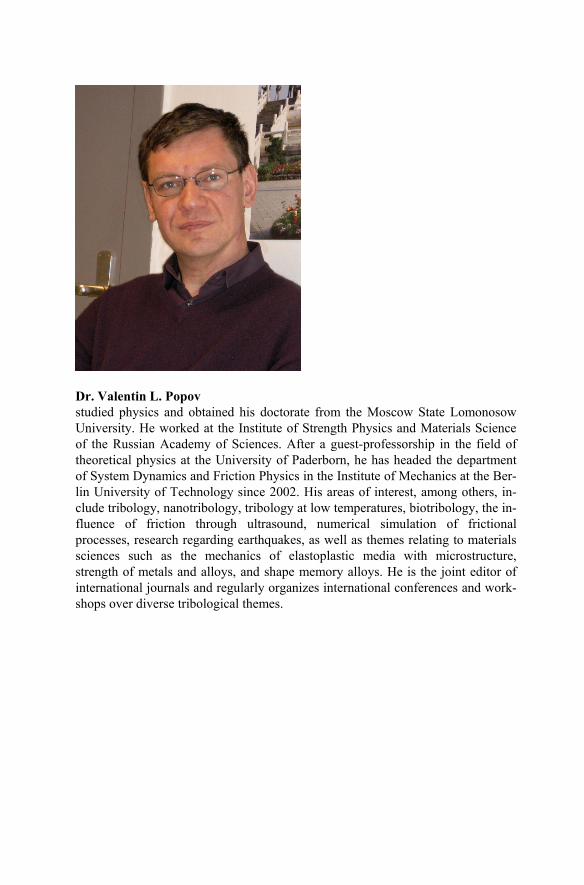
Dr. Valentin L. Popov studied physics and obtained his doctorate from the Moscow State Lomonosow University. He worked at the Institute of Strength Physics and Materials Science of the Russian Academy of Sciences. After a guest-professorship in the field of theoretical physics at the University of Paderborn, he has headed the department of System Dynamics and Friction Physics in the Institute of Mechanics at the Ber-lin University of Technology since 2002. His areas of interest, among others, in-clude tribology, nanotribology, tribology at low temperatures, biotribology, the in-fluence of friction through ultrasound, numerical simulation of frictional processes, research regarding earthquakes, as well as themes relating to materials sciences such as the mechanics of elastoplastic media with microstructure, strength of metals and alloys, and shape memory alloys. He is the joint editor of international journals and regularly organizes international conferences and work-shops over diverse tribological themes.

Preface to the English Edition The English edition of “Contact Mechanics and Friction” lying before you is, for the most part, the text of the 1st German edition (Springer Publishing, 2009). The book was expanded by the addition of a chapter on frictional problems in earth-quake research. Additionally, Chapter 15 was supplemented by a section on elasto-hydrodynamics. The problem sections of several chapters were enriched by the addition of new examples.
This book would not have been possible without the active support of J. Gray, who translated it from the German edition. I would like to thank Prof. G. G. Ko-charyan and Prof. S. Sobolev for discussions and critical comments on the chapter over earthquake dynamics. Dr. R. Heise made significant contributions to the de-velopment and correction of new problems. I would like to convey my affection-ate thanks to Dr. J. Starcevic for her complete support during the composition of this book. I want to thank Ms. Ch. Koll for her patience in creating figures and Dr. R. Heise, M. Popov, M. Heß, S. Kürscher, and B. Grzemba for their help in proof-reading.
Berlin, November 2009 V.L. Popov

Preface to the German Edition He who wishes to better understand the subject of Contact Mechanics and the Physics of Friction would quickly discover that there is almost no other field that is so interdisciplinary, exciting, and fascinating. It combines knowledge from fields such as the theories of elasticity and plasticity, viscoelasticity, materials sci-ence, fluid mechanics (including both Newtonian and non-Newtonian fluids), thermodynamics, electrodynamics, system dynamics, and many others. Contact Mechanics and the Physics of Friction have numerous applications ranging from measurement and system technologies on a nanoscale to the understanding of earthquakes and including the sheer overwhelming subject of industrial tribology. One who has studied and understands Contact Mechanics and the Physics of Fric-tion will have acquired a complete overview of the different methods that are used in the engineering sciences.
One goal of this book is to collect and clearly present, in one work, the most important aspects of this subject and how they relate to each other. Included in these aspects is, first, the entirety of traditional Contact Mechanics including ad-hesion and capillarity, then the theory of friction on a macro scale, lubrication, the foundations of modern nanotribology, system dynamical aspects of machines with friction (friction induced vibrations), friction related to elastomers, and wear. The interplay between these aspects can be very complicated in particular cases. In practical problems, different aspects are always presented in new ways. There is no simple recipe to solve tribological problems. The only universal recipe is that one must first understand the system from a tribological point of view. A goal of this book is to convey this understanding.
It is the solid belief of the author that the essential aspects of mechanical con-tacts and friction are often much easier than they appear. If one limits oneself to qualitative estimations, it is then possible to achieve an extensive qualitative un-derstanding of the countless facets of mechanical contacts and friction. Therefore, qualitative estimations are highly valued in this book.
In analytical calculations, we limit ourselves to a few classical examples which we can then take as building blocks and apply them to understand and solve a wealth of problems with real applications.
A large number of concrete tribological questions, especially if they deal with meticulous optimization of tribological systems, are not solvable in analytical form. This book also offers an overview of methods of Numerical Simulation for Contact Mechanics and Friction. One such method is then explained in detail, which permits a synthesis of several processes related to contact mechanics from different spatial ranges within a single model.
Even though this book is primarily a textbook, it can also serve as a reference for the foundations of this field. Many special cases are presented alongside the theoretical fundamentals with this goal in mind. These cases are presented as ex-ercises in their respective chapters. The solutions are provided for every exercise along with a short explanation and results.
x Preface to the German Edition
The basis of this textbook originates and is drafted from lectures that the author has conducted over Contact Mechanics and the Physics of Friction at the Berlin University of Technology, so that the material can be completed in its entirety in one or two semesters depending on the depth in which it is visited.
Thanks This book would not have been possible without the active support of my col-leagues. Several in the department of “System Dynamics and Frictional Physics,” from the Institute for Mechanics, have contributed to the development of the prac-tice exercises. For this, I thank Dr. M. Schargott, Dr. T. Geike, Mr. M. Hess, and Dr. J. Starcevic. I would like to express a heartfelt thanks to Dr. J. Starcevic for her complete support during the writing of this book as well as to Mr. M. Hess, who checked all of the equations and corrected the many errors. I thank Ms. Ch. Koll for her patience constructing figures as well as M. Popov and Dr. G. Putzar for their help with proofreading. I thank the Dean of Faculty V, Transportation and Machine Systems, for granting me a research semester, during which this book was completed.
Berlin, October 2008 V.L. Popov
Table of Contents 1 Introduction ........................................................................................................ 1
1.1 Contact and Friction Phenomena and their Applications............................. 1 1.2 History of Contact Mechanics and the Physics of Friction.......................... 3 1.3 Structure of the Book................................................................................... 7
2 Qualitative Treatment of Contact Problems – Normal Contact without Adhesion ................................................................................................................ 9
2.1 Material Properties..................................................................................... 10 2.2 Simple Contact Problems .......................................................................... 13 2.3 Estimation Method for Contacts with a Three-Dimensional, Elastic Continuum ....................................................................................................... 16 Problems .......................................................................................................... 20
3 Qualitative Treatment of Adhesive Contacts ................................................. 25 3.1 Physical Background ................................................................................. 26 3.2 Calculation of the Adhesive Force between Curved Surfaces ................... 30 3.3 Qualitative Estimation of the Adhesive Force between Elastic Bodies ..... 31 3.4 Influence of Roughness on Adhesion ........................................................ 33 3.5 Adhesive Tape ........................................................................................... 34 3.6 Supplementary Information about van der Waals Forces and Surface Energies ........................................................................................................... 35 Problems .......................................................................................................... 36
4 Capillary Forces ............................................................................................... 41 4.1 Surface Tension and Contact Angles......................................................... 41 4.2 Hysteresis of Contact Angles..................................................................... 45 4.3 Pressure and the Radius of Curvature........................................................ 45 4.4 Capillary Bridges ....................................................................................... 46 4.5 Capillary Force between a Rigid Plane and a Rigid Sphere ...................... 47 4.6 Liquids on Rough Surfaces........................................................................ 48 4.7 Capillary Forces and Tribology ................................................................. 49 Problems .......................................................................................................... 50
5 Rigorous Treatment of Contact Problems – Hertzian Contact .................... 55 5.1 Deformation of an Elastic Half-Space being Acted upon by Surface Forces .............................................................................................................. 56 5.2 Hertzian Contact Theory............................................................................ 59 5.3 Contact between Two Elastic Bodies with Curved Surfaces ..................... 60 5.4 Contact between a Rigid Cone-Shaped Indenter and an Elastic Half-Space ....................................................................................................... 63 5.5 Internal Stresses in Hertzian Contacts ....................................................... 64 Problems .......................................................................................................... 67
xii Table of Contents
6 Rigorous Treatment of Contact Problems – Adhesive Contact....................71 6.1 JKR-Theory ...............................................................................................72 Problems ..........................................................................................................77
7 Contact between Rough Surfaces....................................................................81 7.1 Model from Greenwood and Williamson ..................................................82 7.2 Plastic Deformation of Asperities ..............................................................88 7.3 Electrical Contacts .....................................................................................89 7.4 Thermal Contacts.......................................................................................92 7.5 Mechanical Stiffness of Contacts...............................................................93 7.6 Seals...........................................................................................................93 7.7 Roughness and Adhesion...........................................................................94 Problems ..........................................................................................................95
8 Tangential Contact Problems ........................................................................105 8.1 Deformation of an Elastic Half-Space being Acted upon by Tangential Forces ..........................................................................106 8.2 Deformation of an Elastic Half-Space being Acted upon by a Tangential Stress Distribution ...............................................................107 8.3 Tangential Contact Problems without Slip ..............................................109 8.4 Tangential Contact Problems Accounting for Slip ..................................110 8.5 Absence of Slip for a Rigid Cylindrical Indenter.....................................114 Problems ........................................................................................................114
9 Rolling Contact ...............................................................................................119 9.1 Qualitative Discussion of the Processes in a Rolling Contact..................120 9.2 Stress Distribution in a Stationary Rolling Contact .................................122 Problems ........................................................................................................128
10 Coulomb’s Law of Friction .........................................................................133 10.1 Introduction............................................................................................133 10.2 Static and Kinetic Friction .....................................................................134 10.3 Angle of Friction....................................................................................135 10.4 Dependence of the Coefficient of Friction on the Contact Time ...........136 10.5 Dependence of the Coefficient of Friction on the Normal Force...........137 10.6 Dependence of the Coefficient of Friction on Sliding Speed.................139 10.7 Dependence of the Coefficient of Friction on the Surface Roughness ..139 10.8 Coulomb’s View on the Origin of the Law of Friction..........................140 10.9 Theory of Bowden and Tabor ................................................................142 10.10 Dependence of the Coefficient of Friction on Temperature.................145 Problems ........................................................................................................146
11 The Prandtl-Tomlinson Model for Dry Friction........................................155 11.1 Introduction............................................................................................155 11.2 Basic Properties of the Prandtl-Tomlinson Model.................................157
...........
Table of Contents xiii
11.3 Elastic Instability ................................................................................... 161 11.4 Superlubricity ........................................................................................ 165 11.5 Nanomachines: Concepts for Micro and Nano-Actuators ..................... 166 Problems ........................................................................................................ 170
12 Frictionally Induced Vibrations.................................................................. 175 12.1 Frictional Instabilities at Decreasing Dependence of the Frictional Force on the Velocity .................................................................................... 176 12.2 Instability in a System with Distributed Elasticity................................. 178 12.3 Critical Damping and Optimal Suppression of Squeal .......................... 181 12.4 Active Suppression of Squeal ................................................................ 183 12.5 Strength Aspects during Squeal ............................................................. 185 12.6 Dependence of the Stability Criteria on the Stiffness of the System ..... 186 12.7 Sprag-Slip .............................................................................................. 191 Problems ........................................................................................................ 193
13 Thermal Effects in Contacts ....................................................................... 199 13.1 Introduction ........................................................................................... 200 13.2 Flash Temperatures in Micro-Contacts.................................................. 200 13.3 Thermo-Mechanical Instability.............................................................. 202 Problems ........................................................................................................ 203
14 Lubricated Systems ...................................................................................... 207 14.1 Flow between two parallel plates........................................................... 208 14.2 Hydrodynamic Lubrication.................................................................... 209 14.3 “Viscous Adhesion”............................................................................... 213 14.4 Rheology of Lubricants ......................................................................... 216 14.5 Boundary Layer Lubrication.................................................................. 218 14.6 Elastohydrodynamics............................................................................. 219 14.7 Solid Lubricants..................................................................................... 222 Problems ........................................................................................................ 223
15 Viscoelastic Properties of Elastomers ......................................................... 231 15.1 Introduction ........................................................................................... 231 15.2 Stress-Relaxation ................................................................................... 232 15.3 Complex, Frequency-Dependent Shear Moduli..................................... 234 15.4 Properties of Complex Moduli .............................................................. 236 15.5 Energy Dissipation in a Viscoelastic Material ....................................... 237 15.6 Measuring Complex Moduli.................................................................. 238 15.7 Rheological Models ............................................................................... 239 15.8 A Simple Rheological Model for Rubber (“Standard Model”).............. 242 15.9 Influence of Temperature on Rheological Properties ............................ 244 15.10 Master Curves...................................................................................... 245 15.11 Prony Series......................................................................................... 246 Problems ........................................................................................................ 250
xiv Table of Contents
16 Rubber Friction and Contact Mechanics of Rubber .................................255 16.1 Friction between an Elastomer and a Rigid Rough Surface...................255 16.2 Rolling Resistance .................................................................................261 16.3 Adhesive Contact with Elastomers ........................................................263 Problems ........................................................................................................265
17 Wear ..............................................................................................................271 17.1 Introduction............................................................................................271 17.2 Abrasive Wear .......................................................................................272 17.3 Adhesive Wear.......................................................................................275 17.4 Conditions for Low-Wear Friction ........................................................278 17.5 Wear as the Transportation of Material from the Friction Zone ............279 17.6 Wear of Elastomers................................................................................280 Problems ........................................................................................................283
18 Friction Under the Influence of Ultrasonic Vibrations .............................285 18.1 Influence of Ultrasonic Vibrations on Friction from a Macroscopic Point of View.................................................................................................286 18.2 Influence of Ultrasonic Vibrations on Friction from a Microscopic Point of View.................................................................................................291 18.3 Experimental Investigations of the Force of Static Friction as a Function of the Oscillation Amplitude...........................................................293 18.4 Experimental Investigations of Kinetic Friction as a Function of Oscillation Amplitude....................................................................................295 Problems ........................................................................................................297
19 Numerical Simulation Methods in Friction Physics ..................................301 19.1 Simulation Methods for Contact and Frictional Problems: An Overview..................................................................................................302
19.1.1 Many-Body Systems ......................................................................302 19.1.2 Finite Element Methods .................................................................303 19.1.3 Boundary Element Method.............................................................304 19.1.4 Particle Methods.............................................................................305
19.2 Reduction of Contact Problems from Three Dimensions to One Dimension......................................................................................................306 19.3 Contact in a Macroscopic Tribological System .....................................307 19.4 Reduction Method for a Multi-Contact Problem ...................................311 19.5 Dimension Reduction and Viscoelastic Properties ................................315 19.6 Representation of Stress in the Reduction Model ..................................316 19.7 The Calculation Procedure in the Framework of the Reduction Method...........................................................................................................317 19.8 Adhesion, Lubrication, Cavitation, and Plastic Deformations in the Framework of the Reduction Method ............................................................318 Problems ........................................................................................................318
Table of Contents xv
20 Earthquakes and Friction............................................................................ 323 20.1 Introduction ........................................................................................... 324 20.2 Quantification of Earthquakes ............................................................... 325
20.2.1 Gutenberg-Richter Law.................................................................. 326 20.3 Laws of Friction for Rocks .................................................................... 327 20.4 Stability during Sliding with Rate- and State-Dependent Friction ........ 331 20.5 Nucleation of Earthquakes and Post-Sliding ......................................... 334
20.7 Continuum Mechanics of Block Media and the Structure of Faults ...... 338 20.8 Is it Possible to Predict Earthquakes? .................................................... 342 Problems ........................................................................................................ 343
Appendix ............................................................................................................ 347
Further Reading ................................................................................................ 351
Figure Reference ............................................................................................... 357
Index................................................................................................................... 359
20.6 Foreshocks and Aftershocks .................................................................. 337
1 Introduction
1.1 Contact and Friction Phenomena and their Applications
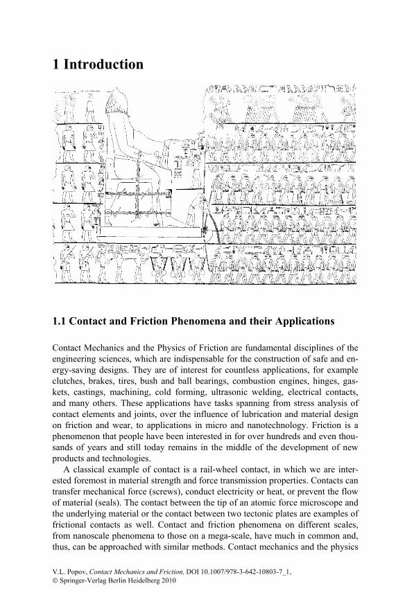
Contact Mechanics and the Physics of Friction are fundamental disciplines of the engineering sciences, which are indispensable for the construction of safe and en-ergy-saving designs. They are of interest for countless applications, for example clutches, brakes, tires, bush and ball bearings, combustion engines, hinges, gas-kets, castings, machining, cold forming, ultrasonic welding, electrical contacts, and many others. These applications have tasks spanning from stress analysis of contact elements and joints, over the influence of lubrication and material design on friction and wear, to applications in micro and nanotechnology. Friction is a phenomenon that people have been interested in for over hundreds and even thou-sands of years and still today remains in the middle of the development of new products and technologies.
A classical example of contact is a rail-wheel contact, in which we are inter-ested foremost in material strength and force transmission properties. Contacts can transfer mechanical force (screws), conduct electricity or heat, or prevent the flow of material (seals). The contact between the tip of an atomic force microscope and the underlying material or the contact between two tectonic plates are examples of frictional contacts as well. Contact and friction phenomena on different scales, from nanoscale phenomena to those on a mega-scale, have much in common and, thus, can be approached with similar methods. Contact mechanics and the physics
V.L. Popov, Contact Mechanics and Friction, DOI 10.1007/978-3-642-10803-7_1, © Springer-Verlag Berlin Heidelberg 2010
2 1 Introduction
of friction has proven to be an enormous field in modern research and technology, stretching from the movement of motor proteins and muscular contractions to earthquake dynamics as well as including the enormous field of industrial tribol-ogy.
Friction leads to energy dissipation and in micro-contacts, where extreme stress is present, to micro-fractures and surface wear. We often try to minimize friction during design in an attempt to save energy. There are, however, many situations in which friction is necessary. Without friction, we cannot enjoy violin music or even walk or drive. There are countless instances, in which friction should be maxi-mized instead of minimized, for example between tires and the road during brak-ing. Also, wear must not always be minimized. Fast and controllable abrasive techniques can actually form the basis for many technological processes, (e.g., grinding, polishing, and sandblasting.)
Friction and wear are very closely connected with the phenomenon of adhe-sion. For adhesion it is important to know if a close contact can be created be-tween two bodies. While adhesion does not play a considerable role on a large-scale in the contact between two “hard bodies” such as metal or wood, in instances in which one of the bodies in contact is soft, the role of adhesion becomes very noticeable and can be taken advantage of in many applications. One can also learn much from contact mechanics for the use of adhesives. In micro-technology, ad-hesion gains even greater importance. Friction and adhesive forces on a micro-scale present a real problem and have been termed “sticktion” (sticking and fric-tion).
Another phenomenon, which is similar to adhesion and will be discussed in this book, is capillary force, which appears in the presence of low quantities of fluid. In very precise mechanisms such as clocks, the moisture contained in the air can cause capillary forces, disturbing the exactness of such mechanisms. Capillary forces can also be used, however, to control the flow of a lubricant to an area of friction.
In a book about contact and friction one cannot silently pass over the closely related sound-phenomena. Brakes, wheel-track contact, and bearings do not only dissipate energy and material. They often squeak and squeal unpleasantly or even with such intensity as to be damaging to one’s hearing. Noise caused by technical systems is a central problem today in many engineering solutions. Friction in-duced vibrations are closely related to the properties of frictional forces and are likewise a subject of this book.
If we had to measure the importance of a tribological field in terms of the amount of money that has been invested in it, lubrication technology would defi-nitely take first place. Unfortunately, it is not possible to grant lubrication a corre-spondingly large section in this book. The fundamentals of hydrodynamic and elasto-hydrodynamic lubrication, however, are of course included.
The subject of contact mechanics and friction is ultimately about our ability to control friction, adhesion, and wear and to mould them to our wishes. For that, a detailed understanding of the dependency of contact, friction, and wear phenom-ena on the materials and system properties is necessary.
1.2 History of Contact Mechanics and the Physics of Friction 3
1.2 History of Contact Mechanics and the Physics of Friction
A first impression of tribological applications and their importance can be con-veyed by its history. The term “Tribology” was suggested by Peter Jost in May of 1966 as a name for the research and engineering subject which occupies itself with contact, friction, and wear. Except for the name, tribology itself is ancient. Its be-ginning is lost in the far reaches of history. The creation of fire through frictional heating, the discovery of the wheel and simple bushings, and the use of fluids to reduce frictional forces and wear were all “tribological inventions” that were al-ready known thousands of years before Christ. In our short overview of the history of tribology, we will jump to the developments that took place during the Renais-sance and begin with the contributions of Leonardo da Vinci.
In his Codex-Madrid I (1495), da Vinci describes the ball-bearing, which he invented, and the composition of a low-friction alloy as well his experimental ex-amination of friction and wear phenomena. He was the first engineer who persis-tently and quantitatively formulated the laws of friction. He arrived at the conclu-sion that can be summarized in today’s language as two fundamental Laws of Friction:
1. The frictional force is proportional to the normal force, or load. 2. The frictional force is independent of the contact surface area. Da Vinci was, de facto, the first to introduce the term coefficient of friction and
to experimentally determine its typical value of ¼. As so often happens in the history of science, these results were forgotten and
around 200 years later, rediscovered by the French physicist Guillaume Amontons (1699). The proportionality of the frictional force to the normal force is, therefore, known as “Amontons’ Law.”
Leonard Euler occupied himself with the mathematical point of view of friction as well as the experimental. He introduced the differentiation between static fric-tional forces and kinetic frictional forces and solved the problem of rope friction, probably the first contact problem to be analytically solved in history (1750). He was the first to lay the foundations of the mathematical way of dealing with the law of dry friction and in this way promoted further development. We have him to thank for the symbol μ as the coefficient of friction. Euler worked with the idea that friction originates from the interlocking between small triangular irregularities and that the frictional coefficient is equal to the gradient of these irregularities. This understanding survived, in different variations, for a hundred years and is also used today as the “Tomlinson Model” in connection with friction on an atomic scale.
An outstanding and still relevant contribution to the examination of dry friction was achieved by the French engineer Charles Augustin Coulomb. The law of dry friction deservingly carries his name. Coulomb confirmed Amontons’ results and established that sliding friction is independent of the sliding speed in a first order approximation. He undertook a very exact quantitative examination of dry friction
4 1 Introduction
between solid bodies in relation to the pairing of materials, surface composition, lubrication, sliding speed, resting time for static friction, atmospheric humidity, and temperature. Only since the appearance of his book “Theory of Simple Ma-chines,” (1781) could the differentiation between kinetic and static friction be quantitatively substantiated and established. Coulomb used the same idea of the origin of friction as Euler, but added another contribution to friction that we would now call the adhesion contribution. It was likewise Coulomb who established de-viations from the known simple law of friction. He found out, for example, that the static force grows with the amount of time the object has remained stationary. For his examinations, Coulomb was well ahead of his time. His book contained practically everything that eventually became the original branches of tribology. Even the name of the measuring instrument, the tribometer, stems from Coulomb.
Examinations of rolling friction have not played as a prominent role in history as sliding friction, probably because rolling friction is much smaller in magnitude than sliding friction and, therefore, less annoying. The first ideas of the nature of rolling friction for rolling on plastically deformable bodies, of which the most im-portant elements are still considered correct, come from Robert Hooke (1685). A heated discussion between Morin and Dupuit that took place in 1841-42 over the form of the law of rolling friction showed that the nature of the friction was very dependent on the material and loading parameters. According to Morin the rolling friction should be inversely proportional to the radius of the rolling body, but ac-cording to Dupuit it should be inversely proportional to the square root of the ra-dius. From today’s point of view both statements are limitedly correct under dif-fering conditions.
Osborne Reynolds was the first to experimentally examine the details of the events happening in the contact area during rolling contact and established that on a driven wheel, there are always areas in which the two bodies are in no-slip con-tact and areas where slipping takes place. It was the first attempt to put tribologi-cal contact underneath a magnifying glass and at the same time the end of the strict differentiation between static friction and kinetic friction. Reynolds ac-counted for the energy loss during rolling with the existence of partial sliding. A quantitative theory could later be achieved by Carter (1926) only after the founda-tions of contact mechanics were laid by Hertz.
Humans have lubricated mechanical contacts for hundreds of years in order to decrease friction, but it was rising industrial demands that coerced researchers ex-perimentally and theoretically to grapple with lubrication. In 1883 N. Petrov per-formed his experimental examinations of journal bearings and formulated the most important laws of hydrodynamic lubrication. In 1886 Reynolds published his the-ory of hydrodynamic lubrication. The “Reynolds Equation,” which he developed, established the basis for calculations in hydrodynamically lubricated systems. Ac-cording to the hydrodynamic lubrication theory, the coefficient of friction has an the order of magnitude of /h Lμ ≈ , where h is the thickness of the lubricating film and L is the length of the tribological contact. This holds true so long as the surfaces do not come so close to one another that the thickness of the lubrication
1.2 History of Contact Mechanics and the Physics of Friction 5
film becomes comparable to the roughness of the two surfaces. Such a system would then fall into the realm of mixed friction which was extensively examined by Stribeck (1902). The dependence of the frictional force on the sliding speed with a characteristic minimum is named the Stribeck-Curve.
Other conditions can come into play with even greater loads or insufficient lu-brication in which only a few molecular layers of lubricant remain between the bodies in contact. The properties of this boundary lubrication were investigated by Hardy (1919-22). He showed that only molecular layer of grease drastically influ-enced the frictional forces and wear of the two bodies. Hardy measured the de-pendence of frictional forces on the molecular weight of the lubricant and the sur-faces of the metals and also recognized that the lubricant adheres to the metal surfaces. The decreased friction is owed to the interaction of the polymer-molecules of the lubricant, which is today sometimes called a “grafted liquid.”
A further advance in our understanding of contact mechanics, as well as dry friction, in the middle of the twentieth century is bound to two names: Bowden and Tabor. They were the first to advise the importance of the roughness of the surfaces of the bodies in contact. Because of this roughness, the real contact area between the two bodies is typically orders of magnitude smaller than the apparent contact area. This understanding abruptly changed the direction of many tribologi-cal examinations and again brought about Coulomb’s old idea of adhesion being a possible mechanism of friction. In 1949, Bowden and Tabor proposed a concept which suggested that the origin of sliding friction between clean, metallic surfaces is explained through the formation and shearing of cold weld junctions. According to this understanding, the coefficient of friction is approximately equal to the ratio of critical shear stress to hardness and must be around 1/6 in isotropic, plastic ma-terials. For many non-lubricated metallic pairings (e.g. steel with steel, steel with bronze, steel with iron, etc.), the coefficient of friction actually does have a value on the order of 0.16μ ∼ .
The works of Bowden and Tabor triggered an entirely new line of theory of contact mechanics regarding rough surfaces. As pioneering work in this subject we must mention the works of Archard (1957), who concluded that the contact area between rough elastic surfaces is approximately proportional to the normal force. Further important contributions were made by Greenwood and Williamson (1966), Bush (1975), and Persson (2002). The main result of these examinations is that the real contact areas of rough surfaces are approximately proportional to the normal force, while the conditions in individual micro-contacts (pressure, size of micro-contact) depend only weakly on the normal force.
With the development of the automobile industry, along with increasing speeds and power, rubber friction has gained a technical importance. The understanding of the frictional mechanisms of elastomers, and above all, the conclusion that the friction of elastomers is connected with the dissipation of energy through defor-mation of the material and consequently with its rheology, a fact that is generally accepted today, can be owed to the classical works of Grosch (1962).
6 1 Introduction
Contact mechanics definitely forms the foundations for today’s understanding of frictional phenomena. In history, frictional phenomena were earlier and more fundamentally examined in comparison to pure contact mechanical aspects. The development of the railroad was most certainly a catalyst for interest in exact cal-culations of stress values, because in wheel-rail contact the stresses can reach the maximum loading capacity for steel.
Classical contact mechanics is associated with Heinrich Hertz above all others. In 1882, Hertz solved the problem of contact between two elastic bodies with curved surfaces. This classical result forms a basis for contact mechanics even to-day. It took almost a century until Johnson, Kendall, and Roberts found a similar solution for adhesive contact (JKR-Theory). This may come from the general ob-servation that solid bodies do not adhere to one another. Only after the develop-ment of micro-technology, did engineers run into the problem of adhesion. Almost at the same time, Derjagin, Müller, and Toporov developed another theory of ad-hesive contact. After an initially fervid discussion, Tabor realized that both theo-ries are correct limiting cases for the general problem.
It is astonishing that wear phenomena, despite their overt significance, were studied seemingly late. The reason for this delay may lie in the fact that the lead-ing cause of wear is through the interactions of micro-contacts, which became an object of tribological research only after the work of Bowden and Tabor. The law of abrasive wear, which states that wear is proportional to load and sliding dis-tance and inversely proportional to hardness of softer contact partners, was dis-covered by M. Kruschov (1956) through experimental examination and later also confirmed by Archard (1966). The examinations of the law of adhesive wear, as with abrasive wear, are tied to Tabor and Rabinowicz. Despite these studies, wear mechanisms, especially under conditions in which very little wear takes place, are still today some of the least understood tribological phenomena.
Since the last decade of the twentieth century, contact mechanics has experi-enced a rebirth. The development of experimental methods for investigating fric-tional processes on the atomic scale (atomic force microscope, friction force mi-croscope, quartz-crystal microbalance, surface force apparatus) and numerical simulation methods have provoked a sudden growth during these years in the number of research activities in the field of friction between solid bodies. Also, the development of micro-technology essentially accounts for the largest pursuit in contact mechanics and the physics of friction. Experimentalists were offered the ability to examine well defined systems with stringently controlled conditions, for instance, the ability to control the thickness of a layer of lubrication or the relative displacement between two fixed surfaces with a resolution on the atomic level. There is, however, a gap between classical tribology and nanotribology that has yet to be closed.

1.3 Structure of the Book 7
1.3 Structure of the Book
Contact and friction always go hand in hand and are interlaced in many ways in real systems. In our theoretical treatment, we must first separate them. We begin our investigation of contact and frictional phenomena with contact mechanics. This, in turn, begins with a qualitative analysis, which provides us with a simple, but comprehensive understanding of the respective phenomena. Afterwards, we will delve into the rigorous treatment of contact problems and subsequently move on to frictional phenomena, lubrication, and wear.
2 Qualitative Treatment of Contact Problems – Normal Contact without Adhesion
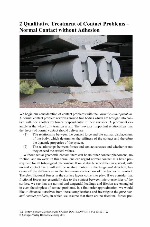
We begin our consideration of contact problems with the normal contact problem. A normal contact problem revolves around two bodies which are brought into con-tact with one another by forces perpendicular to their surfaces. A prominent ex-ample is the wheel of a train on a rail. The two most important relationships that the theory of normal contact should deliver are:
(1) The relationship between the contact force and the normal displacement of the body, which determines the stiffness of the contact and therefore the dynamic properties of the system.
(2) The relationships between forces and contact stresses and whether or not they exceed the critical values.
Without actual geometric contact there can be no other contact phenomena, no friction, and no wear. In this sense, one can regard normal contact as a basic pre-requisite for all tribological phenomena. It must also be noted that, in general, with normal contact there will still be relative motion in the tangential direction, be-cause of the differences in the transverse contraction of the bodies in contact. Thereby, frictional forces in the surface layers come into play. If we consider that frictional forces are essentially due to the contact between micro-asperities of the surface, we see that the normal and tangential loadings and friction are entangled in even the simplest of contact problems. In a first order approximation, we would like to distance ourselves from these complications and investigate the pure nor-mal contact problem, in which we assume that there are no frictional forces pre-
V.L. Popov, Contact Mechanics and Friction, DOI 10.1007/978-3-642-10803-7_2, © Springer-Verlag Berlin Heidelberg 2010
10 2 Qualitative Treatment of Contact Problems – Normal Contact without Adhesion
sent in the contact area. Also, the always present attractive force, adhesion, will be neglected for the time being.
An analytical or numerical analysis of contact problems is even in the simplest of cases very complicated. A qualitative understanding of contact problems, on the other hand, is obtainable with very simple resources. Therefore, we begin our dis-cussion with methods of qualitative analysis of contact phenomena, which can also be used in many cases for dependable, quantitative estimations. A rigorous treatment of the most important classical contact problems continues in the fol-lowing chapters. We will investigate a series of contact problems between bodies of different forms, which can often be used as building blocks for more compli-cated contact problems.
2.1 Material Properties
This book assumes that the reader is acquainted with the fundamentals of elasticity theory. In this chapter, we will summarize only definitions from the most impor-tant material parameters that have bearing on the qualitative investigation of con-tact mechanical questions. This summary does not replace the general definitions and equations of elasticity theory and plasticity theory.
(a) Elastic Properties. In a uniaxial tensile test, a slender beam with a constant cross-sectional area A and an initial length 0l is stretched by Δl . The ratio of the tensile force to the cross-sectional area is the tensile stress
σ =FA
. (2.1)
The ratio of the change in length to the initial length is the tensile strain or defor-mation:
0
ε Δ=
ll
. (2.2)
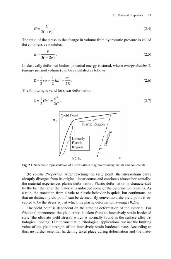
A typical stress-strain diagram for many metals and non-metals is presented in Fig. 2.1. For small stresses, the stress is proportional to the deformation
σ ε= E . (2.3)
The proportionality coefficient E is the modulus of elasticity of the material. The elongation is related to the cross-sectional contraction, which is characterized by Poisson’s Ratio (or transverse contraction coefficient) ν . An incompressible ma-terial has a Poisson’s ratio of 1/ 2ν = .
Similarly, the shear modulus is defined as the proportionality coefficient be-tween the shear stress and the resulting shear deformation. The shear modulus is related to the elasticity coefficient and Poisson’s ratio according to
2.1 Material Properties 11
2(1 )ν
=+EG . (2.4)
The ratio of the stress to the change in volume from hydrostatic pressure is called the compressive modulus:
3(1 2 )ν
=−EK . (2.5)
In elastically deformed bodies, potential energy is stored, whose energy density E (energy per unit volume) can be calculated as follows:
2
21 12 2 2
σεσ ε= = =E EE
. (2.6)
The following is valid for shear deformation:
2
212 2
σε= =E GG
. (2.7)
Plastic Region
0,2 %
LinearlyElasticRegion U
nlo
adin
g
�c
Yield Point
� Fig. 2.1 Schematic representation of a stress-strain diagram for many metals and non-metals.
(b) Plastic Properties. After reaching the yield point, the stress-strain curve abruptly diverges from its original linear course and continues almost horizontally: the material experiences plastic deformation. Plastic deformation is characterized by the fact that after the material is unloaded some of the deformation remains. As a rule, the transition from elastic to plastic behavior is quick, but continuous, so that no distinct “yield point” can be defined. By convention, the yield point is ac-cepted to be the stress σ c , at which the plastic deformation averages 0.2%.
The yield point is dependent on the state of deformation of the material. For frictional phenomena the yield stress is taken from an intensively strain hardened state (the ultimate yield stress), which is normally found in the surface after tri-bological loading. That means that in tribological applications, we use the limiting value of the yield strength of the intensively strain hardened state. According to this, no further essential hardening takes place during deformation and the mate-
12 2 Qualitative Treatment of Contact Problems – Normal Contact without Adhesion
rial can be considered as if it were elastic perfectly-plastic in a first order ap-proximation.
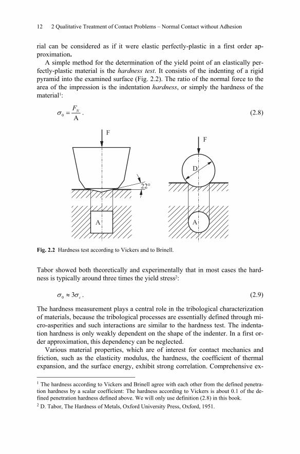
A simple method for the determination of the yield point of an elastically per-fectly-plastic material is the hardness test. It consists of the indenting of a rigid pyramid into the examined surface (Fig. 2.2). The ratio of the normal force to the area of the impression is the indentation hardness, or simply the hardness of the material1:
0 Aσ = NF
. (2.8)
F
22°
F
D
A A
Fig. 2.2 Hardness test according to Vickers and to Brinell.
Tabor showed both theoretically and experimentally that in most cases the hard-ness is typically around three times the yield stress2:
0 3σ σ≈ c . (2.9)
The hardness measurement plays a central role in the tribological characterization of materials, because the tribological processes are essentially defined through mi-cro-asperities and such interactions are similar to the hardness test. The indenta-tion hardness is only weakly dependent on the shape of the indenter. In a first or-der approximation, this dependency can be neglected.
Various material properties, which are of interest for contact mechanics and friction, such as the elasticity modulus, the hardness, the coefficient of thermal expansion, and the surface energy, exhibit strong correlation. Comprehensive ex- 1 The hardness according to Vickers and Brinell agree with each other from the defined penetra-tion hardness by a scalar coefficient: The hardness according to Vickers is about 0.1 of the de-fined penetration hardness defined above. We will only use definition (2.8) in this book. 2 D. Tabor, The Hardness of Metals, Oxford University Press, Oxford, 1951.
2.2 Simple Contact Problems 13
perimental data of these correlations can be found in the excellent book by Ernest Rabinowicz “Friction and Wear of Materials3.”
2.2 Simple Contact Problems
The simplest of contact problems are those in which the deformations are unambi-guously determined by the geometry. This is the case in the four following exam-ples.
(1) Parallelepiped
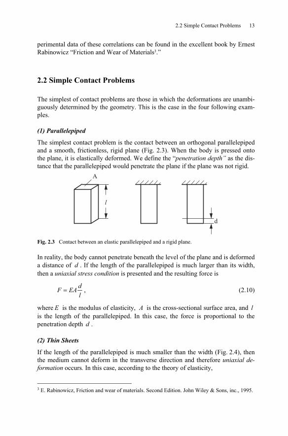
The simplest contact problem is the contact between an orthogonal parallelepiped and a smooth, frictionless, rigid plane (Fig. 2.3). When the body is pressed onto the plane, it is elastically deformed. We define the “penetration depth” as the dis-tance that the parallelepiped would penetrate the plane if the plane was not rigid.
l
A
d
Fig. 2.3 Contact between an elastic parallelepiped and a rigid plane.
In reality, the body cannot penetrate beneath the level of the plane and is deformed a distance of d . If the length of the parallelepiped is much larger than its width, then a uniaxial stress condition is presented and the resulting force is
=dF EAl
, (2.10)
where E is the modulus of elasticity, A is the cross-sectional surface area, and l is the length of the parallelepiped. In this case, the force is proportional to the penetration depth d .
(2) Thin Sheets
If the length of the parallelepiped is much smaller than the width (Fig. 2.4), then the medium cannot deform in the transverse direction and therefore uniaxial de-formation occurs. In this case, according to the theory of elasticity,
3 E. Rabinowicz, Friction and wear of materials. Second Edition. John Wiley & Sons, inc., 1995.
14 2 Qualitative Treatment of Contact Problems – Normal Contact without Adhesion
=dF EAl
, (2.11)
with
(1 )(1 )(1 2 )
νν ν
−=
+ −EE . (2.12)
for metals 1/ 3ν ≈ , so that 1.5E E≈ . For elastomers, which can be viewed as almost incompressible materials, 1 / 2ν ≈ and the modulus for one-sided com-pression ≈E K is much larger than E (around 3 orders of magnitude):
, for elastomersE K E≈ . (2.13)
d
Fig. 2.4 Contact between a thin elastic sheet and a rigid plane.
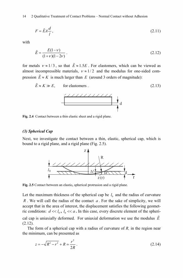
(3) Spherical Cap
Next, we investigate the contact between a thin, elastic, spherical cap, which is bound to a rigid plane, and a rigid plane (Fig. 2.5).
ra
z (r)
�l d
Fig. 2.5 Contact between an elastic, spherical protrusion and a rigid plane.
Let the maximum thickness of the spherical cap be 0l and the radius of curvature R . We will call the radius of the contact a . For the sake of simplicity, we will accept that in the area of interest, the displacement satisfies the following geomet-ric conditions: 0<<d l , 0 <<l a . In this case, every discrete element of the spheri-
cal cap is uniaxially deformed. For uniaxial deformation we use the modulus E (2.12).
The form of a spherical cap with a radius of curvature of R, in the region near the minimum, can be presented as
2
2 2
2= − − +
rz R r RR
. (2.14)
2.2 Simple Contact Problems 15
It can be easily seen in Fig. 2.5 that the relationship between the radius of the con-tact area a and penetration depth d is given by the expression 2 / 2=d a R . From this, we can solve for the contact radius
2=a Rd . (2.15)
The vertical displacement of the surface in terms of the coordinate r is 2 / 2Δ = −l d r R . The corresponding elastic deformation can be calculated using
2
0 0
/ 2( )ε Δ −= =
l d r Rrl l
. (2.16)
The equations of stress and total force in the contact area eventually yield:
( ) ( )σ ε=r E r , 2
2
0 00
/ 22 d ππ⎛ ⎞−
= =⎜ ⎟⎝ ⎠
∫a d r RF E r r E Rd
l l. (2.17)
In this case, the contact force is proportional to the square of the penetration depth. The greatest stress (in the center of the contact area) is
1/ 2
0 0
(0)σπ⎛ ⎞
= = ⎜ ⎟⎝ ⎠
d EFEl l R
. (2.18)
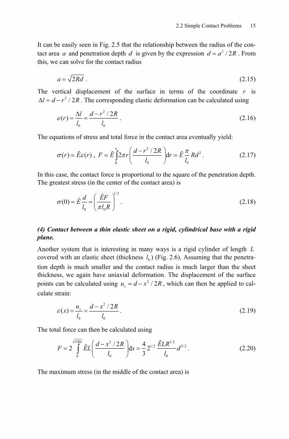
(4) Contact between a thin elastic sheet on a rigid, cylindrical base with a rigid plane.
Another system that is interesting in many ways is a rigid cylinder of length L covered with an elastic sheet (thickness 0l ) (Fig. 2.6). Assuming that the penetra-tion depth is much smaller and the contact radius is much larger than the sheet thickness, we again have uniaxial deformation. The displacement of the surface points can be calculated using 2 / 2= −zu d x R , which can then be applied to cal-culate strain:
2
0 0
/ 2( )ε −= =zu d x Rx
l l. (2.19)
The total force can then be calculated using
2 2 1/ 2
1/ 2 3/2
0 00
/ 2 42 d 23
⎛ ⎞−= =⎜ ⎟
⎝ ⎠∫Rd d x R ELRF EL x d
l l. (2.20)
The maximum stress (in the middle of the contact area) is
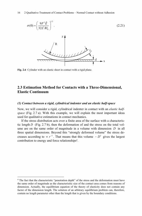
16 2 Qualitative Treatment of Contact Problems – Normal Contact without Adhesion
1/32
20
9(0)32
σ⎛ ⎞
= ⎜ ⎟⎝ ⎠
F EL Rl
. (2.21)
d
Fig. 2.6 Cylinder with an elastic sheet in contact with a rigid plane.
2.3 Estimation Method for Contacts with a Three-Dimensional, Elastic Continuum
(1) Contact between a rigid, cylindrical indenter and an elastic half-space
Now, we will consider a rigid, cylindrical indenter in contact with an elastic half-space (Fig. 2.7 a). With this example, we will explain the most important ideas used for qualitative estimations in contact mechanics.
If the stress distribution acts over a finite area of the surface with a characteris-tic length D (Fig. 2.7 b), then the deformation of and the stress on the total vol-ume are on the same order of magnitude in a volume with dimension D in all three spatial dimensions. Beyond this “strongly deformed volume” the stress de-creases according to 2−∝ r . That means that this volume 3∼ D gives the largest contribution to energy and force relationships4.
4 The fact that the characteristic “penetration depth” of the stress and the deformation must have the same order of magnitude as the characterisitic size of the contact area comes from reasons of dimension. Actually, the equilibrium equation of the theory of elasticity does not contain any factor of the dimension length. The solution of an arbitrary equilibrium problem can, therefore, contain no length parameter other than the length that is given by the boundary conditions.
2.3 Estimation Method for Contacts with a Three-Dimensional, Elastic Continuum 17
a�
D
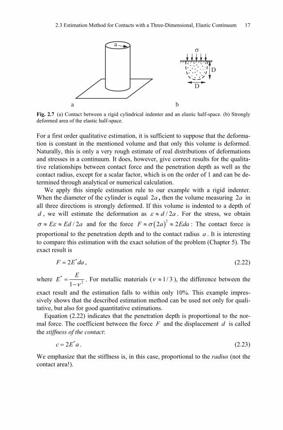
a b
D
Fig. 2.7 (a) Contact between a rigid cylindrical indenter and an elastic half-space. (b) Strongly deformed area of the elastic half-space.
For a first order qualitative estimation, it is sufficient to suppose that the deforma-tion is constant in the mentioned volume and that only this volume is deformed. Naturally, this is only a very rough estimate of real distributions of deformations and stresses in a continuum. It does, however, give correct results for the qualita-tive relationships between contact force and the penetration depth as well as the contact radius, except for a scalar factor, which is on the order of 1 and can be de-termined through analytical or numerical calculation.
We apply this simple estimation rule to our example with a rigid indenter. When the diameter of the cylinder is equal 2a , then the volume measuring 2a in all three directions is strongly deformed. If this volume is indented to a depth of d , we will estimate the deformation as / 2ε ≈ d a . For the stress, we obtain
/ 2E Ed aσ ε≈ ≈ and for the force ( )22 2σ≈ ≈F a Eda : The contact force is proportional to the penetration depth and to the contact radius a . It is interesting to compare this estimation with the exact solution of the problem (Chapter 5). The exact result is
*2=F E da , (2.22)
where *21 ν
=−EE . For metallic materials ( 1/ 3ν ≈ ), the difference between the
exact result and the estimation falls to within only 10%. This example impres-sively shows that the described estimation method can be used not only for quali-tative, but also for good quantitative estimations.
Equation (2.22) indicates that the penetration depth is proportional to the nor-mal force. The coefficient between the force F and the displacement d is called the stiffness of the contact:
*2=c E a . (2.23)
We emphasize that the stiffness is, in this case, proportional to the radius (not the contact area!).
18 2 Qualitative Treatment of Contact Problems – Normal Contact without Adhesion
(2) Contact between a rigid sphere and an elastic half-space
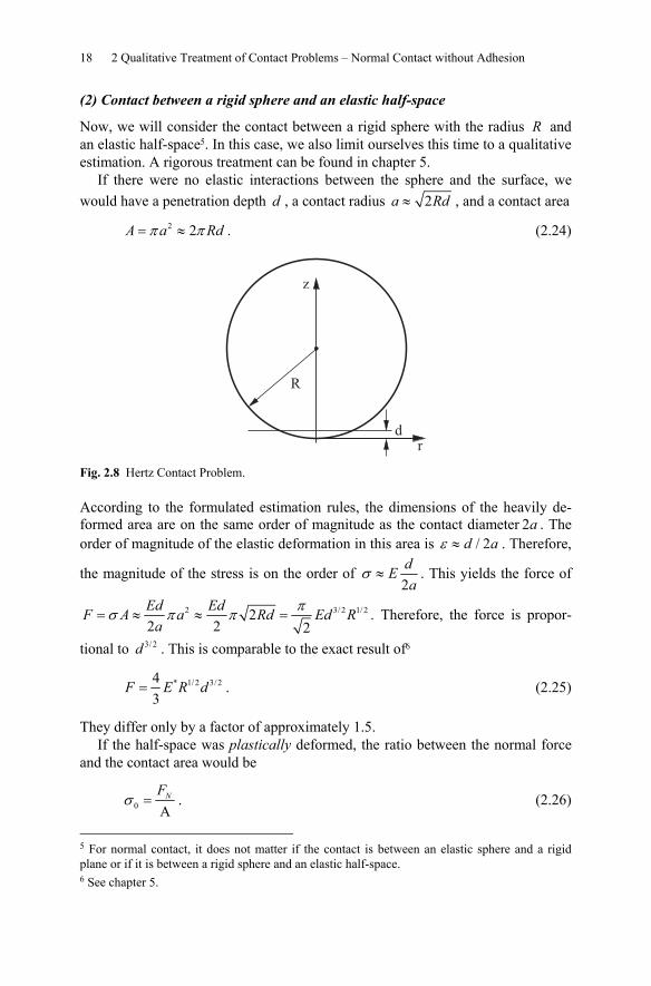
Now, we will consider the contact between a rigid sphere with the radius R and an elastic half-space5. In this case, we also limit ourselves this time to a qualitative estimation. A rigorous treatment can be found in chapter 5.
If there were no elastic interactions between the sphere and the surface, we would have a penetration depth d , a contact radius 2≈a Rd , and a contact area
2 2π π= ≈A a Rd . (2.24)
R
z
rd
Fig. 2.8 Hertz Contact Problem.
According to the formulated estimation rules, the dimensions of the heavily de-formed area are on the same order of magnitude as the contact diameter 2a . The order of magnitude of the elastic deformation in this area is / 2ε ≈ d a . Therefore,
the magnitude of the stress is on the order of 2
σ ≈dEa
. This yields the force of
2 3/ 2 1/222 2 2
πσ π π= ≈ ≈ =Ed EdF A a Rd Ed R
a. Therefore, the force is propor-
tional to 3/ 2d . This is comparable to the exact result of6
* 1/2 3/243
=F E R d . (2.25)
They differ only by a factor of approximately 1.5. If the half-space was plastically deformed, the ratio between the normal force
and the contact area would be
0 Aσ = NF
. (2.26)
5 For normal contact, it does not matter if the contact is between an elastic sphere and a rigid plane or if it is between a rigid sphere and an elastic half-space. 6 See chapter 5.
2.3 Estimation Method for Contacts with a Three-Dimensional, Elastic Continuum 19
Using Equation (2.24) results in
02πσ=NF Rd . (2.27)
In the plastic area, the force is proportional to the depth of the indentation. The average stress remains the same and is equal to the hardness of the material.
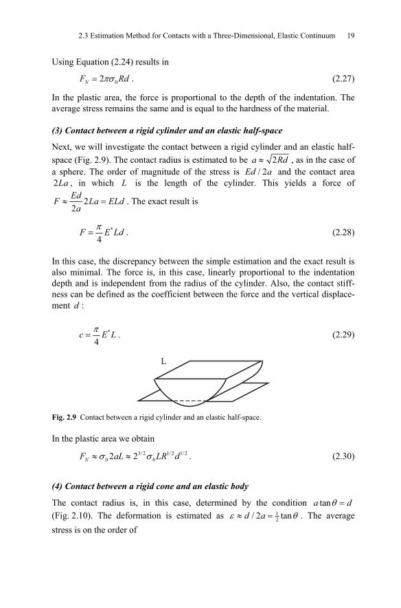
(3) Contact between a rigid cylinder and an elastic half-space
Next, we will investigate the contact between a rigid cylinder and an elastic half-space (Fig. 2.9). The contact radius is estimated to be 2≈a Rd , as in the case of a sphere. The order of magnitude of the stress is / 2Ed a and the contact area 2La , in which L is the length of the cylinder. This yields a force of
22
≈ =EdF La ELd
a. The exact result is
*
4π
=F E Ld . (2.28)
In this case, the discrepancy between the simple estimation and the exact result is also minimal. The force is, in this case, linearly proportional to the indentation depth and is independent from the radius of the cylinder. Also, the contact stiff-ness can be defined as the coefficient between the force and the vertical displace-ment d :
*
4π
=c E L . (2.29)
L
Fig. 2.9 Contact between a rigid cylinder and an elastic half-space.
In the plastic area we obtain
3/2 1/2 1/20 02 2σ σ≈ ≈NF aL LR d . (2.30)
(4) Contact between a rigid cone and an elastic body
The contact radius is, in this case, determined by the condition tanθ =a d (Fig. 2.10). The deformation is estimated as 1
2/ 2 tanε θ≈ =d a . The average stress is on the order of
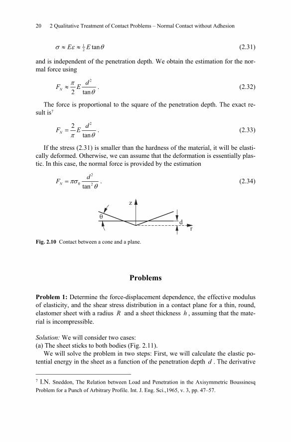
20 2 Qualitative Treatment of Contact Problems – Normal Contact without Adhesion
12 tanσ ε θ≈ ≈E E (2.31)
and is independent of the penetration depth. We obtain the estimation for the nor-mal force using
2
2 tanπ
θ≈N
dF E . (2.32)
The force is proportional to the square of the penetration depth. The exact re-sult is7
22
tanNdF E
π θ= . (2.33)
If the stress (2.31) is smaller than the hardness of the material, it will be elasti-cally deformed. Otherwise, we can assume that the deformation is essentially plas-tic. In this case, the normal force is provided by the estimation
2
0 2tanπσ
θ=N
dF . (2.34)
z
d�
r Fig. 2.10 Contact between a cone and a plane.
Problems
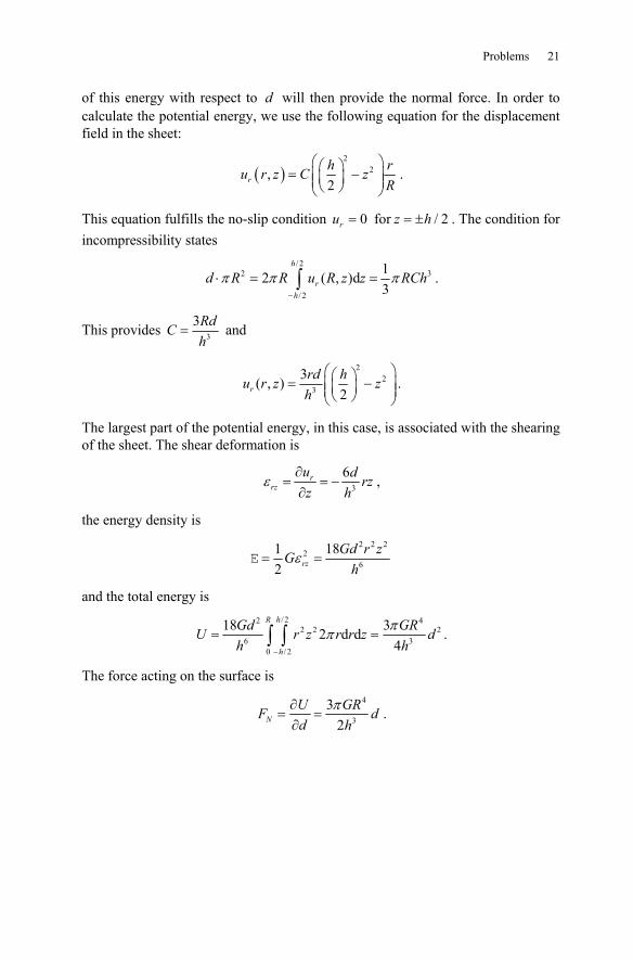
Problem 1: Determine the force-displacement dependence, the effective modulus of elasticity, and the shear stress distribution in a contact plane for a thin, round, elastomer sheet with a radius R and a sheet thickness h , assuming that the mate-rial is incompressible.
Solution: We will consider two cases: (a) The sheet sticks to both bodies (Fig. 2.11).
We will solve the problem in two steps: First, we will calculate the elastic po-tential energy in the sheet as a function of the penetration depth d . The derivative
7 I.N. Sneddon, The Relation between Load and Penetration in the Axisymmetric Boussinesq Problem for a Punch of Arbitrary Profile. Int. J. Eng. Sci.,1965, v. 3, pp. 47–57.
Problems 21
of this energy with respect to d will then provide the normal force. In order to calculate the potential energy, we use the following equation for the displacement field in the sheet:
( )2
2,2rh ru r z C z
R⎛ ⎞⎛ ⎞= −⎜ ⎟⎜ ⎟⎜ ⎟⎝ ⎠⎝ ⎠
.
This equation fulfills the no-slip condition 0=ru for / 2= ±z h . The condition for incompressibility states
/ 22 3
/ 2
12 ( , )d3
π π π−
⋅ = =∫h
rh
d R R u R z z RCh .
This provides 3
3=
RdCh
and
22
3
3( , )2
⎛ ⎞⎛ ⎞= −⎜ ⎟⎜ ⎟⎜ ⎟⎝ ⎠⎝ ⎠r
rd hu r z zh
.
The largest part of the potential energy, in this case, is associated with the shearing of the sheet. The shear deformation is
3
6ε∂
= = −∂
rrz
u d rzz h
,
the energy density is 2 2 2
26
1 182
ε= =E rzGd r zG
h
and the total energy is /22 4
2 2 26 3
0 / 2
18 32 d d4ππ
−
= =∫ ∫R h
h
Gd GRU r z r r z dh h
.
The force acting on the surface is 4
3
32π∂
= =∂NU GRF dd h
.
22 2 Qualitative Treatment of Contact Problems – Normal Contact without Adhesion
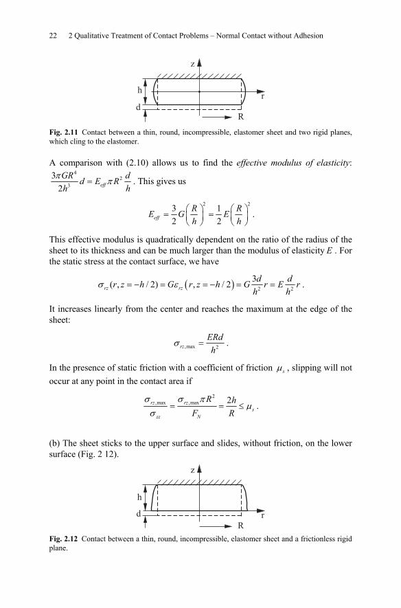
Fig. 2.11 Contact between a thin, round, incompressible, elastomer sheet and two rigid planes, which cling to the elastomer.
A comparison with (2.10) allows us to find the effective modulus of elasticity: 4
23
32π π= eff
GR dd E Rhh
. This gives us
2 23 12 2
⎛ ⎞ ⎛ ⎞= =⎜ ⎟ ⎜ ⎟⎝ ⎠ ⎝ ⎠
effR RE G Eh h
.
This effective modulus is quadratically dependent on the ratio of the radius of the sheet to its thickness and can be much larger than the modulus of elasticity E . For the static stress at the contact surface, we have
( ) 2 2
3( , / 2) , / 2σ ε= − = = − = =rz rzd dr z h G r z h G r E r
h h.
It increases linearly from the center and reaches the maximum at the edge of the sheet:
,max 2σ =rzERdh
.
In the presence of static friction with a coefficient of friction μs , slipping will not occur at any point in the contact area if
2,max ,max 2σ σ π
μσ
= = ≤rz rzs
zz N
R hF R
.
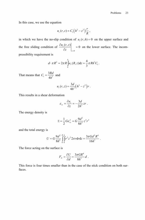
(b) The sheet sticks to the upper surface and slides, without friction, on the lower surface (Fig. 2 12).
Fig. 2.12 Contact between a thin, round, incompressible, elastomer sheet and a frictionless rigid plane.
Problems 23
In this case, we use the equation
( )2 21( , ) = −r
ru r z C h zR
,
in which we have the no-slip condition of ( , ) 0=ru r h on the upper surface and
the free sliding condition of 0
( , )0
=
∂=
∂r
z
u r zz
on the lower surface. The incom-
pressibility requirement is
2 31
0
42 ( , )d3
π π π⋅ = =∫h
rd R R u R z z Rh C .
That means that 1 3
34
=RdCh
and
( )2 23
3( , )4
= −rdu r z h z rh
.
This results in a shear deformation
3
32
ε∂
= = −∂
rrz
u d zrz h
.
The energy density is 2
2 2 26
1 92 8
ε= =E rzdG G z rh
and the total energy is 2 2 4
2 26 3
0 0
9 32 d d8 16
ππ= =∫ ∫R hd Gd RU G r z r r z
h h.
The force acting on the surface is 4
3
38π∂
= =∂NU GRF dd h
.
This force is four times smaller than in the case of the stick condition on both sur-faces.
V.L. Popov, Contact Mechanics and Friction, DOI 10.1007/978-3-642-10803-7_3, © Springer-Verlag Berlin Heidelberg 2010
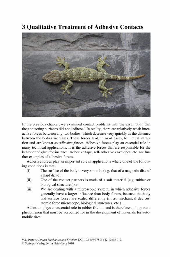
3 Qualitative Treatment of Adhesive Contacts
In the previous chapter, we examined contact problems with the assumption that the contacting surfaces did not “adhere.” In reality, there are relatively weak inter-active forces between any two bodies, which decrease very quickly as the distance between the bodies increases. These forces lead, in most cases, to mutual attrac-tion and are known as adhesive forces. Adhesive forces play an essential role in many technical applications. It is the adhesive forces that are responsible for the behavior of glue, for instance. Adhesive tape, self-adhesive envelopes, etc. are fur-ther examples of adhesive forces.
Adhesive forces play an important role in applications where one of the follow-ing conditions is met:
(i) The surface of the body is very smooth, (e.g. that of a magnetic disc of a hard drive).
(ii) One of the contact partners is made of a soft material (e.g. rubber or biological structures) or
(iii) We are dealing with a microscopic system, in which adhesive forces generally have a larger influence than body forces, because the body and surface forces are scaled differently (micro-mechanical devices, atomic force microscope, biological structures, etc.)
Adhesion plays an essential role in rubber friction and is therefore an important phenomenon that must be accounted for in the development of materials for auto-mobile tires.
26 3 Qualitative Treatment of Adhesive Contacts
In this chapter, we will explain the physical origins of adhesive forces and qua-litatively discuss the fundamental ideas for calculations regarding adhesive con-tacts.
3.1 Physical Background
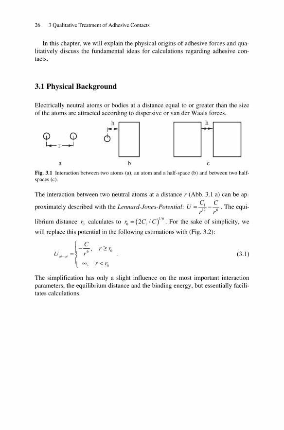
Electrically neutral atoms or bodies at a distance equal to or greater than the size of the atoms are attracted according to dispersive or van der Waals forces.
h
r
h
a b c Fig. 3.1 Interaction between two atoms (a), an atom and a half-space (b) and between two half-spaces (c).
The interaction between two neutral atoms at a distance r (Abb. 3.1 a) can be ap-
proximately described with the Lennard-Jones-Potential: 112 6= −
C CUr r
. The equi-
librium distance 0r calculates to ( )1/60 12 /=r C C . For the sake of simplicity, we
will replace this potential in the following estimations with (Fig. 3.2):
06
0
,
,−
⎧− ≥⎪= ⎨⎪ ∞ <⎩
at at
C r rrU
r r . (3.1)
The simplification has only a slight influence on the most important interaction parameters, the equilibrium distance and the binding energy, but essentially facili-tates calculations.
3.1 Physical Background 27
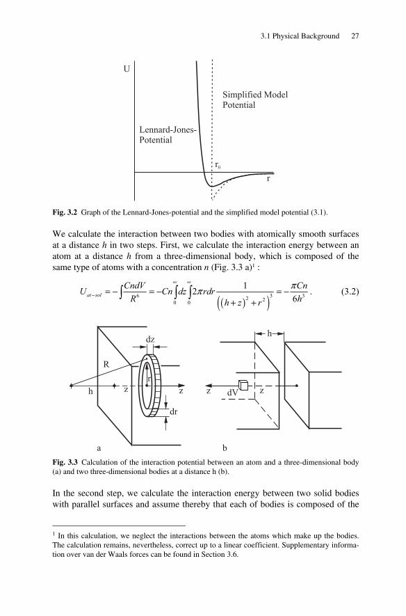
Lennard-Jones-Potential
Simplified ModelPotential
U
r
r0
Fig. 3.2 Graph of the Lennard-Jones-potential and the simplified model potential (3.1).
We calculate the interaction between two bodies with atomically smooth surfaces at a distance h in two steps. First, we calculate the interaction energy between an atom at a distance h from a three-dimensional body, which is composed of the same type of atoms with a concentration n (Fig. 3.3 a)1 :
( )( )6 3 32 20 0
126ππ
∞ ∞
− = − = − = −+ +
∫ ∫ ∫at solCndV CnU Cn dz rdr
R hh z r. (3.2)
R
h
h
z z z z
dz
dV
dr
r
a b Fig. 3.3 Calculation of the interaction potential between an atom and a three-dimensional body (a) and two three-dimensional bodies at a distance h (b).
In the second step, we calculate the interaction energy between two solid bodies with parallel surfaces and assume thereby that each of bodies is composed of the
1 In this calculation, we neglect the interactions between the atoms which make up the bodies. The calculation remains, nevertheless, correct up to a linear coefficient. Supplementary informa-tion over van der Waals forces can be found in Section 3.6.
28 3 Qualitative Treatment of Adhesive Contacts
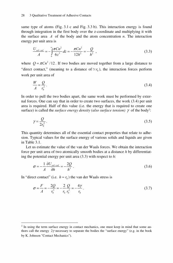
same type of atoms (Fig. 3.1 c and Fig. 3.3 b). This interaction energy is found through integration in the first body over the z-coordinate and multiplying it with the surface area A of the body and the atom concentration n. The interaction energy per unit area is
2 2
3 2 26 12π π∞
− = − = − = −∫sol sol
h
U Cn Cn QdzA z h h
, (3.3)
where 2 /12π=Q Cn . If two bodies are moved together from a large distance to
“direct contact,” (meaning to a distance of 0r ), the interaction forces perform
work per unit area of
20
=W QA r
. (3.4)
In order to pull the two bodies apart, the same work must be performed by exter-nal forces. One can say that in order to create two surfaces, the work (3.4) per unit area is required. Half of this value (i.e. the energy that is required to create one surface) is called the surface energy density (also surface tension) γ of the body2:
202
γ = Qr
. (3.5)
This quantity determines all of the essential contact properties that relate to adhe-sion. Typical values for the surface energy of various solids and liquids are given in Table 3.1.
Let us estimate the value of the van der Waals forces. We obtain the interaction force per unit area of two atomically smooth bodies at a distance h by differentiat-ing the potential energy per unit area (3.3) with respect to h:
3
1 2σ −∂= − = −
∂sol solU Q
A h h. (3.6)
In “direct contact” (i.e. 0≈h r ) the van der Waals stress is
3 20 00 0
2 2 4γσ = = − = − = −F Q QA r rr r
. (3.7)
2 In using the term surface energy in contact mechanics, one must keep in mind that some au-thors call the energy 2γ necessary to separate the bodies the “surface energy” (e.g. in the book
by K. Johnson "Contact Mechanics").
3.1 Physical Background 29
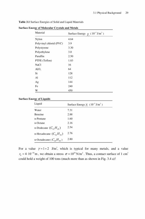
Table 3.1 Surface Energies of Solid and Liquid Materials
Surface Energy of Molecular Crystals and Metals
Material Surface Energy γ s (2 210 J/m− )
Nylon 4.64
Polyvinyl chlorid (PVC) 3.9
Polystyrene 3.30
Polyethylene 3.0
Paraffin 2.50
PTFE (Teflon) 1.83
NaCl 16
Al2O3 64
Si 128
Al 112
Ag 144
Fe 240
W 450
Surface Energy of Liquids
Liquid Surface Energy γ l ( 2 210 J/m− )
Water 7.31
Benzine 2.88
n-Pentane 1.60
n-Octane 2.16
n-Dodecane 12 26( )C H 2.54
n-Hexadecane 16 34( )C H 2.76
n-Octadecane ( 18 38C H ) 2.80
For a value 1 2γ ≈ ÷ J/m2, which is typical for many metals, and a value
100 4 10 m−≈ ⋅r , we obtain a stress 10 210 N/mσ = . Thus, a contact surface of 1 cm2
could hold a weight of 100 tons (much more than as shown in Fig. 3.4 a)!

30 3 Qualitative Treatment of Adhesive Contacts
Solid Beam1 cm²
van der WaalsInteractions
HomogeneousSeparation
Crack
F
a
b
c Fig. 3.4 Van der Waals forces between atomically smooth surfaces are much stronger than can be guessed based on our everyday experiences (a); In real systems, they are strongly reduced in part by the roughness of the surfaces and in part by the fact that fractures propagate through ex-isting flaws in the medium.
Such strong adhesive forces are never observed in reality. This estimation explains Kendall’s statement in his book Molecular Adhesion and its Applications (Kluwer Academic, 2001):
“solids are expected to adhere; the question is to explain why they do not, rather than why they do!”
The solution to this adhesion paradox is explained by the fact that molecular bond fractures on a macroscopic scale are never homogeneous (Fig. 3.4 b), rather they are facilitated by propagating through existing flaws (Fig. 3.4 c), which drastically diminish the adhesive force. Also, the roughness of the surface can lead to a dras-tic reduction of the adhesive force (see the discussion on the influence of rough-ness on adhesion in 3.4).
3.2 Calculation of the Adhesive Force between Curved Surfaces
The first calculation of the adhesive force between solid bodies with curved sur-faces stemmed from Bradley (1932)3. We consider a rigid sphere with a radius R at a distance h from a rigid plane of the same material. We calculate the interac-tion energy between these bodies with an approximation, which we will also use later in most contact problems: We assume that the contact area is significantly smaller than the radius of the sphere, so that one can approximately assume that the surfaces of the two bodies are parallel, although the separation distance re-mains dependent on the longitudinal coordinate (“Half-Space Approximation”).
3 R.S. Bradley, Phil. Mag 1932., v. 13, 853.
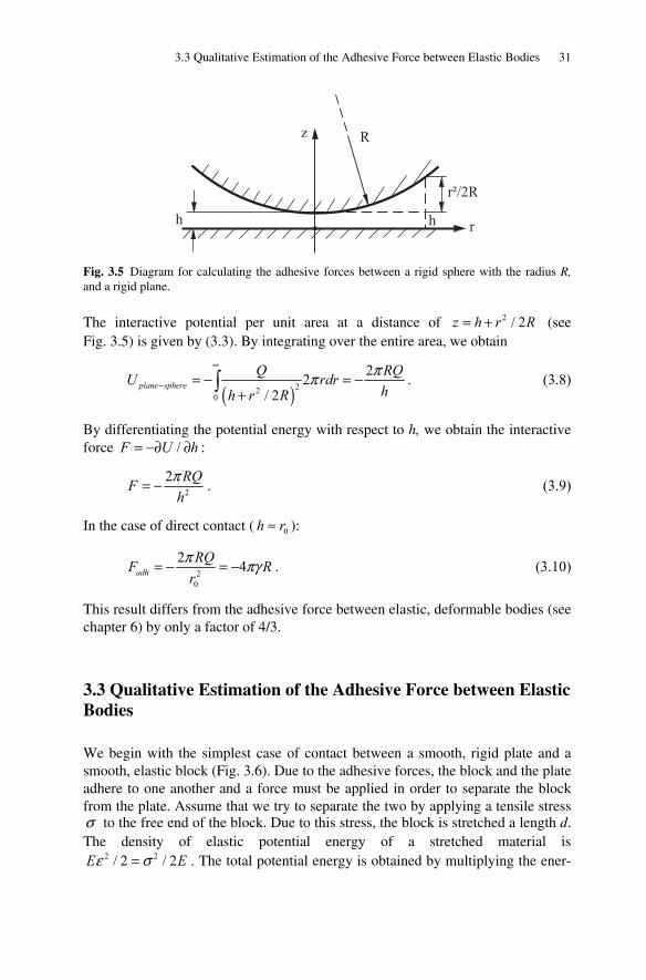
3.3 Qualitative Estimation of the Adhesive Force between Elastic Bodies 31
R
r
r²/2R
h h
z
Fig. 3.5 Diagram for calculating the adhesive forces between a rigid sphere with the radius R, and a rigid plane.
The interactive potential per unit area at a distance of 2 / 2= +z h r R (see Fig. 3.5) is given by (3.3). By integrating over the entire area, we obtain
( )22
0
22/ 2
plane sphereQ RQU rdr
hh r R
ππ∞
− = − = −+
∫ . (3.8)
By differentiating the potential energy with respect to h, we obtain the interactive force /= −∂ ∂F U h :
2
2π= − RQFh
. (3.9)
In the case of direct contact ( 0≈h r ):
20
2 4π πγ= − = −adhRQF R
r. (3.10)
This result differs from the adhesive force between elastic, deformable bodies (see chapter 6) by only a factor of 4/3.
3.3 Qualitative Estimation of the Adhesive Force between Elastic Bodies
We begin with the simplest case of contact between a smooth, rigid plate and a smooth, elastic block (Fig. 3.6). Due to the adhesive forces, the block and the plate adhere to one another and a force must be applied in order to separate the block from the plate. Assume that we try to separate the two by applying a tensile stress σ to the free end of the block. Due to this stress, the block is stretched a length d. The density of elastic potential energy of a stretched material is
2 2/ 2 / 2ε σ=E E . The total potential energy is obtained by multiplying the ener-
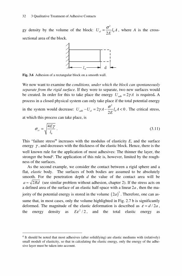
32 3 Qualitative Treatment of Adhesive Contacts
gy density by the volume of the block: 2
02σ=elU l A
E, where A is the cross-
sectional area of the block.
l 0 d Fig. 3.6 Adhesion of a rectangular block on a smooth wall.
We now want to examine the conditions, under which the block can spontaneously separate from the rigid surface. If they were to separate, two new surfaces would be created. In order for this to take place the energy 2γ=adhU A is required. A
process in a closed physical system can only take place if the total potential energy
in the system would decrease: 2
02 02σγ− = − <adh elU U A l A
E. The critical stress,
at which this process can take place, is
0
4 γσ =crEl
. (3.11)
This “failure stress” increases with the modulus of elasticity E, and the surface energy γ , and decreases with the thickness of the elastic block. Hence, there is the
well known rule for the application of most adhesives: The thinner the layer, the stronger the bond4. The application of this rule is, however, limited by the rough-ness of the surfaces.
As the second example, we consider the contact between a rigid sphere and a flat, elastic body. The surfaces of both bodies are assumed to be absolutely smooth. For the penetration depth d the value of the contact area will be
2≈a Rd (see similar problem without adhesion, chapter 2). If the stress acts on a defined area of the surface of an elastic half-space with a linear 2a , then the ma-
jority of the potential energy is stored in the volume ( )32a . Therefore, one can as-
sume that, in most cases, only the volume highlighted in Fig. 2.7 b is significantly deformed. The magnitude of the elastic deformation is described as / 2ε ≈ d a , the energy density as 2 / 2εE , and the total elastic energy as
4 It should be noted that most adhesives (after solidifying) are elastic mediums with (relatively) small moduli of elasticity, so that in calculating the elastic energy, only the energy of the adhe-sive layer must be taken into account.
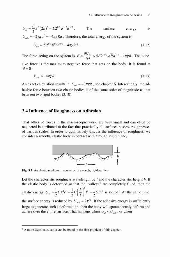
3.4 Influence of Roughness on Adhesion 33
( )32 1/ 2 1/ 2 5 / 22 22elEU a E R dε =~ . The surface energy is
22 4γπ πγ= − = −adhU a Rd . Therefore, the total energy of the system is
1/2 1/ 2 5/ 22 4πγ≈ −totU E R d Rd . (3.12)
The force acting on the system is 1/2 3/ 25 2 4totUF E Rd Rd
πγ−∂≈ ≈ −
∂. The adhe-
sive force is the maximum negative force that acts on the body. It is found at 0d = :
4πγ≈ −adhF R . (3.13)
An exact calculation results in 3πγ= −adhF R , see chapter 6. Interestingly, the ad-
hesive force between two elastic bodies is of the same order of magnitude as that between two rigid bodies (3.10).
3.4 Influence of Roughness on Adhesion
That adhesive forces in the macroscopic world are very small and can often be neglected is attributed to the fact that practically all surfaces possess roughnesses of various scales. In order to qualitatively discuss the influence of roughness, we consider a smooth, elastic body in contact with a rough, rigid plane.
h
l Fig. 3.7 An elastic medium in contact with a rough, rigid surface.
Let the characteristic roughness wavelength be l and the characteristic height h. If the elastic body is deformed so that the “valleys” are completely filled, then the
elastic energy 2
2 3 3 21 1 12 2 2el
hU G l G l Glhl
ε ⎛ ⎞≈ ≈ =⎜ ⎟⎝ ⎠
is stored5. At the same time,
the surface energy is reduced by 22γ≈adhU l . If the adhesive energy is sufficiently
large to generate such a deformation, then the body will spontaneously deform and adhere over the entire surface. That happens when <el adhU U , or when
5 A more exact calculation can be found in the first problem of this chapter.
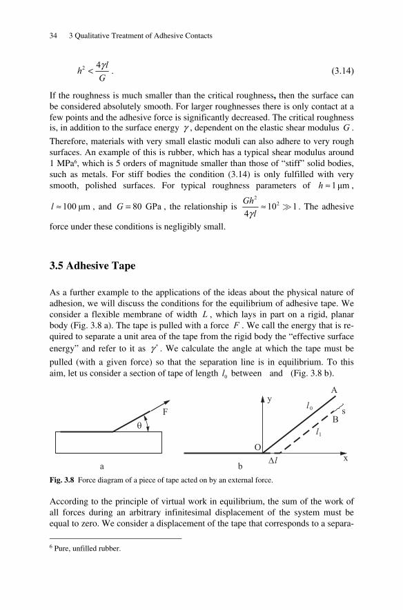
34 3 Qualitative Treatment of Adhesive Contacts
2 4 lhGγ< . (3.14)
If the roughness is much smaller than the critical roughness, then the surface can be considered absolutely smooth. For larger roughnesses there is only contact at a few points and the adhesive force is significantly decreased. The critical roughness is, in addition to the surface energy γ , dependent on the elastic shear modulus G .
Therefore, materials with very small elastic moduli can also adhere to very rough surfaces. An example of this is rubber, which has a typical shear modulus around 1 MPa6, which is 5 orders of magnitude smaller than those of “stiff” solid bodies, such as metals. For stiff bodies the condition (3.14) is only fulfilled with very smooth, polished surfaces. For typical roughness parameters of 1μm≈h ,
100 μm≈l , and 80 GPa=G , the relationship is 2
210 14Gh
lγ≈ . The adhesive
force under these conditions is negligibly small.
3.5 Adhesive Tape
As a further example to the applications of the ideas about the physical nature of adhesion, we will discuss the conditions for the equilibrium of adhesive tape. We consider a flexible membrane of width L , which lays in part on a rigid, planar body (Fig. 3.8 a). The tape is pulled with a force F . We call the energy that is re-quired to separate a unit area of the tape from the rigid body the “effective surface energy” and refer to it as γ ∗ . We calculate the angle at which the tape must be
pulled (with a given force) so that the separation line is in equilibrium. To this aim, let us consider a section of tape of length 0l between and (Fig. 3.8 b).
F
y
O
A
Bs
�l
l0
l1
x
�
a b Fig. 3.8 Force diagram of a piece of tape acted on by an external force.
According to the principle of virtual work in equilibrium, the sum of the work of all forces during an arbitrary infinitesimal displacement of the system must be equal to zero. We consider a displacement of the tape that corresponds to a separa-
6 Pure, unfilled rubber.
3.6 Supplementary Information about van der Waals Forces and Surface Energies 35
tion of the tape from the body of length Δl . With this movement the surface ener-
gy is increased by γ ∗ ΔL l ; the adhesive forces perform thereby work equal to
γ ∗− ΔL l . At the same time, the end of the tape on which the force acts (point B) is
displaced in the direction of the force by a distance s. The work performed by F is equal to Fs. The equilibrium condition is γ ∗= ΔFs L l . It is easy to see that
( )1 cosθ= Δ −s l and, therefore, ( )0 1 cosθ γ ∗− =F L . For the critical “separation
force,” 0F we get
0 1 cosγ
θ
∗
=−
LF . (3.15)
The critical separation force (per unit length) perpendicular to the plane is equal to the surface energy. By pulling in the direction π (opposite to the direction of the tape) the critical force is half as large.
3.6 Supplementary Information about van der Waals Forces and Surface Energies
An extensive theory on van der Waals forces was developed by I.E. Dzyaloshins-kii, E.M. Lifschitz, and L.P. Pitaevskii (1961)7. It says that the van der Waals forces depend significantly on the dielectric constant of the bodies and of the me-dium between the two bodies. If the dielectric constant of the medium εm is
smaller as the dielectric constant of both bodies: 1 2,ε ε ε<m , the bodies attract. If
it lies between ( 1 2ε ε ε< <m ), then the bodies repel! The latter effect is used in
atomic force microscopy to prevent the adhesive forces and related instabilities. According to this theory, a rough first approximation of the van der Waals
force between two bodies is proportional to the product ( )( )
( )1 2
1 2
m mε ε ε εε ε
− −+
. If the
medium between the bodies is a vacuum ( 1ε =m ), then the force is always posi-
tive (the bodies attract) and is proportional to ( )( )
( )1 2
1 2
1 1ε εε ε− −
+. One can give a
rough empirical rule of calculation for relative surface energies in the approxima-tion, in which the equilibrium distance 0r (3.5), for various bodies is approximate-
ly the same and the main difference in the surface energies is caused by the differ-ent polarizability and therefore the dielectric constant.
7 I.E. Dzyaloshinskii, E.M. Lifshitz und L.P. Pitaevskii, General Theory of van der Waals' Forces, Sov. Phys. Usp. 1961, v. 4 153-176.
36 3 Qualitative Treatment of Adhesive Contacts
We define the relative surface energy as the energy (per unit area) that is re-quired to separate the bodies beginning from the equilibrium distance 0r . The
relative surface energy for two identical bodies of material 1 is proportional to
( )21
11 11
12
2ε
γ γε−
= ∝ . Likewise, the relative surface energy for two identical bo-
dies of material 2 is proportional to ( )2
222 2
2
12
2ε
γ γε−
= ∝ . The relative surface
energy for bodies 1 and 2 is ( )( )
( )1 2
121 2
1 1ε εγ
ε ε− −
∝+
, from which we obtain8
12 11 22 1 22γ γ γ γ γ≈ = . (3.16)
The relative surface energy is roughly equal to the geometric average of the sur-face energies of the two solids. In the case of two bodies, each composed of dif-ferent materials, the γ in Equations (3.11) and (3.13) should be replaced with
12 / 2γ , half of the relative surface energy.
Problems
Problem 1: A smooth, elastic body (rubber) is in contact with a rigid, rough sur-face which is characterized by a characteristic wave length l and a characteristic
height h . The “width” of the medium L is much larger than l. Under the as-
sumption that the roughness can be modeled as ( )ˆ cos 2 /π=z h x l , calculate the
critical relationship ˆ /h l , at which the “valleys” will be completely filled. What is the maximum allowable characteristic roughness with 100 mμ=l at which the
rubber will still completely adhere to the rigid surface? Pure (unfilled) rubber has a shear modulus G of about 1 MPa; the relative surface energy of a rigid contact
partner to rubber is around 2 212 3 10 J/mγ −≈ ⋅ .
8 We have thereby replaced the geometric average 1 2ε ε with the arithmetic average
( )1 2 / 2ε ε+ . For the accuracy of the approximation, this assumption is acceptable.
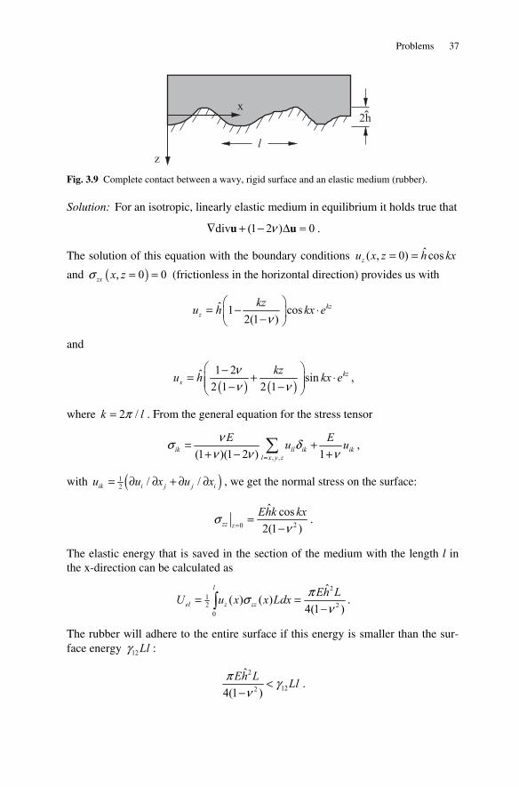
Problems 37
z
x2h
l
Fig. 3.9 Complete contact between a wavy, rigid surface and an elastic medium (rubber).
Solution: For an isotropic, linearly elastic medium in equilibrium it holds true that
div (1 2 ) 0ν∇ + − Δ =u u .
The solution of this equation with the boundary conditions ˆ( , 0) cos= =zu x z h kx
and ( ), 0 0σ = =zx x z (frictionless in the horizontal direction) provides us with
ˆ 1 cos2(1 )ν
⎛ ⎞= − ⋅⎜ ⎟−⎝ ⎠
kzz
kzu h kx e
and
( ) ( )1 2ˆ sin
2 1 2 1νν ν
⎛ ⎞−= + ⋅⎜ ⎟⎜ ⎟− −⎝ ⎠
kzx
kzu h kx e ,
where 2 /π=k l . From the general equation for the stress tensor
, ,(1 )(1 2 ) 1ik ll ik ikl x y z
E Eu uνσ δν ν ν=
= ++ − +∑ ,
with ( )12 / /ik i j j iu u x u x= ∂ ∂ + ∂ ∂ , we get the normal stress on the surface:
20
ˆ cos2(1 )
σν=
=−zz z
Ehk kx .
The elastic energy that is saved in the section of the medium with the length l in the x-direction can be calculated as
212 2
0
ˆ( ) ( )
4(1 )πσ
ν= =
−∫l
el z zzEh LU u x x Ldx .
The rubber will adhere to the entire surface if this energy is smaller than the sur-face energy 12γ Ll :
2
122
ˆ
4(1 )π γ
ν<
−Eh L Ll .
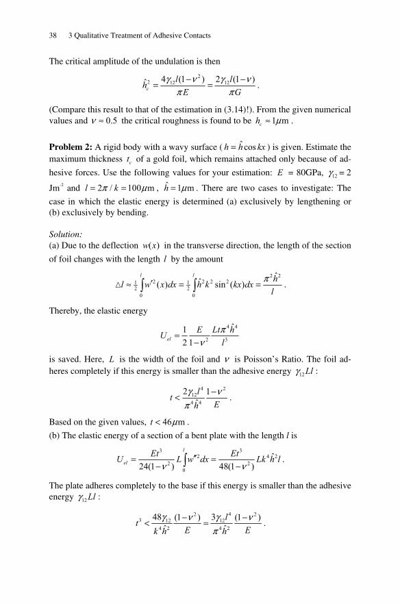
38 3 Qualitative Treatment of Adhesive Contacts
The critical amplitude of the undulation is then
22 12 124 (1 ) 2 (1 )ˆ γ ν γ ν
π π− −
= =cl lh
E G.
(Compare this result to that of the estimation in (3.14)!). From the given numerical values and 0.5ν ≈ the critical roughness is found to be 1 mch μ≈ .
Problem 2: A rigid body with a wavy surface ( ˆ cos=h h kx ) is given. Estimate the maximum thickness ct of a gold foil, which remains attached only because of ad-
hesive forces. Use the following values for your estimation: E = 80GPa, 12γ = 2
Jm-2 and 2 / 100 ml kπ μ= = , ˆ 1 mh μ= . There are two cases to investigate: The
case in which the elastic energy is determined (a) exclusively by lengthening or (b) exclusively by bending.
Solution: (a) Due to the deflection ( )w x in the transverse direction, the length of the section
of foil changes with the length l by the amount
2 22 2 2 21 1
2 20 0
ˆˆ( ) sin ( )l l hl w x dx h k kx dx
lπ′≈ = =∫ ∫ .
Thereby, the elastic energy
4 4
2 3
ˆ12 1
πν
=−elE Lt hU
l
is saved. Here, L is the width of the foil and ν is Poisson’s Ratio. The foil ad-heres completely if this energy is smaller than the adhesive energy 12γ Ll :
4 2124 4
2 1ˆ
γ νπ
−<lt
Eh.
Based on the given values, 46 mμ<t .
(b) The elastic energy of a section of a bent plate with the length l is
3 32 4 2
2 20
ˆ24(1 ) 48(1 )ν ν
′′= =− −∫
l
elEt EtU L w dx Lk h l .
The plate adheres completely to the base if this energy is smaller than the adhesive energy 12γ Ll :
42 23 12 12
4 2 4 2
48 3(1 ) (1 )ˆ ˆ
γ γν νπ
− −< =lt
E Ek h h.
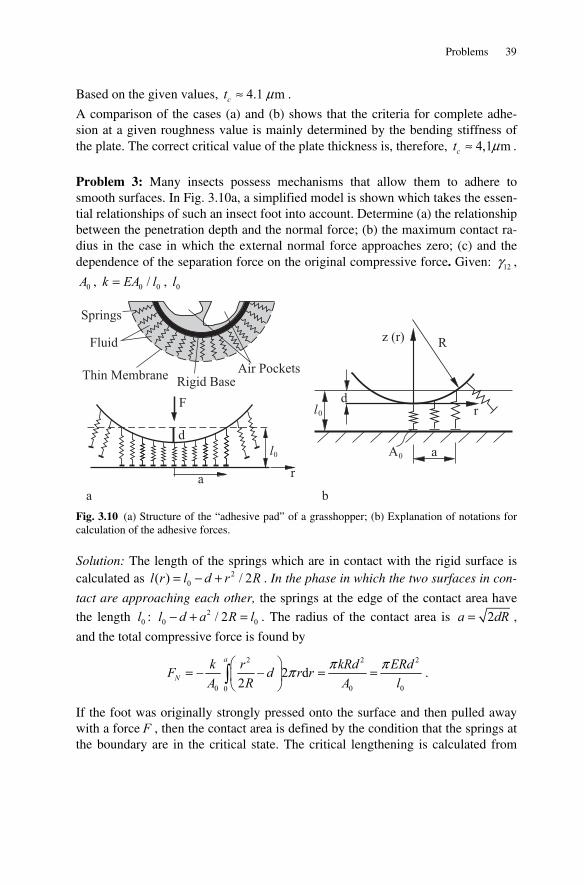
Problems 39
Based on the given values, 4.1 mct μ≈ .
A comparison of the cases (a) and (b) shows that the criteria for complete adhe-sion at a given roughness value is mainly determined by the bending stiffness of the plate. The correct critical value of the plate thickness is, therefore, 4,1 mμ≈ct .
Problem 3: Many insects possess mechanisms that allow them to adhere to smooth surfaces. In Fig. 3.10a, a simplified model is shown which takes the essen-tial relationships of such an insect foot into account. Determine (a) the relationship between the penetration depth and the normal force; (b) the maximum contact ra-dius in the case in which the external normal force approaches zero; (c) and the dependence of the separation force on the original compressive force. Given: 12γ ,
0A , 0 0/=k EA l , 0l
ar
F
l0
d
Springs
Fluid
Thin MembraneRigid Base
Air Pockets
Rz (r)
d
a
r
A
l
0
0
a b Fig. 3.10 (a) Structure of the “adhesive pad” of a grasshopper; (b) Explanation of notations for calculation of the adhesive forces.
Solution: The length of the springs which are in contact with the rigid surface is calculated as 2
0( ) / 2= − +l r l d r R . In the phase in which the two surfaces in con-
tact are approaching each other, the springs at the edge of the contact area have
the length 0l : 20 0/ 2− + =l d a R l . The radius of the contact area is 2=a dR ,
and the total compressive force is found by
2 2 2
0 0 00
2 d2
π ππ⎛ ⎞= − − = =⎜ ⎟
⎝ ⎠∫a
Nk r kRd ERdF d r rA R A l
.
If the foot was originally strongly pressed onto the surface and then pulled away with a force F , then the contact area is defined by the condition that the springs at the boundary are in the critical state. The critical lengthening is calculated from
40 3 Qualitative Treatment of Adhesive Contacts
(3.11) as 12 02γΔ =
llE
and the contact radius from the constraint
2max 12 0
max 0 02
( )2
γ= − + = +
a ll a l d lR E
as:
2 12 0max
22
γ⎛ ⎞= +⎜ ⎟⎜ ⎟
⎝ ⎠
la R dE
.
Therefore, the force acting on the foot is
max 22 212 0 12 0max
0 0 00
2 22 d
2 2γ γπ ππ
⎛ ⎞⎛ ⎞ ⎛ ⎞= − − = − − = − −⎜ ⎟⎜ ⎟ ⎜ ⎟⎜ ⎟ ⎝ ⎠⎝ ⎠ ⎝ ⎠∫
a
Al lk r k EF d r r a d R d
A R A E l E.
The maximum negative value of this force we call the adhesive force.
,max 122πγ=AF R .
A detailed calculation of the arbitrary compressive force NF provides the follow-
ing adhesive forces9
( ) ,max ,max
,max ,max
,
2 ,
≥⎧⎪= ⎨ − <⎪⎩
A N AA N
A N N N A
F F FF F
F F F F F .
9 M. Schargott, V.L. Popov, S. Gorb, Spring model of biological attachment pads. J. Theor. Bi-ology., 2006, v. 243, pp. 48-53.

4 Capillary Forces
In the interactions between solid surfaces and liquids or between solid bodies in the presence of small amounts of liquids, the so called capillary forces play an im-portant role. Capillary forces are responsible for the wetting of solids by liquids or the “repelling” of liquids. The transportation of water in all organs of plants is caused by capillary forces. They are behind the unwanted “spreading” of lubricat-ing oil and its transportation to friction sites in the for-life lubrication of systems. Capillary forces are among the most important causes of “sticktion” between the small components in micro-technology. They can considerably influence frictional forces, especially that of static friction.
4.1 Surface Tension and Contact Angles
The most important physical parameters that influence capillary forces in various situations are the surface tension and the contact angle. In order to clarify the con-cept of surface tension of a liquid, we visualize a soap film stretched within a
V.L. Popov, Contact Mechanics and Friction, DOI 10.1007/978-3-642-10803-7_4, © Springer-Verlag Berlin Heidelberg 2010
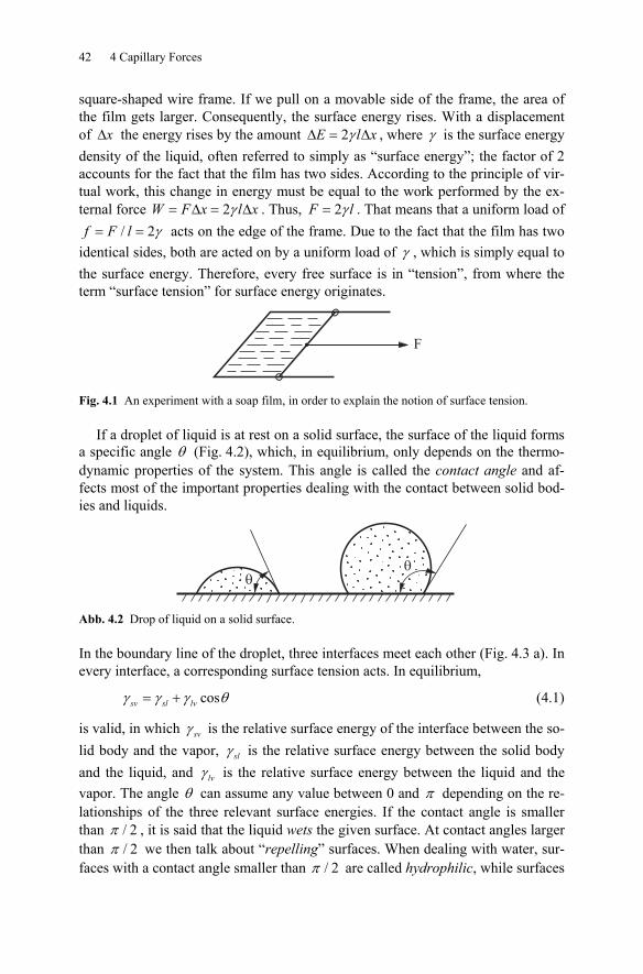
42 4 Capillary Forces
square-shaped wire frame. If we pull on a movable side of the frame, the area of the film gets larger. Consequently, the surface energy rises. With a displacement of Δx the energy rises by the amount 2γΔ = ΔE l x , where γ is the surface energy density of the liquid, often referred to simply as “surface energy”; the factor of 2 accounts for the fact that the film has two sides. According to the principle of vir-tual work, this change in energy must be equal to the work performed by the ex-ternal force 2γ= Δ = ΔW F x l x . Thus, 2γ=F l . That means that a uniform load of
/ 2γ= =f F l acts on the edge of the frame. Due to the fact that the film has two identical sides, both are acted on by a uniform load of γ , which is simply equal to the surface energy. Therefore, every free surface is in “tension”, from where the term “surface tension” for surface energy originates.
F
Fig. 4.1 An experiment with a soap film, in order to explain the notion of surface tension.
If a droplet of liquid is at rest on a solid surface, the surface of the liquid forms a specific angle θ (Fig. 4.2), which, in equilibrium, only depends on the thermo-dynamic properties of the system. This angle is called the contact angle and af-fects most of the important properties dealing with the contact between solid bod-ies and liquids.
�
�
Abb. 4.2 Drop of liquid on a solid surface.
In the boundary line of the droplet, three interfaces meet each other (Fig. 4.3 a). In every interface, a corresponding surface tension acts. In equilibrium,
cosγ γ γ θ= +sv sl lv (4.1)
is valid, in which γ sv is the relative surface energy of the interface between the so-lid body and the vapor, γ sl is the relative surface energy between the solid body and the liquid, and γ lv is the relative surface energy between the liquid and the vapor. The angle θ can assume any value between 0 and π depending on the re-lationships of the three relevant surface energies. If the contact angle is smaller than / 2π , it is said that the liquid wets the given surface. At contact angles larger than / 2π we then talk about “repelling” surfaces. When dealing with water, sur-faces with a contact angle smaller than / 2π are called hydrophilic, while surfaces
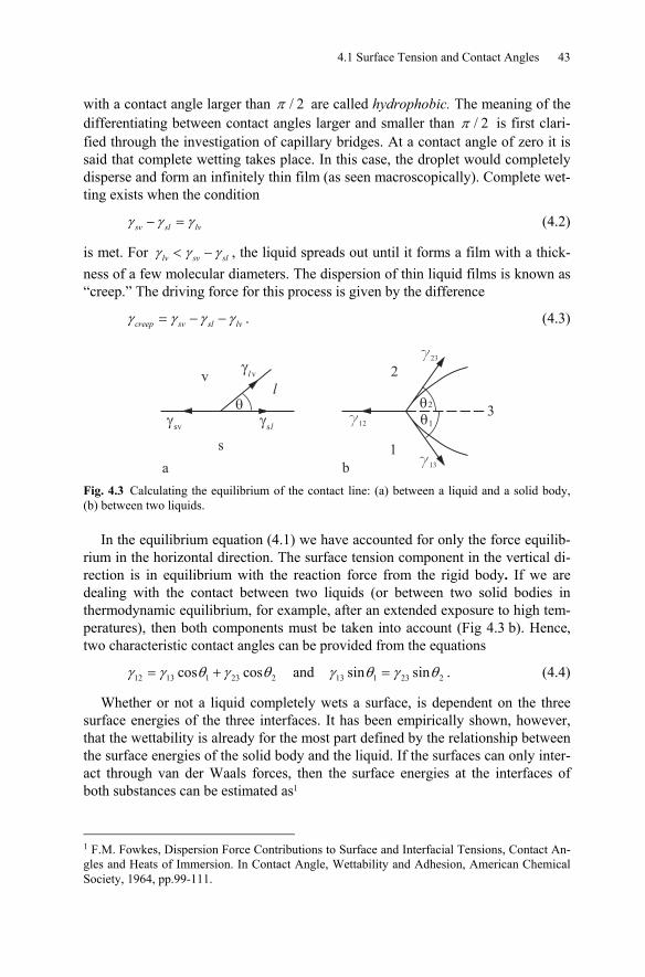
4.1 Surface Tension and Contact Angles 43
with a contact angle larger than / 2π are called hydrophobic. The meaning of the differentiating between contact angles larger and smaller than / 2π is first clari-fied through the investigation of capillary bridges. At a contact angle of zero it is said that complete wetting takes place. In this case, the droplet would completely disperse and form an infinitely thin film (as seen macroscopically). Complete wet-ting exists when the condition
γ γ γ− =sv sl lv (4.2)
is met. For γ γ γ< −lv sv sl , the liquid spreads out until it forms a film with a thick-ness of a few molecular diameters. The dispersion of thin liquid films is known as “creep.” The driving force for this process is given by the difference
creep sv sl lvγ γ γ γ= − − . (4.3)
v v
s
ssv
l
l
l� �
� 2
1
32�
1�g12
g23
g13
�
a b Fig. 4.3 Calculating the equilibrium of the contact line: (a) between a liquid and a solid body, (b) between two liquids.
In the equilibrium equation (4.1) we have accounted for only the force equilib-rium in the horizontal direction. The surface tension component in the vertical di-rection is in equilibrium with the reaction force from the rigid body. If we are dealing with the contact between two liquids (or between two solid bodies in thermodynamic equilibrium, for example, after an extended exposure to high tem-peratures), then both components must be taken into account (Fig 4.3 b). Hence, two characteristic contact angles can be provided from the equations
12 13 1 23 2 13 1 23 2cos cos and sin sinγ γ θ γ θ γ θ γ θ= + = . (4.4)
Whether or not a liquid completely wets a surface, is dependent on the three surface energies of the three interfaces. It has been empirically shown, however, that the wettability is already for the most part defined by the relationship between the surface energies of the solid body and the liquid. If the surfaces can only inter-act through van der Waals forces, then the surface energies at the interfaces of both substances can be estimated as1
1 F.M. Fowkes, Dispersion Force Contributions to Surface and Interfacial Tensions, Contact An-gles and Heats of Immersion. In Contact Angle, Wettability and Adhesion, American Chemical Society, 1964, pp.99-111.
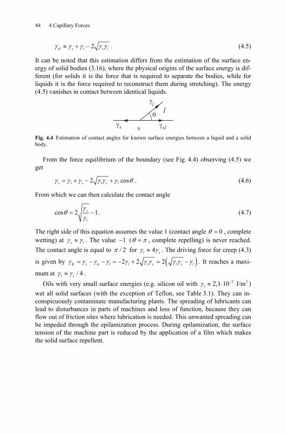
44 4 Capillary Forces
2γ γ γ γ γ≈ + −sl s l s l . (4.5)
It can be noted that this estimation differs from the estimation of the surface en-ergy of solid bodies (3.16), where the physical origins of the surface energy is dif-ferent (for solids it is the force that is required to separate the bodies, while for liquids it is the force required to reconstruct them during stretching). The energy (4.5) vanishes in contact between identical liquids.
s ss
l
l
l� �
�
�
Fig. 4.4 Estimation of contact angles for known surface energies between a liquid and a solid body.
From the force equilibrium of the boundary (see Fig. 4.4) observing (4.5) we get
2 cosγ γ γ γ γ γ θ= + − +s l s l s l . (4.6)
From which we can then calculate the contact angle
cos 2 1γ
θγ
= −s
l
. (4.7)
The right side of this equation assumes the value 1 (contact angle 0θ = , complete wetting) at γ γ≈s l . The value 1− (θ π= , complete repelling) is never reached. The contact angle is equal to / 2π for 4γ γ≈l s . The driving force for creep (4.3)
is given by ( )2 2 2γ γ γ γ γ γ γ γ γ γ= − − = − + = −K s ls l l l s l s l . It reaches a maxi-
mum at / 4γ γ≈l s . Oils with very small surface energies (e.g. silicon oil with 2 22,1 10 J/mlγ
−≈ ⋅ ) wet all solid surfaces (with the exception of Teflon, see Table 3.1). They can in-conspicuously contaminate manufacturing plants. The spreading of lubricants can lead to disturbances in parts of machines and loss of function, because they can flow out of friction sites where lubrication is needed. This unwanted spreading can be impeded through the epilamization process. During epilamization, the surface tension of the machine part is reduced by the application of a film which makes the solid surface repellent.
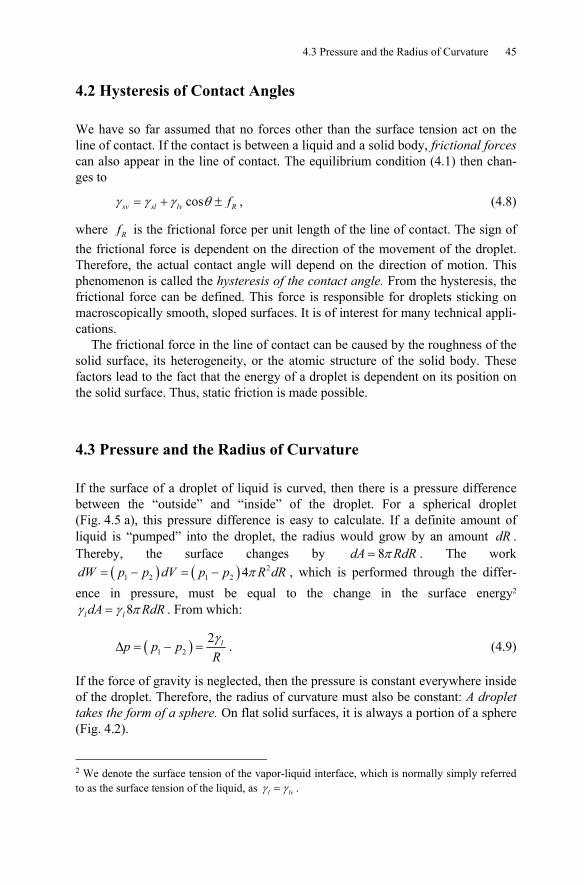
4.3 Pressure and the Radius of Curvature 45
4.2 Hysteresis of Contact Angles
We have so far assumed that no forces other than the surface tension act on the line of contact. If the contact is between a liquid and a solid body, frictional forces can also appear in the line of contact. The equilibrium condition (4.1) then chan-ges to
cosγ γ γ θ= + ±sv sl lv Rf , (4.8)
where Rf is the frictional force per unit length of the line of contact. The sign of the frictional force is dependent on the direction of the movement of the droplet. Therefore, the actual contact angle will depend on the direction of motion. This phenomenon is called the hysteresis of the contact angle. From the hysteresis, the frictional force can be defined. This force is responsible for droplets sticking on macroscopically smooth, sloped surfaces. It is of interest for many technical appli-cations.
The frictional force in the line of contact can be caused by the roughness of the solid surface, its heterogeneity, or the atomic structure of the solid body. These factors lead to the fact that the energy of a droplet is dependent on its position on the solid surface. Thus, static friction is made possible.
4.3 Pressure and the Radius of Curvature
If the surface of a droplet of liquid is curved, then there is a pressure difference between the “outside” and “inside” of the droplet. For a spherical droplet (Fig. 4.5 a), this pressure difference is easy to calculate. If a definite amount of liquid is “pumped” into the droplet, the radius would grow by an amount dR . Thereby, the surface changes by 8π=dA RdR . The work
( ) ( ) 21 2 1 2 4π= − = −dW p p dV p p R dR , which is performed through the differ-
ence in pressure, must be equal to the change in the surface energy2 8γ γ π=l ldA RdR . From which:
( )1 22γ
Δ = − = lp p pR
. (4.9)
If the force of gravity is neglected, then the pressure is constant everywhere inside of the droplet. Therefore, the radius of curvature must also be constant: A droplet takes the form of a sphere. On flat solid surfaces, it is always a portion of a sphere (Fig. 4.2).
2 We denote the surface tension of the vapor-liquid interface, which is normally simply referred to as the surface tension of the liquid, as l lvγ γ= .
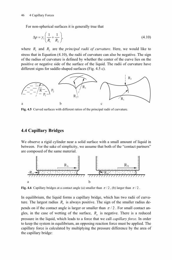
46 4 Capillary Forces
For non-spherical surfaces it is generally true that
1 2
1 1γ⎛ ⎞
Δ = +⎜ ⎟⎝ ⎠
lpR R
, (4.10)
where 1R and 2R are the principal radii of curvature. Here, we would like to stress that in Equation (4.10), the radii of curvature can also be negative. The sign of the radius of curvature is defined by whether the center of the curve lies on the positive or negative side of the surface of the liquid. The radii of curvature have different signs for saddle-shaped surfaces (Fig. 4.5 c).
Rp
1
p2
R1
R2R1
R2
a b c Fig. 4.5 Curved surfaces with different ratios of the principal radii of curvature.
4.4 Capillary Bridges
We observe a rigid cylinder near a solid surface with a small amount of liquid in between. For the sake of simplicity, we assume that both of the “contact partners” are composed of the same material.
-R R
R R
a a
b b
a b Fig. 4.6 Capillary bridges at a contact angle (a) smaller than / 2π , (b) larger than / 2π .
In equilibrium, the liquid forms a capillary bridge, which has two radii of curva-ture. The largest radius bR is always positive. The sign of the smaller radius de-pends on if the contact angle is larger or smaller than / 2π . For small contact an-gles, in the case of wetting of the surface, aR is negative. There is a reduced pressure in the liquid, which leads to a force that we call capillary force. In order to keep the system in equilibrium, an opposing reaction force must be applied. The capillary force is calculated by multiplying the pressure difference by the area of the capillary bridge:
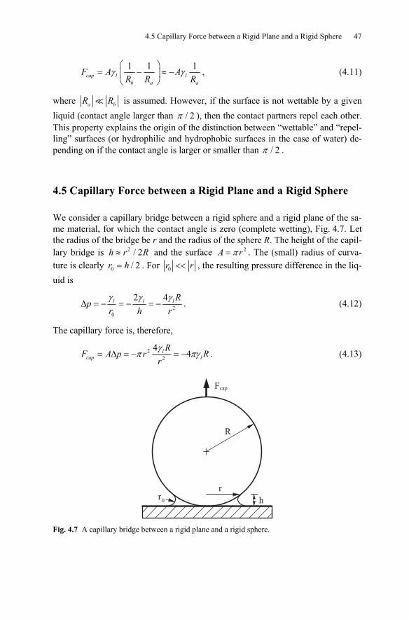
4.5 Capillary Force between a Rigid Plane and a Rigid Sphere 47
1 1 1cap l l
b a a
F A AR R R
γ γ⎛ ⎞
= − ≈ −⎜ ⎟⎝ ⎠
, (4.11)
where a bR R is assumed. However, if the surface is not wettable by a given liquid (contact angle larger than / 2π ), then the contact partners repel each other. This property explains the origin of the distinction between “wettable” and “repel-ling” surfaces (or hydrophilic and hydrophobic surfaces in the case of water) de-pending on if the contact angle is larger or smaller than / 2π .
4.5 Capillary Force between a Rigid Plane and a Rigid Sphere
We consider a capillary bridge between a rigid sphere and a rigid plane of the sa-me material, for which the contact angle is zero (complete wetting), Fig. 4.7. Let the radius of the bridge be r and the radius of the sphere R. The height of the capil-lary bridge is 2 / 2≈h r R and the surface 2π=A r . The (small) radius of curva-ture is clearly 0 / 2=r h . For 0 <<r r , the resulting pressure difference in the liq-uid is
20
2 4γ γ γΔ = − = − = −l l l Rp
r h r. (4.12)
The capillary force is, therefore,
22
44l
cap lR
F A p r Rrγ
π πγ= Δ = − = − . (4.13)
Fig. 4.7 A capillary bridge between a rigid plane and a rigid sphere.
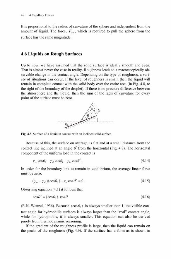
48 4 Capillary Forces
It is proportional to the radius of curvature of the sphere and independent from the amount of liquid. The force, capF , which is required to pull the sphere from the surface has the same magnitude.
4.6 Liquids on Rough Surfaces
Up to now, we have assumed that the solid surface is ideally smooth and even. That is almost never the case in reality. Roughness leads to a macroscopically ob-servable change in the contact angle. Depending on the type of roughness, a vari-ety of situations can occur. If the level of roughness is small, then the liquid will remain in complete contact with the solid body over the entire area (in Fig. 4.8, to the right of the boundary of the droplet). If there is no pressure difference between the atmosphere and the liquid, then the sum of the radii of curvature for every point of the surface must be zero.
��*
�0
Fig. 4.8 Surface of a liquid in contact with an inclined solid surface.
Because of this, the surface on average, is flat and at a small distance from the contact line inclined at an angle *θ from the horizontal (Fig. 4.8). The horizontal component of the uniform load in the contact is
*0 0cos cos cosγ θ γ θ γ θ− −sv sl lv . (4.14)
In order for the boundary line to remain in equilibrium, the average linear force must be zero:
( ) *0cos cos 0γ γ θ γ θ− − =sv sl lv . (4.15)
Observing equation (4.1) it follows that
*0cos cos cosθ θ θ= ⋅ (4.16)
(R.N. Wenzel, 1936). Because 0cosθ is always smaller than 1, the visible con-tact angle for hydrophilic surfaces is always larger than the “real” contact angle, while for hydrophobic, it is always smaller. This equation can also be derived purely from thermodynamic reasoning.
If the gradient of the roughness profile is large, then the liquid can remain on the peaks of the roughness (Fig. 4.9). If the surface has a form as is shown in
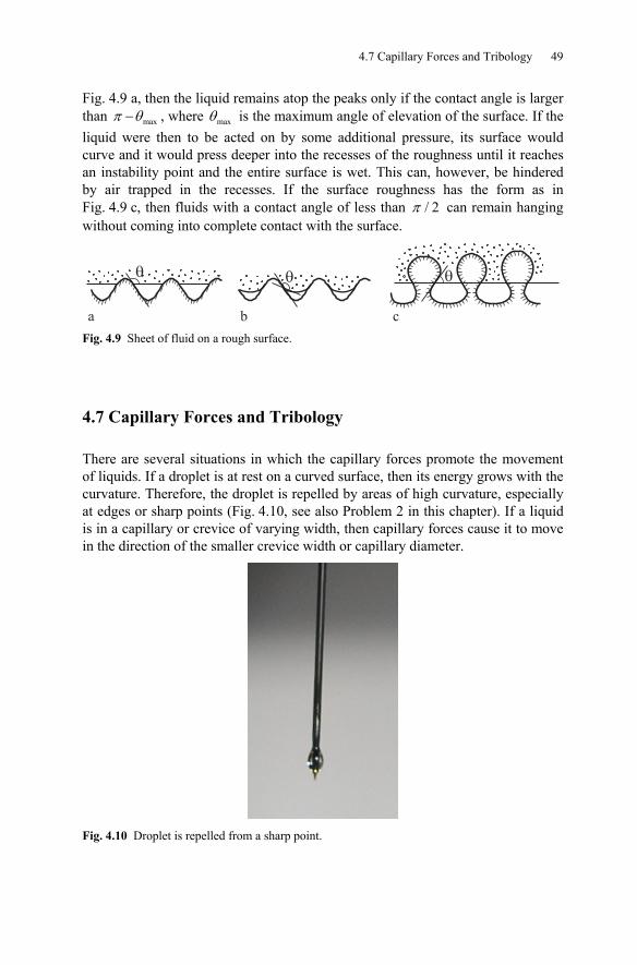
4.7 Capillary Forces and Tribology 49
Fig. 4.9 a, then the liquid remains atop the peaks only if the contact angle is larger than maxπ θ− , where maxθ is the maximum angle of elevation of the surface. If the liquid were then to be acted on by some additional pressure, its surface would curve and it would press deeper into the recesses of the roughness until it reaches an instability point and the entire surface is wet. This can, however, be hindered by air trapped in the recesses. If the surface roughness has the form as in Fig. 4.9 c, then fluids with a contact angle of less than / 2π can remain hanging without coming into complete contact with the surface.
� � �
a b c Fig. 4.9 Sheet of fluid on a rough surface.
4.7 Capillary Forces and Tribology
There are several situations in which the capillary forces promote the movement of liquids. If a droplet is at rest on a curved surface, then its energy grows with the curvature. Therefore, the droplet is repelled by areas of high curvature, especially at edges or sharp points (Fig. 4.10, see also Problem 2 in this chapter). If a liquid is in a capillary or crevice of varying width, then capillary forces cause it to move in the direction of the smaller crevice width or capillary diameter.
Fig. 4.10 Droplet is repelled from a sharp point.
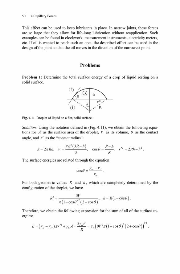
50 4 Capillary Forces
This effect can be used to keep lubricants in place. In narrow joints, these forces are so large that they allow for life-long lubrication without reapplication. Such examples can be found in clockwork, measurement instruments, electricity meters, etc. If oil is wanted to reach such an area, the described effect can be used in the design of the joint so that the oil moves in the direction of the narrowest point.
Problems
Problem 1: Determine the total surface energy of a drop of liquid resting on a solid surface.
h
R
23
1
�
r�
*
Fig. 4.11 Droplet of liquid on a flat, solid surface.
Solution: Using the notation defined in (Fig. 4.11), we obtain the following equa-tions for A as the surface area of the droplet, V as its volume, θ as the contact angle, and *r as the “contact radius”:
( )2*2 23
2 , , cos , 23
ππ θ
− −= = = = −
h R h R hA Rh V r Rh hR
.
The surface energies are related through the equation
cosγ γ
θγ−
= sv sl
lv
.
For both geometric values R and h , which are completely determined by the configuration of the droplet, we have
( ) ( )( )3
2
3 , 1 cos1 cos 2 cos
θπ θ θ
= = −− +
VR h R .
Therefore, we obtain the following expression for the sum of all of the surface en-ergies:
( ) ( ) ( )( )1/32*2 239 1 cos 2 cos
γγ γ π γ γ π θ θ= − + = = − +lv
sl sv lv lvV
E r A VR
.
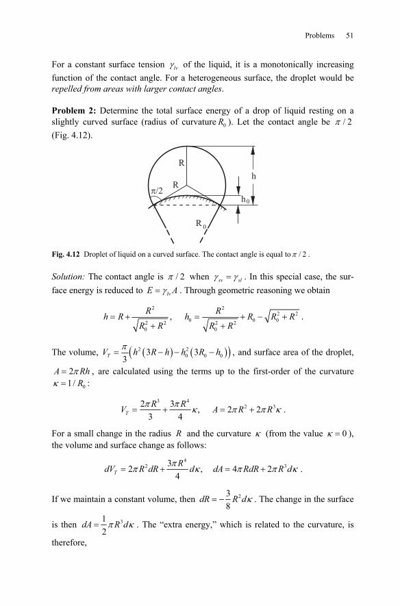
Problems 51
For a constant surface tension γ lv of the liquid, it is a monotonically increasing function of the contact angle. For a heterogeneous surface, the droplet would be repelled from areas with larger contact angles.
Problem 2: Determine the total surface energy of a drop of liquid resting on a slightly curved surface (radius of curvature 0R ). Let the contact angle be / 2π (Fig. 4.12).
h
h
R
R
R
0
0
���
Fig. 4.12 Droplet of liquid on a curved surface. The contact angle is equal to / 2π .
Solution: The contact angle is / 2π when γ γ=sv sl . In this special case, the sur-face energy is reduced to γ= lvE A . Through geometric reasoning we obtain
2 22 2
0 0 02 2 2 20 0
, = + = + − ++ +
R Rh R h R R RR R R R
.
The volume, ( ) ( )( )2 20 0 03 3
3π
= − − −TV h R h h R h , and surface area of the droplet,
2π=A Rh , are calculated using the terms up to the first-order of the curvature 01/κ = R :
3 42 32 3 , 2 2
3 4TR RV A R Rπ π κ π π κ= + = + .
For a small change in the radius R and the curvature κ (from the value 0κ = ), the volume and surface change as follows:
42 332 , 4 2
4ππ κ π π κ= + = +T
RdV R dR d dA RdR R d .
If we maintain a constant volume, then 238
κ= −dR R d . The change in the surface
is then 312π κ=dA R d . The “extra energy,” which is related to the curvature, is
therefore,
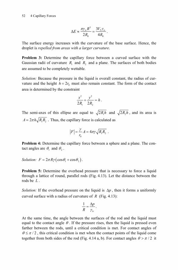
52 4 Capillary Forces
3
0 0
32 4
πγ γΔ ≈ =lv T lvR V
ER R
.
The surface energy increases with the curvature of the base surface. Hence, the droplet is repelled from areas with a larger curvature. Problem 3: Determine the capillary force between a curved surface with the Gaussian radii of curvature 1R and 2R and a plane. The surfaces of both bodies are assumed to be completely wettable. Solution: Because the pressure in the liquid is overall constant, the radius of cur-vature and the height 02=h r must also remain constant. The form of the contact area is determined by the constraint
2 2
1 22 2+ =
x y hR R
.
The semi-axes of this ellipse are equal to 12R h and 22R h , and its area is
1 22π=A h R R . Thus, the capillary force is calculated as
1 20
4γ πγ= =F A R Rr
.
Problem 4: Determine the capillary force between a sphere and a plane. The con-tact angles are 1θ and 2θ . Solution: ( )1 22 cos cosπ γ θ θ= +F R . Problem 5: Determine the overhead pressure that is necessary to force a liquid through a lattice of round, parallel rods (Fig. 4.13). Let the distance between the rods be L .
Solution: If the overhead pressure on the liquid is Δp , then it forms a uniformly curved surface with a radius of curvature of R (Fig. 4.13):
1γΔ
=lv
pR
.
At the same time, the angle between the surfaces of the rod and the liquid must equal to the contact angle θ . If the pressure rises, then the liquid is pressed even farther between the rods, until a critical condition is met. For contact angles of
/ 2θ π≤ , this critical condition is met when the contact points of the liquid come together from both sides of the rod (Fig. 4.14 a, b). For contact angles / 2θ π> it
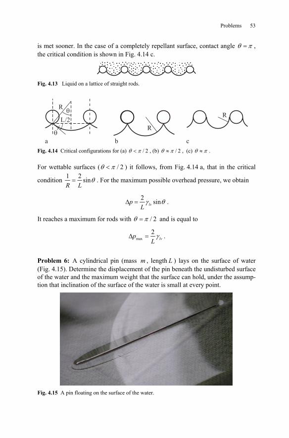
Problems 53
is met sooner. In the case of a completely repellant surface, contact angle θ π= , the critical condition is shown in Fig. 4.14 c.
Fig. 4.13 Liquid on a lattice of straight rods.
�R
R
R
L/2
�
a b c Fig. 4.14 Critical configurations for (a) / 2θ π< , (b) / 2θ π≈ , (c) θ π≈ .
For wettable surfaces ( / 2θ π< ) it follows, from Fig. 4.14 a, that in the critical
condition 1 2 sinθ=R L
. For the maximum possible overhead pressure, we obtain
2 sinγ θΔ = lvpL
.
It reaches a maximum for rods with / 2θ π= and is equal to
max2 γΔ = lvpL
.
Problem 6: A cylindrical pin (mass m , length L ) lays on the surface of water (Fig. 4.15). Determine the displacement of the pin beneath the undisturbed surface of the water and the maximum weight that the surface can hold, under the assump-tion that inclination of the surface of the water is small at every point.
Fig. 4.15 A pin floating on the surface of the water.
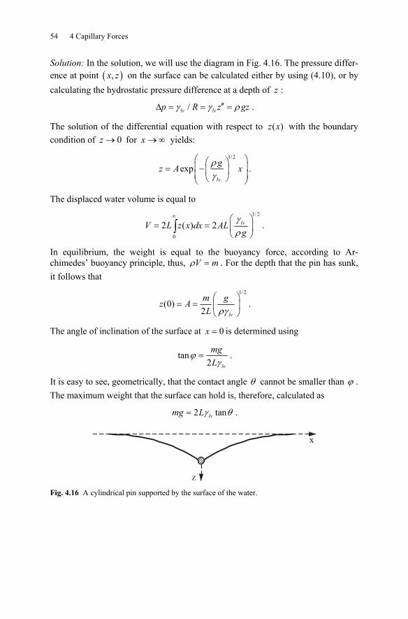
54 4 Capillary Forces
Solution: In the solution, we will use the diagram in Fig. 4.16. The pressure differ-ence at point ( ),x z on the surface can be calculated either by using (4.10), or by calculating the hydrostatic pressure difference at a depth of z :
/γ γ ρ′′Δ = = =lv lvp R z gz .
The solution of the differential equation with respect to ( )z x with the boundary condition of 0→z for →∞x yields:
1/ 2
exp ργ
⎛ ⎞⎛ ⎞⎜ ⎟= −⎜ ⎟⎜ ⎟⎝ ⎠⎝ ⎠lv
gz A x .
The displaced water volume is equal to 1/ 2
0
2 ( ) 2γρ
∞ ⎛ ⎞= = ⎜ ⎟
⎝ ⎠∫ lvV L z x dx AL
g.
In equilibrium, the weight is equal to the buoyancy force, according to Ar-chimedes’ buoyancy principle, thus, ρ =V m . For the depth that the pin has sunk, it follows that
1/ 2
(0)2 ργ
⎛ ⎞= = ⎜ ⎟
⎝ ⎠lv
m gz AL
.
The angle of inclination of the surface at 0=x is determined using
tan2
ϕγ
=lv
mgL
.
It is easy to see, geometrically, that the contact angle θ cannot be smaller than ϕ . The maximum weight that the surface can hold is, therefore, calculated as
2 tanγ θ= lvmg L .
z
x
Fig. 4.16 A cylindrical pin supported by the surface of the water.
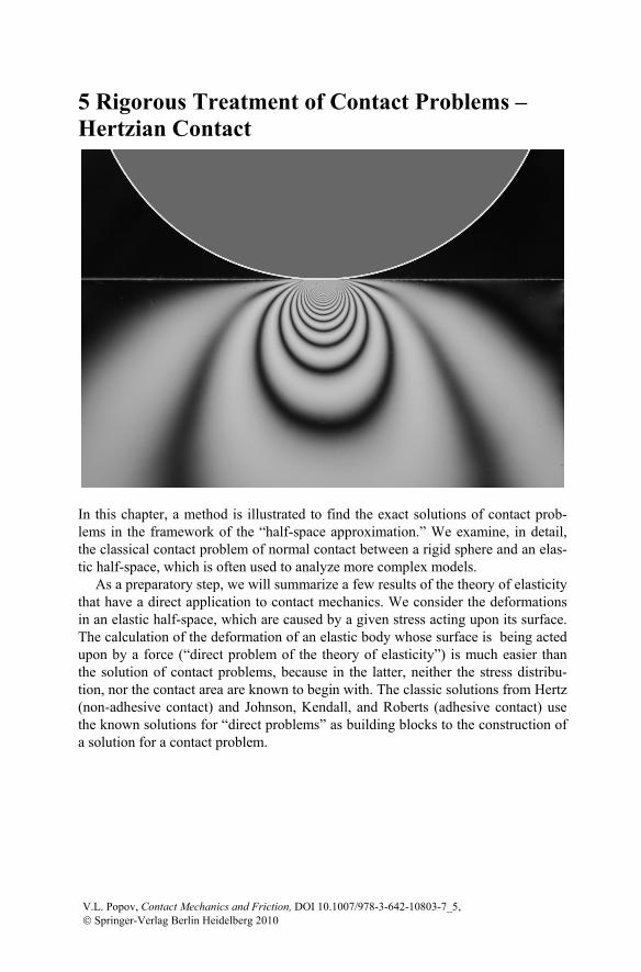
5 Rigorous Treatment of Contact Problems – Hertzian Contact
In this chapter, a method is illustrated to find the exact solutions of contact prob-lems in the framework of the “half-space approximation.” We examine, in detail, the classical contact problem of normal contact between a rigid sphere and an elas-tic half-space, which is often used to analyze more complex models.
As a preparatory step, we will summarize a few results of the theory of elasticity that have a direct application to contact mechanics. We consider the deformations in an elastic half-space, which are caused by a given stress acting upon its surface. The calculation of the deformation of an elastic body whose surface is being acted upon by a force (“direct problem of the theory of elasticity”) is much easier than the solution of contact problems, because in the latter, neither the stress distribu-tion, nor the contact area are known to begin with. The classic solutions from Hertz (non-adhesive contact) and Johnson, Kendall, and Roberts (adhesive contact) use the known solutions for “direct problems” as building blocks to the construction of a solution for a contact problem.
V.L. Popov, Contact Mechanics and Friction, DOI 10.1007/978-3-642-10803-7_5, © Springer-Verlag Berlin Heidelberg 2010
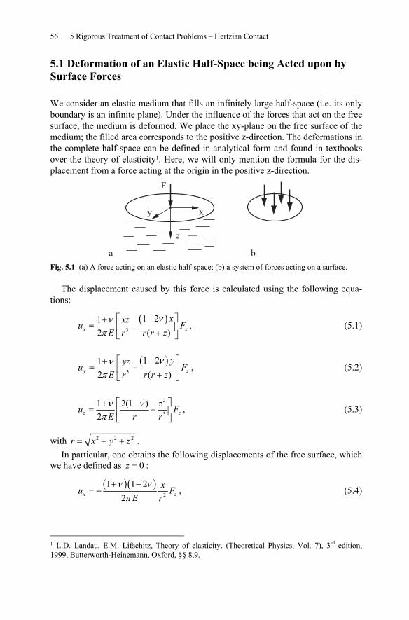
56 5 Rigorous Treatment of Contact Problems – Hertzian Contact
5.1 Deformation of an Elastic Half-Space being Acted upon by Surface Forces
We consider an elastic medium that fills an infinitely large half-space (i.e. its only boundary is an infinite plane). Under the influence of the forces that act on the free surface, the medium is deformed. We place the xy-plane on the free surface of the medium; the filled area corresponds to the positive z-direction. The deformations in the complete half-space can be defined in analytical form and found in textbooks over the theory of elasticity1. Here, we will only mention the formula for the dis-placement from a force acting at the origin in the positive z-direction.
a b
F
x
z
y
Fig. 5.1 (a) A force acting on an elastic half-space; (b) a system of forces acting on a surface.
The displacement caused by this force is calculated using the following equa-tions:
( )
3
1 212 ( )
ννπ
−⎡ ⎤+= −⎢ ⎥+⎣ ⎦
x z
xxzu FE r r zr
, (5.1)
( )
3
1 212 ( )
ννπ
−⎡ ⎤+= −⎢ ⎥+⎣ ⎦
y z
yyzu FE r r zr
, (5.2)
2
3
1 2(1 )2
ν νπ
⎡ ⎤+ −= +⎢ ⎥
⎣ ⎦z z
zu FE r r
, (5.3)
with 2 2 2= + +r x y z . In particular, one obtains the following displacements of the free surface, which
we have defined as 0=z :
( )( )
2
1 1 22ν νπ
+ −= −x z
xu FE r
, (5.4)
1 L.D. Landau, E.M. Lifschitz, Theory of elasticity. (Theoretical Physics, Vol. 7), 3rd edition, 1999, Butterworth-Heinemann, Oxford, §§ 8,9.
5.1 Deformation of an Elastic Half-Space being Acted upon by Surface Forces 57
( )( )
2
1 1 22ν νπ
+ −= −y z
yu FE r
, (5.5)
( )21 1ν
π
−=z zu F
E r, (5.6)
with 2 2= +r x y . If several forces act simultaneously (Fig. 5.1 b), we will get a displacement as
the sum of the respective solutions that result from every individual force. We will continue to work in approximation of the half-space, in which it is as-
sumed that the gradient of the surfaces in the area of contact and within relative proximity is much smaller than one, so that in a first order approximation, the sur-faces are “even.” Although the contact constraints for the two surfaces must con-tinue to be met, the relation between the surface forces and the displacements can be seen, however, exactly as they appear with an elastic half-space.
For contact problems without friction, only the z-component of the displacement (5.6) is of interest within the framework of the half-space approximation. Espe-cially in the case of a continuous distribution of the normal pressure ( , )p x y , the displacement of the surface is calculated using
*
1 ( , )zdx dyu p x y
rEπ′ ′
′ ′= ∫∫ , ( ) ( )2 2′ ′= − + −r x x y y (5.7)
with
( )
*21 ν
=−EE . (5.8)
Before we move on to actual contact problems, we want to solve two prepara-tory problems. We assume that a pressure with a distribution of
( )2 20 1 /= −
np p r a is exerted on a circle-shaped area with the radius a and search
for the vertical displacement of the surface points within the area being acted upon by the pressure. a. Homogeneous Normal Displacement ( 1/ 2= −n ). The coordinate system used is shown in Fig. 5.1. The normal stress is distributed according to the equation
1/ 22
0 21−
⎛ ⎞= −⎜ ⎟
⎝ ⎠
rp pa
. (5.9)
58 5 Rigorous Treatment of Contact Problems – Hertzian Contact
The resulting vertical displacement is2:
0*z
p au
Eπ
= , ≤r a . (5.10)
The vertical displacement is the same for all points in the contact area. From this result, it directly follows how we can produce the assumed pressure distribution: it is produced by the indentation of a rigid cylindrical rod into an elastic half-space. The total force acting on the area under pressure is equal to
20
0
( )2 d 2π π= =∫a
F p r r r p a . (5.11)
The stiffness of the contact is defined as the relationship between the force F and the displacement zu :
*2c aE= . (5.12)
If written in the form
*2 βπ
=Ac E , (5.13)
where A is the contact area of the rigid indenter, Equation (5.12) is also valid for cross-sections that are not round. The constant β always has an order of magni-tude of 1:
Round cross-section: =1.000Triangular cross-section: =1.034Rectangular cross-section: =1.012
βββ
(5.14)
b. Hertzian Pressure Distribution ( 1/ 2=n ). For the pressure distribution of the form
1/ 22
0 21⎛ ⎞
= −⎜ ⎟⎝ ⎠
rp pa
, (5.15)
the resulting vertical displacement (Appendix A) is
( )2 20* 2
4zp
u a rE aπ
= − , ≤r a . (5.16)
The total force follows as
2 A detailed derivation can be found in Appendix A.
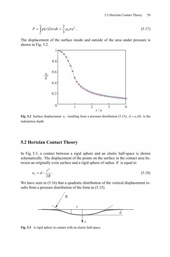
5.2 Hertzian Contact Theory 59
20
0
2( )23
π π= =∫a
F p r rdr p a . (5.17)
The displacement of the surface inside and outside of the area under pressure is shown in Fig. 5.2.
0 1 2 3 4
0.2
0.4
0.6
0.8
1
r / a
uz
d
Fig. 5.2 Surface displacement zu resulting from a pressure distribution (5.15); (0)zd u= is the indentation depth.
5.2 Hertzian Contact Theory
In Fig. 5.3, a contact between a rigid sphere and an elastic half-space is shown schematically. The displacement of the points on the surface in the contact area be-tween an originally even surface and a rigid sphere of radius R is equal to
2
2= −z
ru dR
. (5.18)
We have seen in (5.16) that a quadratic distribution of the vertical displacement re-sults from a pressure distribution of the form in (5.15).
R
r
z
d
Fig. 5.3 A rigid sphere in contact with an elastic half-space.
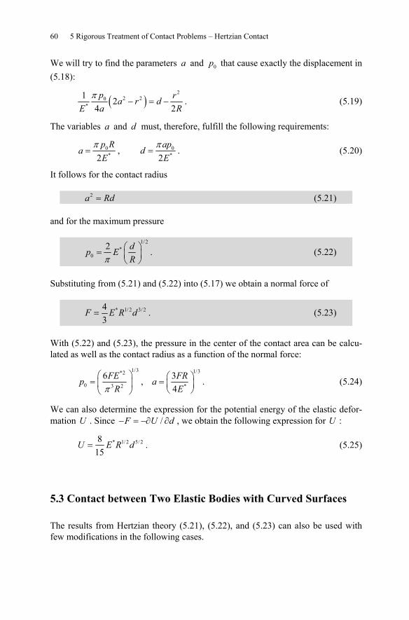
60 5 Rigorous Treatment of Contact Problems – Hertzian Contact
We will try to find the parameters a and 0p that cause exactly the displacement in (5.18):
( )2
2 20*
1 24 2π
− = −p ra r da RE
. (5.19)
The variables a and d must, therefore, fulfill the following requirements:
0*2
π=
p Ra
E, 0
*2π
=ap
dE
. (5.20)
It follows for the contact radius
2a Rd= (5.21)
and for the maximum pressure
1/2
*0
2π
⎛ ⎞= ⎜ ⎟⎝ ⎠
dp ER
. (5.22)
Substituting from (5.21) and (5.22) into (5.17) we obtain a normal force of
* 1/ 2 3/243
=F E R d . (5.23)
With (5.22) and (5.23), the pressure in the center of the contact area can be calcu-lated as well as the contact radius as a function of the normal force:
1/3*2
0 3 2
6π
⎛ ⎞= ⎜ ⎟⎝ ⎠
FEpR
, 1/3
*
34
⎛ ⎞= ⎜ ⎟⎝ ⎠
FRaE
. (5.24)
We can also determine the expression for the potential energy of the elastic defor-mation U . Since /− = −∂ ∂F U d , we obtain the following expression for U :
* 1/2 5/ 2815
=U E R d . (5.25)
5.3 Contact between Two Elastic Bodies with Curved Surfaces
The results from Hertzian theory (5.21), (5.22), and (5.23) can also be used with few modifications in the following cases.
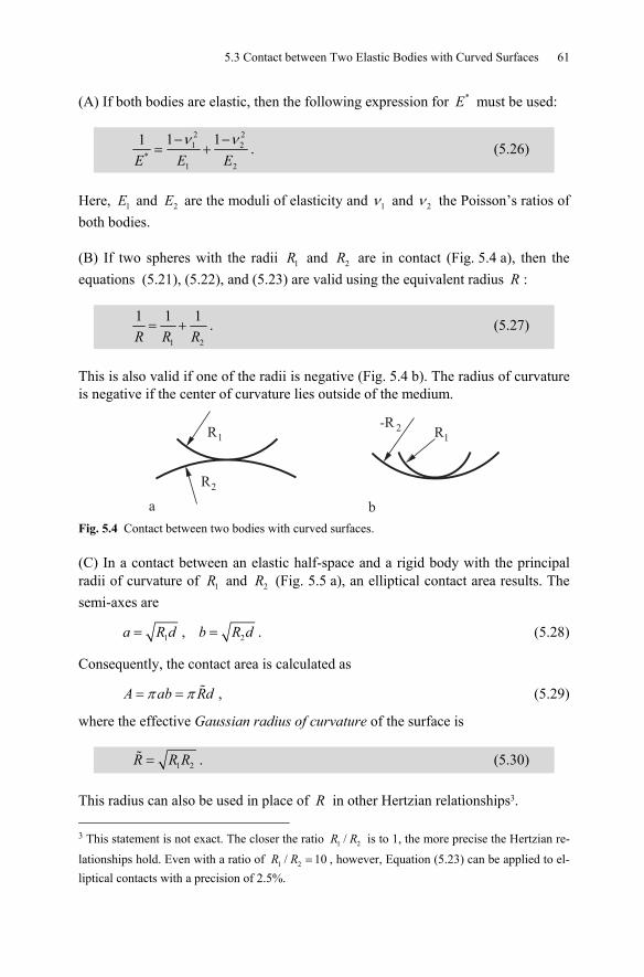
5.3 Contact between Two Elastic Bodies with Curved Surfaces 61
(A) If both bodies are elastic, then the following expression for *E must be used:
2 21 2
*1 2
1 11 ν ν− −= +
E EE. (5.26)
Here, 1E and 2E are the moduli of elasticity and 1ν and 2ν the Poisson’s ratios of both bodies.
(B) If two spheres with the radii 1R and 2R are in contact (Fig. 5.4 a), then the equations (5.21), (5.22), and (5.23) are valid using the equivalent radius R :
1 2
1 1 1= +
R R R. (5.27)
This is also valid if one of the radii is negative (Fig. 5.4 b). The radius of curvature is negative if the center of curvature lies outside of the medium.
R1
R2
R1
-R 2
a b Fig. 5.4 Contact between two bodies with curved surfaces.
(C) In a contact between an elastic half-space and a rigid body with the principal radii of curvature of 1R and 2R (Fig. 5.5 a), an elliptical contact area results. The semi-axes are
1=a R d , 2=b R d . (5.28)
Consequently, the contact area is calculated as
π π= =A ab Rd , (5.29)
where the effective Gaussian radius of curvature of the surface is
1 2=R R R . (5.30)
This radius can also be used in place of R in other Hertzian relationships3. 3 This statement is not exact. The closer the ratio 1 2/R R is to 1, the more precise the Hertzian re-lationships hold. Even with a ratio of 1 2/ 10=R R , however, Equation (5.23) can be applied to el-liptical contacts with a precision of 2.5%.
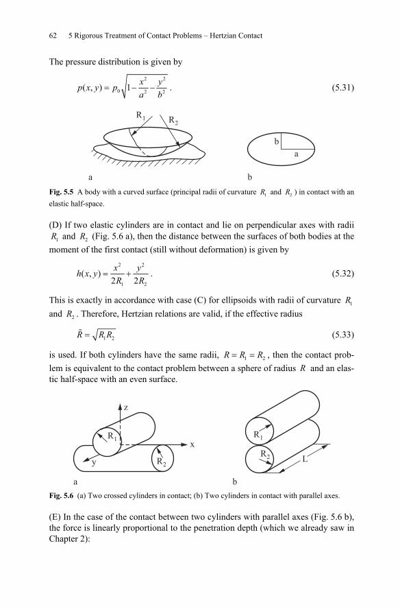
62 5 Rigorous Treatment of Contact Problems – Hertzian Contact
The pressure distribution is given by
2 2
0 2 2( , ) 1= − −x yp x y pa b
. (5.31)
R1 R2
b
a
a b Fig. 5.5 A body with a curved surface (principal radii of curvature 1R and 2R ) in contact with an elastic half-space.
(D) If two elastic cylinders are in contact and lie on perpendicular axes with radii 1R and 2R (Fig. 5.6 a), then the distance between the surfaces of both bodies at the
moment of the first contact (still without deformation) is given by
2 2
1 2
( , )2 2
= +x yh x yR R
. (5.32)
This is exactly in accordance with case (C) for ellipsoids with radii of curvature 1R and 2R . Therefore, Hertzian relations are valid, if the effective radius
1 2=R R R (5.33)
is used. If both cylinders have the same radii, 1 2= =R R R , then the contact prob-lem is equivalent to the contact problem between a sphere of radius R and an elas-tic half-space with an even surface.
R1R1
R2
R2
z
x
y L
a b Fig. 5.6 (a) Two crossed cylinders in contact; (b) Two cylinders in contact with parallel axes.
(E) In the case of the contact between two cylinders with parallel axes (Fig. 5.6 b), the force is linearly proportional to the penetration depth (which we already saw in Chapter 2):
5.4 Contact between a Rigid Cone-Shaped Indenter and an Elastic Half-Space 63
*
4π
=F E Ld . (5.34)
What is interesting is that the radius of curvature does not appear at all in this rela-tionship. Half of the contact width is given through the equation
=a Rd , 1 2
1 1 1= +
R R R, (5.35)
as in the contact between two spheres. The maximum pressure is equal to
1/21/ 2* * *
0 2 2E d E d E Fp
a R LR⎛ ⎞⎛ ⎞= = = ⎜ ⎟⎜ ⎟
⎝ ⎠ ⎝ ⎠. (5.36)
5.4 Contact between a Rigid Cone-Shaped Indenter and an Elastic Half-Space
When indenting an elastic half-space with a rigid cone-shaped indenter (Fig. 5.7 a), the penetration depth and the contact radius are given through the relationship4
tan2
d aπ θ= . (5.37)
The pressure distribution has the form
( )
2
2( ) ln 1
1Ed a ap r
r raπ ν
⎛ ⎞⎛ ⎞⎜ ⎟= − + −⎜ ⎟⎜ ⎟− ⎝ ⎠⎝ ⎠. (5.38)
The stress has a logarithmic singularity (Fig. 5.7 b) at the point of the cone (at the center of the contact area). The total force is calculated as
2
*2tanNdF E
π θ= . (5.39)
4 I.N. Sneddon, The Relation between Load and Penetration in the Axisymmetric Boussinesq Problem for a Punch of Arbitrary Profile. Int. J. Eng. Sci., 1965, v. 3, pp. 47–57.
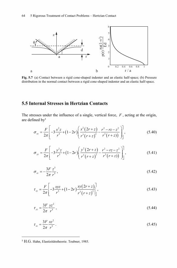
64 5 Rigorous Treatment of Contact Problems – Hertzian Contact
Fig. 5.7 (a) Contact between a rigid cone-shaped indenter and an elastic half-space; (b) Pressure distribution in the normal contact between a rigid cone-shaped indenter and an elastic half-space.
5.5 Internal Stresses in Hertzian Contacts
The stresses under the influence of a single, vertical force, F , acting at the origin, are defined by5
( ) ( )( ) ( )
22 2 2
5 2 33
23 1 2
2 )σ ν
π
⎡ ⎤⎛ ⎞+ − −⎢ ⎥⎜ ⎟= − + − −⎜ ⎟+⎢ ⎥+⎝ ⎠⎣ ⎦
xx
x r zF x z r rz zr r r zr r z
, (5.40)
( ) ( )( ) ( )
22 2 2
5 2 33
23 1 2
2 )σ ν
π
⎡ ⎤⎛ ⎞+ − −⎢ ⎥⎜ ⎟= − + − −⎜ ⎟+⎢ ⎥+⎝ ⎠⎣ ⎦
yy
y r zF y z r rz zr r r zr r z
, (5.41)
3
5
32
σπ
= −zzF z
r, (5.42)
( ) ( )( )5 23
23 1 2
2τ ν
π
⎡ ⎤+= − + −⎢ ⎥
+⎢ ⎥⎣ ⎦xy
xy r zF xyzr r r z
, (5.43)
2
5
32
τπ
=yzF yz
r, (5.44)
2
5
32
τπ
=xzF xz
r. (5.45)
5 H.G. Hahn, Elastizitätstheorie. Teubner, 1985.
5.5 Internal Stresses in Hertzian Contacts 65
The calculation of the stresses by an arbitrary normal pressure distribution p on the surface is made possible through superposition. The normal stress in the z-direction, σ zz , is exemplary
( ) ( )( )
3
5/ 22 2 2( )
3 ( , )( , , )2
σπ
′ ′′ ′= −
′ ′− + − +∫∫zzA
z p x yx y z dx dyx x y y z
, (5.46)
where ( )∫∫A
means the integral over the area being acted upon by the pressure.
For the Hertzian pressure distribution in (5.15), various results are discussed in the following. Fig. 5.8 shows the stresses at the z-axis for 0.33ν = . All of the shear stresses are 0; for all points along the z-axis, the principal axes coincide with the coordinate axes. The analytical solution for the components of the stress tensors provides us with6
12
0 21σ−
⎛ ⎞= − +⎜ ⎟
⎝ ⎠zz
zpa
, (5.47)
( )12
0 2
11 1 arctan 12
σ σ ν−⎡ ⎤⎛ ⎞⎛ ⎞⎢ ⎥= = − + − − +⎜ ⎟⎜ ⎟
⎝ ⎠⎢ ⎥⎝ ⎠⎣ ⎦xx yy
z a zpa z a
. (5.48)
Furthermore, the maximum shear stress, 11 2τ σ σ= −zz xx , is depicted in Fig. 5.8.
One comes to the conclusion that the maximum shear stress lies in the interior, for 0.33ν = at 0.49z a≈ . Fig. 5.9 shows the equivalent stress according to the von
Mises criterion in the x-y plane:
( ) ( ) ( ) ( )1/ 22 22 2 2 21 6
2σ σ σ σ σ σ σ τ τ τ⎡ ⎤= − + − + − + + +⎢ ⎥⎣ ⎦V xx yy xx zz zz yy xy xz yz . (5.49)
6 K.L. Johnson, Contact mechanics. Cambridge University Press, Ninth printing 2003.
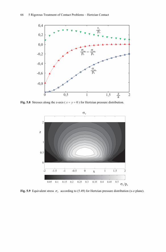
66 5 Rigorous Treatment of Contact Problems – Hertzian Contact
0,4
0,2
0,0
-0,2
-0,4
-0,6
-0,8
0 0,5 1 1,5 2
��
p0
�zz
p0
�xx
p0
�yy
p0=
za
Fig. 5.8 Stresses along the z-axis ( 0= =x y ) for Hertzian pressure distribution.
Fig. 5.9 Equivalent stress σV according to (5.49) for Hertzian pressure distribution (x-z plane).
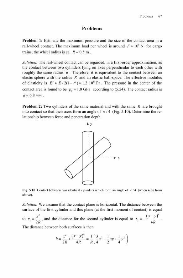
Problems 67
Problems
Problem 1: Estimate the maximum pressure and the size of the contact area in a rail-wheel contact. The maximum load per wheel is around 510 N≈F for cargo trains, the wheel radius is ca. 0.5 mR = .
Solution: The rail-wheel contact can be regarded, in a first-order approximation, as the contact between two cylinders lying on axes perpendicular to each other with roughly the same radius R . Therefore, it is equivalent to the contact between an elastic sphere with the radius R and an elastic half-space. The effective modulus of elasticity is * 2 11/ 2(1 ) 1.2 10 PaE E ν≈ − ≈ ⋅ . The pressure in the center of the contact area is found to be 0 1.0 GPap ≈ according to (5.24). The contact radius is
6.8a mm≈ .
Problem 2: Two cylinders of the same material and with the same R are brought into contact so that their axes form an angle of / 4π (Fig. 5.10). Determine the re-lationship between force and penetration depth.
y
x
Fig. 5.10 Contact between two identical cylinders which form an angle of / 4π (when seen from above).
Solution: We assume that the contact plane is horizontal. The distance between the surface of the first cylinder and this plane (at the first moment of contact) is equal
to 2
1 2=
xzR
, and the distance for the second cylinder is equal to ( )2
2 4−
= −x y
zR
.
The distance between both surfaces is then
( )222 21 3 1 1
2 4 4 2 4x yxh x xy y
R R R− ⎛ ⎞= + = − +⎜ ⎟
⎝ ⎠.
68 5 Rigorous Treatment of Contact Problems – Hertzian Contact
The principal curvatures are calculated as the eigenvalues of this quadratic form, using the equation,
22
3 114 4 0
1 1 84 4
κ κκκ
− −= − + =
− −
R RR R
R R
.
to 1,21 1/ 2
2κ ±
=R
. The principal radii of curvature are accordingly
1,22
1 1/ 2=
±RR . The resulting Gaussian radius of curvature is
1 2 2 2= =R R R R . Because both cylinders are made from the same material,
then according to (5.26) *22(1 )ν
=−EE . In this case, the relationship between the
force and the penetration depth from (5.23) is 7/4
1/ 2 3/ 22
23 (1 )ν
=−EF R d .
Problem 3: Determine the contact time during an impact of an elastic sphere (Ra-dius R) with a flat wall (Hertz, 1882).
Solution: The displacement of the center of the sphere from the moment of initial contact we will call x . The potential energy of the system is given by (5.25) with =d x and *E according to (5.26). During the contact time, the energy is con-
served: 2 2
* 1/2 5/2 082 15 2⎛ ⎞ + =⎜ ⎟⎝ ⎠
mvm dx E R xdt
.
The maximum displacement 0x corresponds to the point in time at which the ve-locity, /dx dt , is zero and is
2/520
0 * 1/2
1516⎛ ⎞
= ⎜ ⎟⎝ ⎠
mvx
E R.
The contact time τ (during which x varies from 0 to 0x and again back to 0) is
( )
0 10 0
5/2 5/20 0 00 00
2 2,942
11 /
ξτξ
= = =−−
∫ ∫x x xdx d
v v vx x.
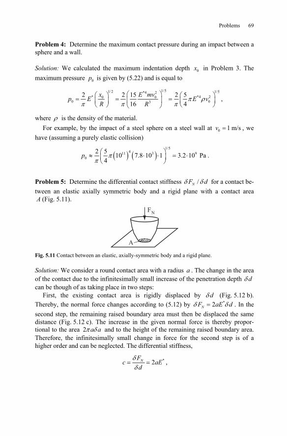
Problems 69
Problem 4: Determine the maximum contact pressure during an impact between a sphere and a wall. Solution: We calculated the maximum indentation depth 0x in Problem 3. The maximum pressure 0p is given by (5.22) and is equal to
1/51/2 1/5*4 2* *4 20 0
0 03
2 2 15 2 516 4
π ρπ π π
⎛ ⎞⎛ ⎞ ⎛ ⎞= = =⎜ ⎟ ⎜ ⎟⎜ ⎟ ⎝ ⎠⎝ ⎠ ⎝ ⎠
x E mvp E E v
R R,
where ρ is the density of the material. For example, by the impact of a steel sphere on a steel wall at 0 1 m/s=v , we
have (assuming a purely elastic collision)
( ) ( )1/5
411 3 90
2 5 10 7.8 10 1 3.2 10 Pa4
p ππ⎛ ⎞≈ ⋅ ⋅ = ⋅⎜ ⎟⎝ ⎠
.
Problem 5: Determine the differential contact stiffness /δ δNF d for a contact be-tween an elastic axially symmetric body and a rigid plane with a contact area A (Fig. 5.11).
A
FN
Fig. 5.11 Contact between an elastic, axially-symmetric body and a rigid plane.
Solution: We consider a round contact area with a radius a . The change in the area of the contact due to the infinitesimally small increase of the penetration depth δ d can be though of as taking place in two steps:
First, the existing contact area is rigidly displaced by δ d (Fig. 5.12 b). Thereby, the normal force changes according to (5.12) by *2δ δ=NF aE d . In the second step, the remaining raised boundary area must then be displaced the same distance (Fig. 5.12 c). The increase in the given normal force is thereby propor-tional to the area 2π δa a and to the height of the remaining raised boundary area. Therefore, the infinitesimally small change in force for the second step is of a higher order and can be neglected. The differential stiffness,
*2δδ
= =NFc aE
d,
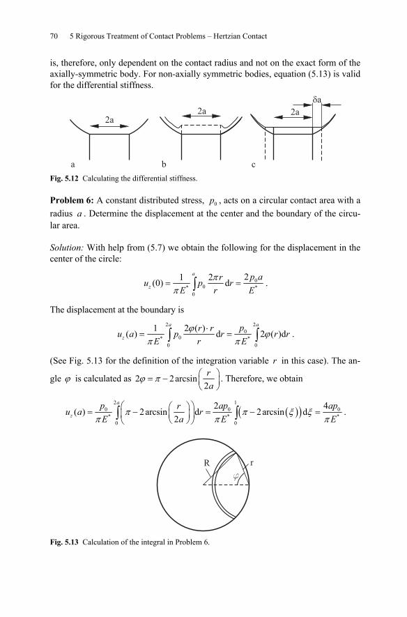
70 5 Rigorous Treatment of Contact Problems – Hertzian Contact
is, therefore, only dependent on the contact radius and not on the exact form of the axially-symmetric body. For non-axially symmetric bodies, equation (5.13) is valid for the differential stiffness.
2a2a 2a
�a
a b c Fig. 5.12 Calculating the differential stiffness.
Problem 6: A constant distributed stress, 0p , acts on a circular contact area with a radius a . Determine the displacement at the center and the boundary of the circu-lar area. Solution: With help from (5.7) we obtain the following for the displacement in the center of the circle:
00* *
0
21 2(0) dππ
= =∫a
zp aru p r
rE E.
The displacement at the boundary is 2 2
00* *
0 0
1 2 ( )( ) d 2 ( )dϕ ϕπ π
⋅= =∫ ∫
a a
zpr ru a p r r r
rE E.
(See Fig. 5.13 for the definition of the integration variable r in this case). The an-
gle ϕ is calculated as 2 2arcsin2
ϕ π ⎛ ⎞= − ⎜ ⎟⎝ ⎠
ra
. Therefore, we obtain
( )( )2 1
0 0 0* * *
0 0
2 4( ) 2arcsin d 2arcsin d
2π π ξ ξ
π π π⎛ ⎞⎛ ⎞= − = − =⎜ ⎟⎜ ⎟
⎝ ⎠⎝ ⎠∫ ∫a
zp ap apru a r
aE E E.
r
f
R
Fig. 5.13 Calculation of the integral in Problem 6.
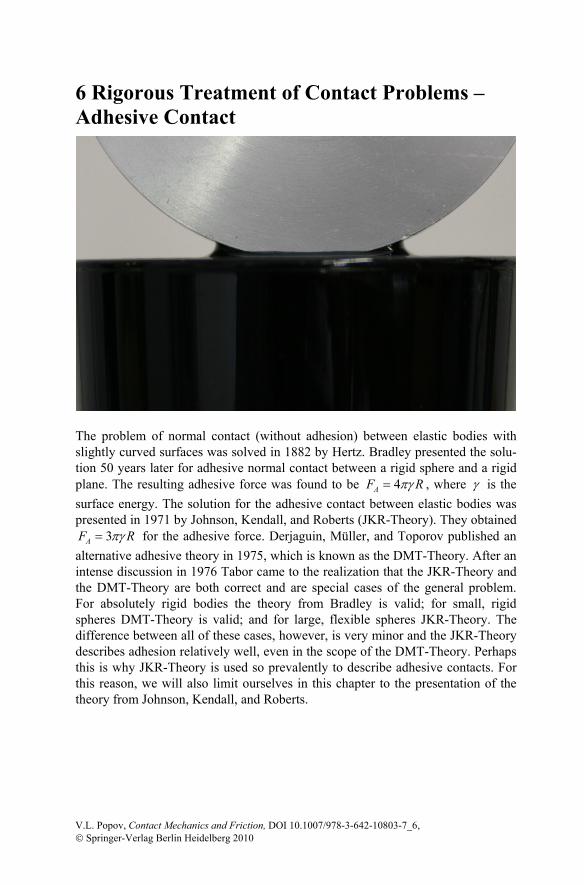
6 Rigorous Treatment of Contact Problems – Adhesive Contact
The problem of normal contact (without adhesion) between elastic bodies with slightly curved surfaces was solved in 1882 by Hertz. Bradley presented the solu-tion 50 years later for adhesive normal contact between a rigid sphere and a rigid plane. The resulting adhesive force was found to be 4AF Rπγ= , where γ is the surface energy. The solution for the adhesive contact between elastic bodies was presented in 1971 by Johnson, Kendall, and Roberts (JKR-Theory). They obtained
3πγ=AF R for the adhesive force. Derjaguin, Müller, and Toporov published an alternative adhesive theory in 1975, which is known as the DMT-Theory. After an intense discussion in 1976 Tabor came to the realization that the JKR-Theory and the DMT-Theory are both correct and are special cases of the general problem. For absolutely rigid bodies the theory from Bradley is valid; for small, rigid spheres DMT-Theory is valid; and for large, flexible spheres JKR-Theory. The difference between all of these cases, however, is very minor and the JKR-Theory describes adhesion relatively well, even in the scope of the DMT-Theory. Perhaps this is why JKR-Theory is used so prevalently to describe adhesive contacts. For this reason, we will also limit ourselves in this chapter to the presentation of the theory from Johnson, Kendall, and Roberts.
V.L. Popov, Contact Mechanics and Friction, DOI 10.1007/978-3-642-10803-7_6, © Springer-Verlag Berlin Heidelberg 2010
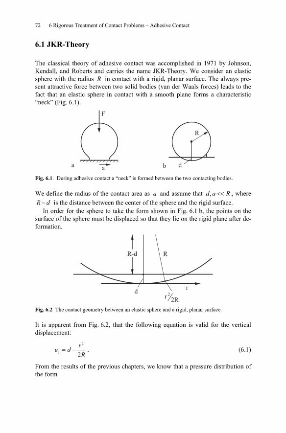
72 6 Rigorous Treatment of Contact Problems – Adhesive Contact
6.1 JKR-Theory
The classical theory of adhesive contact was accomplished in 1971 by Johnson, Kendall, and Roberts and carries the name JKR-Theory. We consider an elastic sphere with the radius R in contact with a rigid, planar surface. The always pre-sent attractive force between two solid bodies (van der Waals forces) leads to the fact that an elastic sphere in contact with a smooth plane forms a characteristic “neck” (Fig. 6.1).
a
F
d
R
a b Fig. 6.1. During adhesive contact a “neck” is formed between the two contacting bodies.
We define the radius of the contact area as a and assume that , <<d a R , where −R d is the distance between the center of the sphere and the rigid surface. In order for the sphere to take the form shown in Fig. 6.1 b, the points on the
surface of the sphere must be displaced so that they lie on the rigid plane after de-formation.
Fig. 6.2 The contact geometry between an elastic sphere and a rigid, planar surface.
It is apparent from Fig. 6.2, that the following equation is valid for the vertical displacement:
2
2= −z
ru dR
. (6.1)
From the results of the previous chapters, we know that a pressure distribution of the form
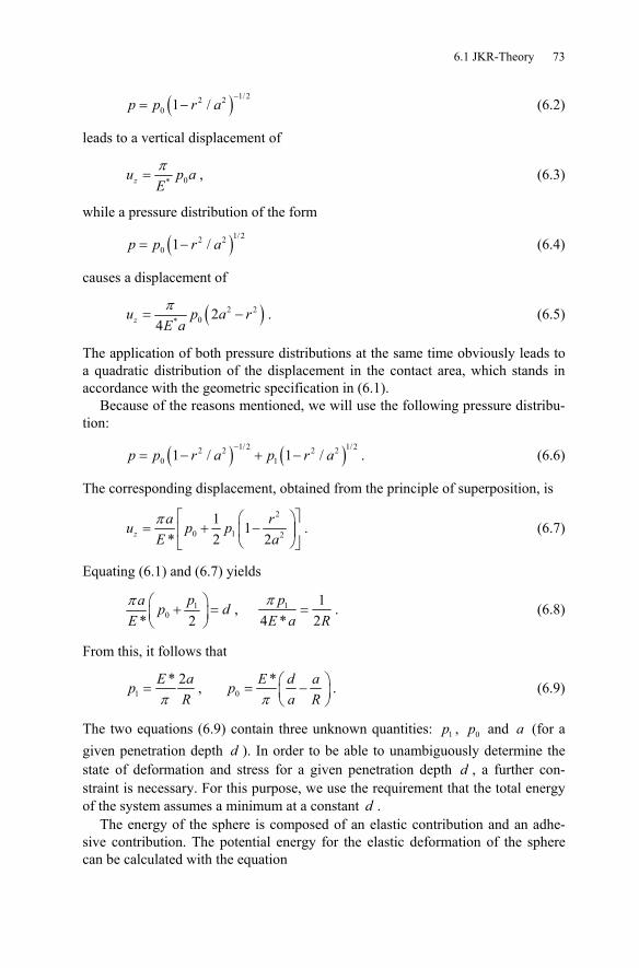
6.1 JKR-Theory 73
( ) 1/22 20 1 /
−= −p p r a (6.2)
leads to a vertical displacement of
0*zu p aEπ
= , (6.3)
while a pressure distribution of the form
( )1/22 20 1 /= −p p r a (6.4)
causes a displacement of
( )2 20* 2
4zu p a rE aπ
= − . (6.5)
The application of both pressure distributions at the same time obviously leads to a quadratic distribution of the displacement in the contact area, which stands in accordance with the geometric specification in (6.1).
Because of the reasons mentioned, we will use the following pressure distribu-tion:
( ) ( )1/ 2 1/22 2 2 20 11 / 1 /
−= − + −p p r a p r a . (6.6)
The corresponding displacement, obtained from the principle of superposition, is
2
0 1 2
1 1* 2 2za ru p p
E aπ ⎡ ⎤⎛ ⎞
= + −⎢ ⎥⎜ ⎟⎝ ⎠⎣ ⎦
. (6.7)
Equating (6.1) and (6.7) yields
10* 2
π ⎛ ⎞+ =⎜ ⎟⎝ ⎠
pa p dE
, 1 14 * 2π
=p
E a R. (6.8)
From this, it follows that
1* 2
π=
E apR
, 0*
π⎛ ⎞= −⎜ ⎟⎝ ⎠
E d apa R
. (6.9)
The two equations (6.9) contain three unknown quantities: 1p , 0p and a (for a given penetration depth d ). In order to be able to unambiguously determine the state of deformation and stress for a given penetration depth d , a further con-straint is necessary. For this purpose, we use the requirement that the total energy of the system assumes a minimum at a constant d .
The energy of the sphere is composed of an elastic contribution and an adhe-sive contribution. The potential energy for the elastic deformation of the sphere can be calculated with the equation

74 6 Rigorous Treatment of Contact Problems – Adhesive Contact
1 ( ) ( )2el z
contactarea
U p u dxdy= ∫ x x , (6.10)
which is valid for arbitrary linearly elastic systems. Substituting (6.6) and (6.1) in-to (6.10) provides us with
( ) ( )21/ 2 1/ 22 2 2 2
0 10
1 / 1 / 12
π− ⎛ ⎞⎡ ⎤= − + − −⎜ ⎟⎢ ⎥⎣ ⎦ ⎝ ⎠
∫a
elrU d r p r a p r a drdR
. (6.11)
After the substitution of 2 21 /ξ = − r a , 22 /ξ = −d rdr a , we obtain
2 2 2
0 12 2 22
2 3 3 15π ⎡ ⎤⎛ ⎞ ⎛ ⎞
= − + −⎢ ⎥⎜ ⎟ ⎜ ⎟⎝ ⎠ ⎝ ⎠⎣ ⎦
elda a aU p p
dR dR (6.12)
and considering (6.9),
3 5
22
2*3 5
⎡ ⎤= − +⎢ ⎥
⎣ ⎦el
da aU E d aR R
. (6.13)
The total energy is1
3 5
2 2122
2*3 5tot
da aU E d a aR R
γ π⎡ ⎤
= − + −⎢ ⎥⎣ ⎦
. (6.14)
We obtain the radius at equilibrium a by requiring that the energy of the system assumes the minimum value:
22 4 2
212 122* 2 2 * 2 0totU da a aE d a E d a
a R RRγ π γ π
⎡ ⎤ ⎛ ⎞∂= − + − = − − =⎜ ⎟⎢ ⎥∂ ⎣ ⎦ ⎝ ⎠
. (6.15)
It follows that
2
122*
aadR E
γ π= ± . (6.16)
Inserting this relationship into (6.14) provides the total energy as a function of the contact radius
25 3
12 122
28 4*15 * 3 *tot
a aa aU EE R ER
γ π γ π⎡ ⎤= + ±⎢ ⎥
⎢ ⎥⎣ ⎦. (6.17)
1 Here is 12γ the relative surface energy.
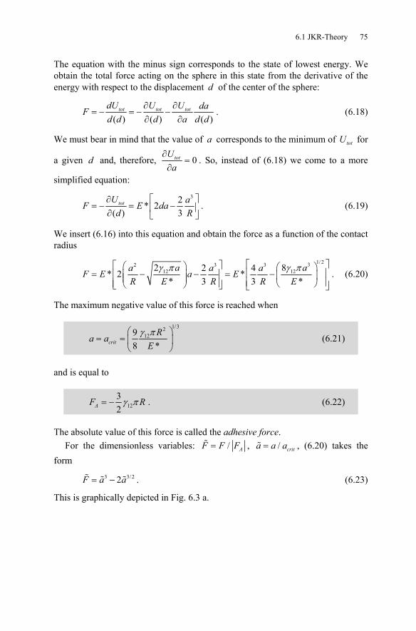
6.1 JKR-Theory 75
The equation with the minus sign corresponds to the state of lowest energy. We obtain the total force acting on the sphere in this state from the derivative of the energy with respect to the displacement d of the center of the sphere:
( ) ( ) ( )
∂ ∂= − = − −
∂ ∂tot tot totdU U U daF
d d d a d d. (6.18)
We must bear in mind that the value of a corresponds to the minimum of totU for
a given d and, therefore, 0∂
=∂
totUa
. So, instead of (6.18) we come to a more
simplified equation:
32* 2
( ) 3⎡ ⎤∂
= − = −⎢ ⎥∂ ⎣ ⎦totU aF E da
d R. (6.19)
We insert (6.16) into this equation and obtain the force as a function of the contact radius
1/232 3 3
12 122 82 4* 2 ** 3 3 *
a aa a aF E a ER E R R E
γ π γ π⎡ ⎤⎡ ⎤⎛ ⎞ ⎛ ⎞⎢ ⎥= − − = −⎢ ⎥⎜ ⎟ ⎜ ⎟⎜ ⎟ ⎢ ⎥⎢ ⎥ ⎝ ⎠⎝ ⎠⎣ ⎦ ⎣ ⎦
. (6.20)
The maximum negative value of this force is reached when
1/32
1298 *crit
Ra a
Eγ π⎛ ⎞
= = ⎜ ⎟⎝ ⎠
(6.21)
and is equal to
1232AF Rγ π= − . (6.22)
The absolute value of this force is called the adhesive force. For the dimensionless variables: /= AF F F , /= crita a a , (6.20) takes the
form
3 3/22= −F a a . (6.23)
This is graphically depicted in Fig. 6.3 a.
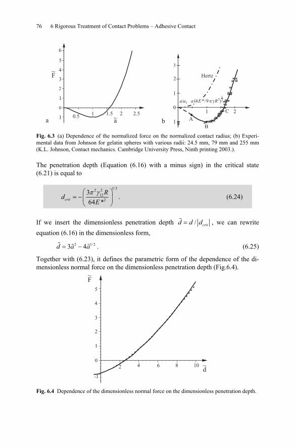
76 6 Rigorous Treatment of Contact Problems – Adhesive Contact
6
5
4
3
2
1
0
1 0.51 1.5 2 2.5
1
0
1
2
3
a/ac a (4E*/9 ��R2)13
21
Hertz
A
B
C
F~
a~a b
Fig. 6.3 (a) Dependence of the normalized force on the normalized contact radius; (b) Experi-mental data from Johnson for gelatin spheres with various radii: 24.5 mm, 79 mm and 255 mm (K.L. Johnson, Contact mechanics. Cambridge University Press, Ninth printing 2003.).
The penetration depth (Equation (6.16) with a minus sign) in the critical state (6.21) is equal to
1/32 2
122
364 *crit
Rd
Eπ γ⎛ ⎞
= −⎜ ⎟⎝ ⎠
. (6.24)
If we insert the dimensionless penetration depth /= critd d d , we can rewrite equation (6.16) in the dimensionless form,
2 1/ 23 4= −d a a . (6.25)
Together with (6.23), it defines the parametric form of the dependence of the di-mensionless normal force on the dimensionless penetration depth (Fig.6.4).
Fig. 6.4 Dependence of the dimensionless normal force on the dimensionless penetration depth.
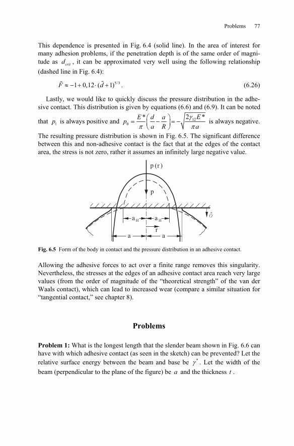
Problems 77
This dependence is presented in Fig. 6.4 (solid line). In the area of interest for many adhesion problems, if the penetration depth is of the same order of magni-tude as critd , it can be approximated very well using the following relationship (dashed line in Fig. 6.4):
5/31 0,12 ( 1)≈ − + ⋅ +F d . (6.26)
Lastly, we would like to quickly discuss the pressure distribution in the adhe-sive contact. This distribution is given by equations (6.6) and (6.9). It can be noted
that 1p is always positive and 120
2 ** EE d apa R a
γπ π
⎛ ⎞= − = −⎜ ⎟⎝ ⎠
is always negative.
The resulting pressure distribution is shown in Fig. 6.5. The significant difference between this and non-adhesive contact is the fact that at the edges of the contact area, the stress is not zero, rather it assumes an infinitely large negative value.
p
a H a H
a ar
( )r
p
d
Fig. 6.5 Form of the body in contact and the pressure distribution in an adhesive contact.
Allowing the adhesive forces to act over a finite range removes this singularity. Nevertheless, the stresses at the edges of an adhesive contact area reach very large values (from the order of magnitude of the “theoretical strength” of the van der Waals contact), which can lead to increased wear (compare a similar situation for “tangential contact,” see chapter 8).
Problems
Problem 1: What is the longest length that the slender beam shown in Fig. 6.6 can have with which adhesive contact (as seen in the sketch) can be prevented? Let the relative surface energy between the beam and base be *γ . Let the width of the beam (perpendicular to the plane of the figure) be a and the thickness t .
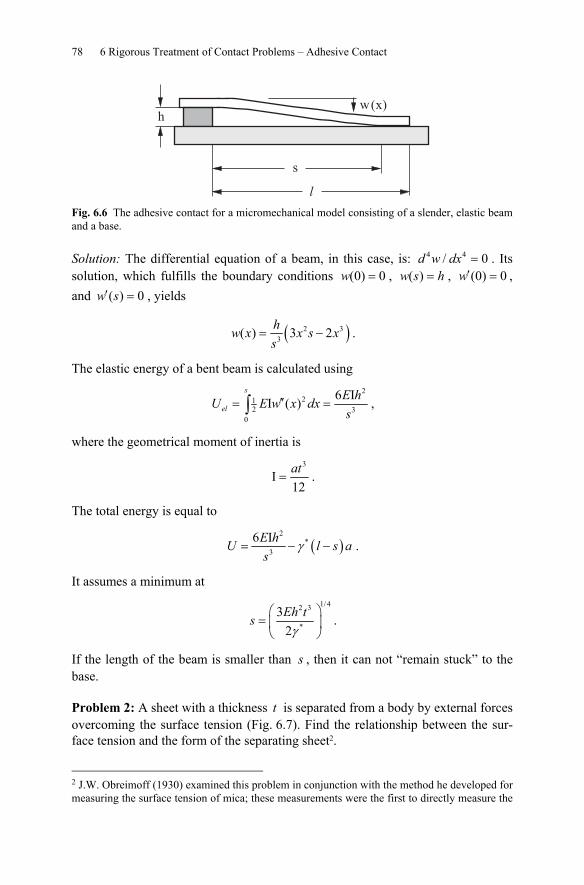
78 6 Rigorous Treatment of Contact Problems – Adhesive Contact
hw(x)
s
l Fig. 6.6 The adhesive contact for a micromechanical model consisting of a slender, elastic beam and a base.
Solution: The differential equation of a beam, in this case, is: 4 4/ 0=d w dx . Its solution, which fulfills the boundary conditions (0) 0=w , ( ) =w s h , (0) 0′ =w , and ( ) 0′ =w s , yields
( )2 33( ) 3 2= −
hw x x s xs
.
The elastic energy of a bent beam is calculated using 2
212 3
0
6 II ( )′′= =∫s
elE hU E w x dxs
,
where the geometrical moment of inertia is 3
I12
=at .
The total energy is equal to
( )2
*3
6 IE hU l s as
γ= − − .
It assumes a minimum at 1/42 3
*
32γ
⎛ ⎞= ⎜ ⎟⎝ ⎠
Eh ts .
If the length of the beam is smaller than s , then it can not “remain stuck” to the base.
Problem 2: A sheet with a thickness t is separated from a body by external forces overcoming the surface tension (Fig. 6.7). Find the relationship between the sur-face tension and the form of the separating sheet2.
2 J.W. Obreimoff (1930) examined this problem in conjunction with the method he developed for measuring the surface tension of mica; these measurements were the first to directly measure the
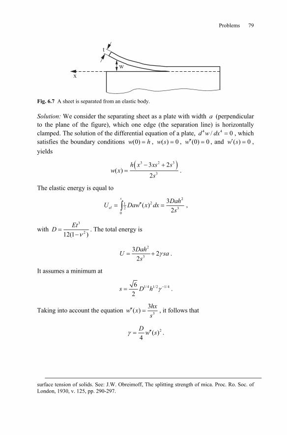
Problems 79
x
t
w
Fig. 6.7 A sheet is separated from an elastic body.
Solution: We consider the separating sheet as a plate with width a (perpendicular to the plane of the figure), which one edge (the separation line) is horizontally clamped. The solution of the differential equation of a plate, 4 4/ 0=d w dx , which satisfies the boundary conditions (0) =w h , ( ) 0=w s , (0) 0′′ =w , and ( ) 0′ =w s , yields
( )3 2 3
3
3 2( )
2
− +=
h x xs sw x
s.
The elastic energy is equal to 2
212 3
0
3( )2
′′= =∫s
elDahU Daw x dx
s,
with 3
212(1 )ν=
−EtD . The total energy is
2
3
3 22
γ= +DahU sa
s.
It assumes a minimum at
1/ 4 1/2 1/462
γ −=s D h .
Taking into account the equation 3
3( )′′ =hxw xs
, it follows that
2( )4
γ ′′=D w s .
surface tension of solids. See: J.W. Obreimoff, The splitting strength of mica. Proc. Ro. Soc. of London, 1930, v. 125, pp. 290-297.
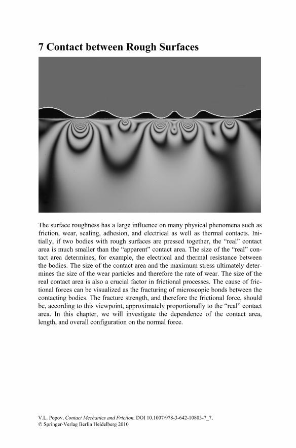
7 Contact between Rough Surfaces
The surface roughness has a large influence on many physical phenomena such as friction, wear, sealing, adhesion, and electrical as well as thermal contacts. Ini-tially, if two bodies with rough surfaces are pressed together, the “real” contact area is much smaller than the “apparent” contact area. The size of the “real” con-tact area determines, for example, the electrical and thermal resistance between the bodies. The size of the contact area and the maximum stress ultimately deter-mines the size of the wear particles and therefore the rate of wear. The size of the real contact area is also a crucial factor in frictional processes. The cause of fric-tional forces can be visualized as the fracturing of microscopic bonds between the contacting bodies. The fracture strength, and therefore the frictional force, should be, according to this viewpoint, approximately proportionally to the “real” contact area. In this chapter, we will investigate the dependence of the contact area, length, and overall configuration on the normal force.
V.L. Popov, Contact Mechanics and Friction, DOI 10.1007/978-3-642-10803-7_7, © Springer-Verlag Berlin Heidelberg 2010
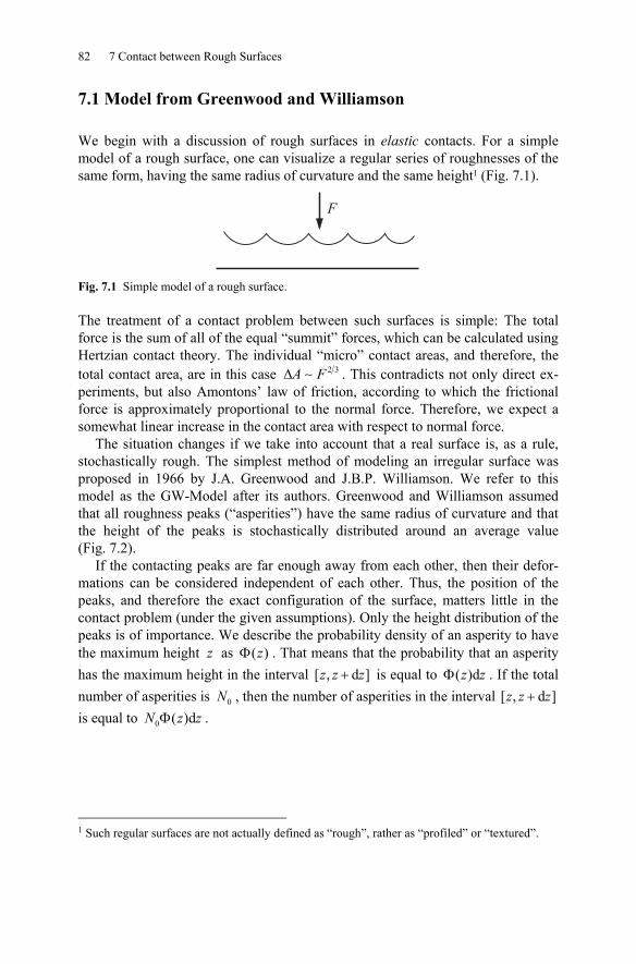
82 7 Contact between Rough Surfaces
7.1 Model from Greenwood and Williamson
We begin with a discussion of rough surfaces in elastic contacts. For a simple model of a rough surface, one can visualize a regular series of roughnesses of the same form, having the same radius of curvature and the same height1 (Fig. 7.1).
F
Fig. 7.1 Simple model of a rough surface.
The treatment of a contact problem between such surfaces is simple: The total force is the sum of all of the equal “summit” forces, which can be calculated using Hertzian contact theory. The individual “micro” contact areas, and therefore, the total contact area, are in this case 2 3Δ ∼A F . This contradicts not only direct ex-periments, but also Amontons’ law of friction, according to which the frictional force is approximately proportional to the normal force. Therefore, we expect a somewhat linear increase in the contact area with respect to normal force.
The situation changes if we take into account that a real surface is, as a rule, stochastically rough. The simplest method of modeling an irregular surface was proposed in 1966 by J.A. Greenwood and J.B.P. Williamson. We refer to this model as the GW-Model after its authors. Greenwood and Williamson assumed that all roughness peaks (“asperities”) have the same radius of curvature and that the height of the peaks is stochastically distributed around an average value (Fig. 7.2).
If the contacting peaks are far enough away from each other, then their defor-mations can be considered independent of each other. Thus, the position of the peaks, and therefore the exact configuration of the surface, matters little in the contact problem (under the given assumptions). Only the height distribution of the peaks is of importance. We describe the probability density of an asperity to have the maximum height z as ( )Φ z . That means that the probability that an asperity has the maximum height in the interval [ , d ]+z z z is equal to ( )dΦ z z . If the total number of asperities is 0N , then the number of asperities in the interval [ , d ]+z z z is equal to 0 ( )dΦN z z .
1 Such regular surfaces are not actually defined as “rough”, rather as “profiled” or “textured”.
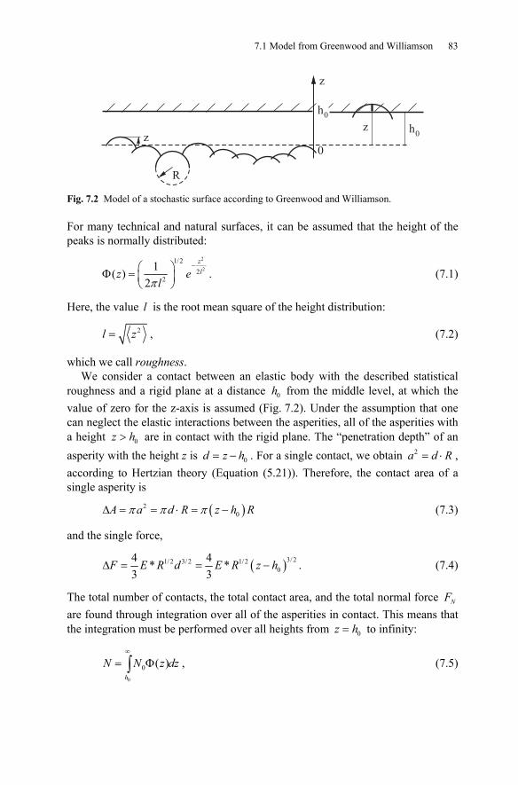
7.1 Model from Greenwood and Williamson 83
z
0
z
h
R
z
0
h0
Fig. 7.2 Model of a stochastic surface according to Greenwood and Williamson.
For many technical and natural surfaces, it can be assumed that the height of the peaks is normally distributed:
2
21/2
22
1( )2π
−⎛ ⎞Φ = ⎜ ⎟⎝ ⎠
zlz e
l. (7.1)
Here, the value l is the root mean square of the height distribution:
2=l z , (7.2)
which we call roughness. We consider a contact between an elastic body with the described statistical
roughness and a rigid plane at a distance 0h from the middle level, at which the value of zero for the z-axis is assumed (Fig. 7.2). Under the assumption that one can neglect the elastic interactions between the asperities, all of the asperities with a height 0>z h are in contact with the rigid plane. The “penetration depth” of an asperity with the height z is 0= −d z h . For a single contact, we obtain 2 = ⋅a d R , according to Hertzian theory (Equation (5.21)). Therefore, the contact area of a single asperity is
( )20π π πΔ = = ⋅ = −A a d R z h R (7.3)
and the single force,
( )3/ 21/ 2 3/ 2 1/20
4 4* *3 3
F E R d E R z hΔ = = − . (7.4)
The total number of contacts, the total contact area, and the total normal force NF are found through integration over all of the asperities in contact. This means that the integration must be performed over all heights from 0=z h to infinity:
0
0 ( )∞
= Φ∫h
N N z dz , (7.5)
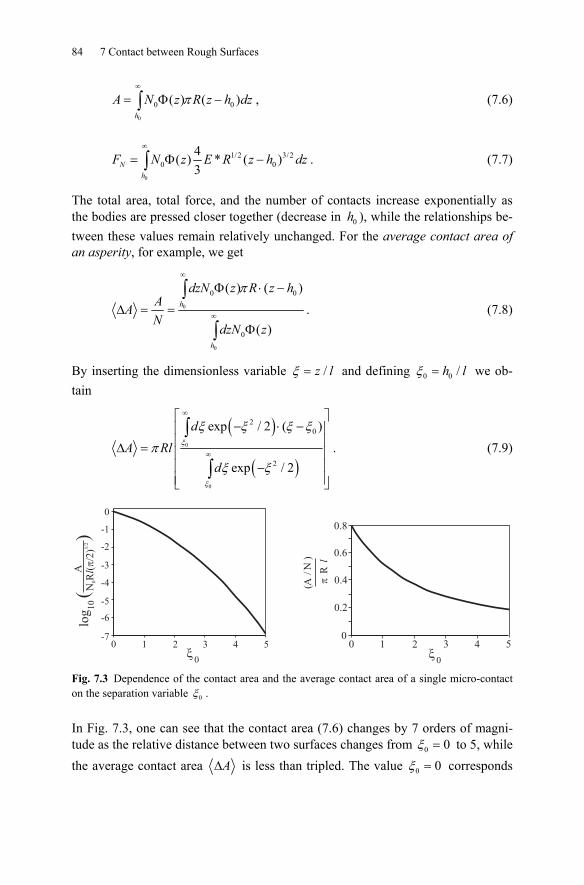
84 7 Contact between Rough Surfaces
0
0 0( ) ( )π∞
= Φ −∫h
A N z R z h dz , (7.6)
0
1/2 3/20 0
4( ) * ( )3
∞
= Φ −∫Nh
F N z E R z h dz . (7.7)
The total area, total force, and the number of contacts increase exponentially as the bodies are pressed closer together (decrease in 0h ), while the relationships be-tween these values remain relatively unchanged. For the average contact area of an asperity, for example, we get
0
0
0 0
0
( ) ( )
( )
π∞
∞
Φ ⋅ −
Δ = =Φ
∫
∫
h
h
dzN z R z hAAN
dzN z. (7.8)
By inserting the dimensionless variable /ξ = z l and defining 0 0 /ξ = h l we ob-tain
( )
( )0
0
20
2
exp / 2 ( )
exp / 2
ξ
ξ
ξ ξ ξ ξ
πξ ξ
∞
∞
⎡ ⎤− ⋅ −⎢ ⎥
⎢ ⎥Δ = ⎢ ⎥⎢ ⎥−⎢ ⎥⎣ ⎦
∫
∫
dA Rl
d. (7.9)
0 1 2 3 4 5
-2
-1
0
-3
-4
-5
-6
-7
log
10
�0
0.8
0.6
0.4
0.2
00 1 2 3 4 5
A/N
()
�R
l
�0
A(
)N
R(
/2)
0l
�1/2
Fig. 7.3 Dependence of the contact area and the average contact area of a single micro-contact on the separation variable 0ξ .
In Fig. 7.3, one can see that the contact area (7.6) changes by 7 orders of magni-tude as the relative distance between two surfaces changes from 0 0ξ = to 5, while the average contact area ΔA is less than tripled. The value 0 0ξ = corresponds
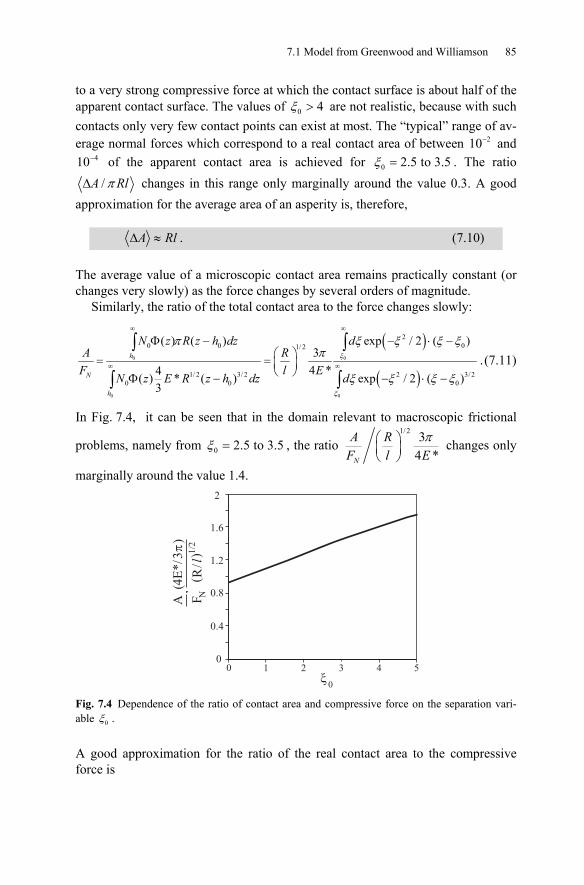
7.1 Model from Greenwood and Williamson 85
to a very strong compressive force at which the contact surface is about half of the apparent contact surface. The values of 0 4ξ > are not realistic, because with such contacts only very few contact points can exist at most. The “typical” range of av-erage normal forces which correspond to a real contact area of between 210− and
410− of the apparent contact area is achieved for 0 2.5 to 3.5ξ = . The ratio /πΔA Rl changes in this range only marginally around the value 0.3. A good
approximation for the average area of an asperity is, therefore,
Δ ≈A Rl . (7.10)
The average value of a microscopic contact area remains practically constant (or changes very slowly) as the force changes by several orders of magnitude.
Similarly, the ratio of the total contact area to the force changes slowly:
( )
( )0 0
0 0
20 0 01/ 2
1/ 2 3/2 2 3/20 0 0
( ) ( ) exp / 2 ( )3
4 *4( ) * ( ) exp / 2 ( )3
ξ
ξ
π ξ ξ ξ ξπ
ξ ξ ξ ξ
∞ ∞
∞ ∞
Φ − − ⋅ −⎛ ⎞= = ⎜ ⎟⎝ ⎠Φ − − ⋅ −
∫ ∫
∫ ∫
h
N
h
N z R z h dz dA R
F l EN z E R z h dz d
. (7.11)
In Fig. 7.4, it can be seen that in the domain relevant to macroscopic frictional
problems, namely from 0 2.5 to 3.5ξ = , the ratio 1/2 3
4 *π⎛ ⎞
⎜ ⎟⎝ ⎠N
A RF l E
changes only
marginally around the value 1.4.
0 1 2 3 4 5�
0
0.8
0.4
0
1.2
1.6
2
(4E
*/3
�)
A FR
/ l1/2
()
N
Fig. 7.4 Dependence of the ratio of contact area and compressive force on the separation vari-able 0ξ .
A good approximation for the ratio of the real contact area to the compressive force is
86 7 Contact between Rough Surfaces
1/2 3.3
*N
A RF l E
⎛ ⎞≈ ⎜ ⎟⎝ ⎠
. (7.12)
The contact area is proportional to the normal force by a factor that weakly de-pends on NF .
The average pressure is found from the same equation through inversion:
1/2
*0.3NF lEA R
σ ⎛ ⎞≈ ≈ ⋅ ⎜ ⎟⎝ ⎠
. (7.13)
In modern literature over contact mechanics, one can often find another form of the ratio /NF A for rough surfaces. One can qualitatively “deduce” this form as follows. The ratio /NF A can be estimated as the average of the individual micro-contacts /Δ ΔF A (with a coefficient of order unity) and this, in turn, as
( )2/Δ ΔF A (again with a coefficient of order unity). Because the ratio /NF A
is only weakly dependent on the compressive force (i.e. the convergence of the
surfaces), we can estimate: ( )2
2 4 */3π
⎛ ⎞Δ Δ ⎜ ⎟⎝ ⎠
∼ ∼NF E zF AA R
at 0 0=h . The
radius of curvature for an asperity is calculated using 1/ ′′= −R z . Therefore, for the ratio /NF A , we get
24 * 4 *3 3
NF E Ez z zA π π
′′ ′− ⋅ =∼ . (7.14)
For the last equation, we have taken into account that the average ′′− ⋅z z is de-
fined as the integral 0
1 ( ) ( )′′− ⋅∫L
z x z x dxL
over a sufficiently large distance L . Par-
tial integration yields 0
1 ( ) ( )′ ′⋅∫L
z x z x dxL
and, thus, 2′z .
This is obviously a very rough estimate. The result (7.14), however, has been verified through precise numerical calculations2. One can summarize Equation (7.14) by using the symbol 2z z′∇ = for the root mean square of the gradient
of the surface profile:
2 S. Hyun, L. Pei, J.-F. Molinari, and M. O. Robbins, Finite-element analysis of contact between elastic self-affine surfaces. Phys. Rev. E, 2004, v. 70, 026117 (12 pp).
7.1 Model from Greenwood and Williamson 87
1 *κ −= ∇NFE z
A, (7.15)
where κ is a coefficient that depends only slightly on the statistical properties of the surface and, as a rule, has an order of magnitude of 2. This equation was proven for various rough, and even fractal, surfaces through exact numerical solu-tions3.
According to this, the average pressure in the real contact area is approximated rather well by multiplying half of the effective modulus *E with the average gra-dient of the surface profile ∇z :
1 *2
NFE z
Aσ = ≈ ∇ . (7.16)
One can arrive at a similar conclusion through the following simple qualitative es-timation: if we consider a body with the surface profile ˆ cos cos= ⋅ ⋅z h kx ky , then
the maximum of the surface has a radius of curvature of 2ˆ1/ =R hk , the root mean square of z is equal to ˆ / 2=l h , and the root mean square of the height gradient is
ˆ 2∇ =z hk . Consequently,
1/2
⎛ ⎞ = ∇⎜ ⎟⎝ ⎠
l zR
. (7.17)
Insertion into (7.13) again leads to an equation of the form in (7.16). Lastly, we estimate the force 0F at which the real contact area A reaches a
value half as large as the apparent contact area 0A :
00 *
4≈ ∇
AF E z . (7.18)
The average pressure σ that is necessary for such a state is equal to
1ˆ *4
σ ≈ ∇E z . (7.19)
3 It is interesting to note that the same equation (7.15) with 2κ ≈ is also valid for sharp abra-sive surfaces (see Problem 7 to this chapter).
88 7 Contact between Rough Surfaces
7.2 Plastic Deformation of Asperities
If the pressure (7.16) is larger than the hardness of the material 0σ and hence,
*
0
2σ∇
Ψ = >E z , (7.20)
then the micro-roughnesses are in a completely plastic state of deformation. The quantity Ψ was introduced by Greenwood and Williamson and is called the plas-ticity index. For 2 / 3Ψ < , the surface behaves elastically during contact. The fact of the matter is that whether the system behaves elastically or plastically is inde-pendent of the normal force!
As an example, we estimate the characteristic value of the critical gradient for a contact between two steel probes: with * 1110 ≈E Pa and 9
0 10 Paσ ≈ , we find that two steel probes in contact deform purely elastically if 22 10z −∇ < ⋅ . For ground surfaces, the profile gradient is normally larger and almost every area of the real contact is in a plastic state of deformation. Conversely, highly polished surfaces with 22 10−∇ ⋅z deform purely elastically.
The gradient ∇z is generally dependent on the resolution with which the sur-face is measured – it is scale dependent! If the gradient is different on different scales, then the surface plastically deforms only on the scales at which the condi-tion *
02 /σ∇ >z E is met. As soon as the stress in the contact area becomes larger than the critical value,
the theory is no longer valid. In a plastic state, we can estimate the size of the con-tact area by noting that the material deforms until the compressive stress reaches the hardness of the material. For the purpose of estimation, we assume that the material has elastic-perfectly plastic characteristics with the indentation hardness
0σ and that the pressure in every asperity is approximately equal to the hardness. According to this, the contact area is proportional to the normal force in the
plastic region as well:
0/σ≈ NA F . (7.21)
As a numerical example, we consider a ground steel cube, with an edge-length of 10 cm, lying on a steel plate. For the parameters 9
0 10 Paσ ≈ and 210 N≈NF , we obtain 2 9 2 210 /10 m 0.1 mmA = = and 5
0/ 10−=A A . For a typical diameter
of a contact, 10μm , the number of contacts is ( )27 510 / 10 1000− −≈ ≈N .
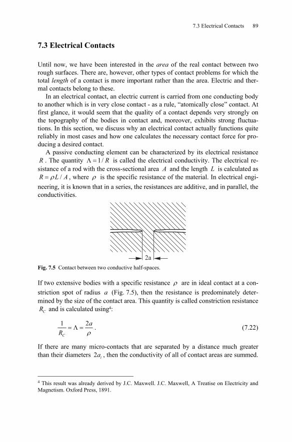
7.3 Electrical Contacts 89
7.3 Electrical Contacts
Until now, we have been interested in the area of the real contact between two rough surfaces. There are, however, other types of contact problems for which the total length of a contact is more important rather than the area. Electric and ther-mal contacts belong to these.
In an electrical contact, an electric current is carried from one conducting body to another which is in very close contact - as a rule, “atomically close” contact. At first glance, it would seem that the quality of a contact depends very strongly on the topography of the bodies in contact and, moreover, exhibits strong fluctua-tions. In this section, we discuss why an electrical contact actually functions quite reliably in most cases and how one calculates the necessary contact force for pro-ducing a desired contact.
A passive conducting element can be characterized by its electrical resistance R . The quantity 1/Λ = R is called the electrical conductivity. The electrical re-sistance of a rod with the cross-sectional area A and the length L is calculated as
/R L Aρ= , where ρ is the specific resistance of the material. In electrical engi-neering, it is known that in a series, the resistances are additive, and in parallel, the conductivities.
2a Fig. 7.5 Contact between two conductive half-spaces.
If two extensive bodies with a specific resistance ρ are in ideal contact at a con-striction spot of radius a (Fig. 7.5), then the resistance is predominately deter-mined by the size of the contact area. This quantity is called constriction resistance
CR and is calculated using4:
1 2
C
aR ρ
= Λ = . (7.22)
If there are many micro-contacts that are separated by a distance much greater than their diameters 2 ia , then the conductivity of all of contact areas are summed.
4 This result was already derived by J.C. Maxwell. J.C. Maxwell, A Treatise on Electricity and Magnetism. Oxford Press, 1891.
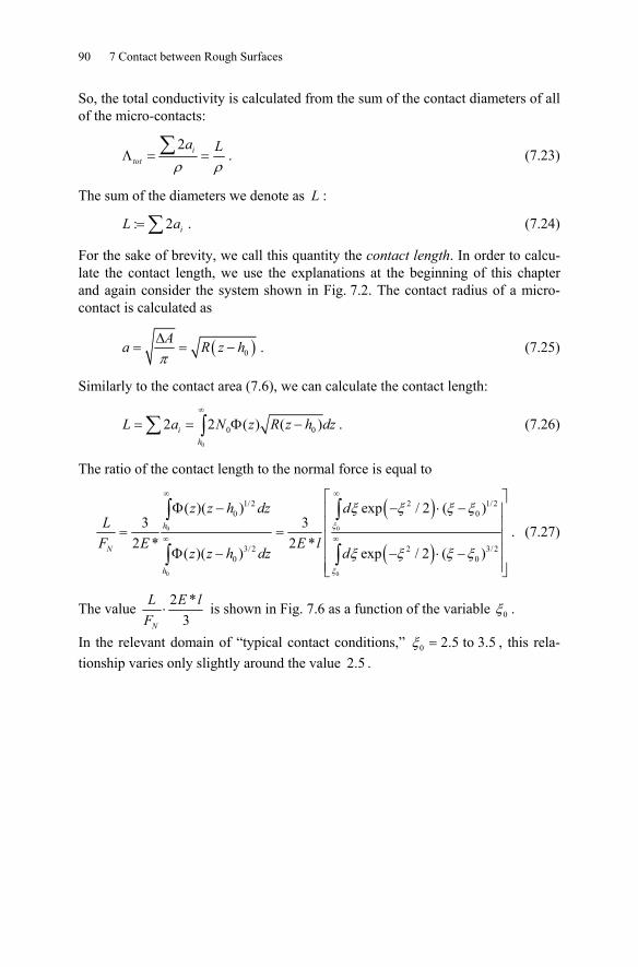
90 7 Contact between Rough Surfaces
So, the total conductivity is calculated from the sum of the contact diameters of all of the micro-contacts:
2 i
tot
a Lρ ρ
Λ = =∑ . (7.23)
The sum of the diameters we denote as L :
: 2= ∑ iL a . (7.24)
For the sake of brevity, we call this quantity the contact length. In order to calcu-late the contact length, we use the explanations at the beginning of this chapter and again consider the system shown in Fig. 7.2. The contact radius of a micro-contact is calculated as
( )0Aa R z hπΔ
= = − . (7.25)
Similarly to the contact area (7.6), we can calculate the contact length:
0
0 02 2 ( ) ( )∞
= = Φ −∑ ∫ih
L a N z R z h dz . (7.26)
The ratio of the contact length to the normal force is equal to
( )
( )0 0
0 0
1/ 2 2 1/20 0
3/2 2 3/ 20 0
( )( ) exp / 2 ( )3 3
2 * 2 *( )( ) exp / 2 ( )
ξ
ξ
ξ ξ ξ ξ
ξ ξ ξ ξ
∞ ∞
∞ ∞
⎡ ⎤Φ − − ⋅ −⎢ ⎥
⎢ ⎥= = ⎢ ⎥⎢ ⎥Φ − − ⋅ −⎢ ⎥⎣ ⎦
∫ ∫
∫ ∫
h
N
h
z z h dz dL
F E E lz z h dz d
. (7.27)
The value 2 *3
⋅N
L E lF
is shown in Fig. 7.6 as a function of the variable 0ξ .
In the relevant domain of “typical contact conditions,” 0 2.5 to 3.5ξ = , this rela-tionship varies only slightly around the value 2.5 .
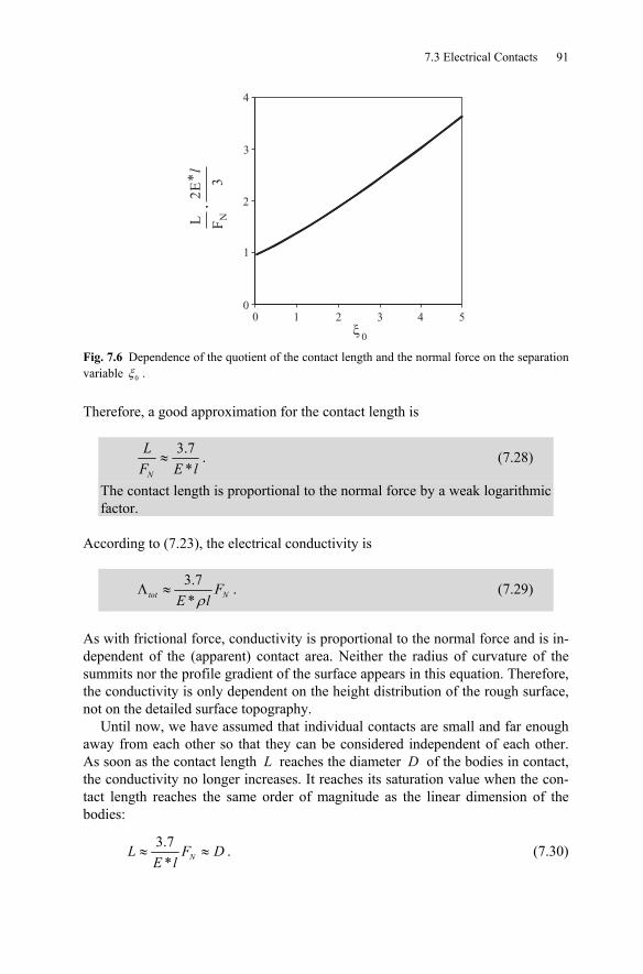
7.3 Electrical Contacts 91
0 1 2 3 4 5
�0
4
3
2
1
0
NL F
2E
* 3
l
Fig. 7.6 Dependence of the quotient of the contact length and the normal force on the separation variable 0ξ .
Therefore, a good approximation for the contact length is
3.7*N
LF E l
≈ . (7.28)
The contact length is proportional to the normal force by a weak logarithmic factor.
According to (7.23), the electrical conductivity is
3.7*tot NF
E lρΛ ≈ . (7.29)
As with frictional force, conductivity is proportional to the normal force and is in-dependent of the (apparent) contact area. Neither the radius of curvature of the summits nor the profile gradient of the surface appears in this equation. Therefore, the conductivity is only dependent on the height distribution of the rough surface, not on the detailed surface topography.
Until now, we have assumed that individual contacts are small and far enough away from each other so that they can be considered independent of each other. As soon as the contact length L reaches the diameter D of the bodies in contact, the conductivity no longer increases. It reaches its saturation value when the con-tact length reaches the same order of magnitude as the linear dimension of the bodies:
3.7* NL F D
E l≈ ≈ . (7.30)
92 7 Contact between Rough Surfaces
The necessary force for this is equal to
,*
3.7N cDE lF ≈ . (7.31)
One can compare this to the force in (7.18), which “squeezes” the surface rough-
nesses to half of the roughness height: 2
0 *4
≈ ∇DF E z . Their ratio is
,
0
4 *3.7 *
N cF E l lF DE z D z
≈ ≈∇ ∇
. (7.32)
For conductors with linear dimensions, /> ∇D l z , an ideal electrical contact is reached more quickly than an ideal “material contact.” This is the case for most contacts with dimensions larger than 0.1 mm .
7.4 Thermal Contacts
The thermal conductivity of a round contact and its mechanical stiffness are also proportional to the radius of the contact. The theory of electrical contacts outlined above can be directly transferred to both of these quantities.
The thermal resistance is the most important characteristic for the sizing of heat sinks for semiconductors or other elements in electrical circuits. It is defined as
TR T Q= Δ , where ΔT is the temperature difference between the ends of the ele-
ment and Q is the amount of heat flowing through the element per second. The thermal conductivity is defined as 1/T TRΛ = . The thermal resistance of a rod of length L and cross-sectional area A is equal to /TR L Aλ= , where λ is the specific thermal conductivity. It is directly analogous to electrical contacts, mean-ing only the specific resistance ρ must be replaced with 1/ λ . Similarly to (7.29), we can immediately write
3.7*T NF
E lλ
Λ ≈ . (7.33)
The thermal conductivity of a rough contact is directly proportional to the compressive force.
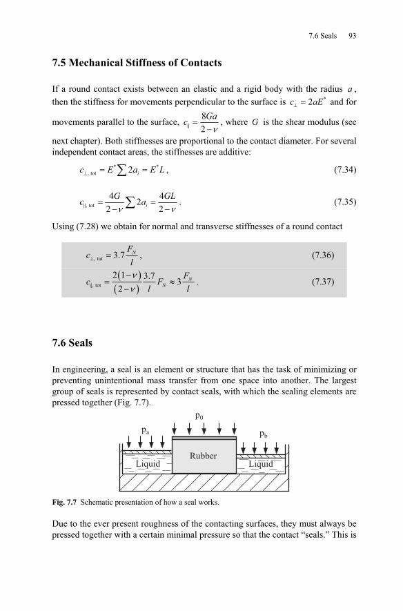
7.6 Seals 93
7.5 Mechanical Stiffness of Contacts
If a round contact exists between an elastic and a rigid body with the radius a , then the stiffness for movements perpendicular to the surface is *2⊥ =c aE and for
movements parallel to the surface, 82 ν
=−Gac , where G is the shear modulus (see
next chapter). Both stiffnesses are proportional to the contact diameter. For several independent contact areas, the stiffnesses are additive:
* *, tot 2 ic E a E L⊥ = =∑ , (7.34)
, tot4 42
2 2iG GLc aν ν
= =− −∑ . (7.35)
Using (7.28) we obtain for normal and transverse stiffnesses of a round contact
, tot 3.7 NFc
l⊥ = , (7.36)
( )( ), tot
2 1 3.7 32
NN
Fc F
l lνν−
= ≈−
. (7.37)
7.6 Seals
In engineering, a seal is an element or structure that has the task of minimizing or preventing unintentional mass transfer from one space into another. The largest group of seals is represented by contact seals, with which the sealing elements are pressed together (Fig. 7.7).
Liquid LiquidRubber
p0
pa pb
Fig. 7.7 Schematic presentation of how a seal works.
Due to the ever present roughness of the contacting surfaces, they must always be pressed together with a certain minimal pressure so that the contact “seals.” This is
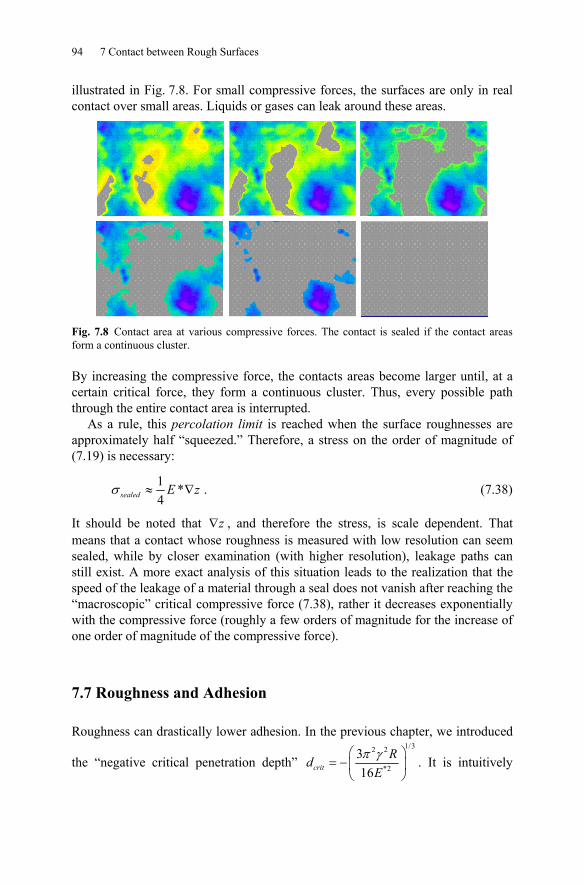
94 7 Contact between Rough Surfaces
illustrated in Fig. 7.8. For small compressive forces, the surfaces are only in real contact over small areas. Liquids or gases can leak around these areas.
Fig. 7.8 Contact area at various compressive forces. The contact is sealed if the contact areas form a continuous cluster.
By increasing the compressive force, the contacts areas become larger until, at a certain critical force, they form a continuous cluster. Thus, every possible path through the entire contact area is interrupted.
As a rule, this percolation limit is reached when the surface roughnesses are approximately half “squeezed.” Therefore, a stress on the order of magnitude of (7.19) is necessary:
1 *4sealed E zσ ≈ ∇ . (7.38)
It should be noted that ∇z , and therefore the stress, is scale dependent. That means that a contact whose roughness is measured with low resolution can seem sealed, while by closer examination (with higher resolution), leakage paths can still exist. A more exact analysis of this situation leads to the realization that the speed of the leakage of a material through a seal does not vanish after reaching the “macroscopic” critical compressive force (7.38), rather it decreases exponentially with the compressive force (roughly a few orders of magnitude for the increase of one order of magnitude of the compressive force).
7.7 Roughness and Adhesion
Roughness can drastically lower adhesion. In the previous chapter, we introduced
the “negative critical penetration depth” 1/32 2
*2
316π γ⎛ ⎞
= −⎜ ⎟⎝ ⎠
critRd
E. It is intuitively
Problems 95
clear that the adhesive behavior of rough surfaces is described by the relationship critd l . If critd l :
1/32 2
*2
316π γ⎛ ⎞
⎜ ⎟⎝ ⎠
R lE
, (7.39)
then the roughness no longer plays a role. By taking the approximation (7.17) into account, one can also present this equation in the form
1/ 2
*
34πγ
⋅∇l zE
. (7.40)
In the opposite case, the adhesive force practically vanishes completely. Numeri-cal simulations show that there is a critical value of the product ⋅∇l z at which the macroscopic adhesive force approaches zero:
[ ] *
γ⋅∇ = ϒ
critl z
E, (7.41)
where ϒ is a constant on the order of magnitude of 1.
Problems
Problem 1: Determine the compressive force that is needed to create an electrical contact with an electrical resistance of 0.1 R m= Ω between two flat copper plates with the roughness 1 μ=l m . Solution: The modulus of elasticity of copper is around 1110 ≈E Pa , Poisson’s ra-tio 0,33ν ≈ , and the specific resistance 81.8 10 ρ −≈ ⋅ Ω ⋅m . The effective elastic modulus *E is calculated as
( ) ( )11
* 112
10 Pa 0.56 10 2 1 0.12 1
EE Paν
= ≈ ≈ ⋅−−
. From equation (7.29), which we
can rewrite in the form 1 3.7* NF
R E lρ= , it follows that
* 11 8 6
3
0.56 10 1.8 10 10 2.7 3.7 3.7 0.1 10NE l Pa m mF N
Rρ − −
−
⋅ ⋅ ⋅ Ω ⋅ ⋅= ≈ ≈
⋅ ⋅ Ω.
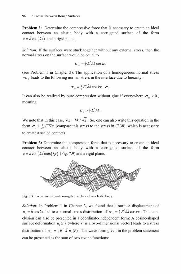
96 7 Contact between Rough Surfaces
Problem 2: Determine the compressive force that is necessary to create an ideal contact between an elastic body with a corrugated surface of the form
( )ˆ cos=z h kx and a rigid plane. Solution: If the surfaces were stuck together without any external stress, then the normal stress on the surface would be equal to
*12
ˆ cosσ =zz E hk kx
(see Problem 1 in Chapter 3). The application of a homogeneous normal stress 0σ− leads to the following normal stress in the interface due to linearity:
*102
ˆ cosσ σ= −zz E hk kx .
It can also be realized by pure compression without glue if everywhere 0σ <zz , meaning
*10 2
ˆσ > E hk .
We note that in this case, ˆ / 2∇ =z hk . So, one can also write this equation in the form *1
0 2σ > ∇E z (compare this stress to the stress in (7.38), which is necessary
to create a sealed contact). Problem 3: Determine the compression force that is necessary to create an ideal contact between an elastic body with a corrugated surface of the form
( ) ( )ˆ cos cos=z h kx ky (Fig. 7.9) and a rigid plane.
Fig. 7.9 Two-dimensional corrugated surface of an elastic body.
Solution: In Problem 1 in Chapter 3, we found that a surface displacement of ˆ coszu h kx= led to a normal stress distribution of *1
2ˆ cosσ =zz E hk kx . This con-
clusion can also be presented in a coordinate-independent form: A cosine-shaped surface deformation ( )zu r (where r is a two-dimensional vector) leads to a stress
distribution of *12 ( )σ =zz zE k u r . The wave form given in the problem statement
can be presented as the sum of two cosine functions:
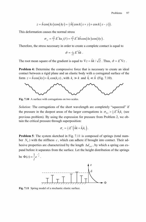
Problems 97
( ) ( ) ( ) ( )( )12
ˆ ˆcos cos cos cos= = + + −z h kx ky h k x y k x y .
This deformation causes the normal stress
( ) ( )* *2 22 2
ˆ( ) cos cosσ = =zz zE ku r E kh kx ky .
Therefore, the stress necessary in order to create a complete contact is equal to *1
2ˆσ = E hk .
The root mean square of the gradient is equal to ˆ / 2∇ =z hk . Thus, *σ = ∇E z . Problem 4: Determine the compressive force that is necessary to create an ideal contact between a rigid plane and an elastic body with a corrugated surface of the form ( ) 1 1
ˆ ˆcos cos( )= +z h kx h k x , with 1k k and 1ˆh h (Fig. 7.10).
Fig. 7.10 A surface with corrugations on two scales.
Solution: The corrugations of the short wavelength are completely “squeezed” if the pressure in the deepest areas of the larger corrugations is *1
0,1 1 12ˆσ > E h k (see
previous problem). By using the expression for pressure from Problem 2, we ob-tain the critical pressure through superposition:
( )*11 12
ˆ ˆσ = +c E hk h k .
Problem 5: The system sketched in Fig. 7.11 is composed of springs (total num-ber 0N ) with the stiffness c , which can adhere if brought into contact. Their ad-hesive properties are characterized by the length Δ critd , by which a spring can ex-pand before it separates from the surface. Let the height distribution of the springs
be 1( )−
Φ =zlz e
l.
z
d
� Fig. 7.11 Spring model of a stochastic elastic surface.
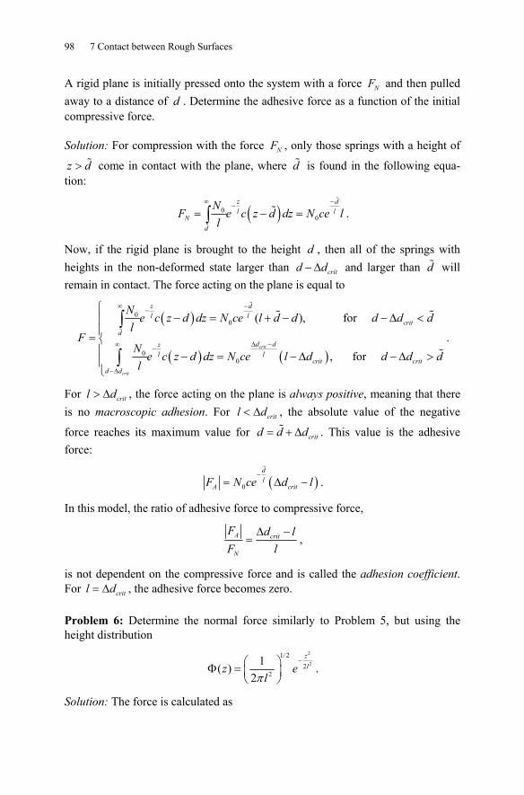
98 7 Contact between Rough Surfaces
A rigid plane is initially pressed onto the system with a force NF and then pulled away to a distance of d . Determine the adhesive force as a function of the initial compressive force.
Solution: For compression with the force NF , only those springs with a height of
>z d come in contact with the plane, where d is found in the following equa-tion:
( )00
∞ −−
= − =∫z dl l
Nd
NF e c z d dz N ce l
l.
Now, if the rigid plane is brought to the height d , then all of the springs with heights in the non-deformed state larger than − Δ critd d and larger than d will remain in contact. The force acting on the plane is equal to
( )
( ) ( )
00
00
( ), for
, for crit
crit
z dl l
critd
d dzl l
crit critd d
Ne c z d dz N ce l d d d d d
lF
Ne c z d dz N ce l d d d d
l
∞ −−
Δ −∞−
−Δ
⎧− = + − − Δ <⎪
⎪= ⎨⎪ − = − Δ − Δ >⎪⎩
∫
∫.
For > Δ critl d , the force acting on the plane is always positive, meaning that there is no macroscopic adhesion. For < Δ critl d , the absolute value of the negative
force reaches its maximum value for = + Δ critd d d . This value is the adhesive force:
( )0
−= Δ −
dl
A critF N ce d l .
In this model, the ratio of adhesive force to compressive force,
Δ −=A crit
N
F d lF l
,
is not dependent on the compressive force and is called the adhesion coefficient. For = Δ critl d , the adhesive force becomes zero. Problem 6: Determine the normal force similarly to Problem 5, but using the height distribution
2
21/2
22
1( )2π
−⎛ ⎞Φ = ⎜ ⎟⎝ ⎠
zlz e
l.
Solution: The force is calculated as
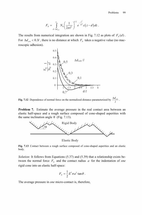
Problems 99
( )2
21/ 2
20 2
12π
∞ −
−Δ
⎛ ⎞= −⎜ ⎟⎝ ⎠∫
crit
zl
Nd d
F N e c z d dzl
.
The results from numerical integration are shown in Fig. 7.12 as plots of ( )NF d . For 0.3critd lΔ < , there is no distance at which NF takes a negative value (no mac-roscopic adhesion).
0.2
0,1
0,5
0,3
0.3
0.1
0.4
0.5
01 1.5
d0,7
dcrit /l
2 2.5 3.53 4
/l
FN N0
1 cl
�
Fig. 7.12 Dependence of normal force on the normalized distance parameterized by critdl
Δ .
Problem 7. Estimate the average pressure in the real contact area between an elastic half-space and a rough surface composed of cone-shaped asperities with the same inclination angle θ (Fig. 7.13).
Rigid Body
Elastic Body
�
Fig. 7.13 Contact between a rough surface composed of cone-shaped asperities and an elastic body.
Solution: It follows from Equations (5.37) and (5.39) that a relationship exists be-tween the normal force NF and the contact radius a for the indentation of one rigid cone into an elastic half-space:
* 21 tan2
π θ=NF E a .
The average pressure in one micro-contact is, therefore,
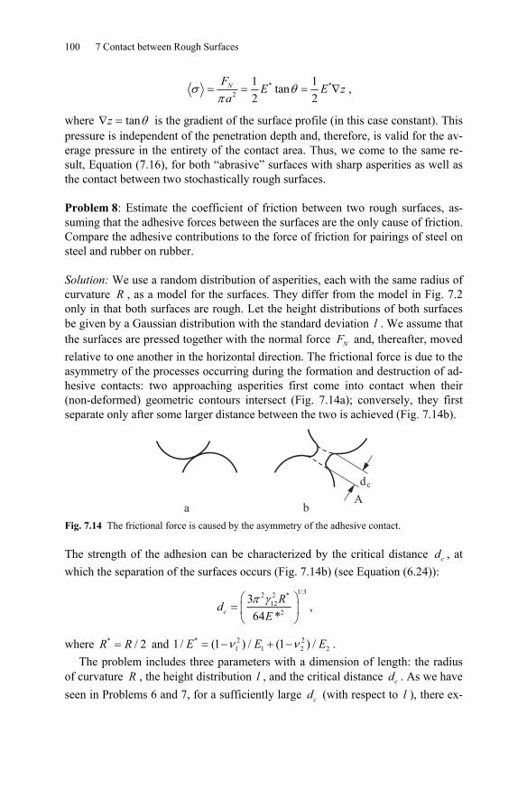
100 7 Contact between Rough Surfaces
* *2
1 1tan2 2
NFE E z
aσ θ
π= = = ∇ ,
where tanθ∇ =z is the gradient of the surface profile (in this case constant). This pressure is independent of the penetration depth and, therefore, is valid for the av-erage pressure in the entirety of the contact area. Thus, we come to the same re-sult, Equation (7.16), for both “abrasive” surfaces with sharp asperities as well as the contact between two stochastically rough surfaces. Problem 8: Estimate the coefficient of friction between two rough surfaces, as-suming that the adhesive forces between the surfaces are the only cause of friction. Compare the adhesive contributions to the force of friction for pairings of steel on steel and rubber on rubber. Solution: We use a random distribution of asperities, each with the same radius of curvature R , as a model for the surfaces. They differ from the model in Fig. 7.2 only in that both surfaces are rough. Let the height distributions of both surfaces be given by a Gaussian distribution with the standard deviation l . We assume that the surfaces are pressed together with the normal force NF and, thereafter, moved relative to one another in the horizontal direction. The frictional force is due to the asymmetry of the processes occurring during the formation and destruction of ad-hesive contacts: two approaching asperities first come into contact when their (non-deformed) geometric contours intersect (Fig. 7.14a); conversely, they first separate only after some larger distance between the two is achieved (Fig. 7.14b).
A
dc
a b Fig. 7.14 The frictional force is caused by the asymmetry of the adhesive contact.
The strength of the adhesion can be characterized by the critical distance cd , at which the separation of the surfaces occurs (Fig. 7.14b) (see Equation (6.24)):
1/32 2 *12
2
364 *π γ⎛ ⎞
= ⎜ ⎟⎝ ⎠
cRd
E,
where * / 2=R R and * 2 21 1 2 21/ (1 ) / (1 ) /ν ν= − + −E E E .
The problem includes three parameters with a dimension of length: the radius of curvature R , the height distribution l , and the critical distance cd . As we have seen in Problems 6 and 7, for a sufficiently large cd (with respect to l ), there ex-
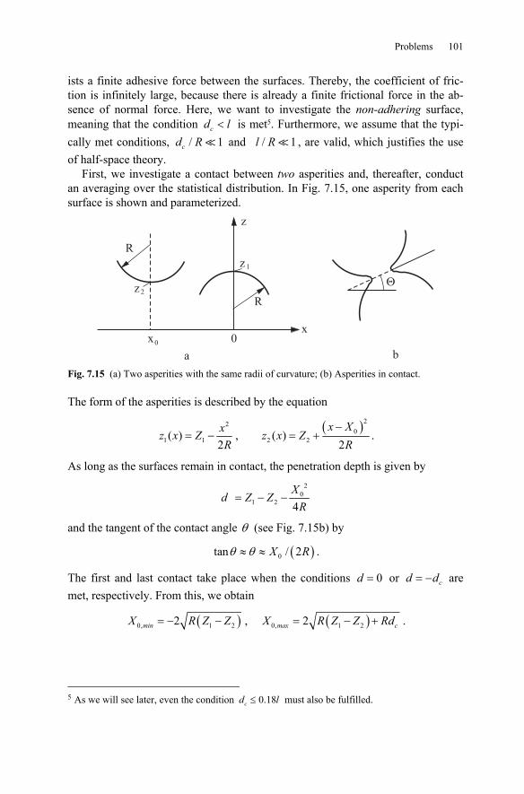
Problems 101
ists a finite adhesive force between the surfaces. Thereby, the coefficient of fric-tion is infinitely large, because there is already a finite frictional force in the ab-sence of normal force. Here, we want to investigate the non-adhering surface, meaning that the condition <cd l is met5. Furthermore, we assume that the typi-cally met conditions, / 1cd R and / 1l R , are valid, which justifies the use of half-space theory.
First, we investigate a contact between two asperities and, thereafter, conduct an averaging over the statistical distribution. In Fig. 7.15, one asperity from each surface is shown and parameterized.
R
R
z
z 1
0x0
z 2
x
�
a b Fig. 7.15 (a) Two asperities with the same radii of curvature; (b) Asperities in contact.
The form of the asperities is described by the equation
2
1 1( )2
= −xz x ZR
, ( )2
2 20( )
2−
= +x X
z x ZR
.
As long as the surfaces remain in contact, the penetration depth is given by 2
1 20
4 = − −
Xd Z Z
R
and the tangent of the contact angle θ (see Fig. 7.15b) by
( )0tan / 2θ θ≈ ≈ X R .
The first and last contact take place when the conditions 0=d or = − cd d are met, respectively. From this, we obtain
( )0, 1 22= − −minX R Z Z , ( )0, 1 22 −= +max cX R Z Z Rd .
5 As we will see later, even the condition 0.18cd l≤ must also be fulfilled.
102 7 Contact between Rough Surfaces
If we denote the force of interaction between the asperities as F , then the z -component of the force NF and the x -component of the force RF , neglecting higher order terms of θ , are given by
≈NF F , ( )0 2/−≈RF F X R .
The coefficient of friction can then be calculated as
/μ = R NF F ,
where the notation .. ..≡ > >x z means an average over the asperity distribu-tion in both the x -direction and the z -direction. The distribution in the x -direction is assumed to be uniform and the distribution in the z -direction is de-fined as
2122
1 11( ) e2π
−Φ =
ZlZ
l,
( )22 022
2 21( ) e2π
−−
Φ =Z Z
lZl
.
Here, 0Z has the sense of the macroscopic separation distance between the sur-faces. We use the approximation (6.26) to calculate the adhesive force:
5/3
0.12 1 1⎛ ⎞⎛ ⎞⎜ ⎟≈ + −⎜ ⎟⎜ ⎟⎝ ⎠⎝ ⎠
cc
dF Fd
, 1 / 10− ≤ ≤cd d ,
with 3122πγ=cF R .
Averaging the forces NF and RF in the x -direction over the macroscopic length L yields
0,max
0,min
00d 1
2 2> = −< ≈∫
X
xX
c cR
X FL
dF X
R LF ,
( )0,max
0,min
13/60 d 1.2 11 1> = ≈ ⎡ ⎤< + − − +⎣ ⎦∫
X
cX
cN x
RdF F X F
L Lξξξ ,
with ( )1 2 /ξ = − cZ Z d . We will not conduct the averaging in the z -direction here and limit ourselves to a rough estimation. The order of magnitude of 1 2−Z Z is ∼ l for an arbitrary rough surface. A comparison with a more exact calculation shows that the approximation provides the best results when the value 3
4 / cl d is assumed for the representative value ξ . The normal force for a “typical asperity” can then be approximated using
( )13/6 334
34 41.2 1 / / / 1⎡ ⎤< + − − +≈ ⎣> ⎦c
cN x c c c
RdF d l dll dF
L.
Problems 103
We obtain the following approximation for the coefficient of friction
( )
1/ 2
13/63 34 4 4
3
1 2
1.2 1 / / / 1
⎛ ⎞ ∇⎜ ⎟⎝ ⎠≈
⎡ ⎤+ − − +⎣ ⎦
c
c c cl
d zl
l d d l dμ ,
where we have used the relation ( )1/2/ ≈ ∇l R z , equation (7.17). This equation is only valid in the domain where the numerator is positive, i.e. / 5.7>cl d . We see that the coefficient of friction is proportional to the root mean square of the sur-face gradient ∇z and, otherwise, depends only on the “adhesive parameter”
/cd l . Near the critical value of this parameter, the coefficient of friction can as-sume an infinitely large value. For small values of /cd l it approaches zero ac-cording to
8/3
7.8⎛ ⎞≈ ∇⎜ ⎟⎝ ⎠
cdz
lμ ,
or more explicitly 8/92 2 *
122 3
37.8
64 *⎛ ⎞
≈ ∇⎜ ⎟⎝ ⎠
Rz
E lπ γ
μ .
For steel with 212 5 J/mγ ≈ , * 1110 Pa≈E , 1 mμ=l , and * 100 mμ=R , we ob-
tain 50.5 10μ −⋅ ∇z : The adhesive contribution to friction in a pairing of steel-steel is negligibly small. For rubber with 2 2
12 5 10 J/mγ −≈ ⋅ , * 610 Pa≈E , 1 mμ=l , and * 100 mμ=R , we obtain 1.1μ ∇z : Adhesive forces can have a
noticeable contribution to the frictional force between elastomers.
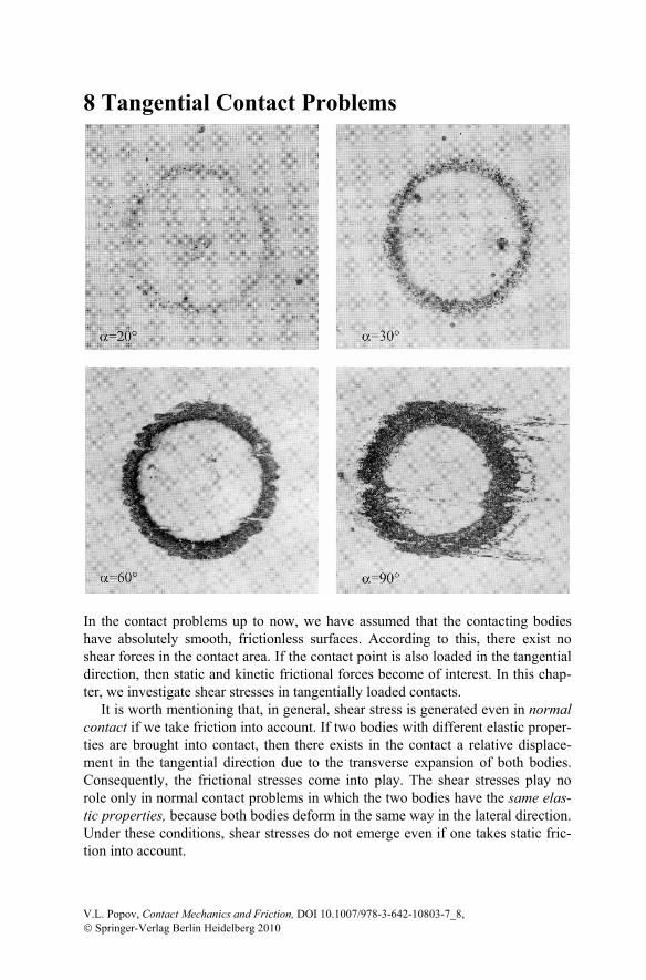
8 Tangential Contact Problems
In the contact problems up to now, we have assumed that the contacting bodies have absolutely smooth, frictionless surfaces. According to this, there exist no shear forces in the contact area. If the contact point is also loaded in the tangential direction, then static and kinetic frictional forces become of interest. In this chap-ter, we investigate shear stresses in tangentially loaded contacts.
It is worth mentioning that, in general, shear stress is generated even in normal contact if we take friction into account. If two bodies with different elastic proper-ties are brought into contact, then there exists in the contact a relative displace-ment in the tangential direction due to the transverse expansion of both bodies. Consequently, the frictional stresses come into play. The shear stresses play no role only in normal contact problems in which the two bodies have the same elas-tic properties, because both bodies deform in the same way in the lateral direction. Under these conditions, shear stresses do not emerge even if one takes static fric-tion into account.
V.L. Popov, Contact Mechanics and Friction, DOI 10.1007/978-3-642-10803-7_8, © Springer-Verlag Berlin Heidelberg 2010
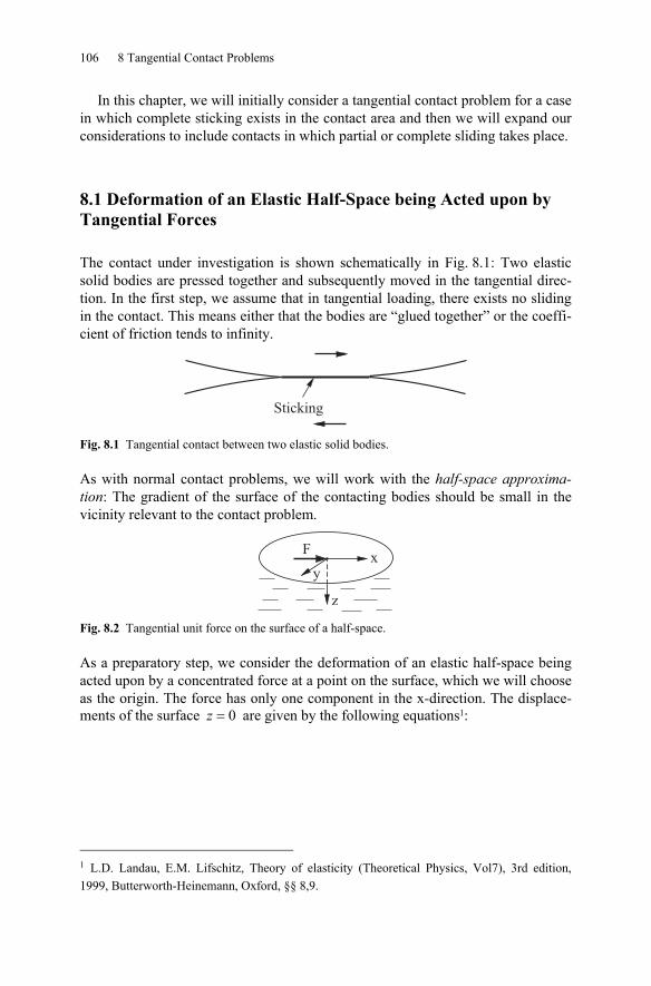
106 8 Tangential Contact Problems
In this chapter, we will initially consider a tangential contact problem for a case in which complete sticking exists in the contact area and then we will expand our considerations to include contacts in which partial or complete sliding takes place.
8.1 Deformation of an Elastic Half-Space being Acted upon by Tangential Forces
The contact under investigation is shown schematically in Fig. 8.1: Two elastic solid bodies are pressed together and subsequently moved in the tangential direc-tion. In the first step, we assume that in tangential loading, there exists no sliding in the contact. This means either that the bodies are “glued together” or the coeffi-cient of friction tends to infinity.
Sticking
Fig. 8.1 Tangential contact between two elastic solid bodies.
As with normal contact problems, we will work with the half-space approxima-tion: The gradient of the surface of the contacting bodies should be small in the vicinity relevant to the contact problem.
Fig. 8.2 Tangential unit force on the surface of a half-space.
As a preparatory step, we consider the deformation of an elastic half-space being acted upon by a concentrated force at a point on the surface, which we will choose as the origin. The force has only one component in the x-direction. The displace-ments of the surface 0=z are given by the following equations1:
1 L.D. Landau, E.M. Lifschitz, Theory of elasticity (Theoretical Physics, Vol7), 3rd edition, 1999, Butterworth-Heinemann, Oxford, §§ 8,9.
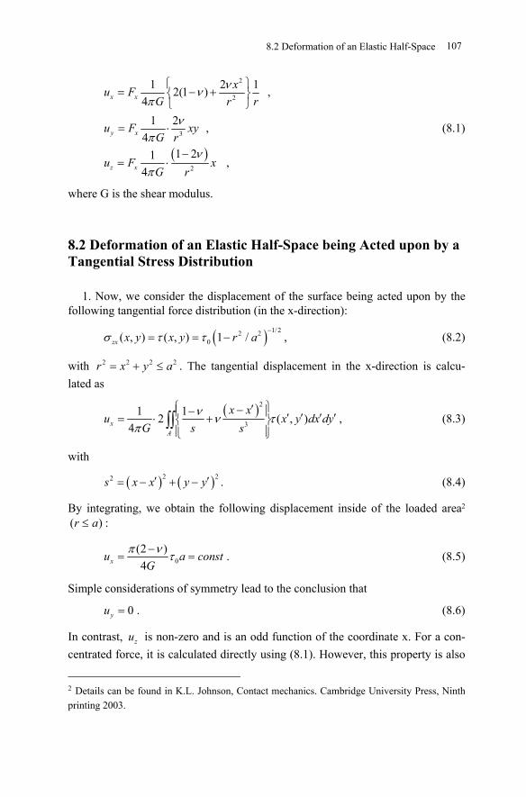
( )
2
2
3
2
1 2 12(1 ) ,4
1 2 ,4
1 21 ,4
x x
y x
z x
xu FG rr
u F xyG r
u F xG r
ννπ
νπ
νπ
⎧ ⎫= − +⎨ ⎬
⎩ ⎭
= ⋅
−= ⋅
(8.1)
where G is the shear modulus.
8.2 Deformation of an Elastic Half-Space being Acted upon by a Tangential Stress Distribution
1. Now, we consider the displacement of the surface being acted upon by the following tangential force distribution (in the x-direction):
( ) 1/22 20( , ) ( , ) 1 /σ τ τ
−= = −zx x y x y r a , (8.2)
with 2 2 2 2= + ≤r x y a . The tangential displacement in the x-direction is calcu-lated as
( )2
3
1 12 ( , )4
ν ν τπ
⎧ ⎫′−−⎪ ⎪ ′ ′ ′ ′= ⋅ +⎨ ⎬⎪ ⎪⎩ ⎭
∫∫xA
x xu x y dx dy
G s s, (8.3)
with
( ) ( )2 22 ′ ′= − + −s x x y y . (8.4)
By integrating, we obtain the following displacement inside of the loaded area2 ( )≤r a :
0(2 )4xu a constG
π ν τ−= = . (8.5)
Simple considerations of symmetry lead to the conclusion that
0=yu . (8.6)
In contrast, zu is non-zero and is an odd function of the coordinate x. For a con-centrated force, it is calculated directly using (8.1). However, this property is also
2 Details can be found in K.L. Johnson, Contact mechanics. Cambridge University Press, Ninth printing 2003.
8.2 Deformation of an Elastic Half-Space 107
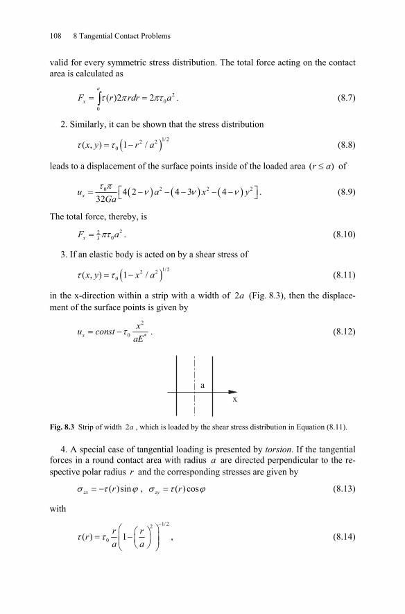
108 8 Tangential Contact Problems
valid for every symmetric stress distribution. The total force acting on the contact area is calculated as
20
0
( )2 2τ π πτ= =∫a
xF r rdr a . (8.7)
2. Similarly, it can be shown that the stress distribution
( )1/22 20( , ) 1 /τ τ= −x y r a (8.8)
leads to a displacement of the surface points inside of the loaded area ( )≤r a of
( ) ( ) ( )2 2 20 4 2 4 3 432τ π
ν ν ν⎡ ⎤= − − − − −⎣ ⎦xu a x yGa
. (8.9)
The total force, thereby, is
2203 πτ=xF a . (8.10)
3. If an elastic body is acted on by a shear stress of
( )1/22 20( , ) 1 /τ τ= −x y x a (8.11)
in the x-direction within a strip with a width of 2a (Fig. 8.3), then the displace-ment of the surface points is given by
2
0 *xxu const
aEτ= − . (8.12)
x
a
Fig. 8.3 Strip of width 2a , which is loaded by the shear stress distribution in Equation (8.11).
4. A special case of tangential loading is presented by torsion. If the tangential forces in a round contact area with radius a are directed perpendicular to the re-spective polar radius r and the corresponding stresses are given by
( )sinσ τ ϕ= −zx r , ( ) cosσ τ ϕ=zy r (8.13)
with
1/ 22
0( ) 1τ τ−
⎛ ⎞⎛ ⎞= −⎜ ⎟⎜ ⎟⎜ ⎟⎝ ⎠⎝ ⎠
r rra a
, (8.14)
8.3 Tangential Contact Problems without Slip 109
then the polar components of the displacement of the surface are equal to3
0
4ϕπτ
=r
uG
, 0=ru , 0=zu . (8.15)
Therefore, the total contact area rigidly turns by an angle of 0 / 4πτ G . Thus, this stress distribution is produced by the torsion of the rigid cylindrical indenter stick-ing to the surface. The total torsional moment is
3403π τ=zM a . (8.16)
8.3 Tangential Contact Problems without Slip
Now, we will move on to the discussion of tangential contact problems. We visu-alize that we have two opposing bodies, and we generate a constant displacement of xu in one of them and − xu in the other, respectively. The corresponding stress distribution (8.2) must exist on one side and the same distribution, with a negative sign, on the other. If we were to now glue both stress areas together, then they re-main in equilibrium due to Newton’s third law of motion (action-reaction). It is important that the “adhering” surfaces exactly match in the z-direction due to the asymmetry of the displacements in the z-direction with respect to x. These consid-erations show that the relative movement of 2 xu of two bodies with the same elas-tic properties results in exactly the stress distribution (8.2):
( ) 1/22 20( , ) 1 /τ τ
−= −x y r a . (8.17)
It can be noticed that the shear stress in the boundary of a sticking area ap-proaches infinity, while the normal stress approaches zero. That means that in most cases, the no-slip condition near the boundary is not met and relative sliding occurs. We will discuss this partial movement – slip – in the next section.
We define the shear stiffness of a contact between two elastic bodies c as the ratio of the tangential force to the relative tangential displacement of the two bod-ies. From equations (8.5) and (8.7) the tangential stiffness is
( )
*4 22 2 ν
= = =−
x
x
F Gac G au
, (8.18)
3 K.L. Johnson, Contact mechanics. Cambridge University Press, Ninth printing 2003.
110 8 Tangential Contact Problems
where we have inserted the effective shear modulus, ( )
* 22 ν
=−GG . Just as with
the normal stiffness, the shear stiffness (8.18) is proportional to the diameter of the contact.
Note that the mentioned equations are not exact in the application to a contact between an elastic half-space and a rigid body, because in this case, the displace-ments in the vertical direction vanish, which is not true in the case of the stress distribution in (8.2). However, they present a good approximation. For a contact between two elastic bodies with the elastic constants 1G , 2G , 1ν , and 2ν , the fol-lowing good approximation is valid for the shear stiffness:
*2= ≈x
rel
Fc G a
u (8.19)
with
1 2*
1 2
2 214 4ν ν− −
= +G GG
. (8.20)
In (8.19), relu is the relative displacement of the two bodies. Equation (8.5), in the case of two bodies with different elastic properties, takes the form
0*
πτ≈rel
au
G. (8.21)
8.4 Tangential Contact Problems Accounting for Slip
Now, we consider a combined contact problem characterized by tangential and normal forces acting simultaneously. We visualize, for example, that two spheres are pressed together with a normal force NF and subsequently pulled in the tan-gential direction with a force xF . It is assumed that between the two bodies, there exists dry friction according to Coulomb’s law of friction in its simplest form: the maximum static friction stress maxτ is equal to the kinetic friction stress kτ and this, in turn, is equal to the normal stress p multiplied with a constant coefficient of friction μ :
maxτ μ= p , k pτ μ= . (8.22)
The condition for sticking yields
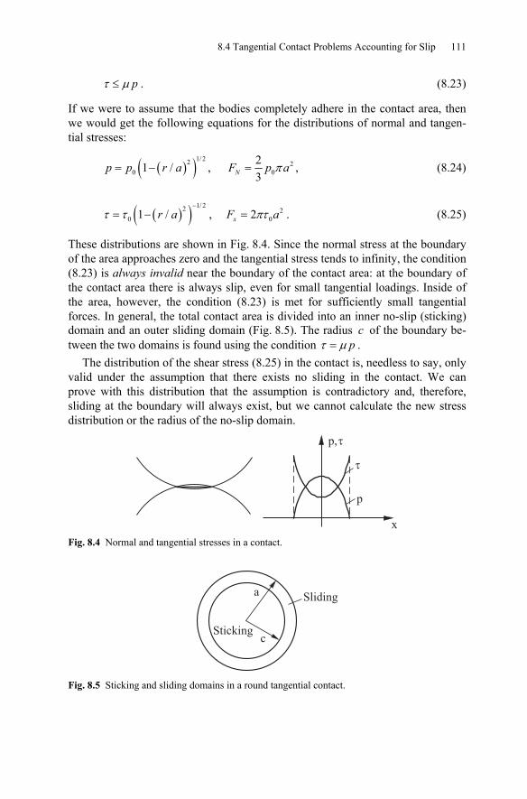
8.4 Tangential Contact Problems Accounting for Slip 111
τ μ≤ p . (8.23)
If we were to assume that the bodies completely adhere in the contact area, then we would get the following equations for the distributions of normal and tangen-tial stresses:
( )( )1/220 1 /= −p p r a , 2
023
π=NF p a , (8.24)
( )( ) 1/ 220 1 /τ τ
−= − r a , 2
02πτ=xF a . (8.25)
These distributions are shown in Fig. 8.4. Since the normal stress at the boundary of the area approaches zero and the tangential stress tends to infinity, the condition (8.23) is always invalid near the boundary of the contact area: at the boundary of the contact area there is always slip, even for small tangential loadings. Inside of the area, however, the condition (8.23) is met for sufficiently small tangential forces. In general, the total contact area is divided into an inner no-slip (sticking) domain and an outer sliding domain (Fig. 8.5). The radius c of the boundary be-tween the two domains is found using the condition τ μ= p .
The distribution of the shear stress (8.25) in the contact is, needless to say, only valid under the assumption that there exists no sliding in the contact. We can prove with this distribution that the assumption is contradictory and, therefore, sliding at the boundary will always exist, but we cannot calculate the new stress distribution or the radius of the no-slip domain.
p,�
p
x
�
Fig. 8.4 Normal and tangential stresses in a contact.
Stickingc
a Sliding
Fig. 8.5 Sticking and sliding domains in a round tangential contact.
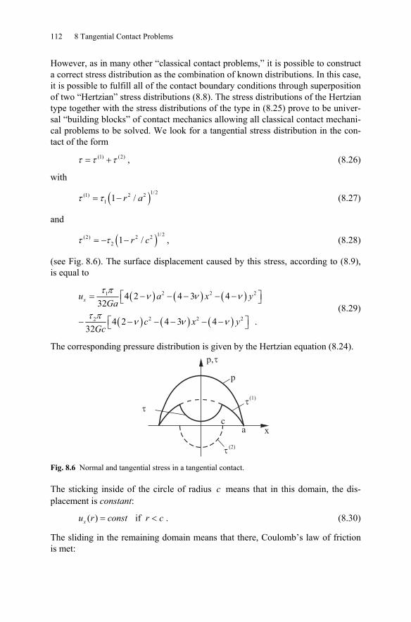
112 8 Tangential Contact Problems
However, as in many other “classical contact problems,” it is possible to construct a correct stress distribution as the combination of known distributions. In this case, it is possible to fulfill all of the contact boundary conditions through superposition of two “Hertzian” stress distributions (8.8). The stress distributions of the Hertzian type together with the stress distributions of the type in (8.25) prove to be univer-sal “building blocks” of contact mechanics allowing all classical contact mechani-cal problems to be solved. We look for a tangential stress distribution in the con-tact of the form
(1) (2)τ τ τ= + , (8.26)
with
( )1/2(1) 2 21 1 /τ τ= − r a (8.27)
and
( )1/ 2(2) 2 22 1 /τ τ= − − r c , (8.28)
(see Fig. 8.6). The surface displacement caused by this stress, according to (8.9), is equal to
( ) ( ) ( )
( ) ( ) ( )
2 2 21
2 2 22
4 2 4 3 432
4 2 4 3 4 .32
τ πν ν ν
τ πν ν ν
⎡ ⎤= − − − − −⎣ ⎦
⎡ ⎤− − − − − −⎣ ⎦
xu a x yGa
c x yGc
(8.29)
The corresponding pressure distribution is given by the Hertzian equation (8.24).
x
p,�
�
�
ca
(2)
�(1)
p
Fig. 8.6 Normal and tangential stress in a tangential contact.
The sticking inside of the circle of radius c means that in this domain, the dis-placement is constant:
( ) if xu r const r c= < . (8.30)
The sliding in the remaining domain means that there, Coulomb’s law of friction is met:
8.4 Tangential Contact Problems Accounting for Slip 113
( ) ( ), if r p r c r aτ μ= < < . (8.31)
The second condition leads to the claim that
1 0τ μ= p . (8.32)
From the condition (8.30), it follows that
2 0τ μ= cpa
. (8.33)
The displacement in the sticking domain is, thereby, equal to
( ) ( )0 2 22
8ν πμ−
= −x
pu a c
Ga. (8.34)
Before complete sliding starts ( 0=c ), the body can be displaced in the tangential direction by at the most
( ) ( )02 3 2
8 16ν πμ ν μ− −
= = Nx
p a Fu
G Ga. (8.35)
The total tangential force in the contact area is calculated using (8.26), (8.27)and (8.28):
( ) ( )2 2 3 31 2 0
2 23 3
ππ τ τ μ= − = −xF a c p a ca
. (8.36)
Taking into account the relationship 2203 π=NF p a , this force can be written in the
form
3
1μ⎛ ⎞⎛ ⎞= −⎜ ⎟⎜ ⎟⎜ ⎟⎝ ⎠⎝ ⎠
x NcF Fa
. (8.37)
Therefore, we obtain a radius for the static area of
1/3
1μ
⎛ ⎞= −⎜ ⎟⎝ ⎠
x
N
Fca F
. (8.38)
The tangential force at which complete sliding is introduced is, as expected, μ=x NF F . We must emphasize, however, that the sliding domain already domi-
nates a large portion of the contact area before this force is reached. Upon reach-ing the force μ=x NF F , there is no longer a transition from sticking to sliding, rather a transition from partial sliding to complete sliding.
We have shown that by applying an arbitrarily small tangential force to a Hertzian contact generated by a normal force, we create a ring-shaped sliding do-
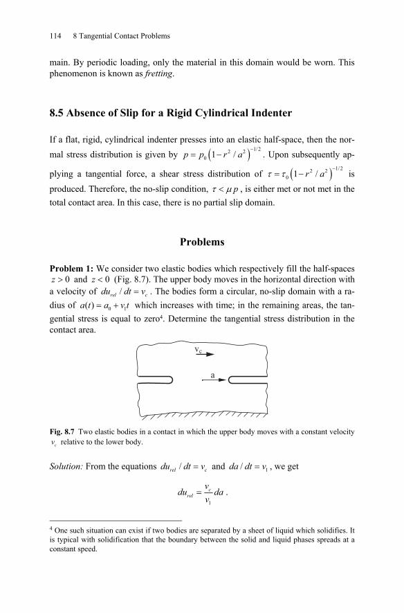
114 8 Tangential Contact Problems
main. By periodic loading, only the material in this domain would be worn. This phenomenon is known as fretting.
8.5 Absence of Slip for a Rigid Cylindrical Indenter
If a flat, rigid, cylindrical indenter presses into an elastic half-space, then the nor-mal stress distribution is given by ( ) 1/22 2
0 1 /−
= −p p r a . Upon subsequently ap-
plying a tangential force, a shear stress distribution of ( ) 1/22 20 1 /τ τ
−= − r a is
produced. Therefore, the no-slip condition, τ μ< p , is either met or not met in the total contact area. In this case, there is no partial slip domain.
Problems
Problem 1: We consider two elastic bodies which respectively fill the half-spaces 0>z and 0<z (Fig. 8.7). The upper body moves in the horizontal direction with
a velocity of / =rel cdu dt v . The bodies form a circular, no-slip domain with a ra-dius of 0 1( ) = +a t a v t which increases with time; in the remaining areas, the tan-gential stress is equal to zero4. Determine the tangential stress distribution in the contact area.
a
vc
Fig. 8.7 Two elastic bodies in a contact in which the upper body moves with a constant velocity
cv relative to the lower body.
Solution: From the equations / =rel cdu dt v and 1/ =da dt v , we get
1
= crel
vdu da
v.
4 One such situation can exist if two bodies are separated by a sheet of liquid which solidifies. It is typical with solidification that the boundary between the solid and liquid phases spreads at a constant speed.
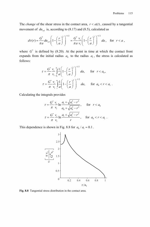
Problems 115
The change of the shear stress in the contact area, ( )<r a t , caused by a tangential movement of reldu is, according to (8.17) and (8.5), calculated as
1/2 1/22 2* *
1
( ) 1 1crel
vG r G rd r du daa a a v a
τπ π
− −⎛ ⎞ ⎛ ⎞⎛ ⎞ ⎛ ⎞= − = −⎜ ⎟ ⎜ ⎟⎜ ⎟ ⎜ ⎟⎜ ⎟ ⎜ ⎟⎝ ⎠ ⎝ ⎠⎝ ⎠ ⎝ ⎠
, for r a< ,
where *G is defined by (8.20). At the point in time at which the contact front expands from the initial radius 0a to the radius 1a , the stress is calculated as follows:
1
0
1
1/ 22*
01
1/22*
0 11
1 1 , for ,
1 1 , for .
ac
a
ac
r
vG r da r av a a
vG r da a r av a a
τπ
τπ
−
−
⎛ ⎞⎛ ⎞= − <⎜ ⎟⎜ ⎟⎜ ⎟⎝ ⎠⎝ ⎠
⎛ ⎞⎛ ⎞= − < <⎜ ⎟⎜ ⎟⎜ ⎟⎝ ⎠⎝ ⎠
∫
∫
Calculating the integrals provides
2 2*1 1
02 21 0 0
2 2*1 1
0 11
ln , for
ln , for .
c
c
a a rvG r av a a r
a a rvG a r av r
τπ
τπ
+ −= <
+ −
+ −= < <
This dependence is shown in Fig. 8.8 for 0 1/ 0.1a a = .
0.2 0.4 0.6 0.8 10
0.5
1
1.5
2
2.5
3
�v 1
G*
v c�
r /a1 Fig. 8.8 Tangential stress distribution in the contact area.
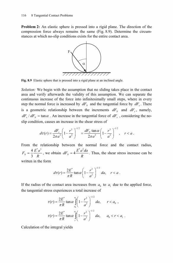
116 8 Tangential Contact Problems
Problem 2: An elastic sphere is pressed into a rigid plane. The direction of the compression force always remains the same (Fig. 8.9). Determine the circum-stances at which no-slip conditions exists for the entire contact area.
F
�
Fig. 8.9 Elastic sphere that is pressed into a rigid plane at an inclined angle.
Solution: We begin with the assumption that no sliding takes place in the contact area and verify afterwards the validity of this assumption. We can separate the continuous increase of the force into infinitesimally small steps, where in every step the normal force is increased by NdF and the tangential force by xdF . There is a geometric relationship between the increments NdF and xdF , namely,
/ tanα=x NdF dF . An increase in the tangential force of xdF , considering the no-slip condition, causes an increase in the shear stress of
1/ 2 1/ 22 2
2 2 2 2
tan( ) 1 1 ,
2 2x NdF dFr rd r r aa a a a
ατ
π π
− −⎛ ⎞ ⎛ ⎞
= − = − <⎜ ⎟ ⎜ ⎟⎝ ⎠ ⎝ ⎠
.
From the relationship between the normal force and the contact radius, * 34
3=N
E aFR
, we obtain * 2
4=NE a dadF
R. Thus, the shear stress increase can be
written in the form 1/2* 2
2
2( ) tan 1 , E rd r da r aR a
τ απ
−⎛ ⎞
= − <⎜ ⎟⎝ ⎠
.
If the radius of the contact area increases from 0a to 1a due to the applied force, the tangential stress experiences a total increase of
1
0
1
1/ 2* 2
02
1/2* 2
0 12
2( ) tan 1 , ,
2( ) tan 1 , .
a
a
a
r
E rr da r aR a
E rr da a r aR a
τ απ
τ απ
−
−
⎛ ⎞= − <⎜ ⎟
⎝ ⎠
⎛ ⎞= − < <⎜ ⎟
⎝ ⎠
∫
∫
Calculation of the integral yields
Problems 117
( ) ( )
( )
* 1/ 2 1/22 2 2 21 0 0
* 1/ 22 21 0 1
2( ) tan , ,
2( ) tan , .
Er a r a r r aR
Er a r a r aR
τ απ
τ απ
⎡ ⎤= ⋅ − − − <⎢ ⎥⎣ ⎦
= ⋅ − < <
The Hertzian pressure distribution is calculated as
( ) ( ) ( )*1/2 1/2 1/ 22 2 2 2 2 20
1 1 131 1
3 2( )2 ππ
= − = − = −Np F Ep r a r a r a ra Ra
.
No sliding exists if the condition ( ) ( )τ μ≤r p r is met over the entire contact area. This is the case when
tanα μ≤ .
If the angle at which the force acts is smaller than the critical angle, then there is no sliding in the contact. Note that the critical angle is equal to the friction angle (see Chapter 10), consequently, these results agree with the macroscopic results in that no sliding takes place at an application angle smaller than the friction angle (see Section 10.3).
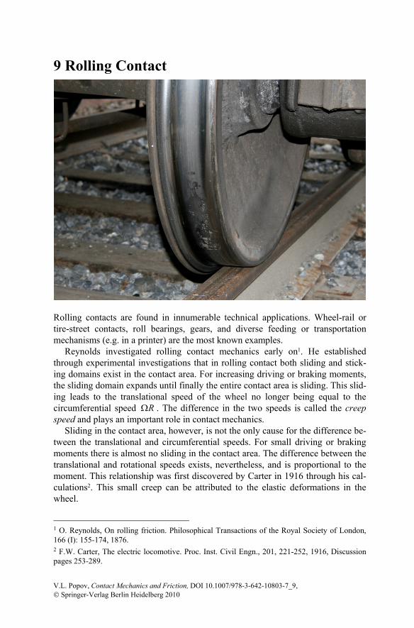
9 Rolling Contact
Rolling contacts are found in innumerable technical applications. Wheel-rail or tire-street contacts, roll bearings, gears, and diverse feeding or transportation mechanisms (e.g. in a printer) are the most known examples.
Reynolds investigated rolling contact mechanics early on1. He established through experimental investigations that in rolling contact both sliding and stick-ing domains exist in the contact area. For increasing driving or braking moments, the sliding domain expands until finally the entire contact area is sliding. This slid-ing leads to the translational speed of the wheel no longer being equal to the circumferential speed ΩR . The difference in the two speeds is called the creep speed and plays an important role in contact mechanics.
Sliding in the contact area, however, is not the only cause for the difference be-tween the translational and circumferential speeds. For small driving or braking moments there is almost no sliding in the contact area. The difference between the translational and rotational speeds exists, nevertheless, and is proportional to the moment. This relationship was first discovered by Carter in 1916 through his cal-culations2. This small creep can be attributed to the elastic deformations in the wheel.
1 O. Reynolds, On rolling friction. Philosophical Transactions of the Royal Society of London, 166 (I): 155-174, 1876. 2 F.W. Carter, The electric locomotive. Proc. Inst. Civil Engn., 201, 221-252, 1916, Discussion pages 253-289.
V.L. Popov, Contact Mechanics and Friction, DOI 10.1007/978-3-642-10803-7_9, © Springer-Verlag Berlin Heidelberg 2010
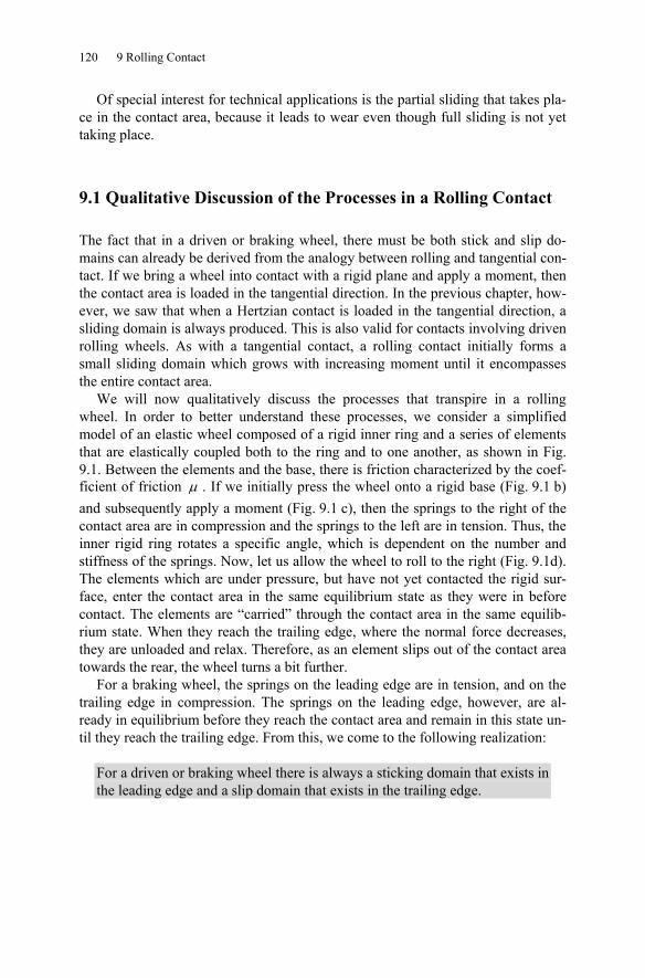
120 9 Rolling Contact
Of special interest for technical applications is the partial sliding that takes pla-ce in the contact area, because it leads to wear even though full sliding is not yet taking place.
9.1 Qualitative Discussion of the Processes in a Rolling Contact
The fact that in a driven or braking wheel, there must be both stick and slip do-mains can already be derived from the analogy between rolling and tangential con-tact. If we bring a wheel into contact with a rigid plane and apply a moment, then the contact area is loaded in the tangential direction. In the previous chapter, how-ever, we saw that when a Hertzian contact is loaded in the tangential direction, a sliding domain is always produced. This is also valid for contacts involving driven rolling wheels. As with a tangential contact, a rolling contact initially forms a small sliding domain which grows with increasing moment until it encompasses the entire contact area.
We will now qualitatively discuss the processes that transpire in a rolling wheel. In order to better understand these processes, we consider a simplified model of an elastic wheel composed of a rigid inner ring and a series of elements that are elastically coupled both to the ring and to one another, as shown in Fig. 9.1. Between the elements and the base, there is friction characterized by the coef-ficient of friction μ . If we initially press the wheel onto a rigid base (Fig. 9.1 b) and subsequently apply a moment (Fig. 9.1 c), then the springs to the right of the contact area are in compression and the springs to the left are in tension. Thus, the inner rigid ring rotates a specific angle, which is dependent on the number and stiffness of the springs. Now, let us allow the wheel to roll to the right (Fig. 9.1d). The elements which are under pressure, but have not yet contacted the rigid sur-face, enter the contact area in the same equilibrium state as they were in before contact. The elements are “carried” through the contact area in the same equilib-rium state. When they reach the trailing edge, where the normal force decreases, they are unloaded and relax. Therefore, as an element slips out of the contact area towards the rear, the wheel turns a bit further.
For a braking wheel, the springs on the leading edge are in tension, and on the trailing edge in compression. The springs on the leading edge, however, are al-ready in equilibrium before they reach the contact area and remain in this state un-til they reach the trailing edge. From this, we come to the following realization:
For a driven or braking wheel there is always a sticking domain that exists in the leading edge and a slip domain that exists in the trailing edge.
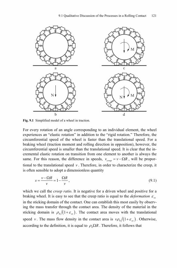
9.1 Qualitative Discussion of the Processes in a Rolling Contact 121
N
1 2 34
N M
1
2 35
4
M
1 24
3
5
a c
b d Fig. 9.1 Simplified model of a wheel in traction.
For every rotation of an angle corresponding to an individual element, the wheel experiences an “elastic rotation” in addition to the “rigid rotation.” Therefore, the circumferential speed of the wheel is faster than the translational speed. For a braking wheel (traction moment and rolling direction in opposition), however, the circumferential speed is smaller than the translational speed. It is clear that the in-cremental elastic rotation on transition from one element to another is always the same. For this reason, the difference in speeds, creepv v R= −Ω , will be propor-tional to the translational speed v . Therefore, in order to characterize the creep, it is often sensible to adopt a dimensionless quantity
1−Ω Ω= = −
v R Rsv v
, (9.1)
which we call the creep ratio. It is negative for a driven wheel and positive for a braking wheel. It is easy to see that the creep ratio is equal to the deformation ε xx in the sticking domain of the contact. One can establish this most easily by observ-ing the mass transfer through the contact area. The density of the material in the sticking domain is ( )0 1ρ ε+ xx . The contact area moves with the translational
speed v . The mass flow density in the contact area is ( )0 1ρ ε+ xxv . Otherwise, according to the definition, it is equal to 0ρ ΩR . Therefore, it follows that
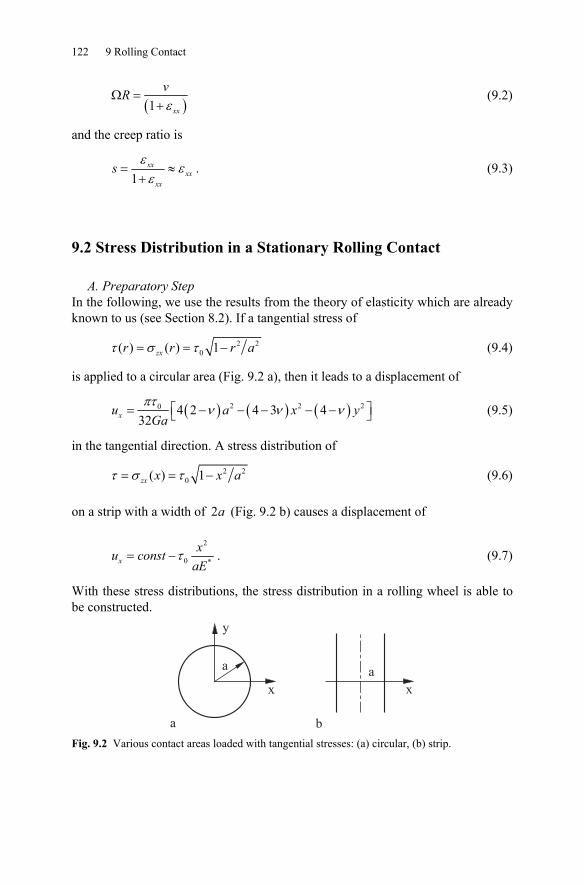
122 9 Rolling Contact
( )1 ε
Ω =+ xx
vR (9.2)
and the creep ratio is
1ε
εε
= ≈+
xxxx
xx
s . (9.3)
9.2 Stress Distribution in a Stationary Rolling Contact
A. Preparatory Step In the following, we use the results from the theory of elasticity which are already known to us (see Section 8.2). If a tangential stress of
2 20( ) ( ) 1τ σ τ= = −zxr r r a (9.4)
is applied to a circular area (Fig. 9.2 a), then it leads to a displacement of
( ) ( ) ( )2 2 20 4 2 4 3 432πτ
ν ν ν⎡ ⎤= − − − − −⎣ ⎦xu a x yGa
(9.5)
in the tangential direction. A stress distribution of
2 20( ) 1τ σ τ= = −zx x x a (9.6)
on a strip with a width of 2a (Fig. 9.2 b) causes a displacement of
2
0 *xxu const
aEτ= − . (9.7)
With these stress distributions, the stress distribution in a rolling wheel is able to be constructed.
y
x
a
x
a
a b Fig. 9.2 Various contact areas loaded with tangential stresses: (a) circular, (b) strip.
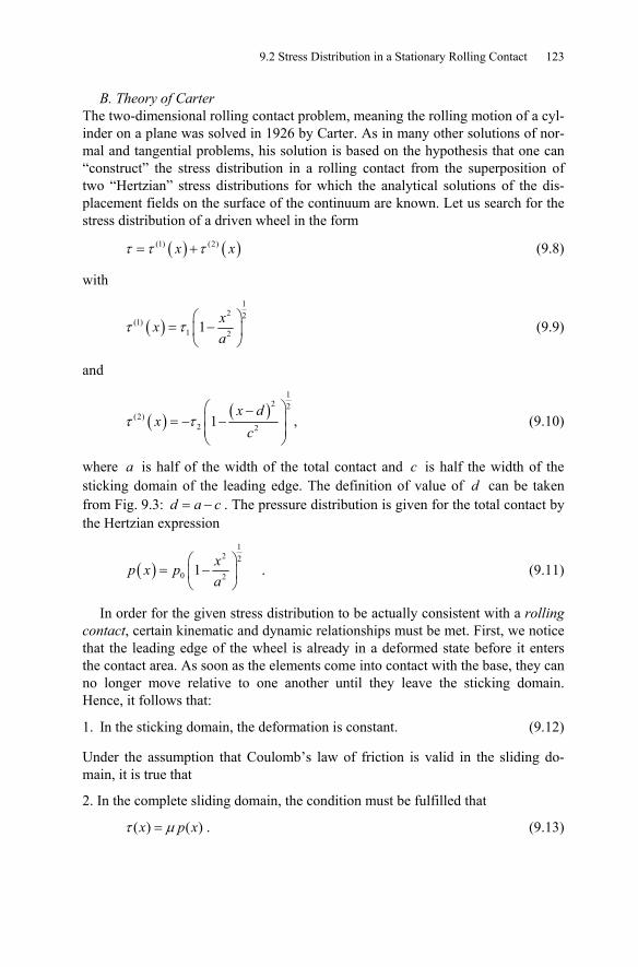
9.2 Stress Distribution in a Stationary Rolling Contact 123
B. Theory of Carter The two-dimensional rolling contact problem, meaning the rolling motion of a cyl-inder on a plane was solved in 1926 by Carter. As in many other solutions of nor-mal and tangential problems, his solution is based on the hypothesis that one can “construct” the stress distribution in a rolling contact from the superposition of two “Hertzian” stress distributions for which the analytical solutions of the dis-placement fields on the surface of the continuum are known. Let us search for the stress distribution of a driven wheel in the form
( ) ( )(1) (2)τ τ τ= +x x (9.8)
with
( )1
2 2(1)
1 21τ τ⎛ ⎞
= −⎜ ⎟⎝ ⎠
xxa
(9.9)
and
( ) ( )1
2 2(2)
2 21τ τ⎛ ⎞−⎜ ⎟= − −⎜ ⎟⎝ ⎠
x dx
c, (9.10)
where a is half of the width of the total contact and c is half the width of the sticking domain of the leading edge. The definition of value of d can be taken from Fig. 9.3: = −d a c . The pressure distribution is given for the total contact by the Hertzian expression
( )1
2 2
0 21⎛ ⎞
= −⎜ ⎟⎝ ⎠
xp x pa
. (9.11)
In order for the given stress distribution to be actually consistent with a rolling contact, certain kinematic and dynamic relationships must be met. First, we notice that the leading edge of the wheel is already in a deformed state before it enters the contact area. As soon as the elements come into contact with the base, they can no longer move relative to one another until they leave the sticking domain. Hence, it follows that:
1. In the sticking domain, the deformation is constant. (9.12)
Under the assumption that Coulomb’s law of friction is valid in the sliding do-main, it is true that
2. In the complete sliding domain, the condition must be fulfilled that
( ) ( )τ μ=x p x . (9.13)
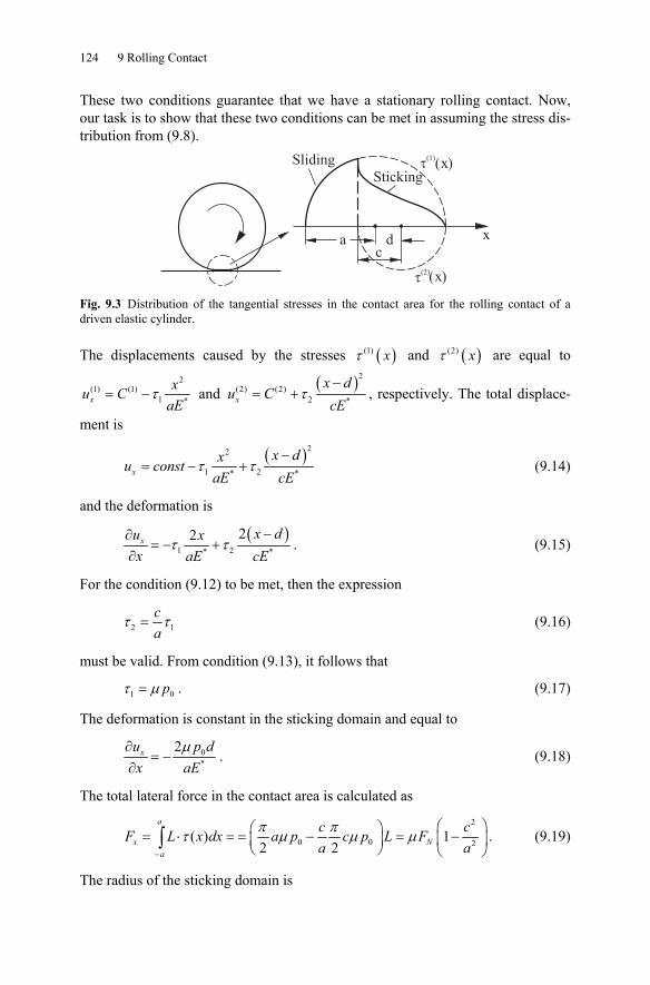
124 9 Rolling Contact
These two conditions guarantee that we have a stationary rolling contact. Now, our task is to show that these two conditions can be met in assuming the stress dis-tribution from (9.8).
a dc
x
����
( )x
����( )x
Sliding
Sticking
Fig. 9.3 Distribution of the tangential stresses in the contact area for the rolling contact of a driven elastic cylinder.
The displacements caused by the stresses ( )(1)τ x and ( )(2)τ x are equal to 2
(1) (1)1 *τ= −x
xu CaE
and ( )2
(2) (2)2 *τ
−= +x
x du C
cE, respectively. The total displace-
ment is
( )22
1 2* *x
x dxu constaE cE
τ τ−
= − + (9.14)
and the deformation is
( )
1 2* *
22τ τ−∂
= − +∂
x x du xx aE cE
. (9.15)
For the condition (9.12) to be met, then the expression
2 1τ τ=ca
(9.16)
must be valid. From condition (9.13), it follows that
1 0τ μ= p . (9.17)
The deformation is constant in the sticking domain and equal to
0*
2μ∂= −
∂xu p d
x aE. (9.18)
The total lateral force in the contact area is calculated as
2
0 0 2( ) 12 2π πτ μ μ μ
−
⎛ ⎞⎛ ⎞= ⋅ = = − = −⎜ ⎟⎜ ⎟⎝ ⎠ ⎝ ⎠
∫a
x Na
c cF L x dx a p c p L Fa a
. (9.19)
The radius of the sticking domain is
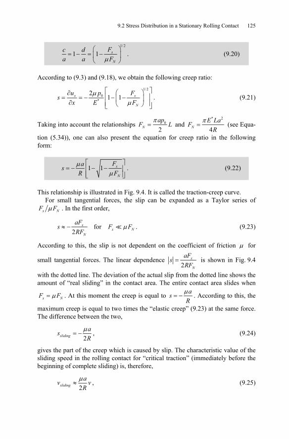
9.2 Stress Distribution in a Stationary Rolling Contact 125
1/ 2
1 1μ
⎛ ⎞= − = −⎜ ⎟
⎝ ⎠x
N
Fc da a F
. (9.20)
According to (9.3) and (9.18), we obtain the following creep ratio:
1/ 2
0*
21 1
μμ
⎡ ⎤⎛ ⎞∂⎢ ⎥= = − − −⎜ ⎟∂ ⎢ ⎥⎝ ⎠⎣ ⎦
x x
N
u p Fs
x FE. (9.21)
Taking into account the relationships 0
2π
=Nap
F L and * 2
4π
=NE LaF
R (see Equa-
tion (5.34)), one can also present the equation for creep ratio in the following form:
1 1 x
N
FasR Fμ
μ⎡ ⎤
= − − −⎢ ⎥⎢ ⎥⎣ ⎦
. (9.22)
This relationship is illustrated in Fig. 9.4. It is called the traction-creep curve. For small tangential forces, the slip can be expanded as a Taylor series of μx NF F . In the first order,
for2
xx N
N
aFs F F
RFμ≈ − . (9.23)
According to this, the slip is not dependent on the coefficient of friction μ for
small tangential forces. The linear dependence 2
= x
N
aFs
RF is shown in Fig. 9.4
with the dotted line. The deviation of the actual slip from the dotted line shows the amount of “real sliding” in the contact area. The entire contact area slides when
μ=x NF F . At this moment the creep is equal to μ= −
asR
. According to this, the
maximum creep is equal to two times the “elastic creep” (9.23) at the same force. The difference between the two,
2sliding
asRμ
= − , (9.24)
gives the part of the creep which is caused by slip. The characteristic value of the sliding speed in the rolling contact for “critical traction” (immediately before the beginning of complete sliding) is, therefore,
2sliding
av vRμ
≈ , (9.25)
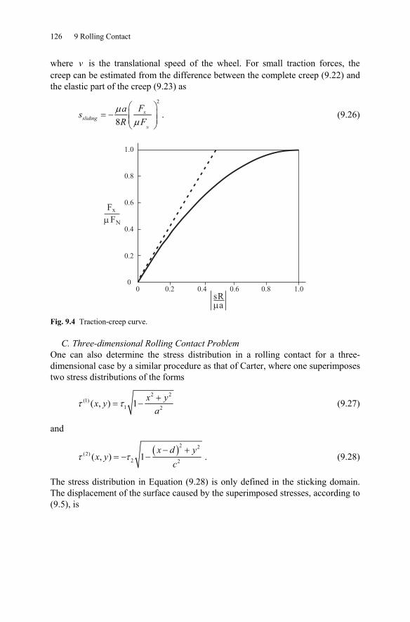
126 9 Rolling Contact
where v is the translational speed of the wheel. For small traction forces, the creep can be estimated from the difference between the complete creep (9.22) and the elastic part of the creep (9.23) as
2
8N
xsliding
FasR Fμ
μ
⎛ ⎞= − ⎜ ⎟⎜ ⎟
⎝ ⎠. (9.26)
Fig. 9.4 Traction-creep curve.
C. Three-dimensional Rolling Contact Problem One can also determine the stress distribution in a rolling contact for a three-dimensional case by a similar procedure as that of Carter, where one superimposes two stress distributions of the forms
2 2
(1)1 2( , ) 1τ τ +
= −x yx y
a (9.27)
and
( )2 2
(2)2 2( , ) 1τ τ
− += − −
x d yx y
c. (9.28)
The stress distribution in Equation (9.28) is only defined in the sticking domain. The displacement of the surface caused by the superimposed stresses, according to (9.5), is
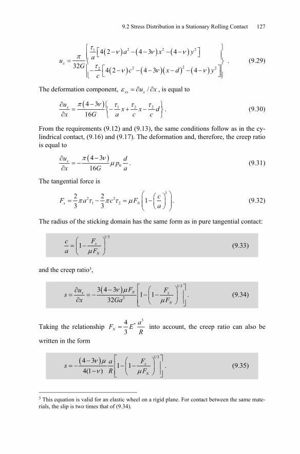
9.2 Stress Distribution in a Stationary Rolling Contact 127
( ) ( ) ( )
( ) ( ) ( ) ( )
2 2 21
22 22
4 2 4 3 4
32 4 2 4 3 4
τν ν ν
πτ
ν ν ν
⎧ ⎫⎡ ⎤− − − − −⎪ ⎪⎣ ⎦⎪ ⎪= ⎨ ⎬⎪ ⎪⎡ ⎤− − − − − − −⎣ ⎦⎪ ⎪⎩ ⎭
x
a x yau
G c x d yc
. (9.29)
The deformation component, /ε = ∂ ∂xx xu x , is equal to
( ) 1 2 24 316
π ν τ τ τ−∂ ⎧ ⎫= − + −⎨ ⎬∂ ⎩ ⎭xu
x x dx G a c c
. (9.30)
From the requirements (9.12) and (9.13), the same conditions follow as in the cy-lindrical contact, (9.16) and (9.17). The deformation and, therefore, the creep ratio is equal to
( )
0
4 316
π νμ
−∂= −
∂xu dp
x G a. (9.31)
The tangential force is
3
2 21 2
2 2 13 3π τ π τ μ
⎛ ⎞⎛ ⎞= − = −⎜ ⎟⎜ ⎟⎜ ⎟⎝ ⎠⎝ ⎠x N
cF a c Fa
. (9.32)
The radius of the sticking domain has the same form as in pure tangential contact:
1/3
1μ
⎛ ⎞= −⎜ ⎟⎝ ⎠
x
N
Fca F
(9.33)
and the creep ratio3,
( ) 1/3
2
3 4 31 1
32ν μ
μ
⎡ ⎤− ⎛ ⎞∂⎢ ⎥= = − − −⎜ ⎟∂ ⎢ ⎥⎝ ⎠⎣ ⎦
Nx x
N
Fu Fs
x FGa. (9.34)
Taking the relationship 3
*43
=NaF ER
into account, the creep ratio can also be
written in the form
( ) 1/34 3
1 14(1 )
ν μν μ
⎡ ⎤− ⎛ ⎞⎢ ⎥= − − −⎜ ⎟− ⎢ ⎥⎝ ⎠⎣ ⎦
x
N
FasR F
. (9.35)
3 This equation is valid for an elastic wheel on a rigid plane. For contact between the same mate-rials, the slip is two times that of (9.34).
128 9 Rolling Contact
For small driving forces, we obtain the following for the first order approximation:
( )
2
4 332
ν−≈ − xF
sGa
. (9.36)
Problems
Problem 1: Estimate the sliding speed (a) in a locomotive wheel (b) in an auto-mobile tire.
Solution: (a) For a locomotive wheel, the creep is calculated according to (9.35):
( ) 1/34 31 1
4(1 )ν μν μ
⎡ ⎤− ⎛ ⎞⎢ ⎥= − − −⎜ ⎟− ⎢ ⎥⎝ ⎠⎣ ⎦
x
N
FasR F
.
We obtain the creep at the critical traction by inserting μ=x NF F :
( )4 34(1 )
ν μν
−=
−asR
.
The sliding speed is calculated by multiplying the creep with the translational speed v . At 0.3μ ≈ , 7 mm≈a , 0.5 mR = , and 1/ 3ν = , the sliding speed is
35 10slidingv v−≈ ⋅ . At a translational speed of 30 m/s (108 km/h), it has a character-istic value of 0.14 m/sslidingv ≈ . (b) For an automobile tire in “critical traction” with 1μ ≈ , 5 cm≈a , 0.3 mR = and 1/ 2ν = , we obtain 0.2slidingv v≈ for the sliding speed. At a translational speed of 15 m/s (54 km/h), the sliding speed is around 3 m/s. At “normal operat-ing conditions” (constant speed of 15 m/s), the sliding speed in a rolling contact between a rubber tire and the street is much smaller and, as a rule, around 1 cm/s.
Problem 2: Estimate the energy loss in a driven or braking wheel.
Solution: We obtain the following estimation for the frictional power W in the contact by multiplying the tangential force acting on the contact with the average sliding speed:
0≈ =xW s F v s W ,
where 0 = xW F v is the “power” of the frictional force.
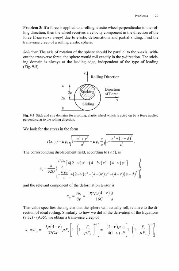
Problems 129
Problem 3: If a force is applied to a rolling, elastic wheel perpendicular to the rol-ling direction, then the wheel receives a velocity component in the direction of the force (transverse creep) due to elastic deformations and partial sliding. Find the transverse creep of a rolling elastic sphere.
Solution: The axis of rotation of the sphere should be parallel to the x-axis; with-out the transverse force, the sphere would roll exactly in the y-direction. The stick-ing domain is always at the leading edge, independent of the type of loading (Fig. 9.5).
Sticking
Sliding
2c
2a
y
x
Rolling Direction
Directionof Force
Fig. 9.5 Stick and slip domains for a rolling, elastic wheel which is acted on by a force applied perpendicular to the rolling direction.
We look for the stress in the form
( )222 2
0 02 2( , ) 1 1τ μ μ+ −+
= − − −x y dx y cx y p p
aa c.
The corresponding displacement field, according to (9.5), is
( ) ( ) ( )
( ) ( ) ( )( )
2 2 20
22 20
4 2 4 3 4
32 4 2 4 3 4
μν ν ν
πμ
ν ν ν
⎧ ⎫⎡ ⎤− − − − −⎪ ⎪⎣ ⎦⎪ ⎪= ⎨ ⎬⎪ ⎪⎡ ⎤− − − − − − −⎣ ⎦⎪ ⎪⎩ ⎭
x
pa x y
aupG c x y da
and the relevant component of the deformation tensor is
( )0 416
πμ νε
−∂= = −∂
xxy
pu dy G a
.
This value specifies the angle at that the sphere will actually roll, relative to the di-rection of ideal rolling. Similarly to how we did in the derivation of the Equations (9.32) - (9.35), we obtain a transverse creep of
( ) ( )1/3 1/3
2
3 4 41 1 1 1
4(1 )32μ ν ν μ
ε μμ ν μ⊥
⎡ ⎤ ⎡ ⎤− −⎛ ⎞ ⎛ ⎞⎢ ⎥ ⎢ ⎥= = − − − = − − −⎜ ⎟ ⎜ ⎟−⎢ ⎥ ⎢ ⎥⎝ ⎠ ⎝ ⎠⎣ ⎦ ⎣ ⎦
x xxy N
N N
F Fas FF R FGa
.
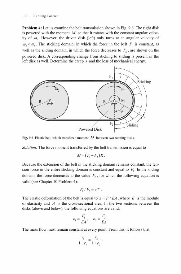
130 9 Rolling Contact
Problem 4: Let us examine the belt transmission shown in Fig. 9.6. The right disk is powered with the moment M so that it rotates with the constant angular veloc-ity of 1ω . However, the driven disk (left) only turns at an angular velocity of
2 1ω ω< . The sticking domain, in which the force in the belt 1F is constant, as well as the sliding domain, in which the force decreases to 2F , are shown on the powered disk. A corresponding change from sticking to sliding is present in the left disk as well. Determine the creep s and the loss of mechanical energy.
Fig. 9.6 Elastic belt, which transfers a moment M between two rotating disks.
Solution: The force moment transferred by the belt transmission is equal to
( )1 2= −M F F R .
Because the extension of the belt in the sticking domain remains constant, the ten-sion force in the entire sticking domain is constant and equal to 1F . In the sliding domain, the force decreases to the value 2F , for which the following equation is valid (see Chapter 10 Problem 4):
1 2/ μϕ=F F e .
The elastic deformation of the belt is equal to /ε = F EA , where E is the module of elasticity and A is the cross-sectional area. In the two sections between the disks (above and below), the following equations are valid:
11ε =
FEA
, 22ε =
FEA
.
The mass flow must remain constant at every point. From this, it follows that
1 2
1 21 1ε ε=
+ +v v .
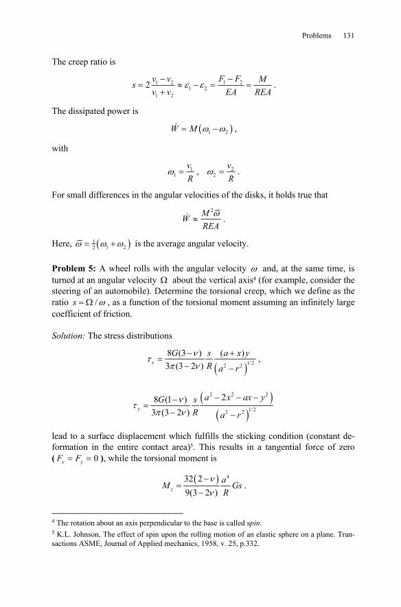
Problems 131
The creep ratio is
1 2 1 21 2
1 2
2 ε ε− −
= ≈ − = =+
v v F F Msv v EA REA
.
The dissipated power is
( )1 2ω ω= −W M ,
with
11ω =
vR
, 22ω =
vR
.
For small differences in the angular velocities of the disks, it holds true that 2ω
≈MWREA
.
Here, ( )11 22ω ω ω= + is the average angular velocity.
Problem 5: A wheel rolls with the angular velocity ω and, at the same time, is turned at an angular velocity Ω about the vertical axis4 (for example, consider the steering of an automobile). Determine the torsional creep, which we define as the ratio /ω= Ωs , as a function of the torsional moment assuming an infinitely large coefficient of friction.
Solution: The stress distributions
( )1/ 22 2
8 (3 ) ( )3 (3 2 )
ντπ ν
− +=
− −x
G s a x yR a r
,
( )( )
2 2 2
1/22 2
28 (1 )3 (3 2 )
ντπ ν
− − −−=
− −y
a x ax yG sR a r
lead to a surface displacement which fulfills the sticking condition (constant de-formation in the entire contact area)5. This results in a tangential force of zero ( 0x yF F= = ), while the torsional moment is
( ) 432 29(3 2 )z
aM GsR
νν−
=−
.
4 The rotation about an axis perpendicular to the base is called spin. 5 K.L. Johnson, The effect of spin upon the rolling motion of an elastic sphere on a plane. Tran-sactions ASME, Journal of Applied mechanics, 1958, v. 25, p.332.

132 9 Rolling Contact
The resulting creep ratio is
( ) 4
9(3 2 )32 2
νν
−=
−zMRs
Ga.

10 Coulomb’s Law of Friction
10.1 Introduction
In this chapter, we will only investigate the dry friction or Coulomb friction between two solid bodies. Friction between solid bodies is an extremely compli-cated physical phenomenon. It encompasses elastic and plastic deformations of the surface layers of the contacting bodies, interactions with wear particles, micro-fractures and the restoration of the continuity of materials, excitation of electrons and phonons, chemical reactions, and the transfer of particles from one body to the other. What is astonishing is the fact that it is possible to formulate a very simple law for dry friction. This first order approximation is sufficient for many engineer-ing applications: The frictional force is proportional to the normal force and as good as independent from the speed. The astounding property of dry friction lies in the fact that in a first order approximation, it is dependent neither on contact area nor on roughness. This property allows us to use the notion of the coefficient of friction. The coefficient of friction, however, gives only a very rough first ap-proximation of the quotient of frictional force to normal force.
Leonardo da Vinci was the first to experimentally investigate the law of friction and formulate the most important principles (e.g. that the frictional resistance is proportional to the weight and independent from the contact area). He derived the latter with the help of the experiments shown in Fig. 10.1.
V.L. Popov, Contact Mechanics and Friction, DOI 10.1007/978-3-642-10803-7_10, © Springer-Verlag Berlin Heidelberg 2010
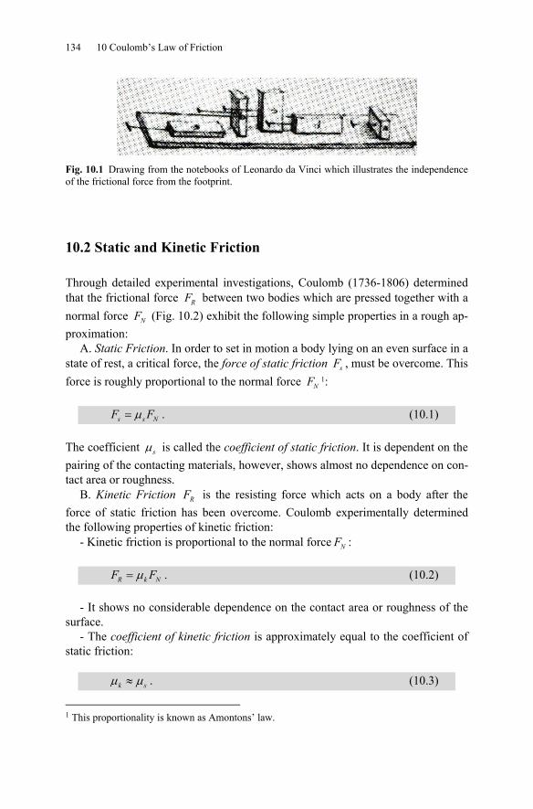
134 10 Coulomb’s Law of Friction
Fig. 10.1 Drawing from the notebooks of Leonardo da Vinci which illustrates the independence of the frictional force from the footprint.
10.2 Static and Kinetic Friction
Through detailed experimental investigations, Coulomb (1736-1806) determined that the frictional force RF between two bodies which are pressed together with a normal force NF (Fig. 10.2) exhibit the following simple properties in a rough ap-proximation:
A. Static Friction. In order to set in motion a body lying on an even surface in a state of rest, a critical force, the force of static friction sF , must be overcome. This force is roughly proportional to the normal force NF 1:
μ=s s NF F . (10.1)
The coefficient μs is called the coefficient of static friction. It is dependent on the pairing of the contacting materials, however, shows almost no dependence on con-tact area or roughness.
B. Kinetic Friction RF is the resisting force which acts on a body after the force of static friction has been overcome. Coulomb experimentally determined the following properties of kinetic friction:
- Kinetic friction is proportional to the normal force NF :
μ=R k NF F . (10.2)
- It shows no considerable dependence on the contact area or roughness of the surface.
- The coefficient of kinetic friction is approximately equal to the coefficient of static friction:
μ μ≈k s . (10.3)
1 This proportionality is known as Amontons’ law.
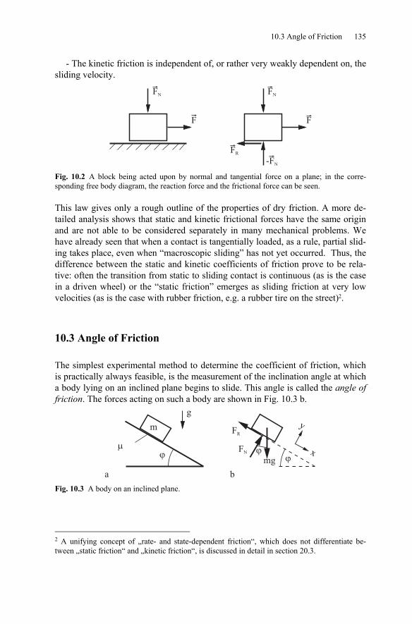
10.3 Angle of Friction 135
- The kinetic friction is independent of, or rather very weakly dependent on, the sliding velocity.
FN
F
FN
F
-FN
FR
Fig. 10.2 A block being acted upon by normal and tangential force on a plane; in the corre-sponding free body diagram, the reaction force and the frictional force can be seen.
This law gives only a rough outline of the properties of dry friction. A more de-tailed analysis shows that static and kinetic frictional forces have the same origin and are not able to be considered separately in many mechanical problems. We have already seen that when a contact is tangentially loaded, as a rule, partial slid-ing takes place, even when “macroscopic sliding” has not yet occurred. Thus, the difference between the static and kinetic coefficients of friction prove to be rela-tive: often the transition from static to sliding contact is continuous (as is the case in a driven wheel) or the “static friction” emerges as sliding friction at very low velocities (as is the case with rubber friction, e.g. a rubber tire on the street)2.
10.3 Angle of Friction
The simplest experimental method to determine the coefficient of friction, which is practically always feasible, is the measurement of the inclination angle at which a body lying on an inclined plane begins to slide. This angle is called the angle of friction. The forces acting on such a body are shown in Fig. 10.3 b.
y
xFN�
�
�
FR
mg�
m
g
a b Fig. 10.3 A body on an inclined plane.
2 A unifying concept of „rate- and state-dependent friction“, which does not differentiate be-tween „static friction“ and „kinetic friction“, is discussed in detail in section 20.3.
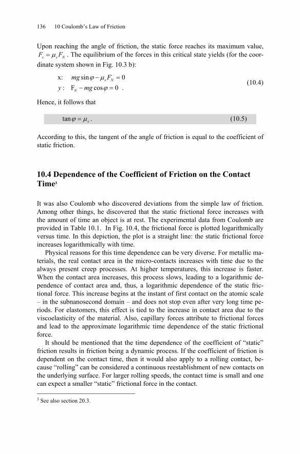
136 10 Coulomb’s Law of Friction
Upon reaching the angle of friction, the static force reaches its maximum value, μ=s s NF F . The equilibrium of the forces in this critical state yields (for the coor-
dinate system shown in Fig. 10.3 b):
x: sin 0
: F cos 0 .ϕ μ
ϕ− =
− =s N
N
mg Fy mg
(10.4)
Hence, it follows that
tanϕ μ= s . (10.5)
According to this, the tangent of the angle of friction is equal to the coefficient of static friction.
10.4 Dependence of the Coefficient of Friction on the Contact Time3
It was also Coulomb who discovered deviations from the simple law of friction. Among other things, he discovered that the static frictional force increases with the amount of time an object is at rest. The experimental data from Coulomb are provided in Table 10.1. In Fig. 10.4, the frictional force is plotted logarithmically versus time. In this depiction, the plot is a straight line: the static frictional force increases logarithmically with time.
Physical reasons for this time dependence can be very diverse. For metallic ma-terials, the real contact area in the micro-contacts increases with time due to the always present creep processes. At higher temperatures, this increase is faster. When the contact area increases, this process slows, leading to a logarithmic de-pendence of contact area and, thus, a logarithmic dependence of the static fric-tional force. This increase begins at the instant of first contact on the atomic scale – in the subnanosecond domain – and does not stop even after very long time pe-riods. For elastomers, this effect is tied to the increase in contact area due to the viscoelasticity of the material. Also, capillary forces attribute to frictional forces and lead to the approximate logarithmic time dependence of the static frictional force.
It should be mentioned that the time dependence of the coefficient of “static” friction results in friction being a dynamic process. If the coefficient of friction is dependent on the contact time, then it would also apply to a rolling contact, be-cause “rolling” can be considered a continuous reestablishment of new contacts on the underlying surface. For larger rolling speeds, the contact time is small and one can expect a smaller “static” frictional force in the contact. 3 See also section 20.3.
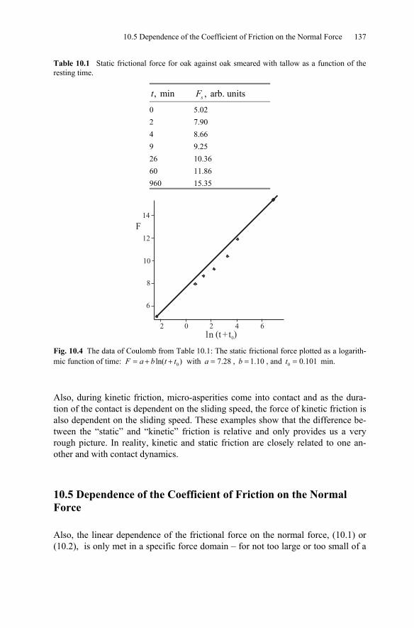
10.5 Dependence of the Coefficient of Friction on the Normal Force 137
Table 10.1 Static frictional force for oak against oak smeared with tallow as a function of the resting time.
, mint , arb. unitssF
0 5.02 2 7.90 4 8.66 9 9.25 26 10.36 60 11.86 960 15.35
14
12
10
8
6
2 0 2 4 6
F
ln (t +t0) Fig. 10.4 The data of Coulomb from Table 10.1: The static frictional force plotted as a logarith-mic function of time: 0ln( )= + +F a b t t with 7.28a = , 1.10b = , and 0 0.101t = min.
Also, during kinetic friction, micro-asperities come into contact and as the dura-tion of the contact is dependent on the sliding speed, the force of kinetic friction is also dependent on the sliding speed. These examples show that the difference be-tween the “static” and “kinetic” friction is relative and only provides us a very rough picture. In reality, kinetic and static friction are closely related to one an-other and with contact dynamics.
10.5 Dependence of the Coefficient of Friction on the Normal Force
Also, the linear dependence of the frictional force on the normal force, (10.1) or (10.2), is only met in a specific force domain – for not too large or too small of a
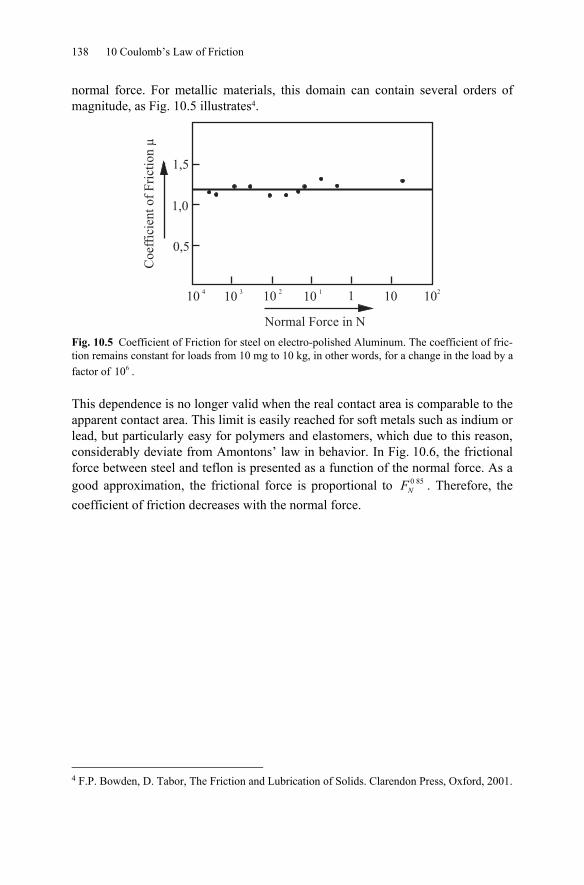
138 10 Coulomb’s Law of Friction
normal force. For metallic materials, this domain can contain several orders of magnitude, as Fig. 10.5 illustrates4.
1,5
1,0
0,5
104
103
101 102
101
102
Co
effi
cien
to
fF
rict
ion
µ
Normal Force in N Fig. 10.5 Coefficient of Friction for steel on electro-polished Aluminum. The coefficient of fric-tion remains constant for loads from 10 mg to 10 kg, in other words, for a change in the load by a factor of 610 .
This dependence is no longer valid when the real contact area is comparable to the apparent contact area. This limit is easily reached for soft metals such as indium or lead, but particularly easy for polymers and elastomers, which due to this reason, considerably deviate from Amontons’ law in behavior. In Fig. 10.6, the frictional force between steel and teflon is presented as a function of the normal force. As a good approximation, the frictional force is proportional to 0 85
NF . Therefore, the coefficient of friction decreases with the normal force.
4 F.P. Bowden, D. Tabor, The Friction and Lubrication of Solids. Clarendon Press, Oxford, 2001.
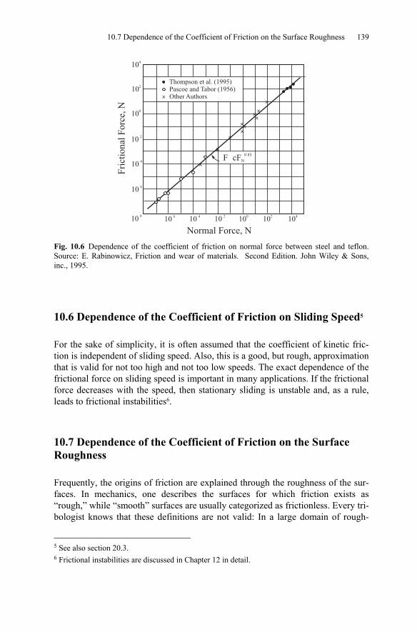
10.7 Dependence of the Coefficient of Friction on the Surface Roughness 139
104
102
100
102
104
106
108
106
104
102
100
102
104
Normal Force, N
Fri
ctio
nal
Fo
rce,
Nx
x
xx
x
x
x
x
x
x
x
Thompson et al. (1995)Pascoe and Tabor (1956)Other Authorsx
F cFN
0 85
Fig. 10.6 Dependence of the coefficient of friction on normal force between steel and teflon. Source: E. Rabinowicz, Friction and wear of materials. Second Edition. John Wiley & Sons, inc., 1995.
10.6 Dependence of the Coefficient of Friction on Sliding Speed5
For the sake of simplicity, it is often assumed that the coefficient of kinetic fric-tion is independent of sliding speed. Also, this is a good, but rough, approximation that is valid for not too high and not too low speeds. The exact dependence of the frictional force on sliding speed is important in many applications. If the frictional force decreases with the speed, then stationary sliding is unstable and, as a rule, leads to frictional instabilities6.
10.7 Dependence of the Coefficient of Friction on the Surface Roughness
Frequently, the origins of friction are explained through the roughness of the sur-faces. In mechanics, one describes the surfaces for which friction exists as “rough,” while “smooth” surfaces are usually categorized as frictionless. Every tri-bologist knows that these definitions are not valid: In a large domain of rough-
5 See also section 20.3. 6 Frictional instabilities are discussed in Chapter 12 in detail.
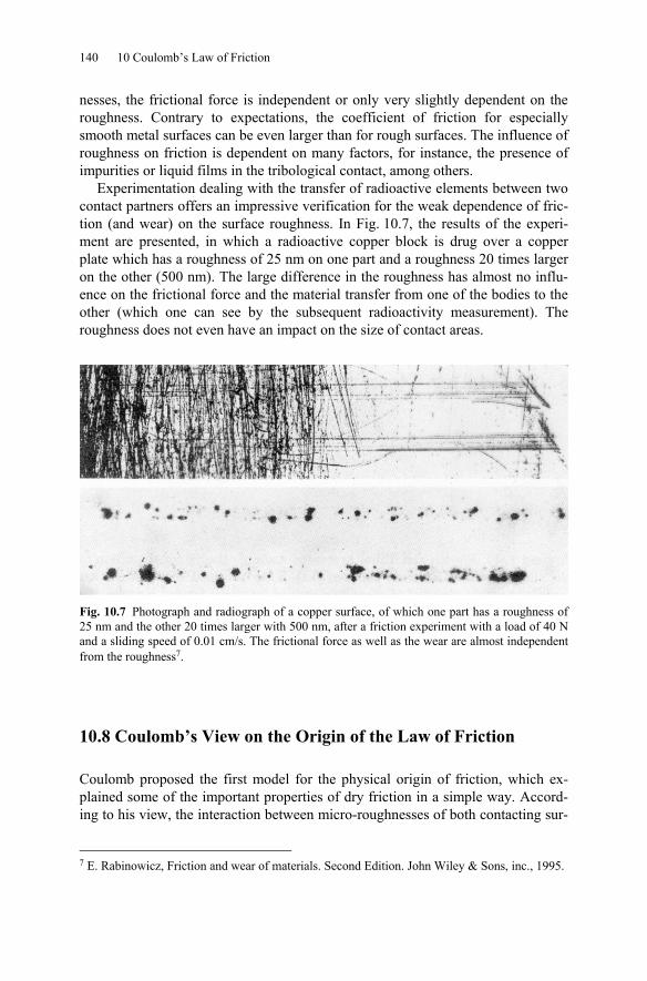
140 10 Coulomb’s Law of Friction
nesses, the frictional force is independent or only very slightly dependent on the roughness. Contrary to expectations, the coefficient of friction for especially smooth metal surfaces can be even larger than for rough surfaces. The influence of roughness on friction is dependent on many factors, for instance, the presence of impurities or liquid films in the tribological contact, among others.
Experimentation dealing with the transfer of radioactive elements between two contact partners offers an impressive verification for the weak dependence of fric-tion (and wear) on the surface roughness. In Fig. 10.7, the results of the experi-ment are presented, in which a radioactive copper block is drug over a copper plate which has a roughness of 25 nm on one part and a roughness 20 times larger on the other (500 nm). The large difference in the roughness has almost no influ-ence on the frictional force and the material transfer from one of the bodies to the other (which one can see by the subsequent radioactivity measurement). The roughness does not even have an impact on the size of contact areas.
Fig. 10.7 Photograph and radiograph of a copper surface, of which one part has a roughness of 25 nm and the other 20 times larger with 500 nm, after a friction experiment with a load of 40 N and a sliding speed of 0.01 cm/s. The frictional force as well as the wear are almost independent from the roughness7.
10.8 Coulomb’s View on the Origin of the Law of Friction
Coulomb proposed the first model for the physical origin of friction, which ex-plained some of the important properties of dry friction in a simple way. Accord-ing to his view, the interaction between micro-roughnesses of both contacting sur-
7 E. Rabinowicz, Friction and wear of materials. Second Edition. John Wiley & Sons, inc., 1995.
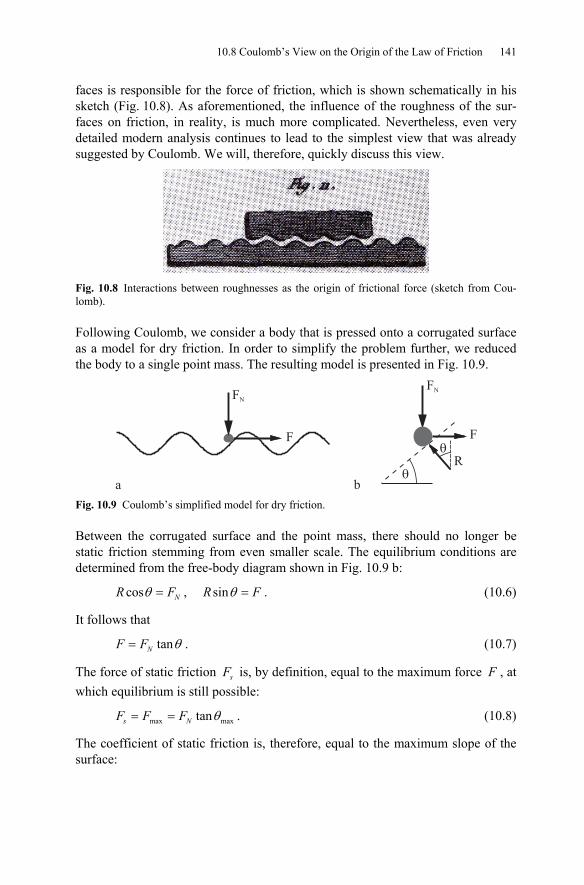
10.8 Coulomb’s View on the Origin of the Law of Friction 141
faces is responsible for the force of friction, which is shown schematically in his sketch (Fig. 10.8). As aforementioned, the influence of the roughness of the sur-faces on friction, in reality, is much more complicated. Nevertheless, even very detailed modern analysis continues to lead to the simplest view that was already suggested by Coulomb. We will, therefore, quickly discuss this view.
Fig. 10.8 Interactions between roughnesses as the origin of frictional force (sketch from Cou-lomb).
Following Coulomb, we consider a body that is pressed onto a corrugated surface as a model for dry friction. In order to simplify the problem further, we reduced the body to a single point mass. The resulting model is presented in Fig. 10.9.
FN
F
�
�
R
F
FN
a b Fig. 10.9 Coulomb’s simplified model for dry friction.
Between the corrugated surface and the point mass, there should no longer be static friction stemming from even smaller scale. The equilibrium conditions are determined from the free-body diagram shown in Fig. 10.9 b:
cosθ = NR F , sinθ =R F . (10.6)
It follows that
tanθ= NF F . (10.7)
The force of static friction sF is, by definition, equal to the maximum force F , at which equilibrium is still possible:
max maxtanθ= =s NF F F . (10.8)
The coefficient of static friction is, therefore, equal to the maximum slope of the surface:
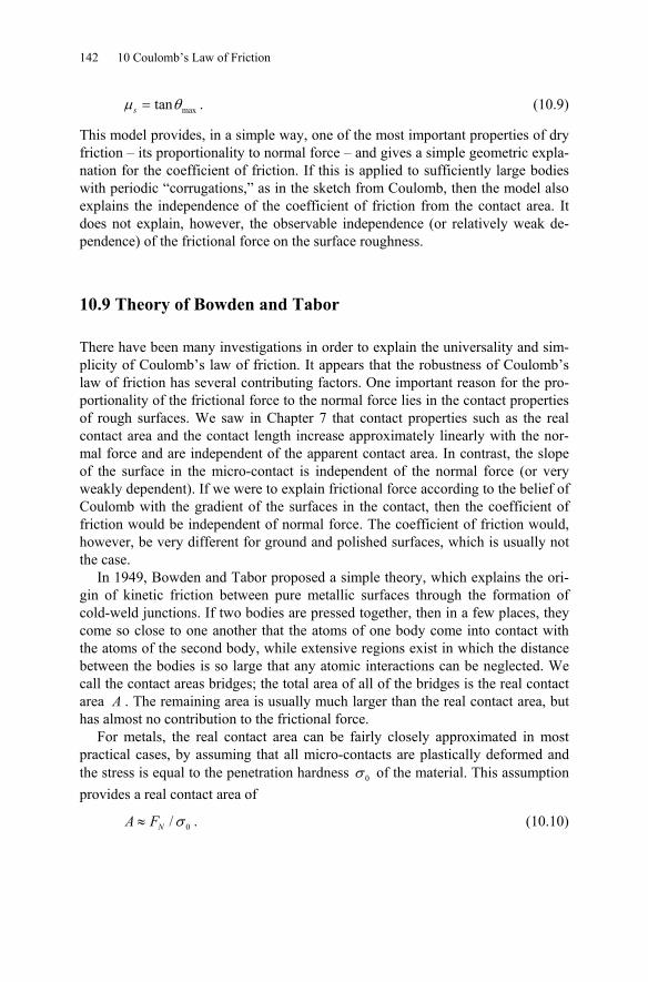
142 10 Coulomb’s Law of Friction
maxtanμ θ=s . (10.9)
This model provides, in a simple way, one of the most important properties of dry friction – its proportionality to normal force – and gives a simple geometric expla-nation for the coefficient of friction. If this is applied to sufficiently large bodies with periodic “corrugations,” as in the sketch from Coulomb, then the model also explains the independence of the coefficient of friction from the contact area. It does not explain, however, the observable independence (or relatively weak de-pendence) of the frictional force on the surface roughness.
10.9 Theory of Bowden and Tabor
There have been many investigations in order to explain the universality and sim-plicity of Coulomb’s law of friction. It appears that the robustness of Coulomb’s law of friction has several contributing factors. One important reason for the pro-portionality of the frictional force to the normal force lies in the contact properties of rough surfaces. We saw in Chapter 7 that contact properties such as the real contact area and the contact length increase approximately linearly with the nor-mal force and are independent of the apparent contact area. In contrast, the slope of the surface in the micro-contact is independent of the normal force (or very weakly dependent). If we were to explain frictional force according to the belief of Coulomb with the gradient of the surfaces in the contact, then the coefficient of friction would be independent of normal force. The coefficient of friction would, however, be very different for ground and polished surfaces, which is usually not the case.
In 1949, Bowden and Tabor proposed a simple theory, which explains the ori-gin of kinetic friction between pure metallic surfaces through the formation of cold-weld junctions. If two bodies are pressed together, then in a few places, they come so close to one another that the atoms of one body come into contact with the atoms of the second body, while extensive regions exist in which the distance between the bodies is so large that any atomic interactions can be neglected. We call the contact areas bridges; the total area of all of the bridges is the real contact area A . The remaining area is usually much larger than the real contact area, but has almost no contribution to the frictional force.
For metals, the real contact area can be fairly closely approximated in most practical cases, by assuming that all micro-contacts are plastically deformed and the stress is equal to the penetration hardness 0σ of the material. This assumption provides a real contact area of
0/σ≈ NA F . (10.10)
10.9 Theory of Bowden and Tabor 143
If a tangential stress of τ c is necessary to shear a cold-weld junction, then the maximum force of static friction is equal to
0
τσ
= cs NF F . (10.11)
Because the shear strength for an isotropic plastic body is around 1/ 3 of the tensile strength and this, in turn, is around 1/3 of the penetration hardness, there should be, as a rule, a universal dependence, ( )1 1
6 5≈ ÷s NF F , leading to a coeffi-
cient of friction of 1 16 5
μ ≈ ÷ . For many non-lubricated metal pairings (e.g. steel
on bronze, steel on brass, or steel on cast iron), the coefficient of friction is effec-tively on the order of 0.16 0.2μ −∼ . For larger compressive forces, the coeffi-cient of friction between pure metals can reach higher values, which is probably related to the larger plastic deformations and, therefore, the resulting considerable changes in surface topography.
Coefficients of friction between different materials are dependent on many pa-rameters. However, based on the ideas of Bowden and Tabor, it is possible to for-mulate a rough classification. Initially, we notice that for strong adhesion in a tri-bological contact there exist both contacts in compression and contacts in tension. The stress in the compressive areas is roughly equal to the hardness, 0 3σ σ≈ c . In the tensile areas, 0σ ζσ≈ c is valid, where ζ in generally smaller than 3. Thus, the normal force is equal to
( )3N c comp tenF A Aσ ζ= − . (10.12) If all of the cold welds are sheared, then the static force of friction is
( )s c comp tenF A Aτ≈ + . (10.13)
The following approximation results for the coefficient of friction:
( )( )3c comp ten
c comp ten
A A
A A
τμ
σ ζ
+≈
−. (10.14)
Assuming / 3c cτ σ≈ , which is valid for plastic isotropic substances, we obtain the approximation
133
comp ten
comp ten
A AA A
μζ
⎛ ⎞+≈ ⎜ ⎟⎜ ⎟−⎝ ⎠
. (10.15)
We consider the following cases:
144 10 Coulomb’s Law of Friction
1. Pure metals in the presence of the smallest amount of lubrication, which has no lubricating effect, however, inhibits metallic adhesion. In this case, 0tenA = and the coefficient of friction has the aforementioned universal value on the order of
1 0.193 3
μ ≈ ≈ . (10.16)
This coefficient of friction is characteristic for dry friction between metals under “normal conditions,” in which the surfaces are covered with oxides as well as other impurities in small amounts.
2. Pure metals with surfaces free of lubricants, but where oxides are present. In this case, one can assume that the adhesion is strong and that the areas being stressed by compression and tension are about the same. The fact that the micro-contacts bear the load is still true because of the difference between the plastic properties in tension and compression. The coefficient of friction is approximated as
1 233
μζ
⎛ ⎞≈ ⎜ ⎟−⎝ ⎠
. (10.17)
For 1 to 2ζ = , this equation yields coefficients of friction in the range of 0.6 to 1.2μ ≈ . We have made this estimation for isotropic media. Pure metals
with cubic crystal lattices (e.g. Fe, Al, Cu, Ni, Pb, Sn) have such coefficients of friction. For metals with hexagonal lattices (Mg, Ti, Zn, Cd), the coefficient of friction is around 0.6.
3. Pure metals with a thin sheet of a soft metal (e.g. lead or tin on steel, copper, silver, …). As long as the sheet is thin enough (around 100 nanometers), Equation (10.11) is valid, where 0σ is the hardness of the harder material and τ c is the shear strength of the softer material. The coefficient of friction is, in this case, smaller than it is with pure metals and can be 0.1 or smaller.
4. Multi-phase materials. Most materials that are used in tribological applica-tions are not pure materials, rather multi-phase alloys, which, as a rule, consist of a harder matrix and softer inclusions. For example, tin bronze and lead bronze have this structure and are used as materials for bearings. One can assume that the func-tion of these alloys is based on the extrusion of the softer metals which forms a thin layer on the sliding surface and reduces the friction according to the mecha-nism described in Case 3.
5. Surfaces that are only elastically deformed. In the case of diamond or a-mourphous carbon coatings, Equation (10.11) is not applicable, because the sur-face deforms purely elastically.
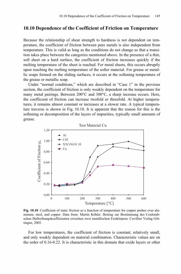
10.10 Dependence of the Coefficient of Friction on Temperature 145
10.10 Dependence of the Coefficient of Friction on Temperature
Because the relationship of shear strength to hardness is not dependent on tem-perature, the coefficient of friction between pure metals is also independent from temperature. This is valid as long as the conditions do not change so that a transi-tion takes place between the categories mentioned above. In the presence of a thin, soft sheet on a hard surface, the coefficient of friction increases quickly if the melting temperature of the sheet is reached. For metal sheets, this occurs abruptly upon reaching the melting temperature of the softer material. For grease or metal-lic soaps formed on the sliding surfaces, it occurs at the softening temperature of the grease or metallic soap.
Under “normal conditions,” which are described in “Case 1” in the previous section, the coefficient of friction is only weakly dependent on the temperature for many metal pairings. Between 200°C and 300°C, a sharp increase occurs. Here, the coefficient of friction can increase twofold or threefold. At higher tempera-tures, it remains almost constant or increases at a slower rate. A typical tempera-ture traverse is shown in Fig. 10.10. It is apparent that the reason for this is the softening or decomposition of the layers of impurities, typically small amounts of grease.
0 100 200 300 400 500 600
1,20
1,00
0,80
0,60
0,40
0,20
0,00
Test Material Cu
Co
effi
cien
to
fF
rict
ion
�0
Temperature [°C]
+
+
+
+
++
+
Al
C45
X5CrNi18 10
Cu
+
Fig. 10.10 Coefficient of static friction as a function of temperature for copper probes over alu-minum, steel, and copper. Data from: Martin Köhler. Beitrag zur Bestimmung des Coulomb-schen Haftreibungskoeffizienten zwischen zwei metallischen Festkörpern. Cuvillier Verlag Göt-tingen, 2005.
For low temperatures, the coefficient of friction is constant, relatively small, and only weakly dependent on material combination. Characteristic values are on the order of 0.16-0.22. It is characteristic in this domain that oxide layers or other
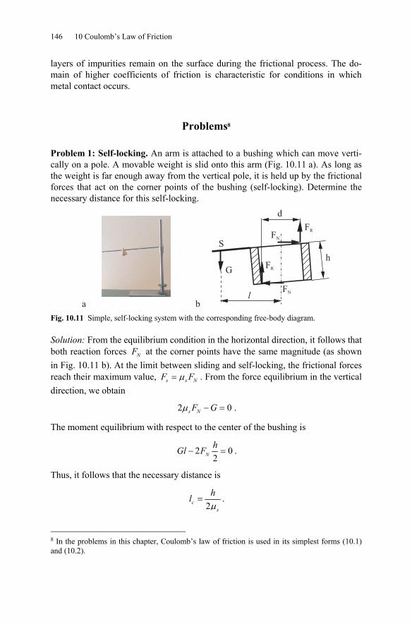
146 10 Coulomb’s Law of Friction
layers of impurities remain on the surface during the frictional process. The do-main of higher coefficients of friction is characteristic for conditions in which metal contact occurs.
Problems8
Problem 1: Self-locking. An arm is attached to a bushing which can move verti-cally on a pole. A movable weight is slid onto this arm (Fig. 10.11 a). As long as the weight is far enough away from the vertical pole, it is held up by the frictional forces that act on the corner points of the bushing (self-locking). Determine the necessary distance for this self-locking.
S
d
G
h
lFN
FR
FN
FR
a b Fig. 10.11 Simple, self-locking system with the corresponding free-body diagram.
Solution: From the equilibrium condition in the horizontal direction, it follows that both reaction forces NF at the corner points have the same magnitude (as shown in Fig. 10.11 b). At the limit between sliding and self-locking, the frictional forces reach their maximum value, μ=s s NF F . From the force equilibrium in the vertical direction, we obtain
2 0s NF Gμ − = .
The moment equilibrium with respect to the center of the bushing is
2 02
− =NhGl F .
Thus, it follows that the necessary distance is
2μ=c
s
hl .
8 In the problems in this chapter, Coulomb’s law of friction is used in its simplest forms (10.1) and (10.2).
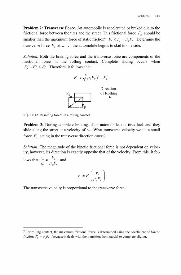
Problems 147
Problem 2: Transverse Force. An automobile is accelerated or braked due to the frictional force between the tires and the street. This frictional force RF should be smaller than the maximum force of static friction9: μ< =R s k NF F F . Determine the transverse force ⊥F at which the automobile begins to skid to one side. Solution: Both the braking force and the transverse force are components of the frictional force in the rolling contact. Complete sliding occurs when
2 2 2⊥+ >R sF F F . Therefore, it follows that
( )2 2μ⊥ > −k N RF F F .
Fig. 10.12 Resulting forces in a rolling contact.
Problem 3: During complete braking of an automobile, the tires lock and they slide along the street at a velocity of 0v . What transverse velocity would a small force ⊥F acting in the transverse direction cause?
Solution: The magnitude of the kinetic frictional force is not dependent on veloc-ity, however, its direction is exactly opposite that of the velocity. From this, it fol-
lows that 0 μ⊥ ⊥≈
k N
v Fv F
and
0
μ⊥ ⊥
⎛ ⎞≈ ⎜ ⎟
⎝ ⎠k N
vv F
F.
The transverse velocity is proportional to the transverse force.
9 For rolling contact, the maximum frictional force is determined using the coefficient of kinetic friction μ=S k NF F , because it deals with the transition from partial to complete sliding.
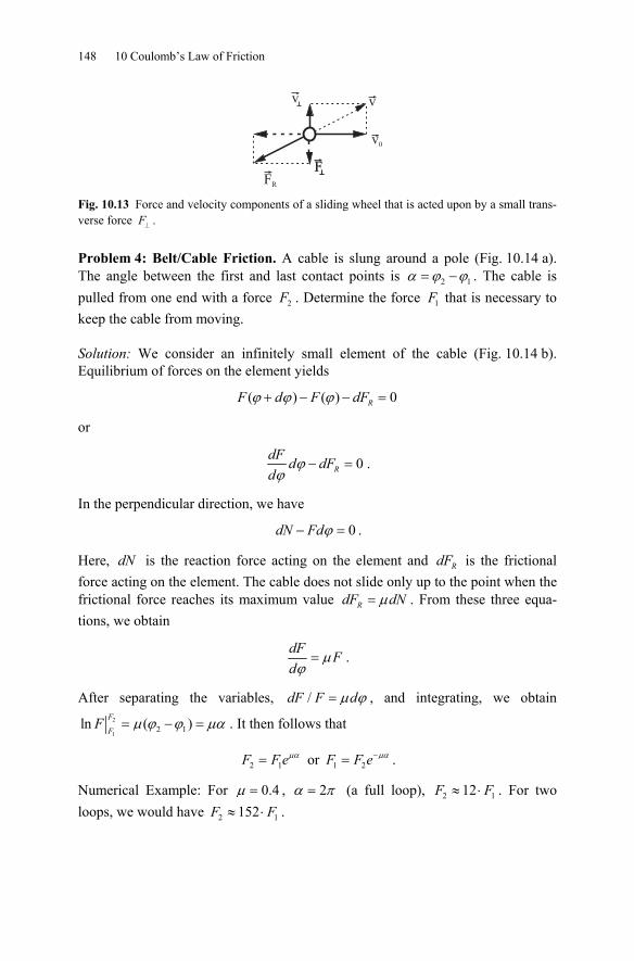
148 10 Coulomb’s Law of Friction
FFR
F
v v
v0
Fig. 10.13 Force and velocity components of a sliding wheel that is acted upon by a small trans-verse force ⊥F .
Problem 4: Belt/Cable Friction. A cable is slung around a pole (Fig. 10.14 a). The angle between the first and last contact points is 2 1α ϕ ϕ= − . The cable is pulled from one end with a force 2F . Determine the force 1F that is necessary to keep the cable from moving.
Solution: We consider an infinitely small element of the cable (Fig. 10.14 b). Equilibrium of forces on the element yields
( ) ( ) 0ϕ ϕ ϕ+ − − =RF d F dF
or
0ϕϕ
− =RdF d dFd
.
In the perpendicular direction, we have
0ϕ− =dN Fd .
Here, dN is the reaction force acting on the element and RdF is the frictional force acting on the element. The cable does not slide only up to the point when the frictional force reaches its maximum value μ=RdF dN . From these three equa-tions, we obtain
μϕ=
dF Fd
.
After separating the variables, / μ ϕ=dF F d , and integrating, we obtain 2
12 1ln ( )μ ϕ ϕ μα= − =F
FF . It then follows that
2 1μα=F F e or 1 2
μα−=F F e .
Numerical Example: For 0.4μ = , 2α π= (a full loop), 2 112≈ ⋅F F . For two loops, we would have 2 1152≈ ⋅F F .
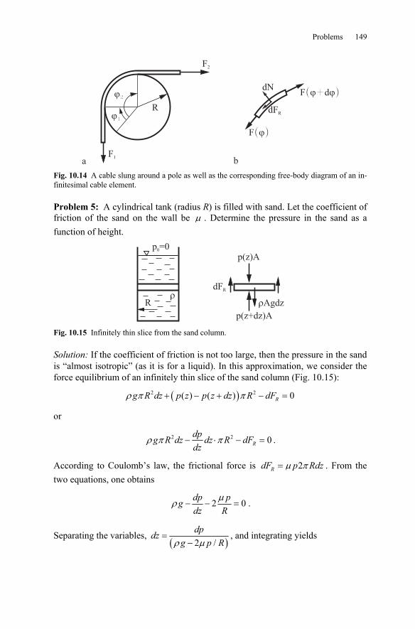
Problems 149
F2
F1
R�1
�2
dFR
F( )�
F d( + )� �dN
a b Fig. 10.14 A cable slung around a pole as well as the corresponding free-body diagram of an in-finitesimal cable element.
Problem 5: A cylindrical tank (radius R) is filled with sand. Let the coefficient of friction of the sand on the wall be μ . Determine the pressure in the sand as a function of height.
R�
p =00
�Agdz
p(z+dz)A
p(z)A
dFR
Fig. 10.15 Infinitely thin slice from the sand column.
Solution: If the coefficient of friction is not too large, then the pressure in the sand is “almost isotropic” (as it is for a liquid). In this approximation, we consider the force equilibrium of an infinitely thin slice of the sand column (Fig. 10.15):
( )2 2( ) ( ) 0ρ π π+ − + − =Rg R dz p z p z dz R dF
or
2 2 0ρ π π− ⋅ − =Rdpg R dz dz R dFdz
.
According to Coulomb’s law, the frictional force is 2μ π=RdF p Rdz . From the two equations, one obtains
2 0μρ − − =dp pgdz R
.
Separating the variables, ( )2 /ρ μ
=−
dpdzg p R
, and integrating yields
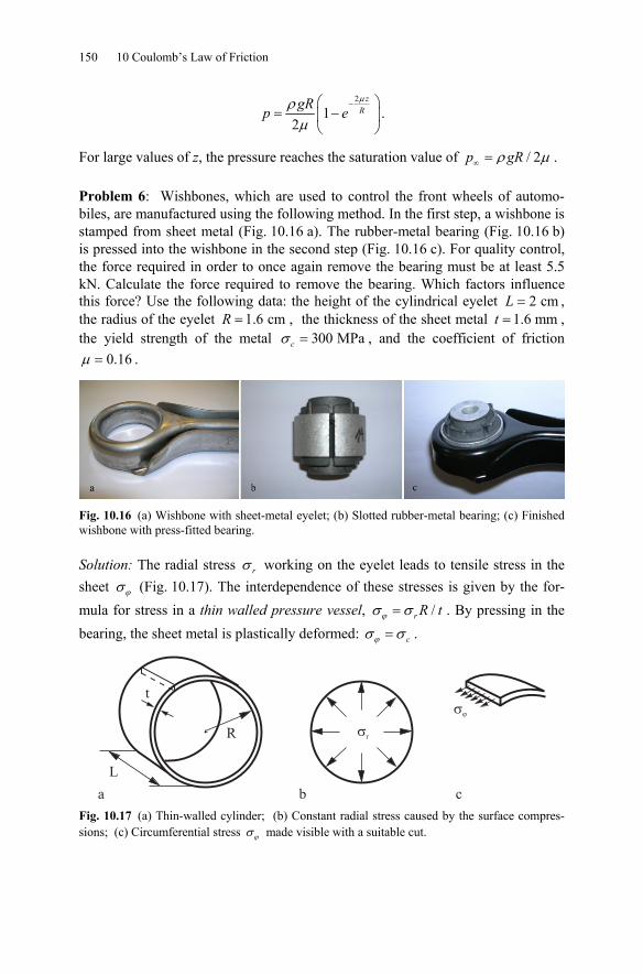
150 10 Coulomb’s Law of Friction
2
12
μρμ
−⎛ ⎞= −⎜ ⎟
⎝ ⎠
zRgRp e .
For large values of z, the pressure reaches the saturation value of / 2ρ μ∞ =p gR .
Problem 6: Wishbones, which are used to control the front wheels of automo-biles, are manufactured using the following method. In the first step, a wishbone is stamped from sheet metal (Fig. 10.16 a). The rubber-metal bearing (Fig. 10.16 b) is pressed into the wishbone in the second step (Fig. 10.16 c). For quality control, the force required in order to once again remove the bearing must be at least 5.5 kN. Calculate the force required to remove the bearing. Which factors influence this force? Use the following data: the height of the cylindrical eyelet 2 cm=L , the radius of the eyelet 1.6 cmR = , the thickness of the sheet metal 1.6 mmt = , the yield strength of the metal 300 MPaσ =c , and the coefficient of friction
0.16μ = .
Fig. 10.16 (a) Wishbone with sheet-metal eyelet; (b) Slotted rubber-metal bearing; (c) Finished wishbone with press-fitted bearing.
Solution: The radial stress σ r working on the eyelet leads to tensile stress in the sheet ϕσ (Fig. 10.17). The interdependence of these stresses is given by the for-mula for stress in a thin walled pressure vessel, /ϕσ σ= r R t . By pressing in the bearing, the sheet metal is plastically deformed: ϕσ σ= c .
R
t
L
�r
��
a b c Fig. 10.17 (a) Thin-walled cylinder; (b) Constant radial stress caused by the surface compres-sions; (c) Circumferential stress ϕσ made visible with a suitable cut.
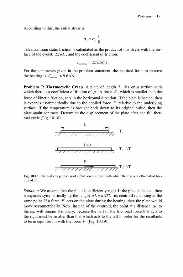
Problems 151
According to this, the radial stress is
σ σ=r ctR
.
The maximum static friction is calculated as the product of this stress with the sur-face of the eyelet, 2πRL , and the coefficient of friction:
2removal cF L tπ μσ= .
For the parameters given in the problem statement, the required force to remove the bearing is 9.6 kNremovalF ≈ . Problem 7: Thermocyclic Creep. A plate of length L lies on a surface with which there is a coefficient of friction of μ . A force F , which is smaller than the force of kinetic friction, acts in the horizontal direction. If the plate is heated, then it expands asymmetrically due to the applied force F relative to the underlying surface. If the temperature is brought back down to its original value, then the plate again contracts. Determine the displacement of the plate after one full ther-mal cycle (Fig. 10.18).
T0
T + T0 D
T + T0 D
F=0
F
L
Fig. 10.18 Thermal creep process of a plate on a surface with which there is a coefficient of fric-tion of μ .
Solution: We assume that the plate is sufficiently rigid. If the plate is heated, then it expands symmetrically by the length αΔ = ΔL TL , its centroid remaining at the same point. If a force F acts on the plate during the heating, then the plate would move asymmetrically. Now, instead of the centroid, the point at a distance Δl to the left will remain stationary, because the part of the frictional force that acts to the right must be smaller than that which acts to the left in order for the resultants to be in equilibrium with the force F (Fig. 10.19).
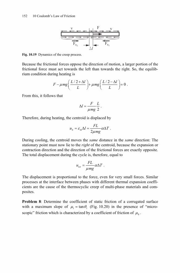
152 10 Coulomb’s Law of Friction
F
Dl
vv
FR2FR1
{ {
Fig. 10.19 Dynamics of the creep process.
Because the frictional forces oppose the direction of motion, a larger portion of the frictional force must act towards the left than towards the right. So, the equilib-rium condition during heating is
/ 2 / 2 0μ μ+ Δ −Δ⎛ ⎞ ⎛ ⎞− + =⎜ ⎟ ⎜ ⎟⎝ ⎠ ⎝ ⎠
L l L lF mg mgL L
.
From this, it follows that
2μΔ =
F Llmg
.
Therefore, during heating, the centroid is displaced by
2ε α
μ= Δ = ΔS th
FLu l Tmg
.
During cooling, the centroid moves the same distance in the same direction: The stationary point must now lie to the right of the centroid, because the expansion or contraction direction and the direction of the frictional forces are exactly opposite. The total displacement during the cycle is, therefore, equal to
totFLu Tmg
αμ
= Δ .
The displacement is proportional to the force, even for very small forces. Similar processes at the interface between phases with different thermal expansion coeffi-cients are the cause of the thermocyclic creep of multi-phase materials and com-posites.
Problem 8: Determine the coefficient of static friction of a corrugated surface with a maximum slope of 1 1tanμ θ= (Fig. 10.20) in the presence of “micro-scopic” friction which is characterized by a coefficient of friction of 0μ .
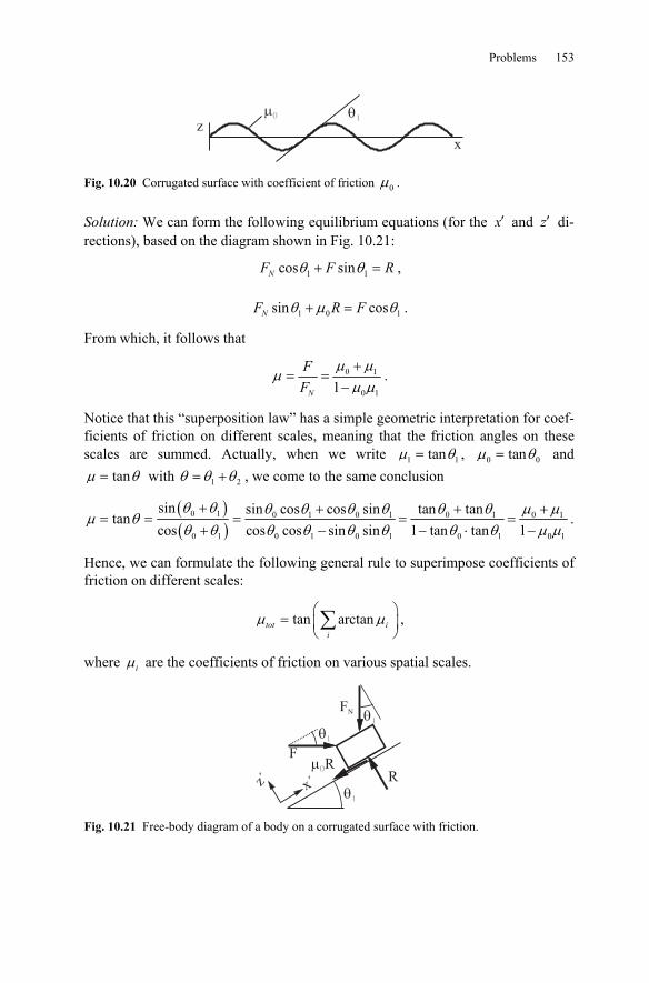
Problems 153
�0 �
1
z
x
Fig. 10.20 Corrugated surface with coefficient of friction 0μ .
Solution: We can form the following equilibrium equations (for the ′x and ′z di-rections), based on the diagram shown in Fig. 10.21:
1 1cos sinθ θ+ =NF F R ,
1 0 1sin cosθ μ θ+ =NF R F .
From which, it follows that
0 1
0 11μ μ
μμ μ+
= =−N
FF
.
Notice that this “superposition law” has a simple geometric interpretation for coef-ficients of friction on different scales, meaning that the friction angles on these scales are summed. Actually, when we write 1 1tanμ θ= , 0 0tanμ θ= and
tanμ θ= with 1 2θ θ θ= + , we come to the same conclusion
( )( )
0 1 0 1 0 1 0 1 0 1
0 1 0 1 0 1 0 1 0 1
sin sin cos cos sin tan tantan
cos cos cos sin sin 1 tan tan 1θ θ θ θ θ θ θ θ μ μ
μ θθ θ θ θ θ θ θ θ μ μ+ + + +
= = = = =+ − − ⋅ −
.
Hence, we can formulate the following general rule to superimpose coefficients of friction on different scales:
tan arctantot ii
μ μ⎛ ⎞= ⎜ ⎟⎝ ⎠∑ ,
where μi are the coefficients of friction on various spatial scales.
z´ x´
FN
�1
�1
�0R
R
F
�1
Fig. 10.21 Free-body diagram of a body on a corrugated surface with friction.
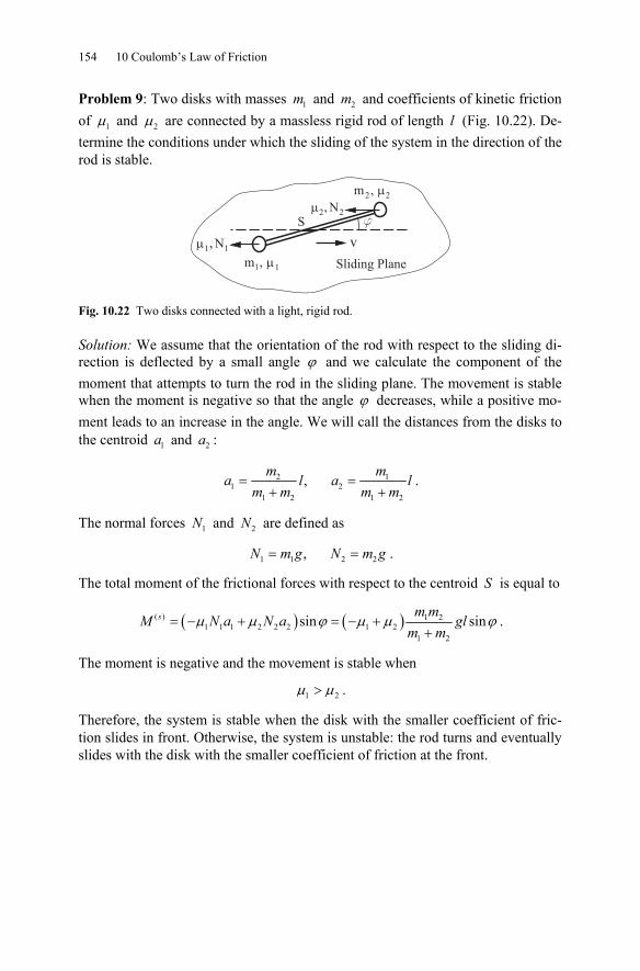
154 10 Coulomb’s Law of Friction
Problem 9: Two disks with masses 1m and 2m and coefficients of kinetic friction of 1μ and 2μ are connected by a massless rigid rod of length l (Fig. 10.22). De-termine the conditions under which the sliding of the system in the direction of the rod is stable.
Sliding Plane
m2, �2
m1, �1
S
�1, N1
�2, N2f
v
Fig. 10.22 Two disks connected with a light, rigid rod.
Solution: We assume that the orientation of the rod with respect to the sliding di-rection is deflected by a small angle ϕ and we calculate the component of the moment that attempts to turn the rod in the sliding plane. The movement is stable when the moment is negative so that the angle ϕ decreases, while a positive mo-ment leads to an increase in the angle. We will call the distances from the disks to the centroid 1a and 2a :
2 11 2
1 2 1 2
, m m
a l a lm m m m
= =+ +
.
The normal forces 1N and 2N are defined as
1 1 2 2, N m g N m g= = .
The total moment of the frictional forces with respect to the centroid S is equal to
( ) ( )( ) 1 21 1 1 2 2 2 1 2
1 2
sin sins m mM N a N a gl
m mμ μ ϕ μ μ ϕ= − + = − +
+.
The moment is negative and the movement is stable when
1 2μ μ> .
Therefore, the system is stable when the disk with the smaller coefficient of fric-tion slides in front. Otherwise, the system is unstable: the rod turns and eventually slides with the disk with the smaller coefficient of friction at the front.
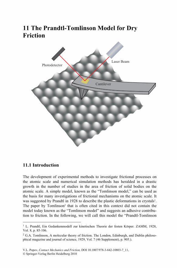
11 The Prandtl-Tomlinson Model for Dry Friction
Cantilever
PhotodetectorLaser Beam
11.1 Introduction
The development of experimental methods to investigate frictional processes on the atomic scale and numerical simulation methods has heralded in a drastic growth in the number of studies in the area of friction of solid bodies on the atomic scale. A simple model, known as the “Tomlinson model,” can be used as the basis for many investigations of frictional mechanisms on the atomic scale. It was suggested by Prandtl in 1928 to describe the plastic deformations in crystals1. The paper by Tomlinson2 that is often cited in this context did not contain the model today known as the “Tomlinson model” and suggests an adhesive contribu-tion to friction. In the following, we will call this model the “Prandtl-Tomlinson 1 L. Prandtl, Ein Gedankenmodell zur kinetischen Theorie der festen Körper. ZAMM, 1928, Vol. 8, p. 85-106. 2 G.A. Tomlinson, A molecular theory of friction. The London, Edinburgh, and Dublin philoso-phical magazine and journal of science, 1929, Vol. 7 (46 Supplement), p. 905.).
V.L. Popov, Contact Mechanics and Friction, DOI 10.1007/978-3-642-10803-7_11, © Springer-Verlag Berlin Heidelberg 2010
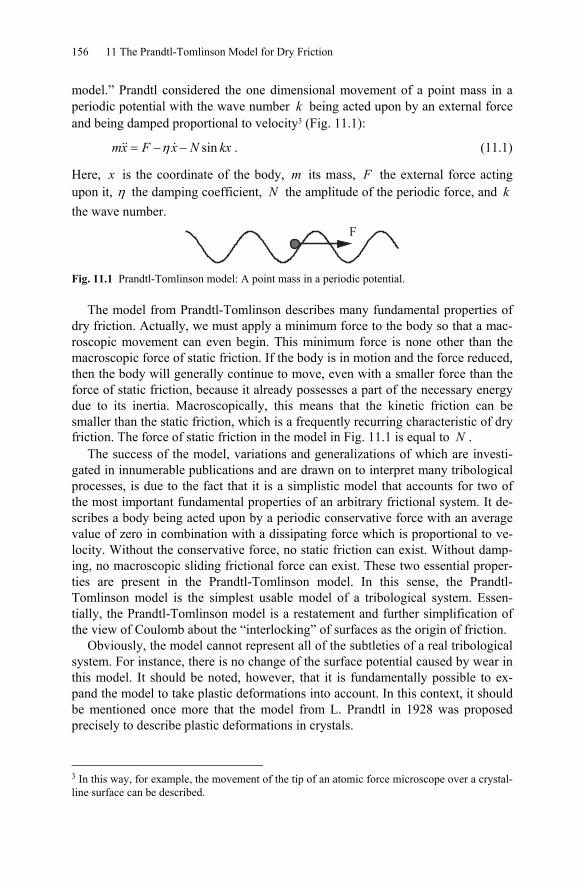
156 11 The Prandtl-Tomlinson Model for Dry Friction
model.” Prandtl considered the one dimensional movement of a point mass in a periodic potential with the wave number k being acted upon by an external force and being damped proportional to velocity3 (Fig. 11.1):
sinη= − −mx F x N kx . (11.1)
Here, x is the coordinate of the body, m its mass, F the external force acting upon it, η the damping coefficient, N the amplitude of the periodic force, and k the wave number.
F
Fig. 11.1 Prandtl-Tomlinson model: A point mass in a periodic potential.
The model from Prandtl-Tomlinson describes many fundamental properties of dry friction. Actually, we must apply a minimum force to the body so that a mac-roscopic movement can even begin. This minimum force is none other than the macroscopic force of static friction. If the body is in motion and the force reduced, then the body will generally continue to move, even with a smaller force than the force of static friction, because it already possesses a part of the necessary energy due to its inertia. Macroscopically, this means that the kinetic friction can be smaller than the static friction, which is a frequently recurring characteristic of dry friction. The force of static friction in the model in Fig. 11.1 is equal to N .
The success of the model, variations and generalizations of which are investi-gated in innumerable publications and are drawn on to interpret many tribological processes, is due to the fact that it is a simplistic model that accounts for two of the most important fundamental properties of an arbitrary frictional system. It de-scribes a body being acted upon by a periodic conservative force with an average value of zero in combination with a dissipating force which is proportional to ve-locity. Without the conservative force, no static friction can exist. Without damp-ing, no macroscopic sliding frictional force can exist. These two essential proper-ties are present in the Prandtl-Tomlinson model. In this sense, the Prandtl-Tomlinson model is the simplest usable model of a tribological system. Essen-tially, the Prandtl-Tomlinson model is a restatement and further simplification of the view of Coulomb about the “interlocking” of surfaces as the origin of friction.
Obviously, the model cannot represent all of the subtleties of a real tribological system. For instance, there is no change of the surface potential caused by wear in this model. It should be noted, however, that it is fundamentally possible to ex-pand the model to take plastic deformations into account. In this context, it should be mentioned once more that the model from L. Prandtl in 1928 was proposed precisely to describe plastic deformations in crystals.
3 In this way, for example, the movement of the tip of an atomic force microscope over a crystal-line surface can be described.
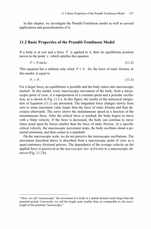
11.2 Basic Properties of the Prandtl-Tomlinson Model 157
In this chapter, we investigate the Prandtl-Tomlinson model as well as several applications and generalizations of it.
11.2 Basic Properties of the Prandtl-Tomlinson Model
If a body is at rest and a force F is applied to it, then its equilibrium position moves to the point x , which satisfies the equation
sin=F N kx . (11.2)
This equation has a solution only when F N≤ . So, the force of static friction, in this model, is equal to
=sF N . (11.3)
For a larger force, no equilibrium is possible and the body enters into macroscopic motion4. In this model, every macroscopic movement of the body, from a micro-scopic point of view, is a superposition of a constant speed and a periodic oscilla-tion, as is shown in Fig. 11.2 a. In this figure, the results of the numerical integra-tion of Equation (11.1) are presented. The tangential force changes slowly from zero to some maximum value larger than the force of static friction and then de-creases afterwards. The curve shows the instantaneous speed as a function of the instantaneous force. After the critical force is reached, the body begins to move with a finite velocity. If the force is decreased, the body can continue to move when acted upon by forces smaller than the force of static friction. At a specific critical velocity, the macroscopic movement stops, the body oscillates about a po-tential minimum, and then comes to a standstill.
On the macroscopic scale, we do not perceive the microscopic oscillations. The movement described above is described from a macroscopic point of view as a quasi-stationary frictional process. The dependence of the average velocity on the applied force is perceived as the macroscopic law of friction to a macroscopic ob-server (Fig. 11.2 b).
4 Here, we call “macroscopic” the movement of a body in a spatial domain much larger than the potential period. Conversely, we call the length scale smaller than, or comparable to, the wave-length of the potential “microscopic.”
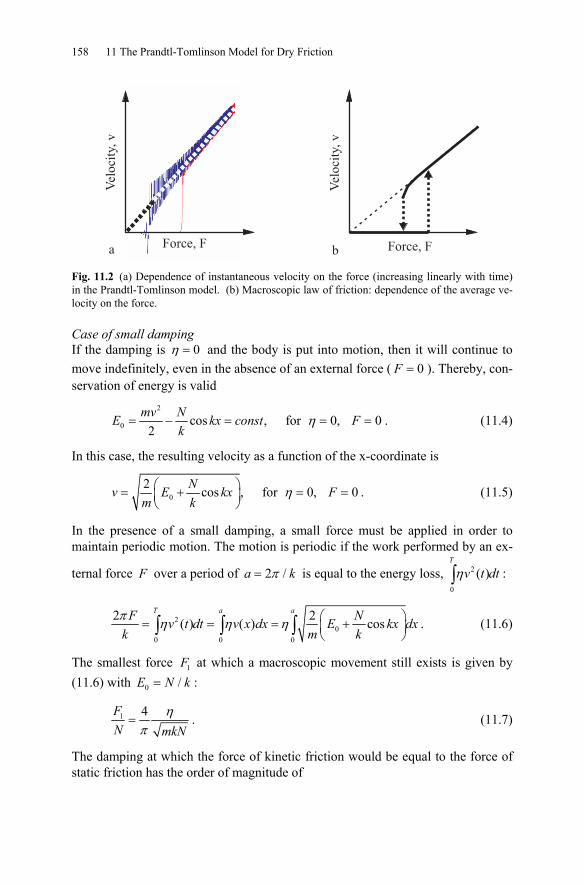
158 11 The Prandtl-Tomlinson Model for Dry Friction
Force, F
Vel
oci
ty,v
Vel
oci
ty,v
a bForce, F
Fig. 11.2 (a) Dependence of instantaneous velocity on the force (increasing linearly with time) in the Prandtl-Tomlinson model. (b) Macroscopic law of friction: dependence of the average ve-locity on the force.
Case of small damping If the damping is 0η = and the body is put into motion, then it will continue to move indefinitely, even in the absence of an external force ( 0=F ). Thereby, con-servation of energy is valid
2
0 cos , for 0, 02
mv NE kx const Fk
η= − = = = . (11.4)
In this case, the resulting velocity as a function of the x-coordinate is
02 cos , for 0, 0Nv E kx Fm k
η⎛ ⎞= + = =⎜ ⎟⎝ ⎠
. (11.5)
In the presence of a small damping, a small force must be applied in order to maintain periodic motion. The motion is periodic if the work performed by an ex-
ternal force F over a period of 2 /π=a k is equal to the energy loss, 2
0
( )η∫T
v t dt :
20
0 0 0
2 2( ) ( ) cosπ η η η ⎛ ⎞= = = +⎜ ⎟⎝ ⎠∫ ∫ ∫
T a aF Nv t dt v x dx E kx dxk m k
. (11.6)
The smallest force 1F at which a macroscopic movement still exists is given by (11.6) with 0 /=E N k :
1 4 ηπ
=FN mkN
. (11.7)
The damping at which the force of kinetic friction would be equal to the force of static friction has the order of magnitude of
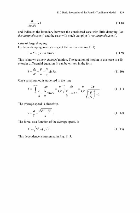
11.2 Basic Properties of the Prandtl-Tomlinson Model 159
1η≈
mkN (11.8)
and indicates the boundary between the considered case with little damping (un-der-damped system) and the case with much damping (over-damped system). Case of large damping For large damping, one can neglect the inertia term in (11.1):
0 sinη= − −F x N kx . (11.9)
This is known as over-damped motion. The equation of motion in this case is a fir-st-order differential equation. It can be written in the form
sinη η
= = −dx F Nx kxdt
. (11.10)
One spatial period is traversed in the time
2 / 2
20 0
2
sin sin 1
π πη η π
η η
= = =⎛ ⎞− − −⎜ ⎟⎝ ⎠
∫ ∫k dx dzT
F N FkN kN Fkx zN N
. (11.11)
The average speed is, therefore,
2 2
η−
= =a F NvT
. (11.12)
The force, as a function of the average speed, is
( )22 η= +F N v . (11.13)
This dependence is presented in Fig. 11.3.
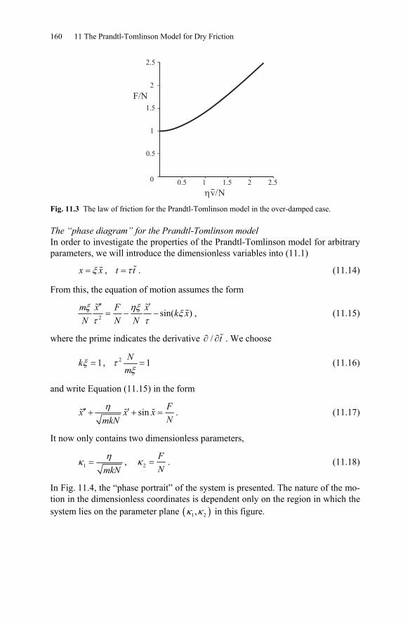
160 11 The Prandtl-Tomlinson Model for Dry Friction
0.5
1.5
1
0 0.5
2
2.5
1 1.5 2 2.5
F/N
�v/N Fig. 11.3 The law of friction for the Prandtl-Tomlinson model in the over-damped case.
The “phase diagram” for the Prandtl-Tomlinson model In order to investigate the properties of the Prandtl-Tomlinson model for arbitrary parameters, we will introduce the dimensionless variables into (11.1)
ξ=x x , τ=t t . (11.14)
From this, the equation of motion assumes the form
2 sin( )ξ ηξ ξττ
′′ ′= − −
m x F x k xN N N
, (11.15)
where the prime indicates the derivative /∂ ∂t . We choose
1ξ =k , 2 1τξ=
Nm
(11.16)
and write Equation (11.15) in the form
sinη′′ ′+ + =Fx x xNmkN
. (11.17)
It now only contains two dimensionless parameters,
1ηκ =
mkN, 2κ =
FN
. (11.18)
In Fig. 11.4, the “phase portrait” of the system is presented. The nature of the mo-tion in the dimensionless coordinates is dependent only on the region in which the system lies on the parameter plane ( )1 2,κ κ in this figure.
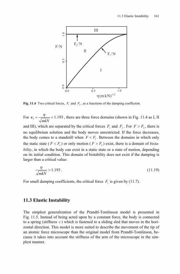
11.3 Elastic Instability 161
0.0 0.5 1.0
00
F/N
05
10
I
II
III
F /N2
F /N1
� (m kN)-1/2
Fig. 11.4 Two critical forces, 1F and 2F , as a functions of the damping coefficient.
For 1 1.193mkNηκ = < , there are three force domains (shown in Fig. 11.4 as I, II
and III), which are separated by the critical forces 1F and 2F . For 2>F F , there is no equilibrium solution and the body moves unrestricted. If the force decreases, the body comes to a standstill when 1<F F . Between the domains in which only the static state ( 1<F F ) or only motion ( 2>F F ) exist, there is a domain of bista-bility, in which the body can exist in a static state or a state of motion, depending on its initial condition. This domain of bistability does not exist if the damping is larger than a critical value:
1.193mkNη
> . (11.19)
For small damping coefficients, the critical force 1F is given by (11.7).
11.3 Elastic Instability
The simplest generalization of the Prandtl-Tomlinson model is presented in Fig. 11.5. Instead of being acted upon by a constant force, the body is connected to a spring (stiffness c ) which is fastened to a sliding sled that moves in the hori-zontal direction. This model is more suited to describe the movement of the tip of an atomic force microscope than the original model from Prandtl-Tomlinson, be-cause it takes into account the stiffness of the arm of the microscope in the sim-plest manner.
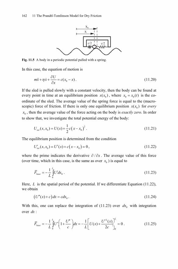
162 11 The Prandtl-Tomlinson Model for Dry Friction
x0
x
c/2 c/2
Fig. 11.5 A body in a periodic potential pulled with a spring.
In this case, the equation of motion is
0( )η ∂+ + = −
∂Umx x c x xx
. (11.20)
If the sled is pulled slowly with a constant velocity, then the body can be found at every point in time at an equilibrium position 0( )x x , where 0 0 ( )=x x t is the co-ordinate of the sled. The average value of the spring force is equal to the (macro-scopic) force of friction. If there is only one equilibrium position 0( )x x for every
0x , then the average value of the force acting on the body is exactly zero. In order to show that, we investigate the total potential energy of the body:
( )20 0
1( , ) ( )2totU x x U x c x x= + − . (11.21)
The equilibrium position is determined from the condition
( )0 0( , ) ( ) 0totU x x U x c x x′ ′= + − = , (11.22)
where the prime indicates the derivative /∂ ∂x . The average value of this force (over time, which in this case, is the same as over 0x ) is equal to
00
1 L
baseF U dxL
′= − ∫ . (11.23)
Here, L is the spatial period of the potential. If we differentiate Equation (11.22), we obtain
( ) 0( )′′ + =U x c dx cdx . (11.24)
With this, one can replace the integration of (11.23) over 0dx with integration over dx :
2
0 0
1 1 ( )1 ( ) 02
LL
baseU U xF U dx U x
L c L c′′ ′⎡ ⎤⎛ ⎞′= − + = − + =⎢ ⎥⎜ ⎟
⎝ ⎠ ⎣ ⎦∫ . (11.25)
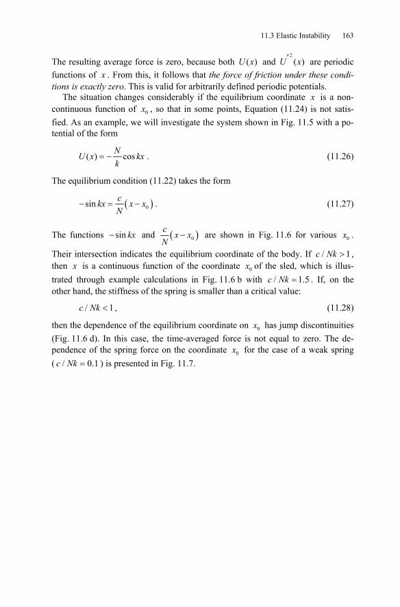
11.3 Elastic Instability 163
The resulting average force is zero, because both ( )U x and 2( )′U x are periodic
functions of x . From this, it follows that the force of friction under these condi-tions is exactly zero. This is valid for arbitrarily defined periodic potentials.
The situation changes considerably if the equilibrium coordinate x is a non-continuous function of 0x , so that in some points, Equation (11.24) is not satis-fied. As an example, we will investigate the system shown in Fig. 11.5 with a po-tential of the form
( ) cos= −NU x kxk
. (11.26)
The equilibrium condition (11.22) takes the form
( )0sin− = −ckx x xN
. (11.27)
The functions sin− kx and ( )0−c x xN
are shown in Fig. 11.6 for various 0x .
Their intersection indicates the equilibrium coordinate of the body. If / 1>c Nk , then x is a continuous function of the coordinate 0x of the sled, which is illus-trated through example calculations in Fig. 11.6 b with / 1.5c Nk = . If, on the other hand, the stiffness of the spring is smaller than a critical value:
/ 1<c Nk , (11.28)
then the dependence of the equilibrium coordinate on 0x has jump discontinuities (Fig. 11.6 d). In this case, the time-averaged force is not equal to zero. The de-pendence of the spring force on the coordinate 0x for the case of a weak spring ( / 0.1c Nk = ) is presented in Fig. 11.7.
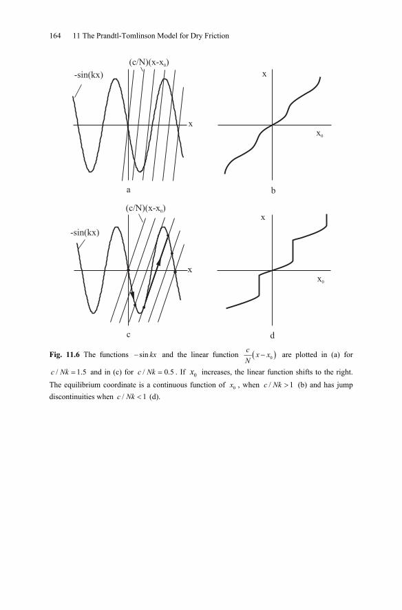
164 11 The Prandtl-Tomlinson Model for Dry Friction
-sin(kx)
(c/N)(x-x )0
x
(c/N)(x-x )0
-sin(kx)
x
x
x
x0
x0
a b
c d
Fig. 11.6 The functions sin− kx and the linear function ( )0c x xN
− are plotted in (a) for
/ 1.5c Nk = and in (c) for / 0.5c Nk = . If 0x increases, the linear function shifts to the right. The equilibrium coordinate is a continuous function of 0x , when / 1c Nk > (b) and has jump discontinuities when / 1c Nk < (d).
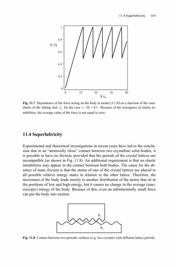
11.4 Superlubricity 165
F/ N
0
1
0.8
0.6
0.4
0.2
10 20 30 40
kx
0
0 Fig. 11.7 Dependence of the force acting on the body in model (11.20) as a function of the coor-dinate of the sliding sled 0x for the case / 0.1c Nk = . Because of the emergence of elastic in-stabilities, the average value of the force is not equal to zero.
11.4 Superlubricity
Experimental and theoretical investigations in recent years have led to the conclu-sion that in an “atomically close” contact between two crystalline solid bodies, it is possible to have no friction, provided that the periods of the crystal lattices are incompatible (as shown in Fig. 11.8). An additional requirement is that no elastic instabilities may appear in the contact between both bodies. The cause for the ab-sence of static friction is that the atoms of one of the crystal lattices are placed in all possible relative energy states in relation to the other lattice. Therefore, the movement of the body leads merely to another distribution of the atoms that sit in the positions of low and high energy, but it causes no change in the average (mac-roscopic) energy of the body. Because of this, even an infinitesimally small force can put the body into motion.
k1
k2
Fig. 11.8 Contact between two periodic surfaces (e.g. two crystals) with different lattice periods.
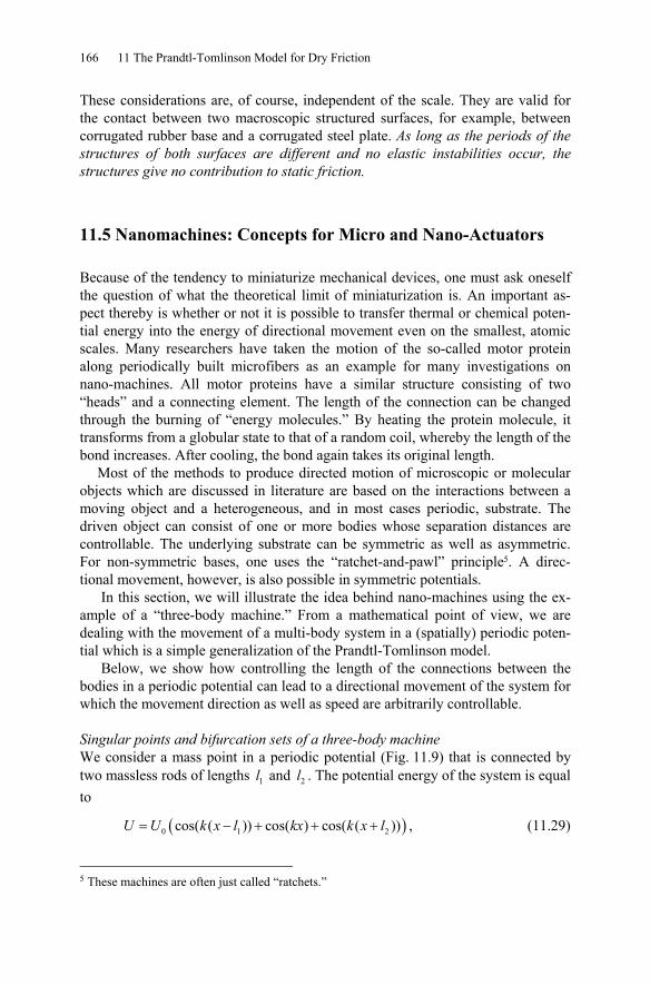
166 11 The Prandtl-Tomlinson Model for Dry Friction
These considerations are, of course, independent of the scale. They are valid for the contact between two macroscopic structured surfaces, for example, between corrugated rubber base and a corrugated steel plate. As long as the periods of the structures of both surfaces are different and no elastic instabilities occur, the structures give no contribution to static friction.
11.5 Nanomachines: Concepts for Micro and Nano-Actuators
Because of the tendency to miniaturize mechanical devices, one must ask oneself the question of what the theoretical limit of miniaturization is. An important as-pect thereby is whether or not it is possible to transfer thermal or chemical poten-tial energy into the energy of directional movement even on the smallest, atomic scales. Many researchers have taken the motion of the so-called motor protein along periodically built microfibers as an example for many investigations on nano-machines. All motor proteins have a similar structure consisting of two “heads” and a connecting element. The length of the connection can be changed through the burning of “energy molecules.” By heating the protein molecule, it transforms from a globular state to that of a random coil, whereby the length of the bond increases. After cooling, the bond again takes its original length.
Most of the methods to produce directed motion of microscopic or molecular objects which are discussed in literature are based on the interactions between a moving object and a heterogeneous, and in most cases periodic, substrate. The driven object can consist of one or more bodies whose separation distances are controllable. The underlying substrate can be symmetric as well as asymmetric. For non-symmetric bases, one uses the “ratchet-and-pawl” principle5. A direc-tional movement, however, is also possible in symmetric potentials.
In this section, we will illustrate the idea behind nano-machines using the ex-ample of a “three-body machine.” From a mathematical point of view, we are dealing with the movement of a multi-body system in a (spatially) periodic poten-tial which is a simple generalization of the Prandtl-Tomlinson model.
Below, we show how controlling the length of the connections between the bodies in a periodic potential can lead to a directional movement of the system for which the movement direction as well as speed are arbitrarily controllable. Singular points and bifurcation sets of a three-body machine We consider a mass point in a periodic potential (Fig. 11.9) that is connected by two massless rods of lengths 1l and 2l . The potential energy of the system is equal to
( )0 1 2cos( ( )) cos( ) cos( ( ))= − + + +U U k x l kx k x l , (11.29)
5 These machines are often just called “ratchets.”
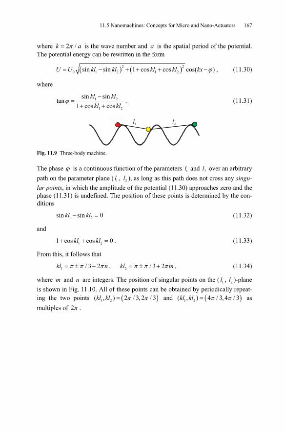
11.5 Nanomachines: Concepts for Micro and Nano-Actuators 167
where 2 /π=k a is the wave number and a is the spatial period of the potential. The potential energy can be rewritten in the form
( ) ( )2 20 1 2 1 2sin sin 1 cos cos cos( )ϕ= − + + + −U U kl kl kl kl kx , (11.30)
where
1 2
1 2
sin sintan
1 cos cosϕ
−=
+ +kl kl
kl kl. (11.31)
l1l2
Fig. 11.9 Three-body machine.
The phase ϕ is a continuous function of the parameters 1l and 2l over an arbitrary path on the parameter plane ( 1l , 2l ), as long as this path does not cross any singu-lar points, in which the amplitude of the potential (11.30) approaches zero and the phase (11.31) is undefined. The position of these points is determined by the con-ditions
1 2sin sin 0− =kl kl (11.32)
and
1 21 cos cos 0+ + =kl kl . (11.33)
From this, it follows that
1 / 3 2π π π= ± +kl n , 2 / 3 2π π π= ± +kl m , (11.34)
where m and n are integers. The position of singular points on the ( 1l , 2l )-plane is shown in Fig. 11.10. All of these points can be obtained by periodically repeat-ing the two points ( )1 2( , ) 2 / 3, 2 / 3π π=kl kl and ( )1 2( , ) 4 / 3, 4 / 3π π=kl kl as multiples of 2π .
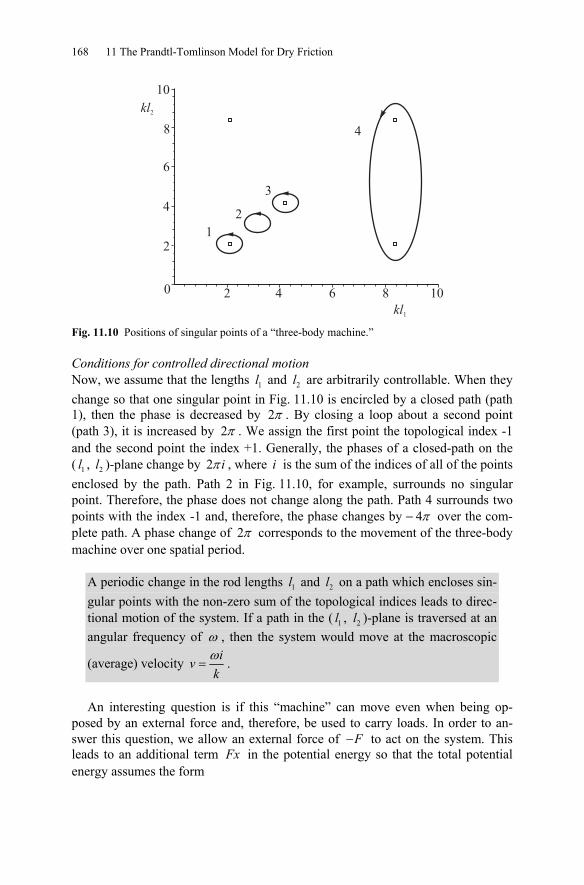
168 11 The Prandtl-Tomlinson Model for Dry Friction
10
8
6
kl2
4
2
0 2 4 6 8 10
kl1
1
2
3
4
Fig. 11.10 Positions of singular points of a “three-body machine.”
Conditions for controlled directional motion Now, we assume that the lengths 1l and 2l are arbitrarily controllable. When they change so that one singular point in Fig. 11.10 is encircled by a closed path (path 1), then the phase is decreased by 2π . By closing a loop about a second point (path 3), it is increased by 2π . We assign the first point the topological index -1 and the second point the index +1. Generally, the phases of a closed-path on the ( 1l , 2l )-plane change by 2π i , where i is the sum of the indices of all of the points enclosed by the path. Path 2 in Fig. 11.10, for example, surrounds no singular point. Therefore, the phase does not change along the path. Path 4 surrounds two points with the index -1 and, therefore, the phase changes by − 4π over the com-plete path. A phase change of 2π corresponds to the movement of the three-body machine over one spatial period.
A periodic change in the rod lengths 1l and 2l on a path which encloses sin-gular points with the non-zero sum of the topological indices leads to direc-tional motion of the system. If a path in the ( 1l , 2l )-plane is traversed at an angular frequency of ω , then the system would move at the macroscopic
(average) velocity ω=
ivk
.
An interesting question is if this “machine” can move even when being op-posed by an external force and, therefore, be used to carry loads. In order to an-swer this question, we allow an external force of −F to act on the system. This leads to an additional term Fx in the potential energy so that the total potential energy assumes the form
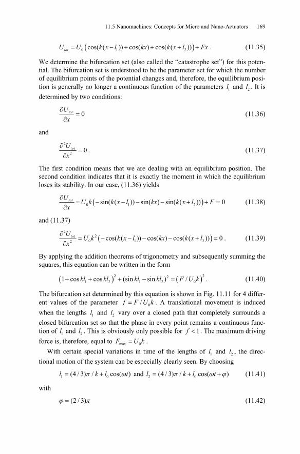
11.5 Nanomachines: Concepts for Micro and Nano-Actuators 169
( )0 1 2cos( ( )) cos( ) cos( ( ))totU U k x l kx k x l Fx= − + + + + . (11.35)
We determine the bifurcation set (also called the “catastrophe set”) for this poten-tial. The bifurcation set is understood to be the parameter set for which the number of equilibrium points of the potential changes and, therefore, the equilibrium posi-tion is generally no longer a continuous function of the parameters 1l and 2l . It is determined by two conditions:
0totUx
∂=
∂ (11.36)
and
2
2 0totUx
∂=
∂. (11.37)
The first condition means that we are dealing with an equilibrium position. The second condition indicates that it is exactly the moment in which the equilibrium loses its stability. In our case, (11.36) yields
( )0 1 2sin( ( )) sin( ) sin( ( )) 0totUU k k x l kx k x l F
x∂
= − − − − + + =∂
(11.38)
and (11.37)
( )2
20 1 22 cos( ( )) cos( ) cos( ( )) 0totU
U k k x l kx k x lx
∂= − − − − + =
∂. (11.39)
By applying the addition theorems of trigonometry and subsequently summing the squares, this equation can be written in the form
( ) ( )2 221 2 1 2 01 cos cos (sin sin ) /+ + + − =kl kl kl kl F U k . (11.40)
The bifurcation set determined by this equation is shown in Fig. 11.11 for 4 differ-ent values of the parameter 0/=f F U k . A translational movement is induced when the lengths 1l and 2l vary over a closed path that completely surrounds a closed bifurcation set so that the phase in every point remains a continuous func-tion of 1l and 2l . This is obviously only possible for 1<f . The maximum driving force is, therefore, equal to max 0=F U k .
With certain special variations in time of the lengths of 1l and 2l , the direc-tional motion of the system can be especially clearly seen. By choosing
1 0(4 / 3) / cos( )π ω= +l k l t and 2 0(4 / 3) / cos( )π ω ϕ= + +l k l t (11.41)
with
(2 / 3)ϕ π= (11.42)
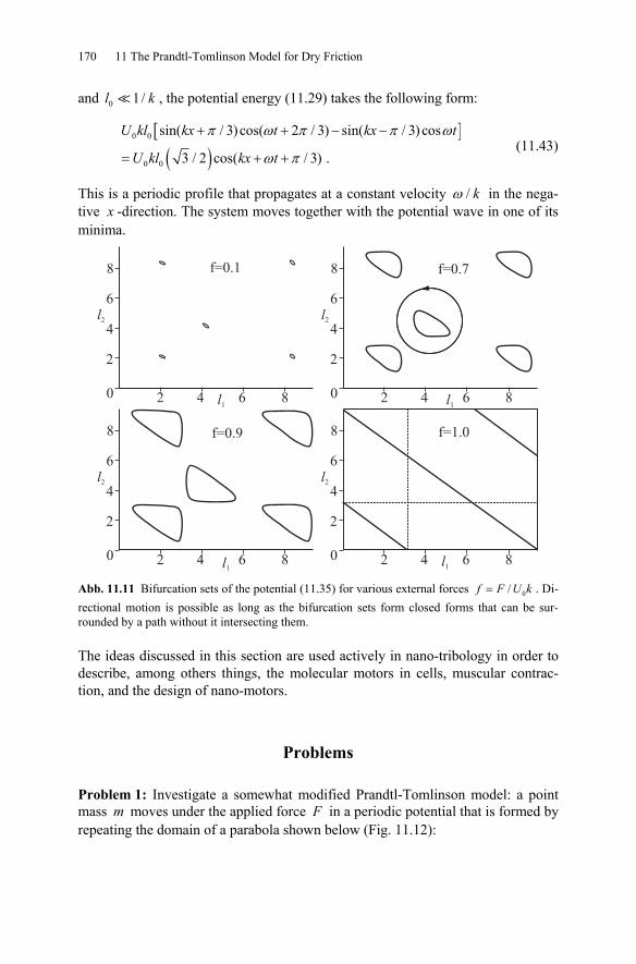
170 11 The Prandtl-Tomlinson Model for Dry Friction
and 0 1/l k , the potential energy (11.29) takes the following form:
[ ]( )
0 0
0 0
sin( / 3)cos( 2 / 3) sin( / 3)cos
3 / 2 cos( / 3) .
U kl kx t kx t
U kl kx t
π ω π π ω
ω π
+ + − −
= + + (11.43)
This is a periodic profile that propagates at a constant velocity /ω k in the nega-tive x -direction. The system moves together with the potential wave in one of its minima.
0
2
4
6
8
2 4 6 8
l2
l1
0
2
4
6
8
2 4 6 8
l2
l1
0
2
4
6
8
2 4 6 8
l2
l1
0
2
4
6
8
2 4 6 8
l2
l1
f=0.1 f=0.7
f=0.9 f=1.0
Abb. 11.11 Bifurcation sets of the potential (11.35) for various external forces 0/=f F U k . Di-rectional motion is possible as long as the bifurcation sets form closed forms that can be sur-rounded by a path without it intersecting them.
The ideas discussed in this section are used actively in nano-tribology in order to describe, among others things, the molecular motors in cells, muscular contrac-tion, and the design of nano-motors.
Problems
Problem 1: Investigate a somewhat modified Prandtl-Tomlinson model: a point mass m moves under the applied force F in a periodic potential that is formed by repeating the domain of a parabola shown below (Fig. 11.12):
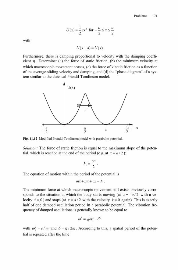
Problems 171
21( )2
=U x cx for 2 2
− ≤ ≤a ax
with
( ) ( )+ =U x a U x .
Furthermore, there is damping proportional to velocity with the damping coeffi-cient η . Determine: (a) the force of static friction, (b) the minimum velocity at which macroscopic movement ceases, (c) the force of kinetic friction as a function of the average sliding velocity and damping, and (d) the “phase diagram” of a sys-tem similar to the classical Prandtl-Tomlinson model.
F
x
U(x)
a2
a2
3a2
a
Fig. 11.12 Modified Prandtl-Tomlinson model with parabolic potential.
Solution: The force of static friction is equal to the maximum slope of the poten-tial, which is reached at the end of the period (e.g. at / 2=x a ):
2=s
caF .
The equation of motion within the period of the potential is
η+ + =mx x cx F .
The minimum force at which macroscopic movement still exists obviously corre-sponds to the situation at which the body starts moving (at / 2= −x a with a ve-locity 0=x ) and stops (at / 2=x a with the velocity 0=x again). This is exactly half of one damped oscillation period in a parabolic potential. The vibration fre-quency of damped oscillations is generally known to be equal to
* 2 20ω ω δ= −
with 20 /ω = c m and / 2δ η= m . According to this, a spatial period of the poten-
tial is repeated after the time
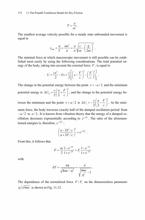
172 11 The Prandtl-Tomlinson Model for Dry Friction
*
πω
=T .
The smallest average velocity possible for a steady state unbounded movement is equal to
2*
min 2ω ηπ π
⎛ ⎞= = = − ⎜ ⎟⎝ ⎠
a a a cvT m m
.
The minimal force at which macroscopic movement is still possible can be estab-lished most easily by using the following considerations. The total potential en-ergy of the body, taking into account the external force F , is equal to
2 22
2 2⎡ ⎤⎛ ⎞ ⎛ ⎞= − = − −⎢ ⎥⎜ ⎟ ⎜ ⎟⎝ ⎠ ⎝ ⎠⎢ ⎥⎣ ⎦
cx c F FU Fx xc c
.
The change in the potential energy between the point / 2= −x a and the minimum
potential energy is 2
0 2 2⎛ ⎞Δ = +⎜ ⎟⎝ ⎠
c a FUc
, and the change in the potential energy be-
tween the minimum and the point / 2=x a is 2
1 2 2⎛ ⎞Δ = − −⎜ ⎟⎝ ⎠
c a FUc
. At the mini-
mum force, the body traverses exactly half of the damped oscillation period: from / 2−a to / 2a . It is known from vibration theory that the energy of a damped os-
cillation decreases exponentially according to 2δ− te . The ratio of the aforemen-tioned energies is, therefore, 2δ− Te :
222 /
2 /δ−−⎛ ⎞ =⎜ ⎟+⎝ ⎠
Ta F c ea F c
.
From this, it follows that
1 12 1 1
δ δ
δ δ
− −
− −
− −= =
+ +
T T
sT T
ac e eF Fe e
with
2
244 1
πη πδη
η
= =− −
Tmcmc
.
The dependence of the normalized force / sF F on the dimensionless parameter
4η mc is shown in Fig. 11.13.
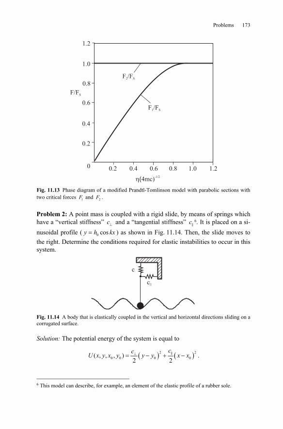
Problems 173
Fig. 11.13 Phase diagram of a modified Prandtl-Tomlinson model with parabolic sections with two critical forces 1F and 2F .
Problem 2: A point mass is coupled with a rigid slide, by means of springs which have a “vertical stiffness” ⊥c and a “tangential stiffness” c 6. It is placed on a si-nusoidal profile ( 0 cos=y h kx ) as shown in Fig. 11.14. Then, the slide moves to the right. Determine the conditions required for elastic instabilities to occur in this system.
c
c
||
|
Fig. 11.14 A body that is elastically coupled in the vertical and horizontal directions sliding on a corrugated surface.
Solution: The potential energy of the system is equal to
( ) ( )2 20 0 0 0( , , , )
2 2⊥= − + −
ccU x y x y y y x x .
6 This model can describe, for example, an element of the elastic profile of a rubber sole.
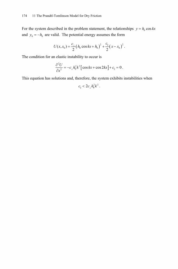
174 11 The Prandtl-Tomlinson Model for Dry Friction
For the system described in the problem statement, the relationships 0 cos=y h kx and 0 0= −y h are valid. The potential energy assumes the form
( ) ( )2 20 0 0 0( , ) cos
2 2⊥= + + −
ccU x x h kx h x x .
The condition for an elastic instability to occur is
[ ]2
2 202 cos cos 2 0⊥
∂= − + + =
∂U c h k kx kx cx
.
This equation has solutions and, therefore, the system exhibits instabilities when 2 202 ⊥<c c h k .

12 Frictionally Induced Vibrations
From a system dynamics point of view, technical systems with friction are non-linear dissipative open systems. Even if it is possible for a system to be in a state of steady motion, it can only practically take place if it is stable relative to small disturbances. Otherwise, the perturbations intensify, resulting in a periodic or cha-otic vibration. If the amplitude of the vibrations is large enough for the relative ve-locity of the surfaces in friction to be occasionally zero, then the movement con-sists of the alternating phases from rest (stick) to sliding (slip) and is called stick-slip-movement.
An instability in the uniform steady-state movement is not, however, the only mechanism for frictionally induced vibrations. Under certain conditions, it is pos-sible for the steady movement of a tribological system to be completely non-existent. In this case, only an oscillating movement is possible. An example is pre-sented by the so-called sprag-slip movement.
The frictional vibrations that occur in many technical frictional systems (brakes, bush bearings, wheel-rail contact, etc.) can on one side lead to higher wear and the formation of unwanted structures on the surface in friction (corruga-tions on rails, formation of cracks, polygonization of locomotive wheels, washboarding), and on the other side, can lead to subjective uncomfortable sounds or vibrations of a varying nature (chattering, howling, whistling, or squealing). Today, there are still no solutions in many fields for the squealing of brakes or of
V.L. Popov, Contact Mechanics and Friction, DOI 10.1007/978-3-642-10803-7_12, © Springer-Verlag Berlin Heidelberg 2010
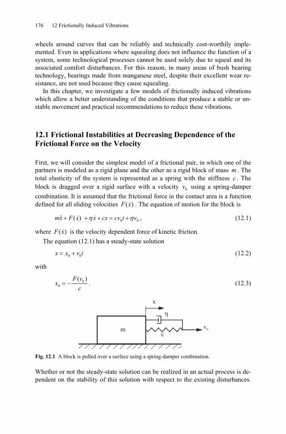
176 12 Frictionally Induced Vibrations
wheels around curves that can be reliably and technically cost-worthily imple-mented. Even in applications where squealing does not influence the function of a system, some technological processes cannot be used solely due to squeal and its associated comfort disturbances. For this reason, in many areas of bush bearing technology, bearings made from manganese steel, despite their excellent wear re-sistance, are not used because they cause squealing.
In this chapter, we investigate a few models of frictionally induced vibrations which allow a better understanding of the conditions that produce a stable or un-stable movement and practical recommendations to reduce these vibrations.
12.1 Frictional Instabilities at Decreasing Dependence of the Frictional Force on the Velocity
First, we will consider the simplest model of a frictional pair, in which one of the partners is modeled as a rigid plane and the other as a rigid block of mass m . The total elasticity of the system is represented as a spring with the stiffness c . The block is dragged over a rigid surface with a velocity 0v using a spring-damper combination. It is assumed that the frictional force in the contact area is a function defined for all sliding velocities ( )F x . The equation of motion for the block is
0 0( ) η η+ + + = +mx F x x cx cv t v , (12.1)
where ( )F x is the velocity dependent force of kinetic friction. The equation (12.1) has a steady-state solution
0 0= +x x v t (12.2)
with
00
( )= −
F vx
c. (12.3)
mc
x
v0
�
Fig. 12.1 A block is pulled over a surface using a spring-damper combination.
Whether or not the steady-state solution can be realized in an actual process is de-pendent on the stability of this solution with respect to the existing disturbances.
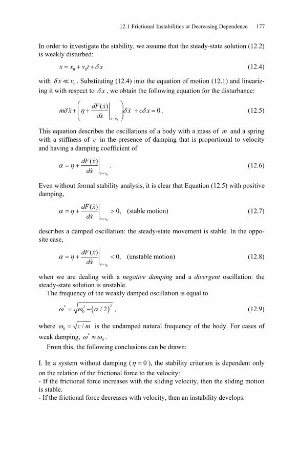
In order to investigate the stability, we assume that the steady-state solution (12.2) is weakly disturbed:
0 0 δ= + +x x v t x (12.4)
with 0δ x v . Substituting (12.4) into the equation of motion (12.1) and lineariz-ing it with respect to δ x , we obtain the following equation for the disturbance:
0
( ) 0δ η δ δ=
⎛ ⎞+ + + =⎜ ⎟⎜ ⎟⎝ ⎠x v
dF xm x x c xdx
. (12.5)
This equation describes the oscillations of a body with a mass of m and a spring with a stiffness of c in the presence of damping that is proportional to velocity and having a damping coefficient of
0
( )α η=
= +x v
dF xdx
. (12.6)
Even without formal stability analysis, it is clear that Equation (12.5) with positive damping,
0
( ) 0, (stable motion)x v
dF xdx
α η=
= + > (12.7)
describes a damped oscillation: the steady-state movement is stable. In the oppo-site case,
0
( ) 0, (unstable motion)x v
dF xdx
α η=
= + < (12.8)
when we are dealing with a negative damping and a divergent oscillation: the steady-state solution is unstable.
The frequency of the weakly damped oscillation is equal to
( )2* 20 / 2ω ω α= − , (12.9)
where 0 /ω = c m is the undamped natural frequency of the body. For cases of weak damping, *
0ω ω≈ . From this, the following conclusions can be drawn:
I. In a system without damping ( 0η = ), the stability criterion is dependent only on the relation of the frictional force to the velocity: - If the frictional force increases with the sliding velocity, then the sliding motion is stable. - If the frictional force decreases with velocity, then an instability develops.
12.1 ecreasing Dependence 177 Frictional Instabilities at D
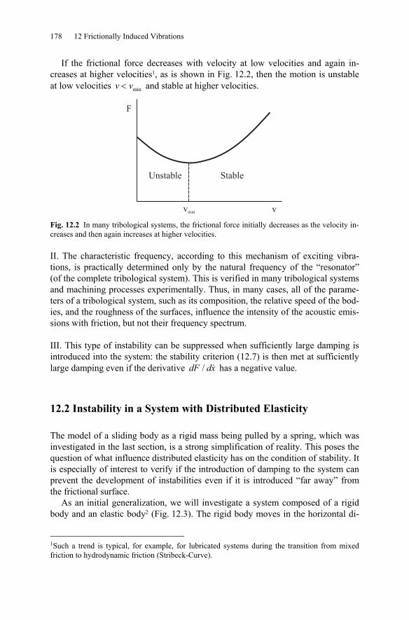
178 12 Frictionally Induced Vibrations
If the frictional force decreases with velocity at low velocities and again in-creases at higher velocities1, as is shown in Fig. 12.2, then the motion is unstable at low velocities min<v v and stable at higher velocities.
Fig. 12.2 In many tribological systems, the frictional force initially decreases as the velocity in-creases and then again increases at higher velocities.
II. The characteristic frequency, according to this mechanism of exciting vibra-tions, is practically determined only by the natural frequency of the “resonator” (of the complete tribological system). This is verified in many tribological systems and machining processes experimentally. Thus, in many cases, all of the parame-ters of a tribological system, such as its composition, the relative speed of the bod-ies, and the roughness of the surfaces, influence the intensity of the acoustic emis-sions with friction, but not their frequency spectrum. III. This type of instability can be suppressed when sufficiently large damping is introduced into the system: the stability criterion (12.7) is then met at sufficiently large damping even if the derivative /dF dx has a negative value.
12.2 Instability in a System with Distributed Elasticity
The model of a sliding body as a rigid mass being pulled by a spring, which was investigated in the last section, is a strong simplification of reality. This poses the question of what influence distributed elasticity has on the condition of stability. It is especially of interest to verify if the introduction of damping to the system can prevent the development of instabilities even if it is introduced “far away” from the frictional surface.
As an initial generalization, we will investigate a system composed of a rigid body and an elastic body2 (Fig. 12.3). The rigid body moves in the horizontal di-
1Such a trend is typical, for example, for lubricated systems during the transition from mixed friction to hydrodynamic friction (Stribeck-Curve).
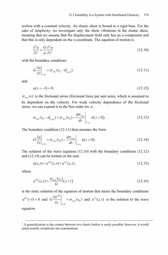
12.2 Instability in a System with Distributed Elasticity 179
rection with a constant velocity. An elastic sheet is bound to a rigid base. For the sake of simplicity, we investigate only the shear vibrations in the elastic sheet, meaning that we assume that the displacement field only has an x-component and that this is only dependent on the z-coordinate. The equation of motion is
2 2
2 2ρ∂ ∂
=∂ ∂
u G ut z
(12.10)
with the boundary conditions
0 00
( )fric zz
uG v uz
σ=
=
∂= −
∂ (12.11)
and
( ) 0= − =u z l . (12.12)
( )fric vσ is the frictional stress (frictional force per unit area), which is assumed to be dependent on the velocity. For weak velocity dependence of the frictional stress, we can expand it in the first order for u :
( )0
0 00( ) ( ) 0fric
fric friczv v
dv u v u z
dvσ
σ σ=
=
− = − = . (12.13)
The boundary condition (12.11) then assumes the form
0
00
( ) ( 0)FricFric
z v v
duG v u zz dv
σσ
= =
∂= − =
∂. (12.14)
The solution of the wave equation (12.10) with the boundary conditions (12.12) and (12.14) can be written as the sum
(0) (1)( , ) ( , ) ( , )= +u z t u z t u z t , (12.15)
where
( )(0) 0( )( , ) Fric v
u z t z lG
σ= + (12.16)
is the static solution of the equation of motion that meets the boundary conditions
(0) ( ) 0− =u l and (0)
00
( )fricz
uG vz
σ=
∂=
∂ and (1) ( , )u z t is the solution to the wave
equation
2 A generalization to the contact between two elastic bodies is easily possible; however, it would unnecessarily complicate our examinations.
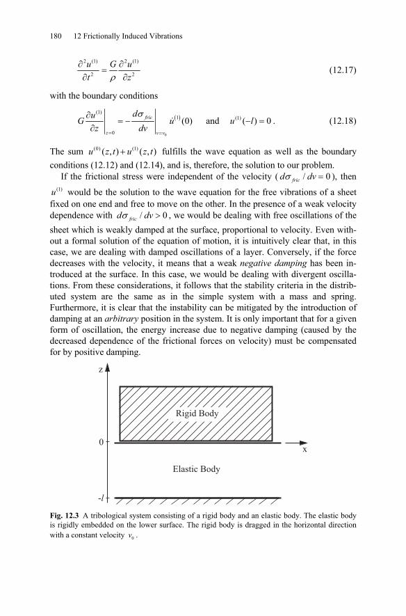
180 12 Frictionally Induced Vibrations
2 (1) 2 (1)
2 2
u G ut zρ
∂ ∂=
∂ ∂ (12.17)
with the boundary conditions
( )
0
(1)1
0
(0)fric
z v v
duG uz dv
σ
= =
∂= −
∂ and (1) ( ) 0u l− = . (12.18)
The sum (0) (1)( , ) ( , )u z t u z t+ fulfills the wave equation as well as the boundary conditions (12.12) and (12.14), and is, therefore, the solution to our problem.
If the frictional stress were independent of the velocity ( / 0fricd dvσ = ), then (1)u would be the solution to the wave equation for the free vibrations of a sheet
fixed on one end and free to move on the other. In the presence of a weak velocity dependence with / 0fricd dvσ > , we would be dealing with free oscillations of the sheet which is weakly damped at the surface, proportional to velocity. Even with-out a formal solution of the equation of motion, it is intuitively clear that, in this case, we are dealing with damped oscillations of a layer. Conversely, if the force decreases with the velocity, it means that a weak negative damping has been in-troduced at the surface. In this case, we would be dealing with divergent oscilla-tions. From these considerations, it follows that the stability criteria in the distrib-uted system are the same as in the simple system with a mass and spring. Furthermore, it is clear that the instability can be mitigated by the introduction of damping at an arbitrary position in the system. It is only important that for a given form of oscillation, the energy increase due to negative damping (caused by the decreased dependence of the frictional forces on velocity) must be compensated for by positive damping.
0
-l
z
Elastic Body
Rigid Body
x
Fig. 12.3 A tribological system consisting of a rigid body and an elastic body. The elastic body is rigidly embedded on the lower surface. The rigid body is dragged in the horizontal direction with a constant velocity 0v .
12.3 Critical Damping and Optimal Suppression of Squeal 181
For weak velocity dependence in a first order approximation, we are dealing with oscillations at the natural frequency of the system, whose amplitude changes only slowly with time (it either increases or decreases depending on which damp-ing – positive or negative – is prevalent in the system). One can consider these os-cillations in “d’Alembert’s picture” of the natural oscillation as the propagation of an elastic wave, which is reflected multiple times from boundaries of the medium and in doing so loses (positive damping) or gains (negative damping) a certain part of its energy with every reflection. It is clear that the damping is determined by how large the energy loss is for every reflection of the wave on the boundary of the medium.
12.3 Critical Damping and Optimal Suppression of Squeal
Based on the view of d’Alembert of natural oscillations, we can argue that we have a case of “ideal damping” if a wave is absorbed in its entirety when it im-pacts a boundary. We will investigate the conditions under which this is possible.
We consider an elastic sheet whose bottom surface is connected to a rigid base by a damping layer (Fig. 12.4). The stress in this layer should be proportional to the relative velocities between the elastic body and the rigid base. From this, we obtain the boundary condition for the elastic sheet on the lower surface:
β=− =−
∂ ∂=
∂ ∂z l z l
u uGz t
, (12.19)
where β is the damping coefficient.
0
-l
z
Elastic Body
Rigid Body
DampingLayer
x
Fig. 12.4 Elastic sheet, which is connected to a rigid base by a damping layer.
182 12 Frictionally Induced Vibrations
The requirement of complete absorption of the wave on the bottom surface means that the equation of motion (12.10) with the boundary condition (12.19) has a solution in the form of a propagating wave in the z-direction:
( , ) ( )= +u z t f z ct , (12.20)
where / ρ=c G is the transverse velocity of the elastic wave. By inserting this special solution of the wave equation into the boundary condition (12.19), we ob-tain
β ρ= G . (12.21)
For this damping there is no reflection of the wave coming from above: Therefore, we have perfect damping. Note that for either a smaller or larger damping coeffi-cient, there is a reflection3. In the cases in which 0β → and β → ∞ , we would actually be dealing with a dissipation free system.
The effect of complete absorption has many applications in physics and technology, the most important of which are listed here: 1. Suppression of squeal. 2. The prevention of acoustic reflections: A so-called “anechoic chamber” should have exactly perfect critical damping on the walls. 3. For molecular dynamics, as well as other numerical simulations, the criti-cal damping at the boundary of the simulation domain must be established in order to suppress the non-physical reflections which are dependent on the size of the simulated domain. 4. In high frequency technologies, the same idea is used to suppress the re-flections in waveguides.
We estimate the required parameters of the damping layer that are necessary to suppress squeal in a steel bearing. According to (12.21) for steel ( 78 GPa≈G ,
3 37.8 10 kg/mρ ≈ ⋅ ), complete damping is achieved with 72.5 10 Pa s/mβ ≈ ⋅ ⋅ . A 1 cm thick polymer sheet with a viscosity somewhat close to that of thick honey, for example, has such a damping coefficient. Experimental investigations show that the installation of a properly dimensioned polymer sheet actually leads to practically complete suppression of squeal (Fig. 12.5).
3 See problem 2 of this chapter.
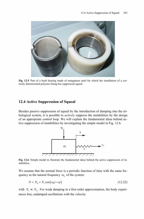
12.4 Active Suppression of Squeal 183
Fig. 12.5 Part of a bush bearing made of manganese steel for which the installation of a cor-rectly dimensioned polymer lining has suppressed squeal.
12.4 Active Suppression of Squeal
Besides passive suppression of squeal by the introduction of damping into the tri-bological system, it is possible to actively suppress the instabilities by the design of an appropriate control loop. We will explain the fundamental ideas behind ac-tive suppression of instabilities by investigating the simple model in Fig. 12.6.
mc
x
v0
N
Fig. 12.6 Simple model to illustrate the fundamental ideas behind the active suppression of in-stabilities.
We assume that the normal force is a periodic function of time with the same fre-quency as the natural frequency 0ω of the system:
( )0 1 0cos ω ϕ= + +N N N t (12.22)
with 1 0N N . For weak damping in a first order approximation, the body experi-ences free, undamped oscillations with the velocity
184 12 Frictionally Induced Vibrations
0 1 0cosω= +v v v t . (12.23)
For a qualitative stability investigation, we calculate the change in energy of the moving body over one oscillation period. Thereby we assume that the frictional force can be presented as product of the normal force and the velocity dependent coefficient of friction:
( )fricF N vμ= . (12.24)
The change in the energy of oscillations is determined by the average power of the frictional force in the reference system that moves with the average velocity 0v :
( ) ( )0 0 0fricdP F v v N v v vdvμμ⎛ ⎞= − ⋅ − = − + ⋅ −⎜ ⎟
⎝ ⎠. (12.25)
Inserting (12.22) and (12.23) into (12.25) yields
( )( ) ( )0 1 0 0 1 0 0 1 0 1 0
1 0 1 1 0 0
cos cos cos cos
1 cos2
dP N N t v t v v t v tdv
d dv N v N vdv dv
μω ϕ μ ω ω ω
μ μμ ϕ
⎛ ⎞= − + + + +⎜ ⎟⎝ ⎠
⎛ ⎞⎛ ⎞= − + +⎜ ⎟⎜ ⎟⎝ ⎠⎝ ⎠
(12.26)
or for weak damping
1 0 1 1 01 cos2
dP v N v Ndvμ μ ϕ⎛ ⎞≈ − +⎜ ⎟
⎝ ⎠. (12.27)
If there are no oscillations in the normal force, then the average power would be
equal to 20 1
12
μ−
dN vdv
. We would then come to the already known result: for de-
creasing frictional force as a function of velocity ( )/ 0μ <d dv , the energy in-creases and the process is unstable. By changing the normal force, however, the power can be made negative and, therefore, the oscillations damped. For this to occur, the following condition must be met:
0 1 1 0 cos 0μ μ ϕ+ >dN v Ndv
. (12.28)
This can only be met when cos 0ϕ > , ideally cos 1ϕ = and therefore 0ϕ = . In other words, the normal force (12.22) should oscillate, as far as possible, in phase with the velocity (12.23). This can be realized using a control loop in which the velocity is measured and the normal force is varied proportionally to the measured velocity ( )0ξΔ = −N x v . In this case, the equation of motion is
( )( )0 0 0 0( ) ξ μ η η+ + − + + = +mx N x v x x cx cv t v . (12.29)
12.5 Strength Aspects during Squeal 185
The linearized equation for a small perturbation of the steady-state solution (12.2) is
0 0 + 0μδ μ ξ η δ δ⎛ ⎞+ + + =⎜ ⎟⎝ ⎠
dm x N x c xdv
. (12.30)
In order for the steady state sliding to remain stable, the total damping in (12.30) must be positive:
0 0 + 0μ μ ξ η+ >dNdv
. (12.31)
For decreasing frictional force as a function of velocity, this can be achieved either through sufficiently large damping η or through a sufficiently strong coupling
0μ ξ between the velocity and the normal force. One can see from Equation (12.31) that the control loop has the same effect as a damper. The advantage of active suppression lies in the simple controllability of a control loop compared to passive damping, whose parameters can only be adjusted by material choice and dimensioning.
12.5 Strength Aspects during Squeal
We want to estimate the stress introduced into a system experiencing squeal in or-der to determine under what conditions the strength of the material can be com-promised. We investigate the system shown in Fig. 12.3. For weak damping, we can find a first order approximation solution to the perturbation equation (12.17) with the boundary conditions
(1)
0
0=
∂=
∂ z
uGz
and (1) ( ) 0− =u l . (12.32)
The solution for the eigenmode with the smallest natural frequency is
( )( , ) sin sin2 2π π⎛ ⎞= + ⋅⎜ ⎟
⎝ ⎠
cu z t A z l tl l
, (12.33)
where / ρ=c G is the velocity of the transverse elastic wave. The oscillation
amplitude of the velocity u is then 2π
=cv Al
, and that of the stress ∂∂uGz
is equal
to 2πσ = AGl
. According to this, the following relationship exists between the
amplitude of the stress and the amplitude of the velocity:
186 12 Frictionally Induced Vibrations
σ ρ= =vG v Gc
. (12.34)
As a rule, the oscillation amplitude of the velocity will have the same order of magnitude as the sliding velocity 0v in the stationary cycle. The order of magni-tude of the stresses in a squealing system can, thus, be estimated with
00σ ρ= =
vG v G
c. (12.35)
This is a very general result which remains valid also for oscillations with higher natural frequencies: the stresses in a limit-cycle are essentially only de-pendent on velocity! The critical velocity, at which the stress reaches the critical shear stress σ F of the material, is given by
σρ
= Fcv
G. (12.36)
For steel with 300 σ =F MPa (which corresponds to a tensile strength of around 500 MPa), we obtain the critical velocity of 0 12v m/s. For larger sliding veloci-ties, the squeal would lead to the failure of a part made of such a steel!
12.6 Dependence of the Stability Criteria on the Stiffness of
the
System
In the previous section, we considered the mechanisms for the development of in-stabilities caused only by the decrease of frictional force with velocity. The stabil-ity criteria are, in this case, independent of the stiffness of the system. In the ex-ample shown in Fig. 12.2, the motion at an average velocity lower than the velocity minv is always unstable. The stiffness of the system influences the fre-quency of the frictionally induced oscillations, but not the stability criteria. In practice, however, it is seen that by changing the stiffness of a system, it can be stabilized. This property, which has been established in numerous experimental investigations means that the simple explanation of instabilities being caused by decreasing frictional force with the velocity may not always be correct.
The reason for this, from the mathematical point of view, lies in the invalid as-sumption that the frictional force is determined only by the instantaneous state of the frictional contact – essentially by the normal force and the sliding velocity. For the force of static friction, this assumption would mean that it always remains con-stant. Since Coulomb, however, it is known that this is not completely correct. Even if the normal force does not change and the “sliding velocity” remains con-
12.6 Dependence of the Stability Criteria on the Stiffness of the System 187
stant (equal to zero), the force of static friction changes over time. The change can have varying physical causes. In metallic substances, creep processes lead to a change in the real contact area and, thereby, account for the change in the fric-tional force. In elastomers, it is the viscosity that is responsible for the delayed re-action. In lubricated systems, the film thickness changes with time even with no change in the normal force. Furthermore, the temperature of the contact partners changes, and with it that of the lubricating oil, which also has an impact on the frictional force. The contribution to the frictional force through the building of capillary bridges is also explicitly time dependent.
All of these processes could be described in every individual case by the intro-duction of additional appropriate variables, called “internal variables,” which suf-ficiently characterize the state of the frictional layer and the intermediate material (also called third body). The idea of internal variables was originally applied to earthquake dynamics by A. Ruina4. In some cases, these variables have clear physical meanings (e.g. temperature); in others, empirical experiences are summa-rized in the internal variables.
We will investigate the simplest phenomenological model that describes the typical dynamics of the “contact state5.” We once again consider the model shown in Fig. 12.1, which is described by the equation of motion
0 0( , ) θ η η+ + + = +mx F x x cx cv t v , (12.37)
where the frictional force ( , )θF x is now not only dependent on the velocity, but also on the internal state variable θ . For this dependence, we assume
( )( , ) θ θ= + −k s kF x F F F . (12.38)
Here, θ is the internal variable that describes the state of the contact zone and changes from 0θ = , at the initial moment of contact, to 1θ = after a long time at rest. Consequently, sF is the force of static friction and kF , that of kinetic fricti-on. For the variable of state θ , we assume the following simple kinetic equation
( )1 11 , 0 1θ θ θτ⎛ ⎞= − − < <⎜ ⎟⎝ ⎠
xD
. (12.39)
For vanishing velocity, 0=x , θ increases with time until a saturation value, 1θ = . If the body is put into motion, then the variable of state decreases faster at
higher velocities. The physical meaning of τ in (12.39) is the characteristic re-laxation time of the parameter θ when the system is at rest, while D is the char-acteristic “relaxation length” of this parameter at the initiation of motion. In a physical view of the contact between two rough surfaces, τ can be understood to
4 A. Ruina, Slip Instability and State Variable Friction Laws. Journal of Geophysical Research, 1983, v.88, N.B12, pp. 10359-10370. 5 A more complicated and realistic rate- and state -dependent frictional law is discussed in Chap-ter 20.
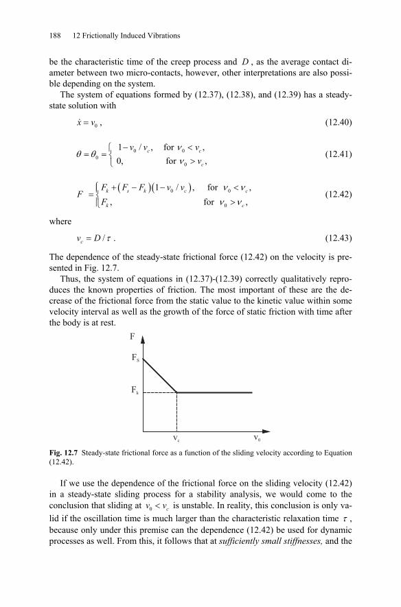
188 12 Frictionally Induced Vibrations
be the characteristic time of the creep process and D , as the average contact di-ameter between two micro-contacts, however, other interpretations are also possi-ble depending on the system.
The system of equations formed by (12.37), (12.38), and (12.39) has a steady-state solution with
0=x v , (12.40)
0 00
0
1 / , for , 0, for ,
c c
c
v v vv
νθ θ
ν− <⎧
= = ⎨ >⎩ (12.41)
( )( )0 0
0
1 / , for ,
, for ,k s k c c
k c
F F F v vF
Fν νν ν
⎧ + − − <⎪= ⎨>⎪⎩
(12.42)
where
/τ=cv D . (12.43)
The dependence of the steady-state frictional force (12.42) on the velocity is pre-sented in Fig. 12.7.
Thus, the system of equations in (12.37)-(12.39) correctly qualitatively repro-duces the known properties of friction. The most important of these are the de-crease of the frictional force from the static value to the kinetic value within some velocity interval as well as the growth of the force of static friction with time after the body is at rest.
F
v0vc
FS
Fk
Fig. 12.7 Steady-state frictional force as a function of the sliding velocity according to Equation (12.42).
If we use the dependence of the frictional force on the sliding velocity (12.42) in a steady-state sliding process for a stability analysis, we would come to the conclusion that sliding at 0 < cv v is unstable. In reality, this conclusion is only va-lid if the oscillation time is much larger than the characteristic relaxation time τ , because only under this premise can the dependence (12.42) be used for dynamic processes as well. From this, it follows that at sufficiently small stiffnesses, and the
12.6 Dependence of the Stability Criteria on the Stiffness of the System 189
correspondingly large oscillation periods, sliding is unstable in reality. Con-versely, for large stiffnesses, and the correspondingly small oscillation periods, the parameter θ has no time to change. The frictional force is then, according to (12.38), completely independent from the velocity, and instability does not occur. In order to investigate the stability of the steady-state solution (12.40)-(12.42) in the generalized case and to obtain the stability limit, dependent on the sliding ve-locity and the stiffness of the system, we consider a small disturbance to the steady-state solution:
0 0 δ= + +x x v t x , 0θ θ δθ= + . (12.44)
The linearized equations are
( ) 0δ ηδ δ δθ+ + + − =s km x x c x F F (12.45)
and
1 1δθ δθ δτ
= − − xD
. (12.46)
We look for a solution to this system of equations in the exponential form
λδ = tx Ae , λδθ = tBe . (12.47)
Insertion into (12.45) and (12.46), provides us
( ) ( )2 0λ ηλ+ + + − =s km c A F F B (12.48)
and
1 1 0λ λτ
⎛ ⎞+ + =⎜ ⎟⎝ ⎠
A BD
. (12.49)
This linear system of equations has a non-trivial solution, when the determinant vanishes:
( )2
01 1
ηλ λ
λ λτ
−⎛ ⎞+ +⎜ ⎟⎝ ⎠ =
⎛ ⎞+⎜ ⎟⎝ ⎠
s kF Fcm m m
D
(12.50)
or
3 2 0λ λ λ+ + + =P Q R (12.51)
with
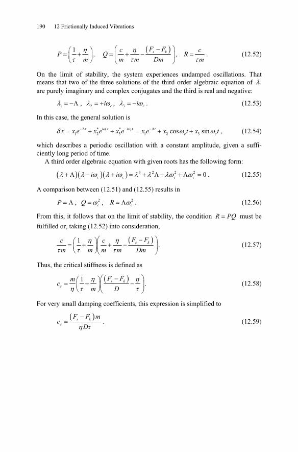
190 12 Frictionally Induced Vibrations
1 ητ⎛ ⎞= +⎜ ⎟⎝ ⎠
Pm
, ( )η
τ−⎛ ⎞
= + −⎜ ⎟⎝ ⎠
s kF FcQm m Dm
, τ
=cRm
. (12.52)
On the limit of stability, the system experiences undamped oscillations. That means that two of the three solutions of the third order algebraic equation of λ are purely imaginary and complex conjugates and the third is real and negative:
1λ = −Λ , 2λ ω= + ci , 3λ ω= − ci . (12.53)
In this case, the general solution is
* *1 2 3 1 2 3cos sinω ωδ ω ω−−Λ −Λ= + + = + +c ci t i tt t
c cx x e x e x e x e x t x t , (12.54)
which describes a periodic oscillation with a constant amplitude, given a suffi-ciently long period of time.
A third order algebraic equation with given roots has the following form:
( )( )( ) 3 2 2 2 0λ λ ω λ ω λ λ λω ω+Λ − + = + Λ + + Λ =c c c ci i . (12.55)
A comparison between (12.51) and (12.55) results in
= ΛP , 2ω= cQ , 2ω= Λ cR . (12.56)
From this, it follows that on the limit of stability, the condition =R PQ must be fulfilled or, taking (12.52) into consideration,
( )1 η η
τ τ τ−⎛ ⎞⎛ ⎞= + + −⎜ ⎟⎜ ⎟
⎝ ⎠⎝ ⎠
s kF Fc cm m m m Dm
. (12.57)
Thus, the critical stiffness is defined as
( )1 η η
η τ τ−⎛ ⎞⎛ ⎞= + −⎜ ⎟⎜ ⎟
⎝ ⎠⎝ ⎠
s kc
F Fmcm D
. (12.58)
For very small damping coefficients, this expression is simplified to
( )
η τ−
= s kc
F F mc
D. (12.59)
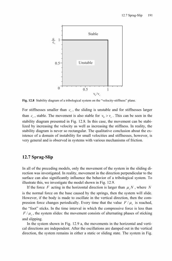
12.7 Sprag-Slip 191
Fig. 12.8 Stability diagram of a tribological system on the “velocity-stiffness” plane.
For stiffnesses smaller than cc , the sliding is unstable and for stiffnesses larger than cc , stable. The movement is also stable for 0 > cv v . This can be seen in the stability diagram presented in Fig. 12.8. In this case, the movement can be stabi-lized by increasing the velocity as well as increasing the stiffness. In reality, the stability diagram is never so rectangular. The qualitative conclusion about the ex-istence of a domain of instability for small velocities and stiffnesses, however, is very general and is observed in systems with various mechanisms of friction.
12.7 Sprag-Slip
In all of the preceding models, only the movement of the system in the sliding di-rection was investigated. In reality, movement in the direction perpendicular to the surface can also significantly influence the behavior of a tribological system. To illustrate this, we investigate the model shown in Fig. 12.9.
If the force F acting in the horizontal direction is larger than μs N , where N is the normal force on the base caused by the springs, then the system will slide. However, if the body is made to oscillate in the vertical direction, then the com-pression force changes periodically. Every time that the value / μsF is reached, the “foot” sticks. In the time interval in which the compressive force is less than
/ μsF , the system slides: the movement consists of alternating phases of sticking and slipping.
In the system shown in Fig. 12.9 a, the movements in the horizontal and verti-cal directions are independent. After the oscillations are damped out in the vertical direction, the system remains in either a static or sliding state. The system in Fig.
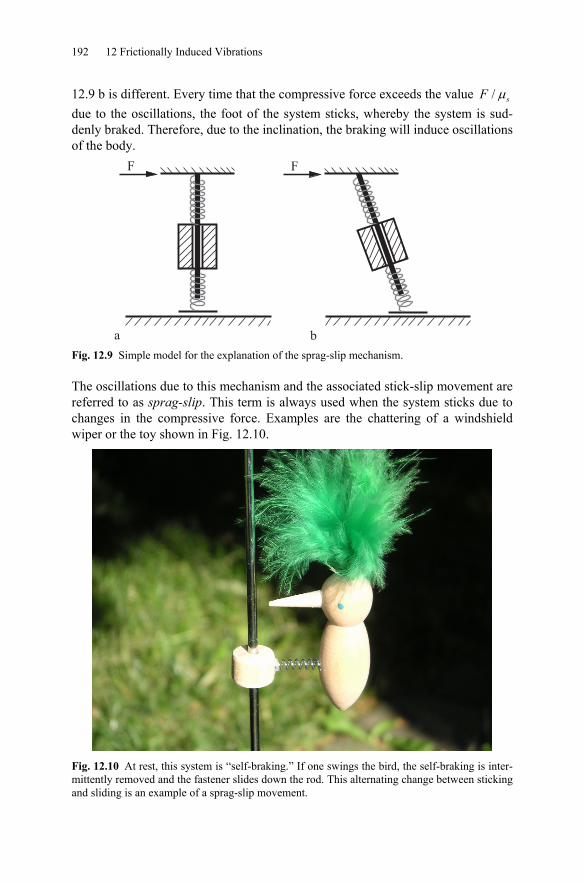
192 12 Frictionally Induced Vibrations
12.9 b is different. Every time that the compressive force exceeds the value / μsF due to the oscillations, the foot of the system sticks, whereby the system is sud-denly braked. Therefore, due to the inclination, the braking will induce oscillations of the body.
F F
a b Fig. 12.9 Simple model for the explanation of the sprag-slip mechanism.
The oscillations due to this mechanism and the associated stick-slip movement are referred to as sprag-slip. This term is always used when the system sticks due to changes in the compressive force. Examples are the chattering of a windshield wiper or the toy shown in Fig. 12.10.
Fig. 12.10 At rest, this system is “self-braking.” If one swings the bird, the self-braking is inter-mittently removed and the fastener slides down the rod. This alternating change between sticking and sliding is an example of a sprag-slip movement.
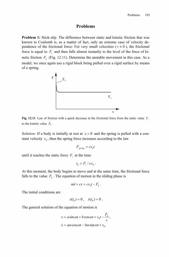
Problems 193
Problems
Problem 1: Stick-slip. The difference between static and kinetic friction that was known to Coulomb is, as a matter of fact, only an extreme case of velocity de-pendence of the frictional force: For very small velocities ( 0≈v ), the frictional force is equal to sF and then falls almost instantly to the level of the force of ki-netic friction kF (Fig. 12.11). Determine the unstable movement in this case. As a model, we once again use a rigid block being pulled over a rigid surface by means of a spring.
FS
Fk
F
v Fig. 12.11 Law of friction with a quick decrease in the frictional force from the static value sF
to the kinetic value kF .
Solution: If a body is initially at rest at 0=x and the spring is pulled with a con-stant velocity 0v , then the spring force increases according to the law
0springF cv t=
until it reaches the static force sF at the time
0 0/= st F cv .
At this moment, the body begins to move and at the same time, the frictional force falls to the value kF . The equation of motion in the sliding phase is
0+ = − kmx cx cv t F .
The initial conditions are
0( ) 0=x t , 0( ) 0=x t .
The general solution of the equation of motion is
0
0
sin cos ,
cos sin .
ω ω
ω ω ω ω
= + + −
= − +
kFx a t b t v t
cx a t b t v
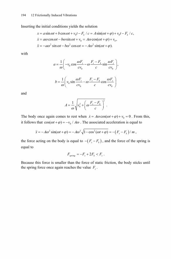
194 12 Frictionally Induced Vibrations
Inserting the initial conditions yields the solution
0 0
0 02 2 2
sin cos / sin( ) / ,cos sin cos( ) ,
sin cos sin( ).
ω ω ω ϕω ω ω ω ω ω ϕ
ω ω ω ω ω ω ϕ
= + + − = + + −= − + = + +
= − − = − +
k kx a t b t v t F c A t v t F cx a t b t v A t v
x a t b t A t
with
00 0
1 cos sinω ω
ωω⎛ ⎞−
= − −⎜ ⎟⎝ ⎠
s s k sF F F Fa v
cv c cv,
00 0
1 sin cosω ω
ωω⎛ ⎞−
= −⎜ ⎟⎝ ⎠
s s k sF F F Fb v
cv c cv
and
220
1 ωω
−⎛ ⎞= + ⎜ ⎟⎝ ⎠
s kF FA v
c.
The body once again comes to rest when 0cos( ) 0ω ω ϕ= + + =x A t v . From this, it follows that 0cos( ) /ω ϕ ω+ = −t v A . The associated acceleration is equal to
( )2 2 2sin( ) 1 cos ( ) /ω ω ϕ ω ω ϕ= − + = − − + = − −s kx A t A t F F m ,
the force acting on the body is equal to ( )− −s kF F , and the force of the spring is equal to
2spring s k sF F F F= − + < .
Because this force is smaller than the force of static friction, the body sticks until the spring force once again reaches the value sF .
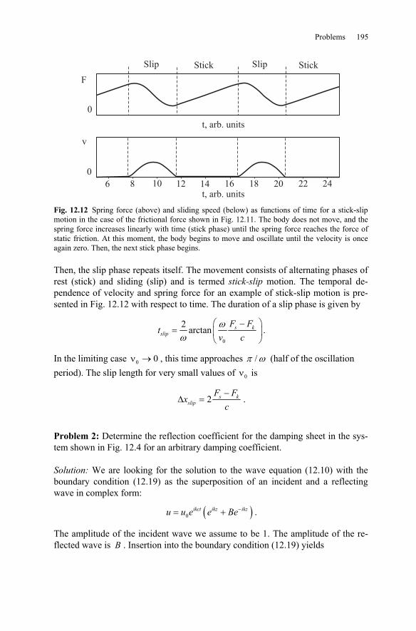
Problems 195
F
0
v
0
Slip Stick Slip Stick
t, arb. units
t, arb. units6 8 10 12 14 16 18 20 22 24
Fig. 12.12 Spring force (above) and sliding speed (below) as functions of time for a stick-slip motion in the case of the frictional force shown in Fig. 12.11. The body does not move, and the spring force increases linearly with time (stick phase) until the spring force reaches the force of static friction. At this moment, the body begins to move and oscillate until the velocity is once again zero. Then, the next stick phase begins.
Then, the slip phase repeats itself. The movement consists of alternating phases of rest (stick) and sliding (slip) and is termed stick-slip motion. The temporal de-pendence of velocity and spring force for an example of stick-slip motion is pre-sented in Fig. 12.12 with respect to time. The duration of a slip phase is given by
0
2 arctan s kslip
F Ft
v cω
ω⎛ ⎞−
= ⎜ ⎟⎝ ⎠
.
In the limiting case 0 0ν → , this time approaches /π ω (half of the oscillation period). The slip length for very small values of 0ν is
2 s kslip
F Fx
c−
Δ = .
Problem 2: Determine the reflection coefficient for the damping sheet in the sys-tem shown in Fig. 12.4 for an arbitrary damping coefficient.
Solution: We are looking for the solution to the wave equation (12.10) with the boundary condition (12.19) as the superposition of an incident and a reflecting wave in complex form:
( )0−= +ikct ikz ikzu u e e Be .
The amplitude of the incident wave we assume to be 1. The amplitude of the re-flected wave is B . Insertion into the boundary condition (12.19) yields
196 12 Frictionally Induced Vibrations
2ikl G cB eG c
ββ
− −=
+.
We define the reflection coefficient as the ratio of the intensity of the incident wave to that of the reflected wave; it is, therefore, equal to 2B :
22 β
β⎛ ⎞−
= ⎜ ⎟+⎝ ⎠
G cBG c
.
The reflection coefficient becomes zero for /G c Gβ ρ= = . For 0β → and β → ∞ , it approaches 1.
Problem 3: Determine the reflection coefficient between an elastic sheet and a liquid film with a dynamic viscosity6 η .
Solution: The equations of motion to be solved are the wave equation
2 2
2 2ρ∂ ∂
=∂ ∂
u G ut z
in the elastic continuum and the Navier-Stokes equation for the liquid medium, which for purely transverse motion has the form
2
2ρ η∂ ∂=
∂ ∂v vt z
.
We place the surface 0=z at the boundary between the elastic medium and the liquid medium. Let the positive z-direction be defined in the direction of the elas-tic layer. The boundary conditions at the interface are
(0, ) (0, )=u t v t (no-slip condition)
and
0 0
η= =
∂ ∂=
∂ ∂z z
u vGz z
(equilibrium condition).
We look for the solution to the wave equation, as we did in Problem 2, in the form of a superposition of an incident and a reflected wave
ω ωω −⎛ ⎞
= +⎜ ⎟⎝ ⎠
i z i zi t c cu e e Be .
6 The dynamic viscosity η should not be confused with the damping coefficient η , which is used earlier in this chapter or in other chapters and has other units.
Problems 197
The solution to the Navier-Stokes equation with the frequency ω , which ap-proaches zero at infinity, is
12
ρωη ω
+
=i z
i tv Ce e .
The application of the boundary conditions at the interface results in the following system of equations:
( )1ω + =i B C ,
( ) 112
ω ρωηη
+− =
iiG B Cc
.
The reflection coefficient is
( )( )
2 22
2 2
1
1
ζ ζ
ζ ζ
− +=
+ +B
with
2 2ρωη ωηζ = =
cG G
.
The reflection coefficient reaches its minimum 2 0.17B ≈ for 1 / 2ζ = . We see that the oscillations can be damped very efficiently by liquid layers (or polymers with corresponding rheological properties), however, only in specific frequency domains. In both limiting cases, a viscosity of zero or infinity, the reflection coef-ficient is equal to 1 as expected.
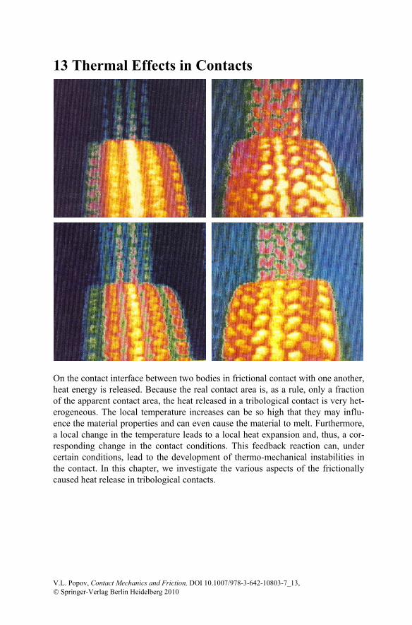
13 Thermal Effects in Contacts
On the contact interface between two bodies in frictional contact with one another, heat energy is released. Because the real contact area is, as a rule, only a fraction of the apparent contact area, the heat released in a tribological contact is very het-erogeneous. The local temperature increases can be so high that they may influ-ence the material properties and can even cause the material to melt. Furthermore, a local change in the temperature leads to a local heat expansion and, thus, a cor-responding change in the contact conditions. This feedback reaction can, under certain conditions, lead to the development of thermo-mechanical instabilities in the contact. In this chapter, we investigate the various aspects of the frictionally caused heat release in tribological contacts.
V.L. Popov, Contact Mechanics and Friction, DOI 10.1007/978-3-642-10803-7_13, © Springer-Verlag Berlin Heidelberg 2010
200 13 Thermal Effects in Contacts
13.1 Introduction
The first systematic investigation of temperature distributions in frictional contacts was carried out in 1935 by F.P. Bowden and K. Riedler1. In the course of these in-vestigations, they used the tribological contact as a natural thermocouple. This ap-proach remains today one of the simplest and most dependable methods to ex-perimentally determine the temperature distribution in a tribological contact. In further studies with Tabor, Bowden measured very high temperatures (around the same magnitude as the melting temperature) in parts of the contact.
By investigating thermal effects in contacts, one can differentiate between three scales: (1) the tribological system as a whole, (2) the “macroscopic contact area,” and (3) the micro-contacts between the rough surfaces. While the temperature of the entire system changes slowly during the process, the temperature in a sliding contact (e.g. between two gears) can change very quickly and reach high values. This is referred to as the “flash temperature.” The theoretical investigation of flash temperatures in “macroscopic contact areas” is, above all, associated with the name H. Blok2. For these conditions, a large Péclet number is characteristic. The temperature dynamics for small Péclet numbers was investigated by J.K. Jaeger3. This theory, as a rule, is applicable to micro-contacts. It has been shown, however, that Jaeger’s theory for small Péclet numbers remains relatively accurate even in the area of validity of Blok’s theory. We limit ourselves in this chapter, therefore, to the case of small Péclet numbers.
13.2 Flash Temperatures in Micro-Contacts
We consider the contact between two rough surfaces in the scope of the model from Greenwood and Williamson (see Chapter 7). At the same time, we assume that there is friction between micro-asperities with the coefficient of friction μ . We calculate the temperature increase in a micro-contact by assuming that the characteristic propagation length of the heat, 2α≈D t , during the existence of a contact, /≈t a v , is much larger than the contact radius: 2αt a or
12αva . (13.1)
1 F.P. Bowden, K.E.W. Riedler, A note on the surface temperature of sliding metals. Proc. Cam-bridge Philos. Soc., 1935, v. 31, Pt.3, p.431. 2 H. Blok, The Dissipation of Frictional Heat. Applied Scientific Research, Section A, 1955, N. 2-3, pp. 151-181. 3 J.K. Jaeger, Moving Sources of Heat and the Temperature of Sliding Contacts. Journal and Proc. Royal Society, New South Walls, 1942, v. 76, Pt. III, pp. 203-224.
13.2 Flash Temperatures in Micro-Contacts 201
Here, α is the thermal diffusivity, a the contact radius, and v the sliding speed. The ratio / 2αva is known as the Péclet number. If the condition (13.1) is met, one can consider the heat propagation at every point in time as a stationary process with a given heat production on the surface. For metallic substances ( 4 210 m /α −≈ s , 5 410 10 m− −≈ −a ), this means that the sliding speed may not be larger than 2 / 2 20 m/sα ≈ −a , which is true in most applications. For ceramics and polymers ( 7 6 2 510 10 m / , 10 mα − − −≈ − ≈s a ), this approximation is valid for sliding speeds under 0.02 0.2 m/s− .
A homogeneous temperature increase ΔT in a round area with the radius a on the surface of a half-space with the thermal conductivity λ produces a heat flux W that is associated with ΔT by the thermal resistance wR :
Δ=
w
TWR
. (13.2)
The thermal resistance for a round contact is equal to
12 λ
=wRa
. (13.3)
We can also use this with equation (13.2) in order to estimate the temperature in-crease of the surface for a given heat flow:
2 λ
Δ =WTa
. (13.4)
Under the assumption that the total heat flows only into one body, we get for one single elastic micro-contact
2μ
λΔ
Δ = NF vT
a. (13.5)
By inserting the Hertzian formula * 1/ 2 3/ 243
Δ =NF E R d and taking into account that
=a Rd , we obtain
*2
3μλ
Δ =E dvT . (13.6)
As we saw in Chapter 7, the average penetration depth d is practically independ-ent from the compressive force and is approximately equal to /πl . Therefore, we obtain an average temperature increase in the micro-contact of
*
0.2 E lvT μλ
Δ ≈ . (13.7)
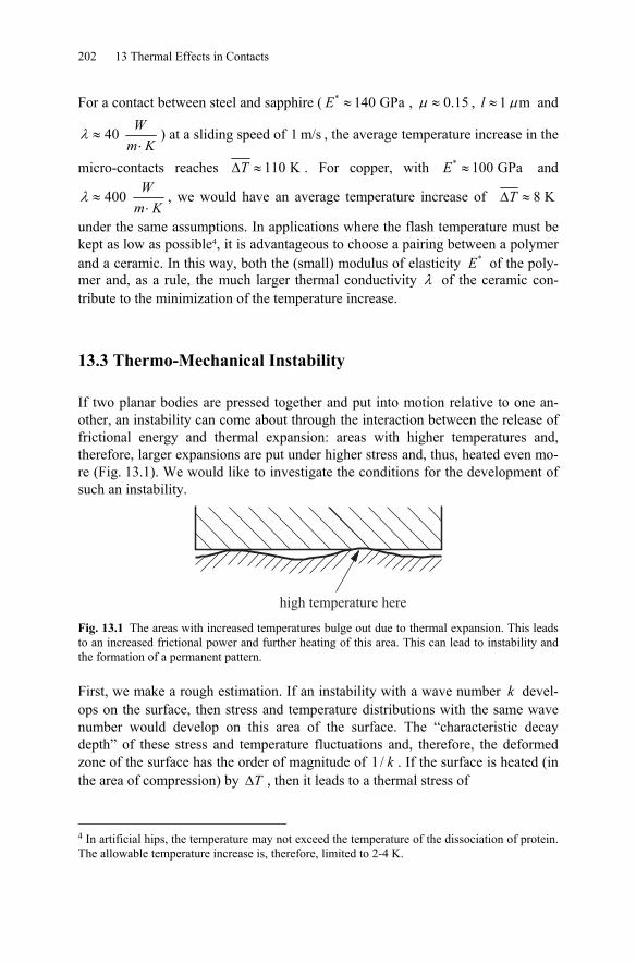
202 13 Thermal Effects in Contacts
For a contact between steel and sapphire ( * 140 GPa≈E , 0.15μ ≈ , 1 mμ≈l and
40 λ ≈⋅
Wm K
) at a sliding speed of 1 m/s , the average temperature increase in the
micro-contacts reaches 110 KΔ ≈T . For copper, with * 100 GPa≈E and
400 λ ≈⋅
Wm K
, we would have an average temperature increase of 8 KΔ ≈T
under the same assumptions. In applications where the flash temperature must be kept as low as possible4, it is advantageous to choose a pairing between a polymer and a ceramic. In this way, both the (small) modulus of elasticity *E of the poly-mer and, as a rule, the much larger thermal conductivity λ of the ceramic con-tribute to the minimization of the temperature increase.
13.3 Thermo-Mechanical Instability
If two planar bodies are pressed together and put into motion relative to one an-other, an instability can come about through the interaction between the release of frictional energy and thermal expansion: areas with higher temperatures and, therefore, larger expansions are put under higher stress and, thus, heated even mo-re (Fig. 13.1). We would like to investigate the conditions for the development of such an instability.
high temperature here Fig. 13.1 The areas with increased temperatures bulge out due to thermal expansion. This leads to an increased frictional power and further heating of this area. This can lead to instability and the formation of a permanent pattern.
First, we make a rough estimation. If an instability with a wave number k devel-ops on the surface, then stress and temperature distributions with the same wave number would develop on this area of the surface. The “characteristic decay depth” of these stress and temperature fluctuations and, therefore, the deformed zone of the surface has the order of magnitude of 1/ k . If the surface is heated (in the area of compression) by ΔT , then it leads to a thermal stress of
4 In artificial hips, the temperature may not exceed the temperature of the dissociation of protein. The allowable temperature increase is, therefore, limited to 2-4 K.
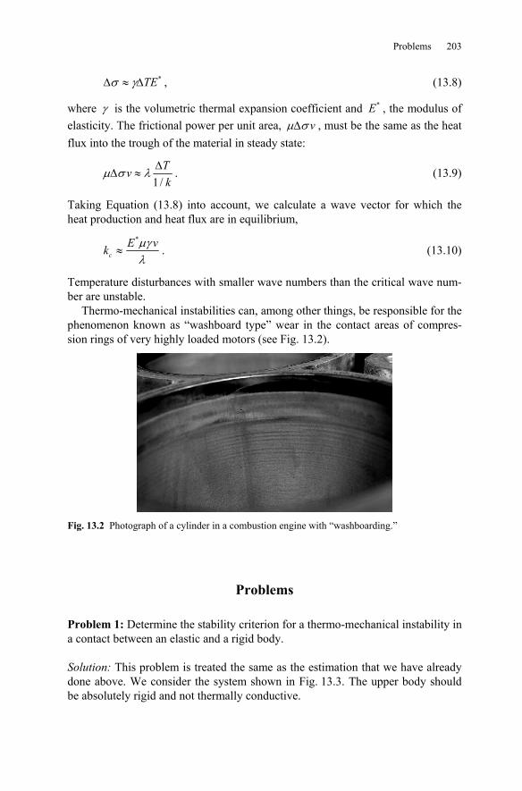
Problems 203
*TEσ γΔ ≈ Δ , (13.8)
where γ is the volumetric thermal expansion coefficient and *E , the modulus of elasticity. The frictional power per unit area, μ σΔ v , must be the same as the heat flux into the trough of the material in steady state:
1 /
μ σ λ ΔΔ ≈
Tvk
. (13.9)
Taking Equation (13.8) into account, we calculate a wave vector for which the heat production and heat flux are in equilibrium,
*
cE vk μγλ
≈ . (13.10)
Temperature disturbances with smaller wave numbers than the critical wave num-ber are unstable.
Thermo-mechanical instabilities can, among other things, be responsible for the phenomenon known as “washboard type” wear in the contact areas of compres-sion rings of very highly loaded motors (see Fig. 13.2).
Fig. 13.2 Photograph of a cylinder in a combustion engine with “washboarding.”
Problems
Problem 1: Determine the stability criterion for a thermo-mechanical instability in a contact between an elastic and a rigid body.
Solution: This problem is treated the same as the estimation that we have already done above. We consider the system shown in Fig. 13.3. The upper body should be absolutely rigid and not thermally conductive.
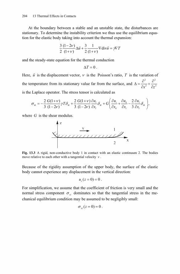
204 13 Thermal Effects in Contacts
At the boundary between a stable and an unstable state, the disturbances are stationary. To determine the instability criterion we thus use the equilibrium equa-tion for the elastic body taking into account the thermal expansion:
3 (1 2 ) 3 1 div2 (1 ) 2 (1 )
ν γν ν
−Δ + ∇ = ∇
+ +u u T
and the steady-state equation for the thermal conduction
0Δ =T .
Here, u is the displacement vector, ν is the Poisson’s ratio, T is the variation of
the temperature from its stationary value far from the surface, and 2 2
2 2
∂ ∂Δ = +
∂ ∂x z
is the Laplace operator. The stress tensor is calculated as
2 (1 ) 2 (1 ) 23 (1 2 ) 3 (1 2 ) 3
ν νσ γ δ δ δν ν
⎛ ⎞∂ ∂ ∂ ∂+ += − + + + −⎜ ⎟− − ∂ ∂ ∂ ∂⎝ ⎠
l i k lik ik ik ik
l k i l
u u u uG GT Gx x x x
,
where G is the shear modulus.
v
x2
1
z
Fig. 13.3 A rigid, non-conductive body 1 in contact with an elastic continuum 2. The bodies move relative to each other with a tangential velocity v .
Because of the rigidity assumption of the upper body, the surface of the elastic body cannot experience any displacement in the vertical direction:
( 0) 0= =zu z .
For simplification, we assume that the coefficient of friction is very small and the normal stress component σ zz dominates so that the tangential stress in the me-chanical equilibrium condition may be assumed to be negligibly small:
( 0) 0σ = =xz z .
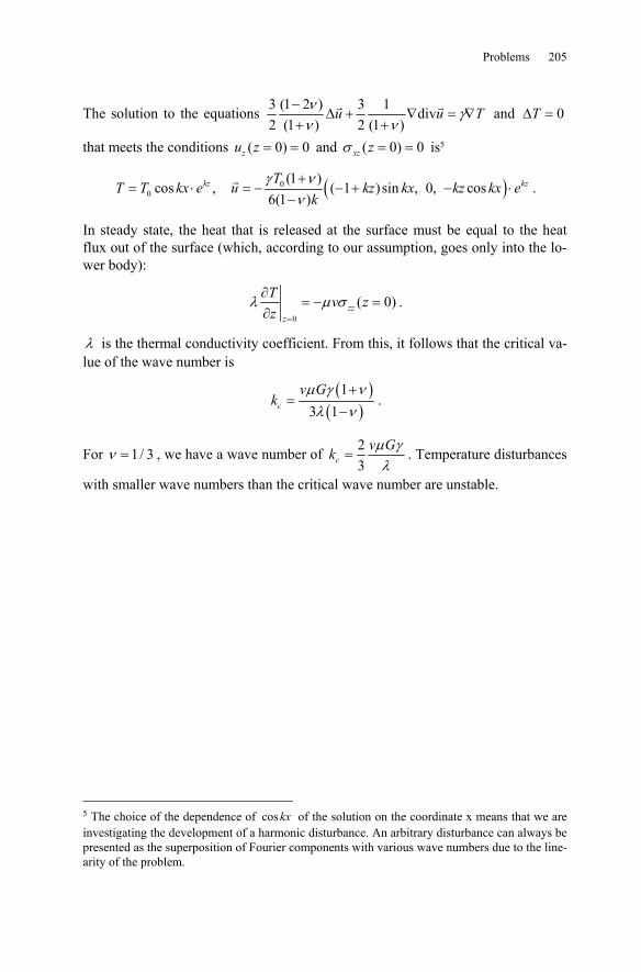
Problems 205
The solution to the equations 3 (1 2 ) 3 1 div2 (1 ) 2 (1 )
ν γν ν
−Δ + ∇ = ∇
+ +u u T and 0Δ =T
that meets the conditions ( 0) 0= =zu z and ( 0) 0σ = =xz z is5
( )00
(1 )cos , ( 1 )sin , 0, cos
6(1 )γ ν
ν+
= ⋅ = − − + − ⋅−
kz kzTT T kx e u kz kx kz kx e
k.
In steady state, the heat that is released at the surface must be equal to the heat flux out of the surface (which, according to our assumption, goes only into the lo-wer body):
0
( 0)λ μ σ=
∂= − =
∂ zzz
T v zz
.
λ is the thermal conductivity coefficient. From this, it follows that the critical va-lue of the wave number is
( )( )
13 1μ γ νλ ν
+=
−c
v Gk .
For 1/ 3ν = , we have a wave number of 23
μ γλ
=cv Gk . Temperature disturbances
with smaller wave numbers than the critical wave number are unstable.
5 The choice of the dependence of cos kx of the solution on the coordinate x means that we are investigating the development of a harmonic disturbance. An arbitrary disturbance can always be presented as the superposition of Fourier components with various wave numbers due to the line-arity of the problem.
14 Lubricated Systems
In order to reduce frictional forces and wear, lubrication has been used for thou-sands of years. It inhibits direct contact between two bodies and, thereby, replaces dry friction with fluid friction. The presence of liquid between two bodies influ-ences not only the tangential, but also the normal forces: two dry sheets of glass can effortlessly be taken apart from one another, while in order to take two wet sheets apart one needs a considerable force. This phenomenon can be attributed, on the one hand, to capillary forces, and on the other, to pure hydrodynamic na-ture: a viscous liquid requires a given time in order to flow in the small space be-tween two sheets. During dynamic loading, this phenomenon leads to an apparent “adhesion” between two lubricated bodies, which we describe as “viscous adhe-sion.”
In most cases in lubricated tribological systems, we deal with non-turbulent flows. Furthermore, the lubricant can be soundly approximated as incompressible. We begin our considerations of hydrodynamic lubrication and viscous adhesion with the investigation of a steady-state flow between two parallel plates, which forms the foundations of lubrication theory.
V.L. Popov, Contact Mechanics and Friction, DOI 10.1007/978-3-642-10803-7_14, © Springer-Verlag Berlin Heidelberg 2010
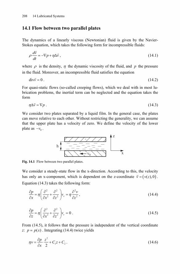
208 14 Lubricated Systems
14.1 Flow between two parallel plates
The dynamics of a linearly viscous (Newtonian) fluid is given by the Navier-Stokes equation, which takes the following form for incompressible fluids:
ρ η= −∇ + Δdv p vdt
, (14.1)
where ρ is the density, η the dynamic viscosity of the fluid, and p the pressure in the fluid. Moreover, an incompressible fluid satisfies the equation
div 0=v . (14.2)
For quasi-static flows (so-called creeping flows), which we deal with in most lu-brication problems, the inertial term can be neglected and the equation takes the form
ηΔ = ∇v p . (14.3)
We consider two plates separated by a liquid film. In the general case, the plates can move relative to each other. Without restricting the generality, we can assume that the upper plate has a velocity of zero. We define the velocity of the lower plate as 0−v .
z
x
-
h
v0 Fig. 14.1 Flow between two parallel plates.
We consider a steady-state flow in the x-direction. According to this, the velocity has only an x-component, which is dependent on the z-coordinate ( )( ),0=v v z . Equation (14.3) takes the following form:
2 2 2
2 2 2η η⎛ ⎞∂ ∂ ∂ ∂
= + =⎜ ⎟∂ ∂ ∂ ∂⎝ ⎠x
p vvx x z z
, (14.4)
2 2
2 2 0η⎛ ⎞∂ ∂ ∂
= + =⎜ ⎟∂ ∂ ∂⎝ ⎠z
p vz x z
. (14.5)
From (14.5), it follows that the pressure is independent of the vertical coordinate z: ( )=p p x . Integrating (14.4) twice yields
2
1 22η ∂
= ⋅ + +∂p zv C z Cx
. (14.6)
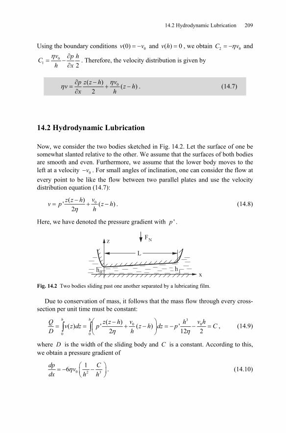
14.2 Hydrodynamic Lubrication 209
Using the boundary conditions 0(0) = −v v and ( ) 0=v h , we obtain 2 0η= −C v and
01 2
v p hCh x
η ∂= −
∂. Therefore, the velocity distribution is given by
0( ) ( )2
vp z z hv z hx h
ηη ∂ −
= + −∂
. (14.7)
14.2 Hydrodynamic Lubrication
Now, we consider the two bodies sketched in Fig. 14.2. Let the surface of one be somewhat slanted relative to the other. We assume that the surfaces of both bodies are smooth and even. Furthermore, we assume that the lower body moves to the left at a velocity 0−v . For small angles of inclination, one can consider the flow at every point to be like the flow between two parallel plates and use the velocity distribution equation (14.7):
0( )' ( )2
vz z hv p z hhη
−= + − . (14.8)
Here, we have denoted the pressure gradient with 'p .
FN
h0
z
L
h1x
Fig. 14.2 Two bodies sliding past one another separated by a lubricating film.
Due to conservation of mass, it follows that the mass flow through every cross-section per unit time must be constant:
3
0 0
0 0
( )( ) ' ( ) '2 12 2
h h v v hQ z z h hv z dz p z h dz p CD hη η
⎛ ⎞−= = + − = − − =⎜ ⎟
⎝ ⎠∫ ∫ , (14.9)
where D is the width of the sliding body and C is a constant. According to this, we obtain a pressure gradient of
0 2 3
16η ⎛ ⎞= − −⎜ ⎟⎝ ⎠
dp Cvdx h h
. (14.10)
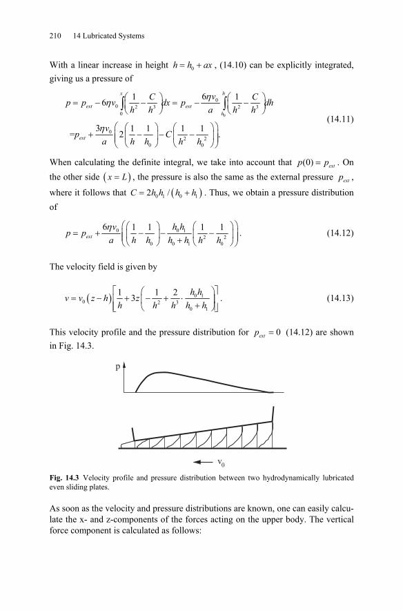
210 14 Lubricated Systems
With a linear increase in height 0= +h h ax , (14.10) can be explicitly integrated, giving us a pressure of
0
00 2 3 2 3
0
02 2
0 0
61 16
3 1 1 1 1 = 2 .
x h
ext exth
ext
vC Cp p v dx p dhah h h h
vp C
a h h h h
ηη
η
⎛ ⎞ ⎛ ⎞= − − = − −⎜ ⎟ ⎜ ⎟⎝ ⎠ ⎝ ⎠
⎛ ⎞⎛ ⎞⎛ ⎞+ − − −⎜ ⎟⎜ ⎟⎜ ⎟⎜ ⎟⎝ ⎠ ⎝ ⎠⎝ ⎠
∫ ∫ (14.11)
When calculating the definite integral, we take into account that (0) = extp p . On the other side ( )=x L , the pressure is also the same as the external pressure extp ,
where it follows that ( )0 1 0 12 /= +C h h h h . Thus, we obtain a pressure distribution of
0 0 12 2
0 0 1 0
6 1 1 1 1η ⎛ ⎞⎛ ⎞⎛ ⎞= + − − −⎜ ⎟⎜ ⎟⎜ ⎟⎜ ⎟+⎝ ⎠ ⎝ ⎠⎝ ⎠
extv h h
p pa h h h h h h
. (14.12)
The velocity field is given by
( ) 0 10 2 3
0 1
1 1 23⎡ ⎤⎛ ⎞
= − + − + ⋅⎢ ⎥⎜ ⎟+⎢ ⎥⎝ ⎠⎣ ⎦
h hv v z h z
h h hh h. (14.13)
This velocity profile and the pressure distribution for 0extp = (14.12) are shown in Fig. 14.3.
v
p
0 Fig. 14.3 Velocity profile and pressure distribution between two hydrodynamically lubricated even sliding plates.
As soon as the velocity and pressure distributions are known, one can easily calcu-late the x- and z-components of the forces acting on the upper body. The vertical force component is calculated as follows:
14.2 Hydrodynamic Lubrication 211
( ) 020
ηα= − =∫N ext
ALvF dxdy p p
h (14.14)
with ( )2
6 2( 1)ln11
ξα ξξξ
⎡ ⎤−= −⎢ ⎥+− ⎣ ⎦
and 1 0/ξ = h h ; =A LD is the apparent “con-
tact area.” The horizontal force component is caused by the viscous stress /σ η= ∂ ∂xz v z and is calculated as
0
00
ηη β
=
∂= =
∂∫RA z
AvvF dxdyz h
, (14.15)
with 1 6( 1)4ln1 1
ξβ ξξ ξ
⎡ ⎤−= −⎢ ⎥− +⎣ ⎦
. We obtain a coefficient of friction of
0 βμα
⎛ ⎞= = ⎜ ⎟⎝ ⎠
R
N
hFF L
. (14.16)
The coefficient of friction is dependent on the average pressure acting on the con-tact area. If we calculate the slot width 0h from (14.14) and insert it into (14.16), we obtain
0 0η ηβ βμα α
= =N
A v vLF LP
. (14.17)
Here, /= NP F A is the average pressure in the contact area. The dependence of
the parameter /β α , as well as /β α , on ξ is shown in Fig. 14.4. In the rele-vant domain of ξ -values, the ratio /β α lies between 5 and 10. Thus, the follow-ing rough estimation for the coefficient of friction is obtained:
010μ ⎛ ⎞≈ ⎜ ⎟⎝ ⎠
hL
. (14.18)
The coefficient of friction is around 10 times the ratio of the smallest width of the slot (i.e. the film thickness) to the length of the contact area. In the large domain of relevant film thickness ratios ξ , the ratio /β α changes only slightly and is roughly equal to 2 (see Fig. 14.4). Hence, a good approximation of (14.17) is
02η
μ ≈v
LP. (14.19)
For the same length of the contact area, the coefficient of friction is a function of the parameter combination 0 /ηv P .
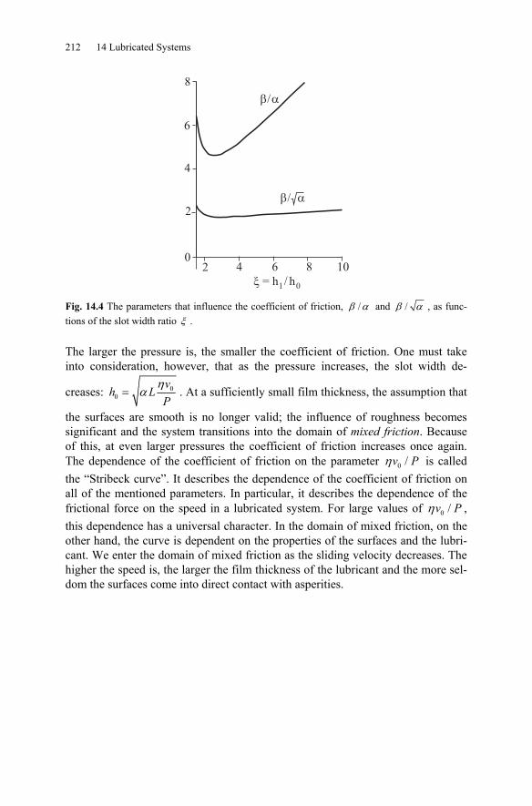
212 14 Lubricated Systems
8
6
4
2
02 4 6 8 10
�/�
�/ �
� = h1/ h0
Fig. 14.4 The parameters that influence the coefficient of friction, /β α and /β α , as func-tions of the slot width ratio ξ .
The larger the pressure is, the smaller the coefficient of friction. One must take into consideration, however, that as the pressure increases, the slot width de-
creases: 00
ηα=
vh L
P. At a sufficiently small film thickness, the assumption that
the surfaces are smooth is no longer valid; the influence of roughness becomes significant and the system transitions into the domain of mixed friction. Because of this, at even larger pressures the coefficient of friction increases once again. The dependence of the coefficient of friction on the parameter 0 /ηv P is called the “Stribeck curve”. It describes the dependence of the coefficient of friction on all of the mentioned parameters. In particular, it describes the dependence of the frictional force on the speed in a lubricated system. For large values of 0 /ηv P , this dependence has a universal character. In the domain of mixed friction, on the other hand, the curve is dependent on the properties of the surfaces and the lubri-cant. We enter the domain of mixed friction as the sliding velocity decreases. The higher the speed is, the larger the film thickness of the lubricant and the more sel-dom the surfaces come into direct contact with asperities.
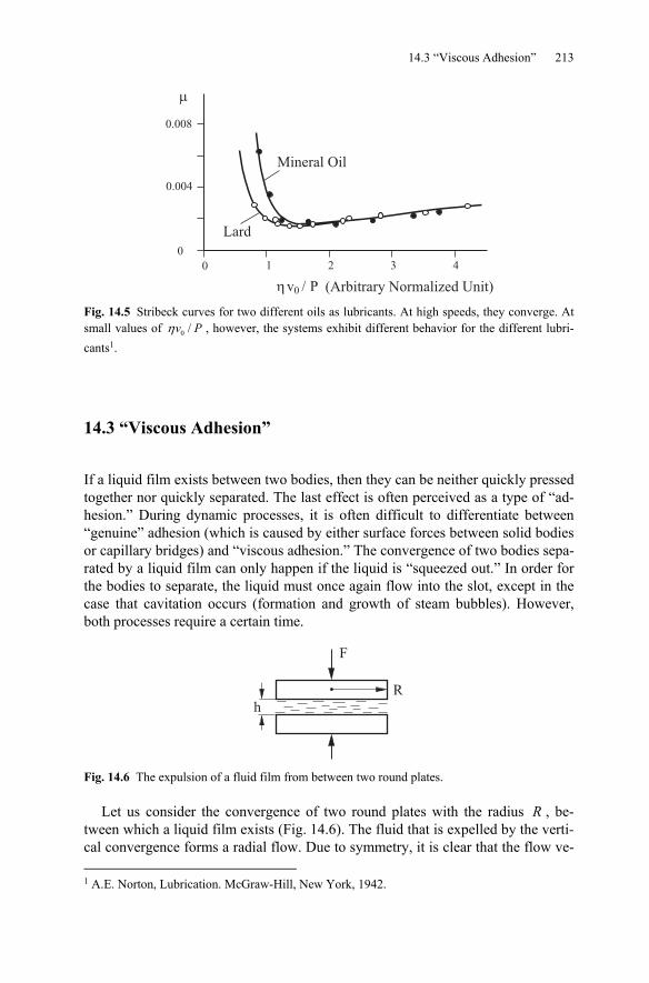
14.3 “Viscous Adhesion” 213
Mineral Oil
Lard
0.008
�
0.004
0
0 1 2 3 4
�v / P0 (Arbitrary Normalized Unit) Fig. 14.5 Stribeck curves for two different oils as lubricants. At high speeds, they converge. At small values of 0 /ηv P , however, the systems exhibit different behavior for the different lubri-cants1.
14.3 “Viscous Adhesion”
If a liquid film exists between two bodies, then they can be neither quickly pressed together nor quickly separated. The last effect is often perceived as a type of “ad-hesion.” During dynamic processes, it is often difficult to differentiate between “genuine” adhesion (which is caused by either surface forces between solid bodies or capillary bridges) and “viscous adhesion.” The convergence of two bodies sepa-rated by a liquid film can only happen if the liquid is “squeezed out.” In order for the bodies to separate, the liquid must once again flow into the slot, except in the case that cavitation occurs (formation and growth of steam bubbles). However, both processes require a certain time.
F
R
h
Fig. 14.6 The expulsion of a fluid film from between two round plates.
Let us consider the convergence of two round plates with the radius R , be-tween which a liquid film exists (Fig. 14.6). The fluid that is expelled by the verti-cal convergence forms a radial flow. Due to symmetry, it is clear that the flow ve- 1 A.E. Norton, Lubrication. McGraw-Hill, New York, 1942.
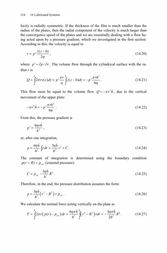
214 14 Lubricated Systems
locity is radially symmetric. If the thickness of the film is much smaller than the radius of the plates, then the radial component of the velocity is much larger than the convergence speed of the plates and we are essentially dealing with a flow be-ing acted upon by a pressure gradient, which we investigated in the first section. According to this, the velocity is equal to
( )'2η−
=z z hv p , (14.20)
where ' /= ∂ ∂p p r . The volume flow through the cylindrical surface with the ra-dius r is
3
0 0
2 ( ) ' ( ) '6
π ππη η
= = − = −∫ ∫h hr rhQ rv z dz p z z h dz p . (14.21)
This flow must be equal to the volume flow 2π= −Q r h , due to the vertical movement of the upper plate:
3
2 '6ππη
− = −rhr h p . (14.22)
From this, the pressure gradient is
3
6' η=
rhph
, (14.23)
or, after one integration,
23 3
6 3η η= = +∫
h hp rdr r Ch h
. (14.24)
The constant of integration is determined using the boundary condition ( ) extp r R p= = (external pressure):
23
3ext
hC p Rhη
= − . (14.25)
Therefore, in the end, the pressure distribution assumes the form:
( )2 23
3ext
hp r R phη
= − + . (14.26)
We calculate the normal force acting vertically on the plate as
( ) ( )2 2 43 3
0 0
6 32 ( )2
R R
exth hF r p r p dr r R rdr R
h hηπ ηππ= − = − = −∫ ∫ . (14.27)
14.3 “Viscous Adhesion” 215
For a given force, we can now calculate the time that is required for the plates to converge from a distance of 0h to a distance of h :
0
4 30
23ηπ
= −∫ ∫t h
h
F dhdtR h
, (14.28)
4 2 20
2 1 1 123ηπ⎛ ⎞
= −⎜ ⎟⎝ ⎠
F tR h h
. (14.29)
For large initial separation distances, this time is practically only dependent on the minimum separation distance, in this case the final separation distance:
4
2
34ηπ
=Rt
Fh. (14.30)
If the force is dependent on the time, then the following is valid:
4
20
3( )4ηπ
=∫t RF t dt
h. (14.31)
This means that the minimum obtainable film thickness is only dependent on the impulse.
In order to illustrate this idea, we consider a body covered with a viscous fluid which is thrown against a ceiling with a velocity v (Fig. 14.7). How long after-wards will it remain hanging on the ceiling? Immediately before the impact, the momentum of the body is equal to Mv . During the impact, the momentum is brought to zero due to the impulse of the reaction force of the ceiling. Thus, the impulse is also equal to Mv . Because the impulse needed to bring the plates to-gether to a distance of h is equal to the impulse needed to separate the plates from a distance of h , then the impulse from gravity, Mgt , must attain a value of Mv in order to “tear” the plate from the ceiling. From this, it follows that =t v g . This is only valid for Newtonian fluids.
From (14.31) it follows that viscous adhesion with Newtonian fluids cannot be used to walk on the ceiling. The situation changes if the viscosity of the liquid is dependent on the velocity gradient. As one can see in Equation (14.31), the im-pulse needed to bring the plates together to a film thickness of h (or to separate the plates to a distance of h) is proportional to viscosity. For non-linearly viscous liq-uids, the viscosity is dependent on the velocity (as a rule, it is smaller at larger ve-locities). If the plates are initially shoved very quickly together and then slowly taken apart, then the positive impulse during impact is smaller than the negative during separation. This difference can be used to hold a moving body in equilib-rium on the ceiling.
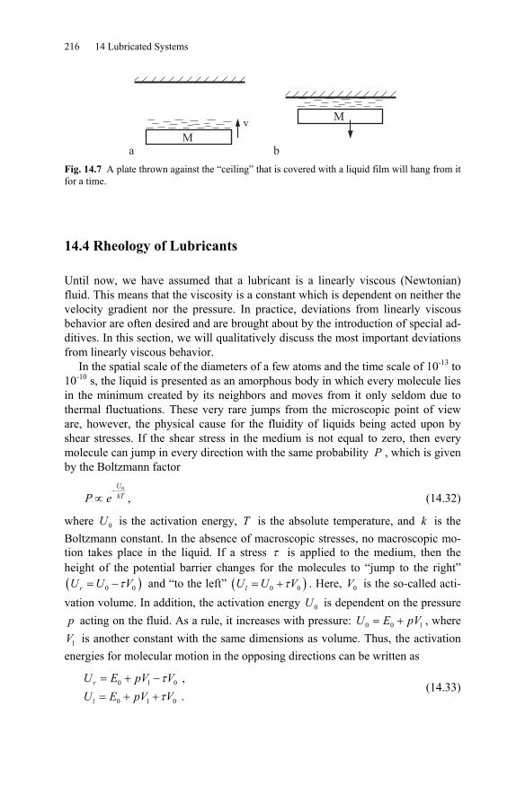
216 14 Lubricated Systems
v
M
M
a b Fig. 14.7 A plate thrown against the “ceiling” that is covered with a liquid film will hang from it for a time.
14.4 Rheology of Lubricants
Until now, we have assumed that a lubricant is a linearly viscous (Newtonian) fluid. This means that the viscosity is a constant which is dependent on neither the velocity gradient nor the pressure. In practice, deviations from linearly viscous behavior are often desired and are brought about by the introduction of special ad-ditives. In this section, we will qualitatively discuss the most important deviations from linearly viscous behavior.
In the spatial scale of the diameters of a few atoms and the time scale of 10-13 to 10-10 s, the liquid is presented as an amorphous body in which every molecule lies in the minimum created by its neighbors and moves from it only seldom due to thermal fluctuations. These very rare jumps from the microscopic point of view are, however, the physical cause for the fluidity of liquids being acted upon by shear stresses. If the shear stress in the medium is not equal to zero, then every molecule can jump in every direction with the same probability P , which is given by the Boltzmann factor
0−
∝UkTP e , (14.32)
where 0U is the activation energy, T is the absolute temperature, and k is the Boltzmann constant. In the absence of macroscopic stresses, no macroscopic mo-tion takes place in the liquid. If a stress τ is applied to the medium, then the height of the potential barrier changes for the molecules to “jump to the right” ( )0 0τ= −rU U V and “to the left” ( )0 0τ= +lU U V . Here, 0V is the so-called acti-vation volume. In addition, the activation energy 0U is dependent on the pressure p acting on the fluid. As a rule, it increases with pressure: 0 0 1= +U E pV , where
1V is another constant with the same dimensions as volume. Thus, the activation energies for molecular motion in the opposing directions can be written as
0 1 0
0 1 0
, .
r
l
U E pV VU E pV V
ττ
= + −
= + + (14.33)
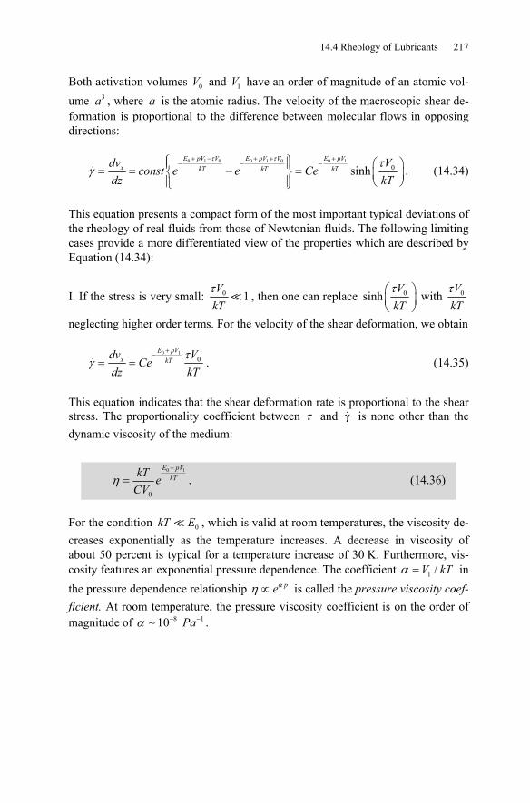
14.4 Rheology of Lubricants 217
Both activation volumes 0V and 1V have an order of magnitude of an atomic vol-ume 3a , where a is the atomic radius. The velocity of the macroscopic shear de-formation is proportional to the difference between molecular flows in opposing directions:
0 1 0 0 1 0 0 1
0sinhE pV V E pV V E pV
x kT kT kTdv Vconst e e Ce
dz kT
τ τ τγ
+ − + + +− − −⎧ ⎫ ⎛ ⎞⎪ ⎪= = − =⎨ ⎬ ⎜ ⎟
⎝ ⎠⎪ ⎪⎩ ⎭. (14.34)
This equation presents a compact form of the most important typical deviations of the rheology of real fluids from those of Newtonian fluids. The following limiting cases provide a more differentiated view of the properties which are described by Equation (14.34):
I. If the stress is very small: 0 1τVkT
, then one can replace 0sinhτ⎛ ⎞⎜ ⎟⎝ ⎠
VkT
with 0τVkT
neglecting higher order terms. For the velocity of the shear deformation, we obtain
0 1
0E pV
x kTdv VCe
dz kTτ
γ+
−= = . (14.35)
This equation indicates that the shear deformation rate is proportional to the shear stress. The proportionality coefficient between τ and γ is none other than the dynamic viscosity of the medium:
0 1
0
η+
=E pV
kTkT eCV
. (14.36)
For the condition 0kT E , which is valid at room temperatures, the viscosity de-creases exponentially as the temperature increases. A decrease in viscosity of about 50 percent is typical for a temperature increase of 30 K. Furthermore, vis-cosity features an exponential pressure dependence. The coefficient 1 /α =V kT in the pressure dependence relationship αη ∝ pe is called the pressure viscosity coef-ficient. At room temperature, the pressure viscosity coefficient is on the order of magnitude of 8 110α − −∼ Pa .
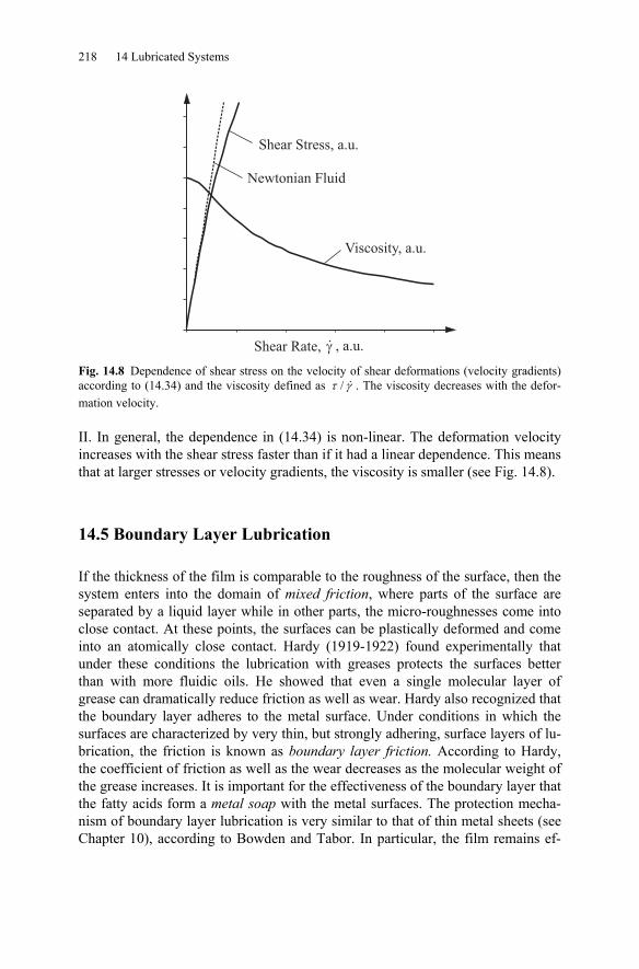
218 14 Lubricated Systems
Fig. 14.8 Dependence of shear stress on the velocity of shear deformations (velocity gradients) according to (14.34) and the viscosity defined as /τ γ . The viscosity decreases with the defor-mation velocity.
II. In general, the dependence in (14.34) is non-linear. The deformation velocity increases with the shear stress faster than if it had a linear dependence. This means that at larger stresses or velocity gradients, the viscosity is smaller (see Fig. 14.8).
14.5 Boundary Layer Lubrication
If the thickness of the film is comparable to the roughness of the surface, then the system enters into the domain of mixed friction, where parts of the surface are separated by a liquid layer while in other parts, the micro-roughnesses come into close contact. At these points, the surfaces can be plastically deformed and come into an atomically close contact. Hardy (1919-1922) found experimentally that under these conditions the lubrication with greases protects the surfaces better than with more fluidic oils. He showed that even a single molecular layer of grease can dramatically reduce friction as well as wear. Hardy also recognized that the boundary layer adheres to the metal surface. Under conditions in which the surfaces are characterized by very thin, but strongly adhering, surface layers of lu-brication, the friction is known as boundary layer friction. According to Hardy, the coefficient of friction as well as the wear decreases as the molecular weight of the grease increases. It is important for the effectiveness of the boundary layer that the fatty acids form a metal soap with the metal surfaces. The protection mecha-nism of boundary layer lubrication is very similar to that of thin metal sheets (see Chapter 10), according to Bowden and Tabor. In particular, the film remains ef-
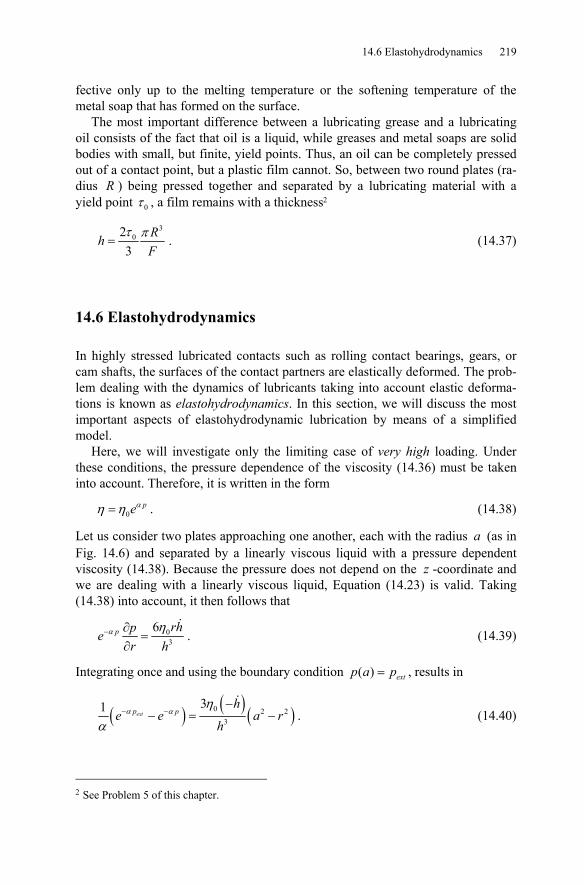
14.6 Elastohydrodynamics 219
fective only up to the melting temperature or the softening temperature of the metal soap that has formed on the surface.
The most important difference between a lubricating grease and a lubricating oil consists of the fact that oil is a liquid, while greases and metal soaps are solid bodies with small, but finite, yield points. Thus, an oil can be completely pressed out of a contact point, but a plastic film cannot. So, between two round plates (ra-dius R ) being pressed together and separated by a lubricating material with a yield point 0τ , a film remains with a thickness2
3
023
RhF
τ π= . (14.37)
14.6 Elastohydrodynamics
In highly stressed lubricated contacts such as rolling contact bearings, gears, or cam shafts, the surfaces of the contact partners are elastically deformed. The prob-lem dealing with the dynamics of lubricants taking into account elastic deforma-tions is known as elastohydrodynamics. In this section, we will discuss the most important aspects of elastohydrodynamic lubrication by means of a simplified model.
Here, we will investigate only the limiting case of very high loading. Under these conditions, the pressure dependence of the viscosity (14.36) must be taken into account. Therefore, it is written in the form
0peαη η= . (14.38)
Let us consider two plates approaching one another, each with the radius a (as in Fig. 14.6) and separated by a linearly viscous liquid with a pressure dependent viscosity (14.38). Because the pressure does not depend on the z -coordinate and we are dealing with a linearly viscous liquid, Equation (14.23) is valid. Taking (14.38) into account, it then follows that
03
6p rhper h
α η− ∂=
∂. (14.39)
Integrating once and using the boundary condition ( ) extp a p= , results in
( ) ( ) ( )0 2 23
31extp p
he e a r
hα α
η
α− −
−− = − . (14.40)
2 See Problem 5 of this chapter.
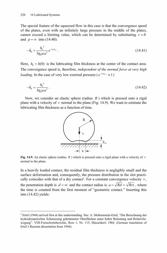
220 14 Lubricated Systems
The special feature of the squeezed flow in this case is that the convergence speed of the plates, even with an infinitely large pressure in the middle of the plates, cannot exceed a limiting value, which can be determined by substituting 0r = and p = ∞ into (14.40):
3
00 2
03extph
h ea
α
η α−− = . (14.41)
Here, 0 (0)h h= is the lubricating film thickness at the center of the contact area. The convergence speed is, therefore, independent of the normal force at very high loading. In the case of very low external pressure ( 1extpe α− ≈ )
3
00 2
03h
haη α
− = . (14.42)
Now, we consider an elastic sphere (radius R ) which is pressed onto a rigid plane with a velocity of v normal to the plane (Fig. 14.9). We want to estimate the lubricating film thickness as a function of time.
0
R
h
v
a Fig. 14.9. An elastic sphere (radius R ) which is pressed onto a rigid plane with a velocity of v normal to the plane.
In a heavily loaded contact, the residual film thickness is negligibly small and the surface deformation and, consequently, the pressure distribution in the slot practi-cally coincides with that of a dry contact3. For a constant convergence velocity v , the penetration depth is d vt= and the contact radius is a Rd Rvt= = , where the time is counted from the first moment of “geometric contact.” Inserting this into (14.42) yields:
3 Ertel (1944) arrived first at this understanding. See: A. Mohrenstein-Ertel, “Die Berechnung der hydrodynamischen Schmierung gekrümmter Oberflächen unter hoher Belastung und Relativbe-wegung”. VDI-Fortschrittsberichte, Row 1, Nr. 115, Düsseldorf, 1984. (German translation of Ertel’s Russian dissertation from 1944).
14.6 Elastohydrodynamics 221
3 3
0 00 2
00 33h h
hRvta η αη α
− = = . (14.43)
Integration yields ( ) ( )2 20 0 01 / 1/ 2 / 3 ln /− =h h Rv t tαη , or in the case of 0h h ,
( )020
1 2 ln /3
t tRvh αη
= . (14.44)
Equation (14.42) is valid under the condition 0 1pα . Thus, for the lower inte-gration limit 0t in (14.44), we insert the time at which the condition 0 1pα ≈ is met, where 0p is the Hertzian pressure at the center of the contact area:
1/21/2
* * 02 2 1vtdE E
R Rα απ π
⎛ ⎞⎛ ⎞ = ≈⎜ ⎟ ⎜ ⎟⎝ ⎠ ⎝ ⎠. (14.45)
From this, it follows that
2
0 2 *24Rt
v Eπα
≈ . (14.46)
The lubricating film thickness is
1/2 1/ 2 1/ 2 1/ 2 1/ 2
01/ 22 *2
1/22
3
42 ln
v Rh
v E tR
α η
απ
=⎛ ⎞⎛ ⎞⎜ ⎟⎜ ⎟
⎝ ⎠⎝ ⎠
. (14.47)
We use this result in order to estimate the film thickness in a lubricated, heavily loaded rolling contact between an elastic sphere (radius R) and an elastic planar body. One can qualitatively consider rolling as the repetitive “placement” of the sphere, where the characteristic “placement time” is given by 2 /t a v≈ ; v is the rolling velocity and a is the contact radius (5.24). Inserting the estimated time into Equation (14.47) yields
1/ 2 1/2 1/2 1/2 1/ 2
01/21/3 2 *5/3 1/3
1/22/3 2
3
3 82 ln4
v Rh
E FR
α η
απ
=⎛ ⎞⎛ ⎞⎛ ⎞⎜ ⎟⎜ ⎟⎜ ⎟⎜ ⎟⎜ ⎟⎝ ⎠⎝ ⎠⎝ ⎠
. (14.48)
The thickness of the lubricating film is only slightly dependent (logarithmically) on the modulus of elasticity and the normal force. For the typical values
8 12 10 Paα − −= ⋅ , 0 0.01 Pa sη = ⋅ , 1 kNF = , 0.025 mR = , * 100 GPaE = , and 1 m/sv = , we obtain an estimation of 0.8 μm≈h .
222 14 Lubricated Systems
Exact numerical solutions from Dowson and Hamrock show4 that the film thickness can be described by the following empirical equations: for a linear con-tact ( l is the length of the bearing contact),
( ) 0 10 56 0 69 0 69 * 0 03 0 410 03.06 /h v E R F lα η −−= ⋅ . (14.49)
For an elliptical point contact,
( )0 53 0 67 0 67 * 0 03 0 47 0 067 0 730 02.69 1 0.61h v E R F e χα η − − −= ⋅ − ⋅ , (14.50)
where /a bχ = , a and b are the semi-axes of the contact ellipse perpendicular and parallel to the direction of motion, and R is the radius of curvature in the plane of motion.
14.7 Solid Lubricants
Under certain conditions, liquid lubricants cannot be applied to reduce friction and wear. Space flight applications are one example where tribological systems must function reliably in either vacuum or in extremely high or low temperatures. In these cases, solid lubricants can be used.
Precursors of today’s solid lubricants – lead, graphite, and molybdenite ( 2MoS ) – have been known for ages. All three substances have similar colors (from grayish-blue to black) and are easily spread on a counter body. Until the 18th century, they were often mistaken for one another. Lead was replaced by graphite and graphite with molybdenite. The name “molybdenite” itself stems from the Greek Μόλυβδος, which means lead. In England, graphite was known as “plum-bago,” which can also be traced back to lead.
The extensive propagation of graphite and molybdenite as solid lubricants was only possible after methods to produce highly pure substances were developed. Both substances were applied at the end of the 19th century and during the 1930’s, respectively, in the form of suspensions.
The most important properties of a solid lubricant are its strong adhesion to sur-faces in friction and its easy deformability. Apart from the layered structure of graphite and molybdenite, other factors may be important. For example, graphite has good lubricating properties only in the presence of a small amount of water or oxygen, but loses its lubricating properties in a vacuum. In contrast, the lubricat-ing properties of molybdenite improve under “water-free” conditions.
As a rule, materials used in modern industry as solid lubricants have a layered structure similar to that of graphite and molybdenite. It is apparent that the mecha- 4 B.J. Hamrock and D. Dowson, Ball Bearing Lubrication. Wiley, New York, 386 S, 1981.
Problems 223
nism of the lubricating action of solid lubricants is similar to that of boundary layer lubrication.
Problems
Problem 1: Calculate the force of friction between a corrugated surface with a pe-riodic profile of cosa kx and an even plane which are separated by a liquid film.
Solution: We will define the separation distance between the two surfaces as
( )=h h x . The gradient ′h is assumed to be very small. Let the slot in between the surfaces be filled with a lubricant with a viscosity of η . The velocity profile of a creeping flow in a parallel slot has the form (14.7):
0( )' ( )2
vz z hv p z hhη
−= + −
with a pressure gradient (14.10)
0 2 3
16η ⎛ ⎞= − −⎜ ⎟⎝ ⎠
dp Cvdx h h
.
Integrating over a spatial period Λ yields
0 2 30
1( ) (0) 6 0( ) ( )
ηΛ ⎛ ⎞
Λ − = − − =⎜ ⎟⎝ ⎠∫
Cp p v dxh x h x
.
Here, we set this integral equal to zero, because the pressure distribution is as-sumed to be a periodic function with the same period Λ as the profile of the cor-rugated surface. From this, it follows that
20
30
( )
( )
Λ
Λ=∫
∫
dxh x
Cdx
h x
.
The shear stress acting in the liquid on the even (lower) surface is equal to
00 2
0
4 32
η∂τ η η∂ =
′ ⎛ ⎞= = − + = −⎜ ⎟⎝ ⎠z
vv p h Cvz h h h
.
For the tangential stress averaged over the period, which we perceive as macro-scopic friction τ R , we obtain
224 14 Lubricated Systems
02
0 0
1 4 3( ) ( )
ητ τ
Λ Λ ⎛ ⎞= = −⎜ ⎟Λ Λ ⎝ ⎠
∫ ∫Rv Cdx dx
h x h x,
or after substituting C ,
1 2
03 2
0 0 0
4 3( ) ( ) ( )
ητ
−Λ Λ Λ⎛ ⎞⎛ ⎞ ⎛ ⎞⎜ ⎟= − ⎜ ⎟ ⎜ ⎟⎜ ⎟Λ ⎝ ⎠ ⎝ ⎠⎝ ⎠∫ ∫ ∫R
v dx dx dxh x h x h x
.
For a constant slot width, this equation becomes the elementary formula 0 /τ η=R v h . Now, we assume that the corrugated surface is given through the
equation
( )0( ) 1 cos( )= + −h x h a kx
so that the minimum slot width is 0h , the amplitude of the corrugations a , and the wave number 2 /π= Λk . In this case, it follows that
2 20 0 0
2 230 0 0 20
2 3121 2 /
ητ
+ +=
+ ++R
v h h a ah h h a aa h
.
In the limiting case 0h a , it is
0
0
2η
τ ≈Rvah
.
Problem 2: Calculate the force that acts between a plane and a sphere (radius R ) approaching this plane. The distance between the sphere and the plane should be much smaller than R .
Solution: In this case, we are dealing purely with the squeezing of a fluid caused by a pressure gradient. The pressure gradient is calculated according to Equation (14.23):
3
6' η=
rhph
.
In our case, the slot height is given by 2
0 / 2≈ +h h r R .
Integrating the pressure gradient, we obtain
( ) ( )3 22 20 0
36/ 2 / 2
ηη∞
= − = −+ +
∫ext extr
rdr Rhp p h ph r R h r R
.
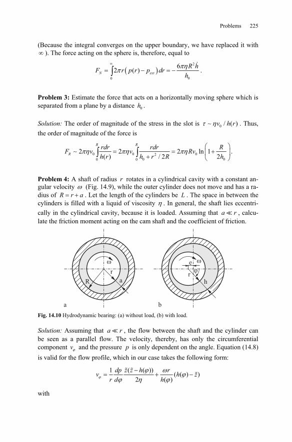
Problems 225
(Because the integral converges on the upper boundary, we have replaced it with ∞ ). The force acting on the sphere is, therefore, equal to
( )2
00
62 ( ) πηπ∞
= − = −∫N extR hF r p r p dr
h.
Problem 3: Estimate the force that acts on a horizontally moving sphere which is separated from a plane by a distance 0h .
Solution: The order of magnitude of the stress in the slot is 0 / ( )τ η∼ v h r . Thus, the order of magnitude of the force is
0 0 02000 0
2 2 2 ln 1( ) 2/ 2
πη πη πη⎛ ⎞
= = +⎜ ⎟+ ⎝ ⎠∫ ∫∼R R
Rrdr rdr RF v v Rvh r hh r R
.
Problem 4: A shaft of radius r rotates in a cylindrical cavity with a constant an-gular velocity ω (Fig. 14.9), while the outer cylinder does not move and has a ra-dius of = +R r a . Let the length of the cylinders be L . The space in between the cylinders is filled with a liquid of viscosity η . In general, the shaft lies eccentri-cally in the cylindrical cavity, because it is loaded. Assuming that a r , calcu-late the friction moment acting on the cam shaft and the coefficient of friction.
R a
�
r
h
�
r�
e
a b Fig. 14.10 Hydrodynamic bearing: (a) without load, (b) with load.
Solution: Assuming that a r , the flow between the shaft and the cylinder can be seen as a parallel flow. The velocity, thereby, has only the circumferential component ϕv and the pressure p is only dependent on the angle. Equation (14.8) is valid for the flow profile, which in our case takes the following form:
1 ( ( )) ( ( ) )2 ( )
dp z z h rv h zr d hϕ
ϕ ω ϕϕ η ϕ
−= + −
with
226 14 Lubricated Systems
( ) cosϕ ϕ≈ +h a e .
The pressure distribution is given by
22 3
0
1( ) (0) 6( ) ( )
ϕ
ϕ ηω ϕϕ ϕ
⎛ ⎞− = + −⎜ ⎟
⎝ ⎠∫
Cp p r dh h
,
where 2
20
2
30
( )
( )
π
π
ϕϕϕϕ
=∫
∫
dh
Cd
h
(see analogous equations in Problem 1). It is an odd function of the angle ϕ . The
horizontal component of the force 2
0
( ) cosπ
ϕ ϕ ϕ= ∫xF Lr p d vanishes, because
( )ϕp is an odd function. The vertical component of the force is calculated as5
( )2 2 3
32 3 2 2 2 2
0 0
1 12( )sin 6 (1 cos )( ) ( ) 2
π π π ηωϕ ϕ ϕ ηω ϕ ϕϕ ϕ
⎛ ⎞= = − − − =⎜ ⎟
+ −⎝ ⎠∫ ∫z
C eLrF Lr p d Lr dh h a e a e
.
The tangential stress is calculated in exactly the same way as in Problem 1 and is
2
4 3( ) ( )
τ ηωϕ ϕ
⎛ ⎞= − −⎜ ⎟
⎝ ⎠
Crh h
.
The moment is
( )( )
3 2 22 22 3
2 2 2 2 20 0
4 24 3( )( ) ( ) 2
π π πηωτ ϕ ϕ ηω ϕ
ϕ ϕ
+⎛ ⎞= = − − = −⎜ ⎟
⎝ ⎠ − +∫ ∫
r L a eCM Lr d L r dh h a e a e
.
For the ratio /μ = zM rF , which plays the role of the coefficient of friction in this case, we obtain
( )2 22
3μ
+=
a e
er.
For larger loads, when →e a , the coefficient of friction assumes the limiting value
5 In reality, the viscous stress also contributes to the vertical force. One can show, however, that this contribution is small under the assumed conditions and can be neglected.
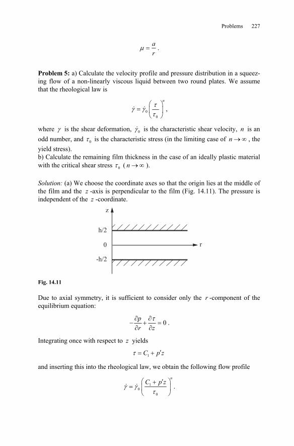
Problems 227
μ =ar
.
Problem 5: a) Calculate the velocity profile and pressure distribution in a squeez-ing flow of a non-linearly viscous liquid between two round plates. We assume that the rheological law is
00
nτγ γτ⎛ ⎞
= ⎜ ⎟⎝ ⎠
,
where γ is the shear deformation, 0γ is the characteristic shear velocity, n is an odd number, and 0τ is the characteristic stress (in the limiting case of n →∞ , the yield stress). b) Calculate the remaining film thickness in the case of an ideally plastic material with the critical shear stress 0τ ( n →∞ ). Solution: (a) We choose the coordinate axes so that the origin lies at the middle of the film and the z -axis is perpendicular to the film (Fig. 14.11). The pressure is independent of the z -coordinate.
z
h/2
-h/2
0 r
Fig. 14.11
Due to axial symmetry, it is sufficient to consider only the r -component of the equilibrium equation:
0∂ ∂− + =∂ ∂pr z
τ .
Integrating once with respect to z yields
1C p zτ ′= +
and inserting this into the rheological law, we obtain the following flow profile
10
0
nC p z
γ γτ
′⎛ ⎞+= ⎜ ⎟
⎝ ⎠.
228 14 Lubricated Systems
The constant 1C must vanish, because ( 0) 0zγ = = must be fulfilled due to rea-sons of symmetry. The equation can now be written in the form
00
nv p zz
γτ
⎛ ⎞′∂= ⎜ ⎟∂ ⎝ ⎠
Integration yields
102
0
'1
nnpv z C
nγ
τ+⎛ ⎞
= +⎜ ⎟+ ⎝ ⎠.
Taking into account the no-slip condition ( ) ( )/ 2 / 2 0v h v h= − = on the solid sur-face, we ultimately come to the following flow profile in the slot:
110
0
'1 2
n nnp hv z
nγ
τ
++
⎛ ⎞⎛ ⎞− ⎛ ⎞= −⎜ ⎟⎜ ⎟ ⎜ ⎟⎜ ⎟+ ⎝ ⎠⎝ ⎠ ⎝ ⎠.
The volume flow through a cylinder barrel with the radius r is calculated as
/2 20
10/2
'2 ( )d 22 2
nh n
nh
p hQ r v z z rnγ
π πτ
+
+−
⎛ ⎞−= = ⎜ ⎟+ ⎝ ⎠
∫ .
From continuity, it follows that
22 0
10
'22 2
n n
n
p hr h rnγ
π πτ
+
+
⎛ ⎞−− = ⎜ ⎟+ ⎝ ⎠
.
For the pressure gradient we get 1/
0 20
22n
n
p nh rr h
τγ +
⎛ ⎞∂ +− = −⎜ ⎟∂ ⎝ ⎠
.
Integrating this equation with the boundary condition 0( )p R p= , we obtain the pressure distribution in the film:
1/ 1 11 1
0 0 2 10
2 121
n
n nn
n
np p h R rh
τγ
+ +
+
⎛ ⎞⎛ ⎞+− = − −⎜ ⎟⎜ ⎟ +⎝ ⎠ ⎝ ⎠
.
The normal force acting on the plate is equal to
( )13 1/
00 21 00
2 22 d3 1
nR n
n
n R nF r p p r hn
h
τ ππγ
+
+
⎛ ⎞+= − = −⎜ ⎟+ ⎝ ⎠∫ .
For 1n = (linearly viscous fluid), we again call upon Equation (14.27).
.
Problems 229
(b) In the limiting case of n →∞ , the equations for pressure distribution and force simplify to
0 02 R rp ph
τ −− =
and 3
023
RFh
τ π= .
In this case, we are dealing with an ideally plastic behavior with a yield point of 0τ . From this equation, the thickness of the film, which remains in the slot and is
not pressed out, can be calculated: 3
023
RhF
τ π= .
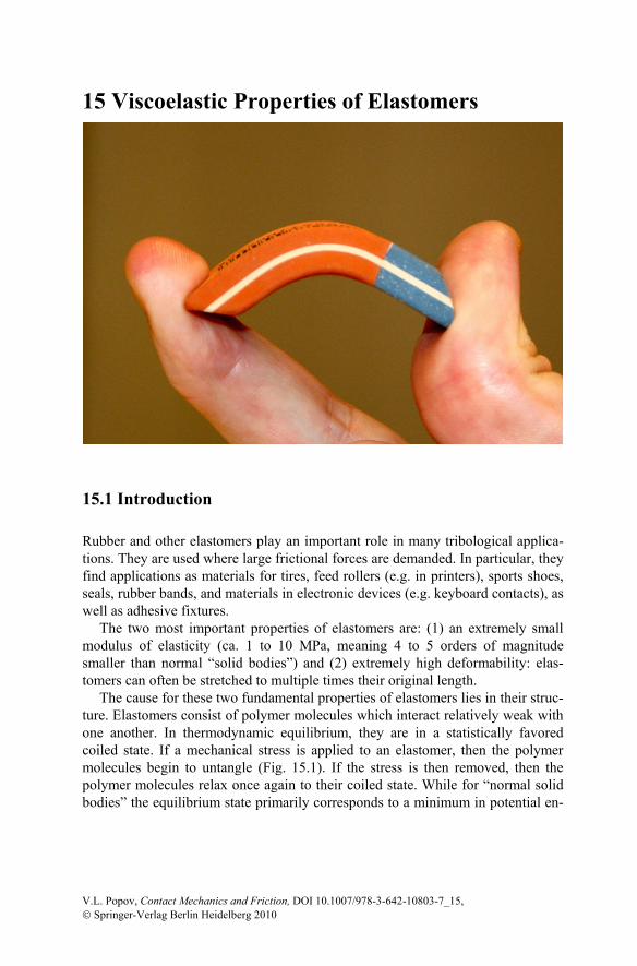
15 Viscoelastic Properties of Elastomers
15.1 Introduction
Rubber and other elastomers play an important role in many tribological applica-tions. They are used where large frictional forces are demanded. In particular, they find applications as materials for tires, feed rollers (e.g. in printers), sports shoes, seals, rubber bands, and materials in electronic devices (e.g. keyboard contacts), as well as adhesive fixtures.
The two most important properties of elastomers are: (1) an extremely small modulus of elasticity (ca. 1 to 10 MPa, meaning 4 to 5 orders of magnitude smaller than normal “solid bodies”) and (2) extremely high deformability: elas-tomers can often be stretched to multiple times their original length.
The cause for these two fundamental properties of elastomers lies in their struc-ture. Elastomers consist of polymer molecules which interact relatively weak with one another. In thermodynamic equilibrium, they are in a statistically favored coiled state. If a mechanical stress is applied to an elastomer, then the polymer molecules begin to untangle (Fig. 15.1). If the stress is then removed, then the polymer molecules relax once again to their coiled state. While for “normal solid bodies” the equilibrium state primarily corresponds to a minimum in potential en-
V.L. Popov, Contact Mechanics and Friction, DOI 10.1007/978-3-642-10803-7_15, © Springer-Verlag Berlin Heidelberg 2010
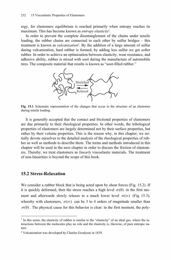
232 15 Viscoelastic Properties of Elastomers
ergy, for elastomers equilibrium is reached primarily when entropy reaches its maximum. This has become known as entropy elasticity1.
In order to prevent the complete disentanglement of the chains under tensile loading, the rubber chains are connected to each other by sulfur bridges – this treatment is known as vulcanization2. By the addition of a large amount of sulfur during vulcanization, hard rubber is formed; by adding less sulfur we get softer rubber. In order to achieve an optimization between elasticity, wear resistance, and adhesive ability, rubber is mixed with soot during the manufacture of automobile tires. The composite material that results is known as “soot-filled rubber.”
Fig. 15.1 Schematic representation of the changes that occur in the structure of an elastomer during tensile loading.
It is generally accepted that the contact and frictional properties of elastomers are due primarily to their rheological properties. In other words, the tribological properties of elastomers are largely determined not by their surface properties, but rather by their volume properties. This is the reason why, in this chapter, we ini-tially devote ourselves to the detailed analysis of the rheological properties of rub-ber as well as methods to describe them. The terms and methods introduced in this chapter will be used in the next chapter in order to discuss the friction of elastom-ers. Thereby, we treat elastomers as linearly viscoelastic materials. The treatment of non-linearities is beyond the scope of this book.
15.2 Stress-Relaxation
We consider a rubber block that is being acted upon by shear forces (Fig. 15.2). If it is quickly deformed, then the stress reaches a high level (0)σ in the first mo-ment and afterwards slowly relaxes to a much lower level ( )σ ∞ (Fig. 15.3), whereby with elastomers, ( )σ ∞ can be 3 to 4 orders of magnitude smaller than
(0)σ . The physical cause for this behavior is clear: in the first moment, the poly-
1 In this sense, the elasticity of rubber is similar to the “elasticity” of an ideal gas, where the in-teractions between the molecules play no role and the elasticity is, likewise, of pure entropic na-ture. 2 Vulcanization was developed by Charles Goodyear in 1839.
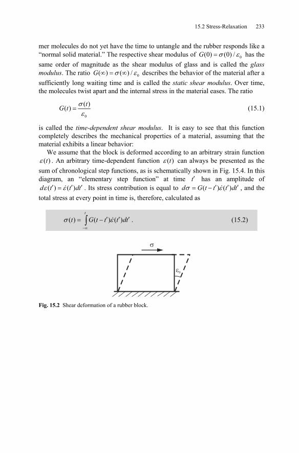
15.2 Stress-Relaxation 233
mer molecules do not yet have the time to untangle and the rubber responds like a “normal solid material.” The respective shear modulus of 0(0) (0) /σ ε=G has the same order of magnitude as the shear modulus of glass and is called the glass modulus. The ratio 0( ) ( ) /σ ε∞ = ∞G describes the behavior of the material after a sufficiently long waiting time and is called the static shear modulus. Over time, the molecules twist apart and the internal stress in the material eases. The ratio
0
( )( ) σε
=tG t (15.1)
is called the time-dependent shear modulus. It is easy to see that this function completely describes the mechanical properties of a material, assuming that the material exhibits a linear behavior:
We assume that the block is deformed according to an arbitrary strain function ( )ε t . An arbitrary time-dependent function ( )ε t can always be presented as the
sum of chronological step functions, as is schematically shown in Fig. 15.4. In this diagram, an “elementary step function” at time ′t has an amplitude of
( ) ( )ε ε′ ′ ′=d t t dt . Its stress contribution is equal to ( ) ( )σ ε′ ′ ′= −d G t t t dt , and the total stress at every point in time is, therefore, calculated as
( ) ( ) ( )σ ε−∞
′ ′ ′= −∫t
t G t t t dt . (15.2)
�
��
Fig. 15.2 Shear deformation of a rubber block.
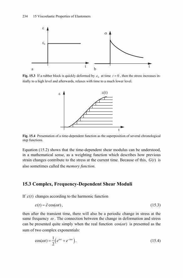
234 15 Viscoelastic Properties of Elastomers
�
��
�
t ta b
Fig. 15.3 If a rubber block is quickly deformed by 0ε at time 0t = , then the stress increases in-itially to a high level and afterwards, relaxes with time to a much lower level.
�
t
�� �t
Fig. 15.4 Presentation of a time-dependent function as the superposition of several chronological step functions.
Equation (15.2) shows that the time-dependent shear modulus can be understood, in a mathematical sense, as a weighting function which describes how previous strain changes contribute to the stress at the current time. Because of this, ( )G t is also sometimes called the memory function.
15.3 Complex, Frequency-Dependent Shear Moduli
If ( )ε t changes according to the harmonic function
( ) cos( )ε ε ω=t t , (15.3)
then after the transient time, there will also be a periodic change in stress at the same frequency ω . The connection between the change in deformation and stress can be presented quite simply when the real function cos( )ωt is presented as the sum of two complex exponentials:
( )1cos( )2
ω ωω −= +i t i tt e e . (15.4)
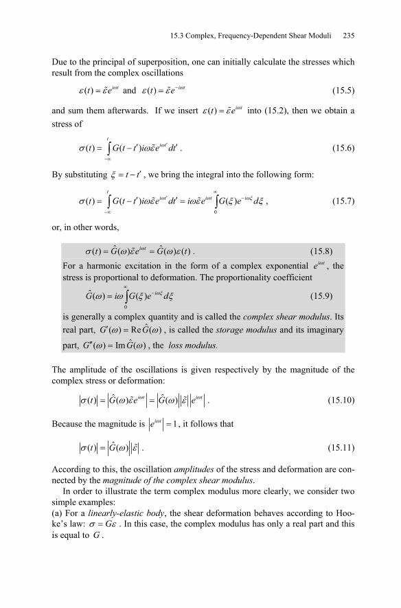
15.3 Complex, Frequency-Dependent Shear Moduli 235
Due to the principal of superposition, one can initially calculate the stresses which result from the complex oscillations
( ) ωε ε= i tt e and ( ) ωε ε −= i tt e (15.5)
and sum them afterwards. If we insert ( ) ωε ε= i tt e into (15.2), then we obtain a stress of
( ) ( ) ωσ ωε ′
−∞
′ ′= −∫t
i tt G t t i e dt . (15.6)
By substituting ξ ′= −t t , we bring the integral into the following form:
0
( ) ( ) ( )ω ω ωξσ ωε ωε ξ ξ∞
′ −
−∞
′ ′= − =∫ ∫t
i t i t it G t t i e dt i e G e d , (15.7)
or, in other words,
ˆ ˆ( ) ( ) ( ) ( )ωσ ω ε ω ε= =i tt G e G t . (15.8) For a harmonic excitation in the form of a complex exponential ωi te , the stress is proportional to deformation. The proportionality coefficient
0
ˆ ( ) ( ) ωξω ω ξ ξ∞
−= ∫ iG i G e d (15.9)
is generally a complex quantity and is called the complex shear modulus. Its real part, ˆ( ) Re ( )ω ω′ =G G , is called the storage modulus and its imaginary
part, ˆ( ) Im ( )ω ω′′ =G G , the loss modulus.
The amplitude of the oscillations is given respectively by the magnitude of the complex stress or deformation:
ˆ ˆ( ) ( ) ( )ω ωσ ω ε ω ε= =i t i tt G e G e . (15.10)
Because the magnitude is 1ω =i te , it follows that
ˆ( ) ( )σ ω ε=t G . (15.11)
According to this, the oscillation amplitudes of the stress and deformation are con-nected by the magnitude of the complex shear modulus.
In order to illustrate the term complex modulus more clearly, we consider two simple examples: (a) For a linearly-elastic body, the shear deformation behaves according to Hoo-ke’s law: σ ε= G . In this case, the complex modulus has only a real part and this is equal to G .
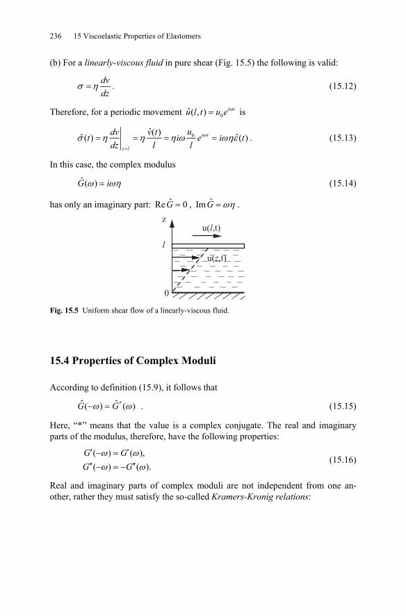
236 15 Viscoelastic Properties of Elastomers
(b) For a linearly-viscous fluid in pure shear (Fig. 15.5) the following is valid:
σ η= dvdz
. (15.12)
Therefore, for a periodic movement 0ˆ( , ) ω= i tu l t u e is
0ˆ( ) ˆˆ ( ) ( )ωσ η η η ω ωηε=
= = = =i t
z l
udv v tt i e i tdz l l
. (15.13)
In this case, the complex modulus
ˆ ( )ω ωη=G i (15.14)
has only an imaginary part: ˆRe 0=G , ˆIm ωη=G .
u( ,t)l
u( ,t)z
0
l
z
Fig. 15.5 Uniform shear flow of a linearly-viscous fluid.
15.4 Properties of Complex Moduli
According to definition (15.9), it follows that
*ˆ ˆ( ) ( ) ω ω− =G G . (15.15)
Here, “*” means that the value is a complex conjugate. The real and imaginary parts of the modulus, therefore, have the following properties:
( ) ( ),
( ) ( ).G GG G
ω ωω ω
′ ′− =′′ ′′− = −
(15.16)
Real and imaginary parts of complex moduli are not independent from one an-other, rather they must satisfy the so-called Kramers-Kronig relations:
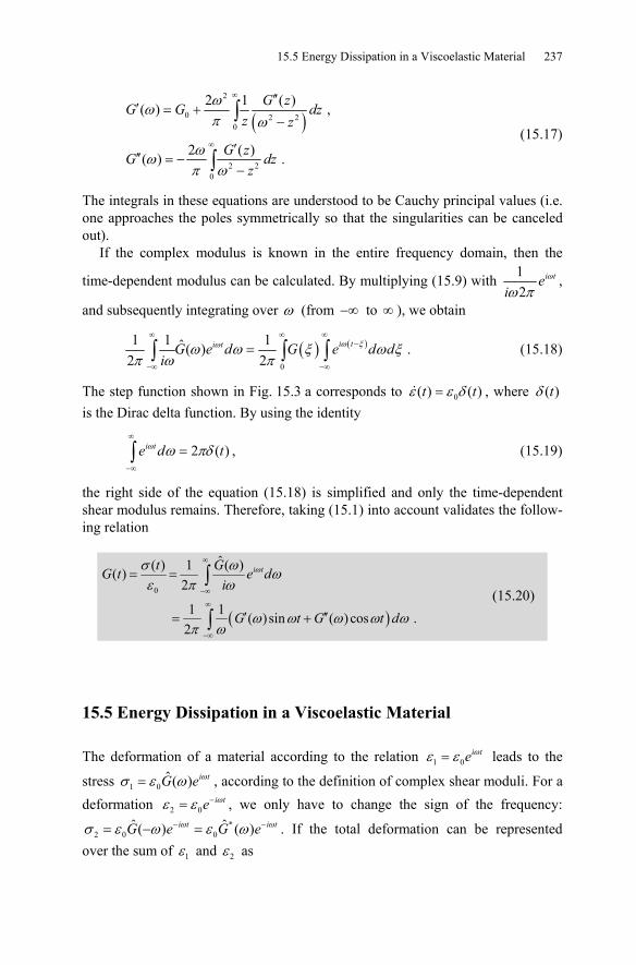
15.5 Energy Dissipation in a Viscoelastic Material 237
( )
2
0 2 20
2 20
2 1 ( )( ) ,
2 ( )( ) .
ωωπ ω
ωωπ ω
∞
∞
′′′ = +
−
′′′ = −
−
∫
∫
G zG G dzz z
G zG dzz
(15.17)
The integrals in these equations are understood to be Cauchy principal values (i.e. one approaches the poles symmetrically so that the singularities can be canceled out).
If the complex modulus is known in the entire frequency domain, then the
time-dependent modulus can be calculated. By multiplying (15.9) with 12
ω
ω πi te
i,
and subsequently integrating over ω (from −∞ to ∞ ), we obtain
( ) ( )
0
1 1 1ˆ ( )2 2
ω ξωω ω ξ ω ξπ ω π
∞ ∞ ∞−
−∞ −∞
=∫ ∫ ∫ i ti tG e d G e d di
. (15.18)
The step function shown in Fig. 15.3 a corresponds to 0( ) ( )ε ε δ=t t , where ( )δ t is the Dirac delta function. By using the identity
2 ( )ω ω πδ∞
−∞
=∫ i te d t , (15.19)
the right side of the equation (15.18) is simplified and only the time-dependent shear modulus remains. Therefore, taking (15.1) into account validates the follow-ing relation
( )
0
ˆ( ) 1 ( )( )2
1 1 ( ) sin ( ) cos .2
i tt GG t e di
G t G t d
ωσ ω ωε π ω
ω ω ω ω ωπ ω
∞
−∞
∞
−∞
= =
′ ′′= +
∫
∫ (15.20)
15.5 Energy Dissipation in a Viscoelastic Material
The deformation of a material according to the relation 1 0ωε ε= i te leads to the
stress 1 0ˆ ( ) ωσ ε ω= i tG e , according to the definition of complex shear moduli. For a
deformation 2 0ωε ε −= i te , we only have to change the sign of the frequency:
*2 0 0
ˆ ˆ( ) ( )ω ωσ ε ω ε ω− −= − =i t i tG e G e . If the total deformation can be represented over the sum of 1ε and 2ε as
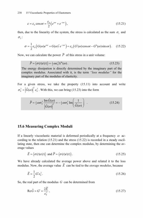
238 15 Viscoelastic Properties of Elastomers
( )00 cos
2ω ωε
ε ε ω −= = +i t i tt e e , (15.21)
then, due to the linearity of the system, the stress is calculated as the sum 1σ and
2σ :
( ) ( )*0 0
1 ( ) ( ) ( ) cos ( )sin2
ω ωσ ε ω ω ε ω ω ω ω− ′ ′′= + = −i t i tG e G e G t G t . (15.22)
Now, we can calculate the power P of this stress in a unit volume:
2102( ) ( ) ( )σ ε ωε ω′′= =P t t G . (15.23)
The energy dissipation is directly determined by the imaginary part of the complex modulus. Associated with it, is the term “loss modulus” for the imaginary part of the modulus of elasticity.
For a given stress, we take the property (15.11) into account and write 22 2
0 0ˆ ( )σ ω ε= G . With this, we can bring (15.23) into the form
2 21 10 02 22
ˆIm ( ) 1Im ˆˆ ( )( )
ωωσ ωσωω
⎛ ⎞= = − ⎜ ⎟⎜ ⎟
⎝ ⎠
GPGG
. (15.24)
15.6 Measuring Complex Moduli
If a linearly viscoelastic material is deformed periodically at a frequency ω ac-cording to the relation (15.21) and the stress (15.22) is recorded in a steady oscil-lating state, then one can determine the complex modulus, by determining the av-erage values
( ) ( ) and ( ) ( )E t t P t tσ ε σ ε= = . (15.25)
We have already calculated the average power above and related it to the loss modulus. Now, the average value E can be tied to the storage modulus, because
20
12
ε′=E G . (15.26)
So, the real part of the modulus G can be determined from
20
2ˆReε
′= =EG G , (15.27)
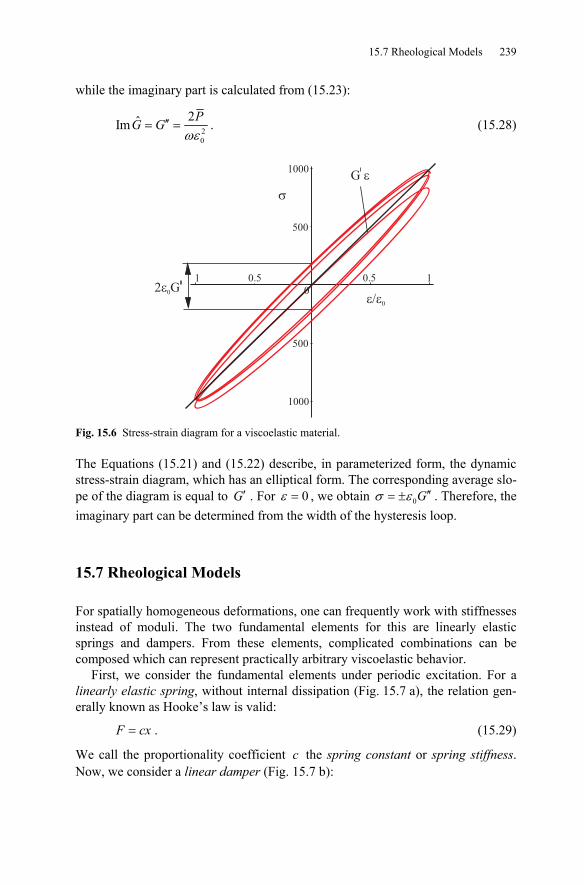
15.7 Rheological Models 239
while the imaginary part is calculated from (15.23):
20
2ˆImωε
′′= =PG G . (15.28)
G �
���G
����
�
1 0.5 0.5 1
1000
500
0
500
1000
Fig. 15.6 Stress-strain diagram for a viscoelastic material.
The Equations (15.21) and (15.22) describe, in parameterized form, the dynamic stress-strain diagram, which has an elliptical form. The corresponding average slo-pe of the diagram is equal to ′G . For 0ε = , we obtain 0σ ε ′′= ± G . Therefore, the imaginary part can be determined from the width of the hysteresis loop.
15.7 Rheological Models
For spatially homogeneous deformations, one can frequently work with stiffnesses instead of moduli. The two fundamental elements for this are linearly elastic springs and dampers. From these elements, complicated combinations can be composed which can represent practically arbitrary viscoelastic behavior.
First, we consider the fundamental elements under periodic excitation. For a linearly elastic spring, without internal dissipation (Fig. 15.7 a), the relation gen-erally known as Hooke’s law is valid:
=F cx . (15.29)
We call the proportionality coefficient c the spring constant or spring stiffness. Now, we consider a linear damper (Fig. 15.7 b):
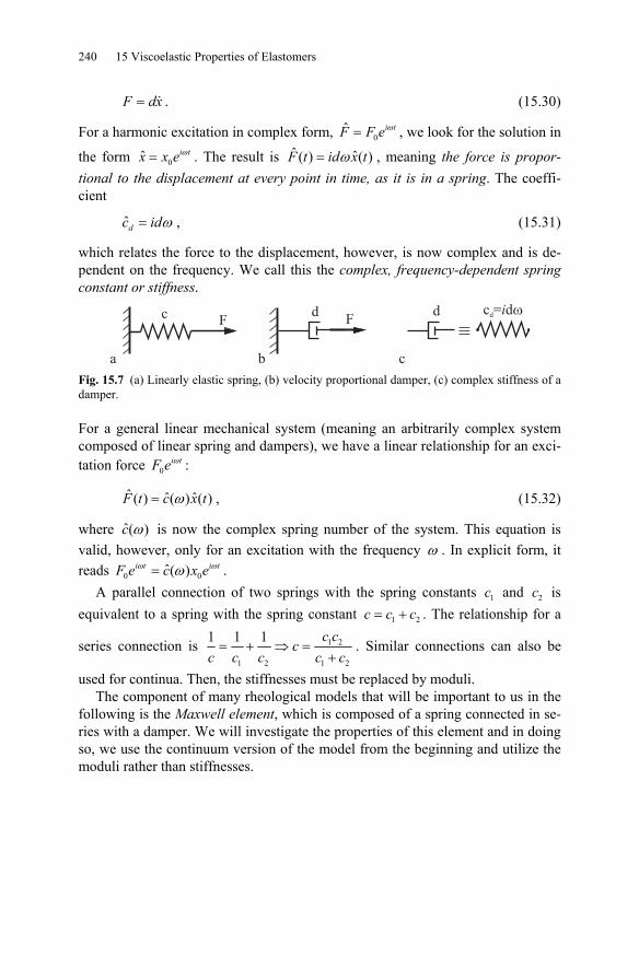
240 15 Viscoelastic Properties of Elastomers
=F dx . (15.30)
For a harmonic excitation in complex form, 0ˆ ω= i tF F e , we look for the solution in
the form 0ˆ i tx x e ω= . The result is ˆ ˆ( ) ( )ω=F t id x t , meaning the force is propor-tional to the displacement at every point in time, as it is in a spring. The coeffi-cient
ˆ ω=dc id , (15.31)
which relates the force to the displacement, however, is now complex and is de-pendent on the frequency. We call this the complex, frequency-dependent spring constant or stiffness.
cF
dF
d c = dd i
a b c Fig. 15.7 (a) Linearly elastic spring, (b) velocity proportional damper, (c) complex stiffness of a damper.
For a general linear mechanical system (meaning an arbitrarily complex system composed of linear spring and dampers), we have a linear relationship for an exci-tation force 0
ωi tF e :
ˆ ˆ ˆ( ) ( ) ( )ω=F t c x t , (15.32)
where ˆ( )ωc is now the complex spring number of the system. This equation is valid, however, only for an excitation with the frequency ω . In explicit form, it reads 0 0ˆ( )i t i tF e c x eω ωω= .
A parallel connection of two springs with the spring constants 1c and 2c is equivalent to a spring with the spring constant 1 2= +c c c . The relationship for a
series connection is 1 2
1 2 1 2
1 1 1= + ⇒ =
+c c
cc c c c c
. Similar connections can also be
used for continua. Then, the stiffnesses must be replaced by moduli. The component of many rheological models that will be important to us in the
following is the Maxwell element, which is composed of a spring connected in se-ries with a damper. We will investigate the properties of this element and in doing so, we use the continuum version of the model from the beginning and utilize the moduli rather than stiffnesses.
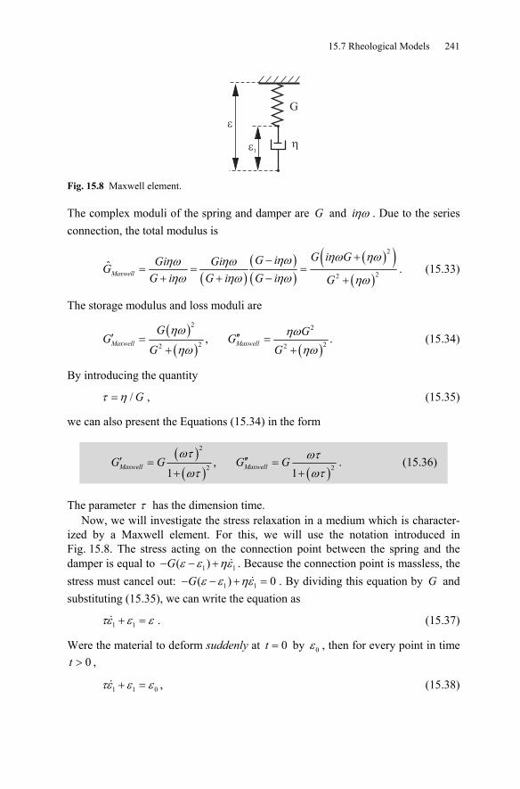
15.7 Rheological Models 241
G
�
�1
Fig. 15.8 Maxwell element.
The complex moduli of the spring and damper are G and ηωi . Due to the series connection, the total modulus is
( )
( )( )
( )( )( )
2
22ˆ
Maxwell
G i GG iGi GiGG i G i G i G
ηω ηωηωηω ηωηω ηω ηω ηω
+−= = =
+ + − +. (15.33)
The storage modulus and loss moduli are
( )( ) ( )
2 2
2 22 2, .
ηω ηωηω ηω
′ ′′= =+ +
Maxwell Maxwell
G GG GG G
(15.34)
By introducing the quantity
/τ η= G , (15.35)
we can also present the Equations (15.34) in the form
( )( ) ( )
2
2 2, 1 1
ωτ ωτωτ ωτ
′ ′′= =+ +
Maxwell MaxwellG G G G . (15.36)
The parameter τ has the dimension time. Now, we will investigate the stress relaxation in a medium which is character-
ized by a Maxwell element. For this, we will use the notation introduced in Fig. 15.8. The stress acting on the connection point between the spring and the damper is equal to 1 1( )ε ε ηε− − +G . Because the connection point is massless, the stress must cancel out: 1 1( ) 0ε ε ηε− − + =G . By dividing this equation by G and substituting (15.35), we can write the equation as
1 1τε ε ε+ = . (15.37)
Were the material to deform suddenly at 0=t by 0ε , then for every point in time 0>t ,
1 1 0τε ε ε+ = , (15.38)
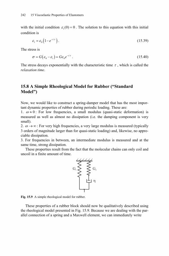
242 15 Viscoelastic Properties of Elastomers
with the initial condition 1(0) 0ε = . The solution to this equation with this initial condition is
( )/1 0 1 τε ε −= − te . (15.39)
The stress is
( ) /0 1 0
τσ ε ε ε −= − = tG G e . (15.40)
The stress decays exponentially with the characteristic time τ , which is called the relaxation time.
15.8 A Simple Rheological Model for Rubber (“Standard Model”)
Now, we would like to construct a spring-damper model that has the most impor-tant dynamic properties of rubber during periodic loading. These are: 1. 0ω ≈ : For low frequencies, a small modulus (quasi-static deformation) is measured as well as almost no dissipation (i.e. the damping component is very small). 2. ω →∞ : For very high frequencies, a very large modulus is measured (typically 3 orders of magnitude larger than for quasi-static loading) and, likewise, no appre-ciable dissipation. 3. For frequencies in between, an intermediate modulus is measured and at the same time, strong dissipation.
These properties result from the fact that the molecular chains can only coil and uncoil in a finite amount of time.
G2
G1
Fig. 15.9 A simple rheological model for rubber.
These properties of a rubber block should now be qualitatively described using the rheological model presented in Fig. 15.9. Because we are dealing with the par-allel connection of a spring and a Maxwell element, we can immediately write
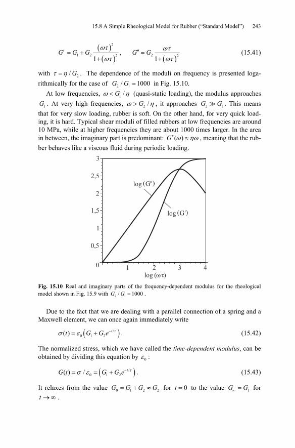
15.8 A Simple Rheological Model for Rubber (“Standard Model”) 243
( )( ) ( )
2
1 2 22 2, 1 1
ωτ ωτωτ ωτ
′ ′′= + =+ +
G G G G G (15.41)
with 2/τ η= G . The dependence of the moduli on frequency is presented loga-rithmically for the case of 2 1/ 1000=G G in Fig. 15.10.
At low frequencies, 1 /ω η< G (quasi-static loading), the modulus approaches
1G . At very high frequencies, 2 /ω η> G , it approaches 2 1G G . This means that for very slow loading, rubber is soft. On the other hand, for very quick load-ing, it is hard. Typical shear moduli of filled rubbers at low frequencies are around 10 MPa, while at higher frequencies they are about 1000 times larger. In the area in between, the imaginary part is predominant: ( )ω ηω′′ ≈G , meaning that the rub-ber behaves like a viscous fluid during periodic loading.
log ( )
3
2,5
2
1,5
1
0,5
0 1 2 3 4
log ( )G
log ( )G
� Fig. 15.10 Real and imaginary parts of the frequency-dependent modulus for the rheological model shown in Fig. 15.9 with 2 1/ 1000=G G .
Due to the fact that we are dealing with a parallel connection of a spring and a Maxwell element, we can once again immediately write
( )/0 1 2( ) τσ ε −= + tt G G e . (15.42)
The normalized stress, which we have called the time-dependent modulus, can be obtained by dividing this equation by 0ε :
( )/0 1 2( ) / τσ ε −= = + tG t G G e . (15.43)
It relaxes from the value 0 1 2 2= + ≈G G G G for 0=t to the value 1∞ =G G for →∞t .
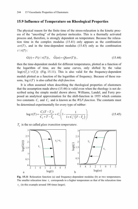
244 15 Viscoelastic Properties of Elastomers
15.9 Influence of Temperature on Rheological Properties
The physical reason for the finite time of the stress-relaxation is the kinetic proc-ess of the “uncoiling” of the polymer molecules. This is a thermally activated process and, therefore, is strongly dependent on temperature. Because the relaxa-tion time in the complex modulus (15.41) only appears as the combination
( )ωτ T , and in the time-dependent modulus (15.43) only as the combination / ( )τt T :
( ) ( / ( ))τ=G t F t T , ˆ ( ) ( ( ))ω ωτ=G Q T , (15.44)
then the time-dependent moduli for different temperatures, plotted as a function of the logarithm of time, are the same curves, only shifted by the value
2 1log( ( ) / ( ))τ τT T (Fig. 15.11). This is also valid for the frequency-dependent moduli plotted as a function of the logarithm of frequency. Because of these rea-sons, log ( )τ T is also called the shift-function.
It is often assumed when describing the rheological properties of elastomers that the assumption made above (15.44) is valid even when the rheology is not de-scribed using the simple model shown above. Williams, Landel, and Ferry pro-posed an analytical approximation for the shift-function in 1955 which contains two constants 1C and 2C and is known as the WLF-function. The constants must be determined experimentally for every type of rubber:
( )
11 1
2 2
( ) 1log ( ) 11
τ−
⎛ ⎞−⎜ ⎟= = −⎜ ⎟+ − + −⎝ ⎠
g
g g
C T TT C
C T T C T T. (15.45)
gT is the so called glass transition temperature.
log(
)G
2 1 0 1 2 3 4 5
2
3
2.5
1.5
1
0.5
05 4 3 2 1 0 1 2
2
3
2.5
1.5
1
0.5
0
log(G
(t))
log(t) log( )
�1
� �2 1>
�1
�2
a b Fig. 15.11 Relaxation function (a) and frequency-dependent modulus (b) at two temperatures. The smaller relaxation time 1τ corresponds to a higher temperature as that of the relaxation time
2τ (in this example around 100 times larger).
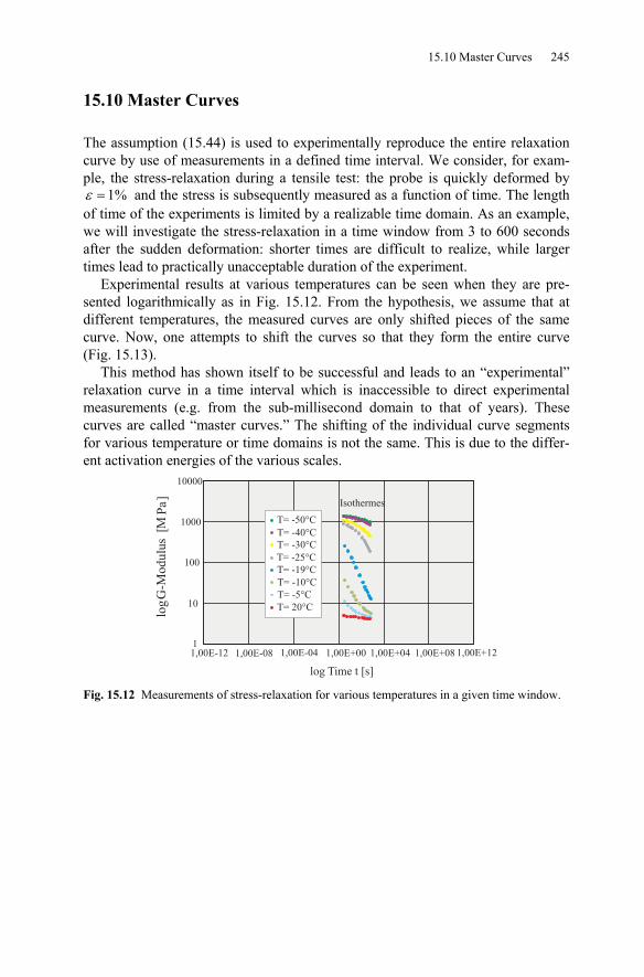
15.10 Master Curves 245
15.10 Master Curves
The assumption (15.44) is used to experimentally reproduce the entire relaxation curve by use of measurements in a defined time interval. We consider, for exam-ple, the stress-relaxation during a tensile test: the probe is quickly deformed by
1%ε = and the stress is subsequently measured as a function of time. The length of time of the experiments is limited by a realizable time domain. As an example, we will investigate the stress-relaxation in a time window from 3 to 600 seconds after the sudden deformation: shorter times are difficult to realize, while larger times lead to practically unacceptable duration of the experiment.
Experimental results at various temperatures can be seen when they are pre-sented logarithmically as in Fig. 15.12. From the hypothesis, we assume that at different temperatures, the measured curves are only shifted pieces of the same curve. Now, one attempts to shift the curves so that they form the entire curve (Fig. 15.13).
This method has shown itself to be successful and leads to an “experimental” relaxation curve in a time interval which is inaccessible to direct experimental measurements (e.g. from the sub-millisecond domain to that of years). These curves are called “master curves.” The shifting of the individual curve segments for various temperature or time domains is not the same. This is due to the differ-ent activation energies of the various scales.
Fig. 15.12 Measurements of stress-relaxation for various temperatures in a given time window.
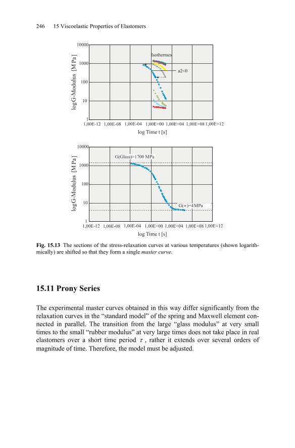
246 15 Viscoelastic Properties of Elastomers
Fig. 15.13 The sections of the stress-relaxation curves at various temperatures (shown logarith-mically) are shifted so that they form a single master curve.
15.11 Prony Series
The experimental master curves obtained in this way differ significantly from the relaxation curves in the “standard model” of the spring and Maxwell element con-nected in parallel. The transition from the large “glass modulus” at very small times to the small “rubber modulus” at very large times does not take place in real elastomers over a short time period τ , rather it extends over several orders of magnitude of time. Therefore, the model must be adjusted.
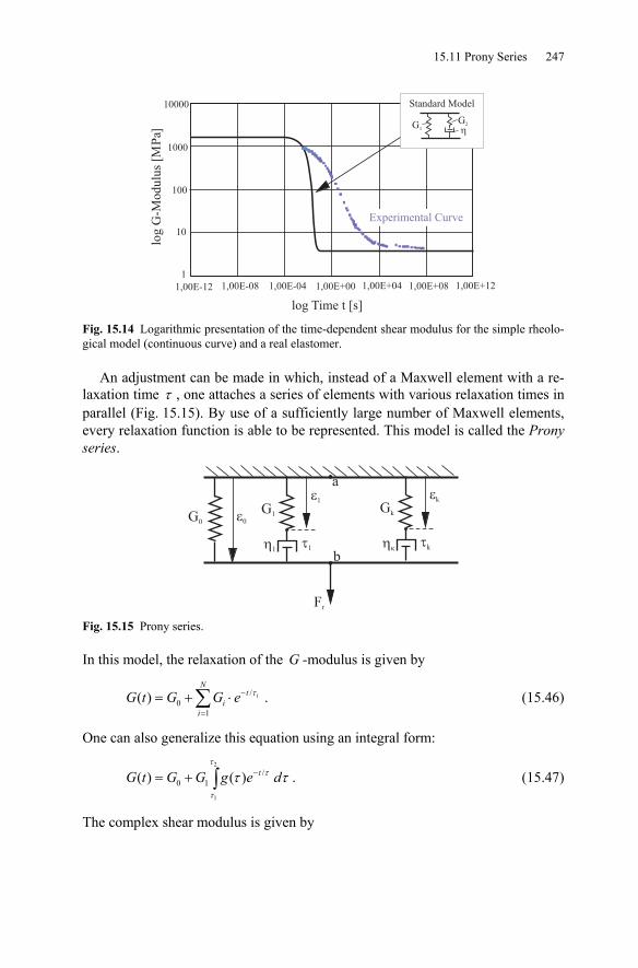
15.11 Prony Series 247
Fig. 15.14 Logarithmic presentation of the time-dependent shear modulus for the simple rheolo-gical model (continuous curve) and a real elastomer.
An adjustment can be made in which, instead of a Maxwell element with a re-laxation time τ , one attaches a series of elements with various relaxation times in parallel (Fig. 15.15). By use of a sufficiently large number of Maxwell elements, every relaxation function is able to be represented. This model is called the Prony series.
�0
�
G0
G1
�1
�1
Gk
�k
�k
a
b
Fr Fig. 15.15 Prony series.
In this model, the relaxation of the G -modulus is given by
/0
1
( ) τ−
=
= + ⋅∑ i
Nt
ii
G t G G e . (15.46)
One can also generalize this equation using an integral form:
2
1
/0 1( ) ( )
ττ
τ
τ τ−= + ∫ tG t G G g e d . (15.47)
The complex shear modulus is given by
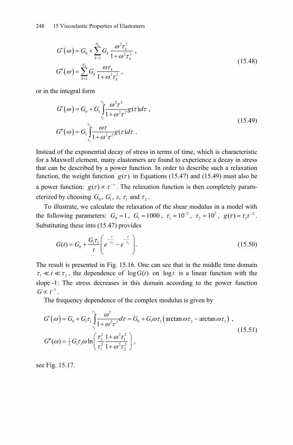
248 15 Viscoelastic Properties of Elastomers
( )
( )
2 2
0 2 21
2 21
,1
,1
ω τω
ω τ
ωτω
ω τ
=
=
′ = ++
′′ =+
∑
∑
k
k
Nk
kk k
Nk
kk k
G G G
G G (15.48)
or in the integral form
( )
( )
2
1
2
1
2 2
0 1 2 2
1 2 2
( ) ,1
( ) .1
τ
τ
τ
τ
ω τω τ τ
ω τ
ωτω τ τω τ
′ = ++
′′ =+
∫
∫
G G G g d
G G g d
(15.49)
Instead of the exponential decay of stress in terms of time, which is characteristic for a Maxwell element, many elastomers are found to experience a decay in stress that can be described by a power function. In order to describe such a relaxation function, the weight function ( )τg in Equations (15.47) and (15.49) must also be a power function: ( )τ τ −∝ sg . The relaxation function is then completely param-eterized by choosing 0 1 1 2, , , and G G s τ τ .
To illustrate, we calculate the relaxation of the shear modulus in a model with the following parameters: 0 1=G , 1 1000=G , 2
1 10τ −= , 22 10τ = , 2
1( )τ τ τ −=g . Substituting these into (15.47) provides
2 11 10( ) τ ττ − −⎛ ⎞
= + −⎜ ⎟⎜ ⎟⎝ ⎠
t tGG t G e e
t. (15.50)
The result is presented in Fig. 15.16. One can see that in the middle time domain 1 2τ τt , the dependence of log ( )G t on log t is a linear function with the
slope -1: The stress decreases in this domain according to the power function 1−∝G t .
The frequency dependence of the complex modulus is given by
( ) ( )
2
1
2
0 1 1 0 1 1 2 12 2
2 2 22 11
1 12 2 2 21 2
arctan arctan ,1
1( ) ln ,
1
G G G d G G
G G
τ
τ
ωω τ τ ωτ ωτ ωτω τ
τ ω τω τ ω
τ ω τ
′ = + = + −+
⎛ ⎞+′′ = ⎜ ⎟+⎝ ⎠
∫ (15.51)
see Fig. 15.17.
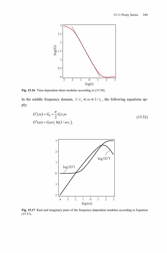
15.11 Prony Series 249
3
2.5
2
1.5
1
0.5
03 2 1 0 1 2 3
log(t)
log(G
)
Fig. 15.16 Time-dependent shear modulus according to (15.50).
In the middle frequency domain, 2 11/ 1/τ ω τ , the following equations ap-ply:
( )
( )0 1 1
1 1 1
2( ) ln 1/ .
πω τ ω
ω ωτ ωτ
′ = +
′′ =
G G G
G G (15.52)
3
2
1
0
3
1
2
4 2 1 0 1 2 3
log ( )G
log()
log ( )G
Fig. 15.17 Real and imaginary parts of the frequency-dependent modulus according to Equation (15.51).
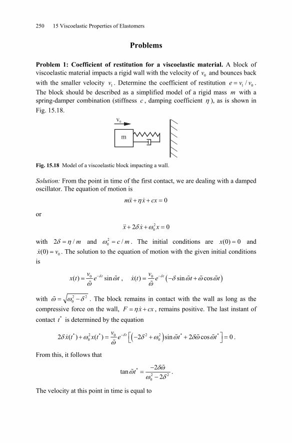
250 15 Viscoelastic Properties of Elastomers
Problems
Problem 1: Coefficient of restitution for a viscoelastic material. A block of viscoelastic material impacts a rigid wall with the velocity of 0v and bounces back with the smaller velocity 1v . Determine the coefficient of restitution 1 0/=e v v . The block should be described as a simplified model of a rigid mass m with a spring-damper combination (stiffness c , damping coefficient η ), as is shown in Fig. 15.18.
m
v0
Fig. 15.18 Model of a viscoelastic block impacting a wall.
Solution: From the point in time of the first contact, we are dealing with a damped oscillator. The equation of motion is
0mx x cxη+ + =
or 202 0δ ω+ + =x x x
with 2 /δ η= m and 20 /ω = c m . The initial conditions are (0) 0=x and
0(0) =x v . The solution to the equation of motion with the given initial conditions is
0( ) sinδ ωω
−= tvx t e t , ( )0( ) sin cosδ δ ω ω ω
ω−= − +tv
x t e t t
with 2 20ω ω δ= − . The block remains in contact with the wall as long as the
compressive force on the wall, η= +F x cx , remains positive. The last instant of contact *t is determined by the equation
( )* 2 * 2 2 * *00 02 ( ) ( ) 2 sin 2 cos 0δδ ω δ ω ω δω ω
ω− ⎡ ⎤+ = − + + =⎣ ⎦
tvx t x t e t t .
From this, it follows that
*2 20
2tan2δωω
ω δ−
=−
t .
The velocity at this point in time is equal to
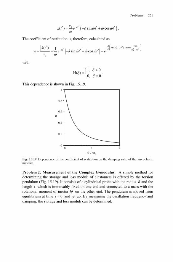
Problems 251
( )** * *0( ) sin cosδ δ ω ω ωω
−= − +tvx t e t t .
The coefficient of restitution is, therefore, calculated as
2 20 2 2*
0
2* H( 2 ) arctan2* *
0
( ) 1 sin cosδ δωπ ω δω ω δδ δ ω ω ω
ω
⎛ ⎞⎜ ⎟− − −⎜ ⎟−− ⎝ ⎠= = − + =t
x te e t t e
v
with
1, 0H( )
0, 0ξ
ξξ>⎧
= ⎨ <⎩.
This dependence is shown in Fig. 15.19. 1
0.8
0.6
0.4
e
0.2
00 1 2
� / 0 Fig. 15.19 Dependence of the coefficient of restitution on the damping ratio of the viscoelastic material.
Problem 2: Measurement of the Complex G-modulus. A simple method for determining the storage and loss moduli of elastomers is offered by the torsion pendulum (Fig. 15.19). It consists of a cylindrical probe with the radius R and the length l which is immovably fixed on one end and connected to a mass with the rotational moment of inertia Θ on the other end. The pendulum is moved from equilibrium at time 0=t and let go. By measuring the oscillation frequency and damping, the storage and loss moduli can be determined.
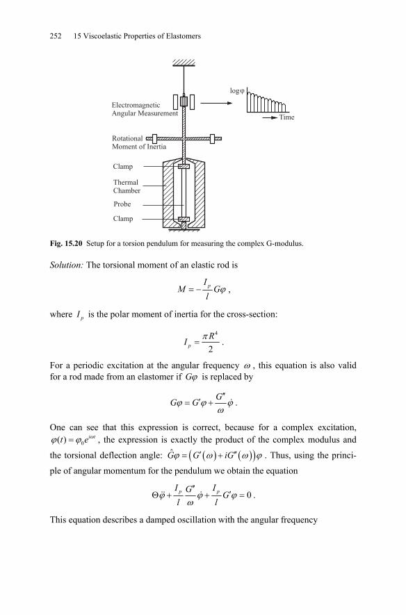
252 15 Viscoelastic Properties of Elastomers
Fig. 15.20 Setup for a torsion pendulum for measuring the complex G-modulus.
Solution: The torsional moment of an elastic rod is
= − pIM G
lϕ ,
where pI is the polar moment of inertia for the cross-section:
4
2=p
RI π .
For a periodic excitation at the angular frequency ω , this equation is also valid for a rod made from an elastomer if Gϕ is replaced by
′′′= +
GG Gϕ ϕ ϕω
.
One can see that this expression is correct, because for a complex excitation, 0( ) = i tt e ωϕ ϕ , the expression is exactly the product of the complex modulus and
the torsional deflection angle: ( ) ( )( )ˆ ′ ′′= +G G iGϕ ω ω ϕ . Thus, using the princi-
ple of angular momentum for the pendulum we obtain the equation
0′′
′Θ + + =p pI IG Gl l
ϕ ϕ ϕω
.
This equation describes a damped oscillation with the angular frequency
Problems 253
′≈
ΘpI G
lω
and the logarithmic decrement
2′′
=Θ
pI Gl
δω
.
The storage and loss moduli are
( )2Θ′ =
p
lGIωω , ( ) 2 Θ′′ =
p
lGIωδω .
Different frequencies can be “sampled” using bodies with different moments of inertia Θ .
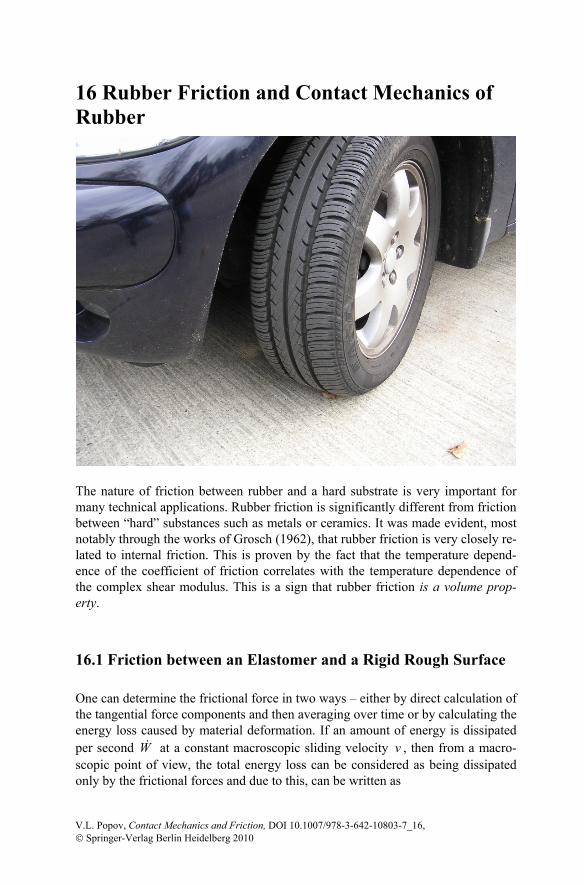
16 Rubber Friction and Contact Mechanics of Rubber
The nature of friction between rubber and a hard substrate is very important for many technical applications. Rubber friction is significantly different from friction between “hard” substances such as metals or ceramics. It was made evident, most notably through the works of Grosch (1962), that rubber friction is very closely re-lated to internal friction. This is proven by the fact that the temperature depend-ence of the coefficient of friction correlates with the temperature dependence of the complex shear modulus. This is a sign that rubber friction is a volume prop-erty.
16.1 Friction between an Elastomer and a Rigid Rough Surface
One can determine the frictional force in two ways – either by direct calculation of the tangential force components and then averaging over time or by calculating the energy loss caused by material deformation. If an amount of energy is dissipated per second W at a constant macroscopic sliding velocity v , then from a macro-scopic point of view, the total energy loss can be considered as being dissipated only by the frictional forces and due to this, can be written as
V.L. Popov, Contact Mechanics and Friction, DOI 10.1007/978-3-642-10803-7_16, © Springer-Verlag Berlin Heidelberg 2010
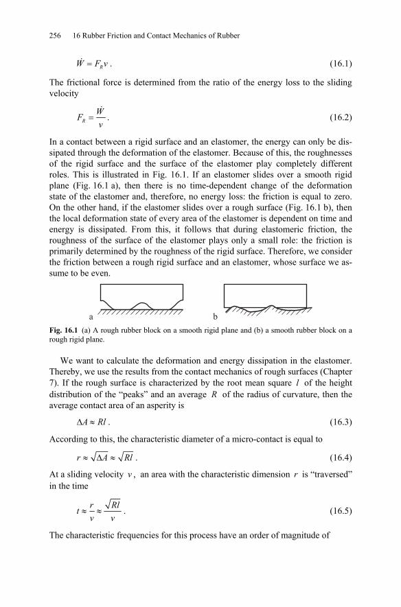
256 16 Rubber Friction and Contact Mechanics of Rubber
= RW F v . (16.1)
The frictional force is determined from the ratio of the energy loss to the sliding velocity
=RWFv
. (16.2)
In a contact between a rigid surface and an elastomer, the energy can only be dis-sipated through the deformation of the elastomer. Because of this, the roughnesses of the rigid surface and the surface of the elastomer play completely different roles. This is illustrated in Fig. 16.1. If an elastomer slides over a smooth rigid plane (Fig. 16.1 a), then there is no time-dependent change of the deformation state of the elastomer and, therefore, no energy loss: the friction is equal to zero. On the other hand, if the elastomer slides over a rough surface (Fig. 16.1 b), then the local deformation state of every area of the elastomer is dependent on time and energy is dissipated. From this, it follows that during elastomeric friction, the roughness of the surface of the elastomer plays only a small role: the friction is primarily determined by the roughness of the rigid surface. Therefore, we consider the friction between a rough rigid surface and an elastomer, whose surface we as-sume to be even.
a b Fig. 16.1 (a) A rough rubber block on a smooth rigid plane and (b) a smooth rubber block on a rough rigid plane.
We want to calculate the deformation and energy dissipation in the elastomer. Thereby, we use the results from the contact mechanics of rough surfaces (Chapter 7). If the rough surface is characterized by the root mean square l of the height distribution of the “peaks” and an average R of the radius of curvature, then the average contact area of an asperity is
Δ ≈A Rl . (16.3)
According to this, the characteristic diameter of a micro-contact is equal to
≈ Δ ≈r A Rl . (16.4)
At a sliding velocity v , an area with the characteristic dimension r is “traversed” in the time
≈ ≈r Rltv v
. (16.5)
The characteristic frequencies for this process have an order of magnitude of
16.1 Friction between an Elastomer and a Rigid Rough Surface 257
1 νω ≈ ≈t r
. (16.6)
The average pressure in the micro-contacts is
1 *σ κ −= = ∇NFE z
A (16.7)
with 2κ ≈ (see Chapter 7). We denote the root mean square of the gradient of the surface as
2′∇ =z z . (16.8)
The effective modulus of elasticity for rubber is equal to1
*2 2
2(1 ) 41 1
νν ν
+= = ≈
− −E GE G . (16.9)
Because the shear modulus is frequency dependent, the characteristic frequency (16.6) must be substituted into the expression for average pressure (16.7):
( )1 ˆ4σ κ ω−= ∇G z . (16.10)
Thereby, we insert the magnitude of the frequency-dependent modulus, because the amplitudes of the stress and deformation are connected by the complex shear modulus. We use the following equation from the previous chapter to calculate the energy dissipation in a unit volume of a micro-contact:
212 2
( )ˆ ( )
ωω σω
′′=
GPG
. (16.11)
Multiplied with the depth of the significantly deformed volume ≈ r , it yields the energy loss per unit area and then, when divided by the normal stress, the coeffi-cient of friction:
( / )ˆ ( / )
μ ξ′′
= ∇G v rzG v r
. (16.12)
Here, ξ is a dimensionless coefficient on the order of unity, which is established by more exact calculation. Numerical simulations show that 1ξ ≈ .
1 Rubber can be assumed to be a practically incompressible medium which has an approximate Poisson’s ratio of 1/ 2ν ≈ .
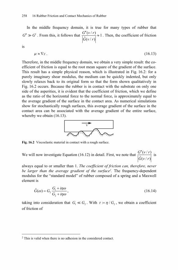
258 16 Rubber Friction and Contact Mechanics of Rubber
In the middle frequency domain, it is true for many types of rubber that
′′ ′G G . From this, it follows that ( / ) 1ˆ ( / )
′′≈
G v rG v r
. Then, the coefficient of friction
is
μ ≈ ∇z . (16.13)
Therefore, in the middle frequency domain, we obtain a very simple result: the co-efficient of friction is equal to the root mean square of the gradient of the surface. This result has a simple physical reason, which is illustrated in Fig. 16.2: for a purely imaginary shear modulus, the medium can be quickly indented, but only slowly relaxes back to its original form so that the form shown qualitatively in Fig. 16.2 occurs. Because the rubber is in contact with the substrate on only one side of the asperities, it is evident that the coefficient of friction, which we define as the ratio of the horizontal force to the normal force, is approximately equal to the average gradient of the surface in the contact area. As numerical simulations show for stochastically rough surfaces, this average gradient of the surface in the contact area can be associated with the average gradient of the entire surface, whereby we obtain (16.13).
v
Fig. 16.2 Viscoelastic material in contact with a rough surface.
We will now investigate Equation (16.12) in detail. First, we note that ( / )ˆ ( / )
′′G v rG v r
is
always equal to or smaller than 1. The coefficient of friction can, therefore, never be larger than the average gradient of the surface2. The frequency-dependent modulus for the “standard model” of rubber composed of a spring and a Maxwell element is
12
2
ˆ ( )ηω
ωηω
+=
+G i
G GG i
, (16.14)
taking into consideration that 1 2G G . With 2: / Gτ η= , we obtain a coefficient of friction of
2 This is valid when there is no adhesion in the considered contact.
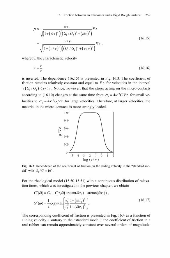
16.1 Friction between an Elastomer and a Rigid Rough Surface 259
( )( ) ( ) ( )( )
( )( ) ( ) ( )( )
2 2 21 2
2 2 21 2
1 /
/ ,1 / / /
ωτμωτ ωτ
≈ ∇+ +
= ∇+ +
zG G
v v zv v G G v v
(16.15)
whereby, the characteristic velocity
τ
=rv (16.16)
is inserted. The dependence (16.15) is presented in Fig. 16.3. The coefficient of friction remains relatively constant and equal to ∇z for velocities in the interval ( )1 2/ < <v G G v v . Notice, however, that the stress acting on the micro-contacts
according to (16.10) changes at the same time from 11 14σ κ −= ∇G z for small ve-
locities to 12 24σ κ −= ∇G z for large velocities. Therefore, at larger velocities, the
material in the micro-contacts is more strongly loaded.
4 2 0 23 1 15
1.0
0.8
0.6
0.4
0.2
0
z�
/
�
log (v/ v ) Fig. 16.3 Dependence of the coefficient of friction on the sliding velocity in the “standard mo-del” with 4
2 1/ 10=G G .
For the rheological model (15.50-15.51) with a continuous distribution of relaxa-tion times, which was investigated in the previous chapter, we obtain
( )( )( )
0 1 1 2 1
2212
1 1 2 21 2
( ) arctan( ) arctan( ) ,
11( ) ln .2 1
G G G
G G
ω τ ω ωτ ωτ
ωττω τ ω
τ ωτ
′ = + −
⎛ ⎞+′′ ⎜ ⎟=
⎜ ⎟+⎝ ⎠
(16.17)
The corresponding coefficient of friction is presented in Fig. 16.4 as a function of sliding velocity. Contrary to the “standard model,” the coefficient of friction in a real rubber can remain approximately constant over several orders of magnitude.
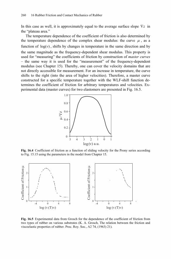
260 16 Rubber Friction and Contact Mechanics of Rubber
In this case as well, it is approximately equal to the average surface slope ∇z in the “plateau area.”
The temperature dependence of the coefficient of friction is also determined by the temperature dependence of the complex shear modulus: the curve μ , as a function of log( )v , shifts by changes in temperature in the same direction and by the same magnitude as the frequency-dependent shear modulus. This property is used for “measuring” the coefficients of friction by construction of master curves – the same way it is used for the “measurement” of the frequency-dependent modulus (see Chapter 15). Thereby, one can cover the velocity domains that are not directly accessible for measurement. For an increase in temperature, the curve shifts to the right (into the area of higher velocities). Therefore, a master curve constructed for a specific temperature together with the WLF-shift function de-termines the coefficient of friction for arbitrary temperatures and velocities. Ex-perimental data (master curves) for two elastomers are presented in Fig. 16.5.
�
1.0
4 2 05
0.8
0.6
0.4
0.2
03 1 1
z�
/
log (v) a.u. Fig. 16.4 Coefficient of friction as a function of sliding velocity for the Prony series according to Fig. 15.15 using the parameters in the model from Chapter 15.
-4 0 4 8
2
1
0
Co
effi
cien
to
fF
rict
ion
�
-4 0 4 8
2
1
0
log (� (T)v)
Co
effi
cien
to
fF
rict
ion
�
log (� (T)v)
Fig. 16.5 Experimental data from Grosch for the dependence of the coefficient of friction from two types of rubber on various substrates (K. A. Grosch, The relation between the friction and viscoelastic properties of rubber. Proc. Roy. Soc., A2 74, (1963) 21).
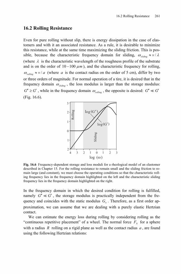
16.2 Rolling Resistance 261
16.2 Rolling Resistance
Even for pure rolling without slip, there is energy dissipation in the case of elas-tomers and with it an associated resistance. As a rule, it is desirable to minimize this resistance, while at the same time maximizing the sliding friction. This is pos-sible, because the characteristic frequency domain for sliding, /sliding vω λ≈ (where λ is the characteristic wavelength of the roughness profile of the substrate and is on the order of 10 100 μ− m ), and the characteristic frequency for rolling,
/rolling v aω ≈ (where a is the contact radius on the order of 5 cm), differ by two or three orders of magnitude. For normal operation of a tire, it is desired that in the frequency domain slidingω , the loss modulus is larger than the storage modulus: ′′ ′≥G G , while in the frequency domain rollingω , the opposite is desired: ′′ ′G G
(Fig. 16.6). 3
2
1
0
1
24 2 0 23 1 1 3
Ro
llin
g
Sli
din
g
log ( )�
log( )G
log ( )G
Fig. 16.6 Frequency-dependent storage and loss moduli for a rheological model of an elastomer described in Chapter 15. For the rolling resistance to remain small and the sliding friction to re-main large (and constant), we must choose the operating conditions so that the characteristic roll-ing frequency lies in the frequency domain highlighted on the left and the characteristic sliding frequency lies in the frequency domain highlighted on the right.
In the frequency domain in which the desired condition for rolling is fulfilled, namely ′′ ′G G , the storage modulus is practically independent from the fre-quency and coincides with the static modulus ∞G . Therefore, as a first order ap-proximation, we can assume that we are dealing with a purely elastic Hertzian contact.
We can estimate the energy loss during rolling by considering rolling as the “continuous repetitive placement” of a wheel. The normal force NF for a sphere with a radius R rolling on a rigid plane as well as the contact radius a , are found using the following Hertzian relations:
262 16 Rubber Friction and Contact Mechanics of Rubber
* 1/2 3/ 2 1/ 2 3/24 163 3 ∞≈ ≈NF E R d G R d , (16.18)
2 ≈a Rd , (16.19)
where d is the penetration depth. We estimate the characteristic frequency with
ω ≈va
(16.20)
and the amplitude of the deformation with
0ε ≈da
. (16.21)
According to (15.23), we obtain a power loss per unit volume of
2
20
1 1( )2 2ωε ω ⎛ ⎞ ⎛ ⎞′′ ′′= ≈ ⎜ ⎟ ⎜ ⎟
⎝ ⎠ ⎝ ⎠
v d vP G Ga a a
(16.22)
and a power loss in the total volume ( )32a∼ of
24 vW vd Ga
⎛ ⎞′′≈ ⎜ ⎟⎝ ⎠
. (16.23)
By dividing the power loss by the velocity, we obtain the resistance force
24wvF d Ga
⎛ ⎞′′≈ ⎜ ⎟⎝ ⎠
. (16.24)
At low frequencies, the loss module is always proportional to the frequency and can, therefore, be written in the form
( )ω ηω′′ =G , (16.25)
where η is the dynamic viscosity at low frequencies. Then, the resistance force is
22 3
24 4wa v aF vR a R
η η⎛ ⎞ ⎛ ⎞≈ =⎜ ⎟ ⎜ ⎟
⎝ ⎠⎝ ⎠. (16.26)
With the Hertzian result (5.24), rewritten using the notation of this section, we get for the deformed volume
3 316 ∞
= NRFa
G. (16.27)
For resistance force we obtain
16.3 Adhesive Contact with Elastomers 263
3 34 4w N N
v vF F FG R Rη τ
∞
≈ = (16.28)
and for “coefficient of rolling friction”
34
Wrolling
N
F vF R
τμ = ≈ , (16.29)
where /τ η ∞= G is the relaxation time of the elastomer. This equation is valid up to a dimensionless constant of magnitude 1. According to this, the rolling friction is proportional to the product of the rolling velocity and the (largest) relaxation time of the rubber and inversely proportional to the radius of curvature of the sphere.
16.3 Adhesive Contact with Elastomers
Until now, we have assumed that there are no adhesive forces between elastomeric and rigid surfaces. This is not the case for sufficiently smooth surfaces. Now, we consider an adhesive contact between a rigid sphere and an elastomer with an even surface (Fig. 16.7). The boundary of the contact can be viewed and treated as the tip of a crack3. In equilibrium, the elastomer can be assumed to be an elastic body with the static shear modulus ∞G and an effective modulus of elasticity of
( )
( )*
2
2 1 24
11G G
E Gν
νν∞ ∞
∞
+= = =
−−. (16.30)
In equilibrium, the JKR equation (6.20) provides us with a relationship between the normal force NF and the contact radius a :
1/ 23 * 34 8*
3 *γ π⎡ ⎤⎛ ⎞
⎢ ⎥= − ⎜ ⎟⎢ ⎥⎝ ⎠⎣ ⎦
Na aF ER E
. (16.31)
Here, *γ is the effective surface energy (i.e. the required energy for producing a unit surface). We can present the condition (16.31) in a form in which it is con-venient to treat the contact boundary as the tip of a crack. To this end, we first solve Equation (16.31) for *γ :
2* 3
*3 *
4 13 8N
E aFR a E
γπ
⎛ ⎞= −⎜ ⎟⎝ ⎠
. (16.32)
3 The original theory of Johnson, Kendall, and Roberts is based on exactly this analogy.
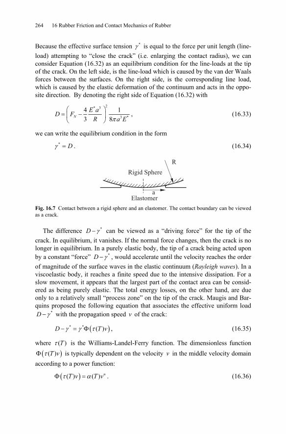
264 16 Rubber Friction and Contact Mechanics of Rubber
Because the effective surface tension *γ is equal to the force per unit length (line-load) attempting to “close the crack” (i.e. enlarging the contact radius), we can consider Equation (16.32) as an equilibrium condition for the line-loads at the tip of the crack. On the left side, is the line-load which is caused by the van der Waals forces between the surfaces. On the right side, is the corresponding line load, which is caused by the elastic deformation of the continuum and acts in the oppo-site direction. By denoting the right side of Equation (16.32) with
2* 3
3 *
4 13 8π
⎛ ⎞= −⎜ ⎟⎝ ⎠
NE aD F
R a E, (16.33)
we can write the equilibrium condition in the form
*γ = D . (16.34)
R
aElastomer
Rigid Sphere
Fig. 16.7 Contact between a rigid sphere and an elastomer. The contact boundary can be viewed as a crack.
The difference *γ−D can be viewed as a “driving force” for the tip of the crack. In equilibrium, it vanishes. If the normal force changes, then the crack is no longer in equilibrium. In a purely elastic body, the tip of a crack being acted upon by a constant “force” *γ−D , would accelerate until the velocity reaches the order of magnitude of the surface waves in the elastic continuum (Rayleigh waves). In a viscoelastic body, it reaches a finite speed due to the intensive dissipation. For a slow movement, it appears that the largest part of the contact area can be consid-ered as being purely elastic. The total energy losses, on the other hand, are due only to a relatively small “process zone” on the tip of the crack. Maugis and Bar-quins proposed the following equation that associates the effective uniform load
*γ−D with the propagation speed v of the crack:
( )* * ( )γ γ τ− = ΦD T v , (16.35)
where ( )τ T is the Williams-Landel-Ferry function. The dimensionless function
( )( )τΦ T v is typically dependent on the velocity v in the middle velocity domain according to a power function:
( )( ) ( )τ αΦ = nT v T v . (16.36)
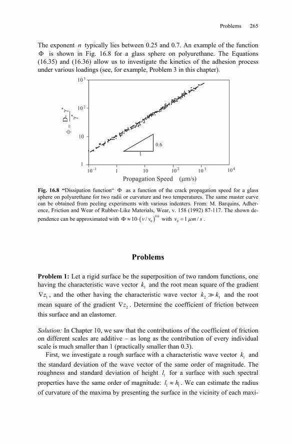
Problems 265
The exponent n typically lies between 0.25 and 0.7. An example of the function Φ is shown in Fig. 16.8 for a glass sphere on polyurethane. The Equations (16.35) and (16.36) allow us to investigate the kinetics of the adhesion process under various loadings (see, for example, Problem 3 in this chapter).
1 1010 -1 102
10 3 104
Propagation Speed (�m s)/
10 3
10 2
10
1
0.6
1
F=
D-
�*
�*
Fig. 16.8 “Dissipation function“ Φ as a function of the crack propagation speed for a glass sphere on polyurethane for two radii or curvature and two temperatures. The same master curve can be obtained from peeling experiments with various indenters. From: M. Barquins, Adher-ence, Friction and Wear of Rubber-Like Materials, Wear, v. 158 (1992) 87-117. The shown de-pendence can be approximated with ( )0.6
010 /Φ ≈ ⋅ v v with 0 1 /μ=v m s .
Problems
Problem 1: Let a rigid surface be the superposition of two random functions, one having the characteristic wave vector 1k and the root mean square of the gradient
1∇z , and the other having the characteristic wave vector 2 1k k and the root mean square of the gradient 2∇z . Determine the coefficient of friction between this surface and an elastomer.
Solution: In Chapter 10, we saw that the contributions of the coefficient of friction on different scales are additive – as long as the contribution of every individual scale is much smaller than 1 (practically smaller than 0.3).
First, we investigate a rough surface with a characteristic wave vector 1k and the standard deviation of the wave vector of the same order of magnitude. The roughness and standard deviation of height 1l for a surface with such spectral properties have the same order of magnitude: 1 1≈l h . We can estimate the radius of curvature of the maxima by presenting the surface in the vicinity of each maxi-
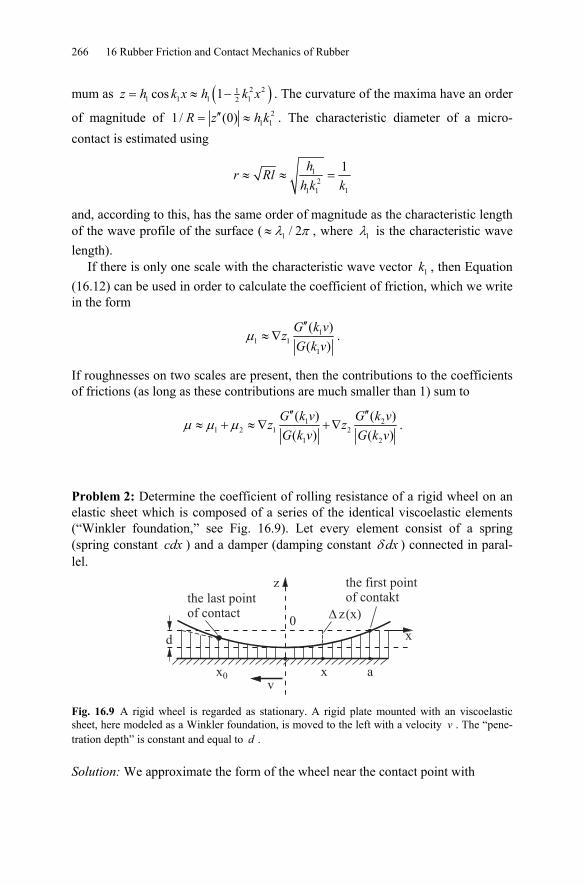
266 16 Rubber Friction and Contact Mechanics of Rubber
mum as ( )2 211 1 1 12cos 1= ≈ −z h k x h k x . The curvature of the maxima have an order
of magnitude of 21 11 / (0)′′= ≈R z h k . The characteristic diameter of a micro-
contact is estimated using
12
11 1
1≈ ≈ =
hr Rl
kh k
and, according to this, has the same order of magnitude as the characteristic length of the wave profile of the surface ( 1 / 2λ π≈ , where 1λ is the characteristic wave length).
If there is only one scale with the characteristic wave vector 1k , then Equation (16.12) can be used in order to calculate the coefficient of friction, which we write in the form
11 1
1
( )( )
G k vz
G k vμ
′′≈ ∇ .
If roughnesses on two scales are present, then the contributions to the coefficients of frictions (as long as these contributions are much smaller than 1) sum to
1 21 2 1 2
1 2
( ) ( )( ) ( )
G k v G k vz z
G k v G k vμ μ μ
′′ ′′≈ + ≈ ∇ +∇ .
Problem 2: Determine the coefficient of rolling resistance of a rigid wheel on an elastic sheet which is composed of a series of the identical viscoelastic elements (“Winkler foundation,” see Fig. 16.9). Let every element consist of a spring (spring constant cdx ) and a damper (damping constant δ dx ) connected in paral-lel.
v
the first pointof contaktthe last point
of contact
d
z
0� z(x)
x
axx0
Fig. 16.9 A rigid wheel is regarded as stationary. A rigid plate mounted with an viscoelastic sheet, here modeled as a Winkler foundation, is moved to the left with a velocity v . The “pene-tration depth” is constant and equal to d .
Solution: We approximate the form of the wheel near the contact point with
Problems 267
2
2= − +
xz dR
,
where d is the penetration depth. The gradient in point x is tan /θ ′= =z x R . A movement of the substrate in the negative direction with the velocity v leads to a spring movement in the vertical direction with the velocity /′= − = −z vz vx R . The force with which an element is acting on the wheel, is equal to
( ) ( )2
2zx xdF cz z dx cz vz dx c d v dxR R
δ δ δ⎛ ⎞⎛ ⎞
′= − − = − + = − − + +⎜ ⎟⎜ ⎟⎜ ⎟⎝ ⎠⎝ ⎠.
The z -component of the total force is calculated as
0
2
2
a
Nx
x xF c d v dxR R
δ⎛ ⎞⎛ ⎞
= − − + +⎜ ⎟⎜ ⎟⎜ ⎟⎝ ⎠⎝ ⎠∫
and the x -component of the total force as
0
2
2
a
wx
x x xF c d v dxR R R
δ⎛ ⎞⎛ ⎞
= − − + +⎜ ⎟⎜ ⎟⎜ ⎟⎝ ⎠⎝ ⎠∫ ,
where the coordinate of the first point of contact on the right is denoted with a and the last point of contact on the left with 0x . The coordinate a is calculated using the condition 0=z and 0x using the condition 0=zdF . From this, it fol-lows that
2=a Rd , 2
0 2 δ δ⎛ ⎞= − + +⎜ ⎟⎝ ⎠
v vx Rdc c
.
By substituting / 2ξ = x Rd , we bring the expressions for NF and wF into the following form
( )0
11/2 1/ 2 3/ 2 22 1
ξ
ξ κξ ξ= − +∫NF R d c d ,
( )0
12 22 1
ξ
ξ κξ ξ ξ= − +∫wF d c d ,
having defined 1/ 2
1/2 1/ 2
2 2v vcacd R
δ δκ = =
and
268 16 Rubber Friction and Contact Mechanics of Rubber
2
0 12 2κ κξ ⎛ ⎞= − + +⎜ ⎟⎝ ⎠
.
The coefficient of rolling resistance is calculated as
( )
( )0
0
12
1/ 2
12
12
1
w
N
dF dF R
d
ξ
ξ
ξ κξ ξ ξ
μξ κξ ξ
− +⎛ ⎞= = ⎜ ⎟⎝ ⎠ − +
∫
∫.
We consider two limiting cases: (a) 1κ : very low velocities. In this case, the approximations
1/2 1/ 2 3/24 23
=NF R d c and 243
κ=wF d c are valid. The coefficient of rolling resis-
tance is, therefore, 1/2
1/ 2 1/22δ τμ κ= = =
d v vcR RR
with /τ δ= c (one can compare this result to that of the approximation (16.29)). (b) 1κ : very high velocities, or traversing a liquid sheet ( 0=c ). In this case,
the approximations δ=NF vd and 3/ 2 3/ 2
1/2
23
δ ⋅=w
d vFR
are valid. The coefficient of
resistance is, therefore4, 1/ 23/ 22
3μ
δ⎛ ⎞= ⎜ ⎟⎝ ⎠
NFvR
.
Problem 3: Determine the kinetics of the process of the separation of a sphere in contact with an elastomer if the sphere is unloaded before 0=t and at time 0=t
a force *32γ π= − = −N AF F R , 1.5N AF F= − ⋅ , or 2= − ⋅N AF F is applied. Use the
following values: 2 mm=R , * 10 MPa=E , * 20.05 J/mγ = , ( )0 5010 /Φ ≈ ⋅ v v ,
0 1 /μ=v m s .
Solution: The problem is solved with Equation (16.35), which we write in the fol-lowing form:
4 For the transition to a three-dimensional system, δ must be replaced by 4η : 1/2
213
NFvR
μη⎛ ⎞
= ⎜ ⎟⎝ ⎠
.
For a more detailed explanation see Chapter 19.
Problems 269
( )0 5* *010 /γ γ− =D v v .
With the denotations for adhesive force and equilibrium radius as
* 33 (in our case 0.47 10 N)2AF Rπγ −= = ⋅
and 1/3* 2
50 9 (in our case 6.56 10 m)
2 *Ra
Eγ π −⎛ ⎞
= = ⋅⎜ ⎟⎝ ⎠
,
respectively, the line load D can be presented in the following form: 23/23/2
* 0
0
14
γ⎡ ⎤⎛ ⎞⎛ ⎞⎢ ⎥= − ⎜ ⎟⎜ ⎟⎢ ⎥⎝ ⎠ ⎝ ⎠⎣ ⎦
N
A
F a aDF a a
.
Before time 0=t there is an equilibrium condition without loading and a contact radius of 0a . At any time after 0=t , the following equation is valid:
23/ 2 0 53/ 2* * *0
0 0
1 104
γ γ γ⎡ ⎤⎛ ⎞ ⎛ ⎞⎛ ⎞⎢ ⎥− − =⎜ ⎟ ⎜ ⎟⎜ ⎟⎢ ⎥⎝ ⎠ ⎝ ⎠ ⎝ ⎠⎣ ⎦
N
A
F a a vF a a v
.
For velocity, it follows that 223/23/ 2
0 0
0
1 1100 4
⎛ ⎞⎡ ⎤⎛ ⎞⎛ ⎞⎜ ⎟⎢ ⎥= − = − −⎜ ⎟⎜ ⎟⎜ ⎟⎢ ⎥⎝ ⎠⎜ ⎟⎝ ⎠⎣ ⎦⎝ ⎠
N
A
v F ada avdt F a a
.
Using the dimensionless variables 0/=a a a and 0 0/100=t tv a , we obtain the equation
223/ 2 3/ 21 1
4−
⎛ ⎞⎡ ⎤⎜ ⎟− = − −⎢ ⎥⎜ ⎟⎣ ⎦⎝ ⎠
N
A
Fda a adt F
with the initial condition 1=a for 0=t . Results of a numerical integration of this equation for three different ratios of /N AF F are presented in Fig. 16.10.
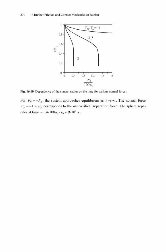
270 16 Rubber Friction and Contact Mechanics of Rubber
0 0,4
F /FA = -1
0,8 1,2 1,6 2
tv0
100a
a/a
0
-2
-1,5
1
0,8
0,6
0,4
0,2
0
0
N
Fig. 16.10 Dependence of the contact radius on the time for various normal forces.
For = −N AF F , the system approaches equilibrium as →∞t . The normal force 1.5N AF F= − ⋅ corresponds to the over-critical separation force. The sphere sepa-
rates at time 30 01.4 100 / 9 10 sa v⋅ ≈ ⋅∼ .
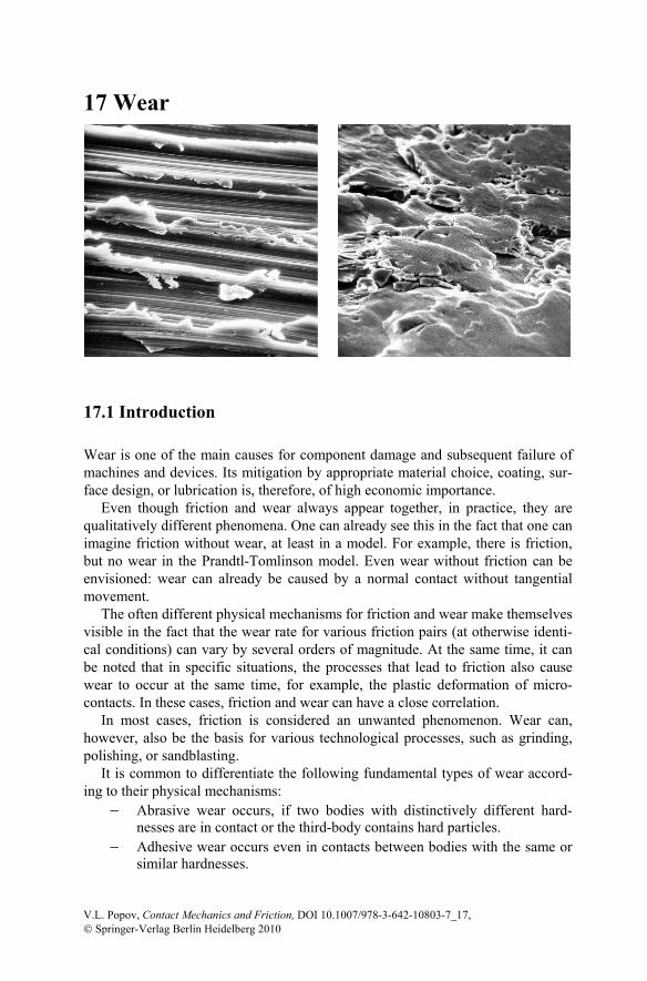
17 Wear
17.1 Introduction
Wear is one of the main causes for component damage and subsequent failure of machines and devices. Its mitigation by appropriate material choice, coating, sur-face design, or lubrication is, therefore, of high economic importance.
Even though friction and wear always appear together, in practice, they are qualitatively different phenomena. One can already see this in the fact that one can imagine friction without wear, at least in a model. For example, there is friction, but no wear in the Prandtl-Tomlinson model. Even wear without friction can be envisioned: wear can already be caused by a normal contact without tangential movement.
The often different physical mechanisms for friction and wear make themselves visible in the fact that the wear rate for various friction pairs (at otherwise identi-cal conditions) can vary by several orders of magnitude. At the same time, it can be noted that in specific situations, the processes that lead to friction also cause wear to occur at the same time, for example, the plastic deformation of micro-contacts. In these cases, friction and wear can have a close correlation.
In most cases, friction is considered an unwanted phenomenon. Wear can, however, also be the basis for various technological processes, such as grinding, polishing, or sandblasting.
It is common to differentiate the following fundamental types of wear accord-ing to their physical mechanisms:
− Abrasive wear occurs, if two bodies with distinctively different hard-nesses are in contact or the third-body contains hard particles.
− Adhesive wear occurs even in contacts between bodies with the same or similar hardnesses.
V.L. Popov, Contact Mechanics and Friction, DOI 10.1007/978-3-642-10803-7_17, © Springer-Verlag Berlin Heidelberg 2010
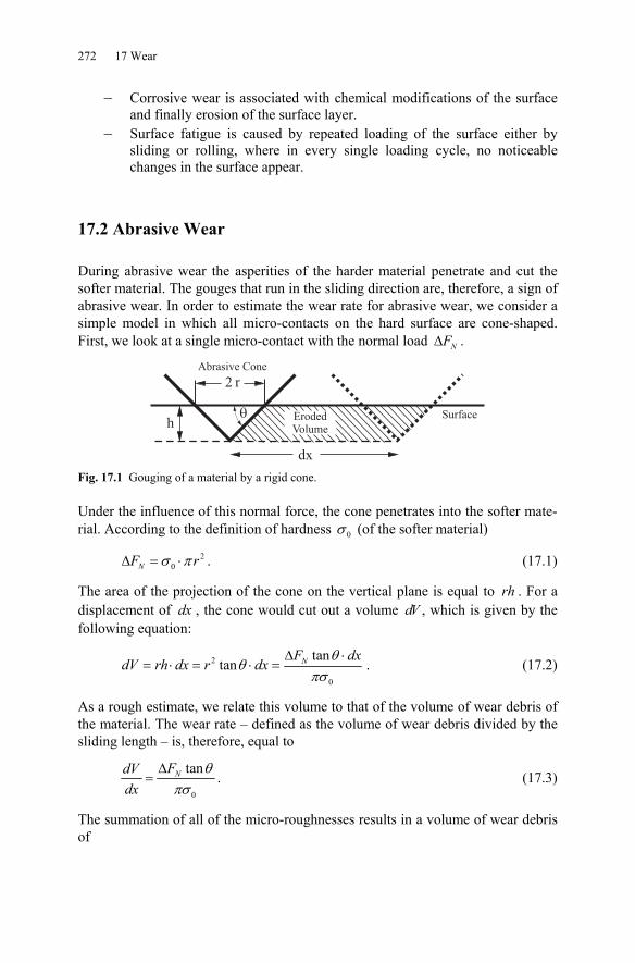
272 17 Wear
− Corrosive wear is associated with chemical modifications of the surface and finally erosion of the surface layer.
− Surface fatigue is caused by repeated loading of the surface either by sliding or rolling, where in every single loading cycle, no noticeable changes in the surface appear.
17.2 Abrasive Wear
During abrasive wear the asperities of the harder material penetrate and cut the softer material. The gouges that run in the sliding direction are, therefore, a sign of abrasive wear. In order to estimate the wear rate for abrasive wear, we consider a simple model in which all micro-contacts on the hard surface are cone-shaped. First, we look at a single micro-contact with the normal load Δ NF .
�
2
hSurface
dx
ErodedVolume
Abrasive Cone
r
Fig. 17.1 Gouging of a material by a rigid cone.
Under the influence of this normal force, the cone penetrates into the softer mate-rial. According to the definition of hardness 0σ (of the softer material)
20σ πΔ = ⋅NF r . (17.1)
The area of the projection of the cone on the vertical plane is equal to rh . For a displacement of dx , the cone would cut out a volume dV , which is given by the following equation:
2
0
tantan
θθ
πσΔ ⋅
= ⋅ = ⋅ = NF dxdV rh dx r dx . (17.2)
As a rough estimate, we relate this volume to that of the volume of wear debris of the material. The wear rate – defined as the volume of wear debris divided by the sliding length – is, therefore, equal to
0
tanθπσ
Δ= NFdV
dx. (17.3)
The summation of all of the micro-roughnesses results in a volume of wear debris of
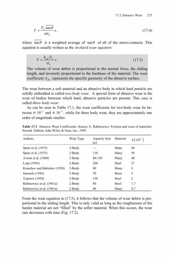
17.2 Abrasive Wear 273
0
tanθπσ
= NFV x , (17.4)
where tanθ is a weighted average of tanθ of all of the micro-contacts. This equation is usually written as the Archard wear equation:
0σ
= abr Nk FV x . (17.5)
The volume of wear debris is proportional to the normal force, the sliding length, and inversely proportional to the hardness of the material. The wear coefficient abrk represents the specific geometry of the abrasive surface.
The wear between a soft material and an abrasive body in which hard particle are solidly embedded is called two-body wear. A special form of abrasive wear is the wear of bodies between which hard, abrasive particles are present. This case is called three-body wear.
As can be seen in Table 17.1, the wear coefficients for two-body wear lie be-tween 26 10−⋅ and 36 10−⋅ , while for three body wear, they are approximately one order of magnitude smaller.
Table 17.1 Abrasive Wear Coefficients. Source: E. Rabinowicz: Friction and wear of materials. Second Edition. John Wiley & Sons, inc., 1995.
Authors Wear Type Asperity Size (µ)
Material ( )3x10k −
Spurr et al. (1975) 2-Body -- Many 60 Spurr et al. (1975) 2-Body 110 Many 50 Avient et al. (1960) 2-Body 40-150 Many 40 Lopa (1956) 2-Body 260 Steel 27 Kruschov and Babichev (1958) 2-Body 80 Many 8 Samuels (1956) 2-Body 70 Brass 5 Toporov (1958) 2-Body 150 Steel 2 Rabinowicz et al. (1961a) 2-Body 80 Steel 1.7 Rabinowicz et al. (1961a) 2-Body 40 Many 0.7 From the wear equation in (17.5), it follows that the volume of wear debris is pro-portional to the sliding length. This is only valid as long as the roughnesses of the harder material are not “filled” by the softer material. When this occurs, the wear rate decreases with time (Fig. 17.2).
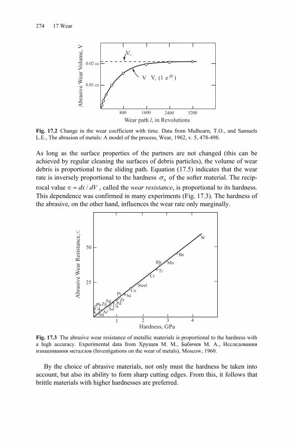
274 17 Wear
Abra
sive
Wea
rV
olu
me,
V
Wear path , in Revolutionsl
0.02 cc
0.01 cc
800 1600 2400 3200
V�
V (1 e-�l )V�
Fig. 17.2 Change in the wear coefficient with time. Data from Mulhearn, T.O., and Samuels L.E., The abrasion of metals: A model of the process, Wear, 1962, v. 5, 478-498.
As long as the surface properties of the partners are not changed (this can be achieved by regular cleaning the surfaces of debris particles), the volume of wear debris is proportional to the sliding path. Equation (17.5) indicates that the wear rate is inversely proportional to the hardness 0σ of the softer material. The recip-rocal value /dx dV∈ = , called the wear resistance, is proportional to its hardness. This dependence was confirmed in many experiments (Fig. 17.3). The hardness of the abrasive, on the other hand, influences the wear rate only marginally.
SnAl
AuCdPb Zn
Ag
Pt
Rh
CuPd
ZrNi
CoSteel
CrTi
Mo
Be
W
Ab
rasi
ve
Wea
rR
esis
tan
ce,v
Hardness, G
25
50
1 2 3 4
Pa Fig. 17.3 The abrasive wear resistance of metallic materials is proportional to the hardness with a high accuracy. Experimental data from Хрущев М. М., Бабичев М. А., Исследования изнашивания металлов (Investigations on the wear of metals), Мoscow, 1960.
By the choice of abrasive materials, not only must the hardness be taken into account, but also its ability to form sharp cutting edges. From this, it follows that brittle materials with higher hardnesses are preferred.
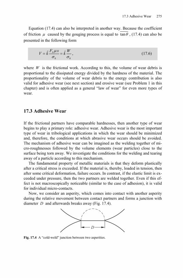
17.3 Adhesive Wear 275
Equation (17.4) can also be interpreted in another way. Because the coefficient of friction μ caused by the gouging process is equal to tanθ , (17.4) can also be presented in the following form
0 0
μσ σ
= =NF x WV k k , (17.6)
where W is the frictional work. According to this, the volume of wear debris is proportional to the dissipated energy divided by the hardness of the material. The proportionality of the volume of wear debris to the energy contribution is also valid for adhesive wear (see next section) and erosive wear (see Problem 1 in this chapter) and is often applied as a general “law of wear” for even more types of wear.
17.3 Adhesive Wear
If the frictional partners have comparable hardnesses, then another type of wear begins to play a primary role: adhesive wear. Adhesive wear is the most important type of wear in tribological applications in which the wear should be minimized and, therefore, the conditions at which abrasive wear occurs should be avoided. The mechanism of adhesive wear can be imagined as the welding together of mi-cro-roughnesses followed by the volume elements (wear particles) close to the surface being torn away. We investigate the conditions for the welding and tearing away of a particle according to this mechanism.
The fundamental property of metallic materials is that they deform plastically after a critical stress is exceeded. If the material is, thereby, loaded in tension, then after some critical deformation, failure occurs. In contrast, if the elastic limit is ex-ceeded under pressure, then the two partners are welded together. Even if this ef-fect is not macroscopically noticeable (similar to the case of adhesion), it is valid for individual micro-contacts.
Now, we consider an asperity, which comes into contact with another asperity during the relative movement between contact partners and forms a junction with diameter D and afterwards breaks away (Fig. 17.4).
D
Fig. 17.4 A “cold-weld” junction between two asperities.
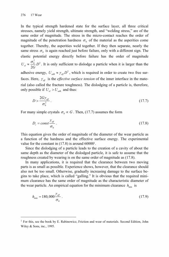
276 17 Wear
In the typical strength hardened state for the surface layer, all three critical stresses, namely yield strength, ultimate strength, and “welding stress,” are of the same order of magnitude. The stress in the micro-contact reaches the order of magnitude of the penetration hardness 0σ of the material as the asperities come together. Thereby, the asperities weld together. If they then separate, nearly the same stress 0σ is again reached just before failure, only with a different sign. The elastic potential energy directly before failure has the order of magnitude
230
2σ
≈elU DG
. It is only sufficient to dislodge a particle when it is larger than the
adhesive energy, 2γ≈adh effU D , which is required in order to create two free sur-faces. Here, γ eff is the effective surface tension of the inner interface in the mate-rial (also called the fracture toughness). The dislodging of a particle is, therefore, only possible if >el adhU U and thus:
20
2 γσ
> effGD . (17.7)
For many simple crystals 0σ ∝ G . Then, (17.7) assumes the form
0
γσ
= effcD const . (17.8)
This equation gives the order of magnitude of the diameter of the wear particle as a function of the hardness and the effective surface energy. The experimental value for the constant in (17.8) is around 600001.
Since the dislodging of a particle leads to the creation of a cavity of about the same depth as the diameter of the dislodged particle, it is safe to assume that the roughness created by wearing is on the same order of magnitude as (17.8).
In many applications, it is required that the clearance between two moving parts is as small as possible. Experience shows, however, that the clearance should also not be too small. Otherwise, gradually increasing damage to the surface be-gins to take place, which is called “galling.” It is obvious that the required mini-mum clearance has the same order of magnitude as the characteristic diameter of the wear particle. An empirical equation for the minimum clearance minh is
min0
180,000 effhγσ
= . (17.9)
1 For this, see the book by E. Rabinowicz, Friction and wear of materials. Second Edition, John Wiley & Sons, inc., 1995.
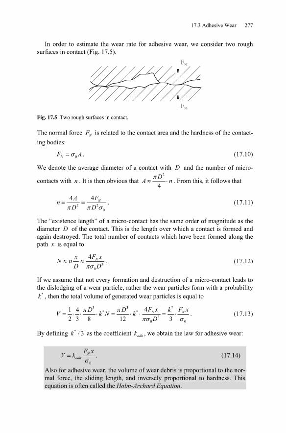
17.3 Adhesive Wear 277
In order to estimate the wear rate for adhesive wear, we consider two rough surfaces in contact (Fig. 17.5).
FN
FN
Fig. 17.5 Two rough surfaces in contact.
The normal force NF is related to the contact area and the hardness of the contact-ing bodies:
0σ=NF A . (17.10)
We denote the average diameter of a contact with D and the number of micro-
contacts with n . It is then obvious that 2
4π
≈ ⋅DA n . From this, it follows that
2 20
44π π σ
= = NFAnD D
. (17.11)
The “existence length” of a micro-contact has the same order of magnitude as the diameter D of the contact. This is the length over which a contact is formed and again destroyed. The total number of contacts which have been formed along the path x is equal to
30
4πσ
≈ ≈ NF xxN nD D
. (17.12)
If we assume that not every formation and destruction of a micro-contact leads to the dislodging of a wear particle, rather the wear particles form with a probability
*k , then the total volume of generated wear particles is equal to
3 3 *
* *3
00
41 42 3 8 12 3
π πσπσ
= ⋅ ⋅ ⋅ = ⋅ ⋅ = ⋅N NF x F xD D kV k N kD
. (17.13)
By defining * / 3k as the coefficient adhk , we obtain the law for adhesive wear:
0σ
= Nadh
F xV k . (17.14)
Also for adhesive wear, the volume of wear debris is proportional to the nor-mal force, the sliding length, and inversely proportional to hardness. This equation is often called the Holm-Archard Equation.
278 17 Wear
Due to the “probability of the generation of a wear particle,” which now comes into play and can be dependent, for example, on the contamination of the surface, the adhesive wear coefficients may vary by a few orders of magnitude. The typical value of the wear coefficient for a non-lubricated contact between two alloy-forming metals is approximately 310−∼adhk , but can be three or four orders of magnitude smaller in the presence of a very good lubricant or for two non-compatible metals.
17.4 Conditions for Low-Wear Friction
The conditions for low-wear sliding are dependent on many parameters and it is difficult to formulate simple rules to deal with it. Different situations present themselves in lubricated and non-lubricated systems. Roughnesses serve as a res-ervoir for lubricants in lubricated systems and in this way, can minimize wear, while in dry operating systems, it is usually desired to create as smooth a surface as possible. If the yield stress of the material is not reached in the micro-contact, then only purely elastic deformation of the surfaces takes place – assuming that no chemical reactions occur between the two surfaces2. Since the average stress in the micro-roughnesses has the order of magnitude *1
2 ∇E z , according to (7.16), and the maximum stress that occurs in the individual micro-contacts can reach ap-proximately *∇E z , the condition *
0σ∇ <E z must be met, or
0*
σ∇ <z
E. (17.15)
For many metallic materials, the hardness correlates with the modulus of elasticity and the following is valid3:
0 0.01E
σ≈ . (17.16)
In order for the frictional partners to deform only elastically, the surfaces must be extremely smooth: the average gradient of the surfaces cannot exceed the value 0.01. Additionally, it is desirable to keep the wave length of the roughness as small as possible, so that the diameter of the micro-contacts remains below that found in (17.8) and the condition for adhesive wear is not fulfilled. If the average gradient is larger than that in (17.15), then the softer material in the contact area
2 A simple criterion for this is that the contacting materials form no alloys. 3 For related statistical data, see: E. Rabinowicz, Friction and Wear of Materials. Second Edition, John Wiley & Sons, inc., 1995.
17.5 Wear as the Transportation of Material from the Friction Zone 279
plastically deforms. The consequences that plastic deformation has on wear are significantly dependent on the properties of the uppermost surface layers.
The description of adhesive wear in the previous section assumes that the for-mation of cold-weld junctions and their subsequent destruction takes place at dif-ferent places in the material. If the material forms a layer of oxides or is lubri-cated, then it is possible that the destruction of the contacts occurs at the same interface as their formation. The relation between the strength of the surface inter-face and the volume strength of the material, therefore, plays a very large role in adhesive wear, even if they are not explicitly represented in Equation (17.14). This motivated Kragelski4 to introduce the “principal of positive hardness gradient” as the essential principal for formulating conditions for low-wear friction. According to this principal, the strength of the uppermost surface layers of the material should increase with the depth. This can be achieved by lubrication, chemical modification of the surface layers, by material softening using local temperature increases, as well as by designing surface layers with low surface energies. For low-wear contacts, it is beneficial if the contacting materials do not form alloys, or at least an alloy for which the strength is smaller than that of both of the base ma-terials. If the hardness gradient is negative for whatever reason, then the wear rate increases abruptly. Therefore, the processes of oxidation and interactions with mo-lecular layers of the lubricating film are very relevant to wear, but until now, have not been able to be brought into the framework of a simple contact mechanical model.
17.5 Wear as the Transportation of Material from the Friction Zone
In order to analyze wear, it is not sufficient to establish the conditions for the dis-lodgment of wear particles. As long as the wear particles remain in the friction zone, they continue to be exposed to intensive tribological loading and are repeat-edly reintegrated into the surfaces of the frictional partners. The wear first be-comes noticeable when the material has left the friction zone. Therefore, the wear is in a broader sense, not only a problem of strength, but also a problem of mate-rial transport out of the friction zone.
According to Kragelski, in order for a material to be wear resistant, it is benefi-cial for the surface to have a lower yield strength than the inner material. We will investigate the wear resistance of a material with such a soft surface layer with a shear strength of τ c and thickness h . Let the diameter of the friction zone be L .
The wear rate can be estimated using the following qualitative considerations. Assuming that the layer exhibits ideal plastic behavior, the tangential stress in the layer remains constant, independent from the sliding velocity, and equal to τ c .
4 I.V. Kragelski, Friction and Wear. Butter Worth, London, 1965, 346 pp.
280 17 Wear
One can formally introduce an effective viscosity of the layer ηeff so that the shear stress in the layer can be calculated using the same rule as with a viscous fluid:
τ η=c effvh
. (17.17)
From this, it follows that
τ
η = ceff
hv
. (17.18)
A surface layer that is already in a state of plastic yielding has no yield strength with respect to other stress components (e.g. normal stress) and behaves, in a first order approximation, like a liquid with the effective viscosity (17.18). Thus, it is squeezed with a velocity that can be estimated using Equation (14.27):
3 2
4 4
2 23 3πη π τ
≈ ≈N Neff c
h h vh F FR R
. (17.19)
The volume that is squeezed out of the friction zone (material that is worn away)
divided by the sliding path is, therefore, equal to 2 28
3 2
π
τ⎛ ⎞= ≈ ⎜ ⎟⎝ ⎠
N
c
h R FdV hdx v R
.
Numerical simulations confirm that this equation is accurate up to a proportional-ity factor. Therefore, the wear equation can be written in the following form5:
2
0σ⎛ ⎞≈ ⎜ ⎟⎝ ⎠
NF hV xL
. (17.20)
Here, we introduced the hardness of the material 0σ . This relationship has the same form as that of the wear equation (17.14), but with a geometric factor ( )2/h L , which accounts for extremely low wear rates for small values of h and large values of L .
17.6 Wear of Elastomers
The wear of elastomers is a very complicated process that is not completely un-derstood even today. We can apply the wear equation (17.14) for a rough estimate of adhesive wear, where the hardness 0σ must be replaced by the average stress (16.10) in the micro-contacts: 5 V.L. Popov, I.Yu. Smolin, A. Gervé and B. Kehrwald, Simulation of wear in combustion en-gines. Computational Materials Science, 2000, v. 19, No.1-4, pp. 285-291.
17.6 Wear of Elastomers 281
ˆ4 ( )
Nadh
F xV k
G vk zκ
=∇
(17.21)
with 2κ ≈ and k being the characteristic wave number of the roughness. In order to characterize the wear of rubber, one often uses the so-called abrad-
ability γ as the ratio of the volume of wear debris to the energy loss6. For this, we have the approximation
2 ˆˆ 4 Im( ( ))4 ( )
κ κγ
μ μ= = =
∇∇adh adh
N
k kVF x z G vkG vk z
. (17.22)
The abradability is inversely proportional to the imaginary part of the complex modulus and exhibits a minimum in the middle velocity domain (Fig. 17.6). The abradability curve determined by experiments is presented in Fig. 17.7 as a func-tion of velocity.
In addition to viscoelastic properties, rubber also exhibits plastic properties. These properties can be characterized by defining a critical stress σ c , the “yield stress,” whereby, this critical stress is even more loosely defined as it is in metals. We assume that the penetration hardness of rubber is three times this value:
0 3σ σ≈ c . According to (16.10), the characteristic stress in the micro-contacts has an order of magnitude of
( )1 ˆ4σ κ −≈ ∇G vk z . (17.23)
If this stress reaches the hardness of the material, then the rubber deforms plasti-cally and the wear increases rapidly. The critical velocity at which this occurs is calculated using the condition
( )0ˆ2σ ≈ ∇cG v k z . (17.24)
A more exact consideration of frictional and wear processes should also take into account changes in temperature in the micro-contacts, because the complex modulus is temperature dependent.
For large coefficients of friction, an instability develops in the frictional contact for which a part of the contact surface is in a sticking state. Further movement of the body is then only possible by the propagation of detachment waves, the so-called Schallamach waves. In this regime, another wear mechanism is characteris-tic, the formation of rubber rolls.
6 Abradability γ should not be confused for the surface tension, for which we use the same let-ter.
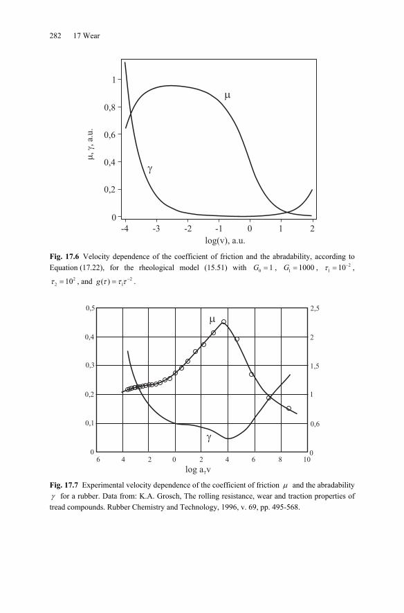
282 17 Wear
�����a.
u.
0
0,2
0,4
0,6
0,8
1
log(v), a.u.
-4 -3 -2 -1 0 1 2
�
�
Fig. 17.6 Velocity dependence of the coefficient of friction and the abradability, according to Equation (17.22), for the rheological model (15.51) with 0 1=G , 1 1000=G , 2
1 10τ −= , 2
2 10τ = , and 21( )τ τ τ −=g .
log a vT
0,5
0,4
0,3
0,2
0,1
06 4 2 0 2 4 6 8 10
0
0,6
1
1,5
2
2,5
�
�
Fig. 17.7 Experimental velocity dependence of the coefficient of friction μ and the abradability γ for a rubber. Data from: K.A. Grosch, The rolling resistance, wear and traction properties of tread compounds. Rubber Chemistry and Technology, 1996, v. 69, pp. 495-568.
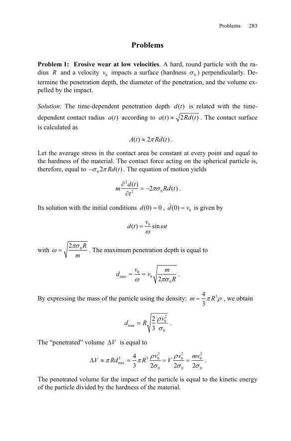
Problems 283
Problems
Problem 1: Erosive wear at low velocities. A hard, round particle with the ra-dius R and a velocity 0v impacts a surface (hardness 0σ ) perpendicularly. De-termine the penetration depth, the diameter of the penetration, and the volume ex-pelled by the impact.
Solution: The time-dependent penetration depth ( )d t is related with the time-
dependent contact radius ( )a t according to ( ) 2 ( )≈a t Rd t . The contact surface is calculated as
( ) 2 ( )π≈A t Rd t .
Let the average stress in the contact area be constant at every point and equal to the hardness of the material. The contact force acting on the spherical particle is, therefore, equal to 0 2 ( )σ π− Rd t . The equation of motion yields
2
02
( ) 2 ( )πσ∂= −
∂d tm Rd tt
.
Its solution with the initial conditions (0) 0=d , 0(0) =d v is given by
0( ) sinωω
=v
d t t
with 02πσω =
Rm
. The maximum penetration depth is equal to
0max 0
02ω πσ= =
v md vR
.
By expressing the mass of the particle using the density: 343
π ρ=m R , we obtain
20
max0
23
ρσ
=v
d R .
The “penetrated” volume ΔV is equal to 2 2 2
2 3 0 0 0max
0 0 0
43 2 2 2
ρ ρπ π
σ σ σΔ ≈ = = =
v v mvV Rd R V .
The penetrated volume for the impact of the particle is equal to the kinetic energy of the particle divided by the hardness of the material.

284 17 Wear
The wear volume is dependent not only on the penetrated volume, but also from the mechanism of the removal of the displaced material. As a rule, however, the wear volume is proportional to the penetrated volume.
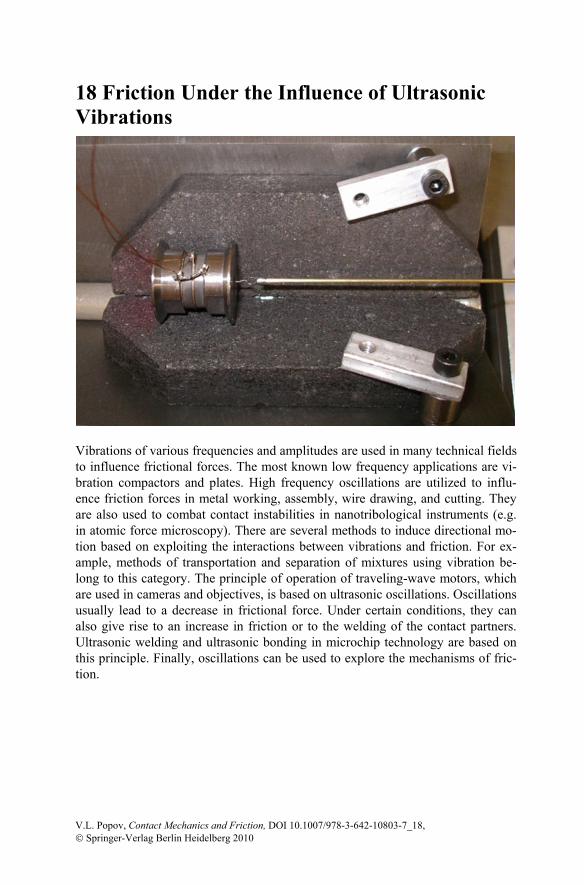
18 Friction Under the Influence of Ultrasonic Vibrations
Vibrations of various frequencies and amplitudes are used in many technical fields to influence frictional forces. The most known low frequency applications are vi-bration compactors and plates. High frequency oscillations are utilized to influ-ence friction forces in metal working, assembly, wire drawing, and cutting. They are also used to combat contact instabilities in nanotribological instruments (e.g. in atomic force microscopy). There are several methods to induce directional mo-tion based on exploiting the interactions between vibrations and friction. For ex-ample, methods of transportation and separation of mixtures using vibration be-long to this category. The principle of operation of traveling-wave motors, which are used in cameras and objectives, is based on ultrasonic oscillations. Oscillations usually lead to a decrease in frictional force. Under certain conditions, they can also give rise to an increase in friction or to the welding of the contact partners. Ultrasonic welding and ultrasonic bonding in microchip technology are based on this principle. Finally, oscillations can be used to explore the mechanisms of fric-tion.
V.L. Popov, Contact Mechanics and Friction, DOI 10.1007/978-3-642-10803-7_18, © Springer-Verlag Berlin Heidelberg 2010
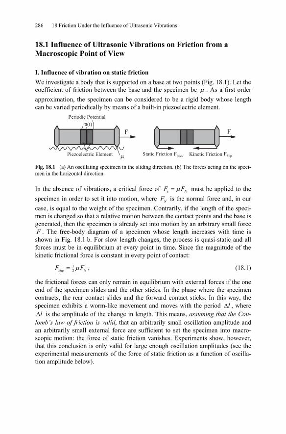
286 18 Friction Under the Influence of Ultrasonic Vibrations
18.1 Influence of Ultrasonic Vibrations on Friction from a Macroscopic Point of View
I. Influence of vibration on static friction We investigate a body that is supported on a base at two points (Fig. 18.1). Let the coefficient of friction between the base and the specimen be μ . As a first order approximation, the specimen can be considered to be a rigid body whose length can be varied periodically by means of a built-in piezoelectric element.
u(t)
Periodic Potential
Piezoelectric Element �
F
Static Friction Kinetic Friction FF
F
Stick Slip Fig. 18.1 (a) An oscillating specimen in the sliding direction. (b) The forces acting on the speci-men in the horizontal direction.
In the absence of vibrations, a critical force of = μs NF F must be applied to the specimen in order to set it into motion, where NF is the normal force and, in our case, is equal to the weight of the specimen. Contrarily, if the length of the speci-men is changed so that a relative motion between the contact points and the base is generated, then the specimen is already set into motion by an arbitrary small force F . The free-body diagram of a specimen whose length increases with time is shown in Fig. 18.1 b. For slow length changes, the process is quasi-static and all forces must be in equilibrium at every point in time. Since the magnitude of the kinetic frictional force is constant in every point of contact:
12slip NF Fμ= , (18.1)
the frictional forces can only remain in equilibrium with external forces if the one end of the specimen slides and the other sticks. In the phase where the specimen contracts, the rear contact slides and the forward contact sticks. In this way, the specimen exhibits a worm-like movement and moves with the period Δl , where Δl is the amplitude of the change in length. This means, assuming that the Cou-lomb’s law of friction is valid, that an arbitrarily small oscillation amplitude and an arbitrarily small external force are sufficient to set the specimen into macro-scopic motion: the force of static friction vanishes. Experiments show, however, that this conclusion is only valid for large enough oscillation amplitudes (see the experimental measurements of the force of static friction as a function of oscilla-tion amplitude below).
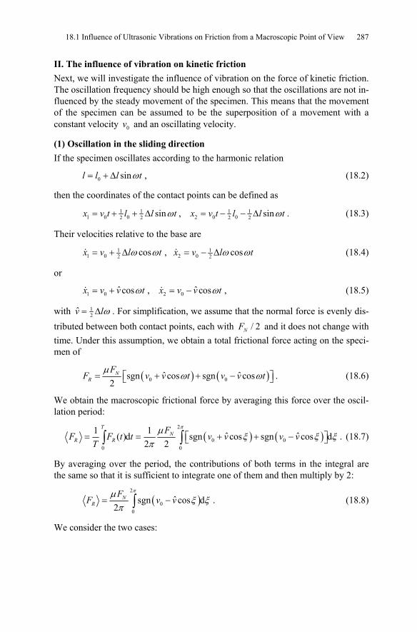
18.1 Influence of Ultrasonic Vibrations on Friction from a Macroscopic Point of View 287
II. The influence of vibration on kinetic friction Next, we will investigate the influence of vibration on the force of kinetic friction. The oscillation frequency should be high enough so that the oscillations are not in-fluenced by the steady movement of the specimen. This means that the movement of the specimen can be assumed to be the superposition of a movement with a constant velocity 0v and an oscillating velocity.
(1) Oscillation in the sliding direction If the specimen oscillates according to the harmonic relation
0 sinl l l tω= + Δ , (18.2)
then the coordinates of the contact points can be defined as
1 11 0 02 2 sinx v t l l tω= + + Δ , 1 1
2 0 02 2 sinx v t l l tω= − − Δ . (18.3)
Their velocities relative to the base are
11 0 2 cosx v l tω ω= + Δ , 1
2 0 2 cosx v l tω ω= − Δ (18.4)
or
1 0 ˆ cos= + ωx v v t , 2 0 ˆ cos= − ωx v v t , (18.5)
with 12v lω= Δ . For simplification, we assume that the normal force is evenly dis-
tributed between both contact points, each with / 2NF and it does not change with time. Under this assumption, we obtain a total frictional force acting on the speci-men of
( ) ( )0 0ˆ ˆsgn cos sgn cos2
= + + −⎡ ⎤⎣ ⎦μ
ω ωNR
FF v v t v v t . (18.6)
We obtain the macroscopic frictional force by averaging this force over the oscil-lation period:
( ) ( )2
0 00 0
1 1 ˆ ˆ( )d sgn cos sgn cos d2 2
= = + + −⎡ ⎤⎣ ⎦∫ ∫πμ
ξ ξ ξπ
TN
R RF
F F t t v v v vT
. (18.7)
By averaging over the period, the contributions of both terms in the integral are the same so that it is sufficient to integrate one of them and then multiply by 2:
( )2
00
ˆsgn cos d2
= −∫πμ
ξ ξπ
NR
FF v v . (18.8)
We consider the two cases:
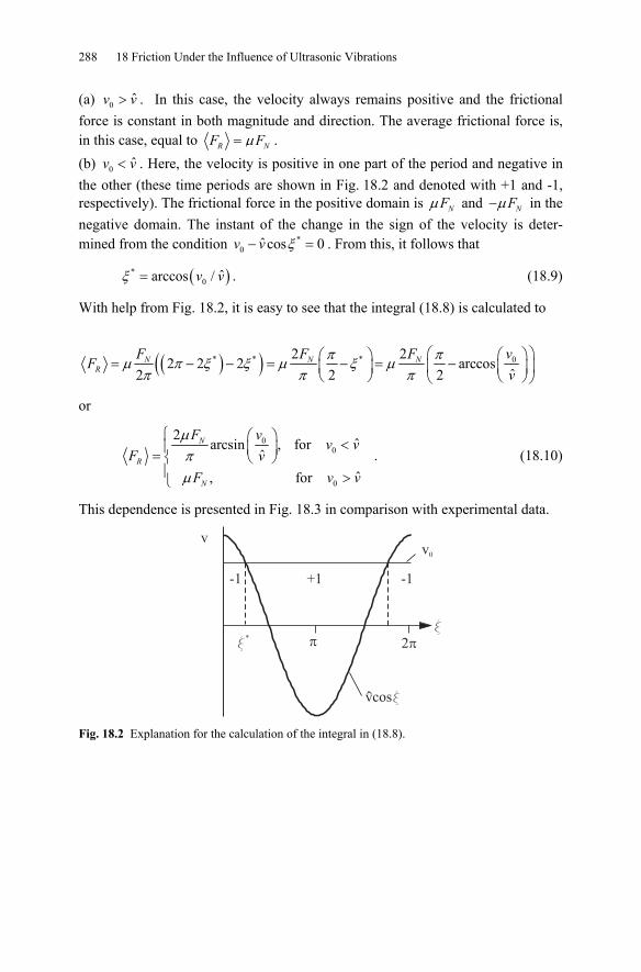
288 18 Friction Under the Influence of Ultrasonic Vibrations
(a) 0 ˆ>v v . In this case, the velocity always remains positive and the frictional force is constant in both magnitude and direction. The average frictional force is, in this case, equal to = μR NF F . (b) 0 ˆ<v v . Here, the velocity is positive in one part of the period and negative in the other (these time periods are shown in Fig. 18.2 and denoted with +1 and -1, respectively). The frictional force in the positive domain is μ NF and −μ NF in the negative domain. The instant of the change in the sign of the velocity is deter-mined from the condition *
0 ˆ cos 0− =ξv v . From this, it follows that
( )*0 ˆarccos /=ξ v v . (18.9)
With help from Fig. 18.2, it is easy to see that the integral (18.8) is calculated to
( )( )* * * 02 22 2 2 arccos
ˆ2 2 2⎛ ⎞⎛ ⎞⎛ ⎞= − − = − = −⎜ ⎟⎜ ⎟ ⎜ ⎟⎝ ⎠ ⎝ ⎠⎝ ⎠
π πμ π ξ ξ μ ξ μπ π πN N N
RF F F v
Fv
or
0
0
0
2 ˆarcsin , for ˆ
ˆ, for
N
R
N
F vv v
F vF v v
μπμ
⎧ ⎛ ⎞ <⎪ ⎜ ⎟= ⎝ ⎠⎨⎪ >⎩
. (18.10)
This dependence is presented in Fig. 18.3 in comparison with experimental data.
vv0
-1 +1 -1
x
x*
vcosx
� ��
Fig. 18.2 Explanation for the calculation of the integral in (18.8).
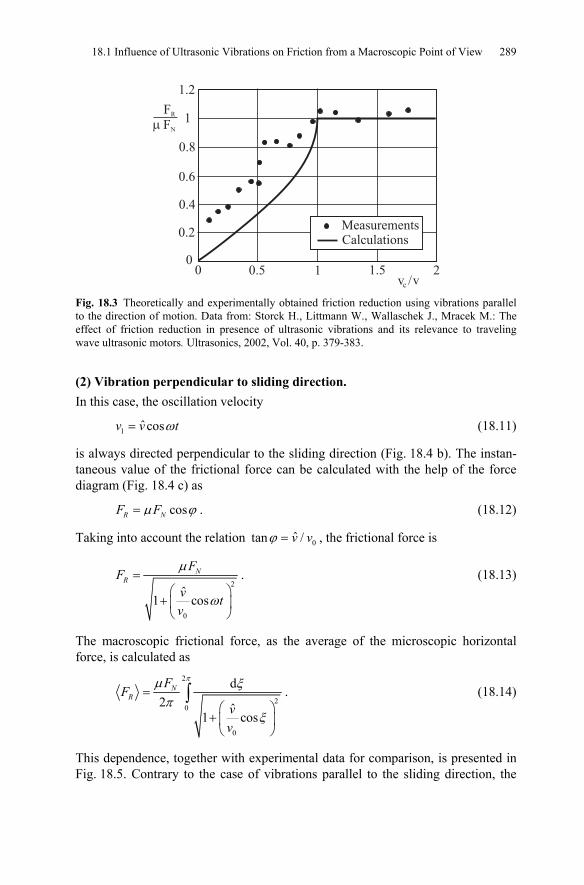
18.1 Influence of Ultrasonic Vibrations on Friction from a Macroscopic Point of View 289
Fig. 18.3 Theoretically and experimentally obtained friction reduction using vibrations parallel to the direction of motion. Data from: Storck H., Littmann W., Wallaschek J., Mracek M.: The effect of friction reduction in presence of ultrasonic vibrations and its relevance to traveling wave ultrasonic motors. Ultrasonics, 2002, Vol. 40, p. 379-383.
(2) Vibration perpendicular to sliding direction. In this case, the oscillation velocity
1 ˆ cos= ωv v t (18.11)
is always directed perpendicular to the sliding direction (Fig. 18.4 b). The instan-taneous value of the frictional force can be calculated with the help of the force diagram (Fig. 18.4 c) as
cos= μ ϕR NF F . (18.12)
Taking into account the relation 0ˆtan /v vϕ = , the frictional force is
2
0
ˆ1 cos
=⎛ ⎞
+ ⎜ ⎟⎝ ⎠
μ
ω
NR
FF
v tv
. (18.13)
The macroscopic frictional force, as the average of the microscopic horizontal force, is calculated as
2
20
0
d2 ˆ
1 cos
=⎛ ⎞
+ ⎜ ⎟⎝ ⎠
∫πμ ξ
πξ
NR
FF
vv
. (18.14)
This dependence, together with experimental data for comparison, is presented in Fig. 18.5. Contrary to the case of vibrations parallel to the sliding direction, the
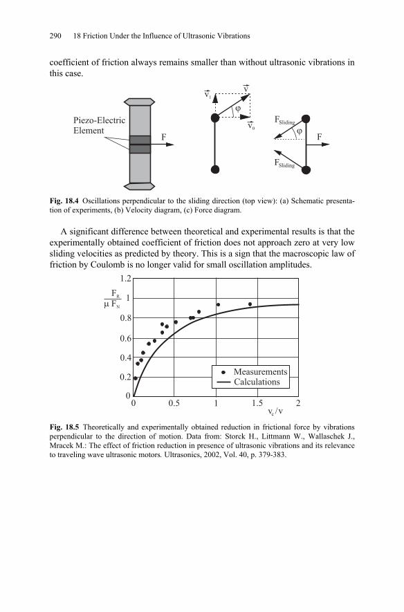
290 18 Friction Under the Influence of Ultrasonic Vibrations
coefficient of friction always remains smaller than without ultrasonic vibrations in this case.
F
Piezo-ElectricElement
F
v
v0
v1
�
�
FSliding
FSliding
Fig. 18.4 Oscillations perpendicular to the sliding direction (top view): (a) Schematic presenta-tion of experiments, (b) Velocity diagram, (c) Force diagram.
A significant difference between theoretical and experimental results is that the experimentally obtained coefficient of friction does not approach zero at very low sliding velocities as predicted by theory. This is a sign that the macroscopic law of friction by Coulomb is no longer valid for small oscillation amplitudes.
Fig. 18.5 Theoretically and experimentally obtained reduction in frictional force by vibrations perpendicular to the direction of motion. Data from: Storck H., Littmann W., Wallaschek J., Mracek M.: The effect of friction reduction in presence of ultrasonic vibrations and its relevance to traveling wave ultrasonic motors. Ultrasonics, 2002, Vol. 40, p. 379-383.
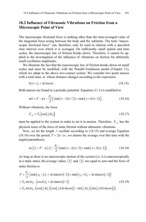
18.2 Influence of Ultrasonic Vibrations on Friction from a Microscopic Point of View 291
18.2 Influence of Ultrasonic Vibrations on Friction from a Microscopic Point of View
The macroscopic frictional force is nothing other than the time-averaged value of the tangential force acting between the body and the substrate. The term “macro-scopic frictional force” can, therefore, only be used in relation with a specified time interval over which it is averaged. On sufficiently small spatial and time scales, the macroscopic law of friction breaks down. Therefore, it cannot be ap-plied to the investigation of the influence of vibrations on friction for arbitrarily small oscillation amplitudes.
We illustrate the fact that the macroscopic law of friction breaks down on small scales and must be modified, with the Prandtl-Tomlinson model (Chapter 11), which we adapt to the above two-contact system. We consider two point masses with a total mass m whose distance changes according to the expression
0( ) sinl t l l tω= + Δ . (18.15)
Both masses are found in a periodic potential. Equation (11.1) is modified to
( ) ( )0 sin ( ) / 2 sin ( ) / 22
= − − − + +⎡ ⎤⎣ ⎦ηF
mx F x k x l t k x l t . (18.16)
Without vibrations, the force
( )1,0 0 02cos=sF F kl (18.17)
must be applied to the system in order to set it in motion. Therefore, ,0sF has the physical sense of the force of static friction without ultrasonic vibrations.
Now, we let the length l oscillate according to (18.15) and average Equation (18.16) over the period 2 /= π ωT ; we denote the average over this time with the angled parentheses:
( ) ( )0 sin ( ) / 2 sin ( ) / 22
= − − − + +ηF
m x F x k x l t k x l t . (18.18)
As long as there is no macroscopic motion of the system (i.e. it is macroscopically in a static state), the average values x and x are equal to zero and the force of static friction is
( )( ) ( )( )( )
( ) ( ) ( ) ( )( )
00 0 0 0
0 0 0
1 1 1 10 0 0 02 2 2 2
sin sin( ) / 2 sin sin( ) / 22sin cos sin( ) / 2
sin cos cos sin sin sin sin .
FF k x l l t k x l l t
F kx k l l t
F kx kl k l t kl k l t
ω ω
ω
ω ω
= − + Δ + + + Δ
= ⋅ + Δ
= ⋅ Δ − Δ
(18.19)
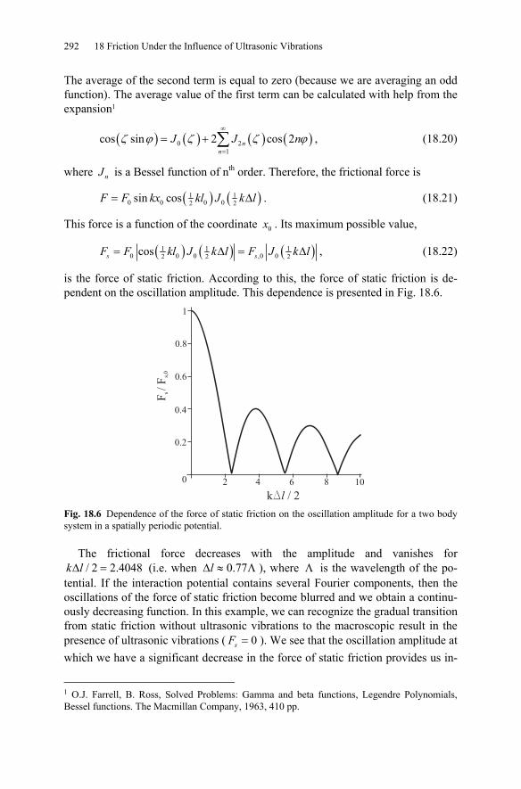
292 18 Friction Under the Influence of Ultrasonic Vibrations
The average of the second term is equal to zero (because we are averaging an odd function). The average value of the first term can be calculated with help from the expansion1
( ) ( ) ( ) ( )0 21
cos sin 2 cos 2∞
=
= + ∑ζ ϕ ζ ζ ϕnn
J J n , (18.20)
where nJ is a Bessel function of nth order. Therefore, the frictional force is
( ) ( )1 10 0 0 02 2sin cos= ΔF F kx kl J k l . (18.21)
This force is a function of the coordinate 0x . Its maximum possible value,
( ) ( ) ( )1 1 10 0 0 ,0 02 2 2cos= Δ = Δs sF F kl J k l F J k l , (18.22)
is the force of static friction. According to this, the force of static friction is de-pendent on the oscillation amplitude. This dependence is presented in Fig. 18.6.
1
0.8
0.6
0.4
0.2
0 2 4 6 8 10
F/
Fs
s,0
k / 2Dl Fig. 18.6 Dependence of the force of static friction on the oscillation amplitude for a two body system in a spatially periodic potential.
The frictional force decreases with the amplitude and vanishes for / 2 2.4048Δ =k l (i.e. when 0.77lΔ ≈ Λ ), where Λ is the wavelength of the po-
tential. If the interaction potential contains several Fourier components, then the oscillations of the force of static friction become blurred and we obtain a continu-ously decreasing function. In this example, we can recognize the gradual transition from static friction without ultrasonic vibrations to the macroscopic result in the presence of ultrasonic vibrations ( 0=sF ). We see that the oscillation amplitude at which we have a significant decrease in the force of static friction provides us in-
1 O.J. Farrell, B. Ross, Solved Problems: Gamma and beta functions, Legendre Polynomials, Bessel functions. The Macmillan Company, 1963, 410 pp.
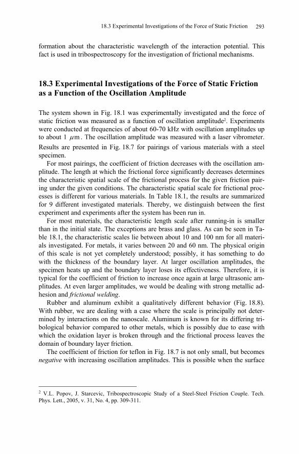
18.3 Experimental Investigations of the Force of Static Friction
formation about the characteristic wavelength of the interaction potential. This fact is used in tribospectroscopy for the investigation of frictional mechanisms.
18.3 Experimental Investigations of the Force of Static Friction as a Function of the Oscillation Amplitude
The system shown in Fig. 18.1 was experimentally investigated and the force of static friction was measured as a function of oscillation amplitude2. Experiments were conducted at frequencies of about 60-70 kHz with oscillation amplitudes up to about 1 mμ . The oscillation amplitude was measured with a laser vibrometer. Results are presented in Fig. 18.7 for pairings of various materials with a steel specimen.
For most pairings, the coefficient of friction decreases with the oscillation am-plitude. The length at which the frictional force significantly decreases determines the characteristic spatial scale of the frictional process for the given friction pair-ing under the given conditions. The characteristic spatial scale for frictional proc-esses is different for various materials. In Table 18.1, the results are summarized for 9 different investigated materials. Thereby, we distinguish between the first experiment and experiments after the system has been run in.
For most materials, the characteristic length scale after running-in is smaller than in the initial state. The exceptions are brass and glass. As can be seen in Ta-ble 18.1, the characteristic scales lie between about 10 and 100 nm for all materi-als investigated. For metals, it varies between 20 and 60 nm. The physical origin of this scale is not yet completely understood; possibly, it has something to do with the thickness of the boundary layer. At larger oscillation amplitudes, the specimen heats up and the boundary layer loses its effectiveness. Therefore, it is typical for the coefficient of friction to increase once again at large ultrasonic am-plitudes. At even larger amplitudes, we would be dealing with strong metallic ad-hesion and frictional welding.
Rubber and aluminum exhibit a qualitatively different behavior (Fig. 18.8). With rubber, we are dealing with a case where the scale is principally not deter-mined by interactions on the nanoscale. Aluminum is known for its differing tri-bological behavior compared to other metals, which is possibly due to ease with which the oxidation layer is broken through and the frictional process leaves the domain of boundary layer friction.
The coefficient of friction for teflon in Fig. 18.7 is not only small, but becomes negative with increasing oscillation amplitudes. This is possible when the surface
2 V.L. Popov, J. Starcevic, Tribospectroscopic Study of a Steel-Steel Friction Couple. Tech. Phys. Lett., 2005, v. 31, No. 4, pp. 309-311.
293
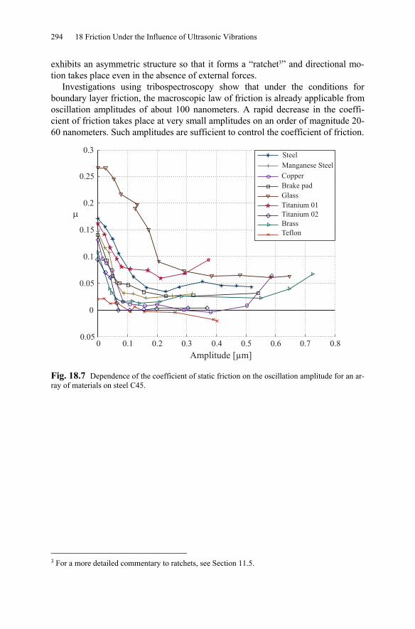
294 18 Friction Under the Influence of Ultrasonic Vibrations
exhibits an asymmetric structure so that it forms a “ratchet3” and directional mo-tion takes place even in the absence of external forces.
Investigations using tribospectroscopy show that under the conditions for boundary layer friction, the macroscopic law of friction is already applicable from oscillation amplitudes of about 100 nanometers. A rapid decrease in the coeffi-cient of friction takes place at very small amplitudes on an order of magnitude 20-60 nanometers. Such amplitudes are sufficient to control the coefficient of friction.
0 0.1 0.2 0.3 0.4 0.5 0.6 0.7 0.80.05
0
0.05
0.1
0.15
0.2
0.25
0.3
�
Amplitude [µm]
Manganese Steel
Copper
Brake pad
Glass
Titanium 01
Titanium 02
Brass
Teflon
Steel
Fig. 18.7 Dependence of the coefficient of static friction on the oscillation amplitude for an ar-ray of materials on steel C45.
3 For a more detailed commentary to ratchets, see Section 11.5.
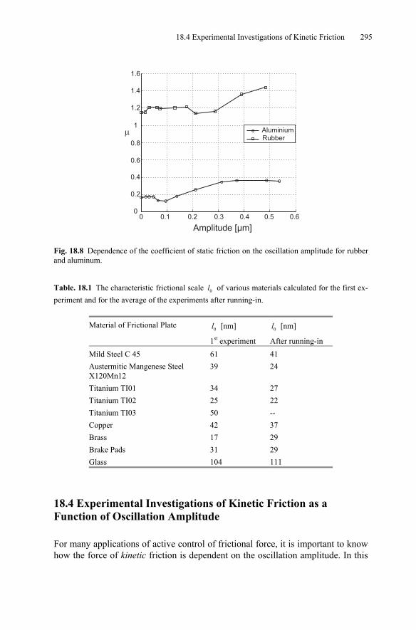
18.4 Experimental Investigations of Kinetic Friction 295
0 0.1 0.2 0.3 0.4 0.5 0.60
0.2
0.4
0.6
0.8
1
1.2
1.4
1.6
�
Amplitude [µm]
Rubber
Aluminium
Fig. 18.8 Dependence of the coefficient of static friction on the oscillation amplitude for rubber and aluminum.
Table. 18.1 The characteristic frictional scale 0l of various materials calculated for the first ex-periment and for the average of the experiments after running-in.
Material of Frictional Plate 0l [nm]
1st experiment 0l [nm]
After running-in Mild Steel C 45 61 41 Austermitic Mangenese Steel X120Mn12
39 24
Titanium TI01 34 27 Titanium TI02 25 22 Titanium TI03 50 -- Copper 42 37 Brass 17 29 Brake Pads 31 29 Glass 104 111
18.4 Experimental Investigations of Kinetic Friction as a Function of Oscillation Amplitude
For many applications of active control of frictional force, it is important to know how the force of kinetic friction is dependent on the oscillation amplitude. In this
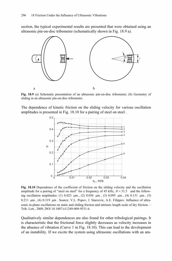
296 18 Friction Under the Influence of Ultrasonic Vibrations
section, the typical experimental results are presented that were obtained using an ultrasonic pin-on-disc tribometer (schematically shown in Fig. 18.9 a).
Fig. 18.9 (a) Schematic presentation of an ultrasonic pin-on-disc tribometer; (b) Geometry of sliding in an ultrasonic pin-on-disc tribometer.
The dependence of kinetic friction on the sliding velocity for various oscillation amplitudes is presented in Fig. 18.10 for a pairing of steel on steel .
0 0.01 0.02 0.03 0.040
0.1
0.2
0.3
0.4
0.5
v0
�
12
3
4
5
6
, m/s Fig. 18.10 Dependence of the coefficient of friction on the sliding velocity and the oscillation amplitude for a pairing of “steel on steel” for a frequency of 45 kHz, 31.5=θ and the follow-ing oscillation amplitudes: (1) 0.023 μm , (2) 0.056 μm , (3) 0.095 μm , (4) 0.131 μm , (5) 0.211 μm , (6) 0.319 μm . Source: V.L. Popov, J. Starcevic, A.E. Filippov. Influence of ultra-sonic in-plane oscillations on static and sliding friction and intrinsic length scale of dry friction. – Trib. Lett., 2009, DOI 10.1007/s11249-009-9531-6.
Qualitatively similar dependences are also found for other tribological pairings. It is characteristic that the frictional force slightly decreases as velocity increases in the absence of vibration (Curve 1 in Fig. 18.10). This can lead to the development of an instability. If we excite the system using ultrasonic oscillations with an am-
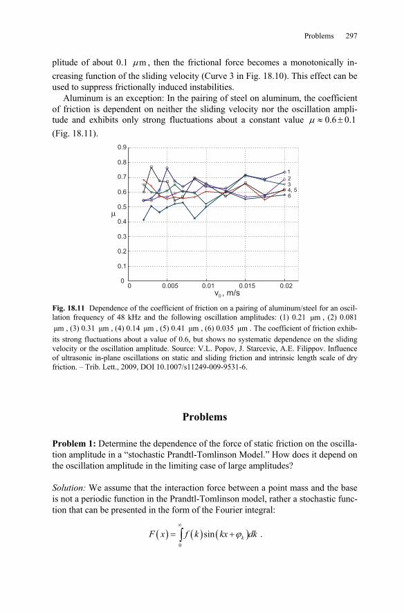
Problems 297
plitude of about 0.1 mμ , then the frictional force becomes a monotonically in-creasing function of the sliding velocity (Curve 3 in Fig. 18.10). This effect can be used to suppress frictionally induced instabilities.
Aluminum is an exception: In the pairing of steel on aluminum, the coefficient of friction is dependent on neither the sliding velocity nor the oscillation ampli-tude and exhibits only strong fluctuations about a constant value 0.6 0.1≈ ±μ (Fig. 18.11).
0 0.005 0.01 0.015 0.020
0.1
0.2
0.3
0.4
0.5
0.6
0.7
0.8
0.9
v0
�
1
234, 56
, m/s Fig. 18.11 Dependence of the coefficient of friction on a pairing of aluminum/steel for an oscil-lation frequency of 48 kHz and the following oscillation amplitudes: (1) 0.21 μm , (2) 0.081 μm , (3) 0.31 μm , (4) 0.14 μm , (5) 0.41 μm , (6) 0.035 μm . The coefficient of friction exhib-its strong fluctuations about a value of 0.6, but shows no systematic dependence on the sliding velocity or the oscillation amplitude. Source: V.L. Popov, J. Starcevic, A.E. Filippov. Influence of ultrasonic in-plane oscillations on static and sliding friction and intrinsic length scale of dry friction. – Trib. Lett., 2009, DOI 10.1007/s11249-009-9531-6.
Problems
Problem 1: Determine the dependence of the force of static friction on the oscilla-tion amplitude in a “stochastic Prandtl-Tomlinson Model.” How does it depend on the oscillation amplitude in the limiting case of large amplitudes?
Solution: We assume that the interaction force between a point mass and the base is not a periodic function in the Prandtl-Tomlinson model, rather a stochastic func-tion that can be presented in the form of the Fourier integral:
( ) ( ) ( )0
sin∞
= +∫ ϕkF x f k kx dk .
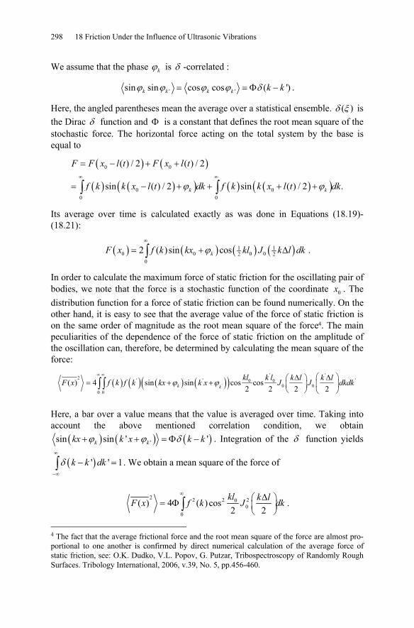
298 18 Friction Under the Influence of Ultrasonic Vibrations
We assume that the phase ϕk is δ -correlated :
' 'sin sin cos cos ( ')= = Φ −ϕ ϕ ϕ ϕ δk k k k k k .
Here, the angled parentheses mean the average over a statistical ensemble. ( )δ ξ is the Dirac δ function and Φ is a constant that defines the root mean square of the stochastic force. The horizontal force acting on the total system by the base is equal to
( ) ( )
( ) ( )( ) ( ) ( )( )
0 0
0 00 0
( ) / 2 ( ) / 2
sin ( ) / 2 sin ( ) / 2 .∞ ∞
= − + +
= − + + + +∫ ∫ϕ ϕk k
F F x l t F x l t
f k k x l t dk f k k x l t dk
Its average over time is calculated exactly as was done in Equations (18.19)-(18.21):
( ) ( ) ( ) ( )1 10 0 0 02 2
0
2 ( )sin cos∞
= + Δ∫ ϕkF x f k kx kl J k l dk .
In order to calculate the maximum force of static friction for the oscillating pair of bodies, we note that the force is a stochastic function of the coordinate 0x . The distribution function for a force of static friction can be found numerically. On the other hand, it is easy to see that the average value of the force of static friction is on the same order of magnitude as the root mean square of the force4. The main peculiarities of the dependence of the force of static friction on the amplitude of the oscillation can, therefore, be determined by calculating the mean square of the force:
( ) ( ) ( ) ( )( )'
' '2 ' ' '0 00 0
0 0
( ) 4 sin sin cos cos2 2 2 2k k
kl k l k l k lF x f k f k kx k x J J dkdkϕ ϕ∞ ∞ ⎛ ⎞Δ Δ⎛ ⎞= + + ⎜ ⎟⎜ ⎟
⎝ ⎠ ⎝ ⎠∫ ∫
Here, a bar over a value means that the value is averaged over time. Taking into account the above mentioned correlation condition, we obtain
( ) ( ) ( )'sin sin ' 'k kkx k x k kϕ ϕ δ+ + = Φ − . Integration of the δ function yields
( )' ' 1k k dkδ∞
−∞
− =∫ . We obtain a mean square of the force of
2 2 2 200
0
( ) 4 ( ) cos2 2
∞ Δ⎛ ⎞= Φ ⎜ ⎟⎝ ⎠∫
kl k lF x f k J dk .
4 The fact that the average frictional force and the root mean square of the force are almost pro-portional to one another is confirmed by direct numerical calculation of the average force of static friction, see: O.K. Dudko, V.L. Popov, G. Putzar, Tribospectroscopy of Randomly Rough Surfaces. Tribology International, 2006, v.39, No. 5, pp.456-460.
Problems 299
If the length 0l is “macroscopically large,” in the sense that it is much larger than an arbitrary characteristic scale of the interaction potential, then the function
2 0cos2
kl in the integral changes much faster than any other factor for arbitrary
changes in 0l and can be replaced by its average 1/ 2 :
( ) ( )2 2 2
00
22
∞ Δ⎛ ⎞= Φ ⎜ ⎟⎝ ⎠∫
k lF x f k J dk .
In this case, the frictional force is independent from the average connecting length and it depends only on the power spectrum ( )f k and the oscillation amplitude Δl .
For large oscillation amplitudes, the Bessel function can be replaced by its as-ymptotic expression
02( ) cos
4J πζ ζ
πζ⎛ ⎞≈ −⎜ ⎟⎝ ⎠
.
The mean square of the force is equal to
( ) ( ) ( ) ( )( )2 2
2 2
0 0
8 4cos 1 sin d2 4
∞ ∞Φ Δ Φ⎛ ⎞= − = + Δ⎜ ⎟Δ Δ⎝ ⎠∫ ∫π
π πf k f kk lF x dk k l k
l k l k.
For large Δl , the second term of the integral can be neglected, because it is a rap-idly oscillating function. According to this, the mean square of the force,
( ) ( )22
0
4 ∞Φ=
Δ ∫πf k
F x dkl k
,
is inversely proportional to the oscillation amplitude and the force itself is in-versely proportional to the square root of the amplitude:
1∝
ΔsF
l.
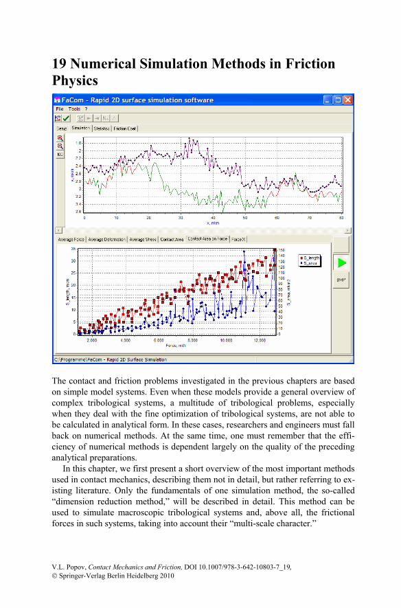
19 Numerical Simulation Methods in Friction Physics
The contact and friction problems investigated in the previous chapters are based on simple model systems. Even when these models provide a general overview of complex tribological systems, a multitude of tribological problems, especially when they deal with the fine optimization of tribological systems, are not able to be calculated in analytical form. In these cases, researchers and engineers must fall back on numerical methods. At the same time, one must remember that the effi-ciency of numerical methods is dependent largely on the quality of the preceding analytical preparations.
In this chapter, we first present a short overview of the most important methods used in contact mechanics, describing them not in detail, but rather referring to ex-isting literature. Only the fundamentals of one simulation method, the so-called “dimension reduction method,” will be described in detail. This method can be used to simulate macroscopic tribological systems and, above all, the frictional forces in such systems, taking into account their “multi-scale character.”
V.L. Popov, Contact Mechanics and Friction, DOI 10.1007/978-3-642-10803-7_19, © Springer-Verlag Berlin Heidelberg 2010
302 19 Numerical Simulation Methods in Friction Physics
19.1 Simulation Methods for Contact and Frictional Problems: An Overview
19.1.1 Many-Body Systems
Computer simulations of many-body systems are indispensable for today’s indus-trial development processes. With increasing demand on accuracy, the interest in reproducing contact and frictional phenomena as precise as possible is also in-creasing. A considerable part of research in this field is concentrated on finding methods for the implementation of simple contact conditions and Coulomb’s law of friction. At the forefront, is the search for the most efficient algorithms possible (in terms of calculation time and implementation costs). Contact is typically seen as one-sided rigid constraint. For the laws of friction, there is assumed that there exists a maximum force of static friction and that the force of kinetic friction de-pend on sliding velocity. Frequently, the force of kinetic friction is assumed to be constant and equal to the maximum force of static friction.
The simplest method for integrating friction into many-body system programs is to approximate the law of friction using a continuous function of frictional force. The frictional force in treated as a given force for which the dependence on sliding velocity is known. Typically, a force in the following form is used (Fig. 19.1):
( )2 ˆarctan /μπ
=R NF F v v . (19.1)
By using this form, one does not need to differentiate between static friction and kinetic friction. The characteristic velocity v must be chosen so that it is signifi-cantly smaller than the characteristic sliding velocity of the system to be simu-lated. In this case, the relation (19.1) expresses the behavior of the forces in both the stick and sliding domains1.
1 In this case, “sticking” is simply sliding at a very low velocity; the frictional force sets itself “automatically” equal to the correct force of static friction between μ− NF and μ+ NF . For many tribological applications, this “trick” corresponds even to the actual properties of the frictional force.
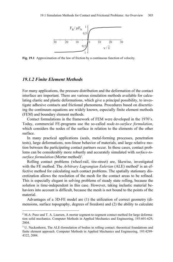
19.1 Simulation Methods for Contact and Frictional Problems: An Overview 303
10 20 300102030
0,5
1
0,5
1F / �FR N
v / v
Fig. 19.1 Approximation of the law of friction by a continuous function of velocity.
19.1.2 Finite Element Methods
For many applications, the pressure distribution and the deformation of the contact interface are important. There are various simulation methods available for calcu-lating elastic and plastic deformations, which give a principal possibility, to inves-tigate adhesive contacts and frictional phenomena. Procedures based on discretiz-ing the continuum equations are widely known, especially finite element methods (FEM) and boundary element methods.
Contact formulations in the framework of FEM were developed in the 1970’s. Today, commercial FE-programs use the so-called node-to-surface formulation, which considers the nodes of the surface in relation to the elements of the other surface.
In many practical applications (seals, metal-forming processes, penetration tests), large deformations, non-linear behavior of materials, and large relative mo-tion between the participating contact partners occur. In these cases, contact prob-lems can be considerably more robustly and accurately simulated with surface-to-surface formulation (Mortar method)2.
Rolling contact problems (wheel-rail, tire-street) are, likewise, investigated with the FE method. The Arbitrary Lagrangian Eulerian (ALE) method3 is an ef-fective method for calculating such contact problems. The spatially stationary dis-cretization allows the resolution of the mesh for the contact areas to be refined. This is especially elegant in solving problems of steady state rolling, because the solution is time-independent in this case. However, taking inelastic material be-haviors into account is difficult, because the mesh is not bound to the points of the material.
Advantages of a 3D-FE model are (1) the utilization of correct geometry (di-mensions, surface topography, degrees of freedom) and (2) the ability to calculate 2 M.A: Puso und T. A. Laursen, A mortar segment-to-segment contact method for large deforma-tion solid mechanics. Computer Methods in Applied Mechanics and Engineering, 193:601-629, 2004. 3 U. Nackenhorst, The ALE-formulation of bodies in rolling contact: theoretical foundations and finite element approach. Computer Methods in Applied Mechanics and Engineering, 193:4299-4322, 2004.
304 19 Numerical Simulation Methods in Friction Physics
stresses and deformations in the entire body. Due to the very fine mesh, however, 3D-FE models require high processing times for rough surfaces. This is an espe-cially clear disadvantage when regarding extensive parameter studies and optimi-zations. Thus, finite element methods are not practical for calculating frictional forces between rough surfaces.
19.1.3 Boundary Element Method
Boundary element method is especially suited for calculating contacts, because only the discretization of the surface is necessary. Because of the importance of this method in contact problems, we will discuss it in more detail. Here, we limit ourselves to normal contact problems between an elastic body and a rigid plane.
The vertical displacement of a point on the surface of an elastic body being acted upon by a continuous pressure distribution is given by (5.7). We divide the parts of the domain to be investigated into ×N N elements and assume the pres-sure is constant in every individual element. The relation between pressure ijp in a quadratic surface element and a vertical surface displacement iju can be analyti-cally calculated:4
ˆ ˆˆ ˆ1 1= =
= ∑∑N N
ij ijij iji j
u K p , (19.2)
with
2 2 2 2
ˆ * 2 2 2 2
2 2 2 2
2 2 2 2
ln ln
ln ln
⎡ ⎤⎛ ⎞ ⎛ ⎞Δ + + + +⎢ ⎥⎜ ⎟ ⎜ ⎟= + +⎜ ⎟ ⎜ ⎟⎢ ⎥+ + + +⎝ ⎠ ⎝ ⎠⎣ ⎦
⎛ ⎞ ⎛ ⎞+ + + +⎜ ⎟ ⎜ ⎟+⎜ ⎟ ⎜ ⎟+ + + +⎝ ⎠ ⎝ ⎠
ijij
c a c d b dK a bE d a b c b c
a a c b b dc db c b a a d
π (19.3)
and
1 1ˆ ˆ , ,2 21 1ˆ ˆ , .2 2
= − + = − −
= − + = − −
a i i b i i
c j j d j j (19.4)
4 A.E.H. Love, A Treatise on the Mathematical Theory of Elasticity. 4th edition., Cambridge, University Press. See also: K. L. Johnson, Contact mechanics. Cambridge University Press, 6th printing of the 1st edition, 2001, p. 54.
19.1 Simulation Methods for Contact and Frictional Problems: An Overview 305
Δ is the mesh spacing. Equation (19.2) can be written in matrix form as
u = Ap , (19.5)
with a matrix A with dimensions 2 2×N N . In contact problems, the size and lo-cation of the contact area is initially unknown. Therefore, contact problems must be solved iteratively. In the contact area, the separation between the surfaces is zero (i.e. in this area, the displacement of the elastic surface is known). Outside of the contact area, the pressure is zero; the displacement, on the other hand, is gen-erally not zero. To begin, a contact area is assumed. The variables are now parti-tioned into the variables ip and iu inside of the contact area and ap and au out-side of the contact area. iu and 0=ap are known. After rearranging according to (19.5), we obtain
⎡ ⎤ ⎧ ⎫⎧ ⎫
⎨ ⎬ ⎨ ⎬⎢ ⎥⎩ ⎭⎣ ⎦ ⎩ ⎭
1 2 ii
3 4 a
A A up=
A A u0 (19.6)
and finally,
1 i iA p = u , (19.7)
3 aiA p = u . (19.8)
The solution to the system of equations in (19.7) yields a pressure in the contact area of ip . With these results, using (19.8), the displacement au in the domain outside of the contact can be calculated. The first iteration step generally yields a negative pressure (tensile stress) in the contact area and a negative separation dis-tance outside of the contact area. The new contact area is now chosen so that all of the points in tensile stress are removed from the contact area and all of the points with a negative separation difference are brought into it. With this new approxi-mation of the contact area, the previously described calculation is repeated. The it-eration continues until no more tensile stresses or negative separation distances exist (to a reasonable approximation).
19.1.4 Particle Methods
Another approach to the simulation of contact and frictional problems is provided by particle methods, for which discrete particles are the focus of the calculations. These particles are not real (physical) objects, rather purely “units for calculation.” The interactions between the particles must be chosen so that the elastic and plas-tic behavior of the material is correctly described. Thus, neither the macroscopic continuum equations nor the microscopic equations of molecular dynamics are
306 19 Numerical Simulation Methods in Friction Physics
solved, rather the microscopic equations of a suitable substitution system. The size of the particles can be adjusted to fit the problem. For example, for the investiga-tion of earthquakes, the particle size can be on the order of meters.
The frictional force is determined by processes such as elastic and plastic de-formation, fracture, and the dislodgement and reintegration of particles. These processes take place in micro-contacts. The movable cellular automata (MCA) method is a particle method with which the processes in micro-contacts are suc-cessfully simulated5.
19.2 Reduction of Contact Problems from Three Dimensions to One Dimension
Now, we will discuss a simulation method that is especially well suited for simula-tion of friction between rough surfaces. The laws of friction obtained using this method can subsequently be used in macroscopic system dynamics simulations. We limit ourselves to “typical tribological systems” which are characterized by the laws of dry friction being approximately met, especially, that the frictional force is approximately proportional to the normal force. This implies that the real contact area remains much smaller than the apparent contact area.
For “typical tribological systems,” there is a series of properties that allow im-mense simplification of the contact problem and in this way, allow quick calcula-tion even in multi-scaled systems. The simplifying properties used in the reduction method are the following: (a) For velocities much smaller than the speed of sound6, deformations can be treated as quasi-static; (b) The potential energy, and therefore, the force-displacement relation, is a local property that depends only on the configuration of the micro-contacts and not the form or size of the body; (c) The kinetic energy, on the other hand, is a “global property” that depends only on the form and size of the body as a whole and not on the configuration of the micro-contacts; (d) Many significant properties in contact mechanics can be well approximated us-ing one-dimensional systems, which allows for crucial reduction in calculation time.
These four properties are found in many macroscopic tribological systems. The application area of the subsequent methods is, accordingly, very wide. One must not forget that when applying these methods, the above conditions must be met. In the following, we will discuss the aforementioned simplifying assumptions in de-tail. 5 V.L. Popov, und S.G. Psakhie, Numerical simulation methods in tribology. Tribology Interna-tional, 2007, v. 40(6), pp. 916-923. 6 This condition is met rather well in most real tribological contacts.
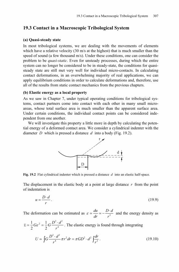
19.3 Contact in a Macroscopic Tribological System 307
19.3 Contact in a Macroscopic Tribological System
(a) Quasi-steady state In most tribological systems, we are dealing with the movements of elements which have a relative velocity (30 m/s at the highest) that is much smaller than the speed of sound (a few thousand m/s). Under these conditions, one can consider the problem to be quasi-static. Even for unsteady processes, during which the entire system can no longer be considered to be in steady-state, the conditions for quasi-steady state are still met very well for individual micro-contacts. In calculating contact deformations, in an overwhelming majority of real applications, we can apply equilibrium conditions in order to calculate deformations and, therefore, use all of the results from static contact mechanics from the previous chapters.
(b) Elastic energy as a local property As we saw in Chapter 7, under typical operating conditions for tribological sys-tems, contact partners come into contact with each other in many small micro-areas, whose total surface area is much smaller than the apparent surface area. Under certain conditions, the individual contact points can be considered inde-pendent from one another.
We will investigate this property a little more in depth by calculating the poten-tial energy of a deformed contact area. We consider a cylindrical indenter with the diameter D which is pressed a distance d into a body (Fig. 19.2).
Fig. 19.2 Flat cylindrical indenter which is pressed a distance d into an elastic half-space.
The displacement in the elastic body at a point at large distance r from the point of indentation is
⋅D dur
. (19.9)
The deformation can be estimated as 2ε ⋅−
du D ddr r
and the energy density as
2 22
4
1 12 2
ε ⋅E
D dG Gr
. The elastic energy is found through integrating
2 2
2 2 24 2π π⋅
= ⋅∫ ∫D d drU G r dr GD d
r r. (19.10)
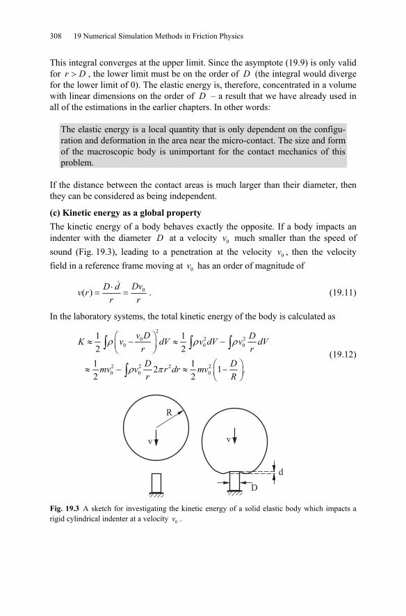
308 19 Numerical Simulation Methods in Friction Physics
This integral converges at the upper limit. Since the asymptote (19.9) is only valid for >r D , the lower limit must be on the order of D (the integral would diverge for the lower limit of 0). The elastic energy is, therefore, concentrated in a volume with linear dimensions on the order of D – a result that we have already used in all of the estimations in the earlier chapters. In other words:
The elastic energy is a local quantity that is only dependent on the configu-ration and deformation in the area near the micro-contact. The size and form of the macroscopic body is unimportant for the contact mechanics of this problem.
If the distance between the contact areas is much larger than their diameter, then they can be considered as being independent.
(c) Kinetic energy as a global property The kinetic energy of a body behaves exactly the opposite. If a body impacts an indenter with the diameter D at a velocity 0v much smaller than the speed of sound (Fig. 19.3), leading to a penetration at the velocity 0v , then the velocity field in a reference frame moving at 0v has an order of magnitude of
0( ) ⋅= =
DvD dv rr r
. (19.11)
In the laboratory systems, the total kinetic energy of the body is calculated as
22 20
0 0 0
2 2 2 20 0 0
1 12 2
1 1 2 1 .2 2
v D DK v dV v dV v dVr rD Dmv v r dr mvr R
ρ ρ ρ
ρ π
⎛ ⎞≈ − ≈ −⎜ ⎟⎝ ⎠
⎛ ⎞≈ − ≈ −⎜ ⎟⎝ ⎠
∫ ∫ ∫
∫ (19.12)
Fig. 19.3 A sketch for investigating the kinetic energy of a solid elastic body which impacts a rigid cylindrical indenter at a velocity 0v .
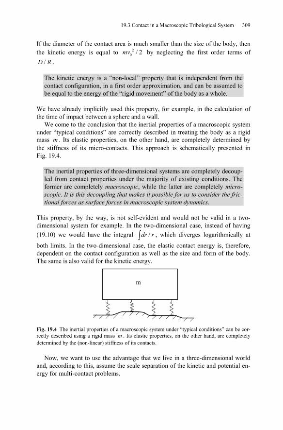
19.3 Contact in a Macroscopic Tribological System 309
If the diameter of the contact area is much smaller than the size of the body, then the kinetic energy is equal to 2
0 / 2mv by neglecting the first order terms of /D R .
The kinetic energy is a “non-local” property that is independent from the contact configuration, in a first order approximation, and can be assumed to be equal to the energy of the “rigid movement” of the body as a whole.
We have already implicitly used this property, for example, in the calculation of the time of impact between a sphere and a wall.
We come to the conclusion that the inertial properties of a macroscopic system under “typical conditions” are correctly described in treating the body as a rigid mass m . Its elastic properties, on the other hand, are completely determined by the stiffness of its micro-contacts. This approach is schematically presented in Fig. 19.4.
The inertial properties of three-dimensional systems are completely decoup-led from contact properties under the majority of existing conditions. The former are completely macroscopic, while the latter are completely micro-scopic. It is this decoupling that makes it possible for us to consider the fric-tional forces as surface forces in macroscopic system dynamics.
This property, by the way, is not self-evident and would not be valid in a two-dimensional system for example. In the two-dimensional case, instead of having (19.10) we would have the integral /∫ dr r , which diverges logarithmically at
both limits. In the two-dimensional case, the elastic contact energy is, therefore, dependent on the contact configuration as well as the size and form of the body. The same is also valid for the kinetic energy.
m
Fig. 19.4 The inertial properties of a macroscopic system under “typical conditions” can be cor-rectly described using a rigid mass m . Its elastic properties, on the other hand, are completely determined by the (non-linear) stiffness of its contacts.
Now, we want to use the advantage that we live in a three-dimensional world and, according to this, assume the scale separation of the kinetic and potential en-ergy for multi-contact problems.
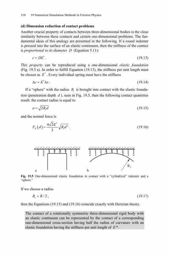
310 19 Numerical Simulation Methods in Friction Physics
(d) Dimension reduction of contact problems Another crucial property of contacts between three-dimensional bodies is the close similarity between these contacts and certain one-dimensional problems. The fun-damental ideas of this analogy are presented in the following. If a round indenter is pressed into the surface of an elastic continuum, then the stiffness of the contact is proportional to its diameter D (Equation 5.11):
*=c DE . (19.13)
This property can be reproduced using a one-dimensional elastic foundation (Fig. 19.5 a). In order to fulfill Equation (19.13), the stiffness per unit length must be chosen as *E . Every individual spring must have the stiffness
*Δ = Δc E x . (19.14)
If a “sphere” with the radius 1R is brought into contact with the elastic founda-tion (penetration depth d ), seen in Fig. 19.5, then the following contact quantities result: the contact radius is equal to
12=a R d (19.15)
and the normal force is
( )*
31
4 23
=NEF d R d . (19.16)
R1
a b Fig. 19.5 One-dimensional elastic foundation in contact with a “cylindrical” indenter and a “sphere.”
If we choose a radius
1 / 2=R R , (19.17)
then the Equations (19.15) and (19.16) coincide exactly with Hertzian theory.
The contact of a rotationally symmetric three-dimensional rigid body with an elastic continuum can be represented by the contact of a corresponding one-dimensional cross-section having half the radius of curvature with an elastic foundation having the stiffness per unit length of *E .
19.4 Reduction Method for a Multi-Contact Problem 311
This rule is exactly correct for every cylindrical indenter and for every parabolic body with an arbitrary radius of curvature.
Since a contact between an ellipsoid and a rigid plane can be approximated by a contact between a sphere and a plane (using the Gaussian radius (1) (2)R R , see (5.30)), the representation of a non-rotationally symmetric contacts in a one-dimensional system is possible as well. Thereby, the Hertzian relation between normal force and contact area is still valid. The stiffness of indenters with non-circular cross-sections (5.13) shows that one-dimensional representation also works for bodies with square or triangular cross-sections with an error of less than 3%. The “one-dimensional diameter” of the contact, in this case, is calculated ac-cording to the rule ( )1/24 /π=D A .
The tangential stiffness of a three-dimensional contact is also proportional to the diameter of the contact:
4 22 ν⊥ ≈ ⋅−Gc a , (19.18)
and thus, can be replicated using a one-dimensional elastic foundation for the same reasons. The tangential stiffness of individual springs in the elastic founda-tion must be chosen according to
42 ν⊥Δ = Δ−Gc x . (19.19)
The fact that the force-penetration depth and the force-contact area relation-ships are independent of scaling for very different rotationally symmetric and non-symmetric individual contacts allows us to draw the hypothesis that this would al-so be the case with a randomly rough surface.
19.4 Reduction Method for a Multi-Contact Problem
In order to cross over to a contact between bodies with rough surfaces, a rule for the production of a one-dimensional profile, which is equivalent to the three-dimensional body in a contact mechanical sense, must be formulated (Fig. 19.6). As the motivation for this replacement, we use a few ideas from the model of Greenwood and Williamson. The results and quality of the replacement system, however, prove to be much better than the Greenwood-Williamson model itself.
In the model of Greenwood and Williamson, the individual contacts are con-sidered to be independent from each other. Under these conditions, only the distri-bution of the heights of the asperities and the radii of curvature play a role. So, our goal is first to generate a one-dimensional system, which has the necessary statistical distributions of heights and radii of curvature.
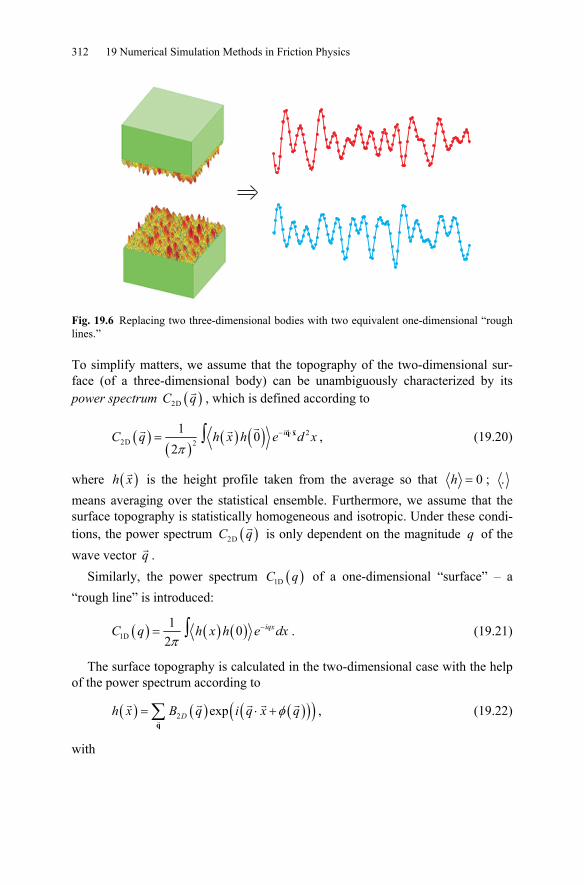
312 19 Numerical Simulation Methods in Friction Physics
Fig. 19.6 Replacing two three-dimensional bodies with two equivalent one-dimensional “rough lines.”
To simplify matters, we assume that the topography of the two-dimensional sur-face (of a three-dimensional body) can be unambiguously characterized by its power spectrum ( )2DC q , which is defined according to
( )( )
( ) ( ) 22D 2
1 02π
− ⋅= ∫ iC q h x h e d xq x , (19.20)
where ( )h x is the height profile taken from the average so that 0=h ; . means averaging over the statistical ensemble. Furthermore, we assume that the surface topography is statistically homogeneous and isotropic. Under these condi-tions, the power spectrum ( )2DC q is only dependent on the magnitude q of the wave vector q .
Similarly, the power spectrum ( )1DC q of a one-dimensional “surface” – a “rough line” is introduced:
( ) ( ) ( )1D1 0
2π−= ∫ iqxC q h x h e dx . (19.21)
The surface topography is calculated in the two-dimensional case with the help of the power spectrum according to
( ) ( ) ( )( )( )2 exp φ= ⋅ +∑ Dh x B q i q x qq
, (19.22)
with
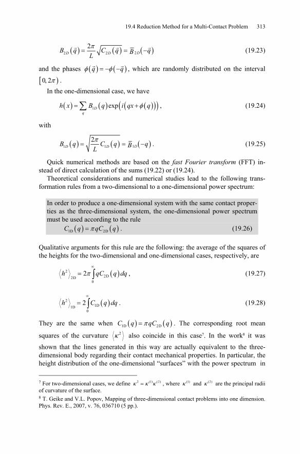
19.4 Reduction Method for a Multi-Contact Problem 313
( ) ( ) ( )22 22π
= = −DD DB q C q qBL (19.23)
and the phases ( ) ( )φ φ= − −q q , which are randomly distributed on the interval
[ )0 2π, . In the one-dimensional case, we have
( ) ( ) ( )( )( )1 exp φ= +∑ Dq
h x B q i qx q , (19.24)
with
( ) ( ) ( )11 12π
= = −DD DB q C q qBL. (19.25)
Quick numerical methods are based on the fast Fourier transform (FFT) in-stead of direct calculation of the sums (19.22) or (19.24).
Theoretical considerations and numerical studies lead to the following trans-formation rules from a two-dimensional to a one-dimensional power spectrum:
In order to produce a one-dimensional system with the same contact proper-ties as the three-dimensional system, the one-dimensional power spectrum must be used according to the rule ( ) ( )1D 2Dπ=C q qC q . (19.26)
Qualitative arguments for this rule are the following: the average of the squares of the heights for the two-dimensional and one-dimensional cases, respectively, are
( )22D2D
0
2π∞
= ∫h qC q dq , (19.27)
( )21D1D
0
2∞
= ∫h C q dq . (19.28)
They are the same when ( ) ( )1D 2Dπ=C q qC q . The corresponding root mean
squares of the curvature 2κ also coincide in this case7. In the work8 it was
shown that the lines generated in this way are actually equivalent to the three-dimensional body regarding their contact mechanical properties. In particular, the height distribution of the one-dimensional “surfaces” with the power spectrum in
7 For two-dimensional cases, we define 2 (1) (2)κ κ κ= , where (1)κ and (2)κ are the principal radii of curvature of the surface. 8 T. Geike and V.L. Popov, Mapping of three-dimensional contact problems into one dimension. Phys. Rev. E., 2007, v. 76, 036710 (5 pp.).
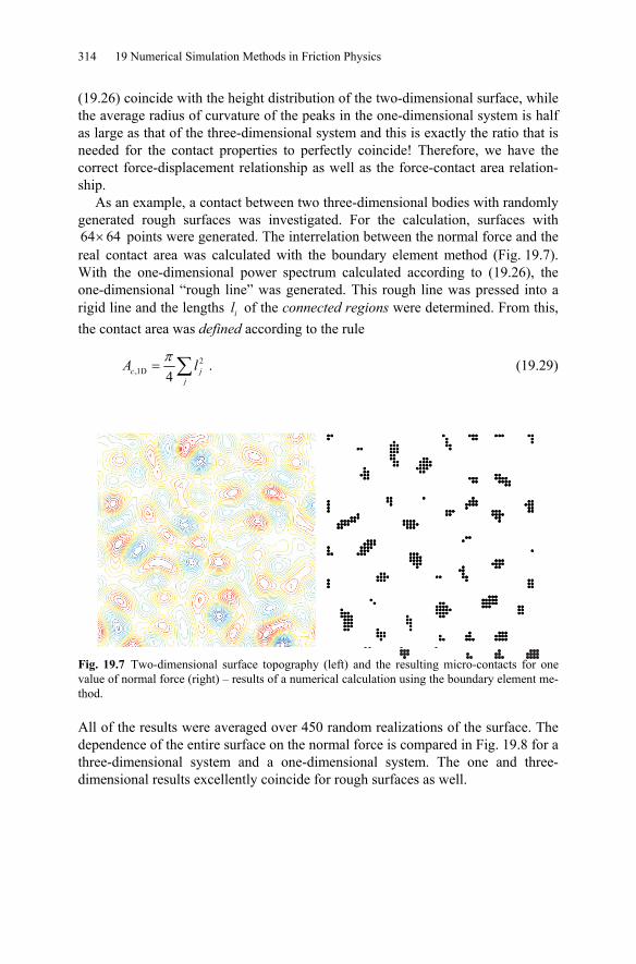
314 19 Numerical Simulation Methods in Friction Physics
(19.26) coincide with the height distribution of the two-dimensional surface, while the average radius of curvature of the peaks in the one-dimensional system is half as large as that of the three-dimensional system and this is exactly the ratio that is needed for the contact properties to perfectly coincide! Therefore, we have the correct force-displacement relationship as well as the force-contact area relation-ship.
As an example, a contact between two three-dimensional bodies with randomly generated rough surfaces was investigated. For the calculation, surfaces with 64 64× points were generated. The interrelation between the normal force and the real contact area was calculated with the boundary element method (Fig. 19.7). With the one-dimensional power spectrum calculated according to (19.26), the one-dimensional “rough line” was generated. This rough line was pressed into a rigid line and the lengths il of the connected regions were determined. From this, the contact area was defined according to the rule
2,1D 4
π= ∑c j
j
A l . (19.29)
Fig. 19.7 Two-dimensional surface topography (left) and the resulting micro-contacts for one value of normal force (right) – results of a numerical calculation using the boundary element me-thod.
All of the results were averaged over 450 random realizations of the surface. The dependence of the entire surface on the normal force is compared in Fig. 19.8 for a three-dimensional system and a one-dimensional system. The one and three-dimensional results excellently coincide for rough surfaces as well.
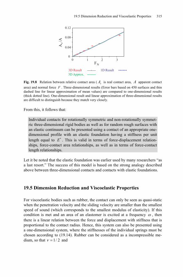
19.5 Dimension Reduction and Viscoelastic Properties 315
Fig. 19.8 Relation between relative contact area ( cA is real contact area, A apparent contact area) and normal force F . Three-dimensional results (Error bars based on 450 surfaces and thin dashed line for linear approximation of mean values) are compared to one-dimensional results (thick dotted line). One-dimensional result and linear approximation of three-dimensional results are difficult to distinguish because they match very closely.
From this, it follows that:
Individual contacts for rotationally symmetric and non-rotationally symmet-ric three-dimensional rigid bodies as well as for random rough surfaces with an elastic continuum can be presented using a contact of an appropriate one-dimensional profile with an elastic foundation having a stiffness per unit length equal to *E . This is valid in terms of force-displacement relation-ships, force-contact area relationships, as well as in terms of force-contact length relationships.
Let it be noted that the elastic foundation was earlier used by many researchers “as a last resort.” The success of this model is based on the strong analogy described above between three-dimensional contacts and contacts with elastic foundations.
19.5 Dimension Reduction and Viscoelastic Properties
For viscoelastic bodies such as rubber, the contact can only be seen as quasi-static when the penetration velocity and the sliding velocity are smaller than the smallest speed of sound (which corresponds to the smallest modulus of elasticity). If this condition is met and an area of an elastomer is excited at a frequency ω , then there is a linear relation between the force and displacement with stiffness that is proportional to the contact radius. Hence, this system can also be presented using a one-dimensional system, where the stiffnesses of the individual springs must be chosen according to (19.14). Rubber can be considered as a incompressible me-dium, so that 1/ 2ν = and
316 19 Numerical Simulation Methods in Friction Physics
( ) ( ) ( ) ( )*2
24
11ω ω
ω ωνν
Δ ≈ Δ = Δ = Δ = Δ−−
E Gc E x x x G x . (19.30)
In the case of rubber, the stiffness of the individual “springs” of the elastic foundation is four times the shear modulus multiplied with the mesh spac-ing.
In the one-dimensional model, the stress-strain relation (15.2) must be replaced by
( ) 4 ( ) ( )δ−∞
′ ′ ′= Δ −∫t
iF t x G t t t dt . (19.31)
19.6 Representation of Stress in the Reduction Model
As long as the bodies are only elastically or viscoelastically deformed, one needs no information about the resulting stresses in the contact area. However, if the bodies are plastically deformed or worn due to stress peaks, then information about the stress occurring in the contact is necessary for the simulation. In the one-dimension model, only the spring forces are directly defined, not the stresses. In the following, it will be shown that in the 1D model, a stress can also be defined that coincides with Hertzian stress distribution in the case of elastic deformation.
The force in a spring is
2
* *
12δ
⎛ ⎞= Δ = Δ −⎜ ⎟
⎝ ⎠i
i ix
F xE xE dR
, (19.32)
where δ i is the displacement of the spring i and Δx is the mesh spacing. Now, we define the stress as
1
σδ
= ii
i
Fb R
. (19.33)
Here, b is the constant still to be determined. The stress is dependent on the ra-dius of curvature and is, therefore, a non-local quantity9.
9 The following arguments can be cited as motivation for this form of the stress: the contact ra-dius for an individual contact is equal to 2δ=a R , where δ is the penetration depth. We have
an approximation for the average stress of 2
/σ
δ∝ ∝ ∝ iN N
FF F aa a R
, where iF is the average
spring force in the contact area. This is exactly the form (19.33). The fact that using the coordi-
19.7 The Calculation Procedure in the Framework of the Reduction Method 317
From (19.33), (19.32), and (19.16) we get:
2
2 2
3 2 14
σ Δ= −N i
iF xx
ba a. (19.34)
For a Hertzian spherical contact, the stress distribution is equal to
2
2 2
31
2σ
π= −NF x
a a. (19.35)
These two stress distributions coincide when
22
π= Δb x . (19.36)
Thus, the stress is calculated from the local spring force iF and the local deforma-tion δ i according to
1
2σ
π δ=
Δi
ii
Fx R
. (19.37)
For the yield criterion, the non-local quantity σ i according to Equation (19.37)
should be used, rather than the local force iF .
19.7 The Calculation Procedure in the Framework of the Reduction Method
The calculation procedure for the reduction method consists of the following steps: 1. The frictional surface is measured (e.g. using a white light interference micro-scope or an atomic force microscope). 2. The two-dimensional power spectrum of the surface is calculated with the fast Fourier transform. 3. This is now transformed into the one-dimensional power spectrum according to the rule in (19.26). 4. With this power spectrum, a one-dimensional “rough line” is generated which has the same contact properties as the original three-dimensional system. 5. The elastic properties are chosen according to the rule in (19.14).
nate-dependent penetration depth δ i leads exactly to the Hertzian stress distribution can be con-sidered an empirical discovery.
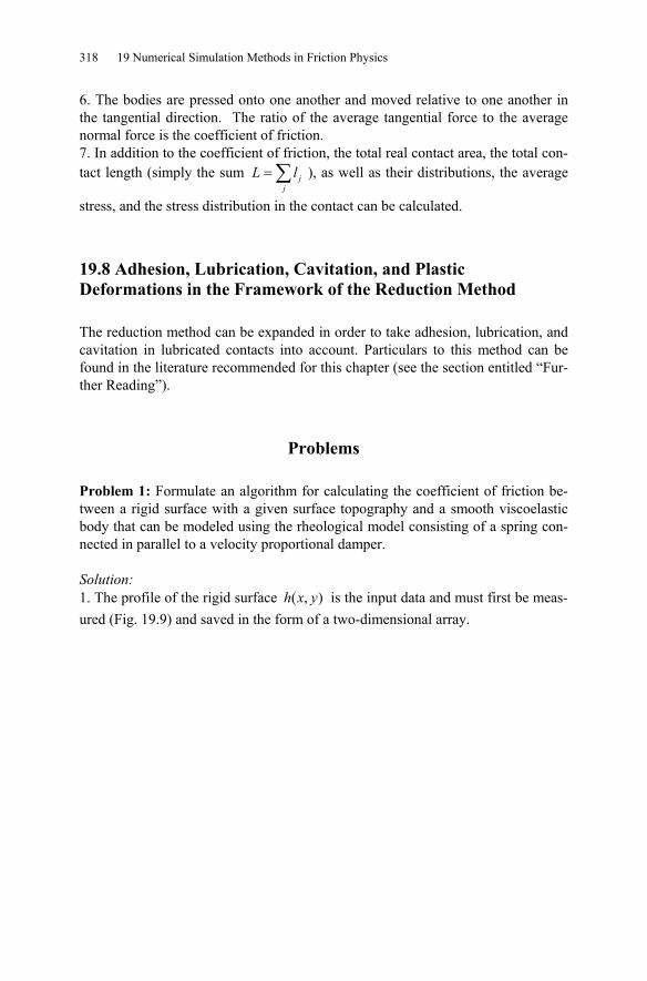
318 19 Numerical Simulation Methods in Friction Physics
6. The bodies are pressed onto one another and moved relative to one another in the tangential direction. The ratio of the average tangential force to the average normal force is the coefficient of friction. 7. In addition to the coefficient of friction, the total real contact area, the total con-tact length (simply the sum j
jL l= ∑ ), as well as their distributions, the average
stress, and the stress distribution in the contact can be calculated.
19.8 Adhesion, Lubrication, Cavitation, and Plastic Deformations in the Framework of the Reduction Method
The reduction method can be expanded in order to take adhesion, lubrication, and cavitation in lubricated contacts into account. Particulars to this method can be found in the literature recommended for this chapter (see the section entitled “Fur-ther Reading”).
Problems
Problem 1: Formulate an algorithm for calculating the coefficient of friction be-tween a rigid surface with a given surface topography and a smooth viscoelastic body that can be modeled using the rheological model consisting of a spring con-nected in parallel to a velocity proportional damper.
Solution: 1. The profile of the rigid surface ( , )h x y is the input data and must first be meas-ured (Fig. 19.9) and saved in the form of a two-dimensional array.
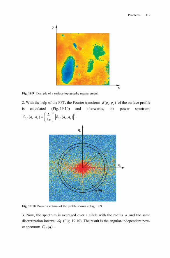
Problems 319
Fig. 19.9 Example of a surface topography measurement.
2. With the help of the FFT, the Fourier transform ( , )x yB q q of the surface profile is calculated (Fig. 19.10) and afterwards, the power spectrum:
22
2 2( , ) ( , )2π
⎛ ⎞= ⎜ ⎟⎝ ⎠
D x y D x yLC q q B q q .
qy
qx
q
dq
Fig. 19.10 Power spectrum of the profile shown in Fig. 19.9.
3. Now, the spectrum is averaged over a circle with the radius q and the same discretization interval dq (Fig. 19.10). The result is the angular-independent pow-er spectrum 2 ( )DC q .
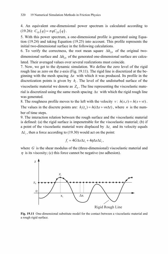
320 19 Numerical Simulation Methods in Friction Physics
4. An equivalent one-dimensional power spectrum is calculated according to (19.26): ( ) ( )1D 2Dπ=C q qC q . 5. With this power spectrum, a one-dimensional profile is generated using Equa-tion (19.24) and taking Equation (19.25) into account. This profile represents the initial two-dimensional surface in the following calculations. 6. To verify the correctness, the root mean square 2Δ Dh of the original two-dimensional surface and 1Δ Dh of the generated one-dimensional surface are calcu-lated. Their averaged values over several realizations must coincide. 7. Now, we get to the dynamic simulation. We define the zero level of the rigid rough line as zero on the z-axis (Fig. 19.11). The rigid line is discretized at the be-ginning with the mesh spacing Δx with which it was produced. Its profile in the discretization points is given by ih . The level of the undisturbed surface of the viscoelastic material we denote as 0Z . The line representing the viscoelastic mate-rial is discretized using the same mesh spacing Δx with which the rigid rough line was generated. 8. The roughness profile moves to the left with the velocity v : ( , ) ( )= +h x t h x vt . The values in the discrete points are: ( ) ( )= Δ + Δi nh t h i x vn t , where n is the num-ber of time steps. 9. The interaction relation between the rough surface and the viscoelastic material is defined: (a) the rigid surface is impenetrable for the viscoelastic material; (b) if a point of the viscoelastic material were displaced by Δ iz and its velocity equals Δ iz , then a force according to (19.30) would act on the point:
4 4η= Δ Δ + Δ Δi i if G x z x z ,
where G is the shear modulus of the (three-dimensional) viscoelastic material and η is its viscosity; (c) this force cannot be negative (no adhesion).
Fig. 19.11 One-dimensional substitute model for the contact between a viscoelastic material and a rough rigid surface.
Problems 321
10. The system is “initialized” by placing the viscoelastic material “near” the rigid line: that means at a distance of about 13Δ Dh from the zero line. Thereby, those points of the body meeting the condition 0≥ih Z come into contact with the rough substrate. We initially set the force acting on the system to be equal to
( )04= −i if G h Z . The total force acting on the viscoelastic material is equal to
( )0points pointsin incontact contact
4i iF f G x h Z= = Δ −∑ ∑ .
In the vertical direction, a normal force − NF is applied. 11. Choice of time step: In the time Δt , the upper body is always displaced by a discretized step of Δx . Thus, the time step is
/Δ = Δt x v .
12. Time loop: In the next state (displaced by Δx ), the condition 1( )+ ≥i n ih t z is checked and in this way, the new points that have come into contact are deter-mined. The force acting on these points is calculated using
( ) ( )1 1 0 1( ) 4 ( ) 4 ( ) ( ) /η+ + += Δ − + Δ − Δi n i n i n i nf t G x h t Z x h t z t t .
For the points that were in contact in the previous step, it is initially assumed that they remain on the surface: therefore, their coordinates change from ( ) ( )=i n i nz t h t to 1 1( ) ( )+ +=i n i nz t h t . The force is calculated using the same formula. If the force is positive, then the points remain in contact. If it is negative, then these points are said to have lost contact and force acting on them is set to zero.
For all points that are not in contact, their new position is determined using the condition that
( )( ) ( ) ( )10 0η + −
⋅ − + =Δ
i n i ni n
z t z tG z t Z
t.
From this, it follows that
( ) ( ) ( )( )1 0η+ = − ⋅Δ −i n i n i nGz t z t t z t Z .
Thereby, the total force acting on the material would be equal to
( ) ( )1 1 0 1( ) 4 ( ) 4 ( ) ( ) /η+ + += = Δ − + Δ − Δ∑ ∑i n i n i n i ni i
F f t G x h t Z x h t z t t ,
which is summed over all of the points found to be in contact. Since, the normal force should remain constant, the state of the upper surface
0Z changes so that the total vertical force is NF . To achieve this, the body is dis-placed by ΔZ . The force resulting from this movement is equal to
322 19 Numerical Simulation Methods in Friction Physics
( ) ( )4 4 / 4 4 /η ηΔ = −Δ Δ + Δ Δ = −Δ Δ + Δ Δ∑i
F Z G x x t ZN G x x t .
Here, N is the number of points in contact. Together with the force calculated in the previous step, it must result in exactly NF :
( )4 4 /η−Δ Δ + Δ Δ + = NZN G x x t F F .
From this, it follows that
( )4 4 /η−
Δ =Δ + Δ Δ
NF FZ
N G x x t, 0 1 0( ) ( )+ = + Δn nZ t Z t Z .
13. In order to calculate the tangential force, the normal force acting on the point i is multiplied with the tangent of the inclination angle of the surface:
1 1, 2
+ −−=
Δi i
x i ih h
f fx
and summed over all contacts:
1 1
pointsincontact
2i i
x ih h
F fx
+ −−=
Δ∑ .
14. The ratio /x NF F is the instantaneous value of the coefficient of friction. Av-eraged over the total time, it provides us the average coefficient of friction.

20 Earthquakes and Friction
Tectonic plate dynamics can also be seen as a part of tribology. The Earth’s crust is composed of tectonic plates which slowly move relative to one another due to convection in the mantel. On a time scale of millions of years, these movements determine the structure of the Earth’s surface. On a small time scale, they are re-sponsible for earthquakes. Frictional models have applications for describing the dynamics of individual faults as well as describing the Earth’s crust as a granular medium. Models for mechanisms of earthquakes are based on the fundamental ob-servation that earthquakes do not arise as a result of a sudden formation and propagation of a new crack in the Earth’s crust, rather they take place as a result of a sudden sliding along an already existing faults. In addition to other evidence, this is confirmed by the fact that the decrease in stress resulting from an earth-quake (a few MPa) is much smaller than the strength of rock. Therefore, earth-quakes are more a phenomenon of frictional physics than of fracture mechanics. Since the work of Brace und Byerlee1, at the latest, earthquakes were understood to be a type of stick-slip instability2.
1 W.F. Brace and J.D. Byerlee, Stick slip as a mechanism for earthquakes. Science, 1966, v. 153, pp. 990-992. 2 This is valid only for earthquakes initiating in the upper part of the Earth’s crust.
V.L. Popov, Contact Mechanics and Friction, DOI 10.1007/978-3-642-10803-7_20, © Springer-Verlag Berlin Heidelberg 2010
324 20 Earthquakes and Friction
20.1 Introduction
Due to the slow movement of tectonic plates, stresses build up in friction areas in the faults, which lead to quick, jerky movements when some critical value is ex-ceeded. We perceive these movements as earthquakes. Similar instabilities appear even in the simplest of tribological laboratory systems, for example, a body that is slowly pulled by means of a soft spring. A few general properties of earthquakes can already be illustrated by mean of such a simple model. In the simplest model of a stick-slip instability (Problem 1 in Chapter 12), it was assumed that sliding begins when the ratio of the shear stress to the normal stress in the contact area exceeds the coefficient of static friction sμ . If the body is put into motion, then the coefficient of friction falls to a smaller value kμ , which leads to a stick-slip type of frictional instability. In Chapter 12 (Problem 1), we saw that the displace-ment u during the stick-slip phase is given by
2 s kF Fu
c−
= , (20.1)
where c is the spring stiffness, s s NF Fμ= is the static friction force, k k NF Fμ= is the kinetic friction force and NF the normal force. The energy dissipated during the slip phase is equal to
( )
2 k s kk
F F FE F u
c−
= = . (20.2)
In a real fault, we have no individual masses and no discrete spring elements. In-stead, the equations of elasticity theory must be solved taking into account the law of friction. Here, we limit ourselves to a simple estimation. We assume that a con-tact area has a linear dimension L smaller than the thickness D of the brittle part of the Earth’s crust (schizosphere)3. A correlated movement in this contact area leads to significant displacements and deformations in a volume with dimensions L L L× × . The stiffness of a cube with such dimensions is on the order of magni-tude c G L≈ ⋅ . From Equations (20.1) and (20.2), the following estimations for the displacement during a slip event and the dissipated energy result:
( )22 s k N
N s kL
u FGL G
μ μ σμ μ
−≈ ≈ − , (20.3)
( )2 32 k s k
k N NE F u LG
μ μ μμ σ
−≈ ≈ , (20.4)
where 2/N NF Lσ = is the normal stress. 3 We call such earthquakes “weak earthquakes.”
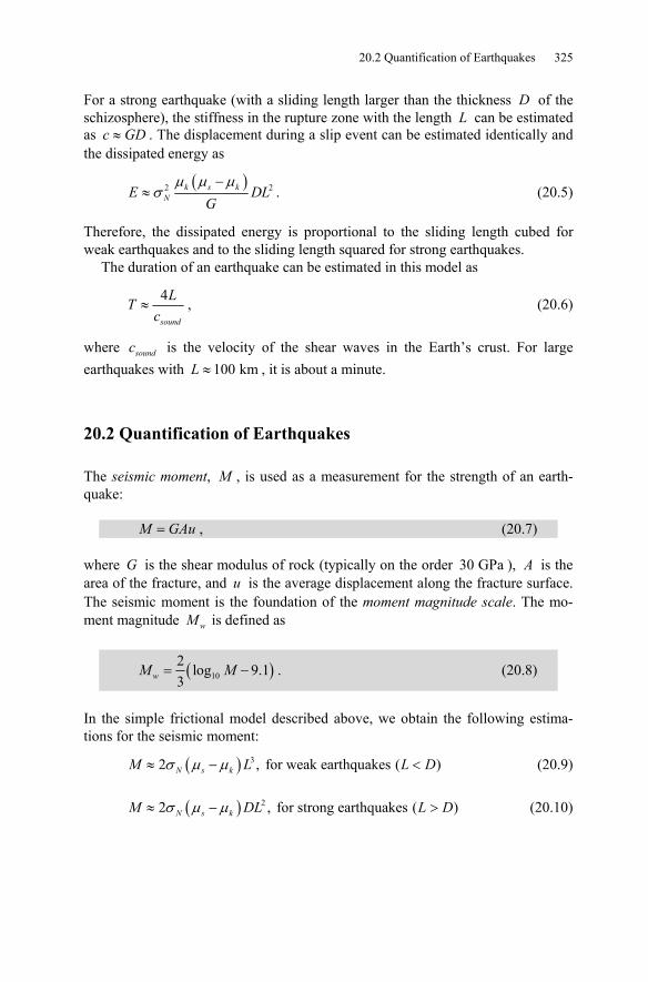
20.2 Quantification of Earthquakes 325
For a strong earthquake (with a sliding length larger than the thickness D of the schizosphere), the stiffness in the rupture zone with the length L can be estimated as c GD≈ . The displacement during a slip event can be estimated identically and the dissipated energy as
( )2 2k s k
NE DLG
μ μ μσ
−≈ . (20.5)
Therefore, the dissipated energy is proportional to the sliding length cubed for weak earthquakes and to the sliding length squared for strong earthquakes.
The duration of an earthquake can be estimated in this model as
4
sound
LTc
≈ , (20.6)
where soundc is the velocity of the shear waves in the Earth’s crust. For large earthquakes with 100 kmL ≈ , it is about a minute.
20.2 Quantification of Earthquakes
The seismic moment, M , is used as a measurement for the strength of an earth-quake:
M GAu= , (20.7)
where G is the shear modulus of rock (typically on the order 30 GPa ), A is the area of the fracture, and u is the average displacement along the fracture surface. The seismic moment is the foundation of the moment magnitude scale. The mo-ment magnitude wM is defined as
( )102 log 9.13wM M= − . (20.8)
In the simple frictional model described above, we obtain the following estima-tions for the seismic moment:
( ) 32 , for weak earthquakes ( )N s kM L L Dσ μ μ≈ − < (20.9)
( ) 22 , for strong earthquakes ( )N s kM DL L Dσ μ μ≈ − > (20.10)
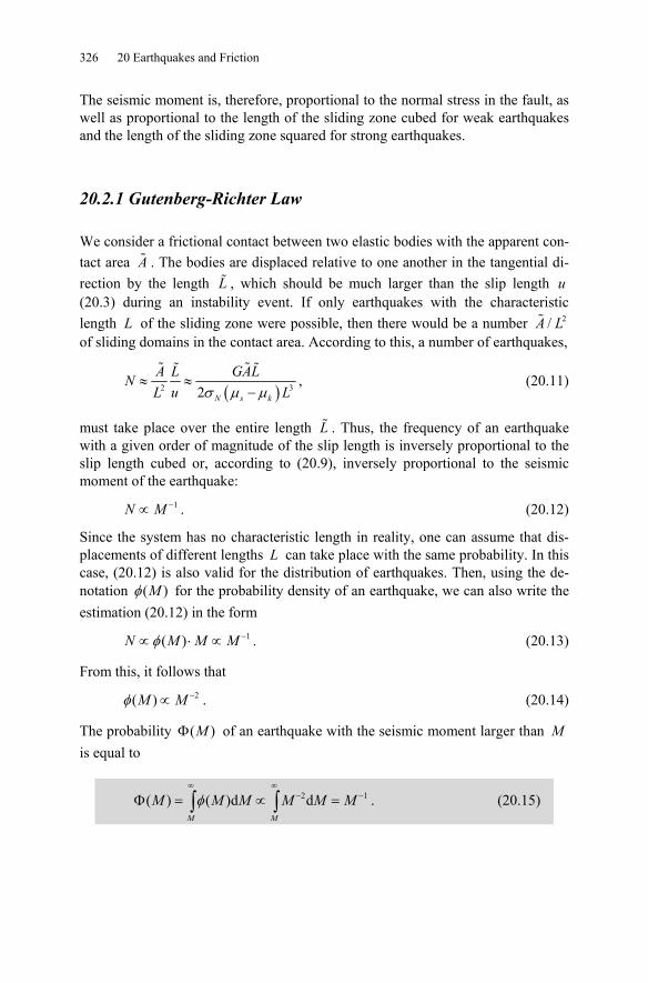
326 20 Earthquakes and Friction
The seismic moment is, therefore, proportional to the normal stress in the fault, as well as proportional to the length of the sliding zone cubed for weak earthquakes and the length of the sliding zone squared for strong earthquakes.
20.2.1 Gutenberg-Richter Law
We consider a frictional contact between two elastic bodies with the apparent con-tact area A . The bodies are displaced relative to one another in the tangential di-rection by the length L , which should be much larger than the slip length u (20.3) during an instability event. If only earthquakes with the characteristic length L of the sliding zone were possible, then there would be a number 2/A L of sliding domains in the contact area. According to this, a number of earthquakes,
( )2 32 N s k
A L GALNuL Lσ μ μ
≈ ≈−
, (20.11)
must take place over the entire length L . Thus, the frequency of an earthquake with a given order of magnitude of the slip length is inversely proportional to the slip length cubed or, according to (20.9), inversely proportional to the seismic moment of the earthquake:
1N M −∝ . (20.12)
Since the system has no characteristic length in reality, one can assume that dis-placements of different lengths L can take place with the same probability. In this case, (20.12) is also valid for the distribution of earthquakes. Then, using the de-notation ( )Mφ for the probability density of an earthquake, we can also write the estimation (20.12) in the form
1( )N M M Mφ −∝ ⋅ ∝ . (20.13)
From this, it follows that
2( )M Mφ −∝ . (20.14)
The probability ( )MΦ of an earthquake with the seismic moment larger than M is equal to
2 1( ) ( )d dM M
M M M M M Mφ∞ ∞
− −Φ = ∝ =∫ ∫ . (20.15)
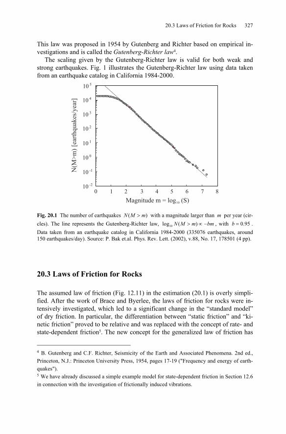
20.3 Laws of Friction for Rocks 327
This law was proposed in 1954 by Gutenberg and Richter based on empirical in-vestigations and is called the Gutenberg-Richter law4.
The scaling given by the Gutenberg-Richter law is valid for both weak and strong earthquakes. Fig. 1 illustrates the Gutenberg-Richter law using data taken from an earthquake catalog in California 1984-2000.
Fig. 20.1 The number of earthquakes ( )N M m> with a magnitude larger than m per year (cir-cles). The line represents the Gutenberg-Richter law, 10log ( )N M m bm> ∝ − , with 0.95b = . Data taken from an earthquake catalog in California 1984-2000 (335076 earthquakes, around 150 earthquakes/day). Source: P. Bak et.al. Phys. Rev. Lett. (2002), v.88, No. 17, 178501 (4 pp).
20.3 Laws of Friction for Rocks
The assumed law of friction (Fig. 12.11) in the estimation (20.1) is overly simpli-fied. After the work of Brace and Byerlee, the laws of friction for rocks were in-tensively investigated, which led to a significant change in the “standard model” of dry friction. In particular, the differentiation between “static friction” and “ki-netic friction” proved to be relative and was replaced with the concept of rate- and state-dependent friction5. The new concept for the generalized law of friction has
4 B. Gutenberg and C.F. Richter, Seismicity of the Earth and Associated Phenomena. 2nd ed., Princeton, N.J.: Princeton University Press, 1954, pages 17-19 ("Frequency and energy of earth-quakes"). 5 We have already discussed a simple example model for state-dependent friction in Section 12.6 in connection with the investigation of frictionally induced vibrations.

328 20 Earthquakes and Friction
turned out to be very successful at describing such aspects as seismogenesis, seis-mic coupling, pre- and post-sliding, as well as the insensitivity to relatively high frequency stress oscillations (such as Earth tides). Therefore, we will extensively discuss the laws of friction for rock in the following.
Coulomb already knew that the coefficient of static friction increases slowly with time and that the coefficient of kinetic friction is velocity dependent. Ex-perimental investigations by Dieterich6, which were summarized in the theory of Ruina7 to a rate- and a state-dependent law of friction, have shown that there is a close relation between these effects. In the law of friction from Dieterich-Ruina, the coefficient of friction is dependent on the instantaneous velocity v as well as the state variable θ :
* *
0 ln 1 ln 1c
v va bv D
θμ μ⎛ ⎞ ⎛ ⎞
= − + + +⎜ ⎟ ⎜ ⎟⎜ ⎟ ⎝ ⎠⎝ ⎠ (20.16)
where the following kinetic equation is valid for the state variable:
1c
vDθ
θ⎛ ⎞
= − ⎜ ⎟⎝ ⎠
. (20.17)
The constants a and b in Equation (20.16) are both positive and have an order of magnitude from 210− to 310− , cD has an order of magnitude of 10 mμ in labora-tory conditions, its scaling for larger systems has not yet been clarified; typical values of *v are on the order of 0.2 m/s . This law of friction proves to be very general and is applicable not only to rock, but also materials of various natures such as polymers, glass, paper, wood, and some metals.
In the static case, tθ = is valid. The state variable θ can, therefore, be inter-preted as the average age of the micro-contacts beginning from the moment they were formed. In the case of motion at a constant velocity v and the initial condi-tion 0(0)θ θ= , the solution to Equation (20.17) is
0( ) expc c
c
v tD Dt
v v Dθ θ
⎛ ⎞ ⎛ ⎞= + − −⎜ ⎟ ⎜ ⎟⎜ ⎟ ⎝ ⎠⎝ ⎠
. (20.18)
The state variable θ relaxes to its new equilibrium value at the sliding length cD . According to this, the value cD can be interpreted as the critical sliding length along which all of the existing micro-contacts are destroyed and replaced by new
6 J.H. Dieterich, Modelling of rock friction: 1. Experimental results and constitutive equations. 1979, J. Geophys. Res., v. 84, pp. 2161-2168. 7 A.I. Ruina, Slip instability and state variable friction laws. J. Geophys. Res., 1983, v. 88, 10359-10370.
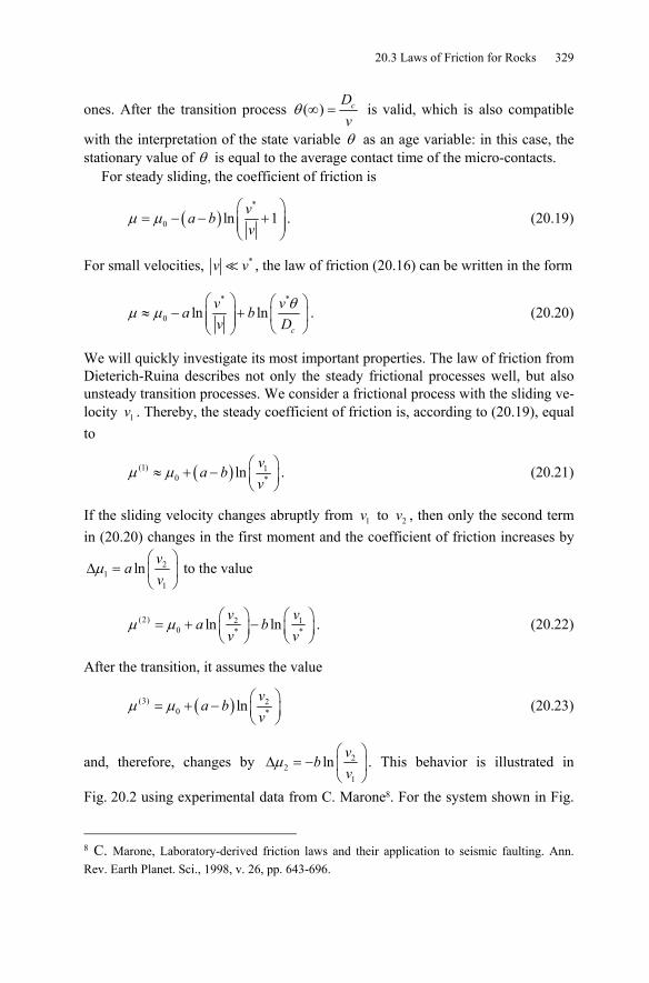
20.3 Laws of Friction for Rocks 329
ones. After the transition process ( ) cDv
θ ∞ = is valid, which is also compatible
with the interpretation of the state variable θ as an age variable: in this case, the stationary value of θ is equal to the average contact time of the micro-contacts.
For steady sliding, the coefficient of friction is
( )*
0 ln 1va bv
μ μ⎛ ⎞
= − − +⎜ ⎟⎜ ⎟⎝ ⎠
. (20.19)
For small velocities, *v v , the law of friction (20.16) can be written in the form
* *
0 ln lnc
v va bv D
θμ μ⎛ ⎞ ⎛ ⎞
≈ − +⎜ ⎟ ⎜ ⎟⎜ ⎟ ⎝ ⎠⎝ ⎠. (20.20)
We will quickly investigate its most important properties. The law of friction from Dieterich-Ruina describes not only the steady frictional processes well, but also unsteady transition processes. We consider a frictional process with the sliding ve-locity 1v . Thereby, the steady coefficient of friction is, according to (20.19), equal to
( )(1) 10 *ln
va b
vμ μ ⎛ ⎞≈ + − ⎜ ⎟
⎝ ⎠. (20.21)
If the sliding velocity changes abruptly from 1v to 2v , then only the second term in (20.20) changes in the first moment and the coefficient of friction increases by
21
1
lnv
av
μ⎛ ⎞
Δ = ⎜ ⎟⎝ ⎠
to the value
(2) 2 10 * *ln ln
v va b
v vμ μ ⎛ ⎞ ⎛ ⎞= + −⎜ ⎟ ⎜ ⎟
⎝ ⎠ ⎝ ⎠. (20.22)
After the transition, it assumes the value
( )(3) 20 *ln
va b
vμ μ ⎛ ⎞= + − ⎜ ⎟
⎝ ⎠ (20.23)
and, therefore, changes by 22
1
lnv
bv
μ⎛ ⎞
Δ = − ⎜ ⎟⎝ ⎠
. This behavior is illustrated in
Fig. 20.2 using experimental data from C. Marone8. For the system shown in Fig.
8 C. Marone, Laboratory-derived friction laws and their application to seismic faulting. Ann. Rev. Earth Planet. Sci., 1998, v. 26, pp. 643-696.
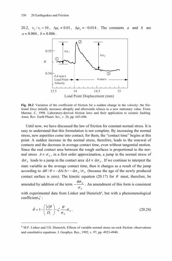
330 20 Earthquakes and Friction
20.2, 2 1/ 10v v = , 1 0.01μΔ ≈ , 2 0.014μΔ ≈ − . The constants a and b are 0.004a ≈ , 0.006b ≈ .
Load Point Displacement (mm)
0.55
0.54
13.5 14 14.5 15
0,4 mm/sLoad PointVelocity
4 mm/s
��1
1
2
3
��2
�
Fig. 20.2 Variation of the coefficient of friction for a sudden change in the velocity: the fric-tional force initially increases abruptly and afterwards relaxes to a new stationary value. From: Marone, C, 1998. Laboratory-derived friction laws and their application to seismic faulting. Annu. Rev. Earth Planet. Sci., v. 26, pp. 643-696.
Until now, we have discussed the law of friction for constant normal stress. It is easy to understand that this formulation is not complete. By increasing the normal stress, new asperities come into contact; for them, the “contact time” begins at this point. A sudden increase in the normal stress, therefore, leads to the renewal of contacts and the decrease in average contact time, even without tangential motion. Since the real contact area between the rough surfaces is proportional to the nor-mal stress NA σ∝ , in a first order approximation, a jump in the normal stress of d Nσ leads to a jump in the contact area d d NA σ∝ . If we continue to interpret the state variable as the average contact time, then it changes as a result of the jump according to d / dA/A= d /N Nθ θ σ σ= − − (because the age of the newly produced contact surface is zero). The kinetic equation (20.17) for θ must, therefore, be
amended by addition of the term N
N
θσσ
− . An amendment of this form is consistent
with experimental data from Linker and Dieterich9, but with a phenomenological coefficientζ :
1 Nc N
vDθ θθ ζ σ
σ⎛ ⎞
= − −⎜ ⎟⎝ ⎠
. (20.24)
9 M.F. Linker and J.H. Dieterich, Effects of variable normal stress on rock friction: observations and constitutive equations. J. Geophys. Res., 1992, v. 97, pp. 4923-4940.
20.4 Stability during Sliding with Rate- and State-Dependent Friction 331
20.4 Stability during Sliding with Rate- and State-Dependent Friction
We consider again the model shown in Fig. 12.1, which is described by the equa-tion of motion
0( , ) mx F x cx cv tθ+ + = , (20.25)
where the frictional force, ( , ) ( , )NF x F xθ μ θ= , is now defined by the Equations (20.20) and (20.17). The steady-state solution is given by
00
( , )
F vx v t
cθ
= − , 00
cDv
θ = . (20.26)
By considering the steady state solution with a small perturbation,
0 0x x v t xδ= + + , 0θ θ δθ= + , (20.27)
we obtain the linearized equation in the form
, , 0vm x F x c x Fθδ δ δ δθ+ + + = , 0
0
1
c
vx
v Dδθ δ δθ= − − (20.28)
with
0 0
,v Nx v
F aF Fx v=
∂= =∂
, 0
0, Nc
bvFF FDθ
θ θθ =
∂= =∂
. (20.29)
Substituting
tx Aeλδ = , tBeλδθ = (20.30)
provides us with the characteristic equation
( )3 2 0 0
0
0NN
c c cRP Q
F a bF a v cvcmv D m mD mD
λ λ λ−⎛ ⎞⎛ ⎞
+ + + + + =⎜ ⎟⎜ ⎟⎝ ⎠ ⎝ ⎠
. (20.31)
The stability criterion demands that R PQ= (See §12.7) or
( )0 0
0
NN
c c c
F a bcv F a v cmD mv D m mD
−⎛ ⎞⎛ ⎞= + +⎜ ⎟⎜ ⎟⎝ ⎠⎝ ⎠
. (20.32)
The critical stiffness follows as
( ) 2
0N
c c
b a mvc F
D aD− ⎛ ⎞
= +⎜ ⎟⎝ ⎠
. (20.33)
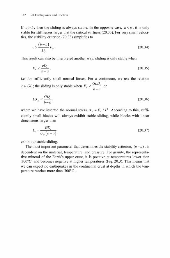
332 20 Earthquakes and Friction
If a b> , then the sliding is always stable. In the opposite case, a b< , it is only stable for stiffnesses larger that the critical stiffness (20.33). For very small veloci-ties, the stability criterion (20.33) simplifies to
( )
Nc
b ac F
D−
> . (20.34)
This result can also be interpreted another way: sliding is only stable when
cN
cDF
b a<
−, (20.35)
i.e. for sufficiently small normal forces. For a continuum, we use the relation
c GL≈ ; the sliding is only stable when cN
GLDF
b a<
− or
cN
GDL
b aσ <
−, (20.36)
where we have inserted the normal stress 2/N NF Lσ ≈ . According to this, suffi-ciently small blocks will always exhibit stable sliding, while blocks with linear dimensions larger than
( )
cc
N
GDL
b aσ=
− (20.37)
exhibit unstable sliding. The most important parameter that determines the stability criterion, ( )b a− , is
dependent on the material, temperature, and pressure. For granite, the representa-tive mineral of the Earth’s upper crust, it is positive at temperatures lower than 300 C° and becomes negative at higher temperatures (Fig. 20.3). This means that we can expect no earthquakes in the continental crust at depths in which the tem-perature reaches more than 300 C° .
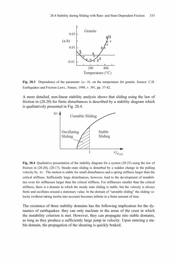
20.4 Stability during Sliding with Rate- and State-Dependent Friction 333
Fig. 20.3 Dependence of the parameter ( )a b− on the temperature for granite. Source: C.H.
Earthquakes and Friction Laws., Nature, 1998, v. 391, pp. 37-42.
A more detailed, non-linear stability analysis shows that sliding using the law of friction in (20.20) for finite disturbances is described by a stability diagram which is qualitatively presented in Fig. 20.4.
Fig. 20.4 Qualitative presentation of the stability diagram for a system (20.25) using the law of friction in (20.20), (20.17). Steady-state sliding is disturbed by a sudden change in the pulling velocity by vΔ . The motion is stable for small disturbances and a spring stiffness larger than the critical stiffness. Sufficiently large disturbances, however, lead to the development of instabili-ties even for stiffnesses larger than the critical stiffness. For stiffnesses smaller than the critical stiffness, there is a domain in which the steady state sliding is stable, but the velocity is always finite and oscillates around a stationary value. In the domain of “unstable sliding” the sliding ve-locity (without taking inertia into account) becomes infinite in a finite amount of time.
The existence of three stability domains has the following implication for the dy-namics of earthquakes: they can only nucleate in the areas of the crust in which the instability criterion is met. However, they can propagate into stable domains, as long as they produce a sufficiently large jump in velocity. Upon entering a sta-ble domain, the propagation of the shearing is quickly braked.
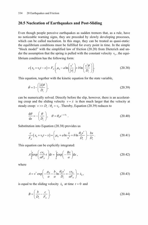
334 20 Earthquakes and Friction
20.5 Nucleation of Earthquakes and Post-Sliding
Even though people perceive earthquakes as sudden tremors that, as a rule, have no noticeable warning signs, they are preceded by slowly developing processes, which can be called nucleation. In this stage, they can be treated as quasi-static: the equilibrium conditions must be fulfilled for every point in time. In the simple “block model” with the simplified law of friction (20.20) from Dieterich and un-der the assumption that the spring is pulled with the constant velocity 0v , the equi-librium condition has the following form:
( )* *
0 0 0 ln lnNc
v vc x v t x F a bv D
θμ⎛ ⎞⎛ ⎞ ⎛ ⎞
+ − = − +⎜ ⎟⎜ ⎟ ⎜ ⎟⎜ ⎟⎜ ⎟⎝ ⎠⎝ ⎠⎝ ⎠. (20.38)
This equation, together with the kinetic equation for the state variable,
1c
xDθ
θ⎛ ⎞
= − ⎜ ⎟⎝ ⎠
, (20.39)
can be numerically solved. Directly before the slip, however, there is an accelerat-ing creep and the sliding velocity v x= is then much larger that the velocity at steady creep: 0 0/cv D vθ>> = . Thereby, Equation (20.39) reduces to
dd cx Dθ θ⎛ ⎞= −⎜ ⎟
⎝ ⎠, /
0cx Deθ θ −= . (20.40)
Substitution into Equation (20.38) provides us
( )*
00 0 0 *ln ln
N c c
vc x bxx v t x a bF D Dv
θμ⎛ ⎞
+ − = + + −⎜ ⎟⎝ ⎠
. (20.41)
This equation can be explicitly integrated:
0
0 0
exp d exp dt x
N
cv BxA t t xaF a
⎛ ⎞ ⎛ ⎞= −⎜ ⎟ ⎜ ⎟⎝ ⎠⎝ ⎠
∫ ∫ , (20.42)
where
*
* 0 0 00exp ln
c N
v cxbA v xa a D aFμ θ⎛ ⎞
= − − + =⎜ ⎟⎝ ⎠
, (20.43)
is equal to the sliding velocity 0x at time 0t = and
c N
b cBD F
⎛ ⎞= −⎜ ⎟⎝ ⎠
. (20.44)
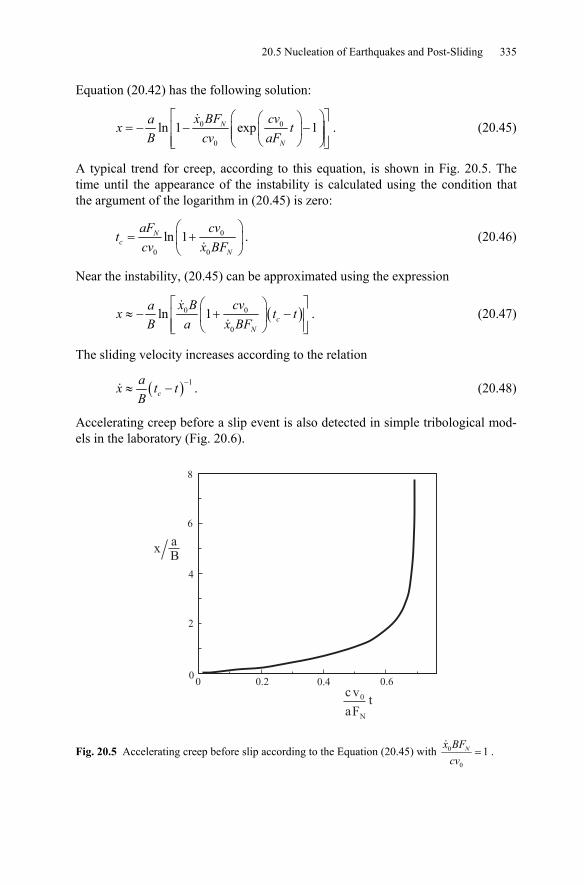
20.5 Nucleation of Earthquakes and Post-Sliding 335
Equation (20.42) has the following solution:
0 0
0
ln 1 exp 1N
N
x BF cvax tB cv aF
⎡ ⎤⎛ ⎞⎛ ⎞= − − −⎢ ⎥⎜ ⎟⎜ ⎟⎜ ⎟⎢ ⎥⎝ ⎠⎝ ⎠⎣ ⎦
. (20.45)
A typical trend for creep, according to this equation, is shown in Fig. 20.5. The time until the appearance of the instability is calculated using the condition that the argument of the logarithm in (20.45) is zero:
0
0 0
ln 1Nc
N
aF cvt
cv x BF⎛ ⎞
= +⎜ ⎟⎝ ⎠
. (20.46)
Near the instability, (20.45) can be approximated using the expression
( )0 0
0
ln 1 cN
x B cvax t tB a x BF
⎡ ⎤⎛ ⎞≈ − + −⎢ ⎥⎜ ⎟
⎢ ⎥⎝ ⎠⎣ ⎦. (20.47)
The sliding velocity increases according to the relation
( ) 1c
ax t tB
−≈ − . (20.48)
Accelerating creep before a slip event is also detected in simple tribological mod-els in the laboratory (Fig. 20.6).
Fig. 20.5 Accelerating creep before slip according to the Equation (20.45) with 0
0
1Nx BFcv
= .
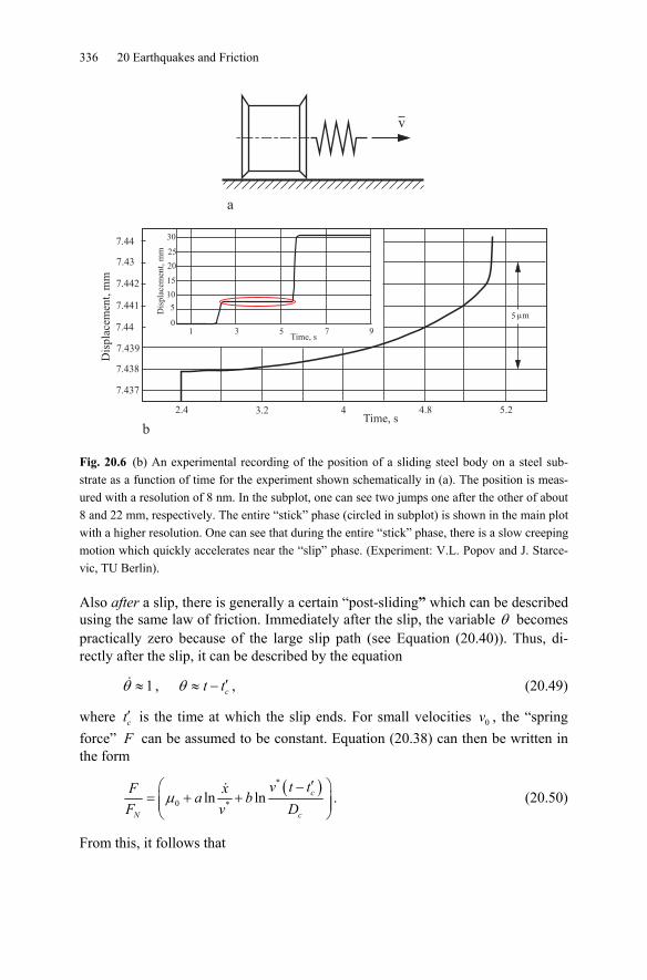
336 20 Earthquakes and Friction
Fig. 20.6 (b) An experimental recording of the position of a sliding steel body on a steel sub-strate as a function of time for the experiment shown schematically in (a). The position is meas-ured with a resolution of 8 nm. In the subplot, one can see two jumps one after the other of about 8 and 22 mm, respectively. The entire “stick” phase (circled in subplot) is shown in the main plot with a higher resolution. One can see that during the entire “stick” phase, there is a slow creeping motion which quickly accelerates near the “slip” phase. (Experiment: V.L. Popov and J. Starce-vic, TU Berlin).
Also after a slip, there is generally a certain “post-sliding” which can be described using the same law of friction. Immediately after the slip, the variable θ becomes practically zero because of the large slip path (see Equation (20.40)). Thus, di-rectly after the slip, it can be described by the equation
1θ ≈ , ct tθ ′≈ − , (20.49)
where ct′ is the time at which the slip ends. For small velocities 0v , the “spring force” F can be assumed to be constant. Equation (20.38) can then be written in the form
( )*
0 *ln ln c
N c
v t tF xa bF Dv
μ′⎛ ⎞−
= + +⎜ ⎟⎜ ⎟⎝ ⎠
. (20.50)
From this, it follows that
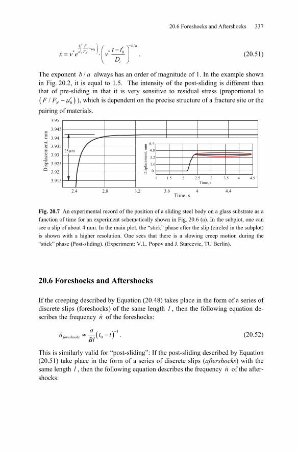
20.6 Foreshocks and Aftershocks 337
0
/1* * 0N
b aFa F
c
t tx v e v
D
μ−⎛ ⎞
−⎜ ⎟⎜ ⎟⎝ ⎠
′⎛ ⎞−= ⋅⎜ ⎟
⎝ ⎠. (20.51)
The exponent /b a always has an order of magnitude of 1. In the example shown in Fig. 20.2, it is equal to 1.5. The intensity of the post-sliding is different than that of pre-sliding in that it is very sensitive to residual stress (proportional to ( )0/ NF F μ′− ), which is dependent on the precise structure of a fracture site or the pairing of materials.
Fig. 20.7 An experimental record of the position of a sliding steel body on a glass substrate as a function of time for an experiment schematically shown in Fig. 20.6 (a). In the subplot, one can see a slip of about 4 mm. In the main plot, the “stick” phase after the slip (circled in the subplot) is shown with a higher resolution. One sees that there is a slowing creep motion during the “stick” phase (Post-sliding). (Experiment: V.L. Popov and J. Starcevic, TU Berlin).
20.6 Foreshocks and Aftershocks
If the creeping described by Equation (20.48) takes place in the form of a series of discrete slips (foreshocks) of the same length l , then the following equation de-scribes the frequency n of the foreshocks:
( ) 10foreshocks
an t tBl
−≈ − . (20.52)
This is similarly valid for “post-sliding”: If the post-sliding described by Equation (20.51) take place in the form of a series of discrete slips (aftershocks) with the same length l , then the following equation describes the frequency n of the after-shocks:
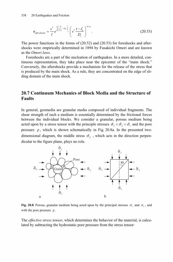
338 20 Earthquakes and Friction
0
/1** 0N
b aFa F
aftershocksc
t tvn e vl D
μ−⎛ ⎞
−⎜ ⎟⎜ ⎟⎝ ⎠
′⎛ ⎞−= ⋅⎜ ⎟
⎝ ⎠. (20.53)
The power functions in the forms of (20.52) and (20.53) for foreshocks and after-shocks were empirically determined in 1894 by Fusakichi Omori and are known as the Omori laws.
Foreshocks are a part of the nucleation of earthquakes. In a more detailed, con-tinuous representation, they take place near the epicenter of the “main shock.” Conversely, the aftershocks provide a mechanism for the release of the stress that is produced by the main shock. As a rule, they are concentrated on the edge of sli-ding domain of the main shock.
20.7 Continuum Mechanics of Block Media and the Structure of Faults
In general, geomedia are granular media composed of individual fragments. The shear strength of such a medium is essentially determined by the frictional forces between the individual blocks. We consider a granular, porous medium being acted upon by a stress tensor with the principle stresses 3 2 1σ σ σ< < and the pore pressure p , which is shown schematically in Fig. 20.8a. In the presented two-dimensional diagram, the middle stress 2σ , which acts in the direction perpen-dicular to the figure plane, plays no role.
Grain
Pore
�~
3
�~
1
�~
3
�~
1
a b
�~
1
�~
3 �~
3
�~
1
�
Fig. 20.8 Porous, granular medium being acted upon by the principal stresses 1σ and 3σ , and with the pore pressure p .
The effective stress tensor, which determines the behavior of the material, is calcu-lated by subtracting the hydrostatic pore pressure from the stress tensor:
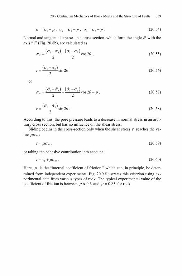
20.7 Continuum Mechanics of Block Media and the Structure of Faults 339
1 1 pσ σ= − , 2 2 pσ σ= − , 3 3 pσ σ= − . (20.54)
Normal and tangential stresses in a cross-section, which form the angle θ with the axis “1” (Fig. 20.8b), are calculated as
( ) ( )1 3 1 3 cos 22 2N
σ σ σ σσ θ
+ −= − , (20.55)
( )1 3 sin 2
2σ σ
τ θ−
= (20.56)
or
( ) ( )1 3 1 3 cos 2
2 2N pσ σ σ σ
σ θ+ −
= − − , (20.57)
( )1 3 sin 22
σ στ θ
−= . (20.58)
According to this, the pore pressure leads to a decrease in normal stress in an arbi-trary cross section, but has no influence on the shear stress.
Sliding begins in the cross-section only when the shear stress τ reaches the va-lue Nμσ :
Nτ μσ= , (20.59)
or taking the adhesive contribution into account
0 Nτ τ μσ= + . (20.60)
Here, μ is the “internal coefficient of friction,” which can, in principle, be deter-mined from independent experiments. Fig. 20.9 illustrates this criterion using ex-perimental data from various types of rock. The typical experimental value of the coefficient of friction is between 0.6μ ≈ and 0.85μ = for rock.
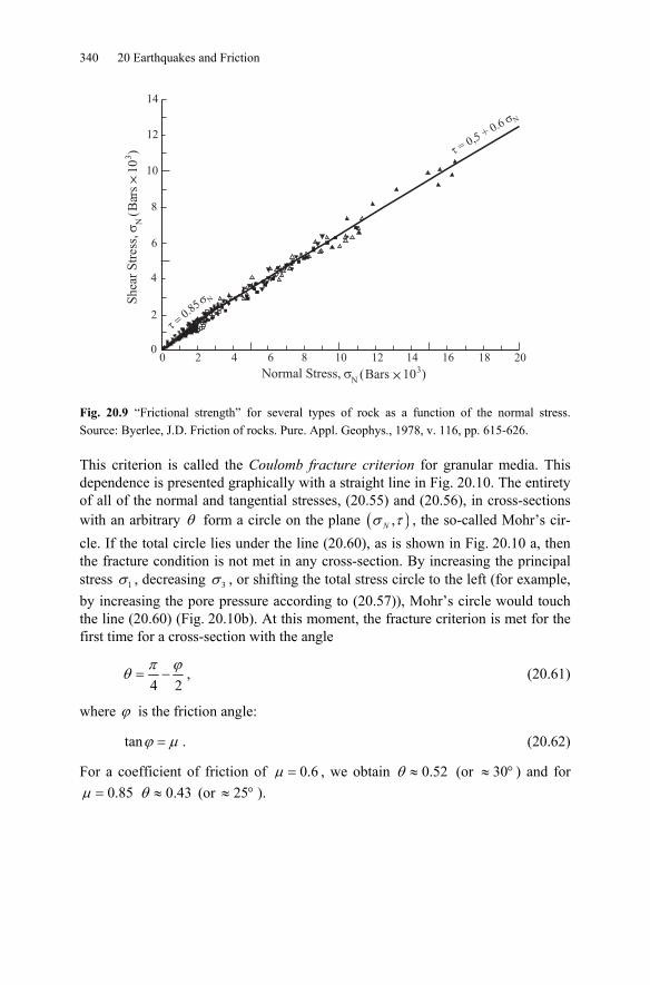
340 20 Earthquakes and Friction
� = 0,5+ 0.6
� N
Normal Stress, �N
��
��
Bars 103)(
10
� N
16 1814121086420 200
2
4
6
8
12
14
Sh
ear
Str
ess,
�N
Bar
s1
03)
(
Fig. 20.9 “Frictional strength” for several types of rock as a function of the normal stress. Source: Byerlee, J.D. Friction of rocks. Pure. Appl. Geophys., 1978, v. 116, pp. 615-626.
This criterion is called the Coulomb fracture criterion for granular media. This dependence is presented graphically with a straight line in Fig. 20.10. The entirety of all of the normal and tangential stresses, (20.55) and (20.56), in cross-sections with an arbitrary θ form a circle on the plane ( ),Nσ τ , the so-called Mohr’s cir-cle. If the total circle lies under the line (20.60), as is shown in Fig. 20.10 a, then the fracture condition is not met in any cross-section. By increasing the principal stress 1σ , decreasing 3σ , or shifting the total stress circle to the left (for example, by increasing the pore pressure according to (20.57)), Mohr’s circle would touch the line (20.60) (Fig. 20.10b). At this moment, the fracture criterion is met for the first time for a cross-section with the angle
4 2π ϕθ = − , (20.61)
where ϕ is the friction angle:
tanϕ μ= . (20.62)
For a coefficient of friction of 0.6μ = , we obtain 0.52θ ≈ (or 30≈ ° ) and for 0.85μ = 0.43θ ≈ (or 25≈ ° ).
20.7 Continuum Mechanics of Block Media and the Structure of Faults 341
Fig. 20.10 Mohr’s circle for plane stress and Coulomb’s fracture criterion.
With the help of Fig. 20.10b, one can express the criterion (20.60) using the prin-cipal stresses:
( ) ( )2 21 3 01 1 2σ μ μ σ μ μ τ+ − − + + = . (20.63)
Therefore, between the principal stresses in the fracture area, there exists a linear dependence. Stress measurements using deep drilling show that this condition is fulfilled at all depths. This means that the Earth’s crust is found to be near the critical state at all depths. If the primary stress 3σ is negative (in tension), then, as a rule, the following criterion is applied to the fracture:
3 0σ σ= − . (20.64)
Anderson10 was the first to recognize that the fundamental types of faults can be easily explained using the properties of granular media. His classification is ba-sed on observations that the principal axes of the stress tensor in the upper crust often lie normal and parallel to the surface, respectively. There are three possibili-ties for the orientation of the axis of the largest principal stress ( )1σ and the axis
of the smallest principal stress ( )3σ with respect to the Earth’s surface, which are shown in Fig. 20.11a-c. The resulting fault types are normal faults (Fig. 20.11a), thrust (reverse) faults (Fig. 20.11b), and strike-slip faults (Fig. 20.11c). If the smallest primary stress is negative, then the surfaces separate in a plane perpen-dicular to the axis of the negative stress (divergent faults, Fig. 20.11d). The type of slip during an earthquake influences, in addition to its magnitude, the resulting de-struction. Strike-slip faulting (c) leads to maximum tangential acceleration and normal faulting, to strong tsunamis (in the case that the earthquake takes place un-der the ocean).
10 E.M. Anderson, The dynamics of faulting. Edinburgh, Oliver & Boyd, 1951.
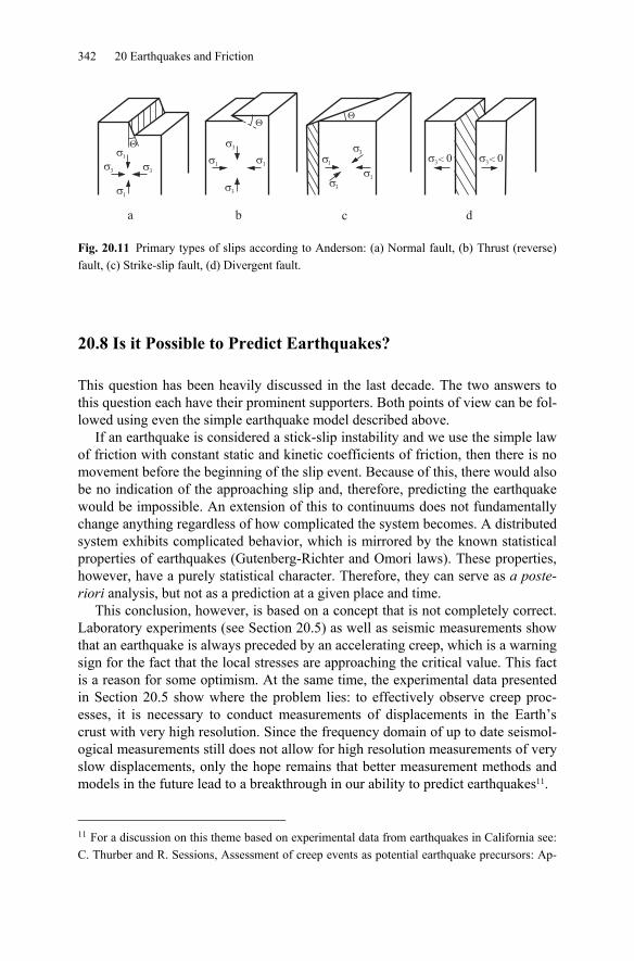
342 20 Earthquakes and Friction
Fig. 20.11 Primary types of slips according to Anderson: (a) Normal fault, (b) Thrust (reverse) fault, (c) Strike-slip fault, (d) Divergent fault.
20.8 Is it Possible to Predict Earthquakes?
This question has been heavily discussed in the last decade. The two answers to this question each have their prominent supporters. Both points of view can be fol-lowed using even the simple earthquake model described above.
If an earthquake is considered a stick-slip instability and we use the simple law of friction with constant static and kinetic coefficients of friction, then there is no movement before the beginning of the slip event. Because of this, there would also be no indication of the approaching slip and, therefore, predicting the earthquake would be impossible. An extension of this to continuums does not fundamentally change anything regardless of how complicated the system becomes. A distributed system exhibits complicated behavior, which is mirrored by the known statistical properties of earthquakes (Gutenberg-Richter and Omori laws). These properties, however, have a purely statistical character. Therefore, they can serve as a poste-riori analysis, but not as a prediction at a given place and time.
This conclusion, however, is based on a concept that is not completely correct. Laboratory experiments (see Section 20.5) as well as seismic measurements show that an earthquake is always preceded by an accelerating creep, which is a warning sign for the fact that the local stresses are approaching the critical value. This fact is a reason for some optimism. At the same time, the experimental data presented in Section 20.5 show where the problem lies: to effectively observe creep proc-esses, it is necessary to conduct measurements of displacements in the Earth’s crust with very high resolution. Since the frequency domain of up to date seismol-ogical measurements still does not allow for high resolution measurements of very slow displacements, only the hope remains that better measurement methods and models in the future lead to a breakthrough in our ability to predict earthquakes11.
11 For a discussion on this theme based on experimental data from earthquakes in California see: C. Thurber and R. Sessions, Assessment of creep events as potential earthquake precursors: Ap-
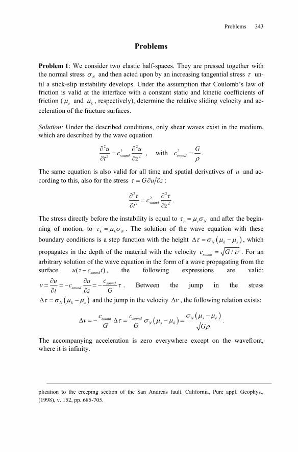
Problems 343
Problems
Problem 1: We consider two elastic half-spaces. They are pressed together with the normal stress Nσ and then acted upon by an increasing tangential stress τ un-til a stick-slip instability develops. Under the assumption that Coulomb’s law of friction is valid at the interface with a constant static and kinetic coefficients of friction ( sμ and kμ , respectively), determine the relative sliding velocity and ac-celeration of the fracture surfaces. Solution: Under the described conditions, only shear waves exist in the medium, which are described by the wave equation
2 22
2 2soundu uc
t z∂ ∂
=∂ ∂
, with 2sound
Gcρ
= .
The same equation is also valid for all time and spatial derivatives of u and ac-cording to this, also for the stress G u zτ = ∂ ∂ :
2 22
2 2soundct zτ τ∂ ∂=
∂ ∂.
The stress directly before the instability is equal to s s Nτ μ σ= and after the begin-ning of motion, to k k Nτ μ σ= . The solution of the wave equation with these boundary conditions is a step function with the height ( )N k sτ σ μ μΔ = − , which
propagates in the depth of the material with the velocity /soundc G ρ= . For an arbitrary solution of the wave equation in the form of a wave propagating from the surface ( )soundu z c t− , the following expressions are valid:
soundsound
cu uv ct z G
τ∂ ∂= = − = −∂ ∂
. Between the jump in the stress
( )N k sτ σ μ μΔ = − and the jump in the velocity vΔ , the following relation exists:
( ) ( )N s ksound soundN s k
c cv
G G Gσ μ μ
τ σ μ μρ−
Δ = − Δ = − = .
The accompanying acceleration is zero everywhere except on the wavefront, where it is infinity.
plication to the creeping section of the San Andreas fault. California, Pure appl. Geophys., (1998), v. 152, pp. 685-705.
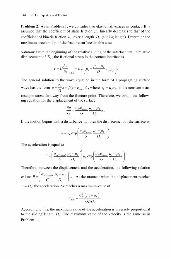
344 20 Earthquakes and Friction
Problem 2: As in Problem 1, we consider two elastic half-spaces in contact. It is assumed that the coefficient of static friction sμ linearly decreases to that of the coefficient of kinetic friction kμ over a length cD (sliding length). Determine the maximum acceleration of the fracture surfaces in this case.
Solution: From the beginning of the relative sliding of the interface until a relative displacement of cD , the frictional stress in the contact interface is
0,0,
s kN s z t
z t c
uG uz D
μ μτ σ μ
==
⎛ ⎞−∂= = −⎜ ⎟∂ ⎝ ⎠
.
The general solution to the wave equation in the form of a propagating surface
wave has the form 0 ( )soundu z f z c tGτ
= + − , where 0 s Nτ μ σ= is the constant mac-
roscopic stress far away from the fracture point. Therefore, we obtain the follow-ing equation for the displacement of the surface
N sound s k
c
cu ut G D
σ μ μ−∂=
∂.
If the motion begins with a disturbance 0u , then the displacement of the surface is
0 exp N sound s k
c
cu u t
G Dσ μ μ⎛ ⎞−
= ⎜ ⎟⎝ ⎠
.
The acceleration is equal to 2
0 expN sound s k N sound s k
c c
c cu u t
G D G Dσ μ μ σ μ μ⎛ ⎞ ⎛ ⎞− −
= ⎜ ⎟ ⎜ ⎟⎝ ⎠ ⎝ ⎠
.
Therefore, between the displacement and the acceleration, the following relation
exists: 2
N sound s k
c
cu u
G Dσ μ μ⎛ ⎞−
= ⎜ ⎟⎝ ⎠
. At the moment when the displacement reaches
cu D= , the acceleration vΔ reaches a maximum value of
( )22
maxN s k
c
uG D
σ μ μρ−
= .
According to this, the maximum value of the acceleration is inversely proportional to the sliding length cD . The maximum value of the velocity is the same as in Problem 1.
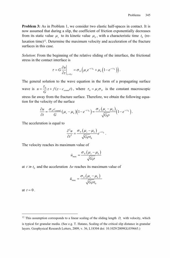
Problems 345
Problem 3: As in Problem 1, we consider two elastic half-spaces in contact. It is now assumed that during a slip, the coefficient of friction exponentially decreases from its static value sμ to its kinetic value kμ , with a characteristic time 0t (re-laxation time)12. Determine the maximum velocity and acceleration of the fracture surfaces in this case. Solution: From the beginning of the relative sliding of the interface, the frictional stress in the contact interface is
( )( )0 0/ /
0,
1t t t tN s k
z t
uG e ez
τ σ μ μ− −
=
∂= = + −
∂.
The general solution to the wave equation in the form of a propagating surface
wave is 0 ( )soundu z f z c tGτ
= + − , where 0 s Nτ μ σ= is the constant macroscopic
stress far away from the fracture surface. Therefore, we obtain the following equa-tion for the velocity of the surface
( )( ) ( ) ( )0 0/ /1 1N s kt t t tN sounds k
cu e et G G
σ μ μσμ μ
ρ− −−∂
= − − = −∂
.
The acceleration is equal to
( )0
2/
20
N s k t tu et G t
σ μ μ
ρ−−∂
=∂
.
The velocity reaches its maximum value of
( )max
N s kuG
σ μ μρ−
=
at 0t t and the acceleration vΔ reaches its maximum value of
( )max
0
N s kuG t
σ μ μ
ρ
−=
at 0t = .
12 This assumption corresponds to a linear scaling of the sliding length cD with velocity, which
is typical for granular media. (See e.g. T. Hatano, Scaling of the critical slip distance in granular layers. Geophysical Research Letters, 2009, v. 36, L18304 doi: 10.1029/2009GL039665.)
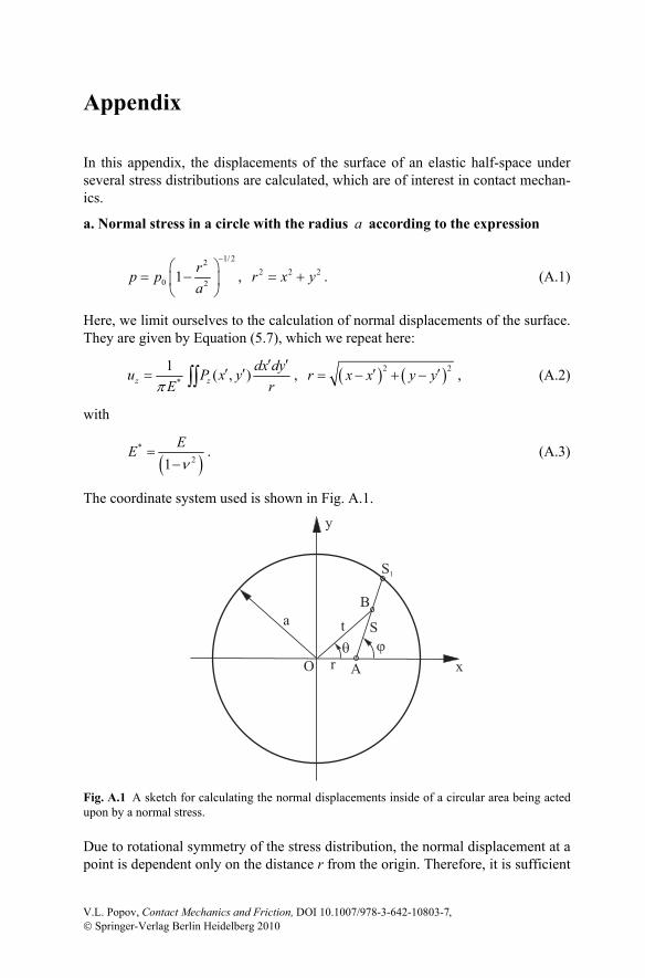
Appendix In this appendix, the displacements of the surface of an elastic half-space under several stress distributions are calculated, which are of interest in contact mechan-ics.
a. Normal stress in a circle with the radius a according to the expression
1/ 22
0 21−
⎛ ⎞= −⎜ ⎟
⎝ ⎠
rp pa
, 2 2 2= +r x y . (A.1)
Here, we limit ourselves to the calculation of normal displacements of the surface. They are given by Equation (5.7), which we repeat here:
*
1 ( , )π
′ ′′ ′= ∫∫z z
dx dyu P x yrE
, ( ) ( )2 2′ ′= − + −r x x y y , (A.2)
with
( )
*21 ν
=−EE . (A.3)
The coordinate system used is shown in Fig. A.1.
a t
S1
S
AO r� �
B
x
y
Fig. A.1 A sketch for calculating the normal displacements inside of a circular area being acted upon by a normal stress.
Due to rotational symmetry of the stress distribution, the normal displacement at a point is dependent only on the distance r from the origin. Therefore, it is sufficient
V.L. Popov, Contact Mechanics and Friction, DOI 10.1007/978-3-642-10803-7, © Springer-Verlag Berlin Heidelberg 2010
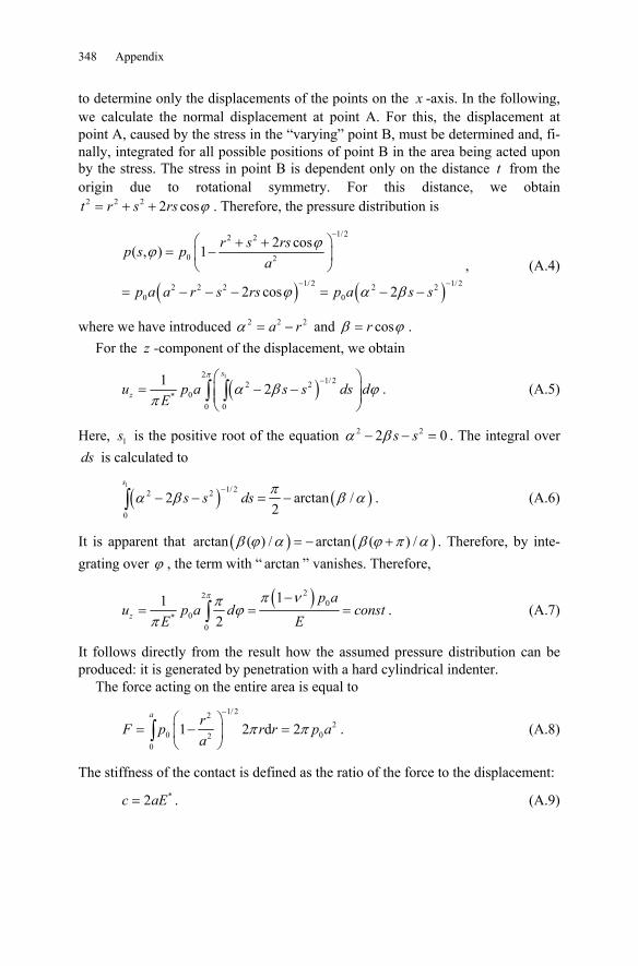
348 Appendix
to determine only the displacements of the points on the x -axis. In the following, we calculate the normal displacement at point A. For this, the displacement at point A, caused by the stress in the “varying” point B, must be determined and, fi-nally, integrated for all possible positions of point B in the area being acted upon by the stress. The stress in point B is dependent only on the distance t from the origin due to rotational symmetry. For this distance, we obtain
2 2 2 2 cosϕ= + +t r s rs . Therefore, the pressure distribution is
( ) ( )
1/22 2
0 2
1/ 2 1/ 22 2 2 2 20 0
2 cos( , ) 1
2 cos 2
ϕϕ
ϕ α β
−
− −
⎛ ⎞+ += −⎜ ⎟
⎝ ⎠
= − − − = − −
r s rsp s pa
p a a r s rs p a s s
, (A.4)
where we have introduced 2 2 2α = −a r and cosβ ϕ= r . For the z -component of the displacement, we obtain
( )12
1/ 22 20*
0 0
1 2π
α β ϕπ
−⎛ ⎞= − −⎜ ⎟⎜ ⎟
⎝ ⎠∫ ∫
s
zu p a s s ds dE
. (A.5)
Here, 1s is the positive root of the equation 2 22 0α β− − =s s . The integral over ds is calculated to
( ) ( )1 1/ 22 2
0
2 arctan /2πα β β α
−− − = −∫
s
s s ds . (A.6)
It is apparent that ( ) ( )arctan ( ) / arctan ( ) /β ϕ α β ϕ π α= − + . Therefore, by inte-grating over ϕ , the term with “ arctan ” vanishes. Therefore,
( )22
00*
0
112
π π νπ ϕπ
−= = =∫z
p au p a d const
EE. (A.7)
It follows directly from the result how the assumed pressure distribution can be produced: it is generated by penetration with a hard cylindrical indenter.
The force acting on the entire area is equal to
1/ 22
20 02
0
1 2 d 2π π−
⎛ ⎞= − =⎜ ⎟
⎝ ⎠∫a rF p r r p a
a. (A.8)
The stiffness of the contact is defined as the ratio of the force to the displacement:
*2=c aE . (A.9)
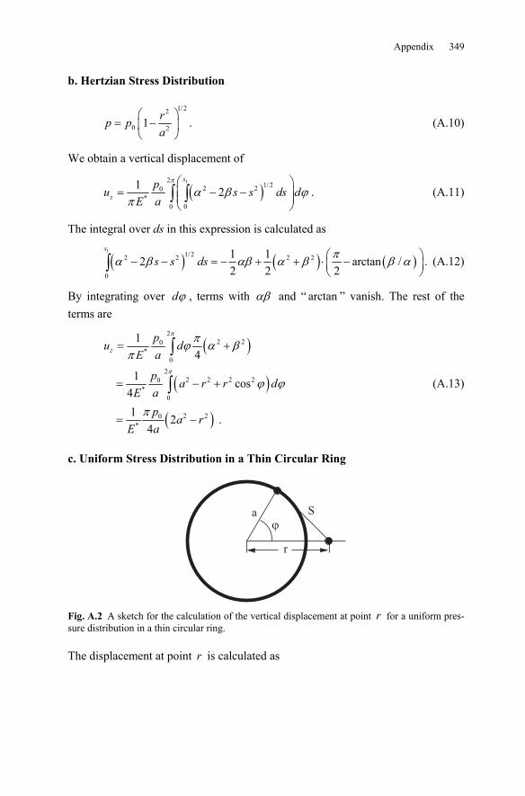
Appendix 349
b. Hertzian Stress Distribution
1/ 22
0 21⎛ ⎞
= −⎜ ⎟⎝ ⎠
rp pa
. (A.10)
We obtain a vertical displacement of
( )12
1/22 20*
0 0
1 2π
α β ϕπ
⎛ ⎞= − −⎜ ⎟⎜ ⎟
⎝ ⎠∫ ∫
s
zp
u s s ds daE
. (A.11)
The integral over ds in this expression is calculated as
( ) ( ) ( )1 1/22 2 2 2
0
1 12 arctan /2 2 2
πα β αβ α β β α⎛ ⎞− − = − + + ⋅ −⎜ ⎟⎝ ⎠∫
s
s s ds . (A.12)
By integrating over ϕd , terms with αβ and “ arctan ” vanish. The rest of the terms are
( )
( )
( )
22 20
*0
22 2 2 20
*0
2 20*
14
1 cos41 2 .
4
zp
u daE
pa r r d
aEp
a raE
π
π
πϕ α βπ
ϕ ϕ
π
= +
= − +
= −
∫
∫ (A.13)
c. Uniform Stress Distribution in a Thin Circular Ring
�
S
r
a
Fig. A.2 A sketch for the calculation of the vertical displacement at point r for a uniform pres-sure distribution in a thin circular ring.
The displacement at point r is calculated as
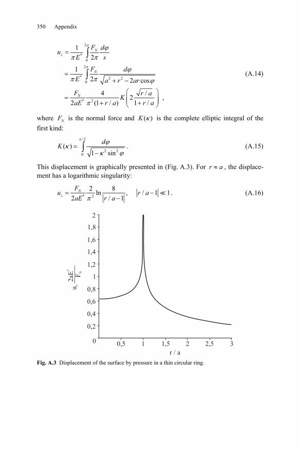
350 Appendix
2
*0
2
* 2 20
* 2
12
1 2 2 cos
4 / 2 ,1 /2 (1 / )
Nz
N
N
F dusE
F dE a r ar
F r aKr aaE r a
π
π
ϕππ
ϕππ ϕ
π
=
=+ −
⎛ ⎞= ⎜ ⎟⎜ ⎟++ ⎝ ⎠
∫
∫ (A.14)
where NF is the normal force and ( )κK is the complete elliptic integral of the first kind:
/ 2
2 20
( )1 sin
dKπ ϕκ
κ ϕ=
−∫ . (A.15)
This displacement is graphically presented in (Fig. A.3). For ≈r a , the displace-ment has a logarithmic singularity:
* 2
2 8ln , / 1 1/ 12 π
= −−
Nz
Fu r a
r aaE. (A.16)
2
1,8
1,6
1,4
1,2
1
0,8
0,6
0,4
0,2
0 0,5 1 1,5 2 2,5 3
r / a
uz
FN
2aE
*
Fig. A.3 Displacement of the surface by pressure in a thin circular ring.
Further Reading This list of literature is in no way complete and serves only as a guide for further study or reference.
Chapter 1 D. Dowson, History of Tribology. Longman Group Limited, London, 1979, 678 pp. E. Rabinowicz, Friction and wear of materials. Second Edition, John Wiley & Sons, inc., 1995. F.P. Bowden, D. Tabor, The Friction and Lubrication of Solids. Clarendon Press, Oxford, 2001. B.N.J. Persson, Sliding Friction. Physical Principles and Applications. Springer, 2002. D.F. Moore, The friction and lubrication of elastomers. Pergamon Press, Oxford, 1972, 288 pp. I.L. Singer and H.M. Pollock (Eds), Fundamentals of Friction: Macroscopic and Microscopic Processes. (Proceedings of the NATO Advanced Study Institute), Kluwer Academic Publishers, 1992. B.N.J. Persson, E. Tosatti (Eds), Physics of Sliding friction. Kluwer, Dordrecht 1996. H. Czichos, K.-H- Habig, Tribologie-Handbuch: Reibung und Verschleiß. 2., übe-rarb. und erw. Aufl., Wiesbaden, Vieweg, 2003. - IX, 666 S. K.V. Frolov (Ed.), Modern Tribology: Results and Perspectives (in Russian). Moscow, 2008, 480 S. Chapter 2 E. Rabinowicz, Friction and wear of materials. Second Edition. John Wiley & Sons, inc., 1995. Chapter 3 J. Israelachvili, Intermolecular and Surface Forces. Academic Press (1985-2004). A.J. Kinloch, Adhesion and Adhesives: Science and Technology, Chapman and Hall, London, 1987, p. 441. B.V. Deryagin, N.A. Krotova and V.P. Smilga, Adhesion of solids. New Y-ork, Consultants Bureau, 1978, p. 457. K. Kendall, Molecular Adhesion and its Applications, Kluwer Academic, 2001. I.E. Dzyaloshinskii, E.M. Lifshitz und L.P. Pitaevskii, General Theory of van der Waals' Forces. Sov. Phys. Usp., 1961, v. 4 153-176. D. Maugis, Contact, adhesion, and rupture of elastic solids. Springer-Verlag Ber-lin, Heidelberg, 2000.
352 Further Reading
Chapter 4 F.M. Fowkes (Ed.), Contact Angle, Wettability and Adhesion. American Chemi-cal Society, 1964. D. Maugis, Contact, adhesion, and rupture of elastic solids. Springer-Verlag Ber-lin, Heidelberg, 2000.
Chapter 5 K.L. Johnson, Contact mechanics. Cambridge University Press, Ninth printing 2003. L.D. Landau, E.M. Lifschitz, Theory of elasticity (Theoretical Physics, Vol7), 3rd edition, 1999, Butterworth-Heinemann, Oxford, §§ 8,9. I.N. Sneddon, The Relation between Load and Penetration in the Axisymmetric Boussinesq Problem for a Punch of Arbitrary Profile. Int. J. Eng. Sci.,1965, v. 3, pp. 47–57. Chapter 6 K.L. Johnson, Contact mechanics. Cambridge University Press, Ninth printing 2003. B. V. Deryagin, N. A. Krotova and V. P. Smilga, Adhesion of solids. New Y-ork, Consultants Bureau, 1978. p. 457. M.K. Chaudhury, T. Weaver, C.Y. Hui, E.J. Kramer, Adhesive contact of cy-lindrical lens and a flat sheet. J. Appl. Phys., 1996, v. 80, No. 1, pp. 30-37. D. Maugis, Contact, adhesion, and rupture of elastic solids. Springer-Verlag Ber-lin, Heidelberg, 2000.
Chapter 7 S. Hyun, L. Pei, J.-F. Molinari, and M. O. Robbins, Finite-element analysis of contact between elastic self-affine surfaces. Phys. Rev. E, 2004, v. 70, 026117 (12 pp). B.N.J. Persson, Contact mechanics for randomly rough surfaces. Surface Science Reports, 2006, v. 61, pp. 201-227. R. Holm, Electric contacts : theory and application. 4th completely rewritten ed. Berlin, Springer, 1967. - XV, p. 482. Chapter 8 K.L. Johnson, Contact mechanics. Cambridge University Press, Ninth printing 2003.
Chapter 9 K.L. Johnson, Contact mechanics. Cambridge University Press, 6th printing of the 1st ed. 2001. J.J. Kalker, Three-dimensional elastic bodies in rolling contact, 1990, Kluwer, Dordrecht, 314 S.
Further Reading 353
A. Böhmer, Auswirkung des Werkstoffverhaltens auf die rechnerisch ermittelte Belastbarkeit der Schiene. VDI-Verlag, Düsseldorf, 2004.
Chapter 10 F.P. Bowden, D. Tabor: The Friction and Lubrication of Solids. Clarendon Press, Oxford, 2001. E. Rabinowicz, Friction and wear of materials. Second Edition. John Wiley & Sons, inc., 1995. M. Köhler, Beitrag zur Bestimmung des Coulombschen Haftreibungskoeffizienten zwischen zwei metallischen Festkörpern. Cuvillier Verlag, Göttingen, 2005. F. Heslot, T. Baumberger, B. Perrin, B. Caroli and C. Caroli, Creep, stick-slip, and dry-friction dynamics: Experiments and a heuristic model. Phys. Rev. E 1994, v. 49, pp. 4973 - 4988. Chapter 11 E. Meyer, R.M. Overney, K. Dransfeld, T. Gyalog, Nanoscience: Friction and Rheology on the Nanometer Scale. Singapore: World Scientific, 1998, p. 373. M.H. Müser, M. Urbakh, M.O. Robbins, Statistical mechanics of static and low-velocity kinetic friction. Advances in Chemical Physics, Ed. by I. Prigogine and S.A. Rice, 2003, v. 126, pp. 187-272. A. E. Filippov and V. L. Popov, Fractal Tomlinson model for mesoscopic friction: From microscopic velocity-dependent damping to macroscopic Coulomb friction. Physical Review E, 2007, v. 75, Art. No. 027103. P. Reimann, Brownian motors: noisy transport far from equilibrium. Physics re-ports, 2002, 361, 57-265. V.L. Popov, Nanomachines: Methods of induce a directed motion at nanscale. Physical Review E, 2003, v. 68, Art. No. 026608. Chapter 12 N.M. Kinkaid, O.M. O'Reilly, P. Papaclopoulos, Automotive disc brake squeal. Journal of sound and vibration, 2003, v. 267, Issue 1, pp. 105-166. M. Schargott, V. Popov, Mechanismen von Stick-Slip- und Losbrech-Instabilitäten. Tribologie und Schmierungstechnik, 2004, Heft 5, S. 9-15. Chapter 13 H. Blok, The flash temperature concept. Wear, 1963, v. 6, pp. 483-494. J.C. Jaeger, Moving sources of heat and the temperature at sliding contacts. Proc. R. Soc., 1942, v. 56, pp. 203-224. V.L. Popov, A. Fischersworring-Bunk, Thermisch-mechanische Instabilität in Reibkontakten. Tribologie und Schmierungstechnik, 2008, Bd. 55, Heft 5, S. 9-11. Chapter 14 D.F. Moore, The friction and lubrication of elastomers. Pergamon Press, Oxford, 1972, 288 p.
354 Further Reading
N. Petrow, O. Reynolds, A. Sommerfeld, A.G.M. Michell, Theorie der hydrody-namischen Schmierung. Verlag Harri Deutsch, 2. Auflage, 2000, 227 S. (Reihe Ostwalds Klassiker, Bd. 218). G. Vogelpohl, Betriebssichere Gleitlager: Berechnungsverfahren für Konstruktion und Betrieb. Springer-Verlag, Berlin, 1958, 315 S. R. Gohar, Elastohydrodynamics, World Scientific Pub Co, 446 p., Second Edition, 2002. M. Wisniewski, Elastohydrodynamische Schmierung. Grundlagen und Anwen-dungen. Renningen-Malmsheim: expert-Verlag, 2000 (Handbuch der Tribologie und Schmierungstechnik; Bd. 9). Chapter 15 G. Saccomandi und R.W. Ogden, Mechanics and Thermomechanics of Rubberlike Solids (CISM International Centre for Mechanical Sciences Courses and Lectu-res). Springer, Wien 2004. D. F. Moore, The friction and lubrication of elastomers. Pergamon Press, Oxford, 1972, 288 p. Chapter 16 K.A. Grosch, The Relation between the Friction and Visco-Elastic Properties of Rubber. Proceedings of the Royal Society of London, Series A, Mathematical and Physical Sciences, 1963, Vol. 274, No. 1356, pp. 21-39. K.A. Grosch, The rolling resistance, wear and traction properties of tread com-pounds. Rubber Chemistry and technology, 1996, v. 69, pp. 495-568. Chapter 17 E. Rabinowicz, Friction and wear of materials. Second Edition. John Wiley & Sons, inc., 1995. I. Kleis, P. Kulu, Solid Particle Erosion. Springer-Verlag, London, 2008, 206 pp. K.-H. zum Gahr, Microstructure and wear of materials, Elsevier, Amsterdam, 1987, 560 S. M. Müller and G.P. Ostermeyer, Cellular automata method for macroscopic sur-face and friction dynamics in brake systems. Tribology International, 2007, v. 40, pp. 942-952. Chapter 18 J. Wallaschek, Contact mechanics of piezoelectric ultrasonic motors. Smart Mate-rials and Structures, 1998, v. 7, pp. 369-381. T. Sashida, T. Kenio, An Introduction to Ultrasonic Motors. Oxford Science Publications, 1994. Chapter 19 P. Wriggers, Computational Contact Mechanics. Springer, 2006, 518 p.
Further Reading 355
P. Wriggers and U. Nackenhorst (Eds), Analysis and Simulation of Contact Prob-lems: (Lecture Notes in Applied and Computational Mechanics). Springer, Berlin, 2006. T. Geike, V.L. Popov, Mapping of three-dimensional contact problems into one dimension. Phys. Rev. E, 2007, v. 76, 036710 (5 pp.). T. Geike, V.L. Popov, Reduzierte Beschreibung des 3D adhäsiven Kontaktes zwi-schen rauen Oberflächen. Tribologie und Schmierungstechnik 2006, v. 53 (3), pp. 5-9. T. Geike, V.L. Popov, Reduction of three-dimensional contact problems to one-dimensional ones. Tribology International, 2007, v. 40, 924-929. T. Geike, V.L. Popov, Reduced description of mixed lubrication. Tribology Inter-national, 2008, v. 41, pp. 542-548. T. Geike, V.L. Popov, Cavitation within the framework of reduced description of mixed lubrication. Tribology International, 2009, v. 42, pp.93-98. T. Geike, Theoretische Grundlagen eines schnellen Berechnungsverfahrens für den Kontakt rauer Oberflächen. Dissertation, Technische Universität Berlin, 2007. (URL: http://opus.kobv.de/tuberlin/volltexte/2008/1748/)
Chapter 20 C.H. Scholz, The Mechanics of Earthquakes and Faulting. Cambridge University Press, 2002. C.H. Scholz, Earthquakes and Friction Laws, Nature, 1998, v. 391, pp. 37-42. J.H. Dieterich, Earthquake nucleation and faults with rate and state-dependent strength. Technophysics, 1992, v. 211, pp. 115-134. M.D. Trifunac and A.G. Brady, On the correlation of seismic intensity scales with the peaks of recorded strong ground motion, Bull. Seism. Soc. Am., 1975, v. 65, No.1, pp. 139-162. Y. Ben-Zion, Collective behavior of earthquakes and faults: Continuum-discrete transitions, progressive evolutionary changes, and different dynamic regimes, Rev. Geophys., 2008, v. 46, RG4006 (70 pp).

Figure Reference Chapter 1: Transportation of an Egyptian Colossus: from the gravestone of Tehuti-Hetep (ca. 1880 B.C.).
Chapter 2: Bearing of a bridge in Berlin Spandau (V. Popov, Institute for Mechan-ics, TU Berlin)
Chapter 3: Gecko on a stony wall (Zhengdong Dai, Institute for Bio-inspired Structure and Surface Engineering, Nanjing University of Aeronautics and Astro-nautics).
Chapter 4: Water drop on a garden plant (V. Popov, Institute for Mechanics, TU Berlin)
Chapter 5: Stress distribution in a contact between a photoelastic plate and a cyl-inder (J. Thaten, Institute for Mechanics, TU Berlin).
Chapter 6: Adhesive contact between a gelatinous body and a steel cylinder (J. Thaten, Institute for Mechanics, TU Berlin).
Chapter 7: Stress distribution in a contact between a photoelastic plate and a rough surface (J. Thaten, Institute for Mechanics, TU Berlin).
Chapter 8: Sliding zones and ring shaped wear (Fretting) in a contact between a plate and a sphere loaded at various angles with respect to the normal (with the friendly consent of K.L. Johnson and Cambridge University Press).
Chapter 9: Wheel-rail contact (J. Starcevic, Institute for Mechanics, TU Berlin).
Chapter 10: A pin on disc tribometer at the Institute for Mechanics at Berlin Insti-tute of Technology (J. Thaten, Institute for Mechanics, TU Berlin).
Chapter 11: Tip of an atomic force microscope on an “atomically smooth” plane (schematic).
Chapter 12: An oscillation eigenmode of a disc brake measured with a scanning laser vibrometer (U. von Wagner, Institute for Mechanics, TU Berlin).
Chapter 13: A thermal image of a rolling tire at various slip angles (F. Böhm: SFB 181 Hochfrequenter Rollkontakt der Fahrzeugräder, Forschungsbericht 2. Halbjahr 1988-1. Halbjahr 1991, TU Berlin, S. A1-68).
Chapter 14: Creeping flow over a corrugated surface – experimentally measured flow lines and comparison to analytical calculation (with the friendly consent of M. Scholle, University of Bayreuth). Source: Scholle, M. Habilitation Treatise. See also: Scholle, M., Wierschem, A., Aksel, N.: Creeping films with vortices over strongly undulated bottoms, Acta Mech., 168, 167-193 (2004).
Chapter 15: Rubber (rubber eraser) (V. Popov, Institute for Mechanics, TU Berlin)
Chapter 16: Rubber tire (V. Popov, Institute for Mechanics, TU Berlin)
358 Figure Reference
Chapter 17: Typical images of abrasive and adhesive wear. Left: abrasive wear of iron on aluminum, right: adhesively caused seizure, C45 hardened and tempered. Source: Bundesanstalt für Materialforschung und –prüfung, Berlin, Ms. Bin-kowski, provided by Dr. H. Kloß.
Chapter 18: Specimen in a tribo-spectrometer at the Institute for Mechanics at Berlin Institute of Technology (J. Starcevic, Institute for Mechanics, TU Berlin).
Chapter 19: A window in a user interface for a software used in the quick calcula-tion of contact properties and friction between rough surfaces (FaCom – Fast Computation of rough surfaces, V. Popov, T. Geike, S. Korostelev, A. Dimaki, In-stitute for Mechanics, TU Berlin).
Chapter 20: West Marin, 1906. Fissures in the Olema area were caused by the 1906 San Francisco earthquake. A photograph by G.K. Gilbert. (Photo courtesy of the Anne T. Kent California Room, Marin County Free Library).

Index A
abradability 281 activation energy 216 activation volume 216 adhesion
- between curved surfaces 30 - between elastic bodies 31 - coefficient 98 - of a foil 38 - of insects 39 - of rough surfaces 36, 94
adhesive force 25, 40, 75 aftershocks 338 Amontons, Guillaume 3 anechoic chamber 182 angle of friction 135, 136 Arbitrary Lagrangian Eulerian method
303 Archard 5, 6, 277
B Barquins 264 belt friction 148 belt transmission 130 bifurcation set 166 block media 338 Blok 200 boundary element method 304 boundary layer friction 218 Bowden 5, 200 Bradley 30
C cable friction 148 capillary force 46 Carter 4, 119, 123 coefficient of friction 143
- dependence on normal force 137 - dependence on sliding speed 139 - dependence on surface roughness
139 - dependence on temperature 145 - internal 340 - kinetic 134 - static 134, 136, 141
complex shear modulus - measurement of 251
constriction resistance 89 contact
- electrical 89 - rolling 119
- stiffness of 93 - tangential 105 - thermal 92
contact angle 41, 42 - hysteresis of 45
contact length 90 contact stiffness
- normal 17, 69 - tangential 109
contact theory - by Greenwood and Williamson 82 - Hertzian 59, 60
Coulomb fracture criterion 340 Coulomb, Charles Augustin 3, 134 creep
- torsional 131 - transverse 129
creep ratio 121 creep speed 119 creeping flows 208
D d’Alembert 181 da Vinci, Leonardo 3, 133 damping
- critical 181 - negative 177, 180
deformation - elastic 10 - plastic 11, 88
Derjagin 6 Dieterich 328 Dowson 222 Dupuit 4 Dzyaloshinskii 35
E earthquake
- energy of 324 - magnitude of 325 - nucleation of 334 - post-sliding 334 - prediction of 342 - seismic moment of 325
earthquakes - scaling laws for 326
effective stress tensor 339 elastic foundation 310 elastic halfspace 16 elastic instability 161 elastohydrodynamics 219

360 Index
elastomers 231 - adhesive contact of 263 - viscoelastic properties of 231
electrical contacts 89 energy density 11 entropy elasticity 232 Ertel 220 Euler, Leonard 3
F fault surface
- acceleration of 344, 345 - velocity of 343
faults - divergent 341 - normal 341 - stability criterion for 332 - strike-slip 341 - structure of 338 - thrust (reverse) 341
finite element method 303 flash temperature 200 fluid
- Newtonian 208 - non-Newtonian 216
foreshocks 338 friction
- adhesive contribution 100 - Coulomb 133 - dry 133 - kinetic 134, 188 - low-wear 278 - mixed 212 - rate- and state-dependent 328 - static 134, 188
friction angle 117 friction coefficient of
- aluminium 145 - brake pad 294 - brass 294 - copper 145, 294 - glass 294 - manganese steel 294 - mild steel 145, 294 - rubber 258 - teflon 294 - titanium 294 - X5CrNi18-10 145
friction force - static 134
friction of rocks 328 frictional force
- dependence on sliding velocity 178 - in the line of contact 45
- influence of ultrasonic vibrations on 286
- state dependent 187 frictional welding 293
G glass transition temperature 244 Goodyear 232 graphite 222 grease 219 Greenwood 5, 82 Grosch 5, 255 Gutenberg-Richter-law 326
H half-space approximation 30, 57 Hamrock 222 hardness 12, 88, 142 Hardy 5, 218 Hertz, Heinrich 6, 68 Holm 277 Hook, Robert 4
I instability
- dynamic 176, 189 - elastic 161, 173 - frictional 176
internal state variable 187 J
Jaeger 200 JKR-theory 72 Johnson 6
K Kendall 6 kinetic friction
- influence of oscillation amplitude on 295
- influence of ultrasonic vibrations on 287
Kragelski 279 Kramers-Kronig-relations 236 Kruschov, M. 6, 274
L lead 222 lead bronze 144 Lennard-Jones-Potential 26 Lifschitz 35 lubricants
- rheologie of 216 - solid 222
lubrication 207 - boundary layer 218 - film thickness 221 - hydrodynamic 209

Index 361
lubrication oil 219 M
Marone 330 master curves 245, 260 materials for bearings 144 Maugis 264 Maxwell element 240 memory function 234 metal soap 218 mixed friction 212, 218 molybdenite 222 Morin 4 MoS2 222 movable cellular automata 306 Müller 6 multi-phase materials 144 Müser, M. 353
N nanomachines 166 Navier-Stokes equation 208 node-to-surface formulation 303 normal contact 9
- adhesive 72 normal contact of
- cone-shaped indenter 19, 63 - cylindrical indenter 16, 19, 57 - slender bar 13 - sphere 18, 59 - spherical cap 14 - thin cylindrical sheet 15 - thin sheet 13
numerical simulation methods 301 O
Obreimov 78 Ostermeyer, G.P. 354
P Péclet number 200, 201 penetration depth 13 percolation limit 94 Persson 5 Petrov, N. 4 Pitaevskii 35 plasticity index 88 Poisson’s Ratio 10 post-sliding 337 Prandtl-Tomlinson-model 155, 157, 297 pre-sliding 335 pressure distribution
- Hertzian 58 pressure viscosity coefficient 217 principal radii of curvature 46, 61, 68 Prony-series 246
R Rabinowicz 6 radius of curvature
- Gaussian 61 ratchet 166 reduction method
- algorithm of 318 - for a multi-contact problem 312
relaxation time 242 Reynolds, Osborne 4, 119 rheological models 239 rheology of
- lubricants 216 - rubber 231
Riedler 200 Robbins, M.O. 353 Roberts 6 rolling contact 119, 123 rolling resistance 261 roughness 83 rubber
- influence of temperature on rheology of 244
- standard model of 242 rubber friction 255
- contribution of different scales 265 - dependence on sliding speed 258 - dependence on temperature 260
Ruina 187, 328 S
scale dependence 88, 94 Schallamach waves 281 Scholz, C.H. 355 seals 93 seismic moment 325 self-locking 146 shear modulus
- complex 235, 236, 238, 251 - glass 233 - loss 235, 238 - measurement of 238 - static 233 - storage 235 - time-dependent 233
shift-function 244 spin 131 sprag-slip 175, 191, 192 squeal 176, 182
- active suppression of 183 - passive suppression of 181
stability - dynamic 331 - quasi-static 161
362 Index
state variable 328 - kinetic equation for 330
static friction - influence of oscillation amplitude
293 stick-slip 175, 193, 195 stress in a Hertzian contact 64 Stribeck 5 Stribeck curve 212 superlubricity 165 surface
- hydrophilic 42, 47 - hydrophobic 43, 47 - repelling 42, 47 - rough 81, 312 - wettable 42, 47
surface energy 28, 41 - relative 35, 74
surface roughness 81 surface tension 28, 41
- effective 34 surface-to-surface formulation 303
T Tabor 5, 200 tangential contact
- with slip 110 - without slip 109
tectonic plate dynamics 323 thermal diffusivity 201 thermocyclic creep 151 tin bronze 144 Tomlinson model 155 Toporov 6 torsion 108 traction-creep curve 125
traveling-wave motors 285 U
ultrasonic vibrations 286 Urbakh, M. 353
V van der Waals forces 26, 35 viscoelastic material
- coefficient of restitution of 250 vulcanization 232
W Wallaschek 289 washboarding 203 wear 271
- abrasive 271, 272 - adhesive 275 - erosive 283 - of elastomers 280 - three-body 273 - two-body 273 - washboard type 203
wear coefficient - abrasive 273 - adhesive 278
wear equation - abrasive 273 - adhesive 277
wear resistance 274 Wenzel 48 wetting 43 Williams-Landel-Ferry-function 264 Williamson 5, 82 WLF-function 244
Y yield stress 11
Related Documents