Consumption Risk-sharing in Social Networks · PDF fileConsumption Risk-sharing in Social Networks ∗ Attila Ambrus Markus Mobius Adam Szeidl Harvard University Harvard University

Consumption Risk-sharing in Social Networks∗

Attila Ambrus Markus Mobius Adam SzeidlHarvard University Harvard University UC - Berkeley

November 2007

Abstract

We build a model of informal risk-sharing among agents organized in a social network.A connection between individuals serves as collateral that can be used to enforce insur-ance payments. We characterize incentive compatible risk-sharing arrangements for anynetwork structure, and develop two main results. (1) Expansive networks, where everygroup of agents have a large number of links with the rest of the community relativeto the size of the group, facilitate better risk-sharing. In particular, “two-dimensional”village networks organized by geography are sufficiently expansive to allow very goodrisk-sharing. (2) In second-best arrangements, agents organize in endogenous “risk-sharing islands” in the network, where shocks are shared fully within but imperfectlyacross islands. As a result, risk-sharing in second-best arrangements is local: sociallycloser agents insure each other more. In an application of the model, we explore thespillover effect of development aid on the consumption of non-treated individuals.

∗E-mails: [email protected], [email protected], [email protected]. We thank In Koo Cho,Erica Field, Drew Fudenberg, Eric Maskin, Stephen Morris, Gabor Pete and seminar participants for helpful commentsand suggestions.

Households in developing countries are often exposed to substantial risk. Obtaining formal

insurance against this risk can be difficult: due to weaknesses in the legal system, financial and

insurance markets are often underdeveloped. To cope with this problem, households sometimes rely

on informal risk-sharing arrangements, such as exchanging gifts or providing transfers and services

to those in need. Evidence suggests that these informal arrangements frequently take place in the

social network. For instance, Townsend (1994) emphasizes the importance of informal insurance

networks in Indian villages; similarly, Udry (1994) documents that the majority of transfers take

place between neighbors and relatives in Northern Nigeria. The prevalence of transfers in the

developing world is also illustrated by Figure 1, which depicts the web of financial and asset transfers

in a shantytown in Peru.

In this paper, we develop a model of informal risk-sharing that formalizes the role of the social

network in providing contract enforcement. In our economy, agents organized in an exogenously

given social network face endowment risk. To obtain insurance, these agents engage in an informal

risk-sharing contract, which specifies a set of transfers contingent on the realization of uncertainty.

This contract involves moral hazard, because ex post, individuals who are required to make transfers

may prefer to deviate and withhold payment. Informal contract enforcement comes from the fact

that failure to make a promised payment to a friend leads to losing the associated link. In turn,

losing a link is costly, because agents derive utility from their remaining network connections. This

utility value of links represents either the present value of future interaction or more direct “social”

benefits, and can be used as social collateral to provide informal contract enforcement.

Our goal is to understand the degree and structure of informal insurance in social networks

using this model. Our first main result is a characterization of the degree of risk-sharing that can

obtain in a given network. We begin with identifying a property of networks — expansiveness,

measured with the number of links that sets of agents have with others in the community, relative

to the number of agents in the set — that facilitates good risk-sharing. To gain intuition about

this property, consider the three example networks depicted in Figure 2. Among these networks,

the infinite line in Figure 2a is the least expansive, because even large sets of consecutive agents

have only two links with the rest of the community. Higher expansion is obtained in the infinite

“plane” network of Figure 2b, where the “perimeter” of square shaped sets of agents grows with

size, and yet more expansive is the infinite binary tree, where the perimeter of all sets grows at

least proportionally with size. The connection between expansiveness and risk-sharing is intuitive:

1

having more links with the rest of the network allows for higher transfers, which makes it easier for

every set of agents to dispose of their set-specific idiosyncratic risk.

To quantify the implications of expansiveness for insurance, we first show that perfect risk-

sharing only obtains in highly expansive networks like the infinite binary tree. In these networks,

the perimeter of every set is at least proportional to its size, which makes full sharing feasible even in

the improbable event when all agents in a large set receive a negative income shock. However, this

high level of expansiveness is unlikely to obtain in real-world networks: as Figure 1 illustrates, in

practice networks of transfers and gifts are organized partly on the basis of geographic closeness, and

hence are more similar to the plane. Motivated by this observation, we turn to explore partial risk-

sharing in less expansive networks. We begin by showing that when shocks are not too correlated,

the plane network allows for reasonably good risk-sharing. For an intuition, assume that endowment

shocks are i.i.d. Independence implies that the standard deviation of the total endowment in any

set of agents is proportional to the square root of set size. But on the plane, the perimeter of sets

is also at least proportional to the square root of size, implying that “typical” shocks can pass

through the perimeter. Thus most sets of agents can dispose of their idiosyncratic shocks, which

results in reasonably good insurance. This logic also shows that risk-sharing is necessarily poor on

the line, because the perimeter of interval sets is uniformly bounded.

What do these results imply about insurance in real-world networks like Figure 1? To address

this question, we next consider a class of “geographic networks,” that have a map representation

where agents tend to have connections in multiple directions. We show that the expansion properties

of these networks are similar to the plane, and hence they allow for very good but imperfect risk-

sharing. In particular, we predict reasonably good informal insurance for real-world villages like the

one depicted in Figure 1, because two-dimensional village networks are likely to be “geographic.”

This theoretical result is consistent with the empirical findings of Townsend (1994), Ogaki and

Zhang (2001) and Mazzocco (2007), who document very good and in some cases perfect risk-sharing

in Indian villages.

The above results constitute a quantitative analysis of the degree of informal risk-sharing. Our

second main contribution is a qualitative analysis of insurance behavior in constrained efficient

“second-best” arrangements. We show that in these arrangements, for every realization of uncer-

tainty, the network can be partitioned into a set of endogenously organized connected components

called “risk-sharing islands.” This partition has the property that shocks are completely shared

within, but only imperfectly across islands. For an intuition, note that in each realization, island

2

boundaries are defined by links where agents are paying the maximum incentive compatible transfer

amount. Higher transfers over these links are not incentive compatible, and hence insurance across

island boundaries is limited; but links inside an island do allow for marginally higher transfers,

explaining complete sharing within boundaries. In this partition the size and location of islands,

and hence the set of agents who fully share each others’ shocks, is endogenous to the endowment

realization. This result differentiates our model from group-based theories of risk-sharing, where

insurance groups are determined exogenously and do not vary with the realization of uncertainty.

One implication of the islands result is that risk-sharing in networks is local. The intuition

is straightforward: because risk-sharing islands are connected subgraphs, agents who are socially

closer are more likely to belong to the same island, and hence insure each other more. This

observation helps characterize the mechanics of informal insurance as a function of shock size.

Risk-sharing works well for relatively small shocks, because both direct and indirect friends help

out. As the size of the shock increases, only a selected group of close friends help shoulder the

additional burden; and risk-sharing completely breaks down for large shocks. This prediction

can be used to test our model against other theories of limited risk-sharing, which do not imply

differences in partial risk-sharing as a function of network distance.

In current work, we are exploring the interaction between government policies and network-

based insurance by simulating the effects of a hypothetical development aid program using network

data from Peru. Aid programs where some agents receive government transfers are common in

the developing world (e.g., Progresa in Mexico). In our model, part of this aid will be transferred

by informal arrangements through the network and therefore also affects the consumption of the

non-treated, consistent with the empirical findings in Angelucci and De Giorgi (2007). Simulations

allow us to better understand the mechanics of aid spillovers. We expect that the identities of the

treated can matter for the overall impact of the program: well-connected individuals are better at

allocating resources to those who need them most. Identifying observable demographic correlates

such as gender or education that help targeting aid to these individuals can have implications for

the optimal design of development aid.

Our work builds on recent theories of informal contracting where the network structure is

explicitly modelled. The paper most closely related to ours is Bloch, Genicot, and Ray (2005),

who build a model of informal insurance in social networks where agents face both informational

and commitment constraints. Their main result is a characterization of network structures that

are stable under certain exogenously specified risk-sharing arrangements. We conduct the opposite

3

investigation: taking the network as exogenous, we study the degree and structure of informal risk-

sharing. Bramoulle and Kranton (2006) and Bramoulle and Kranton (2007) also study insurance

arrangements in networks, but in their models there are no enforcement constraints. Mobius and

Szeidl (2007) explore informal borrowing in networks with a model related to ours, and Dixit

(2003) analyses the trade-off between relational and formal governance when agents are organized

in a circle network.1

Empirical research on insurance in networks includes Dercon and Weerdt (2006), Fafchamps and

Lund (2003) and Fafchamps and Gubert (2007), who use data on village networks, while Mazzocco

(2007) emphasizes the role of within caste-transfers. We also build on the influential early work of

Mace (1991), Cochrane (1991), Townsend (1994) and Udry (1994) on limited risk-sharing.

The rest of this paper is organized as follows. The next Section presents our model of informal

insurance in networks. Section 2 characterizes the limits to risk-sharing, and Section 3 analyses

constrained efficient arrangements. We discuss briefly our current work on the indirect effects of

development aid in Section 4, and conclude in Section 5.

1 A model of risk-sharing in the network

1.1 Setup

The basic logic of our model is the following. We consider an economy where agents face endowment

risk and have no access to formal insurance markets. To reduce their risk exposure, agents agree

on an informal risk-sharing arrangement, which is a set of state-contingent transfers to be paid

after the realization of uncertainty. These transfer payments are used to implement risk-sharing by

compensating those who experience bad shocks. The informal contract is enforced by the threat

of social sanctions: agents keep their promises because failure to make a transfer payment leads to

losing a valuable friend in the network.

More formally, consider a social network G = (W,L) where W is the set of agents (vertices)

and L is the set of links (edges) between agents. Each link in the network represents a friendship

or business relationship. The strength of an (i, j) relationship is exogenous, and is denoted by

1More broadly, our paper is related to the literature on informal contracting in repeated interactions. Ligon(1998), Coate and Ravaillon (1993), Kocherlakota (1996) and Ligon, Thomas, and Worrall (2002) develop models ofconsumption insurance with limited commitment, but do not study the effects of network structure. In earlier work,Kandori (1992), Greif (1993) and Ellison (1994) study community enforcement, and Kranton (1996) analyses theinteraction between relational and formal markets.

4

c(i, j) ≥ 0, where we call c the capacity function. For ease of presentation, we assume that friendship

is symmetric, so that c (i, j) = c (j, i) for all i and j agents.2 We think about the capacity c (i, j) as

a measure of the benefit that i derives from his relationship with j. These benefits can represent

the direct utility that agents enjoy when they are in a social relationship, or the utility or monetary

value of economic interaction in the present or in future periods.

Prior to the realization of uncertainty, agents agree on a transfer arrangement, which is a set

of state-contingent transfer payments tij . Here tij is the net transfer from agent i to agent j, to

be delivered after the endowment shocks are realized. For now, we do not model how the particu-

lar transfer arrangement is chosen. Next, nature moves, and each agent i receives an endowment

realization ei, where the vector of endowments (ei) is drawn from a commonly know joint dis-

tribution. We assume that agents fully observe the endowments of others, effectively ruling out

information-based reasons for limited risk-sharing.

After observing the endowments, agents can send transfers to each other. Let etij be the nettransfer sent by agent i to agent j; by definition, etij = −etji. Whenever an agent i chooses to transfera different amount from what he had promised to pay, etij 6= tij , he loses his friendship link with

j.3 Loss of a friendship is costly, because friends generate utility value: it is this social sanction

that provides incentives to agents to keep their promises. Formally, at the end of the game, agents

derive utility from two sources: goods consumption and friendship. Denoting xi = ei −P

jetij the

total goods consumption of i and ci =P

j ec(i, j) his total remaining friendships, his realized utilityis Ui (xi, ci), where Ui is a smooth, increasing and concave utility function. The ex ante expected

payoff of i is then EUi (xi, ci), where the expectation is taken over the realizations of endowment

shocks.

1.2 Discussion of modelling assumptions

The two main ingredients in the model are the concept of transfer arrangements and the specification

of social sanctions. Transfer arrangements can represent social customs and norms that have

developed in a given community, as well as more explicit informal agreements. While the promised

transfer payments tij are measured in dollar terms, they may also stand for transfers in kind, such

2We emphasize that this assumption is made for presentational purposes only. All our results extend to the casewith asymmtric capacities.

3Such punishments may be less realistic when the value of the link to agent j is high, and the difference betweenthe promised and actual transfer is small. However, the analysis in the paper is unaffected if we assume that makinga lower than promised transfer results in a partial loss of friendship, high enough to make the deviation suboptimal.That is, the “punishment” can be in proportion with the “crime”, without affecting our results.

5

as gifts of goods and services.

In this model, we formalize social sanctions by assuming that when an agent fails to make a

promised transfer, the associated link is automatically lost. This loss of friendship captures the

idea that friendly feelings may cease to exist if a promise is broken. It is possible to provide precise

microfoundations for such behavior: Failure to make a transfer might signal that an agent no

longer values a particular friendship, in which case the former friends might find it optimal not to

interact with each other in the future. Mobius and Szeidl (2007) develop this idea formally. It is

also possible that people break a link because of emotional or instinctive reasons in response to

cheating: Fehr and Gachter (2000) provide evidence for such behavior.

One can imagine other social sanctions as well: for example, a deviating agent could be punished

by all his friends, or by all agents in the community. Because these sanctions are stronger, we expect

that they implement better risk-sharing than what can be obtained in our model. By modelling

sanctions at the level of network connections, we essentially assume that in the event when a

relationship goes bad, outsiders cannot assign the blame: they do not learn who broke a promise.

This assumption is particularly realistic if relationships can go bad for reasons not connected to

risk-sharing arrangements as well, such as personal conflicts.

Two important aspects of relational contracting in practice are repeated interactions and asym-

metric information about endowments. While our model setup is a static one, we emphasize that

it can also be interpreted as a “snapshot” of a more fully dynamic model, where the value of a

network connection derives in part from the ability to conduct transactions through the link in the

future. In any fixed period, conditional on the endogenous link values the dynamic model reduces

to our current setup with quasi-linear utility: Ui(xi, ci) = ui(xi) + ci, where ci is the continuation

value from future relationships.4 Since our static analysis applies for any set of capacities, it follows

that our results about risk-sharing in networks extend to the dynamic model as well. We plan to

analyze the dynamics of risk-sharing more explicitly in future work.

Agents in our model perfectly observe each other’s endowment shocks, and hence we have no

information-based limits to insurance. Thus our results can be interpreted as a benchmark about

the importance of limited commitment in explaining imperfect risk-sharing. Moreover, our full

4 In dynamic settings it may be unrealistic to expect that ci = j 6=i c(i, j), i.e., the continuation value from keepingall links is equal to the sum of continuation values of individual links. However, our analysis remains valid as long asin the underlying dynamic model it is sufficient to consider deviations that involve withholding only one transfer. Tosee this, note that if ci is the continuation value of i if all his links survive the current round and c0i is his continuationvalue if he loses the link with j, then c(i, j) can defined to be ci − c0i. In this case, while ci = j 6=i c(i, j) is notnecessarrily true, we can still verify incentive compatibility based on link-specific capacity values c(i, j). This one-linkdeviation property holds for all settings where the value of a link for an agent increases if he loses other links.

6

information assumption seems reasonable in the village environments that we are most interested

in, where individuals can easily observe important economic attributes like the state of livestock

or crops. This view is also supported by Udry (1994), who shows that asymmetric information

between borrowers and lenders is relatively unimportant in villages in Northern Nigeria. This is

not to say that asymmetric information is irrelevant for consumption insurance in general: the

costs of observability rapidly increase with distance, and hence asymmetric information may be an

important limitation to cross-village risk-sharing.

1.3 Incentive compatible risk-sharing arrangements

We focus on allocations that can be implemented using arrangements where agents always find it

optimal to keep their promises ex post. This leads to the following definition:

Definition 1 A risk-sharing arrangement t is incentive compatible (IC for short) if

Ui (xi, ci) ≥ Ui (xi + tij , ci − c (i, j)) (1)

for all i and j, for all realizations of uncertainty.

Intuitively, agent i must prefer to keep his friendship with j to defaulting on the promised

transfer payment of tij . It is easy to see that if i does not find it optimal do default on a single

transfer, he will also prefer not to default on a set of transfers: this follows from the quasi-concavity

of the isoquants of Ui. Restricting our attention to IC arrangements does not reduce the set of

feasible payoffs: For every non-IC arrangement t, we can construct an alternative IC arrangement t0

by replacing t with a zero promised transfer in whenever it is optimal to default. This arrangement

implements the same transfer payments as t, but no agent ever defaults, and hence utility is weakly

improved.

Perfect substitutes. Our expected utility specification admits a useful special case when goods

and friends are perfect substitutes, i.e., when Ui (xi, ci) = ui (xi + ci). Here a unit increase in

the total capacity of friends is equivalent to a unit increase in goods consumption, and hence

the value of friends is fixed in dollar terms. This case arises naturally when link values come from

contemporaneous economic interactions that have an associated surplus measured in dollars. When

goods and friendship are perfect substitutes, the incentive compatibility condition (1) simplifies

7

considerably: a transfer arrangement is IC if and only if

tij ≤ c(i, j) (2)

holds for all i and j. This condition means that the transfer amount can never exceed the capacity

of a link: agent i cannot credibly commit to paying more to j than the value of their friendship.

The simplicity and transparency of (2) makes this setting highly tractable. Because of this, we pay

particular attention to the perfect substitutes case in the subsequent analysis, while highlighting

how our results extend to general utility functions.

A key tool in extending our results to the imperfect substitutes case is a pair of necessary

and sufficient conditions for incentive compatibility with general utility functions. To derive these

conditions, define the marginal rate of substitution (MRS) between good and friendship consump-

tion as MRSi = (∂Ui/∂ci) / (∂Ui/∂xi). We say that the MRS is uniformly bounded if there exist

constants k < K such that k ≤ MRSi ≤ K for all i, xi and ci. It is easy to see that when the

MRS is uniformly bounded, then (i) any IC arrangement must satisfy tij ≤ K · c (i, j), and (ii) any

arrangement that satisfies tij ≤ k · c (i, j) must be IC. The intuition can be seen by noting that the

MRS measures the relative price of goods and friendship. If this relative price is always between

k and K, then a transfer exceeding Kc (i, j) is always worth more than the link and hence never

IC, but a transfer below kc (i, j) is always worth less than the link and hence is IC. In the perfect

substitutes case, MRSi = 1, so we can set k = K = 1, which yields (2).

2 The limits to risk-sharing

Our goal in this section is to characterize the degree of risk-sharing that obtains in a given social

network. The central theme in the analysis is that good risk-sharing requires networks to have

good expansion properties; that is, all groups of agents should have enough connections with the

rest of the network, relative to group size. The intuition is simple: these connections allow every

subset of agents to off-load their idiosyncratic shocks to the rest of the community. For most of the

analysis, we assume that goods and friendship are perfect substitutes; we discuss how to extend

the results to general utility functions at the end of the section.

8

2.1 An implementation result

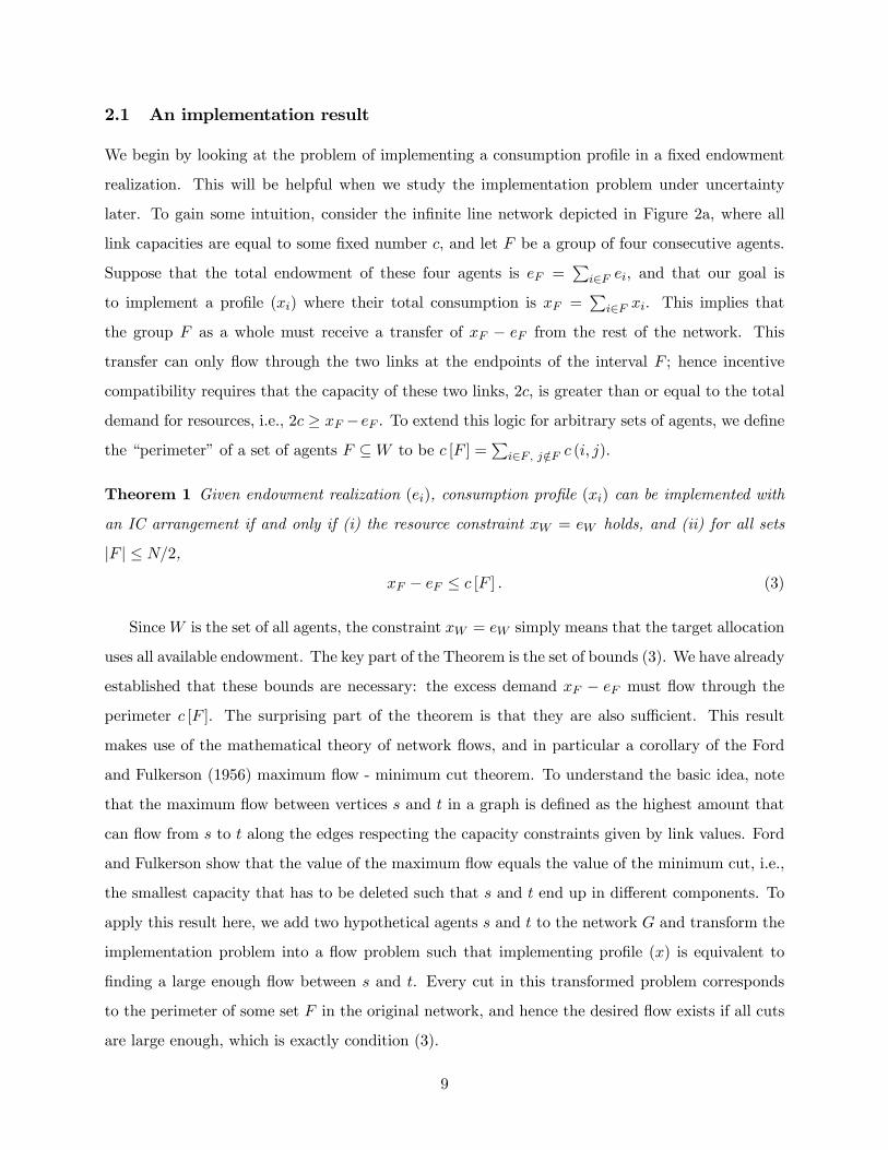
We begin by looking at the problem of implementing a consumption profile in a fixed endowment

realization. This will be helpful when we study the implementation problem under uncertainty

later. To gain some intuition, consider the infinite line network depicted in Figure 2a, where all

link capacities are equal to some fixed number c, and let F be a group of four consecutive agents.

Suppose that the total endowment of these four agents is eF =P

i∈F ei, and that our goal is

to implement a profile (xi) where their total consumption is xF =P

i∈F xi. This implies that

the group F as a whole must receive a transfer of xF − eF from the rest of the network. This

transfer can only flow through the two links at the endpoints of the interval F ; hence incentive

compatibility requires that the capacity of these two links, 2c, is greater than or equal to the total

demand for resources, i.e., 2c ≥ xF −eF . To extend this logic for arbitrary sets of agents, we define

the “perimeter” of a set of agents F ⊆W to be c [F ] =P

i∈F , j /∈F c (i, j).

Theorem 1 Given endowment realization (ei), consumption profile (xi) can be implemented with

an IC arrangement if and only if (i) the resource constraint xW = eW holds, and (ii) for all sets

|F | ≤ N/2,

xF − eF ≤ c [F ] . (3)

SinceW is the set of all agents, the constraint xW = eW simply means that the target allocation

uses all available endowment. The key part of the Theorem is the set of bounds (3). We have already

established that these bounds are necessary: the excess demand xF − eF must flow through the

perimeter c [F ]. The surprising part of the theorem is that they are also sufficient. This result

makes use of the mathematical theory of network flows, and in particular a corollary of the Ford

and Fulkerson (1956) maximum flow - minimum cut theorem. To understand the basic idea, note

that the maximum flow between vertices s and t in a graph is defined as the highest amount that

can flow from s to t along the edges respecting the capacity constraints given by link values. Ford

and Fulkerson show that the value of the maximum flow equals the value of the minimum cut, i.e.,

the smallest capacity that has to be deleted such that s and t end up in different components. To

apply this result here, we add two hypothetical agents s and t to the network G and transform the

implementation problem into a flow problem such that implementing profile (x) is equivalent to

finding a large enough flow between s and t. Every cut in this transformed problem corresponds

to the perimeter of some set F in the original network, and hence the desired flow exists if all cuts

are large enough, which is exactly condition (3).

9

2.2 The limits to full risk-sharing

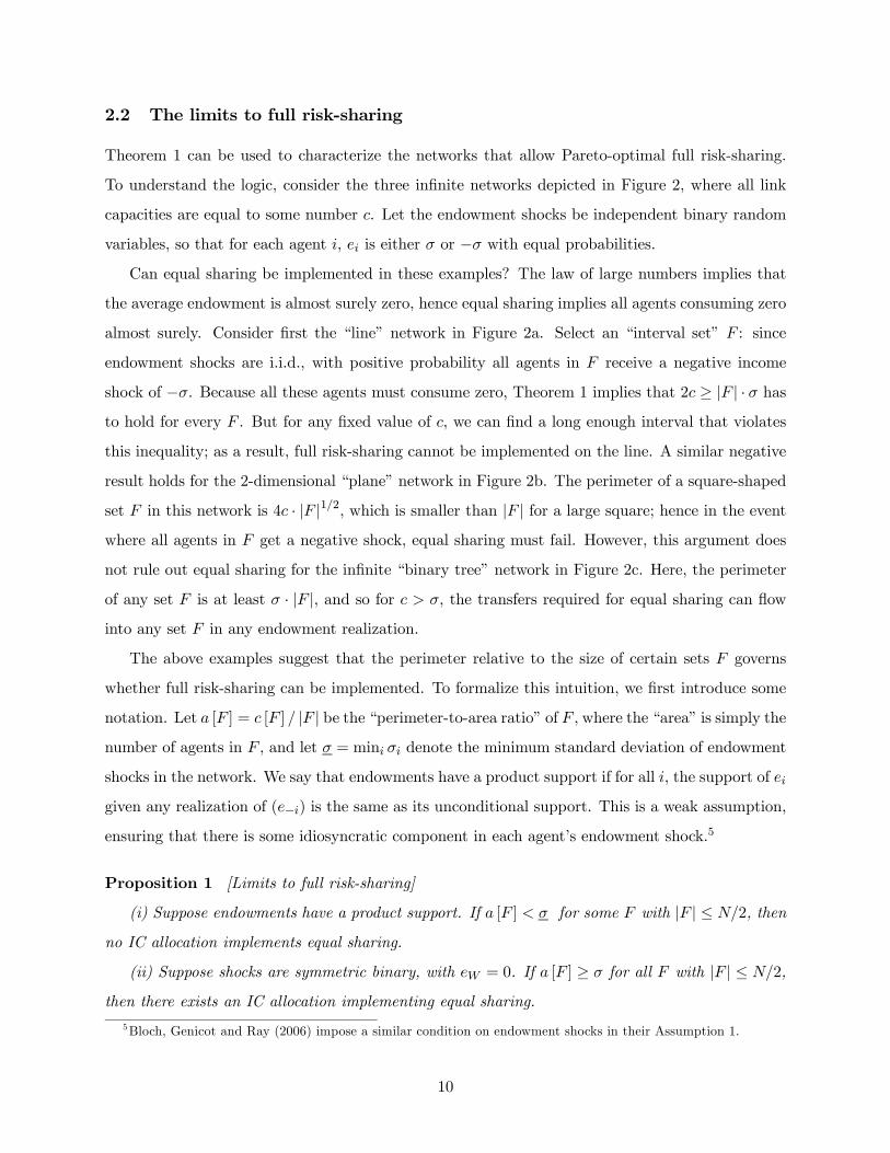
Theorem 1 can be used to characterize the networks that allow Pareto-optimal full risk-sharing.

To understand the logic, consider the three infinite networks depicted in Figure 2, where all link

capacities are equal to some number c. Let the endowment shocks be independent binary random

variables, so that for each agent i, ei is either σ or −σ with equal probabilities.

Can equal sharing be implemented in these examples? The law of large numbers implies that

the average endowment is almost surely zero, hence equal sharing implies all agents consuming zero

almost surely. Consider first the “line” network in Figure 2a. Select an “interval set” F : since

endowment shocks are i.i.d., with positive probability all agents in F receive a negative income

shock of −σ. Because all these agents must consume zero, Theorem 1 implies that 2c ≥ |F | · σ has

to hold for every F . But for any fixed value of c, we can find a long enough interval that violates

this inequality; as a result, full risk-sharing cannot be implemented on the line. A similar negative

result holds for the 2-dimensional “plane” network in Figure 2b. The perimeter of a square-shaped

set F in this network is 4c · |F |1/2, which is smaller than |F | for a large square; hence in the event

where all agents in F get a negative shock, equal sharing must fail. However, this argument does

not rule out equal sharing for the infinite “binary tree” network in Figure 2c. Here, the perimeter

of any set F is at least σ · |F |, and so for c > σ, the transfers required for equal sharing can flow

into any set F in any endowment realization.

The above examples suggest that the perimeter relative to the size of certain sets F governs

whether full risk-sharing can be implemented. To formalize this intuition, we first introduce some

notation. Let a [F ] = c [F ] / |F | be the “perimeter-to-area ratio” of F , where the “area” is simply the

number of agents in F , and let σ = mini σi denote the minimum standard deviation of endowment

shocks in the network. We say that endowments have a product support if for all i, the support of ei

given any realization of (e−i) is the same as its unconditional support. This is a weak assumption,

ensuring that there is some idiosyncratic component in each agent’s endowment shock.5

Proposition 1 [Limits to full risk-sharing]

(i) Suppose endowments have a product support. If a [F ] < σ for some F with |F | ≤ N/2, then

no IC allocation implements equal sharing.

(ii) Suppose shocks are symmetric binary, with eW = 0. If a [F ] ≥ σ for all F with |F | ≤ N/2,

then there exists an IC allocation implementing equal sharing.

5Bloch, Genicot and Ray (2006) impose a similar condition on endowment shocks in their Assumption 1.

10

Part (i) states that when the perimeter/area ratio of at least one set is smaller than the measure

of endowment risk σ, then full risk-sharing cannot be implemented. The intuition is simple: by the

product support assumption, there are realizations where the cumulative idiosyncratic shock inside

F is larger than the perimeter. This shock cannot be completely transferred away, and hence equal

sharing must fail. Part (ii) is a partial converse for symmetric binary shocks and no aggregate

uncertainty. This result follows directly from Theorem 1. When eW = 0, equal sharing means that

all agents must consume zero. Given that shocks are binary, any set F has an excess demand of at

most |F | · σ relative to the target of zero consumption. This demand is less than or equal to the

perimeter c [F ] because a [F ] ≥ σ, and hence can be satisfied for all sets F .

The proposition shows that full risk-sharing imposes very strong expansion conditions on the

network structure, which are unlikely to be satisfied in real-world networks. In fact, since social

networks in practice are often organized on the basis of geographic location, we expect that their

structure more closely resembles the 2-dimensional grid on the plane. For these networks, full

risk-sharing fails by part (i) of the Proposition, and hence we need to explore the degree of partial

risk-sharing that might obtain.

2.3 Partial risk-sharing

We begin our analysis of partial risk-sharing with an intuitive argument. Assume that our goal is to

implement a profile where all agents consume zero. We know from Theorem 1 that the cumulative

shock in a set F can leave the set in a realization if eF ≤ c [F ]. This result suggests that risk-sharing

should be reasonably good when eF ≤ c [F ] holds “most of the time.” This will be the case for

example when σF =stdev[eF ] is small relative to c [F ], because the standard deviation is a measure

of the “typical magnitude” of eF . This logic suggests that we might expect good but imperfect

risk-sharing if c [F ] is sufficiently larger than σF for most sets F .

Note, there is an important difference between this argument and the results in Proposition 1.

In the Proposition, the perimeter/area ratio is compared to the standard deviation of individual

endowment shocks, and hence the correlation structure across agents is not exploited. Here, we

make use of the correlation structure by computing the standard deviation over sets of agents. To

see why this matters, note that full risk-sharing as characterized by Proposition 1 requires c [F ]

to be proportional to |F |. But if endowment shocks are i.i.d., then the standard deviation of eFis only of order |F |1/2, and hence our argument suggests that good risk-sharing can obtain even if

the perimeter is of order |F |1/2, which can be much smaller than |F |. In particular, for the plane

11

network, where the perimeter of square shape sets is c [F ] ∼ |F |1/2, this logic suggests reasonably

good risk-sharing. In contrast, for the line we still expect risk-sharing to be poor, because the

perimeter of long interval sets will be smaller than |F |1/2.

To formalize this intuition, we need to develop a measure of partial risk-sharing. Using the

equal sharing profile where all agents consume e = (1/N)P

i ei as the full risk-sharing benchmark,

assuming that agents have identical preferences over goods consumption, a natural measure of

risk-sharing is

UDISP (x) = E1

N

Xi

{U (e)− U (xi)}

where we ignored the dependence of utility on links to simplify notation. UDISP , or “utility-based

dispersion,” is simply the difference between average expected utility in the allocation (x) relative

to the first best of equal sharing, and hence lower values correspond to better risk-sharing. In

particular, UDISP (x) ≥ 0, with equality if and only if x implements equal sharing. If all agents

have the same quadratic utility function over x, then we can express UDISP as an increasing

function of

SDISP (x) =

∙E1

N

Xxu2

¸1/2, (4)

which is the square-root of the expected cross-sectional variance of x. For non-quadratic utilities,

SDISP (x) can be interpreted as a second order approximation of the utility based measure.

SDISP is highly tractable, and inherits the intuitive properties of UDISP : it is zero only in equal

sharing and positive otherwise, and its magnitude measures the departure from equal sharing: e.g.,

if eu are symmetric binary, then in autarky SDISP (e) = σ. For these reasons, we concentrate on

SDISP in the analysis below.

Before stating the formal results, we make some assumptions about the distribution of shocks.

We assume that the source of uncertainty is a collection of independent random variables yj ,

j = 1, ...,∞, which can represent idiosyncratic shocks like illness as well as aggregate shocks like

weather. Different agents may have different exposure to these shocks, so that ei =P

j αijyj .where

αij measures the extent to which agent i is exposed to shock j. We assume thatP

j α2ij is uniformly

bounded for all agents, and that yj have uniformly bounded support.6 One natural special case

is when ei = yi are i.i.d. We also require that shocks are not too correlated, so that aggregate

uncertainty disappears at a rate σF ≤ K1 · |F |1/2 with some K1 > 0. On the line or the plane, this

6This assumption can be relaxed: we only require bounds on the moment-generating function of yj . Normallydistributed random variables also satisfy these bounds, and hence all our results extend to joinly normal shocks.

12

property holds for example when the correlation between endowment shocks decays geometrically

with network distance. Finally, we assume that a larger group of people face more risk, so that for

all G ⊆ F , we have σG ≤ σF ; and that sharing risk with more people is always good, i.e., that for

all G ⊆ F , we have σF/ |F | ≤ σG/ |G|.

Proposition 2 Under the above conditions, there exist K and K 0 constants such that

(i) On the line with capacities c and i.i.d. shocks, we have SDISP (x) ≥ K/c for all IC

arrangements (x).

(ii) On the plane with capacities c, we have SDISP (x) ≤ exp£−K 0c2/3

¤for some IC arrange-

ment (x).

This proposition formalizes our earlier intuition by comparing the rate of convergence to full risk-

sharing as we increase capacities, between the line and plane networks.7 Intuitively, this criterion

examines the effectiveness of strengthening the existing links in the network. For the line we expect

poor risk-sharing, because the size of shocks grows faster than the perimeter of sets. Formally,

this means that SDISP goes to zero at a slow rate of 1/c as c goes to infinity. But for the plane,

we expect very good risk-sharing because the perimeter has the same order of magnitude as the

standard deviation of the shock; as a result, SDISP should go to zero at a fast, exponential rate.

Risk-sharing on the plane is thus qualitatively different from risk-sharing on the line: convergence

to equal sharing is exponential as opposed to polynomial.

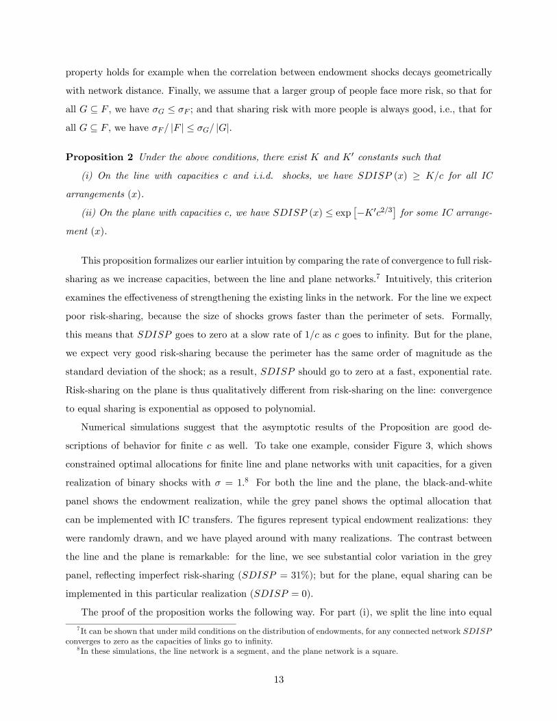
Numerical simulations suggest that the asymptotic results of the Proposition are good de-

scriptions of behavior for finite c as well. To take one example, consider Figure 3, which shows

constrained optimal allocations for finite line and plane networks with unit capacities, for a given

realization of binary shocks with σ = 1.8 For both the line and the plane, the black-and-white

panel shows the endowment realization, while the grey panel shows the optimal allocation that

can be implemented with IC transfers. The figures represent typical endowment realizations: they

were randomly drawn, and we have played around with many realizations. The contrast between

the line and the plane is remarkable: for the line, we see substantial color variation in the grey

panel, reflecting imperfect risk-sharing (SDISP = 31%); but for the plane, equal sharing can be

implemented in this particular realization (SDISP = 0).

The proof of the proposition works the following way. For part (i), we split the line into equal

7 It can be shown that under mild conditions on the distribution of endowments, for any connected network SDISPconverges to zero as the capacities of links go to infinity.

8 In these simulations, the line network is a segment, and the plane network is a square.

13

interval sets, and show that for long intervals, much of the shock over each interval must remain

inside the set. We choose intervals of approximate length 16c2, which implies that σF for each

interval is on the order of¡16c2

¢1/2= 4c. Since the perimeter of each interval is 2c, a standard

deviation of 4c − 2c = 2c must remain in each of these sets. If agents in a set manage to smooth

this residual shock perfectly, then the per capita residual standard deviation will be 2c/ |F | ∼ 1/c,

establishing the desired lower bound.

The result for the plane is more difficult. Here, we have to construct an IC arrangement that

implements very good risk-sharing. We do this in two steps: first we construct an “unconstrained”

arrangement that implements equal sharing on a 2m by 2m sized square for some m chosen as a

function of c; second, we show that this unconstrained arrangement violates capacity constraints

infrequently, and hence there exists an IC arrangement that implements almost as good risk-sharing

as the unconstrained one. For the unconstrained arrangement, we make use of a partition of the

network where we split the square of size 2m by 2m into four equal squares, split each of these

into four smaller squares, and repeat this procedure m times. Then we build the unconstrained

flow from the bottom up: first we smooth consumption in the smallest squares, then we smooth

consumption in the squares at the next level, and so on. There are m steps in this procedure, and

hence each link is used only m times. Assuming that σ = 1, every time a link is used, the required

capacity is of order 1, because the standard deviation in a square F is σF = |F |1/2, and this must be

distributed over the 4 · |F |1/2 links on the perimeter. Thus with m iterations, we implement equal

sharing in the big square while only using a link capacity of order m on average. Equal sharing in

the big square corresponds to an SDISP of order e−m, thus a choice of m = c would implement

exponentially good risk-sharing. However, we have to worry about the exceptional events when

the capacity constraints are violated. Using the theory of large deviations we prove that these

exceptional events can be taken care of with a choice of m = c2/3, resulting in the bound of the

proposition.

2.4 Geographic networks

The results for the plane are interesting because real-world networks are likely to be similarly two-

dimensional. To formalize this idea, suppose that the social network can be represented by a map

on the plane. If the correlation between agents’ endowment shocks falls fast enough with distance

on the map, then we expect that σF grows at the rate of |F |1/2, just like in the plane network.

Moreover, if agents tend to have friends at close geographic distance in multiple directions, then

14

it is plausible that that the perimeter of sets F also grows at a rate of |F |1/2. These observations

suggest that the key properties of the plane are preserved for a wider class of geographic networks,

and hence we expect good risk-sharing for them.

To make this argument precise, consider an infinite network, and let π : W → R2 map agents

in this network to locations in the plane such that different agents are assigned different locations.

To ensure that agents have friends in multiple directions, consider two a by a squares on the plane

sharing a common side, with sides parallel to the axes, and define the crossing density as the

total capacity of all links connecting agents in one square with agents in the other, normalized

by a. We say that the embedding exhibits no separating avenues if the crossing density of all

large enough squares is bounded away from zero. If this holds, then agents in a large square

always have friends in neighboring squares. We also assume that for large squares, the part of

the network that falls into a square is connected; and that the population density in all large

enough squares is bounded from above and below. Regarding the endowment shocks, we require

that the correlation between individual endowments falls geometrically with distance, i.e., that

corr[ei, ej ] ≤ K2 exp [−d (i, j) /K2] for someK2 > 0, where d (u, v) is the Euclidean distance between

π (u) and π (v). A network is called a geographic network if these conditions are satisfied.

Corollary 1 In geographic networks, we have SDISP (x) ≤ exp£−K 0c2/3

¤for some IC arrange-

ment (x).

The proof combines Proposition 2 with a renormalization argument. We take a geographic

network, and superimpose on its planar representation a grid with large squares. Then we merge

all people within each square to create a new network. Because of the no separating avenues

condition, this new network is essentially a plane, and hence Proposition 2 (ii) can be applied to

yield a bound for SDISP of the new network. We thin lift this bound back to the old network

using the assumptions of bounded population density and connectedness inside the squares.

The Corollary is useful because it can help explain stylized facts in development economics.

Real-world village networks are likely to be organized partly on a geographic basis, and hence are

likely to satisfy the properties of a geographic network. As a result, our model predicts very good

informal risk-sharing in these villages, which is consistent with the empirical findings of Townsend

(1994), Ogaki and Zhang (2001), Mazzocco (2007) and others.

15

2.5 Risk-sharing ability of a group

One commonly used approach to test full risk-sharing in the data is to regress the consumption of

an individual or a group on their own endowment shock as well as a community-wide shock. A

variant of this regression when there is no aggregate uncertainty is

xF = α+ β · eF + ε

where consumption in F is regressed on the endowment shock specific to F . It is easy to see

that with full risk-sharing, we get βF = 0; this corresponds to the test of full risk-sharing used

in Cochrane (1991), Mace (1991), Townsend (1994) and others. When β 6= 0, full risk-sharing is

rejected; however, small magnitudes of the coefficient can be interpreted to mean that agents in F

share their risk with the rest of the community reasonably well. The following result supports this

interpretation.

Proposition 3 We have

1− c [F ]

σF≤ β.

The regression coefficient β has a lower bound which is a function of the perimeter c [F ] relative

to the standard deviation of the community-specific shock σF . The intuition is familiar: when the

perimeter of a set is small, there is insufficient capacity for the shock to exit, which yields high

correlation between consumption and shocks. The proposition is related to the empirical findings

in Townsend (1994), who shows that there is considerable risk-sharing among households within an

Indian village, but only limited sharing of village-specific shocks across villages. The proposition

is consistent with these findings if cross-village network ties are weak relative to the size of the

villages.

2.6 The limits to risk-sharing with imperfect substitutes

We now discuss briefly how the results in this section extend to the imperfect substitutes case.

We find that all results extend, but the upper and lower bounds on risk-sharing are weakened

by constant factors that depend on the degree of substitutability between goods and friendship.

Since the results about partial risk-sharing characterize limit behavior, they remain unaffected by

these constant factors. To obtain our extensions, we assume that the marginal rate of substitution

16

(MRS) is uniformly bounded: k < MRSi < K for all agents i in the relevant range of endowment

realizations.

We begin with extending Theorem 1. When the MRS is bounded, the necessary and sufficient

condition in the Theorem is replaced by the following two conditions, one being necessary, the other

sufficient for IC implementation. (i) Any IC profile must satisfy xF − eF ≤ K · c [F ] for all sets F

with |F | ≤ N/2. (ii) A profile that satisfies xF − eF ≤ k · c [F ] for all F with |F | ≤ N/2 is IC. The

extension follows directly from the logic of Theorem 1, noting that bounded MRS implies that the

relative price of friendship and goods is always between k and K. This extension is particularly

informative for environments where k and K are close to each other, e.g., when endowment shocks

have a small support: then, by continuity, the MRS does not vary much in the relevant range of

realizations.

The uniform bound on the MRS can also be used to extend the characterization of environments

where full risk-sharing can be implemented. We continue to find that the first-best can only be

achieved in expander graphs where the perimeter/area ratio is bounded from below: we require

a [F ] ≥ σ/K. We also find that in the binary shock case, full risk-sharing can be implemented when

a [F ] ≥ σ/k. These results imply that full risk-sharing fails for most plausible networks even with

imperfect substitutes. Our findings about partial risk-sharing characterize convergence rates, and

hence they extend without modification to the imperfect substitutes case. In particular, SDISP

continues to converge exponentially for geographic networks, and therefore our argument about

good risk-sharing in real-world networks is unaffected.

The setup where goods and friendship are imperfect substitutes yields some additional impli-

cations as well. If the marginal rate of substitution between goods and friendship is increasing in

consumption, then agents with low consumption value their friends less, reducing the maximum

amount they are willing to transfer to them. As a result, if in a society that experiences a neg-

ative aggregate shock, the scope for insuring idiosyncratic risk is reduced because of the drop in

the dollar value of links. We formalize this intuition in the appendix by showing that when the

MRS is increasing, reducing the endowments of all agents results in a smaller set of IC transfer

arrangements. In particular, SDISP is larger after a negative aggregate shock, because agents

are more constrained in insuring idiosyncratic risk. These results are consistent with the findings

of Kazianga and Udry (2006), who document that during the severe draught of 1981-85 in rural

Burkina Faso, risk-sharing between households was quite limited.

17

3 Constrained efficient risk-sharing

In this section, we study allocations that are optimal subject to the enforcement constraints imposed

by the network. A risk-sharing arrangement is constrained efficient or second-best if it is Pareto-

optimal among the set of IC arrangements. Constrained efficient arrangements provide a natural

benchmark, because they achieve the highest possible level of risk-sharing in a given social network.

In addition, we show below that constrained efficiency can arise both when agents follow simple

rules of thumb for helping each other, and also as a result of dynamic coalitional bargaining. Once

reached, constrained efficient arrangements are likely to remain stable, because they are robust to

both individual and coalitional deviations.

As in the previous section, we start out by assuming that goods and friendship and perfect

substitutes, and extend the results to general preferences later.

3.1 Characterizing constrained efficiency

In this subsection we maintain the assumption that goods and friendship are perfect substitutes.

The study of second-best arrangements is facilitated by the fact that they can be characterized using

a planner’s problem. Formally, let (λi)i∈W be a set of positive weights, and define the planner’s

problem as the constrained optimization problem

maxXi∈W

λi · EUi (xi, ci) (5)

subject to the IC-constraint (1). We then have the following result.

Proposition 4 Every constrained efficient arrangement is the solution to a planner’s problem

with some set of weights (λi). Conversely, any solution to the planner’s problem is constrained

efficient.

Wilson (1968) establishes a similar equivalence result for risk-sharing in syndicates. His proof

builds on the idea that the set of possible payoff vectors is convex. Since an efficient allocation must

lie on the boundary of this set, convexity implies the existence of a tangent hyperplane with some

normal vector (λi). Maximizing a planner’s problem with these (λi) weights will select the efficient

allocation by design. Adapting this argument to our model requires that the set of IC payoff vectors

be convex. In the perfect substitutes case, this follows easily: when two transfers satisfy a capacity

constraint, their convex combination will also satisfy it. As we detail in the Appendix, the result

18

can also be extended to the imperfect substitutes case under an additional condition about the

curvature of the marginal rate of substitution.

Proposition 4 implies that maximizing the planner’s expected utility EP

λiUi is equivalent

to maximizing realized utilityP

λiUi independently for each state, because conditional on the

planner weights, the states are not connected in the maximization problem. This separation of

states simplifies the characterization of second-best arrangements, and makes it easier to solve

for them. In particular, we can derive a set of first-order conditions for the planner’s problem

separately for each state, which allows for a simple characterization of second-best arrangements.

We say that a link from i to j is blocked in a given realization, if tij = c (i, j), that is, if i is sending

the maximum IC amount.

Proposition 5 A transfer arrangement t is constrained efficient iff there exist positive welfare

weights (λi)i∈W such that for every i, j ∈ N one of the following conditions holds:

1) λiU 0i(xi) = λjU0i(xj)

2) λiU 0i(xi) > λjU0j(xj) and the link from j to i is blocked

3) λiU 0i(xi) < λjU0j(xj) and the link from i to j is blocked.

This result states the set of first order necessary and sufficient conditions for the planner’s

problem. To understand the intuition, recall that as Wilson (1968) has shown, unconstrained

Pareto optimal risk-sharing implies that λiU 0i(xi) = λjU0i(xj) for all i and j. If this condition is

violated, e.g., λiU 0i(xi) < λjU0j(xj), then the planner’s objective can be improved by transferring a

small amount from i to j. In a second best arrangement, this transfer must violate the incentive

compatibility constraint; as a result, the maximum possible amount most already be transferred

from i to j. This logic establishes the necessity of the above first order conditions; sufficiency follows

because the planner’s objective function is concave and the domain of IC consumption profiles is

convex. These conditions also guarantee uniqueness.

The Proposition also implies that for any pair of agents i and j, if λiU 0i < λjU0j , then all

paths connecting i and j have to be blocked in the sense that at least one link along each path is

used at maximal capacity. This observation uncovers an important feature of constrained efficient

agreements, namely that in any realization agents can be partitioned into connected “risk-sharing

islands” such that within an island agents share risk perfectly, while cross-island insurance is limited

because boundary links operate at full capacity.

19

Proposition 6 [Risk-sharing islands] In any realization (ei) the set of agents can be partitioned

into connected components Wk such that for i, j ∈ Wk we have λiU 0i = λjU0j and for i ∈ Wk, and

j /∈Wk either tij = c (i, j) or tji = c (j, i).

The sharing island Wk of i is the maximal connected set containing i with the property that

λiU0i = λjU

0j for all j ∈ Wk. For each realization, these sharing islands provide a partition of the

network, and have the property that shocks are fully shared within an island but there is imperfect

insurance across islands. This island structure is illustrated in the line network in Figure 3, where

the grey panel depicts the constrained efficient allocation corresponding to equal planner weights

in one endowment realization. The dashed lines in the figure indicate the boundaries of the islands;

marginal utility and hence consumption is equalized within an island, but differs across islands.

In the island partition, the size and location of islands, and hence the set of agents who fully share

each others’ shocks, is endogenous to the endowment realization. This result differentiates our model

from group-based theories of risk-sharing, where insurance groups are determined exogenously and

do not vary with the realization of uncertainty.

3.2 Spillover effects and local sharing

The characterization of constrained efficient allocations in terms of risk-sharing islands can be used

to explore the degree of partial insurance as a function of network distance. This analysis sheds

light on the spillover effects of shocks in networks, and yields new testable implications about local

risk-sharing.

We begin by introducing a slightly stronger definition of risk-sharing islands. Fix an endowment

realization (ei), and let W (i) denote the sharing island containing i as defined above, i.e., the

maximal connected set with the property that λiU 0i = λjU0j for all j ∈ W (i). We now definecW (i) to be the maximal connected set of agents j such that there exists a path between i and j

along which no links are blocked in either direction. With this definition, cW (i) ⊂ W (i), because

the first order condition of Proposition 5 implies λiU 0i = λjU0i for all j ∈ cW (i). Moreover, except

for knife-edge cases when the transfer amount just reaches the capacity over a link but does not

“bind” yet, these two island definitions are equivalent, and cW (i) = W (i). It can be shown that

these knife-edge cases happen with zero probability when the distribution of endowment shocks

is absolutely continuous; as a result, the two definitions can be treated as equivalent for practical

purposes.

20

To understand the connection between partial risk-sharing and network distance, we explore

the effects of an idiosyncratic shock to one agent’s endowment on the consumption of others. Fix a

constrained efficient arrangement, and consider two endowment realizations e = (ei) and e0 = (e0i),

where e0j = ej for all j 6= i, and e0i < ei. These two realizations can be viewed either as agent

i experiencing an idiosyncratic negative shock in e0 relative to e, or as agent i experiencing an

idiosyncratic positive shock (aid) in e relative to e0. For ease of exposition, in the discussions below

we focus on the first interpretation: that agent i receives a negative shock in e0. We can measure

the impact of this shock on agent j by computing the ratio of marginal utilities

MUCj =U 0j (e

0)

U 0j (e).

HereMUCj measures the marginal utility cost of the shock for agent j. A largerMUCj corresponds

to a higher increase in marginal utility and hence a greater consumption drop.9

Corollary 2 [Spillovers and local sharing]

(i) [Monotonicity] xj(e0) ≤ xj(e) for all j, and if j ∈ cW (i) then xj(e0) < xj(e).

(ii) [Local sharing] There exists ∆ > 0 such that |ei − e0i| < ∆ implies MUCi = MUCj for all

j ∈ cW (i), and xj (e0) = xj (e) for all j ∈W\W (i).

(iii) [More sharing with close friends] For any j 6= i, there exists a path i→ j such that for any

agent l along the path, MUCl ≥MUCj.

Part (i) shows that efficient arrangements are monotone: If one agent receives a negative shock,

the consumption of everybody else either decreases or remains constant. Moreover, the agent

is partially insured by all others who are in the same risk-sharing island, who all reduce their

consumption by a positive amount. As a result, unless i is in a singleton island, he has access

to at least some insurance. The intuition follows from the definition of cW (i): links within the

risk-sharing island of i are not blocked, and hence a small transfer can flow through them to help

out i. As part (ii) shows, for small shocks, the set of agents who insure i is exactly his sharing

island cW (i). All these agents share an equal burden of the shock, and hence experience the same

marginal utility cost. Agents outside of W (i) do not reduce their consumption at all; and in the

knife edge case where cW (i) 6= W (i), agents in W (i) \cW (i) may or may not share. Finally, part

(iii) shows how the utility cost of agents in response to an idiosyncratic shock to i varies by social

9Analysing the impact of a positive iniosyncratic shock to i yields symmetric results.

21

distance. The result states that indirect friends provide less insurance to i than direct friends: for

any agent j 6= i, there exists some direct friend of i, denoted l, who shares at least as much of the

burden of the shock as j does.

The results of the Corollary are also illustrated in Figure 4, which shows the marginal utility

cost of direct and indirect friends in response to an endowment shock to i. The horizontal axis is

the marginal utility cost of agent i himself, and the vertical axis measures the marginal utility cost

of some direct and indirect friends. For small shocks, both direct and indirect friends who are in

the same risk-sharing island as i help out. As the size of the shock grows, some indirect friends hit

their capacity constraints and stop reducing consumption, but some direct friends continue to help.

After a point, all direct friends hit their capacity constraints; as a result, additional increases in the

shock are fully borne by agent i. These implications can be used to test our model against other

theories of limited risk-sharing, which do not predict variation in the degree of partial risk-sharing

as a function of network distance.

3.3 Foundations for constrained efficiency

One reason for analyzing constrained efficient allocations is that they naturally emerge from intu-

itive dynamic mechanisms among agents in the network. Here we briefly discuss two such mecha-

nisms. First, constrained efficient allocations can be obtained in a decentralized procedure where

agents use a simple rule of thumb in helping those who are in need. In every round of this dynamic

procedure, agents attempt to equate weighted marginal utilities between neighbors subject to the

capacity constraints: intuitively, people help out those friends and relatives who are in need. The

appendix shows that this procedure converges to the constrained efficient allocation corresponding

to the welfare weights used. As a result, constrained efficient allocations can emerge even if agents

only use local information: in every round of the procedure, agents engage in binary transactions

that only knowledge about the current resources of the two parties involved.10

A second mechanism that leads to constrained efficient arrangements is collective dynamic

bargaining with renegotiation. Gomes (2005) shows that when agents can propose renegotiable

arrangements to subgroups and make side-payments in a dynamic bargaining procedure, as the

community become infinitely patient, a Pareto-efficient arrangement will be selected.11 This result

can be incorporated in our model by assuming that there is a negotiations phase prior to the

10Bramoulle and Kranton (2007) use a similar procedure with equal welfare weights and no capacity constraints.11Aghion, Antras, and Helpman (2007) establish a similar result in a model involving renegotiating free-trade

agreements.

22

endowment realization, and would imply that agents select a constrained efficient risk-sharing

arrangement.

Finally, constrained efficient arrangements are quite stable in our model, because they are robust

to all possible coalitional deviations. The appendix shows that after any endowment realization,

no group of agents can have a credible and profitable deviation that involves IC transfers among

members of the group, and possibly reneging on some of the transfers to agents outside the group.

3.4 General preferences

We now turn to discuss how our results about constrained efficiency extend to the imperfect sub-

stitutes case. We find that all our conceptual results generalize. The formal results are provided in

the Appendix; here we present an intuitive summary.

The key novelty with imperfect substitutes is that changing the goods consumption of an agent

affects the agent’s link values, and hence his incentive compatibility constraints over transfers.

To characterize constrained efficiency in this environment, we assume that the marginal rate of

substitution MRSi, i.e., the relative price of friendship in terms of goods consumption, is concave

in xi. Intuitively, this means that increases in goods consumption have a diminishing effect on the

value of friendship. When this condition holds, we can generalize Proposition 4, establishing the

equivalence between constrained efficiency and the planner’s problem.

To develop first order conditions, we next analyze the effect of an additional dollar to agent i on

the planner’s objective. With imperfect substitutes, this marginal welfare gain is no longer equal

to λi times his marginal utility of i’s consumption, because increased consumption also softens

i’s IC constraints over transfers to neighboring agents. As a result, it may be optimal from the

planner’s perspective to transfer some of the original dollar to such neighboring agents with whom

the IC constraint of i was previously binding. Due to this difference between private and social

marginal utility, we can have constrained efficient arrangements where i is transferring a positive

amount to i0 even though i0 has lower weighted marginal utility, because this transfer, by keeping

the consumption of i0 high, softens the IC constraint of i0 on transfers to another agent i00, who has

high marginal utility. To get around this issue, in the Appendix we define the marginal social gain

of an additional unit of transfer to i, denoted ∆i, for each agent i using an iterative procedure,

which takes into account the indirect effect of softening IC constraints and transferring further

some of the additional resources.

Using ∆i instead of the private marginal utilities allows us to extend all the results in this

23

section. We obtain first order conditions that are analogous to Proposition 5: in a constrained

efficient arrangement, either ∆i = ∆j of the link between i and j has to be blocked. Using

this result, we can also partition the network into endogenous risk-sharing islands, such that ∆i

is equalized within islands while links are blocked across islands. The results of Corollary 2 on

monotonicity, local sharing, and more sharing with close friends also have analogous extensions to

this environment, which are formally presented in the Appendix.

Finally, for an agent i who is not on the boundary of his risk-sharing island and hence has

no binding IC constraints, the marginal social gain does equal λi times his marginal utility of

consumption; hence, for such agents, the results presented in this section hold without modification.

For example, weighted marginal utilities are equalized for two agents inside the same risk-sharing

island and away from the island boundary. This argument establishes that if risk-sharing islands

are “large”, then the results from the perfect substitute case hold without modification for most

agents.

4 Indirect effects of an aid program

We plan to simulate our model using network data from Peru, to evaluate the indirect effects of a

hypothetical development aid program. Because of network spillovers, in our model aid will also

benefit the non-treated, as shown in Corollary 1 in the previous section. This is consistent with the

empirical findings of Angelucci and De Giorgi (2007). We plan to identify individuals who should

be targeted to maximize both the direct and indirect effect of aid.

5 Conclusion

This paper has developed a theory of informal risk-sharing in social networks. We have shown that

expansive networks facilitate informal insurance, and argued that many real-life social networks are

likely to be sufficiently expansive to allow for good risk-sharing. We also characterized second-best

arrangements and found that they exhibit local risk-sharing. In current work, we are exploring the

implications of our model for the indirect effect of development aid. In future work, we would like

to develop other empirical applications.

24

References

Aghion, P., P. Antras, and E. Helpman (2007): “Negotiating free trade,” Journal of Inter-

national Economics, forthcoming.

Angelucci, M., and G. De Giorgi (2007): “Indirect Effects of an Aid Program: How do Cash

Injections Affect Non-Eligibles’ Consumption?,” Working paper.

Bloch, F., G. Genicot, and D. Ray (2005): “Informal Insurance in Social Networks,” Working

paper, New York University.

Bramoulle, Y., and R. E. Kranton (2006): “Risk-Sharing Networks,” Journal of Economic

Behavior and Organization, forthcoming.

(2007): “Risk Sharing Across Communities,” American Economic Review, Papers and

Proceedings.

Coate, S., and M. Ravaillon (1993): “Reciprocity Without Commitment: Characterization

and Performance of Informal Insurance Arrangements,” Journal of Development Economics, 40,

1—24.

Cochrane, J. H. (1991): “A Simple Test of Consumption Insurance,” Journal of Political Econ-

omy, 99(5), 957—976.

Dercon, S., and J. D. Weerdt (2006): “Risk-sharing networks and insurance against illness,”

Journal of Development Economics, 81, 337—356.

Dixit, A. (2003): “Trade Expansion and Contract Enforcement,” Journal of Political Economy,

111, 1293—1317.

Ellison, G. (1994): “Cooperation in the Prisoner’s Dilemma with Anonymous Random Match-

ing,” Review of Economic Studies, 61, 567—588.

Fafchamps, M., and F. Gubert (2007): “The formation of risk-sharing networks,” Journal of

Development Economics, forthcoming.

Fafchamps, M., and S. Lund (2003): “Risk sharing networks in rural Philippines,” Journal of

Development Economics, 71, 261—287.

25

Fehr, E., and S. Gachter (2000): “Cooperation and punishment in public goods experiments,”

American Economic Review, 90, 980—994.

Ford, L. R. J., and D. R. Fulkerson (1956): “Maximal Flow Through a Network,” Canadian

Journal of Mathematics, pp. 399—404.

Gomes, A. (2005): “Multilateral contracting with externalities,” Econometrica, 73, 1329—1350.

Greif, A. (1993): “Contract Enforceability and Economic Institutions in Early Trade: The

Maghribi Traders’ Coalition,” American Economic Review, 83, 525—548.

Kandori, M. (1992): “Social Norms and Community Enforcement,” Review of Economic Studies,

59, 63—80.

Kazianga, H., and C. Udry (2006): “Consumption smoothing? Livestock, insurance and drought

in rural Burkina Faso,” Journal of Development Economics, 79, 413—446.

Kocherlakota, N. (1996): “Implications of Efficient Risk Sharing without Commitment,” Review

of Economic Studies, 63(4), 595—609.

Kranton, R. E. (1996): “Reciprocal Exchange: A Self-Sustaining System,” American Economic

Review, 86, 830—851.

Ligon, E. (1998): “Risk-sharing and information in village economies,” Review of Economic Stud-

ies, 65, 847—864.

Ligon, E., J. P. Thomas, and T. Worrall (2002): “Informal Insurance Arrangements with

Limited Commitment: Theory and Evidence from Village Economies,” Review of Economic

Studies, 69(1), 209—244.

Mace, B. (1991): “Consumption volatility: borrowing constraints or full insurance,” Journal of

Political Economy, 99, 928—956.

Mazzocco, M. (2007): “Household Intertemporal Behavior: a Collective Characterization and a

Test of Commitment,” Review of Economic Studies, 74(3), 857—895.

Mobius, M., and A. Szeidl (2007): “Trust and Social Collateral,” Working paper no. 13126,

NBER.

26

Ogaki, M., and Q. Zhang (2001): “Deceasing Relative Risk Aversion and Tests of Risk Sharing,”

Econometrica, 69(2), 515—526.

Townsend, R. (1994): “Risk and Insurance in Village India,” Econometrica, 62, 539—591.

Udry, C. (1994): “Risk and Insurance in a Rural Credit Market: An Empirical Investigation in

Northern Nigeria,” Review of Economic Studies, 61(3), 495—526.

Wilson, R. (1968): “The theory of syndicates,” Econometrica, 36, 119—132.

27

Appendix: Proofs

Proof of Theorem 1

We prove the more general version of the theorem allowing for directed links, so that c (i, j)

and c (j, i) may differ. Necessity is immediate. To prove sufficiency, let gi = ei − xi the amount

that i has to transfer away, and let gF =P

i∈F ei for any subset of agents F . Note that gW = 0 by

eW = xW . Let S be the set of agents for whom gi ≥ 0 and let T =W\S. Define the auxiliary graph

G0 which has two additional vertices, s and t, and additional edges connecting s with all agents

in S, and additional edges connecting t with all agents in t. For any i ∈ S, define the capacity

c (s, i) = gi and c (i, s) = 0. Similarly, for any j ∈ T , let c (j, t) = −gj and c (t, j) = 0.

The auxiliary graph is useful, because implementing the desired consumption allocation is equiv-

alent to finding an s → t flow in G0 that has value gS =P

ei≥0 gi. To see why, note that in the

desired allocation, exactly gi must leave each agent i ∈ S. The capacities on the new links ensure

that in any s→ t flow, at most gi can leave agent i. Similarly, to implement the target, exactly −gjmust flow to each agent j ∈ T , and the capacity on the (j, t) link ensures that this is the maximum

that can flow to j. As a result, any flow with valueP

ei≥0 gi must, by construction, take exactly gi

away from i and deliver exactly gj to j.

We have reduced our implementation problem to a flow problem. To compute the maximum

s → t flow, we instead compute the value of the minimum cut. Fix a minimum cut. In this cut,

some links of s and t are cut. Let S1 ⊆ S denote those agents whose link with s is cut in the

minimum cut, and let T1 ⊆ T denote those agents in T whose link with t is cut. Clearly, the total

value of the links cut that connected S1 with s and T1 with t is gS1 − gT1 . Let S2 = S\S1 and

T2 = T\T1. We claim that if we consider the restriction of the cut to the original graph G, then

there will be no S2 → T2 paths that survive. Suppose not; then there is some s2 → t2 path in G

after the cut. But this is also an s2 → t2 path in the auxiliary graph G0, and since s2 is connected

to s and t2 to t after the cut, it generates an s→ t path after the cut, which is a contradiction.

Let H be the set of agents h who can be accessed by s → h paths in G after the cut. By the

above argument, S2 ⊆ H and T2 ⊆ T\H. By construction of H, the value of the cut in G must be

cout [H] = cin [W\H], and therefore the value of the cut in G0 is gS1 − gT1 + cout [H]. Suppose that

|H| ≤ N/2. Then we know from (3) that cout [H] ≥ gH . Thus the value of the cut in G0 can be

bounded from below as

gS1 − gT1 + gH = gS1 − gT1 + (gS2 + gH∩T1 + gH∩S1) ≥ gS1 + gS2 = gS

28

where we used that H can be decomposed as a disjoint union of S2, H ∩ T1 and H ∩ S1 and that

−gT1 ≥ −gT1∩H because gj is negative for all j ∈ T1. It follows that the value of the maximum flow

is at least gS , as desired. Note that the maximum flow cannot exceed gS , because deleting all links

between s and S is a valid cut with value gS. Thus the value of the maximum flow is exactly gS .

When |H| > N/2, an analogous argument can be used with W\H instead of H.

The following Lemma will be useful.

Lemma 1 Let Z be a random variable such that |Z| ≤ c almost surely. Then σZ ≤ c, and this

bound is sharp.

Proof. Let G (z0) be the family of probability distributions of random variables that satisfy

|Z| ≤ c and EZ = z0. This family of measures is tight, and by Prokhorov’s theorem, it is relatively

compact in the weak topology. The variance of a random variable with distribution G ∈ G (z0) isR(z − z0)

2G (dz). Here the integrand is a bounded continuous function because G is concentrated

on the [−c, c] interval, implying that variance is a continuous function with respect to the weak

topology on G (z0), and then compactness implies that there exists G∗ ∈ G (z0) that has the highest

variance.

Let Z∗ be a random variable with distribution G∗. Suppose that |Z∗| < c with positive probabil-

ity; then there is some ε > 0 such that Pr (|Z∗| < c− ε) > ε. Let Y be a random variable indepen-

dent of Z∗ that assigns equal probabilities to+1 and−1, and consider Z 0 = Z∗+χ {|Z∗| < c− ε}·εY

where χ {|Z∗| < c− ε} is an indicator function. It is easy to see that EZ 0 =EZ = z0, and that

|Z 0| ≤ c; thus G0, the probability distribution of Z 0, is in G (z0). The variance of Z 0 can be written

as

Pr (|Z∗| ≥ c− ε)·Eh(Z∗ − z0)

2 | |Z∗| ≥ c− εi+Pr (|Z∗| < c− ε)·E

h(Z∗ − z0 + εY )2 | |Z∗| < c− ε

i.

The second term on the right hand side is

Pr (|Z∗| < c− ε)·nEh(Z∗ − z0)

2 | |Z∗| < c− εi+ ε2

o≥ Pr (|Z∗| < c− ε)·E

h(Z∗ − z0)

2 | |Z∗| < c− εi+ε3

where we used that Y has mean zero, unit variance, and is independent of Z∗. Combining this bound

with the previous expression yields var[Z 0] ≥E(Z∗ − z0)2 + ε3 which contradicts the optimality of

Z∗. It follows that the optimal Z∗ must satisfy |Z∗| = c with probability one. Given that EZ∗ = z0

29

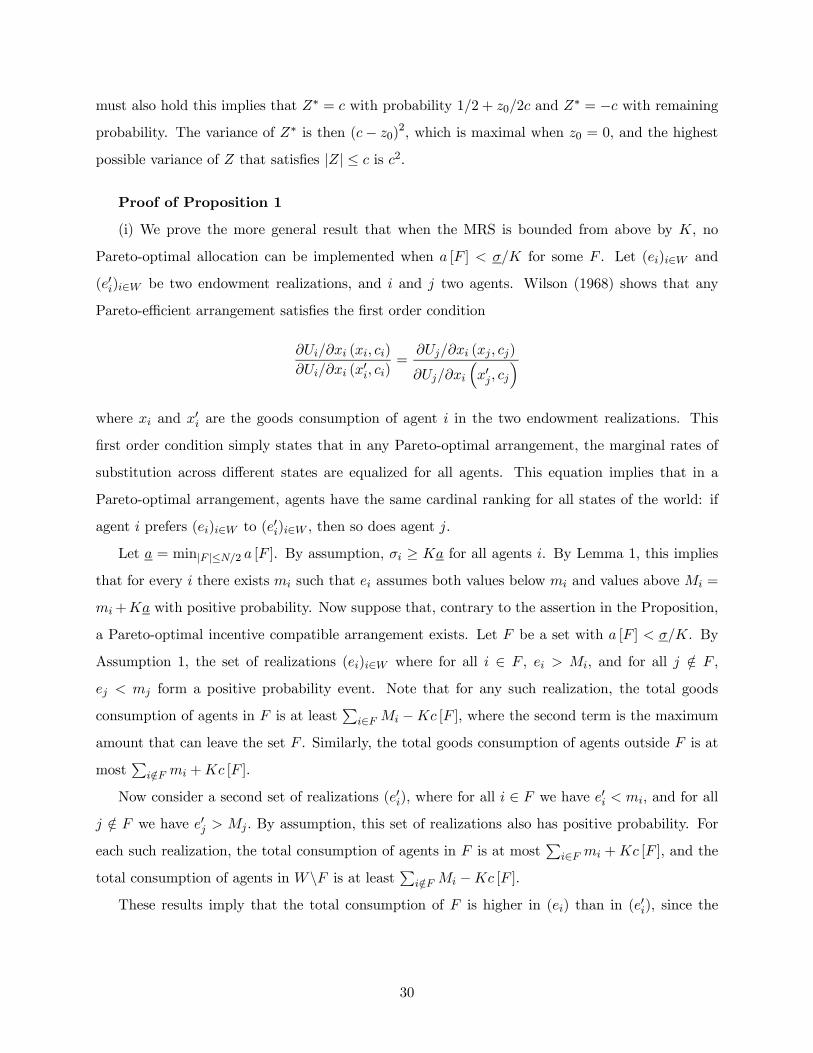
must also hold this implies that Z∗ = c with probability 1/2 + z0/2c and Z∗ = −c with remaining

probability. The variance of Z∗ is then (c− z0)2, which is maximal when z0 = 0, and the highest

possible variance of Z that satisfies |Z| ≤ c is c2.

Proof of Proposition 1

(i) We prove the more general result that when the MRS is bounded from above by K, no

Pareto-optimal allocation can be implemented when a [F ] < σ/K for some F . Let (ei)i∈W and

(e0i)i∈W be two endowment realizations, and i and j two agents. Wilson (1968) shows that any

Pareto-efficient arrangement satisfies the first order condition

∂Ui/∂xi (xi, ci)

∂Ui/∂xi (x0i, ci)=

∂Uj/∂xi (xj , cj)

∂Uj/∂xi

³x0j , cj

´where xi and x0i are the goods consumption of agent i in the two endowment realizations. This

first order condition simply states that in any Pareto-optimal arrangement, the marginal rates of

substitution across different states are equalized for all agents. This equation implies that in a

Pareto-optimal arrangement, agents have the same cardinal ranking for all states of the world: if

agent i prefers (ei)i∈W to (e0i)i∈W , then so does agent j.

Let a = min|F |≤N/2 a [F ]. By assumption, σi ≥ Ka for all agents i. By Lemma 1, this implies

that for every i there exists mi such that ei assumes both values below mi and values above Mi =

mi+Ka with positive probability. Now suppose that, contrary to the assertion in the Proposition,

a Pareto-optimal incentive compatible arrangement exists. Let F be a set with a [F ] < σ/K. By

Assumption 1, the set of realizations (ei)i∈W where for all i ∈ F , ei > Mi, and for all j /∈ F ,

ej < mj form a positive probability event. Note that for any such realization, the total goods

consumption of agents in F is at leastP

i∈F Mi −Kc [F ], where the second term is the maximum

amount that can leave the set F . Similarly, the total goods consumption of agents outside F is at

mostP

i/∈F mi +Kc [F ].

Now consider a second set of realizations (e0i), where for all i ∈ F we have e0i < mi, and for all

j /∈ F we have e0j > Mj . By assumption, this set of realizations also has positive probability. For

each such realization, the total consumption of agents in F is at mostP

i∈F mi +Kc [F ], and the

total consumption of agents in W\F is at leastP

i/∈F Mi −Kc [F ].

These results imply that the total consumption of F is higher in (ei) than in (e0i), since the

30

lower bound in (ei) equals the upper bound in (e0i):

Xi∈F

Mi −Kc [F ] =Xi∈F

mi +Kc [F ]

holds because Mi −mi = Ka = Kc [F ] / |F | by definition. In contrast, the total consumption of

agents in W\F is higher in (e0i) than in (ei), because the upper bound in (ei) is does not exceed

the lower bound in (e0i): Xi/∈F

mi +Kc [F ] ≤Xi/∈F

Mi −Kc [F ]

sinceP

i/∈F Mi −mi = (N − [F ])Ka = Kc [F ] · (N − [F ]) / |F | ≥ Kc [F ]. Taken together, these

findings violate the property of Pareto optimality that agents have a common ranking over states

of the world: there must be some agent in F who prefers (ei) to (e0i), and at the same time there

must be some agent in W\F who prefers (e0i) to (ei). This is a contradiction.

To show that there is an agent in F who is not fully insured, note that there is some i ∈ F who

prefers a positive probability of realizations (ei)i∈W to a positive probability of realizations (e0i)i∈W ;

and within these events, there is j /∈ F who prefers a positive probability of (e0i) to (ei). But this

means that we could improve the expected utility of i and j by transferring a small amount from i

to j in (ei) and transferring a small amount back from j to i in (e0i).

(ii) Theorem 1 provides necessary and sufficient conditions for implementing the profile when

all agents consume zero. For any set F , the excess demand is at most |F | · σ, which must be less

than or equal to c [F ]. This is equivalent to σ ≤ a [F ] for all F with |F | ≤ N/2 .

Proof of Proposition 2

(i) Consider an N long segment on the line, and split it into intervals of length k. For each

segment F , σF = σ√k and c [F ] = 2c. Using Lemma 1, this implies for any IC arrangement

SDISP (x) ≥ σ√k− 2c

k.

To obtain the sharpest bound, let k = 16 (c/σ)2, which gives

SDISP ≥ σ · 18

σ

c

as desired.

31

(ii) We establish a considerably more general result. We begin by listing our assumptions:

(D1) [Thin tails] The yj variables are independent, have zero mean and unit variance, and

satisfy logEexp [θyj ] ≤ Kθ2/2 for some K with all θ ≥ 0.

(D2) [Correlated shocks] The endowment shock of agent i is ei =P

j αijyj whereP

j α2ij <∞.

Here (D1) is a uniform bound on the moment-generating function of yj , and allows us to use

the theory of large deviations to bound the tails of weighted sums of yj . This condition is satisfied

if the yj random variables are i.i.d. normal, or if they have a common compact support, and in

many other cases.

(E1) [No aggregate risk] Endowments satisfy σF / |F | ≤ K1 · |F |−K2 for some K1,K2 > 0.

(E2) [More people have more risk] For all G ⊆ F , we have σG ≤ σF .

(E3) [Sharing with more people is always good.] For all G ⊆ F , we have σF/ |F | ≤ σG/ |G|.

(N1) The network is connected, countably infinite, and there exists a constant K3 such that all

agents have at most K3 direct friends.

We also impose a set of conditions on the network that allows for a decomposition similar to

the square structure on the plane. Specifically, we require that for all m ≥ 1 integers there exist a

collection of sets F ij , where i = 1, ...,m and j = 1, ...,∞ that satisfy the following properties.

(S1) [Partition] For all 1 ≤ i ≤ m, the sets F ij , j = 1, ...,∞ give a partition of the set of agents;

and when i = 1, all sets F 1j are singletons.

(S2) [Ascending chain] For all 1 ≤ i ≤ m − 1 and all j, j0, we have either F ij ∩ F i+1

j0 = ∅ or

F ij ⊆ F i+1

j0 .

(S3) [Exponential growth.] There exist 1 < γ < γ constants such that whenever F ij ⊆ F i+1

j0 , we

have γ¯̄̄F ij

¯̄̄≤ F i+1

j0 ≤ γ¯̄̄F ij

¯̄̄.

Let G ⊆ F be two sets, and define the relative perimeter of G in F , denoted c0 [G]F , as the

perimeter of G in the subgraph generated by the set of vertices F .

(S4) [Relative perimeter] There exists K > 0 such that for any G ⊆ F ij with |G| ≤

¯̄̄F ij

¯̄̄/2 we

have c0 [G]F ij≥ K · c0 [G].

Here (S1) means that for each i, the i-level sets partition the entire network. (S2) requires that

each i + 1-level set is a disjoint union of some i-level sets, so i-level sets partition the i + 1-level

sets.(S3) requires that the size of these sets grows exponentially, and (S4) means that the F ij sets

are good “snapshots” of the network: the perimeter of sets inside F ij is proportional to their total

perimeter.. For the plane a decomposition with squares generates a partition that satisfies these

properties; since there are 4 identical squares in each larger square, we can set γ = γ = 4.

32

The following is the key substantive condition.

(K) [Key perimeter/area condition] There exists c > 0 such that for all i, j, and for all G ⊆ F ij

with |G| ≤¯̄̄F ij

¯̄̄/2, we have σG ≤ c · c0 [G]F i

j.

This is just a version of the usual perimeter/area ratio condition. Together with (S4), it implies

that there exists c0 > 0 such that for all i, j, and for all G ⊆ F ij with |G| ≤

¯̄̄F ij

¯̄̄/2, we have

σG ≤ c0 · c0 [G]F ij. To simplify notation, we redefine c0 to be c0 · c0. Then we have the following

result.

Proposition 7 Under the above conditions, there exist constants K4 andK5 such that SDISP (c) ≤

K4 exp£−K5 · c2/3

¤.

Proposition 2 (i) is an immediate consequence of this result. The proof is the following.

Intuition. Fix m, and consider the decomposition described above. Our strategy is to construct

an unconstrained flow that implements equal sharing within each set Fmj , j = 1, ...,∞ (these are the

“biggest squares” in the plane). We then compute the implied capacity use of this flow for each link.

Then we choose m and c simultaneously in such a way that the unconstrained flow actually satisfies

all capacity constraints “most of the time.” This flow will then implement essentially equal sharing

for the Fm sets, and hence by (E1) implements exponentially small SDISP . But we also have to

bound the impact of the exceptional events when the flow does hit some capacity constraints. This

results in an additional term that is sub-exponential in c; and combining these two terms leads to

the bound of the proposition.

Induction logic. The unconstrained flow is constructed iteratively, by first smoothing consump-

tion within each F 1j set; then smoothing consumption within each F 2j set; and so on. When i = 1,

all sets are singletons, so there is no need to smooth within a set. Now consider the step when we

move from i to i+ 1. Let n³F i+1j

´=¯̄̄nj0|F i

j0 ⊆ F i+1j

o¯̄̄denote the number of i level sets in F i+1

j .

By (S3), there exists some K6 such that for all i and j we have 2 ≤ n³F i+1j

´≤ K6. To simplify

notation, denote F i+1j by F , and denote the i-level sets F i

j0 that are subsets of F by F1,...,Fk where

k ≤ K6. We know from (S1) and (S2) that F1,...,Fk partition F . We will now smooth consumption

in F i+1j by first smoothing the total amount of resources currently present in F1 through the entire

set F ; then smoothing the total amount currently in F2 through the set F , and so on until Fk.

Induction step. To smooth the total consumption of F1 in F , first note that this quantity is

the same as the total endowment in F1, because in each round i, we are smoothing all endowments

within an i-level set. Second, having completely smoothed resources in F1 in the previous round,

33

currently all agents in F1 are allocated eF1/ |F1| units of consumption (for a total of |F1|·eF1/ |F1| =

eF1.)

Flow construction. To smooth this over F , we now define a flow. This is a key step in the

proof. For this flow, focus on the subgraph generated by F together with the original capacities

c0, and assume for the moment that each agent in F1 has σF1/ |F1| units of the consumption good

(so the total in F1 is exactly σF1), while each agent in F\F1 has zero. We will show that a flow

respecting capacities c0 can achieve equal sharing in F from this endowment profile; and then use

this flow to construct an unconstrained flow implementing the desired sharing over F for arbitrary

shock realizations.

To verify that equal sharing can be implemented in the above endowment profile, we use Theo-

rem 1; this is where the key perimeter/area condition (K) plays it’s role. According to the theorem,

we can implement equal sharing if for each set G ⊆ F with |G| ≤ |F | /2, the excess demand for

goods does not exceed the perimeter (relative to F ). What is this excess demand? Since we want

equal sharing, we should allocate σF1/ |F | to every agent in G. But those guys in G who are also

in F1 each have σF1/ |F1|. So the excess demand for goods in G is

ed (G) =|G||F |σF1 −

|G ∩ F1||F1|

σF1 .

If there is a feasible flow, then for every G, the absolute value of this excess demand ed (G) should

be less than c0 [G]F . To check that this holds, first assume that |G| / |F | ≥ |G ∩ F1| / |F1|; then

the above formula implies |ed (G)| ≤ σF1 · |G| / |F |. But from (E2) we have σF1 ≤ σF , implying

|ed (G)| ≤ σF · |G| / |F |; and from (E3), σF / |F | ≤ σG/ |G|, which then implies that |ed (G)| ≤ σG.

Now recall our key condition (K) that σG ≤ c0 [G]F ; it follows that |ed (G)| ≤ c0 [G]F as desired. We

now check that this inequality also holds when |G| / |F | < |G ∩ F1| / |F1|. In this case, the formula

for ed (G) displayed above implies |ed (G)| ≤ σF1 · |G ∩ F1| / |F1|. Since σF1/ |F1| ≤ σG∩F1/ |G ∩ F1|

by (E3), we can bound the right hand side from above by σG∩F1 , which satisfies σG∩F1 ≤ σG ≤

c0 [G]F and we are done.

So the proposed flow can indeed be implemented. Let the associated transfers be denoted by

t1. To get a flow smoothing the consumption of F1 over F for arbitrary shocks, we just use the

transfers t1 · eF1/σF1 ; that is, we scale up the above flow with the actual size of the shock in F1.

Extending this logic, to smooth the endowment of each Fj through the set F , we just construct

t2, ..., tk analogously, and implement the transfers t1 · eF1/σF1 + ...+ tk · eFk/σFk . It is important

34

to note that this construction results in an unconstrained flow. While we used the capacities to

construct the flow (this is how we got t1,..., tk), the actual flow is a stochastic object that may

violate some capacity constraints, both because it is scaled by eF1/σF1 and because it is summed

over all j.

Repeat. We do the above step for all i + 1-level sets F i+1j ; this concludes round i + 1 of the

algorithm. Then we go on to round i + 2, and so on, until finally we implement equal sharing in

each of the highest-level sets Fmj , j = 1,...,∞. How low is SDISP at the end of this procedure?

To answer, recall that (S3) implies¯̄̄Fmj

¯̄̄≥ γm, and (E1) implies σF/ |F | ≤ K1 · |F |−K2 , so

that SDISP ≤ K1 · γ−K2m = K1 · exp [−K7m] for some K7 > 0. This SDISP, however, is

implemented with an unconstrained flow; and now we want to assess how often the flow violates

capacity constraints once we choose c and m. To do this, we need to compute the distribution of

the flow over each link in the network.

Link usage. Consider the step where we smooth the consumption of F1 over the entire set F

using the flow t1 · eF1/σF1 . Fix some (u, v) link; then the use of this link in the flow is t1 (u, v) ·

eF1/σF1 . This is a random variable with mean zero and standard deviation t1 (u, v), since eF1/σF1

has unit standard deviation. Moreover, we know that t1 (u, v) ≤ c0 (u, v) because this is how t1

was constructed (this is why it was important to construct t1 such that it satisfies the capacity

constraints c0.) It follows that the standard deviation of the link use in this flow is at most c0 (u, v).

Now consider link use as we smooth the consumption of all sets F1, ..., Fk over the set F . By

the argument of the previous paragraph, as we smooth each of these sets, we add a flow over the

(u, v) link that is normally distributed, and has a standard deviation of at most c0 (u, v). So the

total standard deviation of the flow over (u, v) generated in one round of the algorithm is at the

most K6 · c0 (u, v). Finally, we have to add up these flow demands over all m rounds; thus the total

standard deviation of the flow demand over a link is at most mK6 · c0 (u, v).

Bounding exceptional event. To bound the contribution of the exceptional events to SDISP, we

first need to specify what is the constrained flow. We do the following: Fix some c and m, and

for each agent u, try to implement his inflows and outflows according to the unconstrained flow

corresponding to m we just constructed. If this is not possible because some of his constraints

are hit, we implement as much of the prescribed flows as possible. This procedure assumes that

binding constraints do not propagate down the network.

Consider some agent u ∈ Fmj = F , and suppose that the constraint binds the unconstrained

flow over an (u, v) link, but on no other link of u. The contribution of this event to the variance of

35

u’s consumption is bounded by

2

Zt(v,u)>c(v,u)

[eF + t (v, u)− c (v, u)]2 dP

where eF = eF/ |F | and P is the probability measure. This can be bounded from above by

6

Zt(v,u)>c(v,u)

e2F+[t (v, u)− c (v, u)]2 dP ≤ 6Z

e2F dP+6

Zt(v,u)>c(v,u)

[t (v, u)− c (v, u)]2 dP. (6)

Here the first term is six times the unconstrained DISP, and the second term is six times the integral

of the square of the random variable (t (u, v)) on a tail event. We now bound this latter term using

(D1), using the theory of large deviations.

Large deviations. Let z =P

j αjyj for some αj satisfyingP

α2j <∞. Then, for any c > 0 and

θ > 0,

Pr [z > c] ≤ E exp [θ (z − c)] = e−θcE exphθX

αjyj

i= e−θc

Yj

E exp [θαjyj ] .

Now we can bound the last term using (D1) to obtain

Pr [z > c] ≤= e−θcYj

E exp£Kα2jθ

2/2¤= e−θcE exp

hKθ2/2 ·

Xα2j

i.

This holds for any θ, in particular, for θ = c/hKP

α2j

i, resulting in the bound

Pr [z > c] ≤ exp∙− c2

2Kσ2z

¸

where we used the fact that the variance of z is σ2z =P

α2j . This shows that the tail probabilities of

z can be bounded by a term exponentially small in (c/σz)2, just like in the case when z is normally

distributed.

Bound on remaining variance. Using the bound on the tail probability, we can estimate the

final term in (6). Let z = t (u, v) which is a weighted sum of the yj shocks by construction; denoting

the c.d.f. of z by H (z) we have

Zt(v,u)>c(v,u)

[t (v, u)− c (v, u)]2 dP =

Z ∞

z=c(u,v)(z − c (u, v))2 dH (z) = −

Z ∞

z=c(u,v)(z − c (u, v))2 d [1−H (z)] =

= −h(z − c (u, v))2 (1−H (z))

i∞c(u,c)

+

Z ∞

z=c(u,v)2 (z − c (u, v)) [1−H (z)] dz

36

where we integrated by parts. The above argument with large deviations implies 1 − H (z) ≤

exp£−z2/2Kσ2z

¤, and hence

Zt(v,u)>c(v,u)

[t (v, u)− c (v, u)]2 dP ≤ K8c (u, v) exph−c (u, v)2 /2Kσ2z

i.

Since the standard deviation of z = t (u, v) is at most mK6c0 (u, v) and c (u, v) = c · c0 (u, v),

the last term is bounded by K8 · exph−K9 · (c/m)2

i. We need to similarly bound the contribution

of the exceptional event for every other link of u where the constraint may be violated, and for

every pair of links, and so on. Since u has a bounded number of links, this will just increase the

above bound by a constant factor. So overall, the exceptional event contributes a constant times

the unconstrained SDISP plus exph−K9 · (c/m)2

ito the SDISP of the constrained allocation. So

in total, we have

SDISP ≤ K7 ·hexp [−K7m] + exp

h−K9 · (c/m)2

ii.

Now let m = c2/3, then we obtain

SDISP ≤ K4 · exph−K5c

2/3i

as desired.

Proof of Corollary 1

We will pick a large enough grid that does not intersect with any of the agents. Inside each of

the squares in the grid, we can get good risk-sharing because there are only a bounded number of

people. To share across squares, we make use of the result that we have good risk-sharing on the

plane, and the fact that the squares in the grid approximate a plane.

Pick a grid size g > K1, and place a grid with this stepsize on the plane that does not overlap

with any agent (this is possible, because there are only a countable number of agents). By (P1),

under capacities c0 there is a capacity of at least 1 between any pair of adjacent squares on the

grid. If some pairs of adjacent squares have capacity exceeding 1, then delete some links or reduce

capacities such that in the resulting network the capacity between any pair of adjacent squares is

exactly 1. Index the squares in the grid by j = 1, ...,∞ and denote the set of agents in square j by

Gj .

We know from (P2) that the subgraph spanned by Gj is connected, and that K1 ≤ |Gj | ≤ K31 .

The upper bound here implies that we have σGj ≤ K7 for K7 = K31σ by assumptions (E4) and

37

(E5). We now do the following. Pick c, and use capacity c/10 to implement between-squares

risk-sharing using the previous Proposition, taking eGj as the “endowment shocks” of the squares.

To see that the previous result is indeed applicable, we only need to check the key condition (K).

But that holds, because for any union of grid-squares G, we have σG ≤ K8 |G|1/2 (here |G| refers

to the number of grid-squares in G) by condition (E5). This allocation generates between-squares

dispersion which is exponentially small in c2/3.

Now we just have to smooth the incoming and outgoing transfers as well as the endowments

within each square. Use capacity 4c/10 within the squares to smooth all incoming and outgoing

transfers across all agents in the square. Since the total perimeter of the square is 4c/10, and Gj is

connected, this can be done with probability one. Now it remains to smooth the total endowment

shock realized in the square, and we still have capacity c/2 to do this. Since the square is a finite

network, the number of agents and the variances of all shocks are bounded, and all pairs of agents

are connected by a path of at least a constant capacity, we know that we can achieve within-square

dispersion on the order of exph−K (c/2)2

iwith shocks satisfying (D1) and (D2). This is smaller

than the main exp£−c2/3

¤term; hence the proof is complete.

Proof of Proposition 3

We have

β =cov [xF , eF ]var [eF ]

=cov [eF − tF , eF ]

var [eF ]= 1− cov [tF , eF ]

var [eF ]

where tF denotes the total transfer leaving F . Using Lemma 1, |cov [tF , eF ]| ≤ c [F ] · σ (eF ), which

implies the claim of the proposition.

Proofs for Section 2.6

The following result is discussed in the text in Section 2.6:

Proposition 8 Assume that MRSi is increasing in xi for all i„ then for any pair of endowment

realizations e and e such that ei ≤ ei for all i, the set of IC transfer arrangements in e is a subset

of the set of IC transfer arrangements in e.

Proof. Let V (yi, ci; si) = Ui (yi + si, ci), then (Vx/Vc) (yi, ci; si) = (Ux/Uc) (yi + si, ci), and

hence the condition that MRSi = (Ux/Uc) (xi, ci) is increasing in xi implies that (Vx/Vc) (yi, ci; s)

is increasing in s for any fixed (yi, ci), i.e., that V (yi, ci; s) satisfies the Spence-Mirrlees single-

crossing condition. Since Ui is continuously differentiable and Ux, Uc > 0, Theorem 3 in Milgrom

38

and Shannon (1994) implies that V has the single crossing property. In particular, V (yi, ci; 0) ≥

V (y0i, c0i; 0) implies V (yi, ci; si) ≥ V (y0i, c

0i; si) for any si ≥ 0, or equivalently, Ui (xi, ci) ≥ Ui (x

0i, c

0i)

implies Ui (xi + si, ci) ≥ Ui (x0i + si, c

0i).

Now let t be an IC transfer arrangement under e and let x be the associated consumption profile.

Incentive compatibility implies Ui (xi, ci) ≥ Ui (xi + tij , c− c (i, j)). Denoting e− e = s ≥ 0, by the

single crossing property we have Ui (xi + si, ci) ≥ Ui (xi + si + tij , c− c (i, j)). But the consumption

profile resulting from the transfer arrangement t under realization e is exactly x = x+s, and hence

the last inequality shows that t is IC under e as well.

Proof of Proposition 4

We prove the following more general result.

Proposition 9 Suppose that the MRSi is concave in xi for every i. Then every constrained

efficient arrangement is the solution to a planner’s problem with some set of weights (λi), and

conversely, any solution to the planner’s problem is constrained efficient.

Proof. Let U∗ ⊆ RW be the set of expected utility profiles that can be achieved by IC transfer

arrangements: U∗ = {(vi)i∈W |∃ IC allocation x such that vi ≤EUi (xi, ci) ∀i}. Our goal is to show

that U is convex. By concave utility, it suffices to prove that the set of IC arrangements is convex.

To show that the convex combination of IC arrangements is IC, fix an endowment realization

e and let x be an IC allocation. Consider an agent i, and for r ≥ 0 define y (r, xi) to be the

consumption level that makes i indifferent between his current allocation and reducing friendship

consumption by r units, that is, U (xi, ci) = U (y (r, xi) , ci − r). For different values of r, the

locations (y (r, xi) , c− r) trace out an indifference curve of i. Note that y (0, xi) = xi and that the

IC constraint for the transfer between i and j can be written as

tij ≤ y (c (i, j) , xi)− xi (7)

since y (c (i, j) , xi)−xi is the dollar gain that makes i accept losing the friendship with j. Moreover,

the implicit function theorem implies that

yr (r, xi) =Uc

Ux(y, ci − r) (8)

which is the marginal rate of substitution MRSi. This is intuitive: MRSi measures the dollar

value of a marginal change in friendship consumption. Using that concavity of the MRS, we will

39

show that y (r, xi) is a concave function in xi for any r ≥ 0. When r = c (i, j), this implies that the

convex combination of IC allocations also satisfies the IC constraint (7), and consequently, that the

set of IC profiles is convex.

To show that y (r, xi) is concave in xi, let x1, x2 be two IC allocations, and let x3i = αx1i +

(1− α)x2i for some 0 ≤ α ≤ 1. Define y (r) = αy¡r, x1i

¢+ (1− α) y

¡r, x2i

¢, so that (y (r) , ci − r)

traces out the convex combination of the indifference curves passing through¡x1i , ci

¢and

¡x2i , ci

¢,

and let f (r) = U (y (r) , ci − r), the utility of agent i along this curve. Clearly, f (0) = U (x3, ci).

Moreover, using (8),

f 0 (r) = Ux (y (r) , ci − r) ·∙αUc

Ux

¡y¡r, x1i

¢, ci − r

¢+ (1− α)

Uc

Ux

¡y¡r, x2i

¢, ci − r

¢¸− Uc (y (r) , ci − r)

≤ Ux (y (r) , ci − r) · Uc

Ux(y (r) , ci − r)− Uc (y (r) , ci − r) = 0

where we used the assumption that Uc/Ux is concave in the first argument. It follows that f is

nonincreasing, and in particular f (r) ≤ f (0) or equivalently U (y (r) , ci − r) ≤ U¡x3i , ci

¢, which

implies that y¡x3i , r

¢≥ y (r) = αy

¡r, x1i

¢+ (1− α) y

¡r, x2i

¢, and hence that y (x, r) is concave.

Finally, let P (U∗) denote the Pareto-frontier of U∗. Since U∗ is convex, the supporting hy-

perplane theorem implies that for every u0 ∈ P (U∗) there exist positive weights λi such that

u0 ∈ argmaxU∗P

i λiui, as desired. The converse statement in the proposition holds for any U∗.

Proof of Proposition 5

Fix realization e, and let t denote the vector of transfers over all links in a given IC arrangement.

Denote the planner’s objective with a given set of weights λi by V (t) =P

i λiUi

³ei −

Pj tij , ci

´.

Then the planner’s maximization problem can be written as maxt V (t) subject to tij ≤ c (i, j) and

tij = −tji for all i and j. It is easy to see that Karush-Kuhn-Tucker first order conditions associated

with this problem are those given in the Proposition. Since we have a concave maximization problem

where the inequality constraints are linear, the Karush-Kuhn-Tucker conditions are both necessary

and sufficient for characterizing a global maximum. For uniqueness, rewrite the planner’s objective

as a function of the consumption profile x, V (x) = V (t). This function is strictly convex in x

and maximized over a convex domain, and hence the maximizing consumption allocation is unique,

although the transfer profile supporting it need not be.

Proof of Proposition 6

For each i and j, say that i and j are in the same equivalence class if there is an i → j path

40

such that for all agents l on this path, including j, we have λiU 0i = λlU0l . The partition generated

by these equivalence classes is the set of risk-sharing islands Wk. If i ∈Wk and j /∈Wk, then either

c (i, j) = 0, in which case tij = c (i, j) by definition, or c (i, j) > 0, which implies that λiU 0i 6= λlU0l

by construction of the equivalence classes. But then Proposition 5 implies that |tij | = c (i, j), as

desired.

Proof of Corollary 2

In this proof we focus on transfer arrangements that are acyclical, i.e., have the property that

after any endowment realization there is no path of linked agents i1 → ik such that i1 = ik, and

til il+1 > 0 ∀ l ∈ {1, ..., k − 1}. This is without loss of generality, as it is easy to show that for any

IC arrangement there is an outcome equivalent acyclical IC arrangement that achieves the same

consumption vector after any endowment realization.

(i): We establish a stronger monotonicity property. Say that a transfer arrangement is strongly

monotone if for any F ⊆W and any two endowment realizations (e) and (e0) such that e0i ≤ ei for

all i ∈ F and t0ji ≤ tji for all i ∈ F and j /∈ F , we have x0i ≤ xi for all i ∈ F . Strong monotonicity

means that for any set of agents F , reducing their endowments and/or their incoming transfers

weakly reduces everybody’s consumption.

Fix a constrained efficient arrangement, and suppose that is not strongly monotone. Let F be

a set where this property fails, and fix a connected component of the subgraph spanned F that

contains an agent i such that x0i > xi. Let S be the set of agents for whom x0i ≤ xi, and T be the

set of agents for whom x0i > xi in this component. S is non-empty, because the total endowment

available in any connected component of F has decreased, and T is non-empty by assumption. In

addition, there exist s ∈ S and t ∈ T such that t0st > tst, because consumption in T is higher under

e0 than under e. But t0st > tst implies c (s, t) > tst and c (t, s) > t0ts, and hence, by Proposition 5,

λsU0s(xs) ≥ λtU

0t(xt) in e, and also λsU 0s(x

0s) ≤ λtU

0t(x

0t) in e0. Since x0t > xt by assumption, strict

concavity implies λtUt(x0t) < λtU

0t(xt), which, combined with the previous two inequalities, yields

λsU0s(x

0s) < λsU

0s(xs). But this implies xs < x0s, which is a contradiction. Finally, the claim that

x0j < xj for all j ∈ cW (i) follows directly from this monotonicity condition combined with (ii) which

is proved below.

(ii): Let bLi denote the set of links connecting agents in cW (i). Let Li denote the set of links

connecting agents in W (i). Let t be an IC transfer arrangement achieving x(e) at endowment

realization e, such that tkl < c(k, l) ∀ (k, l) ∈ Li. Let b = min(k,l)∈Li

(c(k, l) − |tkl|). Let L0i denote

41

the set of links connecting agents in W (i) with agents in N/W (i). For every (k, l) ∈ L0i, let t0kl

be such that λkU 0k(xk(e) − t0kl) = λlU0l (xl(e) + t0kl). By Proposition 5, t

0kl 6= 0 ∀ (k, l) ∈ L0i. Let

b0 = min(k,l)∈L0i

|t0kl|. Let b0 = min(b, b0). Recall that λjU 0j(xj(e)) = λiU0i(xi(e)) ∀ j ∈ W (i). Then for

any |ei − e0i| < b0 there is transfer arrangement t00 such that (i) t+ t00 is IC; (ii) t00ij < b0 ∀ (i, j) ∈ L;

(iii) t00ij = 0 whenever i /∈W (i) or j /∈W (i); (iv) the first-order conditions of Proposition 5 hold for

any (i, j) ∈ Li. Then (ii), (iii), and b0 ≤ b0 imply that the first-order conditions of Proposition 5

hold for any (i, j) ∈ L0. Moreover, (iii) implies that the first-order conditions of Proposition 5 hold

for any (i, j) ∈ L such that i, j /∈ W (i). Therefore the first-order conditions of Proposition 5 hold

for every link at consumption vector e0 + t+ t00 after endowment realization e0. Proposition 5 then

implies that e0+ t+ t00 is the constrained efficient consumption vector after e0. Note that b0 ≤ b and

(ii) above imply tij + t00ij < c(i, j) ∀ (i, j) ∈ bLi, hence by Proposition 5 λjU 0j(xj(e0)) = λiU

0i(xi(e

0))

∀ j ∈ cW (i). Finally, (iii) above implies xj(e0) = xj(e) ∀ j /∈W (i).

(iii): Let t0 be an acyclical transfer arrangement achieving x(e0) after endowment realization

e0. Then we can decompose t0 as the sum of acyclical transfer arrangements t and t00 such that t

achieves x(e) after endowment realization e. By part (i) above, xj0(e0) ≤ xj0(e) ∀ j0 ∈W . Therefore

if xj(e0) = xj(e) then the statement in the claim holds. Assume now that xj(e0) < xj(e). Since

xl(e0) ≤ xl(e) ∀ l ∈ W , for any l ∈ W\{i} it must hold that

Pl0∈W\{l}

t00l0l ≤ 0. This, together

with xj(e0) < xj(e) implies that there is a j → i path such that t00imim+1

> 0 along the path.

Hence, in transfer scheme t no link (im, im+1) along the above j → i path is blocked, implying

λim+1U0im+1

(xim+1 (e)) ≤ λimU0im(xim (e)), and that no link (im+1, im) along the reverse i→ j path

is blocked, implying λim+1U0im+1

(xim+1 (e0)) ≥ λimU

0im(xim (e

0)). Dividing these inequalities yields

the result.

Formal results for Section 3.3

A decentralized exchange implementing any constrained efficient arrangement

We show that for any constrained efficient allocation, there exists a simple iterative procedure

that only uses local information in each round of the iteration, and converges to the allocation

as the number of iterations grow. A simpler version of this procedure, with equal welfare weights

and no capacity constraints, was proposed by Bramoulle and Kranton (2006). The basic idea is to

equalize, subject to the capacity constraints, the marginal utility of every pair of connected agents

at each round of iteration. This procedure can be interpreted as a set of rules of thumb for behavior

that implements constrained efficiency in a decentralized way.

42

Fix an endowment realization e, and denote the efficient allocation corresponding to welfare

weights λi by x∗. Fix an order of all links in the network: l1,...,lL, and let ik and jk denote the agents

connected by lk. To initialize the procedure, set xi = ei and tij = 0 for all i and j. Then, in every

round m = 1, 2, ..., go through the links l1, ..., lL in this order, and for every lk, given the current

values xik , xjk , and tikjk , define the new values x0ikand x0jk and t

0ikjk

= tikjk+x0jk−xjk such that they

satisfy the following two properties: (1) x0ik + x0jk = xik + xjk . (2) Either λikU0ik(x0ik) = λjkU

0(x0jk),

or λikU0ik(x0ik) > λjkU

0(x0jk) and t0ikjk = −c (i, j), or λikU0ik(x0ik) < λjkU

0(x0jk) and t0ikjk = c (i, j).

This amounts to the agent with lower marginal utility helping out his friend up to the the point

where either their marginal utility is equalized, or the capacity constraint starts to bind. Once this

step is completed for link k, we set x = x0 and t = t0 before moving on to link k+1. For m = 1, 2, ...

let xmi denote the value of xi, and let tmij denote the value of tij , at the end of round m. Note that

xm is IC by design for every m.

Proposition 10 If consumption and friendship are perfect substitutes, then xm → x∗ as m→∞.

Proof: Let V (x) denote the value of the planner’s objective in allocation x. The above proce-

dure weakly increases V (x) in every round and for every link lk. Hence V (x1) ≤ V (x2) ≤ .., and

since V (x) ≤ V (x∗) for all x that are IC, we have limm→∞ V (xm) = V ≤ V (x∗). Since the set

of IC allocations is compact, and xm is IC for every m, there exists a convergent subsequence of

xm, with limit x and associated transfers t. Clearly, V (x) = V . If V = V ∗ then x = x∗ since the

optimum is unique. If V < V ∗, then x is not optimal, and hence does not satisfy the first order

condition over all links. Let lk be the first link in the above order for which the first order condition

fails in x and t. Then there is an IC transfer at x that increases the planner’s objective by a strictly

positive amount δ. But this means that for every xm far along the convergent subsequence, the

planner’s objective increases by at least δ/2 at that round, which implies that V (xm) is divergent,

a contradiction. Hence limxm = x∗ along all convergent subsequences, which implies that xm itself

converges to x∗.

Constrained efficient arrangements are robust to coalitional deviations

Given an IC arrangement t, an ex ante coalitional deviation by a set of agents F is a transfer

arrangement t0 among agents in F that takes on values conditional on the endowment realizations

of all agents in W . An ex ante coalitional deviation is profitable if t0 is IC, and given transfer

arrangement that specifies transfers t0 for agents in F and transfers according to t otherwise,

all agents in F are weakly better off and one of them is strictly better off than given transfer

43

arrangement t. Note that we do not require the transfer arrangement that specifies transfers t0 for

agents in F and transfers according to t otherwise to be IC. That is, a coalitional deviation might

involve withholding transfers specified by t to agents outside F , for some state realizations..12

Proposition 11 If goods and friendship are perfect substitutes, then an IC allocation is con-

strained efficient if and only if it admits no profitable ex ante coalitional deviations.

Proof: Fix an IC arrangement x, and consider an ex ante profitable coalitional deviation t0

by agents in a coalition F . With perfect substitutes, incentive compatibility of a transfer over a

link connecting F with W\F depends only on the capacity of the link. As a result, following the

coalitional deviation, agents in F will not default on their promised transfers with agents outside

F . This means that the allocation x0 achieved by the coalitional deviation is IC, weakly improves

all agents’ utility, and strictly improves some agent’s utility, showing that x is not constrained

efficient. Conversely, for any IC x that is Pareto dominated by some IC allocation x0, there exists

a coalitional deviation in x where the coalition of all agents F =W chooses x0.

It is easy to see that nonexistence of profitable ex ante coalitional deviations implies nonexistence

of ex post coalitional deviations, too. In fact, any IC transfer arrangement is immune to ex post

coalitional deviations. The proofs of these claims are straightforward, hence omitted.

First-order conditions for general preferences

To present our characterization result for general preferences, first we define a measure of

marginal social welfare gain of transfers to agents. Fix an IC arrangement x, and recalling the

definition of acyclical transfer arrangements from the proof of Corollary 2, let t be an acyclical

implementation of x in endowment realization e. Consider the following iterative construction. Let

W 1 ⊆W denote the set of agents i for whom there is no j such that c(i, j) > 0 and the IC constraint

from i to j binds. Since t is acyclical, W 1 is nonempty. For any i ∈W 1, let ∆i = λiUi,x(xi, ci), the

marginal benefit of an additional dollar to i. This is both the private and social marginal welfare

gain, because no IC constraint binds for transfers from i.

Suppose now that we have defined the sets W 1, ...,W k−1 and the corresponding ∆i for any

i ∈ ∪l≤k−1W l. Let W k denote the set of agents i such that i /∈ ∪l≤k−1W l but whenever c(i, j) > 0

and the IC constraint from i to j binds, j ∈ ∪l≤k−1W l. To define ∆i, first denote, for every j such

12This definition of a coalitional deviation is closely related to the concept of side-deal proof equilibrium in Mobiusand Szeidl (2007).

44

that the IC constraint from i to j binds, bxi,j = xi + tij , and bci,j = ci − c(i, j), and let

δij = λiUi,x(xi, ci) ·Ui,x(bxi,j ,bci,j)Ui,x(xi, ci)

+∆j ·∙1− Ui,x(bxi,j ,bci,j)

Ui,x(xi, ci)

¸.

As we will show below, δij measures the marginal social gain of an additional dollar to i, under the

assumption that i optimally transfers some of the dollar to j. Intuitively, to transfer to j, i has

to increase his own consumption somewhat to maintain incentive compatibility. More formally, we

show below that a share Ui,x(bxi,j ,bci,j)/Ui,x(xi, ci) of the marginal dollar must be kept by i, and

only the remaining share can be transferred to j, where it has a welfare impact of ∆j . Denote

δii = λiUi,x(xi, ci), and to account for the softening of the IC constraint over all links, let

∆i = max {δij | j : the IC constraint from i to j binds or j = i} .

With this recursive definition, the marginal social welfare of an additional dollar takes into account

both the marginal increase in i’s consumption, and the softening of the IC constraints which allow

transfers of resources through a chain of agents.

Proposition 12 [Constrained efficiency with imperfect substitutes] Assume thatMRSi is concave

in xi for every i.. A transfer arrangement t is constrained efficient iff there exist positive (λi)i∈W

such that for every i, j ∈W one of the following conditions holds:

1) ∆j = ∆i

2) ∆j > ∆i and the IC constraint binds for tij

3) ∆j < ∆i and the IC constraint binds for tji.

Proof. We begin with some preliminary observations. Suppose that the IC constraint from i to

j binds, i.e., Ui(xi, ci) = Ui(xi+ tij ,bci,j), and i receives an additional dollar. Suppose that i keeps ashare α of the dollar and transfers the remaining 1−α such that the IC constraint continues to bind.

Then it must be that αUi,x (xi, ci) = Ui,x (bxi,j ,bci,j), or equivalently, α = Ui,x(xi, ci)/Ui,x(bxi,j ,bci,j).To maintain incentive compatibility, this share of the dollar has to be consumed by i, and only the

remainder can be transferred to j.

Now we establish the necessity part of the proposition. Fix a constrained efficient arrangement,

and let λi be the associated planner weights. Consider realization e. We first show that the marginal

value to the planner of an additional dollar to an agent i is ∆i. Let i ∈ W 1, then the marginal

45

value to the planner of endowing i with an additional dollar is at least ∆i. It cannot be larger,

since that would imply that transferring a dollar away from i increases social welfare in the original

allocation, contradicting constrained efficiency. Hence, the marginal social value of a dollar to i is

exactly ∆i. Suppose we established for all j ∈ ∪l≤k−1W l that the marginal social value of a dollar

to j is ∆j . Let i ∈ W k. For any j such that the IC constraint from i to j is binding, ∆j is at

least as large as the marginal social value of an additional dollar to i, because otherwise optimality

requires reducing tij . Hence the marginal social value of a dollar to i is obtained when i transfers

as much of the dollar as possible under incentive compatibility to some agent j. Given our above

argument, i can transfer at most 1−Ui,x(xi, ci)/Ui,x(bxi,j ,bci,j) to j, hence the marginal welfare gainif he chooses to transfer to j will be δij . Since i will choose to transfer the dollar to the agent where

it is most productive, the marginal social gain will be the maximum of δij over j, which is ∆i.

It follows easily that if∆j > ∆i for some i, j, then the IC constraint for tij has to bind: otherwise

social welfare could be improved by marginally increasing tij . This establishes that in a constrained

efficient allocation, for any endowment realization and any pair of agents one of conditions (1)-(3)

from the theorem have to hold.

For sufficiency, let now x denote the unique welfare maximizing consumption, let t be an IC

transfer scheme achieving this allocation, and let b∆i = ∆i(x, t), for every i ∈ W . Assume now

that there exists another consumption vector x0 6= x achieved by IC transfer scheme t0 such that

(x0, t0) satisfy conditions (1)-(3), and let ∆0i = ∆i(x0, t0), for every i ∈ N . Then there exists an

acyclical nonzero transfer scheme td that achieves x from x0, and which is such that t0+ td is IC. By

definition of x, td from x0 improves social welfare. Let now W d = {i ∈ W |∃ j such that tdij 6= 0},

and partition W d into sets W d0 , ...,W

dK the following way. Let W d

0 = {i ∈ W d| − ∃ j ∈ W d st

tdij > 0}. Given W d0 , ...,W

dk for some k ≥ 0, let W d

k+1 = {i ∈ W d| − ∃ j ∈ W d\( ∪l=0,...,k

W dl ) st

tdij > 0}. Note that x0i > xi ∀ i ∈W d0 , which together with there being no agent j such that t

di j > 0

implies that ∆0i < b∆i. Now we iteratively establish that ∆0i < b∆i ∀ i ∈W d. Suppose that ∆0i < b∆i

∀ i ∈ ∪l=0,...,k

W dl for some k ≥ 0. Let i ∈W d

k+1. Note that by definition there is j ∈ ∪l=0,...,k

W dl such

that tdi j > 0, and there is no j0 ∈ W d\( ∪

l=0,...,kW d

l ) such that tdi j0 > 0. Suppose ∆

0i ≥ b∆i. This can

only be compatible with tdi j > 0, ∆0j < b∆j , and (1)-(3) holding for both (x0, t0) and (x, t0 + td) if

xi > x0i. But xi > x0i, and ∆0i0 <

b∆i0 ∀ i0 ∈ W such that tdii0 > 0 implies ∆0i < b∆i, a contradiction.

Hence ∆0i < b∆i ∀ i ∈ W dk+1, and then by induction ∆

0i <

b∆i ∀ i ∈ W d. But note that for any

i ∈ W dK it holds that xi < x0i and there is no j ∈ W such that tdji > 0, and hence ∆0i > b∆i. This

contradicts ∆0i < b∆i ∀ i ∈ W d, hence there cannot be (x0, t0) satisfying (1)-(3) such that t0 is IC

46

and x0 6= x.

Corollary 2 can also be extended to the imperfect substitutes case. Fix a constrained efficient

arrangement, and let e and e0 be two endowment realizations such that ei < e0i for some i ∈W , and

ej = e0j ∀ j ∈ W\{i}. Let x∗(e) be the consumption in the constrained efficient allocation after e.

Analogously to the perfect substitutes case, let cW (i) the largest set of connected agents containing

i such that all IC constraints within the set are slack.

Corollary 3 [Spillovers with imperfect substitutes] Assume that MRSi is concave, then

(i) [Monotonicity] ∆j(e0) ≥ ∆j(e) for all j, and if j ∈ cW (i) then ∆j(e

0) > ∆j(e).

(ii) [Local sharing] There exists δ > 0 such that |ei − e0i| < δ implies ∆i = ∆j for all j ∈ cW (i).

(iii) [More sharing with close friends] For any j 6= i, there exists a path i→ j such that for any

agent l along the path, ∆l ≤ ∆j.

The proof of this result is analogous to the perfect substitutes case and hence omitted. Note

that (ii) is weaker than in Corollary 2, because even small shocks can spill over the boundaries of

the risk-sharing islands of agent hit by the shocks. Also note that since ∆i = λiUi,x for any agent

not on the boundary of an island, (i) implies that consumption is monotonic in the endowment

realization for such agents.

47

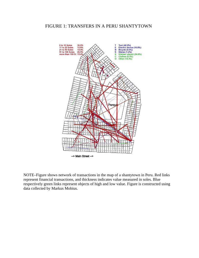
FIGURE 1: TRANSFERS IN A PERU SHANTYTOWN

NOTE–Figure shows network of transactions in the map of a shantytown in Peru. Red linksrepresent financial transactions, and thickness indicates value measured in soles. Bluerespectively green links represent objects of high and low value. Figure is constructed usingdata collected by Markus Mobius.

FIGURE 2: RISKSHARING IN SIMPLE NETWORKS

F

A. Line network

F

B. Plane network

C. Binary tree network

F

FIGURE 3: RISKSHARING SIMULATIONS

0.00 0.33 -0.60 0.00 0.33 -0.14 -0.20 0.00 -0.33 0.43 0.33 0.00

B. Plane

A. Line

NOTE–Figure shows constrained efficient allocations in the line and plane networks withbinary endowment shocks. For both networks, the black and white panel represents theendowment realizations and the grey panel represents the “second best” risksharingarrangement with equal planner weights. The plane allows for better risksharing: in thisrealization, SDISP 31% for the line and SDISP 0% for the plane. The line network alsoillustrates the emergence of risksharing islands: there is perfect smoothing and equalconsumption within islands, but imperfect smoothing across boundaries.

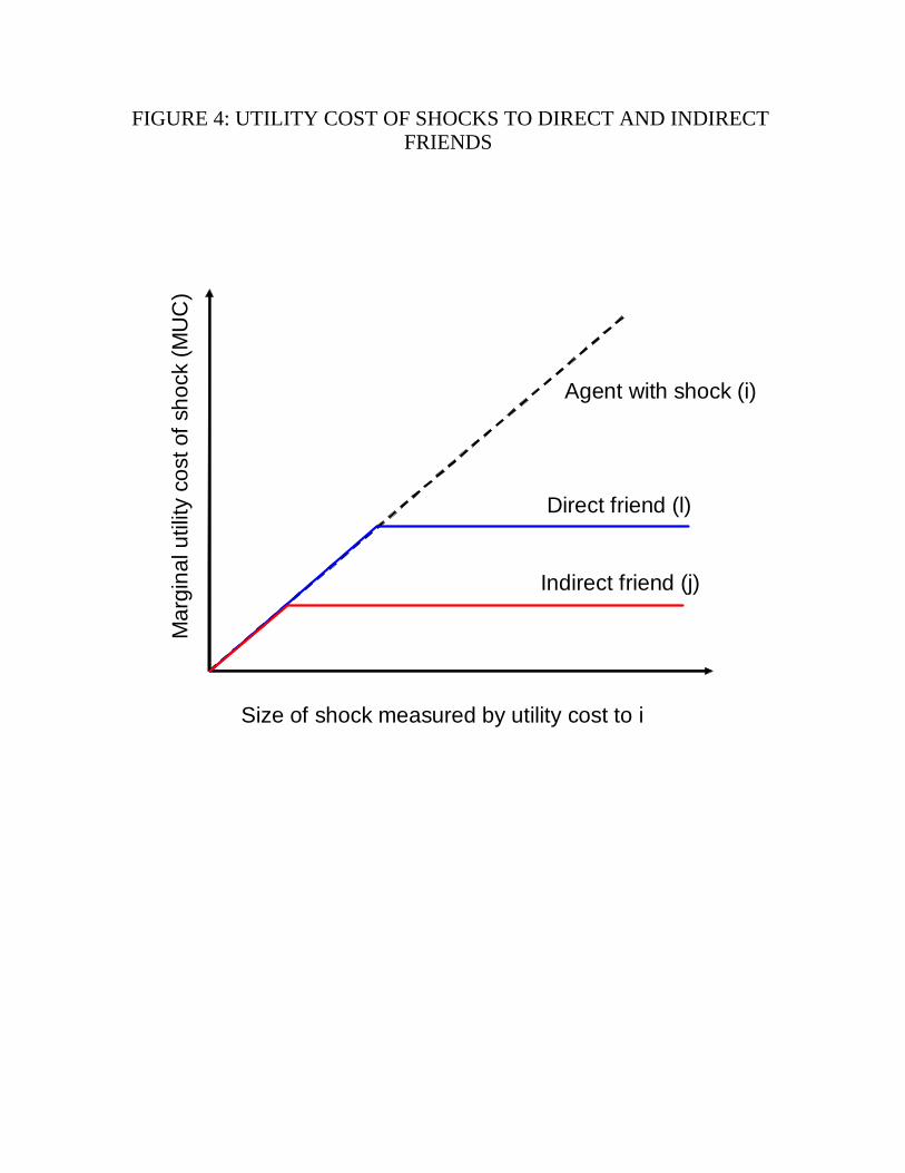
FIGURE 4: UTILITY COST OF SHOCKS TO DIRECT AND INDIRECTFRIENDS

Size of shock measured by utility cost to i

Indirect friend (j)

Direct friend (l)

Agent with shock (i)

Mar

gina

l util

ity c

ost o

f sho

ck (M

UC

)