Consumer Inertia, Choice Dependence and Learning … Inertia, Choice Dependence and Learning from Experience in a Repeated Decision Problem Eugenio J. Miravetey Ignacio Palacios-Huertaz

Consumer Inertia, Choice Dependenceand Learning from Experience in a

Repeated Decision Problem�

Eugenio J. Miravetey Ignacio Palacios-Huertaz

July 2012

Forthcoming Review of Economics and Statistics

Abstract

Understanding when and how individuals think about real-life problems isa central question in economics. This paper studies the role of inertia (inat-tention), state dependence and learning. The natural setting is the Kentuckytari¤ experiment when optional measured tari¤s for local telephone calls wereintroduced. We �nd that consumers tend to align correctly their choices of tar-i¤ and telephone usage levels. Despite low potential savings, mistakes are notpermanent as individuals actively engage in tari¤ switching in order to reducethe monthly cost of telephone services. Ignoring unobservable heterogeneityand the endogeneity of past choices would have reversed these results.

Keywords: Inertia, State Dependence, Learning, Tari¤ Choice.

JEL Codes: D42, D82, L96.

�We thank a co-editor, two anonymous referees, George Akerlof, Manuel Arellano, Raquel Car-rasco, Andrew Foster, Giuseppe Moscarini, Ralph Siebert, Dan Silverman, Johannes Van Biese-broeck and participants at various seminars and conferences for helpful comments and suggestions.

yThe University of Texas at Austin, Department of Economics, BRB 1.116, 1 University StationC3100, Austin, Texas 78712-0301; and CEPR, London, UK. Phone: 512-232-1718. Fax: 512-471-3510. E�mail: [email protected]; http://www.eugeniomiravete.com

zLondon School of Economics, Athletic Club de Bilbao, and Ikerbasque Foundation at UPV/EHU. Email: [email protected] ; http://www.palacios-huerta.com

“Errare humanum est, in errore perservare stultum.”

(“It is human to make a mistake, it is stupid to persist on it.”)

Lucius A. Seneca (4BC–65AD): Ad Lucilium Epistolae Morales

1 Introduction

Choosing among alternatives is the quintessential economic decision that we routinely engage

in. Depending upon the nature of the specific good or service under consideration, it may also

be a rather complex activity. In some cases we revise our plans and previous decisions almost

immediately, in others on a regular basis, and yet in others only when unexpected changes

or extraordinary events compel us to engage again in such a decision process. The different

frequency with which we revise our decisions may reflect our own optimizing behavior with

respect to the decision process itself. As Stigler and Becker (1977) note: “the making of

decisions is costly, and not simply because it is an activity which some people find unpleasant.

In order to make a decision one requires information, and the information must be analyzed.

The costs of searching for information and of applying the information to a new situation may

be such that habit [and inertia] are sometimes a more efficient way to deal with moderate or

temporary changes in the environment than would be a full, apparently utility–maximizing

decision.” Similarly, Knight (1921) indicates: “It is evident that the rational thing to do is

to be irrational where deliberation and estimation cost more than they are worth.”

Consistent with these insights, recent research in the behavioral economics literature

has documented a number of departures from the predictions of simple models of strict

rational behavior (see e.g., DellaVigna (2009) for a review). For instance, without attempting

to be exhaustive, Heiss, McFadden and Winter (2007) shows how consumers make wrong

choices when they first face complex alternatives; Abaluck and Gruber (2010) documents how

individuals appear to pay excessive attention to certain features of different insurance options,

causing them not to choose the least expensive alternative for their consumption. DellaVigna

and Malmendier (2006) and Madrian and Shea (2001) point out that default options and

inertia (time-independent conditions) are among the strongest determinants of individual

choices in the dynamic settings they study. Attempts to explain observed behavior include

loss aversion (Koscegi and Heidhues (2008)), reference-dependent preferences (Koscegi and

Rabin (2006)), and consumer overconfidence in a paper by Grubb (2009) which, as we will

see, is closely related to the present study.

– 1 –

At the same time a few but growing literature appears to provide greater support

for the hypothesis of strict rationality of consumer choices over time. This research hints

at learning as the corrective force fixing apparent choice inconsistencies. See, for instance,

Agarwal, Chomsisengphet, Liu and Souleles (2006), Ketcham, Lucarelli, Miravete and Roe-

buck (2012), Miravete (2003), and other references therein. Learning effects are also studied

in Choi, Laibson, Madrian and Metrick (2009).

This paper contributes to the literature by separating the effects of inertia (likely

caused by inattention in our setting) from state dependence and learning. While we are

not aware of any previous empirical study that attempts to do this, there are separate

literatures which we will review in the next section that relate to this study. Importantly, our

econometric analysis also addresses the role of unobserved heterogeneity and the endogeneity

of other decisions that may influence individuals’ choices and their ability to learn. We show,

in a spirit similar to the empirical contract study by Ackerberg and Botticini (2002), that the

estimation bias resulting from ignoring unobserved heterogeneity arising from the endogenous

sequence of choices that forms individual experiences may be (in fact, turns out to be) large

enough to fully reverse the sign of the effects of past decisions on current choices.

We would expect that various decades of research would have produced systematic

empirical evidence on the type of decision problems where consumers behave irrationally

and the type of problems where they are rational, on how consumer behavior depends on

the cost of acquiring and processing information relative to the benefits of better decision

making, and on the type of situations where subjects tend to reason accurately or tend to

make permanent errors. The fact, however, is that we are quite far from this ideal. There

is a recent theoretical literature modeling rational inattention as well as a theoretical and

experimental literature on bounded rationality. But, to the best of our knowledge, there is

little empirical evidence from real life settings that contributes to the ideal just described.

A number of empirical problems justify the existing situation. In natural settings

there are often great difficulties in finding individual decision-making situations, as opposed

to aggregate market-level situations;1 in observing all the relevant characteristics of individ-

uals; in precisely determining individuals’ choice and strategy sets; in measuring the exact

1 At the market or other aggregate levels downward-slopping demand functions can be derived evenas consequences of agents’ random choices subject to a budget constraint (e.g., Becker (1962) and Gode andSunder (1993)). As a result, it is generally not possible to distinguish rational from irrational behavior atany level of aggregation.

– 2 –

incentive structures that individuals face; in the ability to address selection problems in

settings where preferences are endogenous to the environment or to the behavior of others,

and in knowing the determinants of the endogenous frequency of choices. One or more

of these difficulties typically represent insurmountable obstacles for conducting conclusive

empirical research. In addition, sufficiently rich datasets with repeated individual choices

that allow the study of dynamic learning effects, attention and state dependence, while

controlling for the effects of unobserved heterogeneity, are rarely available.

The main virtue of the natural setting we study is that none of these difficulties are

present. South Central Bell (scb) implemented a detailed tariff experiment for the Kentucky

Public Service Commission in 1986. scb collected demographic and economic information for

about 2,500 households in Louisville. In the Spring of 1986, all households in Kentucky were

on mandatory flat rates, paying $18.70 per month with unlimited local telephone calls. This

was the only tariff available. In July 1986, optional measured services were introduced for

the first time in a way that was unanticipated by consumers. This alternative tariff included

a $14.02 monthly fixed fee, a $5.00 allowance, and a tariff per call that depended on its

duration, distance and period (time of the day and day of the week). The basic problem

that households faced each month was to determine whether their expected demand for local

phone calls next month would be above or below $19.02, as they would not be billed for the

$5.00 allowance unless their usage level exceeded this limit. That is, an attentive household

would have to think at time t about the expected consumption level at t + 1 and the tariff

rate to be applied to that consumption level; consumption choices will then take place at

time t + 1. These choices were repeated every month. Tariffs could be switched at any

time during the month and simply required a free phone call. A rich panel dataset on the

variables and characteristics of interest is available during the months of April-June and

October-December.

Thus, the analysis in this paper takes advantage of the opportunity that this unique

setting provides. We have an individual decision making situation where it is trivial to

determine strategy sets and straightforward to observe individuals’ choices over time. It

is also relatively simple to measure the incentives and rewards that subjects face. Local

telephone services represent a small share of consumers’ budget, and hence we can rule out

strategic and risk-aversion considerations. The monthly frequency of choices is exogenously

given and so there is no need to address any potential endogenous timing of decisions. Finally,

there are no self-selection problems since the penetration of local telephone service is nearly

– 3 –

universal (over 99 percent of the population) and the good in question (telephone services)

is not subject to conspicuous motives.

As anticipation of the results, we find that telephone subscribers do not make per-

manent mistakes, and that while inertia exists, it is likely caused by rational inattention

since individuals actively engage in tariff switching in order to reduce the monthly cost

of local telephone services. We also find that the role of state dependence is critical in

that past individual decisions, rather than impulsiveness or random behavior, shape future

individual actions. Finally, our results show that it is critical to address the endogeneity of

lagged explanatory variables that identify inertia and state dependence. Failing to do this

generates a bias of a large enough magnitude that it would have reversed the conclusions of

the analysis.

The paper proceeds as follows. Section 2 briefly reviews relevant literature. Section 3

describes in detail the Kentucky tariff experiment, the dataset and reports some descriptive

evidence. Section 4 presents a conceptual framework to visualize the problem. Section 5

presents our dynamic discrete choice panel data model, Section 6 the empirical results, and

Section 7 concludes.

2 Related Literature

First, there is a large and growing literature on bounded rationality in which the importance

of deliberation and processing costs is relevant for theories that postulate deviations from

the assumption of rational, computationally unconstrained agents.2 This literature includes

various survey and experimental studies. Lusardi (1999), Lusardi (2003), and Americks,

Caplin and Leahy (2003), for instance, find that a significant fraction of survey respondents

make financial plans infrequently and that their behavior has a significant impact on the

amount of wealth that they accumulate. In the experimental literature, Gabaix, Laibson,

2 These include the game theory literature (Rubinstein (1998)), behavioral industrial organization(Spiegler (2011)), learning and robustness in macroeconomics (i.e., Hansen and Sargent (2008)), the studyof the demand for information in Bayesian decision theory (Moscarini and Smith (2001) and Moscarini andSmith (2002)), the study of cognitive dissonance and near-rational theories (Akerlof and Dickens (1982) andAkerlof and Yellen (1982)), and others. On the infinite regress problem, see Savage (1954) and Lipman (1991).Conslik (1996) reviews various experimental studies where subjects make errors in updating probabilities,display overconfidence, and violate several assumptions of unbounded rationality, as well as other studieswhere subjects reason accurately, especially after practice. Arrow (1987) and Lucas (1987) discuss somelimitations of experiments to study bounded rationality.

– 4 –

Moloche and Weinberg (2006) study a cognition model which successfully predicts the ag-

gregate empirical regularities of information acquisition both within and across experimental

games. Costa-Gomes, Crawford and Broseta (2006) and Costa-Gomes and Crawford (2006)

also study cognition and behavior in different experimental games.

Second, an important recent literature in macroeconomics explores the potential

of modelling rational inattention in consumers and producers. Reis (2006a) studies the

consumption decisions of agents who face costs of acquiring, absorbing and processing

information,3 while Reis (2006b) studies the same problem for producers and applies the

results to a model of inflation. The resulting models are consistent with various puzzles

and fit remarkably well a number of quantitative facts.4 Hellwig, Khols and Veldkamp

(2012) construct a unified framework that compares different information choice technologies

(such as rational inattention, inattentiveness, information markets and costly precision) and

explain why some generate increasing returns while others generate multiple equilibria.

Finally, the asymmetry in choice of tariffs that we study fits well into recent studies

that focus on comparison “friction.” This friction is defined as the wedge between the

availability of comparative information and consumers’ use of it, and economic models typ-

ically assume that it is inconsequential (that is, that consumers will access readily available

information and will make effective choices). Kling, Sendhil, Shafir, Vermeulen and Wrobel

(2012) estimates the effect of reducing comparison friction in the market for prescription

drug insurance plans for senior citizens in an experiment where they delivered personalized

cost information via a letter. Their experimental results suggest that for senior citizens

comparison friction could be effectively large even when the cost of acquiring information

is low. Ketcham et al. (2012), however, find that these concerns are not substantiated in

a large sample of senior citizens that are observed making actual choices. Thanks to social

interactions and the development of market-based institutions that ease learning among very

old and even mentally ill patients, subjects significantly improved their choices and reduced

3 Sims (2003) and Moscarini (2004) develop alternative models focusing on the information problemthat agents face.

4Mankiw and Reis (2002) and Ball, Mankiw and Reis (2005) study inattentiveness on the part ofprice-setting firms and find that the resulting model matches well the dynamics of inflation and outputobserved in the data. In the finance literature, Gabaix and Laibson (2002) assume that investors updatetheir portfolio decisions infrequently, and show how this can help explaining the equity premium puzzle.

– 5 –

overspending over time. Among others, a key difference between these studies and ours is

that we have a fully representative sample, not just seniors.5

Summing up, the literature shows that modeling inertia, learning, and attention and

experimentally studying the predictions of limited rationality models offer a great deal of

promise for improving our understanding of human decision making. Relative to the existing

theoretical, survey and experimental literature, this paper provides what, to the best of our

knowledge, is the first empirical microeconometric study of rational attentiveness in a real

world setting using a large panel dataset of a fully representative sample while controlling for

unobserved heterogeneity and endogeneity of past choices at the same time that we separate

inertia from the effect of state dependence.

3 Description of the Tariff Experiment

In the second half of 1986, South Central Bell (scb) carried out a detailed tariff experiment

aimed at providing the Kentucky Public Service Commission (kpsc) with evidence in favor

of authorizing the introduction of optional measured tariffs for local telephone service.

Prior to this tariff experiment, in the Spring of 1986, all households in Kentucky were

on mandatory flat rates and scb collected demographic and economic information for about

2,500 households in the local exchange of Louisville. In July of 1986, the tariff was modified in

this city. Customers were given the choice to remain in the previous flat tariff regime—paying

$18.70 per month with unlimited calls—or switch to the new measured service option. The

measured service included a $14.02 monthly fixed fee, a $5.00 allowance,6 and distinguished

among setup, duration, peak periods, and distance.7 Choices could be made every month

and, unless a household indicated to scb otherwise, its current choice of tariff would serve

5 Other studies that focus on comparison friction have examined the effect of the Internet in reducingit in various markets (e.g., Brynjolfsson and Smith (2000), Scott-Morton, Zettelmeyer and Silva-Risso (2001),Brown and Goolsbee (2002), and Ellison and Ellison (2009)).

6 Consumers on the measured option were not billed for the first $5.00 unless their usage exceededthat limit. Thus, depending on the accumulated telephone usage over a month, a marginal second ofcommunication could cost $5.00.

7 The tariff differentiated among three periods: peak was from 8 a.m. to 5 p.m. on weekdays;shoulder was between 5 p.m. to 11 p.m. on weekdays and Sunday; and off-peak was any other time. Fordistance band A, measured charges were 2, 1.3, and 0.8 cents for setup and price per minute during the peak,shoulder, and off-peak period, respectively. For distance band B, setup charges were the same but durationwas fixed at 4, 2.6, and 1.6 cents, respectively.

– 6 –

as default choice for the following month.8 The regulated monopolist also collected monthly

information on usage (number and duration of calls classified by time of the day, day of

the week, and distance within the local loop), and payments during two periods of three

months, one right before (March-May) and the other (October-December) three months

after the measured tariff option was introduced.

As indicated earlier, panel datasets that follow the repeated discrete choices of indi-

viduals and their subsequent decisions in environments where framing issues, risk-aversion or

prior experiences can be ruled out for all individuals in a fully representative sample are not

easy to find. It is thus not surprising that this dataset has been used in the past. In chronolog-

ical order: Miravete (2002) identifies the distributions of ex-ante and ex-post telephone usage

to evaluate the profit and welfare performance of sequential pricing mechanisms consisting

of optimal two-part tariffs. The two sources of asymmetry of information are identified

by analyzing the choice of plan separately from the usage decision. Next, Miravete (2003)

evaluates the effect of expectations of future consumption as stated by consumers as well as

the role of potential savings in driving household tariff switching behavior. The interesting

finding is not only that initial expectations are less and less relevant in determining the

choice of tariff plan as consumers gain in experience, but also that they respond by switching

tariffs with the apparent aim at reducing overpayment by an average of five dollars. While

these two articles only evaluate the performance of the two-part tariffs that are offered,

Miravete (2005) uses the empirical distribution of stated future expected consumption to

evaluate the profit and welfare performance of sequential pricing mechanisms where options

are fully nonlinear tariffs. Finally, Narayanan, Chintagunta and Miravete (2007) estimate a

structural discrete/continuous model of plan choice and demand of local telephone service

where consumers update of future usage expectation is conditioned by the choice of tariff

made. Relative to these articles, the contribution of this study is that it separates the

role of inertia (or inattention) from state dependence while allowing for learning through

the accumulated experience, something which makes individuals different from each other

simply because they follow a different sequence of decisions over time.

The dataset has a number of unique features to address the consequences of inertia

(inattention), state-dependence, and learning. First, local telephony is a basic service and

its market penetration is close to 100% in the U.S. Thus, there are no potential self-selection

problems or conspicuous consumption considerations that might lead us to obtain biased

8 Switching tariffs simply required a free phone call to request the change of service.

– 7 –

estimates because of selection into this market. Second, the low magnitude of the cost

differences between the alternative tariff choices, relative to the average household income,

allows us to rule out risk aversion as a potential determinant of permanent mistakes regarding

the choice of tariffs. Third, it is valuable for the purpose of the analysis that in addition

to demographic and economic variables, scb also collected information on customers’ own

telephone usage expectations in the Spring of 1986 (before the experiment took place). That

is, we have a good approximation of consumers’ own expected satiation levels since the

marginal tariffs were nil at that time.

Households receive every month the bill of their consumption. In this sense, the

costs of searching for information are minimal, and thus the costs of deliberation and

cognition relative to the expected payoffs, would appear to be the main, and perhaps only,

determinant of their behavior. For the purpose of the econometric analysis, we will assume

that individuals know immediately whether their consumption exceeds or falls short of what

is optimal for the tariff chosen. Further, there might be important asymmetries in search

costs associated with the problem that a households faces. Households in the measured tariff

simply need to compare their actual bill with the $18.70 cost of the alternative flat tariff in

order to ascertain whether or not they made a mistake. Households in the flat tariff option,

however, would need to monitor each and every phone call they make and compute the total

cost of all of their calls in the month in order to know if they would have spent above or below

$19.02 had they subscribed the measured service (recall that each call is metered differently

depending on their duration, distance and period). Clearly, this task is much more complex

and demands a great deal of monitoring effort. Empirically, therefore, we would expect to

find state dependence on tariff choices and telephone consumption that is associated with

this asymmetry in monitoring effort and cognitive costs.

Table 1 defines the different variables and presents basic descriptive statistics for the

whole sample and for two groups of consumers split according to their choice of tariff in

October. Only active consumers were considered and a number of observations with missing

values for some variables were excluded.9 These descriptive statistics initially suggest that

individual heterogeneity in consumption and tariff subscription is important. Consumers

who subscribe to the flat and measured tariffs are in fact quite different. Households

9 Miravete (2002) documents that excluding households with missing information does not lead tobiased results. The only variable with a substantial number of missings is income. In these cases we recodedthe missing observations to the yearly average income of the population in Louisville and also included adummy variable, dincome, to control for non-responses regarding household earnings.

– 8 –

Table

1:

Vari

able

Definitio

ns

and

Desc

riptive

Sta

tist

ics

Var

iabl

esD

escr

ipti

onall

flat

measu

red

measu

red

Opt

iona

lm

easu

red

serv

ice

chos

enth

ism

onth

0.29

71(0

.46)

0.00

00(0

.00)

1.00

00(0

.00)

expcalls

Hou

seho

ldow

nes

tim

ate

ofw

eekl

yca

lls26

.888

4(3

1.34

)30

.134

1(3

5.05

)19

.210

4(1

7.78

)calls

Cur

rent

wee

kly

num

ber

ofca

lls37

.609

3(3

8.48

)44

.489

8(4

2.62

)21

.332

6(1

7.64

)bia

sC

ALLS

—E

XP

CA

LLS

10.7

209

(39.

92)

14.3

558

(45.

67)

2.12

23(1

8.04

)sw

calls

Hou

seho

ldav

erag

eca

llsdu

ring

Spri

ng37

.943

4(3

7.16

)44

.049

9(4

0.80

)23

.498

0(2

0.32

)sw

bia

sSW

CA

LLS

—E

XP

CA

LLS

11.0

550

(39.

37)

13.9

158

(44.

55)

4.28

76(2

1.39

)bil

lM

onth

lyex

pend

itur

ein

loca

lte

leph

one

serv

ice

19.4

303

(4.4

1)18

.700

0(0

.00)

21.1

578

(7.8

2)sa

vin

gs

Pot

enti

alsa

ving

sof

swit

chin

gta

riff

opti

ons

−9.

9223

(16.

53)−

15.1

557

(16.

45)

2.45

78(7

.82)

savin

gs-

spr

Pot

.sa

v.of

subs

crib

ing

the

mea

sure

dop

tion

−15

.420

6(1

5.27

)−

18.7

859

(16.

21)−

7.45

96(8

.56)

savin

gs-

oct

Pot

enti

alsa

ving

sin

Oct

ober

−9.

4898

(16.

99)−

14.2

444

(17.

61)

1.75

78(7

.60)

savin

gs-

nov

Pot

enti

alsa

ving

sin

Nov

embe

r−

9.28

64(1

5.03

)−

13.6

444

(15.

30)

1.02

30(7

.47)

savin

gs-

dec

Pot

enti

alsa

ving

sin

Dec

embe

r−

10.9

908

(17.

41)−

16.4

967

(17.

22)

2.03

40(8

.83)

income

Mon

thly

inco

me

ofth

eho

useh

old

7.09

99(0

.81)

7.07

67(0

.84)

7.15

47(0

.74)

hhsi

ze

Num

ber

ofpe

ople

who

live

inth

eho

useh

old

2.61

68(1

.51)

2.78

58(1

.56)

2.21

70(1

.28)

teens

Num

ber

ofte

enag

ers

(13–

19ye

ars)

0.24

40(0

.63)

0.29

08(0

.68)

0.13

36(0

.49)

din

come

Hou

seho

lddi

dno

tpr

ovid

ein

com

ein

form

atio

n0.

1577

(0.3

6)0.

1831

(0.3

9)0.

0977

(0.3

0)age

=1

Hou

seho

ldhe

adbe

twee

n15

and

34ye

ars

old

0.06

32(0

.24)

0.06

14(0

.24)

0.06

76(0

.25)

age

=2

Hou

seho

ldhe

adbe

twee

n35

and

54ye

ars

old

0.26

86(0

.44)

0.26

04(0

.44)

0.28

80(0

.45)

age

=3

Hou

seho

ldhe

adab

ove

54ye

ars

old

0.66

82(0

.47)

0.67

82(0

.47)

0.64

44(0

.48)

college

Hou

seho

ldhe

adis

aco

llege

grad

uate

0.22

40(0

.42)

0.18

21(0

.39)

0.32

30(0

.47)

marrie

dH

ouse

hold

head

ism

arri

ed0.

5253

(0.5

0)0.

5342

(0.5

0)0.

5042

(0.5

0)retir

ed

Hou

seho

ldhe

adis

reti

red

0.24

33(0

.43)

0.24

17(0

.43)

0.24

71(0

.43)

black

Hou

seho

ldhe

adis

blac

k0.

1161

(0.3

2)0.

1295

(0.3

4)0.

0843

(0.2

8)church

Tel

epho

neus

edfo

rch

arity

and

chur

chm

atte

rs0.

1711

(0.3

8)0.

1785

(0.3

8)0.

1536

(0.3

6)benefit

sH

ouse

hold

rece

ives

fede

ralor

stat

ebe

nefit

s0.

3095

(0.4

6)0.

3282

(0.4

7)0.

2654

(0.4

4)moved

Hou

seho

ldhe

adm

oved

inth

epa

stfiv

eye

ars

0.40

25(0

.49)

0.38

99(0

.49)

0.43

24(0

.50)

Obs

erva

tion

s1,

344

949

395

Mea

nan

dst

anda

rdde

viat

ion

ofde

mog

raph

ics

and

usag

eva

riab

les.

Thi

sba

lanc

edsa

mpl

eco

ntai

ns1,

344

hous

ehol

dob

serv

atio

ns.

Inco

me

ism

easu

red

inlo

gari

thm

sof

thou

sand

sof

1986

dolla

rs.

– 9 –

Table 2: Joint Distribution of Usage and Tariff Choice

low usage=1 low usage=0

Share Savings Switchers Share Savings Switchers

measured=1 0.0906 -4.68 0.0000 0.1961 6.61 0.1439measured=0 0.0877 4.68 0.1695 0.6256 -16.76 0.0356

Data from October of 1986. Share indicates the percentage of the sample in a particulartariff choice and usage level combination. Savings shows the average dollar gain ofchoosing the other tariff option given the usage level (positive values). Switchersindicate the percentage of those on a particular tariff choice and usage combinationthat end up switching tariff options during the fall of 1986.

subscribing to the optional flat service tend to be larger, with teenagers, and with a

lower level of education than those subscribing to the measured tariff. Further, they not

only differ in their level of local telephone usage, as captured by calls, but also in their

expectations regarding future telephone usage. Subjects tend to underestimate their demand

for telephone services, especially those in the flat tariff in October. Further, there is an

important self-selection effect (not reported in the table): the variability of demand of those

who subscribe to the optional flat tariff, $4.28 per month, almost doubles that of those on

measured service, $2.30 per month, as given by the measured tariff option in Louisville.

This evidence will play a role when accounting for heterogeneity in usage across zone and

time bands).

Table 2 documents the joint distribution of tariff choice and usage levels as well as

“potential savings” (had these individuals switched to the alternative option while keeping

their consumption unchanged) and how many of them ended up switching tariffs. We again

find important asymmetries among consumers. First, most households actually choose the

right option for their realized telephone usage. Most of those choosing the right tariff

subscribed to the flat option (63% of the sample) as their demands clearly exceeded the

usage threshold beyond which the flat tariff is always the least expensive alternative. Had

they chosen the measured option, these individuals would have paid, on average, about 17$

more. Second, switching is more common among those who are overpaying: 14% of those

on measured tariff with too high demand (and average potential savings of 6.61$ a month)

and 17% of those on flat tariff with too low an usage level (and average potential savings

of 4.68$ a month). Lastly, those choosing the right tariff option for their usage level switch

far less frequently: only 3.56% for those rightly choosing the flat tariff, and none among

those who, using telephone only sparsely, chose the measured option.

– 10 –

Switching, therefore, is not random and appears to respond to potential savings. Thus

a main goal of the empirical analysis is to determine whether or not the wrong combination

of tariff choice and usage level tends to induce this switching. Table 1 shows that potential

savings from switching decreases slightly over time, something which hints at learning as

a potential driving force that must qualify the cross-section evidence showing that some

individuals make mistakes. Descriptive statistics alone are, of course, far from sufficient to

determine whether or not this is the case since the environment under study is not stationary

(e.g., demand may change over time).

Despite the remarkable features of the data, there are two issues that are important

to address econometrically. First, about 10% of consumers subscribed to the optional

measured option when given that possibility. Our sample, however, includes 30% of those

customers. Choice-based sampling bias can easily be dealt with using well known methods,

e.g., Amemiya (1985, §9.5). All estimates reported in the analysis take into account this

choice-based sampling as we use the weighting procedure of Lerman and Manski (1977) to

obtain choice-based, heteroskedastic-consistent, standard errors. Second, when the tariff

experiment began in July of 1986, all households were assigned the preexisting flat tariff

as default option. Consumers may learn about their telephone usage profile as they switch

tariff options, and thus, over time, they will differ in their experience as summarized by

the different sequences of past tariff choices and usage levels. Therefore, the importance of

inertia (inattention) and state dependence in the choice of tariff options requires addressing

the endogeneity of past choices and controlling for their induced individual heterogeneity.

To this end we will use the semiparametric estimator suggested by Arellano and Carrasco

(2003) in Section 5. Before undertaking this task, we present additional descriptive evidence.

Next we examine whether households may appear to choose ex-post the correct tariff

option for their usage level by studying the pattern of correlations among tariff choice and

usage decisions using a simple static model of simultaneous choice. We estimate the following

reduced form model:

y∗j = XΠj + vj , j = 1, 2, (1)

where, conditional on observed demographics, we assume that:

(v1, v2) ∼ N (0,Σv) ; Σv =

(1 ρ

ρ 1

). (2)

– 11 –

Table 3: Choice of Tariff and Usage Level

measured low usage

constant −0.6763 (5.56) −0.8099 (7.06)low inc −0.0604 (0.57) 0.0418 (0.46)high inc −0.2317 (1.79) −0.0320 (0.32)dincome −0.4846 (4.23) −0.1144 (1.43)hhsize = 2 −0.3548 (3.32) −0.3128 (3.46)hhsize = 3 −0.5645 (4.29) −0.3979 (3.81)hhsize = 4 −0.4854 (3.17) −0.3866 (2.97)hhsize > 4 −0.7187 (4.04) −0.6709 (4.22)teens −0.1768 (1.27) 0.0115 (0.11)age = 1 −0.0216 (0.14) 0.1761 (1.38)age = 3 −0.0491 (0.53) 0.1707 (2.03)college 0.2910 (3.42) 0.0709 (0.93)married 0.2301 (2.47) −0.0509 (0.66)retired 0.0497 (0.43) −0.1967 (2.24)black 0.0287 (0.26) −0.1845 (1.72)church −0.0274 (0.30) −0.0084 (0.11)benefits −0.2189 (2.03) −0.0360 (0.42)moved −0.0542 (0.64) 0.0915 (1.24)overest −0.3548 (2.42) −0.7881 (5.17)underest −0.4164 (4.14) −1.1597 (9.70)low usageSpring 0.6418 (4.87) 1.4125 (11.26)

ρ 0.2616 (5.05)lnL −2, 463.197Observations 4, 032

Estimates are obtained by weighted maximum likelihood (bivariate probit).Absolute, choice-biased sampling, heteroscedastic consistent, t-statistics arereported between parentheses.

These two equations are estimated simultaneously as a bivariate probit model, thus

providing a consistent estimate of ρ conditional on all available household information. In

this model y1 = 1 if the household subscribes to the measured tariff and y2 = 1 if the

household makes low usage of telephone service defined as consumption below $19.02

when metered according to the measured tariff rate. Thus, a significant positive estimate

of ρ can be interpreted as the result of an unobservable element (e.g., learning, rational

inattention or unbiased expectations) that induce the appropriate tariff choice for each

usage level. The model includes the same set of demographic variables in both equations

to control for the effect of observable individual heterogeneity over the tariff choice and

consumption decisions. The analysis also includes household specific information from the

Spring months that is useful to control for the accuracy of predictions of individual future

usage. In particular, we include two dummies to indicate whether consumers significantly

– 12 –

over- or under-estimated future consumption when marginal consumption was not priced at

all.10 Similarly, we construct an indicator of usage intensity for each household during the

Spring months, low usageSpring, which equals one when the usage level during Spring (at

zero marginal charge) is less than $19.02 had it been metered according to the measured

tariff that will later be available during the Fall. We include this variable in order to account

for any systematic effect of demographics not included in our data on usage levels. Table 3

reports the estimates of these reduced form parameters.

We find a positive estimate of ρ, that is, a positive correlation between the choice of

the measured service and a low demand realization. This finding suggests that consumers

do not tend to make permanent mistakes when choosing among optional tariffs. However,

this is a reduced form estimate which at this stage cannot be attributed to a specific reason,

be it inertia, rational inattention, state dependence, learning or any other. In any case,

this positive estimate is evidence that an unobservable process that aligns tariff choices and

telephone usage levels is at work.11

Various demographics also appear to contribute to observing the choice of tariff

plans and telephone usage levels generally aligned. For instance, larger households tend

to subscribe to the flat tariff option and to realize high usage levels. Similarly, households

with a low usage profile during the Spring months are also more likely to present a low

usage profile in the Fall and, consequently, correctly choose the measured tariff option.

Finally, consumers that either over- or under-estimated their future telephone usage quite

significantly are less likely to subscribe to the measured option, but are also far less likely

to realize a low usage level. Thus, households who made the largest absolute forecast errors

are among those with very high levels of demand, and hence they are more likely to choose

the right option by subscribing to the flat tariff.

Table 2 showed that all consumers not choosing the right tariff-usage combination

were equally likely to switch to the alternative option. Consumers were classified as hav-

ing chosen correctly or incorrectly each tariff option ex-post keeping the usage pattern

10 The underest dummy is equal to one if swcalls exceeds expcalls by more than 50% of thestandard deviation of swbias. The overest dummy is defined accordingly when expcalls exceeds swbias.

11 The approach behind the estimates of Table 3 is similar to that in Chiappori and Salanie (2000).A significant correlation coefficient in this estimation supports the idea of the existence of asymmetricinformation beyond the observable demographics of our data. The results regarding the sign and significanceof all parameter estimates, including ρ, are robust to alternative specifications that exclude the Spring usagepatterns and the individual expectation accuracy dummies.

– 13 –

unchanged, that is independently of price responses, something that provides an approx-

imate upper bound to the gains of switching to a different tariff option. Therefore, those

choosing the measured service while experiencing high demand for telephone were by far

the most common among those making the wrong tariff choice for a given usage pattern.

It is interesting to note that consumers on the measured option enjoy de facto negligible

monitoring and deliberation costs since they just have to compare their past monthly bill to

the cost of the flat option to decide whether or not to switch tariff plans. Among those

more likely to subscribe to the measured option irrespective of their telephone usage are

those households whose head is married, holds a college degree or does not receive any kind

of benefits. At the other end, those experiencing high telephone usage regardless of their

tariff choice include older and retired households.

After this descriptive evidence, we turn toward the more substantive questions: Do

consumers simply stay on their previously chosen tariff because of inertia, i.e., rational

inattention? Do the consumption levels, tariff choices and tariff switching that we observe in

the data provide evidence that consumers are rationally attentive and respond to potential

savings? What is the role of previous tariff choices and demand realizations on the decision

to subscribe to one of the two options? Do consumers learn from past experience or they

persist making wrong choices? In order to answer these questions we need more sophisticated

econometric methods that allow us to account for state dependence, unobserved heterogene-

ity, and dynamic learning. We first provide a simple conceptual framework to visualize the

problem under study and then undertake this task.

4 Conceptual Framework

The choice problem facing a household may be visualized with a simple framework. Bor-

rowing from Kling et al. (2012), for instance, let uij ≡(bij − pij − cij

)denote the utility

for increments to the utility from current consumption for household i from a given tariff

choice j, where bij is the potential benefit to i from tariff j minus switching costs, pij is

the potential cost of tariff j that can be predicted from comparative research based on

extrapolations from consumption in the previous months, and cij is the potential cost that

cannot be predicted from such extrapolations. Let rij denote the “comparison friction”,

that is the costs of undertaking comparative research about all the available tariffs (e.g.,

– 14 –

information, monitoring, and deliberation) which we assume is in the same units as, and

additively separable from, uij.

Without research, the highest level of expected utility across all plans, taking the

expectation over the joint distribution of all the random variables that determine uij, is

given by:

v1i = max

jE(uij)

If research is not undertaken, then the tariff that maximizes the expected utility in this

equation will be chosen. Note that the current choice of tariff need not be the one that

solves this problem, and so the individual may switch tariffs. Both current choices and

switching depend on the effects of inertia (time-invariant determinants of choices), state

dependence (time-varying endogenous determinants) and individual learning effects that are

revised each period as information accumulates. Empirically, therefore, it will be important

to differentiate between these three sources: inertia (which we will denote by γ in the

econometric model), state dependence (which we will denote by β), an individual learning

effects ηi.

When research is undertaken, however, the individual selects the plan j that solves:

v2i (pi1, ..., pij) = max

jE(uij |pij = pij )− ri

where pijis a realization of pij.The decision to undertake research, therefore, involves com-

paring v1i to the expected value of v2

i taken over the joint distribution of the predictable cost

component of all available tariffs, that is comparing it to v3i = E [v2

i (pi1, pi2, ..., pij)] . In other

words, the individual will undertake incremental research such as information gathering,

consumption monitoring and deliberation effort if the expected value of the maximum

expected utility from doing that is greater than the maximum expected utility from the

tariff that is chosen with no research. Otherwise, the individual will not undertake such

incremental research.

When ri varies across households, this simple setting provides a straightforward

testable implication: if research is undertaken (v3i = v1

i , i.e., if inattention is rational) those

who face a greater ri will tend to make more mistakes and learn more slowly than those

who face a lower ri. Thus, the clear asymmetry in the complexity and monitoring costs

across the two tariffs in the Kentucky tariff experiment means that we should expect to

– 15 –

find differences across tariffs in state dependence and learning effects. If the problems were

exactly symmetric (same ri for all households) we would expect no differences.

5 A Model of Repeated Tariff Choice

In this section we first present a semi–parametric, random effects, discrete choice model

with predetermined variables. This model is based on Arellano and Carrasco (2003) and

controls for the effects of unobservable heterogeneity and for state dependence. The model

is essentially a difference estimator in a repeated discrete choice environment, and a result the

effect of time-invariant demographics are not identified. We later estimate two specifications

of this model in Section 6 to study the choices of tariffs and consumption levels over time

and the persistence of wrong tariff-usage choice combination, respectively.

5.1 A Dynamic Discrete Choice Panel Data Model

A risk-neutral individual chooses one of two tariff options in order to minimize the expected

cost of telephone services. The probability of subscribing to a given tariff option may depend

on some intrinsic characteristics of consumers, including their telephone usage profiles and

their expectation on the realization of demand. This can be written as follows:

yit = 1I{γ + βzit + E

(ηi | wt

i

)+ εit ≥ 0

}, εit | wt

i ∼ N(0, σ2

t

), (3)

where yit = 1 (yit = 0) is the measured (flat) tariff option is subscribed. The constant

γ captures the effect of inertia, i.e., the result of all time-invariant determinants of the

choice of individuals.12 The set of predetermined variables zit includes the past realization

of demand xit and the previous choices of tariffs yi(t−1), so that together they define the

particular realization of the state for each individual i when choosing a tariff option at time

t, i.e., wit ={xit, yi(t−1)

}. Thus, the estimates of β identify the effect of state dependence

separately from inertia as zit includes time-varying regressors that are only predetermined,

12 The specification of Arellano and Carrasco (2003) is more general in the sense that it also includesa time-varying component common to all individuals, γt. With the exception of monthly indicators, allour available demographics are time-invariant. We also included these monthly indicators in our empiricalanalysis but they did not improve our estimations, even when interacted with past subscription decisionsand past realizations of demand.

– 16 –

that is not directly correlated with the current or future values of the error εit (although

lagged values of errors εit might be correlated with zit).

The probability of subscribing to a given tariff option, and hence the probability of

switching tariffs in the future, depends on the particular sequence of past choices and past

realizations of demand for each consumer. As time goes by, individuals take different deci-

sions and hence tend to become increasingly different. These decisions can be summarized

by wti = {wi1, . . . , wit}, which is the history of past choices represented by a sequence of

realizations: wit ={xit, yi(t−1)

}. Addressing individual heterogeneity in this model adds

up to controlling for the different observed sequence of decisions of each individual. As

consumers choose differently, they accumulate different experiences and invest differently

in information gathering and deliberation efforts. These experiences in turn change the

information set upon which they decide in the future. For instance, consumers that have

previously chosen the measured option may have learned that their demand is systematically

high, so that in the future they will be more likely to subscribe to the flat tariff option.

Consumers that have always remained on the flat tariff option have accumulated different

experiences, and this also affects their conditional probability of renewing their subscription

to the flat tariff option.

The last element of the model is ηi, an individual effect whose forecast is revised each

period t as the information summarized by the history wti accumulates. In our case ηi is the

intrinsic individual value of tariff option yit = 1. This value of choosing the measured option

is not known to individuals and, hence, only its expectation enters the decision rule. In

other words, the probability of choosing the measured option is not only affected by inertia

(γ) and state dependence (β), but also by the learning effect identified by E (ηi | wti) after

controlling for individual heterogeneity.13

In our second application of this model yit does not represent the choice of tariff, but

whether or not the joint combination of tariff choice and usage level is the right one. In

this second application, γ identifies all the elements conducive to inattention that induce

individuals to make the wrong choice permanently, while the effect of state dependence β

identifies whether or not individuals revise their choices to avoid making mistakes perma-

13 Since this distribution is conditional on the individual’s history wti , and thus, on the observable

subsets of histories available in our sample, which may make estimates subject to the initial conditionsproblem, e.g., see Heckman (1981). Arellano and Carrasco (2003) point out that this feature of the modelis shared by many other discrete choice panel data models when dealing with unobserved heterogeneity,including Chamberlain (1984) and Newey (1994) among them.

– 17 –

nently depending on their past experience. Accounting for individual heterogeneity amounts

to addressing the value of rational inattention, i.e., the cost of choosing wrong combinations

which might eventually trigger switching tariffs.

Summing up, the model defines conditional probabilities for every possible sequence

of realizations of state variables in order to deal with regressors that are predetermined but

not exogenous, such as the previous choices of tariffs and the past realizations of demand.

Then, the estimator computes the probability of subscribing to a given tariff along every

possible path of past realizations of demand and subscription decisions. The panel data

structure allows us to identify the effect of individual unobserved heterogeneity since at each

time consumers may make different decisions even if they have shared the same history of

realizations of state variables until then.

Finally, note that the conditional distribution of the sequence of expectations E (ηi | wti)

is left unrestricted, and hence the process of updating expectations as information accumu-

lates is not explicitly modeled. This is the only aspect that makes the model semi-parametric.

While the assumption of normality of the distribution of errors is not essential, the assump-

tion that the errors εit are not correlated over time is necessary for the estimation. Since

errors are assumed to be normally distributed, conditional on the history of past decisions,

the probability of choosing the measured option at time t for any given history wti can be

written as:

Prob(yit = 1 | wt

i

)= Φ

[γ + βzit + E (ηi | wt

i)

σt

]. (4)

5.2 Econometric Implementation

Since all our regressors are dichotomous variables, their support is a lattice with J points.

The vector wit has a support defined by 2J nodes {φ1, ..., φ2J}. The t×1–vector of regressors

zti = {zi1, ..., zit} has a multinomial distribution and may take up to J t different values.

Similarly, the vector wti is defined on (2J)t values, for j = 1, ..., (2J)t. Given that the

model has discrete support, any individual history can be summarized by a cluster of nodes

representing the sequence of tariff choices and demand realizations for each individuals in

the sample. Thus, the conditional probability can be rewritten as:

pjt = Prob(yit = 1 | wt

i = φtj

)≡ ht

(wt

i = φtj

), j = 1, . . . , (2J)t . (5)

– 18 –

In order to account for unobserved individual effects we compute the proportion of

customers with identical history up to time t that subscribe to the measured tariff option

M at each time t. We then repeat this procedure for every available history in the data.

For each history we compute the percentage of consumers that subscribe to the measured

option. This provides a simple estimate of the unrestricted probability ptj for each possible

history present in the sample. Then, by taking first differences of the inverse of the equation

above we get:

σtΦ−1[ht

(wt

i

)]− σt−1Φ

−1[ht−1

(wt−1

i

)]− β

(zit − zi(t−1)

)= ξit , (6)

and, by the law of iterated expectations, we have:

E[ξit | wt−1

i

]= E

[E(ηi | wt

i

)− E

(ηi | wt−1

i

)∣∣wt−1i

]= 0 . (7)

This conditional moment condition serves as the basis of the GMM estimation of parameters

β after normalizing σ1 = 1. To identify the effect of inertia we make use of:

E[E(ηi | wt−1

i )]

= E[Φ−1

[ht

(wt−1

i

)]− γ − βzit

]= 0 . (8)

Arellano and Carrasco (2003) show that there is no efficiency loss in estimating these

parameters by a two–step GMM method where in the first step the conditional probabilities

ptj are replaced by unrestricted estimates ptj, such as the proportion of consumers with a

given history that subscribe to the measured service. Then:

ht

(wt

i

)=

(2J)t∑j=1

1I{wt

i = φtj

}· ptj , (9)

which is used to define the sample orthogonality conditions of the GMM estimator:14

1

N

N∑i=1

{σtΦ

−1[ht

(wt−1

i

)]− γ − βzit

}= 0 , t = 2, . . . , T , (10)

14 In practice the number of moment conditions is smaller than∑

t (2J)t−1 because we only considerclusters with at least 4 observations. Also, we use the orthogonal deviations suggested by Arellano and Bover(1995) rather than first differences among past values of the state variables.

– 19 –

and

1

N

N∑i=1

dit

{σtΦ

−1[ht

(wt

i

)]− σt−1Φ

−1[ht−1

(wt−1

i

)]− β

(xit − xi(t−1)

)}= 0 , t = 3, . . . , T ,

(11)

and where dit is a vector containing the indicators 1{wt

i = φtj

}for j = 1, ..., (2J)t−1.

6 Empirical Evidence: Inertia, State Dependence and

Learning

Consumers choose every month their tariff option and usage level. In the previous section

we argued that past choices are valid instruments to identify the effect of state dependence

separately from those of inertia and learning. We begin this section by showing in Table 4,

top panel, the transition matrices between tariff choices by previous telephone usage levels.

Given the large probabilities along the diagonal it might be tempting to conclude that tariff

switching is not significant. However, that conclusion would neglect some interesting results.

For instance, if previous usage was high, individuals are twice as likely to correctly switch

from measured service to flat tariff than to incorrectly switch from flat tariff to measured

service. If, on the contrary, previous demand was low, nobody switches from measured service

to the flat tariff while, among switchers, the largest probability occurs when consumers on

flat tariff correctly switch to measured service. This asymmetric pattern is consistent with

the idea advanced earlier that individuals face substantially lower information, monitoring

and deliberation costs when subscribing to the measured option.

Similarly, in order to characterize whether inattention is mainly rational, the bottom

panel of Table 4 shows the transition matrices between ex post right and wrong choices

conditional on previous tariff choices. We find off-diagonal probabilities that are substantially

greater than in the previous case, thus hinting at one of the main results: mistakes are not

permanent. This is consistent with the hypothesis that inattention is rational, particularly

among those who chose the flat tariff option since their demands are large enough. First,

most of those not paying attention remain in the right tariff-usage combination. Second, the

largest transition probability from wrong to right occurs among those who previously chose

the flat tariff option. This 47% is much larger than the 11% of customers in the top panel

who switched from flat to measured because their usage was low, something which hints at

– 20 –

Table 4: Transition Matrices

low usaget−1 high usaget−1

measuredt−1 flatt−1 measuredt−1 flatt−1

measuredt 1.0000 0.1123 0.9199 0.0451flatt 0.0000 0.8877 0.0801 0.9549

measuredt−1 flatt−1

wrongt−1 rightt−1 wrongt−1 rightt−1

wrongt 0.7905 0.3259 0.5205 0.0866rightt 0.2095 0.6741 0.4745 0.9134

Transition probabilities for each state.

temporary reductions of demand. In such a case, not switching away from the flat option is

optimal as demand would tend to return to its normal high level.

In order to account for the dynamic nature of the learning process where individuals

may invest time, cognitive effort, and other resources to gain knowledge about their new

options and about their own demand for telephone services, we next report the results of

two dynamic discrete choice panel data models with predetermined variables that account

for the existence of inertia, state dependence and unobserved individual heterogeneity. The

first model tests for inertia and the second for rational inattention. In both cases we report

the consistent gmm estimator of Arellano and Carrasco (2003). In addition, in order to have

a sense of the extent to which .... play a fundamental role in the analysis, we also report the

standard ml estimator that fails to address the endogeneity of lagged dependent variables

and ignores individual heterogeneity.

6.1 Testing for Inertia in Tariff Choices

The first model studies whether households tend to remain subscribed to the same tariff

option over time regardless of their past realized usage levels:

measuredt = 1I{γ + β1measuredt−1 + β2low usaget−1 + E(ηi | wt

i) + εit ≥ 0}

. (12)

The first row in Table 5 reports the gmm results accounting for predetermined regres-

sors and unobserved individual heterogeneity. As indicated earlier, this estimator accounts

– 21 –

Table 5: Tariff Subscription

Method: constant measuredt−1 low usaget−1

gmm −1.9751 (7.99) −8.9011 (36.02) −4.4181 (17.88)ml −1.7022 (77.82) 3.2177 (43.13) 0.5388 (10.54)

Consistent gmm random effects dynamic estimates of Arellano and Carrasco (2003)with predetermined regressors and inconsistent ml estimates. Absolute, choice-biasedsampling, heteroskedastic-consistent, t-statistics are reported in parentheses.

for every potential path of usage level and choice of tariffs over time. The estimates we obtain

reveal that inertia is important, an aspect that is consistent with the persistence of tariff

choices along the diagonals of Table 4. But we also find that choices vary significantly over

time and are not exclusively determined by static considerations. In particular, we find that

the gmm estimates of the predetermined variables low usaget−1 and measuredt−1 are

both negative and significant.15 The negative estimate of low usaget−1 captures the effect

of the mistakes of consumers with high enough usage levels that still sign up for the optional

measured tariff, an aspect that is consistent with the transition probabilities of Table 4.

Similarly, the negative estimate of measuredt−1 indicates that consumers do switch tariffs

significantly and that, contrary to the hypothesis of habit and inertia, automatic renewal

of tariff subscription options does not necessarily mean that consumers will stay in the

previously chosen tariff indefinitely.16

The second row of Table 5 reports the estimates of a standard probit regression

that fails to address the endogeneity of lagged endogenous regressors and ignores individual

heterogeneity. These results show, quite remarkably, that the sign of state dependence

estimates is the opposite. According to this misspecified model, consumers with low demand

would tend to subscribe to the optional measured service once and for all since the choice of

tariff option also appears to be correlated over time. These results would support the idea

that consumers’ choices are overwhelmingly characterized by inertia and that switching, if

it existed, would not to be relevant or important.

The fact that the consistent gmm method and the static ml method produce opposite

results means that they support very different theories of individual behavior. We could sim-

15 Results are robust across clusters defined by the different dummy demographic indicators employedin Table 3.

16 Impulsiveness or random behavior, e.g., consumers choosing tariffs by flipping a fair coin everymonth, would imply a coefficient for measuredt−1 equal to zero.

– 22 –

ply dismiss the ml estimates because they are inconsistent since they ignore the endogenous

nature of regressors as well as unobserved individual heterogeneity. But we can go further and

use the model to provide an explanation for the upward bias of the ml estimate. Remember

that ηi, the value of subscribing to the optional measured service is unknown to the consumer.

Intuitively, as time elapses the effects of accumulated experience, cognitive efforts, and other

investments materialize by increasing the expected value of subscribing to that option, i.e.,

the updating of E (ηi | wti) increases with history wt

i . In other words, experience should

become a more important determinant of tariff choices over time. Therefore, by ignoring the

effect of E (ηi | wti), what the ml estimates of β1 and β2 are indeed in fact doing is pooling the

effects of measuredt−1 and E (ηi | wti), and of low usaget−1 and E (ηi | wt

i), respectively.

As in the case of Ackerberg and Botticini (2002), it turns out that the bias caused by ignoring

the endogeneity of regressors and unobserved heterogeneity is large enough to reverse the

conclusions. We take this as an empirical warning and an important methodological result.

We thus conclude that individual heterogeneity and state dependence are crucial to

interpret the choice of tariff data, and that our consistent estimates do not support the idea

that consumers’ responses are determined exclusively by inertia or impulsiveness. Instead,

they are consistent with the fact that consumers learn over time and tend to rationally

change their choices based on their individual experiences.

6.2 Rational Inattention in the Choice of Tariffs

The second model addresses the learning process directly by evaluating whether or not those

households that made a mistake are more likely to continue making permanent mistakes in

the future:

wrongt = 1I{γ + β1wrongt−1 + β2measuredt−1 + E(ηi | wt

i) + εit ≥ 0}

. (13)

Table 6 studies the extent to which ex-post mistakes are permanent. The endogenous

variable equals one whenever household i chooses the wrong tariff option ex-post, that is,

either the measured tariff and a high usage level or the flat tariff and a low usage level. The

predetermined variables in this case include whether households made a wrong tariff choice

in the previous period and whether they subscribed to the measured tariff option.

– 23 –

Table 6: Wrong Choice of Tariffs

Method: constant wrongt−1 measuredt−1

gmm −1.5233 (7.02) −1.3889 (6.40) −7.9160 (36.49)ml −1.3560 (77.89) 1.3827 (34.11) 0.8354 (15.90)

Consistent gmm random effects dynamic estimates of Arellano and Carrasco (2003)with predetermined regressors and inconsistent ml estimates. Absolute, choice-biasedsampling, heteroskedastic-consistent, t-statistics are reported in parentheses.

The gmm estimates reported in the first row show that the effect of measuredt−1 is

negative and significant, a result that is robust across all demographic strata (not reported).

Consistent with the descriptive evidence presented in Tables 3 and 4, we can conclude that

the switching of tariffs is not symmetric: consumers previously subscribed to the measured

option are more likely to switch options than those that subscribed to the optional flat

tariff. This asymmetric behavior is consistent with the differences in cognitive, monitoring

and deliberation costs across the tariff choices discussed earlier. In other words, this finding

supports the hypothesis that households that face the less complex problem learn faster and

make fewer mistakes. Importantly, we also obtain a negative estimate for wrongt−1, which

is strongly significant across all demographic strata (not reported). Contrary to claims often

made in the literature, this indicates that mistakes are not permanent and that the switching

between tariff options is aimed at reducing the cost of local telephone service.

Interestingly, the inconsistent ml estimates also reported in Table 6 are again in sharp

contrast with these results (in fact, again with the opposite sign). The logic for the bias of

the ml estimate is similar to the one described earlier. The unobserved cost of making a

wrong choice of tariff-usage level combination increases over time as consumers accumulates

experience with longer histories ωti . Thus, the estimates of state dependence β1 and β2

pool the effect of the state with the unaddressed component of the error conveying the

effect of learning, i.e., E (ηi | wti). This bias is so large that the ml estimates of wrongt−1

and measuredt−1 are positive and strongly significant. In other words, these estimates

would incorrectly lead us to conclude that households make permanent mistakes. These

mistakes would be a characteristic of households driven mostly by rational inattention or

by households which think that they are going to consume below the threshold level but

systematically consume above it (e.g., naıve hyperbolic discounters).

– 24 –

Summing up, individual heterogeneity and state dependence are again methodolog-

ically and empirically crucially important to interpret the choice of tariff data and to

qualify the effects of inertia. Despite the arguably low amounts of money at stake in these

consumption decisions, consumer behavior is not characterized by permanent mistakes.

6.3 Marginal Effects

Before concluding, we pursue further the result that mistakes are a transitory phenomenon,

and compute the marginal effects associated with the transition among different states.

Arellano and Carrasco (2003) show that the probability of subscribing to the wrong tariff

plan when we compare two states zit = z0 and zit = z1 changes by the proportion:

4t =1

N

N∑i=1

{Φ(σ−1

t β(z1−zit

)+Φ−1

[ht

(wt

i

)])−Φ

(σ−1

t β(z0−zit

)+Φ−1

[ht

(wt

i

)])}.

(14)

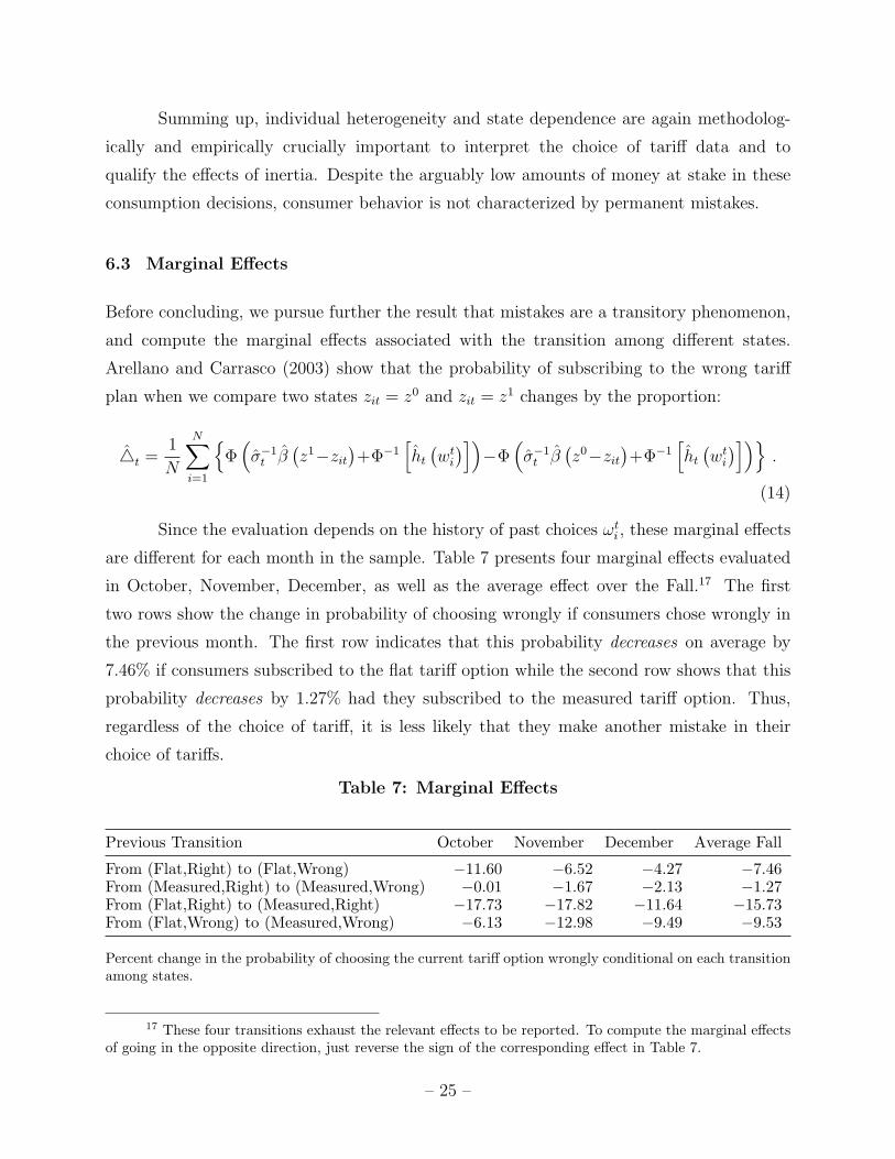
Since the evaluation depends on the history of past choices ωti , these marginal effects

are different for each month in the sample. Table 7 presents four marginal effects evaluated

in October, November, December, as well as the average effect over the Fall.17 The first

two rows show the change in probability of choosing wrongly if consumers chose wrongly in

the previous month. The first row indicates that this probability decreases on average by

7.46% if consumers subscribed to the flat tariff option while the second row shows that this

probability decreases by 1.27% had they subscribed to the measured tariff option. Thus,

regardless of the choice of tariff, it is less likely that they make another mistake in their

choice of tariffs.

Table 7: Marginal Effects

Previous Transition October November December Average Fall

From (Flat,Right) to (Flat,Wrong) −11.60 −6.52 −4.27 −7.46From (Measured,Right) to (Measured,Wrong) −0.01 −1.67 −2.13 −1.27From (Flat,Right) to (Measured,Right) −17.73 −17.82 −11.64 −15.73From (Flat,Wrong) to (Measured,Wrong) −6.13 −12.98 −9.49 −9.53

Percent change in the probability of choosing the current tariff option wrongly conditional on each transitionamong states.

17 These four transitions exhaust the relevant effects to be reported. To compute the marginal effectsof going in the opposite direction, just reverse the sign of the corresponding effect in Table 7.

– 25 –

Fig

ure

1:

Marg

inalEffect

sat

Diff

ere

nt

Mis

take

Thre

shold

s

Fig

ure

3. M

arg

inal

Eff

ects

-7.0

-6.5

-6.0

-5.5

-5.0

-4.5

-4.0

-3.5

-3.0

-2.5

-2.0

0.00

0.25

0.50

0.75

1.00

1.25

1.50

1.75

2.00

2.25

2.50

2.75

3.00

3.25

3.50

3.75

4.00

Fro

m (

0,0)

to (

0,1)

Percentage Change of Probability

-1.4

-1.2-1

-0.8

-0.6

-0.4

-0.2

0.00

0.25

0.50

0.75

1.00

1.25

1.50

1.75

2.00

2.25

2.50

2.75

3.00

3.25

3.50

3.75

4.00

Fro

m (

1,0)

to (

1,1)


-15.

6

-15.

4

-15.

2

-15.

0

-14.

8

-14.

6

-14.

4

-14.

2

0.00

0.25

0.50

0.75

1.00

1.25

1.50

1.75

2.00

2.25

2.50

2.75

3.00

3.25

3.50

3.75

4.00

Fro

m (

0,0)

to (

1,0)


-13.

0

-12.

5

-12.

0

-11.

5

-11.

0

-10.

5

-10.

0

-9.5

0.00

0.25

0.50

0.75

1.00

1.25

1.50

1.75

2.00

2.25

2.50

2.75

3.00

3.25

3.50

3.75

4.00

Fro

m (

0,1)

to (

1,1)


– 26 –

Similarly, the last two rows report the change in probability of choosing wrongly

if consumers subscribed to the optional measured service in the previous month. This

probability falls by 15.73% if consumers subscribed correctly to the optional measured service

in the previous month and by 9.53% if they subscribed wrongly to the optional measured

service. Thus, consistent with the asymmetry in the complexity of the problems discussed

earlier, the probability of making a mistake is substantially lower after subscribing to the

measured option than after subscribing to the flat tariff. This decrease in probability is more

important for those with low demand for which the measured service is the least expensive

option than for those with an usage pattern above the threshold of $18.70.

Finally, it is important to note that in analyzing these marginal effects, wrong is

defined simply to be equal to 1 when consumers pay any positive amount above the cost of

the alternative option. Rather than treating all mistakes equally, we repeat the analysis for

different thresholds in increments of 5 cents from $0.00 to $4.00. This allows us to measure

whether this change in probability varies significantly with the magnitude of the mistake.

Figure 1 reports the average marginal effects for the Fall. Interestingly, we find that marginal

effects experience an abrupt jump in the first 25-30 cents and remain basically constant once

consumers realize a mistake above these 25-30 cents. Recall that under the measured service

option consumers are not billed for the allowance unless their usage is above $19.02. This is

32 cents more than the $18.70 cost of the flat tariff option. We find it remarkable that this

amount is almost identical to 25-30 cents.

7 Concluding Remarks

The systematic analysis of individual responses to changes in the environment is important

for understanding the determinants of attention and inattention, and the extent and forma-

tion of rationality. The natural setting of the Kentucky tariff experiment and a rich panel

dataset that is free from a number of critical obstacles have allowed us to uncover households’

responses in isolation from a number of conflicting considerations which generally exist in

other circumstances.

We find that households recognize that choices today affect their utilities in the future

and actively react to a new option despite potential savings of very small magnitude. They

make no permanent mistakes. Their reactions, however, are not symmetric. Households who

– 27 –

face a more costly and cognitively more difficult tariff problem learn more slowly and are

more likely to make mistakes than households that face a simpler tariff choice problem. The

fact that the evidence turns out to be drastically different when lagged endogenous variables

and unobserved heterogeneity are appropriately treated in the econometric analysis indicates

that they play an important role in the dynamic learning process.

When and why people are attentive or inattentive and, when they are attentive, when

and why people get it right or wrong, are fundamental questions for our understanding of

human decision making. We do not claim that we should expect that the results we have

obtained will systematically generalize to other settings. This is an empirical question whose

answer depends on the degree of complexity, the costs of monitoring and information, the

size of incentives, and all other characteristics of the specific problem and environment under

study. What we hope, however, is that the analysis in this paper will contribute to pave the

way for an empirically-based science of decision making which, together with theoretical and

experimental work on cognitive processes, will improve our understanding of when and how

decision makers think about real life problems.

References

Abaluck, Jason T. and Jonathan Gruber (2010) “Choice Inconsistencies Among the Elderly:Evidence From Plan Choice in the Medicare Part D Program,” American EconomicReview, Vol. 101, pp. 1180–1210.

Ackerberg, Daniel and Maristella Botticini (2002) “Endogenous Matching and the EmpiricalDeterminants of Contract Form,” Journal of Political Economy, Vol. 110, pp. 564–591.

Agarwal, Sumit, Souphala Chomsisengphet, Chunlin Liu, and Nicholas S. Souleles (2006)“Do Consumers Choose the Right Credit Contracts?,” Mimeo, The Wharton School,University of Pennsylvania.

Akerlof, George A. and William T. Dickens (1982) “The Economic Consequences of CognitiveDissonance,” American Economic Review, Vol. 72, pp. 307–319.

Akerlof, George A. and Janet L. Yellen (1982) “Rational Models of Irrational Behavior,”American Economic Review, Vol. 77, pp. 137–142.

Amemiya, Takeshi (1985) Advanced Econometrics, Cambridge, MA: Harvard UniversityPress.

– 28 –

Americks, John, Andrew Caplin, and John Leahy (2003) “Wealth Accumulation and thePropensity to Plan,” Quarterly Journal of Economics, Vol. 118, pp. 1007–1047.

Arellano, Manuel and Olympia Bover (1995) “Another Look at the Instrumental VariableEstimation of Error-Components Model,” Journal of Econometrics, Vol. 68, pp. 29–51.

Arellano, Manuel and Raquel Carrasco (2003) “Binary Choice Panel Data Models withPredetermined Variables,” Journal of Econometrics, Vol. 115, pp. 125–157.

Arrow, Kenneth J. (1987) “Rationality of Self and Others in an Economic System,” in R. M.Hogarth and M. W. Reder eds. Rational Choice. The Contrast Between Economicsand Psychology, Chicago, IL: Chicago University Press.

Ball, Laurence M., N. Gregory Mankiw, and Ricardo Reis (2005) “Monetary Policy forInattentive Economies,” Journal of Monetary Economics, Vol. 52, pp. 703–725.

Becker, Gary S. (1962) “Irrational Behavior and Economic Theory,” Journal of PoliticalEconomy, Vol. 70, pp. 1–3.

Brown, Jeffrey R. and Austan. Goolsbee (2002) “Does the Internet Make Markets More Com-petitive? Evidence from the Life Insurance Industry,” Journal of Political Economy,Vol. 110, pp. 481–507.

Brynjolfsson, Erik and Michael D. Smith (2000) “Frictionless Commerce? A Comparison ofInternet and Conventional Retailers,” Management Science, Vol. 46, pp. 563–585.

Chamberlain, Gary (1984) “Panel Data,” in Z. Griliches and M. D. Intriligator eds. Handbookof Econometrics, Vol. II, New York, NY: North-Holland.

Chiappori, Pierre-Andre and Bernard Salanie (2000) “Testing for Asymmetric Informationin Insurance Markets,” Journal of Political Economy, Vol. 108, pp. 56–78.

Choi, J. J., D. Laibson, B. C. Madrian, and A. Metrick (2009) “Reinforcement Learning andSavings Behavior,” Journal of Finance, Vol. 64, pp. 2515–2534.

Conslik, J. (1996) “Why Bounded Rationality?” Journal of Economic Literature, Vol. 34,pp. 669–700.

Costa-Gomes, Miguel A. and Vincent P. Crawford (2006) “Cognition and Behavior in Two-Person Guessing Games: An Experimental Study,” American Economic Review, Vol.96, pp. 1737–1768.

Costa-Gomes, Miguel A., Vincent P. Crawford, and Bruno Broseta (2006) “Cognition andBehavior in Normal-Form Games: An Experimental Study,” Econometrica, Vol. 69,pp. 1193–1235.

DellaVigna, Stefano (2009) “Psychology and Economics: Evidence from the Field,” Journalof Economic Literature, Vol. 47, pp. 315–372.

– 29 –

DellaVigna, Stefano and Ulrike Malmendier (2006) “Paying Not to Go to the Gym,” Amer-ican Economic Review, Vol. 96, pp. 694–719.

Ellison, Glenn and Sara Fisher Ellison (2009) “Search, Obfuscation, and Price Elasticitieson the Internet,” Econometrica, Vol. 77, No. 2, pp. 427–452.

Gabaix, X., D. Laibson, G. Moloche, and S. Weinberg (2006) “Costly Information Acquisi-tion: Experimental Analysis of a Bounded Rationality Model,” American EconomicReview, Vol. 96, pp. 1043–1048.

Gabaix, Xavier and David Laibson (2002) “The 6D Bias and the Equity Premium Puzzle,”NBER Macroeconomics Annual 2001, pp. 257–311.

Gode, Dan K. and Shyam Sunder (1993) “Allocative Efficiency of Markets with Zero-Intelligence Traders: Market as a Partial Substitute for Individual Rationality,”Journal of Political Economy, Vol. 101, pp. 119–137.

Grubb, Michael D. (2009) “Selling to Overconfident Consumers,” American Economic Re-view, Vol. 99, No. 5, pp. 1770–1807.

Hansen, Lars P. and Thomas J. Sargent (2008) Robustness, Princeton, NJ: Princeton Uni-versity Press.

Heckman, James J. (1981) “The Incidental Parameters Problem and the Problem of InitialConditions in Estimating a Discrete Time - Discrete Data Stochastic Process,” inC. F. Manski and D. L. McFadden eds. Structural Analysis of Discrete Data withApplications, Cambridge, MA: MIT Press.

Heiss, Florian, Daniel McFadden, and Joachim Winter (2007) “Mind the Gap! ConsumerPerceptions and Choices of Medicare Part D Prescription Drug Plans,” Working Paper13627, NBER.

Hellwig, Christian, Sebastian Khols, and Laura Veldkamp (2012) “Information Choice Tech-nologies,” American Economic Review Papers and Proceedings, Vol. 102, pp. 35–40.

Ketcham, Jonathan, Claudio Lucarelli, Eugenio J. Miravete, and M. Christopher Roebuck(2012) “Sinking, Swimming, and Learning to Swim in Medicare Part D,” AmericanEconomic Review, Vol. 102, p. fortchoming.

Kling, Jeffrey R., Mullainathan Sendhil, Eldar Shafir, Lee C. Vermeulen, and Marian V.Wrobel (2012) “Comparison Friction: Experimental Evidence from Medicare DrugPlans,” Quarterly Journal of Economics, Vol. 127, No. 1, pp. 199–235.

Koscegi, Botond and Paul Heidhues (2008) “Competition and Price Variation when Con-sumers are Loss Averse,” American Economic Review, Vol. 98, pp. 1245–1268.

Koscegi, Botond and Matthew Rabin (2006) “A Model of Reference-Dependent Preferences,”Quarterly Journal of Economics, Vol. 121, pp. 1133–1166.

– 30 –

Lerman, Steven R. and Charles F. Manski (1977) “The Estimation of Choice Probabilitiesfrom Choice Based Samples,” Econometrica, Vol. 45, pp. 1977–1988.

Lipman, Barton L. (1991) “How to Decide How to Decide How to ...: Modeling LimitedRationality,” Econometrica, Vol. 59, pp. 1105–1125.

Lucas, Robert E. Jr. (1987) “Adaptive Behavior and Economic Theory,” in R. M. Hoga-rth and M. W. Reder eds. Rational Choice. The Contrast Between Economics andPsychology, Chicago, IL: Chicago University Press.

Lusardi, Annamaria (1999) “Information, Expectations and Savings,” in H. Aaron ed. Behav-ioral Dimensions of Retirement Economics, New York, NY: Rusell Sage Foundation.

(2003) “Planning and Saving for Retirement,” Mimeo, Darmouth College.

Madrian, Brigitte C. and Dennis F. Shea (2001) “The Power of Suggestion: Inertia in 401(k)Participation and Savings Behavior,” Quarterly Journal of Economics, Vol. 116, pp.1149–1187.

Mankiw, N. Gregory and Ricardo Reis (2002) “Sticky Information versus Sticky Prices:A Proposal to Replace the New Keynesian Philips Curve,” Quarterly Journal ofEconomics, Vol. 117, pp. 1295–1328.

Miravete, Eugenio J. (2002) “Estimating Demand for Local Telephone Service with Asym-metric Information and Optimal Calling Plans,” The Review of Economic Studies,Vol. 69, No. 4, pp. 943–971.

(2003) “Choosing the Wrong Calling Plan? Ignorance and Learning,” AmericanEconomic Review, Vol. 93, No. 1, pp. 297–310.

(2005) “The Welfare Performace of Sequential Pricing Mechanisms,” InternationalEconomic Review, Vol. 46, No. 4, pp. 1321–1360.

Moscarini, Giuseppe (2004) “Limited Information Capacity as a Source of Inertia,” Journalof Economic Dynamics and Control, Vol. 28, pp. 2003–2035.

Moscarini, Giuseppe and Lones Smith (2001) “The Optimal Level of Experimentation,”Econometrica, Vol. 69, pp. 1629–1644.

(2002) “The Law of Large Demand for Information,” Econometrica, Vol. 70, pp.2351–2366.

Narayanan, Sridhar, Pradeep K. Chintagunta, and Eugenio J. Miravete (2007) “The Role ofSelf Selection, Usage Uncertainty and Learning in the Demand for Local TelephoneService,” Quantitative Marketing and Economics, Vol. 5, pp. 1–34.

Newey, Whitney K. (1994) “The Asymptotic Variance of Semiparametric Estimators,”Econometrica, Vol. 62, pp. 1349–1382.

– 31 –

Reis, Ricardo (2006a) “Inattentive Consumers,” Journal of Monetary Economics, Vol. 53,pp. 1761–1800.

(2006b) “Inattentive Producers,” Review of Economic Studies, Vol. 73, pp. 793–821.

Rubinstein, Ariel (1998) Modeling Bounded Rationality, Cambride, MA: MIT Press.

Savage, Leonard J. (1954) The Foundations of Statistics, New York, NY: Wiley & Sons.

Scott-Morton, Fiona, Florian Zettelmeyer, and Jorge Silva-Risso (2001) “Internet Car Re-tailing,” Journal of Industrial Economics, Vol. 49, pp. 501–519.

Sims, Christopher A. (2003) “Implications of Rational Inattention,” Journal of MonetaryEconomics, Vol. 50, pp. 665–690.

Spiegler, Ran (2011) Bounded Rationality and Industrial Organization, New York, NY:Oxford University Press.

– 32 –

Consumer Inertia, Choice Dependence and Learning … Inertia, Choice Dependence and Learning from Experience in a Repeated Decision Problem Eugenio J. Miravetey Ignacio Palacios-Huertaz

Documents