Consumer choice prediction: artificial neural networks versus ...

Commerce Division Discussion Paper No. 104

CONSUMER CHOICE PREDICTION: ARTIFICIAL NEURAL NETWORKS VERSUS LOGISTIC MODELS

Christopher Gan Visit Limsombunchai

Mike Clemes and

Amy Weng

July 2005

1 Corresponding author: Associate Professor, Commerce Division, PO Box 84, Lincoln University, Canterbury, New Zealand, Tel: 64-3-325-2811, Fax: 64-3-325-3847, Email: [email protected] 3 Senior Lecturer, Commerce Division, PO Box 84, Lincoln University, Canterbury, New Zealand, Tel: 64-3-325-2811, Fax: 64-3-325-3847, Email: [email protected] 2 and 4 Graduate Student, Commerce Division, PO Box 84, Lincoln University, Canterbury, New Zealand, Tel: 64-3-325-2811,Fax: 64-3-325-3847, Email: [email protected] and [email protected]

Commerce Division Discussion Paper No. 104

CONSUMER CHOICE PREDICTION: ARTIFICIAL NEURAL NETWORKS VERSUS LOGISTIC MODELS

Christopher Gan Visit Limsombunchai

Mike Clemes and

Amy Weng

July 2005

Commerce Division PO Box 84

Lincoln University CANTERBURY

Telephone No: (64) (3) 325 2811 extn 8155

Fax No: (64) (3) 325 3847 E-mail: [email protected]

ISSN 1174-5045

ISBN 1-877176-81-8

Abstract

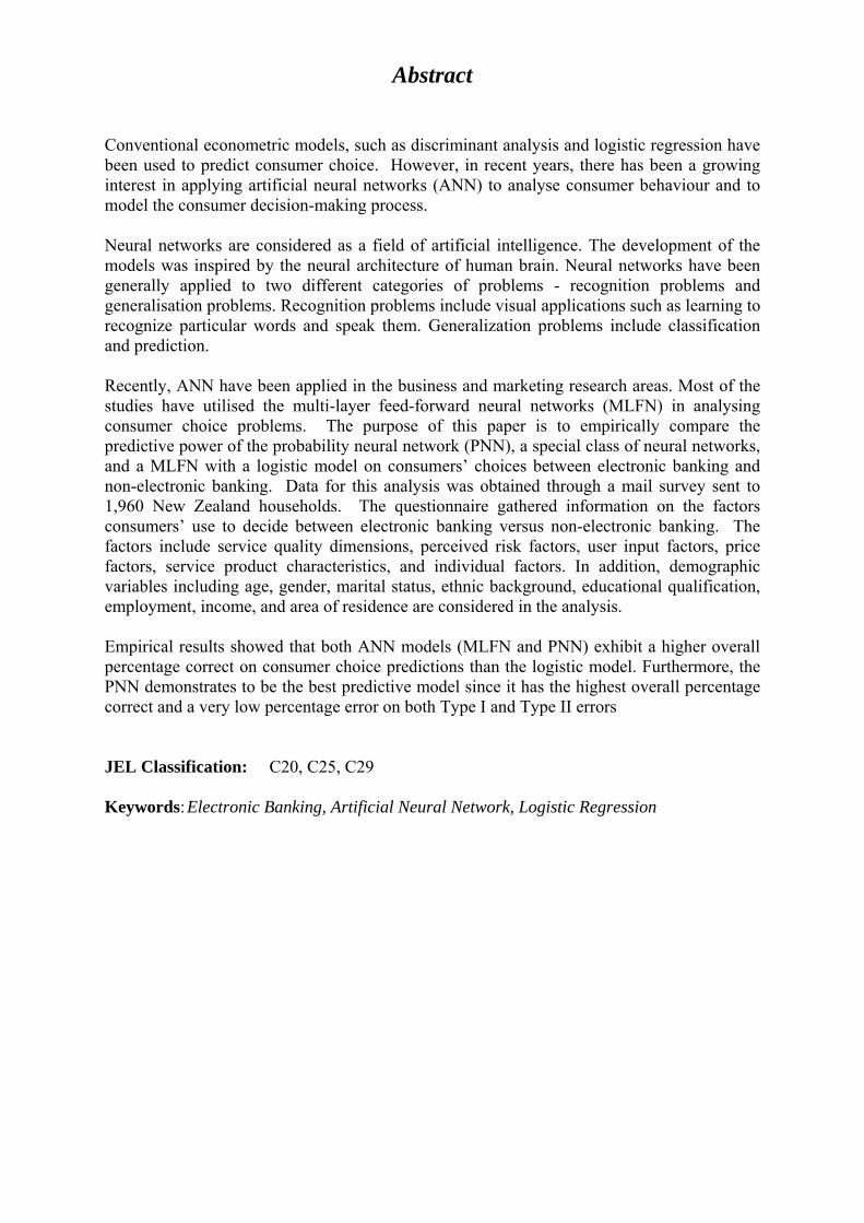
Conventional econometric models, such as discriminant analysis and logistic regression have been used to predict consumer choice. However, in recent years, there has been a growing interest in applying artificial neural networks (ANN) to analyse consumer behaviour and to model the consumer decision-making process. Neural networks are considered as a field of artificial intelligence. The development of the models was inspired by the neural architecture of human brain. Neural networks have been generally applied to two different categories of problems - recognition problems and generalisation problems. Recognition problems include visual applications such as learning to recognize particular words and speak them. Generalization problems include classification and prediction. Recently, ANN have been applied in the business and marketing research areas. Most of the studies have utilised the multi-layer feed-forward neural networks (MLFN) in analysing consumer choice problems. The purpose of this paper is to empirically compare the predictive power of the probability neural network (PNN), a special class of neural networks, and a MLFN with a logistic model on consumers’ choices between electronic banking and non-electronic banking. Data for this analysis was obtained through a mail survey sent to 1,960 New Zealand households. The questionnaire gathered information on the factors consumers’ use to decide between electronic banking versus non-electronic banking. The factors include service quality dimensions, perceived risk factors, user input factors, price factors, service product characteristics, and individual factors. In addition, demographic variables including age, gender, marital status, ethnic background, educational qualification, employment, income, and area of residence are considered in the analysis. Empirical results showed that both ANN models (MLFN and PNN) exhibit a higher overall percentage correct on consumer choice predictions than the logistic model. Furthermore, the PNN demonstrates to be the best predictive model since it has the highest overall percentage correct and a very low percentage error on both Type I and Type II errors JEL Classification: C20, C25, C29 Keywords: Electronic Banking, Artificial Neural Network, Logistic Regression

Contents

List of Tables i List of Figures i 1. INTRODUCTION 1 2. BANKING CHANNELS AND CONSUMER CHOICE THEORY 2 2.1 The Consumer Decision-Making Process 2 2.2 Logistic Model in Electronic Banking 4 3. ARTIFICIAL NEURAL NETWORK MODELS 3.1 Multi-Layer Feed-Forward Neural Network (MLFN) 7 3.2 probabilistic Neural Network (PNN) 9 4. DATA AND METHODOLOGY 11 5. EMPIRICAL RESULTS 11 6. CONCLUSION 15 REFERENCES 17

i

List of Tables

1. Consumer Choice Model (Logistic Regression) 12 2. Neural Networks’ Relative Contribution Factor 14 3. Classification Rates for the Out-of-Sample Forecast 15

List of Figures

1. Consumer Decision-Making Process Model 3 2. Structure of a Computational Unit 8 3. Multi-Layer Feed-Forward Neural Network Structure with One Hidden Layer 8 4. The Probabilistic Neural Network (PNN) Architecture 9

1

1. Introduction

Quantitative analysis for forecasting in business and marketing, especially in consumer

behavior and in the consumer decision-making process (consumer choice model), has become

more popular in business practices. The ability to understand and to accurately predict a

consumer decision can lead to more effectively targeting products, cost effectiveness in

marketing strategies, increasing sales and result in substantial improvement in the overall

profitability of the firm. Conventional econometric models, such as discriminant analysis and

logistic regression can predict consumers’ choices, but recently, there has been a growing

interest in using ANN to analyze and the model consumer decision-making process.

ANN have been applied in many disciplines, including biology, psychology, statistics,

mathematics, medical science, and computer science. Recently ANN have been applied to a

variety of business areas such as accounting and auditing, finance (with special emphasis on

bankruptcy prediction and credit evaluation), management and decision making, marketing

and production (Vellido et al., 1999a). However, the technique has been sparsely used in

modeling consumer choices. For example, Dasgupta et al. (1994) compared the performance

of discriminant analysis and logistic regression models against an ANN model with respect to

their ability to identify a consumer segment based upon their willingness to take financial

risks and to purchase a non-traditional investment product. Fish et al. (1995) examined the

likelihood of clustering managers-customers purchasing from a firm via discriminant analysis,

logistic regression and ANN models. Vellido et al. (1999b), using the Self-Organizing Map

(SOM), an unsupervised neural network model, carried out an exploratory segmentation of

the on-line shopping market while Hu et al. (1999) showed how neural networks can be used

to estimate the posterior probabilities of consumer situational choices on communication

channels (verbal versus non-verbal communications).

Previous studies have utilised the multi-layer feed-forward neural network (MLFN) which is a

family of the ANN. However, very few studies have applied a special class of artificial neural

networks called “Probabilistic Neural Network (PNN)” in modelling consumers’ choices. The

purpose of this study is to empirically compare the predictive power of the probability neural

network (PNN), a special class of neural networks, and the MLFN with the logistic model on

consumers’ banking choices between electronic banking and non-electronic banking.

2

2. Banking Channels and Consumer Choice Theory

The evolution of electronic banking, such as internet banking, has altered the nature of

personal-customer banking relationships and has many advantages over traditional banking

delivery channels. This includes an increased customer base, cost savings, mass

customization and product innovation, marketing and communications, development of non-

core businesses and the offering of services regardless of geographic area and time.

Furthermore, information technological developments in the banking industry have speed up

communication and transactions for customers. The information technology revolution in the

banking industry distribution channels began in the early 1970s, with the introduction of the

credit card, the Automatic Teller Machine (ATM) and the ATM networks. This was followed

by telephone banking, cable television banking in the 1980s, and the progress of Personal

Computer (PC) banking in the late 1980s and in the early 1990s.

Similar to its international counterparts, the adoption of electronic banking such as internet

banking is growing in New Zealand. During the last quarter of 2001, there were

approximately 480,000 regular internet users utilizing internet banking facilities to conduct

their banking transactions. This reflects a 54 percent growth from 170,000 users during the

same quarter of 2000 (Taylor, 2002). It is predicted that the usage of internet banking in New

Zealand will continue to grow in the near future, as customer support for internet banking is

mounting.

Despite its growing popularity, majority of consumer behavior banking studies has focused on

a specific type of electronic banking instead of investigating the concept of electronic banking

as a whole in relation to consumers’ decision making behavior (see Al-Ashban and Burney

2001). Furthermore, the limited electronic banking studies that have been published are

descriptive in nature, providing information on basic concepts of electronic banking instead of

focusing on complex and in-depth consumer decision making processes (Orr, 1998).

2.1 The Consumer Decision-Making Process

The consumer decision-making process pioneered by Dewey (1910) in examining consumer

purchasing behavior toward goods and services involves a five-stage decision process. This

includes problem recognition, search, and evaluation of alternatives, choice, and outcome.

Dewey’s paradigm was adopted and extended by Engel, Kollat and Blackwell (1973) and

Block and Roering (1976). Block and Roering (1976) suggested that the environmental

factors such as income, cultural, family, social and physical factors are crucial factors that

3

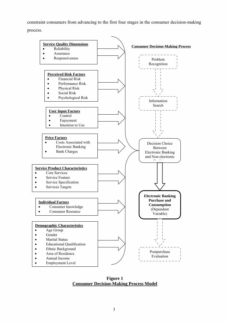
constraint consumers from advancing to the first four stages in the consumer decision-making

process.

Problem Recognition

Information Search

Decision Choice Between

Electronic Banking and Non-electronic

B ki

Electronic Banking Purchase and Consumption

(Dependent Variable)

Postpurchase Evaluation

Service Quality Dimensions • Reliability • Assurance • Responsiveness

Perceived Risk Factors • Financial Risk • Performance Risk • Physical Risk • Social Risk • Psychological Risk

User Input Factors • Control • Enjoyment • Intention to Use

Price Factors • Costs Associated with

Electronic Banking • Bank Charges

Service Product Characteristics • Core Services • Service Feature • Service Specification • Services Targets

Individual Factors • Consumer knowledge • Consumer Resource

Demographic Characteristics • Age Group • Gender • Marital Status • Educational Qualification • Ethnic Background • Area of Residence • Annual Income • Employment Level

Consumer Decision-Making Process

Figure 1 Consumer Decision-Making Process Model

4

Analogous to Dewey’s (1910) paradigm for goods, Zeithaml and Bitner (2003) suggested the

decision-making process could be applied to services. The five stages of the consumer

decision–making process operationalized by Zeithaml and Bitner (2003) were; need

recognition, information search, evaluation of alternatives, purchases and consumption, and

post-purchase evaluation (see Figure 1). Furthermore, the authors imply that in purchasing

services, these five stages do not occur in a linear sequence as they usually do in the purchase

of goods.

2.2 Logistic Model in Electronic Banking

For many durable commodities, the individual's choice is discrete and the traditional demand

theory has to be modified to analyse such a choice (Ben-Akiva and Lerman, 1985). Let

( )iiii zwyU ,, be the utility function of the consumer i, where yi is a dichotomous variable

indicating whether the individual is an electronic banking user, wi is the wealth of the

consumer and zi is a vector of the consumer's characteristics. Also, let c be the average cost of

using electronic banking, then economic theory posits that the consumer will choose to use

electronic banking if

( ) ( )iiiiiiii zw0yUzcw1yU ,,,, =≥−= (1)

Even though the consumer's decision is straightforward, the analyst does not have sufficient

information to determine the individual's choice. Instead, the analyst is able to observe the

consumer's characteristics and choice, and using them to estimate the relationship between

them. Let xi be a vector is of the consumer's characteristics and wealth, ( )iii zwx ,= , then

equation (1) can be formulated as an ex-post model given by:

( )i i iy f x= + ε (2)

where iε is the random term. If the random term is assumed to have a logistic distribution,

then the above represents the standard binary logit model. However, if we assume that the

random term is normally distributed, then the model becomes the binary probit model

(Maddala, 1993; Ben-Akiva and Lerman, 1985; Greene, 1990). The logit model will be used

in this analysis because of convenience as the differences between the two models are slight

(Maddala, 1993). The model will be estimated by the maximum likelihood method used in the

LIMDEP software.

5

The decision to use electronic banking is hypothesised to be a function of the six variables

(measured on a 5-point Likert-type scale) and demographic characteristics. The variables

include service quality dimensions, perceived risk factors, user input factors, price factors,

service product characteristics, and individual factors (see Figure 1). The demographic

variables include age, gender, marital status, ethnic background, educational qualification,

employment, income, and area of residence.

Implicitly, the empirical model can be written under the general form:

EBANKING = f (SQ, PR, UIF, PI, SP, IN, YOUNG, OLD, GEN, MAR, HIGHSCH,

EURO, MAORI, RURAL, HIGH, LOW, BLUE, WHITE,

CASUAL, ε) (3)

where:

EBANKING = 1 if the respondent is an electronic banking user; 0 otherwise

SQ (+) = Service quality dimensions

PR (-) = Perceived risk factors

UIF (+) = User input factors

PI (-) = Price factors

SP (+) = Service product characteristics

IN (+) = Individual factors

YOUNG (+) = Age level; 1 if respondent age is between 18 to 35 years old; 0

otherwise

OLD (-) = Age level; 1 if respondent age is above 56 years old; 0 otherwise

GEN (+) = Gender; 1 if respondent is a male; 0 otherwise

MAR (+) = Marital status; 1 if respondent is married; 0 otherwise

HIGHSCH (-) = Education level; 1 if respondent completed high school; 0 otherwise

EURO (+) = Ethnic group level; 1 if respondent ethic group is New Zealand

European; 0 otherwise

MAORI (+) = Ethnic group level; 1 if respondent ethic group is Maori; 0 otherwise

RURAL (+) = Residence level; 1 if respondent resides in rural area; 0 otherwise

HIGH (+) = Income level; 1 if respondent income level is above $40,000; 0

otherwise

LOW (+) = Income level; 1 if respondent income level is below $19,999; 0

otherwise

6

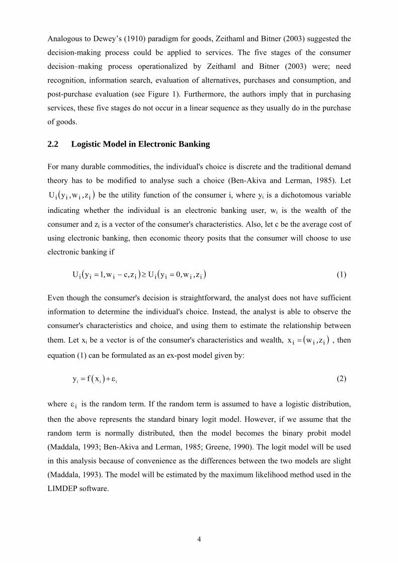
BLUE (+) = Employment level; 1 if respondent is a blue-collar worker; 0 otherwise

WHITE (+) = Employment level; 1 if respondent is a white-collar worker; 0

otherwise

CASUAL (+) = Employment level; 1 if respondent is causal worker (unemployed,

students and house persons; 0 otherwise

ε = Error term

A priori hypotheses are indicated by (+) or (-) in the above specification (see Figure 1). For

example, service quality dimensions such as reliability, assurance and responsiveness are

positively related to the use of electronic banking (Gerrard and Cunningham (2003).

Furthermore, consumers’ decision to use electronic banking is negatively related to financial,

performance, physical risk, social, and psychological risks (Sarin, Sego and Chanvarasuth,

2003).

User input factors such as control, enjoyment, and intention to use have a positive impact on

consumers’ decision to use electronic banking (Ng and Palmer, 1999). Polatoglu and Ekin’s

(2001) study identified that users of electronic banking were negatively influenced by price

factors. Consumers are price sensitive. The service product characteristics of electronic

banking such as consumers’ perception of a standard and consistent service, the time saving

feature of electronic banking, and the absence of personal interactions, have been empirically

found to positively influence consumers’ use of electronic banking (Polatoglu and Ekin, 2001;

Karjaluoto, Mattila and Pento, 2002). Likewise individual factors such as consumers’

knowledge and resources positively influence consumers’ use of electronic banking.

Demographic characteristics such as age, gender, marital status, education, ethnic group, area

of residence, and income were hypothesised to influence the respondent’s decision to use

electronic banking. This research seeks to determine which age group has the greatest

tendency to use electronic banking and whether gender plays a part in differentiating

electronic banking users and non-electronic banking users. Income was divided into low

(below $19,000), medium (between $20,000-$39,000) and high (above $40,000); age group

was divided into young (between 18 to 35 years old), medium (36 to 55 years old) and old

(above 56 years old); ethnic group was divided into New Zealand European, Maori, and

others (Pacific Islander or Asian); and employment level was divided into blue-collar works,

white-collar worker, casual worker (including unemployed, students and house persons) and

retirees. These are dummy variables and one dummy variable is dropped from each group to

avoid the dummy trap problem in the model.

7

3. Artificial Neural Network Models

3.1 Multi-Layer Feed-Forward Neural Network (MLFN)

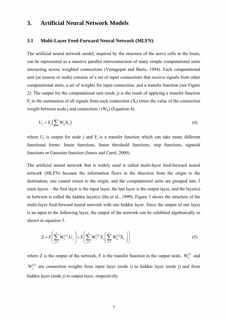
The artificial neural network model, inspired by the structure of the nerve cells in the brain,

can be represented as a massive parallel interconnection of many simple computational units

interacting across weighted connections (Venugopal and Baets, 1994). Each computational

unit (or neuron or node) consists of a set of input connections that receive signals from other

computational units, a set of weights for input connection, and a transfer function (see Figure

2). The output for the computational unit (node j) is the result of applying a transfer function

Fj to the summation of all signals from each connection (Xi) times the value of the connection

weight between node j and connection i (Wij) (Equation 4).

( )j j ij iU F W X= ∑ (4)

where Uj is output for node j and Fj is a transfer function which can take many different

functional forms: linear functions, linear threshold functions, step functions, sigmoid

functions or Gaussian function (James and Carol, 2000).

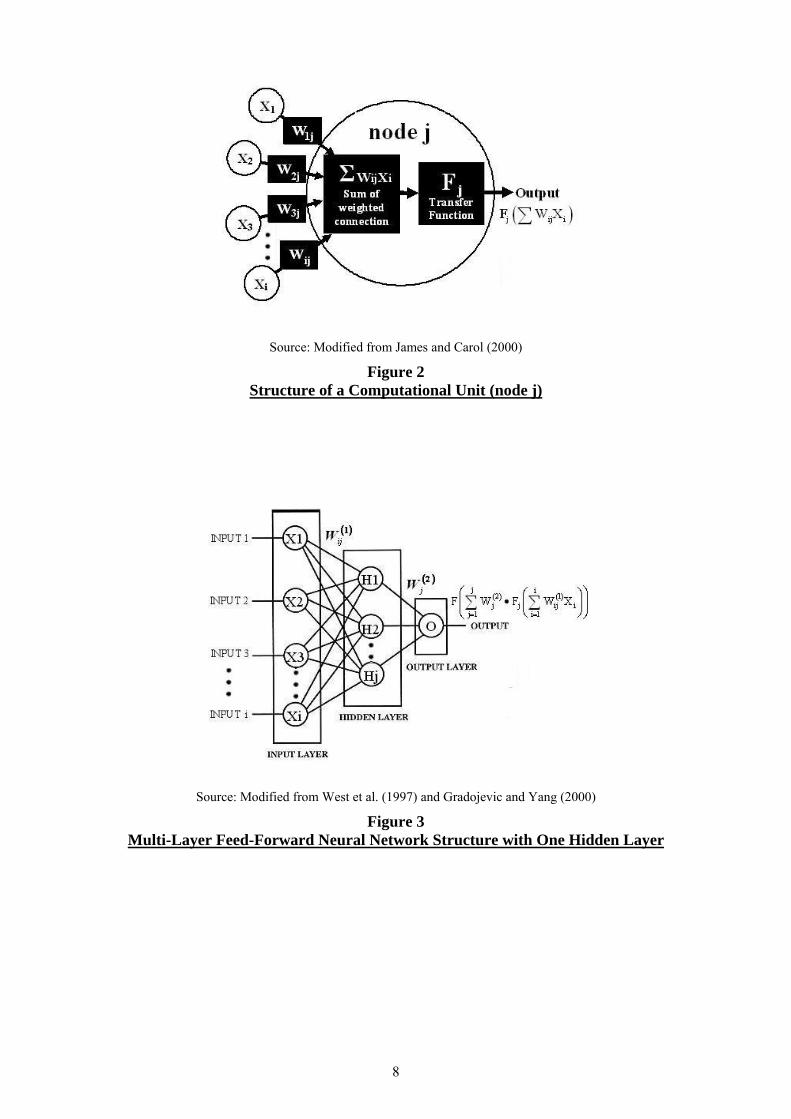
The artificial neural network that is widely used is called multi-layer feed-forward neural

network (MLFN) because the information flows in the direction from the origin to the

destination, one cannot return to the origin, and the computational units are grouped into 3

main layers – the first layer is the input layer, the last layer is the output layer, and the layer(s)

in between is called the hidden layer(s) (Hu et al., 1999). Figure 3 shows the structure of the

multi-layer feed-forward neural network with one hidden layer. Since the output of one layer

is an input to the following layer, the output of the network can be exhibited algebraically as

shown in equation 5.

( ) ( ) ( )J J i

2 2 1j j j j ij i

j 1 j 1 i 1Z F W .U F W .F W X

= = =

⎛ ⎞ ⎛ ⎞⎛ ⎞= =⎜ ⎟ ⎜ ⎟⎜ ⎟

⎝ ⎠⎝ ⎠ ⎝ ⎠∑ ∑ ∑ (5)

where Z is the output of the network, F is the transfer function in the output node, ( )1ijW and

( )2jW are connection weights from input layer (node i) to hidden layer (node j) and from

hidden layer (node j) to output layer, respectively.

8

Source: Modified from James and Carol (2000)

Figure 2 Structure of a Computational Unit (node j)

Source: Modified from West et al. (1997) and Gradojevic and Yang (2000)

Figure 3 Multi-Layer Feed-Forward Neural Network Structure with One Hidden Layer

9

The calculation of the neural network weights is known as training process. The process starts

by randomly initializing connection weights and introduces a set of data inputs and actual

outputs to the network. Then the network calculates the network output and compares it to the

actual output and calculated error. In an attempt to improve the overall predictive accuracy

and to minimise the network total mean squared error, the network adjusts the connection

weights by propagating the error backward through the network to determine how to best

update the interconnection weights between individual neurons. For this reason, the learning

algorithm is called back-propagation (Rao and Ali, 2002).

While the performance of the MLFN can be influenced by the number of hidden nodes and

layers in the network, there is no theoretical framework to determine the appropriate number

of hidden nodes and layers, and also the optimal internal error threshold in a network. Too

few hidden nodes and layers in the network will inhibit the learning ability of network. On the

other hand, too many hidden nodes and layers could reduce the network generalizing ability

and efficiency. In practice, the design of the neural network model is a tedious process of trail

and error to find the optimal model.

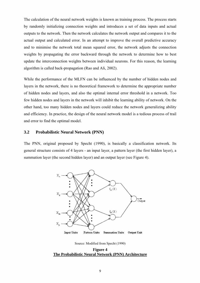
3.2 Probabilistic Neural Network (PNN)

The PNN, original proposed by Specht (1990), is basically a classification network. Its

general structure consists of 4 layers - an input layer, a pattern layer (the first hidden layer), a

summation layer (the second hidden layer) and an output layer (see Figure 4).

Source: Modified from Specht (1990)

Figure 4 The Probabilistic Neural Network (PNN) Architecture

10

PNN is conceptually based on the Bayesian classifier statistical principle. According to the

Bayesian classification theorem, X will be classified into class A, if the inequality in equation

6 holds:

( ) ( )A A A B B Bh c f X h c f X> (6)

where X is the input vector to be classified, hA and hB are prior probabilities for class A and B,

cA and cB are costs of misclassification for class A and B, fA(X) and fB(X) are probabilities of

X given the density function of class A and B, respectively (Albanis and Batchelor, 1999).

To determine the class, the probability density function is estimated by a non-parametric

estimation method developed by Parzen (1962) and extended afterwards by Cacoulos (1966).

The joint probability density function for a set of p variables can be expressed as:

( )( )

( ) ( )Aj AjA2

X Y X Yn2

A p 2 pj 1A

1f X e2 n

′− − −

σ

=

=π σ

∑ (7)

where p is the number of variables in the input vector X, nA is the number of training samples

which belongs to class A, YAj is the jth training sample in class A and σ is a smoothing

parameter (Chen et al., 2003).

The working principle of PNN begins with the input layer, where inputs are distributed to the

pattern units. Then the pattern unit, which is required for every training pattern, is used to

memorize each training sample and estimate the contribution of a particular pattern to the

probability density function. The summation layer comprises of a group of computational

units with the number equal to the total number of classes. Each summation unit that delicate

to a single class sums the pattern layer units corresponding to that summation unit’s class.

Finally, the output neuron(s), which is a threshold discriminator, chooses the class with the

largest response to the inputs (Albanis and Batchelor, 1999; Yang et al., 1999).

11

4. Data and Methodology

Data for this analysis was obtained through a random mail survey sent to 1,960 household in

Canterbury Region, New Zealand. The questionnaire gathered information on consumers’

decision to use electronic banking versus non-electronic banking. The mail survey was

designed and implemented according to the Dillman Total Design Method (1991), which has

proven to result in improved response rates and data quality. The response rate of the survey

was about 27%. The data set consisted of 527 observations (384 primarily electronic banking

users, EB, and 143 primarily non-electronic banking users, NEB). To estimate the consumers’

decision between electronic banking and non electronic banking, all the available data are

utilized in the model building process. LIMDEP software is used to estimate the logistic

regression and NeuroShell2 package is used to construct the artificial neural network models,

both MLFN and PNN.

To examine the predictive power of models, the out-of-sample forecasting technique is

applied. The sample is randomly divided into two sub-samples: a training sample and a

forecasting sample. The training sample and the forecast sample contain 422 observations

(304 electronic banking users and 118 non-electronic banking users) and 105 observations (80

electronic banking users and 25 non-electronic banking users), respectively. All the models

are re-estimated by using only the training samples and the out-of-sample forecasting were

conducted over the forecasting samples. Then, the classification rates (% correct and %

incorrect classifications) of each model are computed and compared. The model with the

highest percentage correct is considered as a superior model.

5. Empirical Results

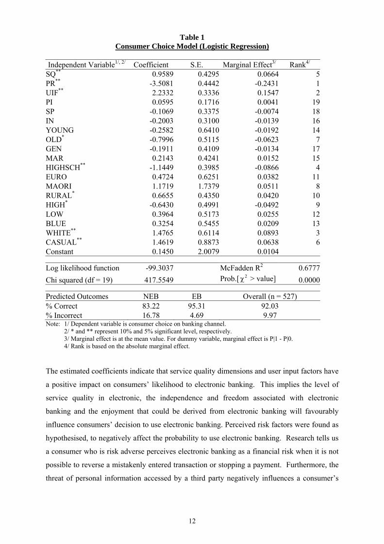
The estimated logistic regression equation (3) is as shown in Table 1. In general, the logistic

model fitted the data quite well. The chi-square test strongly rejected the hypothesis of no

explanatory power and the model correctly predicted 92% of the observations. Furthermore,

SQ, PR, UIF, OLD, WHITE, CASUAL, HIGHSCH, HIGH, and RURAL are statistically

significant and the signs on the parameter estimates support the a priori hypotheses outlined

earlier.

12

Table 1 Consumer Choice Model (Logistic Regression)

Independent Variable1/, 2/ Coefficient S.E. Marginal Effect3/ Rank4/

SQ** 0.9589 0.4295 0.0664 5 PR** -3.5081 0.4442 -0.2431 1 UIF** 2.2332 0.3336 0.1547 2 PI 0.0595 0.1716 0.0041 19 SP -0.1069 0.3375 -0.0074 18 IN -0.2003 0.3100 -0.0139 16 YOUNG -0.2582 0.6410 -0.0192 14 OLD* -0.7996 0.5115 -0.0623 7 GEN -0.1911 0.4109 -0.0134 17 MAR 0.2143 0.4241 0.0152 15 HIGHSCH** -1.1449 0.3985 -0.0866 4 EURO 0.4724 0.6251 0.0382 11 MAORI 1.1719 1.7379 0.0511 8 RURAL* 0.6655 0.4350 0.0420 10 HIGH* -0.6430 0.4991 -0.0492 9 LOW 0.3964 0.5173 0.0255 12 BLUE 0.3254 0.5455 0.0209 13 WHITE** 1.4765 0.6114 0.0893 3 CASUAL** 1.4619 0.8873 0.0638 6 Constant 0.1450 2.0079 0.0104

Log likelihood function -99.3037 McFadden R2 0.6777Chi squared (df = 19) 417.5549 Prob.[ 2χ > value] 0.0000

Predicted Outcomes NEB EB Overall (n = 527) % Correct 83.22 95.31 92.03 % Incorrect 16.78 4.69 9.97 Note: 1/ Dependent variable is consumer choice on banking channel.

2/ * and ** represent 10% and 5% significant level, respectively. 3/ Marginal effect is at the mean value. For dummy variable, marginal effect is P|1 - P|0. 4/ Rank is based on the absolute marginal effect.

The estimated coefficients indicate that service quality dimensions and user input factors have

a positive impact on consumers’ likelihood to electronic banking. This implies the level of

service quality in electronic, the independence and freedom associated with electronic

banking and the enjoyment that could be derived from electronic banking will favourably

influence consumers’ decision to use electronic banking. Perceived risk factors were found as

hypothesised, to negatively affect the probability to use electronic banking. Research tells us

a consumer who is risk adverse perceives electronic banking as a financial risk when it is not

possible to reverse a mistakenly entered transaction or stopping a payment. Furthermore, the

threat of personal information accessed by a third party negatively influences a consumer’s

13

likelihood to use electronic banking. This supports the finding of Ho and Ng (1994) and

Lockett and Littler (1997).

The demographic variables (age, employment, education, income and residence) were also

significant in explaining the respondents’ probability in using electronic banking. For

example, the negative coefficient of the age group above 56 years showed that senior

consumers were less likely to use electronic banking. Senior consumers are more risk adverse

and prefer a personal banking relationship to non personal electronic banking. High school

respondents may be less likely to use electronic banking due to their low income status.

Furthermore, electronic banking transaction could be costly for this age group who primarily

work part-time.

Additional information can be obtained through analysis of the marginal effects calculated as

the partial derivatives of the non-linear probability function, evaluated at each variable’s

sample mean (Greene, 1990). For example, the consumers’ choice of electronic banking is

relatively sensitive to the perceived risk (PR) (Rank = 1) and the user input factor (UIF)

(Rank = 2), where an unit increases in PR and UIN scores would decrease and increase the

probability of being an electronic banking user by 24.31% and 15.47%, respectively.

The overall percentage correct of 92.03 shows that the logistic model is quite accurate in

consumers’ choice prediction. However, the percentage incorrect indicate that the logistic

model is likely to produce Type I error (wrongly reject H0 or accept non-electronic banking

user as electronic banking user) compared to than Type II error (wrongly accept H0 or accept

electronic banking user as non-electronic banking user), as it has 19.78% and 4.69% incorrect

on non-electronic banking and electronic banking classifications, respectively (see Table 1).

Given that the neural network uses nonlinear functions, it is very difficult to spell out the

algebraic relationship between a dependent variable and an independent variable.

Furthermore, the learned output or connection weights could not be elucidated and tested.

Therefore, only the relative contribution factors and the classification rates are presented in

Table 2. Both MLFN and PNN used the same numbers of independent variables as the

logistic model for the input layer nodes. The best network for the MLFN in this study is the

one hidden layer network with 19 hidden neurons (19-19-1) and applies the logistic function

as the activation function on both hidden and output layers. For PNN, the network requires

the number of pattern units must be at least equal the number of training patterns and the

number of summation units must equal to the number of classes (or choices). Thus the

network configuration is 19-527-2-1.

14

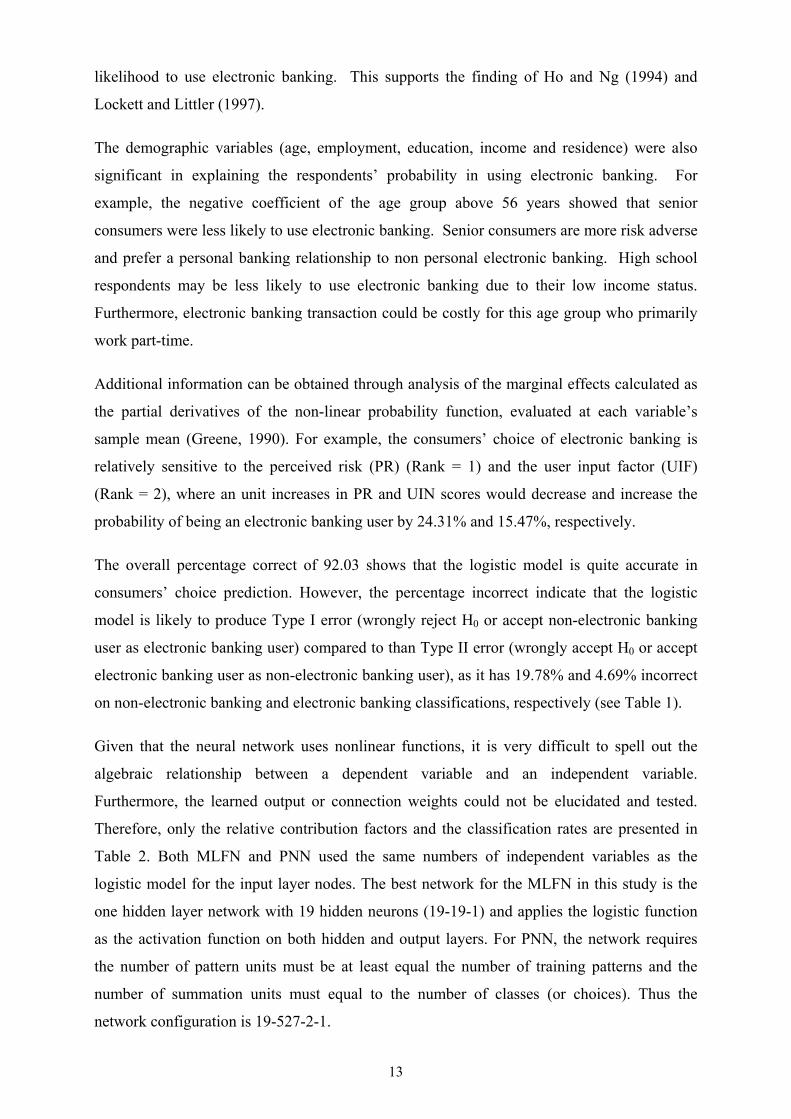
Table 2 Neural Networks’ Relative Contribution Factor

MLPN1/ PNN2/ Input Variable Relative contribution Rank Relative contribution Rank

SQ 0.0648 5 0.0524 11PR 0.1259 1 0.1113 1UIF 0.1165 2 0.1091 2PI 0.0331 16 0.0960 4SP 0.0808 4 0.0563 9IN 0.0811 3 0.0808 6YOUNG 0.0316 17 0.0092 16OLD 0.0406 10 0.0004 18GEN 0.0451 7 0.1082 3MAR 0.0246 19 0.0576 8HIGHSCH 0.0426 8 0.0227 14EURO 0.0386 12 0.0258 12MAORI 0.0377 14 0.0803 7RURAL 0.0480 6 0.0096 15HIGH 0.0425 9 0.0236 13LOW 0.0313 18 0.0000 19BLUE 0.0380 13 0.0559 10WHITE 0.0403 11 0.0070 17CASUAL 0.0371 15 0.0938 5

Predicted Outcome NEB EB Overall (n = 527) NEB EB Overall

(n = 527) % Correct 86.71 97.92 94.88 99.30 100.00 99.81 % Incorrect 13.29 2.08 5.12 0.70 0.00 0.19 Note: 1/ The network is utilized with learning rate = 0.1, momentum = 0.1 and initial weight = 0.3 2/ Smoothing factor: 0.518588

The classification results in Table 2 show that both MLFN and PNN exhibit a superior ability

to learn and memorize the patterns corresponding to consumers’ choice on the electronic

banking. Both of methods have higher overall percentage correct on consumers’ choice

predictions than the logistic model. Generally, the MLFN model can predict quite well on the

electronic banking group but its performance is relatively poor when predicting the non-

electronic banking group. In contrast, the PNN can predict well for both groups. Therefore,

the PNN is assumed to be the best prediction model in this study since it has the highest

overall percentage correct (99.81%) and a very low percentage error on Type I error (0.70%)

with 0.00% of Type II errors.

The relative contribution factors and the ranks in Tables 1 and 2 showed a consistency result

across all the models. That is, both perceived risk (PR) and the user input factor (UIF) have a

strong influence on the consumers’ decision between electronic banking and non electronic

banking in all three models, Rank = 1 and 2 respectively, whereas the other variables have a

15

strong influence in some models but they might have less influence in another model or vice

versa. Therefore, these two factors must be considered and set as high priority factors as they

strongly impact on the consumers’ decision in choosing between electronic banking and non

electronic banking.

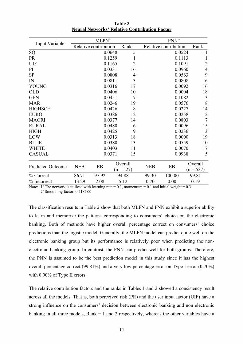
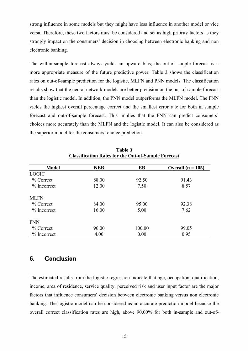
The within-sample forecast always yields an upward bias; the out-of-sample forecast is a

more appropriate measure of the future predictive power. Table 3 shows the classification

rates on out-of-sample prediction for the logistic, MLFN and PNN models. The classification

results show that the neural network models are better precision on the out-of-sample forecast

than the logistic model. In addition, the PNN model outperforms the MLFN model. The PNN

yields the highest overall percentage correct and the smallest error rate for both in sample

forecast and out-of-sample forecast. This implies that the PNN can predict consumers’

choices more accurately than the MLFN and the logistic model. It can also be considered as

the superior model for the consumers’ choice prediction.

Table 3 Classification Rates for the Out-of-Sample Forecast

Model NEB EB Overall (n = 105)

LOGIT % Correct 88.00 92.50 91.43 % Incorrect 12.00 7.50 8.57 MLFN % Correct 84.00 95.00 92.38 % Incorrect 16.00 5.00 7.62 PNN % Correct 96.00 100.00 99.05 % Incorrect 4.00 0.00 0.95

6. Conclusion

The estimated results from the logistic regression indicate that age, occupation, qualification,

income, area of residence, service quality, perceived risk and user input factor are the major

factors that influence consumers’ decision between electronic banking versus non electronic

banking. The logistic model can be considered as an accurate prediction model because the

overall correct classification rates are high, above 90.00% for both in-sample and out-of-

16

sample predictions. However, its performance does not outperform both neural network

models, MLFN and PNN, for both in-sample and out-of-sample forecasts.

The neural networks yield better prediction results but there are some drawbacks on using the

neural networks. Firstly, the neural networks lack theoretical background concerning the

explanatory capabilities. The connection weights in the networks cannot be interpreted or

used to identify the relationships between dependent and independent variables. Secondly,

there are no formal techniques for non-linear methods to test the relative relevance of the

independent variables and to carry out the variable selection process. Lastly, the neural

networks learning process can be very time consuming.

In summary, in term of prediction accuracy, the results present in this paper indicated that the

PNN can be successfully implemented to predict consumers’ choices because it outperforms

both the MLFN and the logistic model. This indicates the superiority of using the PNN for

prediction of consumers’ choices. Furthermore, the study exhibits the potential of the neural

methodology, especially the PNN, as an analysis tool to for marketing research. Since neither

the consumers’ choices are always binary nor the neural network is limited to the binary

choice classification problem, the research on the predictive power of the neural networks on

the multiple level classifications would be an area for further research, particularly on the

consumers’ choice prediction.

17

References

Al-Ashban, A. A., and M. A. Burney (2001), “Customer adoption of tele-banking technology: the case of Saudi Arabia”, The International Journal of Bank Marketing, 19(4/5), pp 191-200.

Albanis, G. T., and R. A. Batchelor (1999), Using probabilistic neural networks and rule

induction techniques to predict long-term bond ratings, in M. Torres (Ed.), Proceeding of the 5th Annual Conference on Information Systems, Analysis and Synthesis, Orlando: IIIS.

Ben-Akiva, M., and S. R. Lerman (1985), Discrete Choice Analysis: Theory and Application

to Travel Demand, MIT Press, Cambridge, Massachusetts. Block, C., and K. J. Roering (1976), Essentials of Consumer Behavior: Based on Engel,

Kollat, and Blackwell’s Consumer Behavior, The Dryden Press. Cacoullos, T. (1966), “Estimation of a multivariate density”, Annals of the Institute of

Statistical Mathematics (Tokyo), 18(2), pp 179-189. Chen, A., Leung, M.T. and H. Daouk (2003), “Application of neural networks to an emerging

financial market: forecasting and trading the Taiwan Stock Index”, Computers & Operations Research, 30(6), pp 901-923.

Dasgupta, C. G., Dispensa, G.S. and S. Ghose (1994), “Comparing the predictive

performance of a neural network model with some traditional market response models”, International Journal of Forecasting, 10(2), pp 235-244.

Dewey, J. (1910), How We Think. Health, New York. Dillman, D. A. (1978), Mail and Telephone Surveys: the Total Design Method, A Wiley-

Interscience Publication, John Wiley and Sons. Engel, J. F. Kollat, D.T. and R. D. Blackwell (1973), Consumer Behavior (2nd ed.), New

York: Holt, Rinehart and Winston, Inc. Fish, K. E., Barnes, J.H. and M. W. Aiken (1995), “Artificial neural networks: A new

methodology for industrial market segmentation”, Industrial Marketing Management, 24(5), pp 431-438.

Gerrard, P. and J. B. Cunningham (2003), “The diffusion of internet banking among

Singapore consumers”, International Journal of Bank Marketing, 21(1), pp 16-28. Greene, W. H. (1990), Econometric Analysis, Macmillan Publishing Company, New York. Ho, S. S. M. and V. T. F. Ng (1994), “Customers’ risk perceptions of electronic payment

systems”, The International Journal of Bank, 12(8), pp 26-39.

18

Hu, M. Y., M. Shanker, and M. S. Hung (1999), “Estimation of posterior probabilities of consumer situational choices with neural network classifiers”, International Journal of Research in Marketing, 16(4), 307-317.

James, R. C., and E. B. Carol (2000), “Artificial neural networks in accounting and finance:

modeling issues”, International Journal of Intelligent Systems in Accounting, Finance and Management, 9(2), 119-144.

Karjaluoto, H., M. Mattila, and T. Pento (2002), “Electronic banking in Finland: consumer

beliefs and reactions to a new delivery channel”, Journal of Financial Service Marketing, 6(4), 346-361.

Lockett, A., and D. Littler (1997), “The adoption of direct banking services”, Journal of

Marketing Management, 13, 791-811. Maddala, G. S. (1993), The Econometrics of Panel Data, Elgar. Ng, T., and E. Palmer (1999), “Customer satisfaction attributes for technology-interface

services”, Unpublished Paper, MSIS Department, School of Business and Economics, University of Auckland, Auckland, New Zealand, No.186. ISSN 1171-557X.

Orr, B. (1998), “Community bank guide to internet banking”, ABA Banking Journal, 90(6),

47-53. Parzen, E. (1962), “On estimation of a probability density function and mode”, Annals of

Mathematical Statistics, 33, 1065-1076. Polatoglu, V. N., and S. Ekin (2001), “An empirical investigation of the Turkish consumers’

acceptance of internet banking services”, International Journal of Bank Marketing, 19(4), 156-165.

Rao, C. P., and J. Ali (2002), “Neural network model for database marketing in the new

global rconomy”, Marketing Intelligence and Planning, 20(1), pp. 35-43. Sarin, S., T. Sego, and N. Chanvarasuth (2003), “Strategic use of bundling for reducing

consumers’ perceived risk associated with the purchase of new high-tech products”, Journal of Marketing Theory and Practice, 11(3), 71-83.

Specht, D. F. (1990), “Probabilistic neural networks”, Neural Networks, 3(1), 109-118. Taylor, K. (2002), “Bank Customers Logging On.” The New Zealand Herald. Available

(August 10, 2003) http://www.nzherald.co.nz/storydisplay.cfm?thesection=technology&thesubsection=&storyID=1291883

Vellido A., P. J. G. Lisboa, and J. Vaughan (1999a), “Neural networks in business: a survey

of applications (1992-1998)”, Expert Systems with Applications, 17(1), 51-70. Vellido A., P. J. G. Lisboa, and K. Meehan (1999b), “Segmentation of the on-line shopping

market using neural networks”, Expert Systems with Applications, 17(4), 303-314.

19

Venugopal, V., and W. Baets (1994) “Neural networks and statistical techniques in marketing research: A conceptual comparison”, Marketing Intelligence and Planning, 12(7), pp. 30-38.

West, P. M., P. L. Brockett, and L. L. Golden (1997), “A comparative analysis of neural

networks and statistical methods for predicting consumer choice”, Marketing Science, 16(4), 370-391.

Yang, Z. R., Platt, M. B. and Platt, H. D. (1999), “Probabilistic neural networks in bankruptcy

prediction”, Journal of Business Research, 44(2), pp. 67-74. Zeithaml, V, A. and M. J. Bitner (2003), Services Marketing: Integrating Customer Focus

across the Firm (3rd ed.), McGraw-Hill Irwin.