Construction of multi-soliton interaction patterns of KdV type

Construction of multi-soliton

interaction patterns of KdV type

equations

Pearu Peterson

Department of Mechanics and Applied Mathematics,Institute of Cybernetics at Tallinn Technical University,Akadeemia Rd. 21, 12618 Tallinn, EstoniaFax: +372 6204161 Phone: +372 6204168E-mail: [email protected]

Abstract. To predict the wave parameters from the inter-action patterns of waves (the inverse problem), thecorresponding direct problem needs to be solved. Inthis paper interaction patterns of multi-soliton so-lutions of KdV type equations are constructed. Theconnection between the multi-soliton interaction pat-terns and the decomposition of a multi-soliton solu-tion into a linear superposition of solitons and in-teraction solitons is demonstrated. All new con-cepts are illustrated for three-soliton solutions of theKadomtshev-Petviashvili equation.

Key words: Wave interaction patterns; Multi-soliton interaction;Direct problem of wave crests.

PACS: 04.30.Nk; 03.40.Kf

1 Introduction

Consider water-air surface waves which form complicated wave patterns dur-ing the propagation. In mathematical terms, a two-dimensional surface and itsperturbations that can propagate in different directions are considered. Ourultimate goal is to predict the wave parameters (amplitudes, traveling direc-tions, etc.) from the geometry of the interaction patterns formed by surfacewaves — the inverse problem of wave crests.

In the following we associate wave crests with solitons. Solitons are foundto be rather robust phenomena (in the theory) of water waves. More impor-tantly, using solitons as a model, we can actually tackle the inverse problemthat would be otherwise too complicated, if not impossible, to solve when usingeven the simplest (no winds, incompressible fluid, etc.) free surface equationsof water waves.

This inverse problem of wave crests was first solved for two wave interac-tions in [1, 2]. To tackle the inverse problem, the direct problem (i.e. con-

92

structing wave interaction patterns from predefined wave parameters) needsto be solved first. The interaction patterns are always stationary in the caseof two waves. That, however, is not true for more than two waves. Then theinteraction patterns are nonstationary, in general, and therefore much morecomplicated to handle.

In this paper we will solve the direct problem of wave crests for an arbitrarynumber of waves. As in [1], we assume that the dynamics of waves is governedby some member in the class of KdV type equations (in Hirota sense) [3, 4].The class of KdV type equations contains large number of nonlinear partialdifferential equations that support soliton solutions. Multi-soliton solutions ofKdV type equations were constructed and analyzed in [5] using Hirota bilinearformalism [6].

There have been other attempts to construct interaction pictures for morethan two solitons. See, for example, [7, 8] where authors describe the three-soliton interactions in terms of the motion of two-soliton resonant interactions(resonance triads). However, the authors recognize among other limitationsthat this description is very much an idealization because at each interactionpoint the condition for a resonant interaction is not met.

The organization of this paper is as follows. KdV type equations and theirmulti-soliton solutions are introduced in the following Section 2. In Section 3a phase pattern set of a multi-soliton solution is defined and a method for itsconstruction is introduced. Actual interaction patterns (real pattern sets) ofsolitons are constructed in Section 4. All new concepts are illustrated for three-soliton solutions of the Kadomtshev-Petviashvili equation. Finally, conclusionsare drawn in Section 5.

2 Multi-soliton solutions of KdV type equations

In this Section a brief overview of multi-soliton solutions of KdV type equationsis given. Detailed treatment can be found in [5].

Consider a (2+1)-dimensional KdV type equation for u(x), x = (x, y, t)T:

K[u] ≡ K(u, ux, uy, ut, . . .) = 0 (1)

that has related Hirota polynomials P = P (µ, ν, ω) and N = N(µ, ν, ω) suchthat

P (Dx)θ · θ = 0 ⇒ K[θ−2N(Dx)θ · θ] = 0

holds for all nontrivial positive functions θ = θ(x), where Dx = (Dx, Dy, Dt)T

is a vector of Hirota derivatives (Defs. 1–3 in [5]).

Notation (Index map κ). For α ∈ {0, 1}g a set κ(α) ∈ ℘({1, . . . , g}) is de-fined such that (i) if αi = 1 then i ∈ κ(α) and (ii) |κ(α)| = αTα. For example,κ((0, 1, 0, 1, 1)T) = {2, 4, 5}. We also write A{2,4,5} as A245, for example.

93

Genus g soliton solution of the KdV type equation (1) reads u(x) = U(Kx)(Theorem III.1 in [5]), where K = (µ,ν,ω), µ,ν,ω ∈ R

g, and

U(ϕ) = Θ−2N(DTϕK)Θ · Θ, (2)

Θ(ϕ) =∑

α∈{0,1}g

Aκ(α)eαTϕ, (3)

Aκ(α) =

1 if αTα < 2,

−P (ki − kj)/P (ki + kj) if κ(α) = {i, j},∏

i,j∈κ(α)i<j

Aij if αTα > 2,(4)

where kTi is the i-th row of a matrix K; DT

ϕK ≡ (KTDϕ)T with Dϕ =

(Dϕ1 , . . . , Dϕg)T denoting Hirota derivatives with respect to phase variables

ϕ = (ϕ1, . . . , ϕg)T. In addition the following conditions must hold:

dispersion relations: P (ki) = 0,

boundness conditions: P (ki + kj)P (ki − kj) 6 0,

Hirota conditions:∑

α∈(β−{0,1}g)∩{0,1}g

Aκ(α)Aκ(β−α)P ((2α − β)TK) = 0,

where β ∈ {0, 1}g and βTβ > 2.

Notation (Excluding variables). For a n-sequence of symbols we use asuperscript rounded with parenthesis to denote a sequence of symbols that is asubset of the n-sequence containing symbols with indices that are not listed inthe superscript and preserving the order. For example, (a, b, c, d)(1,3) = (b, d),(ϕ1, ϕ2, ϕ3)

(2) = (ϕ1, ϕ3).

A multi-soliton solution U = U(ϕ) (in phase variables) is defined to havethe following property (Definition 5 in [5]): limϕi→±∞ U is a genus (g − 1)soliton solution such that that

( limϕi→+∞

U)(ϕ(i)) = ( limϕi→−∞

U)(ϕ(i) −∆i(i)), (5)

where ϕ(i) = (ϕ1, . . . , ϕi−1, ϕi+1, . . . , ϕg)T, ∆ is a symmetric g × g-matrix of

phase variables ∆ij = − lnAij if i 6= j, and ∆ii = 0. The i-th column of ∆ isdenoted by ∆i.

A multi-soliton solution U = U(ϕ) can be decomposed into a superpositionof soliton and interaction soliton terms (Theorem IV.3 in [5]):

U =∑

β∈{0,1}g

Sκ(β), (6)

94

ϕ1

ϕ1

ϕ2ϕ2

−∆12

−∆12 ∆12

∆12

Figure 1: Phase pattern sets (bold lines) of two-soliton solutions with negativeand positive phase shifts, respectively. These illustrations correspond to two-soliton solutions of the KP equation.

where

Sκ(β) =1

2Θ′2

∑

α,α′∈{0,1}g

|α−α′|ew=β

√

Aκ(α)Aκ(α)Aκ(α′)Aκ(α′)N((α − α′)TK)

× cosh ((α − α′)Tϕ +1

2lnAκ(α)Aκ(α′)

Aκ(α)Aκ(α′)), (7)

Θ′ =1√2

∑

α∈{0,1}T

√

Aκ(α)Aκ(α) cosh(α − α)Tϕ + lnAκ(α)/Aκ(α)

2,

|·|ew ≡ (|·1| , . . . , |·g|)T denotes the element-wise absolute value operation, andα ≡ i−α with i ∈ {1}g such that iTi = g. For multi-soliton solutions in realvariables, u = u(x), we write

u =∑

β∈{0,1}g

sκ(β),

where sκ(β)(x) = Sκ(β)(Kx).

3 Phase pattern sets

In [1] we introduced a geometric representation of soliton interaction pictures.In this simplified description, the so-called pattern set is defined to describe thepositions of solitons. For example, for a two-soliton solution in phase variables,

95

ϕ1

ϕ1

ϕ2 ϕ2

−∆12

∆12

ψ

ψ

Figure 2: Construction of the phase pattern sets (bold lines on the (ϕ1, ϕ2)-plane) for two-soliton solutions with negative and positive phase shifts, respec-tively. White arrows indicate the projection of polyhedron edges to the spaceof phase variables.

U = U(ϕ1, ϕ2), the phase pattern set PU consists of two pairs of parallel lineslices and a connecting line segment as shown in Fig. 1. The parallel lineslices correspond to positions of soliton terms S1 and S2, respectively, and theconnecting line segment to the position of interaction soliton S12 [1].

In this section we construct phase pattern sets for multi-soliton solutions.To get a better understanding of the method, we start with the two solitoncase and then extend it for the general multi-soliton case.

3.1 Construction of a phase pattern set for two-soliton solu-

tion

For two-soliton solutions, there are two types of interactions (with positive andwith negative phase shifts, respectively) that have different phase pattern setsas shown in Fig. 1. In order to describe all possible phase pattern sets in anunified manner (also for multi-soliton solutions), we introduce the followingconstruction. Namely, we extend the space of phase variables by definingan auxiliary phase variable, ψ. In this extended space of phase variables(ϕ1, ϕ2, ψ) we define a convex polyhedron such that the orthogonal projectionof its edges to the original space of phase variables does coincide with thephase pattern set of the corresponding two-soliton solution. This constructionis illustrated in Fig. 2.

96

3.2 Construction of a phase pattern set for multi-soliton solu-

tion

In the following we give a general definition for phase pattern sets and in-troduce a method for their construction. First, we need to introduce someauxiliary notations.

Notation. • For A ⊂ Rg, c ∈ R

g we define A+ c ≡ {a + c|a ∈ A}.

• For A ⊂ Rg, B ⊂ R

g−1, ϕ ∈ Rg, i = 1, . . . , g, we write

A|ϕi=−∞ = B

iff ∃c such that {ϕ(i)|ϕ ∈ A and ϕi = c′} = B holds for all c′ < c.

• Similarly, we writeA|ϕi=+∞ = B

iff ∃c such that {ϕ(i)|ϕ ∈ A and ϕi = c′} = B holds for all c′ > c.

Definition 1 (Phase pattern set). A set PU ⊂ Rg is called the phase

pattern set of a genus g soliton solution U = U(ϕ) with the phase shift matrix∆ iff

1. If g = 1, then PU = {0}.

2. If g > 1, then the following conditions are satisfied for i = 1, . . . , g:

PU |ϕi=−∞ = PU(i) , (8)

PU |ϕi=+∞ = PU(i) + ∆i(i), (9)

where PU(i) is the phase pattern set of a genus (g − 1) soliton solutionU (i) ≡ limϕi→−∞ U .

Theorem 3.1 (Construction of a phase pattern set). Let U = U(ϕ) be

a genus g soliton solution with the phase shift matrix ∆. Let H be a convex

polyhedron:

H ={

(ϕ, ψ)|nTϕ + ψ + cn 6 0,n ∈ {−1, 1}g}

, (10)

where

cn = c− 1

4(i + n)T∆(i + n),

c ∈ R is arbitrary. Let R be a set of ridges of the polyhedron H:

R =⋃

n,m∈{−1,1}g

n6=m

Rn,m, (11)

97

µ1

µ2

µ3

|ρ13|

|ρ12|

|ρ23|

Aij > 1 0 < Aij < 1

0 < Aij < 1

Aij < 0Aij = ∓∞

A ij=

0

Aij = 1|ρij |

|ρij |

µi

µj

Aij =ρij

2 − (µi − µj)2

ρij2 − (µi + µj)2

ρij =νi

µi

− νj

µj

Figure 3: “Map” of genus 3 soliton types for the KP equation. The type isdefined by the signs of phase shifts ∆ij = − logAij . Shaded regions correspondto bounded solutions. The case corresponds to ν1 = 0, ρ12 = 0.268, ρ13 =−0.364.

where

Rn,m = H ∩{

(ϕ, ψ)

∣

∣

∣

∣

nTϕ + ψ + cn = 0mTϕ + ψ + cm = 0

}

. (12)

Then an orthogonal projection (ϕ, ψ) 7→ ϕ of R is a phase pattern set of U :

PU = R|ϕ . (13)

Proof. See Appendix A.

3.3 Phase pattern set of a three-soliton solution

In the following we illustrate the connection between phase pattern sets andsoliton solutions for the KP (Kadomtshev-Petviashvili) equation

(ut + 6uux + uxxx)x + 3uyy = 0,

that, as a member of the class of KdV type equations, has related Hirotapolynomials P = µω + µ4 + 3ν2 and N = µ2. In particular, we consider itsthree-soliton solutions.

The boundness conditions A12,13,23 > 0 define regions in the space of µ-parameters where KP three-soliton solutions are bounded as shown in Figure 3.In addition, for different combinations of signs of the phase shift parameters

98

ϕ1

ϕ2

ϕ3

∆13

∆12

∆23

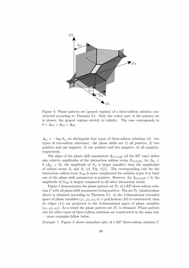
Figure 4: Phase pattern set (grayed regions) of a three-soliton solution con-structed according to Theorem 3.1. Only the center part of the pattern setis shown, the grayed regions stretch to infinity. The case corresponds to0 < ∆13 < ∆12 < ∆23.

∆ij = − logAij we distinguish four types of three-soliton solutions (cf. twotypes of two-soliton solutions): the phase shifts are 1) all positive, 2) twopositive and one negative, 3) one positive and two negative, 4) all negative,respectively.

The signs of the phase shift parameters ∆12,13,23 (of the KP case) definealso relative amplitudes of the interaction soliton terms S12,13,23: for ∆ij <0 (∆ij > 0), the amplitude of Sij is larger (smaller) than the amplitudesof soliton terms Si and Sj (cf. Fig. 1)[1]. The corresponding rule for theinteraction soliton term S123 is more complicated for solution types if at leastone of the phase shift parameters is positive. However, for ∆12,13,23 < 0, theamplitude of S123 is largest compared to all other interaction terms.

Figure 4 demonstrates the phase pattern set PU of a KP three-soliton solu-tion U with all phase shift parameters being positive. The set PU (shaded planeslices) is obtained according to Theorem 3.1: in the 4-dimensional extendedspace of phase variables (ϕ1, ϕ2, ϕ3, ψ) a polyhedron (10) is constructed; thenits ridges (11) are projected to the 3-dimensional space of phase variables(ϕ1, ϕ2, ϕ3). As a result the phase pattern set PU is obtained. Phase patternsets for other types of three-soliton solutions are constructed in the same way— more examples follow below.

Example 1. Figure 5 shows isosurface plot of a KP three-soliton solution U

99

ϕ1

ϕ2

ϕ3

Figure 5: Isosurface plot of a KP three-soliton solution in phase variables.The case corresponds to the point µ = (−0.3996ρ13, ρ12 − 0.4ρ13,−0.5994ρ13)in Figure 3.

with ∆12 > 0 and ∆13,23 < 0. The corresponding phase pattern set is demon-strated in the form of a wireframe in the same plot. Clearly, the phase patternset represents the supporting regions of the function U , or equivalently, thepositions of wave crests in phase variables.

Figure 6 shows isosurface plots of interaction terms S2,3,23,123. These plotsillustrate close connection between the parts of a phase pattern set PU andthe decomposition (6): each plane slice in PU represents a supporting regionof one of the interaction term in the decomposition.

Example 2. Figure 7 shows another example of a KP three-soliton solutionwith ∆12,13 > 0 and ∆23 < 0. In this case the amplitude of the interactionterm S123 is almost zero. The “hole” in the isosurface plot illustrates just that.

4 Interaction patterns

In this section we complete the direct problem of wave crests by constructinginteraction patterns for multi-soliton solutions in real space-time variables.

To demonstrate the dynamics of interaction patterns, in the following wewrite multi-soliton solutions of the KdV type equation (1) as u(x, t) = U(Kx+ωt), where x = (x, y)T and K = (µ,ν). With this notation we associate the

100

ϕ1

ϕ2

ϕ3

ϕ1

ϕ2

ϕ3

ϕ1

ϕ2

ϕ3

ϕ1

ϕ2

ϕ3

Figure 6: Isosurface plots of interaction terms S2, S3 (upper figures), S23, S123

(lower figures) of the KP three-soliton solution in phase variables. The iso-surfaces correspond to half of the amplitude of the corresponding interactionterms.

variable t as the time parameter.

Definition 2 (Real pattern set [1]). A set Pu(t) ⊂ R2 is called the real

pattern set of a genus g soliton solution u(x, t) = U(Kx + ωt) iff

Pu(t) = {x ∈ R2|Kx + ωt ∈ PU}, (14)

where PU is the phase pattern set of the corresponding genus g soliton solutionU = U(ϕ) in phase variables.

Propositon 4.1. If g > 2 and the columns of K are not collinear then the

101

ϕ3

ϕ2

ϕ1

Figure 7: Isosurface plot of a KP three-soliton solution in phase variables. Thecase corresponds to the point µ = (ρ12 −ρ13,−0.999ρ13, 0.999ρ12) in Figure 3.

real pattern set of a genus g soliton solution reads

Pu(t) = (KTK)−1KT(PU ∩ (KR2 + ωt)) − wt, (15)

where w = (KTK)−1KTω.

Proof. Expression (14) is equivalent to

KPu(t) + ωt = PU ∩ (KR2 + ωt). (16)

Due to the non-collinearity of K columns, there exists (KTK)−1. After mul-tiplying the both sides of (16) with (KTK)−1KT, we obtain (15).

To interpret the real pattern set of a multi-soliton solution, we write it inthe following form

Pu(t) = (KTK)−1KT(PU ∩ (KR2 + ω⊥t)) − wt, (17)

where ω⊥ = ω − Kw is perpendicular to the 2-dimensional hyperplane KR2

in the g-dimensional space of phase variables: KTω⊥ = 0. Since the phasepattern set PU represents the supporting regions of the given multi-solitonsolution in phase variables, the intersection PU ∩ (KR

2 + ω⊥t) defines therepresentation of supporting regions of the multi-soliton in real variables after

102

mapping the intersection to the space of real variables with (KTK)−1KT. Ifω⊥ 6= 0, the image of the real space KR

2 is translated in the direction of ω⊥

in the space of phase variables as the time parameter t is increased. Duringthis translation, the intersection PU ∩ (KR

2 +ω⊥t) changes accordingly as theset PU is fixed in the space of phase variables. So, the first term in (17) isresponsible for the nonstationarity of the real pattern set Pu(t). The secondterm in the expression of Pu(t) defines just a translation of the interactionpattern in the space of real variables. The special case ω⊥ = 0 corresponds toa multi-soliton solution that is stationary regardless how large is the numberof solitons.

4.1 Real pattern set of a three-soliton solution

Figures 8 and 9 illustrate the construction of interaction patterns of a KPthree-soliton solution with all phase shift parameters being negative. Figure9 shows two instances of the real pattern set Pu(t) for time moments t =−150 and t = 0, respectively. They are found as the original regions of theintersection PU ∩ (KR

2 + ωt) with respect to the mapping x 7→ Kx + ωt.Figure 8 shows this for the time moment t = 0. As t is increased, the planeKR

2 is translated in the opposite direction of the vector ω in the space ofphase variables. In this particular case, the plane KR

2 in Fig. 8 moves awayas observed by a reader. As a result, the real pattern set Pu(t) is nonstationary.

Because each plane slice of the phase pattern set PU represents one of theinteraction soliton terms S1,2,3,12,13,23,123 in the superposition (6), so does eachline slice of the real pattern set Pu(t) in the space of real variables. However,not all interaction terms may be visible in the real space for all time. Onlythose interaction solitons are visible that correspond to plane slices of PU thathave common points with the plane KR

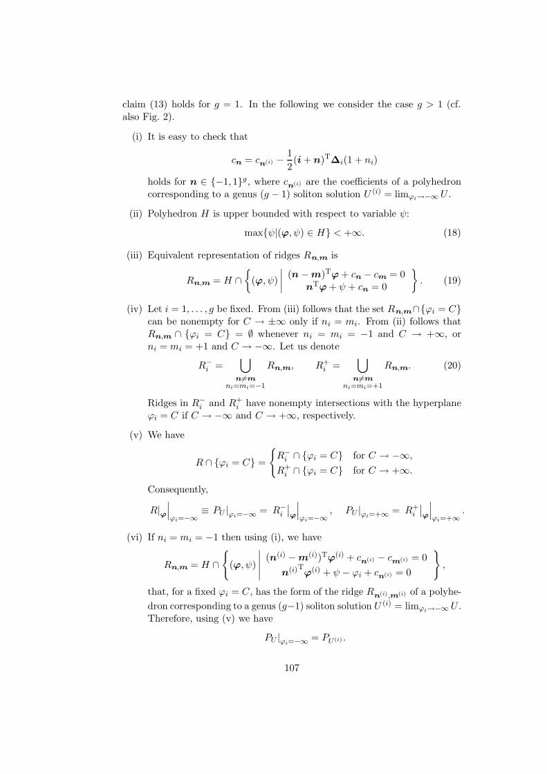
2+ωt at the given time moment t. Forthis reason there is no line slice corresponding to the interaction soliton terms23 in Figure 9. In fact, as time parameter t is increased, the interaction solitonterm s123 disappears eventually and an interaction pattern forms instead withthree subpatterns of pairwise interactions between the three solitons. Thesame happens for decreasing time parameter. In conclusion, the interactionsoliton s123 exists only finite amount of time. Interaction solitons s12,13,23

may disappear only for finite time period but they eventually reappear tothe interaction pattern. Solitons s1,2,3 are always present in the interactionpatterns.

103

ϕ1

ϕ2

ϕ3

KR 2

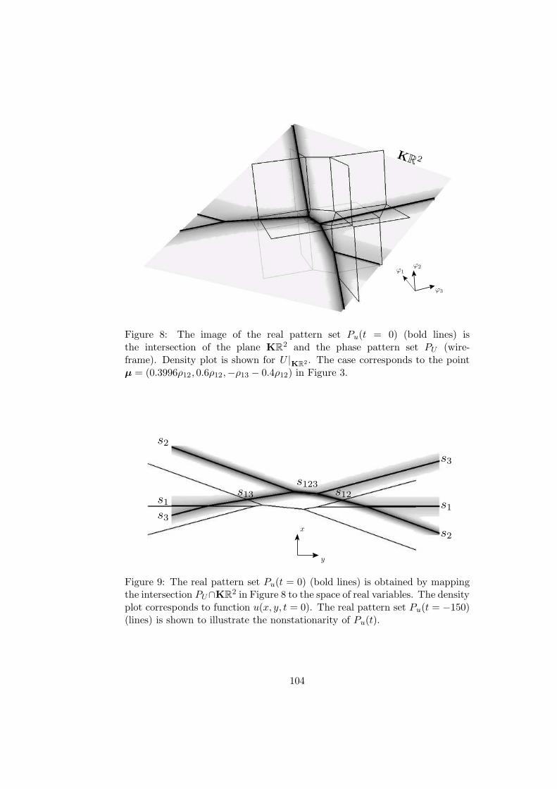
Figure 8: The image of the real pattern set Pu(t = 0) (bold lines) isthe intersection of the plane KR

2 and the phase pattern set PU (wire-frame). Density plot is shown for U |

KR2 . The case corresponds to the pointµ = (0.3996ρ12, 0.6ρ12,−ρ13 − 0.4ρ12) in Figure 3.

x

y

s1

s2

s3

s1

s2

s3

s12s13s123

Figure 9: The real pattern set Pu(t = 0) (bold lines) is obtained by mappingthe intersection PU∩KR

2 in Figure 8 to the space of real variables. The densityplot corresponds to function u(x, y, t = 0). The real pattern set Pu(t = −150)(lines) is shown to illustrate the nonstationarity of Pu(t).

104

1

1

1

14

4

145

45

1245

2

14

1242

14

3134

124

2

12345

151

5

24

1245

3

13

1

3

43

24

4

5

x

y

Figure 10: The real pattern set (white lines) of a five-soliton solution (abstractcase, corresponds to Fig. 1 in [1]). Labels are the indices of the soliton termsof the corresponding decomposition.

4.2 Real pattern set of a five-soliton solution

Figure 10 illustrates a snapshot of an animated density plot of a five-solitonsolution and the corresponding instance of its real pattern set. The latter isconstructed according to the following procedure. First, a phase pattern setPU is constructed according to Theorem 3.1 as a projection of the ridges ofa special 6-dimensional polyhedron to the 5-dimensional space of phase vari-ables. Then, for a fixed time parameter t, an intersection of the set PU anda 2-dimensional hyperplane KR

2 + ωt is found. Finally, this intersection ismapped with (KTK)−1KT to the space of real variables resulting an instanceof a real pattern set Pu(t). As the time parameter t is increased, the hyper-plane KR

2 + ωt shifts in the space of phase variables causing changes to theintersection PU ∩ (KR

2 +ωt). These changes are expressed in the nonstation-arity of the interaction patterns of multi-soliton solutions.

5 Conclusions

In this paper we constructed interaction patterns for multi-soliton solutions ofKdV type equations.

Although, the interaction patterns are, in general, nonstationary and lookcomplicated, their formation can be deterministically constructed for any timemoment. For that, we first considered multi-soliton solutions in phase vari-ables in which these solutions have very regular structures. In particular, torepresent supporting regions of soliton solutions in phase variables, we definedthe so-called phase pattern set. Though, the phase pattern set is defined in a

105

possibly high-dimensional space of phase variables, it can be algorithmicallyconstructed using the tools from the computational geometry. Namely, wediscovered that the phase pattern set of a multi-soliton solution is formed byprojecting the ridges of a special polyhedron in the extended space of phasevariables to the space of phase variables.

To represent actual interaction patterns, we defined the so-called real pat-tern set that is, for a fixed time moment t, isomorphic to an intersection ofthe phase pattern set and a certain two-dimensional hyperplane in the spaceof phase variables. We showed that the nonstationarity of interaction patternsis directly related to the movement of this hyperplane in the space of phasevariables as the time parameter t is varied.

In addition, we demonstrated close connection between the pattern setsdefined above and the decomposition of multi-soliton solutions into a super-position of interaction solitons. In fact, each linear part of the phase (real)pattern set represents the supporting region of one of the terms in the decom-position in phase (real) variables. We also explained possible emergence andabsorption of interaction solitons in the space of real variables.

In conclusion, we solved the direct problem of wave crests for multi-solitonsolutions. These results will be used for solving the corresponding inverseproblem. Initial analysis shows that the inverse problem can be solved, inprinciple, also for multi-soliton solutions. This is due to the fact that thenumber of unknown parameters matches with the number measurable invari-ants (phase shift and angle relations) of a multi-soliton solution. The detailswill be reported in a successive paper.

6 Acknowledgements

The author is grateful to Professor E. van Groesen (Enschede, The Nether-lands) for instructive guidance throughout of this work, and Professor JuriEngelbrecht (Tallinn, Estonia) for continuous support of this work.

I am thankful to Komei Fukuda (Zurich, Switzerland) for making the soft-ware library cddlib[9] available that has been extensively used in this work forpolyhedron manipulations.

A part of this research is sponsored by the Royal Netherlands Academyof Arts and Sciences in the programme for scientific cooperation Netherlands-Indonesia. Financial support from the Estonian Science Foundation is ac-knowledged (grants 2631, 4068).

Appendix A Proof of Theorem 3.1

In the following we show that the phase pattern set, constructed accordingto Theorem 3.1, satisfies Definition 1. It is straightforward to check that the

106

claim (13) holds for g = 1. In the following we consider the case g > 1 (cf.also Fig. 2).

(i) It is easy to check that

cn = cn(i) − 1

2(i + n)T∆i(1 + ni)

holds for n ∈ {−1, 1}g , where cn(i) are the coefficients of a polyhedroncorresponding to a genus (g − 1) soliton solution U (i) = limϕi→−∞U .

(ii) Polyhedron H is upper bounded with respect to variable ψ:

max{ψ|(ϕ, ψ) ∈ H} < +∞. (18)

(iii) Equivalent representation of ridges Rn,m is

Rn,m = H ∩{

(ϕ, ψ)

∣

∣

∣

∣

(n − m)Tϕ + cn − cm = 0nTϕ + ψ + cn = 0

}

. (19)

(iv) Let i = 1, . . . , g be fixed. From (iii) follows that the set Rn,m∩{ϕi = C}can be nonempty for C → ±∞ only if ni = mi. From (ii) follows thatRn,m ∩ {ϕi = C} = ∅ whenever ni = mi = −1 and C → +∞, orni = mi = +1 and C → −∞. Let us denote

R−i =

⋃

n6=mni=mi=−1

Rn,m, R+i =

⋃

n6=mni=mi=+1

Rn,m. (20)

Ridges in R−i and R+

i have nonempty intersections with the hyperplaneϕi = C if C → −∞ and C → +∞, respectively.

(v) We have

R ∩ {ϕi = C} =

{

R−i ∩ {ϕi = C} for C → −∞,

R+i ∩ {ϕi = C} for C → +∞.

Consequently,

R|ϕ∣

∣

∣

ϕi=−∞≡ PU |ϕi=−∞ = R−

i

∣

∣

ϕ

∣

∣

∣

ϕi=−∞, PU |ϕi=+∞ = R+

i

∣

∣

ϕ

∣

∣

∣

ϕi=+∞.

(vi) If ni = mi = −1 then using (i), we have

Rn,m = H ∩{

(ϕ, ψ)

∣

∣

∣

∣

∣

(n(i) − m(i))Tϕ(i) + cn(i) − cm(i) = 0

n(i)Tϕ(i) + ψ − ϕi + cn(i) = 0

}

,

that, for a fixed ϕi = C, has the form of the ridge Rn(i),m(i) of a polyhe-

dron corresponding to a genus (g−1) soliton solution U (i) = limϕi→−∞U .Therefore, using (v) we have

PU |ϕi=−∞ = PU(i) .

107

(vii) If ni = mi = +1 then using (i), we have

Rn,m = H∩{

(ϕ, ψ)

∣

∣

∣

∣

∣

(n(i) − m(i))T(ϕ(i) −∆i(i)) + cn(i) − cm(i) = 0

n(i)T(ϕ(i) −∆i(i)) + ψ + ϕi + iT∆i + cn(i) = 0

}

,

that is exactly a shifted version of the previous case (vi). Consequently,we have

PU |ϕi=+∞ = R+i

∣

∣

ϕ

∣

∣

∣

ϕi=+∞= R−

i

∣

∣

ϕ

∣

∣

∣

ϕi=−∞+ ∆i

(i) = PU(i) + ∆i(i).

References

[1] P. Peterson and E. van Groesen. A direct and inverse problem for wavecrests modelled by interactions of two solitons. Phys. D, 141:316–332,2000.

[2] P. Peterson and E. van Groesen. Sensitivity of the inverse wave crestproblem. Wave Motion, 2001. (Accepted).

[3] J. Hietarinta. A search for bilinear equations passing Hirota’s three-soliton condition. I. KdV-type bilinear equations. J. Math. Phys.,28(8):1732–1742, 1987.

[4] B. Grammaticos, A. Ramani, and J. Hietarinta. A search for integrablebilinear equations: The Painleve approach. J. Math. Phys., 31(11):2572–2578, 1990.

[5] P. Peterson. Construction and decomposition of multi-soliton solutionsof KdV type equations (submitted).

[6] R. Hirota. Direct methods in soliton theory. In Solitons, pages 157–175.

[7] D. Anker and N. C. Freeman. Interpretation of three-soliton interactionsin terms of resonant triad. J. Fluid Mech., 87(1):17–31, 1978.

[8] N. C. Freeman. Soliton interactions in two dimensions. Adv. in Appl.

Mech., 20:1–37, 1980.

[9] K. Fukuda. cddlib reference manual, cddlib Version

091. Swiss Federal Institute of Technology, Lausanneand Zurich, Switzerland, 2000. Program available fromhttp://www.ifor.math.ethz.ch/~fukuda/cdd home/cdd.html

108