Construction and three-way ordination of the Wheat Phenome Atlas

Journal of Applied Probability & Statistics Vol. 5, No. 1, xxx–xxxc©2010 Dixie W Publishing Corporation, U. S. A.

Construction and Three-way Ordination of the Wheat Phenome Atlas

V. N. AriefThe University of Queensland, School of Land, Crop and Food Sciences, Brisbane, Australia.

Email: [email protected]

P. M. KroonenbergDepartment of Education and Child Studies, Leiden University, Leiden, The Netherlands.

Email: [email protected]

I. H. DeLacyThe University of Queensland, School of Land, Crop and Food Sciences and the Australian Centre

for Plant Functional Genomics, Brisbane, Australia.

Email: [email protected]

M. J. DietersThe University of Queensland, School of Land, Crop and Food Sciences, Brisbane, Australia.

Email: [email protected]

J. CrossaInternational Maize and Wheat Improvement Center, Texcoco, Mexico.

Email: [email protected]

S. DreisigackerInternational Maize and Wheat Improvement Center, Texcoco, Mexico.

Email: [email protected]

H.-J. BraunInternational Maize and Wheat Improvement Center, Texcoco, Mexico.

Email: [email protected]

K. E. BasfordThe University of Queensland, School of Land, Crop and Food Sciences and the Australian Centre

for Plant Functional Genomics, Brisbane, Australia.

Email: [email protected]

Abstract

Long-term plant breeding programs generate large quantities of genealogical, geno-typic, phenotypic and environment characterization data. Marker-trait association stud-ies are starting to be used to integrate and represent such data, but the results are context

2 V. N. Arief et al.

dependent, as trait associated markers depend on the germplasm investigated, the envi-ronments in which they are studied, and the interaction of genotype and environment.The concept of a trait-associated marker block, defined as markers in a linkage disequi-librium block that show significant association with a trait, addresses non-independencyof markers in association analysis. A Phenome Atlas is a collection of diagrammaticrepresentations of chromosome regions that affect trait inheritance (phenome maps) todocument the patterns of trait inheritance across the genome. This methodology is il-lustrated using the Wheat Phenome Atlas constructed from a genome wide associationstudy of 20 economically important traits from the first 25 years of an internationalwheat breeding program. Three-way principal component analysis then provides infor-mation about which genotypes carry favourable trait-associated marker block combi-nations, which marker blocks discriminate among genotypes and which marker blockcombinations are available for any given combination of genotypes and traits. Contextdependency is illustrated through different patterns of marker trait association profilesbeing observed when analysing the same genotypes for different marker blocks and traitcombinations, and through data obtained from different combinations of environments.

Keywords: Plant breeding, association analysis, principal component analysis.

2010 Mathematics Subject Classification: 62H25, 62P10, 92C80, 92D10.

1 Introduction

Large amounts of phenotypic, genealogical and environmental information are col-lected in long-term plant breeding programs. For instance, during 40 years of world-wideresearch into wheat breeding and selection by CIMMYT, about 13,000 wheat lines (withfull pedigrees and selection histories) have been grown in over 10,000 field trials [18, 31].This has generated around 17 million phenotypic data points for over 80 economic traits.

The integration of phenotypic and molecular data can be studied by traditional Quanti-tative Trait Loci (QTL) analysis, or in more general terms, marker-trait association studies(also known as linkage disequilibrium mapping [29]). This approach will be most success-ful when trait associated markers (TAMs) are identified in the genetic material used in plantbreeding programs [7, 13].

As seed has been kept from the wheat lines in the CIMMYT breeding program, theavailability of affordable high-throughput molecular marker technology provides a uniqueopportunity to evaluate both qualitative and quantitative traits for the patterns of trait inher-itance across the genome [21], the complexity of gene-to-phenome relationships [9] andthe context dependency of marker-trait association studies (e.g., [10, 32]).

A Phenome Atlas is a collection of tabular (phenome maps) and graphical (phenomeheat maps) representations of the regions of a genome that influence heritable phenotypicvariation for a trait, as well as a description of the methodologies that were used to produce

Construction and Three-way Ordination of the Wheat Phenome Atlas 3

them. Such an atlas integrates all the genealogical, genotypic, phenotypic, and phenotypeby environment data collected from any population (including those derived from plantbreeding programs) into a single information system [1].

This methodology is illustrated by an overview of the construction of a Wheat PhenomeAtlas from a genome wide association study of economically important traits from 25 yearsof an international wheat breeding program.

Although this atlas provides information on TAMs and TAM interactions, it does notcontain information on individual genotypes or interactions with genotypes. Such infor-mation on genotypes is important in order to use a Phenome Atlas for genotype selection.A technique that can provide a summarization and evaluation of various interactions up toand including genotype × TAM × trait interaction would be advantageous, since selectionis usually conducted for several traits simultaneously in a plant breeding program.

There are several ordination techniques that can be applied directly to three-way three-mode data [24]. The term way is mostly used to indicate a collection of indices by whichthe data can be classified and the term mode to indicate the entities that make up oneof the ways of the data box. Three-mode ordination techniques provide advantages overtwo-mode techniques since none of the modes is excluded, thus retaining the structure ofthe data [3, 12]. They also allow a more realistic analysis, since ordination is conductedsimultaneously using the attributes that were part of the selection procedure [8]. For plantbreeding data, three-way principal component analysis (PCA) has been used to analysethree-way three-mode data from multi-environments trials (e.g., [3, 8, 11, 12, 16, 25, 26, 35,42]). This technique is general and can be applied to any three-way three-mode data. Thusit can be applied to a genotype × TAM × trait data array to obtain information about lineperformance over TAMs and traits for selection purposes.

To convey a flavour of the insights that can be obtained, three-way PCA analysis wasapplied to a few of the three-way three-mode genotype × TAM × trait arrays generatedfrom the lines tested in the constructed Wheat Phenome Atlas.

2 Materials and Methods

The Wheat Phenome Atlas Version 1.0, subsequently abbreviated as WPA1.0(http://www.uq.edu.au//phenomeatlas/), consists of 10 phenome maps constructed for 20agro-economically important traits using a genome wide association study of the data andseed from one of the CIMMYT International Wheat Nurseries, the Elite Spring WheatYield Trials (ESWYT) [1]. Full details for constructing the Wheat Phenome Atlas can befound in [1], but some aspects of the data description and analysis are presented here.

Data description

To construct WPA1.0, the first 25 years of CIMMYT’s Elite Spring Wheat Yield Trial

4 V. N. Arief et al.

were considered. Each ESWYT [43] is a two-year cycle (beginning in 1979-80) in which19, 29 or 49 entries of elite lines (distributed by CIMMYT) plus a local elite cultivar (se-lected by the particular international co-operator) were evaluated around the world. Datawere returned from 17 to 91 trials (depending on the cycle), but not on each of the 20 traitswhich are considered here (Table 2.1). Overall, data were returned for 1,455 trials from 400different locations, giving a total of 451,848 data values on 685 unique lines (none of whichwere grown in all 25 cycles, Table 2.2), plus one local check. Prior to analysis, all data (onelite lines plus local elite cultivar) were checked for quality by a combination of graphicaland variance component methods, with a small number of observations being discarded.From here on, the term “lines” shall be used as the standard descriptor for “wheat lines” or“wheat cultivars”.

Marker data for the analyses consisted of 1,380 polymorphic DArT [22] markers (sup-plied by Diversity Arrays Technology Pty Ltd) for 599 of the 685 lines. The remaining86 lines were not genotyped because of insufficient seed or poor quality DNA. DArT is adominant marker system, thus for each wheat line a marker is scored either 1 (present) or0 (absent). When the state of the marker cannot be determined, it was scored as ‘X’ andtreated as a missing value.

Data preparation for association analysis

Phenotypic data were analysed using mixed-model analysis of variance based on re-stricted maximum likelihood (REML) methodology [33] implemented in the ASREMLsoftware [20]. An appropriate G or GE model (sometimes referred to as GE and GGE mod-els, respectively, in the literature [30]) was used for each of the ten structures (see below)to obtain Best Linear Unbiased Predictors (BLUPs) of lines. Only the models used for theoverall analysis and for that which included the partition of the locations into CIMMYTmega-environments (one of the environment structures discussed below) are consideredhere as these maps were chosen for demonstration purposes.

The experimental design, randomized complete block design for ESWYT01 toESWYT13 and α-lattice design for ESWYT14 to ESWYT25, was fitted for each trial forall traits except for grain protein where only data for a single replication were collected. Inall single-stage analyses, environment was fitted as a single fixed effect (specified as trials)but stratified as years and locations for interactions with the random effect for lines (entriesin the trial).

The two models fitted for this study are as follows:

Model for overall analysis

zijkrq = a + tq + design|tq + gi + (gy)ij + (gl)ik + (gyl)ijk + eiqr, (2.1)

where zijkrq is the response for a particular trait measured on line i in cycle j in location k in

Construction and Three-way Ordination of the Wheat Phenome Atlas 5

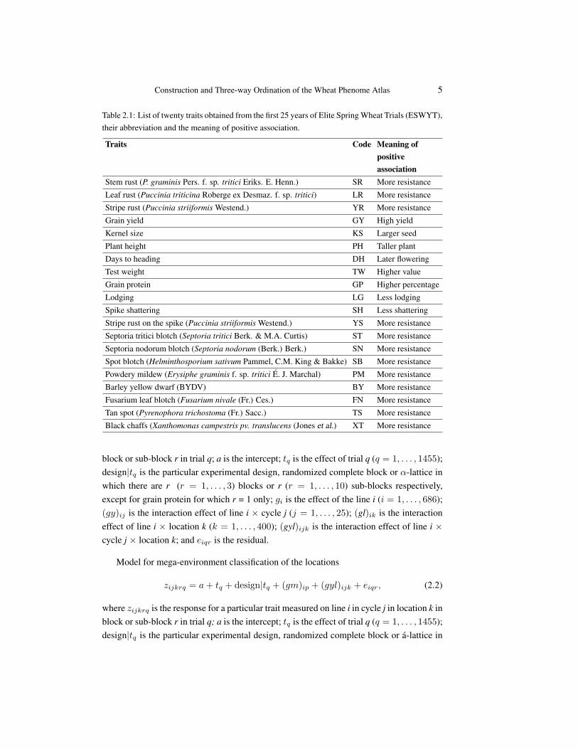
Table 2.1: List of twenty traits obtained from the first 25 years of Elite Spring Wheat Trials (ESWYT),their abbreviation and the meaning of positive association.

Traits Code Meaning ofpositiveassociation

Stem rust (P. graminis Pers. f. sp. tritici Eriks. E. Henn.) SR More resistance

Leaf rust (Puccinia triticina Roberge ex Desmaz. f. sp. tritici) LR More resistance

Stripe rust (Puccinia striiformis Westend.) YR More resistance

Grain yield GY High yield

Kernel size KS Larger seed

Plant height PH Taller plant

Days to heading DH Later flowering

Test weight TW Higher value

Grain protein GP Higher percentage

Lodging LG Less lodging

Spike shattering SH Less shattering

Stripe rust on the spike (Puccinia striiformis Westend.) YS More resistance

Septoria tritici blotch (Septoria tritici Berk. & M.A. Curtis) ST More resistance

Septoria nodorum blotch (Septoria nodorum (Berk.) Berk.) SN More resistance

Spot blotch (Helminthosporium sativum Pammel, C.M. King & Bakke) SB More resistance

Powdery mildew (Erysiphe graminis f. sp. tritici E. J. Marchal) PM More resistance

Barley yellow dwarf (BYDV) BY More resistance

Fusarium leaf blotch (Fusarium nivale (Fr.) Ces.) FN More resistance

Tan spot (Pyrenophora trichostoma (Fr.) Sacc.) TS More resistance

Black chaffs (Xanthomonas campestris pv. translucens (Jones et al.) XT More resistance

block or sub-block r in trial q; a is the intercept; tq is the effect of trial q (q = 1, . . . , 1455);design|tq is the particular experimental design, randomized complete block or α-lattice inwhich there are r (r = 1, . . . , 3) blocks or r (r = 1, . . . , 10) sub-blocks respectively,except for grain protein for which r = 1 only; gi is the effect of the line i (i = 1, . . . , 686);(gy)ij is the interaction effect of line i × cycle j (j = 1, . . . , 25); (gl)ik is the interactioneffect of line i × location k (k = 1, . . . , 400); (gyl)ijk is the interaction effect of line i ×cycle j × location k; and eiqr is the residual.

Model for mega-environment classification of the locations

zijkrq = a + tq + design|tq + (gm)ip + (gyl)ijk + eiqr, (2.2)

where zijkrq is the response for a particular trait measured on line i in cycle j in location k inblock or sub-block r in trial q; a is the intercept; tq is the effect of trial q (q = 1, . . . , 1455);design|tq is the particular experimental design, randomized complete block or a-lattice in

6 V. N. Arief et al.

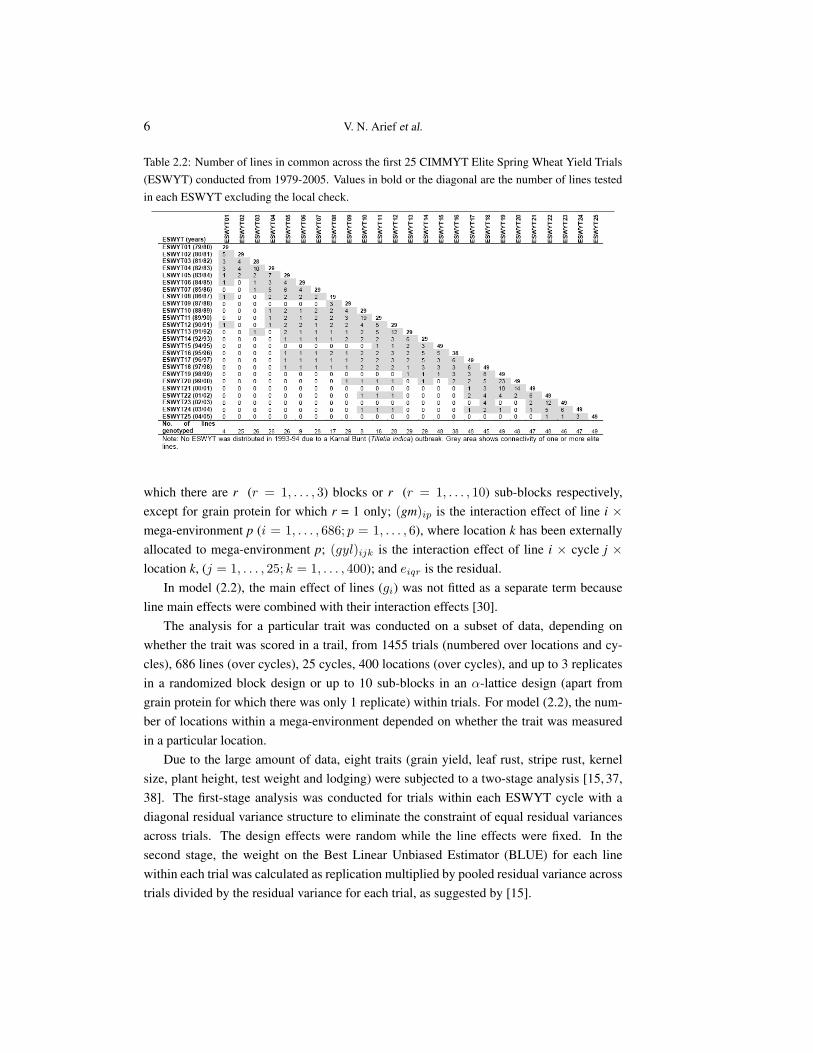
Table 2.2: Number of lines in common across the first 25 CIMMYT Elite Spring Wheat Yield Trials(ESWYT) conducted from 1979-2005. Values in bold or the diagonal are the number of lines testedin each ESWYT excluding the local check.

which there are r (r = 1, . . . , 3) blocks or r (r = 1, . . . , 10) sub-blocks respectively,except for grain protein for which r = 1 only; (gm)ip is the interaction effect of line i ×mega-environment p (i = 1, . . . , 686; p = 1, . . . , 6), where location k has been externallyallocated to mega-environment p; (gyl)ijk is the interaction effect of line i × cycle j ×location k, (j = 1, . . . , 25; k = 1, . . . , 400); and eiqr is the residual.

In model (2.2), the main effect of lines (gi) was not fitted as a separate term becauseline main effects were combined with their interaction effects [30].

The analysis for a particular trait was conducted on a subset of data, depending onwhether the trait was scored in a trail, from 1455 trials (numbered over locations and cy-cles), 686 lines (over cycles), 25 cycles, 400 locations (over cycles), and up to 3 replicatesin a randomized block design or up to 10 sub-blocks in an α-lattice design (apart fromgrain protein for which there was only 1 replicate) within trials. For model (2.2), the num-ber of locations within a mega-environment depended on whether the trait was measuredin a particular location.

Due to the large amount of data, eight traits (grain yield, leaf rust, stripe rust, kernelsize, plant height, test weight and lodging) were subjected to a two-stage analysis [15, 37,38]. The first-stage analysis was conducted for trials within each ESWYT cycle with adiagonal residual variance structure to eliminate the constraint of equal residual variancesacross trials. The design effects were random while the line effects were fixed. In thesecond stage, the weight on the Best Linear Unbiased Estimator (BLUE) for each linewithin each trial was calculated as replication multiplied by pooled residual variance acrosstrials divided by the residual variance for each trial, as suggested by [15].

Construction and Three-way Ordination of the Wheat Phenome Atlas 7

Association analysis

A two-step procedure [40] was adopted for each of the association analyses which pro-duced the ten phenome maps in WPA1.0. Firstly, BLUPs were calculated for each linefor each trait for each structure (see below for definition of structure) using an appropriatemixed-model analysis of variance (as defined above). Secondly, the log scores (probabili-ties expressed as − log10 P for probability P ) that an association with each marker existedwere calculated using a linear contrast of the phenotype BLUP values for marker classes.Single marker genome scans were conducted for each trait and structure. Due to the lackof consensus and physical maps, markers were ordered within each chromosome based onthe haplotype disequilibrium map from the overall analysis [2].

The concept of linkage disequilibrium (LD) blocks was used to deal with the co-linearity problem due to non-independent markers [1]. Strict criteria for declaring LDblocks were used to ensure that the identified block was due to linkage and not other fac-tors that could have caused disequilibrium (such as selection) [17]. A true LD block is a setof markers that are in complete disequilibrium as they have no recombination in the popu-lation studied [39]. In practice, a small amount of recombination is allowed depending onthe map resolution and population size. This approach reduces the number of markers to622 LD blocks (including blocks with a single marker). If any LD block showed significantassociations with a trait (based on a predetermined threshold), this block was referred toas a Trait Associated Marker (TAM) block, e.g. when an LD block has a significant as-sociation with stem rust it is a TAM block for stem rust. Each of these TAM blocks wasconsidered to mark a single putative region of the chromosome. A log-score of four wasdeemed to represent a significant association of marker with trait, as it corresponded to afamily-wise error rate of about 5%. Each TAM block was coded using chromosome asthe first two characters followed by a number that indicated the order of the block in thatchromosome (e.g. 1A.1).

An important characteristic of lines (entries) in the ESWYT is that approximately halfcarry a translocation from the rye genome. An arm of rye chromosome 1 replaces theshort arm of the bread wheat chromosome 1B. The normal bread wheat chromosome isdesignated 1BL/1BS and the one with the translocation is designated 1BL/1RS. This chro-mosome arm in the ESWYT population acts as a single TAM block and is designated as1R.1 in the figures. It will be shown that this block is associated with 14 of the 20 traitsexamined to produce the WPA and, as a consequence, is one of the most influential TAMblocks in the analyses.

8 V. N. Arief et al.

Structures

The effect of population [34, 40, 44] and environment [5, 14] structure onTAM block profiles was investigated by constructing ten different maps, eachthe result of an association analysis on a particular structuring of the data(http://www.uq.edu.au/lcafs/phenomeatlas/).

The first was an association analysis of the overall data. The next six used three pop-ulation structures (grouping lines prior to association analysis based on marker, pedigreeand phenotypic data) by two analytical methods (the first analytical method fitting betweengroup main effects in the prediction of the BLUPs, while the second calculated BLUPs foreach group separately). The next two were for environment structures, the first of whichwas defined by grouping locations based on the CIMMYT mega-environment classifica-tion [6], while the second was defined by grouping locations based on the phenotypic datafor the 20 traits from all trials. The last was a combination of both population and environ-mental structure defined by grouping lines and locations based on the ESWYT cycles.

As indicated earlier, only the analyses from the overall data and from two of CIM-MYT’s mega-environments are presented here. ME1 refers to low latitude (<40◦), irri-gated desert environments, while ME2 refers to low latitude, high rainfall (>500ml/yr)environments [6].

Preparation of the three-way three-mode data

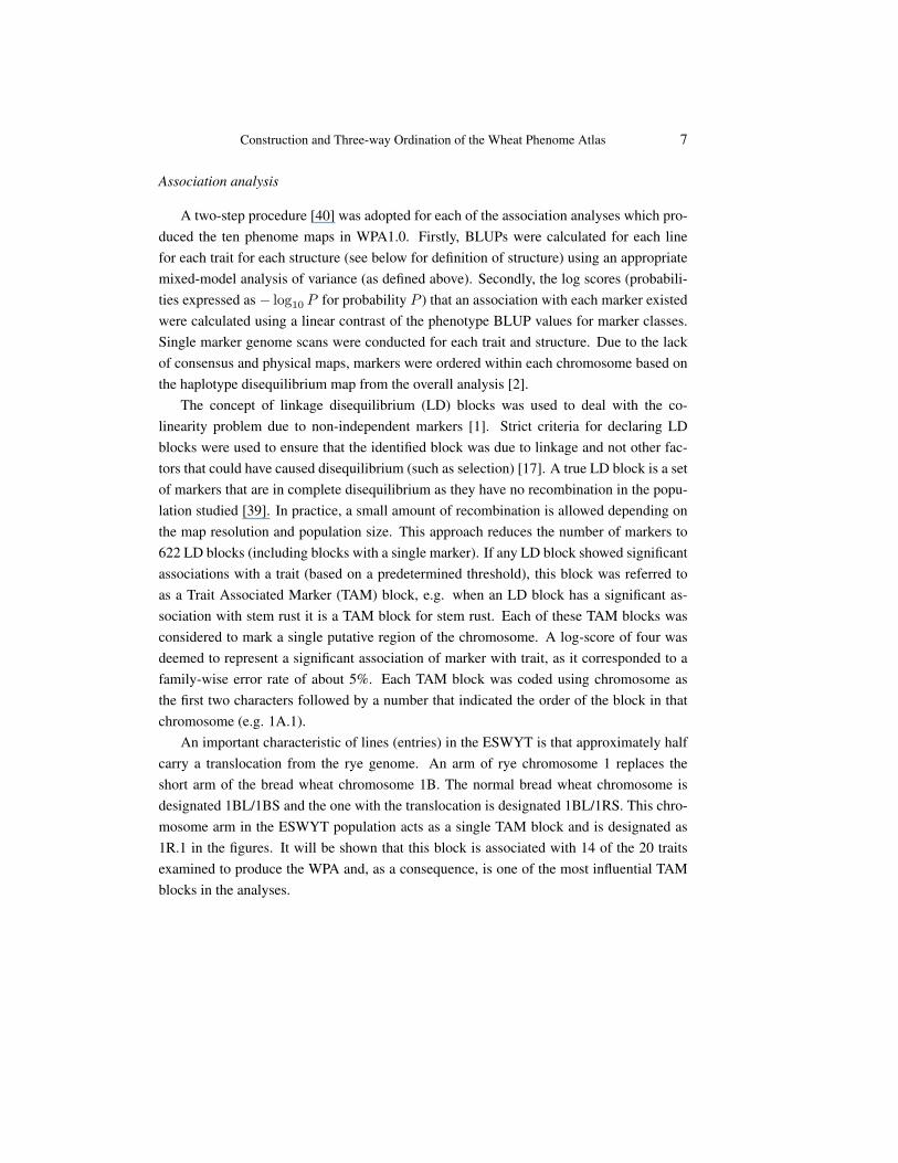
Markers show either positive, negative or no association with a trait. Positive associa-tion was defined as the presence of a marker corresponding to a better phenotypic value,while negative association was the presence of a marker corresponding to a worse pheno-typic value. The combination of presence or absence of a marker with its type of associationwas used to obtain a TAM score for each line (+1 or −1). A score of zero corresponded tono significant association. When a marker was missing, the TAM score for the marker wasset as NA (not applicable) (Figure 2.1a). An LD block score was set equal to the predom-inant TAM score for the markers within the LD block (after eliminating NA values). Thisprocedure was repeated for each of the 599 lines, 622 LD blocks and 20 traits. If an LDblock showed significant association for at least one trait, it was defined as a TAM block.This resulted in a three-way three-mode line× TAM block× trait data array (Figure 2.1b).Traits with all zero TAM block scores were excluded from the datasets being analysed bythree-way PCA.

Three-way PCA

Since information about the lines and their interaction with TAM blocks was of interest,the data were column centred before applying the three-way PCA model [24, Chapter 6].To understand the effect of this centring, the three-way data can be written as if they were

Construction and Three-way Ordination of the Wheat Phenome Atlas 9

Figure 2.1: Schematic diagram of data preparation. (a) Definition of marker-trait association profiles;and (b) their presentation in a three-way three-mode data array. (NA = Not applicable).

generated by a multivariate two-way analysis-of-variance design:

xkij = µk + αk

i + βkj + (αβ)k

ij , (2.3)

where xkij is the value of trait k for line i for TAM block j; µk is the grand mean of trait

k over all lines and TAM blocks; αki is the main effect of line i for trait k across all TAM

blocks; βkj is the main effect of TAM block j for trait k across all lines; and the remaining

term is the line× TAM block interaction for trait k [41,42]. Centring per TAM block acrosslines for each trait leads to

xkij = αk

i + (αβ)kij , (2.4)

where the TAM block means per trait were removed and the line mean per trait and thetwo-way line × TAM block interaction per trait were retained [42]. The choice of centringneeds to be investigated further, as the three-way three-mode array defined above (beforeapplying this centring) has all values of the same type and scale.

While occurrences of missing values are unavoidable, a maximum of 0.4% were ob-tained in the three-way arrays used in the illustrations presented here. These missingvalues were estimated using single imputation via an iterative-expectation maximizationprocedure in which the missing data procedure is incorporated in the model [24, p.150].

Full details of the three-way PCA can be found in [24] and only a brief description isgiven here. The formal model for three-way ordination can be written as

xijk =P∑

p=1

Q∑q=1

R∑r=1

(aipbjqckr)gpqr + eijk, (2.5)

where xijk is the response for line i, TAM block j and trait k; P, Q and R are the number ofcomponents for lines, TAM blocks and traits; aip, bjk, ckr are the component coefficientsfor lines, TAM blocks and traits; gpqr is the joint weight of the pth line component, qth

10 V. N. Arief et al.

TAM block component and rth trait component; and eijk is the residual. The gpqr valuesconstitute the core array and can be interpreted in several ways [24, p.225]. As the squareof each element in this core array indicates the explained variation for that combinationof components, we can interpret their sum (divided by the total sum of squares) to be thepercentage of explained variation by the P×Q×R model of the data. It is desirable to havelow numbers of P, Q and R for ease of interpretation, but some information is inevitably lostwhen the data are represented in a reduced space [25]. Several formal tests are availableto asses the adequacy of the model [24, Chapter 8], however the choice of dimensionalityis not always obvious and can be subjective [26], and should be determined not only on astatistical-based but also on a content-based argument (see [24, p.208] and [3]).

The results of the three-way analysis can be shown in a joint biplot that displays thecomponent scores for two modes associated with each component of the third mode (see[24, pp.273–276] and [25]). This joint biplot is a variant of the standard biplot, thus theinterpretation is similar to that for standard biplots [19]. In interpreting the joint biplotfor a particular trait component, lines distributed along the arrows representing the vectorsof the TAM block are positively associated with that TAM block, while lines distributedalong the opposite direction of the arrow (vector) are negatively associated with that TAMblock [12]. The angle between two arrows (vectors) is a rough indicator of the relationshipbetween these two TAM blocks in that 90◦ indicates no correlation and 180◦ indicates anegative association. Detail explanations about joint biplot interpretation and examples aregiven in [24].

A rotation of components based on the varimax model was conducted for the vectorsin the joint biplot for ease of interpretation [24, pp.237-243]. Symmetrical scaling wasused for all joint biplots [23] and additional rescaling was conducted so that the maximumlength of vectors would be the same as the maximum distance of points from the origin.All three-way PCA analyses were conducted using the 3WayPack software (http://three-mode.leidenuniv.nl/).

For the joint biplots produced here, lines located near the origin of the plots are eithernot modelled well or have an “average” response. For display purposes, only TAM blocksand traits that explained most of the variability in the data were labelled. The names of 32released cultivars (Table 2.3) were displayed in the joint biplot.

3 Results and Discussion

Construction of the WPA1.0

The WPA1.0 can be found at http://www.uq.edu.au/lcafs/phenomeatlas/. The map cor-responding to the association analysis of the overall data (Figure 3.1) and those correspond-ing to mega-environments 1 and 2 (ME1 and ME2; Figure 3.2) are shown here.

Construction and Three-way Ordination of the Wheat Phenome Atlas 11

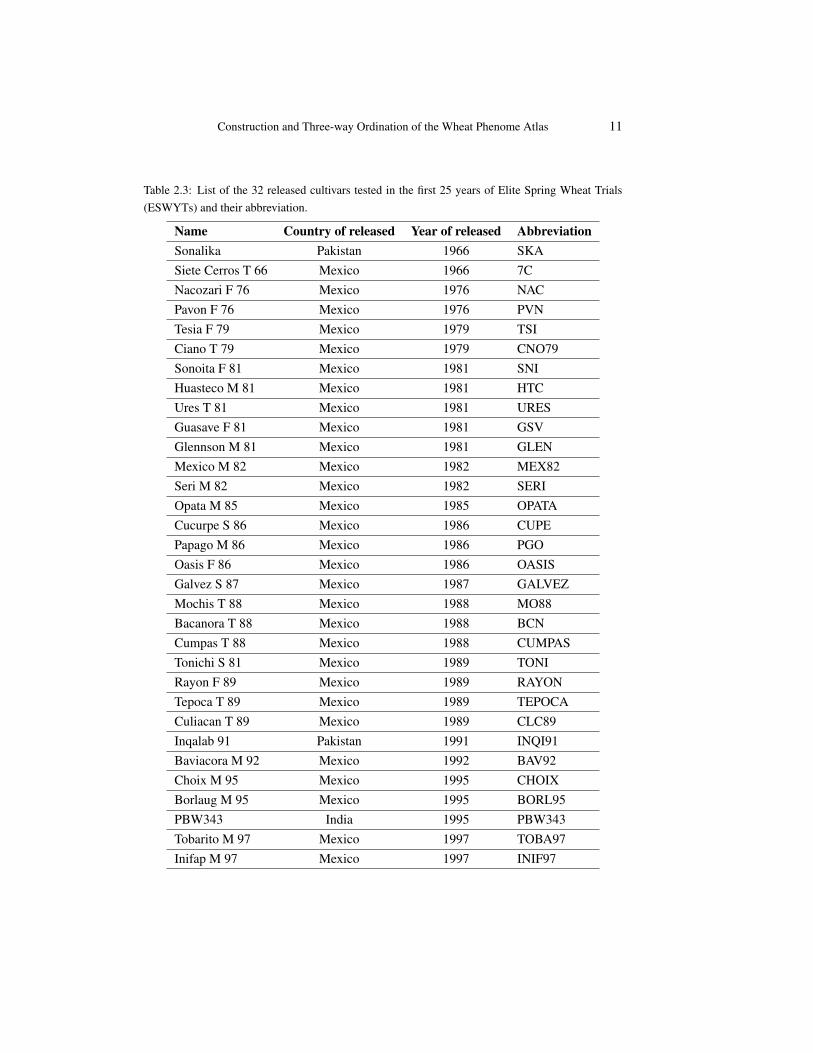
Table 2.3: List of the 32 released cultivars tested in the first 25 years of Elite Spring Wheat Trials(ESWYTs) and their abbreviation.

Name Country of released Year of released AbbreviationSonalika Pakistan 1966 SKASiete Cerros T 66 Mexico 1966 7CNacozari F 76 Mexico 1976 NACPavon F 76 Mexico 1976 PVNTesia F 79 Mexico 1979 TSICiano T 79 Mexico 1979 CNO79Sonoita F 81 Mexico 1981 SNIHuasteco M 81 Mexico 1981 HTCUres T 81 Mexico 1981 URESGuasave F 81 Mexico 1981 GSVGlennson M 81 Mexico 1981 GLENMexico M 82 Mexico 1982 MEX82Seri M 82 Mexico 1982 SERIOpata M 85 Mexico 1985 OPATACucurpe S 86 Mexico 1986 CUPEPapago M 86 Mexico 1986 PGOOasis F 86 Mexico 1986 OASISGalvez S 87 Mexico 1987 GALVEZMochis T 88 Mexico 1988 MO88Bacanora T 88 Mexico 1988 BCNCumpas T 88 Mexico 1988 CUMPASTonichi S 81 Mexico 1989 TONIRayon F 89 Mexico 1989 RAYONTepoca T 89 Mexico 1989 TEPOCACuliacan T 89 Mexico 1989 CLC89Inqalab 91 Pakistan 1991 INQI91Baviacora M 92 Mexico 1992 BAV92Choix M 95 Mexico 1995 CHOIXBorlaug M 95 Mexico 1995 BORL95PBW343 India 1995 PBW343Tobarito M 97 Mexico 1997 TOBA97Inifap M 97 Mexico 1997 INIF97

12 V. N. Arief et al.

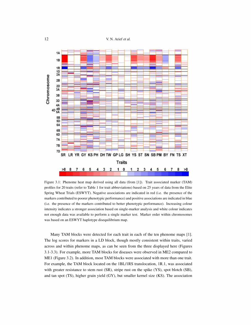
Figure 3.1: Phenome heat map derived using all data (from [1]). Trait associated marker (TAM)profiles for 20 traits (refer to Table 1 for trait abbreviations) based on 25 years of data from the EliteSpring Wheat Trials (ESWYT). Negative associations are indicated in red (i.e. the presence of themarkers contributed to poorer phenotypic performance) and positive associations are indicated in blue(i.e. the presence of the markers contributed to better phenotypic performance). Increasing colourintensity indicates a stronger association based on single-marker analysis and white colour indicatesnot enough data was available to perform a single marker test. Marker order within chromosomeswas based on an ESWYT haplotype disequilibrium map.

Many TAM blocks were detected for each trait in each of the ten phenome maps [1].The log scores for markers in a LD block, though mostly consistent within traits, variedacross and within phenome maps, as can be seen from the three displayed here (Figures3.1-3.3). For example, more TAM blocks for diseases were observed in ME2 compared toME1 (Figure 3.2). In addition, most TAM blocks were associated with more than one trait.For example, the TAM block located on the 1BL/1RS translocation, 1R.1, was associatedwith greater resistance to stem rust (SR), stripe rust on the spike (YS), spot blotch (SB),and tan spot (TS), higher grain yield (GY), but smaller kernel size (KS). The association

Construction and Three-way Ordination of the Wheat Phenome Atlas 13

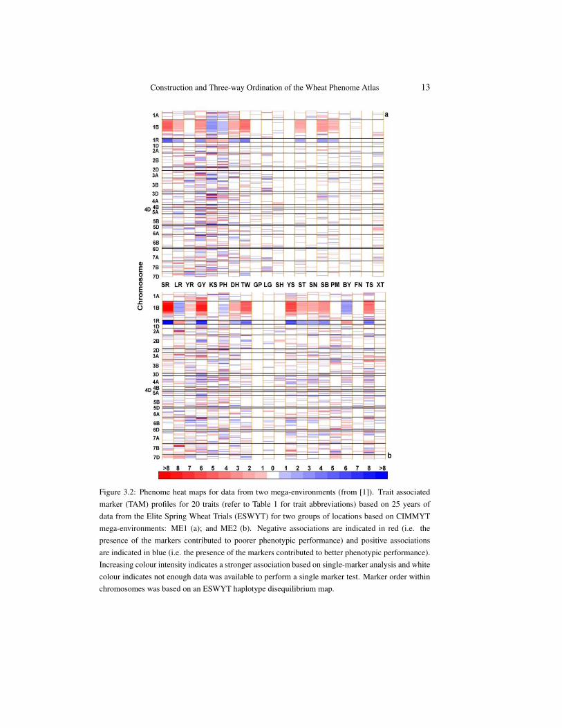
Figure 3.2: Phenome heat maps for data from two mega-environments (from [1]). Trait associatedmarker (TAM) profiles for 20 traits (refer to Table 1 for trait abbreviations) based on 25 years ofdata from the Elite Spring Wheat Trials (ESWYT) for two groups of locations based on CIMMYTmega-environments: ME1 (a); and ME2 (b). Negative associations are indicated in red (i.e. thepresence of the markers contributed to poorer phenotypic performance) and positive associationsare indicated in blue (i.e. the presence of the markers contributed to better phenotypic performance).Increasing colour intensity indicates a stronger association based on single-marker analysis and whitecolour indicates not enough data was available to perform a single marker test. Marker order withinchromosomes was based on an ESWYT haplotype disequilibrium map.

14 V. N. Arief et al.

of this TAM block with stem rust and stripe rust reflects the presence of two linked genes,Sr31 [36] and Yr9 [28], on this translocation.

The three heat maps reported here have demonstrated that the numbers and magni-tude of markers and genomic locations associated with traits varies with the germplasminvestigated, and the environments in which the germplasm was evaluated. Such contextdependency has been reported for QTL studies in several species, including wheat [27].

The use of environment structures based on mega-environment classification reveals in-formation about genotype by environment interactions and can be used to identify TAMs orTAM blocks for specific environments. The comparison of the phenome maps showed thatthere were substantially more associations in the wetter environments (ME2) for the foliardiseases other than rusts compared to the drier environment (ME1). This was expected, asthe non-rust foliar diseases occur more frequently in higher rainfall environments [6].

Three-way PCA

Illustration 1: Overall phenome map

Data set. For this illustration, the overall phenome map was used to obtain TAM blockinformation. The first dataset consisted of 599 lines × 288 TAM blocks × 16 traits andwas chosen to evaluate the line × TAM block × trait pattern of the ESWYTs. For three-way ordination, the 2×3×2 model explained 16.2% of the variability in the data. Due tothe orthogonality of all component matrices, this variability may be partitioned for eachmode separately. In the left-hand column of Figure 3.3, the trait components (Figure 3.3a)explain 13.3% and 2.9% and the axes of the joint biplot for the first trait axis (Figure 3.3b)partition the 13.3% further into 7.5% and 5.8%, while the axes of the second joint biplot(Figure 3.3c) partition the 2.9% into 2.1% and 0.8%. The number of joint biplot axesis equal to the smaller of the number of chosen components for these two modes, i.e., 2here [24, p.273].

Traits (Figure 3.3a). The plot for traits showed grain yield (GY), stem rust (SR) andspot blotch (SB) accounted for most of the variation on the first axis, while kernel size (KS)accounted for the variation on the second axis.

First trait component joint biplot (Figure 3.3b). The joint biplot of lines× TAM blocksfor the first trait component described the pattern of lines × TAM blocks for grain yield(GY), stem rust (SR) and spot blotch (SB). In this figure, the TAM blocks can be seen toconsist of two groups: one dominated by the blocks 1R.1, 1B.3/4/5, the other by the blocks1B.2/6/11 and 4A.11/12. At the same time, we see that the lines appear to be in two majorclusters (referred to as North and South given their location in the plot) a number of whichare explicitly identified. To explain which TAM blocks are responsible for the separation ofthe clusters of lines, we extended the lines of the TAM block groups to their negative sideso that we can evaluate the projections of the lines on the TAM blocks. The North cluster isprimarily characterised by positive values on the 1R.1 and the 1B.3/4/5 TAM blocks, while

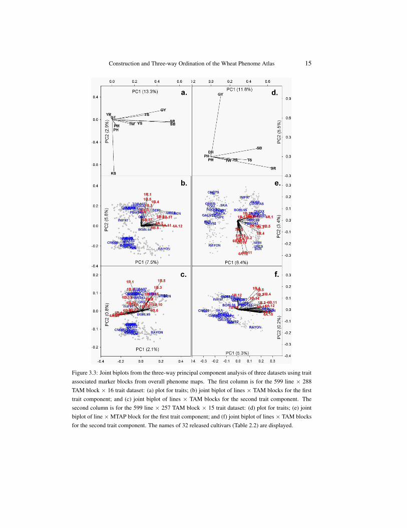
Construction and Three-way Ordination of the Wheat Phenome Atlas 15

Figure 3.3: Joint biplots from the three-way principal component analysis of three datasets using traitassociated marker blocks from overall phenome maps. The first column is for the 599 line × 288TAM block × 16 trait dataset: (a) plot for traits; (b) joint biplot of lines × TAM blocks for the firsttrait component; and (c) joint biplot of lines × TAM blocks for the second trait component. Thesecond column is for the 599 line × 257 TAM block × 15 trait dataset: (d) plot for traits; (e) jointbiplot of line × MTAP block for the first trait component; and (f) joint biplot of lines × TAM blocksfor the second trait component. The names of 32 released cultivars (Table 2.2) are displayed.

16 V. N. Arief et al.

the South cluster of lines have negative values on these TAM blocks. The other group ofTAM blocks, especially 4A.11/12 are responsible for the spread within the two line clustersrather than for their separation. As an example Rayon has positive values on 4A.11/12, butnegative values on 1R.1 and 1B.3/4/5 (within the accuracy of the approximation).

Second trait component joint biplot (Figure 3.3c). The joint biplot for the second traitcomponent described the pattern for kernel size (KS). The same North and South clustersof lines are visible again in this figure, be it that they are more compact. The groupingof the TAM blocks, however, is rather different. For instance, 1R.1 and 1B.4 are stilltogether but not with 1B.3/5 which has a clear angle with the other two TAM blocks. Othergroups of TAM blocks play a dominant role, e.g., several TAM block in chromosome 6Band a group of the lines 4A.20/4, 6B.7 and 1B.1, indicating that for kernel size (KS) therelationship between lines and TAM blocks is rather different from that for the other traits.The North and South clusters are still due to 1R.1, 1B.4 and 1B.3/5, but 1B.3/5 togetherwith 4A.20/4, 6B.7 and 1B.1 are now responsible for the differences within the clusters.Rayon, for instance, shows a strong contrast on the 6th chromosome with positive valueson 6B.6/10 but negative ones on 6B.7/8.

Data. Based on these results, a second dataset was constructed by removing kernelsize (KS) (because it was effectively the only attribute accounting for the variation on thesecond axis), resulting in 599 lines × 257 TAM blocks × 15 traits. The 2×3×2 modelexplained 17.3% of the variability.

Traits (Figure 3.3d). In this dataset, the response for grain yield (GY) is now separatedfrom that for stem rust (SR) and spot blotch (SB).

Lines and TAM blocks (Figures 3.3e and 3.3f).The line × TAM block pattern for spotblotch (SB) and stem rust (SR) still showed TAM blocks 1R.1 and 1B.3/4/5 to be responsi-ble for the two clusters of lines, while chromosomes 4A, 1B, 6B and the 1BL/1RS translo-cation as the ones that contributed to the discrimination among lines (Figure 3.3e). Theline × TAM block pattern for grain yield (GY) showed a similar pattern to the one fromthe previous dataset, but with an additional TAM block in chromosome 7B.

Variation accounted for. It may not seem that accounting for 16-17% of the variation isworthwhile. However, a large part of the systematic variation in the data has been removedby centring. We are looking at only the variation contained in two terms which also containthe main part of the error/noise. The aim is to fit a large part of the systematic variation inthese two terms and this is being achieved, as demonstrated by the clear patterns obtainedfrom the analysis.

Conclusions. In both these datasets, the patterns of lines were consistent. Ures T81 (URES), Bacanora T 88 (BCN) were close to each other. This relationship reflectedtheir parentage (URES is the parent of BCN). Most of these 32 released cultivars weregrouped together, except for Rayon F 89 (RAYON) that seems to have different TAM blockcombinations than the others.

Construction and Three-way Ordination of the Wheat Phenome Atlas 17

Illustration 2: Mega-environments (ME)

Data. For the second illustration, TAM block information was obtained from TAMsobserved for ME1 and ME2. This illustration was chosen to compare patterns in two mega-environments. The ME1 dataset consisted of 599 lines × 202 TAM blocks × 12 traits andthe ME2 dataset consisted of 599 lines × 218 TAM blocks × 17 traits. The 2×3×2 modelexplained 16.4% of the variability in the ME1 dataset and the 2×2×2 model explained16.6% in the ME2 dataset.

Traits (Figures 3.4a and 3.4d). Kernel size (KS) and grain yield (GY) explained mostof the variability in the ME1 dataset (Figure 3.4a); while grain yield (GY) and stem rust(SR) explained most of the variability in the ME2 dataset (Figure 3.4d).

ME1 joint biplots (Figures 3.4b and 3.4c). The joint biplot for the first trait componentin the ME1 dataset described the line × TAM block pattern for grain yield (GY) (Figure3.4b). No major clustering of lines was observed and many TAM blocks displayed variabil-ity. Known high-yielding cultivars (e.g. Seri M 82, SERI) did not have these TAM blockcombinations. The joint biplot for the second trait component (i.e. kernel size (KS), Figure3.4c) showed that the TAM blocks appeared to be in four groups. Two groups of theseTAM block were negatively correlated (5B.8/9 and 6B.2 versus 3A.30, 1B.3/5) indicatingthat none of the 599 lines carry both sets of TAM blocks. No obvious grouping of lineswas observed, indicating that no particular TAM blocks occurred more often in this dataset.The TAM block in the 1BL/1RS translation, i.e. 1R.1, did not have a large variation in thisdataset.

ME2 joint biplots (Figures 3.4e and 3.4f). The joint biplot for the first trait componentin the ME2 dataset described the line × TAM block pattern for grain yield (GY), testweight (TW), stem rust (SR), stripe rust (YR) and tan spot (TS), while the joint biplot forthe second trait component described the pattern for grain yield (GY), test weight (TW) andstem rust (SR) (Figure 3.4d). Similar patterns were observed in both joint biplots (Figure3.4e and 3.4f). Lines appeared to be divided into two clusters, mainly due to TAM blocksin chromosome 1B. 1R.1 contributed as well, but less so in the first joint biplot. The TAMblocks on the 4A chromosome were for a large part responsible for the spread within theclusters of lines.

Different patterns for lines were observed in ME1 and ME2 (Figure 3.4). The patternof lines in ME2 was more similar to that observed in the previous illustration (Figure 3.3a-c). The pattern for the 32 released cultivars in ME2 showed that RAYON tended to havedifferent TAM block combinations than the other cultivars (Figures 3.4e and f), but in ME1it had similar TAM block combinations to BCN and URES.

18 V. N. Arief et al.

Figure 3.4: Joint biplots from the three-way principal component analysis of datasets obtained fromtrait associated marker blocks from phenome maps for each of two mega-environments. The firstcolumn is for the 599 line × 202 TAM block × 12 trait data set for ME1: (a) plot for traits; (b) jointbiplot of lines × TAM blocks for the first trait component; (c) joint biplot of lines × TAM blocksfor the second trait component. The second column is for the 599 line × 218 TAM block × 17 traitdataset for ME2: (d) plot for traits; (e) joint biplot of line × TAM block for the first trait component;and (f) joint biplot of lines × TAM blocks for the second trait component. The names of 32 releasedcultivars (Table 2.2) are displayed.

Construction and Three-way Ordination of the Wheat Phenome Atlas 19

General Comments

In summary, the application of population and environmental structure has shown thatfor associations to be identified there must be polymorphism for both the markers (in theset of germplasm evaluated) and phenotypes (for those lines in the environments of test) inthe study conducted. In addition, that the number and patterns of TAMs or TAM blocks forindividual traits differ in a context-dependent manner is demonstrated by the disappearanceof the 1BL/1RS translocation associations when the population was structured on the basisof mega-environments.

A large number of TAM blocks were identified for most of the 20 traits investigated(Figures 3.1 and 3.2) and association profiles differed for each structure used in the analysis.For diseases, the profiles also were dependent on the presence of the pathogen in any yearor location.

Based on marker-trait association analysis of the overall data, we identified markersthat were suspected to indicate the 1BL/1RS translocation. These results were confirmedby comparing haplotypes of the lines known to be carrying or not carrying the translocation.These markers were assigned to the 1BL/1RS translocation and used in the heatmaps.

A three-way PCA on a line × TAM block × trait dataset provides a practical approachto understanding TAM information in the WPA1.0. This technique provides a summariza-tion of lines × TAM blocks × traits that can be evaluated to gain insight into the complexpatterns in these data arrays. It can also be used to describe the breeding program andto assist in selection. Two illustrations were presented here, with large numbers of lines,TAM blocks and traits able to be considered. The objective of the study will determine theparticular line × TAM block × trait combination to be analysed.

The line × TAM block × trait array observed using overall data provides a descriptionof the ESWYT breeding program over 25 cycles (Figure 3.3). It also provides a descriptionof the germplasm. During this time, half of the lines tested have the 1BL/1RS translocationthat was reflected in the observed pattern. Note that the relative importance of multipleattributes in the analysis depends on their statistical characteristics and this does not nec-essarily correspond to their agronomic or genetic importance [26]. Therefore, the mostimportant TAM blocks were the ones that had the highest variability in the dataset and theydetermine the outcome of the analysis. Thus, removing dominant trait(s) from the analy-sis enables the pattern for less variable traits to be displayed. A similar approach can beapplied to TAM blocks or lines. Illustration 1 demonstrated that over the 25 years of theESWYT breeding program, most of the variability in TAM blocks was from chromosomes1 and 6 in the B genome. However, when kernel size was removed, additional TAM blocksin other genomes (A and D) and chromosomes (2, 4 and 7) became apparent.

Different patterns of lines × TAM blocks were observed from different combinationsof line × TAM block × trait arrays, demonstrating the context dependency of marker-trait

20 V. N. Arief et al.

association studies. In ME2, stem rust (SR) was one of the most important traits (Figure3.4d); while in ME1 it was not important (Figure 3.4a). These results indicated that therewas little or no incidence of stem rust in ME1 in the 25 years of ESWYTs. TAMs fromseveral sources (i.e. phenome maps) can also be combined to study the pattern acrossTAMs.

The results of three-way PCA provide information about which TAM block combi-nations were favourable for particular combinations of traits. It also provides informationabout the TAM block combinations for each line. Note that depending on whether the TAMblock is positively or negatively correlated with a trait, a line that has the TAM blocks caneither have the markers or not. For example, the TAM block in the 1BL/1RS translocation,1R.1, was negatively associated with kernel size. Thus, a line that has this TAM block doesnot carry the translocation and has bigger kernel size (KS) (Figure 3.4c). The observed pat-tern was only for those TAM blocks which associated with the traits and have large enoughvariability. In ME1, the TAM block in 1BL/1RS, 1R.1, was not associated with grain yieldin ME1, but many other TAM blocks were (Figure 3.4b). It also showed the tendency forcultivars that carry this translocation to not have other TAM block combinations (exceptfor Glennson M81, GLEN). The fact that many TAM blocks corresponded to higher yieldalso indicated that there were many possible appropriate combinations with increased grainyield.

The use of known TAMs or cultivars is helpful in understanding and interpreting theresponse pattern. They can help identify new lines which have a similar or opposite patternof response. For example, by comparing with known cultivars new lines with similar oropposite pattern of response can be identified. This information can assist selection, designof crosses, or screening of lines. Note that the TAM blocks presented here are not nec-essarily affecting the traits directly, since association analysis does not infer any causativeeffect [4]. The pattern of the observed TAM blocks can be due to the results of selectionperformed during the breeding program.

Acknowledgments

The first author thanks the Endeavour International Postgraduate Research Scholarshipfor financial support during the course of her PhD Studies. Financial support from theUniversity of Queensland and CIMMYT is also gratefully acknowledged. The authorsacknowledge the co-operation of national partners who kindly recorded the field data usedhere. Helpful referee comments improved the manuscript and were much appreciated.

Construction and Three-way Ordination of the Wheat Phenome Atlas 21

References

[1] V. Arief, I.H. DeLacy, M.J. Dieters, J. Crossa, I. Godwin, J. Batley, G. Davenport,S. Dreisigacker, E. Duveiller, D. Edwards, E. Huttner, C. Lambrides, Y. Manes, T.Payne, R.P. Singh, M. Warburton, P. Wenzl, A. Kilian, G. McLaren, H.-J. Braun,J. Crouch, R. Ortiz and K.E. Basford, (2008). Marker-trait associations identified inspring wheat using 25 years of CIMMYT international trials, in: 11th InternationalWheat Genetics Symposium, R. Appels, R. Eastwood, E. Lagudah, P. Langridge, M.Mackay, L. McIntyre and P. Sharp, Eds., Sydney University Press, Brisbane, 27.http://www.handle.net/2123/3303.

[2] V.N. Arief, I.H. DeLacy, P. Wenzl and M.J. Dieters, (2009). Genetic disequilibriummapping using high-throughput data from a plant breeding program, in: 14th Aus-tralian Plant Breeding and 11th SABRAO, Cairns.

[3] K. E. Basford, P. M. Kroonenberg and I. H. DeLacy, (1991). Three-way methods formultiattribute genotype x environment data: an illustrated partial survey, Field CropsResearch 27, 131–157.

[4] W. D. Beavis, (1998). QTL Analyses: Power, precision, and accuracy, in: MolecularDissection of Complex Traits, A. H. Paterson, Ed., CRC Press, Boca Raton, 145–162.

[5] M. P. Boer, D. Wright, L. Feng, D. W. Podlich, L. Luo, M. Cooper and F. A. vanEeuwijk, (2007). A mixed-model quantitative trait loci (QTL) analysis for multiple-environment trial data using environmental covariables for QTL-by-environment in-teractions, with an example in maize, Genetics 177, 1801–1813.

[6] H.-J. Braun, S. Rajaram and M. van Ginkel, (1996). CIMMYT’s approach to breedingfor wide adaptation, Euphytica 92, 175–183.

[7] F. Breseghello and M. E. Sorrells, (2006). Association analysis as a strategy for im-provement of quantitative traits in plants, Crop Science 46, 1323–1330.

[8] S. C. Chapman, J. Crossa, K. E. Basford and P. M. Kroonenberg, (1997). Genotype byenvironment effects and selection for drought tolerance in tropical maize. 2. Three-mode pattern analysis, Euphytica 95, 11–20.

[9] M. Cooper, S. C. Chapman, D. W. Podlich and G. L. Hammer, (2002). The GP prob-lem: Quantifying gene-to-phenotype relationships, In Silico Biology 2, 151–164.

[10] M. Cooper, F. A. van Eeuwijk, G. L. Hammer, D. W. Podlich and C. Messina, (2009).Modelling QTL for complex traits: detection and context for plant breeding, CurrentOpinion in Plant Biology 12, 231–240.

[11] M. Cooper, D. R. Woodruff, I. G. Phillips, K. E. Basford and A. R. Gilmour, (2001).Genotype-by-management interactions for grain yield and grain protein concentrationof wheat, Field Crops Research 69, 47–67.

[12] J. Crossa, K. Basford, S. Taba, I. DeLacy and E. Silva, (1995). Three-mode analysesof maize using morphological and agronomic attributes measured in multilocationaltrials, Crop Science 35, 1483–1491.

22 V. N. Arief et al.

[13] J. Crossa, J. Burgueno, S. Dreisigacker, M. Vargas, S. A. Herrera-Foessel, M.Lillemo, R. P. Singh, R. Trethowan, M. Warburton, J. Franco, M. Reynolds, J.H. Crouch and R. Ortiz, (2007). Association analysis of historical bread wheatgermplasm using additive genetic covariance of relatives and population structure,Genetics 177, 1889–1913.

[14] J. Crossa, M. Vargas, F. A van Eeuwijk, C. Jiang, G. O. Edmeades and D. Hoisington,(1999). Interpreting genotype x environment interaction in tropical maize using linkedmolecular markers and environmental covariables, Theoretical and Applied Genetics99, 611–625.

[15] B. R. Cullis, F. M. Thomson, J. A. Fisher, A. R. Gilmour and R. Thompson, (1996).The analysis of the NSW wheat variety database. I. Modelling trial error variance,Theoretical and Applied Genetics 92, 21–27.

[16] K. E. D’Andrea, M. E. Otegui and A. J. de la Vega, (2008). Multi-attribute responsesof maize inbred lines across managed environments, Euphytica 162, 381–394.

[17] D. S. Falconer and T. F. C. Mckay, (1996). Introduction to Quantitative Genetics,Longman, Burnt Mill, England.

[18] P. N. Fox, (1996). The CIMMYT wheat program’s international multi-environmenttrials, in: Plant Adaptation and Crop Improvement, M. Cooper, and G.L. Hammer,Eds., CAB International, Wallingford, UK.

[19] K. R. Gabriel, (1971). The biplot graphic display of matrices with application to prin-cipal component analysis, Biometrika 58, 453–467.

[20] A. R. Gilmour, B. J. Gogel, B. R. Cullis, S. J. Welham and R. Thompson, (2006).ASReml User Guide Release 2.0, VSN International Ltd., Hemel Hempstead, HP11ES, UK, 267.

[21] P. K. Gupta, S. Rustgi and P. L. Kulwal, (2005). Linkage disequilibrium and associ-ation studies in higher plants: Present status and future prospects, Plant MolecularBiology 57, 461–485.

[22] D. Jaccoud, K. Peng, D. Feinstein and A. Kilian, (2001). Diversity Arrays: a solidstate technology for sequence information independent genotyping, Nucleic AcidsResearch 29, e25.

[23] P. M. Kroonenberg, (1997). Introduction to biplots for GxE tables, Research ReportNo. 51, Centre for Statistics, The University of Queensland, Brisbane, Australia.

[24] P. M. Kroonenberg, (2008). Applied Mutiway Data Analysis, John Wiley & Sons,Hoboken NJ, USA.

[25] P. M. Kroonenberg and K. E. Basford, (1989). An investigation of multi-attributegenotype response across environments using three-mode principal component anal-ysis, Euphytica 44, 109–123.

[26] P. M. Kroonenberg, K. E. Basford and A. G. M. Ebskamp, (1995). Three-way clusterand component analysis of maize variety trials, Euphytica 84, 31–42.

Construction and Three-way Ordination of the Wheat Phenome Atlas 23

[27] S. Landjeva, V. Korzun and A. Borner, (2007). Molecular markers: actual and po-tential contributions to wheat genome characterization and breeding, Euphytica 156,271–296.

[28] R. C. F. Macer, (1975). Plant pathology in a changing world, Transactions of theBritish Mycological Society 65, 351–374.

[29] I. Mackay and W. Powell, (2007). Methods for linkage disequilibrium mapping incrops, Trends in Plant Science 12, 57–63.

[30] S. O. Omar, P. B. Somonte, L. T. Wilson, A. M. McClung and J. C. Medley, (2005).Targeting cultivars onto rice growing environments using AMMI and SREG GGEbiplot analyses, Crop Science 45, 2414–2424.

[31] R. Ortiz, H.-J. Braun, J. Crossa, J. H. Crouch, G. Davenport, J. Dixon, S. Dreisi-gacker, E. Duveiller, Z. He, J. Huerta, A. K. Joshi, M. Kishii, P. Kosina, Y. Manes,M. Mezzalama, A. Morgounov, J. Murakami, J. Nicol, G. O. Ferrara, J. I. N. Ortiz-Monasterio, T. S. Payne, R. J. Pena, M. P. Reynolds, K. D. Sayre, R. C. Sharma, R.P. Singh, J. Wang, M. Warburton, H. Wu, and M. Iwanaga, (2008). Wheat geneticresources enhancement by the International Maize and Wheat Improvement Center(CIMMYT), Genetic Resources and Crop Evolution, 55, 1095–1140.

[32] A. H. Paterson, S. Damon, J. D. Hewitt, D. Zamir, H. D. Rabinowitch, S.E. Lincoln,E.S. Lander and S.D. Tanksley, (1991). Mendelian factors underlying quantitativetraits in tomato: Comparison across species, generations, and environments, Genetics127, 181–197.

[33] H. D. Patterson and R. Thompson, (1971). Recovery of inter-block information whenblock sizes are unequal, Biometrika 58, 545–554.

[34] J. K. Pritchard, M. Stephens, N. A. Rosenberg and P. Donnelly, (2000). Associationmapping in structured populations, American Journal of Human Genetics 67, 170–181.

[35] F. Rincon, B. Johnson, J. Crossa and S. Taba, (1997). Identifying subsets of maizeaccessions by three-mode principal component analysis, Crop Science 37, 1936–1943.

[36] N. K. Singh, W. Shepperd and R. McIntosh, (1990). Linkage mapping of genes forresistance to leaf, stem and stripe rusts and omega-secalin on the short arm of ryechromosome-1R, Theoretical and Applied Genetics 80, 609–616.

[37] A. Smith, B. Cullis and A. Gilmour, (2001). The analysis of crop variety evaluationdata in Australia, Australian and New Zealand Journal of Statistics 43, 129–145.

[38] A. Smith, B. Cullis and R. Thompson, (2001). Analysis variety by environment datausing multiplicative mixed models and adjustments for spatial field trend, Biometrics57, 1138–1147.

[39] B. Stich, A. E. Melchinger, M. Frisch, H. P. Maurer, M. Heckenberger and J. C. Reif,(2005). Linkage disequilibrium in European elite maize germplasm investigated withSSRs, Theoretical and Applied Genetics 111, 723–730.

24 V. N. Arief et al.

[40] B. Stich, A. E. Melchinger, M. Heckenberger, J. Mohring, A. Schechert and H.-P.Piepho, (2008). Association mapping in multiple segregating populations of sugarbeet (Beta vulgaris L.), Theoretical and Applied Genetics 117, 1167–1179.

[41] F. A. Van Eeuwijk and P. M. Kroonenberg, (1998). Multiplicative models for interac-tion in three-way ANOVA, with applications to plant breeding, Biometrics 54, 1315–1333.

[42] A. J. de la Vega, A. J. Hall and P. M. Kroonenberg, (2002). Investigating the physio-logical bases of predictable and unpredictable genotype by environment interactionsusing three-mode pattern analysis, Field Crops Research 78, 165–183.

[43] J. Wang, M. van Ginkel R. Trethowan and W. Pfeiffer, (2003). Documentation of theCIMMYT Wheat Breeding Programs, Wheat Program CIMMYT, Mexico, 98.

[44] J. Yu and E. S. Buckler, (2006). Genetic association mapping and genome organiza-tion of maize, Current Opinion in Biotechnology 17, 155–160.