Constructing and sampling directed graphs with given degree sequences

This content has been downloaded from IOPscience. Please scroll down to see the full text.

Download details:

IP Address: 23.22.50.124

This content was downloaded on 30/05/2016 at 01:31

Please note that terms and conditions apply.

Constructing and sampling directed graphs with given degree sequences

View the table of contents for this issue, or go to the journal homepage for more

2012 New J. Phys. 14 023012

(http://iopscience.iop.org/1367-2630/14/2/023012)

Home Search Collections Journals About Contact us My IOPscience

T h e o p e n – a c c e s s j o u r n a l f o r p h y s i c s

New Journal of Physics

Constructing and sampling directed graphs withgiven degree sequences

H Kim1,2, C I Del Genio3, K E Bassler4,5 and Z Toroczkai2,6

1 Department of Physics, Virginia Tech, Blacksburg, VA 24061, USA2 Interdisciplinary Center for Network Science and Applications (iCeNSA),Department of Physics, University of Notre Dame, Notre Dame,IN 46556, USA3 Max-Planck-Institut fur Physik Komplexer Systeme, Nothnitzer Str. 38,D-01187 Dresden, Germany4 Department of Physics, University of Houston, 617 Science and Research 1,Houston, TX 77204-5005, USA5 Texas Center for Superconductivity, University of Houston,202 Houston Science Center, Houston, TX 77204-5002, USAE-mail: [email protected]

New Journal of Physics 14 (2012) 023012 (23pp)Received 21 September 2011Published 6 February 2012Online at http://www.njp.org/doi:10.1088/1367-2630/14/2/023012

Abstract. The interactions between the components of complex networksare often directed. Proper modeling of such systems frequently requires theconstruction of ensembles of digraphs with a given sequence of in- and out-degrees. As the number of simple labeled graphs with a given degree sequenceis typically very large even for short sequences, sampling methods are neededfor statistical studies. Currently, there are two main classes of methods thatgenerate samples. One of the existing methods first generates a restricted classof graphs and then uses a Markov chain Monte-Carlo algorithm based on edgeswaps to generate other realizations. As the mixing time of this process is stillunknown, the independence of the samples is not well controlled. The other classof methods is based on the configuration model that may lead to unacceptablymany sample rejections due to self-loops and multiple edges. Here we presentan algorithm that can directly construct all possible realizations of a givenbi-degree sequence by simple digraphs. Our method is rejection-free, guarantees

6 Author to whom any correspondence should be addressed.

New Journal of Physics 14 (2012) 0230121367-2630/12/023012+23$33.00 © IOP Publishing Ltd and Deutsche Physikalische Gesellschaft

2

the independence of the constructed samples and provides their weight. Theweights can then be used to compute statistical averages of network observablesas if they were obtained from uniformly distributed sampling or from any otherchosen distribution.

Contents

1. Introduction and definitions 22. Mathematical foundations 5

2.1. Algorithmic considerations . . . . . . . . . . . . . . . . . . . . . . . . . . . . 62.2. Theorems on which the algorithm is based . . . . . . . . . . . . . . . . . . . . 7

3. The algorithm 93.1. Finding the allowed set . . . . . . . . . . . . . . . . . . . . . . . . . . . . . . 93.2. Summary for finding the allowed set . . . . . . . . . . . . . . . . . . . . . . . 12

4. The sampling problem 124.1. Biased sampling over classes . . . . . . . . . . . . . . . . . . . . . . . . . . . 134.2. Computing the weights . . . . . . . . . . . . . . . . . . . . . . . . . . . . . . 154.3. A simple example . . . . . . . . . . . . . . . . . . . . . . . . . . . . . . . . . 15

5. Complexity of the algorithm 175.1. The Fulkerson–Ryser test revisited . . . . . . . . . . . . . . . . . . . . . . . . 18

6. Discussion 19Acknowledgments 21References 22

1. Introduction and definitions

In network modeling problems [1–7], one often needs to generate ensembles of graphs obeyinga given constraint. A typical constraint is the case when the only information available isthe degrees of the nodes and not the actual connectivity matrix. Note that the node degreesby themselves, that is, the degree sequence in general, does not determine a graph uniquely:there can be a very large number of graphs having the same degree sequence [8]. Full graphconnectivity is uniquely determined by the degree sequence only for a special class of sequences(see [9] for the case of undirected graphs).

Often, the interest lies in the study of network observables, as determined by the givensequence of degrees, and unbiased by anything else. These can be graph theoretical measures orproperties of processes happening on the network (e.g. spreading processes, such as of opinionor disease). The problem of creating and sampling graphs with a given degree sequence, i.e.degree-based graph construction [10, 11], is a well-known and challenging problem that hasattracted considerable interest among researchers [8, 10–20, 22–30]. There are two main classesof algorithms that are used today to achieve the construction of graphs with given degreesequences. One of them is typically referred to as ‘switching’ or edge-swap based [13, 15,16, 25, 27], while the other one is usually called ‘matching’ or stub-matching based [8, 12,14, 17, 26, 31–34]. Switching methods repeatedly swap the ends of two randomly chosenedges within a Markov chain Monte-Carlo (MCMC) scheme until a new, quasi-independent,sample is produced. Unfortunately, the mixing time of MCMC schemes for arbitrary sequences

New Journal of Physics 14 (2012) 023012 (http://www.njp.org/)

3

is not known in the general case. The other class consists of direct construction methods, whichperform pairwise matchings of the half-edges emanating from randomly chosen nodes until alledges are realized. Unfortunately, this method can easily generate multiple edges and self-loops,i.e. edges starting and ending on the same node, after which the sample must be rejected in orderto avoid biases [35]. For a comparison of the two classes of methods, see [23].

Recently, a novel degree-based construction [10] and sampling method [11] was introducedfor undirected graphs, which has a worst-case scaling of O(N M), where M is the numberof edges (2M is the sum of the degrees, which are given). A similar method was obtainedindependently in [34], but that method is less efficient, with a worst-case scaling of O(N 2 M).Although the algorithm in [11] is a direct construction method using stub-matchings, it isrejection free, the samples are statistically independent and the algorithm also provides a weightfor every realization. An application of this algorithm to sequences sampled from power-law(scale-free) degree distributions is presented in [36].

In many systems the interaction between two entities is not mutual but has a directionfrom one to the other, such as in the cases of human relationships in social networks [37],gene interactions in regulatory networks, trophic interactions in food webs [20, 21], etc. Suchsystems require representation by directed graphs (digraphs). In fact, undirected graphs can beinterpreted as digraphs in which there are two, oppositely directed edges for each connectedpair of nodes. Here we present a generalization of the degree-based graph construction problemto directed graphs. Some of the necessary mathematical foundations, laid down in [30], arehere used and expanded to introduce a digraph construction and sampling algorithm. Althoughthe approach follows closely the one introduced by us for the undirected case [11], thegeneralization is not at all straightforward, and there are significant differences that the directednature of the links induces.

Before we present our algorithm, we introduce some notations, based on [30]. Letus denote by d (i)

i and d (o)

i the in- and out-degrees of a node i . Given the sequence D ={(d (i)

1 , d (o)

1

),(

d (i)2 , d (o)

2

), . . . ,

(d (i)

N , d (o)

N

)}of non-negative integer pairs, we want to construct

a simple directed graph G(V, E) such that node k ∈ V has (d (i)k , d (o)

k ) for its in- and out-degrees, respectively, for all k = 1, 2, . . . , N . A simple directed graph is a graph that hasneither self-loops nor multiple directed edges in the same direction between two nodes. Therecan be at most two edges between a pair of nodes, oppositely directed. We call the sequenceD a bi-degree sequence (BDS). When there is a simple digraph with a given BDS D forits degrees, we say that the BDS is graphical and that the digraph realizes D. Equivalently,we will also talk about ‘graphicality’ as a property. We distinguish realizations as labeleddigraphs, and do not deal here with isomorphism questions. That is, if two realizations areidentical up to a permutation of their indices, i.e. they are isomorphic, we will still considerthem distinctly. In order to avoid isolated nodes, in the following we will assume thatd (i)

j + d (o)

j > 0, for all j = 1, . . . , N . As examples, figures 1(a) and (b) show two realizationsof the BDS D1 = {(1, 0), (1, 2), (2, 2), (2, 1), (0, 1)}, and figure 1(c) shows a realization ofD2 = {(3, 0), (3, 0), (1, 2), (1, 2), (1, 2), (1, 2), (1, 2), (1, 2)}.

Examples of non-graphical BDS are the sequences D3 = {(2, 2), (2, 1), (1, 3), (1, 1)} andD4 = {(5, 6), (5, 6), (5, 6), (4, 3), (3, 3), (2, 1), (2, 1), (1, 1)}.

Note that even if a BDS is graphical, not all connection sequences are guaranteed toend up with a simple digraph. For example, figure 1(d) shows a simple digraph realizationof D5 = {(0, 1), (2, 0), (1, 2), (2, 2)}. However, if we were to place the first four edges as in

New Journal of Physics 14 (2012) 023012 (http://www.njp.org/)

4

Figure 1. Examples of realizations of graphical BDSs. Panels (a) and (b) showtwo non-isomorphic realizations of the same BDS. Panel (c) shows a digraph thatcannot be obtained via the Havel–Hakimi (HH) algorithm for digraphs. Panel (d)shows a realization of a different BDS. Panel (e) illustrates that not all possibleconnections lead to a simple digraph even if a BDS is graphical: in fact, theconnections in the figure break the graphical character.

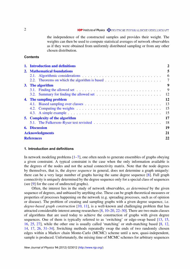
Figure 2. The construction of a digraph realizing a given BDS proceeds byconnecting the out-stubs of the nodes to the in-stubs of other nodes. In this‘bipartite’ representation the vertical gray bars represents single nodes.

figure 1(e), we would break graphicality: from there on, we would not be able to completethe realization of the BDS without creating either self-loops or multiple edges. Hence, it isimportant to find an algorithm that builds digraphs with a given BDS. As we will see, this is achallenging problem in itself.

An algorithm that builds a digraph from a given BDS sequentially connects the out-linksof a node to the in-links of others. We can think of these out- and in-links as ‘out-stubs’ and‘in-stubs’ emanating from a node, which are paired up with the corresponding stubs of othernodes. An intuitive representation of this is shown in figure 2.

As the graph construction algorithm proceeds, the number of stubs of the nodesdecreases. At any time during this process we will call the number of remaining in-stubs

New Journal of Physics 14 (2012) 023012 (http://www.njp.org/)

5

and out-stubs of a node its residual in- and out-degrees, and the corresponding BDS D ={(d (i)

1 , d (o)

1

),(

d (i)2 , d (o)

2

). . . ,

(d (i)

N , d (o)

N

)}the residual BDS.

Finally, another concept we will need to use in what follows is the notion of normalorder [30], which is essentially the lexicographic order on the BDS. That is, we say that a BDSis in normal order if for all 16 j 6 N − 1, we have either d (i)

j > d (i)j+1 or, if d (i)

j = d (i)j+1, then

d (o)

j > d (o)

j+1. Thus, the BDS D6 = {(5, 2), (4, 4), (4, 3), (2, 5), (2, 4), (2, 1)} shown in figure 2 isarranged in normal order. Once a BDS is in normal order, we will use the words ‘left’ or ‘right’to describe the directions towards lower or higher index values in the sequence.

The remainder of this paper is organized as follows. Section 2 introduces the fundamentalmathematical notions and algorithmic considerations that are at the basis of our digraphconstruction algorithm. Section 3 presents the algorithm and its derivation details. Readersinterested only in the algorithm itself7 may skip section 3.1 (which is the most technical part ofthe paper) and proceed directly to the summary described in the beginning of section 3 and insection 3.2. Section 4 deals in detail with the digraph sampling problem, provides the derivationof the sample weights and presents a simple example. Section 5 is dedicated to the complexityof the algorithm and section 6 concludes the paper.

2. Mathematical foundations

As seen from the examples above, not all sequences of non-negative integer pairs can be realizedby simple digraphs. The sufficient and necessary conditions for the realizability of a BDS aregiven by the ‘FR’ theorem [38–40]:

Theorem 1 (Fulkerson–Ryser). A sequence of non-negative integer pairs D ={(d (i)

1 , d (o)

1

), . . . ,

(d (i)

N , d (o)

N

)}with d (i)

1 > d (i)2 > . . .> d (i)

N is graphical iff

d (i)i 6 N − 1, d (o)

i 6 N − 1, 16 i 6 N , (1)

N∑i=1

d (i)i =

N∑i=1

d (o)

i , (2)

and for all 16 k 6 N − 1 :k∑

i=1

d (i)i 6

k∑i=1

min{

k − 1, d (o)

i

}+

N∑i=k+1

min{

k, d (o)

i

}. (3)

Given a BDS, we can easily test if it is graphical using this theorem, and thus we will also refer toit as the ‘FR test’. Condition (1) states that both the number of in- and out-degrees for all nodesmust be not larger than the number of other nodes it could connect to, or receive connectionsfrom. Condition (2) is a consequence of the requirement that every out-stub must join an in-stubsomewhere else; the sequence D3 given in one of the above examples is not graphical because itfails this condition. Condition (3) is less intuitive. Its lhs is the total number of in-stubs that thegroup of k highest in-degree nodes can receive. Within this group, a node’s out-stubs can absorbno more of those in-stubs from the same group than its out-degree or k − 1 (it cannot absorb

7 Source codes and documentation can be downloaded from http://www.biond.org/node/272.

New Journal of Physics 14 (2012) 023012 (http://www.njp.org/)

6

from itself), whichever is smaller (giving the first sum on the rhs of (3)). Outside of this group,a node cannot absorb more of those in-stubs than its out-degree or k, whichever is smaller (thesecond sum on the rhs of (3)). Hence, the necessity of (3). For the complete proof see [39, 40].Note that the example sequence D4 above fails condition 3 for k = 3. The FR test is the directedversion of the Erdos–Gallai (EG) theorem (test) for undirected graphs.

An important note is that BDSs are less constraining than undirected ones. The out-stub ofa node is always connected to an in-stub of another, not affecting that node’s out-stubs, whereassuch a distinction does not exist for the undirected case. Alternatively, if we disregard for amoment the directionality of the links and consider the degree of the node to be the sum ofits in- and out-degrees, then the corresponding graph realizing the BDS can have two edgesrunning between the same pair of nodes, whereas this is not allowed in the undirected case.

2.1. Algorithmic considerations

The FR theorem only tests for graphicality, but it does not provide an algorithm for constructingthe digraph(s) realizing the given BDS. At first sight this might not seem an issue. However,the sequence D5 in figures 1(d) and (e) reminds us that graphicality can easily be broken bya careless connection of stubs. Clearly, for the purposes of digraph construction, it should notmatter which edges we create first, as long as we make sure that every connection made doesnot break graphicality. In other words, the possibility of creating the rest of the edges, so that asimple digraph results in the end, must always be preserved. Thus, the key for the creation of analgorithm that builds simple digraphs realizing a given BDS without rejections is in a theoremthat allows us to check if we would break graphicality by placing a specific connection. Indeed,such theorems exist, and they will be discussed below. However, interestingly, they require thatconnections be made from the same node, until all its stubs are used away into edges. That is,assuming that we already made some connections from a given node i , preserving graphicality,these theorems give necessary and sufficient conditions for keeping graphicality by the nextconnection still involving node i . Simply put, they will not work in general if we attempted anew connection from j to k, where j, k 6= i , while node i still has dangling stubs.

The connections already made from i to some set of nodes Xi represent a constraint forthe new connections from i , as these novel connections must avoid the set Xi . We call such aconstraint associated with a node a star constraint on that node. Once all the stubs of node i areconnected into edges while preserving graphicality, we obtain a graphical residual sequence D′

on at most N − 1 nodes. Clearly, the new connections we make from this point on will not beconstrained in any way by the connections we made from node i . For the purposes of realizingthe sequence D′ we can simply remove node i with its fully completed connections, create arealization by a simple graph of D′ and then, in the end, add back node i with its connections tothis graph in order to obtain a realization of D. The comments above hold both for the undirectedand directed cases.

One might think of using the EG test for the undirected case and the FR test forthe directed case on a residual degree sequence to decide if graphicality was broken afterattempting a new connection from the same node. For the undirected case, we have shownin [11] that the passing of the EG test by the residual sequence is only a necessary conditionif there is already a star constraint on a node. For example, consider the graphical degreesequence d = {6, 5, 5, 3, 3, 2, 1, 1} and assume that we made connections from node i = 3 tonodes X3 = {1, 6, 7}. The residual sequence after these connections is d′

= {5, 5, 2, 3, 3, 1, 0, 1}.

New Journal of Physics 14 (2012) 023012 (http://www.njp.org/)

7

It is easy to check that it passes the EG test. However, we will break graphicality with everyrealization of d′, because it will form a double edge with one of the existing connections fromnode i = 3 to X3. Thus, additional considerations have to be made to ensure the graphicality ofthe residual sequence for the undirected case, as described in [11]. For the directed case here weuse the sufficient and necessary conditions for graphicality under star constraints as provided bytheorem 2 below, proven in [30].

From now on, we will always talk about algorithms that first finish all the out-stubs ofa node before moving onto another node with non-zero out-degree. In the case of a graphicalBDS, once all the out-degrees of all the nodes have been connected into directed edges, we areguaranteed to have completed a digraph, because the total number of in-stubs equals the totalnumber of out-stubs, according to property (2).

2.2. Theorems on which the algorithm is based

An algorithm that builds graphical realizations of degree sequences of simple undirected graphsis the HH algorithm [41, 42]: we choose any node with non-zero residual degree; then weconnect all its stubs to nodes with the largest residual degrees avoiding self-and multipleconnections. This process is repeated with other nodes until all stubs of all nodes are used.There is a corresponding version of the HH algorithm for BDSs as well, introduced first in [43]and then rediscovered independently in [30], the latter providing an alternative proof. The HHalgorithm for BDS proceeds as follows: given a normal-ordered BDS, choose any node withnon-zero residual out-degree, then connect all its out-stubs to nodes with the largest residualin-degrees, without creating multiple edges running in the same direction, nor self-loops.Reorder in normal order the residual sequence and repeat this process until all stubs of allnodes are used. While for any given BDS, the HH algorithm will construct a set of digraphs,it cannot construct all possible digraphs realizing the same sequence, as shown in [30]. Forexample, the HH algorithm can never result in the digraph shown in figure 1(c) realizing theexample sequence D2 above. It is easy to see why: there are two kinds of nodes in this example,with bi-degrees (3, 0) and (1, 2). The only nodes with non-zero out-degrees are the (1, 2) types.Using the HH algorithm, we would have to connect both out-stubs of such a node to the nodeswith the largest in-degrees, that is, to the two (3, 0) types. However, the digraph in figure 1(c)does not have a (1, 2) node being connected to both (3, 0) nodes, yet it realizes the sequence.The limitation of the HH algorithm comes from the fact that it prescribes to connect the out-stub of a node i to an in-stub of the node with the largest residual in-degree that does not yetreceive a connection from node i . However, there can be other nodes whose in-stubs can forma connection with an out-stub of i without breaking graphicality. This shows the importance offinding a method able to build not just a realization of a BDS, but all the possible realizationsof any given BDS.

In the remainder, given a residual BDS D, we denote by Ai(D) the allowed set of i , i.e. theset of all nodes to which an out-stub of i can be connected without breaking graphicality. Also,let us denote by Xi(D) the set of nodes to which connections were already made from i , thusrepresenting the star constraint at that stage.

The graphicality test under a star constraint on node i is provided as theorem 2 below. Inorder to announce it, however, we need to introduce one more definition. Consider a BDS D anda given node i with out-degree d (o)

i > 0 from this BDS. Let us also consider a subset of nodesS ⊂ V such that |S|6 d (o)

i , where |S| denotes the number of nodes in S, i.e. its size, and forevery node j ∈ S, d (i)

j > 0. Next, we take D and reduce by unity the in-degrees of all its nodes in

New Journal of Physics 14 (2012) 023012 (http://www.njp.org/)

8

S and then reduce by |S| the out-degree of node i . The BDS D′ thus obtained will be called theBDS reduced by S about node i from BDS D. Equivalently, D′ is the residual sequence obtainedfrom D after connecting an out-stub from i to an in-stub of every node from S.

Theorem 2 (Star-constrained graphicality). Let D be a BDS in normal order on N nodes,and let Xi , |Xi |6 N − 1 − d (o)

i , be a set of nodes whose in-stubs are forbidden to be connectedto the out-stubs of node i (including i). Define Li as the set of the first (‘leftmost’) d (o)

i nodes inD but not from Xi . Then, there exists a simple digraph which realizes D and avoids connectionsfrom i to Xi , if and only if the BDS D′ reduced by Li about node i from D is graphical.

The proof of this theorem can be found in [30]. What this theorem does is to turn a star-constrained graphicality problem for BDS D into an unconstrained one on the reduced BDSD′. The graphicality of D′ is then easily tested via the FR theorem. The set Li as defined abovewill be called the leftmost set for node i .

Although announced in its full generality, as Xi could be any predefined subset of nodeswith |Xi |6 N − 1 − d (o)

i , this theorem applies directly to the digraph construction process whenXi represents the set of nodes to which connections were already made in previous steps from thesame node i , hence forbidding us to make further connections from i to these very same nodes.In this case, the BDS D represents the residual sequence D at that stage of the constructionprocess.

As discussed above, in order for us to be able to construct all the simple digraphs thatrealize a given BDS, we need to find the allowed set Ai(D) for the next out-stub of i . Clearly,after every connection from the same node i , the residual sequence changes, and along with itthe allowed set may change as well. In order to find Ai(D) for the next out-stub of node i , wecould just simply attempt connections sequentially to every node with non-zero in-degree notin Xi(D) ∪ {i}, and test for graphicality after each attempt using theorem 2. The set of nodes forwhich graphicality would have been preserved would form Ai(D).

However, this would be inefficient and actually not needed. In fact, we can exploit a resultwhich states that, if graphicality is broken by a connection, it will be broken by all otherconnections to the right of the previous one, in the normal order sense. This is expressed inthe following:

Theorem 3. Let D be a graphical BDS in normal order and let Xi be a forbidden set for nodei , with i ∈ Xi . Let j < k be two nodes such that j, k /∈ Xi . If the residual BDS D j obtained fromD after forming an edge directed from i to j is not graphical, then the bi-degree sequence Dk

obtained from D by forming a directed edge from i to k is also not graphical.

This theorem follows from the direct contraposition of lemma 6 in [30]. Thus, what we need todo is to find efficiently the leftmost node q in the residual sequence in normal order, a connectionto which would break graphicality. We will refer to this node q as the leftmost fail-node. Allconnections to this node and to nodes to its right are guaranteed to break (star-constrained)graphicality, whereas all connections to its left (with the exception of forbidden nodes and self)are guaranteed to preserve the graphical character.

Note that both theorems 2 and 3 are based on the HH theorem for BDSs. In fact theorem 2is a generalization of the HH theorem to include star constraints. Also note that, while for theFR theorem only the in-degrees must be ordered non-increasingly, for the HH theorem andhence for both theorems 2 and 3, the BDS must be in normal order, as ordering by in-degreesalone is not sufficient. This is easily seen from the following example of graphical BDS (not

New Journal of Physics 14 (2012) 023012 (http://www.njp.org/)

9

in normal order) D7 = {(2, 0), (2, 1), (0, 1), (0, 2)}. Using the HH theorem, if we do not worryabout normal ordering, but just order by in-degree, we could choose to connect the out-stub ofnode (0, 1) to an in-stub of node (2, 0), then connect the out-stub of node (2, 1) to the remainingin-stub of (2, 0) (connecting to the largest residual allowed residual in-degree), after which wehave clearly broken graphicality: both out-stubs of (0, 2) now must be connected to the twoin-stubs of (2, 1).

We are now ready to present our digraph construction algorithm, which produces randomsamples from the set of all possible simple digraphs realizing a given BDS.

3. The algorithm

Given a graphical BDSs D in normal order (initially D = D):

(1) Define as work-node the lowest-index node i with non-zero (residual) out-degree.

(2) Let Xi be the set of forbidden nodes for the work-node, which includes i , nodes with zeroin-degrees and nodes to which connections were made from i previously. In the beginning,Xi includes only the work-node and zero in-degree nodes.

(3) Find the set of nodes Ai that can be connected to the work-node without breakinggraphicality.

(4) Choose a node m ∈ Ai uniformly at random and connect an out-stub of i to an in-stubof m.

(5) After this connection add node m to Xi .

(6) If node i still has out-stubs, bring the residual sequence in normal order and then repeat theprocedure from (3) until all out-stubs of the work node are connected away into edges.

(7) If there are other nodes left with out-stubs, reorder the residual degree sequence in normalorder and repeat from (1).

The most involved step of the algorithm is finding the allowed set (step (3)), which isintroduced in the next subsection. However, if the reader is interested only in the algorithmitself and less in its derivation, then he/she may skip directly to section 3.2.

3.1. Finding the allowed set

Let i be the work-node chosen as in (1) and let D denote the normal ordered, residual sequenceobtained after having connected some of the out-stubs of i to in-stubs of other nodes, such thatgraphicality is still preserved. These previous connections from node i form the set of forbiddennodes Xi for the next out-stub σ of i . Xi also contains the work-node i itself i ∈ Xi and all othernodes with zero in-degrees. Let Li be the set of the first (lowest index) d

(o)

i nodes from D, notin Xi . As D is (star constrained) graphical, we can connect σ to any of the nodes in Li withoutbreaking graphicality (due to theorem 2), hence Li ⊆ Ai .

Let m be the last element of Li in the normal ordered BDS D and let us ‘color’ (label) red allthe non-forbidden nodes, i.e. all the nodes not in Xi , to the right of node m. Please note that thesecolor labels are associated with the nodes, defined by their bi-degrees, and not with their indicesof location in the sequence. This set of red nodes Ri forms the set of candidates for the leftmostfail-node q. All other nodes are colored (labeled) black. To find the leftmost fail-node we could

New Journal of Physics 14 (2012) 023012 (http://www.njp.org/)

10

simply connect out-stub σ to an in-stub of a red node `, add the new connection temporarilyto the set of forbidden nodes, bring the new residual sequence into normal order, then test forgraphicality using theorem 2. This procedure could then be repeated sequentially, with ` goingover all the red nodes from left to right, until graphicality would fail for the first time at ` = q.However, the considerations in the following paragraphs allow us to define a better method.

For the sake of argument let us perform the sequential testing as explained above. It wouldimply the following steps for a given red node `:

(a) Reduce the out-degree at the work-node i and the in-degree at ` by unity, that is, d(o)

i 7→

d(o)

i − 1 and d(i)` 7→ d

(i)` − 1, resulting in a new residual BDS D`.

(b) Bring D` into normal order (required by theorem 2). Note that ` is the only node whosein-degree has changed and only the work-node had its out-degree changed (its in-degreewas not affected). Thus, when bringing D` into normal order, the relative positioning of allthe other nodes does not change. The work-node might have shifted to the right to a newposition i ′ within the block of nodes with the same in-degree (i ′ > i), and the red node’snew position `′ might have also moved to the right in the normal ordered sequence (`′ > `).

(c) Add `′ to the forbidden set for the work-node.

(d) Now, as required by theorem 2, reduce by unity the in-degrees of the nodes in the leftmostadjacency set Li ′ and reduce the out-degree of the work-node i ′ to zero. This results in thenew sequence D′

`′ .

(e) Order the BDS D′`′ by in-degrees, non-increasingly.

(f) Apply the FR theorem to test for graphicality.

Thus, whether the connection of the work-node i to ` breaks graphicality ultimatelydepends on whether the residual BDS D′

`′ fails (or passes) the FR test. However, as we notedbefore, for the FR test we do not need to have the BDS D′

`′ in normal order, we only need tohave it ordered non-increasingly by the in-degrees. Additionally, observe that in step (d) thereduction of the in-degrees always happens on the same set of nodes, independently of the rednode `; that is, the leftmost adjacency set Li ′ is the same for all `. Thus, in this particular caseof theorem 2’s application, ultimately we do not need to bring D` into normal order (step (b)),only non-increasingly by in-degrees, which would be done anyway in step (e). That means wecan just skip step (b); we do not need to move around any of the nodes at that stage. Thus, theonly difference between the sequences D′

`′ for different `s is at the position of this node afterthe reordering in (e), with respect to the rest of the sequence.

These observations suggest that we should define a BDS D′ obtained from the BDS D by

reducing by unity the in-degrees of all nodes in the set Li \ {m} and by d(o)

i − 1 the out-degreeof the work-node i , leaving only one out-stub (out-stub σ ) at i . Clearly, the BDS D′ is graphical(connecting out-stub σ to an in-stub of node m surely preserves graphicality, by theorem 2). Letus now order D′ non-increasingly by its in-degrees, in a specific way, described as follows. Shiftonly the reduced in-degree nodes in D to the right with respect to the rest of the sequence suchas to restore non-increasing ordering by the in-degrees (if needed). Since only the in-degreesof the nodes in the set Li \ {m} have been reduced, keep the relative ordering of all other nodesin D′ exactly the same as in D. Thus the relative ordering of the red nodes and of the worknode have been preserved as well. Let us denote the new location of the work node in D′ byj ( j 6 i). Connecting now σ to an in-stub of a red node ` in this sequence will produce the

New Journal of Physics 14 (2012) 023012 (http://www.njp.org/)

11

same set of residual bi-degrees as in step (d) above. To be able to apply the FR theorem, thenall we need to do is to shift to the right node ` in the sequence (if needed) to make sure that it isnon-increasingly ordered by in-degrees. Since only the in-degree at ` was modified (reduced byunity), this reordering is very simple: if x denotes the location of the last node of the block ofnodes with the same in-degree as node ` in D′ (x > `), then we simply swap the node at ` withthe node at x after the reduction of the in-degree at `. Let us denote the obtained sequence byD′. Clearly, it is non-increasingly ordered by in-degrees, and thus we can apply the FR theoremto see if it is graphical. Note: it could happen that x = j (e.g. there are many nodes with zeroout-degree but larger in-degree than the work-node as defined in (1)); however, the steps belowcan be applied just the same.

Next, we show how to identify the leftmost red fail-node q by investigating how theinequalities in (3) break down. Since D′ is graphical, we have for all 16 k 6 n − 1 (n is thelast element of D′) that L ′(k)6 R′(k), where L ′ and R′ are the lhs and rhs of inequalities (3)written for D′:

L ′(k) =

k∑s=1

d ′(i)s , (4)

R′(k) =

k∑s=1

min{

k − 1, d ′(o)

s

}+

n∑s=k+1

min{

k, d ′(o)

s

}. (5)

Let us denote by L ′(k) and R′(k) the lhs and rhs of the inequality (3) corresponding to D′. Sincethe rhs of (3) involves only out-degrees, and we only reduced the out-degree of the work-nodefrom 1 to 0, we will always have R′(k) = R′(k) − 1, except when k = 1 and the work-nodeis at j = 1, in which case R′(1) = R′(1). However, in this case, L ′(1) = L ′(1), because onlythe in-degree of j = 1 appears, which does not get changed. Thus, since L ′(1)6 R′(1) (D′

is graphical), graphicality cannot be broken at k = 1 when j = 1. Let us now consider thatthe work-node is still at position j = 1, but k > 1. For 1 < k < x , the in-degrees in D′ are thesame as those in D′, hence L ′(k) = L ′(k). For k > x , however, we have L ′(k) = L ′(k) − 1. Nowconsider j > 1. For 16 k < x , we have L ′(k) = L ′(k) and for k > x , L ′(k) = L ′(k) − 1. Thefollowing summarizes the relationships above:

(A) j = 1:

(A.1) k = 1: L ′(1) = L ′(1), R′(1) = R′(1).(A.2) 1 < k < x : L ′(k) = L ′(k), R′(k) = R′(k) − 1.(A.3) x 6 k: L ′(k) = L ′(k) − 1, R′(k) = R′(k) − 1.

(B) j > 1:

(B.1) 16 k < x : L ′(k) = L ′(k), R′(k) = R′(k) − 1.(B.2) x 6 k: L ′(k) = L ′(k) − 1, R′(k) = R′(k) − 1.

Since L ′(k)6 R′(k) for all k, graphicality for D′ can only be broken (that is to have L ′ > R′ forsome k), if L ′(k) = R′(k) namely in the cases (A.2) and (B.1) above. Observe that L ′(k) andR′(k) are computed from D′; hence they are independent of ` or x . This gives us the followingsimple procedure for finding the leftmost fail-node if it exists. Starting from k = 2 for j = 1,and k = 1 for j > 1, find the smallest k0 for which L ′(k0) = R′(k0). If no such k0 exists, thenthere are no fail-nodes and all non-forbidden nodes are to be included in the allowed set. If

New Journal of Physics 14 (2012) 023012 (http://www.njp.org/)

12

there is such a k0, the first red node q ′ to the right of k0 (q ′ > k0 + 1) is the leftmost fail-nodeof D′, which when identified in the original BDS D will give the leftmost fail-node q. Allnon-forbidden nodes to the left of q are to be included in the allowed set.

3.2. Summary for finding the allowed set

What we discussed in detail in the previous subsection corresponds to step (3) of the mainalgorithm described in the beginning of section 3. Given the normal-ordered BDS D at the endof step (2) of the main algorithm:

(3.1) Identify Li from the first d(o)

i nodes not in Xi .(3.2) Identify the ‘red’ set Ri as those nodes that are neither in Li nor in Xi . Note that the color

label is associated with the node, not its index.(3.3) Build D′ as follows:

d ′(i)b =

{d

(i)b − 1 if b ∈ Li \ {m} ,

d(i)b otherwise

and

d ′(o)

c =

{1 if c = i,

d(o)

c otherwise,

where m is the last node in Li .(3.4) Shift nodes from Li \ {m} to the right in the sequence (and only these) such as to restore

ordering non-increasingly by in-degrees (if needed), preserving the color labels of thenodes in the process. The work-node may have shifted to a new location j after this step.This is the updated sequence D′.

(3.5) Starting from k = 1 if j 6= 1 or from k = 2 if j = 1, find k0 as the smallest k such thatL ′(k) = R′(k), where L ′(k) and R′(k) are computed from the reordered (after step (3.4))D′ using (4) and (5). If there is no such k0, then the allowed set Ai is all the nodes in Dexcept nodes from the forbidden set Xi .

(3.6) Otherwise find the leftmost red node q ′ in the updated BDS D′ to the right of k0, that is,with q ′ > k0. Then the corresponding node q in D will be the leftmost fail node. Note thatq ′ is the new position of the node at q in D after the reordering in (3.4).

(3.7) The allowed set Ai is formed by all nodes in D not in Xi , and to the left of q.

4. The sampling problem

The algorithm generates an independent sample digraph every time it runs, without restartsor rejections, and it guarantees that every possible realization of a graphical BDS by simpledigraphs can be generated with a non-zero probability. However, the algorithm realizesthe digraphs with non-uniform probability. Nevertheless, knowing the relative probability forevery digraph’s occurrence allows us to calculate network observable averages as if they wereobtained from a uniform sampling. In particular, the following expression, which is a well-known result in biased sampling [44, 45], provides these averages as

〈Q〉 =

∑Mj=1 w(s j)Q(s j)∑M

j=1 w(s j), (6)

New Journal of Physics 14 (2012) 023012 (http://www.njp.org/)

13

where Q is an observable measured from the samples s j generated by an algorithm. The w(s j)

sample weight is the inverse of the relative probability of the occurrence of s j and M is thenumber of the samples generated. In section 4.1 we give a detailed derivation of this formula,specialized to our graph construction problem. The weights of the samples generated by ouralgorithm are given by

w(s) =

∏i

d(o)i∏

j=1

ki( j), (7)

where i runs over all the nodes with non-zero out-degree as they are picked by the algorithmto become work-nodes, and ki( j) = |Ai( j)| is the size of the allowed sets Ai( j) just beforeconnecting the j th out-stub of i . Note that w > 1 since there always exists at least one digraphrealizing the BDS. Section 4.2 gives a derivation of (7).

4.1. Biased sampling over classes

Our algorithm sequentially connects all stubs from a series of work nodes and finishes witha simple, labeled digraph. This process can be uniquely described by a path of connectionsequences. Having chosen a work node i1 for the first time, it determines the allowed set Ai1 . Wenext choose uniformly at random a node j1(i1) ∈ Ai1 and connect a stub of i1 to a stub at j1(i1).We could have chosen j1(i1) following any other criterion, but in that case the expression (7)of the weights would have to be modified accordingly. After this connection we recompute thenew allowed set A j1(i1), then connect another stub of i1 and so on until all the stubs have beenused up at i1. Let us denote by s such a path of connection sequences:

s =

{i1, j1(i1), . . . , jd(o)

i1(i1); i2, j2(i2), . . . , jd(o)

i2(i2) . . .

}, (8)

where d (o)

i denotes the residual out-degree of node i . A path s uniquely defines the digraphG(s) created, as the collection of all connections in (8) forms the edge set of the created graphG(s). However, several paths may lead to the same digraph. Also note that the order of theconnections in (8) matters in the calculation of the weight, as the corresponding allowed sets ingeneral depend on the history of connections up to that point. For a finite BDS the number ofdistinct samples (paths) is also finite. Let us denote this set of paths by

5 = {π1, . . . , πP} .

Let us now assume that we built with our algorithm a sequence of samples s1, s2, . . . , sM , andthat the sample number M is large enough for us to see all elements of 5 sufficiently manytimes. Given some path s we compute a quantity Q(s), and we are interested in calculatingthe average of Q over path ensembles. In our case Q is defined on the final graph itselfQ(s) = Q(G(s)), but for now we will not consider that explicitly. If we were just simplycomputing the average of Q over the set of samples, we would obtain an average biased bythe way the algorithm builds the paths from 5:

〈Q〉 =1

M

M∑i=1

Q(si) =

P∑k=1

Mk

MQ(πk), (9)

New Journal of Physics 14 (2012) 023012 (http://www.njp.org/)

14

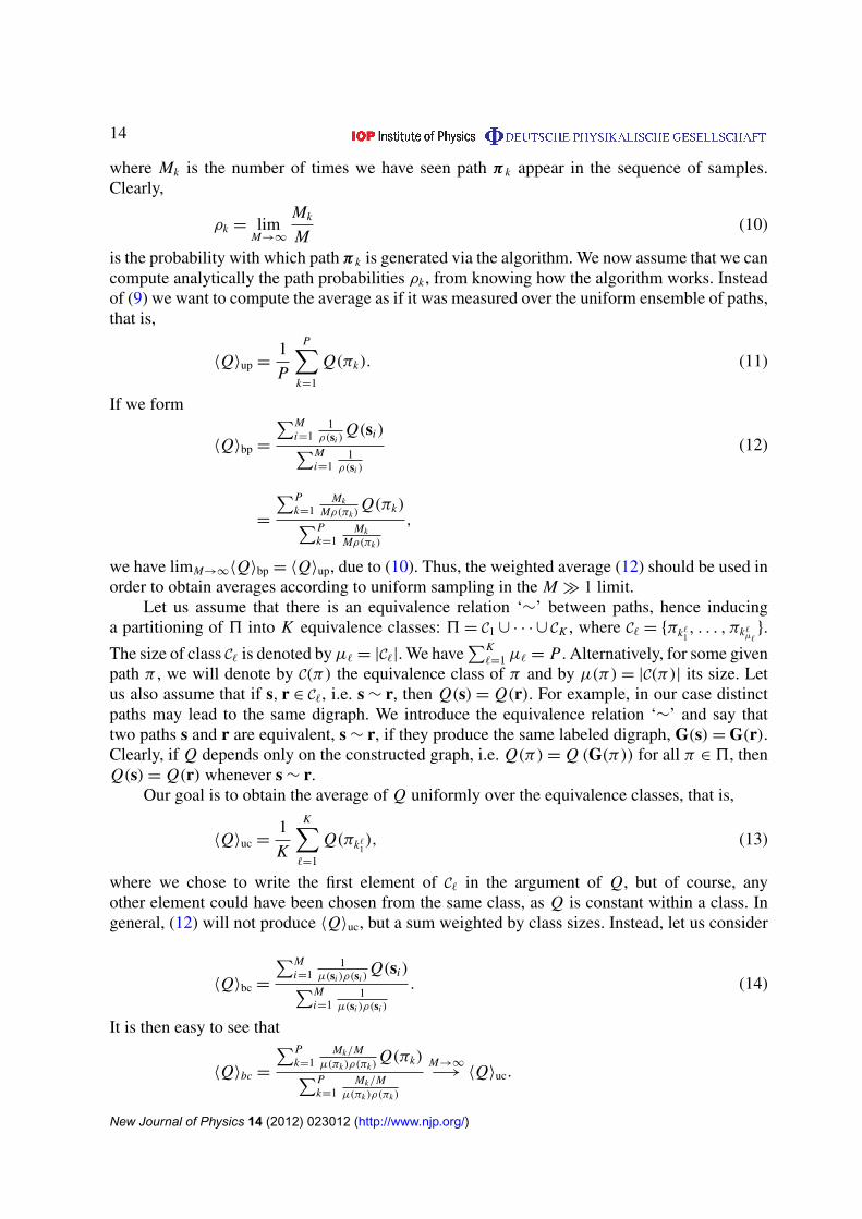
where Mk is the number of times we have seen path π k appear in the sequence of samples.Clearly,

ρk = limM→∞

Mk

M(10)

is the probability with which path π k is generated via the algorithm. We now assume that we cancompute analytically the path probabilities ρk , from knowing how the algorithm works. Insteadof (9) we want to compute the average as if it was measured over the uniform ensemble of paths,that is,

〈Q〉up =1

P

P∑k=1

Q(πk). (11)

If we form

〈Q〉bp =

∑Mi=1

1ρ(si )

Q(si)∑Mi=1

1ρ(si )

(12)

=

∑Pk=1

MkMρ(πk)

Q(πk)∑Pk=1

MkMρ(πk)

,

we have limM→∞〈Q〉bp = 〈Q〉up, due to (10). Thus, the weighted average (12) should be used inorder to obtain averages according to uniform sampling in the M � 1 limit.

Let us assume that there is an equivalence relation ‘∼’ between paths, hence inducinga partitioning of 5 into K equivalence classes: 5 = C1 ∪ · · · ∪ CK , where C` = {πk`

1, . . . , πk`

µ`}.

The size of class C` is denoted by µ` = |C`|. We have∑K

`=1 µ` = P . Alternatively, for some givenpath π , we will denote by C(π) the equivalence class of π and by µ(π) = |C(π)| its size. Letus also assume that if s, r ∈ C`, i.e. s ∼ r, then Q(s) = Q(r). For example, in our case distinctpaths may lead to the same digraph. We introduce the equivalence relation ‘∼’ and say thattwo paths s and r are equivalent, s ∼ r, if they produce the same labeled digraph, G(s) = G(r).Clearly, if Q depends only on the constructed graph, i.e. Q(π) = Q (G(π)) for all π ∈ 5, thenQ(s) = Q(r) whenever s ∼ r.

Our goal is to obtain the average of Q uniformly over the equivalence classes, that is,

〈Q〉uc =1

K

K∑`=1

Q(πk`1), (13)

where we chose to write the first element of C` in the argument of Q, but of course, anyother element could have been chosen from the same class, as Q is constant within a class. Ingeneral, (12) will not produce 〈Q〉uc, but a sum weighted by class sizes. Instead, let us consider

〈Q〉bc =

∑Mi=1

1µ(si )ρ(si )

Q(si)∑Mi=1

1µ(si )ρ(si )

. (14)

It is then easy to see that

〈Q〉bc =

∑Pk=1

Mk/Mµ(πk)ρ(πk)

Q(πk)∑Pk=1

Mk/Mµ(πk)ρ(πk)

M→∞

−→ 〈Q〉uc.

New Journal of Physics 14 (2012) 023012 (http://www.njp.org/)

15

In order for (14) to be useful in practice, one has to be able to compute the size of the equivalenceclass µ(s) from seeing s and knowing how the algorithm works. Fortunately this is possible inour case, as shown next.

4.2. Computing the weights

First, let us note that when connecting the out-stubs of a work-node we are not affecting theout-stubs of any other nodes, but only in-stubs. Hence, all nodes with non-zero out-degreeswill eventually be picked as work-nodes by the algorithm. Since normal ordering is first byin-degrees, the order in which nodes will become work-nodes depends on the sequence ofconnections. Let us now calculate the probability of the path s in (8). Given a residual sequence,the work-node i1 is uniquely determined by the algorithm as described before. Since the nextconnection is picked uniformly at random, the probability of the link from i1 to j1(i1) ∈ Ai1( j1)is |Ai1( j1)|−1. Let ki( j) = |Ai( j)| denote the number of nodes in Ai( j). Then, it is easy to seethat the probability of a path s is given by

ρ(s) =

∏k

d(o)ik∏

j=1

kik ( j)

−1

, (15)

where i1, i2, . . . denote the work-nodes in the order in which they are picked by the algorithm.This expression can be computed readily in a computer as the algorithm progresses. In orderfor us to use (14) it seems that we would need also to obtain the size µ(s) of the class to whichpath s belongs. Clearly, two different paths s and s′ will result in the same graph (s ∼ s′) if andonly if the sequence of connections in one path is a permutation of the connections in the otherpath. Hence, the class size µ(s) is nothing but the number of permutations of the connections,which is the same for all paths; that is, all classes have the same size µ. Since all connectionsare made from a node first before moving on to another, we have µ =

∏Ni=1 d (o)

i !. However, weactually do not need to use this number: one can simply multiply by µ both the numerator andthe denominator of (14) to obtain (6) and (7).

4.3. A simple example

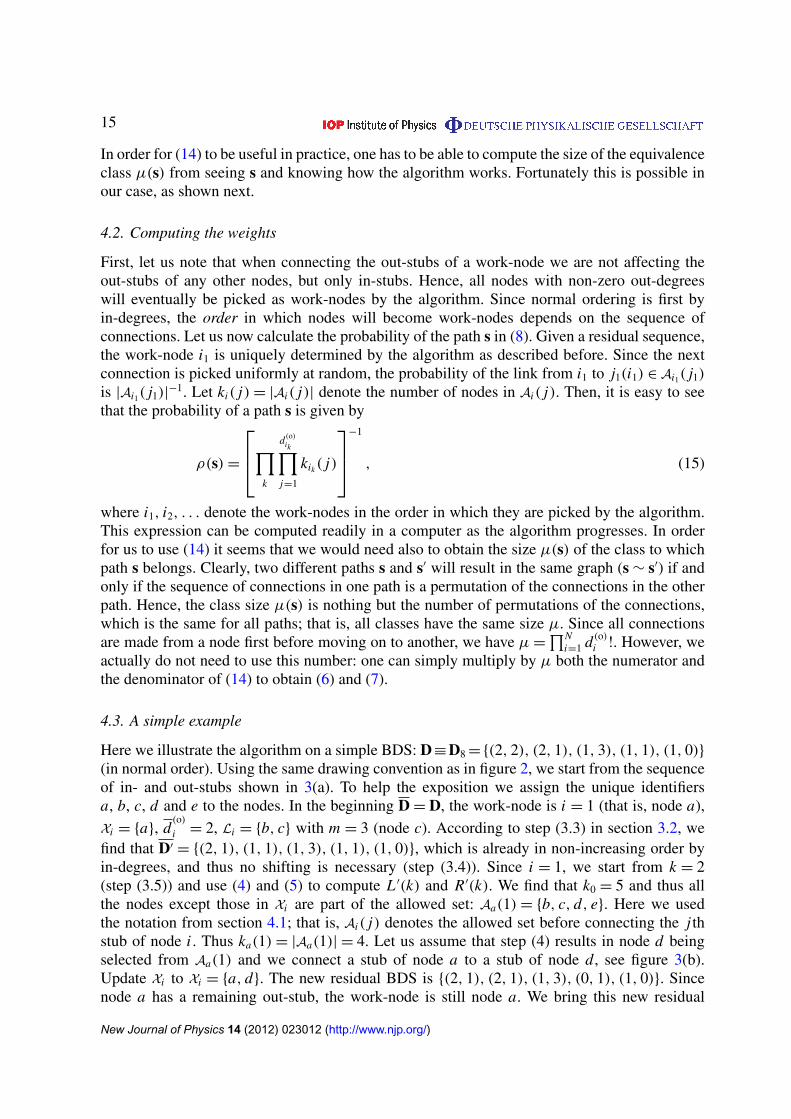
Here we illustrate the algorithm on a simple BDS: D≡D8 ={(2, 2), (2, 1), (1, 3), (1, 1), (1, 0)}

(in normal order). Using the same drawing convention as in figure 2, we start from the sequenceof in- and out-stubs shown in 3(a). To help the exposition we assign the unique identifiersa, b, c, d and e to the nodes. In the beginning D = D, the work-node is i = 1 (that is, node a),

Xi = {a}, d(o)

i = 2, Li = {b, c} with m = 3 (node c). According to step (3.3) in section 3.2, wefind that D′ = {(2, 1), (1, 1), (1, 3), (1, 1), (1, 0)}, which is already in non-increasing order byin-degrees, and thus no shifting is necessary (step (3.4)). Since i = 1, we start from k = 2(step (3.5)) and use (4) and (5) to compute L ′(k) and R′(k). We find that k0 = 5 and thus allthe nodes except those in Xi are part of the allowed set: Aa(1) = {b, c, d, e}. Here we usedthe notation from section 4.1; that is, Ai( j) denotes the allowed set before connecting the j thstub of node i . Thus ka(1) = |Aa(1)| = 4. Let us assume that step (4) results in node d beingselected from Aa(1) and we connect a stub of node a to a stub of node d, see figure 3(b).Update Xi to Xi = {a, d}. The new residual BDS is {(2, 1), (2, 1), (1, 3), (0, 1), (1, 0)}. Sincenode a has a remaining out-stub, the work-node is still node a. We bring this new residual

New Journal of Physics 14 (2012) 023012 (http://www.njp.org/)

16

Figure 3. Illustration of the steps of the algorithm on the BDS D8 (section 4.3).The same drawing convention is used as in figure 2. The nodes are also assignedthe unique identifiers a–e. The (green) rectangles denote the work-node, the ‘X’symbols denote forbidden nodes, nodes from the set Li are denoted by bluehalf-circles (m symbolizing its last element) and nodes from the ‘red’ set Ri

are denoted by red circles.

sequence into normal order, obtaining D = {(2, 1), (2, 1), (1, 3), (1, 0), (0, 1)}, see figure 3(c).

In this ordering, the work-node is i = 1 (node a), Xi = {a, d}, d(o)

i = 1, Li = {b}, m = 2. ThusLi \ {m} = ∅. Step (3.3) then implies that D′ = D and it is already ordered non-increasingly byin-degrees. Since i = 1 we perform step (3.5) starting from k = 2 and find that k0 = 3. Accordingto step (3.6), red node q ′

= 4 (node e) is the fail node. Indeed, this checks out: if we were toconnect the remaining out-stub of node a to the in-stub of node e, we would break graphicality.This is because node c (of index 3 in figure 3(c)) has three out-stubs that need to be connected tothe in-stubs of three different nodes, other than self, but at this stage that would be impossible,as there are only two other nodes left with in-stubs, namely nodes a and b. Thus, the allowedset for the remaining (second) stub of node a is Aa(2) = {b, c} and ka(2) = |Aa(2)| = 2. Let usnow assume that by chance we connected this stub to node b.

We obtain the residual BDS D = {(2, 0), (1, 3), (1, 1), (1, 0), (0, 1)}, which we havealready arranged in normal order, see figure 3(d). Now, the lowest index node with non-zero

out-degree, i.e. the new work-node, is i = 2 (node c), Xi = {c, d}, d(o)

i = 3, Li = {a, b, e},m = 4 (node e). Clearly, there are no nodes left for the red set; that is, Ri = ∅. This impliesthat the allowed set for the first stub of c is formed by all the nodes in Li ; that is, Ac(1) =

{a, b, e} and kc(1) = 3. From here on, the red set will stay empty. This process is then easilyrepeated until we form a graphical realization. For example, by making connections c toa and then obtaining Ac(2) = {b, e}, kc(2) = 2 and (for example) connecting node c to e.Following this, Ac(3) = {b}, kc(3) = 1; that is, there is only one connection that can bemade from c, namely to b. The next work-node becomes node b (only one out-stub) with

New Journal of Physics 14 (2012) 023012 (http://www.njp.org/)

17rM

r theo

[rM

rtheo]21/2

Figure 4. Biased sampling on the example BDS D8. The measure monitored isNewman’s assortativity coefficient r [46]. In (b) the ensemble average was takenover 50 runs.

Ab(1) = {c, a} and kb(1) = 2. Assume that we make the choice of connecting b to a. Theonly work-node left is node d , which must be connected to node c; that is, Ad(1) = {c}and kd(1) = 1. Thus, we have finished a graphical realization along the path of connectionss1 = {(a, d), (a, b); (c, a), (c, e), (c, b); (b, a); (e, c)}. The weight produced along this pathbased on (7) is w(s1) = ka(1)ka(2)kc(1)kc(2)kc(3)kb(1)kd(1) = 4 × 2 × 3 × 2 × 1 × 2 × 1 = 96.There are 11 distinct labeled digraphs realizing D8 and there are 2!1!3!1!0! = 12 paths in a class,leading to the same graph.

Let us now consider the Pearson coefficient r of degree–degree correlations, or theassortativity coefficient defined for directed graphs [46] as our network observable Q = r .For each one of the 11 graphical realizations of D8, r can be calculated exactly, as can theuniform average over this ensemble, obtaining 〈r〉theo = −0.040 506. We will refer to 〈r〉theo asthe ‘theoretical value’. We then let our algorithm run on this sequence to produce M samples anduse (6) and (7) to obtain the corresponding coefficient 〈r〉M . Figure 4(a) shows a few runs withdifferent seeds and their convergence to the theoretical value. Figure 4(b) shows the standarddeviation ([〈r〉M − 〈r〉theo]2)1/2 where the overline denotes an ensemble average over runs.

5. Complexity of the algorithm

To determine the theoretical upper bound for the complexity of the algorithm, i.e. the worst-casecomplexity, note that there are only three steps in the algorithm that require more than O (1)

computational operations, or steps, to complete.Firstly, after each connection is placed, one must bring the residual sequence into normal

order, steps (6) or (7). To accomplish this, both the work-node i and the target node m will haveto move to the right, but the relative positions of all other nodes will remain unchanged. In otherwords, if we were to remove nodes i and m, the rest of the BDS would already be sorted. Thus,in order to complete these steps, one only has to find the new positions of nodes i and m andinsert them into the already sorted BDS. Therefore, the complexity of either one of steps (6) and(7) is simply O (2 log N + N ) ≈ O (N ), where N is the number of the nodes in the sequencebeing ordered.

New Journal of Physics 14 (2012) 023012 (http://www.njp.org/)

18

Secondly, the allowed set A must be built before placing each connection (step 3).Following the summary of this step, given in section 3.2, note that steps (3.1)–(3.4) can allbe finished during a single scan of the residual BDS. This is clearly so for the creation of theleftmost set Li and for setting the ‘red’ color labels (or flags) (steps (3.1) and (3.4)). Concerningthe ordering of the BDS D′, it is possible to create it already sorted by simply scanning the BDSD while keeping track of the in-degree d? of the nodes currently being copied and the index a inD′ of the first node with that in-degree. Then, because D is in normal order, the only possibilityfor a node in D′ to break the order is when its in-degree equals d? + 1. In this case, it can besimply swapped with the node at a, because, as argued in section 3.1, the mechanism to build theallowed set is entirely based on the FR theorem, which does not require the BDS to be in normalorder, but to be simply ordered non-increasingly by its in-degrees. Thus, steps (3.1)–(3.4) canbe completed in O (N ) steps.

Thirdly, the computation of the sums L ′, R′ and their comparison must be conducted, whichis the same step as (3) in an FR test. To determine the complexity of an FR test note thatcomputing the repeated sums for each one of the inequalities (3) is quite inefficient. Instead,below we derive recurrence relations that allow us to complete the FR test in a linear, O (N )

number of steps.The steps of the main algorithm are performed sequentially and thus can all be completed

in a total of O (N ) steps. They must, however, be repeated for each edge in the digraph. Thus, themaximum complexity of the algorithm is O (N M) where M =

∑i d (o)

i is the number of edges.Since O (M)6 O

(N 2

)the maximum complexity of the algorithm is O(N 3). It is important to

note, however, that for a given BDS the complexity of the algorithm can be substantially smaller,similar to the case for our undirected graph sampling algorithm [11].

5.1. The Fulkerson–Ryser test revisited

The most complex part of the FR test is to compute the lhs and the rhs of inequalities (3), whichwe rewrite here for the sake of readability:

L(k) =

k∑s=1

d (i)s ,

R(k) =

k∑s=1

min{k − 1, d (o)

s

}+

N∑s=k+1

min{k, d (o)

s

}.

Our goal is to find recursion relations for L(k) and R(k). For the lhs the relation is simply

L(k + 1) = L(k) + d (i)k ,

with L(1) = d (i)1 .

For the rhs, first note that one can write it as

R(k) = −k +N∑

i=1

min{

k, g(o)

i (k)}

, (16)

where g(o)

i (k) is the family of integer sequences defined as

g(o)

i (k) =

{d (o)

i + 1, ∀i 6 k,

d (o)

i , ∀i > k.

New Journal of Physics 14 (2012) 023012 (http://www.njp.org/)

19

Now, let us introduce Gk (p) =∑N

i=1 δp,g(o)i (k)

, i.e. the number of indices i for which

g(o)

i (k) = p. Then, from (16) it follows that

R(k) = −k +k∑

p=1

pGk (p) + kN∑

p=k+1

Gk (p) , (17)

hence

R(1) = N − 1 − G1 (0) , (18)

where we used the fact that∑N

p=0 Gk (p) = N .Furthermore, let us introduce the following notations:

1Gk (p) ≡ Gk (p) − Gk−1 (p) ,

Gk (q) ≡

q∑i=0

Gk (i) .

Then, after some simple manipulations, from (17) it follows that

R(k) − R(k − 1) = N − 1 − Gk−1 (k − 1) +k−1∑p=1

p1Gk (p) + kN∑

p=k

1Gk (p) . (19)

Finally, note that 1Gk (p) = δp,d(o)k +1 − δp,d(o)

k. Substituting it into (19), we obtain

R(k) =

{R(k − 1) + N − Gk−1(k − 1), ∀d (o)

k < k,

R(k − 1) + N − Gk−1(k − 1) − 1, ∀d (o)

k > k.(20)

Thus, we have turned the problem of finding a recursion relation for R(k) into the problemof finding Gk (k). To solve this, first note that

Gk (k) = Gk−1 (k − 1) + Gk−1 (k) − δk,d(o)k

,

with G1 (1) = G1 (0) + G1 (1). The above equation constitutes a recursion relation for Gk (q).Such a relation can be rewritten as

Gk (k) = Gk−1 (k − 1) + G1 (k) + S (k) ,

where

S (k) =

k−1∑t=2

δk,d(o)t +1 −

k∑t=2

δk,d(o)t

.

Observe that S (k) and G1 (k) can be easily computed while scanning the BDS, and then,calculating L(k) and R(k) for each k requires a single operation. Thus, the entire FR test can becompleted in O (N ) steps.

6. Discussion

In summary, we have developed a graph construction and sampling algorithm to constructsimple directed graphs realizing a given sequence of in- and out-degrees. Such constructionsare needed in practical modeling situations, ranging from epidemics and sociology through

New Journal of Physics 14 (2012) 023012 (http://www.njp.org/)

20

0 50 100 150 200 250 300

log w

0

0.005

0.01

0.015

0.02

0.025

0.03

p

Figure 5. Probability distribution p of the logarithm of weights for an ensembleof BDSs on N = 100 nodes. The in-degrees were drawn from a normalizedpower-law distribution ∼ d−γ

in with γ = 3 and the out-degrees were drawn froma Poisson distribution e−λλdout/dout!, with the same average as the averagein-degree, λ = 〈din〉. The black circles are the simulation data and the redcontinuous line is a Gaussian fit.

food webs to transcriptional regulatory networks, where we are interested in learning about thestatistical properties of the network observables as determined only by the BDS and nothingelse.

Unlike existing algorithms such as the configuration model, which is affected byuncontrolled biases and unacceptably long running times except for a very restricted class ofsequences, our algorithm is rejection-free. Also, it guarantees the independence of the producedsamples, unlike MCMC methods, which have unknown mixing times. While its mathematicalunderpinnings are non-trivial, the algorithm itself is straightforward to implement. In principle,our approach can be extended to include more complex constraints, such as a given sequence ofmotif frequencies, but we have only concentrated on degree sequences since they are, arguably,the most fundamental of constraints. The algorithm can also be used to sample from given in-and out-degree distributions, not just sequences: given such distributions, one first samples agraphical BDS from these, then one applies our algorithm to generate digraphs. In this case,however, the sample weights (7) must be modified to reflect the probability of the occurrence ofthe given graphical BDS when drawn from the distributions.

Just as in the case of undirected graphs, we can expect the distributions of the weights forlarge graphs to be log-normal, as shown in [11]. As an example, figure 5 shows the distributionfor BDSs in which the in-degrees follow a power law with exponent γ = 3 and the out-degrees aPoisson distribution whose mean matches the average in-degree. Indeed, the distribution of theweight logarithms is well approximated by a Gaussian. Similarly, in the undirected case, we find,for all the examples we studied numerically, that the standard deviation σ of the distributionsof weight logarithms grows more slowly than the mean m with the number of nodes N ; seefigure 6 showing the scaling of m and σ for BDSs in which both in-degrees and out-degreesfollow a power-law distribution with exponent γ = 3. Thus, we may expect that typically, in the

New Journal of Physics 14 (2012) 023012 (http://www.njp.org/)

21

m,

100

101

102

103

104

105

N101 102 103 104

Figure 6. Mean m (black circles) and standard deviation σ (red squares) ofthe distributions of the logarithm of the weights versus the number of nodesN of samples. In-degrees and out-degrees are both drawn from a power-lawdistribution P (d) ∼ d−γ , with γ = 3. The solid black line and the dashed redline are data fit results, showing that m and σ follow power-law scaling lawsm ∼ N α and σ ∼ N β . The values of the exponents, given by the slopes of thelines, are α = 1.23 ± 0.02 and β = 0.81 ± 0.02.

N → ∞ limit, the rescaled weight distribution becomes a delta function, making the samplingasymptotically uniform.

Bounds on the complexity of the algorithm could easily be obtained by inspecting thealgorithm, showing a maximum complexity of the order ofO(N M), where M is the total numberof edges, M =

∑Ni=1 d (o)

i .In developing our results, we also provided an efficient way of implementing the FR test,

whose scope of application goes beyond our present algorithm, as it can be used in any contextto determine whether a BDS is graphical.

Acknowledgments

HK was supported in part by the US National Science Foundation (NSF) through grantDMR-1005417 and KEB was supported by the NSF grant DMR-0908286. ZT and HK weresupported in part by the NSF BCS-0826958 and HDTRA 201473-35045 and by the ArmyResearch Laboratory under Cooperative Agreement Number W911NF-09-2-0053. The viewsand conclusions contained in this document are those of the authors and should not beinterpreted as representing the official policies, either expressed or implied, of the ArmyResearch Laboratory or the US Government. The US Government is authorized to reproduceand distribute reprints for Government purposes notwithstanding any copyright notationhere on.

New Journal of Physics 14 (2012) 023012 (http://www.njp.org/)

22

References

[1] Newman M E J 2010 Networks: an Introduction (Oxford: Oxford University Press)[2] Easley D and Kleinberg J 2010 Networks, Crowds, and Markets: Reasoning about a Highly Connected World

(Cambridge: Cambridge University Press)[3] Barrat A, Barthelemy M and Vespignani A 2008 Dynamical Processes on Complex Networks (Cambridge:

Cambridge University Press)[4] Newman M E J, Barabasi A L and Watts D J 2006 The Structure and Dynamics of Networks (Princeton

Studies in Complexity) (Princeton, NJ: Princeton University Press)[5] Boccaletti S, Latora V, Moreno Y, Chavez M and Hwang D-U 2006 Phys. Rep. 424 175[6] Ben-Naim E, Frauenfelder F and Toroczkai Z 2004 Complex Networks (Lecture Notes in Physics) (Berlin:

Springer)[7] Dorogovtsev S N and Mendes J F F 2003 Evolution of Networks: From Biological Nets to the Internet and

WWW (Oxford: Oxford University Press)[8] Bender E A and Canfield E R 1978 J. Comb. Theory A 24 296[9] Koren M 1976 J. Comb. Theory B 21 235

[10] Kim H, Toroczkai Z, Erdos P L, Miklos I and Szekely L A 2009 J. Phys. A: Math. Theor. 42 392001[11] Del Genio C I, Kim H, Toroczkai Z and Bassler K E 2010 PLoS ONE 5 e10012[12] Bollobas B 1980 Eur. J. Comb. 1 311[13] Taylor R 1982 SIAM J. Algebr. Disc. Methods 3 114[14] Molloy M and Reed B 1995 Random Struct. Algebr. 6 161[15] Rao A R, Jana R and Bandyopadhya S 1996 Indian J. Stat. 58 225[16] Kannan R, Tetali P and Vempala S 1999 Random Struct. Algebr. 14 293[17] Newman M E J, Strogatz S H and Watts D J 2001 Phys. Rev. E 64 026118[18] Chung F and Lu L 2002 Ann. Comb. 6 125[19] Maslov S and Sneppen K 2002 Science 296 910[20] Milo R, Shen-Orr S, Itzkovitz S, Kashtan N and Chklovskii D 2002 Science 298 824[21] Morelli L G 2003 Phys. Rev. E 67 066107[22] Itzkovitz S, Milo R, Kashtan N, Ziv G and Alon U 2003 Phys. Rev. E 68 026127[23] Milo R, Kashtan N, Itzkovitz S, Newman M E J and Alon U 2003 arXiv:cond-mat/0312028v2[24] Park J and Newman M E J 2003 Phys. Rev. E 68 026112[25] Viger F and Latapy M 2005 Lect. Notes Comput. Sci. 3595 440–9[26] Britton T, Deijfen M and Martin-Lof A 2006 J. Stat. Phys. 124 1377–97[27] Cooper C, Dyer M and Greenhill C 2007 Comb. Probab. Comput. 16 557–93[28] Bianconi G, Coolen A C C and Perez Vicente C J 2008 Phys. Rev. E 78 016114[29] Bianconi G 2009 Phys. Rev. E 79 036114[30] Erdos P L, Miklos I and Toroczkai Z 2010 Electron. J. Comb. 17 R66[31] Boguna M, Pastor-Satorras R and Vespignani A 2004 Eur. Phys. J. B 38 205[32] Catanzaro M, Boguna M and Pastor-Satorras R 2005 Phys. Rev. E 71 027103[33] Angeles Serrano M and Boguna M 2005 Proc. CNET2004 Am. Inst. Phys. Conf. 776 101–7[34] Blitzstein J and Diaconis P 2011 Internet Math. 6 489[35] Hartmann A K 1999 Practical Guide to Computer Simulations (Singapore: World Scientific)[36] Del Genio C I, Gross T and Bassler K E 2011 Phys. Rev. Lett. 107 178701[37] Wasserman S and Faust K 1994 Social Network Analysis: Methods and Applications (Cambridge: Cambridge

University Press)[38] Chartrand G and Lesniak L 1986 Graphs and Digraphs 2nd edn (Monterey, CA: Wadsworth)[39] Fulkerson D R 1960 Pac. J. Math. 10 831[40] Ryser H 1963 Combinatorial Mathematics (Carus Mathematical Monographs vol 14) (Rahway, NJ:

Mathematical Association of America)

New Journal of Physics 14 (2012) 023012 (http://www.njp.org/)

23

[41] Havel V 1955 Casopis Pest. Mat. 80 477[42] Hakimi S L 1962 J. SIAM Appl. Math. 10 496[43] Kleitman D J and Wang D L 1973 Discrete Math. 6 79[44] Cochran W G 1977 Sampling Techniques 3rd edn (New York: Wiley)[45] Newman M E J and Barkema G T 1999 Monte-Carlo Methods in Statistical Physics (Oxford: Oxford

University Press)[46] Newman M E J 2003 Phys. Rev. E 67 026126

New Journal of Physics 14 (2012) 023012 (http://www.njp.org/)