Constructing a reliable health indicator for bearings ...

Appl. Sci. 2020, 10, 8948; doi:10.3390/app10248948  www.mdpi.com/journal/applsci 

Article 

Constructing a Reliable Health Indicator for Bearings 

Using Convolutional Autoencoder and Continuous 

Wavelet Transform 

Mohammadreza Kaji 1, Jamshid Parvizian 1 and Hans Wernher van de Venn 2,* 

1  Department of Mechanical Engineering, Isfahan University of Technology, Isfahan 84156‐83111, Iran; 

[email protected] (M.K.); [email protected] (J.P.) 2  Institute of Mechatronic Systems, Zurich University of Applied Sciences, 8401 Winterthur, Switzerland 

*  Correspondence: [email protected] 

Received: 23 November 2020; Accepted: 11 December 2020; Published: 15 December 2020 

Abstract: Estimating  the  remaining useful  life  (RUL) of components  is a crucial  task  to enhance 

reliability, safety, productivity, and to reduce maintenance cost. In general, predicting the RUL of a 

component  includes  constructing  a  health  indicator  (𝐻𝐼 )  to  infer  the  current  condition  of  the component,  and modelling  the  degradation  process  in  order  to  estimate  the  future  behavior. 

Although many signal processing and data‐driven methods have been proposed to construct the 

𝐻𝐼, most of the existing methods are based on manual feature extraction techniques and require the 

prior knowledge of experts, or rely on a large amount of failure data. Therefore, in this study, a new 

data‐driven method based on the convolutional autoencoder (CAE)  is presented  to construct the 

𝐻𝐼. For this purpose, the continuous wavelet transform (CWT) technique was used to convert the 

raw acquired vibrational signals into a two‐dimensional image; then, the CAE model was trained 

by the healthy operation dataset. Finally, the Mahalanobis distance (MD) between the healthy and 

failure stages was measured as the 𝐻𝐼. The proposed method was tested on a benchmark bearing 

dataset and compared with several other traditional 𝐻𝐼  construction models. Experimental results 

indicate that the constructed 𝐻𝐼  exhibited a monotonically increasing degradation trend and had 

good performance in terms of detecting incipient faults. 

Keywords:  health  indicator;  performance  degradation  assessment;  deep  learning;  vibration 

monitoring; bearing; remaining useful life; digital twin   

1. Introduction 

Performance  degradation, which  is  almost  inevitable  for mechanical  equipment,  results  in 

machinery  damage,  severe  financial  losses  due  to  replacement  or  repair  work  and  machine 

downtimes, or even personnel injury. Thus, prognostics and health management (PHM) has emerged 

as an engineering discipline to improve availability, reliability, and safety of equipment. As a crucial 

task  in  the  lifecycle monitoring  of  complex  equipment, PHM  is used  to monitor  the  equipment 

condition and to design robust and accurate models in order to assess the health state of equipment, 

as well as to define appropriate maintenance strategies [1]. In recent years, improving PHM methods 

by the Industry 4.0 paradigm, such as digital twin and predictive maintenance, attracts the attention 

of researchers [2–5].   

In a digital twin, a virtual counterpart of the physical system during  its whole  life is created, 

with abilities such as analyzing, evaluating, optimizing, and predicting [6]. Jinjian et al. [5] presented 

a digital  twin model  for  rotating machinery  to diagnose  the unbalance  faults, on  the basis of  the 

dynamic behavior of the rotor system and vibrational status monitoring. Fei et al. [4] proposed a new 

Appl. Sci. 2020, 10, 8948  2  of  21 

approach  for  PHM,  driven  by  digital  twin  for  complex  equipment.  In  this  approach,  a  five‐

dimensional digital  twin model  is  constructed  to  identify  the  health  conditions  of wind  turbine 

gearboxes. Dinardo et al. [7] proposed a prognostic approach to detect the incipient faults of rotating 

machines by means of their vibrational status monitoring. Yan et al. [8] presented a two‐phase digital 

twin  to diagnose  the  fault using  a deep  transfer  learning method.  In  this  approach,  the  trained 

knowledge of the deep neural network is transferred from the virtual space to the physical space for 

real‐time monitoring and predictive maintenance. 

Traditionally,  a  digital  twin  uses  physical‐based  simulation  tools  to  describe  the  current 

behavior  of  a  system  [3].  However,  due  to  manufacturing  tolerances  and  material  variances, 

describing a complex system in a simulation environment usually contains a strong deviation from 

reality [9]. One solution is to obtain a digital representation of the expected behavior of the physical 

system directly from measured data [3]. For this purpose, the first step is to construct a (multi) digital 

health indicator (𝐻𝐼) that describes different aspects of the physical component state during the whole 

life of the component. This 𝐻𝐼  should represent the deviation between the initial conditions of the 

component and its actual conditions during lifetime [1]. This 𝐻𝐼  can be further used for remaining 

useful life (RUL) estimation by implementing statistical estimation techniques, such as exponential 

degradation model [10], particle filter [11], or Kalman filter [12]. Therefore, defining an appropriate 

and  sensitive  𝐻𝐼   that  reflects  the deviation degree  from  normal  health  conditions  is  now  a  hot 

research topic in the RUL estimation field.   

In general, constructing a 𝐻𝐼  can be performed in three steps: (1) signal acquisition, (2) signal 

processing, and (3) feature extraction [13]. Vibration measurement provides a very efficient way of 

monitoring the dynamic conditions of a machine, such as unbalancedness, misalignment, mechanical 

looseness, structural resonance, wear, and shaft bow.  [14]. Developing each  failure mode  leads  to 

varying  system  dynamic  behavior,  resulting  in  significant  deviation  in  vibration  patterns  [15]. 

Vibration  signals  generated  by  the  faulty  component  can  be  analyzed  in  the  time  domain  [16], 

frequency domain [17], or time–frequency domain [18]. Using the time‐domain techniques for feature 

extraction requires the recording of the time‐series vibrations over a long period of time to obtain 

suitable parameters to reveal fault evolution. However, obtaining the necessary data for a complex 

equipment may be expensive or even impossible. Using frequency‐domain techniques such as fast 

Fourier transform (FFT) are powerful diagnostic tools in stationary conditions [18]. Since the FFT is 

essentially an  integral over  time,  it fails to do so  for non‐stationary data, which could result  from 

intermittent defect or evolutionary faults [18]. To address the FFT limitation, time‐frequency signal‐

processing  tools  such  as  the  short‐time  Fourier  transform  (STFT)  [19], Hilbert–Huang  transform 

(HHT) [20], Wigner–Ville distribution (WVD) [21], and wavelet transform [22] are introduced. The 

wavelet transform is a relatively new and powerful tool, able to perform a local analysis of a signal 

and revealing some hidden aspects of the data that the other signal analysis fails to detect [23]. In this 

work,  the wavelet  transform was  selected  for  signal  processing  to  detect  changes  in  vibration 

signatures that are caused by the faulty components. 

Once  the  raw  signal  is  acquired  and  processed,  feature  extraction  techniques  should  be 

employed to extract the representative features that are used for 𝐻𝐼  construction. Feature extraction methods  could  be  roughly  classified  into model‐based methods  and  data‐driven methods  [24]. 

Rodney  et  al.  [12]  obtained  a  bearing  𝐻𝐼   by  fusion  of vibrational  signal  variance  from  the  time 

domain and Choi–Williams distribution from the time–frequency domain. Yaguo et al. [25] presented 

a method  to extract multiple  features  from  the vibrational signal with multiple signal processing 

techniques, and then these features are selected and weighted to form the new 𝐻𝐼. In [26], the authors implemented the discrete wavelet packet transform to decompose the raw signal into different sub‐

bands, and  the 𝐻𝐼 was extracted  from each signal. Although model‐based methods do work and 

achieve  an  extraction  of  an  accurate  𝐻𝐼 ,  they  still  have  two deficiencies:  (1)  Feature  selection  is 

heavily dependent on prior knowledge and diagnostic expertise. Moreover,  it often  focuses on a 

specific fault type, and thus it may be unsuitable for other faults [27,28]. (2) In real industries, acquired 

signals are usually exposed to environmental noises, and are transient and non‐stationary. Therefore, 

Appl. Sci. 2020, 10, 8948  3  of  21 

signal processing technologies need to be employed to filter the collected signals, which can result in 

a loss of information [27,29].   

Data‐driven methods attempt to extract features from measured data using machine learning 

techniques. In recent years, deep learning has emerged as a powerful tool to extract the representative 

feature  from  the  collected  signals  [30,31].  Different  deep  learning  architecture,  including 

convolutional neural network (CNN) [29,32], recurrent neural network (RNN) [33], autoencoder [27], 

and  generative  adversarial  network  (GAN)  [34],  are  successfully  used  to  extract  features 

automatically. The greatest advantage of deep learning is that it needs no prior expert knowledge 

and represents more accurate features [35]. Until now, most studies employ deep learning methods 

in a supervised setting to extract features for classification problems. For this purpose, performance 

data of different degradation levels of a component are prerequisites to creating labeled healthy and 

unhealthy datasets. However, gathering different degradation‐level data requires large failure data, 

which is not available in practice, especially for high‐reliability component [36]. On the other hand, a 

recent  review  on  the  state  of  deep  learning  on  PHM  [37]  revealed  that  studies  from  a  health‐

management point of view have been rather limited, largely due to the unavailability of fault data. 

Moreover, many implementations of deep learning models in the literature are still constrained to 

specific equipment or applications and are not reusable when the predefined conditions change. In 

order  to  address  the  aforementioned  restrictions,  developing  a  single  framework  that  can 

systematically  be  extended  to  all  aspects  of  system  health management  is  necessary  [3,36]. This 

framework has to be able to be trained on‐line without requiring historical data, and must use only 

healthy operational data for training [3]. In addition, it should be applicable to any equipment that 

operates under stationary and non‐stationary conditions; it should also be extendable for different 

components [3]. 

As a step toward the development of a single framework for system health management, this 

paper proposes a method to construct an 𝐻𝐼  from the vibrational signal, on the basis of unsupervised deep learning. This method establishes an online construction of 𝐻𝐼  in the sense that the input data can be acquisitioned while the equipment is being exploited. The proposed method mainly includes 

three steps: First, healthy raw vibrational signals of the equipment are processed with the continuous 

wavelet transform (CWT) technique. These 2D images are considered as input of the deep learning 

model.  In  the  second  step,  a  convolutional autoencoder  (CAE) model  is developed  that  is  solely 

trained by the healthy data. Lastly, during online monitoring, in each assessment interval, throughout 

the entire lifetime of the equipment, the CWT image of the vibrational signal is fed to the trained CAE 

model.  Similar  to  the  training  data,  the  trained  autoencoder  can  reconstruct  images with  small 

reconstruction  errors.  The  distance  between  the  normal  condition  data  and  the  failure  stage  is 

measured by the MD formula and, thus, the 𝐻𝐼  is created.   In this study, to experimentally evaluate the effectiveness of the proposed methods, we chose 

the ball bearing. Ball bearings are known as  the most widely used rotating machine components, 

playing an important role in successful and reliable operation of rotary machines. Health prognostic 

of the ball bearing has great practical significance in reducing the failures of rotating machinery and 

enhancing machine availability. Thus far, fault detection techniques exist for rolling bearing monitor 

vibration, acoustic emission, motor current consumption, temperature, and oil debris. Among these 

techniques,  vibration  monitoring  has  proved  to  be  a  reliable  and  effective  technique  for  fault 

detection in bearings [28]. Therefore, the vibrational analysis technique is selected in this work, and 

the CAE model  is used  to extract  features  from  the vibration data. Overall,  this study proposes a 

method to construct a 𝐻𝐼  on the basis of an unsupervised deep learning method that describes every 

instant condition of the bearing and can be regarded as an indicator for a digital twin. In brief, the 

main contributions of the current work are 

(1) The CAE model is only trained by using healthy operation data at the beginning of an asset’s 

life cycle. Therefore, unlike most methods to construct a 𝐻𝐼, this model can be trained online 

without requiring historical failure data from similar assets or fleets. In addition, since the CAE 

model is trained by the CWT image, it is applicable for equipment that operates under stationary 

and non‐stationary conditions. 

Appl. Sci. 2020, 10, 8948  4  of  21 

(2) The values of the bottleneck nodes of the CAE model are used as extracted features. Using these 

values  reduces  any  dependencies  on  the  prior  knowledge,  and  thus  the  𝐻𝐼   is  constructed automatically.   

The  further  course  of  the  paper  is  organized  as  follows:  Section  2  briefly  introduces  the 

theoretical  background  of  CWT  and  convolutional  networks.  Section  3  presents  the  proposed 

methodology to construct the 𝐻𝐼  in detail. In Section 4, the results of the experimental evaluation are 

presented and discussed. Section 5 provides the conclusions and future work guidelines. 

2. Background Theory 

2.1. Continuous Wavelet Transform 

The purpose of CWT of the raw vibrational signal is to preprocess raw vibration in the time–

frequency domain and convert a 1D signal to a 2D image, as the input of the CAE model. The wavelet 

transform  is widely used  to process non‐stationary  signals over many different  frequencies. The 

wavelet  transform  can  analyze  a  localized  area  of  a  large  signal  without  losing  the  spectral 

information contained therein. Therefore, the wavelet transform can reveal some hidden aspects of 

the signal that other techniques fail to detect. This property can particularly be employed to identify 

the damage (crack) or fault of a component that evolves during the time. There are two main trends 

in how wavelet  transforms  are used,  the CWT  and  the discrete wavelet  transform. Both Fourier 

transform and CWT use inner products to measure the similarity between a signal and an analytic 

function. In the Fourier transform, the analytic function is complex exponentials (𝑒 ) and in the 

CWT, the analytic function is a mother wavelet function, 𝜓 𝑡 . The mother wavelet, 𝜓 ∈ 𝐿 𝑅 ,  is a function of finite length and zero average;  𝐿 𝑅   is the space of square‐integrable complex functions 

[32]. The CWT compares the signal to shifted and compressed or stretched versions of the mother 

wavelet function. Stretching or compressing a function is collectively referred to as dilation or scaling 

and corresponds to the physical notion of scale. The family of time‐scale waveform is obtained by 

shifting and scaling the mother wavelet, which can be expressed as 

𝜓 , 𝑡 1

√𝑎 𝜓

𝑡 𝑏𝑎

  (1)

By comparing the signal with the mother wavelet function at various scales and positions, we 

obtained two continuous variables,  𝑎  and  𝑏;  𝑎  is the dilation and  𝑏  is the translational parameter 

variable. For the given signal,  𝑓 𝑡 , wavelet coefficient 𝜔 𝑎, 𝑏   can be represented as 

𝜔 𝑎, 𝑏 𝑓 𝑡1

√𝑎 𝜓∗ 𝑡 𝑏

𝑎𝑑𝑡  (2)

where 𝜓∗  denotes the complex conjunction of 𝜓.   Since  selecting  of  a mother wavelet  function  is  application‐dependent,  the  selection  of  the 

appropriate function is the first and most important step in the wavelet analysis. As a rule of thumb, 

the most appropriate mother wavelet is a function that has more similarity with the signal. Although 

there  is  no  standard  or  general method  to  select mother wavelet,  the  shape matching  by  visual 

inspection is commonly used to select the appropriate mother wavelet function for the signal. For 

this study, on  the basis of  the visual  inspection and  the result of  the previous studies  [32,38], we 

selected Morlet wavelet in order to extract image features from the raw vibration signal. The Morlet 

function is a Gaussian function modulated by complex exponential, defined as 

𝜓 𝑡 𝑒 ⁄ 𝑒   (3)

where 𝜔   depends on the sampling frequency and usually is taken as 5 [39]. For wavelet transform 

of a real signal, the real part of the Morlet function is employed as the mother wavelet: 

𝜓 𝑡 𝑒 ⁄ cos 5𝑡   (4)

Appl. Sci. 2020, 10, 8948  5  of  21 

2.2. Convolutional Networks 

Convolutional neural network  (CNN)  is a  type of deep network  that uses convolutional and 

pooling operation to extract the topological features of the input data. CNN is primarily used to solve 

difficult image‐driven pattern recognition tasks, and if trained well, it will learn the features of the 

image completely. Therefore, in recent years, CNN has been widely used in image pattern recognition 

and  image  classification. CNN architectures  come  in  several variations; however, a  typical CNN 

includes convolutional layers, pooling layers, and fully connected layers. In the convolutional layer, 

a features map of the previous layer is convolved with multiple filters (also called Kernel) and is sent 

to the activation function to construct the output features map [29]: 

𝑥 𝑓 𝑥∈

∗ 𝑘 𝑏   (5)

where  𝑥   is the  𝑖th input feature map,  ∗ stands for the convolutional operator, 𝐾 denotes a 𝑤 𝑤 convolutional filter,  𝑏   is an additive bias, 𝑀   is a set of input feature map,  𝑙  is the  𝑙th layer in the network, and  𝑓 ∙   is a nonlinear activation function. The mathematical inverse of the convolutional 

layer used in the decoder is known as the deconvolution layer. Different nonlinear functions such as 

a rectified linear unit (ReLU), sigmoid function, and scaled exponential linear unit (SELU) function 

can be used in convolutional layers. SELU is a variant of the ReLU activation function that, due to its 

self‐normalizing properties, makes  learning highly  robust and allows  training of networks which 

have many layers. SELU, ReLU, and sigmoid activation functions are defined as 

𝑆𝐸𝐿𝑈 𝑥 𝜆𝑥, 𝑖𝑓 𝑥 0

𝛼𝑒 𝛼, 𝑖𝑓 𝑥 0 (6)

𝑅𝑒𝐿𝑈 𝑥 max 0,𝑥 (7)

sigmoid x1

1 e (8)

For  standard  scale  inputs  (zero mean  and  standard  deviation),  the  selected  values  for  the 

parameters are  𝛼 1.6732 and λ 1.0507  [40]. The  pooling  layer  usually  follows  the  convolutional  layer  and  is  used  to  reduce  the 

computational load by reducing the size of the features map. Two common pooling methods are max 

pooling  and  average  pooling, which  perform  local max  and  average  operations  over  the  input 

features, respectively. The calculation process of the pooling layer is given as [29] 

𝑋 𝑓 𝛽 ∙ 𝑑𝑜𝑤𝑛 𝑋 𝑏   (9)

where  𝛽   is  the weight  of pooling  and  𝑏   is  the  additive bias,  and  𝑑𝑜𝑤𝑛 𝑥   denotes  the down‐

sampling function, e.g., max pooling. In contrast to the pooling layer, an upsampling layer is a simple 

layer in the decoder with no weights that is used to increase the dimensions of input. 

In a fully connected layer, the features maps are converted into a one‐dimensional feature vector, 

and all neurons of both layers are connected, like a traditional multilayer neural network. The output 

of the fully connected layer can be obtained as [29] 

𝑂 𝑓 𝑥 𝛽 𝑏   (10)

where 𝑂   is the output value;  𝑥   is  the  𝑗th neuron  in the fully connected  layer;  𝛽   and  𝑏   are the weight and  the additive biases corresponding  to 𝑂  and  𝑥 , respectively; and  𝑓 ∙   is an activation function. 

Appl. Sci. 2020, 10, 8948  6  of  21 

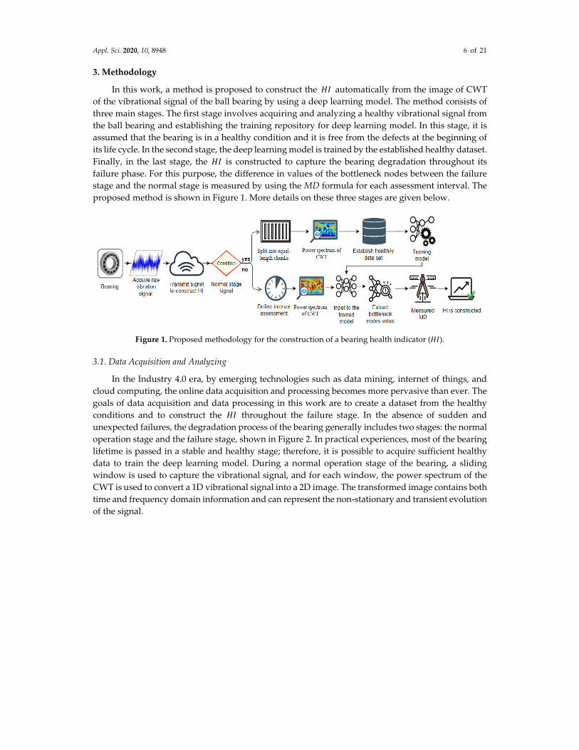
3. Methodology 

In this work, a method is proposed to construct the 𝐻𝐼  automatically from the image of CWT 

of the vibrational signal of the ball bearing by using a deep learning model. The method consists of 

three main stages. The first stage involves acquiring and analyzing a healthy vibrational signal from 

the ball bearing and establishing the training repository for deep learning model. In this stage, it is 

assumed that the bearing is in a healthy condition and it is free from the defects at the beginning of 

its life cycle. In the second stage, the deep learning model is trained by the established healthy dataset. 

Finally,  in  the  last stage,  the 𝐻𝐼  is constructed  to capture  the bearing degradation  throughout  its failure phase. For this purpose, the difference in values of the bottleneck nodes between the failure 

stage and the normal stage is measured by using the MD formula for each assessment interval. The 

proposed method is shown in Figure 1. More details on these three stages are given below. 

Figure 1. Proposed methodology for the construction of a bearing health indicator (𝐻𝐼). 

3.1. Data Acquisition and Analyzing 

In the Industry 4.0 era, by emerging technologies such as data mining, internet of things, and 

cloud computing, the online data acquisition and processing becomes more pervasive than ever. The 

goals of data acquisition and data processing in this work are to create a dataset from the healthy 

conditions  and  to  construct  the  𝐻𝐼   throughout  the  failure  stage.  In  the  absence  of  sudden  and unexpected failures, the degradation process of the bearing generally includes two stages: the normal 

operation stage and the failure stage, shown in Figure 2. In practical experiences, most of the bearing 

lifetime is passed in a stable and healthy stage; therefore, it is possible to acquire sufficient healthy 

data  to  train  the deep  learning model. During a normal operation  stage of  the bearing, a  sliding 

window is used to capture the vibrational signal, and for each window, the power spectrum of the 

CWT is used to convert a 1D vibrational signal into a 2D image. The transformed image contains both 

time and frequency domain information and can represent the non‐stationary and transient evolution 

of the signal. 

Appl. Sci. 2020, 10, 8948  7  of  21 

Figure 2. The lifespan of a bearing is divided into the normal stage and failure stage, and the healthy 

dataset is established from the normal stage data. 

In practical  application,  a  component  is  evolved  from  the  normal  stage  to  the  failure  stage 

gradually  (excluding  sudden  and unexpected  failures)  through  a  series  of degradation  states.  In 

addition,  there  are  high  uncertainties  about  the  ambient  conditions  and  component  properties. 

Therefore, defining a fixed failure threshold that clearly separates the normal stage from the failure 

stage is not feasible. To address this issue, in this paper, we introduced an adaptive failure threshold 

approach,  as  depicted  in  Figure  3. According  to  the  theory  of  statistical  process  control  (SPC), 

measured vibration signals under the normal operation follow a normal distribution (with the mean 

μ and the variance σ) [41]. With the transfer from the normal operation to the failure operation, the 

distribution  pattern  of  the  vibration  signals might  vary  from  normal  distribution  to  unknown 

distribution and, consequently, the mean and variance change. 

Figure  3. The  flowchart of defining  a  failure  threshold  and  establishing  a healthy dataset. The P 

variable is used to count the abnormal consecutive assessment intervals. 

Appl. Sci. 2020, 10, 8948  8  of  21 

In this paper, the Pauta criterion [42] was employed to determine the failure threshold. If the 

mean  of  the  acquired  vibrational  signal  amplitude  for  each  assessment  interval  is  within 

the 𝜇 3𝜎, 𝜇 3𝜎   range, the stage is recognized as a normal stage. Otherwise, the measured data 

are recognized as abnormal. In order to obtain an adaptive failure threshold, we established a healthy 

dataset  𝑋 �̅� , �̅� , … , �̅�   by  collecting  the mean  amplitude of  the vibrational data points  in  the 

normal stage. Then, a  reference  range  𝜇 3𝜎, 𝜇 3𝜎   is computed by using  the  𝑛  data. When a 

new datum  �̅�   is observed, the Pauta criterion is used to determine whether the new data belongs 

to  the healthy dataset.  If  the  �̅�   falls within  the  𝜇 3𝜎,𝜇 3𝜎   range,  it  is added  to  the healthy dataset,  i.e., 𝑋 �̅� , �̅� , … , �̅� , �̅� ,  and  the  reference  range  is  updated. Otherwise,  the  datum  is 

recognized as an abnormal one and the original healthy dataset remains unchanged. If for more than, 

e.g., 500  consecutive assessment  intervals  the means of  the vibrational amplitudes are not  in  the 

reference range, the failure threshold is recognized, and the collected healthy dataset is not changed 

anymore.   

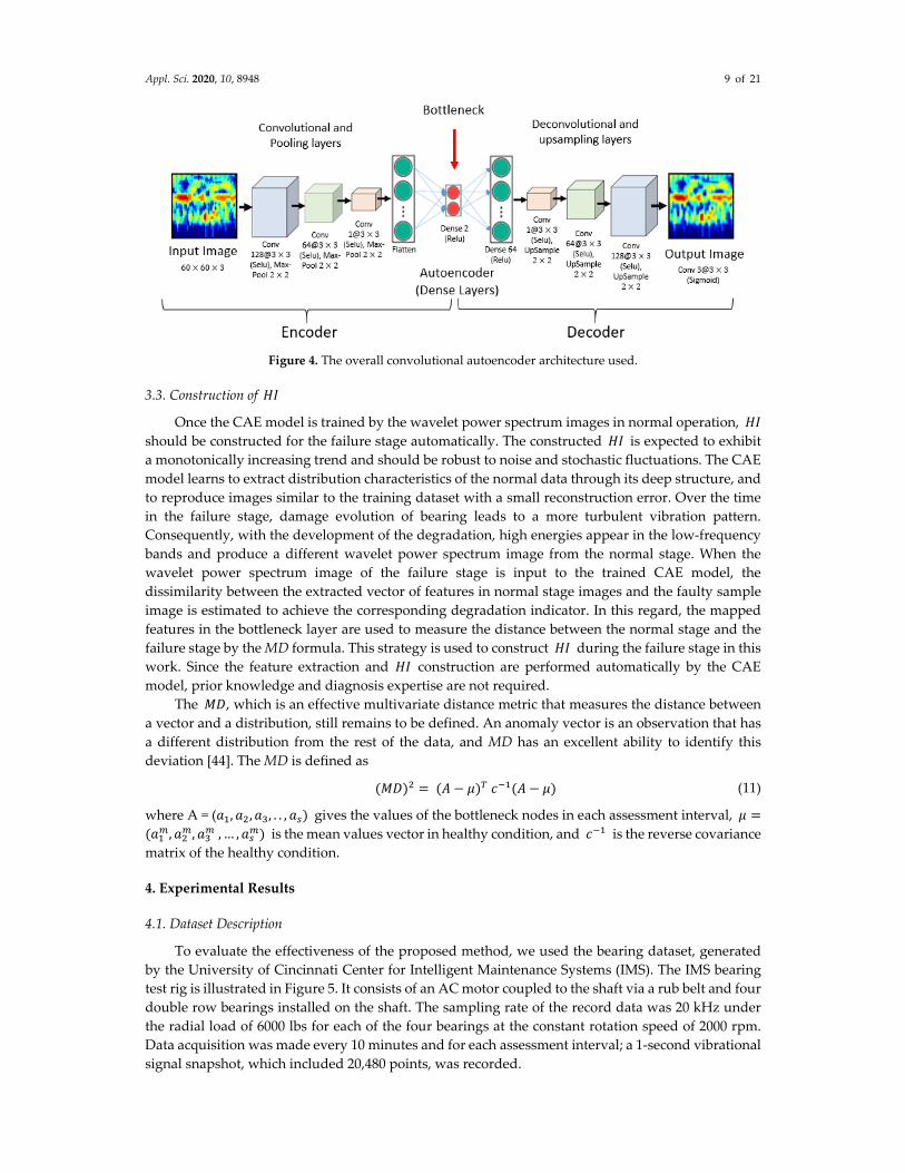
3.2. Convolutional Autoencoder Model 

The main purpose of using a deep learning model in this work is a dimensionality reduction 

through  the  feature  extraction,  and  thus  the  extracted  features  represent  the  conditions of  every 

moment of the ball bearing. Among the developed deep learning models, the CAE was selected in 

this study. CAE is a type of autoencoder (AE) neural network that is used to extract hidden features 

from unlabeled  images. CAE  is  characterized  by  having  identical  input  and  output  sizes  and  is 

trained to predict the input in the output (ℎ , 𝑥 𝑥). One CAE algorithm consists of three layers: the input layer, the hidden layer(s), and the output layer. The idea is that one or several hidden layers 

have lower dimensions than the visible layers (input and output), and thus the input information is 

reconstructed and compressed in the hidden layer(s). The hidden layer that contains the fewest nodes 

is known as a bottleneck. The bottleneck layer represents the maximum point of compression of the 

input data, which contains all necessary data to reconstruct the input data again. Therefore, the CAE 

is constituted by two main parts: an encoder that maps the input into the code, and a decoder that 

maps the code to a reconstruction of the original input in the output layer.   

In the encoding section, some convolutional layers and pooling layers are stacked on the input 

image  to  extract  hierarchical  features.  Then,  all  units  in  the  last  convolutional  layer  have  been 

flattened to form a vector followed by a fully connected layer(s). The bottleneck layer usually has 2 

neurons. Accordingly, the input 2D image (for this study, the input image was 60 × 60 RGB pixels) is 

transformed  into a  two‐dimensional vector  space  (ℝ → ℝ ). To  train  the CAE model  in an 

unsupervised manner, we used the mirror architecture of the encoder in the decoder section. Thus, 

fully  connected  layer(s)  followed  by  some  deconvolutional  and  upsampling  layers  are  used  to 

transform  the embedded  features back  to  the original  image. The structure of  the proposed CAE 

model is shown in Figure 4. After setting up the CAE, it is essential to optimize weights and biases 

by minimizing the reconstruction error, i.e., the loss function. Backpropagation algorithm [43] is used 

to compute the gradient of the loss function with respect to any weight and bias in the network. To 

make  the  output  of  the decoder  as  equivalent  as  possible  to  the  input,  the  binary_crossentropy 

function is employed as the standard CAE loss function, and the Adam optimizer is used to optimize 

the loss function [43].   

Appl. Sci. 2020, 10, 8948  9  of  21 

Figure 4. The overall convolutional autoencoder architecture used. 

3.3. Construction of 𝐻𝐼 

Once the CAE model is trained by the wavelet power spectrum images in normal operation, 𝐻𝐼 should be constructed for the failure stage automatically. The constructed 𝐻𝐼  is expected to exhibit a monotonically increasing trend and should be robust to noise and stochastic fluctuations. The CAE 

model learns to extract distribution characteristics of the normal data through its deep structure, and 

to reproduce images similar to the training dataset with a small reconstruction error. Over the time 

in  the  failure  stage,  damage  evolution  of  bearing  leads  to  a more  turbulent  vibration  pattern. 

Consequently, with the development of the degradation, high energies appear in the low‐frequency 

bands and produce a different wavelet power  spectrum  image  from  the normal stage. When  the 

wavelet  power  spectrum  image  of  the  failure  stage  is  input  to  the  trained  CAE  model,  the 

dissimilarity between the extracted vector of features in normal stage images and the faulty sample 

image is estimated to achieve the corresponding degradation indicator. In this regard, the mapped 

features in the bottleneck layer are used to measure the distance between the normal stage and the 

failure stage by the MD formula. This strategy is used to construct 𝐻𝐼  during the failure stage in this work. Since  the  feature  extraction and  𝐻𝐼  construction are performed automatically by  the CAE 

model, prior knowledge and diagnosis expertise are not required.   

The 𝑀𝐷, which is an effective multivariate distance metric that measures the distance between 

a vector and a distribution, still remains to be defined. An anomaly vector is an observation that has 

a different distribution  from  the  rest of  the data, and MD has an excellent ability  to  identify  this 

deviation [44]. The MD is defined as 

𝑀𝐷 𝐴 𝜇 𝑐 𝐴 𝜇   (11)

where A = (𝑎 , 𝑎 ,𝑎 , . . , 𝑎   gives the values of the bottleneck nodes in each assessment interval,  𝜇𝑎 ,𝑎 , 𝑎 , … ,𝑎   is the mean values vector in healthy condition, and  𝑐   is the reverse covariance 

matrix of the healthy condition. 

4. Experimental Results 

4.1. Dataset Description 

To evaluate the effectiveness of the proposed method, we used the bearing dataset, generated 

by the University of Cincinnati Center for Intelligent Maintenance Systems (IMS). The IMS bearing 

test rig is illustrated in Figure 5. It consists of an AC motor coupled to the shaft via a rub belt and four 

double row bearings installed on the shaft. The sampling rate of the record data was 20 kHz under 

the radial load of 6000 lbs for each of the four bearings at the constant rotation speed of 2000 rpm. 

Data acquisition was made every 10 minutes and for each assessment interval; a 1‐second vibrational 

signal snapshot, which included 20,480 points, was recorded. 

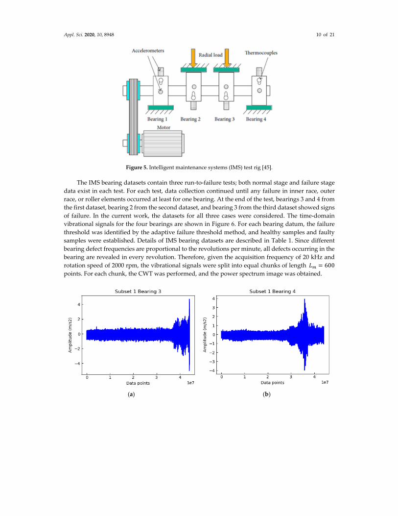
Appl. Sci. 2020, 10, 8948  10  of  21 

Figure 5. Intelligent maintenance systems (IMS) test rig [45]. 

The IMS bearing datasets contain three run‐to‐failure tests; both normal stage and failure stage 

data exist in each test. For each test, data collection continued until any failure in inner race, outer 

race, or roller elements occurred at least for one bearing. At the end of the test, bearings 3 and 4 from 

the first dataset, bearing 2 from the second dataset, and bearing 3 from the third dataset showed signs 

of  failure.  In  the current work,  the datasets  for all  three cases were considered. The  time‐domain 

vibrational signals for the four bearings are shown in Figure 6. For each bearing datum, the failure 

threshold was identified by the adaptive failure threshold method, and healthy samples and faulty 

samples were established. Details of IMS bearing datasets are described in Table 1. Since different 

bearing defect frequencies are proportional to the revolutions per minute, all defects occurring in the 

bearing are revealed in every revolution. Therefore, given the acquisition frequency of 20 kHz and 

rotation speed of 2000 rpm, the vibrational signals were split into equal chunks of length  𝐿 600 points. For each chunk, the CWT was performed, and the power spectrum image was obtained.   

(a)  (b) 

Appl. Sci. 2020, 10, 8948  11  of  21 

(c)  (d) 

Figure 6. Original vibration signals of the IMS bearing dataset [45]: (a) subset 1 bearing 3, (b) subset 

1 bearing 4, (c) subset 2 bearing 1, and (d) subset 3 bearing 3. 

Table 1. Description of IMS bearing dataset [45]. The failure thresholds and the healthy and faulty 

samples were identified by the adaptive failure threshold. 

Bearing Subset 1 

Bearing 3 

Subset 1 

Bearing 4 

Subset 2 

Bearing 1 

Subset 3 

Bearing3 

Load (lbs)  6000  6000  6000  6000 

Speed (rpm)  2000  2000  2000  2000 

Defect type  Inner race  Roller element  Outer race  Outer race 

Endurance duration  34 days 12 h  34 days 12 h  6 days 20 h  45 days 9 h 

Number of healthy 

samples 61,069  43,381 19,146  200,474 

Failure threshold  27 days 20 h  19 days 20 h  3 days 21 h  41 days 2 h 

Number of faulty 

samples 19,800  31,090  14,780  20,230 

4.2. Analysis of Wavelet Power Spectrum Images 

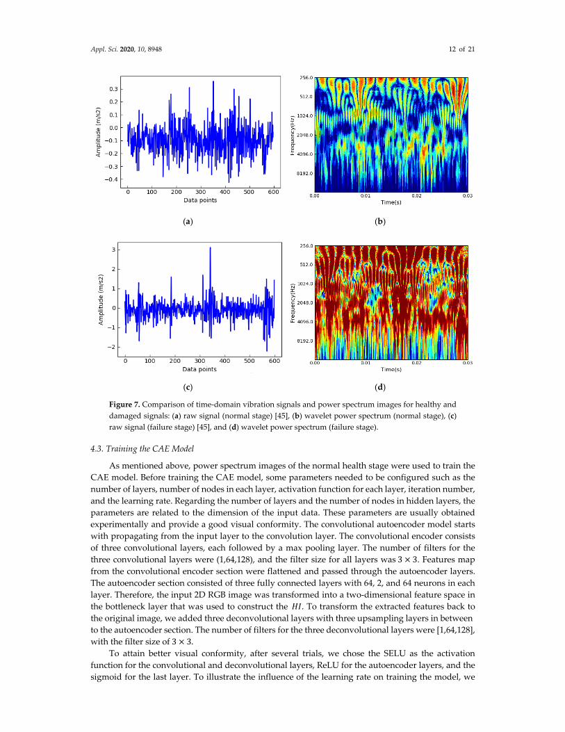
To demonstrate the advantage of the wavelet transform technique, we depicted the time‐domain 

vibrational signals and their corresponding wavelet power spectrums for a normal and a failure stage 

in Figure 7. While periodic vibrations with low amplitude are observed in the normal stage, more 

severe vibrations appear in the failure stage. The wavelet power spectrum represents the variations 

of the energy distribution of the vibration signal for different frequencies over  time. As shown  in 

Figure 7, the wavelet transform can clearly distinguish between the normal stage and the failure stage 

signals. For normal operations, most of  the energy  is  concentrated  in high  frequencies, but  for a 

failure stage, due to the evolution of defects, the burst of energy is observed in a broader range. 

Appl. Sci. 2020, 10, 8948  12  of  21 

(a)  (b) 

(c)  (d) 

Figure 7. Comparison of time‐domain vibration signals and power spectrum images for healthy and 

damaged signals: (a) raw signal (normal stage) [45], (b) wavelet power spectrum (normal stage), (c) 

raw signal (failure stage) [45], and (d) wavelet power spectrum (failure stage). 

4.3. Training the CAE Model 

As mentioned above, power spectrum images of the normal health stage were used to train the 

CAE model. Before training the CAE model, some parameters needed to be configured such as the 

number of layers, number of nodes in each layer, activation function for each layer, iteration number, 

and the learning rate. Regarding the number of layers and the number of nodes in hidden layers, the 

parameters are related to the dimension of the  input data. These parameters are usually obtained 

experimentally and provide a good visual conformity. The convolutional autoencoder model starts 

with propagating from the input layer to the convolution layer. The convolutional encoder consists 

of three convolutional  layers, each followed by a max pooling  layer. The number of filters for the 

three convolutional layers were (1,64,128), and the filter size for all layers was 3 3. Features map 

from the convolutional encoder section were flattened and passed through the autoencoder layers. The autoencoder section consisted of three fully connected layers with 64, 2, and 64 neurons in each 

layer. Therefore, the input 2D RGB image was transformed into a two‐dimensional feature space in 

the bottleneck layer that was used to construct the 𝐻𝐼. To transform the extracted features back to the original image, we added three deconvolutional layers with three upsampling layers in between to the autoencoder section. The number of filters for the three deconvolutional layers were [1,64,128], 

with the filter size of 3 3.   To  attain  better  visual  conformity,  after  several  trials, we  chose  the  SELU  as  the  activation 

function for the convolutional and deconvolutional layers, ReLU for the autoencoder layers, and the 

sigmoid for the last layer. To illustrate the influence of the learning rate on training the model, we 

Appl. Sci. 2020, 10, 8948  13  of  21 

show the reconstruction error under various learning rates in. If the learning rate was too low, the 

convergence was  too  slow  or  overfitting;  if  the  learning  rate was  too  high,  it would  hinder  the 

convergence. Therefore, the learning rate was set to 0.005 for this study. As illustrated in Figure 8, the 

reconstruction  error  did  not  significantly  decrease  after  30  cycles;  therefore,  30  iterations were 

performed  in  this  study. The  experimental model was developed using  the Python‐based Keras 

library [46] with a TensorFlow backend [47]. 

Figure 8. The reconstruction error of deep learning model for different learning rates. 

Since the CAE model is trained in an unsupervised manner, the successful trained CAE should 

learn to extract meaningful features from the images of the normal operation, and to reconstruct a 

closely similar image to the original image in the output. However, perfect reconstruction is usually 

a sign of overfitting where it only learns to copy its input to the output without learning to extract 

intelligent features and generalize to a new instance. Indeed, reasonably close reconstruction with a 

small error demonstrates that the CAE learned the meaningful features of the training dataset and 

had an acceptable generalization. Figure 9 represents the comparison of the original images with the 

reconstructed images by the developed model. Although the CAE model was solely trained by the 

normal operation dataset,  it also reconstructed  faulty  images very well,  indicating  that  the model 

could extract subtle features from images. 

Figure 9. Comparison of the original and reconstructed images of the wavelet power spectrum during 

the run‐to‐failure experiment of the subset 2 bearing 1. 

4.4. Smoothing the 𝐻𝐼 

The preliminary designed 𝐻𝐼  almost always exhibits  local random  fluctuations. To reveal an 

underlying long‐term trend in the designed 𝐻𝐼, we should smooth local spurious fluctuation in the 

Appl. Sci. 2020, 10, 8948  14  of  21 

𝐻𝐼  curve.  In this study, an exponential function was used to remove any sharp changes in the 𝐻𝐼 curve and to improve the monotonicity of the designed 𝐻𝐼  [48]. This function was given by 

𝑀𝐻𝐼 𝑒𝑥𝑝 ∑ / 1 𝑖 𝑁  (12)

where  𝐻𝐼   denotes  the  historical measured  𝐻𝐼 ,  𝑁   is  the  total  number  of  𝐻𝐼   values,  and  𝑀𝐻𝐼  represents the modified value of the current 𝐻𝐼 . In Equation (12), the mean value of the historical 

measurement  from  the  first value 𝐻𝐼   to  the current  𝑖th value 𝐻𝐼   is used  to calculate  the  𝑀𝐻𝐼 . Therefore,  if  the  𝐻𝐼   curve  exhibits  a  significant  oscillation  at  𝐻𝐼   point,  it  will  be  weakened. 

Furthermore,  the  exponential  function  is a monotonically  increasing  function and  it  can  reveal a 

monotonically increasing trend in the 𝐻𝐼  curve. 

4.5. 𝐻𝐼 Results 

Since  the  normal  stage  images  are  used  to  train  the  deep  learning model,  the  𝐻𝐼   is  solely constructed for the failure stage. The trained deep learning model was used to construct on‐line 𝐻𝐼 by applying the MD formula to measure the distance of the values of the bottleneck nodes between 

the normal stage and failure stage. The constructed 𝐻𝐼s for the four IMS bearings are shown in Figure 

10a–d. Intuitively, it can be observed that 𝐻𝐼s evolved gradually at the beginning and dramatically 

at the end; they revealed the true degradation in bearings. Although the initial 𝐻𝐼  curves represented global monotonicity, there still were severe local spurious fluctuations that may have been the result 

of  highly  inaccurate  and  unreliable  data.  Therefore,  the  smoothness  and  monotonicity  of  the 

constructed  𝐻𝐼s were  improved by using  the  exponential  function defined  in Equation  (12);  the 

modified 𝐻𝐼s are shown in Figure 10e–h. The exponential function is an increasing function that uses 

the mean from the starting time to the current time; thus, it can effectively eliminate oscillation and 

enhance monotonicity. It can be seen by the naked eye that the modified 𝐻𝐼s were smoother, and 

gradually  increasing, while  the degradation  trends were effectively  captured as well. The  results 

indicate that the proposed method has a good performance in detecting the early bearing defects and 

abnormal bearing health conditions. Moreover, this method provides an 𝐻𝐼  that is well correlated 

with progressively increasing bearing degradations, and it can lead to better RUL prediction. 

(a)  (e) 

(b)  (f) 

Appl. Sci. 2020, 10, 8948  15  of  21 

(c)  (g) 

(d)  (h) 

Figure 10. 𝐻𝐼  results for the four IMS bearings: (a–d) raw 𝐻𝐼, (e–h) modified 𝐻𝐼. 

4.6. Comparison with Other Traditional Methods 

To verify the effectiveness and superiority of the proposed method, we considered a comparison 

among the proposed method and several traditional 𝐻𝐼 methods. These methods were categorized 

in the two separate groups: five methods that are based on the time‐domain features and a method 

that is based on the time‐frequency domain feature. To compare, the vibration signal of the “subset 2 

bearing 1” was used to construct the 𝐻𝐼  in this section.   (1) In the first group, several commonly used features from the time domain were extracted to 

construct the 𝐻𝐼. The selected features include:   

Root mean square (RMS),   

1𝑁

𝑥    

Variance,   

1𝑁 1

𝑥 �̅�    

Kurtosis,   

1𝑁

𝑥 �̅�𝜎

Appl. Sci. 2020, 10, 8948  16  of  21 

Skewness,   

1𝑁

𝑥 �̅�𝜎

𝑥   is the vibrational signal series;  �̅�  and  𝜎  are the mean value and the variance of the series, 

respectively. 

Approximate entropy  (ApEn). ApEn expresses  the  regularity of  fluctuations over  time‐series 

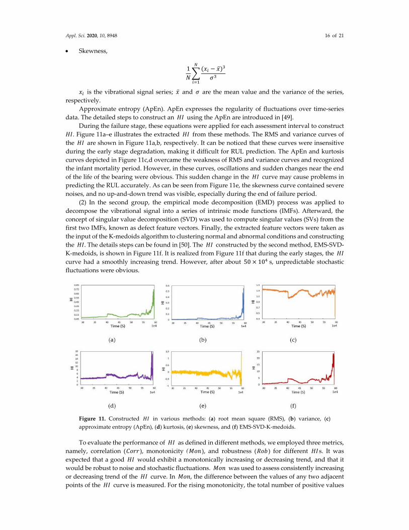
data. The detailed steps to construct an 𝐻𝐼  using the ApEn are introduced in [49].   During the failure stage, these equations were applied for each assessment interval to construct 

𝐻𝐼. Figure 11a–e illustrates the extracted 𝐻𝐼  from these methods. The RMS and variance curves of 

the 𝐻𝐼  are shown in Figure 11a,b, respectively. It can be noticed that these curves were insensitive 

during the early stage degradation, making it difficult for RUL prediction. The ApEn and kurtosis 

curves depicted in Figure 11c,d overcame the weakness of RMS and variance curves and recognized 

the infant mortality period. However, in these curves, oscillations and sudden changes near the end 

of the life of the bearing were obvious. This sudden change in the 𝐻𝐼  curve may cause problems in 

predicting the RUL accurately. As can be seen from Figure 11e, the skewness curve contained severe 

noises, and no up‐and‐down trend was visible, especially during the end of failure period. 

(2)  In  the  second  group,  the  empirical mode decomposition  (EMD)  process was  applied  to 

decompose  the vibrational  signal  into a  series of  intrinsic mode  functions  (IMFs). Afterward,  the 

concept of singular value decomposition (SVD) was used to compute singular values (SVs) from the 

first two IMFs, known as defect feature vectors. Finally, the extracted feature vectors were taken as 

the input of the K‐medoids algorithm to clustering normal and abnormal conditions and constructing 

the 𝐻𝐼. The details steps can be found in [50]. The 𝐻𝐼  constructed by the second method, EMS‐SVD‐

K‐medoids, is shown in Figure 11f. It is realized from Figure 11f that during the early stages, the 𝐻𝐼 curve had a smoothly  increasing  trend. However, after about  50 10 s, unpredictable stochastic fluctuations were obvious.

Figure  11.  Constructed  𝐻𝐼   in  various  methods:  (a)  root  mean  square  (RMS),  (b)  variance,  (c) 

approximate entropy (ApEn), (d) kurtosis, (e) skewness, and (f) EMS‐SVD‐K‐medoids. 

To evaluate the performance of 𝐻𝐼  as defined in different methods, we employed three metrics, 

namely,  correlation  (𝐶𝑜𝑟𝑟), monotonicity  (𝑀𝑜𝑛),  and  robustness  (𝑅𝑜𝑏)  for different  𝐻𝐼s.  It was 

expected that a good 𝐻𝐼 would exhibit a monotonically increasing or decreasing trend, and that it 

would be robust to noise and stochastic fluctuations. 𝑀𝑜𝑛 was used to assess consistently increasing 

or decreasing trend of the 𝐻𝐼  curve. In 𝑀𝑜𝑛, the difference between the values of any two adjacent 

points of the 𝐻𝐼  curve is measured. For the rising monotonicity, the total number of positive values 

Appl. Sci. 2020, 10, 8948  17  of  21 

is more than the total number of negative values and 𝑀𝑜𝑛  is close to 1. On the other hand, for the turbulent and oscillation curves, the total number of positive values is close to the total number of 

negative values and the 𝑀𝑜𝑛  value is close to 0. 𝑀𝑜𝑛  is calculated as follows: 

𝑀𝑜𝑛 𝑁𝑜.𝑜𝑓 𝑑𝑓 0

𝑁 1𝑁𝑜. 𝑜𝑓 𝑑𝑓 0

𝑁 1𝑑𝑓

𝐻𝐼 𝐻𝐼𝑖

1 𝑖 𝑁  (13)

where  𝑑𝑓 is the difference in the values of any two adjacent points in 𝐻𝐼  curve and 𝑁  is the total number of 𝐻𝐼  values.   

𝑅𝑜𝑏  reflects  the  tolerance  of  the  𝐻𝐼   to  random  fluctuations, which may  arise due  to  faulty 

sensors, variations in operating conditions, or unexpected events. 𝑅𝑜𝑏  is defined as 

𝑅𝑜𝑏 1𝑁

𝑒𝑥𝑝𝐻𝐼 𝐻𝐼

𝐻𝐼  (14)

where 𝐻𝐼   is the mean trend value of the 𝐻𝐼.   Similarly,  𝐶𝑜𝑟𝑟  measures  the  degree  of  linear  correlation  between  the  𝐻𝐼   and  time.  It  is 

expected that a good 𝐻𝐼  gradually increases by time. In a strong positive correlation, the  𝐶𝑜𝑟𝑟  value is close to 1 and vice versa.  𝐶𝑜𝑟𝑟  is defined as 

𝐶𝑜𝑟𝑟 ∑ 𝐻𝐼 𝐻𝐼 𝑖 ∑ 𝑖

𝑁

∑ 𝐻𝐼 𝐻𝐼 ∑ 𝑖 ∑ 𝑖𝑁

1 𝑖 𝑁  (15)

Here, 𝐻𝐼  is the mean value of all the 𝐻𝐼  values. Table 2 presents 𝑀𝑜𝑛, 𝑅𝑜𝑏, and  𝐶𝑜𝑟𝑟  values for the proposed 𝐻𝐼  and the traditional health indicators mentioned earlier. The results in Table 2 

show that all 𝑀𝑜𝑛,  𝑅𝑜𝑏, and  𝐶𝑜𝑟𝑟  of the current model are higher than those in other models. The 

obtained results demonstrate that the proposed model  is superior to other models, and it yields a 

better 𝐻𝐼. 

Table  2. Comparison  of  health  indicators  based  on monotonicity  (𝑀𝑜𝑛),  correlation  (𝐶𝑜𝑟𝑟),  and robustness (𝑅𝑜𝑏) for subset 2 bearing 1. 

Metrics Proposed 

Method RMS  Variance  ApEn  Kurtosis  Skewness 

EMD‐SVD‐ K‐

Medoids 

Mon  0.7587  0.0113  0.0140  0.0051  0.0063  0.0016  0.0229 

Rob  0.9484  0.8411  0.7565  0.8790  0.8875  0.4427  0.6971 

Corr  0.9969  0.6363  0.4480  −0.3814  0.3622  −0.4282  0.6358 

5. Discussion 

Constructing a reliable 𝐻𝐼  is the first and most important step in order to estimate the accurate 

RUL for bearings; therefore, this has been the focus of many studies [24]. In general, these methods 

are classified into three categories: mechanical signal processing‐based, model‐based, and machine 

learning‐based. In mechanical signal processing‐based methods, after pre‐processing of the vibration 

signal, statistical parameters are directly used to construct the 𝐻𝐼. Due to the flexibility and simplicity 

of mechanical  signal  processing methods,  these methods  are  widely  used  in  industries.  These 

methods also have an acceptable performance to detect early bearing defects and abnormal bearing 

health  conditions.  However,  it  has  been  experimentally  shown  that  the  indicator  performance 

decreases in the presence of transient conditions caused by bearing’s defects [1]. Compared to these 

methods,  the  proposed  method  is  sensitive  to  initial  degradation,  and  is  consistent  with  the 

degradation process. Nevertheless, in this work, the data of the run to failure vibrations is divided 

into two parts: the first part is used to train the CAE model and the second part is used to construct 

the 𝐻𝐼. However, nothing ensures that a sudden degradation or failure does not happen during the 

training phase. Therefore,  the method proposed  in  this work  is  limited  to  those  faults  that  cause 

particular vibration patterns. In the case of any sudden failure or extremely slow degradation, this 

method is not able to construct the 𝐻𝐼.   

Appl. Sci. 2020, 10, 8948  18  of  21 

In contrast to the time or frequency techniques, which only represent the information in time or 

frequency domain,  time–frequency  techniques provide more  information  in both domains.  In  the 

present work, the CWT technique was used to pre‐process the vibrational signals. The CWT method 

is a joint time–frequency analysis method that can decompose a time series into time and frequency 

spaces  simultaneously.  Therefore,  the  outputs  of  the  CWT  analysis  are  images  that  contain 

information on both time and frequency domains. When a defect appears in the bearing, it generates 

an  impulsive  force  and  excites  resonances  in  the  bearing  and  surrounding  elements. With  the 

progress of the defect over time, the frequency spectrum changes drastically. Since the faulty signals 

are non‐stationary and transient in nature, using the CWT for pre‐processing the vibration signals 

has better performance than time or frequency techniques in constructing the 𝐻𝐼. Furthermore, in 

the proposed method, the 𝐻𝐼  is constructed by comparing the images of normal and failure stages, 

which are acquired for an identical bearing. Therefore, the perpetual background noise will not affect 

the 𝐻𝐼  accuracy. In addition, in this work, a deep learning model is used in extracting features, as 

well as for dimensionality reduction from the pre‐processed vibration signals. This provides a more 

powerful capability of  learning complex nonlinear relationships, which  is able  to extract  the best‐

suited  features automatically. Moreover, using  the exponential  function  improves the smoothness 

and monotonicity of the preliminary designed 𝐻𝐼, which leads to better RUL estimation.   

6. Conclusions 

A  new  data‐driven  approach  to  construct  the  𝐻𝐼   is  presented.  This  𝐻𝐼   represents  every moment conditions of the bearing and can be considered as a digital twin of the bearing during its 

failure stage. Furthermore,  this 𝐻𝐼  can be used  for RUL estimation. First,  the Pauta criterion was 

employed  to determine  the  failure  threshold and a normal dataset. Since  the CWT  is suitable  for 

analyzing  the  non‐stationary  signals,  it  was  used  to  convert  raw  vibrational  signals  into  two‐

dimensional feature  images. The wavelet power spectrum  image clearly revealed  the degradation 

process of the bearing and included information in both time and frequency domains. Subsequently, 

the CAE model was used  for dimensionality reduction  through  the  feature extraction, and  it was 

trained by  the normal operation dataset. The values of  the bottleneck nodes of  the  trained CAE 

represented the conditions of every moment of the ball bearing life; they were used to construct 𝐻𝐼. Finally,  the wavelet power  spectrum  image of  the  failure  stage was  fed  to  the  trained CAE. The 

distance between the values of bottleneck nodes in normal and failure stages was measured by MD 

formula,  and  then  the  𝐻𝐼  was  constructed. To  improve  the  𝐻𝐼   curve monotonicity, we used  an 

exponential function to remove random fluctuations in the 𝐻𝐼  curve. Experiments were conducted 

on the run‐to‐failure IMS dataset to verify the performance of the proposed method.   

The results indicate that the constructed 𝐻𝐼 was capable of representing the health status of the 

bearing and tracking the evolution of degradation over the whole lifetime of the bearing. Moreover, 

constructing the 𝐻𝐼 with the proposed method required no prior knowledge or failure history data. 

Therefore,  it  is  suitable  for  industrial applications. Furthermore,  to prove  the effectiveness of  the 

proposed method, we compared this method with several other methods, such as RMS, EMD‐SVD‐

K‐medoids, skewness, kurtosis, and ApEn, showing a considerable superiority. The method, at the 

current state, is limited to gradual degradation and excludes any sudden failure. 

Future research directions are  to use  the proposed method  for other mechanical components 

such as ball screws, gears, and cutting tools. 

Author Contributions: M.K. proposed  the  idea, set up  the network, and conducted  the calculation.  J.P. and 

H.W.v.d.V. contributed to the supervision of the work, proposed some valuable suggestions, and performed the 

revisions. All authors have read and agreed to the published version of the manuscript.

Funding: This research was partially funded by Leading House South Asia and Iran seed money grant at ZHAW 

Zurich University of Applied Science. 

Conflicts of Interest: The authors declare no conflict of interest. 

Appl. Sci. 2020, 10, 8948  19  of  21 

References 

1. Wang, D.; Tsui, K.‐L.; Miao, Q. Prognostics and Health Management: A Review of Vibration Based Bearing 

and Gear Health Indicators. IEEE Access 2018, 6, 665–676, doi:10.1109/access.2017.2774261.   

2. Yan, J.; Meng, Y.; Lu, L.; Li, L. Industrial Big Data in an Industry 4.0 Environment: Challenges, Schemes, 

and  Applications  for  Predictive  Maintenance.  IEEE  Access  2017,  5,  23484–23491, 

doi:10.1109/access.2017.2765544.   

3. Booyse, W.; Wilke, D.N.; Heyns, P.S. Deep digital twins for detection, diagnostics and prognostics. Mech. 

Syst. Signal Process. 2020, 140, 106612, doi:10.1016/j.ymssp.2019.106612.   

4. Tao,  F.;  Zhang, M.;  Liu,  Y.; Nee, A.Y.C. Digital  twin  driven  prognostics  and  health management  for 

complex equipment. CIRP Ann. 2018, 67, 169–172, doi:10.1016/j.cirp.2018.04.055.   

5. Wang, J.; Ye, L.; Gao, R.X.; Li, C.; Zhang, L. Digital Twin for rotating machinery fault diagnosis in smart 

manufacturing. Int. J. Prod. Res. 2019, 57, 3920–3934, doi:10.1080/00207543.2018.1552032.   

6. Qi, Q.; Tao, F. Digital Twin and Big Data Towards Smart Manufacturing and  Industry 4.0: 360 Degree 

Comparison. IEEE Access 2018, 6, 3585–3593, doi:10.1109/access.2018.2793265.   

7. Dinardo, G.; Fabbiano, L.; Vacca, G. A smart and intuitive machine condition monitoring in the Industry 

4.0 scenario. Measurement 2018, 126, 1–12, doi:10.1016/j.measurement.2018.05.041.   

8. Wan, J.; Sun, Y.; Liu, X.; Zheng, Y. A Digital‐Twin‐Assisted Fault Diagnosis Using Deep Transfer Learning. 

IEEE Access 2019, 7, 19990–19999, doi:10.1109/access.2018.2890566.   

9. Tuegel,  E.  The  Airframe  Digital  Twin:  Some  Challenges  to  Realization.  In  Proceedings  of  the  53rd 

AIAA/ASME/ASCE/AHS/ASC  Structures,  Structural  Dynamics  and  Materials  Conference,  Honolulu, 

Hawaii, 23 April 2012–26 April 2012; pp. 1812–1820. 

10. Li, N.; Lei, Y.; Lin, J.; Ding, S.X. An Improved Exponential Model for Predicting Remaining Useful Life of 

Rolling Element Bearings. IEEE Trans. Ind. Electron. 2015, 62, 7762–7773, doi:10.1109/tie.2015.2455055.   

11. Deutsch,  J.; He, M.; He, D.  Remaining Useful  Life  Prediction  of Hybrid  Ceramic  Bearings Using  an 

Integrated Deep Learning and Particle Filter Approach. Appl. Sci. 2017, 7, 649, doi:10.3390/app7070649.   

12. Singleton,  R.K.;  Strangas,  E.G.;  Aviyente,  S.  Extended  Kalman  Filtering  for  Remaining‐Useful‐Life 

Estimation of Bearings. IEEE Trans. Ind. Electron. 2015, 62, 1781–1790, doi:10.1109/tie.2014.2336616.   

13. Guo, L.; Li, N.; Jia, F.; Lei, Y.; Lin, J. A recurrent neural network based health indicator for remaining useful 

life prediction of bearings. Neurocomputing 2017, 240, 98–109, doi:10.1016/j.neucom.2017.02.045.   

14. Liu, Z.; Zhang, L. A review of failure modes, condition monitoring and fault diagnosis methods for large‐

scale wind turbine bearings. Measurement 2020, 149, 107002, doi:10.1016/j.measurement.2019.107002.   

15. Rai, A.; Upadhyay, S. A review on signal processing techniques utilized in the fault diagnosis of rolling 

element bearings. Tribol. Int. 2016, 96, 289–306, doi:10.1016/j.triboint.2015.12.037.   

16. Fu, S.; Liu, K.; Xu, Y.; Liu, Y. Rolling Bearing Diagnosing Method Based on Time Domain Analysis and 

Adaptive Fuzzy‐means clustering. Shock. Vib. 2015, 2016, 9412787. 

17. Bustos, A.; Rubio, H.; Castejon, C.; Garciaprada, J.C. Condition monitoring of critical mechanical elements 

through  Graphical  Representation  of  State  Configurations  and  Chromogram  of  Bands  of  Frequency. 

Measurement 2019, 135, 71–82, doi:10.1016/j.measurement.2018.11.029.   

18. Al‐Badour,  F.;  Sunar, M.;  Cheded,  L.  Vibration  analysis  of  rotating machinery  using  time–frequency 

analysis  and  wavelet  techniques.  Mech.  Syst.  Signal  Process.  2011,  25,  2083–2101, 

doi:10.1016/j.ymssp.2011.01.017.   

19. Gao, H.; Wan, X.; Chen, X.; Xu, G. Feature extraction and recognition  for  rolling element bearing  fault 

utilizing short‐time Fourier transform and non‐negative matrix factorization. Chin. J. Mech. Eng. 2014, 28, 

96–105, doi:10.3901/cjme.2014.1103.166.   

20. Elbouchikhi,  E.; Choqueuse, V.; Amirat,  Y.;  Benbouzid, M.E.H.;  Turri,  S. An  Efficient Hilbert–Huang 

Transform‐Based Bearing Faults Detection  in  Induction Machines.  IEEE Trans. Energy Convers. 2017, 32, 

401–413, doi:10.1109/tec.2017.2661541.   

21. Singru, P.; Krishnakumar, V.; Natarajan, D.; Raizada, A. Bearing  failure prediction using Wigner‐Ville 

distribution,  modified  Poincare  mapping  and  fast  Fourier  transform.  J.  Vibroeng.  2018,  20,  127–137, 

doi:10.21595/jve.2017.17768.   

22. Li, L.; Liu, P.; Xing, Y.; Guo, H. Time‐frequency analysis of acoustic signals from a high‐lift configuration 

with two wavelet functions. Appl. Acoust. 2018, 129, 155–160, doi:10.1016/j.apacoust.2017.07.024.   

23. Kankar,  P.K.;  Sharma,  S.C.;  Harsha,  S.P.  Fault  diagnosis  of  ball  bearings  using  continuous  wavelet 

transform. Appl. Soft Comput. 2011, 11, 2300–2312, doi:10.1016/j.asoc.2010.08.011.   

Appl. Sci. 2020, 10, 8948  20  of  21 

24. Liu, Z.; Zuo, M.J.; Qin, Y. Remaining Useful Life Prediction of Rolling Ement Bearings Based on Health 

State Assessment. Proc. Inst. Mech. Eng. C J. Mech. Eng. Sci. 2016, 230, 314–330. 

25. Lei, Y.; Li, N.; Gontarz, S.; Lin, J.; Radkowski, S.; Dybala, J. A Model‐Based Method for Remaining Useful 

Life Prediction of Machinery. IEEE Trans. Reliab. 2016, 65, 1314–1326.   

26. Duong, B.P.; Khan, S.A.; Shon, D.; Im, K.; Park, J.; Lim, D.S.; Jang, B.; Kim, J.‐M. A Reliable Health Indicator 

for Fault Prognosis of Bearings. Sensors 2018, 18, 3740. 

27. He, J.; Ouyang, M.; Yong, C.; Chen, D.; Guo, J.; Zhou, Y. A Novel Intelligent Fault Diagnosis Method for 

Rolling  Bearing  Based  on  Integrated  Weight  Strategy  Features  Learning.  Sensors  2020,  20,  1774, 

doi:10.3390/s20061774.   

28. Hasan, J.; Kim, J.M. Bearing Fault Diagnosis under Variable Rotational Speeds Using Stockwell Transform‐

Based Vibration Imaging and Transfer Learning. Appl. Sci. 2018, 8, 2357, doi:10.3390/app8122357.   

29. Zan, T.; Wang, H.; Wang, M.; Liu, Z.; Gao, X.S. Application  of Multi‐Dimension  Input Convolutional 

Neural Network in Fault Diagnosis of Rolling Bearings. Appl. Sci. 2019, 9, 2690, doi:10.3390/app9132690.   

30. Mao, W.; He, J.; Zuo, M.J. Predicting Remaining Useful Life of Rolling Bearings Based on Deep Feature 

Representation  and  Transfer  Learning.  IEEE  Trans.  Instrum.  Meas.  2019,  69,  1594–1608, 

doi:10.1109/tim.2019.2917735.   

31. Yang, F.; Zhang, W.; Tao, L.; Ma, J. Transfer Learning Strategies for Deep Learning‐based PHM Algorithms. 

Appl. Sci. 2020, 10, 2361, doi:10.3390/app10072361.   

32. Yoo, Y.; Baek, J.‐G. A Novel Image Feature for the Remaining Useful Lifetime Prediction of Bearings Based 

on  Continuous  Wavelet  Transform  and  Convolutional  Neural  Network.  Appl.  Sci.  2018,  8,  1102, 

doi:10.3390/app8071102.   

33. Abed, W.; Sharma, S.; Sutton, R.; Motwani, A. A Robust Bearing Fault Detection and Diagnosis Technique 

for Brushless DC Motors Under Non‐stationary Operating Conditions. J. Control Autom. Electr. Syst. 2015, 

26, 241–254.   

34. Yin,  H.;  Li,  Z.;  Zuo,  J.;  Liu,  H.;  Yang,  K.;  Li,  F. Wasserstein  Generative  Adversarial  Network  and 

Convolutional Neural Network (WG‐CNN) for Bearing Fault Diagnosis. Math. Probl. Eng. 2020, 2020, 1–16, 

doi:10.1155/2020/2604191.   

35. Zhang, S.; Zhang, S.; Wang, B.; Habetler, T.G. Deep Learning Algorithms for Bearing Fault Diagnostics—

A Comprehensive Review. IEEE Access 2020, 8, 29857–29881, doi:10.1109/access.2020.2972859.   

36. Liu, H.; Zhou, J.; Xu, Y.; Zheng, Y.; Peng, X.; Jiang, W. Unsupervised fault diagnosis of rolling bearings 

using a deep neural network based on generative adversarial networks. Neurocomputing 2018, 315, 412–424, 

doi:10.1016/j.neucom.2018.07.034.   

37. Khan, S.; Yairi, T. A review on the application of deep learning in system health management. Mech. Syst. 

Signal Process. 2018, 107, 241–265, doi:10.1016/j.ymssp.2017.11.024.   

38. Guo, S.; Yang, T.; Gao, W.; Yang, T. A Novel Fault Diagnosis Method for Rotating Machinery Based on a 

Convolutional Neural Network. Sensors 2018, 18, 1429, doi:10.3390/s18051429.   

39. Tang, B.; Liu, W.;  Song, T. Wind  turbine  fault diagnosis based on Morlet wavelet  transformation  and 

Wigner‐Ville distribution. Renew. Energy 2010, 35, 2862–2866, doi:10.1016/j.renene.2010.05.012.   

40. Kim, D.; Kim, J.; Kim, J. Elastic exponential linear units for convolutional neural networks. Neurocomputing 

2020, 406, 253–266, doi:10.1016/j.neucom.2020.03.051.   

41. Hua, C.; Zhang, Q.; Xu, G.; Zhang, Y.; Xu, T. Performance reliability estimation method based on adaptive 

failure threshold. Mech. Syst. Signal Process. 2013, 36, 505–519, doi:10.1016/j.ymssp.2012.10.019.   

42. Wan,  F.;  Guo,  G.;  Zhang,  C.;  Guo,  Q.;  Liu,  J.  Outlier  Detection  for Monitoring  Data  Using  Stacked 

Autoencoder. IEEE Access 2019, 7, 173827–173837, doi:10.1109/access.2019.2956494.   

43. Bera, S.; Shrivastava, V.K. Analysis of various optimizers on deep convolutional neural network model in 

the application of hyperspectral remote sensing image classification. Int. J. Remote. Sens. 2019, 41, 2664–2683, 

doi:10.1080/01431161.2019.1694725.   

44. Ahn, J.; Lee, M.H.; Lee, J.A. Distance‐based outlier detection for high dimension, low sample size data. J. 

Appl. Stat. 2018, 46, 13–29, doi:10.1080/02664763.2018.1452901.   

45. PCoE  Datasets,  Bearing  Data  Set,  Intelligent  Maintenance  Systems  (IMS),  University  of  Cincinnati. 

Available  online:  https://ti.arc.nasa.gov/tech/dash/groups/pcoe/prognostic‐data‐repository/  (accessed  on 

10 June 2020).   

46. Chollet, F. Keras: The Python Deep Learning API. Available online: https://keras.io/ (accessed on 27 August 

2020).   

Appl. Sci. 2020, 10, 8948  21  of  21 

47. Abadi, M.A.; Barham, P.A.; Brevdo, E.; Chen, Z.; Citro, C.; Corrado, G.S.; Davis, A.; Dean, J.; Devin, M. 

TensorFlow:  Large‐Scale  Machine  Learning  on  Heterogeneous  Systems.  Available  online: 

http://tensorflow.org/ (accessed on 16 May 2020).   

48. Xu, F.; Huang, Z.; Yang, F.; Wang, D.; Tsui, K.L. Constructing a health indicator for roller bearings by using 

a stacked auto‐encoder with an exponential function to eliminate concussion. Appl. Soft Comput. 2020, 89, 

106119, doi:10.1016/j.asoc.2020.106119.   

49. Yan, R.; Gao, R.X. Approximate Entropy as a diagnostic tool for machine health monitoring. Mech. Syst. 

Signal Process. 2007, 21, 824–839, doi:10.1016/j.ymssp.2006.02.009.   

50. Rai, A.; Upadhyay, S. Bearing performance degradation assessment based on a combination of empirical 

mode  decomposition  and  k‐medoids  clustering.  Mech.  Syst.  Signal  Process.  2017,  93,  16–29, 

doi:10.1016/j.ymssp.2017.02.003.   

Publisher’s Note: MDPI stays neutral with regard to jurisdictional claims in published maps and institutional 

affiliations. 

© 2020 by the authors. Licensee MDPI, Basel, Switzerland. This article is an open access 

article distributed under the terms and conditions of the Creative Commons Attribution 

(CC BY) license (http://creativecommons.org/licenses/by/4.0/).