Constraint solving for direct manipulation of features

Constraint solving for direct manipulation of features

DANIEL LOURENÇO,1 PEDRO OLIVEIRA,1 ALEX NOORT,2 and RAFAEL BIDARRA2

1Instituto Superior Técnico, Technical University of Lisbon, Lisbon, Portugal2Faculty of Electrical Engineering, Mathematics and Computer Science, Delft University of Technology, Delft, The Netherlands

(Received October 28, 2005; Accepted July 6, 2006!

Abstract

In current commercial feature modeling systems, support for direct manipulation of features is not commonly avail-able. This is partly due to the strong reliance of such systems on constraints, but also to the lack of speed of currentconstraint solvers. In this paper, an approach to the optimization of geometric constraint solving for direct manipulationof feature dimensions, orientation, and position is described. Details are provided on how this approach was success-fully implemented in the Spiff feature modeling system.

Keywords: Constraint Solving; Direct Manipulation; Feature Modeling; Model Compilation

1. INTRODUCTION

1.1. Feature modeling

Feature modeling is a design paradigm that comes as analternative to the traditional geometry-based design sys-tems. The founding idea of feature modeling is to focus themodeling tasks of the designer on a higher level, facilitat-ing the specification of many different aspects in a productmodel, and gaining insight into their interrelations ~Shah &Mäntylä, 1995!. This is achieved by enabling the designerto associate functional information to the shape informa-tion in the product model.

Although one cannot find a consensual definition of theconcept of feature, one that nicely fits to this research definesa feature as “a representation of shape aspects of a productthat are mappable to a generic shape and are functionallysignificant for some product life-cycle phase” ~Bidarra &Bronsvoort, 2000!. In contrast to conventional computer-aided design ~CAD! systems, in which the design focusmainly lies on geometry, in a feature modeling system thedesigner builds a model out of features, each of which has awell-defined semantics. As an example, for manufacturingplanning purposes it would be appropriate to provide thedesigner with features that correspond to the manufacturing

processes available to manufacture the product beingdesigned ~e.g., slot, pocket, and hole features!.

Feature model semantics is mostly represented by a vari-ety of constraints. Constraints can be used in feature mod-eling systems to express characteristics of the model ~e.g.,to specify some feature faces to be coplanar, or restrict thevolume of a product to a certain maximum!. However, aboveall, constraints are used as the internal constituents of fea-tures that express their semantics ~e.g., a hole feature couldhave constraints to position and orient it, or constraints thatexpress the physical limits of the drilling machinery avail-able!. Because of this central role of constraints, featuremodeling systems have to make an intensive use of con-straint solving techniques. In particular, geometric con-straints and geometric constraint solving techniques are verycommon.

To ensure that feature model semantics is maintained, thevalidity of the feature model has to be checked after eachmodel modification. Feature model validity is usuallychecked by solving the constraints in the model: a validfeature model is a feature model that satisfies all its con-straints. Modeling systems that guarantee feature modelsemantics to be maintained throughout the modeling pro-cess are called semantic feature modeling systems ~Bidarra& Bronsvoort, 2000!.

1.2. Interactive manipulation of features

The specification and the modification of feature param-eters that determine the position, orientation, and dimen-

Reprint requests to: Rafael Bidarra, Faculty of Electrical Engineering,Mathematics and Computer Science, Department of Mediamatics,Computer Graphics and CAD0CAM Group, Delft University of Tech-nology, Mekelweg 4, 2628 CD, Delft, The Netherlands. E-mail:[email protected]

Artificial Intelligence for Engineering Design, Analysis and Manufacturing ~2006!, 20, 369–382. Printed in the USA.Copyright © 2006 Cambridge University Press 0890-0604006 $16.00DOI: 10.10170S0890060406060264

369

sions is in current modeling systems mostly done throughthe input of values in dialog boxes, after which the model isupdated accordingly. The disadvantages of this approachare that redesigning is time-consuming due to the ineffi-cient feedback, the insight given on the consequences of anoperation is poor, and user interaction lacks intuitivenessas, for example, the relation between a feature parameterand the model is not always clear. As a result, all too oftendesigners are forced into using a trial and error approach tofind the right feature parameter to be changed or to find theright value for the parameter.

Good interactive facilities for direct manipulation of fea-tures should always deal with the three drawbacks just men-tioned. In this research, we developed a new approach thatallows the designer to interactively select a parameter of afeature in the model, and subsequently modify its valuewhile being provided with real-time feedback on the con-sequences of the operation. When the designer is satisfiedwith the model, he can choose to provisionally accept thechanges and, eventually, let the system check the modelvalidity.

This article describes the most crucial aspect of thisapproach: being able to provide real-time feedback on thechanges effected to the feature model. Because this visualfeedback has to be generated several times per second tosupport interactive modification of a feature parameter value,all geometric constraints have to be solved several timesper second. Although techniques exist that enable geomet-ric constraint models to be solved multiple times per sec-ond, these techniques are either only applicable to a specificconstraint solving approach, or require a considerable imple-mentation effort. The major challenge in this regard was,therefore, to come up with a technique that reduces the timeneeded to solve a geometric model, can be applied with avariety of geometric constraint solvers, and can be easilyimplemented.

The paper deals with the situation in which a real-valuedfeature parameter that determines a dimension, or position,or orientation of a feature in a fully specified feature model,is interactively manipulated by a designer. Fully specified,here, means that the designer has specified every aspect ofthe geometry that is represented by the model. Therefore,when a feature parameter is manipulated, only those aspectsof the geometry that are dependent on it can possibly change.Note that these changes can affect several features, becausefeatures typically are dependent on each other.

We first give an overview of previous research onconstraint-solving techniques related to interactive appli-cations ~Section 2!. Next, we analyze the requirements forinteractive feature manipulation ~Section 3! and focus onthe crucial problem of model compilation, for which wehave developed a new approach that satisfies the aboverequirements ~Section 4!. After that, we describe a proto-type implementation of the new model compilation approach~Section 5!, and discuss its performance ~Section 6!. Finally,we present some conclusions ~Section 7!.

2. CONSTRAINT SOLVING IN INTERACTIVEAPPLICATIONS

In general, constraint solvers are too slow to be used ininteractive applications, in which the value of one or moreconstraint variables is changed interactively by a user andthe constraint model has to be solved in real time to providefeedback. This is because the necessary constraint solvingalgorithms are too complex to be executed in real time.

Various people have been working on techniques to enableconstraint solvers to be used in interactive applications, suchas user interface construction ~Borning & Duisberg, 1986;Freeman-Benson, 1993; Hosobe, 2001!, and geometric mod-eling systems ~van Emmerik, 1991; Hsu et al., 1997!. Somefocused on reducing the complexity of the model such thatit can be solved in real time, others focused on enabling aspecific constraint solver to solve constraint models in realtime, whereas others focused on techniques to reduce thesize of the constraint model, which can be applied with anyconstraint solver. Some characteristic examples of theseclasses of approaches are given below.

Van Emmerik ~1991! describes an interactive, constraint-based, three-dimensional ~3-D! geometric modeling approachthat uses noncyclic constraint models with predefined solv-ing order, which can be solved in real time. In this approach,the geometric model is represented by geometric primitivesthat are dimensioned and positioned by means of theso-called geometric tree. The geometric tree is a 3-D struc-ture of local coordinate systems, each with three transla-tion, three rotation, and three scaling parameters relative toits parent. The geometric tree initially contains a root coor-dinate system, and new coordinate systems can be fixed tothe root coordinate system or other coordinate systems byusing constraints. Because of the simple structure of theconstraint model, it can be solved by a local propagation-based constraint solver in real time. The constraint solverevaluates the geometric tree by starting at the root node,and solving the constraints in the order in which they havebeen specified. Disadvantages of this approach are that itdoes not support cycles, and does not allow the specifica-tion of constraints that relate a coordinate system to anotherone that had been created after it.

Kramer ~1992! describes a geometric constraint solverbased on degrees of freedom analysis, which splits the con-straint solving process into an analysis phase that is inde-pendent of the actual values of the constraint variables, andan execution phase that depends on the result of the analy-sis phase and the actual values of the constraint variables.In the analysis phase, the structure of the constraint modelis analyzed and a metaphorical assembly plan is generated,which describes the sequence of actions that have to beperformed to satisfy the constraints in the model. In theexecution phase, the actions from the metaphorical assem-bly plan are executed based on the actual values of theconstraint variables, resulting in a model that satisfies allconstraints. In case the value of a constraint variable needs

370 D. Lourenço et al.

to be changed several times, the execution phase is per-formed for each new value of the constraint variable tosatisfy the constraints. The analysis phase only needs to beperformed after the structure of the constraint model haschanged, that is, after a constraint has been added, changed,or removed. A disadvantage of this approach is that eachtime the value of a variable is changed, typically half thenumber of constraints in the model has to be solved.

Hsu et al. ~1997! describe another constraint solver basedon degrees of freedom analysis, which also splits the con-straint solving process into an analysis phase that is inde-pendent of the actual value of the constraint variables, andan execution phase that depends on the result of the analy-sis phase and the actual values of the constraint variables.The analysis phase results in a dependency graph, which isa directed version ~of a subset! of the original constraintgraph, and which indicates the order in which the con-straints have to be solved to satisfy all constraints in themodel. In the execution phase, the constraints are satisfiedin the order specified by the dependency graph, resulting ina model that satisfies all constraints. In case the value of aconstraint variable needs to be changed, first a limited analy-sis is performed once to create the specialized dependencygraph with the constraints that need to be solved if the valueof the constraint variable is going to be changed. Sub-sequently, the execution phase is performed for the con-straints in the specialized dependency graph each time thevalue of the constraint variable is actually changed. Theadvantage of this approach with respect to the approachpresented by Kramer is that a minimal subset of constraintsis solved each time the value of the constraint variable ischanged. A disadvantage is that it can only be applied witha constraint solver that provides dependency graphs.

Weigel and Faltings ~1999! describe an approach that isindependent of the constraint solver used, and aims at com-piling the rigid structures in the constraint model into struc-tures that need less time to satisfy the constraints in it. Theresulting constraint model is subsequently solved by thesame, unchanged, constraint solver that was used to solvethe original model, but in less time. The approach exploitsinteractions between three types of compilation techniques:consistency, decomposition, and interchangeability. Consis-tency techniques prune certain values or value combina-tions from the set of possible solutions of the constraintmodel, and thus reduce the work that needs to be done bythe constraint solver. Decomposition techniques can deter-mine substructures such that the complexity of solving themodel is dominated by the complexity of solving the sub-structures. Interchangeability techniques use the idea ofexploiting equivalences between different variable values:for variable X, a value a is interchangeable with b exactlyif, whenever there is a solution where X � a, there is anothersolution where all assignments are identical except that X �b, and vice versa. An example of an interaction betweenthese techniques that is exploited is that after compiling aconstraint model using a consistency technique, new oppor-

tunities might appear to further compile it with an inter-changeability technique. A complexity analysis of thecomplete approach is not given in the paper, but it is men-tioned that although the compilation technique itself couldbe very slow, it can result in a significant performance gainat run time. The advantage of this approach with respect tothe approach presented by Hsu et al. ~1997! is that it isindependent of the constraint solver used. The disadvan-tage is that it requires excessive programming to implementthe techniques.

In conclusion, existing techniques do not optimally reducethe number of constraints to be solved when modifying aparticular constraint variable, are only applicable to certainconstraint solvers, or require intensive programming to beimplemented.

This paper presents a new technique that optimally reducesthe number of constraints to be solved when modifying aparticular constraint variable, can be applied to many exist-ing geometric constraint solvers, and requires little program-ming. This technique capitalizes on the constraint solverused in order to compile the original constraint model into aspecialized constraint model to be used when modifying aparticular constraint variable.

The new technique is presented in the context of geomet-ric constraint models, consisting of, among others, distanceand angle constraints, in which cycles are allowed, and whichare well constrained. Well constrained means that there is alimited number of solutions to the constraint problem ~Joan-Arinyo et al., 2003!. In our context, the number of solutionsof a constraint model is typically 1.

Manipulation in this context involves changing the valueof real-valued constraint variables of geometric constraints,such as the variable that represents the distance or anglethat should be enforced by a distance or angle constraint,respectively. Depending on the number of real-valued con-straint variables associated with the feature parameter thatis manipulated, several such variables may be affected atthe same time. Take, for example, a pattern feature, consist-ing of two cylinder shapes, and its feature parameter height,associated with the real-valued constraint variables speci-fying the height of each cylinder shape; then, manipulationof the feature parameter height results in manipulation ofboth real-valued constraint variables.

3. MANIPULATION OF FEATURES

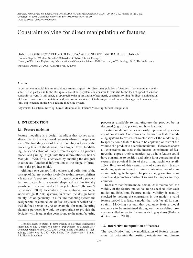
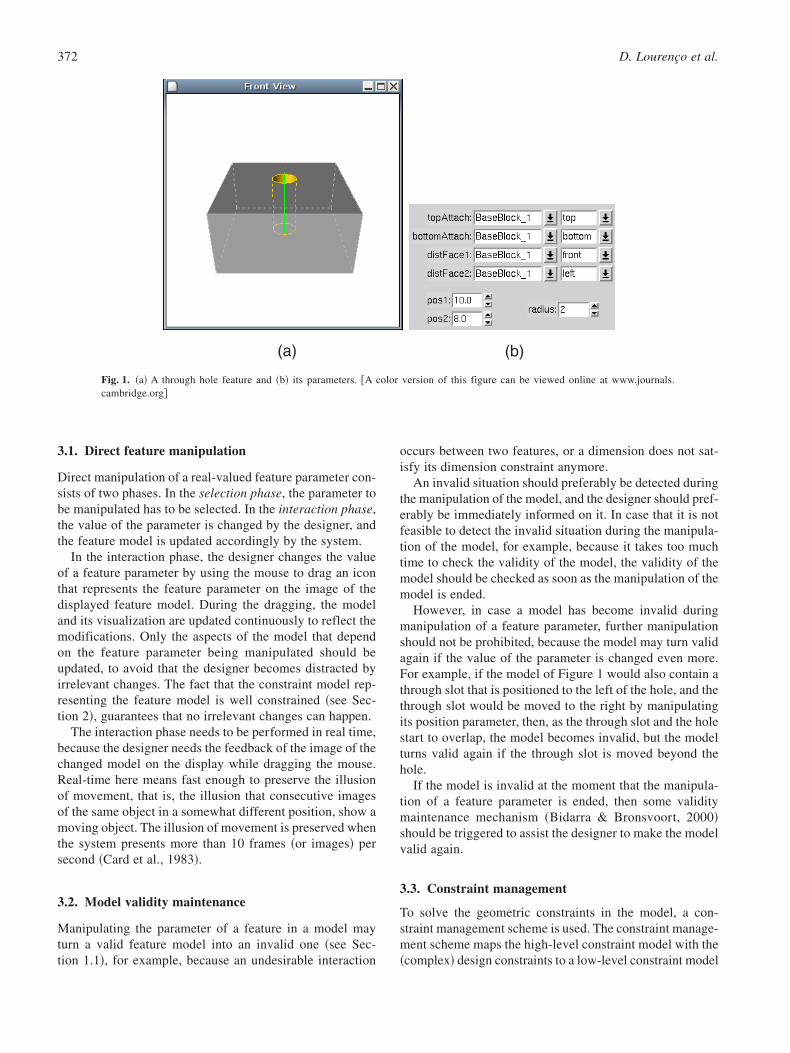
A feature can be modified by manipulating the value of theparameters of the feature. Although a parameter of a featurecan also be a face of another feature to which it is attached,or with respect to which it is positioned, this article onlydeals with manipulation of real-valued feature parameters,such as the dimension of the shape of a feature, the distanceof a feature with respect to a face of another feature, and soforth. An example of a through hole feature with its param-eters is given in Figure 1.

Constraint solving for direct manipulation of features 371

3.1. Direct feature manipulation

Direct manipulation of a real-valued feature parameter con-sists of two phases. In the selection phase, the parameter tobe manipulated has to be selected. In the interaction phase,the value of the parameter is changed by the designer, andthe feature model is updated accordingly by the system.

In the interaction phase, the designer changes the valueof a feature parameter by using the mouse to drag an iconthat represents the feature parameter on the image of thedisplayed feature model. During the dragging, the modeland its visualization are updated continuously to reflect themodifications. Only the aspects of the model that dependon the feature parameter being manipulated should beupdated, to avoid that the designer becomes distracted byirrelevant changes. The fact that the constraint model rep-resenting the feature model is well constrained ~see Sec-tion 2!, guarantees that no irrelevant changes can happen.

The interaction phase needs to be performed in real time,because the designer needs the feedback of the image of thechanged model on the display while dragging the mouse.Real-time here means fast enough to preserve the illusionof movement, that is, the illusion that consecutive imagesof the same object in a somewhat different position, show amoving object. The illusion of movement is preserved whenthe system presents more than 10 frames ~or images! persecond ~Card et al., 1983!.

3.2. Model validity maintenance

Manipulating the parameter of a feature in a model mayturn a valid feature model into an invalid one ~see Sec-tion 1.1!, for example, because an undesirable interaction

occurs between two features, or a dimension does not sat-isfy its dimension constraint anymore.

An invalid situation should preferably be detected duringthe manipulation of the model, and the designer should pref-erably be immediately informed on it. In case that it is notfeasible to detect the invalid situation during the manipula-tion of the model, for example, because it takes too muchtime to check the validity of the model, the validity of themodel should be checked as soon as the manipulation of themodel is ended.

However, in case a model has become invalid duringmanipulation of a feature parameter, further manipulationshould not be prohibited, because the model may turn validagain if the value of the parameter is changed even more.For example, if the model of Figure 1 would also contain athrough slot that is positioned to the left of the hole, and thethrough slot would be moved to the right by manipulatingits position parameter, then, as the through slot and the holestart to overlap, the model becomes invalid, but the modelturns valid again if the through slot is moved beyond thehole.

If the model is invalid at the moment that the manipula-tion of a feature parameter is ended, then some validitymaintenance mechanism ~Bidarra & Bronsvoort, 2000!should be triggered to assist the designer to make the modelvalid again.

3.3. Constraint management

To solve the geometric constraints in the model, a con-straint management scheme is used. The constraint manage-ment scheme maps the high-level constraint model with the~complex! design constraints to a low-level constraint model

(a) (b)

Fig. 1. ~a! A through hole feature and ~b! its parameters. @A color version of this figure can be viewed online at www.journals.cambridge.org#


with primitive constraints that can be solved by the con-straint solvers used, and updates the high-level constraintmodel based on the low-level constraint model after solving.

However, the low-level constraint model of typical fea-ture models generally consists of 100� constraint vari-ables. Most constraint solvers are too slow to solve theseduring interactive feature manipulation, given the high com-plexity of constraint solving algorithms.

Fortunately, in the interaction phase of interactive fea-ture manipulation, only a part of the constraint model needsto be solved. Because only one feature parameter is changedduring the interaction phase, typically, large parts of themodel do not change, that is, they are rigid. Such rigid partscan, therefore, be represented by a single constraint vari-able in the low-level constraint graph, thus avoiding theneed to solve all constraints within these parts.

Constraint management for interactive feature manipula-tion should thus identify all rigid parts of the model, andmap each one to a separate constraint variable in the low-level constraint model that is solved in the interaction phase.The resulting, simple, constraint model can be used to findthe relative position and orientation of the rigid parts dur-ing the interaction phase, given the current value of thefeature parameter that is beeing changed.

Although the rigid parts of the model can be found usingthe algorithms presented by Hsu et al. ~1997! and Weigeland Faltings ~1999!, this article proposes the generationand use, for this purpose, of a special constraint model,because this approach can be applied with many geometricconstraint solvers and requires little implementation effort.The only requirement to the constraint solver is that it shouldbe able to solve an underconstrained model, and return infor-mation on the rigid parts in such a model.

The next sections describe such a constraint solver-driven model compilation approach.

4. CONSTRAINT SOLVER-DRIVEN MODELCOMPILATION

In the constraint solver-driven model compilation approach,the original constraint model is compiled into a manipula-tion constraint model that is optimized to reduce the timeneeded to validate the feature model after manipulating aspecific feature parameter. The compilation is performedby a constraint solver. The optimization is based on thenotion that, in general, a change to the value of a certainfeature parameter causes only limited changes to the fea-ture model, which was described in Subsection 3.3.

4.1. Generating the manipulation constraint model

The manipulation constraint model is generated in the selec-tion phase of the interactive feature manipulation process.It is generated only once when a feature parameter is selectedto be manipulated.

The manipulation constraint model contains a constraintvariable for each rigid part of the original constraint model,and the constraints between these rigid parts. The con-straint variables within a rigid part in the original constraintmodel are replaced by a single constraint variable in themanipulation model, which represents the position and ori-entation of the rigid part. The constraints between the con-straint variables within a rigid part are discarded in themanipulation model, because their relative position and ori-entation will not change during the manipulation phase.The constraints between the constraint variables of differ-ent rigid parts in the original constraint model are in themanipulation constraint model between the constraint vari-ables that represent the rigid parts.

The manipulation constraint model is generated by a con-straint management approach that uses the constraint solverto find the rigid parts in the model. The constraint manage-ment approach finds the rigid parts in the model by havingthe constraint solver solve the original constraint modelexcept for the constraints that represent the feature param-eter that is changed. Based on the rigid parts found, theconstraint management approach generates the manipula-tion model.

Discarding the constraints that represent the feature param-eter that is changed, results in an underconstrained con-straint model with multiple well-constrained ~Joan-Arinyoet al., 2003! submodels. Each well-constrained submodelrepresents a region of the feature model that remains rigidif the feature parameter is changed. Although it is not nec-essary to minimize the number of well-constrained submod-els, reducing the number of submodels cuts down the timeneeded to solve the resulting manipulation constraint model.

The constraint solver that is used by the constraint man-agement approach to solve this model should be capable ofsolving such underconstrained models and returning the sub-models that are well constrained. These capabilities areowned by many geometric constraint solvers.

The constraint management approach generates the manip-ulation constraint model based on the information on thewell-constrained or rigid parts of the model that is returnedby the constraint solver. It creates a constraint variable inthe manipulation constraint model for each rigid part in theoriginal constraint model. In addition, it analyzes the orig-inal constraint model to find the constraints between therigid parts; for each constraint it finds, it creates an identi-cal constraint between the constraint variables in the manip-ulation constraint model that represent the rigid parts. Theseconstraints include the constraints that represent the featureparameter whose value will be changed.

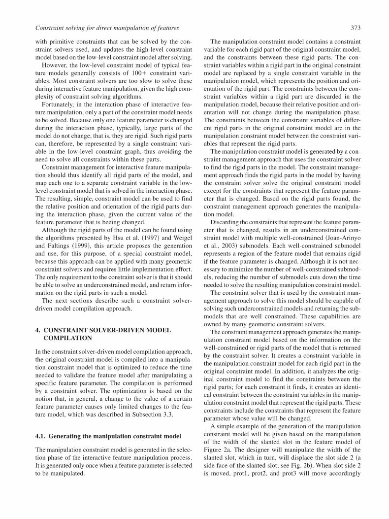
A simple example of the generation of the manipulationconstraint model will be given based on the manipulationof the width of the slanted slot in the feature model ofFigure 2a. The designer will manipulate the width of theslanted slot, which in turn, will displace the slot side 2 ~aside face of the slanted slot; see Fig. 2b!. When slot side 2is moved, prot1, prot2, and prot3 will move accordingly


because they are positioned with respect to slot side 2, eitherdirectly or indirectly ~see Fig. 2c!.

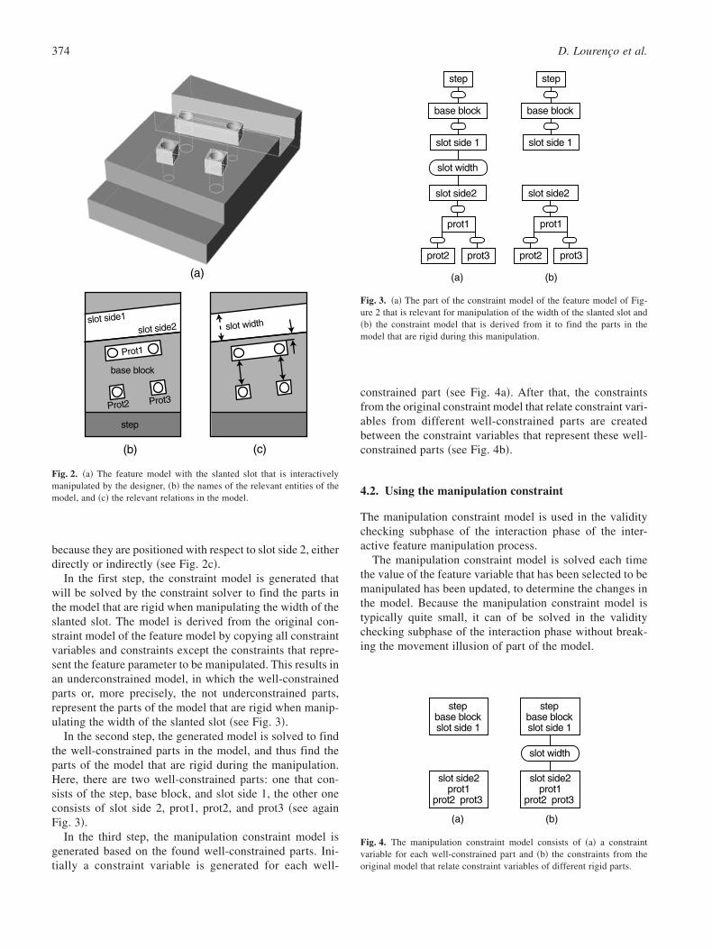
In the first step, the constraint model is generated thatwill be solved by the constraint solver to find the parts inthe model that are rigid when manipulating the width of theslanted slot. The model is derived from the original con-straint model of the feature model by copying all constraintvariables and constraints except the constraints that repre-sent the feature parameter to be manipulated. This results inan underconstrained model, in which the well-constrainedparts or, more precisely, the not underconstrained parts,represent the parts of the model that are rigid when manip-ulating the width of the slanted slot ~see Fig. 3!.

In the second step, the generated model is solved to findthe well-constrained parts in the model, and thus find theparts of the model that are rigid during the manipulation.Here, there are two well-constrained parts: one that con-sists of the step, base block, and slot side 1, the other oneconsists of slot side 2, prot1, prot2, and prot3 ~see againFig. 3!.

In the third step, the manipulation constraint model isgenerated based on the found well-constrained parts. Ini-tially a constraint variable is generated for each well-

constrained part ~see Fig. 4a!. After that, the constraintsfrom the original constraint model that relate constraint vari-ables from different well-constrained parts are createdbetween the constraint variables that represent these well-constrained parts ~see Fig. 4b!.

4.2. Using the manipulation constraint

The manipulation constraint model is used in the validitychecking subphase of the interaction phase of the inter-active feature manipulation process.

The manipulation constraint model is solved each timethe value of the feature variable that has been selected to bemanipulated has been updated, to determine the changes inthe model. Because the manipulation constraint model istypically quite small, it can of be solved in the validitychecking subphase of the interaction phase without break-ing the movement illusion of part of the model.

Prot2 Prot3

Prot1

slot side1

slot side2

step

base block

(b) (c)

(a)

slot width

Fig. 2. ~a! The feature model with the slanted slot that is interactivelymanipulated by the designer, ~b! the names of the relevant entities of themodel, and ~c! the relevant relations in the model.

Fig. 3. ~a! The part of the constraint model of the feature model of Fig-ure 2 that is relevant for manipulation of the width of the slanted slot and~b! the constraint model that is derived from it to find the parts in themodel that are rigid during this manipulation.

Fig. 4. The manipulation constraint model consists of ~a! a constraintvariable for each well-constrained part and ~b! the constraints from theoriginal model that relate constraint variables of different rigid parts.


The changes to the manipulation constraint model arepropagated to the original constraint model each time themanipulation constraint model has been solved. This con-sists of updating the value of the constraint variables in theoriginal constraint model based on the value ~i.e., positionand orientation! of each of the constraint variables in themanipulation constraint model.

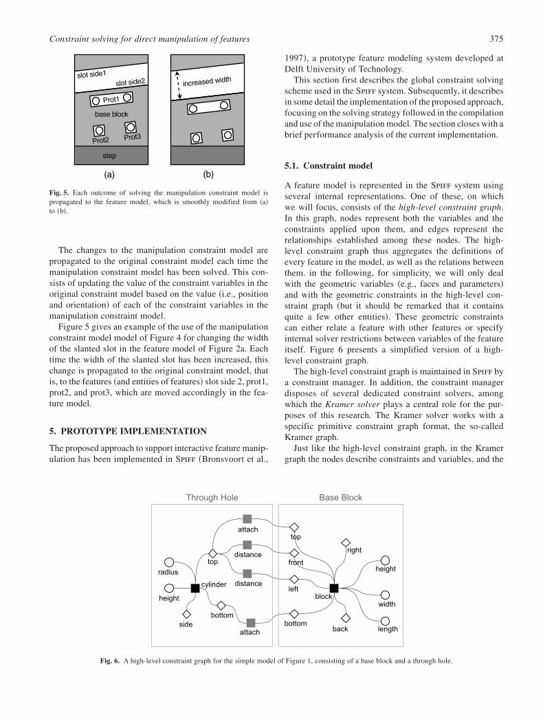
Figure 5 gives an example of the use of the manipulationconstraint model model of Figure 4 for changing the widthof the slanted slot in the feature model of Figure 2a. Eachtime the width of the slanted slot has been increased, thischange is propagated to the original constraint model, thatis, to the features ~and entities of features! slot side 2, prot1,prot2, and prot3, which are moved accordingly in the fea-ture model.

5. PROTOTYPE IMPLEMENTATION

The proposed approach to support interactive feature manip-ulation has been implemented in Spiff ~Bronsvoort et al.,

1997!, a prototype feature modeling system developed atDelft University of Technology.

This section first describes the global constraint solvingscheme used in the Spiff system. Subsequently, it describesin some detail the implementation of the proposed approach,focusing on the solving strategy followed in the compilationand use of the manipulation model. The section closes with abrief performance analysis of the current implementation.

5.1. Constraint model

A feature model is represented in the Spiff system usingseveral internal representations. One of these, on whichwe will focus, consists of the high-level constraint graph.In this graph, nodes represent both the variables and theconstraints applied upon them, and edges represent therelationships established among these nodes. The high-level constraint graph thus aggregates the definitions ofevery feature in the model, as well as the relations betweenthem. in the following, for simplicity, we will only dealwith the geometric variables ~e.g., faces and parameters!and with the geometric constraints in the high-level con-straint graph ~but it should be remarked that it containsquite a few other entities!. These geometric constraintscan either relate a feature with other features or specifyinternal solver restrictions between variables of the featureitself. Figure 6 presents a simplified version of a high-level constraint graph.

The high-level constraint graph is maintained in Spiff bya constraint manager. In addition, the constraint managerdisposes of several dedicated constraint solvers, amongwhich the Kramer solver plays a central role for the pur-poses of this research. The Kramer solver works with aspecific primitive constraint graph format, the so-calledKramer graph.

Just like the high-level constraint graph, in the Kramergraph the nodes describe constraints and variables, and the

Fig. 5. Each outcome of solving the manipulation constraint model ispropagated to the feature model, which is smoothly modified from ~a!to ~b!.

Fig. 6. A high-level constraint graph for the simple model of Figure 1, consisting of a base block and a through hole.


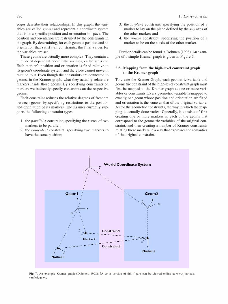
edges describe their relationships. In this graph, the vari-ables are called geoms and represent a coordinate systemthat is in a specific position and orientation in space. Theposition and orientation are restrained by the constraints inthe graph. By determining, for each geom, a position and anorientation that satisfy all constraints, the final values forthe variables are set.

These geoms are actually more complex. They contain anumber of dependent coordinate systems, called markers.Each marker’s position and orientation is fixed relative toits geom’s coordinate system, and therefore cannot move inrelation to it. Even though the constraints are connected togeoms, in the Kramer graph, what they actually relate aremarkers inside those geoms. By specifying constraints onmarkers we indirectly specify constraints on the respectivegeoms.

Each constraint reduces the relative degrees of freedombetween geoms by specifying restrictions to the positionand orientation of its markers. The Kramer currently sup-ports the following constraint types:

1. the parallel-z constraint, specifying the z axes of twomarkers to be parallel;

2. the coincident constraint, specifying two markers tohave the same position;

3. the in-plane constraint, specifying the position of amarker to lay on the plane defined by the x–y axes ofthe other marker; and

4. the in-line constraint, specifying the position of amarker to be on the z axis of the other marker.

Further details can be found in Dohmen ~1998!. An exam-ple of a simple Kramer graph is given in Figure 7.

5.2. Mapping from the high-level constraint graphto the Kramer graph

To create the Kramer Graph, each geometric variable andgeometric constraint of the high-level constraint graph mustfirst be mapped to the Kramer graph as one or more vari-ables or constraints. Every geometric variable is mapped toexactly one geom whose position and orientation are fixedand orientation is the same as that of the original variable.As for the geometric constraints, the way in which the map-ping is actually done varies. Generally, it consists of firstcreating one or more markers in each of the geoms thatcorrespond to the geometric variables of the original con-straint, and then creating a number of Kramer constraintsrelating these markers in a way that expresses the semanticsof the original constraint.

Fig. 7. An example Kramer graph ~Dohmen, 1998!. @A color version of this figure can be viewed online at www.journals.cambridge.org#


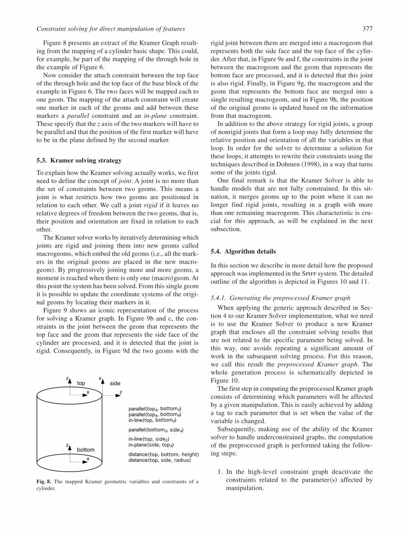
Figure 8 presents an extract of the Kramer Graph result-ing from the mapping of a cylinder basic shape. This could,for example, be part of the mapping of the through hole inthe example of Figure 6.

Now consider the attach constraint between the top faceof the through hole and the top face of the base block of theexample in Figure 6. The two faces will be mapped each toone geom. The mapping of the attach constraint will createone marker in each of the geoms and add between thesemarkers a parallel constraint and an in-plane constraint.These specify that the z axis of the two markers will have tobe parallel and that the position of the first marker will haveto be in the plane defined by the second marker.

5.3. Kramer solving strategy

To explain how the Kramer solving actually works, we firstneed to define the concept of joint. A joint is no more thanthe set of constraints between two geoms. This means ajoint is what restricts how two geoms are positioned inrelation to each other. We call a joint rigid if it leaves norelative degrees of freedom between the two geoms, that is,their position and orientation are fixed in relation to eachother.

The Kramer solver works by iteratively determining whichjoints are rigid and joining them into new geoms calledmacrogeoms, which embed the old geoms ~i.e., all the mark-ers in the original geoms are placed in the new macro-geom!. By progressively joining more and more geoms, amoment is reached when there is only one ~macro!geom. Atthis point the system has been solved. From this single geomit is possible to update the coordinate systems of the origi-nal geoms by locating their markers in it.

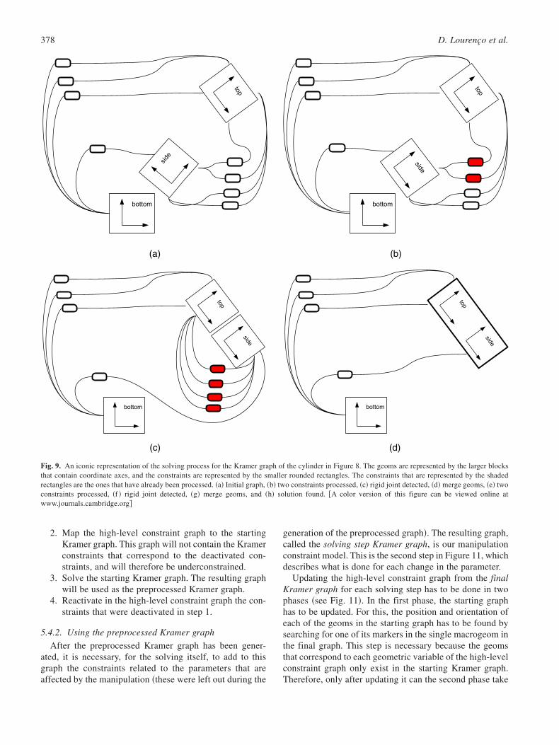
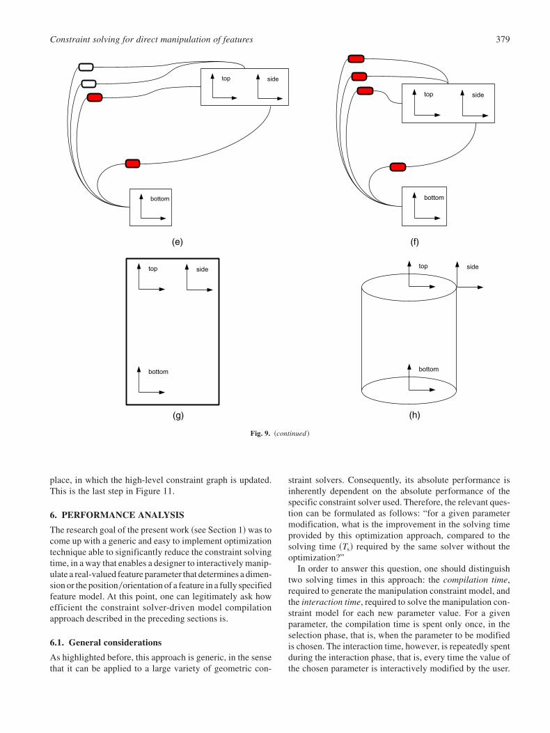
Figure 9 shows an iconic representation of the processfor solving a Kramer graph. In Figure 9b and c, the con-straints in the joint between the geom that represents thetop face and the geom that represents the side face of thecylinder are processed, and it is detected that the joint isrigid. Consequently, in Figure 9d the two geoms with the

rigid joint between them are merged into a macrogeom thatrepresents both the side face and the top face of the cylin-der. After that, in Figure 9e and f, the constraints in the jointbetween the macrogeom and the geom that represents thebottom face are processed, and it is detected that this jointis also rigid. Finally, in Figure 9g, the macrogeom and thegeom that represents the bottom face are merged into asingle resulting macrogeom, and in Figure 9h, the positionof the original geoms is updated based on the informationfrom that macrogeom.

In addition to the above strategy for rigid joints, a groupof nonrigid joints that form a loop may fully determine therelative position and orientation of all the variables in thatloop. In order for the solver to determine a solution forthese loops, it attempts to rewrite their constraints using thetechniques described in Dohmen ~1998!, in a way that turnssome of the joints rigid.

One final remark is that the Kramer Solver is able tohandle models that are not fully constrained. In this sit-uation, it merges geoms up to the point where it can nolonger find rigid joints, resulting in a graph with morethan one remaining macrogeom. This characteristic is cru-cial for this approach, as will be explained in the nextsubsection.

5.4. Algorithm details

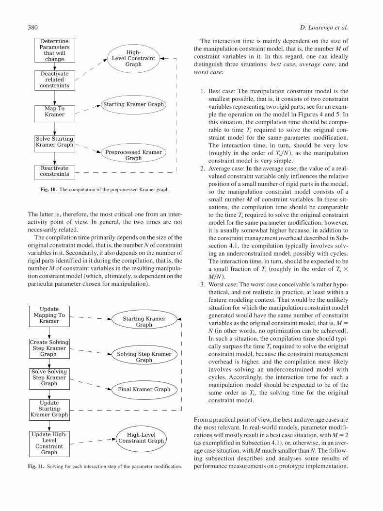
In this section we describe in more detail how the proposedapproach was implemented in the Spiff system. The detailedoutline of the algorithm is depicted in Figures 10 and 11.

5.4.1. Generating the preprocessed Kramer graph

When applying the generic approach described in Sec-tion 4 to our Kramer Solver implementation, what we needis to use the Kramer Solver to produce a new Kramergraph that encloses all the constraint solving results thatare not related to the specific parameter being solved. Inthis way, one avoids repeating a significant amount ofwork in the subsequent solving process. For this reason,we call this result the preprocessed Kramer graph. Thewhole generation process is schematically depicted inFigure 10.

The first step in computing the preprocessed Kramer graphconsists of determining which parameters will be affectedby a given manipulation. This is easily achieved by addinga tag to each parameter that is set when the value of thevariable is changed.

Subsequently, making use of the ability of the Kramersolver to handle underconstrained graphs, the computationof the preprocessed graph is performed taking the follow-ing steps:

1. In the high-level constraint graph deactivate theconstraints related to the parameter~s! affected bymanipulation.

Fig. 8. The mapped Kramer geometric variables and constraints of acylinder.


2. Map the high-level constraint graph to the startingKramer graph. This graph will not contain the Kramerconstraints that correspond to the deactivated con-straints, and will therefore be underconstrained.

3. Solve the starting Kramer graph. The resulting graphwill be used as the preprocessed Kramer graph.

4. Reactivate in the high-level constraint graph the con-straints that were deactivated in step 1.

5.4.2. Using the preprocessed Kramer graph

After the preprocessed Kramer graph has been gener-ated, it is necessary, for the solving itself, to add to thisgraph the constraints related to the parameters that areaffected by the manipulation ~these were left out during the

generation of the preprocessed graph!. The resulting graph,called the solving step Kramer graph, is our manipulationconstraint model. This is the second step in Figure 11, whichdescribes what is done for each change in the parameter.

Updating the high-level constraint graph from the finalKramer graph for each solving step has to be done in twophases ~see Fig. 11!. In the first phase, the starting graphhas to be updated. For this, the position and orientation ofeach of the geoms in the starting graph has to be found bysearching for one of its markers in the single macrogeom inthe final graph. This step is necessary because the geomsthat correspond to each geometric variable of the high-levelconstraint graph only exist in the starting Kramer graph.Therefore, only after updating it can the second phase take

Fig. 9. An iconic representation of the solving process for the Kramer graph of the cylinder in Figure 8. The geoms are represented by the larger blocksthat contain coordinate axes, and the constraints are represented by the smaller rounded rectangles. The constraints that are represented by the shadedrectangles are the ones that have already been processed. ~a! Initial graph, ~b! two constraints processed, ~c! rigid joint detected, ~d! merge geoms, ~e! twoconstraints processed, ~f ! rigid joint detected, ~g! merge geoms, and ~h! solution found. @A color version of this figure can be viewed online atwww.journals.cambridge.org#


place, in which the high-level constraint graph is updated.This is the last step in Figure 11.

6. PERFORMANCE ANALYSIS

The research goal of the present work ~see Section 1!was tocome up with a generic and easy to implement optimizationtechnique able to significantly reduce the constraint solvingtime, in a way that enables a designer to interactively manip-ulate a real-valued feature parameter that determines a dimen-sion or the position0orientation of a feature in a fully specifiedfeature model. At this point, one can legitimately ask howefficient the constraint solver-driven model compilationapproach described in the preceding sections is.

6.1. General considerations

As highlighted before, this approach is generic, in the sensethat it can be applied to a large variety of geometric con-

straint solvers. Consequently, its absolute performance isinherently dependent on the absolute performance of thespecific constraint solver used. Therefore, the relevant ques-tion can be formulated as follows: “for a given parametermodification, what is the improvement in the solving timeprovided by this optimization approach, compared to thesolving time ~Ts! required by the same solver without theoptimization?”

In order to answer this question, one should distinguishtwo solving times in this approach: the compilation time,required to generate the manipulation constraint model, andthe interaction time, required to solve the manipulation con-straint model for each new parameter value. For a givenparameter, the compilation time is spent only once, in theselection phase, that is, when the parameter to be modifiedis chosen. The interaction time, however, is repeatedly spentduring the interaction phase, that is, every time the value ofthe chosen parameter is interactively modified by the user.

Fig. 9. ~continued !


The latter is, therefore, the most critical one from an inter-activity point of view. In general, the two times are notnecessarily related.

The compilation time primarily depends on the size of theoriginal constraint model, that is, the number N of constraintvariables in it. Secondarily, it also depends on the number ofrigid parts identified in it during the compilation, that is, thenumber M of constraint variables in the resulting manipula-tion constraint model ~which, ultimately, is dependent on theparticular parameter chosen for manipulation!.

The interaction time is mainly dependent on the size ofthe manipulation constraint model, that is, the number M ofconstraint variables in it. In this regard, one can ideallydistinguish three situations: best case, average case, andworst case:

1. Best case: The manipulation constraint model is thesmallest possible, that is, it consists of two constraintvariables representing two rigid parts; see for an exam-ple the operation on the model in Figures 4 and 5. Inthis situation, the compilation time should be compa-rable to time Ts required to solve the original con-straint model for the same parameter modification.The interaction time, in turn, should be very low~roughly in the order of Ts0N !, as the manipulationconstraint model is very simple.

2. Average case: In the average case, the value of a real-valued constraint variable only influences the relativeposition of a small number of rigid parts in the model,so the manipulation constraint model consists of asmall number M of constraint variables. In these sit-uations, the compilation time should be comparableto the time Ts required to solve the original constraintmodel for the same parameter modification; however,it is usually somewhat higher because, in addition tothe constraint management overhead described in Sub-section 4.1, the compilation typically involves solv-ing an underconstrained model, possibly with cycles.The interaction time, in turn, should be expected to bea small fraction of Ts ~roughly in the order of Ts �M0N !.

3. Worst case: The worst case conceivable is rather hypo-thetical, and not realistic in practice, at least within afeature modeling context. That would be the unlikelysituation for which the manipulation constraint modelgenerated would have the same number of constraintvariables as the original constraint model, that is, M �N ~in other words, no optimization can be achieved!.In such a situation, the compilation time should typi-cally surpass the time Ts required to solve the originalconstraint model, because the constraint managementoverhead is higher, and the compilation most likelyinvolves solving an underconstrained model withcycles. Accordingly, the interaction time for such amanipulation model should be expected to be of thesame order as Ts, the solving time for the originalconstraint model.

From a practical point of view, the best and average cases arethe most relevant. In real-world models, parameter modifi-cations will mostly result in a best case situation, with M �2~as exemplified in Subsection 4.1!, or, otherwise, in an aver-age case situation, with M much smaller than N. The follow-ing subsection describes and analyses some results ofperformance measurements on a prototype implementation.

Fig. 10. The computation of the preprocessed Kramer graph.

Fig. 11. Solving for each interaction step of the parameter modification.


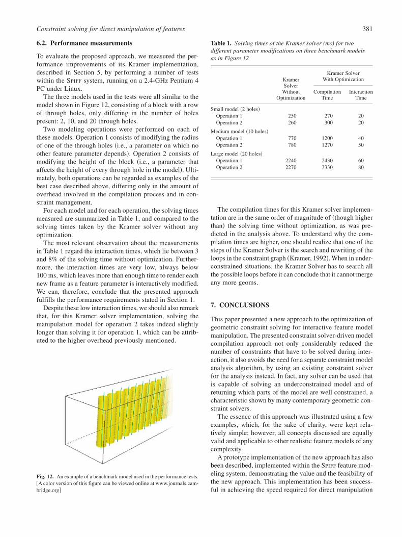
6.2. Performance measurements

To evaluate the proposed approach, we measured the per-formance improvements of its Kramer implementation,described in Section 5, by performing a number of testswithin the Spiff system, running on a 2.4-GHz Pentium 4PC under Linux.

The three models used in the tests were all similar to themodel shown in Figure 12, consisting of a block with a rowof through holes, only differing in the number of holespresent: 2, 10, and 20 through holes.

Two modeling operations were performed on each ofthese models. Operation 1 consists of modifying the radiusof one of the through holes ~i.e., a parameter on which noother feature parameter depends!. Operation 2 consists ofmodifying the height of the block ~i.e., a parameter thataffects the height of every through hole in the model!. Ulti-mately, both operations can be regarded as examples of thebest case described above, differing only in the amount ofoverhead involved in the compilation process and in con-straint management.

For each model and for each operation, the solving timesmeasured are summarized in Table 1, and compared to thesolving times taken by the Kramer solver without anyoptimization.

The most relevant observation about the measurementsin Table 1 regard the interaction times, which lie between 3and 8% of the solving time without optimization. Further-more, the interaction times are very low, always below100 ms, which leaves more than enough time to render eachnew frame as a feature parameter is interactively modified.We can, therefore, conclude that the presented approachfulfills the performance requirements stated in Section 1.

Despite these low interaction times, we should also remarkthat, for this Kramer solver implementation, solving themanipulation model for operation 2 takes indeed slightlylonger than solving it for operation 1, which can be attrib-uted to the higher overhead previously mentioned.

The compilation times for this Kramer solver implemen-tation are in the same order of magnitude of ~though higherthan! the solving time without optimization, as was pre-dicted in the analysis above. To understand why the com-pilation times are higher, one should realize that one of thesteps of the Kramer Solver is the search and rewriting of theloops in the constraint graph ~Kramer, 1992!. When in under-constrained situations, the Kramer Solver has to search allthe possible loops before it can conclude that it cannot mergeany more geoms.

7. CONCLUSIONS

This paper presented a new approach to the optimization ofgeometric constraint solving for interactive feature modelmanipulation. The presented constraint solver-driven modelcompilation approach not only considerably reduced thenumber of constraints that have to be solved during inter-action, it also avoids the need for a separate constraint modelanalysis algorithm, by using an existing constraint solverfor the analysis instead. In fact, any solver can be used thatis capable of solving an underconstrained model and ofreturning which parts of the model are well constrained, acharacteristic shown by many contemporary geometric con-straint solvers.

The essence of this approach was illustrated using a fewexamples, which, for the sake of clarity, were kept rela-tively simple; however, all concepts discussed are equallyvalid and applicable to other realistic feature models of anycomplexity.

A prototype implementation of the new approach has alsobeen described, implemented within the Spiff feature mod-eling system, demonstrating the value and the feasibility ofthe new approach. This implementation has been success-ful in achieving the speed required for direct manipulation

Fig. 12. An example of a benchmark model used in the performance tests.@A color version of this figure can be viewed online at www.journals.cam-bridge.org#

Table 1. Solving times of the Kramer solver (ms) for twodifferent parameter modifications on three benchmark modelsas in Figure 12

Kramer SolverWith OptimizationKramer

SolverWithout

OptimizationCompilation

TimeInteraction

Time

Small model ~2 holes!Operation 1 250 270 20Operation 2 260 300 20

Medium model ~10 holes!Operation 1 770 1200 40Operation 2 780 1270 50

Large model ~20 holes!Operation 1 2240 2430 60Operation 2 2270 3330 80


of features and, as a result, effectively improving the userexperience.

In summary, it can be concluded that the presentedapproach to the optimization of geometric constraint solv-ing during interactive manipulation can be used with manyconstraint solvers and avoids the need for a separate con-straint model analysis algorithm. Both the prototype imple-mentation described and the performance tests executedwith it confirm the high potential of the approach.

REFERENCES

Bidarra, R., & Bronsvoort, W.F. ~2000!. Semantic feature modelling.Computer-Aided Design 32(3), 201–225.

Borning, A., & Duisberg, R. ~1986!. Constraint-based tools for buildinguser interfaces. ACM Transactions on Graphics 5(4), 345–374.

Bronsvoort, W.F., Bidarra, R., Dohmen, M., van Holland, W., & de Kraker,K.J. ~1997!. Multiple-view feature modelling and conversion. In Geo-metric Modeling: Theory and Practice—The State of the Art ~Strasser,W., Klein, R., & Rau, R., Eds.!, pp. 159–174. Berlin: Springer–Verlag.

Card, S.K., Moran, T.P., & Newell, A. ~1983!. The Psychology of Human–Computer Interaction. Hillsdale, NJ: Erlbaum.

Dohmen, M. ~1998!. Constraint-based feature validation. PhD thesis, DelftUniversity of Technology.

Freeman-Benson, B.N. ~1993!. Converting an existing user interface touse constraints. In Proc. ACM Symp. User Interface Software and Tech-nology, pp. 207–215. New York: ACM Press.

Hosobe, H. ~2001!. A modular geometric constraint solver for user inter-face applications. In Proc. 14th Annual ACM Symp. User InterfaceSoftware and Technology, pp. 91–100. New York: ACM Press.

Hsu, C., Huang, Z., Beier, E., & Brüderlin, B. ~1997!. A constraint-basedmanipulator toolset for editing 3D objects. In Proc. of the Fourth ACMSymp. on Solid Modeling and Applications, pp. 168–180. New York:ACM Press.

Joan-Arinyo, R., Soto-Riera, A., Vila-Marta, S., & Vilaplana-Pasto, J. ~2003!.Transforming an underconstrained geometric constraint problem intoa well-constrained one. In Proc. Eighth ACM Symp. Solid Modelingand Applications, pp. 33– 44. New York: ACM Press.

Kramer, G.A. ~1992!. A geometric constraint engine. Artificial Intelli-gence 58(1–3), 327–360.

Shah, J.J., & Mäntylä, M. ~1995!. Parametric and Feature-Based CAD0CAM. New York: Wiley.

van Emmerik, M.J.G.M. ~1991!. Interactive design of 3D models withgeometric constraints. The Visual Computer 7(506), 309–325.

Weigel, R., & Faltings, B. ~1999!. Compiling constraint satisfaction prob-lems. Artificial Intelligence 115(2), 257–287.

Daniel Lourenço attained a degree in computer science in2005 at Instituto Superior Técnico, Lisbon, Portugal. His

graduation project, which was performed with PedroOliveira, was carried out at the Computer Graphics andCAD0CAM Group at Delft University of Technology. Theproject dealt with real-time direct manipulation of featuremodels and eventually led to the work described in thisarticle. Daniel works as a Consultant for the agile soft-ware company Outsystems.

Pedro Oliveira graduated in computer science in 2005 atInstituto Superior Técnico, Lisbon, Portugal. His gradua-tion project, which was performed with Daniel Lourenço,was carried out at the Computer Graphics and CAD0CAMGroup at Delft University of Technology. The project dealtwith real-time direct manipulation of feature models andeventually led to the work described in this article. Pedrocurrently works as a Consultant at the Business TechnologyOffice of McKinsey & Company.

Alex Noort works as computer scientist at The NetherlandsBureau for Economic Policy Analysis in The Hague. Hereceived his MS degree in computer science in 1997 and hisPhD degree in 2002, both from Delft University of Tech-nology. His master’s thesis was written on solving overcon-strained geometric models, and his PhD thesis dealt withmultiple-view feature modeling with model adjustment. Dr.Noort’s main research interests are feature modeling, inparticular multiple-view feature modeling and constraintsolving.

Rafael Bidarra is Assistant Professor of geometric model-ing in the Faculty of Electrical Engineering, Mathematicsand Computer Science of Delft University of Technology.He graduated with a degree in electronics engineering atthe University of Coimbra, Portugal, in 1987, and receivedhis PhD degree in computer science from Delft Universityof Technology in 1999. He currently leads the research workon computer games at the Computer Graphics and CAD0CAM Group. His current research interests include proce-dural, parametric, and semantic modeling and geometricreasoning. He has published many papers in internationaljournals, books, and conference proceedings and has servedas a member of several program committees.


Constraint solving for direct manipulation of features

Documents