1 Constraining global isoprene emissions with GOME formaldehyde column measurements Changsub Shim 1 , Yuhang Wang 1 , Yunsoo Choi 1 , Paul I. Palmer 2 , Dorian S. Abbot 2 , and Kelly Chance 3 1 Department of Earth and Atmospheric Sciences, Georgia Institute of Technology, Atlanta, Georgia 2 Department of Earth and Planetary Sciences and Division of Engineering and Applied Sciences, Harvard University, Cambridge, Massachusetts 3 Harvard-Smithsonian Center for Astrophysics, Cambridge, Massachusetts J. Geophys. Res., In Press

Welcome message from author
This document is posted to help you gain knowledge. Please leave a comment to let me know what you think about it! Share it to your friends and learn new things together.
Transcript

1
Constraining global isoprene emissions with GOME formaldehyde column
measurements
Changsub Shim1, Yuhang Wang1, Yunsoo Choi1, Paul I. Palmer2, Dorian S. Abbot2, and Kelly Chance3 1Department of Earth and Atmospheric Sciences, Georgia Institute of Technology, Atlanta, Georgia 2Department of Earth and Planetary Sciences and Division of Engineering and Applied Sciences, Harvard University, Cambridge, Massachusetts 3Harvard-Smithsonian Center for Astrophysics, Cambridge, Massachusetts
J. Geophys. Res., In Press

Abstract
Biogenic isoprene plays an important role in tropospheric chemistry. Current isoprene
emission estimates are highly uncertain due to a lack of direct observations. Formaldehyde
(HCHO) is a high-yield product of isoprene oxidation. The short photochemical lifetime of
HCHO allows the observations of this trace gas to help constrain isoprene emissions. We use
HCHO column observations by the Global Ozone Monitoring Experiment (GOME). These
global data are particularly useful for studying large isoprene emissions from the tropics, where
in situ observations are sparse. Using the global GEOS-CHEM chemical transport model as the
forward model, a Bayesian inversion of GOME HCHO observations from September 1996 to
August 1997 is conducted to calculate global isoprene emissions. Column contributions to
HCHO from 10 biogenic sources, in addition to biomass burning and industrial sources are
considered. The inversion of these 12 HCHO sources is conducted separately for 8 geographical
regions (North America, Europe, East Asia, India, Southeast Asia, South America, Africa, and
Australia). GOME measurements with high signal-to-noise ratios are used. The a priori
simulation greatly underestimates global HCHO columns over the 8 geographical regions (bias: -
14 – -46%, R: 0.52 – 0.84). The a posteriori solution shows generally higher isoprene and
biomass burning emissions and these emissions reduce the model biases for all regions (bias: -
3.6 – -25%, R = 0.56 – 0.84). The negative bias in the a posteriori estimate reflects in part the
uncertainty in GOME measurements. The a posteriori estimate of the annual global isoprene
emissions of 566 Tg C yr-1 is about 50% larger than the a priori estimate. This increase of global
isoprene emissions significantly affects tropospheric chemistry, decreasing the global mean OH
concentration by 10.8% to 0.95×10⁶ molecules/cm3. The atmospheric lifetime of CH3CCl3
increases from 5.2 to 5.7 years.
2

1. Introduction
Volatile organic compounds (VOCs) play an important role in oxidiation chemistry in the
troposphere [Chameides et al., 1992; Moxim et al., 1997; Houweling et al., 1998; Wang et al.,
1998b; Poisson et al., 2000]. Biogenic emissions are major sources of VOCs [e.g., Zimmerman,
1979; Lamb et al., 1987; Mueller, 1992]. Isoprene, in particular, represents almost half of the
total source of biogenic VOCs, and almost 40% of total VOC emissions on a global scale
[Guenther et al., 1995]. Furthermore, the formation of secondary organic aerosols via
photooxidation of isoprene affects the global climate [Limbeck et al., 2003; Claeys et al., 2004].
Isoprene emissions depend on vegetation types, light intensity, temperature and leaf area
index (LAI) [Lamb et al., 1987; Guenther et al., 1995]. Global emissions of isoprene are
generally estimated by extrapolating from limited laboratory and field measurements to the
prescribed global ecosystems. Various emission parameterizations have been proposed [e.g.,
Lamb et al., 1987; Guenther et al., 1995]. Despite these efforts, large uncertainties still remain in
the estimates [Hewitt and Street, 1992; Guenther et al., 1995]. The difficulty lies in the scarcity
of direct measurements. The problem is most acute for tropical ecosystems [Guenther et al.,
1995; Pierce et al., 1998], which collectively account for more than half of global isoprene
emissions [Guenther et al., 1995].
Formaldehyde is a product of VOC oxidation. The main sinks of HCHO are photolysis and
the reaction with atmospheric OH, and its lifetime against oxidation (order of hours) is short
enough not to be significantly affected by transport. Methane is an important HCHO source, but
it is well mixed in the troposphere due to its long lifetime. Methane oxidation provides the
background HCHO levels.
3
Previously, isoprene emissions over North America in summer have been derived using
HCHO column measurements from the Global Ozone Monitoring Experiment (GOME) [Chance
et al., 2000; Palmer et al., 2003a; Abbot et al., 2003]. It was found that isoprene is the dominant
contributor to HCHO over North America in the growing season; the enhancements above the
CH4-oxidation induced background levels are generally linear with local isoprene emissions over
North America [Chance et al., 2000; Palmer et al., 2003a]. Using that information, the seasonal
and interannual variations in GOME HCHO columns over North America has been investigated
[Abbot et al., 2003]. Here we extend these previous studies to the global scale and we also
explicitly consider isoprene emissions from 10 vegetation groups to capture the large difference
in base emissions for different types of vegetations. The sources from biomass burning and
industry are also treated separately.
In this work, we apply GOME observations of HCHO column from September 1996 to
August 1997 to constrain global isoprene emissions. In order to obtain best estimations of
isoprene emissions, we use statistical inferences to fit the model simulated HCHO column
concentrations toward GOME-observed HCHO column concentrations (inverse modeling). To
minimize the effects of GOME measurement uncertainties, we selected 8 regions with high
signal-to-noise ratios (the ratio of slant column to signal fitting error > 4). These regions are
located over North America, Europe, East Asia, India, Southeast Asia, South America, Africa,
and Australia.
Model parameters (state vector) considered for the HCHO sources include the oxidation of
isoprene from 9 major vegetation groups; the 10th group includes isoprene from all other
vegetation types and biogenic VOCs other than isoprene. The other two HCHO sources
considered are biomass burning (combined with biofuel burning) and industry. The sources
4

include primary emissions of HCHO and secondary chemical production during the oxidation of
other VOCs.
Uncertainties of model source parameters and GOME measurements are taken into account
through Bayesian inverse modeling [Rodgers, 2000] to produce the a posteriori global isoprene
emissions. The global GEOS-CHEM chemical transport model [Bey et al., 2001] is used for the
a priori estimate. We conduct for each region an inversion of 12 different source types using
monthly mean observations during growing seasons. The effects of a posteriori change of
isoprene emissions on global O3 and OH are estimated.
2. HCHO as a proxy for isoprene emissions.
The HCHO yield from isoprene oxidation on a per carbon basis is in the range of 0.3 –
0.45; it increases with NOX concentrations [Horowitz et al., 1998; Palmer et al., 2003a]. Palmer
et al. [2003a] discussed the robustness of the isoprene-oxidation chemical mechanism in the
model over North America in July 1996. They did not include the kinetics uncertainty in their
inversion calculation. We assume in this work that this uncertainty in the estimated HCHO yield
is small compared to GOME retrieval errors, which are fairly large (section 3). Quantitative
assessment of the kinetics uncertainty with critical laboratory measurements is beyond the scope
of this work.
Formaldehyde can be produced within an hour from isoprene emissions because the
lifetime of isoprene is about 0.5 hour during late morning. The corresponding lifetimes of major
secondary products of isoprene oxidation are about 1.5 – 2.5 hours [Carslaw et al., 2000]. At
GOME measurement time of 10:30 a.m. local time (LT), the impact of secondary products is
5

also mitigated by the relatively weak isoprene emissions before the measurement time due to less
light intensity and lower temperature. At surface wind speed of 0 – 10 m/s, the transport distance
of secondary products is < 150 km since 6:30 am LT, much less than the model grid size
(4°×5°). Thus, the relatively short lifetimes of isoprene, its major secondary products, and
HCHO render the effect of transport insignificant in a coarse-resolution model. The isoprene
oxidation with O3 is insignificant because the reaction is much slower than that with OH and the
HCHO yield is small (<0.2) [Atkinson et al., 1994]. The per-carbon HCHO yields from larger
biogenic VOCs, such as monoterpenes, are known to be much less than that of isoprene because
of the efficient aerosol uptake of the oxidation products [Kamens et al., 1982; Hatakeyama et al.,
1991; Orlando et al., 2000; Palmer et al., 2003a]. Methanol (CH3OH), the other main biogenic
HCHO source, has a much longer lifetime (several days). Formaldehyde from CH3OH oxidation
is distributed over large regions relative to the model grid size [Palmer et al., 2003a].
Industrial VOCs including alkanes, alkenes, and aromatics contribute less to HCHO than
isoprene during growing seasons. The lifetimes of alkenes are generally longer than that of
isoprene [Atkinson, 1994] and those of alkanes are much longer [Atkinson, 1994]. Therefore
HCHO from these VOCs are distributed over large regions. During growing seasons, their
contributions to HCHO are relatively small over the regions with substantial biogenic isoprene
emissions (to be shown in Table 3). The latter regions are the focus of our inverse modeling. The
HCHO yields of aromatics are generally very small (less than a few percent) [Dumdei et al.,
1988]. Therefore the impact of those species is not important in this study.
Methane oxidation has a yield of about 1 HCHO per unit carbon and CH4 is well mixed in
the atmosphere because of its long lifetime (~10 years). Its contribution of about 30% to HCHO
column defines the atmospheric HCHO background concentrations [Palmer et. al., 2003a].
6
Recent studies [Palmer et. al. 2003a; Abbot et al., 2003] show that the variability of HCHO
columns at northern mid latitudes reflects the production from isoprene oxidation. On a global
scale, the variability of HCHO columns is also mostly affected by emissions and photochemistry
over the regions of interest.
3. GOME HCHO column measurements and the uncertainties
GOME is on board the ERS-2 satellite launched in 1995 to monitor atmospheric trace gases.
It measures solar backscattered radiances with spectral resolutions of 0.2 – 0.4 nm in a relatively
wide spectral range (237 – 794 nm, UV – near IR) [Burrows et al., 1999]. The satellite moves in
descending node passing the equator at 10:30 a.m. (local time) in a sun-synchronous orbit. In the
nadir-viewing mode, it has a 32° across-track scan angle. It has a spatial resolution of 40×320
km2 and takes ~3 days to cover the globe. The HCHO absorption spectra at 337 – 356 nm are
fitted to reference spectra to determine slant columns with a fitting uncertainty of 4.0×10¹⁵
molecules cm-2 [Chance et al., 2000].
In our analysis, the GOME data that have cloud fraction > 40% are excluded using an
improved GOME cloud product, the GOME Clould AlgoriThm (GOMECAT) [Kurosu et al.,
1999]. The GOME measurements are affected by the South Atlantic Anomaly (SAA), where
radiation is exceptionally strong due to the anomaly of the earth magnetic field [Heirtzler, 2002].
The region is to be shown in Figure 4. We do not include the region in inverse modeling.
In order to convert slant columns to vertical columns, air mass factors (AMFs) are
calculated by a radiative transfer model (LIDORT) [Spurr et al., 2002] with the vertical profiles
7

of HCHO taken from the GEOS-CHEM simulation [Palmer et al., 2001; Martin et al., 2002]. The
sources of uncertainty in the AMF calculation are due to the uncertainties in UV albedo, vertical
distribution of HCHO, and aerosols. Following the work by Palmer et al. [2001] and Martin et al.
[2002], we calculate the AMF uncertainties, which are in the range of 1.0 – 13 ×1015 molecules
cm-2.
The GOME instrument is affected by a diffuser plate problem, and it must be corrected in
data retrieval [Martin et al., 2002; Palmer et al., 2003a]. As a result of that artifact, HCHO
columns over the remote ocean can be much higher than the background levels due to methane
oxidation (< 5.0×10¹⁵ molecules cm-2) [Abbot et al., 2003]. In order to correct the artifact,
Martin et al. [2002] and Palmer et al. [2003a] used the following procedure. First, subtract the
mean HCHO column over the Pacific from the corresponding GOME column for each latitude
band. Second, add GEOS-CHEM simulated HCHO columns over the Pacific to GOME columns.
The difference between GOME and simulated HCHO columns over the Pacific reflects the errors
due to the diffuser plate artifact.
When applying the same procedure, we find high HCHO variability and noise over the
Atlantic, Indian, and Southern Oceans (not shown). Instead of assuming that the HCHO columns
over the Pacific represent background concentrations, we calculate the background HCHO
column for each latitude band as the value at the lower 20th percentile. We subtract the
background column from GOME HCHO column and then add the 20th percentile value from
GEOS-CHEM for each latitude band on a daily basis. In addition to the above procedure, we
exclude the data that have slant column uncertainties greater than 2σ (σ is the HCHO fitting
uncertainty of 4.0×10¹⁵ molecules cm-2) because these data are usually associated with large
8

HCHO variability over the ocean. We find that the new procedure results in much lower GOME
HCHO variability over the oceans. The magnitude of this correction is about 2×10¹⁵ molecules
cm-2 and the corresponding uncertainty is about 8×10¹⁴ molecules cm-2. The vertical columns
with 20th percentile corrections are about 10 % less than those with the Pacific mean corrections.
Taking into account of these uncertainties, we obtain the overall GOME HCHO retrieval
uncertainty in the range of 6 – 15×1015 molecules cm-2 (or 53 – 69% to be shown in Table 2.).
In inverse modeling, we consider only the regions with relatively high signal-to-noise
ratios in GOME measurements. Over these regions, daily GOME HCHO slant columns are > 4σ
(1.6×10¹⁶ molecules cm-2) and the observations satisfying this condition must be available for
more than a season. This criterion is applied for defining the regions for inverse modeling.
Shown in Figure 1 are such determined source regions over North America (eastern U.S.),
Europe (western Europe), East Asia, India, Southeast Asia, South America (Amazon), Africa,
and Australia. For the regions at mid latitudes, only during the growing season (May-August) do
GOME measurements meet the data selection criterion. As previously stated, the SAA region is
not included. The northern equatorial Africa (4 – 12°N) was not included in inverse modeling for
reasons described in section 5.2.9.
4. Model description and applications
4.1 GEOS-CHEM model
GEOS-CHEM is a global 3-D chemical transport model driven by assimilated
meteorological data (GEOS-STRAT for 1996 – 1997) from the Global Modeling Assimilation
9

Office (GMAO) [Schubert et al., 1993]. The 3-D meteorological fields are updated every 6 hours,
and the surface fields and mixing depths are updated every 3 hours. We use version 5.05 here
with a horizontal resolution of 4°×5° and 26 vertical layers. GEOS-CHEM includes a
comprehensive tropospheric O3-NOx-VOC chemical mechanism [Bey et al., 2001], which
includes the oxidation mechanisms of 6 VOCs (ethane, propane, lumped >C3 alkanes, lumped
>C2 alkenes, isoprene, and terpenes). In the a priori and a posteriori simulations, the model was
spun up for a year and the second year’s results are used.
Isoprene emissions are estimated using the algorithm of Guenther et al. [1995] with updates
[Wang et al., 1998a; Bey et al., 2001]. The Global vegetation distribution of 73 ecosystem types
is from Olson [1992]. A GEOS-CHEM grid (4°×5°) contains a maximum of 15 ecosystem types,
each of which has its own area fraction and base emission. The seasonality is determined by light
intensity, temperature, and LAI. The LAI values are based on satellite observations [Wang et al.,
1998a]. The seasonal cycle of light intensity is largely a function of month. We found that the
seasonal cycles of GEOS-STRAT surface temperature in some regions led to disagreement with
the observations (section 5.2). Bey et al. [2001] reduced base isoprene emission rates for several
tropical ecosystems (tropical rain forest, tropical montane, tropical seasonal forest, and drought
deciduous) and for grass/shrub by a factor of 3 based on available measurements of isoprene
concentrations and fluxes [Helmig et al., 1998; Klinger et al., 1998]. We here use the updates by
Bey et al. [2001]. The resulting global isoprene source during September 1996 – August 1997 is
375 Tg C yr-1 (397 Tg C yr-1 in 1994 [Bey et al., 2001]).
GEOS-CHEM uses the emission inventories of industrial NOX and VOCs for 1985 by
Wang et al. [1998a]. Those emissions are scaled for specific years with national emission data
[Bey et al., 2001]. Biomass burning emissions of CO are constrained by satellite observations of
10

fire counts from the ATSR (Along Track Scanning Radiometer) and AVHRR (Advanced Very
high Resolution Radiometer), and AI (Aerosol Index) from TOMS (Total Ozone Mapping
Spectrometer) [Duncan et al., 2003]. Biomass burning emissions of NOX and VOCs are derived
by applying their emission ratios to CO [Wang et al., 1998a]. We use HCHO/CO molar emission
ratios by Andreae and Merlet [2001] as a function of fuel type. The average emission ratio is
0.01. The primary biomass burning emission of HCHO accounts for about 22% of total VOC
emissions from biomass burning in the model. The GEOS-CHEM simulated HCHO columns are
sampled along the GOME orbit tracks at the GOME observation time (10 – 11 a.m. local time)
on a daily basis. However, we conduct inverse modeling of monthly averages since GOME
HCHO columns have a large day-to-day variability, which is not captured by GEOS-CHEM [e.g.,
Palmer et al., 2003a].
4.2 Inverse modeling
We apply inverse modeling to estimate the source parameters of HCHO (state vector) using
monthly GOME measurements with GEOS-CHEM as the forward model. The Bayesian least-
squares method is used [Rodgers, 2000]. The relationship between the observation vector y and
state vector x can be described as,
y = Kx + ε (1)
where the K matrix (Jacobian matrix) represents HCHO sensitivities to the state vector defined
by the forward model, and ε is the error term. The uncertainties are used for weightings of the
11

observations and the a priori state vector. We consider the measurement and a priori model
parameter errors. The a posteriori state vector x is [Rodgers, 2000], ˆ
ˆ ε ε− − − −= + + −T 1 1 1 T 1
a ax x (K S K S ) K S (y Kxa) (2)
where xa is the a priori state vector, Sa is the estimated error covariance matrix for xa, and Sε is
the error covariance matrix for observation errors. The a posteriori error covariance matrix is,
ˆε− − −= +T 1 1
aS (K S K S ) 1 (3)
In inverse modeling, we consider 12 HCHO source parameters in the a priori state vector
that contribute to HCHO column concentrations: isoprene emissions from 9 different vegetation
groups, other biogenic VOCs including isoprene emissions from the rest of vegetation groups,
and two additional HCHO sources from biomass burning and industry. Table 1 shows the global
isoprene emissions estimates by Guenther et al. [1995] for the defined vegetation groups. Some
vegetation groups are the major isoprene emitters for specific regions: agricultural lands for India,
dry evergreen and crop/woods for Australia, and regrowing woods for North America. Figure 2
shows the global distribution of the vegetation groups.
The measurement errors from GOME retrievals are discussed in section 3. As discussed in
the section 2.2, transport does not significantly affect GOME HCHO measurements used in
inverse modeling, which are dominated by isoprene. Transport error is therefore not included in
inverse modeling. The model parameter errors reflect the uncertainties of the source parameters
in the forward model. We assign the source parameter errors for the vegetation types with field
12

or laboratory measurements to 300% [Guenther et al., 1995], and to 400% for those without
measurements. The assigned isoprene emission errors include all the variables in the model for
estimating the natural VOC emissions [Guenther et al., 1995]. The emissions of HCHO from
biomass burning are calculated using the CO biomass burning emission inventory and the
HCHO/CO molar emission ratios. The CO biomass burning emissions have an uncertainty of
50% [Palmer et al., 2003b], while the HCHO/CO molar emission ratios as a function of fuel type
were based on limited measurements compiled by Andreae and Merlet [2001]. Therefore, we
assume the uncertainty of HCHO emission from biomass burning is as high as that of isoprene
(300%). We assign the error of 50% for industrial emissions [Palmer et al., 2003b]. As stated in
section 2.2, CH4 provides the background source of HCHO. We do not include the CH4
contributions in the inverse modeling because the uncertainty of HCHO from CH4 oxidation is
much smaller than that of isoprene emissions. Assigning the relatively small uncertainty to
HCHO produced from CH4 oxidation in inverse modeling results in no a posteriori change in this
source.
In the forward model calculations, we compute the sensitivity of HCHO columns to the
emissions from the 12 source categories. The sensitivity calculation of HCHO columns to each
source category is complicated by the feedbacks of these emissions on OH concentrations. When
reducing isoprene emissions, OH concentrations increase affecting HCHO production and loss.
In our calculations, we archive hourly OH, NO, and O3 concentrations from the standard
simulation. The sensitivity of HCHO columns to each source category is calculated by removing
that source while holding hourly OH, NO, and O3 concentrations to the values in the standard
model. The procedure is necessary because the inverse model assumes that the Jacobian matrix is
linear. The validity of the linear assumption is then checked by conducting a full chemistry
13

simulation with the a posteriori sources and comparing the resulting HCHO columns with the
linear projections by the inverse model (section 5.3). In this study, we find that the sensitivities
of source parameters are close to linear in the range of emission variability for all 8 regions with
high signal-to-noise ratios in GOME HCHO measurements.
We apply the inverse modeling to each region separately because the same vegetation
types on different continents in the Olson [1992] map can have different species compositions [A.
Guenther, personal communication, 2003]. The regions for inverse modeling are shown in Figure
1. The selection of the significant source parameters in the state vector to avoid numerical errors
in the inversion is described in section 5.3. In order to estimate the global a posteriori isoprene
inventory, we extend a posteriori source parameters for isoprene for the 8 regions (shaded
regions in Figure 1) to their respective continents between 40°S – 60°N where > 95% of isoprene
emissions take place (rectangle regions in Figure 1) by scaling each ecosystem emission with the
a posteriori / a priori ratio of the corresponding source parameter (section 6).
5. Analysis
The annual global distributions of isoprene for the GEIA 1990 inventory [Guenther et al.,
1995], and the September 1996 – August 1997 a priori and a posteriori GEOS-CHEM estimates
are presented in Figure 3. The a posteriori isoprene emissions are increased (vs. the a priori
emissions) over all the regions, particularly over the tropics. Compared to the GEIA inventory,
the a posteriori isoprene emissions are generally higher at mid latitudes but lower in the tropics.
The exception is the much higher a posteriori estimate over Australia. Table 2 shows the
estimates of the annual isoprene emissions from the 8 regions.
14
5.1 Observed and simulated HCHO columns
The observed annual mean global HCHO columns from GOME and the corresponding
columns simulated GEOS-CHEM with the a priori and a posteriori emissions are shown in
Figure 4. The a priori GEOS-CHEM simulation significantly underestimates the global HCHO
columns by > 30%. The mean correlation coefficient between the a priori model simulation and
GOME observations is 0.68. The discrepancies are particularly large over the tropical South
America and Africa, where more than one third of global isoprene is emitted according to the a
priori isoprene emissions.
The uncertainties of GOME retrievals are large in the range of 53 – 69% over the 8
selected regions, even though the regions are chosen based on high signal-to-noise ratios. Table 2
shows the GOME uncertainty, correlation coefficient, and model bias for each region of inverse
modeling. North America has the smallest bias (-14%) during the growing season (May –
August). Africa has the highest bias (-46%).
Figure 4 shows the annual mean GEOS-CHEM HCHO columns with a posteriori
emissions. Full model simulations using the a posteriori emissions are in much better agreement
with GOME observations over high isoprene regions. The regional biases of the a priori model
are reduced by about 50% (Table 2). The a posteriori uncertainties are greatly reduced due to the
constraints by GOME observations. The a posteriori model still has a low bias compared to
GOME observations partly because of the relatively large GOME measurement uncertainties.
Despite these improvements, there is still serious disagreement between GOME and a posteriori
HCHO columns over the northern equatorial Africa (Figure 4), which will be discussed in
section 5.2.9.
15
5.2. Regional isoprene emissions
Figure 5 compares simulated and observed GOME monthly column concentrations of
HCHO over the 8 selected regions (shaded regions in Figure 1). Table 3 shows the contribution
by each emission category to both a priori GEOS-CHEM and a posteriori inverse-model
projected HCHO columns. The relative a posteriori changes of HCHO contributions from
different vegetation groups are the same as those from isoprene emissions since the inversion is
linear. We discuss the results by region in the following sections.
5.2.1 North America (Eastern U.S.)
We compare observed and simulated monthly HCHO columns (4°×5°) only for the
growing season between May – August (section 3). The corresponding data correlation between
a priori estimates and GOME observations is rather high. This correlation coefficient (R) of 0.84
is comparable to the previous study (for July 1996) [Palmer et al., 2003a]. According to the a
priori estimate, regrowing woods is the largest isoprene emission group, and temperate mixed
and temperate deciduous are the second largest group. The monthly contributions of the major a
priori sources to HCHO columns are shown in Figure 6. The oxidation of CH4 provides the
background levels of HCHO columns (~25% of the total). The a priori biogenic emissions
account for 63% of HCHO columns. The a posteriori source parameters suggest relatively small
changes for most emission categories (Table 3), which implies that isoprene emissions over
North America are relatively well estimated. The result is expected because the base emissions
for vegetations in this region and Europe are better measured than over the other regions
[Guenther et al., 1995]. The a posteriori biogenic emissions of 26 Tg C yr-1 in this region are
about 15% higher and the resulting HCHO columns are in better agreement with GOME.
16
5.2.2. Europe
This region has the a priori isoprene emissions of 9.5 Tg C yr-1. As for North America, we
consider only the growing season between May and August. The a priori biogenic emissions
account for 58% of HCHO columns in that season (Table3). The largest change in the a
posteriori emissions is in those from agricultural lands. The inverse modeling results suggest an
increase of this source by a factor of 3.4 (Table 3). Similarly large increases for this source
category are found for East and Southeast Asia. It is possible that this problem is due to incorrect
classification of vegetation types. Another possibility is that crop and farming practice over those
regions are different from North America, resulting in different emissions. The total a posteriori
isoprene source of 12 Tg C yr-1 for the region is 26% higher than a priori (Table 2). The model
bias improves from the a priori –29.9% to a posteriori –11.9%.
5.2.3. East Asia
This region includes eastern China, Korea, and Japan with the a priori isoprene source of
17 Tg C yr-1. The seasonal variation is similar to that of other northern mid latitude regions. We
consider only the growing season (May – August) for inverse modeling. The a priori biogenic
emissions account for 56% of HCHO columns in that season. Although the total isoprene source
change is 43% (Table 2), large changes are found for individual sources including a factor of 2 –
4 increase in the emissions from grass/shrub, agricultural lands, and regrowing woods. The
increase of the other biogenic sources is also significant. The emissions from mixed deciduous
forests decrease by a factor of 10 (Table 3). These large changes appear to indicate problems in
the Olson [1992] vegetation distribution. The a posteriori biomass burning source of HCHO
increases by a factor of 4 (Table 3), making it the most significant source in spring (not shown).
17

After an increase of 43% in the a posteriori isoprene emissions to 24.8 Tg C yr-1, the model is
still biased low by 18.6% (Table 2).
5.2.4. India
The rapid increase of GOME HCHO columns in March (Figure 5) coincides with biomass
burning in this region. The model captures this seasonal change. However, the simulated
biogenic emissions do not show the large increase from winter to summer as observed. Therefore,
the a posteriori model underestimates GOME HCHO columns in summer. The sources from
industry and CH4 oxidation do not have a large seasonal variation either. The most likely
candidate to explain the seasonal change of GOME HCHO column is the biogenic sources. The
current emission algorithm apparently does not simulate the seasonal cycle correctly. This region
has the a priori isoprene emissions of 11 Tg C yr-1. Inverse modeling suggests a factor 2 – 3
increase for isoprene emissions from grass/shrub, regrowing woods, and the rest of vegetation
category. With an increase of 37% to 14.4 Tg C yr-1, the model bias improves from the a priori –
33.2% to a posteriori –18.4%.
5.2.5. Southeast Asia
This region includes the Indochina Peninsula and Indonesia (4°S – 30°N) with the a priori
isoprene source of 20 Tg C yr-1. The biogenic emissions account for 40% of HCHO column
concentrations. There are two features in the region that are similar to India. First, the large
March maximum (Figure 5) is largely due to biomass burning emissions. The inverse modeling
suggests a factor of 2 increase of this source. Second, the observed large seasonal shift from
winter to summer cannot be reproduced by the model. Large increases of isoprene emissions (by
18

about a factor of 3) are needed for agriculture lands and the rest of vegetations group. The a
posteriori isoprene emissions increase by 44% to 29.1 Tg C yr-1and the model bias is reduced
from the a priori -35.8% to a posteriori -19.4%.
5.2.6. South America (Amazon)
This region including Amazon has a large source of isoprene (~80 Tg C yr-1), accounting
for > 20% of the global a priori source. Biogenic emissions account for 65% of the simulated
HCHO column concentrations here. GOME HCHO observations show a distinct seasonal
variation with a maximum in July – September (Figure 5). The simulated HCHO monthly
columns are lower with a smaller seasonal variation. Figure 6 shows the source contributions of
isoprene from tropical rain forest, tropical seasonal forest, grass/shrub, savanna, and that from
biomass burning. Among the major sources, the contributions from biomass burning, savanna,
and tropical seasonal forest emissions show the observed austral spring maximum. To capture
the observed seasonal variation, the inverse modeling results suggest a factor of 5 increase in
biomass burning, a factor of 2 increase in tropical seasonal forest emissions and a factor of 2
decrease in grass/shrub emissions. The posteriori isoprene emissions increase by 34% to 106 Tg
C yr-1, but are still 35% less than the corresponding GEIA estimate. The a posteriori model bias
is decreased to -12.6%.
5.2.7. Africa
This region (40°S – 4°N) has the a priori isoprene emissions of 60 Tg yr-1. Biogenic
emissions account for > 50% of the model HCHO columns. The a priori simulation shows a
large underestimate of the GOME observations (model bias: -46%). The inverse modeling results
19

suggest large increases (a factor of 2 – 4) in emissions from tropical rain forest, grass/shrub,
drought deciduous, and the other vegetation group. The HCHO source from biomass burning is
increased by factor of 2 (Table 3). The a posteriori model reproduces reasonably well the
seasonal increase from austral spring to summer due to increasing biogenic emissions, but fails
to capture the high values in June-August. There are significant discrepancies between the
simulated and GOME HCHO columns over the northern equatorial Africa (Figure 5), where the
model overestimates the observations. We investigate the causes in section 5.2.9. The inverse
modeling shows a 71% increase of isoprene emissions 103.3 Tg C yr-1 and the a posteriori model
bias is decreased by 49% to -23.6%.
5.2.8. Australia
This region (12 – 40°S) shows a seasonal cycle typical for the southern hemisphere
(Figure 5). Biogenic emissions account for 70% of the model HCHO columns. The a priori
simulation greatly underestimates GOME observations in this region (-40%). The inverse
modeling results suggest significant increases in the emissions from savanna, regrowing woods,
and the rest of vegetations group. With a 52% increase of isoprene emissions to 51 Tg C yr-1, the
a posteriori model bias is decreased to -24.8% (Table 3).
The model shows a small minimum in January when GOME observations show a
maximum. The simulated decrease is due to a corresponding change in GEOS-STRAT surface
temperature, which reduces isoprene emissions (not shown). A more prominent illustration of a
similar problem over the northern equatorial African region is discussed in the next section. The
European Centre for Medium-range Weather Forecasting (ECMWF) surface temperature for the
20
same period does not show this seasonal change, likely indicating a problem in GEOS-STRAT
surface temperature simulation for this region.
5.2.9. Discrepancies over the northern equatorial Africa
The largest discrepancy in the seasonal HCHO column variations between GOME
observations and GEOS-CHEM simulations is found over the northern equatorial Africa (4 –
12°N). The dominant ecosystems over this region are savanna, tropical seasonal forest & thorn
woods, drought deciduous, and grass/shrubs. The distributions and ecosystem types are different
from other African regions (Figure 2). This region is excluded in the inversion for Africa due to
the large discrepancy between observed and simulated HCHO seasonal cycles. The GEOS-
CHEM monthly mean HCHO columns show a seasonal maximum in November and December,
whereas GOME shows a maximum in May (Figure 7). The monthly variations of the GEOS-
STRAT and ECMWF surface temperature and GEOS-CHEM LAI for this region are also shown
in Figure 7. The seasonal cycle of LAI is consistent with that of monthly GOME HCHO columns.
However, the GEOS-STRAT surface temperature has an opposite seasonal cycle. In comparison,
the seasonal cycle of the corresponding surface temperature simulated by ECMWF is consistent
with GOME observations. Everything else being the same, isoprene emissions increase by 50%
when temperature increases from 297 to 301K.
The GEIA emission inventory does not have the bias likely because the International
Institute for Applied Systems Analysis (IIASA) monthly mean climatological surface
temperature field [Leemans et al., 1991] was used. For the same reason, Wang et al. [1998a]
showed much lower isoprene emissions in January than July over the northern equatorial Africa.
21

The discrepancy appears to be caused by GEOS-STRAT overestimates of surface temperature
for this region in fall and winter.
5.3. Degrees of freedom of the Jacobian matrix and nonlinearity
The state vector has a total of 12 source parameters in the inverse model. We selected only
the parameters with significant contributions based on the a priori emissions because the noises
introduced by small sources are sometimes manifested in the a posteriori results for significant
sources. The resulting significant source parameters in the inversion are 7 to 9 for each region
(Table 4). It is important to know if GOME HCHO measurements provide enough information to
resolve these parameters. We evaluate the degree of freedom in inverse modeling by calculating
the singular values of the pre-whitened Jacobian matrix ( 1/2a
1/2KSSK −= ε ) [Rodgers, 2000; Heald et
al., 2004]; the degree of freedom is defined by the number of singular values > 1. We find that
GOME observations are generally enough to resolve the significant parameters in inverse
modeling (Table 4) because the estimated number of significant parameters is close to the state
vector size. The slightly large size of the state vector indicates some inter-dependence in the a
posteriori estimates of source parameters.
The sensitivities of the source parameters to HCHO columns in the inversion are assumed
to be linear. We compare the linear projection of the inverse modeling with the a posteriori full
chemistry simulation in Table 4. The largest nonlinearity of ~8% is over Southeast Asia and
Africa. The smallest nonlinearity of < 2% is over North America and Europe. The other regions
have a nonlinearity of 2 – 5%.
22

6. Effects of the Isoprene emission change on global OH and O3 concentrations.
We extended the inverse modeling results (Table 3) to the adjacent continental regions
(Figure 1) to estimate the isoprene emissions for each continent. We estimate the a posteriori
global isoprene source of 566 Tg C yr-1. It is ~50% higher than that of the a priori source (375 Tg
C yr-1), but is slightly higher (12%) than the GEIA inventory of 503 Tg C yr-1 [Guenther et al.,
1995]. The a posteriori global isoprene source is also comparable to that of 597 Tg C yr-1
estimated by Wang et al. [1998a]. The a posteriori isoprene emissions from tropical rain forest
and tropical seasonal forest are increased by about 60% globally. When compared to the GEIA
inventory, these emissions are lower (globally) by about 30% (Table 5). Therefore GOME
HCHO observations support a general reduction of isoprene emissions from these tropical
ecosystems but not as drastic as assumed in the a priori model. Of particular interest is that a
posteriori isoprene emissions suggest that the reduction depends strongly on the continent. For
example, the a posteriori reduction for the tropical rain forest emissions is a factor of 2.5 from
GEIA over South America but is negligible over Africa (Table 5).
Isoprene is the most dominant reactive VOC in the troposphere. The increase of isoprene
emissions affects global tropospheric OH and O3 concentrations [Wang and Jacob, 1998;
Spivakovsky, 2000]. Generally the OH concentrations are reduced by reacting with isoprene and
its oxidized products such as methyl vinyl ketone. The tropospheric annual mean OH
concentration calculated by the a posteriori GEOS-CHEM simulation decreases by 10.8% to
0.95×10⁶ molecules/cm3 resulting in an atmospheric methyl chloroform (CH3CCl3) lifetime
against the tropospheric OH of 5.7 years (5.2 years for the a priori simulation), in better
agreement with 5.99 (+0.95/-0.71) years estimated by Prinn et al. [2001]. The atmospheric
CH3CCl3 lifetime is estimated in the same manner as Bey et al. [2001].
23

The percent decreases of annual and zonal mean concentrations of OH and NOx due to the
increase of the a posteriori isoprene and the other biogenic emissions are shown in Figure 8. The
upper tropospheric reduction of OH in the tropics is due in part to convective transport of
isoprene and its oxidation products to the region and in part to the significantly reduced NOx
concentrations. The loss of NOx is due to the formation of PAN through the reaction of
peroxyacetyl radicals and NO2. Isoprene is a major precursor for peroxyacetyl radicals. The
lifetime of PAN strongly depends on temperature. The effect is most significant in the upper
troposphere, where low temperature leads to a long lifetime of PAN.
The decrease of OH is also notable in the lower and upper troposphere at northern
midlatitudes (30°– 60°N). It is due to isoprene emissions over North America, Europe, and
Siberia in summer. The impact of increased isoprene emissions on global tropospheric O3 is
much less than that of OH. The a posteriori tropospheric annual mean global O3 burden increases
only by 1.5% to 333 Tg.
7. Conclusions
Atmospheric VOCs play an essential role in the tropospheric chemistry. Globally isoprene
accounts for a major fraction of the reactivity of VOCs. Current biogenic isoprene sources are
highly uncertain due to limited global measurements, particularly over the tropics. We have
presented the first Bayesian inverse modeling analysis of the global HCHO column
measurements by GOME in order to evaluate the global isoprene emissions during September
1996 – August 1997. Different HCHO sources are explicitly taken into account in the inversion
using GEOS-CHEM as the forward model.
24

We selected 8 regions with high signal-to-noise ratios in GOME measurements to conduct
the inversion. To facilitate inverse modeling, we applied archived OH, NO, and O3
concentrations from the standard simulation to estimate the sensitivities of HCHO columns to
biogenic emissions from 10 vegetation groups, biomass burning, and industrial VOCs.
Sensitivities are close to linearity in the range of emission changes in this study. The largest
deviations of ~ 8% from linearity are found over Southeast Asia and Africa.
The a priori simulation greatly underestimates global HCHO columns over the 8 regions
(model bias: -14 – -46%, R: 0.52 – 0.84). The a posteriori results show generally higher isoprene
and biomass burning emissions. Comparison between the a priori and the a posteriori HCHO
source parameters for the 8 regions shows some general tendencies (Table 3). First, isoprene
emissions from agricultural lands, tropical rain forest, tropical seasonal forest, and rest of the
ecosystems are increased in almost all regions. Second, isoprene emissions from dry evergreen
and crop/woods are reduced in most regions. Despite those tendencies, the a posteriori changes
still depend on the continents. The HCHO sources from biomass burning emissions are increased
in all regions. The biomass burning HCHO enhancements are > 400% over South America and
East Asia, >200% over Southeast Asia, and ~50% over Africa. The a posteriori simulation
improves the model bias for all regions (model bias: -3.6 – -25%, R = 0.56 – 0.84).
There is a significant discrepancy between the seasonality of GOME measured and GEOS-
CHEM simulated HCHO columns over the northern equatorial Africa. We attribute this problem
to the incorrect seasonal cycle in surface temperature used in GEOS-CHEM. As a result,
isoprene emissions over the region are overestimated. We also find that the model cannot
reproduce the observed seasonal HCHO column increase from winter to summer over Southeast
Asia and India. A major limitation of this study is due to the large uncertainties of the GOME
25

HCHO column measurements resulting in relatively large uncertainties in the a posteriori
emission estimates.
The a posteriori estimate of the annual global isoprene emissions of 566 Tg C yr-1 is about
50% larger than the a priori estimate. Table 5 shows the ratios of the a posteriori base emission
rates to those of GEIA for different vegetation types and continents (the monthly mean a
posteriori isoprene emissions are available at http://apollo.eas.gatech.edu/data/isoprene_05). The
increase of global isoprene emissions significantly perturbs tropospheric chemistry, decreasing
the global mean OH concentration by 10.8% from 1.06 to 0.95×10⁶ molecules/cm3 and
increasing the tropospheric O3 burden by 1.5% from 328 to 333 Tg. The atmospheric lifetime of
CH3CCl3 increases from 5.2 to 5.7 years in closer agreement with the estimate by Prinn et al.
[2001].
We find that the a posteriori global isoprene annual emissions are generally higher at mid
latitudes and lower in the tropics when compared to the GEIA inventory [Guenther et al., 1995].
The large reduction (a factor of 3) of isoprene emissions for some tropical ecosystems based on
limited in situ measurements as used in the a priori simulations appears to be supported only for
tropical rain forest in South America and tropical seasonal forest in Africa. Our results indicate
large variations in the reduction factor ranging from 0 to 250% depending on region and
ecosystem.
In summary, the a posteriori results suggest higher isoprene emissions than a priori for
agricultural lands, tropical rain forest, tropical seasonal forest, and rest of the ecosystems and
lower isoprene base emissions for dry evergreen and crop/woods. The a posteriori biomass
burning HCHO sources increase by a factor of 2 – 4 in most regions with significant emissions
except for India (only ~10%). The industrial HCHO sources are higher by ~20% except for East
26

Asia and India (~60%). Lastly, the a posteriori uncertainties of emissions, although greatly
reduced, are still high (~90%) reflecting the relatively large uncertainties in GOME retrievals.
We did not include the kinetics uncertainty of HCHO yields from isoprene oxidation in the
inversion. Further studies are merited on how to properly account for this uncertainty. Given the
complexity of biogenic emissions and the enormous biodiversity in ecosystems, improved in situ
measurements are likely to be available only for specific regions like North America and Europe,
where the research capability and resources are up to this difficult task. On the global scale,
however, more accurate HCHO or other proxy observations from the next generation satellites
are necessary to improve the biogenic emission inventories.
27

Acknowledgments. We thank Alex Guenther for his suggestion of conducting inverse modeling
on a regional basis. We thank Daniel Jacob and Robert Yantosca for their help. We thank Mark
Jacobson for his suggestions. We also thank three anonymous reviewers for their insightful
comments. The GEOS-CHEM model is managed at Harvard University with support from the
NASA Atmospheric Chemistry Modeling and Analysis Program. This work was supported by
the NASA ACMAP program.
28

References Abbot, D.S., P.I. Palmer, R.V. Martin, K.V. Chance, D.J. Jacob, and A. Guenther, Seasonal and interannual variability of North American isoprene emissions as determined by formaldehyde column measurements from space, Geophys. Res. Lett., 30(17), 1886, doi:10.1029/2003GL017336, 2003. Andreae, M.O., and P. Merlet, Emission of trace gases and aerosols from biomass burning, Global Biogeochem. Cycles, 15, 955-966, 2001. Atkinson, R., Gas-phase tropospheric chemistry of organic compounds, J. Phys. Chem. Ref. Data Monogr., 2, 13-46, 1994. Bey, I., D.J. Jacob, R.M. Yantosca, J.A. Logan, B.D. Field, A.M. Fiore, Q. Li, H.Y. Liu, L.J. Mickley, and M.G. Schultz, Global modeling of troposheric chemistry with assimilated meteorology: Model description and evaluation, J. Geophys. Res., 106, 23,073-23,096, 2001. Burrows, J.P., et al., The Global Ozone Monitoring Experiment (GOME): Mission concept and first scientific results, J. Atmos. Sci., 56, 151-175, 1999.
Carslaw, N., N. Bell, A.C. Lewis, J.B. McQuaid, and M.J. Pilling 2000. A detailed case study of isoprene chemistry during the EASE96 Mace Head campaign. Atmos. Environ. 34, 2827-2836, 2000.
Chameides, W.L., et al., Ozone precursor relationship in the ambient atmosphere, J. Geosphys. Res., 97, 6037-6055, 1992. Chance, K., P.I. Palmer, R.J.D. Spurr, R.V. Martin, T.P. Kurosu, and D.J. Jacob, Satellite observations of formaldehyde over North America from GOME, Geosphys. Res. Lett., 27, 3461-3464, 2000. Claeys M., B. Graham, G. Vas, W. Wang, R. Vermeylen, V. Pashynska, J. Cafmeyer, P. Guyon, M.O. Andreae, P. Artaxo, W. Maenhaut, Formation of Secondary Organic Aerosols Through Photooxidation of Isoprene, Sience, 303, 1173-1176, 2004. Dumdei, B. E., Kenny, D. V., Shepson, P. B., Kleindienst, T. E., Nero, C. M., Cupitt, L. T., and Claxton, L. D.: Ms Ms Analysis of the Products of Toluene Photooxidation and Measurement of Their Mutagenic Activity, Environ. Sci. Technol., 22, 12, 1493–1498, 1988. Duncan, B. N., R.V. Martin, A.C. Staudt, R. Yevich, and J.A. Logan, Interannual and seasonal variability of biomass burning emissions constrained by satellite observations, J. Geosphys. Res. 108, doi: 10.1029/2002JD002378, 2003.
29

Guenther, A., C.N. Hewitt, D. Erickson, R. Fall, C. Geron, T. Graedel, P. Harley, L. Klinger, M. Lerdau, W.A. Mckay, T. Pierce, B. Scholes, R. Steinbrecher, R. Tallamraju, J. Taylor, and P. Zimmerman, A global model of natural volatile organic compound emissions, J. Geosphys. Res. 100, 8873-8892, 1995. Hatakeyama, S., K. Izumi, T. Fukuyama, H. Akimoto, and N. Washida, Reactions of OH with α-pinene and β-pinene in air: Estimate of global CO production and atmospheric oxidation of terpenes, J. Geophys. Res., 96, 947-958, 1991. Heald, C.L., et al., Comparative inverse analysis of satellite (MOPITT) and aircraft (TRACE-P) observations to emstimate Asian sources of carbon monoxide, J. Geosphys. Res. Submitted, 2004. Heirtzler, J. R., The future of the South Atlantic anomaly and implications for radiation damage in space, J. Atmos. Sol. Terr. Phys., 64, 1701–1708, 2002. Helmig, D., et al., Vertical profiling and determination of landscape fluxes of biogenic nonmethane hydrocarbons within the planetary boundary layer in the Peruvian Amazon, J. Geosphys. Res. 103, 25,519-25,432, 1998. Hewitt, C.N., and R. Street, A qualitative assessment of the emission of non-methane hydrocarbons from the biosphere to the atmosphere in the U.K. :Present knowledge and uncertainties, Atmos. Environ., 26, 3067-3077, 1992. Horowitz, L. W., J. Liang, G. M. Gardner, and D.J. Jacob, Export of reactive nitrogen from North America during summertime: Sensitivity to hydrocarbon chemistry, J. Geophys. Res., 103, 13,451-13,476, 1998. Houweling, S., F. Dentener, and J. Lelieveld, The impact of non-methane hydrocarbon compounds on tropospheric photochemistry, J. Geosphys. Res. 103, 10,673-10,696, 1998.
Klinger, L.F., J. Greenberg, A. Guenther, G. Tyndall, P. Zimmerman, M. M’ Bangui, J.M. Moutsambot, and D. Kenfck, Patterns in volatile organic compound emissions along a savanna rainforesst gradient in central Africa, J. Geophys. Res., 103, 1443-1454, 1998.
Kamens, R. M., M.W. Gery, H. E. Jeffries, M. Jackson, and E. I. Cole, Ozone-isoprene reactions: Product formation and aerosol potential, Int. J. Chem. Kinet., 14, 955-975, 1982. Kurosu, T.P., K. Chance, and R.J.D. Spurr, GRAG: Cloud Retrieval Algorithm for the European Space Agency’s Global Ozone Monitoring Experiment, in Proceedings of the European Symposium of Atmospheric Measurements From Space, opp. 513-521, Eur. Space Agency, Paris, 1999. Lamb, B., A. Guenther, D. Gay, and H. Westberg, A national inventory of biogenic hydrocarbon emissions, Atmos. Environ., 21, 1695-1705, 1987.
30
Leemans, R., and Cramer, W.P. 1992. IIASA Database for Mean Monthly Values of Temperature, Precipitation, and Cloudiness on a Global Terrestrial Grid. Digital Raster Data on a 30 minute Cartesian Orthonormal Geodetic (lat/long) 360x720 grid. In: Global Ecosystems Database Version 2.0. Boulder, CO: NOAA National Geophysical Data Center. Thirty-six independent single-attribute spatial layers. 15,588,254 bytes in 77 files. [first published in 1991] Limbeck, A., M. Kulmala and H. Puxbaum, Secondary organic aerosol formation in the atmosphere via heterogeneous reaction of gaseous isoprene on acidic particles, Geophys. Res. Lett. 30, 1996, 2003. Martin, R.V., K. Chance, D.J. Jacob, T.P. Kurosu, R.J.D. Spurr, E. Bucsela, J.F. Gleason, P.I. Palmer, I. Bey, A.M. Fiore, Q. Li, R.M. Yantosca, and R.B.A. Koelemeijer, An improved retrieval of tropospheric nitrogen dioxide from GOME, J. Geophys. Res., 107(D20), 4437, doi:10.1029/2001JD001027, 2002. Martin, R.V., D.J. Jacob, K.V. Chance, T.P. Kurosu, P.I. Palmer, and M.J. Evans, Global inventory of nitrogen oxide emissions constrained by space based observations of NO2 columns, J. Geophys. Res., 2003. Moxim, W.J., H. Levy II, and P.S. Kasibhatlan, Simulated global troposhperic PAN: Its transport and impact on NOX, J. Geosphys. Res. 101, 12,621-12,638, 1996. Mueller, J.-F., Geographical distribution and seasonal variation of surface emissions and deposition velocities of atmospheric trace gases, J. Geosphys. Res., 97, 3787-3804, 1992. Olson, J., World ecosystems (WE1.4): Digital raster data on a 10 minute geosgraphic 1080 x 2160 grid, in Global ecosystems database, Version 1.0: Disc A, edited by NOAA National Geophysical Data Center, Boulder, CO, 1992. Orlando, J.J., B. Nozière, G. S. Tyndall, G. E. Orzechowska, S. E. Paulson, and Y. Rudich, Product studies of the OH-and ozone initiated oxidation of some monoterpenes, J. Geophys. Res., 105, 11,561-11,572, 2000. Palmer, P. I., D. J. Jacob, K. Chance, R. V. Martin, R. J. D, Spurr, T. P. Kurosu, I. Bey, R. Yantosca, A. Fiore, and Q.B. Li. Air mass factor formulation for spectroscopic measurements from satellites: application to formaldehyde retrievals from GOME, J. Geophys. Res., 106, 14,539-14,550, 2001. Palmer, P. I., D. J. Jacob, A. M. Fiore, R. V. Martin, K. Chance, and T. P. Kurosu, Mapping isoprene emissions over North America using formaldehyde column observations from space, J. Geosphys. Res. 108, doi:10.1029/2000JD002153, 2003a. Palmer, P. I., D. J. Jacob, D. B. A. Jones, C. L. Heald, R. M. Yantosca, J. A. Logan, G. W. Sachse, and D. G. Streets, Inverting for emissions of carbon monoxide from Asia using aircraft observations over the western Pacific , J. Geophys. Res., 108, 8825, doi:10.1029/2002JD003176, 2003b.
31

Pierce, T., C. Geron, L. Bender, R. Dennis, G. Tonnesen, and A. Guenther, Influence of increased isoprene emissions on regional ozone modeling, J. Geosphys. Res. 103, 25,611-25,629, 1998. Poisson, N., M. Kanankidou, and P.J. Crutzen, Impact of non-methane hydrocarbons on tropospheric chemistry and the oxidizing power of the global troposphere, 3-dimensional modeling results, J. Atmos, Chem., 36, 157-230, 2000. Prinn, R., et al., Evidence for substantial variations of atmospheric hydorxly radicals in the past two decades, Science, 292, 1882-1888, 2001. Rodgers, C.D., Inverse Methods for Atmospheric Sounding: Theory and Practice, World Sci., River Edge, N. J., 2000. Schubert, S.D., R.B. Rood, and J. Pfaendtner, An assimilated data set for earth science applications, Bull. Amer. Meteorol. Soc., 105, 19,991-20,011, 2000. Spivakovsky, C. M., J. A. Logan, S. A. Montzka, Y. J. Balkanski, M. Foreman-Fowler, D. B. A. Jones, L. W. Horowitz, A. C. Fusco, C. A. M. Brenninkmeijer, M. J. Prather, S. C. Wofsy, and M. B. McElroy. Three-dimensional climatological distribution of tropospheric OH: Update and evaluation. J. Geophys. Res., 105, 8931-8980, 2000. Spurr, R.J.D., Simultaneous derivation of intensities and weighting functions in a general pseudo-spherical discrete ordinate radiative transfer treatment, J. Quant. Spectros. Radiat. Transfer, 75, 129-175, 2002. Wang, Y., and D.J. Jacob, Anthropogenic forcing on tropospheric ozone and OH since
preindustrial times, J. Geophys. Res., 103, 31,123-31,135, 1998.
Wang, Y., D.J. Jacob, and J.A. Logan, Global simulation of tropospheric O3-NOx-hydrocarbon
chemistry, 1. Model formulation, J. Geophys. Res., 103/D9, 10,713-10,726, 1998a.
Wang, Y., D.J. Jacob, and J.A. Logan, Global simulation of tropospheric O3-NOX-hydrocarbon chemistry, 3. origin of troposheric ozone and effects of non-methane hydrocarbons, J. Geosphys. Res. 103, 10,757-10,767, 1998b. Zimmerman, P., Testing of hydrocarbon emissions from vegetation, leaf litter and aquatic surfaces, and development of a method for compiling biogenic emission inventories, Rep. EPA-450-4-70-004, U.S.Environ, Prot. Agency, Research Triangle Park, N.C., 1979.
32

Tables and Figures
Table 1. Isoprene emitting ecosystem groups applied in inverse modeling. Global emissions A priori
Ecosystem groups Olson Code (Tg C yr-1) uncertainty (%) 1. Tropical rain forest 33 84.4 300 2. Grass /shrub (hot, cool) 40, 41 91.7 400 3. Savanna 43 48.3 400 4. Tropical seasonal forest & thorn woods 29, 59 80.1 300 5. Temperate mixed & temperate deciduous 24, 26 11.3 300 6. Agricultural lands 31, 36 20.9 300 7. Dry evergreen & crop/woods (warm) 48, 58 16.9 300 8. Regrowing woods 56 27.5 300 9. Drought deciduous 32 60.5 300 10. Rest of the ecosystems1 61.4 300
Total 503 Ecosystem types are defined by Olson [1992]. The global isoprene emissions are taken from Guenther et al. [1995]. 1 Includes all other ecosystems with biogenic emissions assigned by Guenther et al. [1995]. Table 2. Regional statistics of GOME and simulated HCHO columns, and the priori, posteriori and GEIA estimates of the annual isoprene emissions for the inversion regions1.
GOME Weighted
uncertainties2(%) Correlation
coefficient(R)3 Model bias (%) Isoprene emission (Tg C/yr)
Regions Ω (%)4 priori posteriori Priori Posteriori priori posteriori priori posteriori GEIA
North America 59 291 69 0.84 0.84 -14.3 -3.6 22.2 25.7 21.4
Europe 69 287 96 0.52 0.60 -29.9 -11.9 9.5 12.0 6.1
East Asia 56 280 63 0.63 0.75 -39.2 -18.6 17.4 24.8 12.8
India 59 285 122 0.57 0.56 -33.2 -18.4 10.5 14.4 15.2
Southeast Asia 54 298 110 0.66 0.69 -35.8 -19.4 20.2 29.1 38.2
South America 54 337 75 0.58 0.64 -31.8 -12.6 79.4 106.4 163.5
Africa 53 332 102 0.56 0.54 -46.3 -23.6 60.3 103.3 105.7
Australia 69 302 96 0.52 0.56 -40 -24.8 33.3 50.6 31.1
Global 60 0.68 -35 375 566 503 1 The values are for the shaded area (Figure 1) during the growing seasons. 2 Weighted uncertainties of the state vector (source parameters). 3 Calculated based on 4°×5° monthly mean GOME and model data. 4 Ω denotes the overall percentage GOME retrieval uncertainties with respect to the vertical columns.
33
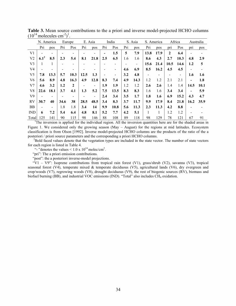
Table 3. Mean source contributions to the a priori and inverse model-projected HCHO columns (1014 molecules cm-2)1.
N. America Europe E. Asia India S. Asia S. America Africa Australia Pri pos Pri Pos Pri pos Pri Pos Pri pos Pri pos pri Pos pri pos
V1 - - - - - - - 1.5 5 7.9 13.8 17.9 2 6.4 - - V2 6.12 8.5 2.3 5.4 8.1 21.8 2.5 6.5 1.6 1.6 8.6 4.3 2.7 10.3 4.8 2.9 V3 1 1 - - - - - - - - 15.6 21.4 10.5 14.6 1.2 5 V4 - - - - - - - - 4.6 6.9 8.5 16.2 4.5 4.5 - - V5 7.8 13.3 5.7 10.3 12.5 1.3 - - 3.2 4.8 - - - - 1.6 1.6 V6 5.6 8.9 4.8 16.3 4.9 12.8 8.3 7.4 4.9 14.3 1.2 1.2 2.1 2.1 - 1.8 V7 4.6 3.2 1.2 2 - - 1.9 1.9 1.2 1.2 2.6 2.6 1.4 1.4 14.5 10.1 V8 22.6 18.1 3.7 4.1 1.3 5.2 7.5 13.5 8.3 8.3 1.6 1.6 3.4 3.4 - 5.9 V9 - - - - - - 2.4 3.4 3.5 1.7 1.8 1.6 6.9 15.2 4.3 4.7 RV 30.7 40 34.6 38 28.5 48.5 3.4 8.3 3.7 11.7 9.9 17.9 8.4 21.8 16.2 35.9 BB - - 1.8 1.8 3.4 14 9.9 10.8 5.6 11.3 2.3 11.3 4.2 8.8 - - IND 6 7.2 5.4 6.4 4.8 8.1 5.2 7.7 4.2 5.1 1 1 1.2 1.2 - - Total 125 141 90 115 98 146 88 108 89 118 98 129 78 121 67 91
1The inversion is applied for the individual region. All the inversion quantities here are for the shaded areas in Figure 1. We considered only the growing season (May – August) for the regions at mid latitudes. Ecosystem classification is from Olson [1992]. Inverse model-projected HCHO columns are the products of the ratio of the a posteriori / priori source parameters and the corresponding a priori HCHO columns.
2Bold faced values denote that the vegetation types are included in the state vector. The number of state vectors for each region is listed in Table 4.
“- ”denotes the values < 1.0 x 10¹⁴ molec/cm2. “pri”: The a priori emission contributions. “post”: the a posteriori inverse-model projections. “V1 – V9”: Isoprene contributions from tropical rain forest (V1), grass/shrub (V2), savanna (V3), tropical seasonal forest (V4), temperate mixed & temperate deciduous (V5), agricultural lands (V6), dry evergreen and crop/woods (V7), regrowing woods (V8), drought deciduous (V9), the rest of biogenic sources (RV), biomass and biofuel burning (BB), and industrial VOC emissions (IND). “Total” also includes CH4 oxidation.
34

Table 4. Samples, state vector size, significant eigenvalues, and nonlinearity.
N. America Europe E. Asia India S. Asia S. America Africa Australia
Samples1 152 148 216 162 261 660 792 564
State vector size2 7 7 7 9 9 8 8 8
Significant eigenvalues3 6 5 6 6 8 7 7 6
Nonlinearity(%)4 1.7 0.4 5.3 4.3 8 2.1 7.8 7.5
1 The number of monthly mean GOME HCHO measurements that meet our criteria for the usage of inversion. 2 The number of significant parameters (see text for details) 3 The number of singular values of the pre-whitened Jacobian that are >1. 4 [1 – (the a posteriori simulated HCHO column) / (inverse-model linearly projected HCHO column)]×100.
Table 5. Ratios of the a posteriori isoprene base emission rates to those of GEIA.
N. America Europe E. Asia India S. Asia S. America Africa Australia
V1 - - - 1.26 0.48 0.39 0.96 - V2 0.42 0.69 0.81 0.78 - 0.15 1.14 0.18 V3 - - - - - 1.12 1.12 3.44 V4 - - - - 0.59 0.74 0.39 - V5 1.19 1.26 0.07 - 1.05 - - 0.70 V6 1.28 2.08 2.08 0.72 2.32 - - 3.28 V7 0.63 1.44 - 0.9 - 0.90 - 0.63 V8 0.64 0.88 3.20 1.44 0.80 - 0.80 5.20 V9 - - - 0.42 0.15 0.27 0.66 0.33 RV 1.04 0.88 1.36 1.92 2.56 1.44 2.08 1.76
The definitions of vegetation types are listed in Table 3. Only vegetation groups included in the state vector are shown.
35

Figures
Figure 1. Inverse modeling regions with high signal-to-noise ratios in GOME HCHO column measurements are shown by shaded areas. The a posteriori source parameters (state vector) are applied to the rectangle regions in order to estimate the global a posteriori isoprene emissions.
36

Figure 2. Global distribution of the 10 ecosystem groups (Table 1) applied in inverse modeling, including tropical rain forest (V1), grass/shrub (V2), savanna (V3), tropical seasonal forest & thorn woods (V4), temperate mixed & temperate deciduous (V5), agricultural lands (V6), dry evergreen & crop/woods (warm) (V7), regrowing woods (V8), drought deciduous (V9), and the rest of ecosystems (V10). The ecosystem types are defined by Olson [1992] with a resolution of 0.5°×0.5°.
37
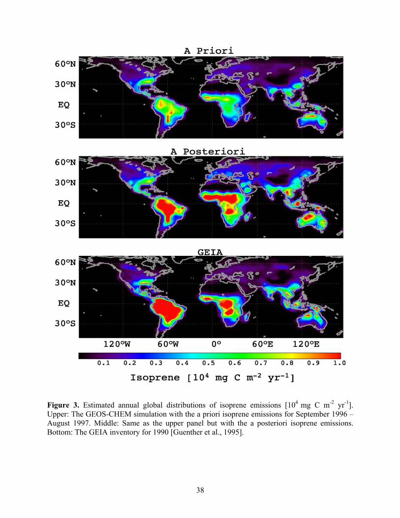
Figure 3. Estimated annual global distributions of isoprene emissions [104 mg C m-2 yr-1]. Upper: The GEOS-CHEM simulation with the a priori isoprene emissions for September 1996 –August 1997. Middle: Same as the upper panel but with the a posteriori isoprene emissions. Bottom: The GEIA inventory for 1990 [Guenther et al., 1995].
38
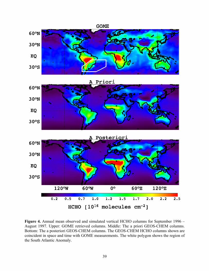
Figure 4. Annual mean observed and simulated vertical HCHO columns for September 1996 – August 1997. Upper: GOME retrieved columns. Middle: The a priori GEOS-CHEM columns. Bottom: The a posteriori GEOS-CHEM columns. The GEOS-CHEM HCHO columns shown are coincident in space and time with GOME measurements. The white polygon shows the region of the South Atlantic Anomaly.
39
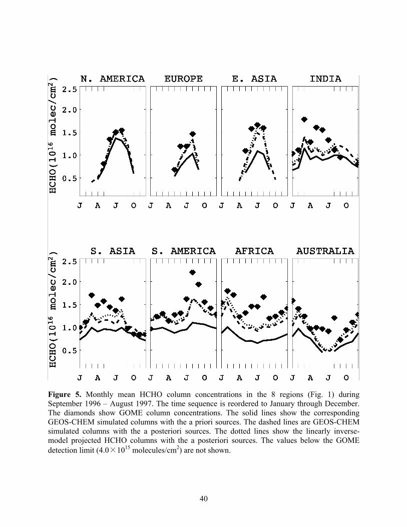
Figure 5. Monthly mean HCHO column concentrations in the 8 regions (Fig. 1) during September 1996 – August 1997. The time sequence is reordered to January through December. The diamonds show GOME column concentrations. The solid lines show the corresponding GEOS-CHEM simulated columns with the a priori sources. The dashed lines are GEOS-CHEM simulated columns with the a posteriori sources. The dotted lines show the linearly inverse-model projected HCHO columns with the a posteriori sources. The values below the GOME detection limit (4.0×10¹⁵ molecules/cm2) are not shown.
40

Figure 6. Contributions of the a priori sources to the simulated monthly mean HCHO column concentrations over North America (Eastern U.S.) and South America (Amazon). The diamonds are GOME HCHO columns. “With all emissions” denotes the simulated HCHO column concentration with all emission sources. “CH4” denotes HCHO from CH4 oxidation. The other source contributions are: “Deciduous” (temperate mixed and temperate deciduous), “ONVOC” (isoprene from the other ecosystems), “T. Rain” (tropical rain forest), “T. Season” (tropical seasonal forest and thorn woods), “Regrow” (regrowing woods), “Grass” (grass/shrub), and “BBF” (biomass and biofuel burning).
41

Figure 7. The discrepancy between monthly GOME measured and GEOS-CHEM simulated HCHO columns over the northern equatorial Africa (4 – 12°N). The corresponding monthly mean LAI, ECMWF surface temperature, and GEOS-STRAT surface temperature are shown in the lower panel. There are no GOME HCHO measurements that match our data selection criteria for inversion in November 1996 over this region.
42

Figure 8. Percent changes of annual and zonal mean concentrations of OH and NOx due to the increase of the a posteriori isoprene and the other biogenic emissions.
43
Related Documents