constrained total variational deblurring models and fast ...

CONSTRAINED TOTAL VARIATIONAL DEBLURRING MODELS AND FAST

ALGORITHMS BASED ON ALTERNATING DIRECTION METHOD OF MULTIPLIERS

RAYMOND H. CHAN1 , MIN TAO2 , AND XIAOMING YUAN3

Abstract. The total variation (TV) model is attractive for being able to preserve sharp attributes in images. However,

the restored images from TV-based methods do not usually stay in a given dynamic range, and hence projection is required to

bring them back into the dynamic range for visual presentation or for storage in digital media. This will affect the accuracy

of the restoration as the projected image will no longer be the minimizer of the given TV model. In this paper, we show that

one can get much more accurate solutions by imposing box constraints on the TV models and solving the resulting constrained

models. Our numerical results show that for some images where there are many pixels with values lying on the boundary of

the dynamic range, the gain can be as great as 10.28dB in peak signal-to-noise ratio. One traditional hinderance of using the

constrained model is that it is difficult to solve. However, in this paper, we propose to use the alternating direction method of

multipliers (ADMM) to solve the constrained models. This leads to a fast and convergent algorithm that is applicable for both

Gaussian and impulse noise. Numerical results show that our ADMM algorithm is better than some state-of-the-art algorithms

for unconstrained models both in terms of accuracy and robustness with respect to the regularization parameter.

Key words. Total variation, deblurring, alternating direction method of multipliers, box constraint

AMS subject classifications. 68U10, 65J22, 65K10, 65T50, 90C25

1. Introduction. In this paper, we consider the problem of deblurring digital images under Gaussian

or impulse noise. Without loss of generality, we consider all images being square images of size n-by-n. Let

x ∈ Rn2

be a given original image concatenated into an n2-vector, K ∈ Rn2×n2

be a blurring operator acting

on the image, and ω ∈ Rn2

be the Gaussian or impulse noise added onto the image. The observed image

f ∈ Rn2

can be modeled by f = Kx+ ω, and our objective is to recover x from f .

It is well known that recovering x from f by directly inverting K is unstable and can produce very noisy

result because K is highly ill-conditioned. Instead one usually solves

minxΦreg(x) + µΦfit(x, f), (1.1)

where Φreg(x) regularizes the solution by enforcing certain prior constraints, Φfit(x, f) measures how fit

x is to the observation f , and µ is the regularization parameter balancing these two terms. Traditional

choices for Φreg(x) include the Tikhonov-like regularization [37], the total variation (TV) regularization [30],

Mumford-Shah regularization [23] and its variants [1, 32]. In this paper, we consider the TV regularization

[30, 29] as it has been shown to preserve sharp edges both experimentally and theoretically. For Φfit(x),

we consider ∥Kx − f∥22 and ∥Kx − f∥1, which are, respectively, suitable data-fitting terms for images

corrupted by Gaussian [39, 42, 43] and impulse noise [2, 7, 9, 41, 42]. The corresponding problems (1.1) with

TV regularization are called the TV-L2 and TV-L1 problems respectively. There are many good existing

algorithms for solving these problems, for examples [30, 29, 40, 39, 42, 43, 27, 9, 2, 7, 41] just to mention

a few. In the literature, some authors also discuss other non-quadratic fidelity terms besides the L1 fidelity

term, e.g., [13, 33, 34].

In this paper, we consider the case where the images are digital images so that their pixel values have to

lie in a certain dynamic range [l, u]. For example, for 8-bit images, we have [l, u] = [0, 255]. Notice that for

1([email protected]) Department of Mathematics, The Chinese University of Hong Kong, Shatin, NT, Hong Kong.

Research is supported in part by HKRGC Grant No. CUHK400510 and CUHK Direct Allocation Grant 2060408.2([email protected]) School of Science, Nanjing University of Posts and Telecommunications, Nanjing, Jiangsu, China. Re-

search is supported by the Scientific Research Foundation of Nanjing University of Posts and Telecommunications (NY210049).3([email protected]) Department of Mathematics, Hong Kong Baptist University, Hong Kong, China. Research is

supported by the Hong Kong General Research Fund: 203311.

1

many existing algorithms such as those listed in the last paragraph, their restored image x will not necessarily

be in [l, u]. Therefore if x is to be stored or displayed digitally, its pixel values must first be projected onto

[l, u]. There are many ways to do this. One can just map all pixels with values that are less than l to l and

those that are bigger than u to u. We call this “truncation”. Another way is to linearly stretch the pixel

values of x to [l, u] by a linear mapping, and we call this “stretching”. The MATLAB command “imshow”

provides both kinds of projections with “stretching” being the default method. Clearly, after projection,

the image no longer minimizes the unconstrained model. In fact, we will see in the numerical examples in

Section 4 that this minimize-and-project approach usually gives inferior solutions.

For digital image restoration, a more accurate model for x is to explicitly constrain the solution in [l, u],

i.e. we solve the constrained model:

minx∈ΩΦreg(x) + µΦfit(x, f). (1.2)

Here Ω = x ∈ Rn2 | l ≤ x ≤ u, with l, u ∈ Rn2

+ and the constraints are to be interpreted entry-wise, i.e.,

li ≤ xi ≤ ui, for any 1 ≤ i ≤ n2. Constrained TV-L2 models have recently been considered in [4] where their

numerical tests indicate that one can get more than 2dB improvement on PSNR for some special images

by simply imposing the box constraint in the TV-L2 model. (See (4.1) for the definition of PSNR.) Our

numerical experiments in Section 4 reveal that the improvement can even be as big as 9.58dB for an image

with all pixel values either at l or at u. It is therefore advantageous to solve the constrained model (1.2)

directly than to use the minimize-and-project approach provided that we have an efficient solver to do so.

Constrained problems are usually much more difficult to solve than the unconstrained one. However,

there are some existing methods that solve the constrained image restoration model (1.2). For constrained

L2-L2 problems, i.e. the regularization term is the L2-norm of some derivatives of x, there are several

methods that based on Newton-like methods, see [10, 22]. For constrained TV problems, the singularity

of the TV functional prohibits the application of Newton-like methods. Recently, Beck and Teboulle [4]

proposed a fast gradient-based algorithm for solving constrained TV-L2 problems. As far as we know, there

are no solvers for constrained TV-L1 problems yet. In this paper, we derive a solver for both the constrained

TV-L2 and TV-L1 problems. Our solver is based on the alternating direction method of multipliers (ADMM)

which was developed back in the 1970’s [18, 17]. The convergence of our algorithms are thus guaranteed

by the classical theory in ADMM literature, e.g. [21]. We compare our algorithms with the state-of-the-art

solvers, like FTVd [39] and the augmented Lagrange method (ALM) [41] for the unconstrained model (1.1);

and MFISTA [4] for the constrained model (1.2). Numerical results show that our algorithms are faster

than MFISTA for solving the same model while yielding more accurate restored images than those from the

unconstrained model. Also our algorithms are more robust with respect to the changes in the regularization

parameter µ.

The rest of this paper is organized as follows. In Section 2, we recall briefly existing solvers for uncon-

strained TV-L1 and TV-L2 problems. In Section 3, we derive our ADMM-based algorithms to solve the

constrained TV-L1 and TV-L2 problems. In Section 4, numerical comparisons with existing methods are

carried out to confirm the effectiveness of our approach. Finally, some concluding remarks are drawn in

Section 5.

2. TV-deblurring Models and Solvers. In this section, we briefly review some relating methods for

solving TV deblurring problems. We start with the TV-L2 model which is good for deblurring images under

the corruption by Gaussian noise [30, 29, 39, 42, 43, 27]:

minx

n2∑i=1

∥Dix∥2 +µ

2∥Kx− f∥22

, (2.1)

2

where Dix ∈ R2 represents the first-order finite difference of x at pixel i in both horizontal and vertical di-

rections. More specifically, let x = (x1, x2, . . . , xn2)⊤ and that x is extended by periodic boundary condition.

Then Dix := ((D(1)x)i, (D(2)x)i)

⊤ ∈ R2 (i = 1, . . . , n2), where

(D(1)x)i :=

xi+n − xi, if 1 ≤ i ≤ n(n− 1);

xmod(i,n) − xi. otherwise.(2.2)

(D(2)x)i :=

xi+1 − xi, if mod(i, n) = 0;

xi−n+1 − xi. otherwise.(2.3)

Here, the discrete gradient operators D(1) and D(2) are n2-by-n2 matrices, and the i-rows of D(1) and

D(2) correspond to the first and second rows of Di, respectively. The quantity ∥Dix∥2 measures the total

variation of x at pixel i. The resulting TV is called isotropic. We emphasize that our approach also applies

to anisotropic (1-norm) TV deconvolution problems. For simplicity, we will focus on the isotropic case in

detail and mention the anisotropic case when necessary.

One fast TV deblurring algorithm for (2.1), called FTVd, was recently proposed in [39]. To make use of

the structure of (2.1), the authors first formulate (2.1) as an equivalent constrained problem:

minx,y

n2∑i=1

∥yi∥2 +µ

2∥Kx− f∥22 : yi = Dix, i = 1, . . . , n2

, (2.4)

where yi ∈ R2 is an auxiliary vector. The vector y is defined as

y :=

(y(1)

y(2)

)∈ R2n2

, and yi :=

((y(1))i

(y(2))i

)∈ R2, i = 1, . . . , n2, (2.5)

(cf. (D(1)x)i and (D(2)x)i in the definitions (2.2) and (2.3) respectively). Then, they consider the un-

constrained version of (2.4) where the linear constraints in (2.4) are penalized by a quadratic term in the

objective function. Finally, an alternate minimization scheme with respect to x and y, together with a

continuation scheme on the penalty parameter, is implemented to the unconstrained version. Since every

subproblem in each iteration can be solved by either shrinkage or fast Fourier transforms, FTVd performs

much better than a number of existing methods such as the lagged diffusivity algorithm [38], some Fourier

and wavelet shrinkage methods [24] and the MATLAB Image Processing Toolbox functions “deconvwnr” and

“deconvreg”. Very recently, an inexact version of ALM was proposed to solve TV model with non-quadratic

fidelity [41], which is also applicable for solving TV-L2 model (2.1).

Another class of algorithms of particular interest to us is the iterative shrinkage/thresholding (IST)-

based algorithms which are proposed and analyzed in different fields [8, 14, 15, 35, 36]. The convergence

rate of IST-based algorithms, however, is only O(k−1) where k is the number of iterations. There are many

efforts to improve its speed, such as, the two-step IST (TwIST) algorithm [5], and the fast IST algorithm

(FISTA) [3]. In particular, FISTA is inspired by the work of Nesterov [25] and it performs better than ISTA

and TwIST according to the numerical results reported in [3]. In fact, the authors have shown in [3] that

the convergence rate of FISTA is O(k−2).

In [4], Beck and Teboulle presented a monotone version of FISTA, called MFISTA, for solving the

constrained TV-L2 problem:

minx∈Ω

n2∑i=1

∥Dix∥2 +µ

2∥Kx− f∥22

. (2.6)

3

Like FISTA, they solve (2.6) by solving a series of denoising problems where the problems are now constrained

onto Ω. The constrained denoising problems are transformed into their dual problems and solved by a fast

projection gradient method. It was shown that MFISTA also has the convergence rate of O(k−2). Numerical

tests in [4] indicate that by simply imposing the box constraint, the constrained model (2.6) can yield more

than 2dB improvement on PSNR for some special images.

Besides the TV-L2 model, another interesting TV deblurring problem is the TV-L1 model which is good

for deblurring images under the corruption of impulse noise [9, 2, 7, 41, 43]:

minx

n2∑i=1

∥Dix∥2 + µ∥Kx− f∥1

. (2.7)

The authors of FTVd has extended their method to cover this case, see [43]. Besides that, an inexact version

of ALM was proposed to solve TV-L1 problem (2.7) [41]. To the best of our knowledge, MFISTA has not

been extended to (2.7). Also so far no one has yet addressed the constrained TV-L1 model:

minx∈Ω

n2∑i=1

∥Dix∥2 + µ∥Kx− f∥1

. (2.8)

As we have mentioned, in this paper we apply ADMM to solve both the constrained TV-L2 model (2.6) and

the constrained TV-L1 model (2.8).

3. Applying ADMM to constrained TV-Lp models. In this section, we apply ADMM idea to

derive algorithms for solving the constrained TV-L2 model (2.6) and the constrained TV-L1 model (2.8).

Recall that the basic idea of ADMM goes back to the work of Glowinski and Marocco [18] and Gabay and

Mercier [17], and we refer to some applications in image processing which can be solved by ADMM, e.g.,

[19, 16, 31, 27, 44, 40, 45, 46, 12].

3.1. Constrained TV-L2 model. To apply ADMM idea to (2.6), we first introduce two auxiliary

variables y and z to change it to the equivalent form:

minz∈Ω,x,y

∑i

∥yi∥2 +µ

2∥Kx− f∥22 : yi = Dix, i = 1, . . . , n2;x = z

. (3.1)

The auxiliary variable yi, as defined in (2.5), is to liberate the discrete derivative operator Dix out of the

non-differentiable term ∥ · ∥2, and the variable z plays the role of x within the box constraint so that the box

constraint is now imposed on z instead of x. By grouping the variables into two blocks x and (y, z), we see

that the objective function of (3.1) is the sum of a function of x and a function of (y, z) and thus ADMM is

applicable. In the following, we show that each subproblem of ADMM either has a closed form solution or

can be solved by a fast solver.

Let LA(x, y, z;λ, ξ) be the augmented Lagrangian function of (3.1) which is defined as follows:

LA(x, y, z;λ, ξ) ≡∑i

(∥yi∥2 − λ⊤

i (yi −Dix) +β1

2∥yi −Dix∥22

)+µ

2∥Kx− f∥22 − ξ⊤(z − x) +

β2

2∥z − x∥22,

where β1, β2 > 0; and λ ∈ R2n2

and ξ ∈ Rn2

are the Lagrange multipliers. Started at x = xk, λ = λk and

4

ξ = ξk, applying ADMM in [18, 17] yields the iterative scheme:(yk+1

zk+1

)← arg min

z∈Ω,yLA(x

k, y, z;λk, ξk), (3.2)

xk+1 ← argminxLA(x, y

k+1, zk+1;λk, ξk), (3.3)(λk+1

ξk+1

)←

(λk − γβ1(y

k+1 −Dxk+1)

ξk − γβ2(zk+1 − xk+1)

). (3.4)

The parameters β1, β2 correspond to the linear constraints yi = Dix and x = z in (3.1). Theoretically any

positive values of β1 and β2 ensure the convergence of ADMM [21], and the specific choice of β’s we used in

the experiments will be specified later.

We now show that the minimization (3.2) with respect to y and z can be separated into two independent

subproblems. Firstly, the z-subproblem can be implemented by the simple projection PΩ onto the box:

zk+1 = PΩ

[xk − ξk

β2

]. (3.5)

The y-subproblem is equivalent to n2 number of two-dimensional problems in the form

minyi∈R2

∥yi∥2 +

β1

2

∥∥∥∥yi − (Dixk +

1

β1(λk)i

)∥∥∥∥22

, i = 1, 2, . . . , n2. (3.6)

According to [39, 42], the solution of (3.6) is given explicitly by the two-dimensional shrinkage:

yk+1i = max

∥∥∥∥Dixk +

1

β1(λk)i

∥∥∥∥2

− 1

β1, 0

Dix

k + 1β1(λk)i

∥Dixk + 1β1(λk)i∥2

, i = 1, 2, . . . , n2, (3.7)

where 0 · (0/0) = 0 is assumed. The computational cost of (3.7) is therefore linear with respect to n2.

We note that, when the 1-norm is used in the definition of TV, i.e. the TV is anisotropic, yk+1i will be

given by the simpler one-dimensional shrinkage:

yk+1i = max

∣∣∣∣Dixk +

1

β1(λk)i

∣∣∣∣− 1

β1, 0

sgn(Dix

k +1

β1(λk)i), i = 1, 2, . . . , n2,

where “” and “sgn” represent, respectively, the point-wise product and the signum function, and all oper-

ations are done componentwise.

Next the minimization (3.3) with respect to x is just a least squares problem and the corresponding

normal equation is(D⊤D +

µ

β1K⊤K +

β2

β1I

)x = D⊤

(yk+1 − 1

β1λk

)+

µ

β1K⊤f +

β2

β1

(zk+1 − ξk

β2

), (3.8)

where D ≡

(D(1)

D(2)

)∈ R2n2×n2

is the global first-order finite difference operator with D(1) and D(2) being

matrices defined by (2.2) and (2.3). Notice that the coefficient matrix in (3.8) is non-singular whenever

β1, β2 > 0. This is an advantage over other splitting methods [39, 42, 43] which, in order to guarantee

non-singularity, require the intersection of the null space of K⊤K and the null space of D⊤D to be the

zero vector only. Under the periodic boundary conditions for x, both D⊤D and K⊤K are block circulant

matrices with circulant blocks, see e.g. [20, 11], and thus are diagonalizable by the 2D discrete Fourier

transforms (FFT). As a result, (3.8) can be solved by one forward FFT and one inverse FFT, each at a cost

5

of O(n2 log n). If the boundary condition is Neumann and the blur is symmetric, then the coefficient matrix

can be diagonalized by discrete cosine transform (DCT) in the same amount of cost, see [26].

Finally, the update (3.4) for λ and ξ can be done straightforwardly in O(n2) operations.

In conclusion, the main cost per iteration for the scheme (3.2)–(3.4) is dominated by two FFT or

DCT operations, and hence is of O(n2 log n). Below we give our ADMM-based algorithm for solving the

constrained TV-L2 model (2.6).

Algorithm 1. ADMM for the constrained TV-L2 problem (2.6)

Input f , K, µ > 0, β1, β2 > 0 and λ0. Initialize x = f and λ = λ0, ξ = ξ0.

While “a stopping criterion is not satisfied”, Do

1) Compute yk+1 according to (3.7).

2) Compute zk+1 according to (3.5).

3) Compute xk+1 by solving (3.8).

4) Update λk+1 and ξk+1 via (3.4).

End Do

Since our method is basically an application of ADMM for the case with two blocks of variables x and

(y, z), its convergence is guaranteed by classical results in ADMM literature, e.g. [6, 17, 18]. We summarize

the convergence of Algorithm 1 below.

Theorem 3.1. For β1, β2 > 0 and γ ∈ (0, 1+√5

2 ), the sequence (xk, yk, zk, λk, ξk) generated by

Algorithm 1 from any initial point (x0, λ0, ξk) converges to (x∗, y∗, z∗, λ∗, ξ∗), where (x∗, y∗, z∗) is a solution

of (2.6).

3.2. Constrained TV-L1 model. In this section, we apply ADMM to solve the constrained TV-L1

model (2.8). Similar to the constrained TV-L2 case, we introduce three auxiliary variables in (2.8) and

transform it to:

minw∈Ω,x,y,z

∑i

∥yi∥2 + µ∥z∥1 : yi = Dix, i = 1, . . . , n2, z = Kx− f, w = x

. (3.9)

Note that the constraint is now imposed on w instead of x. The augmented Lagrangian function of (3.9) is

LA(x, y, z, w;λ, ξ, ζ) =∑i

∥yi∥2 − λ⊤(y −Dx) +β1

2

∑i

∥yi −Dix∥22

+µ∥z∥1 − ξ⊤[z − (Kx− f)] +β2

2∥z − (Kx− f)∥22

−ζ⊤(w − x) +β3

2∥w − x∥22, (3.10)

where β1, β2, β3 > 0; and λ ∈ R2n2

, ξ ∈ Rn2

and ζ ∈ Rn2

are the Lagrange multipliers. According to

the scheme of ADMM, for a given (xk, λk, ξk, ζk), the next iterate (xk+1, yk+1, zk+1, λk+1, ξk+1, ζk+1) is

generated as follows:

1. Fix x = xk, λ = λk, ξ = ξk and ζ = ζk, and minimize LA in (3.10) with respect to y, z and w to

obtain yk+1, zk+1 and wk+1. The minimizers are given explicitly by

yk+1i = max

∥∥∥∥Dixk +

(λ1)ki

β1

∥∥∥∥2

− 1

β1, 0

Dix

k + (λ1)ki /β1

∥Dixk + (λ1)ki /β1∥2, i = 1, 2, . . . , n2, (3.11)

zk+1 = sgn(Kxk − f + ξk/β2) max|Kxk − f + ξk/β2| − µ/β2, 0, (3.12)

wk+1 = PΩ

[xk +

ζk

β3

], (3.13)

where | · | and sgn represent the componentwise absolute value and signum function, respectively.

6

2. Compute xk+1 by solving the normal equation(D⊤D +

β2

β1K⊤K +

β3

β1I

)x = D⊤

(yk+1 − λk

β1

)+

β2

β1K⊤

(zk+1 − ξk

β2

)+β2

β1K⊤f +

β3

β1

(wk+1 − ζk

β3

). (3.14)

3. Update the multipliers via λk+1 = λk − γβ1(y

k+1 −Dxk+1),

ξk+1 = ξk − γβ2[zk+1 − (Kxk+1 − f)],

ζk+1 = ζk − γβ3(wk+1 − xk+1).

(3.15)

Below we present ADMM-based algorithm for solving the constrained TV-L1 model (2.8).

Algorithm 2. ADMM for the constrained TV-L1 model (2.8)

Input f , K, µ > 0, β1, β2, β3 > 0 and λ0. Initialize x = f and λ = λ0, ξ = ξ0, ζ = ζ0.

While “a stopping criterion is not satisfied”, Do

1) Compute yk+1, zk+1 and wk+1 according to (3.11), (3.12) and (3.13).

2) Compute xk+1 by solving (3.14).

3) Update λk+1, ξk+1 and ζk+1 via (3.15).

End Do

Again, Algorithm 2 is an application of ADMM for the case with two blocks of variables (y, z, w) and x.

Thus, its convergence is guaranteed by the theory of ADMM and we summarize it below.

Theorem 3.2. For β1, β2, β3 > 0 and γ ∈ (0, 1+√5

2 ), the sequence (xk, yk, zk, wk, λk, ξk, ζk) gen-

erated by Algorithm 2 from any initial point (x0, λ0, ξ0, ζ0) converges to (x∗, y∗, z∗, w∗, λ∗, ξ∗, ζ∗), where

(x∗, y∗, z∗, w∗) is a solution of (2.8).

4. Numerical experiments. In this section, we apply our algorithms to solve the constrained TV-L2

problem (2.6) and TV-L1 problem (2.8) and compare them with some state-of-the-art algorithms. The code

of our algorithms was written in MATLAB 7.12 (R2011a) and all the numerical experiments were conducted

on a ThinkPad notebook with an Intel Core i5-2140M CPU with 2.3 GHz and 4 GB of memory. The quality

of our restoration is measured by the peak signal-to-noise ratio (PSNR) in decible (dB):

PSNR(x) = 20 log10xmax√Var(x, x)

with Var(x, x) =

∑n2

j=1[x(j)− x(j)]2

n2. (4.1)

Here x is the true image and xmax is the maximum possible pixel value of the image. To make it easier to

compare across different models and different methods, we used one uniform stopping criterion for all the

algorithms we tested, and that is

|J k+1 − J k||J k|

< 10−5, (4.2)

where J k is the objective function value of the respective model in the kth iteration.

The test images are 256-by-256 images as shown in Fig. 4.1: (a) Text.png, (b) Satellite.pgm, (c)

Chart.tiff, (d) Church.jpg, and (e) Cameraman.tif. Their pixel values are all scaled to the interval [0, 1] first

so the box constraint in the constrained models is simply [0,1] (i.e., li = 0 and ui = 1 for all i’s). We note

that the percentages of extreme-value pixels (i.e., pixels with the value 0 or 1) in the five test images are

100%, 89.81%, 84.66%, 22.54% and 0% respectively.

7

(a) Text (b) Satellite (c) Chart (d) Church (e) Cameraman

Fig. 4.1. Original images.

One may argue that for digital images, the pixel values have to be integer too, besides being in a suitable

dynamic range. For example, for 8-bit images, the values of x should be integers in [0, 255]. We will see in

Section 4.3 that for 8-bit images, the additional requirement that all pixels being integers in [0,255] affects

the restored PSNR values only in the second decimal place, see Tables 4.4 and 4.5. Hence in the following

experiments, we will not impose integer constraints onto the solution but just the box constraint [0,1]. In

Section 4.4, we illustrate that our method is robust against the choice of the regularization parameter µ.

About the penalty parameters β’s in Algorithms 1 and 2, theoretically any positive values of β1 and β2

ensure the convergence of ADMM [21] and we usually have two ways to determine them in practice. One is

to try some values and pick a value with satisfactory performance, and then fix it throughout; the other is to

apply some self-adaptive adjustment rules in the literature with an arbitrary initial guess and this strategy

requires no tuning. Since the latter requires expensive computation to realize the self-adaptive adjustments

for imaging applications, we used the former strategy. Our experience is that a well-tuned constant value

performs almost the same as a self-adaptive strategy.

4.1. Experiments for TV-L2. In this subsection, we focus on the TV deblurring problem with Gaus-

sian noise. Our purposes are: i) to show the accuracy of the constrained TV-L2 model (2.6) over the

unconstrained model, and ii) to demonstrate the efficiency of the proposed Algorithm 1. The efficiency of

Algorithm 1 is shown mainly by comparison with the FTVd in [39], an inexact version of ALM (see Algo-

rithm 4.2 in [41]), and the MFISTA in [4]. The inexact version of ALM (i.e. Algorithm 4.2 in [41]) coincides

with the split Bregam algorithm in [19]. In this way, we have also compared with the split Bregam algorithm

in [19]. Note that Algorithm 4.2 in [41] requires an inner iteration to solve the primal variables alternatively.

In [41], the authors mentioned that “the split Bregman method will waste the accuracy of the inner iteration

and does not speed up dramatically when the inner iteration number L > 1”. Therefore, in the numerical

tests of [41], the authors simply set the inner iteration number L = 1. Thus, we also set L = 1 in our

comparison. In the following, we denote Algorithm 4.2 in [41] as ALM.

4.1.1. Comparison with FTVd and ALM. We first compare our Algorithm 1 with FTVd and ALM.

Recall that FTVd and ALM solve the unconstrained model (2.1) while Algorithm 1 tackles the constrained

model (2.6). As we have mentioned, one can solve the unconstrained TV-L2 model (2.1) first and then

project the restored image onto the box constraint by either the “truncation” or the “stretching” procedure.

Therefore we report the result of FTVd and ALM with these two minimize-and-project procedures (denoted

respectively by “ALM-T”, “ALM-S”, “ALM-T” and “ALM-S”) in addition to the original FTVd and ALM.

The ten blurred and noisy images in our tests are degraded as follows. Since the periodic boundary

condition is used to generate the convolution operator in [39, 41], we use the same boundary condition to

blur the test images. Two types of blurring kernels are tested: Type I (fspecial (’average’,9)), and

Type II (fspecial (’gaussian’,[9,9],3)). For each case, the blurred images are further corrupted by

8

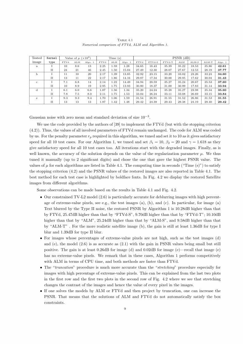
Table 4.1

Numerical comparison of FTVd, ALM and Algorithm 1.

Tested Kernel Value of µ (×104) Time (s) PSNR (dB)image type FTVd ALM Algo. 1 FTVd ALM Algo. 1 FTVd FTVd-S FTVd-T ALM ALM-S ALM-T Algo. 1

a I 10 8.6 13 2.25 1.59 1.28 34.65 18.43 35.39 35.22 18.53 35.86 42.61

II 24 21 46 2.45 1.50 15.04 27.49 12.30 28.07 27.67 12.53 28.19 37.77

b I 11 10 20 2.17 1.39 13.85 32.92 23.15 33.20 33.02 23.26 33.24 34.60

II 13 11 22 2.17 1.86 14.16 29.87 17.34 30.00 29.95 17.62 30.04 31.43

c I 7.1 6.8 14 2.14 1.22 14.49 34.94 20.59 35.27 35.24 20.67 35.53 37.60

II 10 8.9 19 2.95 1.75 13.93 30.80 18.37 31.00 30.99 17.83 31.14 33.94

d I 6.1 6.0 6.6 1.87 1.56 1.34 35.20 24.24 35.28 35.27 23.98 35.34 35.60

II 7.8 7.5 8.0 2.11 1.75 1.53 33.04 26.24 33.11 33.08 26.69 33.15 33.84

e I 9.3 9.3 9.4 1.70 1.06 1.59 31.54 26.91 31.55 31.52 26.86 31.53 31.55

II 13 13 13 1.97 1.42 1.48 29.42 24.39 29.43 29.38 24.19 29.40 29.42

Gaussian noise with zero mean and standard deviation of size 10−3.

We use the code provided by the authors of [39] to implement the FTVd (but with the stopping criterion

(4.2)). Thus, the values of all involved parameters of FTVd remain unchanged. The code for ALM was coded

by us. For the penalty parameter rp required in this algorithm, we tuned and set it to 10 as it gives satisfactory

speed for all 10 test cases. For our Algorithm 1, we tuned and set β1 = 10, β2 = 20 and γ = 1.618 as they

give satisfactory speed for all 10 test cases too. All iterations start with the degraded images. Finally, as is

well known, the accuracy of the solution depends on the value of the regularization parameter µ. We thus

tuned it manually (up to 2 significant digits) and chose the one that gave the highest PSNR value. The

values of µ for each algorithms are listed in Table 4.1. The computing time in seconds (“Time (s)”) to satisfy

the stopping criterion (4.2) and the PSNR values of the restored images are also reported in Table 4.1. The

best method for each test case is highlighted by boldface fonts. In Fig. 4.2 we display the restored Satellite

images from different algorithms.

Some observations can be made based on the results in Table 4.1 and Fig. 4.2.

• Our constrained TV-L2 model (2.6) is particularly accurate for deblurring images with high percent-

age of extreme-value pixels, see e.g., the test images (a), (b), and (c). In particular, for image (a)

Text blurred by the Type II noise, the restored PSNR by Algorithm 1 is 10.28dB higher than that

by FTVd, 25.47dB higher than that by “FTVd-S”, 9.70dB higher than that by “FTVd-T”; 10.10dB

higher than that by “ALM”, 25.24dB higher than that by “ALM-S”, and 9.58dB higher than that

by “ALM-T” . For the more realistic satellite image (b), the gain is still at least 1.36dB for type I

blur and 1.39dB for type II blur.

• For images whose percentages of extreme-value pixels are not high, such as the test images (d)

and (e), the model (2.6) is as accurate as (2.1) with the gain in PSNR values being small but still

positive. The gain is at least 0.26dB for image (d) and 0.02dB for image (e)—recall that image (e)

has no extreme-value pixels. We remark that in these cases, Algorithm 1 performs competitively

with ALM in terms of CPU time, and both methods are faster than FTVd.

• The “truncation” procedure is much more accurate than the “stretching” procedure especially for

images with high percentage of extreme-value pixels. This can be explained from the last two plots

in the first row and the first two plots in the second row of Fig. 4.2 where we see that stretching

changes the contrast of the images and hence the value of every pixel in the images.

• If one solves the models by ALM or FTVd and then project by truncation, one can increase the

PSNR. That means that the solutions of ALM and FTVd do not automatically satisfy the box

constraints.

9

Blurred & Noisy, 23.96dB FTVd−S, 17.34dB FTVd−T, 30.00dB

ALM−S, 17.62dB ALM−T, 30.04dB Algo. 1, 31.43dB

Fig. 4.2. Top row: blurred and noisy image (left), restored images of FTVd-S (middle), FTVd-T (right); Bottom row:

ALM-S (left), ALM-T (middle) and Algorithm 1 (right) (type II blur).

4.1.2. Comparison with MFISTA. In this subsection, we compare Algorithm 1 with MFISTA in

[4] for TV-L2 deblurring problems. Recall that MFISTA also solves the constrained TV-L2 problem (2.6).

Following [4], we use the Neumann boundary condition to generate the blur, where the kernel size is 9× 9.

The blurred images are further corrupted by Gaussian noise with zero mean and standard deviation of size

2× 10−2.

We use the original MFISTA code provided by the authors of [4] but with the stopping criterion (4.2).

MFISTA applies a fast projection gradient (FPG) method to solve the constrained model (2.6). At each

FPG step, it is required to solve a constrained denoising problem. The authors apply the same FPG method

to solve its dual form, and a fixed number of ten FPG steps is recommended in [4]. We followed their

suggestion and used ten FPG steps here. To implement Algorithm 1, we take β1 = β2 = 0.01 and γ = 1.618.

As in Section 4.1.1, we tune the value of µ manually to two significant digits and the best values are listed in

Table 4.2. In Table 4.2, we also report the computing time in seconds, the restored PSNR, and the objective

function value (“obj-end”) when the stopping criterion (4.2) is satisfied. Table 4.2 shows that Algorithm 1

can restore images with the same quality as those by MFISTA (which is not surprising as the two algorithms

are solving the same constrained TV-L2 model), but with a much faster speed. To illustrate this more

clearly, in Fig. 4.3, we depict the objective function value and the PSNR value against the computing time

for image (a). Clearly our method converges much faster than MFISTA. Similar curves and conclusion can

be drawn for the other four test images.

4.2. Experiments for TV-L1. In this subsection, we focus on the TV debluring problem with impulse

noise. Our purposes are: i) to show the accuracy of the constrained TV-L1 model (2.8) over the unconstrained

alternative (2.7); and ii) to demonstrate the efficiency of Algorithm 2, mainly via a comparison with FTVd

[43], and ALM [41].

10

Table 4.2

Numerical comparison of MFISTA and Algorithm 1 for model (2.6).

Tested Value of µ (×103) Time (s) PSNR (dB) obj-endImage in (2.6) MFISTA Algo. 1 MFISTA Algo. 1 MFISTA Algo. 1

a 6.3 23.56 6.19 20.52 20.59 26.16 26.12

b 1.0 31.34 6.10 26.91 26.92 27.12 27.10

c 2.3 24.57 7.32 23.18 23.20 28.25 28.22

d 0.9 19.62 2.85 26.98 27.01 28.23 28.23

e 1.0 21.82 5.72 24.39 24.39 27.72 27.72

0 2 4 6 8 10

30

40

50

60

70

80

CPU Time (s)

Objective function value history

Algo. 1MFISTA

0 5 10 15 20

15

16

17

18

19

20

CPU Time (s)

PS

NR

(dB

)

PSNR history

Algo. 1MFISTA

Fig. 4.3. Objective function value history (left) and PSNR history (right) against the CPU time.

Fifteen degraded test images are generated in a similar way as in Section 4.1. That is, we first generated

the blurred image with the periodic boundary condition and then corrupted the blurred images by salt-and-

pepper impulse noise with the noise level 40%, 50%, and 60%. The blurring operator is the Gaussian blur

used in [43] which has a kernel size of 7 × 7 and standard deviation 5. Again, we use the original code

of FTVd but with the stopping criterion (4.2). To get a best performance, we set rp = 5, and rz = 20

in ALM (see [41]). In Algorithm 2, we set β1 = 5, β2 = 20, β3 = 10, γ = 1.618. We tune µ manually for

each algorithm and their best values are listed in Table 4.3. The FTVd and ALM with the ‘truncation” or

“stretching” projection are also compared.

Similar conclusions as in Section 4.1.1 can be made based on the results in Table 4.3. For example,

when compared to the unconstrained model (2.7) with or without a projection procedure, the constrained

TV-L1 model (2.8) is always more accurate, with a possible improvement of more than 2.06 dB in PSNR

(see image (a) with a 40% level of noise). Again, this superiority is more obvious for images with higher

percentages of extreme-value pixels. In addition, Algorithm 2 outperforms FTVd in speed for all cases. Also

the “truncation” procedure is again more accurate than the “stretching” procedure.

Finally, in Fig. 4.4, we display the degraded image and the restored text images for 50% level of noise

by the three methods. We can easily see visual improvement in the image by using our method.

4.3. Integer constraints. One may remark that for digital images, the pixel values have to be integer

too, besides being in the dynamic range [l, u]. We repeated the experiments in Tables 4.1 and 4.3 but this

time we scaled and rounded the pixel values of the restored images to integers in [0,255]. Tables 4.4 and 4.5

give the resulting PSNR. In the tables, R means we do not impose the integer constraints, and all restored

images are in [0,1], while Z means we have imposed the integer constraints. From the tables we see that

the integer constraints only affect the PSNR values in the second decimal place. The results justify our

consideration of imposing only the box constraint [0,1].

11

Table 4.3

Numerical comparison of FTVd, ALM and Algorithm 2.

Image Noise Value of µ Time (s) PSNR (dB)level FTVd ALM Algo. 2 FTVd ALM Algo. 2 FTVd FTVd-S FTVd-T ALM ALM-S ALM-T Algo. 2

40% 21 35 55 4.38 3.63 4.01 19.53 9.75 19.64 21.33 7.98 21.68 23.74

a 50% 12 25 50 5.07 2.39 4.21 16.64 11.81 16.65 18.37 7.53 18.62 20.17

60% 3.7 16 28 6.69 1.73 2.42 15.08 14.62 15.08 16.23 8.66 16.31 17.04

40% 25 23 24 4.71 2.20 2.20 28.67 18.52 28.71 28.04 23.20 28.07 28.45

b 50% 25 23 24 4.68 1.33 2.01 27.57 20.60 27.60 27.46 24.63 27.48 27.92

60% 7.2 10 10 5.91 1.19 1.54 26.75 25.13 26.76 26.90 24.94 26.93 27.06

40% 17 32 36 5.66 4.18 5.13 23.94 15.88 23.98 26.46 13.89 26.66 27.59

c 50% 11 21 33 5.55 3.43 4.31 20.42 13.74 20.46 22.86 213.81 23.05 24.19

60% 6 14 21 5.77 2.07 3.37 18.01 13.86 18.03 19.51 12.89 19.65 20.79

40% 17 20 17 4.63 2.98 3.92 30.81 24.31 30.84 30.62 23.40 30.68 31.16

d 50% 12 14 17 5.02 2.07 3.70 28.55 20.98 28.58 28.98 21.75 29.01 29.44

60% 7.8 12 12 6.41 1.95 2.65 26.16 19.71 26.17 26.91 18.83 26.95 27.22

40% 11 25 25 4.38 3.03 4.12 25.78 25.58 25.78 26.55 20.20 26.57 26.60

e 50% 5.9 17 20 4.60 1.98 3.14 24.37 22.32 24.37 25.43 22.72 25.44 25.50

60% 2.9 12 11 5.99 1.78 2.61 22.97 20.54 22.97 24.23 22.10 24.23 24.23

Blurred & Noisy, 5.75dB FTVd−S, 11.81dB FTVd−T, 16.65dB

ALM−S, 7.53dB ALM−T, 18.62dB Algo. 2, 20.17dB

Fig. 4.4. Top row: blurred and noisy image (left), restored images of FTVd-S (middle), FTVd-T ( right); Bottom row:

ALM-S (left), ALM-T (middle) and Algorithm 2 (right).

4.4. Robustness to µ. In this subsection, we point out an important advantage of our algorithms. So

far the numerical results are presented on the fact that the regularization parameter µ is tuned manually,

with the purpose of maximizing the PSNR value of the restored image. Here we compare the constrained and

unconstrained models simultaneously for a wide range of possible µ, as shown in Fig. 4.5. For succinctness,

we only give the comparison for the TV-L1 problem and the results for the TV-L2 problem are analogous.

Since it has been shown that the FTVd-S and ALM-S are significantly worse than the FTVd-T and ALM-T,

we only focus on the comparison of FTVd, FTVd-T, ALM, ALM-T and Algorithm 2. Recall that Algorithm

2 solves the constrained model (2.8) while FTVd and ALM both solve the unconstrained model (2.7).

12

Table 4.4

PSNR comparison when integer constraints are added to Table 4.1.

Tested Kernel FTVd-S FTVd-T ALM-S ALM-T Algo. 2

image type R Z R Z R Z R Z R Za I 18.43 18.43 35.39 35.38 18.53 18.53 35.86 35.85 42.61 42.58

II 12.30 12.30 28.07 28.06 12.53 12.53 28.19 28.19 37.77 37.78

b I 23.15 23.14 33.20 33.20 23.26 23.25 33.24 33.24 34.60 34.60

II 17.34 17.34 30.00 30.00 17.62 17.62 30.04 30.04 31.43 31.43

c I 20.59 20.59 35.27 35.26 20.67 20.68 35.53 35.52 37.60 37.59

II 18.37 18.37 31.00 30.99 17.83 17.83 31.14 31.14 33.94 33.94

d I 24.24 24.24 35.28 35.27 23.98 23.98 35.34 35.32 35.60 35.59

II 26.24 26.24 33.11 33.11 26.69 26.69 33.15 33.14 33.84 33.83

e I 26.91 26.91 31.55 31.54 26.86 26.86 31.53 31.52 31.55 31.54

II 24.39 24.39 29.43 29.43 24.19 24.19 29.40 29.39 29.42 29.42

Table 4.5

PSNR comparison when integer constraints are added to Table 4.3.

Tested Noise FTVd-S FTVd-T ALM-S ALM-T Algo. 1

image level R Z R Z R Z R Z R Za 40% 9.75 9.78 19.64 19.64 7.98 7.98 21.68 21.67 23.74 23.74

50% 11.81 11.79 16.65 16.65 7.53 7.52 18.62 18.62 20.17 20.17

60% 14.62 14.62 15.08 15.08 8.66 8.68 16.31 16.31 17.04 17.04

b 40% 18.52 18.53 28.71 28.71 23.20 23.17 28.07 28.06 28.45 28.45

50% 20.60 20.63 27.60 27.60 24.63 24.58 27.48 27.48 27.92 27.92

60% 25.13 25.11 26.76 26.76 24.94 26.93 26.93 26.93 27.06 27.06

c 40% 15.88 15.85 23.98 23.98 13.89 13.86 26.66 26.66 27.59 27.59

50% 13.74 13.76 20.46 20.46 13.81 13.84 23.05 23.05 24.19 24.19

60% 13.86 13.88 18.03 18.03 12.89 12.87 19.65 19.65 20.79 20.79

d 40% 24.31 24.30 30.84 30.84 23.40 23.41 30.68 30.68 31.16 31.16

50% 20.98 20.97 28.58 28.57 21.75 21.75 29.01 29.01 29.44 29.44

60% 19.71 19.71 26.17 26.17 18.83 18.83 26.95 26.95 27.22 27.22

e 40% 25.58 25.58 25.78 25.77 20.20 20.20 26.57 26.57 26.60 26.59

50% 22.32 22.31 24.37 24.37 22.72 22.72 25.44 25.44 25.50 25.50

60% 20.54 20.54 22.97 22.97 22.10 22.10 24.23 24.23 24.23 24.23

In Fig. 4.5, we plot the restored PSNR values for FTVd, FTVd-T, ALM, ALM-T and Algorithm 2

against different values of µ. Each column in Fig. 4.5 corresponds to the three cases with three different

impulsive noise levels (40%, 50%, and 60%). The stopping criterion is still (4.2). For simplicity, only images

(a), (c) and (e) with noise levels 40%, 50% and 60% are shown. Fig. 4.5 further verifies that box constraints

in TV deblurring models can improve the restoration quality significantly. In fact, for all µ, our Algorithm 2

always gives higher PSNR values than FTVd, FTVd-T, ALM, and ALM-T. This advantage is more obvious

for an image with many extreme-value pixels (e.g., image (a)). Moreover, the PSNR curves of Algorithm 2

are flatter than the curves from the other four methods, showing that our Algorithm 2 is a good method

for a wider range of µ. However, one may get very bad restoration from FTVd if a larger than optimal µ is

chosen as its PSNR curves dive rapidly after they peak. Thus, the constrained TV models are more robust

than their unconstrained counterparts against the changes in the regularization parameter µ.

5. Concluding remarks. In this paper, we show the necessity of considering box constraints in total

variational (TV) models for image deblurring problems. We discuss both the cases of Gaussian and impulse

noise, and propose accordingly the box-constrained TV-L2 and TV-L1 models. We demonstrate that the

constrained TV models can easily be solved by the alternating direction method of multipliers (ADMM). Two

fast ADMM-based algorithms are thus developed for solving the constrained TV-L2 and TV-L1 models. The

accuracy of our proposed constrained TV models (compared to unconstrained TV models) and the efficiency

of the ADMM-based algorithms (compared to some state-of-the-art methods) are verified by numerical

examples. Clearly if the true images do not have many pixels that are on the boundary of the constraints

13

10 20 30 40 50 60 70 80 90 100 1100

5

10

15

20

µ

PS

NR

(dB

)

impulsive noise 40%

FTVd: Image (a)FTVd−T: Image (a)ALM: Image (a)ALM−T: Image (a)Algo. 2: Image (a)

10 20 30 40 50 60

2

4

6

8

10

12

14

16

18

20

µ

PS

NR

(dB

)

impulsive noise 50%

FTVd: Image (a)FTVd−T: Image (a)ALM: Image (a)ALM−T: Image (a)Algo. 2: Image (a)

10 20 30 40 500

2

4

6

8

10

12

14

16

µ

PS

NR

(dB

)

impulsive noise 60%

FTVd: Image (a)FTVd−T: Image (a)ALM: Image (a)ALM−T: Image (a)Algo. 2: Image (a)

20 30 40 50 60 70

6

8

10

12

14

16

18

20

22

24

26

µ

PS

NR

(dB

)

impulsive noise 40%

FTVd: Image (c)FTVd−T: Image (c)ALM: Image (c)ALM−T: Image (c)Algo. 2: Image (c)

10 20 30 40 50 60

4

6

8

10

12

14

16

18

20

22

24

µ

PS

NR

(dB

)

impulsive noise 50%

FTVd: Image (c)FTVd−T: Image (c)ALM: Image (c)ALM−T: Image (c)Algo. 2: Image (c)

5 10 15 20 25 30 35 40 45 50

2

4

6

8

10

12

14

16

18

20

µ

PS

NR

(dB

)

impulsive noise 60%

FTVd: Image (c)FTVd−T: Image (c)ALM: Image (c)ALM−T: Image (c)Algo. 2: Image (c)

5 10 15 20 25 30 35 40 45 50

10

12

14

16

18

20

22

24

26

µ

PS

NR

(dB

)

impulsive noise 40%

FTVd: Image (e)FTVd−T: Image (e)ALM: Image (e)ALM−T: Image (e)Algo. 2: Image (e)

5 10 15 20 25 30 35

10

15

20

25

µ

PS

NR

(dB

)

impulsive noise 50%

FTVd: Image (e)FTVd−T: Image (e)ALM: Image (e)ALM−T: Image (e)Algo. 2: Image (e)

5 10 15 20 25

8

10

12

14

16

18

20

22

24

µ

PS

NR

(dB

)

impulsive noise 60%

FTVd: Image (e)FTVd−T: Image (e)ALM: Image (e)ALM−T: Image (e)Algo. 2: Image (e)

Fig. 4.5. Restored PSNR against µ for FTVd, FTVd-T, ALM, ALM-T and Algorithm 2. Row 1, image (a); Row 2,

image (c); Row 3, image (e). Noise level: Column 1, 40 %; Column 2, 50 %; Column 3, 60 %.

(e.g. the Cameraman image has none), then one may prefer not to use our method as our method will waste

time in enforcing the box constraints. However, the numerical results show that the overhead is not big even

in those cases.

REFERENCES

[1] L. Ambrosio and V. Tortorelli, Approximation of functionals depending on jumps by elliptic functionals via Γ-convergence,

Comm. Pure Appl. Math., 43 (1990), pp. 999–1036.

[2] L. Bar, A. Brook, N. Sochen, and N. Kiryati, Deblurring of color images corrupted by salt-and-pepper noise, IEEE Trans.

Image Process., 16 (2007), pp. 1101–1111.

[3] A. Beck and M. Teboulle, A fast iterative shrinkage-thresholding algorithm for linear inverse problems, SIAM J. Imag.

Sci., 2 (2009), pp. 183–202.

[4] A. Beck and M. Teboulle, Fast gradient-based algorithms for constrained total variation image denoising and deblurring

problems, IEEE Trans. Imag. Process., 18 (2009), pp. 2419–2434.

[5] J. M. Bioucas-Dias and M. A. T. Figueiredo, A new TwIST: Two-step iterative shrinkage/thresholding algorithms for

image restoration, IEEE Trans. Imag. Process., 16 (2007), pp. 2992–3004.

[6] S. Boyd, N. Parikh, E. Chu, B. Peleato, and J. Eckstein, Distributed optimization and statistical learning via the alternating

direction method of multipliers, Found. Trends Mach. Learn., 3 (2010), pp. 1–122.

14

[7] J. F. Cai, R. H. Chan, and M. Nikolova, Fast two-phase image deblurring under impulse noise, J. Math. Imag. Vis., 36

(2010), pp. 46–53.

[8] J. F. Cai, R. H. Chan, and Z. W. Shen, A framelet-based image inpainting algorithm, Appl. Comput. Harmon. Anal., 24

(2008), pp. 131-149.

[9] R. H. Chan, C. W. Ho, and M. Nikolova, Salt-and-pepper noise removal by median-type noise detectors and edge-preserving

regularization, IEEE Trans. Imag. Process., 14(10) (2005), pp. 1479–1485.

[10] R. H. Chan, B. Morini, and M. Porcelli, Affine scaling methods for image deblurring problems, American Insti. Phy.

Confer. Proc., 1281(2) (2010), pp. 1043–1046.

[11] R. H. Chan and M. K. Ng, Conjugate gradient method for Toeplitz systems, SIAM Review, 38 (1996), pp. 427–482.

[12] R. H. Chan, J. Yang, and X. M. Yuan, Alternating direction method for image inpainting in wavelet domain, SIAM J.

Imag. Sci., 4 (2011), pp. 807–826.

[13] S. Durand, J. Fadili, M., M. Nikolova, Multiplicative noise cleaning via a variational method involving curvelet coefficients,

In: Tai, X.-C., Morken, K., Lysaker, M., Lie, K.-A. (eds.) Scale Space and Variational Methods in Computer Vision.

LNCS, vol. 5567, pp. 282?94. Springer, Berlin (2009)

[14] M. Elad, Why simple shrinkage is still relevant for redundant representations?, IEEE Trans. Inform. Theory, 52 (2006),

pp. 5559–5569.

[15] M. Elad, B. Matalon, and M. Zibulevsky, Image denoising with shrinkage and redundant representations, in Proc. IEEE

Computer Society Conference on Computer Vision and Pattern Recognition, New York, 2006.

[16] E. Esser, Applications of Lagrangian-Based alternating direction methods and connections to split Bregman, UCLA CAM

Report 09–31, 2009.

[17] D. Gabay and B. Mercier, A dual algorithm for the solution of nonlinear variational problems via finite-element approx-

imations, Comput. Math. Appl., 2 (1976), pp. 17–40.

[18] R. Glowinski and A. Marrocco, Sur lapproximation par elements finis dordre un, et la resolution par penalisation-dualite

dune classe de problemes de Dirichlet nonlineaires, Rev. Francaise dAut. Inf. Rech. Oper., 2 (1975), pp. 41–76.

[19] T. Goldstein and S. Osher, The split Bregman method for L1-Regularized Prolbems, SIAM J. Imag. Sci., 2 (2009), pp.

323–343.

[20] R. Gonzalez and R. Woods, Digital Image Processing, Addison-Wesley, Reading, MA, 1992.

[21] B. S. He, H. Yang, Some Convergence Properties of a Method of multipliers for linearly constrained monotone variational

inequalities, Operations Research Letters, 23 (1998), pp. 151–161.

[22] B. Morini, M. Porcelli, and R. H. Chan, A reduced Newton method for constrained linear least-squares problems, J.

Comput. Applied Math., 233 (2010), pp. 2200–2212.

[23] D. Mumford and J. Shah, Optimal approximations by piecewise smooth functions and associated variational problems,

Commun. Pure Appl. Math., 42 (1989), pp. 577–685.

[24] R. Neelamani, H. Choi, and R.G. Baraniuk, Wavelet-based deconvolution for ill-conditioned systems, in Proc. IEEE

ICASSP, 6 (1999), pp. 3241–3244.

[25] Y. E. Nesterov, A method for solving the convex programming problem with convergence rate O(1/k2), Dokl. Akad. Nauk

SSSR, 269 (1983), pp. 543–547 (in Russian).

[26] M. K. Ng, R. H. Chan, and W.-C. Tang, A fast algorithm for deblurring models with Neumann boundary conditions,

SIAM J. Sci. Comput., 21 (1999), pp. 851–866.

[27] M. K. Ng, P. Weiss, and X. M. Yuan, Solving constrained total-variation problems via alternating direction methods,

SIAM J. Sci. Comput., 32 (2010), pp. 2710–2736.

[28] M. Nikolova, Local strong homogeneity of a regularized estimator, SIAM J. Appl. Math., 61 (2000), pp. 633–658.

[29] L. Rudin and S. Osher, Total variation based image restoration with free local constraints, Proc. 1st IEEE ICIP, 1 (1994),

pp. 31–35.

[30] L. I. Rudin, S. Osher, and E. Fatemi, Nonlinear total variation based noise removal algorithms, Physica D, 60 (1992), pp.

259–268.

[31] S. Setzer, Split Bregman Algorithm, Douglas-Rachford splitting and frame shrinkage, scale space and variational methods

in computer vision, Lec. Note Comput. Sci., 5567 (2009), pp. 464–476.

[32] J. Shah, A common framework for curve evolution, segmentation and anisotropic diffusion, in Proc. IEEE Conf. CVPR,

(1996), pp. 136–142.

[33] J. Shi, S. Osher, A nonlinear inverse scale space method for a convex multiplicative noise model, SIAM J. Imag. Sci. 1(3),

294-321 (2008).

[34] T. Shi, L. L. Wang and X. C. Tai, Geometry of total variation regularized Lp-model, J. Comput. Appl. Math., 236 (2012),

pp. 2223-2234.

[35] J. L. Starck, E. Candes, and D. Donoho, Astronomical image representation by the curvelet transform, Astronomy and

Astrophysics, 398 (2003), pp. 785–800.

[36] J. L. Starck, M. Nguyen, and F. Murtagh, Wavelets and curvelets for image deconvolution: a combined approach, Signal

15

Processing, 83 (2003), pp. 2279–2283.

[37] A. Tikhonov and V. Arsenin, Solution of Ill-Posed Problems, Winston, Washington, 1977.

[38] C. R. Vogel and M. E. Oman, Iterative methods for total variation denoising, SIAM J. Sci. Comput., 17 (1996), pp.

227–238.

[39] Y. Wang, J. Yang, W. Yin, and Y. Zhang, A new alteranting minimization alrorithm for total variation image recon-

struction, SIAM J. Imag. Sci., 1 (2008), pp. 948–951.

[40] C. L. Wu and X. C. Tai, Augmented Lagrangian method, Dual methods and Split-Bregman iterations for ROF, vectorial

TV and higher order models, SIAM J. Imag. Sci., 3(3) (2010), pp. 300–339.

[41] C. L. Wu, J. Zhang and X. C. Tai, Augmented Lagrangian method for total variation restoration with non-quadratic

fidelity, Inver. Prob. Imag., 5(1) (2011), pp. 237-261.

[42] J. Yang, W. Yin, Y. Zhang, and Y. Wang, A fast algorithm for edge-preserving variational multichannel image restoration,

SIAM J. Imag. Sci., 2 (2009), pp. 569–592.

[43] J. Yang, Y. Zhang, and W. Yin, An efficient TVL1 algorithm for deblurring multichannel images corrupted by impulsive

noise, SIAM J. Sci. Comput., 31 (2009), pp. 2842–2865.

[44] J. Yang, Y. Zhang, and W. Yin, A fast alternating direction method for TVL1-L2 signal reconstruction from partial

Fourier data, IEEE Select. Topics Sign. Proces., 4(2) (2010), pp. 288–297.

[45] X. Q. Zhang, M. Burger, X. Bresson, and S. Osher, Bregmanized nonlocal regularization for deconvolution and sparse

reconstruction, SIAM J. Imag. Sci., 3(3) (2010), pp. 253-276.

[46] X. Q. Zhang, M. Burger, and S. Osher, A unified primal-dual algorithm framework based on Bregman iteration, J. Sci.

Computing, 46(1) (2010), pp. 20-46.

16