Constrained locally weighted clustering

Constrained Locally Weighted Clustering

Hao Cheng, Kien A. Hua and Khanh VuSchool of Electrical Engineering and Computer Science

University of Central FloridaOrlando, FL, 32816

{haocheng, kienhua, khanh}@eecs.ucf.edu

ABSTRACTData clustering is a difficult problem due to the complexand heterogeneous natures of multidimensional data. Toimprove clustering accuracy, we propose a scheme to cap-ture the local correlation structures: associate each clusterwith an independent weighting vector and embed it in thesubspace spanned by an adaptive combination of the di-mensions. Our clustering algorithm takes advantage of theknown pairwise instance-level constraints. The data pointsin the constraint set are divided into groups through in-ference; and each group is assigned to the feasible clusterwhich minimizes the sum of squared distances between allthe points in the group and the corresponding centroid. Ourtheoretical analysis shows that the probability of points be-ing assigned to the correct clusters is much higher by thenew algorithm, compared to the conventional methods. Thisis confirmed by our experimental results, indicating thatour design indeed produces clusters which are closer to theground truth than clusters created by the current state-of-the-art algorithms.

1. INTRODUCTIONA cluster is a set of data points which share similar char-

acteristics to one another compared to those not belong-ing to the cluster [18]. While the definition is fairly intu-itive, it is non trivial at all to partition a multi-dimensionaldataset into meaningful clusters. Such a problem has at-tracted much research attention from various Computer Sci-ence disciplines because clustering has many interesting andimportant applications [19].

In general, data objects are represented as feature vec-tors in clustering algorithms. Although the feature space isusually complex, it is believed that the intrinsic dimension-ality of the data is generally much smaller than the originalone [27]. Furthermore, the data are often heterogeneous.That is, different subsets of the data may exhibit differentcorrelations; and in each subset, the correlations may varyalong different dimensions [25]. As a result, each feature

Permission to copy without fee all or part of this material is granted providedthat the copies are not made or distributed for direct commercial advantage,the VLDB copyright notice and the title of the publication and its date appear,and notice is given that copying is by permission of the Very Large DataBase Endowment. To copy otherwise, or to republish, to post on serversor to redistribute to lists, requires a fee and/or special permission from thepublisher, ACM.VLDB ‘08, August 24-30, 2008, Auckland, New ZealandCopyright 2008 VLDB Endowment, ACM 000-0-00000-000-0/00/00.

dimension may not necessarily be uniformly important fordifferent regions of the entire data space. These observationsmotivate a lot of interest in constructing a new ‘meaning-ful’ feature space over a given set of data. Many globaldimension reduction techniques such as [13] work on thederivation of new axes in the reduced space, onto which theoriginal data space is projected. Recent studies in manifoldlearning [37] embed the space onto low-dimensional mani-folds in order to discover the intrinsic structure of the entirespace, which have shown encouraging results. To directlytackle the heterogeneous issue, adaptive distance metricshave been proposed [14], which define the degree of simi-larity between data points with regard to their surroundingsubspaces. Basically, the focus of the above research is towork out a new salient representation of the data in orderto improve the clustering performance.

Although clustering is traditionally an unsupervised learn-ing problem, a recent research trend is to utilize partial in-formation to aid in the unsupervised clustering process. Ithas been pointed out that the pairwise instance-level con-straints are accessible in many clustering practices [29], eachof which indicates whether a pair of data points must residein the same cluster or not. The constraint set is useful intwo ways. One way is to learn an appropriate distance met-ric. The other way is to direct the algorithm to find a moresuitable data partitioning by enforcing the constraints andpenalizing any violations of them.

In this paper, we propose to improve the accuracy of theclustering process in two aspects:

1. We capture the local structures and associate eachcluster with its own local weighting vector. For eachcluster, a dimension along which the data values ofthe cluster exhibit strong correlations receives a largeweight; while a small one is assigned to a dimension oflarge value variations.

2. We integrate the constrained learning into the localweighting scheme. The data points in the constraintset are arranged into disjoint groups, each assigned asa whole to a cluster according to our defined criteria.

Our experimental results as well as the theoretical analysisreveal advantages of the proposed technique.

The remainder of the paper is organized as follows. Sec-tion 2 provides a survey of the related works. The locallyweighted cluster concept, and the constrained learning arediscussed in Section 3 and 4, respectively. The experimentalresults are reported in Section 5. Finally we conclude thepaper in Section 6.

90

Permission to make digital or hard copies of portions of this work for personal or classroom use is granted without fee provided that copies are not made or distributed for profit or commercial advantage and that copies bear this notice and the full citation on the first page. Copyright for components of this work owned by others than VLDB Endowment must be honored. Abstracting with credit is permitted. To copy otherwise, to republish, to post on servers or to redistribute to lists requires prior specific permission and/or a fee. Request permission to republish from: Publications Dept., ACM, Inc. Fax +1 (212) 869-0481 or [email protected]. PVLDB '08, August 23-28, 2008, Auckland, New Zealand Copyright 2008 VLDB Endowment, ACM 978-1-60558-305-1/08/08

2. RELATED WORKIn this section, we will discuss the related research works

in different areas, including clustering, dimension reduction,manifold learning, and constrained clustering.

There are different types of clustering algorithms, such aspartitional clustering and hierarchical clustering. An exam-ple of partitional clustering is K-Means [17, 33], in whicha cluster is represented by its centroid. K-Means takes theiterative approach to minimize the sum of distances betweendata points and their respective nearest centroid. In hierar-chical clustering, an agglomerative tree structure on a givendataset is generally created in either a bottom-up or top-down fashion. In the bottom-up approach, each data pointis initially treated as a cluster by itself; and these clusters aremerged in subsequent steps according to some specific cri-teria, such as Single-Link, Complete-Link or Ward’s method[21]. A limitation of these methods is that they are sensitiveto outliers [35]. A representative of top-down clustering isBisection K-Means [36], which starts with the entire datasetas one big cluster and iteratively picks a cluster and dividesit into two parts using K-Means until the desired numberof clusters has been reached. Since the clusters producedby this repeated bisection procedure tend to have relativelyuniform sizes, this approach generally has a more robust per-formance compared to the bottom-up clustering algorithms[35]. Recently there are also some proposals on graph theo-retic clustering techniques [24, 34]. Generally, they are verycomputationally intensive [37].

Dimension reduction techniques aim to reduce the di-mensionality of the original data space. One well-knowntechnique is Principal Component Analysis [13], which min-imizes the information loss caused by the reduction. Sinceit optimizes the mapping based on the global correlationsin the dataset, PCA is likely to distort the local correlationstructures of individual clusters that might reside in differentsubspaces. To address this problem, the Locality Preserv-ing Projection [37] encodes the local neighborhood informa-tion into a similarity matrix and derives a low-dimensionallinear manifold embedding as the optimal approximationto this neighborhood structure. Nonetheless, this type ofglobal transformation schemes lacks the flexibility to directlymodel different shapes of individual clusters. As each clus-ter generally is compactly embedded in a different subspace,ProClus and its generalization [3, 4] seek to directly deter-mine the subspaces for individual clusters. One disadvan-tage of these methods is that it may not be easy to deter-mine the optimal dimensionality of the reduced space or thesubspaces [25]. To overcome these problems, all the featuredimensions are properly weighted in the Locally AdaptiveClustering technique [14]. Specifically, the local feature se-lection is adopted so that different weighted distance metricsare in effect around the neighborhoods of different clusters.LAC and our local weighting scheme share the same mo-tivation and both formulate the clustering problem as anoptimization problem. However, as detailed in Section 3,our proposal differs in defining the objective function andthe constraints. Moreover, our method does not require anytuning to control the weighting scheme and thus the perfor-mance is more stable, while that of LAC is fairly sensitiveto its own tunable factor [5].

In constrained clustering, instance-level constraints indi-cate whether the corresponding pairs of data points belongto the same cluster or not. The constraints are usually used

in learning a suitable Mahalanobis distance metric [6, 32] sothat the data points marked similar are kept close to eachother and the points which are identified dissimilar are dis-persed far apart. The constraints are also used to directlyguide the cluster assignment process. For a given set ofconstraints, it is desirable that a clustering algorithm doesnot violate any of them when producing data partitions.Constrained K-Means [30] adopted this idea and strictly en-forces all the constraints over the cluster assignments. How-ever, it has been shown that constrained clustering is a hardproblem [10] and it is not necessarily a good idea to derivethe partitions strictly satisfying every constraint [28]. In-stead of enforcing the constraints directly, recent techniquesintroduced penalties on constraint violations; for example,the proposal in [10] seeks to minimize the constrained vectorquantization error. The unified method, MPCK-Means [8]performs metric learning in every clustering iteration andpenalizes the violations of the constraints. This techniquealso uses seeding to infer the initial centroids from the givenconstraint set to further improve the clustering performance[7]. In [16], a systematic approach is developed to tune theweights of dimensions to achieve a better clustering quality,which is defined as a weighted combination of the proportionof constraints satisfied in the output and an objective clus-ter validity index. Other interesting related research includethe study of the utility of the constraint set [11, 12], andthe modification of the Complete-Link clustering algorithmby exploring the spatial implications from the instance-levelconstraints [22].

In this paper, we integrate the local distance metric learn-ing with constrained learning: the locally weighting schemecan well discover clusters residing in different subspaces, andour chunklet assignment strategy aggressively utilizes theinput constraints to guide the clustering process. The im-provement of the clustering accuracy has been observed inour experimental study.

3. LOCALLY WEIGHTED CLUSTERINGLet <m be the m-dimensional data space containing a set

of N data points ~xi, whose jth component is xij . In theK-Means clustering, a cluster is represented by its centroid~ck ∈ <m, and a given point is assigned to the closest centroidbased on the Euclidean distance or some global Mahalanobisdistance. As discussed before, global distance metrics areineffective to capture the local structures.

Instead, our scheme allows different weighted distancemetrics for different clusters. Specifically, besides the cen-troid ~ck, a cluster is now associated with an adaptive weight-ing vector ~wk, which is determined based on the points inthis cluster. The weights ~wk are used to re-scale the distancefrom a data point ~x to the centroid ~ck, i.e.,

L2, ~wk(~x,~ck) =

√

√

√

√

m∑

j=1

wkj |ckj − xj |2.

Each data point is placed in its nearest cluster accordingto the adaptive distance metric. Formally, the membershipfunction φc, the mapping of a point ~x to one of the K clus-ters, is

φc(~x) = arg min1≤k≤K

L2, ~wk(~x,~ck). (1)

Accordingly, all the points which belong to the kth cluster

91

are denoted as,

Ck = {~x | φc(~x) = k}.To achieve optimal clustering, the set of centroids and the

corresponding clusters’ weights together must minimize thesum of squared weighted distances from all the data pointsto their respective centroid, which is

N∑

i=1

L22, ~wφc(~xi)

(~xi,~cφc(~xi)), (2)

subject to ∀k∏m

j=1 wkj = 1.

Our formulation differs from Locally Adaptive Clustering(LAC) [14]. In LAC, the constraint is the sum of weightsto be one, which can lead to a trivial solution: the dimen-sion along which the data exhibit the smallest variation isweighted one and the other dimensions receive zero weights.Thus, a regulation term representing the negative entropyof weights is added to the objective function with a coeffi-cient. Consequently, the clustering objective is a weightedsum of vector quantization error and the regulation term.However, the critical coefficient greatly affects the qualityof clustering outputs in practice, and there does not exista simple and principal way to determine its value in LAC.In our proposal, we use the constraint that the product ofthe weights of any cluster must be equal to 1. This de-sign is not trapped with the above mentioned trivial solu-tion, and the regulation term is avoided. We do not needany user-specified parameters to control the locally weight-ing scheme. Note that the Euclidean distance is a specialweighted distance measurement with all the weights being1 and therefore the constraint conditions are satisfied. Ourconstrained minimization problem can be solved using theLagrange Multipliers. We state major conclusions below:

Theorem 1. For the problem defined in Eq. 2, the opti-mal cluster centroids are, for 1 ≤ k ≤ K, 1 ≤ j ≤ m,

ckj =1

|Ck|∑

~x∈Ck

xj , (3)

and the optimal weights are,

wkj =λk

∑

~x∈Ck|xj − ckj |2

, (4)

in which λk =(

∏m

j=1(∑

~x∈Ck|xj − ckj |2)

) 1m

.

Proof. See Appendix A.

It is highly desired that Eqs. 3 and 4 are the closed-formformulae so that the centroids and weights can be computedfairly efficiently during the clustering iterations. It is also in-teresting to see that in our scheme, the centroid of a clusteris still the center of all the points in the cluster irrespectiveof the different weights. As Eq. 4 shows, the local weight-ing coefficients of a cluster are non-negative and completelydetermined by all the points it encloses and are not directlyaffected by other clusters. Specifically, the component wkj

is inversely proportional to the variance of the values in thejth dimension of all data points in Ck. If the points in thekth cluster differ greatly in dimension j, the weight wkj issmaller. On the other hand, if the points exhibit a strongcorrelation in the jth dimension, then a larger weight is as-signed to this dimension. In general, the adaptive weights

can characterize the shapes of the clusters and are expectedto well reflect the heterogeneous natures of different clusters.Our formulation is intuitive and has a stable performancewith no tuning.

It is possible that for some cluster k and some dimensionj, the value

∑

~x∈Ck|xj − ckj |2 can be very small and even

zero, which can cause troubles in computing the weights ofthis cluster. To circumvent this problem, we set a thresh-old in practice and when the value

∑

~x∈Ck|xj − ckj |2 falls

below this threshold, we use the threshold instead in thesubsequent computations of wkj (in the experiments of thispaper, the threshold is 10−6). On the other hand, if the val-ues

∑

~x∈Ck|xj − ckj |2 are very large for some dimensions,

it is likely that the direct computation of λk could result inan overflow. Eq. 4 to compute weights can be rewritten inlogarithm to avoid this problem, as below:

log wkj =1

m

m∑

i=1

log(∑

~x∈Ck

|xi − cki|2) − log(∑

~x∈Ck

|xj − ckj |2).

The adaptiveness of locally weighted clustering can be fur-ther extended by considering (the inverse of) the covariancematrix of each individual cluster in computing the Maha-lanobis distance, which can describe any arbitrarily orientedellipsoid centered at the centroid. However, as pointed outin [31], it is not robust when a small number of data pointsare used to compute the covariance matrix. During the clus-tering process, some intermediate clusters may only haveseveral points and the estimated ill-conditioned covariancematrix can potentially compromise the clustering accuracy.Therefore, in this paper, we fit the shapes of the clusters tobe ellipsoids aligned with the axes for stable performance.

Algorithm 1 Locally Weighted Clustering (LWC)

Require: a dataset of N points ~xi ∈ <m, the number ofclusters K.

Ensure: K cluster centroids ~ck and weights ~wk.1: Start with K initial centroids and set all the weights to

be 1, i.e., wkj = 1 for 1 ≤ k ≤ K, 1 ≤ j ≤ m.2: E-Step: Compute the membership decision φc(~xi) for

all the N data points according to Eq. 1 and derive K

cluster sets Ck.3: M-Step: For each cluster, recompute the centroid ~ck

with regard to all the points it has, according to Eq. 3and then update the weights ~wk according to Eq. 4.

4: Repeat steps 2 and 3 until converge.

Similar to K-Means, we propose an iterative procedure toreach a good partition for a given dataset, as shown in Algo-rithm 1. In the initial phase, we can use either Forgy initial-ization or subset furthest first for the centroid selection [17].At the beginning, we assume that the shape of each cluster isa sphere and therefore all the weights are set to 1, indicatingthat the Euclidean distance is used. After the initialization,the whole procedure alternates between cluster assignments(E-step) and the updates of the centroids and the weightsfor individual clusters (M-step). In the E-step, each pointis assigned to the closest cluster based on the local distancemetric, and therefore the objective function defined in Eq.2 for the new assignments surely becomes smaller. In theM-step, the centroids and the weights of the clusters are re-estimated using all the points which now belong to them,and this also certainly reduces the objective function, which

92

has been proved in Theorem 1. There are a finite number ofpartitions dividing N points into K sets, and the objectivefunction keeps decreasing from iteration to iteration. There-fore Algorithm 1 guarantees to converge and the converged~ck and ~wk give a local minimum of the objective function(the detailed proof is available in Appendix B). In practice,our algorithm LWC stops if either the data placements arestable or the user-specified maximum number of iterationsis reached.

4. CLUSTERING UNDER CONSTRAINTSLet φg denote the membership function of data points

in the dataset according to the ground truth. Thus, φg(~x)represents the true cluster label for ~x. Define the binaryrelation Rg for any pair of data points to be either 1 if theyboth belong to the same cluster or 0 otherwise:

Rg(~xi, ~xj) =

{

1, if φg(~xi) = φg(~xj),

0, otherwise.(5)

For a dataset of N points, there are (N−1)∗N

2unique pairs

of relations in Rg between different points. As pointed outby Wagstaff et al [29, 30], a small part of the relation Rg isusually accessible in the clustering practice and they arenaturally represented as instance-level constraints. Thatis, there are a certain number of pairs in the constraintset C and we know Rg(~xi, ~xj) for all the pairs in C. IfRg(~xi, ~xj) = 1, these two points must belong to the samecluster and this is called a Must-Link constraint. Otherwise,it is a Cannot-Link constraint. It is desired to have the clus-tering outputs satisfying these pairwise instance-level con-straints. It has been shown that this partial information isfairly useful to improve the clustering accuracy and the semi-supervised clustering under constraints is a promising re-search direction. One example is the Constrained K-Means[30], in which each data point is individually placed in its‘closest feasible’ cluster in the assignment phase. This moti-vates us to integrate our locally weighted clustering schemewith the constraints-driven clustering process.

4.1 Chunklet Assignment BasicsAharon et al. [6] defined a chunklet as ‘a subset of points

that are known to belong to the same although unknownclass’. Note that for a given set of pairwise constraints, itis possible to combine them to form chunklets based on thetransitive closure of the must-link constraints. For instance,if Rg(~x1, ~x2) = 1 and Rg(~x2, ~x3) = 1, then Rg(~x1, ~x3) = 1can be inferred and a chunklet can be formed by includ-ing these three points: ∆ = {~x1, ~x2, ~x3}, whose size is thenumber of data points in the set, i.e., s(∆) = 3. The othertype of the constraints, cannot-link, defines the relationshipsamong different chunklets. Suppose, besides ∆, there is an-other chunklet ∆′ = {~x4, ~x5}. Given that Rg(~x3, ~x4) = 0,then it can be inferred that chunklets ∆ and ∆′ should notbe placed in the same cluster. Consequently, given a set ofinstance-level constraints, we can derive a set of chunkletsand their relationships.

The conventional clustering procedures assign data pointsto clusters in one-by-one fashion. Given a chunklet, we cannow consider assigning the points in the chunklet in bulk.Moreover, if we know two chunklets should not be in thesame cluster, then their membership decisions are indeedrelated and we can also consider placing them at the same

time. This is the basic idea of our chunklet assignment strat-egy, and how we decide the memberships of the chunkletsare explored in detail:For an isolated chunklet ∆, which does not have any cannot-link constraints with any other chunklets, all points in ∆ areassigned to the cluster which minimizes the sum of squareddistances between all the points in ∆ and the centroid ~ci:

∑

~x∈∆

L22, ~wi

(~x,~ci). (6)

When there are two neighboring chunklets ∆ and ∆′ andthere are cannot-link constraints between them, then theyhave to belong to different clusters. We assign ∆ to clus-ter i and ∆′ to cluster j, (i 6= j), in order to minimize theobjective:

∑

~x∈∆

L22, ~wi

(~x,~ci) +∑

~x∈∆′

L22, ~wj

(~x,~cj). (7)

In the following, we examine the theoretical background ofthe above strategies and in the next subsection, we discusshow the theory can be applied in practice.

Consider a simple scenario: there are two clusters C1

and C2 in the dataset. For cluster Ci, the data values inthe jth dimension follow the normal distribution N(µij , 1),(1 ≤ j ≤ m), which has the mean value µij and the unitvariance for simplicity, and values of different dimensions aremutually independent. Ideally, the centroids in the groundtruth are ~c1 = (µ11, . . . , µ1m) and ~c2 = (µ21, . . . , µ2m). Asthe variances are 1 in all the dimensions of both clusters,the Euclidean distance, denoted as L2,~1, is adopted in thefollowing analysis.

Suppose there is a chunklet ∆, that belongs to cluster i,i.e, ∆ ⊆ Ci (1 ≤ i ≤ 2). According to Eq. 6, ∆ is assignedto cluster j, if for 1 ≤ j, p ≤ 2, j 6= p,

∑

~x∈∆ L22,~1

(~x,~cj) <∑

~x∈∆ L22,~1

(~x,~cp).

The probability of this event is denoted as,

P∆(j | i) = P (∆ is assigned to Cj | ∆ ⊆ Ci),

which can be computed as below.

Theorem 2. For clusters C1, C2 and chunklet ∆,

P∆(1 | 1) = P∆(2 | 2) = Pa(s(∆)),

P∆(2 | 1) = P∆(1 | 2) = Pa(−s(∆)),

in which s(∆) is the number of data points in the chunklet∆ and Pa(x) is defined as,

Pa(x) = Φ

x

2√

|x|

√

√

√

√

m∑

j=1

(µ1j − µ2j)2

,

and Φ(x) is the cumulative distribution function of the stan-dard normal distribution N(0, 1), i.e.,

Φ(x) =1√2π

∫ x

−∞

exp(−u2

2)du.

Proof. See Appendix C.

The function Φ(x) is the cumulative distribution function,that is monotonically increasing with respect to x. Hence,Pa(x) is also a monotonically increasing function. The prob-ability to assign ∆ to its true cluster is

∑2i=1 P (∆ ⊆ Ci)P∆(i | i) = Pa(s(∆)).

93

Similarly, we have the mistake probability Pa(−s(∆)). Thechance of correct assignments goes up rapidly with the in-crease of the size of the chunklet, while that of mistake as-signments decreases. In other words, if there are more datapoints in a chunklet, it is more likely that ∆ is assigned toits true cluster using Eq. 6. As there are multiple pointsin a chunklet and they are independent, the chance thatall of them are far away from their true centroid is muchsmaller than the chance that any of them is far from the cen-

troid. Note that√

∑m

j=1(µ1j − µ2j)2 is exactly the distance

of the true centroids, i.e., L2,~1(~c1,~c2). The value Pa(s(∆))becomes larger as ~c1 and ~c2 have a greater distance. There-fore, if the two centroids are far away from each other, itis generally easier to distinguish these two clusters and theprobability of mistake assignments is much smaller. Theo-rem 2 reflects this intuition well.

To examine the theoretical advantage of our assignmentstrategy, we compare the Average Number of Correct As-signments (ANCA) of some well-known clustering techniques.Specifically, assume each method can find the true centroidsin the ground truth and we would like to count on average,how many data points in the chunklet are assigned to theirrespective true cluster. The conventional K-Means [17] doesnot utilize any constraints: it determines the membershipof each point individually. The probability to assign a point~x ∈ Ci correctly is P{~x}(i | i) = Pa(1), because a single pointitself is a chunklet sized 1. Since the assignments of datapoints are independent, the occurrence of correct assign-ments is a binomial process with n = s(∆) and p = Pa(1)[20]. Therefore, the ANCA of K-Means is

2∑

i=1

P (∆ ⊆ Ci)(

s(∆)∑

j=0

j(s(∆)

j

)(

Pa(1))j(

1 − Pa(1))s(∆)−j)

= s(∆)Pa(1).

Another approach, Constrained K-Means [30], decides thecluster assignment for the first point in ∆ and all the restpoints in ∆ are forced to follow this decision and assigned tothe same cluster due to the must-link constraints. Therefore,the assignments of the whole chunklet are either completelyright or wrong, which solely depend on the decision of thefirst point. The chance of the first decision being correct isP{~x}(i | i). Hence, its ANCA is

∑2i=1 P (∆ ⊆ Ci)

(

s(∆) ∗ Pa(1) + 0 ∗ (1 − Pa(1)))

= s(∆)Pa(1).

Interestingly, in the described scenario, the above two schemeshave the same number of correct assignments on average.Unlike these two methods, our chunklet assignment strat-egy makes a joint decision for all points in ∆ at once withthe chance of totally correct assignments being Pa(s(∆)).Consequently our ANCA is

∑2i=1 P (∆ ⊆ Ci)

(

s(∆) ∗ Pa(s(∆)) + 0 ∗ (1 − Pa(s(∆))))

= s(∆)Pa(s(∆)).

Because Pa(s(∆)) is far larger than Pa(1), clearly our clusterassignment is superior.

Next, we consider the assignments of two chunklets ∆ and∆′ with cannot-link constraints in between, which shouldnot be placed in the same cluster. The ANCA of K-Meansis (s(∆) + s(∆′))Pa(1). For Constrained K-Means, the cor-rectness of the assignments is determined by the first deci-sion of the points in the chunklets and the ANCA is also

(s(∆) + s(∆′))Pa(1). Instead, we use Eq. 7 to decide theirmemberships. The two chunklets ∆ ⊆ Ci and ∆ ⊆ Cj areplaced in two different clusters, Cp and Cq, in order to min-imize the aggregated distances (1 ≤ i, j, p, q ≤ 2, i 6= j, p 6=q). This occurs with a probability,

P∆,∆′(p, q | i, j) =

P (∆, ∆′ are respectively assigned to Cp, Cq | ∆ ⊆ Ci, ∆′ ⊆ Cj),

which can be computed according to the below theorem.

Theorem 3. For clusters C1, C2 and chunklets ∆, ∆′,

P∆,∆′(1, 2 | 1, 2) = P∆,∆′(2, 1 | 2, 1) = Pa(s(∆) + s(∆′)),

P∆,∆′(2, 1 | 1, 2) = P∆,∆′(1, 2 | 2, 1) = Pa(−s(∆) − s(∆′)).

Proof. See Appendix D.

Accordingly, the ANCA of our rule in Eq. 7 is the biggest,which is (s(∆) + s(∆′))Pa(s(∆) + s(∆′)). Intuitively, whenwe consider the memberships of ∆ and ∆′ together, thecannot-link constraints actually reduce the search space ofall possible assignments and it is much more likely that ajoint decision for the two chunklets is correct. In summary,Theorems 2 and 3 indicate that it is better to group pointsinto chunklets and do chunklet assignments with Eqs. 6 and7. When we consider the memberships of more points col-lectively (either one chunklet or two neighboring chunklets),it is more likely that we assign them to their true clusters.

4.2 Constrained ClusteringFor a given set of pairwise constraints, our Constrained

Locally Weighted Clustering (CLWC) first builds the chun-klets and then the chunklet graph. Initially, each point inthe constraint set is a chunklet of size 1. For every must-link constraint, we merge the chunklets containing the twopoints of the constraint. This procedure continues until allmust-link constraints have been processed. Next, we con-struct the chunklet graph by representing each chunklet asa vertex. For each cannot-link constraint, an edge is addedbetween the two vertices whose chunklets enclose any oneof the points in the constraint. Eventually, an edge in theresulting graph indicates that the chunklets of the verticesconnected by the edge (neighbor chunklets in the graph)should belong to different clusters. The generated graph,denoted as Gc, is used to guide the cluster assignment stepand this has implicit impacts on the updates of the newcentroids and the weights during iterations.

In each E-step, the memberships of all data points arere-examined. For the points not participating in any con-straints, they are assigned to their closest clusters as usual.The main difference is that the chunklet assignment strat-egy is applied for the points of all the chunklets in Gc. Atthe start of the E-step, all chunklets are unassigned (to anycluster). CLWC picks either one or two chunklets at a timeand decides their memberships until all the chunklets areassigned. As there are usually a number of chunklets in Gc,two questions need to be answered: which chunklets shouldbe first chosen from Gc for consideration of the membershipsand which clusters they should be assigned to.

According to Theorems 2 and 3, the probability of cor-rect assignments of the two neighboring nodes ∆ and ∆′ isproportional to the number of data points in they two, i.e.,s(∆)+ s(∆′). This suggests that we should pick the biggestchunklets first. To make decisions for chunklet ∆, it is bestto combine its assignment with that of its largest unassigned

94

neighbor ∆′ if available. Only if ∆ does not have any neigh-bors or all its neighbors have already been assigned, is themembership of this chunklet considered singly. Specifically,let Nu(∆) denote the set of the immediate neighbor chun-klets of ∆ in Gc which have not yet been assigned. Definethe score for each unassigned chunklet,

score(∆) =

{

s(∆) if Nu(∆) = ∅,

s(∆) + max({s(∆′) | ∆′ ∈ Nu(∆)}) otherwise.

The max function is used in the score computation so thata chunklet and its largest unassigned neighbor (if available)can be decided jointly, corresponding to a smallest probabil-ity of mis-assignments. The score of ∆ is the maximum num-ber of data points that can be considered for the member-ships along with ∆. Hence, if chunklet ∆ of the biggest score(draws are broken randomly) has undetermined neighbors, itand its largest unassigned neighbor are selected. Otherwiseonly ∆ is chosen for the determination of its membershipat this time. As chunklets are assigned to clusters in thedescending order of their sizes, the assignment decisions aregenerally correct and more reliable.

Next, we consider the question of how to make the as-signment decision. When a single chunklet ∆ is in consid-eration, some of its neighbors may already be assigned tosome clusters and therefore these clusters are blocked fromaccepting ∆ due to the possible violations of the cannot-linkconstraints between ∆ and its neighbors. This effectivelylimits the search space for the assignment of ∆. Among allthe remaining feasible clusters, we pick the one which hasthe minimum sum of squared distance between the centroidand all the points in the chunklet. If such a cluster cannotbe found, a conflict is encountered: no matter which clusterthe chunklet is assigned to, some constraints are surely go-ing to be broken. As to find cluster assignments to enforceall the constraints (specifically the cannot-links) is an NP-Hard problem [10], CLWC deals with this situation by tol-erating some violations and assigning ∆ to its closest clusterwithout considering the cannot-link constraints between it-self and its assigned neighbor chunklets. As observed in ourexperimental study, violations are indeed a rare exception.

A similar process is designed to make a joint decision forchunklet ∆ and its neighbor ∆′. First we find cluster can-didates for ∆ and ∆′ respectively. Among all the feasiblechoices (without putting both of them in the same clus-ter and violating the constraints with their already assignedneighbor chunklets), we select the one that minimizes theobjective in Eq. 7. If we fail to find a feasible assignment,this indicates that any assignments of the two chunklets willcause conflicts with some of their assigned neighbor chun-klets. In this case, we ignore the decisions of all the assignedchunklets, and put ∆ and ∆′ in the clusters which minimizethe objective defined in Eq. 7. Again, constraint violationsare surely incurred, however, they rarely happen in practice.

The time complexity of our chunklet assignment algorithmis competitive to that of the K-Means. The cost of eachiteration of K-Means is O(|X|Km) [15] in which |X| is thesize of the dataset, K is the number of clusters and m is thedimensionality. In an efficient implementation of CLWC,at the start of each iteration, the distances between eachchunklet and each cluster are computed first, which are usedto decide the membership of each chunklet in the subsequentprocess of the iteration. The worst case time complexity ofthe assignment procedure is still O(|X|Km). In addition,

our algorithm takes fewer iterations to converge comparedwith K-Means, as observed in the experiments.

5. EXPERIMENTAL RESULTS

5.1 Methods and DatasetsWe evaluated the clustering performance of our proposals,

LWC and CLWC and compared them with other state-of-the-art techniques. All the methods are listed below.

1. K-Means [17]: K-Means using the default Euclideandistance metric.

2. Bisection K-Means [36]: repeatedly partition the datasetinto two parts using K-Means.

3. PCAC [13]: K-Means over the reduced space generatedby Principal Component Analysis (PCA).

4. LPC [37]: K-Means over the reduced space generatedby Locality Preserving Projection (LPP).

5. LAC [14]: Locally Adaptive Clustering.

6. LWC: The proposed Locally Weighted Clustering.

7. COP-KMeans [30]: Constrained K-Means.

8. MPCK-Means [8]: involves both metric learning andconstraints satisfaction.

9. CLWC: The proposed Constrained Locally WeightedClustering.

We implemented those methods except for LPP and MPCK-Means, which we obtained from the authors’ web sites [1,2]. Techniques 1 through 6 are unsupervised learning ones,while the last 3 utilize instance-level constraints to guidethe cluster assignment process as well as learning the dis-tance metric. Since the optimal number of clusters K foreach dataset is already known, we used them in our exper-iments. In the case that additional tuning parameters wereneeded, we used the default parameters and followed theauthors’ recommendations. When they were not available,we manually tuned and reported only the best performance.Extensive experiments were carried out over the datasetsin Table 1. Most datasets were downloaded from the UCIrepository [23], among which the Digits and Letter datasetswere sampled by respectively extracting characters 3, 8, 9and A, B, as in [5, 8]. The Protein dataset was used in [32].

dataset N m K

Soybean Small 47 35 4Protein 116 20 6Iris Plant 150 4 3Wine Recognition 178 13 3Heart Stat Log 270 13 2Ionosphere 351 34 2Balance Scale 625 4 3Wisconsin Breast Cancer 683 9 2Digits (3,8,9) 1008 16 3Letter (A,B) 1555 16 2

Table 1: Datasets used in the experiments

95

5.2 Evaluation MetricsWe used two common metrics to evaluate the qualities of

clustering outputs of different methods. The first metric isthe Rand Index [26]. Given the membership φc(~x) for eachpoint ~x by a clustering algorithm, a pairwise relation Rc isdefined for each pair of points, similar to Eq. 5. Then theRand index is the percentage of pairs in the relations Rg

and Rc, which agree with each other, i.e,

Rand(φg, φc) =

∑N

i=1

∑N

j=(i+1) 1(Rg(~xi, ~xj) − Rc(~xi, ~xj))

(N−1)N2

,

in which 1(x) is the indicator function, equal to 1 if x =0, and 0 otherwise. The second metric is the NormalizedMutual Information [5, 37], which measures the consistencyof the clustering output compared to the ground truth. Itreaches the maximum value of 1 only if φc perfectly matchesφg and the minimal zero if the assignments of φc and φg areindependent. Formally,

NMI(φg, φc) =

∑K

i=1

∑K

j=1 pg,c(i, j) logpg,c(i,j)

pg(i)pc(j)

min(∑K

i=1 pg(i) log 1pg(i)

,∑K

j=1 pc(j) log 1pc(j)

),

where pg(i) is the percentage of points in Cluster i according

to the ground truth, i.e. pg(i) =∑N

k=1 1(φg(~xk)−i)

N. Similarly,

pc(j) =∑N

k=1 1(φc(~xk)−j)

Nand pg,c(i, j) is the percentage of

points that belong to Cluster i in φg and also Cluster j in

φc, i.e. pg,c(i, j) =∑N

k=1 1(φg(~xk)−i)1(φc(~xk)−j)

N.

The above defined metrics were used to evaluate the accu-racy of the clustering algorithms in addition to the numberof violated constraints for the semi-supervised ones. We willreport the number of iterations our proposals take to con-verge compared to the efficient techniques.

5.3 Unsupervised Clustering AccuracyEach of the six unsupervised clustering methods was run

100 times with different initializations over all the datasets.For LPC and PCAC, we tested them with all the possi-ble reduced dimensionalities and recorded their best perfor-mances. Similarly we tried different h’s for LAC. The aver-aged Rand index and NMI are summarized in Table 2. Themethods that performed the best on different datasets withregard to a particular metric are highlighted (boldface).

In general, the two evaluation metrics are quite consistent.Although no single method can outperform all the othersfor all the datasets, the proposed LWC is effective in manycases. According to the Rand index (or NMI), the LWC hasthe best performances in 4 (5 for NMI) datasets. For theother datasets, it is within 3.9% (respectively 8.8%) com-pared to the best method except in the sampled hand digitsdataset. In addition to good overall performance, LWC doesnot require any parameter tuning. Thus, our method is anadvanced unsupervised method for the real-world clusteringproblems.

5.4 Semi-Supervised Clustering AccuracyTo generate constraints, we adopted the methodology in

[29, 30]: for each constraint, two data points were randomlypicked from the dataset and if both were in the same clusterin the ground truth, a must-link constraint between themwas generated. Otherwise it was a cannot-link constraint.In each dataset, totally 1000 sets of constraints of differ-

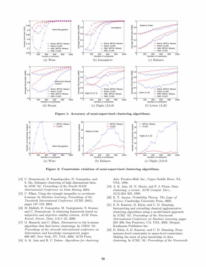
ent sizes were created (every 50 sets were of the same size),typically ranging from 50 to 1000 constraints (25 to 500for the Soybean dataset). The semi-supervised methods,COP-KMeans, MPCK-Means and the proposed CLWC weretested over all constraint sets, whose average performancesare reported in Table 3 and Figures 1(a) to 1(f). SinceCOP-KMeans strictly enforces all the constraints, for manydatasets, it failed to produce any feasible clustering parti-tions (with different initializations) when given more than100 constraints. We therefore only report its performancesin experiments with a small number of constraints.

As shown, CLWC generally produces much better clusterscompared to the other two methods: the accuracy curvesof CLWC are almost always higher than those of MPCK-Means for the datasets. As the number of the constraintsbecomes larger, indicating more partial information is usedto guide the clustering process, the accuracy of both CLWCand MPCK-Means improves consistently. Note that the per-formance curves of MPCK-Means may drop when given asmall number of constraints, and the performances underconstraints may be even a little worse than those withoutconstraints for several datasets, for example, the perfor-mance degradation in the wine dataset under around 300constraints. This is consistent with observations in [8], whichis due to the fact that its metric learning may become biasedwhen there is not enough information to train the metric pa-rameters. It is interesting to observe that CLWC does notsuffer this problem, having a much smoother performancewith additional constraints; there are rarely noticeable ‘dips’in the performance of CLWC.

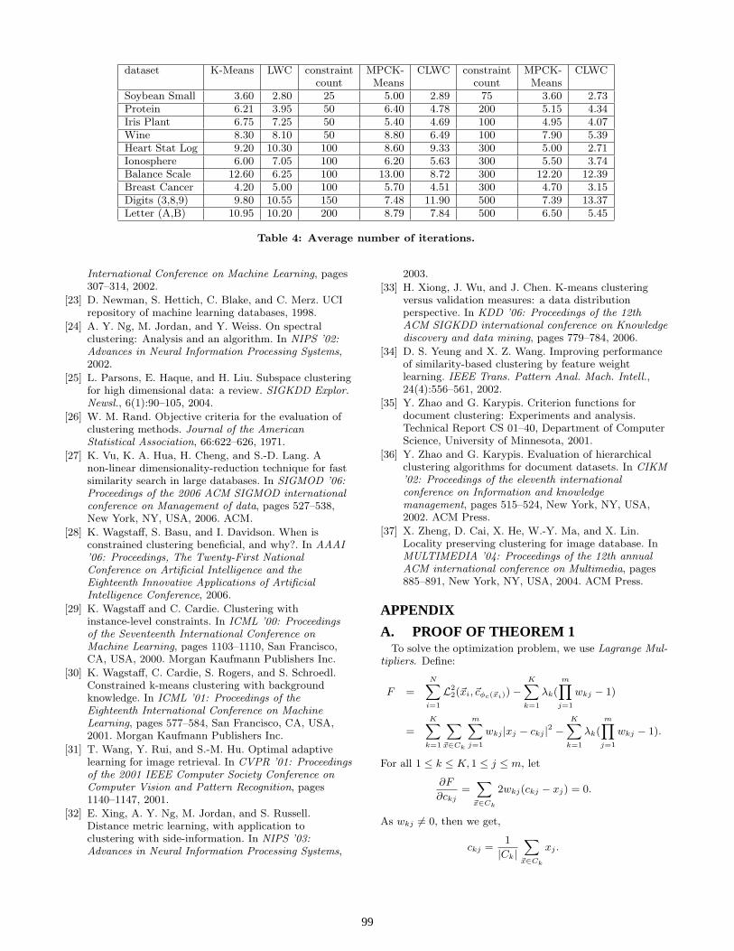
Although our constrained clustering algorithm does notguarantee the satisfaction of all constraints, only a smallnumber of constraints were observed broken by our methodin the experiments. The average numbers of violated con-straints for the datasets are shown in Figures 2(a) - 2(c):they grow slowly as the number of pairwise constraints in-creases and are much smaller compared to those of MPCK-Means.

5.5 Clustering EfficiencyWe summarize the average number of iterations the clus-

tering algorithms took to reach convergence in Table 4. The4th and 7th columns are the numbers of the constraints inuse. Compared with K-Means, which is an efficient algo-rithm [18], the LWC algorithm converges fairly quickly andit took a comparable number of iterations to generate theclusters. The CLWC algorithm generally took even fewer it-erations to converge than K-Means and MPCK-Means, andthe more constraints were given, the faster CLWC completedthe data partition. Therefore, our proposals are also quiteefficient.

6. CONCLUSIONSIn this paper, we proposed to use local weighting vectors

in order to capture the heterogeneous structures of data clus-ters in the feature space. Each set of weights defines the sub-space spanned by the corresponding cluster. We integratedthe constrained learning into our locally weighted clusteringalgorithm. A set of chunklets are built upon constraints,whose points are assigned to clusters collectively. Theoreti-cal analysis and experiments have confirmed the superiorityof our new proposals.

Currently, we are investigating the proposed technique for

96

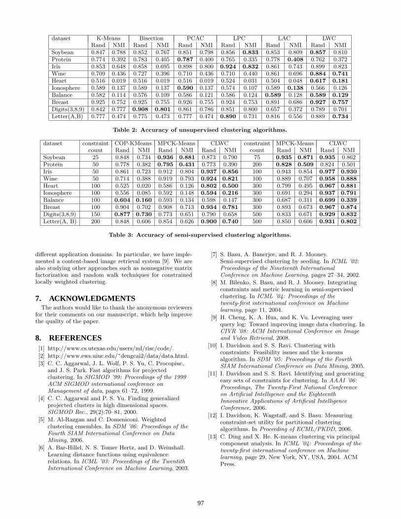
dataset K-Means Bisection PCAC LPC LAC LWCRand NMI Rand NMI Rand NMI Rand NMI Rand NMI Rand NMI

Soybean 0.847 0.788 0.852 0.767 0.851 0.798 0.856 0.833 0.853 0.809 0.857 0.810Protein 0.774 0.392 0.783 0.405 0.787 0.400 0.765 0.335 0.778 0.408 0.762 0.372Iris 0.853 0.648 0.858 0.695 0.898 0.800 0.924 0.832 0.861 0.743 0.899 0.823Wine 0.709 0.436 0.727 0.396 0.710 0.436 0.710 0.440 0.861 0.696 0.884 0.741

Heart 0.516 0.019 0.516 0.019 0.516 0.019 0.524 0.031 0.504 0.048 0.617 0.181

Ionosphere 0.589 0.137 0.589 0.137 0.590 0.137 0.574 0.107 0.589 0.138 0.566 0.126Balance 0.582 0.114 0.576 0.109 0.586 0.121 0.586 0.124 0.589 0.128 0.589 0.129

Breast 0.925 0.752 0.925 0.755 0.926 0.755 0.924 0.753 0.891 0.686 0.927 0.757

Digits(3,8,9) 0.842 0.777 0.908 0.801 0.861 0.786 0.851 0.800 0.657 0.372 0.789 0.701Letter(A,B) 0.777 0.474 0.775 0.473 0.777 0.474 0.890 0.731 0.816 0.556 0.889 0.734

Table 2: Accuracy of unsupervised clustering algorithms.

dataset constraint COP-KMeans MPCK-Means CLWC constraint MPCK-Means CLWCcount Rand NMI Rand NMI Rand NMI count Rand NMI Rand NMI

Soybean 25 0.848 0.734 0.936 0.881 0.873 0.790 75 0.935 0.871 0.935 0.862Protein 50 0.778 0.382 0.795 0.431 0.773 0.390 200 0.828 0.509 0.824 0.501Iris 50 0.861 0.723 0.912 0.804 0.937 0.856 100 0.943 0.854 0.977 0.930

Wine 50 0.714 0.388 0.919 0.793 0.924 0.821 100 0.889 0.707 0.958 0.888

Heart 100 0.525 0.020 0.586 0.126 0.802 0.500 300 0.799 0.495 0.967 0.881

Ionosphere 100 0.556 0.085 0.592 0.148 0.594 0.216 300 0.691 0.294 0.937 0.791

Balance 100 0.604 0.160 0.593 0.134 0.598 0.147 300 0.687 0.311 0.699 0.339

Breast 100 0.904 0.702 0.908 0.713 0.934 0.781 300 0.893 0.673 0.967 0.874

Digits(3,8,9) 150 0.877 0.730 0.773 0.651 0.790 0.658 500 0.833 0.671 0.929 0.832

Letter(A, B) 200 0.848 0.606 0.854 0.626 0.900 0.740 500 0.850 0.606 0.931 0.802

Table 3: Accuracy of semi-supervised clustering algorithms.

different application domains. In particular, we have imple-mented a content-based image retrieval system [9]. We arealso studying other approaches such as nonnegative matrixfactorization and random walk techniques for constrainedlocally weighted clustering.

7. ACKNOWLEDGMENTSThe authors would like to thank the anonymous reviewers

for their comments on our manuscript, which help improvethe quality of the paper.

8. REFERENCES[1] http://www.cs.utexas.edu/users/ml/risc/code/.

[2] http://www.ews.uiuc.edu/~dengcai2/data/data.html.

[3] C. C. Aggarwal, J. L. Wolf, P. S. Yu, C. Procopiuc,and J. S. Park. Fast algorithms for projectedclustering. In SIGMOD ’99: Proceedings of the 1999ACM SIGMOD international conference onManagement of data, pages 61–72, 1999.

[4] C. C. Aggarwal and P. S. Yu. Finding generalizedprojected clusters in high dimensional spaces.SIGMOD Rec., 29(2):70–81, 2000.

[5] M. Al-Razgan and C. Domeniconi. Weightedclustering ensembles. In SDM ’06: Proceedings of theFourth SIAM International Conference on DataMining, 2006.

[6] A. Bar-Hillel, N. S. Tomer Hertz, and D. Weinshall.Learning distance functions using equivalencerelations. In ICML ’03: Proceedings of the TwentithInternational Conference on Machine Learning, 2003.

[7] S. Basu, A. Banerjee, and R. J. Mooney.Semi-supervised clustering by seeding. In ICML ’02:Proceedings of the Nineteenth InternationalConference on Machine Learning, pages 27–34, 2002.

[8] M. Bilenko, S. Basu, and R. J. Mooney. Integratingconstraints and metric learning in semi-supervisedclustering. In ICML ’04: Proceedings of thetwenty-first international conference on Machinelearning, page 11, 2004.

[9] H. Cheng, K. A. Hua, and K. Vu. Leveraging userquery log: Toward improving image data clustering. InCIVR ’08: ACM International Conference on Imageand Video Retrieval, 2008.

[10] I. Davidson and S. S. Ravi. Clustering withconstraints: Feasibility issues and the k-meansalgorithm. In SDM ’05: Proceedings of the FourthSIAM International Conference on Data Mining, 2005.

[11] I. Davidson and S. S. Ravi. Identifying and generatingeasy sets of constraints for clustering. In AAAI ’06:Proceedings, The Twenty-First National Conferenceon Artificial Intelligence and the EighteenthInnovative Applications of Artificial IntelligenceConference, 2006.

[12] I. Davidson, K. Wagstaff, and S. Basu. Measuringconstraint-set utility for partitional clusteringalgorithms. In Proceeding of ECML/PKDD, 2006.

[13] C. Ding and X. He. K-means clustering via principalcomponent analysis. In ICML ’04: Proceedings of thetwenty-first international conference on Machinelearning, page 29, New York, NY, USA, 2004. ACMPress.

97

0 200 400 600 800 10000.65

0.7

0.75

0.8

0.85

0.9

0.95

1

Number of constraints

Ave

rage

Ran

d in

dex

(NM

I)

Rand, MPCK−MeansRand, CLWCNMI, MPCK−MeansNMI, CLWC

Wine Recognition

(a) Wine

0 200 400 600 800 10000

0.2

0.4

0.6

0.8

1

Number of constraints

Ave

rage

Ran

d in

dex

(NM

I)

Rand, MPCK−MeansRand, CLWCNMI, MPCK−MeansNMI, CLWC

Ionosphere

(b) Ionosphere

0 200 400 600 800 10000

0.2

0.4

0.6

0.8

1

Number of constraints

Ave

rage

Ran

d in

dex

(NM

I)

Rand, MPCK−MeansRand, CLWCNMI, MPCK−MeansNMI, CLWC

Balance Scale

(c) Balance

0 200 400 600 800 10000.6

0.7

0.8

0.9

1

Number of constraints

Ave

rage

Ran

d in

dex

(NM

I)

Rand, MPCK−MeansRand, CLWCNMI, MPCK−MeansNMI, CLWC

Wisconsin BreastCancer

(d) Breast

0 200 400 600 800 10000.4

0.5

0.6

0.7

0.8

0.9

1

Number of constraints

Ave

rage

Ran

d in

dex

(NM

I)

Rand, MPCK−MeansRand, CLWCNMI, MPCK−MeansNMI, CLWC

Digits (3, 8, 9)

(e) Digits (3,8,9)

0 200 400 600 800 10000.4

0.5

0.6

0.7

0.8

0.9

1

Number of constraints

Ave

rage

Ran

d in

dex

(NM

I)

Rand, MPCK−MeansRand, CLWCNMI, MPCK−MeansNMI, CLWC

Letter (A, B)

(f) Letter (A,B)

Figure 1: Accuracy of semi-supervised clustering algorithms.

0 200 400 600 800 10000

1

2

3

4

5

6

Number of constraints

Num

ber

of c

onst

rain

ts v

iola

ted MPCK−Means

CLWC

Wine Recognition

(a) Wine

0 200 400 600 800 10000

5

10

15

20

Number of constraints

Num

ber

of c

onst

rain

ts v

iola

ted MPCK−Means

CLWC

Balance Scale

(b) Balance

0 200 400 600 800 10000

5

10

15

20

25

30

Number of constraints

Num

ber

of c

onst

rain

ts v

iola

ted MPCK−MeansCLWC

Digits (3, 8, 9)

(c) Digits (3,8,9)

Figure 2: Constraints violation of semi-supervised clustering algorithms.

[14] C. Domeniconi, D. Papadopoulos, D. Gunopulos, andS. Ma. Subspace clustering of high dimensional data.In SDM ’04: Proceedings of the Fourth SIAMInternational Conference on Data Mining, 2004.

[15] C. Elkan. Using the triangle inequality to acceleratek-means. In Machine Learning, Proceedings of theTwentieth International Conference (ICML 2003),pages 147–153, 2003.

[16] M. Halkidi, D. Gunopulos, M. Vazirgiannis, N. Kumar,and C. Domeniconi. A clustering framework based onsubjective and objective validity criteria. ACM Trans.Knowl. Discov. Data, 1(4):1–25, 2008.

[17] G. Hamerly and C. Elkan. Alternatives to the k-meansalgorithm that find better clusterings. In CIKM ’02:Proceedings of the eleventh international conference onInformation and knowledge management, pages600–607, New York, NY, USA, 2002. ACM Press.

[18] A. K. Jain and R. C. Dubes. Algorithms for clustering

data. Prentice-Hall, Inc., Upper Saddle River, NJ,USA, 1988.

[19] A. K. Jain, M. N. Murty, and P. J. Flynn. Dataclustering: a review. ACM Comput. Surv.,31(3):264–323, 1999.

[20] E. T. Jaynes. Probability Theory: The Logic ofScience. Cambridge University Press, 2003.

[21] S. D. Kamvar, D. Klein, and C. D. Manning.Interpreting and extending classical agglomerativeclustering algorithms using a model-based approach.In ICML ’02: Proceedings of the NineteenthInternational Conference on Machine Learning, pages283–290, San Francisco, CA, USA, 2002. MorganKaufmann Publishers Inc.

[22] D. Klein, S. D. Kamvar, and C. D. Manning. Frominstance-level constraints to space-level constraints:Making the most of prior knowledge in dataclustering. In ICML ’02: Proceedings of the Nineteenth

98

dataset K-Means LWC constraint MPCK- CLWC constraint MPCK- CLWCcount Means count Means

Soybean Small 3.60 2.80 25 5.00 2.89 75 3.60 2.73Protein 6.21 3.95 50 6.40 4.78 200 5.15 4.34Iris Plant 6.75 7.25 50 5.40 4.69 100 4.95 4.07Wine 8.30 8.10 50 8.80 6.49 100 7.90 5.39Heart Stat Log 9.20 10.30 100 8.60 9.33 300 5.00 2.71Ionosphere 6.00 7.05 100 6.20 5.63 300 5.50 3.74Balance Scale 12.60 6.25 100 13.00 8.72 300 12.20 12.39Breast Cancer 4.20 5.00 100 5.70 4.51 300 4.70 3.15Digits (3,8,9) 9.80 10.55 150 7.48 11.90 500 7.39 13.37Letter (A,B) 10.95 10.20 200 8.79 7.84 500 6.50 5.45

Table 4: Average number of iterations.

International Conference on Machine Learning, pages307–314, 2002.

[23] D. Newman, S. Hettich, C. Blake, and C. Merz. UCIrepository of machine learning databases, 1998.

[24] A. Y. Ng, M. Jordan, and Y. Weiss. On spectralclustering: Analysis and an algorithm. In NIPS ’02:Advances in Neural Information Processing Systems,2002.

[25] L. Parsons, E. Haque, and H. Liu. Subspace clusteringfor high dimensional data: a review. SIGKDD Explor.Newsl., 6(1):90–105, 2004.

[26] W. M. Rand. Objective criteria for the evaluation ofclustering methods. Journal of the AmericanStatistical Association, 66:622–626, 1971.

[27] K. Vu, K. A. Hua, H. Cheng, and S.-D. Lang. Anon-linear dimensionality-reduction technique for fastsimilarity search in large databases. In SIGMOD ’06:Proceedings of the 2006 ACM SIGMOD internationalconference on Management of data, pages 527–538,New York, NY, USA, 2006. ACM.

[28] K. Wagstaff, S. Basu, and I. Davidson. When isconstrained clustering beneficial, and why?. In AAAI’06: Proceedings, The Twenty-First NationalConference on Artificial Intelligence and theEighteenth Innovative Applications of ArtificialIntelligence Conference, 2006.

[29] K. Wagstaff and C. Cardie. Clustering withinstance-level constraints. In ICML ’00: Proceedingsof the Seventeenth International Conference onMachine Learning, pages 1103–1110, San Francisco,CA, USA, 2000. Morgan Kaufmann Publishers Inc.

[30] K. Wagstaff, C. Cardie, S. Rogers, and S. Schroedl.Constrained k-means clustering with backgroundknowledge. In ICML ’01: Proceedings of theEighteenth International Conference on MachineLearning, pages 577–584, San Francisco, CA, USA,2001. Morgan Kaufmann Publishers Inc.

[31] T. Wang, Y. Rui, and S.-M. Hu. Optimal adaptivelearning for image retrieval. In CVPR ’01: Proceedingsof the 2001 IEEE Computer Society Conference onComputer Vision and Pattern Recognition, pages1140–1147, 2001.

[32] E. Xing, A. Y. Ng, M. Jordan, and S. Russell.Distance metric learning, with application toclustering with side-information. In NIPS ’03:Advances in Neural Information Processing Systems,

2003.

[33] H. Xiong, J. Wu, and J. Chen. K-means clusteringversus validation measures: a data distributionperspective. In KDD ’06: Proceedings of the 12thACM SIGKDD international conference on Knowledgediscovery and data mining, pages 779–784, 2006.

[34] D. S. Yeung and X. Z. Wang. Improving performanceof similarity-based clustering by feature weightlearning. IEEE Trans. Pattern Anal. Mach. Intell.,24(4):556–561, 2002.

[35] Y. Zhao and G. Karypis. Criterion functions fordocument clustering: Experiments and analysis.Technical Report CS 01–40, Department of ComputerScience, University of Minnesota, 2001.

[36] Y. Zhao and G. Karypis. Evaluation of hierarchicalclustering algorithms for document datasets. In CIKM’02: Proceedings of the eleventh internationalconference on Information and knowledgemanagement, pages 515–524, New York, NY, USA,2002. ACM Press.

[37] X. Zheng, D. Cai, X. He, W.-Y. Ma, and X. Lin.Locality preserving clustering for image database. InMULTIMEDIA ’04: Proceedings of the 12th annualACM international conference on Multimedia, pages885–891, New York, NY, USA, 2004. ACM Press.

APPENDIX

A. PROOF OF THEOREM 1To solve the optimization problem, we use Lagrange Mul-

tipliers. Define:

F =

N∑

i=1

L22(~xi,~cφc(~xi)) −

K∑

k=1

λk(

m∏

j=1

wkj − 1)

=K

∑

k=1

∑

~x∈Ck

m∑

j=1

wkj |xj − ckj |2 −K

∑

k=1

λk(m∏

j=1

wkj − 1).

For all 1 ≤ k ≤ K, 1 ≤ j ≤ m, let

∂F

∂ckj

=∑

~x∈Ck

2wkj(ckj − xj) = 0.

As wkj 6= 0, then we get,

ckj =1

|Ck|∑

~x∈Ck

xj .

99

Similarly, let

∂F

∂wkj

=∑

~x∈Ck

|xj − ckj |2 − λk

m∏

j′=1,j′ 6=j

wkj′

=∑

~x∈Ck

|xj − ckj |2 −λk

wkj

= 0.

Then we have,

wkj =λk

∑

~x∈Ck|xj − ckj |2

.

As for 1 ≤ k ≤ K,∏m

j=1 wkj = 1, we have

λk =(

m∏

j=1

(∑

~x∈Ck

|xj − ckj |2)) 1

m.

The second order partial derivatives of F are computed as:

∂2F

∂c2kj

∂2F∂ckj∂wkj

∂2F∂wkj∂ckj

∂2F

∂w2kj

=

[

2∑

~x∈Ckwkj

∑

~x∈Ck2(ckj − xj)

∑

~x∈Ck2(ckj − xj)

λk

w2kj

]

.

Its determinant is positive at the derived optimal weightsand centroids, and therefore, they represent a minimum.

B. PROOF OF CONVERGENCE OF LOCALLYWEIGHTED CLUSTERING

Corollary 1. The Locally Weighted Clustering Algorithm(Algorithm 1) converges to a local minimum of the objectivefunction defined in Eq. 2.

Proof. The objective function f is defined for the givenassignments φ and centroids ~c and weights ~w:

f(φ,~c, ~w) =

N∑

i=1

L22, ~wφ(~xi)

(~xi,~cφ(~xi)).

Algorithm 1 starts from an initial assignment and runs fromiteration to iteration. Each iteration consists of two steps: todetermine cluster assignments (E-step, Line 2 in Algorithm1) and to compute centroids and weights for individual clus-ters (M-step, Line 3).

Formally, let ~ci, ~wi and φic respectively denote the cen-

troids, weights, assignments derived in the ith iteration. ~c0

and ~w0 are the initial configuration, while in the algorithmφ0

c is not initialized and can be any assignment. In φic, each

point ~xi is assigned to its closest cluster according to weightsand centroids in the last iteration, ~ci−1 and ~wi−1. Therefore,each E-step reduces the objective value, i.e.,

f(φic,~c

i−1, ~w

i−1) ≤ f(φi−1c ,~c

i−1, ~w

i−1).

In each M-step, for the given φic, the optimal ~ci and ~wi are

computed using Eqs. 3 and 4 (as in Appendix A). Hence,each M-step reduces the objective value, i.e.,

f(φic,~c

i, ~w

i) ≤ f(φic,~c

i−1, ~w

i−1).

Overall, we have f(φic,~c

i, ~wi) no greater than f(φi−1c ,~ci−1, ~wi−1).

It is guaranteed that Algorithm 1 reduces the objective valuein iterations.

The clustering problem is to group N points into K dis-joint sets and there are only a finite number of data parti-tions. For a given φc, the minimal objective value is deter-mined for the corresponding optimal centroids and weights.

Therefore, the objective value for a given assignment is lower-bounded. The objective value in Algorithm 1 decreasesgradually until the value reaches a fixed point. This fixedpoint is a local minimal of f(φ,~c, ~w).

C. PROOF ON ONE CHUNKLETThere are K clusters, C1, C2, . . . , CK . For cluster Ci, the

data values in the jth dimension follow the normal distribu-tion N(µij , 1).

For a chunklet ∆ that belongs to cluster s in the groundtruth, (∆ ⊆ Cs), the conditional probability that the sum ofdistances from points in ∆ to cluster i is smaller than thatto cluster p, (i 6= p), is denoted as,

Pd,1(i, p | s) = P(

∑

~x∈∆

L22,~1(~x,~ci) <

∑

~x∈∆

L22,~1(~x,~cp) | ∆ ⊆ Cs

)

.

Theorem 4. For 1 ≤ i, p, s ≤ K, i 6= p we have

Pd,1(i, p | s)

= Φ(−s(∆)

∑m

r=1(µpr − µir)µsr + 12s(∆)

∑m

r=1(µ2pr − µ2

ir)√

s(∆)∑m

r=1(µpr − µir)2

)

.

Proof. We can rewrite the left hand side (LHS) as below,

LHS = P(

∑

~x∈∆

m∑

r=1

((xr − µir)2 − (xr − µpr)2) < 0 | ∆ ⊆ Cs

)

= P(

∑

~x∈∆

m∑

r=1

(µpr − µir)xr <1

2s(∆)

m∑

r=1

(µ2pr − µ2

ir) | ∆ ⊆ Cs

)

.

As xr follows N(µsr, 1), denoted as xr ∼ N(µsr, 1), then

(µpr − µir)xr ∼ N((µpr − µir)µsr, (µpr − µir)2).

Define Y =∑

~x∈∆

∑m

r=1(µpr − µir)xr, following a normaldistribution,

N(s(∆)∑m

r=1(µpr − µir)µsr, s(∆)∑m

r=1(µpr − µir)2).

We can normalize Y into a random variable of the standardnormal distribution, YN ∼ N(0, 1), i.e.,

YN =Y − s(∆)

∑m

r=1(µpr − µir)µsr√

s(∆)∑m

r=1(µpr − µir)2.

Therefore, we have,

LHS = P(

YN <−s(∆)

∑

r(µpr − µir)µsr + 12s(∆)

∑

r(µ2pr − µ2

ir)√

s(∆)∑m

r=1(µpr − µir)2

)

.

As YN ∼ N(0, 1), the above equation can be further rewrit-ten using the cumulative distribution function Φ of N(0, 1).

According to the definition of Pd,1(i, p | s), for 1 ≤ i, p, s ≤K, we have

Pd,1(i, p | s) = 1 − Pd,1(p, i | s).

As the probability distribution function of N(0, 1) is sym-metric with regard to the x = 0, there is a special propertyof its cumulative function Φ(x), that is,

Φ(x) + Φ(−x) = 1.

Therefore, we have,

Pd,1(i, p | s) = Φ(A),

Pd,1(p, i | s) = Φ(−A),

100

in which

A =−s(∆)

∑m

r=1(µpr − µir)µsr + 12s(∆)

∑m

r=1(µ2pr − µ2

ir)√

s(∆)∑m

r=1(µpr − µir)2.

DISCUSSIONS:

According to Theorem 4, the event that the sum of dis-tances of the points in ∆ ⊆ Cs to its true cluster Cs issmaller than that to some cluster Cp, occurs with the prob-ability,

Pd,1(s, p | s) = Φ(

√

s(∆)

2

√

√

√

√

m∑

r=1

(µpr − µsr)2)

.

In chunklet assignment, in case of two clusters C1 and C2,the chance to place ∆ correctly is Pd,1(1, 2 | 1) (or Pd,1(2, 1 |2)). This is the conclusion in Theorem 2. In case of morethan two clusters, ∆ is assigned to cluster i if cluster i isthe one closest to the points in the chunklet, i.e., for all1 ≤ p ≤ K, and p 6= i,

∑

~x∈∆ L22,~1

(~x,~ci) <∑

~x∈∆ L22,~1

(~x,~cp).

Each of these events,∑

~x∈∆ L22,~1

(~x,~ci) <∑

~x∈∆ L22,~1

(~x,~cp),

is not necessarily independent. Consider there are 3 clustersin 2-dimensional space, ~c1 = 〈1, 0〉, ~c2 = 〈2, 0〉, ~c3 = 〈3, 0〉,it is true that, for any point ~x, if it is closer to c1 than c2,then ~x is also closer to c1 than c3. Thus, for this example,

P(

∑

~x∈∆

L22,~1

(~x,~c1) <∑

~x∈∆

L22,~1

(~x,~c2)⋂

∑

~x∈∆

L22,~1

(~x,~c1) <∑

~x∈∆

L22,~1

(~x,~c3) | ∆ ⊆ C1

)

= Pd,1(1, 2 | 1) 6= Pd,1(1, 2 | 1)Pd,1(1, 3 | 1).

Although the probability to assign ∆ correctly is not ex-pressed in a closed form for more than two clusters, gen-erally this probability is related to Pd,1(s, p | s). The moredata points the chunklet ∆ has, the larger the positive value√

s(∆)

2

√∑m

r=1(µpr − µsr)2 is. Hence, the corresponding prob-ability Pd,1(s, p | s) is larger, and Pd,1(p, s | s) is smaller. Itis more likely that the points in ∆ are close to the clusterthey belong to, as a group. Consequently, the probability todecide the membership of ∆ correctly becomes larger withthe increase of the size of the chunklet, s(∆).

D. PROOF ON TWO CHUNKLETSFor chunklets ∆ ⊆ Cs and ∆′ ⊆ Ct, (s 6= t, i 6= p∩ j 6= q),

denote

Pd,2(i, j, p, q | s, t)

= P(

∑

~x∈∆ L22,~1

(~x,~ci) +∑

~x∈∆′ L22,~1

(~x,~cj) <

∑

~x∈∆ L22,~1

(~x,~cp) +∑

~x∈∆′ L22,~1

(~x,~cq) | ∆ ⊆ Cs, ∆′ ⊆ Ct

)

.

Theorem 5. For 1 ≤ i, j, p, q, s, t ≤ K, s 6= t, i 6= p∩ j 6=q, we have

Pd,2(i, j, p, q | s, t) = Φ( A

B

)

,

in which

A = −s(∆)∑m

r=1(µpr − µir)µsr − s(∆′)∑m

r=1(µqr − µjr)µtr

+ 12s(∆)

∑m

r=1(µ2pr − µ2

ir) + 12s(∆′)

∑m

r=1(µ2qr − µ2

jr),

B =√

s(∆)∑m

r=1(µpr − µir)2 + s(∆′)∑m

r=1(µqr − µjr)2.

Proof. The left hand side (LHS) can be rewritten as,

LHS = P(

∑

~x∈∆

m∑

r=1

(µpr − µir)xr +∑

~x∈∆′

m∑

r=1

(µqr − µjr)xr <

1

2(∑

~x∈∆

m∑

r=1

(µ2pr − µ2

ir) +∑

~x∈∆′

m∑

r=1

(µ2qr − µ2

jr)) | ∆ ⊆ Cs, ∆′ ⊆ Ct

)

.

Define Y =∑

~x∈∆

∑

r(µpr −µir)xr +∑

~x∈∆′

∑

r(µqr −µjr)xr,that follows a normal distribution with the mean

s(∆)∑m

r=1(µpr − µir)µsr + s(∆′)∑m

r=1(µqr − µjr)µtr,

and the variance

s(∆)∑m

r=1(µpr − µir)2 + s(∆′)

∑m

r=1(µqr − µjr)2.

Y can be normalized, YN ∼ N(0, 1), and we can derive theresult of this theorem in the similar process in Theorem4.

According to the definition, for 1 ≤ i, j, p, q, s, t ≤ K, wealso have,

Pd,2(i, j, p, q | s, t) = 1 − Pd,2(p, q, i, j | s, t).

DISCUSSIONS:

According to Theorem 5, we have,

Pd,2(s, t, p, q | s, t)

= Φ(1

2

√

√

√

√s(∆)

m∑

r=1

(µpr − µsr)2 + s(∆′)

m∑

r=1

(µqr − µtr)2)

.

Without prior knowledge, if the distances among cluster cen-troids are the same, (i.e., for i, j, L2,~1(~ci,~cj) is some con-stant), then

Pd,2(s, t, p, q | s, t) = Φ(

√

s(∆) + s(∆′)

2

√

√

√

√

m∑

r=1

(~csr − ~ctr)2)

.

For two clusters C1 and C2, the probability to determinethe memberships of ∆ and ∆′ with no mistakes is relatedto Pd,2(1, 2, 2, 1 | 1, 2) and Pd,2(2, 1, 1, 2 | 2, 1). This is theconclusion in Theorem 3. Similar to the analysis of onechunklet in the previous section, in case of more than twoclusters, the probability to assign ∆ and ∆′ correctly is notnecessarily equal to

K∏

p=1,q=1,p 6=s∩q 6=t

Pd,2(s, t, p, q | s, t).

In general, if the sizes of the two chunklets s(∆) + s(∆′)are bigger, the value (s(∆)+s(∆′))

∑

r(µsr −µtr)2 is larger,

so is s(∆)∑

r(µpr − µsr)2 + s(∆′)

∑

r(µqr − µtr)2. There-

fore, the probability is larger that ∆ and ∆′ are closerto their true clusters rather than any other clusters, andPd,2(p, q, s, t | s, t) is smaller. Hence, the probability to de-cide the membership of the two chunklets correctly is gen-erally larger with more data points in ∆ and ∆′.

101