Consideration of 2-150 kHz Disturbances in North American ...

Consideration of 2-150 kHz Disturbances in North American Power Systems

by

Elizabeth Anne Devore

A thesis submitted to the Graduate Faculty of Auburn University

in partial fulfillment of the requirements for the Degree of

Master of Science

Auburn, Alabama August 5, 2017

Keywords: power line communication, high frequency disturbances, EMC standardization, commutation notches

Copyright 2017 by Elizabeth Anne Devore

Approved by

S. Mark Halpin, Chair, Alabama Power Company Distinguished Professor of Electrical and Computer Engineering

R. Mark Nelms, Professor and Chair of Electrical and Computer Engineering Charles A. Gross, Professor Emeritus of Electrical and Computer Engineering

ii

Abstract

This is an evaluation of considerations for electromagnetic compatibility (EMC)

limits for power line communication (PLC) based on North American standards. In the

vast majority of cases, smart meters are located in the low voltage (LV) environment and

must be designed to operate suitably in the presence of disturbances bounded by set

compatibility levels (CLs). In Europe, without standardized limits for emissions in the

frequency range allotted for smart meters (2-150 kHz), levels have reached the point where

smart meter communication disturbances occur. In the United States, there are no defined

CLs for 2-150 kHz, but there are limits for voltage notches in IEEE Standard 519. In this

evaluation, compatibility level curves proposed by European utilities and end user

equipment manufacturers are used to consider the emission limits set by North American

commutation notch limits. The proposed CLs are also evaluated based on end user device

measurements taken in North America. Further consideration is given to the propagation

from the point of measurements to the point of common coupling (PCC). It is found that

North American commutation notch limits may be considered for the purpose of setting

emission limits.

iii

Acknowledgments

To Demi, Jacob, Christian, and Tyler – thank you for making every day brighter. I

love y’all to the moon and back.

To my advisor Dr. Mark Halpin – thank you for your patience and clarifying my

sometimes jumbled understanding of this work.

iv

Table of Contents

Abstract .............................................................................................................................. ii

Acknowledgments............................................................................................................. iii

List of Tables .................................................................................................................... vi

List of Figures .................................................................................................................. vii

List of Abbreviations ...................................................................................................... viii

Chapter 1: Introduction ...................................................................................................... 1

Chapter 2: Disturbance Limits and Levels......................................................................... 4

2.1 Compatibility Levels ........................................................................................ 5

2.1.1 IEC Proposed CLs............................................................................. 5

2.2 Planning Levels ................................................................................................ 8

2.3 Emission Limits ............................................................................................... 8

Chapter 3: Commutation Notches ................................................................................... 11

3.1 IEEE Standard 519 ......................................................................................... 13

Chapter 4: Fourier Series of Commutation Notches ........................................................ 15

4.1 Trigonometric Fourier Series ......................................................................... 15

4.2 Exponential Fourier Series ............................................................................. 17

Chapter 5: Measurements ................................................................................................ 20

5.1 Measured End-Use Device Results ................................................................ 22

5.2 Line Resonance Considerations ..................................................................... 26

5.2.1 Line Impedance Measurements ...................................................... 27

5.2.2 Line Impedance Model ................................................................... 28

Chapter 6: Summary ....................................................................................................... 30

Chapter 7: Recommendations and Future Work ............................................................. 32

References ....................................................................................................................... .33

Appendix 1 ....................................................................................................................... 35

Appendix 1.1 ........................................................................................................ 35

v

Appendix 1.2 ........................................................................................................ 36

Appendix 1.3 ........................................................................................................ 37

vi

List of Tables

Table 1. Summation Law Exponents (50 Hz system)...................................................... 10

Table 2. IEEE Std. 519 Recommended Commutation Notch Limits .............................. 13

Table 3. Notch Limit Results at Select Frequencies ........................................................ 17

vii

List of Figures

Fig. 1. Relationship Between Disturbance Limits and Levels ........................................... 4

Fig. 2. IEC Proposed CLs .................................................................................................. 6

Fig. 3. Bridge Rectifier .................................................................................................... 12

Fig. 4. Commutation Notch Example .............................................................................. 12

Fig. 5. Definition of Notch Depth for Notch Area Calculation ....................................... 13

Fig. 6. Plot of f(t) ............................................................................................................. 16

Fig. 7. Notch Limit Results Using Trigonometric Fourier Series.................................... 17

Fig. 8. Notch Limit Results Using Exponential Fourier Series ....................................... 18

Fig. 9. Example PLs vs. Notch Limits and Proposed CLs .............................................. 19

Fig. 10. Load Equipment Measurement Setup................................................................. 20

Fig. 11. High-Pass Filter Designed to Remove Power Frequency .................................. 21

Fig. 12. High-Pass Filter Transfer Function .................................................................... 21

Fig. 13. 72-hour Background Emission Levels vs. Utility Proposed CLs ....................... 22

Fig. 14. CFL Measurements vs. Utility Proposed CLs .................................................... 24

Fig. 15. LED Measurements vs. Utility Proposed CLs.................................................... 25

Fig. 16. Television Measurements vs. Utility Proposed CLs .......................................... 26

Fig. 17. Romex Cable Measurement Setup ..................................................................... 27

Fig. 18. Impedance Analyzer Measurements of 12-3 Romex Cable ............................... 28

Fig. 19. Per-Meter Romex Cable Line Model ................................................................. 29

viii

List of Abbreviations

CL Compatibility Level

EHV Extra High Voltage

EL Emission Level

EMC Electromagnetic Compatibility

HV High Voltage

IL Immunity Level

LV Low Voltage

MV Medium Voltage

PCC Point of Common Coupling

PL Planning Level

PLC Power Line Communication

1

Chapter 1: Introduction

The smart grid offers a robust set of networks that facilitate bidirectional exchange

of data for power supplies and electrical equipment connected to the power grid. The

technologies that make up the smart grid enable effective monitoring of the operation and

conditions of the grid, providing the benefits of a more efficient power system that can

regulate and control the distribution of electricity based on consumption without failures

or outages. Therefore, communication is a major advantage to having a smart grid. These

smart grid technologies can provide system operators with near real-time information about

the system and consumer usage that is obtainable remotely. A primary use of remote

communication techniques involves smart meters.

Smart meters have rapidly become a dominant metering option for utilities in North

America and abroad. Primarily, wireless radio is used by utilities to receive demand

information for customer billing in North America. This option is attractive because it is

wireless and does not require much additional infrastructure. However, there are some

locations where wireless radio may not be reliable. In these locations, another technique,

such as power line communication (PLC), is beneficial because very little additional

infrastructure is needed to establish links for reliable, remote communication.

Using PLC relies on already established power lines and therefore is subject to the

imperfect system conditions that result from electrical equipment connected to the grid.

2

Specifically, high frequency disturbances must be considered. Harmonics are the integer

multiples of the fundamental frequency, which is 60 Hz in North America and most of

South America, and 50 Hz in Europe and the majority of the rest of the world. Harmonics

result from repeating signals, such as the sinusoidal voltage and current waveforms

transmitted on the power grid and converted by end user devices such as cell phone

chargers and stereos. The sum of harmonics produced by all end user devices seen at the

meter, which often serves as the point of common coupling (PCC), must not exceed certain

levels to prevent disturbances with communications technology. In order to combat

disturbances for PLC, further study of the frequency range allotted to smart meters, 9-150

kHz, must be completed. These disturbances are referred to as high frequency

disturbances. Manufacturers have not previously considered this frequency band when

designing appliances, and utilities have not previously had issues with the lack of standards

in this range. Setting standards for the allotted frequency range for smart meters requires

testing to measure what is currently seen in the environment and analysis of related

standards. Therefore, measurements and comparable standards must be considered.

Although smart meters are not exclusively used by all utilities in the United States,

it is important to consider future use of this technology. Currently, in Europe, there are

cited issues with retrieving reliable data for billing customers using PLC. These issues

have brought attention to the need for setting electromagnetic compatibility (EMC) levels

in the 2-150 kHz range. Established compatibility levels (CLs) could be modified to help

prepare for any future roadblocks with implementing smart meters using PLC in North

America. The Institute of Electrical and Electronics Engineers (IEEE) develops industry

standards in North America, and the International Electrotechnical Commission (IEC) is

3

responsible for creating standards internationally. Therefore, development of IEC

standards in cooperation with IEEE standards could make for truly international

disturbance level management procedures for high frequency disturbances that could

impact PLC.

It is in the best interest of IEEE to follow and aid in work being done by IEC.

Setting CLs based on international considerations will help to make future considerations

by IEEE readily adopted. Although there are no standards in North America that are

directly related to the CLs being planned by the IEC, there are recommended practices in

IEEE Standard 519 that relate to disturbance limits that would be required to not exceed

defined CLs when summed at the PCC. Consideration of these limits, measurements of

the high frequency environment, and measurements of the propagation from the

disturbance source to the PCC are relevant and could aid in the development of EMC

standards worldwide. Each of these topics is considered in this thesis.

4

Chapter 2: Disturbance Limits and Levels

Harmonics are the sinusoidal waveforms at frequencies that are integer multiples

of the fundamental frequency. Power system harmonics are a primary cause of distortion

of mains voltage and load current waveforms. In order to combat these distortions, limits

are set to handle interference with devices connected to the system, such as the equipment

used for PLC systems. These disturbance or emission levels (ELs) account for varying

levels of disturbances present at a location. The goal of setting disturbance limits is to

safeguard a globally acceptable electromagnetic environment for all system elements to

work normally. Disturbance or emission limits are set to deal with the normal and worst-

case levels of allowable disturbances. The relationship between these limits and levels is

shown in Fig. 1 [1].

Fig. 1. Relationship Between Disturbance Limits and Levels

5

2.1 Compatibility Level

The maximum level that the sum of emission limits for a system cannot pass is

referred to as the reference or compatibility level (CL) for a particular electromagnetic

disturbance. By convention, the CL is chosen so that it will be exceeded by the actual EL

only with a probability of no more than ~5 %. Since an immunity level (IL) represents the

level equipment can tolerate and still function properly in a specific environment (such as

the LV network), then all equipment intended to operate in that environment is required to

have immunity at least at that level of disturbance. Therefore, a reasonable margin

representative of the equipment operating in that environment is provided between the CLs

and the ILs [1]. These CLs are specified for different frequency ranges and environments

so that there is limited probability that they will be exceeded by the actual system ELs.

Power system EMC is a condition of the electromagnetic environment such that the

EL is sufficiently low and the ILs are sufficiently high to assure that all devices and systems

(such as the PLC system) operate as intended. This requires coordinated control of ELs

and ILs in order to ensure that the ILs of the equipment and systems at any location are not

exceeded by the EL at that location resulting from the cumulative emissions of all sources

and equipment impedances. As a result, EMC is assumed to exist if the probability of the

deviation from expected performance is negligible – less than 5 % [2].

2.1.1 Proposed CLs for 2-150 kHz

In order to combat the issues encountered by European utilities using PLC,

emission limits are being set, beginning with considerations for CLs in the 2-150 kHz

range. The International Electrotechnical Commission’s Technical Committee 77, Sub-

6

Committee 77A, Working Group 8 is working on a revision of IEC 61000-2-2 that will

provide CLs for high frequency disturbances. More work, and possibly new documents,

are needed to define limits that satisfy the utility’s need for accurate billing information,

while not requiring a lot of costly changes to manufactured devices. These proposed CLs

for LV networks are shown in Fig. 2. The units dB-µV are used in order to represent the

ratio between the measured or specified voltage emissions and 1 microvolt (µV). Referring

to these limits in dB (decibels) rather than by absolute quantities allows for larger ranges

(between µV and volts) in numbers to be represented on a relatable scale [3]. Emissions

in the 2-150 kHz frequency range are usually on the order of millivolts (mV), around 10-

100 mV or, 80-100 dB-µV. Therefore, choosing the units dB-µV for the purpose of

analyzing all high frequency phenomena (levels and limits) allows for larger variation in

mV to be represented on a smaller scale.

Fig. 2. IEC Proposed CLs

7

Working Group 8 manufacturing and utility experts have reached an agreement on

the CLs between 2-30 kHz. There are two options, shown in Fig. 2, that are being

considered for the 30-150 kHz range. Option A is supported by experts related to general

industry manufacturing and usage equipment, not including communication systems.

Experts recommending option A are in favor of this higher-level curve, arguing that initial

estimates have shown the use of filters systematically in all equipment to reduce

disturbance ELs is far more expensive than solving the electromagnetic interference to

communication system issues on a case by case basis. Further, reports show that PLC

technology is operating as intended in more than 97 % of the locations in Finland, with no

emission limits existing in the 2-150 kHz range for most equipment [4]. Alternatively,

supporters of option B, experts in electricity distribution and the communication systems

industry, argue that the emission limits for non-intentional emissions provided in IEC

61000-3-8 have been assumed as reference for designing PLC technologies used for smart

metering and other smart grid services in Europe and worldwide. The proposed option B

curve is based on CLs derived from the IEC 61000-3-8 curve for non-intentional emissions.

Therefore, option B would insure proper operation of technologies for smart grid

communications. Additionally, based on data collected recently in Italy, it has been shown

that the non-intentional emissions generated by several pieces of equipment (such as

lighting equipment) were below this proposed CL curve, minus 3 dB, leaving room for

deviation from estimates.

Further investigation of the benefits and concerns for both options for CLs in the

30-150 kHz range is required in order to come to a final consensus. It is assumed by all

experts involved in the revision of IEC 61000-2-2 that the implementation of this standard

8

for all equipment will assure that ELs in LV networks will be kept at the same level for the

future. Also, new limits will certainly need to be defined with the intent to produce

minimum costs to society.

2.2 Planning Level

Planning levels (PLs) are set based on the summation of individual emission limits

for normal operation. These PLs are accepted as a reference to coordinate emission limits

set for consumer load devices connected to the power system. Therefore, these levels are

generally lower than the CL by a specific margin that takes into account the structure and

electrical characteristics of the local supply network. This margin is necessary to make

allowance for possible system resonance and for an upward drift in the levels on the

network due to future loads that may be connected. Such loads include computers and

other home and office electronic equipment that contain switched-mode power supplies.

Additionally, there is uncertainty about the impedance of the supply systems and the

customers’ equipment at harmonic frequencies. As a result, PLs are determined after CLs

are defined.

2.3 Emission Limits

Provided PLs, emission limits can be determined. Emission limits are limits set for

individual end user devices [3]. Setting emission limits is necessary in order to limit the

total disturbance at the meter and throughout the system as a whole. Determining emission

limits requires the PL to be set so that emission limits for individual devices may be

selected to reasonably account for the total sum of emissions system-wide.

9

Knowledge of the present harmonic environment in the 2-150 kHz range is

necessary to assist the industry and utilities with specifying new emission limits.

Information about high frequency disturbances is also useful in setting reasonable

standards so that neither manufacturers nor utilities require major changes for appliances

or communication methods, respectively. There has been some activity in Europe [5] and

in North America [6] in investigating ELs of lamps, televisions, and common household

appliances. Analysis of ELs at the power supply outlet may be used to preliminarily

consider emissions produced by a distinct device. Nonetheless, a summation law for the

2-150 kHz range will be required to provide approximate emission limits for individual

devices given the total EL at the PCC, or installation-level emission limits.

There are installation-level emission limits in IEC Standard 61000-3-6 [7] that have

a designated summation law for harmonics up to 2 kHz for medium voltage (MV), high

voltage (HV) and extra high voltage (EHV) systems (1). This summation law is defined

by α, the summation law exponent chosen according to the harmonic order, defined in

Table 1; Uhi, the hth harmonic for a single customer i; and Uh, the total hth harmonic voltage

component produced collectively by all users. At this time, no summation law exists in

the 2-150 kHz LV environment.

𝑈𝑈ℎ = 𝑈𝑈ℎ𝑖𝑖𝛼𝛼

𝑖𝑖

𝛼𝛼 (1)

10

Table 1. Summation Law Exponents (50 Hz system)

Harmonic Order Frequency Range 𝛼𝛼 5 ≤ h ≤ 10 250 – 500 Hz 1.4

11 ≤ h ≤ 40 550 – 2000 Hz 2

Consideration of a summation law in this environment, in the higher-order

harmonic range, requires CLs and PLs to be defined. Therefore, determining CLs and PLs,

and setting a summation law for the 2-150 kHz range may be aided by analyzing standards

that are set for types of disturbances that may attribute to the high frequency disturbances

that are of consequence to PLC systems. Analyzing current standards relevant to these

disturbances caused by end user devices could assist in choosing different levels.

11

Chapter 3: Commutation Notches

End user devices, such as a computer or a television, contain AC to DC converters,

known as rectifiers. The process of converting an alternating current to a direct current is

known as rectification. An example of a rectifier is shown in Fig. 3. The bridge rectifier

shown has two diode pairs. One diode pair is switched on while the other is switched off

for each half-cycle of Vac. When current flow transitions from one diode pair to another,

this is known as commutation. Ideally, AC voltages and currents are perfect sinusoids

without distortion. In an actual power system, this is not the case due to harmonics

resulting from non-linear loads. Harmonics are sinusoidal voltages and currents at integer

multiples of the system’s fundamental frequency, which is 60 Hz in North America and 50

Hz in Europe. There are standards that limit power system disturbances above 150 kHz

(in IEC 61000-3) and below 3 kHz (in IEEE-519) and 2 kHz (in IEC 61000-2), but no

standards are currently set for the range between 2-150 kHz used by wired smart meters.

Higher integer (higher-order) voltage distortion can affect revenue billing due to

communication failures, resulting in inaccurate discernment of kilowatt-hour consumption

for billing.

12

Fig. 3. Bridge Rectifier

An example of a recurring disturbance seen during the normal operation of an end

user device that contains a rectifier is a commutation notch. Commutation notches occur

as a result of current flow transitions from one diode pair to another, represented in Fig. 4.

The resulting voltage notches can be characterized by harmonics because notching occurs

in steady-state and can be distinguished by the harmonic spectrum of the voltage, and by

transients because they are a repetitive event [8]. Voltage notches introduce harmonic

frequencies in the radio frequency range, 3 kHz to 300 GHz, causing negative operational

effects in communication circuits.

Fig. 4. Commutation Notch Example

13

3.1 IEEE Standard 519

The only standard in North America that contains limits for commutation notches

is IEEE-519 [9]. The requirements for dedicated systems that supply a specific consumer

or consumer load, general systems, and special applications such as airports are listed in

Table 2. These limits are defined in Fig 5. The limits set for notch area represent the total

area deviation from the normal sinusoidal waveform of a period of one half-cycle.

Table 2. IEEE Std. 519 Recommended Commutation Notch Limits

Special applications General System Dedicated system

Notch depth (d) 10% 20% 50%

Notch area (AN)a, b 16400 2280 36500 aIn volt-microseconds at rated voltage and current. bThe value for AN have been developed for a 480 V system. It is necessary to multiply the values given by V/480 for application by all other voltages.

Fig 5. Definition of Notch Depth for Notch Area Calculation

These notch limits are not representative of the considerations used in deciding the

proposed CLs discussed in Chapter 2. Notch limits are limits – they are not levels of any

14

kind. First CLs must be defined, then PLs will be set, and finally, emission limits can be

derived. For the purposes of this evaluation, the commutation notch limits defined for

general systems are used to establish PLs for the 2-150 kHz band. Once the PL curve is

defined, individual shares for users or equipment can be divided to establish ELs. These

shares will likely be based on a summation law for the 2-150 kHz range. In order to

consider these commutation notch limits for the development of PLs in the 2-150 kHz

range, the notch limits detailed in IEEE-519 must be considered in the frequency domain

over the specified range.

15

Chapter 4: Fourier Series of Commutation Notches

In order to compare the commutation notch limits to the CLs in Chapter 2, Fourier

analysis is performed to transform the notch area limits defined in the time domain to the

frequency domain. Again, the results based on commutation notch limits defined in IEEE

Standard 519 are not used to compare to the CLs that will be set by IEC, but the results

should provide an indication of what PLs must be set in order to consider emission limits

allotted for individual end user devices and households. All of these considerations will

also require a summation law for the 2-150 kHz range.

4.1 Trigonometric Fourier Series

In order to calculate the Fourier coefficient, cn (2), the coefficients an (3) and bn (4)

were calculated for each integer harmonic in the 2-150 kHz range based on [10]. These

calculations were performed for a 50 Hz system. The waveform f(t), shown in Fig. 6, was

defined for a full cycle (20 ms) with a notch set at the maximum allowable area set for

general systems in IEEE Standard 519. In order to normalize results of the notch limits

over the range 2-150 kHz for a general system, the area was divided by 480 V. The angle

at which the notch was centered was chosen at 60 degrees and 240 degrees for the positive

and negative half cycle, respectively. It is important to note that this angle was varied and

no change to the final results was observed.

16

Fig. 6. Per- Unit f(t) for Fourier Analysis

𝑐𝑐𝑛𝑛 = 𝑎𝑎𝑛𝑛2 + 𝑏𝑏𝑛𝑛2 (2)

𝑎𝑎𝑛𝑛 =2𝑇𝑇 𝑓𝑓(𝑡𝑡) ∗ cos(𝑛𝑛 ∗ 𝜔𝜔𝑜𝑜 ∗ 𝑡𝑡) 𝑑𝑑𝑡𝑡𝑇𝑇

0 (3)

𝑏𝑏𝑛𝑛 =2𝑇𝑇 𝑓𝑓(𝑡𝑡) ∗ sin(𝑛𝑛 ∗ 𝜔𝜔𝑜𝑜 ∗ 𝑡𝑡) 𝑑𝑑𝑡𝑡 (4)𝑇𝑇

0

MATLAB was used to calculate and plot the results of the Fourier coefficients. The

best-fit line for the output cn is shown in Fig. 7. The best-fit line is used to represent the

maximum notch limits over the range. A selection of results at noted frequencies from the

IEC utility proposed CLs are shown in Table 3. Based on the specifications of the notch

limits in IEEE-519 and the characteristics of the summation of emissions for lower order

disturbances, the notch limits are clearly representative of single disturbances and not the

17

summation of disturbances represented by the proposed CL curve. Therefore, the

commutation notch limits seem to reasonably represent future considerations for

equipment limits.

Fig. 7. Notch Limit Results Using Trigonometric Fourier Series

Table 3. Notch Limit Results at Select Frequencies

Frequency (kHz) CLs (dB µV) Notch Limits – 50 Hz (dB µV) 2 130 76.3 3 130 70.9 30 116 52.7 40 95 50.1 150 83 38

4.2 Exponential Fourier Series

Calculating the Fourier coefficient, ck (5), for each integer harmonic in the 2-150

kHz range required fewer calculations using the exponential Fourier series [10] and serves

18

as a validation of the results in Fig. 7. The results of the Fourier analysis are shown in Fig.

8. The results for the exponential Fourier analysis were the same as the results in Fig. 7.

The results of the exponential Fourier analysis verify the results from the trigonometric

Fourier analysis.

𝑐𝑐𝑘𝑘 =1𝑇𝑇 𝑓𝑓(𝑡𝑡) ∗ 𝑒𝑒−𝑗𝑗∗𝑘𝑘∗𝜔𝜔𝑜𝑜∗𝑡𝑡𝑑𝑑𝑡𝑡𝑇𝑇

0 (5)

Fig. 8. Notch Limit Results Using Exponential Fourier Series

Evaluating IEEE-519 to assess the utility proposed CLs may not be directly useful

in setting CLs, but it is useful in determining suitable PLs and ELs for individual end-user

devices. An example of possible PLs, compared to the notch limit results and proposed

CLs, is shown in Fig. 9. This illustrates the relationship between CLs, PLs, and individual

device emission limits – where the sum of individual device limits will not exceed the PLs,

19

and the PLs are roughly an order of magnitude less than CLs. Since CLs must be chosen

first, other analyses are required before the actual PL curve can be identified. It is

reasonable to use measurements of the present system environment in order to further

consider the IEC proposed CLs.

Fig. 9. Example PLs vs. Notch Limits and Proposed CLs

20

Chapter 5: Measurements

To better consider the proposed IEC levels, measurements of end-user devices are

necessary to inspect the existing high frequency environment. Measurements of common

end-user devices, such as lamps and kitchen appliances, have been conducted in Europe

and reported in the literature [11, 12]. However, there is limited data available from North

America. Again, it is beneficial to consider measurements and standards internationally in

order to set reasonable ELs.

To obtain a reasonable representation of the 9-150 kHz environment (the band

particularly critical for smart meters) based on current conditions, common household

items such as lighting and televisions were tested in North America. A 100 MHz digitizing

oscilloscope with built-in Fourier analysis tools was used to take voltage signal

measurements directly from the local public network. Equipment was connected to the

public supply source (wall outlet) using a standard three-wire cable. Measurements were

taken at (1) the wall outlet, and (2) the load equipment connection at the other end of the

three-wire cable, as represented in Fig. 10 [6].

Fig. 10. Load Equipment Measurement Setup

21

Further, the fourth-order high-pass filter with an estimated cutoff frequency, fc, of

1 kHz, shown in fig. 11, was added at the wall outlet. The purpose of the high-pass filter

was to attenuate the 60 Hz power frequency to remove small spectral components that

would otherwise be added over the 9-150 kHz range [6]. The transfer function, Vout/Vin,

of the high-pass filter was analyzed using the Solartron SI 1260 Impedance/Gain-Phase

Analyzer, and the results in Fig. 12 verify that the filter attenuates well above the power

frequency, and offers minimal attenuation in the 9-150 kHz frequency range.

Fig. 11. High-Pass Filter Designed to Remove Power Frequency

Fig. 12. High-Pass Filter Transfer Function

140 nF

400 Ω

20 mH

66 nF

1 kΩ

10 nF

12 kΩ

+

vout

-

+

vin

-

22

5.1 Measured End-Use Device Results

Measurements were initially performed at the wall outlet with no end-use devices

operating to establish a baseline condition of the high frequency environment. The ability

to recognize and analyze expected variations in background ELs over a long period of time

was obtained by measuring over a 72-hour evaluation period including an ordinary

workday, multiple nighttime periods, an end-of-week day, and a holiday. The results were

averaged over a period defined by a date and hour-of-day range, and are shown in Fig. 13.

The magnitudes of the recorded measurements were converted from RMS to peak values

so that they may be considered on the same scale as the proposed CLs.

Fig. 13. 72-hour Background Emission Levels vs. Utility Proposed CLs

Variations in the background ELs are negligible over the 9-150 kHz range. The

most significant note from these results is the background emissions in the 60-70 kHz range

that exceed or nearly exceed the proposed CL curve. These longer period background

23

levels will be useful for evaluating potential measurement errors, as erroneous

measurements would likely deviate significantly from the established background levels

shown in Fig. 13.

Provided the background EL results, specific end-use devices were measured on

both ends of the supply cable (at the wall outlet and at the load) and with and without the

end-use device in operation. For the cases with the end-use device disconnected,

measurements were made both before and after the end-use device was connected and

operating. This means the reference levels immediately before and after each test could be

known and, for validation purposes, compared to the averaged time results of Fig. 13.

The results of two different compact fluorescent lamp (CFL) tests are shown in Fig.

14 (a) and (b). These results clearly show that one of the CFLs produces a noticeable

emission around 120 kHz whereas the other tested lamp provides an attenuating effect

around 80 kHz at the load terminals, but not at the supply terminals. From these two tested

lamps, it does not appear reasonable to draw generalized conclusions. However,

comparing the test results to the proposed CL curve, it is evident that ELs still exceed the

proposed CL between 60-70 kHz. In this case, the 3-5 dBµV increase in magnitude in the

60-70 kHz range represents the additive effects of end-use devices and is indicative of the

EL of each of the tested CFLs.

24

(a) (b)

Fig. 14. CFL Measurements vs. Utility Proposed CLs

The results of four LED lamp tests are shown in Fig. 15 (a)-(d). These results show

the effects of a general change with some increases and some decreases (a) and (d), an

increasing change in background emissions (b), and the effects of a decreasing change in

background emissions (c). For all the tested LED lamps, there is no significant impact on

emissions relative to the background levels at either the wall outlet or load terminals.

Again, all the tested LED lamps contribute to exceeding or nearly exceeding the proposed

CL curve in the 60-70 kHz range for each of the tests conducted. In tests (b) and (c), before

the reference and after, respectively, there is a lower EL than measurements taken while

the end-use device was in service for the entire 9-150 kHz range.

25

(a) (b)

(c) (d)

Fig. 15. LED Measurements vs. Utility Proposed CLs

The results of four television/display tests are shown in Fig. 16 (a)-(d). Tests (b)

and (d) show some amplification and attenuation effects of the power cable, particularly

around 40-60 kHz and 110-120 kHz (b), and 120-130 kHz (d). The other two tests do not

appear to have any single dominant features but it is clear the ELs change with and without

the end-use device in operation in all cases. Again, all tests show that ELs in the 60-70

kHz band exceed the utility proposed CL curve.

26

(a) (b)

(c) (d)

Fig. 16. Television Measurements vs. Utility Proposed CLs

5.2 Line Resonance Considerations

So that the measurements at the supply terminals (wall outlet) will represent the

measurements at the PCC, measured data at the wall outlet must be multiplied by the

transfer function of the line that connects between these two points. Therefore, the transfer

function of a line connecting the wall outlet to the PCC was determined by measuring a

50ft (approximately 15.24m), Romex 12 gauge, 3 conductor indoor non-metallic sheathed

cable using an impedance analyzer. Further, the line model was approximated based on

the specifications of the Romex cable. This wire was chosen because it is commonly used

27

in the United States to wire residential indoor branch circuits for outlets, switches, and

other loads.

5.2.1 Line Impedance Measurements

The Solartron Impedance/Gain-Phase Analyzer was set up once more so that a

signal input and output were measured on opposite ends between two of the Romex cable

conductors, as shown in Fig. 17. The input signal was set at 10V. The analyzer was set up

to measure transfer function Vout/Vin (V2/V1) over the total frequency range 2-150 kHz.

The results are shown in Fig. 18. The measurements were conducted over the 2 kHz-20

MHz frequency range to determine resonances that occur in the line, even beyond the range

of interest. It is evident from the measurements shown that resonances in the wire do not

occur until the MHz range, and the gain is approximately 1V/V in the 2-150 kHz range.

Fig. 17. Romex Cable Measurement Setup

28

Fig. 18. Impedance Analyzer Measurements of 12-3 Romex Cable

5.2.2 Line Impedance Model

An equivalent, per-meter line model based on RLC parameters was calculated to

determine the resonant frequency (f0) of the Romex cable to verify the measured results.

The series dc conductor resistance R, series inductance L, and shunt capacitance C

parameters were calculated using (6), (7), and (8) based on single line calculations [13].

The per-meter line model design is shown in Fig. 19. It is important to note that resonances

at high frequencies cause issues, however, the length of the line is important when

considering line modeling [14]. The f0 based on the calculated LC values (for the 15.24m

line) is approximately 2.8 MHz according to (9). Recognizing the free space for conductors

to move in the Romex cable, the measured distance between conductors (D) is not exact.

Still, considering the measured transfer function in Fig. 18, the calculated value for f0 is

reasonable.

29

𝑅𝑅𝑑𝑑𝑑𝑑 = 𝜌𝜌𝜌𝜌𝐴𝐴

(6)

𝐿𝐿 = µ2𝜋𝜋𝑙𝑙𝑛𝑛 𝐷𝐷

𝑟𝑟′ (7)

𝐶𝐶 = 2𝜋𝜋𝜋𝜋

ln 𝐷𝐷𝑟𝑟 (8)

Fig. 19. Per-Meter Romex Cable Line Model

𝑓𝑓0 = 1

2𝜋𝜋√𝐿𝐿𝐿𝐿 (9)

Based on the calculations and measurements of the Romex cable, it is reasonable

to state that for short lines used in residential homes in the United States (i.e. 100ft), a

single equivalent RLC circuit is sufficient for modeling the line between the wall outlet

and the meter. This claim is based on the electrical wavelength, λ, for this line. The

wavelength (10) is approximately 1.5x105 m – 2x103 m from 2-150 kHz. Assuming an

electrically short line is λ/4, the Romex cables used in residential buildings can be assumed

to be electrically short and modeled using a single RLC line model rather than a distributed

parameter line model [14], such as the one in Fig. 19.

𝜆𝜆 = 𝑣𝑣

𝑓𝑓 (10)

30

Chapter 6: Summary

Although North America has not (yet) faced the same issues with PLC for smart

meter communication, it is of interest for North America to follow and make

recommendations for future proposals made by the IEC in order to prepare for

implementation of alternative metering methods such as PLC that may be utilized in the

future. Considering the CLs proposed in Europe, CLs based on established standards in

North America should also be considered. Since the limits for specific disturbance sources

exist only in IEEE Standard 519, there are no true CLs defined in the 2-150 kHz range that

can be directly considered and compared to the maximum EL that is defined by CL curve

proposed by the IEC. However, the analysis of limits based on IEEE Standard 519

commutation notches are reasonable to consider for development of PLs and a summation

law for the higher-order harmonics in the 2-150 kHz range. These PLs and a summation

law may only be considered once a CL curve is established. It is clear from the results of

the Fourier Analysis of the 519 commutation notch limits for general systems that they are

a reasonable representation of emission limits that may be set if the CLs proposed are

chosen.

The ultimate objective of defining these different ELs is for the emission limits for

individual disturbing sources to result in total summated PLs, considering all disturbance

sources, which are below the established CLs. These PLs are based on a reasonable range

so that they do not exceed the maximum permissible total ELs, the CLs. Both sets of the

31

IEC proposed CLs drop off as frequency increases, however, the IEEE limits are based

solely on commutation notches, and therefore only represent a single type of disturbance.

The CL curve is representative of the limit for the sum of all disturbances seen at the PCC.

Based on the results from the measurements taken at a wall outlet compared to the

IEC proposed CLs, it is evident that the total level of disturbance, based on background

ELs and the different end-user devices analyzed, exceeds the utility proposed CL curve

when the tested equipment is in service. However, comparing the measurements to the

manufacturer proposed CL curve shows that the curves are not exceeded, with or without

the tested equipment in service, in the 60-70 kHz range. Therefore, based on the North

American measurements conducted, the manufacturer proposed CLs in the 30-150 kHz are

a better choice than the utility proposed CLs. If the utility proposed CL curves were to be

adopted in the United States, filtering (added on devices or at the PCC) would be required

to help reduce undesired harmonics to values below the defined CLs in the 60-70 kHz

range.

It is important to note that the different end-user devices and the averaged

background EL measurements were conducted at the wall outlet and not at the PCC.

However, based on the measurements and calculations performed to analyze the

propagation from the wall outlet to the probable smart meter location, it is reasonable to

assume that there is no need to multiply measurements taken at a wall outlet by anything.

Therefore, measurements taken at the wall outlet reasonably represent measurements seen

at the meter PCC.

32

Chapter 7: Recommendations and Future Work

After CLs are standardized to reflect a compromise between utilities and

manufacturers, considerations for an internationally accepted summation law must be

established. This summation law should be based on combining multiple items of

equipment, each complying with the notch limits in 519 or similar emission limits, that

results in some reasonable number of items of equipment combining with a summated

result equal to the PL. This summation law would define how many pieces of equipment,

each complying with the notch or similar limits, can be in service at the same time before

the total EL at the PCC reaches the PL. Such a summation law could alternatively be used

to provide an approximate identification of emissions produced by individual end user

devices from total measured levels.

Further, measurements of total emissions based on allotted established limits

requires the development of testing and measurement specifications that are applicable to

the general 2-150 kHz range similar to those which exist for products at frequencies below

2 kHz, as specified in the 61000-4 series IEC standards. Specifically, measurements at the

PCC (the summation of connected devices) and at the public supply source (the individual

devices) will provide insight for this summation law.

33

References

[1] J. Arrillaga and N. R. Watson, “Subject Definition and Objective” in Power System Harmonics, 2nd ed. Chichester, UK: Wiley, 2003, pp. 5-11.

[2] Electromagnetic Compatibility (EMC) - Part 2-2 Environment – Compatibility Levels for Low Frequency Conducted Disturbances and Signaling in Public Low- Voltage Power Supply Systems, IEC Standard 61000-2-2 Ed.2, March 2002.

[3] C. A. Paul, Introduction to Electromagnetic Compatibility, 2nd ed. Hoboken, NJ: Wiley, 2006, pp. 23-85.

[4] International Electrotechnical Commission, Subcommittee 77A, Working Group 8, “Changes in IEC 61000-2-2 to implement compatibility levels in the frequency range 2 – 150 kHz”, April 2015.

[5] S. Ronnberg et al.,“Measurements of Interaction Between Equipment in the Frequency Range 9 to 95 kHz,” 20th International Conference on Electricity Distribution (CIRED), June 2009.

[6] E. A. Devore, A. Birchfield and S. M. Halpin, “Considerations for Proposed Compatibility Levels for 9-150 kHz Harmonic Emissions Based on Conducted Measurements and Limits in the United States,” International Journal on Advances in Intelligent Systems, vol. 8, no. 3 & 4, December 2015, pp. 458-466.

[7] Electromagnetic compatibility (EMC) - Part 3-6: Limits -Assessment of emission limits for the connection of distorting installations to MV, HV and EHV power systems, IEC Standard 61000-3-6 Ed.2, February 2008.

[8] IEEE Recommended Practice for Monitoring ElectricPower Quality, IEEE Standard 1159™, 2009.

[9] IEEE Recommended Practice and Requirements for Harmonic Control in Electric Power System, IEEE Standard 519™, 2014.

[10] R. J. Beerends et al., “Fourier Series: Definition and Properties” in Fourier and Laplace Transforms, Cambridge, UK: Cambridge Press, 2003, pp. 60-80.

[11] E.O.A Larsson, C.M. Lundmark, and M.H.J. Bollen, “Distortion of Fluorescent Lamps in the Frequency Range 2-150 kHz,” 7th International Conference on Harmonics and the Quality of Power, September 2006.

34

[12] M. Coenen and A. van Roermund, “Conducted Mains Test Method in the 2-150 kHz Band,” 2014 International Symposium on Electromagnetic Compatibility,” September 2014.

[13] C.A. Gross, “Transmission Lines” in Power System Analysis, 2nd ed. New York: Wiley, 1986, pp. 100-114.

[14] R. Langella et al., “Preliminary Analysis of MV Cable Line Models for High Frequency Harmonic Penetration Studies,” Power and Energy Society General Meeting, July 2011.

35

Appendix 1

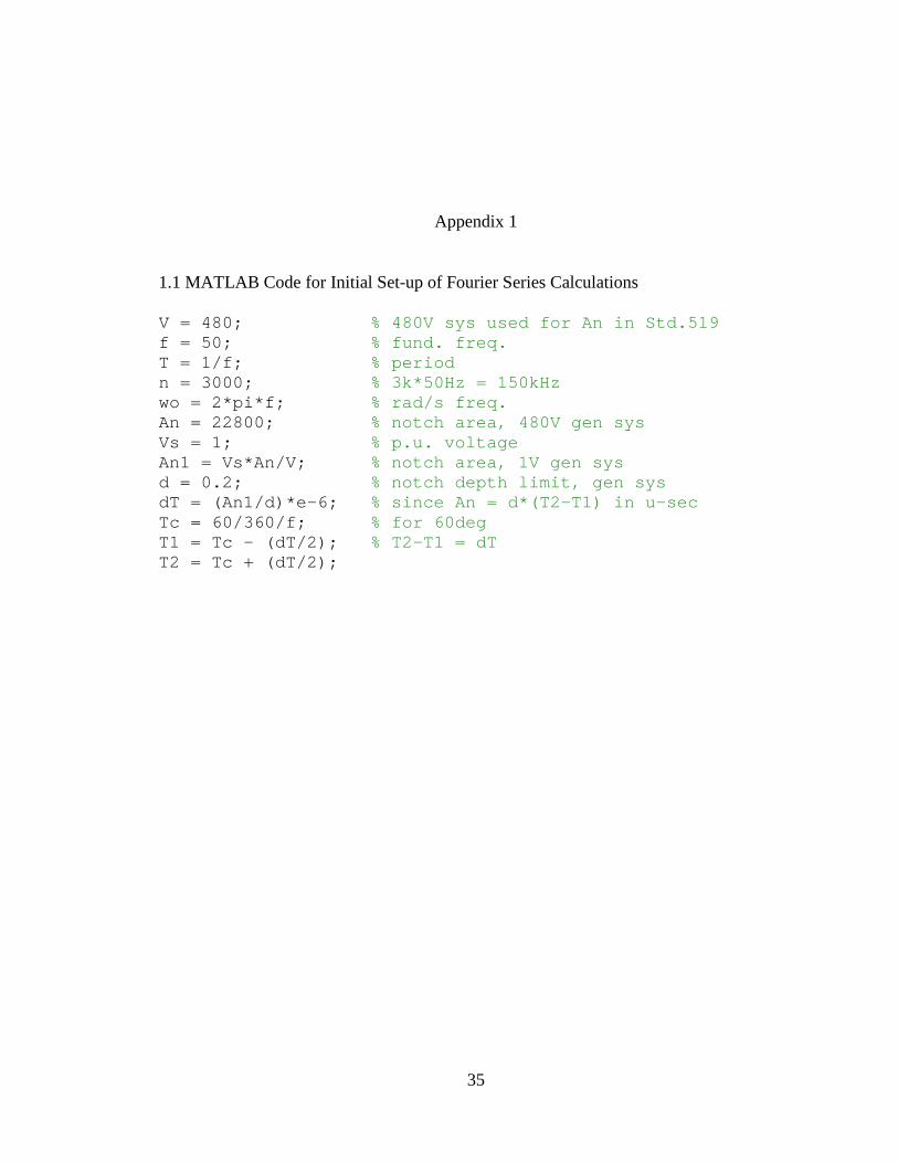
1.1 MATLAB Code for Initial Set-up of Fourier Series Calculations V = 480; % 480V sys used for An in Std.519 f = 50; % fund. freq. T = 1/f; % period n = 3000; % 3k*50Hz = 150kHz wo = 2*pi*f; % rad/s freq. An = 22800; % notch area, 480V gen sys Vs = 1; % p.u. voltage An1 = Vs*An/V; % notch area, 1V gen sys d = 0.2; % notch depth limit, gen sys dT = (An1/d)*e-6; % since An = d*(T2-T1) in u-sec Tc = 60/360/f; % for 60deg T1 = Tc - (dT/2); % T2-T1 = dT T2 = Tc + (dT/2);

36

1.2 MATLAB Code for Calculating the Fourier Series – Trigonometric % Calculate Fourier Series – 2-150kHz for k = 1:n fun1 = @(t) sin(wo*t).*cos(k*wo*t); fa1(k) = integral(fun1,0,T1); fun2 = @(t) (((sin(T1*wo)+sin(T2*wo))/2)-d).*cos(k*wo*t); fa2(k) = integral(fun2,T1,T2); fun3 = @(t) sin(wo*t).*cos(k*wo*t); fa3(k) = integral(fun3,T2,T/2+T1); fun4 = @(t) (((sin((T/2+T1)*wo)+sin((T/2+T2)*wo))/2)+d).*cos(k*wo*t); fa4(k) = integral(fun4,T/2+T1,T/2+T2); fun5 = @(t) sin(wo*t).*cos(k*wo*t); fa5(k) = integral(fun5,T/2+T2,T); Ak(k) = 2*f*(fa1(k)+fa2(k)+fa3(k)+fa4(k)+fa5(k)); fun6 = @(t) sin(wo*t).*sin(k*wo*t); fb1(k) = integral(fun6,0,T1); fun7 = @(t) (((sin(T1*wo)+sin(T2*wo))/2)-d).*sin(k*wo*t); fb2(k) = integral(fun7,T1,T2); fun8 = @(t) sin(wo*t).*sin(k*wo*t); fb3(k) = integral(fun8,T2,T/2+T1); fun9 = @(t) (((sin((T/2+T1)*wo)+sin((T/2+T2)*wo))/2)+d).*sin(k*wo*t); fb4(k) = integral(fun9,T/2+T1,T/2+T2); fun10 = @(t) sin(wo*t).*sin(k*wo*t); fb5(k) = integral(fun10,T/2+T2,T); Bk(k) = 2*f*(fb1(k)+fb2(k)+fb3(k)+fb4(k)+fb5(k)); fs(k) = (k*f); Ckn(k) = sqrt((Ak(k)^2)+(Bk(k)^2)); Ck(k) = mag2db(Ckn(k))+120; % +120 for dBuV, end plot((fs(39:2:n-1))/1000,Ck(39:2:n-1)) xlabel('Frequency (kHz)'); ylabel('dB \muV');

37

1.3 MATLAB Code for Calculating the Fourier Series – Exponential % Calculate Fourier Series – 2-150kHz for k = 1:n fun1 = @(t) sin(wo*t).*exp(-1j*k*wo*t); fc1(k) = integral(fun1,0,T1); fun2 = @(t) (((sin(T1*wo)+sin(T2*wo))/2)-d).*exp(-1j*k*wo*t); fc2(k) = integral(fun2,T1,T2); fun3 = @(t) sin(wo*t).*exp(-1j*k*wo*t); fc3(k) = integral(fun3,T2,T/2+T1); fun4 = @(t) (((sin((T/2+T1)*wo)+sin((T/2+T2)*wo))/2)+d).*exp(-1j*k*wo*t); fc4(k) = integral(fun4,T/2+T1,T/2+T2); fun5 = @(t) sin(wo*t).*exp(-1j*k*wo*t); fc5(k) = integral(fun5,T/2+T2,T); C15(k) = fc1(k)+fc2(k)+fc3(k)+fc4(k)+fc5(k); Ckn(k) = 2*f*(abs(C15(k))); fs(k) = (k*f); Ck(k) = mag2db(Ckn(k))+120; % +120 for dBuV, end plot((fcn(39:2:n-1))/1000,Cn(39:2:n-1)) xlabel('Frequency (kHz)'); ylabel('dB \muV');