Master Thesis, Department of Geosciences Conodonts and depositional environment of the Middle and Upper Cambrian Alum Shale, Slemmestad, Oslo Region Katarina Skagestad Kleppe

Welcome message from author
This document is posted to help you gain knowledge. Please leave a comment to let me know what you think about it! Share it to your friends and learn new things together.
Transcript

Master Thesis, Department of Geosciences
Conodonts and depositional
environment of the Middle and
Upper Cambrian Alum Shale,
Slemmestad, Oslo Region
Katarina Skagestad Kleppe


Conodonts and depositional
environment of the Middle and
Upper Cambrian Alum Shale,
Slemmestad, Oslo Region
Katarina Skagestad Kleppe
Master Thesis in Geosciences
Discipline: Geology
Department of Geosciences
Faculty of Mathematics and Natural Sciences
University of Oslo
01.06.2014

© Katarina Skagestad Kleppe, 2014
This work is published digitally through DUO – Digitale Utgivelser ved UiO
http://www.duo.uio.no
It is also catalogued in BIBSYS (http://www.bibsys.no/english)
All rights reserved. No part of this publication may be reproduced or transmitted, in any form or by any means,
without permission.

Forewords
This master thesis has not only made me a geologist, it has also increased my passion for
geosciences. During this five year long master program, I also met my husband at the
Geology building in my first weeks as a student, which I married 21.04.2012, and had a
wonderful purple Amethyst-theme wedding. I also got my dearest baby girl during this
education, which came to the world 03.02.13, when I was supposed to be in class.
This master thesis was written in the time between August 2013 and June 2014, but the field
work and preparation for the thesis started in March 2013. By having a full semester during
the spring 2013, with my baby girl born February, this would never have been possible if it
was not for my exceptionally supportive, understanding and helpful supervisor Hans Arne
Nakrem who accommodated every class as well as examination dates. He has also been
supporting and helpful and has given excellent supervision despite the long distance when I
moved to Bergen with my family in December 2013. You are a wonderful person and I
couldn’t have had a better supervisor!
I sincerely want to thank Johan Petter Nystuen and Krzysztof Hryniewicz for helping me
with thin section analysis, and Harald Folvik and Hans Jørgen Berg for helping me with
SEM-analysis at NHM, and Gunborg Bye Fjeld for helping me during heavy liquid
separations. I am also very grateful for the help by Magne Høyberget during field work and
for being helpful answering questions and David Bruton who showed interest and
enthusiasm for this thesis. I would also like to thank Bjørn Funke for giving me some of his
collected material for this research, and Berit Løken Berg for helping me with SEM-analysis
at Blindern. A big thank to Salahalldin Akhavan for preparing my thin section. And a
special thank to Svend Stouge for helping identify the conodonts, and to teach me a lot about
conodonts.
I want to thank my supportive, helpful and positive dear friends especially Camilla
Rytterager Henriksen, who have helped me babysitting, and took good care of my baby when
I was at the laboratory when my husband was at work. I would never have finished this
master thesis at time if it was not for your help! I am forever grateful. Of course I want to
thank my fellow students, especially Christopher Kjølstad, Martin Sandbakken and Orhan
Mahmic, for making these years a wonderful time. I’m going to miss all the coffee breaks
and laughter at “Steinrommet”. This room, U39C at Blindern, will always have a special
place in my heart. I would also like to thank my family in Bergen who always have been
supportive and motivated me, and for babysitting my daughter during the weekends so I
could work on my thesis.
Last but not least, I would like to thank my geologist husband, who always have been
supportive, helpful and a wonderful father. Thank you for all the help and patient and for all
the hours you have spent at NHM and Blindern with me so I could have been around my
baby despite all the work I had to do. I could never have done this without your help and
support. And so, to my dearest daughter, who I always have had a bad conscience for when
not being present: From now, I will ALWAYS pay you all attention you want, and give you
everything you want (yes, you can use this against me when you are a teenager).
Except a horse… (Pers. Comm. Steinar Kleppe, 2014)
Katarina Skagestad Kleppe


Abstract
The bituminous Cambrian and lowermost Ordovician Alum Shale from Slemmestad in the
Oslo Region, Norway, is for the first time investigated for conodonts and other microfossils.
Microfacies analysis is also done based on thin section analysis. This thesis is done in order
to increase the understanding of the Alum Shale and the Cambrian fauna.
Nine samples were taken from limestone-rich levels ranging from the Middle Cambrian
Paradoxides paradoxissimus trilobite zone to the Lower Ordovician Boeckaspis trilobite
zone. The samples were dissolved in acetic acid and the acid resistant residue was studied for
biogenic material using microscope and SEM. The acid resistant residue from 63µm –
500µm was heavy liquid separated in order to extract conodonts. Depositional environment
interpretation was done based on microfacies analysis and microfossils present in acid
resistant material.
Conodonts were present in five of the samples. Species recorded are all, except Cordylodus
proavus, previously reported from age equivalent deposits in Sweden. The identified
conodont species are Phakelodus tenuis, Phakelodus elongatus, Westergaardodina
polymorpha, Westergaardodina ligula, Problematoconites perforatus, Trolmenia acies and
Cordyldus proavus. All the conodont faunas represent the cold water realm. The presence of
Cordylodus proavus may be regarded as its first occurrence in Scandinavia.
From the thin section analysis five different facies is identified, representing both high and
low energy depositional conditions, with an overall upward deepening trend containing sea-
level fluctuations. In one of the facies trace fossils from the ichnogenus Phacosiphon is
present. Microfossils of environmental interpretation importance found in the samples are
phosphatocopine ostracods, inarticulate brachiopods and fecal pellets.


1
Table of content
1 INTRODUCTION ................................................................................................................. 3 1.1 GENERAL INTRODUCTION .................................................................................................. 3
1.2 PURPOSE OF STUDY ............................................................................................................ 4
2 GEOLOGICAL BACKGROUND ....................................................................................... 5 2.1 REGIONAL GEOLOGY .......................................................................................................... 5
2.1.1 The Alum Shale ......................................................................................................... 6
2.1.2 Paleogeography and paleoclimate .......................................................................... 11
2.1.3 Tectonics .................................................................................................................. 13
2.2 THE OSLO REGION ........................................................................................................... 14
2.3 LOCAL GEOLOGY IN THE SLEMMESTAD AREA .................................................................. 15
3 PALEONTOLOGY ............................................................................................................. 16 3.1 BIOSTRATIGRAPHY .......................................................................................................... 17
3.1.1 Trilobites .................................................................................................................. 18
3.1.2 Conodonts ................................................................................................................ 20
3.2 TRILOBITE FAUNA AND BIOFACIES ................................................................................... 21
3.2.1 The olenids ............................................................................................................... 22
3.2.2 The non-olenids ........................................................................................................ 23
3.3 CONODONT FAUNA AND BIOPROVINCES ........................................................................... 23
3.4 CONTROLLING FACTORS FOR PROVINCIALISM .................................................................. 24
3.5 BALTIC CONODONTS ........................................................................................................ 25
3.6 CONODONTS FROM THE OSLO REGION ............................................................................. 26
4 MATERIAL AND METHODS .......................................................................................... 28 4.1 FIELD WORK ..................................................................................................................... 28
4.2 PREPARATION OF SLABS AND THIN SECTIONS ................................................................... 33
4.3 ACID PROCESSING OF SAMPLES ........................................................................................ 33
4.4 MICROSCOPY ................................................................................................................... 33
4.5 SCANNING ELECTRON MICROSCOPE (SEM) .................................................................... 33
4.6 MICROFACIES ANALYSIS .................................................................................................. 34
5. CONODONTS .................................................................................................................... 35 5.1 PREVIOUS WORK .............................................................................................................. 36
5.1.1 Conodont morphology.............................................................................................. 37
5.1.1.1 Soft anatomy ..................................................................................................... 37
5.1.1.2 Conodont elements ............................................................................................ 38
5.1.2 Cambrian conodonts ................................................................................................ 42
5.1.2.1 Mode of growth ................................................................................................. 44
5.1.3 Paleoecology and Paleobiogeography .................................................................... 45
5.1.3.1 Mode of life ....................................................................................................... 45
5.1.3.2 Distribution of Cambrian conodont lineages..................................................... 46
5.1.4 Taphonomy ............................................................................................................... 47
5.2 RESULTS .......................................................................................................................... 50
5.2.1 Conodont identification ........................................................................................... 53
Phakelodus elongatus .................................................................................................... 53
Phakelodus tenuis .......................................................................................................... 54
Westergaardodina ligula ............................................................................................... 54
Westergaardodina polymorpha ..................................................................................... 54
Trolmenia acies ............................................................................................................. 55
Problematoconites perforatus ....................................................................................... 55
Cordylodus proavus ...................................................................................................... 55
2
5.2.2 Conodont fauna and stratigraphic distribution ....................................................... 60
6 MICROFACIES ANALYSIS AND DEPOSITIONAL ENVIRONMENTS ................. 62 6.1 PREVIOUS WORK .............................................................................................................. 62
6.2 RESULTS MICROFACIES ANALYSIS .................................................................................... 62
6.2.1 Matrix ....................................................................................................................... 63
6.2.2 Grains ...................................................................................................................... 64
6.3 FACIES DESCRIPTION ........................................................................................................ 66
6.3.1 Neomorphized Recrystallized Limestone (Facies 1) ................................................ 68
6.3.2 Carbonate Skeletal Pack- to Grainstone (Facies 2) ............................................... 69
6.3.3 Carbonate Packstone (Facies 3) .............................................................................. 69
6.3.4 Carbonate Wacke- to Packstone (Facies 4) ............................................................. 70
6.3.5 Massive Clay-rich Mudstone (Facies 5) .................................................................. 70
6.4 RESULTS ACID INSOLUBLE RESIDUE ................................................................................. 71
6.4.1 Inarticulate brachiopods .......................................................................................... 71
6.4.2 Ostracods ................................................................................................................. 72
6.4.3Trilobites ................................................................................................................... 73
6.4.4 Bioclasts of uncertain biological affinity and origin ............................................... 73
7 DISCUSSION ...................................................................................................................... 76 7.1 CONODONTS .................................................................................................................... 76
7.1.1 Stratigraphy ............................................................................................................. 76
7.1.2 Fauna assemblage ................................................................................................... 77
7.1.3 Color alteration index (CAI) .................................................................................... 80
7.2 MICRO FACIES ANALYSIS AND DEPOSITIONAL ENVIRONMENT .......................................... 81
7.2.1 Matrix ....................................................................................................................... 81
7.2.1.1 Neomorphized recrystallized limestones .......................................................... 81
7.2.1.2 Sparite ................................................................................................................ 83
7.2.2 FACIES INTERPRETATION .............................................................................................. 83
7.2.2.1 Neomorphized Recrystallized Limestones (Facies 1) ....................................... 83
7.2.2.2 Carbonate Skeletal Pack- to Grainstone (Facies 2) ........................................... 84
7.2.2.3 Carbonate Packstone (Facies 3) ........................................................................ 85
7.2.2.4 Carbonate Wacke- to Packstone (Facies 4) ....................................................... 86
7.2.2.5 Massive Clay-rich Mudstone (Facies 5) ............................................................ 87
7.2.3 Acid insoluble residue .............................................................................................. 89
7.2.3.1 Brachiopods ....................................................................................................... 89
7.2.3.2 Ostracods ........................................................................................................... 90
7.2.3.3 Trilobites ........................................................................................................... 90
7.2.3.4 Biogenic material of uncertain origin ................................................................ 91
8 CONCLUSIONS .................................................................................................................. 92 FURTHER RESEARCH .............................................................................................................. 92
9 REFERENCES .................................................................................................................... 93
APPENDIX ........................................................................................................................... 102 APPENDIX 1 PREPARATION OF SAMPLES. ............................................................................. 102
APPENDIX 2 RAW DATA FROM THIN SECTION COUNTING ..................................................... 103
APPENDIX 3 SEM EDS QUALITATIVE SPECTRA FROM SAMPLES. ......................................... 104
APPENDIX 4 EVIDENCE OF GYPSUM PERIMORPHOSIS ........................................................... 107
APPENDIX 5 LIST OF FIGURES .............................................................................................. 108
APPENDIX 6 LIST OF TABLES ................................................................................................ 110

3
1 Introduction
1.1 General introduction
The Cambrian to lowermost Ordovician Alum Shale exposed in the village of Slemmestad (figure 1),
SW of Oslo, is well known primarily for its rich fossil fauna dominated by olenid trilobites, and has
been studied by several paleontologists and geologists since Brøgger in 1880. How the Alum Shale
Formation was formed, as well as biostratigraphical correlation based on trilobites has been of
interests for a long time. The most substantial work in this respect is the systematic treatment of
trilobites by Henningsmoen (1957), which through several stages of amendments has resulted in the
current accepted stratigraphical scheme (Nielsen et. al., 2014). The Alum Shale has a high
concentration of organic carbon, which makes this a good source rock when exposed to right
temperatures. However, the Alum Shale in the Oslo area has been exposed to too high temperatures
due to Permian intrusion (Figure 1). Even though the Alum Shale at Slemmestad is not a source rock,
it is indeed a source of information regarding the Cambrian fauna and depositional environment.
Figure 1. Photo showing Cambrian Alum Shale between Precambrian basement and a Permian sill, in the
village of Slemmestad.
One of the faunal contributors in the Alum Shale Sea during the Cambrian was conodonts. The only
conodont investigation from the Cambrian Alum Shale in Norway was done by Bruton et. al. (1988) at
Nærsnes beach nearby Slemmestad. Hence Norwegian Cambrian conodonts are a rather unexplored
topic relative to other Cambrian faunal components like trilobites.
During a project in 2006 two pilot samples were taken from the Middle Cambrian (GIBB06) and from
the Upper Cambrian (PEL06) in Slemmestad (Pers. Comm. 2014). The samples contained conodonts.
The findings of conodonts in these pilot samples supported a further research on Cambrian conodonts
from these deposits in Slemmestad.

4
Conodonts were small eel like animals known from small phosphatic teeth like elements from their
feeding apparatus, known as conodont elements. Conodonts are widely used for biostratigraphy, and
they are also used for paleoecological and biogeographical studies. They may also provide
information regarding basin history, regional metamorphism and state of hydrocarbon generation.
Conodonts from Cambrian Alum Shale outside the Oslo Region are well known (Müller, 1959;
Szaniawski, 1971; 1987; Bednarczyk, 1979; Andres, 1981; 1988; Borovko and Sergeyeva, 1985; Kaljo
et. al., 1986; Viira, et. al. 1987; Müller and Hinz, 1991; 1998; Hinz, 1992; Mens et. al. 1993; 1996;
Szaniawski and Bengtson 1993; 1998; Bagnoli and Stouge, 2013). The conodonts were studied for
taxonomy, histology, for providing zonal schemes, and for conodont associations.
1.2 Purpose of study
The purpose of this study is to investigate if the microfossil assemblages, as well as microfacies
analysis from the Alum Shale in Slemmestad may provide information regarding the depositional
environment, as well as whether the conodonts found are of biostratigraphical importance. Another
aim is also to investigate if there is a correlation between the different facies and conodont faunas, as
well as to contribute to the understanding of the faunal composition in the Cambrian Alum Shale of
this part of the Oslo area.
Samples collected during field work represent different levels primarily through the Upper Cambrian.
Limestone-rich intervals were selected for sampling, thin sections were made, and the samples were
dissolved in acetic acid. The acid insoluble residue was heavy liquid separated for further investigation
using optical microscope and scanning electron microscope.
Hopefully, the interpretations and conclusions from this thesis may contribute to the knowledge
regarding the environment during deposition of the Alum Shale in Slemmestad, and hopefully give
information regarding the conodont fauna.

5
2 Geological background
2.1 Regional geology
The Cambrian period lasted for 55.6 million years (541-485.4 Ma), and is the first period in
the Paleozoic Era (Peng et. al., 2012). This period is important in the history of life on earth,
and presents one of the greatest evolutionary events in the Earth’s history; the Cambrian
Explosion (Waggoner and Collins, 1994).
The Cambrian stratigraphic sequence in Norway occurs locally as allochtonous or
autochtonous layers in or along the lower Caledonian nappe units (Nielsen and Schovsbo,
2011). In Oslo region the Cambrian succession is recognized with sedimentary layers of dark
bituminous shale interacting with limestone layers, also known as the Alum Shale Formation
(Buchardt et.al., 1997).
The paleocontinent Baltica was located at 45-60 degrees south during Cambrian time and
included areas where Norway, Sweden, Denmark, Russia, and the Baltic countries are located
today (Torsvik and Rehnström, 2001). As seen in figure 2, Baltica was surrounded by the
Ægir Sea and The Iapetus Ocean during the Late Cambrian. The term Baltoscandia is used for
the part of Baltica including Norway, Sweden and Denmark.
Figure 2. Distribution of the paleocontinents on the southern hemisphere during the Late Cambrian
(Torsvik and Rehnström, 2001).

6
The Cambrian period is divided into global series and stages. As shown in Figure 3, the global
series represents the Lower (Terreneuvian), Middle (Series 2 and 3) and Upper Cambrian
(Furongian). The stages are further subdivided into trilobite zones and subzones (see
Figure16, section 3.1.1). The main global series of interest for this study is the Furongian
lasting from 497-485.4 Ma (Peng et. al., 2012). Uppermost Middle Cambrian (series 3) and
lowermost Tremadocian (earliest Ordovician) are also of interest.
Figure 3. The Cambrian global time scale (Peng et. al., 2012)
2.1.1 The Alum Shale
The Alum Shale was formed on the present western and southern part of Baltica (Buchardt
et.al., 1997), and includes strata from Middle Cambrian (Series 3), to close to the top of the
Lower Ordovician Tremadocian Series (Høyberget and Bruton, 2012). The formation is
present throughout much of Baltoscandia, and the “Alum Shale Sea” covered areas from
western Norway to St. Petersburg in the east and from Poland in the south to Finnmark in
northern Norway at its maximum extent (Buchardt et.al., 1997). The Alum Shale Formation is

7
the term used for the whole lithostratigraphic unit throughout Scandinavia (Nielsen and
Schovsbo, 2007).
The Alum Shale Formation appears to be uniform over a large area, with sedimentation rates
as low as 1mm per 1000 years (Bjørlykke, 1974). It consists of bituminous brown to black
shales and mudstones with alternating limestone- and siltstone beds, and the type section is
defined in the Gislövshammar-2 core, from southern Sweden (Buchardt et. al., 1997). It is
finely laminated, and bioturbation is not present except from some horizons at the lower and
upper part (Nielsen and Schovsbo, 2011). Trilobites are almost always absent in the shale, and
it is rich in organic carbon suggesting anoxic conditions (Thickpenny, 1984). Bituminous
limestone concretions (anthraconites) occur as discontinuous to semi-continuous lenses
throughout the entire formation (Thickpenny, 1984).
The Alum Shale is characterized by its high content of organic matter and trace elements,
mainly uranium and vanadium (Bergström and Gee, 1985). In addition it is well known for
its rich fossil fauna, dominated by agnostid and olenid trilobites in the limestone rich layers
(Buchardt et. al., 1997). In the Oslo Region the Furongian Alum Shale itself is usually
unfossiliferous, but the anthraconite concretions can be extremely fossiliferous, dominated by
olenid trilobites (Høyberget and Bruton, 2012).
The base of the Alum Shale Formation is progressively getting older when moving from the
east towards the west. In the southern and western part of Baltoscandia, the Alum Shale first
appears in the early Middle Cambrian, where it overlays lower Cambrian sand- and silt
deposits, or lays directly on top of Precambrian continental basement (Thickpenny, 1984). In
southwestern part of Sweden it first appears during middle Mid-Cambrian, while it first
appears during Late Cambrian in eastern part of Sweden and Poland. In Estonia, it first
appears during Tremadocian. This evolution reflects a sea level rise which with time covered
large areas of the Baltic Shield and thereby led to the deposition of mud on the shelf (Nielsen
and Schovsbo, 2011).
The formation of the anthraconites has been explained as the remnants of a dissolved
continuous limestone bed (Bjørlykke, 1973), and as early stage concretions (Henningsmoen,
1974). According to Thickpenny (1984), the formation of the anthraconites is similar to the
explanation of early formed diagenetic concretion of Raiswell (1971). This explanation
suggests that the concretions is formed by nucleation on fossiliferous layers, probably on the
sea floor, growing during early stages of compaction, hence not the remnants of a dissolved
limestone bed. Intra-basinal heights on the shelf that penetrated the anoxic-oxic boundary in

8
the water column are suggested as starting points for the formation of the concretions
(Thickpenny, 1984). This penetration may have allowed trilobite faunas adapted to such
environment environment to colonize (Figure 4), resulting in the fossiliferous concretion
despite the surrounding unfertile shale (Henningsmoen, 1957). The anthraconites consist of
micritic to coarse sparitic calcite with content of pyrite (Dworatzek, 1987). The micritic and
fine sparitic anthraconites consist of dark grey to black calcite with a high content of clay
particles and organic material impurities. These anthraconites have no structures, but may
show some lamination from the clay matrix they grew in, as relic laminations (Buchardt et.
al., 1997). The grain size in central parts of the concretions are commonly of arenitic grain
size (Thickpenny, 1984), which include a size range from 0.0625mm – 2 mm (Encyclopedia
Britannica, 2013). In thin-sections the carbonate primarily consists of rounded sand-sized
grains of random orientation in a poorly laminated matrix (Thickpenny, 1984). The coarse
sparitic anthraconites consist of grey to brown calcite crystals which may be up to 10cm in
length, and this form of anthrachonite may account for 0% to 100% of a concretion (Buchardt
et. al., 1997).
Figure 4. Illustration of intra-basinal heights penetrating the anoxic-oxic boundary, allowing trilobite
colonization.
The Alum Shale Formation is over- and underlain by shallow marine deposits over the entire
basinal area (Thickpenny, 1984). Little variation in the lithology of these deposits may
suggest that Alum Shale also is deposited in shallow water (< 200m). In shallow water,
stagnation away from the open ocean may occur (Thickpenny, 1984). The constant lithology
throughout the Alum Shale Formation, and the surrounding lithology, suggests that this
formation was formed by shallow marine deposits (Figure 5) under such stagnating conditions
(Thickpenny, 1984). This resulted in anoxic conditions favoring preservation of organic
matter (Nielsen, 2004).

9
Figure 5. Depositional setting in the Oslo Region during Late Cambrian (modified from Ramberg et. al.,
2010).
Slow sedimentation rates in shallow water environment, and restricted detrial supply,
probably reflects the high sea level during this time (Thickpenny, 1984). Rareness of
redeposited sediments reflects a gentle topography on the sea floor, and hence, the sediments
have been deposited from suspension, but based on the concretions, topography on the sea
floor must have been significant (Thickpenny, 1984).
The thickness of the formation varies from less than 1m near the edge of the Baltic syncline,
to over 130m in Kattegat (Buchardt et. al., 1997) (Figure 6). These variations reflect the
structural differences in the southern part of Baltoscandia. In the Oslo area, the thicker part
seems to correspond to the Oslo Graben. The shale decreases in thickness towards east and
north in Sweden, which most likely reflects the depositional environment, while the thinner
part of the formation towards the eastern part of the Baltic syncline is due to erosion. The
difference in thickness of the shale throughout the formation is due to the different facies
environment on the Baltic Shield, which are condensed facies and the shelf facies. The latter
is typical for the areas in southern Norway among others (Buchardt et. al., 1997). On the
platform, the shale is rarely over 25m in thickness, and is characterized with a high content of
digenetic formed limestone (up to 50%) often as beds and the shale has abundant hiatuses.
The shale near the paleoshelf on the other hand, is thicker in general, and consists of less than
10% limestone occurring primarily as concretions or lenses (Buchardt et. al., 1997).

10
Figure 6. Variation in thickness (m) of the Alum Shale Formation in southern Baltoscandia (modified
from Buchardt et. al., 1997).
Figure 7 shows the lithostratigraphic setting of the Alum Shale Formation in the Oslo Region.
The figure also includes estimated thickness as well as the shallow deposited sediments from
Pre Cambrian, Lower Cambrian and Lower Ordovician.
Figure 7. Lithostratigraphic setting of the Cambrian and Lower Ordovician sediments in the Oslo Region
(modified from Calner et.al., 2013).

11
2.1.2 Paleogeography and paleoclimate
During the Cambrian, the paleocontinents were located on the southern hemisphere, and due
to the fragmentation of the Proterozoic supercontinent Rodinia, the landmasses were scattered
(Waggoner and Collins, 1994). As shown in Figure 2, Baltica is estimated to have been
located between 45o-60
o on the southern hemisphere (Torsvik and Rehnström, 2001).
Figure 8. Global sea level and temperature changes during Cambrian and Ordovicium (Modified from
Dudley, 2000).
The Cambrian world was bracketed between the late Proterozoic and the Ordovician Ice Age.
The temperature was higher and more stable than today, causing retreatment of the
Proterozoic ice (Waggoner and Collins, 1994). This led to higher sea levels (Figure 8), and
most of the lowland areas such as Baltica were covered with shallow epicontinental seas
(Waggoner and Collins, 1994), and epeiric platforms covered large areas (Figure 9)(Boggs,
2006).
Figure 9. An epeiric platform, characteristic for flooded continental shelves (modified from Boggs, 2006).
The overall higher temperature during the Cambrian caused a higher rate of evaporation. This
led to an elevated salinity in the shallow oceans which resulted in density contrasts in the
water column (Jenkins et.al., 2012). This density induced layering of the water column led to

12
stagnation of the in the epicontinental seas. Since no oxygen rich surface water was able to
descend towards the bottom, the water near the bottom became progressively more anoxic due
to oxygen consuming bacteria (Bjørlykke, 2004). These conditions allowed the deposition of
the Alum Shale (Figure 10).
Figure 10. The processes occurring in the stagnated epicontinental sea covering Baltica, causing deposition
of the Alum Shale (Bjørlykke, 2004).
As illustrated in Figure 11, the oxygen level during Cambrian was lower than today (Dudley,
2000), but during this time oxygen was for the first time mixed into the oceans in significant
amount (Waggoner and Collins, 1994). During this period the number of oxygen-depleting
bacteria was reduced, which made dissolved oxygen available to the diversity of animals. This
was probably the foundation of the “Cambrian Explosion” (Waggoner and Collins, 1994).
Figure 11. Atmospheric oxygen consentrations during the Phanerozoic. PAL: present atmospheric level
(20.95%) (Dudley, 2000).

13
2.1.3 Tectonics
Baltica was attached to the Proterozoic continent Rodinia in Precambrian, but was separated
from this continent during late Precambrian time (Torsvik and Cocks, 2005). Baltica was a
separated continent until Silurian time, when it collided with the continents Laurentia and
Avalonia (Torsvik and Cocks, 2005).
The Caledonian Orogeny was initiated during the Late Ordovician (Liu et. al., 2010) as a
result of the closure of the Iapetus Ocean and Tornquist Sea (Buchardt et. al., 1997). This led
to deformation and folding of the shelf areas south and west of the Baltic Shield, but the
deposited sediments on the shelf were practically unaffected (Buchardt et. al., 1997). The
orogenic event strongly affected the Lower Paleozoic deposits in the Oslo area. This
deformation, with Alum Shale working as thrust plane, led to shortening of the Lower
Paleozoic sequence in the Oslo-Asker region, due to folding, faulting and thrusting (Bruton
and Owen, 1982). A foreland basin was developed along the margin of the Caledonides on the
Baltic Shield (Buchardt et. al., 1997). This has led to foreland-basin type structural
deformations in the Oslo-Asker area (Figure 12). The Carboniferous-Permian extensional
rifting of the supercontinent Pangaea led to exposure, hence erosion of the Upper Paleozoic
deposits along the Baltic Shield (Buchardt et. al., 1997).
Figure 12. Illustration of the development of the foreland basin due to the Caledonian orogenic event, with
the Alum Shale working as a thrust plane (Bjørlykke, 1983).

14
2.2 The Oslo Region
The Oslo Region is located within a graben structure, formed during the Carboniferous-
Permian extensional rifting (Neumann et. al., 2004), and is well known for its variety of
rocks. The rocks present in the
Oslo Region ranges from Lower
Paleozoic deposits and Upper
Carboniferous sediments, as well
as igneous rocks of Late
Carboniferous to Permian age
(Ramberg et. al., 2010).
The Oslo Region extends a
distance of about 200 km north
and south of Oslo starting from
Langesundsfjorden to the
northernmost part of Mjøsa
district (Figure 13). The width
varies from 35 to 65 km and is
bordered by major normal fault-
zones to the east (Neumann et.
al., 2004; Ramberg et. al.,
2010).
Due to the graben-structure
Lower Paleozoic deposits are
preserved in the Oslo Region,
and the Alum Shale is common
throughout the area (Buchardt et.
al., 1997). Post-rifting, the
Lower Paleozoic deposits were
covered by erosion material
from the surrounding horst area and by volcanic and magmatic rocks (Andersen, 1998). The
lower Paleozoic deposits in the northern part of the Oslo Graben are strongly deformed and
folded due to the Caledonian event, while the southern part is strongly affected by Permian
magmatism (Buchardt et. al., 1997).
Figure 13. Geological map of the Oslo Region (modified from
Heldal et. al., 2010).

15
The Alum Shale has worked as a thrust plane for the lower Caledonian nappe units and is
overall deformed and thermally altered (Bruton and Owen, 1982).
2.3 Local geology in the Slemmestad area
The lower Paleozoic succession in Slemmestad, which is located approximately in the middle
part of the Oslo-graben, is strongly deformed and folded due to the Caledonian orogenic
event. The Alum Shale Fm. in Slemmestad is exposed in several localities (Figure 14).
Figure 14. A) Geological map of the Slemmestad area (modified from NGU geological map). B) Location
of Slemmestad is marked on a regional map (google maps).

16
3 Paleontology
During the Cambrian period, life on earth went through extreme changes from very primitive
animals during the Precambrian to relatively advanced animals as well as the evolution of the
first known vertebrates (Benton and Harper, 2009). Almost every metazoan phylum with hard
parts, evolved during this period. This evolution of life, the ”Cambrian Explosion”, is one of
the greatest evolutionary events in the history of life on Earth (Waggoner and Collins, 1994).
The fossil fauna not only provides important information regarding the evolution of life, but
also important information about the depositional environment including water depth, current
directions, and sedimentation rates. In addition the fossil fauna can provide information on
temperature, salinity, as well as the thermal maturation of the fossil hosting sediments
(Armstrong and Brasier, 2005).
The fauna in the Cambrian (Figure 15) was dominated by arthropods, with trilobites as the
most abundant group. Brachiopods, mollusks, echinoderms, sponges, jawless vertebrates were
also a part of the Cambrian fauna (Benton and Harper, 2009).
Figure 15. Artistic illustration of the Cambrian fauna in Burgess Shale (Pitman, 2014)
The fossil fauna of the Cambrian Alum Shale is dominated by agnostid and olenid trilobites.
Brachiopods, phosphatized ostracods and conodonts among other less abundant organisms are
also present (Buchardt et. al., 1997; Szaniawski and Bengtson, 1998). The fauna in the Upper

17
Cambrian Alum Shale has pelagic organisms, which differs from the benthic fauna of Middle
Cambrian and earliest Ordovician (Müller and Hinz, 1991). In the Tremadocian graptolites
occur, and defines the transition between Cambrian and Ordovician with the index fossil of
Rhabdinopora flabelliforme (Buchardt et. al., 1997; Landing et. al., 2000).
The Cambrian conodont fauna was dominated by protoconodonts and paraconodonts, since
the euconodonts first appeared in the Late Cambrian (Armstrong and Brasier, 2005). For more
details regarding Cambrian conodonts, see chapter 5.
Cambrian conodont studies have been used for stratigraphy, phylogeny and evolution,
morphology, histology and function, systematic position, facies, provincialism, temperature
control, geochemistry and chemoevolution (Müller and Hinz, 1991). Based on this, as well
Color Alteration Index, the conodonts may provide information regarding the environmental
conditions during deposition, as well as the maturation history of the surrounding sediments,
which is of interest for source rock studies (Armstrong and Brasier, 2005).
This chapter presents previous work on Cambrian conodonts regarding stratigraphy and
faunal studies. Due to the correlation between conodont zones and trilobite zones, trilobite
groups relevant as biostratigraphic and depositional indicators are also mentioned. Conodont
morphology, paleoecology and taphonomy are described in chapter 5. Microfacies analysis, as
well as other microfossil groups present in the Alum Shale Fm. is presented in chapter 6.
3.1 Biostratigraphy
Trilobites dominated the Cambrian fauna, especially the dysoxic environments, in addition
they evolved rapidly during this period. Hence they are commonly used as biostratigraphical
indicators in Cambrian black shales (Buchardt et. al., 1997). Cambrian conodonts are also
used for biostratigraphy, but are less precise time markers relative to trilobites, but are used as
biostratigraphical indicators within the trilobite series (Müller and Hinz, 1991).
Conodonts and trilobites have different hard part compositions, and will therefore have
different preservation potentials in different lithologies. Hence, conodonts may be of
biostratigrahpical importance where trilobites have not been preserved, such as in as in
Estonia (Kaljo et. al., 1986; Mens et. al., 1993; 1996). Conodont biostratigraphy has primarily
been applied on the Cambrian-Ordovician boundary, on all continents except Africa (Müller
and Hinz, 1991). Conodont research on the Cambrian – Ordovician boundary in Norway is
presented by Bruton et. al. (1988).

18
3.1.1 Trilobites
The trilobite zonal – subzonal system of the Alum Shale Formation is revised several times -
since Westergård (1922) established his trilobite zonation system - based on taxa from the
almost complete successions in Scania (Sweden) and partly from the Furongian and
Tremadocian succession in the Oslo region (Westergård, 1946; 1947; Henningsmoen, 1957;
Ahlberg, 2003; Terfelt et. al., 2008; 2011; Ahlberg and Terfelt, 2012; Babcock et. al., 2012;
Nielsen et. al., 2014). A trilobite zonation based on agnostids and polymerids from the
Furongian Series in Scandinavia has also been suggested by Terfelt et. al. (2011), but revised
in Nielsen et. al. (2014) as shown in Figure 16.

19
Figure 16. Trilobite zonations proposed for the Alum Shale (Modified from Nielsen et. al,. 2014).

20
3.1.2 Conodonts
For biostratigraphical purpose Lower-, Middle-, and lower Upper Cambrian conodonts have
been less studied than Upper Cambrian conodonts due to their rarity (Müller and Hinz, 1991).
Paraconodonts have not been used in Scandinavia for stratigraphy, despite their abundance
(Müller and Hinz, 1991). The euconodonts were not used widely for stratigraphic correlations
of the Cambrian in Baltoscandia until the late 1990’s by Szaniawski and Bengtson (1998).
The first conodont zonal scheme from the Upper Cambrian of Baltica was presented by Kaljo
et.al. (1986). They established the C.? andresi zone and C.proavus zones based on material
from the Estonian-western Russian succession. The upper Cambrian euconodont zonation
from Baltica was reviewed by Szanianski and Bengtson (1998) from material from
Kinnekulle in southwestern Sweden, which is now the conodont zonal scheme used for the
Upper Cambrian of Baltica (Figure 17). Szaniawski and Bengtson (1998) established the
Proconodontus Zone with its two subzones Proconodontus transitans and P. muelleri. The
upper boundary of the Proconodontus Zone is defined by the FAD of Cordylodus? andresi.
Figure 17. Correation of Conodont zonation of the uppermost Cambrian of Sweden with North America
and Estonia (Szaniawski and Bengtson, 1998).

21
The Cordylodus? andresi Zone is defined by the FAD of C. andresi, and with its upper
boundary defined by the FAD of C. proavus (Kaljo et. al., 1986; Szaniawski and Bengtson,
1998) which also defines the C. proavus Zone.
The C. proavus Zone is not recognized in Sweden (Szaniawski and Bengtson, 1998), but has
been reported in Scandinavia, from the Oslo Region in upper part of Acerocare Zone (Bruton
et. al., 1988), which corresponds to pre-Tremadocian age. According to Szaniawski and
Bengtson (1998), insufficient preservation of the conodonts reported in Bruton et. al. (1988)
causes some of the designations to be uncertain, and they have therefore not been regarded as
certain enough for defining the boundary of the C. proavus Zone in Scandinavia.
3.2 Trilobite fauna and biofacies
Fossiliferous occurrences in black shales, as the Alum Shale - which is interpreted to have
been deposited under anoxic conditions - have led to different hypotheses regarding the living
conditions of the individuals (Buchardt et. al., 1997). Interpretations of the living conditions
for the trilobites suggested they were allochtonous deposited (Dworatzek, 1987), or that
agnostids were living near the surface attached to seaweed (Bergström, 1973). Further
research has made these allegations rather doubtable due to how the assemblages are sorted
and the type of specimens in them (for more detailed discussion see Buchardt et. al., 1997).
Due to the assemblages and the further research on the morphology of the trilobites, it is now
assumed that olenids and agnostids probably were adapted to dysoxic environment. The high
dominance and low diversity also support this theory. The high abundance, high dominance
and their adaption to such environments make them suitable for biostratigraphical use in black
shale environments (Buchardt et. al., 1997).
The trilobite assemblages in the Alum Shale may be divided into two groups: Olenid and non-
olenid trilobites based on the morphology and associated faunal elements. The non-olenids
include “normal” trilobites and agnostids, and represents dysoxic to oxic environment (Figure
18). Brachiopods often occur with the non-olenids. The olenids represent dysoxic to anoxic
environments as illustrated in Figure 18 (Schovsbo, 2001).

22
Figure 18. Depositional model and environmental tolerance for the different faunal types in the Alum
Shale. S.l., n.w., s.w., representing sea level, normal wave-base and storm wave-base respectively
(Schovsbo, 2001).
3.2.1 The olenids
The olenid trilobites can be divided in three main morphotypes: the Olenus-type, the Peltura-
type and the Ctenopyge-type (Buchardt et. al., 1997).
The Olenus-type is assumed to have been a benthic living trilobite, but some of the trilobites
within this group may have been nektobenthic. Within this group, the Parabolina species
probably reflects higher oxygen levels than other members of this group (Buchardt et. al.,
1997), based on their morphology and distribution in the basin (Bergström, 1980), and may
therefore be placed within the non-olenids (Schovsbo, 2001).
The Peltura-type is based on their morphology interpreted to have lived an active swimming
mode of life (Schovsbo, 2001). This group is more abundant in Middle Sweden and Öland
than further south such as the Oslo area, where representatives from Ctenopyge and
Sphaerophtalmus of the same age dominate (Buchardt et. al., 1997). The Ctenopyge-type is
interpreted to have been pelagic, floating in the water column (Schovsbo, 2001).

23
3.2.2 The non-olenids
The non-olenid trilobites include agnostids and “normal trilobites”. Agnostids were small
trilobites which lived enrolled (Robinson, 1972). It has been argued that they were pelagic
based on the almost cosmopolite distribution of some species (Robinson, 1972). However, the
agnostids in the Cambrian were restricted to black shale environments, indicating adaption to
such environment and were therefore, probably benthic adapted to the bottom water
environment (Nielsen, 1997). It has been stated that agnostids are comparable with ostracods
(Buchardt et. al., 1997).
Brachiopods occur with the non-olenids in the Alum shale and are therefore assumed to have
been adapted to similar environment (Popov and Holmer, 1994). Both orthide and phosphatic
forms are included in the Cambrian brachiopods, and include several Lingula-type
brachiopods (Bergström, 1980).
3.3 Conodont fauna and bioprovinces
During the Cambrian, as well as through the early Tremadocian most conodont faunas were
relatively cosmopolitan. However, conodont provincialism was established during the late
Tremadocian (Charpentier, 1984). Hence, most of the provincialism studies have focused on
the Ordovician period, and only few reports exist regarding Cambrian conodonts faunal
provincialism (Miller, 1984; Bergström, 1990).
The Upper Cambrian conodont fauna is dominated by paraconodonts and protoconodonts,
which consists of a large variety of simple cone elements. In Baltica the genera Furnishina
and Westergaardodina are the most abundant and comprise several species (Müller and Hinz,
1991). The group protoconodont is mostly represented by the long ranging genus Phakelodus
(Bagnoli and Stouge, 2013). During the Late Cambrian diverse paraconodonts as well as the
first euconodonts appear which makes this period important regarding conodont evolution
(Jeong and Lee, 2000).
According to Miller (1984) the protoconodonts and paraconodonts represent the cold water
realms in mid- to high latitudes, such as Scandinavia, Great Britain, Turkey, Iran, South China
and deep water areas along the margins of North America, India, Kazakhstan and other low-
paleolatitudes land masses.
The euconodont zonation starting from Proconodontus up to C. proavus zone is typical for the
warm water realm in low latitudes, such as the Laurentian platform in North America (Miller
1980; 1984), North China (An, 1981; 1983), South China (Dong et. al., 2004), Kazakhstan

24
(Dubinina, 2000), Iran (Müller, 1973), Korea (Lee and Lee, 1988) and Australia (Druce and
Jones, 1971).
Miller (1984) and Bergström (1990) suggested based on the differentiation of cold- and warm
faunal realm during the Cambrian, that provincialism may have started in the Late Cambrian,
and probably was the early stage of the development of the Ordovician realms that now are
called the Midcontinent Realm and the North Atlantic Realm. However, according to Jeong
and Lee (2000), this provincialism may not be an initial stage of the Ordovician conodont
provincialism, but a separate branch in the evolution of conodonts, considering the end-
Cambrian extinction.
Based on quantitative studies by Jeong and Lee (2000), conodonts exhibited provincialism on
a global scale during the Late Cambrian. Faunas and associated Simpson Index (SI) values are
shown in figure 19. Simpson Index (SI) reflects the number of taxa in common between two
faunas, where low SI reflect high provincialism between two areas.
Figure 19. SI values between Sweden and other localities in Asia. Low SI values indicate strong
provincialism (modified from Jeong and Lee, 2000).
3.4 Controlling factors for provincialism
Climate and physical barriers are the two factors controlling provincialism of conodonts, as
well as for other marine organisms (Bergström, 1990). Physical barriers include emerged
areas and ocean currents, while climatic factors include water temperatures and salinities.
Areas with unfavorable climatic conditions may form migration barriers (Jeong and Lee,
2000). Water depth is not regarded as an important factor, based on for example the
hypothesis that some conodonts were able to change position within the water column to

25
favorable conditions (Miller, 1984). It is suggested that water temperature was one of the
most controlling factor in the distribution of conodonts (Jeong and Lee, 2000).
Another factor that may have affected the provincialism was the ecological mode of life of the
conodonts, but their habitat being benthic, necto-benthic or pelagic is still not certainly known
(Jeong and Lee, 2000). Miller (1984) suggested that protoconodonts, paraconodonts and early
euconodonts were pelagic and cosmopolitan. This may be the reason why conodont
provincialism was not strong in the Cambrian (Jeong and Lee, 2000). For more details
regarding Cambrian conodonts and their mode of life, see section 5.1.3.1.
3.5 Baltic Conodonts
Baltoscandian conodonts are well known based on conodonts from the Swedish Alum Shale
(Bruton et. al., 1988; Müller and Hinz, 1991; Szaniawski and Bengtson, 1998; Bagnoli and
Stouge, 2013). The Upper Cambrian euconodont succession in Baltica is not similar to the
coeval Midcontinent euconodont succession, representing warm water realm. In northeastern
Europe, the Laurentian Eoconodontus Biozone, with its two subzones, has not been identified
(Bagnoli and Stouge, 2013). The cosmopolitan euconodont species P. muelleri and E.
notchpeakensis are most common in Baltica, but E. notchpeakensis is extremely rare before
the appearance of C. proavus (Bagnoli and Stouge, 2013). The presence of E. notchpeakensis
in the C.? andresi Zone in Estonia and Öland, Sweden, may suggest that this zone can be
correlated to the Eoconodontus Zone of the Midcontinent Realm as shown in Figure 20
(Bagnoli and Stouge, 2013). The C.? andresi Zone established by Bagnoli and Stouge (2013),
is only known from the Baltoscandic region (Bagnoli and Stouge, 2013). Bagnoli and Stouge
(2012) consider specimens that are assigned to C. andresi outside the Baltoscandic region to
belong to C.? aff. andresi, in the Acerocarina superzone.
26
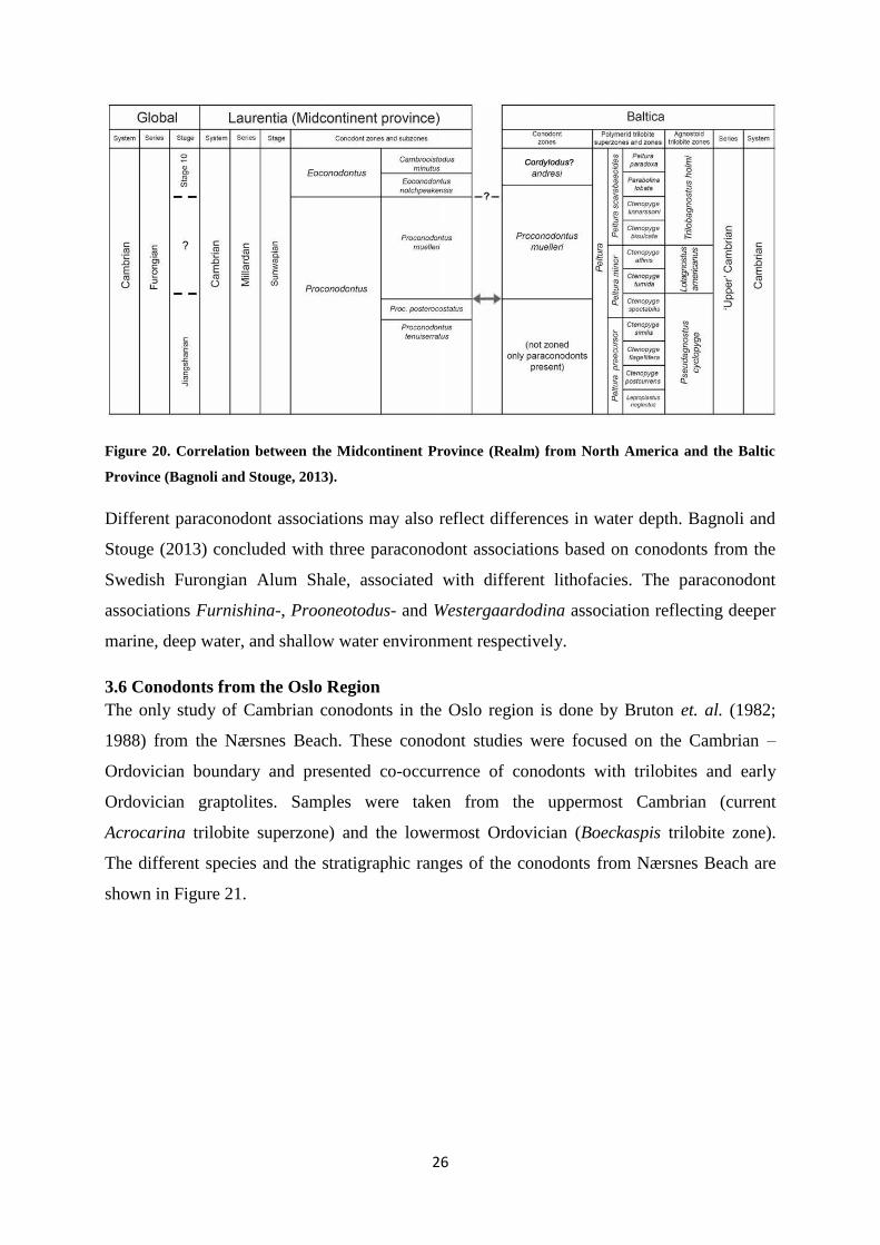
Figure 20. Correlation between the Midcontinent Province (Realm) from North America and the Baltic
Province (Bagnoli and Stouge, 2013).
Different paraconodont associations may also reflect differences in water depth. Bagnoli and
Stouge (2013) concluded with three paraconodont associations based on conodonts from the
Swedish Furongian Alum Shale, associated with different lithofacies. The paraconodont
associations Furnishina-, Prooneotodus- and Westergaardodina association reflecting deeper
marine, deep water, and shallow water environment respectively.
3.6 Conodonts from the Oslo Region
The only study of Cambrian conodonts in the Oslo region is done by Bruton et. al. (1982;
1988) from the Nærsnes Beach. These conodont studies were focused on the Cambrian –
Ordovician boundary and presented co-occurrence of conodonts with trilobites and early
Ordovician graptolites. Samples were taken from the uppermost Cambrian (current
Acrocarina trilobite superzone) and the lowermost Ordovician (Boeckaspis trilobite zone).
The different species and the stratigraphic ranges of the conodonts from Nærsnes Beach are
shown in Figure 21.

27
Figure 21. Stratigraphic ranges of the conodonts at Nærsnes Beach. A = Acerocarina trilobite superzone, B
= Boeckaspis trilobite zone (modified from Bruton et. al., 1988).

28
4 Material and methods
4.1 Field work
The fieldwork of this study was done during the spring 2013. Sections of the Alum Shale
Formation, spanning from the Cambrian “Series 3” into the Lower Ordovician (Tremadocian)
were investigated and sampled in Slemmestad. Slemmestad is located in Røyken commune in
the county of Buskerud (Figure 22).
The exposed sections at Slemmestad used for this field work include a section of Middle
Cambrian, a section of the earliest part of Furongian, and a section of the upper half of
Furongian which spans the Cambrian-Ordovician boundary, in addition to an entire section of
the Tremadocian.
The field work was done together with supervisor Hans Arne Nakrem and Magne Høyberget.
Material from six different stratigraphic levels was collected from two different areas in
Slemmestad during this field work. In total, samples from nine different levels were collected
in purpose of this thesis. Two of them were collected and kept in the museum collection
before this fieldwork took place, and one was collected and provided for study by Bjørn
Funke from a presently inaccessible locality.
The nine samples are collected from five different outcrops in Slemmestad, and are marked on
the map below (Figure 22). Sample KAM1 and KAM2 are collected inside the Norcem
industrial area where access requires permission.

29
Figure 22. Map showing the location of the different sampled localities within the Slemmestad area (Map
source: www.norgeskart.no).
The nine samples were collected from levels ranging from the Middle Cambrian (Series 3)
representing the trilobite superzone Paradoxides paradoxissimus to the lowermost Ordovician
(Tremadocian), representing the Boeckaspis trilobite zone. The samples were collected
according to the well-established trilobite zones by Nielsen et. al. (2014) (see Figure 16,
section 3.1.1). The different samples with corresponding GPS coordinates, trilobite
superzones and weights are shown in Table 1.

30
Table 1. The different samples with corresponding coordinates, trilobite superzones and weight.
Sample name UTM Coordinates Superzone
Weight
(kg)
KAM7 32V 584007E, 6628263N Boeckaspis 5,00
KAM6 32V 584059E, 6628274N Acerocarina 5,00
KAM4 32V 584122E, 6628290N Acerocarina 5,00
KAM5 32V 584122E, 6628290N Peltura 5,00
KAM1 32V 584132E, 6628279N Peltura 5,00
PEL13 32V 583925E, 6628054N Peltura 7,00
KAM2 32V 584057E, 6628171N Parabolina 5,00
KAM8 No coordinates
Paradoxides
paradoxissimus 5,00
GIBB13 32V 584134E, 6627885N
Paradoxides
paradoxissimus 7,00
An improvement of the available logs on the sections used for this study would require an
extensive field work. The purpose of this thesis was not to do detailed logging. Since a less
comprehensive logging would not add any further details to the existing logs, no logging was
done.
The exposed succession where GIBB13 was collected includes Middle Cambrian Alum Shale
deposits underlain by Precambrian basement, and is overlain by a Permian sill (Figure 23).
Other samples were collected from limestone beds and nodules in the alum shale (Figure 24).

31
Figure 23. Location of sample GIBB13. Middle Cambrian Alum Shale underlain by Precambrian
basement and overlain by a Permian sill.
Figure 24. A) Limestone nodule in the Acerocarina superzone, upper half of the Furongian. Scale bar is
30cm. B) Limestone bed in the Acerocarina superzone.

32
The sections at Slemmestad used for this study are presented as a simplified composite
profile. The lithology and biostratigraphic location of the samples within the associated
trilobite superzones is presented in the log (Figure 25).
Figure 25. Composite and simplified log of the sections used for this study. The log illustrates which
trilobite superzone the different samples are taken from, and which samples that is taken from beds or
concretions, as well as relative size and stratigraphic order. The log is shortened, and only shows zones
where samples are taken from.

33
4.2 Preparation of slabs and thin sections
Material from the samples were cut with a rock saw to slabs at approximately 3 x 2 x1 cm and
polished with carborundum polishing paper. In total, 25 standard petrographic thin sections
(30µm thickness) were made from the nine analyzed samples by Salahalldin Akhavan at the
Department of Geosciences, University of Oslo. Thin sections were made both parallel and
perpendicular to bedding.
4.3 Acid processing of samples
All the nine samples were processed using standard conodont procedures. The samples were,
however, not crushed, but placed in 10-15% diluted acetic acid. Undissolved fractions
between 63µm – 500µm were sieved and dried. The fractions <500µm were heavy liquid
separated using the heavy liquid diodomethane diluted with acetone to a density of ±
3.00g/ml. The heavy liquid was stepwise thinned out to a density of ±2.75g/ml and all the
fractions between were washed with acetone, dried, collected and analyzed for conodonts and
other biogenic material by using a Leica microscope. Conodonts and other biogenic material
were then handpicked from the samples and studied. For details regarding the acid
processing, see Appendix 1.
4.4 Microscopy
Both transmitting and reflective microscopes were used for this study. A Leica DMLP
transmitting light microscope at NHM was used for analysis of thin sections and to
photograph relevant conodont elements in transmitted light. Photographs were taken with a
digital Leica DC 300 camera mounted on the microscope. A Leica MZ16A reflective light
microscope at NHM was used for analyzing conodonts and other biogenic material. A Nikon
D5100 camera mounted on the reflective microscope was used to photograph the specimens.
The computer software Helicon focus was used to sharpen the photographs of each specimen
photographed with the reflective light microscope.
4.5 Scanning Electron Microscope (SEM)
A Hitachi 3600N-model scanning electron microscope (SEM) located at NHM was used for
imaging conodonts, and other biogenic material as well as for investigation of thin sections.
Photography was done using low vacuum, and the objects were not coated.
A detector in the SEM records secondary electrons that are emitted from the surface due to
irradiation of primary electrons from an electron gun. The detector records more secondary
electrons from faces pointing towards the detector. These faces brighten up in the resulting

34
image. Faces pointing away from the detector are shown as dark areas in the image. The
image hence show the object as it was illuminated from an angle, giving a 3D effect.
Chemical analyses are done using the energy dispersive spectrometer (EDS) on the SEM.
When atoms are irradiated by electrons, they get excited and emit X-rays with wave lengths
and energies characteristic for the atom. The EDS records the energies of the X-ray photons
and can thus tell what atoms that are present at the spot where the electron beam is focused.
This is used for mineral identification on a mineral grain or a microfossil. For semi
quantitative analyses of areas within a thin section, the electron beam is scanned over the field
of interest, with the EDS continuously recording.
Imaging and chemical analyses were primarily done at low vacuum, not requiring carbon
coating. For chemical analyses of carbonate rosettes, high vacuum was used and hence the
samples required carbon coating. The high vacuum analyses were done at the JEOL-JSM-
6460LV scanning electron microscope at the Department of Geosciences, University of Oslo.
4.6 Microfacies analysis
The thin sections were scanned using a 4000 dpi Nikon Super Coolscan 4000 slide scanner at
NHM. Point counting was then done using the computer software JMicrovision. At least 400
counts in each thin section were recorded using the recursive grid function. Dunham
carbonate classification was used to classify the carbonates based on point counting results.
To distinguish different fossil groups as well as microstructure analysis a Leica DMLP
transmitting light microscope was used, with both plain polarized and cross polarized light.

35
5. Conodonts
Conodonts (Figure 26) were a group of primitive jawless vertebrates, and are placed within
the phylum Chordata: animals with a notochord. These animals were the first vertebrates to
produce an internal mineralized skeleton, and they can be compared to the modern hagfish
(Armstrong and Brasier, 2005). They are primarily known as small calcium phosphatic teeth-
like elements from their feeding apparatuses, referred to as conodont elements. True
conodonts, or euconodonts, evolved during the Late Cambrian and ranged to the end of the
Triassic. Protoconodonts and paraconodonts are known from Cambrian and Ordovician, and
are by definition not true conodonts due to different modes of growth and internal structures,
and are by some authors combined in the order Protoconodontida (Armstrong and Brasier,
2005).
Conodonts are the main microfossil group used for dating Paleozoic shallow marine
carbonates. They are also used in paleoecological and biogeographical studies. Conodont
color alteration index (CAI) is used for basin history interpretations, thermal maturation
studies, and for search of hydrocarbons (Armstrong and Brasier, 2005).
Figure 26. Illustration of the conodont animal (karencarr.com).
The morphology, ecology and taphonomy of conodonts with focus on conodonts from Upper
Cambrian Alum Shale will be briefly described in this section. Their use in biostratigraphy
and faunal studies are described in the section 3.1.2 and 3.3 respectively. Due to limited
information on the morphology and anatomy of Cambrian conodonts, euconodonts are used
for illustrations.

36
5.1 Previous work
The conodont animal affinity was debated until complete fossils of conodont animals were
first discovered in the Carboniferous Granton Shrimp bed in 1983, now referred to as the
Granton conodonts (Briggs et. al., 1983). Based on excellent preservation detailed
information on the anatomy of these animals was provided, and this study, among other
studies placed conodonts within the phylum Chordata (Armstrong and Brasier, 2005).
The function of the conodont elements was also debated. Pander (1856) suggested the
conodont elements to have teeth function, Lindström (1974) suggested that they functioned as
internal supporting organs, while Conway Morris (1976) suggested they functioned as
lophoporate-supporting structures. Today, conodont elements are accepted as having a teeth
function (Armstrong and Brasier, 2005).
Conodonts were first illustrated by Pander (1856), and were described as the remains of an
unknown group of Paleozoic fish, and based on the teeth like shape he named the whole group
“conodonts”. Hinde (1879) found a cluster of conodont elements in one of his samples from
the Devonian and interpreted this cluster as an apparatus of a single specimen. Later work
described each element as a separate species based on form taxonomy. Multi-element
taxonomy, was first applied from the early 1960’s, using different elements to reconstruct the
whole apparatus for classifying a single species (Armstrong and Brasier, 2005). Walliser
(1964) and Sweet and Bergström (1969) were important in the development of using the
multi-element system of classifying conodonts, and this is now the system used (Armstrong
and Brasier, 2005).
Several conodont classification schemes have been suggested since 1970, based on the multi-
element system. The scheme proposed by Clark with others in Moore (1962), modified by
Sweet (1988) and Aldridge and Smith (in Benton, 1993) is the most complete. The Conodonta
in this scheme is organized based on two coniform ancestral lineages which first appeared in
the Late Cambrian: the Teridontus lineage and the Proconodontus lineage. The Teridontus
lineage is interpreted as being the ancestral to all familiar conodont taxa, whereas the
Proconodontus lineage is impoverished (Sweet and Donoghue, 2001). The latter have been
the lineage of interest regarding Cambrian - Ordovician studies of Baltica (Szaniawski and
Bengtson, 1998) shown in Figure 27.

37
Figure 27. Evolution of the Proconodontus lineage (Szaniawski and Bengtson, 1998).
5.1.1 Conodont morphology
5.1.1.1 Soft anatomy
Due to the rareness of conodont animal fossils their anatomy is primarily based on the
Granton conodont animals (Armstrong and Brasier, 2005). These conodonts are about 40mm
long, eel-like and laterally compressed. The head region is distinguished with two lobe-
shaped structures representing where the eyes were positioned, as well as conodont elements,
representing the feeding apparatus (Briggs et. al., 1983). Notochord, chevron-shaped muscle
blocks and caudal fin rays are the main structures preserved in the body, shown in Figure 28.

38
Figure 28. Illustration of the Granton conodont animal (Armstrong and Brasier, 2005).
5.1.1.2 Conodont elements
The conodont elements represent elements from the feeding apparatus of the conodont animal.
These elements are composed of calcium phosphate, and have a size range from 0.25-2mm
(Armstrong and Brasier, 2005).
Most of the pre-Carboniferous euconodont elements consist of two parts, the crown and the
basal body (Armstrong and Brasier, 2005; Murdock et. al., 2013). The basal body is
positioned in an opening in the crown, called the basal cavity (Figure 29).

39
Figure 29. Illustration of conodont element with basal body (Armstrong and Brasier, 2005).
The crown in euconodonts comprises hyaline lamella tissue with growth lines and “white
matter”, an internal opaque tissue commonly seen in the cusp and the cores of the serrated
denticles (Szaniawski and Bengtson, 1998; Armstrong and Brasier, 2005). White matter is
absent in conodonts of the order Protoconodontida, which makes this a distinguishable feature
between the Proto- and Euconodontida (Szaniawski and Bengtson, 1998).
Representatives of the order Protoconodontida consists of large variety of simple cone
elements (Müller and Hinz, 1998), which differs from the more complex euconodonts with
more differentiated morphotypes (Szaniawski and Bengtson, 1998).
Function
Different morphology of the elements is interpreted as representing different function within
the apparatus (Szaniawski and Bengtson, 1998).
Relatively few three-dimensional conodont apparatuses are known, and those are of younger
age than Cambrian. Morphologically and functionally differences divide the elements in at
least two distinct domains, the coniform taxa and the non-coniform taxa. The stereotype for
all non-coniform species is the apparatus of the Silurian ozarkodinid conodonts, shown in
Figure 30. The morphologically different elements in non-coniform taxa are divided in
domains of paired elements representing different function within the apparatus termed the

40
rostral domain which comprises of paired S elements, and caudal domain comprising paired
M and P elements) shown in Figure 30. The locations of the elements within the domains are
interpreted from the shapes, and are not of relevance for this study. For more detailed
information see Armstrong and Brasier (2005). The function of the S and M elements is
interpreted as grasping the food (bar type elements), while P elements had a slicing (blade
type elements) and crushing function (platform type elements) (Armstrong and Brasier, 2005).
The different types of elements described above are shown in Figure 31, showing
morphological terminology.
Figure 30. Conodont apparatus of an ozarkodinid conodont showing orientation and nomenclature of the
different elements (Armstrong and Brasier, 2005).

41
Figure 31. Morphological terminology used for the different elements (ucl.ac.uk)
No real consensus of reconstruction and description of coniform apparatuses exist. A scheme
for the Silurian panderodontid conodonts was suggested based on fused clusters of elements
and natural assemblages of the Panderodus animal by Sansom et. al. (1994). The apparatus

42
may be divided in a rostral domain containing q elements and a caudal domain containing p
elements, and contains morphologically different elements within the domains. The elements
were paired and lay across the midline of the animal as shown in Figure 32. It is interpreted
that the q elements (rostral domain) had a grasping function, while the p elements (caudal
domain) processed the food (Armstrong and Brasier, 2005).
Figure 32. Illustration of the Phanderous unicostatus apparatus. a) Rorstal view. b) Lateral view. c)
Location and terminology of the elements. (Armstrong and Brasier, 2005)
5.1.2 Cambrian conodonts
Most of the Cambrian conodonts belong to the protoconodonts and paraconodonts (Müller
and Hinz, 1991), which by some authors are combined in the order Protoconodontida
(Armstrong and Brasier, 2005). Representatives from the oldest known euconodonts (true
conodonts) are from the order Proconodontida (Armstrong and Brasier, 2005).

43
Order Protoconodontida includes the protoconodonts, known from the Precambrian-Cambrian
transition and Ordovician, and the paraconodonts, known form the Cambrian and Ordovician
(Miller 1984; Armstrong and Brasier, 2005). Armstrong and Brasier (2005) describes these
conodonts as “a number of weakly phosphatisized elements bearing a superficial resemblance
to conodonts”. Protoconodonts and paraconodonts are by definition not true conodonts due to
different modes of growth and internal structure (Armstrong and Brasier, 2005). The order
Proconodontida, containing the first euconodonts, evolved in the Late Cambrian (Miller 1984;
Armstrong and Brasier, 2005).
Lineages of the different Cambrian conodont orders are illustrated in figure 33.
Figure 33. The Cambrian conodont lineages (Miller, 1984).

44
It has been suggested that paraconodonts evolved from protoconodonts (Bengston, 1976), but
this relationship has not been confirmed (Armstrong and Brasier, 2005). Protoconodonts are
excluded from euconodont ancestry, while it is suggested that euconodonts are derived from
paraconodonts (Murdock et. al., 2013).
For discussion regarding the evolutionary relationship between proto-, para-, and euconodonts
see Bengston (1983), Andres (1988) and Murdock et. al. (2013).
5.1.2.1 Mode of growth
The elements of euconodonts had a centrifugal appositional mode of growth, which means
that laminae in the crown and basal body are added synchronously (Murdock et. al., 2013), so
that the inner lamella is the oldest (Armstrong and Brasier, 2005). Hence, these elements were
growing by deposition over the entire surface (Bengtson, 1976). Protoconodonts and
paraconodonts have a different mode of growth, with resemblance to the centripetal structure
of teeth, and have different internal structure than euconodonts (Müller and Hinz, 1991).
Paraconodont elements are similar to the euconodont basal body alone due to their apposition
of lamella only to the proximal surface (Murdock et. al., 2013). Hence, unlike euconodonts,
elements of paraconodons grew by deposition only basally (Bengston, 1976). The different
modes of growth of proto-, para- and euonodonts are illustrated in Figure 34.
Figure 34. . Illustration of the different modes of growth of the A) proto-, B) para-, C) and euconodonts,
showing the similarity between the paraconodonts and euconodont basal body (modified from Armstrong
and Brasier, 2005).
Some of the earliest euconodonts may be difficult to distinguish from paraconodonts and may
only be possible under high magnification and when the preservation is good (Szaniawski and

45
Bengtson, 1998). Euconodonts are characterized by their sharp contrast between the dark
basal body, and the colorless translucent crown, white matter, but there is also a
morphological difference in the elements within the apparatuses (Szaniawski and Bengtson,
1998). Several incomplete clusters of paraconodont apparatuses are known and they consist of
two, three or four very similar elements mainly differing in size (Andres, 1981; Szaniawski,
1987; Müller and Hinz, 1991; Szaniawski and Bengtson, 1998). However, the recognition of
Cambrian paraconodonts apparatuses is still unknown, and difficult to accomplish for most of
the Cambrian simple cone taxa (Müller and Hinz, 1991; Bagnoli and Stouge, 2013). Within
euconodont apparatuses however, the elements are strongly differentiated. This morphological
difference within the apparatus was probably due to the elements developing different
function (Szaniawski and Bengtson, 1998).
5.1.3 Paleoecology and Paleobiogeography
Interpretations of conodont paleoecology have favored both pelagic (Sheddon and Sweet,
1971), and nektobenthic mode of life (Barnes et. al., 1973; Barnes and Fåhraeus, 1975).
Klapper and Barrick (1978) concluded based on arguments form previous publications
arguing for a pelagic versus nektobenthic mode of life, that it is not possible to distinguish this
based on distribution data. They concluded that the only evidence for a pelagic mode of life is
conodonts in black shales, with lack of benthic organisms and bioturbation, reflecting
deposition in anoxic bottom conditions (Miller, 1984).
There is not much detailed information regarding conodont paleoecology of Cambrian and
earliest Ordovician age. The only detailed work is done by Miller et. al. (1981), Miller (1984),
Cooper et. al. (1981), and Landing et. al. (1980) who briefly considered Cambrian-Ordovician
conodont biofacies, and by Bagnoli and Stouge (2013) who studied Upper Cambrian
conodonts from Sweden.
5.1.3.1 Mode of life
Conodonts mode of life have been interpreted based on functional morphology, faunal
associations and facies distribution. Conodonts were exclusively marine and lived within
habitats from hypersaline to bathyal, and abyssal. Conodont elements are found deposited
below the calcite compensation depth (CCD), but these were probably nektonic or pelagic
animals (Armstrong and Brasier, 2005). Highest numbers of conodont elements are found in
limestone samples from shallow marine tropical and subtropical environments, probably
reflecting they were among the dominant groups in these habitats (Armstrong and Brasier,
2005).

46
Most of the conodonts show facies dependence to some extent, indicating they lived close to
the sea floor, as nektobenthic animals. Both the Granton animals and fossils of conodont
animals from Soom Shale have characters indicating they were active nectobenthonic
predators or scavengers. The coniform taxa on the other hand, are found in a wider range of
facies suggesting a nektonic or pelagic mode of life (Armstrong and Brasier, 2005).
Conodonts are interpreted as macrophagous based on functional morphological studies of the
feeding apparatuses, meaning that they fed on living or recently dead prey. Based on the lack
of jaws, it is suggested that the conodont animal pulled chunks from the pray instead of bite,
such as the modern hagfish (Armstrong and Brasier, 2005).
At various times in conodonts history, they show provincialism which is interpreted as
reflecting they were sensitive to temperature. Based on this, two distinct conodont faunas
were established representing the separate faunas during Ordovician at high and low latitudes.
The faunas are commonly known as the North Atlantic and American Midcontinent Provinces
respectively (Armstrong and Brasier, 2005). The provincialism has also been used for Late
Cambrian conodonts (Jeong and Lee, 2000). For more details regarding Cambrian conodont
provincialism see section 3.3.
5.1.3.2 Distribution of Cambrian conodont lineages
In this section different genera representative for each order is mentioned. The genera relevant
for Baltica, and their distribution is more elaborated.
Protoconodonts includes the four genera Protohertzia, Amphigeisina, Gapparodus and
Phakelodus, and is known from Precambrian-Cambrian transition. Phakelodus is the only
cosmopolitan genus. Both Phakelodus and Amphigeistina are present in the Alum Shale
Formation in Sweden, and are based on this interpreted as being pelagic. According to Miller
et. al. (1981) Phakelodus occurs in facies ranging from “shallow, normal marine, to possible
restricted platform-margin and shelf paleoenvironments … to deep continental slope deposits”
(Miller, 1984). This genus is reported from equatorial to high paleolatitudes in western North
America, Sweden (Müller, 1959) and Poland (Szaniawski, 1980). Based on the broad range of
latitudes, Phakelodus had probably high tolerance for temperature variations, or that they only
lived in preferable temperatures by changing their position in the water column. They were
probably not tolerant to very shallow water or high salinity (Miller, 1984).

47
Paraconodonts, as a group, were probably cosmopolitan, but some genera were more wide
spread than others. They are interpreted as having the same required environments as the
protoconodonts, due to the occurrence in the Alum Shale in Sweden, and hence, they are
interpreted as being pelagic (Miller, 1984). Most Cambrian strata that contain coniform
paraconodonts contain Westergaardodina. Paraconodonts include several genera, but in
Sweden the genera Westergaardodina and Furnishina are the most abundant ones (Müller and
Hinz, 1991). They were probably tolerant to variations in water temperature or possibly depth,
but were probably intolerant for elevated salinity. Phakelodus often occurs with
paraconodonts (Miller, 1984).
Proconodonts include the four genera, Proconodontus, Eoconodontus, Cordylodus, known
from North America, Asia, Europe and Australian in Cambrian deposits (Miller, 1984; Bruton
et. al., 1988; Müller and Hinz, 1991; Bagnoli and Stouge, 2013), and Cambrooistodus, known
from North America and China. Cordylodus was cosmopolitan during the late Cambrian and
Tremadocian (Miller, 1984). Genera of this lineage are found in various depositional
environments, most reported from shallow platform carbonates, but they are all also reported
from deep continental-slope deposits, but it is possible that these have been redeposited from
shallower-water deposits (Miller, 1984). Proconodontus and Cambrooistodus are mostly
found in sediments representing warm equatorial and mid-paleolatitudinal regions, and they
were probably intolerant for high salinity. Proconodontus was probably cosmopolitan and
intolerant for cold temperatures, and they were both probably pelagic (with some uncertainties
regarding Cambrooistodus). Proconodontus is however also known from the Scandinavian
Alum Shale (Müller and Hinz, 1991). Cordylodus and Eoconodontus did probably not prefer
high salinity, but they were probably tolerant to it. Due to their presence in the Alum Shale
they are also interpreted as being pelagic (Miller, 1984).
5.1.4 Taphonomy
Preservation of the soft tissue from conodont animals is extremely rare (Briggs et. al., 1983)
and requires exceptional preservation conditions including anoxic environment and rapid
burial. Hence, soft tissue from the conodont animal is only known from three locations
worldwide, including the Granton conodont animals from the Carboniferous Granton Shrimp
Bed (Aldridge and Theron, 1993; Briggs et. al., 1983). Favorable conditions of low
turbulence and rapid burial can preserve complete feeding apparatuses of 15 elements or more
(Armstrong and Brassier, 2005). In addition to these criteria, preservation of partly organic

48
basal bodies in euconodonts requires a rapid post mortem phosphatization (Szaniawski and
Bengtson, 1998).
The conodont animals that lived a nektobenthic mode of life probably settled rapidly from the
water column after their death, and were hence probably deposited autochtonous (Coussens,
2002). The nektonic and pelagic conodonts, however, may have been transported laterally in
the water column before deposition (Heckel and Baesemann, 1975). Conodonts from all the
above mentioned modes of life may have been deposited in coprolites from predators or
carnivores feeding on conodonts (Clark, 1989). Therefore the conodonts may have been
transported and deposited allochtonous, despite their nektobenthic mode of life. Nektobenthic
and shallow water living conodonts may be redeposited by gravity flows or turbidites to
deeper marine environment (Dumoulin et. al., 1996).
Conodonts are, in addition to other microfossils, used in sequence stratigraphy to interpret
different tracts and surfaces as shown in Figure 35 (Emery and Myers, 1996) and may be used
to reconstruct depositional environment within a basin.
Figure 35. Conodonts associated with other microfossil groups to interpret different tracts and surfaces
(Emery and Myers, 1996)

49
Due to the composition of the conodont elements, they are more resistant to dissolution than
other calcareous fossils, and may be deposited beneath Carbonate Compensation Depth
(CCD).
Based on their composition, conodonts change their color when exposed to thermal
maturation (heating). The color change extends from pale yellow to black or colorless,
depending on the degree of burial and heating, shown in Figure 36 (Epstein et. al., 1977). This
process is irreversible and the color-change therefore reflects the maximum temperature the
sediments have been exposed for. This color-change is the base for the Color Alteration Index
(CAI), first introduced by Epstein et. al. (1977), used to interpret thermal maturation, basin
history and hence, maturation study of source rocks and the state of hydrocarbons (Armstrong
and Brasier, 2005) shown in Figure 63 (Section 7.1.3).
Figure 36. Color alteration index with associated color on conodont elements both experimentally
produced and from field collections (Epstein et. al., 1977).

50
5.2 Results
Conodonts were present in the acid insoluble residue due to pyritization and by their original
calcium phosphatic composition. Conodonts were found in the samples GIBB13, KAM2,
PEL13, KAM5 and KAM6, and were picked from the heavy mineral separated fractions. The
specimens were studied and photographed by using transmitted and reflecting microscope and
SEM. For more details regarding methods used see chapter 4.
Only few conodont specimens were present in the samples (Table 2 and Table 3), except from
PEL13 and to some extent KAM2, which had a high content of fragmented protoconodonts,
which are not of interest for biostratigraphical or faunal assemblage studies. Hence, the results
are not representative for quantitative analysis. The abundance of conodonts in the five
conodont bearing samples, as well as other fossils present in the acid insoluble residue is
presented in Table 2. The fossil abundance including conodonts and the other microfossils
extracted from the acid insoluble residue in the samples is divided in low, medium and high,
corresponding to 1-5 specimens, 6-10 specimens and 11 or more specimens respectively.
Table 2. Results from the acid insoluble residue. Abundance of fossils and conodonts are presented.
Unidentified objects are biogenic material biological affinity.
Raw material Insoluble sample residue
Sample Weight (kg) Weight (g)
Fossil abundance
Identified
Other conodont
low medium high elements fossils
KAM7 5 1 340 - -
KAM6 5 1 840 x 4 -
KAM4 5 1 030 x Trilobites
KAM5 5 40
x 19
Brachiopod
Unidentified
objects
KAM1 5 1 300 - -
PEL13 7 290
x 47
Ostracods
Trilobites
Unidentified
objects
Fecal pellets
KAM2 5 560
x 41
Trilobites
Fecal pellets
Unidentified
objects
KAM8 5 780 - -
GIBB13 7
1 550
x 5
Unidentified
objects
Brachiopods

51
The conodonts show a CAI of 4 to 4.5, shown in Figure 37.
Figure 37. Conodonts in reflected light with representatives from all the conodont bearing samples. A)
GIBB13, PMO 221.748/2. B) KAM5, PMO 221.739/40. C,D,E) PEL13, PMO 221.742/25/44/63 respectively
F) KAM2, PMO 221.746/21 upper. G,H) KAM6, PMO 221.737/1/3 respectively.
The conodonts were identified together with Professor Svend Stouge from the University of
Copenhagen. They were mainly identified based on the taxonomic descriptions by Müller and
Hinz (1991). Morphological terminology used is based on Müller and Hinz (1991), for both
simple cones (Figure 38) and Westergaardodina (Figure 39).
One of the species present, Cordylodus proavus, is not described by Müller and Hinz (1991).
Identification of this species is based on description from Pyles and Barnes (2000). The
apparatus of Cordylodus consists of dolabrate elements, which are elements that only have
caudal processes, commonly pick shaped (Armstrong and Brasier, 2005). Morphological
terminology on dolabrate elements is based on Armstrong and Brasier (2005), shown in
Figure 40.
The conodont ranges in the different samples are shown in Figure 43.

52
Figure 38. Terminology used for simple cones, by Müller and Hinz (1991).
Figure 39. Terminology used for Westergaardodina, by Müller and Hinz (1991).
Figure 40. Terminology used for dolabrate elements (Modified from Armstrong and Brasier, 2005 and
personal.kent.edu).

53
5.2.1 Conodont identification
The conodonts were identified using reflecting light microscope. Some of the conodonts are
well preserved, but they are very fragile. The conodont specimens present in the samples
belong to the order Protoconodontida with representatives of the genera Phakelodus,
Westergaardodina, Trolmenia, Problematoconites and the order Proconodontida with
representatives of the genus Cordylodus. The abundance of the different conodont species
present in the samples is summarized in Table 3.
Table 3. Number of conodont species in the different samples.
Species KAM7 KAM6 KAM4 KAM5 KAM1 PEL13 KAM2 KAM8 GIBB13
Cordylodus proavus 3
Problematoconites perforatus 4
Trolmenia acies 1
Westergaardodina ligula 2
Westergaardodina polymorpha 7 2
Westergaardodina sp. 4
Phakelodus elongatus 1 2 13 25 4
Phakelodus tenuis 2 32 12 1
Systematic composition
Phylum CHORDATA Bateson 1886
Class CONODONTA Eichenberg 1930
Order PARACONODONTIDA Müller 1962
Genus Phakelodus Miller 1984
Phakelodus elongatus An 1983
Figure 44 A, D, F, H, J and K-M.
Material: 45
Occurrence: GIBB13 (4 specimens), KAM2 (25 specimens), PEL13 (13 specimens), KAM5
(2 specimens), KAM6 (1 specimen), Alum Shale Formation, Slemmestad, Norway.
Stratigraphic distribution: Middle to Upper Cambrian, Paradoxides paradoxissimus
superzone to Acerocarina superzone.

54
Description: Slender, gently recurved elements. Rounded anterior side and keeled posterior
side. The cross-section is tear-shaped at the basis. They may also occur as clusters.
Phakelodus tenuis Müller 1959
Figure 44 B, C, E, G and I.
Material: 47 specimens.
Occurrence: GIBB13 (1 specimens), KAM2 (12 specimens), PEL13 (32 specimens), KAM5
(2 specimens), Alum Shale Formation, Slemmestad, Norway
Stratigraphic distribution: Middle to Upper Cambrian, Paradoxides paradoxissimus
superzone to Peltura superzone.
Description: slender, gently recurved elements. Rounded anterior side and posterior side. The
cross-section is oval at the basis.
Genus Westergaardodina Müller 1959
Westergaardodina ligula Müller and Hinz 1991
Figure 45 D and E.
Material: 3 specimens
Occurrence: KAM5 (3 specimens), Alum Shale Formation, Slemmestad, Norway.
Stratigraphic distribution: Upper Cambrian, Peltura superzone.
Description: tricuspidate elements with extremely small median projection. The anterior side
is strongly convex. The posterior side is deeply excavated giving it a spoon appearance.
Westergaardodina polymorpha Müller and Hinz 1991
Figure 45 A-C E,F, H and I.
Material: 9 specimens
Occurrence: PEL13 (2 specimens), KAM5 (7 specimens), Alum Shale Formation,
Slemmestad, Norway.
Stratigraphic distribution: Upper Cambrian, Peltura superzone.

55
Description: gently recurved bicuspidate elements with a much larger posterior side than
anterior side. The profile is rather flat and median projection is very small, or absent. The
lateral projections diverge increasingly during growth. The posterior side is often enlarged in
the basal part.
Genus Trolmenia Müller and Hinz 1991
Trolmenia acies Müller and Hinz 1991
Figure 46 E.
Material: 1 specimen
Occurrence: KAM5 (1 specimen), Alum Shale Formation, Slemmestad, Norway.
Stratigraphic distribution: Upper Cambrian, Peltura superzone.
Description: Slender, broadly recurved simple cone element. The anterior side has a short keel
at the base. The flanks are rounded and the cusp is long and narrow.
Genus Problematoconites Müller 1959
Problematoconites perforatus Müller 1959
Figure 46 A-D.
Material: 4 specimens
Occurrence: KAM5 (4 specimens), Alum Shale Formation, Slemmestad, Norway.
Stratigraphic distribution: Upper Cambrian, Peltura superzone.
Description: Clearly recurved elements with a large basal opening, and rounded tip. Cross-
section is oval at the basis.
Order Euconodonta Müller and Hinz 1991
Genus Cordylodus Pander 1856
Cordylodus proavus Müller 1959
Figure 41, Figure 42 and Figure 46 F-H.

56
Material: 3 specimens
Occurrence: KAM6 (3 specimens), Alum Shale Formation, Slemmestad, Norway.
Stratigraphic distribution: Upper Cambrian, Acerocarina superzone.
Description: Dolabrate elements, with clearly recurved main denticle, and deep basal cavity.
The cusp tip and denticles are filled with white matter. This species includes three different
morphotype elements; rounded, compressed and twisted.
Figure 41. Cordylodus proavus specimens from the sample KAM6, representing three different
morphotypes A) Compressed, B) rounded, C) "twisted". A-C) PMO 221.737/1/3/2 respectively. White
matter is visible in the denticles.
Based on the well preserved specimens of this species, this species was identified using a
reflected light microscope. To identify this species transmitted microscope is often used.
Photograph in transmitted microscope was attempted, but the specimen broke during
mounting, and photograph of the crown was hence not acquired, but white matter is clearly
visible in the denticles (Figure 42).
Figure 42. Cordylodus proavus rounded element with transmitted light microscope, showing white matter
in the denticles. PMO 221.737/3.

57
Figure 43. Stratigraphical ranges for conodonts in samples correlated with trilobite zones

58
Figure 44. Phakelodus elongatus: A, D, F, H, J-M. Phakelodus tenuis: B, C, E, G, I. A) KAM5, PMO
221.739/40. B) PEL13, PMO 221.742/63. C) PEL13, PMO 221.742/55. D) PEL13, PMO 221.742/40. E)
PEL13, PMO 221.742/45. (F) PEL13, PMO 221.742/44. G) PEL13, PMO 221.742/25. H) GIBB13, PMO
221.748/1. I) KAM2, PMO 221.746/19. J) KAM6, PMO 221.737/5. K) KAM2, PMO 221.746/22. L-M)
fragmentary clusters KAM2, PMO 221.746/56/17 respectively.

59
Figure 45. Westergaardodina polymorpha A-C, F-I. Westergaardodina ligula D, E. Westergaardodina sp. J-
L. A-B) PEL13, PMO 221.742/1/2, anterior view (A), posterior view (B) respectively. C) PEL13, PMO
221.742/2. D) KAM5, PMO 221.739/2. E) KAM5, PMO 221.739/1. F) KAM5, PMO 221.739/17 upper. G)
KAM5, PMO 221.739/18. H) KAM5, PMO 221.739/17 lower. I) KAM5, PMO 221.739/21. J-L) KAM2,
PMO 221.746/28.

60
Figure 46. Problematoconites perforates A-D. Trolmenia acies E. Cordylodus proavus F-H. A-B) KAM5,
PMO 221.740/20 /17. C-D) KAM5, PMO 221.721/11 /12. E) KAM5, PMO 221.741/2. F-H) KAM6, PMO
221.737/2 (twisted)/1 (compressed)/3 (rounded) respectively.
5.2.2 Conodont fauna and stratigraphic distribution
The paraconodont species are reported from older or age equivalent deposits from Sweden
(see Müller and Hinz, 1991, p. 9; Bagnoli and Stouge, 2013). Cordylodus proavus is not
certainly identified from Scandinavia, but is reported from age equivalent deposits outside
Scandinavia (Miller, 1984; Mens et. al., 1993; 1996). The protoconodont species are reported
from older and age equivalent deposits (Miller, 1984; Müller and Hinz, 1991).
All the conodont faunas are representative for the cold-water realms. The conodont faunas
comprise the protoconodonts Phakelodus tenuis and Phakelodus elongatus. The succession of
the protoconodonts begins in the lowermost sample, GIBB13, correlating to the Paradoxides
paradoxissimus superzone, and includes both the species mentioned above (Table 3).
Phakelodus tenuis has its upper range in sample KAM5, correlating to the Peltura superzone,
while Phakelodus elongatus is present in all the conodont bearing samples (Table 3).
The paraconodonts is present in three of the five conodont bearing samples (Table 3). The
succession of the paraconodonts begins with one unidentifiable species of the genus
Westergaardodina in KAM2, correlating to the Parabolina superzone. Westergaardodina
polymorpha is present in PEL13 and KAM5, both representing the Peltura superzone. The

61
fauna changes in KAM5 with its diverse fauna compared to the other samples (Table 3). Here
Westegaardodina ligula, Trolmenia acies and Problematoconites perforatus are present. The
paraconodont succession has its last occurence in sample KAM5 correlating to the Peltura
superzone.
Only one species belongs to the order Proconodontida, Cordylodus proavus, and is present in
KAM6, correlative to the Acerocarina superzone.

62
6 Microfacies analysis and depositional environments
6.1 Previous work
As previously mentioned, microfossils may provide information regarding the depositional
environment. However, studies regarding faunal composition of the Cambrian Alum Shale in
Oslo Region have mostly been devoted to trilobites (Henningsmoen, 1957; Bruton et.al.,
1982; 1988; Høyberget and Bruton, 2012). Hence, information regarding other faunal
elements (besides the well studied trilobites) such as brachiopods and ostracods is scarce. As
mentioned, the only Cambrian conodont research from the Alum Shale in the Oslo Region is
done by Bruton et. al. (1982; 1988), who in addition recorded early Ordovician graptolites
and trilobites and presented co-occurrences of these fossil groups. Other microfossils in the
Cambrian Alum Shale in the Oslo region are found, but no detailed description has been done.
The fossils found are representatives of “small shelly fossils”. The term “small shelly fossils”
is used for small originally phosphatic or secondarily phosphatized fossils recovered from
Lower Paleozoic limestones by etching the rocks in acetic acid (Dzik, 1994). Published
material on such microfossils is very limited from the Cambrian Alum Shale in the Oslo
region, but is reported (Worsley and Nakrem, 2008).
Microfacies analysis also provides information regarding the depositional environment, as
well as diagenesis. As for the faunal components, microfacies analysis has not been
extensively used for the Cambrian Alum Shale in the Oslo Region. According to Bjørlykke
(1974) limestones of the Upper Cambrian Alum Shale from this area primarily consist of
grain supported limestones of trilobite exoskeletons, with matrix consisting of both limemud
and sparry calcite.
6.2 Results microfacies analysis
25 thin sections from the nine conodont samples were studied using a petrographic
microscope, and 20 of the thin sections were analyzed by computerized point-counting using
the computer software JMicrovision. The point counting was done according to Flügel (2010)
by at least 400 counts (see Appendix 2) in each thin section using the dual point counting
method in a recursive grid. Classification of the samples was done according to the Dunham
Classification (Figure 47). The results from the point counting are presented in Figure 48, and
the raw data is presented in Appendix 2. Due to strongly differentiated laminations in KAM1,
the laminations are counted separately for a depositional interpretation purpose.

63
Figure 47. Dunham's classification scheme for carbonate rocks (Modified from Loucks et. al., 2003)
Figure 48. Percentage amount of matrix versus skeletal grains in the nine samples.
6.2.1 Matrix
The matrix of the limestone nodules in the Alum Shale Formation consists primarily of fine-
grained carbonate to coarse sparitic calcite, and includes high amounts of bitumen and pyrite.
The matrix content is rather high in all the samples, except PEL13 and KAM5 which have
lower matrix content with approximately 1% and 50% respectively. The matrix in KAM6
differs from the others with its high content of bitumen and silt sized silisiclastic particles.
0% 20% 40% 60% 80% 100%
KAM7
KAM6
KAM4
KAM5
KAM1 matrix dominated
KAM1 grain dominated
PEL13
KAM2
KAM8
GIBB13
Matrix
Grains

64
The matrix of the finer grained limestone nodules is recrystallized. Trilobites and calcareous
brachiopod fragments are visible in hand specimens, but in thin sections they often appear as
matrix due to recrystallization and are often visible as relict structures (Figure 49). The
sparitic calcite is typically present in the cemented grain supported limestones.
Figure 49. Relict structure appearing as matrix in a finer grained limestone (KAM2, PMO 221.693).
6.2.2 Grains
The grains mainly consist of trilobite fragments as well as some grains of ostracods and other
unidentified fragments. The trilobite fragments are of various sizes, and are recognized by
their shape and undulating light extinction under cross polarized light. Fragments have
characteristic shapes which is easily recognized, as the `shepherd’s crooks’ (Figure 50), and
the characteristic tri-lobe shapes of thorax fragments (Figure 51). Trilobite fragments are
present in thin sections with increasing abundance from GIBB13, KAM4, KAM1, KAM5 to
PEL13. These samples are all within the Peltura superzone except GIBB13 which is from the
Paradoxides paradoxissimus superzone.

65
Figure 50. Trilobite fragment in sample GIBB13, showing the characteristic "shepherds hook". PMO
221.631.
Figure 51. Trilobite fragment in sample PEL13 showing tri-lobe shape characteristic for trilobites. PMO
221.660
Well preserved ostracods are present in some of the thin sections and are recognized by their
small shells which are almost of equal shape, but with slightly different size, and a
characteristic overlap of one valve by the other. As the trilobites they show undulating light
extinction under cross polarized light. They are easily recognized by their shape, and they are
well preserved, often with blocky crystal calcite growth inside (Figure 52). This group is
present in GIBB13, KAM1 and PEL13.

66
Figure 52. Ostracod from sample GIBB13 showing hinge. PMO 221.632.
6.3 Facies description
Based on microfacies analysis of the 25 thin sections, five different facies (Facies 1 - 5) are
identified. Four are carbonate facies, while one is silisiclastic mudstone facies (Figure 53).
The different facies are described in this section, based on point counting results, fossil
content, grain sizes and structures.
Due to recrystallization, some of the finer grained carbonates appear rather homogenous, and
structures, if present, are only visible as relict structures. In the sparitic carbonates, structures
such as cross bedding and geopetals are present. Burrows are observed in the silisiclastic
mudstone facies.
Thin section analysis was done under supervision by Johan Petter Nystuen and Krzysztof
Hryniewicz.

67
Figure 53. Different facies identified from samples. A-B) Neomorphized Recrystallized Limestone. PMO
221.631 and 221.704 respectively. C) Carbonate Skeletal Pack- to Grainstone. PMO 221.658. D)
Carbonate Packstone. PMO 221.698. E) Carbonate Wacke- to Packstone. PMO 221.690. F) Massive Clay-
rich Mudstone. PMO 221.700.

68
6.3.1 Neomorphized Recrystallized Limestone (Facies 1)
Facies 1 represents samples that consist of massive recrystallized fine grained limestone, with
less than 10% fossil fragments. Sample GIBB13, KAM8, KAM2, KAM4 and KAM7 are all
members of this facies. Due to recrystallization the grain sizes correspond to pseudospar
(Flügel, 2010).
Some of the thin sections of this facies show relict laminations with an upward fining trend as
shown in figure 54. The most fine-grained (< 100µm) samples within this facies are rather
homogenous with respect to grain size and shape (Figure 54A), while the more recrystallized
samples have larger and various grain sizes (Figure 54B). The latter also typically contains
rosettes of calcium carbonate (Figure 54C) showing mosaic texture (Figure 54D). The
uppermost of the samples within this facies, KAM7, shows increased silisiclastic material
(primarily silt sized corroded quartz particles) relative to the others samples.
Fossil fragments in this facies are often preserved as relict structures and are strongly
recrystallized, but are in some samples well preserved. The fragments, if present, are usually
randomly scattered and they typically show no trend in orientation. The fossil fragments are
mainly trilobite fragments. Well preserved ostracodes, possibly of the order Bradoriida, are
present in GIBB13.
Figure 54. Different textures within Facies 1. A) Homogeneous texture. PMO 221.693. B) Heterogeneous
grain size. PMO 221.704. C) Calcite rosette. PMO 221.705. D) Strongly recrystallized with silisiclastic
material. PMO 221.703.

69
6.3.2 Carbonate Skeletal Pack- to Grainstone (Facies 2)
This facies consists mainly of sparitic calcite and trilobite fragments. The only sample
representative from this facies is PEL13. This facies consists of laminated skeletal-type grain
supported limestone, with low amounts of carbonate mud. The samples within this facies are
laminated with alternating laminas of two different matrix compositions. The laminas can be
divided into packstone and grainstone. The contacts between the laminas vary from sharp to
gradual, and cross lamination is present (Figure 55B).
This facies show extensive recrystallization of fossils fragments, which are of sub-centimeter
in size. The larger fossil fragments are oriented parallel or sub-parallel to the bedding,
whereas the smaller grains typically lack orientation. The convex side of the larger grains is
mainly oriented up, showing geopetal structures (Figure 55A). Clear, blocky calcite cement
fills all porosity between the fragments within the grainstone beds, and no bioturbation is
present in this facies.
Since the thin sections from PEL13 are point counted regardless the different laminas, the
percentage of matrix from the point counting is higher than expected for a grainstone.
Figure 55. A) Geopetal structure in trilobite fragment from PEL13, PMO 221.660. B) Laminations and
cross beddings in PEL13, PMO 221.658.
6.3.3 Carbonate Packstone (Facies 3)
This facies consists mainly of trilobite fragments and finer grained carbonate matrix (>10%),
and is classified as packstone, represented by KAM5. This facies is not cemented such as
Facies 2, and the main pore filling component is the finer grained carbonate matrix. The fossil
fragments are well preserved while some are partly recrystallized. The fragments are sub-

70
centimeter in size, and are usually equal in size. They show no trend in orientation, and no
bioturbation is observed.
6.3.4 Carbonate Wacke- to Packstone (Facies 4)
This facies consists of alternating wackestone laminas and trilobite-rich packstone beds, and
is represented by KAM1. Most of the grains within the packstone laminas consist of trilobite
debris and possible small bivalved arthropods and circular calcareous fossils (Figure 56A) of
uncertain origin, referred to as calcispheres.
The packstone beds are partly recrystallized and the fossil fragments are preferably oriented
parallel/ sub-parallel to bedding, with both concave and convex side facing upwards.
However, larger grains are mainly facing concave side upwards (Figure 56B). The packstone
laminas contacts with underlying wackestone laminas are sharp, and they show normal
grading. In addition, load casts occur in contacts with overlaying thick packstone laminas.
The wackestone laminas are dominated by calcispheres, possible ostracods. In addition,
fragments of trilobites and unidentified larger elongated calcareous fragments oriented
parallel to the laminas are present throughout (Figure 56A).
Figure 56. Thin section images from PMO 221.690. A) Elongated calcareous fossils. B) Larger grains
facing concave side up.
6.3.5 Massive Clay-rich Mudstone (Facies 5)
This facies consists of massive mudstone made up of clay- and silt sized particles, in addition
to a high content of bitumen, and is represented by KAM6. Corroded silt-sized quartz is
present throughout the sample. This facies shows normal graded laminas/beds with mixed
grain sizes occurring rather frequently near the top of the beds. Burrows occur, with a rather
low calculated Bioturbation Index (BI) 1 according to James and Dalymple (2010) on the top
of the beds. The burrows appear to be fodinichinas, with possible representatives from the
ichnogenus Phycosiphon (Figure 57). No fossil fragments are present in this facies.

71
Figure 57. Bioturbation in sample KAM6, possibly from ichnogenus Phycosiphon. PMO 221.700
6.4 Results acid insoluble residue
In addition to conodonts, the samples contain microfossil groups found in the acetic acid
insoluble residue and include inarticulate brachiopods and phosphatizised ostracods.
Fragments of trilobites, in addition to other biogenic material such as fecal pellets and
fragments of uncertain biological affinity or origin are also present in the acid insoluble
residue. The specimens were handpicked from the heavy mineral separated fractions, and
studied and photographed with microscope and SEM.
Table 2 summarizes the groups of fossils found in the different samples.
6.4.1 Inarticulate brachiopods
One inarticulate brachiopod specimen was found in the pilot sample GIBB06 (From the same
level as GIBB13 from this study, see Section 1.1) (Figure 58A) and one in KAM5 (Figure
58B). Detailed taxonomic identification was not done due to bad preservation, but they are
possible representatives of the order Acrotretida based on descriptions by Bruton and Harper
(2000) due to circular shape and shallow pits (Figure 58B). A few additional possible
inarticulate brachiopod fragments were present in GIBB13 (Figure 58C-E), however they are
too fragmented to identify certainly.

72
Figure 58. Brachiopods and fragments possibly from the order Acrotretida. A) From sample KAM5,
PMO 221.740/34. B) From sample GIBB06, PMO 221.649/13. C-E) From GIBB13, PMO 221.748/22/19/20
respectively.
6.4.2 Ostracods
One phosphatocopine ostracod (Figure 59A), and one possible phosphatocopine ostracod
(Figure 59B), were found in the sample PEL13. No detailed taxonomic identification was
done, but they are probably representatives of the order Bradoriida (Armstrong and Brasier,
2005).
Figure 59. Possible phosphatocopine ostracods of the order Bradoriida. A) From sample PEL13, PMO
221.740/17. B) From sample PEL13, PMO 221.740/64.

73
6.4.3Trilobites
Trilobite fragments are presented in Figure 60. Due to perimorphose trilobite fragments occur
as casts of gypsum (See Appendix 4) in both KAM2 and in KAM4 (fraction >500µm).
Perimorphosis occurs when a mineral or fossil is covered by a layer of secondary deposited
mineral, and hence preserve the original shape as a cast (Minerlaienatlas.de). Other trilobite
fragments were also present due to phosphatization in sample PEL13 (fraction <500µm). No
identification was done.
Figure 60. Trilobite fragments present in the acid insoluble residue. A-D) perimorphosed trilobite
fragments of thorax segments from KAM4, PMO 221.738/3/23/18//2 respectively. E) Phosphatizised
thorax segment from PEL13, PMO 221.745/36. F-G) Phosphatizised trilobite fragments from PEL13,
PMO 221.745/51 upper/49 respectively. H) Phosphatized trilobite fragment from PEL13, PMO
221.744/46.
6.4.4 Bioclasts of uncertain biological affinity and origin
Other biogenic material was found in the samples KAM2, KAM5 and PEL13.A selection of
biogenic material of unknown affinity is presented in Figure 61. This group includes pyritized
tubes (Figure 61B-D), fragments (Figure 61I-K), and phosphatizised objects of various shapes
(Figure 61A, E-H, L).
Fecal pellets from samples KAM2 and PEL13, and spherical objects from samples PEL13 and
KAM5 were also found (Figure 62). The spherical objects are possibly representatives of balls
from the conodont genus Westergaardodina (Müller and Hinz (1991, plate 31, fig.10; plate
32, figs. 13-14)). They are preserved as phosphate (PEL13) or pyrite (KAM5).

74
Figure 61. Plates of unidentified biogenic material. A) PEL13, PMO 221.745/50 lower. B) GIBB13,
PMO221.748/50. C) KAM5, PMO 221.740/02. D) KAM5, PMO 221.739/47. E) KAM5, PMO 221.741/57. F)
PEL13, PMO 221.745/51 lower. G) PEL13, PMO 221.745/64. H) PEL13, PMO 221.743/37. I) KAM5, PMO
221.739/63 J) KAM5, PMO 221.739/46, K) KAM5, PMO 221.740/19. L) PEL13, PMO 221.744/18 upper.

75
Figure 62. Possible spherules from Westergaardodina and fecal pellets. A-D) KAM5, PMO
221.740/49/51/54/59 respectively. . E-F) PEL13, PMO 221.744/20 left /20 right respectively. G) PEL13,
PMO 221.745/35. H) PEL13, PMO 221.743/38. I) KAM2, PMO 221.746/60.

76
7 Discussion
Based on the results from this thesis and literature study, a discussion on the conodonts, as
well as microfacies analysis and depositional environment are presented in this chapter.
7.1 Conodonts
Despite the few conodont specimens extracted from the different samples, the elements of
Cordyodus proavus in sample KAM6, from the Acerocarina trilobite superzone is of
biostratigraphical importance. Based on the few specimens from the different samples,
information regarding the depositional environment and paleoecology is difficult to obtain.
According to Müller and Hinz (1991), both the abundance and preservation of species may
vary within very short distances in the same horizon. Whether or not a sample contains
conodonts is difficult to recognize during field work. Hence, the results from the different
samples may not be representative for the given horizon.
7.1.1 Stratigraphy
As mentioned, both the protoconodonts and paraconodonts are not of stratigraphical
importance because they are recorded in younger and age equivalent stratas from Sweden (see
Müller and Hinz, 1991; Bagnoli and Stouge, 2013). Their stratigraphic range correlated with
trilobite superzones are presented in Figure 63.
The occurrence of Cordylodus proavus in sample KAM6, corresponding to the Acerocarina
trilobite superzone is of biostratigraphical significance. This may be regarded as first
occurrence of this species in Scandinavia. The C. proavus zone is not recognized in Sweden
(Szaniawski and Bengston, 1998), but is well known in many regions globally (Szaniawski
and Bengston, 1998).
C. proavus has been recorded from Upper Cambrian deposits in Oslo area by Bruton et. al.
(1988). However, Szaniawski and Bengston (1998) concluded that the identification of the
specimens found by Bruton et. al. (1988) was uncertain due to bad preservation, and suggests
that the specimens may possibly belong to C. andresi. No further research on Cambrian
conodonts from the Oslo area is done, and the zonal scheme proposed by Szaniawski and
Bengston (1998) modified from Kaljo et. al. (1986) has been the scheme used for Upper
Cambrian conodont zonation of Baltica. The specimens of the species C. proavus found in
this study however, support the results by Bruton et. al. (1988) that C. proavus is present in
pre-Tremadocian strata in Scandinavia, and hence, may be correlated to the C. proavus zone
from North America and Estonia.

77
Figure 63. Correlation of the Cordylodus proavus Zone of Scandinavia with North America and Estonia
(modified from Szaniawski and Bengtson, 1998).
7.1.2 Fauna assemblage
The conodont faunas from this study contain typical taxa for the cold-water realms (Müller
and Hinz, 1991), except the fauna in sample KAM6, which includes Cordylodus proavus,
which in turn is a species appearing both in the warm- and cold-water realm (Miller, 1984).
All faunal elements present, except C. proavus are recorded from Sweden in age equivalent
deposits, and hence do not provide new information regarding the already associated faunal
elements or paleoecology (Müller and Hinz, 1991; Bagnoli and Stouge, 2013).
The distribution of protoconodonts and paraconodonts, which are common contributors to the
Alum Shale fauna, fits well with the correlation of conodonts with trilobite zones done by
Müller and Hinz (1991). The proto- and paraconodonts are interpreted as reflecting the same
environment and hence, discussion based on small changes within these genera in the
different samples may not be regarded as reflecting changes of the environment. The absence
of representatives from the expected protoconodonts and paraconodonts in some of the
samples is probably due to loosing specimens during preparation, or the variability of
abundance and preservation within the same horizon, rather than faunal changes. However,

78
different fauna associations may reflect difference in water depth, as proposed by Bagnoli and
Stouge (2013).
The paraconodont fauna comprises primarily Westergaardodina which is a common genus in
the Alum Shale Formation (see Müller and Hinz, 1991). In general, more robust conodont
elements, which are characteristic for the Westergaardodinas in KAM5 as well as KAM2,
may reflect higher energy environments. However this interpretation is more widely used for
younger conodont faunas. The difference in conodont sizes between samples may be due to
other factors rather than reflecting different energy settings. It is however worth noting that
the samples containing larger elements are both reflecting high energy deposits (see section
6.3). However the specimen of Trolmenia acies present in KAM5 is rather small and fragile.
This species in addition to the other paraconodont species in KAM5, makes this sample
correlative with the Westergaardodina association proposed by Bagnoli and Stouge (2013).
Based on the small amount of species recorded from this study, conclusion regarding faunal
association is uncertain, but of the three associations proposed by Bagnoli and Stouge (2013)
this sample at least contains species characteristic for the Westergardodina association. This
association reflects deposition in shallow water environments.
The only proconodont species is C. proavus from sample KAM6. According to Miller (1984),
representatives from the order Proconodontida, including Cordylodus represent shallow
higher energy environments, but Cordylodus was cosmopolitan during the Late Cambrian,
and hence, lived in both faunal realms. Contrary to the proto- and paraconodonts taxa this
genus probably tolerated higher salinity environments. This might explain the absence of
paraconodonts in this sample. However, one single protoconodont of the genus Phakelodus is
present in the same sample, and hence the absence of paraconodonts is probably due to
variations of preservation and abundance rather than elevated salinity. As for the other
samples, the few recorded conodont elements make paleoecological interpretations uncertain.
The absence of representatives from the paraconodont genus Furnishina may be of
environmental importance. This genus, as well as Westergaardodina, is one of the most
common and abundant genera in the Alum Shale from Sweden (Müller and Hinz, 1991;
Bagnoli and Stouge, 2013). Based on the paraconodont associations proposed by Bagnoli and
Stouge (2013), the absence of Furnishina in the samples may reflect a shallower water
environment. Representatives from the paraconodont genus Prooneotodus which among
others comprise the Prooneotodus association are not present either. The absence of

79
representatives from both Furnishina and Prooneotodus, in addition to the presence of
Westergaardodina in most of the samples, may reflect an environment comparable to the
water depth for the Westergaardodina association. This reflects shallow water, high energy
environments during deposition, correlating with the high energy domain as shown in Figure
64.
Figure 64. Depositional model for an epeiric sea (After Waters and Sando (1987) and James and
Dalrymple (2010)).
Due to the low abundance of conodonts from the sample KAM6 (Acerocarina superzone) and
the absence of conodonts from the sample KAM7 (Boeckaspis trilobite zone) correlation with
the conodont ranges and faunas reported from the Oslo region by Bruton et. al., (1988) is
difficult. The differences is probably due to variations in abundance and preservation,
especially based on the absence of conodonts in sample KAM7, compared to the relative high
conodont abundance from the same zone at Nærsnes. However, conodonts from two equal
genera are reported from the Acerocarina superzone from this study and from Nærsnes;
Phakelodus and Cordylodus. Both genera are present in older and age equivalent deposits
from Sweden (Müller and Hinz, 1991; Bagnoli and Stouge, 2013). The genera recorded from
Nærsnes, includes Eoconodontus which lived in the same environment as Cordylodus (Miller,
1984), and is a common species in Baltica after the appearance of C. proavus (Bagnoli and
Stouge, 2013) which may explain their co-occurance.
However, despite the rather high abundance of conodonts from Nærsnes, the absence of
Westergaardodina makes it more possible that this genus may not be present due to changes
in the environment.

80
7.1.3 Color alteration index (CAI)
The CAI of the conodonts is rather high due to the thermal alteration these deposits have been
exposed for due to primarily intrusions associated with the Permian rifting. The conodonts
show a CAI value of 4-4.5, which indicates a heating of 190oC to more than 300
oC. The
higher CAI of some of the conodonts, may be due to locally higher temperatures reflecting
different distances from intrusions. The presence of a sill a few meters above the deposits
containing the sample GIBB13, may have caused the slightly higher CAI of these conodonts
(Figure 37). Such high temperatures cause the hydrocarbons in the Alum Shale at Slemmestad
to be supermature, as shown in figure 65.
Figure 65. Correlation of CAI with organic metamorphic facies and associated hydrocarbons (Metcalfie
and Riley, 2010).

81
7.2 Micro facies analysis and depositional environment
7.2.1 Matrix
The matrixes of the finer grained recrystallized carbonate rocks (Facies 1) are classified as
Neomorphized Recrystallized Limestones based on texture (Flügel, 2010). Recrystallized
carbonate rocks develop microspar and pseudospar with increasing crystal sizes respectively
(Flügel, 2010), reflecting increasing grade of aggrading neomorphism. Such recrystallization
is controlled by burial diagenesis, pressure and changes in temperature (Flügel, 2010). These
recrystallized limestones may also have been affected by the high temperatures, and intrusion
during the Permian rifting, also indicated by the high CAI of the conodont elements. Even
though the matrix of the neomorphized recrystallized limestones is recrystallized, some of the
samples show relict depositional structures. The matrix of the coarser, pack to grainstone
facies (Facies 2) is of sparitic composition. Growth of such carbonate cement is favored by
high pH and higher temperatures (Flügel, 2010). Sparite and pseudospar are distinguished
based on texture since both are coarse grained (Flügel, 2010).
7.2.1.1 Neomorphized recrystallized limestones
The finer grained matrix in the neomorphized recrystallized samples shows pseudosparitic
crystals ranging in sizes from several tenths to hundreds microns. Pseudospar is formed by
continuing diagenesis of microspar (5µm – 30 µm). A diagnostic feature for neomorphized
recrystallized limestones is crystals of different sizes, with mainly curved interfaces between
crystals and larger crystals associated with the smaller crystals (Flügel, 2010) (Figure 54,
section 6.3.1). However, based on the rather homogenous texture and smaller crystal sizes of
some of the samples within Facies 1, they show an earlier stage of the aggrading neomorphic
process relative to the coarser samples, and may be intermediates between microspar and
pseudospar.
There are several explanations of how microspar is formed. Among these are 1)
recrystalization of micrite due to aggrading neomorphism, where crystal size increase and
finer crystal mosaics are replaced by coarser crystal mosaic as shown in Figure 66. 2)
recrystallization of silt-sized carbonate grains and 3) one-step neomorphic process of
cementation and replacement of aragonite-dominated precursors to microspar (Figure 66)
(Flügel, 2010).

82
Figure 66. Microspar-forming processes (Flügel, 2010).
Recrystallized carbonate rocks may lose depositional characteristics, depending on the degree
of recrystallization (Flügel, 2010). In some of the finer grained samples, relict laminas, as
well as relict skeletal grains are preserved.
Relict structures of grains may be due to a gradual in situ dissolution-reprecipitation process
of aragonite by calcite, so that the original skeletal grains may be preserved as these
structures. (Flügel, 2010). The few skeletal grains present in some of the thin sections may be
preserved due to their originally calcite composition which is more resistant than aragonite.
Aragonite is metastable, hence with time, all carbonate sediments are transformed to calcite.
Dissolution of aragonitic skeletal grains causing secondary porosity, and aragonite crystals are
replaced by larger calcite crystals which may explain the larger crystals in some of the
samples.

83
Due to the high amount of bitumen, which is not dissolved during recrystalization, the calcite
crystals are surrounded by a thin layer of bitumen and are hence separated from each other,
not allowing typical mosaic texture to form.
7.2.1.2 Sparite
The coarser pack- to grainstone facies (Facies 2) has sparitic texture due to early cementation.
The cement is pore filling both within and between the skeletal grains, representing growth
from a free substrate into the pore space (Flügel, 2010). Such crystal growth may form
different types of cement based on texture. The texture of this facies represents radiaxial
fibrous cement (Flügel, 2010), which is interpreted as cements of for example syndepositional
marine and shallow- marine origin. Unlike the diagnostic features of neomorphized
recrystallized limestones mentioned above, the boundaries between the pore filling sparite and
the pore limits as well as the crystal boundaries are sharp.
The favored conditions for carbonate cementation growth are high pH and high water
temperatures (Flügel, 2010). A high carbonate input in addition to an efficient fluid flow is
required for cementation of carbonates at or near the sediment-water interface. The source of
carbonate in burial environments is usually from the sediment (Flügel, 2010). Several factors
control the cementation of carbonate and the dissolution of carbonate. Some of the main
factors are the primary porosity and permeability, the composition of the pore fluids, the flow
rate of water through the pores which is dependent of energy levels. In shallow marine
environments water energy and the sedimentation rate are also important factors.
7.2.2 Facies interpretation
7.2.2.1 Neomorphized Recrystallized Limestones (Facies 1)
Due to recrystallization, sedimentary structures are not so easily visible in most of the samples
from this facies. In terms of facies interpretation all the neomorphized recrystallized
limestones are in the same category. They show some differences in grain sizes, but due to the
lack of structures, as well as grains in some of the samples, the facies interpretation is based
on the similarity of the thin sections. Facies interpretation of such recrystallized limestones is
difficult, hence some of the interpretation of this facies is uncertain. Samples providing
information on depositional environment such as relict structures, preserved skeletal grains
and silisiclastic input is considered as the basis for this facies interpretation.
In some of the samples of this facies, relict laminations are slightly visible, showing normal
grading. This may be recrystallized coarse suspension layers reflecting episodic high energy

84
events. One of the samples (KAM7) of this facies which otherwise not contain any structures
or fossils, however contain higher amount of silisiclastic material, which therefore also may
reflect calmer environments allowing fine grained terrigneous material to settle from the
water column. Sample KAM2 shows no depositional structures due to recrystallization.
However, this sample is taken from the Parabolina superzone which also includes high
amounts of the brachiopod Orusia lenticularis. This species is preferably living on firmer
substrates (Lehnert et. al., 2012), which may reflect shallower water, higher energy and
oxygenated bottom conditions which correlates with the non-olenid trilobite fauna (Figure
18).
The well preserved small possibly bivalved crustaceans in GIBB13 may be representatives
from the arthropod order Bradoriida. These reflect oxygenated bottom conditions where
benthic living organisms could live. Representatives of this order from age equivalent
deposits in Australia reflect benthic mode of live (Walossek et. al., 1993), and may suggest
that the bradoriids in this sample also were benthic living organisms. This sample shows relict
normal grading and skeletal grains parallel to bedding reflecting currents reaching the sea
floor, or higher energy environment. This sample may reflect the shallow environments with
high energy proposed by Bjørlykke (1974) as the depositional environment for Middle
Cambrian deposits of the Alum shale in the Oslo area. Oxygenated bottom conditions and
shallow water environments correlate with the non-olenid trilobite fauna (Figure 18), which
also correlates with the high abundance of agnostid trilobites in the Paradoxides
paradoxissimus superzone. GIBB13, however, is the only sample of this facies with
bradoriids, hence oxygenated bottom conditions during deposition is not necessarily
representative for the other samples within this facies based on thin section analysis. The
presence of this group in some of the samples however, reflects periods of oxygenated bottom
conditions.
7.2.2.2 Carbonate Skeletal Pack- to Grainstone (Facies 2)
The large grain sizes, low content of mud, lamination and the abundance of marine fossils and
their orientation, probably reflects deposition in environments with periodic high energy
events, were fine grained material was probably winnowed away. The orientation of the fossil
fragments reflects an environment without any bioturbation, which may reflect a bottom
environment without living organisms probably due to anoxic conditions. The larger grains
are mainly facing convex side up, used as an indicator for water currents (Eklöf et. al., 1999).

85
This facies shows early cementation, and the calcite cementation characteristic for this facies
also requires flow rate to supply sufficient carbonate (Flügel, 2010). This flow is a result of
higher energy environment during deposition, due to the syndepositional cement growth of
such calcite crystals (Flügel, 2010).
Within this facies laminas are present and clearly visible, reflecting varying energy during
deposition. The presence of cross lamination reflects a shallower water environment. This
reflects periods where the ocean currents have reached the sea bottom and have eroded the sea
floor, which causes the formation of cross laminations. However, the thin walled trilobite
exoskeletons are often well preserved, especially in the most cemented layers, which in higher
energy would be fragmented. This probably reflects rapid burial, and contrary to the layers
with cross lamination, they were not further eroded by ocean currents reaching down to the
sea floor. The few ostracods present in this facies occur in these layers. These were probably
part of the pelagic fauna.
Geopetal structures which are formed when cavities in fossils are filled with calcite cement
are also common in this facies, and require favorable conditions. Such geopetal structures are
commonly formed in rapidly buried fossils during storm events, probably reflecting the
conditions during deposition of this facies (Wieczorek, 1979; Flügel, 2010). This is in
addition to cross laminations and the packstone and grainstone layers, typical for storm
deposits (Flügel, 2010), suggest that this facies was deposited during high energy events.
The suggested anoxic environment due to the lack of bioturbation correlates to the olenid
trilobite fauna (Figure 18), which is also supported by the trilobites in the Peltura superzone.
However, based on the structures mentioned above deposition of this facies requires relatively
shallow water conditions where currents in periods have reached the sea floor.
7.2.2.3 Carbonate Packstone (Facies 3)
This facies consists of high amount of trilobite skeletal grains, and finer grained recrystallized
carbonate matrix as the main pore filling component in this facies. No bioturbation is present,
suggesting anoxic environment. Some of the skeletal grains are partly recrystallized, and
cementation occurs within few of the grains. The skeletal grains show no trend in orientation,
and are well preserved. This probably excludes bed load transport or current flow, and
suggests a rapid burial with no further erosion, transportation or destroying of the skeletal
grains. The skeletal grains are of rather equal size, and show no sign of abrasion or
bioerosion, which in addition to the lack of orientation and well preservation is characteristic

86
for tempestites (Flügel, 2010), which is a storm deposit. Hence, this facies was deposited
during high energy events.
The lack of bioturbation, suggesting anoxic environment also correlates to the olenid trilobite
fauna (Figure 18), which is also supported by the trilobites in the Peltura superzone.
However, this facies was probably deposited in relatively shallow water exposed for higher
energy events.
7.2.2.4 Carbonate Wacke- to Packstone (Facies 4)
This facies is characterized by clearly differentiated laminas of wacke- and packstones. Such
clearly alternating layers indicate, according to Flügel (2010), environments where current
flow varies considerably. However, based on the orientation of the fossil fragments, no
specific sign of current is present. If currents were present during deposition the fragments
would have been oriented parallel to each other and subparallel to bedding plane, and the
convex side would have been facing upward (Eklöf et. al., 1999). Based on this, it may seem
that these beds were deposited due to accumulation of dead organisms sinking from the water
column. They would then have fallen randomly down, with the concave side dominating
upward, which are seen at the base of the laminas. Their somehow parallel orientation to the
bedding may also have been due to the compression of overlying sediments after deposition,
and may have tilted upward standing fragments with both convex and concave side facing
upward, as seen in some of the smaller fossil grains. However, very small grains may behave
as small particles, hence not so dependent on which side facing upward during deposition.
Hence the larger grains are more reliable for indicating currents during deposition. This
interpretation, as well as the absence of bioturbation, suggests that this facies was deposited
under calm, anoxic environment.
The material that formed the packstone beds has probably been transported basin ward from
shallower environments by suspension flows during storm events. The material was deposited
below storm wave base, and created these sharp basal contacts with underlying beds in calm
anoxic environments. The wackestone layers between the packstone laminas are reflecting
periods of calm environments with less input of skeletal material, where pelagic organisms
have randomly fallen down from the water column.
The possible small bivalved arthropods may be representatives from the order Archaeocopida
due to the calcareous carapace, common within this order (Armstrong an Brasier, 2009). They

87
are also interpreted as having had a pelagic mode of life due to the presence in Cambrian
pelagic limestones (Lehmann and Hillmer, 1983).
The mode of life for calcispheres is difficult to elaborate due to their unknown origin
(Berkyovà and Munnecke, 2010). However, they are often present in pelagic sediments
(Flügel, 2010), hence representing a pelagic mode of life in such deposits, which may be the
depositional setting for this facies.
There is a possibility that some of the calcispheres, especially in the packstone beds with high
amount of trilobite fragments, may be trilobite legs in cross section. Trilobite legs cut
longitudinally may then represent some of the larger elongated grains parallel to the bedding
plane (Figure 56A). This may also reflect calm environment resulting in fossil grains parallel
to the bedding plane, but with no systematic orientation relative to each other.
The high content of fine grained sediments, both within the wacke- and packstone reflects
deposition in calm environments, allowing fine grained material to settle. The size of the
calcispheres and other fragments, also suggests particles settling from the water column in
calm environments. Transportation of such larger grains relative to the fine grained matrix
would have required energy levels resulting in winnowing of the finer grained particles.
The calm environment, probably due to higher sea level, and the anoxic bottom conditions
correlate to the olenid trilobite fauna (Figure 18) also supported by the trilobites in the Peltura
superzone.
7.2.2.5 Massive Clay-rich Mudstone (Facies 5)
This facies consists of massive clay-rich mudstone with corroded silt sized quartz particles
and high content of bitumen. No fossil grains were recorded in this facies, but bioturbation is
present at the top of the beds. Traces of graded bedding are present, but partly destroyed
probably due to bioturbation resulting in mixed grain sizes. The burrows are probably
fodinichinas, with possibly representatives from the ichnogenus Phycosiphon.
The silt sized quartz grains are corroded, reflecting abrasion during longer transportation,
which compare well with the more distal part of the shelf. Input of such terringeous material
into carbonate environments may be due to for example fluvial transport or eolian transport
(Flügel, 2010). The latter is most probable in this setting due to the geological setting, but the
sediments may have been deposited more proximal, and transported with low energy currents
more distally before settling.

88
The fine grained sediments could have been deposited by suspension or by low energy
currents. Despite the mixed grain sizes, a normal grading trend is visible, reflecting a decrease
in energy during deposition, typical for deposition by currents. Phycosiphon ichnogenus is
common in fine grained sediments and representatives from this genus indicate that the
conditions were oxygenated during deposition, and that the substrate probably was firm
(MacQuaker et. al., 2007). This ichnogenus is euryhaline (McIlroy, 2004), and is hence
present in environments with variable salinity. This ichnogenus is often a part of the
Cruziana ichnofacies, with ichnogeneras characteristic for low energy off-shore marine
settings such as shelves or epeiric seas (Gibert and Martinell, 1999; Hastois, 2013).
Phycosiphon is often used as an indicator for location within basins, because it is interpreted
as reflecting the distal part of shelves, which also correlates with Cruziana distribution on the
shelf, as shown in figure 67. This correlates with the depositional setting as well as the fine
grained material in this facies, reflecting low energy environments. However, distal parts of
Cruziana ichnofacies, often overlaps with the Zoophycos ichnofacies, characteristic for anoxic
deposition and sediments containing high content of organic matter. Despite the deeper
location of Zoophycos ichnofacies (Figure 67), this ichnofacies is common in shallower
oxygen restricted environments and are used as indicator for anoxic depositional
environments (James and Dalrylumpe, 2010). Hence, it is possible that these two ichnofacies
in periods have overlapped each other, resulting in this massive clay-rich mudstone facies.
Despite the fine grained material reflecting calm environment probably due to higher sea
level, the presence of Phycosiphon and the trilobites in the Acerocarina superzone correlating
with the non-olenid trilobite fauna probably supports the dysoxic environment during the
latest Cambrian (Terfelt et.al., 2013).

89
Figure 67. Distribution of different ichnofacies, showing Cruziana correlates to outer shelf (from
ulb.ac.be).
7.2.3 Acid insoluble residue
Biogenic material was recovered from the acid insoluble residue due to non-carbonate
composition, and may also provide information regarding depositional environment. A
discussion regarding the different biogenic material of importance for environmental
interpretations is presented in this section. Some of the biogenic material of uncertain
biological origin is also discussed.
7.2.3.1 Brachiopods
Brachiopod fragments were present in the lowermost sample, GIBB13, and one specimen in
KAM5. The brachiopod fragments in GIBB13 are fragmented, while the one specimen from
KAM5 is well preserved. Such small phosphatic inarticulate brachiopods present in GIBB13,
from the Middle Cambrian (Paradoxides paradoxissimus superzone) are also found in Middle
Cambrian deposits from for example Ritland (Bruton and Harper, 2000), and the brachiopod
fragments from the current study may belong to the order Acrotretida, based on description by
Bruton and Harper (2000). This order was common in a wide range of marine environments
during the Cambrian (Bassett et. al., 1999), and hence do not provide information regarding
special environmental settings such as depth or energy. However, autochthonous brachiopods
represent oxygenated bottom conditions during deposition, and therefore represent the same
environment as for the non-olenid trilobites (Figure 18) and may therefore explain the
presence of brachiopods within this sample, representing the non-olenid fauna.
However, the possible brachiopod fragments from this sample are all fractured, probably
representing high energy shallow water environments resulting in breakage. This

90
interpretation fits well with the shallow, high energy environment suggested by Bjørlykke
(1974) as the environment these sediments were deposited in during the Middle Cambrian in
Oslo region.
The brachiopod shell from sample KAM5 on the other hand, is well preserved, and shows no
sign of breakage. This may be explained by deposition of tempestites, where fossils often are
well preserved (Flügel, 2010). The presence of only one valve also support this theory rather
than a faunal component which would have contained more brachiopod specimens if a faunal
community was rapidly buried in situ. This explanation suggests unfavorable bottom
conditions for brachiopods which may be explained by anoxic bottom conditions, as proposed
by Bjørlykke (1974) for these deposits in Upper Cambrian in Oslo region, and correlates with
the olenid trilobite fauna (Figure 18).
7.2.3.2 Ostracods
The phosphatocopine ostracod possibly of the order Bradoriida present in sample PEL13 is
well preserved with both valves.
Mode of life for phosphatocopids (benthic, necto-benthic, pelagic) lacks undisputed evidence
(Vannier and Walossek, 1998), but their occurrence in black mudstones favor a nektonic or
pelagic mode of life due to their dependence of oxygenated conditions, which may have been
the mode of life of the phosphatocopine present in this sample. This specimen would probably
have become disarticulated during high energy or transportation. Based on the occurrence in
the olenid trilobite fauna, reflecting unfavorable bottom conditions due to anoxic
environments also support the possibility for this specimen as a part of the pelagic fauna,
deposited during calmer periods and then possibly rapid buried, allowing preservation of both
valves (Figure 59A).
Another possible phosphatocopine was also found in this sample. However this specimen is
uncertain due to preservation. The fractures on the shell may be due to post-burial
deformation. However, the shape, size and the trace of a midline between two valves, makes
this specimen possibly a phosphatocopine rather than for example a phosphatic ball from
Westergaardodina.
7.2.3.3 Trilobites
Based on the knowledge of the different trilobite fauna associated with the different samples,
the trilobite fragments do not provide additional information regarding the oxygen conditions
near the sea floor. However, they may reflect chemical components available resulting in for

91
example post-deposition precipitation of gypsum, but are not of relevance for this study. The
casts of the perimorphosed trilobite fragments from sample KAM2 and KAM4 both
representatives from Facies 1, however, include well preserved casts of the trilobite
exoskeleton, probably reflecting rapid burial, or calm environment resulting in low grade of,
or no disarticulation of the thorax segments.
7.2.3.4 Biogenic material of uncertain origin
The spheric balls from the sample KAM5 are pyritized and rather large. These balls are
probably representatives of pyritized balls typical for Westergaardodina conodonts as shown
in Müller and Hinz (1991, plate 31, fig. 10; plate 32, figs. 13-14). In KAM5, larger pyritized
Westergaardodinas are present, which make it possible that these balls originate from these
conodonts. Likewise, the possible phosphatic balls from the sample PEL13 are smaller, and
then correlate with both size and composition with the smaller Westergaardodinas from the
same sample. This suggests that these balls may have a conodont origin.
Based on the consistency of fecal pellets, exceptional preservation is required to preserve such
soft material. High energy or transportation would dissolve the pellets, which makes them
indicators for calm anoxic bottom environment (Robbins et. al., 1985), deposited from
organisms living higher in the water column. However, according to Friis (1994) fecal pellets
may be preserved in higher energy environments if they are deposited as aggregates of mud
and buried rapidly, instead of settling down from suspension.

92
8 Conclusions
Based on microfacies analysis and microfossil study of the Alum Shale ranging in time from
the Middle Cambrian Paradoxides paradoxissimus trilobite zone to the Early Ordovician
Boeckaspis trilobite zone environmental interpretations are presented. An overall upward
deepening trend is recognized based on increasing amount of fine grained particles, from
shallow water with oxygenated bottom conditions inhabited by benthic living organisms in
the Middle Cambrian to the earlier parts of the Late Cambrian deposits. Primarily anoxic
bottom conditions without benthic living organisms existed during the later part of the Late
Cambrian. However, alternating shallower high energy episodes and deeper calm
environment conditions during the Late Cambrian probably reflects sea-level fluctuations.
One type of trace fossil was found, probably a species of the ichnogenus Phycosiphon,
supporting the latest Cambrian dysoxic environment.
All the conodont faunas are typical cold water realm forms. By comparing the paraconodont
species from this study with the paraconodont associations proposed by Bagnoli and Stouge
(2013), the absence of the common conodont species of the genus Furnishina and the
dominance of species from the genus Westergaardodina may reflect that the sea level was
relatively low during deposition of the paraconodont bearing sediments. This is supported by
their occurrence in shallower marine high energy deposits as interpreted from the microfacies
analysis.
The presence of the species Cordylodus proavus in the Acerocarina superzone, which
represents Upper Cambrian strata, may be regarded as the first occurrence in Scandinavia.
Based on this correlation with the global C. proavus zone can be done.
The conodonts show a color alteration index (CAI) of 4 – 4.5. This implies that the sediments
were exposed to temperatures from 190oC to more than 300
oC, which can primarily be
explained by the high temperatures associated with Permian intrusion common in the
Slemmestad area. These high temperatures have made this otherwise potential source rock
supramature.
Further research
Further research on condonts from the Cambrian Alum Shale at Slemmestad should include
larger samples so that quantitative analyses can be done. This should be done in order to see if
there is a correlation between conodont associations and lithology and hence environment.

93
9 References
Ahlberg P. 2003. Trilobites and intercontinental tie points in the Upper Cambrian of
Scandinavia. Geologica Acta 1, 127-134.
Ahlberg P. and Terfelt F. 2012. Furongian (Cambrian) agnostoids of Scandinavia and their
implications for intercontinental correlation. Geological Magazine 149, 1001-1012.
Aldridge R.J. and Theron J.N. 1993. Conodonts with preserved soft tissue from a new
Ordovician Konservat-Lagerstätte. Journal of Micropalaeontology 12, 113-117.
An T-X. 1981. Recent progress in Cambrian and Ordovician conodont biostratigraphy of
China. Geological Society of America, Special Papers187, 209-226.
An T-X. 1983. In An T-X., Zhang F., Xiang W., Zhang Y., Xu X., Zhang H., Jiang D., Yang
D., Lin C., Cui Z. and Yang X. 1983. The conodonts of North China and adjacent regions.
Science Publishing Company, Beijing, 223 pp.
Andersen T. B. 1998. Extensional tectonics in the Caledonides of south Norway, an overview.
Tectonophysics 285, 333-351.
Andres D. 1981. Beziehungen zwischen kambrischen Conodonten und Euconodonten.
Berliner geowissenschaftlice Abhandlungen 32, 19-31.
Andres D. 1988. Struktur, Apparate und Phylogenie primitiver Conodonten.
Paläontographica A (200) (4-6), 105 pp.
Armstrong H.A. and Brasier M.D. 2005. Microfossils second edition. Blackwell publishing,
296 pp.
Babcock L., Ahlberg P., Peng S., Terfelt F. and Eriksson M.E. 2012. Morphologic variations,
tapohonomy and biostratigraphic range of the agnostid Lotagnostus (Cambrian, Furongian)
from Sweden. P. 154-155 in In Zhao Y., Zhu M. Peng J., Gaines R.R. and Parsley R.L. (eds).
Cryogenian–Ediacaran to Cambrian Stratigraphy and Palaeontology of Guizhou, China.
Journal of Guizhou University, Natural Sciences 29.
Bagnoli G. and Stouge S. 2013. Upper Furongian (Cambrian) conodonts from the
Daegerhamn quarry road section, southern Öland, Sweden. GFF 0, 1-23.
Barnes C.R., Rexroad C.B. and Miller J.F. 1973. Lower Paleozoic conodont provincialism. p
157-190 in Rhodes F.H.T. (ed). Conodont paleozoology. Geological Society of America
Special Paper 141.
Barnes. 1974. Invertebrate Zoology 3rd
edition. Holt, Rinehart & Winston, Incorporated. 845
pp.
Barnes C.R. and Fåhraeus L.E. 1975. Provinces, communities, and the proposed nektobenthic
habit of Ordovician conodontophorids. Lethaia 8, 133-149.
Bassett M.G., Popov L.E. and Holmer L.E. 1999. Organophosphatic brachiopods, patterns of
biodiversification and extinction in the Early Palaeozoic. Geobios 32, 145-163.
Bateson W. 1886. The ancestry of the chordate. Quarterly Journal of Microscopical Science
26, 535-571.
Bednarczyk W. 1979. Upper Cambrian to Lower Ordovician conodonts from Leba Elevation,
NW Poland, and their stratigraphic significance. Acta Geologica Polonica 29, 409-442.

94
Bengtson S. 1976. The structure of some Middle Cambrian conodonts, and the early evolution
of conodont structure and function. Lethaia 9, 185-206.
Bengtson S. 1983. The early history of the Conodonta. Fossils and Strata 15, 5-19.
Benton M.J. 1993. The Fossil Record 2. Chapman Hall, London, 845 pp.
Benton M.J. and Harper D.A.T. (eds.) 2009. Paleobiology and the Fossil Record. Blackwell
Publishing. 591 pp.
Bergström J. 1973. Organization, life and systematic of trilobites. Fossils and Strata 2, 69 pp.
Bergström J. 1980. Middle and Upper Cambrian biostratigraphy and sedimentation in south
central Jämtland. Geologiska Föreningens i Stockholm Förhandlingar 102, 373-376.
Bergström J. and Gee D.G. 1985. The Cambrian in Scandinavia. In Gee D.G. and Sturt B.A.
(eds). The Caledonide Orogen – Scandinavia and Related Areas. Wiley and Sons Inc, 1298
pp.
Bergström J. 1990. Relations between conodont provincialism and the changing
palaeogeography during Early Palaeozoic. Geological Society of London, Memoirs 12, 105-
121.
Berkyová S. and Munnecke A. 2010. “Calcispheres” as a source of lime mud and peloids –
evidence from the early Middle Devonian of the Prague Basin, the Czech Republic. Bulletin
of Geosciences 85(4), 585-602.
Bjørlykke K. 1973. Origin of limestone nodules in the Lower palaeozoic of the Oslo region.
Norsk geologisk tidsskrift 53, 419-431.
Bjørlykke K. 1974. Depositional History and Geochemical Composition of Lower Palaeozoic
Epicontinental Sediments from the Oslo Region. Norges Geologiske Undersøkelser 305, 1-
81.
Bjørlykke K. 1983. Subsidence and tectonics in late Precambrian and Palaeozoic sedimentary
basins of southern Norway. Norges Geologiske Undersøkelse Bulletin 380, 159-172.
Boggs S. Jr. 2006. Principles of Sedimentology and Stratigraphy (4th
edition). Pearson
Trentice Hall, 662 pp.
Borokov N.G. and Sergeyeva S.P. 1985. Conodonts of the Upper Cambrian deposits of the
Baltic-Ladoga klint. Proceedings of the Academy of Science of the Estonian SSR, Geology 34,
125-129.
Briggs D.E.G., Clarkson E.N.K and Aldridge R.J. 1983. The conodont animal. Lethaia 16, 1-
14.
Bruton D. L. and Owen A. W. 1982. The Ordovician of Norway. P. 10-14 In Bruton, D. L.
and Williams, S. H. (Eds.): Field excursion guide. IV Int. Symp. Ordovician System.
Palaeontological Contributions from the University of Oslo 279.
Bruton D.L., Koch L. and Repetski J.E. 1988. The Nærsnes section, Oslo Region, Norway:
trilobite, graptolite and conodont fossils reviewed. Geological Magazine 125, 451-455.
Bruton D.L. and Harper D.A.T. 2000. A mid-Cambrian shelly fauna from Ritland, western
Norway and its palaeogeographical implications. Bulletin of the Geological Society of
Denmark 47, 29-51.
Buchardt B., Nielsen A.T. and Schovsbo N.H. 1997. Alun Skiferen i Skandinavien.
Geologisk Tidsskrift 3, 1-30.

95
Calner M., Ahlberg P., Lehnert O. and Erlström M. 2013 (eds.). The Lower Palaeozoic of
southern Sweden and the Oslo Region, Norway. Field Guide for the 3rd
Annual Meeting of the
IGCP Project 591, 5pp.
Charpentier R.R. 1984. Conodonts through time and space: Studies in conodont
provincialism. Geological Society of America, Special Paper 196, 11-32.
Clark N.D.L. 1989. Short communication – Carboniferous coprolitic bacteria from the
Ardross Shrimp Bed, Fife. Scottish Journal of Geology 25, 99-104.
Conway Morris S. 1976. A new Cambrian lopophorate from the Burgess Shale of British
Columbia. Palaeontology 19, 199-222.
Cooper J.H., Miller R.H. and Sundberg F.A. 1981. Upper Cambrian depositional
environments, southeastern California and southern Nevada. p 57-62 in Taylor M.E. (ed).
Short papers for the 2nd
International Symposium on the Cambrian System. U.S. Geological
Survey Open-File Report 81-743.
Dong X.P. Repetski J.E. and Bergström S.M. 2004. Conodont biostratigraphy of the Middel
Cambrian through Lowermost Ordovician in Hunan, South China. Acta Geologica Sinica 78,
1185-1206.
Donoghue P.C.J., Forey P.L. and Aldridge R.J. 2000. Conodont affinity and chordate
phylogeny. Biological Reviews 75, 191-251.
Druce E.C. and Jones P.J. 1971. Cambro-Ordovician conodonts from the Burke River
structural belt. Queensland. Australia Bureau of Mineral Resources, Geology and Geophysics
Bulletin 110, 1-159.
Dubinina S.V. 2000. Conodonts and zonal stratigraphy of the Cambrian and Tremadocian
boundary deposits. Trudy Geologicheskogo Instituta RAN 517, 239pp.
Dudley R. 2000. The evolutionary physiology of animal flight: Paleobiological and present
perspectives. Annual Rev Physiology 62, 135-155.
Dumoulin J.A., Bradley D.C. and Harris A.G. 1996. Sedimentology, Conodonts, Structure
and regional Correlation of Silurian and Devonian Metasedimentary Rocks in Denali National
Park, Alaska. p 71-98 in Gray J.E. and Riehle J.R (eds) Geologic Studies in Alaska by the U.S.
Geological Survey. U.S. Geological Survey Professional Paper 1595.
Dworatzek M. 1987. Sedimentology and petrology of carbonate intercalculations in the Upper
Cambrian olenid shale facies of Southern Sweden. Sveriges Geologiska Undersöking C819, 1-
73.
Dzik J. 1994. Evolution of ‘small shelly fossils’ assemblages of the early Paleozoic. Acta
Palaeontologcia Polonica 39, 247-313.
Eichenberg W. 1930. Conodonten aus dem Culm des Harzes. Paläontologische Zeitschrift 12,
177-182.
Eklöf J., Rydell J., Fröjmark J., Johansson M. and Seilacher A. 1999. Orientation of agnostid
shields in Alum Shale (Upper Cambrian): Implications for the depositional environment. GFF
121, 301-306.
Emery D. and Myers K. 1996. Sequence Stratigraphy. Wiley-Blackwell. 304 pp.
Epstein A.G., Epstein J.B. and Harris L.D. 1977. Conodont color alteration: an index to
organic metamorphism. USGS Professional Paper 995.
Flügel E. 2010. Microfacies of Carbonate rocks. Springer-Verlag. 929 pp.

96
Friis H. 1999. The role of faecel pellets in deposition of marine muddy sediments – examples
from the Danish Tertiary. Bulletin of the Geological Society of Denmark 42, 68-73.
Gibert J.M. and Martinell J. 1999. Proximal-distal variations of trace fossil assemblages in a
Pliocene Ria, Baix Llobregat, northeastern Spain. Revista de la Sociedad Geólogica de
España 12 (2), 209-214.
Hastois S. 2013. Ichnocoenoses vs Ichnofabrics. Accessed 29.05.2014 from
http://ichnology.ku.edu/poi/poi/models.html
Heckel P.H. and Baesemann J.F. 1975. Environmental Interpretation of Conodont
Distribution in Upper Pennsylvanian (Missourian) Megacyclothems in eastern Kansas. The
American Association of Petroleum Geologist Bullettin 59, 486-509.
Henningsmoen G. 1957. The trilobite family Olenidea, with description of Norwegian
material and remarks on the Olenid and Tremadocian Series. Norsk Videnskapsakademi i
Oslo, Skrifter 1, Matematisk-naturvitenskapelig Klasse 1, 303 pp.
Henningsmoen G. 1974. A comment. Origin of limestone nodules in the Lower Palaeozoic of
the Oslo region. Norsk Geologisk Tidsskrift 54, 401-412.
Hinde G.J. 1879. On Conodonts from the Chazy and Cincinnati group of the Cambro-Silurian
and from the Hamilton and Genesee Shale divisions of Devonian, in Canada and the United
States. Quarterly Journal of the Geological Society of London 35, 351-369.
Hinz I. 1991. Oberkambrische Conodonten aus Schweden. Archiv für Geschiebekunde 1, 241-
270.
Høyberget M. and Bruton D.L. 2012. Revision of the trilobite genus Sphaerophthalmus and
relatives from the Furongian (Cambrian) Alum Shale Formation, Oslo Region, Norway.
Norwegian Journal of Geology 92, 433-450.
James N.P. and Dalrymple R.W. (eds). 2010. Facies Models 4. Geological association of
Canada, 586 pp.
Jenkins S., Paduan J., Robers P., Schlenk D. and Weis J. Management of Brine Discharge to
Coastal Waters: Recommendations of a science Advisory Panel. Southern California Coastal
Water Research Project, Technical Report 694.
Jeong H. and Lee Y.I. 2000. Late Cambrian biogeography: conodont bioprovinces from
Korea. Palaeogeography, Palaeoclimatology, Palaeoecology 162, 119-136.
Kaljo D., Borovko N., Heinsalu H., Khazanovich K., Mens., Popov L., Sergeyeva S.,
Sobolevskaya R. and Viira V. 1986. The Cambrian-Ordovician Boundary in the Baltic-
Ladoga Clint Area (North Estonia and Leningrad Region, USSR). Proceedings of the
Academy of Science of the Estonian SSR. Geology 35, 97-108.
Klapper G. and Barrick J.E. 1978. Conodont ecology: pelagic versus benthic. Lathaia 11, 15-
23.
Landing E., Ludvigsen R. and von Bitter P.H. 1980. Upper Cambrian to Lower Ordovician
conodont biostratigraphy and biofacies, Rabbitkettle Formation, District of Mackenzie. Royal
Ontario Museum, Life Sciences Contributions 126, 1-42.
Landing E., Bowring S.A., Davidek K.L., Rushton A.W.A., Fortey R.A. and Wimbledon
W.A.P. 2000. Cambrian-Ordovician boundary age and duration of the lowest Ordovician
Tremadoc Series based on U-Pb zircon dates from Avalonian Wales. Geological Magazine
137, 485-494.

97
Lee B.S. and Lee H.Y. 1988. Upper Cambrian conodonts from the Hwajeol Formation in the
southern limb of the Baegunsan syncline, eastern Yeonweol and Samcheog areas, Kangweon-
do, Korea. Journal of the Geological Society of Korea 24, 195-208.
Lehmann U. and Hillmer G. (eds.) 1983. Fossil Invertebrates. Cambridge University Press,
350 pp.
Lehnert O., Calner M., Ahlberg P. and Harper D.A. 2012. Multiple palaeokarst horizons in
the Lower Palaeozoic of Baltoscandia challenging the dogma of a deep epicontinental sea.
Geophysical Research Abstracts 14.
Lindström M. 1974. The conodont apparatus as a food-gathering mechanism. Palaeontology
17, 729-744.
Liu R., Zhou H., Zhang L., Zhong Z., Zeng W., Xiang H., Jin S., Lu X. and Li C., 2010.
Zircon U-Pb ages and Hf isotope composition of the Mayuan migmatite complex, NW Fujian
Provinc, Southeast China: Constraints on the timing and nature of a regional tectonothermal
event associated with the Caledonian Orogeny. Lithos 119 (3-4), 163-180.
MacQuaker J.H.S., Taylor K.G. and Gawthorpe R.L. 2007. High-resolution facies analyses of
mudstones: implications for paeoenvironmental and sequence stratigraphic interpretations of
offshore ancient mud-dominated successions. Journal of Sedimentary research 77, 324-339.
McIlroy D. 2004. Ichnofacies and sedimentary facies of a tide-dominated delta: Jurrasic Ile
Formation of Kristin Field, Haltenbanken, offshore Mid-Norway. P. 237-273 in McIlroy D.
(Ed.) The Application of Ichnology to Palaeoenvironmental and Stratigraphic Analysis.
Geological Society, Lonon, Special Publications 228, 481 pp.
Mens K., Viira V., Paalits I. and Puura I. 1993. Upper Cambrian biostratigraphy of Estonia.
Proceedings of the Estonian Academy of Science, Geologia 42, 148-159.
Mens K., Heinsalu H., Jegonjan K., Kurvits T., Puura I., and Viira V. 1996. Cambrian-
Ordovician Boundary beds in the Pakri Cape Section. Proceedings of the Estonian Academy
of Science, Geology 45, 9-21.
Metcalfie I. and Riley N.J. 2010. Conodont Colour Alteration pattern in the Carboniferous of
the Craven Basin and adjacent areas, northern England. Proceedings of Yorkshire Geological
Society 581-8.
Miller R.H. 1980. Taxonomic revisions of some Upper Cambrian and Lower Ordovician
conodonts with comments on their evolution. Paleontological Contributions 99, University of
Kansas.
Miller R.H., Cooper J.D. and Sundberg F.A. 1981. Upper Cambrian faunal distribution in
southeastern California and southern Nevada. p 138-142 in Taylor M.E. (ed). Short papers for
the 2nd
International Symposium on the Cambrian System. U.S. Geological Survey Open-File
Report 81-743.
Miller J.F. 1984. Cambrian and the earliest Ordovician conodont evolution, biofacies, and
provincialism. Geological Society of America, Special Papers 196, 43-68.
Moore R.C. (ed). 1962. Treatise on Invertebrate Paleontology W (Miscellanea), W246-W249.
Geological Society of America and University of Kansas Press.
Murdock D.J.E., Dong X-P., Repetski J.E., Marone F., Stampanoni M. and Donoghue P.C.J.
2013. The origin of conodonts and of vertebrate mineralized skeletons. Nature, 1-4.
Müller K.J. 1959. Kambrischen Conodonten. Zeitschrift der Deutchen Geologischen
Gesellschaft 111, 434-485.

98
Müller K.J. 1962. Supplement to systematic of conodonts. In Moore R.C. (ed). Treatise on
Invertebrate Paleontology W (Miscellanea), W246-W249. Geological Society of America and
University of Kansas Press.
Müller K.J. 1973. Late Cambrian and Early Ordovician conodonts from Northern Iran.
Geological Survey of Iran 30, 77pp.
Müller K.J. and Hinz I. 1991. Upper Cambrian Conodonts from Sweden. Universitetsforlaget
152 pp.
Müller K.J. and Hinz I. 1998. Internal structure of Cambrian conodonts. Journal of
Paleontology 79, 91-112.
Neumann E-R., Wilson M., Heeremans M., Spencer E.A., Obst K., Timmermann M.J. and
Kirstein L. 2004. Carboniferous-Permian rifting and magmatism in southern Scandinavia, the
North Sea and northern Germany: a review. Geological Society ofLondon, Special
Publications 223, 11-40.
Nielsen A.T. 1997. A review of Ordovician agnostid genera (Trilobita). Transactions of the
Royal Society of Edinburgh: Earth Science 87, 463-501.
Nielsen A.T. 2004. Ordovician sea level changes: A Baltoscandian perspective, p 84-93 in
B.D. Webby, F. Paris, M.L. Droser and L.G. Percival (Eds.). The Great Ordovician
Biodiversification Event. Columbia University Press.
Nielsen A.T. and Schovsbo N.H. 2007. Cambrian to basal Ordovician lithostratigraphy in
southern Scandinavia. Bulletin of the Geological Society of Denmark 54, 47-92.
Nielsen A.T. and Schovsbo M.H. 2011. The Lower Cambrian of Scandinavia: Depositional
environment, sequence stratigraphy and palaeogeography. Earth-Science Reviews 107, 207-
310.
Nielsen A.T., Weidner T., Terfelt F. and Høyberget M. 2014. Upper Cambrian (Furongian)
biostratigraphy in Scandinavia revisited: Definition of superzones.GFF 00¸1-5.
Pander C.H. 1856. Monographic der fossilen Fische des Silurischen Systems der Russisch-
Balticschen Gouvernments. Kais. Akad. Wissenschaften St. Petersburg, 1-91.
Peng S., Babcock L.E. and Cooper R.A. 2012. The Cambrian Period. In Gradstein F.M., Ogg
J.G., Scmitz M.D. and Ogg G.M. (eds.) The Geological Time Scale 2012. Elsevier
publications 2012, 1144 pp.
Popov L. and Holmer L.E. 1994. Cambrian-Ordovician lingulate brachiopods from the
Scandinavia, Kazakhstan and South Ural Mountains. Fossils and Strata 35, 1-156.
Pyles L.J. and Barnes C.R. 2000. Upper Cambrian to Lower Silurian stratigraphic framework
of platform-to-basin facies, northeast British Columbia. Bulletin of Canadian Petroleum
Geology 48, 123-149.
Raiswell R. 1971. The growth of Cambrian and Liassic concretions. Sedimentology 17, 147-
171.
Ramberg I.B., Bryhni I. and Nøttvedt A. (eds). 2007. Landet blir til: Norges geologi (2.
utgave). Norsk Geologisk Forening, 608 pp.
Robbins E.I., Porter K.G. and Haberyan K.A. 1985. Pellet microfossils: Possible evidence for
metazoan life in Early Proterozoic time. Proceedings of the Natural Academy of Science of
the United States of America 82, 5809-5813.
Robinson R.A. 1972. Hypostome of agnostid trilobites. Lethaia 5, 239-248.

99
Sansom I.J., Armstrong H.A. and Smith M.P. 1994. The apparatus architecture of Panderodus
and its implications for coniform classification. Palaeontology 37, 781-799.
Schovsbo N.H. 2001. Why barren intervals? A taphonomic case study of the Scandinavian
Alum Shale and its faunas. Lethaia 34, 271-285.
Sheddon G. and Sweet W.C. 1971. An ecological model for conodonts. Journal of
Paleontology 45, 869-880.
Sweet W.C. and Bergström S.M. 1969. The generic concept in conodont taxonomy.
Proceedings North American Paleontological Convention 1, 29-42.
Sweet W.C. 1988. The Conodonta: morphology, taxonomy, paleoecology and evolutionary
history of a long extinct animal phylum. Oxford Monographs in Geology and Geophysics 10,
Oxford University Press, New York.
Sweet W.C. and Donoghue P.J. 2001. Conodonts: past, present and future. Journal of
Paleontology 75, 1174-1184.
Szaniawski H. 1971. New species of Upper Cambrian conodonts from Poland. Acta
Palaeontologica Polonica 16, 401-412.
Szaniawski H. 1980. Fused Clusters of paraconodonts. Page 211 in Schönlaub H.P. (ed.).
Abstracts for the 2nd
European Conodont Symposium (ECOS II). Abhandlungen der
Geologischen Landesanstalt Wien 35.
Szaniawski H. 1987. Preliminary structural comparisons of proto-conodont, paraconodont and
euconodont elements. P 35-47 In Aldridge R.J. (ed). 1987. Paleobiology of Conodonts, Ellis
Horwood, Chichester, 180 pp.
Szaniawski H. and Bengtson S. 1993. Origin of euconodont elements. Journal of
Paleontology 67, 640-654.
Szaniawski H. and Bengtson S. 1998. Late Cambrian euconodonts from Sweden.
Palaeontologia Polonica 58, 7-29.
Terfelt F., Eriksson M.E., Ahlberg P. and Babcock L. 2008. Furonigan Series (Cambrian)
biostratigraphy of Scandinavia – a revision. Norwegian Journal of Geology 88, 73-87.
Terfelt F., Ahlberg P. and Eriksson M. 2011. Complete record of Furongian polymerid
trilobites and agnostoids of Scandinavia – a biostratigraphical scheme. Lethaia 44, 8-14.
Terfelt F., Eriksson M.E. and Schmitz B. 2013. The Cambrian-Ordovician transition in
dysoxic facies in Baltica – diverse faunas and carbon isotope anomalies. Palaeogeography,
Palaeoclimatology, Palaeoecology 394, 59-73.
Thickpenny A. 1984. The sedimentology of the Swedish Alum Shales. Geological Society of
London15, 511-525.
Torsvik T. H. and Rehnström E.F. 2001. Cambrian palaeomagnetic data from Baltica:
implications for true polar wander and Cambrian palaeogeography. Journal of the Geological
Society of London 158, 321-329.
Torsvik T.H. and Cocks L.R.M. 2005. Norway in space and time: a centennial cavalcade.
Norwegian Journal of Geology 85, 73-86.
Vannier J. and Wallosek D. 1998. Cambrian bivalve arthropods. Lethaia Reviews 31, 97-98.
Viira V., Sergeeva S. and Popov L. 1987. Earliest representatives of the genus Cordylodus
(Conodonta) from Cambro-Ordovician boundary beds of North Estonia and Leningrad
Region. Proceedings of the Academy of Science of the Estonian SSR, Geology 36, 145-153.

100
Walliser O.H. 1964. Conodonten des Silurs. Abhandlungen hessisches Landesamt für
Bodenforschung, Wiesbaden 41, 1-106.
Wallosek D., Hinz-Schallreuter I., Shergold J.H. and Müller K.J. 1993. Three-dimensional
preservation of arthropod integument from the Middle Cambrian of Australia. Lethaia 26, 7-
15.
Waters D.L. and Sando W.J. 1987. Depositional cycles in the Mississippian Mission Canyon
Limestone and Charles Formation, Williston Basin, North Dakota. Fifth International
Williston Basin Symposium, 123-133.
Westergård A.H. 1922. Sveriges Olenidskiffer. Sveriges Geologiska Undersöking, Serie C18,
1-205.
Westergård A.H. 1946. Agonstidea of the Middel Cambrian of Sweden. Sveriges Geologiska
Undersöking serie C 477, 1-140.
Westergård A.H. 1947. Supplementary notes on the Upper Cambrian trilobites of Sweden.
Sveriges Geologiska Undersöking C 489, 1-28.
Wieczorek J. 1979. Geopetal structures as indicators of top and bottom. Annales Societatis
Geologorum Poloniae 49(3-4), 215-221.
Worsley D. and Nakrem H.A. 2008. The Lower Palaeozoic – Cambrian, Ordovician and
Silurian – the sea teems with life; 542-416 Ma. P. 148-177 in Ramberg, I., Bryhni, I.,
Nøttvedt, A. & Rangnes, K. (eds.) The Making of a Land. Geology of Norway. Norsk
Geologisk Forening, Trondheim.
Zhylkaidarov A. 1998. Conodonts from Ordovician ophiolites of central Kazakhstan. Acta
Palaeontologica 43, 53-68.
Web references
Bjørlykke K. 2004. Oslo-områdets geologi. En kort oversikt som vedlegg til film (DVD) fra
områdene rundt indre Oslofjord. Accessed 31.05.2014 from http://www.mn.uio.no/geo/tjenester/kunnskap/geologi-oslofeltet/geologi-slofeltet.k.b.pdf
Coussens T. 2002. The Soom Shale – Taphonomy. Accessed 13.04.2014 from http://palaeo.gly.bris.ac.uk/palaeofiles/lagerstatten/soom/Taphonomy.html
Encyclopedia of Britannica: Arenite. Accessed 31.05.2014 from http://global.britannica.com/EBchecked/topic/33490/arenite
Heldal T., Kjølle I., Meyer G. and Dahlgren S. 2010. National Treassure. Accsessed
17.04.2014 from http://www.geoportalen.no/nasjonalbergart/artikler/nationaltreasure/
Karencarr.com: Conodont image accessed 29.05.2014 from http://www.karencarr.com/portfolio-images/Dinosaurs-and-ancient-life/Cambrian/The-Teaching-Company/Conodonts/507
Loucks R.G., Kerans C. and Janson X. 2003. Introduction to Carbonate Environments, Facies
and Facies Tracts. Accessed 29.05.2014 from http://www.beg.utexas.edu/lmod/_IOL-CM01/cm01-step03.htm
Mineralienatlas.de. Perimorphose. Accessed 29.05.2014 from http://www.mineralienatlas.de/lexikon/index.php/Perimorphose
Personal.kent.edu: Invertebrate Paleontology Lab #12. Accessed 29.05.2014 from http://www.personal.kent.edu/~alisonjs/paleo/paleolab12graptolites&conodonts.htm

101
Pitman S., 2014. Debate between Stephen Meyer and Charles Marshall. Accessed 18.04.2014
from http://www.educatetruth.com/media/debate-between-stephen-meyer-and-charles-marshall/
Ucl.ac.uk: University College London, Conodonts. Accessed 01.06.2014 from http://www.ucl.ac.uk/GeolSci/micropal/conodont.html
Ulb.ac.be. Ichnologie. Accessed 29.05.2014 from http://www.ulb.ac.be/sciences/dste/sediment/Paleonto/fossiles/ichnologie.html
Waggoner B.M. and Collins A.G. 1994. The Cambrian period. Accessed 10.04.2014 from http://www.ucmp.berkeley.edu/cambrian/cambrian.php

102
Appendix
Appendix 1 Preparation of samples.
Table 4. Acid preparation summary of samples. Additional samples were collected, but did not provide
any further information.
Table 5. Summary of heavy liquid separation.
Sample Initiated
Fluid density Fluid density
Finished
Number of
start (g/cm3) finish (g/cm3) fractions
KAM1 19.sep 2,98 2,80 20.sep 9
KAM2 16.oct 2,97 2,46 17.oct 10
KAM4 22.aug 2,20 22.aug 13
KAM5 02.sep 3,05 2,83 03.sep
KAM6 28.aug >2,85 <2,75 28.aug 5
KAM7 04.sep 2,93 2,73 05.sep 9
KAM8 18.sep 3,02 2,70 19.sep 8

103
Appendix 2 Raw data from thin section counting
KAM7
PEL13
PMO % counts
PMO % counts
221.702 Matrix 100 % 400
221.658
Matrix 11,25 % 45
Grains 0 % 0
Grains 88,75 % 355
221.703 Matrix 100 % 400
221.660
Matrix 14,25 % 57
Grains 0 % 0
Grains 85,75 % 343
KAM6
KAM2
PMO % counts
PMO % counts
221.700 Matrix 100 % 421
221.692
Matrix 99,75 % 399
Grains 0 0
Grains 0,25 % 1
221.701 Matrix 100 % 400
221.693
Matrix 99,75 % 399
Grains 0 0
Grains 0,25 % 1
KAM4
KAM8
PMO % counts
PMO % counts
221.696 Matrix 98,50 % 394
221.704
Matrix 100 % 421
Grains 1,50 % 6
Grains 0 0
221.697 Matrix 98,75 % 395
221.705
Matrix 100 % 400
Grains 1,25 % 5
Grains 0 0
KAM5
GIBB13
PMO % counts
PMO % counts
221.698 Matrix 49,00 % 196
221.632
Matrix 98,75 % 395
Grains 51,00 % 204
Grains 1,25 % 5
221.699 Matrix 53,50 % 214
221.631
Matrix 98,50 % 394
Grains 46,50 % 186
Grains 1,50 % 6
KAM1
PMO
Grain dominated
bed % counts
221.691
Matrix 52,11 % 210
Grains 47,89 % 193
Matrix dominated bed
221.691
Matrix 82,25 % 329
Grains 17,75 % 71

104
Appendix 3 SEM EDS qualitative spectra from samples.
KAM7, PMO 221.702
Spectra 1 = calcite, Spectra 2 = Quartz, Spectra 3 = Pyrite
Figure 68. BSE image of KAM7
Figure 69. Qualitative SEM EDS spectra from KAM 7.

105
KAM7, PMO 221.702
Spectra 1 and 2 = Pyrite, Spectra 3 = Dolomite, Spectra 4 = Calcite
Figure 70. BSE image of KAM7
Figure 71. Qualitative SEM EDS spectra from KAM 7.

106
KAM8, PMO 221.705
Spectra 1= Calcite, Spectra 2=Quartz, Spectra 3=Muscovite, Spectra 4 = Pyrite
Figure 73. Figure 72. BSE image of KAM8.
Figure 73. Qualitative SEM EDS spectra from KAM 8.

107
Appendix 4 Evidence of gypsum perimorphosis
Trilobite from KAM4, PMO 221.738/8.
Figure 744. BSE image of trilobite in KAM4.
Figure 755. Semi quantitative EDS spectra of perimorphosed trilobite, proving gypsum.

108
Appendix 5 List of figures
Figure 1. Photo showing Cambrian Alum Shale between Precambrian basement and a Permian sill, in the village
of Slemmestad. ........................................................................................................................................................ 3
Figure 2. Distribution of the paleocontinents on the southern hemisphere during the Late Cambrian (Torsvik and
Rehnström, 2001). ................................................................................................................................................... 5
Figure 3. The Cambrian global time scale (Peng et. al., 2012) ............................................................................... 6
Figure 4. Illustration of intra-basinal heights penetrating the anoxic-oxic boundary, allowing trilobite
colonization. ............................................................................................................................................................ 8
Figure 5. Depositional setting in the Oslo Region during Late Cambrian (modified from Ramberg et. al., 2010). 9
Figure 6. Variation in thickness (m) of the Alum Shale Formation in southern Baltoscandia (modified from
Buchardt et. al., 1997). .......................................................................................................................................... 10
Figure 7. Lithostratigraphic setting of the Cambrian and Lower Ordovician sediments in the Oslo Region
(modified from Calner et.al., 2013). ..................................................................................................................... 10
Figure 8. Global sea level and temperature changes during Cambrian and Ordovicium (Modified from Dudley,
2000). .................................................................................................................................................................... 11
Figure 9. An epeiric platform, characteristic for flooded continental shelves (modified from Boggs, 2006). ...... 11
Figure 10. The processes occurring in the stagnated epicontinental sea covering Baltica, causing deposition of
the Alum Shale (Bjørlykke, 2004). ....................................................................................................................... 12
Figure 11. Atmospheric oxygen consentrations during the Phanerozoic. PAL: present atmospheric level
(20.95%) (Dudley, 2000). ..................................................................................................................................... 12
Figure 12. Illustration of the development of the foreland basin due to the Caledonian orogenic event, with the
Alum Shale working as a thrust plane (Bjørlykke, 1983). .................................................................................... 13
Figure 13. Geological map of the Oslo Region (modified from Heldal et. al., 2010). .......................................... 14
Figure 14. A) Geological map of the Slemmestad area (modified from NGU geological map). B) Location of
Slemmestad is marked on a regional map (google maps). .................................................................................... 15
Figure 15. Artistic illustration of the Cambrian fauna in Burgess Shale (Pitman, 2014) ...................................... 16
Figure 16. Trilobite zonations proposed for the Alum Shale (Modified from Nielsen et. al,. 2014). ................... 19
Figure 17. Correation of Conodont zonation of the uppermost Cambrian of Sweden with North America and
Estonia (Szaniawski and Bengtson, 1998). ........................................................................................................... 20
Figure 18. Depositional model and environmental tolerance for the different faunal types in the Alum Shale. S.l.,
n.w., s.w., representing sea level, normal wave-base and storm wave-base respectively (Schovsbo, 2001). ....... 22
Figure 19. SI values between Sweden and other localities in Asia. Low SI values indicate strong provincialism
(modified from Jeong and Lee, 2000). .................................................................................................................. 24
Figure 20. Correlation between the Midcontinent Province (Realm) from North America and the Baltic Province
(Bagnoli and Stouge, 2013). .................................................................................................................................. 26
Figure 21. Stratigraphic ranges of the conodonts at Nærsnes Beach. A = Acerocarina trilobite superzone, B =
Boeckaspis trilobite zone (modified from Bruton et. al., 1988). ........................................................................... 27
Figure 22. Map showing the location of the different sampled localities within the Slemmestad area (Map source:
www.norgeskart.no). ............................................................................................................................................. 29
Figure 23. Location of sample GIBB13. Middle Cambrian Alum Shale underlain by Precambrian basement and
overlain by a Permian sill. ..................................................................................................................................... 31
Figure 24. A) Limestone nodule in the Acerocarina superzone, upper half of the Furongian. Scale bar is 30cm.
B) Limestone bed in the Acerocarina superzone. ................................................................................................. 31
Figure 25. Composite and simplified log of the sections used for this study. The log illustrates which trilobite
superzone the different samples are taken from, and which samples that is taken from beds or concretions, as
well as relative size and stratigraphic order. The log is shortened, and only shows zones where samples are taken
from. ...................................................................................................................................................................... 32
Figure 26. Illustration of the conodont animal (karencarr.com). ........................................................................... 35
Figure 27. Evolution of the Proconodontus lineage (Szaniawski and Bengtson, 1998). ....................................... 37
Figure 28. Illustration of the Granton conodont animal (Armstrong and Brasier, 2005). ..................................... 38
Figure 29. Illustration of conodont element with basal body (Armstrong and Brasier, 2005). ............................. 39

109
Figure 30. Conodont apparatus of an ozarkodinid conodont showing orientation and nomenclature of the
different elements (Armstrong and Brasier, 2005). ............................................................................................... 40
Figure 31. Morphological terminology used for the different elements (ucl.ac.uk) .............................................. 41
Figure 32. Illustration of the Phanderous unicostatus apparatus. a) Rorstal view. b) Lateral view. c) Location
and terminology of the elements. (Armstrong and Brasier, 2005) ........................................................................ 42
Figure 33. The Cambrian conodont lineages (Miller, 1984). ................................................................................ 43
Figure 34. . Illustration of the different modes of growth of the A) proto-, B) para-, C) and euconodonts, showing
the similarity between the paraconodonts and euconodont basal body (modified from Armstrong and Brasier,
2005). .................................................................................................................................................................... 44
Figure 35. Conodonts associated with other microfossil groups to interpret different tracts and surfaces (Emery
and Myers, 1996) .................................................................................................................................................. 48
Figure 36. Color alteration index with associated color on conodont elements both experimentally produced and
from field collections (Epstein et. al., 1977). ........................................................................................................ 49
Figure 37. Conodonts in reflected light with representatives from all the conodont bearing samples. A) GIBB13,
PMO 221.748/2. B) KAM5, PMO 221.739/40. C,D,E) PEL13, PMO 221.742/25/44/63 respectively F) KAM2,
PMO 221.746/21 upper. G,H) KAM6, PMO 221.737/1/3 respectively. ............................................................... 51
Figure 38. Terminology used for simple cones, by Müller and Hinz (1991). ....................................................... 52
Figure 39. Terminology used for Westergaardodina, by Müller and Hinz (1991). .............................................. 52
Figure 40. Terminology used for dolabrate elements (Modified from Armstrong and Brasier, 2005 and
personal.kent.edu). ................................................................................................................................................ 52
Figure 41. Cordylodus proavus specimens from the sample KAM6, representing three different morphotypes A)
Compressed, B) rounded, C) "twisted". A-C) PMO 221.737/1/3/2 respectively. White matter is visible in the
denticles. ............................................................................................................................................................... 56
Figure 42. Cordylodus proavus rounded element with transmitted light microscope, showing white matter in the
denticles. PMO 221.737/3. .................................................................................................................................... 56
Figure 43. Stratigraphical ranges for conodonts in samples correlated with trilobite zones ................................. 57
Figure 44. Phakelodus elongatus: A, D, F, H, J-M. Phakelodus tenuis: B, C, E, G, I. A) KAM5, PMO
221.739/40. B) PEL13, PMO 221.742/63. C) PEL13, PMO 221.742/55. D) PEL13, PMO 221.742/40. E) PEL13,
PMO 221.742/45. (F) PEL13, PMO 221.742/44. G) PEL13, PMO 221.742/25. H) GIBB13, PMO 221.748/1. I)
KAM2, PMO 221.746/19. J) KAM6, PMO 221.737/5. K) KAM2, PMO 221.746/22. L-M) fragmentary clusters
KAM2, PMO 221.746/56/17 respectively. ........................................................................................................... 58
Figure 45. Westergaardodina polymorpha A-C, F-I. Westergaardodina ligula D, E. Westergaardodina sp. J-L.
A-B) PEL13, PMO 221.742/1/2, anterior view (A), posterior view (B) respectively. C) PEL13, PMO 221.742/2.
D) KAM5, PMO 221.739/2. E) KAM5, PMO 221.739/1. F) KAM5, PMO 221.739/17 upper. G) KAM5, PMO
221.739/18. H) KAM5, PMO 221.739/17 lower. I) KAM5, PMO 221.739/21. J-L) KAM2, PMO 221.746/28. 59
Figure 46. Problematoconites perforates A-D. Trolmenia acies E. Cordylodus proavus F-H. A-B) KAM5, PMO
221.740/20 /17. C-D) KAM5, PMO 221.721/11 /12. E) KAM5, PMO 221.741/2. F-H) KAM6, PMO 221.737/2
(twisted)/1 (compressed)/3 (rounded) respectively. .............................................................................................. 60
Figure 47. Dunham's classification scheme for carbonate rocks (Modified from Loucks et. al., 2003) ............... 63
Figure 48. Percentage amount of matrix versus skeletal grains in the nine samples. ............................................ 63
Figure 49. Relict structure appearing as matrix in a finer grained limestone (KAM2, PMO 221.693)................. 64
Figure 50. Trilobite fragment in sample GIBB13, showing the characteristic "shepherds hook". PMO 221.631. 65
Figure 51. Trilobite fragment in sample PEL13 showing tri-lobe shape characteristic for trilobites. PMO 221.660
.............................................................................................................................................................................. 65
Figure 52. Ostracod from sample GIBB13 showing hinge. PMO 221.632. .......................................................... 66
Figure 53. Different facies identified from samples. A-B) Neomorphized Recrystallized Limestone. PMO
221.631 and 221.704 respectively. C) Carbonate Skeletal Pack- to Grainstone. PMO 221.658. D) Carbonate
Packstone. PMO 221.698. E) Carbonate Wacke- to Packstone. PMO 221.690. F) Massive Clay-rich Mudstone.
PMO 221.700. ....................................................................................................................................................... 67
Figure 54. Different textures within Facies 1. A) Homogeneous texture. PMO 221.693. B) Heterogeneous grain
size. PMO 221.704. C) Calcite rosette. PMO 221.705. D) Strongly recrystallized with silisiclastic material. PMO
221.703.................................................................................................................................................................. 68

110
Figure 55. A) Geopetal structure in trilobite fragment from PEL13, PMO 221.660. B) Laminations and cross
beddings in PEL13, PMO 221.658........................................................................................................................ 69
Figure 56. Thin section images from PMO 221.690. A) Elongated calcareous fossils. B) Larger grains facing
concave side up. .................................................................................................................................................... 70
Figure 57. Bioturbation in sample KAM6, possibly from ichnogenus Phycosiphon. PMO 221.700................... 71
Figure 58. Brachiopods and fragments possibly from the order Acrotretida. A) From sample KAM5, PMO
221.740/34. B) From sample GIBB06, PMO 221.649/13. C-E) From GIBB13, PMO 221.748/22/19/20
respectively. .......................................................................................................................................................... 72
Figure 59. Possible phosphatocopine ostracods of the order Bradoriida. A) From sample PEL13, PMO
221.740/17. B) From sample PEL13, PMO 221.740/64. ...................................................................................... 72
Figure 60. Trilobite fragments present in the acid insoluble residue. A-D) perimorphosed trilobite fragments of
thorax segments from KAM4, PMO 221.738/3/23/18//2 respectively. E) Phosphatizised thorax segment from
PEL13, PMO 221.745/36. F-G) Phosphatizised trilobite fragments from PEL13, PMO 221.745/51 upper/49
respectively. H) Phosphatized trilobite fragment from PEL13, PMO 221.744/46. ............................................... 73
Figure 61. Plates of unidentified biogenic material. A) PEL13, PMO 221.745/50 lower. B) GIBB13,
PMO221.748/50. C) KAM5, PMO 221.740/02. D) KAM5, PMO 221.739/47. E) KAM5, PMO 221.741/57. F)
PEL13, PMO 221.745/51 lower. G) PEL13, PMO 221.745/64. H) PEL13, PMO 221.743/37. I) KAM5, PMO
221.739/63 J) KAM5, PMO 221.739/46, K) KAM5, PMO 221.740/19. L) PEL13, PMO 221.744/18 upper. ..... 74
Figure 62. Possible spherules from Westergaardodina and fecal pellets. A-D) KAM5, PMO 221.740/49/51/54/59
respectively. . E-F) PEL13, PMO 221.744/20 left /20 right respectively. G) PEL13, PMO 221.745/35. H) PEL13,
PMO 221.743/38. I) KAM2, PMO 221.746/60. ................................................................................................... 75
Figure 63. Correlation of the Cordylodus proavus Zone of Scandinavia with North America and Estonia
(modified from Szaniawski and Bengtson, 1998). ................................................................................................ 77
Figure 64. Depositional model for an epeiric sea (After Waters and Sando (1987) and James and Dalrymple
(2010))................................................................................................................................................................... 79
Figure 65. Correlation of CAI with organic metamorphic facies and associated hydrocarbons (Metcalfie and
Riley, 2010). .......................................................................................................................................................... 80
Figure 66. Microspar-forming processes (Flügel, 2010). ..................................................................................... 82
Figure 67. Distribution of different ichnofacies, showing Cruziana correlates to outer shelf (from ulb.ac.be). ... 89
Figure 68. BSE image of KAM7 ......................................................................................................................... 104
Figure 69. Qualitative SEM EDS spectra from KAM 7. ..................................................................................... 104
Figure 70. BSE image of KAM7 ......................................................................................................................... 105
Figure 71. Qualitative SEM EDS spectra from KAM 7. ..................................................................................... 105
Figure 72. BSE image of KAM8. ........................................................................................................................ 106
Figure 73. ............................................................................................................................................................ 106
Figure 744. BSE image of trilobite in KAM4. .................................................................................................... 107
Figure 755. Semi quantitative EDS spectra of perimorphosed trilobite, proving gypsum. ................................. 107
Appendix 6 List of tables
Table 1. The different samples with corresponding coordinates, trilobite superzones and weight. ...................... 30
Table 2. Results from the acid insoluble residue. Abundance of fossils and conodonts are presented.
Unidentified objects are biogenic material biological affinity. ............................................................................. 50
Table 3. Number of conodont species in the different samples. ............................................................................ 53
Table 4. Acid preparation summary of samples. Additional samples were collected, but did not provide any
further information. ............................................................................................................................................. 102
Table 5. Summary of heavy liquid separation. .................................................................................................... 102
Related Documents