Connecting Orbits and Invariant Manifolds in the Spatial Three-Body Problem

C����������� Dynamical S�� �����

CA L T EC H

Connecting orbits andinvariant manifolds in thespatial three-body problem

Shane D. RossControl and Dynamical Systems, Caltech

Work with G. Gomez, W. Koon, M. Lo, J. Marsden, J. Masdemont

Special Session on Celestial Mechanics, January 7, 2004

Introduction

�Goal

� Use dynamical systems techniques to identify key trans-port mechanisms and useful orbits for space missions.

�Outline

� Circular restricted three-body problem

� Equilibrium points and invariant manifold structures

� Construction of trajectories with prescribed itineraries

� Connecting orbits, e.g., heteroclinic connections

� Tours of Jupiter’s moons

2

Introduction

�Current research importance

� Development of some NASA mission trajectories, suchas the recently launched Genesis Discovery Mission,and the upcoming Jupiter Icy Moons Orbiter

� Of current astrophysical interest for understandingthe transport of solar system material (eg, how ejectafrom Mars gets to Earth, etc.)

3

Three-Body Problem

�Circular restricted 3-body problem

� the two primary bodies move in circles; the muchsmaller third body moves in the gravitational field ofthe primaries, without affecting them

� the two primaries could be Jupiter and a moon

� the smaller body could be a spacecraft or asteroid

� we consider the planar and spatial problems

� there are five equilibrium points in the rotating frame,places of balance which generate interesting dynamics

4

Three-Body Problem

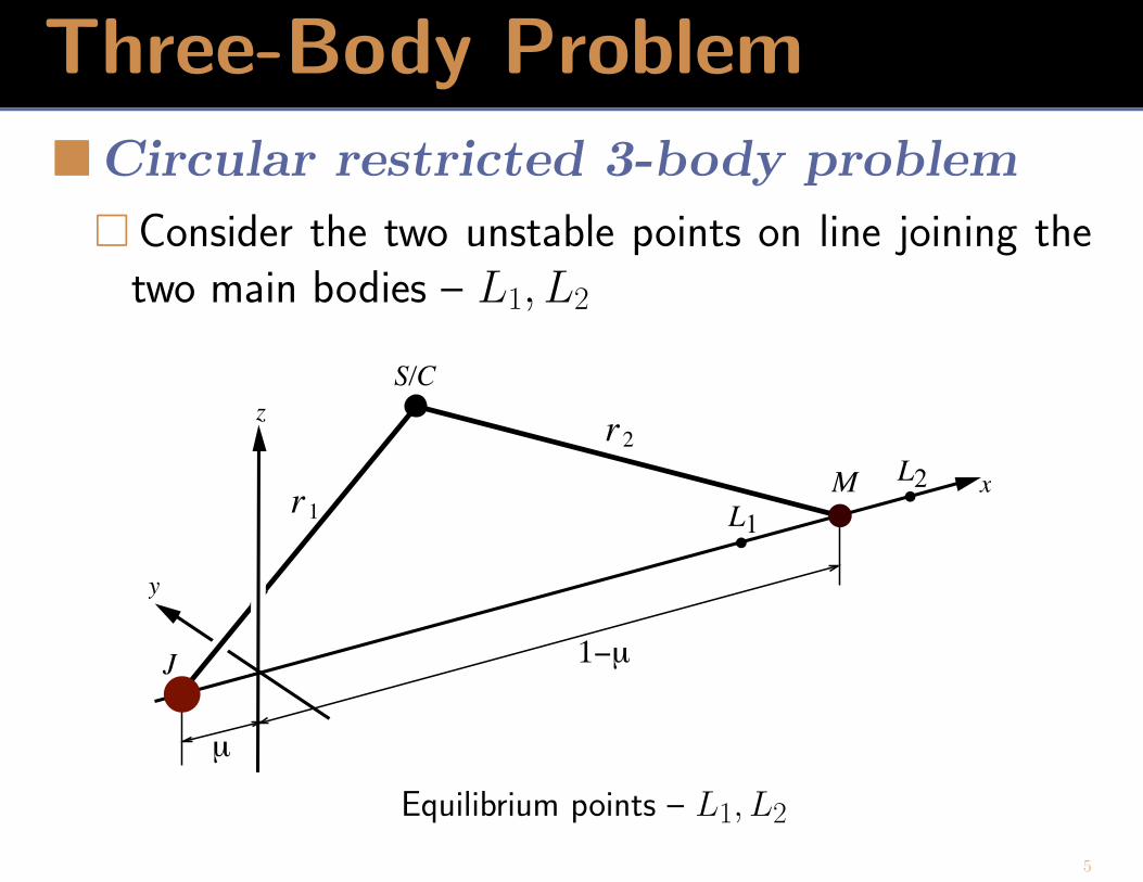
�Circular restricted 3-body problem

� Consider the two unstable points on line joining thetwo main bodies – L1, L2

µ

1−µ

x

z

y

J

S/C

M

2r

1r L1

L2

Equilibrium points – L1, L2

5

Three-Body Problem� orbits exist around L1 and L2; both periodic and quasi-

periodic

• Lyapunov, halo and Lissajous orbits

� one can draw the invariant manifolds assoicated to L1

(and L2) and the orbits surrounding them

� these invariant manifolds play a key role in what follows

6

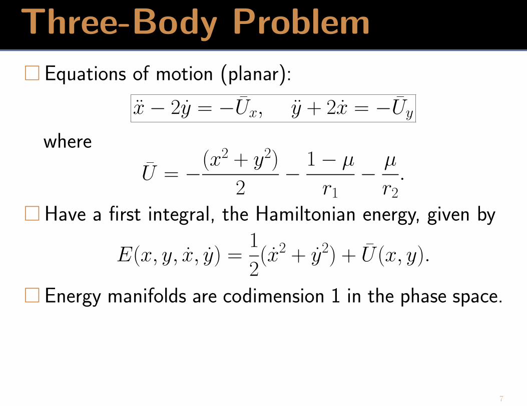
Three-Body Problem� Equations of motion (planar):

x− 2y = −Ux, y + 2x = −Uy

where

U = −(x2 + y2)

2− 1− µ

r1− µ

r2.

� Have a first integral, the Hamiltonian energy, given by

E(x, y, x, y) =1

2(x2 + y2) + U(x, y).

� Energy manifolds are codimension 1 in the phase space.

7

Realms of Possible Motion

�Effective potential

� In a rotating frame, the equations of motion describea particle moving in an effective potential plus a mag-netic field (goes back to work of Jacobi, Hill, etc).

8

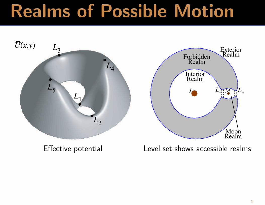
Realms of Possible Motion

U(x,y)_

L4

L5

L3

L1

L2

J ML1 L2

ExteriorRealm

InteriorRealm

MoonRealm

ForbiddenRealm

Effective potential Level set shows accessible realms

9

Motion Near Equilibria

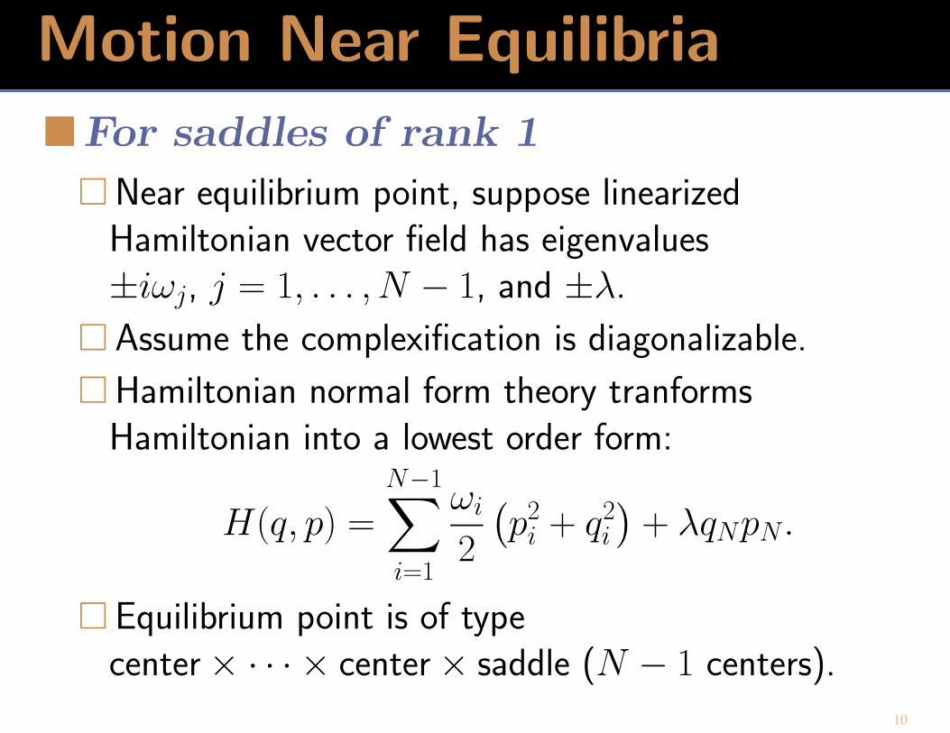
�For saddles of rank 1

� Near equilibrium point, suppose linearizedHamiltonian vector field has eigenvalues±iωj, j = 1, . . . , N − 1, and ±λ.

� Assume the complexification is diagonalizable.

� Hamiltonian normal form theory tranformsHamiltonian into a lowest order form:

H(q, p) =

N−1∑i=1

ωi

2

(p2

i + q2i

)+ λqNpN .

� Equilibrium point is of typecenter× · · · × center× saddle (N − 1 centers).

10

Motion Near Equilibria

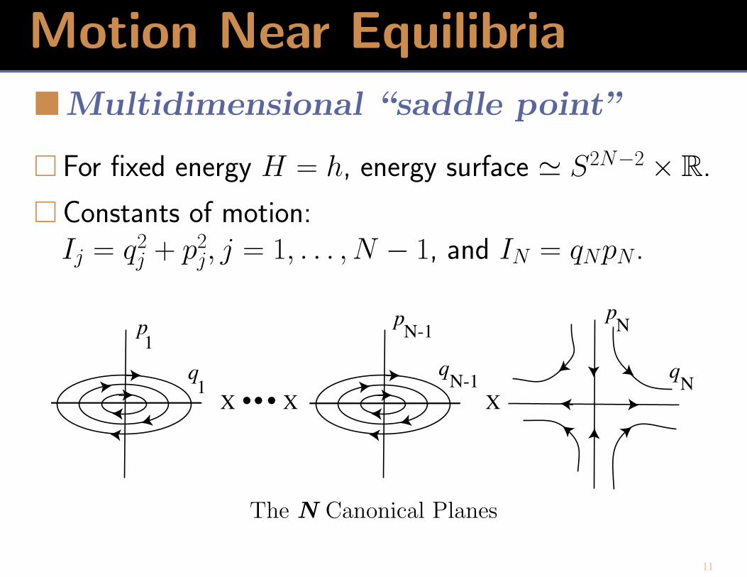
�Multidimensional “saddle point”

� For fixed energy H = h, energy surface ' S2N−2 × R.

� Constants of motion:Ij = q2

j + p2j, j = 1, . . . , N − 1, and IN = qNpN .

1q

1p N-1

p

qN-1

X X X

Np

qN

The N Canonical Planes

11

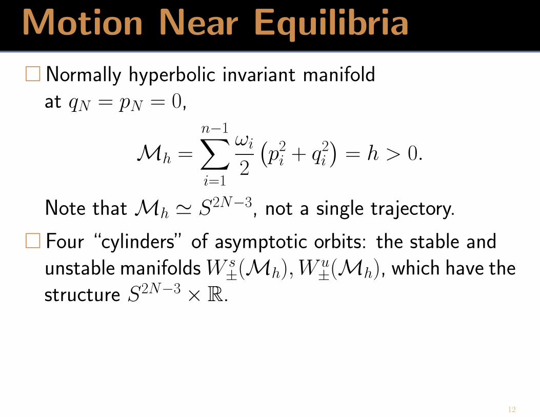
Motion Near Equilibria� Normally hyperbolic invariant manifold

at qN = pN = 0,

Mh =

n−1∑i=1

ωi

2

(p2

i + q2i

)= h > 0.

Note that Mh ' S2N−3, not a single trajectory.

� Four “cylinders” of asymptotic orbits: the stable andunstable manifolds W s

±(Mh), Wu±(Mh), which have the

structure S2N−3 × R.

12

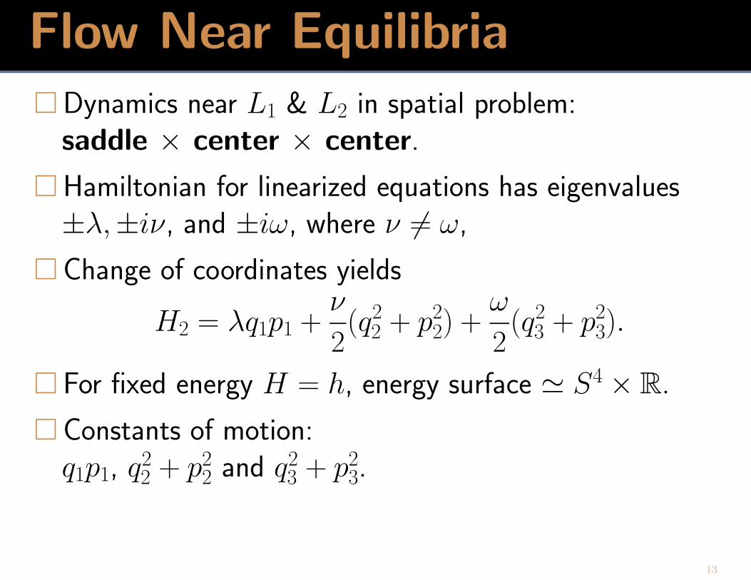
Flow Near Equilibria� Dynamics near L1 & L2 in spatial problem:

saddle × center × center.

� Hamiltonian for linearized equations has eigenvalues±λ,±iν, and ±iω, where ν 6= ω,

� Change of coordinates yields

H2 = λq1p1 +ν

2(q2

2 + p22) +

ω

2(q2

3 + p23).

� For fixed energy H = h, energy surface ' S4 × R.

� Constants of motion:q1p1, q2

2 + p22 and q2

3 + p23.

13

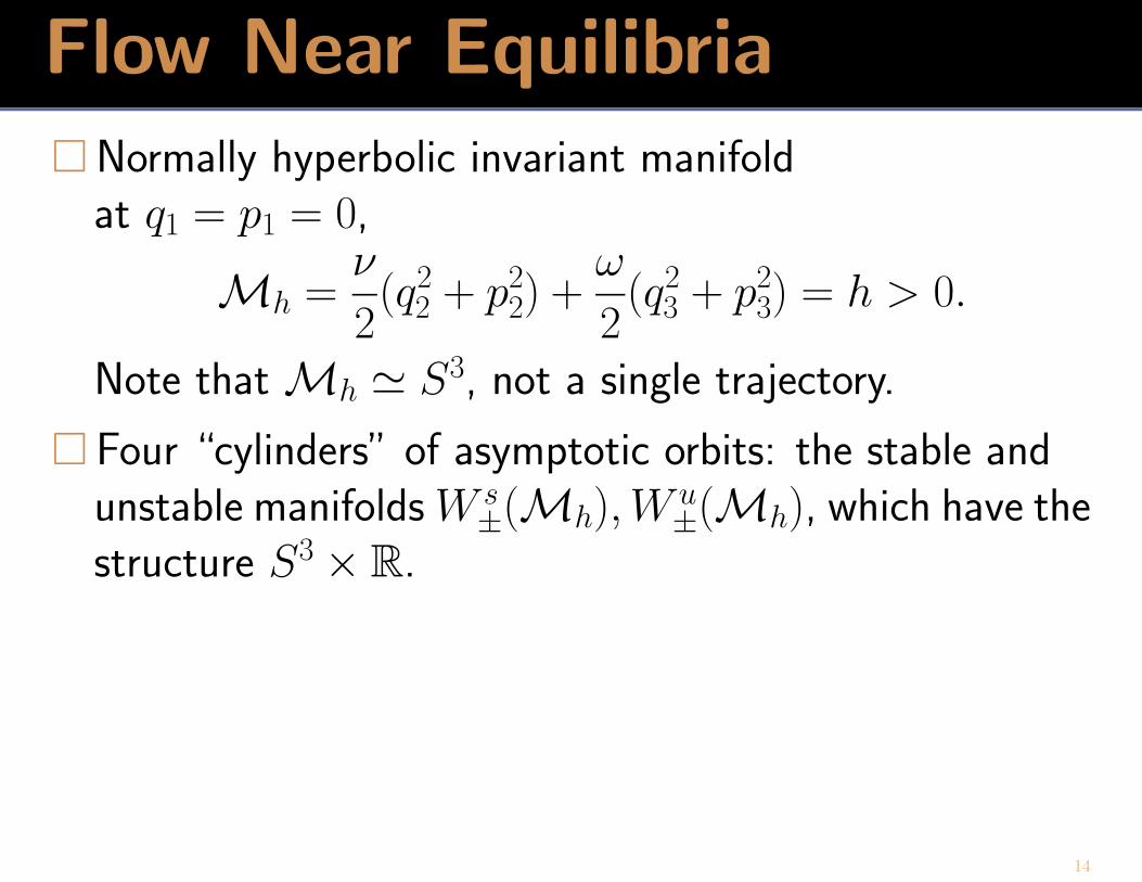
Flow Near Equilibria� Normally hyperbolic invariant manifold

at q1 = p1 = 0,

Mh =ν

2(q2

2 + p22) +

ω

2(q2

3 + p23) = h > 0.

Note that Mh ' S3, not a single trajectory.

� Four “cylinders” of asymptotic orbits: the stable andunstable manifolds W s

±(Mh), Wu±(Mh), which have the

structure S3 × R.

14

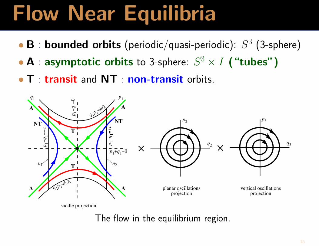
Flow Near Equilibria•B : bounded orbits (periodic/quasi-periodic): S3 (3-sphere)

•A : asymptotic orbits to 3-sphere: S3 × I (“tubes”)

•T : transit and NT : non-transit orbits.

p1−q1=−c

p1−q1=+c

p1−q1=0

p1+q1=0

n1 n2

p1q1

q2

p2

q3

p3

saddle projection

planar oscillationsprojection

vertical oscillationsprojection

q 1p 1=h/λ

q 1p 1=h/

λ

NTNT

T

T

A

A

A

A

The flow in the equilibrium region.

15

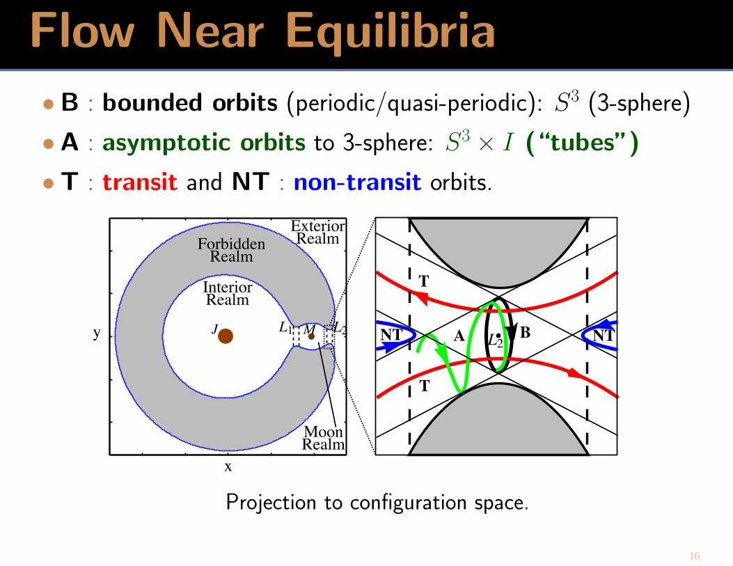
Flow Near Equilibria•B : bounded orbits (periodic/quasi-periodic): S3 (3-sphere)

•A : asymptotic orbits to 3-sphere: S3 × I (“tubes”)

•T : transit and NT : non-transit orbits.

x

y J ML1 L2

ExteriorRealm

InteriorRealm

MoonRealm

ForbiddenRealm

L2B

T

T

A NTNT

Projection to configuration space.

16

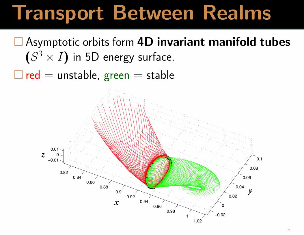
Transport Between Realms� Asymptotic orbits form 4D invariant manifold tubes

(S3 × I) in 5D energy surface.

� red = unstable, green = stable

0.82

0.84

0.86

0.88

0.9

0.92

0.94

0.96

0.98

1

1.02

−0.02

0

0.02

0.04

0.06

0.08

0.1−0.01

0

0.01

x

z

y

17

Transport Between Realms• These manifold tubes play an important role in governing what

orbits approach or depart from a moon (transit orbits)

• and orbits which do not (non-transit orbits)

• transit possible for objects “inside” the tube, otherwise notransit — this is important for transport issues

18

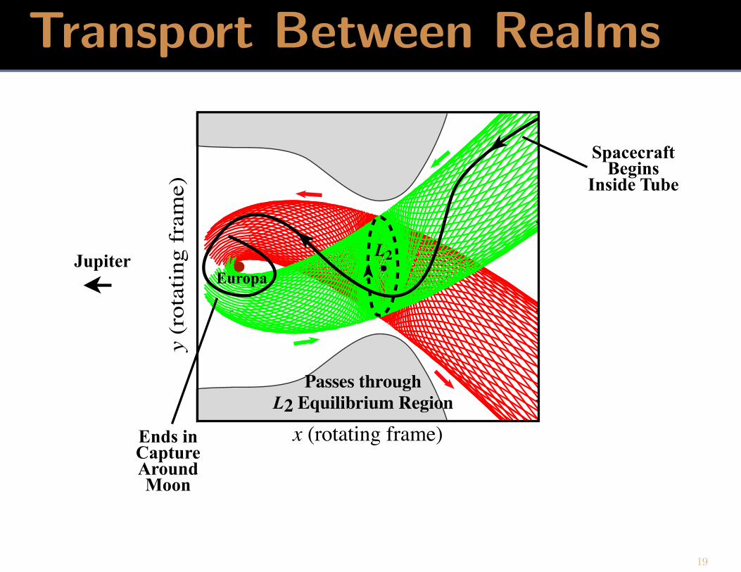
Transport Between Realms

x (rotating frame)

y (

rota

tin

g f

ram

e)

Passes through

L2 Equilibrium Region

JupiterEuropa

L2

Ends inCaptureAround Moon

SpacecraftBegins

Inside Tube

19

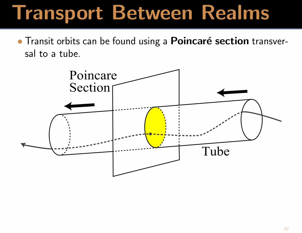
Transport Between Realms• Transit orbits can be found using a Poincare section transver-

sal to a tube.

Poincare

Section

Tube

20

Construction of Trajectories� One can systematically construct new trajectories, which

use little fuel.

• by linking stable and unstable manifold tubes in the right order

• and using Poincare sections to find trajectories “inside” thetubes

� One can construct trajectories involving multiple 3-bodysystems.

21

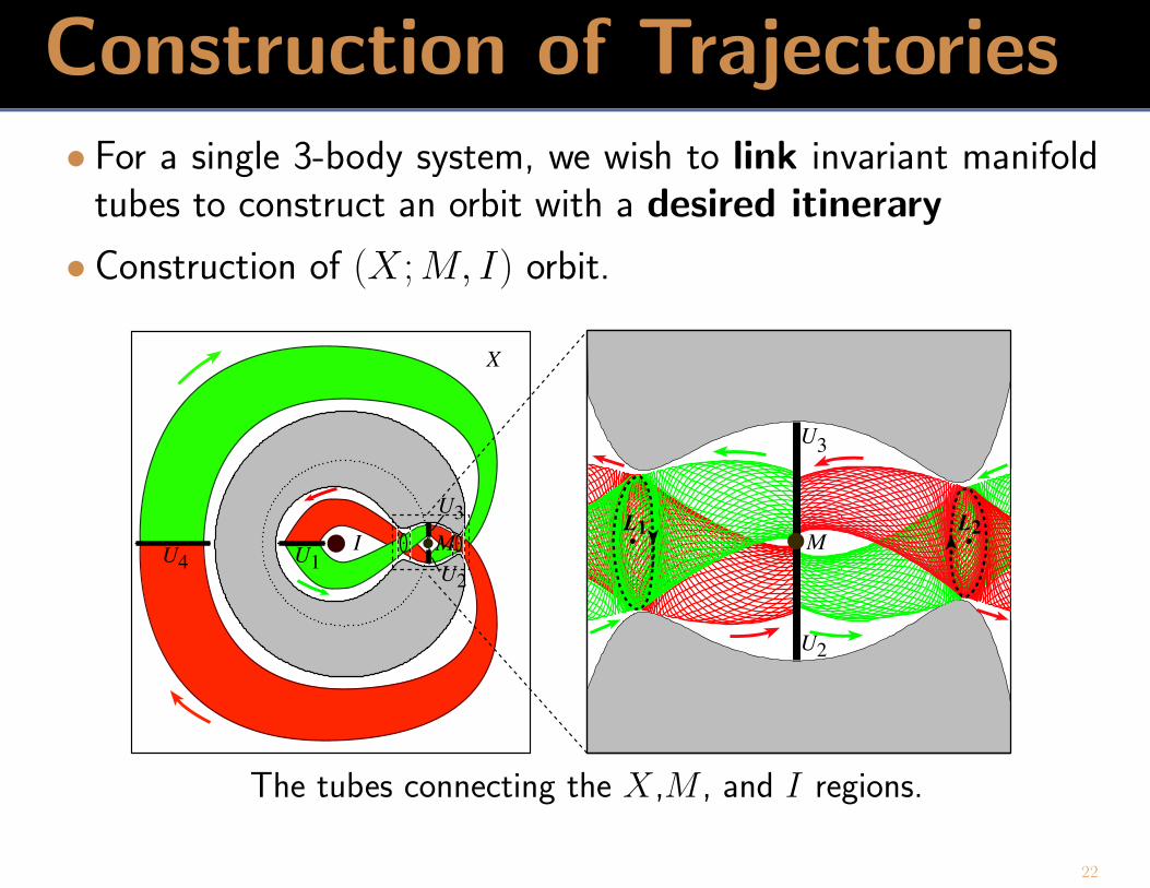
Construction of Trajectories• For a single 3-body system, we wish to link invariant manifold

tubes to construct an orbit with a desired itinerary

• Construction of (X ; M, I) orbit.

X

I M

L1 L2M

U3

U2

U1U4

U3

U2

The tubes connecting the X,M , and I regions.

22

Construction of Trajectories• First, integrate two tubes until they pierce a common Poincaresection transversal to both tubes.

• Second, pick a point in the region of intersection and integrateit forward and backward.

23

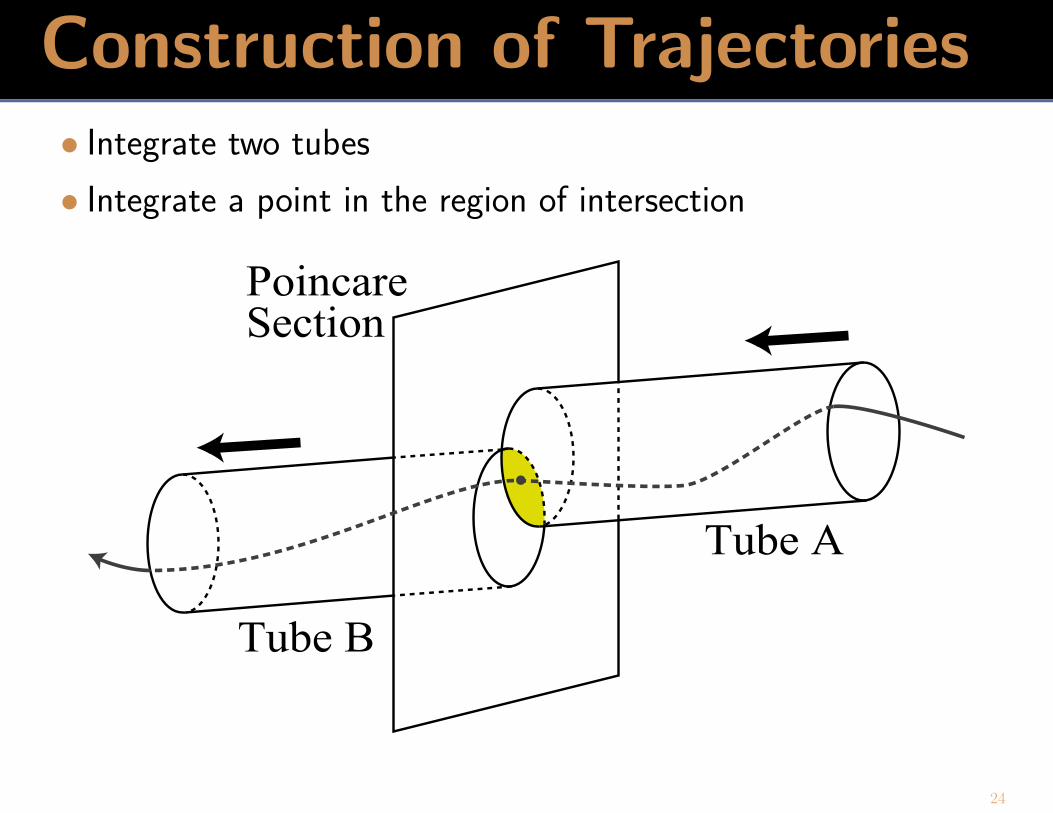
Construction of Trajectories• Integrate two tubes

• Integrate a point in the region of intersection

Poincare

Section

Tube A

Tube B

24

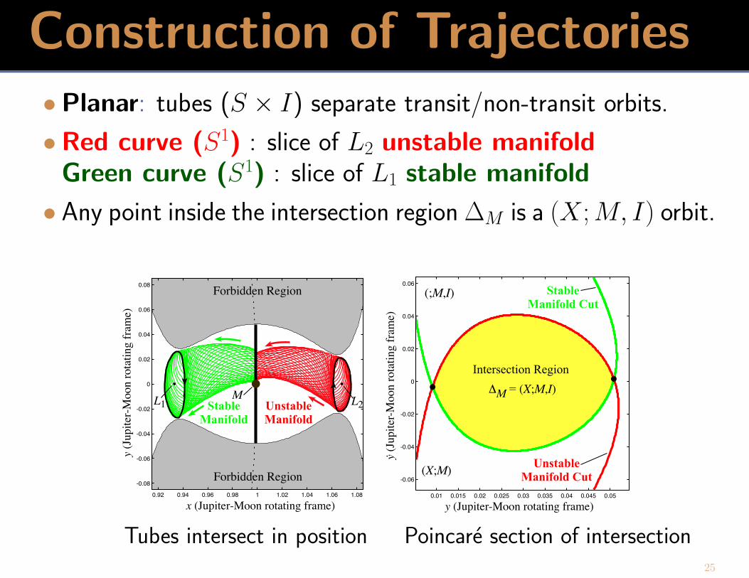
Construction of Trajectories•Planar: tubes (S × I) separate transit/non-transit orbits.

•Red curve (S1) : slice of L2 unstable manifoldGreen curve (S1) : slice of L1 stable manifold

• Any point inside the intersection region ∆M is a (X ; M, I) orbit.

∆M = (X;M,I)

Intersection Region

0.92 0.94 0.96 0.98 1 1.02 1.04 1.06 1.08

-0.08

-0.06

-0.04

-0.02

0

0.02

0.04

0.06

0.08

x (Jupiter-Moon rotating frame)

y (

Jup

iter

-Mo

on

ro

tati

ng

fra

me)

ML1 L2

0.01 0.015 0.02 0.025 0.03 0.035 0.04 0.045 0.05

-0.06

-0.04

-0.02

0

0.02

0.04

0.06

y (Jupiter-Moon rotating frame)

(X;M)

(;M,I)

y (

Jupit

er-M

oon r

ota

ting f

ram

e).

Forbidden Region

Forbidden Region

Stable

Manifold

Unstable

Manifold

Stable

Manifold Cut

Unstable

Manifold Cut

Tubes intersect in position Poincare section of intersection25

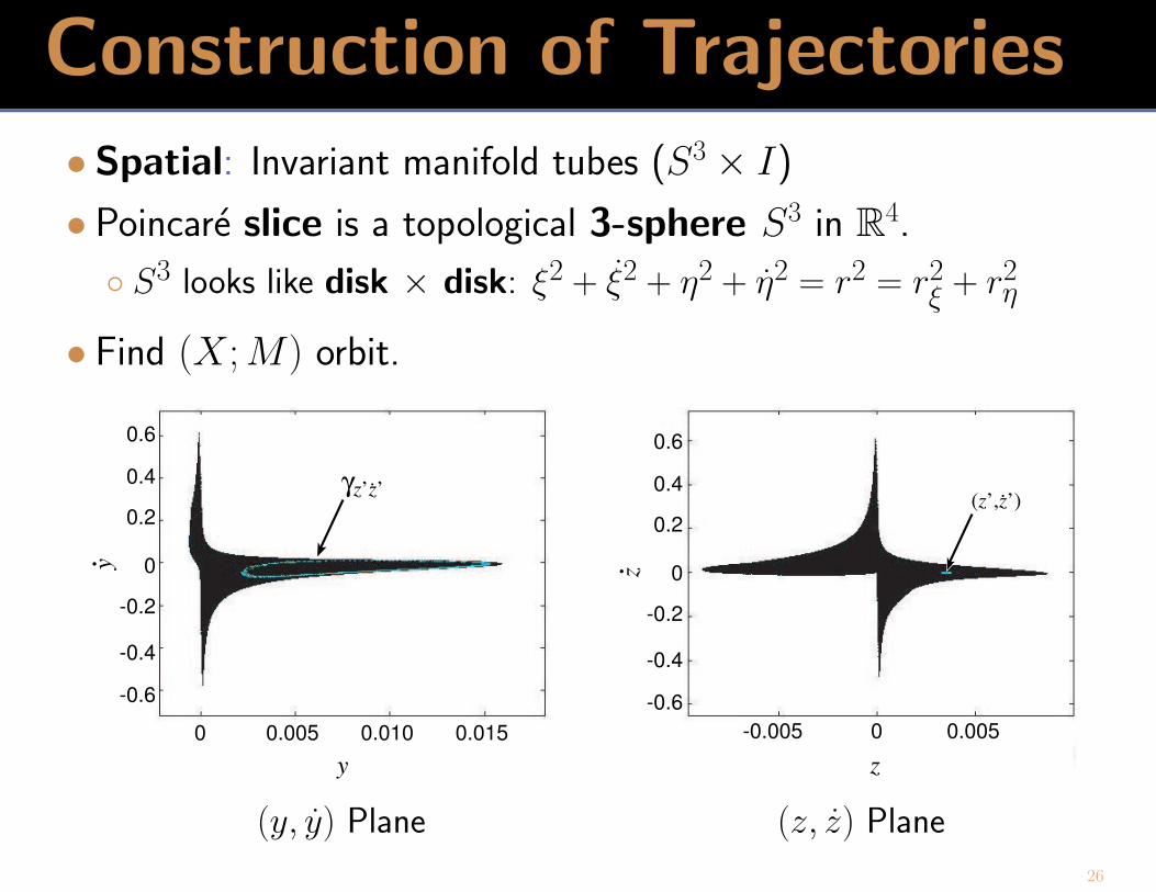
Construction of Trajectories• Spatial: Invariant manifold tubes (S3 × I)

• Poincare slice is a topological 3-sphere S3 in R4.

◦ S3 looks like disk × disk: ξ2 + ξ2 + η2 + η2 = r2 = r2ξ + r2

η

• Find (X ; M) orbit.

-0.005 0.0050

z

0.6

0.4

0.2

-0.2

0

-0.6

-0.4z.

0 0.0100.005

y0.015

0.6

0.4

0.2

-0.2

0

-0.6

-0.4

y.

γz’z’. (z’,z’).

(y, y) Plane (z, z) Plane

26

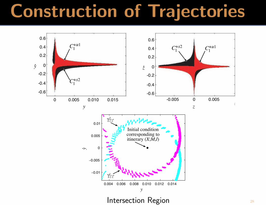
Construction of Trajectories• Similarly, while the cut of the stable manifold tube is S3, its

projection on (y, y) plane is a curve for z = c, z = 0.

• Any point inside this curve is a (M, I) orbit.

• Hence, any point inside the intersection region ∆M is a(X ; M, I) orbit.

27

Construction of Trajectories

-0.005 0.0050

z

0.6

0.4

0.2

-0.2

0

-0.6

-0.4

z

.

0 0.0100.005

y

0.015

0.6

0.4

0.2

-0.2

0

-0.6

-0.4

y

.

C+u11

C+s21

C+u11

C+s21

0.004 0.006 0.008 0.010 0.012 0.014

−0.01

−0.005

0

0.005

0.01

y

y.

γz'z'.1

γz'z'.2

Initial conditioncorresponding toitinerary (X;M,I)

Intersection Region 28

Construction of Trajectories

0.96 0.98 1 1.02 1.04-0.04

-0.02

0

0.02

0.04

x

y

0.96 0.98 1 1.02 1.04-0.04

-0.02

0

0.02

0.04

x

z

-0.005 0 0.005 0.010 0.015 0.020

-0.010

-0.005

0

0.005

y

z

z

0.981

1.021.04

-0.04-0.02

00.02

0.04-0.04

-0.02

0

0.02

0.04

xy

0.96

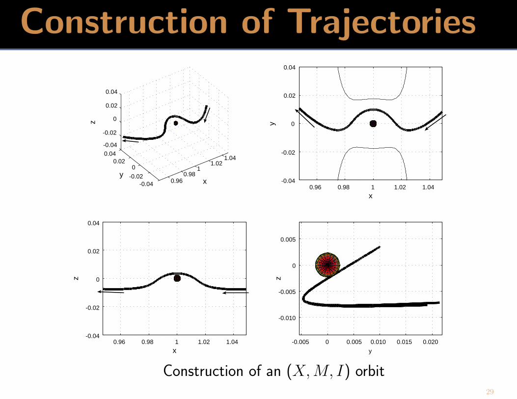
Construction of an (X, M, I) orbit29

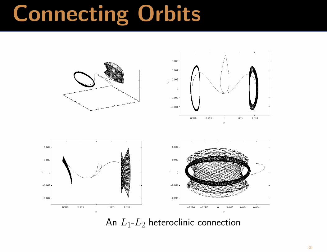
Connecting Orbits

y0.002

0.004

0.006

−0.002

−0.004

0

1 1.005 1.0100.9950.990

x

z

0.002

0.004

−0.002

−0.004

0

1 1.005 1.0100.9950.990

x

z

0.002

0.004

−0.002

−0.004

0

0 0.002 0.004−0.002−0.004

y

0.006

An L1-L2 heteroclinic connection

30

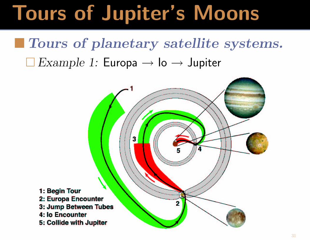
Tours of Jupiter’s Moons

�Tours of planetary satellite systems.

� Example 1: Europa → Io → Jupiter

31

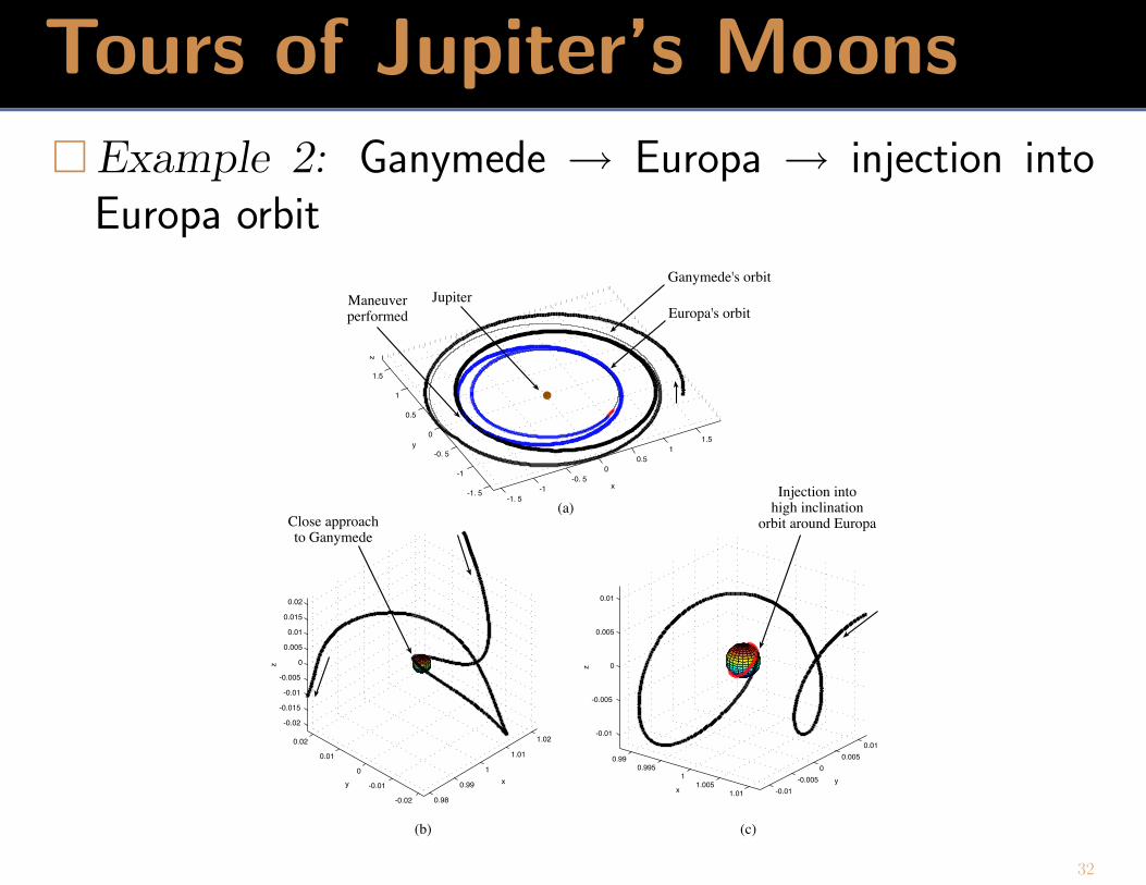
Tours of Jupiter’s Moons� Example 2: Ganymede → Europa → injection into

Europa orbitGanymede's orbit

Jupiter

0.98

0.99

1

1.01

1.02

-0.02

-0.01

0

0.01

0.02

-0.02

-0.015

-0.01

-0.005

0

0.005

0.01

0.015

0.02

xy

z

0.99

0.995

1

1.005

1.01 -0.01

-0.005

0

0.005

0.01

-0.01

-0.005

0

0.005

0.01

y

x

z

Close approachto Ganymede

Injection intohigh inclination

orbit around Europa

Europa's orbit

(a)

(b) (c)

-1. 5

-1

-0. 5

0

0.5

1

1.5

-1. 5

-1

-0. 5

0

0.5

1

1.5

x

y

z

Maneuverperformed

32

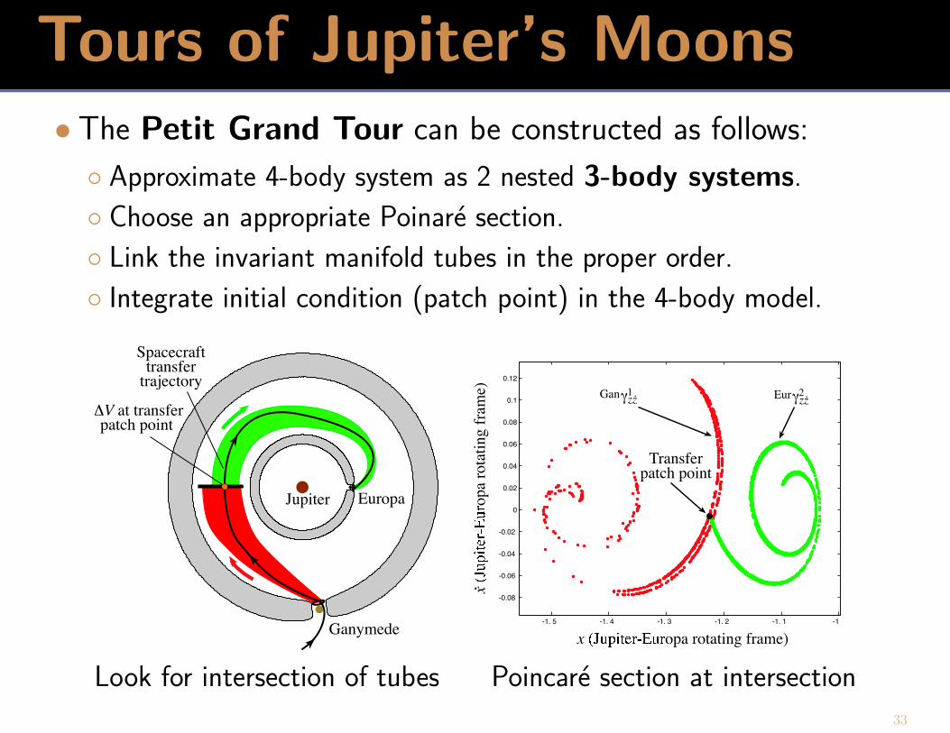
Tours of Jupiter’s Moons• The Petit Grand Tour can be constructed as follows:

◦ Approximate 4-body system as 2 nested 3-body systems.

◦ Choose an appropriate Poinare section.

◦ Link the invariant manifold tubes in the proper order.

◦ Integrate initial condition (patch point) in the 4-body model.

Jupiter Europa

Ganymede

Spacecrafttransfer

trajectory

∆V at transferpatch point

-1. 5 -1. 4 -1. 3 -1. 2 -1. 1 -1

-0.08

-0.06

-0.04

-0.02

0

0.02

0.04

0.06

0.08

0.1

0.12

x������������ �������

opa rotating frame)

x

� ����� � ����� �� o

pa

rota

tin

g f

ram

e)

.

Gan γzz.1 Eur γzz.

2

Transferpatch point

Look for intersection of tubes Poincare section at intersection

33

Some References• Gomez, G., W.S. Koon, M.W. Lo, J.E. Marsden, J. Masdemont and S.D.

Ross [2001] Connecting orbits and invariant manifolds in the spa-tial three-body problem. submitted to Nonlinearity.

• Gomez, G., W.S. Koon, M.W. Lo, J.E. Marsden, J. Masdemont and S.D. Ross[2001] Invariant manifolds, the spatial three-body problem and spacemission design. AAS/AIAA Astrodynamics Specialist Conference.

• Koon, W.S., M.W. Lo, J.E. Marsden and S.D. Ross [2000] Heteroclinic con-nections between periodic orbits and resonance transitions in celes-tial mechanics. Chaos 10(2), 427–469.

The End

34