CoNLL-X Proceedings of the Tenth Conference on Computational Natural Language Learning 8-9 June 2006 New York City, USA

Welcome message from author
This document is posted to help you gain knowledge. Please leave a comment to let me know what you think about it! Share it to your friends and learn new things together.
Transcript
CoNLL-X
Proceedings of the
Tenth Conference onComputational Natural
Language Learning
8-9 June 2006New York City, USA

Production and Manufacturing byOmnipress Inc.2600 Anderson StreetMadison, WI 53704
c©2006 The Association for Computational Linguistics
Order copies of this and other ACL proceedings from:
Association for Computational Linguistics (ACL)209 N. Eighth StreetStroudsburg, PA 18360USATel: +1-570-476-8006Fax: [email protected]
ii
Foreword
CoNLL has turned ten! With a mix of pride and amazement over how time flies, we now celebratethe tenth time that ACL’s special interest group on natural language learning, SIGNLL, holds its yearlyconference.
Having a yearly meeting was the major pillar of the design plan for SIGNLL, drawn up by a circle ofenthusiastic like-minded people around 1995, headed by first president David Powers and first secretaryWalter Daelemans. The first CoNLL was organized as a satellite event of ACL-97 in Madrid, in thecapable hands of Mark Ellison. Since then, no single year has gone by without a CoNLL. The boardsof SIGNLL (with consecutive presidents Michael Brent, Walter Daelemans, and Dan Roth) have madesure that CoNLL toured the world; twice it was held in the Asian-Pacific part of the world, four timesin Europe, and four times in the North-American continent.
Over time, the field of computational linguistics got to know CoNLL for its particular take on empiricalmethods for NLP and the ties these methods have with areas outside the focus of the typical ACLconference. The image of CoNLL was furthermore boosted by the splendid concept of the sharedtask, the organized competition that tackles timely tasks in NLP and has produced both powerful andsobering scientific insights. The CoNLL shared tasks have produced benchmark data sets and resultson which a significant body of work in computational linguistics is based nowadays. The first sharedtask was organized in 1999 on NP bracketing, by Erik Tjong Kim Sang and Miles Osborne. Withthe help of others, Erik continued the organization of shared tasks until 2003 (on syntactic chunking,clause identification, and named-entity recognition), after which Lluıs Marquez and Xavier Carrerasorganized two consecutive shared tasks on semantic role labeling (2004, 2005). This year’s shared taskon multi-lingual dependency parsing holds great promise in becoming a new landmark in NLP research.
With great gratitude we salute all past CoNLL programme chairs and reviewers who have made CoNLLpossible, and who have contributed to this conference series, which we believe has a shining futureahead. We are still exploring unknown territory in the fields of language learning, where models ofhuman learning and natural language processing may on one day be one. We hope we will see a longseries of CoNLLs along that path.
1997 - Madrid, Spain (chair: T. Mark Ellison)1998 - Sydney, Australia (chair: David Powers)1999 - Bergen, Norway (chairs: Miles Osborne and Erik Tjong Kim Sang)2000 - Lisbon, Portugal (chairs: Claire Cardie, Walter Daelemans, and Erik Tjong Kim Sang)2001 - Toulouse, France (chairs: Walter Daelemans and Remi Zajac)2002 - Taipei, Taiwan (chairs: Dan Roth and Antal van den Bosch)2003 - Edmonton, Canada (chairs: Walter Daelemans and Miles Osborne)2004 - Boston, MA, USA (chairs: Hwee Tou Ng and Ellen Riloff)2005 - Ann Arbor, MI, USA (chairs: Ido Dagan and Dan Gildea)2006 - New York City, NY, USA (chairs: Lluıs Marquez and Dan Klein)
Antal van den Bosch, PresidentHwee Tou Ng, Secretary
iii

iv

Preface
The 2006 Conference on Computational Natural Language Learning is the tenth in a series of yearlymeetings organized by SIGNLL, the ACL special interest group on natural language learning. Due tothe special occasion, we have brought out the celebratory Roman numerals: welcome to CoNLL-X!Presumably, next year we will return to CoNLL-2007 (until 2016, when perhaps we will see CoNLL-XX). CoNLL-X will be held in New York City on June 8-9, in conjunction with the HLT-NAACL 2006conference.
A total of 52 papers were submitted to CoNLL’s main session, from which only 18 were accepted. The35% acceptance ratio maintains the high competitiveness of recent CoNLLs and is an indicator of thisyear’s high-quality programme. We are very grateful to the CoNLL community for the large amountof exciting, diverse, and high-quality submissions we received. We are equally grateful to the programcommittee for their service in reviewing these submissions, on a very tight schedule. Your efforts madeour job a pleasure.
As in previous years, we defined a topic of special interest for the conference. This year, we particularlyencouraged submissions describing architectures, algorithms, methods, or models designed to improvethe robustness of learning-based NLP systems. While the topic of interest was directly addressed byonly a small number of the main session submissions, the shared task setting contributed significantlyin this direction.
Also following CoNLL tradition, a centerpiece of the confernence is a shared task, this year onmultilingual dependency parsing. The shared task was organized by Sabine Buchholz, Amit Dubey,Yuval Krymolwski, and Erwin Marsi, who worked very hard to make the shared task the success ithas been. Up to 13 different languages were treated. 19 teams submitted results, from which 17 arepresenting description papers in the proceedings. In our opinion, the current shared task constitutes aqualitative step ahead in the evolution of CoNLL shared tasks, and we hope that the resources createdand the body of work presented will both serve as a benchmark and also have a substantial impact onfuture research on syntactic parsing.
Finally, we are delighted to announce that this year’s invited speakers are Michael Collins and WalterDaelemans. In accordance with the tenth anniversary celebration, Walter Daelemans will look back atthe 10 years of CoNLL conferences, presenting the state of the art in computational natural languagelearning, and suggesting a new “mission” for the future of field. Michael Collins, in turn, will talk aboutone of the important current research lines in the field: global learning architectures for structural andrelational learning problems in natural language.
In addition to the program committee and shared task organizers, we are very indebted to the SIGNLLboard members for very helpful discussion and advice, Erik Tjong Kim Sang, who acted as theinformation officer, and the HLT-NAACL 2006 conference organizers, in particular Robert Moore,Brian Roark, Sanjeev Khudanpur, Lucy Vanderwende, Roberto Pieraccini, and Liz Liddy for their helpwith local arrangements and the publication of the proceedings.
To all the attendees, enjoy the CoNLL-X conference!
Lluıs Marquez and Dan KleinCoNLL-X Program Co-Chairs
v

Organizers:
Lluıs Marquez, Technical University of Catalonia, SpainDan Klein, University of California at Berkeley, USA
Shared Task Organizers:
Sabine Buchholz, Toshiba Research Europe Ltd, UKAmit Dubey, University of Edinburgh, UKYuval Krymolowski, University of Haifa, IsraelErwin Marsi, Tilburg University, The Netherlands
Information Officer:
Erik Tjong Kim Sang, University of Amsterdam, The Netherlands
Program Committee:
Eneko Agirre, University of the Basque Country, SpainRegina Barzilay, Massachusetts Institute of Technology, USAThorsten Brants, Google Inc., USAXavier Carreras, Polytechnical University of Catalunya, SpainEugene Charniak, Brown University, USAAlexander Clark, Royal Holloway University of London, UKJames Cussens, University of York, UKWalter Daelemans, University of Antwerp, BelgiumHal Daum, ISI, University of Southern California, USARadu Florian, IBM, USADayne Freitag, Fair Isaac Corporation, USADaniel Gildea, University of Rochester, USATrond Grenager, Stanford University, USAMarti Hearst, I-School, UC Berkeley, USAPhilipp Koehn, University of Edinburgh, UKRoger Levy, University of Edinburgh, UKRob Malouf, San Diego State University, USAChristopher Manning, Stanford University, USAYuji Matsumoto, Nara Institute of Science and Technology, JapanAndrew McCallum, University of Massachusetts Amherst, USARada Mihalcea, University of North Texas, USAAlessandro Moschitti, University of Rome Tor Vergata, ItalyJohn Nerbonne, University of Groningen, The NetherlandsHwee Tou Ng, National University of Singapore, SingaporeFranz Josef Och, Google Inc., USAMiles Osborne, University of Edinburgh, UK
vii
David Powers, Flinders University, AustraliaEllen Riloff, University of Utah, USADan Roth, University of Illinois at Urbana-Champaign, USAAnoop Sarkar, Simon Fraser University, CanadaNoah Smith, Johns Hopkins University, USASuzanne Stevenson, University of Toronto, CanadaMihai Surdeanu, Polytechnical University of Catalunya, SpainCharles Sutton, University of Massachusetts Amherst, USAKristina Toutanova, Microsoft Research, USAAntal van den Bosch, Tilburg University, The NetherlandsJanyce Wiebe, University of Pittsburgh, USADekai Wu, Hong Kong University of Science and Technology, Hong Kong
Additional Reviewers:
Sander Canisius, Michael Connor, Andras Csomai, Aron Culotta, Quang Do, Gholamreza Haf-fari, Yudong Liu, David Martinez, Vanessa Murdoch, Vasin Punyakanok, Lev Ravitov, KevinSmall,Dong Song, Adam Vogel
Invited Speakers:
Michael Collins, Massachusetts Institute of Technology, USAWalter Daelemans, University of Antwerp, Belgium
viii
Table of Contents
Invited Paper
A Mission for Computational Natural Language LearningWalter Daelemans . . . . . . . . . . . . . . . . . . . . . . . . . . . . . . . . . . . . . . . . . . . . . . . . . . . . . . . . . . . . . . . . . . . . . . . . .1
Main Session
Porting Statistical Parsers with Data-Defined KernelsIvan Titov and James Henderson . . . . . . . . . . . . . . . . . . . . . . . . . . . . . . . . . . . . . . . . . . . . . . . . . . . . . . . . . . . . .6
Non-Local Modeling with a Mixture of PCFGsSlav Petrov, Leon Barrett and Dan Klein . . . . . . . . . . . . . . . . . . . . . . . . . . . . . . . . . . . . . . . . . . . . . . . . . . . . .14
Improved Large Margin Dependency Parsing via Local Constraints and Laplacian RegularizationQin Iris Wang, Colin Cherry, Dan Lizotte and Dale Schuurmans . . . . . . . . . . . . . . . . . . . . . . . . . . . . . . .21
What are the Productive Units of Natural Language Grammar? A DOP Approach to the Automatic Identi-fication of Constructions.
Willem Zuidema . . . . . . . . . . . . . . . . . . . . . . . . . . . . . . . . . . . . . . . . . . . . . . . . . . . . . . . . . . . . . . . . . . . . . . . . . .29
Resolving and Generating Definite Anaphora by Modeling Hypernymy using Unlabeled CorporaNikesh Garera and David Yarowsky . . . . . . . . . . . . . . . . . . . . . . . . . . . . . . . . . . . . . . . . . . . . . . . . . . . . . . . . .37
Investigating Lexical Substitution Scoring for Subtitle GenerationOren Glickman, Ido Dagan, Walter Daelemans, Mikaela Keller and Samy Bengio. . . . . . . . . . . . . . . .45
Semantic Role Recognition Using Kernels on Weighted Marked Ordered Labeled TreesJun’ichi Kazama and Kentaro Torisawa . . . . . . . . . . . . . . . . . . . . . . . . . . . . . . . . . . . . . . . . . . . . . . . . . . . . . .53
Semantic Role Labeling via Tree Kernel Joint InferenceAlessandro Moschitti, Daniele Pighin and Roberto Basili . . . . . . . . . . . . . . . . . . . . . . . . . . . . . . . . . . . . . .61
Can Human Verb Associations Help Identify Salient Features for Semantic Verb Classification?Sabine Schulte im Walde . . . . . . . . . . . . . . . . . . . . . . . . . . . . . . . . . . . . . . . . . . . . . . . . . . . . . . . . . . . . . . . . . . .69
Applying Alternating Structure Optimization to Word Sense DisambiguationRie Kubota Ando. . . . . . . . . . . . . . . . . . . . . . . . . . . . . . . . . . . . . . . . . . . . . . . . . . . . . . . . . . . . . . . . . . . . . . . . . .77
Unsupervised Parsing with U-DOPRens Bod . . . . . . . . . . . . . . . . . . . . . . . . . . . . . . . . . . . . . . . . . . . . . . . . . . . . . . . . . . . . . . . . . . . . . . . . . . . . . . . . .85
A Lattice-Based Framework for Enhancing Statistical Parsers with Information from Unlabeled CorporaMichaela Atterer and Hinrich Schutze . . . . . . . . . . . . . . . . . . . . . . . . . . . . . . . . . . . . . . . . . . . . . . . . . . . . . . .93
Word Distributions for Thematic Segmentation in a Support Vector Machine ApproachMaria Georgescul, Alexander Clark and Susan Armstrong . . . . . . . . . . . . . . . . . . . . . . . . . . . . . . . . . . . .101
ix
Which Side are You on? Identifying Perspectives at the Document and Sentence LevelsWei-Hao Lin, Theresa Wilson, Janyce Wiebe and Alexander Hauptmann . . . . . . . . . . . . . . . . . . . . . .109
Unsupervised Grammar Induction by Distribution and AttachmentDavid J. Brooks . . . . . . . . . . . . . . . . . . . . . . . . . . . . . . . . . . . . . . . . . . . . . . . . . . . . . . . . . . . . . . . . . . . . . . . . . .117
Learning Auxiliary Fronting with Grammatical InferenceAlexander Clark and Remi Eyraud . . . . . . . . . . . . . . . . . . . . . . . . . . . . . . . . . . . . . . . . . . . . . . . . . . . . . . . . .125
Using Gazetteers in Discriminative Information ExtractionAndrew Smith and Miles Osborne . . . . . . . . . . . . . . . . . . . . . . . . . . . . . . . . . . . . . . . . . . . . . . . . . . . . . . . . .133
A Context Pattern Induction Method for Named Entity ExtractionPartha Pratim Talukdar, Thorsten Brants, Mark Liberman and Fernando Pereira . . . . . . . . . . . . . . . .141
Shared Task
CoNLL-X Shared Task on Multilingual Dependency ParsingSabine Buchholz and Erwin Marsi . . . . . . . . . . . . . . . . . . . . . . . . . . . . . . . . . . . . . . . . . . . . . . . . . . . . . . . . .149
The Treebanks Used in the Shared Task. . . . . . . . . . . . . . . . . . . . . . . . . . . . . . . . . . . . . . . . . . . . . . . . . . . . . . . . . . . . . . . . . . . . . . . . . . . . . . . . . . . . . . . .165
Experiments with a Multilanguage Non-Projective Dependency ParserGiuseppe Attardi . . . . . . . . . . . . . . . . . . . . . . . . . . . . . . . . . . . . . . . . . . . . . . . . . . . . . . . . . . . . . . . . . . . . . . . . .166
LingPars, a Linguistically Inspired, Language-Independent Machine Learner for Dependency TreebanksEckhard Bick . . . . . . . . . . . . . . . . . . . . . . . . . . . . . . . . . . . . . . . . . . . . . . . . . . . . . . . . . . . . . . . . . . . . . . . . . . . .171
Dependency Parsing by Inference over High-recall Dependency PredictionsSander Canisius, Toine Bogers, Antal van den Bosch, Jeroen Geertzen and Erik Tjong Kim Sang176
Projective Dependency Parsing with PerceptronXavier Carreras, Mihai Surdeanu and Lluıs Marquez. . . . . . . . . . . . . . . . . . . . . . . . . . . . . . . . . . . . . . . . .181
A Pipeline Model for Bottom-Up Dependency ParsingMing-Wei Chang, Quang Do and Dan Roth . . . . . . . . . . . . . . . . . . . . . . . . . . . . . . . . . . . . . . . . . . . . . . . . .186
Multi-lingual Dependency Parsing at NAISTYuchang Cheng, Masayuki Asahara and Yuji Matsumoto . . . . . . . . . . . . . . . . . . . . . . . . . . . . . . . . . . . . .191
Dependency Parsing with Reference to Slovene, Spanish and SwedishSimon Corston-Oliver and Anthony Aue. . . . . . . . . . . . . . . . . . . . . . . . . . . . . . . . . . . . . . . . . . . . . . . . . . . .196
Vine Parsing and Minimum Risk Reranking for Speed and PrecisionMarkus Dreyer, David A. Smith and Noah A. Smith . . . . . . . . . . . . . . . . . . . . . . . . . . . . . . . . . . . . . . . . .201
Investigating Multilingual Dependency ParsingRichard Johansson and Pierre Nugues . . . . . . . . . . . . . . . . . . . . . . . . . . . . . . . . . . . . . . . . . . . . . . . . . . . . . .206
x
Dependency Parsing Based on Dynamic Local OptimizationTing Liu, Jinshan Ma, Huijia Zhu and Sheng Li . . . . . . . . . . . . . . . . . . . . . . . . . . . . . . . . . . . . . . . . . . . . .211
Multilingual Dependency Analysis with a Two-Stage Discriminative ParserRyan McDonald, Kevin Lerman and Fernando Pereira . . . . . . . . . . . . . . . . . . . . . . . . . . . . . . . . . . . . . . .216
Labeled Pseudo-Projective Dependency Parsing with Support Vector MachinesJoakim Nivre, Johan Hall, Jens Nilsson, Gulsen Eryigit and Svetoslav Marinov . . . . . . . . . . . . . . . . .221
Multi-lingual Dependency Parsing with Incremental Integer Linear ProgrammingSebastian Riedel, Ruket Cakıcı and Ivan Meza-Ruiz . . . . . . . . . . . . . . . . . . . . . . . . . . . . . . . . . . . . . . . . .226
Language Independent Probabilistic Context-Free Parsing Bolstered by Machine LearningMichael Schiehlen and Kristina Spranger . . . . . . . . . . . . . . . . . . . . . . . . . . . . . . . . . . . . . . . . . . . . . . . . . . .231
Maximum Spanning Tree Algorithm for Non-projective Labeled Dependency ParsingNobuyuki Shimizu . . . . . . . . . . . . . . . . . . . . . . . . . . . . . . . . . . . . . . . . . . . . . . . . . . . . . . . . . . . . . . . . . . . . . . .236
The Exploration of Deterministic and Efficient Dependency ParsingYu-Chieh Wu, Yue-Shi Lee and Jie-Chi Yang . . . . . . . . . . . . . . . . . . . . . . . . . . . . . . . . . . . . . . . . . . . . . . .241
Dependency Parsing as a Classication ProblemDeniz Yuret . . . . . . . . . . . . . . . . . . . . . . . . . . . . . . . . . . . . . . . . . . . . . . . . . . . . . . . . . . . . . . . . . . . . . . . . . . . . .246
xi


Conference Program
Thursday, June 8, 2006
8:45–8:50 Welcome
Session 1: Syntax and Statistical Parsing
8:50–9:15 Porting Statistical Parsers with Data-Defined KernelsIvan Titov and James Henderson
9:15–9:40 Non-Local Modeling with a Mixture of PCFGsSlav Petrov, Leon Barrett and Dan Klein
9:40–10:05 Improved Large Margin Dependency Parsing via Local Constraints and LaplacianRegularizationQin Iris Wang, Colin Cherry, Dan Lizotte and Dale Schuurmans
10:05–10:30 What are the Productive Units of Natural Language Grammar? A DOP Approachto the Automatic Identification of Constructions.Willem Zuidema
10:30–11:00 coffee break
11:00–11:50 Invited Talk by Michael Collins
Session 2: Anaphora Resolution and Paraphrasing
11:50–12:15 Resolving and Generating Definite Anaphora by Modeling Hypernymy using Unla-beled CorporaNikesh Garera and David Yarowsky
12:15–12:40 Investigating Lexical Substitution Scoring for Subtitle GenerationOren Glickman, Ido Dagan, Walter Daelemans, Mikaela Keller and Samy Bengio
12:40–14:00 lunch
Session 3: Shared Task on Dependency Parsing
14:00–15:30 Introduction and System presentation I
15:30–16:00 coffee break
16:00–18:00 System presentation II and Discussion
xiii

Friday, June 9, 2006
Session 4: Semantic Role Labeling and Semantics
8:50–9:15 Semantic Role Recognition Using Kernels on Weighted Marked Ordered Labeled TreesJun’ichi Kazama and Kentaro Torisawa
9:15–9:40 Semantic Role Labeling via Tree Kernel Joint InferenceAlessandro Moschitti, Daniele Pighin and Roberto Basili
9:40–10:05 Can Human Verb Associations Help Identify Salient Features for Semantic Verb Classifi-cation?Sabine Schulte im Walde
10:05–10:30 Applying Alternating Structure Optimization to Word Sense DisambiguationRie Kubota Ando
10:30–11:00 coffee break
11:00–11:50 Invited Talk by Walter Daelemans
Session 5: Syntax and Unsupervised Learning
11:50–12:15 Unsupervised Parsing with U-DOPRens Bod
12:15–12:40 A Lattice-Based Framework for Enhancing Statistical Parsers with Information from Un-labeled CorporaMichaela Atterer and Hinrich Schutze
12:40–14:00 lunch
13:30–14:00 SIGNLL business meeting
Session 6: Thematic Segmentation and Discourse Analysis
14:00–14:25 Word Distributions for Thematic Segmentation in a Support Vector Machine ApproachMaria Georgescul, Alexander Clark and Susan Armstrong
14:25–14:50 Which Side are You on? Identifying Perspectives at the Document and Sentence LevelsWei-Hao Lin, Theresa Wilson, Janyce Wiebe and Alexander Hauptmann
xiv

Friday, June 9, 2006 (continued)
Session 7: Grammatical Inference
14:50–15:15 Unsupervised Grammar Induction by Distribution and AttachmentDavid J. Brooks
15:15–15:40 Learning Auxiliary Fronting with Grammatical InferenceAlexander Clark and Remi Eyraud
15:40–16:00 coffee break
Session 8: Information Extraction and Named Entity Extraction
16:00–16:25 Using Gazetteers in Discriminative Information ExtractionAndrew Smith and Miles Osborne
16:25–16:50 A Context Pattern Induction Method for Named Entity ExtractionPartha Pratim Talukdar, Thorsten Brants, Mark Liberman and Fernando Pereira
16:50–17:00 Best Paper Award
17:00 Closing
xv

Proceedings of the 10th Conference on Computational Natural Language Learning (CoNLL-X),pages 1–5, New York City, June 2006.c©2006 Association for Computational Linguistics
A Mission for Computational Natural Language Learning
Walter DaelemansCNTS Language Technology Group
University of AntwerpBelgium
Abstract
In this presentation, I will look back at10 years of CoNLL conferences and thestate of the art of machine learning of lan-guage that is evident from this decade ofresearch. My conclusion, intended to pro-voke discussion, will be that we currentlylack a clear motivation or “mission” tosurvive as a discipline. I will suggest thata new mission for the field could be foundin a renewed interest for theoretical work(which learning algorithms have a biasthat matches the properties of language?,what is the psycholinguistic relevance oflearner design issues?), in more sophis-ticated comparative methodology, and insolving the problem of transfer, reusabil-ity, and adaptation of learned knowledge.
1 Introduction
When looking at ten years of CoNLL conferences,it is clear that the impact and the size of the con-ference has enormously grown over time. The tech-nical papers you will find in this proceedings noware comparable in quality and impact to those ofother distinguished conferences like the Conferenceon Empirical Methods in Natural Language Pro-cessing or even the main conferences of ACL, EACLand NAACL themselves. An important factor inthe success of CoNLL has been the continued se-ries of shared tasks (notice we don’t use terms likechallenges or competitions) that has produced a use-
ful set of benchmarks for comparing learning meth-ods, and that has gained wide interest in the field.It should also be noted, however, that the successof the conferences is inversely proportional withthe degree to which the original topics which mo-tivated the conference are present in the programme.Originally, the people driving CoNLL wanted it tobe promiscuous (i) in the selection of partners (wewanted to associate with Machine Learning, Lin-guistics and Cognitive Science conferences as wellas with Computational Linguistics conferences) and(ii) in the range of topics to be presented. We wantedto encourage linguistically and psycholinguisticallyrelevant machine learning work, and biologically in-spired and innovative symbolic learning methods,and present this work alongside the statistical andlearning approaches that were at that time only start-ing to gradually become the mainstream in Compu-tational Linguistics. It has turned out differently,and we should reflect on whether we have becometoo much of a mainstream computational linguisticsconference ourselves, a back-off for the good papersthat haven’t made it in EMNLP or ACL because ofthe crazy rejection rates there (with EMNLP in itsturn a back-off for good papers that haven’t madeit in ACL). Some of the work targeted by CoNLLhas found a forum in meetings like the workshop onPsycho-computational models of human languageacquisition, the International Colloquium on Gram-matical Inference, the workshop on Morphologicaland Phonological Learning etc. We should ask our-selves why we don’t have this type of work morein CoNLL. In the first part of the presentation Iwill sketch very briefly the history of SIGNLL and
1
CoNLL and try to initiate some discussion on whata conference on Computational Language Learningshould be doing in 2007 and after.
2 State of the Art in ComputationalNatural Language Learning
The second part of my presentation will be a dis-cussion of the state of the art as it can be found inCoNLL (and EMNLP and the ACL conferences).The field can be divided into theoretical, method-ological, and engineering work. There has beenprogress in theory and methodology, but perhapsnot sufficiently. I will argue that most progress hasbeen made in engineering with most often incre-mental progress on specific tasks as a result ratherthan increased understanding of how language canbe learned from data.Machine Learning of Natural Language (MLNL),
or Computational Natural Language Learning(CoNLL) is a research area lying in the intersec-tion of computational linguistics and machine learn-ing. I would suggest that Statistical Natural Lan-guage Processing (SNLP) should be treated as partof MLNL, or perhaps even as a synonym. Symbolicmachine learning methods belong to the same partof the ontology as statistical methods, but have dif-ferent solutions for specific problems. E.g., Induc-tive Logic Programming allows elegant addition ofbackground knowledge, memory-based learning hasimplicit similarity-based smoothing, etc.There is no need here to explain the success of
inductive methods in Computational Linguistics andwhy we are all such avid users of the technology:availability of data, fast production of systems withgood accuracy, robustness and coverage, cheaperthan linguistic labor. There is also no need hereto explain that many of these arguments in favor oflearning in NLP are bogus. Getting statistical andmachine learning systems to work involves design,optimization, and smoothing issues that are some-thing of a black art. For many problems, gettingsufficient annotated data is expensive and difficult,our annotators don’t sufficiently agree, our trainedsystems are not really that good. My favorite exam-ple for the latter is part of speech tagging, which isconsidered a solved problem, but still has error ratesof 20-30% for the ambiguities that count, like verb-
noun ambiguity. We are doing better than hand-crafted linguistic knowledge-based approaches butfrom the point of view of the goal of robust lan-guage understanding unfortunately not that signifi-cantly better. Twice better than very bad is not nec-essarily any good. We also implicitly redefined thegoals of the field of Computational Linguistics, for-getting for example about quantification, modality,tense, inference and a large number of other sen-tence and discourse semantics issues which do notfit the default classification-based supervised learn-ing framework very well or for which we don’t haveannotated data readily available. As a final irony,one of the reasons why learning methods have be-come so prevalent in NLP is their success in speechrecognition. Yet, there too, this success is relative;the goal of spontaneous speaker-independent recog-nition is still far away.
2.1 TheoryThere has been a lot of progress recently in theoret-ical machine learning(Vapnik, 1995; Jordan, 1999).Statistical Learning Theory and progress in Graph-ical Models theory have provided us with a well-defined framework in which we can relate differ-ent approaches like kernel methods, Naive Bayes,Markov models, maximum entropy approaches (lo-gistic regression), perceptrons and CRFs. Insightinto the differences between generative and discrim-inative learning approaches has clarified the rela-tions between different learning algorithms consid-erably.However, this work does not tell us something
general about machine learning of language. The-oretical issues that should be studied in MLNL arefor example which classes of learning algorithms arebest suited for which type of language processingtask, what the need for training data is for a giventask, which information sources are necessary andsufficient for learning a particular language process-ing task, etc. These fundamental questions all re-late to learning algorithm bias issues. Learning isa search process in a hypothesis space. Heuristiclimitations on the search process and restrictions onthe representations allowed for input and hypothe-sis representations together define this bias. There isnot a lot of work on matching properties of learningalgorithms with properties of language processing
2
tasks, or more specifically on how the bias of partic-ular (families of) learning algorithms relates to thehypothesis spaces of particular (types of) languageprocessing tasks.As an example of such a unifying approach,
(Roth, 2000) shows that several different algorithms(memory-based learning, tbl, snow, decision lists,various statistical learners, ...) use the same typeof knowledge representation, a linear representationover a feature space based on a transformation of theoriginal instance space. However, the only relationto language here is rather negative with the claimthat this bias is not sufficient for learning higherlevel language processing tasks.As another example of this type of work,
Memory-Based Learning (MBL) (Daelemans andvan den Bosch, 2005), with its implicit similarity-based smoothing, storage of all training evidence,and uniform modeling of regularities, subregulari-ties and exceptions has been proposed as having theright bias for language processing tasks. Languageprocessing tasks are mostly governed by Zipfiandistributions and high disjunctivity which makes itdifficult to make a principled distinction betweennoise and exceptions, which would put eager learn-ing methods (i.e. most learning methods apart fromMBL and kernel methods) at a disadvantage.More theoretical work in this area should make it
possible to relate machine learner bias to propertiesof language processing tasks in a more fine-grainedway, providing more insight into both language andlearning. An avenue that has remained largely unex-plored in this respect is the use of artificial data emu-lating properties of language processing tasks, mak-ing possible a much more fine-grained study of theinfluence of learner bias. However, research in thisarea will not be able to ignore the “no free lunch”theorem (Wolpert and Macready, 1995). Referringback to the problem of induction (Hume, 1710) thistheorem can be interpreted that no inductive algo-rithm is universally better than any other; general-ization performance of any inductive algorithm iszero when averaged over a uniform distribution ofall possible classification problems (i.e. assuminga random universe). This means that the only wayto test hypotheses about bias and necessary infor-mation sources in language learning is to performempirical research, making a reliable experimental
methodology necessary.
2.2 MethodologyEither to investigate the role of different informationsources in learning a task, or to investigate whetherthe bias of some learning algorithm fits the proper-ties of natural language processing tasks better thanalternative learning algorithms, comparative experi-ments are necessary. As an example of the latter, wemay be interested in investigating whether part-of-speech tagging improves the accuracy of a Bayesiantext classification system or not. As an example ofthe former, we may be interested to know whethera relational learner is better suited than a propo-sitional learner to learn semantic function associa-tion. This can be achieved by comparing the accu-racy of the learner with and without the informationsource or different learners on the same task. Crucialfor objectively comparing algorithm bias and rele-vance of information sources is a methodology toreliably measure differences and compute their sta-tistical significance. A detailed methodology hasbeen developed for this involving approaches likek-fold cross-validation to estimate classifier quality(in terms of measures derived from a confusion ma-trix like accuracy, precision, recall, F-score, ROC,AUC, etc.), as well as statistical techniques like Mc-Nemar and paired cross-validation t-tests for deter-mining the statistical significance of differences be-tween algorithms or between presence or absence ofinformation sources. This methodology is generallyaccepted and used both in machine learning and inmost work in inductive NLP.CoNLL has contributed a lot to this compara-
tive work by producing a successful series of sharedtasks, which has provided to the community a richset of benchmark language processing tasks. Othercompetitive research evaluations like senseval, thePASCAL challenges and the NIST competitionshave similarly tuned the field toward comparativelearning experiments. In a typical comparative ma-chine learning experiment, two or more algorithmsare compared for a fixed sample selection, featureselection, feature representation, and (default) al-gorithm parameter setting over a number of trials(cross-validation), and if the measured differencesare statistically significant, conclusions are drawnabout which algorithm is better suited to the problem
3
being studied and why (mostly in terms of algorithmbias). Sometimes different sample sizes are used toprovide a learning curve, and sometimes parametersof (some of the) algorithms are optimized on train-ing data, or heuristic feature selection is attempted,but this is exceptional rather than common practicein comparative experiments.Yet everyone knows that many factors potentially
play a role in the outcome of a (comparative) ma-chine learning experiment: the data used (the sam-ple selection and the sample size), the informationsources used (the features selected) and their repre-sentation (e.g. as nominal or binary features), theclass representation (error coding, binarization ofclasses), and the algorithm parameter settings (mostML algorithms have various parameters that can betuned). Moreover,all these factors are known to in-teract. E.g., (Banko and Brill, 2001) demonstratedthat for confusion set disambiguation, a prototypi-cal disambiguation in context problem, the amountof data used dominates the effect of the bias of thelearning method employed. The effect of trainingdata size on relevance of POS-tag information on topof lexical information in relation finding was studiedin (van den Bosch and Buchholz, 2001). The pos-itive effect of POS-tags disappears with sufficientdata. In (Daelemans et al., 2003) it is shown thatthe joined optimization of feature selection and algo-rithm parameter optimization significantly improvesaccuracy compared to sequential optimization. Re-sults from comparative experiments may thereforenot be reliable. I will suggest an approach to im-prove methodology to improve reliability.
2.3 EngineeringWhereas comparative machine learning work canpotentially provide useful theoretical insights and re-sults, there is a distinct feeling that it also leads toan exaggerated attention for accuracy on the dataset.Given the limited transfer and reusability of learnedmodules when used in different domains, corporaetc., this may not be very relevant. If a WSJ-trainedstatistical parser looses 20% accuracy on a compa-rable newspaper testcorpus, it doesn’t really mattera lot that system A does 1% better than system B onthe default WSJ-corpus partition.In order to win shared tasks and perform best on
some language processing task, various clever archi-
tectural and algorithmic variations have been pro-posed, sometimes with the single goal of gettinghigher accuracy (ensemble methods, classifier com-bination in general, ...), sometimes with the goal ofsolving manual annotation bottlenecks (active learn-ing, co-training, semisupervised methods, ...).This work is extremely valid from the point of
view of computational linguistics researchers look-ing for any old method that can boost performanceand get benchmark natural language processingproblems or applications solved. But from the pointof view of a SIG on computational natural languagelearning, this work is probably too much theory-independent and doesn’t teach us enough about lan-guage learning.However, engineering work like this can suddenly
become theoretically important when motivated notby a few percentage decimals more accuracy butrather by (psycho)linguistic plausibility. For exam-ple, the current trend in combining local classifierswith holistic inference may be a cognitively relevantprinciple rather than a neat engineering trick.
3 ConclusionThe field of computational natural language learn-ing is in need of a renewed mission. In two par-ent fields dominated by good engineering use of ma-chine learning in language processing, and interest-ing developments in computational language learn-ing respectively, our field should focus more on the-ory. More research should address the question whatwe can learn about language from comparative ma-chine learning experiments, and address or at leastacknowledge methodological problems.
4 AcknowledgementsThere are many people that have influenced me,most of my students and colleagues have done soat some point, but I would like to single out DavidPowers and Antal van den Bosch, and thank themfor making this strange field of computational lan-guage learning such an interesting and pleasant play-ground.
ReferencesMichele Banko and Eric Brill. 2001. Mitigating thepaucity-of-data problem: exploring the effect of train-
4
ing corpus size on classifier performance for natu-ral language processing. In HLT ’01: Proceedingsof the first international conference on Human lan-guage technology research, pages 1–5, Morristown,NJ, USA. Association for Computational Linguistics.
Walter Daelemans and Antal van den Bosch. 2005.Memory-Based Language Processing. CambridgeUniversity Press, Cambridge, UK.
Walter Daelemans, Veronique Hoste, Fien De Meulder,and Bart Naudts. 2003. Combined optimization offeature selection and algorithm parameter interactionin machine learning of language. In Proceedings ofthe 14th European Conference on Machine Learn-ing (ECML-2003), Lecture Notes in Computer Sci-ence 2837, pages 84–95, Cavtat-Dubrovnik, Croatia.Springer-Verlag.
D. Hume. 1710. A Treatise Concerning the Principles ofHuman Knowledge.
M. I. Jordan. 1999. Learning in graphical models. MIT,Cambridge, MA, USA.
D. Roth. 2000. Learning in natural language: The-ory and algorithmic approaches. In Proc. of the An-nual Conference on Computational Natural LanguageLearning (CoNLL), pages 1–6, Lisbon, Portugal.
Antal van den Bosch and Sabine Buchholz. 2001. Shal-low parsing on the basis of words only: a case study.In ACL ’02: Proceedings of the 40th Annual Meetingon Association for Computational Linguistics, pages433–440,Morristown, NJ, USA. Association for Com-putational Linguistics.
Vladimir N. Vapnik. 1995. The nature of statisticallearning theory. Springer-VerlagNew York, Inc., NewYork, NY, USA.
David H. Wolpert and William G. Macready. 1995. Nofree lunch theorems for search. Technical Report SFI-TR-95-02-010, Santa Fe, NM.
5

Proceedings of the 10th Conference on Computational Natural Language Learning (CoNLL-X),pages 6–13, New York City, June 2006.c©2006 Association for Computational Linguistics
Porting Statistical Parsers with Data-Defined Kernels
Ivan TitovUniversity of Geneva
24, rue General DufourCH-1211 Geneve 4, [email protected]
James HendersonUniversity of Edinburgh
2 Buccleuch PlaceEdinburgh EH8 9LW, United Kingdom
Abstract
Previous results have shown disappointingperformance when porting a parser trainedon one domain to another domain whereonly a small amount of data is available.We propose the use of data-defined ker-nels as a way to exploit statistics from asource domain while still specializing aparser to a target domain. A probabilisticmodel trained on the source domain (andpossibly also the target domain) is used todefine a kernel, which is then used in alarge margin classifier trained only on thetarget domain. With a SVM classifier anda neural network probabilistic model, thismethod achieves improved performanceover the probabilistic model alone.
1 Introduction
In recent years, significant progress has been madein the area of natural language parsing. This re-search has focused mostly on the development ofstatistical parsers trained on large annotated corpora,in particular the Penn Treebank WSJ corpus (Marcuset al., 1993). The best statistical parsers have showngood results on this benchmark, but these statisticalparsers demonstrate far worse results when they areapplied to data from a different domain (Roark andBacchiani, 2003; Gildea, 2001; Ratnaparkhi, 1999).This is an important problem because we cannot ex-pect to have large annotated corpora available formost domains. While identifying this problem, pre-vious work has not proposed parsing methods which
are specifically designed for porting parsers. Insteadthey propose methods for training a standard parserwith a large amount of out-of-domain data and asmall amount of in-domain data.
In this paper, we propose using data-defined ker-nels and large margin methods to specifically ad-dress porting a parser to a new domain. Data-definedkernels are used to construct a new parser which ex-ploits information from a parser trained on a largeout-of-domain corpus. Large margin methods areused to train this parser to optimize performance ona small in-domain corpus.
Large margin methods have demonstrated sub-stantial success in applications to many machinelearning problems, because they optimize a mea-sure which is directly related to the expected test-ing performance. They achieve especially good per-formance compared to other classifiers when onlya small amount of training data is available. Mostof the large margin methods need the definition of akernel. Work on kernels for natural language parsinghas been mostly focused on the definition of kernelsover parse trees (e.g. (Collins and Duffy, 2002)),which are chosen on the basis of domain knowledge.In (Henderson and Titov, 2005) it was proposed toapply a class of kernels derived from probabilisticmodels to the natural language parsing problem.
In (Henderson and Titov, 2005), the kernel is con-structed using the parameters of a trained proba-bilistic model. This type of kernel is called a data-defined kernel, because the kernel incorporates in-formation from the data used to train the probabilis-tic model. We propose to exploit this property totransfer information from a large corpus to a statis-
6
tical parser for a different domain. Specifically, wepropose to train a statistical parser on data includingthe large corpus, and to derive the kernel from thistrained model. Then this derived kernel is used in alarge margin classifier trained on the small amountof training data available for the target domain.
In our experiments, we consider two differentscenarios for porting parsers. The first scenario isthe pure porting case, which we call “transferring”.Here we only require a probabilistic model trainedon the large corpus. This model is then reparameter-ized so as to extend the vocabulary to better suit thetarget domain. The kernel is derived from this repa-rameterized model. The second scenario is a mixtureof parser training and porting, which we call “focus-ing”. Here we train a probabilistic model on boththe large corpus and the target corpus. The kernelis derived from this trained model. In both scenar-ios, the kernel is used in a SVM classifier (Tsochan-taridis et al., 2004) trained on a small amount of datafrom the target domain. This classifier is trained torerank the candidate parses selected by the associ-ated probabilistic model. We use the Penn TreebankWall Street Journal corpus as the large corpus andindividual sections of the Brown corpus as the tar-get corpora (Marcus et al., 1993). The probabilis-tic model is a neural network statistical parser (Hen-derson, 2003), and the data-defined kernel is a TOPreranking kernel (Henderson and Titov, 2005).
With both scenarios, the resulting parser demon-strates improved accuracy on the target domain overthe probabilistic model alone. In additional experi-ments, we evaluate the hypothesis that the primaryissue for porting parsers between domains is differ-ences in the distributions of words in structures, andnot in the distributions of the structures themselves.We partition the parameters of the probability modelinto those which define the distributions of wordsand those that only involve structural decisions, andderive separate kernels for these two subsets of pa-rameters. The former model achieves virtually iden-tical accuracy to the full model, but the later modeldoes worse, confirming the hypothesis.
2 Data-Defined Kernels for Parsing
Previous work has shown how data-defined kernelscan be applied to the parsing task (Henderson and
Titov, 2005). Given the trained parameters of a prob-abilistic model of parsing, the method defines a ker-nel over sentence-tree pairs, which is then used torerank a list of candidate parses.
In this paper, we focus on the TOP reranking ker-nel defined in (Henderson and Titov, 2005), whichare closely related to Fisher kernels. The rerank-ing task is defined as selecting a parse tree from thelist of candidate trees (y1, . . . , ys) suggested by aprobabilistic model P (x, y|θ), where θ is a vector ofmodel parameters learned during training the prob-abilistic model. The motivation for the TOP rerank-ing kernel is given in (Henderson and Titov, 2005),but for completeness we note that the its feature ex-tractor is given by:
φθ(x, yk) =
(v(x, yk, θ),∂v(x,yk,θ)
∂θ1, . . . ,
∂v(x,yk,θ)∂θl
),(1)
where v(x, yk, θ) = log P (x, yk|θ) −log
∑t6=k P (x, yt|θ). The first feature reflects
the score given to (x, yk) by the probabilisticmodel (relative to the other candidates for x), andthe remaining features reflect how changing theparameters of the probabilistic model would changethis score for (x, yk).
The parameters θ used in this feature extractor donot have to be exactly the same as the parameterstrained in the probabilistic model. In general, wecan first reparameterize the probabilistic model, pro-ducing a new model which defines exactly the sameprobability distribution as the old model, but with adifferent set of adjustable parameters. For example,we may want to freeze the values of some parame-ters (thereby removing them from θ), or split someparameters into multiple cases (thereby duplicatingtheir values in θ). This flexibility allows the featuresused in the kernel method to be different from thoseused in training the probabilistic model. This can beuseful for computational reasons, or when the kernelmethod is not solving exactly the same problem asthe probabilistic model was trained for.
3 Porting with Data-Defined Kernels
In this paper, we consider porting a parser trained ona large amount of annotated data to a different do-main where only a small amount of annotated datais available. We validate our method in two different
7
scenarios, transferring and focusing. Also we verifythe hypothesis that addressing differences betweenthe vocabularies of domains is more important thanaddressing differences between their syntactic struc-tures.
3.1 Transferring to a Different Domain
In the transferring scenario, we are given just a prob-abilistic model which has been trained on a largecorpus from a source domain. The large corpus isnot available during porting, and the small corpusfor the target domain is not available during trainingof the probabilistic model. This is the case of pureparser porting, because it only requires the sourcedomain parser, not the source domain corpus. Be-sides this theoretical significance, this scenario hasthe advantage that we only need to train a singleprobabilistic parser, thereby saving on training timeand removing the need for access to the large cor-pus once this training is done. Then any number ofparsers for new domains can be trained, using onlythe small amount of annotated data available for thenew domain.
Our proposed porting method first constructs adata-defined kernel using the parameters of thetrained probabilistic model. A large margin clas-sifier with this kernel is then trained to rerank thetop candidate parses produced by the probabilisticmodel. Only the small target corpus is used duringtraining of this classifier. The resulting parser con-sists of the original parser plus a very computation-ally cheap procedure to rerank its best parses.
Whereas training of standard large margin meth-ods, like SVMs, isn’t feasible on a large corpus, itis quite tractable to train them on a small target cor-pus.1 Also, the choice of the large margin classifieris motivated by their good generalization propertieson small datasets, on which accurate probabilisticmodels are usually difficult to learn.
We hypothesize that differences in vocabularyacross domains is one of the main difficulties withparser portability. To address this problem, we pro-pose constructing the kernel from a probabilisticmodel which has been reparameterized to better suit
1In (Shen and Joshi, 2003) it was proposed to use an en-semble of SVMs trained the Wall Street Journal corpus, but webelieve that the generalization performance of the resulting clas-sifier is compromised in this approach.
the target domain vocabulary. As in other lexicalizedstatistical parsers, the probabilistic model we usetreats words which are not frequent enough in thetraining set as ‘unknown’ words (Henderson, 2003).Thus there are no parameters in this model whichare specifically for these words. When we considera different target domain, a substantial proportionof the words in the target domain are treated as un-known words, which makes the parser only weaklylexicalized for this domain.
To address this problem, we reparameterize theprobability model so as to add specific parametersfor the words which have high enough frequencyin the target domain training set but are treated asunknown words by the original probabilistic model.These new parameters all have the same values astheir associated unknown words, so the probabilitydistribution specified by the model does not change.However, when a kernel is defined with this repa-rameterized model, the kernel’s feature extractor in-cludes features specific to these words, so the train-ing of a large margin classifier can exploit differ-ences between these words in the target domain. Ex-panding the vocabulary in this way is also justifiedfor computational reasons; the speed of the proba-bilistic model we use is greatly effected by vocabu-lary size, but the large-margin method is not.
3.2 Focusing on a Subdomain
In the focusing scenario, we are given the large cor-pus from the source domain. We may also be givena parsing model, but as with other approaches to thisproblem we simply throw this parsing model awayand train a new one on the combination of the sourceand target domain data. Previous work (Roark andBacchiani, 2003) has shown that better accuracy canbe achieved by finding the optimal re-weighting be-tween these two datasets, but this issue is orthogonalto our method, so we only consider equal weighting.After this training phase, we still want to optimizethe parser for only the target domain.
Once we have the trained parsing model, our pro-posed porting method proceeds the same way in thisscenario as in transferring. However, because theoriginal training set already includes the vocabularyfrom the target domain, the reparameterization ap-proach defined in the preceding section is not nec-essary so we do not perform it. This reparameter-
8

ization could be applied here, thereby allowing usto use a statistical parser with a smaller vocabulary,which can be more computationally efficient bothduring training and testing. However, we would ex-pect better accuracy of the combined system if thesame large vocabulary is used both by the proba-bilistic parser and the kernel method.
3.3 Vocabulary versus Structure
It is commonly believed that differences in vo-cabulary distributions between domains effects theported parser performance more significantly thanthe differences in syntactic structure distributions.We would like to test this hypothesis in our frame-work. The probabilistic model (Henderson, 2003)allows us to distinguish between those parametersresponsible for the distributions of individual vocab-ulary items, and those parameters responsible for thedistributions of structural decisions, as described inmore details in section 4.2. We train two additionalmodels, one which uses a kernel defined in terms ofonly vocabulary parameters, and one which uses akernel defined in terms of only structure parameters.By comparing the performance of these models andthe model with the combined kernel, we can drawconclusion on the relative importance of vocabularyand syntactic structures for parser portability.
4 An Application to a Neural NetworkStatistical Parser
Data-defined kernels can be applied to any kindof parameterized probabilistic model, but they areparticularly interesting for latent variable models.Without latent variables (e.g. for PCFG models), thefeatures of the data-defined kernel (except for thefirst feature) are a function of the counts used to esti-mate the model. For a PCFG, each such feature is afunction of one rule’s counts, where the counts fromdifferent candidates are weighted using the probabil-ity estimates from the model. With latent variables,the meaning of the variable (not just its value) islearned from the data, and the associated features ofthe data-defined kernel capture this induced mean-ing. There has been much recent work on latentvariable models (e.g. (Matsuzaki et al., 2005; Kooand Collins, 2005)). We choose to use an earlierneural network based probabilistic model of pars-
ing (Henderson, 2003), whose hidden units can beviewed as approximations to latent variables. Thisparsing model is also a good candidate for our exper-iments because it achieves state-of-the-art results onthe standard Wall Street Journal (WSJ) parsing prob-lem (Henderson, 2003), and data-defined kernels de-rived from this parsing model have recently beenused with the Voted Perceptron algorithm on theWSJ parsing task, achieving a significant improve-ment in accuracy over the neural network parseralone (Henderson and Titov, 2005).
4.1 The Probabilistic Model of Parsing
The probabilistic model of parsing in (Henderson,2003) has two levels of parameterization. The firstlevel of parameterization is in terms of a history-based generative probability model. These param-eters are estimated using a neural network, theweights of which form the second level of param-eterization. This approach allows the probabilitymodel to have an infinite number of parameters; theneural network only estimates the bounded numberof parameters which are relevant to a given partialparse. We define our kernels in terms of the secondlevel of parameterization (the network weights).
A history-based model of parsing first defines aone-to-one mapping from parse trees to sequencesof parser decisions, d1,..., dm (i.e. derivations). Hen-derson (2003) uses a form of left-corner parsingstrategy, and the decisions include generating thewords of the sentence (i.e. it is generative). Theprobability of a sequence P (d1,..., dm) is then de-composed into the multiplication of the probabilitiesof each parser decision conditioned on its history ofprevious decisions ΠiP (di|d1,..., di−1).
4.2 Deriving the Kernel
The complete set of neural network weights isn’tused to define the kernel, but instead reparameteriza-tion is applied to define a third level of parameteriza-tion which only includes the network’s output layerweights. As suggested in (Henderson and Titov,2005) use of the complete set of weights doesn’tlead to any improvement of the resulting rerankerand makes the reranker training more computation-ally expensive.
Furthermore, to assess the contribution of vocab-ulary and syntactic structure differences (see sec-
9
tion 3.3), we divide the set of the parameters into vo-cabulary parameters and structural parameters. Weconsider the parameters used in the estimation of theprobability of the next word given the history repre-sentation as vocabulary parameters, and the param-eters used in the estimation of structural decisionprobabilities as structural parameters. We define thekernel with structural features as using only struc-tural parameters, and the kernel with vocabulary fea-tures as using only vocabulary parameters.
5 Experimental Results
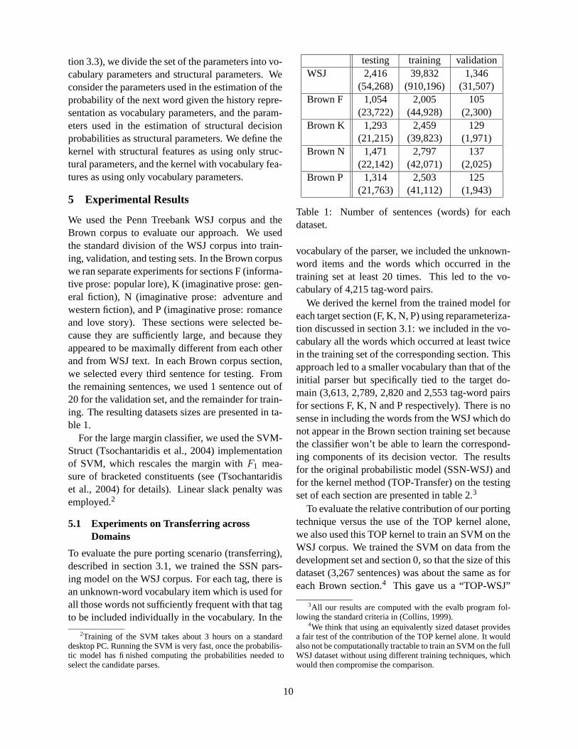
We used the Penn Treebank WSJ corpus and theBrown corpus to evaluate our approach. We usedthe standard division of the WSJ corpus into train-ing, validation, and testing sets. In the Brown corpuswe ran separate experiments for sections F (informa-tive prose: popular lore), K (imaginative prose: gen-eral fiction), N (imaginative prose: adventure andwestern fiction), and P (imaginative prose: romanceand love story). These sections were selected be-cause they are sufficiently large, and because theyappeared to be maximally different from each otherand from WSJ text. In each Brown corpus section,we selected every third sentence for testing. Fromthe remaining sentences, we used 1 sentence out of20 for the validation set, and the remainder for train-ing. The resulting datasets sizes are presented in ta-ble 1.
For the large margin classifier, we used the SVM-Struct (Tsochantaridis et al., 2004) implementationof SVM, which rescales the margin with F1 mea-sure of bracketed constituents (see (Tsochantaridiset al., 2004) for details). Linear slack penalty wasemployed.2
5.1 Experiments on Transferring acrossDomains
To evaluate the pure porting scenario (transferring),described in section 3.1, we trained the SSN pars-ing model on the WSJ corpus. For each tag, there isan unknown-word vocabulary item which is used forall those words not sufficiently frequent with that tagto be included individually in the vocabulary. In the
2Training of the SVM takes about 3 hours on a standarddesktop PC. Running the SVM is very fast, once the probabilis-tic model has finished computing the probabilities needed toselect the candidate parses.
testing training validationWSJ 2,416 39,832 1,346
(54,268) (910,196) (31,507)Brown F 1,054 2,005 105
(23,722) (44,928) (2,300)Brown K 1,293 2,459 129
(21,215) (39,823) (1,971)Brown N 1,471 2,797 137
(22,142) (42,071) (2,025)Brown P 1,314 2,503 125
(21,763) (41,112) (1,943)
Table 1: Number of sentences (words) for eachdataset.
vocabulary of the parser, we included the unknown-word items and the words which occurred in thetraining set at least 20 times. This led to the vo-cabulary of 4,215 tag-word pairs.
We derived the kernel from the trained model foreach target section (F, K, N, P) using reparameteriza-tion discussed in section 3.1: we included in the vo-cabulary all the words which occurred at least twicein the training set of the corresponding section. Thisapproach led to a smaller vocabulary than that of theinitial parser but specifically tied to the target do-main (3,613, 2,789, 2,820 and 2,553 tag-word pairsfor sections F, K, N and P respectively). There is nosense in including the words from the WSJ which donot appear in the Brown section training set becausethe classifier won’t be able to learn the correspond-ing components of its decision vector. The resultsfor the original probabilistic model (SSN-WSJ) andfor the kernel method (TOP-Transfer) on the testingset of each section are presented in table 2.3
To evaluate the relative contribution of our portingtechnique versus the use of the TOP kernel alone,we also used this TOP kernel to train an SVM on theWSJ corpus. We trained the SVM on data from thedevelopment set and section 0, so that the size of thisdataset (3,267 sentences) was about the same as foreach Brown section.4 This gave us a “TOP-WSJ”
3All our results are computed with the evalb program fol-lowing the standard criteria in (Collins, 1999).
4We think that using an equivalently sized dataset providesa fair test of the contribution of the TOP kernel alone. It wouldalso not be computationally tractable to train an SVM on the fullWSJ dataset without using different training techniques, whichwould then compromise the comparison.
10
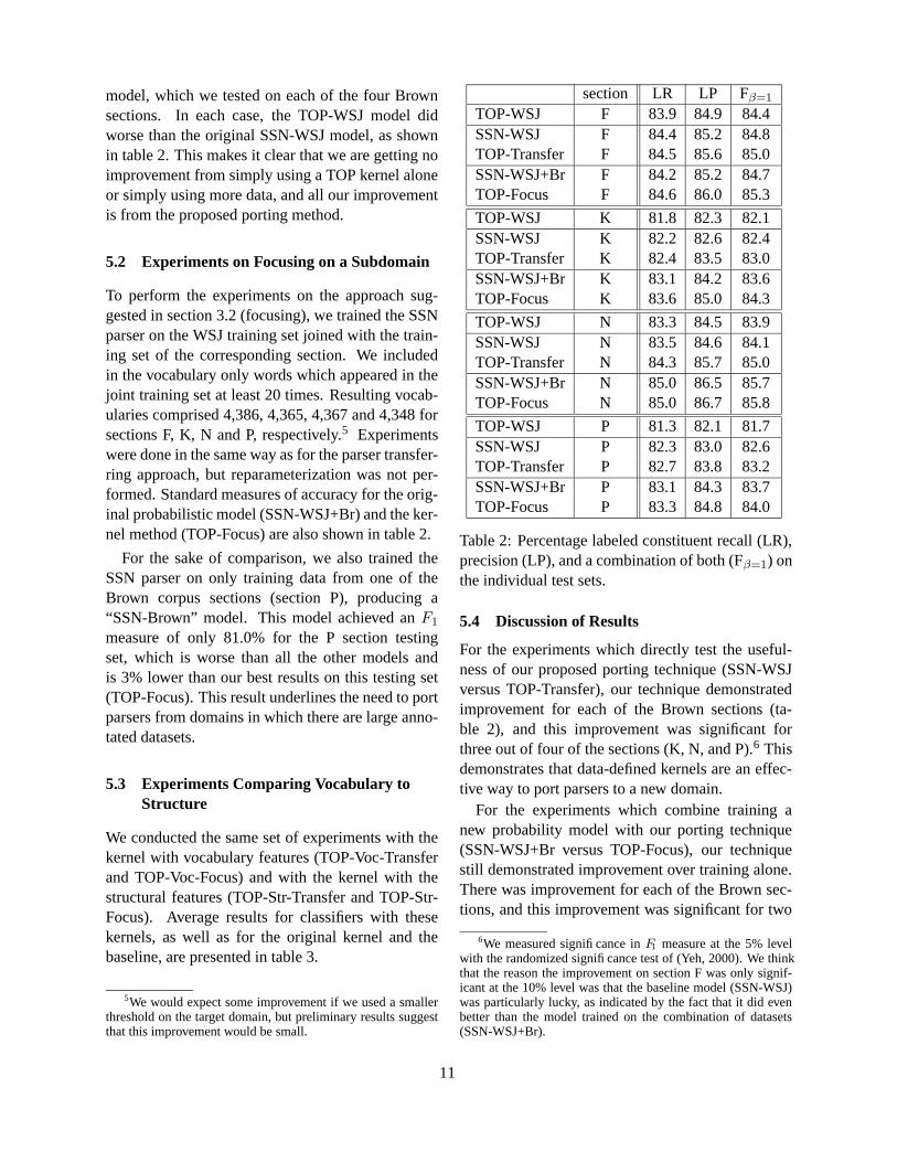
model, which we tested on each of the four Brownsections. In each case, the TOP-WSJ model didworse than the original SSN-WSJ model, as shownin table 2. This makes it clear that we are getting noimprovement from simply using a TOP kernel aloneor simply using more data, and all our improvementis from the proposed porting method.
5.2 Experiments on Focusing on a Subdomain
To perform the experiments on the approach sug-gested in section 3.2 (focusing), we trained the SSNparser on the WSJ training set joined with the train-ing set of the corresponding section. We includedin the vocabulary only words which appeared in thejoint training set at least 20 times. Resulting vocab-ularies comprised 4,386, 4,365, 4,367 and 4,348 forsections F, K, N and P, respectively.5 Experimentswere done in the same way as for the parser transfer-ring approach, but reparameterization was not per-formed. Standard measures of accuracy for the orig-inal probabilistic model (SSN-WSJ+Br) and the ker-nel method (TOP-Focus) are also shown in table 2.
For the sake of comparison, we also trained theSSN parser on only training data from one of theBrown corpus sections (section P), producing a“SSN-Brown” model. This model achieved an F1
measure of only 81.0% for the P section testingset, which is worse than all the other models andis 3% lower than our best results on this testing set(TOP-Focus). This result underlines the need to portparsers from domains in which there are large anno-tated datasets.
5.3 Experiments Comparing Vocabulary toStructure
We conducted the same set of experiments with thekernel with vocabulary features (TOP-Voc-Transferand TOP-Voc-Focus) and with the kernel with thestructural features (TOP-Str-Transfer and TOP-Str-Focus). Average results for classifiers with thesekernels, as well as for the original kernel and thebaseline, are presented in table 3.
5We would expect some improvement if we used a smallerthreshold on the target domain, but preliminary results suggestthat this improvement would be small.
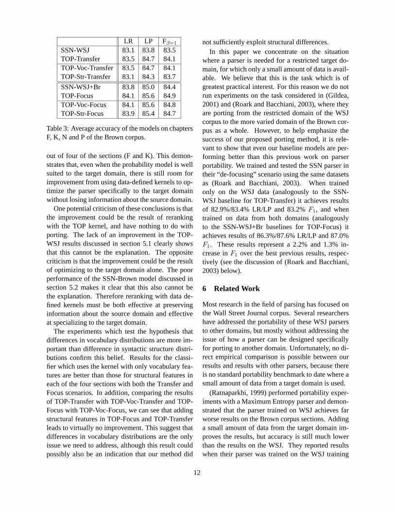
section LR LP Fβ=1
TOP-WSJ F 83.9 84.9 84.4SSN-WSJ F 84.4 85.2 84.8TOP-Transfer F 84.5 85.6 85.0SSN-WSJ+Br F 84.2 85.2 84.7TOP-Focus F 84.6 86.0 85.3
TOP-WSJ K 81.8 82.3 82.1SSN-WSJ K 82.2 82.6 82.4TOP-Transfer K 82.4 83.5 83.0SSN-WSJ+Br K 83.1 84.2 83.6TOP-Focus K 83.6 85.0 84.3
TOP-WSJ N 83.3 84.5 83.9SSN-WSJ N 83.5 84.6 84.1TOP-Transfer N 84.3 85.7 85.0SSN-WSJ+Br N 85.0 86.5 85.7TOP-Focus N 85.0 86.7 85.8
TOP-WSJ P 81.3 82.1 81.7SSN-WSJ P 82.3 83.0 82.6TOP-Transfer P 82.7 83.8 83.2SSN-WSJ+Br P 83.1 84.3 83.7TOP-Focus P 83.3 84.8 84.0
Table 2: Percentage labeled constituent recall (LR),precision (LP), and a combination of both (Fβ=1) onthe individual test sets.
5.4 Discussion of Results
For the experiments which directly test the useful-ness of our proposed porting technique (SSN-WSJversus TOP-Transfer), our technique demonstratedimprovement for each of the Brown sections (ta-ble 2), and this improvement was significant forthree out of four of the sections (K, N, and P).6 Thisdemonstrates that data-defined kernels are an effec-tive way to port parsers to a new domain.
For the experiments which combine training anew probability model with our porting technique(SSN-WSJ+Br versus TOP-Focus), our techniquestill demonstrated improvement over training alone.There was improvement for each of the Brown sec-tions, and this improvement was significant for two
6We measured significance in F1 measure at the 5% levelwith the randomized significance test of (Yeh, 2000). We thinkthat the reason the improvement on section F was only signif-icant at the 10% level was that the baseline model (SSN-WSJ)was particularly lucky, as indicated by the fact that it did evenbetter than the model trained on the combination of datasets(SSN-WSJ+Br).
11
LR LP Fβ=1
SSN-WSJ 83.1 83.8 83.5TOP-Transfer 83.5 84.7 84.1TOP-Voc-Transfer 83.5 84.7 84.1TOP-Str-Transfer 83.1 84.3 83.7
SSN-WSJ+Br 83.8 85.0 84.4TOP-Focus 84.1 85.6 84.9TOP-Voc-Focus 84.1 85.6 84.8TOP-Str-Focus 83.9 85.4 84.7
Table 3: Average accuracy of the models on chaptersF, K, N and P of the Brown corpus.
out of four of the sections (F and K). This demon-strates that, even when the probability model is wellsuited to the target domain, there is still room forimprovement from using data-defined kernels to op-timize the parser specifically to the target domainwithout losing information about the source domain.
One potential criticism of these conclusions is thatthe improvement could be the result of rerankingwith the TOP kernel, and have nothing to do withporting. The lack of an improvement in the TOP-WSJ results discussed in section 5.1 clearly showsthat this cannot be the explanation. The oppositecriticism is that the improvement could be the resultof optimizing to the target domain alone. The poorperformance of the SSN-Brown model discussed insection 5.2 makes it clear that this also cannot bethe explanation. Therefore reranking with data de-fined kernels must be both effective at preservinginformation about the source domain and effectiveat specializing to the target domain.
The experiments which test the hypothesis thatdifferences in vocabulary distributions are more im-portant than difference in syntactic structure distri-butions confirm this belief. Results for the classi-fier which uses the kernel with only vocabulary fea-tures are better than those for structural features ineach of the four sections with both the Transfer andFocus scenarios. In addition, comparing the resultsof TOP-Transfer with TOP-Voc-Transfer and TOP-Focus with TOP-Voc-Focus, we can see that addingstructural features in TOP-Focus and TOP-Transferleads to virtually no improvement. This suggest thatdifferences in vocabulary distributions are the onlyissue we need to address, although this result couldpossibly also be an indication that our method did
not sufficiently exploit structural differences.In this paper we concentrate on the situation
where a parser is needed for a restricted target do-main, for which only a small amount of data is avail-able. We believe that this is the task which is ofgreatest practical interest. For this reason we do notrun experiments on the task considered in (Gildea,2001) and (Roark and Bacchiani, 2003), where theyare porting from the restricted domain of the WSJcorpus to the more varied domain of the Brown cor-pus as a whole. However, to help emphasize thesuccess of our proposed porting method, it is rele-vant to show that even our baseline models are per-forming better than this previous work on parserportability. We trained and tested the SSN parser intheir “de-focusing” scenario using the same datasetsas (Roark and Bacchiani, 2003). When trainedonly on the WSJ data (analogously to the SSN-WSJ baseline for TOP-Transfer) it achieves resultsof 82.9%/83.4% LR/LP and 83.2% F1, and whentrained on data from both domains (analogouslyto the SSN-WSJ+Br baselines for TOP-Focus) itachieves results of 86.3%/87.6% LR/LP and 87.0%F1. These results represent a 2.2% and 1.3% in-crease in F1 over the best previous results, respec-tively (see the discussion of (Roark and Bacchiani,2003) below).
6 Related Work
Most research in the field of parsing has focused onthe Wall Street Journal corpus. Several researchershave addressed the portability of these WSJ parsersto other domains, but mostly without addressing theissue of how a parser can be designed specificallyfor porting to another domain. Unfortunately, no di-rect empirical comparison is possible between ourresults and results with other parsers, because thereis no standard portability benchmark to date where asmall amount of data from a target domain is used.
(Ratnaparkhi, 1999) performed portability exper-iments with a Maximum Entropy parser and demon-strated that the parser trained on WSJ achieves farworse results on the Brown corpus sections. Addinga small amount of data from the target domain im-proves the results, but accuracy is still much lowerthan the results on the WSJ. They reported resultswhen their parser was trained on the WSJ training
12
set plus a portion of 2,000 sentences from a Browncorpus section. They achieved 80.9%/80.3% re-call/precision for section K, and 80.6%/81.3% forsection N.7 Our analogous method (TOP-Focus)achieved much better accuracy (3.7% and 4.9% bet-ter F1, respectively).
In addition to portability experiments with theparsing model of (Collins, 1997), (Gildea, 2001)provided a comprehensive analysis of parser porta-bility. On the basis of this analysis, a tech-nique for parameter pruning was proposed leadingto a significant reduction in the model size with-out a large decrease of accuracy. Gildea (2001)only reports results on sentences of 40 or lesswords on all the Brown corpus sections combined,for which he reports 80.3%/81.0% recall/precisionwhen training only on data from the WSJ corpus,and 83.9%/84.8% when training on data from theWSJ corpus and all sections of the Brown corpus.
(Roark and Bacchiani, 2003) performed experi-ments on supervised and unsupervised PCFG adap-tation to the target domain. They propose to usethe statistics from a source domain to define pri-ors over weights. However, in their experimentsthey used only trivial sub-cases of this approach,namely, count merging and model interpolation.They achieved very good improvement over theirbaseline and over (Gildea, 2001), but the absoluteaccuracies were still relatively low (as discussedabove). They report results with combined Browndata (on sentences of 100 words or less), achieving81.3%/80.9% when training only on the WSJ cor-pus and 85.4%/85.9% with their best method usingthe data from both domains.
7 Conclusions
This paper proposes a novel technique for improv-ing parser portability, applying parse reranking withdata-defined kernels. First a probabilistic model ofparsing is trained on all the available data, includinga large set of data from the source domain. Thismodel is used to define a kernel over parse trees.Then this kernel is used in a large margin classifier
7The sizes of Brown sections reported in (Ratnaparkhi,1999) do not match the sizes of sections distributed in the PennTreebank 3.0 package, so we couldn’t replicate their split. Wesuspect that a preliminary version of the corpus was used fortheir experiments.
trained on a small set of data only from the target do-main. This classifier is used to rerank the top parsesproduced by the probabilistic model on the target do-main. Experiments with a neural network statisticalparser demonstrate that this approach leads to im-proved parser accuracy on the target domain, with-out any significant increase in computational cost.
ReferencesMichael Collins and Nigel Duffy. 2002. New ranking algo-
rithms for parsing and tagging: Kernels over discrete struc-tures and the voted perceptron. In Proc. ACL 2002 , pages263–270, Philadelphia, PA.
Michael Collins. 1997. Three generative, lexicalized modelsfor statistical parsing. In Proc. ACL/EACL 1997 , pages 16–23, Somerset, New Jersey.
Michael Collins. 1999. Head-Driven Statistical Models forNatural Language Parsing. Ph.D. thesis, University ofPennsylvania, Philadelphia, PA.
Daniel Gildea. 2001. Corpus variation and parser performance.In Proc. EMNLP 2001 , Pittsburgh, PA.
James Henderson and Ivan Titov. 2005. Data-defined kernelsfor parse reranking derived from probabilistic models. InProc. ACL 2005 , Ann Arbor, MI.
James Henderson. 2003. Inducing history representations forbroad coverage statistical parsing. In Proc. NAACL/HLT2003 , pages 103–110, Edmonton, Canada.
Terry Koo and Michael Collins. 2005. Hidden-variable modelsfor discriminative reranking. In Proc. EMNLP 2005 , Van-couver, B.C., Canada.
Mitchell P. Marcus, Beatrice Santorini, and Mary AnnMarcinkiewicz. 1993. Building a large annotated corpusof English: The Penn Treebank. Computational Linguistics,19(2):313–330.
Takuya Matsuzaki, Yusuke Miyao, and Jun’ichi Tsujii. 2005.Probabilistic CFG with latent annotations. In Proc. ACL2005 , Ann Arbor, MI.
Adwait Ratnaparkhi. 1999. Learning to parse natural languagewith maximum entropy models. Machine Learning, 34:151–175.
Brian Roark and Michiel Bacchiani. 2003. Supervised andunsuperised PCFG adaptation to novel domains. In Proc.HLT/ACL 2003 , Edmionton, Canada.
Libin Shen and Aravind K. Joshi. 2003. An SVM based votingalgorithm with application to parse reranking. In Proc. 7thConf. on Computational Natural Language Learning, pages9–16, Edmonton, Canada.
Ioannis Tsochantaridis, Thomas Hofmann, Thorsten Joachims,and Yasemin Altun. 2004. Support vector machine learningfor interdependent and structured output spaces. In Proc.21st Int. Conf. on Machine Learning, pages 823–830, Banff,Alberta, Canada.
Alexander Yeh. 2000. More accurate tests for the statisticalsignificance of the result differences. In Proc. 17th Int. Conf.on Computational Linguistics, pages 947–953, Saarbruken,Germany.
13

Proceedings of the 10th Conference on Computational Natural Language Learning (CoNLL-X),pages 14–20, New York City, June 2006.c©2006 Association for Computational Linguistics
Non-Local Modeling with a Mixture of PCFGs
Slav Petrov Leon Barrett Dan KleinComputer Science Division, EECS Department
University of California at BerkeleyBerkeley, CA 94720
{petrov, lbarrett, klein}@eecs.berkeley.edu
Abstract
While most work on parsing with PCFGshas focused on local correlations betweentree configurations, we attempt to modelnon-local correlations using a finite mix-ture of PCFGs. A mixture grammar fitwith the EM algorithm shows improve-ment over a single PCFG, both in parsingaccuracy and in test data likelihood. Weargue that this improvement comes fromthe learning of specialized grammars thatcapture non-local correlations.
1 Introduction
The probabilistic context-free grammar (PCFG) for-malism is the basis of most modern statisticalparsers. The symbols in a PCFG encode context-freedom assumptions about statistical dependenciesin the derivations of sentences, and the relative con-ditional probabilities of the grammar rules inducescores on trees. Compared to a basic treebankgrammar (Charniak, 1996), the grammars of high-accuracy parsers weaken independence assumptionsby splitting grammar symbols and rules with ei-ther lexical (Charniak, 2000; Collins, 1999) or non-lexical (Klein and Manning, 2003; Matsuzaki et al.,2005) conditioning information. While such split-ting, or conditioning, can cause problems for sta-tistical estimation, it can dramatically improve theaccuracy of a parser.
However, the configurations exploited in PCFGparsers are quite local: rules’ probabilities may de-pend on parents or head words, but do not dependon arbitrarily distant tree configurations. For exam-ple, it is generally not modeled that if one quantifier
phrase (QP in the Penn Treebank) appears in a sen-tence, the likelihood of finding another QP in thatsame sentence is greatly increased. This kind of ef-fect is neither surprising nor unknown – for exam-ple, Bock and Loebell (1990) show experimentallythat human language generation demonstrates prim-ing effects. The mediating variables can not only in-clude priming effects but also genre or stylistic con-ventions, as well as many other factors which are notadequately modeled by local phrase structure.
A reasonable way to add a latent variable to agenerative model is to use a mixture of estimators,in this case a mixture of PCFGs (see Section 3).The general mixture of estimators approach was firstsuggested in the statistics literature by Titteringtonet al. (1962) and has since been adopted in machinelearning (Ghahramani and Jordan, 1994). In a mix-ture approach, we have a new global variable onwhich all PCFG productions for a given sentencecan be conditioned. In this paper, we experimentwith a finite mixture of PCFGs. This is similar to thelatent nonterminals used in Matsuzaki et al. (2005),but because the latent variable we use is global, ourapproach is more oriented toward learning non-localstructure. We demonstrate that a mixture fit with theEM algorithm gives improved parsing accuracy andtest data likelihood. We then investigate what is andis not being learned by the latent mixture variable.While mixture components are difficult to interpret,we demonstrate that the patterns learned are betterthan random splits.
2 Empirical Motivation
It is commonly accepted that the context freedomassumptions underlying the PCFG model are too
14
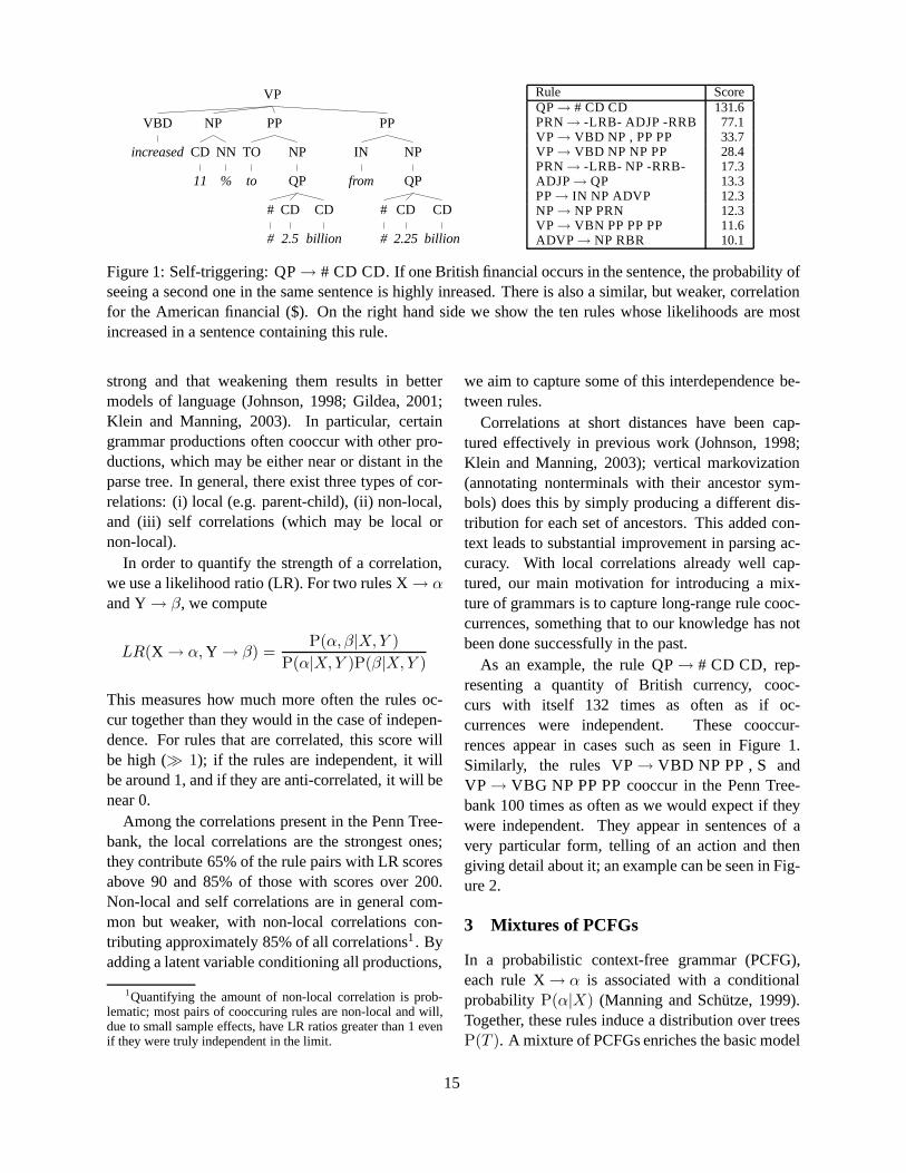
VP
VBD
increased
NP
CD
11
NN
%
PP
TO
to
NP
QP
#
#
CD
2.5
CD
billion
PP
IN
from
NP
QP
#
#
CD
2.25
CD
billion
Rule ScoreQP→ # CD CD 131.6PRN→ -LRB- ADJP -RRB 77.1VP→ VBD NP , PP PP 33.7VP→ VBD NP NP PP 28.4PRN→ -LRB- NP -RRB- 17.3ADJP→ QP 13.3PP→ IN NP ADVP 12.3NP→ NP PRN 12.3VP→ VBN PP PP PP 11.6ADVP→ NP RBR 10.1
Figure 1: Self-triggering: QP→ # CD CD. If one British financial occurs in the sentence, the probability ofseeing a second one in the same sentence is highly inreased. There is also a similar, but weaker, correlationfor the American financial ($). On the right hand side we show the ten rules whose likelihoods are mostincreased in a sentence containing this rule.
strong and that weakening them results in bettermodels of language (Johnson, 1998; Gildea, 2001;Klein and Manning, 2003). In particular, certaingrammar productions often cooccur with other pro-ductions, which may be either near or distant in theparse tree. In general, there exist three types of cor-relations: (i) local (e.g. parent-child), (ii) non-local,and (iii) self correlations (which may be local ornon-local).
In order to quantify the strength of a correlation,we use a likelihood ratio (LR). For two rules X→ α
and Y→ β, we compute
LR(X → α, Y → β) =P(α, β|X,Y )
P(α|X,Y )P(β|X,Y )
This measures how much more often the rules oc-cur together than they would in the case of indepen-dence. For rules that are correlated, this score willbe high (≫ 1); if the rules are independent, it willbe around 1, and if they are anti-correlated, it will benear 0.
Among the correlations present in the Penn Tree-bank, the local correlations are the strongest ones;they contribute 65% of the rule pairs with LR scoresabove 90 and 85% of those with scores over 200.Non-local and self correlations are in general com-mon but weaker, with non-local correlations con-tributing approximately 85% of all correlations1. Byadding a latent variable conditioning all productions,
1Quantifying the amount of non-local correlation is prob-lematic; most pairs of cooccuring rules are non-local and will,due to small sample effects, have LR ratios greater than 1 evenif they were truly independent in the limit.
we aim to capture some of this interdependence be-tween rules.
Correlations at short distances have been cap-tured effectively in previous work (Johnson, 1998;Klein and Manning, 2003); vertical markovization(annotating nonterminals with their ancestor sym-bols) does this by simply producing a different dis-tribution for each set of ancestors. This added con-text leads to substantial improvement in parsing ac-curacy. With local correlations already well cap-tured, our main motivation for introducing a mix-ture of grammars is to capture long-range rule cooc-currences, something that to our knowledge has notbeen done successfully in the past.
As an example, the rule QP→ # CD CD, rep-resenting a quantity of British currency, cooc-curs with itself 132 times as often as if oc-currences were independent. These cooccur-rences appear in cases such as seen in Figure 1.Similarly, the rules VP→ VBD NP PP , S andVP→ VBG NP PP PP cooccur in the Penn Tree-bank 100 times as often as we would expect if theywere independent. They appear in sentences of avery particular form, telling of an action and thengiving detail about it; an example can be seen in Fig-ure 2.
3 Mixtures of PCFGs
In a probabilistic context-free grammar (PCFG),each rule X→ α is associated with a conditionalprobability P(α|X) (Manning and Schutze, 1999).Together, these rules induce a distribution over treesP(T ). A mixture of PCFGs enriches the basic model
15
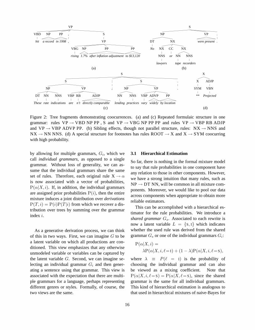
VP
VBD
hit
NP
a record
PP
in 1998
,
,
S
VP
VBG
rising
NP
1.7%
PP
after inflation adjustment
PP
to $13,120
S
NP
DT
No
NX
NX
NNS
lawyers
CC
or
NX
NN
tape
NNS
recorders
VP
were present
.
.
(a) (b)
S
S
NP
DT
These
NN
rate
NNS
indications
VP
VBP
are
RB
n’t
ADJP
directly comparable
:
;
S
NP
NN
lending
NNS
practices
VP
VBP
vary
ADVP
widely
PP
by location
.
.
X
X
SYM
**
ADJP
VBN
Projected
(c) (d)
Figure 2: Tree fragments demonstrating coocurrences. (a) and (c) Repeated formulaic structure in onegrammar: rules VP→ VBD NP PP , S and VP→ VBG NP PP PP and rules VP→ VBP RB ADJPand VP→ VBP ADVP PP. (b) Sibling effects, though not parallel structure, rules: NX→ NNS andNX → NN NNS. (d) A special structure for footnotes has rules ROOT→ X and X→ SYM coocurringwith high probability.
by allowing for multiple grammars,Gi, which wecall individual grammars, as opposed to a singlegrammar. Without loss of generality, we can as-sume that the individual grammars share the sameset of rules. Therefore, each original rule X→ α
is now associated with a vector of probabilities,P(α|X, i). If, in addition, the individual grammarsare assigned prior probabilitiesP(i), then the entiremixture induces a joint distribution overderivationsP(T, i) = P(i)P(T |i) from which we recover a dis-tribution over trees by summing over the grammarindexi.
As a generative derivation process, we can thinkof this in two ways. First, we can imagineG to bea latent variable on which all productions are con-ditioned. This view emphasizes that any otherwiseunmodeled variable or variables can be captured bythe latent variableG. Second, we can imagine se-lecting an individual grammarGi and then gener-ating a sentence using that grammar. This view isassociated with the expectation that there are multi-ple grammars for a language, perhaps representingdifferent genres or styles. Formally, of course, thetwo views are the same.
3.1 Hierarchical Estimation
So far, there is nothing in the formal mixture modelto say that rule probabilities in one component haveany relation to those in other components. However,we have a strong intuition that many rules, such asNP→ DT NN, will be common in all mixture com-ponents. Moreover, we would like to pool our dataacross components when appropriate to obtain morereliable estimators.
This can be accomplished with a hierarchical es-timator for the rule probabilities. We introduce ashared grammarGs. Associated to each rewrite isnow a latent variableL = {S, I} which indicateswhether the used rule was derived from the sharedgrammarGs or one of the individual grammarsGi:
P(α|X, i) =
λP(α|X, i, ℓ= I) + (1− λ)P(α|X, i, ℓ=S),
where λ ≡ P (ℓ = I) is the probability ofchoosing the individual grammar and can alsobe viewed as a mixing coefficient. Note thatP(α|X, i, ℓ=S) = P(α|X, ℓ=S), since the sharedgrammar is the same for all individual grammars.This kind of hierarchical estimation is analogous tothat used in hierarchical mixtures of naive-Bayes for
16
text categorization (McCallum et al., 1998).The hierarchical estimator is most easily de-
scribed as a generative model. First, we choose aindividual grammarGi. Then, for each nonterminal,we select a level from the back-off hierarchy gram-mar: the individual grammarGi with probabilityλ,and the shared grammarGs with probability1 − λ.Finally, we select a rewrite from the chosen level. Toemphasize: the derivation of a phrase-structure treein a hierarchically-estimated mixture of PCFGs in-volves two kinds of hidden variables: the grammarG used for each sentence, and the levelL used ateach tree node. These hidden variables will impactboth learning and inference in this model.
3.2 Inference: Parsing
Parsing involves inference for a given sentenceS.One would generally like to calculate themost prob-able parse– that is, the treeT which has the high-est probability P(T |S) ∝
∑i P(i)P(T |i). How-
ever, this is difficult for mixture models. For a singlegrammar we have:
P(T, i) = P(i)∏
X→α∈T
P(α|X, i).
This score decomposes into a product and it is sim-ple to construct a dynamic programming algorithmto find the optimalT (Baker, 1979). However, for amixture of grammars we need to sum over the indi-vidual grammars:
∑
i
P(T, i) =∑
i
P(i)∏
X→α∈T
P(α|X, i).
Because of the outer sum, this expression unfor-tunately does not decompose into a product overscores of subparts. In particular, a tree which maxi-mizes the sum need not be a top tree for any singlecomponent.
As is true for many other grammar formalisms inwhich there is a derivation / parse distinction, an al-ternative to finding the most probable parse is to findthe most probable derivation(Vijay-Shankar andJoshi, 1985; Bod, 1992; Steedman, 2000). Insteadof finding the treeT which maximizes
∑i P(T, i),
we find both the treeT and componenti which max-imize P(T, i). The most probable derivation can befound by simply doing standard PCFG parsing oncefor each component, then comparing the resultingtrees’ likelihoods.
3.3 Learning: Training
Training a mixture of PCFGs from a treebank is anincomplete data problem. We need to decide whichindividual grammar gave rise to a given observedtree. Moreover, we need to select a generation path(individual grammar or shared grammar) for eachrule in the tree. To learn estimate parameters, wecan use a standard Expectation-Maximization (EM)approach.
In the E-step, we compute the posterior distribu-tions of the latent variables, which are in this caseboth the componentG of each sentence and the hier-archy levelL of each rewrite. Note that, unlike dur-ing parsing, there is no uncertainty over the actualrules used, so the E-step does not require summingover possible trees. Specifically, for the variableG
we have
P(i|T ) =P(T, i)∑j P(T, j)
.
For the hierarchy levelL we can write
P(ℓ = I|X → α, i, T ) =
λP(α|X, ℓ= I)
λP(α|X, i, ℓ= I) + (1− λ)P(α|X, ℓ=S),
where we slightly abuse notation since the ruleX → α can occur multiple times in a tree T.
In the M-step, we find the maximum-likelihoodmodel parameters given these posterior assign-ments; i.e., we find the best grammars given the waythe training data’s rules are distributed between in-dividual and shared grammars. This is done exactlyas in the standard single-grammar model using rela-tive expected frequencies. The updates are shown inFigure 3.3, whereT = {T1, T2, . . . } is the trainingset.
We initialize the algorithm by setting the assign-ments from sentences to grammars to be uniformbetween all the individual grammars, with a smallrandom perturbation to break symmetry.
4 Results
We ran our experiments on the Wall Street Jour-nal (WSJ) portion of the Penn Treebank using thestandard setup: We trained on sections 2 to 21,and we used section 22 as a validation set for tun-ing model hyperparameters. Results are reported
17
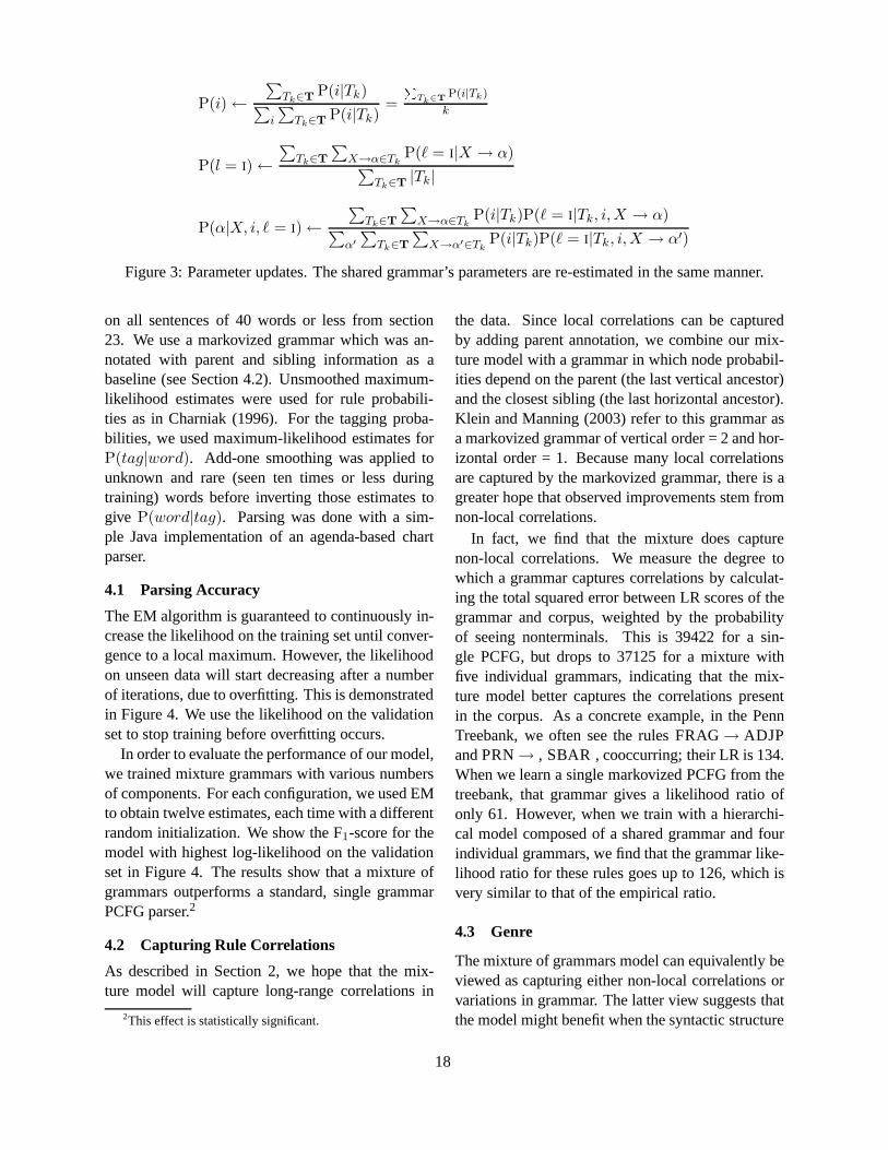
P(i)←
∑Tk∈T
P(i|Tk)∑
i
∑Tk∈T
P(i|Tk)=
PTk∈T
P(i|Tk)
k
P(l = I)←
∑Tk∈T
∑X→α∈Tk
P(ℓ = I|X → α)∑
Tk∈T|Tk|
P(α|X, i, ℓ = I)←
∑Tk∈T
∑X→α∈Tk
P(i|Tk)P(ℓ = I|Tk, i,X → α)∑
α′
∑Tk∈T
∑X→α′∈Tk
P(i|Tk)P(ℓ = I|Tk, i,X → α′)
Figure 3: Parameter updates. The shared grammar’s parameters are re-estimated in the same manner.
on all sentences of 40 words or less from section23. We use a markovized grammar which was an-notated with parent and sibling information as abaseline (see Section 4.2). Unsmoothed maximum-likelihood estimates were used for rule probabili-ties as in Charniak (1996). For the tagging proba-bilities, we used maximum-likelihood estimates forP(tag|word). Add-one smoothing was applied tounknown and rare (seen ten times or less duringtraining) words before inverting those estimates togive P(word|tag). Parsing was done with a sim-ple Java implementation of an agenda-based chartparser.
4.1 Parsing Accuracy
The EM algorithm is guaranteed to continuously in-crease the likelihood on the training set until conver-gence to a local maximum. However, the likelihoodon unseen data will start decreasing after a numberof iterations, due to overfitting. This is demonstratedin Figure 4. We use the likelihood on the validationset to stop training before overfitting occurs.
In order to evaluate the performance of our model,we trained mixture grammars with various numbersof components. For each configuration, we used EMto obtain twelve estimates, each time with a differentrandom initialization. We show the F1-score for themodel with highest log-likelihood on the validationset in Figure 4. The results show that a mixture ofgrammars outperforms a standard, single grammarPCFG parser.2
4.2 Capturing Rule Correlations
As described in Section 2, we hope that the mix-ture model will capture long-range correlations in
2This effect is statistically significant.
the data. Since local correlations can be capturedby adding parent annotation, we combine our mix-ture model with a grammar in which node probabil-ities depend on the parent (the last vertical ancestor)and the closest sibling (the last horizontal ancestor).Klein and Manning (2003) refer to this grammar asa markovized grammar of vertical order = 2 and hor-izontal order = 1. Because many local correlationsare captured by the markovized grammar, there is agreater hope that observed improvements stem fromnon-local correlations.
In fact, we find that the mixture does capturenon-local correlations. We measure the degree towhich a grammar captures correlations by calculat-ing the total squared error between LR scores of thegrammar and corpus, weighted by the probabilityof seeing nonterminals. This is 39422 for a sin-gle PCFG, but drops to 37125 for a mixture withfive individual grammars, indicating that the mix-ture model better captures the correlations presentin the corpus. As a concrete example, in the PennTreebank, we often see the rules FRAG→ ADJPand PRN→ , SBAR , cooccurring; their LR is 134.When we learn a single markovized PCFG from thetreebank, that grammar gives a likelihood ratio ofonly 61. However, when we train with a hierarchi-cal model composed of a shared grammar and fourindividual grammars, we find that the grammar like-lihood ratio for these rules goes up to 126, which isvery similar to that of the empirical ratio.
4.3 Genre
The mixture of grammars model can equivalently beviewed as capturing either non-local correlations orvariations in grammar. The latter view suggests thatthe model might benefit when the syntactic structure
18
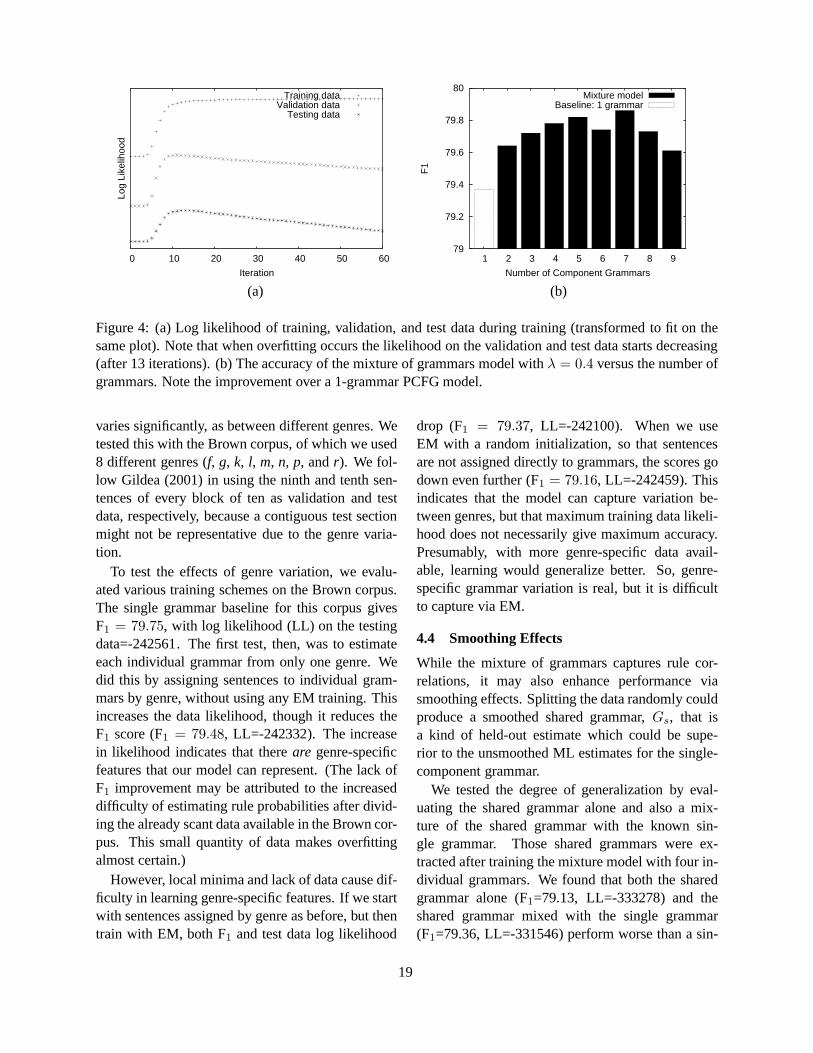
0 10 20 30 40 50 60
Log
Like
lihoo
d
Iteration
Training dataValidation data
Testing data
79
79.2
79.4
79.6
79.8
80
1 2 3 4 5 6 7 8 9
F1
Number of Component Grammars
Mixture modelBaseline: 1 grammar
(a) (b)
Figure 4: (a) Log likelihood of training, validation, and test data during training (transformed to fit on thesame plot). Note that when overfitting occurs the likelihoodon the validation and test data starts decreasing(after 13 iterations). (b) The accuracy of the mixture of grammars model withλ = 0.4 versus the number ofgrammars. Note the improvement over a 1-grammar PCFG model.
varies significantly, as between different genres. Wetested this with the Brown corpus, of which we used8 different genres (f, g, k, l, m, n, p, andr). We fol-low Gildea (2001) in using the ninth and tenth sen-tences of every block of ten as validation and testdata, respectively, because a contiguous test sectionmight not be representative due to the genre varia-tion.
To test the effects of genre variation, we evalu-ated various training schemes on the Brown corpus.The single grammar baseline for this corpus givesF1 = 79.75, with log likelihood (LL) on the testingdata=-242561. The first test, then, was to estimateeach individual grammar from only one genre. Wedid this by assigning sentences to individual gram-mars by genre, without using any EM training. Thisincreases the data likelihood, though it reduces theF1 score (F1 = 79.48, LL=-242332). The increasein likelihood indicates that thereare genre-specificfeatures that our model can represent. (The lack ofF1 improvement may be attributed to the increaseddifficulty of estimating rule probabilities after divid-ing the already scant data available in the Brown cor-pus. This small quantity of data makes overfittingalmost certain.)
However, local minima and lack of data cause dif-ficulty in learning genre-specific features. If we startwith sentences assigned by genre as before, but thentrain with EM, both F1 and test data log likelihood
drop (F1 = 79.37, LL=-242100). When we useEM with a random initialization, so that sentencesare not assigned directly to grammars, the scores godown even further (F1 = 79.16, LL=-242459). Thisindicates that the model can capture variation be-tween genres, but that maximum training data likeli-hood does not necessarily give maximum accuracy.Presumably, with more genre-specific data avail-able, learning would generalize better. So, genre-specific grammar variation is real, but it is difficultto capture via EM.
4.4 Smoothing Effects
While the mixture of grammars captures rule cor-relations, it may also enhance performance viasmoothing effects. Splitting the data randomly couldproduce a smoothed shared grammar,Gs, that isa kind of held-out estimate which could be supe-rior to the unsmoothed ML estimates for the single-component grammar.
We tested the degree of generalization by eval-uating the shared grammar alone and also a mix-ture of the shared grammar with the known sin-gle grammar. Those shared grammars were ex-tracted after training the mixture model with four in-dividual grammars. We found that both the sharedgrammar alone (F1=79.13, LL=-333278) and theshared grammar mixed with the single grammar(F1=79.36, LL=-331546) perform worse than a sin-
19
gle PCFG (F1=79.37, LL=-327658). This indicatesthat smoothing is not the primary learning effectcontributing to increasedF1.
5 Conclusions
We examined the sorts of rule correlations that maybe found in natural language corpora, discoveringnon-local correlations not captured by traditionalmodels. We found that using a model capable ofrepresenting these non-local features gives improve-ment in parsing accuracy and data likelihood. Thisimprovement is modest, however, primarily becauselocal correlations are so much stronger than non-local ones.
References
J. Baker. 1979. Trainable grammars for speech recog-nition. Speech Communication Papers for the 97thMeeting of the Acoustical Society of America, pages547–550.
K. Bock and H. Loebell. 1990. Framing sentences.Cog-nition, 35:1–39.
R. Bod. 1992. A computational model of language per-formance: Data oriented parsing.International Con-ference on Computational Linguistics (COLING).
E. Charniak. 1996. Tree-bank grammars. InProc. ofthe 13th National Conference on Artificial Intelligence(AAAI), pages 1031–1036.
E. Charniak. 2000. A maximum–entropy–inspiredparser. InProc. of the Conference of the North Ameri-can chapter of the Association for Computational Lin-guistics (NAACL), pages 132–139.
M. Collins. 1999. Head-Driven Statistical Models forNatural Language Parsing. Ph.D. thesis, Univ. ofPennsylvania.
Z. Ghahramani and M. I. Jordan. 1994. Supervisedlearning from incomplete data via an EM approach. InAdvances in Neural Information Processing Systems(NIPS), pages 120–127.
D. Gildea. 2001. Corpus variation and parser perfor-mance.Conference on Empirical Methods in NaturalLanguage Processing (EMNLP).
M. Johnson. 1998. Pcfg models of linguistic tree repre-sentations.Computational Linguistics, 24:613–632.
D. Klein and C. Manning. 2003. Accurate unlexicalizedparsing. Proc. of the 41st Meeting of the Associationfor Computational Linguistics (ACL), pages 423–430.
C. Manning and H. Schutze. 1999.Foundations of Sta-tistical Natural Language Processing. The MIT Press,Cambridge, Massachusetts.
T. Matsuzaki, Y. Miyao, and J. Tsujii. 2005. Probabilis-tic CFG with latent annotations. InProc. of the 43rdMeeting of the Association for Computational Linguis-tics (ACL), pages 75–82.
A. McCallum, R. Rosenfeld, T. Mitchell, and A. Ng.1998. Improving text classification by shrinkage in ahierarchy of classes. InInt. Conf. on Machine Learn-ing (ICML), pages 359–367.
M. Steedman. 2000.The Syntactic Process.The MITPress, Cambridge, Massachusetts.
D. Titterington, A. Smith, and U. Makov. 1962.Statisti-cal Analysis of Finite Mixture Distributions. Wiley.
K. Vijay-Shankar and A. Joshi. 1985. Some computa-tional properties of tree adjoining grammars.Proc. ofthe 23th Meeting of the Association for ComputationalLinguistics (ACL), pages 82–93.
20
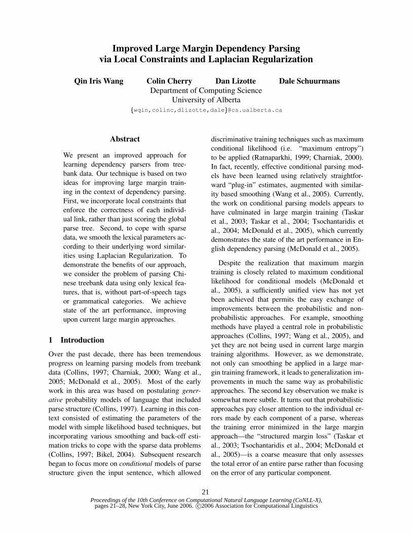
Proceedings of the 10th Conference on Computational Natural Language Learning (CoNLL-X),pages 21–28, New York City, June 2006.c©2006 Association for Computational Linguistics
Improved Large Margin Dependency Parsingvia Local Constraints and Laplacian Regularization
Qin Iris Wang Colin Cherry Dan Lizotte Dale SchuurmansDepartment of Computing Science
University of Alberta�wqin,colinc,dlizotte,dale � @cs.ualberta.ca
Abstract
We present an improved approach forlearning dependency parsers from tree-bank data. Our technique is based on twoideas for improving large margin train-ing in the context of dependency parsing.First, we incorporate local constraints thatenforce the correctness of each individ-ual link, rather than just scoring the globalparse tree. Second, to cope with sparsedata, we smooth the lexical parameters ac-cording to their underlying word similar-ities using Laplacian Regularization. Todemonstrate the benefits of our approach,we consider the problem of parsing Chi-nese treebank data using only lexical fea-tures, that is, without part-of-speech tagsor grammatical categories. We achievestate of the art performance, improvingupon current large margin approaches.
1 Introduction
Over the past decade, there has been tremendousprogress on learning parsing models from treebankdata (Collins, 1997; Charniak, 2000; Wang et al.,2005; McDonald et al., 2005). Most of the earlywork in this area was based on postulating gener-ative probability models of language that includedparse structure (Collins, 1997). Learning in this con-text consisted of estimating the parameters of themodel with simple likelihood based techniques, butincorporating various smoothing and back-off esti-mation tricks to cope with the sparse data problems(Collins, 1997; Bikel, 2004). Subsequent researchbegan to focus more on conditional models of parsestructure given the input sentence, which allowed
discriminative training techniques such as maximumconditional likelihood (i.e. “maximum entropy”)to be applied (Ratnaparkhi, 1999; Charniak, 2000).In fact, recently, effective conditional parsing mod-els have been learned using relatively straightfor-ward “plug-in” estimates, augmented with similar-ity based smoothing (Wang et al., 2005). Currently,the work on conditional parsing models appears tohave culminated in large margin training (Taskaret al., 2003; Taskar et al., 2004; Tsochantaridis etal., 2004; McDonald et al., 2005), which currentlydemonstrates the state of the art performance in En-glish dependency parsing (McDonald et al., 2005).
Despite the realization that maximum margintraining is closely related to maximum conditionallikelihood for conditional models (McDonald etal., 2005), a sufficiently unified view has not yetbeen achieved that permits the easy exchange ofimprovements between the probabilistic and non-probabilistic approaches. For example, smoothingmethods have played a central role in probabilisticapproaches (Collins, 1997; Wang et al., 2005), andyet they are not being used in current large margintraining algorithms. However, as we demonstrate,not only can smoothing be applied in a large mar-gin training framework, it leads to generalization im-provements in much the same way as probabilisticapproaches. The second key observation we make issomewhat more subtle. It turns out that probabilisticapproaches pay closer attention to the individual er-rors made by each component of a parse, whereasthe training error minimized in the large marginapproach—the “structured margin loss” (Taskar etal., 2003; Tsochantaridis et al., 2004; McDonald etal., 2005)—is a coarse measure that only assessesthe total error of an entire parse rather than focusingon the error of any particular component.
21
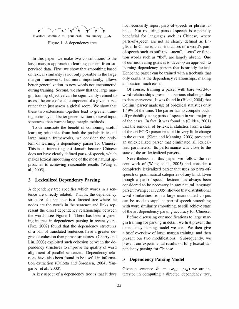
funds Investors continue to pour cash into money
Figure 1: A dependency tree
In this paper, we make two contributions to thelarge margin approach to learning parsers from su-pervised data. First, we show that smoothing basedon lexical similarity is not only possible in the largemargin framework, but more importantly, allowsbetter generalization to new words not encounteredduring training. Second, we show that the large mar-gin training objective can be significantly refined toassess the error of each component of a given parse,rather than just assess a global score. We show thatthese two extensions together lead to greater train-ing accuracy and better generalization to novel inputsentences than current large margin methods.
To demonstrate the benefit of combining usefullearning principles from both the probabilistic andlarge margin frameworks, we consider the prob-lem of learning a dependency parser for Chinese.This is an interesting test domain because Chinesedoes not have clearly defined parts-of-speech, whichmakes lexical smoothing one of the most natural ap-proaches to achieving reasonable results (Wang etal., 2005).
2 Lexicalized Dependency Parsing
A dependency tree specifies which words in a sen-tence are directly related. That is, the dependencystructure of a sentence is a directed tree where thenodes are the words in the sentence and links rep-resent the direct dependency relationships betweenthe words; see Figure 1. There has been a grow-ing interest in dependency parsing in recent years.(Fox, 2002) found that the dependency structuresof a pair of translated sentences have a greater de-gree of cohesion than phrase structures. (Cherry andLin, 2003) exploited such cohesion between the de-pendency structures to improve the quality of wordalignment of parallel sentences. Dependency rela-tions have also been found to be useful in informa-tion extraction (Culotta and Sorensen, 2004; Yan-garber et al., 2000).
A key aspect of a dependency tree is that it does
not necessarily report parts-of-speech or phrase la-bels. Not requiring parts-of-speech is especiallybeneficial for languages such as Chinese, whereparts-of-speech are not as clearly defined as En-glish. In Chinese, clear indicators of a word’s part-of-speech such as suffixes “-ment”, “-ous” or func-tion words such as “the”, are largely absent. Oneof our motivating goals is to develop an approach tolearning dependency parsers that is strictly lexical.Hence the parser can be trained with a treebank thatonly contains the dependency relationships, makingannotation much easier.
Of course, training a parser with bare word-to-word relationships presents a serious challenge dueto data sparseness. It was found in (Bikel, 2004) thatCollins’ parser made use of bi-lexical statistics only1.49% of the time. The parser has to compute back-off probability using parts-of-speech in vast majorityof the cases. In fact, it was found in (Gildea, 2001)that the removal of bi-lexical statistics from a stateof the art PCFG parser resulted in very little changein the output. (Klein and Manning, 2003) presentedan unlexicalized parser that eliminated all lexical-ized parameters. Its performance was close to thestate of the art lexicalized parsers.
Nevertheless, in this paper we follow the re-cent work of (Wang et al., 2005) and consider acompletely lexicalized parser that uses no parts-of-speech or grammatical categories of any kind. Eventhough a part-of-speech lexicon has always beenconsidered to be necessary in any natural languageparser, (Wang et al., 2005) showed that distributionalword similarities from a large unannotated corpuscan be used to supplant part-of-speech smoothingwith word similarity smoothing, to still achieve stateof the art dependency parsing accuracy for Chinese.
Before discussing our modifications to large mar-gin training for parsing in detail, we first present thedependency parsing model we use. We then givea brief overview of large margin training, and thenpresent our two modifications. Subsequently, wepresent our experimental results on fully lexical de-pendency parsing for Chinese.
3 Dependency Parsing Model
Given a sentence � � ������� � � ������ we are in-terested in computing a directed dependency tree,
22
�, over � . In particular, we assume that a di-
rected dependency tree�
consists of ordered pairs������������� of words in � such that each word ap-pears in at least one pair and each word has in-degreeat most one. Dependency trees are usually assumedto be projective (no crossing arcs), which means thatif there is an arc ������������� , then ��� is an ancestorof all the words between ��� and ��� . Let � �!�"� de-note the set of all the directed, projective trees thatspan � .
Given an input sentence � , we would like to beable to compute the best parse; that is, a projectivetree,
�$# � �!�"� , that obtains the highest “score”.In particular, we follow (Eisner, 1996; Eisner andSatta, 1999; McDonald et al., 2005) and assume thatthe score of a complete spanning tree
�for a given
sentence, whether probabilistically motivated or not,can be decomposed as a sum of local scores for eachlink (a word pair). In which case, the parsing prob-lem reduces to�&% �('*),+.-/'�0132*46587:9 ;5=<?>�@A<CB,9D2�1 s ��� � �E� � � (1)
where the score s �����F� ���G� can depend on anymeasurable property of ��� and ��� within the tree�
. This formulation is sufficiently general to capturemost dependency parsing models, including proba-bilistic dependency models (Wang et al., 2005; Eis-ner, 1996) as well as non-probabilistic models (Mc-Donald et al., 2005). For standard scoring functions,parsing requires an H:��IKJ�� dynamic programmingalgorithm to compute a projective tree that obtainsthe maximum score (Eisner and Satta, 1999; Wanget al., 2005; McDonald et al., 2005).
For the purpose of learning, we decompose eachlink score into a weighted linear combination of fea-tures
s ��� � �L� � �.� M6NKOP��� � �$� � � (2)
where M are the weight parameters to be estimatedduring training.
Of course, the specific features used in any realsituation are critical for obtaining a reasonable de-pendency parser. The natural sets of features to con-sider in this setting are very large, consisting at thevery least of features indexed by all possible lexicalitems (words). For example, natural features to use
for dependency parsing are indicators of each possi-ble word pairQ�R�S �����3�E���G�.� T 5U<?>WV R 9 T 5=<CBXV S 9which allows one to represent the tendency of twowords, Y and Z , to be directly linked in a parse. Inthis case, there is a corresponding parameter [ RS tobe learned for each word pair, which represents thestrength of the possible linkage.
A large number of features leads to a serious riskof over-fitting due to sparse data problems. The stan-dard mechanisms for mitigating such effects are tocombine features via abstraction (e.g. using parts-of-speech) or smoothing (e.g. using word similaritybased smoothing). For abstraction, a common strat-egy is to use parts-of-speech to compress the featureset, for example by only considering the tag of theparentQ]\�S �����^�L���G�.� T 5 pos
5=<?>_9WV \ 9 T 5U<CB`V S 9However, rather than use abstraction, we will followa purely lexical approach and only consider featuresthat are directly computable from the words them-selves (or statistical quantities that are directly mea-surable from these words).
In general, the most important aspect of a linkfeature is simply that it measures something abouta candidate word pair that is predictive of whetherthe words will actually be linked in a given sen-tence. Thus, many other natural features, beyondparts-of-speech and abstract grammatical categories,immediately suggest themselves as being predictiveof link existence. For example, one very useful fea-ture is simply the degree of association between thetwo words as measured by their pointwise mutualinformationQ
PMI �����^�L���G�.� PMI �����a����G�(We describe in Section 6 below how we computethis association measure on an auxiliary corpus ofunannotated text.) Another useful link feature issimply the distance between the two words in thesentence; that is, how many words they have be-tween themQ
dist �����3�E�����b� c position �����d�fe position ��������c23

In fact, the likelihood of a direct link between twowords diminishes quickly with distance, which mo-tivates using more rapidly increasing functions ofdistance, such as the squareQ
dist2 �����g�$�����h�i� position �����D�je position ���������akIn our experiments below, we used only these sim-
ple, lexically determined features, l QmRS*n , Q PMI,Q
dist
andQ
dist2, without the parts-of-speech l Q�\�S*n . Cur-rently, we only use undirected forms of these fea-tures, where, for example,
Q RS � Q S,Rfor all pairs
(or, put another way, we tie the parameters [ RS �[ S,R together for all YK�Z ). Ideally, we would liketo use directed features, but we have already foundthat these simple undirected features permit state ofthe art accuracy in predicting (undirected) depen-dencies. Nevertheless, extending our approach to di-rected features and contextual features, as in (Wanget al., 2005), remains an important direction for fu-ture research.
4 Large Margin Training
Given a training set of sentences annotated with theircorrect dependency parses, �!� � � � �`�� � � ��!�poh � o&� ,the goal of learning is to estimate the parameters ofthe parsing model, M . In particular, we seek valuesfor the parameters that can accurately reconstruct thetraining parses, but more importantly, are also ableto accurately predict the dependency parse structureon future test sentences.
To train M we follow the large margin training ap-proach of (Taskar et al., 2003; Tsochantaridis et al.,2004), which has been applied with great success todependency parsing (Taskar et al., 2004; McDonaldet al., 2005). Large margin training can be expressedas minimizing a regularized loss (Hastie et al., 2004)
-:qsrMt u M N M v (3)
; � -/'�0wC>yx �{z��| � �d�fe}� s �DMK � �d�~e s �DMK,z��d���where
� � is the target tree for sentence � � ; z �ranges over all possible alternative trees in � �!���!� ;s �DMf � ��� � 5=<?>_@ <CB�9D2�1 M6NfOC�����i� ���G� ; andx �{z��| � �d� is a measure of distance between the twotrees z�� and
� � .
Using the techniques of (Hastie et al., 2004) onecan show that minimizing (4) is equivalent to solvingthe quadratic program
-/qsr�G� � t u M6NfM�vb��NK� subject to (4)� �f� x � � �a,z��d�gv s �DMK,z��D�~e s �DMf � �!�for all �,,z�� # � �!���D�
which corresponds to the training problem posed in(McDonald et al., 2005).
Unfortunately, the quadratic program (4) has threeproblems one must address. First, there are expo-nentially many constraints—corresponding to eachpossible parse of each training sentence—whichforces one to use alternative training procedures,such as incremental constraint generation, to slowlyconverge to a solution (McDonald et al., 2005;Tsochantaridis et al., 2004). Second, and related,the original loss (4) is only evaluated at the globalparse tree level, and is not targeted at penalizing anyspecific component in an incorrect parse. Although(McDonald et al., 2005) explicitly describes thisas an advantage over previous approaches (Ratna-parkhi, 1999; Yamada and Matsumoto, 2003), belowwe find that changing the loss to enforce a more de-tailed set of constraints leads to a more effective ap-proach. Third, given the large number of bi-lexicalfeatures l Q*RS�n in our model, solving (4) directly willover-fit any reasonable training corpus. (Moreover,using a large
tto shrink the M values does not mit-
igate the sparse data problem introduced by havingso many features.) We now present our refinementsthat address each of these issues in turn.
5 Training with Local Constraints
We are initially focusing on training on just anundirected link model, where each parameter in themodel is a weight [ <�<�� between two words, � and��� , respectively. Since links are undirected, theseweights are symmetric [ <�<�� ��[ <���< , and we canalso write the score in an undirected fashion as:s ������ � ����M N OC������ � � . The main advantage ofworking with the undirected link model is that theconstraints needed to ensure correct parses on thetraining data are much easier to specify in this case.Ignoring the projective (no crossing arcs) constraintfor the moment, an undirected dependency parse can
24

be equated with a maximum score spanning tree of asentence. Given a target parse, the set of constraintsneeded to ensure the target parse is in fact the max-imum score spanning tree under the weights M , byat least a minimum amount, is a simple set of lin-ear constraints: for any edge ���,� k that is not in thetarget parse, one simply adds two constraints
M�NfOP���A��� � � �(� M6NfOC���A��� k �gv�TM�NfOP��� k �� �k �(� M6NfOC��� � �� k �gv�T (5)
where the edges ���,� � � and � k � �k are the adjacentedges that actually occur in the target parse that arealso on the path between ��� and � k . (These wouldhave to be the only such edges, or there would bea loop in the parse tree.) These constraints behavevery naturally by forcing the weight of an omittededge to be smaller than the adjacent included edgesthat would form a loop, which ensures that the omit-ted edge would not be added to the maximum scorespanning tree before the included edges.
In this way, one can simply accumulate the set oflinear constraints (5) for every edge that fails to beincluded in the target parse for the sentences whereit is a candidate. We denote this set of constraints by� � l�M N OP���A���� � � ���}M N OC���A��� k �3v�T nImportantly, the constraint set
�is convex in the link
weight parameters M , as it consists only of linearconstraints.
Ignoring the non-crossing condition, the con-straint set
�is exact. However, because of the
non-crossing condition, the constraint set�
is morerestrictive than necessary. For example, considerthe word sequence � � �����{���s�K�,��� � k ���s� J � � � , where theedge ���s�K�,���s� J is in the target parse. Then the edge� � � � � k can be ruled out of the parse in one of twoways: it can be ruled out by making its score lessthan the adjacent scores as specified in (5), or itcan be ruled out by making its score smaller thanthe score of ���s�K�����s� J . Thus, the exact constraintcontains a disjunction of two different constraints,which creates a non-convex constraint in M . (Theunion of two convex sets is not necessarily convex.)This is a weakening of the original constraint set
�.
Unfortunately, this means that, given a large train-ing corpus, the constraint set
�can easily become
infeasible.
Nevertheless, the constraints in�
capture muchof the relevant structure in the data, and are easyto enforce. Therefore, we wish to maintain them.However, rather than impose the constraints exactly,we enforce them approximately through the intro-duction of slack variables � . The relaxed constraintscan then be expressed asM N OC���A���� � � �a��M N OC���A��� k �gv�T�e � <g�D<�� � <g�D< � � (6)
and therefore a maximum soft margin solution canthen be expressed as a quadratic program
-/qsr�� � t u M N M�v � N � subject to (7)
lGM6NfOC���A��� � � ����M6NfOC���A��� k �^v�T�e � <g�D<�� � <g�D< � � nfor all constraints in
�where � denotes the vector of all 1’s.
Even though the slacks are required because wehave slightly over-constrained the parameters, giventhat there are so many parameters and a sparse dataproblem as well, it seems desirable to impose astronger set of constraints. A set of solution pa-rameters achieved in this way will allow maximumweight spanning trees to correctly parse nearly allof the training sentences, even without the non-crossing condition (see the results in Section 8).
This quadratic program has the advantage of pro-ducing link parameters that will correctly parse mostof the training data. Unfortunately, the main draw-back of this method thus far is that it does not of-fer any mechanism by which the link weights [ <�< �can be generalized to new or rare words. Given thesparse data problem, some form of generalization isnecessary to achieve good test results. We achievethis by exploiting distributional similarities betweenwords to smooth the parameters.
6 Distributional Word Similarity
Treebanks are an extremely precious resource. Theaverage cost of producing a treebank parse can runas high as 30 person-minutes per sentence (20 wordson average). Similarity-based smoothing, on theother hand, allows one to tap into auxiliary sourcesof raw unannotated text, which is practically unlim-ited. With this extra data, one can estimate parame-ters for words that have never appeared in the train-ing corpus.
25
The basic intuition behind similarity smoothingis that words that tend to appear in the same con-texts tend to have similar meanings. This is knownas the Distributional Hypothesis in linguistics (Har-ris, 1968). For example, the words test and exam aresimilar because both of them can follow verbs suchas administer, cancel, cheat on, conduct, etc.
Many methods have been proposed to computedistributional similarity between words, e.g., (Hin-dle, 1990; Pereira et al., 1993; Grefenstette, 1994;Lin, 1998). Almost all of the methods represent aword by a feature vector where each feature corre-sponds to a type of context in which the word ap-peared. They differ in how the feature vectors areconstructed and how the similarity between two fea-ture vectors is computed.
In our approach below, we define the features ofa word � to be the set of words that occurred withina small window of � in a large corpus. The con-text window of � consists of the closest non-stop-word on each side of � and the stop-words in be-tween. The value of a feature � � is defined as thepointwise mutual information between the ��� and� : PMI ���¡�{��A�¢�L£s¤¥+���¦ 5=< � < � 9¦ 5=<g9 ¦ 5U<��89 � . The similaritybetween two words, §�������� k � , is then defined asthe cosine of the angle between their feature vectors.
We use this similarity information both in trainingand in parsing. For training, we smooth the parame-ters according to their underlying word-pair similar-ities by introducing a Laplacian regularizer, whichwill be introduced in the next section. For parsing,the link scores in (1) are smoothed by word similar-ities (similar to the approach used by (Wang et al.,2005)) before the maximum score projective depen-dency tree is computed.
7 Laplacian Regularization
We wish to incorporate similarity based smoothingin large margin training, while using the more re-fined constraints outlined in Section 5.
Recall that most of the features we use, and there-fore most of the parameters we need to estimate arebased on bi-lexical parameters [ <�<�� that serve asundirected link weights between words � and � � inour dependency parsing model (Section 3). Here wewould like to ensure that two different link weights,[ <g�D< � � and [ <��|< �� , that involve similar words also
take on similar values. The previous optimization(7) needs to be modified to take this into account.
Smoothing the link parameters requires us to firstextend the notion of word similarity to word-pairsimilarities, since each link involves two words.Given similarities between individual words, com-puted above, we then define the similarity betweenword pairs by the geometric mean of the similaritiesbetween corresponding words.
§����A�,� � � �� k � �k �¨� © §����A��� k ��§���� � � �� �k � (8)
where §���� ��� k � is defined as in Section 6 above.Then, instead of just solving the constraint system(7) we can also ensure that similar links take on sim-ilar parameter values by introducing a penalty ontheir deviations that is weighted by their similarityvalue. Specifically, we use
;<g�D< � � ;<��|< �� §����A�,� � � �� k � �k �]�{[ < � < � � eª[ < � < �� � k� u M � N z&�!§��«M � (9)
Here z¡�!§�� is the Laplacian matrix of § , whichis defined by z¡�!§��¬� ®�!§��/e¯§ where ®�!§��is a diagonal matrix such that <3�{< � � � <g�D< � � �� <��|< �� §����A�,���� �� k ���k � . Also, M � corresponds to thevector of bi-lexical parameters. In this penalty func-tion, if two edges � � � � � and � k � �k have a high sim-ilarity value, their parameters will be encouraged totake on similar values. By contrast, if two edgeshave low similarity, then there will be little mutualattraction on their parameter values.
Note, however, that we do not smooth the param-eters, [ PMI, [ dist, [ dist2, corresponding to the point-wise mutual information, distance, and squared dis-tance features described in Section 5, respectively.We only apply similarity smoothing to the bi-lexicalparameters.
The Laplacian regularizer (9) provides a naturalsmoother for the bi-lexical parameter estimates thattakes into account valuable word similarity informa-tion computed as above. The Laplacian regularizeralso has a significant computational advantage: it isguaranteed to be a convex quadratic function of theparameters (Zhu et al., 2001). Therefore, by com-bining the constraint system (7) with the Laplaciansmoother (9), we can obtain a convex optimization
26
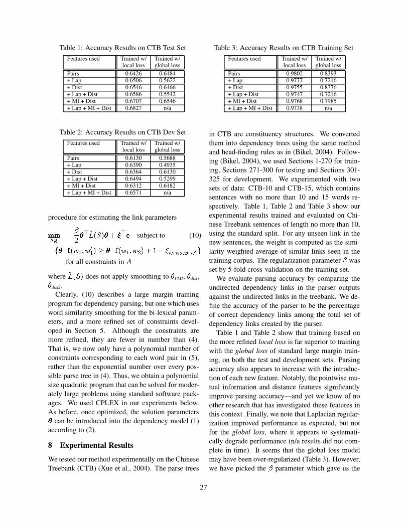
Table 1: Accuracy Results on CTB Test SetFeatures used Trained w/ Trained w/
local loss global lossPairs 0.6426 0.6184+ Lap 0.6506 0.5622+ Dist 0.6546 0.6466+ Lap + Dist 0.6586 0.5542+ MI + Dist 0.6707 0.6546+ Lap + MI + Dist 0.6827 n/a
Table 2: Accuracy Results on CTB Dev SetFeatures used Trained w/ Trained w/
local loss global lossPairs 0.6130 0.5688+ Lap 0.6390 0.4935+ Dist 0.6364 0.6130+ Lap + Dist 0.6494 0.5299+ MI + Dist 0.6312 0.6182+ Lap + MI + Dist 0.6571 n/a
procedure for estimating the link parameters
-/qsr�G� � t u M N�°z&�!§��«M�v±� N � subject to (10)
l�M N OC���A��� � � ���²M N OP���A��� k �gv�T�e � <g�D<�� � <g�D< � � nfor all constraints in
�where °z¡�!§�� does not apply smoothing to [ PMI, [ dist,[ dist2.
Clearly, (10) describes a large margin trainingprogram for dependency parsing, but one which usesword similarity smoothing for the bi-lexical param-eters, and a more refined set of constraints devel-oped in Section 5. Although the constraints aremore refined, they are fewer in number than (4).That is, we now only have a polynomial number ofconstraints corresponding to each word pair in (5),rather than the exponential number over every pos-sible parse tree in (4). Thus, we obtain a polynomialsize quadratic program that can be solved for moder-ately large problems using standard software pack-ages. We used CPLEX in our experiments below.As before, once optimized, the solution parametersM can be introduced into the dependency model (1)according to (2).
8 Experimental Results
We tested our method experimentally on the ChineseTreebank (CTB) (Xue et al., 2004). The parse trees
Table 3: Accuracy Results on CTB Training SetFeatures used Trained w/ Trained w/
local loss global lossPairs 0.9802 0.8393+ Lap 0.9777 0.7216+ Dist 0.9755 0.8376+ Lap + Dist 0.9747 0.7216+ MI + Dist 0.9768 0.7985+ Lap + MI + Dist 0.9738 n/a
in CTB are constituency structures. We convertedthem into dependency trees using the same methodand head-finding rules as in (Bikel, 2004). Follow-ing (Bikel, 2004), we used Sections 1-270 for train-ing, Sections 271-300 for testing and Sections 301-325 for development. We experimented with twosets of data: CTB-10 and CTB-15, which containssentences with no more than 10 and 15 words re-spectively. Table 1, Table 2 and Table 3 show ourexperimental results trained and evaluated on Chi-nese Treebank sentences of length no more than 10,using the standard split. For any unseen link in thenew sentences, the weight is computed as the simi-larity weighted average of similar links seen in thetraining corpus. The regularization parameter
twas
set by 5-fold cross-validation on the training set.We evaluate parsing accuracy by comparing the
undirected dependency links in the parser outputsagainst the undirected links in the treebank. We de-fine the accuracy of the parser to be the percentageof correct dependency links among the total set ofdependency links created by the parser.
Table 1 and Table 2 show that training based onthe more refined local loss is far superior to trainingwith the global loss of standard large margin train-ing, on both the test and development sets. Parsingaccuracy also appears to increase with the introduc-tion of each new feature. Notably, the pointwise mu-tual information and distance features significantlyimprove parsing accuracy—and yet we know of noother research that has investigated these features inthis context. Finally, we note that Laplacian regular-ization improved performance as expected, but notfor the global loss, where it appears to systemati-cally degrade performance (n/a results did not com-plete in time). It seems that the global loss modelmay have been over-regularized (Table 3). However,we have picked the
tparameter which gave us the
27
best resutls in our experiments. One possible ex-planation for this phenomenon is that the interactionbetween the Laplician regularization in training andthe similarity smoothing in parsing, since distribu-tional word similarities are used in both cases.
Finally, we compared our results to the probabilis-tic parsing approach of (Wang et al., 2005), which onthis data obtained accuracies of 0.7631 on the CTBtest set and 0.6104 on the development set. How-ever, we are using a much simpler feature set here.
9 Conclusion
We have presented two improvements to the stan-dard large margin training approach for dependencyparsing. To cope with the sparse data problem, wesmooth the parameters according to their underlyingword similarities by introducing a Laplacian regular-izer. More significantly, we use more refined localconstraints in the large margin criterion, rather thanthe global parse-level losses that are commonly con-sidered. We achieve state of the art parsing accuracyfor predicting undirected dependencies in test data,competitive with previous large margin and previousprobabilistic approaches in our experiments.
Much work remains to be done. One extensionis to consider directed features, and contextual fea-tures like those used in current probabilistic parsers(Wang et al., 2005). We would also like to apply ourapproach to parsing English, investigate the confu-sion showed in Table 3 more carefully, and possiblyre-investigate the use of parts-of-speech features inthis context.
ReferencesDan Bikel. 2004. Intricacies of collins’ parsing model. Com-
putational Linguistics, 30(4).
Eugene Charniak. 2000. A maximum entropy inspired parser.In Proceedings of NAACL-2000, pages 132–139.
Colin Cherry and Dekang Lin. 2003. A probability model toimprove word alignment. In Proceedings of ACL-2003.
M. J. Collins. 1997. Three generative, lexicalized models forstatistical parsing. In Proceedings of ACL-1997.
Aron Culotta and Jeffery Sorensen. 2004. Dependency treekernels for relation extraction. In Proceedings of ACL-2004.
J. Eisner and G. Satta. 1999. Efficient parsing for bilexicalcontext-free grammars and head-automaton grammars. InProceedings of ACL-1999.
J. Eisner. 1996. Three new probabilistic models for depen-dency parsing: An exploration. In Proc. of COLING-1996.
Heidi J. Fox. 2002. Phrasal cohesion and statistical machinetranslation. In Proceedings of EMNLP-2002.
Daniel Gildea. 2001. Corpus variation and parser performance.In Proceedings of EMNLP-2001, Pittsburgh, PA.
Gregory Grefenstette. 1994. Explorations in Automatic The-saurus Discovery. Kluwer Academic Press, Boston, MA.
Zelig S. Harris. 1968. Mathematical Structures of Language.Wiley, New York.
T. Hastie, S. Rosset, R. Tibshirani, and J. Zhu. 2004. The entireregularization path for the support vector machine. JMLR, 5.
Donald Hindle. 1990. Noun classification from predicate-argument structures. In Proceedings of ACL-1990.
Dan Klein and Christopher D. Manning. 2003. Accurate un-lexicalized parsing. In Proceedings of ACL-2003.
Dekang Lin. 1998. Automatic retrieval and clustering of simi-lar words. In Proceedings of COLING/ACL-1998.
R. McDonald, K. Crammer, and F. Pereira. 2005. Online large-margin training of dependency parsers. In Proceedings ofACL-2005.
F. Pereira, N. Tishby, and L. Lee. 1993. Distributional cluster-ing of english words. In Proceedings of ACL-1993.
Adwait Ratnaparkhi. 1999. Learning to parse natural languagewith maximum entropy models. Machine Learning, 34(1-3).
B. Taskar, C. Guestrin, and D. Koller. 2003. Max-marginmarkov networks. In Proc. of NIPS-2003.
B. Taskar, D. Klein, M. Collins, D. Koller, and C. Manning.2004. Max-margin parsing. In Proceedings of EMNLP.
I. Tsochantaridis, T. Hofmann, T. Joachims, and Y. Altun.2004. Support vector machine learning for interdependentand structured output spaces. In Proceedings of ICML-2004.
Q. Wang, D. Schuurmans, and D. Lin. 2005. Strictly lexicaldependency parsing. In Proceedings of IWPT-2005.
N. Xue, F. Xia, F. Chiou, and M. Palmer. 2004. The penn chi-nese treebank: Phrase structure annotation of a large corpus.Natural Language Engineering, 10(4):1–30.
H. Yamada and Y. Matsumoto. 2003. Statistical dependencyanalysis with support vector machines. In Proceedings ofIWPT-2003.
R. Yangarber, R. Grishman, P. Tapanainen, and S. Huttunen.2000. Unsupervised discovery of scenario-level patterns forinformation extraction. In Proceedings of ANLP/NAACL-2000.
Xiaojin Zhu, John Lafferty, and Zoublin Ghahramani. 2001.Semi-supervised learning using gaussian fields and harmonicfunctions. In Proceedings of ICML-2003.
28

Proceedings of the 10th Conference on Computational Natural Language Learning (CoNLL-X),pages 29–36, New York City, June 2006.c©2006 Association for Computational Linguistics
What are the Productive Units of Natural Language Grammar? A DOPApproach to the Automatic Identification of Constructions.
Willem ZuidemaInstitute for Logic, Language and Computation
University of AmsterdamPlantage Muidergracht 24, 1018 TV, Amsterdam, the Netherlands.
Abstract
We explore a novel computational ap-proach to identifying “constructions” or“multi-word expressions” (MWEs) in anannotated corpus. In this approach,MWEs have no special status, but emergein a general procedure for finding the beststatistical grammar to describe the train-ing corpus. The statistical grammar for-malism used is that of stochastic tree sub-stitution grammars (STSGs), such as usedin Data-Oriented Parsing. We present analgorithm for calculating the expected fre-quencies of arbitrary subtrees given theparameters of an STSG, and a methodfor estimating the parameters of an STSGgiven observed frequencies in a tree bank.We report quantitative results on the ATIScorpus of phrase-structure annotated sen-tences, and give examples of the MWEsextracted from this corpus.
1 Introduction
Many current theories of language use and acquisi-tion assume that language users store and use muchlarger fragments of language than the single wordsand rules of combination of traditional linguisticmodels. Such fragments are often called construc-tions, and the theories that assign them a centralrole “construction grammar” (Goldberg, 1995; Kayand Fillmore, 1999; Tomasello, 2000; Jackendoff,2002, among others). For construction grammar-
ians, multi-word expressions (MWEs) such as id-ioms, collocations, fixed expressions and compoundverbs and nouns, are not so much exceptions to therule, but rather extreme cases that reveal some fun-damental properties of natural language.
In the construction grammar tradition, co-occurrence statistics from corpora have often beenused as evidence for hypothesized constructions.However, such statistics are typically gathered ona case-by-case basis, and no reliable procedure ex-ists to automatically identify constructions. In con-trast, in computational linguistics, many automaticprocedures are studied for identifying MWEs (Saget al., 2002) – with varying success – but here theyare treated as exceptions: identifying multi-word ex-pressions is a pre-processing step, where typicallyadjacent words are grouped together after which theusual procedures for syntactic or semantic analysiscan be applied. In this paper I explore an alter-native formal and computational approach, wheremulti-word constructions have no special status,but emerge in a general procedure to find the beststatistical grammar to describe a training corpus.Crucially, I use a formalism known as “StochasticTree Substitution Grammars” (henceforth, STSGs),which can represent single words, contiguous andnoncontiguous MWEs, context-free rules or com-plete parse trees in a unified representation.
My approach is closely related to work in statisti-cal parsing known as Data-Oriented Parsing (DOP),an empirically highly successful approach with la-beled recall and precision scores on the Penn TreeBank that are among the best currently obtained(Bod, 2003). DOP, first proposed in (Scha, 1990),
29
can be seen as an early formalization and combina-tion of ideas from construction grammar and statis-tical parsing. Its key innovations were (i) the pro-posal to use fragments of trees from a tree bank asthe symbolic backbone; (ii) the proposal to allow, inprinciple, trees of arbitrary size and shape as the el-ementary units of combination; (iii) the proposal touse the occurrence and co-occurrence frequencies asthe basis for structural disambiguation in parsing.
The model I develop in this paper is true to thesegeneral DOP ideals, although it differs in impor-tant respects from the many DOP implementationsthat have been studied since its first inception (Bod,1993; Goodman, 1996; Bod, 1998; Sima’an, 2002;Collins and Duffy, 2002; Bod et al., 2003, and manyothers). The crucial difference is in the estimationprocedure for choosing the weights of the STSGbased on observed frequencies in a corpus. ExistingDOP models converge to STSGs that either (i) giveall subtrees of the observed trees nonzero weights(Bod, 1993; Bod, 2003), or (ii) give only the largestpossible fragments nonzero weights (Sima’an andBuratto, 2003; Zollmann and Sima’an, 2005). Themodel in this paper, in contrast, aims at finding thesmallest set of productive units that explain the oc-currences and co-occurrences in a corpus. Largesubtrees only receive non-zero weights, if they occurmore frequently than can be expected on the basis ofthe weights of smaller subtrees.
2 Formalism, Notation and Definitions
2.1 Stochastic Tree Substitution Grammars
STSGs are a simple generalization of Stochas-tic Context Free Grammars (henceforth, SCFGs),where the productive units are elementary trees ofarbitrary size instead of the rewrite rules in SCFGs(which can be viewed as trees of depth 1). STSGsform a restricted subclass of Stochastic Tree Adjoin-ing Grammars (henceforth, STAGs) (Resnik, 1992;Schabes, 1992), the difference being that STSGsonly allow for substitution and not for adjunction(Joshi and Sarkar, 2003). This limits the genera-tive capacity to that of context-free grammars, andmeans STSGs cannot be fully lexicalized. Theselimitations notwithstanding, the close relationshipwith STAGs is an attractive feature with extensionsto the class of mildly context-sensitive languages
(Joshi et al., 1991) in mind. Most importantly, how-ever, STSGs are already able to model a vast rangeof statistical dependencies between words and con-stituents, which allows them to rightly predict theoccurrences of many constructions (Bod, 1998).
For completeness, we include the usual defi-nitions of STSGs, the substitution operation andderivation and parse probabilities (Bod, 1998), us-ing our own notation. An STSG is a 5-tuple〈Vn, Vt, S, T, w〉, where Vn is the set of non-terminalsymbols; Vt is the set of terminal symbols; S ∈ Vn isthe start symbol; T is a set of elementary trees, suchthat for every t ∈ T the unique root node r(t) ∈ Vn,the set of internal nodes i(t) ⊂ Vn and the set of leafnodes l(t) ⊂ Vn ∪ Vt; finally, w : T → [0, 1] is aprobability (weight) distribution over the elementarytrees, such that for any t ∈ T ,
∑t′∈R(t) w(t′) = 1,
where R(t) is the set of elementary trees with thesame root label as t. It will prove useful to also de-fine the set of all possible trees θ over the definedalphabets (with the same conditions on root, internaland leaf nodes as for T ), and the set of all possiblecomplete parse trees Θ (with r(t) = S and all leafnodes l(t) ⊂ Vt). Obviously, T ⊂ θ and Θ ⊂ θ.
The substitution operation ◦ is defined if the left-most nonterminal leaf in t1 is identical to the root oft2. Performing substitution t1 ◦ t2 yields t3, if t3 isidentical to t1 with the leftmost nonterminal leaf re-placed by t2. A derivation is a sequence of elemen-tary trees, where the first tree t ∈ T has root-labelS and every next tree combines through substitutionwith the result of the substitutions before it. Theprobability of a derivation d is defined as the prod-uct of weights of the elementary trees involved:
P (d = t1 ◦ . . . ◦ tn) =
n∏
i=1
(w (ti)) . (1)
A parse tree is any tree t ∈ Θ. Multiple derivationscan yield the same parse tree; the probability of aparse tree p equals the sum of the probabilities ofthe different derivations that yield that same tree:
P (p) =∑
d:d=p
(P (d)) , (2)
where d is the tree derived by derivation d.In this paper, we are only concerned with gram-
mars that define proper probability distributions over
30
trees, such that the probability of all derivations sumup to 1 and no probability mass gets lost in deriva-tions that never reach a terminal yield. We require:
∑
p∈Θ
P (p) =∑
d:d∈Θ
P (d) = 1. (3)
2.2 Usage Frequency and OccurrenceFrequency
In addition to these conventional definitions, we willmake use in this paper of the concepts “usage fre-quency” and “occurrence frequency”. When weconsider an arbitrary subtree t, the usage frequencyu(t) describes the relative frequency with which el-ementary tree t is involved in a set of derivations.Given a grammar G ∈ STSG, the expected usagefrequency is:
u(t) =∑
d:t∈d
(P (d) C (t, d)) , (4)
where C (t, d) gives the number of occurrences oft in d. The set of derivations, and hence usage fre-quency, is usually considered hidden information.
The occurrence frequency f(t) describes the rela-tive frequency with which t occurs as a subtree of aset of parse trees, which is usually assumed to beobservable information. If grammar G is used togenerate trees, it will create a tree bank where eachparse tree will occur with an expected frequency asin equation (2). More generally, the expected oc-currence frequency f(t) (relative to the number n ofcomplete trees in the tree bank) of a subtree t is:
E[f(t)] =∑
p:t∈p∗
(P (p)C (t, p∗)) , (5)
where p∗ is the multiset of all subtrees of p.Hence, w(t), u(t) and f(t) all assign values (the
latter two not necessarily between 0 and 1) to trees.An important question is how these different val-ues can be related. For STSGs which have onlyelementary trees of depth 1, and are thus equiva-lent to SCFGs, these relations are straightforward:the usage frequency of an elementary tree simplyequals its expected frequency, and can be derivedfrom the weights by multiplying inside and out-side probabilities (Lari and Young, 1990). Estimat-ing the weights of an (unconstrained and untrans-formed) SCFG from an tree bank is straightforward,
as weights, in the limit, simply equal the relativefrequency of each depth-1 subtree (relative to otherdepth-1 subtrees with the same root label).
When elementary trees can be of arbitrary depth,however, many different derivations can yield thesame tree, and a given subtree t can emerge with-out the corresponding elementary tree ever havingbeen used. The expected frequencies are sums ofproducts, and – if one wants to avoid exhaustivelyenumerating all possible parse trees – surprisinglydifficult to calculate, as will become clear below.
2.3 From weights to usage frequencies andback
Relating usage frequencies to weights is relativelysimple. With a bit of algebra we can work out thefollowing relations:
u(t) =
w(t) if r(t) = S
w(t)∑
t′ :r(t)∈l(t′)
u(t′)Ct′
t otherwise
(6)where C t′
t gives the number of occurrences of theroot label r(t) of t among the leaves of t′. The in-verse relation is straightforward:
w(t) =u(t)∑
t′∈R(t) u(t′). (7)
2.4 From usage frequency to expectedfrequency
The two remaining problems – calculating expectedfrequencies from weights and estimating the weightsfrom observed frequencies – are surprisingly dif-ficult and heretofore not satisfactorily solved. In(Zuidema, 2006) we evaluate existing estimationmethods for Data-Oriented Parsing, and show thatthey are ill-suited for learning tasks such as stud-ied in this paper. In the next section, we present anew algorithm for estimation, which makes use ofa method for calculating expected frequencies thatwe sketch in this section. This method makes use ofsub- and supertree relations that we explain first.
We define two types of subtrees of a given tree t,which, for lack of better terminology, we will call“twigs” and “prunes” of t. Twigs are those subtreesheaded by any of t’s internal nodes and everything
31
below. Prunes are those subtrees headed by t’s root-node, pruned at any number (≥ 0) of internal nodes.Using ◦ to indicate left-most substitution, we write:• t1 is a twig of t2, if either t1 = t2 or ∃t3, such
that t3 ◦ t1 = t2;• t1 is a prune of t2, if either t1 = t2 or ∃t3 . . . tn,
such that t1 ◦ t3 . . . ◦ tn = t2;• t′ = prx(t), if x is a set of nodes in t, such that
if t is pruned at each i ∈ x it equals t′.Thus defined, the set of all subtrees st(t) of t cor-responds to the set of all prunes of all twigs of t:st(t) = {t′′|∃t′(t′ ∈ tw(t) ∧ t′′ ∈ pr(t′)).
We further define the sets of supertwigs, super-prunes and supertrees as follows:• tw(t) = {t′|t ∈ tw(t′)}• prx(t) = {t′|t = prx(t′)}• st(t) = {t′|t ∈ st(t′)}.Using these sets, and the set of derivations D(t) of
the fragment t, a general expression for the expectedfrequency of t is:
E[f(t)] =∑
d∈D(t)
αβ
α =∑
τ∈ctw(d1)
∑
τ ′∈ dprx(t)(τ)
u(τ ′)
β =∏
t′∈〈d2,...,dn〉
∑
τ ′∈ dprx(t)(t′)
w(τ ′
)(8)
where 〈d1, . . . , dn〉 is the sequence of elementarytrees in derivation d. A derivation of this equationis provided on the author’s website1. Note that it
1http://staff.science.uva.nl/∼jzuidema. The intuition behindit is as follows. Observe first that there are many ways in whichan arbitrary fragment t can emerge, many of which do not in-volve the usage of the elementary tree t. It is useful to partitionthe set of all derivations of complete parse trees according to thesubstitution sites inside t that they involve, and hence accordingto the corresponding derivations of t. The first summation in (8)simply sums over all these cases.
Each derivation of t involves a first elementary tree d1, andpossibly a sequence of further elementary trees 〈d2, . . . , dn〉.Roughly speaking, the α-term in equation (8) describes the fre-quency with which a d1 will be generated. The β-term thendescribes the probability that d1 will be expanded as t. Theequation simplifies considerably for those fragments that haveno nonterminal leaves: the set dprx(t) then only contains t, andthe two summations over this set disappear. The equation fur-ther simplifies if only depth-1 elementary trees have nonzeroweights (i.e. for SCFGs): α and β then essentially give outsideand inside probabilities (Lari and Young, 1990). However, forunconstrained STSGs we need all sums and products in (8).
will, in general, be computationally extremely ex-pensive to calculate E[f(t)] . We will come back tocomputational efficiency issues in the discussion.
3 Estimation: push-n-pull
The goal of this paper is an automatic discoveryprocedure for finding “constructions” based on oc-currence and co-occurrence frequencies in a corpus.Now that we have introduced the necessary termi-nology, we can reformulate this goal as follows:What are the elementary trees with multiple wordswith the highest usage frequency in the STSG esti-mated from an annotated corpus? Thus phrased, thecrucial next step is to decide on an estimation proce-dure for learning an STSG from a corpus.
Here we develop an estimation procedure we call“push-n-pull”. The basic idea is as follows. Givenan initial setting of the parameters, the method cal-culates the expected frequency of all complete andincomplete trees. If a tree’s expected frequency ishigher than its observed frequency, the method sub-tracts the difference from the tree’s score, and dis-tributes (“pushes”) it over the trees involved in itsderivations. If it is lower, it “pulls” the differencefrom these same derivations. The method includes abias for moving probability mass to smaller elemen-tary trees, to avoid overfitting; its effects becomesmaller as more data gets observed.
Because the method for calculating estimated fre-quency works with usage-frequencies, the push-n-pull algorithm also uses these as parameters. Moreprecisely, it manipulates a “score”, which is theproduct of usage frequency and the total number ofparse trees observed. Implicit here is the assumptionthat by shifting usage frequencies between differentderivations, the relation with weights remains as inequation (6). Simulations suggest this is reasonable.
In the current implementation, the method startswith all frequency mass in the longest derivations,i.e. in the depth-1 elementary trees. Finally, the cur-rent implementation is incremental. It keeps track ofthe frequencies with which it observes subtrees in acorpus. For each tree received, it finds all derivationsand all probabilities, updates frequencies and scoresaccording to the rules sketched above. In pseudo-code, the push-n-pull algorithm is as follows:
for each observed parse tree p
32
for each depth-1 subtree t in pupdate-score(t, 1.0)
for each subtree t of p∆ =min(sc(t), B + γ(E[f(t)]− f(t)))∆′ = 0for each of n derivations d of t
let t′ . . . t′′ be all elementary trees in dδ =min(sc(t′), . . . , sc(t′′),−∆/n)
∆′− = δfor each elementary tree t′ in d
update-score(t′ , δ)update-score (t,∆′)
where sc(t) is the score of t, B is the bias to-wards smaller subtrees, γ is the learning rate param-eter and f(t) is the observed frequency of t. ∆′ thusgives the actual change in the score of t, based onthe difference between expected and observed fre-quency, bias, learning rate and how much scores canbe pushed or pulled2. For computational efficiency,only subtrees with a depth no larger than d = 3 ord = 4 and only derivations involving 2 elementarytrees are considered.
4 Results
We have implemented the algorithms for calculat-ing the expected frequency, and the push-n-pull al-gorithm for estimation. We have evaluated the algo-rithms on a number of simple example STSGs andfound that the expected frequency algorithm cor-rectly predicts observed frequencies. We have fur-ther found that – unlike existing estimation meth-ods – the push-n-pull algorithm converges to STSGsthat closely model the observed frequencies (i.e. thatmaximize the likelihood of the data) without puttingall probability mass in the largest elementary trees(i.e. whilst retaining generalizations about the data).
Here we report first quantitative results on theATIS3 corpus (Hemphill et al., 1990). Before pro-cessing, all trees (train and test set) were convertedto a format that our current implementation requires(all non-terminal labels are unique, all internal nodeshave two daughters, all preterminal nodes have asingle lexical daughter; all unary productions andall traces were removed). The set of trees was ran-domly split in a train set of 462 trees, and a test set
2An important topic for future research is to clarify the rela-tion between push-n-pull and Expectation Maximization.
of 116 trees. The push-n-pull algorithm was thenrun in 10 passes over the train set, with d = 3,B = 0 and γ = 0.1. By calculating the most proba-ble parse3 for each yield of the trees in test set, andrunning “evalb” we arrive at the following quantita-tive results: a string set coverage of 84% (19 failedparses), labeled recall of 95.07, and labeled preci-sion of 95.07. We obtained almost identical num-bers on the same data with a reimplementation ofthe DOP1 algorithm (Bod, 1998).
method # rules Cov. LR LP EMDOP1 77852 84% 95.07 95.07 83.5p-n-p 58799 84% 95.07 95.07 83.5
Table 1: Parseval scores of DOP1 and push-n-pullon the same 462-116 random train-testset split of atreebank derived from the ATIS3 corpus (we empha-size that all trees, also those of the test-set, were con-verted to Chomsky Normal Form, whereby unaryproduction and traces were removed and top-nodesrelabeled “TOP”. These results are thus not compa-rable to previous methods evaluated on the ATIS3corpus.) EM is “exact match”.
method # rules Cov. LR LP EMsc > 0.3 8593 77% 80.8 80.8 46.3sc > 0.1 98443 77% 81.9 81.9 48.8
Table 2: Parseval scores using a p-n-p inducedSTSG on the same treebank as in table 1, using adifferent random 525-53 train-testset split. Shownare results were only elementary trees with scoreshigher than 0.3 and 0.1 respectively are used.
However, more interesting is a qualitative anal-ysis of the STSG induced, which shows that, un-like DOP1, push-n-pull arrives at a grammar thatgives high weights (and scores) to those elementary
3We approximated the most probable parse as follows (fol-lowing (Bod, 2003)). We first converted the induced STSG toan isomorph SCFG, by giving the internal nodes of every ele-mentary tree t unique address-labels, and reading off all CFGproductions (all with weight 1.0, except for the top-production,which receives the weight of t). An existing SCFG parser(Schmid, 2004) was then used, with a simple unknown wordheuristic, to generate the Viterbi n-best parses with n = 100,and, after removing the address labels, all equal parses and theirprobabilities were summed, and the one with highest probabil-ity chosen.
33
trees that best explain the overrepresentation of cer-tain constructions in the data. For instance, in a runwith d = 4, γ = 1.0, B = 1.0, the 50 elemen-tary trees with the highest scores, as shown in fig-ure 1, are all exemplary of frequent formulas in theATIS corpus such as “show me X”, “I’d like to X”,“which of these”, “what is the X”, “cheapest fare”and “flights from X to Y”. In short, the push-n-pullalgorithm – while starting out considering all possi-ble subtrees – converges to a grammar which makeslinguistically relevant generalizations. This allowsfor a more compact grammar (58799 rules in theSCFG reduction, vs. 77852 for DOP1), whilst re-taining DOP’s excellent empirical performance.
5 Discussion
Calculating E[f(t)] using equation (8) can be ex-tremely expensive in computational terms. One willtypically want to calculate this value for all subtrees,the number of which is exponential in the size of thetrees in the training data. For each subtree t, we willneed to consider the set of all its derivations (expo-nential in the size of t), and for each derivation theset of supertwigs of the first elementary trees and,for incompletely lexicalized subtrees, the set of su-perprunes of all elementary trees in their derivations.The latter two sets, however, need not be constructedfor every time the expected frequency E[f(t)] is cal-culated. Instead, we can, as we do in the current im-plementation, keep track of the two sums for everychange of the weights.
However, there are many further possibilities forimproving the efficiency of the algorithm that arecurrently not implemented. Equation (8) remainsvalid under various restrictions on the elementarytrees that we are willing to consider as productiveunits. Some of these will remove the exponential de-pendence on the size of the trees in the training data.For instance, in the case where we restrict the pro-ductive units (with nonzero weights) to depth-1 trees(i.e. CFG rules), equation (8) collapses to the prod-uct of inside and outside probabilities, which can becalculated using dynamical programming in polyno-mial time (Lari and Young, 1990). A major topic forfuture research is to define linguistically motivatedrestrictions that allow for efficient computation.
Another concern is the size of the grammar the
estimation procedure produces, and hence the timeand space efficiency of the resulting parser. Ta-ble 1 already showed that push-n-pull leads to amore concise grammar. The reason is that many po-tential elementary trees receive a score (and weight)0. More generally, push-n-pull generates extremelytilted score distributions, which allows for evenmore compact but highly accurate approximations.In table 2 we show, for the d = 4 grammar of fig-ure 1, that a 10-fold reduction of the grammar sizeby pruning elementary trees with low scores, leadsonly to a small decrease in the LP and LR measures.
Another interesting question is if and how thecurrent algorithm can be extended to the full classof Stochastic Tree-Adjoining Grammars (Schabes,1992; Resnik, 1992). With the added operation ofadjunction, equation (8) is not valid anymore. Giventhe computational complexities that it already givesrise to, however, it seems that issue of linguisti-cally motivated restrictions (other than lexicaliza-tion) should be considered first. Finally, given thatthe current approach is dependent on the availabilityof a large annotated corpus, an important questionis if and how it can be extended to work with un-labeled data. That is, can we transform the push-n-pull algorithm to perform the unsupervised learningof STSGs? Although most work on unsupervisedgrammar learning concerns SCFGs (including someof our own (Zuidema, 2003)) it is interesting to notethat much of the evidence for construction grammarin fact comes from the language acquisition litera-ture (Tomasello, 2000).
6 Conclusions
Theoretical linguistics has long strived to accountfor the unbounded productivity of natural languagesyntax with as few units and rules of combinationas possible. In contrast, construction grammar andrelated theories of grammar postulate a heteroge-neous and redundant storage of “constructions”. Ifthis view is correct, we expect to see statistical sig-natures of these constructions in the distributionalinformation that can be derived from corpora of nat-ural language utterances. How can we recover thosesignatures? In this paper we have presented an ap-proach to identifying the relevant statistical correla-tions in a corpus based on the assumption that the
34

TOP
VB
”SHOW”
VP*
PRP
”ME”
NP
NP*
DT NNS
NP**
PP-DIR PP-DIR*
(a) The “show me NP PP” frame,which occurs very frequently inthe training data and is repre-sented in several elementary treeswith high weight.
WHNP-1
WDT
”WHICH”
PP
IN
”OF”
NP
DT
”THESE”
NNS
”FLIGHTS”
(b) The complete parse treefor the sentence “Which ofthese flights”, which occurs16 times in training data.
TOP
NNS
”FLIGHTS”
NP*
PP-DIR
IN
”FROM”
NP**
NNP NNP*
PP-DIR*
TO
”TO”
NNP**
(c) The frame for “flights from NP toNP”
1. ((TOP (VB ”SHOW”) (VP* (PRP ”ME”) (NP (NP* DT NNS) (NP** PP-DIR PP-DIR*)))) 17.79 0.008 30)2. ((TOP (VB ”SHOW”) (VP* (PRP ”ME”) (NP (NP* DT NNS) NP**))) 10.34 0.004 463. (TOP (PRP ”I”) (VP (MD ”WOULD”) (VP* (VB ”LIKE”) (VP** TO VP***)))) 10.02 0.009 204. (WHNP-1 (WDT ”WHICH”) (PP (IN ”OF”) (NP (DT ”THESE”) (NNS ”FLIGHTS”)))) 8.80 0.078 165. (TOP (WP ”WHAT”) (SQ (VBZ ”IS”) (NP-SBJ (DT ”THE”) (NN ”PRICE”)))) 8.76 0.005 206. (TOP (WHNP (WDT ”WHAT”) (NNS ”FLIGHTS”)) (SQ (VBP ”ARE”) (SQ* (EX ”THERE”) SQ**))) 8.25 0.006 367. (VP* (PRP ”ME”) (NP (NP* (DT ”THE”) (NNS ”FLIGHTS”)) (NP** (PP-DIR IN NNP) (PP-DIR* TO NNP*)))) 7.90 0.023 188. (TOP (WHNP (WDT ”WHAT”) (NNS ”FLIGHTS”)) (SQ (VBP ”ARE”) (SQ* (EX ”THERE”) (SQ** PP-DIR-3 PP-DIR-4)))) 6.64 0.005 269. (TOP (PRP ”I”) (VP MD (VP* (VB ”LIKE”) (VP** TO VP***)))) 6.48 0.006 20
10. (TOP (PRP ”I”) (VP (VBP ”NEED”) (NP (NP* DT NN) (NP** PP-DIR NP***)))) 5.01 0.004 1011. (TOP (VB ”SHOW”) (VP* (PRP ”ME”) (NP (DT ”THE”) NNS))) 4.94 0.002 1612. (TOP WP (SQ (VBZ ”IS”) (NP-SBJ (DT ”THE”) (NN ”PRICE”)))) 4.91 0.0028 2013. (TOP (WHNP (WDT ”WHAT”) (NNS ”FLIGHTS”)) (SQ (VBP ”ARE”) (SQ* EX (SQ** PP-DIR-3 PP-DIR-4)))) 4.16 0.003 2614. (TOP (VB ”SHOW”) (VP* (PRP ”ME”) (NP (NNS ”FLIGHTS”) NP*))) 4.01 0.001 1615. (TOP (VB ”SHOW”) (VP* (PRP ”ME”) (NP (DT ”THE”) NP*))) 3.94 0.002 1216. (TOP (WHNP (WDT ”WHAT”) (NNS ”FLIGHTS”)) (SQ (VBP ”ARE”) (SQ* EX SQ**))) 3.92 0.003 3617. (TOP (PRP ”I”) (VP (VBP ”NEED”) (NP (NP* DT NN) NP**))) 3.85 0.003 1418. (TOP (WP ”WHAT”) (SQ VBZ (NP-SBJ (DT ”THE”) (NN ”PRICE”)))) 3.79 0.002 2019. (WHNP-1 (WDT ”WHICH”) (PP (IN ”OF”) (NP (DT ”THESE”) NNS))) 3.65 0.032 1620. (TOP (VB ”SHOW”) (VP* (PRP ”ME”) (NP NP* (SBAR WDT VP**)))) 3.64 0.002 1421. (TOP (VB ”SHOW”) (VP* PRP (NP (NP* DT NNS) (NP** PP-DIR PP-DIR*)))) 3.61 0.002 3022. (TOP (WHNP (WDT ”WHAT”) NNS) (SQ (VBP ”ARE”) (SQ* (EX ”THERE”) (SQ** PP-DIR-3 PP-DIR-4)))) 3.30 0.002 2623. (VP (MD ”WOULD”) (VP* (VB ”LIKE”) (VP** (TO ”TO”) (VP*** VB* VP****)))) 3.25 0.012 1624. (TOP (WDT ”WHICH”) VP) 3.1460636 0.001646589 1225. (TOP (VB ”SHOW”) (VP* (PRP ”ME”) (NP (NP* DT NP**) NP***))) 3.03 0.001 1226. (TOP (VB ”SHOW”) (VP* (PRP ”ME”) (NP NP* (NP*** PP-DIR PP-DIR*)))) 2.97 0.001 1227. (PP (IN ”OF”) (NP* (NN* ”FLIGHT”) (NP** NNP (NP*** NNP* NP****)))) 2.95 0.015 828. (TOP (VB ”SHOW”) (VP* (PRP ”ME”) (NP (DT ”THE”) (NNS ”FARES”)))) 2.85 0.001 829. (VP (VBP ”NEED”) (NP (NP* (DT ”A”) (NN ”FLIGHT”)) (NP** PP-DIR NP***))) 2.77 0.009 1230. (TOP (VB ”SHOW”) (VP* (PRP ”ME”) (NP NP* (NP** PP-DIR PP-DIR*)))) 2.77 0.001 3431. (TOP (JJS ”CHEAPEST”) (NN ”FARE”)) 2.74 0.001 632. (TOP (VB ”SHOW”) (VP* (PRP ”ME”) (NP (NP* DT NP**) (NP*** PP-DIR PP-DIR*)))) 2.71 0.001 833. (TOP (NN ”PRICE”) (PP (IN ”OF”) (NP* (NN* ”FLIGHT”) (NP** NNP NP***)))) 2.69 0.001 634. (TOP (NN ”PRICE”) (PP (IN ”OF”) (NP* (NN* ”FLIGHT”) NP**))) 2.68 0.001 835. (PP-DIR (IN ”FROM”) (NP (NNP ”WASHINGTON”) (NP* (NNP* ”D”) (NNP** ”C”)))) 2.67 0.006 636. (PP-DIR (IN ”FROM”) (NP** (NNP ”NEWARK”) (NP*** (NNP* ”NEW”) (NNP** ”JERSEY”)))) 2.60 0.005 637. (S* (PRP ”I”) (VP (MD ”WOULD”) (VP* (VB ”LIKE”) (VP** TO VP***)))) 2.59 0.11 838. (TOP (VBZ ”DOES”) (SQ* (NP-SBJ DT (NN ”FLIGHT”)) (VP (VB ”SERVE”) (NN* ”DINNER”)))) 2.48 0.002 839. (TOP (PRP ”I”) (VP (MD ”WOULD”) (VP* (VB ”LIKE”) VP**))) 2.37 0.002 2040. (TOP (WP ”WHAT”) (SQ (VBZ ”IS”) (NP-SBJ DT (NN ”PRICE”)))) 2.33 0.001 2041. (S* (PRP ”I”) (VP MD (VP* (VB ”LIKE”) (VP** TO VP***)))) 2.33 0.100 842. (WHNP**** (PP-TMP (IN* ”ON”) (NNP** ”FRIDAY”)) (PP-LOC (IN** ”ON”) (NP (NNP*** ”AMERICAN”) (NNP**** ”AIRLINES”)))) 2.30 0.086 643. (VP* (PRP ”ME”) (NP (NP* (DT ”THE”) NNS) (NP** (PP-DIR IN NNP) (PP-DIR* TO NNP*)))) 2.29 0.007 1844. (TOP (WHNP* (WDT ”WHAT”) (NNS ”FLIGHTS”)) (WHNP** (PP-DIR (IN ”FROM”) NNP) (WHNP*** (PP-DIR* TO NNP*) (PP-TMP IN* NNP**)))) 2.28 0.001 1245. (SQ (VBP ”ARE”) (SQ* EX (SQ** (PP-DIR-3 IN NNP) (PP-DIR-4 TO NNP*)))) 2.26 0.015 1446. (TOP (VB ”SHOW”) (VP* (PRP ”ME”) (NP (NP* DT NNS) (SBAR WDT VP**)))) 2.22 0.001 847. (TOP (NNS ”FLIGHTS”) (NP* (PP-DIR (IN ”FROM”) (NP** NNP NNP*)) (PP-DIR* (TO ”TO”) NNP**))) 2.20 0.001 10)48. ((VP (VBP ”NEED”) (NP (NP* (DT ”A”) (NN ”FLIGHT”)) (NP** (PP-DIR IN NNP) NP***))) 2.1346128 0.007185978 10)49. ((NP (NP* (DT ”THE”) (NNS ”FLIGHTS”)) (NP** (PP-DIR (IN ”FROM”) (NNP ”BALTIMORE”)) (PP-DIR* (TO ”TO”) (NNP* ”OAKLAND”)))) 2.1335514 0.00381956 10)50. ((TOP (VB ”SHOW”) (VP* (PRP ”ME”) (NP (NP* DT NNS) (NP** PP-DIR NP***)))) 2.09 0.001 8)
Figure 1: Three examples and a list of the first 50 elementary trees with multiple words of an STSG inducedusing the push-n-pull algorithm on the ATIS3 corpus. For use in the current implementation, the parsetrees have been converted to Chomsky Normal Form (all occurrences of A → B, B → ω are replaced byA → ω; all occurrences of A → BCω are replaced by A → BA∗, A∗ → Cω), all non-terminal labels aremade unique for a particular parse tree (address labeling not shown) and all top nodes are replaced by thenon-terminal “TOP”. Listed are the elementary trees of the induced STSG with for each tree the score, theweight and the frequency with which it occurs in the training set.
35
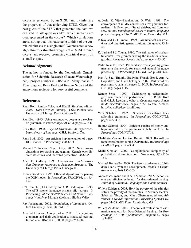
corpus is generated by an STSG, and by inferringthe properties of that underlying STSG. Given ourbest guess of the STSG that generated the data, wecan start to ask questions like: which subtrees areoverrepresented in the corpus? Which correlationsare so strong that it is reasonable to think of the cor-related phrases as a single unit? We presented a newalgorithm for estimating weights of an STSG from acorpus, and reported promising empirical results ona small corpus.
Acknowledgments
The author is funded by the Netherlands Organi-sation for Scientific Research (Exacte Wetenschap-pen), project number 612.066.405. Many thanks toYoav Seginer, Rens Bod and Remko Scha and theanonymous reviewers for very useful comments.
References
Rens Bod, Remko Scha, and Khalil Sima’an, editors.2003. Data-Oriented Parsing. CSLI Publications,University of Chicago Press, Chicago, IL.
Rens Bod. 1993. Using an annotated corpus as a stochas-tic grammar. In Proceedings EACL’93, pages 37–44.
Rens Bod. 1998. Beyond Grammar: An experience-based theory of language. CSLI, Stanford, CA.
Rens Bod. 2003. An efficient implementation of a newDOP model. In Proceedings EACL’03.
Michael Collins and Nigel Duffy. 2002. New rankingalgorithms for parsing and tagging: Kernels over dis-crete structures, and the voted perceptron. ACL’02.
Adele E. Goldberg. 1995. Constructions: A Construc-tion Grammar Approach to Argument Structure. TheUniversity of Chicago Press, Chicago, IL.
Joshua Goodman. 1996. Efficient algorithms for parsingthe DOP model. In Proceedings EMNLP’96, p. 143–152.
C.T. Hemphill, J.J. Godfrey, and G.R. Doddington. 1990.The ATIS spoken language systems pilot corpus. InProceedings of the DARPA Speech and Natural Lan-guage Workshop. Morgan Kaufman, Hidden Valley.
Ray Jackendoff. 2002. Foundations of Language. Ox-ford University Press, Oxford, UK.
Aravind Joshi and Anoop Sarkar. 2003. Tree adjoininggrammars and their application to statistical parsing.In Bod et al. (Bod et al., 2003), pages 253–282.
A. Joshi, K. Vijay-Shanker, and D. Weir. 1991. Theconvergence of mildly context-sensitive grammar for-malisms. In Peter Sells, Stuart Shieber, and Tom Wa-sow, editors, Foundational issues in natural languageprocessing, pages 21–82. MIT Press, Cambridge MA.
P. Kay and C. Fillmore. 1999. Grammatical construc-tions and linguistic generalizations. Language, 75:1–33.
K. Lari and S.J. Young. 1990. The estimation of stochas-tic context-free grammars using the inside-outside al-gorithm. Computer Speech and Language, 4:35–56.
Philip Resnik. 1992. Probabilistic tree-adjoining gram-mar as a framework for statistical natural languageprocessing. In Proceedings COLING’92, p. 418–424.
Ivan A. Sag, Timothy Baldwin, Francis Bond, Ann A.Copestake, and Dan Flickinger. 2002. Multiword ex-pressions: A pain in the neck for NLP. In ProceedingsCICLing, pages 1–15.
Remko Scha. 1990. Taaltheorie en taaltechnolo-gie; competence en performance. In R. de Kortand G.L.J. Leerdam, editors, Computertoepassingenin de Neerlandistiek, pages 7–22. LVVN, Almere.http://iaaa.nl/rs/LeerdamE.html.
Yves Schabes. 1992. Stochastic lexicalized tree-adjoining grammars. In Proceedings COLING’92,pages 425–432.
Helmut Schmid. 2004. Efficient parsing of highly am-biguous context-free grammars with bit vectors. InProceedings COLING’04.
Khalil Sima’an and Luciano Buratto. 2003. Backoff pa-rameter estimation for the DOP model. In ProceedingsECML’03, pages 373–384.
Khalil Sima’an. 2002. Computational complexity ofprobabilistic disambiguation. Grammars, 5(2):125–151.
Michael Tomasello. 2000. The item-based nature of chil-dren’s early syntactic development. Trends in Cogni-tive Science, 4(4):156–163.
Andreas Zollmann and Khalil Sima’an. 2005. A consis-tent and efficient estimator for data-oriented parsing.Journal of Automata, Languages and Combinatorics.
Willem Zuidema. 2003. How the poverty of the stimulussolves the poverty of the stimulus. In Suzanna Becker,Sebastian Thrun, and Klaus Obermayer, editors, Ad-vances in Neural Information Processing Systems 15,pages 51–58. MIT Press, Cambridge, MA.
Willem Zuidema. 2006. Theoretical evaluation of esti-mation methods for Data-Oriented Parsing. In Pro-ceedings EACL’06 (Conference Companion), pages183–186.
36
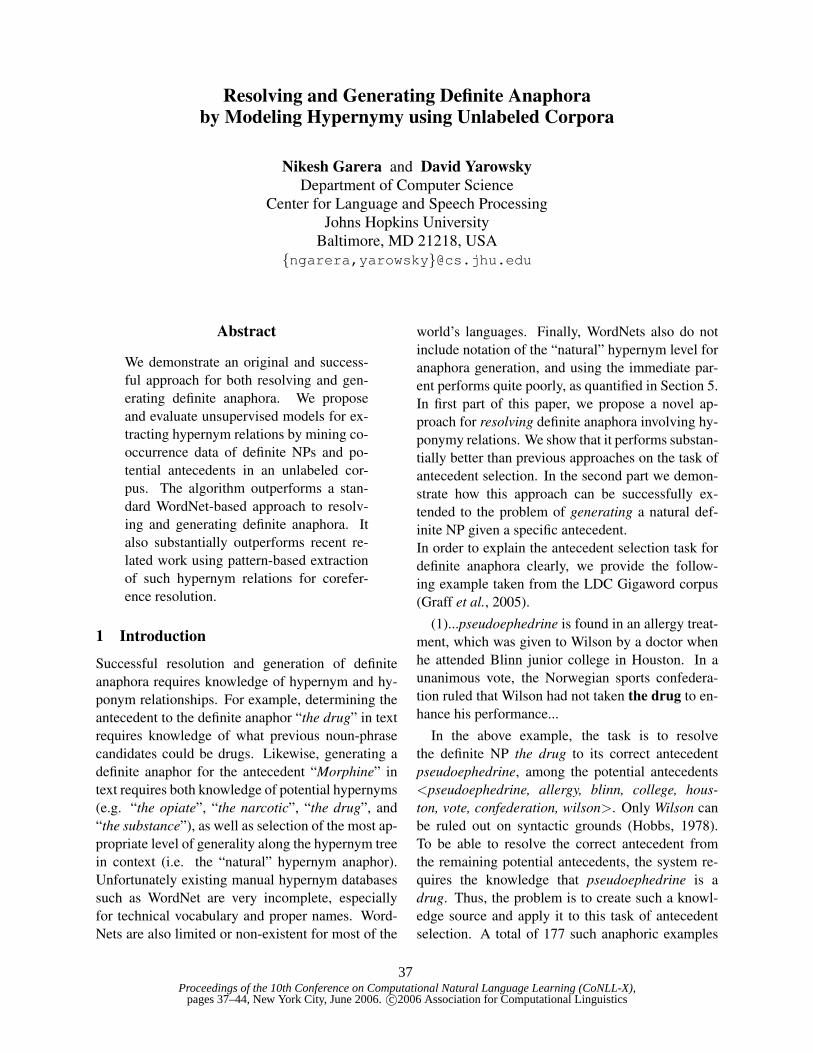
Proceedings of the 10th Conference on Computational Natural Language Learning (CoNLL-X),pages 37–44, New York City, June 2006.c©2006 Association for Computational Linguistics
Resolving and Generating Definite Anaphoraby Modeling Hypernymy using Unlabeled Corpora
Nikesh Garera and David YarowskyDepartment of Computer Science
Center for Language and Speech ProcessingJohns Hopkins University
Baltimore, MD 21218, USA{ngarera,yarowsky}@cs.jhu.edu
Abstract
We demonstrate an original and success-ful approach for both resolving and gen-erating definite anaphora. We proposeand evaluate unsupervised models for ex-tracting hypernym relations by mining co-occurrence data of definite NPs and po-tential antecedents in an unlabeled cor-pus. The algorithm outperforms a stan-dard WordNet-based approach to resolv-ing and generating definite anaphora. Italso substantially outperforms recent re-lated work using pattern-based extractionof such hypernym relations for corefer-ence resolution.
1 Introduction
Successful resolution and generation of definiteanaphora requires knowledge of hypernym and hy-ponym relationships. For example, determining theantecedent to the definite anaphor “the drug” in textrequires knowledge of what previous noun-phrasecandidates could be drugs. Likewise, generating adefinite anaphor for the antecedent “Morphine” intext requires both knowledge of potential hypernyms(e.g. “the opiate”, “the narcotic”, “the drug”, and“the substance”), as well as selection of the most ap-propriate level of generality along the hypernym treein context (i.e. the “natural” hypernym anaphor).Unfortunately existing manual hypernym databasessuch as WordNet are very incomplete, especiallyfor technical vocabulary and proper names. Word-Nets are also limited or non-existent for most of the
world’s languages. Finally, WordNets also do notinclude notation of the “natural” hypernym level foranaphora generation, and using the immediate par-ent performs quite poorly, as quantified in Section 5.In first part of this paper, we propose a novel ap-proach for resolving definite anaphora involving hy-ponymy relations. We show that it performs substan-tially better than previous approaches on the task ofantecedent selection. In the second part we demon-strate how this approach can be successfully ex-tended to the problem of generating a natural def-inite NP given a specific antecedent.In order to explain the antecedent selection task fordefinite anaphora clearly, we provide the follow-ing example taken from the LDC Gigaword corpus(Graff et al., 2005).
(1)...pseudoephedrine is found in an allergy treat-ment, which was given to Wilson by a doctor whenhe attended Blinn junior college in Houston. In aunanimous vote, the Norwegian sports confedera-tion ruled that Wilson had not taken the drug to en-hance his performance...
In the above example, the task is to resolvethe definite NP the drug to its correct antecedentpseudoephedrine, among the potential antecedents<pseudoephedrine, allergy, blinn, college, hous-ton, vote, confederation, wilson>. Only Wilson canbe ruled out on syntactic grounds (Hobbs, 1978).To be able to resolve the correct antecedent fromthe remaining potential antecedents, the system re-quires the knowledge that pseudoephedrine is adrug. Thus, the problem is to create such a knowl-edge source and apply it to this task of antecedentselection. A total of 177 such anaphoric examples
37
were extracted randomly from the LDC Gigawordcorpus and a human judge identified the correct an-tecedent for the definite NP in each example (given acontext of previous sentences).1 Two human judgeswere asked to perform the same task over the sameexamples. The agreement between the judges was92% (of all 177 examples), indicating a clearly de-fined task for our evaluation purposes.We describe an unsupervised approach to this taskthat extracts examples containing definite NPs froma large corpus, considers all head words appearingbefore the definite NP as potential antecedents andthen filters the noisy <antecedent, definite-NP> pairusing Mutual Information space. The co-occurencestatistics of such pairs can then be used as a mecha-nism for detecting a hypernym relation between thedefinite NP and its potential antecedents. We com-pare this approach with a WordNet-based algorithmand with an approach presented by Markert and Nis-sim (2005) on resolving definite NP coreference thatmakes use of lexico-syntactic patterns such as ’Xand Other Ys’ as utilized by Hearst (1992).
2 Related workThere is a rich tradition of work using lexical and se-mantic resources for anaphora and coreference res-olution. Several researchers have used WordNet asa lexical and semantic resource for certain types ofbridging anaphora (Poesio et al., 1997; Meyer andDale, 2002). WordNet has also been used as an im-portant feature in machine learning of coreferenceresolution using supervised training data (Soon etal., 2001; Ng and Cardie, 2002). However, sev-eral researchers have reported that knowledge incor-porated via WordNet is still insufficient for definiteanaphora resolution. And of course, WordNet is notavailable for all languages and is missing inclusionof large segments of the vocabulary even for cov-ered languages. Hence researchers have investigateduse of corpus-based approaches to build a Word-Net like resource automatically (Hearst, 1992; Cara-
1The test examples were selected as follows: First, allthe sentences containing definite NP “The Y” were extractedfrom the corpus. Then, the sentences containing instancesof anaphoric definite NPs were kept and other cases of defi-nite expressions (like existential NPs “The White House”,“Theweather”) were discarded. From this anaphoric set of sentences,177 sentence instances covering 13 distinct hypernyms wererandomly selected as the test set and annotated for the correctantecedent by human judges.
ballo, 1999; Berland and Charniak, 1999). Also,several researchers have applied it to resolving dif-ferent types of bridging anaphora (Clark, 1975).Poesio et al. (2002) have proposed extracting lexicalknowledge about part-of relations using Hearst-stylepatterns and applied it to the task of resolving bridg-ing references. Poesio et al. (2004) have suggestedusing Google as a source of computing lexical dis-tance between antecedent and definite NP for mere-ological bridging references (references referring toparts of an object already introduced). Markert et al.(2003) have applied relations extracted from lexico-syntactic patterns such as ’X and other Ys’ for Other-Anaphora (referential NPs with modifiers other oranother) and for bridging involving meronymy.There has generally been a lack of work in the exist-ing literature for automatically building lexical re-sources for definite anaphora resolution involvinghyponyms relations such as presented in Example(1). However, this issue was recently addressed byMarkert and Nissim (2005) by extending their workon Other-Anaphora using lexico syntactic pattern ’Xand other Y’s to antecedent selection for definite NPcoreference. However, our task is more challeng-ing since the anaphoric definite NPs in our test setinclude only hypernym anaphors without includingthe much simpler cases of headword repetition andother instances of string matching. For direct eval-uation, we also implemented their corpus-based ap-proach and compared it with our models on identicaltest data.We also describe and evaluate a mechanism for com-bining the knowledge obtained from WordNet andthe six corpus-based approaches investigated here.The resulting models are able to overcome the weak-nesses of a WordNet-only model and substantiallyoutperforms any of the individual models.
3 Models for Lexical Acquisition3.1 TheY-ModelOur algorithm is motivated by the observation that ina discourse, the use of the definite article (“the”) in anon-deictic context is primarily licensed if the con-cept has already been mentioned in the text. Hence asentence such as “The drug is very expensive” gen-erally implies that either the word drug itself waspreviously mentioned (e.g. “He is taking a new drugfor his high cholesterol.”) or a hyponym of drug was
38
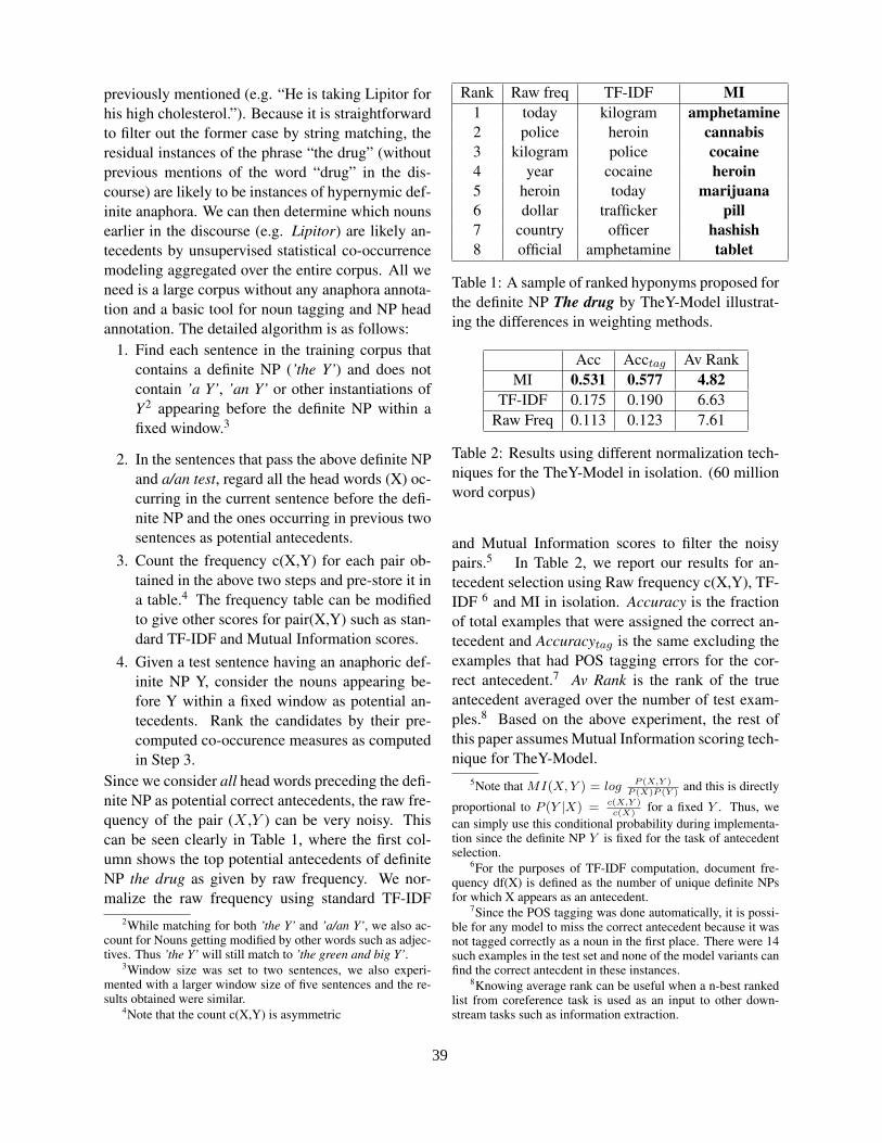
previously mentioned (e.g. “He is taking Lipitor forhis high cholesterol.”). Because it is straightforwardto filter out the former case by string matching, theresidual instances of the phrase “the drug” (withoutprevious mentions of the word “drug” in the dis-course) are likely to be instances of hypernymic def-inite anaphora. We can then determine which nounsearlier in the discourse (e.g. Lipitor) are likely an-tecedents by unsupervised statistical co-occurrencemodeling aggregated over the entire corpus. All weneed is a large corpus without any anaphora annota-tion and a basic tool for noun tagging and NP headannotation. The detailed algorithm is as follows:
1. Find each sentence in the training corpus thatcontains a definite NP (’the Y’) and does notcontain ’a Y’, ’an Y’ or other instantiations ofY2 appearing before the definite NP within afixed window.3
2. In the sentences that pass the above definite NPand a/an test, regard all the head words (X) oc-curring in the current sentence before the defi-nite NP and the ones occurring in previous twosentences as potential antecedents.
3. Count the frequency c(X,Y) for each pair ob-tained in the above two steps and pre-store it ina table.4 The frequency table can be modifiedto give other scores for pair(X,Y) such as stan-dard TF-IDF and Mutual Information scores.
4. Given a test sentence having an anaphoric def-inite NP Y, consider the nouns appearing be-fore Y within a fixed window as potential an-tecedents. Rank the candidates by their pre-computed co-occurence measures as computedin Step 3.
Since we consider all head words preceding the defi-nite NP as potential correct antecedents, the raw fre-quency of the pair (X ,Y ) can be very noisy. Thiscan be seen clearly in Table 1, where the first col-umn shows the top potential antecedents of definiteNP the drug as given by raw frequency. We nor-malize the raw frequency using standard TF-IDF
2While matching for both ’the Y’ and ’a/an Y’, we also ac-count for Nouns getting modified by other words such as adjec-tives. Thus ’the Y’ will still match to ’the green and big Y’.
3Window size was set to two sentences, we also experi-mented with a larger window size of five sentences and the re-sults obtained were similar.
4Note that the count c(X,Y) is asymmetric
Rank Raw freq TF-IDF MI1 today kilogram amphetamine2 police heroin cannabis3 kilogram police cocaine4 year cocaine heroin5 heroin today marijuana6 dollar trafficker pill7 country officer hashish8 official amphetamine tablet
Table 1: A sample of ranked hyponyms proposed forthe definite NP The drug by TheY-Model illustrat-ing the differences in weighting methods.
Acc Acctag Av RankMI 0.531 0.577 4.82
TF-IDF 0.175 0.190 6.63Raw Freq 0.113 0.123 7.61
Table 2: Results using different normalization tech-niques for the TheY-Model in isolation. (60 millionword corpus)
and Mutual Information scores to filter the noisypairs.5 In Table 2, we report our results for an-tecedent selection using Raw frequency c(X,Y), TF-IDF 6 and MI in isolation. Accuracy is the fractionof total examples that were assigned the correct an-tecedent and Accuracytag is the same excluding theexamples that had POS tagging errors for the cor-rect antecedent.7 Av Rank is the rank of the trueantecedent averaged over the number of test exam-ples.8 Based on the above experiment, the rest ofthis paper assumes Mutual Information scoring tech-nique for TheY-Model.
5Note that MI(X, Y ) = log P (X,Y )P (X)P (Y )
and this is directly
proportional to P (Y |X) = c(X,Y )c(X)
for a fixed Y . Thus, wecan simply use this conditional probability during implementa-tion since the definite NP Y is fixed for the task of antecedentselection.
6For the purposes of TF-IDF computation, document fre-quency df(X) is defined as the number of unique definite NPsfor which X appears as an antecedent.
7Since the POS tagging was done automatically, it is possi-ble for any model to miss the correct antecedent because it wasnot tagged correctly as a noun in the first place. There were 14such examples in the test set and none of the model variants canfind the correct antecdent in these instances.
8Knowing average rank can be useful when a n-best rankedlist from coreference task is used as an input to other down-stream tasks such as information extraction.
39
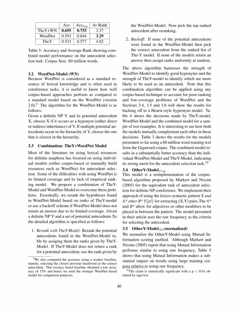
Acc Acctag Av RankTheY+WN 0.695 0.755 3.37WordNet 0.593 0.644 3.29
TheY 0.531 0.577 4.82
Table 3: Accuracy and Average Rank showing com-bined model performance on the antecedent selec-tion task. Corpus Size: 60 million words.
3.2 WordNet-Model (WN)Because WordNet is considered as a standard re-source of lexical knowledge and is often used incoreference tasks, it is useful to know how wellcorpus-based approaches perform as compared toa standard model based on the WordNet (version2.0).9 The algorithm for the WordNet-Model is asfollows:Given a definite NP Y and its potential antecedentX, choose X if it occurs as a hyponym (either director indirect inheritance) of Y. If multiple potential an-tecedents occur in the hierarchy of Y, choose the onethat is closest in the hierarchy.
3.3 Combination: TheY+WordNet ModelMost of the literature on using lexical resourcesfor definite anaphora has focused on using individ-ual models (either corpus-based or manually buildresources such as WordNet) for antecedent selec-tion. Some of the difficulties with using WordNet isits limited coverage and its lack of empirical rank-ing model. We propose a combination of TheY-Model and WordNet-Model to overcome these prob-lems. Essentially, we rerank the hypotheses foundin WordNet-Model based on ranks of TheY-modelor use a backoff scheme if WordNet-Model does notreturn an answer due to its limited coverage. Givena definite NP Y and a set of potential antecedents Xsthe detailed algorithm is specified as follows:
1. Rerank with TheY-Model: Rerank the potentialantecedents found in the WordNet-Model ta-ble by assiging them the ranks given by TheY-Model. If TheY-Model does not return a rankfor a potential antecedent, use the rank given by
9We also computed the accuracy using a weaker baseline,namely, selecting the closest previous headword as the correctantecedent. This recency based baseline obtained a low accu-racy of 15% and hence we used the stronger WordNet basedmodel for comparison purposes.
the WordNet-Model. Now pick the top rankedantecedent after reranking.
2. Backoff: If none of the potential antecedentswere found in the WordNet-Model then pickthe correct antecedent from the ranked list ofThe-Y model. If none of the models return ananswer then assign ranks uniformly at random.
The above algorithm harnesses the strength ofWordNet-Model to identify good hyponyms and thestrength of TheY-model to identify which are morelikely to be used as an antecedent. Note that thiscombination algorithm can be applied using anycorpus-based technique to account for poor-rankingand low-coverage problems of WordNet and theSections 3.4, 3.5 and 3.6 will show the results forbacking off to a Hearst-style hypernym model. Ta-ble 4 shows the decisions made by TheY-model,WordNet-Model and the combined model for a sam-ple of test examples. It is interesting to see how boththe models mutually complement each other in thesedecisions. Table 3 shows the results for the modelspresented so far using a 60 million word training textfrom the Gigaword corpus. The combined model re-sults in a substantially better accuracy than the indi-vidual WordNet-Model and TheY-Model, indicatingits strong merit for the antecedent selection task.10
3.4 OtherY-Modelfreq
This model is a reimplementation of the corpus-based algorithm proposed by Markert and Nissim(2005) for the equivalent task of antecedent selec-tion for definite NP coreference. We implement theirapproach of using the lexico-syntactic pattern X andA* other B* Y{pl} for extracting (X,Y) pairs.The A*and B* allow for adjectives or other modifiers to beplaced in between the pattern. The model presentedin their article uses the raw frequency as the criteriafor selecting the antecedent.3.5 OtherY-ModelMI (normalized)We normalize the OtherY-Model using Mutual In-formation scoring method. Although Markert andNissim (2005) report that using Mutual Informationperforms similar to using raw frequency, Table 5shows that using Mutual Information makes a sub-stantial impact on results using large training cor-pora relative to using raw frequency.
10The claim is statistically significant with a p < 0.01 ob-tained by sign-test
40
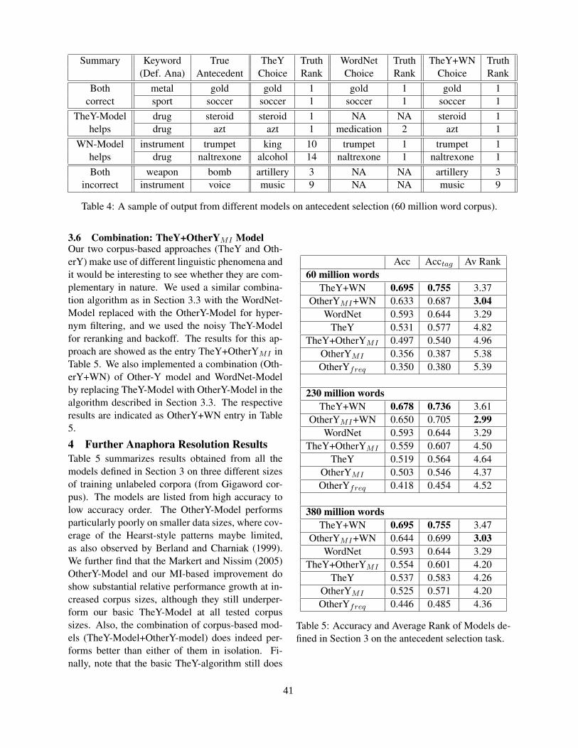
Summary Keyword True TheY Truth WordNet Truth TheY+WN Truth(Def. Ana) Antecedent Choice Rank Choice Rank Choice Rank
Both metal gold gold 1 gold 1 gold 1correct sport soccer soccer 1 soccer 1 soccer 1
TheY-Model drug steroid steroid 1 NA NA steroid 1helps drug azt azt 1 medication 2 azt 1
WN-Model instrument trumpet king 10 trumpet 1 trumpet 1helps drug naltrexone alcohol 14 naltrexone 1 naltrexone 1Both weapon bomb artillery 3 NA NA artillery 3
incorrect instrument voice music 9 NA NA music 9
Table 4: A sample of output from different models on antecedent selection (60 million word corpus).
3.6 Combination: TheY+OtherYMI ModelOur two corpus-based approaches (TheY and Oth-erY) make use of different linguistic phenomena andit would be interesting to see whether they are com-plementary in nature. We used a similar combina-tion algorithm as in Section 3.3 with the WordNet-Model replaced with the OtherY-Model for hyper-nym filtering, and we used the noisy TheY-Modelfor reranking and backoff. The results for this ap-proach are showed as the entry TheY+OtherYMI inTable 5. We also implemented a combination (Oth-erY+WN) of Other-Y model and WordNet-Modelby replacing TheY-Model with OtherY-Model in thealgorithm described in Section 3.3. The respectiveresults are indicated as OtherY+WN entry in Table5.
4 Further Anaphora Resolution ResultsTable 5 summarizes results obtained from all themodels defined in Section 3 on three different sizesof training unlabeled corpora (from Gigaword cor-pus). The models are listed from high accuracy tolow accuracy order. The OtherY-Model performsparticularly poorly on smaller data sizes, where cov-erage of the Hearst-style patterns maybe limited,as also observed by Berland and Charniak (1999).We further find that the Markert and Nissim (2005)OtherY-Model and our MI-based improvement doshow substantial relative performance growth at in-creased corpus sizes, although they still underper-form our basic TheY-Model at all tested corpussizes. Also, the combination of corpus-based mod-els (TheY-Model+OtherY-model) does indeed per-forms better than either of them in isolation. Fi-nally, note that the basic TheY-algorithm still does
Acc Acctag Av Rank60 million words
TheY+WN 0.695 0.755 3.37OtherYMI+WN 0.633 0.687 3.04
WordNet 0.593 0.644 3.29TheY 0.531 0.577 4.82
TheY+OtherYMI 0.497 0.540 4.96OtherYMI 0.356 0.387 5.38OtherYfreq 0.350 0.380 5.39
230 million wordsTheY+WN 0.678 0.736 3.61
OtherYMI+WN 0.650 0.705 2.99WordNet 0.593 0.644 3.29
TheY+OtherYMI 0.559 0.607 4.50TheY 0.519 0.564 4.64
OtherYMI 0.503 0.546 4.37OtherYfreq 0.418 0.454 4.52
380 million wordsTheY+WN 0.695 0.755 3.47
OtherYMI+WN 0.644 0.699 3.03WordNet 0.593 0.644 3.29
TheY+OtherYMI 0.554 0.601 4.20TheY 0.537 0.583 4.26
OtherYMI 0.525 0.571 4.20OtherYfreq 0.446 0.485 4.36
Table 5: Accuracy and Average Rank of Models de-fined in Section 3 on the antecedent selection task.
41
relatively well by itself on smaller corpus sizes,suggesting its merit on resource-limited languageswith smaller available online text collections and theunavailability of WordNet. The combined modelsof WordNet-Model with the two corpus-based ap-proaches still significantly (p < 0.01) outperformany of the other individual models.11
5 Generation TaskHaving shown positive results for the task of an-tecedent selection, we turn to a more difficult task,namely generating an anaphoric definite NP givena nominal antecedent. In Example (1), this wouldcorrespond to generating “the drug” as an anaphorknowing that the antecedent is pseudoephedrine.This task clearly has many applications: current gen-eration systems often limit their anaphoric usage topronouns and thus an automatic system that doeswell on hypernymic definite NP generation can di-rectly be helpful. It also has strong potential appli-cation in abstractive summarization where rewritinga fluent passage requires a good model of anaphoricusage.There are many interesting challenges in this prob-lem: first of all, there maybe be multiple acceptablechoices for definite anaphor given a particular an-tecedent, complicating automatic evaluation. Sec-ond, when a system generates a definite anaphora,the space of potential candidates is essentially un-bounded, unlike in antecdent selection, where it islimited only to the number of potential antecedentsin prior context. In spite of the complex natureof this problem, our experiments with the humanjudgements, WordNet and corpus-based approachesshow a simple feasible solution. We evaluate ourautomatic approaches based on exact-match agree-ment with definite anaphora actually used in the cor-pus (accuracy) and also by agreement with definiteanaphora predicted independently by a human judgein an absence of context.
11Note that syntactic co-reference candidate filters such asthe Hobbs algorithm were not utilized in this study. To assessthe performance implications, the Hobbs algorithm was appliedto a randomly selected 100-instance subset of the test data. Al-though the Hobbs algorithm frequently pruned at least one ofthe coreference candidates, in only 2% of the data did such can-didate filtering change system output. However, since both ofthese changes were improvements, it could be worthwhile toutilize Hobbs filtering in future work, although the gains wouldlikely be modest.
5.1 Human experiment
We extracted a total of 103 <true antecedent, defi-nite NP> pairs from the set of test instances used inthe resolution task. Then we asked a human judge (anative speaker of English) to predict a parent classof the antecedent that could act as a good definiteanaphora choice in general, independent of a par-ticular context. Thus, the actual corpus sentencecontaining the antecedent and definite NP and itscontext was not provided to the judge. We tookthe predictions provided by the judge and matchedthem with the actual definite NPs used in the corpus.The agreement between corpus and the human judgewas 79% which can thus be considered as an upperbound of algorithm performance. Table 7 shows asample of decisions made by the human and howthey agree with the definite NPs observed in the cor-pus. It is interesting to note the challenge of thesense variation and figurative usage. For example,“corruption” is refered to as a “tool” in the actualcorpus anaphora, a metaphoric usage that would bedifficult to predict unless given the usage sentenceand its context. However, a human agreement of79% indicate that such instances are relatively rareand the task of predicting a definite anaphor with-out its context is viable. In general, it appears fromour experiements that humans tend to select froma relatively small set of parent classes when gener-ating hypernymic definite anaphora. Furthermore,there appears to be a relatively context-independentconcept of the “natural” level in the hypernym hi-erarchy for generating anaphors. For example, al-though <“alkaloid”, “organic compound”, “com-pound”, “substance”, “entity”> are all hypernymsof “Pseudoephederine” in WordNet, “the drug”appears to be the preferred hypernym for definiteanaphora in the data, with the other alternatives be-ing either too specific or too general to be natural.This natural level appears to be difficult to define byrule. For example, using just the immediate parenthypernym in the WordNet hierarchy only achieves4% match with the corpus data for definite anaphorgeneration.
5.2 Algorithms
The following sections presents our corpus-based al-gorithms as more effective alternatives.
42
Agreement Agreementw/ human w/ corpus
judgeTheY+OtherY+WN 47% 46%
OtherY +WN 43% 43%TheY+WN 42% 37%
TheY +OtherY 39% 36%OtherY 39% 36%
WordNet 4% 4%Human judge 100% 79%
Corpus 79% 100%
Table 6: Agreement of different generation modelswith human judge and with definite NP used in thecorpus.
5.2.1 Individual Models
For the corpus-based approaches, the TheY-Modeland OtherY-Model were trained in the same manneras for the antecedent selection task. The only differ-ence was that in the generation case, the frequencystatistics were reversed to provide a hypernym givena hyponym. Additionally, we found that raw fre-quency outperformed either TF-IDF or Mutual In-formation and was used for all results in Table 6.The stand-alone WordNet model is also very simple:Given an antecedent, we lookup its direct hypernym(using first sense) in the WordNet and use it as thedefinite NP, for lack of a better rule for preferred hy-pernym location.
5.2.2 Combining corpus-based approaches andWordNet
Each of the corpus-based approaches was combinedwith WordNet resulting in two different models asfollows: Given an antecedent X, the corpus-basedapproach looks up in its table the hypernym of X,for example Y, and only produces Y as the output ifY also occurs in the WordNet as hypernym. ThusWordNet is used as a filtering tool for detecting vi-able hypernyms. This combination resulted in twomodels: ’TheY+WN’ and ’OtherY+WN’.We also combined all the three approaches, ’TheY’,’OtherY’ and WordNet resulting in a single model’TheY+OtherY+WN’. This was done as follows: Wefirst combine the models ’TheY’ and ’OtherY’ usinga backoff model. The first priority is to use the hy-
Antecedent Corpus Human TheY+OtherYDef Ana Choice +WN
racing sport sport sportazt drug drug drug
missile weapon weapon weaponalligator animal animal animal
steel metal metal metalosteporosis disease disease condition
grenade device weapon devicebaikonur site city station
corruption tool crime activity
Table 7: Sample of decisions made by hu-man judge and our best performing model(TheY+OtherY+WN) on the generation task.
pernym from the model ’OtherY’, if not found thenuse the hypernym from the model ’TheY’. Given adefinite NP from the backoff model, apply the Word-Net filtering technique, specifically, choose it as thecorrect definite NP if it also occurs as a hypernym inthe WordNet hierarchy of the antecedent.
5.3 Evaluation of Anaphor Generation
We evaluated the resulting algorithms from Section5.2 on the definite NP prediction task as describedearlier. Table 6 shows the agreement of the algo-rithm predictions with the human judge as well aswith the definite NP actually observed in the corpus.It is interesting to see that WordNet by itself per-forms very poorly on this task since it does not haveany word-specific mechanism to choose the correctlevel in the hierarchy and the correct word sense forselecting the hypernym. However, when combinedwith our corpus-based approaches, the agreementincreases substantially indicating that the corpus-based approaches are effectively filtering the spaceof hypernyms that can be used as natural classes.Likewise, WordNet helps to filter the noisy hyper-nyms from the corpus predictions. Thus, this inter-play between the corpus-based and WordNet algo-rithm works out nicely, resulting in the best modelbeing a combination of all three individual modelsand achieving a substantially better agreement withboth the corpus and human judge than any of the in-dividual models. Table 7 shows decisions made bythis algorithm on a sample test data.
43
6 ConclusionThis paper provides a successful solution to theproblem of incomplete lexical resources for definiteanaphora resolution and further demonstrates howthe resources built for resolution can be naturally ex-tended for the less studied task of anaphora genera-tion. We first presented a simple and noisy corpus-based approach based on globally modeling head-word co-occurrence around likely anaphoric definiteNPs. This was shown to outperform a recent ap-proach by Markert and Nissim (2005) that makes useof standard Hearst-style patterns extracting hyper-nyms for the same task. Even with a relatively smalltraining corpora, our simple TheY-model was ableto achieve relatively high accuracy, making it suit-able for resource-limited languages where annotatedtraining corpora and full WordNets are likely notavailable. We then evaluated several variants of thisalgorithm based on model combination techniques.The best combined model was shown to exceed 75%accuracy on the resolution task, beating any of theindividual models. On the much harder anaphorageneration task, where the stand-alone WordNet-based model only achieved an accuracy of 4%, weshowed that our algorithms can achieve 35%-47%accuracy on blind exact-match evaluation, thus mo-tivating the use of such corpus-based learning ap-proaches on the generation task as well.
AcknowledgementsThanks to Charles Schafer for sharing his tools onPOS/Headword tagging for the Gigaword corpus.
ReferencesM. Berland and E. Charniak. 1999. Finding parts in
very large corpora. In Proceedings of the 37th AnnualMeeting of the Association for Computational Linguis-tics, pages 57–64.
S. Caraballo. 1999. Automatic construction of ahypernym-labeled noun hierarchy from text. In Pro-ceedings of the 37th Annual Meeting of the Associationfor Computational Linguistics, pages 120–126.
H. H. Clark. 1975. Bridging. In Proceedings of theConference on Theoretical Issues in Natural LanguageProcessing, pages 169–174.
D. Connoly, J. D. Burger, and D. S. Day. 1997. A ma-chine learning approach to anaphoric reference. InProceedings of the International Conference on NewMethods in Language Processing, pages 133–144.
D. Graff, J. Kong, K. Chen, and K. Maeda. 2005. En-glish Gigaword Second Edition. Linguistic Data Con-sortium, catalog number LDC2005T12.
S. Harabagiu, R. Bunescu, and S. J. Maiorano. 2001.Text and knowledge mining for coreference resolu-tion. In Proceedings of the Second Meeting of theNorth American Chapter of the Association for Com-putational Linguistics, pages 55–62.
M. Hearst. 1992. Automatic acquisition of hyponymsfrom large text corpora. In Proceedings of the 14th In-ternational Conference on Computational Linguistics,pages 539–545.
J. Hobbs. 1978. Resolving pronoun references. Lingua,44:311–338.
K. Markert and M. Nissim. 2005. Comparing knowl-edge sources for nominal anaphora resolution. Com-putational Linguistics, 31(3):367–402.
K. Markert, M. Nissim, and N. N. Modjeska. 2003. Us-ing the web for nominal anaphora resolution. In Pro-ceedings of the EACL Workshop on the ComputationalTreatment of Anaphora, pages 39–46.
J. Meyer and R. Dale. 2002. Mining a corpus to sup-port associative anaphora resolution. In Proceedingsof the Fourth International Conference on DiscourseAnaphora and Anaphor Resolution.
V. Ng and C. Cardie. 2002. Improving machine learn-ing approaches to coreference resolution. In Proceed-ings of the 40th Annual Meeting of the Association forComputational Linguistics, pages 104–111.
M. Poesio, R. Vieira, and S. Teufel. 1997. Resolvingbridging references in unrestricted text. In Proceed-ings of the ACL Workshop on Operational Factors inRobust Anaphora, pages 1–6.
M. Poesio, T. Ishikawa, S. Schulte im Walde, andR. Viera. 2002. Acquiring lexical knowledge foranaphora resolution. In Proccedings of the Third Con-ference on Language Resources and Evaluation, pages1220–1224.
M. Poesio, R. Mehta, A. Maroudas, and J. Hitzeman.2004. Learning to resolve bridging references. In Pro-ceedings of the 42nd Annual Meeting of the Associa-tion for Computational Linguistics, pages 143–150.
W. M. Soon, H. T. Ng, and D. C. Y. Lim. 2001. A ma-chine learning approach to coreference resolution ofnoun phrases. Computational Linguistics, 27(4):521–544.
M. Strube, S. Rapp, and C. Muller. 2002. The influ-ence of minimum edit distance on reference resolution.In Proceedings of the 2002 Conference on EmpiricalMethods in Natural Language Processing, pages 312–319.
R. Vieira and M. Poesio. 2000. An empirically-basedsystem for processing definite descriptions. Computa-tional Linguistics, 26(4):539–593.
X. Yang, G. Zhou, J. Su, and C. L. Tan. 2003. Corefer-ence resolution using competition learning approach.In Proceedings of the 41st Annual Meeting of the Asso-ciation for Computational Linguistics, pages 176–183.
44
Proceedings of the 10th Conference on Computational Natural Language Learning (CoNLL-X),pages 45–52, New York City, June 2006.c©2006 Association for Computational Linguistics
Investigating Lexical Substitution Scoring for Subtitle GenerationOren Glickman and Ido Dagan
Computer Science DepartmentBar Ilan UniversityRamat Gan, Israel
{glikmao,dagan}@cs.biu.ac.il
Mikaela Keller and Samy BengioIDIAP Research Institute
Martigny,Switzerland
{mkeller,bengio}@idiap.ch
Walter DaelemansCNTS
Antwerp, [email protected]
Abstract
This paper investigates an isolated settingof the lexical substitution task of replac-ing words with their synonyms. In par-ticular, we examine this problem in thesetting of subtitle generation and evaluatestate of the art scoring methods that pre-dict the validity of a given substitution.The paper evaluates two context indepen-dent models and two contextual models.The major findings suggest that distribu-tional similarity provides a useful comple-mentary estimate for the likelihood thattwo Wordnet synonyms are indeed substi-tutable, while proper modeling of contex-tual constraints is still a challenging taskfor future research.
1 Introduction
Lexical substitution - the task of replacing a wordwith another one that conveys the same meaning -is a prominent task in many Natural Language Pro-cessing (NLP) applications. For example, in queryexpansion for information retrieval a query is aug-mented with synonyms of the original query words,aiming to retrieve documents that contain these syn-onyms (Voorhees, 1994). Similarly, lexical substi-tutions are applied in question answering to identifyanswer passages that express the sought answer indifferent terms than the original question. In natu-ral language generation it is common to seek lex-ical alternatives for the same meaning in order toreduce lexical repetitions. In general, lexical sub-stitution aims to preserve a desired meaning while
coping with the lexical variability of expressing thatmeaning. Lexical substitution can thus be viewedwithin the general framework of recognizing entail-ment between text segments (Dagan et al., 2005), asmodeling entailment relations at the lexical level.
In this paper we examine the lexical substitu-tion problem within a specific setting of text com-pression for subtitle generation (Daelemans et al.,2004). Subtitle generation is the task of generat-ing target language TV subtitles for video recordingsof a source language speech. The subtitles shouldbe of restricted length, which is often shorter thanthe full translation of the original speech, yet theyshould maintain as much as possible the meaningof the original content. In a typical (automated)subtitling process the original speech is first trans-lated fully into the target language and then the tar-get translation is compressed to optimize the lengthrequirements. One of the techniques employed inthe text compression phase is to replace a target lan-guage word in the original translation with a shortersynonym of it, thus reducing the character length ofthe subtitle. This is a typical lexical substitutiontask, which resembles similar operations in othertext compression and generation tasks (e.g. (Knightand Marcu, 2002)).
This paper investigates the task of assigning like-lihood scores for the correctness of such lexical sub-stitutions, in which words in the original translationare replaced with shorter synonyms. In our experi-ments we use WordNet as a source of candidate syn-onyms for substitution. The goal is to score the like-lihood that the substitution is admissible, i.e. yield-ing a valid sentence that preserves the original mean-ing. The focus of this paper is thus to utilize thesubtitling setting in order to investigate lexical sub-
45
stitution models in isolation, unlike most previousliterature in which this sub-task has been embeddedin larger systems and was not evaluated directly.
We examine four statistical scoring models, oftwo types. Context independent models score thegeneral likelihood that the original word is “replace-able” with the candidate synonym, in an arbitrarycontext. That is, trying to filter relatively bizarresynonyms, often of rare senses, which are abundantin WordNet but are unlikely to yield valid substitu-tions. Contextual models score the “fitness” of thereplacing word within the context of the sentence, inorder to filter out synonyms of senses of the originalword that are not the right sense in the given context.
We set up an experiment using actual subti-tling data and human judgements and evaluate thedifferent scoring methods. Our findings suggestthe dominance, in this setting, of generic context-independent scoring. In particular, considering dis-tributional similarity amongst WordNet synonymsseems effective for identifying candidate substitu-tions that are indeed likely to be applicable in actualtexts. Thus, while distributional similarity alone isknown to be too noisy as a sole basis for meaning-preserving substitutions, its combination with Word-Net allows reducing the noise caused by the manyWordNet synonyms that are unlikely to correspondto valid substitutions.
2 Background and Setting
2.1 Subtitling
Automatic generation of subtitles is a summariza-tion task at the level of individual sentences or occa-sionally of a few contiguous sentences. Limitationson reading speed of viewers and on the size of thescreen that can be filled with text without the imagebecoming too cluttered, are the constraints that dy-namically determine the amount of compression incharacters that should be achieved in transformingthe transcript into subtitles. Subtitling is not a trivialtask, and is expensive and time-consuming when ex-perts have to carry it out manually. As for other NLP
tasks, both statistical (machine learning) and linguis-tic knowledge-based techniques have been consid-ered for this problem. Examples of the former are(Knight and Marcu, 2002; Hori et al., 2002), and ofthe latter are (Grefenstette, 1998; Jing and McKe-
own, 1999). A comparison of both approaches inthe context of a Dutch subtitling system is providedin (Daelemans et al., 2004). The required sentencesimplification is achieved either by deleting mate-rial, or by paraphrasing parts of the sentence intoshorter expressions with the same meaning. As aspecial case of the latter, lexical substitution is oftenused to achieve a compression target by substitutinga word by a shorter synonym. It is on this subtaskthat we focus in this paper. Table 1 provides a fewexamples. E.g. by substituting “happen” by “occur”(example 3), one character is saved without affectingthe sentence meaning .
2.2 Experimental Setting
The data used in our experiments was collected inthe context of the MUSA (Multilingual Subtitling ofMultimedia Content) project (Piperidis et al., 2004)1
and was kindly provided for the current study. Thedata was provided by the BBC in the form of Hori-zon documentary transcripts with the correspondingaudio and video. The data for two documentarieswas used to create a dataset consisting of sentencesfrom the transcripts and the corresponding substitu-tion examples in which selected words are substi-tuted by a shorter Wordnet synonym. More con-cretely, a substitution example thus consists of anoriginal sentence s = w1 . . . wi . . . wn, a specificsource word wi in the sentence and a target (shorter)WordNet synonym w′ to substitute the source. SeeTable 1 for examples. The dataset consists of 918substitution examples originating from 231 differentsentences.
An annotation environment was developed to al-low efficient annotation of the substitution exampleswith the classes true (admissible substitution, in thegiven context) or false (inadmissible substitution).About 40% of the examples were judged as true.Part of the data was annotated by an additional an-notator to compute annotator agreement. The Kappascore turned out to be 0.65, corresponding to ”Sub-stantial Agreement” (Landis and Koch, 1997). Sincesome of the methods we are comparing need tuningwe held out a random subset of 31 original sentences(with 121 corresponding examples) for developmentand kept for testing the resulting 797 substitution ex-
1http://sinfos.ilsp.gr/musa/
46
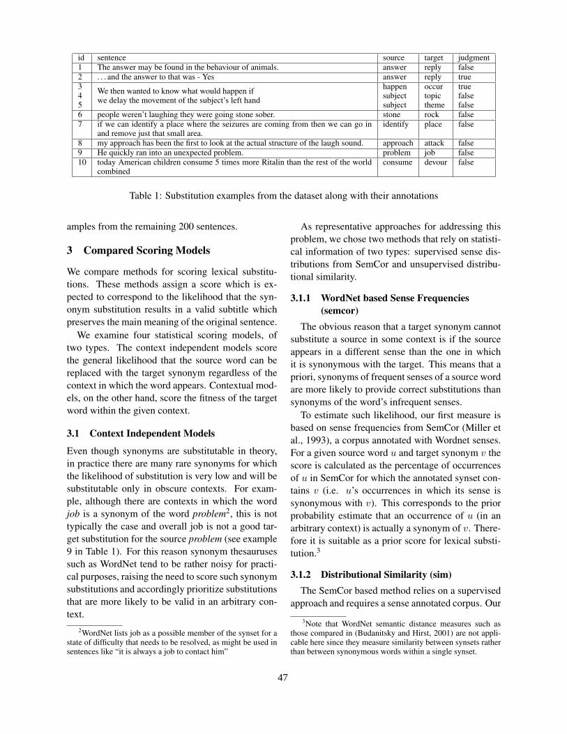
id sentence source target judgment1 The answer may be found in the behaviour of animals. answer reply false2 . . . and the answer to that was - Yes answer reply true3 We then wanted to know what would happen if
we delay the movement of the subject’s left hand
happen occur true4 subject topic false5 subject theme false6 people weren’t laughing they were going stone sober. stone rock false7 if we can identify a place where the seizures are coming from then we can go in
and remove just that small area.identify place false
8 my approach has been the first to look at the actual structure of the laugh sound. approach attack false9 He quickly ran into an unexpected problem. problem job false10 today American children consume 5 times more Ritalin than the rest of the world
combinedconsume devour false
Table 1: Substitution examples from the dataset along with their annotations
amples from the remaining 200 sentences.
3 Compared Scoring Models
We compare methods for scoring lexical substitu-tions. These methods assign a score which is ex-pected to correspond to the likelihood that the syn-onym substitution results in a valid subtitle whichpreserves the main meaning of the original sentence.
We examine four statistical scoring models, oftwo types. The context independent models scorethe general likelihood that the source word can bereplaced with the target synonym regardless of thecontext in which the word appears. Contextual mod-els, on the other hand, score the fitness of the targetword within the given context.
3.1 Context Independent Models
Even though synonyms are substitutable in theory,in practice there are many rare synonyms for whichthe likelihood of substitution is very low and will besubstitutable only in obscure contexts. For exam-ple, although there are contexts in which the wordjob is a synonym of the word problem2, this is nottypically the case and overall job is not a good tar-get substitution for the source problem (see example9 in Table 1). For this reason synonym thesaurusessuch as WordNet tend to be rather noisy for practi-cal purposes, raising the need to score such synonymsubstitutions and accordingly prioritize substitutionsthat are more likely to be valid in an arbitrary con-text.
2WordNet lists job as a possible member of the synset for astate of difficulty that needs to be resolved, as might be used insentences like “it is always a job to contact him”
As representative approaches for addressing thisproblem, we chose two methods that rely on statisti-cal information of two types: supervised sense dis-tributions from SemCor and unsupervised distribu-tional similarity.
3.1.1 WordNet based Sense Frequencies(semcor)
The obvious reason that a target synonym cannotsubstitute a source in some context is if the sourceappears in a different sense than the one in whichit is synonymous with the target. This means that apriori, synonyms of frequent senses of a source wordare more likely to provide correct substitutions thansynonyms of the word’s infrequent senses.
To estimate such likelihood, our first measure isbased on sense frequencies from SemCor (Miller etal., 1993), a corpus annotated with Wordnet senses.For a given source word u and target synonym v thescore is calculated as the percentage of occurrencesof u in SemCor for which the annotated synset con-tains v (i.e. u’s occurrences in which its sense issynonymous with v). This corresponds to the priorprobability estimate that an occurrence of u (in anarbitrary context) is actually a synonym of v. There-fore it is suitable as a prior score for lexical substi-tution.3
3.1.2 Distributional Similarity (sim)The SemCor based method relies on a supervised
approach and requires a sense annotated corpus. Our
3Note that WordNet semantic distance measures such asthose compared in (Budanitsky and Hirst, 2001) are not appli-cable here since they measure similarity between synsets ratherthan between synonymous words within a single synset.
47
second method uses an unsupervised distributionalsimilarity measure to score synonym substitutions.Such measures are based on the general idea ofHarris’ Distributional Hypothesis, suggesting thatwords that occur within similar contexts are seman-tically similar (Harris, 1968).
As a representative of this approach we use Lin’sdependency-based distributional similarity database.Lin’s database was created using the particular dis-tributional similarity measure in (Lin, 1998), appliedto a large corpus of news data (64 million words) 4.Two words obtain a high similarity score if they oc-cur often in the same contexts, as captured by syn-tactic dependency relations. For example, two verbswill be considered similar if they have large commonsets of modifying subjects, objects, adverbs etc.
Distributional similarity does not capture directlymeaning equivalence and entailment but rather alooser notion of meaning similarity (Geffet and Da-gan, 2005). It is typical that non substitutable wordssuch as antonyms or co-hyponyms obtain high sim-ilarity scores. However, in our setting we applythe similarity score only for WordNet synonyms inwhich it is known a priori that they are substitutableis some contexts. Distributional similarity may thuscapture the statistical degree to which the two wordsare substitutable in practice. In fact, it has beenshown that prominence in similarity score corre-sponds to sense frequency, which was suggested asthe basis for an unsupervised method for identifyingthe most frequent sense of a word (McCarthy et al.,2004).
3.2 Contextual Models
Contextual models score lexical substitutions basedon the context of the sentence. Such modelstry to estimate the likelihood that the target wordcould potentially occur in the given context of thesource word and thus may replace it. More con-cretely, for a given substitution example consist-ing of an original sentence s = w1 . . . wi . . . wn,and a designated source word wi, the contextualmodels we consider assign a score to the substi-tution based solely on the target synonym v andthe context of the source word in the original sen-
4available at http://www.cs.ualberta.ca/˜lindek/downloads.htm
tence, {w1, . . . , wi−1, wi+1, . . . , wn}, which is rep-resented in a bag-of-words format.
Apparently, this setting was not investigated muchin the context of lexical substitution in the NLP lit-erature. We chose to evaluate two recently proposedmodels that address exactly the task at hand: the firstmodel was proposed in the context of lexical model-ing of textual entailment, using a generative NaıveBayes approach; the second model was proposedin the context of machine learning for informationretrieval, using a discriminative neural network ap-proach. The two models were trained on the (un-annotated) sentences of the BNC 100 million wordcorpus (Burnard, 1995) in bag-of-words format. Thecorpus was broken into sentences, tokenized, lem-matized and stop words and tokens appearing onlyonce were removed. While training of these modelsis done in an unsupervised manner, using unlabeleddata, some parameter tuning was performed usingthe small development set described in Section 2.
3.2.1 Bayesian Model (bayes)The first contextual model we examine is the one
proposed in (Glickman et al., 2005) to model tex-tual entailment at the lexical level. For a given tar-get word this unsupervised model takes a binary textcategorization approach. Each vocabulary word isconsidered a class, and contexts are classified as towhether the given target word is likely to occur inthem. Taking a probabilistic Naıve-Bayes approachthe model estimates the conditional probability ofthe target word given the context based on corpus co-occurrence statistics. We adapted and implementedthis algorithm and trained the model on the sen-tences of the BNC corpus.
For a bag-of-words context C ={w1, . . . , wi−1, wi+1, . . . , wn} and target wordv the Naıve Bayes probability estimation for theconditional probability of a word v may occur in agiven a context C is as follows:
P(v|C) =P(C|v) P(v)
P(C|v) P(v)+P(C|¬v) P(¬v) ≈P(v)
∏w∈C P(w|v)
P(v)∏
w∈C P(w|v)+P(¬v)∏
w∈C P(w|¬v)
(1)
where P(w|v) is the probability that a word w ap-pears in the context of a sentence containing v andcorrespondingly P(w|¬v) is the probability that w
48
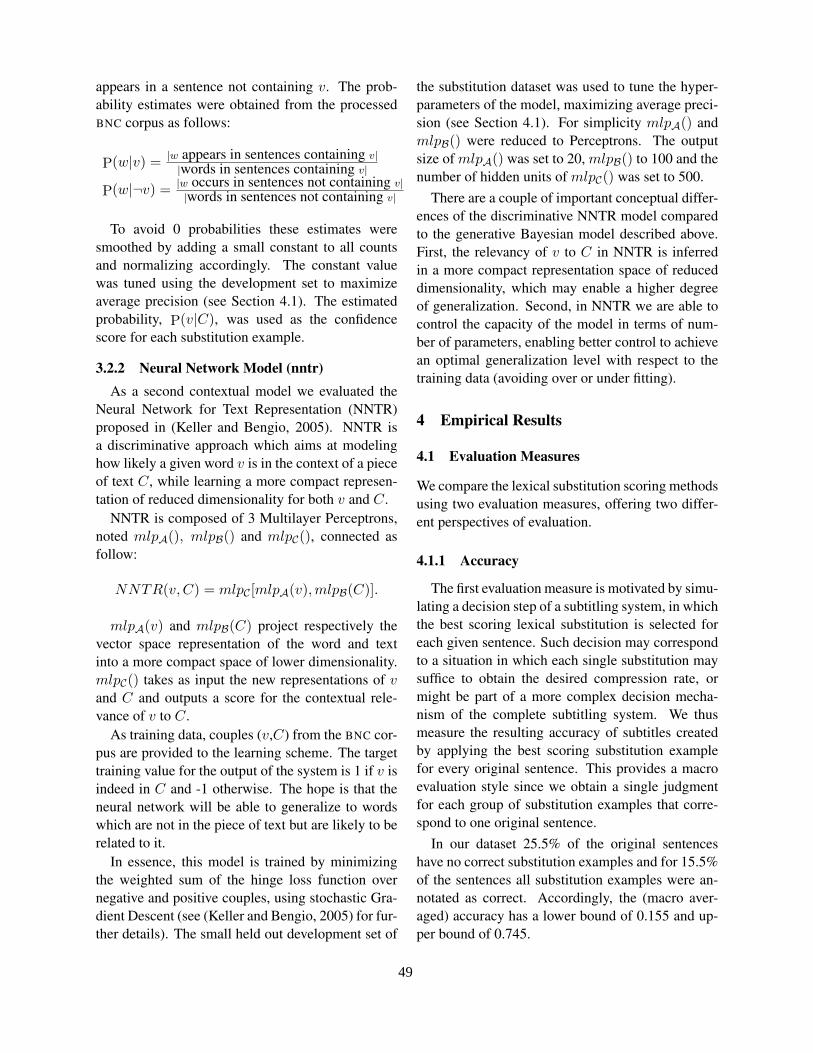
appears in a sentence not containing v. The prob-ability estimates were obtained from the processedBNC corpus as follows:
P(w|v) = |w appears in sentences containing v||words in sentences containing v|
P(w|¬v) = |w occurs in sentences not containing v||words in sentences not containing v|
To avoid 0 probabilities these estimates weresmoothed by adding a small constant to all countsand normalizing accordingly. The constant valuewas tuned using the development set to maximizeaverage precision (see Section 4.1). The estimatedprobability, P(v|C), was used as the confidencescore for each substitution example.
3.2.2 Neural Network Model (nntr)As a second contextual model we evaluated the
Neural Network for Text Representation (NNTR)proposed in (Keller and Bengio, 2005). NNTR isa discriminative approach which aims at modelinghow likely a given word v is in the context of a pieceof text C, while learning a more compact represen-tation of reduced dimensionality for both v and C.
NNTR is composed of 3 Multilayer Perceptrons,noted mlpA(), mlpB() and mlpC(), connected asfollow:
NNTR(v, C) = mlpC [mlpA(v),mlpB(C)].
mlpA(v) and mlpB(C) project respectively thevector space representation of the word and textinto a more compact space of lower dimensionality.mlpC() takes as input the new representations of vand C and outputs a score for the contextual rele-vance of v to C.
As training data, couples (v,C) from the BNC cor-pus are provided to the learning scheme. The targettraining value for the output of the system is 1 if v isindeed in C and -1 otherwise. The hope is that theneural network will be able to generalize to wordswhich are not in the piece of text but are likely to berelated to it.
In essence, this model is trained by minimizingthe weighted sum of the hinge loss function overnegative and positive couples, using stochastic Gra-dient Descent (see (Keller and Bengio, 2005) for fur-ther details). The small held out development set of
the substitution dataset was used to tune the hyper-parameters of the model, maximizing average preci-sion (see Section 4.1). For simplicity mlpA() andmlpB() were reduced to Perceptrons. The outputsize of mlpA() was set to 20, mlpB() to 100 and thenumber of hidden units of mlpC() was set to 500.
There are a couple of important conceptual differ-ences of the discriminative NNTR model comparedto the generative Bayesian model described above.First, the relevancy of v to C in NNTR is inferredin a more compact representation space of reduceddimensionality, which may enable a higher degreeof generalization. Second, in NNTR we are able tocontrol the capacity of the model in terms of num-ber of parameters, enabling better control to achievean optimal generalization level with respect to thetraining data (avoiding over or under fitting).
4 Empirical Results
4.1 Evaluation Measures
We compare the lexical substitution scoring methodsusing two evaluation measures, offering two differ-ent perspectives of evaluation.
4.1.1 Accuracy
The first evaluation measure is motivated by simu-lating a decision step of a subtitling system, in whichthe best scoring lexical substitution is selected foreach given sentence. Such decision may correspondto a situation in which each single substitution maysuffice to obtain the desired compression rate, ormight be part of a more complex decision mecha-nism of the complete subtitling system. We thusmeasure the resulting accuracy of subtitles createdby applying the best scoring substitution examplefor every original sentence. This provides a macroevaluation style since we obtain a single judgmentfor each group of substitution examples that corre-spond to one original sentence.
In our dataset 25.5% of the original sentenceshave no correct substitution examples and for 15.5%of the sentences all substitution examples were an-notated as correct. Accordingly, the (macro aver-aged) accuracy has a lower bound of 0.155 and up-per bound of 0.745.
49
4.1.2 Average PrecisionAs a second evaluation measure we compare the
average precision of each method over all the exam-ples from all original sentences pooled together (amicro averaging approach). This measures the po-tential of a scoring method to ensure high precisionfor the high scoring examples and to filter out low-scoring incorrect substitutions.
Average precision is a single figure measure com-monly used to evaluate a system’s ranking ability(Voorhees and Harman, 1999). It is equivalent to thearea under the uninterpolated recall-precision curve,defined as follows:
average precision =∑N
i=1 P(i)T (i)∑N
i=1T (i)
P(i) =∑i
k=1T (k)
i
(2)
where N is the number of examples in the testset (797 in our case), T (i) is the gold annotation(true=1, false=0) and i ranges over the examplesranked by decreasing score. An average precisionof 1.0 means that the system assigned a higher scoreto all true examples than to any false one (perfectranking). A lower bound of 0.26 on our test set cor-responds to a system that ranks all false examplesabove the true ones.
4.2 ResultsFigure 1 shows the accuracy and average precisionresults of the various models on our test set. The ran-dom baseline and corresponding significance levelswere achieved by averaging multiple runs of a sys-tem that assigned random scores. As can be seen inthe figures, the models’ behavior seems to be con-sistent in both evaluation measures.
Overall, the distributional similarity basedmethod (sim) performs much better than theother methods. In particular, Lin’s similarityalso performs better than semcor, the othercontext-independent model. Generally, the contextindependent models perform better than the contex-tual ones. Between the two contextual models, nntris superior to Bayes. In fact the Bayes model is notsignificantly better than random scoring.
4.3 Analysis and DiscussionWhen analyzing the data we identified several rea-sons why some of the WordNet substitutions were
judged as false. In some cases the source word asappearing in the original sentence is not in a sensefor which it is a synonym of the target word. For ex-ample, in many situations the word answer is in thesense of a statement that is made in reply to a ques-tion or request. In such cases, such as in example 2from Table 1, answer can be successfully replacedwith reply yielding a substitution which conveys theoriginal meaning. However, in situations such as inexample 1 the word answer is in the sense of a gen-eral solution and cannot be replaced with reply. Thisis also the case in examples 4 and 5 in which subjectdoes not appear in the sense of topic or theme.
Having an inappropriate sense, however, is not theonly reason for incorrect substitutions. In example 8approach appears in a sense which is synonymouswith attack and in example 9 problem appears in asense which is synonymous with a quite uncommonuse of the word job. Nevertheless, these substitu-tions were judged as unacceptable since the desiredsense of the target word after the substitution is notvery clear from the context. In many other cases,such as in example 7, though semantically correct,the substitution was judged as incorrect due to stylis-tic considerations.
Finally, there are cases, such as in example 6in which the source word is part of a collocationand cannot be replaced with semantically equivalentwords.
When analyzing the mistakes of the distributionalsimilarity method it seems as if many were not nec-essarily due to the method itself but rather to imple-mentation issues. The online source we used con-tains only the top most similar words for any word.In many cases substitutions were assigned a score ofzero since they were not listed among the top scoringsimilar words in the database. Furthermore, the cor-pus that was used for training the similarity scoreswas news articles in American English spelling anddoes not always supply good scores to words ofBritish spelling in our BBC dataset (e.g. analyse,behavioural, etc.).
The similarity based method seems to performbetter than the SemCor based method since, as notedabove, even when the source word is in the appro-priate sense it not necessarily substitutable with thetarget. For this reason we hypothesize that apply-ing Word Sense Disambiguation (WSD) methods to
50
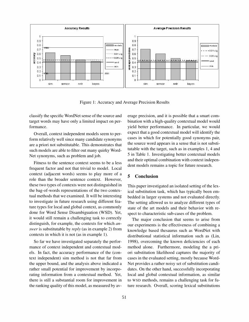
Figure 1: Accuracy and Average Precision Results
classify the specific WordNet sense of the source andtarget words may have only a limited impact on per-formance.
Overall, context independent models seem to per-form relatively well since many candidate synonymsare a priori not substitutable. This demonstrates thatsuch models are able to filter out many quirky Word-Net synonyms, such as problem and job.
Fitness to the sentence context seems to be a lessfrequent factor and not that trivial to model. Localcontext (adjacent words) seems to play more of arole than the broader sentence context. However,these two types of contexts were not distinguished inthe bag-of-words representations of the two contex-tual methods that we examined. It will be interestingto investigate in future research using different fea-ture types for local and global context, as commonlydone for Word Sense Disambiguation (WSD). Yet,it would still remain a challenging task to correctlydistinguish, for example, the contexts for which an-swer is substitutable by reply (as in example 2) fromcontexts in which it is not (as in example 1).
So far we have investigated separately the perfor-mance of context independent and contextual mod-els. In fact, the accuracy performance of the (con-text independent) sim method is not that far fromthe upper bound, and the analysis above indicated arather small potential for improvement by incorpo-rating information from a contextual method. Yet,there is still a substantial room for improvement inthe ranking quality of this model, as measured by av-
erage precision, and it is possible that a smart com-bination with a high-quality contextual model wouldyield better performance. In particular, we wouldexpect that a good contextual model will identify thecases in which for potentially good synonyms pair,the source word appears in a sense that is not substi-tutable with the target, such as in examples 1, 4 and5 in Table 1. Investigating better contextual modelsand their optimal combination with context indepen-dent models remains a topic for future research.
5 Conclusion
This paper investigated an isolated setting of the lex-ical substitution task, which has typically been em-bedded in larger systems and not evaluated directly.The setting allowed us to analyze different types ofstate of the art models and their behavior with re-spect to characteristic sub-cases of the problem.
The major conclusion that seems to arise fromour experiments is the effectiveness of combining aknowledge based thesaurus such as WordNet withdistributional statistical information such as (Lin,1998), overcoming the known deficiencies of eachmethod alone. Furthermore, modeling the a pri-ori substitution likelihood captures the majority ofcases in the evaluated setting, mostly because Word-Net provides a rather noisy set of substitution candi-dates. On the other hand, successfully incorporatinglocal and global contextual information, as similarto WSD methods, remains a challenging task for fu-ture research. Overall, scoring lexical substitutions
51

is an important component in many applications andwe expect that our findings are likely to be broadlyapplicable.
References[Budanitsky and Hirst2001] Alexander Budanitsky and
Graeme Hirst. 2001. Semantic distance in word-net: An experimental, application-oriented evalua-tion of five measures. In Workshop on WordNet andOther Lexical Resources: Second Meeting of the NorthAmerican Chapter of the Association for Computa-tional Linguistics, pages 29–34.
[Burnard1995] Lou Burnard. 1995. Users ReferenceGuide for the British National Corpus. Oxford Uni-versity Computing Services, Oxford.
[Daelemans et al.2004] Walter Daelemans, Anja Hothker,and Erik Tjong Kim Sang. 2004. Automatic sen-tence simplification for subtitling in dutch and english.In Proceedings of the 4th International Conferenceon Language Resources and Evaluation, pages 1045–1048.
[Dagan et al.2005] Ido Dagan, Oren Glickman, andBernardo Magnini. 2005. The pascal recognising tex-tual entailment challenge. Proceedings of the PAS-CAL Challenges Workshop on Recognising TextualEntailment.
[Geffet and Dagan2005] Maayan Geffet and Ido Dagan.2005. The distributional inclusion hypotheses and lex-ical entailment. In Proceedings of the 43rd AnnualMeeting of the Association for Computational Linguis-tics (ACL’05), pages 107–114, Ann Arbor, Michigan,June. Association for Computational Linguistics.
[Glickman et al.2005] Oren Glickman, Ido Dagan, andMoshe Koppel. 2005. A probabilistic classifica-tion approach for lexical textual entailment. In AAAI,pages 1050–1055.
[Grefenstette1998] Gregory Grefenstette. 1998. Produc-ing Intelligent Telegraphic Text Reduction to Providean Audio Scanning Service for the Blind. pages 111–117, Stanford, CA, March.
[Harris1968] Zelig Harris. 1968. Mathematical Struc-tures of Language. New York: Wiley.
[Hori et al.2002] Chiori Hori, Sadaoki Furui, Rob Malkin,Hua Yu, and Alex Waibel. 2002. Automaticspeech summarization applied to english broadcastnews speech. volume 1, pages 9–12.
[Jing and McKeown1999] Hongyan Jing and Kathleen R.McKeown. 1999. The decomposition of human-written summary sentences. In SIGIR ’99: Proceed-ings of the 22nd annual international ACM SIGIR con-ference on Research and development in information
retrieval, pages 129–136, New York, NY, USA. ACMPress.
[Keller and Bengio2005] Mikaela Keller and Samy Ben-gio. 2005. A neural network for text representation.In Wodzisaw Duch, Janusz Kacprzyk, and Erkki Oja,editors, Artificial Neural Networks: Biological Inspi-rations ICANN 2005: 15th International Conference,Warsaw, Poland, September 11-15, 2005. Proceedings,Part II, volume 3697 / 2005 of Lecture Notes in Com-puter Science, page p. 667. Springer-Verlag GmbH.
[Knight and Marcu2002] Kevin Knight and DanielMarcu. 2002. Summarization beyond sentenceextraction: a probabilistic approach to sentencecompression. Artif. Intell., 139(1):91–107.
[Landis and Koch1997] J. R. Landis and G. G. Koch.1997. The measurements of observer agreement forcategorical data. Biometrics, 33:159–174.
[Lin1998] Dekang Lin. 1998. Automatic retrieval andclustering of similar words. In Proceedings of the17th international conference on Computational lin-guistics, pages 768–774, Morristown, NJ, USA. Asso-ciation for Computational Linguistics.
[McCarthy et al.2004] Diana McCarthy, Rob Koeling,Julie Weeds, and John Carroll. 2004. Finding predom-inant senses in untagged text. In ACL, pages 280–288,Morristown, NJ, USA. Association for ComputationalLinguistics.
[Miller et al.1993] George A. Miller, Claudia Leacock,Randee Tengi, and Ross T. Bunker. 1993. A semanticconcordance. In HLT ’93: Proceedings of the work-shop on Human Language Technology, pages 303–308, Morristown, NJ, USA. Association for Compu-tational Linguistics.
[Piperidis et al.2004] Stelios Piperidis, Iason Demiros,Prokopis Prokopidis, Peter Vanroose, Anja Hothker,Walter Daelemans, Elsa Sklavounou, Manos Kon-stantinou, and Yannis Karavidas. 2004. Multimodalmultilingual resources in the subtitling process. InProceedings of the 4th International Language Re-sources and Evaluation Conference (LREC 2004), Lis-bon.
[Voorhees and Harman1999] Ellen M. Voorhees andDonna Harman. 1999. Overview of the seventh textretrieval conference. In Proceedings of the SeventhText REtrieval Conference (TREC-7). NIST SpecialPublication.
[Voorhees1994] Ellen M. Voorhees. 1994. Query expan-sion using lexical-semantic relations. In SIGIR ’94:Proceedings of the 17th annual international ACM SI-GIR conference on Research and development in infor-mation retrieval, pages 61–69, New York, NY, USA.Springer-Verlag New York, Inc.
52
Proceedings of the 10th Conference on Computational Natural Language Learning (CoNLL-X),pages 53–60, New York City, June 2006.c©2006 Association for Computational Linguistics
Semantic Role Recognition using Kernels on Weighted Marked OrderedLabeled Trees
Jun’ichi Kazama and Kentaro TorisawaJapan Advanced Institute of Science and Technology (JAIST)
Asahidai 1-1, Nomi, Ishikawa, 923-1292 Japan{kazama, torisawa}@jaist.ac.jp
Abstract
We present a method for recognizing se-mantic role arguments using a kernel onweighted marked ordered labeled trees(the WMOLT kernel). We extend thekernels on marked ordered labeled trees(Kazama and Torisawa, 2005) so that themark can be weighted according to its im-portance. We improve the accuracy bygiving more weights on subtrees that con-tain the predicate and the argument nodeswith this ability. Although Kazama andTorisawa (2005) presented fast trainingwith tree kernels, the slow classificationduring runtime remained to be solved. Inthis paper, we give a solution that uses anefficient DP updating procedure applica-ble in argument recognition. We demon-strate that the WMOLT kernel improvesthe accuracy, and our speed-up methodmakes the recognition more than 40 timesfaster than the naive classification.
1 Introduction
Semantic role labeling (SRL) is a task that recog-nizes the arguments of a predicate (verb) in a sen-tence and assigns the correct role to each argument.As this task is recognized as an important step after(or the last step of) syntactic analysis, many stud-ies have been conducted to achieve accurate seman-tic role labeling (Gildea and Jurafsky, 2002; Mos-chitti, 2004; Hacioglu et al., 2004; Punyakanok etal., 2004; Pradhan et al., 2005a; Pradhan et al.,2005b; Toutanova et al., 2005).
Most of the studies have focused on machinelearning because of the availability of standarddatasets, such as PropBank (Kingsbury and Palmer,2002). Naturally, the usefulness of parse trees in
this task can be anticipated. For example, the recentCoNLL 2005 shared task (Carreras and Marquez,2005) provided parse trees for use and their useful-ness was ensured. Most of the methods heuristicallyextract features from parse trees, and from othersources, and use them in machine learning methodsbased on feature vector representation. As a result,these methods depend on feature engineering, whichis time-consuming.
Tree kernels (Collins and Duffy, 2001; Kashimaand Koyanagi, 2002) have been proposed to directlyhandle trees in kernel-based methods, such as SVMs(Vapnik, 1995). Tree kernels calculate the similar-ity between trees, taking into consideration all of thesubtrees, and, therefore there is no need for such fea-ture engineering.
Moschitti and Bejan (2004) extensively studiedtree kernels for semantic role labeling. However,they reported that they could not successfully buildan accurate argument recognizer, although the roleassignment was improved. Although Moschitti et al.(2005) reported on argument recognition using treekernels, it was a preliminary evaluation because theyused oracle parse trees.
Kazama and Torisawa (2005) proposed a new treekernel for node relation labeling, as which SRL canbe cast. This kernel is defined on marked ordered la-beled trees, where a node can have a mark to indicatethe existence of a relation. We refer to this kernelas the MOLT kernel. Compared to (Moschitti andBejan, 2004) where tree fragments are heuristicallyextracted before applying tree kernels, the MOLTkernel is general and desirable since it does not re-quire such fragment extraction. However, the eval-uation conducted by Kazama and Torisawa (2005)was limited to preliminary experiments for role as-signment. In this study, we first evaluated the per-formance of the MOLT kernel for argument recogni-tion, and found that the MOLT kernel cannot achievea high accuracy if used in its original form.
53
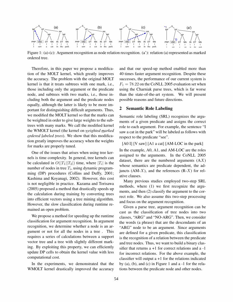
a catI saw the parkin
DT NNPRP VBD DT NNIN
NP
S
NP VP
NP
PP
(a)
a catI saw the parkin
DT NNPRP VBD DT NNIN
NP
S
NP VP
NP
PP
(b)
a catI saw the parkin
DT NNPRP VBD DT NNIN
NP
S
NP VP
NP
PP
(c)
a catI saw the parkin
DT NNPRP VBD DT NNIN
NP
S
NP VP
NP
PP
(a')
*0
*1
Figure 1: (a)-(c): Argument recognition as node relation recognition. (a’): relation (a) represented as markedordered tree.
Therefore, in this paper we propose a modifica-tion of the MOLT kernel, which greatly improvesthe accuracy. The problem with the original MOLTkernel is that it treats subtrees with one mark, i.e.,those including only the argument or the predicatenode, and subtrees with two marks, i.e., those in-cluding both the argument and the predicate nodesequally, although the latter is likely to be more im-portant for distinguishing difficult arguments. Thus,we modified the MOLT kernel so that the marks canbe weighted in order to give large weights to the sub-trees with many marks. We call the modified kernelthe WMOLT kernel (the kernel on weighted markedordered labeled trees). We show that this modifica-tion greatly improves the accuracy when the weightsfor marks are properly tuned.
One of the issues that arises when using tree ker-nels is time complexity. In general, tree kernels canbe calculated in O(|T1||T2|) time, where |Ti| is thenumber of nodes in tree Ti, using dynamic program-ming (DP) procedures (Collins and Duffy, 2001;Kashima and Koyanagi, 2002). However, this costis not negligible in practice. Kazama and Torisawa(2005) proposed a method that drastically speeds upthe calculation during training by converting treesinto efficient vectors using a tree mining algorithm.However, the slow classification during runtime re-mained an open problem.
We propose a method for speeding up the runtimeclassification for argument recognition. In argumentrecognition, we determine whether a node is an ar-gument or not for all the nodes in a tree . Thisrequires a series of calculations between a supportvector tree and a tree with slightly different mark-ing. By exploiting this property, we can efficientlyupdate DP cells to obtain the kernel value with lesscomputational cost.
In the experiments, we demonstrated that theWMOLT kernel drastically improved the accuracy
and that our speed-up method enabled more than40 times faster argument recognition. Despite thesesuccesses, the performance of our current system isF1 = 78.22 on the CoNLL 2005 evaluation set whenusing the Charniak parse trees, which is far worsethan the state-of-the-art system. We will presentpossible reasons and future directions.
2 Semantic Role Labeling
Semantic role labeling (SRL) recognizes the argu-ments of a given predicate and assigns the correctrole to each argument. For example, the sentence “Isaw a cat in the park” will be labeled as follows withrespect to the predicate “see”.
[A0 I] [V saw] [A1 a cat] [AM-LOC in the park]
In the example, A0, A1, and AM-LOC are the rolesassigned to the arguments. In the CoNLL 2005dataset, there are the numbered arguments (AX)whose semantics are predicate dependent, the ad-juncts (AM-X), and the references (R-X) for rel-ative clauses.
Many previous studies employed two-step SRLmethods, where (1) we first recognize the argu-ments, and then (2) classify the argument to the cor-rect role. We also assume this two-step processingand focus on the argument recognition.
Given a parse tree, argument recognition can becast as the classification of tree nodes into twoclasses, “ARG” and “NO-ARG”. Then, we considerthe words (a phrase) that are the descendants of an“ARG” node to be an argument. Since argumentsare defined for a given predicate, this classificationis the recognition of a relation between the predicateand tree nodes. Thus, we want to build a binary clas-sifier that returns a +1 for correct relations and a -1for incorrect relations. For the above example, theclassifier will output a +1 for the relations indicatedby (a), (b), and (c) in Figure 1 and a -1 for the rela-tions between the predicate node and other nodes.
54
Since the task is the classification of trees withnode relations, tree kernels for usual ordered la-beled trees, such as those proposed by Collins andDuffy (2001) and Kashima and Koyanagi (2002),are not useful. Kazama and Torisawa (2005) pro-posed to represent a node relation in a tree as amarked ordered labeled tree and presented a kernelfor it (MOLT kernel). We adopted the MOLT kerneland extend it for accurate argument recognition.
3 Kernels for Argument Recognition
3.1 Kernel-based classificationKernel-based methods, such as support vector ma-chines (SVMs) (Vapnik, 1995), consider a mappingΦ(x) that maps the object x into a, (usually high-dimensional), feature space and learn a classifier inthis space. A kernel function K(xi, xj) is a functionthat calculates the inner product ⟨Φ(xi), Φ(xj)⟩ inthe feature space without explicitly computing Φ(x),which is sometimes intractable. Then, any classifierthat is represented by using only the inner productsbetween the vectors in a feature space can be re-written using the kernel function. For example, anSVM classifier has the form:
f(x) =∑
i
αiK(xi, x) + b,
where αi and b are the parameters learned in thetraining. With kernel-based methods, we can con-struct a powerful classifier in a high-dimensionalfeature space. In addition, objects x do not needto be vectors as long as a kernel function is defined(e.g., x can be strings, trees, or graphs).
3.2 MOLT kernelA marked ordered labeled tree (Kazama and Tori-sawa, 2005) is an ordered labeled tree in which eachnode can have a mark in addition to a label. We canencode a k-node relation by using k distinct marks.In this study, we determine an argument node with-out considering other arguments of the same pred-icate, i.e., we represent an argument relation as atwo-node relation using two marks. For example,the relation (a) in Figure 1 can be represented as themarked ordered labeled tree (a’).1
1Note that we use mark *0 for the predicate node and mark*1 for the argument node.
Table 1: Notations for MOLT kernel.
• ni denotes a node of a tree. In this paper, ni is an ID assigned in thepost-order traversal.
• |Ti| denotes the number of nodes in tree Ti.
• l(ni) returns the label of node ni.
• m(ni) returns the mark of node ni. If ni has no mark, m(ni)returns the special mark no-mark.
• marked(ni) returns true iff m(ni) is not no-mark.
• nc(ni) is the number of children of node ni.
• chk(ni) is the k-th child of node ni.
• pa(ni) is the parent of node ni.
• root(Ti) is the root node of Ti
• ni ≽ nj means that ni is an elder sister of nj .
Kazama and Torisawa (2005) presented a kernelon marked ordered trees (the MOLT kernel), whichis defined as:2
K(T1, T2) =E∑
i=1
W (Si) ·#Si(T1) ·#Si(T2),
where Si is a possible subtree and #Si(Tj) isthe number of times Si is included in Tj . Themapping corresponding to this kernel is Φ(T ) =(√
W (S1)#S1(T ), · · · ,√
W (SE)#SE(T )), which
maps the tree into the feature space of all the possi-ble subtrees.
The tree inclusion is defined in many ways. Forexample, Kashima and Koyanagi (2002) presentedthe following type of inclusion.
1 DEFINITION S is included in T iff there exists aone-to-one function ψ from a node of S to a nodeof T , such that (i) pa(ψ(ni)) = ψ(pa(ni)), (ii)ψ(ni) ≽ ψ(nj) iff ni ≽ nj , , and (iii) l(ψ(ni)) =l(ni) (and m(ψ(ni)) = m(ni) in the MOLT kernel).
See Table 1 for the meaning of each function. Thisdefinition means that any subtrees preserving theparent-child relation, the sibling relation, and label-marks, are allowed. In this paper, we employ thisdefinition, since Kazama and Torisawa (2005) re-ported that the MOLT kernel with this definition hasa higher accuracy than one with the definition pre-sented by Collins and Duffy (2001).
W (Si) is the weight of subtree Si. The weight-ing in Kazama and Torisawa (2005) is written as fol-
2This notation is slightly different from (Kazama and Tori-sawa, 2005).
55
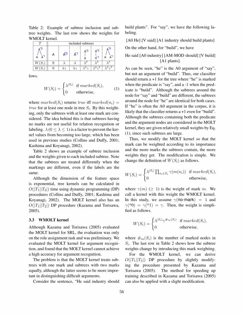
Table 2: Example of subtree inclusion and sub-tree weights. The last row shows the weights forWMOLT kernel.
T included subtrees
W (Si) 0 λ λ λ2 λ2 λ3
W (Si) 0 λγ λγ λ2γ λ2γ2 λ3γ2
lows.
W (Si) =
{λ|Si| if marked(Si),0 otherwise,
(1)
where marked(Si) returns true iff marked(ni) =true for at least one node in tree Si. By this weight-ing, only the subtrees with at least one mark are con-sidered. The idea behind this is that subtrees havingno marks are not useful for relation recognition orlabeling. λ (0 ≤ λ ≤ 1) is a factor to prevent the ker-nel values from becoming too large, which has beenused in previous studies (Collins and Duffy, 2001;Kashima and Koyanagi, 2002).
Table 2 shows an example of subtree inclusionand the weights given to each included subtree. Notethat the subtrees are treated differently when themarkings are different, even if the labels are thesame.
Although the dimension of the feature spaceis exponential, tree kernels can be calculated inO(|T1||T2|) time using dynamic programming (DP)procedures (Collins and Duffy, 2001; Kashima andKoyanagi, 2002). The MOLT kernel also has anO(|T1||T2|) DP procedure (Kazama and Torisawa,2005).
3.3 WMOLT kernel
Although Kazama and Torisawa (2005) evaluatedthe MOLT kernel for SRL, the evaluation was onlyon the role assignment task and was preliminary. Weevaluated the MOLT kernel for argument recogni-tion, and found that the MOLT kernel cannot achievea high accuracy for argument recognition.
The problem is that the MOLT kernel treats sub-trees with one mark and subtrees with two marksequally, although the latter seems to be more impor-tant in distinguishing difficult arguments.
Consider the sentence, “He said industry should
build plants”. For “say”, we have the following la-beling.
[A0 He] [V said] [A1 industry should build plants]
On the other hand, for “build”, we have
He said [A0 industry] [AM-MOD should] [V build][A1 plants].
As can be seen, “he” is the A0 argument of “say”,but not an argument of “build”. Thus, our classifiershould return a +1 for the tree where “he” is markedwhen the predicate is “say”, and a -1 when the pred-icate is “build”. Although the subtrees around thenode for “say” and “build” are different, the subtreesaround the node for “he” are identical for both cases.If “he” is often the A0 argument in the corpus, it islikely that the classifier returns a +1 even for “build”.Although the subtrees containing both the predicateand the argument nodes are considered in the MOLTkernel, they are given relatively small weights by Eq.(1), since such subtrees are large.
Thus, we modify the MOLT kernel so that themark can be weighted according to its importanceand the more marks the subtrees contain, the moreweights they get. The modification is simple. Wechange the definition of W (Si) as follows.
W (Si) =
{λ|Si| ∏
ni∈Siγ(m(ni)) if marked(Si),
0 otherwise,
where γ(m) (≥ 1) is the weight of mark m. Wecall a kernel with this weight the WMOLT kernel.In this study, we assume γ(no-mark) = 1 andγ(*0) = γ(*1) = γ. Then, the weight is simpli-fied as follows.
W (Si) =
{λ|Si|γ#m(Si) if marked(Si),0 otherwise,
where #m(Si) is the number of marked nodes inSi. The last row in Table 2 shows how the subtreeweights change by introducing this mark weighting.
For the WMOLT kernel, we can deriveO(|T1||T2|) DP procedure by slightly modify-ing the procedure presented by Kazama andTorisawa (2005). The method for speeding uptraining described in Kazama and Torisawa (2005)can also be applied with a slight modification.
56
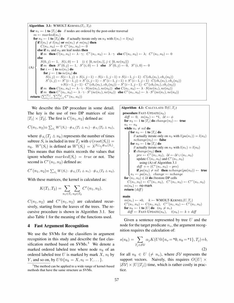
Algorithm 3.1: WMOLT-KERNEL(T1, T2)
for n1 ← 1 to |T1| do // nodes are ordered by the post-order traversalm ← marked(n1)for n2 ← 1 to |T2| do // actually iterate only on n2 with l(n1) = l(n2)
(A)
8
>
>
>
>
>
>
>
>
>
>
>
>
>
>
>
>
>
>
>
>
<
>
>
>
>
>
>
>
>
>
>
>
>
>
>
>
>
>
>
>
>
:
if l(n1) = l(n2) or m(n1) = m(n2) thenC(n1, n2) ← 0 Cr(n1, n2) ← 0
else if n1 and n2 are leaf nodes thenif m then C(n1, n2) ← λ · γ; Cr(n1, n2) ← λ · γ else C(n1, n2) ← λ; Cr(n1, n2) ← 0
elseS(0, j) ← 1, S(i, 0) ← 1 (i ∈ [0, nc(n1)], j ∈ [0, nc(n2)])if m then Sr(0, j) ← 1, Sr(i, 0) ← 1 else Sr(0, j) ← 0, Sr(i, 0) ← 0for i ← 1 to nc(n1) do
for j ← 1 to nc(n2) doS(i, j) ← S(i−1, j) + S(i, j−1)− S(i−1, j−1) + S(i−1, j−1) · C(chi(n1), chj(n2))Sr(i, j) ← Sr(i−1, j) + Sr(i, j−1)− Sr(i−1, j−1) + Sr(i−1, j−1) · C(chi(n1), chj(n2))
+S(i−1, j−1) · Cr(chi(n1), chj(n2))− Sr(i−1, j−1) · Cr(chi(n1), chj(n2))if m then C(n1, n2) ← λ · γ · S(nc(n1), nc(n2)) else C(n1, n2) ← λ · S(nc(n1), nc(n2))if m then Cr(n1, n2) ← λ · γ · Sr(nc(n1), nc(n2)) else Cr(n1, n2) ← λ · Sr(nc(n1), nc(n2))
return (P|T1|
n1=1
P|T2|n2=1 Cr(n1, n2))
We describe this DP procedure in some detail.The key is the use of two DP matrices of size|T1| × |T2|. The first is C(n1, n2) defined as:
C(n1, n2)≡P
SiW ′(Si) ·#Si(T1 △ n1) ·#Si(T2 △ n2),
where #Si(Tj △ nk) represents the number of timessubtree Si is included in tree Tj with ψ(root(Si)) =nk. W ′(Si) is defined as W ′(Si) = λ|Si|γ#m(Si).This means that this matrix records the values thatignore whether marked(Si) = true or not. Thesecond is Cr(n1, n2) defined as:
Cr(n1, n2)≡P
SiW (Si) ·#Si(T1 △ n1) ·#Si(T2 △ n2).
With these matrices, the kernel is calculated as:
K(T1, T2) =∑
n1∈T1
∑n2∈T2
Cr(n1, n2).
C(n1, n2) and Cr(n1, n2) are calculated recur-sively, starting from the leaves of the trees. The re-cursive procedure is shown in Algorithm 3.1. Seealso Table 1 for the meaning of the functions used.
4 Fast Argument Recognition
We use the SVMs for the classifiers in argumentrecognition in this study and describe the fast clas-sification method based on SVMs.3 We denote amarked ordered labeled tree where node nk of anordered labeled tree U is marked by mark X , nl byY , and so on, by U@{nk = X,nl = Y, . . . }.
3The method can be applied to a wide range of kernel-basedmethods that have the same structure as SVMs.
Algorithm 4.1: CALCULATE-T(U, Tj)
procedure FAST-UPDATE(nk)diff ← 0, m(nk) ← *1, U ← φfor n2 ← 1 to |Tj | do change(n2) ← truen1 ← nk
while n1 = nil do8
>
>
>
>
>
>
>
>
>
>
>
>
>
>
>
>
<
>
>
>
>
>
>
>
>
>
>
>
>
>
>
>
>
:
for n2 ← 1 to |Tj | do// actually iterate only on n2 with l(pa(n1)) = l(n2)nchange(n2) ← false
for n2 ← 1 to |Tj | do// actually iterate only on n2 with l(n1) = l(n2)if change(n2) then
pre ← Cr(n1, n2), U ← U ∪ (n1, n2)update C(n1, n2) and Cr(n1, n2)
using (A) of Algorithm 3.1diff += (Cr(n1, n2)− pre)if pa(n2) = nil then nchange(pa(n2)) ← true
n1 ← pa(n1), change ← nchangefor (n1, n2) ∈ U do //restore DP cells
C(n1, n2) ← C′(n1, n2), Cr(n1, n2) ← Cr ′(n1, n2)m(nk) ← no-markreturn (diff )
mainm(nv) ← ∗0, k ← WMOLT-KERNEL(U, Tj)C′(n1, n2) ← C(n1, n2), Cr ′(n1, n2) ← Cr(n1, n2)for nk ← 1 to |U | do (nk = nv)
diff ← FAST-UPDATE(nk), t(nk) ← k + diff
Given a sentence represented by tree U and thenode for the target predicate nv, the argument recog-nition requires the calculation of:
s(nk) =∑
Tj∈SVαjK(U@{nv =*0, nk =*1}, Tj)+b,
(2)for all nk ∈ U (= nv), where SV represents thesupport vectors. Naively, this requires O(|U | ×|SV| × |U ||Tj |) time, which is rather costly in prac-tice.
57
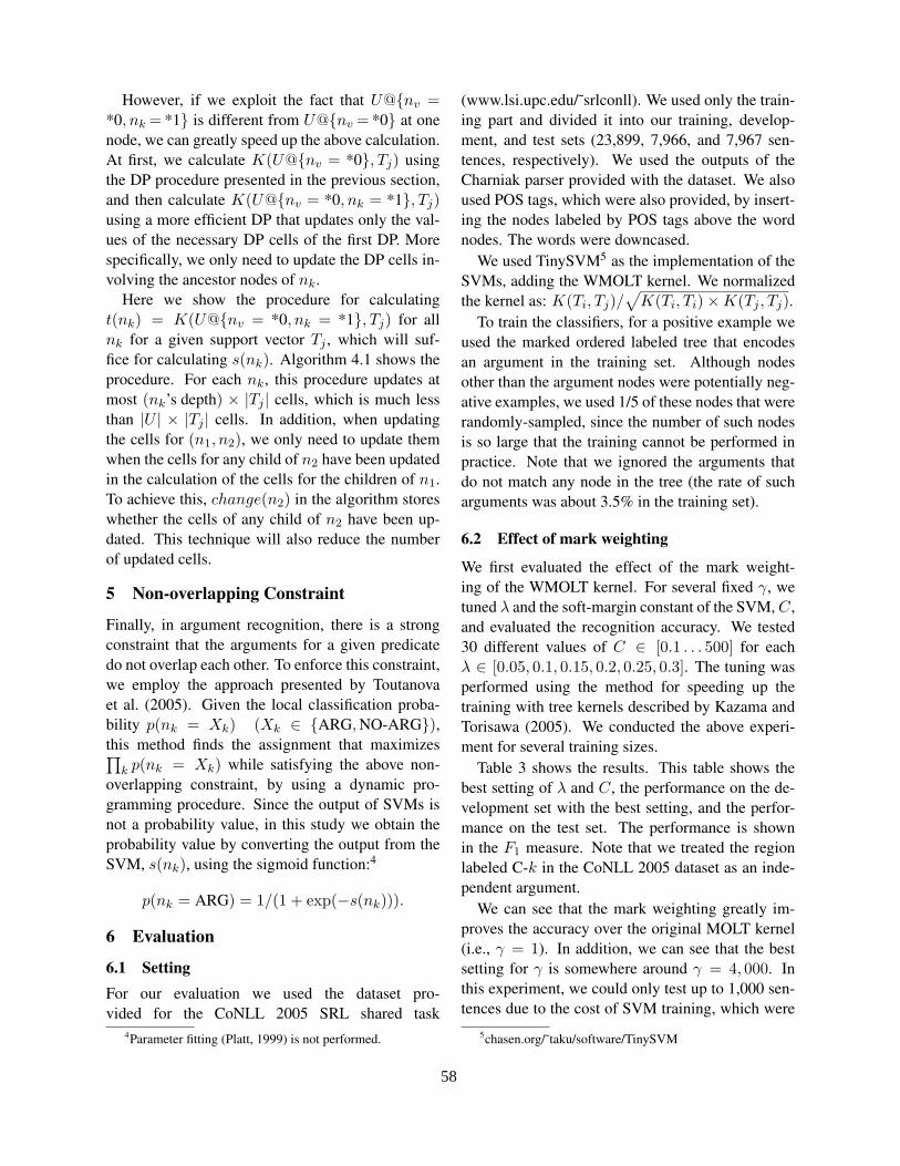
However, if we exploit the fact that U@{nv =*0, nk = *1} is different from U@{nv = *0} at onenode, we can greatly speed up the above calculation.At first, we calculate K(U@{nv = *0}, Tj) usingthe DP procedure presented in the previous section,and then calculate K(U@{nv = *0, nk = *1}, Tj)using a more efficient DP that updates only the val-ues of the necessary DP cells of the first DP. Morespecifically, we only need to update the DP cells in-volving the ancestor nodes of nk.
Here we show the procedure for calculatingt(nk) = K(U@{nv = *0, nk = *1}, Tj) for allnk for a given support vector Tj , which will suf-fice for calculating s(nk). Algorithm 4.1 shows theprocedure. For each nk, this procedure updates atmost (nk’s depth) × |Tj | cells, which is much lessthan |U | × |Tj | cells. In addition, when updatingthe cells for (n1, n2), we only need to update themwhen the cells for any child of n2 have been updatedin the calculation of the cells for the children of n1.To achieve this, change(n2) in the algorithm storeswhether the cells of any child of n2 have been up-dated. This technique will also reduce the numberof updated cells.
5 Non-overlapping Constraint
Finally, in argument recognition, there is a strongconstraint that the arguments for a given predicatedo not overlap each other. To enforce this constraint,we employ the approach presented by Toutanovaet al. (2005). Given the local classification proba-bility p(nk = Xk) (Xk ∈ {ARG, NO-ARG}),this method finds the assignment that maximizes∏
k p(nk = Xk) while satisfying the above non-overlapping constraint, by using a dynamic pro-gramming procedure. Since the output of SVMs isnot a probability value, in this study we obtain theprobability value by converting the output from theSVM, s(nk), using the sigmoid function:4
p(nk = ARG) = 1/(1 + exp(−s(nk))).
6 Evaluation
6.1 SettingFor our evaluation we used the dataset pro-vided for the CoNLL 2005 SRL shared task
4Parameter fitting (Platt, 1999) is not performed.
(www.lsi.upc.edu/˜srlconll). We used only the train-ing part and divided it into our training, develop-ment, and test sets (23,899, 7,966, and 7,967 sen-tences, respectively). We used the outputs of theCharniak parser provided with the dataset. We alsoused POS tags, which were also provided, by insert-ing the nodes labeled by POS tags above the wordnodes. The words were downcased.
We used TinySVM5 as the implementation of theSVMs, adding the WMOLT kernel. We normalizedthe kernel as: K(Ti, Tj)/
√K(Ti, Ti)×K(Tj , Tj).
To train the classifiers, for a positive example weused the marked ordered labeled tree that encodesan argument in the training set. Although nodesother than the argument nodes were potentially neg-ative examples, we used 1/5 of these nodes that wererandomly-sampled, since the number of such nodesis so large that the training cannot be performed inpractice. Note that we ignored the arguments thatdo not match any node in the tree (the rate of sucharguments was about 3.5% in the training set).
6.2 Effect of mark weighting
We first evaluated the effect of the mark weight-ing of the WMOLT kernel. For several fixed γ, wetuned λ and the soft-margin constant of the SVM, C,and evaluated the recognition accuracy. We tested30 different values of C ∈ [0.1 . . . 500] for eachλ ∈ [0.05, 0.1, 0.15, 0.2, 0.25, 0.3]. The tuning wasperformed using the method for speeding up thetraining with tree kernels described by Kazama andTorisawa (2005). We conducted the above experi-ment for several training sizes.
Table 3 shows the results. This table shows thebest setting of λ and C, the performance on the de-velopment set with the best setting, and the perfor-mance on the test set. The performance is shownin the F1 measure. Note that we treated the regionlabeled C-k in the CoNLL 2005 dataset as an inde-pendent argument.
We can see that the mark weighting greatly im-proves the accuracy over the original MOLT kernel(i.e., γ = 1). In addition, we can see that the bestsetting for γ is somewhere around γ = 4, 000. Inthis experiment, we could only test up to 1,000 sen-tences due to the cost of SVM training, which were
5chasen.org/˜taku/software/TinySVM
58
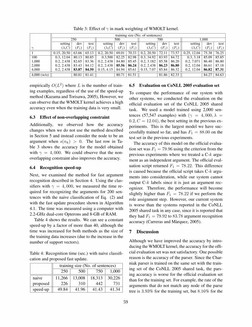
Table 3: Effect of γ in mark weighting of WMOLT kernel.training size (No. of sentences)
250 500 700 1,000setting dev test setting dev test setting dev test setting dev test
γ (λ,C) (F1) (F1) (λ,C) (F1) (F1) (λ,C) (F1) (F1) (λ,C) (F1) (F1)1 0.15, 20.50 63.66 65.13 0.2, 20.50 69.01 70.33 0.2, 20.50 72.11 73.57 0.25, 12.04 75.38 76.25100 0.3, 12.04 80.13 80.85 0.3,500 82.25 82.98 0.3, 34.92 83.93 84.72 0.3, 3.18 85.09 85.851,000 0.2, 2.438 82.65 83.36 0.2, 2.438 84.80 85.45 0.2, 3.182 85.58 86.20 0.2, 7.071 86.40 86.802,000 0.2, 2.438 83.43 84.12 0.2, 2.438 85.56 86.24 0.2, 2.438 86.23 86.80 0.2, 12.04 86.61 87.184,000 0.2, 2.438 83.87 84.50 0.15, 4.15 84.94 85.61 0.15, 7.07 85.84 86.32 0.2, 12.04 86.82 87.314,000 (w/o) 80.81 81.41 80.71 81.51 81.86 82.33 84.27 84.63
empirically O(L2) where L is the number of train-ing examples, regardless of the use of the speed-upmethod (Kazama and Torisawa, 2005), However, wecan observe that the WMOLT kernel achieves a highaccuracy even when the training data is very small.
6.3 Effect of non-overlapping constraint
Additionally, we observed how the accuracychanges when we do not use the method describedin Section 5 and instead consider the node to be anargument when s(nk) > 0. The last row in Ta-ble 3 shows the accuracy for the model obtainedwith γ = 4, 000. We could observe that the non-overlapping constraint also improves the accuracy.
6.4 Recognition speed-up
Next, we examined the method for fast argumentrecognition described in Section 4. Using the clas-sifiers with γ = 4, 000, we measured the time re-quired for recognizing the arguments for 200 sen-tences with the naive classification of Eq. (2) andwith the fast update procedure shown in Algorithm4.1. The time was measured using a computer with2.2-GHz dual-core Opterons and 8-GB of RAM.
Table 4 shows the results. We can see a constantspeed-up by a factor of more than 40, although thetime was increased for both methods as the size ofthe training data increases (due to the increase in thenumber of support vectors).
Table 4: Recognition time (sec.) with naive classifi-cation and proposed fast update.
training size (No. of sentences)250 500 750 1,000
naive 11,266 13,008 18,313 30,226proposed 226 310 442 731speed-up 49.84 41.96 41.43 41.34
6.5 Evaluation on CoNLL 2005 evaluation set
To compare the performance of our system withother systems, we conducted the evaluation on theofficial evaluation set of the CoNLL 2005 sharedtask. We used a model trained using 2,000 sen-tences (57,547 examples) with (γ = 4, 000, λ =0.2, C = 12.04), the best setting in the previous ex-periments. This is the largest model we have suc-cessfully trained so far, and has F1 = 88.00 on thetest set in the previous experiments.
The accuracy of this model on the official evalua-tion set was F1 = 79.96 using the criterion from theprevious experiments where we treated a C-k argu-ment as an independent argument. The official eval-uation script returned F1 = 78.22. This differenceis caused because the official script takes C-k argu-ments into consideration, while our system cannotoutput C-k labels since it is just an argument rec-ognizer. Therefore, the performance will becomeslightly higher than F1 = 78.22 if we perform therole assignment step. However, our current systemis worse than the systems reported in the CoNLL2005 shared task in any case, since it is reported thatthey had F1 = 79.92 to 83.78 argument recognitionaccuracy (Carreras and Marquez, 2005).
7 Discussion
Although we have improved the accuracy by intro-ducing the WMOLT kernel, the accuracy for the offi-cial evaluation set was not satisfactory. One possiblereason is the accuracy of the parser. Since the Char-niak parser is trained on the same set with the train-ing set of the CoNLL 2005 shared task, the pars-ing accuracy is worse for the official evaluation setthan for the training set. For example, the rate of thearguments that do not match any node of the parsetree is 3.93% for the training set, but 8.16% for the
59
evaluation set. This, to some extent, explains whyour system, which achieved F1 = 88.00 for our testset, could only achieved F1 = 79.96. To achieve ahigher accuracy, we need to make the system morerobust to parsing errors. Some of the non-matchingarguments are caused by incorrect treatment of quo-tation marks and commas. These errors seem to besolved by using simple pre-processing. Other majornon-matching arguments are caused by PP attach-ment errors. To solve these errors, we need to ex-plore more, such as using n-best parses and the useof several syntactic views (Pradhan et al., 2005b).
Another reason for the low accuracy is the size ofthe training data. In this study, we could train theSVM with 2,000 sentences (this took more than 30hours including the conversion of trees), but this isa very small fraction of the entire training set. Weneed to explore the methods for incorporating a largetraining set within a reasonable training time. Forexample, the combination of small SVMs (Shen etal., 2003) is a possible direction.
The contribution of this study is not the accuracyachieved. The first contribution is the demonstrationof the drastic effect of the mark weighting. We willexplore more accurate kernels based on the WMOLTkernel. For example, we are planning to use dif-ferent weights depending on the marks. The sec-ond contribution is the method of speeding-up argu-ment recognition. This is of great importance, sincethe proposed method can be applied to other taskswhere all nodes in a tree should be classified. In ad-dition, this method became possible because of theWMOLT kernel, and it is hard to apply to Moschittiand Bejan (2004) where the tree structure changesduring recognition. Thus, the architecture that usesthe WMOLT kernel is promising, if we assume fur-ther progress is possible with the kernel design.
8 ConclusionWe proposed a method for recognizing semantic rolearguments using the WMOLT kernel. The markweighting introduced in the WMOLT kernel greatlyimproved the accuracy. In addition, we presenteda method for speeding up the recognition, which re-sulted in more than a 40 times faster recognition. Al-though the accuracy of the current system is worsethan the state-of-the-art system, we expect to furtherimprove our system.
ReferencesX. Carreras and L. Marquez. 2005. Introduction to the
CoNLL-2005 shared task: Semantic role labeling. InCoNLL 2005.
M. Collins and N. Duffy. 2001. Convolution kernels fornatural language. In NIPS 2001.
D. Gildea and D. Jurafsky. 2002. Automatic labeling ofsemantic roles. Computational Linguistics, 28(3).
K. Hacioglu, S. Pradhan, W. Ward, J. H. Martin, andD. Jurafsky. 2004. Semantic role labeling by taggingsyntactic chunks. In CoNLL 2004.
H. Kashima and T. Koyanagi. 2002. Kernels for semi-structured data. In ICML 2002, pages 291–298.
J. Kazama and K. Torisawa. 2005. Speeding up trainingwith tree kernels for node relation labeling. In EMNLP2005.
P. Kingsbury and M. Palmer. 2002. From treebank topropbank. In LREC 02.
A. Moschitti and C. A. Bejan. 2004. A semantic kernelsfor predicate argument classification. In CoNLL 2004.
A. Moschitti, B. Coppola, D. Pighin, and B. Basili. 2005.Engineering of syntactic features for shallow semanticparsing. In ACL 2005 Workshop on Feature Enginner-ing for Machine Learning in Natural Language Pro-cessing.
A. Moschitti. 2004. A study on convolution kernels forshallow semantic parsing. In ACL 2004.
J. C. Platt. 1999. Probabilistic outputs for support vectormachines and comparisons to regularized likelihoodmethods. Advances in Large Margin Classifiers.
S. Pradhan, K. Hacioglu, W. Ward, D. Jurafsky, and J. H.Martin. 2005a. Support vector learning for semanticargument classification. Machine Learning, 60(1).
S. Pradhan, W. Ward, K. Hacioglu, J. H. Martin, andD. Jurafsky. 2005b. Semantic role labeling using dif-ferent syntactic views. In ACL 2005.
V. Punyakanok, D. Roth, W. Yih, and D. Zimak. 2004.Semantic role labeling via integer linear programminginference. In COLING 2004.
L. Shen, A. Sarkar, and A. K. Joshi. 2003. Using LTAGbased features in parse reranking. In EMNLP 2003.
K. Toutanova, A. Haghighi, and C. D. Manning. 2005.Joint learning improves semantic role labeling. In ACL2005.
V. Vapnik. 1995. The Nature of Statistical Learning The-ory. Springer Verlag.
60
Proceedings of the 10th Conference on Computational Natural Language Learning (CoNLL-X),pages 61–68, New York City, June 2006.c©2006 Association for Computational Linguistics
Semantic Role Labeling via Tree Kernel Joint Inference
Alessandro Moschitti, Daniele Pighin and Roberto BasiliDepartment of Computer ScienceUniversity of Rome ”Tor Vergata”
00133 Rome, Italy{moschitti,basili }@info.uniroma2.it
Abstract
Recent work on Semantic Role Labeling(SRL) has shown that to achieve highaccuracy a joint inference on the wholepredicate argument structure should be ap-plied. In this paper, we used syntactic sub-trees that span potential argument struc-tures of the target predicate in tree ker-nel functions. This allows Support Vec-tor Machines to discern between correctand incorrect predicate structures and tore-rank them based on the joint probabil-ity of their arguments. Experiments on thePropBank data show that both classifica-tion and re-ranking based on tree kernelscan improve SRL systems.
1 Introduction
Recent work on Semantic Role Labeling (SRL)(Carreras and Marquez, 2005) has shown that toachieve high labeling accuracy a joint inference onthe whole predicate argument structure should beapplied. For this purpose, we need to extract fea-tures from the sentence’s syntactic parse tree thatencodes the target semantic structure. This task israther complex since we do not exactly know whichare the syntactic clues that capture the relation be-tween the predicate and its arguments. For exam-ple, to detect the interesting context, the modelingof syntax/semantics-based features should take intoaccount linguistic aspects like ancestor nodes or se-mantic dependencies (Toutanova et al., 2004).
A viable approach to generate a large number offeatures has been proposed in (Collins and Duffy,2002), where convolution kernels were used to im-plicitly define a tree substructure space. The selec-tion of the relevant structural features was left to theVoted Perceptron learning algorithm. Such success-ful experimentation shows that tree kernels are verypromising for automatic feature engineering, espe-cially when the available knowledge about the phe-nomenon is limited.
In a similar way, we can model SRL systems withtree kernels to generate large feature spaces. Morein detail, most SRL systems split the labeling pro-cess into two different steps: Boundary Detection(i.e. to determine the text boundaries of predicatearguments) and Role Classification (i.e. labelingsuch arguments with a semantic role, e.g. Arg0 orArg1 as defined in (Kingsbury and Palmer, 2002)).The former relates to the detection of syntactic parsetree nodes associated with constituents that corre-spond to arguments, whereas the latter considers theboundary nodes for the assignment of the suitablelabel. Both steps require the design and extractionof features from parse trees. As capturing the tightlyinterdependent relations among a predicate and itsarguments is a complex task, we can apply tree ker-nels on the subtrees thatspan the whole predicateargument structure to generate the feature space ofall the possible subtrees.
In this paper, we apply the traditional bound-ary (TBC) and role (TRC) classifiers (Pradhanet al., 2005a), which are based on binary predi-cate/argument relations, to label all parse tree nodescorresponding to potential arguments. Then, we ex-
61

tract the subtrees which span the predicate-argumentdependencies of such arguments, i.e. ArgumentSpanning Trees (ASTs). These are used in a treekernel function to generate all possible substructuresthat encoden-ary argument relations, i.e. we carryout an automatic feature engineering process.
To validate our approach, we experimented withour model and Support Vector Machines for the clas-sification of valid and invalidASTs. The resultsshow that this classification problem can be learnedwith high accuracy. Moreover, we modeled SRL as are-ranking task in line with (Toutanova et al., 2005).The large number of complex features provided bytree kernels for structured learning allows SVMs toreach the state-of-the-art accuracy.
The paper is organized as follows: Section 2 intro-duces the Semantic Role Labeling based on SVMsand the tree kernel spaces; Section 3 formally de-fines theASTs and the algorithm for their classifi-cation and re-ranking; Section 4 shows the compara-tive results between our approach and the traditionalone; Section 5 presents the related work; and finally,Section 6 summarizes the conclusions.
2 Semantic Role Labeling
In the last years, several machine learning ap-proaches have been developed for automatic rolelabeling, e.g. (Gildea and Jurasfky, 2002; Prad-han et al., 2005a). Their common characteristic isthe adoption of attribute-value representations forpredicate-argument structures. Accordingly, our ba-sic system is similar to the one proposed in (Pradhanet al., 2005a) and it is hereby described.
We use a boundary detection classifier (for anyrole type) to derive the words compounding an ar-gument and a multiclassifier to assign the roles (e.g.Arg0 or ArgM) described in PropBank (Kingsburyand Palmer, 2002)). To prepare the training data forboth classifiers, we used the following algorithm:
1. Given a sentence from thetraining-set, generatea full syntactic parse tree;2. LetP andA be respectively the set of predicatesand the set of parse-tree nodes (i.e. the potential ar-guments);3. For each pair〈p, a〉 ∈ P ×A:
- extract the feature representation set,Fp,a;
- if the subtree rooted ina covers exactly thewords of one argument ofp, putFp,a in theT+
set (positive examples), otherwise put it in theT− set (negative examples).
The outputs of the above algorithm are theT+ andT− sets. These sets can be directly used to train aboundary classifier (e.g. an SVM). Regarding theargument type classifier, a binary labeler for a roler(e.g. an SVM) can be trained on theT+
r, i.e. its pos-
itive examples andT−r , i.e. its negative examples,whereT+ = T+
r ∪ T−r , according to the ONE-vs-ALL scheme. The binary classifiers are then usedto build a general role multiclassifier by simply se-lecting the argument associated with the maximumamong the SVM scores.
Regarding the design of features for predicate-argument pairs, we can use the attribute-values de-fined in (Gildea and Jurasfky, 2002) or tree struc-tures (Moschitti, 2004). Although we focus onthe latter approach, a short description of the for-mer is still relevant as they are used byTBC andTRC. They include thePhrase Type, PredicateWord, Head Word, Governing Category, PositionandVoice features. For example, thePhrase Typeindicates the syntactic type of the phrase labeled asa predicate argument and theParse Tree Pathcon-tains the path in the parse tree between the predicateand the argument phrase, expressed as a sequence ofnonterminal labels linked by direction (up or down)symbols, e.g.V ↑ VP↓ NP.
A viable alternative to manual design of syntac-tic features is the use of tree-kernel functions. Theseimplicitly define a feature space based on all possi-ble tree substructures. Given two treesT1 andT2, in-stead of representing them with the whole fragmentspace, we can apply the kernel function to evaluatethe number of common fragments.
Formally, given a tree fragment spaceF ={f1, f2, . . . , f|F|}, the indicator function Ii(n)is equal to 1 if the targetfi is rooted atnode n and equal to 0 otherwise. A tree-kernel function overt1 and t2 is Kt(t1, t2) =∑
n1∈Nt1
∑n2∈Nt2
∆(n1, n2), whereNt1 and Nt2
are the sets of thet1’s andt2’s nodes, respectively. Inturn ∆(n1, n2) =
∑|F|i=1 λl(fi)Ii(n1)Ii(n2), where
0 ≤ λ ≤ 1 and l(fi) is the height of the subtreefi. Thusλl(fi) assigns a lower weight to larger frag-
62
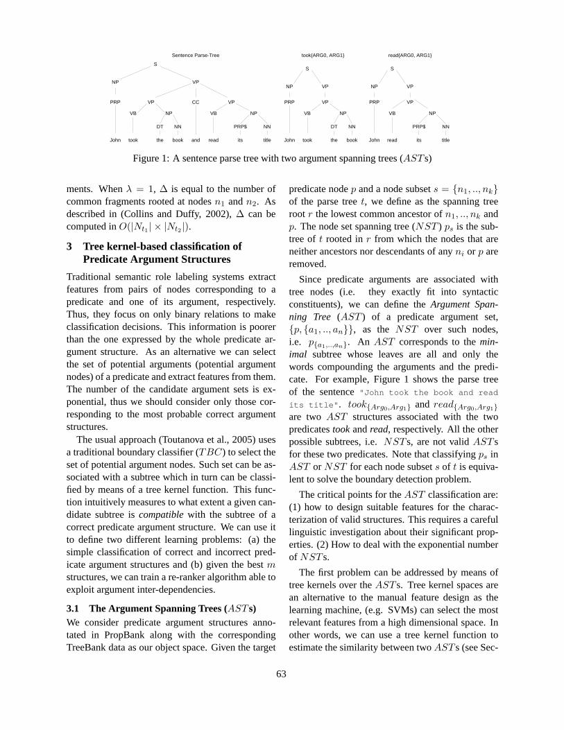
S
NP VP
PRP
John
VP CC VP
VB NP
and
VB NP
took
DT NN
the book read
PRP$ NN
its title
Sentence Parse-Tree
S
NP VP
PRP
John
VP
VB NP
took
DT NN
the book
took{ARG0, ARG1}
S
NP VP
PRP
John
VP
VB NP
read
PRP$ NN
its title
read{ARG0, ARG1}
Figure 1: A sentence parse tree with two argument spanning trees (ASTs)
ments. Whenλ = 1, ∆ is equal to the number ofcommon fragments rooted at nodesn1 andn2. Asdescribed in (Collins and Duffy, 2002),∆ can becomputed inO(|Nt1 | × |Nt2 |).3 Tree kernel-based classification of
Predicate Argument Structures
Traditional semantic role labeling systems extractfeatures from pairs of nodes corresponding to apredicate and one of its argument, respectively.Thus, they focus on only binary relations to makeclassification decisions. This information is poorerthan the one expressed by the whole predicate ar-gument structure. As an alternative we can selectthe set of potential arguments (potential argumentnodes) of a predicate and extract features from them.The number of the candidate argument sets is ex-ponential, thus we should consider only those cor-responding to the most probable correct argumentstructures.
The usual approach (Toutanova et al., 2005) usesa traditional boundary classifier (TBC) to select theset of potential argument nodes. Such set can be as-sociated with a subtree which in turn can be classi-fied by means of a tree kernel function. This func-tion intuitively measures to what extent a given can-didate subtree iscompatiblewith the subtree of acorrect predicate argument structure. We can use itto define two different learning problems: (a) thesimple classification of correct and incorrect pred-icate argument structures and (b) given the bestmstructures, we can train a re-ranker algorithm able toexploit argument inter-dependencies.
3.1 The Argument Spanning Trees (ASTs)We consider predicate argument structures anno-tated in PropBank along with the correspondingTreeBank data as our object space. Given the target
predicate nodep and a node subsets = {n1, .., nk}of the parse treet, we define as the spanning treeroot r the lowest common ancestor ofn1, .., nk andp. The node set spanning tree (NST ) ps is the sub-tree oft rooted inr from which the nodes that areneither ancestors nor descendants of anyni or p areremoved.
Since predicate arguments are associated withtree nodes (i.e. they exactly fit into syntacticconstituents), we can define theArgument Span-ning Tree (AST ) of a predicate argument set,{p, {a1, .., an}}, as the NST over such nodes,i.e. p{a1,..,an}. An AST corresponds to themin-imal subtree whose leaves are all and only thewords compounding the arguments and the predi-cate. For example, Figure 1 shows the parse treeof the sentence"John took the book and read
its title" . took{Arg0,Arg1} and read{Arg0,Arg1}are two AST structures associated with the twopredicatestookandread, respectively. All the otherpossible subtrees, i.e.NSTs, are not validASTsfor these two predicates. Note that classifyingps inAST or NST for each node subsets of t is equiva-lent to solve the boundary detection problem.
The critical points for theAST classification are:(1) how to design suitable features for the charac-terization of valid structures. This requires a carefullinguistic investigation about their significant prop-erties. (2) How to deal with the exponential numberof NSTs.
The first problem can be addressed by means oftree kernels over theASTs. Tree kernel spaces arean alternative to the manual feature design as thelearning machine, (e.g. SVMs) can select the mostrelevant features from a high dimensional space. Inother words, we can use a tree kernel function toestimate the similarity between twoASTs (see Sec-
63
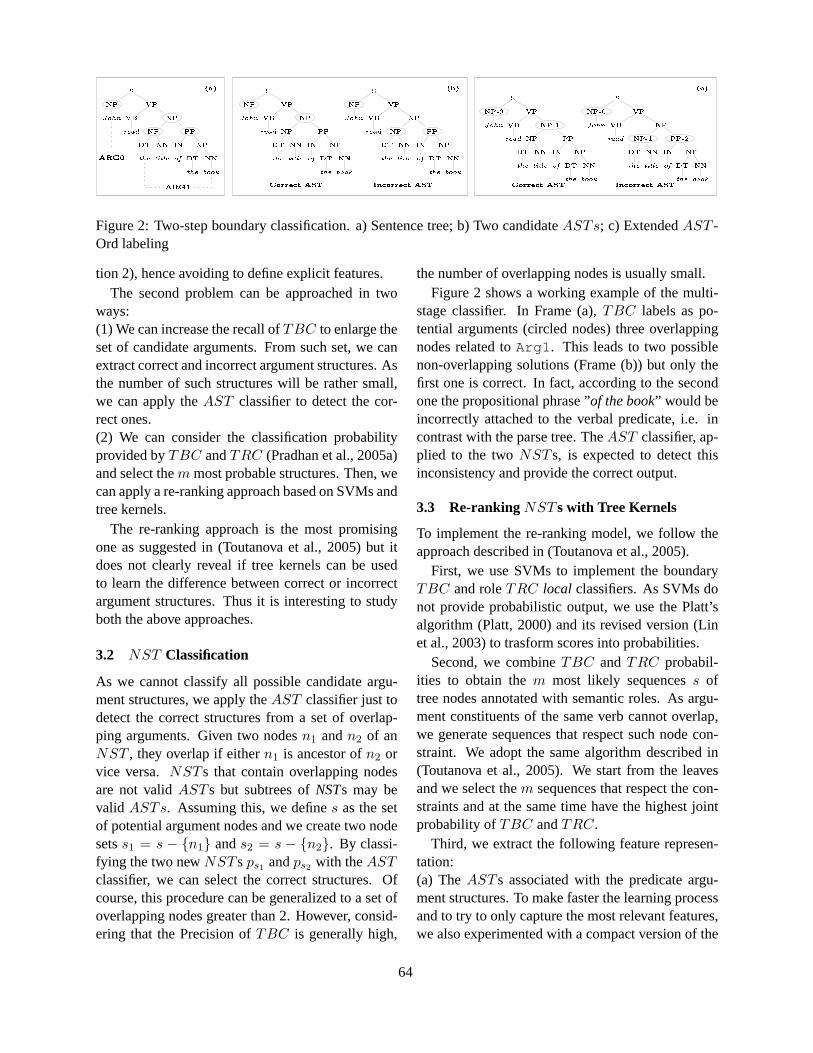
Figure 2: Two-step boundary classification. a) Sentence tree; b) Two candidateASTs; c) ExtendedAST -Ord labeling
tion 2), hence avoiding to define explicit features.The second problem can be approached in two
ways:(1) We can increase the recall ofTBC to enlarge theset of candidate arguments. From such set, we canextract correct and incorrect argument structures. Asthe number of such structures will be rather small,we can apply theAST classifier to detect the cor-rect ones.(2) We can consider the classification probabilityprovided byTBC andTRC (Pradhan et al., 2005a)and select them most probable structures. Then, wecan apply a re-ranking approach based on SVMs andtree kernels.
The re-ranking approach is the most promisingone as suggested in (Toutanova et al., 2005) but itdoes not clearly reveal if tree kernels can be usedto learn the difference between correct or incorrectargument structures. Thus it is interesting to studyboth the above approaches.
3.2 NST Classification
As we cannot classify all possible candidate argu-ment structures, we apply theAST classifier just todetect the correct structures from a set of overlap-ping arguments. Given two nodesn1 andn2 of anNST , they overlap if eithern1 is ancestor ofn2 orvice versa. NSTs that contain overlapping nodesare not validASTs but subtrees ofNSTs may bevalid ASTs. Assuming this, we defines as the setof potential argument nodes and we create two nodesetss1 = s − {n1} ands2 = s − {n2}. By classi-fying the two newNSTsps1 andps2 with theASTclassifier, we can select the correct structures. Ofcourse, this procedure can be generalized to a set ofoverlapping nodes greater than 2. However, consid-ering that the Precision ofTBC is generally high,
the number of overlapping nodes is usually small.Figure 2 shows a working example of the multi-
stage classifier. In Frame (a),TBC labels as po-tential arguments (circled nodes) three overlappingnodes related toArg1 . This leads to two possiblenon-overlapping solutions (Frame (b)) but only thefirst one is correct. In fact, according to the secondone the propositional phrase ”of the book” would beincorrectly attached to the verbal predicate, i.e. incontrast with the parse tree. TheAST classifier, ap-plied to the twoNSTs, is expected to detect thisinconsistency and provide the correct output.
3.3 Re-rankingNSTs with Tree Kernels
To implement the re-ranking model, we follow theapproach described in (Toutanova et al., 2005).
First, we use SVMs to implement the boundaryTBC and roleTRC local classifiers. As SVMs donot provide probabilistic output, we use the Platt’salgorithm (Platt, 2000) and its revised version (Linet al., 2003) to trasform scores into probabilities.
Second, we combineTBC andTRC probabil-ities to obtain them most likely sequencess oftree nodes annotated with semantic roles. As argu-ment constituents of the same verb cannot overlap,we generate sequences that respect such node con-straint. We adopt the same algorithm described in(Toutanova et al., 2005). We start from the leavesand we select them sequences that respect the con-straints and at the same time have the highest jointprobability ofTBC andTRC.
Third, we extract the following feature represen-tation:(a) TheASTs associated with the predicate argu-ment structures. To make faster the learning processand to try to only capture the most relevant features,we also experimented with a compact version of the
64

AST which is pruned at the level of argument nodes.(b) Attribute value features (standard features) re-lated to the whole predicate structure. These includethe features for each arguments (Gildea and Juras-fky, 2002) and global features like the sequence ofargument labels, e.g.〈Arg0, Arg1, ArgM〉.
Finally, we prepare the training examples for there-ranker considering them best annotations of eachpredicate structure. We use the approach adoptedin (Shen et al., 2003), which generates all possiblepairs from them examples, i.e.
(m2
)pairs. Each pair
is assigned to a positive example if the first mem-ber of the pair has a higher score than the secondmember. The score that we use is the F1 measureof the annotated structure with respect to the goldstandard. More in detail, given training/testing ex-amplesei = 〈t1i , t2i , v1
i , v2i 〉, wheret1i andt2i are two
ASTs andv1i andv2
i are two feature vectors associ-ated with two candidate predicate structuress1 ands2, we define the following kernels:
1) Ktr(e1, e2) = Kt(t11, t12) + Kt(t21, t
22)
−Kt(t11, t22)−Kt(t21, t
12),
wheretji is the j-th AST of the pairei, Kt is thetree kernel function defined in Section 2 andi, j ∈{1, 2}.
2) Kpr(e1, e2) = Kp(v11, v
12) + Kp(v2
1, v22)
−Kp(v11, v
22)−Kp(v2
1, v12),
wherevji is thej-th feature vector of the pairei and
Kp is the polynomial kernel applied to such vectors.The final kernel that we use for re-ranking is the
following:
K(e1, e2) =Ktr(e1, e2)|Ktr(e1, e2)| +
Kpr(e1, e2)|Kpr(e1, e2)|
Regarding tree kernel feature engineering, thenext section show how we can generate more effec-tive features given an established kernel function.
3.4 Tree kernel feature engineering
Consider the Frame (b) of Figure 2, it shows twoperfectly identicalNSTs, consequently, their frag-ments will also be equal. This prevents the algorithmto learn something from such examples. To solve theproblem, we can enrich theNSTs by marking theirargument nodes with a progressive number, starting
from the leftmost argument. For example, in the firstNST of Frame (c), we mark asNP-0 andNP-1 thefirst and second argument nodes whereas in the sec-ondNST we trasform the three argument node la-bels inNP-0 , NP-1 andPP-2 . We will refer to theresulting structure as aAST -Ord (ordinal number).This simple modification allows the tree kernel togenerate different argument structures for the aboveNSTs. For example, from the firstNST in Fig-ure 2.c, the fragments[NP-1 [NP][PP]] , [NP[DT][NN]] and [PP [IN][NP]] are gener-ated. They do not match anymore with the[NP-0[NP][PP]] , [NP-1 [DT][NN]] and [PP-2[IN][NP]] fragments generated from the secondNST in Figure 2.c.
Additionally, it should be noted that the semanticinformation provided by the role type can remark-ably help the detection of correct or incorrect predi-cate argument structures. Thus, we can enrich the ar-gument node label with the role type, e.g. theNP-0andNP-1 of the correctAST of Figure 2.c becomeNP-Arg0 andNP-Arg1 (not shown in the figure).We refer to this structure asAST -Arg. Of course,to apply theAST -Arg classifier, we need thatTRClabels the arguments detected byTBC.
4 The experiments
The experiments were carried out within the set-ting defined in the CoNLL-2005 Shared Task(Carreras and Marquez, 2005). In particular,we adopted the Charniak parse trees available atwww.lsi.upc.edu/ ∼srlconll/ along with the of-ficial performance evaluator.
All the experiments were performed withthe SVM-light-TK software available athttp://ai-nlp.info.uniroma2.it/moschitti/
which encodes ST and SST kernels in SVM-light(Joachims, 1999). ForTBC andTRC, we used thelinear kernel with a regularization parameter (option-c ) equal to 1. A cost factor (option-j ) of 10 wasadopted forTBC to have a higher Recall, whereasfor TRC, the cost factor was parameterized accord-ing to the maximal accuracy of each argument classon the validation set. For theAST -based classifierswe used aλ equal to0.4 (see (Moschitti, 2004)).
65

Section 21 Section 23AST Class. P. R. F1 P. R. F1
− 69.8 77.9 73.7 62.2 77.1 68.9Ord 73.7 81.2 77.3 63.7 80.6 71.2Arg 73.6 84.7 78.7 64.2 82.3 72.1
Table 1: AST , AST -Ord, andAST -Arg perfor-mance on sections 21 and 23.
4.1 Classification of whole predicate argumentstructures
In these experiments, we trainedTBC on sections02-08 whereas, to achieve a very accurate role clas-sifier, we trainedTRC on all sections 02-21. Totrain theAST , AST -Ord (AST with ordinal num-bers in the argument nodes), andAST -Arg (ASTwith argument type in the argument nodes) clas-sifiers, we applied theTBC and TRC over sec-tions 09-20. Then, we considered all the structureswhose automatic annotation showed at least an ar-gument overlap. From these, we extracted 30,220valid ASTs and 28,143 non-validASTs, for a totalof 183,642 arguments.
First, we evaluate the accuracy of theAST -basedclassifiers by extracting 1,975ASTs and 2,220 non-ASTs from Section 21 and the 2,159ASTs and3,461 non-ASTs from Section 23. The accuracyderived on Section 21 is an upperbound for our clas-sifiers since it is obtained using an ideal syntacticparser (the Charniak’s parser was trained also onSection 21) and an ideal role classifier.
Table 1 shows Precision, Recall andF1 mea-sures of theAST -based classifiers over the aboveNSTs. Rows 2, 3 and 4 report the performance ofAST , AST -Ord, andAST -Arg classifiers, respec-tively. We note that: (a) The impact of parsing ac-curacy is shown by the gap of about 6% points be-tween sections 21 and 23. (b) The ordinal number-ing of arguments (Ord) and the role type informa-tion (Arg) provide tree kernels with more meaning-ful fragments since they improve the basic modelof about 4%. (c) The deeper semantic informationgenerated by theArg labels provides useful clues toselect correct predicate argument structures since itimproves theOrd model on both sections.
Second, we measured the impact of theAST -based classifiers on the accuracy of both phases ofsemantic role labeling. Table 2 reports the results
on sections 21 and 23. For each of them, Precision,Recall andF1 of different approaches to bound-ary identification (bnd) and to the complete task,i.e. boundary and role classification (bnd+class)are shown. Such approaches are based on differ-ent strategies to remove the overlaps, i.e. with theAST , AST -Ord andAST -Arg classifiers and usingthe baseline (RND), i.e. a random selection of non-overlapping structures. The baseline corresponds tothe system based onTBC andTRC1.We note that: (a) for any model, the boundary de-tectionF1 on Section 21 is about 10 points higherthan theF1 on Section 23 (e.g. 87.0% vs. 77.9%for RND). As expected the parse tree quality is veryimportant to detect argument boundaries. (b) On thereal test (Section 23) the classification introduces la-beling errors which decrease the accuracy of about5% (77.9 vs 72.9 for RND). (c) TheOrd andArgapproaches constantly improve the baselineF1 ofabout 1%. Such poor impact does not surprise asthe overlapping structures are a small percentage ofthe test set, thus the overall improvement cannot bevery high.
Third, the comparison with the CoNLL 2005 re-sults (Carreras and Marquez, 2005) can only becarried out with respect to the whole SRL task(bnd+class in table 2) since boundary detection ver-sus role classification is generally not provided inCoNLL 2005. Moreover, our best global result, i.e.73.9%, was obtained under two severe experimentalfactors: a) the use of just 1/3 of the available train-ing set, and b) the usage of the linear SVM modelfor the TBC classifier, which is much faster than thepolynomial SVMs but also less accurate. However,we note the promising results of theAST meta-classifier, which can be used with any of the bestfigure CoNLL systems.
Finally, the overall results suggest that the treekernel model is robust to parse tree errors since pre-serves the same improvement across trees derivedwith different accuracy, i.e. thesemi-automatictreesof Section 21 and the automatic tree of Section 23.Moreover, it shows a high accuracy for the classi-fication of correct and incorrectASTs. This lastproperty is quite interesting as the best SRL systems
1We needed to remove the overlaps from the baseline out-come in order to apply the CoNLL evaluator.
66

(Punyakanok et al., 2005; Toutanova et al., 2005;Pradhan et al., 2005b) were obtained by exploit-ing the information on the whole predicate argumentstructure.
Next section shows our preliminary experimentson re-ranking using theAST kernel based approach.
4.2 Re-ranking based on Tree Kernels
In these experiments, we used the output ofTBCand TRC2 to provide an SVM tree kernel with aranked list of predicate argument structures. More indetail, we applied a Viterbi-like algorithm to gener-ate the 20 most likely annotations for each predicatestructure, according to the joint probabilistic modelof TBC andTRC. We sorted such structures basedon theirF1 measure and used them to learn the SVMre-ranker described in 3.3.
For training, we used Sections 12, 14, 15, 16and 24, which contain 24,729 predicate structures.For each of them, we considered the 5 annotationshaving the highest F1 score (i.e. 123,674NSTs)on the span of the 20 best annotations provided byViterbi algorithm. With such structures, we ob-tained 294,296 pairs used to train the SVM-basedre-ranker. As the number of such structures is verylarge the SVM training time was very high. Thus,we sped up the learning process by using only theASTs associated with the core arguments. From thetest sentences (which contain 5,267 structures), weextracted the 20 best Viterbi annotated structures,i.e. 102,343 (for a total of 315.531 pairs), whichwere used for the following experiments:
First, we selected the best annotation (accordingto theF1 provided by the gold standard annotations)out of the 20 provided by the Viterbi’s algorithm.The resultingF1 of 88.59% is the upperbound of ourapproach.
Second, we selected the top ranked annotation in-dicated by the Viterbi’s algorithm. This provides ourbaselineF1 measure, i.e. 75.91%. Such outcome isslightly higher than our official CoNLL result (Mos-chitti et al., 2005) obtained without converting SVMscores into probabilities.
Third, we applied the SVM re-ranker to select
2With the aim of improving the state-of-the-art, we appliedthe polynomial kernel for all basic classifiers, at this time.We used the models developed during our participation to theCoNLL 2005 shared task (Moschitti et al., 2005).
the best structures according to the core roles. Weachieved 80.68% which is practically equal to theresult obtained in (Punyakanok et al., 2005; Car-reras and Marquez, 2005) for core roles, i.e. 81%.Their overall F1 which includes all the argumentswas 79.44%. This confirms that the classification ofthe non-core roles is more complex than the otherarguments.
Finally, the high computation time of the re-ranker prevented us to use the larger structureswhich include all arguments. The major complexityissue was the slow training and classification timeof SVMs. The time needed for tree kernel functionwas not so problematic as we could use the fast eval-uation proposed in (Moschitti, 2006). This roughlyreduces the computation time to the one required bya polynomial kernel. The real burden is therefore thelearning time of SVMs that is quadratic in the num-ber of training instances. For example, to carry outthe re-ranking experiments required approximatelyone month of a 64 bits machine (2.4 GHz and 4GbRam). To solve this problem, we are going to studythe impact on the accuracy of fast learning algo-rithms such as the Voted Perceptron.
5 Related Work
Recently, many kernels for natural language applica-tions have been designed. In what follows, we high-light their difference and properties.
The tree kernel used in this article was proposedin (Collins and Duffy, 2002) for syntactic parsingre-ranking. It was experimented with the VotedPerceptron and was shown to improve the syntac-tic parsing. In (Cumby and Roth, 2003), a featuredescription language was used to extract structuralfeatures from the syntactic shallow parse trees asso-ciated with named entities. The experiments on thenamed entity categorization showed that when thedescription language selects an adequate set of treefragments the Voted Perceptron algorithm increasesits classification accuracy. The explanation was thatthe complete tree fragment set contains many irrel-evant features and may cause overfitting. In (Pun-yakanok et al., 2005), a set of different syntacticparse trees, e.g. then best trees generated by theCharniak’s parser, were used to improve the SRLaccuracy. These different sources of syntactic infor-mation were used to generate a set of different SRL
67
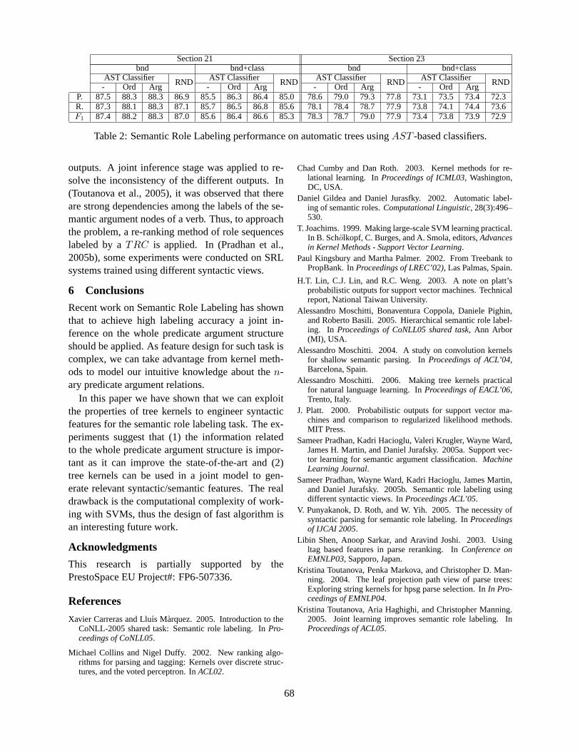
Section 21 Section 23bnd bnd+class bnd bnd+class
AST Classifier RND AST Classifier RND AST Classifier RND AST Classifier RND- Ord Arg - Ord Arg - Ord Arg - Ord ArgP. 87.5 88.3 88.3 86.9 85.5 86.3 86.4 85.0 78.6 79.0 79.3 77.8 73.1 73.5 73.4 72.3R. 87.3 88.1 88.3 87.1 85.7 86.5 86.8 85.6 78.1 78.4 78.7 77.9 73.8 74.1 74.4 73.6F1 87.4 88.2 88.3 87.0 85.6 86.4 86.6 85.3 78.3 78.7 79.0 77.9 73.4 73.8 73.9 72.9
Table 2: Semantic Role Labeling performance on automatic trees usingAST -based classifiers.
outputs. A joint inference stage was applied to re-solve the inconsistency of the different outputs. In(Toutanova et al., 2005), it was observed that thereare strong dependencies among the labels of the se-mantic argument nodes of a verb. Thus, to approachthe problem, a re-ranking method of role sequenceslabeled by aTRC is applied. In (Pradhan et al.,2005b), some experiments were conducted on SRLsystems trained using different syntactic views.
6 Conclusions
Recent work on Semantic Role Labeling has shownthat to achieve high labeling accuracy a joint in-ference on the whole predicate argument structureshould be applied. As feature design for such task iscomplex, we can take advantage from kernel meth-ods to model our intuitive knowledge about then-ary predicate argument relations.
In this paper we have shown that we can exploitthe properties of tree kernels to engineer syntacticfeatures for the semantic role labeling task. The ex-periments suggest that (1) the information relatedto the whole predicate argument structure is impor-tant as it can improve the state-of-the-art and (2)tree kernels can be used in a joint model to gen-erate relevant syntactic/semantic features. The realdrawback is the computational complexity of work-ing with SVMs, thus the design of fast algorithm isan interesting future work.
Acknowledgments
This research is partially supported by thePrestoSpace EU Project#: FP6-507336.
References
Xavier Carreras and Lluıs Marquez. 2005. Introduction to theCoNLL-2005 shared task: Semantic role labeling. InPro-ceedings of CoNLL05.
Michael Collins and Nigel Duffy. 2002. New ranking algo-rithms for parsing and tagging: Kernels over discrete struc-tures, and the voted perceptron. InACL02.
Chad Cumby and Dan Roth. 2003. Kernel methods for re-lational learning. InProceedings of ICML03, Washington,DC, USA.
Daniel Gildea and Daniel Jurasfky. 2002. Automatic label-ing of semantic roles.Computational Linguistic, 28(3):496–530.
T. Joachims. 1999. Making large-scale SVM learning practical.In B. Scholkopf, C. Burges, and A. Smola, editors,Advancesin Kernel Methods - Support Vector Learning.
Paul Kingsbury and Martha Palmer. 2002. From Treebank toPropBank. InProceedings of LREC’02), Las Palmas, Spain.
H.T. Lin, C.J. Lin, and R.C. Weng. 2003. A note on platt’sprobabilistic outputs for support vector machines. Technicalreport, National Taiwan University.
Alessandro Moschitti, Bonaventura Coppola, Daniele Pighin,and Roberto Basili. 2005. Hierarchical semantic role label-ing. In Proceedings of CoNLL05 shared task, Ann Arbor(MI), USA.
Alessandro Moschitti. 2004. A study on convolution kernelsfor shallow semantic parsing. InProceedings of ACL’04,Barcelona, Spain.
Alessandro Moschitti. 2006. Making tree kernels practicalfor natural language learning. InProceedings of EACL’06,Trento, Italy.
J. Platt. 2000. Probabilistic outputs for support vector ma-chines and comparison to regularized likelihood methods.MIT Press.
Sameer Pradhan, Kadri Hacioglu, Valeri Krugler, Wayne Ward,James H. Martin, and Daniel Jurafsky. 2005a. Support vec-tor learning for semantic argument classification.MachineLearning Journal.
Sameer Pradhan, Wayne Ward, Kadri Hacioglu, James Martin,and Daniel Jurafsky. 2005b. Semantic role labeling usingdifferent syntactic views. InProceedings ACL’05.
V. Punyakanok, D. Roth, and W. Yih. 2005. The necessity ofsyntactic parsing for semantic role labeling. InProceedingsof IJCAI 2005.
Libin Shen, Anoop Sarkar, and Aravind Joshi. 2003. Usingltag based features in parse reranking. InConference onEMNLP03, Sapporo, Japan.
Kristina Toutanova, Penka Markova, and Christopher D. Man-ning. 2004. The leaf projection path view of parse trees:Exploring string kernels for hpsg parse selection. InIn Pro-ceedings of EMNLP04.
Kristina Toutanova, Aria Haghighi, and Christopher Manning.2005. Joint learning improves semantic role labeling. InProceedings of ACL05.
68
Proceedings of the 10th Conference on Computational Natural Language Learning (CoNLL-X),pages 69–76, New York City, June 2006.c©2006 Association for Computational Linguistics
Can Human Verb Associations Help IdentifySalient Features for Semantic Verb Classification?
Sabine Schulte im WaldeComputational Linguistics
Saarland UniversitySaarbrucken, Germany
Abstract
This paper investigates whether human as-sociations to verbs as collected in a webexperiment can help us to identify salientverb features for semantic verb classes.Assuming that the associations model as-pects of verb meaning, we apply a clus-tering to the verbs, as based on the as-sociations, and validate the resulting verbclasses against standard approaches to se-mantic verb classes, i.e. GermaNet andFrameNet. Then, various clusterings ofthe same verbs are performed on the basisof standard corpus-based types, and eval-uated against the association-based clus-tering as well as GermaNet and FrameNetclasses. We hypothesise that the corpus-based clusterings are better if the instan-tiations of the feature types show moreoverlap with the verb associations, andthat the associations therefore help toidentify salient feature types.
1 Introduction
There are a variety of manual semantic verb clas-sifications; major frameworks are the Levin classes(Levin, 1993), WordNet (Fellbaum, 1998), andFrameNet (Fontenelle, 2003). The different frame-works depend on different instantiations of seman-tic similarity, e.g. Levin relies on verb similarityreferring to syntax-semantic alternation behaviour,WordNet uses synonymy, and FrameNet relies onsituation-based agreement as defined in Fillmore’sframe semantics (Fillmore, 1982). As an alterna-tive to the resource-intensive manual classifications,
automatic methods such as classification and clus-tering are applied to induce verb classes from cor-pus data, e.g. (Merlo and Stevenson, 2001; Joanisand Stevenson, 2003; Korhonen et al., 2003; Steven-son and Joanis, 2003; Schulte im Walde, 2003; Fer-rer, 2004). Depending on the types of verb classesto be induced, the automatic approaches vary theirchoice of verbs and classification/clustering algo-rithm. However, another central parameter for theautomatic induction of semantic verb classes is theselection of verb features.
Since the target classification determines the sim-ilarity and dissimilarity of the verbs, the verb fea-ture selection should model the similarity of inter-est. For example, Merlo and Stevenson (2001) clas-sify 60 English verbs which alternate between an in-transitive and a transitive usage, and assign them tothree verb classes, according to the semantic role as-signment in the frames; their verb features are cho-sen such that they model the syntactic frame alterna-tion proportions and also heuristics for semantic roleassignment. In larger-scale classifications such as(Korhonen et al., 2003; Stevenson and Joanis, 2003;Schulte im Walde, 2003), which model verb classeswith similarity at the syntax-semantics interface, itis not clear which features are the most salient. Theverb features need to relate to a behavioural com-ponent (modelling the syntax-semantics interplay),but the set of features which potentially influencethe behaviour is large, ranging from structural syn-tactic descriptions and argument role fillers to ad-verbial adjuncts. In addition, it is not clear howfine-grained the features should be; for example,how much information is covered by low-level win-dow co-occurrence vs. higher-order syntactic framefillers?
69
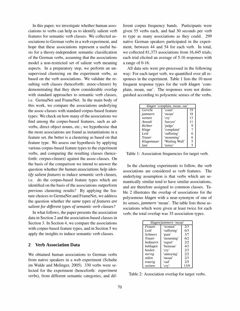
In this paper, we investigate whether human asso-ciations to verbs can help us to identify salient verbfeatures for semantic verb classes. We collected as-sociations to German verbs in a web experiment, andhope that these associations represent a useful ba-sis for a theory-independent semantic classificationof the German verbs, assuming that the associationsmodel a non-restricted set of salient verb meaningaspects. In a preparatory step, we perform an un-supervised clustering on the experiment verbs, asbased on the verb associations. We validate the re-sulting verb classes (henceforth: assoc-classes) bydemonstrating that they show considerable overlapwith standard approaches to semantic verb classes,i.e. GermaNet and FrameNet. In the main body ofthis work, we compare the associations underlyingthe assoc-classes with standard corpus-based featuretypes: We check on how many of the associations wefind among the corpus-based features, such as ad-verbs, direct object nouns, etc.; we hypothesise thatthe more associations are found as instantiations in afeature set, the better is a clustering as based on thatfeature type. We assess our hypothesis by applyingvarious corpus-based feature types to the experimentverbs, and comparing the resulting classes (hence-forth: corpus-classes) against the assoc-classes. Onthe basis of the comparison we intend to answer thequestion whether the human associations help iden-tify salient features to induce semantic verb classes,i.e. do the corpus-based feature types which areidentified on the basis of the associations outperformprevious clustering results? By applying the fea-ture choices to GermaNet and FrameNet, we addressthe question whether the same types of features aresalient for different types of semantic verb classes?
In what follows, the paper presents the associationdata in Section 2 and the association-based classes inSection 3. In Section 4, we compare the associationswith corpus-based feature types, and in Section 5 weapply the insights to induce semantic verb classes.
2 Verb Association Data
We obtained human associations to German verbsfrom native speakers in a web experiment (Schulteim Walde and Melinger, 2005). 330 verbs were se-lected for the experiment (henceforth: experimentverbs), from different semantic categories, and dif-
ferent corpus frequency bands. Participants weregiven 55 verbs each, and had 30 seconds per verbto type as many associations as they could. 299native German speakers participated in the experi-ment, between 44 and 54 for each verb. In total,we collected 81,373 associations from 16,445 trials;each trial elicited an average of 5.16 responses witha range of 0-16.
All data sets were pre-processed in the followingway: For each target verb, we quantified over all re-sponses in the experiment. Table 1 lists the 10 mostfrequent response types for the verb klagen ‘com-plain, moan, sue’. The responses were not distin-guished according to polysemic senses of the verbs.
klagen ‘complain, moan, sue’Gericht ‘court’ 19jammern ‘moan’ 18weinen ‘cry’ 13Anwalt ‘lawyer’ 11Richter ‘judge’ 9Klage ‘complaint’ 7Leid ‘suffering’ 6Trauer ‘mourning’ 6Klagemauer ‘Wailing Wall’ 5laut ‘noisy’ 5
Table 1: Association frequencies for target verb.
In the clustering experiments to follow, the verbassociations are considered as verb features. Theunderlying assumption is that verbs which are se-mantically similar tend to have similar associations,and are therefore assigned to common classes. Ta-ble 2 illustrates the overlap of associations for thepolysemous klagen with a near-synonym of one ofits senses, jammern ‘moan’. The table lists those as-sociations which were given at least twice for eachverb; the total overlap was 35 association types.
klagen/jammern ‘moan’Frauen ‘women’ 2/3Leid ‘suffering’ 6/3Schmerz ‘pain’ 3/7Trauer ‘mourning’ 6/2bedauern ‘regret’ 2/2beklagen ‘bemoan’ 4/3heulen ‘cry’ 2/3nervig ‘annoying’ 2/2nolen ‘moan’ 2/3traurig ‘sad’ 2/5weinen ‘cry’ 13/9
Table 2: Association overlap for target verbs.
70
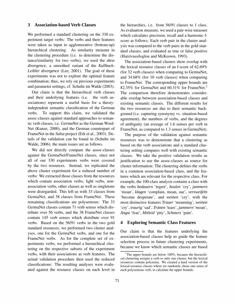
3 Association-based Verb Classes
We performed a standard clustering on the 330 ex-periment target verbs: The verbs and their featureswere taken as input to agglomerative (bottom-up)hierarchical clustering. As similarity measure inthe clustering procedure (i.e. to determine the dis-tance/similarity for two verbs), we used the skewdivergence, a smoothed variant of the Kullback-Leibler divergence (Lee, 2001). The goal of theseexperiments was not to explore the optimal featurecombination; thus, we rely on previous experimentsand parameter settings, cf. Schulte im Walde (2003).
Our claim is that the hierarchical verb classesand their underlying features (i.e. the verb as-sociations) represent a useful basis for a theory-independent semantic classification of the Germanverbs. To support this claim, we validated theassoc-classes against standard approaches to seman-tic verb classes, i.e. GermaNet as the German Word-Net (Kunze, 2000), and the German counterpart ofFrameNet in the Salsa project (Erk et al., 2003). De-tails of the validation can be found in (Schulte imWalde, 2006); the main issues are as follows.
We did not directly compare the assoc-classesagainst the GermaNet/FrameNet classes, since notall of our 330 experiments verbs were coveredby the two resources. Instead, we replicated theabove cluster experiment for a reduced number ofverbs: We extracted those classes from the resourceswhich contain association verbs; light verbs, non-association verbs, other classes as well as singletonswere disregarded. This left us with 33 classes fromGermaNet, and 38 classes from FrameNet. Theseremaining classifications are polysemous: The 33GermaNet classes contain 71 verb senses which dis-tribute over 56 verbs, and the 38 FrameNet classescontain 145 verb senses which distribute over 91verbs. Based on the 56/91 verbs in the two goldstandard resources, we performed two cluster anal-yses, one for the GermaNet verbs, and one for theFrameNet verbs. As for the complete set of ex-periments verbs, we performed a hierarchical clus-tering on the respective subsets of the experimentverbs, with their associations as verb features. Theactual validation procedure then used the reducedclassifications: The resulting analyses were evalu-ated against the resource classes on each level in
the hierarchies, i.e. from 56/91 classes to 1 class.As evaluation measure, we used a pair-wise measurewhich calculates precision, recall and a harmonic f-score as follows: Each verb pair in the cluster anal-ysis was compared to the verb pairs in the gold stan-dard classes, and evaluated as true or false positive(Hatzivassiloglou and McKeown, 1993).
The association-based clusters show overlap withthe lexical resource classes of an f-score of 62.69%(for 32 verb classes) when comparing to GermaNet,and 34.68% (for 10 verb classes) when comparingto FrameNet. The corresponding upper bounds are82.35% for GermaNet and 60.31% for FrameNet.1The comparison therefore demonstrates consider-able overlap between association-based classes andexisting semantic classes. The different results forthe two resources are due to their semantic back-ground (i.e. capturing synonymy vs. situation-basedagreement), the numbers of verbs, and the degreesof ambiguity (an average of 1.6 senses per verb inFrameNet, as compared to 1.3 senses in GermaNet).
The purpose of the validation against semanticresources was to demonstrate that a clustering asbased on the verb associations and a standard clus-tering setting compares well with existing semanticclasses. We take the positive validation results asjustification to use the assoc-classes as source forcluster information: The clustering defines the verbsin a common association-based class, and the fea-tures which are relevant for the respective class. Forexample, the 100-class analysis contains a class withthe verbs bedauern ‘regret’, heulen ‘cry’, jammern‘moan’, klagen ‘complain, moan, sue’, verzweifeln‘become desperate’, and weinen ‘cry’, with themost distinctive features Trauer ‘mourning’, weinen‘cry’, traurig ‘sad’, Tranen ‘tears’, jammern ‘moan’,Angst ‘fear’, Mitleid ‘pity’, Schmerz ‘pain’.
4 Exploring Semantic Class Features
Our claim is that the features underlying theassociation-based classes help us guide the featureselection process in future clustering experiments,because we know which semantic classes are based
1The upper bounds are below 100%, because the hierarchi-cal clustering assigns a verb to only one cluster, but the lexicalresources contain polysemy. We created a hard version of thelexical resource classes where we randomly chose one sense ofeach polysemous verb, to calculate the upper bounds.
71
on which associations/features. We rely on theassoc-classes in the 100-class analysis of the hier-archical clustering2 and features which exist for atleast two verbs in a common class (and thereforehint to a minimum of verb similarity), and comparethe associations underlying the assoc-classes withstandard corpus-based feature types: We check onhow many of the associations we find among thecorpus-based features, such as adverbs, direct objectnouns, etc. There are various possibilities to deter-mine corpus-based features that potentially cover theassociations; we decided in favour of feature typeswhich have been suggested in related work:
a) Grammar-based relations: Previous workon distributional similarity has focused either ona specific word-word relation (such as Pereira etal. (1993) and Rooth et al. (1999) referring to a directobject noun for describing verbs), or used any syn-tactic relationship detected by a chunker or a parser(such as Lin (1998) and McCarthy et al. (2003)). Weused a statistical grammar (Schulte im Walde, 2003)to filter all verb-noun pairs where the nouns repre-sent nominal heads in NPs or PPs in syntactic rela-tion to the verb (subject, object, adverbial function,etc.), and to filter all verb-adverb pairs where the ad-verbs modify the verbs.
b) Co-occurrence window: In previous work(Schulte im Walde and Melinger, 2005), we showedthat only 28% of all noun associates were identi-fied by the above statistical grammar as subcate-gorised nouns, but 69% were captured by a 20-wordco-occurrence window in a 200-million word news-paper corpus. This finding suggests to use a co-occurrence window as alternative source for verbfeatures, as compared to specific syntactic relations.We therefore determined the co-occurring words forall experiment verbs in a 20-word window (i.e. 20words preceding and following the verb), irrespec-tive of the part-of-speech of the co-occurring words.
Relying on the verb information extracted for a)and b), we checked for each verb-association pairwhether it occurred among the grammar or windowpairs. Table 3 illustrates which proportions of theassociations we found in the two resource types.For the grammar-based relations, we checked argu-
2The exact number of classes or the verb-per-class ratio arenot relevant for investigating the use of associations.
ment NPs and PPs (as separate sets and together),and in addition we checked verb-noun pairs in themost common specific NP functions: n refers to the(nominative) intransitive subject, na to the transi-tive subject, and na to the transitive (accusative) ob-ject. For the windows, all checks on co-occurrenceof verbs and associations in the whole 200-millionword corpus. cut also checks the whole corpus, butdisregards the most and least frequent co-occurringwords: verb-word pairs were only considered if theco-occurrence frequency of the word over all verbswas above 100 (disregarding low frequency pairs)and below 200,000 (disregarding high frequencypairs). Using the cut-offs, we can distinguish therelevance of high- and low-frequency features. Fi-nally, ADJ, ADV, N, V perform co-occurrence checksfor the whole corpus, but breaks down the all resultswith respect to the association part-of-speech.
As one would have expected, most of the as-sociations (66%) were found in the 20-word co-occurrence window, because the window is neitherrestricted to a certain part-of-speech, nor to a certaingrammar relation; in addition, the window is poten-tially larger than a sentence. Applying the frequencycut-offs reduces the overlap of association types andco-occurring words to 58%. Specifying the windowresults for the part-of-speech types illustrates thatthe nouns play the most important role in describingverb meaning (39% of the verb association types inthe assoc-classes were found among the nouns in thecorpus windows, 16% among the verbs, 9% amongthe adjectives, and 2% among the adverbs).3
The proportions of the nouns with a specificgrammar relationship to the verbs show that we findmore associations among direct objects than intran-sitive/transitive subjects. This insight confirms theassumption in previous work where only direct ob-ject nouns were used as salient features in distribu-tional verb similarity, such as Pereira et al. (1993).However, the proportions are all below 10%. Con-sidering all NPs and/or PPs, we find that the pro-portions increase for the NPs, and that the NPs playa more important role than the PPs. This insightconfirms work on distributional similarity where notonly direct object nouns, but all functional nouns
3Caveat: These numbers correlate with the part-of-speechtypes of all associate responses: 62% of the responses werenouns, 25% verbs, 11% adjectives, and 2% adverbs.
72
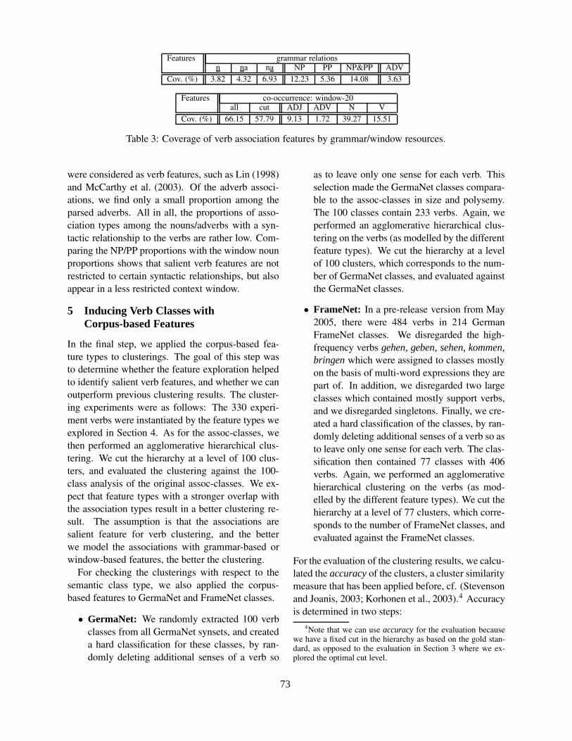
Features grammar relationsn na na NP PP NP&PP ADV
Cov. (%) 3.82 4.32 6.93 12.23 5.36 14.08 3.63
Features co-occurrence: window-20all cut ADJ ADV N V
Cov. (%) 66.15 57.79 9.13 1.72 39.27 15.51
Table 3: Coverage of verb association features by grammar/window resources.
were considered as verb features, such as Lin (1998)and McCarthy et al. (2003). Of the adverb associ-ations, we find only a small proportion among theparsed adverbs. All in all, the proportions of asso-ciation types among the nouns/adverbs with a syn-tactic relationship to the verbs are rather low. Com-paring the NP/PP proportions with the window nounproportions shows that salient verb features are notrestricted to certain syntactic relationships, but alsoappear in a less restricted context window.
5 Inducing Verb Classes withCorpus-based Features
In the final step, we applied the corpus-based fea-ture types to clusterings. The goal of this step wasto determine whether the feature exploration helpedto identify salient verb features, and whether we canoutperform previous clustering results. The cluster-ing experiments were as follows: The 330 experi-ment verbs were instantiated by the feature types weexplored in Section 4. As for the assoc-classes, wethen performed an agglomerative hierarchical clus-tering. We cut the hierarchy at a level of 100 clus-ters, and evaluated the clustering against the 100-class analysis of the original assoc-classes. We ex-pect that feature types with a stronger overlap withthe association types result in a better clustering re-sult. The assumption is that the associations aresalient feature for verb clustering, and the betterwe model the associations with grammar-based orwindow-based features, the better the clustering.
For checking the clusterings with respect to thesemantic class type, we also applied the corpus-based features to GermaNet and FrameNet classes.
• GermaNet: We randomly extracted 100 verbclasses from all GermaNet synsets, and createda hard classification for these classes, by ran-domly deleting additional senses of a verb so
as to leave only one sense for each verb. Thisselection made the GermaNet classes compara-ble to the assoc-classes in size and polysemy.The 100 classes contain 233 verbs. Again, weperformed an agglomerative hierarchical clus-tering on the verbs (as modelled by the differentfeature types). We cut the hierarchy at a levelof 100 clusters, which corresponds to the num-ber of GermaNet classes, and evaluated againstthe GermaNet classes.
• FrameNet: In a pre-release version from May2005, there were 484 verbs in 214 GermanFrameNet classes. We disregarded the high-frequency verbs gehen, geben, sehen, kommen,bringen which were assigned to classes mostlyon the basis of multi-word expressions they arepart of. In addition, we disregarded two largeclasses which contained mostly support verbs,and we disregarded singletons. Finally, we cre-ated a hard classification of the classes, by ran-domly deleting additional senses of a verb so asto leave only one sense for each verb. The clas-sification then contained 77 classes with 406verbs. Again, we performed an agglomerativehierarchical clustering on the verbs (as mod-elled by the different feature types). We cut thehierarchy at a level of 77 clusters, which corre-sponds to the number of FrameNet classes, andevaluated against the FrameNet classes.
For the evaluation of the clustering results, we calcu-lated the accuracy of the clusters, a cluster similaritymeasure that has been applied before, cf. (Stevensonand Joanis, 2003; Korhonen et al., 2003).4 Accuracyis determined in two steps:
4Note that we can use accuracy for the evaluation becausewe have a fixed cut in the hierarchy as based on the gold stan-dard, as opposed to the evaluation in Section 3 where we ex-plored the optimal cut level.
73
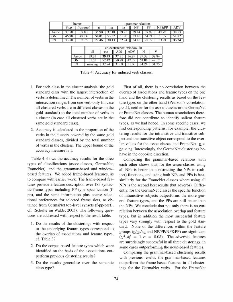
frames grammar relationsf-pp f-pp-pref n na na NP PP NP&PP ADV
Assoc 37.50 37.80 35.90 37.18 39.25 39.14 37.97 41.28 38.53GN 46.98 49.14 58.01 53.37 51.90 53.10 54.21 51.77 51.82FN 33.50 32.76 29.46 30.13 32.74 34.16 28.72 33.91 35.24
co-occurrence: window-20all cut ADJ ADV N V
Assoc 39.33 39.45 37.31 36.89 39.33 38.84GN 51.53 52.42 50.88 47.79 52.86 49.12FN missing 32.84 31.08 31.00 34.24 31.75
Table 4: Accuracy for induced verb classes.
1. For each class in the cluster analysis, the goldstandard class with the largest intersection ofverbs is determined. The number of verbs in theintersection ranges from one verb only (in caseall clustered verbs are in different classes in thegold standard) to the total number of verbs ina cluster (in case all clustered verbs are in thesame gold standard class).
2. Accuracy is calculated as the proportion of theverbs in the clusters covered by the same goldstandard classes, divided by the total numberof verbs in the clusters. The upper bound of theaccuracy measure is 1.
Table 4 shows the accuracy results for the threetypes of classifications (assoc-classes, GermaNet,FrameNet), and the grammar-based and window-based features. We added frame-based features, asto compare with earlier work: The frame-based fea-tures provide a feature description over 183 syntac-tic frame types including PP type specification (f-pp), and the same information plus coarse selec-tional preferences for selected frame slots, as ob-tained from GermaNet top-level synsets (f-pp-pref),cf. (Schulte im Walde, 2003). The following ques-tions are addressed with respect to the result table.
1. Do the results of the clusterings with respectto the underlying feature types correspond tothe overlap of associations and feature types,cf. Table 3?
2. Do the corpus-based feature types which wereidentified on the basis of the associations out-perform previous clustering results?
3. Do the results generalise over the semanticclass type?
First of all, there is no correlation between theoverlap of associations and feature types on the onehand and the clustering results as based on the fea-ture types on the other hand (Pearson’s correlation,p>.1), neither for the assoc-classes or the GermaNetor FrameNet classes. The human associations there-fore did not contribute to identify salient featuretypes, as we had hoped. In some specific cases, wefind corresponding patterns; for example, the clus-tering results for the intransitive and transitive sub-ject and the transitive object correspond to the over-lap values for the assoc-classes and FrameNet: n <
na < na. Interestingly, the GermaNet clusterings be-have in the opposite direction.
Comparing the grammar-based relations witheach other shows that for the assoc-classes usingall NPs is better than restricting the NPs to (sub-ject) functions, and using both NPs and PPs is best;similarly for the FrameNet classes where using allNPs is the second best results (but adverbs). Differ-ently, for the GermaNet classes the specific functionof intransitive subjects outperforms the more gen-eral feature types, and the PPs are still better thanthe NPs. We conclude that not only there is no cor-relation between the association overlap and featuretypes, but in addition the most successful featuretypes vary strongly with respect to the gold stan-dard. None of the differences within the featuregroups (n/na/na and NP/PP/NP&PP) are significant(χ2, df = 1, α = 0.05). The adverbial featuresare surprisingly successful in all three clusterings, insome cases outperforming the noun-based features.
Comparing the grammar-based clustering resultswith previous results, the grammar-based featuresoutperform the frame-based features in all cluster-ings for the GermaNet verbs. For the FrameNet
74

verbs and the experiment verbs, they outperform theframe-based features only in specific cases. Theadverbial features outperform the frame-based fea-tures in any clustering. However, none of the differ-ences between the frame-based clusterings and thegrammar-based clusterings are significant (χ2, df =
1, α = 0.05).For all gold standards, the best window-based
clustering results are below the best grammar-basedresults. Especially the all results demonstrateonce more the missing correlation between associa-tion/feature overlap and clustering results. However,it is interesting that the clusterings based on win-dow co-occurrence are not significantly worse (andin some cases even better) than the clusterings basedon selected grammar-based functions. This meansthat a careful choice and extraction of specific rela-tionships for verb features does not have a signifi-cant impact on semantic classes.
Comparing the window-based features againsteach other shows that even though we discovereda much larger proportion of association types in anunrestricted window all than elsewhere, the resultsin the clusterings do not differ accordingly. Apply-ing the frequency cut-offs has almost no impact onthe clustering results, which means that it does noharm to leave away the rather unpredictable features.Somehow expected but nevertheless impressive isthe fact that only considering nouns as co-occurringwords is as successful as considering all words inde-pendent of the part-of-speech.
Finally, the overall accuracy values are muchbetter for the GermaNet clusterings than for theexperiment-based and the FrameNet clusterings.The differences are all significant (χ2, df = 1, α =
0.05). The reason for these large differences couldbe either (a) that the clustering task was easier forthe GermaNet verbs, or (b) that the differences arecaused by the underlying semantics. We argueagainst case (a) since we deliberately chose the samenumber of classes (100) as for the association-basedgold standard; however, the verbs-per-class ratio forGermaNet vs. the assoc-classes and the FrameNetclasses is different (2.33 vs. 3.30/5.27) and we can-not be sure about this influence. In addition, theaverage verb frequencies in the GermaNet classes(calculated in a 35 million word newspaper corpus)are clearly below those in the other two classifica-
tions (1,040 as compared to 2,465 and 1,876), andthere are more low-frequency verbs (98 out of 233verbs (42%) have a corpus frequency below 50, ascompared to 41 out of 330 (12%) and 54 out of 406(13%)). In the case of (b), the difference in the se-mantic class types is modelling synonyms with Ger-maNet as opposed to situation-based agreement inFrameNet. The association-based class semanticsis similar to FrameNet, because the associations areunrestricted in their semantic relation to the experi-ment verb (Schulte im Walde and Melinger, 2005).
6 Summary
The questions we posed in the beginning of this pa-per were (i) whether human associations help iden-tify salient features to induce semantic verb classes,and (ii) whether the same types of features aresalient for different types of semantic verb classes.An association-based clustering with 100 classesserved as source for identifying a set of potentiallysalient verb features, and a comparison with stan-dard corpus-based features determined proportionsof feature overlap. Applying the standard featurechoices to verbs underlying three gold standard verbclassifications showed that (a) in our experimentsthere is no correlation between the overlap of associ-ations and feature types and the respective clusteringresults. The associations therefore did not help in thespecific choice of corpus-based features, as we hadhoped. However, the assumption that window-basedfeatures do contribute to semantic verb classes – thisassumption came out of an analysis of the associ-ations – was confirmed: simple window-based fea-tures were not significantly worse (and in some caseseven better) than selected grammar-based functions.This finding is interesting because window-basedfeatures have often been considered too simple forsemantic similarity, as opposed to syntax-based fea-tures. (b) Several of the grammar-based nomi-nal and adverbial features and also the window-based features outperformed feature sets in previ-ous work, where frame-based features (plus prepo-sitional phrases and coarse selectional preferenceinformation) were used. Surprisingly well did ad-verbs: they only represent a small number of verbfeatures, but obviously this small selection can out-perform frame-based features and even some nomi-
75
nal features. (c) The clustering results were signif-icantly better for the GermaNet clusterings than forthe experiment-based and the FrameNet clusterings,so the chosen feature sets might be more appropri-ate for the synonymy-based than the situation-basedclassifications.
Acknowledgements Thanks to Christoph Clodoand Marty Mayberry for their system administrativehelp when running the cluster analyses.
References
Katrin Erk, Andrea Kowalski, Sebastian Pado, and Man-fred Pinkal. 2003. Towards a Resource for Lexical Se-mantics: A Large German Corpus with Extensive Se-mantic Annotation. In Proceedings of the 41st AnnualMetting of the Association for Computational Linguis-tics, Sapporo, Japan.
Christiane Fellbaum, editor. 1998. WordNet – An Elec-tronic Lexical Database. Language, Speech, andCommunication. MIT Press, Cambridge, MA.
Eva Esteve Ferrer. 2004. Towards a Semantic Classi-fication of Spanish Verbs based on SubcategorisationInformation. In Proceedings of the 42nd Annual Meet-ing of the Association for Computational Linguistics,Barcelona, Spain.
Charles J. Fillmore. 1982. Frame Semantics. Linguisticsin the Morning Calm, pages 111–137.
Thierry Fontenelle, editor. 2003. FrameNet and FrameSemantics, volume 16(3) of International Journal ofLexicography. Oxford University Press. Special issuedevoted to FrameNet.
Vasileios Hatzivassiloglou and Kathleen R. McKeown.1993. Towards the Automatic Identification of Ad-jectival Scales: Clustering Adjectives According toMeaning. In Proceedings of the 31st Annual Meet-ing of the Association for Computational Linguistics,pages 172–182, Columbus, Ohio.
Eric Joanis and Suzanne Stevenson. 2003. A GeneralFeature Space for Automatic Verb Classification. InProceedings of the 10th Conference of the EuropeanChapter of the Association for Computational Linguis-tics, Budapest, Hungary.
Anna Korhonen, Yuval Krymolowski, and Zvika Marx.2003. Clustering Polysemic Subcategorization FrameDistributions Semantically. In Proceedings of the 41stAnnual Meeting of the Association for ComputationalLinguistics, pages 64–71, Sapporo, Japan.
Claudia Kunze. 2000. Extension and Use of GermaNet,a Lexical-Semantic Database. In Proceedings of the2nd International Conference on Language Resourcesand Evaluation, pages 999–1002, Athens, Greece.
Lillian Lee. 2001. On the Effectiveness of the Skew Di-vergence for Statistical Language Analysis. ArtificialIntelligence and Statistics, pages 65–72.
Dekang Lin. 1998. Automatic Retrieval and Cluster-ing of Similar Words. In Proceedings of the 17th In-ternational Conference on Computational Linguistics,Montreal, Canada.
Diana McCarthy, Bill Keller, and John Carroll. 2003.Detecting a Continuum of Compositionality in PhrasalVerbs. In Proceedings of the ACL-SIGLEX Workshopon Multiword Expressions: Analysis, Acquisition andTreatment, Sapporo, Japan.
Paola Merlo and Suzanne Stevenson. 2001. AutomaticVerb Classification Based on Statistical Distributionsof Argument Structure. Computational Linguistics,27(3):373–408.
Fernando Pereira, Naftali Tishby, and Lillian Lee. 1993.Distributional Clustering of English Words. In Pro-ceedings of the 31st Annual Meeting of the Associationfor Computational Linguistics, pages 183–190.
Mats Rooth, Stefan Riezler, Detlef Prescher, Glenn Car-roll, and Franz Beil. 1999. Inducing a SemanticallyAnnotated Lexicon via EM-Based Clustering. In Pro-ceedings of the 37th Annual Meeting of the Associationfor Computational Linguistics, Maryland, MD.
Sabine Schulte im Walde and Alissa Melinger. 2005.Identifying Semantic Relations and Functional Prop-erties of Human Verb Associations. In Proceedings ofthe joint Conference on Human Language Technologyand Empirial Methods in Natural Language Process-ing, pages 612–619, Vancouver, Canada.
Sabine Schulte im Walde. 2003. Experiments on the Au-tomatic Induction of German Semantic Verb Classes.Ph.D. thesis, Institut fur Maschinelle Sprachverar-beitung, Universitat Stuttgart. Published as AIMS Re-port 9(2).
Sabine Schulte im Walde. 2006. Human Verb Associa-tions as the Basis for Gold Standard Verb Classes: Val-idation against GermaNet and FrameNet. In Proceed-ings of the 5th Conference on Language Resources andEvaluation, Genoa, Italy.
Suzanne Stevenson and Eric Joanis. 2003. Semi-supervised Verb Class Discovery Using Noisy Fea-tures. In Proceedings of the 7th Conference on NaturalLanguage Learning, pages 71–78, Edmonton, Canada.
76
Proceedings of the 10th Conference on Computational Natural Language Learning (CoNLL-X),pages 77–84, New York City, June 2006.c©2006 Association for Computational Linguistics
Applying Alternating Structure Optimizationto Word Sense Disambiguation
Rie Kubota AndoIBM T.J. Watson Research Center
Yorktown Heights, NY 10598, [email protected]
Abstract
This paper presents a new application ofthe recently proposed machine learningmethod Alternating Structure Optimiza-tion (ASO), to word sense disambiguation(WSD). Given a set of WSD problemsand their respective labeled examples, weseek to improve overall performance onthat set by using all the labeled exam-ples (irrespective of target words) for theentire set in learning a disambiguator foreach individual problem. Thus, in effect,on each individual problem (e.g., disam-biguation of “art”) we benefit from train-ing examples for other problems (e.g.,disambiguation of “bar”, “canal”, and soforth). We empirically study the effectiveuse of ASO for this purpose in the multi-task and semi-supervised learning config-urations. Our performance results rivalor exceed those of the previous best sys-tems on several Senseval lexical sampletask data sets.
1 Introduction
Word sense disambiguation (WSD) is the task ofassigning pre-defined senses to words occurring insome context. An example is to disambiguate an oc-currence of “bank” between the “money bank” senseand the “river bank” sense. Previous studies e.g.,(Lee and Ng, 2002; Florian and Yarowsky, 2002),have applied supervised learning techniques to WSDwith success.
A practical issue that arises in supervised WSDis the paucity of labeled examples (sense-annotateddata) available for training. For example, the train-ing set of the Senseval-21 English lexical sample
1http://www.cs.unt.edu/~rada/senseval/. WSD systems have
task has only 10 labeled training examples per senseon average, which is in contrast to nearly 6K trainingexamples per name class (on average) used for theCoNLL-2003 named entity chunking shared task2.One problem is that there are so many words and somany senses that it is hard to make available a suf-ficient number of labeled training examples for eachof a large number of target words.
On the other hand, this indicates that the totalnumber of available labeled examples (irrespectiveof target words) can be relatively large. A naturalquestion to ask is whether we can effectively useallthe labeled examples (irrespective of target words)for learning on each individual WSD problem.
Based on these observations, we study a newapplication of Alternating Structure Optimization(ASO)(Ando and Zhang, 2005a; Ando and Zhang,2005b) to WSD. ASO is a recently proposed ma-chine learning method for learning predictive struc-ture (i.e., information useful for predictions) sharedby multiple prediction problems via joint empiri-cal risk minimization. It has been shown that onseveral tasks, performance can be significantly im-proved by a semi-supervised application of ASO,which obtains useful information fromunlabeleddata by learning automatically created predictionproblems. In addition to such semi-supervised learn-ing, this paper explores ASOmulti-task learning,which learns a number of WSD problems simul-taneously to exploit the inherent predictive struc-ture shared by these WSD problems. Thus, in ef-fect, each individual problem (e.g., disambiguationof “art”) benefits fromlabeled training examples forother problems(e.g., disambiguation of “bar”, dis-ambiguation of “canal”, and so forth).
The notion of benefiting from training data forother word senses is not new by itself. For instance,
been evaluated in the series of Senseval workshops.2http://www.cnts.ua.ac.be/conll2003/ner/
77
on the WSD task with respect to WordNet synsets,Kohomban and Lee (2005) trained classifiers for thetop-level synsets of the WordNet semantic hierar-chy, consolidating labeled examples associated withthe WordNet sub-trees. To disambiguate test in-stances, these coarse-grained classifiers are first ap-plied, and then fine-grained senses are determinedusing a heuristic mapping. By contrast, our ap-proach does not require pre-defined relations amongsenses such as the WordNet hierarchy. Rather, welet the machine learning algorithm ASO automati-cally and implicitly find relations with respect to thedisambiguation problems (i.e., finding shared pre-dictive structure). Interestingly, in our experiments,seemingly unrelated or only loosely related word-sense pairs help to improve performance.
This paper makes two contributions. First, wepresent a new application of ASO to WSD. We em-pirically study the effective use of ASO and showthat labeled examples of all the words can be effec-tively exploited in learning each individual disam-biguator. Second, we report performance results thatrival or exceed the state-of-the-art systems on Sen-seval lexical sample tasks.
2 Alternating structure optimization
This section gives a brief summary of ASO. We firstintroduce a standard linear prediction model for asingle task and then extend it to a joint linear modelused by ASO.
2.1 Standard linear prediction models
In the standard formulation of supervised learning,we seek apredictor that maps an input vector (orfeature vector) x 2 X to the corresponding outputy 2 Y. For NLP tasks, binary features are often used– for example, if the word to the left is “money”, setthe corresponding entry ofx to 1; otherwise, set it to0. A k-way classification problem can be cast askbinary classification problems, regarding outputy =+1 and y = �1 as “in-class” and “out-of-class”,respectively.
Predictors based onlinear prediction modelstakethe form:f(x) = wTx, wherew is called aweightvector. A common method to obtain a predictorf is regularizedempirical risk minimization, whichminimizes an empirical loss of the predictor (with
regularization) on then labeled training examplesf(Xi; Yi)g:f = argminf nXi=1 L(f(Xi); Yi) + r(f)! : (1)
A loss functionL(�) quantifies the difference be-tween the predictionf(Xi) and the true outputYi,andr(�) is a regularization term to control the modelcomplexity.
2.2 Joint linear models for ASO
Considerm prediction problems indexed by 2f1; : : : ;mg, each withn` samples(Xi ; Y `i ) for i 2f1; : : : ; n`g, and assume that there exists a low-dimensional predictive structure shared by thesemproblems. Ando and Zhang (2005a) extend theabove traditional linear model to a joint linear modelso that a predictor for problemis in the form:f`(�;x) = wTx+ vT�x ; ��T = I ; (2)
where I is the identity matrix. w` and v` areweight vectors specific to each problem. Predic-tive structure is parameterized by thestructure ma-trix � shared by all them predictors. The goal ofthis model can also be regarded as learning a com-mon good feature map�x used for all them prob-lems.
2.3 ASO algorithmAnalogous to (1), we compute� and predictors sothat they minimize the empirical risk summed overall the problems:[�; ff`g℄ = argmin�;ff`g mX=1 nXi=1 L(f`(�;Xi); Yi )n` + r(f`)! :
(3)
It has been shown in (Ando and Zhang, 2005a) thatthe optimization problem (3) has a simple solutionusingsingular value decomposition (SVD)when wechoose square regularization:r(f`) = �kw`k22where� is a regularization parameter. Letu` =w` + �Tv` : Then (3) becomes the minimizationof the joint empirical risk written as:mX=1 nXi=1 L(uTXi ; Yi )n` + �ku` ��Tv`k22! : (4)
This minimization can be approximately solved byrepeating the following alternating optimization pro-cedure until a convergence criterion is met:
78
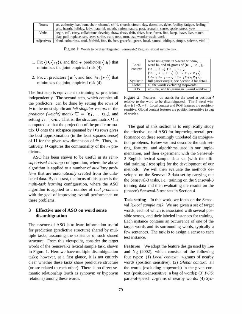
Nouns art, authority, bar, bum, chair, channel, child, church, circuit, day, detention, dyke, facility, fatigue, feeling,grip, hearth, holiday, lady, material, mouth, nation, nature, post, restraint, sense, spade, stress, yew
Verbs begin, call, carry, collaborate, develop, draw, dress, drift, drive, face, ferret, find, keep, leave, live, match,play, pull, replace, see, serve strike, train, treat, turn,use, wander wash, work
Adjectives blind, colourless, cool, faithful, fine, fit, free, graceful, green, local, natural, oblique, simple, solemn, vital
Figure 1:Words to be disambiguated; Senseval-2 English lexical sample task.
1. Fix (�; fv`g), and findm predictorsfu`g thatminimizes the joint empirical risk (4).
2. Fixm predictorsfu`g, and find(�; fv`g) thatminimizes the joint empirical risk (4).
The first step is equivalent to trainingm predictorsindependently. The second step, which couples allthe predictors, can be done by setting the rows of� to the most significantleft singular vectorsof thepredictor (weight) matrixU = [u1; : : : ;um℄, andsettingv` = �u`. That is, the structure matrix� iscomputed so that the projection of the predictor ma-trix U onto the subspace spanned by�’s rows givesthe best approximation (in the least squares sense)of U for the given row-dimension of�. Thus, in-tuitively, � captures the commonality of them pre-dictors.
ASO has been shown to be useful in itssemi-supervised learningconfiguration, where the abovealgorithm is applied to a number ofauxiliary prob-lems that areautomatically createdfrom the unla-beled data. By contrast, the focus of this paper is themulti-task learningconfiguration, where the ASOalgorithm is applied to a number ofreal problemswith the goal of improving overall performance onthese problems.
3 Effective use of ASO on word sensedisambiguation
The essence of ASO is to learn information usefulfor prediction (predictive structure) shared by mul-tiple tasks, assuming the existence of such sharedstructure. From this viewpoint, consider the targetwords of the Senseval-2 lexical sample task, shownin Figure 1. Here we have multiple disambiguationtasks; however, at a first glance, it is not entirelyclear whether these tasks share predictive structure(or are related to each other). There is no direct se-mantic relationship (such as synonym or hyponymrelations) among these words.
word uni-grams in 5-word window,Local word bi- and tri-grams of(w�2; w�1),
context (w+1; w+2); (w�1; w+1),(w�3; w�2; w�1); (w+1; w+2; w+3),(w�2; w�1; w+1); (w�1; w+1; w+2).Syntactic full parser output; see Section 3 for detail.Global all the words excluding stopwords.POS uni-, bi-, and tri-grams in 5-word window.
Figure 2: Features. wi stands for the word at positionirelative to the word to be disambiguated. The 5-word win-dow is [�2;+2℄. Local context and POS features are position-sensitive. Global context features are position insensitive (a bagof words).
The goal of this section is to empirically studythe effective use of ASO for improving overall per-formance on these seemingly unrelated disambigua-tion problems. Below we first describe the task set-ting, features, and algorithms used in our imple-mentation, and then experiment with the Senseval-2 English lexical sample data set (with the offi-cial training / test split) for the development of ourmethods. We will then evaluate the methods de-veloped on the Senseval-2 data set by carrying outthe Senseval-3 tasks, i.e., training on the Senseval-3training data and then evaluating the results on the(unseen) Senseval-3 test sets in Section 4.
Task setting In this work, we focus on the Sense-val lexical sample task. We are given a set of targetwords, each of which is associated with several pos-sible senses, and their labeled instances for training.Each instance contains an occurrence of one of thetarget words and its surrounding words, typically afew sentences. The task is to assign a sense to eachtest instance.
Features We adopt the feature design used by Leeand Ng (2002), which consists of the followingfour types: (1)Local context: n-grams of nearbywords (position sensitive); (2)Global context: allthe words (excluding stopwords) in the given con-text (position-insensitive; a bag of words); (3)POS:parts-of-speechn-grams of nearby words; (4)Syn-
79

tactic relations: syntactic information obtained fromparser output. To generate syntactic relation fea-tures, we use the Slot Grammar-based full parserESG (McCord, 1990). We use as features syntacticrelation types (e.g., subject-of, object-of, and nounmodifier), participants of syntactic relations, and bi-grams of syntactic relations / participants. Details ofthe other three types are shown in Figure 2.
Implementation Our implementation followsAndo and Zhang (2005a). We use a modifi-cation of the Huber’s robust loss for regression:L(p; y) = (max(0; 1�py))2 if py � �1; and�4pyotherwise; with square regularization (� = 10�4),and perform empirical risk minimization bystochastic gradient descent (SGD)(see e.g., Zhang(2004)). We perform one ASO iteration.
3.1 Exploring the multi-task learningconfiguration
The goal is to effectively apply ASO to the set ofword disambiguation problems so that overall per-formance is improved. We consider two factors:fea-ture splitandpartitioning of prediction problems.
3.1.1 Feature split and problem partitioning
Our features described above inherently consist offour feature groups: local context (LC), global con-text (GC), syntactic relation (SR), and POS features.To exploit such a natural feature split, we explore thefollowing extension of the joint linear model:f`(f�jg;x) = wTx+Xj2F v(j)` T�jx(j) ; (5)
where�j�Tj = I for j 2 F , F is a set of dis-
joint feature groups, andx(j) (or v(j)` ) is a portionof the feature vectorx (or the weight vectorv`) cor-responding to the feature groupj, respectively. Thisis a slight modification of the extension presentedin (Ando and Zhang, 2005a). Using this model,ASO computes the structure matrix�j for each fea-ture group separately. That is, SVD is applied tothe sub-matrix of the predictor (weight) matrix cor-responding to each feature groupj, which resultsin more focused dimension reduction of the predic-tor matrix. For example, suppose thatF = fSRg.Then, we compute the structure matrix�SR from
the corresponding sub-matrix of the predictor ma-trix U, which is the gray region of Figure 3 (a). Thestructure matrices�j for j =2 F (associated with thewhite regions in the figure) should be regarded asbeing fixed to the zero matrices. Similarly, it is pos-sible to compute a structure matrix from a subset ofthe predictors (such as noun disambiguators only),as in Figure 3 (b). In this example, we apply theextension of ASO withF = fSRg to three sets ofproblems (disambiguation of nouns, verbs, and ad-jectives, respectively) separately.
LC
GC
SR
POS
(a) Partitioned by features: F = { SR }
mpredictors
ΘΘΘΘSR
predictors for nouns
predictors for verbs
predictors for adjectives
ΘΘΘΘSR,Adj
ΘΘΘΘSR,Verb
ΘΘΘΘSR,Noun(b) Partitioned by F = { SR }
and problem types.
LC
GC
SR
POS
Predictor matrix U Predictor matrix U
Figure 3:Examples of feature split and problem partitioning.
To see why such partitioning may be useful forour WSD problems, consider the disambiguation of“bank” and the disambiguation of “save”. Since a“bank” as in “money bank” and a “save” as in “sav-ing money” may occur in similar global contexts,certain global context features effective for recog-nizing the “money bank” sense may be also effectivefor disambiguating “save”, and vice versa. However,with respect to the position-sensitive local contextfeatures, these two disambiguation problems maynot have much in common since, for instance, wesometimes say “the bank announced”, but we rarelysay “the save announced”. That is, whether prob-lems share predictive structure may depend on fea-ture types, and in that case, seeking predictive struc-ture for each feature group separately may be moreeffective. Hence, we experiment with the configu-rations with and without various feature splits usingthe extension of ASO.
Our target words are nouns, verbs, and adjec-tives. As in the above example of “bank” (noun)and “save” (verb), the predictive structure of globalcontext features may be shared by the problems ir-respective of the parts of speech of the target words.However, the other types of features may be moredependent on the target word part of speech. There-
80
fore, we explore two types of configuration. Oneapplies ASO to all the disambiguation problems atonce. The other applies ASO separately to each ofthe three sets of disambiguation problems (noun dis-ambiguation problems, verb disambiguation prob-lems, and adjective disambiguation problems) anduses the structure matrix�j obtained from the noundisambiguation problems only for disambiguatingnouns, and so forth.
Thus, we explore combinations of two parame-ters. One is the set of feature groupsF in the model(5). The other is the partitioning of disambiguationproblems.
3.1.2 Empirical results
64.5
65
65.5
66
66.5
67
67.5
68
1 2 3 4 5 6 7 8
all problems at
once
nouns, verbs,
adjectives,
separately
Baseline {LC} {GC} {SR}{POS} {LC,SR,GC}
{LC+SR+GC}
no feature split
Feature group set F
Problem partitioning
Figure 4: F-measure on Senseval-2 English test set. Multi-task configurations varying feature group setF and problempartitioning. Performance at the best dimensionality of�j (inf10; 25; 50; 100; � � � g) is shown.
In Figure 4, we compare performance on theSenseval-2 test set produced by training on theSenseval-2 training set using the various configura-tions discussed above. As the evaluation metric, weuse the F-measure (micro-averaged)3 returned by theofficial Senseval scorer. Our baseline is the standardsingle-taskconfiguration using the same loss func-tion (modified Huber) and the same training algo-rithm (SGD).
The results are in line with our expectation. Tolearn the shared predictive structure of local context(LC) and syntactic relations (SR), it is more advanta-geous to apply ASO to each of the three sets of prob-lems (disambiguation of nouns, verbs, and adjec-tives, respectively), separately. By contrast, globalcontext features (GC) can be more effectively ex-ploited when ASO is applied to all the disambigua-
3Our precision and recall are always the same since our sys-tems assign exactly one sense to each instance. That is, ourF-measure is the same as ‘micro-averaged recall’ or ‘accuracy’used in some of previous studies we will compare with.
tion problems at once. It turned out that the con-figurationF = fPOSg does not improve the per-formance over the baseline. Therefore, we excludePOS from the feature group setF in the rest of ourexperiments. Comparison ofF = fLC+SR+GCg(treating the features of these three types as onegroup) andF = fLC;SR;GCg indicates that useof this feature split indeed improves performance.Among the configurations shown in Figure 4, thebest performance (67.8%) is obtained by applyingASO to the three sets of problems (correspondingto nouns, verbs, and adjectives) separately, with thefeature splitF = fLC;SR;GCg.
ASO has one parameter, the dimensionality of thestructure matrix�j (i.e., the number of left singularvectors to compute). The performance shown in Fig-ure 4 is the ceiling performance obtained at the bestdimensionality (inf10; 25; 50; 100; 150; � � � g). InFigure 5, we show the performance dependency on�j ’s dimensionality when ASO is applied to all theproblems at once (Figure 5 left), and when ASO isapplied to the set of the noun disambiguation prob-lems (Figure 5 right). In the left figure, the config-urationF = fGCg (global context) produces bet-ter performance at a relatively low dimensionality.In the other configurations shown in these two fig-ures, performance is relatively stable as long as thedimensionality is not too low.
64.5
65
65.5
66
66.5
67
67.5
0 100 200 300 400 500dimensionality
69
70
71
72
73
74
0 100 200 300dimensionality
{LC,GC,SR}
{LC+GC+SR}
{LC}
{GC}
{SR}
baseline
Figure 5: Left: Applying ASO to all the WSD problems atonce. Right: Applying ASO to noun disambiguation problemsonly and testing on the noun disambiguation problems only.x-axis: dimensionality of�j .3.2 Multi-task learning procedure for WSD
Based on the above results on the Senseval-2 test set,we develop the following procedure using the fea-ture split and problem partitioning shown in Figure6. LetN ;V, andA be sets of disambiguation prob-lems whose target words are nouns, verbs, and ad-jectives, respectively. We write�(j;s) for the struc-
81
predictors for nouns
predictors for verbs
predictors for adjectives
LCGC
SR
POS
We compute seven structure matrices Θj,s each from the seven shaded regions of the predictor matrix U.
Figure 6:Effective feature split and problem partitioning.
ture matrix associated with the feature groupj andcomputed from a problem sets. That is, we replace�j in (5) with�(j;s).� Apply ASO to the three sets of disambigua-
tion problems (corresponding to nouns, verbs,and adjectives), separately, using the extendedmodel (5) withF = fLC;SRg. As a result,we obtain�(j;s) for every(j; s) 2 fLC;SRg�fN ;V;Ag.� Apply ASO to all the disambiguation problemsat once using the extended model (5) withF =fGCg to obtain�(GC;N[V[A).� For a problem 2 P 2 fN ;V;Ag, our finalpredictor is based on the model:f`(x) = wTx+ X(j;s)2T v(j;s)` T�(j;s)x(j) ;whereT = f(LC; P ); (SR; P ); (GC;N [ V [A)g. We obtain predictorf` by minimizing theregularized empirical risk with respect tow`andv`.
We fix the dimension of the structure matrix cor-responding to global context features to 50. The di-mensions of the other structure matrices are set to0.9 times the maximum possible rank to ensure rela-tively high dimensionality. This procedure produces68:1% on the Senseval-2 English lexical sample testset.
3.3 Previous systems on Senseval-2 data set
Figure 7 compares our performance with those ofprevious best systems on the Senseval-2 English lex-ical sample test set. Since we used this test set for thedevelopment of our method above, our performanceshould be understood as thepotential performance.(In Section 4, we will present evaluation results on
ASO multi-task learning (optimum config.)68.1classifier combination [FY02] 66.5polynomial KPCA [WSC04] 65.8SVM [LN02] 65.4Our single-task baseline 65.3Senseval-2 (2001) best participant 64.2
Figure 7: Performance comparison with previous best sys-tems on Senseval-2 English lexical sample test set. FY02 (Flo-rian and Yarowsky, 2002), WSC04 (Wu et al., 2004), LN02 (Leeand Ng, 2002)
the unseenSenseval-3 test sets.) Nevertheless, it isworth noting that our potential performance (68.1%)exceeds those of the previous best systems.
Our single-task baseline performance is almostthe same as LN02 (Lee and Ng, 2002), whichuses SVM. This is consistent with the fact that weadopted LN02’s feature design. FY02 (Florian andYarowsky, 2002) combines classifiers by linear av-erage stacking. The best system of the Senseval-2competition was an early version of FY02. WSC04used a polynomial kernel via the kernel PrincipalComponent Analysis (KPCA) method (Scholkopf etal., 1998) with nearest neighbor classifiers.
4 Evaluation on Senseval-3 tasks
In this section, we evaluate the methods developedon the Senseval-2 data set above on the standardSenseval-3 lexical sample tasks.
4.1 Our methods in multi-task andsemi-supervised configurations
In addition to the multi-task configuration describedin Section 3.2, we test the following semi-supervisedapplication of ASO. We first create auxiliary prob-lems following Ando and Zhang (2005a)’s partially-supervised strategy (Figure 8) with distinct fea-ture maps1 and2 each of which uses one offLC;GC;SRg. Then, we apply ASO to these auxil-iary problems using the feature split and the problempartitioning described in Section 3.2.
Note that the difference between the multi-taskand semi-supervised configurations is the source ofinformation. The multi-task configuration utilizesthe label informationof the training examples thatare labeled for the rest of the multiple tasks, andthe semi-supervised learning configuration exploitsa large amount ofunlabeled data.
82
1. Train a classifierC1 only using feature map1 on thelabeled data for the target task.
2. Auxiliary problems are to predict the labels assigned byC1 to the unlabeled data, using the other feature map2.3. Apply ASO to the auxiliary problems to obtain�.4. Using the joint linear model (2), train the final
predictor by minimizing the empirical risk for fixed�on the labeled data for the target task.
Figure 8: Ando and Zhang (2005a)’s ASO semi-supervisedlearning method using partially-supervised procedure forcreat-ing relevant auxiliary problems.
4.2 Data and evaluation metric
We conduct evaluations on four Senseval-3 lexicalsample tasks (English, Catalan, Italian, and Spanish)using the official training / test splits. Data statis-tics are shown in Figure 9. On the Spanish, Cata-lan, and Italian data sets, we use part-of-speech in-formation (as features) and unlabeled examples (forsemi-supervised learning) provided by the organizer.Since the English data set was not provided withthese additional resources, we use an in-house POStagger trained with the PennTree Bank corpus, andextract 100K unlabeled examples from the Reuters-RCV1 corpus. On each language, the number of un-labeled examples is 5–15 times larger than that of thelabeled training examples. We use syntactic relationfeatures only for English data set. As in Section 3,we report micro-averaged F measure.
4.3 Baseline methods
In addition to the standard single-task supervisedconfiguration as in Section 3, we test the followingmethod as an additional baseline.
Output-based method The goal of our multi-tasklearning configuration is to benefit from having thelabeled training examples of a number of words. Analternative to ASO for this purpose is to use directlyas features the output values of classifiers trainedfor disambiguating the other words, which we call‘output-based method’ (cf. Florian et al. (2003)).We explore several variations similarly to Section3.1 and report the ceiling performance.
4.4 Evaluation results
Figure 10 shows F-measure results on the fourSenseval-3 data sets using the official training / testsplits. Both ASO multi-task learning and semi-supervised learning improve performance over the
#words #train avg #sense avg #trainper word per sense
English 73 8611 10.7 10.0Senseval-3 data sets
English 57 7860 6.5 21.3Catalan 27 4469 3.1 53.2Italian 45 5145 6.2 18.4
Spanish 46 8430 3.3 55.5
Figure 9:Data statistics of Senseval-2 English lexical sampledata set (first row) and Senseval-3 data sets. On each data set, #of test instances is about one half of that of training instances.
single-task baseline on all the data sets. The bestperformance is achieved when we combine multi-task learning and semi-supervised learning by usingall the corresponding structure matrices�(j;s) pro-duced by both multi-task and semi-supervised learn-ing, in the final predictors. This combined configu-ration outperforms the single-task supervised base-line by up to 5.7%.
Performance improvements over the supervisedbaseline are relatively small on English and Span-ish. We conjecture that this is because the supervisedperformance is already close to the highest perfor-mance that automatic methods could achieve. Onthese two languages, our (and previous) systems out-perform inter-human agreement, which is unusualbut can be regarded as an indication that these tasksare difficult.
The performance of the output-based method(baseline) is relatively low. This indicates that out-put values or proposed labels are not expressiveenough to integrate information from other predic-tors effectively on this task. We conjecture that forthis method to be effective, the problems are re-quired to be more closely related to each other asin Florian et al. (2003)’s named entity experiments.
A practical advantage of ASO multi-task learningover ASO semi-supervised learning is that shortercomputation time is required to produce similarperformance. On this English data set, trainingfor multi-task learning and semi-supervised learningtakes 15 minutes and 92 minutes, respectively, usinga Pentium-4 3.20GHz computer. The computationtime mostly depends on the amount of the data onwhich auxiliary predictors are learned. Since our ex-periments use unlabeled data 5–15 times larger thanlabeled training data, semi-supervised learning takeslonger, accordingly.
83
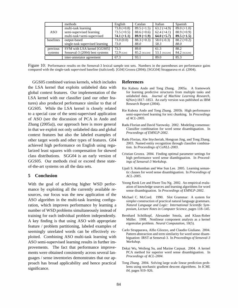
methods English Catalan Italian Spanishmulti-task learning 73.8 (+0.8) 89.5 (+1.5) 63.2 (+4.9) 89.0 (+1.0)
ASO semi-supervised learning 73.5 (+0.5) 88.6 (+0.6) 62.4 (+4.1) 88.9 (+0.9)multi-task+semi-supervised 74.1 (+1.1) 89.9 (+1.9) 64.0 (+5.7) 89.5 (+1.5)
baselines output-based 73.0 (0.0) 88.3 (+0.3) 58.0 (-0.3) 88.2 (+0.2)single-task supervised learning 73.0 88.0 58.3 88.0
previous SVM with LSA kernel [GGS05] 73.3 89.0 61.3 88.2systems Senseval-3 (2004) best systems 72.9[G04] 85.2[SGG04] 53.1[SGG04] 84.2 [SGG04]
inter-annotator agreement 67.3 93.1 89.0 85.3
Figure 10:Performance results on the Senseval-3 lexical sample test sets. Numbers in the parentheses are performance gainscompared with the single-task supervised baseline (italicized). [G04] Grozea (2004); [SGG04] Strapparava et al. (2004).
GGS05 combined various kernels, which includesthe LSA kernel that exploits unlabeled data withglobal context features. Our implementation of theLSA kernel with our classifier (and our other fea-tures) also produced performance similar to that ofGGS05. While the LSA kernel is closely relatedto a special case of the semi-supervised applicationof ASO (see the discussion of PCA in Ando andZhang (2005a)), our approach here is more generalin that we exploit not only unlabeled data and globalcontext features but also the labeled examples ofother target words and other types of features. G04achieved high performance on English using regu-larized least squares with compensation for skewedclass distributions. SGG04 is an early version ofGGS05. Our methods rival or exceed these state-of-the-art systems on all the data sets.
5 Conclusion
With the goal of achieving higher WSD perfor-mance by exploiting all the currently available re-sources, our focus was the new application of theASO algorithm in the multi-task learning configu-ration, which improves performance by learning anumber of WSD problems simultaneously instead oftraining for each individual problem independently.A key finding is that using ASO with appropriatefeature / problem partitioning, labeled examples ofseemingly unrelated words can be effectively ex-ploited. Combining ASO multi-task learning withASO semi-supervised learning results in further im-provements. The fact that performance improve-ments were obtained consistently across several lan-guages / sense inventories demonstrates that our ap-proach has broad applicability and hence practicalsignificance.
ReferencesRie Kubota Ando and Tong Zhang. 2005a. A framework
for learning predictive structures from multiple tasks andunlabeled data. Journal of Machine Learning Research,6(Nov):1817–1853. An early version was published as IBMResearch Report (2004).
Rie Kubota Ando and Tong Zhang. 2005b. High performancesemi-supervised learning for text chunking. InProceedingsof ACL-2005.
Radu Florian and David Yarowsky. 2002. Modeling consensus:Classifier combination for word sense disambiguation. InProceedings of EMNLP-2002.
Radu Florian, Abe Ittycheriah, Hongyan Jing, and Tong Zhang.2003. Named entity recognition through classifier combina-tion. In Proceedings of CoNLL-2003.
Cristian Grozea. 2004. Finding optimal parameter settingsforhigh performance word sense diambiguation. InProceed-ings of Senseval-3 Workshop.
Upali S. Kohomban and Wee Sun Lee. 2005. Learning seman-tic classes for word sense disambiguation. InProceedings ofACL-2005.
Yoong Keok Lee and Hwee Tou Ng. 2002. An empirical evalu-ation of knowledge sources and learning algorithms for wordsense disambiguation. InProceedings of EMNLP-2002.
Michael C. McCord. 1990. Slot Grammar: A system forsimpler construction of practical natural language grammars.Natural Language and Logic: International Scientific Sym-posium, Lecture Notes in Computer Science, pages 118–145.
Bernhard Scholkopf, Alexander Smola, and Klaus-RoberMuller. 1998. Nonlinear component analysis as a kerneleigenvalue problem.Neural Computation, 10(5).
Carlo Strapparava, Alfio Gliozzo, and Claudio Giuliano. 2004.Pattern abstraction and term similarity for word sense disam-biguation: IRST at Senseval-3. InProceedings of Senseval-3Workshop.
Dekai Wu, Weifeng Su, and Marine Carpuat. 2004. A kernelPCA method for superior word sense disambiguation. InProceedings of ACL-2004.
Tong Zhang. 2004. Solving large scale linear prediction prob-lems using stochastic gradient descent algorithms. InICML04, pages 919–926.
84
Proceedings of the 10th Conference on Computational Natural Language Learning (CoNLL-X),pages 85–92, New York City, June 2006.c©2006 Association for Computational Linguistics
Unsupervised Parsing with U-DOP
Rens BodSchool of Computer ScienceUniversity of St AndrewsNorth Haugh, St AndrewsKY16 9SX Scotland, UK
Abstract
We propose a generalization of the super-vised DOP model to unsupervised learning.This new model, which we call U-DOP,initially assigns all possible unlabeled binarytrees to a set of sentences and next uses allsubtrees from (a large subset of) these binarytrees to compute the most probable parsetrees. We show how U-DOP can beimplemented by a PCFG-reduction tech-nique and report competitive results onEnglish (WSJ), German (NEGRA) andChinese (CTB) data. To the best of ourknowledge, this is the first paper whichaccurately bootstraps structure for WallStreet Journal sentences up to 40 wordsobtaining roughly the same accuracy as abinarized supervised PCFG. We show thatprevious approaches to unsupervised parsinghave shortcomings in that they eitherconstrain the lexical or the structural context,or both.
1 Introduction
How can we learn syntactic structure from unlabeleddata in an unsupervised way? The importance ofunsupervised parsing is nowadays widely acknow-ledged. While supervised parsers suffer fromshortage of hand-annotated data, unsupervisedparsers operate with unlabeled raw data, of whichunlimited quantities are available. During the lastfew years there has been considerable progress inunsupervised parsing. To give a brief overview: vanZaanen (2000) achieved 39.2% unlabeled f-score onATIS word strings by a sentence-aligning techniquecalled ABL. Clark (2001) reports 42.0% unlabeled
f-score on the same data using distributionalclustering, and Klein and Manning (2002) obtain51.2% unlabeled f-score on ATIS part-of-speechstrings using a constituent-context model calledCCM. Moreover, on Penn Wall Street Journal p-o-s-strings ≤ 10 (WSJ10), Klein and Manning (2002)report 71.1% unlabeled f-score. And the hybridapproach of Klein and Manning (2004), whichcombines a constituency and a dependency model,leads to a further increase of 77.6% f-score.
Although there has thus been steadyprogress in unsupervised parsing, all theseapproaches have shortcomings in that they eitherconstrain the lexical or the structural context that istaken into account, or both. For example, the CCMmodel by Klein and Manning (2005) is said todescribe "all contiguous subsequences of asentence" (Klein and Manning 2005: 1410). Whilethis is a very rich lexical model, it is still limited inthat it neglects dependencies that are non-contiguoussuch as between more and than in "BA carriedmore people than cargo". Moreover, by using an"all-substrings" approach, CCM risks to under-represent structural context. Similar shortcomingscan be found in other unsupervised models.
In this paper we will try to directly modelstructural as well as lexical context withoutconstraining any dependencies beforehand. Anapproach that may seem apt in this respect is an all-subtrees approach (e.g Bod 2003; Goodman 2003;Collins and Duffy 2002). Subtrees can model bothcontiguous and non-contiguous lexical dependencies(see section 2) and they also model constituents in ahierarchical context. Moreover, we can view the all-subtrees approach as a generalization of Klein andManning's all-substrings approach and van Zaanen'sABL model.
In the current paper, we will use the all-subtrees approach as proposed in Data-Oriented
85
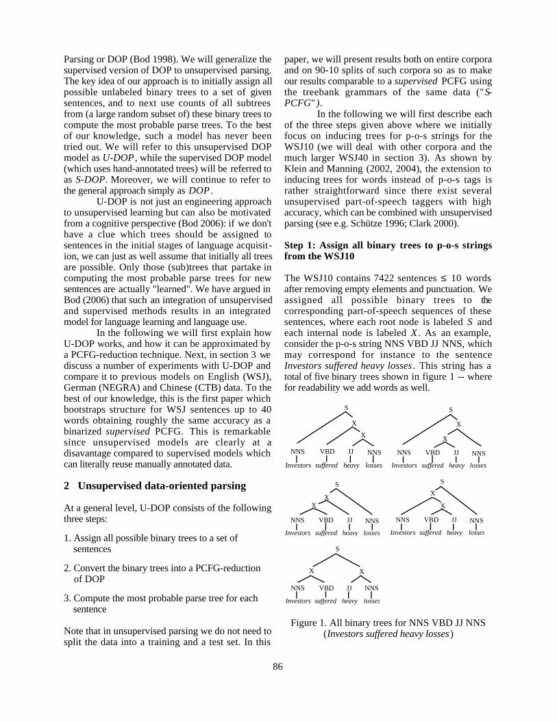
Parsing or DOP (Bod 1998). We will generalize thesupervised version of DOP to unsupervised parsing.The key idea of our approach is to initially assign allpossible unlabeled binary trees to a set of givensentences, and to next use counts of all subtreesfrom (a large random subset of) these binary trees tocompute the most probable parse trees. To the bestof our knowledge, such a model has never beentried out. We will refer to this unsupervised DOPmodel as U-DOP, while the supervised DOP model(which uses hand-annotated trees) will be referred toas S-DOP. Moreover, we will continue to refer tothe general approach simply as DOP.
U-DOP is not just an engineering approachto unsupervised learning but can also be motivatedfrom a cognitive perspective (Bod 2006): if we don'thave a clue which trees should be assigned tosentences in the initial stages of language acquisit-ion, we can just as well assume that initially all treesare possible. Only those (sub)trees that partake incomputing the most probable parse trees for newsentences are actually "learned". We have argued inBod (2006) that such an integration of unsupervisedand supervised methods results in an integratedmodel for language learning and language use.
In the following we will first explain howU-DOP works, and how it can be approximated bya PCFG-reduction technique. Next, in section 3 wediscuss a number of experiments with U-DOP andcompare it to previous models on English (WSJ),German (NEGRA) and Chinese (CTB) data. To thebest of our knowledge, this is the first paper whichbootstraps structure for WSJ sentences up to 40words obtaining roughly the same accuracy as abinarized supervised PCFG. This is remarkablesince unsupervised models are clearly at adisavantage compared to supervised models whichcan literally reuse manually annotated data.
2 Unsupervised data-oriented parsing
At a general level, U-DOP consists of the followingthree steps:
1. Assign all possible binary trees to a set of sentences
2. Convert the binary trees into a PCFG-reduction of DOP
3. Compute the most probable parse tree for each sentence
Note that in unsupervised parsing we do not need tosplit the data into a training and a test set. In this
paper, we will present results both on entire corporaand on 90-10 splits of such corpora so as to makeour results comparable to a supervised PCFG usingthe treebank grammars of the same data ("S-PCFG" ).
In the following we will first describe eachof the three steps given above where we initiallyfocus on inducing trees for p-o-s strings for theWSJ10 (we will deal with other corpora and themuch larger WSJ40 in section 3). As shown byKlein and Manning (2002, 2004), the extension toinducing trees for words instead of p-o-s tags israther straightforward since there exist severalunsupervised part-of-speech taggers with highaccuracy, which can be combined with unsupervisedparsing (see e.g. Schütze 1996; Clark 2000).
Step 1: Assign all binary trees to p-o-s stringsfrom the WSJ10
The WSJ10 contains 7422 sentences ≤ 10 wordsafter removing empty elements and punctuation. Weassigned all possible binary trees to thecorresponding part-of-speech sequences of thesesentences, where each root node is labeled S andeach internal node is labeled X. As an example,consider the p-o-s string NNS VBD JJ NNS, whichmay correspond for instance to the sentenceInvestors suffered heavy losses. This string has atotal of five binary trees shown in figure 1 -- wherefor readability we add words as well.
NNS VBD JJ NNS
Investors suffered heavy losses
X
X
S
NNS VBD JJ NNS
Investors suffered heavy losses
X
X
S
NNS VBD JJ NNS
Investors suffered heavy losses
XX
S
NNS VBD JJ NNS
Investors suffered heavy losses
X
X
S
NNS VBD JJ NNS
Investors suffered heavy losses
XX
S
Figure 1. All binary trees for NNS VBD JJ NNS(Investors suffered heavy losses)
86

The total number of binary trees for a sentence oflength n is given by the Catalan number Cn−1,where Cn = (2n)!/((n+1)!n!). Thus while a sentenceof 4 words has 5 binary trees, a sentence of 8 wordshas already 429 binary trees, and a sentence of 10words has 4862 binary trees. Of course, we canrepresent the set of binary trees of a string inpolynomial time and space by means of a chart,resulting in a chart-like parse forest if we alsoinclude pointers. But if we want to extract rules orsubtrees from these binary trees -- as in DOP -- weneed to unpack the parse forest. And since the totalnumber of binary trees that can be assigned to theWSJ10 is almost 12 million, it is doubtful whetherwe can apply the unrestricted U-DOP model to sucha corpus.
However, for longer sentences the binarytrees are highly redundant. In these larger trees, thereare many rules like X → XX which bear littleinformation. To make parsing with U-DOP possiblewe therefore applied a simple heuristic which takesrandom samples from the binary trees for sentences≥ 7 words before they are fed to the DOP parser.These samples were taken from the distribution ofall binary trees by randomly choosing nodes andtheir expansions from the chart-like parse forests ofthe sentences (which effectively favors trees withmore frequent subtrees). For sentences of 7 wordswe randomly sample 60% of the trees, and forsentences of 8, 9 and 10 words we samplerespectively 30%, 15% and 7.5% of the trees. In thisway, the set of remaining binary trees contains 8.23* 105 trees, which we will refer to as the binarytree-set. Although it can happen that the correct treeis deleted for some sentence in the binary tree-set,there is enough redundancy in the tree-set such thateither the correct binary tree can be generated byother subtrees or that a remaining tree onlyminimally differs from the correct tree. Of course,we may expect better results if all binary trees arekept, but this involves enormous computationalresources which will be postponed to futureresearch.
Step 2: Convert the trees into a PCFG-reduction of DOP
The underlying idea of U-DOP is to take all subtreesfrom the binary tree-set to compute the mostprobable tree for each sentence. Subtrees from thetrees in figure 1 include for example the subtrees infigure 2 (where we again added words forreadability). Note that U-DOP takes into accountboth contiguous and non-contiguous substrings.
NNS VBD
Investors suffered
X
X
S
VBD
suffered
X
X
NNS NNS
Investors losses
X
X
S
JJ NNS
heavy losses
XX
S
JJ NNS
heavy losses
X
NNS VBD
Investors suffered
X
VBD JJ
suffered heavy
X
Figure 2. Some subtrees from the binary trees forNNS VBD JJ NNS given in figure 1
As in the supervised DOP approach (Bod 1998), U-DOP parses a sentence by combining corpus-subtrees from the binary tree-set by means of aleftmost node substitution operation, indicated as °.The probability of a parse tree is computed bysumming up the probabilities of all derivationsproducing it, while the probability of a derivation iscomputed by multiplying the (smoothed) relativefrequencies of its subtrees. That is, the probability ofa subtree t is taken as the number of occurrences of tin the binary tree-set, | t |, divided by the totalnumber of occurrences of all subtrees t' with thesame root label as t. Let r(t) return the root label of t:
P(t) =
| t |
Σ t': r ( t')=r ( t) | t' |
The subtree probabilities are smoothed by applyingsimple Good-Turing to the subtree distribution (seeBod 1998: 85-87). The probability of a derivationt1°...°tn is computed by the product of theprobabilities of its subtrees t i:
P(t1°...°tn) = Π i P(ti)
Since there may be distinct derivations that generatethe same parse tree, the probability of a parse tree T
87
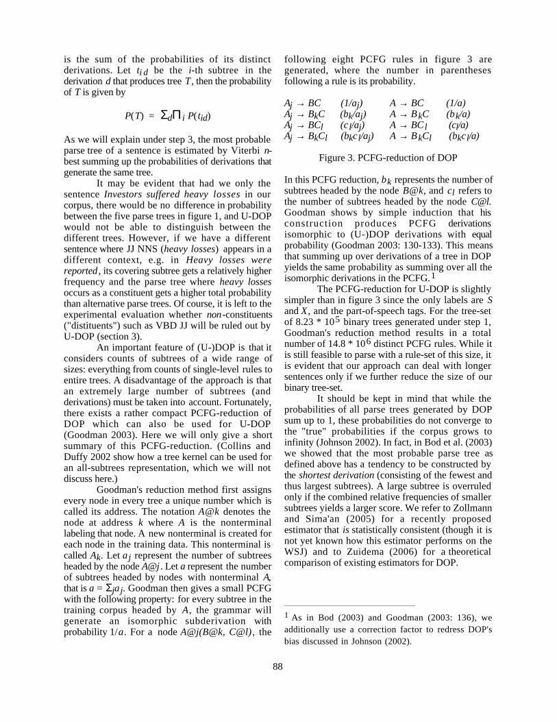
is the sum of the probabilities of its distinctderivations. Let ti d be the i-th subtree in thederivation d that produces tree T, then the probabilityof T is given by
P(T) = ΣdΠi P(tid)
As we will explain under step 3, the most probableparse tree of a sentence is estimated by Viterbi n-best summing up the probabilities of derivations thatgenerate the same tree.
It may be evident that had we only thesentence Investors suffered heavy losses in ourcorpus, there would be no difference in probabilitybetween the five parse trees in figure 1, and U-DOPwould not be able to distinguish between thedifferent trees. However, if we have a differentsentence where JJ NNS (heavy losses) appears in adifferent context, e.g. in Heavy losses werereported, its covering subtree gets a relatively higherfrequency and the parse tree where heavy lossesoccurs as a constituent gets a higher total probabilitythan alternative parse trees. Of course, it is left to theexperimental evaluation whether non-constituents("distituents") such as VBD JJ will be ruled out byU-DOP (section 3).
An important feature of (U-)DOP is that itconsiders counts of subtrees of a wide range ofsizes: everything from counts of single-level rules toentire trees. A disadvantage of the approach is thatan extremely large number of subtrees (andderivations) must be taken into account. Fortunately,there exists a rather compact PCFG-reduction ofDOP which can also be used for U-DOP(Goodman 2003). Here we will only give a shortsummary of this PCFG-reduction. (Collins andDuffy 2002 show how a tree kernel can be used foran all-subtrees representation, which we will notdiscuss here.)
Goodman's reduction method first assignsevery node in every tree a unique number which iscalled its address. The notation A@k denotes thenode at address k where A is the nonterminallabeling that node. A new nonterminal is created foreach node in the training data. This nonterminal iscalled Ak. Let aj represent the number of subtreesheaded by the node A@j. Let a represent the numberof subtrees headed by nodes with nonterminal A,that is a = Σjaj. Goodman then gives a small PCFGwith the following property: for every subtree in thetraining corpus headed by A, the grammar willgenerate an isomorphic subderivation withprobability 1/a. For a node A@j(B@k, C@l), the
following eight PCFG rules in figure 3 aregenerated, where the number in parenthesesfollowing a rule is its probability.
Aj → BC (1/aj) A → BC (1/a)Aj → BkC (bk/aj) A → BkC (bk/a)Aj → BCl (cl/aj) A → BCl (cl/a)Aj → BkCl (bkcl/aj) A → BkCl (bkcl/a)
Figure 3. PCFG-reduction of DOP
In this PCFG reduction, bk represents the number ofsubtrees headed by the node B@k, and cl refers tothe number of subtrees headed by the node [email protected] shows by simple induction that hisconstruction produces PCFG derivationsisomorphic to (U-)DOP derivations with equalprobability (Goodman 2003: 130-133). This meansthat summing up over derivations of a tree in DOPyields the same probability as summing over all theisomorphic derivations in the PCFG.1
The PCFG-reduction for U-DOP is slightlysimpler than in figure 3 since the only labels are Sand X, and the part-of-speech tags. For the tree-setof 8.23 * 105 binary trees generated under step 1,Goodman's reduction method results in a totalnumber of 14.8 * 106 distinct PCFG rules. While itis still feasible to parse with a rule-set of this size, itis evident that our approach can deal with longersentences only if we further reduce the size of ourbinary tree-set.
It should be kept in mind that while theprobabilities of all parse trees generated by DOPsum up to 1, these probabilities do not converge tothe "true" probabilities if the corpus grows toinfinity (Johnson 2002). In fact, in Bod et al. (2003)we showed that the most probable parse tree asdefined above has a tendency to be constructed bythe shortest derivation (consisting of the fewest andthus largest subtrees). A large subtree is overruledonly if the combined relative frequencies of smallersubtrees yields a larger score. We refer to Zollmannand Sima'an (2005) for a recently proposedestimator that is statistically consistent (though it isnot yet known how this estimator performs on theWSJ) and to Zuidema (2006) for a theoreticalcomparison of existing estimators for DOP.
1 As in Bod (2003) and Goodman (2003: 136), weadditionally use a correction factor to redress DOP'sbias discussed in Johnson (2002).
88
Step 3: Compute the most probable parse treefor each WSJ10 string
While Goodman's reduction method allows forefficiently computing the most probable derivationfor each sentence (i.e. the Viterbi parse), it does notallow for an efficient computation of (U-)DOP'smost probable parse tree since there may beexponentially many derivations for each tree whoseprobabilities have to be summed up. In fact, theproblem of computing the most probable tree inDOP is known to be NP hard (Sima'an 1996). Yet,the PCFG reduction in figure 4 can be used toestimate DOP's most probable parse tree by aViterbi n-best search in combination with a CKYparser which computes the n most likely derivationsand next sums up the probabilities of the derivationsproducing the same tree. (We can considerablyimprove efficiency by using k-best hypergraphparsing as recently proposed by Huang and Chiang2005, but this will be left to future research).
In this paper, we estimate the most probableparse tree from the 100 most probable derivations(at least for the relatively small WSJ10). Althoughsuch a heuristic does not guarantee that the mostprobable parse is actually found, it is shown in Bod(2000) to perform at least as well as the estimationof the most probable parse with Monte Carlotechniques. However, in computing the 100 mostprobable derivations by means of Viterbi it isprohibitive to keep track of all subderivations at eachedge in the chart. We therefore use a pruningtechnique which deletes any item with a probabilityless than 10−5 times of that of the best item fromthe chart.
To make our parse results comparable tothose of Klein and Manning (2002, 2004, 2005), wewill use exactly the same evaluation metrics forunlabeled precision (UP) and unlabeled recall (UR),defined in Klein (2005: 21-22). Klein's definitionsslightly differ from the standard PARSEVALmetrics: multiplicity of brackets is ignored, bracketsof span one are ignored and the bracket labels areignored. The two metrics of UP and UR arecombined by the unlabled f-score F1 which isdefined as the harmonic mean of UP and UR: F1 =2*UP*UR/(UP+UR). It should be kept in mind thatthese evaluation metrics were clearly inspired by theevaluation of supervised parsing which aims atmimicking given tree annotations as closely aspossible. Unsupervised parsing is different in thisrespect and it is questionable whether an evaluationon a pre-annotated corpus such as the WSJ is the
most appropriate one. For a subtle discussion onthis issue, see Clark (2001) or Klein (2005).
3 Experiments
3.1 Comparing U-DOP to previous work
Using the method described above, our parsingexperiment with all p-o-s strings from the WSJ10results in an f-score of 78.5%. We next tested U-DOP on two additional domains from Chinese andGerman which were also used in Klein andManning (2002, 2004): the Chinese treebank (Xueet al. 2002) and the NEGRA corpus (Skut et al.1997). The CTB10 is the subset of p-o-s stringsfrom the Penn Chinese treebank containing 10words or less after removal of punctuation (2437strings). The NEGRA10 is the subset of p-o-sstrings of the same length from the NEGRA corpususing the supplied converson into Penn treebankformat (2175 strings). Table 1 shows the results ofU-DOP in terms of UP, UR and F1 compared tothe results of the CCM model by Klein andManning (2002), the DMV dependency learningmodel by Klein and Manning (2004) together withtheir combined model DMV+CCM.
Model English German Chinese(WSJ10) (NEGRA10) (CTB10)
UP UR F1 UP UR F1 UP UR F1
CCM 64.2 81.6 71.9 48.1 85.5 61.6 34.6 64.3 45.0
DMV 46.6 59.2 52.1 38.4 69.5 49.5 35.9 66.7 46.7
DMV+CCM 69.3 88.0 77.6 49.6 89.7 63.9 33.3 62.0 43.3
U-DOP 70.8 88.2 78.5 51.2 90.5 65.4 36.3 64.9 46.6
Table 1. Results of U-DOP compared to previousmodels on the same data
Table 1 indicates that our model scores slightlybetter than Klein and Manning's combinedDMV+CCM model, although the differences aresmall (note that for Chinese the single DMV modelscores better than the combined model and slightlybetter than U-DOP). But where Klein andManning's combined model is based on both aconstituency and a dependency model, U-DOP is,like CCM, only based on a notion of constituency.Compared to CCM alone, the all-subtrees approachemployed by U-DOP shows a clear improvement(except perhaps for Chinese). It thus seems to payoff to use all subtrees rather than just all(contiguous) substrings in bootstrapping
89
constituency. It would be interesting to investigatean extension of U-DOP towards dependencyparsing, which we will leave for future research. It isalso noteworthy that U-DOP does not employ aseparate class for non-constituents, so-calleddistituents, while CCM does. Thus good results canbe obtained without keeping track of distituents butby simply assigning all binary trees to the stringsand letting the DOP model decide which substringsare most likely to form constituents.
To give an idea of the constituents learnedby U-DOP for the WSJ10, table 2 shows the 10most frequently constituents in the trees induced byU-DOP together with the 10 actually mostfrequently occurring constituents in the WSJ10 andthe 10 most frequently occurring part-of-speechsequences (bigrams) in the WSJ10.
Rank Most frequent Most Frequent Most frequentU-DOP constituents WSJ10 constituents WSJ10 substrings
1 DT NN DT NN NNP NNP2 NNP NNP NNP NNP DT NN3 DT JJ NN CD CD JJ NN4 IN DT NN JJ NNS IN DT5 CD CD DT JJ NN NN IN6 DT NNS DT NNS DT JJ7 JJ NNS JJ NN JJ NNS8 JJ NN CD NN NN NN9 VBN IN IN NN CD CD10 VBD NNS IN DT NN NN VBZ
Table 2. Most frequently learned constituents byU-DOP together with most frequently occurringconstituents and p-o-s sequences (for WSJ10)
Note that there are no distituents among U-DOP's10 most frequently learned constituents, whilst thethird column shows that distituents such as IN DTor DT JJ occur very frequently as substrings in theWSJ10. This may be explained by the fact that (theconstituent) DT NN occurs more frequently as asubstring in the WSJ10 than (the distituent) IN DT,and therefore U-DOP's probability model will favora covering subtree for IN DT NN which consists ofa division into IN X and DT NN rather than into INDT and X NN, other things being equal. The samekind reasoning can be made for a subtree for DT JJNN where the constituent JJ NN occurs morefrequently as a substring than the distituent DT JJ.Of course the situation is somewhat more complexin DOP's sum-of-products model, but our argumentmay illustrate why distituents like IN DT or DT JJare not proposed among the most frequentconstituents by U-DOP while larger constituentslike IN DT NN and DT JJ NN are in fact proposed.
3.2 Testing U-DOP on held-out sets and longersentences (up to 40 words)
We were also interested in U-DOP's performanceon a held-out test set such that we could compare themodel with a supervised PCFG treebank grammartrained and tested on the same data (S-PCFG). Westarted by testing U-DOP on 10 different 90%/10%splits of the WSJ10, where 90% was used forinducing the trees, and 10% to parse new sentencesby subtrees from the binary trees from the trainingset (or actually a PCFG-reduction thereof). Thesupervised PCFG was right-binarized as in Kleinand Manning (2005). The following table shows theresults.
Model UP UR F1
U-DOP 70.6 88.1 78.3
S-PCFG 84.0 79.8 81.8
Table 3. Average f-scores of U-DOP compared to asupervised PCFG (S-PCFG) on 10 different 90-10
splits of the WSJ10
Comparing table 1 with table 3, we see that on 10held-out WSJ10 test sets U-DOP performs with anaverage f-score of 78.3% (SD=2.1%) only slightlyworse than when using the entire WSJ10 corpus(78.5%). Next, note that U-DOP's results come nearto the average performance of a binarized supervisedPCFG which achieves 81.8% unlabeled f-score(SD=1.8%). U-DOP's unlabeled recall is evenhigher than that of the supervised PCFG. Moreover,according to paired t-testing, the differences in f-scores were not statistically significant. (If thePCFG was not post-binarized, its average f-scorewas 89.0%.)
As a final test case for this paper, we wereinterested in evaluating U-DOP on WSJ sentences ≤40 words, i.e. the WSJ40, which is with almost50,000 sentences a much more challenging test casethan the relatively small WSJ10. The main problemfor U-DOP is the astronomically large number ofpossible binary trees for longer sentences, whichtherefore need to be even more heavily pruned thanbefore.
We used a similar sampling heuristic as insection 2. We started by taking 100% of the trees forsentences ≤ 7 words. Next, for longer sentences wereduced this percentage with the relative increase ofthe Catalan number. This effectively means that werandomly selected the same number of trees foreach sentence ≥ 8 words, which is 132 (i.e. the
90
number of possible binary trees for a 7-wordsentence). As mentioned in section 2, our samplingapproach favors more frequent trees, and trees withmore frequent subtrees. The binary tree-set obtainedin this way for the WSJ40 consists of 5.11 * 106
different trees. This resulted in a total of 88+ milliondistinct PCFG rules according to the reductiontechnique in section 2. As this is the largest PCFGwe have ever attempted to parse with, it wasprohibitive to estimate the most probable parse treefrom 100 most probable derivations using Viterbi n-best. Instead, we used a beam of only 15 mostprobable derivations, and selected the most probableparse from these. (The number 15 is admittedly adhoc, and was inspired by the performance of the so-called SL-DOP model in Bod 2002, 2003). Thefollowing table shows the results of U-DOP on theWSJ40 using 10 different 90-10 splits, compared toa supervised binarized PCFG (S-PCFG) and asupervised binarized DOP model (S-DOP) on thesame data.
Model F1
U-DOP 64.2
S-PCFG 64.7
S-DOP 81.9
Table 4. Performance of U-DOP on WSJ40using10 different 90-10 splits, compared to a
binarized S-PCFG and a binarized S-DOP model.
Table 4 shows that U-DOP obtains about the sameresults as a binarized supervised PCFG on WSJsentences ≤ 40 words. Moreover, the differencesbetween U-DOP and S-PCFG were not statisticallysignificant. This result is important as it shows thatit is possible to parse the rather challinging WSJ in acompletely unsupervised way obtaining roughly thesame accuracy as a supervised PCFG. This seemsto be in contrast with the CCM model which quicklydegrades if sentence length is increased (see Klein2005). As Klein (2005: 97) notes, CCM's strengthis finding common short constituent chunks. U-DOP on the other hand has a preference for large(even largest possible) constituent chunks. Klein(2005: 97) reports that the combination of CCM andDMV seems to be more stable with increasingsentence length. It would be extremely interesting tosee how DMV+CCM performs on the WSJ40.
It should be kept in mind that simpletreebank PCFGs do not constitute state-of-the-artsupervised parsers. Table 4 indicates that U-DOP's
performance remains still far behind that of S-DOP(and indeed of other state-of-the-art supervisedparsers such as Bod 2003 or Charniak and Johnson2005). Moreover, if S-DOP is not post-binarized, itsaverage f-score on the WSJ40 is 90.1% -- and thereare some hybrid DOP models that obtain evenhigher scores (see Bod 2003). Our long-term goal isto try to outperform S-DOP by U-DOP. Animportant advantage of U-DOP is of course that itonly needs unannotated data of which unlimitedquanitities are available. Thus it would be interestingto test how U-DOP performs if trained on e.g. 100times more data. Yet, as long as we compute our f-scores on hand-annotated data like Penn's WSJ, theS-DOP model is clearly at an advantage. Wetherefore plan to compare U-DOP and S-DOP (andother supervised parsers) in a concrete applicationsuch as phrase-based machine translation or as alanguage model for speech recognition.
4 Conclusions
We have shown that the general DOP approach canbe generalized to unsupervised learning, effectivelyleading to a single model for both supervised andunsupervised parsing. Our new model, U-DOP,uses all subtrees from (in principle) all binary treesof a set of sentences to compute the most probableparse trees for (new) sentences. Although heavypruning of trees is necessary to make our approachfeasible in practice, we obtained competitive resultson English, German and Chinese data. Our parsingresults are similar to the performance of a binarizedsupervised PCFG on the WSJ ≤ 40 sentences. Thistriggers the provocative question as to whether it ispossible to beat supervised parsing by unsupervisedparsing. To cope with the problem of evaluation, wepropose to test U-DOP in specific applicationsrather than on hand-annotated data.
References
Bod, R. 1998. Beyond Grammar: An Experience-Based Theory of Language, Stanford: CSLIPublications (Lecture notes number 88),distributed by Cambridge University Press.
Bod, R. 2000. An improved parser for data-orientedlexical-functional analysis. ProceedingsACL'2000, Hong Kong.
Bod, R. 2002. A unified model of structuralorganization in language and music. Journal of
91
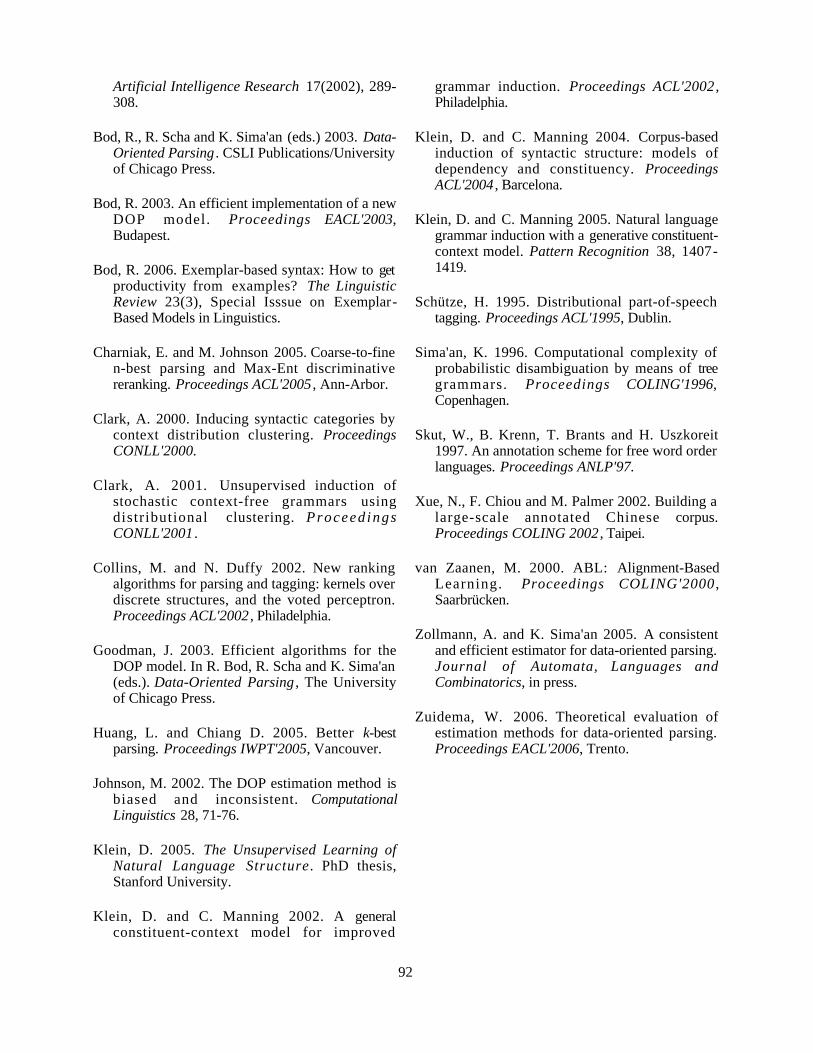
Artificial Intelligence Research 17(2002), 289-308.
Bod, R., R. Scha and K. Sima'an (eds.) 2003. Data-Oriented Parsing. CSLI Publications/Universityof Chicago Press.
Bod, R. 2003. An efficient implementation of a newDOP model. Proceedings EACL'2003,Budapest.
Bod, R. 2006. Exemplar-based syntax: How to getproductivity from examples? The LinguisticReview 23(3), Special Isssue on Exemplar-Based Models in Linguistics.
Charniak, E. and M. Johnson 2005. Coarse-to-finen-best parsing and Max-Ent discriminativereranking. Proceedings ACL'2005, Ann-Arbor.
Clark, A. 2000. Inducing syntactic categories bycontext distribution clustering. ProceedingsCONLL'2000.
Clark, A. 2001. Unsupervised induction ofstochastic context-free grammars usingdistr ibutional clustering. Proceed ingsCONLL'2001.
Collins, M. and N. Duffy 2002. New rankingalgorithms for parsing and tagging: kernels overdiscrete structures, and the voted perceptron.Proceedings ACL'2002, Philadelphia.
Goodman, J. 2003. Efficient algorithms for theDOP model. In R. Bod, R. Scha and K. Sima'an(eds.). Data-Oriented Parsing, The Universityof Chicago Press.
Huang, L. and Chiang D. 2005. Better k-bestparsing. Proceedings IWPT'2005, Vancouver.
Johnson, M. 2002. The DOP estimation method isbiased and inconsistent. ComputationalLinguistics 28, 71-76.
Klein, D. 2005. The Unsupervised Learning ofNatural Language Structure. PhD thesis,Stanford University.
Klein, D. and C. Manning 2002. A generalconstituent-context model for improved
grammar induction. Proceedings ACL'2002,Philadelphia.
Klein, D. and C. Manning 2004. Corpus-basedinduction of syntactic structure: models ofdependency and constituency. ProceedingsACL'2004, Barcelona.
Klein, D. and C. Manning 2005. Natural languagegrammar induction with a generative constituent-context model. Pattern Recognition 38, 1407-1419.
Schütze, H. 1995. Distributional part-of-speechtagging. Proceedings ACL'1995, Dublin.
Sima'an, K. 1996. Computational complexity ofprobabilistic disambiguation by means of treegrammars. Proceedings COLING'1996,Copenhagen.
Skut, W., B. Krenn, T. Brants and H. Uszkoreit1997. An annotation scheme for free word orderlanguages. Proceedings ANLP'97.
Xue, N., F. Chiou and M. Palmer 2002. Building alarge-scale annotated Chinese corpus.Proceedings COLING 2002, Taipei.
van Zaanen, M. 2000. ABL: Alignment-BasedLearning. Proceedings COLING'2000,Saarbrücken.
Zollmann, A. and K. Sima'an 2005. A consistentand efficient estimator for data-oriented parsing.Journal of Automata, Languages andCombinatorics, in press.
Zuidema, W. 2006. Theoretical evaluation ofestimation methods for data-oriented parsing.Proceedings EACL'2006, Trento.
92
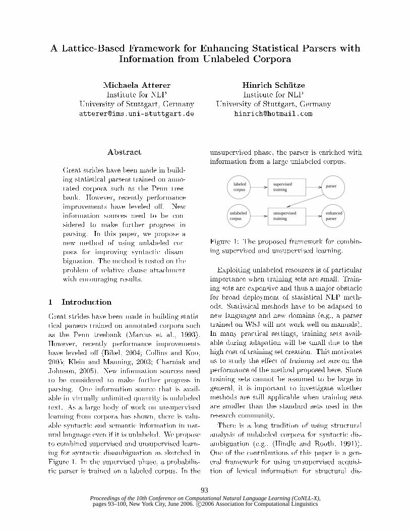
Proceedings of the 10th Conference on Computational Natural Language Learning (CoNLL-X),pages 93–100, New York City, June 2006.c©2006 Association for Computational Linguistics
� � ��������� ��� ������ ������� �� ����� !��� " #%$%��#%���#%& '(��������)�������* + ���������� � �,��$- #% !���.� �������# /����� 0 #%*��1 �*�� 2 ����3 �����
4 57698;:�<�=>: ? @A@B<�CD<�CEGF�HJI/KLI/M�I/NPO>QSR�T%U;V
WXF�KLYZN[R\H\KLI^] Q�O�_�I/M�I\I/`)a�RJIAbdceN[R\f a�Fg]h�i�i�jSk�jSk�l.m[n�o�p7q�r�m�s)oDi)qti�itu�hZk)ivp,wxj
y 57z;C957698 {�698�|�@B})<EGF�HJI/KLI/M�I/NPO>QSR�T%U;V
WXF�KLYZN[R\H\KLI^] Q�O�_�I/M�I\I/`)a�RJIAbdceN[R\f a�Fg]~ mAr�k�m)� ~ l ~�� iSn�h�mS��p\� � n
? ����@BCD:.6�@
�(����[���G�G�G���)�!�����������x�!�/� � �A�)����� �)�)����������)� �G�J�[�G���G�G�����[�¡ ��[���/��¢�G�J�[�����!� £A� �[�)��£[��J�[��!� �!£A�G x£A�J� �G���¤� �A� �G��� ¥¦�/�)� �G��!�\����[�)§�¨ ©(£«ª¬�/���/��®��!�!�/�¯�G��° x�/�,±²£A�G� �[���!����e )�£«���/� �/�¯�� ������� ���/���/���!� £[³�¨ ´(�/ª���S±²£A�G� �[�G��£A� �£A�)��!�!� ���!�!� �£ �x� �!£A�S��G���)�/��!� �£ � �[§�� ±µ�)�G�G���/� )�£A�B��!�� ��� ��[��G���)��¨ ¶7� �G�)��� ��[ x�/���ª¬� )�£A x£B�� ����/ª � �/�G��£¯� £[± ���G���)� �)�)�L�[�x�/���!� �!£A�,� x£A�J� ±²£A� ���e )�£«�����)� �G°��¯�J�A�/�G��� �S���J�[�·��)���B���[�G��£A��¨¹¸������ �/�G��£¯�P������!�G��!�P£A�P�G��� )�£A�)���/� £[±º��/�L�[�G����� �/�L�[���� �[�G�J�A�¤�)� �/�¯�ª����G� �/���!£A�)�J�[�B���)� ��!�G�)�����¨
» ¼ z @BCD½�¾®¿®6�@D5>½ z�(����[�À�G�G�G���)�!�����������x�!�/� � �A�)�(��� �)�)�����S���)� �G�J�[�G���,��G�����[�¦ ��[���/��(�G�J�[�����!� £A� �[�)��£A�J�[��!� �!£A�G x£A�J� �G���¤��A� �G��� ¥¦�/�)� �G��!�/���[�)§ ÁµÂ �[��/��� �/� �[�>¨� Ã�ÄBÄBÅDÆ\¨©(£«ª¬�/���/�� ��!�!�/�¯�G��° x�/�,±²£A�G� �[���!� ���e )�£«���/� �/�¯��������� ���/���/���!� £[³ ÁµÇ���§��/�>ÉÈBÊBÊ[Ë�Ì�Í�£A��������� �[��� Î�£¯£)ÈBÊBÊBÏSÌ�ÎÐ���/��� �[���  �[�)�)���)��®ÈBÊBÊBÅSÌ�Í®���[�G�)�L�[§ �[���Ñ £A�)���£A���ÈBÊBÊBÏDÆ\¨ ´(�/ª ���S±²£A�G� �[�G��£A� �£A�)��!�!�Ò���!�!��£ �x� �!£A���G���)�/��!� �£ � �[§�� ±µ�)�G�G���/� )�£A�B��!�� ��� ��[��G���)��¨ Ó���� ���S±²£A�G� �[�G��£A� �£A�)��!� �G���[� ��� ���B�[���Ô��[�)���(��� �����G�G���[����° �)�)�����e����!� Õ9���[�¯�G���Ö° �����)�)�L�[�x�/���!���\×S��¨·Ø(��� �L�[�G�D�P�x£¯�S° £[±¬ª¬£A�G§ £A� �)���G�) x�/�G������!������[�G�)���)� ±µ�£A� �!£A�G x£A�J� ���A�v�G��£«ª�����G���/��Ù���º�B�[���S��[�)���Ú�G°��¯�J�A�/�G���Ù�[��� ��/� �[�¯�G���X���S±²£A�G� �[�G��£A� ��� ���[�,��)�J�[�Z�L�[�)�B���[�D���/���/�·�Ô±t�������¦�)�)�L�[�x�/���!�.¨�Û �É )�£A x£B���£%�!£A�Ú�)�����!� �G�) x�/�G������!� �[��� �)���G�) x�/�G������!� �����[�G�S����)� ±²£A�X�G°��¯�J�A�/�G��� �S���J�[�Ú�)���B���[�G��£A� �A�Ú�G§��/��¤���!� ���Ü ���B�)�� ÃB¨�¶7� �G���Ú�G�) x�/�G������!� )���A��Bx�P )�£A���[�)�������,��G���� ��[���/�������G�J�[�����!� £A� �e�L�[�x�/���!� �!£A�G )����¨�¶7� �G���
�)���G�) x�/�G������!� )���A��B��G���Ú ��[���/�º���º�/�)�G���¤���!� ª����G����S±²£A�G� �[�G��£A� ±µ�£A� �Ù�L�[�G�D�Ý�)�)�L�[�x�/���!� �!£A�G )����¨
labeledcorpus
unlabeledcorpus
supervisedtraining
unsupervisedtraining
parser
enhancedparser
Ü ���B�)�� ÃBÞº¸����Ù )�£A x£B��!� ±µ�J�[� �/ª¬£A�G§ ±²£A�Ý�!£A�Ú�)���S����)� �G�) x�/�G������!� �[��� �)���G�) x�/�G������!� �����[�G�)���)��¨
ß ×S )��£A���G���)�%�)�)�L�[�x�/���!� ��!�£A�)��!�!�®���®£[±¡ ��[�G�G���/�)�L�[����e x£A�G�J�[���!�ݪ����/� �G�J�[���)���)� ��/����[��v�G� �[���>¨à¸d�J�[���S����)�Ù��/��¬�[����\×S x�/���G�����(�[��� �G�¯�����Ý� ��áG£A�¬£A���G�J�A�/���±²£A�%�)�£D�A� �)�/ )��£«°�� �/�¯� £[±(�G�J�[�G���G�G�����[��´(â�¥ � �/�G�S�£¯�)��¨Úã9�J�[�G���G�G�����[��� �/�G��£¯�)�Ð�������%�£ �x�e�A���[ )��!� �£���/ª �L�[�)�B���[�D�!�Ú�[��� ���/ª �)£A� �[����� Áµ�B¨ä��¨�å� ��[���/��G�J�[�����!� £A� Û ã Ñ ª���������£A��ª¬£A�G§ ª¬�/���¡£A� � �[�¯���[���\Æ\¨¶7� � �[�¯° )�J�A�/�G�����[�v��/�G�G���)�D����G�J�[���)���)� ��/�� ���B�[���Ô��[�)��� �S�)�G���)� �A���[ ��[�G��£A� ª������É�x� �G� �[�����S��� �£ �G����)���B�·�!£B�G��£[±��G�J�[���)���)�v��/�¦�/����[�G��£A��¨�¸��)���å� £A�G���B�[��!������£ �G�G���S° �G���X�\³.�!�/��£[±�æµç^èAéëê�éëê�ì í�î/æ®í\é�ï�î�£A� �G��� x�/�,±²£A�G� �[���!��£[±��G����� �/�G��£¯�Ù )�£A x£B��!�Ù���/��B¨àã9�����!��G�J�[���)���)� ��/��Ù���[�)��£A�Ù�x� �A��G�)� �!� �£ �x� �L�[�G�D� ����D�/���/�J�[�>���� ��� ���e x£A�G�J�[�¯� �£ ���¯���!�G�G���9�[�� ª����/�G���/�� �/�G��£¯�)� �[�� �G�G�������[ ) )�������[�)��� ª����/� �G�J�[���)���)� ��/���[�� �G� �[�����/�P�G���[� �G��� �G�J�[�����[�� ��/��Ù����!� ��� �G�����!����[��¤� �!£A�e�Ú�)�)���Ö°�¨¸����/�� ��� � ��£A�)� �G�J�A�S���G��£A� £[±v���G���)� �G�G�G���/�G�)�J�[�
�[���[��°S�G���·£[±��)�)�L�[�x�/���!� �!£A�G x£A�J� ±²£A�·�G°��¯�J�A�/�G��� �S���,��[�Ú�)���B���[�G��£A� Áµ�B¨ä��¨�ÚÁµ©������S��� �[��� ð�£¯£A�G��ÒÃ�ÄBÄSÃ�ÆGÆ\¨Ó����Ù£[±®�G���Ù�!£A�¯�G�G���)�)�G��£A���ñ£[±®�G�)���( ��[ x�/�Ð���v� �D�/�S��/�J�[�¢±µ�J�[� �/ª¬£A�G§ ±²£A� ���G���)� �)���G�) x�/�G������!� �A�!Õ9�)���G�Ô��G��£A� £[± ���\×S�����[� ���S±²£A�G� �[�G��£A� ±²£A� �G�G�G���/�G�)�J�[� �S���,�
93
�[�Ú�)���B���[�G��£A��¨ ¸��)���Ù±µ�J�[� �/ª¬£A�G§ ���·���A��!� £A� ���\×�������[�Ú�)�/ x�/���)�/���/���!� �x�!���[���� �G���/° �[�� � £B�G�G��° ��£[����[�å�[��� ���[� �G���/��\±²£A��ñ�x�Ý�\×S�G�J�A�/��!� ��/���L�[�)��° ±µ�£A��)�)�L�[�x�/���!� ��\×S��¨ ØÀ� �G��� �J�[� � �G��� �BX�G���!�� �\×���G�J�A�/��!� �)�/ x�/���)�/���/���!�����[� �x�v���A�G����° �����!£A�G x£A�J�[��!����¯�£ �G��� �G�J�[�����!� ��[���/��¨ �Ð�/ x�/���)�/���/���!�e�[�� �G�¯���ª¬�/���Ô�7�G�)����!� �£ ��/�G���ñ�A�À�G���ñ�!£A�e� £A� �/�)�G��/���/° ±²£A����¯��/�B�J�[�G���)� ���S±²£A�G� �[�G��£A� ��� �!£A�Ú�)�����!� �G�) x�/�G������!��[��� �)���G�) x�/�G������!� �����[�G�)���)��¨
� {�@BC9¿®6�@D¿;CD:.=�� 57�[:�� ��5�� ¿;:�@D5>½ zÍ�£A���!�/ )�G���[����°�媬�eª¬£A�)��� ����§��P�£ ±>�A�/�£A���G���e ��[��,����)� )�£A�)���/� ���¯�£ �)�!�/���G��£A��� �G���[� ���[� �x� � �A�)�£A� )�)��/��° �G�G�G���/�G�)�J�[�º�B�£A�)���)� Áµ�B¨ä��¨����!�!£A�B�)���G��£A�£[±É���A��·´(¥;�\Æ��[��� � £A��P�S�� �/�)���X�[�G�J�A�¤�)� �/�¯�Ò�)�\��/���G��£A����v��� ��[�G�G���/�)�L�[� �G��£B�� �G���[� ��!Õ9�)���� ª¬£A�G���§���£«ª����!�S�D�B �B¨ä��¨���� ß ×��[�e )��� Ã
Á,Ã�Æ Â ��¨�Ç��[§��/� ±²£A�)��� �[� £A x�/�)���)���P�)���)�/� ä�G�����£A���� ���G���[� ��î�� æ�� � ±µ�)� �\���������!� �!£D�[���e�����B¨
�У¯�!���G����£A x�/�)���)� �����A� �£P�G���ñ�!£D�[���e�����B�£A���)£¯�!��G���À��£A������ Û ��� �[§����G���¢�G���e )���Ô±µ°����)�Ú�A��G�)�e )�G��£A��G���[��� ��/� �[�¯�G��� � �[�G�J�A�¤�)� �/�¯� �)�!�/���G��£A��� �[�� �����)�\� x�/���)�/�¯��£[±����A�¤� £A�G���/��¨;¸��)���¢���¢£[±µ��/� �G���ñ���A��Ý£A��v )�)��/��° �G°��¯�J�A�/�G�������/���/���[���G��£A�)�B� ��� ���É�/�����[�G��°e��£A��G�G������/� �[�¯�G�����[����°P�G�����!�À��/� �[�¯�G�����[����°Ù�����!£A���G���G��/�¯��[�G�J�A�¤�)� �/�¯��à���[�·�B�����®�G����®�£������!£A���/��/�¯������A�S���)�D��¨Û � ±²£A�G� �[������� �[� �[�G�J�A�¤�)� �/�¯� �[�Ú�)���B�)���Ö° �A� �
)�)�J�A����Ð¥ ���������)� �Öª¬£ £A�Ð� £A��· x£B��G���)��� �[�G�J�A�¤�S�� �/�¯�Ý x£A���¯���� �"!#�%$&!('('('.��� � ��/�¯��/���!� ã�¨ â��/�ñð �x��G���� ��[���Ú£[±É� ��/�¯��/���!�eã ª����G� �Ð¥ ��/� £«���!�.¨�¸å£� �[§�� �[� �[�G�J�A�¤�)� �/�¯� �)�!�/���G��£A��(ª¬� ±²£A�G� �G�G�� )���!�£[±P�G��� ±²£A�G� ) ð*!#�+!#�Ð¥ , ª����/�� � ��� � x£B��G�Ô��)��� �[�G�J�A�¤�)� �/�¯� ��£¯�)� ±²£A� �Ð¥ ��� ðÒ¨ Û � �)� ������ ��/��£[±¬�D�/���/�J�[�������[�G��£A� ±µ�)���/�G��£A���*- . /"0�132 �G���[�� �[ Ò�G�G�� )���!�d���¯�£�� £A��à�D�/���/�J�[�9�G�G�� )���!��¨�ã�£A� �¹±µ�)���\��G��£A�����G���e )��° �)�/���/��ñ� �[��/�G�L�[�>��B¨ä��¨�g�G�����G�)�SáG�!�/��£[±�G��� ��/�¯��/���!�B¨ Ó��G���/�� ��/ )�L�A�!� ��£A�)��� ª����G� �G���/����/�L�A���!�� �B¨ä��¨�4�GÍ��[���A����� ª����G� � �!£A�)�¯�G�G°5�J¨ ß �A�¤� 0�1� £¯�S����!�¦�/���G���/��ð £A�6�Ð¥���)�)� ��£A� �x£A�G��¨�¸�����±µ�)���\��G��£A���º���[� �x�·�[ ) )�����!� ��� �[�¯° £A��)�/��¨ Ü �)���/�G��£A���70�1�G���[��ª¬£A�)��� �)�/���/��Ý�G���Ý��£¯�)�8�¬�[��v��£A�¢ x�/�G�e���G��!�.¨Û � �)� ����� � �G�)���G�)�e )�G��£A� ��/�L�[�G��£A���G�)�� 9 £A�
�G��� ��/�P£[±��G�G�� )���!�P )�£¯�S���!�!� ±µ�£A� ) ð*!#�+!#�Ð¥ ,ÒÞ) :;�"!#�+!�<4�7,*9*) :=$&!#�+!�<>$8, �Ô³ :;�?9 :=$ñ�[��� <4�79<>$ Aª����/����� )�)�J�A����G�G�G���/�G�)����G��!�A@B�������G�)���G�)� �!��¯°C@D$À�Ô³ �G���¢��£¯�)�!�É£[±4@B�����[� �x��� �[ ) x�!� £A�¯�£E@D$
)��!��/�G�����)� �)£A�e�����[���!� �[��� �Ô±¬��£¯�)�!�Ò�[��·� �[ ) x�!�£A�¯�£Ý���)�/�¯�G�����[����£¯�)�!�®£A�;� £A����G x�!�/�������£¯�)�!�(Áµ�B¨ä��¨�� �!£A�)�¯�G�G°5�·£A�¯�£ �GÍ��[���A�����,Æ\¨ÒØ����;0�1Ù£A�x�/° �G���·�!£A�S��G�G�J�[���¯�F0�1HGI) ð*!#�+!#�Ð¥ ,KJL9*) ð*!#�+!#�Ð¥ ,Ò¨¸d�G�� )���!� �[�� �/�B�[�����[��!� �¯° �[� �/�B�[�����[�G��£A� ±µ�)���\�
�G��£A� M �G���[� �A���!���!� �G��� �G�) ) x£A�G� £[±ñ�G��� ���\×S�����[���/�L�[�G��£A���G�)�� ��X��� �G���e�G�G�� )��� ��� �G���e�)�)�L�[�x�/���!� �!£A�,� )��� NeÞ MDGI) ð*!#�+!#�Ð¥ ,KJ O P ¨ �Ð�/���/�J�[�������[�G��£A��������!�!�!��J�[�G° �x�!���[����Ú�G���Ú ��[�G�G���/�)�L�[�ñ��/�У[± ª¬£A��)�±²£A�)��� ��� �·��/�¯��/���!�vª������¡�J�[��/��° £¯�!�/�)�¢��� N Q �[����/���/� �Ô±����X�)£¯�!��ª¬� �)£A�SRä�Ò§���£«ª ª����[���G��� �!£A�G��!�/� ��[��� £[±��G��� ��/�¯��/���!� ����¨ ¸����e±µ�)���/�G��£A���*0�1 )�£[��S���!� � ��/�G���!�Ý£[±�� £A�� �[��� � £A�� �[���G�G�J�A�/�Ý�G�G�� )���!��£ �A�¢�£e�B���[�J�[�¯��!�Ò�G���[�TN �!£A�¯�J�[�������/��£A�)�B� ���[�J�±²£A���/�B�[�����[�G��£A��¨¸������ ���A�G�)���ª¬����������/����£Ú�/�B�[�����[����G�G�� )���!�É���
x£A���¯�Öª�����¢�Ú�)�G���[� ���S±²£A�G� �[�G��£A� ª����G� ��!�G x�!�/�;�£Ò�[��)�)�L�[�x�/���!� �!£A�G )���KNe¨�Û �Ý�)� �����BÞ
UWVYX Z\[�]�[_^ `Da b c deVYX Z\[f]�[g^ `Dab hjilk�mSn VYX Z\[�]�[_^ `Da
n VoZ6a n Vp^qarsut n VYX Z\[�]�[_^ `Dav[ n VoZ6av[ n Vp^qa\wb xUWVYX Z\[f]�[g^ `Da b x suy�z3{%t�|S}�~�{
ª����/�� �G��� )�£A���[�)�������G���!� �[�� �!�G�G��� �[��!� £A� �G����)�)�L�[�x�/���!� �!£A�G )��� Ne¨ @ G ¸KJ �[��� @ G��EJ �[�� �G��� )�£A���[�)�������G���!�v£[± �)�/ x�/���)�/���/° �G�G�G���/�G�)��!�K: �[��� <£¯�!�/�)�G�G���)� ��� N �[��� @ GI) ¸�!#�+!�� ,KJ������G���v )�£A������)�������Ö° £[±;�G���X�)�/ x�/���)�/���/° �G�G�G���/�G�)��!�º£[± ¸ �[��� �eª����G� � �[�G�J�A�¤���!� �[�¢��£¯�)�8� ��� ¸Ýg£¯�!�/�)�G�G���)� ��� Ne¨¸����Ù��/�º£[±®�G�G�� )���!�8� GI) ð*!#�+!#�Ð¥ ,*!�-�J��)�/�G�����!�
±µ�£A� ) ð*!#�+!#�Ð¥ , �¯° �G���!�!�!��G�����·�[ ) )�������[�G��£A����£[±£A���B �Öª¬£v£A��� £A��¬�D�/���/�J�[�������[�G��£A�e±µ�)���/�G��£A���D0�1�O -±²£A�G� �¦�À�L�[�G�G���!�®ª����G�X��!�G x�!�/�å�£E9Ò¨�) ð*!#�+!#�Ð¥ , ����G��� �G�) )��/�Ú�)� �[��� ) ��!#�+!���, �G���à�������Ú�)� £[±)�G�)����L�[�G�G���!�B¨àØ�� �\×��[�e )���º£[± �G���¤� ���L�[�G�G���!�������G��£«ª�� ���Ü ���B�)��ÉÈñÁµ��!���x�/��£«ª ±²£A�¡� £A�� �)�/�J�[�����!�X�S����/����G��£A��Æ\¨MDGI) ��!#�+!���,KJà�����)� �����!� �A�À�Ò�!£A���G�J�[�¯�� ª��)���¤� �)�\� x�/���)�v£A� �G���Ù�S���J�[�Ú�)���B���[�G��£A� �J�A�G§ �[�º���[���.¨vÛ ��J�[§�� �A�S�B�[�¯�J�[�D� £[±��G��� �L�[�G�G���!� �G�G�G���/�G�)�� �£ �!£A�·� )�)�� �G��� èI� ê�éµæg� � �x�/�Öª¬�!�/� ð �[��� �Ð¥ ª��)���¤��\×S )��!���!� �£Òª����[���\×S��/�¯�À�[�G�J�A�¤�)� �/�¯��£[±S�Ð¥ ��� ð�[�à��£¯�)���d���à�G�) ) x£A�G��!� �¯°%���\×S�����[� �)�/ x�/���)�/���/���!� ���Ne¨�Û �Ð )�£A x£B��Ý�G�)��!���S�Ô³.�/��/�¯���)� ���)���G��£A����£[±��%Þ
� ¸���� � ��×S���Ú�)� ª����G� ��!�G x�!�/� �£ ) £A� P Þ�*� . � ������G%/&MDG_�HJ"���CO �C2&J
94
� ¸����ñ�G�)� £«���/�¢�G���v�L�[�G�G���!�BÞ���� . � ����� MDG_�HJ
� ¸����  ¶ £[±Ù�G��� � ��×S���Ú�)� ª����G� ��!�G x�!�/� �£9ÒÞ �� . MDGY� �����G%/ �W��� O � !�MDG_�HJ �. ��2&J JÁë�Ô±å�G���/����[��Ð��/���/�J�[��� ��×S��� �[�S�S�ª¬�º�J�[§��(�G��������/�J�[�D�ñ£[±��G���/���� ¶ �B�[�����!�\Æ
¶7�¯�G�)���G�����/��°�¯ª¬�v�[��º����[��¤�)���)�%±²£A���/�����)�/���!�(��� N�G���[�L�Ð¥ �[��� ð ����ª¬�/�����£A�D�/�G���/������§��v�Ò§��/° �[��� ���£¯�¤§�¨�Ø � �)���Ö°Ò� ���A�G�)��L�*� ��/���!�/����G���É�x�!�G�;���G�G���)��D�/���/�J�[�������[�G��£A� £[±��G�����G�G�� )���¬ª����/����A����� �!£A���G���)�/���G���ºáG£A���¯�Ò�/�����)�/���!� £[±¢�[���à�G�G�� )���!��¨  ��×S���Ú�)� �[����G�)� ���[� £A�)��°Ù�x���!£A�e )�)��!� �Ô± �G���À�L�[�G�G���!�����;�G� �[���>¨Â ���A�G�)�� �� ���A�;�G�����A�S�B�[�¯�J�[�D��£[±¡�/����/�)�Ú���/�¯�G���)��G��� ���!�!� £[±·�!£A�e )�)�G���)� �G��� �/�¯�G���� �L�[�G�G���!�B¨ Û �� £«���º�)£«ª�� ±µ�£A� �G���º£A�G���B�����[� �G�G�� )���º�)�¯�G���xª¬�7������ �7�L��°��/�I� £[±Ú�G��� �L�[�G�G���!� ª����/�� )�£A���[�)�������G���!� �[����£A� ���/�£)¨ ¶7� �G�)���X ��[ x�/��¹ª¬� £A�)��° ��/ x£A�G�Ù��!�G�)����±²£A� �*� ¨¸���� �A�/�G���[�%�G°��¯�J�A�/�G��� �S���J�[�Ú�)���B���[�G��£A� ��� x�/�,�
±²£A�G� �!� �¯° �!£A�e ��[�G���)� �G��� ��� �)���G���!� ��Gf� GI)ð*!#�� 5!#�Ð¥ ,KJ J�±²£A���G���� x£B��G���)���%�[�G�J�A�¤�)� �/�¯�(��£¯�)�!�� �"!#�%$&!('('('S�[��� ��/���!�/�G���)�X�G���¢��£¯�)��ª����G� �G�����)���B���!�G���� �)���Ö°�¨� ����� <�C95v� <�z @B:.=v{�<)@D¿ �Û ���/� �!£A�e )�)�G���)� �G���·�Ú�)�G���[�;���S±²£A�G� �[�G��£A� £[±¢�[��[�G�J�A�¤�)� �/�¯���!£A���G��/���L�[�G��£A��Z�G���(��!Õ9�)����!� )�£A���[�)���Ô����G���!�Ò�[��P�!�G�G��� �[��!� ���A��!� £A� �)�/ x�/���)�/���/° ��[���!�£[± �G��� �)�)�L�[�x�/���!� �!£A�G )��� )�£¯�S���!�!� �¯°  ���)�� ��[�Áµâ.���� Ã�ÄBÄ��DÆ\ � �)�/ x�/���)�/���/° ��[���/� �G���[� ��!�!£A�A��)�����!� � ª����)� �J�[�)�D� £[± �)�/ x�/���)�/���/���!��¨ Û � �����G��� ð��/�)��/�� ð�Í��·Ã �!£A�G )��� Áµâ��/ª���� �/� �[�>¨��ÈBÊBÊ[Ë�Æ�A� £A�)� �)�)�L�[�x�/���!� �!£A�G )����¨ ¸���� ����G� ÏBÊ ª¬�!�/§S�Á²�[�x£A�)���BÊS ÊBÊBÊS ÊBÊBÊ�ª¬£A��)�\Æ�ª¬�/��à ��[���!��ª����G�Ú ���)�Ô� ��[�e�[��� �)�/ x�/���)�/���/���!�e�G�£A��!� ��� �[� ���¯���/�G��!� ���S��)�\×e±²£A�¬���A�G° Õ9���/�G°����)��¨¹¸��������¯���/�G��!� �����)�\× ���®���·� )���/� �/�¯��!� ���G���)� â.���!�/��� Áµâ.���!�/���B(ÈBÊBÊ��DÆ\¨ ¸��)�����/�G�) �/���[�)���!������[��¤�)���)�Ù±²£A���G����±µ��!Õ9���/���/° £[±å���\×�������[���)�/ x�/���)�/���/���!��¨ Ü £A� �\×��[�e )���Bɪ¬� ���[� Õ9���/�G°±²£A�e�G��� �¯�)�Ú�x�/� £[±Ð�G��� �!�e�G���[� �¤èBæ�ªÀ�A� �G��� �G�)�S�áG�!�/� £[± ���Sè[í�î/·�[��� ª¬� ���[� �!�G�G��� �[�� �G��� )�£A�S��[�)�������G���!� @ GY:TJ/ @ G_< J/Ù�[��� @ GI) :?!#�+!�< ,KJ �A���/�L�[�G����� ±µ��!Õ9���/���/���!�P�¯° �!£A�)�¯�G���)� �G��� �¯�)�Ú�x�/� £[±�G��� �!�Ú�G��� �!£A�G��!�G x£A���S���)� �)�/ x�/���)�/���/° �G�G�G���/�G�)��!�£¯�!�/�)�%��� �G��� �!£A�G )����¨ Ø �!£A���G��/���L�[�G��£A� Á :X\< �£A�) :?!#�+!�< ,ºÆ����q����G�É��/ )��!��/�¯��!� �A�����)�/ x�/���)�/���/°�G�G�G���/�G�)��Ð�[���.D±²£A� ����A�£A����£[±d� � �/���/���/°���G�����¯�)�·��x�/�У[±É£¯�!�/�)�G��/���!�!�ñ£[± �G�)���º�)�/ x�/���)�/���/° �G�G�G���/�G�)��
�����G���/� �[ ) )�£�×S��� �[��!� �A�¦�G�����¯�)�Ú�x�/�;£[±���/�¯��/���!�!��G���[�å�!£A�¯�J�[���Ù�[���D�)�����[�G°Ý�)�/ x�/���)�/���/���!�å�����G���;�G�G�G���\��G�)��B¨�Û �Ð�J�[§��Ò�%�G�J�[�����!� ��[���/�ÚÁµÂ ���)�� ��[����£A�¢�G���Í�£A��������� ��[���/��º�)�/ x�/���S���)� £A� �G��� �\×S x�/�G��� �/�¯�\Æ\�G�)�����d£A�X¥¦�/�)�X¸d��!�/���[�)§ñ��/�¯��/���!�!��[����[��¤�ݱ²£A�¡�G����Ö°� x�Ú£[±¬�[�G�J�A�¤�)� �/�¯�Ò�[�Ú�)���B�)���Ö° ª¬�·�[��X���¯��/��!�G��!���� �[���.��Ô±Ò��� £¯�!�/�)���� )��!��/�¯� �Öª¬£ �G�G�� )���!� £[±��G���±²£A�G� ) ð*!#�+!#�Ð¥ , �[��� ) ð*! � !#�Ð¥ , �£ �G���%�S���,��[�Ú�)���B���[�G��£A� �!£A�e x£A���/�¯��.ª����/�� ���[��� � �[��Ú�Öª¬£ x£B��G���)���e�[�G�J�A�¤�)� �/�¯�Ò�G����!��±²£A���Ð¥ ��� ðX¨.ã��!�/�G��£A���ÊBÊ Q�Ã�ÈÚ£[±d�G����Û ã Ñ ª¬�/�������!� �A�®�G���º�)�/���/��£A )� �/�¯���/�� �[��� ��!�/�G��£A���ÒÃ�Å QSÈ[Ë �A���G���Ý��!�G����/��¨
! ? ��� =7576S:�@D5>½ z @B½ " #%$ &('*),+-# . $ &0/�12#3 '4'�&0576�8 #%9-'
:���;=<��;?>!�A@CBEDGFH<JILKMBE>NF2Ot��P?F2QRKMO��TS2UV��OWF2<XBZY��T>�OWF2[?D�\^]T_a` F2<X<bF4>dcMQ ��;=<eF2QgfMBZh�[MBZ<JIji
k S4<Xc F2<X<bF4>dcMQ ��;=<lDmF2V�nh�VbF2QRQ F2<XBE>NF2O ofM[M<pBZ;=<X[rqBZ<XBZY���OZI sbtvu�w?xywLzRBEDmQ S4V� OZBZ{���OZI <lS S=>|>�[MVA}aBZ<Xc <Xc��Y���VXf?DT~Eu��*��S4V�~Eu��*��� s�<Xc%F2; �rs4�7�Nu�i���[MV�c=ILK�S4<Xc��|DXBEDBED�<Xc%F2<�<XcMBED�<JILKx�S2U�KMVbF2h�Q F2<XBE>n{L;?S�}aO��|�rhD� \ S4Kx��;rqBZ;Mh*D�O��NF4� <lS�DlS4Q ��<XcMBZ;Mh?o�c?S4[?D�|DC�MS4;���< ` }aBZOZOfx��V��q���|>�<�|� BZ; �)��Kx��;?�)��;?>�B��|D ��Pr<XVbF4>�<�|� U^VlS4Q F OWF2VXhD�>|S4VXKM[?DNin��Pr<XVbF4>�<XBZ;Mh �)��Kx��;?�)��;?>�B��|DmBEDHK%F2VX<XBE>�[MOWF2VXOZIBZQRK�S4VX<bF2;=<AF4D ]T_ F2<X<bF4>dcMQ ��;=<mBED�F Q S4V���rB�� >�[MOZ<KMVlS4fMO���Q <Xc%F2; ��� F2<X<bF4>dcMQ ��;=< F4D <Xc�� U,S4OZOES�}aBZ;Mh��P?F2QRKMO��|DTDXc?S�}i
\,�*` � ��P?F4>|S � ;?>�i�V��K�S4VX<�|� ¡¢F2; @�@¤£ BZ;?>�V�NF4D��¥�BZ;¡�<XcMBZVl�Lq ¦7[%F2VX<��VÝ�NF2VX;MBZ;Mh*D§¥ o¨}acMBE>dc BZ<����,�^©�x ª��r� u��K%F2VX<XOZI�<lS�<Xc���>|S4QRK%F2;=I�«D�Q F4DlDXBZY��CV�|DX<XVX[?>�<X[MV§qBZ;Mh ¡ZiZiZi¬¥
\,*` ��F2VXOZB���V<XcMBEDeI��NF2V®�� _ ¯ >|¦7[MBEDXBZ<XBES4; Q F4�)� ¡¢F° @N±¤q�F¤q DXc%F2V�eS2².��V§¥(U,S4V�¡«®�F2<bF2KMVlS=�r[?>�<lD§¥ o�}acMBE>dc<Xc��m®�F2<bF2KMVlS=�r[?>�<lDTf�S*F2Vl� DbF2BE� BZ<m©duy³Nu�´|� u�� ¡ZiZiZi¬¥
\yµL` ¡ZiZiZi¬¥ DbF2BE� ���rQ F2Vn¶ �|�r;MBEDNo·¡�<Xc��e��PrKx��VX<m>|S4Q�qQ ��;=<bF2<lS4V§¥�U,S4V ¡�<Xc�� Q F2<l>dcr¥ og}acMBE>dc }CF4D ���^¸� u�w(�7u��ef=I c=[M;?�rV�|�MDpS2U�>dc��|DlD¹U F2;?DNi
]T_ F2<X<bF4>dcMQ ��;=< BZ;=<��VbF4>�<lD�}aBZ<Xc F }aBE�)��V�VbF2;MhD�S2Uºh�VbF2QRQ F2<XBE>NF2O¨KMc���;?S4Q ��;%Fm<Xc%F2; ��� F2<X<bF4>dcMQ ��;=<\ ��i�h?iZo�S4fr»G�|>�< YrDNi�DX[Mfr»G�|>�< V��OWF2<XBZY��|DNo¹K%F4DlDXBZY���o�F2;?�F2h�V�!��Q ��;=< ` i ¯ OEDlSMo*Q F2;=I >NF4D�|D�S2U¼��� F2<X<bF4>dcMQ ��;=<>NF2; fx� V�|DlS4OZY��|� DX<XVX[?>�<X[MVbF2OZOZIji ½vS4V ��P?F2QRKMO���o�F2;
¾J¿�À¢Á2À¢Â4ÃlÄ·ÃlÅ,Å ÃbÆ Ç2ȧÉ-Ä È§ÊËÃlÅ À¢Ì�È�ƧÊËÃbÍ2É,ȧÉ�Ê¢ÎXÏ Ð|ÑeÒ¤È�ÓZÃbÍ2Ê«ÅXÔÕÄ È�ÖÉ,Í2Ê«Å À¢Á2×RÀ¢Á Ø�ÃbÁ|Ñ À¢Á2ƧÎbÄ,Ä È§Æ�Å�ÃlÅ,Å ÃbÆ Ç2ØaȧÁ|ÅpҤȧƧÀ¢É,À¢Î�Á2ɧ٠ÚNÀ¢Á2ƧÈÄ È§ÊËÃlÅ À¢Ì�È�ƧÊËÃbÍ2É,ȧÉ�ÃlÄ È·Ä ÃlÄ È�ÔÛÏÈ�Ò¤ÎaÁ2ÎbÅÜÉ^ѤÉ^ŠȧØ�ÃlÅ À¢ÆXÃbʢʫÑ�ȧʢÀ¢ØaÀ«ÖÁ4ÃlÅ ÈÝÅ Ç2餯 Ï�Ç2ȧÁHƧÎ�ØaÂ2ͤŠÀ¢Á2×·ÞyÍ2Á2ÊËÃbÐ�ȧʢÈXÒNßÝÉ^Å ÃlÅ À¢É^Å À¢Æ§É§Ù
95
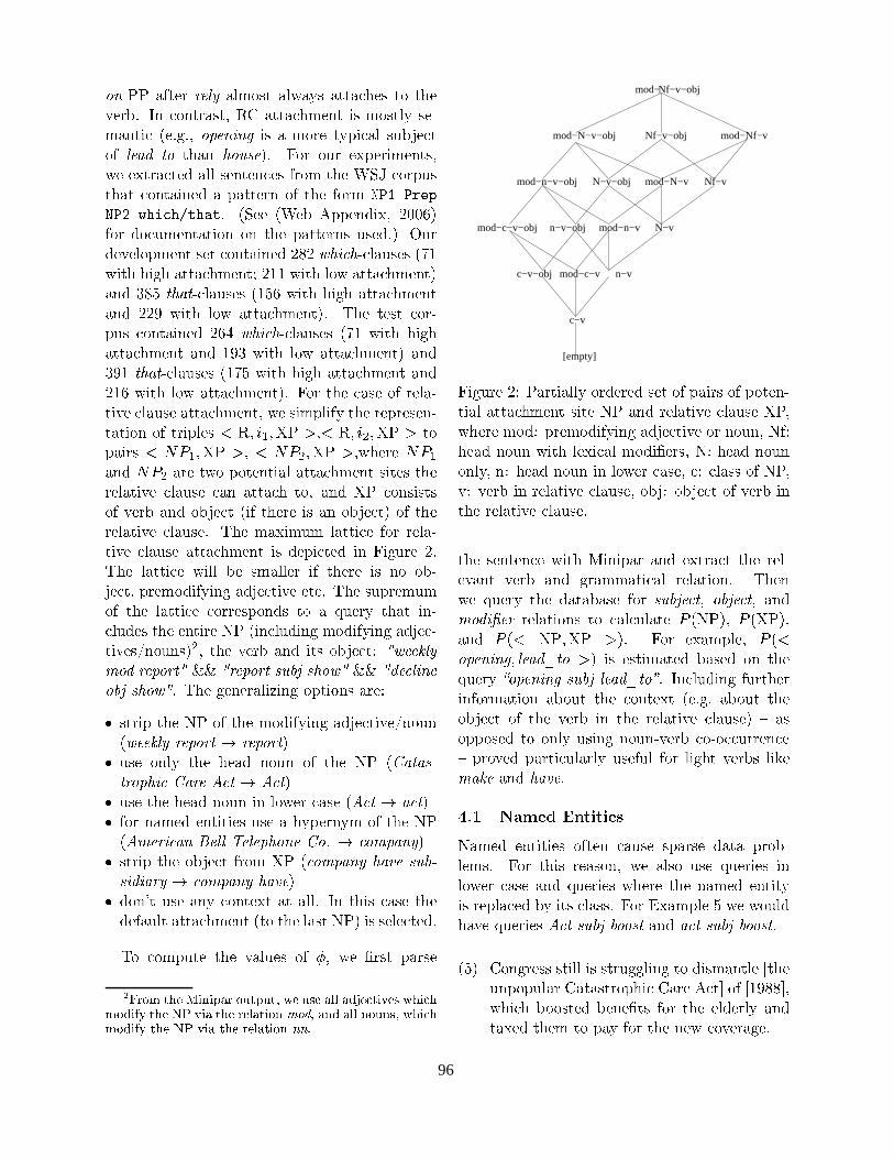
s4w�q ��� F¤U^<��V ©du�~�� F2OZQ S�DX< F2OZ}CF IrDRF2<X<bF4>dc��|D�<lS <Xc��Y���VXf�i�� ; >|S4;=<XVbF4DX<No ]T_ F2<X<bF4>dcMQ ��;=<nBED�Q S�DX<XOZI D��qQ F2;=<XBE> \ ��i�h?iZo�sbtvu�w?xywLz BED F Q S4V� <JILKMBE>NF2OaDX[Mfr»G�|>�<S2U ~Eu��*� � s <Xc%F2; �rs4�7�Nu ` i ½vS4V S4[MV ��PrKx��VXBZQ ��;=<lDNo}¬�v��Pr<XVbF4>�<�|� F2OZO D��;=<��;?>!�|D�U^VlS4Q <Xc���� :�� >|S4VXKM[?D<Xc%F2<g>|S4;=<bF2BZ;��|� F K%F2<X<��VX; S2UC<Xc���U,S4VXQ ���� �� �������� ��������� ����� ���(i \ :���� \ � ��f ¯ KMK���;?�rB�P0o � � � !*`U,S4V��MS=>�[MQ ��;=<bF2<XBES4; S4; <Xc"� K%F2<X<#��VX;?D�[?D#�|�0i ` ��[MV� ��Y$��OES4KMQ ��;=< D#��<·>|S4;=<bF2BZ;"�|� � %��'& �7x,´��Nq >�OWF2[?D#�|D \)( @}aBZ<Xc�cMBZh�c F2<X<bF4>dcMQ ��;=<+* � @�@�}aBZ<Xc�OES�} F2<X<bF4>dcMQ ��;=< `F2;?� % ± �y�r��� q >�OWF2[?D#�|D \ @N± ! }aBZ<Xc cMBZh�c F2<X<bF4>dcMQ ��;=<F2;?� ��� , }aBZ<Xc OES�} F2<X<bF4>dcMQ ��;=< ` i � c"� <#�|DX< >|S4V§qKM[?D >|S4;=<bF2BZ;"�|� � !2µ & �7x,´��Nq >�OWF2[?D#�|D \)( @ }aBZ<Xc cMBZh�cF2<X<bF4>dcMQ ��;=< F2;?� @ ,� }aBZ<Xc OES�} F2<X<bF4>dcMQ ��;=< ` F2;?� , @ �y�r��� q >�OWF2[?D#�|D \ @ ( ± }aBZ<Xc cMBZh�c F2<X<bF4>dcMQ ��;=<F2;?�� @ ! }aBZ<Xc OES�} F2<X<bF4>dcMQ ��;=< ` i�½vS4Vp<Xc"��>NF4D#�AS2U�V#��OWF¤q<XBZY$� >�OWF2[?D#�CF2<X<bF4>dcMQ ��;=<No�}-��DXBZQRKMOZB�U^Im<Xc"�GV#��KMV#�|D#��;rq<bF2<XBES4; S2U�<XVXBZKMO.�|D0/ ]2143#56147 � 8no9/ ]2143;:�147 � 8 <lSK%F2BZVlD / < = 5+147 � 8no>/ < = :�147 � 8no�}ac"��V#� < = 5F2;?� < = : F2V#��<J}�S�K�S4<#��;=<XBWF2O F2<X<bF4>dcMQ ��;=<pDXBZ<#�|DC<Xc"�V#��OWF2<XBZY$� >�OWF2[?D#� >NF2; F2<X<bF4>dc <lSMo�F2;?� 7 � >|S4;?DXBEDX<lDS2UGY$��VXf F2;?� S4fr»?�|>�< \ B�U�<Xc"��V#��BEDmF2; S4fr»?�|>�< ` S2UG<Xc"�V#��OWF2<XBZY$� >�OWF2[?D#��i � c"� Q F¤PrBZQg[MQ OWF2<X<XBE>�� U,S4V�V#��OWF¤q<XBZY$� >�OWF2[?D#� F2<X<bF4>dcMQ ��;=<RBED�� ��KMBE>�<#�|� BZ; ½ BZh�[MV#� � i� c"� OWF2<X<XBE>�� }aBZOZO�f�� DXQ F2OZO.��V B�U <Xc"��V#� BED ;?S S4frq»?�|>�<NojKMV#��Q S=�rB�U^ILBZ;Mh F4�2»?�|>�<XBZY$�@��<l>�i � c"�pDX[MKMV#��Qg[MQS2U�<Xc"� OWF2<X<XBE>�� >|S4VXV#�|DXK�S4;?�MD <lS F ¦7["��VXI <Xc%F2< BZ;rq>�OZ[?� �|D�<Xc"�A��;=<XBZV#�CB�� \ BZ;?>�OZ[?�rBZ;MhQ S=�rB�U^ILBZ;MhAF4�2»?�|>�q<XBZY$�|DED¤;?S4[M;?D `;F o¼<Xc"� Y$��VXf F2;?� BZ<lDAS4fr»?�|>�<+G H & uduJI¤~��K s��g©du t s4©��LHNMOM H ©du t s4©��-���?ªy³T�b�rs & HPMOM H§�7u�´�~ xywus7ªy³e�b�rs & H�i � c"�eh���;"��VbF2OZBRQ|BZ;Mh S4KM<XBES4;?D�F2V#� GS DX<XVXBZK <Xc"�TB�� S2U·<Xc"�Q S=�rB�U^ILBZ;Mh F4�2»?�|>�<XBZY$��D¤;?S4[M;
\;& uduJI¤~�� ©du t s4©��VU ©du t s4©�� `S [?D#� S4;MOZI <Xc"� c"�NF4� ;?S4[M; S2U <Xc"� B�� \�W ��� �2��¸
�^©�sbt%�7x,´ W �4©duYXT´|�VU XT´|� `S [?D#�e<Xc"�ec"�NF4� ;?S4[M; BZ; OES�}-��V�>NF4D#� \ XT´|�VU �*´|� `S U,S4V�;%F2Q �|� ��;=<XBZ<XB.�|DH[?D#��F c=ILK���VX;=ILQ S2U <Xc"�ZB��
\ X K u�©�x,´d�4w [�u�~ ~A\(u�~Eu t%�rs4wu W s�]^U ´ds K t �4w"� `S DX<XVXBZK <Xc"��S4fr»?�|>�<pU^VlS4Q 7 � \ ´ds K t �4w"� �r��_4u����?ª�¸
��x,�4x,�4©E�`U ´ds K t �4w"�R�r��_4u `S �MS4;���<m[?D#�RF2;=I >|S4;=<#��Pr<AF2<AF2OZO i�� ; <XcMBEDm>NF4D#��<Xc"�
� ��U F2[MOZ<�F2<X<bF4>dcMQ ��;=< \ <lS�<Xc"�·OWF4DX<aB�� ` BED-D#��O.�|>�<#�|�0i
� S >|S4QRKM[M<#� <Xc"� Y�F2OZ["�|D S2U bÜom}-� c?VlDX< K%F2VlD#�
dfe�Ä Î�Ø Å Ç2È ¿�À¢Á2À¢Â4ÃlÄ?Î�ͤŠÂ2ͤÅXÔdÏÈÍ2É,È0ÃbÊ¢Ê Ã�Ò#g^ȧÆ�Å À¢Ì�ȧÉ�Ï�Ç2À¢Æ ÇØaÎNÒ¤À«Ó Ñ·Å Ç2È�hjiÌNÀËüŠÇ2È¨Ä È§ÊËÃlÅ À¢Î�Á�kml?nbÔ ÃbÁ4ÒGÃbÊ¢Ê Á2Î�Í2Á2ɧÔbÏ�Ç2À¢Æ ÇØaÎNÒ¤À«Ó Ñ�Å Ç2Èohji ÌNÀËÃ�Å Ç2ÈÝÄ È§ÊËÃlÅ À¢Î�ÁZpLp2Ù
mod−
Nf−v−obj mod−Nf−vmod−N−v−obj
mod−n−v−obj N−v−obj mod−N−v Nf−v
mod−c−v−obj n−v−obj N−v
c−v
[empty]
n−vmod−c−vc−v−obj
mod−n−v
Nf−v−obj
½ BZh�[MV#� � GÝ� F2VX<XBWF2OZOZI S4Vl� ��V#�|� D#��< S2U0K%F2BZVlD S2U K�S4<#��;rq<XBWF2O�F2<X<bF4>dcMQ ��;=<mDXBZ<#�'B�� F2;?� V#��OWF2<XBZY$��>�OWF2[?D#� 7 �Ýo}ac"��V#��Q S=�PGÝKMV#��Q S=�rB�U^ILBZ;Mh�F4�2»?�|>�<XBZY$��S4V ;?S4[M;�o�B�U?Gc"�NF4� ;?S4[M; }aBZ<Xc O.��PrBE>NF2OÜQ S=�rBqc���VlDNorBsG?c"�NF4� ;?S4[M;S4;MOZIjo ;NG�c"�NF4� ;?S4[M; BZ; OES�}-��V�>NF4D#��oM> G >�OWF4DlDaS2UjB��ÝoYrG�Y$��VXf BZ; V#��OWF2<XBZY$�A>�OWF2[?D#��o%S4fr»�G�S4fr»?�|>�<�S2U�Y$��VXf BZ;<Xc"�eV#��OWF2<XBZY$�>�OWF2[?D#��i
<Xc"� D#��;=<#��;?>�� }aBZ<Xc ¶ BZ;MBZK%F2V F2;?� ��Pr<XVbF4>�<�<Xc"� V#��O�q��Y�F2;=< Y$��VXf F2;?� h�VbF2QRQ F2<XBE>NF2O V#��OWF2<XBES4;�i � c"��;}-� ¦7["��VXI <Xc"� �?F2<bF2f%F4D#� U,S4V ���?ªy³Nu�´|�,o�s7ªy³Nu�´|�,o�F2;?�K s��4xut¹u�© V#��OWF2<XBES4;?D <lS >NF2OE>�[MOWF2<#� = vwB��yx 1 = v 7 �yx�oF2;?� = vz/ B�� 147 � 8{x�i ½vS4V ��P?F2QRKMO.��o = vz/sbtvu�w?xywLz 1 ~Eu��*�+|�� s 8{x BED �|DX<XBZQ F2<#�|� f%F4D#�|� S4; <Xc"�¦7["��VXI }^sbtvu�w?xywLz ���?ªy³g~Eu��*�+|�� s ~§i�� ;?>�OZ[?�rBZ;Mh U^[MVX<Xc"��VBZ;rU,S4VXQ F2<XBES4; F2f�S4[M< <Xc"� >|S4;=<#��Pr< \ ��i�h?iaF2f�S4[M< <Xc"�S4fr»?�|>�< S2UA<Xc"� Y$��VXf BZ; <Xc"� V#��OWF2<XBZY$� >�OWF2[?D#� `0� F4DS4KMK�S�D#�|� <lS S4;MOZI [?DXBZ;Mh ;?S4[M;rq Y$��VXf >|S2q S=>|>�[MVXV#��;?>��� KMVlS�Y$�|� K%F2VX<XBE>�[MOWF2VXOZI [?D#��U^[MO�U,S4VgOZBZh�c=<�Y$��VXf?D�OZBZ{$�K �LI�u�F2;?� �r��_4u�i
�N��� � �"� ��� ��������������B�F2Q �|� ��;=<XBZ<XB.�|D S2U^<#��; >NF2[?D#� DXK%F2VlD#� �?F2<bF KMVlS4frqO.��Q DNi ½vS4V <XcMBED V#�NF4DlS4;�oH}-� F2OEDlS [?D#� ¦7["��VXB.�|D BZ;OES�}-��V�>NF4D#� F2;?� ¦7["��VXB.�|Dn}ac"��V#� <Xc"� ;%F2Q �|� ��;=<XBZ<JIBED·V#��KMOWF4>��|� f=I�BZ<lD >�OWF4DlDNi�½vS4V���P?F2QRKMO.��±�}-��}�S4[MOE�c%F Y$�m¦7["��VXB.�|D�XT´|�·���?ªy³�ª�s�s2���¼F2;?� �*´|�·���?ªy³�ª�s�s2���,i
\ ± ` _ S4;Mh�V#�|DlD�DX<XBZOZO�BED�DX<XVX[Mh�h�OZBZ;Mh<lSe�rBEDXQ F2;=<XO.�¡�<Xc"�[M;MK�S4KM[MOWF2V _ F2<bF4DX<XVlS4KMcMBE> _ F2V#� ¯ >�<§¥ S2UÝ¡Z@ , % % ¥ o}acMBE>dc f�S=S�DX<#�|� f���;"�Ec?<lD�U,S4Vg<Xc"� ��OE� ��VXOZI F2;?�<bF¤P �|� <Xc"��Q <lS�K%F I U,S4V�<Xc"�e;"��} >|S�Y$��VbF2h���i
96
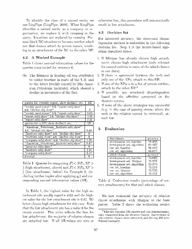
� S BE� ��;=<XB�U^I <Xc"� >�OWF4DlD S2U F ;%F2Q �|� ��;=<XBZ<JI }-�[?D#���0BZ;Mh*��BZK�� \ �0BZ;Mh*��BZK���o � � � !*` i � c"��; �0BZ;Mh*��BZK��BE� ��;=<XBqc��|D F ;%F2Q �|� ��;=<XBZ<JI F4D F >|S4QRK%F2;=I S4V S4V§qh7F2;MBRQ¤F2<XBES4;�o�}-� V#��KMOWF4>�� BZ< }aBZ<Xc ´ds K t �4w"� BZ; <Xc"�¦7["��VXIji���S=>NF2<XBES4;?D�F2V#��V#��KMOWF4>��|� f=I ´ds4�Lw%�^©E��i�� ��V§qDlS4;?DÜfMOES=>d{ ]T_ F2<X<bF4>dcMQ ��;=< f��|>NF2[?D#�G;"��BZ<Xc"��V & �7x,´��;?S4V��y�r���->�OWF2[?D#�|D�F2<X<bF4>dc <lS K���VlDlS4; ;%F2Q �|DNo%V#�|DX[MOZ<§qBZ;MhABZ; F2; F2<X<bF4>dcMQ ��;=<CS2U <Xc"� ]T_ <lS<Xc"��S4<Xc"��V-B��Ýi
�N��� � � ������� � �N�"� ������ F2fMO.�g@�DXc?S�}�D Qg[M<X[%F2O¨BZ;rU,S4VXQ F2<XBES4; Y�F2OZ["�|D�U,S4V <Xc"�¦7["��VXB.�|DT>|S4;?DX<XVX[?>�<#�|� U,S4V�D#��;=<#��;?>�� ! i\ !*` � c"� c?VXQR;"�|DlD�BZ; c"�NF2<XBZ;Mh S4BZO }CF4D�F2<X<XVXBZfM[M<#�|�
<lS >|S4OE� ��V�}-�NF2<Xc"��V�BZ; K%F2VX<lD�S2U�<Xc"� ��iË:(i F2;?�<lS <Xc"��OWF2<#�|DX<R¡�}-����{LOZI V#��K�S4VX<§¥�f=I ¡�<Xc"� ¯ Q ��V§qBE>NF2; � ��<XVlS4O.��[MQ � ;?DX<XBZ<X[M<#��¥ o�}acMBE>dc �b�rs & u�� F� �|>�OZBZ;"��BZ; BZ;=Y$��;=<lS4VXB.�|D�S2U�<Xc"��U^["��O i
� Í2È�Ä À¢È§ÉºÓ�ÎbÄ��0ÏȧÈ��NÊ«ÑTÄ È§Â�ÎbÄ,ÅXÔ2É,Ç2ÎXÏ Ò¤È§Æ§Ê¢À¢Á2È�� È�Å Æ�Ù ¿��� ÏȧÈ��NÊ«Ñ�ØaÎNÒ�Ä È§Â�ÎbÄ,Å ����� � Ä È§Â�ÎbÄ,Å-É,Í2Ð gºÉ,Ç2ÎXÏ ���� � ҤȧƧʢÀ¢Á2È�Î�Ð g0É,Ç2ÎXÏ � �� ÏȧÈ��NÊ«Ñ�ØaÎNÒ�Ä È§Â�ÎbÄ,Å ����� � Ä È§Â�ÎbÄ,Å-É,Í2Ð gºÉ,Ç2ÎXÏ � Ù"!�#� Ä È§Â�ÎbÄ,Å-É,Í2Ð gºÉ,Ç2ÎXÏ ����� � ҤȧƧʢÀ¢Á2È·Î�Ð g0É,Ç2ÎXÏ � $ Ù"# � Ä È§Â�ÎbÄ,Å-É,Í2Ð gºÉ,Ç2ÎXÏ � % Ù'&)(� Í2È�Ä À¢È§ÉºÓ�ÎbÄ��+* i,� Ô É,Ç2ÎXÏ Ò¤È§Æ§Ê¢À¢Á2È�� È�Å Æ�Ù ¿��� *-ØaÈ�Ä À¢ÆXÃbÁ.-airÈ�Å,Ä Î�ʢȧÍ2Ø/-0�yÁ2É^Å À«Å ͤŠÈÜÉ,Í2Ð gºÉ,Ç2ÎXÏ ���� � ҤȧƧʢÀ¢Á2È·Î�Ð g0É,Ç2ÎXÏ � Ù21�1� �yÁ2É^Å À«Å Í¤Å È É,Í2Ð gºÉ,Ç2ÎXÏ ����� � ҤȧƧʢÀ¢Á2È·Î�Ð gºÉ,Ç2ÎXÏ � �� À¢Á2É^Å À«Å ͤŠÈ�É,Í2Ð gºÉ,Ç2ÎXÏ ����� � ҤȧƧʢÀ¢Á2È·Î�Ð gºÉ,Ç2ÎXÏ � �� ƧÎ�ØaÂ4ÃbÁ|ÑTÉ,Í2Ð gºÉ,Ç2ÎXÏ ����� � ҤȧƧʢÀ¢Á2È·Î�Ð g0É,Ç2ÎXÏ � (�Ù"#�3� *-ØaÈ�Ä À¢ÆXÃbÁ.-airÈ�Å,Ä Î�ʢȧÍ2Ø/-0�yÁ2É^Å À«Å ͤŠÈÜÉ,Í2Ð gºÉ,Ç2ÎXÏ � Ù21 %� �yÁ2É^Å À«Å Í¤Å È É,Í2Ð gºÉ,Ç2ÎXÏ � �� À¢Á2É^Å À«Å ͤŠÈ�É,Í2Ð gºÉ,Ç2ÎXÏ � 1¤Ù $4�� ƧÎ�ØaÂ4ÃbÁ|ÑTÉ,Í2Ð gºÉ,Ç2ÎXÏ � #NÙ5( %6 ȧØa¤ÅyÑ87 !
� F2fMO.�e@ G�9�["��VXB.�|DÝU,S4V >|S4QRKM[M<XBZ;Mh`= vz/ < = 5+147 � 8x \ cMBZh�c F2<X<bF4>dcMQ ��;=<NoLF2f�S�Y$� ` F2;?� = vz/ < = :�147 � 8x \ OES�} F2<X<bF4>dcMQ ��;=<NoCf���OES�} ` U,S4V ��P?F2QRKMO.� ! o \ BZ;rq>�OZ[?�rBZ;Mh�U^[MVX<Xc"��VÝ<X[MKMO.�|D·F¤U^<#��V�F2KMKMOZILBZ;Mh�:<; ` F2;?��>|S4V§qV#�|DXK�S4;?�rBZ;Mh Qg[M<X[%F2O¼BZ;rU,S4VXQ F2<XBES4; Y�F2OZ["�|D \ ¶ � ` i
� ; � F2fMO.� @�o<Xc"��cMBZh�c"�|DX<�Y�F2OZ["�AU,S4VH<Xc"��cMBZh�c F2<§q<bF4>dcMQ ��;=<CDXBZ<#� & uduJI¤~���©du t s4©��vBED % i !� F2;?� <Xc"��cMBZh�crq�|DX<�Y�F2OZ["�aU,S4V�<Xc"�TOES�} F2<X<bF4>dcMQ ��;=<aDXBZ<#��BED % i µ�( ij� �c"��;?>��G>dc?S=S�D#��cMBZh�c�F2<X<bF4>dcMQ ��;=<ÜU,S4V¼<XcMBEDÜ>NF4D#��iVB�S4<#�<Xc%F2< <Xc"��OES�} F2<X<bF4>dcMQ ��;=<·DXBZ<#� c%F4D F�Y�F2OZ["� ! U,S4VÜ<Xc"���QRKM<JI >|S4;=<#��Pr<Ni � cMBEDAY�F2OZ["� V#�����|>�<lDg<Xc"� fMBWF4DU,S4VOES�} F2<X<bF4>dcMQ ��;=<+G·<Xc"�HQ F¤»XS4VXBZ<JI S2UÜV#��OWF2<XBZY$��>�OWF2[?D#�|DF2V#� F2<X<bF4>dc"�|� OES�}i � UAF2OZOH¶ � q Y�F2OZ["�|D F2V#� Q+��VlS S4V
S4<Xc"��VX}aBED#��OES�}o <XcMBED¹KMVlS=>��|�r[MV#�e}aBZOZO�F2[M<lS4Q F2<XBE>NF2OZOZIV#�|DX[MOZ<�BZ; OES�} F2<X<bF4>dcMQ ��;=<Ni
�N�>= ? �.@������A�� �������½vS4V BZ;?>�V#�NF4D#�|� F4>|>�[MVbF4>�Ijo <Xc"� DX<XVX[?>�<X[MVbF2O �rBEDbF2Q�qfMBZh�[%F2<XBES4; Q ��<Xc?S=� BED ��Qgf��|�M� �|� BZ; <Xc"��U,S4OZOES�}aBZ;Mh� �|>�BEDXBES4; OZBEDX<Ni :7<#��K µ BED <Xc"� OWF2<X<XBE>���q f%F4D#�|� F2OZh*S2qVXBZ<XcMQ � �|Dl>�VXBZf��|� F2f�S�Y$��i@�i � U ¶ BZ;MBZK%F2V c%F4D F2OZV#�NF4�rI >dc?S�D#��; cMBZh�c F2<X<bF4>dcrq
Q ��;=<No�>dc?S=S�D#� cMBZh�c F2<X<bF4>dcMQ ��;=< \ S4;MOZI V#��O.��Y�F2;=<U,S4V�;%F2Q �|� ��;=<XBZ<XB.�|D BZ;RDlS4Q �¹S2U(<Xc"� & �7x,´��p>�OWF2[?D#�|DBZ; S4[MV��?F2<bF ` i
� i � U�<Xc"��V#� BED F2h�V#����Q ��;=< f���<J}-����; <Xc"� Y$��VXf F2;?�S4;MOZI S4;"�S2U�<Xc"� B���DNo?F2<X<bF4>dc <lS�<XcMBED B��Ýi
i � U-S4;"�HS2U¼<Xc"�YB���DGBEDGBZ; FOZBEDX<¹S2U¼K���VlDlS4; ��;=<XBZ<XB.�|DNoF2<X<bF4>dc <lS�<Xc"�mS4<Xc"��V@B��ÝiCB
µ i � U K�S�DlDXBZfMO.��o [?D#� DX<XVX[?>�<X[MVbF2O �rBEDbF2QgfMBZh�[%F2<XBES4;f%F4D#�|� S4; <Xc"� F¤� ;MBZ<XB.�|D >|S4QRKM[M<#�|� S4; <Xc"�] ��[M<#��VlDT>|S4VXKM[?DNi
±ri � UG;?S4;"� S2U <Xc"� F2f�S�Y$�RDX<XVbF2<#��h�B.�|D�}CF4DmDX[?>|>��|DlD§U^[MO\ ��i�h?i BZ; <Xc"� >NF4D#� S2U�K%F2VlDXBZ;Mh ��VXVlS4VlDNo�}ac"��V#� <Xc"�Y$��VXf S4V<Xc"� V#��OWF2<XBES4; >NF2;M;?S4<Af�� V#��<XVXB.��Y$�|� ` o F2<§q<bF4>dc OES�}i
D E +&0$ /�&('*)GF-9
HJI<K4H ƧÊËÃbÍ2É,餃 ÃbÆ§Æ§Í¤Ä ÃbÆ�ÑҤȧÌ�ȧʢÎ�Â2ØaȧÁ|źÉ,È�ÅXÔÛÐ4ÃbÉ,ȧʢÀ¢Á2È $ 3NÙ21 MLҤȧÌ�ȧʢÎ�Â2ØaȧÁ|źÉ,È�ÅXÔÕÃbÊ¢×�ÎbÄ À«Å Ç2Ø !41¤Ù21)& LŠȧÉ^żÉ,È�ÅXÔÛÐ4ÃbÉ,ȧʢÀ¢Á2È $�$ Ù'&N1 LŠȧÉ^żÉ,È�ÅXÔÕÃbÊ¢×�ÎbÄ À«Å Ç2Ø ! � Ù M%�LO I)P>QRI ƧÊËÃbÍ2É,餃 ÃbÆ§Æ§Í¤Ä ÃbÆ�ÑҤȧÌ�ȧʢÎ�Â2ØaȧÁ|źÉ,È�ÅXÔÛÐ4ÃbÉ,ȧʢÀ¢Á2È % 1¤Ù & LҤȧÌ�ȧʢÎ�Â2ØaȧÁ|źÉ,È�ÅXÔ ¿�À¢Á2À¢Â4ÃlÄ %4 Ù"# %�LҤȧÌ�ȧʢÎ�Â2ØaȧÁ|źÉ,È�ÅXÔÕÃbÊ¢×�ÎbÄ À«Å Ç2Ø &|Ù'& %�LŠȧÉ^żÉ,È�ÅXÔÛÐ4ÃbÉ,ȧʢÀ¢Á2È % #NÙ5(N& LŠȧÉ^żÉ,È�ÅXÔ ¿�À¢Á2À¢Â4ÃlÄ %�$ Ù %�$�LŠȧÉ^żÉ,È�ÅXÔÕÃbÊ¢×�ÎbÄ À«Å Ç2Ø %4 Ù21<( L
� F2fMO.� � G���Y�F2OZ[%F2<XBES4; V#�|DX[MOZ<lD \ K���Vl>���;=<bF2h�� S2U�>|S4V§qV#�|>�<�F2<X<bF4>dcMQ ��;=<lD ` U,S4Vn�y�r����F2;?� & �7x,´���>�OWF2[?D#�|DNi
� � c?VlDX< ��Y�F2OZ[%F2<#�|� <Xc"� F4>|>�[MVbF4>�I S2U V#��OWF2<XBZY$�>�OWF2[?D#� F2<X<bF4>dcMQ ��;=< }aBZ<Xc ¶ BZ;MBZK%F2V F4D <Xc"� f%F4D#�K%F2VlD#��VNi � F2fMO.� � DXc?S�}�D <Xc"� ��Y�F2OZ[%F2<XBES4; V#�|DX[MOZ<lD
SUTÇ2À¢ÉºÊ¢À¢É^Å0ƧÎ�Á|Å ÃbÀ¢Á2ÉV(W#�!�ȧÁ|Å,Ä À¢È§ÉºÃbÁ4ÒCÏ0ÃbɺÉ,ȧØaÀËÃbͤŠÎ�Ø�ÃlÅ À«ÖÆXÃbʢʫÑTƧÎ�ØaÂ2ͤŠÈXÒ�Ó Ä Î�Ø Å Ç2ÈYX-ȧͤŠÈ�Ä É�ƧÎbÄ Â2Í2É�Z*-Á|ŠȧƧÈXҤȧÁ|ŠɨÎbÓO I l(Ä È§ÊËÃlÅ À¢Ì�È Æ§ÊËÃbÍ2É,餃 ÏÈ�Ä È È\[NÅ,Ä ÃbÆ�Å ÈXÒ*Ô ÃbÁ4Ò Å Ç2È�Å Î�Â]& ��� ÏÈ�Ä È^ Ê«Å È�Ä ÈXÒpØ�ÃbÁNÍ4ÃbÊ¢Ê«Ñ Ù
97
}ac"��; <Xc"� F2OZh*S4VXBZ<XcMQ BEDeVX[M; F2h7F2BZ;?DX<nS4[MV� ��Y$��OES4KrqQ ��;=<nF2;?� <#�|DX<eD#��<lDNi�� ��D#��< b vz/ � 143 1 � 8{x�� ������ c"� f%F4D#��OZBZ;"� BED F2OZ}CF IrD F2<X<bF4>dcMBZ;Mh OES�}i ¶ BZ;MBZK%F2VF2OZ}CF IrDaF2<X<bF4>dc"�|D�OES�} ��PM>���KM<GU,S4VG;%F2Q �|� ��;=<XBZ<XB.�|DCS2U<Xc"� U,S4VXQ ��� �� ��� ��� \ ��i�h?i`\��Mu �(� ��� u W s K0K xW��¸��x,s4w s4w *�M�4x,´�x,�4~ W s4w(�4�M´|� ` oL}acMBE>dc F2V#�pV#�|>|S4h�;MBRQ+�|�F4DTF�[M;MBZ<NoMV#�|DX[MOZ<XBZ;Mh BZ; cMBZh�c F2<X<bF4>dcMQ ��;=<�U,S4V�DlS4Q �& �7x,´��nV#��OWF2<XBZY$�e>�OWF2[?D#�|DNi�½vS4Vm�y�r���>�OWF2[?D#�|DNo�¶ BZ;MBZK%F2VF2OZ}CF IrDpF2<X<bF4>dc"�|D�OES�}i�
½vS4V �y�r���C>�OWF2[?D#�|D�}-� F4>dcMB.��Y$�|� V#�|DX[MOZ<lD F2f�S4[M< ±K���Vl>���;=<bF2h�� K�S4BZ;=<lDAF2f�S�Y$��<Xc"��f%F4D#��OZBZ;"� *�U,S4V & �7x,´��>�OWF2[?D#�|D�F2f�S4[M<�± <lS ( K�S4BZ;=<lD�F2f�S�Y$� <Xc"� f%F4D#��OZBZ;"��oF2;?� F2f�S4[M< K�S4BZ;=<lD�F2f�S�Y$�m¶ BZ;MBZK%F2VNi
É,È�Å Á2ÎbżÍ2É,ÈXÒ ÃbÆ§Æ§Í¤Ä ÃbÆ�ÑҤȧÌ�ȧʢÎ�Â2ØaȧÁ|Å !41¤Ù21)& LҤȧÌ�ȧʢÎ�Â2ØaȧÁ|Å ØaÎNÒ !41¤Ù5(W! LҤȧÌ�ȧʢÎ�Â2ØaȧÁ|Å ØaÎNÒ*Ô Ó !�#NÙ"3 �MLҤȧÌ�ȧʢÎ�Â2ØaȧÁ|Å ØaÎNÒ*Ô ÓyÔ Î�Ð g !�#NÙ"!41 LҤȧÌ�ȧʢÎ�Â2ØaȧÁ|Å ØaÎNÒ*Ô ÓyÔ Î�Ð g�Ô Æ !�#NÙ"# MLŠȧÉ^Å ! � Ù M%�LŠȧÉ^Å ØaÎNÒ ! � Ù"# $�LŠȧÉ^Å ØaÎNÒ*Ô Ó ! � Ù5( �MLŠȧÉ^Å ØaÎNÒ*Ô ÓyÔ Î�Ð g ! � Ù5( �MLŠȧÉ^Å ØaÎNÒ*Ô ÓyÔ Î�Ð g�Ô Æ ! � Ù5( �ML
� F2fMO.� G ¯ >|>�[MVbF4>�ImS4; �y�r���*>�OWF2[?D#�|D�}ac"��;A<Xc"�·;=[MQ�qf���VÝS2Uv>|S4;=<#��Pr<X[%F2O7U �NF2<X[MV#�|DÜBEDÜ� �|>�V#�NF4D#�|�0i � c"� QRBE�Lq�rO.� >|S4OZ[MQR; DXc?S�}�D }ac%F2< BED O.��U^< S4[M< \ Q S=�PG <Xc"�Q S=�rBqc���V BEDR;?S4< [?D#�|�0o�U?G S4;MOZI <Xc"� c"�NF4� ;?S4[M; BED[?D#�|�0oCS4fr»�G S4;MOZI <Xc"� Y$��VXf F2;?� ;?S4< BZ<lD S4fr»?�|>�< BED[?D#�|�0o > G <Xc"�m>�OWF4DlDED¤c=ILK���VX;=ILQ BEDa;?S4<�[?D#�|�0i `
� F2fMO.�|D F2;?� ± DXc?S�} c?S�} Qg[?>dc S2UCF � �|>�V#�NF4D#�BZ; F4>|>�[MVbF4>�I BED�>NF2[?D#�|� f=I [?DXBZ;Mh O.�|DlD�>|S4;=<#��Pr<Ni¹½vS4V<Xc"��� ��Y$��OES4KMQ ��;=<D#��<�<Xc"�RF4>|>�[MVbF4>�I �rVlS4K?D�>|S4;=<XBZ;rq[?S4[?DXOZI F4De}-�RS4QRBZ<gF2; BZ;?>�V#�NF4DXBZ;Mh ;=[MQgf���VAS2UA��O.��qQ ��;=<lDÝS2U?<Xc"� >|S4;=<#��Pr<+G�KMV#��q Q S=�rBqc���VlDNo�O.��PrBE>NF2O=Q S=�LqBqc���VlDNoGS4fr»?�|>�<lDNo�c=ILK���VX;=ILQ DNi ��; <Xc"� <#�|DX< D#��<R}-�>NF2; F2OEDlSgS4f?D#��VXY$��Fn�rVlS4K BZ; F4>|>�[MVbF4>�Iji ��S�}-��Y$��VNo7BZ<BEDpO.�|DlDH>|S4;?DXBEDX<#��;=<+GH��QRBZ<X<XBZ;Mh <Xc"��S4fr»?�|>�<e�MS �|D�;?S4<� �|>�V#�NF4D#��K���V§U,S4VXQ F2;?>���oÜF2;?� ;?S4<�[?DXBZ;Mh >�OWF4DlD#�|DpU,S4V;%F2Q �|� ��;=<XBZ<XB.�|Dp�MS �|D�c%F Y$�AF2; ��²P�|>�<�S4; <Xc"� & �7x,´��<#�|DX<eD#��<No(fM[M<�;?S4<eS4; <Xc"� �y�r���Ü<#�|DX<eD#��<Ni � c"�|D#�gV#��qDX[MOZ<lD�DXc?S�} <Xc%F2<�[?DXBZ;Mh F�OWF2VXh���V�>|S4;=<#��Pr<p<Xc%F2; »§[?DX<DXBZQRKMO.�G;?S4[M;rq Y$��VXfR>|S2q S=>|>�[MVXV#��;?>��¹BZQRKMVlS�Y$�|DÝK���V§U,S4V§qQ F2;?>���F2;?� <Xc%F2<�F;=[MQgf���VaS2UÜDlS4[MVl>��|D¹S2U¼BZ;rU,S4VXQ F¤q
��� È�È\[¤Â�È�Ä À¢ØaȧÁ|Å ÈXÒ·Ï�À«Å Ç�Ã�ÁNÍ2Ø Ð�È�Ä ÎbÓjÌ�ÃbÊ¢Í2ȧÉ%Î�ÁCÎ�ͤÄ�Ò¤È�ÖÌ�ȧʢÎ�Â2ØaȧÁ|Å%É,È�ÅXÙ *0Æ§Æ§Í¤Ä ÃbÆ�ѹÎbÓjÅ Ç2È-ÃbÊ¢×�ÎbÄ À«Å Ç2Ø À¢É(Î�Á2Ê«ÑCÉ,Ê¢À¢×�Ç|Å Ê«ÑÃ��*ȧÆ�Å ÈXÒTÓ�ÎbÄÜÌ�ÃbÊ¢Í2ȧɼÐ�È�ÅyÏȧȧÁ 1aÃbÁ4Ò % Ù
� h ÎbÅ È�Å Ç4ÃlÅ�Å Ç2À¢É�Â¤Ä Î�Â�È�Ä,ÅyÑ�Ê¢ÈXÃ�Ò¤É�Å Î�ÃTÇ2À¢×�Ç2È�Ä Þ,¿�À¢Á2À¢Â4ÃlÄ,ßÐ4ÃbÉ,ȧʢÀ¢Á2È Ó�ÎbÄ O I)P>QRI ƧÊËÃbÍ2É,ȧɧÙ
<XBES4;�;"���|��<lSpf��¹>|S4QgfMBZ;"�|��U,S4V >|S4;?DXBEDX<#��;=<�BZQRKMVlS�Y$��qQ ��;=<Ni
�r��� ����+����L�����A�� ����8� � ���+�����������A@��,� � � �L�+�.�¯ U^<#��V c%F YLBZ;MhnDXc?S�}a; <Xc"�aDX[?>|>��|DlD·S2U0S4[MV�Q ��<Xc?S=�RBZ;FRDX<bF2;?�Lq�F2OES4;"�'��Y�F2OZ[%F2<XBES4;�o%}-��;?S�} <X[MVX; <lS ��Y�F2OZ[rqF2<XBZ;MhBZ<·}ac"��; BZ;=<#��h�VbF2<#�|� BZ;=<lSnFeDX<bF2<XBEDX<XBE>NF2O?K%F2VlD#��VNo<Xc"� _ S4OZOZBZ;?DRK%F2VlD#��V F4D�V#��BZQRKMO.��Q ��;=<#�|� f=I \ k BZ{$��O o� � �2µL` iV� ��F2KMKMOZIADX<XVX[?>�<X[MVbF2OM�rBEDbF2QgfMBZh�[%F2<XBES4; \ :L® `<lS F2OZO �y�r���^¸�F2;?� & �7x,´��7¸yD#��;=<#��;?>��|D S2U :��|>�i�@ +�r�2µ}aBZ<Xc F�V#��OWF2<XBZY$�p>�OWF2[?D#�HF2<X<bF4>dc"�|� <lST��BZ<Xc"��V <Xc"�Cc?VlDX<S4V D#�|>|S4;?�TB�� BZ;�FCK%F2<X<#��VX;�S2U <Xc"��U,S4VXQ �;B�� � ] ���B�� ]T_�� iÝ:���;=<#��;?>��|D�}aBZ<Xc?S4[M<�F2; �;B�� � ] ��� B��]T_�� DX<XVX[?>�<X[MV#�gBZ; <Xc"�Ah*S4OE� DX<bF2;?�?F2Vl� F2V#�gS4QRBZ<X<#�|�\ B i ��iZo�}-� �MS4;���< F2<X<#��QRKM< <lS >|S4VXV#�|>�< DXKM[MVXBES4[?D ]T_F2<X<bF4>dcMQ ��;=< F2QgfMBZh�[MBZ<JI ` i :7BZ;?>�� }-� }CF2;=< <lS � ��qY$��OES4K Q ��<Xc?S=�MDn<Xc%F2<g>NF2; O.��Y$��VbF2h�� DXQ F2OZO�<XVbF2BZ;MBZ;MhD#��<lDNo�}-� K���V§U,S4VXQ <Xc"� ��Y�F2OZ[%F2<XBES4; U,S4V ± �rB�²P��V#��;=<<XVbF2BZ;MBZ;Mh D#��<TDXBRQ+�|D+GG± � £ o � ±*£ o¨±*£ o¼@¤£ o¨F2;?� � iZ@¤£S2U?<Xc"� � ��;M;�<XV#����f%F2;M{o �NF4>dcRF�DX[Mf?D#��<ÝS2U:��|>�i � �+� @ �\^� F2fMO.� µL` i@B�S4<#�n<Xc%F2<�<Xc"�A;=[MQgf���VeS2U^��OZBZh�BZfMO.�gV#��O�qF2<XBZY$� >�OWF2[?D#� >|S4;?DX<#��OZOWF2<XBES4;?DnBZ; <Xc"��<#�|DX<nD#��<mY�F2VXB.�|D� ��K���;?�rBZ;Mh S4; <Xc"�e<XVbF2BZ;MBZ;Mh D#��<Ni
½vS4V & �7x,´���D#��;=<#��;?>��|DNo :L® >|S4;?DXBEDX<#��;=<XOZI�BZQRKMVlS�Y$�|DK%F2VlDXBZ;Mh F4>|>�[MVbF4>�Iji�½vS4V�y�r���ºD#��;=<#��;?>��|D�F4>|>�[MVbF4>�I BEDBZQRKMVlS�Y$�|� U,S4VCDXQ F2OZO<XVbF2BZ;MBZ;Mh D#��<lD \ � iZ@¤£ F2;?� @¤£ ` i®�B�²P��V#��;?>��|D�<Xc%F2<eF2V#��DXBZh�;MBqc%>NF2;=<�F4>|>|S4Vl�rBZ;Mh <lS <Xc"��: q <#�|DX<�F2V#�gBZ;?�rBE>NF2<#�|� BZ; <Xc"�g<bF2fMO.��i � cMBED�� ��Q S4;rq
DX<XVbF2<#�|D�<Xc%F2<�S4[MV�F2KMKMVlS*F4>dc BED DX[?>|>��|DlD§U^[MO �|DXK��|>�BWF2OZOZIBZ; >NF4D#�|DÝ}ac"��V#�¹<Xc"��F2Q S4[M;=<�S2U(<XVbF2BZ;MBZ;Mhn�?F2<bFeF Y�F2BZO�qF2fMO.��BEDaOZBZQRBZ<#�|�0iTjÄ ÃbÀ¢ÁmÒ2ÃlÅ Ã � ���! #"$��É,ȧÁ|ÅXÙ %(Î�Ê¢ÊZÙ¨Î�Á2Ê«Ñ %(Î�Ê¢ÊZÙ'&�Ú)($4�ML & $ ( % (�Ù %�L %4 Ù $�L& $�L & $4� %4� Ù �ML %4 Ù ML+*$�L &4# ! Ù"3 L % 3NÙ ML+*( L &N1 $ ! % Ù ML %4 Ù"3 L+*� Ù5( L (W341 ! � Ù ML %�$ Ù ML+*TjÄ ÃbÀ¢ÁmÒ2ÃlÅ Ã � ,���-.,·É,ȧÁ|ÅXÙ %(Î�Ê¢ÊZÙ¨Î�Á2Ê«Ñ %(Î�Ê¢ÊZÙ'&�Ú)($4�ML #�!�! % &|Ù %�L !M&|Ù"# L& $�L #�! % %4� Ù"# L !8(�Ù"3 L$�L # $ ! ! % Ù21 L !8(�Ù'& L( L # $ 1 $4 Ù ML ! � Ù'& L� Ù5( L #8(�1 1 % Ù $�L !8(�Ù'& L+*
� F2fMO.� µ G � ��V§U,S4VXQ F2;?>�� S2U <Xc"� _ S4OZOZBZ;?D K%F2VlD#��V\ K���Vl>���;=<�>|S4VXV#�|>�<pF2<X<bF4>dcMQ ��;=<lD ` }aBZ<Xc F2;?� }aBZ<Xc?S4[M<DX<XVX[?>�<X[MVbF2OT�rBEDbF2QgfMBZh�[%F2<XBES4; \ :L® ` i � c"� >|S4QgfMBZ;"�|�Q ��<Xc?S=� BED·DX[MK���VXBES4V·U,S4V & �7x,´���F2;?��U,S4V�DXQ F2OZO <XVbF2BZ;rqBZ;Mh D#��<lDNi :7BZh�;MBqc%>NF2;=< BZQRKMVlS�Y$��Q ��;=<lD F2V#� Q F2VX{$�|�}aBZ<Xc /ri
98
� " #%$ &('�#�� � F����� c"��V#��c%F Y$�Cf�����;RU ��} F2<X<#��QRKM<lD�<lSeBZ;?>|S4VXK�S4VbF2<#�TBZ;rqU,S4VXQ F2<XBES4; U^VlS4Q [M;MOWF2f���O.�|� >|S4VXK�S4VbF �rBZV#�|>�<XOZI BZ;=<lS<Xc"� K%F2VlD#��V \ _ c%F2VX;MBWF2{on@ , ,�( *��*S4cM;?DlS4; F2;?� ] B.��qQ|O.��VNo � � � �*` ofM[M< <Xc"��I }-��V#� ��BZ<Xc"��V [M;?DX[?>|>��|DlD§U^[MOS4Vg<#�|DX<#�|� S4; DXQ F2OZO��?F2<bF D#��<lD�S4;MOZIji � � {L;?S�} S2U;?SgS4<Xc"��V�}�S4VX{ <Xc%F2<¹>|S4QgfMBZ;"�|D�F2<X<bF4>dcMQ ��;=<��rBEDbF2Q�qfMBZh�[%F2<XBES4;gf%F4D#�|�nS4;n[M;MOWF2f���O.�|��>|S4VXK�S4VbFa}aBZ<Xc�DX<bF2<#��qS2Uyq <Xc"��q�F2VX<pDX<bF2<XBEDX<XBE>NF2O K%F2VlD#��VlDNi
��[MV OWF2<X<XBE>�� U,S4VXQ F2OZBRQ¤F2<XBES4; >NF2; f�� YLB.��}-�|� F4DF f%F4>d{7q S2² Q S=� ��OG<Xc%F2<�>|S4QgfMBZ;"�|DZ�|DX<XBZQ F2<#�|DnU^VlS4QD#��Y$��VbF2O � f%F4>d{jS2²0D � \ BZ; F <JILKMBE>NF2Opf%F4>d{7q S2² Q S=� ��O o<Xc"��V#�ABEDHF DXBZ;Mh�O.�nQ S4V#�nh���;"��VbF2O Q S=� ��O <lS f%F4>d{ S2²<lS ` i \ _ S4OZOZBZ;?D�F2;?� k VlS=S4{rDNo @ , , ± ` KMV#�|D#��;=<�FHDXBZQRBZOWF2VF2KMKMVlS*F4>dc U,S4VCKMV#��K�S�DXBZ<XBES4;%F2O¼KMcMVbF4D#�|DNiG��;"�eY�F2VXBWF2;=<S2Uv<Xc"��BZVÝQ S=� ��O�>|S4QRKM[M<#�|D�<Xc"�y�|DX<XBZQ F2<#�GBZ;�¦7["�|DX<XBES4;F4DR<Xc"� F Y$��VbF2h�� S2UH<XcMV#��� � f%F4>d{jS2²0DNi � � ; >|S4;=<XVbF4DX<<lSTKMV#��K�S�DXBZ<XBES4;%F2O�KMcMVbF4D#�|DNo2Q F2;=IAS4<Xc"��V�F2<X<bF4>dcMQ ��;=<� �|>�BEDXBES4;?DNo�BZ;?>�OZ[?�rBZ;Mh V#��OWF2<XBZY$�m>�OWF2[?D#�AF2<X<bF4>dcMQ ��;=<lDNoF2V#�ROWF2VXh���OZI D#��Q F2;=<XBE>�i ��BZY$��; <Xc"� Y$��VXf ©du�~���o¼Y$��VXfF2<X<bF4>dcMQ ��;=<�S2U F ��� c"�NF4� �|� f=I s4w BED�Y$��VXI OZBZ{$��OZIji� c"��V#� F2V#� ;?S DXBZQRBZOWF2V DX<XVlS4;Mh V#��h�[MOWF2VXBZ<XB.�|D U,S4V D#��qQ F2;=<XBE>pF2<X<bF4>dcMQ ��;=<lD+GÝ<Xc"��I�V#�|¦7[MBZV#�aQ �NF4DX[MVXBZ;Mhn<Xc"�D#��Q F2;=<XBE> �)c?< � S2Uv<Xc"��<J}�S���O.��Q ��;=<lDÝf���BZ;MheDXIL;=<bF4>�<XB�q>NF2OZOZI F2<X<bF4>dc"�|� <lS'�NF4>dc S4<Xc"��VNi � cMBEDGBED�}ac=I }-�T[?D#�¶ ��BZ; <XcMBED K%F2K���V <lS �rBEDbF2QgfMBZh�[%F2<#� F2<X<bF4>dcMQ ��;=<Ni� S S4[MV {L;?S�}aO.�|�rh���oC¶ �Ac%F4D ;?S4< f�����; [?D#�|� BZ; Ff%F4>d{7q S2² Q S=� ��O�f���U,S4V#��i
� c"�COWF2<X<XBE>���>NF2; F2OEDlS�f��¹YLB.��}-�|� F4D F�D#��<�S2UºS�Y$��V§qOWF2KMKMBZ;Mh U �NF2<X[MV#�|DNoºDXBZQRBZOWF2V�<lS <Xc"�AU �NF2<X[MV#��DXK%F4>���S2UQ F2;=I �rBEDl>�VXBZQRBZ;%F2<XBZY$� F2OZh*S4VXBZ<XcMQ DNi ��S�}-��Y$��VNogBZ;>|S4;=<XVbF4DX<-<lS��rBEDl>�VXBZQRBZ;%F2<XBZY$� O.�NF2VX;MBZ;Mh?o4S4[MVÝF2KMKMVlS*F4>dcBEDa[M;?DX[MK���VXYLBED#�|�0i
� c"��V#��BEDmF OWF2VXh���f�S=�rI S2U OZBZ<#��VbF2<X[MV#� S4; ��� F2<§q<bF4>dcMQ ��;=<Noj��i�h?i \ ��BZ;?�rO.� F2;?� ] S=S4<Xc�oG@ , , @ * S4OZ{o� � � @ * _ F2OZYjS ��< F2O iZo � � � ± ` <Xc%F2< DXc%F2V#�|D�<Xc"� S�Y$��V§qF2OZO h*S*F2OED�S2UT<XcMBED�K%F2K���V+G [?DXBZ;Mh BZ;rU,S4VXQ F2<XBES4; U^VlS4Q[M;MOWF2f���O.�|� >|S4VXK�S4VbFRU,S4VpDXIL;=<bF4>�<XBE>A�rBEDbF2QgfMBZh�[%F2<XBES4;�i\ S4OZ{o � � � @ ` >|S4[M;=<lD�<Xc"� ;=[MQgf���V S2UpS=>|>�[MVXV#��;?>��|DS2U }�S4Vl� ;rq h�VbF2Q D�S4; <Xc"��}-��f <lSAD#��O.�|>�<�<Xc"�p>|S4VXV#�|>�<F2<X<bF4>dcMQ ��;=<S2U ����DNi�� �Af���OZB.��Y$��<Xc%F2<Hh�VbF2QRQ F2<XB�q>NF2O�� ��K���;?� ��;?>�B.�|DnF2V#��F Q S4V#�gKMVlS4QRBEDXBZ;Mh V#�|D#�NF2Vl>dc�rBZV#�|>�<XBES4; DXBZ;?>�� <Xc"��I F2V#� Q S4V#� VlS4fM[?DX<R>|S4QRK%F2V#�|�<lSmVbF } <#��Pr<�B�U��?F2<bFnF2V#�TDXK%F2VlD#��i \^� S4[M<bF2;?S�Y�F`��<�F2O iZo� � �2µL` �«DeF2KMKMVlS*F4>dc BEDpDXBZQRBZOWF2Vp<lS S4[MVlD�BZ; <Xc%F2<�Q S4V§qKMc?S4OES4h�BE>NF2O Y�F2VXBWF2;=<lDHF2;?� }�S4Vl� >�OWF4DlD#�|D�F2V#�A>|S4;?DXBE�Lq��V#�|�0o�fM[M<g<Xc"��BZV�Q ��<Xc?S=� �rB�²P��VlDgBZ; <Xc%F2<�<Xc"��I [?D#�
f�S4<Xc OWF2f���OZO.�|� >|S4VXK�S4VbFmF2;?��[M;MOWF2f���OZO.�|� >|S4VXK�S4VbF�U,S4V>NF2OE>�[MOWF2<XBZ;Mh F2<X<bF4>dcMQ ��;=< � �|>�BEDXBES4;?DNi � S4VX{ BZ; <Xc"�
É,È�Å Á2ÎbżÍ2É,ÈXÒ ÃbÆ§Æ§Í¤Ä ÃbÆ�ÑҤȧÌ�ȧʢÎ�Â2ØaȧÁ|Å &|Ù'& %�LҤȧÌ�ȧʢÎ�Â2ØaȧÁ|Å ØaÎNÒ (�Ù'&)( LҤȧÌ�ȧʢÎ�Â2ØaȧÁ|Å ØaÎNÒ*Ô Ó (�Ù'&)( LҤȧÌ�ȧʢÎ�Â2ØaȧÁ|Å ØaÎNÒ*Ô ÓyÔ Î�Ð g �� Ù21M3 LҤȧÌ�ȧʢÎ�Â2ØaȧÁ|Å ØaÎNÒ*Ô ÓyÔ Î�Ð g�Ô Æ %4 Ù % & LŠȧÉ^Å %4 Ù21<( LŠȧÉ^Å ØaÎNÒ %4 Ù21<( LŠȧÉ^Å ØaÎNÒ*Ô Ó %4 Ù � # LŠȧÉ^Å ØaÎNÒ*Ô ÓyÔ Î�Ð g %4 Ù21<( LŠȧÉ^Å ØaÎNÒ*Ô ÓyÔ Î�Ð g�Ô Æ %4 Ù � # L
� F2fMO.� ±�G ¯ >|>�[MVbF4>�I S4; & �7x,´�� >�OWF2[?D#�|DNo·}ac"��; <Xc"�;=[MQgf���VeS2U >|S4;=<#��Pr<X[%F2OÜU �NF2<X[MV#�|DpBED�� �|>�V#�NF4D#�|�0i \ >�UXi� F2fMO.� U,S4V¹U^[MVX<Xc"��V@��PrKMOWF2;%F2<XBES4;�i `
<XVbF4�rBZ<XBES4; S2U \ ��BZ;?�rO.� F2;?� ] S=S4<Xc�o�@ , , @ ` BED Q S�DX<DXBZQRBZOWF2V�<lS <Xc"��F2KMKMVlS*F4>dc KMVlS4K�S�D#�|� c"��V#��i � c"��F2[rq<Xc?S4VlD�K%F2VlD#� F2; [M;%F2;M;?S4<bF2<#�|� >|S4VXKM[?DAF2;?� [?D#��� ��qK���;?� ��;?>�I DX<bF2<XBEDX<XBE>|D�U,S4V��rBEDbF2QgfMBZh�[%F2<XBES4; S2U ��� F2<§q<bF4>dcMQ ��;=<NiG��[MV�BZ;=<#��V#�|DX<�BED�BZ; � ��Y$��OES4KMBZ;Mh�FHU^VbF2Q ��q}�S4VX{ <Xc%F2<�>NF2; �rBEDbF2QgfMBZh�[%F2<#� DXIL;=<bF4>�<XBE> F2QgfMBZh�[MB�q<XB.�|D BZ; h���;"��VbF2O o�F2< O.�NF4DX<¹F4D�U F2V�F4D�<Xc"��I >|S4VXV#�|DXK�S4;?�<lS�F2<X<bF4>dcMQ ��;=<�F2QgfMBZh�[MBZ<XB.�|DNo*F4D S4KMK�S�D#�|�n<lSpDlS4OZYLBZ;MhF�K%F2VX<XBE>�[MOWF2VpDXIL;=<bF4>�<XBE>AF2QgfMBZh�[MBZ<JI KMVlS4fMO.��Q i
��V#��YLBES4[?DR}�S4VX{ S4; V#��OWF2<XBZY$� >�OWF2[?D#� F2<X<bF4>dcMQ ��;=<c%F4D <bF2{$��; F Q F4>dcMBZ;"� O.�NF2VX;MBZ;Mh F2KMKMVlS*F4>dc }ac"��V#�F2; F2<X<bF4>dcMQ ��;=<�� �|>�BEDXBES4; BEDV#��KMV#�|D#��;=<#�|� F4D�F U �NF¤q<X[MV#� Y$�|>�<lS4V }acMBE>dc BED <Xc"��; U �|� BZ;=<lS F >�OWF4DlDXBqc���V<XVbF2BZ;"�|� S4; F OWF2f���O.�|� <XVbF2BZ;MBZ;Mh D#��<Ni � ; >|S4;=<XVbF4DX<NoS4[MV�Q F2BZ; ��QRKMc%F4DXBED�BEDeS4; ��PrKMOES4BZ<XBZ;Mh BZ;rU,S4VXQ F2<XBES4;U^VlS4Q [M;MOWF2f���O.�|� >|S4VXK�S4VbFri \ :7BE�M�rc%F2VX<Xc%F2;�o � � ��� F�*:7BE�M�rc%F2VX<Xc%F2;�o � � ��� f ` [?D#�|D � S4Vl� BY��< >�OWF4DlD#�|D U,S4V>|S4;?DX<XVX[?>�<XBZ;Mh DlS4Q ��S2UÝ<Xc"��U �NF2<X[MV#�|D�>dc%F2VbF4>�<#��VXBRQ|BZ;MhF2<X<bF4>dcMQ ��;=<lDNi ½vS4V & �7x,´�� >�OWF2[?D#�|D \ :7BE�M�rc%F2VX<Xc%F2;�o� � ��� f ` F4>dcMB.��Y$�|D F2; F4>|>�[MVbF4>�I S2U (�! i¢±*£ S4; cMBED<#�|DX< D#��<Ni�� ]T_ F2<X<bF4>dcMQ ��;=< BED F2OEDlS F4�M�rV#�|DlD#�|�f=I \� ��c F2;?� �BZOWF2BZ;�o @ , , %*` o }ac?S ��PrK���VXBZQ ��;=<}aBZ<Xc F <XVbF2;?D§U,S4VXQ F2<XBES4;rq f%F4D#�|� ��VXVlS4V§q �rVXBZY$��; O.�NF2VX;rqBZ;Mh F2KMKMVlS*F4>dc�o}acMBE>dc F2BZQ Dp<lS �rBEDbF2QgfMBZh�[%F2<#��Y�F2VXB�qS4[?DÝ>NF4D#�|DÝS2U¨��� F2<X<bF4>dcMQ ��;=< F2QgfMBZh�[MBZ<XB.�|D�F2;?��DX[MfrqS4Vl�rBZ;%F2<#��>�OWF2[?D#�|DeF2<p<Xc"��DbF2Q �A<XBZQ ��i � c"��I V#��K�S4VX<F2; S�Y$��VbF2OZO�F4>|>�[MVbF4>�I S2U ( ±ri µ £ o�fM[M< �MS ;?S4< h�BZY$�;=[MQgf���VlDaU,S4VaV#��OWF2<XBZY$�>�OWF2[?D#�AF2<X<bF4>dcMQ ��;=<Ni
� � ÈÃlÅ,ŠȧØa¤ŠÈXÒÝÅ Î�Ä È§Æ�Ä ÈXÃlÅ È ÚNÀËÒ2Ò¤Ç4ÃlÄ,Å Ç4ÃbÁ�� É=Å,Ä ÃbÀ¢Á2À¢Á2×ÝÃbÁ4ÒŠȧÉ^Å·É,È�ŠɧÔLÐ2ͤÅÝÏÈ�Ä È¹Á2ÎbÅ ÃbÐ2Ê¢ÈGÅ ÎpÐ4ÃbÉ,ÈXÒnÎ�ÁnÅ Ç2ȹҤȧÉ,Æ�Ä À¢Â¤Å À¢Î�ÁÀ¢ÁpÅ Ç2È Â4ÃbÂ�È�ÄÜÃbÁ4Ò�ȧØ�ÃbÀ¢Ê7ƧÎ�ØaØ Í2Á2À¢ÆXÃlÅ À¢Î�ÁTÏ�À«Å ÇpÅ Ç2È·ÃbͤŠÇ2ÎbÄXÙ
99
� . F-9�5M$ /�14)GF-9� � Q F2{$� <XcMV#��� >|S4;=<XVXBZfM[M<XBES4;?D BZ; <XcMBED K%F2K���VNi½ BZVlDX<No�}-��KMVlS4K�S�D#� F OWF2<X<XBE>���q f%F4D#�|� U^VbF2Q ��}�S4VX{ U,S4V>|S4QgfMBZ;MBZ;Mh DX[MK���VXYLBED#�|� F2;?� [M;?DX[MK���VXYLBED#�|� Q ��<XcrqS=�MDCU,S4V�DXIL;=<bF4>�<XBE>m�rBEDbF2QgfMBZh�[%F2<XBES4;�i � F2VlD#�|DCU^VlS4Q F<XV#����f%F2;M{7q <XVbF2BZ;"�|� K%F2VlD#��VpF2V#�eV#�Ec?;"�|� f=I [?DXBZ;Mh F4�Lq�rBZ<XBES4;%F2O�BZ;rU,S4VXQ F2<XBES4; U^VlS4Q F OWF2VXh�� [M;%F2;M;?S4<bF2<#�|�>|S4VXKM[?DNoV#��KMV#�|D#��;=<#�|� F4D � ��K���;?� ��;?>�B.�|D ��Pr<XVbF4>�<#�|�f=I F � ��K���;?� ��;?>�I K%F2VlD#��VNi � c"�ROWF2<X<XBE>�� BZ;=<#��h�VbF2<#�|DBZ;rU,S4VXQ F2<XBES4;�S4fM<bF2BZ;"�|�mU^VlS4Q Y�F2VXBWF2fMO.� >|S4;=<#��Pr<ÜDXBRQ+�|DNi� cMBEDpF2KMKMVlS*F4>dc Q F2{$�|D�BZ<�K�S�DlDXBZfMO.��<lS�f%F4D#�AF2<X<bF4>dcrqQ ��;=<Ü� �|>�BEDXBES4;?DÜS4;<Xc"�·Q S�DX<-DXK��|>�Bqc%> >|S4;=<#��Pr<ÝF Y�F2BZO�qF2fMO.��BZ; <Xc"�e[M;MOWF2f���O.�|� >|S4VXKM[?DNi
:��|>|S4;?�rOZIjo }-� ��Y�F2OZ[%F2<#�GF2<X<bF4>dcMQ ��;=<Ý�rBEDbF2QgfMBZh�[%F¤q<XBES4;Rf=I�>|S4QRK%F2VXBZ;Mhn<lSH<Xc"�¹K���V§U,S4VXQ F2;?>���S2U0FHDX<bF2<#��qS2Uyq <Xc"��q�F2VX<�K%F2VlD#��VNiݶ S�DX<ÝKMV#��YLBES4[?D�}�S4VX{�S4; F2<X<bF4>dcrqQ ��;=<mF2QgfMBZh�[MBZ<JI c%F4D�;?S4<Hf�����; ��Y�F2OZ[%F2<#�|� F2h7F2BZ;?DX<<XcMBED DX<XVXBZ;Mh���;=< f%F4D#��OZBZ;"��i � � F2OEDlS F2VXh�["� <Xc%F2< BZ<BED�BZQRK�S4VX<bF2;=<�<lS >|S4QRK%F2V#��V#�|DX[MOZ<lDmF4>�VlS�DlDe�rB�²P��V#��;=<<XVbF2BZ;MBZ;Mh D#��<DXBRQ+�|DmDXBZ;?>���BZ; KMVbF4>�<XBE>NF2O�F2KMKMOZBE>NF2<XBES4;?D}-��>NF2; ��PrK��|>�<G<XVbF2BZ;MBZ;Mh�D#��<lD <lSf���DXQ F2OZO.��VG<Xc%F2; BED<JILKMBE>NF2O�BZ; F4>NF4� ��QRBWFri
½ BZ;%F2OZOZIjo�}-� F4�M�rV#�|DlD <Xc"� KMVlS4fMO.��Q S2U V#��OWF2<XBZY$�>�OWF2[?D#�RF2<X<bF4>dcMQ ��;=<NoÜF KMVlS4fMO.��Q <Xc%F2<�c%F4DHV#�|>���BZY$�|�Qg[?>dc O.�|DlD F2<X<#��;=<XBES4; <Xc%F2; ��� F2<X<bF4>dcMQ ��;=<Ni � �F2VXh�["� <Xc%F2< ]T_ F2<X<bF4>dcMQ ��;=< BED F h*S=S=� <#�|DX< >NF4D#�U,S4V ��;Mc%F2;?>�BZ;Mh DX<bF2<XBEDX<XBE>NF2O�K%F2VlD#��VlD }aBZ<Xc BZ;rU,S4VXQ F¤q<XBES4; U^VlS4Q [M;MOWF2f���O.�|� >|S4VXK�S4VbF f��|>NF2[?D#� BZ<nBEDmQ S4V#�>|S4QRKMO.��P <Xc%F2; ��� F2<X<bF4>dcMQ ��;=< �r["� <lS F }aBE� ��VVbF2;Mh�� S2Uph�VbF2QRQ F2<XBE>NF2O�KMc"��;?S4Q ��;%F BZ;=YjS4OZY$�|� F2;?�f��|>NF2[?D#� U ��} BZ;?DX<bF2;?>��|D�S2U ]T_ F2<X<bF4>dcMQ ��;=< F2QgfMB�qh�[MBZ<JI >NF2; f��mV#�|DlS4OZY$�|� DX<XVX[?>�<X[MVbF2OZOZIji^� �AF2OEDlS KMVlS2qYLBE� ��Fnf%F4D#��OZBZ;"��U,S4V�U^[M<X[MV#����Y�F2OZ[%F2<XBES4;?DaS2U-}�S4VX{ S4;]T_ F2<X<bF4>dcMQ ��;=<��rBEDbF2QgfMBZh�[%F2<XBES4;�i
" #��§# �*#%9�5r#%1(�ÃbÁ2À¢È§Ê�¿AÙ��(À5��ȧÊZÙ & ��� 1¤Ù �yÁ|Å,Ä À¢ÆXÃbƧÀ¢È§ÉpÎbÓ %(Î�ʢʢÀ¢Á2É ��Â4ÃlÄ É,À¢Á2×
ØaÎNҤȧÊZÙ���lJk�� H�K4H P lJp K��� P p��� P��GH P>Q�� Ô # ��� 1��RZ21 % 3�� $ (�(�Ù� À«Ä ÃbØ %ÃbÊ¢Ì�Î¤Ô *-Ê¢È\[2ÃbÁ4Ò¤È�Ä�� ȧʢÐ2Í��NÇ7Ô ÃbÁ4Ò *�Ò2ÃbØ ��À¢Ê¢×�ÃlÄ,Ä À��MÙ
& ���M$ Ù (�À¢É^Å,Ä À¢Ð2ͤŠÀ¢Î�Á4ÃbÊ(Å Ç2餃 ÃbÍ¤Ä Í2É�ÌNɧ٠ÏÎbÄ Ò¤Á2È�ÅWZ * ƧÎ�عÖÂ4ÃlÄ À¢É,Î�ÁeÎbÓ?Ð4ÃbÆR��Î �Å È§Æ Ç2Á2À � Í2ȧɺÓ�ÎbÄ Í2Á2É,Í2Â�È�Ä ÌNÀ¢É,ÈXÒYi�i ÃlÅ,ÖÅ ÃbÆ Ç2ØaȧÁ|ÅXÙ �yÁ � �!� P p��#"lÙ
$�%'&�(*)'( %,+-!. )'/ -4�0- )132 -!.G�04�5�+ )'6 5 )87 & ���M$ 7 %,59-!. 6:(�;=< 5 ;^ )'(>)�;@?�(*6A<�B -!. 6:/C)'& - )1D2 -N[ $�)�<E1�/C6:F . /CGH/C) - <I/CJ9( . ( .K- ) � ;/C)'&�7 � )ML � ON'P 7
$�%'&�(*)'( %,+-!. )'/ -4� 7 (W3�3 % 7 Q�< - <I/C6A<I/CF -�R B -!. 6:/C)'& ST/U< +- F 5 )�<I( [ <:;=V . (*( & .K- GHG -!. - )1 S 5�. 1 6A< - <I/C6A<I/CF*6*7 WX)LYLYL �=Z'� LYL �I[ B - &�(*6]\�^�_ ��`�a�b 7
2c/CF +- ( REd,5�RCR /C)'6 - )1 49- GH(*6fe .I5�5�g 6*7Dh�^�^9\�7ji . (*B 5 6:/U<I/ 5 ) -�R- <:< - F + GH(*)�<k< +�.I5 %'& + - ? - F g (�1�; 5�l G 5 1�( R 7 WX) m - J�/n1o -!.I5 J�6 g�p - )1 � (*)')'(�< + d,+ % . F +8[ (�1�/U< 5�. 6 [�q,r:s�tKuIu:v�w�x�y�zsA{�|�}'uc~�}�w�r:v ��s�rI�!z:}�sK� s�x �uKrK�H����r=y�u���s�r@��s�r:��[ B - &�(*6���*� b _ [ Q 5 GH( . 6:(�< [�� (�S 4 ( . 6:( p 7��Y6:6 5 F*/ - <I/ 5 )�V 5�.]d,5 GHB'%�;< - <I/ 5 ) -�R�� /C)'&�%'/C6A<I/CF*6*7
2c/CF +- ( R�d,5�RCR /C)'6 - )1 ��( .:.:p ��5�5 7 � a�a \�7 m�/C6:F . /CGH/C) - <I/CJ9(. ( .K- ) g /C)'& V 5�. ) - <I% .K-�RDRn- )'&�% - &�( B -!. 6:/C)'&�7 ��s������|@���|�w=s�x�������w�x�y���w�zI|�w=t�zI[�b h9�Ah! K¡ � \ ��� a�[ 2 -!. F + 7
m 5 ) -�R 1£¢�/C)1 R ( - )1 2 - <I6¥¤ 5�5 < + 7¦h�^�^�h�7¦Q�< . %'F�<I% .K-�R,- GD;?'/C&�%'/U< p - )1 R (�§�/CF -�R¨. ( Rn- <I/ 5 )'6*7 WX) q,r:s�t!©DsA{ L ��� ª�«�[B - &�(*6 ��� ^ ��� b�`�[ 2 5�.:. /C6A< 5 ST) ��4 7¬�Y6:6 5 F*/ - <I/ 5 ) 5 V d,5 GD;B'%�< - <I/ 5 ) -�R�� /C)'&�%'/C6A<I/CF*6*7
2 -!.Ig 4�5�+ )'6 5 ) - )1 Q�<I(�V - ) ¤Y/C(* R ( . 7 � a�a�a 7 $�§�B RC5 /U<I/C)'&- %�§�/ R / -!.:p 1�/C6A< . /C?'%�<I/ 5 )'6�/C)£6A< 5 F +- 6A<I/CF®%')'/U¯F - <I/ 5 )�;@? - 6:(�1& .K- GHG -!. 6*7¬WX)M°YLYL ��� 7
m - ) ��R (*/C) - )1 d,+�. /C6A< 5 B + ( . m�7E2 - )')'/C)'&�7 � a�a�b 7 �±F*F*%�;.K- <I(²%') R (�§�/CF -�R /C*(�1³B -!. 6:/C)'&�7¥WX) q,r:s�tKuIu:v�w�x�y�z´sA{¥|�}'u N�µ zI|L x'x'�'����¶¦uIuK|�w�x�y#sA{]|�}'u L zIz�s�t�w=��|�w=s�x�{*s�rD��s������|@��|�w=s�x������w�x�y���w�zI|�w=t�z 7
m - J�/n10m�7 � (�ST/C6 [ o�/CGH/C)'&�o - )'& [ � 5 ) p¸· 7 ¤ 5 6:( [�- )1£¹ - )� /�7 � a�a�º 7»¤ d,¼ h�¡¬� )'(�S ?�(*)'F + G -!.Ig F 5�RCR (*F�<I/ 5 )®V 5�. <I(�§�<F - <I(*& 5�. /C - <I/ 5 ) . (*6:( -!. F + 7Y½ ©8¶¾�9tK}'©¿� u:��rKxÀ©�ÁTuKz*©C[ \�7
m�( gÂ- )'& � /C)87 h�^�^�_�7 m�(*B�(*)1�(*)'F p ;@? - 6:(�1 (*J -�R % - <I/ 5 ) 5 V2cW � WAiÃ�Y¤¨7kWX) ��s�rI�!z:}�sK� s�x |�}'u®Ä,Å����Æ�'��|�w=s�x sA{Dq±��rKzK�w�x�yDÇ'��zI|XuK��zI[¿·Y.K- ) - 1 -�[ Q�B - /C)87
� /C)'&9i�/CB�(�7 � a�a�` 7 + <:<IB8¡ÆÈ�È�S±S±S�7 -�R / - 6A;@/�7ÉF 5 G#È R /C)'&�B'/CB�(!È�7� %'F*(*)'(�7 � a�a�` 7 + <:<IB8¡ÆÈ�È R %'F*(*)'(�7 - B - F + (�7 5�. &�72c/U<IF + ( RCR i�7E2 -!. F*%'6 [ e,( - < . /CF*(ÊQ - )�< 5�. /C)'/ [>- )1 2 -!.:p �Y)')2 -!. F*/C) g /C(�ST/CF*�7 h�^�^ b 7 e,%'/ R 1�/C)'& -¦Rn-!. &�(M) - <I% .K-�RËRn- )�;&�% - &�(jF 5�. B'%'6 5 V,$�)'& R /C6 + ¡>< + (�B�(*)')c< . (*(*? - ) g 7 ��s�������|@��|�w=s�x�������w�x�y���w�zI|�w=t�zI[ h�^�¡ b h b � b�b�a 7
�T1�J - /U< + Q�/n1'1 +-!. < +- )87 � a�a � - 7̤Y(*6 5�R J�/C)'& - <:< - F + GH(*)�< - )1F Rn- %'6:(¦? 5 %')1 -!.:p - G�?'/C&�%'/U<I/C(*6#V 5�. 6:/CGHB R /UV p /C)'& . ( Rn- <I/CJ9(F Rn- %'6:( F 5 )'6A< . %'F�<I6*7 WX) Ç'|��'v�uKx'|ÍÁTuKz*u:��r:tK} ��s�rI�!z:}�sK�ÎL ��� 7
�T1�J - /U< + Q�/n1'1 +-!. < +- )87 � a�a � ?87ʤY(*6 5�R J�/C)'& . ( Rn- <I/CJ9(´F Rn- %'6:(- <:< - F + GH(*)�< - G�?'/C&�%'/U<I/C(*6¨%'6:/C)'&ÏG - F + /C)'( R ( -!. )'/C)'&Ï<I(*F + ;)'/nÐ�%'(*6 - )1 S 5�. 1�)'(�< + /C( .K-!. F + /C(*6*7 WX) q,r:s�tKuIu:v�w�x�y�z sA{|�}'u N |�}®Ñ�w�z�tIs���rKz*u L x��K�'}�s�r:�Ò��x�v L x��K�'}�s�r:�²ÁTuKz�s��Æ��|�w=s�x��s����Cs�Ó���w���� Ô�Ñ LYL Á�� ª�Õ9Õ!ª�Ö 7
��. /C6A<I/C) - � 5 %�< - ) 5 J -�[×d,+�. /C6A< 5 B + ( . m�7»2 - )')'/C)'& [,- )1¸�Y)�;1 . (�S o�7 � &�7 � a�a�º 7 � ( -!. )'/C)'& .K- )1 5 G S -�RCg G 5 1�( R 6�V 5�./C)1�%'F*/C)'&ÒS 5�. 1¦1�(*B�(*)1�(*)'F p 1�/C6A< . /C?'%�<I/ 5 )'6*7DWX) q,r:s�tKuIu:v��w�x�y�z�sA{�Ø!� ¶c� 7
2 -!. <I/C) ¼»5�RCg 7 � a�a h�7E$�§�B RC5 /U<I/C)'&�< + (�Ù Ù Ù - 6 - F 5�. B'%'6�< 5. (*6 5�R J9(²B'B - <:< - F + GH(*)�< - G�?'/C&�%'/U<I/C(*6*7¨WX) q,r:s�tKuIu:v�w�x�y�z´sA{��s�r@���zÚ��w�x�y���w�zI|�w=t�z�ª�Õ9Õ µ 7
Ù£(*? �YB'B�(*)1�/U§À7 � a�a�` 7 + <:<IB8¡ÆÈ�È�S±S±S�7É/CGH6*7É%')'/U;6A<I%�<:<I& -!. <�7Û1�(!ÈÝÜÞ6:F + %'(�<I*(!È!F 5 ) RCRna�` È - BÀ1�§À7 + <IG R 7
� R (�§ - )1�( . Q�79oE( +Ò- )1Ò2 -!. F�eY7 ¼ / Rn- /C)87±h�^�^�_�7ÌQ 5 GH(TB .I5 B�;( . <I/C(*6 5 V±B . (*B 5 6:/U<I/ 5 ) - )1¾6:%'? 5�. 1�/C) - <I(DF 5 )�ßA%')'F�<I/ 5 ) - <:;< - F + GH(*)�<I6*7�WX) ��s��Æw�x�y µ�à 7
100
Proceedings of the 10th Conference on Computational Natural Language Learning (CoNLL-X),pages 101–108, New York City, June 2006.c©2006 Association for Computational Linguistics
Word Distributions for Thematic Segmentation in a Support VectorMachine Approach
Maria GeorgesculISSCO/TIM, ETI
University of Geneva1211 Geneva, Switzerland
Alexander ClarkDepartment of Computer Science
Royal Holloway University of LondonEgham, Surrey TW20 0EX, UK
Susan ArmstrongISSCO/TIM, ETI
University of Geneva1211 Geneva, Switzerland
Abstract
We investigate the appropriateness of us-ing a technique based on support vectormachines for identifying thematic struc-ture of text streams. The thematic seg-mentation task is modeled as a binary-classification problem, where the differentclasses correspond to the presence or theabsence of a thematic boundary. Exper-iments are conducted with this approachby using features based on word distri-butions through text. We provide em-pirical evidence that our approach is ro-bust, by showing good performance onthree different data sets. In particu-lar, substantial improvement is obtainedover previously published results of word-distribution based systems when evalua-tion is done on a corpus of recorded andtranscribed multi-party dialogs.
1 Introduction
(Todd, 2005) distinguishes between “local-level top-ics (of sentences, utterances and short discourse seg-ments)” and “discourse topics (of more extendedstretches of discourse)”.1 (Todd, 2005) points outthat “discourse-level topics are one of the most elu-sive and intractable notions in semantics”. Despitethis difficulty in giving a rigorous definition ofdis-course topic, the task of discourse/dialogue segmen-tation into thematic episodes can be described by
1In this paper, we make use of the termtopic or themeasreferring to the discourse/dialogue topic.
invoking an “intuitive notion of topic” (Brown andYule, 1998). Thematic segmentation also relatesto several notions such as speaker’s intention, topicflow and cohesion.
In order to find out if thematic segment identi-fication is a feasible task, previous state-of-the-artworks appeal to experiments, in which several hu-man subjects are asked to mark thematic segmentboundaries based on their intuition and a minimalset of instructions. In this manner, previous studies,e.g. (Passonneau and Litman, 1993; Galley et al.,2003), obtained a level of inter-annotator agreementthat is statistically significant.
Automatic thematic segmentation (TS), i.e. thesegmentation of a text stream into topically coher-ent segments, is an important component in ap-plications dealing with large document collectionssuch as information retrieval and document brows-ing. Other tasks that could benefit from the thematictextual structure include anaphora resolution, auto-matic summarisation and discourse understanding.
The work presented here tackles the problemof TS by adopting a supervised learning approachfor capturing linear document structure of non-overlapping thematic episodes. A prerequisite forthe input data to our system is that texts are dividedinto sentences or utterances.2 Each boundary be-tween two consecutive utterances is a potential the-matic segmentation point and therefore, we modelthe TS task as a binary-classification problem, whereeach utterance should be classified as marking the
2Occasionally within this document we employ the term ut-terance to denote either a sentence or an utterance in its propersense.
101
presence or the absence of a topic shift in the dis-course/dialogue based only on observations of pat-terns in vocabulary use.
The remainder of the paper is organised as fol-lows. The next section summarizes previous tech-niques, describes how our method relates to themand presents the motivations for a support vector ap-proach. Sections 3 and 4 present our approach inadopting support vector learning for thematic seg-mentation. Section 5 outlines the empirical method-ology and describes the data used in this study. Sec-tion 6 presents and discusses the evaluation results.The paper closes with Section 7, which briefly sum-marizes this work and offers some conclusions andfuture directions.
2 Related Work
As in many existing approaches to the thematic seg-mentation task, we make the assumption that thethematic coherence of a text segment is reflected atlexical level and therefore we attempt to detect thecorrelation between word distribution and thematicchanges throughout the text. In this manner, (Hearst,1997; Reynar, 1998; Choi, 2000) start by using asimilarity measure between sentences or fixed-sizeblocks of text, based on their word frequencies inorder to find changes in vocabulary use and there-fore the points at which the topic changes. Sen-tences are then grouped together by using a cluster-ing algorithm. (Utiyama and Isahara, 2001) modelsthe problem of TS as a problem of finding the mini-mum cost path in a graph and therefore adopts a dy-namic programming algorithm. The main advantageof such methods is that no training time and corporaare required.
By modeling TS as binary-classification problem,we introduce a new technique based on support vec-tor machines (SVMs). The main advantage offeredby SVMs with respect to methods such as those de-scribed above is related to the distance (or similarity)function used. Thus, although (Choi, 2000; Hearst,1997) employ a distance function (i.e.cosine dis-tance) to detect thematic shifts, SVMs are capableof using a larger variety of similarity functions.
Moreover, SVMs can employ distance functionsthat operate in extremely high dimensional featurespaces. This is an important property for our task,
where handling high dimensionality data represen-tation is necessary (see section 4).
An alternative to dealing with high dimensiondata may be to reduce the dimensionality of thedata representation. Therefore, linear algebra di-mensionality reduction methods like singular valuedecomposition have been adopted by (Choi et al.,2001; Popescu-Belis et al., 2004) in Latent Seman-tic Analysis (LSA) for the task of thematic segmen-tation. A Probabilistic Latent Semantic Analysis(PLSA) approach has been adopted by (Brants etal., 2002; Farahat and Chen, 2006) for the TS task.(Blei and Moreno, 2001) proposed a TS approach,by embedding a PLSA model in an extended Hid-den Markov Model (HMM) approach, while (Yam-ron et al., 1998) have previously proposed a HMMapproach for TS.
A shortcoming of the methods described aboveis due to their typically generative manner of train-ing, i.e. using the maximum likelihood estimationfor a joint sampling model of observation and la-bel sequences. This poses the challenge of findingmore appropriateobjective functions, i.e. alterna-tives to the log-likelihood that are more closely re-lated to application-relevant performance measures.Secondly, efficient inference and learning for the TStask often requires making questionable conditionalindependence assumptions. In such cases, improvedperformance may be obtained by using methodswith a more discriminative character, by allowingdirect dependencies between a label and past/futureobservations and by efficient handling higher-ordercombinations of input features. Given the discrim-inative character of SVMs, we expect our model toattain similar benefits.
3 Support Vector Learning Task andThematic Segmentation
The theory of Vapnik and Chervonenkis (Vapnik,1995) motivated the introduction of support vectorlearning. SVMs have originally been used for clas-sification purposes and their principles have been ex-tended to the task of regression, clustering and fea-ture selection. (Kauchak and Chen, 2005) employedSVMs using features (derived for instance from in-formation given by the presence of paragraphs, pro-nouns, numbers) that can be reliably used for topic
102
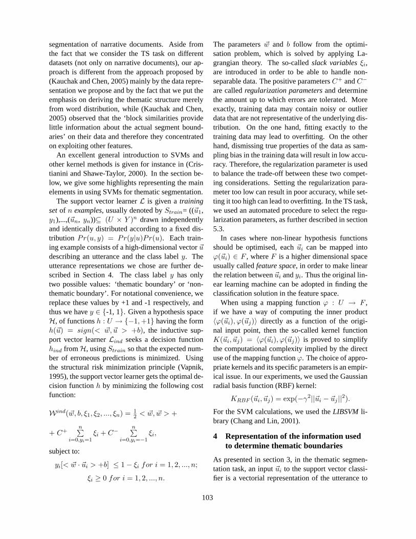
segmentation of narrative documents. Aside fromthe fact that we consider the TS task on differentdatasets (not only on narrative documents), our ap-proach is different from the approach proposed by(Kauchak and Chen, 2005) mainly by the data repre-sentation we propose and by the fact that we put theemphasis on deriving the thematic structure merelyfrom word distribution, while (Kauchak and Chen,2005) observed that the ‘block similarities providelittle information about the actual segment bound-aries’ on their data and therefore they concentratedon exploiting other features.
An excellent general introduction to SVMs andother kernel methods is given for instance in (Cris-tianini and Shawe-Taylor, 2000). In the section be-low, we give some highlights representing the mainelements in using SVMs for thematic segmentation.
The support vector learnerL is given atrainingsetof n examples, usually denoted byStrain= ((~u1,y1),...,(~un, yn))⊆ (U × Y )n drawn independentlyand identically distributed according to a fixed dis-tribution Pr(u, y) = Pr(y|u)Pr(u). Each train-ing example consists of a high-dimensional vector~udescribing an utterance and the class labely. Theutterance representations we chose are further de-scribed in Section 4. The class labely has onlytwo possible values: ‘thematic boundary’ or ‘non-thematic boundary’. For notational convenience, wereplace these values by +1 and -1 respectively, andthus we havey ∈ {-1, 1}. Given a hypothesis spaceH, of functionsh : U → {−1,+1} having the formh(~u) = sign(< ~w, ~u > +b), the inductive sup-port vector learnerLind seeks a decision functionhind fromH, usingStrain so that the expected num-ber of erroneous predictions is minimized. Usingthe structural risk minimization principle (Vapnik,1995), the support vector learner gets the optimal de-cision functionh by minimizing the following costfunction:
W ind(~w, b, ξ1, ξ2, ..., ξn) = 12 < ~w, ~w > +
+ C+n∑
i=0,yi=1ξi + C−
n∑i=0,yi=−1
ξi,
subject to:
yi[< ~w · ~ui > +b] ≤ 1− ξi for i = 1, 2, ..., n;
ξi ≥ 0 for i = 1, 2, ..., n.
The parameters~w and b follow from the optimi-sation problem, which is solved by applying La-grangian theory. The so-calledslack variablesξi,are introduced in order to be able to handle non-separable data. The positive parametersC+ andC−
are calledregularization parametersand determinethe amount up to which errors are tolerated. Moreexactly, training data may contain noisy or outlierdata that are not representative of the underlying dis-tribution. On the one hand, fitting exactly to thetraining data may lead to overfitting. On the otherhand, dismissing true properties of the data as sam-pling bias in the training data will result in low accu-racy. Therefore, the regularization parameter is usedto balance the trade-off between these two compet-ing considerations. Setting the regularization para-meter too low can result in poor accuracy, while set-ting it too high can lead to overfitting. In the TS task,we used an automated procedure to select the regu-larization parameters, as further described in section5.3.
In cases where non-linear hypothesis functionsshould be optimised, each~ui can be mapped intoϕ(~ui) ∈ F , whereF is a higher dimensional spaceusually calledfeature space, in order to make linearthe relation between~ui andyi. Thus the original lin-ear learning machine can be adopted in finding theclassification solution in the feature space.
When using a mapping functionϕ : U → F ,if we have a way of computing the inner product〈ϕ(~ui), ϕ(~uj)〉 directly as a function of the origi-nal input point, then the so-called kernel functionK(~ui, ~uj) = 〈ϕ(~ui), ϕ(~uj)〉 is proved to simplifythe computational complexity implied by the directuse of the mapping functionϕ. The choice of appro-priate kernels and its specific parameters is an empir-ical issue. In our experiments, we used the Gaussianradial basis function (RBF) kernel:
KRBF (~ui, ~uj) = exp(−γ2||~ui − ~uj ||2).
For the SVM calculations, we used theLIBSVM li-brary (Chang and Lin, 2001).
4 Representation of the information usedto determine thematic boundaries
As presented in section 3, in the thematic segmen-tation task, an input~ui to the support vector classi-fier is a vectorial representation of the utterance to
103
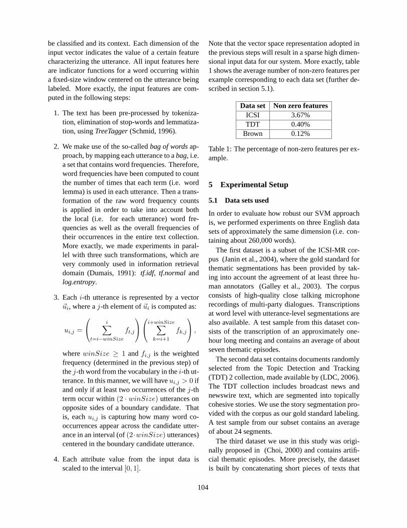
be classified and its context. Each dimension of theinput vector indicates the value of a certain featurecharacterizing the utterance. All input features hereare indicator functions for a word occurring withina fixed-size window centered on the utterance beinglabeled. More exactly, the input features are com-puted in the following steps:
1. The text has been pre-processed by tokeniza-tion, elimination of stop-words and lemmatiza-tion, usingTreeTagger(Schmid, 1996).
2. We make use of the so-calledbag of wordsap-proach, by mapping each utterance to abag, i.e.a set that contains word frequencies. Therefore,word frequencies have been computed to countthe number of times that each term (i.e. wordlemma) is used in each utterance. Then a trans-formation of the raw word frequency countsis applied in order to take into account boththe local (i.e. for each utterance) word fre-quencies as well as the overall frequencies oftheir occurrences in the entire text collection.More exactly, we made experiments in paral-lel with three such transformations, which arevery commonly used in information retrievaldomain (Dumais, 1991):tf.idf, tf.normal andlog.entropy.
3. Eachi-th utterance is represented by a vector~ui, where aj-th element of~ui is computed as:
ui,j =
i∑t=i−winSize
ft,j
i+winSize∑k=i+1
fk,j
,
wherewinSize ≥ 1 andfi,j is the weightedfrequency (determined in the previous step) ofthej-th word from the vocabulary in thei-th ut-terance. In this manner, we will haveui,j > 0 ifand only if at least two occurrences of thej-thterm occur within(2 · winSize) utterances onopposite sides of a boundary candidate. Thatis, eachui,j is capturing how many word co-occurrences appear across the candidate utter-ance in an interval (of(2·winSize) utterances)centered in the boundary candidate utterance.
4. Each attribute value from the input data isscaled to the interval[0, 1].
Note that the vector space representation adopted inthe previous steps will result in a sparse high dimen-sional input data for our system. More exactly, table1 shows the average number of non-zero features perexample corresponding to each data set (further de-scribed in section 5.1).
Data set Non zero featuresICSI 3.67%TDT 0.40%
Brown 0.12%
Table 1: The percentage of non-zero features per ex-ample.
5 Experimental Setup
5.1 Data sets used
In order to evaluate how robust our SVM approachis, we performed experiments on three English datasets of approximately the same dimension (i.e. con-taining about 260,000 words).
The first dataset is a subset of the ICSI-MR cor-pus (Janin et al., 2004), where the gold standard forthematic segmentations has been provided by tak-ing into account the agreement of at least three hu-man annotators (Galley et al., 2003). The corpusconsists of high-quality close talking microphonerecordings of multi-party dialogues. Transcriptionsat word level with utterance-level segmentations arealso available. A test sample from this dataset con-sists of the transcription of an approximately one-hour long meeting and contains an average of aboutseven thematic episodes.
The second data set contains documents randomlyselected from the Topic Detection and Tracking(TDT) 2 collection, made available by (LDC, 2006).The TDT collection includes broadcast news andnewswire text, which are segmented into topicallycohesive stories. We use the story segmentation pro-vided with the corpus as our gold standard labeling.A test sample from our subset contains an averageof about 24 segments.
The third dataset we use in this study was origi-nally proposed in (Choi, 2000) and contains artifi-cial thematic episodes. More precisely, the datasetis built by concatenating short pieces of texts that
104
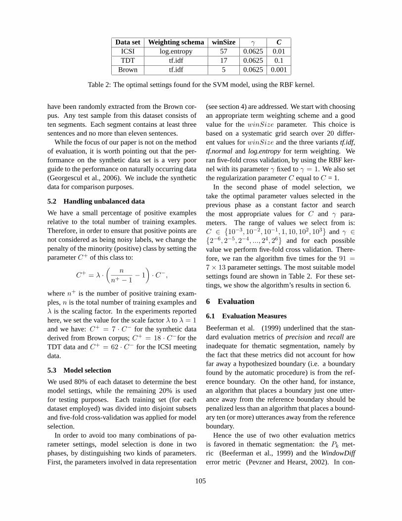
Data set Weighting schema winSize γ CICSI log.entropy 57 0.0625 0.01TDT tf.idf 17 0.0625 0.1
Brown tf.idf 5 0.0625 0.001
Table 2: The optimal settings found for the SVM model, using the RBF kernel.
have been randomly extracted from the Brown cor-pus. Any test sample from this dataset consists often segments. Each segment contains at least threesentences and no more than eleven sentences.
While the focus of our paper is not on the methodof evaluation, it is worth pointing out that the per-formance on the synthetic data set is a very poorguide to the performance on naturally occurring data(Georgescul et al., 2006). We include the syntheticdata for comparison purposes.
5.2 Handling unbalanced data
We have a small percentage of positive examplesrelative to the total number of training examples.Therefore, in order to ensure that positive points arenot considered as being noisy labels, we change thepenalty of the minority (positive) class by setting theparameterC+ of this class to:
C+ = λ ·(
n
n+ − 1− 1
)· C−,
wheren+ is the number of positive training exam-ples,n is the total number of training examples andλ is the scaling factor. In the experiments reportedhere, we set the value for the scale factorλ to λ = 1and we have:C+ = 7 · C− for the synthetic dataderived from Brown corpus;C+ = 18 · C−for theTDT data andC+ = 62 · C− for the ICSI meetingdata.
5.3 Model selection
We used 80% of each dataset to determine the bestmodel settings, while the remaining 20% is usedfor testing purposes. Each training set (for eachdataset employed) was divided into disjoint subsetsand five-fold cross-validation was applied for modelselection.
In order to avoid too many combinations of pa-rameter settings, model selection is done in twophases, by distinguishing two kinds of parameters.First, the parameters involved in data representation
(see section 4) are addressed. We start with choosingan appropriate term weighting scheme and a goodvalue for thewinSize parameter. This choice isbased on a systematic grid search over 20 differ-ent values forwinSize and the three variantstf.idf,tf.normal and log.entropyfor term weighting. Weran five-fold cross validation, by using the RBF ker-nel with its parameterγ fixed toγ = 1. We also setthe regularization parameterC equal toC = 1.
In the second phase of model selection, wetake the optimal parameter values selected in theprevious phase as a constant factor and searchthe most appropriate values forC and γ para-meters. The range of values we select from is:C ∈
{10−3, 10−2, 10−1, 1, 10, 102, 103
}and γ ∈{
2−6, 2−5, 2−4, ..., 24, 26}
and for each possiblevalue we perform five-fold cross validation. There-fore, we ran the algorithm five times for the91 =7× 13 parameter settings. The most suitable modelsettings found are shown in Table 2. For these set-tings, we show the algorithm’s results in section 6.
6 Evaluation
6.1 Evaluation Measures
Beeferman et al. (1999) underlined that the stan-dard evaluation metrics ofprecisionand recall areinadequate for thematic segmentation, namely bythe fact that these metrics did not account for howfar away a hypothesized boundary (i.e. a boundaryfound by the automatic procedure) is from the ref-erence boundary. On the other hand, for instance,an algorithm that places a boundary just one utter-ance away from the reference boundary should bepenalized less than an algorithm that places a bound-ary ten (or more) utterances away from the referenceboundary.
Hence the use of two other evaluation metricsis favored in thematic segmentation: thePk met-ric (Beeferman et al., 1999) and theWindowDifferror metric (Pevzner and Hearst, 2002). In con-
105
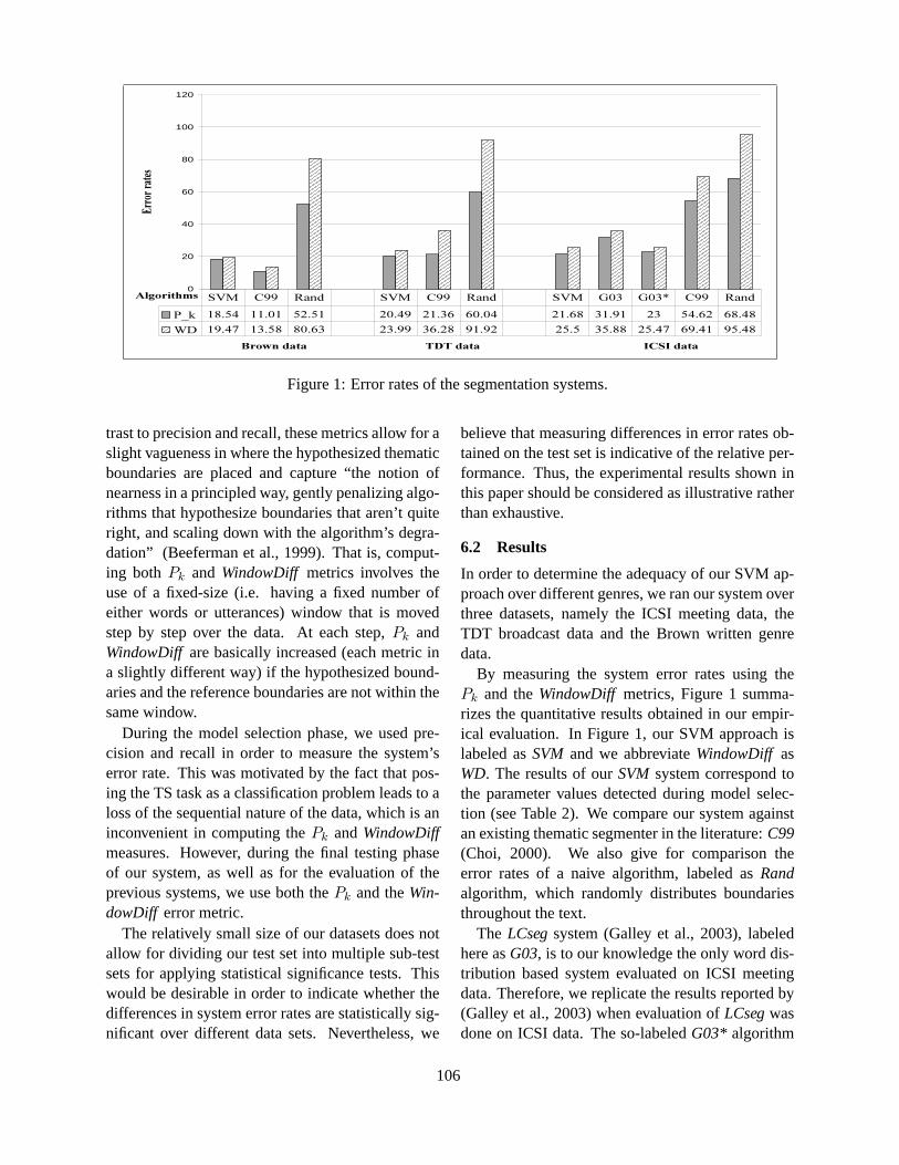
0
20
40
60
80
100
120
Algorithms
Error
rates
P_k 18.54 11.01 52.51 20.49 21.36 60.04 21.68 31.91 23 54.62 68.48WD 19.47 13.58 80.63 23.99 36.28 91.92 25.5 35.88 25.47 69.41 95.48
SVM C99 Rand SVM C99 Rand SVM G03 G03* C99 Rand
Brown data TDT data ICSI data
Figure 1: Error rates of the segmentation systems.
trast to precision and recall, these metrics allow for aslight vagueness in where the hypothesized thematicboundaries are placed and capture “the notion ofnearness in a principled way, gently penalizing algo-rithms that hypothesize boundaries that aren’t quiteright, and scaling down with the algorithm’s degra-dation” (Beeferman et al., 1999). That is, comput-ing both Pk and WindowDiff metrics involves theuse of a fixed-size (i.e. having a fixed number ofeither words or utterances) window that is movedstep by step over the data. At each step,Pk andWindowDiff are basically increased (each metric ina slightly different way) if the hypothesized bound-aries and the reference boundaries are not within thesame window.
During the model selection phase, we used pre-cision and recall in order to measure the system’serror rate. This was motivated by the fact that pos-ing the TS task as a classification problem leads to aloss of the sequential nature of the data, which is aninconvenient in computing thePk andWindowDiffmeasures. However, during the final testing phaseof our system, as well as for the evaluation of theprevious systems, we use both thePk and theWin-dowDiff error metric.
The relatively small size of our datasets does notallow for dividing our test set into multiple sub-testsets for applying statistical significance tests. Thiswould be desirable in order to indicate whether thedifferences in system error rates are statistically sig-nificant over different data sets. Nevertheless, we
believe that measuring differences in error rates ob-tained on the test set is indicative of the relative per-formance. Thus, the experimental results shown inthis paper should be considered as illustrative ratherthan exhaustive.
6.2 Results
In order to determine the adequacy of our SVM ap-proach over different genres, we ran our system overthree datasets, namely the ICSI meeting data, theTDT broadcast data and the Brown written genredata.
By measuring the system error rates using thePk and theWindowDiff metrics, Figure 1 summa-rizes the quantitative results obtained in our empir-ical evaluation. In Figure 1, our SVM approach islabeled asSVM and we abbreviateWindowDiff asWD. The results of ourSVM system correspond tothe parameter values detected during model selec-tion (see Table 2). We compare our system againstan existing thematic segmenter in the literature:C99(Choi, 2000). We also give for comparison theerror rates of a naive algorithm, labeled asRandalgorithm, which randomly distributes boundariesthroughout the text.
The LCsegsystem (Galley et al., 2003), labeledhere asG03, is to our knowledge the only word dis-tribution based system evaluated on ICSI meetingdata. Therefore, we replicate the results reported by(Galley et al., 2003) when evaluation ofLCsegwasdone on ICSI data. The so-labeledG03* algorithm
106
indicates the error rates obtained by (Galley et al.,2003) when extra (meeting specific) features havebeen adopted in a decision tree classifier. However,note that the results reported by (Galley et al.) arenot directly comparable with our results because ofa slight difference in the evaluation procedure: (Gal-ley et al.) performed 25-fold cross validation and theaveragePk andWD error rates have been computedon the held-out sets.
Figure 1 illustrates the following interesting re-sults. For the ICSI meeting data, our SVM approachprovides the best performance relative to the com-peting word distribution based state-of-the-art meth-ods. This proves that our SVM-based system is ableto build a parametric model that leads to a segmenta-tion that highly correlates to a human thematic seg-mentation. Furthermore, by taking into account therelatively small size of the data set we used for train-ing, it can be concluded that the SVM can buildqualitatively good models even with a small train-ing data. The work of (Galley et al., 2003) showsthat theG03* algorithm is better thanG03 by ap-proximately 10%, which indicates that on meetingdata the performance of our word-distribution basedapproach could possibly be increased by using othermeeting-specific features.
By examining the error rates given byPk metricfor the three systems on the TDT data set, we ob-serve that our system andC99 performed more orless equally. With respect to theWindowDiff met-ric, our system has an error rate approximately 10%smaller thanC99.
On the synthetic data set, theSVM approachperformed slightly worse thanC99, avoiding how-ever catastrophic failure, as observed with theC99method on ICSI data.
7 Conclusions
We have introduced a new approach based on worddistributions for performing thematic segmentation.The thematic segmentation task is modeled here asa binary classification problem and support vectormachine learning is adopted. In our experiments, wemake a comparison of our approach versus existinglinear thematic segmentation systems reported in theliterature, by running them over three different datasets. When evaluating on real data, our approach ei-
ther outperformed the other existing methods or per-forms comparably to the best. We view this as astrong evidence that our approach provides a unifiedand robust framework for the thematic segmentationtask. The results also suggest that word distributionsthemselves might be a good candidate for capturingthe thematic shifts of text and that SVM learning canplay an important role in building an adaptable cor-relation.
Our experiments also show the sensitivity of asegmentation method to the type of a corpus onwhich it is tested. For instance, the C99 algorithmwhich achieves superior performance on a syntheticcollection performs quite poorly on the real-life datasets.
While we have shown empirically that our tech-nique can provide considerable gains by using sin-gle word distribution features, future work will in-vestigate whether the system can be improved by ex-ploiting other features derived for instance from syn-tactic, lexical and, when available, prosodic infor-mation. If further annotated meeting data becomesavailable, it would be also interesting to replicate ourexperiments on a bigger data set in order to verifywhether our system performance improves.
Acknowledgments This work is partially sup-ported by the Interactive Multimodal InformationManagement project (http://www.im2.ch/). Manythanks to the reviewers for their insightful sugges-tions. We are grateful to the International ComputerScience Institute (ICSI), University of California forsharing the data with us. The authors also thankMichael Galley who kindly provided us the thematicannotations of the ICSI data.
References
Doug Beeferman, Adam Berger, and John Lafferty.1999. Statistical Models for Text Segmentation.Ma-chine Learning, 34(1-3):177–210.
David M. Blei and Pedro J. Moreno. 2001. Topic Seg-mentation with an Aspect Hidden Markov Model. InProceedings of the 24th annual international ACM SI-GIR conference on Research and development in in-formation retrieval, pages 343–348. ACM Press.
Thorsten Brants, Francine Chen, and Ioannis Tsochan-taridis. 2002. Topic-Based Document Segmentationwith Probabilistic Latent Semantic Analysis. InPro-ceedings of the Eleventh International Conference on
107
Information and Knowledge Management, pages 211–218, McLean, Virginia, USA. ACM Press.
Gillian Brown and George Yule. 1998.Discourse Analy-sis. Cambridge Textbooks in Linguistics, Cambridge.
Chih-Chung Chang and Chih-Jen Lin. 2001. LIBSVM:a library for support vector machines. Software avail-able at http://www.csie.ntu.edu.tw/ cjlin/libsvm.
Freddy Choi, Peter Wiemer-Hastings, and JohannaMoore. 2001. Latent Semantic Analysis for Text Seg-mentation. InProceedings of the 6th Conference onEmpirical Methods in Natural Language Processing,Seattle, WA.
Freddy Choi. 2000. Advances in Domain IndependentLinear Text Segmentation. InProceedings of the 1stConference of the North American Chapter of the As-sociation for Computational Linguistics, pages 26–33,Seattle, USA.
Nello Cristianini and John Shawe-Taylor. 2000.AnIntroduction to Support Vector Machines and otherkernel-based learning methods. Cambridge Univer-sity Press, Cambridge, UK.
Susan Dumais. 1991. Improving the retrieval of informa-tion from external sources.Behavior Research Meth-ods, Instruments and Computers, 23(2):229–236.
Ayman Farahat and Francine Chen. 2006. ImprovingProbabilistic Latent Semantic Analysis with PrincipalComponent Analysis. InProceedings of the 11th Con-ference of the European Chapter of the Asociation forComputational Linguistics, Trento, Italy.
Michael Galley, Kathleen McKeown, Eric Fosler-Luissier, and Hongyan Jing. 2003. Discourse Seg-mentation of Multy-Party Conversation. InProceed-ings of the 41st Annual Meeting of the Association forComputational Linguistics, pages 562–569.
Maria Georgescul, Alexander Clark, and Susan Arm-strong. 2006. An Analysis of Quantitative Aspects inthe Evaluation of Thematic Segmentation Algorithms.To appear.
Marti Hearst. 1997. TextTiling: Segmenting Text intoMulti-Paragraph Subtopic Passages.ComputationalLinguistics, 23(1):33–64.
Adam Janin, Jeremy Ang, Sonali Bhagat, Rajdip Dhillon,Jane Edwards, Javier Macias-Guarasa, Nelson Mor-gan, Barbara Peskin, Elizabeth Shriberg, AndreasStolcke, Chuck Wooters, and Britta Wrede. 2004. TheICSI Meeting Project: Resources and Research. InICASSP 2004 Meeting Recognition Workshop (NISTRT-04 Spring Recognition Evaluation), Montreal.
David Kauchak and Francine Chen. 2005. Feature-Based Segmentation of Narrative Documents. InPro-ceedings of the ACL Workshop on Feature Engineeringfor Machine Learning in Natural Language Process-ing, pages 32–39, Ann Arbor; MI; USA.
LDC. 2006. The Linguistic Data Consortium. Availablefrom World Wide Web: http://www.ldc.upenn.edu.
Rebecca J. Passonneau and Diane J. Litman. 1993.Intention-based Segmentation: Human Reliability andCorrelation with Linguistic Cues. InProceedings ofthe 31st conference on Association for ComputationalLinguistics, pages 148 – 155, Columbus, Ohio.
Lev Pevzner and Marti Hearst. 2002. A Critique and Im-provement of an Evaluation Metric for Text Segmen-tation. Computational Linguistics, 16(1):19–36.
Andrei Popescu-Belis, Alexander Clark, Maria Georges-cul, Sandrine Zufferey, and Denis Lalanne. 2004.Shallow Dialogue Processing Using Machine Learn-ing Algorithms (or Not). In Bourlard H. and Ben-gio S., editors,Multimodal Interaction and RelatedMachine Learning Algorithms, pages 277–290. LNCS3361, Springer-Verlag, Berlin.
Jeffrey Reynar. 1998.Topic Segmentation: Algorithmsand Applications. Ph.D. thesis, University of Pennsyl-vania.
Helmut Schmid. 1996. Probabilistic Part-of-Speech Tag-ging Using Decision Trees. Technical report, Insti-tute for Computational Linguistics of the Universityof Stuttgart.
Richard Watson Todd. 2005. A fuzzy approach to dis-course topics.Journal of the International Associationfor Semiotic Studies, 155:93–123.
Masao Utiyama and Hitoshi Isahara. 2001. A Statis-tical Model for Domain-Independent Text Segmenta-tion. In Proceedings of the 39th Annual Meeting ofthe ACL joint with the 10th Meeting of the EuropeanChapter of the ACL, pages 491–498, Toulouse, France.
Vladimir Naumovich Vapnik. 1995.The Nature of Sta-tistical Learning Theory. Springer-Verlag, New York.
Jonathan P. Yamron, Ira Carp, Lawrence Gillick, SteweLowe, and Paul van Mulbregt. 1998. A HiddenMarkov Model Approach to Text Segmentation andEvent Tracking. InProceedings of the IEEE Confer-ence on Acoustics, Speech, and Signal Processing, vol-ume 17, pages 333–336, Seattle, WA.
108

Proceedings of the 10th Conference on Computational Natural Language Learning (CoNLL-X),pages 109–116, New York City, June 2006.c©2006 Association for Computational Linguistics
Which Side are You on? Identifying Perspectives at the Document andSentence Levels
Wei-Hao LinLanguage Technologies Institute
Carnegie Mellon UniversityPittsburgh, PA [email protected]
Theresa Wilson, Janyce WiebeIntelligent Systems Program
University of PittsburghPittsburgh, PA 15260
{twilson,wiebe}@cs.pitt.edu
Alexander HauptmannSchool of Computer ScienceCarnegie Mellon University
Pittsburgh, PA [email protected]
Abstract
In this paper we investigate a new problemof identifying theperspective from whicha document is written. By perspective wemean a point of view, for example, fromthe perspective of Democrats or Repub-licans. Can computers learn to identifythe perspective of a document? Not everysentence is written strongly from a per-spective. Can computers learn to identifywhich sentences strongly convey a partic-ular perspective? We develop statisticalmodels to capture how perspectives areexpressed at the document and sentencelevels, and evaluate the proposed mod-els on articles about the Israeli-Palestinianconflict. The results show that the pro-posed models successfully learn how per-spectives are reflected in word usage andcan identify the perspective of a documentwith high accuracy.
1 Introduction
In this paper we investigate a new problem of au-tomatically identifying theperspective from whicha document is written. By perspective we meana “subjective evaluation of relative significance, apoint-of-view.”1 For example, documents about thePalestinian-Israeli conflict may appear to be aboutthe same topic but reveal different perspectives:
1The American Heritage Dictionary of the English Lan-guage, 4th ed.
(1) The inadvertent killing by Israeli forces ofPalestinian civilians – usually in the course ofshooting at Palestinian terrorists – isconsidered no different at the moral and ethicallevel than the deliberate targeting of Israelicivilians by Palestinian suicide bombers.
(2) In the first weeks of the Intifada, for example,Palestinian public protests and civiliandemonstrations were answered brutally byIsrael, which killed tens of unarmed protesters.
Example 1 is written from an Israeli perspective;Example 2 is written from a Palestinian perspec-tive. Anyone knowledgeable about the issues ofthe Israeli-Palestinian conflict can easily identify theperspectives from which the above examples werewritten. However, can computers learn to identifythe perspective of a document given a training cor-pus?
When an issue is discussed from different per-spectives, not every sentence strongly reflects theperspective of the author. For example, the follow-ing sentences were written by a Palestinian and anIsraeli.
(3) The Rhodes agreements of 1949 set them asthe ceasefire lines between Israel and the Arabstates.
(4) The green line was drawn up at the RhodesArmistice talks in 1948-49.
Examples 3 and 4 both factually introduce the back-ground of the issue of the “green line” without ex-pressing explicit perspectives. Can we develop a
109
system to automatically discriminate between sen-tences that strongly indicate a perspective and sen-tences that only reflect shared background informa-tion?
A system that can automatically identify the per-spective from which a document is written will bea valuable tool for people analyzing huge collec-tions of documents from different perspectives. Po-litical analysts regularly monitor the positions thatcountries take on international and domestic issues.Media analysts frequently survey broadcast news,newspapers, and weblogs for differing viewpoints.Without the assistance of computers, analysts haveno choice but to read each document in order to iden-tify those from a perspective of interest, which is ex-tremely time-consuming. What these analysts needis to find strong statements from different perspec-tives and to ignore statements that reflect little or noperspective.
In this paper we approach the problem of learningindividual perspectives in a statistical framework.We develop statistical models to learn how perspec-tives are reflected in word usage, and we treat theproblem of identifying perspectives as a classifica-tion task. Although our corpus contains document-level perspective annotations, it lacks sentence-levelannotations, creating a challenge for learning theperspective of sentences. We propose a novel sta-tistical model to overcome this problem. The ex-perimental results show that the proposed statisti-cal models can successfully identify the perspectivefrom which a document is written with high accu-racy.
2 Related Work
Identifying the perspective from which a documentis written is a subtask in the growing area of au-tomatic opinion recognition and extraction. Sub-jective language is used to express opinions, emo-tions, and sentiments. So far, research in automaticopinion recognition has primarily addressed learn-ing subjective language (Wiebe et al., 2004; Riloffet al., 2003), identifying opinionated documents (Yuand Hatzivassiloglou, 2003) and sentences (Yu andHatzivassiloglou, 2003; Riloff et al., 2003), and dis-criminating between positive and negative language(Pang et al., 2002; Morinaga et al., 2002; Yu and
Hatzivassiloglou, 2003; Turney and Littman, 2003;Dave et al., 2003; Nasukawa and Yi, 2003; Popescuand Etzioni, 2005; Wilson et al., 2005). While by itsvery nature we expect much of the language that isused when presenting a perspective or point-of-viewto be subjective, labeling a document or a sentenceas subjective is not enough to identify the perspec-tive from which it is written. Moreover, the ideol-ogy and beliefs authors possess are often expressedin ways other than positive or negative language to-ward specific targets.
Research on the automatic classification of movieor product reviews as positive or negative (e.g.,(Pang et al., 2002; Morinaga et al., 2002; Turneyand Littman, 2003; Nasukawa and Yi, 2003; Mullenand Collier, 2004; Beineke et al., 2004; Hu and Liu,2004)) is perhaps the most similar to our work. Aswith review classification, we treat perspective iden-tification as a document-level classification task, dis-criminating, in a sense, between different types ofopinions. However, there is a key difference. A pos-itive or negative opinion toward a particular movieor product is fundamentally different from an overallperspective. One’s opinion will change from movieto movie, whereas one’s perspective can be seen asmore static, often underpinned by one’s ideology orbeliefs about the world.
There has been research in discourse analysis thatexamines how different perspectives are expressedin political discourse (van Dijk, 1988; Pan et al.,1999; Geis, 1987). Although their research mayhave some similar goals, they do not take a compu-tational approach to analyzing large collections ofdocuments. To the best of our knowledge, our ap-proach to automatically identifying perspectives indiscourse is unique.
3 Corpus
Our corpus consists of articles published on thebitterlemonswebsite2. The website is set up to“contribute to mutual understanding [between Pales-tinians and Israelis] through the open exchange ofideas.”3 Every week an issue about the Israeli-Palestinian conflict is selected for discussion (e.g.,
2http://www.bitterlemons.org3http://www.bitterlemons.org/about/
about.html
110
“Disengagement: unilateral or coordinated?”), anda Palestinian editor and an Israeli editor each con-tribute one article addressing the issue. In addition,the Israeli and Palestinian editors invite one Israeliand one Palestinian to express their views on theissue (sometimes in the form of an interview), re-sulting in a total of four articles in a weekly edi-tion. We choose thebitterlemons website fortwo reasons. First, each article is already labeledas either Palestinian or Israeli by the editors, allow-ing us to exploit existing annotations. Second, thebitterlemons corpus enables us to test the gen-eralizability of the proposed models in a very real-istic setting: training on articles written by a smallnumber of writers (two editors) and testing on arti-cles from a much larger group of writers (more than200 different guests).
We collected a total of 594 articles published onthe website from late 2001 to early 2005. The dis-tribution of documents and sentences are listed inTable 1. We removed metadata from all articles, in-
Palestinian IsraeliWritten by editors 148 149Written by guests 149 148Total number of documents297 297Average document length 740.4 816.1Number of sentences 8963 9640
Table 1: The basic statistics of the corpus
cluding edition numbers, publication dates, topics,titles, author names and biographic information. Weused OpenNLP Tools4 to automatically extract sen-tence boundaries, and reduced word variants usingthe Porter stemming algorithm.
We evaluated the subjectivity of each sentence us-ing the automatic subjective sentence classifier from(Riloff and Wiebe, 2003), and find that 65.6% ofPalestinian sentences and 66.2% of Israeli sentencesare classified as subjective. The high but almostequivalent percentages of subjective sentences in thetwo perspectives support our observation in Sec-tion 2 that a perspective is largely expressed usingsubjective language, but that the amount of subjec-tivity in a document is not necessarily indicative of
4http://sourceforge.net/projects/opennlp/
its perspective.
4 Statistical Modeling of Perspectives
We develop algorithms for learning perspectives us-ing a statistical framework. Denote a training corpusas a set of documentsWn and their perspectives la-belsDn, n = 1, . . . ,N , whereN is the total numberof documents in the corpus. Given a new documentW with a unknown document perspective, the per-spectiveD is calculated based on the following con-ditional probability.
P (D|W , {Dn,Wn}Nn=1) (5)
We are also interested in how strongly each sen-tence in a document conveys perspective informa-tion. Denote the intensity of them-th sentence ofthen-th document as a binary random variableSm,n.To evaluateSm,n, how strongly a sentence reflectsa particular perspective, we calculate the followingconditional probability.
P (Sm,n|{Dn,Wn}Nn=1) (6)
4.1 Naıve Bayes Model
We model the process of generating documents froma particular perspective as follows:
π ∼ Beta(απ, βπ)
θ ∼ Dirichlet(αθ)
Dn ∼ Binomial(1, π)
Wn ∼ Multinomial(Ln, θd)
First, the parametersπ andθ are sampled once fromprior distributions for the whole corpus. Beta andDirichlet are chosen because they are conjugate pri-ors for binomial and multinomial distributions, re-spectively. We set the hyperparametersαπ, βπ, andαθ to one, resulting in non-informative priors. Adocument perspectiveDn is then sampled from a bi-nomial distribution with the parameterπ. The valueof Dn is eitherd0 (Israeli) ord1 (Palestinian). Wordsin the document are then sampled from a multino-mial distribution, whereLn is the length of the doc-ument. A graphical representation of the model isshown in Figure 1.
111
π θ
Dn Wn
N
Figure 1: Naıve Bayes Model
The model described above is commonly knownas a naıve Bayes (NB) model. NB models havebeen widely used for various classification tasks,including text categorization (Lewis, 1998). TheNB model is also a building block for the modeldescribed later that incorporates sentence-level per-spective information.
To predict the perspective of an unseen documentusing naıve Bayes , we calculate the posterior distri-bution ofD in (5) by integrating out the parameters,
∫ ∫P (D, π, θ|{(Dn,Wn)}N
n=1, W )dπdθ (7)
However, the above integral is difficult to compute.As an alternative, we use Markov Chain MonteCarlo (MCMC) methods to obtain samples from theposterior distribution. Details about MCMC meth-ods can be found in Appendix A.
4.2 Latent Sentence Perspective Model
We introduce a new binary random variable,S, tomodel how strongly a perspective is reflected at thesentence level. The value ofS is eithers1 or s0,where s1 indicates a sentence is written stronglyfrom a perspective whiles0 indicates it is not. Thewhole generative process is modeled as follows:
π ∼ Beta(απ, βπ)
τ ∼ Beta(ατ , βτ )
θ ∼ Dirichlet(αθ)
Dn ∼ Binomial(1, π)
Sm,n ∼ Binomial(1, τ)
Wm,n ∼ Multinomial(Lm,n, θ)
The parametersπ andθ have the same semantics asin the naıve Bayes model.S is naturally modeled asa binomial variable, whereτ is the parameter ofS.S represents how likely it is that a sentence stronglyconveys a perspective. We call this model the La-tent Sentence Perspective Model (LSPM) becauseS
is not directly observed. The graphical model repre-sentation of LSPM is shown in Figure 2.
π τ θ
Dn
Sm,n Wm,n
NMn
Figure 2: Latent Sentence Perspective Model
To use LSPM to identify the perspective of a newdocumentD with unknown sentence perspectivesS,we calculate posterior probabilities by summing outpossible combinations of sentence perspective in thedocument and parameters.
∫ ∫ ∫ ∑Sm,n
∑S
P (D, Sm,n, S, π, τ, θ| (8)
{(Dn,Wn)}Nn=1, W )dπdτdθ
As before, we resort to MCMC methods to samplefrom the posterior distributions, given in Equations(5) and (6).
As is often encountered in mixture models, thereis an identifiability issue in LSPM. Because the val-ues ofS can be permuted without changing the like-lihood function, the meanings ofs0 ands1 are am-biguous. In Figure 3a, fourθ values are used to rep-resent the four possible combinations of documentperspectived and sentence perspective intensitys. Ifwe do not impose any constraints,s1 ands0 are ex-changeable, and we can no longer strictly interprets1 as indicating a strong sentence-level perspectiveands0 as indicating that a sentence carries little orno perspective information. The other problem ofthis parameterization is that any improvement fromLSPM over the naıve Bayes model is not necessarily
112
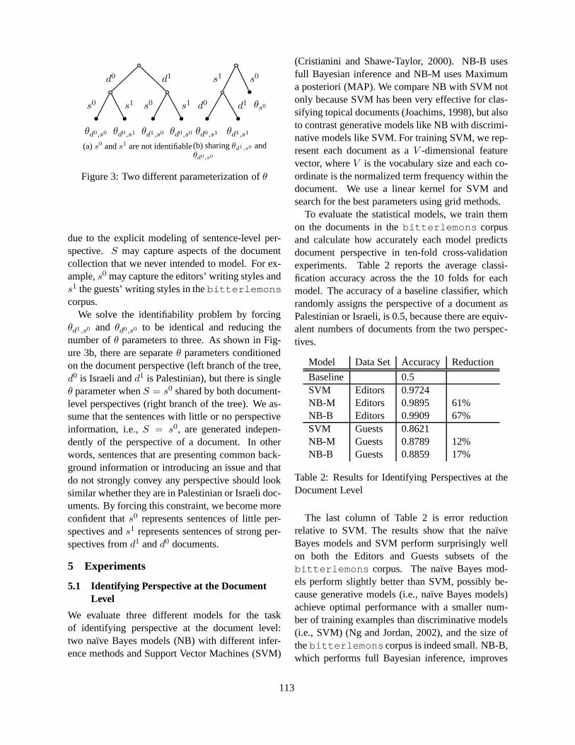
d0
θd0,s0
s0
θd0,s1
s1
d1
θd1,s0
s0
θd0,s0
s1
(a)s0 ands1 are not identifiable
s1
θd0,s1
d0
θd1,s1
d1 θs0
s0
(b) sharingθd1,s0 andθd0,s0
Figure 3: Two different parameterization ofθ
due to the explicit modeling of sentence-level per-spective. S may capture aspects of the documentcollection that we never intended to model. For ex-ample,s0 may capture the editors’ writing styles ands1 the guests’ writing styles in thebitterlemonscorpus.
We solve the identifiability problem by forcingθd1,s0 and θd0,s0 to be identical and reducing thenumber ofθ parameters to three. As shown in Fig-ure 3b, there are separateθ parameters conditionedon the document perspective (left branch of the tree,d0 is Israeli andd1 is Palestinian), but there is singleθ parameter whenS = s0 shared by both document-level perspectives (right branch of the tree). We as-sume that the sentences with little or no perspectiveinformation, i.e.,S = s0, are generated indepen-dently of the perspective of a document. In otherwords, sentences that are presenting common back-ground information or introducing an issue and thatdo not strongly convey any perspective should looksimilar whether they are in Palestinian or Israeli doc-uments. By forcing this constraint, we become moreconfident thats0 represents sentences of little per-spectives ands1 represents sentences of strong per-spectives fromd1 andd0 documents.
5 Experiments
5.1 Identifying Perspective at the DocumentLevel
We evaluate three different models for the taskof identifying perspective at the document level:two naıve Bayes models (NB) with different infer-ence methods and Support Vector Machines (SVM)
(Cristianini and Shawe-Taylor, 2000). NB-B usesfull Bayesian inference and NB-M uses Maximuma posteriori (MAP). We compare NB with SVM notonly because SVM has been very effective for clas-sifying topical documents (Joachims, 1998), but alsoto contrast generative models like NB with discrimi-native models like SVM. For training SVM, we rep-resent each document as aV -dimensional featurevector, whereV is the vocabulary size and each co-ordinate is the normalized term frequency within thedocument. We use a linear kernel for SVM andsearch for the best parameters using grid methods.
To evaluate the statistical models, we train themon the documents in thebitterlemons corpusand calculate how accurately each model predictsdocument perspective in ten-fold cross-validationexperiments. Table 2 reports the average classi-fication accuracy across the the 10 folds for eachmodel. The accuracy of a baseline classifier, whichrandomly assigns the perspective of a document asPalestinian or Israeli, is 0.5, because there are equiv-alent numbers of documents from the two perspec-tives.
Model Data Set Accuracy Reduction
Baseline 0.5SVM Editors 0.9724NB-M Editors 0.9895 61%NB-B Editors 0.9909 67%SVM Guests 0.8621NB-M Guests 0.8789 12%NB-B Guests 0.8859 17%
Table 2: Results for Identifying Perspectives at theDocument Level
The last column of Table 2 is error reductionrelative to SVM. The results show that the naıveBayes models and SVM perform surprisingly wellon both the Editors and Guests subsets of thebitterlemons corpus. The naıve Bayes mod-els perform slightly better than SVM, possibly be-cause generative models (i.e., naıve Bayes models)achieve optimal performance with a smaller num-ber of training examples than discriminative models(i.e., SVM) (Ng and Jordan, 2002), and the size ofthebitterlemonscorpus is indeed small. NB-B,which performs full Bayesian inference, improves
113
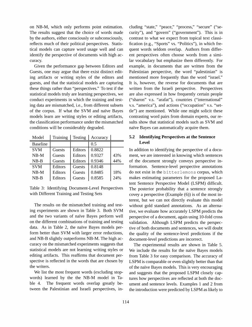
on NB-M, which only performs point estimation.The results suggest that the choice of words madeby the authors, either consciously or subconsciously,reflects much of their political perspectives. Statis-tical models can capture word usage well and canidentify the perspective of documents with high ac-curacy.
Given the performance gap between Editors andGuests, one may argue that there exist distinct edit-ing artifacts or writing styles of the editors andguests, and that the statistical models are capturingthese things rather than “perspectives.” To test if thestatistical models truly are learning perspectives, weconduct experiments in which the training and test-ing data are mismatched, i.e., from different subsetsof the corpus. If what the SVM and naıve Bayesmodels learn are writing styles or editing artifacts,the classification performance under the mismatchedconditions will be considerably degraded.
Model Training Testing Accuracy
Baseline 0.5SVM Guests Editors 0.8822NB-M Guests Editors 0.9327 43%NB-B Guests Editors 0.9346 44%SVM Editors Guests 0.8148NB-M Editors Guests 0.8485 18%NB-B Editors Guests 0.8585 24%
Table 3: Identifying Document-Level Perspectiveswith Different Training and Testing Sets
The results on the mismatched training and test-ing experiments are shown in Table 3. Both SVMand the two variants of naıve Bayes perform wellon the different combinations of training and testingdata. As in Table 2, the naıve Bayes models per-form better than SVM with larger error reductions,and NB-B slightly outperforms NB-M. The high ac-curacy on the mismatched experiments suggests thatstatistical models are not learning writing styles orediting artifacts. This reaffirms that document per-spective is reflected in the words that are chosen bythe writers.
We list the most frequent words (excluding stop-words) learned by the the NB-M model in Ta-ble 4. The frequent words overlap greatly be-tween the Palestinian and Israeli perspectives, in-
cluding “state,” “peace,” “process,” “secure” (“se-curity”), and “govern” (“government”). This is incontrast to what we expect from topical text classi-fication (e.g., “Sports” vs. “Politics”), in which fre-quent words seldom overlap. Authors from differ-ent perspectives often choose words from a simi-lar vocabulary but emphasize them differently. Forexample, in documents that are written from thePalestinian perspective, the word “palestinian” ismentioned more frequently than the word “israel.”It is, however, the reverse for documents that arewritten from the Israeli perspective. Perspectivesare also expressed in how frequently certain people(“sharon” v.s. “arafat”), countries (“international”v.s. “america”), and actions (“occupation” v.s. “set-tle”) are mentioned. While one might solicit thesecontrasting word pairs from domain experts, our re-sults show that statistical models such as SVM andnaıve Bayes can automatically acquire them.
5.2 Identifying Perspectives at the SentenceLevel
In addition to identifying the perspective of a docu-ment, we are interested in knowing which sentencesof the document strongly conveys perspective in-formation. Sentence-level perspective annotationsdo not exist in thebitterlemons corpus, whichmakes estimating parameters for the proposed La-tent Sentence Perspective Model (LSPM) difficult.The posterior probability that a sentence stronglycovey a perspective (Example (6)) is of the most in-terest, but we can not directly evaluate this modelwithout gold standard annotations. As an alterna-tive, we evaluate how accurately LSPM predicts theperspective of a document, again using 10-fold crossvalidation. Although LSPM predicts the perspec-tive of both documents and sentences, we will doubtthe quality of the sentence-level predictions if thedocument-level predictions are incorrect.
The experimental results are shown in Table 5.We include the results for the naıve Bayes modelsfrom Table 3 for easy comparison. The accuracy ofLSPM is comparable or even slightly better than thatof the naıve Bayes models. This is very encouragingand suggests that the proposed LSPM closely cap-tures how perspectives are reflected at both the doc-ument and sentence levels. Examples 1 and 2 fromthe introduction were predicted by LSPM as likely to
114
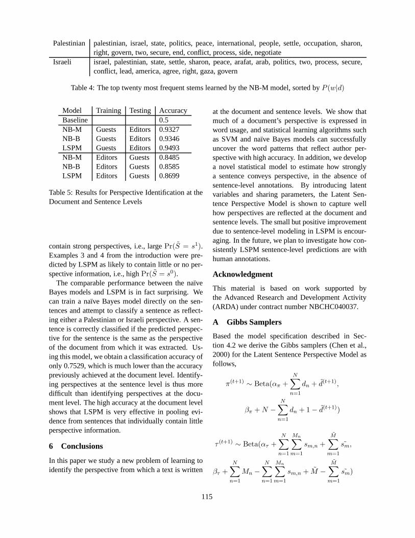
Palestinian palestinian, israel, state, politics, peace, international, people, settle, occupation, sharon,right, govern, two, secure, end, conflict, process, side, negotiate
Israeli israel, palestinian, state, settle, sharon, peace, arafat, arab, politics, two, process, secure,conflict, lead, america, agree, right, gaza, govern
Table 4: The top twenty most frequent stems learned by the NB-M model, sorted byP (w|d)
Model Training Testing AccuracyBaseline 0.5NB-M Guests Editors 0.9327NB-B Guests Editors 0.9346LSPM Guests Editors 0.9493NB-M Editors Guests 0.8485NB-B Editors Guests 0.8585LSPM Editors Guests 0.8699
Table 5: Results for Perspective Identification at theDocument and Sentence Levels
contain strong perspectives, i.e., largePr(S = s1).Examples 3 and 4 from the introduction were pre-dicted by LSPM as likely to contain little or no per-spective information, i.e., highPr(S = s0).
The comparable performance between the naıveBayes models and LSPM is in fact surprising. Wecan train a naıve Bayes model directly on the sen-tences and attempt to classify a sentence as reflect-ing either a Palestinian or Israeli perspective. A sen-tence is correctly classified if the predicted perspec-tive for the sentence is the same as the perspectiveof the document from which it was extracted. Us-ing this model, we obtain a classification accuracy ofonly 0.7529, which is much lower than the accuracypreviously achieved at the document level. Identify-ing perspectives at the sentence level is thus moredifficult than identifying perspectives at the docu-ment level. The high accuracy at the document levelshows that LSPM is very effective in pooling evi-dence from sentences that individually contain littleperspective information.
6 Conclusions
In this paper we study a new problem of learning toidentify the perspective from which a text is written
at the document and sentence levels. We show thatmuch of a document’s perspective is expressed inword usage, and statistical learning algorithms suchas SVM and naıve Bayes models can successfullyuncover the word patterns that reflect author per-spective with high accuracy. In addition, we developa novel statistical model to estimate how stronglya sentence conveys perspective, in the absence ofsentence-level annotations. By introducing latentvariables and sharing parameters, the Latent Sen-tence Perspective Model is shown to capture wellhow perspectives are reflected at the document andsentence levels. The small but positive improvementdue to sentence-level modeling in LSPM is encour-aging. In the future, we plan to investigate how con-sistently LSPM sentence-level predictions are withhuman annotations.
Acknowledgment
This material is based on work supported bythe Advanced Research and Development Activity(ARDA) under contract number NBCHC040037.
A Gibbs Samplers
Based the model specification described in Sec-tion 4.2 we derive the Gibbs samplers (Chen et al.,2000) for the Latent Sentence Perspective Model asfollows,
π(t+1) ∼ Beta(απ +N∑
n=1
dn + d(t+1),
βπ + N −
N∑n=1
dn + 1− d(t+1))
τ (t+1) ∼ Beta(ατ +N∑
n=1
Mn∑m=1
sm,n +M∑
m=1
sm,
βτ +
N∑n=1
Mn −
N∑n=1
Mn∑m=1
sm,n + M −
M∑m=1
sm)
115
θ(t+1) ∼ Dirichlet(αθ +N∑
n=1
Mn∑m=1
wm,n)
Pr(S(t+1)n,m = s1) ∝ P (Wm,n|Sm,n = 1, θ(t))
Pr(S(t+1)m,n = 1|τ,Dn)
Pr(D(t+1) = d1) ∝M∏
m=1
dbinom(τ(t+1)d
)
M∏m=1
dmultinom(θd,m(t))dbinom(π(t))
where dbinom and dmultinom are the density func-tions of binomial and multinomial distributions, re-spectively. The superscriptt indicates that a sampleis from thet-th iteration. We run three chains andcollect 5000 samples. The first half of burn-in sam-ples are discarded.
References
Philip Beineke, Trevor Hastie, and ShivakumarVaithyanathan. 2004. The sentimental factor:Improving review classification via human-providedinformation. InProceedings of ACL-2004.
Ming-Hui Chen, Qi-Man Shao, and Joseph G. Ibrahim.2000. Monte Carlo Methods in Bayesian Computa-tion. Springer-Verlag.
Nello Cristianini and John Shawe-Taylor. 2000.AnIntroduction to Support Vector Machines and OtherKernel-based Learning Methods. Cambridge Univer-sity Press.
Kushal Dave, Steve Lawrence, and David M. Pennock.2003. Mining the peanut gallery: Opinion extractionand semantic classification of product reviews. InPro-ceedings of WWW-2003.
Michael L. Geis. 1987. The Language of Politics.Springer.
Minqing Hu and Bing Liu. 2004. Mining and summariz-ing customer reviews. InProceedings of KDD-2004.
Thorsten Joachims. 1998. Text categorization with sup-port vector machines: Learning with many relevantfeatures. InProceedings of ECML-1998.
David D. Lewis. 1998. Naive (Bayes) at forty: The inde-pendence assumption in information retrieval. InPro-ceedings of ECML-1998.
S. Morinaga, K. Yamanishi, K. Tateishi, andT. Fukushima. 2002. Mining product reputations onthe web. InProceedings of KDD-2002.
Tony Mullen and Nigel Collier. 2004. Sentiment analy-sis using support vector machines with diverse infor-mation sources. InProceedings of EMNLP-2004.
T. Nasukawa and J. Yi. 2003. Sentiment analysis: Cap-turing favorability using natural language processing.In Proceedings of K-CAP 2003.
Andrew Y. Ng and Michael Jordan. 2002. On discrim-inative vs. generative classifiers: A comparison of lo-gistic regression and naive bayes. InNIPS-2002, vol-ume 15.
Zhongdang Pan, Chin-Chuan Lee, Joseph Man Chen, andClement Y.K. So. 1999. One event, three stories: Me-dia narratives of the handover of hong kong in culturalchina.Gazette, 61(2):99–112.
Bo Pang, Lillian Lee, and Shivakumar Vaithyanathan.2002. Thumbs up? Sentiment classification using ma-chine learning techniques. InProceedings of EMNLP-2002.
Ana-Maria Popescu and Oren Etzioni. 2005. Extractingproduct features and opinions from reviews. InPro-ceedings of HLT/EMNLP-2005, pages 339–346.
Ellen Riloff and Janyce Wiebe. 2003. Learning extrac-tion patterns for subjective expressions. InProceed-ings of EMNLP-2003.
Ellen Riloff, Janyce Wiebe, and Theresa Wilson. 2003.Learning subjective nouns using extraction patternbootstrapping. InProceedings of CoNLL-2003.
Peter Turney and Michael L. Littman. 2003. Measuringpraise and criticism: Inference of semantic orientationfrom association.ACM TOIS, 21(4):315–346.
T.A. van Dijk. 1988. News as Discourse. LawrenceErlbaum, Hillsdale, NJ.
Janyce Wiebe, Theresa Wilson, Rebecca Bruce, MatthewBell, and Melanie Martin. 2004. Learning subjectivelanguage.Computational Linguistics, 30(3).
Theresa Wilson, Janyce Wiebe, and Paul Hoffmann.2005. Recognizing contextual polarity in phrase-levelsentiment analysis. InProceedings of HLT/EMNLP-2005.
Hong Yu and Vasileios Hatzivassiloglou. 2003. Towardsanswering opinion questions: Separating facts fromopinions and identifying the polarity of opinion sen-tences. InProceedings of EMNLP-2003.
116
Proceedings of the 10th Conference on Computational Natural Language Learning (CoNLL-X),pages 117–124, New York City, June 2006.c©2006 Association for Computational Linguistics
Unsupervised Grammar Induction by Distribution and Attachment
David J. BrooksSchool of Computer ScienceUniversity of BirminghamBirmingham, B15 2TT, UK
Abstract
Distributional approaches to grammar in-duction are typically inefficient, enumer-ating large numbers of candidate con-stituents. In this paper, we describe asimplified model of distributional analy-sis which uses heuristics to reduce thenumber of candidate constituents underconsideration. We apply this model toa large corpus of over 400000 words ofwritten English, and evaluate the resultsusing EVALB. We show that the perfor-mance of this approach is limited, provid-ing a detailed analysis of learned structureand a comparison with actual constituent-context distributions. This motivates amore structured approach, using a processof attachment to form constituents fromtheir distributional components. Our find-ings suggest that distributional methodsdo not generalize enough to learn syntaxeffectively from raw text, but that attach-ment methods are more successful.
1 Introduction
Distributional approaches to grammar induction ex-ploit the principle of substitutability: constituents ofthe same type may be exchanged with one anotherwithout affecting the syntax of the surrounding con-text. Reversing this notion, if we can identify “sur-rounding context” by observation, we can hypothe-size that word sequences occurring in that context
will be constituents of the same type. Thus, distri-butional methods can be used to segment text intoconstituents and classify the results. This work fo-cuses on distributional learning from raw text.
Various models of distributional analysis havebeen used to induce syntactic structure, but mostuse probabilistic metrics to decide between candi-date constituents. We show that the efficiency ofthese systems can be improved by exploiting someproperties of probable constituents, but also that thisreliance on probability is problematic for learningfrom text. As a consequence, we propose an exten-sion to strict distributional learning that incorporatesmore information about constituent boundaries.
The remainder of this paper describes our expe-riences with a heuristic system for grammar induc-tion. We begin with a discussion of previous dis-tributional approaches to grammar induction in Sec-tion 2 and describe their implications in Section 3.We then introduce a heuristic distributional systemin Section 4, which we analyze empirically againsta treebank. Poor system performance leads us to ex-amine actual constituent-context distributions (Sec-tion 5), the implications of which motivate a morestructured extension to our learning system, whichwe describe and analyze in Section 6.
2 Previous approaches
Distributional methods analyze text byalignment,aiming to find equivalence classes covering substi-tutable units. We align common portions of textstermedcontexts, leaving distinct contiguous word-sequences, termedexpressions. An expression andits context form analignment pattern, which is de-
117
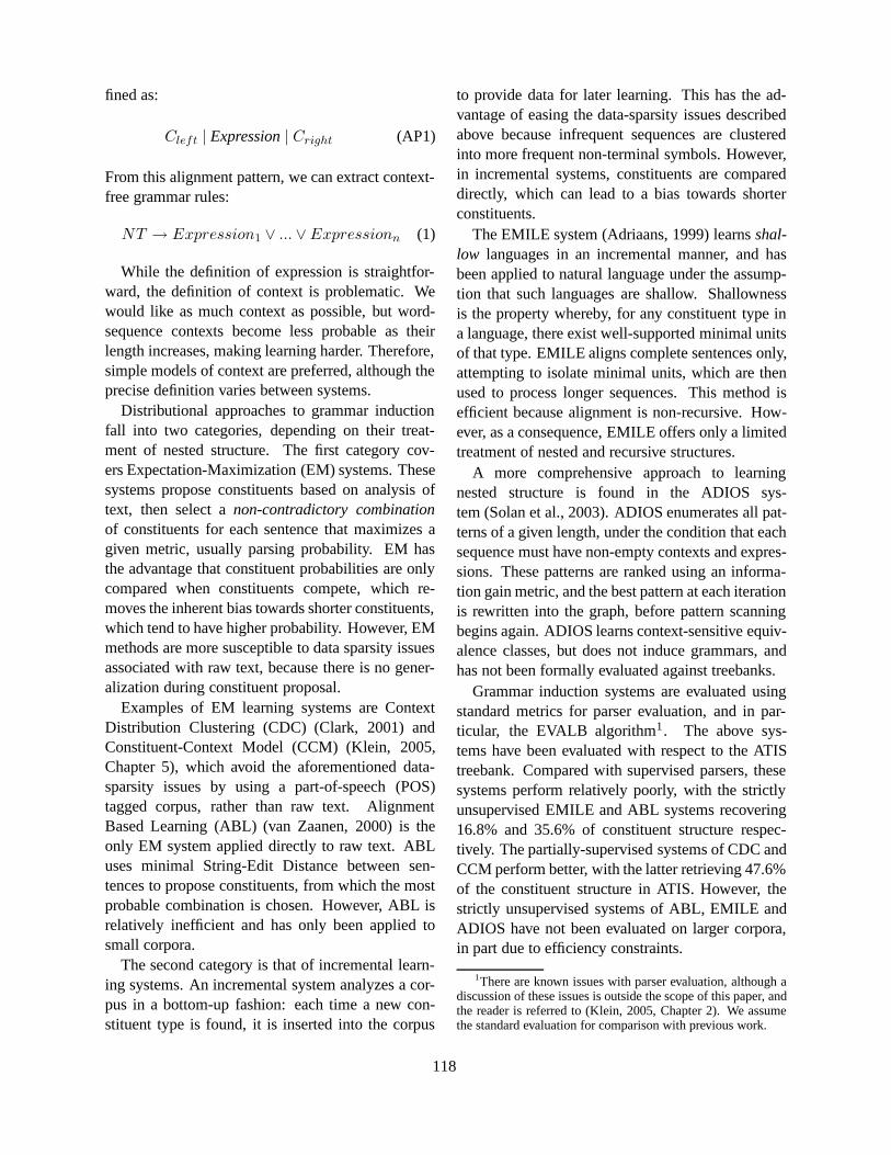
fined as:
Cleft | Expression | Cright (AP1)
From this alignment pattern, we can extract context-free grammar rules:
NT → Expression1 ∨ ... ∨ Expressionn (1)
While the definition of expression is straightfor-ward, the definition of context is problematic. Wewould like as much context as possible, but word-sequence contexts become less probable as theirlength increases, making learning harder. Therefore,simple models of context are preferred, although theprecise definition varies between systems.
Distributional approaches to grammar inductionfall into two categories, depending on their treat-ment of nested structure. The first category cov-ers Expectation-Maximization (EM) systems. Thesesystems propose constituents based on analysis oftext, then select anon-contradictory combinationof constituents for each sentence that maximizes agiven metric, usually parsing probability. EM hasthe advantage that constituent probabilities are onlycompared when constituents compete, which re-moves the inherent bias towards shorter constituents,which tend to have higher probability. However, EMmethods are more susceptible to data sparsity issuesassociated with raw text, because there is no gener-alization during constituent proposal.
Examples of EM learning systems are ContextDistribution Clustering (CDC) (Clark, 2001) andConstituent-Context Model (CCM) (Klein, 2005,Chapter 5), which avoid the aforementioned data-sparsity issues by using a part-of-speech (POS)tagged corpus, rather than raw text. AlignmentBased Learning (ABL) (van Zaanen, 2000) is theonly EM system applied directly to raw text. ABLuses minimal String-Edit Distance between sen-tences to propose constituents, from which the mostprobable combination is chosen. However, ABL isrelatively inefficient and has only been applied tosmall corpora.
The second category is that of incremental learn-ing systems. An incremental system analyzes a cor-pus in a bottom-up fashion: each time a new con-stituent type is found, it is inserted into the corpus
to provide data for later learning. This has the ad-vantage of easing the data-sparsity issues describedabove because infrequent sequences are clusteredinto more frequent non-terminal symbols. However,in incremental systems, constituents are compareddirectly, which can lead to a bias towards shorterconstituents.
The EMILE system (Adriaans, 1999) learnsshal-low languages in an incremental manner, and hasbeen applied to natural language under the assump-tion that such languages are shallow. Shallownessis the property whereby, for any constituent type ina language, there exist well-supported minimal unitsof that type. EMILE aligns complete sentences only,attempting to isolate minimal units, which are thenused to process longer sequences. This method isefficient because alignment is non-recursive. How-ever, as a consequence, EMILE offers only a limitedtreatment of nested and recursive structures.
A more comprehensive approach to learningnested structure is found in the ADIOS sys-tem (Solan et al., 2003). ADIOS enumerates all pat-terns of a given length, under the condition that eachsequence must have non-empty contexts and expres-sions. These patterns are ranked using an informa-tion gain metric, and the best pattern at each iterationis rewritten into the graph, before pattern scanningbegins again. ADIOS learns context-sensitive equiv-alence classes, but does not induce grammars, andhas not been formally evaluated against treebanks.
Grammar induction systems are evaluated usingstandard metrics for parser evaluation, and in par-ticular, the EVALB algorithm1. The above sys-tems have been evaluated with respect to the ATIStreebank. Compared with supervised parsers, thesesystems perform relatively poorly, with the strictlyunsupervised EMILE and ABL systems recovering16.8% and 35.6% of constituent structure respec-tively. The partially-supervised systems of CDC andCCM perform better, with the latter retrieving 47.6%of the constituent structure in ATIS. However, thestrictly unsupervised systems of ABL, EMILE andADIOS have not been evaluated on larger corpora,in part due to efficiency constraints.
1There are known issues with parser evaluation, although adiscussion of these issues is outside the scope of this paper, andthe reader is referred to (Klein, 2005, Chapter 2). We assumethe standard evaluation for comparison with previous work.
118
3 Issues for distributional learning
There are many issues with distributional learning,especially when learning from raw text. First, previ-ous systems hypothesize and select constituents ac-cording to the probability of their contexts: ABL,EMILE and CCM use the probability of proposedequivalence classes, or the equivalent context prob-ability; ADIOS uses an information gain metric,again favouring probable contexts. However, whenlearning from raw text, this preference for hypothe-ses with more probable contexts means that open-class words will seldom be considered as contexts.In POS-based learners, it is possible to align open-class POS contexts. These contexts are demonstra-bly important despite low word probabilities, whichsuggests that selecting contexts on the basis of prob-ability will be limited in success.
The second problem relates to word-senses.Alignment proceeds by matching orthographictypes, but these types can have numerous associatedsyntactic senses. For example, ‘to’ plays two distinctroles: infinitive marker or preposition. If we alignusing the orthographic type, we will often misalignwords, as seen in the following alignment:
I gave it to the man in the grey jacketJohn agreed to see me in 20 minutes
Here, we are (mis)aligning a prepositional ‘to’, withan infinitive marker. The result would be a correctlyidentified noun-phrase, ‘the man’, and an incorrectstructure, contradicting both the verb-group ‘to see’and the noun-phrase ‘me’. This problem does notaffect POS-based learning systems, as POS tags areunambiguously assigned.
Finally, grammar induction systems are typicallyinefficient, which prohibits training over large cor-pora. Distributional analysis is an expensive proce-dure, and must be performed for large numbers ofword sequences. Previous approaches have tendedto enumerate all alignment patterns, of which thebest are selected using probabilistic metrics. How-ever, given the preference for probable alignments,there is considerable wasted computation here, andit is on this issue that we shall focus.
4 A heuristic approach to alignment
Rather than enumerating all word sequences in acorpus, we propose a heuristic for guiding distribu-
tional systems towards more favourable alignmentpatterns, in a system calledDirected Alignment. Inthis system, we define context as the ordered pairof left- and right-context for a given constituent,〈Cleft − Cright〉, whereCleft andCright are single-units. The atomic units of this system are words, butlearned constituents may also act as context-units.
The probability of a pattern depends primarily onits contexts, since they are common to all matchingsequences. We can reduce the task of finding proba-ble alignments to simply finding probable context-pairs. However, we can reduce this further: fora context-pair to be probable, its components mustalso be probable. Therefore, rather than enumerat-ing all patterns in the corpus, we direct the alignmentprocedure towards patterns whereCleft andCright
are probable.The first stage of direction creates an index for the
corpus, compiling a list of unit types, where unitsare initially words. From this list of types, the mostprobable 1% are selected ascontext-units. Thesecontext-units are the only types allowed to fill therolesCleft andCright in alignment patterns.
Alignments are created directly from the context-unit index. For each context-unit tokencu in theindex, we locatecu in the corpus and create analignment pattern, such thatcu is the left context(Cleft). Next, we scan the sequence of words fol-lowing cu, extending the alignment pattern until an-other context-unitcu′ is found, or a fixed lengththreshold is exceeded. Ifcu′ is found, it fills the roleof right context (Cright), and the completed align-ment pattern is cached; otherwise, the pattern is dis-regarded.
Direction permits two forms of valid expressionsin the context〈cu − cu′〉:
1. nc1 . . . ncn, where eachnci is a non-context
2. c1 . . . cn, where eachci is a context-unit
The first of these forms allows us to examine non-nested alignments. The second allows us to analyzenested alignments only after inner constituents havebeen learned. These constraints reduce the numberof constituents under consideration at any time toa manageable level. As a result, we can scan verylarge numbers of alignment patterns with relativelylittle overhead.
119

As an example, consider the following sequence,with context units underlined:
put thewhole egg ,all the seasonings andvegeta-bles intothebowl andprocess for10 seconds untilsmoothly pured .
This would be broken into non-recursive expres-sions2:
(put) the (whole egg) , all the (seasonings) and (veg-etables) into the (bowl) and (process) for (10 sec-onds) until (smoothly pureed) .
These expressions will be replaced by non-terminalunit representing the class of expressions, such thateach class contains all units across the corpus thatoccur in the same context:
NT0 the NT1 , all the NT2 and NT3 into the NT2and NT4 for NT5 until NT6 .
Following this generalization nested structures canbe discovered using the same process.
This approach has some interesting parallels withchunking techniques, most notably that of function-word phrase identification (Smith and Witten, 1993).This similarity is enforced by disallowing nestedstructures. Unlike chunking systems, however, thiswork will also attempt to recover nested structuresby means of incremental learning.
4.1 Selecting alignment patterns
The direction process extracts a set of candidatealignments, and from this set we select the bestalignment to rewrite as an equivalence class. Previ-ous approaches offer a number of metrics for rank-ing constituents, based around constituent or contextprobability (ABL and CCM), Mutual Information(CDC), and information gain (ADIOS). We have im-plemented several of these metrics, but our expe-riences suggest that context probability is the mostsuccessful.
The probability of an alignment is effectively thesum of all path probabilities through the alignment:
P (Cleft, Cright) = ΣP (pathleft,right) (2)
where eachpathleft,right is a unique word sequencestarting withleft and ending withright, under the
2For clarity, we have shown all alignments for the given sen-tence simultaneously. However, the learning process is incre-mental, so each alignment would be proposed during a distinctlearning iteration.
constraints on expressions described above. There isan important practical issue here: probability sumssuch as that in Equation 2 do not decrease when ex-pressions are replaced with equivalence classes. Toalleviate this problem, we rewrite the units when up-dating the distribution, but discard paths that matchthe current alignment. This prevents looping whileallowing the rewritten paths to contribute to nestedstructures.
4.2 Generalizing expression classes
The model outlined above is capable of learningstrictly context-sensitive constituents. While thisdoes allow for nested constituents, it is problematicfor generalization. Consider the following equiva-lence classes, which are proposed relatively early inDirected Alignment:
the NT1 ofthe NT2 in
Here, the non-terminals have been assigned on thebasis of context-pairs: NT1 is defined by〈the− of〉and NT2 is defined by〈the − in〉. These types aredistinct, although intuitively they account for simplenoun-phrases. If we then propose an alignment pat-tern with NT1 asCleft, it must be followed by ‘of’,which removes any possibility of generalizing ‘of’and ‘in’.
We alleviate this problem by generalizing equiv-alence classes, using a simple clustering algorithm.For each new alignment, we compare the set of ex-pressions with all existing expression classes, rank-ing the comparisons by the degree of overlap withthe current alignment. If this degree of overlap ex-ceeds a fixed threshold, the type of the existing classis assumed; otherwise, a new class is created.
4.3 Experiments, results and analysis
To evaluate our algorithm, we follow the standardapproach of comparing the output of our systemwith that of a treebank. We use the EVALB algo-rithm, originally designed for evaluating supervisedparsing systems, with identical configuration to thatof (van Zaanen, 2000). However, we apply our algo-rithms to a different corpus: the written sub-corpusof the International Corpus of English, Great BritainComponent (henceforth ICE-GB), with punctuationremoved. This consists of 438342 words, in 22815sentences. We also include a baseline instantiation
120

System UP UR F1 CBFWB 30.0 11.0 16.0 0.36DA 23.3 8.0 11.9 0.30DAcluster 23.6 8.1 12.0 0.30
Table 1: EVALB results after 500 iterations of Di-rected Alignment applied to ICE-GB, showing bothcontext-sensitive (DA) and clustered (DAcluster)alignment. The columns represent Unlabeled Preci-sion, Unlabeled Recall, Unlabeled F-Score and theproportion of sentence with crossing brackets re-spectively.
of our algorithm, which chunks text into expres-sions between function words, which we refer to asFunction-Word Bracketing (FWB).
Table 1 summarizes the EVALB scores for two500-iteration runs of Directed Alignment over ICE-GB: DA is the standard context-sensitive version ofthe algorithm;DAcluster is the version with contextclustering. FWB precision is relatively low, withonly 30% of proposed structures appearing in thetreebank. Recall is even lower, with only 11% ofstructure retrieved. This is unsurprising, as no nestedconstructions are considered.
In comparison, both versions of Directed Align-ment perform significantly worse, withDAcluster
being only fractionally better than standardDA. Ex-periments over more learning iterations suggest thatthe performance ofDA converges onFWB, withfew nested constituents discovered. Both variantsof the system produce very poor performance, withvery little nested structure recovered. While theseresults seem discouraging, it is worth investigatingsystem performance further.
Table 2, summarizes the success of the algorithmat discovering different types of constituent. Notethat these results are unlabeled, so we are examiningthe proportion of each type of constituent in ICE-GB that has been identified. Here, Directed Align-ment exhibits the most success at identifying non-clauses, of which the primary source of success isshort sentence fragments. Around 10% of noun-phrases (NP), verb-phrases (VP) and subordinate-phrases (SUBP) were recovered, this limited suc-cess reflects the nature of the constituents: all threehave relatively simple constructions, whereby a sin-gle word represents the constituent. In contrast, con-
Recall (%)Category Frequency FWB DA DAcluster
NP 117776 11.81 10.83 10.79CL 28641 0.50 1.21 1.14VP 50280 20.88 9.58 9.89PP 42134 0.10 0.67 0.73
SUBP 7474 1.10 11.05 11.15NONCL 1919 4.27 22.98 22.98
Table 2: Constituent retrieval results for Function-Word Bracketing (FWB) and Directed Alignment(DA andDAcluster), categorized by gold-type
(a) DA, top 5 noun-matches of271
Learned Recall PrecisionNT0 4.61 84.53NT5 1.58 93.44NT7 1.36 87.14NT4 1.09 75.10NT10 0.82 84.54
(b) DAcluster, top 5 noun-matches of 135
Learned Recall PrecisionNT0 6.93 87.09NT4 6.48 89.91NT8 2.62 40.48NT11 0.86 68.60NT10 0.58 16.95
Table 3: The top five expression classes to match N(noun) in ICE-GB, ranked by recall.
stituent types that comprise multiple units, such asprepositional-phrases (PP), are seldom recovered.
4.3.1 Class generalization
During learning inDAcluster, we induce gener-alized classes using the expression clustering algo-rithm. This generalization can be evaluated, com-paring induced classes with those in the treebank us-ing precision and recall. Table 2(a) shows the topfive proposed classes matching the type noun (N)in ICE-GB during 500 iterations of context-sensitiveDirected Alignment. There are 271 types matchingnoun, and as can be seen, the top five account fora very small proportion of all nouns, some 9.46%(recall).
Table 2(b) shows the same analysis for DirectedAlignment with class generalization. For nounmatches, we can see that there are far fewer pro-posed classes (135), and that those classes are muchmore probable, the top five accounting for 17.47%
121
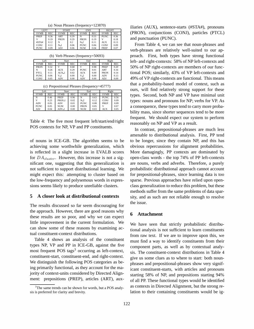
(a) Noun Phrases (frequency=123870)LEFT START END RIGHT
SYMB REC SYMB REC SYMB REC SYMB RECPREP 0.36 ART 0.29 N 0.53 PUNC 0.36V 0.19 PRON 0.29 PRON 0.19 V 0.18#STA# 0.12 N 0.2 N 2 0.11 AUX 0.13CONJ 0.11 N 1 0.06 PUNC 0.06 CONJ 0.09PUNC 0.09 ADJ 0.06 NUM 0.04 PREP 0.07
(b) Verb Phrases (frequency=50693)Left Start End Right
SYMB REC SYMB REC SYMB REC SYMB RECPRON 0.32 V 0.68 V 0.98 PREP 0.20N 0.26 AUX 0.29 PUNC 0.01 ART 0.16PTCL 0.11 AUX 1 0.02 AUX 0.00 PRON 0.14PUNC 0.06 V 1 0.00 V 2 0.00 ADV 0.13CONJ 0.05 ADV 0.00 ADV 0.00 ADJ 0.09
(c) Prepositional Phrases (frequency=45777)Left Start End Right
SYMB REC SYMB REC SYMB REC SYMB RECN 0.46 PREP 0.96 N 0.63 PUNC 0.56V 0.23 PREP1 0.02 N 2 0.12 CONJ 0.09ADV 0.05 ADV 0.01 PUNC 0.08 PREP 0.09PUNC 0.05 NUM 0.00 PRON 0.05 V 0.07ADJ 0.04 ADV 1 0.00 NUM 0.03 AUX 0.05
Table 4: The five most frequent left/start/end/rightPOS contexts for NP, VP and PP constituents.
of nouns in ICE-GB. The algorithm seems to beachieving some worthwhile generalization, whichis reflected in a slight increase in EVALB scoresfor DAcluster. However, this increase is not a sig-nificant one, suggesting that this generalization isnot sufficient to support distributional learning. Wemight expect this: attempting to cluster based onthe low-frequency and polysemous words in expres-sions seems likely to produce unreliable clusters.
5 A closer look at distributional contexts
The results discussed so far seem discouraging forthe approach. However, there are good reasons whythese results are so poor, and why we can expectlittle improvement in the current formulation. Wecan show some of these reasons by examining ac-tual constituent-context distributions.
Table 4 shows an analysis of the constituenttypes NP, VP and PP in ICE-GB, against the fivemost frequent POS tags3 occurring as left-context,constituent-start, constituent-end, and right-context.We distinguish the following POS categories as be-ing primarily functional, as they account for the ma-jority of context-units considered by Directed Align-ment: prepositions (PREP), articles (ART), aux-
3The same trends can be shown for words, but a POS analy-sis is preferred for clarity and brevity.
iliaries (AUX), sentence-starts (#STA#), pronouns(PRON), conjunctions (CONJ), particles (PTCL)and punctuation (PUNC).
From Table 4, we can see that noun-phrases andverb-phrases are relatively well-suited to our ap-proach. First, both types have strong functionalleft- and right-contexts: 58% of NP left-contexts and50% of NP right-contexts are members of our func-tional POS; similarly, 43% of VP left-contexts and49% of VP right-contexts are functional. This meansthat a probability-based model of context, such asours, will find relatively strong support for thesetypes. Second, both NP and VP have minimal unittypes: nouns and pronouns for NP; verbs for VP. Asa consequence, these types tend to carry more proba-bility mass, since shorter sequences tend to be morefrequent. We should expect our system to performreasonably on NP and VP as a result.
In contrast, prepositional-phrases are much lessamenable to distributional analysis. First, PP tendto be longer, since they contain NP, and this hasobvious repercussions for alignment probabilities.More damagingly, PP contexts are dominated byopen-class words - the top 74% of PP left-contextsare nouns, verbs and adverbs. Therefore, a purelyprobabilistic distributional approach cannot accountfor prepositional-phrases, since learning data is toosparse. Previous approaches have relied upon open-class generalization to reduce this problem, but thesemethods suffer from the same problems of data spar-sity, and as such are not reliable enough to resolvethe issue.
6 Attachment
We have seen that strictly probabilistic distribu-tional analysis is not sufficient to learn constituentsfrom raw text. If we are to improve upon this, wemust find a way to identify constituents from theircomponent parts, as well as by contextual analy-sis. The constituent-context distributions in Table 4give us some clues as to where to start: both noun-phrases and prepositional-phrases show very signif-icant constituent-starts, with articles and pronounsstarting 58% of NP, and prepositions starting 94%of all PP. These functional types would be identifiedas contexts in Directed Alignment, but the strong re-lation to their containing constituents would be ig-
122
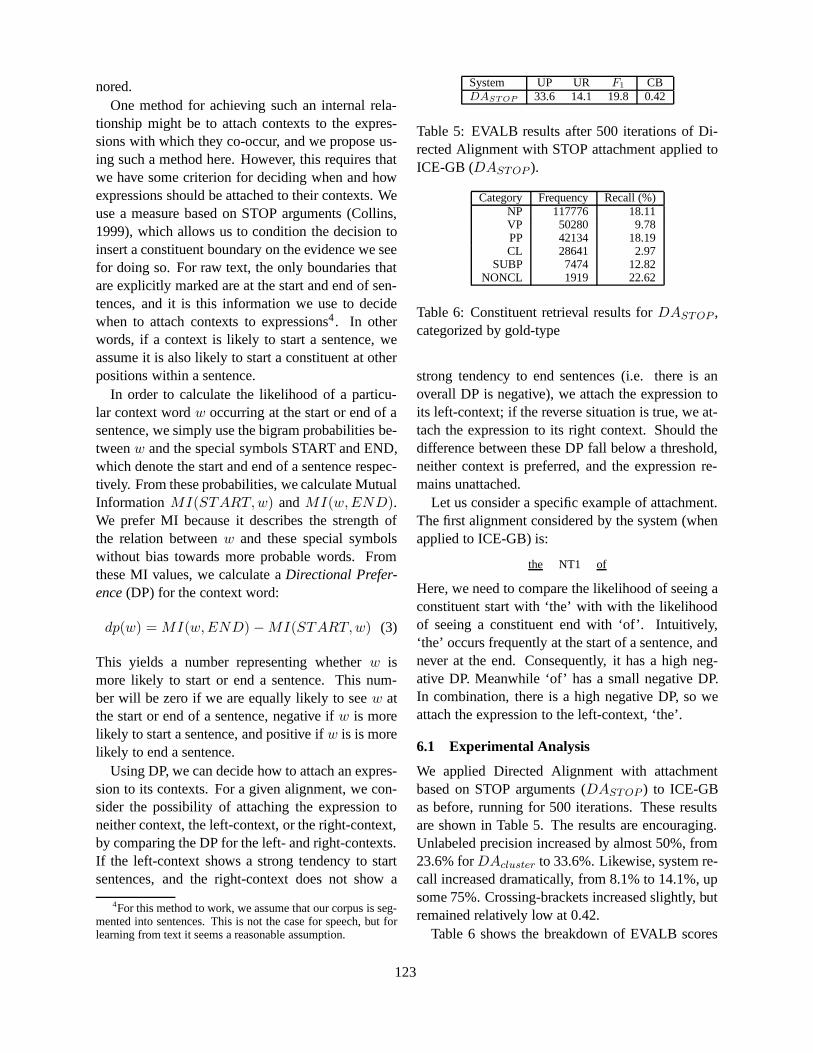
nored.One method for achieving such an internal rela-
tionship might be to attach contexts to the expres-sions with which they co-occur, and we propose us-ing such a method here. However, this requires thatwe have some criterion for deciding when and howexpressions should be attached to their contexts. Weuse a measure based on STOP arguments (Collins,1999), which allows us to condition the decision toinsert a constituent boundary on the evidence we seefor doing so. For raw text, the only boundaries thatare explicitly marked are at the start and end of sen-tences, and it is this information we use to decidewhen to attach contexts to expressions4. In otherwords, if a context is likely to start a sentence, weassume it is also likely to start a constituent at otherpositions within a sentence.
In order to calculate the likelihood of a particu-lar context wordw occurring at the start or end of asentence, we simply use the bigram probabilities be-tweenw and the special symbols START and END,which denote the start and end of a sentence respec-tively. From these probabilities, we calculate MutualInformation MI(START,w) andMI(w,END).We prefer MI because it describes the strength ofthe relation betweenw and these special symbolswithout bias towards more probable words. Fromthese MI values, we calculate aDirectional Prefer-ence (DP) for the context word:
dp(w) = MI(w,END) −MI(START,w) (3)
This yields a number representing whetherw ismore likely to start or end a sentence. This num-ber will be zero if we are equally likely to seew atthe start or end of a sentence, negative ifw is morelikely to start a sentence, and positive ifw is is morelikely to end a sentence.
Using DP, we can decide how to attach an expres-sion to its contexts. For a given alignment, we con-sider the possibility of attaching the expression toneither context, the left-context, or the right-context,by comparing the DP for the left- and right-contexts.If the left-context shows a strong tendency to startsentences, and the right-context does not show a
4For this method to work, we assume that our corpus is seg-mented into sentences. This is not the case for speech, but forlearning from text it seems a reasonable assumption.
System UP UR F1 CBDASTOP 33.6 14.1 19.8 0.42
Table 5: EVALB results after 500 iterations of Di-rected Alignment with STOP attachment applied toICE-GB (DASTOP ).
Category Frequency Recall (%)NP 117776 18.11VP 50280 9.78PP 42134 18.19CL 28641 2.97
SUBP 7474 12.82NONCL 1919 22.62
Table 6: Constituent retrieval results forDASTOP ,categorized by gold-type
strong tendency to end sentences (i.e. there is anoverall DP is negative), we attach the expression toits left-context; if the reverse situation is true, we at-tach the expression to its right context. Should thedifference between these DP fall below a threshold,neither context is preferred, and the expression re-mains unattached.
Let us consider a specific example of attachment.The first alignment considered by the system (whenapplied to ICE-GB) is:
the NT1 of
Here, we need to compare the likelihood of seeing aconstituent start with ‘the’ with with the likelihoodof seeing a constituent end with ‘of’. Intuitively,‘the’ occurs frequently at the start of a sentence, andnever at the end. Consequently, it has a high neg-ative DP. Meanwhile ‘of’ has a small negative DP.In combination, there is a high negative DP, so weattach the expression to the left-context, ‘the’.
6.1 Experimental Analysis
We applied Directed Alignment with attachmentbased on STOP arguments (DASTOP ) to ICE-GBas before, running for 500 iterations. These resultsare shown in Table 5. The results are encouraging.Unlabeled precision increased by almost 50%, from23.6% forDAcluster to 33.6%. Likewise, system re-call increased dramatically, from 8.1% to 14.1%, upsome 75%. Crossing-brackets increased slightly, butremained relatively low at 0.42.
Table 6 shows the breakdown of EVALB scores
123

for the major non-terminal types, as before. Theimprovement in EVALB scores is attributableto a marked increase in success at identifyingprepositional-phrases, with a lesser increase innoun-phrase identification.
6.2 Discussion
The attachment procedure described above is moresuccessful at discovering nested constituents thandistributional methods. There are good reasons whythis should be the case. First, attachment compressesthe corpus, removing the bias towards shorter se-quences. Indeed, the algorithm seems capable ofretrieving complex constituents of up to ten wordsin length during the first 500 iterations.
Second, the STOP-conditioning criterion, whilesomewhatad hoc in relation to distributional meth-ods, allows us to assess where constituent bound-aries are likely to occur. As such, this can be seenas a rudimentary method for establishing argumentrelations, such as those observed in (Klein, 2005,Chapter 6).
Despite these improvements, the attachment pro-cess also makes some systematic mistakes. Some ofthese may be attributed to discrepancies between thesyntactic theory used to annotate the treebank andthe attachment process. For example, verbs are rou-tinely attached to their subjects before objects, con-tradicting the more traditional interpretation presentin treebanks. Some of the remaining mistakes canbe attributed to the misalignment, due to the ortho-graphic match problem described in Section 3.
7 Future Work
The major problem when applying distributionalmethods to raw text is that of orthographic match-ing, which causes misalignments between alterna-tive senses of a particular word-form. To reduce thisproblem, context-units must be classified in someway to disambiguate these different senses. Suchclassification could be used as a precursor to align-ment in the system we have described.
In addition, to better evaluate the quality of at-tachment, dependency representations and treebankscould be used, which do not have an explicit order onattachment. This would give a more accurate evalu-ation where subject-verb attachment is concerned.
8 Conclusions
We have presented an incremental grammar induc-tion system that uses heuristics to improve the effi-ciency of distributional learning. However, in testsover a large corpus, we have shown that it is capableof learning only a small subset of constituent struc-ture. We have analyzed actual constituent-contextdistributions to explain these limitations. This anal-ysis provides the motivation for a more structuredlearning method, which incorporates knowledge ofverifiable constituent boundaries - the starts andends of sentences. This improved system performssignificantly better, with a 75% increase in recallover distributional methods, and a significant im-provement at retrieving structures that are problem-atic for distributional methods alone.
ReferencesPieter Adriaans. 1999. Learning shallow context-free
languages under simple distributions. Technical Re-port PP-1999-13, Institute for Logic, Language, andComputation, Amsterdam.
Alexander Clark. 2001. Unsupervised induction ofstochastic context free grammars with distributionalclustering. In Proceedings of the Fifth Confer-ence on Natural Language Learning, pages 105–112,Toulouse, France, July.
Michael Collins. 1999.Head-Driven Statistical Modelsfor Natural Language Parsing. Ph.D. thesis, Univer-sity of Pennsylvania.
Dan Klein. 2005.The Unsupervised Learning of Natu-ral Language Structure. Ph.D. thesis, Department ofComputer Science, Stanford University, March.
Tony C. Smith and Ian H. Witten. 1993. Language in-ference from function words. Working Paper Series1170-487X-1993/3, Department of Computer Science,University of Waikato, Hamilton, New Zealand, Au-gust.
Zach Solan, David Horn, Eytan Ruppin, and ShimonEdelman. 2003. Unsupervised efficient learning andrepresentation of language structures. In R. Altermanand D. Kirsch, editors,Proceedings of the 25th Con-ference of the Cognitive Science Society, Hillsdale, NJ.Erlbaum.
Menno van Zaanen. 2000. Learning structure usingAlignment Based Learning. InProceedings of theThird Annual Doctoral Research Colloquium (CLUK),pages 75–82.
124
Proceedings of the 10th Conference on Computational Natural Language Learning (CoNLL-X),pages 125–132, New York City, June 2006.c©2006 Association for Computational Linguistics
Learning Auxiliary Fronting with Grammatical Inference
Alexander ClarkDepartment of Computer Science
Royal Holloway University of LondonEgham, Surrey TW20 [email protected]
Remi EyraudEURISE
23, rue du Docteur Paul Michelon42023 Saint-Etienne Cedex 2
Abstract
We present a simple context-free gram-matical inference algorithm, and provethat it is capable of learning an inter-esting subclass of context-free languages.We also demonstrate that an implementa-tion of this algorithm is capable of learn-ing auxiliary fronting in polar interroga-tives (AFIPI) in English. This has beenone of the most important test cases inlanguage acquisition over the last fewdecades. We demonstrate that learningcan proceed even in the complete absenceof examples of particular constructions,and thus that debates about the frequencyof occurrence of such constructions are ir-relevant. We discuss the implications ofthis on the type of innate learning biasesthat must be hypothesized to explain firstlanguage acquisition.
1 Introduction
For some years, a particular set of examples hasbeen used to provide support for nativist theoriesof first language acquisition (FLA). These exam-ples, which hinge around auxiliary inversion in theformation of questions in English, have been con-sidered to provide a strong argument in favour ofthe nativist claim: that FLA proceeds primarilythrough innately specified domain specific mecha-nisms or knowledge, rather than through the oper-ation of general-purpose cognitive mechanisms. A
key point of empirical debate is the frequency of oc-currence of the forms in question. If these are van-ishingly rare, or non-existent in the primary linguis-tic data, and yet children acquire the construction inquestion, then the hypothesis that they have innateknowledge would be supported. But this rests on theassumption that examples of that specific construc-tion are necessary for learning to proceed. In thispaper we show that this assumption is false: that thisparticular construction can be learned without thelearner being exposed to any examples of that par-ticular type. Our demonstration is primarily mathe-matical/computational: we present a simple experi-ment that demonstrates the applicability of this ap-proach to this particular problem neatly, but the datawe use is not intended to be a realistic representationof the primary linguistic data, nor is the particularalgorithm we use suitable for large scale grammarinduction.
We present a general purpose context-free gram-matical algorithm that is provably correct under acertain learning criterion. This algorithm incorpo-rates no domain specific knowledge: it has no spe-cific information about language; no knowledge ofX-bar schemas, no hidden sources of information toreveal the structure. It operates purely on unanno-tated strings of raw text. Obviously, as all learn-ing algorithms do, it has an implicit learning bias.This very simple algorithm has a particularly clearbias, with a simple mathematical description, that al-lows a remarkably simple characterisation of the setof languages that it can learn. This algorithm doesnot use a statistical learning paradigm that has to betested on large quantities of data. Rather it uses a
125
symbolic learning paradigm, that works efficientlywith very small quantities of data, while being verysensitive to noise. We discuss this choice in somedepth below.
For reasons that were first pointed out by Chom-sky (Chomsky, 1975, pages 129–137), algorithmsof this type are not capable of learning all of nat-ural language. It turns out, however, that algorithmsbased on this approach are sufficiently strong tolearn some key properties of language, such as thecorrect rule for forming polar questions.
In the next section we shall describe the disputebriefly; in the subsequent sections we will describethe algorithm we use, and the experiments we haveperformed.
2 The Dispute
We will present the dispute in traditional terms,though later we shall analyse some of the assump-tions implicit in this description. In English, po-lar interrogatives (yes/no questions) are formed byfronting an auxiliary, and adding a dummy auxiliary“do” if the main verb is not an auxiliary. For exam-ple,
Example 1a The man is hungry.
Example 1b Is the man hungry?When the subject NP has a relative clause that also
contains an auxiliary, the auxiliary that is moved isnot the auxiliary in the relative clause, but the one inthe main (matrix) clause.
Example 2a The man who is eating is hungry.
Example 2b Is the man who is eating hungry?An alternative rule would be to move the first oc-
curring auxiliary, i.e. the one in the relative clause,which would produce the form
Example 2c Is the man who eating is hungry?In some sense, there is no reason that children
should favour the correct rule, rather than the in-correct one, since they are both of similar com-plexity and so on. Yet children do in fact, whenprovided with the appropriate context, produce sen-tences of the form of Example 2b, and rarely if everproduce errors of the form Example 2c (Crain andNakayama, 1987). The problem is how to accountfor this phenomenon.
Chomsky claimed first, that sentences of the typein Example 2b are vanishingly rare in the linguis-tic environment that children are exposed to, yetwhen tested they unfailingly produce the correctform rather than the incorrect Example 2c. This isput forward as strong evidence in favour of innatelyspecified language specific knowledge: we shall re-fer to this view as linguistic nativism.
In a special volume of the Linguistic Review, Pul-lum and Scholz (Pullum and Scholz, 2002), showedthat in fact sentences of this type are not rare at all.Much discussion ensued on this empirical questionand the consequences of this in the context of ar-guments for linguistic nativism. These debates re-volved around both the methodology employed inthe study, and also the consequences of such claimsfor nativist theories. It is fair to say that in spiteof the strength of Pullum and Scholz’s arguments,nativists remained completely unconvinced by theoverall argument.
(Reali and Christiansen, 2004) present a possiblesolution to this problem. They claim that local statis-tics, effectively n-grams, can be sufficient to indi-cate to the learner which alternative should be pre-ferred. However this argument has been carefully re-butted by (Kam et al., 2005), who show that this ar-gument relies purely on a phonological coincidencein English. This is unsurprising since it is implausi-ble that a flat, finite-state model should be powerfulenough to model a phenomenon that is clearly struc-ture dependent in this way.
In this paper we argue that the discussion aboutthe rarity of sentences that exhibit this particularstructure is irrelevant: we show that simple gram-matical inference algorithms can learn this propertyeven in the complete absence of sentences of thisparticular type. Thus the issue as to how frequentlyan infant child will see them is a moot point.
3 Algorithm
Context-free grammatical inference algorithms areexplored in two different communities: in gram-matical inference and in NLP. The task in NLP isnormally taken to be one of recovering appropri-ate annotations (Smith and Eisner, 2005) that nor-mally represent constituent structure (strong learn-ing), while in grammatical inference, researchers
126
are more interested in merely identifying the lan-guage (weak learning). In both communities, thebest performing algorithms that learn from raw posi-tive data only 1, generally rely on some combinationof three heuristics: frequency, information theoreticmeasures of constituency, and finally substitutabil-ity. 2 The first rests on the observation that stringsof words generated by constituents are likely to oc-cur more frequently than by chance. The secondheuristic looks for information theoretic measuresthat may predict boundaries, such as drops in condi-tional entropy. The third method which is the foun-dation of the algorithm we use, is based on the distri-butional analysis of Harris (Harris, 1954). This prin-ciple has been appealed to by many researchers inthe field of grammatical inference, but these appealshave normally been informal and heuristic (van Za-anen, 2000).
In its crudest form we can define it as follows:given two sentences “I saw a cat over there”, and “Isaw a dog over there” the learner will hypothesizethat “cat” and “dog” are similar, since they appearin the same context “I saw a __ there”. Pairs ofsentences of this form can be taken as evidence thattwo words, or strings of words are substitutable.
3.1 Preliminaries
We briefly define some notation.An alphabet Σ is a finite nonempty set of sym-
bols called letters. A string w over Σ is a finite se-quence w = a1a2 . . . an of letters. Let |w| denotethe length of w. In the following, letters will be in-dicated by a, b, c, . . ., strings by u, v, . . . , z, and theempty string by λ. Let Σ∗ be the set of all strings,the free monoid generated by Σ. By a language wemean any subset L ⊆ Σ∗. The set of all substringsof a language L is denoted Sub(L) = {u ∈ Σ+ :∃l, r, lur ∈ L} (notice that the empty word does notbelong to Sub(L)). We shall assume an order ≺ or� on Σ which we shall extend to Σ∗ in the normalway by saying that u ≺ v if |u| < |v| or |u| = |v|and u is lexicographically before v.
A grammar is a quadruple G = 〈V, Σ, P, S〉where Σ is a finite alphabet of terminal symbols, V
1We do not consider in this paper the complex and con-tentious issues around negative data.
2For completeness we should include lexical dependenciesor attraction.
is a finite alphabet of variables or non-terminals, Pis a finite set of production rules, and S ∈ V is astart symbol.
If P ⊆ V × (Σ∪V )+ then the grammar is said tobe context-free (CF), and we will write the produc-tions as T → w.
We will write uTv ⇒ uwv when T → w ∈ P .∗
⇒ is the reflexive and transitive closure of ⇒.In general, the definition of a class L relies on
a class R of abstract machines, here called rep-resentations, together with a function L from rep-resentations to languages, that characterize all andonly the languages of L: (1) ∀R ∈ R,L(R) ∈ Land (2) ∀L ∈ L, ∃R ∈ R such that L(R) = L.Two representations R1 and R2 are equivalent iffL(R1) = L(R2).
3.2 Learning
We now define our learning criterion. This is identi-fication in the limit from positive text (Gold, 1967),with polynomial bounds on data and computation,but not on errors of prediction (de la Higuera, 1997).
A learning algorithm A for a class of represen-tations R, is an algorithm that computes a functionfrom a finite sequence of strings s1, . . . , sn toR. Wedefine a presentation of a language L to be an infinitesequence of elements of L such that every elementof L occurs at least once. Given a presentation, wecan consider the sequence of hypotheses that the al-gorithm produces, writing Rn = A(s1, . . . sn) forthe nth such hypothesis.
The algorithm A is said to identify the class R inthe limit if for every R ∈ R, for every presentationof L(R), there is an N such that for all n > N ,Rn = RN and L(R) = L(RN ).
We further require that the algorithm needs onlypolynomially bounded amounts of data and compu-tation. We use the slightly weaker notion defined byde la Higuera (de la Higuera, 1997).
Definition A representation class R is identifiablein the limit from positive data with polynomial timeand data iff there exist two polynomials p(), q() andan algorithm A such that S ⊆ L(R)
1. Given a positive sample S of size m A returnsa representation R ∈ R in time p(m), such that
2. For each representation R of size n there exists
127
a characteristic set CS of size less than q(n)such that if CS ⊆ S, A returns a representationR′ such that L(R) = L(R′).
3.3 Distributional learning
The key to the Harris approach for learning a lan-guage L, is to look at pairs of strings u and v and tosee whether they occur in the same contexts; that isto say, to look for pairs of strings of the form lur andlvr that are both in L. This can be taken as evidencethat there is a non-terminal symbol that generatesboth strings. In the informal descriptions of this thatappear in Harris’s work, there is an ambiguity be-tween two ideas. The first is that they should appearin all the same contexts; and the second is that theyshould appear in some of the same contexts. We canwrite the first criterion as follows:
∀l, r lur ∈ L if and only if lvr ∈ L (1)
This has also been known in language theory by thename syntactic congruence, and can be written u ≡L
v.The second, weaker, criterion is
∃l, r lur ∈ L and lvr ∈ L (2)
We call this weak substitutability and write it asu
.=L v. Clearly u ≡L v implies u
.=L v when u is
a substring of the language. Any two strings that donot occur as substrings of the language are obviouslysyntactically congruent but not weakly substitutable.
First of all, observe that syntactic congruence is apurely language theoretic notion that makes no ref-erence to the grammatical representation of the lan-guage, but only to the set of strings that occur init. However there is an obvious problem: syntac-tic congruence tells us something very useful aboutthe language, but all we can observe is weak substi-tutability.
When working within a Gold-style identificationin the limit (IIL) paradigm, we cannot rely on statis-tical properties of the input sample, since they willin general not be generated by random draws from afixed distribution. This, as is well known, severelylimits the class of languages that can be learned un-der this paradigm. However, the comparative sim-plicity of the IIL paradigm in the form when thereare polynomial constraints on size of characteristic
sets and computation(de la Higuera, 1997) makes ita suitable starting point for analysis.
Given these restrictions, one solution to this prob-lem is simply to define a class of languages wheresubstitutability implies congruence. We call thesethe substitutable languages: A language L is substi-tutable if and only if for every pair of strings u, v,u
.=L v implies u ≡L v. This rather radical so-
lution clearly rules out the syntax of natural lan-guages, at least if we consider them as strings ofraw words, rather than as strings of lexical or syn-tactic categories. Lexical ambiguity alone violatesthis requirement: consider the sentences “The rosedied”, “The cat died” and “The cat rose from its bas-ket”. A more serious problem is pairs of sentenceslike “John is hungry” and “John is running”, whereit is not ambiguity in the syntactic category of theword that causes the problem, but rather ambigu-ity in the context. Using this assumption, whetherit is true or false, we can then construct a simplealgorithm for grammatical inference, based purelyon the idea that whenever we find a pair of stringsthat are weakly substitutable, we can generalise thehypothesized language so that they are syntacticallycongruent.
The algorithm proceeds by constructing a graphwhere every substring in the sample defines a node.An arc is drawn between two nodes if and only ifthe two nodes are weakly substitutable with respectto the sample, i.e. there is an arc between u and v ifand only if we have observed in the sample stringsof the form lur and lvr. Clearly all of the strings inthe sample will form a clique in this graph (considerwhen l and r are both empty strings). The connectedcomponents of this graph can be computed in timepolynomial in the total size of the sample. If thelanguage is substitutable then each of these compo-nents will correspond to a congruence class of thelanguage.
There are two ways of doing this: one way, whichis perhaps the purest involves defining a reductionsystem or semi-Thue system which directly capturesthis generalisation process. The second way, whichwe present here, will be more familiar to computa-tional linguists, and involves constructing a gram-mar.
128
3.4 Grammar construction
Simply knowing the syntactic congruence might notappear to be enough to learn a context-free gram-mar, but in fact it is. In fact given the syntactic con-gruence, and a sample of the language, we can sim-ply write down a grammar in Chomsky normal form,and under quite weak assumptions this grammar willconverge to a correct grammar for the language.
This construction relies on a simple property ofthe syntactic congruence, namely that is in fact acongruence: i.e.,
u ≡L v implies ∀l, r lur ≡L lvr
We define the syntactic monoid to be the quo-tient of the monoid Σ∗/ ≡L. The monoid operation[u][v] = [uv] is well defined since if u ≡L u′ andv ≡L v′ then uv ≡L u′v′.
We can construct a grammar in the following triv-ial way, from a sample of strings where we are giventhe syntactic congruence.
• The non-terminals of the grammar are iden-tified with the congruence classes of the lan-guage.
• For any string w = uv , we add a production[w] → [u][v].
• For all strings a of length one (i.e. letters of Σ),we add productions of the form [a] → a.
• The start symbol is the congruence class whichcontains all the strings of the language.
This defines a grammar in CNF. At first sight, thisconstruction might appear to be completely vacu-ous, and not to define any strings beyond those inthe sample. The situation where it generalises iswhen two different strings are congruent: if uv =w ≡ w′ = u′v′ then we will have two different rules[w] → [u][v] and [w] → [u′][v′], since [w] is thesame non-terminal as [w′].
A striking feature of this algorithm is that it makesno attempt to identify which of these congruenceclasses correspond to non-terminals in the targetgrammar. Indeed that is to some extent an ill-posedquestion. There are many different ways of assign-ing constituent structure to sentences, and indeed
some reputable theories of syntax, such as depen-dency grammars, dispense with the notion of con-stituent structure all together. De facto standards,such as the Penn treebank annotations are a some-what arbitrary compromise among many differentpossible analyses. This algorithm instead relies onthe syntactic monoid, which expresses the combina-torial structure of the language in its purest form.
3.5 Proof
We will now present our main result, with an outlineproof. For a full proof the reader is referred to (Clarkand Eyraud, 2005).
Theorem 1 This algorithm polynomially identi-fies in the limit the class of substitutable context-freelanguages.
Proof (Sketch) We can assume without loss ofgenerality that the target grammar is in Chomskynormal form. We first define a characteristic set, thatis to say a set of strings such that whenever the sam-ple includes the characteristic set, the algorithm willoutput a correct grammar.
We define w(α) ∈ Σ∗ to be the smallest word,according to ≺, generated by α ∈ (Σ ∪ V )+. Foreach non-terminal N ∈ V define c(N) to be thesmallest pair of terminal strings (l, r) (extending ≺from Σ∗ to Σ∗ × Σ∗, in some way), such that S
∗
⇒lNr.
We can now define the characteristic set CS ={lwr|(N → α) ∈ P, (l, r) = c(N), w = w(α)}.The cardinality of this set is at most |P | whichis clearly polynomially bounded. We observe thatthe computations involved can all be polynomiallybounded in the total size of the sample.
We next show that whenever the algorithm en-counters a sample that includes this characteristicset, it outputs the right grammar. We write G forthe learned grammar. Suppose [u]
∗
⇒G
v. Thenwe can see that u ≡L v by induction on the max-imum length of the derivation of v. At each stepwe must use some rule [u′] ⇒ [v′][w′]. It is easyto see that every rule of this type preserves the syn-tactic congruence of the left and right sides of therules. Intuitively, the algorithm will never generatetoo large a language, since the languages are sub-stitutable. Conversely, if we have a derivation of astring u with respect to the target grammar G, by
129
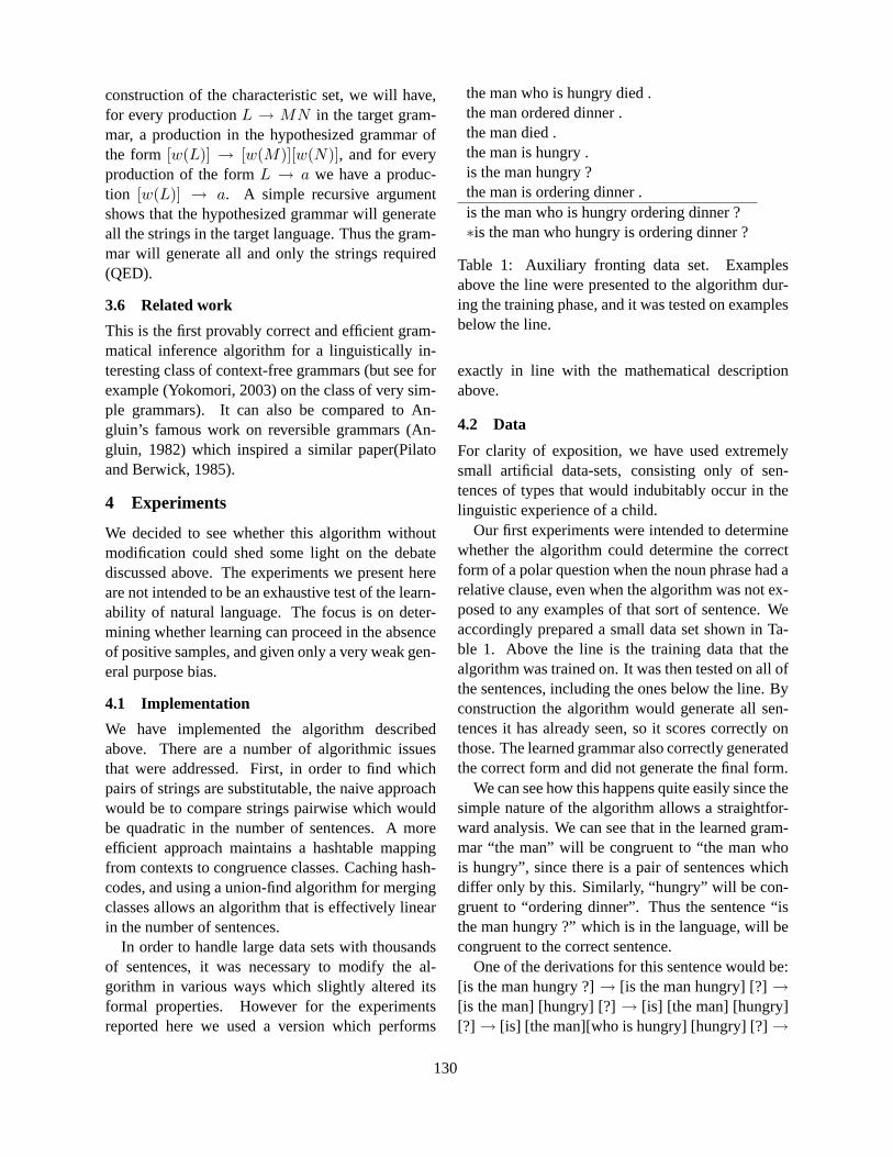
construction of the characteristic set, we will have,for every production L → MN in the target gram-mar, a production in the hypothesized grammar ofthe form [w(L)] → [w(M)][w(N)], and for everyproduction of the form L → a we have a produc-tion [w(L)] → a. A simple recursive argumentshows that the hypothesized grammar will generateall the strings in the target language. Thus the gram-mar will generate all and only the strings required(QED).
3.6 Related work
This is the first provably correct and efficient gram-matical inference algorithm for a linguistically in-teresting class of context-free grammars (but see forexample (Yokomori, 2003) on the class of very sim-ple grammars). It can also be compared to An-gluin’s famous work on reversible grammars (An-gluin, 1982) which inspired a similar paper(Pilatoand Berwick, 1985).
4 Experiments
We decided to see whether this algorithm withoutmodification could shed some light on the debatediscussed above. The experiments we present hereare not intended to be an exhaustive test of the learn-ability of natural language. The focus is on deter-mining whether learning can proceed in the absenceof positive samples, and given only a very weak gen-eral purpose bias.
4.1 Implementation
We have implemented the algorithm describedabove. There are a number of algorithmic issuesthat were addressed. First, in order to find whichpairs of strings are substitutable, the naive approachwould be to compare strings pairwise which wouldbe quadratic in the number of sentences. A moreefficient approach maintains a hashtable mappingfrom contexts to congruence classes. Caching hash-codes, and using a union-find algorithm for mergingclasses allows an algorithm that is effectively linearin the number of sentences.
In order to handle large data sets with thousandsof sentences, it was necessary to modify the al-gorithm in various ways which slightly altered itsformal properties. However for the experimentsreported here we used a version which performs
the man who is hungry died .the man ordered dinner .the man died .the man is hungry .is the man hungry ?the man is ordering dinner .is the man who is hungry ordering dinner ?∗is the man who hungry is ordering dinner ?
Table 1: Auxiliary fronting data set. Examplesabove the line were presented to the algorithm dur-ing the training phase, and it was tested on examplesbelow the line.
exactly in line with the mathematical descriptionabove.
4.2 Data
For clarity of exposition, we have used extremelysmall artificial data-sets, consisting only of sen-tences of types that would indubitably occur in thelinguistic experience of a child.
Our first experiments were intended to determinewhether the algorithm could determine the correctform of a polar question when the noun phrase had arelative clause, even when the algorithm was not ex-posed to any examples of that sort of sentence. Weaccordingly prepared a small data set shown in Ta-ble 1. Above the line is the training data that thealgorithm was trained on. It was then tested on all ofthe sentences, including the ones below the line. Byconstruction the algorithm would generate all sen-tences it has already seen, so it scores correctly onthose. The learned grammar also correctly generatedthe correct form and did not generate the final form.
We can see how this happens quite easily since thesimple nature of the algorithm allows a straightfor-ward analysis. We can see that in the learned gram-mar “the man” will be congruent to “the man whois hungry”, since there is a pair of sentences whichdiffer only by this. Similarly, “hungry” will be con-gruent to “ordering dinner”. Thus the sentence “isthe man hungry ?” which is in the language, will becongruent to the correct sentence.
One of the derivations for this sentence would be:[is the man hungry ?] → [is the man hungry] [?] →[is the man] [hungry] [?] → [is] [the man] [hungry][?] → [is] [the man][who is hungry] [hungry] [?] →
130
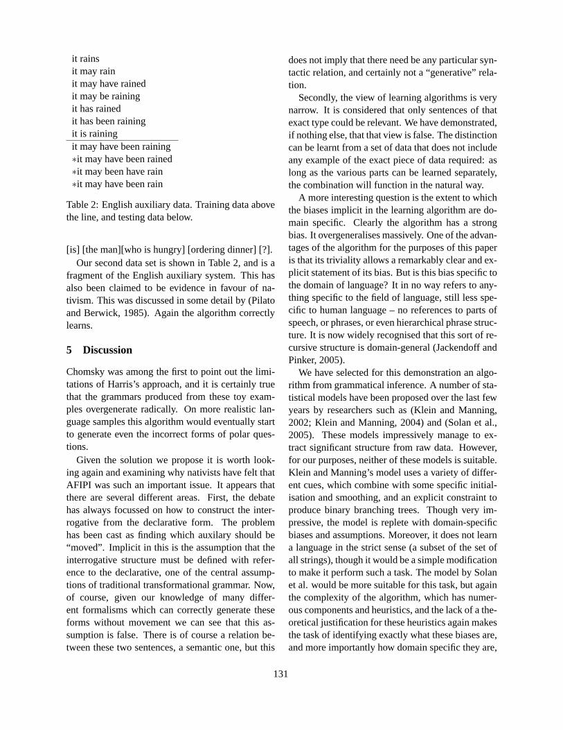
it rainsit may rainit may have rainedit may be rainingit has rainedit has been rainingit is rainingit may have been raining∗it may have been rained∗it may been have rain∗it may have been rain
Table 2: English auxiliary data. Training data abovethe line, and testing data below.
[is] [the man][who is hungry] [ordering dinner] [?].Our second data set is shown in Table 2, and is a
fragment of the English auxiliary system. This hasalso been claimed to be evidence in favour of na-tivism. This was discussed in some detail by (Pilatoand Berwick, 1985). Again the algorithm correctlylearns.
5 Discussion
Chomsky was among the first to point out the limi-tations of Harris’s approach, and it is certainly truethat the grammars produced from these toy exam-ples overgenerate radically. On more realistic lan-guage samples this algorithm would eventually startto generate even the incorrect forms of polar ques-tions.
Given the solution we propose it is worth look-ing again and examining why nativists have felt thatAFIPI was such an important issue. It appears thatthere are several different areas. First, the debatehas always focussed on how to construct the inter-rogative from the declarative form. The problemhas been cast as finding which auxilary should be“moved”. Implicit in this is the assumption that theinterrogative structure must be defined with refer-ence to the declarative, one of the central assump-tions of traditional transformational grammar. Now,of course, given our knowledge of many differ-ent formalisms which can correctly generate theseforms without movement we can see that this as-sumption is false. There is of course a relation be-tween these two sentences, a semantic one, but this
does not imply that there need be any particular syn-tactic relation, and certainly not a “generative” rela-tion.
Secondly, the view of learning algorithms is verynarrow. It is considered that only sentences of thatexact type could be relevant. We have demonstrated,if nothing else, that that view is false. The distinctioncan be learnt from a set of data that does not includeany example of the exact piece of data required: aslong as the various parts can be learned separately,the combination will function in the natural way.
A more interesting question is the extent to whichthe biases implicit in the learning algorithm are do-main specific. Clearly the algorithm has a strongbias. It overgeneralises massively. One of the advan-tages of the algorithm for the purposes of this paperis that its triviality allows a remarkably clear and ex-plicit statement of its bias. But is this bias specific tothe domain of language? It in no way refers to any-thing specific to the field of language, still less spe-cific to human language – no references to parts ofspeech, or phrases, or even hierarchical phrase struc-ture. It is now widely recognised that this sort of re-cursive structure is domain-general (Jackendoff andPinker, 2005).
We have selected for this demonstration an algo-rithm from grammatical inference. A number of sta-tistical models have been proposed over the last fewyears by researchers such as (Klein and Manning,2002; Klein and Manning, 2004) and (Solan et al.,2005). These models impressively manage to ex-tract significant structure from raw data. However,for our purposes, neither of these models is suitable.Klein and Manning’s model uses a variety of differ-ent cues, which combine with some specific initial-isation and smoothing, and an explicit constraint toproduce binary branching trees. Though very im-pressive, the model is replete with domain-specificbiases and assumptions. Moreover, it does not learna language in the strict sense (a subset of the set ofall strings), though it would be a simple modificationto make it perform such a task. The model by Solanet al. would be more suitable for this task, but againthe complexity of the algorithm, which has numer-ous components and heuristics, and the lack of a the-oretical justification for these heuristics again makesthe task of identifying exactly what these biases are,and more importantly how domain specific they are,
131
a very significant problem.In this model, the bias of the algorithm is com-
pletely encapsulated in the assumption u.= v im-
plies u ≡ v. It is worth pointing out that this doesnot even need hierarchical structure – the modelcould be implemented purely as a reduction systemor semi-Thue system. The disadvantage of usingthat approach is that it is possible to construct somebizarre examples where the number of reductionscan be exponential.
Using statistical properties of the set of strings,it is possible to extend these learnability results toa more substantial class of context free languages,though it is unlikely that these methods could be ex-tended to a class that properly contains all naturallanguages.
6 Conclusion
We have presented an analysis of the argument thatthe acquisition of auxiliary fronting in polar inter-rogatives supports linguistic nativism. Using a verysimple algorithm based on the ideas of Zellig Har-ris, with a simple domain-general heuristic, we showthat the empirical question as to the frequency of oc-currence of polar questions of a certain type in child-directed speech is a moot point, since the distinctionin question can be learned even when no such sen-tences occur.
Acknowledgements This work has been partiallysupported by the EU funded PASCAL Network ofExcellence on Pattern Analysis, Statistical Mod-elling and Computational Learning.
References
D. Angluin. 1982. Inference of reversible languages.Communications of the ACM, 29:741–765.
Noam Chomsky. 1975. The Logical Structure of Lin-guistic Theory. University of Chicago Press.
Alexander Clark and Remi Eyraud. 2005. Identificationin the limit of substitutable context free languages. InSanjay Jain, Hans Ulrich Simon, and Etsuji Tomita,editors, Proceedings of The 16th International Confer-ence on Algorithmic Learning Theory, pages 283–296.Springer-Verlag.
S. Crain and M. Nakayama. 1987. Structure dependencein grammar formation. Language, 63(522-543).
C. de la Higuera. 1997. Characteristic sets for poly-nomial grammatical inference. Machine Learning,(27):125–138. Kluwer Academic Publishers. Manu-factured in Netherland.
E. M. Gold. 1967. Language indentification in the limit.Information and control, 10(5):447 – 474.
Zellig Harris. 1954. Distributional structure. Word,10(2-3):146–62.
Ray Jackendoff and Steven Pinker. 2005. The nature ofthe language faculty and its implications for the evolu-tion of language. Cognition, 97:211–225.
X. N. C. Kam, I. Stoyneshka, L. Tornyova, J. D. Fodor,and W. G. Sakas. 2005. Non-robustness of syntaxacquisition from n-grams: A cross-linguistic perspec-tive. In The 18th Annual CUNY Sentence ProcessingConference, April.
Dan Klein and Christopher D. Manning. 2002. A gener-ative constituent-context model for improved grammarinduction. In Proceedings of the 40th Annual Meetingof the ACL.
Dan Klein and Chris Manning. 2004. Corpus-based in-duction of syntactic structure: Models of dependencyand constituency. In Proceedings of the 42nd AnnualMeeting of the ACL.
Samuel F. Pilato and Robert C. Berwick. 1985. Re-versible automata and induction of the english auxil-iary system. In Proceedings of the ACL, pages 70–75.
Geoffrey K. Pullum and Barbara C. Scholz. 2002. Em-pirical assessment of stimulus poverty arguments. TheLinguistic Review, 19(1-2):9–50.
Florencia Reali and Morten H. Christiansen. 2004.Structure dependence in language acquisition: Uncov-ering the statistical richness of the stimulus. In Pro-ceedings of the 26th Annual Conference of the Cogni-tive Science Society, Mahwah, NJ. Lawrence Erlbaum.
Noah A. Smith and Jason Eisner. 2005. Contrastive esti-mation: Training log-linear models on unlabeled data.In Proceedings of the 43rd Annual Meeting of the As-sociation for Computational Linguistics, pages 354–362, Ann Arbor, Michigan, June.
Zach Solan, David Horn, Eytan Ruppin, and ShimonEdelman. 2005. Unsupervised learning of natural lan-guages. Proc. Natl. Acad. Sci., 102:11629–11634.
Menno van Zaanen. 2000. ABL: Alignment-based learn-ing. In COLING 2000 - Proceedings of the 18th Inter-national Conference on Computational Linguistics.
Takashi Yokomori. 2003. Polynomial-time identificationof very simple grammars from positive data. Theoret-ical Computer Science, 298(1):179–206.
132
Proceedings of the 10th Conference on Computational Natural Language Learning (CoNLL-X),pages 133–140, New York City, June 2006.c©2006 Association for Computational Linguistics
Using Gazetteers in Discriminative Information Extraction
Andrew SmithDivision of InformaticsUniversity of Edinburgh
United [email protected]
Miles OsborneDivision of InformaticsUniversity of Edinburgh
United [email protected]
Abstract
Much work on information extraction hassuccessfully used gazetteers to recogniseuncommon entities that cannot be reliablyidentified from local context alone. Ap-proaches to such tasks often involve theuse of maximum entropy-style models,where gazetteers usually appear as highlyinformative features in the model. Al-though such features can improve modelaccuracy, they can also introduce hiddennegative effects. In this paper we de-scribe and analyse these effects and sug-gest ways in which they may be overcome.In particular, we show that by quarantin-ing gazetteer features and training themin a separate model, then decoding usinga logarithmic opinion pool (Smith et al.,2005), we may achieve much higher accu-racy. Finally, we suggest ways in whichother features with gazetteer feature-likebehaviour may be identified.
1 Introduction
In recent years discriminative probabilistic modelshave been successfully applied to a number of infor-mation extraction tasks in natural language process-ing (NLP), such as named entity recognition (NER)(McCallum and Li, 2003), noun phrase chunking(Sha and Pereira, 2003) and information extractionfrom research papers (Peng and McCallum, 2004).Discriminative models offer a significant advantage
over their generative counterparts by allowing thespecification of powerful, possibly non-independentfeatures which would be difficult to tractably encodein a generative model.
In a task such as NER, one sometimes encoun-ters an entity which is difficult to identify using lo-cal contextual cues alone because the entity has notbe seen before. In these cases, a gazetteer or dic-tionary of possible entity identifiers is often useful.Such identifiers could be names of people, places,companies or other organisations. Using gazetteersone may define additional features in the model thatrepresent the dependencies between a word’s NERlabel and its presence in a particular gazetteer. Suchgazetteer features are often highly informative, andtheir inclusion in the model should in principle re-sult in higher model accuracy. However, these fea-tures can also introduce hidden negative effects tak-ing the form of labelling errors that the model makesat places where a model without the gazetteer fea-tures would have labelled correctly. Consequently,ensuring optimal usage of gazetteers can be difficult.
In this paper we describe and analyse the labellingerrors made by a model, and show that they gen-erally result from the model’s over-dependence onthe gazetteer features for making labelling decisions.By including gazetteer features in the model wemay, in some cases, transfer too much explanatorydependency to the gazetteer features from the non-gazetteer features. In order to avoid this problem, amore careful treatment of these features is requiredduring training. We demonstrate that a traditionalregularisation approach, where different features areregularised to different degrees, does not offer a sat-
133
isfactory solution. Instead, we show that by traininggazetteer features in a separate model to the otherfeatures, and decoding using a logarithmic opinionpool (LOP) (Smith et al., 2005), much greater ac-curacy can be obtained. Finally, we identify otherfeatures with gazetteer feature-like properties andshow that similar results may be obtained using ourmethod with these features.
We take as our model a linear chain conditionalrandom field (CRF), and apply it to NER in English.
2 Conditional Random Fields
A linear chain conditional random field (CRF) (Laf-ferty et al., 2001) defines the conditional probabilityof a label sequence s given an observed sequence ovia:
p�s � o ��� 1
Z�o � exp
�T � 1
∑t � 1
∑k
λk fk�st � 1 st o t �� (1)
where T is the length of both sequences, λk are pa-rameters of the model and Z
�o � is a partition func-
tion that ensures that (1) represents a probability dis-tribution. The functions fk are feature functions rep-resenting the occurrence of different events in thesequences s and o.
The parameters λk can be estimated by maximis-ing the conditional log-likelihood of a set of labelledtraining sequences. At the maximum likelihood so-lution the model satisfies a set of feature constraints,whereby the expected count of each feature underthe model is equal to its empirical count on the train-ing data:
E p � o s ��� fk ��� Ep � s � o ��� fk � � 0 �� k
In general this cannot be solved for the λk in closedform, so numerical optimisation must be used. Forour experiments we use the limited memory variablemetric (LMVM) (Sha and Pereira, 2003) routine,which has become the standard algorithm for CRFtraining with a likelihood-based objective function.
To avoid overfitting, a prior distribution over themodel parameters is typically used. A common ex-ample of this is the Gaussian prior. Use of a priorinvolves adding extra terms to the objective and itsderivative. In the case of a Gaussian prior, these ad-ditional terms involve the mean and variance of thedistribution.
3 Previous Use of Gazetteers
Gazetteers have been widely used in a variety of in-formation extraction systems, including both rule-based systems and statistical models. In addition tolists of people names, locations, etc., recent workin the biomedical domain has utilised gazetteers ofbiological and genetic entities such as gene names(Finkel et al., 2005; McDonald and Pereira, 2005).In general gazetteers are thought to provide a usefulsource of external knowledge that is helpful whenan entity cannot be identified from knowledge con-tained solely within the data set used for training.However, some research has questioned the useful-ness of gazetteers (Krupka and Hausman, 1998).Other work has supported the use of gazetteers ingeneral but has found that lists of only moderatesize are sufficient to provide most of the benefit(Mikheev et al., 1999). Therefore, to date the ef-fective use of gazetteers for information extractionhas in general been regarded as a “black art”. In thispaper we explain some of the likely reasons for thesefindings, and propose ways to more effectively han-dle gazetteers when they are used by maxent-stylemodels.
In work developed independently and in parallelto the work presented here, Sutton et al. (2006) iden-tify general problems with gazetteer features andpropose a solution similar to ours. They present re-sults on NP-chunking in addition to NER, and pro-vide a slightly more general approach. By contrast,we motivate the problem more thoroughly throughanalysis of the actual errors observed and throughconsideration of the success of other candidate solu-tions, such as traditional regularisation over featuresubsets.
4 Our Experiments
In this section we describe our experimental setup,and provide results for the baseline models.
4.1 Task and Dataset
Named entity recognition (NER) involves the iden-tification of the location and type of pre-defined en-tities within a sentence. The CRF is presented witha set of sentences and must label each word so asto indicate whether the word appears outside an en-tity, at the beginning of an entity of a certain type or
134
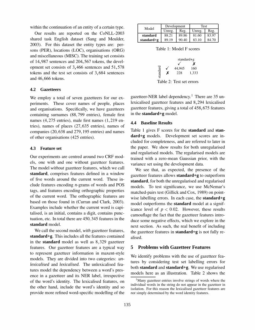
within the continuation of an entity of a certain type.Our results are reported on the CoNLL-2003
shared task English dataset (Sang and Meulder,2003). For this dataset the entity types are: per-sons (PER), locations (LOC), organisations (ORG)and miscellaneous (MISC). The training set consistsof 14 987 sentences and 204 567 tokens, the devel-opment set consists of 3 466 sentences and 51 578tokens and the test set consists of 3 684 sentencesand 46 666 tokens.
4.2 Gazetteers
We employ a total of seven gazetteers for our ex-periments. These cover names of people, placesand organisations. Specifically, we have gazetteerscontaining surnames (88 799 entries), female firstnames (4 275 entries), male first names (1 219 en-tries), names of places (27 635 entries), names ofcompanies (20 638 and 279 195 entries) and namesof other organisations (425 entries).
4.3 Feature set
Our experiments are centred around two CRF mod-els, one with and one without gazetteer features.The model without gazetteer features, which we callstandard, comprises features defined in a windowof five words around the current word. These in-clude features encoding n-grams of words and POStags, and features encoding orthographic propertiesof the current word. The orthographic features arebased on those found in (Curran and Clark, 2003).Examples include whether the current word is capi-talised, is an initial, contains a digit, contains punc-tuation, etc. In total there are 450 345 features in thestandard model.
We call the second model, with gazetteer features,standard+g. This includes all the features containedin the standard model as well as 8 329 gazetteerfeatures. Our gazetteer features are a typical wayto represent gazetteer information in maxent-stylemodels. They are divided into two categories: un-lexicalised and lexicalised. The unlexicalised fea-tures model the dependency between a word’s pres-ence in a gazetteer and its NER label, irrespectiveof the word’s identity. The lexicalised features, onthe other hand, include the word’s identity and soprovide more refined word-specific modelling of the
Model Development TestUnreg. Reg. Unreg. Reg.
standard 88.21 89.86 81.60 83.97standard+g 89.19 90.40 83.10 84.70
Table 1: Model F scores
standard+g�✗
stand
ard �
44,945 160✗ 228 1,333
Table 2: Test set errors
gazetteer-NER label dependency.1 There are 35 un-lexicalised gazetteer features and 8 294 lexicalisedgazetteer features, giving a total of 458 675 featuresin the standard+g model.
4.4 Baseline Results
Table 1 gives F scores for the standard and stan-dard+g models. Development set scores are in-cluded for completeness, and are referred to later inthe paper. We show results for both unregularisedand regularised models. The regularised models aretrained with a zero-mean Gaussian prior, with thevariance set using the development data.
We see that, as expected, the presence of thegazetteer features allows standard+g to outperformstandard, for both the unregularised and regularisedmodels. To test significance, we use McNemar’smatched-pairs test (Gillick and Cox, 1989) on point-wise labelling errors. In each case, the standard+gmodel outperforms the standard model at a signif-icance level of p � 0 � 02. However, these resultscamouflage the fact that the gazetteer features intro-duce some negative effects, which we explore in thenext section. As such, the real benefit of includingthe gazetteer features in standard+g is not fully re-alised.
5 Problems with Gazetteer Features
We identify problems with the use of gazetteer fea-tures by considering test set labelling errors forboth standard and standard+g. We use regularisedmodels here as an illustration. Table 2 shows the
1Many gazetteer entries involve strings of words where theindividual words in the string do not appear in the gazetteer inisolation. For this reason the lexicalised gazetteer features arenot simply determined by the word identity features.
135
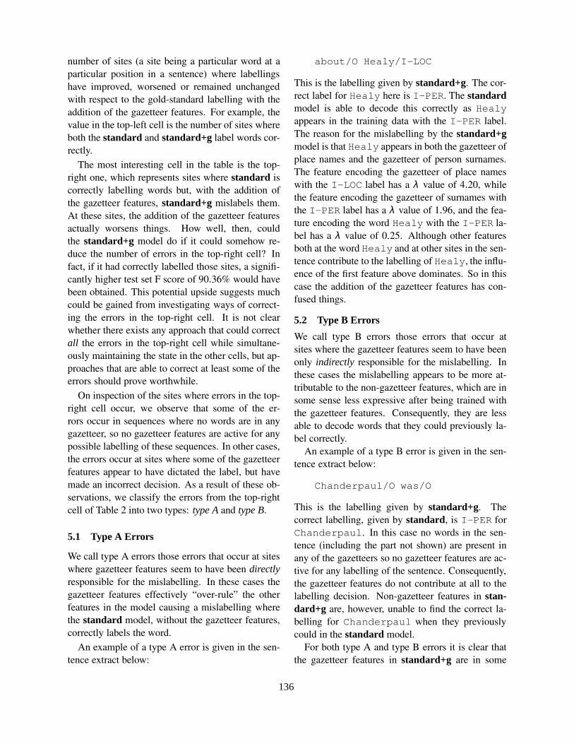
number of sites (a site being a particular word at aparticular position in a sentence) where labellingshave improved, worsened or remained unchangedwith respect to the gold-standard labelling with theaddition of the gazetteer features. For example, thevalue in the top-left cell is the number of sites whereboth the standard and standard+g label words cor-rectly.
The most interesting cell in the table is the top-right one, which represents sites where standard iscorrectly labelling words but, with the addition ofthe gazetteer features, standard+g mislabels them.At these sites, the addition of the gazetteer featuresactually worsens things. How well, then, couldthe standard+g model do if it could somehow re-duce the number of errors in the top-right cell? Infact, if it had correctly labelled those sites, a signifi-cantly higher test set F score of 90 � 36% would havebeen obtained. This potential upside suggests muchcould be gained from investigating ways of correct-ing the errors in the top-right cell. It is not clearwhether there exists any approach that could correctall the errors in the top-right cell while simultane-ously maintaining the state in the other cells, but ap-proaches that are able to correct at least some of theerrors should prove worthwhile.
On inspection of the sites where errors in the top-right cell occur, we observe that some of the er-rors occur in sequences where no words are in anygazetteer, so no gazetteer features are active for anypossible labelling of these sequences. In other cases,the errors occur at sites where some of the gazetteerfeatures appear to have dictated the label, but havemade an incorrect decision. As a result of these ob-servations, we classify the errors from the top-rightcell of Table 2 into two types: type A and type B.
5.1 Type A Errors
We call type A errors those errors that occur at siteswhere gazetteer features seem to have been directlyresponsible for the mislabelling. In these cases thegazetteer features effectively “over-rule” the otherfeatures in the model causing a mislabelling wherethe standard model, without the gazetteer features,correctly labels the word.
An example of a type A error is given in the sen-tence extract below:
about/O Healy/I-LOC
This is the labelling given by standard+g. The cor-rect label for Healy here is I-PER. The standardmodel is able to decode this correctly as Healyappears in the training data with the I-PER label.The reason for the mislabelling by the standard+gmodel is that Healy appears in both the gazetteer ofplace names and the gazetteer of person surnames.The feature encoding the gazetteer of place nameswith the I-LOC label has a λ value of 4 � 20, whilethe feature encoding the gazetteer of surnames withthe I-PER label has a λ value of 1 � 96, and the fea-ture encoding the word Healy with the I-PER la-bel has a λ value of 0 � 25. Although other featuresboth at the word Healy and at other sites in the sen-tence contribute to the labelling of Healy, the influ-ence of the first feature above dominates. So in thiscase the addition of the gazetteer features has con-fused things.
5.2 Type B Errors
We call type B errors those errors that occur atsites where the gazetteer features seem to have beenonly indirectly responsible for the mislabelling. Inthese cases the mislabelling appears to be more at-tributable to the non-gazetteer features, which are insome sense less expressive after being trained withthe gazetteer features. Consequently, they are lessable to decode words that they could previously la-bel correctly.
An example of a type B error is given in the sen-tence extract below:
Chanderpaul/O was/O
This is the labelling given by standard+g. Thecorrect labelling, given by standard, is I-PER forChanderpaul. In this case no words in the sen-tence (including the part not shown) are present inany of the gazetteers so no gazetteer features are ac-tive for any labelling of the sentence. Consequently,the gazetteer features do not contribute at all to thelabelling decision. Non-gazetteer features in stan-dard+g are, however, unable to find the correct la-belling for Chanderpaul when they previouslycould in the standard model.
For both type A and type B errors it is clear thatthe gazetteer features in standard+g are in some
136
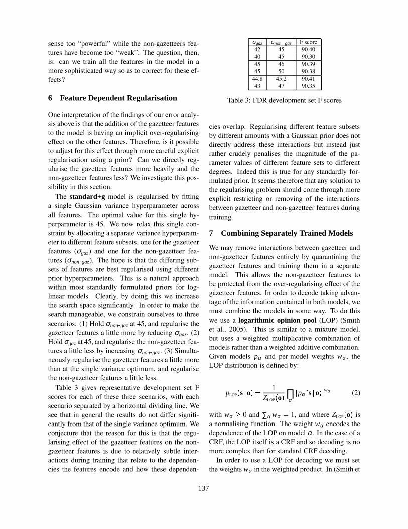
sense too “powerful” while the non-gazetteers fea-tures have become too “weak”. The question, then,is: can we train all the features in the model in amore sophisticated way so as to correct for these ef-fects?
6 Feature Dependent Regularisation
One interpretation of the findings of our error analy-sis above is that the addition of the gazetteer featuresto the model is having an implicit over-regularisingeffect on the other features. Therefore, is it possibleto adjust for this effect through more careful explicitregularisation using a prior? Can we directly reg-ularise the gazetteer features more heavily and thenon-gazetteer features less? We investigate this pos-sibility in this section.
The standard+g model is regularised by fittinga single Gaussian variance hyperparameter acrossall features. The optimal value for this single hy-perparameter is 45. We now relax this single con-straint by allocating a separate variance hyperparam-eter to different feature subsets, one for the gazetteerfeatures (σgaz) and one for the non-gazetteer fea-tures (σnon-gaz). The hope is that the differing sub-sets of features are best regularised using differentprior hyperparameters. This is a natural approachwithin most standardly formulated priors for log-linear models. Clearly, by doing this we increasethe search space significantly. In order to make thesearch manageable, we constrain ourselves to threescenarios: (1) Hold σnon-gaz at 45, and regularise thegazetteer features a little more by reducing σgaz. (2)Hold σgaz at 45, and regularise the non-gazetteer fea-tures a little less by increasing σnon-gaz. (3) Simulta-neously regularise the gazetteer features a little morethan at the single variance optimum, and regularisethe non-gazetteer features a little less.
Table 3 gives representative development set Fscores for each of these three scenarios, with eachscenario separated by a horizontal dividing line. Wesee that in general the results do not differ signifi-cantly from that of the single variance optimum. Weconjecture that the reason for this is that the regu-larising effect of the gazetteer features on the non-gazetteer features is due to relatively subtle inter-actions during training that relate to the dependen-cies the features encode and how these dependen-
σgaz σnon � gaz F score42 45 90.4040 45 90.3045 46 90.3945 50 90.38
44.8 45.2 90.4143 47 90.35
Table 3: FDR development set F scores
cies overlap. Regularising different feature subsetsby different amounts with a Gaussian prior does notdirectly address these interactions but instead justrather crudely penalises the magnitude of the pa-rameter values of different feature sets to differentdegrees. Indeed this is true for any standardly for-mulated prior. It seems therefore that any solution tothe regularising problem should come through moreexplicit restricting or removing of the interactionsbetween gazetteer and non-gazetteer features duringtraining.
7 Combining Separately Trained Models
We may remove interactions between gazetteer andnon-gazetteer features entirely by quarantining thegazetteer features and training them in a separatemodel. This allows the non-gazetteer features tobe protected from the over-regularising effect of thegazetteer features. In order to decode taking advan-tage of the information contained in both models, wemust combine the models in some way. To do thiswe use a logarithmic opinion pool (LOP) (Smithet al., 2005). This is similar to a mixture model,but uses a weighted multiplicative combination ofmodels rather than a weighted additive combination.Given models pα and per-model weights wα , theLOP distribution is defined by:
pLOP�s � o ��� 1
ZLOP�o � ∏
α� pα
�s � o � � wα (2)
with wα� 0 and ∑α wα � 1, and where ZLOP
�o � is
a normalising function. The weight wα encodes thedependence of the LOP on model α . In the case of aCRF, the LOP itself is a CRF and so decoding is nomore complex than for standard CRF decoding.
In order to use a LOP for decoding we must setthe weights wα in the weighted product. In (Smith et
137
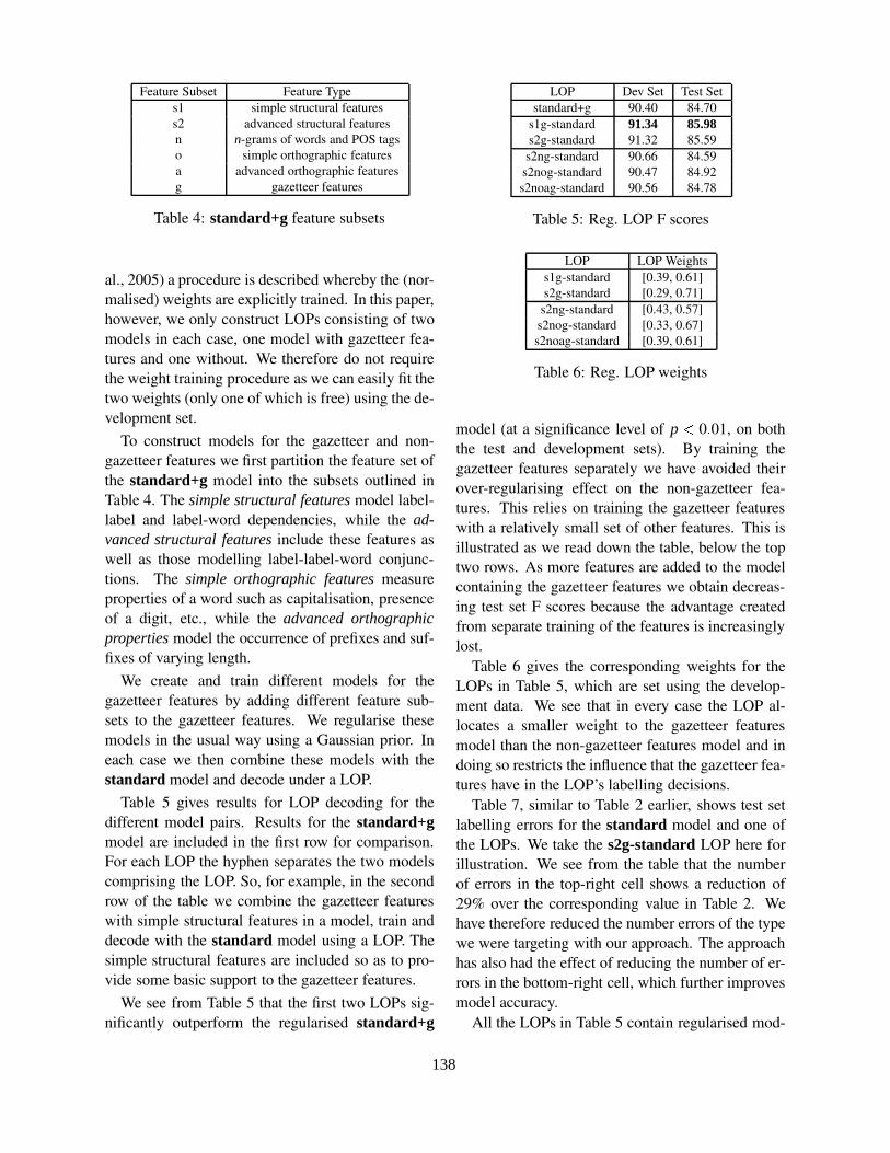
Feature Subset Feature Types1 simple structural featuress2 advanced structural featuresn n-grams of words and POS tagso simple orthographic featuresa advanced orthographic featuresg gazetteer features
Table 4: standard+g feature subsets
al., 2005) a procedure is described whereby the (nor-malised) weights are explicitly trained. In this paper,however, we only construct LOPs consisting of twomodels in each case, one model with gazetteer fea-tures and one without. We therefore do not requirethe weight training procedure as we can easily fit thetwo weights (only one of which is free) using the de-velopment set.
To construct models for the gazetteer and non-gazetteer features we first partition the feature set ofthe standard+g model into the subsets outlined inTable 4. The simple structural features model label-label and label-word dependencies, while the ad-vanced structural features include these features aswell as those modelling label-label-word conjunc-tions. The simple orthographic features measureproperties of a word such as capitalisation, presenceof a digit, etc., while the advanced orthographicproperties model the occurrence of prefixes and suf-fixes of varying length.
We create and train different models for thegazetteer features by adding different feature sub-sets to the gazetteer features. We regularise thesemodels in the usual way using a Gaussian prior. Ineach case we then combine these models with thestandard model and decode under a LOP.
Table 5 gives results for LOP decoding for thedifferent model pairs. Results for the standard+gmodel are included in the first row for comparison.For each LOP the hyphen separates the two modelscomprising the LOP. So, for example, in the secondrow of the table we combine the gazetteer featureswith simple structural features in a model, train anddecode with the standard model using a LOP. Thesimple structural features are included so as to pro-vide some basic support to the gazetteer features.
We see from Table 5 that the first two LOPs sig-nificantly outperform the regularised standard+g
LOP Dev Set Test Setstandard+g 90.40 84.70
s1g-standard 91.34 85.98s2g-standard 91.32 85.59s2ng-standard 90.66 84.59
s2nog-standard 90.47 84.92s2noag-standard 90.56 84.78
Table 5: Reg. LOP F scores
LOP LOP Weightss1g-standard [0.39, 0.61]s2g-standard [0.29, 0.71]
s2ng-standard [0.43, 0.57]s2nog-standard [0.33, 0.67]s2noag-standard [0.39, 0.61]
Table 6: Reg. LOP weights
model (at a significance level of p � 0 � 01, on boththe test and development sets). By training thegazetteer features separately we have avoided theirover-regularising effect on the non-gazetteer fea-tures. This relies on training the gazetteer featureswith a relatively small set of other features. This isillustrated as we read down the table, below the toptwo rows. As more features are added to the modelcontaining the gazetteer features we obtain decreas-ing test set F scores because the advantage createdfrom separate training of the features is increasinglylost.
Table 6 gives the corresponding weights for theLOPs in Table 5, which are set using the develop-ment data. We see that in every case the LOP al-locates a smaller weight to the gazetteer featuresmodel than the non-gazetteer features model and indoing so restricts the influence that the gazetteer fea-tures have in the LOP’s labelling decisions.
Table 7, similar to Table 2 earlier, shows test setlabelling errors for the standard model and one ofthe LOPs. We take the s2g-standard LOP here forillustration. We see from the table that the numberof errors in the top-right cell shows a reduction of29% over the corresponding value in Table 2. Wehave therefore reduced the number errors of the typewe were targeting with our approach. The approachhas also had the effect of reducing the number of er-rors in the bottom-right cell, which further improvesmodel accuracy.
All the LOPs in Table 5 contain regularised mod-
138

s2g-standard LOP�✗
stand
ard �
44,991 114✗ 305 1,256
Table 7: Test set errors
LOP Dev Set Test Sets1g-standard 90.58 84.87s2g-standard 90.70 84.28s2ng-standard 89.70 84.01
s2nog-standard 89.48 83.99s2noag-standard 89.40 83.70
Table 8: Unreg. LOP F scores
els. Table 8 gives test set F scores for the cor-responding LOPs constructed from unregularisedmodels. As we would expect, the scores are lowerthan those in Table 5. However, it is interesting tonote that the s1g-standard LOP still outperformsthe regularised standard+g model.
In summary, by training the gazetteer featuresand non-gazetteer features in separate models anddecoding using a LOP, we are able to overcomethe problems described in earlier sections and canachieve much higher accuracy. This shows thatsuccessfully deploying gazetteer features withinmaxent-style models should involve careful consid-eration of restrictions on how features interact witheach other, rather than simply considering the abso-lute values of feature parameters.
8 Gazetteer-Like Features
So far our discussion has focused on gazetteer fea-tures. However, we would expect that the problemswe have described and dealt with in the last sec-tion also occur with other types of features that havesimilar properties to gazetteer features. By applyingsimilar treatment to these features during training wemay be able harness their usefulness to a greater de-gree than is currently the case when training in a sin-gle model. So how can we identify these features?
The task of identifying the optimal partitioningfor creation of models in the previous section is ingeneral a hard problem as it relies on clustering thefeatures based on their explanatory power relative toall other clusters. It may be possible, however, to de-vise some heuristics that approximately correspond
to the salient properties of gazetteer features (withrespect to the clustering) and which can then be usedto identify other features that have these properties.In this section we consider three such heuristics. Allof these heuristics are motivated by the observationthat gazetteer features are both highly discriminativeand generally very sparse.
Family Singleton Features We define a featurefamily as a set of features that have the same con-junction of predicates defined on the observations.Hence they differ from each other only in the NERlabel that they encode. Family singleton featuresare features that have a count of 1 in the trainingdata when all other members of that feature familyhave zero counts. These features have a flavour ofgazetteer features in that they represent the fact thatthe conjunction of observation predicates they en-code is highly predictive of the corresponding NERlabel, and that they are also very sparse.
Family n-ton Features These are features thathave a count of n (greater than 1) in the trainingdata when all other members of that feature familyhave zero counts. They are similar to family sin-gleton features, but exhibit gazetteer-like propertiesless and less as the value of n is increased because alarger value of n represents less sparsity.
Loner Features These are features which occurwith a low mean number of other features in thetraining data. They are similar to gazetteer featuresin that, at the points where they occur, they are insome sense being relied upon more than most fea-tures to explain the data. To create loner feature setswe rank all features in the standard+g model basedon the mean number of other features they are ob-served with in the training data, then we take subsetsof increasing size. We present results for subsets ofsize 500, 1000, 5000 and 10000.
For each of these categories of features we addsimple structural features (the s1 set from earlier),to provide basic structural support, and then train aregularised model. We also train a regularised modelconsisting of all features in standard+g except thefeatures from the category in question. We decodethese model pairs under a LOP as described earlier.
Table 9 gives test set F scores for LOPs cre-ated from each of the categories of features above
139

LOP Test SetFSF 85.79FnF 84.78
LF 500 85.80LF 1000 85.70LF 5000 85.77
LF 10000 85.62
Table 9: Reg. LOP F scores
(with abbreviated names derived from the categorynames). The results show that for the family single-ton features and each of the loner feature sets weobtain LOPs that significantly outperform the reg-ularised standard+g model (p � 0 � 0002 in everycase). The family n-ton features’ LOP does not doas well, but that is probably due to the fact that someof the features in this set have a large value of n andso behave much less like gazetteer features.
In summary, we obtain the same pattern of resultsusing our quarantined training and LOP decodingmethod with these categories of features that we dowith the gazetteer features. We conclude that theproblems with gazetteer features that we have iden-tified in this paper are exhibited by general discrim-inative features with gazetteer feature-like proper-ties, and our method is also successful with thesemore general features. Clearly, the heuristics thatwe have devised in this section are very simple, andit is likely that with more careful engineering betterfeature partitions can be found.
9 Conclusion and future work
In this paper we have identified and analysed nega-tive effects that can be introduced to maxent-stylemodels by the inclusion of highly discriminativegazetteer features. We have shown that such ef-fects manifest themselves through errors that gen-erally result from the model’s over-dependence onthe gazetteer features for decision making. To over-come this problem a more careful treatment of thesefeatures is required during training. We have pro-posed a solution that involves quarantining the fea-tures and training them separately to the other fea-tures in the model, then decoding the separate mod-els with a logarithmic opinion pool. In fact, the LOPprovides a natural way to handle the problem, withdifferent constituent models for the different fea-
ture types. The method leads to much greater ac-curacy, and allows the power of gazetteer featuresto be more effectively harnessed. Finally, we haveidentified other feature sets with gazetteer feature-like properties and shown that similar results may beobtained using our method with these feature sets.
In this paper we defined intuitively-motivated fea-ture partitions (gazetteer feature-based or otherwise)using heuristics. In future work we will focus on au-tomatically determining such partitions.
ReferencesJames Curran and Stephen Clark. 2003. Language independent
NER using a maximum entropy tagger. In Proc. CoNLL-2003.
Jenny Finkel, Shipra Dingare, Christopher D. Manning, Malv-ina Nissim, Beatrice Alex, and Claire Grover. 2005. Ex-ploring the boundaries: gene and protein identification inbiomedical text. BMC Bioinformatics, (6).
L. Gillick and Stephen Cox. 1989. Some statistical issues inthe comparison of speech recognition algorithms. In Inter-national Conference on Acoustics, Speech and Signal Pro-cessing, volume 1, pages 532–535.
George R. Krupka and Kevin Hausman. 1998. Isoquest Inc:Description of the NetOwl (TM) extractor system as usedfor MUC-7. In Proc. MUC-7.
John Lafferty, Andrew McCallum, and Fernando Pereira. 2001.Conditional random fields: Probabilistic models for seg-menting and labeling sequence data. In Proc. ICML 2001.
Andrew McCallum and Wei Li. 2003. Early results for namedentity recognition with conditional random fields, feature in-duction and web-enhanced lexicons. In Proc. CoNLL-2003.
Ryan McDonald and Fernando Pereira. 2005. Identifying geneand protein mentions in text using conditional random fields.BMC Bioinformatics, (6).
Andrei Mikheev, Marc Moens, and Claire Grover. 1999.Named entity recognition without gazetteers.
Fuchun Peng and Andrew McCallum. 2004. Accurate informa-tion extraction from research papers using conditional ran-dom fields. In Proc. HLT-NAACL 2004.
Erik F. Tjong Kim Sang and Fien De Meulder. 2003. Introduc-tion to the CoNLL-2003 shared task: Language-independentnamed entity recognition. In Proc. CoNLL-2003.
Fei Sha and Fernando Pereira. 2003. Shallow parsing withconditional random fields. In Proc. HLT-NAACL 2003.
Andrew Smith, Trevor Cohn, and Miles Osborne. 2005. Loga-rithmic opinion pools for conditional random fields. In Proc.ACL 2005.
Charles Sutton, Michael Sindelar, and Andrew McCallum.2006. Reducing weight undertraining in struxctured dis-criminative learning. In Proc. HLT/NAACL 2006.
140
Proceedings of the 10th Conference on Computational Natural Language Learning (CoNLL-X),pages 141–148, New York City, June 2006.c©2006 Association for Computational Linguistics
A Context Pattern Induction Method for Named Entity Extraction
Partha Pratim TalukdarCIS Department
University of PennsylvaniaPhiladelphia, PA [email protected]
Thorsten BrantsGoogle, Inc.
1600 Amphitheatre Pkwy.Mountain View, CA 94043
Mark Liberman Fernando PereiraCIS Department
University of PennsylvaniaPhiladelphia, PA 19104
{myl,pereira}@cis.upenn.edu
Abstract
We present a novel context pattern in-duction method for information extrac-tion, specifically named entity extraction.Using this method, we extended severalclasses of seed entity lists into much largerhigh-precision lists. Using token member-ship in these extended lists as additionalfeatures, we improved the accuracy of aconditional random field-based named en-tity tagger. In contrast, features derivedfrom the seed lists decreased extractor ac-curacy.
1 Introduction
Partial entity lists and massive amounts of unla-beled data are becoming available with the growthof the Web as well as the increased availability ofspecialized corpora and entity lists. For example,the primary public resource for biomedical research,MEDLINE, contains over 13 million entries and isgrowing at an accelerating rate. Combined withthese large corpora, the recent availability of entitylists in those domains has opened up interesting op-portunities and challenges. Such lists are never com-plete and suffer from sampling biases, but we wouldlike to exploit them, in combination with large un-labeled corpora, to speed up the creation of infor-mation extraction systems for different domains andlanguages. In this paper, we concentrate on explor-ing utility of such resources for named entity extrac-tion.
Currently available entity lists contain a smallfraction of named entities, but there are orders ofmagnitude more present in the unlabeled data1. Inthis paper, we test the following hypotheses:
i. Starting with a few seed entities, it is possibleto induce high-precision context patterns by ex-ploiting entity context redundancy.
ii. New entity instances of the same category canbe extracted from unlabeled data with the in-duced patterns to create high-precision exten-sions of the seed lists.
iii. Features derived from token membership in theextended lists improve the accuracy of learnednamed-entity taggers.
Previous approaches to context pattern induc-tion were described by Riloff and Jones (1999),Agichtein and Gravano (2000), Thelen and Riloff(2002), Lin et al. (2003), and Etzioni et al. (2005),among others. The main advance in the presentmethod is the combination of grammatical inductionand statistical techniques to create high-precisionpatterns.
The paper is organized as follows. Section 2 de-scribes our pattern induction algorithm. Section 3shows how to extend seed sets with entities extractedby the patterns from unlabeled data. Section 4 givesexperimental results, and Section 5 compares ourmethod with previous work.
1For example, based on approximate matching, there is anoverlap of only 22 organizations between the 2403 organiza-tions present in CoNLL-2003 shared task training data and theFortune-500 list.
141

2 Context Pattern Induction
The overall method for inducing entity context pat-terns and extending entity lists is as follows:
1. LetE = seed set,T = text corpus.
2. Find the contextsC of entities inE in the cor-pusT (Section 2.1).
3. Selecttrigger wordsfrom C (Section 2.2).
4. For each trigger word, induce a pattern automa-ton (Section 2.3).
5. Use induced patternsP to extract more entitiesE′ (Section 3).
6. RankP andE′ (Section 3.1).
7. If needed, add high scoring entities inE′ to E
and return to step 2. Otherwise, terminate withpatternsP and extended entity listE ∪ E′ asresults.
2.1 Extracting Context
Starting with the seed list, we first find occurrencesof seed entities in the unlabeled data. For each suchoccurrence, we extract a fixed numberW (contextwindow size) of tokens immediately preceding andimmediately following the matched entity. As weare only interested in modeling the context here, wereplace all entity tokens by the single token-ENT-.This token now represents aslot in which an entitycan occur. Examples of extracted entity contexts areshown in Table 1. In the work presented in this pa-pers, seeds are entity instances (e.g.Googleis a seedfor organization category).
increased expression of-ENT- in vad micethe expression of-ENT- mrna was greater
expression of the-ENT- gene in mouse
Table 1: Extracted contexts of known genes withW = 3.
The set of extracted contexts is denoted byC. Thenext step is to automatically induce high-precisionpatterns containing the token-ENT- from such ex-tracted contexts.
2.2 Trigger Word Selection
To induce patterns, we need to determine their starts.It is reasonable to assume that some tokens are morespecific to particular entity classes than others. Forexample, in the examples shown above,expressioncan be one such word for gene names. Wheneverone comes across such a token in text, the proba-bility of finding an entity (of the corresponding en-tity class) in its vicinity is high. We call such start-ing tokenstrigger words. Trigger words mark thebeginning of a pattern. It is important to note thatsimply selecting the first token of extracted contextsmay not be a good way to select trigger words. Insuch a scheme, we would have to varyW to searchfor useful pattern starts. Instead of that brute-forcetechnique, we propose an automatic way of select-ing trigger words. A good set of trigger words isvery important for the quality of induced patterns.Ideally, we want a trigger word to satisfy the follow-ing:
• It is frequent in the setC of extracted contexts.
• It is specific to entities of interest and therebyto extracted contexts.
We use a term-weighting method to rank candi-date trigger words from entity contexts. IDF (In-verse Document Frequency) was used in our experi-ments but any other suitable term-weighting schememay work comparably. The IDF weightfw for awordw occurring in a corpus is given by:
fw = log
(
N
nw
)
whereN is the total number of documents in thecorpus andnw is the total number of documents con-tainingw. Now, for each context segmentc ∈ C, weselect adominating worddc given by
dc = arg maxw∈c
fw
There is exactly one dominating word for eachc ∈ C. All dominating words for contexts inC formmultisetM . Let mw be the multiplicity of the dom-inating wordw in M . We sortM by decreasingmw
and select the topn tokens from this list as potentialtrigger words.
142
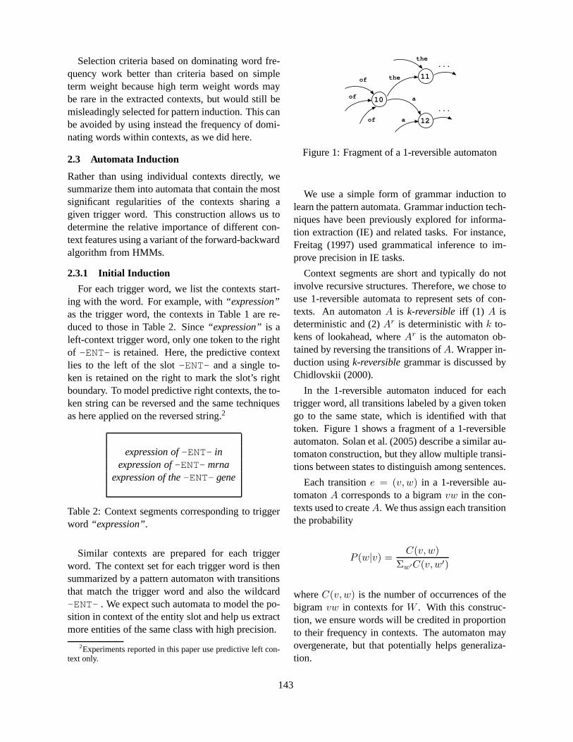
Selection criteria based on dominating word fre-quency work better than criteria based on simpleterm weight because high term weight words maybe rare in the extracted contexts, but would still bemisleadingly selected for pattern induction. This canbe avoided by using instead the frequency of domi-nating words within contexts, as we did here.
2.3 Automata Induction
Rather than using individual contexts directly, wesummarize them into automata that contain the mostsignificant regularities of the contexts sharing agiven trigger word. This construction allows us todetermine the relative importance of different con-text features using a variant of the forward-backwardalgorithm from HMMs.
2.3.1 Initial Induction
For each trigger word, we list the contexts start-ing with the word. For example, with“expression”as the trigger word, the contexts in Table 1 are re-duced to those in Table 2. Since“expression” is aleft-context trigger word, only one token to the rightof -ENT- is retained. Here, the predictive contextlies to the left of the slot-ENT- and a single to-ken is retained on the right to mark the slot’s rightboundary. To model predictive right contexts, the to-ken string can be reversed and the same techniquesas here applied on the reversed string.2
expression of-ENT- inexpression of-ENT- mrna
expression of the-ENT- gene
Table 2: Context segments corresponding to triggerword “expression”.
Similar contexts are prepared for each triggerword. The context set for each trigger word is thensummarized by a pattern automaton with transitionsthat match the trigger word and also the wildcard-ENT- . We expect such automata to model the po-sition in context of the entity slot and help us extractmore entities of the same class with high precision.
2Experiments reported in this paper use predictive left con-text only.
10
11
12
of
of
of
the
the
a
...
...
a
Figure 1: Fragment of a 1-reversible automaton
We use a simple form of grammar induction tolearn the pattern automata. Grammar induction tech-niques have been previously explored for informa-tion extraction (IE) and related tasks. For instance,Freitag (1997) used grammatical inference to im-prove precision in IE tasks.
Context segments are short and typically do notinvolve recursive structures. Therefore, we chose touse 1-reversible automata to represent sets of con-texts. An automatonA is k-reversibleiff (1) A isdeterministic and (2)Ar is deterministic withk to-kens of lookahead, whereAr is the automaton ob-tained by reversing the transitions ofA. Wrapper in-duction usingk-reversiblegrammar is discussed byChidlovskii (2000).
In the 1-reversible automaton induced for eachtrigger word, all transitions labeled by a given tokengo to the same state, which is identified with thattoken. Figure 1 shows a fragment of a 1-reversibleautomaton. Solan et al. (2005) describe a similar au-tomaton construction, but they allow multiple transi-tions between states to distinguish among sentences.
Each transitione = (v,w) in a 1-reversible au-tomatonA corresponds to a bigramvw in the con-texts used to createA. We thus assign each transitionthe probability
P (w|v) =C(v,w)
Σw′C(v,w′)
whereC(v,w) is the number of occurrences of thebigramvw in contexts forW . With this construc-tion, we ensure words will be credited in proportionto their frequency in contexts. The automaton mayovergenerate, but that potentially helps generaliza-tion.
143
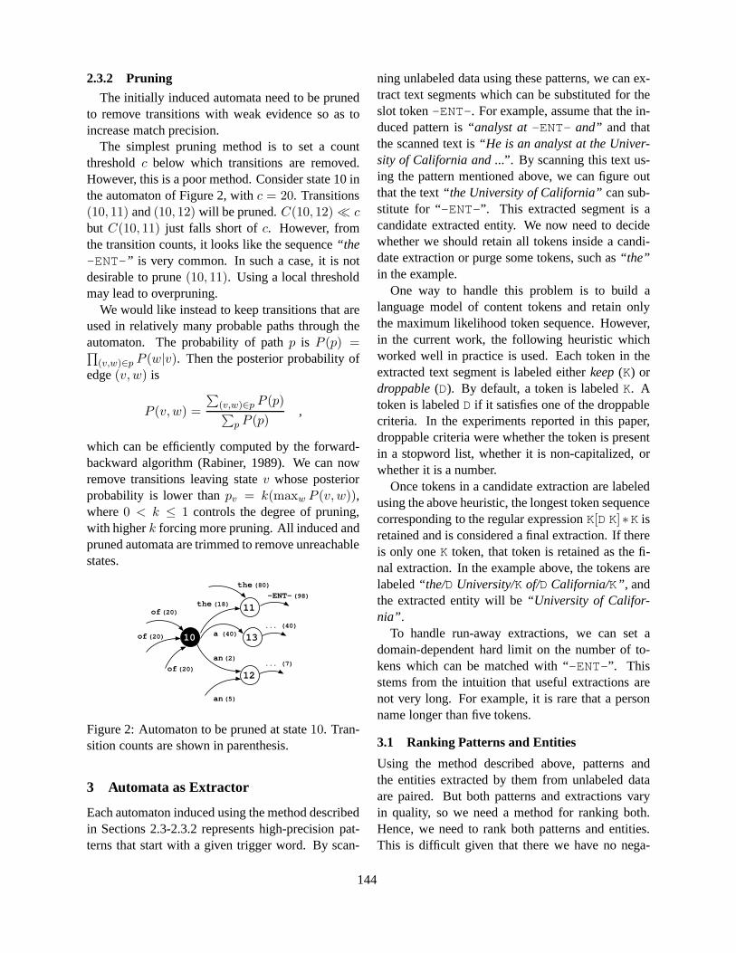
2.3.2 Pruning
The initially induced automata need to be prunedto remove transitions with weak evidence so as toincrease match precision.
The simplest pruning method is to set a countthresholdc below which transitions are removed.However, this is a poor method. Consider state 10 inthe automaton of Figure 2, withc = 20. Transitions(10, 11) and(10, 12) will be pruned.C(10, 12) � c
but C(10, 11) just falls short ofc. However, fromthe transition counts, it looks like the sequence“the-ENT-” is very common. In such a case, it is notdesirable to prune(10, 11). Using a local thresholdmay lead to overpruning.
We would like instead to keep transitions that areused in relatively many probable paths through theautomaton. The probability of pathp is P (p) =∏
(v,w)∈p P (w|v). Then the posterior probability ofedge(v,w) is
P (v,w) =
∑
(v,w)∈p P (p)∑
p P (p),
which can be efficiently computed by the forward-backward algorithm (Rabiner, 1989). We can nowremove transitions leaving statev whose posteriorprobability is lower thanpv = k(maxw P (v,w)),where0 < k ≤ 1 controls the degree of pruning,with higherk forcing more pruning. All induced andpruned automata are trimmed to remove unreachablestates.
10
11
12
of
of
of
the
the
an
(98)
13a
an
... (40)
... (7)
(5)
(80)
(18)
(40)(20)
(20)
(20)
(2)
-ENT-
Figure 2: Automaton to be pruned at state10. Tran-sition counts are shown in parenthesis.
3 Automata as Extractor
Each automaton induced using the method describedin Sections 2.3-2.3.2 represents high-precision pat-terns that start with a given trigger word. By scan-
ning unlabeled data using these patterns, we can ex-tract text segments which can be substituted for theslot token-ENT-. For example, assume that the in-duced pattern is“analyst at -ENT- and” and thatthe scanned text is“He is an analyst at the Univer-sity of California and ...”. By scanning this text us-ing the pattern mentioned above, we can figure outthat the text“the University of California” can sub-stitute for “-ENT-”. This extracted segment is acandidate extracted entity. We now need to decidewhether we should retain all tokens inside a candi-date extraction or purge some tokens, such as“the”in the example.
One way to handle this problem is to build alanguage model of content tokens and retain onlythe maximum likelihood token sequence. However,in the current work, the following heuristic whichworked well in practice is used. Each token in theextracted text segment is labeled eitherkeep(K) ordroppable(D). By default, a token is labeledK. Atoken is labeledD if it satisfies one of the droppablecriteria. In the experiments reported in this paper,droppable criteria were whether the token is presentin a stopword list, whether it is non-capitalized, orwhether it is a number.
Once tokens in a candidate extraction are labeledusing the above heuristic, the longest token sequencecorresponding to the regular expressionK[D K]∗K isretained and is considered a final extraction. If thereis only oneK token, that token is retained as the fi-nal extraction. In the example above, the tokens arelabeled“the/D University/K of/D California/K” , andthe extracted entity will be“University of Califor-nia” .
To handle run-away extractions, we can set adomain-dependent hard limit on the number of to-kens which can be matched with “-ENT-”. Thisstems from the intuition that useful extractions arenot very long. For example, it is rare that a personname longer than five tokens.
3.1 Ranking Patterns and Entities
Using the method described above, patterns andthe entities extracted by them from unlabeled dataare paired. But both patterns and extractions varyin quality, so we need a method for ranking both.Hence, we need to rank both patterns and entities.This is difficult given that there we have no nega-
144
tive labeled data. Seed entities are the only positiveinstances that are available.
Related previous work tried to address this prob-lem. Agichtein and Gravano (2000) seek to extractrelations, so their pattern evaluation strategy consid-ers one of the attributes of an extracted tuple as akey. They judge the tuple as a positive or a negativematch for the pattern depending on whether there areother extracted values associated with the same key.Unfortunately, this method is not applicable to entityextraction.
The pattern evaluation mechanism used here issimilar in spirit to those of Etzioni et al. (2005) andLin et al. (2003). With seeds for multiple classesavailable, we consider seed instances of one classas negative instances for the other classes. A pat-tern is penalized if it extracts entities which belongto the seed lists of the other classes. Letpos(p) andneg(p) be respectively the number of distinct pos-itive and negative seeds extracted by patternp. Incontrast to previous work mentioned above, we donot combinepos(p) andneg(p) to calculate a singleaccuracy value. Instead, we discard all patternsp
with positiveneg(p) value, as well as patterns whosetotal positive seed (distinct) extraction count is lessthan certain thresholdηpattern. This scoring is veryconservative. There are several motivations for sucha conservative scoring. First, we are more interestedin precision than recall. We believe that with mas-sive corpora, large number of entity instances canbe extracted anyway. High accuracy extractions al-low us to reliably (without any human evaluation)use extracted entities in subsequent tasks success-fully (see Section 4.3). Second, in the absence ofsophisticated pattern evaluation schemes (which weare investigating — Section 6), we feel it is best toheavily penalize any pattern that extracts even a sin-gle negative instance.
Let G be the set of patterns which are retainedby the filtering scheme described above. Also, letI(e, p) be an indicator function which takes value 1when entitye is extracted by patternp and 0 other-wise. The score ofe, S(e), is given by
S(e) = Σp∈GI(e, p)
This whole process can be iterated by includ-ing extracted entities whose score is greater than orequal to a certain thresholdηentity to the seed list.
4 Experimental Results
For the experiments described below, we used 18billion tokens (31 million documents) of news dataas the source of unlabeled data. We experimentedwith 500 and 1000 trigger words. The results pre-sented were obtained after a single iteration of theContext Pattern Induction algorithm (Section 2).
4.1 English LOC, ORG and PER
For this experiment, we used as seed sets subsets ofthe entity lists provided with CoNLL-2003 sharedtask data.3 Only multi-token entries were includedin the seed lists of respective categories (location(LOC), person (PER) & organization (ORG) in thiscase). This was done to partially avoid incorrectcontext extraction. For example, if the seed entity is“California” , then the same string present in“Uni-versity of California” can be incorrectly consideredas an instance of LOC. A stoplist was used for drop-ping tokens from candidate extractions, as describedin Section 3. Examples of top ranking induced pat-terns and extracted entities are shown in Table 9.Seed list sizes and experimental results are shownin Table 3. The precision numbers shown in Table 3were obtained by manually evaluating 100 randomlyselected instances from each of the extended lists.
Category SeedSize
PatternsUsed
ExtendedSize
Precision
LOC 379 29 3001 70%ORG 1597 276 33369 85%PER 3616 265 86265 88%
Table 3: Results of LOC, ORG & PER entity list ex-tension experiment withηpattern = 10 set manually.
The overlap4 between the induced ORG list andthe Fortune-500 list has 357 organization names,which is significantly higher than the seed list over-lap of 22 (see Section 1). This shows that we havebeen able to improve coverage considerably.
4.2 Watch Brand Name
A total of 17 watch brand names were used asseeds. In addition to the pattern scoring scheme
3A few locally available entities in each category were alsoadded. These seeds are available upon request from the authors.
4Using same matching criteria as in Section 1.
145
of Section 3.1, only patterns containing sequence“watch” were finally retained. Entities extractedwith ηentity = 2 are shown in Table 5. Extractionprecision is 85.7%.
Corum, Longines, Lorus, Movado, Accutron, Au-demars Piguet, Cartier, Chopard, Franck Muller,IWC, Jaeger-LeCoultre, A. Lange & Sohne, PatekPhilippe, Rolex, Ulysse, Nardin, Vacheron Con-stantin
Table 4: Watch brand name seeds.
Rolex Fossil SwatchCartier Tag Heuer Super BowlSwiss Chanel SPOT
Movado Tiffany SekondaSeiko TechnoMarine RolexesGucci Franck Muller Harry Winston
Patek Philippe Versace Hampton SpiritPiaget Raymond Weil Girard PerregauxOmega Guess Frank MuellerCitizen Croton David YurmanArmani Audemars Piguet ChopardDVD DVDs Chinese
Breitling Montres Rolex ArmitronTourneau CD NFL
Table 5: Extended list of watch brand names aftersingle iteration of pattern induction algorithm.
This experiment is interesting for several reasons.First, it shows that the method presented in this pa-per is effective even with small number of seed in-stances. From this we conclude that the unambigu-ous nature of seed instances is much more importantthan the size of the seed list. Second, no negativeinformation was used during pattern ranking in thisexperiment. This suggests that for relatively unam-biguous categories, it is possible to successfully rankpatterns using positive instances only.
4.3 Extended Lists as Features in a Tagger
Supervised models normally outperform unsuper-vised models in extraction tasks. The downside ofsupervised learning is expensive training data. Onthe other hand, massive amounts of unlabeled dataare readily available. The goal of semi-supervisedlearning to combine the best of both worlds. Recentresearch have shown that improvements in super-vised taggers are possible by including features de-rived from unlabeled data (Miller et al., 2004; Liang,2005; Ando and Zhang, 2005). Similarly, automati-cally generated entity lists can be used as additional
features in a supervised tagger.
System F1 (Precision, Recall)Florian et al. (2003),best single, no list
89.94 (91.37, 88.56)
Zhang and Johnson(2003), no list
90.26 (91.00, 89.53)
CRF baseline, no list 89.52 (90.39, 88.66)
Table 6: Baseline comparison on 4 categories (LOC,ORG, PER, MISC) on Test-a dataset.
For this experiment, we started with a conditionalrandom field (CRF) (Lafferty et al., 2001) taggerwith a competitive baseline (Table 6). The base-line tagger was trained5 on the full CoNLL-2003shared task data. We experimented with the LOC,ORG and PER lists that were automatically gener-ated in Section 4.1. In Table 7, we show the accuracyof the tagger for the entity types for which we hadinduced lists. The test conditions are just baselinefeatures with no list membership, baseline plus seedlist membership features, and baseline plus inducedlist membership features. For completeness, we alsoshow in Table 8 accuracy on the full CoNLL task(four entity types) without lists, with seed list only,and with the three induced lists. The seed lists (Sec-tion 4.1) were prepared from training data itself andhence with increasing training data size, the modeloverfitted as it became completely reliant on theseseed lists. From Tables 7 & 8 we see that incor-poration of token membership in the extended listsas additional membership features led to improve-ments across categories and at all sizes of trainingdata. This also shows that the extended lists are ofgood quality, since the tagger is able to extract usefulevidence from them.
Relatively small sizes of training data pose inter-esting learning situation and is the case with practi-cal applications. It is encouraging to observe that thelist features lead to significant improvements in suchcases. Also, as can be seen from Table 7 & 8, theselists are effective even with mature taggers trainedon large amounts of labeled data.
5Standard orthographic information, such as character n-grams, capitalization, tokens in immediate context, chunktags,and POS were used as features.
146
Training Data Test-a Test-b(Tokens) No List Seed List Unsup. List No List Seed List Unsup. List
9268 68.16 70.91 72.82 60.30 63.83 65.5623385 78.36 79.21 81.36 71.44 72.16 75.3246816 82.08 80.79 83.84 76.44 75.36 79.6492921 85.34 83.03 87.18 81.32 78.56 83.05203621 89.71 84.50 91.01 84.03 78.07 85.70
Table 7: CRF tagger F-measure on LOC, ORG, PER extraction.
Training Data Test-a Test-b(Tokens) No List Seed List Unsup. List No List Seed List Unsup. List
9229 68.27 70.93 72.26 61.03 64.52 65.60204657 89.52 84.30 90.48 83.17 77.20 84.52
Table 8: CRF tagger F-measure on LOC, ORG, PER and MISC extraction.
5 Related Work
The method presented in this paper is similar inmany respects to some of the previous work oncontext pattern induction (Riloff and Jones, 1999;Agichtein and Gravano, 2000; Lin et al., 2003; Et-zioni et al., 2005), but there are important differ-ences. Agichtein and Gravano (2000) focus on rela-tion extraction while we are interested in entity ex-traction. Moreover, Agichtein and Gravano (2000)depend on an entity tagger to initially tag unlabeleddata whereas we do not have such requirement. Thepattern learning methods of Riloff and Jones (1999)and the generic extraction patterns of Etzioni et al.(2005) use language-specific information (for exam-ple, chunks). In contrast, the method presented hereis language independent. For instance, the Englishpattern induction system presented here was appliedon German data without any change. Also, in thecurrent method, induced automata compactly repre-sent all induced patterns. The patterns induced byRiloff and Jones (1999) extract NPs and that deter-mines the number of tokens to include in a singleextraction. We avoid using such language dependentchunk information as the patterns in our case includeright6 boundary tokens thus explicitly specifying theslot in which an entity can occur. Another interest-ing deviation here from previous work on contextpattern induction is the fact that on top of extending
6In case of predictive left context.
seed lists at high precision, we have successfully in-cluded membership in these automatically generatedlexicons as features in a high quality named entitytagger improving its performance.
6 Conclusion
We have presented a novel language-independentcontext pattern induction method. Starting with afew seed examples, the method induces in an unsu-pervised way context patterns and extends the seedlist by extracting more instances of the same cat-egory at fairly high precision from unlabeled data.We were able to improve a CRF-based high qualitynamed entity tagger by using membership in theseautomatically generated lists as additional features.
Pattern and entity ranking methods need furtherinvestigation. Thorough comparison with previ-ously proposed methods also needs to be carried out.Also, it will be interesting to see whether the fea-tures generated in this paper complement some ofthe other methods (Miller et al., 2004; Liang, 2005;Ando and Zhang, 2005) that also generate featuresfrom unlabeled data.
7 Acknowledgements
We thank the three anonymous reviewers as well asWojciech Skut, Vrishali Wagle, Louis Monier, andPeter Norvig for valuable suggestions. This work issupported in part by NSF grant EIA-0205448.
147
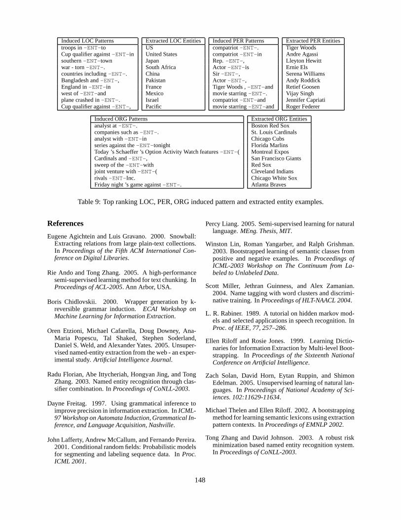
Induced LOC Patternstroops in-ENT-toCup qualifier against-ENT-insouthern-ENT-townwar - torn-ENT-.countries including-ENT-.Bangladesh and-ENT-,England in-ENT-inwest of-ENT-andplane crashed in-ENT-.Cup qualifier against-ENT-,
Extracted LOC EntitiesUSUnited StatesJapanSouth AfricaChinaPakistanFranceMexicoIsraelPacific
Induced PER Patternscompatriot-ENT-.compatriot-ENT-inRep.-ENT-,Actor -ENT-isSir-ENT-,Actor -ENT-,Tiger Woods ,-ENT-andmovie starring-ENT-.compatriot-ENT-andmovie starring-ENT-and
Extracted PER EntitiesTiger WoodsAndre AgassiLleyton HewittErnie ElsSerena WilliamsAndy RoddickRetief GoosenVijay SinghJennifer CapriatiRoger Federer
Induced ORG Patternsanalyst at-ENT-.companies such as-ENT-.analyst with-ENT-inseries against the-ENT-tonightToday ’s Schaeffer ’s Option Activity Watch features-ENT-(Cardinals and-ENT-,sweep of the-ENT-withjoint venture with-ENT-(rivals-ENT-Inc.Friday night ’s game against-ENT-.
Extracted ORG EntitiesBoston Red SoxSt. Louis CardinalsChicago CubsFlorida MarlinsMontreal ExposSan Francisco GiantsRed SoxCleveland IndiansChicago White SoxAtlanta Braves
Table 9: Top ranking LOC, PER, ORG induced pattern and extracted entity examples.
References
Eugene Agichtein and Luis Gravano. 2000. Snowball:Extracting relations from large plain-text collections.In Proceedings of the Fifth ACM International Con-ference on Digital Libraries.
Rie Ando and Tong Zhang. 2005. A high-performancesemi-supervised learning method for text chunking. InProceedings of ACL-2005. Ann Arbor, USA.
Boris Chidlovskii. 2000. Wrapper generation by k-reversible grammar induction.ECAI Workshop onMachine Learning for Information Extraction.
Oren Etzioni, Michael Cafarella, Doug Downey, Ana-Maria Popescu, Tal Shaked, Stephen Soderland,Daniel S. Weld, and Alexander Yates. 2005. Unsuper-vised named-entity extraction from the web - an exper-imental study.Artificial Intelligence Journal.
Radu Florian, Abe Ittycheriah, Hongyan Jing, and TongZhang. 2003. Named entity recognition through clas-sifier combination. InProceedings of CoNLL-2003.
Dayne Freitag. 1997. Using grammatical inference toimprove precision in information extraction. InICML-97 Workshop on Automata Induction, Grammatical In-ference, and Language Acquisition, Nashville.
John Lafferty, Andrew McCallum, and Fernando Pereira.2001. Conditional random fields: Probabilistic modelsfor segmenting and labeling sequence data. InProc.ICML 2001.
Percy Liang. 2005. Semi-supervised learning for naturallanguage.MEng. Thesis, MIT.
Winston Lin, Roman Yangarber, and Ralph Grishman.2003. Bootstrapped learning of semantic classes frompositive and negative examples. InProceedings ofICML-2003 Workshop on The Continuum from La-beled to Unlabeled Data.
Scott Miller, Jethran Guinness, and Alex Zamanian.2004. Name tagging with word clusters and discrimi-native training. InProceedings of HLT-NAACL 2004.
L. R. Rabiner. 1989. A tutorial on hidden markov mod-els and selected applications in speech recognition. InProc. of IEEE, 77, 257–286.
Ellen Riloff and Rosie Jones. 1999. Learning Dictio-naries for Information Extraction by Multi-level Boot-strapping. InProceedings of the Sixteenth NationalConference on Artificial Intelligence.
Zach Solan, David Horn, Eytan Ruppin, and ShimonEdelman. 2005. Unsupervised learning of natural lan-guages. InProceedings of National Academy of Sci-iences. 102:11629-11634.
Michael Thelen and Ellen Riloff. 2002. A bootstrappingmethod for learning semantic lexicons using extractionpattern contexts. InProceedings of EMNLP 2002.
Tong Zhang and David Johnson. 2003. A robust riskminimization based named entity recognition system.In Proceedings of CoNLL-2003.
148
Proceedings of the 10th Conference on Computational Natural Language Learning (CoNLL-X),pages 149–164, New York City, June 2006.c©2006 Association for Computational Linguistics
CoNLL-X shared task on Multilingual Dependency Parsing
Sabine BuchholzSpeech Technology GroupCambridge Research LabToshiba Research EuropeCambridge CB2 3NH, UK
Erwin MarsiCommunication & Cognition
Tilburg University5000 LE Tilburg, The Netherlands
Abstract
Each year the Conference on Com-putational Natural Language Learning(CoNLL)1 features a shared task, in whichparticipants train and test their systems onexactly the same data sets, in order to bet-ter compare systems. The tenth CoNLL(CoNLL-X) saw a shared task on Multi-lingual Dependency Parsing. In this pa-per, we describe how treebanks for 13 lan-guages were converted into the same de-pendency format and how parsing perfor-mance was measured. We also give anoverview of the parsing approaches thatparticipants took and the results that theyachieved. Finally, we try to draw gen-eral conclusions about multi-lingual pars-ing: What makes a particular language,treebank or annotation scheme easier orharder to parse and which phenomena arechallenging for any dependency parser?
Acknowledgement
Many thanks to Amit Dubey and Yuval Kry-molowski, the other two organizers of the sharedtask, for discussions, converting treebanks, writingsoftware and helping with the papers.2
1see http://ilps.science.uva.nl/˜erikt/signll/conll/2Thanks also to Alexander Yeh for additional help with the
paper reviews. His work was made possible by the MITRE Cor-poration’s Sponsored Research Program.
1 Introduction
Previous CoNLL shared tasks focused on NP chunk-ing (1999), general chunking (2000), clause iden-tification (2001), named entity recognition (2002,2003), and semantic role labeling (2004, 2005). Thisshared task on full (dependency) parsing is the log-ical next step. Parsing is an important preprocess-ing step for many NLP applications and thereforeof considerable practical interest. It is a complextask and as it is not straightforwardly mappable to a“classical” segmentation, classification or sequenceprediction problem, it also poses theoretical chal-lenges to machine learning researchers.
During the last decade, much research has beendone on data-driven parsing and performance has in-creased steadily. For training these parsers, syntac-tically annotated corpora (treebanks) of thousandsto tens of thousands of sentences are necessary; soinitially, research has focused on English. Dur-ing the last few years, however, treebanks for otherlanguages have become available and some parsershave been applied to several different languages.See Section 2 for a more detailed overview of re-lated previous research.
So far, there has not been much comparison be-tween different dependency parsers on exactly thesame data sets (other than for English). One of thereasons is the lack of a de-facto standard for an eval-uation metric (labeled or unlabeled, separate root ac-curacy?), for splitting the data into training and test-ing portions and, in the case of constituency tree-banks converted to dependency format, for this con-version. Another reason are the various annotation
149
schemes and logical data formats used by differenttreebanks, which make it tedious to apply a parser tomany treebanks. We hope that this shared task willimprove the situation by introducing a uniform ap-proach to dependency parsing. See Section 3 for thedetailed task definition and Section 4 for informationabout the conversion of all 13 treebanks.
In this shared task, participants had two to threemonths3 to implement a parsing system that could betrained for all these languages and four days to parseunseen test data for each. 19 participant groups sub-mitted parsed test data. Of these, all but one parsedall 12 required languages and 13 also parsed the op-tional Bulgarian data. A wide variety of parsingapproaches were used: some are extensions of pre-viously published approaches, others are new. SeeSection 5 for an overview.
Systems were scored by computing thelabeledattachment score (LAS), i.e. the percentage of“scoring” tokens for which the system had predictedthe correct head and dependency label. Punctuationtokens were excluded from scoring. Results acrosslanguages and systems varied widely from 37.8%(worst score on Turkish) to 91.7% (best score onJapanese). See Section 6 for detailed results.
However, variations are consistent enough to al-low us to draw some general conclusions. Section 7discusses the implications of the results and analyzesthe remaining problems. Finally, Section 8 describespossible directions for future research.
2 Previous research
Tesniere (1959) introduced the idea of a dependencytree (a “stemma” in his terminology), in whichwords stand in direct head-dependent relations, forrepresenting the syntactic structure of a sentence.Hays (1964) and Gaifman (1965) studied the for-mal properties ofprojective dependency grammars,i.e. those where dependency links are not allowed tocross. Mel’cuk (1988) describes a multistratal de-pendency grammar, i.e. one that distinguishes be-tween several types of dependency relations (mor-phological, syntactic and semantic). Other theoriesrelated to dependency grammar are word grammar
3Some though had significantly less time: One participantregistered as late as six days before the test data release (reg-istration was a prerequisite to obtain most of the data sets)andstill went on to submit parsed test data in time.
(Hudson, 1984) and link grammar (Sleator and Tem-perley, 1993).
Some relatively recent rule-based full depen-dency parsers are Kurohashi and Nagao (1994) forJapanese, Oflazer (1999) for Turkish, Tapanainenand Jarvinen (1997) for English and Elworthy(2000) for English and Japanese.
While phrase structure parsers are usually evalu-ated with the GEIG/PARSEVAL measures of preci-sion and recall over constituents (Black et al., 1991),Lin (1995) and others have argued for an alterna-tive, dependency-based evaluation. That approach isbased on a conversion from constituent structure todependency structure by recursively defining a headfor each constituent.
The same idea was used by Magerman (1995),who developed the first “head table” for the PennTreebank (Marcus et al., 1994), and Collins (1996),whose constituent parser is internally based on prob-abilities of bilexical dependencies, i.e. dependenciesbetween two words. Collins (1997)’s parser andits reimplementation and extension by Bikel (2002)have by now been applied to a variety of languages:English (Collins, 1999), Czech (Collins et al., 1999),German (Dubey and Keller, 2003), Spanish (Cowanand Collins, 2005), French (Arun and Keller, 2005),Chinese (Bikel, 2002) and, according to Dan Bikel’sweb page, Arabic.
Eisner (1996) introduced a data-driven depen-dency parser and compared several probability mod-els on (English) Penn Treebank data. Kudo andMatsumoto (2000) describe a dependency parser forJapanese and Yamada and Matsumoto (2003) an ex-tension for English. Nivre’s parser has been testedfor Swedish (Nivre et al., 2004), English (Nivre andScholz, 2004), Czech (Nivre and Nilsson, 2005),Bulgarian (Marinov and Nivre, 2005) and ChineseCheng et al. (2005), while McDonald’s parser hasbeen applied to English (McDonald et al., 2005a),Czech (McDonald et al., 2005b) and, very recently,Danish (McDonald and Pereira, 2006).
3 Data format, task definition
The training data derived from the original treebanks(see Section 4) and given to the shared task partic-ipants was in a simple column-based format that is
150
an extension of Joakim Nivre’s Malt-TAB format4
for the shared task and was chosen for its processingsimplicity. All the sentences are in one text file andthey are separated by a blank line after each sen-tence. A sentence consists of one or more tokens.Each token is represented on one line, consisting of10 fields. Fields are separated from each other by aTAB.5 The 10 fields are:
1) ID: Token counter, starting at 1 for each newsentence.
2) FORM: Word form or punctuation symbol.For the Arabic data only, FORM is a concatenationof the word in Arabic script and its transliteration inLatin script, separated by an underscore. This rep-resentation is meant to suit both those that do andthose that do not read Arabic.
3) LEMMA : Lemma or stem (depending on theparticular treebank) of word form, or an underscoreif not available. Like for the FORM, the values forArabic are concatenations of two scripts.
4) CPOSTAG: Coarse-grained part-of-speechtag, where the tagset depends on the treebank.
5) POSTAG: Fine-grained part-of-speech tag,where the tagset depends on the treebank. It is iden-tical to the CPOSTAG value if no POSTAG is avail-able from the original treebank.
6) FEATS: Unordered set of syntactic and/ormorphological features (depending on the particu-lar treebank), or an underscore if not available. Setmembers are separated by a vertical bar (|).
7) HEAD: Head of the current token, which iseither a value of ID, or zero (’0’) if the token linksto the virtual root node of the sentence. Note thatdepending on the original treebank annotation, theremay be multiple tokens with a HEAD value of zero.
8) DEPREL: Dependency relation to the HEAD.The set of dependency relations depends on the par-ticular treebank. The dependency relation of a to-ken with HEAD=0 may be meaningful or simply’ROOT’ (also depending on the treebank).
9) PHEAD: Projective head of current token,which is either a value of ID or zero (’0’), or an un-derscore if not available. The dependency structure
4http://w3.msi.vxu.se/ nivre/research/MaltXML.html5Consequently, field values cannot contain TABs. In the
shared task data, field values are also not supposed to con-tain any other whitespace (although unfortunately some spacesslipped through in the Spanish data).
resulting from the PHEAD column is guaranteed tobe projective (but is not available for all data sets),whereas the structure resulting from the HEAD col-umn will be non-projective for some sentences ofsome languages (but is always available).
10) PDEPREL: Dependency relation to thePHEAD, or an underscore if not available.
As should be obvious from the description above,our format assumes that each token has exactly onehead. Some dependency grammars, and also sometreebanks, allow tokens to have more than one head,although often there is a distinction between primaryand optional secondary relations, e.g. in the DanishDependency Treebank (Kromann, 2003), the DutchAlpino Treebank (van der Beek et al., 2002b) andthe German TIGER treebank (Brants et al., 2002).For this shared task we decided to ignore any ad-ditional relations. However the data format couldeasily be extended with additional optional columnsin the future. Cycles do not occur in the shared taskdata but are scored as normal if predicted by parsers.The character encoding of all data files is Unicode(specifically UTF-8), which is the only encoding tocover all languages and therefore ideally suited formultilingual parsing.
While the training data contained all 10 columns(although sometimes only with dummy values, i.e.underscores), the test data given to participants con-tained only the first 6. Participants’ parsers thenpredicted the HEAD and DEPREL columns (anypredicted PHEAD and PDEPREL columns were ig-nored). The predicted values were compared to thegold standard HEAD and DEPREL.6 The officialevaluation metric is thelabeled attachment score(LAS), i.e. the percentage of “scoring” tokens forwhich the system has predicted the correct HEADand DEPREL. The evaluation script defines a non-scoring token as a token where all characters of theFORM value have the Unicode category property“Punctuation”.7
6The official scoring scripteval.pl, data sets for somelanguages and instructions on how to get the rest, the softwareused for the treebank conversions, much documentation, fullresults and other related information will be available from thepermanent URLhttp://depparse.uvt.nl (also linkedfrom the CoNLL web page).
7Seeman perlunicode for the technical details and theshared task website for our reasons for this decision. Notethat an underscore and a percentage sign also have the Unicode“Punctuation” property.
151
We tried to take a test set that was representativeof the genres in a treebank and did not cut throughtext samples. We also tried to document how weselected this set.8 We aimed at having roughly thesame size for the test sets of all languages: 5,000scoring tokens. This is not an exact requirement aswe do not want to cut sentences in half. The rel-atively small size of the test set means that evenfor the smallest treebanks the majority of tokens isavailable for training, and the equal size means thatfor the overall ranking of participants, we can sim-ply compute the score on the concatenation of alltest sets.
4 Treebanks and their conversion
In selecting the treebanks, practical considerationswere the major factor. Treebanks had to be actuallyavailable, large enough, have a license that allowedfree use for research or kind treebank providers whotemporarily waived the fee for the shared task, andbe suitable for conversion into the common formatwithin the limited time. In addition, we aimed at abroad coverage of different language families.9 Asa general rule, we did not manually correct errors intreebanks if we discovered some during the conver-sion, see also Buchholz and Green (2006), althoughwe did report them to the treebank providers andseveral got corrected by them.
4.1 Dependency treebanks
We used the following six dependency treebanks:Czech: Prague Dependency Treebank10 (PDT)(Bohmova et al., 2003);Arabic : Prague Arabic De-pendency Treebank11 (PADT) (Hajic et al., 2004;Smrz et al., 2002);Slovene: Slovene DependencyTreebank12 (SDT) (Dzeroski et al., 2006);Danish:
8See the shared task website for a more detailed discussion.9That was also the reason why we decided not to include
a fifth Germanic language (English) although the freely avail-able SUSANNE treebank (Sampson, 1995) or possibly the PennTreebank would have qualified otherwise.
10Many thanks to Jan Hajic for granting the temporary li-cense for CoNLL-X and talking to LDC about it, to Christo-pher Cieri for arranging distribution through LDC and to TonyCastelletto for handling the distribution.
11Many thanks to Yuval Krymolowski for converting the tree-bank, Otakar Smrz for valuable help during the conversion andthanks again to Jan Hajic, Christopher Cieri and Tony Castel-letto.
12Many thanks to the SDT people for granting the speciallicense for CoNLL-X and to Tomaz Erjavec for converting the
Danish Dependency Treebank13 (Kromann, 2003);Swedish: Talbanken0514 (Teleman, 1974; Einars-son, 1976; Nilsson et al., 2005);Turkish : Metu-Sabancı treebank15 (Oflazer et al., 2003; Atalay etal., 2003).
The conversion of these treebanks was the easi-est task as the linguistic representation was alreadywhat we needed, so the information only had to beconverted from SGML or XML to the shared taskformat. Also, the relevant information had to be dis-tributed appropriately over the CPOSTAG, POSTAGand FEATS columns.
For the Swedish data, no predefined distinctioninto coarse and fine-grained PoS was available, sothe two columns contain identical values in our for-mat. For the Czech data, we sampled both our train-ing and test data from the official “training” partitionbecause only that one contains gold standard PoStags, which is also what is used in most other datasets. The Czech DEPREL values include the suf-fixes to mark coordination, apposition and parenthe-sis, while these have been ignored during the con-version of the much smaller Slovene data. For theArabic data, sentences with missing annotation werefiltered out during the conversion.
The Turkish treebank posed a special problembecause it analyzes each word as a sequence ofone or more inflectional groups (IGs). Each IGconsists of either a stem or a derivational suffixplus all the inflectional suffixes belonging to thatstem/derivational suffix. The head of a whole wordis not just another word but a specific IG of anotherword.16 One can easily map this representation toone in which the head of a word is a word but that
treebank for us.13Many thanks to Matthias Trautner Kromann and assistants
for creating the DDT and releasing it under the GNU GeneralPublic License and to Joakim Nivre, Johan Hall and Jens Nils-son for the conversion of DDT to Malt-XML.
14Many thanks to Jens Nilsson, Johan Hall and Joakim Nivrefor the conversion of the original Talbanken to Talbanken05and for making it freely available for research purposes andtoJoakim Nivre again for prompt and proper respons to all ourquestions.
15Many thanks to Bilge Say and Kemal Oflazer for grant-ing the license for CoNLL-X and answering questions and toGulsen Eryigit for making many corrections to the treebank anddiscussing some aspects of the conversion.
16This is a bit like saying that in “the usefulness of X forY”, “for Y” links to “use-” and not to “usefulness”. Only thatin Turkish, “use”, “full” and “ness” each could have their owninflectional suffixes attached to them.
152
mapping would lose information and it is not clearwhether the result is linguistically meaningful, prac-tically useful, or even easier to parse because in theoriginal representation, each IG has its own PoS andmorphological features, so it is not clear how that in-formation should be represented if all IGs of a wordare conflated. We therefore chose to represent eachIG as a separate token in our format. To make theresult a connected dependency structure, we definedthe HEAD of each non-word-final IG to be the fol-lowing IG and the DEPREL to be “DERIV”. We as-signed the stem of the word to the first IG’s LEMMAcolumn, with all non-first IGs having LEMMA ‘’,and the actual word form to the last IG, with all non-last IGs having FORM ‘’. As already mentioned inSection 3, the underscore has the punctuation char-acter property, therefore non-last IGs (whose HEADand DEPREL were introduced by us) are not scoringtokens. We also attached or reattached punctuation(see the README available at the shared task web-site for details.)
4.2 Phrase structure with functions for allconstituents
We used the following five treebanks of this type:German: TIGER treebank17 (Brants et al., 2002);Japanese: Japanese Verbmobil treebank18 (Kawataand Bartels, 2000);Portuguese: The Bosque partof the Floresta sinta(c)tica19 (Afonso et al., 2002);Dutch: Alpino treebank20 (van der Beek et al.,2002b; van der Beek et al., 2002a);Chinese: Sinica
17Many thanks to the TIGER team for allowing us to use thetreebank for the shared task and to Amit Dubey for convertingthe treebank.
18Many thanks to Yasuhiro Kawata, Julia Bartels and col-leagues from Tubingen University for the construction of theoriginal Verbmobil treebank for Japanese and to Sandra Kublerfor providing the data and granting the special license forCoNLL-X.
19Many thanks to Diana Santos, Eckhard Bick and otherFloresta sint(c)tica project members for creating the treebankand making it publicly available, for answering many questionsabout the treebank (Diana and Eckhard), for correcting prob-lems and making new releases (Diana), and for sharing scriptsand explaining the head rules implemented in them (Eckhard).Thanks also to Jason Baldridge for useful discussions and toBen Wing for independently reporting problems which Dianathen fixed.
20Many thanks to Gertjan van Noord and the other people atthe University of Groningen for creating the Alpino Treebankand releasing it for free, to Gertjan van Noord for answeringallour questions and for providing extra test material and to Antalvan den Bosch for help with the memory-based tagger.
treebank21 (Chen et al., 2003).Their conversion to dependency format required
the definition of a head table. Fortunately, in con-trast to the Penn Treebank for which the head ta-ble is based on POS22 we could use the gram-matical functions annotated in these treebanks.Therefore, head rules are often of the form: thehead child of a VP/clause is the child with theHD/predicator/hd/Head function. The DEPRELvalue for a token is the function of the biggest con-stituent of which this token is the lexical head. If theconstituent comprising the complete sentence didnot have a function, we gave its lexical head tokenthe DEPREL “ROOT”.
For the Chinese treebank, most functions are notgrammatical functions (such as “subject”, “object”)but semantic roles (such as “agent”, “theme”). Forthe Portuguese treebank, the conversion was compli-cated by the fact that a detailed specification existedwhich tokens should be the head of which other to-kens, e.g. the finite verb must be the head of thesubject and the complementzier but the main verbmust be the head of the complements and adjuncts.23
Given that the Floresta sinta(c)tica does not use tra-ditional VP constituents but rather verbal chunks(consisting mainly of verbs), a simple Magerman-Collins-style head table was not sufficient to derivethe required dependency structure. Instead we useda head table that defined several types of heads (syn-tactic, semantic) and a link table that specified whatlinked to which type of head.24
Another problem existed with the Dutch tree-bank. Its original PoS tag set is very coarse andthe PoS and the word stem information is not veryreliable.25 We therefore decided to retag the tree-bank automatically using the Memory-Based Tag-ger (MBT) (Daelemans et al., 1996) which uses avery fine-grained tag set. However, this created aproblem with multiwords. MBT does not have theconcept of multiwords and therefore tags all of their
21Many thanks to Academia Sinica for granting the tempo-rary license for CoNLL-X, to Keh-Jiann Chen for answeringour questions and to Amit Dubey for converting the treebank.
22containing rules such as: the head child of a VP is the left-most “to”, or else the leftmost past tense verb, or else etc.
23Eckhard Bick, p.c.24See the conversion scriptbosque2MALT.py and the
README file at the shared task website for details.25http://www.let.rug.nl/vannoord/trees/Papers/diffs.pdf
153
components individually. As Alpino does not pro-vide an internal structure for multiwords, we hadto treat multiwords as one token. However, wethen lack a proper PoS for the multiword. Aftermuch discussion, we decided to assign each multi-word the CPOSTAG “MWU” (multiword unit) anda POSTAG which is the concatenation of the PoSof all the components as predicted by MBT (sepa-rated by an underscore). Likewise, the FEATS area concatenation of the morphological features of allcomponents. This approach resulted in many dif-ferent POSTAG values for the training set and evenin unseen values in the test set. It remains to betested whether our approach resulted in data sets bet-ter suited for parsing than the original.
4.3 Phrase structure with some functions
We used two treebanks of this type:Spanish:Cast3LB26 (Civit Torruella and Martı Antonın,2002; Navarro et al., 2003; Civit et al., 2003);Bul-garian: BulTreeBank27 (Simov et al., 2002; Simovand Osenova, 2003; Simov et al., 2004; Osenova andSimov, 2004; Simov et al., 2005).
Converting a phrase structure treebank with onlya few functions to a dependency format usually re-quires linguistic competence in the treebank’s lan-guage in order to create the head table and miss-ing function labels. We are grateful to Chanev etal. (2006) for converting the BulTreeBank to theshared task format and to Montserrat Civit for pro-viding us with a head table and a function mappingfor Cast3LB.28
4.4 Data set characteristics
Table 1 shows details of all data sets. FollowingNivre and Nilsson (2005) we use the following def-inition: “an arc (i, j) is projective iff all nodes oc-curring between i and j are dominated by i (wheredominates is the transitive closure of the arc rela-
26Many thanks to Montserrat Civit and Toni Martı for allow-ing us to use Cast3LB for CoNLL-X and to Amit Dubey forconverting the treebank.
27Many thanks to Kiril Simov and Petya Osenova for allow-ing us to use the BulTreeBank for CoNLL-X.
28Although unfortunately, due to a bug, the function list wasnot used and the Spanish data in the shared task ended up withmany DEPREL values being simply ‘’. By the time we dis-covered this, the test data release date was very close and wedecided not to release new bug-fixed training material that late.
tion)”.29
5 Approaches
Table 2 tries to give an overview of the wide varietyof parsing approaches used by participants. We referto the individual papers for details. There are severaldimensions along which to classify approaches.
5.1 Top-down, bottom-up
Phrase structure parsers are often classified in termsof the parsing order: top-down, bottom-up or var-ious combinations. For dependency parsing, thereseem to be two different interpretations of the term“bottom-up”. Nivre and Scholz (2004) uses thisterm with reference to Yamada and Matsumoto(2003), whose parser has to find all children of atoken before it can attach that token to its head.We will refer to this as “bottom-up-trees”. An-other use of “bottom-up” is due to Eisner (1996),who introduced the notion of a “span”. A spanconsists of a potential dependency arcr betweentwo tokensi and j and all those dependency arcsthat would be spanned byr, i.e. all arcs betweentokensk and l with i ≤ k, l ≤ j. Parsing inthis order means that the parser has to find all chil-dren and siblings on one side of a token before itcan attach that token to a head on the same side.This approach assumes projective dependency struc-tures. Eisner called this approach simply “bottom-up”, while Nivre, whose parser implicitly also fol-lows this order, called it “top-down/bottom-up” todistinguish it from the pure “bottom-up(-trees)” or-der of Yamada and Matsumoto (2003). To avoidconfusion, we will refer to this order as “bottom-up-spans”.
5.2 Unlabeled parsing versus labeling
Given that the parser needs to predict the HEAD aswell as the DEPREL value, different approaches arepossible: predict the (probabilities of the) HEADsof all tokens first, or predict the (probabilities ofthe) DEPRELs of all tokens first, or predict theHEAD and DEPREL of one token before predict-ing these values for the next token. Within thefirst approach, each dependency can be labeled in-dependently (Corston-Oliver and Aue, 2006) or a
29Thanks to Joakim Nivre for explaining this.
154
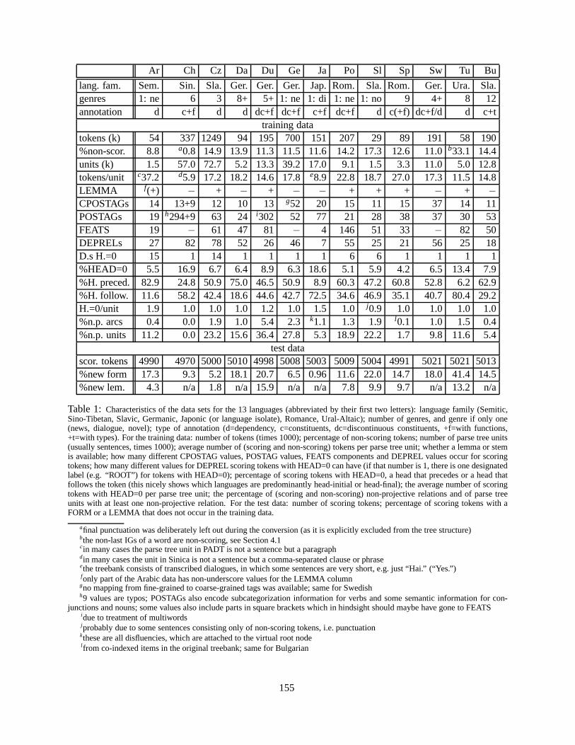
Ar Ch Cz Da Du Ge Ja Po Sl Sp Sw Tu Bu
lang. fam. Sem. Sin. Sla. Ger. Ger. Ger. Jap. Rom. Sla. Rom. Ger. Ura. Sla.genres 1: ne 6 3 8+ 5+ 1: ne 1: di 1: ne 1: no 9 4+ 8 12annotation d c+f d d dc+f dc+f c+f dc+f d c(+f) dc+f/d d c+t
training datatokens (k) 54 337 1249 94 195 700 151 207 29 89 191 58 190%non-scor. 8.8 a0.8 14.9 13.9 11.3 11.5 11.6 14.2 17.3 12.6 11.0 b33.1 14.4units (k) 1.5 57.0 72.7 5.2 13.3 39.2 17.0 9.1 1.5 3.3 11.0 5.0 12.8tokens/unit c37.2 d5.9 17.2 18.2 14.6 17.8 e8.9 22.8 18.7 27.0 17.3 11.5 14.8LEMMA f(+) − + − + − − + + + − + −
CPOSTAGs 14 13+9 12 10 13 g52 20 15 11 15 37 14 11POSTAGs 19 h294+9 63 24 i302 52 77 21 28 38 37 30 53FEATS 19 − 61 47 81 − 4 146 51 33 − 82 50DEPRELs 27 82 78 52 26 46 7 55 25 21 56 25 18D.s H.=0 15 1 14 1 1 1 1 6 6 1 1 1 1%HEAD=0 5.5 16.9 6.7 6.4 8.9 6.3 18.6 5.1 5.9 4.2 6.5 13.4 7.9%H. preced. 82.9 24.8 50.9 75.0 46.5 50.9 8.9 60.3 47.2 60.8 52.8 6.2 62.9%H. follow. 11.6 58.2 42.4 18.6 44.6 42.7 72.5 34.6 46.9 35.1 40.7 80.4 29.2H.=0/unit 1.9 1.0 1.0 1.0 1.2 1.0 1.5 1.0 j0.9 1.0 1.0 1.0 1.0%n.p. arcs 0.4 0.0 1.9 1.0 5.4 2.3 k1.1 1.3 1.9 l0.1 1.0 1.5 0.4%n.p. units 11.2 0.0 23.2 15.6 36.4 27.8 5.3 18.9 22.2 1.7 9.8 11.6 5.4
test datascor. tokens 4990 4970 5000 5010 4998 5008 5003 5009 5004 4991 5021 5021 5013%new form 17.3 9.3 5.2 18.1 20.7 6.5 0.96 11.6 22.0 14.7 18.0 41.4 14.5%new lem. 4.3 n/a 1.8 n/a 15.9 n/a n/a 7.8 9.9 9.7 n/a 13.2 n/a
Table 1: Characteristics of the data sets for the 13 languages (abbreviated by their first two letters): language family (Semitic,Sino-Tibetan, Slavic, Germanic, Japonic (or language isolate), Romance, Ural-Altaic); number of genres, and genre ifonly one(news, dialogue, novel); type of annotation (d=dependency, c=constituents, dc=discontinuous constituents, +f=with functions,+t=with types). For the training data: number of tokens (times 1000); percentage of non-scoring tokens; number of parsetree units(usually sentences, times 1000); average number of (scoring and non-scoring) tokens per parse tree unit; whether a lemma or stemis available; how many different CPOSTAG values, POSTAG values, FEATS components and DEPREL values occur for scoringtokens; how many different values for DEPREL scoring tokenswith HEAD=0 can have (if that number is 1, there is one designatedlabel (e.g. “ROOT”) for tokens with HEAD=0); percentage of scoring tokens with HEAD=0, a head that precedes or a head thatfollows the token (this nicely shows which languages are predominantly head-initial or head-final); the average numberof scoringtokens with HEAD=0 per parse tree unit; the percentage of (scoring and non-scoring) non-projective relations and of parse treeunits with at least one non-projective relation. For the test data: number of scoring tokens; percentage of scoring tokens with aFORM or a LEMMA that does not occur in the training data.
afinal punctuation was deliberately left out during the conversion (as it is explicitly excluded from the tree structure)bthe non-last IGs of a word are non-scoring, see Section 4.1cin many cases the parse tree unit in PADT is not a sentence but aparagraphdin many cases the unit in Sinica is not a sentence but a comma-separated clause or phraseethe treebank consists of transcribed dialogues, in which some sentences are very short, e.g. just “Hai.” (“Yes.”)fonly part of the Arabic data has non-underscore values for the LEMMA columngno mapping from fine-grained to coarse-grained tags was available; same for Swedishh9 values are typos; POSTAGs also encode subcategorization information for verbs and some semantic information for con-
junctions and nouns; some values also include parts in square brackets which in hindsight should maybe have gone to FEATSidue to treatment of multiwordsjprobably due to some sentences consisting only of non-scoring tokens, i.e. punctuationkthese are all disfluencies, which are attached to the virtualroot nodel from co-indexed items in the original treebank; same for Bulgarian
155
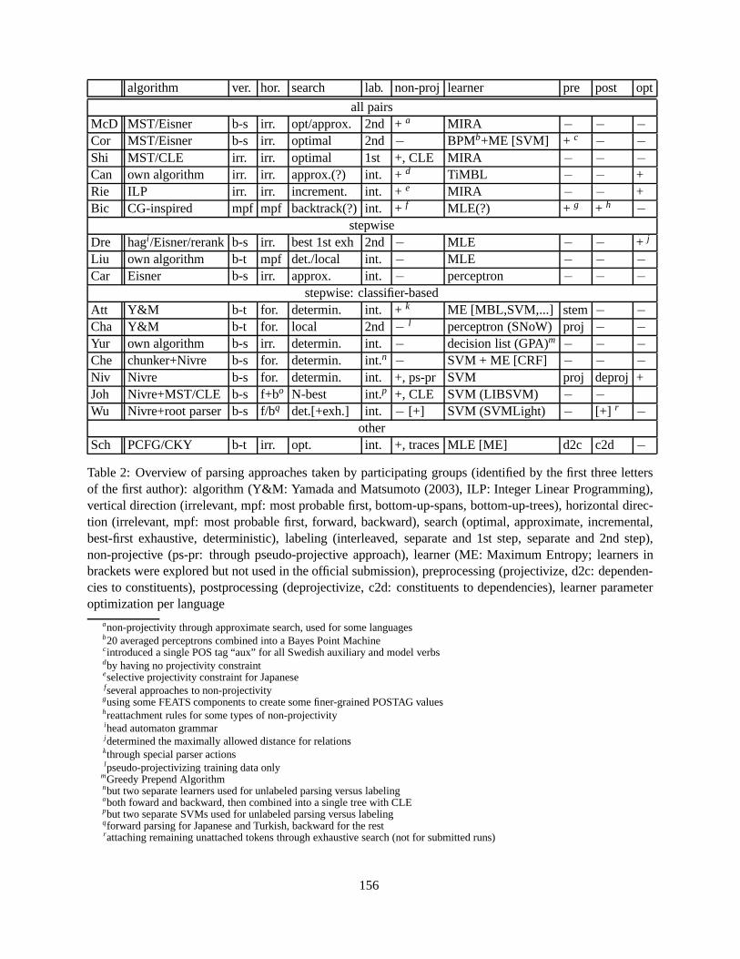
algorithm ver. hor. search lab. non-proj learner pre post opt
all pairsMcD MST/Eisner b-s irr. opt/approx. 2nd + a MIRA − − −
Cor MST/Eisner b-s irr. optimal 2nd − BPMb+ME [SVM] + c − −
Shi MST/CLE irr. irr. optimal 1st +, CLE MIRA − − −
Can own algorithm irr. irr. approx.(?) int. + d TiMBL − − +Rie ILP irr. irr. increment. int. + e MIRA − − +Bic CG-inspired mpf mpf backtrack(?)int. + f MLE(?) + g + h −
stepwiseDre hagi /Eisner/rerankb-s irr. best 1st exh 2nd − MLE − − + j
Liu own algorithm b-t mpf det./local int. − MLE − − −
Car Eisner b-s irr. approx. int. − perceptron − − −
stepwise: classifier-basedAtt Y&M b-t for. determin. int. + k ME [MBL,SVM,...] stem − −
Cha Y&M b-t for. local 2nd − l perceptron (SNoW) proj − −
Yur own algorithm b-s irr. determin. int. − decision list (GPA)m − − −
Che chunker+Nivre b-s for. determin. int.n − SVM + ME [CRF] − − −
Niv Nivre b-s for. determin. int. +, ps-pr SVM proj deproj +Joh Nivre+MST/CLE b-s f+bo N-best int.p +, CLE SVM (LIBSVM) − −
Wu Nivre+root parser b-s f/bq det.[+exh.] int. − [+] SVM (SVMLight) − [+] r −
otherSch PCFG/CKY b-t irr. opt. int. +, traces MLE [ME] d2c c2d −
Table 2: Overview of parsing approaches taken by participating groups (identified by the first three lettersof the first author): algorithm (Y&M: Yamada and Matsumoto (2003), ILP: Integer Linear Programming),vertical direction (irrelevant, mpf: most probable first, bottom-up-spans, bottom-up-trees), horizontal direc-tion (irrelevant, mpf: most probable first, forward, backward), search (optimal, approximate, incremental,best-first exhaustive, deterministic), labeling (interleaved, separate and 1st step, separate and 2nd step),non-projective (ps-pr: through pseudo-projective approach), learner (ME: Maximum Entropy; learners inbrackets were explored but not used in the official submission), preprocessing (projectivize, d2c: dependen-cies to constituents), postprocessing (deprojectivize, c2d: constituents to dependencies), learner parameteroptimization per language
anon-projectivity through approximate search, used for some languagesb20 averaged perceptrons combined into a Bayes Point Machinecintroduced a single POS tag “aux” for all Swedish auxiliary and model verbsdby having no projectivity constrainteselective projectivity constraint for Japanesefseveral approaches to non-projectivitygusing some FEATS components to create some finer-grained POSTAG valueshreattachment rules for some types of non-projectivityihead automaton grammarjdetermined the maximally allowed distance for relationskthrough special parser actionslpseudo-projectivizing training data only
mGreedy Prepend Algorithmnbut two separate learners used for unlabeled parsing versuslabelingoboth foward and backward, then combined into a single tree with CLEpbut two separate SVMs used for unlabeled parsing versus labelingqforward parsing for Japanese and Turkish, backward for the restrattaching remaining unattached tokens through exhaustivesearch (not for submitted runs)
156
sequence classifier can label all children of a tokentogether (McDonald et al., 2006). Within the thirdapproach, HEAD and DEPREL can be predicted si-multaneously, or in two separate steps (potentiallyusing two different learners).
5.3 All pairs
At the highest level of abstraction, there are two fun-damental approaches, which we will call “all pairs”and “stepwise”. In an “all pairs” approach, everypossible pair of two tokens in a sentence is consid-ered and some score is assigned to the possibilityof this pair having a (directed) dependency relation.Using that information as building blocks, the parserthen searches for the best parse for the sentence.This approach is one of those described in Eisner(1996). The definition of “best” parse depends onthe precise model used. That model can be one thatdefines the score of a complete dependency tree asthe sum of the scores of all dependency arcs in it.The search for the best parse can then be formalizedas the search for the maximum spanning tree (MST)(McDonald et al., 2005b). If the parse has to be pro-jective, Eisner’s bottom-up-span algorithm (Eisner,1996) can be used for the search. For non-projectiveparses, McDonald et al. (2005b) propose using theChu-Liu-Edmonds (CLE) algorithm (Chu and Liu,1965; Edmonds, 1967) and McDonald and Pereira(2006) describe an approximate extension of Eis-ner’s algorithm. There are also alternatives to MSTwhich allow imposing additional constraints on thedependency structure, e.g. that at most one depen-dent of a token can have a certain label, such as “sub-ject”, see Riedel et al. (2006) and Bick (2006). Bycontrast, Canisius et al. (2006) do not even enforcethe tree constraint, i.e. they allow cycles. In a vari-ant of the “all pairs” approach, only those pairs oftokens are considered that are not too distant (Cani-sius et al., 2006).
5.4 Stepwise
In a stepwise approach, not all pairs are considered.Instead, the dependency tree is built stepwise andthe decision about what step to take next (e.g. whichdependency to insert) can be based on informationabout, in theory all, previous steps and their results(in the context of generative probabilistic parsing,Black et al. (1993) call this the history). Stepwise
approaches can use an explicit probability modelover next steps, e.g. a generative one (Eisner, 1996;Dreyer et al., 2006), or train a machine learner topredict those. The approach can be deterministic (ateach point, one step is chosen) or employ varioustypes of search. In addition, parsing can be done ina bottom-up-constituent or a bottom-up-spans fash-ion (or in another way, although this was not done inthis shared task). Finally, parsing can start at the firstor the last token of a sentence. When talking aboutlanguages that are written from left to right, this dis-tinction is normally referred to as left-to-right ver-sus right-to-left. However, for multilingual parsingwhich includes languages that are written from rightto left (Arabic) or sometimes top to bottom (Chi-nese, Japanese) this terminology is confusing be-cause it is not always clear whether a left-to-rightparser for Arabic would really start with the left-most (i.e. last) token of a sentence or, like for otherlanguages, with the first (i.e. rightmost). In general,starting with the first token (“forward”) makes moresense from a psycholinguistic point of view but start-ing with the last (“backward”) might be beneficialfor some languages (possibly related to them beinghead-initial versus head-final languages). The pars-ing order directly determines what information willbe available from the history when the next decisionneeds to be made. Stepwise parsers tend to inter-leave the prediction of HEAD and DEPREL.
5.5 Non-projectivity
All data sets except the Chinese one contain somenon-projective dependency arcs, although their pro-portion varies from 0.1% to 5.4%. Participants tookthe following approaches to non-projectivity:
• Ignore, i.e. predict only projective parses. De-pending on the way the parser is trained, itmight be necessary to at least projectivize thetraining data (Chang et al., 2006).
• Always allow non-projective arcs, by not im-posing any projectivity constraint (Shimizu,2006; Canisius et al., 2006).
• Allow during parsing under certain conditions,e.g. for tokens with certain properties (Riedelet al., 2006; Bick, 2006) or if no alternativeprojective arc has a score above the threshold
157
(Bick, 2006) or if the classifier chooses a spe-cial action (Attardi, 2006) or the parser predictsa trace (Schiehlen and Spranger, 2006).
• Introduce through post-processing, e.g.through reattachment rules (Bick, 2006) orif the change increases overall parse treeprobability (McDonald et al., 2006).
• The pseudo-projective approach (Nivre andNilsson, 2005): Transform non-projectivetraining trees to projective ones but encodethe information necessary to make the inversetransformation in the DEPREL, so that this in-verse transformation can also be carried out onthe test trees (Nivre et al., 2006).
5.6 Data columns used
Table 3 shows which column values havebeen used by participants. Nobody used thePHEAD/PDEPREL column in any way. It is likelythat those who did not use any of the other columnsdid so mainly for practical reasons, such as thelimited time and/or the difficulty to integrate it intoan existing parser.
5.6.1 FORM versus LEMMA
Lemma or stem information has often been ig-nored in previous dependency parsers. In the sharedtask data, it was available in just over half the datasets. Both LEMMA and FORM encode lexical in-formation. There is therefore a certain redundancy.Participants have used these two columns in differ-ent ways:
• Use only one (see Table 3).
• Use both, in different features. Typically, a fea-ture selection routine and/or the learner itself(through weights) will decide about the impor-tance of the resulting features.
• Use a variant of the FORM as a substitute fora missing LEMMA. Bick (2006) used the low-ercased FORM if the LEMMA is not available,Corston-Oliver and Aue (2006) a prefix and At-tardi (2006) a stem derived by a rule-based sys-tem for Danish, German and Swedish.
form lem. cpos pos feats
McD ++ a + b −? + +, co+cr.pr.Cor + + + c ++ +, co+cr.pr.d
Shi + − + − −
Can + − − + −
Rie + e + + + f + cr.pr.Bic (+) + + g + (+)
Dre ++ h + rer. rer. −
Liu (+) + ++ + −
Car ++ + ++ + + comp.
Att (+) + + − (+)Cha − + − + + atomicYur + + + + + comp.Che + + + + + atomic?Niv + + + + + comp.Joh + − + + + comp.Wu + − + + −
Sch ? (+)i ? (+) (+)
Table 3: Overview of data columns used by partici-pating groups. ‘−’: a column value was not used atall. ‘+’: used in at least some features. ‘(+)’: Vari-ant of FORM used only if LEMMA is missing, oronly parts of FEATS used. ‘++’: used more exten-sively than another column containing related infor-mation (where FORM and LEMMA are related, asare CPOSTAG and POSTAG), e.g. also in combina-tion features or features for context tokens in addi-tion to features for the focus token(s). “rer.”: usedin the reranker only. For the last column: atomic,comp. = components, cr.pr. = cross-product.
aalso prefix and suffix for labelerbinstead of form for Arabic and Spanishcinstead of POSTAG for Dutch and Turkishdfor labeler; unlab. parsing: only some for global featuresealso prefixfalso 1st character of POSTAGgonly as backoffhreranker: also suffix; if no lemma, use prefix of FORMiLEMMA, POSTAG, FEATS only for back-off smoothing
5.6.2 CPOSTAG versus POSTAG
All data sets except German and Swedish had dif-ferent values for CPOSTAG and POSTAG, althoughthe granularity varied widely. Again, there are dif-ferent approaches to dealing with the redundancy:
• Use only one for all languages.
158
• Use both, in different features. Typically, a fea-ture selection routine and/or the learner itself(through weights) will decide about the impor-tance of the resulting features.
• Use one or the other for each language.
5.6.3 Using FEATS
By design, a FEATS column value has internalstructure. Splitting it at the ‘|’30 results in a set ofcomponents. The following approaches have beenused:
• Ignore the FEATS.
• Treat the complete FEATS value as atomic, i.e.do not split it into components.
• Use only some components, e.g. Bick (2006)uses only case, mood and pronoun subclass andAttardi (2006) uses only gender, number, per-son and case.
• Use one binary feature for each component.This is likely to be useful if grammatical func-tion is indicated by case.
• Use one binary feature for each cross-productof the FEATS components ofi and the FEATScomponents ofj. This is likely to be useful foragreement phenomena.
• Use one binary feature for each FEATS com-ponent ofi that also exists forj. This is a moreexplicit way to model agreement.
5.7 Types of features
When deciding whether there should be a depen-dency relation between tokensi and j, all parsersuse at least information about these two tokens. Inaddition, the following sources of information canbe used (see Table 4): token context (tc): a limitednumber (determined by the window size) of tokensdirectly preceding or followingi or j; children: in-formation about the already found children ofi andj; siblings: in a set-up where the decision is not “isthere a relation betweeni andj” but “is i the head ofj” or in a separate labeling step, the siblings ofi arethe already found children ofj; structural context
30or for Dutch, also at the ‘’
tc ch si sc di in gl co ac la op
McD + l + l ? l l + − l (+)a
Cor + l b l + p − + + − − (+)c
Shi + − − − + − − + − + −
Can + − − − + − − − − − −
Rie + − + d − ? ? − + − + e +Bic + + f + g − + + h − + − ++ (+)i
Dre r r + r + r − + − r rLiu − + − + + − − + − − −
Car + − + − + + − + − + −
Att − + + + − − − − + + (+)j
Cha + + − l − − − + + − −
Yur + + − ? − − − − − − +Che − + + + + − − − − − −
Niv + + − + − − − − − + +Joh + + − + − − − − − + −
Wu + + − + − − − + − + −
Sch − + − − − − − − − + −
Table 4: Overview of features used by participatinggroups. See the text for the meaning of the columnabbreviations. For separate HEAD and DEPREL as-signment: p: only for unlabeled parsing, l: only forlabeling, r: only for reranking.
aFORM versus LEMMAbnumber of tokens governed by childcPOSTAG versus CPOSTAGdfor arity constraintefor arity constraintffor “full” head constraintgfor uniqueness constrainthfor barrier constraintiof constraintsjPOS window size
(sc) other than children/siblings: neighboring sub-trees/spans, or ancestors ofi andj; distance fromi
to j; information derived from all the tokensin be-tweeni andj (e.g. whether there is an interveningverb or how many intervening commas there are);global features (e.g. does the sentence contain a fi-nite verb); explicit featurecombinations (dependingon the learner, these might not be necessary, e.g. apolynomial kernel routinely combines features); forclassifier-based parsers: the previousactions, i.e.classifications; whether information aboutlabels isused as input for other decisions. Finally, the pre-cise set of features can beoptimized per language.
159
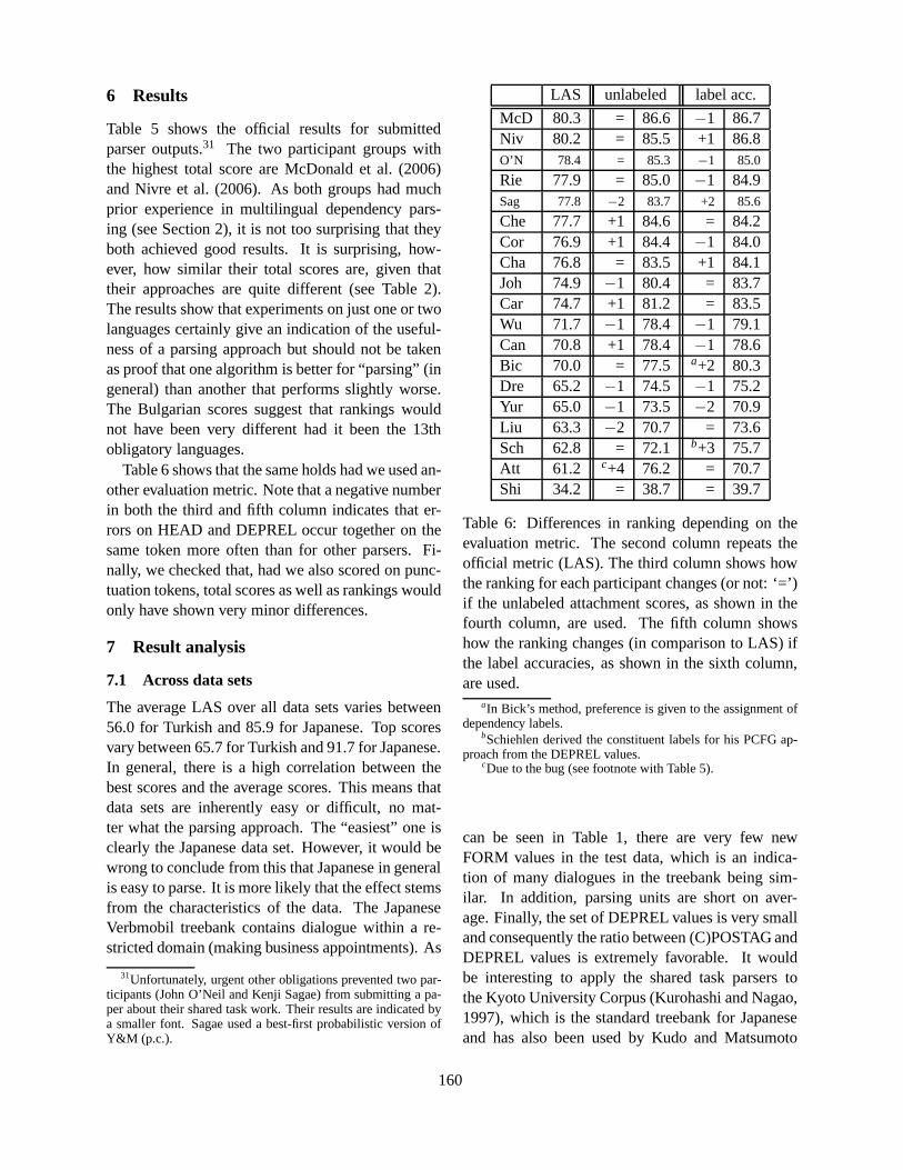
6 Results
Table 5 shows the official results for submittedparser outputs.31 The two participant groups withthe highest total score are McDonald et al. (2006)and Nivre et al. (2006). As both groups had muchprior experience in multilingual dependency pars-ing (see Section 2), it is not too surprising that theyboth achieved good results. It is surprising, how-ever, how similar their total scores are, given thattheir approaches are quite different (see Table 2).The results show that experiments on just one or twolanguages certainly give an indication of the useful-ness of a parsing approach but should not be takenas proof that one algorithm is better for “parsing” (ingeneral) than another that performs slightly worse.The Bulgarian scores suggest that rankings wouldnot have been very different had it been the 13thobligatory languages.
Table 6 shows that the same holds had we used an-other evaluation metric. Note that a negative numberin both the third and fifth column indicates that er-rors on HEAD and DEPREL occur together on thesame token more often than for other parsers. Fi-nally, we checked that, had we also scored on punc-tuation tokens, total scores as well as rankings wouldonly have shown very minor differences.
7 Result analysis
7.1 Across data sets
The average LAS over all data sets varies between56.0 for Turkish and 85.9 for Japanese. Top scoresvary between 65.7 for Turkish and 91.7 for Japanese.In general, there is a high correlation between thebest scores and the average scores. This means thatdata sets are inherently easy or difficult, no mat-ter what the parsing approach. The “easiest” one isclearly the Japanese data set. However, it would bewrong to conclude from this that Japanese in generalis easy to parse. It is more likely that the effect stemsfrom the characteristics of the data. The JapaneseVerbmobil treebank contains dialogue within a re-stricted domain (making business appointments). As
31Unfortunately, urgent other obligations prevented two par-ticipants (John O’Neil and Kenji Sagae) from submitting a pa-per about their shared task work. Their results are indicated bya smaller font. Sagae used a best-first probabilistic version ofY&M (p.c.).
LAS unlabeled label acc.
McD 80.3 = 86.6 −1 86.7Niv 80.2 = 85.5 +1 86.8O’N 78.4 = 85.3 −1 85.0
Rie 77.9 = 85.0 −1 84.9Sag 77.8 −2 83.7 +2 85.6
Che 77.7 +1 84.6 = 84.2Cor 76.9 +1 84.4 −1 84.0Cha 76.8 = 83.5 +1 84.1Joh 74.9 −1 80.4 = 83.7Car 74.7 +1 81.2 = 83.5Wu 71.7 −1 78.4 −1 79.1Can 70.8 +1 78.4 −1 78.6Bic 70.0 = 77.5 a+2 80.3Dre 65.2 −1 74.5 −1 75.2Yur 65.0 −1 73.5 −2 70.9Liu 63.3 −2 70.7 = 73.6Sch 62.8 = 72.1 b+3 75.7Att 61.2 c+4 76.2 = 70.7Shi 34.2 = 38.7 = 39.7
Table 6: Differences in ranking depending on theevaluation metric. The second column repeats theofficial metric (LAS). The third column shows howthe ranking for each participant changes (or not: ‘=’)if the unlabeled attachment scores, as shown in thefourth column, are used. The fifth column showshow the ranking changes (in comparison to LAS) ifthe label accuracies, as shown in the sixth column,are used.
aIn Bick’s method, preference is given to the assignment ofdependency labels.
bSchiehlen derived the constituent labels for his PCFG ap-proach from the DEPREL values.
cDue to the bug (see footnote with Table 5).
can be seen in Table 1, there are very few newFORM values in the test data, which is an indica-tion of many dialogues in the treebank being sim-ilar. In addition, parsing units are short on aver-age. Finally, the set of DEPREL values is very smalland consequently the ratio between (C)POSTAG andDEPREL values is extremely favorable. It wouldbe interesting to apply the shared task parsers tothe Kyoto University Corpus (Kurohashi and Nagao,1997), which is the standard treebank for Japaneseand has also been used by Kudo and Matsumoto
160
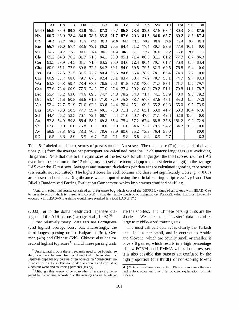
Ar Ch Cz Da Du Ge Ja Po Sl Sp Sw Tu Tot SD BuMcD 66.9 85.9 80.2 84.8 79.2 87.390.7 86.8 73.4 82.3 82.6 63.2 80.3 8.4 87.6Niv 66.7 86.9 78.4 84.8 78.6 85.8 91.7 87.6 70.3 81.3 84.6 65.7 80.2 8.5 87.4O’N 66.7 86.7 76.6 82.8 77.5 85.4 90.6 84.7 71.1 79.8 81.8 57.578.4 9.4 85.2
Rie 66.7 90.0 67.4 83.6 78.6 86.2 90.5 84.4 71.2 77.4 80.7 58.677.9 10.1 0.0Sag 62.7 84.7 75.2 81.6 76.6 84.9 90.486.0 69.1 77.7 82.0 63.2 77.8 9.0 0.0
Che 65.2 84.3 76.2 81.7 71.8 84.1 89.9 85.1 71.4 80.5 81.1 61.277.7 8.7 86.3Cor 63.5 79.9 74.5 81.7 71.4 83.5 90.0 84.672.4 80.4 79.7 61.7 76.9 8.5 83.4Cha 60.9 85.1 72.9 80.6 72.9 84.2 89.1 84.0 69.5 79.7 82.3 60.576.8 9.4 0.0Joh 64.3 72.5 71.5 81.5 72.7 80.4 85.6 84.6 66.4 78.2 78.1 63.474.9 7.7 0.0Car 60.9 83.7 68.8 79.7 67.3 82.4 88.1 83.4 68.4 77.2 78.7 58.174.7 9.7 83.3Wu 63.8 74.8 59.4 78.4 68.5 76.5 90.1 81.5 67.8 73.0 71.7 55.171.7 9.7 79.7Can 57.6 78.4 60.9 77.9 74.6 77.6 87.4 77.4 59.2 68.3 79.2 51.170.8 11.1 78.7Bic 55.4 76.2 63.0 74.6 69.5 74.7 84.8 78.2 64.3 71.4 74.1 53.970.0 9.3 79.2Dre 53.4 71.6 60.5 66.6 61.6 71.0 82.9 75.3 58.7 67.6 67.6 46.165.2 9.9 74.8Yur 52.4 72.7 51.9 71.6 62.8 63.8 84.4 70.4 55.1 69.6 65.2 60.365.0 9.5 73.5Liu 50.7 75.3 58.5 77.7 59.4 68.1 70.8 71.1 57.2 65.1 63.8 41.763.3 10.4 67.6Sch 44.4 66.2 53.3 76.1 72.1 68.7 83.4 71.0 50.7 47.0 71.1 49.862.8 13.0 0.0Att 53.8 54.9 59.8 66.4 58.2 69.8 65.4 75.4 57.2 67.4 68.8 37.8a61.2 9.9 72.9Shi 62.8 0.0 0.0 75.8 0.0 0.0 0.0 0.0 64.6 73.2 79.5 54.234.2 36.3 0.0Av 59.9 78.3 67.2 78.3 70.7 78.6 85.9 80.6 65.2 73.5 76.4 56.0 80.0SD 6.5 8.8 8.9 5.5 6.7 7.5 7.1 5.8 6.8 8.4 6.5 7.7 6.3
Table 5: Labeled attachment scores of parsers on the 13 test sets. The total score (Tot) and standard devia-tions (SD) from the average per participant are calculated over the 12 obligatory languages (i.e. excludingBulgarian). Note that due to the equal sizes of the test sets for all languages, the total scores, i.e. the LASover the concatenation of the 12 obligatory test sets, are identical (up to the first decimal digit) to the averageLAS over the 12 test sets. Averages and standard deviations per data set are calculated ignoring zero scores(i.e. results not submitted). The highest score for each column and those not significantly worse (p < 0.05)are shown in bold face. Significance was computed using the official scoring scripteval.pl and DanBikel’s Randomized Parsing Evaluation Comparator, which implements stratified shuffling.
aAttardi’s submitted results contained an unfortunate bug which caused the DEPREL values of all tokens with HEAD=0 tobe an underscore (which is scored as incorrect). Using the simple heuristic of assigning the DEPREL value that most frequentlyoccured with HEAD=0 in training would have resulted in a total LAS of 67.5.
(2000), or to the domain-restricted Japanese dia-logues of the ATR corpus (Lepage et al., 1998).32
Other relatively “easy” data sets are Portuguese(2nd highest average score but, interestingly, thethird-longest parsing units), Bulgarian (3rd), Ger-man (4th) and Chinese (5th). Chinese also has thesecond highest top score33 and Chinese parsing units
32Unfortunately, both these treebanks need to be bought, sothey could not be used for the shared task. Note also thatJapanese dependency parsers often operate on “bunsetsus” in-stead of words. Bunsetsus are related to chunks and consist ofa content word and following particles (if any).
33Although this seems to be somewhat of a mystery com-pared to the ranking according to the average scores. Riedelet
are the shortest. and Chinese parsing units are theshortest. We note that all “easier” data sets offerlarge to middle-sized training sets.
The most difficult data set is clearly the Turkishone. It is rather small, and in contrast to Arabicand Slovene, which are equally small or smaller, itcovers 8 genres, which results in a high percentageof new FORM and LEMMA values in the test set.It is also possible that parsers get confused by thehigh proportion (one third!) of non-scoring tokens
al. (2006)’s top score is more than 3% absolute above the sec-ond highest score and they offer no clear explanation for theirsuccess.
161
and the many tokens with ‘’ as either the FORM orLEMMA. There is a clear need for further researchto check whether other representations result in bet-ter performance.
The second-most difficult data set is Arabic. It isquite small and has by far the longest parsing units.The third-most difficult data set is Slovene. It hasthe smallest training set. However, its average aswell as top score far exceed those for Arabic andTurkish, which are larger. Interestingly, although thetreebank text comes from a single source (a transla-tion of Orwell’s novel “1984”), there is quite a highproportion of new FORM and LEMMA values in thetest set. The fourth-most difficult data set is Czechin terms of the average score and Dutch in terms ofthe top score. The diffence in ranking for Czech isprobably due to the fact that it has by far the largesttraining set and ironically, several participants couldnot train on all data within the limited time, or elsehad to partition the data and train one model for eachpartition. Likely problems with the Dutch data setare: noisy (C)POSTAG and LEMMA, (C)POSTAGfor multiwords, and the highest proportion of non-projectivity.
Factors that have been discussed so far are: thesize of the training data, the proportion of newFORM and LEMMA values in the test set, the ra-tio of (C)POSTAG to DEPREL values, the averagelength of the parsing unit the proportion of non-projective arcs/parsing units. It would be interest-ing to derive a formula based on those factors thatfits the shared task data and see how well it pre-dicts results on new data sets. One factor that seemsto be irrelevant is the head-final versus head-initialdistinction, as both the “easiest” and the most dif-ficult data sets are for head-final languages. Thereis also no clear proof that some language familiesare easier (with current parsing methods) than oth-ers. It would be interesting to test parsers on theHebrew treebank (Sima’an et al., 2001), to compareperformance to Arabic, the other Semitic languagein the shared task, or on the Hungarian Szeged Cor-pus (Csendes et al., 2004), for another agglutinativelanguage.
7.2 Across participants
For most parsers, their ranking for a specific lan-guage differs at most a few places from their over-
all ranking. There are some outliers though. Forexample, Johansson and Nugues (2006) and Yuret(2006) are seven ranks higher for Turkish than over-all, while Riedel et al. (2006) are five ranks lower.Canisius et al. (2006) are six and Schiehlen andSpranger (2006) even eight ranks higher for Dutchthan overall, while Riedel et al. (2006) are six rankslower for Czech and Johansson and Nugues (2006)also six for Chinese. Some of the higher rankingscould be related to native speaker competence andresulting better parameter tuning but other outliersremain a mystery. Even though McDonald et al.(2006) and Nivre et al. (2006) obtained very simi-lar overall scores, a more detailed look at their per-formance shows clear differences. Taken over all 12obligatory languages, both obtain a recall of morethan 89% on root tokens (i.e. those with HEAD=0)but Nivre’s precision on them is much lower thanMcDonald’s (80.91 versus 91.07). This is likely tobe an effect of the different parsing approaches.
7.3 Across part-of-speech tags
When breaking down by part-of-speech the resultsof all participants on all data sets, one can observesome patterns of “easy” and “difficult” parts-of-speech, at least in so far as tag sets are compara-ble across treebanks. The one PoS that everybodygot 100% correct are the German infinitival mark-ers (tag PTKZU; like “to” in English). Accuracy onthe Swedish equivalent (IM) is not far off at 98%.Other easy PoS are articles, with accuracies in thenineties for German, Dutch, Swedish, Portugueseand Spanish. As several participants have remarkedin their papers, prepositions are much more difficult,with typical accuracies in the fifties or sixties. Simi-larly, conjunctions typically score low, with accura-cies even in the forties for Arabic and Dutch.
8 Future research
There are many directions for interesting researchbuilding on the work done in this shared task. Oneis the question which factors make data sets “easy”or difficult. Another is finding out how much ofparsing performance depends on annotations suchas the lemma and morphological features, whichare not yet routinely part of treebanking efforts. Inthis respect, it would be interesting to repeat ex-
162
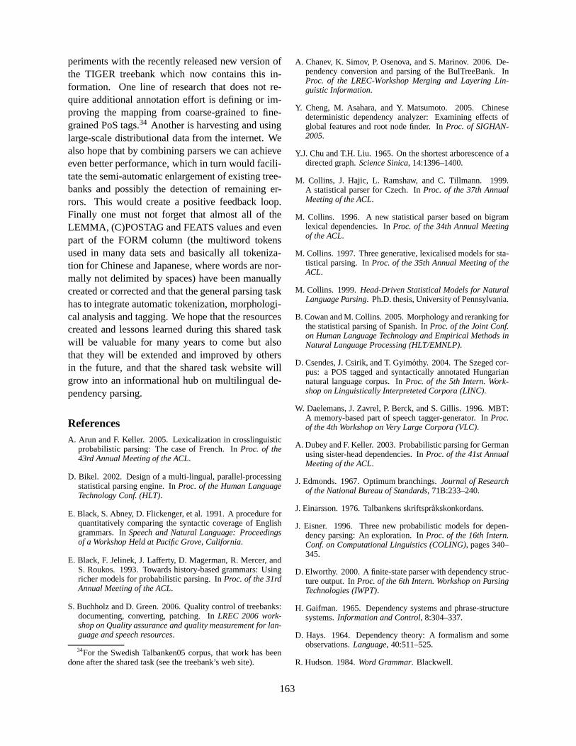
periments with the recently released new version ofthe TIGER treebank which now contains this in-formation. One line of research that does not re-quire additional annotation effort is defining or im-proving the mapping from coarse-grained to fine-grained PoS tags.34 Another is harvesting and usinglarge-scale distributional data from the internet. Wealso hope that by combining parsers we can achieveeven better performance, which in turn would facili-tate the semi-automatic enlargement of existing tree-banks and possibly the detection of remaining er-rors. This would create a positive feedback loop.Finally one must not forget that almost all of theLEMMA, (C)POSTAG and FEATS values and evenpart of the FORM column (the multiword tokensused in many data sets and basically all tokeniza-tion for Chinese and Japanese, where words are nor-mally not delimited by spaces) have been manuallycreated or corrected and that the general parsing taskhas to integrate automatic tokenization, morphologi-cal analysis and tagging. We hope that the resourcescreated and lessons learned during this shared taskwill be valuable for many years to come but alsothat they will be extended and improved by othersin the future, and that the shared task website willgrow into an informational hub on multilingual de-pendency parsing.
ReferencesA. Arun and F. Keller. 2005. Lexicalization in crosslinguistic
probabilistic parsing: The case of French. InProc. of the43rd Annual Meeting of the ACL.
D. Bikel. 2002. Design of a multi-lingual, parallel-processingstatistical parsing engine. InProc. of the Human LanguageTechnology Conf. (HLT).
E. Black, S. Abney, D. Flickenger, et al. 1991. A procedure forquantitatively comparing the syntactic coverage of Englishgrammars. InSpeech and Natural Language: Proceedingsof a Workshop Held at Pacific Grove, California.
E. Black, F. Jelinek, J. Lafferty, D. Magerman, R. Mercer, andS. Roukos. 1993. Towards history-based grammars: Usingricher models for probabilistic parsing. InProc. of the 31rdAnnual Meeting of the ACL.
S. Buchholz and D. Green. 2006. Quality control of treebanks:documenting, converting, patching. InLREC 2006 work-shop on Quality assurance and quality measurement for lan-guage and speech resources.
34For the Swedish Talbanken05 corpus, that work has beendone after the shared task (see the treebank’s web site).
A. Chanev, K. Simov, P. Osenova, and S. Marinov. 2006. De-pendency conversion and parsing of the BulTreeBank. InProc. of the LREC-Workshop Merging and Layering Lin-guistic Information.
Y. Cheng, M. Asahara, and Y. Matsumoto. 2005. Chinesedeterministic dependency analyzer: Examining effects ofglobal features and root node finder. InProc. of SIGHAN-2005.
Y.J. Chu and T.H. Liu. 1965. On the shortest arborescence of adirected graph.Science Sinica, 14:1396–1400.
M. Collins, J. Hajic, L. Ramshaw, and C. Tillmann. 1999.A statistical parser for Czech. InProc. of the 37th AnnualMeeting of the ACL.
M. Collins. 1996. A new statistical parser based on bigramlexical dependencies. InProc. of the 34th Annual Meetingof the ACL.
M. Collins. 1997. Three generative, lexicalised models forsta-tistical parsing. InProc. of the 35th Annual Meeting of theACL.
M. Collins. 1999.Head-Driven Statistical Models for NaturalLanguage Parsing. Ph.D. thesis, University of Pennsylvania.
B. Cowan and M. Collins. 2005. Morphology and reranking forthe statistical parsing of Spanish. InProc. of the Joint Conf.on Human Language Technology and Empirical Methods inNatural Language Processing (HLT/EMNLP).
D. Csendes, J. Csirik, and T. Gyimothy. 2004. The Szeged cor-pus: a POS tagged and syntactically annotated Hungariannatural language corpus. InProc. of the 5th Intern. Work-shop on Linguistically Interpreteted Corpora (LINC).
W. Daelemans, J. Zavrel, P. Berck, and S. Gillis. 1996. MBT:A memory-based part of speech tagger-generator. InProc.of the 4th Workshop on Very Large Corpora (VLC).
A. Dubey and F. Keller. 2003. Probabilistic parsing for Germanusing sister-head dependencies. InProc. of the 41st AnnualMeeting of the ACL.
J. Edmonds. 1967. Optimum branchings.Journal of Researchof the National Bureau of Standards, 71B:233–240.
J. Einarsson. 1976. Talbankens skriftsprakskonkordans.
J. Eisner. 1996. Three new probabilistic models for depen-dency parsing: An exploration. InProc. of the 16th Intern.Conf. on Computational Linguistics (COLING), pages 340–345.
D. Elworthy. 2000. A finite-state parser with dependency struc-ture output. InProc. of the 6th Intern. Workshop on ParsingTechnologies (IWPT).
H. Gaifman. 1965. Dependency systems and phrase-structuresystems.Information and Control, 8:304–337.
D. Hays. 1964. Dependency theory: A formalism and someobservations.Language, 40:511–525.
R. Hudson. 1984.Word Grammar. Blackwell.
163
T. Kudo and Y. Matsumoto. 2000. Japanese dependency struc-ture analysis based on support vector machines. InProc. ofthe Joint Conf. on Empirical Methods in Natural LanguageProcessing and Very Large Corpora (EMNLP/VLC).
S. Kurohashi and M. Nagao. 1994. KN parser: Japanese depen-dency/case structure analyzer. InProceedings of the Work-shop on Sharable Natural Language, pages 48–55.
S. Kurohashi and M. Nagao. 1997. Kyoto University text cor-pus project. InProc. of the 5th Conf. on Applied NaturalLanguage Processing (ANLP), pages 115–118.
Y. Lepage, S. Ando, S. Akamine, and H. Iida. 1998. An anno-tated corpus in Japanese using Tesniere’s structural syntax.In ACL-COLING Workshop on Processing of Dependency-Based Grammars, pages 109–115.
D. Lin. 1995. A dependency-based method for evaluatingbroad-coverage parsers. InProc. of the International JointConference on Artificial Intelligence (IJCAI).
D. Magerman. 1995. Statistical decision-tree models for pars-ing. In Proc. of the 33rd Annual Meeting of the ACL, pages276–283.
M. Marcus, G. Kim, M. Marcinkiewicz, R. Mac-Intyre, A. Bies,M. Ferguson, K. Katz, and B. Schasberger. 1994. The Penntreebank: Annotating predicate argument structure. InProc.of the Workshop on Human Language Technology (HLT).
S. Marinov and J. Nivre. 2005. A data-driven dependencyparser for Bulgarian. InProc. of the 4th Workshop on Tree-banks and Linguistic Theories (TLT), pages 89–100.
R. McDonald and F. Pereira. 2006. Online learning of approx-imate dependency parsing algorithms. InProc. of the 11thConf. of the European Chapter of the ACL (EACL).
R. McDonald, K. Crammer, and F. Pereira. 2005a. Onlinelarge-margin training of dependency parsers. InProc. of the43rd Annual Meeting of the ACL.
R. McDonald, F. Pereira, K. Ribarov, and J. Hajic. 2005b.Non-projective dependency parsing using spanning tree al-gorithms. InProc. of the Joint Conf. on Human LanguageTechnology and Empirical Methods in Natural LanguageProcessing (HLT/EMNLP).
I. Mel’cuk. 1988. Dependency Syntax: Theory and Practice.The SUNY Press, Albany, N.Y.
J. Nivre and J. Nilsson. 2005. Pseudo-projective dependencyparsing. InProc. of the 43rd Annual Meeting of the ACL,pages 99–106.
J. Nivre and M. Scholz. 2004. Deterministic dependency pars-ing of English text. InProc. of the 20th Intern. Conf. onComputational Linguistics (COLING), pages 64–70.
J. Nivre, J. Hall, and J. Nilsson. 2004. Memory-based depen-dency parsing. InProc. of the 8th Conf. on ComputationalNatural Language Learning (CoNLL), pages 49–56.
K. Oflazer. 1999. Dependency parsing with an extended finitestate approach. InProc. of the 37th Annual Meeting of theACL, pages 254–260.
G. Sampson. 1995.English for the Computer: The SUSANNECorpus and analytic scheme. Clarendon Press.
K. Sima’an, A. Itai, Y. Winter, A. Altman, and N. Nativ. 2001.Building a tree-bank of modern Hebrew text. InJournalTraitement Automatique des Langues (t.a.l.) — Special Issueon Natural Language Processing and Corpus Linguistics.
D. Sleator and D. Temperley. 1993. Parsing English with a linkgrammar. InProc. of the 3rd Intern. Workshop on ParsingTechnologies (IWPT).
P. Tapanainen and T. Jarvinen. 1997. A non-projective depen-dency parser. InProc. of the 5th Conf. on Applied NaturalLanguage Processing (ANLP).
U. Teleman, 1974.Manual for grammatisk beskrivning av taladoch skriven svenska (MAMBA).
L. Tesniere. 1959.Element de syntaxe structurale. Klinck-sieck, Paris.
H. Yamada and Y. Matsumoto. 2003. Statistical dependencyanalysis with support vector machines. InProc. of the 8th In-tern. Workshop on Parsing Technologies (IWPT), pages 195–206.
Papers by participants of CoNLL-X (this volume)
G. Attardi. 2006. Experiments with a multilanguage non-projective dependency parser.
E. Bick. 2006. LingPars, a linguistically inspired, language-independent machine learner for dependency treebanks.
S. Canisius, T. Bogers, A. van den Bosch, J. Geertzen, andE. Tjong Kim Sang. 2006. Dependency parsing by infer-ence over high-recall dependency predictions.
M. Chang, Q. Do, and D. Roth. 2006. A pipeline model forbottom-up dependency parsing.
S. Corston-Oliver and A. Aue. 2006. Dependency parsing withreference to Slovene, Spanish and Swedish.
M. Dreyer, D. Smith, and N. Smith. 2006. Vine parsing andminimum risk reranking for speed and precision.
R. Johansson and P. Nugues. 2006. Investigating multilingualdependency parsing.
R. McDonald, K. Lerman, and F. Pereira. 2006. Multilingualdependency analysis with a two-stage discriminative parser.
J. Nivre, J. Hall, J. Nilsson, G. Eryigit, and S. Marinov. 2006.Labeled pseudo-projective dependency parsing with supportvector machines.
S. Riedel, R. Cakıcı, and I. Meza-Ruiz. 2006. Multi-lingual de-pendency parsing with incremental integer linear program-ming.
M. Schiehlen and K. Spranger. 2006. Language indepen-dent probabilistic context-free parsing bolstered by machinelearning.
N. Shimizu. 2006. Maximum spanning tree algorithm for non-projective labeled dependency parsing.
D. Yuret. 2006. Dependency parsing as a classication problem.
164

Proceedings of the 10th Conference on Computational Natural Language Learning (CoNLL-X),page 165, New York City, June 2006.c©2006 Association for Computational Linguistics
The Treebanks Used in the Shared Task
This page contains references to all the treebanksused in the CoNLL-X shared task. This page shouldbe consulted whenever a shared task paper refers toa treebank without including the actual reference.
ReferencesA. Abeille, editor. 2003.Treebanks: Building and Us-
ing Parsed Corpora, volume 20 ofText, Speech andLanguage Technology. Kluwer Academic Publishers,Dordrecht.
S. Afonso, E. Bick, R. Haber, and D. Santos. 2002. “Flo-resta sinta(c)tica”: a treebank for Portuguese. InProc.of the Third Intern. Conf. on Language Resources andEvaluation (LREC), pages 1698–1703.
N. B. Atalay, K. Oflazer, and B. Say. 2003. The annota-tion process in the Turkish treebank. InProc. of the 4thIntern. Workshop on Linguistically Interpreteted Cor-pora (LINC).
A. Bohmova, J. Hajic, E. Hajicova, and B. Hladka. 2003.The PDT: a 3-level annotation scenario. In Abeille(Abeille, 2003), chapter 7.
S. Brants, S. Dipper, S. Hansen, W. Lezius, and G. Smith.2002. The TIGER treebank. InProc. of theFirst Workshop on Treebanks and Linguistic Theories(TLT).
K. Chen, C. Luo, M. Chang, F. Chen, C. Chen, C. Huang,and Z. Gao. 2003. Sinica treebank: Design criteria,representational issues and implementation. In Abeille(Abeille, 2003), chapter 13, pages 231–248.
M. Civit, MaA. Martı, B. Navarro, N. Bufi, B. Fernandez,and R. Marcos. 2003. Issues in the syntactic annota-tion of Cast3LB. InProc. of the 4th Intern. Workshopon Linguistically Interpreteted Corpora (LINC).
M. Civit Torruella and Ma A. Martı Antonın. 2002. De-sign principles for a Spanish treebank. InProc. of theFirst Workshop on Treebanks and Linguistic Theories(TLT).
S. Dzeroski, T. Erjavec, N. Ledinek, P. Pajas,Z. Zabokrtsky, and A.Zele. 2006. Towards a Slovenedependency treebank. InProc. of the Fifth Intern.Conf. on Language Resources and Evaluation (LREC).
J. Hajic, O. Smrz, P. Zemanek, J.Snaidauf, and E. Beska.2004. Prague Arabic dependency treebank: Develop-ment in data and tools. InProc. of the NEMLAR In-tern. Conf. on Arabic Language Resources and Tools,pages 110–117.
Y. Kawata and J. Bartels. 2000. Stylebook for theJapanese treebank in VERBMOBIL. Verbmobil-Report 240, Seminar fur Sprachwissenschaft, Univer-sitat Tubingen.
M. T. Kromann. 2003. The Danish dependency treebankand the underlying linguistic theory. InProc. of theSecond Workshop on Treebanks and Linguistic Theo-ries (TLT).
B. Navarro, M. Civit, Ma A. Martı, R. Marcos, andB. Fernandez. 2003. Syntactic, semantic and prag-matic annotation in Cast3LB. InProc. of the Work-shop on Shallow Processing of Large Corpora (SPro-LaC).
J. Nilsson, J. Hall, and J. Nivre. 2005. MAMBA meetsTIGER: Reconstructing a Swedish treebank from an-tiquity. In Proc. of the NODALIDA Special Session onTreebanks.
K. Oflazer, B. Say, D. Zeynep Hakkani-Tur, and G. Tur.2003. Building a Turkish treebank. In Abeille(Abeille, 2003), chapter 15.
P. Osenova and K. Simov. 2004. BTB-TR05: Bul-TreeBank stylebook. BulTreeBank version 1.0. Bul-treebank project technical report. Available at:http://www.bultreebank.org/TechRep/BTB-TR05.pdf.
K. Simov and P. Osenova. 2003. Practical annotationscheme for an HPSG treebank of Bulgarian. InProc.of the 4th Intern. Workshop on Linguistically Inter-preteted Corpora (LINC), pages 17–24.
K. Simov, G. Popova, and P. Osenova. 2002. HPSG-based syntactic treebank of Bulgarian (BulTreeBank).In A. Wilson, P. Rayson, and T. McEnery, editors,ARainbow of Corpora: Corpus Linguistics and the Lan-guages of the World, pages 135–142. Lincom-Europa,Munich.
K. Simov, P. Osenova, and M. Slavcheva. 2004.BTB-TR03: BulTreeBank morphosyntac-tic tagset. BTB-TS version 2.0. Bultree-bank project technical report. Available at:http://www.bultreebank.org/TechRep/BTB-TR03.pdf.
K. Simov, P. Osenova, A. Simov, and M. Kouylekov.2005. Design and implementation of the BulgarianHPSG-based treebank. InJournal of Research on Lan-guage and Computation – Special Issue, pages 495–522. Kluwer Academic Publishers.
L. van der Beek, G. Bouma, R. Malouf, and G. van No-ord. 2002. The Alpino dependency treebank. InCom-putational Linguistics in the Netherlands (CLIN).
165
Proceedings of the 10th Conference on Computational Natural Language Learning (CoNLL-X),pages 166–170, New York City, June 2006.c©2006 Association for Computational Linguistics
Experiments with a Multilanguage Non-Projective
Dependency Parser
Giuseppe Attardi
Dipartimento di Informatica
largo B. Pontecorvo, 3
I-56127 Pisa, Italy
1 Introduction
Parsing natural language is an essential step in
several applications that involve document
analysis, e.g. knowledge extraction, question
answering, summarization, filtering. The best
performing systems at the TREC Question
Answering track employ parsing for analyzing
sentences in order to identify the query focus, to
extract relations and to disambiguate meanings of
words.
These are often demanding applications, which
need to handle large collections and to provide
results in a fraction of a second. Dependency
parsers are promising for these applications since a
dependency tree provides predicate-argument
relations which are convenient for use in the later
stages. Recently statistical dependency parsing
techniques have been proposed which are
deterministic and/or linear (Yamada and
Matsumoto, 2003; Nivre and Scholz, 2004). These
parsers are based on learning the correct sequence
of Shift/Reduce actions used to construct the
dependency tree. Learning is based on techniques
like SVM (Vapnik 1998) or Memory Based
Learning (Daelemans 2003), which provide high
accuracy but are often computationally expensive.
Kudo and Matsumoto (2002) report a two week
learning time on a Japanese corpus of about 8000
sentences with SVM. Using Maximum Entropy
(Berger, et al. 1996) classifiers I built a parser that
achieves a throughput of over 200 sentences per
second, with a small loss in accuracy of about 2-
3 %.
The efficiency of Maximum Entropy classifiers
seems to leave a large margin that can be exploited
to regain accuracy by other means. I performed a
series of experiments to determine whether
increasing the number of features or combining
several classifiers could allow regaining the best
accuracy. An experiment cycle in our setting
requires less than 15 minutes for a treebank of
moderate size like the Portuguese treebank
(Afonso et al., 2002) and this allows evaluating the
effectiveness of adding/removing features that
hopefully might apply also when using other
learning techniques.
I extended the Yamada-Matsumoto parser to
handle labeled dependencies: I tried two
approaches: using a single classifier to predict
pairs of actions and labels and using two separate
classifiers, one for actions and one for labels.
Finally, I extended the repertoire of actions used
by the parser, in order to handle non-projective
relations. Tests on the PDT (Böhmovà et al., 2003)
show that the added actions are sufficient to handle
all cases of non-projectivity. However, since the
cases of non-projectivity are quite rare in the
corpus, the general learner is not supplied enough
of them to learn how to classify them accurately,
hence it may be worthwhile to exploit a second
classifier trained specifically in handling non-
projective situations.
1. Summary of the approach
The overall parsing algorithm is an inductive
statistical parser, which extends the approach by
Yamada and Matsumoto (2003), by adding six new
reduce actions for handling non-projective
relations and also performs dependency labeling.
Parsing is deterministic and proceeds bottom-up.
Labeling is integrated within a single processing
step.
166
The parser is modular: it can use several
learning algorithms: Maximum Entropy, SVM,
Winnow, Voted Perceptron, Memory Based
Learning, as well as combinations thereof. The
submitted runs used Maximum Entropy and I
present accuracy and performance comparisons
with other learning algorithms.
No additional resources are used.
No pre-processing or post-processing is used,
except stemming for Danish, German and Swedish.
2 Features
Columns from input data were used as follows.
LEMMA was used in features whenever
available, otherwise the FORM was used. For
Danish, German and Swedish the Snowball
stemmer (Porter 2001) was used to generate a
value for LEMMA. This use of stemming slightly
improved both accuracy and performance.
Only CPOSTAG were used. PHEAD/PDEPREL
were not used.
FEATS were used to extract a single token
combining gender, number, person and case,
through a language specific algorithm.
The selection of features to be used in the parser
is controlled by a number of parameters. For ex-
ample, the parameter PosFeatures determines
for which tokens the POS tag will be included in
the context, PosLeftChildren determines how
many left outermost children of a token to con-
sider, PastActions tells how many previous ac-
tions to include as features.
The settings used in the submitted runs are listed
below and configure the parser for not using any
word forms. Positive numbers refer to input to-
kens, negative ones to token on the stack.
LemmaFeatures -2 -1 0 1 2 3 PosFeatures -2 -1 0 1 2 3 MorphoFeatures -1 0 1 2 DepFeatures -1 0 PosLeftChildren 2 PosLeftChild -1 0 DepLeftChild -1 0 PosRightChildren 2 PosRightChild -1 0 DepRightChild -1 PastActions 1
The context for POS tags consisted of 1 token left
and 3 tokens to the right of the focus words, except
for Czech and Chinese were 2 tokens to the left
and 4 tokens to the right were used. These values
were chosen by performing experiments on the
training data, using 10% of the sentences as held-
out data for development.
3 Inductive Deterministic Parsing
The parser constructs dependency trees employing
a deterministic bottom-up algorithm which per-
forms Shift/Reduce actions while analyzing input
sentences in left-to-right order.
Using a notation similar to (Nivre and Scholz,
2003), the state of the parser is represented by a
quadruple ⟨S, I, T, A⟩, where S is the stack, I is the
list of (remaining) input tokens, T is a stack of
temporary tokens and A is the arc relation for the
dependency graph.
Given an input string W, the parser is initialized
to ⟨(), W, (), ()⟩, and terminates when it reaches a
configuration ⟨S, (), (), A⟩.
The parser by Yamada and Matsumoto (2003)
used the following actions:
Shift in a configuration ⟨S, n|I, T, A⟩, pushes
n to the stack, producing the configura-
tion ⟨n|S, I, T, A⟩.
Right1 in a configuration ⟨s1|S, n|I, T, A⟩, adds
an arc from s1 to n and pops s1 from the
stack, producing the configuration ⟨S,
n|I, T, A∪{(s1, r, n)}⟩.
Left in a configuration ⟨s1|S, n|I, T, A⟩, adds
an arc from n to s1, pops n from input,
pops s1 from the stack and moves it
back to I, producing the configuration
⟨S, s1|I, T, A∪{(n, r, s1)}⟩.
At each step the parser uses classifiers trained on
treebank data in order to predict which action to
perform and which dependency label to assign
given the current configuration.
4 Non-Projective Relations
For handling non-projective relations, Nivre and
Nilsson (2005) suggested applying a pre-
processing step to a dependency parser, which con-
sists in lifting non-projective arcs to their head re-
peatedly, until the tree becomes pseudo-projective.
A post-processing step is then required to restore
the arcs to the proper heads.
1 Nivre and Scholz reverse the direction, while I follow here
the terminology in Yamada and Matsumoto (2003).
167
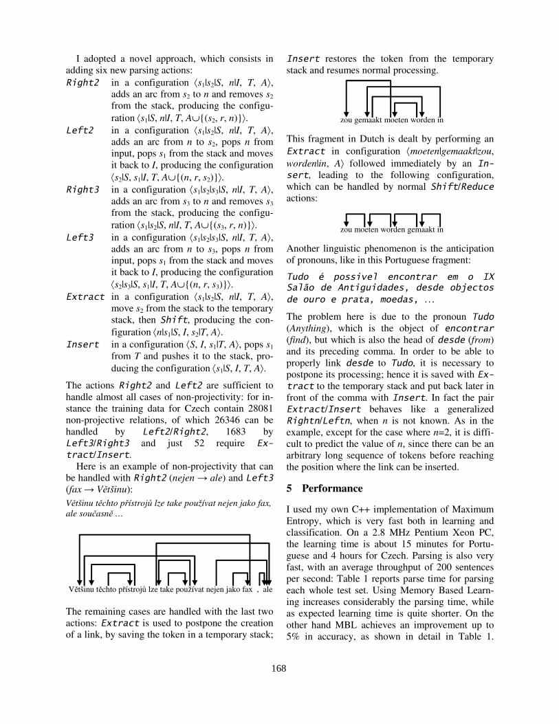
I adopted a novel approach, which consists in
adding six new parsing actions:
Right2 in a configuration ⟨s1|s2|S, n|I, T, A⟩,
adds an arc from s2 to n and removes s2
from the stack, producing the configu-
ration ⟨s1|S, n|I, T, A∪{(s2, r, n)}⟩.
Left2 in a configuration ⟨s1|s2|S, n|I, T, A⟩,
adds an arc from n to s2, pops n from
input, pops s1 from the stack and moves
it back to I, producing the configuration
⟨s2|S, s1|I, T, A∪{(n, r, s2)}⟩.
Right3 in a configuration ⟨s1|s2|s3|S, n|I, T, A⟩,
adds an arc from s3 to n and removes s3
from the stack, producing the configu-
ration ⟨s1|s2|S, n|I, T, A∪{(s3, r, n)}⟩.
Left3 in a configuration ⟨s1|s2|s3|S, n|I, T, A⟩,
adds an arc from n to s3, pops n from
input, pops s1 from the stack and moves
it back to I, producing the configuration
⟨s2|s3|S, s1|I, T, A∪{(n, r, s3)}⟩.
Extract in a configuration ⟨s1|s2|S, n|I, T, A⟩,
move s2 from the stack to the temporary
stack, then Shift, producing the con-
figuration ⟨n|s1|S, I, s2|T, A⟩.
Insert in a configuration ⟨S, I, s1|T, A⟩, pops s1
from T and pushes it to the stack, pro-
ducing the configuration ⟨s1|S, I, T, A⟩.
The actions Right2 and Left2 are sufficient to
handle almost all cases of non-projectivity: for in-
stance the training data for Czech contain 28081
non-projective relations, of which 26346 can be
handled by Left2/Right2, 1683 by
Left3/Right3 and just 52 require Ex-
tract/Insert.
Here is an example of non-projectivity that can
be handled with Right2 (nejen → ale) and Left3
(fax → Většinu):
Většinu těchto přístrojů lze take používat nejen jako fax,
ale současně …
The remaining cases are handled with the last two
actions: Extract is used to postpone the creation
of a link, by saving the token in a temporary stack;
Insert restores the token from the temporary
stack and resumes normal processing.
This fragment in Dutch is dealt by performing an
Extract in configuration ⟨moeten|gemaakt|zou,
worden|in, A⟩ followed immediately by an In-
sert, leading to the following configuration,
which can be handled by normal Shift/Reduce
actions:
Another linguistic phenomenon is the anticipation
of pronouns, like in this Portuguese fragment:
Tudo é possivel encontrar em o IX Salão de Antiguidades, desde objectos
de ouro e prata, moedas, …
The problem here is due to the pronoun Tudo
(Anything), which is the object of encontrar
(find), but which is also the head of desde (from)
and its preceding comma. In order to be able to
properly link desde to Tudo, it is necessary to
postpone its processing; hence it is saved with Ex-
tract to the temporary stack and put back later in
front of the comma with Insert. In fact the pair
Extract/Insert behaves like a generalized
Rightn/Leftn, when n is not known. As in the
example, except for the case where n=2, it is diffi-
cult to predict the value of n, since there can be an
arbitrary long sequence of tokens before reaching
the position where the link can be inserted.
5 Performance
I used my own C++ implementation of Maximum
Entropy, which is very fast both in learning and
classification. On a 2.8 MHz Pentium Xeon PC,
the learning time is about 15 minutes for Portu-
guese and 4 hours for Czech. Parsing is also very
fast, with an average throughput of 200 sentences
per second: Table 1 reports parse time for parsing
each whole test set. Using Memory Based Learn-
ing increases considerably the parsing time, while
as expected learning time is quite shorter. On the
other hand MBL achieves an improvement up to
5% in accuracy, as shown in detail in Table 1.
zou moeten worden gemaakt in
zou gemaakt moeten worden in
Většinu těchto přístrojů lze take používat nejen jako fax , ale
168
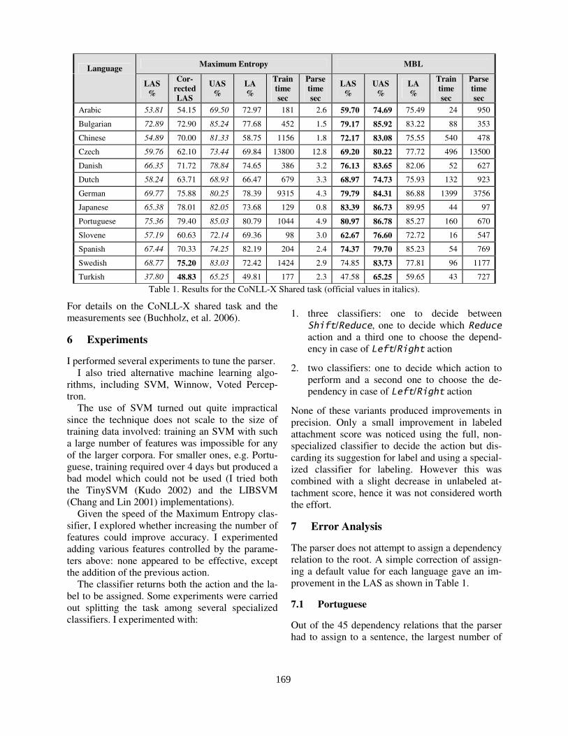
Language Maximum Entropy MBL
LAS
%
Cor-
rected
LAS
UAS
%
LA
%
Train
time
sec
Parse
time
sec
LAS
%
UAS
%
LA
%
Train
time
sec
Parse
time
sec
Arabic 53.81 54.15 69.50 72.97 181 2.6 59.70 74.69 75.49 24 950
Bulgarian 72.89 72.90 85.24 77.68 452 1.5 79.17 85.92 83.22 88 353
Chinese 54.89 70.00 81.33 58.75 1156 1.8 72.17 83.08 75.55 540 478
Czech 59.76 62.10 73.44 69.84 13800 12.8 69.20 80.22 77.72 496 13500
Danish 66.35 71.72 78.84 74.65 386 3.2 76.13 83.65 82.06 52 627
Dutch 58.24 63.71 68.93 66.47 679 3.3 68.97 74.73 75.93 132 923
German 69.77 75.88 80.25 78.39 9315 4.3 79.79 84.31 86.88 1399 3756
Japanese 65.38 78.01 82.05 73.68 129 0.8 83.39 86.73 89.95 44 97
Portuguese 75.36 79.40 85.03 80.79 1044 4.9 80.97 86.78 85.27 160 670
Slovene 57.19 60.63 72.14 69.36 98 3.0 62.67 76.60 72.72 16 547
Spanish 67.44 70.33 74.25 82.19 204 2.4 74.37 79.70 85.23 54 769
Swedish 68.77 75.20 83.03 72.42 1424 2.9 74.85 83.73 77.81 96 1177
Turkish 37.80 48.83 65.25 49.81 177 2.3 47.58 65.25 59.65 43 727
Table 1. Results for the CoNLL-X Shared task (official values in italics).
For details on the CoNLL-X shared task and the
measurements see (Buchholz, et al. 2006).
6 Experiments
I performed several experiments to tune the parser.
I also tried alternative machine learning algo-
rithms, including SVM, Winnow, Voted Percep-
tron.
The use of SVM turned out quite impractical
since the technique does not scale to the size of
training data involved: training an SVM with such
a large number of features was impossible for any
of the larger corpora. For smaller ones, e.g. Portu-
guese, training required over 4 days but produced a
bad model which could not be used (I tried both
the TinySVM (Kudo 2002) and the LIBSVM
(Chang and Lin 2001) implementations).
Given the speed of the Maximum Entropy clas-
sifier, I explored whether increasing the number of
features could improve accuracy. I experimented
adding various features controlled by the parame-
ters above: none appeared to be effective, except
the addition of the previous action.
The classifier returns both the action and the la-
bel to be assigned. Some experiments were carried
out splitting the task among several specialized
classifiers. I experimented with:
1. three classifiers: one to decide between
Shift/Reduce, one to decide which Reduce
action and a third one to choose the depend-
ency in case of Left/Right action
2. two classifiers: one to decide which action to
perform and a second one to choose the de-pendency in case of Left/Right action
None of these variants produced improvements in
precision. Only a small improvement in labeled
attachment score was noticed using the full, non-
specialized classifier to decide the action but dis-
carding its suggestion for label and using a special-
ized classifier for labeling. However this was
combined with a slight decrease in unlabeled at-
tachment score, hence it was not considered worth
the effort.
7 Error Analysis
The parser does not attempt to assign a dependency
relation to the root. A simple correction of assign-
ing a default value for each language gave an im-
provement in the LAS as shown in Table 1.
7.1 Portuguese
Out of the 45 dependency relations that the parser
had to assign to a sentence, the largest number of
169
errors occurred assigning N<PRED (62), ACC (46),
PIV (43), CJT (40), N< (34), P< (30).
The highest number of head error occurred at
the CPOS tags PRP with 193 and V with 176. In
particular just four prepositions (em, de, a, para)
accounted for 120 head errors.
Most of the errors occur near punctuations. Of-
ten this is due to the fact that commas introduce
relative phrases or parenthetical phrases (e.g. “o
suspeito, de 38 anos, que trabalha”),
that produce diversions in the flow. Since the
parser makes decisions analyzing only a window
of tokens of a limited size, it gets confused in cre-
ating attachments. I tried to add some global con-
text features, to be able to distinguish these cases,
in particular, a count of the number of punctuation
marks seen so far, whether punctuation is present
between the focus words. None of them helped
improving precision and were not used in the sub-
mitted runs.
7.2 Czech
Most current parsers for Czech do not perform well
on Apos (apposition), Coord (coordination) and
ExD (ellipses), but they are not very frequent. The
largest number of errors occur on Obj (166), Adv
(155), Sb (113), Atr (98). There is also often con-
fusion among these: 33 times Obj instead of Adv,
32 Sb instead of Obj, 28 Atr instead of Adv.
The high error rate of J (adjective) is expected,
mainly due to coordination problems. The error of
R (preposition) is also relatively high. Prepositions
are problematic, but their error rate is higher than
expected since they are, in terms of surface order,
rather regular and close to the noun. It could be
that the decision by the PDT to hang them as heads
instead of children, causes a problem in attaching
them. It seems that a post-processing may correct a
significant portion of these errors.
The labels ending with _Co, _Ap or _Pa are
nodes who are members of the Coordination, Ap-
position or the Parenthetical relation, so it may be
worth while omitting these suffixes in learning and
restore them by post-processing.
An experiment using as training corpus a subset
consisting of just sentences which include non-
projective relations achieved a LAS of 65.28 %
and UAS of 76.20 %, using MBL.
Acknowledgments. Kiril Ribarov provided in-
sightful comments on the results for Czech.
The following treebanks were used for training the
parser: (Afonso et al., 2002; Atalay et al., 2003;
Böhmovà et al., 2003; Brants et al., 2002; Chen et
al., 2003; Civit Torruella and Martì Antonìn, 2002;
Džeroski et al., 2006; Hajiç et al., 2004; Kawata
and Bartels, 2000; Kromann, 2003; Nilsson et al.,
2005; Oflazer et al., 2003; Simov et al., 2005; van
der Beek et al., 2002).
References
A. Berger, S. Della Pietra, and M. Della Pietra. 1996. A
Maximum Entropy Approach to Natural Language
Processing. Computational Linguistics, 22(1).
S. Buchholz, et al. 2006. CoNLL-X Shared Task on
Multilingual Dependency Parsing. In Proc. of the
Tenth CoNLL.
C.-C. Chang, C.-J. Lin. 2001. LIBSVM: a library for
support vector machines.
http://www.csie.ntu.edu.tw/~cjlin/libsvm/
W. Daelemans, J. Zavrel, K. van der Sloot, and A. van
den Bosch. 2003. Timbl: Tilburg memory based
learner, version 5.0, reference guide. Technical Re-
port ILK 03-10, Tilburg University, ILK.
T. Kudo. 2002. tinySVM.
http://www.chasen.org/~taku/software/TinySVM/
T. Kudo, Y. Matsumoto. 2002. Japanese Dependency
Analysis using Cascaded Chunking. In Proc. of the
Sixth CoNLL.
R. McDonald, et al. 2005. Non-projective Dependency
Parsing using Spanning Tree Algorithms. In Proc. of
HLT-EMNLP.
J. Nivre, et al. 2004. Memory-based Dependency Pars-
ing. In Proc.s of the Eighth CoNLL, ed. H. T. Ng and
E. Riloff, Boston, Massachusetts, pp. 49–56.
J. Nivre and M. Scholz. 2004. Deterministic Depend-
ency Parsing of English Text. In Proc. of COLING
2004, Geneva, Switzerland, pp. 64–70.
J. Nivre and J. Nilsson, 2005. Pseudo-Projective De-
pendency Parsing. In Proc. of the 43rd Annual Meet-
ing of the ACL, pp. 99-106.
M.F. Porter. 2001. Snowball Stemmer.
http://www.snowball.tartarus.org/
V. N. Vapnik. 1998. The Statistical Learning Theory.
Springer.
H. Yamada and Y. Matsumoto. 2003. Statistical De-
pendency Analysis with Support Vector Machines. In
Proc. of the 8th International Workshop on Parsing
Technologies (IWPT), pp. 195–206.
170
Proceedings of the 10th Conference on Computational Natural Language Learning (CoNLL-X),pages 171–175, New York City, June 2006.c©2006 Association for Computational Linguistics
LingPars, a Linguistically Inspired, Language-Independent Machine Learner for Dependency Treebanks
Eckhard BickInstitute of Language and Communication
University of Southern Denmark5230 Odense M, [email protected]
Abstract
This paper presents a Constraint Grammar-inspired machine learner and parser, LingPars, that assigns dependencies to morphologically annotated treebanks in a function-centred way. The system not only bases attachment probabilities for PoS, case, mood, lemma on those features' function probabilities, but also uses topological features like function/PoS n-grams, barrier tags and daughter-sequences. In the CoNLL shared task, performance was below average on attachment scores, but a relatively higher score for function tags/deprels in isolation suggests that the system's strengths were not fully exploited in the current architecture.
1 Introduction
This paper describes LingPars, a Constraint Grammar-inspired language-independent treebank-learner developed from scratch between January 9th and March 9th 2006 in the context of the CoNLL-X 2006 shared task (http://nextens.uvt.nl/~conll/), organized by Sabine Buchholz, Erwin Marsi, Yval Krymolowski and Amit Dubey. Training treebanks and test data were provided for 13 different languages: Arabic (Smrž et al. 2002), Chinese (Chen et al. 2003), Czech (Hajič et al. 2001), Danish (Kromann 2003), Dutch (van der Beek et al. 2002), German (Brants et.al 2002), Japanese (Kawata and Bartels), Portuguese (Afonso et al. 2002), Slovene (Džerosky et al. 2006), Spanish (Palomar et al. 2004), Swedish (Nilsson et al. 2005), Turkish
(Oflazer et al. 2003 and Nart et.al 2003), Bulgarian (Simov et al. 2005). A number of these treebanks were not originally annotated in dependency style, but transformed from constituent tree style for the task, and all differ widely in terms of tag granularity (21-302 part-of-speech tags, 7-82 function labels). Also, not all treebanks included morphological information, and only half offered a lemma field. Such descriptive variation proved to be a considerable constraint for our parser design, as will be explained in chapter 2. No external resources and no structural preprocessing were used1.
2 Language independence versus theory independence
While manual annotation and/or linguistic, rule-based parsers are necessary for the creation of its training data, only a machine learning based parser (as targeted in the CoNNL shared task) can hope to be truly language independent in its design. The question is, however, if this necessarily implies independence of linguistic/descriptive theory.
In our own approach, LingPars, we thus departed from the Constraint Grammar descriptive model (Karlsson et al. 2005), where syntactic function tags (called DEPREL or dependency relations in the shared task) rank higher than dependency/constituency and are established before head attachments, rather than vice versa (as would be the case for many probabilistic, chunker based systems, or
1The only exception is what we consider a problem in the dependency-version of the German TIGER treebank, where postnominal attributes of nouns appear as dependents of that noun's head if the latter is a preposition, but not otherwise (e.g. if the head's head is a preposition). LingPars failed to learn this somewhat idiosyncratic distinction, but performance improved when the analysis was preprocessed with an additional np-layer (to be re-flattened after parsing.).
171
the classical PENN treebank descriptive model). In our hand-written, rule based parsers, dependency treebanks are constructed by using sequential attachment rules, generally attaching functions (e.g. subject, object, postnominal) to forms (finite verb, noun) or lexical tags (tense, auxiliary, transitive), with a direction condition and the possibility of added target, context or barrier conditions (Bick 2005).
In LingPars, we tried to mimic this methodology by trying to learn probabilities for both CG style syntactic-function contexts and function-to-form attachment rules. We could not, however, implement the straightforward idea of learning probabilities and optimal ordering for an existing body of (manual) seeding rules, because the 13 treebanks were not harmonized in their tag sets and descriptive conventions2.
As an example, imagine a linguistic rule that triggers "subclause-hood" for a verb-headed dependency-node as soon as a subordinator attaches to it, and then, implementing "subclause-hood", tries to attach the verb not to the root, but to another verb left of the subordinator, or right to a root-attaching verb. For the given set of treebanks probabilities and ordering priorities for this rule cannot be learned by one and the same parser, simply because some treebanks attach the verb to the subordinator rather than vice versa, and for verb chains, there is no descriptive consensus as to whether the auxiliary/construction verb (e.g. Spanish) or the main verb (e.g. Swedish) is regarded as head.
3 System architecture
The point of departure for pattern learning in LingPars were the fine-grained part of speech (PoS) tags (POSTAG) and the LEMMA tag. For those languages that did not provide a lemma tag, lower-cased word form was used instead. Also, where available from the FEATS field and not already integrated into the PoS tag, the following information was integrated into the PoS tag:
a) case, which was regarded as a good predictor for function, as well as a good dependency-indicator for e.g. preposition- and adnominal attachment
b) mood/finiteness, in order to predict subordination and verb chaining, especially in the absence of
2 Neither was there time (and for some languages: reading knowledge) to write the necessary converters to and from a normalized standard formalism for each treebank.
auxiliary class information in the FEATS fieldc) pronoun subclass, in order to predict adnomi
nal vs. independent function as well as subordinating function (relatives and interrogatives)
A few treebanks did not classify subordinating words as conjunctions, relatives, interrogatives etc., but lumped them into the general adverb and pronoun classes. Danish is a case in point - here, the treebank classified all non-inflecting words as PoS 'U'3. Our solution, implemented only for Danish and Swedish, was to introduce a list of structure-words, that would get their PoS appended with an '-S', enabling the learner to distinguish between e.g. "ordinary" ADV, and "structural" ADV-S.
3.1 The parser
In a first round, our parser calculates a preference list of functions and dependencies for each word, examining all possible mother-daughter pairs and n-grams in the sentence (or paragraph). Next, dependencies are adjusted for function, basically summing up the frequency-, distance- and direction-calibrated function→PoS attachment probabilities for all contextually allowed functions for a given word. Finally, dependency probabilities are weighted using linked probabilities for possible mother-, daughter- and sister-tags in a second pass.
The result are 2 arrays, one for possible daughter→mother pairs, one for word:function pairs. Values in both arrays are normalized to the 0..1 interval, meaning that for instance even an originally low probability, long distance attachment will get high values after normalization if there are few or no competing alternatives for the word in question.
LingPars then attempts to "effectuate" the dependency (daughter→mother) array, starting with the - in normalized terms - highest value4. If the daughter candidate is as yet unattached, and the dependency does not produce circularities or crossing branches, the corresponding part of the (ordered) word:function array is calibrated for the suggested dependency, and the top-ranking function chosen.
In principle, one pass through the dependency array would suffice to parse a sentence. However, 3For the treebank as such, no information is lost, since it will be recoverable from the function tag. In a training situation, however, there is much less to train on than in a treebank with a more syntactic definition of PoS.4 Though we prefer to think of attachments as bottom-up choices, the value-ordered approach is essentially neither bottom-up nor top-down, depending on the language and the salience of relations in a sentence, all runs had a great variation in the order of attachments. A middle-level attachment like case-based preposition-attachment, for instance, can easily outperform (low) article- or (high) top-node-attachment.
172
due to linguistic constraints like uniqueness principle, barrier tags and "full" heads5, some words may be left unattached or create conflicts for their heads. In these cases, weights are reduced for the conflicting functions, and increased for all daughter→mother values of the unattached word. The value arrays are then recomputed and rerun. In the case of unattached words, a complete rerun is performed, allowing problematic words to attach before those words that would otherwise have blocked them. In the case of a function (e.g subject uniqueness) conflict, only the words involved in the conflict are rerun. If no conflict-free solution is found after 19 runs, barrier-, uniqueness- and projectivity-constraints are relaxed for a last run6.
Finally, the daughter-sequence for each head (with the head itself inserted) is checked against the probability of its function sequence (learned not from n-grams proper, but from daughter-sequences in the training corpus). For instance, the constituents of a clause would make up such a sequence and allow to correct a sequence like SUBJ VFIN ARG2 ARG1 into SUBJ VFIN ARG1 ARG2, where ARG1 and ARG2 are object functions with a preferred order (for the language learned) of ARG1 ARG2.
3.2 Learning functions (deprels)
LingPars computes function probabilities (Vf, function value) at three levels: First, each lemma and PoS is assigned local (context-free) probabilities for all possible functions. Second, the probability of a given function occurring at a specific place in a function n-gram (func-gram, example (a)) is calculated (with n between 2 and 6). The learner only used endocentric func-grams, marking which of the function positions had their head within the func-gram. If no funcgram supported a given function, its probability for the word in question was set to zero. At the third level, for each endocentric n-gram of word classes (PoS), the probability for a given function occurring at a given position in the n-gram (position 2 in example (b)) was computed. Here, only the longest possible n-grams were used by the parser, and first and last positions of the n-gram were used only to provide context, not to assign function probabilities.
5Head types with a limited maximum number of dependents (usually, one)6In the rare case of still missing heads or functions, these are computed using probabilities for a simplified set of word classes (mostly the CPOSTAG), or - as a last resort - set to ROOT-attachment.
(a)>N→2 SUBJ→4 <N→2 AUX MV→4 ACC→5(b) art→2 n:SUBJ→4 adj→2 v-fin v-inf→4 n→5
3.3 Learning dependencies
In a rule based Constraint Grammar system, dependency would be expressed as attachment of functions to forms (i.e. subject to verb, or modifier to adjective). However, with empty deprel fields, LingPars cannot use functions directly, only their probabilities. Therefore, in a first pass, it computes the probability for the whole possible attachment matrix for a sentence, using learned mother- and daughter-normalized frequencies for attachments of type (a) PoS→PoS, (b) PoS→Lex, (c) Lex→PoS and (d) Lex→Lex, taking into account also the learned directional and distance preferences. Each matrix cell is then filled with a value Vfa ("function attachment value") - the sum of the individual normalized probabilities of all possible functions for that particular daughter given that particular mother multiplied with the preestablished, attachment-independent Vf value for that token-function combination.
Inspired by the BARRIER conditions in CG rule contexts, our learner also records the frequency of those PoS and those functions (deprels) that may appear between a dependent of PoS A and a head of PoS B. The parser then regards all other, non-registered interfering PoS or functions as blocking tokens for a given attachment pair, reducing its attachment value by a factor of 1/100.
In a second pass, the attachment matrix is calibrated using the relative probabilities for dependent daughters, dependent sisters and head mother given. This way, probabilities of object and object complement sisters will enhance each other, and given the fact that treebanks differ as to which element of a verb chain arguments attach to, a verbal head can be treated differently depending on whether it has a high probability for another verb (with auxiliary, modal or main verb function) as mother or daughter or not.
Finally, like for functions, n-grams are used to calculate attachment probabilities. For each endocentric PoS n-gram (of length 6 or less), the probabilities of all treebank-supported PoS:function chains and their dependency arcs are learned, and the value for an attachment word pair occurring in the chain will be corrected using both the chain/n-gram probability and the Vf value for the function
173
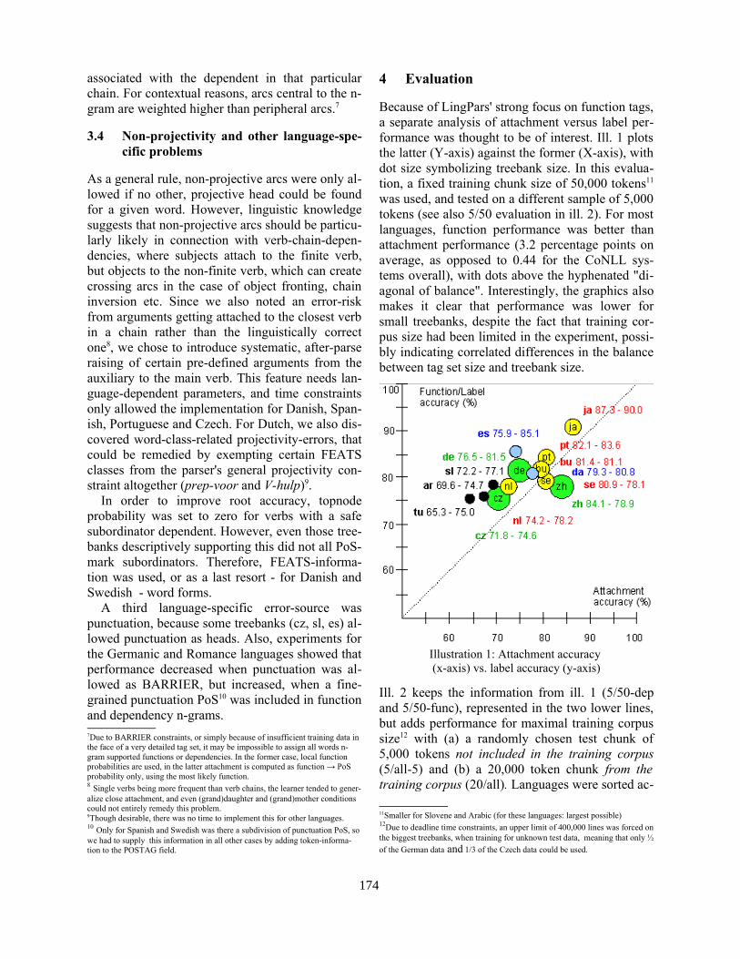
associated with the dependent in that particular chain. For contextual reasons, arcs central to the n-gram are weighted higher than peripheral arcs.7
3.4 Non-projectivity and other language-specific problems
As a general rule, non-projective arcs were only allowed if no other, projective head could be found for a given word. However, linguistic knowledge suggests that non-projective arcs should be particularly likely in connection with verb-chain-dependencies, where subjects attach to the finite verb, but objects to the non-finite verb, which can create crossing arcs in the case of object fronting, chain inversion etc. Since we also noted an error-risk from arguments getting attached to the closest verb in a chain rather than the linguistically correct one8, we chose to introduce systematic, after-parse raising of certain pre-defined arguments from the auxiliary to the main verb. This feature needs language-dependent parameters, and time constraints only allowed the implementation for Danish, Spanish, Portuguese and Czech. For Dutch, we also discovered word-class-related projectivity-errors, that could be remedied by exempting certain FEATS classes from the parser's general projectivity constraint altogether (prep-voor and V-hulp)9.
In order to improve root accuracy, topnode probability was set to zero for verbs with a safe subordinator dependent. However, even those treebanks descriptively supporting this did not all PoS-mark subordinators. Therefore, FEATS-information was used, or as a last resort - for Danish and Swedish - word forms.
A third language-specific error-source was punctuation, because some treebanks (cz, sl, es) allowed punctuation as heads. Also, experiments for the Germanic and Romance languages showed that performance decreased when punctuation was allowed as BARRIER, but increased, when a fine-grained punctuation PoS10 was included in function and dependency n-grams.7Due to BARRIER constraints, or simply because of insufficient training data in the face of a very detailed tag set, it may be impossible to assign all words n-gram supported functions or dependencies. In the former case, local function probabilities are used, in the latter attachment is computed as function → PoS probability only, using the most likely function.8 Single verbs being more frequent than verb chains, the learner tended to generalize close attachment, and even (grand)daughter and (grand)mother conditions could not entirely remedy this problem.9Though desirable, there was no time to implement this for other languages.10 Only for Spanish and Swedish was there a subdivision of punctuation PoS, so we had to supply this information in all other cases by adding token-information to the POSTAG field.
4 Evaluation
Because of LingPars' strong focus on function tags, a separate analysis of attachment versus label performance was thought to be of interest. Ill. 1 plots the latter (Y-axis) against the former (X-axis), with dot size symbolizing treebank size. In this evaluation, a fixed training chunk size of 50,000 tokens11 was used, and tested on a different sample of 5,000 tokens (see also 5/50 evaluation in ill. 2). For most languages, function performance was better than attachment performance (3.2 percentage points on average, as opposed to 0.44 for the CoNLL systems overall), with dots above the hyphenated "diagonal of balance". Interestingly, the graphics also makes it clear that performance was lower for small treebanks, despite the fact that training corpus size had been limited in the experiment, possibly indicating correlated differences in the balance between tag set size and treebank size.
Illustration 1: Attachment accuracy (x-axis) vs. label accuracy (y-axis)
Ill. 2 keeps the information from ill. 1 (5/50-dep and 5/50-func), represented in the two lower lines, but adds performance for maximal training corpus size12 with (a) a randomly chosen test chunk of 5,000 tokens not included in the training corpus (5/all-5) and (b) a 20,000 token chunk from the training corpus (20/all). Languages were sorted ac
11Smaller for Slovene and Arabic (for these languages: largest possible)12Due to deadline time constraints, an upper limit of 400,000 lines was forced on the biggest treebanks, when training for unknown test data, meaning that only ½ of the German data and 1/3 of the Czech data could be used.
174
cording to 20/all-func accuracy. As can be seen from the dips in the remaining (lower) curves, small training corpora (asterisk-marked languages) made it difficult for the parser (1) to match 20/all attachment performance on unknown data, and (2) to learn labels/functions in general (dips in all function curves, even 20/all). For the larger treebanks, the parser performed better (1-3 percentage points) for the full training set than for the 50,000 token training set.
Illustration 2: Performance with different training corpus sizes (upper 2 curves: Test data included)
5 Outlook
We have shown that a probabilistic dependency parser can be built on CG-inspired linguistic principles with a strong focus on function and tag sequences. Given the time constraint and the fact that the learner had to be built from scratch, its performance would encourage further research. In particular, a systematic parameter/performance analysis13 should be performed for the individual languages. In the long term, a notational harmonization of the treebanks should allow the learner to be seeded with existing hand-written dependency rules.
References Afonso, S., E. Bick, R. Haber and D. Santos. Floresta
Sintá(c)tica: A treebank of Portuguese. In Proceedings of LREC'02. pp. 1698-1703 . Paris: ELRA
van der Beek, L. G. Bouma, R. Malouf, G. van Noord. 2002. The Alpino Dependency Treebank. In: Computational Linguistics in the Netherlands CLIN 2001.
13Parameters like uniqueness and directedness are already learned by the system (through probability thresholds), while others, like function weights, structural word classes and frequency thresholds for barriers and lexeme n-grams are used now, but with a fixed value for all languages.
pp. 8-22. RodopiBick, Eckhard. 2005. Turning Constraint Grammar Data
into Running Dependency Treebanks. In: Civit, Montserrat & Kübler, Sandra & Martí, Ma. Antònia (ed.), Proceedings of TLT 2005, Barcelona. pp.19-2
Brants, S., S. Dipper, S. Hansen, W. Lezius, G. Smith. 2002. The TIGER Treebank. Proc. of TLT1, Sozopol
Džerosky, S., T. Erjavec, N. Ledinek, P. Pajas, Z. Žabokrtsky, A. Žele. 2006. Towards a Slovene Dependency Treebank. In Proc. of LREC'06, Genoa
Hajič, J., B. Hladká, and P. Pajas. 2001. The Prague Dependency Treebank: Annotation Structure and Support. In Proc. of the IRCS Workshop on Linguistic Databases, pp. 105-114. University of Pennsylvania.
Karlsson, Fred, Atro Vouitilainen, Jukka Heikkilä and A. Anttila. 1995. Constraint Grammar - A Language-Independent System for Parsing Unrestricted Text. Mouton de Gruyter: Berlin.
Kawata, Y. and J. Bartels. 2000. Stylebook for the Japanese Treebank in VERBMOBIL. Universität Tübingen: Verbmobil-Report 240.
Chen, Keh-Jiann, Chu-Ren Huang, Feng-Yi Chen, Chi-Ching Luo, Ming-Chung Chang, Chao-Jan Chen, and Zhao-Ming Gao. 2003. Sinica Treebank: Design Criteria, Representational Issues and Implementation. In A. Abeille (ed.) Treebanks Building and Using Parsed Corpora. Dordrecht:Kluwer, pp231-248.
Kromann, M. T. 2003. The Danish Dependency Treebank. In J. Nivre and E. Hinrichs (ed.) Proceedings of TLT2003. Växjö University Press, Sweden
Nart, B. Atalay, Kemal Oflazr, Bilge Say. 2003. The Annotation Process in the Turkish Treebank. In Proceedings of the EACL Workshop on Linguistically Interpreted Corpora - LINC 2003. Budapest
Nilsson, J, J. Hall and J. Nivre. 2005. MAMBA Meets TIGER: Reconstructing a Swedish Treebank from Antiquity. In Proceedings NODALIDA 2005. Joenssu
Oflazer, K., B. Say, D.Z. Hakkani-Tür, G. Tür. 2003. Building a Turkish Treebank. In A. Abeillé (ed.) Building and Exploiting Syntactically-annotated Corpora. Kluwer
Palomar, M. et. al. 2004. Construcción de una base de datos de árboles sintáctico-semánticos para el catalán, euskera y castellano. In: Proceedings of SEPLN XX, pp 81-88. Barcelona: ISSN 1135-5948
Simov, K., P. Osenova, A. Simov, M. Kouylekov. 2004. Design and Implementation of the Bulgarian HPSG-based Treebank. In E. Hinrichs and K. Simov (ed.), Journal of Research on Language and Computation, Vol. 2, No. 4 , pp. 495-522. Kluwer
Smrž, Otakar, Jan Šnaidauf, and Petr Zemánek. 2002. Prague Dependency Treebank for Arabic: Multi-Level Annotation of Arabic corpus. In Proceedings of the International Symposium on Processing of Arabic, pages 147-155, Manouba, Tunisia, April 2002.
cz de pt bu se nl tu *
ar *
sl *
da ja es *
zh65
67,5
70
72,575
77,5
80
82,585
87,5
9092,5
95
97,5
5/50 dep5/50 func20/all dep20/all func5/all-5 dep5/all-5 func
175

Proceedings of the 10th Conference on Computational Natural Language Learning (CoNLL-X),pages 176–180, New York City, June 2006.c©2006 Association for Computational Linguistics
Dependency Parsing by Inference over High-recall Dependency Predictions
Sander Canisius, Toine Bogers,Antal van den Bosch, Jeroen GeertzenILK / Computational Linguistics and AI
Tilburg University, P.O. Box 90153,NL-5000 LE Tilburg, The Netherlands{S.V.M.Canisius,A.M.Bogers,
Antal.vdnBosch,J.Geertzen}@uvt.nl
Erik Tjong Kim SangInformatics Institute
University of Amsterdam, Kruislaan 403NL-1098 SJ Amsterdam, The Netherlands
1 Introduction
As more and more syntactically-annotated corporabecome available for a wide variety of languages,machine learning approaches to parsing gain inter-est as a means of developing parsers without havingto repeat some of the labor-intensive and language-specific activities required for traditional parser de-velopment, such as manual grammar engineering,for each new language. The CoNLL-X shared taskon multi-lingual dependency parsing (Buchholz etal., 2006) aims to evaluate and advance the state-of-the-art in machine learning-based dependency pars-ing by providing a standard benchmark set compris-ing thirteen languages1. In this paper, we describetwo different machine learning approaches to theCoNLL-X shared task.
Before introducing the two learning-based ap-proaches, we first describe a number of baselines,which provide simple reference scores giving somesense of the difficulty of each language. Next, wepresent two machine learning systems: 1) an ap-proach that directly predicts all dependency relationsin a single run over the input sentence, and 2) a cas-cade of phrase recognizers. The first approach hasbeen found to perform best and was selected for sub-mission to the competition. We conclude this paperwith a detailed error analysis of its output for two ofthe thirteen languages, Dutch and Spanish.
1The data sets were extracted from various existing tree-banks (Hajic et al., 2004; Simov et al., 2005; Simov and Osen-ova, 2003; Chen et al., 2003; Bohmova et al., 2003; Kromann,2003; van der Beek et al., 2002; Brants et al., 2002; Kawata andBartels, 2000; Afonso et al., 2002; Dzeroski et al., 2006; CivitTorruella and Martı Antonın, 2002; Nilsson et al., 2005; Oflazeret al., 2003; Atalay et al., 2003)
2 Baseline approaches
Given the diverse range of languages involved inthe shared task, each having different characteristicsprobably requiring different parsing strategies, wedeveloped four different baseline approaches for as-signing labeled dependency structures to sentences.All of the baselines produce strictly projective struc-tures. While the simple rules implementing thesebaselines are insufficient for achieving state-of-the-art performance, they do serve a useful role in givinga sense of the difficulty of each of the thirteen lan-guages. The heuristics for constructing the trees andlabeling the relations used by each of the four base-lines are described below.
Binary right-branching trees The first baselineproduces right-branching binary trees. The first to-ken in the sentence is marked as the top node withHEAD 0 and DEPREL ROOT. For the rest of thetree, token n − 1 serves as the HEAD of token n.Figure 1 shows an example of the kind of tree thisbaseline produces.
Binary left-branching trees The binary left-branching baseline mirrors the previous baseline.The penultimate token in the sentence is marked asthe top node with HEAD 0 and DEPREL ROOTsince punctuation tokens can never serve as ROOT2.For the rest of the tree, the HEAD of token n is tokenn+1. Figure 2 shows an example of a tree producedby this baseline.
2We simply assume the final token in the sentence to bepunctuation.
176

Inward-branching trees In this approach, thefirst identified verb3 is marked as the ROOT node.The part of the sentence to the left of the ROOT isleft-branching, the part to the right of the ROOT isright-branching. Figure 3 shows an example of atree produced by this third baseline.
Nearest neighbor-branching trees In our mostcomplex baseline, the first verb is marked as theROOT node and the other verbs (with DEPREL vc)point to the closest preceding verb. The other to-kens point in the direction of their nearest neighbor-ing verb, i.e. the two tokens at a distance of 1 froma verb have that verb as their HEAD, the two tokensat a distance of 2 have the tokens at a distance of 1as their head, and so on until another verb is a closerneighbor. In the case of ties, i.e. tokens that areequally distant from two different verbs, the token islinked to the preceding token. Figure 4 clarifies thiskind of dependency structure in an example tree.
verb verb punct
ROOT
Figure 1: Binary right-branching tree for an examplesentence with two verbs.
verb verb punct
ROOT
Figure 2: Binary left-branching tree for the examplesentence.
verb verb punct
ROOT
Figure 3: Binary inward-branching tree for the ex-ample sentence.
3We consider a token a verb if its CPOSTAG starts with a‘V’. This is an obviously imperfect, but language-independentheuristic choice.
ROOT
verb verb punct
Figure 4: Nearest neighbor-branching tree for theexample sentence.
Labeling of identified relations is done using athree-fold back-off strategy. From the training set,we collect the most frequent DEPREL tag for eachhead-dependent FORM pair, the most frequent DE-PREL tag for each FORM, and the most frequentDEPREL tag in the entire training set. The rela-tions are labeled in this order: first, we look up if theFORM pair of a token and its head was present inthe training data. If not, then we assign it the mostfrequent DEPREL tag in the training data for thatspecific token FORM. If all else fails we label thetoken with the most frequent DEPREL tag in the en-tire training set (excluding punct4 and ROOT).
language baseline unlabeled labeledArabic left 58.82 39.72Bulgarian inward 41.29 29.50Chinese NN 37.18 25.35Czech NN 34.70 22.28Danish inward 50.22 36.83Dutch NN 34.07 26.87German NN 33.71 26.42Japanese right 67.18 64.22Portuguese right 25.67 22.32Slovene right 24.12 19.42Spanish inward 32.98 27.47Swedish NN 34.30 21.47Turkish right 49.03 31.85
Table 1: The labeled and unlabeled scores for thebest performing baseline for each language (NN =nearest neighbor-branching).
The best baseline performance (labeled and un-labeled scores) for each language is listed in Table1. There was no single baseline that outperformedthe others on all languages. The nearest neighborbaseline outperformed the other baselines on fiveof the thirteen languages. The right-branching and
4Since the evaluation did not score on punctuation.
177
inward-branching baselines were optimal on fourand three languages respectively. The only languagewhere the left-branching trees provide the best per-formance is Arabic.
3 Parsing by inference over high-recalldependency predictions
In our approach to dependency parsing, a machinelearning classifier is trained to predict (directed) la-beled dependency relations between a head and a de-pendent. For each token in a sentence, instances aregenerated where this token is a potential dependentof each of the other tokens in the sentence5. Thelabel that is predicted for each classification caseserves two different purposes at once: 1) it signalswhether the token is a dependent of the designatedhead token, and 2) if the instance does in fact corre-spond to a dependency relation in the resulting parseof the input sentence, it specifies the type of this re-lation, as well.
The features we used for encoding instances forthis classification task correspond to a rather simpledescription of the head-dependent pair to be clas-sified. For both the potential head and dependent,there are features encoding a 2-1-2 window of wordsand part-of-speech tags6; in addition, there are twospatial features: a relative position feature, encodingwhether the dependent is located to the left or to theright of its potential head, and a distance feature thatexpresses the number of tokens between the depen-dent and its head.
One issue that may arise when considering eachpotential dependency relation as a separate classifi-cation case is that inconsistent trees are produced.For example, a token may be predicted to be a de-pendent of more than one head. To recover a validdependency tree from the separate dependency pre-dictions, a simple inference procedure is performed.Consider a token for which the dependency relationis to be predicted. For this token, a number of clas-sification cases have been processed, each of them
5To prevent explosion of the number of classification casesto be considered for a sentence, we restrict the maximum dis-tance between a token and its potential head. For each language,we selected this distance so that, on the training data, 95% of thedependency relations is covered.
6More specifically, we used the part-of-speech tags from thePOSTAG column of the shared task data files.
indicating whether and if so how the token is relatedto one of the other tokens in the sentence. Some ofthese predictions may be negative, i.e. the token isnot a dependent of a certain other token in the sen-tence, others may be positive, suggesting the tokenis a dependent of some other token.
If all classifications are negative, the token is as-sumed to have no head, and consequently no depen-dency relation is added to the tree for this token; thenode in the dependency tree corresponding to thistoken will then be an isolated one. If one of the clas-sifications is non-negative, suggesting a dependencyrelation between this token as a dependent and someother token as a head, this dependency relation isadded to the tree. Finally, there is the case in whichmore than one prediction is non-negative. By defi-nition, at most one of these predictions can be cor-rect; therefore, only one dependency relation shouldbe added to the tree. To select the most-likely can-didate from the predicted dependency relations, thecandidates are ranked according to the classificationconfidence of the base classifier that predicted them,and the highest-ranked candidate is selected for in-sertion into the tree.
For our base classifier we used a memory-basedlearner as implemented by TiMBL (Daelemans etal., 2004). In memory-based learning, a machinelearning method based on the nearest-neighbor rule,the class for a given test instance is predicted by per-forming weighted voting over the class labels of acertain number of most-similar training instances.As a simple measure of confidence for such a pre-diction, we divide the weight assigned to the major-ity class by the total weight assigned to all classes.Though this confidence measure is a rather ad-hocone, which should certainly not be confused withany kind of probability, it tends to work quite wellin practice, and arguably did so in the context ofthis study. The parameters of the memory-basedlearner have been optimized for accuracy separatelyfor each language on training and development datasampled internally from the training set.
The base classifier in our parser is faced with aclassification task with a highly skewed class dis-tribution, i.e. instances that correspond to a depen-dency relation are largely outnumbered by those thatdo not. In practice, such a huge number of nega-tive instances usually results in classifiers that tend
178
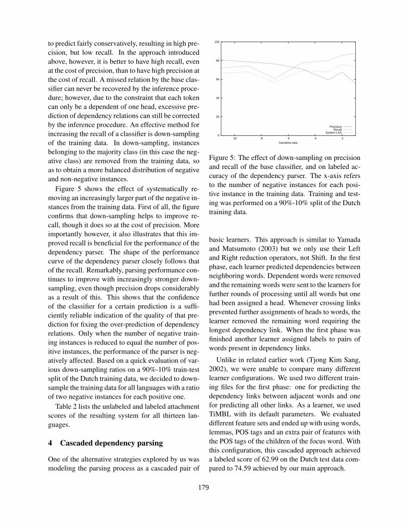
to predict fairly conservatively, resulting in high pre-cision, but low recall. In the approach introducedabove, however, it is better to have high recall, evenat the cost of precision, than to have high precision atthe cost of recall. A missed relation by the base clas-sifier can never be recovered by the inference proce-dure; however, due to the constraint that each tokencan only be a dependent of one head, excessive pre-diction of dependency relations can still be correctedby the inference procedure. An effective method forincreasing the recall of a classifier is down-samplingof the training data. In down-sampling, instancesbelonging to the majority class (in this case the neg-ative class) are removed from the training data, soas to obtain a more balanced distribution of negativeand non-negative instances.
Figure 5 shows the effect of systematically re-moving an increasingly larger part of the negative in-stances from the training data. First of all, the figureconfirms that down-sampling helps to improve re-call, though it does so at the cost of precision. Moreimportantly however, it also illustrates that this im-proved recall is beneficial for the performance of thedependency parser. The shape of the performancecurve of the dependency parser closely follows thatof the recall. Remarkably, parsing performance con-tinues to improve with increasingly stronger down-sampling, even though precision drops considerablyas a result of this. This shows that the confidenceof the classifier for a certain prediction is a suffi-ciently reliable indication of the quality of that pre-diction for fixing the over-prediction of dependencyrelations. Only when the number of negative train-ing instances is reduced to equal the number of pos-itive instances, the performance of the parser is neg-atively affected. Based on a quick evaluation of var-ious down-sampling ratios on a 90%-10% train-testsplit of the Dutch training data, we decided to down-sample the training data for all languages with a ratioof two negative instances for each positive one.
Table 2 lists the unlabeled and labeled attachmentscores of the resulting system for all thirteen lan-guages.
4 Cascaded dependency parsing
One of the alternative strategies explored by us wasmodeling the parsing process as a cascaded pair of
0
20
40
60
80
100
2 4 6 8 10
Sampling ratio
PrecisionRecall
System LAS
Figure 5: The effect of down-sampling on precisionand recall of the base classifier, and on labeled ac-curacy of the dependency parser. The x-axis refersto the number of negative instances for each posi-tive instance in the training data. Training and test-ing was performed on a 90%-10% split of the Dutchtraining data.
basic learners. This approach is similar to Yamadaand Matsumoto (2003) but we only use their Leftand Right reduction operators, not Shift. In the firstphase, each learner predicted dependencies betweenneighboring words. Dependent words were removedand the remaining words were sent to the learners forfurther rounds of processing until all words but onehad been assigned a head. Whenever crossing linksprevented further assignments of heads to words, thelearner removed the remaining word requiring thelongest dependency link. When the first phase wasfinished another learner assigned labels to pairs ofwords present in dependency links.
Unlike in related earlier work (Tjong Kim Sang,2002), we were unable to compare many differentlearner configurations. We used two different train-ing files for the first phase: one for predicting thedependency links between adjacent words and onefor predicting all other links. As a learner, we usedTiMBL with its default parameters. We evaluateddifferent feature sets and ended up with using words,lemmas, POS tags and an extra pair of features withthe POS tags of the children of the focus word. Withthis configuration, this cascaded approach achieveda labeled score of 62.99 on the Dutch test data com-pared to 74.59 achieved by our main approach.
179
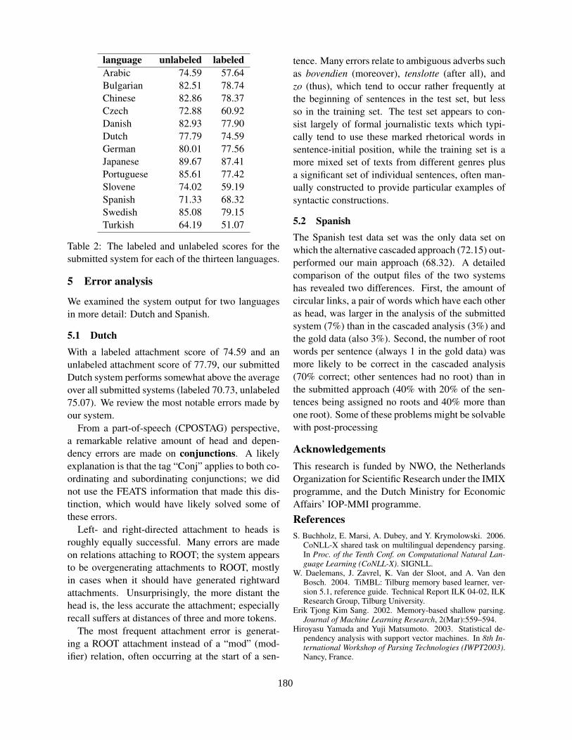
language unlabeled labeledArabic 74.59 57.64Bulgarian 82.51 78.74Chinese 82.86 78.37Czech 72.88 60.92Danish 82.93 77.90Dutch 77.79 74.59German 80.01 77.56Japanese 89.67 87.41Portuguese 85.61 77.42Slovene 74.02 59.19Spanish 71.33 68.32Swedish 85.08 79.15Turkish 64.19 51.07
Table 2: The labeled and unlabeled scores for thesubmitted system for each of the thirteen languages.
5 Error analysis
We examined the system output for two languagesin more detail: Dutch and Spanish.
5.1 DutchWith a labeled attachment score of 74.59 and anunlabeled attachment score of 77.79, our submittedDutch system performs somewhat above the averageover all submitted systems (labeled 70.73, unlabeled75.07). We review the most notable errors made byour system.
From a part-of-speech (CPOSTAG) perspective,a remarkable relative amount of head and depen-dency errors are made on conjunctions. A likelyexplanation is that the tag “Conj” applies to both co-ordinating and subordinating conjunctions; we didnot use the FEATS information that made this dis-tinction, which would have likely solved some ofthese errors.
Left- and right-directed attachment to heads isroughly equally successful. Many errors are madeon relations attaching to ROOT; the system appearsto be overgenerating attachments to ROOT, mostlyin cases when it should have generated rightwardattachments. Unsurprisingly, the more distant thehead is, the less accurate the attachment; especiallyrecall suffers at distances of three and more tokens.
The most frequent attachment error is generat-ing a ROOT attachment instead of a “mod” (mod-ifier) relation, often occurring at the start of a sen-
tence. Many errors relate to ambiguous adverbs suchas bovendien (moreover), tenslotte (after all), andzo (thus), which tend to occur rather frequently atthe beginning of sentences in the test set, but lessso in the training set. The test set appears to con-sist largely of formal journalistic texts which typi-cally tend to use these marked rhetorical words insentence-initial position, while the training set is amore mixed set of texts from different genres plusa significant set of individual sentences, often man-ually constructed to provide particular examples ofsyntactic constructions.
5.2 SpanishThe Spanish test data set was the only data set onwhich the alternative cascaded approach (72.15) out-performed our main approach (68.32). A detailedcomparison of the output files of the two systemshas revealed two differences. First, the amount ofcircular links, a pair of words which have each otheras head, was larger in the analysis of the submittedsystem (7%) than in the cascaded analysis (3%) andthe gold data (also 3%). Second, the number of rootwords per sentence (always 1 in the gold data) wasmore likely to be correct in the cascaded analysis(70% correct; other sentences had no root) than inthe submitted approach (40% with 20% of the sen-tences being assigned no roots and 40% more thanone root). Some of these problems might be solvablewith post-processing
AcknowledgementsThis research is funded by NWO, the NetherlandsOrganization for Scientific Research under the IMIXprogramme, and the Dutch Ministry for EconomicAffairs’ IOP-MMI programme.
ReferencesS. Buchholz, E. Marsi, A. Dubey, and Y. Krymolowski. 2006.
CoNLL-X shared task on multilingual dependency parsing.In Proc. of the Tenth Conf. on Computational Natural Lan-guage Learning (CoNLL-X). SIGNLL.
W. Daelemans, J. Zavrel, K. Van der Sloot, and A. Van denBosch. 2004. TiMBL: Tilburg memory based learner, ver-sion 5.1, reference guide. Technical Report ILK 04-02, ILKResearch Group, Tilburg University.
Erik Tjong Kim Sang. 2002. Memory-based shallow parsing.Journal of Machine Learning Research, 2(Mar):559–594.
Hiroyasu Yamada and Yuji Matsumoto. 2003. Statistical de-pendency analysis with support vector machines. In 8th In-ternational Workshop of Parsing Technologies (IWPT2003).Nancy, France.
180
Proceedings of the 10th Conference on Computational Natural Language Learning (CoNLL-X),pages 181–185, New York City, June 2006.c©2006 Association for Computational Linguistics
Projective Dependency Parsing with Perceptron
Xavier Carreras, Mihai Surdeanu and Llu ıs MarquezTALP Research Centre – Software Department (LSI)
Technical University of Catalonia (UPC)Campus Nord - Edifici Omega, Jordi Girona Salgado 1–3, E-08034 Barcelona
{carreras,surdeanu,lluism }@lsi.upc.edu
Abstract
We describe an online learning depen-dency parser for the CoNLL-X SharedTask, based on the bottom-up projectivealgorithm of Eisner (2000). We experi-ment with a large feature set that mod-els: the tokens involved in dependenciesand their immediate context, the surface-text distance between tokens, and the syn-tactic context dominated by each depen-dency. In experiments, the treatment ofmultilingual information was totally blind.
1 IntroductionWe describe a learning system for the CoNLL-XShared Task on multilingual dependency parsing(Buchholz et al., 2006), for 13 different languages.
Our system is a bottom-up projective dependencyparser, based on the cubic-time algorithm by Eisner(1996; 2000). The parser uses a learning functionthat scores all possible labeled dependencies. Thisfunction is trained globally with online Perceptron,by parsing training sentences and correcting its pa-rameters based on the parsing mistakes. The featuresused to score, while based on the previous work independency parsing (McDonald et al., 2005), intro-duce some novel concepts such as better codificationof context and surface distances, and runtime infor-mation from dependencies previously parsed.
Regarding experimentation, the treatment of mul-tilingual data has been totally blind, with no spe-cial processing or features that depend on the lan-guage. Considering its simplicity, our system
achieves moderate but encouraging results, with anoverall labeled attachment accuracy of 74.72% onthe CoNLL-X test set.
2 Parsing and Learning AlgorithmsThis section describes the three main components ofthe dependency parsing: the parsing model, the pars-ing algorithm, and the learning algorithm.
2.1 Model
Let 1, . . . , L be the dependency labels, defined be-forehand. Letx be a sentence ofn words,x1 . . . xn.Finally, letY(x) be the space of well-formed depen-dency trees forx. A dependency treey ∈ Y(x) is aset ofn dependencies of the form[h,m, l], whereh is the index of the head word (0 ≤ h ≤ n,where 0 means root),m is the index of the modi-fier word (1 ≤ m ≤ n), and l is the dependencylabel (1 ≤ l ≤ L). Each word ofx participates as amodifier in exactly one dependency ofy.
Our dependency parser,dp, returns the maximumscored dependency tree for a sentencex:
dp(x,w) = arg maxy∈Y(x)
∑
[h,m,l]∈ysco([h,m, l], x, y,w)
In the formula, w is the weight vector of theparser, that is, the set of parameters used to score de-pendencies during the parsing process. It is formedby a concatenation of L weight vectors, one for eachdependency label,w = (w1, . . . ,wl, . . . ,wL). Weassume a feature extraction function,φ, that repre-sents an unlabeled dependency[h,m] in a vector ofD features. Each of thewl hasD parameters ordimensions, one for each feature. Thus, the global
181
weight vectorw maintainsL × D parameters. Thescoring function is defined as follows:
sco([h,m, l], x, y,w) = φ(h,m, x, y) · wl
Note that the scoring of a dependency makes useof y, the tree that contains the dependency. As de-scribed next, at scoring timey just contains the de-pendencies found betweenh andm.
2.2 Parsing Algorithm
We use the cubic-time algorithm for dependencyparsing proposed by Eisner (1996; 2000). This pars-ing algorithm assumes that trees are projective, thatis, dependencies never cross in a tree. While this as-sumption clearly does not hold in the CoNLL-X data(only Chinese trees are actually 100% projective),we chose this algorithm for simplicity. As it will beshown, the percentage of non-projective dependen-cies is not very high, and clearly the error rates weobtain are caused by other major factors.
The parser is a bottom-up dynamic programmingalgorithm that visits sentence spans of increasinglength. In a given span, from words to word e, itcompletes two partial dependency trees that coverall words within the span: one rooted ats and theother rooted ate. This is done in two steps. First, theoptimal dependency structure internal to the span ischosen, by combining partial solutions from inter-nal spans. This structure is completed with a depen-dency covering the whole span, in two ways: froms to e, and frome to s. In each case, the scoringfunction is used to select the dependency label thatmaximizes the score.
We take advantage of this two-step processing tointroduce features for the scoring function that rep-resentsomeof the internal dependencies of the span(see Section 3 for details). It has to be noted thatthe parsing algorithm we use does not score depen-dencies on top of every possible internal structure.Thus, by conditioning on features extracted fromywe are making the search approximative.
2.3 Perceptron Learning
As learning algorithm, we use Perceptron tailoredfor structured scenarios, proposed by Collins (2002).In recent years, Perceptron has been used in a num-ber of Natural Language Learning works, such as in
w = 0for t = 1 to T
foreachtraining example(x, y) doy = dp(x,w)foreach [h,m, l] ∈ y\y do
wl = wl + φ(h,m, x, y)foreach [h,m, l] ∈ y\y do
wl = wl − φ(h,m, x, y)returnw
Figure 1: Pseudocode of the Perceptron Algorithm.T is aparameter that indicates the number of epochs that the algorithmcycles the training set.
partial parsing (Carreras et al., 2005) or even depen-dency parsing (McDonald et al., 2005).
Perceptron is an online learning algorithm thatlearns by correcting mistakes made by the parserwhen visiting training sentences. The algorithm isextremely simple, and its cost in time and memoryis independent from the size of the training corpora.In terms of efficiency, though, the parsing algorithmmust be run at every training sentence.
Our system uses the regular Perceptron workingin primal form. Figure 1 sketches the code. Giventhe number of languages and dependency types inthe CoNLL-X exercise, we found prohibitive towork with a dual version of Perceptron, that wouldallow the use of a kernel function to expand features.
3 Features
The feature extraction function,φ(h,m, x, y), rep-resents in a feature vector a dependency from wordpositionsm toh, in the context of a sentencex and adependency treey. As usual in discriminative learn-ing, we work with binary indicator features: if a cer-tain feature is observed in an instance, the value ofthat feature is 1; otherwise, the value is 0. For con-venience, we describeφ as a composition of severalbase feature extraction functions. Each extracts anumber of disjoint features. The feature extractionfunctionφ(h,m, x, y) is calculated as:
φtoken(x, h, “head”) + φtctx(x, h, “head”) +φtoken(x,m, “mod”) + φtctx(x,m, “mod”) +φdep(x,mmdh,m) + φdctx(x,mmdh,m) +φdist(x,mmdh,m) + φruntime(x, y, h,m, dh,m)
where φtoken extracts context-independent tokenfeatures,φtctx computes context-based token fea-tures, φdep computes context-independent depen-
182
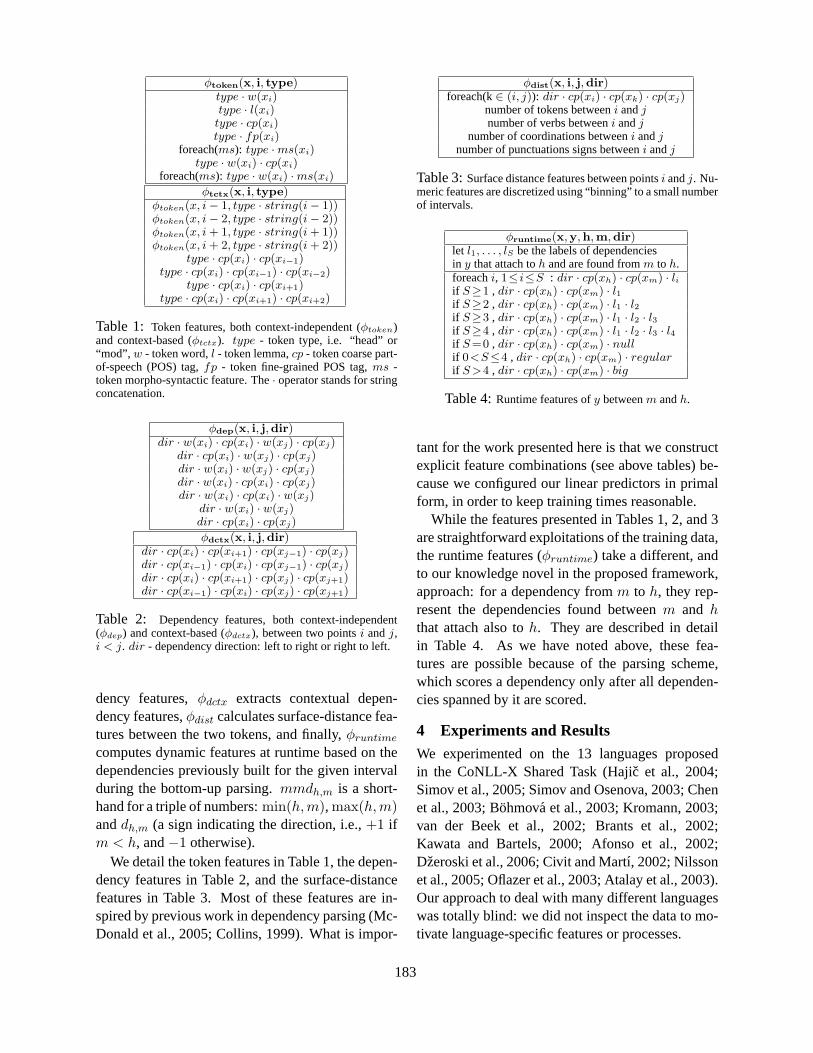
φtoken(x, i, type)type · w(xi)type · l(xi)type · cp(xi)type · fp(xi)
foreach(ms): type ·ms(xi)type · w(xi) · cp(xi)
foreach(ms): type · w(xi) ·ms(xi)φtctx(x, i, type)
φtoken(x, i− 1, type · string(i− 1))φtoken(x, i− 2, type · string(i− 2))φtoken(x, i+ 1, type · string(i+ 1))φtoken(x, i+ 2, type · string(i+ 2))
type · cp(xi) · cp(xi−1)type · cp(xi) · cp(xi−1) · cp(xi−2)
type · cp(xi) · cp(xi+1)type · cp(xi) · cp(xi+1) · cp(xi+2)
Table 1: Token features, both context-independent (φtoken)and context-based (φtctx). type - token type, i.e. “head” or“mod”, w - token word,l - token lemma,cp - token coarse part-of-speech (POS) tag,fp - token fine-grained POS tag,ms -token morpho-syntactic feature. The· operator stands for stringconcatenation.
φdep(x, i, j,dir)dir · w(xi) · cp(xi) · w(xj) · cp(xj)
dir · cp(xi) · w(xj) · cp(xj)dir · w(xi) · w(xj) · cp(xj)dir · w(xi) · cp(xi) · cp(xj)dir · w(xi) · cp(xi) · w(xj)
dir · w(xi) · w(xj)dir · cp(xi) · cp(xj)φdctx(x, i, j,dir)
dir · cp(xi) · cp(xi+1) · cp(xj−1) · cp(xj)dir · cp(xi−1) · cp(xi) · cp(xj−1) · cp(xj)dir · cp(xi) · cp(xi+1) · cp(xj) · cp(xj+1)dir · cp(xi−1) · cp(xi) · cp(xj) · cp(xj+1)
Table 2: Dependency features, both context-independent(φdep) and context-based (φdctx), between two pointsi andj,i < j. dir - dependency direction: left to right or right to left.
dency features,φdctx extracts contextual depen-dency features,φdist calculates surface-distance fea-tures between the two tokens, and finally,φruntimecomputes dynamic features at runtime based on thedependencies previously built for the given intervalduring the bottom-up parsing.mmdh,m is a short-hand for a triple of numbers:min(h,m), max(h,m)anddh,m (a sign indicating the direction, i.e.,+1 ifm < h, and−1 otherwise).
We detail the token features in Table 1, the depen-dency features in Table 2, and the surface-distancefeatures in Table 3. Most of these features are in-spired by previous work in dependency parsing (Mc-Donald et al., 2005; Collins, 1999). What is impor-
φdist(x, i, j,dir)foreach(k∈ (i, j)): dir · cp(xi) · cp(xk) · cp(xj)
number of tokens betweeni andjnumber of verbs betweeni andj
number of coordinations betweeni andjnumber of punctuations signs betweeni andj
Table 3:Surface distance features between pointsi andj. Nu-meric features are discretized using “binning” to a small numberof intervals.
φruntime(x,y,h,m,dir)let l1, . . . , lS be the labels of dependenciesin y that attach toh and are found fromm to h.foreachi, 1≤ i≤S : dir · cp(xh) · cp(xm) · liif S≥1 , dir · cp(xh) · cp(xm) · l1if S≥2 , dir · cp(xh) · cp(xm) · l1 · l2if S≥3 , dir · cp(xh) · cp(xm) · l1 · l2 · l3if S≥4 , dir · cp(xh) · cp(xm) · l1 · l2 · l3 · l4if S=0 , dir · cp(xh) · cp(xm) · nullif 0<S≤4 , dir · cp(xh) · cp(xm) · regularif S>4 , dir · cp(xh) · cp(xm) · big
Table 4:Runtime features ofy betweenm andh.
tant for the work presented here is that we constructexplicit feature combinations (see above tables) be-cause we configured our linear predictors in primalform, in order to keep training times reasonable.
While the features presented in Tables 1, 2, and 3are straightforward exploitations of the training data,the runtime features (φruntime) take a different, andto our knowledge novel in the proposed framework,approach: for a dependency fromm to h, they rep-resent the dependencies found betweenm and hthat attach also toh. They are described in detailin Table 4. As we have noted above, these fea-tures are possible because of the parsing scheme,which scores a dependency only after all dependen-cies spanned by it are scored.
4 Experiments and ResultsWe experimented on the 13 languages proposedin the CoNLL-X Shared Task (Hajic et al., 2004;Simov et al., 2005; Simov and Osenova, 2003; Chenet al., 2003; Bohmova et al., 2003; Kromann, 2003;van der Beek et al., 2002; Brants et al., 2002;Kawata and Bartels, 2000; Afonso et al., 2002;Dzeroski et al., 2006; Civit and Martı, 2002; Nilssonet al., 2005; Oflazer et al., 2003; Atalay et al., 2003).Our approach to deal with many different languageswas totally blind: we did not inspect the data to mo-tivate language-specific features or processes.
183
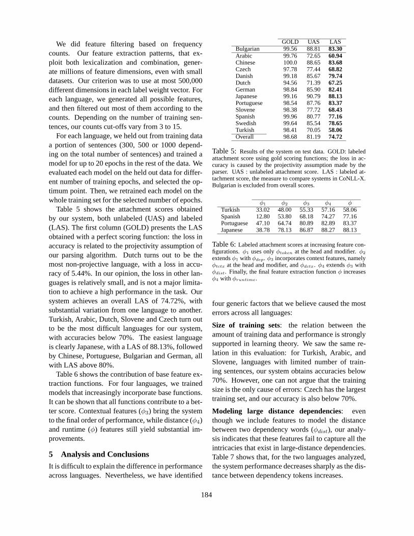
We did feature filtering based on frequencycounts. Our feature extraction patterns, that ex-ploit both lexicalization and combination, gener-ate millions of feature dimensions, even with smalldatasets. Our criterion was to use at most 500,000different dimensions in each label weight vector. Foreach language, we generated all possible features,and then filtered out most of them according to thecounts. Depending on the number of training sen-tences, our counts cut-offs vary from 3 to 15.
For each language, we held out from training dataa portion of sentences (300, 500 or 1000 depend-ing on the total number of sentences) and trained amodel for up to 20 epochs in the rest of the data. Weevaluated each model on the held out data for differ-ent number of training epochs, and selected the op-timum point. Then, we retrained each model on thewhole training set for the selected number of epochs.
Table 5 shows the attachment scores obtainedby our system, both unlabeled (UAS) and labeled(LAS). The first column (GOLD) presents the LASobtained with a perfect scoring function: the loss inaccuracy is related to the projectivity assumption ofour parsing algorithm. Dutch turns out to be themost non-projective language, with a loss in accu-racy of 5.44%. In our opinion, the loss in other lan-guages is relatively small, and is not a major limita-tion to achieve a high performance in the task. Oursystem achieves an overall LAS of 74.72%, withsubstantial variation from one language to another.Turkish, Arabic, Dutch, Slovene and Czech turn outto be the most difficult languages for our system,with accuracies below 70%. The easiest languageis clearly Japanese, with a LAS of 88.13%, followedby Chinese, Portuguese, Bulgarian and German, allwith LAS above 80%.
Table 6 shows the contribution of base feature ex-traction functions. For four languages, we trainedmodels that increasingly incorporate base functions.It can be shown that all functions contribute to a bet-ter score. Contextual features (φ3) bring the systemto the final order of performance, while distance (φ4)and runtime (φ) features still yield substantial im-provements.
5 Analysis and ConclusionsIt is difficult to explain the difference in performanceacross languages. Nevertheless, we have identified
GOLD UAS LASBulgarian 99.56 88.81 83.30Arabic 99.76 72.65 60.94Chinese 100.0 88.65 83.68Czech 97.78 77.44 68.82Danish 99.18 85.67 79.74Dutch 94.56 71.39 67.25German 98.84 85.90 82.41Japanese 99.16 90.7988.13Portuguese 98.54 87.76 83.37Slovene 98.38 77.72 68.43Spanish 99.96 80.77 77.16Swedish 99.64 85.54 78.65Turkish 98.41 70.05 58.06Overall 98.68 81.19 74.72
Table 5: Results of the system on test data. GOLD: labeledattachment score using gold scoring functions; the loss in ac-curacy is caused by the projectivity assumption made by theparser. UAS : unlabeled attachment score. LAS : labeled at-tachment score, the measure to compare systems in CoNLL-X.Bulgarian is excluded from overall scores.
φ1 φ2 φ3 φ4 φTurkish 33.02 48.00 55.33 57.16 58.06Spanish 12.80 53.80 68.18 74.27 77.16Portuguese 47.10 64.74 80.89 82.89 83.37Japanese 38.78 78.13 86.87 88.27 88.13
Table 6:Labeled attachment scores at increasing feature con-figurations.φ1 uses onlyφtoken at the head and modifier.φ2
extendsφ1 with φdep. φ3 incorporates context features, namelyφtctx at the head and modifier, andφdctx. φ4 extendsφ3 withφdist. Finally, the final feature extraction functionφ increasesφ4 with φruntime.
four generic factors that we believe caused the mosterrors across all languages:
Size of training sets: the relation between theamount of training data and performance is stronglysupported in learning theory. We saw the same re-lation in this evaluation: for Turkish, Arabic, andSlovene, languages with limited number of train-ing sentences, our system obtains accuracies below70%. However, one can not argue that the trainingsize is the only cause of errors: Czech has the largesttraining set, and our accuracy is also below 70%.
Modeling large distance dependencies: eventhough we include features to model the distancebetween two dependency words (φdist), our analy-sis indicates that these features fail to capture all theintricacies that exist in large-distance dependencies.Table 7 shows that, for the two languages analyzed,the system performance decreases sharply as the dis-tance between dependency tokens increases.
184
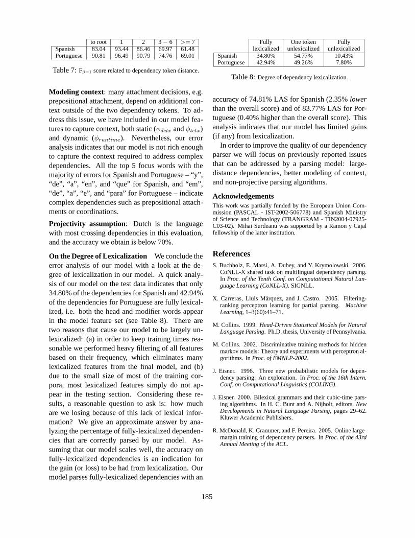
to root 1 2 3− 6 >= 7Spanish 83.04 93.44 86.46 69.97 61.48Portuguese 90.81 96.49 90.79 74.76 69.01
Table 7:Fβ=1 score related to dependency token distance.
Modeling context: many attachment decisions, e.g.prepositional attachment, depend on additional con-text outside of the two dependency tokens. To ad-dress this issue, we have included in our model fea-tures to capture context, both static (φdctx andφtctx)and dynamic (φruntime). Nevertheless, our erroranalysis indicates that our model is not rich enoughto capture the context required to address complexdependencies. All the top 5 focus words with themajority of errors for Spanish and Portuguese – “y”,“de”, “a”, “en”, and “que” for Spanish, and “em”,“de”, “a”, “e”, and “para” for Portuguese – indicatecomplex dependencies such as prepositional attach-ments or coordinations.
Projectivity assumption: Dutch is the languagewith most crossing dependencies in this evaluation,and the accuracy we obtain is below 70%.
On the Degree of Lexicalization We conclude theerror analysis of our model with a look at the de-gree of lexicalization in our model. A quick analy-sis of our model on the test data indicates that only34.80% of the dependencies for Spanish and 42.94%of the dependencies for Portuguese are fully lexical-ized, i.e. both the head and modifier words appearin the model feature set (see Table 8). There aretwo reasons that cause our model to be largely un-lexicalized: (a) in order to keep training times rea-sonable we performed heavy filtering of all featuresbased on their frequency, which eliminates manylexicalized features from the final model, and (b)due to the small size of most of the training cor-pora, most lexicalized features simply do not ap-pear in the testing section. Considering these re-sults, a reasonable question to ask is: how muchare we losing because of this lack of lexical infor-mation? We give an approximate answer by ana-lyzing the percentage of fully-lexicalized dependen-cies that are correctly parsed by our model. As-suming that our model scales well, the accuracy onfully-lexicalized dependencies is an indication forthe gain (or loss) to be had from lexicalization. Ourmodel parses fully-lexicalized dependencies with an
Fully One token Fullylexicalized unlexicalized unlexicalized
Spanish 34.80% 54.77% 10.43%Portuguese 42.94% 49.26% 7.80%
Table 8:Degree of dependency lexicalization.
accuracy of 74.81% LAS for Spanish (2.35%lowerthan the overall score) and of 83.77% LAS for Por-tuguese (0.40% higher than the overall score). Thisanalysis indicates that our model has limited gains(if any) from lexicalization.
In order to improve the quality of our dependencyparser we will focus on previously reported issuesthat can be addressed by a parsing model: large-distance dependencies, better modeling of context,and non-projective parsing algorithms.
AcknowledgementsThis work was partially funded by the European Union Com-mission (PASCAL - IST-2002-506778) and Spanish Ministryof Science and Technology (TRANGRAM - TIN2004-07925-C03-02). Mihai Surdeanu was supported by a Ramon y Cajalfellowship of the latter institution.
ReferencesS. Buchholz, E. Marsi, A. Dubey, and Y. Krymolowski. 2006.
CoNLL-X shared task on multilingual dependency parsing.In Proc. of the Tenth Conf. on Computational Natural Lan-guage Learning (CoNLL-X). SIGNLL.
X. Carreras, Lluıs Marquez, and J. Castro. 2005. Filtering-ranking perceptron learning for partial parsing.MachineLearning, 1–3(60):41–71.
M. Collins. 1999.Head-Driven Statistical Models for NaturalLanguage Parsing. Ph.D. thesis, University of Pennsylvania.
M. Collins. 2002. Discriminative training methods for hiddenmarkov models: Theory and experiments with perceptron al-gorithms. InProc. of EMNLP-2002.
J. Eisner. 1996. Three new probabilistic models for depen-dency parsing: An exploration. InProc. of the 16th Intern.Conf. on Computational Linguistics (COLING).
J. Eisner. 2000. Bilexical grammars and their cubic-time pars-ing algorithms. In H. C. Bunt and A. Nijholt, editors,NewDevelopments in Natural Language Parsing, pages 29–62.Kluwer Academic Publishers.
R. McDonald, K. Crammer, and F. Pereira. 2005. Online large-margin training of dependency parsers. InProc. of the 43rdAnnual Meeting of the ACL.
185
Proceedings of the 10th Conference on Computational Natural Language Learning (CoNLL-X),pages 186–190, New York City, June 2006.c©2006 Association for Computational Linguistics
A Pipeline Model for Bottom-Up Dependency Parsing
Ming-Wei Chang Quang Do Dan RothDepartment of Computer Science
University of Illinois at Urbana-ChampaignUrbana, IL 61801
{mchang21, quangdo2, danr}@uiuc.edu
Abstract
We present a new machine learning frame-work for multi-lingual dependency pars-ing. The framework uses a linear, pipelinebased, bottom-up parsing algorithm, witha look ahead local search that serves tomake the local predictions more robust.As shown, the performance of the firstgeneration of this algorithm is promising.
1 System Description
1.1 Parsing as a PipelinePipeline computation is a common computationalstrategy in natural language processing, where a taskis decomposed into several stages that are solved se-quentially. For example, a semantic role labelingprogram may start by using a part-of-speech tagger,than apply a shallow parser to chunk the sentenceinto phrases, and continue by identifying predicatesand arguments and then classifying them.
(Yamada and Matsumoto, 2003) proposed abottom-up dependency parsing algorithm, where thelocal actions, chosen from among Shift, Left, Right,are used to generate a dependency tree using ashift-reduce parsing approach. Moreover, they usedSVMs to learn the parsing decisions between pairsof consecutive words in the sentences 1. This isa true pipeline approach in that the classifiers aretrained on individual decisions rather than on theoverall quality of the parser, and chained to yield the
1A pair of words may become consecutive after the wordsbetween them become the children of these two words
global structure. It suffers from the limitations ofpipeline processing, such as accumulation of errors,but nevertheless, yields very competitive parsing re-sults.
We devise two natural principles for enhancingpipeline models. First, inference procedures shouldbe incorporated to make robust prediction for eachstage. Second, the number of predictions shouldbe minimized to prevent error accumulation. Ac-cording to these two principles, we propose an im-proved pipeline framework for multi-lingual depen-dency parsing that aims at addressing the limitationsof the pipeline processing. Specifically, (1) we uselocal search, a look ahead policy, to improve the ac-curacy of the predicted actions, and (2) we argue thatthe parsing algorithm we used minimizes the num-ber of actions (Chang et al., 2006).
We use the set of actions: Shift, Left, Right, Wait-Left, WaitRight for the parsing algorithm. The pureWait action was suggested in (Yamada and Mat-sumoto, 2003). However, here we come up withthese five actions by separating actions Left into(real) Left and WaitLeft, and Right into (real) Rightand WaitRight. Predicting these turns out to be eas-ier due to finer granularity. We then use local searchover consecutive actions and better exploit the de-pendencies among them.
The parsing algorithm is a modified shift-reduceparser (Aho et al., 1986) that makes use of the ac-tions described above and applies them in a leftto right manner on consecutive word pairs (a, b)(a < b) in the word list T . T is initialized as the fullsentence. Latter, the actions will change the contentsof T . The actions are used as follows:
186
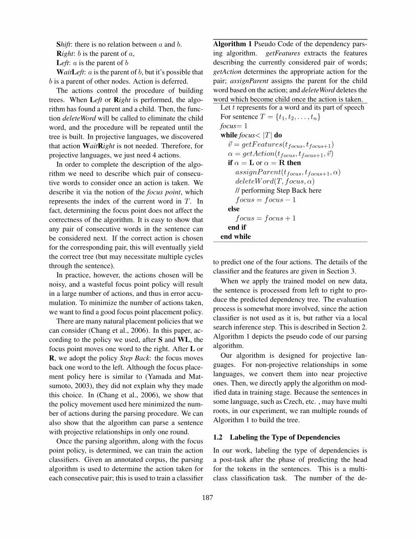
Shift: there is no relation between a and b.Right: b is the parent of a,Left: a is the parent of b
WaitLeft: a is the parent of b, but it’s possible thatb is a parent of other nodes. Action is deferred.
The actions control the procedure of buildingtrees. When Left or Right is performed, the algo-rithm has found a parent and a child. Then, the func-tion deleteWord will be called to eliminate the childword, and the procedure will be repeated until thetree is built. In projective languages, we discoveredthat action WaitRight is not needed. Therefore, forprojective languages, we just need 4 actions.
In order to complete the description of the algo-rithm we need to describe which pair of consecu-tive words to consider once an action is taken. Wedescribe it via the notion of the focus point, whichrepresents the index of the current word in T . Infact, determining the focus point does not affect thecorrectness of the algorithm. It is easy to show thatany pair of consecutive words in the sentence canbe considered next. If the correct action is chosenfor the corresponding pair, this will eventually yieldthe correct tree (but may necessitate multiple cyclesthrough the sentence).
In practice, however, the actions chosen will benoisy, and a wasteful focus point policy will resultin a large number of actions, and thus in error accu-mulation. To minimize the number of actions taken,we want to find a good focus point placement policy.
There are many natural placement policies that wecan consider (Chang et al., 2006). In this paper, ac-cording to the policy we used, after S and WL, thefocus point moves one word to the right. After L orR, we adopt the policy Step Back: the focus movesback one word to the left. Although the focus place-ment policy here is similar to (Yamada and Mat-sumoto, 2003), they did not explain why they madethis choice. In (Chang et al., 2006), we show thatthe policy movement used here minimized the num-ber of actions during the parsing procedure. We canalso show that the algorithm can parse a sentencewith projective relationships in only one round.
Once the parsing algorithm, along with the focuspoint policy, is determined, we can train the actionclassifiers. Given an annotated corpus, the parsingalgorithm is used to determine the action taken foreach consecutive pair; this is used to train a classifier
Algorithm 1 Pseudo Code of the dependency pars-ing algorithm. getFeatures extracts the featuresdescribing the currently considered pair of words;getAction determines the appropriate action for thepair; assignParent assigns the parent for the childword based on the action; and deleteWord deletes theword which become child once the action is taken.
Let t represents for a word and its part of speechFor sentence T = {t1, t2, . . . , tn}focus= 1while focus< |T | do
~v = getFeatures(tfocus, tfocus+1)α = getAction(tfocus, tfocus+1, ~v)if α = L or α = R then
assignParent(tfocus, tfocus+1, α)deleteWord(T, focus, α)// performing Step Back herefocus = focus− 1
elsefocus = focus + 1
end ifend while
to predict one of the four actions. The details of theclassifier and the features are given in Section 3.
When we apply the trained model on new data,the sentence is processed from left to right to pro-duce the predicted dependency tree. The evaluationprocess is somewhat more involved, since the actionclassifier is not used as it is, but rather via a localsearch inference step. This is described in Section 2.Algorithm 1 depicts the pseudo code of our parsingalgorithm.
Our algorithm is designed for projective lan-guages. For non-projective relationships in somelanguages, we convert them into near projectiveones. Then, we directly apply the algorithm on mod-ified data in training stage. Because the sentences insome language, such as Czech, etc. , may have multiroots, in our experiment, we ran multiple rounds ofAlgorithm 1 to build the tree.
1.2 Labeling the Type of Dependencies
In our work, labeling the type of dependencies isa post-task after the phase of predicting the headfor the tokens in the sentences. This is a multi-class classification task. The number of the de-
187
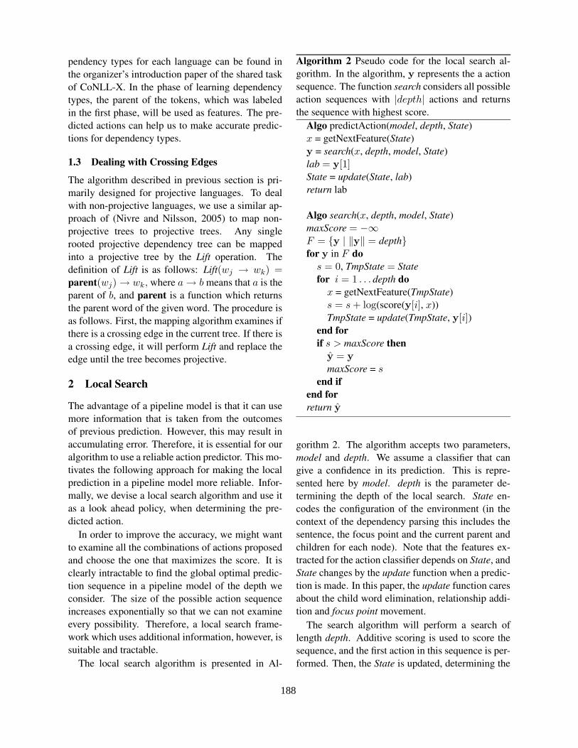
pendency types for each language can be found inthe organizer’s introduction paper of the shared taskof CoNLL-X. In the phase of learning dependencytypes, the parent of the tokens, which was labeledin the first phase, will be used as features. The pre-dicted actions can help us to make accurate predic-tions for dependency types.
1.3 Dealing with Crossing Edges
The algorithm described in previous section is pri-marily designed for projective languages. To dealwith non-projective languages, we use a similar ap-proach of (Nivre and Nilsson, 2005) to map non-projective trees to projective trees. Any singlerooted projective dependency tree can be mappedinto a projective tree by the Lift operation. Thedefinition of Lift is as follows: Lift(wj → wk) =parent(wj) → wk, where a → b means that a is theparent of b, and parent is a function which returnsthe parent word of the given word. The procedure isas follows. First, the mapping algorithm examines ifthere is a crossing edge in the current tree. If there isa crossing edge, it will perform Lift and replace theedge until the tree becomes projective.
2 Local Search
The advantage of a pipeline model is that it can usemore information that is taken from the outcomesof previous prediction. However, this may result inaccumulating error. Therefore, it is essential for ouralgorithm to use a reliable action predictor. This mo-tivates the following approach for making the localprediction in a pipeline model more reliable. Infor-mally, we devise a local search algorithm and use itas a look ahead policy, when determining the pre-dicted action.
In order to improve the accuracy, we might wantto examine all the combinations of actions proposedand choose the one that maximizes the score. It isclearly intractable to find the global optimal predic-tion sequence in a pipeline model of the depth weconsider. The size of the possible action sequenceincreases exponentially so that we can not examineevery possibility. Therefore, a local search frame-work which uses additional information, however, issuitable and tractable.
The local search algorithm is presented in Al-
Algorithm 2 Pseudo code for the local search al-gorithm. In the algorithm, y represents the a actionsequence. The function search considers all possibleaction sequences with |depth| actions and returnsthe sequence with highest score.
Algo predictAction(model, depth, State)x = getNextFeature(State)y = search(x, depth, model, State)lab = y[1]State = update(State, lab)return lab
Algo search(x, depth, model, State)maxScore = −∞F = {y | ‖y‖ = depth}for y in F do
s = 0, TmpState = Statefor i = 1 . . . depth do
x = getNextFeature(TmpState)s = s + log(score(y[i], x))TmpState = update(TmpState, y[i])
end forif s > maxScore then
y = y
maxScore = s
end ifend forreturn y
gorithm 2. The algorithm accepts two parameters,model and depth. We assume a classifier that cangive a confidence in its prediction. This is repre-sented here by model. depth is the parameter de-termining the depth of the local search. State en-codes the configuration of the environment (in thecontext of the dependency parsing this includes thesentence, the focus point and the current parent andchildren for each node). Note that the features ex-tracted for the action classifier depends on State, andState changes by the update function when a predic-tion is made. In this paper, the update function caresabout the child word elimination, relationship addi-tion and focus point movement.
The search algorithm will perform a search oflength depth. Additive scoring is used to score thesequence, and the first action in this sequence is per-formed. Then, the State is updated, determining the
188
next features for the action classifiers and search iscalled again.
One interesting property of this framework is thatwe use future information in addition to past infor-mation. The pipeline model naturally allows accessto all the past information. But, since our algorithmuses the search as a look ahead policy, it can producemore robust results.
3 Experiments and Results
In this work we used as our learning algorithm aregularized variation of the perceptron update ruleas incorporated in SNoW (Roth, 1998; Carlson etal., 1999), a multi-class classifier that is specificallytailored for large scale learning tasks. SNoW usessoftmax over the raw activation values as its confi-dence measure, which can be shown to be a reliableapproximation of the labels’ probabilities. This isused both for labeling the actions and types of de-pendencies. There is no special language enhance-ment required for each language. The resources pro-vided for 12 languages are described in: (Hajic etal., 2004; Chen et al., 2003; Bohmova et al., 2003;Kromann, 2003; van der Beek et al., 2002; Brantset al., 2002; Kawata and Bartels, 2000; Afonso etal., 2002; Dzeroski et al., 2006; Civit Torruella andMartı Antonın, 2002; Nilsson et al., 2005; Oflazer etal., 2003; Atalay et al., 2003).
3.1 Experimental Setting
The feature set plays an important role in the qual-ity of the classifier. Basically, we used the samefeature set for the action selection classifiers andfor the label classifiers. In our work, each exam-ple has average fifty active features. For each wordpair (w1, w2), we used their LEMMA, the POSTAGand also the POSTAG of the children of w1 andw2. We also included the LEMMA and POSTAGof surrounding words in a window of size (2, 4).We considered 2 words before w1 and 4 words af-ter w2 (we agree with the window size in (Yamadaand Matsumoto, 2003)). The major difference ofour feature set compared with the one in (Yamadaand Matsumoto, 2003) is that we included the pre-vious predicted action. We also added some con-junctions of the above features to ensure expressive-ness of the model. (Yamada and Matsumoto, 2003)
made use of the polynomial kernel of degree 2 sothey in fact use more conjunctive features. Besidethese features, we incorporated the information ofFEATS for the languages when it is available. Thecolumns in the data files we used for our work arethe LEMMA, POSTAG, and the FEATS, which istreated as atomic. Due to time limitation, we did notapply the local search algorithm for the languageshaving the FEATS features.
3.2 ResultsTable 1 shows our results on Unlabeled AttachmentScores (UAS), Labeled Attachment Scores (LAS),and Label Accuracy score (LAC) for 12 languages.Our results are compared with the average scores(AV) and the standard deviations (SD), of all the sys-tems participating in the shared task of CoNLL-X.
Our average UAS for 12 languages is 83.54%with the standard deviation 6.01; and 76.80% withthe standard deviation 9.43 for average LAS.
4 Analysis and Discussion
We observed that our UAS for Arabic is generallylower than for other languages. The reason for thelow accuracy of Arabic is that the sentence is verylong. In the training data for Arabic, there are 25%sentences which have more than 50 words. Sincewe use a pipeline model in our algorithm, it requiredmore predictions to complete a long sentence. Morepredictions in pipeline models may result in moremistakes. We think that this explains our relativelylow Arabic result. Moreover, in our current system,we use the same window size (2,4) for feature ex-traction in all languages. Changing the windows sizeseems to be a reasonable step when the sentences arelonger.
For Czech, one reason for our relatively low resultis that we did not use the whole training corpus dueto time limitation 2 . Actually, in our experimenton the development set, when we increase the sizeof training data in the training phase we got signif-icantly higher result than the system trained on thesmaller data. The other problem for Czech is thatCzech is one of the languages with many types ofpart of speech and dependency types, and also the
2Training our system for most languages takes 30 minutesor 1 hour for both phases of labeling HEAD and DEPREL. Ittakes 6-7 hours for Czech with 50% training data.
189
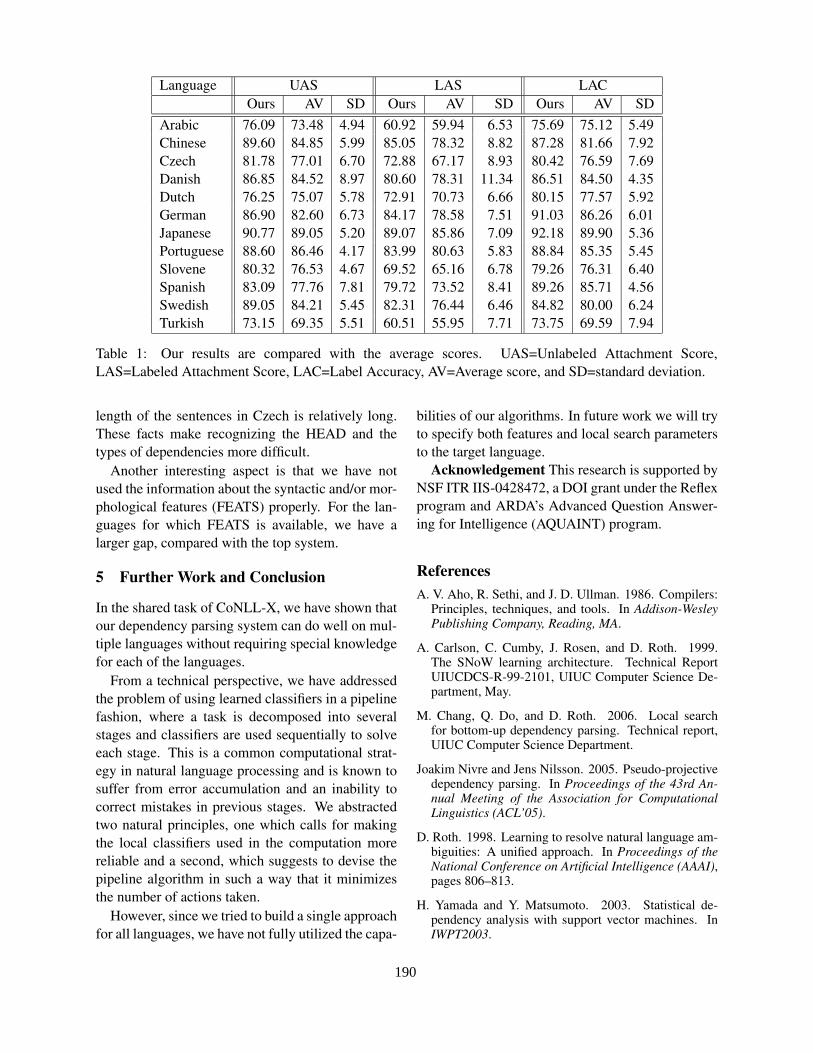
Language UAS LAS LACOurs AV SD Ours AV SD Ours AV SD
Arabic 76.09 73.48 4.94 60.92 59.94 6.53 75.69 75.12 5.49Chinese 89.60 84.85 5.99 85.05 78.32 8.82 87.28 81.66 7.92Czech 81.78 77.01 6.70 72.88 67.17 8.93 80.42 76.59 7.69Danish 86.85 84.52 8.97 80.60 78.31 11.34 86.51 84.50 4.35Dutch 76.25 75.07 5.78 72.91 70.73 6.66 80.15 77.57 5.92German 86.90 82.60 6.73 84.17 78.58 7.51 91.03 86.26 6.01Japanese 90.77 89.05 5.20 89.07 85.86 7.09 92.18 89.90 5.36Portuguese 88.60 86.46 4.17 83.99 80.63 5.83 88.84 85.35 5.45Slovene 80.32 76.53 4.67 69.52 65.16 6.78 79.26 76.31 6.40Spanish 83.09 77.76 7.81 79.72 73.52 8.41 89.26 85.71 4.56Swedish 89.05 84.21 5.45 82.31 76.44 6.46 84.82 80.00 6.24Turkish 73.15 69.35 5.51 60.51 55.95 7.71 73.75 69.59 7.94
Table 1: Our results are compared with the average scores. UAS=Unlabeled Attachment Score,LAS=Labeled Attachment Score, LAC=Label Accuracy, AV=Average score, and SD=standard deviation.
length of the sentences in Czech is relatively long.These facts make recognizing the HEAD and thetypes of dependencies more difficult.
Another interesting aspect is that we have notused the information about the syntactic and/or mor-phological features (FEATS) properly. For the lan-guages for which FEATS is available, we have alarger gap, compared with the top system.
5 Further Work and Conclusion
In the shared task of CoNLL-X, we have shown thatour dependency parsing system can do well on mul-tiple languages without requiring special knowledgefor each of the languages.
From a technical perspective, we have addressedthe problem of using learned classifiers in a pipelinefashion, where a task is decomposed into severalstages and classifiers are used sequentially to solveeach stage. This is a common computational strat-egy in natural language processing and is known tosuffer from error accumulation and an inability tocorrect mistakes in previous stages. We abstractedtwo natural principles, one which calls for makingthe local classifiers used in the computation morereliable and a second, which suggests to devise thepipeline algorithm in such a way that it minimizesthe number of actions taken.
However, since we tried to build a single approachfor all languages, we have not fully utilized the capa-
bilities of our algorithms. In future work we will tryto specify both features and local search parametersto the target language.
Acknowledgement This research is supported byNSF ITR IIS-0428472, a DOI grant under the Reflexprogram and ARDA’s Advanced Question Answer-ing for Intelligence (AQUAINT) program.
ReferencesA. V. Aho, R. Sethi, and J. D. Ullman. 1986. Compilers:
Principles, techniques, and tools. In Addison-WesleyPublishing Company, Reading, MA.
A. Carlson, C. Cumby, J. Rosen, and D. Roth. 1999.The SNoW learning architecture. Technical ReportUIUCDCS-R-99-2101, UIUC Computer Science De-partment, May.
M. Chang, Q. Do, and D. Roth. 2006. Local searchfor bottom-up dependency parsing. Technical report,UIUC Computer Science Department.
Joakim Nivre and Jens Nilsson. 2005. Pseudo-projectivedependency parsing. In Proceedings of the 43rd An-nual Meeting of the Association for ComputationalLinguistics (ACL’05).
D. Roth. 1998. Learning to resolve natural language am-biguities: A unified approach. In Proceedings of theNational Conference on Artificial Intelligence (AAAI),pages 806–813.
H. Yamada and Y. Matsumoto. 2003. Statistical de-pendency analysis with support vector machines. InIWPT2003.
190
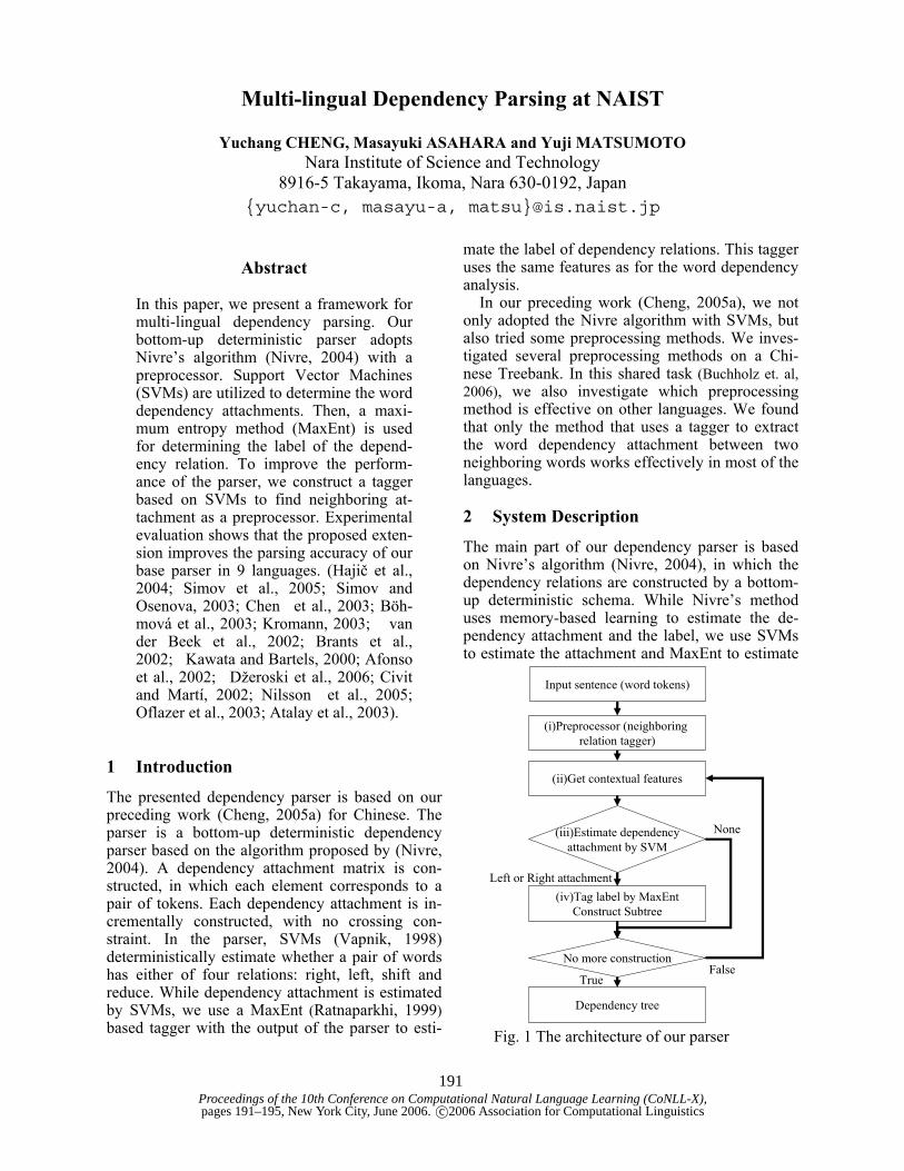
Proceedings of the 10th Conference on Computational Natural Language Learning (CoNLL-X),pages 191–195, New York City, June 2006.c©2006 Association for Computational Linguistics
Multi-lingual Dependency Parsing at NAIST
Yuchang CHENG, Masayuki ASAHARA and Yuji MATSUMOTO Nara Institute of Science and Technology
8916-5 Takayama, Ikoma, Nara 630-0192, Japan {yuchan-c, masayu-a, matsu}@is.naist.jp
Abstract
In this paper, we present a framework for multi-lingual dependency parsing. Our bottom-up deterministic parser adopts Nivre’s algorithm (Nivre, 2004) with a preprocessor. Support Vector Machines (SVMs) are utilized to determine the word dependency attachments. Then, a maxi-mum entropy method (MaxEnt) is used for determining the label of the depend-ency relation. To improve the perform-ance of the parser, we construct a tagger based on SVMs to find neighboring at-tachment as a preprocessor. Experimental evaluation shows that the proposed exten-sion improves the parsing accuracy of our base parser in 9 languages. (Hajič et al., 2004; Simov et al., 2005; Simov and Osenova, 2003; Chen et al., 2003; Böh-mová et al., 2003; Kromann, 2003; van der Beek et al., 2002; Brants et al., 2002; Kawata and Bartels, 2000; Afonso et al., 2002; Džeroski et al., 2006; Civit and Martí, 2002; Nilsson et al., 2005; Oflazer et al., 2003; Atalay et al., 2003).
1 Introduction
The presented dependency parser is based on our preceding work (Cheng, 2005a) for Chinese. The parser is a bottom-up deterministic dependency parser based on the algorithm proposed by (Nivre, 2004). A dependency attachment matrix is con-structed, in which each element corresponds to a pair of tokens. Each dependency attachment is in-crementally constructed, with no crossing con-straint. In the parser, SVMs (Vapnik, 1998) deterministically estimate whether a pair of words has either of four relations: right, left, shift and reduce. While dependency attachment is estimated by SVMs, we use a MaxEnt (Ratnaparkhi, 1999) based tagger with the output of the parser to esti-
mate the label of dependency relations. This tagger uses the same features as for the word dependency analysis.
In our preceding work (Cheng, 2005a), we not only adopted the Nivre algorithm with SVMs, but also tried some preprocessing methods. We inves-tigated several preprocessing methods on a Chi-nese Treebank. In this shared task (Buchholz et. al, 2006), we also investigate which preprocessing method is effective on other languages. We found that only the method that uses a tagger to extract the word dependency attachment between two neighboring words works effectively in most of the languages.
2 System Description
The main part of our dependency parser is based on Nivre’s algorithm (Nivre, 2004), in which the dependency relations are constructed by a bottom-up deterministic schema. While Nivre’s method uses memory-based learning to estimate the de-pendency attachment and the label, we use SVMs to estimate the attachment and MaxEnt to estimate
Fig. 1 The architecture of our parser
(i)Preprocessor (neighboring relation tagger)
(ii)Get contextual features
(iii)Estimate dependencyattachment by SVM
(iv)Tag label by MaxEntConstruct Subtree
No more construction
Dependency tree
FalseTrue
Left or Right attachment
None
Input sentence (word tokens)
191
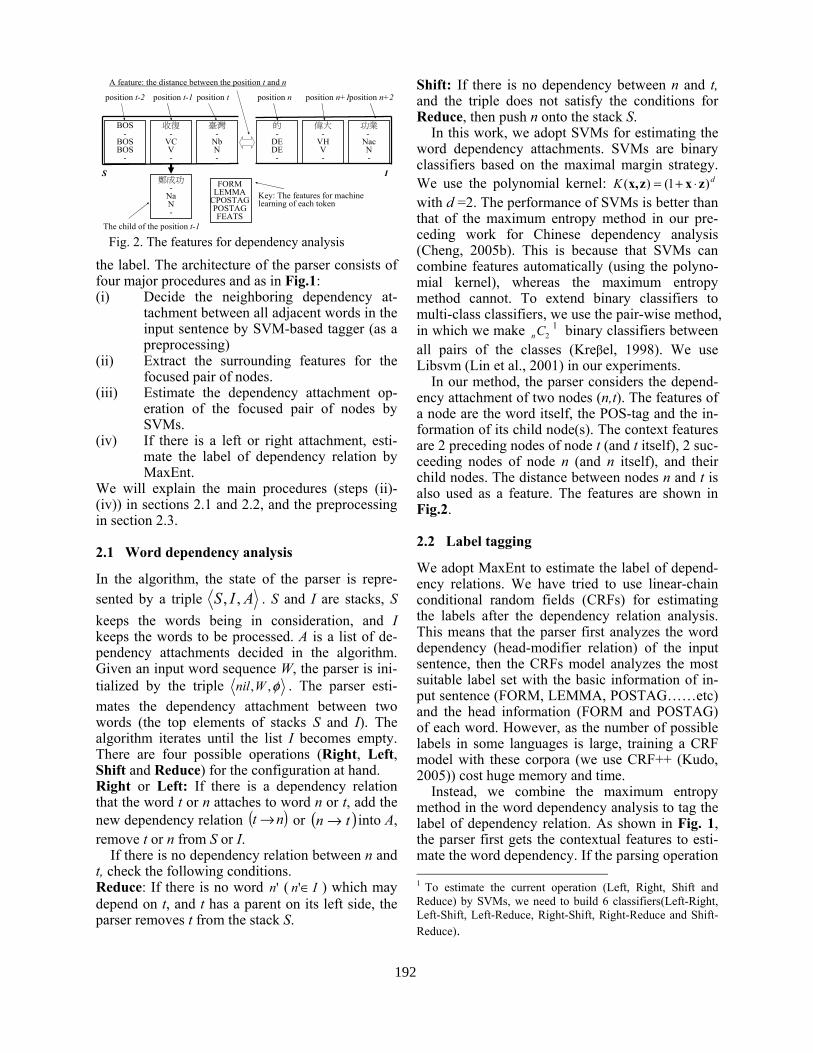
Fig. 2. The features for dependency analysis
BOS-
BOSBOS
-
收復-
VCV-
臺灣-
NbN-
的-
DEDE-
偉大-
VHV-
功業-
NacN-
鄭成功-
NaN-
S I
position t-1position t-2
The child of the position t-1
position n position n+1position n+2position t
A feature: the distance between the position t and n
FORM LEMMA
CPOSTAG POSTAG FEATS
Key: The features for machine learning of each token
the label. The architecture of the parser consists of four major procedures and as in Fig.1: (i) Decide the neighboring dependency at-
tachment between all adjacent words in the input sentence by SVM-based tagger (as a preprocessing)
(ii) Extract the surrounding features for the focused pair of nodes.
(iii) Estimate the dependency attachment op-eration of the focused pair of nodes by SVMs.
(iv) If there is a left or right attachment, esti-mate the label of dependency relation by MaxEnt.
We will explain the main procedures (steps (ii)-(iv)) in sections 2.1 and 2.2, and the preprocessing in section 2.3.
2.1 Word dependency analysis
In the algorithm, the state of the parser is repre-sented by a triple AIS ,, . S and I are stacks, S keeps the words being in consideration, and I keeps the words to be processed. A is a list of de-pendency attachments decided in the algorithm. Given an input word sequence W, the parser is ini-tialized by the triple φ,,Wnil . The parser esti-mates the dependency attachment between two words (the top elements of stacks S and I). The algorithm iterates until the list I becomes empty. There are four possible operations (Right, Left, Shift and Reduce) for the configuration at hand. Right or Left: If there is a dependency relation that the word t or n attaches to word n or t, add the new dependency relation ( )nt → or ( )tn → into A, remove t or n from S or I.
If there is no dependency relation between n and t, check the following conditions. Reduce: If there is no word 'n ( In ∈' ) which may depend on t, and t has a parent on its left side, the parser removes t from the stack S.
Shift: If there is no dependency between n and t, and the triple does not satisfy the conditions for Reduce, then push n onto the stack S.
In this work, we adopt SVMs for estimating the word dependency attachments. SVMs are binary classifiers based on the maximal margin strategy. We use the polynomial kernel: dK )1()( zxzx, ⋅+= with d =2. The performance of SVMs is better than that of the maximum entropy method in our pre-ceding work for Chinese dependency analysis (Cheng, 2005b). This is because that SVMs can combine features automatically (using the polyno-mial kernel), whereas the maximum entropy method cannot. To extend binary classifiers to multi-class classifiers, we use the pair-wise method, in which we make 2Cn
1 binary classifiers between all pairs of the classes (Kreβel, 1998). We use Libsvm (Lin et al., 2001) in our experiments.
In our method, the parser considers the depend-ency attachment of two nodes (n,t). The features of a node are the word itself, the POS-tag and the in-formation of its child node(s). The context features are 2 preceding nodes of node t (and t itself), 2 suc-ceeding nodes of node n (and n itself), and their child nodes. The distance between nodes n and t is also used as a feature. The features are shown in Fig.2.
2.2 Label tagging
We adopt MaxEnt to estimate the label of depend-ency relations. We have tried to use linear-chain conditional random fields (CRFs) for estimating the labels after the dependency relation analysis. This means that the parser first analyzes the word dependency (head-modifier relation) of the input sentence, then the CRFs model analyzes the most suitable label set with the basic information of in-put sentence (FORM, LEMMA, POSTAG……etc) and the head information (FORM and POSTAG) of each word. However, as the number of possible labels in some languages is large, training a CRF model with these corpora (we use CRF++ (Kudo, 2005)) cost huge memory and time.
Instead, we combine the maximum entropy method in the word dependency analysis to tag the label of dependency relation. As shown in Fig. 1, the parser first gets the contextual features to esti-mate the word dependency. If the parsing operation 1 To estimate the current operation (Left, Right, Shift and Reduce) by SVMs, we need to build 6 classifiers(Left-Right, Left-Shift, Left-Reduce, Right-Shift, Right-Reduce and Shift-Reduce).
192
is “Left” or “Right”, the parser then use MaxEnt with the same features to tag the label of relation. This strategy can tag the label according to the cur-rent states of the focused word pair. We divide the training instances according to the CPOSTAG of the focused word n, so that a classifier is con-structed for each of distinct POS-tag of the word n.
2.3 Preprocessing
2.3.1 Preceding work In our preceding work (Cheng, 2005a), we dis-cussed three problems of our basic methods (adopt Nivre’s algorithm with SVMs) and proposed three preprocessing methods to resolve these problems. The methods include: (1) using global features and a two-steps process to resolve the ambiguity be-tween the parsing operations “Shift” and “Reduce”. (2) using a root node finder and dividing the sen-tence at the root node to make use of the top-down information. (3) extracting the prepositional phrase (PP) to resolve the problem of identifying the boundary of PP.
We incorporated Nivre’s method with these preprocessing methods for Chinese dependency analysis with Penn Chinese Treebank and Sinica Treebank (Chen et al., 2003). This was effective because of the properties of Chinese: First, there is no multi-root in Chinese Treebank. Second, the boundary of prepositional phrases is ambiguous. We found that these methods do not always im-prove the accuracy of all the languages in the shared task.
We have tried the method (1) in some lan-guages to see if there is any improvement in the parser. We attempted to use global features and two-step analysis to resolve the ambiguity of the operations. In Chinese (Chen et al., 2003) and Danish (Kromann, 2003), this method can improve the parser performance. However, in other lan-guages, such as Arabic (Hajič et al., 2004), this method decreased the performance. The reason is that the sentence in some languages is too long to use global features. In our preceding work, the global features include the information of all the un-analyzed words. However, for analyzing long sentences, the global features usually include some useless information and will confuse the two-step process. Therefore, we do not use this method in this shared task.
In the method (2), we construct an SVM-based root node finder to identify the root node and di-vided the sentence at the root node in the Chinese
Treebank. This method is based on the properties of dependency structures “One and only one ele-ment is independent” and “An element cannot have modifiers lying on the other side of its own head”. However, there are some languages that include multi-root sentences, such as Arabic, Czech, and Spanish (Civit and Martí, 2002), and it is difficult to divide the sentence at the roots. In multi-root sentences, deciding the head of the words between roots is difficult. Therefore, we do not use the method (2) in the share task.
The method (3) –namely PP chunker– can iden-tify the boundary of PP in Chinese and resolve the ambiguity of PP boundary, but we cannot guaran-tee that to identify the boundary of PP can improve the parser in other languages. Even we do not un-derstand construction of PP in all languages. Therefore, for the robustness in analyzing different languages, we do not use this method.
2.3.2 Neighboring dependency attachment tagger In the bottom-up dependency parsing approach, the features and the strategies for parsing in early stage (the dependency between adjacent2 words) is dif-ferent from parsing in upper stage (the dependency between phrases). Parsing in upper stage needs the information at the phrases not at the words alone. The features and the strategies for parsing in early and upper stages should be separated into distinct. Therefore, we divide the neighboring dependency attachment (for early stage) and normal depend-ency attachment (for upper stage), and set the neighboring dependency attachment tagger as a preprocessor.
When the parser analyzes an input sentence, it extracts the neighboring dependency attachments first, then analyzes the sentence as described be-fore. The results show that tagging the neighboring dependency word-pairs can improve 9 languages out of 12 scoring languages, although in some lan-guages it degrades the performance a little. Poten-tially, there may be a number of ways for decomposing the parsing process, and the current method is just the simplest decomposition of the process. The best method of decomposition or dy-namic changing of parsing models should be inves-tigated as the future research.
2 We extract all words that depend on the adjacent word (right or left).
193

3 Experiment
3.1 Experimental setting Our system consists of three parts; first, the SVM-based tagger extracts the neighboring attachment relations of the input sentence. Second, the parser analyzes further dependency attachments. If a new dependency attachment is generated, the MaxEnt based tagger estimates the label of the relation. The three parts of our parser are trained on the avail-able data of the languages.
In our experiment, we used the full information of each token (FORM, LEMMA, CPOSTAG, POSTAG, FEATS) when we train and test the model. Fig. 2 describes the features of each token. Some languages do not include all columns; such that the Chinese data does not include LEMMA and FEATURES, these empty columns are shown by the symbol “-” in Fig. 2. The features for the neighboring dependency tagging are the informa-tion of the focused word, two preceding words and two succeeding words. Fig. 2 shows the window size of our features for estimating the word de-pendency in the main procedures. These features include the focused words (n, t), two preceding words and two succeeding words and their children. The features for estimating the relation label are the same as the features used for word dependency analysis. For example, if the machine learner esti-mates the operation of this situation as “Left” or “Right” by using the features in Fig. 2, the parser uses the same features in Fig. 2 and the depend-ency relation to estimate the label of this relation.
For training the models efficiently, we divided the training instances of all languages at the CPOSTAG of the focused word n in Fig .2. In our preceding work, we found this procedure can get better performance than training with all the in-stances at once. However, only the instances in Czech are divided at the CPOSTAG of the focused word-pair t-n3. The performance of this procedure is worse than using the CPOSTAG of the focused word n, because the training instances of each CPOSTAG-pair will become scarce. However, the data size of Czech is much larger than other lan-guages; we couldn’t finish the training of Czech using the CPOSTAG of the focused word n, before the deadline for submitting. Therefore we used this procedure only for the experiment of Czech. 3 For example, we have 15 SVM-models for Arabic according to the CPOSTAG of Arabic (A, C, D, F, G…etc.). However, we have 139 SVM-models for Czech according the CPOSTAG pair of focused words (A-A, A-C, A-D…etc.)
All our experiments were run on a Linux ma-chine with XEON 2.4GHz and 4.0GB memory. The program is implemented in JAVA.
3.2 Results
Table 1 shows the results of our parser. We do not take into consideration the problem of cross rela-tion. Although these cross relations are few in training data, they would make our performance worse in some languages. We expect that this is one reason that the result of Dutch is not good. The average length of sentences and the size of training data may have affected the performance of our parser. Sentences of Arabic are longer and training data size of Arabic is smaller than other languages; therefore our parser is worse in Arabic. Similarly, our result in Turkish is also not good because the data size is small. We compare the result of Chinese with our pre-ceding work. The score of this shared task is better than our preceding work. It is expected that we selected the FORM and CPOSTAG of each nodes as features in the preceding work. However, the POSTAG is also a useful feature for Chinese, and we grouped the original POS tags of Sinica Tree-bank from 303 to 54 in our preceding work. The number of CPOSTAG(54) in our preceding work is more than the number of CPOSTAG(22) in this shared task, the training data of each CPOSTAG in our preceding work is smaller than in this work. Therefore the performance of our preceding work in Sinica Treebank is worse than this task. The last column of the Table 1 shows the unla-beled scores of our parser without the preprocess-ing. Because our parser estimates the label after the dependency relation is generated. We only con-sider whether the preprocessing can improve the unlabeled scores. Although the preprocessing can not improve some languages (such as Chinese, Spanish and Swedish), the average score shows that using preprocessing is better than parsing without preprocessing. Comparing the gold standard data and the sys-tem output of Chinese, we find the CPOSTAG with lowest accuracy is “P (preposition)”, the accu-racy that both dependency and head are correct is 71%. As we described in our preceding work and Section 2.3, we found that boundaries of preposi-tional phrases are ambiguous for Chinese. The bot-tom-up algorithm usually wrongly parses the prepositional phrase short. The parser does not capture the correct information of the children of the preposition. According to the results, this prob-lem does not cause the accuracy of head of
194
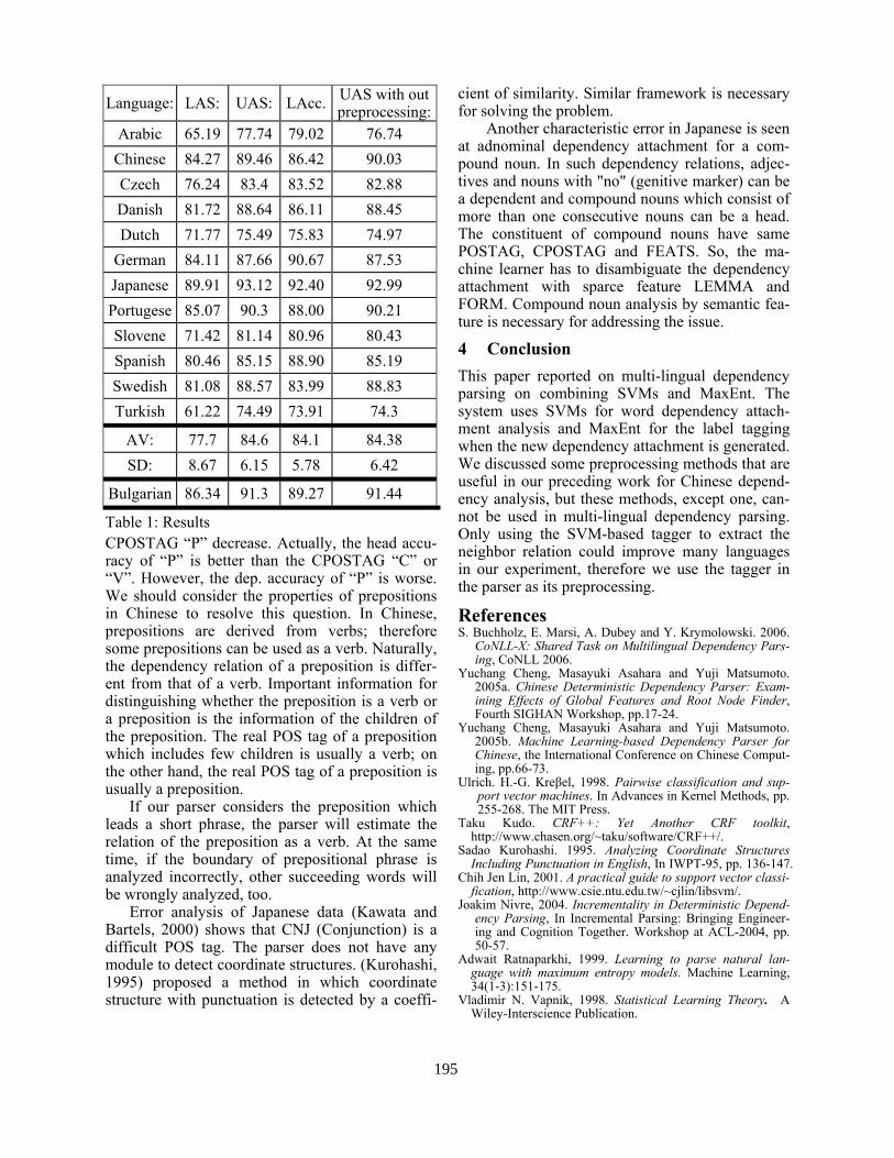
CPOSTAG “P” decrease. Actually, the head accu-racy of “P” is better than the CPOSTAG “C” or “V”. However, the dep. accuracy of “P” is worse. We should consider the properties of prepositions in Chinese to resolve this question. In Chinese, prepositions are derived from verbs; therefore some prepositions can be used as a verb. Naturally, the dependency relation of a preposition is differ-ent from that of a verb. Important information for distinguishing whether the preposition is a verb or a preposition is the information of the children of the preposition. The real POS tag of a preposition which includes few children is usually a verb; on the other hand, the real POS tag of a preposition is usually a preposition.
If our parser considers the preposition which leads a short phrase, the parser will estimate the relation of the preposition as a verb. At the same time, if the boundary of prepositional phrase is analyzed incorrectly, other succeeding words will be wrongly analyzed, too.
Error analysis of Japanese data (Kawata and Bartels, 2000) shows that CNJ (Conjunction) is a difficult POS tag. The parser does not have any module to detect coordinate structures. (Kurohashi, 1995) proposed a method in which coordinate structure with punctuation is detected by a coeffi-
cient of similarity. Similar framework is necessary for solving the problem.
Another characteristic error in Japanese is seen at adnominal dependency attachment for a com-pound noun. In such dependency relations, adjec-tives and nouns with "no" (genitive marker) can be a dependent and compound nouns which consist of more than one consecutive nouns can be a head. The constituent of compound nouns have same POSTAG, CPOSTAG and FEATS. So, the ma-chine learner has to disambiguate the dependency attachment with sparce feature LEMMA and FORM. Compound noun analysis by semantic fea-ture is necessary for addressing the issue.
4 Conclusion This paper reported on multi-lingual dependency parsing on combining SVMs and MaxEnt. The system uses SVMs for word dependency attach-ment analysis and MaxEnt for the label tagging when the new dependency attachment is generated. We discussed some preprocessing methods that are useful in our preceding work for Chinese depend-ency analysis, but these methods, except one, can-not be used in multi-lingual dependency parsing. Only using the SVM-based tagger to extract the neighbor relation could improve many languages in our experiment, therefore we use the tagger in the parser as its preprocessing.
References S. Buchholz, E. Marsi, A. Dubey and Y. Krymolowski. 2006.
CoNLL-X: Shared Task on Multilingual Dependency Pars-ing, CoNLL 2006.
Yuchang Cheng, Masayuki Asahara and Yuji Matsumoto. 2005a. Chinese Deterministic Dependency Parser: Exam-ining Effects of Global Features and Root Node Finder, Fourth SIGHAN Workshop, pp.17-24.
Yuchang Cheng, Masayuki Asahara and Yuji Matsumoto. 2005b. Machine Learning-based Dependency Parser for Chinese, the International Conference on Chinese Comput-ing, pp.66-73.
Ulrich. H.-G. Kreβel, 1998. Pairwise classification and sup-port vector machines. In Advances in Kernel Methods, pp. 255-268. The MIT Press.
Taku Kudo. CRF++: Yet Another CRF toolkit, http://www.chasen.org/~taku/software/CRF++/.
Sadao Kurohashi. 1995. Analyzing Coordinate Structures Including Punctuation in English, In IWPT-95, pp. 136-147.
Chih Jen Lin, 2001. A practical guide to support vector classi-fication, http://www.csie.ntu.edu.tw/~cjlin/libsvm/.
Joakim Nivre, 2004. Incrementality in Deterministic Depend-ency Parsing, In Incremental Parsing: Bringing Engineer-ing and Cognition Together. Workshop at ACL-2004, pp. 50-57.
Adwait Ratnaparkhi, 1999. Learning to parse natural lan-guage with maximum entropy models. Machine Learning, 34(1-3):151-175.
Vladimir N. Vapnik, 1998. Statistical Learning Theory. A Wiley-Interscience Publication.
Language: LAS: UAS: LAcc. UAS with out preprocessing:
Arabic 65.19 77.74 79.02 76.74 Chinese 84.27 89.46 86.42 90.03 Czech 76.24 83.4 83.52 82.88 Danish 81.72 88.64 86.11 88.45 Dutch 71.77 75.49 75.83 74.97
German 84.11 87.66 90.67 87.53 Japanese 89.91 93.12 92.40 92.99 Portugese 85.07 90.3 88.00 90.21 Slovene 71.42 81.14 80.96 80.43 Spanish 80.46 85.15 88.90 85.19 Swedish 81.08 88.57 83.99 88.83 Turkish 61.22 74.49 73.91 74.3
AV: 77.7 84.6 84.1 84.38 SD: 8.67 6.15 5.78 6.42
Bulgarian 86.34 91.3 89.27 91.44
Table 1: Results
195
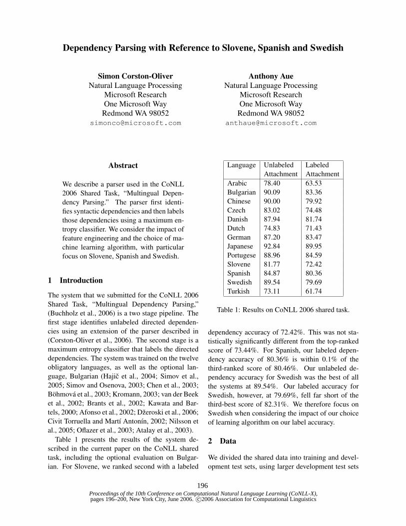
Proceedings of the 10th Conference on Computational Natural Language Learning (CoNLL-X),pages 196–200, New York City, June 2006.c©2006 Association for Computational Linguistics
Dependency Parsing with Reference to Slovene, Spanish and Swedish
Simon Corston-OliverNatural Language Processing
Microsoft ResearchOne Microsoft Way
Redmond WA [email protected]
Anthony AueNatural Language Processing
Microsoft ResearchOne Microsoft Way
Redmond WA [email protected]
Abstract
We describe a parser used in the CoNLL2006 Shared Task, “Multingual Depen-dency Parsing.” The parser first identi-fies syntactic dependencies and then labelsthose dependencies using a maximum en-tropy classifier. We consider the impact offeature engineering and the choice of ma-chine learning algorithm, with particularfocus on Slovene, Spanish and Swedish.
1 Introduction
The system that we submitted for the CoNLL 2006Shared Task, “Multingual Dependency Parsing,”(Buchholz et al., 2006) is a two stage pipeline. Thefirst stage identifies unlabeled directed dependen-cies using an extension of the parser described in(Corston-Oliver et al., 2006). The second stage is amaximum entropy classifier that labels the directeddependencies. The system was trained on the twelveobligatory languages, as well as the optional lan-guage, Bulgarian (Hajic et al., 2004; Simov et al.,2005; Simov and Osenova, 2003; Chen et al., 2003;Bohmova et al., 2003; Kromann, 2003; van der Beeket al., 2002; Brants et al., 2002; Kawata and Bar-tels, 2000; Afonso et al., 2002; Dzeroski et al., 2006;Civit Torruella and Martı Antonın, 2002; Nilsson etal., 2005; Oflazer et al., 2003; Atalay et al., 2003).
Table 1 presents the results of the system de-scribed in the current paper on the CoNLL sharedtask, including the optional evaluation on Bulgar-ian. For Slovene, we ranked second with a labeled
Language Unlabeled LabeledAttachment Attachment
Arabic 78.40 63.53Bulgarian 90.09 83.36Chinese 90.00 79.92Czech 83.02 74.48Danish 87.94 81.74Dutch 74.83 71.43German 87.20 83.47Japanese 92.84 89.95Portugese 88.96 84.59Slovene 81.77 72.42Spanish 84.87 80.36Swedish 89.54 79.69Turkish 73.11 61.74
Table 1: Results on CoNLL 2006 shared task.
dependency accuracy of 72.42%. This was not sta-tistically significantly different from the top-rankedscore of 73.44%. For Spanish, our labeled depen-dency accuracy of 80.36% is within 0.1% of thethird-ranked score of 80.46%. Our unlabeled de-pendency accuracy for Swedish was the best of allthe systems at 89.54%. Our labeled accuracy forSwedish, however, at 79.69%, fell far short of thethird-best score of 82.31%. We therefore focus onSwedish when considering the impact of our choiceof learning algorithm on our label accuracy.
2 Data
We divided the shared data into training and devel-opment test sets, using larger development test sets
196
for the languages supplied with more data. The de-velopment test set consisted of 250 sentences forArabic, Slovene, Spanish and Turkish, 500 sen-tences for Danish and Portuguese, and 1,000 sen-tences for the other languages.
3 The Parser
The baseline parser predicts unlabeled directed de-pendencies. As described in (Corston-Oliver et al.,2006), we reimplemented the parser described in(McDonald et al., 2005) and validated their resultsfor Czech and English.
The parser finds the highest-scoring parse yamong all possible parses y ∈ Y for a given sen-tence:
y = arg maxy∈Y
s(y) (1)
The score s of a given parse y is the sum of thescores of all the dependency links (i,j) ∈ y:
s(y) =∑
(i,j)∈y
d(i, j) =∑
(i,j)∈y
w · f(i, j) (2)
where the link (i,j) indicates a parent-child depen-dency between the token at position i and the tokenat position j. The score d(i, j) of each dependencylink (i,j) is further decomposed as the weighted sumof its features f(i, j).
To set w, we trained twenty averaged perceptronson different shuffles of the training data, using thedevelopment test set to determine when the percep-trons had converged. The averaged perceptrons werethen combined to make a Bayes Point Machine (Har-rington et al., 2003). At both training and run time,edges are scored independently, and Eisner’s O(N3)decoder (Eisner, 1996) is used to find the optimalparse. This decoder produces only projective analy-ses, although it does allow for analyses with multipleroots.
The features used for scoring the edges prior toapplying Eisner’s algorithm are extracted from eachpossible parent-child dependency. The features in-clude the case-normalized original form and lemma1
of each token , the part of speech (POS) tag of eachtoken, the POS tag of each intervening token and
1If no lemma was specified, we truncated the original formby taking the first two characters for Chinese words consistingof two characters or more and the first five characters for wordsconsisting of five characters or more in the other languages.
of each token to the left and right of the parent andchild. Additional features are created by combiningthese atomic features, as described in (McDonald etal., 2005). All features are in turn combined withthe direction of attachment and the distance betweentokens. Distance was discretized, with individualbuckets for distances 0-4, a single bucket for 5-9,and a single bucket for 10+. In sections 3.1 and 3.2we discuss the feature engineering we performed.
3.1 Part of Speech Features
We experimented with using the coarse POS tag andthe fine POS tag. In our official submission, weused fine POS tags for all languages except Dutchand Turkish. For Dutch and Turkish, using the finePOS tag resulted in a reduction in unlabeled depen-dency accuracy of 0.12% and 0.43% respectivelyon the development test sets, apparently because ofthe sparsity of the fine POS tags. For German andSwedish, the fine and coarse POS tags are the sameso using the fine POS tag had no effect. For otherlanguages, using the fine POS tag showed modestimprovements in unlabeled dependency accuracy.
For Swedish, we performed an additional manipu-lation on the POS tags, normalizing the distinct POStags assigned to each verbal auxiliary and modal toa single tag “aux”. For example, in the Swedishdata all inflected forms of the verb “vara” (“be”) aretagged as AV, and all inflected forms of the modal“maste” (“must”) are tagged as MV. This normaliza-tion caused unlabeled dependency accuracy on theSwedish development set to improve from 89.23%to 89.45%.
3.2 Features for Root Identification
Analysis of the baseline parser’s errors suggestedthe need for additional feature types to improve theidentification of the root of the sentence. In particu-lar, the parser was frequently making errors in iden-tifying the root of periphrastic constructions involv-ing an auxiliary verb or modal and a participle. InGermanic languages, for example, the auxiliary ormodal typically occurs in second position in declar-ative main clauses or in initial position in cases ofsubject-aux inversion. We added a collection of fea-tures intended to improve the identification of theroot. The hope was that improved root identifica-tion would have a positive cascading effect in the
197
identification of other dependencies, since a failureto correctly identify the root of the sentence usuallymeans that the parse will have many other errors.
We extracted four feature types, the original formof the first and last tokens in the sentence and thePOS of the first and last tokens in the sentence.These features were intended to identify declarativevs. interrogative sentences.
For each child and parent token being scored, wealso noted the following four features: “child/parentis first non-punctuation token in sentence”,“child/parent is second non-punctuation token insentence”. The features that identify the secondtoken in the sentence were intended to improvethe identification of verb-second phenomena. Ofcourse, this is a linguistic oversimplification. Verb-second phenomena are actually sensitive to the orderof constituents, not words. We therefore added fourfeature types that considered the sequence of POStags to the left of the child or parent if they occurredwithin ten tokens of the beginning of the sentenceand the sequence of POS tags to the right of thechild or parent if they occurred within ten tokens ofthe end of the sentence.
We also added features intended to improve theidentification of the root in sentences without a fi-nite verb. For example, the Dutch training datacontained many simple responses to a question-answering task, consisting of a single noun phrase.Four simple features were used “Child/Parent is theleftmost noun in the sentence”, “Child/Parent is anoun but not the leftmost noun in the sentence”.These features were combined with an indicator“Sentence contains/does not contain a finite verb”.
Child or parent tokens that were finite verbs wereflagged as likely candidates for being the root ofthe sentence if they were the leftmost finite verb inthe sentence and not preceded by a subordinatingconjunction or relative pronoun. Finite verbs wereidentified by POS tags and morphological features,e.g. in Spanish, verbs without the morphologicalfeature “mod=n” were identified as finite, while inPortuguese the fine POS tag “v-fin” was used.
Similarly, various sets of POS tags were used toidentify subordinating conjunctions or relative pro-nouns for different languages. For example, in Bul-garian the fine POS tag “pr” (relative pronoun) and“cs” (subordinating conjunction) were used. For
Dutch, the morphological features “onder”, “betr”and “voorinf” were used to identify subordinatingconjunctions and relative pronouns.
These features wreaked havoc with Turkish, averb-final language. For certain other languages,dependency accuracy measured on the develop-ment test set improved by a modest amount, withmore dramatic improvements in root accuracy (F1measure combining precision and recall for non-punctuation root tokens).
Since the addition of these features had been mo-tivated by verb-second phenomena in Germanic lan-guages, we were surprised to discover that the onlyGermanic language to demonstrate a marked im-provement in unlabeled dependency accuracy wasDanish, whose accuracy on the development set rosefrom 87.51% to 87.72%, while root accuracy F1rose from 94.12% to 94.72%. Spanish showed amodest improvement in unlabeled dependency accu-racy, from 85.08% to 85.13%, but root F1 rose from80.08% to 83.57%.
The features described above for identifying theleftmost finite verb not preceded by a subordinat-ing conjunction or relative pronoun did not im-prove Slovene unlabeled dependency accuracy, andso were not included in the set of root-identifyingfeatures in our Slovene CoNLL submission. Closerexamination of the Slovene corpus revealed that pe-riphrastic constructions consisting of one or moreauxiliaries followed by a participle were annotatedwith the participle as the head, whereas for otherlanguages in the shared task the consensus view ap-pears to be that the auxiliary should be annotatedas the head. Singling out the leftmost finite verb inSlovene when a participle ought to be selected as theroot of the sentence is therefore counter-productive.The other root identification features did improveroot F1 in Slovene. Root F1 on the development testset rose from 45.82% to 46.43%, although overallunlabeled dependency accuracy on the developmenttest set fell slightly from 80.24% to 79.94%.
3.3 Morphological FeaturesAs the preceding discussion shows, morphologicalinformation was occasionally used to assist in mak-ing finer-grained POS distinctions than were madein the POS tags, e.g., for distinguishing subordi-nating vs. coordinating conjunctions. Aside from
198
these surgical uses of the morphological informationpresent in the CoNLL data, morphology was not ex-plicitly used by the baseline parser. For example,there were no features that considered subject-verbagreement nor agreement of an adjective with thenumber or lexical gender of the noun it modified.However, it is possible that morphological informa-tion influenced the training of edge weights if theinformation was implicit in the POS tags.
4 The Dependency Labeler
4.1 Classifier
We used a maximum entropy classifier (Berger et al.,1996) to assign labels to the unlabeled dependen-cies produced by the Bayes Point Machine. We usedthe same training and development test split that wasused to train the dependency parser. We chose to usemaximum entropy classifiers because they can betrained relatively quickly while still offering reason-able classification accuracy and are robust in the faceof large numbers of superfluous features, a desirableproperty given the requirement that the same parserhandle multiple languages. Furthermore, maximumentropy classifiers provide good probability distribu-tions over class labels. This was important to us be-cause we had initially hoped to find the optimal setof dependency labels for the children of a given nodeby modeling the probability of each set of labelsconditioned on the lemma and POS of the parent.For example, labeling each dependant of a parentnode independently might result in three OBJECTrelations dependent on a single verb; modeling setsof relations ought to prevent this. Unfortunately, thisapproach did not outperform labeling each node in-dependently.
Therefore, the system we submitted labeled eachdependency independently, using the most probablelabel from the maximum entropy classifier. We havenoted in previous experiments that our SVM imple-mentation often gives better one-best classificationaccuracy than our maximum entropy implementa-tion, but did not have time to train SVM classifiers.
To see how much the choice of classification al-gorithm affected our official results, we trained a lin-ear SVM classifier for Swedish after the competitionhad ended, tuning parameters on the developmenttest set. As noted in section 1, our system scored
highest for Swedish in unlabeled dependency accu-racy at 89.54% but fell well short of the third-rankedsystem when measuring labeled dependency accu-racy. Using an SVM classifier instead of a maxi-mum entropy classifier, Swedish label accuracy rosefrom 82.33% to 86.06%, and labeled attachment ac-curacy rose from 79.69% to 82.95%, which fallsbetween the first-ranked score of 84.58% and thesecond-ranked score of 82.55%. Similarly, Japaneselabel accuracy rose from 93.20% to 93.96%, andlabeled attachment accuracy rose from 89.95% to90.77% when we replaced a maximum entropy clas-sifier with an SVM. This labeled attachment resultof 90.77% is comparable to the official second placeresult of 90.71% for Japanese. We conclude that atwo stage pipeline such as ours, in which the sec-ond stage labels dependencies in isolation, is greatlyimpacted by the choice of classifier.
4.2 Features Used for LabelingWe extracted features from individual nodes in thedependency tree, parent-child features and featuresthat took nodes other than the parent and child intoaccount.
The features extracted from each individual par-ent and child node were the original surface form,the lemma (see footnote 1 above), the coarse and finePOS tags and each morphological feature.
The parent-child features are the direction ofmodification, the combination of the parent andchild lemmata, all combinations of parent and childlemma and coarse POS tag (e.g. child lemma com-bined with coarse POS tag of the parent) and all pair-wise combinations of parent and child morphologyfeatures (e.g. parent is feminine and child is plural).
Additional features were verb position (whetherthe parent or child is the first or last verb in the sen-tence), coarse POS and lemma of the left and rightneighbors of the parent and child, coarse POS andlemma of the grandparent, number and coarse POStag sequence of siblings to the left and to the right ofthe child, total number of siblings of the child, num-ber of tokens governed by child, whether the par-ent has a verbal ancestor, lemma and morphologicalfeatures of the verb governing the child (if any), andcoarse POS tag combined with relative offset of eachsibling (e.g., the sibling two to the left of the child isa determiner).
199
For Slovene, the label accuracy using all of thefeatures above was 81.91%. We retrained our max-imum entropy classifier by removing certain classesof features in order to determine their contribu-tion. Removing the weight features caused a notabledrop, with label accuracy on the development test setfalling 0.52% to 81.39%. Removing the grandpar-ent features (but including weight features) causedan even greater drop of 1.03% to 80.88%. One placewhere the grandparent features were important wasin distinguishing between Adv and Atr relations. Itappears that the relation between a noun and its gov-erning preposition or between a verb and its govern-ing conjunction is sensitive to the part of speech ofthe grandparent. For example, we observed a num-ber of cases where the relation between a noun andits governing preposition had been incorrectly la-beled as Adv when it should have been Atr. Theaddition of grandparent features allowed the classi-fier to make the distinction by looking at the POS ofthe grandparent; when the POS was noun, the clas-sifier tended to correctly choose the Atr label.
5 Conclusion
We have described a two stage pipeline that first pre-dicts directed unlabeled dependencies and then la-bels them. The system performed well on Slovene,Spanish and Swedish. Feature engineering playedan important role both in predicting dependenciesand in labeling them. Finally, replacing the maxi-mum entropy classifier used to label dependencieswith an SVM improves upon our official results.
ReferencesAdam L. Berger, Stephen Della Pietra, and Vincent
J. Della Pietra. 1996. A maximum entropy approachto natural language processing. Computational Lin-guistics, 22(1):39–71.
S. Buchholz, E. Marsi, A. Dubey, and Y. Krymolowski.2006. CoNLL-X shared task on multilingual depen-dency parsing. In Proc. of the Tenth Conf. on Com-putational Natural Language Learning (CoNLL-X).SIGNLL.
Simon Corston-Oliver, Anthony Aue, Kevin Duh, andEric Ringger. 2006. Multilingual dependency parsingusing bayes point machines. In Proc. of HLT-NAACL2006.
J. Eisner. 1996. Three new probabilistic models fordependency parsing: An exploration. In Proc. ofthe 16th Intern. Conf. on Computational Linguistics(COLING), pages 340–345.
Edward Harrington, Ralf Herbrich, Jyrki Kivinen,John C. Platt, and Robert C. Williamson. 2003. On-line bayes point machines. In Proceedings of SeventhPacific-Asia Conference on Knowledge Discovery andData Mining, pages 241–252.
Ryan McDonald, Koby Crammer, and Fernando Pereira.2005. Online large-margin training of dependencyparsers. In Proceedings of the 43rd Annual Meetingof the Assocation for Computational Linguistics.
200
Proceedings of the 10th Conference on Computational Natural Language Learning (CoNLL-X),pages 201–205, New York City, June 2006.c©2006 Association for Computational Linguistics
Vine Parsing and Minimum Risk Reranking for Speed and Precision∗
Markus Dreyer, David A. Smith, and Noah A. SmithDepartment of Computer Science / Center for Language and Speech Processing
Johns Hopkins University, Baltimore, MD 21218 USA{markus, {d,n }asmith }@cs.jhu.edu
Abstract
We describe our entry in the CoNLL-X shared task.The system consists of three phases: a probabilisticvine parser (Eisner and N. Smith, 2005) that pro-duces unlabeled dependency trees, a probabilisticrelation-labeling model, and a discriminative mini-mum risk reranker (D. Smith and Eisner, 2006). Thesystem is designed for fast training and decoding andfor high precision. We describe sources of cross-lingual error and ways to ameliorate them. We thenprovide a detailed error analysis of parses producedfor sentences in German (much training data) andArabic (little training data).
1 Introduction
Standard state-of-the-art parsing systems (e.g.,Charniak and Johnson, 2005) typically involve twopasses. First, aparser produces a list of the mostlikely n parse trees under a generative, probabilisticmodel (usually some flavor of PCFG). A discrim-inative reranker then chooses among trees in thislist by using an extended feature set (Collins, 2000).This paradigm has many advantages: PCFGs arefast to train, can be very robust, and perform bet-ter as more data is made available; and rerankerstrain quickly (compared to discriminative models),require few parameters, and permit arbitrary fea-tures.
We describe such a system fordependencypars-ing. Our shared task entry is a preliminary systemdeveloped in only 3 person-weeks, and its accuracyis typically one s.d. below the average across sys-tems and 10–20 points below the best system. On
∗This work was supported by NSF ITR grant IIS-0313193,an NSF fellowship to the second author, and a Fannie and JohnHertz Foundation fellowship to the third author. The views ex-pressed are not necessarily endorsed by the sponsors. We thankCharles Schafer, Keith Hall, Jason Eisner, and Sanjeev Khudan-pur for helpful conversations.
the positive side, its decoding algorithms have guar-anteedO(n) runtime, and training takes only a cou-ple of hours. Having designed primarily forspeedandrobustness, we sacrifice accuracy. Betteresti-mation, reranking on larger datasets, and more fine-grained parsing constraints are expected to boost ac-curacy while maintaining speed.
2 Notation
Let a sentencex = 〈x1, x2, ..., xn〉, where eachxi isa tuple containing a part-of-speech tagti and a wordwi, and possibly more information.1 x0 is a specialwall symbol, $, on the left. A dependency treeyis defined by three functions:yleft andyright (both{0, 1, 2, ..., n} → 2{1,2,...,n}) that map each word toits sets of left and right dependents, respectively, andylabel : {1, 2, ..., n} → D, which labels the relation-ship between wordi and its parent from label setD.
In this work, the graph is constrained to be apro-jectivetree rooted at $: each word except $ has a sin-gle parent, and there are no cycles or crossing depen-dencies. Using a simple dynamic program to find theminimum-error projective parse, we find that assum-ing projectivity need not harm accuracy very much(Tab. 1, col. 3).
3 Unlabeled Parsing
The first component of our system is an unlabeledparser that, given a sentence, finds theU best un-labeled trees under a probabilistic model using abottom-up dynamic programming algorithm.2 Themodel is a probabilistic head automaton grammar(Alshawi, 1996) that assumes conditional indepen-
1We used words and fine tags in our parser and labeler, withcoarse tags in one backoff model. Other features are used inreranking; we never used the given morphological features orthe “projective” annotations offered in the training data.
2The execution model we use is best-first, exhaustive search,as described in Eisner et al. (2004). All of our dynamic pro-gramming algorithms are implemented concisely in the Dynalanguage.
201

B` Br
projective oracle
(B` , B
r )-vine oracle
20-best unlabeled oracle
1-best unlabeled
unlabeled, reranked
20×50-best labeled oracle
1×1-best labeled
reranked (labeled)
(unlabeled)
(non-$ unl. recall)
(non-$ unl. precision)Arabic 10 4 99.8 90.7 71.5 68.1 68.7 59.7 52.0 53.4 68.5 63.4 76.0Bulgarian 5 4 99.6 90.7 86.4 80.1 80.5 85.1 73.0 74.8 82.0 74.3 86.3Chinese 4 4 100.0 93.1 89.9 79.4 77.7 88.6 72.6 71.6 77.6 61.4 80.8Czech 6 4 97.8 90.5 79.2 70.3 71.5 72.8 58.1 60.5 70.7 64.8 75.7Danish 5 4 99.2 91.4 84.6 77.7 78.6 79.3 65.5 66.6 77.5 71.4 83.4Dutch 6 5 94.6 88.3 77.5 67.9 68.8 73.6 59.4 61.6 68.3 60.4 73.0German 8 7 98.8 90.9 83.4 75.5 76.2 82.3 70.1 71.0 77.0 70.2 82.9Japanese 4 1 99.2 92.2 90.7 86.3 85.1 89.4 81.6 82.9 86.0 68.5 91.5Portuguese 5 5 98.8 91.5 85.9 81.4 82.5 83.7 73.4 75.3 82.4 76.2 87.0Slovene 6 4 98.5 91.7 80.5 72.0 73.3 72.8 57.5 58.7 72.9 66.3 78.5Spanish 5 6 100.0 91.2 77.3 71.5 72.6 74.9 66.2 67.6 72.9 69.3 80.7Swedish 4 5 99.7 94.0 87.5 79.3 79.6 81.0 65.5 67.6 79.5 72.6 83.3Turkish 6 1 98.6 89.5 73.0 61.0 61.8 64.4 44.9 46.1 60.5 48.5 61.6
parser reranker labeler reranker
1 2 3 4 5 6 7 8 9 10 11 12 13
Table 1: Parameters and performance on test data.B` andBr were chosen to retain 90% of dependenciesin training data. We show oracle, 1-best, and reranked performance on the test set at different stages of thesystem. Boldface marks oracle performance that, given perfect downstream modules, would supercede thebest system. Italics mark the few cases where the reranker increased error rate. Columns 8–10 show labeledaccuracy; column 10 gives the final shared task evaluation scores.
dence between the left yield and the right yield ofa given head, given the head (Eisner, 1997).3 Thebest known parsing algorithm for such a model isO(n3) (Eisner and Satta, 1999). TheU -best list isgenerated using Algorithm 3 of Huang and Chiang(2005).
3.1 Vine parsing (dependency length bounds)
Following Eisner and N. Smith (2005), we also im-pose a bound on the string distance between every
3To empirically test this assumption across languages, wemeasured the mutual information between different features ofyleft(j) andyright(j), givenxj . (Mutual information is a statis-tic that equals zero iff conditional independence holds.) A de-tailed discussion, while interesting, is omitted for space, but wehighlight some of our findings. First, unsurprisingly, the split-head assumption appears to be less valid for languages withfreer word order (Czech, Slovene, German) and more valid formore fixed-order languages (Chinese, Turkish, Arabic) or cor-pora (Japanese). The children of verbs and conjunctions are themost frequent violators. The mutual information between thesequence of dependency labels on the left and on the right, giventhe head’s (coarse) tag, only once exceeded 1 bit (Slovene).
child and its parent, with the exception of nodes at-taching to $. Bounds of this kind are intended to im-prove precision of non-$ attachments, perhaps sac-rificing recall. Fixing boundB`, no left dependencymay exist between childxi and parentxj such thatj−i > B` (similarly for right dependencies andBr).As a result, edge-factored parsing runtime is reducedfrom O(n3) to O(n(B2
` + B2r )). For each language,
we chooseB` (Br) to be the minimum value thatwill allow recovery of 90% of the left (right) depen-dencies in the training corpus (Tab. 1, cols. 1, 2, and4). In order to match the training data to the parsingmodel, we re-attach disallowed long dependenciesto $ during training.
3.2 Estimation
The probability model predicts, for each parent wordxj , {xi}i∈yleft (j) and{xi}i∈yright (j). An advantageof head automaton grammars is that, for a given par-ent nodexj , the children on the same side,yleft(j),
202
for example, can depend on each other (cf. McDon-ald et al., 2005). Child nodes in our model are gener-ated outward, conditional on the parent and the mostrecent same-side sibling (MRSSS). This increasesour parser’s theoretical runtime toO(n(B3
` + B3r )),
which we found was quite manageable.Let pary : {1, 2, ..., n} → {0, 1, ..., n} map each
node to its parent iny. Let predy : {1, 2, ..., n} →{∅, 1, 2, ..., n} map each node to the MRSSS iny ifit exists and∅ otherwise. Let∆i = |i − j| if j is i’sparent. Our (probability-deficient) model defines
p(y) =
n∏j=1
∏i∈yleft (j)
p(xi, ∆i | xj , xpredy(i), left)
×p(STOP | xj , xminyleft (j) j , left)
×
∏i∈yright (j)
p(xi, ∆i | xj , predy(i), right)
×p(STOP | xj , xmaxyright (j) j , right) (1)
Due to the familiar sparse data problem, a maxi-mum likelihood estimate for theps in Eq. 1 performsvery badly (2–23% unlabeled accuracy). Good sta-tistical parsers smooth those distributions by mak-ing conditional independence assumptionsamongvariables, including backoff and factorization. Ar-guably the choice of assumptions made (or interpo-lated among) is central to the success of many exist-ing parsers.
Noting that (a) there are exponentially many suchoptions, and (b) the best-performing independenceassumptions will almost certainly vary by language,we use a mixture among 8 such models. The samemixture is used for all languages. The models werenot chosen with particular care,4 and the mixture isnot trained—the coefficients are fixed at uniform,with a unigram coarse-tag model for backoff. Inprinciple, this mixture should be trained (e.g., tomaximize likelihood or minimize error on a devel-opment dataset).
The performance of our unlabeled model’s topchoice and the top-20 oracle are shown in Tab. 1,cols. 5–6. In 5 languages (boldface), perfect label-ing and reranking at this stage would have resulted inperformance superior to the language’s best labeled
4Our infrastructure provides a concise, interpreted languagefor expressing the models to be mixed, so large-scale combina-tion and comparison are possible.
system, although the oracle is never on par with thebestunlabeledperformance.
4 Labeling
The second component of our system is a labelingmodel thatindependentlyselects a label fromD foreach parent/child pair in a tree. Given theU bestunlabeled trees for a sentence, the labeler producesthe L best labeled trees for each unlabeled one.The computation involves anO(|D|n) dynamic pro-gramming algorithm, the output of which is passedto Huang and Chiang’s (2005) algorithm to generatetheL-best list.
We separate the labeler from the parser for tworeasons: speed and candidate diversity. In prin-ciple the vine parser could jointly predict depen-dency labels along with structures, but parsing run-time would increase by at least a factor of|D|. Thetwo stage process also forces diversity in the candi-date list (20 structures with 50 labelings each); the1,000-best list ofjointly-decoded parses often con-tained many (bad) relabelings of the same tree.
In retrospect, assuming independence among de-pendency labels damages performance substantiallyfor some languages (Turkish, Czech, Swedish, Dan-ish, Slovene, and Arabic); note the often large dropin oracle performance between Tab. 1, cols. 5 and8. This assumption is necessary in our framework,because theO(|D|M+1n) runtime of decoding withanM th-order Markov model of labels5 is in generalprohibitive—in some cases|D| > 80. Pruning andsearch heuristics might ameliorate runtime.
If xi is a child ofxj in directionD, andxpred isthe MRSSS (possibly∅), where∆i = |i− j|, we es-timatep(`, xi, xj , xpred ,∆i | D) by a mixture (un-trained, as in the parser) of four backed-off, factoredestimates.
After parsing and labeling, we have for each sen-tence a list ofU × L candidates. Both the oracleperformance of the best candidate in the(20 × 50)-best list and the performance of the top candidate areshown in Tab. 1, cols. 8–9. It should be clear fromthe drop in both oracle and 1-best accuracy that ourlabeling model is a major source of error.
5We tested first-order Markov models that conditioned onparent or MRSSS dependency labels.
203

5 Reranking
We train a log-linear model combining many featurescores (see below), including the log-probabilitiesfrom the parser and labeler. Training minimizesthe expected error under the model; we use deter-ministic annealing to smooth the error surface andavoid local minima (Rose, 1998; D. Smith and Eis-ner, 2006).
We reserved 200 sentences in each language fortraining the reranker, plus 200 for choosing amongrerankers trained on different feature sets and differ-ent(U × L)-best lists.6
Features Our reranking features predict tags, la-bels, lemmata, suffixes and other information givenall or some of the following non-local conditioningcontext: bigrams and trigrams of tags or dependencylabels; parent and grandparent dependency labels;subcategorization frames (in terms of tags or depen-dency labels); the occurrence of certain tags betweenhead and child; surface features like the lemma7 andthe 3-character suffix. In some cases the children ofa node are considered all together, and in other casesleft and right are separated.
The highest-ranked features during training, forall languages, are the parser and labeler probabil-ities, followed byp(∆i | tparent), p(direction |tparent), p(label | labelpred , label succ , subcat), andp(coarse(t) | D, coarse(tparent),Betw), whereBetw is TRUE iff an instance of the coarse tag typewith the highest mutual information between its leftand right children (usually verb) is between the childand its head.
Feature and Model Selection For training speedand to avoid overfitting, only a subset of the abovefeatures are used in reranking. Subsets of differ-ent sizes (10, 20, and 40, plus “all”) are identifiedfor each language using two naıve feature-selectionheuristics based on independent performance of fea-tures. The feature subset with the highest accuracyon the 200 heldout sentences is selected.
6In training our system, we made a serious mistake in train-ing the reranker on only 200 sentences. As a result, our pre-testing estimates of performance (on data reserved for modelselection) were very bad. The reranker, depending on condition,had only 2–20 times as many examples as it had parameters toestimate, with overfitting as the result.
7The first 4 characters of a word are used where the lemmais not available.
Performance Accuracy of the top parses afterreranking is shown in Tab. 1, cols. 10–11. Rerankingalmost always gave some improvement over 1-bestparsing.8 Because of the vine assumption and thepreprocessing step that re-attaches all distant chil-dren to $, our parser learns to over-attach to $, treat-ing $-attachment as a default/agnostic choice. Formany applications a local, incomplete parse may besufficiently useful, so we also measured non-$ unla-beled precision and recall (Tab. 1, cols. 12–13); ourparser has> 80% precision on 8 of the languages.We also applied reranking (with unlabeled features)to the 20-best unlabeled parse lists (col. 7).
6 Error Analysis: German
The plurality of errors (38%) in German were er-roneous $ attachments. For ROOT dependency la-bels, we have a high recall (92.7%), but low pre-cision (72.4%), due most likely to the dependencylength bounds. Among the most frequent tags, oursystem has most trouble finding the correct heads ofprepositions (APPR), adverbs (ADV), finite auxil-iary verbs (VAFIN), and conjunctions (KON), andfinding the correct dependency labels for preposi-tions, nouns, and finite auxiliary verbs.
The German conjunctionund is the single wordwith the most frequent head attachment errors. Inmany of these cases, our system does not learnthe subtle difference between enumerations that areheaded byA in A und B, with two childrenundandB on the right, and those headed byB, with undandA as children on its left.
Unlike in some languages, our labeled oracle ac-curacy is nearly as good as our unlabeled oracle ac-curacy (Tab. 1, cols. 8, 5). Among the ten most fre-quent dependency labels, our system has the mostdifficulty with accusative objects (OA), genitive at-tributes (AG), and postnominal modifiers (MNR).Accusative objects are often mistagged as subject(SB), noun kernel modifiers (NK), or AG. About32% of the postnominal modifier relations (ein Platzin der Geschichte, ‘a place in history’) are labeledas modifiers (in die Stadt fliegen, ‘fly into the city’).Genitive attributes are often tagged as NK since bothare frequently realized as nouns.
8The exception is Chinese, where the training set for rerank-ing is especially small (see fn. 6).
204
7 Error Analysis: Arabic
As with German, the greatest portion of Arabic er-rors (40%) involved attachments to $. Prepositionsare consistently attached too low and accounted for26% of errors. For example, if a form in construct(idafa) governed both a following noun phrase anda prepositional phrase, the preposition usually at-taches to the lower noun phrase. Similarly, prepo-sitions usually attach to nearby noun phrases whenthey should attach to verbs farther to the left.
We see a more serious casualty of the dependencylength bounds with conjunctions. In ground truthtest data, 23 conjunctions are attached to $ and 141to non-$ to using the COORD relation, whereas 100conjunctions are attached to $ and 67 to non-$ us-ing the AUXY relation. Our system overgeneralizesand attaches 84% of COORD and 71% of AUXYrelations to $. Overall, conjunctions account for15% of our errors. The AUXY relation is definedas “auxiliary (in compound expressions of variouskinds)”; in the data, it seems to be often used forwaw-consecutive or paratactic chaining of narrativeclauses. If the conjunctionwa (‘and’) begins a sen-tence, then that conjunction is tagged in ground truthas attaching to $; if the conjunction appears in themiddle of the sentence, it may or may not be at-tached to $.
Noun attachments exhibit a more subtle problem.The direction of system attachments is biased morestrongly to the left than is the case for the true data.In canonical order, Arabic nouns do generally attachon the right: subjects and objects follow the verb; inconstruct, the governed noun follows its governor.When the data deviate from this canonical order—when, e.g, a subject precedes its verb—the systemprefers to find some other attachment point to theleft. Similarly, a noun to the left of a conjunctionoften erroneously attaches to its left. Such ATR re-lations account for 35% of noun-attachment errors.
8 Conclusion
The tradeoff between speed and accuracy is famil-iar to any parsing researcher. Rather than startingwith an accurate system and then applying corpus-specific speedups, we start by imposing carefully-chosen constraints (projectivity and length bounds)for speed, leaving accuracy to the parsing and
reranking models. As it stands, our system performspoorly, largely because the estimation is not state-of-the-art, but also in part due to dependency lengthbounds, which are rather coarse at present. Better re-sults are achievable by picking different bounds fordifferent head tags (Eisner and N. Smith, 2005). Ac-curacy should not be difficult to improve using bet-ter learning methods, especially given our models’linear-time inference and decoding.
References
H. Alshawi. 1996. Head automata and bilingualtiling: Translation with minimal representations.In Proc. of ACL.
E. Charniak and M. Johnson. 2005. Coarse-to-finen-best parsing and maxent discriminative rerank-ing. In Proc. of ACL.
M. Collins. 2000. Discriminative reranking for nat-ural language parsing. InProc. of ICML.
J. Eisner and G. Satta. 1999. Efficient parsingfor bilexical context-free grammars and head au-tomaton grammars. InProc. of ACL.
J. Eisner and N. A. Smith. 2005. Parsing with softand hard constraints on dependency length. InProc. of IWPT.
J. Eisner, E. Goldlust, and N. A. Smith. 2004.Dyna: A declarative language for implementingdynamic programs. InProc. of ACL(companionvolume).
J. Eisner. 1997. Bilexical grammars and a cubic-time probabilistic parser. InProc. of IWPT.
L. Huang and D. Chiang. 2005. Betterk-best pars-ing. In Proc. of IWPT.
R. McDonald, F. Pereira, K. Ribarov, and J. Hajic.2005. Non-projective dependency parsing us-ing spanning tree algorithms. InProc. of HLT-EMNLP.
K. Rose. 1998. Deterministic annealing for cluster-ing, compression, classification, regression, andrelated optimization problems.Proc. of the IEEE,86(11):2210–2239.
D. A. Smith and J. Eisner. 2006. Minimum risk an-nealing for training log-linear models. To appearin Proc. of COLING-ACL.
205
Proceedings of the 10th Conference on Computational Natural Language Learning (CoNLL-X),pages 206–210, New York City, June 2006.c©2006 Association for Computational Linguistics
Investigating Multilingual Dependency Parsing
Richard Johansson
Department of Computer ScienceLTH, Lund University221 00 Lund, Sweden
Pierre Nugues
Department of Computer ScienceLTH, Lund University221 00 Lund, Sweden
Abstract
In this paper, we describe a system forthe CoNLL-X shared task of multilin-gual dependency parsing. It uses a base-line Nivre’s parser (Nivre, 2003) that firstidentifies the parse actions and then la-bels the dependency arcs. These two stepsare implemented as SVM classifiers usingLIBSVM. Features take into account thestatic context as well as relations dynami-cally built during parsing.
We experimented two main additions toour implementation of Nivre’s parser: N -best search and bidirectional parsing. Wetrained the parser in both left-right andright-left directions and we combined theresults. To construct a single-head, rooted,and cycle-free tree, we applied the Chu-Liu/Edmonds optimization algorithm. Weran the same algorithm with the same pa-rameters on all the languages.
1 Nivre’s Parser
Nivre (2003) proposed a dependency parser that cre-ates a projective and acyclic graph. The parser is anextension to the shift–reduce algorithm. As with theregular shift–reduce, it uses a stack S and a list ofinput words W . However, instead of finding con-stituents, it builds a set of arcs G representing thegraph of dependencies.Nivre’s parser uses two operations in addition to
shift and reduce: left-arc and right-arc. Given a se-quence of words, possibly annotated with their part
of speech, parsing simply consists in applying a se-quence of operations: left-arc (la), right-arc (ra),reduce (re), and shift (sh) to the input sequence.
2 Parsing an Annotated Corpus
The algorithm to parse an annotated corpus isstraightforward from Nivre’s parser and enables usto obtain, for any projective sentence, a sequence ofactions taken in the set {la,ra,re,sh} that parsesit. At a given step of the parsing process, let TOP
be the top of the stack and FIRST , the first token ofthe input list, and arc, the relation holding betweena head and a dependent.
1. if arc(TOP,FIRST ) ∈ G, then ra;
2. else if arc(FIRST, TOP ) ∈ G, then la;
3. else if ∃k ∈ Stack, arc(FIRST, k) ∈ G orarc(k, FIRST ) ∈ G, then re;
4. else sh.
Using the first sentence of the Swedish corpusas input (Table 1), this algorithm produces the se-quence of 24 actions: sh, sh, la, ra, re, la, sh,sh, sh, la, la, ra, ra, sh, la, re, ra, ra, ra,re, re, re, re, and ra (Table 2).
3 Adapting Nivre’s Algorithm to
Machine–Learning
3.1 Overview
We used support vector machines to predict theparse action sequence and a two step procedure to
206
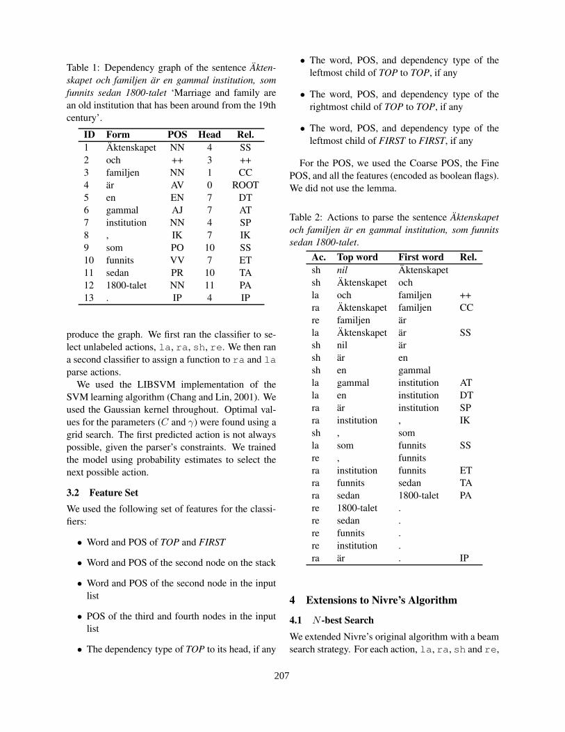
Table 1: Dependency graph of the sentence Äkten-skapet och familjen är en gammal institution, somfunnits sedan 1800-talet ‘Marriage and family arean old institution that has been around from the 19thcentury’.
ID Form POS Head Rel.
1 Äktenskapet NN 4 SS2 och ++ 3 ++3 familjen NN 1 CC4 är AV 0 ROOT5 en EN 7 DT6 gammal AJ 7 AT7 institution NN 4 SP8 , IK 7 IK9 som PO 10 SS10 funnits VV 7 ET11 sedan PR 10 TA12 1800-talet NN 11 PA13 . IP 4 IP
produce the graph. We first ran the classifier to se-lect unlabeled actions, la, ra, sh, re. We then rana second classifier to assign a function to ra and laparse actions.We used the LIBSVM implementation of the
SVM learning algorithm (Chang and Lin, 2001). Weused the Gaussian kernel throughout. Optimal val-ues for the parameters (C and γ) were found using agrid search. The first predicted action is not alwayspossible, given the parser’s constraints. We trainedthe model using probability estimates to select thenext possible action.
3.2 Feature Set
We used the following set of features for the classi-fiers:
• Word and POS of TOP and FIRST
• Word and POS of the second node on the stack
• Word and POS of the second node in the inputlist
• POS of the third and fourth nodes in the inputlist
• The dependency type of TOP to its head, if any
• The word, POS, and dependency type of theleftmost child of TOP to TOP, if any
• The word, POS, and dependency type of therightmost child of TOP to TOP, if any
• The word, POS, and dependency type of theleftmost child of FIRST to FIRST, if any
For the POS, we used the Coarse POS, the FinePOS, and all the features (encoded as boolean flags).We did not use the lemma.
Table 2: Actions to parse the sentence Äktenskapetoch familjen är en gammal institution, som funnitssedan 1800-talet.
Ac. Top word First word Rel.
sh nil Äktenskapetsh Äktenskapet ochla och familjen ++ra Äktenskapet familjen CCre familjen ärla Äktenskapet är SSsh nil ärsh är ensh en gammalla gammal institution ATla en institution DTra är institution SPra institution , IKsh , somla som funnits SSre , funnitsra institution funnits ETra funnits sedan TAra sedan 1800-talet PAre 1800-talet .re sedan .re funnits .re institution .ra är . IP
4 Extensions to Nivre’s Algorithm
4.1 N -best Search
We extended Nivre’s original algorithm with a beamsearch strategy. For each action, la, ra, sh and re,
207
we computed a probability score using LIBSVM.These scores can then be used to carry out an N -best search through the set of possible sequences ofactions.We measured the improvement over a best-first
strategy incrementing values ofN . We observed thelargest difference between N = 1 and N = 2, thenleveling off and we used the latter value.
4.2 Bidirectionality and Voting
Tesnière (1966) classified languages as centrifuge(head to the left) and centripetal (head to the right)in a table (page 33 of his book) that nearly exactlyfits corpus evidence from the CONLL data. Nivre’sparser is inherently left-right. This may not fit allthe languages. Some dependencies may be easierto capture when proceeding from the reverse direc-tion. Jin et al. (2005) is an example of it for Chinese,where the authors describe an adaptation of Nivre’sparser to bidirectionality.We trained the model and ran the algorithm in
both directions (left to right and right to left). Weused a voting strategy based on probability scores.Each link was assigned a probability score (simplyby using the probability of the la or ra actions foreach link). We then summed the probability scoresof the links from all four trees. To construct a single-head, rooted, and cycle-free tree, we finally appliedthe Chu-Liu/Edmonds optimization algorithm (Chuand Liu, 1965; Edmonds, 1967).
5 Analysis
5.1 Experimental Settings
We trained the models on “projectivized” graphs fol-lowing Nivre and Nilsson (2005) method. We usedthe complete annotated data for nine langagues. Dueto time limitations, we could not complete the train-ing for three languages, Chinese, Czech, and Ger-man.
5.2 Overview of the Results
We parsed the 12 languages using exactly the samealgorithms and parameters. We obtained an averagescore of 74.93 for the labeled arcs and of 80.39 forthe unlabeled ones (resp. 74.98 and 80.80 for thelanguages where we could train the model using thecomplete annotated data sets). Table 3 shows the
results per language. As a possible explanation ofthe differences between languages, the three lowestfigures correspond to the three smallest corpora. Itis reasonable to assume that if corpora would havebeen of equal sizes, results would have been moresimilar. Czech is an exception to this rule that ap-plies to all the participants. We have no explanationfor this. This language, or its annotation, seems tobe more complex than the others.The percentage of nonprojective arcs also seems
to play a role. Due to time limitations, we trainedthe Dutch and German models with approximatelythe same quantity of data. While both languagesare closely related, the Dutch corpus shows twiceas much nonprojective arcs. The score for Dutch issignificantly lower than for German.Our results across the languages are consistent
with the other participants’ mean scores, where weare above the average by a margin of 2 to 3% ex-cept for Japanese and even more for Chinese wherewe obtain results that are nearly 7% less than the av-erage for labeled relations. Results are similar forunlabeled data. We retrained the data with the com-plete Chinese corpus and you obtained 74.41 for thelabeled arcs, still far from the average. We have noexplanation for this dip with Chinese.
5.3 Analysis of Swedish and Portuguese
Results
5.3.1 Swedish
We obtained a score of 78.13% for the labeled at-tachments in Swedish. The error breakdown showssignificant differences between the parts of speech.While we reach 89% of correct head and dependentsfor the adjectives, we obtain 55% for the preposi-tions. The same applies to dependency types, 84%precision for subjects, and 46% for the OA type ofprepositional attachment.There is no significant score differences for the
left and right dependencies, which could attributedto the bidirectional parsing (Table 4). Distance playsa dramatic role in the error score (Table 5). Preposi-tions are the main source of errors (Table 6).
5.3.2 Portuguese
We obtained a score 84.57% for the labeled at-tachments in Portuguese. As for Swedish, errordistribution shows significant variations across the
208
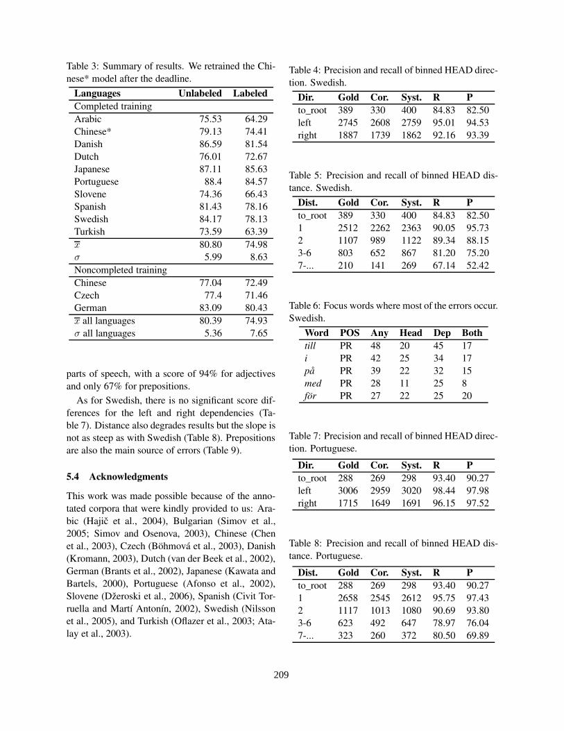
Table 3: Summary of results. We retrained the Chi-nese* model after the deadline.
Languages Unlabeled Labeled
Completed trainingArabic 75.53 64.29Chinese* 79.13 74.41Danish 86.59 81.54Dutch 76.01 72.67Japanese 87.11 85.63Portuguese 88.4 84.57Slovene 74.36 66.43Spanish 81.43 78.16Swedish 84.17 78.13Turkish 73.59 63.39x 80.80 74.98σ 5.99 8.63Noncompleted trainingChinese 77.04 72.49Czech 77.4 71.46German 83.09 80.43x all languages 80.39 74.93σ all languages 5.36 7.65
parts of speech, with a score of 94% for adjectivesand only 67% for prepositions.
As for Swedish, there is no significant score dif-ferences for the left and right dependencies (Ta-ble 7). Distance also degrades results but the slope isnot as steep as with Swedish (Table 8). Prepositionsare also the main source of errors (Table 9).
5.4 Acknowledgments
This work was made possible because of the anno-tated corpora that were kindly provided to us: Ara-bic (Hajic et al., 2004), Bulgarian (Simov et al.,2005; Simov and Osenova, 2003), Chinese (Chenet al., 2003), Czech (Böhmová et al., 2003), Danish(Kromann, 2003), Dutch (van der Beek et al., 2002),German (Brants et al., 2002), Japanese (Kawata andBartels, 2000), Portuguese (Afonso et al., 2002),Slovene (Džeroski et al., 2006), Spanish (Civit Tor-ruella and Martí Antonín, 2002), Swedish (Nilssonet al., 2005), and Turkish (Oflazer et al., 2003; Ata-lay et al., 2003).
Table 4: Precision and recall of binned HEAD direc-tion. Swedish.
Dir. Gold Cor. Syst. R P
to_root 389 330 400 84.83 82.50left 2745 2608 2759 95.01 94.53right 1887 1739 1862 92.16 93.39
Table 5: Precision and recall of binned HEAD dis-tance. Swedish.
Dist. Gold Cor. Syst. R P
to_root 389 330 400 84.83 82.501 2512 2262 2363 90.05 95.732 1107 989 1122 89.34 88.153-6 803 652 867 81.20 75.207-... 210 141 269 67.14 52.42
Table 6: Focus words where most of the errors occur.Swedish.
Word POS Any Head Dep Both
till PR 48 20 45 17i PR 42 25 34 17på PR 39 22 32 15med PR 28 11 25 8för PR 27 22 25 20
Table 7: Precision and recall of binned HEAD direc-tion. Portuguese.
Dir. Gold Cor. Syst. R P
to_root 288 269 298 93.40 90.27left 3006 2959 3020 98.44 97.98right 1715 1649 1691 96.15 97.52
Table 8: Precision and recall of binned HEAD dis-tance. Portuguese.
Dist. Gold Cor. Syst. R P
to_root 288 269 298 93.40 90.271 2658 2545 2612 95.75 97.432 1117 1013 1080 90.69 93.803-6 623 492 647 78.97 76.047-... 323 260 372 80.50 69.89
209
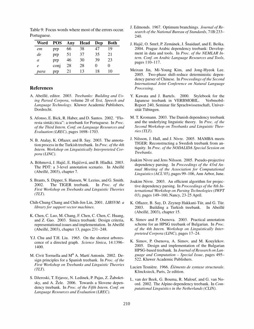
Table 9: Focus words where most of the errors occur.Portuguese.
Word POS Any Head Dep Both
em prp 66 38 47 19de prp 51 37 35 21a prp 46 30 39 23e conj 28 28 0 0para prp 21 13 18 10
References
A. Abeillé, editor. 2003. Treebanks: Building and Us-ing Parsed Corpora, volume 20 of Text, Speech andLanguage Technology. Kluwer Academic Publishers,Dordrecht.
S. Afonso, E. Bick, R. Haber, and D. Santos. 2002. “Flo-resta sintá(c)tica”: a treebank for Portuguese. In Proc.of the Third Intern. Conf. on Language Resources andEvaluation (LREC), pages 1698–1703.
N. B. Atalay, K. Oflazer, and B. Say. 2003. The annota-tion process in the Turkish treebank. In Proc. of the 4thIntern. Workshop on Linguistically Interpreteted Cor-pora (LINC).
A. Böhmová, J. Hajic, E. Hajicová, and B. Hladká. 2003.The PDT: a 3-level annotation scenario. In Abeillé(Abeillé, 2003), chapter 7.
S. Brants, S. Dipper, S. Hansen, W. Lezius, and G. Smith.2002. The TIGER treebank. In Proc. of theFirst Workshop on Treebanks and Linguistic Theories(TLT).
Chih-Chung Chang and Chih-Jen Lin, 2001. LIBSVM: alibrary for support vector machines.
K. Chen, C. Luo, M. Chang, F. Chen, C. Chen, C. Huang,and Z. Gao. 2003. Sinica treebank: Design criteria,representational issues and implementation. In Abeillé(Abeillé, 2003), chapter 13, pages 231–248.
Y.J. Chu and T.H. Liu. 1965. On the shortest arbores-cence of a directed graph. Science Sinica, 14:1396–1400.
M. Civit Torruella and Ma A. Martí Antonín. 2002. De-sign principles for a Spanish treebank. In Proc. of theFirst Workshop on Treebanks and Linguistic Theories(TLT).
S. Džeroski, T. Erjavec, N. Ledinek, P. Pajas, Z. Žabokrt-sky, and A. Žele. 2006. Towards a Slovene depen-dency treebank. In Proc. of the Fifth Intern. Conf. onLanguage Resources and Evaluation (LREC).
J. Edmonds. 1967. Optimum branchings. Journal of Re-search of the National Bureau of Standards, 71B:233–240.
J. Hajic, O. Smrž, P. Zemánek, J. Šnaidauf, and E. Beška.2004. Prague Arabic dependency treebank: Develop-ment in data and tools. In Proc. of the NEMLAR In-tern. Conf. on Arabic Language Resources and Tools,pages 110–117.
Meixun Jin, Mi-Young Kim, and Jong-Hyeok Lee.2005. Two-phase shift-reduce deterministic depen-dency parser of Chinese. In Proceedings of the SecondInternational Joint Conference on Natural LanguageProcessing.
Y. Kawata and J. Bartels. 2000. Stylebook for theJapanese treebank in VERBMOBIL. Verbmobil-Report 240, Seminar für Sprachwissenschaft, Univer-sität Tübingen.
M. T. Kromann. 2003. The Danish dependency treebankand the underlying linguistic theory. In Proc. of theSecond Workshop on Treebanks and Linguistic Theo-ries (TLT).
J. Nilsson, J. Hall, and J. Nivre. 2005. MAMBA meetsTIGER: Reconstructing a Swedish treebank from an-tiquity. In Proc. of the NODALIDA Special Session onTreebanks.
Joakim Nivre and Jens Nilsson. 2005. Pseudo-projectivedependency parsing. In Proceedings of the 43rd An-nual Meeting of the Association for ComputationalLinguistics (ACL’05), pages 99–106, Ann Arbor, June.
Joakim Nivre. 2003. An efficient algorithm for projec-tive dependency parsing. In Proceedings of the 8th In-ternational Workshop on Parsing Technologies (IWPT03), pages 149–160, Nancy, 23-25 April.
K. Oflazer, B. Say, D. Zeynep Hakkani-Tür, and G. Tür.2003. Building a Turkish treebank. In Abeillé(Abeillé, 2003), chapter 15.
K. Simov and P. Osenova. 2003. Practical annotationscheme for an HPSG treebank of Bulgarian. In Proc.of the 4th Intern. Workshop on Linguistically Inter-preteted Corpora (LINC), pages 17–24.
K. Simov, P. Osenova, A. Simov, and M. Kouylekov.2005. Design and implementation of the BulgarianHPSG-based treebank. In Journal of Research on Lan-guage and Computation – Special Issue, pages 495–522. Kluwer Academic Publishers.
Lucien Tesnière. 1966. Éléments de syntaxe structurale.Klincksieck, Paris, 2e edition.
L. van der Beek, G. Bouma, R. Malouf, and G. van No-ord. 2002. The Alpino dependency treebank. In Com-putational Linguistics in the Netherlands (CLIN).
210
Proceedings of the 10th Conference on Computational Natural Language Learning (CoNLL-X),pages 211–215, New York City, June 2006.c©2006 Association for Computational Linguistics
Dependency Parsing Based on Dynamic Local Optimization
Ting Liu Jinshan Ma Huijia Zhu Sheng LiInformation Retrieval Lab
Harbin Institute of TechnologyHarbin, 150001, China
{tliu,mjs,hjzhu,ls}@ir.hit.edu.cn
Abstract
This paper presents a deterministic pars-ing algorithm for projective dependencygrammar. In a bottom-up way the al-gorithm finds the local optimum dynam-ically. A constraint procedure is madeto use more structure information. Thealgorithm parses sentences in linear timeand labeling is integrated with the parsing.This parser achieves 63.29% labeled at-tachment score on the average in CoNLL-X Shared Task.
1 Introduction
Recently, dependency grammar has gained renewedattention in the parsing community. Good resultshave been achieved in some dependency parsers(Yamada and Matsumoto, 2003; Nivre et al., 2004).With the availability of many dependency treebanks(van der Beek et al., 2002; Hajic et al., 2004;Bohmova et al., 2003; Kromann, 2003; Dzeroski etal., 2006) and more other treebanks which can beconverted to dependency annotation (Brants et al.,2002; Nilsson et al., 2005; Chen et al., 2003; Kawataand Bartels, 2000), multi-lingual dependency pars-ing is proposed in CoNLL shared task (Buchholz etal., 2006).
Many previous works focus on unlabeled parsing,in which exhaustive methods are often used (Eis-ner, 1996). Their global searching performs wellin the unlabeled dependency parsing. But with theincrease of parameters, efficiency has to be consid-
ered in labeled dependency parsing. Thus determin-istic parsing was proposed as a robust and efficientmethod in recent years. Such method breaks theconstruction of dependency tree into a series of ac-tions. A classifier is often used to choose the mostprobable action to assemble the dependency tree.(Yamada and Matsumoto, 2003) defined three ac-tions and used a SVM classifier to choose one ofthem in a bottom-up way. The algorithm in (Nivreet al., 2004) is a blend of bottom-up and top-downprocessing. Its classifier is trained by memory-basedlearning.
Deterministic parsing derives an analysis withoutredundancy or backtracking, and linear time can beachieved. But when searching the local optimum inthe order of left-to-right, some wrong reduce mayprevent next analysis with more possibility. (Jin etal., 2005) used a two-phase shift-reduce to decreasesuch errors, and improved the accuracy of long dis-tance dependencies.
In this paper a deterministic parsing based on dy-namic local optimization is proposed. According tothe probabilities of dependency arcs, the algorithmdynamically finds the one with the highest probabil-ities instead of dealing with the sentence in order.A procedure of constraint which can integrate morestructure information is made to check the rational-ity of the reduce. Finally our results and error anal-ysis are presented.
2 Dependency Probabilities
An example of Chinese dependency tree is showedin Figure1. The tree can be represented as a directedgraph with nodes representing word tokens and arcs
211
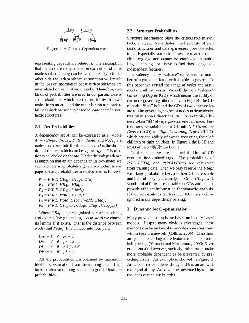
Figure 1: A Chinese dependency tree
representing dependency relations. The assumptionthat the arcs are independent on each other often ismade so that parsing can be handled easily. On theother side the independence assumption will resultin the loss of information because dependencies areinterrelated on each other actually. Therefore, twokinds of probabilities are used in our parser. One isarc probabilities which are the possibility that twonodes form an arc, and the other is structure proba-bilities which are used to describe some specific syn-tactic structures.
2.1 Arc Probabilities
A dependency arc Ai can be expressed as a 4-tupleAi = <Nodei, Nodej , D, R>. Nodei and Nodej arenodes that constitute the directed arc. D is the direc-tion of the arc, which can be left or right. R is rela-tion type labeled on the arc. Under the independenceassumption that an arc depends on its two nodes wecan calculate arc probability given two nodes. In ourpaper the arc probabilities are calculated as follows:
P1 = P(R,D|CTagi, CTagj , Dist)P2 = P(R,D|FTagi, FTagj)P3 = P(R,D|CTagi, Wordj)P4 = P(R,D|Wordi, CTagj)P5 = P(R,D|Wordi,CTagi, Wordj ,CTagj)P6 = P(R,D|CTagi−1, CTagi, CTagj , CTagj+1)
Where CTag is coarse-grained part of speech tagand FTag is fine-grained tag. As to Word we chooseits lemma if it exists. Dist is the distance betweenNodei and Nodej . It is divided into four parts:
Dist = 1 if j-i = 1Dist = 2 if j-i = 2Dist = 3 if 3 j-i 6Dist = 4 if j-i > 6
All the probabilities are obtained by maximumlikelihood estimation from the training data. Theninterpolation smoothing is made to get the final arcprobabilities.
2.2 Structure Probabilities
Structure information plays the critical role in syn-tactic analysis. Nevertheless the flexibility of syn-tactic structures and data sparseness pose obstaclesto us. Especially some structures are related to spe-cific language and cannot be employed in multi-lingual parsing. We have to find those language-independent features.
In valency theory “valence” represents the num-ber of arguments that a verb is able to govern. Inthis paper we extend the range of verbs and argu-ments to all the words. We call the new “valence”Governing Degree (GD), which means the ability ofone node governing other nodes. In Figure1, the GDof node “ ” is 2 and the GDs of two other nodesare 0. The governing degree of nodes in dependencytree often shows directionality. For example, Chi-nese token “ ” always governs one left node. Fur-thermore, we subdivide the GD into Left GoverningDegree (LGD) and Right Governing Degree (RGD),which are the ability of words governing their leftchildren or right children. In Figure 1 the LGD andRGD of verb “ ” are both 1.
In the paper we use the probabilities of GDover the fine-grained tags. The probabilities ofP(LDG|FTag) and P(RGD|FTag) are calculatedfrom training data. Then we only reserve the FTagswith large probability because their GDs are stableand helpful to syntactic analysis. Other FTags withsmall probabilities are unstable in GDs and cannotprovide efficient information for syntactic analysis.If their probabilities are less than 0.65 they will beignored in our dependency parsing.
3 Dynamic local optimization
Many previous methods are based on history-basedmodels. Despite many obvious advantages, thesemethods can be awkward to encode some constrainswithin their framework (Collins, 2000). Classifiersare good at encoding more features in the determin-istic parsing (Yamada and Matsumoto, 2003; Nivreet al., 2004). However, such algorithm often makemore probable dependencies be prevented by pre-ceding errors. An example is showed in Figure 2.Arc a is a frequent dependency and b is an arc withmore probability. Arc b will be prevented by a if thereduce is carried out in order.
212
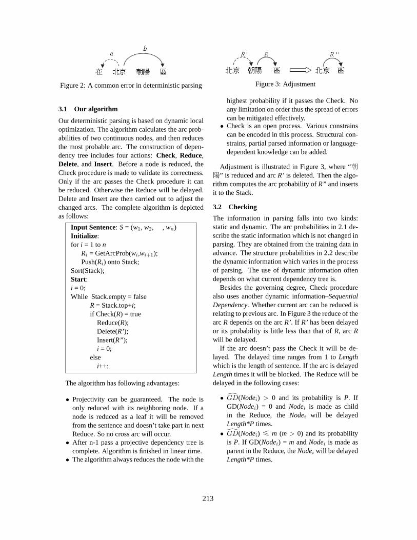
Figure 2: A common error in deterministic parsing
3.1 Our algorithm
Our deterministic parsing is based on dynamic localoptimization. The algorithm calculates the arc prob-abilities of two continuous nodes, and then reducesthe most probable arc. The construction of depen-dency tree includes four actions: Check, Reduce,Delete, and Insert. Before a node is reduced, theCheck procedure is made to validate its correctness.Only if the arc passes the Check procedure it canbe reduced. Otherwise the Reduce will be delayed.Delete and Insert are then carried out to adjust thechanged arcs. The complete algorithm is depictedas follows:
Input Sentence: S = (w1, w2, , wn)Initialize:for i = 1 to n
Ri = GetArcProb(wi,wi+1);Push(Ri) onto Stack;
Sort(Stack);Start:i = 0;While Stack.empty = false
R = Stack.top+i;if Check(R) = true
Reduce(R);Delete(R’);Insert(R”);i = 0;
elsei++;
The algorithm has following advantages:
• Projectivity can be guaranteed. The node isonly reduced with its neighboring node. If anode is reduced as a leaf it will be removedfrom the sentence and doesn’t take part in nextReduce. So no cross arc will occur.
• After n-1 pass a projective dependency tree iscomplete. Algorithm is finished in linear time.
• The algorithm always reduces the node with the
Figure 3: Adjustment
highest probability if it passes the Check. Noany limitation on order thus the spread of errorscan be mitigated effectively.
• Check is an open process. Various constrainscan be encoded in this process. Structural con-strains, partial parsed information or language-dependent knowledge can be added.
Adjustment is illustrated in Figure 3, where “” is reduced and arc R’ is deleted. Then the algo-
rithm computes the arc probability of R” and insertsit to the Stack.
3.2 Checking
The information in parsing falls into two kinds:static and dynamic. The arc probabilities in 2.1 de-scribe the static information which is not changed inparsing. They are obtained from the training data inadvance. The structure probabilities in 2.2 describethe dynamic information which varies in the processof parsing. The use of dynamic information oftendepends on what current dependency tree is.
Besides the governing degree, Check procedurealso uses another dynamic information–SequentialDependency. Whether current arc can be reduced isrelating to previous arc. In Figure 3 the reduce of thearc R depends on the arc R’. If R’ has been delayedor its probability is little less than that of R, arc Rwill be delayed.
If the arc doesn’t pass the Check it will be de-layed. The delayed time ranges from 1 to Lengthwhich is the length of sentence. If the arc is delayedLength times it will be blocked. The Reduce will bedelayed in the following cases:
• GD(Nodei) > 0 and its probability is P. IfGD(Nodei) = 0 and Nodei is made as childin the Reduce, the Nodei will be delayedLength*P times.
• GD(Nodei) m (m > 0) and its probabilityis P. If GD(Nodei) = m and Nodei is made asparent in the Reduce, the Nodei will be delayedLength*P times.
213
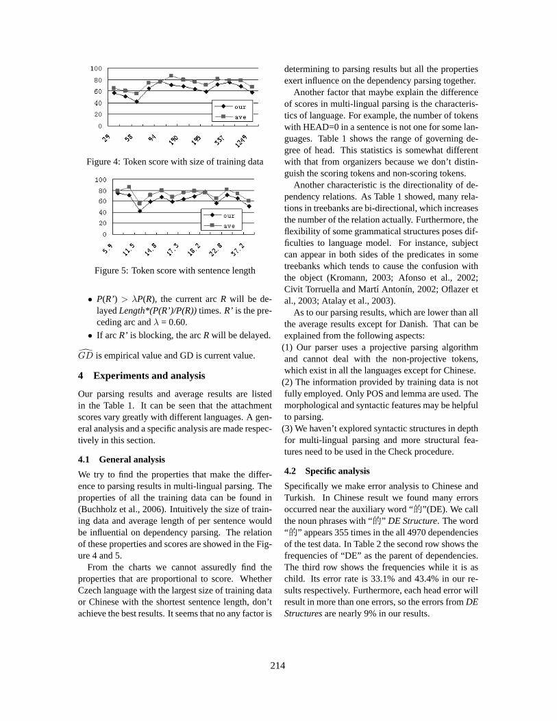
Figure 4: Token score with size of training data
Figure 5: Token score with sentence length
• P(R’) > λP(R), the current arc R will be de-layed Length*(P(R’)/P(R)) times. R’ is the pre-ceding arc and λ = 0.60.
• If arc R’ is blocking, the arc R will be delayed.
GD is empirical value and GD is current value.
4 Experiments and analysis
Our parsing results and average results are listedin the Table 1. It can be seen that the attachmentscores vary greatly with different languages. A gen-eral analysis and a specific analysis are made respec-tively in this section.
4.1 General analysis
We try to find the properties that make the differ-ence to parsing results in multi-lingual parsing. Theproperties of all the training data can be found in(Buchholz et al., 2006). Intuitively the size of train-ing data and average length of per sentence wouldbe influential on dependency parsing. The relationof these properties and scores are showed in the Fig-ure 4 and 5.
From the charts we cannot assuredly find theproperties that are proportional to score. WhetherCzech language with the largest size of training dataor Chinese with the shortest sentence length, don’tachieve the best results. It seems that no any factor is
determining to parsing results but all the propertiesexert influence on the dependency parsing together.
Another factor that maybe explain the differenceof scores in multi-lingual parsing is the characteris-tics of language. For example, the number of tokenswith HEAD=0 in a sentence is not one for some lan-guages. Table 1 shows the range of governing de-gree of head. This statistics is somewhat differentwith that from organizers because we don’t distin-guish the scoring tokens and non-scoring tokens.
Another characteristic is the directionality of de-pendency relations. As Table 1 showed, many rela-tions in treebanks are bi-directional, which increasesthe number of the relation actually. Furthermore, theflexibility of some grammatical structures poses dif-ficulties to language model. For instance, subjectcan appear in both sides of the predicates in sometreebanks which tends to cause the confusion withthe object (Kromann, 2003; Afonso et al., 2002;Civit Torruella and Martı Antonın, 2002; Oflazer etal., 2003; Atalay et al., 2003).
As to our parsing results, which are lower than allthe average results except for Danish. That can beexplained from the following aspects:
(1) Our parser uses a projective parsing algorithmand cannot deal with the non-projective tokens,which exist in all the languages except for Chinese.
(2) The information provided by training data is notfully employed. Only POS and lemma are used. Themorphological and syntactic features may be helpfulto parsing.
(3) We haven’t explored syntactic structures in depthfor multi-lingual parsing and more structural fea-tures need to be used in the Check procedure.
4.2 Specific analysis
Specifically we make error analysis to Chinese andTurkish. In Chinese result we found many errorsoccurred near the auxiliary word “ ”(DE). We callthe noun phrases with “ ” DE Structure. The word“ ” appears 355 times in the all 4970 dependenciesof the test data. In Table 2 the second row shows thefrequencies of “DE” as the parent of dependencies.The third row shows the frequencies while it is aschild. Its error rate is 33.1% and 43.4% in our re-sults respectively. Furthermore, each head error willresult in more than one errors, so the errors from DEStructures are nearly 9% in our results.
214
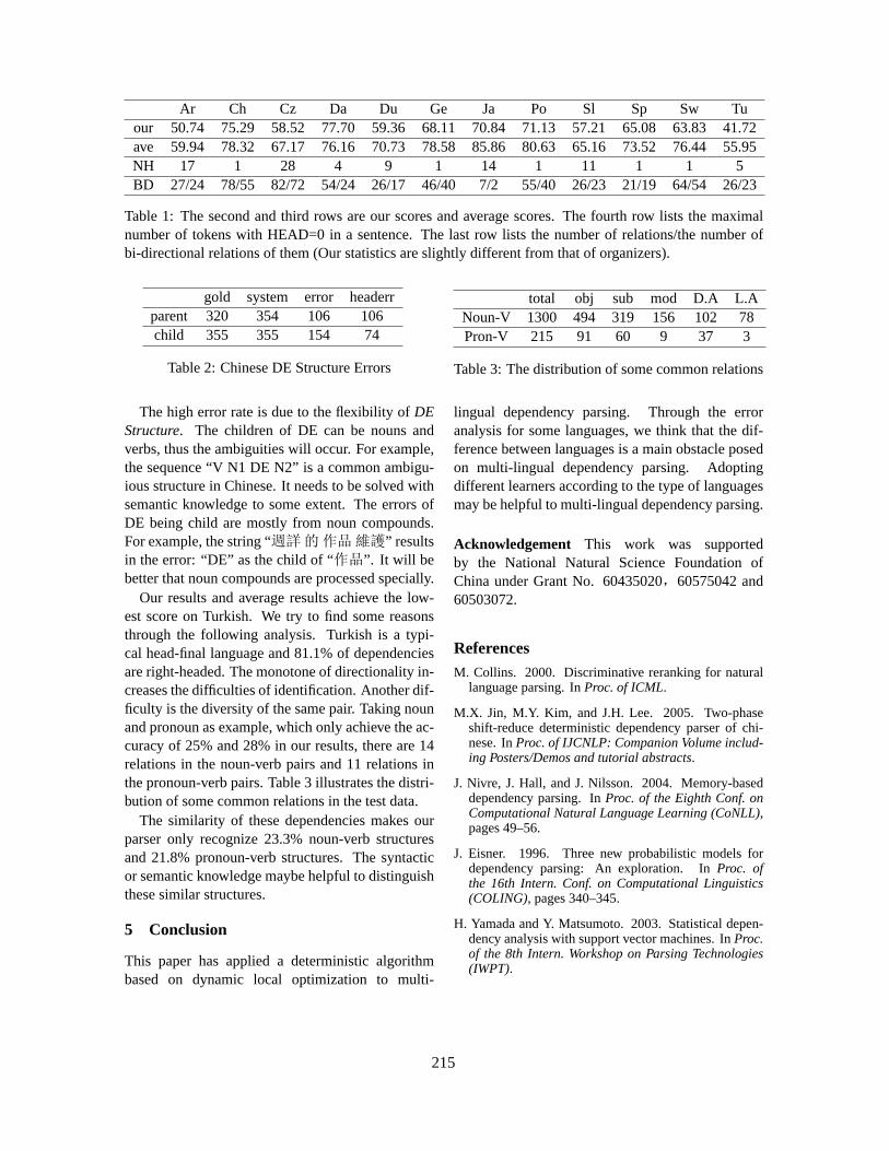
Ar Ch Cz Da Du Ge Ja Po Sl Sp Sw Tuour 50.74 75.29 58.52 77.70 59.36 68.11 70.84 71.13 57.21 65.08 63.83 41.72ave 59.94 78.32 67.17 76.16 70.73 78.58 85.86 80.63 65.16 73.52 76.44 55.95NH 17 1 28 4 9 1 14 1 11 1 1 5BD 27/24 78/55 82/72 54/24 26/17 46/40 7/2 55/40 26/23 21/19 64/54 26/23
Table 1: The second and third rows are our scores and average scores. The fourth row lists the maximalnumber of tokens with HEAD=0 in a sentence. The last row lists the number of relations/the number ofbi-directional relations of them (Our statistics are slightly different from that of organizers).
gold system error headerrparent 320 354 106 106child 355 355 154 74
Table 2: Chinese DE Structure Errors
The high error rate is due to the flexibility of DEStructure. The children of DE can be nouns andverbs, thus the ambiguities will occur. For example,the sequence “V N1 DE N2” is a common ambigu-ious structure in Chinese. It needs to be solved withsemantic knowledge to some extent. The errors ofDE being child are mostly from noun compounds.For example, the string “ ” resultsin the error: “DE” as the child of “ ”. It will bebetter that noun compounds are processed specially.
Our results and average results achieve the low-est score on Turkish. We try to find some reasonsthrough the following analysis. Turkish is a typi-cal head-final language and 81.1% of dependenciesare right-headed. The monotone of directionality in-creases the difficulties of identification. Another dif-ficulty is the diversity of the same pair. Taking nounand pronoun as example, which only achieve the ac-curacy of 25% and 28% in our results, there are 14relations in the noun-verb pairs and 11 relations inthe pronoun-verb pairs. Table 3 illustrates the distri-bution of some common relations in the test data.
The similarity of these dependencies makes ourparser only recognize 23.3% noun-verb structuresand 21.8% pronoun-verb structures. The syntacticor semantic knowledge maybe helpful to distinguishthese similar structures.
5 Conclusion
This paper has applied a deterministic algorithmbased on dynamic local optimization to multi-
total obj sub mod D.A L.ANoun-V 1300 494 319 156 102 78Pron-V 215 91 60 9 37 3
Table 3: The distribution of some common relations
lingual dependency parsing. Through the erroranalysis for some languages, we think that the dif-ference between languages is a main obstacle posedon multi-lingual dependency parsing. Adoptingdifferent learners according to the type of languagesmay be helpful to multi-lingual dependency parsing.
Acknowledgement This work was supportedby the National Natural Science Foundation ofChina under Grant No. 60435020 60575042 and60503072.
ReferencesM. Collins. 2000. Discriminative reranking for natural
language parsing. In Proc. of ICML.
M.X. Jin, M.Y. Kim, and J.H. Lee. 2005. Two-phaseshift-reduce deterministic dependency parser of chi-nese. In Proc. of IJCNLP: Companion Volume includ-ing Posters/Demos and tutorial abstracts.
J. Nivre, J. Hall, and J. Nilsson. 2004. Memory-baseddependency parsing. In Proc. of the Eighth Conf. onComputational Natural Language Learning (CoNLL),pages 49–56.
J. Eisner. 1996. Three new probabilistic models fordependency parsing: An exploration. In Proc. ofthe 16th Intern. Conf. on Computational Linguistics(COLING), pages 340–345.
H. Yamada and Y. Matsumoto. 2003. Statistical depen-dency analysis with support vector machines. In Proc.of the 8th Intern. Workshop on Parsing Technologies(IWPT).
215
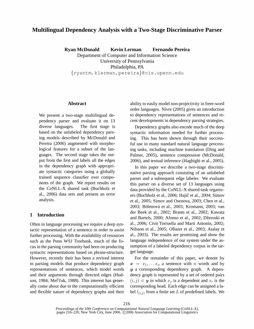
Proceedings of the 10th Conference on Computational Natural Language Learning (CoNLL-X),pages 216–220, New York City, June 2006.c©2006 Association for Computational Linguistics
Multilingual Dependency Analysis with a Two-Stage Discriminative Parser
Ryan McDonald Kevin Lerman Fernando PereiraDepartment of Computer and Information Science
University of PennsylvaniaPhiladelphia, PA
{ryantm,klerman,pereira}@cis.upenn.edu
Abstract
We present a two-stage multilingual de-pendency parser and evaluate it on 13diverse languages. The first stage isbased on the unlabeled dependency pars-ing models described by McDonald andPereira (2006) augmented with morpho-logical features for a subset of the lan-guages. The second stage takes the out-put from the first and labels all the edgesin the dependency graph with appropri-ate syntactic categories using a globallytrained sequence classifier over compo-nents of the graph. We report results onthe CoNLL-X shared task (Buchholz etal., 2006) data sets and present an erroranalysis.
1 Introduction
Often in language processing we require a deep syn-tactic representation of a sentence in order to assistfurther processing. With the availability of resourcessuch as the Penn WSJ Treebank, much of the fo-cus in the parsing community had been on producingsyntactic representations based on phrase-structure.However, recently their has been a revived interestin parsing models that produce dependency graphrepresentations of sentences, which model wordsand their arguments through directed edges (Hud-son, 1984; Mel′cuk, 1988). This interest has gener-ally come about due to the computationally efficientand flexible nature of dependency graphs and their
ability to easily model non-projectivity in freer-wordorder languages. Nivre (2005) gives an introductionto dependency representations of sentences and re-cent developments in dependency parsing strategies.
Dependency graphs also encode much of the deepsyntactic information needed for further process-ing. This has been shown through their success-ful use in many standard natural language process-ing tasks, including machine translation (Ding andPalmer, 2005), sentence compression (McDonald,2006), and textual inference (Haghighi et al., 2005).
In this paper we describe a two-stage discrimi-native parsing approach consisting of an unlabeledparser and a subsequent edge labeler. We evaluatethis parser on a diverse set of 13 languages usingdata provided by the CoNLL-X shared-task organiz-ers (Buchholz et al., 2006; Hajic et al., 2004; Simovet al., 2005; Simov and Osenova, 2003; Chen et al.,2003; Bohmova et al., 2003; Kromann, 2003; vander Beek et al., 2002; Brants et al., 2002; Kawataand Bartels, 2000; Afonso et al., 2002; Dzeroski etal., 2006; Civit Torruella and Martı Antonın, 2002;Nilsson et al., 2005; Oflazer et al., 2003; Atalay etal., 2003). The results are promising and show thelanguage independence of our system under the as-sumption of a labeled dependency corpus in the tar-get language.
For the remainder of this paper, we denote byx = x1, . . . xn a sentence withn words and byy a corresponding dependency graph. A depen-dency graph is represented by a set of ordered pairs(i, j) ∈ y in which xj is a dependent andxi is thecorresponding head. Each edge can be assigned a la-bel l(i,j) from a finite setL of predefined labels. We
216
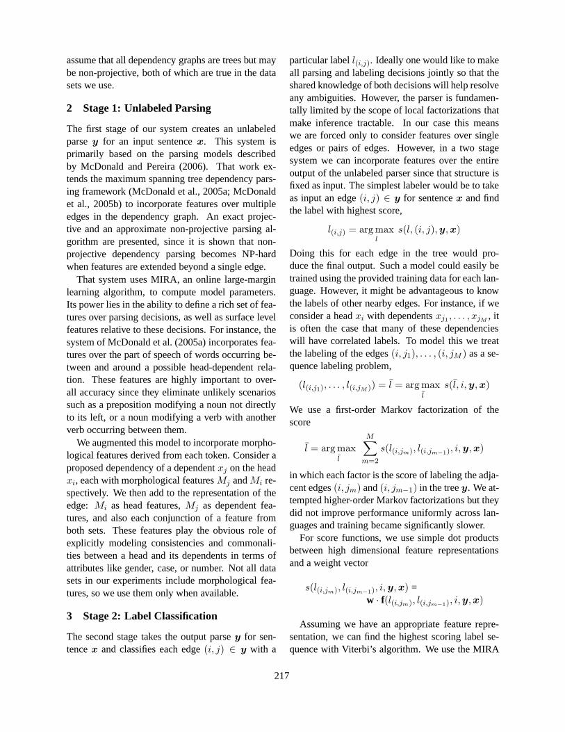
assume that all dependency graphs are trees but maybe non-projective, both of which are true in the datasets we use.
2 Stage 1: Unlabeled Parsing
The first stage of our system creates an unlabeledparsey for an input sentencex. This system isprimarily based on the parsing models describedby McDonald and Pereira (2006). That work ex-tends the maximum spanning tree dependency pars-ing framework (McDonald et al., 2005a; McDonaldet al., 2005b) to incorporate features over multipleedges in the dependency graph. An exact projec-tive and an approximate non-projective parsing al-gorithm are presented, since it is shown that non-projective dependency parsing becomes NP-hardwhen features are extended beyond a single edge.
That system uses MIRA, an online large-marginlearning algorithm, to compute model parameters.Its power lies in the ability to define a rich set of fea-tures over parsing decisions, as well as surface levelfeatures relative to these decisions. For instance, thesystem of McDonald et al. (2005a) incorporates fea-tures over the part of speech of words occurring be-tween and around a possible head-dependent rela-tion. These features are highly important to over-all accuracy since they eliminate unlikely scenariossuch as a preposition modifying a noun not directlyto its left, or a noun modifying a verb with anotherverb occurring between them.
We augmented this model to incorporate morpho-logical features derived from each token. Consider aproposed dependency of a dependentxj on the headxi, each with morphological featuresMj andMi re-spectively. We then add to the representation of theedge: Mi as head features,Mj as dependent fea-tures, and also each conjunction of a feature fromboth sets. These features play the obvious role ofexplicitly modeling consistencies and commonali-ties between a head and its dependents in terms ofattributes like gender, case, or number. Not all datasets in our experiments include morphological fea-tures, so we use them only when available.
3 Stage 2: Label Classification
The second stage takes the output parsey for sen-tencex and classifies each edge(i, j) ∈ y with a
particular labell(i,j). Ideally one would like to makeall parsing and labeling decisions jointly so that theshared knowledge of both decisions will help resolveany ambiguities. However, the parser is fundamen-tally limited by the scope of local factorizations thatmake inference tractable. In our case this meanswe are forced only to consider features over singleedges or pairs of edges. However, in a two stagesystem we can incorporate features over the entireoutput of the unlabeled parser since that structure isfixed as input. The simplest labeler would be to takeas input an edge(i, j) ∈ y for sentencex and findthe label with highest score,
l(i,j) = arg maxl
s(l, (i, j),y,x)
Doing this for each edge in the tree would pro-duce the final output. Such a model could easily betrained using the provided training data for each lan-guage. However, it might be advantageous to knowthe labels of other nearby edges. For instance, if weconsider a headxi with dependentsxj1 , . . . , xjM
, itis often the case that many of these dependencieswill have correlated labels. To model this we treatthe labeling of the edges(i, j1), . . . , (i, jM ) as a se-quence labeling problem,
(l(i,j1), . . . , l(i,jM )) = l = arg maxl
s(l, i,y,x)
We use a first-order Markov factorization of thescore
l = arg maxl
M∑
m=2
s(l(i,jm), l(i,jm−1), i,y,x)
in which each factor is the score of labeling the adja-cent edges(i, jm) and(i, jm−1) in the treey. We at-tempted higher-order Markov factorizations but theydid not improve performance uniformly across lan-guages and training became significantly slower.
For score functions, we use simple dot productsbetween high dimensional feature representationsand a weight vector
s(l(i,jm), l(i,jm−1), i,y,x) =w · f(l(i,jm), l(i,jm−1), i,y,x)
Assuming we have an appropriate feature repre-sentation, we can find the highest scoring label se-quence with Viterbi’s algorithm. We use the MIRA
217
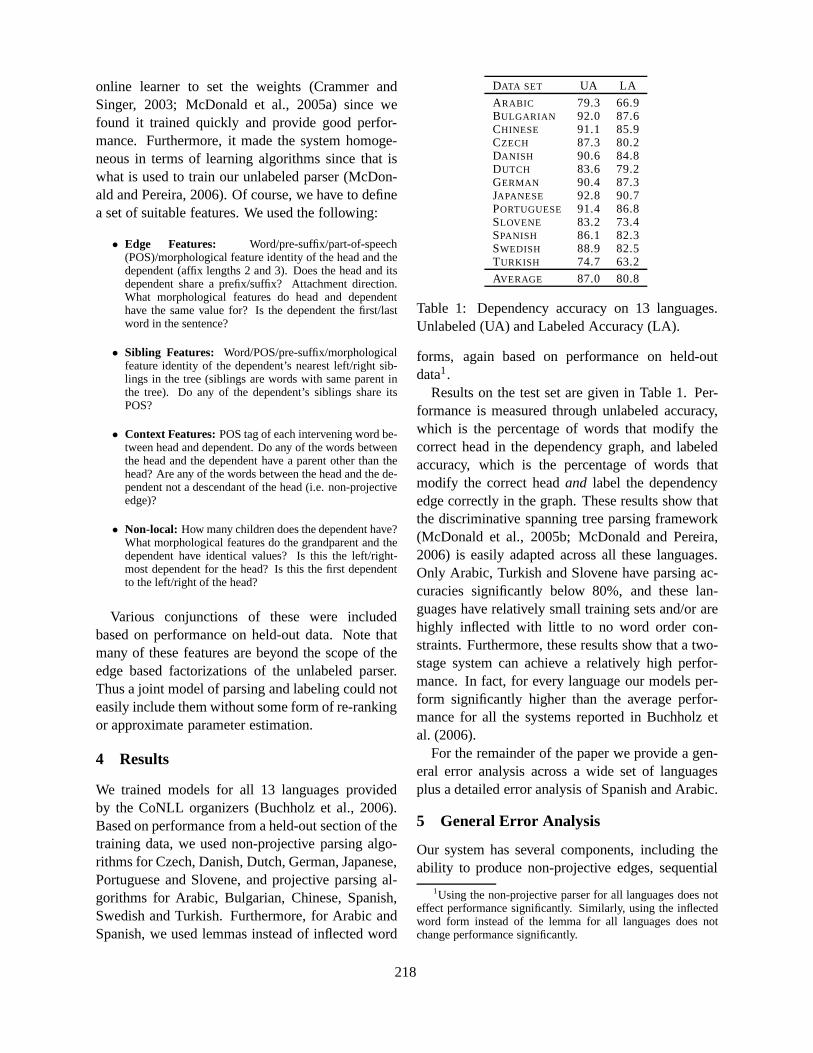
online learner to set the weights (Crammer andSinger, 2003; McDonald et al., 2005a) since wefound it trained quickly and provide good perfor-mance. Furthermore, it made the system homoge-neous in terms of learning algorithms since that iswhat is used to train our unlabeled parser (McDon-ald and Pereira, 2006). Of course, we have to definea set of suitable features. We used the following:
• Edge Features: Word/pre-suffix/part-of-speech(POS)/morphological feature identity of the head and thedependent (affix lengths 2 and 3). Does the head and itsdependent share a prefix/suffix? Attachment direction.What morphological features do head and dependenthave the same value for? Is the dependent the first/lastword in the sentence?
• Sibling Features: Word/POS/pre-suffix/morphologicalfeature identity of the dependent’s nearest left/right sib-lings in the tree (siblings are words with same parent inthe tree). Do any of the dependent’s siblings share itsPOS?
• Context Features:POS tag of each intervening word be-tween head and dependent. Do any of the words betweenthe head and the dependent have a parent other than thehead? Are any of the words between the head and the de-pendent not a descendant of the head (i.e. non-projectiveedge)?
• Non-local: How many children does the dependent have?What morphological features do the grandparent and thedependent have identical values? Is this the left/right-most dependent for the head? Is this the first dependentto the left/right of the head?
Various conjunctions of these were includedbased on performance on held-out data. Note thatmany of these features are beyond the scope of theedge based factorizations of the unlabeled parser.Thus a joint model of parsing and labeling could noteasily include them without some form of re-rankingor approximate parameter estimation.
4 Results
We trained models for all 13 languages providedby the CoNLL organizers (Buchholz et al., 2006).Based on performance from a held-out section of thetraining data, we used non-projective parsing algo-rithms for Czech, Danish, Dutch, German, Japanese,Portuguese and Slovene, and projective parsing al-gorithms for Arabic, Bulgarian, Chinese, Spanish,Swedish and Turkish. Furthermore, for Arabic andSpanish, we used lemmas instead of inflected word
DATA SET UA LA
ARABIC 79.3 66.9BULGARIAN 92.0 87.6CHINESE 91.1 85.9CZECH 87.3 80.2DANISH 90.6 84.8DUTCH 83.6 79.2GERMAN 90.4 87.3JAPANESE 92.8 90.7PORTUGUESE 91.4 86.8SLOVENE 83.2 73.4SPANISH 86.1 82.3SWEDISH 88.9 82.5TURKISH 74.7 63.2
AVERAGE 87.0 80.8
Table 1: Dependency accuracy on 13 languages.Unlabeled (UA) and Labeled Accuracy (LA).
forms, again based on performance on held-outdata1.
Results on the test set are given in Table 1. Per-formance is measured through unlabeled accuracy,which is the percentage of words that modify thecorrect head in the dependency graph, and labeledaccuracy, which is the percentage of words thatmodify the correct headand label the dependencyedge correctly in the graph. These results show thatthe discriminative spanning tree parsing framework(McDonald et al., 2005b; McDonald and Pereira,2006) is easily adapted across all these languages.Only Arabic, Turkish and Slovene have parsing ac-curacies significantly below 80%, and these lan-guages have relatively small training sets and/or arehighly inflected with little to no word order con-straints. Furthermore, these results show that a two-stage system can achieve a relatively high perfor-mance. In fact, for every language our models per-form significantly higher than the average perfor-mance for all the systems reported in Buchholz etal. (2006).
For the remainder of the paper we provide a gen-eral error analysis across a wide set of languagesplus a detailed error analysis of Spanish and Arabic.
5 General Error Analysis
Our system has several components, including theability to produce non-projective edges, sequential
1Using the non-projective parser for all languages does noteffect performance significantly. Similarly, using the inflectedword form instead of the lemma for all languages does notchange performance significantly.
218
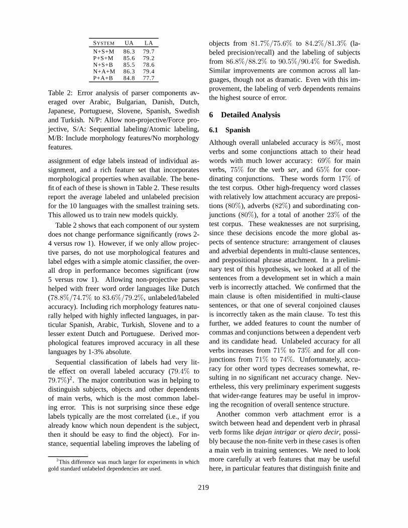
SYSTEM UA LA
N+S+M 86.3 79.7P+S+M 85.6 79.2N+S+B 85.5 78.6N+A+M 86.3 79.4P+A+B 84.8 77.7
Table 2: Error analysis of parser components av-eraged over Arabic, Bulgarian, Danish, Dutch,Japanese, Portuguese, Slovene, Spanish, Swedishand Turkish. N/P: Allow non-projective/Force pro-jective, S/A: Sequential labeling/Atomic labeling,M/B: Include morphology features/No morphologyfeatures.
assignment of edge labels instead of individual as-signment, and a rich feature set that incorporatesmorphological properties when available. The bene-fit of each of these is shown in Table 2. These resultsreport the average labeled and unlabeled precisionfor the 10 languages with the smallest training sets.This allowed us to train new models quickly.
Table 2 shows that each component of our systemdoes not change performance significantly (rows 2-4 versus row 1). However, if we only allow projec-tive parses, do not use morphological features andlabel edges with a simple atomic classifier, the over-all drop in performance becomes significant (row5 versus row 1). Allowing non-projective parseshelped with freer word order languages like Dutch(78.8%/74.7% to 83.6%/79.2%, unlabeled/labeledaccuracy). Including rich morphology features natu-rally helped with highly inflected languages, in par-ticular Spanish, Arabic, Turkish, Slovene and to alesser extent Dutch and Portuguese. Derived mor-phological features improved accuracy in all theselanguages by 1-3% absolute.
Sequential classification of labels had very lit-tle effect on overall labeled accuracy (79.4% to79.7%)2. The major contribution was in helping todistinguish subjects, objects and other dependentsof main verbs, which is the most common label-ing error. This is not surprising since these edgelabels typically are the most correlated (i.e., if youalready know which noun dependent is the subject,then it should be easy to find the object). For in-stance, sequential labeling improves the labeling of
2This difference was much larger for experiments in whichgold standard unlabeled dependencies are used.
objects from81.7%/75.6% to 84.2%/81.3% (la-beled precision/recall) and the labeling of subjectsfrom 86.8%/88.2% to 90.5%/90.4% for Swedish.Similar improvements are common across all lan-guages, though not as dramatic. Even with this im-provement, the labeling of verb dependents remainsthe highest source of error.
6 Detailed Analysis
6.1 Spanish
Although overall unlabeled accuracy is86%, mostverbs and some conjunctions attach to their headwords with much lower accuracy:69% for mainverbs, 75% for the verb ser, and 65% for coor-dinating conjunctions. These words form17% ofthe test corpus. Other high-frequency word classeswith relatively low attachment accuracy are preposi-tions (80%), adverbs (82%) and subordinating con-junctions (80%), for a total of another23% of thetest corpus. These weaknesses are not surprising,since these decisions encode the more global as-pects of sentence structure: arrangement of clausesand adverbial dependents in multi-clause sentences,and prepositional phrase attachment. In a prelimi-nary test of this hypothesis, we looked at all of thesentences from a development set in which a mainverb is incorrectly attached. We confirmed that themain clause is often misidentified in multi-clausesentences, or that one of several conjoined clausesis incorrectly taken as the main clause. To test thisfurther, we added features to count the number ofcommas and conjunctions between a dependent verband its candidate head. Unlabeled accuracy for allverbs increases from71% to 73% and for all con-junctions from71% to 74%. Unfortunately, accu-racy for other word types decreases somewhat, re-sulting in no significant net accuracy change. Nev-ertheless, this very preliminary experiment suggeststhat wider-range features may be useful in improv-ing the recognition of overall sentence structure.
Another common verb attachment error is aswitch between head and dependent verb in phrasalverb forms likedejan intrigar or qiero decir, possi-bly because the non-finite verb in these cases is oftena main verb in training sentences. We need to lookmore carefully at verb features that may be usefulhere, in particular features that distinguish finite and
219
non-finite forms.In doing this preliminary analysis, we noticed
some inconsistencies in the reference dependencystructures. For example, in the test sentenceLoque decia Mae West de si misma podrıamos decirlotambien los hombres:..., decia’s head is given asde-cirlo, although the main verbs of relative clauses arenormally dependent on what the relative modifies, inthis case the articleLo.
6.2 Arabic
A quick look at unlabeled attachment accuracies in-dicate that errors in Arabic parsing are the mostcommon across all languages: prepositions (62%),conjunctions (69%) and to a lesser extent verbs(73%). Similarly, for labeled accuracy, the hard-est edges to label are for dependents of verbs, i.e.,subjects, objects and adverbials. Note the differ-ence in error between the unlabeled parser and theedge labeler: the former makes mistakes on edgesinto prepositions, conjunctions and verbs, and thelatter makes mistakes on edges into nouns (sub-ject/objects). Each stage by itself is relatively ac-curate (unlabeled accuracy is79% and labeling ac-curacy3 is also79%), but since there is very littleoverlap in the kinds of errors each makes, overall la-beled accuracy drops to67%. This drop is not nearlyas significant for other languages.
Another source of potential error is that the aver-age sentence length of Arabic is much higher thanother languages (around 37 words/sentence). How-ever, if we only look at performance for sentencesof length less than 30, the labeled accuracy is stillonly 71%. The fact that Arabic has only 1500 train-ing instances might also be problematic. For exam-ple if we train on 200, 400, 800 and the full trainingset, labeled accuracies are54%, 60%, 62% and67%.Clearly adding more data is improving performance.However, when compared to the performance ofSlovene (1500 training instances) and Spanish (3300instances), it appears that Arabic parsing is lagging.
7 Conclusions
We have presented results showing that the spanningtree dependency parsing framework of McDonald et
3Labeling accuracy is the percentage of words that correctlylabel the dependency between the head that they modify, evenif the right head was not identified.
al. (McDonald et al., 2005b; McDonald and Pereira,2006) generalizes well to languages other than En-glish. In the future we plan to extend these mod-els in two ways. First, we plan on examining theperformance difference between two-staged depen-dency parsing (as presented here) and joint parsingplus labeling. It is our hypothesis that for languageswith fine-grained label sets, joint parsing and label-ing will improve performance. Second, we plan onintegrating any available morphological features ina more principled manner. The current system sim-ply includes all morphological bi-gram features. Itis our hope that a better morphological feature setwill help with both unlabeled parsing and labelingfor highly inflected languages.
ReferencesS. Buchholz, E. Marsi, A. Dubey, and Y. Krymolowski.
2006. CoNLL-X shared task on multilingual depen-dency parsing. SIGNLL.
K. Crammer and Y. Singer. 2003. Ultraconservative on-line algorithms for multiclass problems.JMLR.
Y. Ding and M. Palmer. 2005. Machine translation usingprobabilistic synchronous dependency insertion gram-mars. InProc. ACL.
A. Haghighi, A. Ng, and C. Manning. 2005. Robusttextual inference via graph matching. InProc. HTL-EMNLP.
R. Hudson. 1984.Word Grammar. Blackwell.
R. McDonald and F. Pereira. 2006. Online learning ofapproximate dependency parsing algorithms. InProc.EACL.
R. McDonald, K. Crammer, and F. Pereira. 2005a. On-line large-margin training of dependency parsers. InProc. ACL.
R. McDonald, F. Pereira, K. Ribarov, and J. Hajic. 2005b.Non-projective dependency parsing using spanningtree algorithms. InProc. HLT-EMNLP.
R. McDonald. 2006. Discriminative sentence compres-sion with soft syntactic constraints. InProc. EACL.
I.A. Mel′cuk. 1988. Dependency Syntax: Theory andPractice. State University of New York Press.
J. Nivre. 2005. Dependency grammar and dependencyparsing. Technical Report MSI report 05133, VaxjoUniversity: School of Mathematics and Systems Engi-neering.
220
Proceedings of the 10th Conference on Computational Natural Language Learning (CoNLL-X),pages 221–225, New York City, June 2006.c©2006 Association for Computational Linguistics
Labeled Pseudo-Projective Dependency Parsingwith Support Vector Machines
Joakim NivreJohan Hall
Jens NilssonSchool of Mathematics
and Systems EngineeringVaxjo University
35195 Vaxjo, Sweden{nivre,jha,jni}@msi.vxu.se
Gulsen EryigitDepartment of
Computer EngineeringIstanbul Technical University
34469 Istanbul, [email protected]
Svetoslav MarinovSchool of Humanities
and InformaticsUniversity of Skovde
Box 40854128 Skovde, Sweden
Abstract
We use SVM classifiers to predict the nextaction of a deterministic parser that buildslabeled projective dependency graphs inan incremental fashion. Non-projectivedependencies are captured indirectly byprojectivizing the training data for theclassifiers and applying an inverse trans-formation to the output of the parser. Wepresent evaluation results and an erroranalysis focusing on Swedish and Turkish.
1 Introduction
The CoNLL-X shared task consists in parsing textsin multiple languages using a single dependencyparser that has the capacity to learn from treebankdata. Our methodology for performing this task isbased on four essential components:
• A deterministic algorithm for building labeledprojective dependency graphs (Nivre, 2006).
• History-based feature models for predicting thenext parser action (Black et al., 1992).
• Support vector machines for mapping historiesto parser actions (Kudo and Matsumoto, 2002).
• Graph transformations for recovering non-projective structures (Nivre and Nilsson, 2005).
All experiments have been performed using Malt-Parser (Nivre et al., 2006), version 0.4, which ismade available together with the suite of programsused for pre- and post-processing.1
1www.msi.vxu.se/users/nivre/research/MaltParser.html
2 Parsing Methodology
2.1 Parsing Algorithm
The parsing algorithm used for all languages is thedeterministic algorithm first proposed for unlabeleddependency parsing by Nivre (2003) and extendedto labeled dependency parsing by Nivre et al. (2004).The algorithm builds a labeled dependency graph inone left-to-right pass over the input, using a stackto store partially processed tokens and adding arcsusing four elementary actions (wheretop is the tokenon top of the stack andnextis the next token):
• SHIFT: Pushnextonto the stack.• REDUCE: Pop the stack.• RIGHT-ARC(r): Add an arc labeledr from top
to next; pushnextonto the stack.• LEFT-ARC(r): Add an arc labeledr from next
to top; pop the stack.
Although the parser only derives projective graphs,the fact that graphs are labeled allows non-projectivedependencies to be captured using the pseudo-projective approach of Nivre and Nilsson (2005) .
Another limitation of the parsing algorithm is thatit does not assign dependency labels to roots, i.e., totokens havingHEAD=0. To overcome this problem,we have implemented a variant of the algorithm thatstarts by pushing an artificial root token withID=0onto the stack. Tokens havingHEAD=0 can nowbe attached to the artificial root in a RIGHT-ARC(r)action, which means that they can be assigned anylabel. Since this variant of the algorithm increasesthe overall nondeterminism, it has only been usedfor the data sets that include informative root labels(Arabic, Czech, Portuguese, Slovene).
221
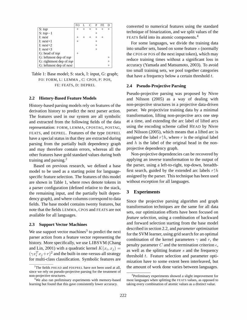
FO L C P FE D
S: top + + + + + +S: top−1 +I: next + + + + +I: next+1 + +I: next+2 +I: next+3 +G: head oftop +G: leftmost dep oftop +G: rightmost dep oftop +G: leftmost dep ofnext +
Table 1: Base model; S: stack, I: input, G: graph;FO: FORM, L: LEMMA , C: CPOS, P: POS,
FE: FEATS, D: DEPREL
2.2 History-Based Feature Models
History-based parsing models rely on features of thederivation history to predict the next parser action.The features used in our system are all symbolicand extracted from the following fields of the datarepresentation:FORM, LEMMA , CPOSTAG, POSTAG,FEATS, andDEPREL. Features of the typeDEPREL
have a special status in that they are extracted duringparsing from the partially built dependency graphand may therefore contain errors, whereas all theother features have gold standard values during bothtraining and parsing.2
Based on previous research, we defined a basemodel to be used as a starting point for language-specific feature selection. The features of this modelare shown in Table 1, where rows denote tokens ina parser configuration (defined relative to the stack,the remaining input, and the partially built depen-dency graph), and where columns correspond to datafields. The base model contains twenty features, butnote that the fieldsLEMMA , CPOSandFEATSare notavailable for all languages.
2.3 Support Vector Machines
We use support vector machines3 to predict the nextparser action from a feature vector representing thehistory. More specifically, we use LIBSVM (Changand Lin, 2001) with a quadratic kernelK(xi, xj) =(γxT
i xj +r)2 and the built-in one-versus-all strategyfor multi-class classification. Symbolic features are
2The fieldsPHEAD andPDEPRELhave not been used at all,since we rely on pseudo-projective parsing for the treatment ofnon-projective structures.
3We also ran preliminary experiments with memory-basedlearning but found that this gave consistently lower accuracy.
converted to numerical features using the standardtechnique of binarization, and we split values of theFEATSfield into its atomic components.4
For some languages, we divide the training datainto smaller sets, based on some features (normallytheCPOSor POSof the next input token), which mayreduce training times without a significant loss inaccuracy (Yamada and Matsumoto, 2003). To avoidtoo small training sets, we pool together categoriesthat have a frequency below a certain thresholdt.
2.4 Pseudo-Projective Parsing
Pseudo-projective parsing was proposed by Nivreand Nilsson (2005) as a way of dealing withnon-projective structures in a projective data-drivenparser. We projectivize training data by a minimaltransformation, lifting non-projective arcs one stepat a time, and extending the arc label of lifted arcsusing the encoding scheme called HEAD by Nivreand Nilsson (2005), which means that a lifted arc isassigned the labelr↑h, wherer is the original labelandh is the label of the original head in the non-projective dependency graph.
Non-projective dependencies can be recovered byapplying an inverse transformation to the output ofthe parser, using a left-to-right, top-down, breadth-first search, guided by the extended arc labelsr↑h
assigned by the parser. This technique has been usedwithout exception for all languages.
3 Experiments
Since the projective parsing algorithm and graphtransformation techniques are the same for all datasets, our optimization efforts have been focused onfeature selection, using a combination of backwardand forward selection starting from the base modeldescribed in section 2.2, andparameter optimizationfor the SVM learner, using grid search for an optimalcombination of the kernel parametersγ andr, thepenalty parameterC and the termination criterionǫ,as well as the splitting features and the frequencythresholdt. Feature selection and parameter opti-mization have to some extent been interleaved, butthe amount of work done varies between languages.
4Preliminary experiments showed a slight improvement formost languages when splitting theFEATS values, as opposed totaking every combination of atomic values as a distinct value.
222
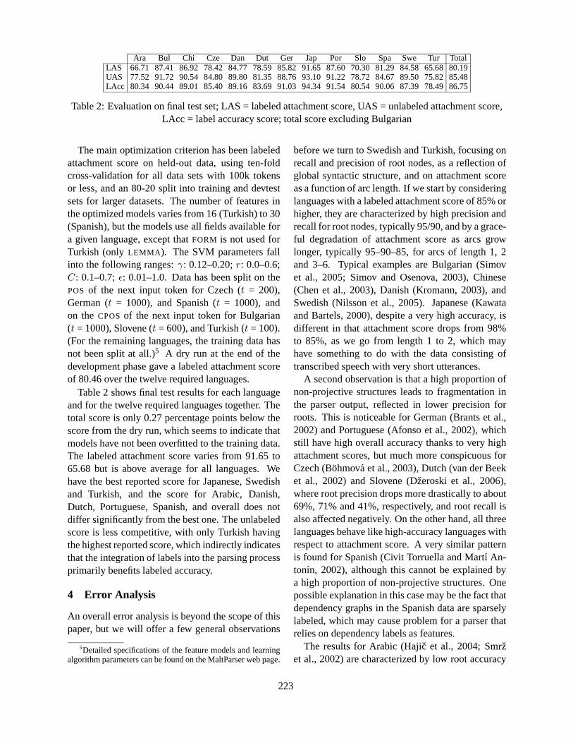
Ara Bul Chi Cze Dan Dut Ger Jap Por Slo Spa Swe TurTotalLAS 66.71 87.41 86.92 78.42 84.77 78.59 85.82 91.65 87.60 70.30 81.29 84.58 65.6880.19UAS 77.52 91.72 90.54 84.80 89.80 81.35 88.76 93.10 91.22 78.72 84.67 89.50 75.8285.48LAcc 80.34 90.44 89.01 85.40 89.16 83.69 91.03 94.34 91.54 80.54 90.06 87.39 78.4986.75
Table 2: Evaluation on final test set; LAS = labeled attachment score, UAS = unlabeled attachment score,LAcc = label accuracy score; total score excluding Bulgarian
The main optimization criterion has been labeledattachment score on held-out data, using ten-foldcross-validation for all data sets with 100k tokensor less, and an 80-20 split into training and devtestsets for larger datasets. The number of features inthe optimized models varies from 16 (Turkish) to 30(Spanish), but the models use all fields available fora given language, except thatFORM is not used forTurkish (only LEMMA ). The SVM parameters fallinto the following ranges:γ: 0.12–0.20;r: 0.0–0.6;C: 0.1–0.7;ǫ: 0.01–1.0. Data has been split on thePOS of the next input token for Czech (t = 200),German (t = 1000), and Spanish (t = 1000), andon theCPOSof the next input token for Bulgarian(t = 1000), Slovene (t = 600), and Turkish (t = 100).(For the remaining languages, the training data hasnot been split at all.)5 A dry run at the end of thedevelopment phase gave a labeled attachment scoreof 80.46 over the twelve required languages.
Table 2 shows final test results for each languageand for the twelve required languages together. Thetotal score is only 0.27 percentage points below thescore from the dry run, which seems to indicate thatmodels have not been overfitted to the training data.The labeled attachment score varies from 91.65 to65.68 but is above average for all languages. Wehave the best reported score for Japanese, Swedishand Turkish, and the score for Arabic, Danish,Dutch, Portuguese, Spanish, and overall does notdiffer significantly from the best one. The unlabeledscore is less competitive, with only Turkish havingthe highest reported score, which indirectly indicatesthat the integration of labels into the parsing processprimarily benefits labeled accuracy.
4 Error Analysis
An overall error analysis is beyond the scope of thispaper, but we will offer a few general observations
5Detailed specifications of the feature models and learningalgorithm parameters can be found on the MaltParser web page.
before we turn to Swedish and Turkish, focusing onrecall and precision of root nodes, as a reflection ofglobal syntactic structure, and on attachment scoreas a function of arc length. If we start by consideringlanguages with a labeled attachment score of 85% orhigher, they are characterized by high precision andrecall for root nodes, typically 95/90, and by a grace-ful degradation of attachment score as arcs growlonger, typically 95–90–85, for arcs of length 1, 2and 3–6. Typical examples are Bulgarian (Simovet al., 2005; Simov and Osenova, 2003), Chinese(Chen et al., 2003), Danish (Kromann, 2003), andSwedish (Nilsson et al., 2005). Japanese (Kawataand Bartels, 2000), despite a very high accuracy, isdifferent in that attachment score drops from 98%to 85%, as we go from length 1 to 2, which mayhave something to do with the data consisting oftranscribed speech with very short utterances.
A second observation is that a high proportion ofnon-projective structures leads to fragmentation inthe parser output, reflected in lower precision forroots. This is noticeable for German (Brants et al.,2002) and Portuguese (Afonso et al., 2002), whichstill have high overall accuracy thanks to very highattachment scores, but much more conspicuous forCzech (Bohmova et al., 2003), Dutch (van der Beeket al., 2002) and Slovene (Dzeroski et al., 2006),where root precision drops more drastically to about69%, 71% and 41%, respectively, and root recall isalso affected negatively. On the other hand, all threelanguages behave like high-accuracy languages withrespect to attachment score. A very similar patternis found for Spanish (Civit Torruella and Martı An-tonın, 2002), although this cannot be explained bya high proportion of non-projective structures. Onepossible explanation in this case may be the fact thatdependency graphs in the Spanish data are sparselylabeled, which may cause problem for a parser thatrelies on dependency labels as features.
The results for Arabic (Hajic et al., 2004; Smrzet al., 2002) are characterized by low root accuracy
223
as well as a rapid degradation of attachment scorewith arc length (from about 93% for length 1 to 67%for length 2). By contrast, Turkish (Oflazer et al.,2003; Atalay et al., 2003) exhibits high root accu-racy but consistently low attachment scores (about88% for length 1 and 68% for length 2). It is note-worthy that Arabic and Turkish, being “typologicaloutliers”, show patterns that are different both fromeach other and from most of the other languages.
4.1 Swedish
A more fine-grained analysis of the Swedish resultsreveals a high accuracy for function words, whichis compatible with previous studies (Nivre, 2006).Thus, the labeled F-score is 100% for infinitivemarkers (IM) and subordinating conjunctions (UK),and above 95% for determiners (DT). In addition,subjects (SS) have a score above 90%. In all thesecases, the dependent has a configurationally defined(but not fixed) position with respect to its head.
Arguments of the verb, such as objects (DO, IO)and predicative complements (SP), have a slightlylower accuracy (about 85% labeled F-score), whichis due to the fact that they “compete” in the samestructural positions, whereas adverbials (labels thatend in A) have even lower scores (often below 70%).The latter result must be related both to the relativelyfine-grained inventory of dependency labels for ad-verbials and to attachment ambiguities that involveprepositional phrases. The importance of this kindof ambiguity is reflected also in the drastic differ-ence in accuracy between noun pre-modifiers (AT)(F> 97%) and noun post-modifiers (ET) (F≈ 75%).
Finally, it is worth noting that coordination, whichis often problematic in parsing, has high accuracy.The Swedish treebank annotation treats the secondconjunct as a dependent of the first conjunct and asthe head of the coordinator, which seems to facil-itate parsing.6 The attachment of the second con-junct to the first (CC) has a labeled F-score above80%, while the attachment of the coordinator to thesecond conjunct (++) has a score well above 90%.
4.2 Turkish
In Turkish, very essential syntactic information iscontained in the rich morphological structure, where
6The analysis is reminiscent of the treatment of coordinationin the Collins parser (Collins, 1999).
concatenated suffixes carry information that in otherlanguages may be expressed by separate words. TheTurkish treebank therefore divides word forms intosmaller units, called inflectional groups (IGs), andthe task of the parser is to construct dependenciesbetween IGs, not (primarily) between word forms(Eryigit and Oflazer, 2006). It is then importantto remember that an unlabeled attachment scoreof 75.8% corresponds to a word-to-word score of82.7%, which puts Turkish on a par with languageslike Czech, Dutch and Spanish. Moreover, whenwe break down the results according to whether thehead of a dependency is part of a multiple-IG wordor a complete (single-IG) word, we observe a highlysignificant difference in accuracy, with only 53.2%unlabeled attachment score for multiple-IG headsversus 83.7% for single-IG heads. It is hard to sayat this stage whether this means that our methodsare ill-suited for IG-based parsing, or whether it ismainly a case of sparse data for multiple-IG words.
When we break down the results by dependencytype, we can distinguish three main groups. The firstconsists of determiners and particles, which havean unlabeled attachment score over 80% and whichare found within a distance of 1–1.4 IGs from theirhead.7 The second group mainly contains subjects,objects and different kinds of adjuncts, with a scorein the range 60–80% and a distance of 1.8–5.2 IGs totheir head. In this group, information about case andpossessive features of nominals is important, whichis found in theFEATSfield in the data representation.We believe that one important explanation for ourrelatively good results for Turkish is that we breakdown theFEATS information into its atomic com-ponents, independently ofPOSand CPOStags, andlet the classifier decide which one to use in a givensituation. The third group contains distant depen-dencies, such as sentence modifiers, vocatives andappositions, which have a much lower accuracy.
5 Conclusion
The evaluation shows that labeled pseudo-projectivedependency parsing, using a deterministic parsingalgorithm and SVM classifiers, gives competitiveparsing accuracy for all languages involved in the
7Given that the average IG count of a word is 1.26 in thetreebank, this means that they are normally adjacent to the headword.
224
shared task, although the level of accuracy variesconsiderably between languages. To analyze indepth the factors determining this variation, and toimprove our parsing methods accordingly to meetthe challenges posed by the linguistic diversity, willbe an important research goal for years to come.
Acknowledgments
We are grateful for the support from TUBITAK(The Scientific and Technical Research Council ofTurkey) and the Swedish Research Council. We alsowant to thank Atanas Chanev for assistance withSlovene, the organizers of the shared task for alltheir hard work, and the creators of the treebanksfor making the data available.
ReferencesA. Abeill e, editor. 2003. Treebanks: Building and Using
Parsed Corpora, volume 20 ofText, Speech and LanguageTechnology. Kluwer Academic Publishers, Dordrecht.
S. Afonso, E. Bick, R. Haber, and D. Santos. 2002. “Florestasinta(c)tica”: a treebank for Portuguese. InProc. of LREC-2002, pages 1698–1703.
N. B. Atalay, K. Oflazer, and B. Say. 2003. The annotationprocess in the Turkish treebank. InProc. of LINC-2003.
E. Black, F. Jelinek, J. D. Lafferty, D. M. Magerman, R. L. Mer-cer, and S. Roukos. 1992. Towards history-based grammars:Using richer models for probabilistic parsing. InProc. of the5th DARPA Speech and Natural Language Workshop, pages31–37.
A. Bohmova, J. Hajic, E. Hajicova, and B. Hladka. 2003. ThePDT: a 3-level annotation scenario. In Abeille (Abeille,2003), chapter 7.
S. Brants, S. Dipper, S. Hansen, W. Lezius, and G. Smith. 2002.The TIGER treebank. InProc. of TLT-2002.
C.-C. Chang and C.-J. Lin, 2001. LIBSVM: A Libraryfor Support Vector Machines. Software available athttp://www.csie.ntu.edu.tw/ cjlin/libsvm.
K. Chen, C. Luo, M. Chang, F. Chen, C. Chen, C. Huang, andZ. Gao. 2003. Sinica treebank: Design criteria, representa-tional issues and implementation. In Abeille (Abeille, 2003),chapter 13, pages 231–248.
M. Civit Torruella and Ma A. Martı Antonın. 2002. Designprinciples for a Spanish treebank. InProc. of TLT-2002.
M. Collins. 1999.Head-Driven Statistical Models for NaturalLanguage Parsing. Ph.D. thesis, University of Pennsylvania.
S. Dzeroski, T. Erjavec, N. Ledinek, P. Pajas, Z.Zabokrtsky, andA. Zele. 2006. Towards a Slovene dependency treebank. InProc. of LREC-2006.
G. Eryigit and K. Oflazer. 2006. Statistical dependency parsingof Turkish. InProc. of EACL-2006.
J. Hajic, O. Smrz, P. Zemanek, J.Snaidauf, and E. Beska. 2004.Prague Arabic dependency treebank: Development in dataand tools. InProc. of NEMLAR-2004, pages 110–117.
Y. Kawata and J. Bartels. 2000. Stylebook for the Japanesetreebank in VERBMOBIL. Verbmobil-Report 240, Seminarfur Sprachwissenschaft, Universitat Tubingen.
M. T. Kromann. 2003. The Danish dependency treebank andthe underlying linguistic theory. InProc. of TLT-2003.
T. Kudo and Y. Matsumoto. 2002. Japanese dependency anal-ysis using cascaded chunking. InProc. of CoNLL-2002,pages 63–69.
J. Nilsson, J. Hall, and J. Nivre. 2005. MAMBA meets TIGER:Reconstructing a Swedish treebank from antiquity. InProc.of the NODALIDA Special Session on Treebanks.
J. Nivre and J. Nilsson. 2005. Pseudo-projective dependencyparsing. InProc. of ACL-2005, pages 99–106.
J. Nivre, J. Hall, and J. Nilsson. 2004. Memory-based depen-dency parsing. InProc. CoNLL-2004, pages 49–56.
J. Nivre, J. Hall, and J. Nilsson. 2006. MaltParser: A data-driven parser-generator for dependency parsing. InProc. ofLREC-2006.
J. Nivre. 2003. An efficient algorithm for projective depen-dency parsing. InProc. of IWPT-2003, pages 149–160.
J. Nivre. 2006.Inductive Dependency Parsing. Springer.
K. Oflazer, B. Say, D. Zeynep Hakkani-Tur, and G. Tur. 2003.Building a Turkish treebank. In Abeille (Abeille, 2003),chapter 15.
K. Simov and P. Osenova. 2003. Practical annotation schemefor an HPSG treebank of Bulgarian. InProc. of LINC-2003,pages 17–24.
K. Simov, P. Osenova, A. Simov, and M. Kouylekov. 2005.Design and implementation of the Bulgarian HPSG-basedtreebank. InJournal of Research on Language and Com-putation – Special Issue, pages 495–522. Kluwer AcademicPublishers.
O. Smrz, J. Snaidauf, and P. Zemanek. 2002. Prague depen-dency treebank for Arabic: Multi-level annotation of Arabiccorpus. InProc. of the Intern. Symposium on Processing ofArabic, pages 147–155.
L. van der Beek, G. Bouma, R. Malouf, and G. van Noord.2002. The Alpino dependency treebank. InComputationalLinguistics in the Netherlands (CLIN).
H. Yamada and Y. Matsumoto. 2003. Statistical dependencyanalysis with support vector machines. InProc. of IWPT-2003, pages 195–206.
225
Proceedings of the 10th Conference on Computational Natural Language Learning (CoNLL-X),pages 226–230, New York City, June 2006.c©2006 Association for Computational Linguistics
Multi-lingual Dependency Parsing with Incremental Integer LinearProgramming
Sebastian Riedeland Ruket Cakıcı and Ivan Meza-RuizICCS
School of InformaticsUniversity of Edinburgh
Edinburgh, EH8 9LW, UKS.R.Riedel,R.Cakici,[email protected]
Abstract
Our approach to dependency parsing isbased on the linear model of McDonaldet al.(McDonald et al., 2005b). Instead ofsolving the linear model using the Max-imum Spanning Tree algorithm we pro-pose an incremental Integer Linear Pro-gramming formulation of the problem thatallows us to enforce linguistic constraints.Our results show only marginal improve-ments over the non-constrained parser. Inaddition to the fact that many parses didnot violate any constraints in the first placethis can be attributed to three reasons: 1)the next best solution that fulfils the con-straints yields equal or less accuracy, 2)noisy POS tags and 3) occasionally ourinference algorithm was too slow and de-coding timed out.
1 Introduction
This paper presents our submission for the CoNLL2006 shared task of multilingual dependency pars-ing. Our parser is inspired by McDonald etal.(2005a) which treats the task as the search for thehighest scoring Maximum Spanning Tree (MST) ina graph. This framework is efficient for both pro-jective and non-projective parsing and provides anonline learning algorithm which combined with arich feature set creates state-of-the-art performanceacross multiple languages (McDonald and Pereira,2006).
However, McDonald and Pereira (2006) mentionthe restrictive nature of this parsing algorithm. Intheir original framework, features are only definedover single attachment decisions. This leads to caseswhere basic linguistic constraints are not satisfied(e.g. verbs with two subjects). In this paper wepresent a novel way to implement the parsing al-gorithms for projective and non-projective parsingbased on a more generic incremental Integer LinearProgramming (ILP) approach. This allows us to in-clude additional global constraints that can be usedto impose linguistic information.
The rest of the paper is organised in the followingway. First we give an overview of the Integer LinearProgramming model and how we trained its param-eters. We then describe our feature and constraintsets for the 12 different languages of the task (Hajicet al., 2004; Chen et al., 2003; Bohmova et al., 2003;Kromann, 2003; van der Beek et al., 2002; Brantset al., 2002; Kawata and Bartels, 2000; Afonso etal., 2002; Dzeroski et al., 2006; Civit Torruella andMartı Antonın, 2002; Nilsson et al., 2005; Oflazer etal., 2003; Atalay et al., 2003). Finally, our results arediscussed and error analyses for Chinese and Turk-ish are presented.
2 Model
Our model is based on the linear model presented inMcDonald et al. (2005a),
s (x,y) =∑
(i,j)∈y
s (i, j) =∑
w · f (i, j)(1)
wherex is a sentence,y a parse ands a score func-tion over sentence-parse pairs.f (i, j) is a multidi-
226
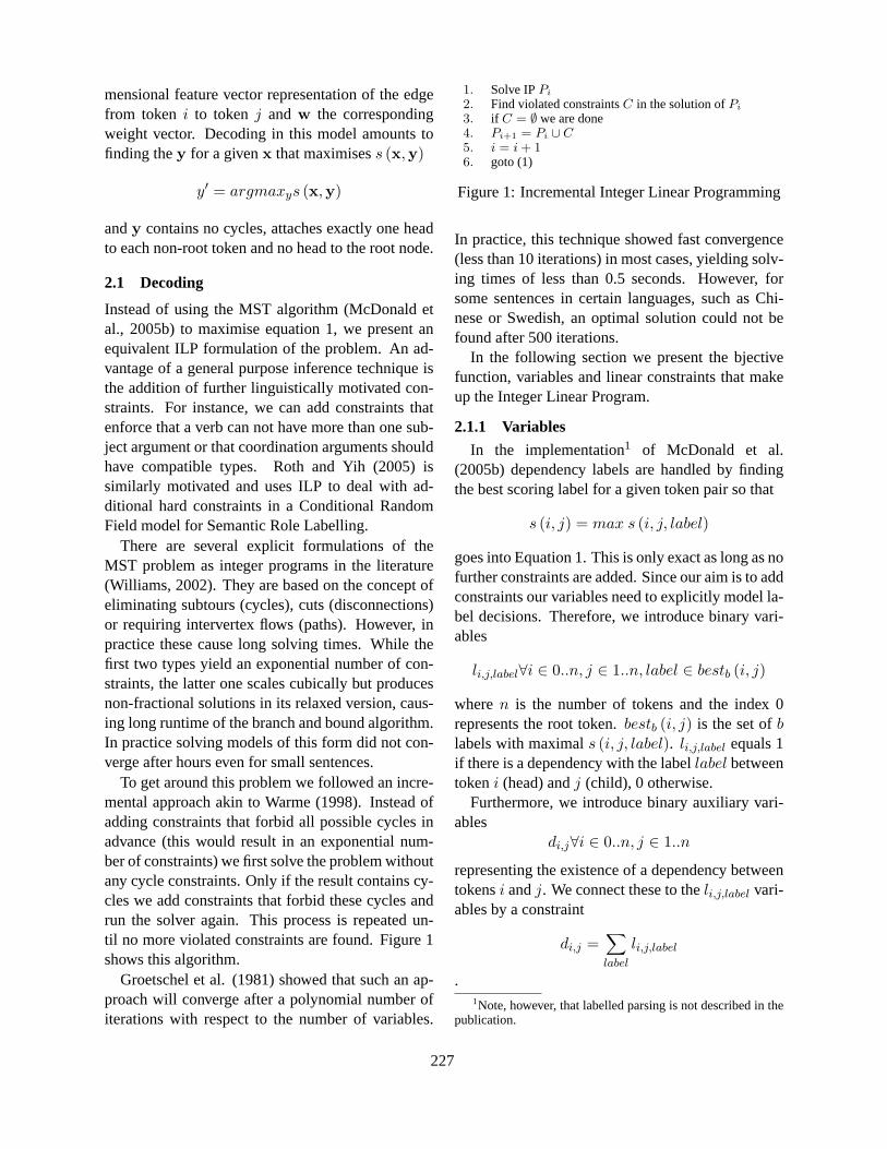
mensional feature vector representation of the edgefrom token i to tokenj and w the correspondingweight vector. Decoding in this model amounts tofinding they for a givenx that maximisess (x,y)
y′ = argmaxys (x,y)
andy contains no cycles, attaches exactly one headto each non-root token and no head to the root node.
2.1 Decoding
Instead of using the MST algorithm (McDonald etal., 2005b) to maximise equation 1, we present anequivalent ILP formulation of the problem. An ad-vantage of a general purpose inference technique isthe addition of further linguistically motivated con-straints. For instance, we can add constraints thatenforce that a verb can not have more than one sub-ject argument or that coordination arguments shouldhave compatible types. Roth and Yih (2005) issimilarly motivated and uses ILP to deal with ad-ditional hard constraints in a Conditional RandomField model for Semantic Role Labelling.
There are several explicit formulations of theMST problem as integer programs in the literature(Williams, 2002). They are based on the concept ofeliminating subtours (cycles), cuts (disconnections)or requiring intervertex flows (paths). However, inpractice these cause long solving times. While thefirst two types yield an exponential number of con-straints, the latter one scales cubically but producesnon-fractional solutions in its relaxed version, caus-ing long runtime of the branch and bound algorithm.In practice solving models of this form did not con-verge after hours even for small sentences.
To get around this problem we followed an incre-mental approach akin to Warme (1998). Instead ofadding constraints that forbid all possible cycles inadvance (this would result in an exponential num-ber of constraints) we first solve the problem withoutany cycle constraints. Only if the result contains cy-cles we add constraints that forbid these cycles andrun the solver again. This process is repeated un-til no more violated constraints are found. Figure 1shows this algorithm.
Groetschel et al. (1981) showed that such an ap-proach will converge after a polynomial number ofiterations with respect to the number of variables.
1. Solve IPPi
2. Find violated constraintsC in the solution ofPi
3. if C = ∅ we are done4. Pi+1 = Pi ∪ C5. i = i + 16. goto (1)
Figure 1: Incremental Integer Linear Programming
In practice, this technique showed fast convergence(less than 10 iterations) in most cases, yielding solv-ing times of less than 0.5 seconds. However, forsome sentences in certain languages, such as Chi-nese or Swedish, an optimal solution could not befound after 500 iterations.
In the following section we present the bjectivefunction, variables and linear constraints that makeup the Integer Linear Program.
2.1.1 Variables
In the implementation1 of McDonald et al.(2005b) dependency labels are handled by findingthe best scoring label for a given token pair so that
s (i, j) = max s (i, j, label)
goes into Equation 1. This is only exact as long as nofurther constraints are added. Since our aim is to addconstraints our variables need to explicitly model la-bel decisions. Therefore, we introduce binary vari-ables
li,j,label∀i ∈ 0..n, j ∈ 1..n, label ∈ bestb (i, j)
wheren is the number of tokens and the index 0represents the root token.bestb (i, j) is the set ofblabels with maximals (i, j, label). li,j,label equals 1if there is a dependency with the labellabel betweentokeni (head) andj (child), 0 otherwise.
Furthermore, we introduce binary auxiliary vari-ables
di,j∀i ∈ 0..n, j ∈ 1..n
representing the existence of a dependency betweentokensi andj. We connect these to theli,j,label vari-ables by a constraint
di,j =∑label
li,j,label
.1Note, however, that labelled parsing is not described in the
publication.
227
2.1.2 Objective Function
Given the above variables our objective functioncan be represented as∑
i,j
∑label∈bestk(i,j)
s (i, j, label) · li,j,label
with a suitablek.
2.1.3 Constraints Added in Advance
Only One Head In all our languages every tokenhas exactly one head. This yields∑
i>0
di,j = 1
for non-root tokensj > 0 and∑i
di,0 = 0
for the artificial root node.
Typed Arity Constraints We might encounter so-lutions of the basic model that contain, for instance,verbs with two subjects. To forbid these we simplyaugment our model with constraints such as∑
j
li,j,subject ≤ 1
for all verbsi in a sentence.
2.1.4 Incremental Constraints
No Cycles If a solution contains one or more cy-clesC we add the following constraints to our IP:For everyc ∈ C we add∑
(i,j)∈c
di,j ≤ |c| − 1
to forbid c.
Coordination Argument Constraints In coordi-nation conjuncts have to be of compatible types. Forexample, nouns can not coordinate with verbs. Weimplemented this constraint by checking the parsesfor occurrences of incompatible arguments. If wefind two argumentsj, k for a conjunctioni: di,j anddi,k andj is a noun andk is a verb then we add
di,j + di,k ≤ 1
to forbid configurations in which both dependenciesare active.
Projective Parsing In the incremental ILP frame-work projective parsing can be easily implementedby checking for crossing dependencies after each it-eration and forbidding them in the next. If we seetwo dependencies that cross,di,j anddk,l, we addthe constraint
di,j + dk,l ≤ 1
to prevent this in the next iteration. This can alsobe used to prevent specific types of crossings. Forinstance, in Dutch we could only allow crossing de-pendencies as long as none of the dependencies is a“Determiner” relation.
2.2 Training
We used single-best MIRA(Crammer and Singer,2003).For all experiments we used10 training iter-ations and non-projective decoding. Note that weused the original spanning tree algorithm for decod-ing during training as it was faster.
3 System Summary
We use four different feature sets. The first fea-ture set,BASELINE, is taken from McDonald andPereira (2005b). It uses theFORMand thePOSTAGfields. This set also includes features that combinethe label and POS tag of head and child such as(Label, POSHead) and(Label, POSChild−1). Forour Arabic and Japanese development sets we ob-tained the best results with this configuration. Wealso use this configuration for Chinese, German andPortuguese because training with other configura-tions took too much time (more than 7 days).
The BASELINE also uses pseudo-coarse-POS tag(1st character of thePOSTAG) and pseudo-lemmatag (4 characters of theFORM when the lengthis more than3). For the next configuration wesubstitute these pseudo-tags by theCPOSTAGandLEMMAfields that were given in the data. This con-figuration was used for Czech because for other con-figurations training could not be finished in time.
The third feature set tries to exploit the genericFEATSfield, which can contain a list features suchas case and gender. A set of features per depen-dency is extracted using this information. It con-sists of cross product of the features inFEATS. Weused this configuration for Danish, Dutch, Spanish
228
and Turkish where it showed the best results duringdevelopment.
The fourth feature set uses the triplet of la-bel, POS child and head as a feature such as(Label, POSHead, POSChild). It also uses theCPOSTAGand LEMMA fields for the head. Thisconfiguration is used for Slovene and Swedish datawhere it performed best during development.
Finally, we add constraints for Chinese, Dutch,Japanese and Slovene. In particular, arity constraintsto Chinese and Slovene, coordination and arity con-straints to Dutch, arity and selective projectivityconstraints for Japanese2. For all experimentsb wasset to 2. We did not apply additional constraints toany other languages due to lack of time.
4 Results
Our results on the test set are shown in Table 1.Our results are well above the average for all lan-guages but Czech. For Chinese we perform signif-icantly better than all other participants (p = 0.00)and we are in the top three entries for Dutch, Ger-man, Danish. Although Dutch and Chinese are lan-guages were we included additional constraints, ourscores are not a result of these. Table 2 compares theresult for the languages with additional constraints.Adding constraints only marginally helps to improvethe system (in the case of Slovene a bug in our im-plementation even degraded accuracy). A more de-tailed explanation to this observation is given in thefollowing section. A possible explanation for ourhigh accuracy in Chinese could be the fact that wewere not able to optimise the feature set on the de-velopment set (see the previous section). Maybe thisprevented us from overfitting. It should be noted thatwe did use non-projective parsing for Chinese, al-though the corpus was fully projective. Our worstresults in comparison with other participants can beseen for Czech. We attribute this to the reducedtraining set we had to use in order to produce amodel in time, even when using the original MSTalgorithm.
2This is done in order to capture the fact that crossing de-pendencies in Japanese could only be introduced through dis-fluencies.
4.1 Chinese
For Chinese the parser was augmented with a set ofconstraints that disallowed more than one argumentof the typeshead, goal, nominal, range, theme, rea-son, DUMMY, DUMMY1andDUMMY2.
By enforcing arity constraints we could either turnwrong labels/heads into right ones and improve ac-curacy or turn right labels/heads into wrong ones anddegrade accuracy. For the test set the number of im-provements (36) was higher than the number of er-rors (22). However, this margin was outweighed bya few sentences we could not properly process be-cause our inference method timed out. Our overallimprovement was thus unimpressive 7 tokens.
In the context of duplicate “head” dependencies(that is, dependencies labelled “head”) the num-ber of sentences where accuracy dropped far out-weighed the number of sentences where improve-ments could be gained. Removing the arity con-straints on “head” labels therefore should improveour results.
This shows the importance of good second bestdependencies. If the dependency with the secondhighest score is the actual gold dependency and itsscore is close to the highest score, we are likely topick this dependency in the presence of additionalconstraints. On the other hand, if the dependencywith the second highest score is not the gold one andits score is too high, we will probably include thisdependency in order to fulfil the constraints.
There may be some further improvement to begained if we train our model usingk-best MIRAwith k > 1 since it optimises weights with respectto thek best parses.
4.2 Turkish
There is a considerable gap between the unlabelledand labelled results for Turkish. And in terms of la-bels the POS typeNoungives the worst performancebecause many times a subject was classified as ob-ject or vice a versa.
Case information in Turkish assigns argumentroles for nouns by marking different semantic roles.Many errors in the Turkish data might have beencaused by the fact that this information was not ad-equately used. Instead of fine-tuning our feature setto Turkish we used the feature cross product as de-
229
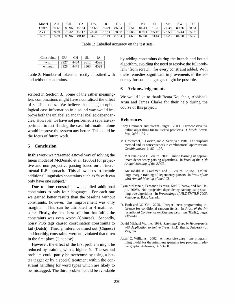
Model AR CH CZ DA DU GE JP PO SL SP SW TUOURS 66.65 89.96 67.64 83.63 78.59 86.24 90.51 84.43 71.20 77.38 80.66 58.61AVG 59.94 78.32 67.17 78.31 70.73 78.58 85.86 80.63 65.16 73.53 76.44 55.95TOP 66.91 89.96 80.18 84.79 79.19 87.34 91.65 87.60 73.44 82.25 84.58 65.68
Table 1: Labelled accuracy on the test sets.
Constraints DU CH SL JAwith 3927 4464 3612 4526
without 3928 4471 3563 4528
Table 2: Number of tokens correctly classified withand without constraints.
scribed in Section 3. Some of the rather meaning-less combinations might have neutralised the effectof sensible ones. We believe that using morpho-logical case information in a sound way would im-prove both the unlabelled and the labelled dependen-cies. However, we have not performed a separate ex-periment to test if using the case information alonewould improve the system any better. This could bethe focus of future work.
5 Conclusion
In this work we presented a novel way of solving thelinear model of McDonald et al. (2005a) for projec-tive and non-projective parsing based on an incre-mental ILP approach. This allowed us to includeadditional linguistics constraints such as “a verb canonly have one subject.”
Due to time constraints we applied additionalconstraints to only four languages. For each onewe gained better results than the baseline withoutconstraints, however, this improvement was onlymarginal. This can be attributed to 4 main rea-sons: Firstly, the next best solution that fulfils theconstraints was even worse (Chinese). Secondly,noisy POS tags caused coordination constraints tofail (Dutch). Thirdly, inference timed out (Chinese)and fourthly, constraints were not violated that oftenin the first place (Japanese).
However, the effect of the first problem might bereduced by training with a higherk. The secondproblem could partly be overcome by using a bet-ter tagger or by a special treatment within the con-straint handling for word types which are likely tobe mistagged. The third problem could be avoidable
by adding constraints during the branch and boundalgorithm, avoiding the need to resolve the full prob-lem “from scratch” for every constraint added. Withthese remedies significant improvements to the ac-curacy for some languages might be possible.
6 Acknowledgements
We would like to thank Beata Kouchnir, AbhishekArun and James Clarke for their help during thecourse of this project.
ReferencesKoby Crammer and Yoram Singer. 2003. Ultraconservative
online algorithms for multiclass problems.J. Mach. Learn.Res., 3:951–991.
M. Groetschel, L. Lovasz, and A. Schrijver. 1981. The ellipsoidmethod and its consequences in combinatorial optimization.Combinatorica, I:169– 197.
R. McDonald and F. Pereira. 2006. Online learning of approx-imate dependency parsing algorithms. InProc. of the 11thAnnual Meeting of the EACL.
R. McDonald, K. Crammer, and F. Pereira. 2005a. Onlinelarge-margin training of dependency parsers. InProc. of the43rd Annual Meeting of the ACL.
Ryan McDonald, Fernando Pereira, Kiril Ribarov, and Jan Ha-jic. 2005b. Non-projective dependency parsing using span-ning tree algorithms. InProceedings of HLT/EMNLP 2005,Vancouver, B.C., Canada.
D. Roth and W. Yih. 2005. Integer linear programming in-ference for conditional random fields. InProc. of the In-ternational Conference on Machine Learning (ICML), pages737–744.
David Michael Warme. 1998.Spanning Trees in Hypergraphswith Application to Steiner Trees. Ph.D. thesis, University ofVirginia.
Justin C. Williams. 2002. A linear-size zero - one program-ming model for the minimum spanning tree problem in pla-nar graphs.Networks, 39:53–60.
230

Proceedings of the 10th Conference on Computational Natural Language Learning (CoNLL-X),pages 231–235, New York City, June 2006.c©2006 Association for Computational Linguistics
Language Independent Probabilistic Context-Free ParsingBolstered by Machine Learning
Michael Schiehlen Kristina SprangerInstitute for Computational Linguistics
University of StuttgartD-70174 Stuttgart
[email protected]@ims.uni-stuttgart.de
Abstract
Unlexicalized probabilistic context-freeparsing is a general and flexible approachthat sometimes reaches competitive re-sults in multilingual dependency parsingeven if a minimum of language-specificinformation is supplied. Furthermore, in-tegrating parser results (good at long de-pendencies) and tagger results (good atshort range dependencies, and more easilyadaptable to treebank peculiarities) givescompetitive results in all languages.
1 Introduction
Unlexicalized probabilistic context-free parsing isa simple and flexible approach that neverthelesshas shown good performance (Klein and Manning,2003). We applied this approach to the shared task(Buchholz et al., 2006) for Arabic (Hajic et al.,2004), Chinese (Chen et al., 2003), Czech (Böh-mová et al., 2003), Danish (Kromann, 2003), Dutch(van der Beek et al., 2002), German (Brants et al.,2002), Japanese (Kawata and Bartels, 2000), Por-tuguese (Afonso et al., 2002), Slovene (Džeroski etal., 2006), Spanish (Civit Torruella and Martí An-tonín, 2002), Swedish (Nilsson et al., 2005), Turk-ish (Oflazer et al., 2003; Atalay et al., 2003), butnot Bulgarian (Simov et al., 2005). In our ap-proach we put special emphasis on language inde-pendence: We did not use any extraneous knowl-edge; we did not do any transformations on thetreebanks; we restricted language-specific parame-
ters to a small, easily manageable set (a classifica-tion of dependency relations into complements, ad-juncts, and conjuncts/coordinators, and a switch forJapanese to include coarse POS tag information, seesection 3.4). In a series of post-submission experi-ments, we investigated how much the parse resultscan help a machine learner.
2 Experimental Setup
For development, we chose the initial � sentences ofevery treebank, where � is the number of the sen-tences in the test set. In this way, the sizes wererealistic for the task. For parsing the test data, weadded the development set to the training set.
All the evaluations on the test sets were performedwith the evaluation script supplied by the conferenceorganizers. For development, we used labelled F-score computed from all tokens except the ones em-ployed for punctuation (cf. section 3.2).
3 Context Free Parsing
3.1 The Parser
Basically, we investigated the performance of astraightforward unlexicalized statistical parser, viz.BitPar (Schmid, 2004). BitPar is a CKY parser thatuses bit vectors for efficient representation of thechart and its items. If frequencies for the grammat-ical and lexical rules in a training set are available,BitPar uses the Viterbi algorithm to extract the mostprobable parse tree (according to PCFG) from thechart.
231
3.2 Converting Dependency Structure toConstituency Structure
In order to determine the grammar rules required bythe context-free parser, the dependency trees in theCONLL format have to be converted to constituencytrees. Gaifman (1965) proved that projective de-pendency grammars can be mapped to context-freegrammars. The main information that needs to beadded in going from dependency to constituencystructure is the category of non-terminals. The usageof special knowledge bases to determine projectionsof categories (Xia and Palmer, 2001) would havepresupposed language-dependent knowledge, so weinvestigated two other options: Flat rules (Collinset al., 1999) and binary rules. In the flat rules ap-proach, each lexical category projects to exactly onephrasal category, and every projection chain has alength of at most one. The binary rules approachmakes use of the X-bar-scheme and thus introducesalong with the phrasal category an intermediate cate-gory. The phrasal category must not occur more thanonce in a projection chain, and a projection chainmust not end in an intermediate category. In both ap-proaches, projection is only triggered if dependentsare present; in case a category occurs as a depen-dent itself, no projection is required. In coordinationstructures, the parent category is copied from that ofthe last conjunct.
Non-projective relations can be treated as un-bounded dependencies so that their surface posi-tion (antecedent position) is related to the positionof their head (trace position) with an explicit co-indexed trace (like in the Penn treebank). To findthe position of trace and antecedent we assume threeconstraints: The antecedent should c-command itstrace. The antecedent is maximally near to the tracein depth of embedding. The trace is maximally nearto the antecedent in surface order.
Finally the placement of punctuation signs hasa major impact on the performance of a parser(Collins et al., 1999). In most of the treebanks, notmuch effort is invested into the treatment of punc-tuation. Sometimes, punctuation signs play a rolein predicate-argument structure (commas acting ascoordinators), but more often they do not, in whichcase they are marked by special roles (e.g. “pnct”,“punct”, “PUNC”, or “PUNCT”). We used a general
mechanism to re-insert such signs, for all languagesbut CH (no punctuation signs) and AR, CZ, SL (re-liable annotation). Correct placement of punctua-tion presupposes knowledge of the punctuation rulesvalid in a language. In the interest of generality, weopted for a suboptimal solution: Punctuation signsare inserted in the highest possible position in a tree.
3.3 Subcategorization and Coordination
The most important language-specific informationthat we made use of was a classification of de-pendency relations into complements, coordina-tors/conjuncts, and other relations (adjuncts).
Given knowledge about complement relations, itis fairly easy to construct subcategorization framesfor word occurrences: A subcategorization frame issimply the set of the complement relations by whichdependents are attached to the word. To give theparser access to these lists, we annotated the cate-gory of a subcategorizing word with its subcatego-rization frame. In this way, the parser can learn to as-sociate the subcategorization requirements of a wordwith its local syntactic context (Schiehlen, 2004).
Coordination constructions are marked either inthe conjuncts (CH, CZ, DA, DU, GE, PO, SW) orthe coordinator (AR, SL). If conjuncts show coordi-nation, a common representation of asyndetic coor-dination has one conjunct point to another conjunct.It is therefore important to distinguish coordinatorsfrom conjuncts. Coordinators are either singled outby special dependency relations (DA, PO, SW) or bytheir POS tags (CH, DU). In German, the first con-junct phrase is merged with the whole coordinatedphrase (due to a conversion error?) so that determin-ing the coordinator as a head is not possible.
We also experimented with attaching the POStags of heads to the categories of their adjunct de-pendents. In this way, the parser could differenti-ate between e.g. verbal and nominal adjuncts. Inour experiments, the performance gains achieved bythis strategy were low, so we did not incorporate itinto the system. Possibly, better results could beachieved by restricting annotation to special classesof adjuncts or by generalizing the heads’ POS tags.
3.4 Categories
As the treebanks provide a lot of information withevery word token, it is a delicate question to de-
232

Ch Da Du Ge Ja Po Sp Tucoarse POS 72.99 69.38 69.27 – 79.07 66.09fine POS 61.21 69.78 67.72 7.40 73.44 71.75 54.96POS + feat – 42.67 40.40 –dep-rel 76.61 72.77 70.70 70.31 78.12 72.93 66.93 65.03coarse + dep-rel 77.61 67.56 69.43 – 81.36 64.03fine + dep-rel 51.21 57.72 68.55 46.28 36.59 54.97
Figure 1: Types of Categories (Development Results)
cide on the type and granularity of the information touse in the categories of the grammar. The treebanksspecify for every word a (fine-grained) POS tag, acoarse-grained POS tag, a collection of morphosyn-tactic features, and a dependency relation (dep-rel).Only the dependency relation is really orthogonal;the other slots contain various generalizations of thesame morphological information. We tested sev-eral options: coarse-grained POS tag (if available),fine-grained POS tag, fine-grained POS tag withmorphosyntactic features (if available), name of de-pendency relation, and the combinations of coarse-grained or fine-grained POS tags with the depen-dency relation.
Figure 1 shows F-score results on the develop-ment set for several languages and different com-binations. The best overall performer is dep-rel;this somewhat astonishing fact may be due to thesuperior quality of the annotations in this slot (de-pendency relations were annotated by hand, POStags automatically). Furthermore, being checked inevaluation, dependency relations directly affect per-formance. Since we wanted a general language-independent strategy, we used always the dep-reltags but for Japanese. The Japanese treebank fea-tures only 8 different dependency relations, so weadded coarse-grained POS tag information. In thecategories for Czech, we deleted the suffixes mark-ing coordination, apposition and parenthesis (Co,Ap, Pa), reducing the number of categories roughlyby a factor of four. In coordination, conjuncts inheritthe dep-rel category from the parent.
Whereas the dep-rel information is submitted tothe parser directly in terms of the categories, theinformation in the lemma, POS tag and morpho-syntactic features slot was used only for back-offsmoothing when associating lexical items with cate-
Cz Ge Sp Swdep-rel 52.66 70.31 66.93 72.91new classific 58.92 74.32 66.09 61.59new + dep-rel 56.94 78.40 64.03 66.32
Figure 4: Manual POS Tag Classes (Development)
gories. A grammar with this configuration was usedto produce the results submitted (cf. line labelled CFin Figures 2 and 3).
Instead of using the category generalizations sup-plied with the treebanks directly, manual labour canbe put into discovering classifications that behavebetter for the purposes of statistical parsing. So,Collins et al. (1999) proposed a tag classificationfor parsing the Czech treebank. We also investi-gated a classification for German1, as well as one forSwedish and one for Spanish, which were modelledafter the German classification. The results in Fig-ure 4 show that new classifications may have a dra-matic effect on performance if the treebank is suf-ficiently large. In the interest of generality, we didnot make use of the language dependent tag classifi-cations for the results submitted, but we will never-theless report results that could have been achievedwith these classifications.
3.5 Markovization
Another strategy that is often used in statistical pars-ing is Markovization (Collins, 1999): Treebanks
1punctuation {$( $” $, $.} adjectives {ADJA ADJD CARD}adverbs {ADV PROAV PTKA PTKNEG PTKVZ PWAV}prepositions {APPR APPO APZR APPRART KOKOM} nouns{NN NE NNE PDS PIS PPER PPOSS PRELS PRF PWSSYM} determiners {ART PDAT PIAT PRELAT PPOSATPWAT} verb forms {VAFIN VMFIN VVFIN} {VAIMPVVIMP} {VAINF VMINF VVINF} {VAPP VMPP VVPP}{VVIZU PTKZU} clause-like items {ITJ PTKANT KOUS}
233
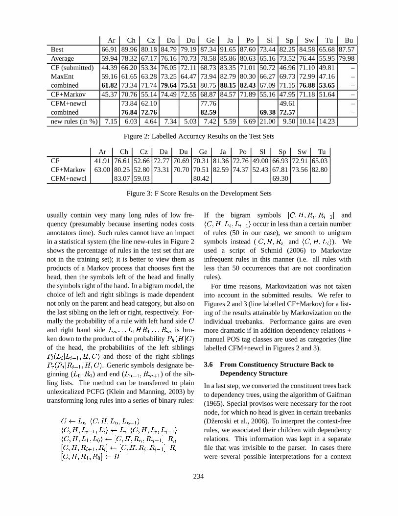
Ar Ch Cz Da Du Ge Ja Po Sl Sp Sw Tu BuBest 66.91 89.96 80.18 84.79 79.19 87.34 91.65 87.60 73.44 82.25 84.58 65.68 87.57Average 59.94 78.32 67.17 76.16 70.73 78.58 85.86 80.63 65.16 73.52 76.44 55.95 79.98CF (submitted) 44.39 66.20 53.34 76.05 72.11 68.73 83.35 71.01 50.72 46.96 71.10 49.81 –MaxEnt 59.16 61.65 63.28 73.25 64.47 73.94 82.79 80.30 66.27 69.73 72.99 47.16 –combined 61.82 73.34 71.74 79.64 75.51 80.75 88.15 82.43 67.09 71.15 76.88 53.65 –CF+Markov 45.37 70.76 55.14 74.49 72.55 68.87 84.57 71.89 55.16 47.95 71.18 51.64 –CFM+newcl 73.84 62.10 77.76 49.61 –combined 76.84 72.76 82.59 69.38 72.57 –new rules (in %) 7.15 6.03 4.64 7.34 5.03 7.42 5.59 6.69 21.00 9.50 10.14 14.23
Figure 2: Labelled Accuracy Results on the Test Sets
Ar Ch Cz Da Du Ge Ja Po Sl Sp Sw TuCF 41.91 76.61 52.66 72.77 70.69 70.31 81.36 72.76 49.00 66.93 72.91 65.03CF+Markov 63.00 80.25 52.80 73.31 70.70 70.51 82.59 74.37 52.43 67.81 73.56 82.80CFM+newcl 83.07 59.03 80.42 69.30
Figure 3: F Score Results on the Development Sets
usually contain very many long rules of low fre-quency (presumably because inserting nodes costsannotators time). Such rules cannot have an impactin a statistical system (the line new-rules in Figure 2shows the percentage of rules in the test set that arenot in the training set); it is better to view them asproducts of a Markov process that chooses first thehead, then the symbols left of the head and finallythe symbols right of the hand. In a bigram model, thechoice of left and right siblings is made dependentnot only on the parent and head category, but also onthe last sibling on the left or right, respectively. For-mally the probability of a rule with left hand side
�and right hand side ������������� ������������� is bro-ken down to the product of the probability �������� ���of the head, the probabilities of the left siblings�������! "� �! $#���%� % ��� and those of the right siblings�'&(��� � � )#�� %� % ��� . Generic symbols designate be-ginning ( ��*(%��+* ) and end ( ���-,'��%����.,'� ) of the sib-ling lists. The method can be transferred to plainunlexicalized PCFG (Klein and Manning, 2003) bytransforming long rules into a series of binary rules:
�0/ � �21 � %�3%�� � %�� �4#���51 � %� %��! 6,'�7%��� 5 / �! 1 � %� %��! 8%��! $#�� 51 � %� %���9%���* 5 /;:<� %� %����=%����>#��8?����:<� %� %��� 6,'�@%��� A? /B:<� %�3%��� C%��� $#��8?��� :<� %� %����@%��+*�? /
If the bigram symbols:<� %�3%�� %�� $#�� ? and
1 � %� %��! 8%��� )#�� 5 occur in less than a certain numberof rules (50 in our case), we smooth to unigramsymbols instead (
:<� %�3%��D �? and 1 � %� %��� 5 ). Weused a script of Schmid (2006) to Markovizeinfrequent rules in this manner (i.e. all rules withless than 50 occurrences that are not coordinationrules).
For time reasons, Markovization was not takeninto account in the submitted results. We refer toFigures 2 and 3 (line labelled CF+Markov) for a list-ing of the results attainable by Markovization on theindividual treebanks. Performance gains are evenmore dramatic if in addition dependency relations +manual POS tag classes are used as categories (linelabelled CFM+newcl in Figures 2 and 3).
3.6 From Constituency Structure Back toDependency Structure
In a last step, we converted the constituent trees backto dependency trees, using the algorithm of Gaifman(1965). Special provisos were necessary for the rootnode, for which no head is given in certain treebanks(Džeroski et al., 2006). To interpret the context-freerules, we associated their children with dependencyrelations. This information was kept in a separatefile that was invisible to the parser. In cases therewere several possible interpretations for a context
234
free rule, we always chose the most frequent one inthe training data (Schiehlen, 2004).
4 Machine Learning
While the results coming from the statistical parserare not really competitive, we believe that they nev-ertheless present valuable information for a machinelearner. To give some substance to this claim, weundertook experiments with the Zhang Le’s Max-Ent Toolkit2. For this work, we recast the depen-dency parsing problem as a classification problem:Given some feature information on the word to-ken, in which dependency relations does it standto which head? While the representation of depen-dency relations is straightforward, the representationof heads is more difficult. Building on past exper-iments (Schiehlen, 2003), we chose the “nth-tag”representation which consists of three pieces of in-formation: the POS tag of the head, the direction inwhich the head lies (left or right), and the number ofwords with the same POS tag between head and de-pendent. We used the following features to describea word token: the fine-grained POS tag, the lemma(or full form) if it occurs at least 10 times, the mor-phosyntactic features, and the POS tags of the fourpreceding and the four following word tokens. Thelearner was trained in standard configuration (30 it-erations). The results for this method on the test dataare shown in Figure 2 (line MaxEnt).
In a second experiment we added parsing results(obtained by 10-fold cross validation on the trainingset) in two features: proposed dependency relationand proposed head. Results of the extended learningapproach are shown in Figure 2 (line combined).
5 Conclusion
We have presented a general approach to parsingarbitrary languages based on dependency treebanksthat uses a minimum overhead of language-specificinformation and nevertheless supplies competitiveresults in some languages (Da, Du). Even better re-sults can be reached if POS tag classifications areused in the categories that are optimized for specificlanguages (Ge). Markovization usually brings animprovement of up to 2%, a higher gain is reached inSlovene (where many new rules occur in the testset)
2http://homepages.inf.ed.ac.uk/s0450736/maxent_toolkit.html
and Chinese (which has the highest number of de-pendency relations). Comparable results in the liter-ature are Schiehlen’s (2004) 81.03% dependency f-score reached on the German NEGRA treebank andCollins et al.’s (1999) 80.0% labelled accuracy onthe Czech PDT treebank. Collins (1999) used a lex-icalized approach, Schiehlen (2004) used the manu-ally annotated phrasal categories of the treebank.
Our second result is that context-free parsingcan also boost the performance of a simple tagger-like machine learning system. While a maximum-entropy learner on its own achieves competitive re-sults for only three languages (Ar, Po, Sl), compet-itive results in basically all languages are producedwith access to the results of the probabilistic parser.
Thanks go to Helmut Schmid for providing sup-port with his parser and the Markovization script.
ReferencesS. Buchholz, E. Marsi, A. Dubey, and Y. Krymolowski.
2006. CoNLL-X shared task on multilingual depen-dency parsing. In CoNLL-X. SIGNLL.
Michael J. Collins, Jan Hajic, Lance Ramshaw, andChristoph Tillmann. 1999. A Statistical Parser forCzech. In ACL’99, College Park, MA.
Michael J. Collins. 1999. Head-Driven Statistical Meth-ods for Natural Language Parsing. Ph.D. thesis, Univ.of Pennsylvania.
Haim Gaifman. 1965. Dependency Systems andPhrase-Structure Systems. Information and Control,8(3):304–337.
Dan Klein and Christopher Manning. 2003. AccurateUnlexicalized Parsing. In ACL’03, pages 423–430.
Michael Schiehlen. 2003. Combining Deep and Shal-low Approaches in Parsing German. In ACL’03, pages112–119, Sapporo, Japan.
Michael Schiehlen. 2004. Annotation Strategies forProbabilistic Parsing in German. In COLING ’04,pages 390–396, Geneva, Switzerland, August.
Helmut Schmid. 2004. Efficient Parsing of Highly Am-biguous Context-Free Grammars with Bit Vectors. InCOLING ’04, Geneva, Switzerland.
Helmut Schmid. 2006. Trace Prediction and Recoverywith Unlexicalized PCFGs and Gap Threading. Sub-mitted to COLING ’06.
Fei Xia and Martha Palmer. 2001. Converting depen-dency structures to phrase structures. In HLT 2001.
235
Proceedings of the 10th Conference on Computational Natural Language Learning (CoNLL-X),pages 236–240, New York City, June 2006.c©2006 Association for Computational Linguistics
Maximum Spanning Tree Algorithm for Non-projective LabeledDependency Parsing
Nobuyuki ShimizuDept. of Computer Science
State University of New York at AlbanyAlbany, NY, 12222, USA
Abstract
Following (McDonald et al., 2005), wepresent an application of a maximumspanning tree algorithm for a directedgraph to non-projective labeled depen-dency parsing. Using a variant of thevoted perceptron (Collins, 2002; Collinsand Roark, 2004; Crammer and Singer,2003), we discriminatively trained ourparser in an on-line fashion. After just oneepoch of training, we were generally ableto attain average results in the CoNLL2006 Shared Task.
1 Introduction
Recently, we have seen dependency parsing growmore popular. It is not rare to see dependency re-lations used as features, in tasks such as relation ex-traction (Bunescu and Mooney, 2005) and machinetranslation (Ding and Palmer, 2005). Although En-glish dependency relations are mostly projective, inother languages with more flexible word order, suchas Czech, non-projective dependencies are more fre-quent. There are generally two methods for learn-ing non-projective dependencies. You could map anon-projective dependency tree to a projective one,learn and predict the tree, then bring it back to thenon-projective dependency tree (Nivre and Nilsson,2005). Non-projective dependency parsing can alsobe represented as search for a maximum spanningtree in a directed graph, and this technique has beenshown to perform well in Czech (McDonald et al.,
2005). In this paper, we investigate the effective-ness of (McDonald et al., 2005) in the various lan-guages given by the CoNLL 2006 shared task fornon-projective labeled dependency parsing.
The paper is structured as follows: in section 2and 3, we review the decoding and learning aspectsof (McDonald et al., 2005), and in section 4, we de-scribe the extension of the algorithm and the featuresneeded for the CoNLL 2006 shared task.
2 Non-Projective Dependency Parsing
2.1 Dependency Structure
Let us definex to be a generic sequence of input to-kens together with their POS tags and other morpho-logical features, andy to be a generic dependencystructure, that is, a set of edges forx. We use theterminology in (Taskar et al., 2004) for a genericstructured output prediction, and define apart.
A part represents an edge together with its label.A part is a tuple〈DEPREL, i, j〉 wherei is the startpoint of the edge,j is the end point, andDEPREListhe label of the edge. The token ati is the head ofthe token atj.
Table 1 shows our formulation of building a non-projective dependency tree as a prediction problem.The task is to predicty, the set of parts (column 3,Table 1), givenx, the input tokens and their features(column 1 and 2, Table 1).
In this paper we use the common method of fac-toring the score of the dependency structure as thesum of the scores of all the parts.
A dependency structure is characterized by itsfeatures, and for each feature, we have a correspond-
236
Token POS Edge PartJohn NN 〈SUBJ, 2, 1〉saw VBD 〈PRED, 0, 2〉a DT 〈DET, 4, 3〉dog NN 〈OBJ, 2, 4〉yesterday RB 〈ADJU, 2, 5〉which WDT 〈MODWH, 7, 6〉was VBD 〈MODPRED, 4, 7〉a DT 〈DET, 10, 8〉Yorkshire NN 〈MODN, 10, 9〉Terrier NN 〈OBJ, 7, 10〉. . 〈., 10, 11〉
Table 1: Example Parts
ing weight. The score of a dependency structureis the sum of these weights. Now, the dependencystructures are factored by the parts, so that each fea-ture is some type of a specialization of a part. Eachpart in a dependency structure maps to several fea-tures. If we sum up the weights for these features,we have the score for the part, and if we sum up thescores of the parts, we have the score for the depen-dency structure.
For example, let us say we would like to find thescore of the part〈OBJ, 2, 4〉. This is the edge goingto the 4th token ”dog” in Table 1. Suppose there aretwo features for this part.
• There is an edge labeled with ”OBJ” that pointsto the right. ( =DEPREL, dir(i, j) )
• There is an edge labeled with ”OBJ” starting atthe token ”saw” which points to the right. ( =DEPREL, dir(i, j), wordi )
If a statement is never true during the training, theweight for it will be 0. Otherwise there will be apositive weight value. The score will be the sum ofall the weights of the features given by the part.
In the upcoming section, we explain a decodingalgorithm for the dependency structures, and laterwe give a method for learning the weight vector usedin the decoding.
2.2 Maximum Spanning Tree Algorithm
As in (McDonald et al., 2005), the decoding algo-rithm we used is the Chu-Liu-Edmonds (CLE) al-gorithm (Chu and Liu, 1965; Edmonds, 1967) forfinding the Maximum Spanning Tree in a directedgraph. The following is a nice summary by (Mc-Donald et al., 2005).
Informally, the algorithm has each vertexin the graph greedily select the incomingedge with highest weight.
Note that the edge is coming from the parent to thechild. This means that given a child nodewordj, weare finding the parent, or the headwordi such thatthe edge(i, j) has the highest weight among alli,i 6= j.
If a tree results, then this must be the max-imum spanning tree. If not, there must bea cycle. The procedure identifies a cycleand contracts it into a single vertex andrecalculates edge weights going into andout of the cycle. It can be shown that amaximum spanning tree on the contractedgraph is equivalent to a maximum span-ning tree in the original graph (Leonidas,2003). Hence the algorithm can recur-sively call itself on the new graph.
3 Online Learning
Again following (McDonald et al., 2005), we haveused the single best MIRA (Crammer and Singer,2003), which is a variant of the voted perceptron(Collins, 2002; Collins and Roark, 2004) for struc-tured prediction. In short, the update is executedwhen the decoder fails to predict the correct parse,and we compare the correct parseyt and the incor-rect parsey′ suggested by the decoding algorithm.The weights of the features iny′ will be lowered, andthe weights of the features inyt will be increased ac-cordingly.
4 Experiments
Our experiments were conducted on CoNLL-Xshared task, with various datasets (Hajic et al., 2004;Simov et al., 2005; Simov and Osenova, 2003; Chenet al., 2003; Bohmova et al., 2003; Kromann, 2003;van der Beek et al., 2002; Brants et al., 2002;Kawata and Bartels, 2000; Afonso et al., 2002;Dzeroski et al., 2006; Civit Torruella and Martı An-tonın, 2002; Nilsson et al., 2005; Oflazer et al.,2003; Atalay et al., 2003) .
4.1 Dependency Relation
The CLE algorithm works on a directed graph withunlabeled edges. Since the CoNLL-X shared task
237
Given a part〈DEPREL, i, j〉DEPREL, dir(i, j)DEPREL, dir(i, j), wordi
DEPREL, dir(i, j), posi
DEPREL, dir(i, j), wordj
DEPREL, dir(i, j), posj
DEPREL, dir(i, j), wordi, posi
DEPREL, dir(i, j), wordj , posj
DEPREL, dir(i, j), wordi−1
DEPREL, dir(i, j), posi−1
DEPREL, dir(i, j), wordi−1, posi−1
DEPREL, dir(i, j), wordj−1
DEPREL, dir(i, j), posj−1
DEPREL, dir(i, j), wordj−1, posj−1
DEPREL, dir(i, j), wordi+1
DEPREL, dir(i, j), posi+1
DEPREL, dir(i, j), wordi+1, posi+1
DEPREL, dir(i, j), wordj+1
DEPREL, dir(i, j), posj+1
DEPREL, dir(i, j), wordj+1, posj+1
DEPREL, dir(i, j), posi−2
DEPREL, dir(i, j), posi+2
DEPREL, dir(i, j), distance =|j − i|additional featuresDEPREL, dir(i, j), wordi, wordj
DEPREL, dir(i, j), posi+1, posi, posi+1
DEPREL, dir(i, j), posi+1, wordi, posi+1
DEPREL, dir(i, j), wordi, posi, posj
DEPREL, dir(i, j), posi, wordj , posj
Table 2: Binary Features for Each Part
requires the labeling of edges, as a preprocessingstage, we created a directed complete graph with-out multi-edges, that is, given two distinct nodesi
and j, exactly two edges exist between them, onefrom i to j, and the other fromj to i. There is noself-pointing edge. Then we labeled each edge withthe highest scoring dependency relation. This com-plete graph was given to the CLE algorithm and theedge labels were never altered in the course of find-ing the maximum spanning tree. The result is thenon-projective dependency tree with labeled edges.
4.2 Features
The features we used to score each part (edge)〈DEPREL, i, j〉 are shown in Table 2. The indexiis the position of the parent andj is that of the child.
wordj = the word token at the positionj.posj = the coarse part-of-speech atj.dir(i, j) = R if i < j, and L otherwise.
No other features were used beyond the combina-tions of the CPOS tag and the word token in Table 2.
We have evaluated our parser on Arabic, Danish,Slovene, Spanish, Turkish and Swedish, and used
the ”additional features” listed in Table 2 for all lan-guages except for Danish and Swedish. The reasonfor this is simply that the model with the additionalfeatures did not fit in the 4 GB of memory used inthe training.
Although we could do batch learning by runningthe online algorithm multiple times, we run the on-line algorithm just once. The hardware used is anIntel Pentinum D at 3.0 Ghz with 4 GB of memory,and the software was written in C++. The trainingtime required was Arabic 204 min, Slovene 87 min,Spanish 413 min, Swedish 1192 min, Turkish 410min, Danish 381 min.
5 Results
The results are shown in Table 3. Although our fea-ture set is very simple, the results were around theaverages. We will do error analysis of three notablelanguages: Arabic, Swedish and Turkish.
5.1 Arabic
Of 4990 words in the test set, 800 are prepositions.The prepositions are the most frequently found to-kens after nouns in this set. On the other hand,our head attachment error was 44% for prepositions.Given the relatively large number of prepositionsfound in the test set, it is important to get the prepo-sition attachment right to achieve a higher mark inthis language. The obvious solution is to have a fea-ture that connects the head of a preposition to thechild of the preposition. However, such a featureeffects the edge based factoring and the decoding al-gorithm, and we will be forced to modify the MSTalgorithm in some ways.
5.2 Swedish
Due to the memory constraint on the computer, wedid not use the additional features for Swedish andour feature heavily relied on the CPOS tag. At thesame time, we have noticed that relatively higherperformance of our parser compared to the averagecoincides with the bigger tag set for CPOS for thiscorpus. This suggests that we should be using morefine grained POS in other languages.
5.3 Turkish
The difficulty with parsing Turkish stems from thelarge unlabeled attachment error rate on the nouns
238
Language LAS AV SDArabic 62.83% 59.92% 6.53Danish 75.81% 78.31% 5.45Slovene 64.57% 65.61% 6.78Spanish 73.17% 73.52% 8.41Swedish 79.49% 76.44% 6.46Turkish 54.23% 55.95% 7.71Language UAS AV SDArabic 74.27% 73.48% 4.94Danish 81.72% 84.52% 4.29Slovene 74.88% 76.53% 4.67Spanish 77.58% 77.76% 7.81Swedish 86.62% 84.21% 5.45Turkish 68.77% 69.35% 5.51
Table 3: Labeled and Unlabeled Attachment Score
(39%). Since the nouns are the most frequently oc-curring words in the test set (2209 out of 5021 to-tal), this seems to make Turkish the most challeng-ing language for any system in the shared task. Onthe average, there are 1.8 or so verbs per sentence,and nouns have a difficult time attaching to the cor-rect verb or postposition. This, we think, indicatesthat there are morphological features or word order-ing features that we really need in order to disam-biguate them.
6 Future Work
As well as making use of fine-grained POS tags andother morphological features, given the error analy-sis on Arabic, we would like to add features that aredependent on two or more edges.
6.1 Bottom-Up Non-Projective Parsing
In order to incorporate features which depend onother edges, we propose Bottom-Up Non-ProjectiveParsing. It is often the case that dependency rela-tions can be ordered by how close one relation is tothe root of dependency tree. For example, the de-pendency relation between a determiner and a nounshould be decided before that between a prepositionand a noun, and that of a verb and a preposition, andso on. We can use this information to do bottom-upparsing.
Suppose all words have a POS tag assigned tothem, and every edge labeled with a dependency re-lation is attached to a specific POS tag at the endpoint. Also assume that there is an ordering of POStags such that the edge going to the POS tag needsbe decided before other edges. For example, (1) de-
terminer, (2) noun, (3) preposition, (4) verb wouldbe one such ordering. We propose the following al-gorithm:
• Assume we have tokens as nodes in a graph and no edgesare present at first. For example, we have tokens ”I”,”ate”, ”with”, ”a”, ”spoon”, and no edges between them.
• Take the POS tag that needs to be decided next. Find alledges that go to each token labeled with this POS tag,and put them in the graph. For example, if the POS isnoun, put edges from ”ate” to ”I”, from ”ate” to ”spoon”,from ”with” to ”I”, from ”with” to ”spoon”, from ”I” to”spoon”, and from ”spoon” to ”I”.
• Run the CLE algorithm on this graph. This selects thehighest incoming edge to each token with the POS tag weare looking at, and remove cycles if any are present.
• Take the resulting forests and for each edge, bring the in-formation on the child node to the parent node. For ex-ample, if this time POS was noun, and there is an edge toa preposition ”with” from a noun ”spoon”, then ”spoon”is absorbed by ”with”. Note that since no remaining de-pendency relation will attach to ”spoon”, we can safelyignore ”spoon” from now on.
• Go back and repeat until no POS is remaining and wehave a dependency tree. Now in the next round, whendeciding the score of the edge from ”ate” to ”with”, wecan use the all information at the token ”with”, including”spoon”.
7 Conclusion
We have extended non-projective unlabeled de-pendency parsing (McDonald et al., 2005) to avery simple non-projective labeled dependency andshowed that the parser performs reasonably wellwith small number of features and just one itera-tion of training. Based on the analysis of the Ara-bic parsing results, we have proposed a bottom-up non-projective labeled dependency parsing algo-rithm that allows us to use features dependent onmore than one edge, with very little disadvantagecompared to the original algorithm.
References
A. Abeille, editor. 2003.Treebanks: Building and Us-ing Parsed Corpora, volume 20 ofText, Speech andLanguage Technology. Kluwer Academic Publishers,Dordrecht.
S. Afonso, E. Bick, R. Haber, and D. Santos. 2002. “Flo-resta sinta(c)tica”: a treebank for Portuguese. InProc.of the Third Intern. Conf. on Language Resources andEvaluation (LREC), pages 1698–1703.
239
N. B. Atalay, K. Oflazer, and B. Say. 2003. The annota-tion process in the Turkish treebank. InProc. of the 4thIntern. Workshop on Linguistically Interpreteted Cor-pora (LINC).
A. Bohmova, J. Hajic, E. Hajicova, and B. Hladka. 2003.The PDT: a 3-level annotation scenario. In Abeille(Abeille, 2003), chapter 7.
S. Brants, S. Dipper, S. Hansen, W. Lezius, and G. Smith.2002. The TIGER treebank. InProc. of theFirst Workshop on Treebanks and Linguistic Theories(TLT).
R. Bunescu and R. Mooney. 2005. A shortest path de-pendency kernel for relation extraction. InProc. ofthe Joint Conf. on Human Language Technology andEmpirical Methods in Natural Language Processing(HLT/EMNLP).
K. Chen, C. Luo, M. Chang, F. Chen, C. Chen, C. Huang,and Z. Gao. 2003. Sinica treebank: Design criteria,representational issues and implementation. In Abeille(Abeille, 2003), chapter 13, pages 231–248.
Y.J. Chu and T.H. Liu. 1965. On the shortest arbores-cence of a directed graph. InScience Sinica, page14:13961400.
M. Civit Torruella and Ma A. Martı Antonın. 2002. De-sign principles for a Spanish treebank. InProc. of theFirst Workshop on Treebanks and Linguistic Theories(TLT).
M. Collins and B. Roark. 2004. Incremental parsing withthe perceptron algorithm. InProc. of the 42rd AnnualMeeting of the ACL.
M. Collins. 2002. Discriminative training methods forhidden markov models: Theory and experiments withperceptron algorithms. InProc. of Empirical Methodsin Natural Language Processing (EMNLP).
K. Crammer and Y. Singer. 2003. Ultraconservative on-line algorithms for multiclass problems. InJMLR.
Y. Ding and M. Palmer. 2005. Machine translation usingprobabilistic synchronous dependency insertion gram-mars. InProc. of the 43rd Annual Meeting of the ACL.
S. Dzeroski, T. Erjavec, N. Ledinek, P. Pajas,Z. Zabokrtsky, and A.Zele. 2006. Towards a Slovenedependency treebank. InProc. of the Fifth Intern.Conf. on Language Resources and Evaluation (LREC).
J. Edmonds. 1967. Optimum branchings. InJournal ofResearch of the National Bureau of Standards, page71B:233240.
J. Hajic, O. Smrz, P. Zemanek, J.Snaidauf, and E. Beska.2004. Prague Arabic dependency treebank: Develop-ment in data and tools. InProc. of the NEMLAR In-tern. Conf. on Arabic Language Resources and Tools,pages 110–117.
Y. Kawata and J. Bartels. 2000. Stylebook for theJapanese treebank in VERBMOBIL. Verbmobil-Report 240, Seminar fur Sprachwissenschaft, Univer-sitat Tubingen.
M. T. Kromann. 2003. The Danish dependency treebankand the underlying linguistic theory. InProc. of theSecond Workshop on Treebanks and Linguistic Theo-ries (TLT).
G. Leonidas. 2003. Arborescence optimization problemssolvable by edmonds algorithm. InTheoretical Com-puter Science, page 301:427 437.
R. McDonald, F. Pereira, K. Ribarov, and J. Hajic. 2005.Non-projective dependency parsing using spanningtree algorithms. InProc. of the Joint Conf. on Hu-man Language Technology and Empirical Methods inNatural Language Processing (HLT/EMNLP).
J. Nilsson, J. Hall, and J. Nivre. 2005. MAMBA meetsTIGER: Reconstructing a Swedish treebank from an-tiquity. In Proc. of the NODALIDA Special Session onTreebanks.
J. Nivre and J. Nilsson. 2005. Pseudo-projective depen-dency parsing. InProc. of the 43rd Annual Meeting ofthe ACL.
K. Oflazer, B. Say, D. Zeynep Hakkani-Tur, and G. Tur.2003. Building a Turkish treebank. In Abeille(Abeille, 2003), chapter 15.
K. Simov and P. Osenova. 2003. Practical annotationscheme for an HPSG treebank of Bulgarian. InProc.of the 4th Intern. Workshop on Linguistically Inter-preteted Corpora (LINC), pages 17–24.
K. Simov, P. Osenova, A. Simov, and M. Kouylekov.2005. Design and implementation of the BulgarianHPSG-based treebank. InJournal of Research on Lan-guage and Computation – Special Issue, pages 495–522. Kluwer Academic Publishers.
B. Taskar, D. Klein, M. Collins, D. Koller, and C. Man-ning. 2004. Max-margin parsing. InProc. ofEmpirical Methods in Natural Language Processing(EMNLP).
L. van der Beek, G. Bouma, R. Malouf, and G. van No-ord. 2002. The Alpino dependency treebank. InCom-putational Linguistics in the Netherlands (CLIN).
240

Proceedings of the 10th Conference on Computational Natural Language Learning (CoNLL-X),pages 241–245, New York City, June 2006.c©2006 Association for Computational Linguistics
The Exploration of Deterministic and Efficient Dependency Parsing
Yu-Chieh Wu Yue-Shi Lee Jie-Chi YangDept. of Computer Science and
Information Engineering Dept. of Computer Science and
Information Engineering Graduate Institute of Net-
work Learning Technology National Central University Ming Chuan University National Central University
Taoyuan, Taiwan Taoyuan, Taiwan Taoyuan, Taiwan [email protected] [email protected] [email protected]
Abstract
In this paper, we propose a three-step multilingual dependency parser, which generalizes an efficient parsing algorithm at first phase, a root parser and post-processor at the second and third stages. The main focus of our work is to provide an efficient parser that is practical to use with combining only lexical and part-of-speech features toward language inde-pendent parsing. The experimental results show that our method outperforms Malt-parser in 13 languages. We expect that such an efficient model is applicable for most languages.
1 Introduction
The target of dependency parsing is to automati-cally recognize the head-modifier relationships between words in natural language sentences. Usu-ally, a dependency parser can construct a similar grammar tree with the dependency graph. In this year, CoNLL-X shared task (Buchholz et al., 2006) focuses on multilingual dependency parsing with-out taking the language-specific knowledge into account. The ultimate goal of this task is to design an ideal multilingual portable dependency parsing system. To accomplish the shared task, we present a very light-weight and efficient parsing model to the 13 distinct treebanks (Haji et al., 2004; Simov et al., 2005; Simov and Osenova, 2003; Chen et al., 2003;
Böhmová et al., 2003; Kromann 2003; van der Beek et al., 2002; Brants et al., 2002; Kawata and Bartels, 2000; Afonso et al., 2002; Džeroski et al., 2006; Civit and Martí 2002; Nivre et al., 2005; Oflazer et al., 2003; Atalay et al., 2003) with a three-step process, Nivre’s algorithm (Nivre, 2003), root parser, and post-processing. Our method is quite different from the conventional three-pass processing, which usually exhaustively processes the whole dataset three times, while our method favors examining the “un-parsed” tokens, which incrementally shrink. At the beginning, we slightly modify the original parsing algorithm (proposed by (Nivre, 2003)) to construct the initial dependency graph. A root parser is then used to recognize root words, which were not parsed during the previous step. At the third phase, the post-processor (which is another learner) recognizes the still un-parsed words. However, in this paper, we aim to build a multilingual portable parsing model without em-ploying deep language-specific knowledge, such as lemmatization, morphologic analyzer etc. Instead, we only make use of surface lexical and part-of-speech (POS) information. Combining these shal-low features, our parser achieves a satisfactory re-sult for most languages, especially Japanese. In the remainder of this paper, Section 2 describes the proposed parsing model, and Section 3 lists the experimental settings and results. Section 4 pre-sents the discussion and analysis of our parser with three selected languages. In Section 5, we draw the future direction and conclusion.
2 System Description
241
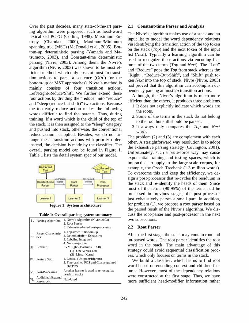
Over the past decades, many state-of-the-art pars-ing algorithm were proposed, such as head-word lexicalized PCFG (Collins, 1998), Maximum En-tropy (Charniak, 2000), Maximum/Minimum spanning tree (MST) (McDonald et al., 2005), Bot-tom-up deterministic parsing (Yamada and Ma-tsumoto, 2003), and Constant-time deterministic parsing (Nivre, 2003). Among them, the Nivre’s algorithm (Nivre, 2003) was shown to be most ef-ficient method, which only costs at most 2n transi-tion actions to parse a sentence (O(n3) for the bottom-up or MST approaches). Nivre’s method is mainly consists of four transition actions, Left/Right/Reduce/Shift. We further extend these four actions by dividing the “reduce” into “reduce” and “sleep (reduce-but-shift)” two actions. Because the too early reduce action makes the following words difficult to find the parents. Thus, during training, if a word which is the child of the top of the stack, it is then assigned to the “sleep” category and pushed into stack, otherwise, the conventional reduce action is applied. Besides, we do not ar-range these transition actions with priority order, instead, the decision is made by the classifier. The overall parsing model can be found in Figure 1. Table 1 lists the detail system spec of our model.
Figure 1: System architecture
Table 1: Overall parsing system summary . Parsing Algorithm: 1. Nivre's Algorithm (Nivre, 2003)
2. Root Parser 3. Exhaustive-based Post-processing
. Parser Characteris-tics:
1. Top-down + Bottom-up 2. Deterministic + Exhaustive 3. Labeling integrated 4. Non-Projective
. Learner: SVMLight (Joachims, 1998) (1) One-versus-One
(2) Linear Kernel . Feature Set: 1. Lexical (Unigram/Bigram)
2. Fine-grained POS and Coarse grained BiCPOS
. Post-Processing: Another learner is used to re-recognize heads in stacks
. Additional/External Resources: Non-Used
2.1 Constant-time Parser and Analysis
The Nivre’s algorithm makes use of a stack and an input list to model the word dependency relations via identifying the transition action of the top token on the stack (Top) and the next token of the input list (Next). Typically a learning algorithm can be used to recognize these actions via encoding fea-tures of the two terms (Top and Next). The “Left” and “Reduce” pops the Top from stack whereas the “Right”, “Reduce-But-Shift”, and “Shift” push to-ken Next into the top of stack. Nivre (Nivre, 2003) had proved that this algorithm can accomplish de-pendency parsing at most 2n transition actions.
Although, the Nivre’s algorithm is much more efficient than the others, it produces three problems.
1. It does not explicitly indicate which words are the roots.
2. Some of the terms in the stack do not belong to the root but still should be parsed.
3. It always only compares the Top and Nextwords.
The problem (2) and (3) are complement with each other. A straightforward way resolution is to adopt the exhaustive parsing strategy (Covington, 2001). Unfortunately, such a brute-force way may cause exponential training and testing spaces, which is impractical to apply to the large-scale corpus, for example, the Czech Treebank (1.3 million words). To overcome this and keep the efficiency, we de-sign a post-processor that re-cycles the residuum in the stack and re-identify the heads of them. Since most of the terms (90-95%) of the terms had be processed in previous stages, the post-processor just exhaustively parses a small part. In addition, for problem (1), we propose a root parser based on the parsed result of the Nivre’s algorithm. We dis-cuss the root-parser and post-processor in the next two subsections.
2.2 Root Parser
After the first stage, the stack may contain root and un-parsed words. The root parser identifies the root word in the stack. The main advantage of this strategy could avoid sequential classification proc-ess, which only focuses on terms in the stack.
We build a classifier, which learns to find root word based on encoding context and children fea-tures. However, most of the dependency relations were constructed at the first stage. Thus, we have more sufficient head-modifier information rather
242
than only taking the contexts into account. The used features are listed as follows.
Neighbor terms,bigrams,POS,BiCPOS (+/-2 window) Left most child term, POS, Bigram, BiCPOS Right most child term, POS, Bigram, BiCPOS
2.3 Post-Processing
Before post-processing, we remove the root words from stack, which were identified by root-parser. The remaining un-parsed words in stack were used to construct the actual dependency graph via ex-haustive comparing with parsed-words. It is neces-sary to build a post-processor since there are about 10% un-parsed words in each training set. We pro-vide the un-parsed rate of each language in Table 2 (the r.h.s. part).
By applying previous two steps (constant-time parser and root parser) to the training data, the re-maining un-parsed tokens were recorded. Not only using the forward parsing direction, the backward direction is also taken into account in this statistics. Averagely, the un-parsed rates of the forward and backward directions are 13% and 4% respectively. The back ward parsing often achieves lower un-parsed rate among all languages (except for Japa-nese and Turkish).
To find the heads of the un-parsed words, we copy the whole sentence into the word list again, and re-compare the un-parsed tokens (in stack) and all of the words in the input list. Comparing with the same words is disallowed. The comparing process is going on until the actual head is found. Acquiescently, we use the nearest root words as its head. Although such a brute force way is time-consuming. However, it only parses a small part of un-parsed tokens (usually, 2 or 3 words per sen-tence).
2.4 Features and Learners
For the constant-time parser of the first stage, we employ the features as follows.
Basic features: Top.word,Top.pos,Top.lchild.pos,Top.lchild.relation,Top.rchild.pos, Top.rchild.relation,Top.head.pos, Top.head.relation,Next.word, Next.pos, Next.lchild.pos, Next.lchild.relation, Next+1.pos, Next+2.pos, Next+3.pos
Enhanced features: Top.bigram,Top.bicpos,Next.bigram,Next.bicpos,Next+1.word,Next+2.word,Next+3.word
In this paper, we use the support vector machines (SVM) (Joachims, 1998) as the learner. SVM is widely used in many natural language processing (NLP) areas, for example, POS tagging (Wu et al., 2006). However, the SVM is a binary classifier which only recognizes true or false. For multiclass problem, we use the so-called one-versus-one (OVO) method with linear kernel to combine the results of each pairwise subclassifier. The final class in testing phase is mainly determined by ma-jority voting. For all languages, our parser uses the same set-tings and features. For all the languages (except Japanese and Turkish), we use backward parsing direction to keep the un-parsed token rate low.
3 Experimental Result
3.1 Dataset and Evaluation Metrics
The testing data is provided by the (Buchholz et al., 2006) which consists of 13 language treebanks. The experimental results are mainly evaluated by the unlabeled and labeled attachment scores. The CoNLL also provided a perl-scripter to automatic compute these rates.
3.2 System Results
Table 2 presents the overall parsing performance of the 13 languages. As shown in Table 2, we list two parsing results at the second and third columns (new and old). It is worth to note that the result B is produced by removing the enhanced features and the post-processing step from our parser, while the result A is the complete use of the enhanced fea-tures and the overall three-step parsing. In this year, we submit result B to the CoNLL shared task due to the time limitation. In addition, we also apply the Maltparser, which is implemented with the Nivre’s algorithm (Nivre, 2003) to be compared. The Maltpaser also includes the SVM and memory-based learner (MBL). Nev-ertheless, it does not optimize the SVM where the training and testing times are too long to be com-pared even the linear kernel is used. Therefore we use the default MBL and feature model 3 (M3) in this experiment. We also perform the significant test to evaluate the statistical difference among the three results. If the answer is “Yes”, it means the two systems are significant difference under at least 95% confidence score (p < 0.05).
243
Table 2: A general statistical table of labeled attachment score, test and un-parsed rate (percentage) Statistic test Un-Parsed Rate A
(New result) B
(Old result)C
(Maltparser) A vs. B B vs. C A vs. C Forward Backward Arabic 63.75 63.81 54.11 No Yes Yes 10.3 1.4Chinese 81.25 74.81 73.92 Yes No Yes 4.01 2.3Czech 71.24 59.36 59.36 Yes No Yes 16.1 5.6Danish 79.52 78.38 77.31 No No No 12.8 2.5Dutch 68.45 68.45 63.61 No Yes Yes 18.4 9.8German 79.57 76.52 76.52 Yes No Yes 12.7 9.2Japanese 91.43 90.11 89.07 Yes No Yes 1.1 4.4Portugese 81.33 81.47 75.38 No Yes Yes 24.3 3.17Slovene 68.41 67.83 55.04 No Yes Yes 14.9 5.5Spanish 74.65 72.99 72.81 Yes No Yes 20 0.5Swedish 79.53 71.72 76.28 Yes Yes Yes 19.1 2.8Turkish 55.33 55.09 52.18 No Yes Yes 2.5 4Bulgarian 81.23 79.73 79.73 No No No 15.7 1.2AVG 75.05 72.32 69.64 13.22 4.02
4 Discussion
4.1 Analysis of Overview Aspect
Although our method is efficient for parsing that achieves satisfactory result, it is still away from the state-of-the-art performance. Many problems give rise to not only the language-specific characteris-tics, but also the parsing strategy. We found that our method is weak to the large-scale training size and large dependency class datasets, for example, German (Brants et al., 2002) and Czech. For Dutch, we observe that the large non-projective tokens and relations in this set. Overall, we conclude the four main limitations of our parsing model.
1.Unbalanced and large dependency relation classes
2.Too fine or coarse POS tag 3.Long sentences and non-projective token rates 4.Feature engineering and root accuracy
The main reason of the first problem is still caused by the unbalanced distribution of the training data. Usually, the right-action categories obtain much fewer training examples. For example, in the Turk-ish data, 50 % of the categories receive less than 0.1% of the training examples, 2/3 are the right dependency group. For the Czech, 74.6% of the categories receive less than 0.1% of the training examples.
Second, the too fine grained size of POS tag set often cause the features too specific that is difficult to be generalized by the learner. Although we found the grained size is not the critical factor of our parser, it is closely related to the fourth prob-lem, feature engineering. For example, in Chinese (Chen et al., 2003), there are 303 fine grained POS types which achieves better result on the labeled attachment score is higher than the coarse grained
(81.25 vs. 81.17). Intuitively, the feature combina-tions deeply affect the system performance (see A vs. C where we extend more features than the original Nivre’s algorithm).
Problem 3 exposes the disadvantage of our method, which is weak to identify the long dis-tance dependency. The main reason is resulted from the Nivre’s algorithm in step 1. This method is quite sensitive and non error-recovered since it is a deterministic parsing strategy. Abnormal or wrong push or pop actions usually cause the error propagation to the remaining words in the list. For example, there are large parts of errors are caused by too early reduce or missed left arc makes some words could not find the actual heads. On the con-trary, one can use an N-best selection to choose the optimal dependency graph or applying MST or exhaustive parsing schema. Usually, these ap-proaches are quite inefficient which requires at least O(n3).
Finally, in this paper, we only take the surface lexical word and POS tag into account without employing the language-specific features, such as Lemma, Morph…etc. Actually, it is an open ques-tion to compile and investigate the feature engi-neering. On the other hand, we also find the performance of the root parser in some languages is poor. For example, for Dutch the root precision rate is only 38.52, while the recall rate is 76.07. It indicates most of the words in stack were wrongly recognized as root. This is because there are sub-stantially un-parsed rate that left many un-parsed words remain in stack. One way to remedy the problem can adjust the root parser to independently identify root word by sequential word classifica-tion at first step and then apply the Nivre’s algo-rithm. We left the comparison of the issue as future work.
244
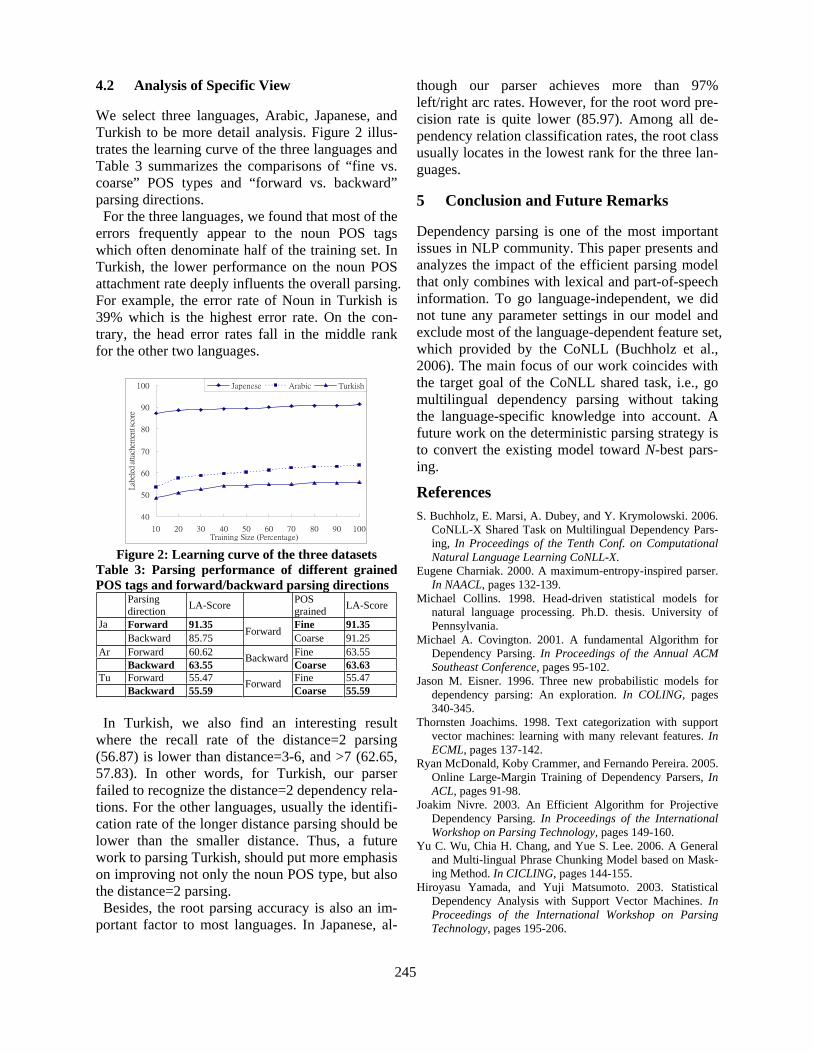
4.2 Analysis of Specific View
We select three languages, Arabic, Japanese, and Turkish to be more detail analysis. Figure 2 illus-trates the learning curve of the three languages and Table 3 summarizes the comparisons of “fine vs. coarse” POS types and “forward vs. backward” parsing directions. For the three languages, we found that most of the errors frequently appear to the noun POS tags which often denominate half of the training set. In Turkish, the lower performance on the noun POS attachment rate deeply influents the overall parsing. For example, the error rate of Noun in Turkish is 39% which is the highest error rate. On the con-trary, the head error rates fall in the middle rank for the other two languages.
Figure 2: Learning curve of the three datasets Table 3: Parsing performance of different grained POS tags and forward/backward parsing directions
Parsing direction LA-Score POS
grained LA-Score
Ja Forward 91.35 Fine 91.35 Backward 85.75 Forward Coarse 91.25 Ar Forward 60.62 Fine 63.55
Backward 63.55 Backward Coarse 63.63 Tu Forward 55.47 Fine 55.47
Backward 55.59 Forward Coarse 55.59
In Turkish, we also find an interesting result where the recall rate of the distance=2 parsing (56.87) is lower than distance=3-6, and >7 (62.65, 57.83). In other words, for Turkish, our parser failed to recognize the distance=2 dependency rela-tions. For the other languages, usually the identifi-cation rate of the longer distance parsing should be lower than the smaller distance. Thus, a future work to parsing Turkish, should put more emphasis on improving not only the noun POS type, but also the distance=2 parsing. Besides, the root parsing accuracy is also an im-portant factor to most languages. In Japanese, al-
though our parser achieves more than 97% left/right arc rates. However, for the root word pre-cision rate is quite lower (85.97). Among all de-pendency relation classification rates, the root class usually locates in the lowest rank for the three lan-guages.
5 Conclusion and Future Remarks
Dependency parsing is one of the most important issues in NLP community. This paper presents and analyzes the impact of the efficient parsing model that only combines with lexical and part-of-speech information. To go language-independent, we did not tune any parameter settings in our model and exclude most of the language-dependent feature set, which provided by the CoNLL (Buchholz et al., 2006). The main focus of our work coincides with the target goal of the CoNLL shared task, i.e., go multilingual dependency parsing without taking the language-specific knowledge into account. A future work on the deterministic parsing strategy is to convert the existing model toward N-best pars-ing.
References S. Buchholz, E. Marsi, A. Dubey, and Y. Krymolowski. 2006.
CoNLL-X Shared Task on Multilingual Dependency Pars-ing, In Proceedings of the Tenth Conf. on Computational Natural Language Learning CoNLL-X.
Eugene Charniak. 2000. A maximum-entropy-inspired parser. In NAACL, pages 132-139.
Michael Collins. 1998. Head-driven statistical models for natural language processing. Ph.D. thesis. University of Pennsylvania.
Michael A. Covington. 2001. A fundamental Algorithm for Dependency Parsing. In Proceedings of the Annual ACM Southeast Conference, pages 95-102.
Jason M. Eisner. 1996. Three new probabilistic models for dependency parsing: An exploration. In COLING, pages 340-345.
Thornsten Joachims. 1998. Text categorization with support vector machines: learning with many relevant features. In ECML, pages 137-142.
Ryan McDonald, Koby Crammer, and Fernando Pereira. 2005. Online Large-Margin Training of Dependency Parsers, InACL, pages 91-98.
Joakim Nivre. 2003. An Efficient Algorithm for Projective Dependency Parsing. In Proceedings of the International Workshop on Parsing Technology, pages 149-160.
Yu C. Wu, Chia H. Chang, and Yue S. Lee. 2006. A General and Multi-lingual Phrase Chunking Model based on Mask-ing Method. In CICLING, pages 144-155.
Hiroyasu Yamada, and Yuji Matsumoto. 2003. Statistical Dependency Analysis with Support Vector Machines. In Proceedings of the International Workshop on Parsing Technology, pages 195-206.
245
Proceedings of the 10th Conference on Computational Natural Language Learning (CoNLL-X),pages 246–250, New York City, June 2006.c©2006 Association for Computational Linguistics
Dependency Parsing as a Classification Problem
Deniz YuretKoc UniversityIstanbul, Turkey
Abstract
This paper presents an approach to depen-dency parsing which can utilize any stan-dard machine learning (classification) al-gorithm. A decision list learner was usedin this work. The training data providedin the form of a treebank is converted to aformat in which each instance representsinformation about one word pair, and theclassification indicates the existence, di-rection, and type of the link between thewords of the pair. Several distinct mod-els are built to identify the links betweenword pairs at different distances. Thesemodels are applied sequentially to give thedependency parse of a sentence, favoringshorter links. An analysis of the errors,attribute selection, and comparison of dif-ferent languages is presented.
1 Introduction
This paper presents an approach to supervised learn-ing of dependency relations in a language using stan-dard machine learning techniques. The treebanks(Hajic et al., 2004; Chen et al., 2003; Bohmovaet al., 2003; Kromann, 2003; van der Beek et al.,2002; Brants et al., 2002; Kawata and Bartels, 2000;Afonso et al., 2002; Dzeroski et al., 2006; Civit Tor-ruella and Martı Antonın, 2002; Nilsson et al., 2005;Oflazer et al., 2003; Atalay et al., 2003) provided forthe CoNLL shared task(Buchholz et al., 2006) wereconverted to a set of instances each of which con-sists of the attributes of a candidate word pair with
a classification that indicates the existence, directionand type of the dependency link between the pair.
An initial model is built to identify dependencyrelations between adjacent word pairs using a deci-sion list learning algorithm. To identify longer dis-tance relations, the adjacent modifiers are droppedfrom the sentence and a second order model is builtbased on the word pairs that come into contact. Atotal of three models were built using this techniquesuccessively and used for parsing.
All given attributes are considered as candidatesin an attribute selection process before building eachmodel. In addition, attributes indicating suffixes ofvarious lengths and character type information wereconstructed and used.
To parse a given sentence, the models are appliedsequentially, each one considering candidate wordpairs and adding new links without deleting the ex-isting links or creating conflicts (cycles or crossings)with them. Thus, the algorithm can be considered abottom-up, multi-pass, deterministic parser. Givena candidate word pair, the models may output “nolink”, or give a link with a specified direction andtype. Thus labeling is an integrated step. Wordpair candidates that may form cycles or crossingsare never considered, so the parser will only gen-erate projective structures.
Section 2 gives the details of the learning algo-rithm. Section 3 describes the first pass model oflinks between adjacent words. Section 4 detailsthe approach for identifying long distance links andpresents the parsing results.
246

2 The Learning Algorithm
The Greedy Prepend Algorithm (Yuret and Ture,2006) was used to build decision lists to identify de-pendency relations. A decision list is an ordered listof rules where each rule consists of a pattern and aclassification (Rivest, 1987). The first rule whosepattern matches a given instance is used for its clas-sification. In our application the pattern specifies theattributes of the two words to be linked such as partsof speech and morphological features. The classi-fication indicates the existence and the type of thedependency link between the two words.
Table 1 gives a subset of the decision list that iden-tifies links between adjacent words in German. Theclass column indicates the type of the link, the pat-tern contains attributes of the two candidate words Xand Y, as well as their neighbors (XL1 indicates theleft neighbor of X). For example, given the part ofspeech sequence APPR-ART-NN, there would be anNK link between APPR and ART (matches rule 3), butthere would be no link between ART and NN (rule 1overrides rule 2).
Rule Class Pattern1 NONE XL1:postag=APPR2 L:NK X:postag=ART Y:postag=NN3 R:NK X:postag=APPR4 NONE
Table 1: A four rule decision list for adjacent worddependencies in German
The average training instance for the depen-dency problem has over 40 attributes describing thetwo candidate words including suffixes of differentlengths, parts of speech and information on neigh-boring words. Most of this information may be re-dundant or irrelevant to the problem at hand. Thenumber of distinct attribute values is on the orderof the number of distinct word-forms in the train-ing set. GPA was picked for this problem becauseit has proven to be fairly efficient and robust in thepresence of irrelevant or redundant attributes in pre-vious work such as morphological disambiguationin Turkish (Yuret and Ture, 2006) and protein sec-ondary structure prediction (Kurt, 2005).
3 Dependency of Adjacent Words
We start by looking at adjacent words and try to pre-dict whether they are linked, and if they are, whattype of link they have. This is a nice subproblem tostudy because: (i) It is easily converted to a standardmachine learning problem, thus amenable to com-mon machine learning techniques and analysis, (ii)It demonstrates the differences between languagesand the impact of various attributes. The machinelearning algorithm used was GPA (See Section 2)which builds decision lists.
Table 2 shows the percentage of adjacent tokensthat are linked in the training sets for the languagesstudied1 . Most languages have approximately halfof the adjacent words linked. German, with 42.15%is at the low end whereas Arabic and Turkish withabove 60% are at the high end. The differences maybe due to linguistic factors such as the ubiquity offunction words which prefer short distance links, orit may be an accident of data representation: for ex-ample each token in the Turkish data represents aninflectional group, not a whole word.
Arabic 61.02 Japanese 54.81Chinese 56.59 Portuguese 50.81Czech 48.73 Slovene 45.62Danish 55.93 Spanish 51.28Dutch 55.54 Swedish 48.26German 42.15 Turkish 62.60
Table 2: Percentage of adjacent tokens linked.
3.1 AttributesThe five attributes provided for each word in thetreebanks were the wordform, the lemma, thecoarse-grained and fine-grained parts of speech, anda list of syntactic and/or morphological features. Inaddition I generated two more attributes for eachword: suffixes of up to n characters (indicatedby suffix[n]), and character type information, i.e.whether the word contains any punctuation charac-ters, upper case letters, digits, etc.
Two questions to be answered empirically are: (i)How much context to include in the description ofeach instance, and (ii) Which attributes to use foreach language.
1Including non-scoring tokens
247
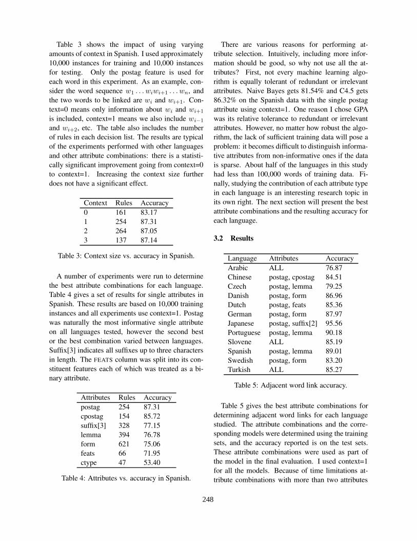
Table 3 shows the impact of using varyingamounts of context in Spanish. I used approximately10,000 instances for training and 10,000 instancesfor testing. Only the postag feature is used foreach word in this experiment. As an example, con-sider the word sequence w1 . . . wiwi+1 . . . wn, andthe two words to be linked are wi and wi+1. Con-text=0 means only information about wi and wi+1
is included, context=1 means we also include wi−1
and wi+2, etc. The table also includes the numberof rules in each decision list. The results are typicalof the experiments performed with other languagesand other attribute combinations: there is a statisti-cally significant improvement going from context=0to context=1. Increasing the context size furtherdoes not have a significant effect.
Context Rules Accuracy0 161 83.171 254 87.312 264 87.053 137 87.14
Table 3: Context size vs. accuracy in Spanish.
A number of experiments were run to determinethe best attribute combinations for each language.Table 4 gives a set of results for single attributes inSpanish. These results are based on 10,000 traininginstances and all experiments use context=1. Postagwas naturally the most informative single attributeon all languages tested, however the second bestor the best combination varied between languages.Suffix[3] indicates all suffixes up to three charactersin length. The FEATS column was split into its con-stituent features each of which was treated as a bi-nary attribute.
Attributes Rules Accuracypostag 254 87.31cpostag 154 85.72suffix[3] 328 77.15lemma 394 76.78form 621 75.06feats 66 71.95ctype 47 53.40
Table 4: Attributes vs. accuracy in Spanish.
There are various reasons for performing at-tribute selection. Intuitively, including more infor-mation should be good, so why not use all the at-tributes? First, not every machine learning algo-rithm is equally tolerant of redundant or irrelevantattributes. Naive Bayes gets 81.54% and C4.5 gets86.32% on the Spanish data with the single postagattribute using context=1. One reason I chose GPAwas its relative tolerance to redundant or irrelevantattributes. However, no matter how robust the algo-rithm, the lack of sufficient training data will pose aproblem: it becomes difficult to distinguish informa-tive attributes from non-informative ones if the datais sparse. About half of the languages in this studyhad less than 100,000 words of training data. Fi-nally, studying the contribution of each attribute typein each language is an interesting research topic inits own right. The next section will present the bestattribute combinations and the resulting accuracy foreach language.
3.2 Results
Language Attributes AccuracyArabic ALL 76.87Chinese postag, cpostag 84.51Czech postag, lemma 79.25Danish postag, form 86.96Dutch postag, feats 85.36German postag, form 87.97Japanese postag, suffix[2] 95.56Portuguese postag, lemma 90.18Slovene ALL 85.19Spanish postag, lemma 89.01Swedish postag, form 83.20Turkish ALL 85.27
Table 5: Adjacent word link accuracy.
Table 5 gives the best attribute combinations fordetermining adjacent word links for each languagestudied. The attribute combinations and the corre-sponding models were determined using the trainingsets, and the accuracy reported is on the test sets.These attribute combinations were used as part ofthe model in the final evaluation. I used context=1for all the models. Because of time limitations at-tribute combinations with more than two attributes
248
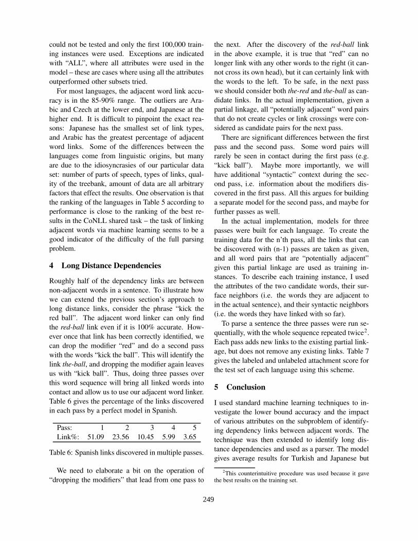
could not be tested and only the first 100,000 train-ing instances were used. Exceptions are indicatedwith “ALL”, where all attributes were used in themodel – these are cases where using all the attributesoutperformed other subsets tried.
For most languages, the adjacent word link accu-racy is in the 85-90% range. The outliers are Ara-bic and Czech at the lower end, and Japanese at thehigher end. It is difficult to pinpoint the exact rea-sons: Japanese has the smallest set of link types,and Arabic has the greatest percentage of adjacentword links. Some of the differences between thelanguages come from linguistic origins, but manyare due to the idiosyncrasies of our particular dataset: number of parts of speech, types of links, qual-ity of the treebank, amount of data are all arbitraryfactors that effect the results. One observation is thatthe ranking of the languages in Table 5 according toperformance is close to the ranking of the best re-sults in the CoNLL shared task – the task of linkingadjacent words via machine learning seems to be agood indicator of the difficulty of the full parsingproblem.
4 Long Distance Dependencies
Roughly half of the dependency links are betweennon-adjacent words in a sentence. To illustrate howwe can extend the previous section’s approach tolong distance links, consider the phrase “kick thered ball”. The adjacent word linker can only findthe red-ball link even if it is 100% accurate. How-ever once that link has been correctly identified, wecan drop the modifier “red” and do a second passwith the words “kick the ball”. This will identify thelink the-ball, and dropping the modifier again leavesus with “kick ball”. Thus, doing three passes overthis word sequence will bring all linked words intocontact and allow us to use our adjacent word linker.Table 6 gives the percentage of the links discoveredin each pass by a perfect model in Spanish.
Pass: 1 2 3 4 5Link%: 51.09 23.56 10.45 5.99 3.65
Table 6: Spanish links discovered in multiple passes.
We need to elaborate a bit on the operation of“dropping the modifiers” that lead from one pass to
the next. After the discovery of the red-ball linkin the above example, it is true that “red” can nolonger link with any other words to the right (it can-not cross its own head), but it can certainly link withthe words to the left. To be safe, in the next passwe should consider both the-red and the-ball as can-didate links. In the actual implementation, given apartial linkage, all “potentially adjacent” word pairsthat do not create cycles or link crossings were con-sidered as candidate pairs for the next pass.
There are significant differences between the firstpass and the second pass. Some word pairs willrarely be seen in contact during the first pass (e.g.“kick ball”). Maybe more importantly, we willhave additional “syntactic” context during the sec-ond pass, i.e. information about the modifiers dis-covered in the first pass. All this argues for buildinga separate model for the second pass, and maybe forfurther passes as well.
In the actual implementation, models for threepasses were built for each language. To create thetraining data for the n’th pass, all the links that canbe discovered with (n-1) passes are taken as given,and all word pairs that are “potentially adjacent”given this partial linkage are used as training in-stances. To describe each training instance, I usedthe attributes of the two candidate words, their sur-face neighbors (i.e. the words they are adjacent toin the actual sentence), and their syntactic neighbors(i.e. the words they have linked with so far).
To parse a sentence the three passes were run se-quentially, with the whole sequence repeated twice2.Each pass adds new links to the existing partial link-age, but does not remove any existing links. Table 7gives the labeled and unlabeled attachment score forthe test set of each language using this scheme.
5 Conclusion
I used standard machine learning techniques to in-vestigate the lower bound accuracy and the impactof various attributes on the subproblem of identify-ing dependency links between adjacent words. Thetechnique was then extended to identify long dis-tance dependencies and used as a parser. The modelgives average results for Turkish and Japanese but
2This counterintuitive procedure was used because it gavethe best results on the training set.
249
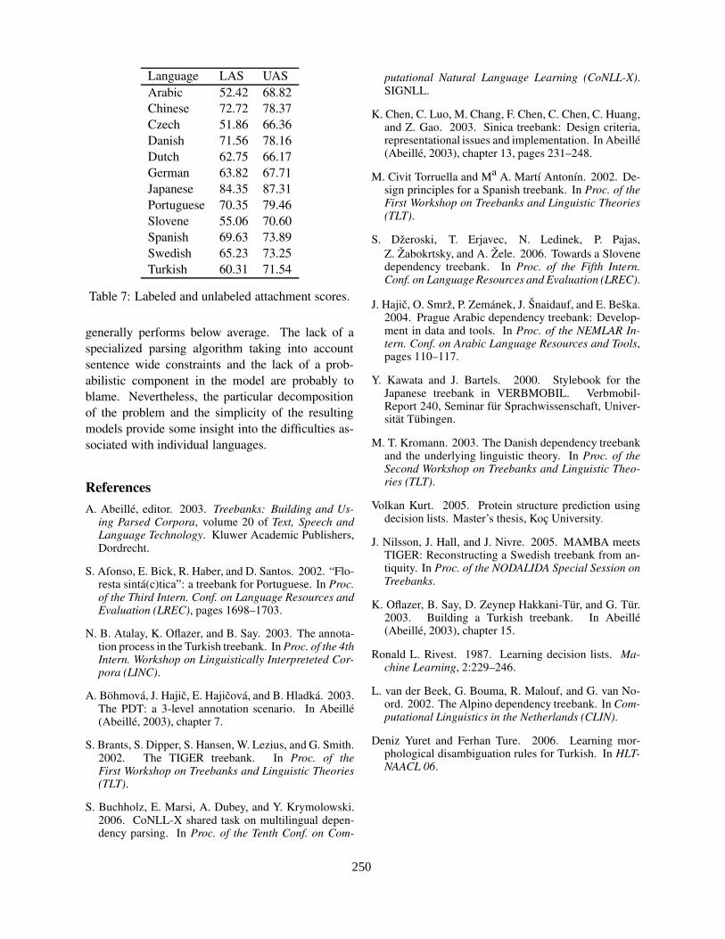
Language LAS UASArabic 52.42 68.82Chinese 72.72 78.37Czech 51.86 66.36Danish 71.56 78.16Dutch 62.75 66.17German 63.82 67.71Japanese 84.35 87.31Portuguese 70.35 79.46Slovene 55.06 70.60Spanish 69.63 73.89Swedish 65.23 73.25Turkish 60.31 71.54
Table 7: Labeled and unlabeled attachment scores.
generally performs below average. The lack of aspecialized parsing algorithm taking into accountsentence wide constraints and the lack of a prob-abilistic component in the model are probably toblame. Nevertheless, the particular decompositionof the problem and the simplicity of the resultingmodels provide some insight into the difficulties as-sociated with individual languages.
ReferencesA. Abeille, editor. 2003. Treebanks: Building and Us-
ing Parsed Corpora, volume 20 of Text, Speech andLanguage Technology. Kluwer Academic Publishers,Dordrecht.
S. Afonso, E. Bick, R. Haber, and D. Santos. 2002. “Flo-resta sinta(c)tica”: a treebank for Portuguese. In Proc.of the Third Intern. Conf. on Language Resources andEvaluation (LREC), pages 1698–1703.
N. B. Atalay, K. Oflazer, and B. Say. 2003. The annota-tion process in the Turkish treebank. In Proc. of the 4thIntern. Workshop on Linguistically Interpreteted Cor-pora (LINC).
A. Bohmova, J. Hajic, E. Hajicova, and B. Hladka. 2003.The PDT: a 3-level annotation scenario. In Abeille(Abeille, 2003), chapter 7.
S. Brants, S. Dipper, S. Hansen, W. Lezius, and G. Smith.2002. The TIGER treebank. In Proc. of theFirst Workshop on Treebanks and Linguistic Theories(TLT).
S. Buchholz, E. Marsi, A. Dubey, and Y. Krymolowski.2006. CoNLL-X shared task on multilingual depen-dency parsing. In Proc. of the Tenth Conf. on Com-
putational Natural Language Learning (CoNLL-X).SIGNLL.
K. Chen, C. Luo, M. Chang, F. Chen, C. Chen, C. Huang,and Z. Gao. 2003. Sinica treebank: Design criteria,representational issues and implementation. In Abeille(Abeille, 2003), chapter 13, pages 231–248.
M. Civit Torruella and Ma A. Martı Antonın. 2002. De-sign principles for a Spanish treebank. In Proc. of theFirst Workshop on Treebanks and Linguistic Theories(TLT).
S. Dzeroski, T. Erjavec, N. Ledinek, P. Pajas,Z. Zabokrtsky, and A. Zele. 2006. Towards a Slovenedependency treebank. In Proc. of the Fifth Intern.Conf. on Language Resources and Evaluation (LREC).
J. Hajic, O. Smrz, P. Zemanek, J. Snaidauf, and E. Beska.2004. Prague Arabic dependency treebank: Develop-ment in data and tools. In Proc. of the NEMLAR In-tern. Conf. on Arabic Language Resources and Tools,pages 110–117.
Y. Kawata and J. Bartels. 2000. Stylebook for theJapanese treebank in VERBMOBIL. Verbmobil-Report 240, Seminar fur Sprachwissenschaft, Univer-sitat Tubingen.
M. T. Kromann. 2003. The Danish dependency treebankand the underlying linguistic theory. In Proc. of theSecond Workshop on Treebanks and Linguistic Theo-ries (TLT).
Volkan Kurt. 2005. Protein structure prediction usingdecision lists. Master’s thesis, Koc University.
J. Nilsson, J. Hall, and J. Nivre. 2005. MAMBA meetsTIGER: Reconstructing a Swedish treebank from an-tiquity. In Proc. of the NODALIDA Special Session onTreebanks.
K. Oflazer, B. Say, D. Zeynep Hakkani-Tur, and G. Tur.2003. Building a Turkish treebank. In Abeille(Abeille, 2003), chapter 15.
Ronald L. Rivest. 1987. Learning decision lists. Ma-chine Learning, 2:229–246.
L. van der Beek, G. Bouma, R. Malouf, and G. van No-ord. 2002. The Alpino dependency treebank. In Com-putational Linguistics in the Netherlands (CLIN).
Deniz Yuret and Ferhan Ture. 2006. Learning mor-phological disambiguation rules for Turkish. In HLT-NAACL 06.
250
Author Index
Cakıcı, Ruket,226
Ando, Rie Kubota,77Armstrong, Susan,101Asahara, Masayuki,191Attardi, Giuseppe,166Atterer, Michaela,93Aue, Anthony,196
Barrett, Leon,14Basili, Roberto,61Bengio, Samy,45Bick, Eckhard,171Bod, Rens,85Bogers, Toine,176Brants, Thorsten,141Brooks, David J.,117Buchholz, Sabine,149
Canisius, Sander,176Carreras, Xavier,181Chang, Ming-Wei ,186Cheng, Yuchang,191Cherry, Colin,21Clark, Alexander,101, 125Corston-Oliver, Simon ,196
Daelemans, Walter,1, 45Dagan, Ido,45Do, Quang,186Dreyer, Markus,201
Eryigit, Gulsen ,221Eyraud, Remi,125
Garera, Nikesh,37Geertzen, Jeroen,176Georgescul, Maria,101Glickman, Oren,45
Hall, Johan,221Hauptmann, Alexander,109Henderson, James,6
Johansson, Richard,206
Kazama, Jun’ichi,53Keller, Mikaela,45Klein, Dan,14
Lee, Yue-Shi,241Lerman, Kevin,216Li, Sheng,211Liberman, Mark,141Lin, Wei-Hao,109Liu, Ting, 211Lizotte, Dan,21
Ma, Jinshan,211Marinov, Svetoslav,221Marquez, Lluıs,181Marsi, Erwin,149Matsumoto, Yuji,191McDonald, Ryan,216Meza-Ruiz, Ivan,226Moschitti, Alessandro,61
Nilsson, Jens,221Nivre, Joakim ,221Nugues, Pierre,206
Osborne, Miles,133
Pereira, Fernando,141, 216Petrov, Slav,14Pighin, Daniele,61
Riedel, Sebastian,226Roth, Dan,186
Schiehlen, Michael,231
251
Schulte im Walde, Sabine,69Schutze, Hinrich,93Schuurmans, Dale,21Shimizu, Nobuyuki,236Smith, Andrew,133Smith, David A. ,201Smith, Noah A.,201Spranger, Kristina,231Surdeanu, Mihai,181
Talukdar, Partha Pratim,141Titov, Ivan,6Tjong Kim Sang, Erik,176Torisawa, Kentaro,53
van den Bosch, Antal,176
Wang, Qin Iris,21Wiebe, Janyce,109Wilson, Theresa,109Wu, Yu-Chieh,241
Yang, Jie-Chi,241Yarowsky, David,37Yuret, Deniz,246
Zhu, Huijia,211Zuidema, Willem,29
Related Documents