CONJUGATION PROBLEMS FOR HIRSCH FOLIATIONS

CONJUGATION PROBLEMS FOR HIRSCH FOLIATIONS

BY

JOSEPH H. SHIVEB.S. (University of Illinois at Chicago 1991)M.S. (University of Illinois at Chicago 2001)

THESIS

Submitted in partial fulfillment of the requirementsfor the degree of Doctor of Philosophy in Mathematics

in the Graduate College of theUniversity of Illinois at Chicago, 2005

Chicago, Illinois

Copyright by

Joseph H. Shive

2005

Dedicated to the Memory of Donna J. Shive (1938-2001)

iii

ACKNOWLEDGMENTS

Any list of acknowledgements will, of course be incomplete. Ther are professors who took

extra time to explain concepts, friends and family who have provided emotional and material

support, and fellow students with whom I have discussed mathematics. I will try to thank the

most important few:

My advisor Steve Hurder, for his patience and guidance over the years.

My dad Jim, and his wife Charlotte, and my brothers and sisters Geoff and Lois, Peg and Peter,

Jon and Shirley, who have all supported me in every way possible.

John, Tony, Gaspar and Ken, for their good friendship.

JHS

iv

TABLE OF CONTENTS

CHAPTER PAGE

1 INTRODUCTION . . . . . . . . . . . . . . . . . . . . . . . . . . . . . . . . 11.1 Introduction . . . . . . . . . . . . . . . . . . . . . . . . . . . . . . 11.2 Some background for the casual reader . . . . . . . . . . . . . . 11.2.1 Cookie Cutters . . . . . . . . . . . . . . . . . . . . . . . . . . . . 11.2.2 Foliations and the Hirsch Example . . . . . . . . . . . . . . . . 61.2.3 The conjugation problem . . . . . . . . . . . . . . . . . . . . . . 91.2.4 The conjugation problem for cookie cutters. . . . . . . . . . . . 121.2.5 Dynamically defined Cantor sets on the circle . . . . . . . . . . 131.2.6 The Conjugation Problem for Hirsch Foliations . . . . . . . . . 18

2 DEFINITIONS AND CONCEPTS . . . . . . . . . . . . . . . . . . . . 212.1 Lipschitz and Holder Continuity . . . . . . . . . . . . . . . . . . 212.2 Coarse Equivalence . . . . . . . . . . . . . . . . . . . . . . . . . 292.3 Pseudogroups . . . . . . . . . . . . . . . . . . . . . . . . . . . . . 302.4 Foliations . . . . . . . . . . . . . . . . . . . . . . . . . . . . . . . 322.4.1 The holonomy groupoid . . . . . . . . . . . . . . . . . . . . . . . 342.5 Limit Sets And Invariant Sets . . . . . . . . . . . . . . . . . . . 362.5.1 Orbits . . . . . . . . . . . . . . . . . . . . . . . . . . . . . . . . . 362.5.2 Minimal Sets . . . . . . . . . . . . . . . . . . . . . . . . . . . . . 382.5.3 Paths To Infinity. . . . . . . . . . . . . . . . . . . . . . . . . . . . 412.5.4 Cantor Sets . . . . . . . . . . . . . . . . . . . . . . . . . . . . . . 412.5.5 Bernoulli Shift Spaces . . . . . . . . . . . . . . . . . . . . . . . . 432.5.6 Labeled Cantor sets. . . . . . . . . . . . . . . . . . . . . . . . . . 462.6 Bounded Geometry. . . . . . . . . . . . . . . . . . . . . . . . . . 492.7 Cookie Cutters II . . . . . . . . . . . . . . . . . . . . . . . . . . . 502.8 Exceptional Minimal Sets . . . . . . . . . . . . . . . . . . . . . . 542.9 The scaling function for a Markov exceptional set. . . . . . . . 57

3 EXAMPLES . . . . . . . . . . . . . . . . . . . . . . . . . . . . . . . . . . . . 583.1 Pseudogroups On S1 . . . . . . . . . . . . . . . . . . . . . . . . . 583.1.1 Cookie cutters on the circle. . . . . . . . . . . . . . . . . . . . . 583.1.2 A period two interval . . . . . . . . . . . . . . . . . . . . . . . . 603.1.3 A free group acting on the circle . . . . . . . . . . . . . . . . . . 653.2 The Hirsch Foliation . . . . . . . . . . . . . . . . . . . . . . . . . 673.2.1 The Shape of Leaves . . . . . . . . . . . . . . . . . . . . . . . . . 693.2.2 The holonomy of the Hirsch foliation . . . . . . . . . . . . . . . 703.2.3 The Hirsch Example With Linear Generators . . . . . . . . . . 72

v

TABLE OF CONTENTS (Continued)

CHAPTER PAGE

3.2.4 Limit Sets of Ends and Paths . . . . . . . . . . . . . . . . . . . 743.2.5 The Hirsch Example With A Cookie Cutter . . . . . . . . . . . 753.3 The Double Suspension . . . . . . . . . . . . . . . . . . . . . . . 773.4 Generalizing Hirsch’s Construction . . . . . . . . . . . . . . . . 77

4 RESULTS ON S1 AND I . . . . . . . . . . . . . . . . . . . . . . . . . . . 804.1 The Conjugation Problem for Cookie Cutters . . . . . . . . . . 804.1.1 Automorphisms of Cookie Cutter Sets . . . . . . . . . . . . . . 804.1.2 C1+λ Equivalence . . . . . . . . . . . . . . . . . . . . . . . . . . . 864.1.3 Ck+λ Equivalence . . . . . . . . . . . . . . . . . . . . . . . . . . 954.2 The Conjugation Problem for Markov Exceptional Sets . . . . 1034.3 The Conjugation Problem For Hirsch Foliations . . . . . . . . 106

CITED LITERATURE . . . . . . . . . . . . . . . . . . . . . . . . . . . . 109

VITA . . . . . . . . . . . . . . . . . . . . . . . . . . . . . . . . . . . . . . . . . 113

vi

LIST OF FIGURES

FIGURE PAGE

1 The Middle Third Set . . . . . . . . . . . . . . . . . . . . . . . . . . . . . . 2

2 The function F which preserves the middle third set . . . . . . . . . . . 3

3 A cookie cutter map with two generators . . . . . . . . . . . . . . . . . . 5

4 The Hirsch Foliation: We glue the top of the cylinder to the bottom toget a solid torus with another solid torus removed. Then we glue theinside component to the outside component to get the Hirsch foliation. 7

5 As we sew pairs of pants together to get the leaves, we see that the leaveswill be coarsely equivalent to a tree. . . . . . . . . . . . . . . . . . . . . . 8

6 A cookie cutter on the circle . . . . . . . . . . . . . . . . . . . . . . . . . . 14

7 A map with a period two interval. f [G1] = G2 and f [G2] = G1, soG1 ∪ G2 acts as a trap for the dynamics of f . If f ′ > 1 off of G1 ∪ G2,then the backwards images of G1 ∪ G2 form the gaps of an invariantCantor set. . . . . . . . . . . . . . . . . . . . . . . . . . . . . . . . . . . . . 15

8 The nested interval structure of a function with a period two interval.As we iterate the process, the intervals Iw will nest down to an invariantCantor set. . . . . . . . . . . . . . . . . . . . . . . . . . . . . . . . . . . . . 17

9 the middle third set . . . . . . . . . . . . . . . . . . . . . . . . . . . . . . . 42

10 The function x 7→ 3x (mod 1) which has the middle third set as aninvariant set. . . . . . . . . . . . . . . . . . . . . . . . . . . . . . . . . . . . 50

11 A cookie cutter map with two generators . . . . . . . . . . . . . . . . . . 52

12 A cookie cutter map on the circle . . . . . . . . . . . . . . . . . . . . . . . 58

13 A map with a period two interval . . . . . . . . . . . . . . . . . . . . . . . 61

14 The minimal set of a period two interval . . . . . . . . . . . . . . . . . . . 62

vii

SUMMARY

In this thesis, we study the problem of when two Cr-foliations of codimension one on

compact manifolds which are topologically conjugate must be Cr-conjugate, or at least Cr-

conjugate on exceptional minimal sets. The transverse geometry of an exceptional minimal

set in codimension one is that of a geometric Cantor set, and for a Markov minimal set, there

is a finite set of linearly contracting generators for the induced holonomy pseudogroup. Our

main result gives a solution of the conjugacy problem for Markov minimal sets in terms of

the asymptotic ratio function defined on the endset of the typical leaf in the minimal set. The

solution is obtained by studying the conjugacy problem first on Cantor sets in the line, and then

extending and interpreting this solution in the context of maps between foliations. The second

part of this thesis is the investigation of the conjugacy problem for a class of codimension one

foliations which generalize a construction by M. Hirsch.

viii

CHAPTER 1

INTRODUCTION

1.1 Introduction

In this thesis, we study the problem of when two Cr-foliations of codimension one on

compact manifolds which are topologically conjugate must be Cr-conjugate, or at least Cr-

conjugate on exceptional minimal sets. The transverse geometry of an exceptional minimal

set in codimension one is that of a geometric Cantor set, and for a Markov minimal set, there

is a finite set of linearly contracting generators for the induced holonomy pseudogroup. Our

main result gives a solution of the conjugacy problem for Markov minimal sets in terms of

the asymptotic ratio function defined on the endset of the typical leaf in the minimal set. The

solution is obtained by studying the conjugacy problem first on Cantor sets in the line, and then

extending and interpreting this solution in the context of maps between foliations. The second

part of this thesis is the investigation of the conjugacy problem for a class of codimension one

foliations which generalize a construction by M. Hirsch.

1.2 Some background for the casual reader

1.2.1 Cookie Cutters

A casual reader of this thesis, if there is one, might be familiar with geometric objects called

fractals. Fractals are described in the popular literature as self-similar sets, i.e. a small part

1

2

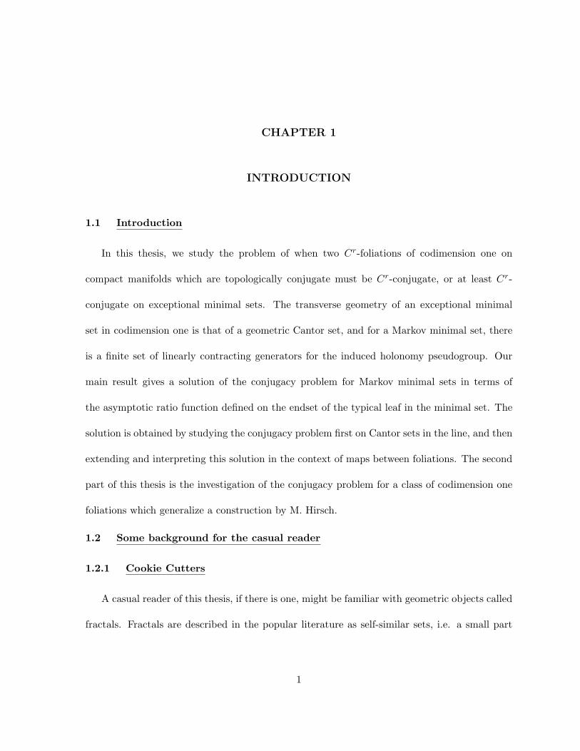
of the set will be a scaled down replica of the whole set. Perhaps the simplest example of a

self-similar fractal is the Cantor middle-third set.

To construct the middle third set, we begin with the interval I = [0, 1]. We subdivide I into

thirds, and remove the middle third G = (13 ,

23). After this removal, we’re left with I0 = [0, 1

3 ]

and I1 = [23 , 1].

We repeat this process on both I0 and I1, removing the middle thirds, which we call G0

and G1, respectively from both of them. The second approximation consists of the intervals

I00 = [0, 19 ], I01 = [29 ,

13 ], I10 = [23 ,

79 ], and I01 = [89 , 1]. We remove the middle thirds from

each of these four intervals, G00, G01, G10, and G01 respectively, obtaining eight disjoint closed

intervals, I000, I001, I010, I011, I100, I101, I110, and I111,each with length 127 . If w is any finite

string of 0s and 1s, we then Iw will eventually be defined in this process. We continue this an

infinite number of times to obtain C. The intervals Iw shrink down to points in C.

Figure 1. The Middle Third Set

3

We say Gw is the gap of Iw. Note that each of the subsets Cw = C⋂Iw are similar to the

whole set C, since we simply repeated the same construction on each of the sub-intervals as we

did on the whole set, so we call Cw a clone and Iw a clone interval.

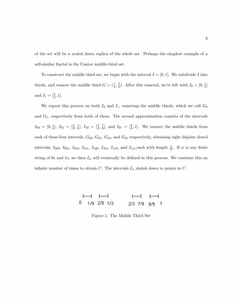
The self-similarity of C shows us that if we take either of the clones, C0 or C1, and stretch

them out by a factor of 3, we get C back. That is, C is preserved by the map

F : x 7→

3x x ∈ [0, 1

3 ]

3x− 2 x ∈ [23 , 1]

Figure 2. The function F which preserves the middle third set

4

F has two right inverses,

F−10 : x 7→ x

3

F−11 : x 7→ x+ 2

3

We can use F to define the intervals:

I0 = F−10 [I] I1 = F−1

1 [I]

I00 = F−10 [I0] I01 = f−1

0 [I1]

and so forth, where F−10 [I] =

{F−1

0 (x)|x ∈ I}. In general for w a finite word, Iiw = F−1

i [Iw],

and conversely F [Iiw] = Iw. As the sub-intervals shrink down to points in C, we see that

for F (xε0ε1...) = xε1.... We note that C is totally disconnected, perfect, compact, and has

the cardinality of the reals. This classifies C up to homeomorphism; any topological space

with these properties is homeomorphic to C. We call any set which is homeomorphic to the

middle-third set Cantor set.

A cookie cutter function set (see page 50) is a generalization of the function F defined above.

We let I0 = [0, a] and I1 = [b, 1] be disjoint intervals, and let h0 : I0 −→ I and h1 : I1 −→ I be

functions whose derivatives are bounded above 1. Then define

I0 = h−10 [I] I1 = h−1

1 [I]

I00 = h−10 [I0] I01 = h−1

0 [I1]

5

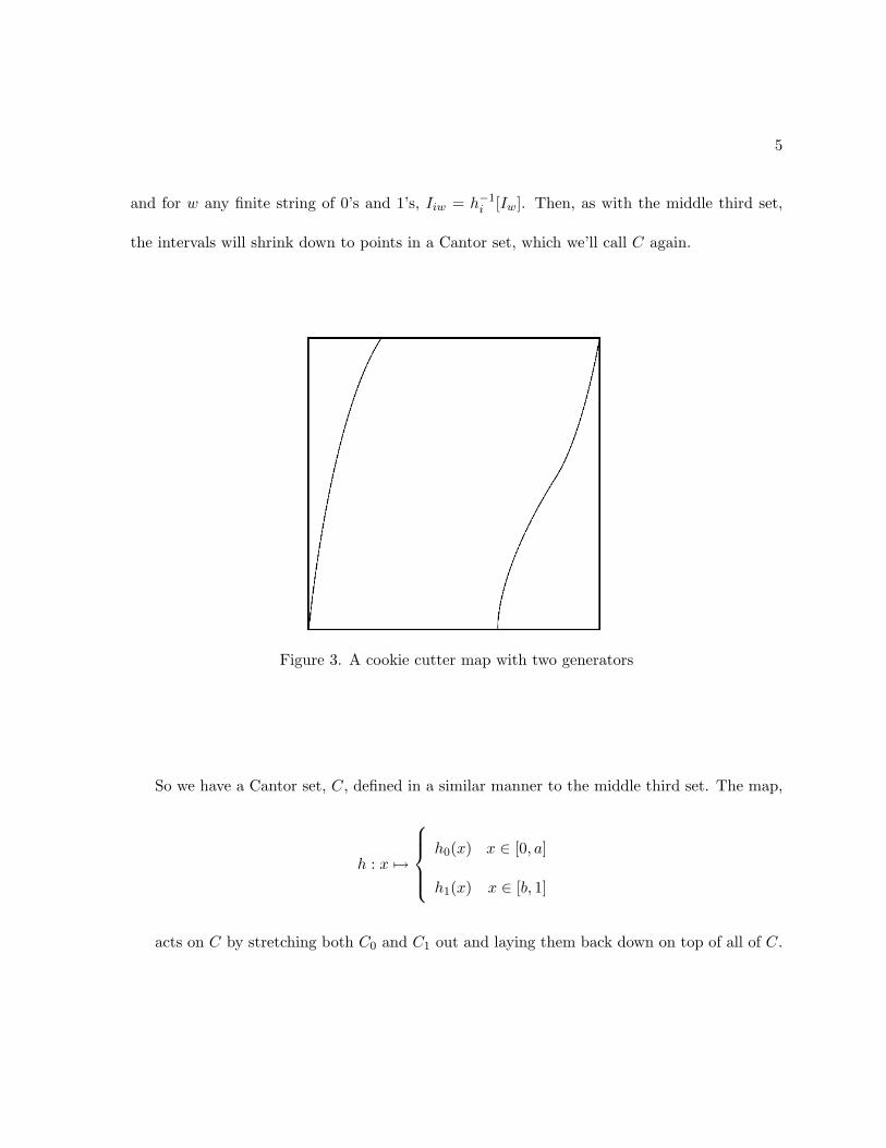
and for w any finite string of 0’s and 1’s, Iiw = h−1i [Iw]. Then, as with the middle third set,

the intervals will shrink down to points in a Cantor set, which we’ll call C again.

Figure 3. A cookie cutter map with two generators

So we have a Cantor set, C, defined in a similar manner to the middle third set. The map,

h : x 7→

h0(x) x ∈ [0, a]

h1(x) x ∈ [b, 1]

acts on C by stretching both C0 and C1 out and laying them back down on top of all of C.

6

If we know the lengths of all the gaps and clone intervals, of course, we then know how

to construct C. If we know the relative sizes of the intervals, we can construct C up to affine

rescaling. For all finite words w, we let l(w), g(w), and r(w) denote |Iw0||Iw| ,

|Gw||Iw| , and |Iw1|

|Iw|

respectively, where |Iw| is the length of Iw. Then, all we need, besides l(w), g(w), and r(w) for

all w, to construct C is the interval I (the convex hull of C). Thus we have the ratio geometry

function, w 7→ (l(w), g(w), r(w)) = ( |Iw0||Iw| ,

|Gw||Iw| ,

I|w1||Iw| ) whose domain is {0, 1}N, and whose range

is contained in the unit two-simplex {(x, y, z)|x + y + z < 1}. The middle third set has ratio

geometry (13 ,

13 ,

13) for every word w.

1.2.2 Foliations and the Hirsch Example

In this thesis, we’ll look at Cantor sets which arise in the context of dynamical systems,

and ultimately at Cantor sets which arise in the context of foliations. We think of a foliation

as a manifold with a local product structure. The examples we consider will all be three

dimensional manifolds with two dimensional ( codimension 1) foliations. Informally, we say

that the neighborhood of any point looks like a stack of papers, or the pages in a book. These

stacks overlap, so that papers in one stack continue on into the neighboring stack, but as you

move from one stack to another the corresponding pages might get closer together or farther

apart. The “stacks of papers” are formally called foliation charts and each individual page

is called a plaque. If we start with one page in one stack, and follow it in to a neighboring

stack, and from there to another neighboring stack, we build up the leaf, which consists of

all the plaques which you can ever reach this way. A leaf will be a two-dimensional manifold

embedded in the ambient three-manifold. For a more formal definition, see Section 2.4.

7

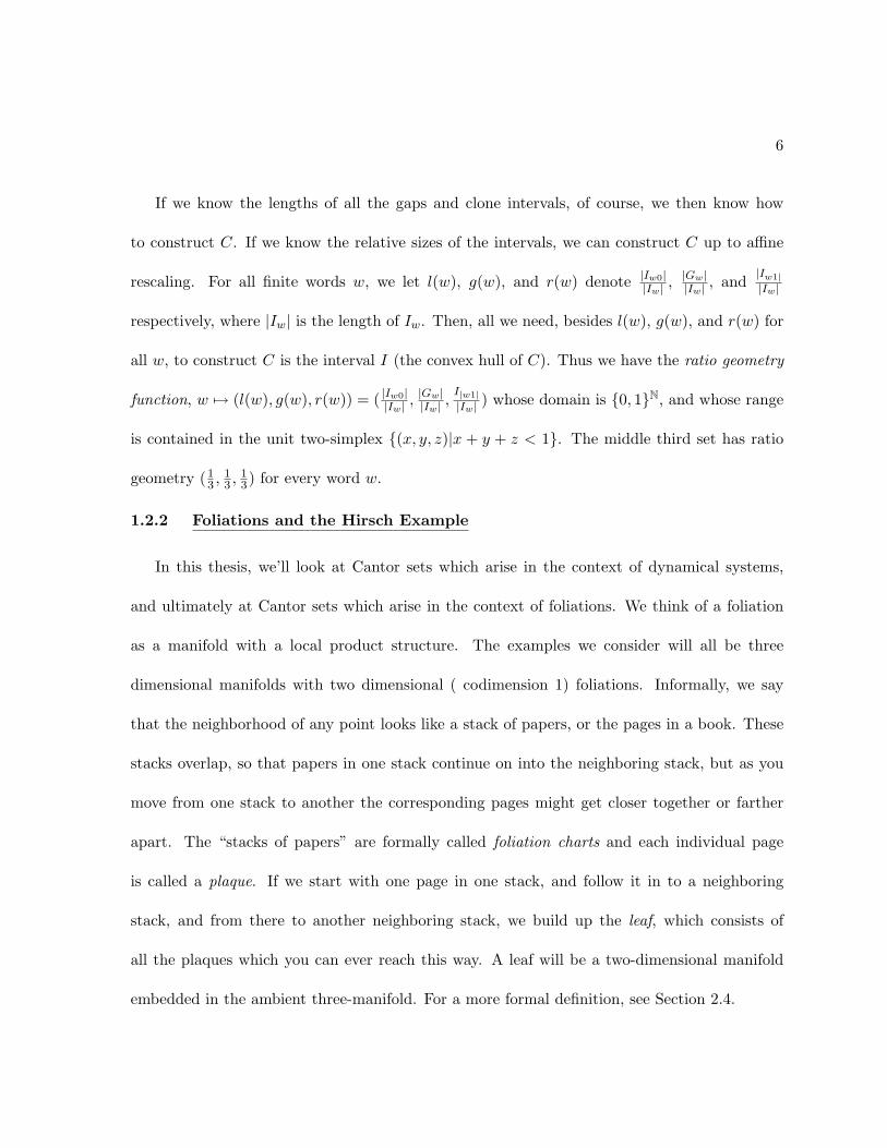
The examples of foliations we consider will all be generalizations of the Hirsch foliation (23),

which we describe in detail in Section 3.2. We obtain the Hirsch foliation by starting with a

solid torus and, from the interior, removing another solid torus which wraps around twice. This

gives us a manifold, foliated by two-holed disks, with two transverse toruses as boundary com-

ponents. The exterior component is a torus which wraps around once, the interior component

is a torus which wraps around twice. We then glue the exterior boundary component to the

interior component to obtain a foliated manifold without boundary. In order to preserve the

foliation, the gluing map must identify latitudinal circles from the interior boundary component

to latitudinal circles on the exterior component. In the longitudinal direction, the gluing map

reduces to a 2 to 1 local homeomorphism of the circle.

Figure 4. The Hirsch Foliation: We glue the top of the cylinder to the bottom to get a solidtorus with another solid torus removed. Then we glue the inside component to the outside

component to get the Hirsch foliation.

8

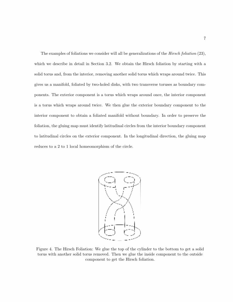
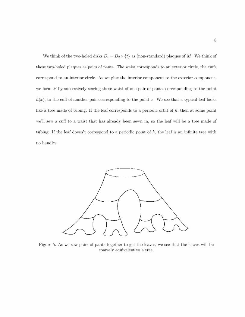
We think of the two-holed disks Di = D2×{t} as (non-standard) plaques of M . We think of

these two-holed plaques as pairs of pants. The waist corresponds to an exterior circle, the cuffs

correspond to an interior circle. As we glue the interior component to the exterior component,

we form F by successively sewing these waist of one pair of pants, corresponding to the point

h(x), to the cuff of another pair corresponding to the point x. We see that a typical leaf looks

like a tree made of tubing. If the leaf corresponds to a periodic orbit of h, then at some point

we’ll sew a cuff to a waist that has already been sewn in, so the leaf will be a tree made of

tubing. If the leaf doesn’t correspond to a periodic point of h, the leaf is an infinite tree with

no handles.

Figure 5. As we sew pairs of pants together to get the leaves, we see that the leaves will becoarsely equivalent to a tree.

9

1.2.3 The conjugation problem

One of the basic questions about foliations asked by H.B. Lawson in his survey on foliations

(see sections 5 and 8 of (26)) is: if two foliations are homeomorphic, are they necessarily

diffeomorphic?

Let (M1,F1) and (M2,F2) be foliations of transverse differentiability class Ck+λ and Φ:M1 →

M2 a Cr-homeomorphism, for r ≤ k, which maps the leaves of F1 to the leaves of F2. The

conjugacy problem for foliations is to find conditions on the foliations and the map Φ which

are sufficient to imply that the map Φ is also Ck+λ.

The study of conjugacy problems has a long tradition in dynamical systems. One of the most

influential results is due to D. Anosov, who showed in his Thesis (1) that there are C∞-flows on

3-manifolds which are C1 conjugate but cannot be C2 conjugate. The work of S. Hurder and

A. Katok (24) showed that the crucial question is the regularity of the weak-stable foliations

associated to these Anosov flows. The foliations themselves are transversally C1+λ for any real

number 0 < λ < 1, but if the weak-stable foliations are C2 then the flow is smoothly conjugate

to an algebraic model.

One of the key tools for the study of the conjugacy problem is the so-called “bootstrapping

process” for proving the regularity of a map conjugating two smooth hyperbolic dynamical

systems on compact manifolds, introduced in a series of foundational papers by R. de la Llave,

J. Marco, and R. Moriyon (10; 11; 12; 13; 27; 28). This was further developed for the study of

the conjugations between stable foliations by B. Hasselblatt in the papers (19; 20; 21) who gave

10

obstacles to regularity in the form of “bunching data” for the eigenvalues at periodic points of

the hyperbolic maps.

The foundational papers of D. Sullivan (37; 38) on the conjugacy problem for geometri-

cally defined Cantor sets and “cookie-cutter” dynamical systems used the “ratio geometry” for

an exceptional minimal set to define a scaling function. The scaling function introduced by

Feigenbaum to study k to 1 maps of the circle with dense minimal sets. The scaling function

is defined on the dual Cantor set associated to the dynamical system, and classifies the local

differentiable structure of the Cantor set. These methods were subsequently applied by T. Bed-

ford and A.M. Fisher (2), to study the “scenery process” during which they flushed out the

proofs from Sullivan’s original work.

The study of the geometry and dynamics of a foliation F on a compact manifold encompasses

all of the issues with the dynamical systems defined by a flow (as a flow defines a foliation with

1-dimensional leaves) plus much more. When the leaves have higher dimension, the geometry of

the leaves can make the dynamics of the foliation far more complicated than that encountered in

the study of flows. This complexity forces the study of foliations to focus on “model problems”,

which are typical examples where a solution provides a model for more general cases.

In this thesis we study the conjugacy problem for the “Hirsch foliations”. The original

Hirsch foliation was a construction of a codimension one foliation on a compact 3-manifold

such that the foliation was real analytic and had an exceptional minimal set.(23)

One of the points of this thesis is to present a generalization of the Hirsch construction

which results in a very broad class of dynamical behavior for the resulting foliations. These

11

will be our model problems which will motivate our discussion of the conjugacy problem. The

theory we develop will mostly solve problem 1, while only laying a possible background for

problems 2 and 3.

Problem 1 Let (M1,F1) and (M2,F2) be generalized Hirsch foliations of transverse differen-

tiability class Ck+λ and Φ:M1 → M2 a Cr-homeomorphism, for r ≤ k, which maps the leaves

of F1 to the leaves of F2. Find conditions which imply that Φ is Ck+λ.

Ghys and Tusboi considered the conjugacy problems for C2 foliations on compact manifolds

in (14). Their basic technique was similar to the classical method used in Shub and Sullivan

(36), and is based on the observation that a C2-map which commutes with a linear contraction is

itself linear. Another purpose of this thesis is to develop and apply the more general techniques

of bootstrapping and ratio geometry, which were developed for the study of standard dynamical

systems, to the study of the conjugacy problems for foliations, so that it applies to foliations

whose differentiability is at least C1. Note that Cantwell and Conlon exhibited foliations of all

degree of differentiability which cannot be smoothed to a higher degree in (6; 8).

The boot strapping techniques used in this thesis applies to the holonomy of Hirsch foliation,

not just in a neighborhood of the minimal set, but everywhere holonomy element which doesn’t

have a non-hyperbolic fixed point.

Problem 2 What can be said about the conjugacy problem for generalized Hirsch foliations

whose holonomy has special points, and is not completely hyperbolic?

12

Finally, the work in this thesis suggests a very general problem, which we only begin to

solve.

Problem 3 Classify the holonomy pseudogroups which arise from the generalized Hirsch foli-

ations.

1.2.4 The conjugation problem for cookie cutters.

Sullivan’s solution of the conjugation problem for cookie cutters uses the ratio geometry to

define the scaling function, which categorizes the differentiable structure. The ratio geometry

is of an interval Iω is given by the relative lengths of Iω0, Gω, and Iω1. So we get the ordered

triplet ( |Iω0||Iω | ,

|Gω ||Iω | ,

|Iω1||Iω | ). We normally just think of this as a function of ω. These ratios look a

little bit like difference quotients for f−1, but, for instance, if we write ω = wnwn−1 . . . w2w1,

then Iω0 = f−1wn

◦ f−1wn−1

◦ . . . ◦ f−1w2

◦ f−1w1

◦ f−10 ◦ fn[Iω].

As it turns out, the conjugacy class of f determines the ratio geometry exponentially closely,

which is our first main theorem for cookie cutters, which is proved on page 90.

Theorem 1 (Sullivan) If two cookie cutters are C1+λ conjugate, then their ratio geometries

are exponentially equivalent.

A corollary of this is that as we add symbols to the left of ω, the ratio geometry converges

exponentially fast to a limiting geometry which we call the scaling function. This gives us our

second main theorem for cookie cutters which is proved on page 91.

Theorem 2 (Sullivan) C and C ′ are exponentially equivalent cookie cutters if and only if they

have the same scaling function.

13

Taken together, these two theorems imply that C1+λ-conjugate cookie cutters have the

same scaling function. As we add symbols to the left of ω, the intervals Iwn+k,...wn+2wn+1ω gets

smaller and smaller, so in as much as the ratio geometry looks like difference quotients, the

scaling function looks like derivatives. But besides the fact that we aren’t really forming a

difference quotient, Iwn+k,...wn+2wn+1ω will bounce around depending on whether Iwn+kis 0 or 1.

Even though, in a neighborhood of the minimal set, the converse of the above two theorems are

true (page 94), hence the scaling function is just what is needed to classify the C1+λ structure:

Theorem 3 (Sullivan) Let C and C ′ be two exponentially equivalent labeled Cantor sets. Then

they’re C1+λ conjugate in some neighborhood of C.

Theorems 2 and 3 taken together imply that two Cantor sets with the same scaling function

are C1+λ-conjugate on some open neighborhood.

Furthermore, using the bootstrapping method, the scaling function φ : Σ−2 −→ int∆2

classifies the Ck+λ structure (page 102), where Σ−2 is the set of left-infinite strings on two

symbols, and ∆2 is the 2-simplex{(x, y, z) ∈ R3|x2 + y2 + z2 ≤ 1

}.

Theorem 4 (Sullivan) Let φ be a C1+λ conjugation between Ck+λ cookie cutters. Then φ is

itself Ck+λ

1.2.5 Dynamically defined Cantor sets on the circle

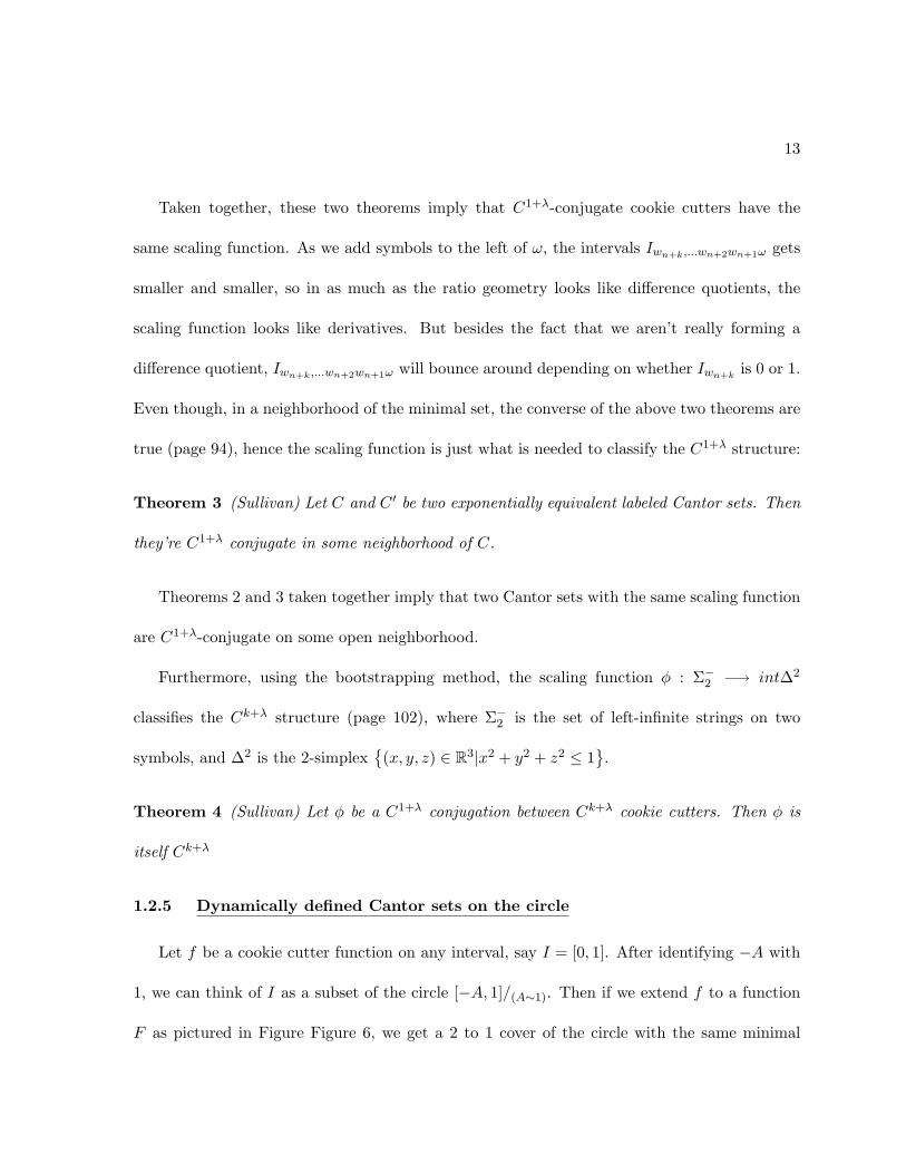
Let f be a cookie cutter function on any interval, say I = [0, 1]. After identifying −A with

1, we can think of I as a subset of the circle [−A, 1]/(A∼1). Then if we extend f to a function

F as pictured in Figure Figure 6, we get a 2 to 1 cover of the circle with the same minimal

14

set as f . We see that the fixed interval H = (−A, 0) acts as a trap for forward iterations of

F . The gaps of C are all backwards iterates of the fixed interval. This was the function Hirsch

described in his construction.

Figure 6. A cookie cutter on the circle

On I0 and I1, F = f so the dynamics of F are the same, and the discussion about ratio

geometry and the scaling function still applies. We’ve extended f to the gaps G and H. But

the backwards iterates of G still consists of all the gaps in I0 ∪ I1, and the only forward iterate

15

of the interval G is the interval H. On H, as we’ve drawn F , there’s an attracting fixed point,

p, but the backwards orbit of p approaches the Cantor set C.

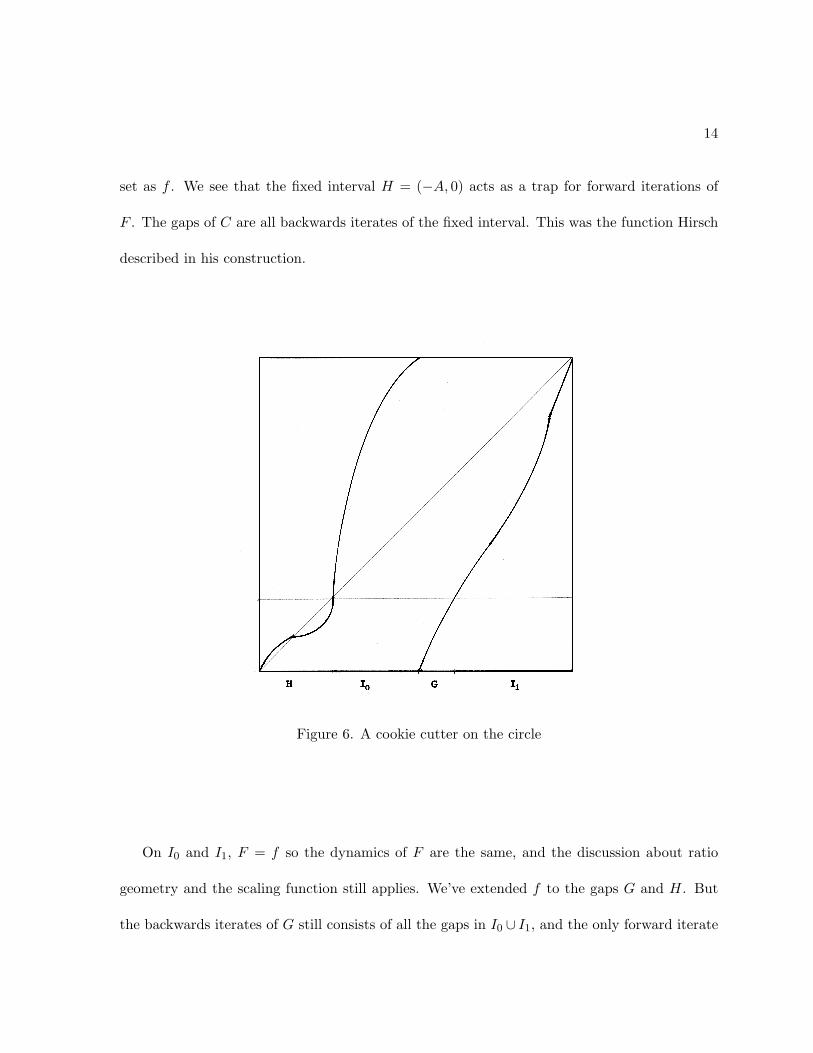
Figure 7. A map with a period two interval. f [G1] = G2 and f [G2] = G1, so G1 ∪G2 acts as atrap for the dynamics of f . If f ′ > 1 off of G1 ∪G2, then the backwards images of G1 ∪G2

form the gaps of an invariant Cantor set.

In general, the way we construct a C1 function, f on a one dimensional manifold which

generates a Cantor set, C is we have an interval, G, that traps the dynamics of f . Once we

land in G, we can’t get back out. The backwards iterates of G are the gaps of C. For a cookie

16

cutter on the interval, f isn’t even defined on G, so once we land in G, we can’t iterate f at all.

When we extended f to the circle, the trap is the interval H. Once the orbit of a point lands

in H, it stays there, and so is asymptotic to a fixed point.

We could also trap the dynamics of f by having a periodic interval. In Figure Figure 7,

we graph a 2 to 1 local diffeomorphism on S1 with a period 2 interval, G1. f [G1] = G2 and

f [G2] = G1. Once an orbit of a point lands in G1 ∪G2, it stays there. If f is hyperbolic off of

G1 ∪G2, then the inverse orbit of G1 ∪G2 is a dense set of open intervals, and hence forms the

gaps of a closed totally disconnected space, and as it turns out are the gaps of a Cantor set, C.

C is the minimal set for f .

Just as we did with the cookie cutter, we can use the dynamics of f to define a structure

of nested sub-intervals and gaps. We start with the three closed intervals I0, I1, and I2. But

instead of labeling the gaps according to the interval they’re inside of, as we did for the cookie

cutter, we label them according to the interval they’re next to. We arbitrarily choose to label

them according to the interval to their right. Remember that we’ve identified the endpoints to

get a circle, so that f is continuous on I1. Also I0 and I2 share an endpoint.

We restrict f to three domains to get the three diffeomorphisms acting on intervals:

f0 = f |I0 f1 = f |G1∪I1 f2 = f |G2∪I2

17

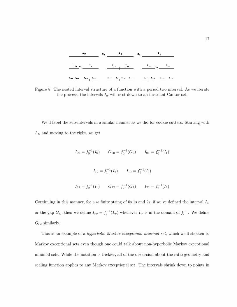
Figure 8. The nested interval structure of a function with a period two interval. As we iteratethe process, the intervals Iw will nest down to an invariant Cantor set.

We’ll label the sub-intervals in a similar manner as we did for cookie cutters. Starting with

I00 and moving to the right, we get

I00 = f−10 (I0) G00 = f−1

0 (G0) I01 = f−10 (I1)

I12 = f−11 (I2) I10 = f−1

1 (I0)

I21 = f−12 (I1) G22 = f−1

2 (G2) I22 = f−12 (I2)

Continuing in this manner, for a w finite string of 0s 1s and 2s, if we’ve defined the interval Iw

or the gap Gw, then we define Iiw = f−1i (Iw) whenever Iw is in the domain of f−1

i . We define

Giw similarly.

This is an example of a hyperbolic Markov exceptional minimal set, which we’ll shorten to

Markov exceptional sets even though one could talk about non-hyperbolic Markov exceptional

minimal sets. While the notation is trickier, all of the discussion about the ratio geometry and

scaling function applies to any Markov exceptional set. The intervals shrink down to points in

18

the Cantor set, and so define a labeling on points of C. But since I2 and I0 overlap at their

endpoint, the coding is not unique, and because not all words are realized, the labeling on C is

a semiconjugacy to a subshift.

We can still define the ratio geometry, and scaling function which classify the differentiable

structure, giving us the same picture as for the cookie cutters. See page 103 for a discussion of

the following theorems. The proofs are almost identical to theorems 1, 2, and 4 requiring only

changing to the notation outlined on page 56. We don’t need to state an analogue to theorem 3

since we already stated it in a more general setting.

Theorem 5 Let C and C ′ be C1+λ conjugate Markov exceptional sets. Then the ratio geometry

of C is exponentially equivalent to the ratio geometry of C ′.

Theorem 6 Let C and C ′ be Markov exceptional sets. Then they are exponentially equivalent

if and only if they have the same scaling function.

Theorem 7 Let φ be a C1+λ conjugation between Ck+λ Markov exceptional sets. Then φ is

itself Ck+λ.

1.2.6 The Conjugation Problem for Hirsch Foliations

The transverse dynamics of the Hirsch foliation is given by an orientation preserving two to

one local diffeomorphism, of the circle h. A leaf corresponds to a total orbit of h, and a point

of period k corresponds to a handle composed of k plaques. We will choose M to be a Hirsch

foliation whose holonomy function h has a Markov exceptional set. Then the earlier discussion

must apply to h. For instance, we can use a Markov basis for h to define a ratio geometry on

19

the transversal of M . In this situation, the theory of Markov exceptional sets applies to the

transversals of M , so we have the following theorems. (See page 107.)

Theorem 8 Let F : (M1,F1) → F : (M2,F2) be a C1+λ diffeomorphism. Then the transverse

ratio geometry of F1 is exponentially equivalent to the transverse ratio geometry of F2.

This theorem is trivially true as a special case of theorem 5. But the context of the foliation

gives us another geometrical interpretation of the ratio geometry. The two branches of h−1

are both holonomy elements. That means there exists a path γ0 so that we apply h−10 to a

sub-interval, J , of the transverse circle by flowing J along the path γ0, and likewise for h−11 .

The holonomy along the catenation the paths γi is given by iterating h−10 and h−1

1 . So instead

of defining the scaling function on an abstract dual Cantor set, we can define it on a set of

infinitely long holonomy paths.

Theorem 9 For a foliation with a Markov exceptional set, as we flow along an infinitely long

path with contracting holonomy, the transverse ratio geometry will converge to the scaling func-

tion of the transverse minimal set.

Observation 1 For a Hirsch foliation, this gives us a nice geometric interpretation for the

dual Cantor set on which the scaling function is defined. The paths we flow along, in general,

will go to an end of the leaf. (Though it might also go around a handle.) In particular, if we

choose a leaf L with no handles, then the domain of the scaling function is a subset of the endset

of L.

20

Theorem 10 Let F1 and F2 be C1+λ conjugate foliations with Markov exceptional sets. Then

they have the same scaling function.

Theorem 11 Let φ be a C1+λ diffeomorphism between Ck+λ foliations (M1,F1) and (M2,F2)

with Markov minimal sets. Then, φ is itself transversally Ck+λ in a neighborhood of the excep-

tional minimal set.

By applying a smoothing lemma, we have the application:

Theorem 12 Let φ be a C1+λ diffeomorphism between Ck+λ foliations (M1,F1) and (M2,F2)

with Markov minimal sets. Then φ is C0 close to a Ck+λ function in a neighborhood of the

minimal set.

CHAPTER 2

DEFINITIONS AND CONCEPTS

2.1 Lipschitz and Holder Continuity

Definition 1 A map φ : X −→ Y between two metric spaces is said to be Lipschitz if it only

scales distances by a bounded amount. That is there exists a constant K such that for all x and

y ∈ X,

d(φ(x), φ(y)) ≤ Kd(x, y)

For maps of the real line, we can reformulate this definition to say that the difference

quotient is bounded: ∣∣∣∣φ(x)− φ(y)x− y

∣∣∣∣ ≤ K

K is called the Lipschitz constant for φ. We say that φ is less than K in the Lipschitz

norm. So if K is minimal, then K is the Lipschitz norm of φ. A Lipschitz map can easily be

non-differentiable − for instance a piecewise linear map is Lipschitz − but since the difference

quotient is bounded, a Lipschitz map is better behaved than an arbitrary continuous map. If

we let the domain of φ be the compact interval I = [a, b], then by the Mean Value Theorem, if φ

is C1, then φ is Lipschitz. Furthermore, a Lipschitz map is C0, so if we restrict our domains to

compact intervals, the Lipschitz condition provides an intermediate level of smoothness between

C0 and C1.

21

22

Example 1 A differentiable map on a compact interval I = [a, b] is Lipschitz. By the mean

value theorem, for x, y ∈ [a, b], there exists z ∈ [x, y] such that f(x) − f(y) = f ′(z)(x − y) so

C = maxz∈[a,b]

f ′(z) works as the Lipschitz constant.

Example 2 Let φ : I −→ R be piecewise Lipschitz. That is let I = [a, b] and a = a0 < a1 <

a2 < . . . < aN = b. On each interval Ii = [ai, ai+1], let |φ(x) − φ(y)| ≤ Ci|x − y|. Then φ is

Lipschitz on I.

Proof: Let i < j, x ∈ Ii and y ∈ Ij , then

|φ(y)− φ(x)| ≤ |φ(y)− φ(aj)|+ |φ(aj)− φ(aj−1)|+ . . .+ |φ(ai+1)− φ(x)|

≤ Ci|y − aj |+ Ci−1|aj − aj−1|+ . . .+ Ci|ai+1 − x|

≤ maxCi [(y − aj) + (aj − aj−1) + . . . (ai+1 − x)]

= C|y − x|

Note that this example can be generalized. We break the interval I up into an infinite

number of sub-intervals. We require that φ be Lipschitz on each interval Ii and that the

Lipschitz constants Ci are all bounded. Then φ is Lipschitz on all of I.

Proposition 1 Let the series∑fi(x) be absolutely convergent on [0, 1]. Let φ be a Lipschitz

map on [0, 1]. Set φ(0) = fi(0) = 0. Then the series∑φ ◦ fi is also absolutely convergent.

23

Proof:

∑|φ ◦ fi(x)| ≤

∑|φ(fi(x))− φ(fi(0))|

≤∑

K|fi(x)− fi(0)|

≤∑

K|fi(x)|

which converges since fi is absolutely convergent. �

Proposition 2 Let f and g be Lipschitz maps on a compact interval I. Then f + g, f · g, and

f ◦ g are all Lipschitz.

Proof:

1. f + g is Lipschitz by the triangle inequality.

2. |f(x)g(x)− f(z)g(z)| ≤ |f(x)| · |g(x)− g(z)|+ |g(z)| · |f(x)− f(z)|

3. |f ◦ g(x)− f ◦ g(z)| ≤ Cf |g(x)− g(z)| ≤ CfCg|x− z|.

�

Definition 2 Let 0 < λ ≤ 1. Then φ is Holder continuous of degree λ if there exists numbers

0 < δ < 1 and K > 0 such that when |x − y| < δ, |φ(x) − φ(y)| ≤ K|x − y|λ. K is called the

Holder constant for φ.

24

The Holder condition is a generalization of the Lipschitz condition which allows us to define

more intermediate degrees of smoothness between C0 and Lipschitz. Note that Holder of degree

λ = 1 is exactly the same as Lipschitz.

The following two propositions justify the statement that Holder continuity provides frac-

tional degrees of smoothness between C0 and Lipschitz.

Proposition 3 For λ ≤ κ, Cκ implies Cλ I.e. if φ : I −→ J be a map of compact intervals

which is Holder of degree κ, then φ is also Holder of degree λ.

Proof: Let x = a0 < a1 < . . . < an = y be a partition of [x, y] with ai − ai−1 < 1. Then

|φ(x)− φ(y)| ≤n∑

i=1

|φ(xn)− φ(xn−1)|

≤n∑

i=1

K|xn − xn−1|κ

≤n∑

i=1

K|xn − xn−1|λ

≤ K|n∑

i=1

xn − xn−1|λ

≤ K|x− y|λ

�

Proposition 4 Let λ ≤ κ Let f be Cλ and g be Cκ. Then f + g and f · g are Cλ, and f ◦ g is

Cλκ.

The proof is exactly the same as for the Lipschitz case, but using the Holder inequality

instead of the triangle inequality.

25

Since Holder continuity provides intermediate gradations of smoothness between C0 and

C1, for λ < 1 we adopt the notation that φ is Cλ if φ is Holder of degree λ. For λ = 1, this

notation is imprecise, since C1 is already reserved to mean once differentiable. For λ = 1 we

simply use the word Lipschitz, or the notation C0+1. We could define the Holder condition for

λ > 1, but we will restrict our attention to functions with compact domains, in which case

Holder of degree > 1 implies that the function is locally constant.

The following example shows why we define Holder continuity as a local condition.

Example 3 The identity: R −→ R, doesn’t satisfy a global Holder condition. If λ < 1, and

limn→∞ xn = ∞, then limn→∞|xn−0||xn−0|λ = limn→∞ x1−λ

n = ∞. �

Example 4 Since the tangent line for f(x) =√x is vertical at x = 0, (and hence the difference

quotient is unbounded,) f is neither differentiable nor Lipschitz on the interval [0, 1]. f is Holder

of degree 12 though.

Proof: Without loss of generality, take x ≥ y. Then we need to show that√x−√y ≤

√x− y.

x ≤ x+ 2√x− y

√y

≤ (x− y) + 2√x− y

√y + y

= (√x− y +

√y)2

√x ≤

√x− y +

√y

√x−√y ≤

√x− y

26

�

Proposition 5 If φ is Lipschitz, then√φ is Holder of degree 1

2 .

Example 5 Unlike Lipschitz maps, composition with Holder maps need not preserve absolute

convergence. Let fn(x) = xn2 and φ(x) =

√x. Then

∑fn(x) = x

∑ 1n2 which converges

absolutely, but∑φ ◦ fn(x) =

√x

∑ 1n which doesn’t converge. �

While Holder continuous functions don’t necessarily preserve absolute convergence, they do

preserve geometric sums. This is exactly what we will need to prove the regularity theorems.

Proposition 6 Let r < 1, λ < 1, and |fn(x)| ≤ rn. Let φ be Holder of degree λ. Further let

φ(0) = fn(0) = 0. Then φ◦fn(x) is also bounded by a geometric series, and hence is summable.

Proof:

∑|φ ◦ fn(x)| ≤

∑C|fn(x)|λ

≤∑

Crλn

≤ C

1− rλ

�

The Holder condition gives us intermediate degrees of smoothness between C0 and C1.

We extend this to get intermediate degrees between Ck and Ck+1 simply by requiring the kth

derivative to satisfy the Holder condition: f is Ck+λ if |f (k)(x)− f (k)(y)| ≤ Cf |x− y|λ.

27

Again we note that this notation is insufficient when λ = 1, since Ck+1 doesn’t just mean

that the kth derivative is Lipschitz, but that the k + 1st derivative is continuous. When it’s

clear from context we’ll use this notation for the Lipschitz case too. For instance when we say

a map is C0+1 we’ll mean Lipschitz, as opposed to C1 which means once differentiable.

Recall that f is less than K in the Ck norm if f (j)(x) ≤ K for all j ≤ k and all x ∈ I. We

say that K bounds f in the Ck+λ norm if in addition K is a Holder constant for f (k).

Proposition 7 Let f and g be two Ck+λ maps. Then f + g, f · g, and f ◦ g are all Ck+λ too.

Proof:

i) f+g is Ck+λ:

Let |x− z| < min(δf , δg). Then

∣∣∣(f + g)(k)(x)− (f + g)(k)(z)∣∣∣ ≤ |f (k)(x)− f (k)(z)|+ g(k)(x)− g(k)(z)|

≤ Cf |x− z|λ + Cg|x− z|λ

≤ K|x− z|λ

ii) (f · g) is Ck+λ:

∣∣∣(f · g)(k)(x)− (f · g)(k)(y)∣∣∣ ≤

k∑j=0

(k

j

) ∣∣∣f (j)(x)g(k−j)(x)− f (j)(y)g(k−j)(y)∣∣∣

≤k∑

j=0

(k

j

) [∣∣∣f (j)(x)(g(k−j)(x)− g(k−j)(y))∣∣∣

+∣∣∣g(k−j)(y)(f (j)(x)− f (j)(y))

∣∣∣]

28

≤ M |x− y|λ

iii) f ◦ g is Ck+λ:

By induction on k. For k = 1,

|f ◦ g′(x)− f ◦ g′(z)| = |f ′g(x)g′(x)− f ′(g(z))g′(z)|

≤ |f ′g(x)||g′(x)− g′(z)|+ |g′(z)||f ′g(x)− f ′g(z)|

≤ K|x− z|λ

So the theorem is true for k = 1. Now suppose it’s true for k < j. Then since f ′ and g are

both Cj−1+λ, so is f ′ ◦g and hence the product f ′(g(x))g′(x) = (f ◦g)′(x) is Cj−1+λ too, which

is to say that f ◦ g is Cj+λ. �

Corollary 1 Any finite combination of sums, products and compositions of Ck+λ maps on

compact intervals is itself Ck+λ.

We can use Holder continuity to relax the hypothesis of Taylor’s theorem. Usually if we

want the kth Taylor polynomial to be a good approximation of f , we require f to be k+1 times

differentiable. But it is enough to require f to be Ck+λ.

Theorem 13 (Taylor’s Ck+λ Theorem) Let f : I ⊂ R → R be a Ck+λ map and let |x−a| <

δ. Then f(x) = f(a) + f ′(a)(x− a) + . . .+ f (k)(a)k! (x− a)k +O(x− a)k+λ.

29

Proof:

To restate the theorem, we say that f(x)−Pk(x) = O(x− a)k+λ where Pk is the kth Taylor

polynomial. Since f is Ck, the regular Taylor theorem states that

f(x) = Pk−1(x) +f (k)(c)k!

(x− a)k

for some c ∈ [a, x]. So

|f(x)− Pk(x)| =

∣∣∣∣∣f(x)− Pk−1(x)−f (k)(a)k!

(x− a)k

∣∣∣∣∣=

∣∣∣∣∣f (k)(c)k!

(x− a)k − f (k)(a)k!

(x− a)k

∣∣∣∣∣= |x− a|k ·

∣∣∣∣∣f (k)(c)k!

− f (k)(a)k!

∣∣∣∣∣≤ |x− a|k ·D|c− a|λ

= O(x− a)λ

�

2.2 Coarse Equivalence

Intuitively, we will define two metric spaces to be coarsely equivalent, or quasi-isometric, if

from far away they look the same. For instance the light bulbs in the letter “a” on a dot-matrix

marquis sign are discreet points . But we see them from far enough away that they look like the

continuous letter “a”. So we say that the discreet set of points is quasi-isometric to the letter

30

“a”. A quasi-isometry will be a function which only distorts distances by a bounded amount.

A quasigeodesic will be a path which is quasi-isometric to a true geodesic.

A a C-net in the metric space Y is a subset W ⊂ Y such that for all y ∈ Y there exists a

w ∈W so that d(w, y) ≤ C .

A map f : X −→ Y is called a quasi-isometry if f [X] is a C-net in Y and

1Cd(x, y)− C ≤ d(f(x), f(y)) ≤ Cd(x, y) + C

A map f : R −→ Y is a quasigeodesic if it is a quasi-isometry onto it’s range.

Example 6 Any two bounded metric spaces are quasi-isometric.

Example 7 The inclusion from the integers to the real numbers is a quasi-isometry.

2.3 Pseudogroups

Definition 3 A pseudogroup acting on the topological space X is a set Γ of homeomorphisms

whose domains are either open subsets or the closure of open subsets in X. We only require Γ

to be closed under composition. That is if γ1 : U1 −→ X and γ2 : U2 −→ X, are both elements

of Γ, then γ1 ◦ γ2 : U2⋂γ−1

2 (U1) is also an element of Γ.

The domain, Dom(Γ), is the union⋃γ∈Γ

Dom(γ). We say that Γ is C1, Ck, piecewise linear,

etc, if all of its elements have the given property. We write γ1γ2 for the composition of two

elements and γk for the iteration of γ. We will only consider symmetric pseudogroups. That is

if γ ∈ Γ, then γ−1 ∈ Γ as well. But γ−1 doesn’t act as an inverse on the algebraic level, since

31

γ1γ2γ−12 will generally have a smaller domain than γ1 The germ of γ−1 does act as an algebraic

inverse for the germ of γ. For a symmetric pseudogroup, if γ ∈ Γ, then the identity restricted

to the domain of γ is in Γ as well.

Example 8 For any space X, any group of homeomorphisms acting on X can also be viewed

as a pseudogroup. For instance the sets of homeomorphisms, and homeomorphisms which fix a

specific point, are both pseudogroups. If X has the appropriate structure on it, then the set of

piecewise linear, Cα or Ck homeomorphisms will form a group, and hence a pseudogroup acting

on X.

Definition 4 If A = {γα : Uα −→ Vα|Uα ⊂ X,Vα ⊂ X} is any set of homeomorphisms, then

the pseudogroup generated by A, is the set of all finite compositions of homeomorphisms in A.

Γ(A), the symmetric pseudogroup generated by A will be the pseudogroup generated by A⋃A−1

where A−1 = {γ−1|γ ∈ A}.

We will say that any set A = {γα : Uα −→ Vα|Uα ⊂ X,Vα ⊂ X} of local homeomorphisms

also generates a pseudogroup, but to be precise we have to define the domains of Γ(A). For

each γ ∈ A we need to choose a way to break the domain up into pieces so that γ restricts to

a homeomorphism on each piece.

Definition 5 Γ1 and Γ2 are equivalent pseudogroups acting on X if for every x ∈ X, and

every γi ∈ Γi with x in it’s domain, there exists γj ∈ Γj so that γi and γj have the same germs.

More generally we’ll say two pseudogroups Γ1 acting on X1 and Γ2 acting on X2 are equivalent

32

if there exists a homeomorphism φ :⋃

γ∈Γ1

Domγ −→⋃

γ∈Γ2

Domγ so that {φγ|γ ∈ Γ1} and Γ2 are

equivalent pseudogroups acting on⋃

γ∈Γ2

Domγ.

Example 9 If A is a set of local homeomorphisms, it will generate the same equivalence class

of pseudogroups no matter how we chop up the domains.

Example 10 If X is an open subset of Y and Γ is a pseudogroup acting on X, then we can

also think of Γ as a pseudogroup acting on Y . Likewise if Γ is a pseudogroup acting on Y , then

Γ restricts to a pseudogroup acting on X.

2.4 Foliations

A C0-foliation F of a paracompact smooth manifold V m is a continuous partition of V into

tamely embedded C2-submanifolds (the leaves) of constant dimension p and codimension q. We

require that these leaves be locally given as the level sets (plaques) of local foliation coordinate

charts which satisfy four conditions:

(1) There is given a uniformly locally-finite covering {Uα | α ∈ A} of V ; that is, there exists

m(A) > 0 so that for any α ∈ A the set {β ∈ A | Uα ∩ Uβ 6= ∅} has cardinality at most m(A)

(2) There are local coordinate charts φα : Uα → (−1, 1)m, so that each map φα admits an

extension to a homeomorphism φα : Uα → (−2, 2)m where Uα contains the closure of the open

set Uα

(3) For each z ∈ (−2, 2)q, the pre-image φ−1α ((−2, 2)p × {z}) ⊂ Uα is the connected com-

ponent containing φ−1α ({0} × {z}) of the intersection of the leaf of F through φ−1

α ({0} × {z})

with the set Uα.

33

The extensibility condition in (2) is made to guarantee that the topological structure on the

leaves remains tame out to the boundary of the chart φα. The collection {(Uα, φα) | α ∈ A} is

called a regular foliation atlas for F .

The inverse images

Pα(z) = φ−1α ((−1, 1)p × {z}) ⊂ Uα

are topological discs contained in the leaves of F , called the plaques associated to this atlas.

We will assume that the covering is chosen so that all plaques have diameter at most 1. One

thinks of the plaques as “tiling stones” which cover the leaves in a regular fashion. The plaques

are indexed by the complete transversal

T =⋃

α∈ATα associated to the given covering, where Tα = (−1, 1)q. The charts φα define

tame embeddings

tα = φ−1α ({0} × ·) : Tα → Uα ⊂ V

We will implicitly identify the set T with its image in V under the maps tα, though the union

of these maps may not be not injective, but is at most finite-to-one.

Finally, the fourth condition ensures that the leaves are C2-manifolds:

(1.4) For each z ∈ (−2, 2)q, and β so that φα((−1, 1)p×{z})∩Uβ 6= ∅ the transition function

φαβ,z is C2 uniformly in the parameter z, where

φαβ,z = φβ ◦ φ−1α : (−2, 2)p × {z} ∩ φ−1(Uα ∩ Uβ) −→ (−2, 2)p

34

The foliation F is said to be Cr if the foliation charts {φα | α ∈ A} can be chosen to be

Cr-diffeomorphisms.

2.4.1 The holonomy groupoid

A pair of indices α and β is admissible if Uα ∩ Uβ 6= ∅. For each admissible pair α, β define

Tαβ = {z ∈ Tα = (−1, 1)m such that Pα(φ−1α (z)) ∩ Uβ 6= ∅}.

Then there is a well-defined transition function γαβ : Tαβ −→ Tβα, which for x ∈ Tαβ is given

by taking the plaque through φ−1α (x) and projecting it onto the transversal of Uβ. The formula

for γαβ(x) is

γαβ(x) = πβ ◦ φβ[Pα(φ−1(x)) ∩ Uβ] ∈ Tβα

where πβ is the projection of φβ(U) onto Tβ. The continuity of the charts φα implies that each

γαβ is continuous; in fact, one can see that γαβ is a local homeomorphism from Tαβ onto Tβα

and that γ−1αβ = γβα.

A leaf-wise path γ is a continuous map γ : [0, 1] → M whose image is contained in a

single leaf of F . Suppose that a leafwise path γ has initial point γ(0) = tα(z0) and final point

γ(1) = tβ(z1), then γ determines a local holonomy map hγ by composing the local holonomy

maps γαβ along the plaques which γ intersects.

hγ is a local homeomorphism from a neighborhood of z0 to a neighborhood of z1. More

generally, if the initial point γ(0) lies in the plaque Pα(z0) and γ(1) lies in the plaque Pβ(z1),

then γ again defines a local homeomorphism hγ . Note that the holonomy of a concatenation

35

of two paths is the composition of their holonomy maps. We say that two leafwise paths γ1

and γ2 with γ1(0) = γ2(0) and γ1(1) = γ2(1) have the same holonomy if hγ1 and hγ2 agree on

a common open set about z0.

Define an equivalence relation on pointed leafwise paths by specifying that γ1 ∼h γ2 if γ1 and

γ2 have the same holonomy. This definition is independent of choice of foliation charts. If Uα,

Uβ, and Uδ are three foliation charts with Uα∩Uβ∩Uδ 6= ∅, then to evaluate γβδ◦γαβ(z), take the

plaque through Pα(φ−1α (z)) and project it onto the transversal Tβ to get γαβ(z). Now to apply

γβδ to γαβ(z) we take the plaque Pβ(φ−1β (γαβ(z)), which by definition intersects Pα(φ−1

α (z)),

and project it to the transversal Tδ.

To evaluate γαδ(z) we project the plaque Pα(φ−1α (z)) to the transversal Tδ. But since

Pβ(φ−1β (γαβ(z)) intersects Pα(φ−1

α (z)), they both project to the same point on Tδ. So γβδ◦γαβ(z)

and γαδ(z) agree on their common domain.

Now let γ : [0, 1] −→ M be a leafwise path in M . Choose two coverings of its image by

plaques, Uα = {Pα1 . . .Pαk} and Uβ = {Pβ1 . . .Pβl

}. Define the holonomy function γα1...αk=

γαk−1αk◦ . . . ◦ γα2α3 ◦ γα1α2 and γ′α1...αk

= γαk−1αk◦ . . . ◦ γαrαr+1 ◦ γβαr ◦ γαr−1β ◦ . . . ◦ γα1α2 .

Now γβαr ◦ γαr−1β = γαr−1αr on their common domain so γα1αk = γ′α1αk on their common

domain. By induction the holonomy functions defined by Uα and Uβ are both equivalent to the

one defined by Uα ∪ Uβ and hence are both equivalent to each other.

The holonomy groupoid GF is the set of ∼h equivalence classes of pointed leafwise paths for

F , equipped with the topology whose basic sets are generated by “neighborhoods of leafwise

36

paths” (cf. section 2, (?)). The manifold M embeds into GF by associating to x ∈ M the

constant path ∗x at x.

Observation 2 If f : M1 −→ M2 is a leaf preserving Ck diffeomorphism, and let U1, . . . , Uk

be a cover of M1 by foliation charts. Then f [U1], . . . f [Uk] are foliation charts on M2 with

coordinate functions ψk = φk ◦ f−1. Let Vα be a foliation chart on M2 with coordinate func-

tion ψα. Then, since f is a diffeomorphism, ψα ◦ ψ−1j = ψα ◦ fφ−1

j is Ck. And since f is

leaf preserving, ψ−1j [(−2, 2)p × {z}] = f ◦ φ−1

j [(−2, 2)p × {z}] is the connected component of

Lφ−1[(0,z)] ∩ Uj. f is a leaf-preserving diffeomorphism, so ψ−1j [(−2, 2)p × {z}] is a connected

component of Lφ−1[(0,z)] ∩ f [Uj ].

2.5 Limit Sets And Invariant Sets

2.5.1 Orbits

For any dynamical system we will have concepts of limit sets and invariant sets. In the

simplest case we iterate a function f : X −→ X. If f(x) = x then x is a fixed point of f . If

there is some natural number k so that fk+1(x) = fk(x), then c is an eventually fixed point. So

x is an eventually fixed point precisely when some iterate of f is a fixed point. If there is some

natural number r so that f r(x) = x, then x is a periodic point. If r is the smallest number

for which f r(x) = x, then x is a periodic point with period r. If there exists numbers k and

r so that fk+r(x) = fk(x) with r minimal, then x is an eventually periodic point of period r.

So a periodic point of period r is a fixed point for f r, and an eventually periodic point is an

eventually fixed point for f r.

37

O+(x), the forward orbit of x, consists of x and all of its iterates. SoO+(x) = {x, f(x), . . . , fn(x) . . .}.

While we define the forwards orbit as a set, sometimes we’ll abuse the language and mean the

sequence x, f(x), . . . , fn(x) . . .. If f is not defined globally, it’s possible that fk(x) is not defined,

so the orbit of x could be a finite sequence. If x is a periodic point, we call O(x) a periodic

orbit.

The backwards orbit of x, O−(x), consists of all points which have x in their forwards orbits.

So O−(x) =∞⋃

n=1

f−n(x). Unless f is invertible, it does not generally make sense to think of

the backwards orbit as a sequence, but if f−1 has k branches, for instance, we will think of

the sequence . . . f−1i3, f−1

i2, f−1

i1as determining one of many possible sequences which we’ll call

a backwards orbit.

The total orbit of x, Otot(x) consists of all points which we can arrive at by successively

applying f or any branch of f−1. Otot(x) is the set of all the points y so that there exists m and

n with fm(x) = fn(y) which is equal to the union of the backwards orbits of all the iterates of

x.

For a pseudogroup, Γ, acting on X, we define O(x) = {γ(x)|γ ∈ Γ}. This is analogous

to the total orbit of a point for a function, but in general we don’t have analogues for the

forwards orbit or the backwards orbit. However given a basis B which generates Γ, we adopt the

convention that applying an element of B takes us forwards, so O+(x) = {γm . . . γ2γ1|γi ∈ B},

and O−(x) ={γ−1

m . . . γ−12 γ−1

1 |γi ∈ B}.

We can think of a foliation as a dynamical system as well, but instead of having discrete

time periods in which we iterate functions, we have a continuum of time during which we can

38

flow along a leaf. As a matter of fact, we can think of the holonomy pseudogroup acting on a

total transversal as a discretization of the continuous dynamics along the leaves. So a leaf of a

foliation is analogous to the orbit of a point in a pseudogroup. Again, we don’t normally have

a way to define forwards and backwards directions, but in most of our examples, we’ll have a

basis for the holonomy pseudogroup, which will then define forwards and backwards directions.

Furthermore all of the basis elements in these examples will have expanding dynamics, so for

these examples, independently of the basis, we can define forward directions to have expanding

holonomy, and backwards directions have contracting holonomy.

2.5.2 Minimal Sets

An invariant set of a dynamical system is a set which is fixed by that system. For a single

function f , the invariant set is a set K so that f(K) = K. For a pseudogroup, Γ, an invariant

set is a set K such that Γ(K) = K, i.e.⋃γ∈Γ

γ(K) = K. Motivated by the observation that K

is an invariant set for a pseudogroup Γ if and only if K is a union of orbits. The corresponding

term for a foliation is an F-saturated set. A F-saturated set is a union of leaves.

Proposition 8 Let K be an invariant set for a homeomorphism f : X −→ X. Then K is an

invariant set as well.

Proof: Let x ∈ K. Then there exists a sequence xn −→ x with xn ∈ K. By continuity of f ,

f(xn) −→ f(x). Since f(xn) ∈ K, f(x) must be an element of K. Conversely, by a similar

argument, f−1(x) is an element of K as well, so K is truly an invariant set. �

For an arbitrary pseudogroup, Γ, there’s no reason that the closure of an invariant set must

be invariant. The closure of an invariant set might not even be contained in the domain of Γ.

39

And even if it is, if xn −→ x, we can’t be sure that every xn and x are all in the domain of the

same element of Γ. For instance, if X = [−1, 1], γ1 : x 7→ 12x+ 1 on [−1, 0) and γ2 : x 7→ x on

(0, 1]. Then (0, 1] is an invariant set, but it’s closure, [0, 1] isn’t.

A minimal set is a closed invariant set which contains no proper closed invariant subsets.

Proposition 9 Let Γ be a symmetric pseudogroup generated by a finite basis whose domains

are all closed, then any minimal set K for Γ is the closure of an orbit.

Proof: We’ve seen that any invariant set must be a union of orbits. So for any x ∈ K, we need

to show that O(x) is invariant. Then O(x) is a subset of K, but it can’t be a proper subset,

so K must equal O(x). So let y ∈ O(x). Then there must a sequence ζn(x) −→ y Then since

Γ is generated by a finite basis, there must be a γ in the basis so that an infinite subsequence

ζnj (x) which are all in the domain of γ and since the domain of γ is closed, y must be in the

domain of γ as well. Hence γζnj (x) −→ γy, and so Γ(O(x)) ⊂ O(x). Similarly, ζnj+1(x) must

be in the range of γ, so γ−1ζnj+1(x) −→ γ−1y, and hence O(x) ⊂ Γ(O(x)). �

While the minimal set must be the closure of an orbit, the converse is not true. For any

point x not in a minimal set, O(x) will not be minimal.

An exhaustion sequence for a leaf L is an increasing sequence of connected compact sets

K1 ⊂ K2 ⊂ · · ·Kn ⊂ · · · ⊂ L

whose union is all of L. The ω-limit set of a leaf L is the intersection

ω(L) =∞⋂

n=1

L−Kn

40

where the closures are formed with respect to the topology on V .

Proposition 10 ω(L) is a compact, saturated set, independent of the choice of exhaustion

sequence. Moreover, if L−Kn is connected for all n then ω(L) is also connected.

A leaf L is proper if the inclusion L ↪→ V induces from V the metric topology on L. It is

an easy exercise that a leaf is proper exactly when L ∩ ω(L) = ∅.

An end ε of a non-compact manifold L is determined by a choice of an open neighborhood

system of ε, which is a collection {Uα}α∈A such that

• each Uα is an open subset of L with non-compact closure,

• each finite intersection Uα1 ∩ . . . ∩ Uαq is connected and nonempty,

• the infinite intersection ∩∞1 Uαi = ∅.

Two open neighborhood systems {Uα}α∈A and {Uβ}β∈B define the same end if for every β ∈ B

there exists α ∈ A such that Uβ ⊂ Uα.

Given an open neighborhood system {Uα}α∈A of ε, the ε-limit set

limε(L) =⋂α∈A

Uα

Clearly, for each end ε, we have limε(L) ⊂ ω(L). But ω(L) may include more points than

just the union of the ε-limit sets of L. An end ε of L is proper if L is not contained in limε(L),

and ε is totally proper if limε(L) is a union of proper leaves.

A leaf L′ is said to be the asymptote of a leaf L if ω(L) = L′. Note this implies that

ω(L′) = ∅ and hence L′ must be compact.

A compact, non-empty, F-saturated set X is minimal for F if each leaf of X is dense in

X. Equivalently, X is minimal with respect to the properties that it be closed, non-empty and

41

F-saturated. Zorn’s Lemma implies that for each end ε of L, there is a minimal set contained

in limε(L).

2.5.3 Paths To Infinity.

Let γ : [0,∞) −→ L be a leaf-wise path. We say that γ is a path to infinity if for any

compact set K ⊂ L, there exists m so that if t > m then γ(t) 6∈ K. There is a natural map

from the set of paths to infinity to the set of ends. If (Kn) is an exhaustion sequence, then for

large enough m, the path γ restricted to the interval [m,∞) remains outside of Kn, and hence

must stay in a connected component of L −Kn. Therefore, if ε is the end which is associated

to γ, it also makes sense to call γ a path to the end ε. Note that if γ is a path to the end

ε, we could define the omega limit set ω(γ) in the obvious way, but it need only be true that

ω(γ) ⊂ limε(L), not that ω(γ) = limε(L)

2.5.4 Cantor Sets

We recall the construction of the Cantor middle-third set, C. Begin with the interval

I = [0, 1]. We subdivide I into thirds, and remove G = (13 ,

23). After this removal, we’re left

with I0 = [0, 13 ] and I1 = [23 , 1].

We continue in this way, removing the middle thirds from both I0 and I1. The second

approximation consists of the intervals I00 = [0, 19 ], I01 = [29 ,

13 ], I10 = [23 ,

79 ], and I01 = [89 , 1].

We continue this an infinite number of times to obtain C.

To define C more rigorously, we let w be a string of k zeroes and ones. Assume Iw has been

defined. Remove Gw, the interior of the middle third of Iw being left with Iw0 and Iw1. This

defines Iw inductively for any finite string w. Then the nth approximation, Cn =⋃|w|=n Iw.

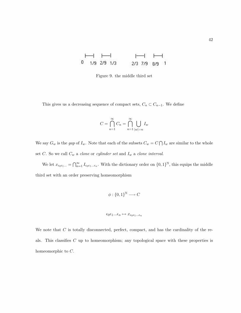
42

Figure 9. the middle third set

This gives us a decreasing sequence of compact sets, Cn ⊂ Cn−1. We define

C =∞⋂

n=1

Cn =∞⋂

n=1

⋃|w|=n

Iw

We say Gw is the gap of Iw. Note that each of the subsets Cw = C⋂Iw are similar to the whole

set C. So we call Cw a clone or cylinder set and Iw a clone interval.

We let xε0ε1... =⋂∞

n=1 Iε0ε1...εn . With the dictionary order on {0, 1}N, this equips the middle

third set with an order preserving homeomorphism

φ : {0, 1}N −→ C

ε0ε1...εn 7→ xε0ε1...εn

We note that C is totally disconnected, perfect, compact, and has the cardinality of the re-

als. This classifies C up to homeomorphism; any topological space with these properties is

homeomorphic to C.

43

2.5.5 Bernoulli Shift Spaces

We have seen that points in the middle third set, C, can be labeled with infinite strings

of 0s and 1s, that is elements of the set Σ2 = {0, 1}N. We can also model the dynamics

of f , the function which generated C. Define the Bernoulli shift space on k ≥ 2 symbols,

Σk = {0, 1 . . . , k − 1}N be the set of all right infinite words from the alphabet {0, 1, . . . , k − 1}.

If we equip Σk with the product topology, so the basic open sets are strings which begin with

the same prefix, then Σk is homeomorphic to C. A basic open set is of the form

Ua1...am = {ω ∈ Xk|ω = a1a2 . . . amwm+1wm+2 . . .}

We call Ua1...am a cylinder set of Σk.

The (right) shift map, σ is a k to 1 local homeomorphism which acts on Σk by forgetting

the first component.

σ : w1w2w3 . . . 7→ w2w3 . . .

σ is a k to 1 covering map Σk −→ Σk.

A subshift is a closed subset W ⊂ Σk which is invariant under σ. In the sections about

dynamically defined Cantor sets, all of our examples will be conjugate to a subshift. Subshifts

which come up in the context of geometric examples tend to be Markov, and hence the periodic

points are dense. Again we define a clone of a subshift to be the set of all words which begin

with a given finite word.

44

Example 11 Let X = {0, 1}N. Let W = {w1w2 . . . ∈ X2| if wi = 0, then wi+1 = 1}. W is a

subshift of X.

Example 12 Via the inclusion {0, 1}N −→ {0, 1, 2}N, we can view Σ2 as a subshift of Σ3. The

dynamics of Σ2 are also closely related to the dynamics of Σ4. Let φ : Σ4 −→ Σ2 be defined by

0 7→ 00

1 7→ 01

2 7→ 10

3 7→ 11

Then φ conjugates σ on Σ4 to σ2 on Σ2

Example 13 (A subshift with no periodic orbits.) Let X be a subshift without periodic

orbits, and let x ∈ X. Then for any finite string of zeroes and ones, w, there must be a bound on

the number of times in a row that w appears in x. If there is no bound on the number of times

w appears in a row, then for any m ∈ N, there exists some k so that σk(x) = (w)mxixi+1 . . ..

Then since X is closed, the periodic point www... is in X. On the other hand, if we start with

such an element x, we find that {σn(x)} is a countable set which is invariant under σ, but which

has no periodic points . Since σ is continuous we take the closure of this set, which produces

a subshift which, since no block repeats in an unbounded way, still has no periodic points. By

alternating digits from this (possibly countable) set with arbitrary digits, we get an uncountable

subshift which still has no periodic points.

45

Now we construct an infinite word x which has no finite strings occurring three times in a

row: Let x1 = 0, x2 = 01, x4 = 0110, x8 = 0110 1001, inductively define x2m+1 = x2mx2m,

where 0 = 1 and 1 = 0 and define ω = limk→∞ xk.

We see that ω is composed of two types of blocks of four digits, 0110 and 1001. So there are

at most eight (23) possible blocks of length 12 beginning in the 4kth position. But we also see

that 0110 does not repeat 3 times in a row, and neither does 1001. So there are only six possible

blocks of length twelve beginning in the 4kth position:

011001101001

011010010110

011010011001

and three more which you get by swapping the 0s and 1s in the above three. By inspecting these

six blocks we see that ω contains no blocks of size 1, 2 or 3 which repeats more than twice in a

row. Now if we remove every other digit from ω, we obtain ω back again, so this shows that no

block of size 2k or 3 · 2k repeats more than twice in a row. For instance, if a block of size six

repeated 3 times in a row, we could remove every other digit from ω and get a block of size 3

which repeats three times in a row.

Now we look at blocks of length 4k + 1. Let B be a block of length 4k + 1 which begins in

4m + 1th spot. Then B begins with 0110 or 1001, and the next three digits after B are either

46

110 or 001. So B doesn’t repeat twice in a row. Similar arguments work for all blocks of length

4k+1 starting in the 4k+ ith position, as well as blocks of length 4k+3 starting in the 4k+ ith

position and so no block of odd length greater than one repeats twice in a row. And once again,

since removing every other digit from ω gives ω back again, no even block repeats three times

in a row either, so ω has the desired property. �

2.5.6 Labeled Cantor sets.

We could try to construct Cantor sets similarly to the way we constructed the middle third

set: Start with an interval I in the line, remove an open interval from the interior of I leaving

I0 and I1, and so forth. This process won’t guarantee the creation of a Cantor set though; for

the resulting set to be totally disconnected, we need to make the set of gaps dense in I.

Instead, we will define a Cantor set to be any set which is homeomorphic to {0, 1}N (and

hence to the middle third set). These are all the totally disconnected perfect sets with the

cardinality of the continuum. We will consider Cantor sets which are embedded in a closed

interval.

We say the Cantor set C ⊂ R is labeled by the shift space Σk if there is an order preserving

homeomorphism φ : Σk −→ C. The point x in C is labeled by the infinite word ω ∈ Σk. We

write xω for the point φ(ω).

A labeled Cantor sets inherits a nested structure of gaps and clones from its labelings. Let

(C, φ) be a labeled Cantor set conjugate to X2. We write xw1w2... = φ(w1w2 . . .). Let w be a

finite string of 0s and 1s. Then we define Iw as the closed interval

47

Iw = [xw00..., xw(k−1)(k−1)...]

and Gw as the open interval

Gw = (xw0(k−1)(k−1)..., xw(k−1)000...)

We write |Iw| and |Gw| for the respective lengths of Iw and Gw. If w contains m symbols,

then we say Iw (or Gw) is a level m clone (or gap). So in general, a lower level clone (gap) will

be longer than a higher level clone (gap). A Cantor set embedded in the line can have many

different labelings on it. The set of clone intervals will be different for two different labelings,

while the set of gaps is dependent only on the underlying set. The middle third set is an

example of a labeled Cantor set.

We note that the underlying Cantor set C can have many different labelings on it. Since

a Cantor set is closed, its complement is open, so the set of gaps depends only on C and not

on the labeling of C. The set of clone intervals depends on the choice of labeling (as does the

labeling of gaps and clone intervals by finite words.)

We can also define a Cantor set which is labeled by a subshift, but for an arbitrary subshift

it would be a little more difficult to extend the labels to the gaps. We can still define the clone

Cw = φ(wεkεk+1 . . .) and then we can define Iw as the convex hull of Cw. The gaps might

48

be a little more difficult to label, but we could describe the gaps by the clones which they’re

between.

The set {0, 1}N comes equipped with the (left) shift map

σ : {0, 1}N −→ {0, 1}N

ε1ε2ε3ε4 . . . 7→ ε2ε3ε4 . . . .

The map σ is a two-to-one local homeomorphism.

Let C be a labeled Cantor set. The shift map on {0, 1}N induces a map σ : C → C, with

σ(xε1ε2ε3ε4...) = xε2ε3ε4.... We also call this map on C the shift map.

Let C and C ′ be labeled Cantor sets in R. Then the map which preserves the labeling is

the unique order-preserving homeomorphism φ : C → C ′ which commutes with the shift map.

We write φ(xε1ε2ε3ε4...) = x′ε1ε2ε3ε4....

Note that we use σ to denote the shift map on {0, 1}N as well as the map which it induces

on C1.

To review our situation, so far we have a Cantor set, C, defined in a similar manner to the

middle third set. The shift map, σ, acts on C by stretching both C0 and C1 out and laying

them back down on top of all of C.

If we know the lengths of all the gaps and clone intervals, of course, we then know how

to construct C. If we know the relative sizes of the intervals, we can construct C up to

49

affine rescaling. For all finite words w, we let l(w), g(w), and r(w) denote |Iw0||Iw| ,

|Gw||Iw| , and

|Iw1||Iw| respectively. Then, all we need, besides l(w), g(w), and r(w) for all w, to construct C

is the interval I (the convex hull of C). Thus we have the ratio geometry function, w 7→

(l(w), g(w), r(w)) = ( |Iw0||Iw| ,

|Gw||Iw| ,

I|w1||Iw| ) whose domain is {0, 1}N, and whose range is contained in

the unit two-simplex {(x, y, z)|x+ y + z < 1}.

2.6 Bounded Geometry.

We say that C has bounded geometry if there exists α and β with 0 < α < β < 1 such

that for all w, l(w), g(w), and r(w) are all between α and β. Bounded geometry is analogous

to hyperbolicity of σ, or equivalently to hyperbolicity of both branches of σ−1. Suppose we

require σ to be hyperbolic, say σ−10 and σ−1

1 both extend to hyperbolic functions, f0 and f1.

We take fi ≤ β ≤ 1. Then the difference quotient, say for σ−10 , over the interval Iw, we get

|I0w||Iw| ≤ β, whereas bounded geometry requires that l(w) = |Iw0|

|Iw| ≤ β.

We note that if C has bounded geometry, then αn ≤ |Iw| ≤ βn. The middle third set, of

course, has bounded geometry with α = β = 13 .

Proposition 11 Let C and C ′ be labeled Cantor sets with bounded geometry. Let φ : C → C ′

be the homeomorphism induced by the shift map.

Iσ−→ I

φ ↓ ↓ φ

I ′σ′−→ I ′

Then φ is Holder continuous.

50

Proof:

Let x, y ∈ C. Then there exists a word w ∈ {0, 1}k, for some k, such that Gw ⊂ [x, y] ⊂ Iw.

We denote φ(Gw) = Hw and φ(Iw) = Jw. Then |φ(x)− φ(y)| ≤ |Jw| ≤ βn ≤ βαλn ≤ β|Gw|λ ≤

β|x− y|λ, where λ = logα β. �

2.7 Cookie Cutters II

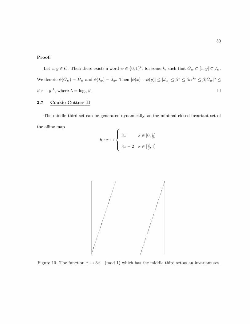
The middle third set can be generated dynamically, as the minimal closed invariant set of

the affine map

h : x 7→

3x x ∈ [0, 1

3 ]

3x− 2 x ∈ [23 , 1]

Figure 10. The function x 7→ 3x (mod 1) which has the middle third set as an invariant set.

51

Alternately, we consider the two branches of h−1:

h−10 =

x

3

h−11 =

x+ 23

Then C is the omega limit set of {h−10 , h−1

1 }. We note that h affinely scales Ii onto I for i = 0, 1.

Let ω = ω1ω2 . . . ∈ {0, 1}N. Then

f(Iω1ω2...ωk) = Iω2...ωk

f(Gω1ω2...ωk) = Gω2...ωk

f(xω1ω2...) = xω2ω3...

f−1i (Iω1ω2...ωk

) = Iiω1ω2...ωk

f−1i (Gω1ω2...ωk

) = Giω1ω2...ωk

f−1i (xω1ω2...) = xiω1ω2...

So h|C commutes with the shift map σ on {0, 1}N.

σ : ε1ε2 . . . 7→ ε2ε3 . . .

52

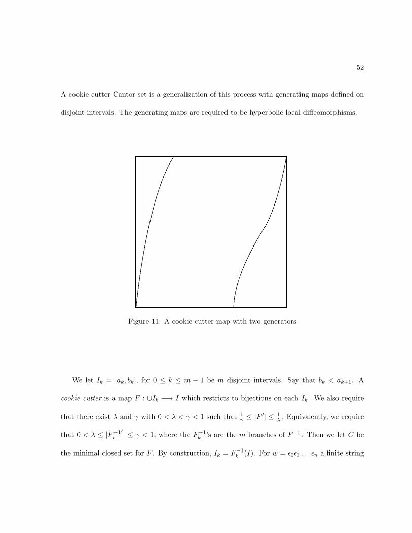
A cookie cutter Cantor set is a generalization of this process with generating maps defined on

disjoint intervals. The generating maps are required to be hyperbolic local diffeomorphisms.

Figure 11. A cookie cutter map with two generators

We let Ik = [ak, bk], for 0 ≤ k ≤ m − 1 be m disjoint intervals. Say that bk < ak+1. A

cookie cutter is a map F : ∪Ik −→ I which restricts to bijections on each Ik. We also require

that there exist λ and γ with 0 < λ < γ < 1 such that 1γ ≤ |F ′| ≤ 1

λ . Equivalently, we require

that 0 < λ ≤ |F−1i

′| ≤ γ < 1, where the F−1k ’s are the m branches of F−1. Then we let C be

the minimal closed set for F . By construction, Ik = F−1k (I). For w = ε0ε1 . . . εn a finite string

53

from the alphabet {0, . . . ,m− 1}, we define Iw = F−1ε0 F

−1ε1 . . . F−1

εn(I). Then C =

⋃n

⋂|w|=n Iw.

Again we have the same situation as the middle third set,with F : C −→ C being conjugate

to σ : {0, . . . ,m − 1}N −→ {0, . . . ,m − 1}N. If F is Ck+λ, we call F a Ck+λ cookie cutter

Cantor set . We say that C is generated by F−10 . . . F−1

m−1 and that C has m generators. We use

hyperbolicity to guarantee that the resulting set is totally disconnected. F induces a labeling

on C so that F is conjugate to the shift map. We say that C is an affine Cantor set if F is affine

on each subinterval. For the sake of simplicity, we will mostly consider cookie cutters with two

generators.

Proposition 12 A cookie cutter Cantor set has bounded geometry.

Proof: Let C be a cookie cutter set with k generators. We will use the Mean Value Theorem

to show that |Iw||Gj

w|is bounded above, and hence |Gj

w||Iw| is bounded below. The proof will apply

to |Iwj ||Iw| as well. When replacing Gj

w by Iwj . Then since all of these values add up to one, and

they are all bounded below, they’re all bounded above too.

Fn(Iw) = I and Fn(Gjw) = Gj so there exists z0 and z1 ∈ Iw so that |I| = Fn′(z0)|Iw| and

|Gj | = Fn′(z1)|Gjw| so

|I||Gj |

=Fn(Iw)

Fn(Gjw)

=Fn′(z0)|Iw|Fn′(z1)|Gj

w||Iw||Gj

w|=

Fn′(z1)|I|Fn′(z0)|Gj |

54

log|Iw||Gj

w|= logFn′(z1)− logFn′(z0) + log

|I||Gj |

=n−1∑i=0

∣∣logF ′(F i(z1))− logF ′(F i(z0))∣∣ + log

|I||Gj |

≤n−1∑i=0

K|F i(z1)− F i(z0)|λ + log|I||Gj |

≤n−1∑i=0

Kγiλ + log|I||Gj |

≤ K ′

. �

2.8 Exceptional Minimal Sets

For a pseudogroup acting on either the circle or the line, an exceptional minimal set is a

minimal set which is homeomorphic to the Cantor set. For a foliation, an exceptional minimal

set is a minimal set whose intersection with the transversal is a Cantor set. Of particular

interest are Markov exceptional minimal sets. All of the known examples of Ck foliations with

exceptional minimal sets are Markov if k ≥ 2.

Definition: Let Γ be a pseudogroup of local C1+λ diffeomorphisms of a compact 1-dimensional

manifold T . Let C be an exceptional minimal set for Γ. C is Markov if there exist elements

γ1, . . . , γm of Γ and closed intervals I1 . . . , Im of T such that

1. Int Iks are pairwise disjoint,

2. C ⊂ ∪mk=1Ik,

3. C∩ Int Ik 6= ∅ for each k,

55

4. the domain of γk contains Ik for each k,

5. γk|Ik ∩ C’s generate Γ|C, and

6. if γk(Ik)∩ Int Ij 6= ∅, then γk(Ik) ⊃ Ij

We call (I0, . . . Im; γ0, . . . γm) a Markov basis. We call a Markov basis hyperbolic if 1 < 1β ≤

γ′k ≤1α . A Markov exceptional minimal set is hyperbolic if it can be generated by a hyperbolic

Markov basis.

Since we don’t require the Ik’s to be pairwise disjoint, (they might share endpoints,) there

might be a countable number of points which have two different labelings on them.

To apply the theory of cookie cutters to Markov exceptional sets, we need to modify the

notation a little bit. We let C be a Markov exceptional set with basis B = {(γk, Ik)}, k =

0 . . .M . Without loss of generality, we assume that Ik is no bigger than it needs to be. That

is, for each k an end points of γk(Ik) is an endpoint of γj , for some j, with Ij ⊂ γk(Ik). If not

we shrink the domain of γk so that it If we only need to repeat this process a finite number of

times, in which case we’re left with B, with smaller domains, but which still is a basis for C. If

we need to repeat this an infinite number of times, then the intervals in question shrink down

to a point, which means they weren’t necessary in B in the first place.

So we assume that the domains of B are no bigger than they need to be, which means that

γj(Ij) doesn’t have gaps on its ends. Then if Ij1 ⊂ γj2(Ij2), we define Ij2j1 = γ−1j2

(Ij1). And if

56

Ij2 ⊂ γj3(Ij3) as well, we define Ij3j2j1 = γ−1j3

(Ij2j1). We see that Iw shrinks down to a point as

the length of w increases to infinity. And that

C =⋂n

⋃|w|=n

Iw

where w is a word jnjn−1 . . . j1 with jk ⊂ γk−1(Ijk−1) Thus C is labeled by the subshift ΣB ={

jnjn−1 . . . j1 ⊂ ΣM : jk ⊂ γk−1(Ijk−1)}.

Now unlike a cookie cutter, the nested interval structure of a Markov exceptional set need

not be homogeneous. There could be a different number of level-1 gaps in each cylinder set. If

there are M elements in the basis, there could be as many as M different local versions of the

nested interval structure. We’ll label the gaps according to the interval to their right. If Ijk

has a gap to its left which is also in Ij , we label that gap Gjk. Then Gijk = γ−1i (Gjk) which

will be directly to the left of Iijk, and so on. In this way we label all the gaps in Dom(B). We

could just as easily named the gaps according to the intervals on their right. We just arbitrarily

chose the interval on their left.

We also note that since the domains of (B) might share a common end point, we might

have a countable number of points with two labelings on them. So the map φ : ΣB −→ C is

continuous, but not a homeomorphism. Hence φ is only a semiconjugacy between σ and Γ.

57

2.9 The scaling function for a Markov exceptional set.

The ratio geometry is defined the same for a Markov exceptional set as it is for a cookie

cutter. If Ijkjk−1...j1w, (respectively Gjkjk−1...j1w) is a subinterval of Ijkjk−1...j1 , then

˛Ijkjk−1...j1w

˛˛Ijkjk−1...j1

˛ ,

(resp.

˛Gjkjk−1...j1w

˛˛Ijkjk−1...j1

˛ ) is a component of the ratio geometry.

In particular, Ij1 has a finite number of sub-intervals and a finite number of sub-gaps. We

write the intervals as Ij1k1 , Ij1k2 . . . Ij1km with k1 < k2 . . . < km, and we write the gaps as

Gj1l1 , Gj1l2 . . . Gj1ln where {l1, l2 . . . ln} ⊂ {k1, k2 . . . km}, and l1 < l2 < . . . < ln. Then the ratio

geometry for Iji is the (m+ n)-tuple

(|Ijik1 ||Ij1 |

,|Ij1k2 ||Ij1 |

, . . . ,|Ijikm ||Ij1 |

,|Gj1l1 ||Ij1 |

. . .|Gj1ln ||Ij1 |

)

whose components add to 1.

For a different sub-interval, Ip, we might have a different number of sub-intervals and sub-

gaps, so the ratio geometry will have a different number of components. If, however, Ij2j1 is a

sub-interval of Ij2 , Then the level one sub-intervals of Ij2j1 are precisely Ij2j1k1 , Ij2j1k2 . . . Ij2j1km ,

and similarly for the sub-gaps, so the ratio geometry of Ij2j1 consists of an (m + n)-tuple as

well. We see that this is true for any finite word which ends with j1. The ratio geometry of the

interval Ijr...j2j1 consists of the (m+ n)-tuple

(|Ijr...j2j1k1 |

|Ij1 |,|Ijr...j2j1k2 ||Ijr...j2j1 |

, . . . ,|Ijr...j2j1km ||Ijr...j2j1 |

,|Gjr...j2j1l1 |

|Ij1 |. . .

|Gjr...j2j1ln ||Ij1 |

)

whose components also add to 1.

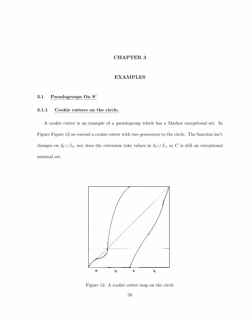
CHAPTER 3

EXAMPLES

3.1 Pseudogroups On S1

3.1.1 Cookie cutters on the circle.

A cookie cutter is an example of a pseudogroup which has a Markov exceptional set. In

Figure Figure 12 we extend a cookie cutter with two generators to the circle. The function isn’t

changes on I0 ∪ I1, nor does the extension take values in I0 ∪ I1, so C is still an exceptional

minimal set.

Figure 12. A cookie cutter map on the circle

58

59

Since F extends f , and C is the unique minimal set for f we see that any closed invariant

set for F which contains a point of I0⋃I1 must contain C. Since the image of G and G′ under

F doesn’t intersect C, C must be a minimal set for F also.

In fact F has two invariant sets, C and {x′}. We note that C is also invariant under F−1,

whereas the backwards orbit of x′ is asymptotic to C. So C is the unique minimal set for F .

Let f0 : (0,m] −→ (0, 1] and f1 : (m, 1] −→ (0, 1] be increasing maps for m ∈ (0, 1). And let

fi be such that

f1(a, b) = (c, d)

and

f2(c, d) = (a, b)

If f ′0(x) > 1 and f ′1(x) > 1 for x 6∈ (a, b)⋃

(c, d) Then the system {f0, f1} Generates a Markov

exceptional set.

For ease of discussion, we’ll write m = 12 and

f(x) =

f0(x) x ∈ [0, 1

2 ]

f1(x) x ∈ [12 , 1]

and ignore that f is not well-defined at 12 . Then (a, b)

⋃(c, d) acts as a trap for f . As soon as

x ∈ (a, b), the forward orbit f(x), f2(x), f3(x), . . . will ping pong between (a, b) and (c, d), and

the backwards orbit of (a, b)⋃

(c, d) will consist of a countable number of disjoint intervals.

60

If we let f be C1+λ with 1α > f ′(x) > 1

β > 1 for x 6∈ (a, b) ∪ (c, d) then O(1) will be

a Cantor set. We would have two “level zero” gaps, (a, b) and (c, d). f−11 (a, b) = (c, d) and

f−10 (c, d) = (a, b), so there are only 2 “level one” gaps as well, f−1

0 (a, b) and f−11 (c, d).

But there are 4 level-two gaps, f−20 (a, b), f−1

1 f−10 (a, b), f−2

0 (c, d) and f−10 f−1

1 (c, d). There

will be eight level-3 gaps, and so forth. Since we bounded the derivatives of f ′, we have

α2(b− a) ≤ f−20 (a, b) ≤ β2(b− a) and so on.

Furthermore, we have

f−10 [0, a] ⊂ [0, a] f−1

1 [0, a] = [12 , c]

f−10 [b, 1

2 ] ⊂ [0, a] f−11 [b, 1

2 ] ⊂ [d, 1]

f−10 [12 , c] ⊂ [0, a] f−1

1 [12 , c] ⊂ [d, 1]

f−10 [d, 1] = [0, 1

2 ] f−11 [d, 1] ⊂ [d, 1]

So these four intervals form a

Markov basis for f . Hence f has a hyperbolic exceptional minimal set.

3.1.2 A period two interval

If we define the circle, S1, to be the interval [0, 1] with its end points identified, then since

f0(12) = 1 and f1(1

2) = 0, f defines a function on S1 which is no longer ill-defined at 12 . So

we can think of f as a function on the circle with the discussion above still holding, but since

f0(12) = 1, and f1(1

2) = 0, and we’ve identified the points 1 and 0 in order to form the circle,

we only need 3 subintervals, as shown. We could define this example a little more generally.

The fixed point need not be at 0, and the point m whose image is the fixed point need not be

12 , but for ease of discussion, we’ll keep these values.

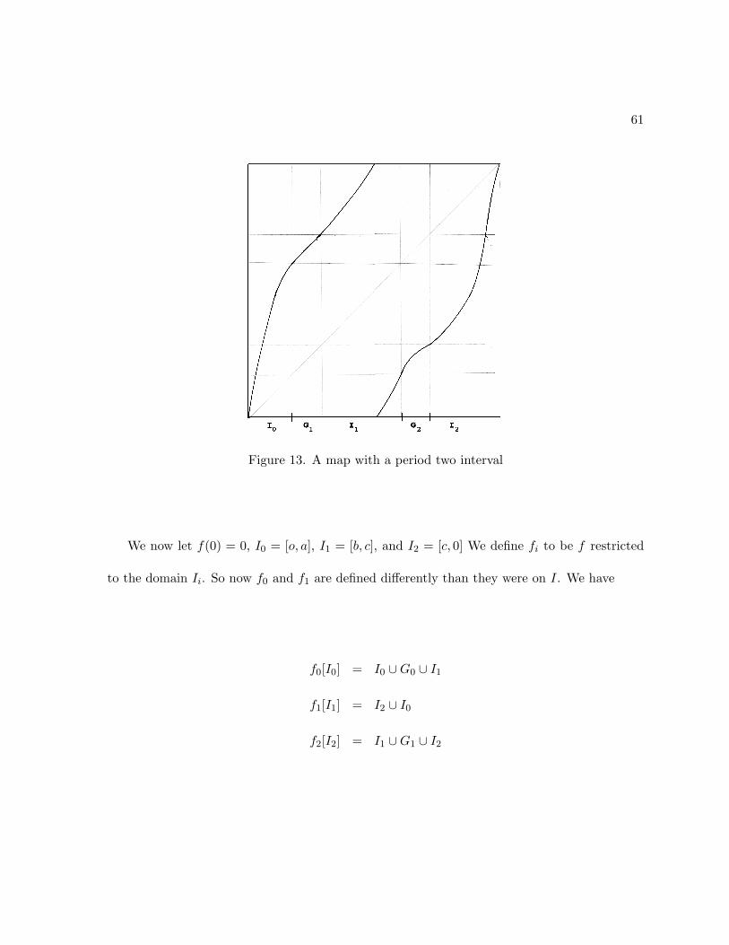
61

Figure 13. A map with a period two interval

We now let f(0) = 0, I0 = [o, a], I1 = [b, c], and I2 = [c, 0] We define fi to be f restricted

to the domain Ii. So now f0 and f1 are defined differently than they were on I. We have

f0[I0] = I0 ∪G0 ∪ I1

f1[I1] = I2 ∪ I0

f2[I2] = I1 ∪G1 ∪ I2

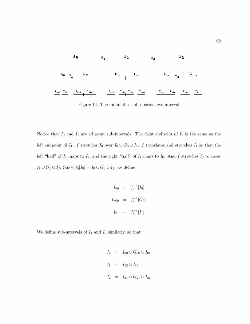
62

Figure 14. The minimal set of a period two interval

Notice that I0 and I1 are adjacent sub-intervals. The right endpoint of I2 is the same as the

left endpoint of I1. f stretches I0 over I0 ∪ G0 ∪ I1. f translates and stretches I1 so that the

left “half” of I1 maps to I2, and the right “half” of I1 maps to I0. And f stretches I2 to cover

I1 ∪G1 ∪ I2. Since f0[I0] = I0 ∪G0 ∪ I1, we define

I00 = f−10 [I0]

G00 = f−10 [G0]

I01 = f−10 [I1]

We define sub-intervals of I1 and I2 similarly, so that

I0 = I00 ∪G00 ∪ I01

I1 = I12 ∪ I10

I2 = I21 ∪G21 ∪ I22

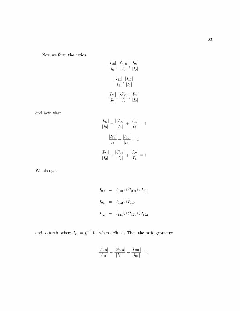
63

Now we form the ratios

|I00||I0|

,|G00||I0|

,|I01||I0|

|I12||I1|

,|I10||I1|

|I21||I2|

,|G21||I2|

,|I22||I2|

and note that

|I00||I0|

+|G00||I0|

+|I01||I0|

= 1

|I12||I1|

+|I10||I1|

= 1

|I21||I2|

+|G21||I2|

+|I22||I2|

= 1

We also get

I00 = I000 ∪G000 ∪ I001

I01 = I012 ∪ I010

I12 = I121 ∪G121 ∪ I122

and so forth, where Iiω = f−1i [Iω] when defined. Then the ratio geometry

|I000||I00|

+|G000||I00|

+|I001||I00|

= 1

64

|I012||I01|

+|I010||I01|

= 1

|I121||I12|

+|G121||I12|

+|I122||I12|

= 1

and so forth.

Continuing this process, we see will encode the intervals and gaps with finite words ω ∈⋃{0, 1, 2}n. But not all words in

⋃{0, 1, 2}n are allowed. If ω indexes a gap, then ω must end

with a 0 or a 2. More specifically, if ω encodes one of these intervals and there’s a 0 in the nth

spot, then there must be either a 0 or 1 in the n+ 1st spot. Similarly, a 1 must be followed by

a 0 or a 2, and a 2 must be followed by a 1 or a 2.

Now since F is hyperbolic, we see that the lengths of level-n intervals and gaps must be

bounded as they were for cookie cutters. If ω is a word of length n, then α < |Iσi||Iσ | < β, and

αn < |Iσ| < βn. The same bounds also work for gaps.

Now the lengths of the clone intervals go to 0 exponentially fast, and a co-gap consists

of at most two clone intervals, so the lengths of the co-gaps go to zero exponentially fast as

well. Therefore the invariant set we get will be totally disconnected. The end points are in the

invariant set, and any point in the invariant set can be approximated by end points, so the set

is perfect. We also see that the backwards orbit of zero is dense, so that this set is indeed a

Markov exceptional set.

If x ∈ C, we can encode x by the subshift of {0, 1, 2}N which is given by the constraints that

a 0 or 1 must follow a 0, a 0 or 2 must follow a 1, and a 1 or 2 must follow a 2. Notice that

this encoding is not entirely unique, since xσ0000000000... and xσ2222222222... are the same point.

65

We can use variations of this example to get a whole class of examples of Markov exceptional

set defined on the circle. We could let f have a period three interval so that f(a1, b1) = (a2, b2),

f(a2, b2) = (a3, b3), and f(a3, b3) = (a1, b1). If f is hyperbolic off of these three intervals, then

f will again generate an Markov exceptional set. f , as constructed, has 3 level zero gaps, 3

level-1 gaps, 6 level-2 gaps, 12 level-3 gaps, etc.

We could also let f be 3 to 1. If we play this ping pong game with two intervals, so

f(a, b) = (c, d) and f(c, d) = (a, b), bounding the derivatives as we did before, then the forward

iterates of f are still trapped in (a, b) ∪ (c, d). And since we make f hyperbolic off of these

intervals, f still generates a Markov exceptional set. Constructed this way, f has two level-0

gaps. But it now has four level-1 gaps. (In general, the inverse image of two intervals would

contain 6 intervals, since f is 3 to 1. This is true of our two intervals, (a, b) and (c, d), but these

six intervals include (a, b) and (c, d), so there are only four new intervals, which are level-1 gaps.

There are 12 level-2 gaps, 36 level-3 gaps and so on.

We could keep constructing such examples by using n to 1 functions, with as many periodic

intervals as we want. In fact we can derive the topological types of these examples by starting

with the function x 7→ nx (mod 1) and “thickening up” one (or more) periodic orbit to get a

periodic interval.

3.1.3 A free group acting on the circle

Let φ and ψ be diffeomorphisms of the circle. Let φ have exactly two fixed points: u−,

which is repelling, and u+, which is attracting. Similarly let ψ have two fixed points v−,

which is repelling, and v+, which is attracting. Further let U−, U+, V−, and V+ be disjoint

66

neighborhoods of u−, u+, v−, and v+ respectively so that φ(v−) ∈ U+, φ(v+) ∈ U+, φ−1(v−) ∈

U−, φ−1(v+) ∈ U−, ψ(u−) ∈ V+, ψ(u+) ∈ V+, ψ−1(u−) ∈ V−, ψ−1(u+) ∈ V− Then Γ, the free

group generated by φ and ψ, acts on the circle with a Cantor set as the minimal set.

Proof: Let x be any point other than u−. Then φn(x) −→ u+. So u+ is in the closure of

the orbit of x. But ψ(u−) 6= u−, so φn ◦ ψ(u−) −→ u+) as well, hence u+ is in the closure

of any orbit. So we only need to show that O(u+) is totally disconnected and perfect. So let

x = γj ◦ . . . ◦ γ1(u+) and y = ξk ◦ . . . ◦ ξ1(u+) be two different points in O(u+), where γi and

ξi ∈ {φ, φ−1, ψ, ψ−1}.

Since u+ is a fixed point for φ, we take γ1, ξ1 ∈ {ψ,ψ−1}. Let r be the smallest number for

which γj−r 6= ξk−r. Then γj−r ◦ . . .◦γ1(u+) and ξk−r ◦ . . .◦ξ1(u+) are in different neighborhoods

U+, U−, V+, V−. E.g. if γj−r = φ and ξk−r = ψ−1, then γj−r ◦ . . . ◦ γ1(u+) ∈ U+ and ξk−r ◦

. . . ◦ ξ1(u+) ∈ V−. We note that O(u) ∈ U+ ∪ U− ∪ V+ ∪ V−, so γj−r ◦ . . . ◦ γ1(u+) and

ξk−r ◦ . . .◦ ξ1(u+) have a neighborhood, N between them which contains no elements of O(u+).

Therefore γj ◦ . . . ◦ γ1(u+) and ξk ◦ . . . ◦ ξ1(u+) have a neighborhood, γj ◦ . . . ◦ γj−r(N) between

them which also contains no points of O(u+). That is O(u+) is nowhere dense, and therefore

O(u+) is also nowhere dense, and hence it’s totally disconnected.

Now to show that O(u+) is perfect, we let x 6= u+, x ∈ O(u+) then since u+ is the attracting

fixed point for φ, φn(x) −→ u+. Then if γ ∈ Γ, γφn(x) −→ γ(u+). Therefore O(u+) is perfect,

and hence O(u+) is an exceptional minimal set.

67

3.2 The Hirsch Foliation

Hirsch’s construction gives us a rich source of examples. We obtain the Hirsch foliation

(23) by starting with a solid torus and removing from the interior another solid torus which

wraps around twice. This gives us a manifold, foliated by two-holed disks, with two transverse

toruses as boundary components. We then glue the exterior boundary component to the interior

component to obtain a foliated manifold without boundary.

To describe this construction more rigorously, we’ll start with D2, the closed disk with two

holes. D2 has three circular boundary components which we’ll call the two interior components

S0 and S1 and the exterior component S2. We’ll also view D2 as a pair of pants, in which case

we’ll call S0 and S1 the cuffs and we’ll call S2 the waist.

We form the cartesian product of D2 with a closed interval. D2×[a, b] is a solid cylinder with

two open solid cylinders removed from the interior. We decompose the boundary of D2 × [a, b]

into five pieces: one exterior vertical cylinder, S0× [a, b], two interior vertical cylinders S1× [a, b]

and S2× [a, b], the bottom slice D2×{a}, and the top slice D2×{b}. We think of D2× [a, b] as

a foliation whose leaves are the level sets D2 × {x} where x ∈ [a, b]. The top and bottom slices

are boundary leaves, and the vertical boundary cylinders are transverse.

We form the foliated manifold N by gluing the bottom slice to the top slice with a half

twist. (That is we glue S1×{a} to S2×{b} and we glue S1×{b} to S2×{a}). Since we glued

with a half twist, we connected the two interior boundary cylinders together into one torus. N

is a solid torus with an open solid torus which wraps around twice removed from the inside.

Since we glued the boundary leaves of D2× [a, b] together, we still have a foliation whose leaves

68

are pairs of pants. N has two boundary components: the exterior boundary torus, Te and the

interior boundary torus, Ti, which wraps around twice. We will identify the circle [a, b]/a∼b

with a longitudinal circle Se ∈ Te which wraps around once, and hence hits each leaf once. We

use Se to index the leaves of N . For x ∈ Se, we let Px be the leaf of N whose waist intersects

Se at the point x.

We could actually view N as a fiber bundle over D2, whose fibers are circles. Then we could

choose Se to be the fiber over a point of S2. But it suits our needs just to think ofN as a foliation

with two transverse boundary toruses. We’ll call the circles of intersection between leaves of

N and Te latitudinal circles, and we’ll call circles which are parallel to Se longitudinal circles.

We’ll name longitudinal and latitudinal circles for Ti similarly. So longitudes are transverse

circles and latitudes are leaf-wise circles.

We now form the Hirsch foliation by gluing Te ∈ N to Ti, using a diffeomorphism H :

Te −→ Ti. We require H to take latitudinal circles of Te to latitudinal circles of Ti. That is H

preserves the the foliation on the transverse boundary components. So the quotient manifold

(M,F) remains a foliated manifold. We use the same two-holed discs, or pairs of pants, which

were leaves of N , as non-standard plaques of M . These plaques are non-standard not only

because they are not homeomorphic to open balls, but also because they need not intersect in

regular position. We will see that there must be at least one plaque which intersects itself, and

at least one pair of plaques which intersect each other in two components.

Te and Ti have been glued together to produce a single transverse torus, T , in the quotient

manifold M . We define Si ⊂ Ti in N by Si = H−1(Se). Then Se and Si get glued together in

69

M to form the transverse circle S ∈ T . S still hits the waist of each plaque exactly once, so we

can still index these plaques by S. For x ∈ S, we let Px be the plaque whose waist hits S at

the point x. S hits either cuff of each plaque exactly once as well.

In general, for t ∈ S, the plaque Pt has three boundary components, S0×{t}, S1×{t}, and

S2 × {t}; each of which intersects exactly one other plaque. (Recall that S0 × {a} = S1 × {b}.)

As H preserves the leaves on the boundary torus, π ◦ H restricted to S is a two to one local

homeomorphism h : S −→ S, where π is leaf-wise projection onto S in N . Depending on our

choice of gluing map H, h could be any two to one local diffeomorphism. As it happens, h

completely determines both the transverse and the leaf-wise dynamics of F . For any t ∈ S,

S2 × {t} intersects one of the cuffs of. So Pt intersects Ph(t). Similarly if h−1i either of the two

branches of h−1, then Pt intersects Ph−1i (t)

3.2.1 The Shape of Leaves

For s ∈ S, what does the leaf, Ls, containing s look like? We think of the plaques Ps as

pairs of pants whose waist is the exterior circle S2 × {s}, and the cuffs are the interior circles

S0×{s} and S1×{s}. In General, Ps intersects three other plaques, Ph(s), Ph−10 (s) and Ph−1

1 (s).

So we build up the leaf by sewing the cuffs of Ps to the waists of Ph−10 (s) and Ph−1

1 (s) and by

sewing the waist of Ps to Ph(s).

We continue in this fashion. In the rth step, we obtain Lrs, the union of all plaques within

a distance r from Ps. Lrs consists of all plaques parametrized by

Or(s) = {t ∈ S | there exists j, k > 0 with j + k = r such that hj(s) = hk(t)}.

Thus Ls consists of all the plaques parametrized by the total orbit of s,

70

O(s) = {t ∈ S| there exists j, k > 0 such that hj(s) = hk(t)}.

That is Ls =⋃

t∈OsPt.

We see that Lrs is a tubular neighborhood of a finite tree, the root of which is the waist of

Phr(s), and the ends of which consist of 2r+1 + 2r − 1 cuffs. If s is an eventually periodic point

of h, then one of these cuffs will eventually be sewn to the root of Lrs.

So Ls consists either of a tubular neighborhood of an infinite tree, possibly with one handle

depending on whether s is an eventually periodic point of h. In either case, Ls is quasi-isometric

to a tree. In the first case, Ls is homeomorphic to a sphere minus a Cantor set. In the second

case, Ls is homeomorphic to a torus minus a Cantor set. The Cantor set we remove corresponds

to the set of ends of Ls.

3.2.2 The holonomy of the Hirsch foliation

The non-standard plaques we use come up naturally in the construction, and they made it

easy to describe the shape of leaves, but we also use them because they are parametrized by S,

making S a totally transverse circle. The holonomy on S with respect to these plaques is easy

to describe since the holonomy on N is trivial, and H preserves the foliation. We define a map

h : S −→ S, with h(t) = r. h is a two to one map of the circle. The map h is the holonomy

function of F on S. The self-intersecting plaques mentioned above correspond to fixed points of

h, and the pairs of plaques which intersect in two components correspond to period two points.

We note that h is the holonomy function on S, so all of the dynamics of F are encoded by

h. We saw that a leaf corresponds to a total orbit of h, and a point of period k corresponds to

a handle of length k in the plaque metric.

71

Lrs is an exhaustion sequence for Ls, and the plaques of Lr

s are parametrized by Or(s), which

itself is an exhaustion sequence for O(s). So ω(Ls) =⋃

t∈ω(s) Lt.

If we fix the point s ∈ S as a base-point of Ls. An end of Ls corresponds either to the

sequence

s, h(s), h2(s) . . .

or a sequence

s, h(s), h2(s) . . . hk(s), h−1ik+1

(hk(s)), h−1ik+2

(hk(s)) . . .

The end which corresponds to the first sequence will be called the expanding end. An end

which corresponds to a sequence of the second type will be called an eventually contracting end.

An end which only corresponds to a backwards orbit of s will be called a contracting end. Note

that the designation of an end as eventually contracting is not natural as it depends on the

arbitrary choice of a base-point.

An invariant set of F corresponds to an invariant set of h. If X ⊂ M is an invariant set

for F , then X ∪ S will be an invariant set for h, and if W ⊂ S is an invariant set for h, then

X = {Px|x ∈W} = {Lx|x ∈W} is an invariant set of F .

Before gluing the boundary toruses together, the holonomy of N is trivial. This means that

for paths that stay away from the torus T , the holonomy of M is trivial as well. The only

non-trivial holonomy we get in M is created by the gluing map H. If Px ⊂ M is any of the

two-holed plaques, and γ is a path which stays in the interior of Px, then the holonomy along

γ is trivial. Likewise, if γ stays in Px and begins and ends at the same boundary component

72

of Px, the holonomy is trivial as well. The only γ can be a path in Px whose holonomy is

non-trivial is if it begins at one boundary component of Px, and ends in another component.

Since a path between the cuffs of Px can be homotoped to a path from one cuff to the waist to

the other cuff, we need only consider paths from the waist to one cuff.

We may as well consider paths that begin and end in the transverse circle S. We fix a point

x ∈ S. Then Px is the plaque whose waist hits S at x. We think of S as being the circle

[a, b]|a∼b embedded into the manifold M . If γ begins at x ∈ S and travels from the waist of the

plaque Px to one of its cuffs, then the endpoint of γ is, in general, a different point of S.

Indeed, thinking of γ as a curve inN , instead of a curve inM , and thinking ofN asD2×[a, b]

with the top and bottom identified, then γ begins at the point (w0, x) with w0 ∈ Se ⊂ D2 and

x ∈ [a, b], and γ ends at either (w1, x) with w1 ∈ Si ⊂ D2 or (w2, x) with w2 ∈ Si. We’ll let γ0

be the path that ends at (w0, x) and γ1 the path that ends at (w1, x) . This labeling really only

works for x 6= a, since we could label that plaque either Pa or Pb. But the point is that γ is a

path from the exterior component of D2 × {x} to one of its interior components. So returning

to the manifold M , there are two paths from the waist of Px to one of its cuffs. We call these

two paths γ0 and γ1. The holonomy along these two paths are the two right inverses of the

map h, which we get by projecting the gluing map H to a longitudinal circle of N .

3.2.3 The Hirsch Example With Linear Generators

Given any k to 1 local homeomorphism of the circle h, the Hirsch construction produces a

foliation whose transverse dynamics are given by iterating h and the k branches of h−1.

73

We examine the dynamics of some possible two to one functions h : S1 −→ S1 in the context

of the Hirsch foliation, where S1 = [a, b]/a∼b. In the linear case, h(x) = 2x mod 1, each leaf is

dense, so the ω(L) = M . (A leaf parametrized by an rational number will be a tree made of

tubing, with one handle added. A leaf parametrized by a irrational number will be a tree with

no handles.)

To show that the backwards orbits of h(x) = 2x mod 1 are dense, we note that h has two

inverse maps:

h−10 : x −→ x

2

h−11 : x −→ x+ 1

2

Since h0 contracts to 0 it suffices to show that the backwards orbit of 0 is dense. But the

backwards orbit of 0 consists of all the dyadic numbers, and hence is dense. The limit set of an

end is also dense.

Example 14 Take [a, b] = [0, 1], and use a gluing map H which projects to the map x 7→ 2x

(mod 1). Then, for any x ∈ S, the waist of the plaque Px is sewn to one of the cuffs of P2x.

The path which starts at x, then travels up the leg of P2x, and ends at 2x ∈ S has h : x 7→ 2x

(mod 1) as a holonomy function. A path in the opposite direction will have one of the branches

of h−1 = 12x (mod 1) as its holonomy. If we take x ∈ (0, 1) ⊂ S, then there are two paths, γ−1

0

and γ−11 , from the waist of Px to one of its cuffs. The holonomy along γ−1

0 will be the function

x2 and the holonomy along γ−1

1 will be the function x+12 .

74

This means that the leaf Lx has one direction with expanding holonomy. Locally Lx has

two directions with contracting holonomy, Globally it has an infinitely branching number of

directions with contracting holonomy. If you take any two sub-intervals of S, and flow them

along a path from the waist to one of the cuffs of a plaque Px, then either of the two subintervals

will be contracted by a factor of 12 , so their relative lengths don’t change. If we do this with the

appropriate intervals to define the ratio geometry of h, we get a constant value of 12 .

3.2.4 Limit Sets of Ends and Paths

An end ε corresponds to an infinite branch of the tree, the limit set of ε is determined by a

decreasing neighborhood of that branch.

Let γ be a path to the end ε. Then depending on ε, the limit set of γ could be dense a

countable set or a Cantor set.

To generate a Cantor set, we need only specify the set of gaps. This will consist of the

interval (14 ,

38) along with all of its iterates under the maps

h−10 : x −→ x

2

h−11 : x −→ x+ 1

2

Since the image of any point is dense under these maps, the specified set of gaps must be dense,

and hence its compliment is totally disconnected. We see that some of the iterates are contained

in earlier iterates. Taking this into account, we see that the endpoints consist of elements of

[0, 1] whose base two expansion terminate either with 011 or 01, and which contain no instance

75

of 010. If an instance of 010 occurs, that means the gap got translated into the interior of an

earlier iterate. This shows that our desired set is perfect, and hence is a Cantor set.

To find a path whose limit set actually generates this set, we simply concatenate all finite

sequences which contain no instance of 010, interspersing an extra 1 when necessary. One

example is the sequence . . . 100 011 001 1 000 11 10 01 1 00 1 1 0.

3.2.5 The Hirsch Example With A Cookie Cutter

If the gluing map, H, projects to a cookie cutter, h, on the transverse circle, S, then we

have much the same situation. Globally a leaf, in general, has one direction with expanding

holonomy, as you travel up the tree; and an infinitely branching number of directions with

contracting holonomy, as you travel down the tree. Locally a leaf, in general, has two directions

with contracting holonomy. Actually if the leaf is part of the minimal set, then it’s holonomy

is strictly expanding as you travel up the tree, and strictly contracting as you travel down the

tree, but for leaves off of the minimal set, this is only a general picture.

Either way, as you travel up the tree starting from the plaque Px, you successively hit

the plaques Ph(x), Ph2(x), Ph3(x), etc. As you travel down the tree starting from the plaque

Px, depending on which branches you choose, you might hit the plaques Ph−10 (x), Ph−1

1 h−10 (x),

Ph−11 h−1

1 h−10 (x), etc.

Since h is a cookie cutter on S, it doesn’t matter that S and h arose in the context of

the Hirsch foliation. h is a cookie cutter on the circle S, therefore all of the theory of cookie

cutters applies to h. h has a Cantor set C as a minimal set. We can write S = H ∪ I where

I = I0 ∪ G ∪ I1. Then for w any finite string of 0s and 1s, we can define I0w = h−10 [Iw], and

76

so forth. This gives us the structure of nested intervals Iw = Iw0 ∪Gw ∪ Iw1, which we use to

label C. C will have bounded geometry, and the scaling function will classify the differentiable

structure of C.

But now we can also view h as the holonomy of M in the expanding direction, and h−10

and h−11 as the holonomy of M in the contracting directions. At least, off of the interval H,

these are the expanding and contracting directions respectively. So let xω ∈ S and take any

two subintervals J and K of I0∪G∪I1. Choose a branch of the leaf to travel in the contracting

direction, say we use a path from Pxω to Px0ω to Px0ω to Px10ω to Px110ω , etc. As we flow J

and K down this path, say we get the intervals J0 and K0, J10 and K10, J110 and K110, etc.

Each time we add a 0 or a 1 to the left, that’s the same as flowing from the waist to one of the

cuffs of whichever plaque we’ve arrived at. So we are traveling to an end of the leaf Lx in the

contracting direction. Since the derivatives of h−11 are above by β < 1, the intervals Jw and Kw

are exponentially small. That means that the holonomy functions h−1i are getting closer and

closer to linear, and the ratio of Jw and Kw converges exponentially fast.

But the intervals we’re interested in are I0, G, and I1 and I. As we flow I0 and I, for

instance, in a contracting direction on the leaf, their ratios converge exponentially fast to the

first component of the scaling function. So, having fixed the base point x, the scaling function

can be defined on the set of infinitely long paths beginning from x with contracting holonomy

instead of some abstract dual Cantor set. These paths correspond to contracting ends of the

leaf Lx, possibly with the handle thrown in as well if Lx has a handle.

77

3.3 The Double Suspension

The double suspension can be used to construct a foliated manifold with a holonomy group,

acting on a transverse circle, generated by two diffeomorphisms φ and ψ of the circle. We

describe the double suspension informally by starting with Σ2×S1. Where Σ2 denotes the two-

holed torus. We then cut Σ2 twice, once along each handle, and glue the cuts back together

using φ and ψ.

More formally we note that when we cut Σ2, we’re left with D3, a disk with three holes.

So we begin with D3 × S1. This is a foliated manifold with four boundary components, each

of which is a transverse torus. We glue these together pairwise, using a gluing map which is

φ in the transverse direction for the first pair, and a gluing map which is ψ in the transverse

direction for the second pair. We see that we get a foliation whose holonomy is the free group

generated by φ and ψ acting on the transverse circle.

3.4 Generalizing Hirsch’s Construction

Let f1, . . . , fn be local diffeomorphisms of the circle. Then we can modify the Hirsch foliation

to produce a foliation whose dynamics are given by f1 through fn. Since fk : S1 −→ S1 is a

local diffeomorphism, it must be an rk to 1 map.

As before we begin with a solid torus, and remove 2n + 1 worm holes from the center, so

that we have a manifold with one exterior boundary component, and 2n+ 1 interior boundary

components, all of which are tori. We label the interior boundary components T0, . . . , T2n. We

remove the worm holes in such a way that T0 through Tn each wraps around once longitudinally,

78

and Tn+k wraps around rk times. We glue T0 to the exterior torus with a map that is the identity

in the longitudinal direction. We then glue Tk to Tn+k using fk in the longitudinal direction.

Example 15 We defined the double suspension of two circle maps in this way.

Example 16 Let X be a solid torus with two solid toruses removed from the inside, one which

wraps around twice, and one which wraps around three times. We then have a foliated manifold

with three boundary components, whose leaves are 5-holed latitudinal discs. If we identify the

two interior boundary components, we get a foliated manifold with a transverse torus as the

boundary. We think of the five-holed discs as non-standard plaques which are parametrized by

a longitudinal circle on the boundary. The transverse dynamics will be given by a 3 to 2 local

homeomorphism of the circle. The dynamics of such a map are difficult to analyze. In general

they will not be Markov, because there are two ways of going forwards and three ways of going

backwards.

We can further generalize Hirsch’s construction. Let (M,F) be any codimension one folia-

tion of a compact manifold and let T be a solid torus with a transverse boundary. We can then

hollow out solid toruses from the middle of T and glue their boundary components together. We

then get a new codimension one foliation whose holonomy is generated by the holonomy of F

along with the gluing maps used in the construction. Note that whenever we have a transverse

circle, we can take a neighborhood of the transverse circle to get a transverse torus.

Example 17 Let R be a Reeb component. We can hollow out two solid toruses from R, one

which wraps around once, and one which wraps around twice. If we glue their boundaries

79

together with a cookie cutter function, we get a foliation whose minimal set is the boundary

torus, but which has a local exceptional set which is Markov and hyperbolic.

Example 18 Let N1 be a solid torus with another solid torus removed from the inside. Let the

interior torus wrap around twice in the longitudinal direction, but only once in the latitudinal

direction. This interior torus is unknotted as a subset of R3. We form the Hirsch foliation on

the manifold M1 by identifying the boundary components using the diffeomorphism H1, which

projects to the 2 to 1 map h on the transverse circle. Getting a holonomy function h acting on

the transverse circle S.

Let N2 also be a solid torus with another solid torus removed from the inside. But this time,

let the interior torus be knotted as a trefoil which wraps around twice in the longitudinal direction

and three times in the latitudinal direction. Again, we form a Hirsch foliation on the manifold

M2 by gluing the interior component to the exterior component, using the diffeomorphism H2.

If H2 projects to the same map h, on the transverse circle, then the leaves of M1 are identical

to the leaves of M2, and the transverse dynamics of M1 is identical to the transverse dynamics

of M2, but the ambient manifolds are not diffeomorphic.

CHAPTER 4

RESULTS ON S1 AND I

4.1 The Conjugation Problem for Cookie Cutters

4.1.1 Automorphisms of Cookie Cutter Sets

We give a partial classification of the outer automorphisms of cookie cutter Cantor sets.

For cookie cutter Cantor sets with two affine generators, such diffeomorphisms have to be given

by a finite number of clone maps. This also holds true for labeled Cantor sets with the proper

pinching on the ratio geometry, and hence for cookie cutter set with the proper pinching on the

derivative.

Theorem 14 Let C be an affine cookie cutter set with two generators. Let φ : I −→ I be an

order preserving C1 diffeomorphism with φ(C) = C. Then there is a finite cover of C by clone

intervals Iw0 , . . . Iwm so that for each wi, φ restricts to a clone map on Cwi.

Proof: We’ll look at a sufficiently small gap, G, of C. Then by the smoothness of φ, we have

a good approximation for the sizes of images of nearby gaps. This will show that we have only

one choice for the image of each nearby gap, and that will define a clone map.

We let I0 = [0, α] and I1 = [1 − β, 1]. Then f0 = 1αx, f1 = 1

βx and 1α and 1

β are the two

rates of expansion. Without loss of generality, we let α ≤ β. We let γ be the relative length of

all the gaps (and so α+ β + γ = 1). Let a ∈ C. We show that there is a clone containing a on

80

81

which φ restricts to a clone map. Then since a is an arbitrary element, we can cover C by such

clones, and since C is compact, we can take a finite sub-cover.

So we let a ∈ C, and choose ε sufficiently small. I.e. ε < min(

γφ′(a)2α+γ ,

(1−β)φ′(a)1+β

).

Now we choose U to be a small enough neighborhood of a, that for u ∈ U , |φ′(a)−φ′(u)| ≤ ε.

Then we take Iω ⊂ U to be a clone interval in U with a ∈ Iω. Since φ preserves C, it must

take gaps to gaps. So we set Gω′ = φ(Gω), and claim that φ(Gw0) = Gw′0 and φ(Gw1) = Gw′1.

Then, by induction on m, we show that φ(Gωε0...εm) = φ(Gω′ε0...εm). And since the gaps are

dense, this will show that φ is a clone map on Cω.

Since Gw and Gw′ are gaps in an affine Cantor set, there are integers j, k, j′, and k′ so that

|Gω| = αjβkγ

|Gω′ | = αj′βk′γ

and

|Gω′ ||Gω|

= αj′−jβk′−k = φ′(z)

and hence

|αj′−jβk′−k − φ′(a)| < ε.

We first show that φ(Gω0) ⊂ Iω′0. We suppose that this is not so. Then since φ is order

preserving, and φ(Gω) = Gω′ , φ(Gω0) is to the left of Iω′ , and hence contains the gap, Gγ ,

82

directly to the left of Iω′ . Now, since Gγ 6⊂ Iw′0, Gγ has to be a lower level (and hence bigger)

gap than Gω′ , and so

|φ(Iω0)| > (α+ γ)αj′βk′ .

Therefore

α+ γ

α[φ′(a)− ε] <

α+ γ

α

j′−j

βk′−k

<|φ(Iω0)||Iω0|

= φ′(z)

≤ φ′(a) + ε

This inequality implies that ε > γφ′(a)2α+γ , which, of course, contradicts ε being sufficiently small.

Now we show that φ(Gω0) = Gω′0. Again we suppose otherwise. Then since φ(Gω0) ⊂ Iω0,

|φ(Gω0)| ≤ αj+1βk+1γ.

Since β > α, we have that

φ′(a)− ε ≤ φ′(z)

=|φ(Gω0)||Gω0|

≤ βαj′−jβk′−k

< β(φ′(a) + ε)

83

This inequality implies that ε > φ′(a)(1−β)1+β which, of course, again contradicts ε being small.

This shows that φ(Gω0) = Gω′0. The same argument shows that φ(Gω1) = Gω′1 and hence φ

is a clone map on Cω. �

Example 19 For cookie cutters with more than two generators this theorem becomes false. We

let C be the middle third Cantor set, as generated by the following function

f(x) =

9x x ∈ [0, 19 ]

9x− 2 x ∈ [29 ,13 ]

3x x ∈ [23 , 1]

We define the function φ : C −→ C.

φ(x) =

3x x ∈ [0, 19 ]

x+ 49 x ∈ [29 ,

13 ]

13x+ 2

3 x ∈ [23 , 1]

We see that any clone interval with left end point at 0 is of the form I = [0, 132n ], and

φ(I) = [0, 132n−1 ] which, with our chosen function, is not a clone interval. We have a similar

situation at the point x = 23 . Note that while locally φ isn’t an element of the pseudogroup,

the germ of φ at a point will be the germ of a pseudogroup element.

84

Theorem 15 Let C be a labeled Cantor set generated by two generators, with bounded geometry

α ≤ r ≤ β with β3 < α2. If φ is a C1+λ outer automorphism of C, (i.e φ extends to a C1+λ

map of I) then φ restricts to a piecewise clone map.

Proof:

We proceed as before, by pegging down one gap, and showing that nearby gaps must fall

into place. Let φ be such a map. Take a ∈ C. Let ε be sufficiently small. (ε ≤ α2−β3

α2+β3φ′(a).) For

any clone interval Iw which contains a, and is small enough that |φ′(u) − φ′(a)| ≤ ε, we claim

that φ restricts to a clone map on Iw.

Let Gw′ = φ(Gw) and show that φ(Iw0) = Iw′0 and that φ(Iw1) = Iw′1.

Suppose φ(Iw0) 6⊂ Iw′0. Then Iw′0 ∪Gv ⊂ φ(Iw0) where Gv is the gap directly to the left of

Iw′ . In which case

φ′(a) + ε >|φ(Iw0)||Iw0|

>|Iw′0|+ |Gv|

|Iw0|

=|Iw′0||Iw0|

+|Gv||Iw0|

=|Iw′0||Iw′ |

· |Iw′ |

|Gw′ |· |Gw′ ||Gw|

· |Gw||Iw|

· |Iw||Iw0|

+|Gw′

1...w′k|

|Iw′1...wk

|·|Iw′

1...w′k|

|Iw′1...wk+1

|· . . . ·

|Iw′1...w′

l−i|

|Iw′1...wl

|· |Iw

′ ||Gw′ |

· |Gw′ ||Gw|

· |Gw||Iw|

· |Iw||Iw0|

≥ α2

β2

(φ′(a)− ε

)+

α

βl−k· 1β·(φ′(a)− ε

)· αβ

≥(α2

β2+α2

β3

) (φ′(a)− ε

)

85

and so

φ′(a) + ε ≥(α2

β2+α2

β3

) (φ′(a)− ε

)(

1 +α2

β2+α2

β3

)ε ≥

(α2

β2+α2

β3− 1

)φ′(a)

ε >α2β + α2 − β3

α2β + α2 + β3· φ′(a)

>α2 − β3

α2 + β3· φ′(a)

which contradicts ε being small which goes to show that φ(Iw0) ⊂ Iw′0.

We now show that φ(Gw0) = Gw′0. Suppose not. Then since φ(Gw0) ⊂ Iw′0, φ(Gw0) =

Gw′0ε1...εkand hence

φ′(a)− ε <|φ(Gw0)||Gw0|

=|Gw′0ε...εk

||Gw0|

=|Gw′0ε...εk

||Iw′0ε1...εk

|·|Iw′0ε1...εk

||Iw′0ε1...εk−1

|. . .

|Iw′0ε1 ||Iw′0|

· |Iw′0|

|Iw′ |· |Iw

′ ||Gw′ |

· |Gw′ ||Gw|

· |Gw||Iw|

· |Iw||Iw0|

<βk+1

α(φ′(a) + ε) · β

α

<β3

α2(φ′(a) + ε)

This gives us that

ε >α2 − β3

α2 + β3φ′(a)

86

This is a contradiction hence φ(Gw0) = Gw′0. Similarly φ(Gw1) = Gw′1, and by induction

φ(Gωα) = Gω′α. Therefore φ restricts to a clone map on Cw. �

Like the theorem for affine Cantor sets, the proof given here relies on the fact that C is

generated by two generators. The counter example given, however, doesn’t provide a counter

example for this version of the theorem though, since in the example α = 19 and β = 1

3 , so

β3 > α2.

4.1.2 C1+λ Equivalence

In (37; 38), Sullivan used the scaling function, as defined by Feigenbaum in a different

setting, to categorize the C1+λ structure of cookie cutter Cantor sets. C1+λ cookie cutters

have bounded geometry. The ratio geometry converges along backwards orbits of F to the

scaling function, which is a Holder continuous function from left-infinite words. If two cookie

cutters are C1=α1+λ conjugate, then their ratio geometries are exponentially close, which means

that they have the same scaling function. Using the boot-strapping method, if φ is any Ck+λ

conjugation between Ck+λ cookie cutters, then φ must itself be Ck+λ as well. There’s a partial

converse. Given any Holder scaling function, we can construct a cookie cutter which has that

scaling function, and any two cookie cutters with the same scaling function are C1+λ conjugate

in a neighborhood of the minimal set.

Proposition 11 shows that if two Cantor sets have bounded geometry, the label-preserving

map, φ, is Holder. But the ratio geometry determines the Cantor set, up to affine rescaling.

And since C is a perfect set, this is enough to determine the smooth structure in a neighborhood

of C. By Taylor’s theorem, since the length of Iw is exponentially small, the non-linear part of

87

φ is also exponentially small, which means that the ratio geometry is determined exponentially

closely by the smooth structure of C. If the conditions of the following proposition are met, we

say that C and C ′ are exponentially close.

Proposition 13 Let φ : C −→ C ′ be the label preserving map between Cantor sets with bounded

geometry. We write Jw = φ(Iw). Then the following conditions are equivalent:

There exists ξ < 1 and K > 0 such that for every word w of length n,

1)∣∣∣ |Iwi||Iw| −

|Jwi||Jw|

∣∣∣ ≤ Kξn for i ∈ {0, 1}

2) (1−K)ξn |Iwi||Iw| ≤

|Jwi||Jw| ≤ (1 +Kξn) |Iwi|

|Iw|

3) e−Kξn |Iwi||Iw| ≤

|Jwi||Jw| ≤ eKξn |Iwi|

|Iw|

4) for any finite word α, e−kξn |Iwα||Iw| ≤

|Jwα||Jw| ≤ ekξn |Iwα|

|Iw|

5) for any u, v, x, y ∈ Iw, e−Kξn · u−vx−y ≤

φ(u)−φ(v)φ(x)−φ(y) ≤ eKξn · u−v

x−y

Proof: We prove the implications for the upper bounds, and the lower bounds will be the

same.

1) ⇒ 2):

|Jwi||Jw|

≤ |Iwi||Iw|

+Kξn

=|Iwi||Iw|

∣∣∣∣1 +|Iw||Iwi|

Kξn

∣∣∣∣≤ |Iwi|

|Iw|·∣∣∣∣1 +

K

αξn

∣∣∣∣

88

2) ⇒ 1):

|Jwi||Jw|

≤ |Iwi||Iw|

(1 +Kξn)

=|Iwi||Iw|

+Kξn |Iwi||Iw|

≤ |Iwi||Iw|

+Kξnγ

3) ⇒ 2):

|Jwi||Jw|

≤ eKξn |Iwi||Iw|

= [1 +O(ξn)]|Iwi||Iw|

2) ⇒ 3)

|Iwi||Iw|

|Jw||Jwi|

≤ 1 +Kξn

≤ 1 +Kξn +(Kξn)2

2+ . . .

= eKξn

Now we need to show that there exists K2 such that e−K2ξn ≤ |Iwi||Iw|

|Jw||Jwi| , for which it suffices

to show that e−K2ξn ≤ 1−Kξn. So choose K1 > K. Then e−K1ξn ≤ 1−K1 + CK12ξ2n. Now

choose N big enough so that for n > N , K1ξn −CK − 12ξ2n > Kξn. Then e−K1ξn

< 1−Kξn.

Now replacing K1 with K2 = maxn≤N (Kn,K), we have e−K′′ξn ≤ 1−Kξn for all n > 0.

89

This completes the proof that 1), 2), and 3) are equivalent. 5) ⇒ 4) ⇒ 3) is immediate, so

now we need to show that 3) ⇒ 4) ⇒ 5).

3) ⇒ 4) Write α = v0v1 . . . vm. Then

|Jwα||Jw|

=|Jwv0 ||Jw|

|Jwv0v1 ||Jwv0 |

. . .|Jwv0...vm ||Jwv0...vm−1 |

≤ eKξn |Iwv0 ||Iw|

eKξn+1 |Iwv0v1 ||Iwv0 |

. . . eKξn+m |Iwv0...vm ||Iwv0...vm−1 |

= eKξn(1+ξ+ξ2+...+ξm) |Iwv0 ||Iw|

|Iwv0v1 ||Iwv0 |

. . .|Iwv0...vm ||Iwv0...vm−1 |

≤ eK

1−ξξn |Iwα||Iw|

4) ⇒ 5): We have x, y, u, and v ∈ Iw. If we show that |φ(x)−φ(y)||Jw| ≤ eKξn |x−y|

|Iw| , then since x

and y are arbitrary elements of Iw, this applies to u and v also, and hence

|φ(x)− φ(y)||φ(u)− φ(v)|

=|φ(x)− φ(y)|

|Jw||Jw|

|φ(u)− φ(v)|

≤ eKξn |x− y||Iw|

ekξn |Iw||u− v|

= e2Kξn |x− y||u− v|

Now write [x, y] =⋃∞

t=1Gt where each Gt is a gap contained in [x, y]. Write Ht = φ(Gt). Then

|φ(x)− φ(y)||Jw|

=∑|Ht||Jw|

=∑ |Ht|

|Jw|

≤∑

eKξn |Gt||Iw|

90

= eKξn |x− y||Iw|

�

Theorem 1 Let C1 and C2 be C1+λ conjugate cookie cutters. Then they are exponentially

equivalent.

Proof: For any finite word w, Taylor’s theorem implies that |φ(Iw)| = φ′(a)|Iw|+O(|Iw|1+λ).

So

|φ(Iw0)||φ(Iw)|

≤ φ′(a)|Iw0|+ C|Iw0|1+λ

φ′(a)|Iw| − C|Iw|1+λ

=|Iw0|+D1|Iw0|1+λ

|Iw| |1−D1|Iw|λ |

=|Iw0|+D1|Iw0|1+λ

|Iw|(1 +O(|Iw|λ)).

≤ |Iw0||Iw|

+D1|Iw0||Iw|

|Iw|λ +D2|Iw0||Iw|

|Iw|λ +D1D2|Iw0|1+λ|Iw|λ

≤ |Iw0||Iw|

+D1γ|Iw0|λ +D2γ|Iw|λ +D1D2|Iw0|1+λ|Iw|λ

≤ |Iw0||Iw|

+D1γγ(n+1)λ +D2γγ

nλ +D1D2γn(1+λ)γnλ

≤ |Iw0||Iw|

+D3γλn.

Where D1 = Cmin φ′(a) , D2 is the O-constant for 1

1−D1x and D3 is the maximum of D1, D2 and

D1 ·D2. �

91

Theorem 2 The scaling function converges for a cookie cutter set, and depends only on the

exponential class of the ratio geometry.

Proof: We let ω = . . . ε3ε2ε1 be a left infinite word of zeroes and ones. We write Rk(ω) =(|Iεk...ε3ε2ε10||Iεk...ε3ε2ε1 |

,|Gεk...ε3ε2ε1 ||Iεk...ε3ε2ε1 |

,|Iεk...ε3ε2ε11||Iεk...ε3ε2ε1 |

). Then since F is itself C1+λ, C0 and C1 are both conjugate

to C via F . Therefore, by Theorem 1, the ratios are only changed by an exponentially small

amount, i.e.

|Rk(ω)| − Cγk ≤ |Rk+1(ω)| ≤ |Rk(ω)|+ Cγk

which implies that

|Rk(ω)| − C

1− γγk ≤ |Rk+m(ω)| ≤ |Rk(ω)| − C

1− γγk

Therefore Rk(ω) is a Cauchy sequence and hence converges. Furthermore we see that

convergence is exponentially fast. �

The converse of Theorem 1 is true as well, but as an intermediate step, we show the weaker

condition that φ is Lipschitz.

Lemma 1 Suppose that for all w of length k, e−ak |Jw0||Jw| ≤

|Iw0||Iw| ≤ eak |Jw0|

|Jw| . Where (ak) is a

summable sequence; say∑ak = A. Then φ is Lipschitz.

92

Proof: Since the set of gaps, Cc1, is dense, we only need to prove that φ is Lipschitz on Cc

1.

That is φ is Lipschitz on each gap with a uniform Lipschitz constant. Write Hw = φ(Gw).

Then

|Hε1ε2...εn | =|Hε1ε2...εn ||Jε1ε2...εn |

|Jε1ε2...εn|

|Jε1ε2...εn−1 ||Jε1ε2...εn−1 ||Jε1ε2...εn−2 |

. . .|Jε1 ||J |

|J |

≤ e−an|Gε1ε2...εn ||Iε1ε2...εn |

e−an−1|Iε1ε2...εn ||Iε1ε2...εn−1 |

e−an−2|Iε1ε2...εn−1 ||Iε1ε2...εn−2 |

. . . e−a0|Iε1 ||I|

|J |

≤ eA[|Gε1ε2...εn ||Iε1ε2...εn |

|Iε1ε2...εn ||Iε1ε2...εn−1 |

|Iε1ε2...εn−1 ||Iε1ε2...εn−2 |

. . .|Iε1 ||I|

]|J |

= eA|J ||I||Gw|

�

We’ll also need the following two extension lemmas:

Lemma 2 Let h : X → Y be a Holder continuous map from a metric space X to a complete

metric space Y . Then, since h preserves Cauchy sequences, h extends to the closure of X.

Proposition 14 Let C1 and C2 be Cantor sets with Lebesgue measure 0 embedded in I =

[0, 1]. Let φ : C1 → C2 be an order preserving homeomorphism which is C1+λ, that is g(x) =

limx→y,x∈C1

φ(x)−φ(y)x−y exists and is Holder. Then φ extends to a C1+λ map I → I

Let (a, b) be a gap in C1. Since φ is order preserving (φ(a), φ(b)) is a gap in C2. To extend

φ to (a, b), we extend g in such a way that∫ ba g(x)dx = φ(b) − φ(a). Then φ(x) =

∫ xa g(t)dt

extends φ.

93

So let m = a+b2 . Set g(m) to 2D(b, a) − .5g(a) − .5g(b) = 2D(b, a) − .5D(a, a) − .5D(b, b).

And set g to be linear on the intervals (a,m) and (m, b). Then

∫ b

ag(x)dx = φ(b)− φ(a)

Furthermore

|g(m)− g(a)| = |2D(b, a)− .5D(a, a)− .5D(b, b)−D(a, a)|

≤ 1.5|D(a, b)−D(a, a)|+ .5|D(a, b)−D(b, b)|

≤ 2λC|m− a|λ.

Since g is linear on [a,m], this shows that g is Cλ on [a,m]. Similarly, g is Cλ on [m, b].

Extend g to each gap of C1 in this way, and then g is Cλ on all of I: Let x < y ∈ I −C1. Then

there exists gaps (a1, b1) and (a2, b2) with x ∈ (a1, b1) and y ∈ (a2, b2). Then

g(y)− g(x) = g(b1)− g(x) + g(a2)− g(b1) + g(y)− g(a2)

≤ 2λC|b1 − x|λ + C|a2 − b1|λ + 2λC|y − a2|λ ≤ 2λC|y − x|λ

So φ′(x) = g(x) is Holder, and for end points of C1, φ = φ, so, by continuity, φ = φ on all of

C1. �

94

Theorem 3 Let C1 and C2 be labeled Cantor sets with bounded geometry. Let φ : C1 −→ C2

be the map which preserves labels. If φ only changes the ratio geometry by exponentially small

amounts, then φ extends to a C1+λ map in a neighborhood of C1.

Proof: We proceed in three steps:

a) φ′ is defined on C1. That is limx→y,w∈C1

φ(x)−φ(y)x−y exists.

b) φ′ is Holder on C1.

c) By Proposition 14, φ extends to a C1+λ function of the interval I.

Proof of a) We first show that φ′ is defined on C1. Let x, xn ∈ C1 and limn→∞xn = x. We

show that φ(x)−φ(xm)x−xm

is a Cauchy sequence, and hence converges. Given r ∈ N, Choose N so

that for m > N , |x − xm| ≤ γr. In particular, if Iw is the level-r clone interval containing x,

then Iw contains xm for all m > N . So if m,n > N , then

∣∣∣∣φ(x)− φ(xm)x− xm

− φ(x)− φ(xn)x− xn

∣∣∣∣ =|φ(x)− φ(xm)|

|x− xm|·∣∣∣∣1− x− xm

x− xn· φ(x)− φ(xn)φ(x)− φ(xm)

∣∣∣∣≤ C|1− ekξn

y|

= O(ξn)

and hence φ(x)−φ(xm)x−xm

converges.

Proof of b) φ′ is Holder. Let x, y ∈ C1. Let w ∈ {0, 1}N be the word such thatGw ⊂ [x, y] ⊂ Iw.

Choose sequences xn −→ x and yn −→ y. We write D(a, b) for the difference quotient φ(a)−φ(b)a−b .

Then |φ′(x)− φ′(y)| ≤ |φ′(x)−D(x, xn)|+ |D(x, xn)−D(y, yn)|+ |D(y, yn)− φ′(y)|. The first

95

and last term on the right hand side tend to zero, and by the previous paragraph, the middle

term is O(ξr). So |φ′(x)− φ′(y)| ≤ Kξr = Kαµr ≤ K|Gw|µ ≤ K|x− y|µ. �

While this theorem works to extend the label preserving map to an open neighborhood of

the Cantor set, it cannot be used to build conjugations of cookie cutters. If C1 and C2 are

exponentially close, then the label preserving map, φ extends to a C1+λ map, φ on I. But

while φ conjugates F1 to F2 on C1, in general it won’t conjugate them off of C1. To do so we

would have extend φ over a single gap and use the dynamics of F1 and F2 to push it around to

the other gaps. But then there’s no way to ensure that the derivative on one gap will match

the nearby gaps, so the function wouldn’t necessarily be differentiable on the Cantor set.

In fact theorem 16 will show that if F1 and F2 are Ck+λ, then any C1+λ of extension φ

to the whole interval is automatically Ck+λ. The particular extension we described was only

C2 + 1, so if φ is C3 and we used the dynamics of F1 and F2 to define φ on the whole interval.

We could extend φ to be Ck+λ on any one gap, and use the dynamics of F1 and F2 to define φ

on the other gaps, then φ wouldn’t even be C1 on the Cantor set.

4.1.3 Ck+λ Equivalence

Theorem 16 Let F and G be Ck+λ maps of 1 dimensional manifolds. Let F (a) = a, F ′(a) 6= 1

and let h be a C1+λ diffeomorphism conjugating F to G. Then h is Ck+λ on a neighborhood, U

of a. In fact any U such that F ′ is bounded away from 1 on U , and G′ is bounded away from

1 on h(U) will work.

96

XF−→ X

h ↓ ↓ h

YG−→ Y

We will prove the result for F ′(a) > 1. Then if F ′(a) < 1, we can apply the result to

F−1 and G−1. Following de la Llave[], we write h as G ◦ h ◦ F−1, which we can then write as

Gn ◦h ◦F−n. We then linearize h and show that Gn(h′(0)) ·F−n is a good approximation of h.

We use this approximation, along with the dynamics of F and G to show that h is Ck+λ. We

begin with a couple of lemmas which show that∑∞

n=1 F−n(x) is Ck+λ.

Lemma 3 Let η be a Ck+λ function, and let fn : I → I be a sequence of positive functions

which are uniformly bounded in the Ck+λ norm and let f ′n(x) ≤ γ < 1 for all n. Write F0 = f0.

Set Fk = fk ◦ fk−1 ◦ . . . ◦ f1 ◦ f0. Then there exists a Dk such that for all n, the kth derivative

F(k)n (x) ≤ Dkγ

n. Moreover, if we write Hn = η ◦ Fn then there exists Dk such that for all n,

H(k)n (x) ≤ Dkγ

n.

Proof: First we prove the result for Fn. We proceed by induction on k. For k = 1, F ′n(x) =

f ′n−1[Fn−1(x)] · . . . · f ′1[F0(x)] · f ′0(x) ≤ γn+1 so the lemma applies with D1 = γ. So suppose that

for all r < k, there exists a Dr such that for all n, F (r)n ≤ Drγ

n. Then for n ≥ 2,

97

|F (k)n (x)| = (fn ◦ Fn−1)(k)(x)

=

∣∣∣∣∣∣k∑

j=1

∑a1+...+aj=k

σa1...ajf(j)n [Fn−1(x)] · F (a1)

n−1 (x) · . . . · F (aj)n−1(x)

∣∣∣∣∣∣≤

∣∣∣f ′n ◦ Fn−1(x) · F (k)n−1(x)

∣∣∣+

k∑j=2

∑a1+...+aj=k

σa1...aj

∣∣∣f (j)n [Fn−1(x)] · F (a1)

n−1 (x) · . . . · F (aj)n−1(x)

∣∣∣≤ γ|F (k)

n−1(x)|+k∑

j=2

∑a1+...+aj=k

σa1...ajCDa1γn−1 . . . Dajγ

(n−1)

≤ γ|F (k)n−1(x)|+

k∑j=2

∑a1+...+aj=k

σa1...ajCDa1 . . . Dajγj(n−1)

≤ γ|F (k)n−1(x)|+

k∑j=2

∑a1+...+aj=k

K1γ2n

≤ K2γ2n + γ|F (k)

n−1(x)|

≤ K2γ2n + γ[Kγ2(n−1) + γ|F (k)

n−2(x)|]

= K2[γ2n + γ2n−1] + γ2|F (k)n−2(x)|

= K2

[γ2n + γ2n−1 + γ2n−2 + . . .+ γ2n−n

]+ γn+1|F (k)

0 (x)|

≤ Dkγn

And so the result holds true for Fn. Now we prove the result for Hn = η◦Fn. Again we proceed

by induction on k. For k = 1 we have H ′n(x) = η′(x)f ′n(xn−1)f ′n−1(xn−2) . . . f ′1(x) ≤ Cηγ

n. So

we suppose that |H(k)(x)| ≤ Dkγn. Then

98

|H(k+1)(x)| = |(ηn ◦ Fn)(k+1)(x)|

=(η′(xn)F ′n(x)

)(k)

=k∑

j=0

(k

j

)(η′Fn(x))(j)F ′n(x)(k−j)

=k∑

j=0

(k

j

)(η′Fn(x))(j)Fn(x)(k−j+1)

≤k∑

j=0

M1Dk−jγn

≤ M2γn

Lemma 4 With the same setup as above, there exists an M such that for all n, |H(k)n (x) −

H(k)n (z)| ≤Mγnα|x− z|λ.

Proof: First we note that it is sufficient to show the result for Fn. By the above lemma, there

exists an integerm so thatHnn−m

′ = (η ◦ fn ◦ fn−1 ◦ . . . ◦ fn−m)′ (x) ≤ γ. So if the lemma is true

for Fn, then by replacing fn−m with Hn−m, we get |H(k)n (x)−H

(k)n (z)| ≤Mγ(n−m)λ|x− z|λ =

Mγmλγ

nλ|x− z|λ.

We show the result for Fn by induction on k. For k = 0, we have |Fn(x)− Fn(z)| =

F ′n(w)|x − z| ≤ γn|x − z|. Now suppose that for r < k, there exists a Dr such that for all n,

|F (r)n (x)− F

(r)n (z)| ≤ Drγ

n|x− z|. Then∣∣∣F (k)

n (x)− F(k)n (z)

∣∣∣ is estimated by

99

≤∣∣∣f ′n ◦ Fn−1(x)F

(k)n−1(x)− f ′n ◦ Fn−1(z)F

(k)n−1(z)

∣∣∣+

∣∣∣f (k)n ◦ Fn−1(x)[F ′n−1(x)]

k − f (k)n ◦ Fn−1(z)[F ′n−1(z)]

k∣∣∣

+k−1∑j=2

∑a1+...+aj=k

σa1...aj

∣∣∣f (j)n Fn−1(x)F

(a1)n−1 (x) . . . F (aj)

n−1(x)− f (j)n Fn−1(z)F

(a1)n−1 (z) . . . F (aj)

n−1(z)∣∣∣

≤ |f ′n(Fn−1(x))|∣∣∣F (k)

n−1(x)− F(k)n−1(z)

∣∣∣ + |F (k)n−1(z)|

∣∣f ′n(Fn−1(x)− f ′n(Fn−1(z)∣∣

+|f (k)n Fn−1(x)|

∣∣∣[F ′n−1(x)]k − [F ′n−1(z)]

k∣∣∣ + |[F ′n−1(z)]

k|∣∣∣f (k)

n Fn−1(x)− f (k)n Fn−1(z)

∣∣∣+

k−1∑j=2

∑a1+...+aj=k

σa1...aj

∣∣∣f (j)n (Fn−1(x)− f (j)

n (Fn−1(z)∣∣∣ ·[

|F (r1)n−1(∗) . . . F

(rj)n−1(∗)|

+|F (r1)n−1(x)− F

(r1)n−1(z)||f

(j)n Fn−1(∗)F (r2)

n−1(∗) . . . F(rj)n−1(∗)|

+ . . .+

+|F (rj)n−1(x)− F

(rj)n−1(z)||f

(j)n Fn−1(∗)F (r1)

n−1(∗) . . . F(rj−1)n−1 (∗)|

]≤ γ|F (k)

n−1(x)− F(k)n−1(z)|

+Dkγn−1C |Fn−1(x)− Fn−1(z)|+ C

∣∣F ′n−1(x)− F ′n−1(z)∣∣ [F ′n−1(x)]

k−1

+[F ′n−1(x)]k−2[F ′n−1(z)]

+ . . .+

+∣∣∣[Fn−1(z)]k−1

∣∣∣ + γk(n−1)C |Fn−1(x)− Fn−1(z)|λ

+k−1∑j=2

∑a1+...+aj=k

C |Fn−1(x)− Fn−1(z)|Dr1 . . . Drjγ2(n−1)

+F (r1+1)n−1 (w)|x− z|CDr2 . . . Drjγ

2(n−1)

100

+ . . .+

+F (rj+1)n−1 (w)|x− z|CDr1 . . . Drj−1γ

2(n−1)

≤ γ|F (k)n−1(x)− F

(k)n−1(z)|

+Mγ2n +Mγn−1|x− z|+ γ(n−1)kCγλ(n−1)|x− z|λ +Mγn|x− z|

≤ γ|F (k)n−1(x)− F

(k)n−1(z)|+Mγ2nλ|x− z|λ

≤ Mγ(n−1)λ|x− z|λ

�

The second inequality is obtained by multiple applications of the inequality |ab − cd| ≤

|a||b − d| + |d||a − c|. Each ∗ stands for either x or z. Note that we have no control over the

size of M . This is of no matter, since we’re dealing with a fixed k.

Now we recall a theorem from calculus:

Theorem 17 Suppose that {fn} is a sequence of C1 functions on [a, b] and that {fn} converges

to f . Suppose, moreover, that {f ′n} converges uniformly to some function g. Then f is C1 and

f ′(x) = g.

Corollary 2 Let η be a Ck+λ function, and let fn :→ I be a sequence of functions which is

uniformly bounded in the Ck+λ norm. Let Hn(x) = η ◦ fn(x). Then Hn converges to a Ck+λ

function H.

101

Theorem 18 (Livsic Ck+λ Theorem) Let I be a subinterval of R. Let η : I −→ I and

F : I −→ I be Ck+λ maps. Let F have a fixed point a and let F ′(y) > 1. Then if ψ satisfies

the equation

ψ(F (x))− ψ(x) = η(x)

then ψ is itself Ck+λ on a neighborhood of a.

Proof:

Since

ψ(x) = ψ(F−1(x)) + η(F−1(x))

we get

ψ(x) = ψ(F−n(x)) +n−1∑k=1

η(F−i(x)) = ψ(a) +∞∑

k=1

η(F−i(x))

We then differentiate this sum term by term to get a candidate for the kth derivative. By the

previous two lemmas,∑∞

i=1(η ◦ F−i(x)) exists and is Ck+λ. Since this sum is Cλ, it must be

uniformly convergent, and hence is the kth derivative. �

Now we return to theorem 16. Differentiating the formula

h(f(x)) = g(h(x))

h′(f(x))f ′(x) = g′(h(x))h′(x)

⇒ log(h′ ◦ f(x))− log(h′(x)) = log g′(h(x))− log f ′(x)

102

We apply the Livsic Ck+λ theorem with log h′ as ψ and log g′h − log f ′ as η. Since g′ and f ′

are Ck−1+λ, and h is C1+λ, η is C1+λ. So by the Livsic theorem, ψ = log h′ is C1+λ. Hence

h is C2+λ. But since h is C2+λ, we repeat the above argument to show that h is C3+λ. We

repeat this process until we have shown that ψ is Ck−1+λ, and hence h is Ck+λ. We note that

this whole proof is valid in any neighborhood U of the fixed point a, as long as f ′ > 1 on U

and g′ > 1 on h(U). As a corollary, we obtain

Theorem 4 Let F : I0⋃I1 −→ I and G : J0

⋃J1 −→ J be two Ck+λ cookie cutters. Let

φ : I −→ J , conjugating F to G be C1+λ. For convenience’ sake, we take I = [0, 1]. Since

F ′ > 1 and G′ > 1, the theorem applies with 0 as the fixed point, and I0 as U . So φ is Ck+λ

on I0. Similarly, using 1 as the fixed point, φ is Ck+λ on I1.

While we’re concerned primarily with the minimal set of a cookie cutter, if f and g are Ck+λ

cookie cutters on the circle and φ is a C1+λ diffeomorphism, the bootstrapping method allows

us to say that φ is in fact Ck+λ in some neighborhood of any hyperbolic fixed point. But since

φ = g ◦φf−1, if φ is Ck+λ on the neighborhood U , then φ is Ck+λ on the neighborhood f [U ] as

well. So by iterating f on U , we can extend the differentiability of phi, not just on the minimal

set, but actually on any interval which contains a hyperbolic fixed point, but no non-hyperbolic

fixed points. For instance, if f has only one fixed point, x0, in the interior of the fixed interval

H, then φ will be Ck+λ everywhere except possibly at x0. And if x0 is hyperbolic as well, then

φ is Ck+α everywhere.

103

Corollary 3 Let M and N be two Ck+λ manifolds. Let M have a resilient leaf, L. Let

φ : M −→ N , transversally C1+λ, induce conjugations of the holonomy maps. (This forces

φ(L) to be a resilient leaf of N .) Then φ is transversally Ck+λ.

4.2 The Conjugation Problem for Markov Exceptional Sets

Hyperbolic Markov exceptional minimal sets are generalizations which retain all of the key

properties of cookie cutter Cantor sets. The Markov condition ensures that we have a geometry

of nested gaps and co-gaps, as we did with a cookie cutter. Hyperbolicity ensures that the

estimates we made for cookie cutters on the ratio geometry and the derivatives also work for

exceptional Markov sets. So the general picture we have for cookie cutters still applies to

Markov exceptional sets.

We can still define a ratio geometry which converges to a scaling function. The scaling

function will classify the C1+λ structure. And we may boot strap to show that two Ck+λ Markov

exceptional sets with the same C1+λ structure necessarily have the same Ck1+λ structure.

Because the nested interval structure of a Markov exceptional minimal set is not uniform,

the definition of the ratio geometry function is just a little trickier than for the special case of

Cookie Cutter sets. But the Markov condition ensures that the structure of gaps and clones

gets preserved by the pseudogroup Γ. Since there may be more than one level-one subgap of

the interval, we don’t label the gaps according to the interval of which they are a sub-gap, but

instead we (arbitrarily) choose to label the gaps with the same label as the interval to their

right. So if there is a gap H ⊂ I0 which is directly to the left of I01, then we’ll label H = G01.

104

In our discussion of the C1+λ and Ck+λ structure of a cookie cutter set, we used the nested

structure of gaps and clones, and the hyperbolicity of the defining function. We have all of

these tools in the slightly more general case of a Markov exceptional set, so we can repeat those

theorems with minor modifications. There are only two issues in adapting the proofs which

we gave for cookie cutters with two generators to the corresponding theorems on hyperbolic

Markov exceptional minimal sets. One is purely notational. Instead of having the gap Gw

as a subgap of Iw, we write Gwik as a subgap of Iw. We need to replace f and fn with the

appropriate functions γi and γi1 ◦ . . .◦γin , depending on the domain. The other issue is that for

a given word w, Iw (or Gw) might not be defined. If it is not defined, we don’t have to consider

it, if it is defined, all of the statements we made about cookie cutters will still be true when

adapted to the new notation. In particular, the following theorems, which are generalizations

of the theorems we proved for cookie cutters are still true, and with the changes noted above,

their proofs are still valid.

Propositions 11 and 12 hold as well for subshifts as it does for full shifts.

Proposition 15 Let C and C ′ be two Cantor sets, both labeled by the same subshift X and let

C and C ′ both have bounded geometry. Then the label preserving map φ : C −→ C ′ is Holder

continuous.

Proof: The proof is identical to that of Proposition 11.

Proposition 16 A hyperbolic Markov exceptional minimal set has bounded geometry.

105

Proof: As in Proposition 12 the gap Gjw = γwn−1 ◦γwn−2 ◦ . . .◦γ0[Gj ] and Iw = γwn−1 ◦γwn−2 ◦

. . . ◦ γ0[Iw0 ] and since each γi is hyperbolic, we can apply the mean value theorem to get the

result.

Theorem 5 Let C and C ′ be C1+λ conjugate Markov exceptional sets. Then the ratio geometry

of C is exponentially equivalent to the ratio geometry of C ′.

The proof is identical to that of theorem 1

Theorem 6 Let C and C ′ be C1+λ-conjugate Markov exceptional sets. Then they have the

same scaling function.

Theorem 7 Let φ be a C1+λ conjugation between Ck+λ Markov exceptional sets. Then φ is

itself Ck+λ

Theorem 19 Let C1 and C2 be two Markov exceptional sets defined by the pseudogroups Γ1 =<

γ11 , . . . , γ

1k > and Γ2 =< γ2

1 . . . , γ2k >, and let Γ1 and Γ2 induce the same subshift on {1, . . . k}N.

Further let the label preserving map φ : C1 −→ C2 change the ratio geometry by an exponentially

small amount. Then φ extends to a C1+λ map on a neighborhood of C1.

In the case where C is a Markov exceptional set with basis (I0, . . . Ik; γ0, . . . γk) and let

Γ be the pseudogroup generated by (γ0, . . . γk). Then, just like the case of a cookie cutter,

since the Ijs are disjoint and γj : Ij −→⋃k

i=0, we can combine the γjs into one function

F :⋃k

i=0 I1 −→ T . Then since Γ is generated by F , Γ has one forward end and an uncountable

number of backwards ends.

106

4.3 The Conjugation Problem For Hirsch Foliations

We will let (M1,F1) and (M2,F2) be Cr+λ codimension 1 manifolds with hyperbolic minimal

sets X1 and X2.

Theorem 20 Let f : M1 −→ M2 be a leaf preserving Cm map for m ≤ r + λ. Then there

exists total transversals T1 ⊂M1 and T2 ⊂M2 such that f induces a C1+λ map f : T1 −→ T2.

Proof: Let (V1, . . . Vn) be a cover of M2 by foliation charts ψj : Vj −→ Rn−1 × R1. Then

(f−1(V1), . . . f−1(Vk)) is an open cover of M1. Let (U1, . . . , Ud) be a cover of M by foliation

charts φi : Ui −→ Rn−1 × R1 so that for all i, there exists a j with f [Ui] ⊂ Vj . Then in local

coordinates, we have

ψjfφ−1i (x, y) = (F1(x, y), F2(y))

where F1 : Rn−1 × R1 −→ Rn−1 and F2 : R1 −→ R1 are Cm functions. So we define f(y) to be

F2(y) in local coordinates. Then f is Cm map on T 1. �

We now return to the theorems stated in the introduction. We let (M1,F1) be a Cr+λ

foliation with a Markov exceptional set, and let B1 = {γ1, . . . , γk} be a Markov basis for the

holonomy pseudogroup Γ1. If φ : (M1,F1) −→ (M2,F2) is a Cr+λ diffeomorphism, then φ

conjugates the Γ1 to Γ2, the holonomy pseudogroup of F2. In particular (M2,F2) has a Markov

exceptional set as well, and B2 ={φγ1φ

−1, . . . , φγkφ−1

}is a Markov basis for it’s holonomy.

Γ2 needs not be hyperbolic, but it is eventually hyperbolic, and the fixed points of the minimal

set of Γ2 are hyperbolic fixed points. We can then use B1 and B2 to define the respective ratio

geometries.

107

Since Γ2 is eventually hyperbolic, that’s sufficient to show that the ratio geometry of C1 =

X1 ∪ T 1 and C2 = X2 ∪ T 2 are exponentially equivalent.

Theorem 8 Let F : (M1,F1) → F : (M2,F2) be a C1+λ diffeomorphism. Then the transverse

ratio geometry of F1 is exponentially equivalent to the transverse ratio geometry of F2.

Theorem 9 As we flow along an infinitely long path with contracting holonomy, the transverse

ratio geometry will converge to a scaling function.

Observation 3 For a Hirsch foliation, this gives us a nice geometric interpretation for the

dual Cantor set on which the scaling function is defined. The paths we flow along, in general,

will go to an end of the leaf. (Though it might also go around a handle.) In particular, if we

choose a leaf L with no handles, then the domain of the scaling function is a subset of the endset

of L.

Theorem 10 Let F1 and F2 be C1+λ conjugate foliations with Markov exceptional sets. Then

they have the same scaling function.

And because the fixed points of Γ2 in C2 are hyperbolic, the boot strapping process works,

and so the scaling function classifies the transverse Cr+λ structure of the foliation.

Theorem 11 Let φ be a C1+λ diffeomorphism between Cr+λ foliations (M1,F1) and (M2,F2)

Then by the corresponding theorem on Markov exceptional sets, φ is itself transversally Cr+λ

in a neighborhood of the exceptional minimal set. We can then apply a smoothing lemma along

the leaves to get that φ is Ck+λ in a neighborhood of the minimal set.

108

It would be an interesting result if we could say that φ is Ck+λ in the leaf-wise direction,

but it’s not clear that there’s any reason this should be true. However we can approximate φ

as closely as we like with a smooth map, φε

109

CITED LITERATURE

1. D. V. Anosov, Geodesic Flows on Closed Riemannian Manifolds with Negative Curvature,Proc. Steklov Inst. Math., volume 90 (1967), Amer. Math. Soc., 1969.

2. T. Bedford and A.M. Fisher, Ratio geometry, rigidity and the scenery process for hyperbolicCantor sets, Ergodic Theory and Dynamical Systems, 17:531–564, 1997.

3. C. Camacho and A. Lins Neto, Geometric Theory of Foliations, Translated from the Por-tuguese by Sue E. Goodman, Progress in Mathematics, Birkhauser Boston, MA,1985.

4. A. Candel and L. Conlon, Foliations I, Amer. Math. Soc., Providence, R.I., 2000.

5. J. Cantwell and L. Conlon, Smoothability of proper foliations, Ann. Inst. Fourier (Greno-ble), 38:219–244, 1988.

6. J. Cantwell and L. Conlon, Foliations and subshifts, Tohoku Math. J., 40:165–187, 1988.

7. J. Cantwell and L. Conlon, Leaves of Markov local minimal sets in foliations of codimensionone, Publications Matematiques, 33:461–484, 1989. Published by the UniversitatAutonoma de Barcelona.

8. J. Cantwell and L. Conlon, Topological obstructions to smoothing proper foliations, In Dif-ferential Topology, Foliations and Group Actions. Rio de Janeiro 1992, Contemp.Math. Vol. 161, Amer. Math. Soc., Providence, R.I., 1991:1-20.

9. J. Cantwell and L. Conlon, Endsets of exceptional leaves; a theorem of G. Duminy, InFoliations: Geometry and Dynamics (Warsaw, 2000), World Scientific PublishingCo. Inc., River Edge, N.J., 2002:225–261.

10. R. de la Llave, Invariants for smooth conjugacy of hyperbolic dynamical systems. II,Comm. Math. Phys., 109:369–378, 1987.

11. R. de la Llave, Smooth conjugacy and S-R-B measures for uniformly and non-uniformlyhyperbolic systems, Comm. Math. Phys., 150:289–320, 1992.

110

12. R. de la Llave, J.M. Marco and R. Moriyon, Canonical perturbation theory of Anosovsystems and regularity results for the Livsic cohomology equation Ann. of Math. (2)123:537–611, 1986.

13. R. de la Llave and R. Moriyon, Invariants for smooth conjugacy of hyperbolic dynamicalsystems, IV, Comm. Math. Phys., 116:185–192, 1988.

14. E. Ghys and T. Tsuboi, Differentiabilite des conjugaisons entre systemes dynamiques dedimension 1, Ann. Inst. Fourier (Grenoble), 38: 215-244, 1988.

15. A. Haefliger, Structures feulletees et cohomologie a valeur dans un faisceau de groupoıdes,Comment. Math. Helv., 32:248–329, 1958.

16. A. Haefliger, Varietes feulletees, Ann. Scuola Norm. Sup. Pisa, 16:367–397, 1962.

17. A. Haefliger, Groupoıdes d’holonomie et classifiants, In Transversal structure of foliations(Toulouse, 1982), Asterisque, 177-178, Societe Mathematique de France, 1984:70–97.

18. J. Harrison, Unsmoothable diffeomorphisms Ann. of Math. (2) 102:85–94, 1975.

19. B. Hasselblatt, Bootstrapping regularity of the Anosov splitting Proc. Amer. Math. Soc.115:817–819, 1992.

20. B. Hasselblatt, Regularity of the Anosov splitting and of horospheric foliations ErgodicTheory Dynam. Systems 14:645–666, 1994.

21. B. Hasselblatt, Regularity of the Anosov splitting. II Ergodic Theory Dynam. Systems17:169–172, 1997.

22. G. Hector and U. Hirsch, Introduction to the Geometry of Foliations, Parts A,B, Vieweg,Braunschweig, 1981.

23. M. Hirsch, A stable analytic foliation with only exceptional minimal sets, Springer LectureNotes in Math., Vol. 468:9–10, 1975.

24. S. Hurder and A. Katok, Differentiability, rigidity and Godbillon-Vey classes for Anosovflows, Publ. Math. Inst. Hautes Etudes Sci., 72:5–61, 1991.

111

25. R. Langevin. A list of questions about foliations, In Differential Topology, Foliations andGroup Actions. Rio de Janeiro 1992, Contemp. Math. Vol. 161, Amer. Math. Soc.,Providence, R.I., 1991:59–80.

26. H.B. Lawson, Jr., Foliations, Bulletin Amer. Math. Soc., 8:369–418, 1974.

27. J.M. Marco and R. Moriyon, Invariants for smooth conjugacy of hyperbolic dynamicalsystems. I, Comm. Math. Phys., 109:681–689, 1987.

28. J.M. Marco and R. Moriyon, Invariants for smooth conjugacy of hyperbolic dynamicalsystems. III, Comm. Math. Phys., 112:317–333, 1987.

29. S. Matsumoto, Measure of exceptional minimal sets of codimension one foliations, In AFete of Topology, Academic Press, Boston, 1988, 81–94.

30. M. Mostow and P.A. Schweitzer, Foliation problem session, In Algebraic and geometrictopology (Proc. Sympos. Pure Math., Stanford Univ., Stanford, Calif., 1976), Part2, Proc. Sympos. Pure Math., XXXII, Amer. Math. Soc., Providence, R.I., 1978,269–271.

31. G. Raby, Invariance de classes de Godbillon-Vey par C1-diffeomorphismes, Ann. Inst.Fourier (Grenoble), 38(1):205–213, 1988.

32. G. Reeb, Sur certaines proprits topologiques des varietes feuilletees, Act. Sci. et Ind.1183:91–154, 1952.

33. D. Rolfsen, Knots and Links, Publish or Perish Press, Wilmington, DE, 1976.

34. H. Rosenberg and R. Roussarie, Les feuilles exceptionnelles ne sont pas exceptionnelles,Comment. Math. Helv. 45:517–523, 1970.

35. R. Sacksteder, Foliations and pseudogroups, American Jour. Math., 87:79–102, 1965.

36. M. Shub and D.. Sullivan, Expanding endomorphisms of the circle revisited Ergodic TheoryDynam. Systems 5:285–289, 1985.

37. D. Sullivan, Differentiable structures on fractal-like sets, determined by intrinsic scalingfunctions on dual Cantor sets, In The mathematical heritage of Hermann Weyl(Durham, NC, 1987), Proc. Sympos. Pure Math. Vol. 48:15–23, 1988.

112

38. D. Sullivan, Bounds, quadratic differentials, and renormalization conjectures, In AmericanMathematical Society centennial publications, Vol. II (Providence, RI, 1988), 417–466, 1992.

39. I. Tamura, Topology of foliations: an introduction, Translated from the 1976 Japaneseedition and with an afterword by Kiki Hudson, With a foreword by Takashi Tsuboi,American Mathematical Society, Providence, R.I., 1992.

40. E. Winkelnkemper, The graph of a foliation, Ann. Global Ann. Geo., 1:51–75, 1983.

41. J.W. Wood, Foliations on 3-manifolds Ann. of Math. (2) 89:336–358, 1969.

113

VITA

BORN: August 10, 1968, Chicago, Illinois.

CITIZENSHIP: USA.

EDUCATION:

B.S. in Mathematics, University of Illinois at Chicago, June, 1991.

M.S. in Mathematics, University of Illinois at Chicago, December, 2001.

Ph.D. in Mathematics, University of Illinois at Chicago, August, 2005.

EMPLOYMENT:

Adjunct Professor, Daley College, Chicago, Illinois (2001-2005)

Teaching Assistant, UIC Mathematics Department (1991-1998; 2004-2005)

Tutor, East Village Youth Program (1991-1997)

TALKS:

Foliations 2000, Banach Center, Warsaw, Poland, June 2000.

Graduate Student Seminar, UIC, November, 1998.

Graduate Student Seminar, UIC, October, 1997.