Conformal affine Toda model of two-dimensional black holes: The end-point state and the S matrix

arX

iv:h

ep-t

h/93

0201

1v1

3 F

eb 1

993

ROM2F-93-03

February 1, 2008

A CONFORMAL AFFINE TODA

MODEL OF 2D-BLACK HOLES

THE END-POINT STATE AND THE S-MATRIX

F. Belgiorno, A. S. Cattaneo⋆

Dipartimento di Fisica, Universita di Milano, 20133 Milano, Italy

F. Fucito

Dipartimento di Fisica, Universita di Roma II “Tor

Vergata” and INFN sez. di Roma II,00173 Roma, Italy

and

M. Martellini†

Dipartimento di Fisica, Universita di Roma I “La Sapienza”, 00185 Roma, Italy

ABSTRACT

In this paper we investigate in more detail our previous formulation of the

dilaton-gravity theory by Bilal–Callan–de Alwis as a SL2-conformal affine Toda

(CAT) theory. Our main results are:

i) a field redefinition of the CAT-basis in terms of which it is possible to get

the black hole solutions already known in the literature;

⋆ Also Sezione I.N.F.N. dell’Universita di Milano, 20133 Milano, Italy† Permanent address: Dipartimento di Fisica, Universita di Milano, 20133 Milano, Italy and

also Sezione I.N.F.N. dell’Universita di Pavia, 27100 Pavia, Italy

ii) an investigation the scattering matrix problem for the quantum black hole

states.

It turns out that there is a range of values of the N free-falling shock matter

fields forming the black hole solution, in which the end-point state of the black hole

evaporation is a zero temperature regular remnant geometry. It seems that the

quantum evolution to this final state is non-unitary, in agreement with Hawking’s

scenario for the black hole evaporation.

2

1. Introduction

In a series of recent papers1− 6

a dilaton-gravity 2D-theory which has black hole

solutions, known as the Callan–Giddings–Harvey–Strominger (CGHS) model, was

formulated in order to clarify the problem of the black hole evaporation due to

Hawking radiation. Later Bilal and Callan7

and de Alwis8

have reformulated the

CGHS-model as a Liouville-like field theory, so that one may obtain some exact

results using just Liouville-like techniques.

However the resulting theory, which we shall call the Liouville-like black hole

(LBH) theory, is still ill-defined when the string coupling constant e2φ (φ is the

dilaton) is of the order of a certain critical value 1κ , with κ the coefficient of the

Polyakov kinetic term in the LBH-model. In this limit a singularity must oc-

cur. Furthermore the CGHS and LBH models are consistent if one could neglect

graviton-dilaton quantum effects. This amounts to require a “large” number N of

conformal invariant matter fields interacting with the black hole geometry. In the

LBH-model this condition implies large positive κ, since κ = N−2412 . At finite N

orders, quantum loop effects of the graviton and dilaton are important and their

resulting effective 2D-geometry may be totally different from the one derived by

the LBH-model, say for N<∼ 24 (κ

<∼ 0).

In this paper we extend the results of our previous analysis,9

in which we showed

that when e2φ ∼ 1κ , the LBH-model can be reformulated as a conformally invariant

integrable theory based on the SL2-Kac–Moody algebra, which is known as the

conformal affine Toda (CAT) theory.10

In the following we shall call our 2D black-

hole model the conformal affine Toda black hole (CATBH). The CATBH-model

allows a standard perturbative quantization and in our picture such a quantization

is just a device to unveal the quantum effect of the dilaton φ and graviton ρ because

1

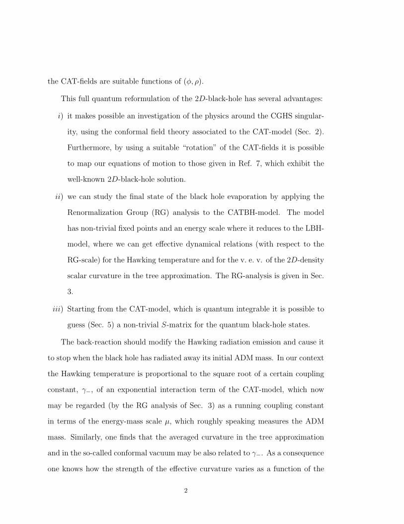
the CAT-fields are suitable functions of (φ, ρ).

This full quantum reformulation of the 2D-black-hole has several advantages:

i) it makes possible an investigation of the physics around the CGHS singular-

ity, using the conformal field theory associated to the CAT-model (Sec. 2).

Furthermore, by using a suitable “rotation” of the CAT-fields it is possible

to map our equations of motion to those given in Ref. 7, which exhibit the

well-known 2D-black-hole solution.

ii) we can study the final state of the black hole evaporation by applying the

Renormalization Group (RG) analysis to the CATBH-model. The model

has non-trivial fixed points and an energy scale where it reduces to the LBH-

model, where we can get effective dynamical relations (with respect to the

RG-scale) for the Hawking temperature and for the v. e. v. of the 2D-density

scalar curvature in the tree approximation. The RG-analysis is given in Sec.

3.

iii) Starting from the CAT-model, which is quantum integrable it is possible to

guess (Sec. 5) a non-trivial S-matrix for the quantum black-hole states.

The back-reaction should modify the Hawking radiation emission and cause it

to stop when the black hole has radiated away its initial ADM mass. In our context

the Hawking temperature is proportional to the square root of a certain coupling

constant, γ−, of an exponential interaction term of the CAT-model, which now

may be regarded (by the RG analysis of Sec. 3) as a running coupling constant

in terms of the energy-mass scale µ, which roughly speaking measures the ADM

mass. Similarly, one finds that the averaged curvature in the tree approximation

and in the so-called conformal vacuum may be also related to γ−. As a consequence

one knows how the strength of the effective curvature varies as a function of the

2

Hawking temperature for fixed µ. In particular if we formulate an ansatz for the

black hole solution interacting with N in-falling free shock waves, one may study

the thermodynamics of the end point of the black hole evaporation by extrapolating

the RG-effective couplings to the (classical) energy scale t where the initial ADM-

mass goes to zero. This picture gives an approximate self consistent scheme to take

into account the back reaction problem in the mechanism of the Hawking radiation:

the back reaction lies in a dependence of the Hawking temperature over an energy

scale t = log µ and the end point of the black hole evaporation is characterized

in the CATBH-model by the limit t → t where M(t) → M(t) ∼ 0. Here M(t) is

the classical ADM-mass parametrized by t and M(t) ∼ 0 describes the end point

state in which all the initial ADM-mass has been radiated away. We shall show

in Sec. 4 that the end-point state of the black-hole evaporation of a 2D-CGHS

black-hole interacting with N shock waves, when N ∈ (16, 23), is characterized by

a zero-temperature regular remnant geometry.

In the last section, Sec. 5, we shall use the quantum integrability of the CATBH

model to extract the universal R-matrix, which turns out to be associated to the

quantized affine centrally extended sl2-algebra. Regarding the R-matrix (up to a

function) as a two body S-matrix operator, one gets the evolution operator between

the states which describe the full quantum 2D-black hole in the conformal affine

Toda basis. Pulling back such a CAT S-matrix to the “physical” black hole basis

described by the states |χ, u = v〉, associated to the fields χ, u, v of Sec. 2, one

obtains the S-matrix operator Sbh corresponding to the quantum evolution of the

black-hole geometry. It results that Sbh is not unitary, thus confirming Hawking’s

scenario11

for the black hole evaporation and the loss of quantum coherence.

3

2. Conformal Affine Toda Black Hole Model

Bilal and Callan7

have recently shown how to cast the CGHS black hole model

in a non standard Liouville-like form. Their key idea is to mimic the Distler–

Kawai12

approach to 2D-quantum gravity and include in the action a dilaton de-

pendent renormalization of the cosmological constant as well as a Polyakov effective

term induced by the “total” conformal anomaly. The effect of the Polyakov term in

the “flat” conformal gauge gµν = −12e2ρηµν will be to replace the coefficient N

12 of

CGHS by a coefficient κ, where κ will be fixed by making the matter central charge

(due to the N free scalar fields) cancel against the c = −26 diffeomorphism-ghosts

contribution. More specifically they were able to simplify the graviton-dilaton

action through a field redefinition of the form

ω = e−φ

√κ, χ = 1

2(ρ + ω2) , (2.1)

where φ and ρ are respectively the dilaton and the Liouville mode and, in the

LBH-model, κ = N−2412 as it follows by the requirement of conformal invariance.

According to our way of thinking κ must now be a free parameter. However for

positive κ a singularity appears in the regime ω2 → 1, which is also a strong

coupling limit for small κ.

Our purpose, as stated in the introduction, is to define an improvement of the

Bilal–Callan theory that allows for a well defined exact conformal field theory to

exists also in the positive κ “phase”and ω2 ∼ 1. The surprise is that such a theory

must be a sort of “massive deformation” (which must be conformal at the same

time) of the true Liouville theory, as we shall see in the following.

4

The kinetic part of the Bilal–Callan action is given by

Skin =1

π

∫d2σ

[−4κ∂+χ∂−χ + 4κ(ω2 − 1)∂+ω∂−ω +

1

2

N∑

i=1

∂+fi∂−fi

], (2.2)

and the energy-momentum tensor has the Feigin–Fuchs form

T± = −4κ∂±χ∂±χ + 2κ∂2±χ + 4κ(ω2 − 1)∂±ω∂±ω +

1

2

N∑

i=1

∂±fi∂±fi. (2.3)

When ω2 > 1 the action and the stress tensor can be simplified by setting

Ω =1

2ω√

ω2 − 1 − 1

2log (ω +

√ω2 − 1), (2.4)

leading to the canonical kinetic term 4κ∂+Ω∂−Ω.

When ω2 < 1 we must use the alternative definition

Ω′ =1

2ω√

1 − ω2 − 1

2arccos ω, (2.5)

obtaining the “ghost-like” kinetic term −4κ∂+Ω′∂−Ω′.

We thus have two different theories describing different regions of the space-

time (remember that ω is a field), in the first one we have a real positive valued

field Ω, in the latter a ghost field Ω′ with range in [−π4 , 0]. The first theory is the

one we are interested in when considering the classical limit ω → +∞ and has

been studied in Ref. 7. If we choose not to constrain the range of values of ω, the

quantization of the LBH theory (the one in which ω ∈ [1,∞]) should provide an

IR effective theory of the complete one in which ω has its natural range from 0 to

∞. In other words, in a full quantized theory one cannot forget that somewhere

the field ω(σ) can take values less than 1, in which case the ghost-like action form

must be used.

5

Particularly interesting is the region where ω2(σ) − 1 is changing sign. Let

us suppose that ω2(σ1) > 1 and ω2(σ2) < 1, where σ1 and σ2 are two very close

points. Then our idea is to define an improved Bilal–Callan kinetic action term

in which both fields Ω(σ1) and Ω′(σ2) appear. Namely we assume the following

contribution to such an improved action:

4κ(∂+Ω(σ1)∂−Ω(σ1) − ∂+Ω′(σ2)∂−Ω′(σ2)) = 2(∂+u(σ)∂−v(σ) + ∂−u(σ)∂+v(σ)),

where the new fields

u(σ) =√

κ(Ω(σ1) + Ω′(σ2)),

v(σ) =√

κ(Ω(σ1) − Ω′(σ2)),(2.6)

are defined in the point σ = σ1+σ2

2 .

Let us now consider a field ω(σ) taking values everywhere near 1 and rapidly

fluctuating. We can renormalize (a la Wilson) the above theory in which the

undefined Bilal–Callan kinetic term (ω2 − 1)∂+ω∂−ω has been replaced by the

undefined kinetic term ∂+u∂−v + ∂−u∂+v. From a naive dimensional argument

when ω2 ∼ 1 the Laplacian term ∂+ω∂−ω must be very large in order to have a

non trivial propagator for the ω field. This means that our theory is a sort of “UV

effective theory” for the LBH model. It is to be noted that the new fields v and u

are limited from below, but since the region of interest is around 0 this constraint

is significative only for u, which has to be positive.

The kinetic part of the “averaged” LBH model has now the form:

S =1

2π

∫d2x

(−1

2∂µχ∂µχ + ∂µu∂µv

), (2.7)

where we have come back to the coordinates x0 = (σ++σ−)/2 and x1 = (σ+−σ−)/2

6

and χ =√

2κχ. We then take a potential term of the form

V− = γ−e

√8κ

(χ−u+v√

2

)

, (2.8)

so that the equations of motion take the form:

∂µ∂µχ = −γ−

√8

κe

√8κ

(χ−u+v√

2

)

,

∂µ∂µu = ∂µ∂µv = − γ−√2

√8

κe

√8κ

(χ−u+v√

2

)

.

(2.9)

Notice that there is a class of solutions in which u = v, which is equivalent to

Ω′ = 0 and to ω2 > 1. This is the class we are interested in when considering

classical solutions with boundary conditions corresponding to the linear dilaton

vacuum, where ω2 → +∞. Putting u = v =√

κΩ in (2.9), as required by (2.6),

we obtain the equations of motion of the LBH model. The coupling constant γ−

can now be recognized, apart from a multiplicative factor, as the square of the

cosmological constant.

We can further handle the action (2.7) considering a “rotation” G of the fields

χ

u

v

= G ·

ϕ

ξ

η

, (2.10)

which keeps the kinetic term unchanged, i.e. in terms of ϕ, ξ, η:

S =1

2π

∫d2x

(−1

2∂µϕ∂µϕ + ∂µξ∂µη

). (2.11)

G is explicitly given by

G = 1 + A sinh√

2ab + c2 + A2(cosh√

2ab + c2 − 1), (2.12)

7

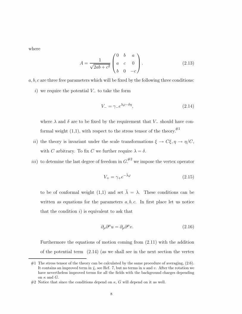
where

A =1√

2ab + c2

0 b a

a c 0

b 0 −c

. (2.13)

a, b, c are three free parameters which will be fixed by the following three conditions:

i) we require the potential V− to take the form

V− = γ−eλϕ−δη, (2.14)

where λ and δ are to be fixed by the requirement that V− should have con-

formal weight (1,1), with respect to the stress tensor of the theory.#1

ii) the theory is invariant under the scale transformations ξ → Cξ, η → η/C,

with C arbitrary. To fix C we further require λ = δ.

iii) to detemine the last degree of freedom in G.#2

we impose the vertex operator

V+ = γ+e−λϕ (2.15)

to be of conformal weight (1,1) and set λ = λ. These conditions can be

written as equations for the parameters a, b, c. In first place let us notice

that the condition i) is equivalent to ask that

∂µ∂µu = ∂µ∂µv. (2.16)

Furthermore the equations of motion coming from (2.11) with the addition

of the potential term (2.14) (as we shall see in the next section the vertex

#1 The stress tensor of the theory can be calculated by the same procedure of averaging, (2.6).It contains an improved term in χ, see Ref. 7, but no terms in u and v. After the rotation wehave nevertheless improved terms for all the fields with the background charges dependingon κ and G.

#2 Notice that since the conditions depend on κ, G will depend on it as well.

8

(2.15) decouples by quantum effect) imply that

∂µ∂µϕ

λ=

∂µ∂µξ

δ. (2.17)

(2.16) and (2.17) give

(G21 − G31)λ = (G32 − G22)δ, (2.18)

where

λ =

√8

κ

(G11 −

G21 + G31√2

),

δ = −√

8

κ

(G13 −

G23 + G33√2

).

(2.19)

Using condition ii), we get

G21 − G31 = G32 − G22, (2.20)

and

G11 −G21 + G31√

2=

G23 + G33√2

− G13. (2.21)

Condition iii) will be exploited in the next section, eq. (3.31).

We are now in a position to further generalize the LBH model adding to it the

vertex V+, which, by construction, does not alter the conformal invariance of the

theory. Thus we obtain the conformal affine Toda theory based on sl(2) proposed

by Babelon and Bonora in Ref. 10:

S =1

2π

∫d2x

(−1

2∂µϕ∂µϕ + ∂µη∂µξ + γ+e−λϕ + γ−eλϕ−δη

). (2.22)

Even if this is not the most general action constructed with conformal perturbations

of weight (1,1) (as other exponential combinations of the fields ϕ, ξ and η are

9

possible), we think that it is actually sufficient. Indeed very recently Giddings and

Strominger13

have argued that there is an infinite number of quantum theories of

dilaton-gravity and the basic problem is to find physical criteria to narrow the class

of solutions. Our approach here is to consider a theory that

i) is at the same time classically integrable, i.e. admitting a Lax pair and con-

formally invariant,#3

ii) reduces to the solutions of the LBH model at a suitable energy scale, as it

will be shown in the next section.

3. Renormalization Group Analysis

We want to consider here the renormalization group flow of the classical Babelon-

Bonora action

SBB =1

2π

∫d2x

[1

2∂µϕ∂µϕ + ∂µη∂µξ − 2

(e2ϕ + e2η−2ϕ

)]. (3.1)

At the quantum level one must implement wave and vertex function renormal-

izations so that in (3.1) one must introduce different bare coupling constants in

front of the fields as well as in front of the vertex interaction terms. As a conse-

quence one ends with the form (2.22). However, according to the general spirit of

the renormalization procedure we have also to consider Feigin–Fuchs terms (the

ones involving the 2D-scalar curvature) since all generally covariant dimension 2

counter terms are possible in (2.22). This ansatz is in agreement with the pertur-

bative theory as one could show following Distler and Kawai. In our context the

#3 Notice that (2.22) is the unique action coming from the homogeneous gradation of the sl2Kac–Moody algebra in terms of three scalar fields.

10

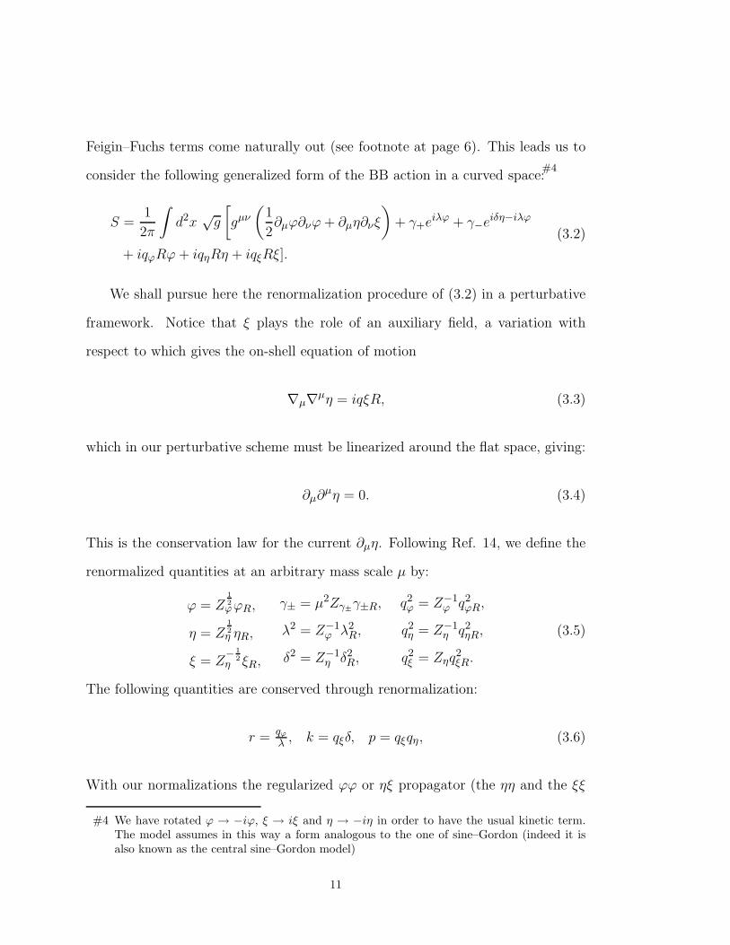
Feigin–Fuchs terms come naturally out (see footnote at page 6). This leads us to

consider the following generalized form of the BB action in a curved space:#4

S =1

2π

∫d2x

√g

[gµν

(1

2∂µϕ∂νϕ + ∂µη∂νξ

)+ γ+eiλϕ + γ−eiδη−iλϕ

+ iqϕRϕ + iqηRη + iqξRξ].

(3.2)

We shall pursue here the renormalization procedure of (3.2) in a perturbative

framework. Notice that ξ plays the role of an auxiliary field, a variation with

respect to which gives the on-shell equation of motion

∇µ∇µη = iqξR, (3.3)

which in our perturbative scheme must be linearized around the flat space, giving:

∂µ∂µη = 0. (3.4)

This is the conservation law for the current ∂µη. Following Ref. 14, we define the

renormalized quantities at an arbitrary mass scale µ by:

ϕ = Z12ϕϕR,

η = Z12η ηR,

ξ = Z− 1

2η ξR,

γ± = µ2Zγ±γ±R,

λ2 = Z−1ϕ λ2

R,

δ2 = Z−1η δ2

R,

q2ϕ = Z−1

ϕ q2ϕR,

q2η = Z−1

η q2ηR,

q2ξ = Zηq

2ξR.

(3.5)

The following quantities are conserved through renormalization:

r = qϕ

λ , k = qξδ, p = qξqη, (3.6)

With our normalizations the regularized ϕϕ or ηξ propagator (the ηη and the ξξ

#4 We have rotated ϕ → −iϕ, ξ → iξ and η → −iη in order to have the usual kinetic term.The model assumes in this way a form analogous to the one of sine–Gordon (indeed it isalso known as the central sine–Gordon model)

11

propagators are identically zero) is:

G(z − z′) = −1

2logm2

0[(z − z′)2 + ǫ2], (3.7)

where m0 and ǫ are an IR and an UV cutoff respectively. Then we normal order

the vertices, to eliminate tadpole divergences, with the replacements:

eiλϕ → (m20ǫ

2)λ2

4 : eiλϕ :

e−iλϕ+iδη → (m20ǫ

2)λ2

4 : e−iλϕ+iδη :

(3.8)

Since λϕ = λRϕR and δη = δRηR, the renormalization of the vertices is simply

obtained by setting

Zγ± = (µ2ǫ2)−λ2/4, (3.9)

which gives the β functions for the coupling constants γ in absence of curvature

terms (i.e. with the q’s set to zero):

β± := µdγ±dµ

= 2γ±R

(λ2

R

4− 1

), (3.10)

so that in this case the ratio γ+

γ−is conserved through the renormalization.

As in Ref. 14 we can calculate the field renormalizations considering the aver-

age of the vertices < V+V− > (where V± are the exponential interaction terms of

(3.2)) which, for λ2 ∼ 4, gives a contribution to the kinetic term of the form:

−1

4γ+Rγ−R log(µ2ǫ2)

1

2(λR∂ϕR − δR∂ηR)2.

Then the correct kinetic terms are obtained by putting:

Zϕ = 1 +1

4γ+Rγ−Rλ2

R log µ2ǫ2,

Zη = 1 +1

4γ+Rγ−Rδ2

R log µ2ǫ2.

(3.11)

Notice that the renormalization has produced new terms proportional to ∂µ∂µη,

12

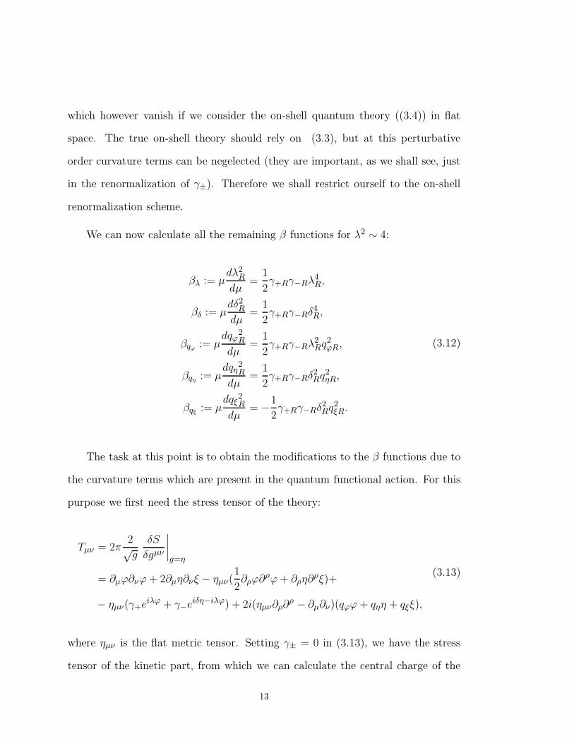
which however vanish if we consider the on-shell quantum theory ((3.4)) in flat

space. The true on-shell theory should rely on (3.3), but at this perturbative

order curvature terms can be negelected (they are important, as we shall see, just

in the renormalization of γ±). Therefore we shall restrict ourself to the on-shell

renormalization scheme.

We can now calculate all the remaining β functions for λ2 ∼ 4:

βλ := µdλ2

R

dµ=

1

2γ+Rγ−Rλ4

R,

βδ := µdδ2

R

dµ=

1

2γ+Rγ−Rδ4

R,

βqϕ:= µ

dqϕ2R

dµ=

1

2γ+Rγ−Rλ2

Rq2ϕR,

βqη:= µ

dqη2R

dµ=

1

2γ+Rγ−Rδ2

Rq2ηR,

βqξ:= µ

dqξ2R

dµ= −1

2γ+Rγ−Rδ2

Rq2ξR.

(3.12)

The task at this point is to obtain the modifications to the β functions due to

the curvature terms which are present in the quantum functional action. For this

purpose we first need the stress tensor of the theory:

Tµν = 2π2√g

δS

δgµν

∣∣∣∣g=η

= ∂µϕ∂νϕ + 2∂µη∂νξ − ηµν(1

2∂ρϕ∂ρϕ + ∂ρη∂ρξ)+

− ηµν(γ+eiλϕ + γ−eiδη−iλϕ) + 2i(ηµν∂ρ∂ρ − ∂µ∂ν)(qϕϕ + qηη + qξξ),

(3.13)

where ηµν is the flat metric tensor. Setting γ± = 0 in (3.13), we have the stress

tensor of the kinetic part, from which we can calculate the central charge of the

13

free theory:

c = 3 − 24q2ϕ − 48qξqη. (3.14)

Notice that the total central charge, i.e. the one involving also matter and the

ghosts contribution, is

ctot = c + N − 26. (3.15)

The trace of the stress tensor is easily calculated:

T µµ = −2[γ+eiλϕ + γ−eiδη−iλϕ + 2i∂µ∂µ(qϕϕ + qηη + qξξ)], (3.16)

and, using the classical equations of motion in flat space

∂µ∂µϕ = iλ(γ+eiλϕ − γ−eiδη−iλϕ),

∂µ∂µη = 0,

∂µ∂µξ = iδγ−eiδη−iλϕ,

(3.17)

we find the classical expression:

T µµ = −2[(1 + qϕλ)γ+eiλϕ + (1 − qϕλ + qξδ)γ−eiδη−iλϕ]. (3.18)

Following Zamolodchikov,15

we obtain by (3.18) the modified β± functions:

β+ = 2γ+

(λ2

4− 1 − qϕλ

),

β− = 2γ−

(λ2

4− 1 + qϕλ − qξδ

),

(3.19)

while the others remain unchanged at this perturbative order. From now on, for

the sake of simplicity, we will omit the R subscripts.

14

Putting together the equations (3.12), we find that also the following quantity

is conserved through renormalization:#5

d =1

δ2− 1

λ2. (3.20)

Using the non-perturbative RG-invariants in (3.6), the RG equations for the γ’s

can be simply rewritten as:

d

dtlog(γ+γ−) = λ2 − 4 − 2k

d

dtlog

γ−γ+

= 4rλ2 − 2k,(3.21)

where t = log µ.

From the first of (3.21) and the first of (3.12) in the approximate form

βλ ∼ 8γ+γ−, we easily obtain:

dλ2

dt=

1

2(λ2 − 4 − 2k)2 − b2

2, (3.22)

where b is an integration constant supposed to be real in order to have RG fixed

points. These are located at:

λ2± = 4 + 2k ∓ b, (3.23)

where, taking b positive, λ+ is the UV fixed point and λ− the IR fixed point.

#5 This result, deriving from (3.12), needs not be valid beyond this perturbative order, whileit is obviously true for the quantities in (3.6). Notice moreover that putting λ = δ at anarbitrary scale sets d = 0, and since d is a RG-invariant the condition λ = δ then holds atany scale.

15

(3.22) can now be solved in the form:

t − t0 =1

blog

∣∣∣∣λ2− − λ2

λ2 − λ2+

∣∣∣∣ , (3.24)

where t0 is another integration constant. Solving (3.24) with respect to λ2 we

have:

λ2(t) =eb(t−t0)λ2

+ + λ2−

eb(t−t0) + 1= 2k + 4 − b tanh

b(t − t0)

2. (3.25)

Now we can also easily integrate (3.21) to get:

γ2− = Ae(8rk+16r−2k)(t−t0)

[cosh

b(t − t0)

2

]−2−8r

γ2+ = Be−(8rk+16r−2k)(t−t0)

[cosh

b(t − t0)

2

]−2+8r

,

(3.26)

where A and B are arbitrary constants. Notice that the first of (3.12) imposes

that γ+ and γ− have opposite signs.

So far we have described the most general situation in which all the parameters

are unconstrained. Indeed, following the reasoning of Sec. 2, we have to request

that at a certain scale t, which shall be proved to exist, both vertex operators have

a conformal weight (1, 1). This is achieved imposing the following constraints:#6

(1

4− r

)λ2 = 1,

(1

4+ r

)λ2 = k + 1.

(3.27)

#6 Notice that imposing these conditions is equivalent to asking that, at the scale t, both β±

in (3.12) vanish.

16

Solving (3.27) we obtain:

λ2 = 2k + 4 =4

1 − 4r,

r =k

4(2 + k).

(3.28)

This means by (3.25) that the scale t is just the renormalization scale t0. At this

scale we also require the vanishing of the total central charge, (3.15), which gives:

c = N − 23 − 24r2λ2(t0) − 48p

= N − 23 − 24

(4r2

1 − 4r+ 2p

)= 0.

(3.29)

Notice moreover that we must have

r <1

4, (3.30)

if we want λ to be real. It is also easily seen that the particular combination

8rk + 16r − 2k vanishes identically for any value of k, so that γ± now read:

γ±(t) ∝[cosh

b(t − t0)

2

]−(1∓4r)

. (3.31)

This implies that γ± are even functions of the scale t − t0 and hence do not dis-

tinguish between IR and UV scales. The requirement of having vertex operators

with the right conformal weight at the defining scale t0 forces the theory to be dual

(under the exchange of the IR and UV scales). The asymptotic form of γ− is

γ−|t−t0|→∞∼ const. e−2s|t−t0|, (3.32)

where we have set

s =1 + 4r

4|b|. (3.33)

The next step in fixing the parameters is achieved considering what must hap-

17

pen at the scale tBC , where the theory becomes the LBH model. This amounts to

require that the vertex operator V+ must disappear at the scale tBC , i.e. we must

impose that∣∣∣∣γ−(tBC)

γ+(tBC)

∣∣∣∣ >> 1. (3.34)

By (3.31), this requires that:

r < 0, (3.35)

and

|b(tBC − t0)| >> 1. (3.36)

From (3.36) it follows that λ(tBC) must be equal to the asymptotic value λ± given

by eq. (3.23).

We first notice that as a consequence of the rotation (2.10), we have that

qϕ(tBC) = G11

√κ

2,

qξ(tBC) = G12

√κ

2,

qη(tBC) = G13

√κ

2,

(3.37)

By (2.19) and (3.6) we get:

r =κ

4

G11

G11 − G21+G31√2

,

k = −2G12

(G13 −

G23 + G33√2

),

p =κG12G13

2.

(3.38)

18

The condition iii) of Sec. 2, together with (3.28) and (3.38) imply that:

G12y2 − κG11G12y − κG11 = 0, (3.39)

where we have put

y = G11 −G21 + G31√

2. (3.40)

We have found a solution of (2.20), (2.21) and (3.39) numerically. We look for

those solutions such that

a) r, given by (3.38), is negative, in order to have the flow to the LBH model

and, at the same time, the consistency with (2.16);

b) s, given by (3.33), is positive so that γ− is bounded for large energy scale.

A numerical solution satisfying the above conditions for r and s can be found

for −2 < κ < 0 and 14 < N < 23. κ is defined in (2.1). Its functional relation with

the physical parameter N is defined implicitly in (3.29)and (3.38). To compute s

we also need the parameter b, implicitly defined by (3.23), which turns out to be:

b = λ2(tBC) − λ2(t0) =8

κx2 − 4

1 − 4r. (3.41)

19

4. Black Hole Thermodynamics

In this section we want to discuss how our RG results affect the black-hole

thermodynamics. Our strategy is to observe that at the scale tBC our theory

reduces to the LBH model which contains the simple black-hole solution of CGHS,

where the black-hole is formed by N in-falling shock-waves. Now by replacing the

parameters of this solution (which we thus interpret as an ”effective” solution for

our model with u = v) with those obtained with our RG analysis, we can identify

a temperature and the v.e.v. of the curvature. The Hawking temperature TH is

proportional to√

γ−(tBC):

TH(t) ∝ µ√

γ−(t), (4.1)

which, by (3.32), goes asymptotically as

TH(t)|t−t0|→∞∼ const. ete−s|t−t0|. (4.2)

Using our solution it is immediate to see that there exists a dynamical regime for

23 < N < 30 in which TH vanishes both in the UV and IR regions.

The relation between the v. e. v. of the operator-valued scalar curvature√−gR

and the other CATBH running coupling constant λ(−)(t) in the conformal gauge

gµν = −12e2λρηµν and in the tree approximation is:

<√−gR >= 2λ(−)(t)∂µ∂µ < ρ > . (4.3)

We may then state something about the end-point state of black hole evaporation

if we use the CGHS-solution to describe the black hole formation by N -shock waves

20

fi. In our contest, the CGHS-ansatz for the classical solution < ρ >≡< ρ >tree

looks:

e−2λ(−)(t)<ρ(x+)> = 1 − 2λ(−)(t) < ρ(x+) > +O(λ(−)2)

= −κaθ(x+ − x+0 )(x+ − x+

0 ) − e2tγ−(t)x+x−,

(4.4)

where x± ≡ x0 ±x1 and a ≡ const. Therefore, at x+ = x+0 we have by (4.3), using

the light-cone coordinates x±:

<√−g(x+)R(x+) >= ∂+∂−[2λ(−)(t) < ρ(x+) >] ∼ e2tγ−(t), x+ → x+

0 . (4.5)

Since here we have two scales x+0 and µ, where t ≡ log(µ), it is reasonable to set

(in c = h = 1) x+0 ≡ 1

µ , and x+0 is the natural scale which describes the classical

black hole formation. Therefore:

< [√

−gR](e−t) >∝ e2tγ−(t). (4.6)

The Hawking temperature, (4.1), and the averaged density of the scalar curvature,

(4.6), are asymptotically controlled by γ−(t).

Since in the CGHS ansatz (Ref. 1) the black hole mass mbh grows linearly

with x+0 , i.e. mbh ∝ M2

Plx+0 where MPl is the Planck mass, we get mbh ∼ 1/µ.

This relation may also be obtained by a dimensional argument relying on Witten’s

relation16

between the black hole mass and the value a of the dilaton field on the

horizon (namely mbh ∼ ea), and, on the other hand, on the conformal properties

of the vertex e−2φ, which is recognized to be a primary field of conformal (mass)

dimension 2, so that, at a semiclassical level, we may write e−2a ∼ µ2. Thus we

get the previously stated relation mbh ∼ 1/µ.

21

As a consequence of the above arguments, we get that (4.2)may be rewritten

as follows:

TH(mbh)mbh→0∼ T0

(mbh

m0

)s−1

, (4.7)

and

TH(mbh)mbh→∞∼ T ′

0

(m0

mbh

)s+1

, (4.8)

where T0, T′0 and m0 are arbitrary constants. The vanishing of the Hawking tem-

perature for small and large black hole masses occurs for s > 1, which according

to our numerical solution of Sec. 3 requires 16 < N < 23. This is a consequence of

the duality between the UV and IR limit of our quantum theory. In the following

we understand N to be taken in the above range.

The end point state of the black hole evaporation is characterized by the

limit mbh → 0. But in this limit TH and by (4.6) also <√−gR > are van-

ishing. We understand this result as a signal that at the end point the black hole

disappears completely from our 2D-universe, leaving a zero temperature flat rem-

nant solution. This scenario has been suggested by Hawking11

and ’t Hooft,17

but

with a basic difference: for Hawking (’t Hooft) the final state is a mixed (pure)

state. Of course at the level of the above RG analysis we cannot say anything on

the quantum black hole Hilbert space. However, we have an explicit quantum field

model for answering, in principle, to the above question. Our point of view is to see

whether the S-matrix associated with the “quantum” black hole states, which are

in correspondence with the “rotated” Babelon-Bonora theory at the energy scale

tBC , i.e. in terms of the u = v and χ fields, is unitary or not. Clearly a unitary S-

matrix may be in agreement only with ’t Hooft’s scenario. In the following section,

22

we shall give some arguments which seem to support the non-unitarity picture,

and hence Hawking’s point of view.

5. Quantum Black Hole S-Matrix

One starting point is the Babelon-Bonora version of our CATBH-model, namely

(2.22). Using its Hopf algebra structure, namely Uq(sl(2)), we shall get a quantum

S-matrix and then we shall pull it back to the physical black hole basis described

by the fields u = v and χ of (2.1) and (2.6).

The defining relations for the quantum Kac–Moody algebra Uq(sl(2)) are:

[Hi, Hj] = 0,

[Hi, E±j ] = ±~αi · ~αj E±

j ,

[E+i , E−

j ] = δijqHi − q−Hi

q − q−1,

(5.1)

where i = 0, 1; here ~α0 = −~α1 and |~α1|2 = 2. The center of Uq(sl(2)) is

K = H0 + H1. (5.2)

A new basis in Uq(sl(2)) is generated#7

by Hi, Qi and Qi:

Qi = E+i q

Hi2 ,

Qi = E−i q

Hi2 .

(5.3)

#7 With CCR given by:

[Hi, Qj ] = ~αi · ~αj Qj,

[Hi, Qj ] = −~αi · ~αj Qj ,

QiQi − q−2QiQi =1 − q2Hi

q−2 − 1.

23

The algebra Uq(sl(2)) is a quasitriangular Hopf algebra18− 19

with comultiplication

∆ : Uq(sl(2)) → Uq(sl(2)) ⊗ Uq(sl(2))

defined by

∆(Hi) = Hi ⊗ 1 + 1 ⊗ Hi,

∆(Qi) = Qi ⊗ 1 + qHi ⊗ Qi,

∆(Qi) = Qi ⊗ 1 + qHi ⊗ Qi.

(5.4)

The CAT model is associated to the Uq(sl(2)) Kac–Moody algebra by the so-called

homogeneous gradation:

E+0 = x2σ−, E−

0 = x−2σ+,

E+1 = σ+, E−

1 = σ−,(5.5)

where x is the “spectral parameter” and the Pauli spin matrices σ± are the usual

step operators of sl(2). Together with the Pauli spin matrix σ3, they form the

so-called Chevalley basis for sl(2). The commutator in the loop algebra associated

with our centered sl(2) is defined as:

[A(x), B(x)] = A(x) · B(x) − B(x) · A(x) +1

2πi

∮dx tr[∂xA(x) · B(x)] K,

= A(x) · B(x) − B(x) · A(x) + K(A, B).

(5.6)

The asymptotic soliton states are labelled by |τϕ, τη, θ〉, where θ is the rapidity, τϕ

and τη are topological charges defined by:

x = eθ( 4

λ2−1),

τϕ =λ

2π

+∞∫

−∞

dx ∂xϕ,

τη = −λ3

4π

+∞∫

−∞

dx ∂xη.

(5.7)

24

One has that

τϕ = −H0,

τη = K,(5.8)

and the relation with the Hi’s is the following

H0 = −σ3 + K,

H1 = σ3.(5.9)

The representation of Uq(sl(2)) on the space of one-soliton states can be shown to

be:

Q+ = cQ1 = cσ+qσ32 , Q− = cQ0 = cx2σ−q

−σ3+K

2 ,

Q− = cQ1 = cσ−qσ32 , Q+ = cQ0 = cx−2σ+q

−σ3+K

2 ,(5.10)

where c is a constant depending linearly on γ and the deformation parameter q is

given by:

q = e4πi

λ2 . (5.11)

The two-soliton to two-soliton S-matrix S is an operator from V1⊗V2 to V2⊗V1, Vi

are the vector spaces spanned by |τϕ, τη, θ〉. The S-matrix must commute20

with

the action of Uq(sl(2)), since it is the symmetry group of the theory:

[S, ∆(Hi)] = [S, ∆(Q±)] = [S, ∆(Q±)] = 0. (5.12)

The representation of eq. (5.12) on V1 ⊗ V2 is explicitly given by:

[S, σ3 ⊗ 1 + 1 ⊗ σ3] = 0, (5.13)

S · (σ+qσ32 ⊗ 1 + qσ3 ⊗ σ+q

σ32 ) + K(S, ∆(Q+)) =

(σ+qσ32 ⊗ 1 + qσ3 ⊗ σ+q

σ32 ) · S,

S · (x21σ−q

−σ3+K12 ⊗ 1 + q−σ3+K1 ⊗ x2

2σ−q−σ3+K2

2 ) + K(S, ∆(Q−)) =

(x22σ−q

−σ3+K22 ⊗ 1 + q−σ3+K2 ⊗ x2

1σ−q−σ3+K1

2 ) · S,

(5.14)

25

S · (x−21 σ+q

−σ3+K12 ⊗ 1 + q−σ3+K1 ⊗ x−2

2 σ+q−σ3+K2

2 ) + K(S, ∆(Q+)) =

(x−22 σ+q

−σ3+K22 ⊗ 1 + q−σ3+K2 ⊗ x−2

1 σ+q−σ3+K1

2 ) · S,

S · (σ−qσ32 ⊗ 1 + qσ3 ⊗ σ−q

σ32 ) + K(S, ∆(Q−)) =

(σ−qσ32 ⊗ 1 + qσ3 ⊗ σ−q

σ32 ) · S.

(5.15)

A solution S = S(x1/x2, K1, K2, q) of eq. (5.12) is of the following form:21

S = f(x1/x2, q, K1, K2)R(x1/x2, q, K1, K2), (5.16)

where R is the universal quantum R-matrix associated to Uq(sl(2)), whose existence

has been proved in Ref. 18. One can easily show that R satisfies the quantum

Yang–Baxter equation, which is required for the factorization of the multisoliton

S-matrix:

R12(x)R13(xy)R23(y) = R23(y)R13(xy)R12(x). (5.17)

An explicit form of the universal S-matrix for Uq(sl(2)) is given in Ref. 22 and 23.

In the “bootstrap” approach the overall factor f can be found by imposing crossing

and unitarity conditions. Of course, this is consistent if the CAT-model belongs

to the class of 2D relativistic quantum field theories studied by Zamolodchikov

and Zamolodchikov.24

However in our context it is not necessary to answer to this

question and to find an explicit form for f , since the relevant two-body scattering

matrix is the one, denoted by Sbh, acting on the black hole basis |χ, u = v〉. We

shall see below that, even if a unitary S-matrix in the CAT basis could be found,

Sbh is not. Formally Sbh is defined by

Sbh = U†SU, (5.18)

where U = PG, and G is the operator associated to the rotation (2.10) and P

26

is the projection operator from |χ, u, v〉 onto the black hole basis |χ, u = v〉. It is

evident that Sbh is no more an automorphism of the Hilbert space H spanned by

the CAT-basis and hence, for a well-known theorem,25

is not an unitary operator

on H. The conclusion that we draw for the black hole evaporation scenario is that

the final state is approached incoherently, even if full quantum gravity effects are

taken into account, supporting Hawking’s point of view.

Acknowledgements: L. Bonora and A. Ashtekar are thanked for some illuminating

discussions.

27

REFERENCES

1. C. G. Callan, S. B. Giddings, J. A. Harvey, and A. Strominger, Phys.

Rev. D45(1992), R1005.

2. T. Banks, A. Dabholkar, M. R. Douglas, and M. O’Loughlin, Phys. Rev. D45(1992),

3607.

3. J. G. Russo, L. Susskind, and L. Thorlacius, Black Hole Evaporation in 1+1

Dimensions, Stanford preprint SU-ITP-92-4, January 1992;

L. Susskind and L. Thorlacius, Hawking Radiation and Back-Reaction,

Stanford preprint SU-ITP-92-12, hepth@xxx/9203054, March 1992.

4. B. Birnir, S. B. Giddings, J. A. Harvey and A. Strominger, Quantum Black

Holes, Santa Barbara preprint UCSB-TH-92-08, hepth@xxx/9203042, March

1992.

5. A. Strominger, Faddeev–Popov Ghosts and 1 + 1 Dimensional Black Hole

Evaporation, UC Santa Barbara preprint UCSB-TH-92-18, hept@xxx/9205028,

May 1992.

6. S. W. Hawking, Evaporation of Two Dimensional Black Holes, CALTECH

preprint CALT-68-1774, March 1992.

7. A. Bilal and C. Callan, Liouville Models of Black Hole Evaporation, Princeton

preprint PUPT-1320, hept@xxx/9205089, May 1992.

8. S. P. de Alwis, Black Hole Physics from Liouville Theory, Colorado preprint

COLO-HEP-284, hepth@xxx/9206020, June 1992.

9. F. Belgiorno A.S. Cattaneo, F. Fucito and M. Martellini, A Conformal

Affine Toda Model of 2D Black Holes: A Quantum Study of the Evaporation

End-Point, ROM2F 92/52, October 1992,

28

F. Belgiorno, A.S. Cattaneo, F. Fucito and M. Martellini, Quantum Models

of Black-Hole Evaporation in Proceedings of the Roma Conference on “String

Theory, Quantum Gravity and the Unification of Fundamental Interactions”,

preprint ROM2F 92/60, November 1992.

10. O. Babelon and L. Bonora, Phys. Lett. B244(1990), 220;

O. Babelon and L. Bonora, Phys. Lett. B267(1991),71.

11. S.W. Hawking, Phys. Rev. D14(1976), 2460.

12. J. Distler and H. Kawai, Nucl. Phys. B321(1989), 509.

13. S. B. Giddings and A. Strominger, Quantum Theory of Dilaton Gravity, UC

Santa Barbara preprint, UCSB-TH-92-28, hepth@xxx/9207034, July 1992.

14. M. T. Grisaru, A. Lerda, S. Penati and D. Zanon, Nucl. Phys. B342(1990),

564.

15. A.B. Zamolodchikov, Sov. J. Nucl. Phys. 46(1987), 1090.

16. E. Witten, Phys. Rev. D44(1991), 314.

17. G. ’t Hooft, Nucl. Phys. B335(1990), 138.

18. N.Y. Reshetikhin and M.A. Semenon–Tian–Shansky, Lett. Math. Phys. 19(1990),

133

19. B.M. Khoroshkin and V.N. Tolstoy, to apppear in Funkz. Analyz. i ego pril.

20. D. Bernard and A. LeClair, Comm. Math. Phys. 142(1991), 99

21. M. Jimbo, Comm. Math. Phys. 102(1986), 537.

22. M. Rosso, Comm. Math. Phys. 124(1989), 307.

23. A.N. Kirillov and N. Reshetikhin, q-Weyl Group and Multiplicative Formula

for Universal R-Matrices, preprint HUTMP 90/B261.

24. A.B. Zamolodchikov and A.B. Zamolodchikov, Ann. Phys. 120(1979), 253.

29

25. J.Weidmann,Linear Operators in Hilbert Space, Springer-Verlag (New York,1980).

30