Confidence sets in boundary and set estimation

CONFIDENCE SETS IN BOUNDARY AND SET ESTIMATION

HANNA K. JANKOWSKI*, LARISSA I. STANBERRY

Abstract. Let p1 ≤ p2 and consider estimating a fixed set x : p1 ≤ f(x) ≤ p2by the random set x : p1 ≤ fn(x) ≤ p2, where fn is a consistent estimator ofthe continuous function f . This paper gives consistency conditions for these sets,and provides a new method to construct confidence regions from empirical averagesof sets. The method can also be used to construct confidence regions for sets ofthe form x : f(x) ≤ p and x : f(x) = p. We then apply this approach to setand boundary estimation. We describe conditions for strong consistency for theempirical average sets and study the fluctuations of these via confidence regions.We illustrate the proposed methods on several examples.

1. Introduction

The ability to estimate a set and its boundary is of primary importance in manyfields. As an example, consider estimating the domain of covariates which yielddangerous blood pressure levels.

In this paper, we study the estimation of sets of the form

F (p) = x ∈ D : f(x) ≤ p,∂F (p) = x ∈ D : f(x) = p,

F (p1, p2) = x ∈ D : p1 ≤ f(x) ≤ p2,(1.1)

where D ⊂ Rd is a compact set, and f is a continuous function, f : D 7→ R. Note thatthe boundary of the set F (p) may not necessarily be equal to ∂F (p), but we use the

notation nonetheless. Let fn denote a consistent estimator of f . We estimate the sets

(1.1) using “plug-in” estimators obtained by replacing f with fn in the definition:

Fn(p) = x ∈ D : fn(x) ≤ p,∂Fn(p) = x ∈ D : fn(x) = p,

Fn(p1, p2) = x ∈ D : p1 ≤ fn(x) ≤ p2.(1.2)

Our first goal is to provide conditions on the consistency of these estimators. Next,to assess the accuracy of the estimators, we construct appropriate confidence regions:

Date: March 10, 2009.Key words and phrases. random closed set, oriented distance functions, set expectation, boundary

estimation, level set, simultaneous confidence interval.*Corresponding author.To reference this technical report, please use arXiv:0903.1869.

1

2 HANNA K. JANKOWSKI*, LARISSA I. STANBERRY

random sets which cover the sets (1.1) with at least a 100(1 − α)% probability. Werefer to these as confidence sets or confidence regions to differentiate from confidenceintervals or simultaneous confidence bands in function estimation.

Sets of the form (1.1) appear in various statistical problems, such as estimationof contour clusters [Nol, Pol] or the estimation of density support [KT]. Here, weconsider the problem of estimating the domain of covariates with specified responselevel(s), which arise for example in treatment comparisons [TWS] and toxic doseestimation [BT].

Another application of the proposed method is set and boundary estimation, and alarge part of this paper is dedicated to this topic. The observed data here are randomsets: primate skulls, mammograms, or cell images. Population characteristics may besummarized by the expected set (or expected boundary), which in turn are estimatedusing empirical averages. In [SJ], new definitions of the expectation of a random setand the expected random boundary were given. The definitions have a number ofdesirable properties, particularly suitable for problems in image analysis. Moreover,both the expected set and expected boundary have the same form as in (1.1). Weapply our results to determine conditions for consistency of the empirical averages,and study when and if these conditions fail under a variety of random set models.Furthermore, we construct confidence regions for the expected set and the expectedboundary. Thus, jointly with [SJ], our work provides a statistical framework forinference about random sets and their boundaries.

Suppose then that fn is a random, continuous function such that

(A1) supx∈D|fn(x)− f(x)| → 0 almost surely as n→∞.

The sets (1.1) are estimated by (1.2). Consistency of Fn(p) as an estimator for F (p)

was studied in [Mol]. We extend these results to the sets ∂Fn(p) and Fn(p1, p2). Wethen show how to construct simultaneous confidence sets for these estimators, underthe assumption of weak convergence

(A2)√nfn(·)− f(·) ⇒ Z(·),

where Z(·) is a continuous random field on D. The methods extend naturally to thecase where the scaling required is not

√n, however, we restrict our discussion to this

setting. We expect that, for the√n scaling, the limiting field Z will most often be

Gaussian, or a Gaussian transform. For increased accuracy, the confidence sets maybe restricted to any compact window W ⊂ D ⊂ Rd. Although fluctuation resultsexist for F (p) and for mean sets (see eg. [Cre, BM, Mol]), these appear to be of atheoretical quality. To our knowledge, the work presented here is the first attempt toconstruct confidence regions for level sets and expected random sets.

The outline of this paper is as follows. Section 2 looks at the consistency of the sets(1.2), and Section 3 discusses how to form the confidence regions. Sections 3.1 and

CONFIDENCE SETS IN BOUNDARY AND SET ESTIMATION 3

4 cover the two main applications of our methods: covariate domain estimation, andrandom set and boundary estimation. In Section 5, we give some further examples.Proofs of all results appear in the Appendix.

1.1. Notation and Assumptions. Unless otherwise stated, we assume that D isthe working domain and write, for example, F (p) = x : f(x) ≤ p without statingthat x ∈ D explicitly. As previously noted, we assume that D is a compact subset ofRd, and denote the Euclidean norm of x as |x|. In practice, D will most likely be asimple geometric shape, such as a d-dimensional rectangle, or a d-dimensional ball.

We write Br(x0) = x : |x− x0| ≤ r for the closed ball of radius r centred at x0.For a set A, we write Ao, A,Ac and ∂A to denote its interior, closure, complementand boundary. Unless noted otherwise, set operations are calculated relative to thedomain D. That is, Ac = D \ A, and so forth. Furthermore, for a set A, we defineAδ = x : Bδ(x) ∩A 6= ∅ = ∪x∈ABδ(x). Deterministic sets are denoted using capitalletters A,B . . ., while bold upper-case lettering, A,B, . . ., is used for random sets.

The notation C(D) is used to denote the space of continuous functions C(D) =f : D 7→ R, f continuous endowed with the uniform metric. We write Xn ⇒ Xto say that Xn converges weakly to X. Throughout the paper, when handling weakconvergence of stochastic processes or random fields, we assume that they take valuesin C(D).

2. Consistency

Let F be the family of closed sets of Rd and let K denote the family of all compactsubsets of Rd. For a probability triple (Ω,A, P ), a random closed set is the mappingA : Ω 7→ F such that for every compact set K ∈ K

ω : A(ω) ∩K 6= ∅ ∈ A,

(cf. [Mat]). We write r.c.s. for random closed set, although the notation RACS isalso used in the literature. Note that

Fn(p) ∩K 6= ∅ =

infx∈K

fn(x) ≤ p

,

Fn(p1, p2) ∩K 6= ∅ =

infx∈K

∣∣∣∣fn(x)− p1 + p2

2

∣∣∣∣ ≤ p2 − p1

2

,

∂Fn(p) ∩K 6= ∅ =

infx∈K|fn(x)− p | ≤ 0

.

Therefore, since by assumption the functions fn are continuous almost surely, theestimators (1.2) satisfy the measurability requirement and are well-defined.

Recall that the Hausdorff distance between two sets, A and B, is defined as

ρ(A,B) = infδ > 0 : A ⊂ Bδ, B ⊂ Aδ

.


Following [Mol], we say that a r.c.s. An converges strongly to a deterministic set Aif ρ(An, A)→ 0 almost surely. For other notions of convergence for random sets see,for example, [SVW, SW].

The key conditions for the consistency of the estimators (1.2) are

x : f(x) ≤ p = x : f(x) < p(2.3)

x : p ≤ f(x) = x : p < f(x).(2.4)

Proposition 2.1. Condition (2.3) is equivalent to ∂x : f(x) ≥ p = x : f(x) = p,and condition (2.4) is equivalent to ∂x : f(x) ≤ p = x : f(x) = p.

Theorem 2.2 (Theorem 2.1 in [Mol]). Under assumption (A1), the estimator Fn(p)converges strongly to F (p) if the condition (2.3) holds at p.

Note that this theorem also holds if f and fn are lower semi-continuous. We now

extend the results to Fn(p1, p2) and ∂Fn(p).

Theorem 2.3. Under assumption (A1), the estimator Fn(p1, p2) converges stronglyto F (p1, p2) if the function f satisfies condition (2.3) at p = p2 and condition (2.4)at p = p1. Moreover, (2.3) and (2.4) are necessary in the following sense:1. Suppose that x0 is a point such that there exists a neighbourhood Bδ(x0) and

a subsequence nk such that fnk(x) > f(x) for all x ∈ Bδ(x0). If Fn(p1, p2) is

consistent, then (2.3) must hold at x0 for p = p2 in the sense that

x0 /∈ x : f(x) ≤ p2 \ x : f(x) < p2.2. Suppose that x0 is a point such that there exists a neighbourhood Bδ(x0) and

a subsequence nk such that fnk(x) < f(x) for all x ∈ Bδ(x0). If Fn(p1, p2) is

consistent, then (2.4) must hold at x0 for p = p1 in the sense that

x0 /∈ x : p1 ≤ f(x) \ x : p1 < f(x).

Corollary 2.4. Under assumption (A1), the estimator ∂Fn(p) converges strongly to∂F (p) if the function f satisfies both (2.3) and (2.4) at p.

The conditions (2.3) and (2.4) arise in three different ways: through local minima,local maxima, and through flat regions. For example, suppose that ∂F (p) = x :f(x) = p is a connected subset of D ⊂ Rd with positive Lebesgue measure in Rd.Then neither (2.3) nor (2.4) hold at p, see Figure 1 (left). On the other hand, if f(x)has a local minimum on ∂F (p), then (2.3) does not hold (Figure 1, middle), whereasif f(x) has a local maximum on ∂F (p), then (2.4) does not hold (Figure 1, right).

The examples in Figure 1 also clarify the necessity of the conditions. Supposethat f is of the form shown in Figure 1 (right) and we want to estimate the set

x : 0 ≤ f(x) ≤ 0.2 = 0.5. If a subsequence nk of fn(x) approaches f from

below, then for this subsequence Fnk(0, 0.2) = ∅ and consistency does not hold.


-0.5 0 0.5 1 1.5

-0.4

-0.2

0

0.2

0.4

-0.5 0 0.5 1 1.5

-0.4

-0.2

0

0.2

0.4

-0.5 0 0.5 1 1.5

-0.4

-0.2

0

0.2

0.4

Figure 1. Examples of functions which do not satisfy the consistencyconditions for p = p1 = p2 = 0: (right) the function does not satisfy(2.4); (centre) the function does not satisfy (2.3); (left) the functionsatisfies neither (2.3) nor (2.4). Here, D = [−0.5, 1.5] ⊂ R.

The following proposition shows that increasing functions always satisfy the con-sistency conditions.

Proposition 2.5. Suppose that f is continuous and that there exists a directione0 ∈ Rd such that f(x) is strictly increasing in the direction e0 for all x ∈ D. That is,suppose that there exists an e0 such that for all x0 ∈ D, the function h(t) = f(x0+te0)is strictly increasing as a function of t ∈ R+. Then f satisfies conditions (2.3) and(2.4) for any value of p.

Remark 2.6. Note that if f is differentiable, then the condition of the previousproposition is satisfied if, for some e0 ∈ Rd,

∇f(x) · e0 > 0 for all x ∈ D.

Example 1 (disc with random centre). Let D = [−2, 2]2 ⊂ R2 with f(x) = |x|and F (1) = x : f(x) ≤ 1, i.e. F (1) is the disc with radius one centred at theorigin. Suppose U1, . . . , Un are IID random variables from the uniform distribution

on [−1, 1]2, and let Un denote their bivariate sample mean. Then fn(x) = |x −Un| converges uniformly to f(x) on D, and f(x) satisfies (2.3) and (2.4) at p = 1.

Therefore, Fn(1) and ∂Fn(1) are consistent for F (1) and ∂F (1) = x : |x| = 1. In

this case, the Hausdorff distance ρ(Fn(1), F (1)) = ρ(∂Fn(1), ∂F (1)) = |Un| convergesto zero almost surely. Figure 2 shows an example of the estimator for several valuesof n.

Remark 2.7. We note that in both Theorem 2.2 and Theorem 2.3 the restriction thatD is compact may be removed. For a closed and unbounded domain D, assumption


(A1) for convergence of fn should be replaced with

supx∈K∩D

|fn(x)− f(x)| → 0 as n→∞ almost surely,

for all compact sets K ⊂ Rd.

-2 -1 0 1 2-2

-1

0

1

2

-2 -1 0 1 2-2

-1

0

1

2

-2 -1 0 1 2-2

-1

0

1

2

-2 -1 0 1 2-2

-1

0

1

2

-2 -1 0 1 2-2

-1

0

1

2

-2 -1 0 1 2-2

-1

0

1

2

Figure 2. For each of n = 25, 100, 1000 (from left to right), the esti-

mate ∂F (1) (Example 1) is shown in grey in the top row, with its 95%confidence interval (Example 2) shown in the bottom row. The trueset ∂F (1) is shown in black for comparison.

3. Confidence Regions for Level Sets

Suppose that the estimating functions fn satisfy assumption (A2). That is, theempirical fluctuation field Zn(x)x∈D converges to the continuous field Z(x)x∈Dweakly in C(D):

Zn(·) ≡√n(fn(·)− f(·))⇒ Z(·).


Let W ⊆ D ⊂ Rd be a compact set and define q1 and q2 to be the quantiles of theprocess supx∈W Z(x) such that

pr

(supx∈W

Z(x) ≤ q1

)= 1− α and pr

(supx∈W|Z(x)| ≤ q2

)= 1− α.

Then x ∈ W : fn(x) ≤ p+ 1√

nq1

,

x ∈ W : p1 − 1√nq2 ≤ fn(x) ≤ p2 + 1√

nq2

,

x ∈ W : |fn(x)− p| ≤ 1√nq2

(3.5)

form 100(1− α)% confidence regions for the sets

FW(p) ≡ x ∈ W : f(x) ≤ p,FW(p1, p2) ≡ x ∈ W : p1 ≤ f(x) ≤ p2,∂FW(p) ≡ x ∈ W : f(x) = p

respectively. If W = D then FW(p) = F (p) and so on. Note that the randomvariables supx∈W |Z(x)| and supx∈W Z(x) are well-defined because W is compact andZ has continuous sample paths. This also implies that we may use maxx∈W |Z(x)|and maxx∈W Z(x) to calculate the quantiles, which is computationally easier.

The confidence sets are conservative in the sense that they capture the set of interestat least 100(1 − α)% of the time. To illustrate this, we consider estimating ∂F (p),with α = 0.05. The other cases follow a similar reasoning.

By definition of q2, we know that with a probability of 95%,

supx∈D|fn(x)− f(x)| ≤ q2/

√n,

and, if this holds, then the set of interest ∂F (p) is contained within the setx : p− q2√

n≤ fn(x) ≤ p+

q2√n

.

Hence, the confidence set captures ∂F (p) with at least 95% certainty. Alternatively,the probability that there exists an x which is not in the confidence region but satisfiesf(x) = p is at most 5%. The exact probability of missing a point of ∂F (p) is givenby pr

(supx∈∂F (p) |Z(x)| > q2

).

On the other hand, we want to make sure that points x such that f(x) 6= p,are not included in the confidence set for ∂F (p). For a fixed ε, consider the setx : |f(x)− p| ≥ ε. The probability that these are included in the confidence set for


∂F (p) is

pr

(sup

x:|f(x)−p|≥ε|fn(x)− p| ≤ q2√

n

)

≈ pr

(sup

x:|f(x)−p|≥ε|Z(x) +

√n(f(x)− p)| ≤ q2

).

This quantity behaves in a manner similar to type II error: for fixed ε it converges tozero as n→∞, and for fixed n it decreases as ε increases.

We also make the following remarks regarding the definition of the confidence set.

1. In practice, the quantiles q1 and q2 may not be straightforward to calculate exactly.However, they can be estimated using sampling or re-sampling methods such asthe bootstrap. In this case, it may be easier to use the asymmetric quantilespr(q21 ≤ minx∈D Z(x)) = 0.025 and pr(maxx∈D Z(x) ≤ q22) = 0.975 instead ofq2. This avoids the maximization of |Z(x)|, which is often computationally moreintensive. For asymmetric quantiles, the confidence sets for FW(p1, p2) and ∂FW(p)become

x ∈ W : p1 +q21√n≤ fn(x) ≤ p2 +

q22√n

,

and

x ∈ W :

q21√n≤ fn(x)− p ≤ q22√

n

,

respectively.

2. Notice that the consistency conditions play no role in the design of the confidencesets (3.5). Indeed, the confidence region functions as intended even if consistencyis violated. Example 14 in Section 4 illustrates this point.

3. The smoothness and variability of the field Z determines the “size” of the con-fidence set, which may not be uniform over D. For this reason, we can selectthe set W to be a strict subset of D, to obtain confidence regions for W ∩ F (p) =FW(p),W∩∂F (p) = ∂FW(p) andW∩F (p1, p2) = FW(p1, p2). Note that the largerthe windowW is chosen, the wider the confidence set is. Consider, for example, theestimation of F (p) and suppose thatW1 ⊂ W2 ⊂ D. Let q1, q

∗1 be the quantiles ob-

tained for the two confidence sets:pr(supx∈W1

Z(x) ≤ q1) = pr(supx∈W2Z(x) ≤ q∗1) = 0.95. Then

x ∈ W1 : fn(x) ≤ q1/√n ⊆ W1 ∩ x ∈ W2 : fn(x) ≤ q∗1/

√n.

This idea is illustrated in Example 16.

4. In practice, assumption (A2) can be checked using the techniques described in[Bil, Var] for D ⊂ R or [Kun] for D ⊂ Rd.


Example 2 (confidence sets for Example 1). Using the methods outlined above,we derive a 95% confidence set for ∂F (p) = x : |x| = 1 withW = D = [−2, 2]2. Wecalculate

Zn(x) =√n(|x− Un| − |x|

),

where Un is the average of n independent Uniform[−1, 1]2 random variables. Clearly,Zn(x) has continuous sample paths. Also, |Zn(x)| ≤

√n|Un| for all x and, since this is

realized at x = 0, we obtain that supx∈D |Zn(x)| =√n|Un|. The limiting distribution

is therefore easy to calculate exactly. Let U11 , . . . , U

1n, U

21 , . . . , U

2n be a sequence of

independent Uniform[−1, 1] random variables, and let

U in =

1

n

n∑j=1

U ij , i = 1, 2.

Then√n|Un| =

√(√n U1

n)2 + (√n U2

n)2 ⇒√

3−1(Z21 + Z2

2),

where Un = (U1n, U

2n) and Z1, Z2 are independent standard normal variables. Hence,

95% = pr

(supx∈D|Z(x)| ≤ q2

)= pr

(Z2

1 + Z22 ≤ 3q2

2

)and therefore q2 =

√5.99/3 = 1.41. Figure 2 shows the resulting confidence set for

∂F (1), for different values of n.

3.1. Covariate Domain Estimation. Consider a linear model of the form

f(x) = E[Y |x] = β · x,where Y is the observed response variable, x is the vector of covariates, β = (β0, . . . , βp)is the vector of parameters, and x is a function of the covariates. For example, iff(x) = E[Y |x] = β0+β1x1+β2x2+β3x1x2, then d = 2, p = 3 and x = (1, x1, x2, x1x2).We stray from conventional notation to differentiate between the covariates measured(e.g. weight, blood pressure) and their use in the model (e.g. the constant or anycross-terms). Thus, x : Rd 7→ Rp+1 is a function of x and we assume that it is contin-uous. We also assume that the covariates are not categorical and lie within a compactset D ⊂ Rd.

Let F (α0) = x ∈ D : E[Y |x] ≤ α0 and F (α0, α1) = x ∈ D : α0 ≤ E[Y |x] ≤ α1denote the domain of covariates for which the response variable Y lies within thetarget range. We next use the proposed method to estimate F (α0) and F (α0, α1),and to construct confidence regions for these sets. Although we focus on the linearmodel, our methods can be easily extended to generalized linear models.

Recall that in the normal linear model, the maximum likelihood estimators βn of βare consistent, efficient and asymptotically normal. Consider the estimating equation

fn(x) = y = β · x,


where n is the number of observations. Since x is continuous, the image of D under

x is compact. It follows that fn(x) converges uniformly to f(x) and therefore, fnsatisfies assumption (A1). The conditions (2.3) and (2.4) need to be checked on acase by case basis. For example, for f(x) = β0 +β1x1 +β2x2 +β3x1x2, both conditionsare satisfied for any value of p, as long as at least one of β1, β2, β3 is non-negative;this follows from Proposition 2.5.

Next, let Zn(x) =√n(fn(x)− f(x)). As β is asymptotically normal, we have that√

n(β − β) ⇒ Z, where Z is multivariate normal with mean zero and variance Σ. Ifunknown, Σ is estimated using standard methods. Since x is continuous, it followsthat Zn(x) converges weakly in C(D) to a continuous, mean zero Gaussian field,Z(x) = Z · x, with covariance structure given by

cov(Z(x),Z(x′)) = xΣ · x.

Therefore, fn satisfies assumption (A2), and confidence sets may be formed as de-scribed above. Since Z(x) is linear in Z, approximations for the quantiles of supx∈D Z(x)and supx∈D |Z(x)| are calculated using either sampling or re-sampling methods (suchas the parametric or nonparametric bootstrap). Depending on the form of x as afunction of x, simplifications to supx∈D Z(x) are also possible, as shown in the nextexample.

Example 3. We illustrate the method on the data set trees available from [R].Here, girth (in inches), height (in feet) and volume (in cubic feet) of timber wererecorded for 31 felled black cherry trees. Set x1 = girth and x2 = height. Fittingthe model

E[log Y |x] = β0 + β1 log x1 + β2x2,

we obtain estimates β0 = −6.63 (p-value = 5.1e−09), β1 = 1.98 (p-value < 2e−16)

and β2 = 1.12 (p-value = 7.8e − 06). The estimates are not far from the formulavolume = height× girth2/4π.

Set D = [5, 25] × [50, 100], and suppose that we are interested in the domain ofcovariates for which the log-volume is at least log 30 (≈ 3.4), that is,

F (− log 30) = x ∈ D : E[log Y |x] ≥ log 30= x ∈ D : −β0 − β1 log(x1)− β2 log(x2) ≤ − log 30.

Figure 3 shows the estimator Fn(− log 30) = x ∈ D : fn(x) ≤ − log 30, where

fn(x) = −β0 − β1 log(x1)− β2 log(x2) = β · x,and x = (−1,− log(x1),− log(x2)). Note that x is continuous on D.

The true function f(x) = −β0−β1 log(x1)−β2 log(x2) is strictly decreasing in bothx1 and x2. Therefore, by Proposition 2.5, it satisfies condition (2.3) at p = − log 30,or for any other choice of p. Condition (2.4) is also satisfied, although we do not

require it here. It follows that the set Fn(− log 30) is consistent for F (− log 30).


5 10 15 20 25Girth

50

60

70

80

90

100

Height

5 10 15 20 25Girth

50

60

70

80

90

100

Height

Figure 3. The estimated set Fn(− log 30) (left), with the 95 % con-fidence region (right). The boundary of the estimated set is superim-posed in black for comparison.

The 95% confidence set for F (− log 30) is x : fn(x) ≤ − log 30 + q1/√

31, whereq1 is the value such that pr(supx∈D Z(x) ≤ q1) = 0.95. In this case, the fluctuationprocess is Z(x) = Z · x, where Z = (Z0, Z1, Z2) is multivariate Gaussian. Under thenormal linear model, a consistent estimator of the covariance matrix of Z is

Σ = σ2(X ′X)−1

=

0.6397 0.0208 −0.16010.0208 0.0056 −0.0081−0.1601 −0.0081 0.0418

,where X is the design matrix of the regression. The supremum of Z must occur onone of the corners of D,

supz∈D

Z(x) = max Z(a1, b1),Z(a1, b2),Z(a2, b1),Z(a2, b2) ,

for a1 = log 5, a2 = log 25, b1 = log 50 and b2 = log 100. We estimate the quantile by

repeated sampling from a multivariate Gaussian with variance Σ, to obtain

x ∈ D : −β0 − β1 log(x1)− β2 log(x2) ≤ − log 30 + 0.2303/√

31

as the approximate 95% confidence region. The resulting set (Figure 3, right) is quitetight.

Note that for domain D = [0, 25]× [50, 100], the function x is not continuous on D,and hence our theory does not apply. Specifically, the function Z(x) is not boundedfor this choice of D, and confidence sets cannot be computed.


4. The Expected Set and Expected Boundary

In classical statistics, the object of interest takes values in Rd, a linear space. Thisleads to a natural definition of the average and expectation. However, the family ofclosed sets is nonlinear, and therefore the expected set is not easily defined.

In [SJ], a new definition of the expectation and the expected boundary of a randomclosed set was given. The proposed definitions are easy to implement and have anumber of desirable properties. In particular, they satisfy certain natural inclusion,equivariance and preservation properties. In what follows, we study the consistencyof the boundary estimator and discuss the construction of confidence sets for theexpected set and the expected boundary.

4.1. Definition. The definitions of the expected set and expected boundary arebased on the oriented distance function (ODF), which has been studied extensivelyin the context of shape analysis [DZ2, DZ1].

Suppose that we observe data within a compact window D ⊂ Rd. The distancefunction is defined for any nonempty set A ⊂ D as

dA(x) = infy∈A|x− y| for x ∈ D.

We note that dA(x) ≡ dB(x) if and only if A = B and hence the distance functionpartitions the family of sets into equivalence classes of sets with equal closure. Giventhe distance function of A, the original set may be recovered (up to equivalence class)via A = x : dA(x) = 0. Also, the Hausdorff distance may be calculated using thedistance function as

ρ(A,B) = max

supx∈A

d(x,B), supx∈B

d(x,A)

= sup

x∈D|dA(x)− dB(x)|,

for any sets A,B ⊂ D [DZ1].The oriented distance function of any set A ⊂ D such that ∂A 6= 0 is given by

bA(x) = dA(x)− dAc(x) for x ∈ D.

The ODF takes into account both the set and its interior, and therefore provides moreinformation than the distance function. Here, bA(x) ≡ bB(x) if and only if A = Band ∂A = ∂B, giving a finer partition of the family of sets. The set and its boundarymay now be recovered (again, up to equivalence class) by A = x : bA(x) ≤ 0and ∂A = x : bA(x) = 0. Note that it is not necessary that the domain D be acompact set in the definition of the ODF. We make this assumption as it is necessaryto compute confidence regions, and because it is a natural assumption to make inpractice. Figure 4 shows some examples of oriented distance functions.


We also note here that there exist several efficient algorithms to calculate thedistance function, and hence the ODF, of any set A [BGKW, FBF, RP]. This allowsfor easy implementation of our methods. More details are given in [SJ].

Figure 4. Examples of ODFs for different sets: a “filled” square (left),a disc (centre), and a “pacman” - a disc with the upper-right segmentremoved (right). The boundary of the set (white) is superimposed onthe grey scale image of the ODF.

For a random closed set A we define the random function bA(x), and denote itspointwise mean as E[bA(x)]. The mean set and mean boundary are then defined asfollows.

Definition 4.1. Suppose that A is a random closed set such that ∂A 6= ∅ almostsurely and assume that E[|bA(x0)|] <∞ for some x0 ∈ D. Then

E[A] = x ∈ D : E[bA(x)] ≤ 0,E[∂A] = x ∈ D : E[bA(x)] = 0.

To provide some insight into this definition, we consider the following examples.

Example 4 (disc with random radius). Suppose that A = x : |x| ≤ Θ, forsome integrable real-valued random variable Θ. Then bA(x) = |x| − Θ and henceE[A] = x : |x| ≤ E[Θ] and E[∂A] = x : |x| = E[Θ]. That is, the expected set isa disc with radius E[Θ].

Example 5 (interval with random centre). Let Θ be a Uniform[−1, 1] randomvariable, and let A ⊂ R be the r.c.s. given by x : |x − Θ| ≤ 1. We may think ofthis as a special case of the disc in R with random centre, in contrast to Example 1.Then

E[bA(x)] =

−x− 1, x ≤ −10.5x2 − 0.5, x ∈ [−1, 1]x− 1, x ≥ 1

,


and therefore E[A] = [−1, 1] and E[∂A] = −1, 1. Another example of a disc withrandom centre is also considered in Example 13.

4.2. Consistency. Suppose that we observe A1, . . . ,An random sets, and let

bn(x) =1

n

n∑i=1

bAi(x).

Then the empirical mean set and the empirical mean boundary are defined as

An = x : bn(x) ≤ 0 and ∂An = x : bn(x) = 0.Consistency of these estimators may now be established using the results of Section 2.

Corollary 4.2. Suppose that

limn

supx∈D|bn(x)− E[bA(x)]| = 0 almost surely,(4.6)

and that E[A] is well-defined. Suppose also that the expected ODF, E[bA(x)], satisfies

x : E[bA(x)] ≤ 0 = x : E[bA(x)] < 0.(4.7)

Then Am converges strongly to E[A]. If E[bA(x)] also satisfies

x : E[bA(x)] ≥ 0 = x : E[bA(x)] > 0,(4.8)

then ∂Am converges strongly to E[∂A].

Recall that Figure 1 explains these conditions for a general function f , and in thiscase we have that f(x) = E[bA(x)] and p = 0. It is of interest to understand how theconditions (4.7) and (4.8) arise, if at all, for E[bA(x)] under different types of randomset models. We explore this question by considering a variety of different examples.

Remark 4.3. Condition (4.6) is of course condition (A1) for the random set ODFs.We say that the random sets A1, . . . ,An are independent and identically distributed(IID) if their oriented distance functions bA1 , . . . , bAn are IID as random functionson D. Under this assumption, condition (4.6) follows immediately. A more detaileddiscussion of independent random closed sets is given in the Appendix, Section 6.3.

Example 6 (half plane). For D ⊂ Rd, consider the r.c.s. A = A(Θ) = x ∈D : x1 ≤ Θ, where Θ is a real-valued random variable with finite mean E[Θ]. ThenbA(x) = x1−Θ, and E[bA(x)] = x1−E[Θ]. The mean ODF satisfies both conditions(4.7) and (4.8), and therefore An = x : x1 ≤ Θn and ∂An = x : x1 = Θn areconsistent estimators of E[A] = x : x1 ≤ E[Θ] and E[∂A] = x : x1 = E[Θ].Indeed, we may easily check that ρ(E[A], An) = ρ(E[∂A], ∂An) = |Θn−E[Θ]| whichconverges to zero almost surely.

Example 7 (set and its boundary). Suppose that A ⊂ R is either [0, 1] or 0, 1with equal probability. Then E[A] = E[∂A] = [0, 1]. On the other hand, if [0, 1] isseen with probability p, then


if p < 0.5, E[A] = E[∂A] = 0, 1;if p > 0.5, E[A] = [0, 1] and E[∂A] = 0, 1.

The case p = 0.5 provides a setting where neither (4.7) nor (4.8) are satisfied.Suppose we observe n independent sets A1,A2, . . . ,An, where each Ai is either

[0, 1] or 0, 1 with equal probability. Let pn denote the proportion of the randomsets equal to [0, 1]. Then

bn(x) = pnb[0,1](x) + (1− pn)b0,1(x),

and it follows that whenever pn < 0.5, An = ∂An = 0, 1, and for pn > 0.5An = [0, 1] while ∂An = 0, 1. Clearly, convergence to the expected set [0, 1] cannever be achieved.

We may also consider empirical versions of the consistency conditions:

x : bn(x) ≤ 0 = x : bn(x) < 0,x : bn(x) ≥ 0 = x : bn(x) > 0.

Returning to Example 7 with pn < 0.5, we calculate

0, 1 = x : bn(x) ≤ 0 6= x : bn(x) < 0 = ∅.On the other hand, if pn > 0.5, we obtain that

[0, 1] = x : bn(x) ≤ 0 = x : bn(x) < 0 = [0, 1].

Therefore, the empirical versions of (4.7) and (4.8) are not sufficient to ascertainconvergence.

Figure 5. Mean sets for Example 8: The expected boundary (white)superimposed on a grey scale image of E[bA(x)]. The interior of theboundary (with darker values of the grey scale image) is the expectedset. The three pictures correspond to p = 0.1 (left), p = 0.25 (centre),and p = 1/2 (right). For comparison, the boundary of the donut is alsoshown in grey.


Remark 4.4. It is possible that E[bA(x)] violates the conditions (4.7) and/or (4.8)and consistency still holds. For example, consider the r.c.s. A = x0 ⊂ Rd almostsurely. Then IID sampling trivially produces a consistent estimate, but E[bA(x)] failsto satisfy (4.7).

Although it fails to satisfy the consistency conditions, it is natural to view Exam-ple 7 as somewhat pathological and unrealistic. The next two examples are designedto study more realistic versions of removing the “middle” of a set.

Example 8 (missing timbit). Suppose that A is either a disc or a donut in R2;that is,

A =

x : |x| ≤ 1 with probability p,x : 0.5 ≤ |x| ≤ 1 otherwise.

Then the expected set E[A] is a donut for p < 1/3, and a disc for p ≥ 1/3 (Figure 5).For p 6= 1/3, the expected ODF satisfies both (4.7) and (4.8). For p = 1/3, we have

E[bA(x)] =

|x| − 1 for |x| ≥ 0.75,−|x|/3 otherwise,

and hence E[A] = x : |x| ≤ 1 while E[∂A] = x : |x| = 0, 1 6= ∂E[A]. SinceE[bA(x)] has a local maximum at x = 0, it fails to satisfy (4.8), and therefore thispoint may be omitted by estimators ∂An.

Figure 6. The expected boundary (white) for Example 9 is superim-posed on a grey scale image of the expected ODF.

Example 9 (blinking square). Suppose that the r.c.s. A is either a rectangle ora union of two squares with equal probability. Specifically, define

A1 = x : 0 ≤ x1 ≤ 3, 0 ≤ x2 ≤ 1,A2 = x : 0 ≤ x1 ≤ 1, 0 ≤ x2 ≤ 1 ∪ x : 2 ≤ x1 ≤ 3, 0 ≤ x2 ≤ 1.

Then A = A1 with probability 0.5, and otherwise A = A2. Thus, half of the time theA has its “middle” removed. The resulting mean set and mean boundary are shown


in Figure 6. Here, the expected ODF has no local maxima, minima, or flat regionsalong the boundary, and therefore both (4.7) and (4.8) are satisfied.

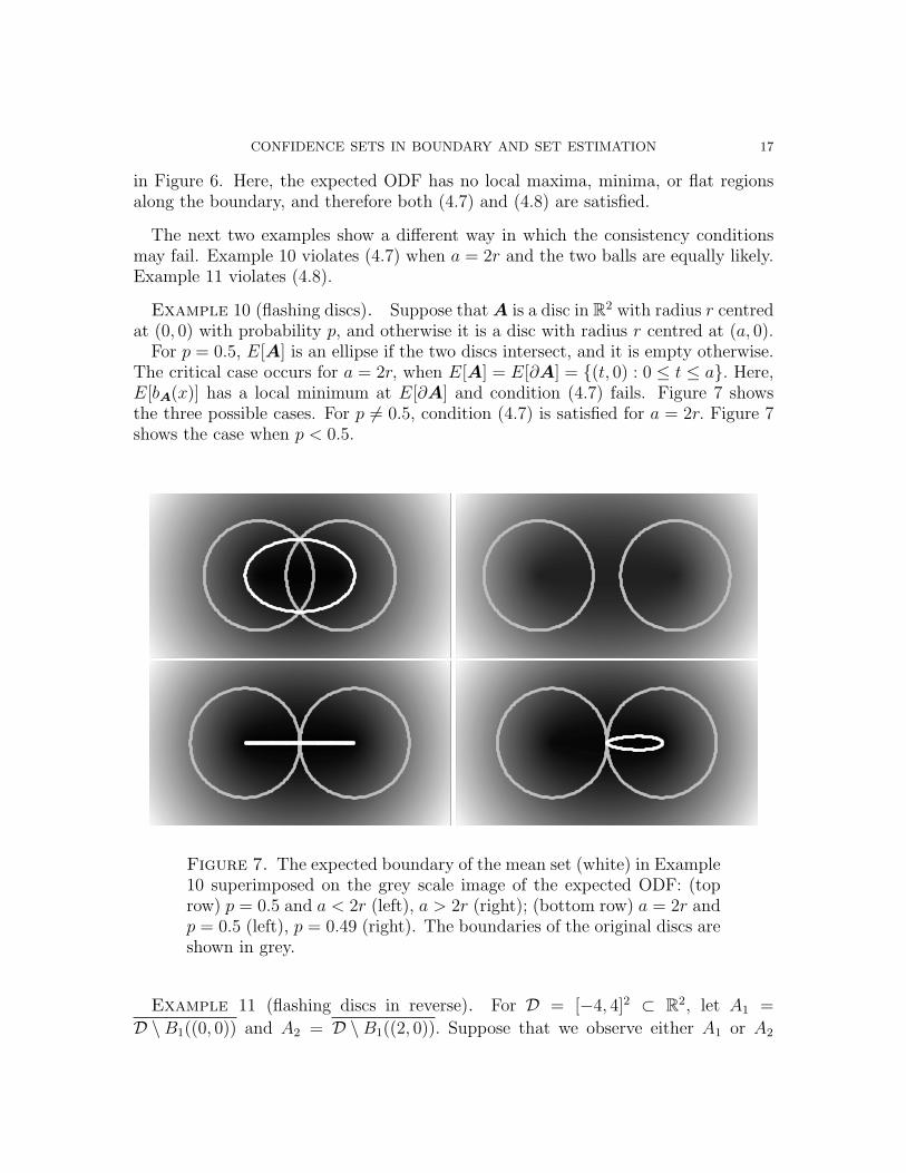
The next two examples show a different way in which the consistency conditionsmay fail. Example 10 violates (4.7) when a = 2r and the two balls are equally likely.Example 11 violates (4.8).

Example 10 (flashing discs). Suppose that A is a disc in R2 with radius r centredat (0, 0) with probability p, and otherwise it is a disc with radius r centred at (a, 0).

For p = 0.5, E[A] is an ellipse if the two discs intersect, and it is empty otherwise.The critical case occurs for a = 2r, when E[A] = E[∂A] = (t, 0) : 0 ≤ t ≤ a. Here,E[bA(x)] has a local minimum at E[∂A] and condition (4.7) fails. Figure 7 showsthe three possible cases. For p 6= 0.5, condition (4.7) is satisfied for a = 2r. Figure 7shows the case when p < 0.5.

Figure 7. The expected boundary of the mean set (white) in Example10 superimposed on the grey scale image of the expected ODF: (toprow) p = 0.5 and a < 2r (left), a > 2r (right); (bottom row) a = 2r andp = 0.5 (left), p = 0.49 (right). The boundaries of the original discs areshown in grey.

Example 11 (flashing discs in reverse). For D = [−4, 4]2 ⊂ R2, let A1 =

D \B1((0, 0)) and A2 = D \B1((2, 0)). Suppose that we observe either A1 or A2


with equal probability. These sets are the complements of the flashing discs fromExample 10 at the critical case a = 2r. Here, we obtain

E[bA(x1, 0)] =

x1, x1 ≤ 00, x1 ∈ [0, 2]−x1, x1 ≥ 2,

and E[bA(x1, x2)] < 0 for x2 6= 0. Hence E[A] = D and E[∂A] = [0, 2] × [0, 1].Therefore, E[bA(x)] has a local maximum along E[∂A] and does not satisfy condition(4.8).

The preceding examples show that the consistency conditions of Corollary 4.2 canbe violated in a number of ways. The following result provides further insight intothese conditions.

Proposition 4.5. Condition (4.7) holds iff E[A] = (E[Ac])c. Condition (4.8) holds

iff E[Ac] = (E[A])c. Furthermore, condition (4.7) holds iff ∂E[Ac] = E[∂A], andcondition (4.8) holds iff ∂E[A] = E[∂A].

We need to address certain technical details in the above result. As stated, thedefinition of E[A] is valid for a r.c.s. with non-zero boundary. However, if A isclosed, then Ac is not necessarily closed, and the closure of Ac may have an emptyboundary (e.g. 0, 1c), whereby bAc is not well defined. However, since bA is a well-defined random variable, and since bAc(x) = −bA(x), then Ac has a well-defined ODF.We therefore use the definition E[Ac] = x : E[bAc(x)] ≤ 0 = x : E[bA(x)] ≥ 0.

4.3. Confidence Sets. Using the method of Section 3, we obtain confidence regionsfor the expected set and the expected boundary. In this section, we assume that theobserved sets A1, . . . ,An are IID.

Theorem 4.6. Suppose that E[b2A(x0)] <∞ for some x0 ∈ D. Then

Zn(x) ≡√n(bn(x)− E[bA(x)])⇒ Z(x),

where Z is a Gaussian random field with mean zero and covariance

cov(Z(x),Z(y)) = E[bA(x)bA(y)]− E[bA(x)]E[bA(y)] for x, y ∈ D.

The next result shows that Z has smooth sample paths. Recall that a functionf : Rd 7→ R is Lipschitz of order α if it satisfies

|f(x)− f(y)| ≤ K|x− y|α,for some positive finite constant K and α > 0, for all x, y in the domain of f .

Proposition 4.7. For any x, y, x′, y′ ∈ Dvar(Z(x)− Z(y)) ≤ |x− y|2,(4.9)

|cov(Z(y)− Z(x),Z(y′)− Z(x′))| ≤ 2|y − x||y′ − x′|.(4.10)

Moreover, the sample paths of Z are Lipshitz of order α, for any α < 1.


We now construct confidence sets for both E[A] and E[∂A]. Let W ⊂ D be acompact set, and define q1 to be a number such that pr(supx∈W Z(x) ≤ q1) = 1− α,then

x ∈ W : bn(x) ≤ 1√nq1

(4.11)

is a 100(1 − α)% confidence region for E[A] ∩ W = x ∈ W : E[bA(x)] ≤ 0 . Also,let q2 denote a number such that pr(supx∈W |Z(x)| ≤ q2) = 1− α, then

x ∈ W : |bn(x)| ≤ 1√nq2

(4.12)

is a 100(1 − α)% confidence region for E[∂A] ∩ W = x ∈ W : E[bA(x)] = 0 . ForW = D, (4.11) and (4.12) give confidence sets for E[A] or E[∂A], respectively. Thequantiles may be approximated using a bootstrap approach.

To properly define the quantiles q1 and q2, we need the process Z to be continuouswith probability one. Proposition 4.7 asserts this, and more: Z is Lipschitz of orderα < 1. In particular, this tells us that the process is smoother than Brownianmotion. The latter satisfies var(Z(t) − Z(s)) = |t − s|, and is Lipshitz of orderα < 1/2. To obtain differentiability of Z, we would need it to be of Lipschitz orderα = 1, and hence the above proposition provides no information in this direction.However, differentiability can be examined using the results in [CL]. Understandingthe path properties of the process Z, such as smoothness, provides information aboutthe variability of the quantiles q1 and q2 and therefore also on the tightness of theconfidence sets.

Theorem 4.8 (Theorem on page 185 in [CL]). Suppose that r(x, y) = cov(Z(x),Z(y))has a continuous mixed derivative r11(x, y) = ∂x∂yr(x, y) satisfying

4δδr11(x, x) ≡ r11(x+ δ, x+ δ)− 2r11(x, x+ δ) + r11(x, x) ≤ C

| log |δ||a,

for some constants C > 0, a > 3 and sufficiently small δ, for all a ≤ x ≤ b for somea, b ∈ R. Then Z(x) has a derivative Z′(x) which is continuous on [a, b].

Example 12 (continuation of Example 5). Let Θ be a Uniform[−1, 1] randomvariable, and consider A = x ∈ R : |x−Θ| ≤ 1. Then, after some calculations, weobtain that

r11(x, y) =

1 + x− y − xy x, y ∈ [−1, 1] and x ≤ y,1 + y − x− xy x, y ∈ [−1, 1] and y ≤ x,0 otherwise.

Hence, for any ε > 0, there exists a δ, sufficiently small, such that

4δδr11(x, x) =

2|δ| − δ2 x ∈ (−1 + ε, 1− ε)0 x < −1− ε, or x > 1 + ε.


Therefore, by Theorem 4.8, Z(x) is continuously differentiable on compact intervalsinside (−∞,−1), (−1, 1) or (1,∞).

Example 13 (disc in R2 with random centre). The random set is a disc withradius one centred at (Θ, 0) where Θ ∼Uniform[0, 2], and suppose that we observe100 IID random sets from this model. The expected set E[A] is shown in Figure 8.Moreover, since E[bA(x)] ≥ |x − x0| − 1 where x0 = (E[Θ], 0), it follows that E[A]is contained inside the disc of radius one centered at (1, 0). Confidence regions wereformed for both E[∂A] and E[A] using re-sampling techniques to estimate the quan-tiles of supx∈W Z(x) and supx∈W |Z(x)| where the windowW = [−2, 2]×[−1, 3]. Theseare illustrated in Figure 8.

0 1 2 3

-1

0

1

2

0 1 2 3

-1

0

1

2

0 1 2 3

-1

0

1

2

Figure 8. Confidence regions for Example 13: (left) the mean bound-ary E[∂A] in black and the empirical boundary ∂An in grey; (centre) a95% bootstrap confidence set for E[A]; (right) a 95% bootstrap confi-dence set for E[∂A]. The expected boundary E[∂A] is shown in blackfor comparison.

Recall that the confidence set is immune to the consistency conditions (2.3) and(2.4) or (4.7) and (4.8). That is, the empirical set may not be consistent for the meanset E[A], but the confidence set still captures all of E[A] at least 100(1−α)% of thetime. We illustrate this point with the following example.

Example 14 (continuation of Example 7). Let [0, 1] ⊂ D ⊂ R and suppose thatA is either 0, 1 or [0, 1] with equal probability. Suppose also that we observe asimple random sample of size n from this model. Recall that E[A] = E[∂A] = [0, 1],and E[bA(x)] satisfies neither (4.7) nor (4.8). As before, let pn denote the proportionof times that the set [0, 1] is observed. If pn > 0.5, then An = ∂An = 0, 1 6= [0, 1].If pn < 0.5, then An = [0, 1] with ∂An = 0, 1 6= E[∂A].


The fluctuation field is given by

Zn(x) =√n(pn − 0.5)

(b[0,1](x)− b0,1(x)

)⇒ Z

(b[0,1](x)− b0,1(x)

),

where Z is a univariate normal random variable with mean zero and variance 0.25.The largest difference for b[0,1](x) − b0,1(x) occurs at x = 0.5, and hence, for anywindow such that [0, 1] ⊂ W , we have

supx∈W

Z(x) = max−Z, 0, and supx∈W|Z(x)| = |Z|.

Therefore, the exact quantiles are q1 = 0.5·1.645 and q2 = 0.5·1.96, and the confidenceregion for E[∂A] is given by x : |bn(x)| ≤ 0.5 · 1.96/

√n.

0 0.25 0.5 0.75 1

-0.05

0

0.05

0 0.25 0.5 0.75 1

-0.05

0

0.05

Figure 9. Confidence sets for Example 7: the empirical ODF bn withthe quantile levels −q2, q2 (left) and the confidence set in grey withE[∂A] shown in black (right).

Figure 9 illustrates the formation of the confidence set in this case for n = 1000. Inthis example, the proportion of times that [0, 1] was observed is pn = 0.489 and hence∂An = 0, 1. The left panel of Figure 9 shows the observed function bn(x) (black)along with the lower and upper quantile levels −q2, q2 = −0.5 · 1.96/

√1000, 0.5 ·

1.96/√

1000 (grey). The confidence interval for E[∂A] = [0, 1] is then (−0.031, 1.031)(Figure 9, right).

Now, for any n, maxx∈[0,1] |bn(x)| = |bn(0.5)| = |0.5− pn|. Therefore the confidenceregion misses a part of E[∂A] = [0, 1] if and only if |0.5 − pn| > 0.5 · 1.96/

√n.

This happens with probability 0.95, for sufficiently large n. On the other hand, theHausdorff distance ρ(E[∂A], ∂An) = 0.5 whenever pn 6= 0.5.

4.4. Separable Random Closed Sets. As in [SJ], we say that a random closed setis separable if there exists a random variable Θ and functions hj, gj, j = 1, . . . , k such


that

bA(x) ≡k∑j=1

hj(x)gj(Θ) almost surely.

For example, the ball centered at x0 with random radius R is separable, as bA(x) =|x − x0| − R. Notably, the mean of a separable random set has the same geometricstructure as the original sets. The same is true of the expected boundary. In thissection, we investigate the confidence regions for this special class of random closedsets.

To this end, suppose that we observe IID samples of the random variable Θ, andlet gn,j = 1/n

∑ni=1 gj(Θi). We assume that E[gj(Θ)2] < ∞ for all j = 1, . . . , k. It

follows immediately that E[bA(x)] =∑k

j=1 hj(x)E[gj(Θ)] and that

Zn(x) =k∑j=1

√n(gn,j − E[gj(Θ)])hj(x)⇒

k∑j=1

Zjhj(x),

where Z = Z1, . . . , Zk is a multivariate normal random variable with mean zeroand variance matrix given by cov(Zj, Zm) = cov(gj(Θ), gm(Θ)).

Remark 4.9. Consider the special case bA(x) = h(x) + g(θ). Then An = x :h(x) + gn ≤ 0, ∂An = x : h(x) + gn = 0, E[A] = x : h(x) + E[g(Θ)] ≤ 0and E[∂A] = x : h(x) + E[g(Θ)] ≤ 0. Note that by definition h(x) is continuous.If h(x) satisfies condition (2.3) at p = −E[g(Θ)], then An converges strongly toE[A]. In addition, if h(x) satisfies condition (2.4) at p = −E[g(Θ)], then ∂An

converges strongly to E[∂A]. Also, Zn(x) =√n(gn − E[g(Θ)]), which converges to

Z ∼Normal(0, var(g(Θ))). Thus, q1 and q2 are easily calculated from the quantiles ofthe univariate normal distribution.

Example 15 (confidence set for disc with random radius). Suppose that A isa disc with random radius R with µ = E[R] and σ2 = var(R). Then the expectedset is a circle with radius µ. Also, the 95% confidence interval for E[A] is a circlewith radius µ + 1.645σ/

√n, while the 95% confidence set for E[∂A] is the band

x : µ− 1.96σ/√n ≤ |x| ≤ µ+ 1.96σ/

√n.

Example 16 (upper half-plane at random angle). Suppose that A = x : x2 ≥x1 tan Θ, the upper half plane making angle Θ with the x1-axis, and suppose thatΘ ∼Uniform[a,b] with 0 < b− a < 2π. Then bA(x) = x1 sin(Θ)− x2 cos(Θ) and

E[bA(x)] =2

b− asin

(b− a

2

)x1 sin

(b+ a

2

)− x2 cos

(b+ a

2

)so that E[A] =

x : x2 ≥ x1 tan

(a+b2

). Because at least one of sin((a + b)/2) or

cos((a + b)/2) is non-zero, the expected ODF E[bA(x)] is linear (and non-constant),and therefore satisfies both of the consistency conditions.


-0.5 0 0.5

-0.5

0

0.5

-0.5 0 0.5

-0.5

0

0.5

-0.5 0 0.5

-0.5

0

0.5

Figure 10. Left: the expected boundary E[∂A] (black), its estimatebased on 25 samples (grey) and the boundary of a pacman with radius0.5 (dashed); centre and right: 95% bootstrapped confidence regionsfor E[A] and E[∂A], respectively. The confidence sets are denoted bythe shaded area, while the black line shows E[∂A].

Next, the limiting fluctuation process is Z(x) = x1Z1 − x2Z2, where cov(Z1, Z2) =cov(cos(Θ), sin(Θ)). For a fixed window W , the maximum of Z occurs on the bound-ary with probability one. Therefore, the variability of Z depends on the radius ofW , maxx∈W |x|. Suppose that W1 = x : |x1| ≤ 1, |x2| ≤ 1 and W2 = x : |x1| ≤2, |x2| ≤ 2. We then have

maxx∈W1

Z(x) = maxZ1 − Z2, Z1 + Z2,−Z1 − Z2,−Z1 + Z2 = |Z1|+ |Z2|,

and maxx∈W2 Z(x) = 2 maxx∈W1 Z(x). For the special case of a = 0, b = π, we obtainthat E[bA(x)] = 2x1/π,E[A] = x : x1 ≥ 0 and the variance of Z = Z1, Z2is equal to I/2, where I is the 2 × 2 identity matrix. From simulations, we findP (maxx∈W1 Z(x) ≤ 2.23) = 0.95. Therefore, 95% confidence regions for the set E[A]over the windows W1 and W2 are

x ∈ W1 : bn(x) ≤ 2.23/√n, and x ∈ W2 : bn(x) ≤ 4.46/

√n.

respectively. As expected, the smaller window W1 yields a tighter confidence region.

Example 17 (pacman in R2). Define the pacman with radius r, A(r), to be adisc with radius r centred at the origin with its upper left quadrant removed. Thatis,

A(r) = x : |x| ≤ r ∩ x : x1 ≤ 0 ∪ x : x2 ≤ 0 .Figure 4 (right) shows the ODF of A(r) for r = 1.

Suppose that A = A(R), where R is a uniform random variable on [0, 1]. Then theexpected set E[A] is a smoothed version of A(0.5), as seen in Figure 10 (left). Thefigure also shows bootstrapped 95% confidence sets for both E[A] and E[∂A].


The accuracy of the estimate and the apparent centering of the confidence intervalsaround the mean set may be explained upon closer inspection of the sample. TheODF of the pacman is similar to that of the circle; indeed, they are identical in thelower left quadrant. Therefore, the behaviour of the estimators and of the confidenceregions is not unlike that of estimators and confidence intervals for the real-valuedE[R] = 0.5. For our sample of n = 25, we observed R = 0.496, which explains theaccuracy of the estimator ∂An. On the other hand, the confidence region still showsthe large variability of ∂An.

5. Further Examples

5.1. Application to Image Reconstruction. Image averaging arises in varioussituations, for example, when multiple images of the same scene are observed or whenthe acquired images represent objects of the same class and the goal is to determinethe average object (shape) that can be described as typical. Here we consider theexample of image averaging studied in [BM]. An original newspaper image (see Figure11) was contaminated and then reconstructed using an Ising prior model. The detailsare given in [BM], Section 6. The data consists of 15 independent binary images ofthe reconstructed image.

Figure 11. From left to right are shown the original image, thedistance-average reconstruction and the ODF-average reconstruction.

In [BM], the original image (Figure 11, left) was reconstructed using the distance-average approach based on the ODF; see Figure (centre) and Figure 6 in [BM]. TheODF-reconstruction using the method proposed in [SJ] is also shown in Figure 11(right). This reconstruction, which we call the ODF-average here, outperforms thedistance-average both in terms of misclassification error and the L2-distance consis-tent with the distance-average construction [SJ].

Next, we compute 95% confidence regions for the ODF-average reconstructionbased on 5K bootstrap samples. Figure 12 (left top – full image, left bottom – inset)shows the confidence set for E[A] with the boundary of the true image overlayedin black. The confidence set contains all of the true text image and appears tight,although there are a number of spurious bounds induced by noise. The confidence set


Figure 12. Confidence regions for the expected set (left) and the ex-pected boundary (right) shown with the boundary of the true image(black). The bottom row shows insets of the original image.

Figure 13. Confidence regions for the expected boundary with theboundary of the true image (green) using the true sample size (left)and hypothetical sample sizes of n = 50, 100 (middle and right, respec-tively). The pictures shown are insets of the full image.


for E[∂A] is also shown in Figure 12 (right top – full image, right bottom – inset).The boundary of the lower confidence set consists of only a few closed contours scat-tered throughout the text. The lack of tightness in the confidence set is explained bythe small sample size and a relatively thin font width. Hypothetically increasing thesample size would produce tighter confidence sets for both the expected set and itsboundary. For example, the bootstrap confidence set for the boundary based on 50and 100 samples is tighter as compared to the one based on 15 samples (see Figure13). It should be noted that confidence intervals in Figure 13 were created using theoriginal window D, and that the picture is a close-up of the result.

5.2. Application to Medical Imaging. We next consider an example of boundaryreconstruction in mammography, where the skin-air contour is used to determine theradiographic density of the tissue and to estimate breast asymmetry. Both measuresare known to be associated with the risk of developing breast cancer [SMW+, DWW+].

Figure 14. Confidence sets for the reconstructed skin-air boundaryin a mammogram: the original image (left), and the digitally enhancedimage (centre) with the reconstructed boundary (solid line) and confi-dence region (dashed line). Three insets are also shown (right).


In [SB], B-spline curves were used to reconstruct a smooth connected boundaryof an object in a noisy image, and the method was applied to estimate the tissueboundary in mammograms. The method is Bayesian and uses a loss function basedon ODFs to determine the optimal estimator for the boundary. More details on thereconstruction method and image acquisition can be found in [SB]. Here, we applythe proposed method to construct a confidence set for the boundary estimator, whichis given by the zero-level isocontour of the curve samples from the posterior. Weemphasize that the confidence region is not a credible set, but rather it describes thevariability of the sample curves.

Figure 14 (left) shows a typical digitized mammogram image, characterised by alow contrast-to-noise ratio. A probability integral transform improves the contrastby increasing the dynamic range of image intensities (Figure 14, centre). The 95%confidence set (dashed) for the boundary estimator (solid) in Figure 14 is obtainedusing a bootstrap resampling of size 1000. The confidence set is tight and fits theimage well. It also shows that the reconstructed boundary is more variable towardthe inside of the breast tissue. Note that what appears to be a nipple is, in fact, aduct system leading to the nipple, so that the estimators correctly follow the skinline. More details can be seen in insets in Figure 14 (right).

Note that the method proposed in this paper assumes that the observed sets areindependent and identically distributed, whilst the boundary reconstruction is basedon Monte Carlo sampling from the posterior. To ensure the independence of thecurve samples, we construct the confidence set for the boundary using 100 samplesfrom the posterior, which were acquired every 250th sweep after a burn-in period of1000 sweeps. It remains open to extend the method of confidence sets to dependentsamples, in particular, in the context of Bayesian inference.

Appendix

This section contains certain technical details, as well as proofs of the results dis-cussed in this paper.

6.3. Independent Random Closed Sets. In Remark 4.3 we define two r.c.s. Aand B to be independent if their ODFs are independent as random functions on D.In this section we give a brief discussion of this definition.

Recall that in [Mat] (page 40), two sets A and B are said to be independent if

P (A ∩K1 6= ∅ and B ∩K2 6= ∅) = P (A ∩K1 6= ∅)P (B ∩K2 6= ∅),

for any compact sets K1, K2 ⊂ D. To differentiate it from our definition, we call thisM-independence.

Proposition 6.1. The relationship between independence and M-independence is asfollows.


1. Two sets A and B are M-independent if and only if their distance functions,dA(x) and dB(x), are independent random functions.

2. Two sets A and B are independent if and only if the sets A and B, and ∂A and∂B, are both M-independent.

3. Two boundary sets ∂A and ∂B are M-independent if and only if |bA(x)| and|bB(x)| are independent random functions.

Thus independence is a stronger notion than M-independence. Recall that dA(x) ≡dB(x) iff A = B, whereas bA(x) ≡ bB(x) iff A = B and ∂A = ∂B (e.g. consider thesets A = [0, 1] ∩ Q ⊂ R and B = [0, 1]; then A = B, but ∂A 6= ∂B, and hencedA ≡ dB but bA 6= bB). Thus, the ODF encapsulates more information about a setthan the distance function, and hence more information is required to ascertain itsindependence.

Proof. We first prove the first part of the statement. Suppose that dA and dB areindependent random functions. Then, since for any compact K,

A ∩K 6= ∅ = infx∈K

dA(x) ≤ 0,

it follows that A and B are also M-independent. For the other direction, supposethat A and B are M-independent. Then by the relation

dA(x) ≤ α = A ∩Bα(x) 6= ∅,for any α ∈ R, the random functions dA and dB are also independent.

The second part of the proposition is proved in a similar manner. Here, the keyrelations are

A ∩K 6= ∅ = infx∈K

bA(x) ≤ 0,

∂A ∩K 6= ∅ = infx∈K|bA(x)| = 0,

as well as

bA(x) ≤ α = A ∩Bα(x) 6= ∅ if α ≥ 0,bA(x) < α = ∂A ∩B|α|(x) 6= ∅c ∩ A ∩ x 6= ∅ if α < 0.

The third statement follows from the first statement, since for any set A, we have|bA(x)| = d∂A(x). This completes the proof.

6.4. Proofs.

Proof of Proposition 2.1. Suppose first that (2.4) holds. Then, by the continuity of f ,

∂x : f(x) ≤ p = x : f(x) ≤ p ∩ x : f(x) > p= x : f(x) = p ∩ x : f(x) > p= x : f(x) = p ∩ x : f(x) ≥ p= x : f(x) = p.


On the other hand, if ∂x : f(x) ≤ p = x : f(x) = p then x : f(x) = p =

x : f(x) > p∩x : f(x) = p. Therefore, appealing again to the continuity of f , wefind that

x : f(x) < p

=(x : f(x) < p ∩ x : f(x) < p

)∪(x : f(x) < p ∩ x : f(x) = p

)= x : f(x) < p ∪ x : f(x) = p= x : f(x) ≤ p,

as desired. The proof of the first claim is similar, and we omit the details.

Lemma 6.2. Suppose that f is continuous. Then

x : p1 ≤ f(x)ε ∩ x : f(x) ≤ p2ε = x : p1 ≤ f(x) ≤ p2ε.

Proof. Suppose y is in the set

x : p1 ≤ f(x)ε ∩ x : f(x) ≤ p2ε \ x : p1 ≤ f(x) ≤ p2.

Then one of two possibilities exists: Either f(y) < p1 or f(y) > p2. The argumentfor both cases is the same, so we present only the first instance.

Assume then that y is such that f(y) < p1. By definition of y, there exists an x1

such that p1 ≤ f(x1) and y ∈ Bε(x1), or an x2 such that f(x2) ≤ p2 and y ∈ Bε(x2).In the first setting, since f is continuous, there also exists a z such that p1 ≤ f(z) ≤ p2

and d(y, z) ≤ ε. For example, one such z must fall on the line between y and x1,which would clearly satisfy |y− z| ≤ ε. A similar argument shows that if y ∈ Bε(x2),then there exists a z such that p1 ≤ f(z) ≤ p2 and |y − z| ≤ ε. It follows thaty ∈ B(z, ε). This proves that

x : p1 ≤ f(x)ε ∩ x : f(x) ≤ p2ε ⊂ x : p1 ≤ f(x) ≤ p2ε.

Containment in the other direction is immediate, completing the proof.

Proof of Theorem 2.3. The proof here is similar to that of [Mol]. If f : D 7→ R is acontinuous function satisfying the conditions of the theorem, then

ϕ(±ε) = ρ(x : f(x) ≤ p2, x : f(x) ≤ p2 ± ε)ϕ(±ε) = ρ(x : p1 ≤ f(x), x : p1 ± ε ≤ f(x))

are all continuous for ε near zero, and moreover, they both converge to zero as ε→ 0.

Now, by (A1), we know that fn converges uniformly to f with probability one. Let

ηn = supx∈D|f(x)− fn(x)|,

and also define

εn = maxϕ(ηn), ϕ(−ηn), ϕ(ηn), ϕ(−ηn)


which converges to zero as n→∞ almost surely. We will next show that ρ(x : p1 ≤fn(x) ≤ p2, x : p1 ≤ f(x) ≤ p2) ≤ εn. To this end

x : p1 ≤ f(x) ≤ p2 ⊂ x : f(x) ≤ p2 − ηnϕ(−ηn)

⊂ x : fn(x) ≤ p2ϕ(−ηn)

⊂ x : fn(x) ≤ p2εn .

Repeating in the other direction, we obtain

x : p1 ≤ f(x) ≤ p2 ⊂ x : p1 + ηn ≤ f(x)ϕ(ηn)

⊂ x : p1 ≤ fn(x)ϕ(ηn)

⊂ x : p1 ≤ fn(x)εn .

and hence, by Lemma 6.2,

x : p1 ≤ f(x) ≤ p2 ⊂ x : p1 ≤ fn(x) ≤ p2εn .(A-1)

For the other direction,

x : p1 ≤ fn(x) ≤ p2 ⊂ x : f(x) ≤ p2 + ηn⊂ x : f(x) ≤ p2εn .

A similar argument shows that x : p1 ≤ fn ≤ p2 ⊂ x : p1 ≤ f(x)εn , from whichit follows

x : p1 ≤ fn(x) ≤ p2 ⊂ x : p1 ≤ f(x) ≤ p2εn

by Lemma 6.2. Together with (A-1) this proves the result.To address necessity, suppose that there exists a neighbourhood of x0, Bδ(x0), and

a subsequence nk such that fnk(x) < f(x) for all x ∈ Bδ(x0). Assume also that

x0 ∈ x : p1 ≤ f(x) \ x : p1 < f(x). In particular, this implies that (2.4) is not

satisfied, and hence there exists an ε > 0 such that ρ(x0, x : p1 < f(x) ≤ p2) > ε.

It follows that ρ(Fnk(p1, p2), F (p1, p2)) > min(ε, δ) > 0, proving the result. A similar

argument proves the other claim.

Proof of Proposition 2.5. Without loss of generality, we assume that p = 0. For anyfixed x0 ∈ D, and for t ∈ R+ define the function h(t) = f(x0 + te0). By assumption,it is a strictly increasing function in t. Let t∗ denote a value such that

h(t∗) = 0.

Then for all t > t∗ we have that x0 + te0 ∈ x : f(x) > 0 and for all t < t∗ we havethat x0 +te0 ∈ x : f(x) < 0. Note also that for all x ∈ ∂F (0) = x ∈ D : f(x) = 0,there exists an x0 such that x0 + te0 = x for some t. It follows that for all x ∈ ∂F (0)and for all ε > 0, Bε(x)∩x ∈ D : f(x) < 0 6= ∅ and Bε(x)∩x ∈ D : f(x) > 0 6= ∅.Therefore,

x : f(x) < 0 = x : f(x) ≤ 0 and x : f(x) > 0 = x : f(x) ≥ 0,


as required.

Proof of Remark 2.7. The extension to unbounded domains of the consistency resultsis immediate, because strong convergence of An to A is defined as

ρ(An ∩K,A ∩K)→ 0, a.s. as n→∞,for each compact set K ⊂ Rd.

Proof of Corollary 4.2. Since the functions bn(x) and E[bA(x)] are continuous, theresult follows directly from Theorems 2.2 and 2.3.

Proof of Remark 4.3. It is well known that the oriented distance function is uniformlyLipshitz [DZ2]. That is, for a fixed set A,

|bA(x)− bA(y)| ≤ |x− y|, for all x, y ∈ D.(A-2)

This property immediately follows also for E[bA(x)] and for the empirical ODF, bn(x).It follows also that if E[|bA(x0)|] <∞ for some x0 ∈ D, then the mean E[bA(x)] existsfor all x ∈ D. Moreover, since the window D ⊂ Rd is compact, we immediately obtainthe uniform convergence of bn(x). That is,

limn→∞

supx∈D|bn(x)− E[bA(x)]| = 0,

as required.

Proof of Proposition 4.5. From the definition of the oriented distance function, wehave that bA(x) = −bAc(x) almost surely. Therefore E[bA(x)] = −E[bAc(x)] andhence

E[Ac] = x : E[bA(x)] ≥ 0.Therefore we have the following relation

(E[A])c = x : E[bA(x)] > 0 = x : E[bA(x)] ≥ 0 = E[Ac],

which holds iff (4.8) is satisfied. Similarly,

(E[Ac])c = x : E[bA(x)] < 0 = x : E[bA(x)] ≤ 0 = E[A],

which holds iff (4.7) is satisfied. The last statement of the proposition is a directcorollary of Proposition 2.1.

Theorem 6.3 (Theorem 1.4.7 on page 38 in [Kun]: Kolmogorov’s tightness crite-rion.). For a compact set D ⊂ Rd, let Yn(x) : x ∈ D be a sequence of continuousrandom fields with values in R. Assume that there exist positive constants γ, C andα1, . . . , αd with

∑di=1 α

−1i < 1 such that

E[|Yn(x)− Yn(y)|γ] ≤ C

(d∑i=1

|xi − yi|αi

)for every x, y ∈ D,

E[|Yn(x)|γ] ≤ C, for all x ∈ D,


holds for any n. Then Yn is tight in C(D).

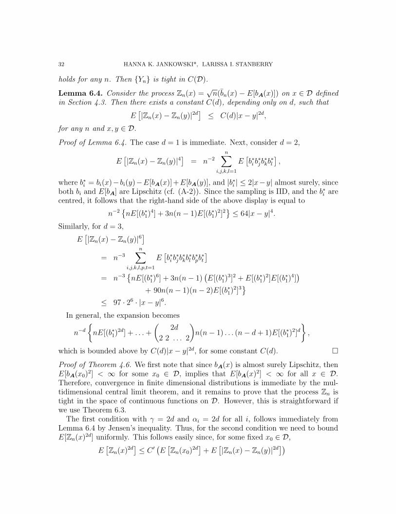
Lemma 6.4. Consider the process Zn(x) =√n(bn(x)− E[bA(x)]) on x ∈ D defined

in Section 4.3. Then there exists a constant C(d), depending only on d, such that

E[|Zn(x)− Zn(y)|2d

]≤ C(d)|x− y|2d,

for any n and x, y ∈ D.

Proof of Lemma 6.4. The case d = 1 is immediate. Next, consider d = 2,

E[|Zn(x)− Zn(y)|4

]= n−2

n∑i,j,k,l=1

E[b∗i b∗jb∗kb∗l

],

where b∗i = bi(x)− bi(y)−E[bA(x)]+E[bA(y)], and |b∗i | ≤ 2|x−y| almost surely, sinceboth bi and E[bA] are Lipschitz (cf. (A-2)). Since the sampling is IID, and the b∗i arecentred, it follows that the right-hand side of the above display is equal to

n−2nE[(b∗1)

4] + 3n(n− 1)E[(b∗1)2]2≤ 64|x− y|4.

Similarly, for d = 3,

E[|Zn(x)− Zn(y)|6

]= n−3

n∑i,j,k,l,p,t=1

E[b∗i b∗jb∗kb∗l b∗pb∗t

]= n−3

nE[(b∗1)

6] + 3n(n− 1)(E[(b∗1)

3]2 + E[(b∗1)2]E[(b∗1)

4])

+ 90n(n− 1)(n− 2)E[(b∗1)2]3

≤ 97 · 26 · |x− y|6.In general, the expansion becomes

n−dnE[(b∗1)

2d] + . . .+

(2d

2 2 . . . 2

)n(n− 1) . . . (n− d+ 1)E[(b∗1)

2]d,

which is bounded above by C(d)|x− y|2d, for some constant C(d).

Proof of Theorem 4.6. We first note that since bA(x) is almost surely Lipschitz, thenE[bA(x0)

2] < ∞ for some x0 ∈ D, implies that E[bA(x)2] < ∞ for all x ∈ D.Therefore, convergence in finite dimensional distributions is immediate by the mul-tidimensional central limit theorem, and it remains to prove that the process Zn istight in the space of continuous functions on D. However, this is straightforward ifwe use Theorem 6.3.

The first condition with γ = 2d and αi = 2d for all i, follows immediately fromLemma 6.4 by Jensen’s inequality. Thus, for the second condition we need to boundE[Zn(x)2d] uniformly. This follows easily since, for some fixed x0 ∈ D,

E[Zn(x)2d

]≤ C ′

(E[Zn(x0)

2d]

+ E[|Zn(x)− Zn(y)|2d

])


for come constant C ′ (depending on d), again applying Jensen’s inequality. We havealready placed a bound on the second term of the right-hand side of the above equa-tion, and a bound on the first term follows from the central limit theorem.

Let D be a compact subset of Rd. We recall a theorem of [Win]. Proposition 4.7follows immediately.

Theorem 6.5 (SATZ 6 on page 837 of [Win]). Let Y (x), x ∈ D ⊂ Rd be a Gaussianrandom field such that for τ → 0 the inequality

E[|Y (x+ τ)− Y (x)|2

]≤ C|τ |ε

holds for some ε > 0 and 0 < C <∞. Then for almost all realizations there exists arandom number δ(ω) so that for any x1, xt2 ∈ D with |x1−x2| < δ(ω) and 0 < η < ε/2the inequality

|Y (x1)− Y (x2)| ≤ C0|x1 − x2|η

holds. In particular, it follows that Y (x), x ∈ D is continuous with probability one.

Proof of Proposition 4.7. To prove this result we again recall that both bA(x) andE[bA(x)] are Lipschitz and satisfy inequality (A-2). Therefore,

var(Z(x)− Z(y)) = var(bA(x)− bA(y))

≤ E[(bA(x)− bA(y))2] ≤ |x− y|2.

A similar approach shows the bound for the covariance. We may now use this result,along with Theorem 6.5 to prove that the sample paths of Z are continuous almostsurely.

Acknowledgements

The first author would like to thank Tom Salisbury for several useful discussions.

References

[BGKW] H. Breu, J. Gil, D. Kirkpatrick, and M. Werman. Linear time euclidean distance transformalgorithms. IEEE Trans. Pattern Anal. Mach. Intell., 17:529–533, 1995.

[Bil] Patrick Billingsley. Convergence of probability measures. John Wiley & Sons Inc., NewYork, 1968.

[BM] Adrian Baddeley and Ilya Molchanov. Averaging of random sets based on their distancefunctions. J. Math. Imaging Vision, 8(1):79–92, 1998.

[BT] B. Nebiyou Bekele and Peter F. Thall. Dose-finding based on multiple toxicities in a softtissue sarcoma trial. J. Amer. Statist. Assoc., 99(465):26–35, 2004.

[CL] Harald Cramer and M. R. Leadbetter. Stationary and related stochastic processes. Samplefunction properties and their applications. John Wiley & Sons Inc., New York, 1967.

[Cre] Noel Cressie. A central limit theorem for random sets. Z. Wahrsch. Verw. Gebiete,49(1):37–47, 1979.


[DWW+] J. Ding, R.M.L. Warren, I. Warsi, N. Day, D. Thompson, M. Brady, C. Tromans, R. High-nam, and D. Easton. Evaluating the effectiveness of using standard mammogram form topredict breast cancer risk: Case-control study. Cancer Epidemiology Biomarkers and Pre-vention, 17:1074–1081, 2008.

[DZ1] M. C. Delfour and J.-P. Zolesio. Shapes and geometries, volume 4 of Advances in Designand Control. Society for Industrial and Applied Mathematics (SIAM), Philadelphia, PA,2001. Analysis, differential calculus, and optimization.

[DZ2] Michel C. Delfour and Jean-Paul Zolesio. Shape analysis via oriented distance functions.J. Funct. Anal., 123(1):129–201, 1994.

[FBF] J.H. Freidman, J.L. Bentley, and R.A. Finkel. An algorithm for finding best matches inlogrithmic expected time. ACM Trans. Pattern Anal. Softw., 3:209–226, 1977.

[KT] A. P. Korostelev and A. B. Tsybakov. Minimax theory of image reconstruction, volume 82of Lecture Notes in Statistics. Springer-Verlag, New York, 1993.

[Kun] Hiroshi Kunita. Stochastic flows and stochastic differential equations, volume 24 of Cam-bridge Studies in Advanced Mathematics. Cambridge University Press, Cambridge, 1990.

[Mat] G. Matheron. Random sets and integral geometry. John Wiley & Sons, New York-London-Sydney, 1975. With a foreword by Geoffrey S. Watson, Wiley Series in Probability andMathematical Statistics.

[Mol] Ilya S. Molchanov. A limit theorem for solutions of inequalities. Scandinavian Journal ofStatistics, 25:235–242, 1998.

[Nol] D. Nolan. The excess-mass ellipsoid. J. Multivariate Anal., 39(2):348–371, 1991.[Pol] Wolfgang Polonik. Measuring mass concentrations and estimating density contour

clusters—an excess mass approach. Ann. Statist., 23(3):855–881, 1995.[R] R Development Core Team. R: A Language and Environment for Statistical Computing.

R Foundation for Statistical Computing, Vienna, Austria, 2008. ISBN 3-900051-07-0.[RP] A. Rosenfeld and J. Pfaltz. Sequential operations in digital picture processing. J. ACM,

13:471–494, 1966.[SB] Larissa Stanberry and Julian Besag. Boundary reconstruction in binary images using

splines. In preparation., 2008.[SJ] Larissa Stanberry and Hanna Jankowski. Expectations of random sets and their bound-

aries using oriented distance functions. In preparation., 2008.[SMW+] D. Scutt, J. Manning, G. Whitehouse, S. Leinster, and C. Massey. The relationship be-

tween breast asymmetry, breast size and the occurrence of breast cancer. Br. J. Radiol,70((838)):1017–1021, 1997.

[SVW] G. Salinetti, W. Vervaat, and R. J.-B. Wets. On the convergence in probability of randomsets (measurable multifunctions). Math. Oper. Res., 11(3):420–422, 1986.

[SW] Gabriella Salinetti and Roger J.-B. Wets. On the convergence in distribution of measur-able multifunctions (random sets), normal integrands, stochastic processes and stochasticinfima. Math. Oper. Res., 11(3):385–419, 1986.

[TWS] Peter F. Thall, Leiko H. Wooten, and Elizabeth J. Shpall. A geometric approach tocomparing treatments for rapidly fatal diseases. Biometrics, 62(1):193–201, 318–319, 2006.

[Var] S. R. S. Varadhan. Stochastic processes, volume 16 of Courant Lecture Notes in Mathe-matics. Courant Institute of Mathematical Sciences, New York, 2007.

[Win] Wolfgang Winkler. Stetigkeitseigenschaften der Realisierungen Gauss’scher zufalligerFelder. In Trans. Third Prague Conf. Information Theory, Statist. Decision Functions,Random Processes (Liblice, 1962), pages 831–839. Publ. House Czech. Acad. Sci., Prague,1964.


Department of Mathematics and Statistics, York Universitye-mail: [email protected]

University of Bristol, School of Mathematicse-mail: [email protected]

Confidence sets in boundary and set estimation

Documents