Proceedings MFOI-2020 Conference on Mathematical Foundations of Informatics Kyiv Interservice 2021 Taras Shevchenko National University of Kyiv January 12-16, 2021, Kyiv, Ukraine

Welcome message from author
This document is posted to help you gain knowledge. Please leave a comment to let me know what you think about it! Share it to your friends and learn new things together.
Transcript
Proceedings MFOI-2020
Conference on Mathematical
Foundations of Informatics
Kyiv
Interservice
2021
Taras Shevchenko National University of KyivJanuary 12-16, 2021, Kyiv, Ukraine
УДК 510; 004.4; 004.8
Рекомендовано до друку Вченою радою факультету комп’ютернихнаук та кібернетики Київського національного університету
імені Тараса Шевченка, протокол 10 від 8 лютого 2021 року.
Конференція з математичних основ інформатики MFOI-2020:Праці; 12-16 січня 2021, Київ: Інтерсервіс, 2021. – 446 с.
Цей том містить праці VI Міжнародної конференції з математичних
основ інформатики MFOI-2020. До нього входять запрошені та подані статті,
які були ретельно прорецензовані. Статті присвячені основам скінчено-
підтримуваних множин, основам та використанню логіки в інформатиці та
штучному інтелекті, обробці природних мов та систематичній розробці
програмного забезпечення.
Conference on Mathematical Foundations of Informatics:
Proceedings MFOI-2020; 12-16 Jan. 2021, Kyiv: Interservice, 2021. –
446 p.
This volume represents the Proceedings of the VI International Conference
on Mathematical Foundations of Informatics MFOI-2020. It comprises invited
and contributed papers that were carefully peer-reviewed. The papers are devoted
to foundations of finitely supported sets, to foundations and use of logic in
computer science and artificial intelligence, to natural language processing,
and to systematic software development.
ISBN 978-966-999-143-0
© Faculty of Computer Science andCybernetics of Taras Shevchenko National
University of Kyiv, Ukraine,
Vladimir Andrunachievici Institute of Mathematics and Computer Science, Moldova, 2021
All rights reserved.
Preface
This volume represents the Proceedings of the VI International
Conference on Mathematical Foundations of Informatics MFOI-2020. It
comprises invited and contributed papers that were carefully peer-reviewed. In
view of the outbreak of the Coronavirus disease (COVID-19) the MFOI-2020
was postponed to 2021. The conference was held in Kyiv (Ukraine) on January
12–16, 2021.
The annual International Conference on Mathematical
Foundations of Informatics is intended to add synergy to the efforts of
the researchers working on the development of the mathematical
foundations of Computer Science, Logic, and Artificial Intelligence.
The conference was organized by
Taras Shevchenko National University of Kyiv, Ukraine
Vladimir Andrunachievici Institute of Mathematics and Computer
Science, Chisinau, Moldova
Alexandru Ioan Cuza University of Iasi, Romania
International Society for Logic and Artificial Intelligence, Chisinau,
Moldova
Ukrainian Logic Society, Ukraine
Program Committee Co-Chairs:
Mykola Nikitchenko (Kyiv, Ukraine)
Svetlana Cojocaru (Chisinau, Moldova)
Adrian Iftene (Iasi, Romania)
Ioachim Drugus (Chisinau, Moldova)
Invited Speakers:
Prof. Dr. Andrei Arusoaie, Alexandru Ioan Cuza University of Iasi,
Romania
Prof. Dr. Adrian Iftene, Alexandru Ioan Cuza University of Iasi,
Romania
Prof. Dr. Alexei Muravitsky, Northwestern State University,
Natchitoches, USA
Prof. Dr. Segiy Kryvyi, Taras Shevchenko National University of Kyiv,
Ukraine
3
Prof. Dr. Mykola Nikitchenko, Taras Shevchenko National University
of Kyiv, Ukraine
Prof. Dr. Grygoriy Zholtkevych, V.N.Karazin Kharkiv National
University, Ukraine
Program Committee:
Artiom Alhazov
Bogdan Aman
Gabriel Ciobanu
Anatoliy Doroshenko
Constantin Gaindric
Daniela Gifu
Sergiy Kryvyi
Alboaie Lenuta
Alexander Lyaletski
Taras Panchenko
Vladimir Peschanenko
Dmytro Terletskyi
Ferucio Laurentiu Tiplea
Oleksii Tkachenko
Sergey Verlan
Kostiantyn Zhereb
Grygoriy Zholtkevych
Organizing Committee:
Mykola Nikitchenko
(Chair)
Olena Shyshatska
Oleksiy Tkachenko
Yaroslav Kohan
Oleksandra Timofieieva
Natalia Polishchuk
Ganna Denischuk
Iryna Semenchuk
Tudor Bumbu
MFOI2020 was devoted to the World Logic Day. The following
collocated one-day events occurred on January 14:
Symposium on Logic and Artificial Intelligence (SLAI), Chisinau,
Moldova;
Moldovan Prizes in Logic and Artificial Intelligence;
Romanian Prizes in Logic and Artificial Intelligence;
Ukrainian Logic Society Prize.
We would like to thank all people who contributed to the success of MFOI-2020.
Editors: Mykola Nikitchenko, Svetlana Cojocaru,
Adrian Iftene, Ioachim Drugus
4
Proceedings of the Conference on Mathematical Foundations of Informatics
MFOI2020, January 12-16, 2021, Kyiv, Ukraine
Properties of Finitely Supported Binary
Relations between Atomic Sets
Andrei Alexandru and Gabriel Ciobanu
Abstract
In the framework of finitely supported sets, we introduce thenotion of atomic cardinality and present some finiteness prop-erties of the finitely supported binary relations between infiniteatomic sets.
Keywords: binary relations, atomic sets, finiteness.
1 Introduction
Finitely supported structures are related to permutation models ofZermelo-Fraenkel set theory with atoms (ZFA) and to the theory ofnominal sets. They were originally introduced in 1930s by Fraenkel,Lindenbaum and Mostowski to prove the independence of the axiomof choice from the other axioms of Zermelo-Fraenkel set theory (ZF),and recently used to study the binding, freshness and renaming in pro-gramming languages and related systems [1, 5]. Inductively definedfinitely supported sets involving the name-abstraction together withCartesian product and disjoint union can encode a formal syntax mod-ulo renaming of bound variables. In this way, the standard theory ofalgebraic data types can be extended to include signatures involvingbinding operators. The theory of finitely supported sets also allows thestudy of structures which are possibly infinite, but contain enough sym-metries such that they can be concisely represented and manipulated.In this paper we present some finiteness properties of finitely supportedbinary relations between infinite atomic sets.
©2020 by Andrei Alexandru, Gabriel Ciobanu
5
Andrei Alexandru and Gabriel Ciobanu
2 Preliminary Results
We consider an infinite set A called ‘the set of atoms’. Atoms areentities whose internal structure is ignored (i.e. they can be checkedonly for equality), and which are considered as basic for a higher-orderconstruction. A transposition of A is a function (a b) : A → A thatinterchanges only a and b. A permutation of A is a bijection of Agenerated by composing finitely many transpositions. We denote by SAthe group of all permutations of A. We proved in [1] that an arbitrarybijection on A is finitely supported if and only if it is a permutation.
Definition 2.1. 1. Let X be a ZF set. An SA-action on X is a groupaction · of SA on X. An SA-set is a pair (X, ·), where X is a ZF set,and · is an SA-action on X.
2. Let (X, ·) be an SA-set. Then S ⊂ A supports x whenever foreach π ∈ Fix(S) we have π · x = x, where Fix(S) = π |π(a) = a
for all a ∈ S. The least finite set (w.r.t. the inclusion relation)supporting x (which exists according to [1]) is called the support of x,denoted by supp(x). An empty supported element is called equivariant.
3. Let (X, ·) be an SA-set. We say that X is an invariant set if foreach x ∈ X there exists a finite set Sx ⊂ A which supports x.
Proposition 2.2. [1] Let (X, ·) and (Y, ⋄) be SA-sets.1. The set A of atoms is an invariant set with the SA-action ·
defined by π · a := π(a) for all π ∈ SA and a ∈ A.2. Let π ∈ SA. If x ∈ X is finitely supported, then π · x is finitely
supported and supp(π · x) = π(u) |u ∈ supp(x) := π(supp(x)).3. The Cartesian product X × Y is also an SA-set with the SA-
action ⊗ defined by π ⊗ (x, y) = (π · x, π ⋄ y) for all π ∈ SA and allx ∈ X, y ∈ Y . If (X, ·) and (Y, ⋄) are invariant sets, then (X × Y,⊗)is also an invariant set.
4. The powerset ℘(X) = Z |Z ⊆ X is also an SA-set with theSA-action ⋆ defined by π ⋆ Z := π · z | z ∈ Z for all π ∈ SA, and allZ ⊆ X. For each invariant set (X, ·), we denote by ℘fs(X) the set ofelements in ℘(X) which are finitely supported according to the action ⋆.(℘fs(X), ⋆|℘fs(X)) is an invariant set.
6
Properties of Finitely Supported Binary Relations between Atomic Sets
5. The finite powerset of X denoted by ℘fin(X) = Y ⊆X |Y finite and the cofinite powerset of X denoted by ℘cofin(X) =Y ⊆ X |X \ Y finite are both SA-sets with the SA-action ⋆ definedas in the previous item (4). If X is an invariant set, then both℘fin(X) and ℘cofin(X) are invariant sets. Particularly, ℘fs(A) =℘fin(A) ∪ ℘cofin(A).
6. Any non-atomic ZF-set X is an invariant set with the singlepossible SA-action · defined by π · x := x for all π ∈ SA and x ∈ X.
7. The disjoint union of X and Y is given by X +Y = (0, x) |x ∈X ∪ (1, y) | y ∈ Y . X + Y is an SA-set with the SA-action ⋆ definedby π ⋆ z = (0, π · x) if z = (0, x) and π ⋆ z = (1, π ⋄ y) if z = (1, y). If(X, ·) and (Y, ⋄) are invariant sets, then (X + Y, ⋆) is also invariant.
Definition 2.3. Let (X, ·) be an SA-set. A subset Z of X is calledfinitely supported if and only if Z ∈ ℘fs(X). A subset Z of X isuniformly supported if all the elements of Z are supported by the sameset S (and so Z is itself supported by S).
A subset Z of an invariant set (X, ·) is finitely supported by a setS ⊆ A if and only if π ⋆ Z ⊆ Z for all π ∈ Fix(S), i.e. if and only ifπ ·z ∈ Z for all π ∈ SA and all z ∈ Z. This is because any permutationof atoms should have a finite order.
Proposition 2.4. [4] Let X be a uniformly supported (particularly, afinite) subset of an invariant set (U, ·). Then X is finitely supportedand supp(X) = ∪supp(x) |x ∈ X.
Definition 2.5. Let X and Y be invariant sets.
1. A binary relation between X and Y is finitely supported if it isfinitely supported as an element of the SA-set ℘(X × Y ).
2. A function f : X → Y is finitely supported if f ∈ ℘fs(X × Y ).
3. Let Z be a finitely supported subset of X, and T a finitely sup-ported subset of Y . A function f : Z → T is finitely supported iff ∈ ℘fs(X × Y ). The set of all finitely supported functions from Z
to T is denoted by TZfs.
7
Andrei Alexandru and Gabriel Ciobanu
Proposition 2.6. [1] Let (X, ·) and (Y, ⋄) be two invariant sets.1. Y X (i.e. the set of all functions from X to Y ) is an SA-set with
the SA-action ⋆ : SA×Y X → Y X defined by (π⋆f)(x) = π⋄(f(π−1 ·x))for all π ∈ SA, f ∈ Y X and x ∈ X. A function f : X → Y is finitelysupported (in the sense of Definition 2.5) if and only if it is finitelysupported with respect the permutation action ⋆.
2. Let Z be a finitely supported subset of X and T a finitely sup-ported subset of Y . A function f : Z → T is supported by a finite setS ⊆ A if and only if for all x ∈ Z and all π ∈ Fix(S) we have π ·x ∈ Z,π ⋄ f(x) ∈ T and f(π · x) = π ⋄ f(x).
3 Cardinalities of Finitely Supported Sets
Definition 3.1. Two finitely supported sets X and Y are equipollentif there exists a finitely supported bijective mapping f : X → Y .
Theorem 3.2. The equipollence relation is an equivariant equivalencerelation on the family of all finitely supported sets.
Proof. 1. The equipollence relation is equivariant.For any finitely supported sets X and Y , whenever there is a finitely
supported bijection f : X → Y , for any π ∈ SA we have that π ⋆ f :π⋆X → π⋆Y , defined by (π⋆f)(π·x) = π·f(x) for all x ∈ X, is bijectiveand finitely supported by π(supp(f)) ∪ π(supp(X)) ∪ π(supp(Y )); wedenoted by ⋆ the actions on powersets and on function spaces). Indeed,according to Proposition 2.2 we have that π(supp(X)) supports π ⋆ Xand π(supp(Y )) supports π⋆Y . Let σ ∈ Fix(π(supp(f))∪π(supp(X))∪π(supp(Y ))). Thus, σ(π(a)) = π(a) for all a ∈ supp(f). Therefore,π−1(σ(π(a))) = π−1(π(a)) = a for all a ∈ supp(f). Thus, we haveπ−1 σ π ∈ Fix(supp(f)). From Proposition 2.6, this means (π−1 σ π) ·x ∈ X and f((π−1 σ π) ·x) = (π−1 σ π) ·f(x) for all x ∈ X.Fix an arbitrary x ∈ X. We have that σ · (π · x) ∈ π ⋆ X, i.e. thereexists x′ ∈ X such that (σ π) · x = π · x′, and so x′ = (π−1 σ π) · x.According to Proposition 2.6, we have (π⋆f)(σ·(π·x)) = (π⋆f)(π·x′) =π ·f(x′) = π ·f((π−1σπ)·x) = π ·((π−1σπ)·f(x)) = (σπ)·f(x) =
8
Properties of Finitely Supported Binary Relations between Atomic Sets
σ · (π · f(x)) = σ · (π ⋆ f)(π ·x). From Proposition 2.6 we conclude thatπ ⋆ f is finitely supported. The bijectivity of π ⋆ f is obvious. Thus,π ⋆ X is equipollent with π ⋆ Y whenever X is equipollent with Y .
2. The equipollence relation is reflexive because for each finitelysupported set X, the identity of X is a finitely supported (by supp(X))bijection from X to X.
3. The equipollence relation is symmetric because for any finitelysupported sets X and Y , whenever there exists a finitely supportedbijection f : X → Y , we have that f−1 : Y → X is bijec-tive and supported by supp(f) ∪ supp(X) ∪ supp(Y ). Indeed, letπ ∈ Fix(supp(f) ∪ supp(X) ∪ supp(Y )), and consider an arbitraryy ∈ Y . Since π−1 ∈ Fix(supp(f) ∪ supp(X) ∪ supp(Y )), we havef−1(π · y) = z ⇔ f(z) = π · y ⇔ π−1 · f(z) = y ⇔ f(π−1 · z) = y ⇔π−1 · z = f−1(y) ⇔ z = π · f−1(y). Therefore, f−1(π · y) = π · f−1(y)for all y ∈ Y , which means that f−1 is finitely supported (in the viewof Proposition 2.6).
4. The equipollence relation is transitive because for any finitelysupported sets X, Y and Z, whenever there are two finitely supportedbijections f : X → Y and g : Y → Z, there exists a bijection g f :X → Z which is finitely supported by supp(f) ∪ supp(g). Indeed, letπ ∈ Fix(supp(f) ∪ supp(g)). According to Proposition 2.6, we getπ ·x ∈ X, π ·f(x) ∈ Y , π ·g(f(x)) ∈ Z and (g f)(π ·x) = g(f(π ·x)) =g(π · f(x)) = π · g(f(x)) = π · (g f)(x) for all x ∈ X, and so theconclusion follows by involving again Proposition 2.6.
Definition 3.3. The cardinality of X, denoted by |X|, is defined asthe equivalence class of all finitely supported sets equipollent to X.
According to Definition 3.3 for two finitely supported sets X and Y ,we have |X| = |Y | if and only if there exists a finitely supported bi-jection f : X → Y . On the family of cardinalities we can define therelation ≤ by |X| ≤ |Y | if and only if there is a finitely supportedinjective (one-to-one) mapping f : X → Y . From Theorem 4.1 andTheorem 4.5 in [2] and Lemma 3 in [3], we get that ≤ is well-defined,equivariant, reflexive, anti-symmetric and transitive, but it is not total.
9
Andrei Alexandru and Gabriel Ciobanu
Similarly, the relation ≤⋆ defined by |X| ≤⋆ |Y | if and only if there is afinitely supported surjective (onto) mapping f : Y → X, is well-defined,equivariant, reflexive and transitive, but it is not anti-symmetric, nortotal [3].
As in the ZF case, we can define operations between cardinalities.
Definition 3.4. Let X and Y be finitely supported subsets of invariantsets. We define:
|X|+ |Y | = |X + Y |;|X| · |Y | = |X × Y |;|Y ||X| = |Y X
fs | = |f : X → Y | f is finitely supported|.
We prove that the above definitions are correct (i.e. they do notdepend on the chosen representatives for equivalence classes modulothe equipollence relation). Let us assume that there exist the finitelysupported sets X ′, Y ′ with |X| = |X ′| and |Y | = |Y ′|. We genericallydenote the (possibly different) actions on the invariant sets containingX,Y,X ′, Y ′ by ·, the actions on functions spaces by ⋆, the actions onCartesian products by ⊗, and the actions on disjoint unions by ⋄.
1. There are two finitely supported bijective mappings f : X → X ′
and g : Y → Y ′. Define h : X+Y → X ′+Y ′ by h((0, x)) = (0, f(x)) forall x ∈ X and h((1, y)) = (1, g(y)) for all y ∈ Y . Clearly, h is bijective.Let π ∈ Fix(supp(f)∪supp(g)). According to Proposition 2.6, we haveh(π⋄(0, x)) = h((0, π ·x)) = (0, f(π ·x)) = (0, π ·f(x)) = π⋄(0, f(x)) =π ⋄ h((0, x)) for all x ∈ X, and similarly, h(π ⋄ (1, y)) = h((1, π · y)) =(1, g(π · y)) = (1, π · g(y)) = π ⋄ h((1, y)) for all y ∈ Y . According toProposition 2.6, we get that h is supported by supp(f) ∪ supp(g), andso |X + Y | = |X ′ + Y ′|.
2. There are two finitely supported bijective mappings f : X → X ′
and g : Y → Y ′. We define h : X × Y → X ′ × Y ′ by h(x, y) =(f(x), g(y)) for all x ∈ X and all y ∈ Y . Clearly, h is bijective. Letπ ∈ Fix(supp(f) ∪ supp(g)). According to Proposition 2.6, we haveh(π⊗ (x, y)) = h(π ·x, π · y) = (f(π ·x), g(π, ·y)) = (π · f(x), π · g(y)) =π ⊗ (f(x), g(y)) = π ⊗ h(x, y) for all x ∈ X and all y ∈ Y . Accordingto Proposition 2.6, we get that h is supported by supp(f) ∪ supp(g),and so |X × Y | = |X ′ × Y ′|.
10
Properties of Finitely Supported Binary Relations between Atomic Sets
3. There are two finitely supported bijective mappings f : X → X ′
and g : Y → Y ′. Define ϕ : Y Xfs → Y ′X′
fs by ϕ(h) = g h f−1 for anyfinitely supported mapping h : X → Y . Clearly, ϕ is bijective. Let π ∈Fix(supp(f)∪ supp(g)) and h an arbitrary finitely supported mappingfrom X to Y . Fix an arbitrary x′ ∈ X ′. According to Proposition 2.6and because f−1 is also supported by supp(f), we have ϕ(π ⋆ h)(x′) =(g (π ⋆ h) f−1)(x′) = g((π ⋆ h)(f−1(x′))) = g(π · h(π−1 · f−1(x′))) =g(π · h(f−1(π−1 · x′))) = π · g(h(f−1(π−1 · x′))) = π · ϕ(h)(π−1 · x′) =(π ⋆ ϕ(h))(x′). Therefore ϕ(π ⋆ h) = π ⋆ ϕ(h) for all h ∈ Y X
fs , andso ϕ is finitely supported according to Proposition 2.6, which means|Y ||X| = |Y ′||X
′|.
Proposition 3.5. Let X,Y, Z be finitely supported subsets of invariantsets. The following properties hold:
1. |Z||X|·|Y | = (|Z||Y |)|X|;
2. |Z||X|+|Y | = |Z||X| · |Z||Y |;
3. (|X| · |Y |)|Z| = |X||Z| · |Y ||Z|.
Proof. We generically denote the (possibly different) actions of the in-variant sets containing X,Y, Z by ·, the actions on Cartesian productsby ⊗, the actions of function spaces by ⋆, and the actions on disjointunions by ⋄.
1. We prove that there is a bijection between ZX×Yfs and (ZY
fs)Xfs,
finitely supported by S = supp(X) ∪ supp(Y ) ∪ supp(Z).
Let us define ϕ : ZX×Yfs → (ZY
fs)Xfs in the following way: for each
finitely supported mapping f : X×Y → Z and each x ∈ X we considerϕ(f) : X → ZY
fs to be the function defined by (ϕ(f)(x))(y) = f(x, y)for all y ∈ Y . Let us prove that ϕ is well-defined. For a fixed x ∈ X, wefirstly prove that ϕ(f)(x) is a finitely supported mapping from Y to Z.Indeed, according to Proposition 2.6 (since π fixes supp(f) pointwiseand supp(f) supports f), for π ∈ Fix(supp(x) ∪ supp(f) ∪ S) we have(ϕ(f)(x))(π · y) = f(x, π · y) = f(π · x, π · y) = f(π ⊗ (x, y)) = π ·f(x, y) = π · (ϕ(f)(x))(y) for all y ∈ Y ; using again Proposition 2.6,we obtain that ϕ(f)(x) is a finitely supported function. Now we provethat ϕ(f) : X → ZY
fs is finitely supported by supp(f) ∪ S. Let π ∈
11
Andrei Alexandru and Gabriel Ciobanu
Fix(supp(f)∪S). In the view of Proposition 2.6 we have to prove thatϕ(f)(π · x) = π ⋆ ϕ(f)(x) for all x ∈ X. Fix x ∈ X and consider anarbitrary y ∈ Y . We have (ϕ(f)(π · x))(y) = f(π · x, y). According toProposition 2.6, we also have (π ⋆ ϕ(f)(x))(y) = π · (ϕ(f)(x))(π1 · y) =π ·f(x, π−1 ·y) = f(π⊗(x, π−1 ·y)) = f(π ·x, y). Thus, ϕ(f) : X → ZY
fs
is finitely supported. Now we claim that ϕ is finitely supported by S.Let π ∈ Fix(S). In the view of Proposition 2.6 we have to prove thatϕ(π ⋆ f) = π ⋆ ϕ(f) for all f : X × Y → Z. Fix f : X × Y → Z,and prove that ϕ(π ⋆ f)(x) = (π ⋆ ϕ(f))(x) for all x ∈ X. Fix somex ∈ X and consider an arbitrary y ∈ Y . We have (ϕ(π ⋆ f)(x))(y) =(π ⋆ f)(x, y) = π · f(π−1 ⊗ (x, y)) = π · f(π−1 · x, π−1 · y). Furthermore,((π⋆ϕ(f))(x))(y) = (π⋆ϕ(f)(π−1 ·x))(y) = π ·(ϕ(f)(π−1 ·x))(π−1 ·y) =π · f(π−1 · x, π−1 · y), and so our claim follows.
Similarly, define ψ : (ZYfs)
Xfs → ZX×Y
fs in the following way: for
any finitely supported function g : X → ZYfs, ψ(g) : X × Y → Z is
defined by ψ(g)(x, y) = (g(x))(y) for all x ∈ X and y ∈ Y . Firstly,we prove that ψ(g) is well-defined. Let π ∈ Fix(supp(g)); according toProposition 2.6 we get ψ(g)(π⊗(x, y)) = ψ(g)(π ·x, π ·y) = (g(π ·x))(π ·y) = (π⋆g(x))(π ·y) = π ·(g(x))(π−1 ·(π ·y)) = π ·(g(x))(y) = π ·ψ(x, y)for all (x, y) ∈ X×Y . Thus, according to Proposition 2.6, we concludethat ψ(g) is supported by supp(g). Now, let us prove that ψ is finitelysupported by S. We should prove that, for π ∈ Fix(S), ψ(π ⋆ g) =π ⋆ ψ(g) for any finitely supported function g : X → ZY
fs. Let us fixsuch a g, and consider some arbitrary x ∈ X, y ∈ Y . Then, we haveψ(π⋆g)(x, y) = ((π⋆g)(x))(y) = (π⋆g(π−1 ·x))(y) = π ·(g(π−1 ·x))(π−1 ·y) = π ·ψ(g)(π−1 ·x, π−1 · y) = π ·ψ(g)(π−1⊗ (x, y)) = (π ⋆ψ(g))(x, y).
It is a routine to prove that ψ ϕ = 1|ZX×Yfs
and ϕ ψ = 1|(ZYfs
)Xfs,
and so ψ and ϕ are bijective, one being the inverse of the other.
2. We prove that there is a bijection between ZX+Yfs and ZX
fs×ZYfs,
finitely supported by S = supp(X) ∪ supp(Y ) ∪ supp(Z). We defineϕ : ZX+Y
fs → ZXfs × ZY
fs as follows: if f : X + Y → Z is a finitelysupported mapping, then ϕ(f) = (f1, f2) where f1 : X → Z, f1(x) =f((0, x)) for all x ∈ X, and f2 : Y → Z, f2(y) = f((1, y)) for ally ∈ Y . Clearly, ϕ is well-defined since f1 and f2 are both supported
12
Properties of Finitely Supported Binary Relations between Atomic Sets
by supp(f). Furthermore, ϕ is bijective. It remains to prove that ϕis supported by S. Let π ∈ Fix(S) and consider an arbitrary f :X+Y → Z. We have ϕ(π⋆f) = (g1, g2) where g1(x) = (π⋆f)((0, x)) =π · f(π−1 ⋄ (0, x)) = π · f((0, π−1 · x)) = π · f1(π
−1 · x) = (π ⋆ f1)(x) forall x ∈ X, and similarly, g2(y) = (π ⋆ f)((1, y)) = π · f(π−1 ⋄ (1, y)) =π · f((1, π−1 · y)) = π · f2(π
−1 · y) = (π ⋆ f2)(y) for all y ∈ Y . Thus,ϕ(π⋆f) = (g1, g2) = (π⋆f1, π⋆f2) = π⊗(f1, f2) = π⊗ϕ(f). Accordingto Proposition 2.6, we have that ϕ is supported by S.
3. We prove that there is a bijection between (X×Y )Zfs and XZfs×
Y Zfs, finitely supported by S = supp(X)∪supp(Y )∪supp(Z). We define
ϕ : XZfs × Y Z
fs → (X × Y )Zfs by ϕ(f1, f2)(z) = (f1(z), f2(z)) for all f1 ∈
XZfs, all f2 ∈ Y Z
fs and all z ∈ Z. Fix some finitely supported mappingsf1 : Z → X and f2 : Z → Y . For π ∈ Fix(supp(f1) ∪ supp(f2)),according to Proposition 2.6, ϕ(f1, f2)(π · z) = (f1(π · z), f2(π · z)) =(π · f1(z), π · f2(z)) = π⊗ (f1(z), f2(z)) = π⊗ϕ(f1, f2)(z) for all z ∈ Z.Thus, ϕ(f1, f2) is a finitely supported mapping, and so ϕ is well-defined.Furthermore, ϕ is bijective. Let us prove that ϕ is finitely supportedby S. Let π ∈ Fix(S), and fix some arbitrary f1 ∈ XZ
fs, f2 ∈ Y Zfs and
z ∈ Z. We have ϕ(π⊗(f1, f2))(z) = ϕ(π⋆f1, π⋆f2)(z) = ((π⋆f1)(z), (π⋆f2)(z)) = (π ·f1(π
−1 ·z), π ·f2(π−1 ·z)) = π⊗ (f1(π
−1 ·z), f2(π−1 ·z)) =
π⊗ϕ(f1, f2)(π−1 ·z) = (π⋆ϕ(f1, f2))(z). According to Proposition 2.6,
ϕ is finitely supported.
Theorem 3.6. Let (X, ·) be a finitely supported subset of an invariantset (Z, ·). There exists a one-to-one mapping from ℘fs(X) onto 0, 1Xfswhich is finitely supported by supp(X).
Proof. Let Y be a finitely supported subset of Z contained in X,and ϕY be the characteristic function on Y , i.e. ϕY : X → 0, 1
defined by ϕY (x)def=
1 for x ∈ Y
0 for x ∈ X \ Y. We prove that ϕY is a
finitely supported function from X to 0, 1.Firstly, we prove that ϕY is supported by supp(Y ) ∪ supp(X). Let
us take π ∈ Fix(supp(Y ) ∪ supp(X)). Thus, π ⋆ Y = Y (where ⋆represents the canonical permutation action on ℘(Z)), and so π ·x ∈ Y
13
Andrei Alexandru and Gabriel Ciobanu
if and only if x ∈ Y . Since we additionally have π ⋆ X = X, we obtainπ · x ∈ X \ Y if and only if x ∈ X \ Y . Thus, ϕY (π · x) = ϕY (x)for all x ∈ X. Furthermore, because π fixes supp(X) pointwise, wehave π · x ∈ X for all x ∈ X; from Proposition 2.6 we get that ϕY issupported by supp(Y ) ∪ supp(X).
We remark that 0, 1Xfs is a finitely supported subset of the set(℘fs(Z×0, 1), ⋆). Let π ∈ Fix(supp(X)) and f : X → 0, 1 finitelysupported. We have π⋆f = (π · x, π ⋄ y) | (x, y) ∈ f = (π · x,y) | (x, y) ∈ f because ⋄ is the trivial action on 0, 1. Thus, π⋆f is afunction with the domain π ⋆ X = X which is finitely supported as anelement of (℘(Z × 0, 1), ⋆) according to Proposition 2.2. Moreover,(π⋆f)(π · x) = f(x) for all x ∈ X (1).
According to Proposition 2.6, to prove that g := Y 7→ ϕY de-fined on ℘fs(X) (with the codomain contained in 0, 1Xfs) is sup-ported by supp(X), we have to prove that π⋆g(Y ) = g(π ⋆ Y ) forall π ∈ Fix(supp(X)) and all Y ∈ ℘fs(X) (where ⋆ symbolizes theinduced SA-action on 0, 1Xfs). This means that we need to verify therelation π⋆ϕY = ϕπ⋆Y for all π ∈ Fix(supp(X)) and all Y ∈ ℘fs(X).Let us consider π ∈ Fix(supp(X)) (which means π · x ∈ X for allx ∈ X) and Y ∈ ℘fs(X). For any x ∈ X, we know that x ∈ π ⋆ Y ifand only if π−1 ·x ∈ Y . Thus, ϕY (π
−1 ·x) = ϕπ⋆Y (x) for all x ∈ X, and
so (π⋆ϕY )(x)(1)= ϕY (π
−1 · x) = ϕπ⋆Y (x) for all x ∈ X. Moreover, fromProposition 2.2, π ⋆ Y is a finitely supported subset of Z contained inπ ⋆ X = X. According to Proposition 2.6, we have that g is finitelysupported.
Obviously, g is one-to-one. Now we prove that g is onto. Letus consider an arbitrary finitely supported function f : X → 0, 1,
and Yfdef= x ∈ X | f(x) = 1. We claim that Yf ∈ ℘fs(X). Let
π ∈ Fix(supp(f)). According to Proposition 2.6 we have π ·x ∈ X andf(π ·x) = f(x) for all x ∈ X. Thus, for each x ∈ Yf , we have π ·x ∈ Yf .Thus, π ⋆ Yf = Yf , and so Yf is finitely supported by supp(f) as asubset of Z; moreover, it is contained in X. A simple calculation showus that g(Yf ) = f , and so g is onto.
14
Properties of Finitely Supported Binary Relations between Atomic Sets
4 Relations between Classical Atomic Sets
Theorem 4.1. [4] Let X and Y be two finitely supported subsets ofan invariant set Z. If neither X nor Y contain infinite uniformlysupported subsets, then X × Y does not contain an infinite uniformlysupported subset.
Lemma 4.2. Let S = s1, . . . , sn be a finite subset of an invariantset (U, ·) and X a finitely supported subset of an invariant set (V, ⋄).Then if X does not contain an infinite uniformly supported subset, wehave that XS
fs does not contain an infinite uniformly supported subset.
Proof. We prove that there is a finitely supported injection g from XSfs
into X |S|. For f ∈ XSfs, we define g(f) = (f(s1), . . . , f(sn)). Clearly, g
is injective (and it is also surjective). Let π ∈ Fix(supp(s1) ∪ . . . ∪supp(sn) ∪ supp(X)). Thus, g(π⋆f) = (π ⋄ f(π−1 · s1), . . . , π ⋄ f(π−1 ·sn)) = (π ⋄ f(s1), . . . , π ⋄ f(sn)) = π ⊗ g(f) for all f ∈ XS
fs, where ⊗
is the SA-action on X |S| defined as in Proposition 2.2. Hence g isfinitely supported, and the conclusion follows by repeatedly applyingTheorem 4.1 (since |S| is finite).
Theorem 4.3. Let X be a finitely supported subset of an invariantset (Y, ·) such that X does not contain an infinite uniformly supportedsubset. Then the function space XA
fs also does not contain an infiniteuniformly supported subset.
Proof. Assume by contradiction that for a certain finite set S ⊆ A thereexist infinitely many functions f : A → X that are supported by S.Each S-supported function f : A → X can be uniquely decomposedinto a pair of two S-supported functions f |S and f |A\S (this followsfrom Proposition 2.6 and because both S and A \ S are supportedby S, and so they are left invariant by every π ∈ Fix(S) under theeffect of the canonical action defined on ℘fs(A)). Since there exist onlyfinitely many functions from S toX supported by S (see Lemma 4.2), itshould exist an infinite family H of functions g : (A\S) → X which aresupported by S (the functions g are the restrictions of the functions f
15
Andrei Alexandru and Gabriel Ciobanu
to A \ S). Let us fix an element x ∈ A \ S, and consider an arbitraryS-supported function g : (A \ S) → X. For each π ∈ Fix(S ∪ x),according to Proposition 2.6 we have π · g(x) = g(π(x)) = g(x) whichmeans that g(x) is supported by S ∪ x. However, in X there are atmost finitely many elements supported by S ∪ x. Therefore, thereis n ∈ N such that h1(x), . . . , hn(x) are distinct elements in X withh1, . . . , hn ∈ H, and h(x) ∈ h1(x), . . . , hn(x) for all h ∈ H. Fix someh ∈ H and an arbitrary y ∈ A \ S (meaning that the transposition(x y) fixes S pointwise). We have that there is i ∈ 1, . . . , n suchthat h(x) = hi(x). Since h, hi are supported by S and (x y) ∈ Fix(S),from Proposition 2.6 we have h(y) = h((x y)(x)) = (x y) ·h(x) = (x y) ·hi(x) = hi((x y)(x)) = hi(y), which finally leads to h = hi since ywas arbitrarily chosen from their domain of definition. Thus, we haveH = h1, . . . , hn, meaning that H is finite; a contradiction.
Corollary 4.4. Let X be a finitely supported subset of an invariantset (Y, ·) such that X does not contain an infinite uniformly supportedsubset. Then the function space XAn
fs also does not contain an infiniteuniformly supported subset, whenever n ∈ N.
Proof. We prove the result by induction on n. For n = 1, the resultfollows from Theorem 4.3. Assume that XAk−1
fs does not contain aninfinite uniformly supported subset for some k ∈ N k ≥ 2. Accord-
ing to Proposition 3.5, we have |XAk
fs | = |XAk−1×Afs | = |X||A
k−1×A| =
|X||Ak−1|·|A| = (|X||A
k−1|)|A| = |(XAk−1
fs )Afs|, which means that there is
a finitely supported bijection between XAk
fs and (XAk−1
fs )Afs. However,
by Theorem 4.3, (XAk−1
fs )Afs does not contain an infinite uniformly sup-
ported subset (since the set T = XAk−1
fs does not contain an infinite uni-formly supported subset according to the inductive hypothesis). Theresult follows easily.
Corollary 4.5. The set ℘fs(An), where An is the n-times Cartesian
product of A, does not contain an infinite uniformly supported subset.
16
Properties of Finitely Supported Binary Relations between Atomic Sets
Proof. According to Theorem 3.6, we have |℘fs(An)| = |0, 1A
n
fs |. Theresult follows from Corollary 4.4 because 0, 1 is finite, and so it doesnot contain an infinite uniformly supported subset.
We are now able to present the main new result of this paper.
Theorem 4.6.
1. Let k, l ∈ N⋆. Given an arbitrary finite set S of atoms, there
exist at most finitely many S-supported relations between Ak and Al.
2. Given an arbitrary non-empty finite set S of atoms, there ex-ist at most finitely many S-supported functions from Am to ℘fin(A)(where m is an arbitrary positive integer), but there are infinitely manyS-supported relations between S and ℘fin(A).
3. Given an arbitrary non-empty finite set S of atoms, there ex-ist at most finitely many S-supported functions from Am to Tfin(A)(where m is an arbitrary positive integer), but there exist infinitelymany S-supported relations between S and Tfin(A), where Tfin(A) isthe set of all finite injective tuples of atoms.
4. Given an arbitrary non-empty finite set S of atoms, there ex-ist at most finitely many S-supported functions from Am to ℘fs(A)(where m is an arbitrary positive integer), but there exist infinitelymany S-supported relations between S and ℘fs(A).
Proof.
1. A relation between Ak and Al is a subset of Ak × Al. How-ever, there exists an equivariant bijection between ℘fs(A
k × Al) and℘fs(A
k+l). Since, according to Corollary 4.5, ℘fs(Ak+l) does not con-
tain an infinite uniformly supported subset, we have that ℘fs(Ak×Al)
does not contain an infinite uniformly supported subset. Therefore,there are at most finitely many elements from ℘fs(A
k × Al) (i.e. atmost finitely many subsets of Ak ×Al) that are supported by S.
2. The first part of the result follows from Corollary 4.4 because℘fin(A) does not contain an infinite uniformly supported subset (forany finite set S of atoms, the finite subsets of A supported by S areprecisely the subsets of S). Now, let us consider a ∈ A. For any n ∈ N,
17
Andrei Alexandru and Gabriel Ciobanu
the relation Rn = (a,X) |X ∈ ℘n(A), where ℘n(A) is the familyof all n-sized subsets of A, is a-supported (and so it is S-supportedsince a ∈ S). This is because ℘n(A) is equivariant for any n ∈ N (sincepermutations of A are bijective, an n-sized subset of A is transformedinto another n-sized subset of A under the effect of a permutation of A),and so for π ∈ Fix(a) we have π⊗(a,X) = (π(a), π⋆X)) = (a, π⋆X)with π ⋆X ∈ ℘n(A), for any X ∈ ℘n(A). Thus, π⊗ (a,X) ∈ Rn for all(a,X) ∈ Rn, and so π ⋆ Rn = Rn.
3. Tfin(A) does not contain an infinite uniformly supported subsetbecause the finite injective tuples of atoms supported by a finite set Sare only those injective tuples formed by elements of S, being at most
1+A1|S|+A
2|S|+. . .+A
|S||S| such tuples, where Ak
n = n(n−1) . . . (n−k+1).The first part of the result follows from Corollary 4.4. Now, let us con-sider a ∈ A. For any n ∈ N, the relation Rn = (a,X) |X ∈ Tn(A)with Tn(A) the family of all n-sized injective tuples of A is a-supported (and so it is S-supported because a ∈ S). This is becauseTn(A) is equivariant for any n ∈ N (since permutations of A are bijec-tive, an n-sized injective tuple of A is transformed into another n-sizedinjective tuple of A under the effect of a permutation of A), and so forπ ∈ Fix(a) we have π ⊗ (a,X) = (π(a), π ⋆ X)) = (a, π ⋆ X) withπ ⋆ X ∈ Tn(A), for any X ∈ Tn(A). Thus, π ⊗ (a,X) ∈ Rn for all(a,X) ∈ Rn, and so π ⋆ Rn = Rn.
4. ℘fs(A) does not contain an infinite uniformly supported subsetbecause the elements of ℘fs(A) supported by a finite set S are preciselythe subsets of S and the supersets of A \S. The first part of the resultfollows from Corollary 4.4, and the second part follows from item 2.
5 Conclusion
We prove that for an arbitrary positive integer m, the function spaces℘fin(A)
Am
fs , Tfin(A)Am
fs , ℘fs(A)Am
fs and the set of all finitely supported
relations between Ak and Al (for k, l positive integers) do not containinfinite uniformly supported subsets. This means that these very large
18
Properties of Finitely Supported Binary Relations between Atomic Sets
sets are actually Dedekind finite in the framework of finitely supportedsets, namely they do not contain infinite but finitely supported count-able subsets (since finitely supported countable subsets are necessarilyuniformly supported). Therefore, these sets satisfy the properties pre-sented in [2]. On the other hand, both sets of finitely supported rela-tions between A and ℘fin(A) and between A and Tfin(A) are Dedekindinfinite in the framework of finitely supported sets.
References
[1] A. Alexandru, G. Ciobanu. Finitely Supported Mathematics: AnIntroduction, Springer, 2016.
[2] A. Alexandru, G. Ciobanu. On the foundations of finitely sup-ported sets. Journal of Multiple-Valued Logic and Soft Computing,vol. 32, no. 5-6 (2019), pp. 541–564.
[3] A. Alexandru, G. Ciobanu. Properties of the atoms in finitely sup-ported structures. Archive for Mathematical Logic, vol. 59, no. 1-2(2020), pp. 229–256.
[4] A. Alexandru, G. Ciobanu. Uniformly supported sets and fixedpoints properties. Carpathian Journal of Mathematics, vol. 36,no. 3 (2020), pp. 351–364.
[5] A.M. Pitts. Nominal Sets Names and Symmetry in Computer Sci-ence, Cambridge University Press, 2013.
Andrei Alexandru, Gabriel Ciobanu
Romanian Academy, Institute of Computer Science, Iasi, Romania
A.I.Cuza University, Faculty of Computer Science, Iasi, Romania
Email: [email protected]
Email: [email protected]
19
Proceedings of the Conference on Mathematical Foundations of Informatics
MFOI2020, January 12-16, 2021, Kyiv, Ukraine
Finitely Supported Mappings Defined on
the Finite Powerset of Atoms in FSM
Andrei Alexandru
Abstract
The theory of finitely supported algebraic structures repre-sents a reformulation of Zermelo-Fraenkel set theory in whichevery construction is finitely supported according to the actionof a group of permutations of some basic elements named atoms.It provides a way of representing infinite structures in a discretemanner. In this paper we present some finiteness and fixed pointproperties of finitely supported self-mappings defined on the fi-nite powerset of atoms.
Keywords: finitely supported structures, atoms, finite pow-erset, injectivity, surjectivity, fixed points.
1 Introduction
Finitely Supported Mathematics (FSM) is a general name for the the-ory of finitely supported sets equipped with finitely supported internaloperations or with finitely supported relations [1]. Finitely supportedsets are related to the recent development of the Fraenkel-Mostowskiaxiomatic set theory, to the theory of admissible sets of Barwise (par-ticularly by generalizing the theory of hereditary finite sets) and to thetheory of nominal sets. Fraenkel-Mostowski set theory (FM) representsan axiomatization of the Fraenkel Basic Model of the Zermelo-Fraenkelset theory with atoms (ZFA); its axioms are the ZFA axioms togetherwith an axiom of finite support claiming that any set-theoretical con-struction has to be finitely supported modulo a canonical hierarchically
©2020 by Andrei Alexandru
20
Andrei Alexandru
defined permutation action. An alternative approach for FM set theorythat works in the classical Zermelo-Fraenkel (ZF) set theory (i.e. with-out being necessary to consider an alternative set theory obtained byweakening the ZF axiom of extensionality) is related to the theory ofnominal sets that are defined as usual ZF sets equipped with canonicalpermutation actions of the group of all one-to-one and onto transforma-tions of a fixed infinite, countable ZF set formed by basic elements (i.e.by elements whose internal structure is not taken into consideration,called ‘atoms’) satisfying a finite support requirement (traduced as ‘forevery element x in a nominal set there should exist a finite subset ofbasic elements S such that any one-to-one and onto transformation ofbasic elements that fixes S pointwise also leaves x invariant under theeffect of the permutation action with who the nominal set is equipped’).
Nominal sets [4] are related to binding, freshness and renaming inthe computation of infinite structures containing enough symmetriessuch that they can be concisely manipulated. Ignoring the require-ment regarding the countability of A in the definition of a nominal set,and motivated by Tarski’s approach regarding logicality (a logical no-tion is defined by Tarski as one that is invariant under the one-to-onetransformations of the universe of discourse onto itself), we introduceinvariant sets. A finitely supported set is defined as a finitely sup-ported element in the powerset of an invariant set. Equipping finitelysupported sets with finitely supported mappings and relations, we getfinitely supported algebraic structures that form FSM.
In this paper we collect specific properties of finitely supportedmappings defined of the finite powerset of atoms [1, 2, 3]. We are par-ticularly focused on proving the equivalence between injectivity andsurjectivity for such mappings, together with some fixed point proper-ties. Therefore, although the finite powerset of atoms is infinite, it hassome finiteness properties. Furthermore, although the finite powersetof atoms is not a complete lattice in FSM, some fixed points of Tarskitype hold. Particularly, finitely supported self-mappings defined on thefinite powerset of atoms have infinitely many fixed points if they satisfysome properties (such as strict monotony, injectivity or surjectivity).
21
Finitely Supported Mappings Defined on the Finite Powerset of Atoms
2 Preliminary Results
A finite set (without other specification) is referred to a set for whichthere is a bijection with a finite ordinal, i.e. to a set that can berepresented as x1, . . . , xn for some n ∈ N. An infinite set (withoutother specification) means “a set which is not finite”. We consider afixed infinite ZF set A (called ‘the set of atoms’ by analogy with ZFAset theory; however, despite classical set theory with atoms, we shouldnot modify the axiom of extensionality in order to define A). Theatoms are entities whose internal structure is irrelevant (their internalstructure is ignored), and which are considered as basic for a higher-order construction; atoms can be checked only for equality.
A transposition is a function (a b) : A → A that interchanges only aand b. A permutation of A in FSM is a bijection of A generated bycomposing finitely many transpositions. We denote by SA the group ofall permutations of A. According to Proposition 2.11 and Remark 2.2in [1], an arbitrary bijection on A is finitely supported if and only if itis a permutation of A.
Definition 2.1.
1. Let X be a ZF set. An SA-action on X is a group action · of SA
on X. An SA-set is a pair (X, ·), where X is a ZF set, and · isan SA-action on X.
2. Let (X, ·) be an SA-set. We say that S ⊂ A supports x when-ever for each π ∈ Fix(S) we have π · x = x, where Fix(S) =π |π(a) = a, ∀a ∈ S. The least finite set (w.r.t. the inclusionrelation) supporting x (which exists according to [1]) is called thesupport of x and is denoted by supp(x). An empty supportedelement is called equivariant.
3. Let (X, ·) be an SA-set. We say that X is an invariant set if foreach x ∈ X there exists a finite set Sx ⊂ A which supports x.
Proposition 2.2. [1, 4] Let (X, ·) and (Y, ⋄) be SA-sets.
22
Andrei Alexandru
1. The set A of atoms is an invariant set with the SA-action · :SA × A → A defined by π · a := π(a) for all π ∈ SA and a ∈ A.Furthermore, supp(a) = a for each a ∈ A.
2. Let π ∈ SA. If x ∈ X is finitely supported, then π · x is finitelysupported and supp(π · x) = π(u) |u ∈ supp(x) := π(supp(x)).
3. The Cartesian product X×Y is also an SA-set with the SA-action⊗ : SA × (X × Y ) → (X × Y ) defined by π⊗ (x, y) = (π · x, π ⋄ y)for all π ∈ SA and all x ∈ X, y ∈ Y . If (X, ·) and (Y, ⋄) areinvariant sets, then (X × Y,⊗) is also an invariant set.
4. The powerset ℘(X) = Z |Z ⊆ X is also an SA-set with the SA-action ⋆ : SA × ℘(X) → ℘(X) defined by π ⋆ Z := π · z | z ∈ Zfor all π ∈ SA, and all Z ⊆ X. For each invariant set (X, ·), wedenote by ℘fs(X) the set of elements in ℘(X) which are finitelysupported according to the action ⋆ . (℘fs(X), ⋆|℘fs(X)) is aninvariant set.
5. The finite powerset of X denoted by ℘fin(X) = Y ⊆ X |Y finiteand the cofinite powerset of X denoted by ℘cofin(X) = Y ⊆X |X \ Y finite are both SA-sets with the SA-action ⋆ defined asin the previous item. If X is an invariant set, then both ℘fin(X)and ℘cofin(X) are invariant sets.
6. We have ℘fs(A) = ℘fin(A) ∪ ℘cofin(A). If X ∈ ℘fin(A), thensupp(X) = X. If X ∈ ℘cofin(A), then supp(X) = A \X.
7. Any ordinary (non-atomic) ZF-set X (such as N,Z,Q or R forexample) is an invariant set with the single possible SA-action· : SA ×X → X defined by π · x := x for all π ∈ SA and x ∈ X.
Definition 2.3. Let (X, ·) be an SA-set. A subset Z of X is calledfinitely supported if and only if Z ∈ ℘fs(X). A subset Z of X isuniformly supported if all the elements of Z are supported by the sameset S (and so Z is itself supported by S).
23
Finitely Supported Mappings Defined on the Finite Powerset of Atoms
From Definition 2.1, a subset Z of an invariant set (X, ·) is finitelysupported by a set S ⊆ A if and only if π ⋆ Z ⊆ Z for all π ∈ Fix(S),i.e. if and only if π · z ∈ Z for all π ∈ SA and all z ∈ Z. This is becauseany permutation of atoms should have finite order, and so the relationπ ⋆ Z ⊆ Z is equivalent to π ⋆ Z = Z.
Proposition 2.4. [1] Let X be a uniformly supported (particularly, afinite) subset of an invariant set (U, ·). Then X is finitely supportedand supp(X) = ∪supp(x) |x ∈ X.
Definition 2.5. Let X and Y be invariant sets.
1. A function f : X → Y is finitely supported if f ∈ ℘fs(X × Y ).
2. Let Z be a finitely supported subset of X and T a finitely supportedsubset of Y . A function f : Z → T is finitely supported iff ∈ ℘fs(X×Y ). The set of all finitely supported functions from Zto T is denoted by TZ
fs.
Proposition 2.6. [1, 4] Let (X, ·) and (Y, ⋄) be two invariant sets.
1. Y X (i.e. the set of all functions from X to Y ) is an SA-setwith the SA-action ⋆ : SA × Y X → Y X defined by (π⋆f)(x) =π ⋄ (f(π−1 · x)) for all π ∈ SA, f ∈ Y X and x ∈ X. A functionf : X → Y is finitely supported (in the sense of Definition 2.5)if and only if it is finitely supported with respect the permutationaction ⋆.
2. Let Z be a finitely supported subset of X and T a finitely supportedsubset of Y . A function f : Z → T is supported by a finite setS ⊆ A if and only if for all x ∈ Z and all π ∈ Fix(S) we haveπ · x ∈ Z, π ⋄ f(x) ∈ T and f(π · x) = π ⋄ f(x).
3 Finitely Supported Self-Mappings
on the Finite Powerset of A
This section collects surprising finiteness and fixed point properties offinitely supported self mappings defined on ℘fin(A). We involve specific
24
Andrei Alexandru
FSM proving techniques, especially properties of uniformly supportedsets. Details regarding these aspects can be found in [1, 2, 3].
Theorem 3.1. A finitely supported mapping f : ℘fin(A) → ℘fin(A) isinjective if and only if it is surjective.
Proof. 1. For proving the direct implication, assume, by contradiction,that f : ℘fin(A) → ℘fin(A) is a finitely supported injection havingthe property that Im(f) ( ℘fin(A). This means that there existsX0 ∈ ℘fin(A) such that X0 /∈ Im(f). We can construct a sequenceof elements from ℘fin(A) which has the first term X0 and the generalterm Xn+1 = f(Xn) for all n ∈ N. Since X0 /∈ Im(f), it follows thatX0 6= f(X0). Since f is injective and X0 /∈ Im(f), according to theinjectivity of f , we obtain that fn(X0) 6= fm(X0) for all n,m ∈ N
with n 6= m. Furthermore, Xn+1 is supported by supp(f) ∪ supp(Xn)for all n ∈ N. Indeed, let π ∈ Fix(supp(f) ∪ supp(Xn)). Accordingto Proposition 2.6, π ⋆ Xn+1 = π ⋆ f(Xn) = f(π ⋆ Xn) = f(Xn) =Xn+1. Since supp(Xn+1) is the least set supporting Xn+1, we obtainsupp(Xn+1) ⊆ supp(f)∪supp(Xn) for all n ∈ N. By induction on n, wehave supp(Xn) ⊆ supp(f) ∪ supp(X0) for all n ∈ N. Thus, all Xn aresupported by the same set of atoms S = supp(f) ∪ supp(X0), whichmeans that the family (Xn)n∈N is infinite and uniformly supported,contradicting the fact that ℘fin(A) has only finitely many elementssupported by S, namely the subsets of S.
2. In order to prove the reverse implication, let us consider a finitelysupported surjection f : ℘fin(A) → ℘fin(A). Let X ∈ ℘fin(A). Thensupp(X) = X and supp(f(X)) = f(X) according to Proposition 2.4.Since supp(f) supports f and supp(X) supports X, for any π fixingpointwise supp(f)∪ supp(X) = supp(f)∪X we have π ⋆ f(X) = f(π ⋆X) = f(X) which means that supp(f)∪X supports f(X), i.e. f(X) =supp(f(X)) ⊆ supp(f) ∪X (1).
For a fixed m ≥ 1, let us fix m (arbitrarily considered) atomsb1, . . . , bm ∈ A\supp(f). Let F = a1, . . . , an, b1, . . . , bm | a1, . . . , an ∈supp(f), n ≥ 1 ∪ b1, . . . , bm. The set F is finite because supp(f)is finite and the elements b1, . . . , bm ∈ A \ supp(f) are fixed. Let us
25
Finitely Supported Mappings Defined on the Finite Powerset of Atoms
consider an arbitrary Y ∈ F , that is Y \supp(f) = b1, . . . , bm. Thereexists Z ∈ ℘fin(A) such that f(Z) = Y . According to (1), Z must be ei-ther of form Z = c1, . . . , ck, bi1 , . . . , bil with c1, . . . , ck ∈ supp(f) andbi1 , . . . , bil ∈ A\supp(f), or of form Z = bi1 , . . . , bil with bi1 , . . . , bil ∈A \ supp(f). In both cases we have b1, . . . , bm ⊆ bi1 , . . . , bil. Weshould prove that l = m (and so the above sets are equal). Assume,by contradiction, that there exists bij with j ∈ 1, . . . , l such thatbij /∈ b1, . . . , bm. Then (bij b1) ⋆ Z = Z, since both bij , b1 ∈ Z and Zis a finite subset of A (bij and b1 are interchanged in Z under the effectof the transposition (bij b1), while the other atoms belonging to Z areleft unchanged, meaning that the entire Z is left invariant under theaction ⋆). Moreover, since bij , b1 /∈ supp(f) we have that transposi-tion (bij b1) fixes supp(f) pointwise, and because supp(f) supports f(from Proposition 2.6), we get f(Z) = f((bij b1) ⋆ Z) = (bij b1) ⋆ f(Z)which is a contradiction because b1 ∈ f(Z), while bij /∈ f(Z). Thus,bi1 , . . . , bil = b1, . . . , bm, and so Z ∈ F . Therefore, F ⊆ f(F)which means |F| ≤ |f(F)|. However, because f is a function and F isa finite set, we obtain |f(F)| ≤ |F|. We finally get |F| = |f(F)| and,because F is finite with F ⊆ f(F), we obtain F = f(F) (2) whichmeans that f |F : F → F is surjective. Since F is finite, f |F should beinjective, i.e. f(F1) 6= f(F2) whenever F1, F2 ∈ F with F1 6= F2 (3).
Whenever d1, . . . , du ∈ A\supp(f) with d1, . . . , du 6= b1, . . . , bm,u ≥ 1, and considering U = a1, . . . , an, d1, . . . , du | a1, . . . , an ∈supp(f), n ≥ 1∪d1, . . . , du, we conclude that F and U are disjoint.Whenever F1 ∈ F and U1 ∈ U , we have f(F1) ∈ F and f(U1) ∈ U byusing the same arguments used to prove (2), and so f(F1) 6= f(U1) (4).If T = a1, . . . , an | a1, . . . , an ∈ supp(f) and Y ∈ T , then there isT ′ ∈ ℘fin(A) such that Y = f(T ′). Similarly to (2), we should haveT ′ ∈ T . Otherwise, if T ′ belonged to some U considered above, i.e.if T ′ contains an element outside supp(f), we would get the contradic-tion Y = f(T ′) ∈ U . Hence T ⊆ f(T ), from which T = f(T ) since Tis finite (using similar arguments as those involved to prove (3) fromF ⊆ f(F)). Thus, f |T : T → T is surjective. Since T is finite, f |Tshould be also injective, namely f(T1) 6= f(T2) whenever T1, T2 ∈ T
26
Andrei Alexandru
with T1 6= T2 (5). The case supp(f) = ∅ is contained in the above anal-ysis; it leads to f(∅) = ∅ and f(X) = X for all X ∈ ℘fin(A). We alsohave f(T1) 6= f(U1) whenever T1 ∈ T and U1 ∈ U since f(T1) ∈ T ,f(U1) ∈ U with T and U being disjoint (6). Since b1, . . . , bm andd1, . . . , du were arbitrarily chosen from A \ supp(f), the injectivity of fleads from the claims (3), (4), (5) and (6) covering all the possible casesfor two different finite subsets of atoms and comparison of the valuesof f over the related subsets of atoms.
Proposition 3.2. Let f : ℘fin(A) → ℘fin(A) be finitely supported andinjective. For each X ∈ ℘fin(A) we have X \ supp(f) 6= ∅ if and onlyif f(X) \ supp(f) 6= ∅. Furthermore, X \ supp(f) = f(X) \ supp(f).Moreover, if f is monotone (i.e. order preserving), then X \supp(f) =f(X \ supp(f)) for all X ∈ ℘fin(A), and f(supp(f)) = supp(f).
Proof. Let us consider Y ∈ ℘fin(A). Then we have supp(Y ) = Y .According to Proposition 2.6, for any permutation π ∈ Fix(supp(f) ∪supp(Y )) = Fix(supp(f) ∪ Y ) we have π ⋆ f(Y ) = f(π ⋆ Y ) = f(Y )meaning that supp(f)∪Y supports f(Y ), that is f(Y ) = supp(f(Y )) ⊆supp(f) ∪ Y (1). If Y ⊆ supp(f), we have f(Y ) ⊆ supp(f) (2). LetX ∈ ℘fin(X) with X ⊆ supp(f). From (2) we get f(X) ⊆ supp(f).Conversely, assume f(X) ⊆ supp(f). By successively applying (2), weobtain fn(X) ⊆ supp(f) for all n ∈ N∗ (3). Since supp(f) is finite,there should exist l,m ∈ N∗ with l 6= m such that f l(X) = fm(X).Assume l > m. Since f is injective, we obtain f l−m(X) = X, and soby (3) we conclude that X ⊆ supp(f). Therefore, X ⊆ supp(f) if andonly if f(X) ⊆ supp(f), and hence X \ supp(f) 6= ∅ if and only iff(X) \ supp(f) 6= ∅.
Let T ∈ ℘fin(A) such that f(T ) \ supp(f) 6= ∅, or equiva-lently T \ supp(f) 6= ∅. Thus, T should have either the formT = a1, . . . , an, b1, . . . , bm with a1, . . . , an ∈ supp(f) and b1, . . . , bm ∈A \ supp(f), m ≥ 1, or the form T = b1, . . . , bm with b1, . . . , bm ∈A \ supp(f), m ≥ 1. According to (1), we should have f(T ) =c1, . . . , ck, bi1 , . . . , bil with c1, . . . , ck ∈ supp(f) and bi1 , . . . , bil ∈ A \supp(f), or f(T ) = bi1 , . . . , bil with bi1 , . . . , bil ∈ A \ supp(f), having
27
Finitely Supported Mappings Defined on the Finite Powerset of Atoms
in any case the property that bi1 , . . . , bil is non-empty (i.e. it shouldcontain at least one element, say bi1) and bi1 , . . . , bil ⊆ b1, . . . , bm.If m = 1, then l = 1, bi1 = b1; thus, it is done. So let m > 1.Assume by contradiction that there exists j ∈ 1, . . . ,m such thatbj /∈ bi1 , . . . , bil. Then (bi1 bj) ⋆ T = T since both bi1 , bj ∈ T and Tis a finite subset of atoms (bi1 and bj are interchanged in T under theeffect of the transposition (bi1 bj), but the whole T is left invariant).Furthermore, since bi1 , bj /∈ supp(f) we have that the transposition(bi1 bj) fixes supp(f) pointwise, and hence by Proposition 2.6 we obtainf(T ) = f((bi1 bj)⋆T ) = (bi1 bj)⋆f(T ) which is a contradiction becausebi1 ∈ f(T ), while bj /∈ f(T ). Thus, bi1 , . . . , bil = b1, . . . , bm, and soT \ supp(f) = f(T ) \ supp(f).
Assume now that f is monotone. Let us fix X ∈ ℘fin(A), andconsider the case X \ supp(f) 6= ∅, that is X = a1, . . . , an, b1, . . . , bmwith a1, . . . , an ∈ supp(f) and b1, . . . , bm ∈ A\supp(f), m ≥ 1, or X =b1, . . . , bm with b1, . . . , bm ∈ A \ supp(f), m ≥ 1. Therefore we getX \ supp(f) = b1, . . . , bm, and by involving the above arguments, weshould have f(X \ supp(f)) = x1, . . . , xi, b1, . . . , bm with x1, . . . , xi ∈supp(f) or f(X \ supp(f)) = b1, . . . , bm. In either case we obtainX \ supp(f) ⊆ f(X \ supp(f)), and since f is monotone we constructan ascending chain X \ supp(f) ⊆ f(X \ supp(f)) ⊆ . . . ⊆ fk(X \supp(f)) ⊆ . . .. Since for any k ∈ N we have that fk(X \ supp(f))is supported by supp(f) ∪ supp(X \ supp(f)) = supp(f) ∪ supp(X)and ℘fin(A) does not contain an infinite uniformly supported subset,the related chain should be stationary, that is there exists n ∈ N suchthat fn(X \ supp(f)) = fn+1(X \ supp(f)) which, according to theinjectivity of f , leads to X \ supp(f) = f(X \ supp(f)).
It remains to analyze the case X ⊆ supp(f), or equivalently X \supp(f) = ∅. We have f(∅) ⊆ supp(f). In the finite set supp(f) we candefine the chain of subsets ∅ ⊆ f(∅) ⊆ f2(∅) ⊆ . . . ⊆ fm(∅) ⊆ . . . whichis uniformly supported by supp(f). Then the related chain should bestationary, meaning that there should exist k ∈ N such that fk(∅) =fk+1(∅). According to the injectivity of f , we get X \ supp(f) = ∅ =f(∅) = f(X \ supp(f)).
28
Andrei Alexandru
According to (2), we have f(supp(f)) ⊆ supp(f), and because f ispreserves the inclusion relation, we construct in supp(f) the chain . . . ⊆fm(supp(f)) ⊆ . . . ⊆ f(supp(f)) ⊆ supp(f). Since supp(f) is finite,the chain should be stationary, and so fk+1(supp(f)) = fk(supp(f))for some positive integer k which, because f is injective, leads tof(supp(f)) = supp(f).
Remark 3.3. From the proof of Proposition 3.2, if f : ℘fin(A) →℘fin(A) is finitely supported (even if it is not injective) with X ⊆supp(f) we have f(X) ⊆ supp(f). If f(X) \ supp(f) 6= ∅, thenX \ supp(f) = f(X) \ supp(f).
Corollary 3.4. Let f : ℘fin(A) → ℘fin(A) be finitely supported andsurjective. Then for each X ∈ ℘fin(A) we have X \ supp(f) 6= ∅ if andonly if f(X) \ supp(f) 6= ∅. In either of these cases X \ supp(f) =f(X) \ supp(f). If, furthermore, f is monotone, then X \ supp(f) =f(X \ supp(f)) for all X ∈ ℘fin(A), and f(supp(f)) = supp(f).
Proof. From Theorem 3.1, a finitely supported surjective mapping f :℘fin(A) → ℘fin(A) should be injective. Now the result follows fromProposition 3.2.
Theorem 3.5. Let f : ℘fin(A) → ℘fin(A) be finitely supported andstrictly monotone (i.e. f has the property that X ( Y implies f(X) (f(Y )). Then we have X \ supp(f) = f(X \ supp(f)) for all X ∈℘fin(A).
Proof. Let X ∈ ℘fin(A). According to Proposition 2.4 we havesupp(X) = X and supp(f(X)) = f(X). According to Proposition 2.6,for any permutation π ∈ Fix(supp(f)∪ supp(X)) = Fix(supp(f)∪X)we get π⋆f(X) = f(π⋆X) = f(X) meaning that supp(f)∪X supportsf(X), that is f(X) = supp(f(X)) ⊆ supp(f) ∪X (1).
If supp(f) = ∅, we obtain f(X) ⊆ X for all X ∈ ℘fin(A). If thereexists Y ∈ ℘fin(A) with f(Y ) ( Y , then we can construct the sequence. . . ( fk(Y ) ( . . . ( f2(Y ) ( f(Y ) ( Y which is infinite and uniformlysupported by supp(Y ) ∪ supp(f). This is a contradiction because the
29
Finitely Supported Mappings Defined on the Finite Powerset of Atoms
finite set Y cannot contain infinitely many distinct subsets, and sof(X) = X for all X ∈ ℘fin(A).
Assume now that supp(f) is non-empty. If X ⊆ supp(f), thenf(X \ supp(f)) = f(∅) = ∅ = X \ supp(f). The second identity followsbecause f is strictly monotone; otherwise we could construct an infinitestrictly ascending chain in ℘fin(A), uniformly supported by supp(f),namely ∅ ( f(∅) ( . . . ( fk(∅) ( . . ., contradicting the fact that℘fin(A) does not contain an infinite uniformly supported subset.
Now we prove an intermediate result. Let us consider an arbi-trary set T = b1, . . . , bn such that b1, . . . , bn ∈ A \ supp(f), n ≥ 1and f(T ) \ supp(f) 6= ∅. We prove that f(T ) = T (2). Accordingto (1), f(T ) should be f(T ) = c1, . . . , ck, bi1 , . . . , bil with c1, . . . , ck ∈supp(f) and bi1 , . . . , bil ∈ A \ supp(f), or f(T ) = bi1 , . . . , bil withbi1 , . . . , bil ∈ A \ supp(f). In both cases we have that bi1 , . . . , bil isnon-empty (i.e. it should contain at least one element, say bi1 , becausewe assumed that f(T ) contains at least one element outside supp(f))and bi1 , . . . , bil ⊆ b1, . . . , bn. If n = 1, then l = 1 and bi1 = b1.Now let us consider n > 1. Assume by contradiction that there isj ∈ 1, . . . , n such that bj /∈ bi1 , . . . , bil. Then (bi1 bj) ⋆ T = T sinceboth bi1 , bj ∈ T and T is a finite subset of atoms (bi1 and bj are inter-changed in T under the effect of the transposition (bi1 bj), while theother atoms belonging to T are left unchanged, which means the en-tire T is left invariant under the effect of the related transposition underthe induced action ⋆). Furthermore, since bi1 , bj /∈ supp(f) we have thetransposition (bi1 bj) fixes supp(f) pointwise, and by Proposition 2.6we get f(T ) = f((bi1 bj) ⋆ T ) = (bi1 bj) ⋆ f(T ) which is a contradictionbecause bi1 ∈ f(T ), while bj /∈ f(T ). Thus, bi1 , . . . , bil = b1, . . . , bn.Now we prove that f(T ) = T . Assume, by contradiction, that we are inthe case f(T ) = c1, . . . , ck, b1, . . . , bn with c1, . . . , ck ∈ supp(f). ThenT ( f(T ), and since f is strictly monotone we can construct a strictlyascending chain T ( f(T ) ( . . . ( f l(T ) ( . . .. Since for any i ∈ N wehave that f l(T ) is supported by supp(f)∪ supp(T ) (this follows by in-duction on l involving Proposition 2.6) and ℘fin(A) does not contain aninfinite uniformly supported subset (the elements of ℘fin(A) supported
30
Andrei Alexandru
by supp(f) ∪ supp(T ) are exactly the subsets of supp(f) ∪ supp(T )),we get a contradiction. Thus, f(T ) = T .
We return to the proof of our theorem and consider the re-maining case X \ supp(f) 6= ∅. We should have that either X =a1, . . . , ap, d1, . . . , dm with a1, . . . , ap ∈ supp(f) and d1, . . . , dm ∈A\supp(f), m ≥ 1, or X = d1, . . . , dm with d1, . . . , dm ∈ A\supp(f),m ≥ 1. We have that X \ supp(f) = d1, . . . , dm. Denote byU = X \ supp(f). If f(U) \ supp(f) 6= ∅, then f(U) = U accord-ing to (2). Assume by contradiction that f(U) \ supp(f) = ∅, thatis f(U) = x1, . . . , xk with x1, . . . , xk ∈ supp(f), k ≥ 1 (we can-not have f(U) = ∅ because f is strictly monotone f(∅) = ∅ and∅ ( U). Since supp(f) has only finitely many subsets, A is infi-nite and f is strictly monotone, there should exist V ∈ ℘fin(A),V ( A \ supp(f) such that U ( V and f(V ) contains at least one ele-ment outside supp(f); for example, we can choose finitely many distinctatoms dm+1, . . . , dm+2|supp(f)|+1 ∈ A\(supp(f)∪d1, . . . , dm), and con-sider V = d1, . . . , dm, dm+1, . . . , dm+2|supp(f)|+1; since d1, . . . , dm (
d1, . . . , dm, dm+1 ( . . . ( d1, . . . , dm, . . . , dm+2|supp(f)|+1 and f isstrictly monotone, we get that f(V ) should contain at least one ele-ment outside the finite set supp(f). However, in this case f(V ) = Vaccording to (2), and since f(U) ( f(V ) = V , we get x1, . . . , xk ⊆ V ,i.e. x1, . . . , xk are outside supp(f), a contradiction. Therefore, wenecessarily have f(U) \ supp(f) 6= ∅, and hence f(U) = U , that isX \ supp(f) = f(X \ supp(f)) for all X ∈ ℘fin(A).
Theorem 3.6. Let f : ℘fin(A) → ℘fin(A) be a finitely supportedprogressive function (i.e. f has the property that X ⊆ f(X) for allX ∈ ℘fin(A)). There are infinitely many fixed points of f , namely thefinite subsets of A containing all the elements of supp(f).
Proof. Let X ∈ ℘fin(A). Since the support of a finite subset of atomscoincides with the related subset (according to Proposition 2.4 andthe trivial remark that any finite set is uniformly supported), we havesupp(X) = X and supp(f(X)) = f(X). According to Proposition 2.6,for any permutation π fixing supp(f) ∪ supp(X) = supp(f) ∪X point-
31
Finitely Supported Mappings Defined on the Finite Powerset of Atoms
wise we have π ⋆ f(X) = f(π ⋆ X) = f(X) meaning that supp(f) ∪Xsupports f(X), that is f(X) = supp(f(X)) ⊆ supp(f) ∪X (1). Sincewe also have X ⊆ f(X), we obtain X \ supp(f) ⊆ f(X) \ supp(f) ⊆X \ supp(f), that is X \ supp(f) = f(X) \ supp(f) (2). If supp(f) = ∅,the result follows immediately. Let us consider the case supp(f) =a1, . . . , ak. According to (1) and to the hypothesis, we havesupp(f) ⊆ f(supp(f)) ⊆ supp(f), and so f(supp(f)) = supp(f). If Xhas the form X = a1, . . . , ak, b1, . . . , bn with b1, . . . , bn ∈ A\ supp(f),n ≥ 1, we should have by hypothesis that a1, . . . , ak ∈ f(X), and by(2) f(X) \ supp(f) = X \ supp(f) = b1, . . . , bn. Since no other el-ements different from a1, . . . , ak are in supp(f), from (1) we obtainf(X) = a1, . . . , ak, b1, . . . , bn = X.
Theorem 3.7. Let f : ℘fin(A) → ℘fin(A) be a finitely supportedmonotone function. Then there exists a least X0 ∈ ℘fin(A) supportedby supp(f) such that f(X0) = X0.
Proof. Since ∅ ⊆ f(∅) and f is monotone (order preserving), we candefine the ascending sequence ∅ ⊆ f(∅) ⊆ f2(∅) ⊆ . . . ⊆ fn(∅) ⊆ . . ..More exactly, we have that (fn(∅))n∈N is an ascending chain, wherefn(∅) = f(fn−1(∅)) and f0(∅) = ∅.
We prove by induction that (fn(∅))n is uniformly supported bysupp(f), that is supp(fn(∅)) ⊆ supp(f) for each n ∈ N. From thedefinition of ∅, we have ∅ ⊆ π⋆∅ and ∅ ⊆ π−1⋆ ∅ for each π, which means∅ = π ⋆ ∅ and supp(∅) = ∅. We have supp(f0(∅)) = supp(∅) = ∅ ⊆supp(f). Let us suppose that supp(fk(∅)) ⊆ supp(f) for some k ∈ N.We have to prove that supp(fk+1(∅)) ⊆ supp(f). Equivalently, we haveto prove that each permutation π which fixes supp(f) pointwise alsofixes fk+1(∅). Let π ∈ Fix(supp(f)). From the inductive hypothesis,we have π ∈ Fix(supp(fk(∅))), and so π ⋆ fk(∅) = fk(∅).
According to Proposition 2.6, we have π ⋆ fk+1(∅) = π ⋆ f(fk(∅)) =f(π ⋆ fk(∅)) = f(fk(∅)) = fk+1(∅). Therefore, (fn(∅))n∈N ⊆ ℘fin(A)is uniformly supported by supp(f). Thus, (fn(∅))n∈N should be finitesince ℘fin(A) does not contain an infinite uniformly supported subset,and so there exists m0 ∈ N such that fm(∅) = fm0(∅) for all m ≥ m0.
32
Andrei Alexandru
Thus, f(fm0(∅)) = fm0+1(∅) = fm0(∅), and so fm0(∅) is a fixed pointof f ; furthermore, it is supported by supp(f).
If T is another fixed point of f , then from ∅ ⊆ T it follows thatfn(∅) ⊆ fn(T ) for all n ∈ N. Therefore, fm0(∅) ⊆ fm0(T ) = T , and sofm0(∅) is the least fixed point of f .
4 Conclusion
We proved that injectivity is equivalent to surjectivity for finitely sup-ported self-mappings defined on ℘fin(A). These mappings also satisfysome fixed point properties if some particular requirements (such asinjectivity, surjectivity, monotony or progressivity) are introduced.
References
[1] A. Alexandru, G. Ciobanu. Foundations of Finitely SupportedStructures: a set theoretical viewpoint, Springer, 2020.
[2] A. Alexandru, G. Ciobanu. Fixed point results for finitely sup-ported algebraic structures. Fuzzy Sets and Systems, vol. 397(2020), pp. 1–27.
[3] A. Alexandru, G. Ciobanu. Uniformly supported sets and fixedpoints properties. Carpathian Journal of Mathematics, vol. 36, no.3(2020), pp. 351–364.
[4] A.M. Pitts. Nominal Sets Names and Symmetry in Computer Sci-ence, Cambridge University Press, 2013.
Andrei Alexandru
Romanian Academy, Institute of Computer Science, Iasi, Romania
Email: [email protected]
33
Proceedings of the Conference on Mathematical Foundations of Informatics
MFOI2020, January 12-16, 2021, Kyiv, Ukraine
Certification in Matching Logic
Andrei Arusoaie
Abstract
Matching Logic (ML) is a framework designed to formallydefine programming languages and prove properties about pro-grams. Although there are several prototype implementationsof ML, none of them is concerned with certification of proofs.Modern provers like Coq or Isabelle/HOL satisfy the deBruijncriterion, that is, a generated proof object can be mechanicallyverified using a trusted proof checker.
In this material we discuss the current challenges with respectto certification in ML. In particular, we address the certificationof unification and anti-unification in ML. We present some resultsthat we obtained and we explain how these results are used togenerate proof certificates.
Keywords: matching logic, program verification, certifica-tion.
Andrei Arusoaie1
1Alexandru Ioan Cuza, University of Iasi
Email: [email protected]
2021 by Andrei Arusoaie
34
Proceedings of the Conference on Mathematical Foundations of Informatics
MFOI2020, January 12-16, 2021, Kyiv, Ukraine
Ensuring Access to the Moldovan Legacy using
Elements of Artificial Intelligence
Tudor Bumbu, Iulian Cernei
Abstract
With digital age arrival, problem of preserving national legacyhas shifted from libraries, archives, museums and local storagedevices to the Web. This paper describes the use of innovativetechnologies, such as artificial intelligence, for the scope of ensur-ing access to Moldovan heritage.
Keywords: digitization and digitalization, ensuring access,Moldovan legacy, artificial intelligence.
1 Introduction
The Internet as a source of information is the most attractive placefor consumers of information. This general trend is observed in theRepublic of Moldova as well. According to an opinion poll conductedby “Business Intelligent Service”, 75% of Moldovan prefer to read thenews online [1]. We assume that the Internet is the primary source forcontent consumers on a global scale.
Ensuring access to Moldovan legacy refers to digitization and digi-talization of elements that are part of the Moldovan legacy. Consideringthe fact that the heritage presented in the form of text and image isthe most appropriate and informative representation, we aim to ensureaccess to items from the following collections of the national heritage:newspapers and magazines; archive documents; books; manuscripts,museums in villages; and folk art created and collected in past cen-turies.
©2020 by Tudor Bumbu, Iulian Cernei
35
Tudor Bumbu, et al.
In this paper, the words “digitization” and “digitalization” refer toa technological process that converts and transforms an item in somecollections of the national legacy into a digital item published on theInternet. An item can be one or more pages from a newspaper, amagazine or a book; a historical document; one or more exhibits froma Moldovan village, etc.
Our work begins with ensuring access to the newspapers and mag-azines printed in the Moldovan Cyrillic alphabet since the 1989 in re-verse chronological order. We consider newspapers and magazines as apriority collection since they include the life of Moldovans with manytruths left in the past which now are very difficult to access. Newspa-pers and magazines of the 20th century are preserved in many librariesin the country, such as the National Library of Moldova, the CentralScientific Library “A. Lupan”, Central Library of the State Universityof Moldova etc. We shall mention that a good Internet resource isthe National Digital Library Moldavica (www.moldavica.bnrm.md) - acentral database of scanned copies of heritage documents included inthe Register of the National Program “Memoria Moldovei” and a Webservice to ensure access to digital copies of heritage documents.
The advancement of intelligent solutions dedicated to image andnatural language processing is encouraging. Moreover, artificial intel-ligence (AI) is the field where the key technology is being developed.AI offers and will offer us a lot of possibilities, including the possibilityto bring our heritage on the Internet.
In the next section we make an overview about what digitizationand digitalization is. Also, we present the technological process anddescribe each technological module in part.
2 The technology
In this section one can find the main modules included in the processof digitization and digitalization. But at first let’s see what these termsmean nowadays.
Digitization describes the pure analog-to-digital conversion of exist-
36
Ensuring Access to the Moldovan Legacy
ing data and documents, such as: scanning a document or convertinga printed book page to a PDF. It is assumed that the item itself is notchanged but it is encoded in a digital format.
Digitalization is “the use of digital technologies to change a businessmodel and provide new revenue and value-producing opportunities; itis the process of moving to a digital business.” [2]. Digitalization ismore than digitization as it enables information technology to entirelytransform the processes. If digitization is a conversion of data, digital-ization is a transformation. We assume that our project uses both ofthem: digitization and digitalization.
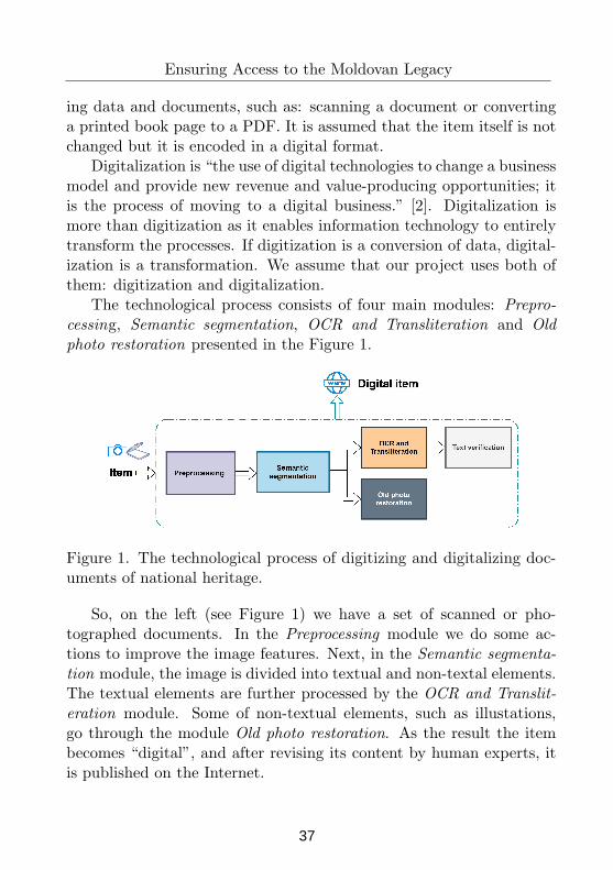
The technological process consists of four main modules: Prepro-
cessing, Semantic segmentation, OCR and Transliteration and Old
photo restoration presented in the Figure 1.
Figure 1. The technological process of digitizing and digitalizing doc-uments of national heritage.
So, on the left (see Figure 1) we have a set of scanned or pho-tographed documents. In the Preprocessing module we do some ac-tions to improve the image features. Next, in the Semantic segmenta-
tion module, the image is divided into textual and non-textal elements.The textual elements are further processed by the OCR and Translit-
eration module. Some of non-textual elements, such as illustations,go through the module Old photo restoration. As the result the itembecomes “digital”, and after revising its content by human experts, itis published on the Internet.
37
Tudor Bumbu, et al.
In the next subsections we try to describe the above mentionedmodules.
2.1 Preprocessing
Scanned or camera captured documents are obtained from differentsources, so they may have different quality. The purpose of preprocess-ing is to improve the features of the photos for further transformations.Preprocessing is an important step in machine learning, because at thisstage the initial data is adapted to be a compatible input into a neuralnetwork. The neural network that will process the scanned documentshas a fixed input size, i.e. it cannot receive images of different sizes asinput. Thus, at the current stage, the collected documents ought to beresized to a specific size.
Basic procedure that is being applied to the scanned documents isfinding their correct orientation. It allows the text to be displayed asusual, e.g. from left to right in Romanian. If the neural network thatrecognizes characters in the image is not taught to recognize them inany possible position, then document orientation is essential.
Currently, there are various free tools for image preprocessing.In artificial intelligence and especially deep learning, the OpenCV(www.opencv.org) library has widely supported the implementation ofmany real applications. Therefore, the use of this library is convenientfor the problem of document preprocessing.
Following the preprocessing module, the data is being sent to theSemantic segmentation module. This module identifies and extractstextual and non-textual elements in the document.
2.2 Semantic segmentation
Semantic segmentation of a document or document layout analysis isthe process of identifying and classifying regions of interest in an im-age. A reading system requires segmenting text areas (blocks) fromnon-textual ones and rendering them in the correct order of reading[3]. Detecting and labeling different blocks such as blocks of text and
38
Ensuring Access to the Moldovan Legacy
illustrations, mathematical symbols and tables embedded in a docu-ment is called geometric layout analysis [4]. Text blocks play differ-ent logical roles within the document (titles, subtitles, footnotes, etc.),and this type of semantic labeling is the scope of logical layout anal-ysis. Sometimes the segmentation phase is included in the documentpreprocessing stage.
A tool used for document segmentation tasks is Layout Parser [5].With the help of deep learning, the analyzer of geometric and logicallayouts supports the analysis and segmentation of very complex docu-ments and the processing of their hierarchical structure. This softwareis publicly available.
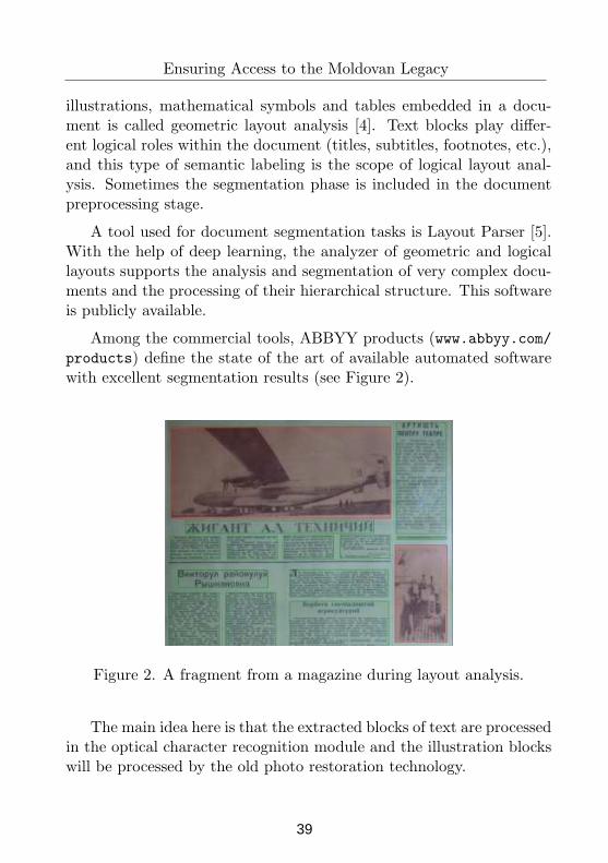
Among the commercial tools, ABBYY products (www.abbyy.com/products) define the state of the art of available automated softwarewith excellent segmentation results (see Figure 2).
Figure 2. A fragment from a magazine during layout analysis.
The main idea here is that the extracted blocks of text are processedin the optical character recognition module and the illustration blockswill be processed by the old photo restoration technology.
39
Tudor Bumbu, et al.
2.3 Old photo restoration
Old pictures are objects that portray the history and culture ofmankind. Restoring old photos is an opportunity to give them anew life. In the process of digitalization we will try to give a newlife to old photos from newspapers and magazines and also to photosof Moldovans working in the sovkhoz, women singing at vechornytsi(traditional gatherings), young boys who go to the army, Moldovanweddings, etc.
There exists an open-source tool that uses advanced deep learn-ing techniques, namely Bringing Old Photos Back to Life [6]. It helpsrestore photos that have been degraded over time, making them looknewer. In the case of newspapers and magazines, the process of restor-ing the blocks of illustrations can begin after the successful completionof the segmentation stage and can take place in parallel with the OCRand transliteration processes.
2.4 OCR and Transliteration
Optical character recognition, abbreviated as OCR, is the electronictranslation of scanned or photographed documents into editable text.
The software tool we use for optical character recognition is AB-BYY FineReader 15 (FR15). It has a learning module where a usertrains a neural network to recognize letters, punctuation and othercharacters. Once the system is well-trained, it manages to recognizethe characters it has already seen. FR15 does not learn as people learn.When recognizing a text block, it has a set of pre-trained neural net-work models, but there are also mechanisms that calculate some statis-tics and improve the recognition process. Thus, character by character,it uses the experience gained previously. Contextual information playsa significant role and is used in the FR15 OCR engine in a mannersimilar to what a person does when reading a text: people often pre-dict words and check themselves based on the meaning of the wholesentence. However, the experience gained is not shared between pagesor documents. The result of the training is an optical character recog-
40
Ensuring Access to the Moldovan Legacy
nition model.OCR models trained under Moldavian and Romanian Cyrillic al-
phabets are described in the paper [7]. We apply some of these modelsto blocks of text extracted from newspapers and magazines printed inthe 20th century.
Considering the fact that in Moldova we no longer use the Cyril-lic alphabet, a technology for transliterating the recognized text intoLatin script is absolutely necessary. Transliteration is the term used todescribe the process of converting a language from one unique writingsystem to another.
In the past, the Cyrillic alphabet was used in Moldova to printdocuments. Transliteration in this context is the replacement of Cyril-lic letters with Latin letters according to some specific rules. As amatter of fact, the transliteration of the Romanian language from the“Moldovan” writing into the Latin one started with the implementa-tion of Law no. 3462 of August 31, 1989, adopted by the Parliamentof the Republic of Moldova [8].
A technology for transliteration from the Cyrillic alphabet intothe Latin alphabet is being developed at the Institute of Math-ematics and Computer Science V. Andrunachievici from Moldova(www.translitera.cc). We use this tool for texts that have beenprocessed by FR15.
In the next subsection, we try to describe the handling of the texterrors after OCR and transliteration.
2.5 Text verification
In this paper text verification is about spell checking. It can be the laststep in the technological process before the digital item is published.The collections of the Moldovan written legacy that went through themodule of optical character recognition and transliteration, may havespelling mistakes. In order to place the digital items on the Internet,they must be verified and validated. We cannot depend entirely on anintelligent system to validate the text, thus an editor must perform thisjob but with the help of an intelligent system.
41
Tudor Bumbu, et al.
In recent years, a lot of work has been done on systems whichuse neural networks to correct an erroneous text. Some spell-checkingsystems are described in papers [9], [10]. The most common system ofthis kind is when we search on Google, and type a wrong word in thesearch bar. Google corrects us and returns the expected results.
A good spell-checking system is LanguageTool or LT(www.languagetool.org). It is a free text correction software in 25languages, including Romanian. LT can be used for linguistic correc-tion - stylistic, grammatical or orthographic. We use it to spell checktransliterated texts.
In the next section we describe the resources of newspapers andmagazines printed in the second half of the 20th century available inMoldova’s archives.
3 The resources
In 1944, the publication of the main periodicals before the war was re-sumed. Just as Latin script was banned at the time, most publicationswere printed in Cyrillic script. At the beginning of 1951, 180 newspa-per and 12 magazine titles were registered. The main publications wereMoldova Socialista, Sovietskaya Maldavia, Tanarul leninist. Until the1980s, other publications appeared, such as Literatura s
,i Arta, Femeia
Moldovei. Many publications published during this period have beenrenamed or replaced with new ones. Thus, until 1985, 13 republicannewspapers, 81 city and district newspapers and over 50 magazineswere published [1].
According to the Fund Manager of the Archive of Social and Polit-ical Organizations of the Republic of Moldova, most newspapers andmagazines were published monthly, on average, for 15 years [11]. Inaddition, there were weekly newspapers, such as the newspaper Cul-
tura. Only from the Fund Manager of the Archive of the social-politicalorganizations of the Republic of Moldova there are about 2000 uniquepublications. In addition to these, newspapers of kolkhozes were alsopublished, which raises the number of unique publications. The aprox-
42
Ensuring Access to the Moldovan Legacy
imative amount of newspapers and magazines printed from 1960 until1985 is 16 920 newspapers (94 titles) and 9 000 magazines (50 titles).The average number of pages of a newspaper and a magazine is 8. So,it is a huge amount of work to be done. These resources are stored inmany archives from the country. Two institutions we are working withnow are the Central Scientific Library “A. Lupan” and the NationalLibrary of Moldova.
4 Conclusion
This paper describes the innovative technologies used at digitizationand digitalization of some collections from the Moldovan legacy. Someof these technologies, such as OCR, Semantic segmentation and theOld photo restauration, use machine learning to excel in solving theproblem. By now we have more than 100 digized items, 13 of whichwere verified and published on www.emoldova.org. The digitization ofa newspaper page takes about 15 minutes, the text validation takes 30-50 minutes, the other technological processes take several seconds. Abig problem encountered is that practically there are no scanned news-papers and magazines from 1945 till 1989 and, temporary, we scan themusing our smartphones. In the future we plan to collaborate with Na-tional Library of Moldova and other archive institutions from Moldovain order to manage the priority of scanning the collections. The filemanagement is also an issue and we work at integration of GoogleDrive Api in our Web application. To reduce the time of publishing aresource we are going to optimize the tecnological process.
Acknowledgments. This work is supported by Est ComputerSRL in the E-Moldova project. The article was also written as a partof project 20.80009.5007.22 “Intelligent information systems for solvingill-structured problems, processing knowledge and big data”.
43
Tudor Bumbu, et al.
References
[1] C. MARIN. Mass-media. Enciclopedie. Chis, inau: BibliotecaS, tiint, ifica Centrala “A.Lupan” (Institut) a AS,M, 2016, pp. 761–778.
[2] Gartner Glossary. Digitalization, 2021.https://www.gartner.com/en/information-technol-ogy/glossary/digitalization.
[3] Baird, K.S. Anatomy of a versatile page reader. Proceedings of theIEEE. 80 (7), 1992, pp. 1059—1065.
[4] Cattoni, R.; Coianiz, T.; Messelodi, S.; Modena, C. M. Geometric
Layout Analysis Techniques for Document Image Understanding:
a Review. IRST, Trento, Italy, Tech. Rep. 9703-09, 2000.
[5] Z. Shen, R. Zhang, M. Dell. LayoutParser, 2020.https://github.com/Layout-Parser/layout-parser.
[6] Z. Wan, B. Zhang, D. Chen, P. Zhang, D. Chen, J.Liao, F. Wen. Bringing Old Photos Back to Life, 2020.https://arxiv.org/pdf/2004.09484.pdf.
[7] S. Cojocaru, A. Colesnicov, L. Malahov, T. Bumbu. Optical
Character Recognition Applied to Romanian Printed Texts of the
18th–20th Century. Computer Science Journal of Moldova, vol.24,no.1(70), 2016.
[8] Parlamentul Republicii Moldova. Legile din 31 august 1989
privind revenirea limbii moldovenes,ti la grafia latina. 1989.
https://bit.ly/3n76YSs.
[9] Sh. Ghosh, P. O. Kristensson. Neural Networks for Text
Correction and Completion in Keyboard Decoding, 2017.https://arxiv.org/pdf/1709.06429.pdf.
44
Ensuring Access to the Moldovan Legacy
[10] G. Lewis. Sentence Correction using Recurrent Neural Networks,
2016. https://cs224d.stanford.edu/reports/Lewis.pdf.
[11] Agent, ia Nat, ionala a Arhivelor. Indrumatorului Fondurilor al
Arhivei organizat,iilor social-politice a RM, pp. 60, 2019.
Tudor Bumbu1, Iulian Cernei2
1Vladimir Andrunachievici Institute of Mathematics and Computer Science
Email:[email protected]
1Moldova State University
Email:[email protected]
1Technical University of Moldova
Email:[email protected]
2Est Computer LLC
Email:[email protected]
45
Proceedings of the Conference on Mathematical Foundations of Informatics
MFOI’2020, January 12-16, 2021, Kyiv, Ukraine
© 2021 by Olesea Caftanatov1, Daniela Caganovshi2, Lucia Erhan3, Ecaterina
Hilea4
State of the Art: Augmented
reality Business Cards
Olesea Caftanatov1, Daniela Caganovschi2, Lucia Erhan3,
Ecaterina Hilea4
Abstract
In this work, we presented some reviews regarding business
cards evolution and new trends in applying augmented reality in
creating them. Additionally, we intend to present a few design
samples of various types of cards including business cards that our
team created for E-Moldova Project.
Keywords: business cards, augmented reality, E-Moldova.
1 Introduction
First of all, we will start with describing a situation that most of us
are familiar with. Let’s say, we are at some networking event and we handed our business card to someone, but after, we never hear from them
again. For this kind of situations, there are many reasons and one of it is
that people intend to forget whose these business cards are. When we are
handed dozens of business cards, it is difficult to remember each person
from whom the business card was received, what he did, and if so, how
the connection could benefit us. That’s why we may hard try to stand out
in the networking game.
An augmented reality (AR) business card would be a perfect
outcome for this problem, because with an AR business card we can stand
out from other outstanding people, so the other person will find it easier
for us. All they need to do is to point their phone at our business card. By
this article, we intend to revise the progress of business cards and their
variations (see Sections 4-5). Moreover, we want to present how AR
46
Olesea Caftanatov, et al.
technologies are used in creating business cards, (see Section 6). In
Section seven, we observed the importance of business card and review
some creativity approaches in designing them. Yet, we will start with a
description and provenance of business cards, (see Sections 2-3).
2 What is a business card?
According to the Cambridge Dictionary [1] and other sources [2-4],
a business card is a small, printed card with somebody’s name and details of their job and company on it.
The business card is an instrument of communication: it positions
us in a certain space, defines our status and the roles we fulfill in society,
thus indirectly providing information on education, professional training,
experience, socio-economic status, and degree of taking responsibility. An
almost necessary accessory in business relationships and not only, that
represents and defines us. It is part of the arsenal of the first impression,
along with the outfit, facial expressions, gestures, tone and timbre of the
voice, attitude and behavior, in general. Its role is well highlighted in
marketing, because it "sells" our image, our personal brand or the
company we present and represent. That is why we believe that business
cards are still relevant today, we still need them and in this regard we will
find new approaches to create more original and creative business cards,
so we could impress our final user. However, before we describe the
implementation of augmented reality technologies in creating business
cards, we will give a short review of its origins.
3 Origins of business cards
The first recorded use of business cards is dated in the 15th
century in Asia, China, which was as a kind of ticket used for commercial
purposes, named Meishi, see Figure 1. According to [5] Meishi contains
the Chinese characters for “name” (mei) and “to stick” (shi). The kanji,
for the verb “to stick” can be read as “card” or “paper”, which explains,
why meishi is sometimes incorrectly translated as “card name”. From
royalty to wealthy businessmen and traders these tickets (cards) were used
for the purpose of presentation in case of visits.
47
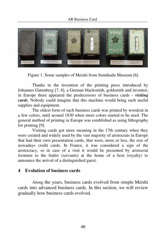
AR Business Card
Figure 1. Some samples of Meishi from Sumikadu Museum [6]
Thanks to the invention of the printing press introduced by
Johannes Gutenberg [7, 8], a German blacksmith, goldsmith and inventor,
in Europe there appeared the predecessors of business cards - visiting
cards. Nobody could imagine that this machine would bring such useful
supplies and equipment.
The oldest form of such business cards was printed by woodcut in
a few colors, until around 1830 when more colors started to be used. The
general method of printing in Europe was established as using lithography
for printing [9].
Visiting cards got more meaning in the 17th century when they
were created and widely used by the vast majority of aristocrats in Europe
that had their own presentation cards, that were, more or less, the size of
nowadays credit cards. In France, it was considered a sign of the
aristocracy, so in case of a visit it would be presented by aristocrat
footmen to the butler (servants) at the home of a host (royalty) to
announce the arrival of a distinguished guest.
4 Evolution of business cards
Along the years, business cards evolved from simple Meishi
cards into advanced business cards. In this section, we will review
gradually how business cards evolved.
48
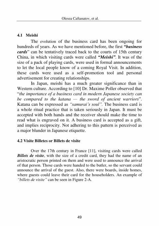
Olesea Caftanatov, et al.
4.1 Meishi
The evolution of the business card has been ongoing for
hundreds of years. As we have mentioned before, the first “business cards” can be tentatively traced back to the courts of 15th century
China, in which visiting cards were called “Meishi”. It was of the
size of a pack of playing cards, were used in formal announcements
to let the local people know of a coming Royal Visit. In addition,
these cards were used as a self-promotion tool and personal
advertisement for creating relationships.
In Japan, meishi has a much greater significance than in
Western culture. According to [10] Dr. Maxime Poller observed that
“the importance of a business card in modern Japanese society can
be compared to the katana — the sword of ancient warriors”. Katana can be expressed as “samurai’s soul”. The business card is
a whole ritual practice that is taken seriously in Japan. It must be
accepted with both hands and the receiver should make the time to
read what is engraved on it. A business card is accepted as a gift,
and implies reciprocity. Not adhering to this pattern is perceived as
a major blunder in Japanese etiquette.
4.2 Visite Billetes or Billets de visite
Over the 17th century in France [11], visiting cards were called
Billets de visite, with the size of a credit card, they had the name of an
aristocratic person printed on them and were used to announce the arrival
of that person. Those cards were handed to the butler, so the servant could
announce the arrival of the guest. Also, there were boards, inside homes,
where guests could leave their card for the householders. An example of
“billets de visite” can be seen in Figure 2-A.
49
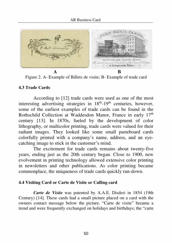
AR Business Card
A B
Figure 2. A- Example of Billets de visite; B- Example of trade card
4.3 Trade Cards
According to [12] trade cards were used as one of the most
interesting advertising strategies in 18th-19th centuries, however,
some of the earliest examples of trade cards can be found in the
Rothschild Collection at Waddesdon Manor, France in early 17th
century [13]. In 1870s, fueled by the development of color
lithography, or multicolor printing, trade cards were valued for their
radiant images. They looked like some small pasteboard cards
colorfully printed with a company’s name, address, and an eye-
catching image to stick in the customer’s mind. The excitement for trade cards remains about twenty-five
years, ending just as the 20th century began. Close to 1900, new
evolvement in printing technology allowed extensive color printing
in newsletters and other publications. As color printing became
commonplace, the uniqueness of trade cards quickly run-down.
4.4 Visiting Card or Carte de Visite or Calling card
Carte de Visite was patented by A.A.E. Disderi in 1854 (19th
Century) [14]. These cards had a small picture placed on a card with the
owners contact message below the picture. “Carte de visite” became a
trend and were frequently exchanged on holidays and birthdays; the “carte
50
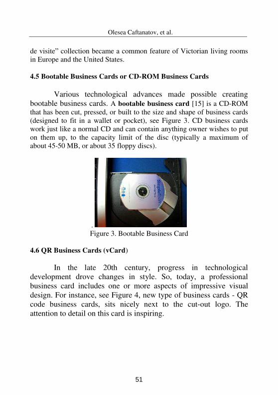
Olesea Caftanatov, et al.
de visite” collection became a common feature of Victorian living rooms
in Europe and the United States.
4.5 Bootable Business Cards or CD-ROM Business Cards
Various technological advances made possible creating
bootable business cards. A bootable business card [15] is a CD-ROM
that has been cut, pressed, or built to the size and shape of business cards
(designed to fit in a wallet or pocket), see Figure 3. CD business cards
work just like a normal CD and can contain anything owner wishes to put
on them up, to the capacity limit of the disc (typically a maximum of
about 45-50 MB, or about 35 floppy discs).
.
Figure 3. Bootable Business Card
4.6 QR Business Cards (vCard)
In the late 20th century, progress in technological
development drove changes in style. So, today, a professional
business card includes one or more aspects of impressive visual
design. For instance, see Figure 4, new type of business cards - QR
code business cards, sits nicely next to the cut-out logo. The
attention to detail on this card is inspiring.
51

AR Business Card
Figure 4. Example of QR code Business Card
QR Business Cards [16-17] are the simplest way to connect online
with offline and bring a substantial addition to traditional design being an
inexpensive marketing strategy. Any kind of relevant information can be
encoded in the text, referenced on the website, in the contact section or
encoded in a digital business card. Thus, the person benefits from a double
advantage: traditional business card, offered in printed form, on support of
normal cardboard, colored, plastic or semi-transparent polypropylene, and
information encoded in the QR code, which can send the scanner
information directly to the owner's website, Facebook, Twitter or other
social media account.
4.7 Augmented Reality Business Cards
Augmented Reality (AR) business cards bring the ability to
expand the information contained in a business card, without needing to
make it larger or assemble it with many things. So, how does it work? AR
apps work using real world objects (markers) that trigger some reactions
when recognized and then these markers are superimposed with digital
information, when a user points a camera at them. To achieve an AR
business card, certain things are needed:
52
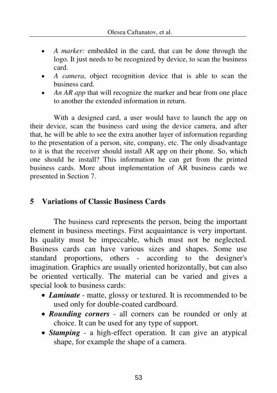
Olesea Caftanatov, et al.
A marker: embedded in the card, that can be done through the
logo. It just needs to be recognized by device, to scan the business
card.
A camera, object recognition device that is able to scan the
business card.
An AR app that will recognize the marker and bear from one place
to another the extended information in return.
With a designed card, a user would have to launch the app on
their device, scan the business card using the device camera, and after
that, he will be able to see the extra another layer of information regarding
to the presentation of a person, site, company, etc. The only disadvantage
to it is that the receiver should install AR app on their phone. So, which
one should he install? This information he can get from the printed
business cards. More about implementation of AR business cards we
presented in Section 7.
5 Variations of Classic Business Cards
The business card represents the person, being the important
element in business meetings. First acquaintance is very important.
Its quality must be impeccable, which must not be neglected.
Business cards can have various sizes and shapes. Some use
standard proportions, others - according to the designer's
imagination. Graphics are usually oriented horizontally, but can also
be oriented vertically. The material can be varied and gives a
special look to business cards:
Laminate - matte, glossy or textured. It is recommended to be
used only for double-coated cardboard.
Rounding corners - all corners can be rounded or only at
choice. It can be used for any type of support.
Stamping - a high-effect operation. It can give an atypical
shape, for example the shape of a camera.
53
AR Business Card
Selective varnish application - to highlight certain graphic
elements of the business card.
Folio - for printing dark cardboard with gold, silver or other
special colors.
Emboss - to highlight certain graphic elements of the business
card.
Traditionally, business cards were made with all kinds of
ornaments and drawings, more and more elaborate and colorful, true
works of art, which were later abandoned, in favor of simpler
business cards. Sometimes the cards were engraved with gold and
typefaces, or were decorated with ornaments and sometimes -
elegant coats of arms. However, due to technology progress,
business cards became more sophisticated. There are new
approaches in creating BC, for example, using augmented reality to
add a hidden layer of information on printed cards. In next, sections
we will describe few types of AR used in designing business cards.
6 Marker-Based Augmented Reality Business Cards
With emerging tech like augmented reality, the interaction
between printed and digital media became possible. Our objective is
to explore this interaction in order to create business cards. We
study few types of AR technologies and decided to use marker-
based augmented reality to create business cards.
Marker-based augmented reality is one of the most common
types; it uses markers to trigger an augmented experience. Right to
its use of image recognition, this type of AR is occasionally called
also recognition-based augmented reality. Marker-based AR works
when a camera or app is scanned over visual marker. A brief
example, of a visual marker is a QR code or a 2D cipher. Generally,
54
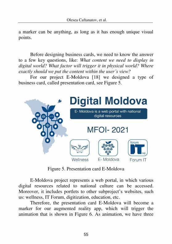
Olesea Caftanatov, et al.
a marker can be anything, as long as it has enough unique visual
points.
Before designing business cards, we need to know the answer
to a few key questions, like: What content we need to display in
digital world? What factor will trigger it in physical world? Where
exactly should we put the content within the user’s view?
For our project E-Moldova [18] we designed a type of
business card, called presentation card, see Figure 5.
Figure 5. Presentation card E-Moldova
E-Moldova project represents a web portal, in which various
digital resources related to national culture can be accessed.
Moreover, it includes portlets to other subproject’s websites, such us: wellness, IT Forum, digitization, education, etc.
Therefore, the presentation card E-Moldova will become a
marker for our augmented reality app, which will trigger the
animation that is shown in Figure 6. As animation, we have three
55
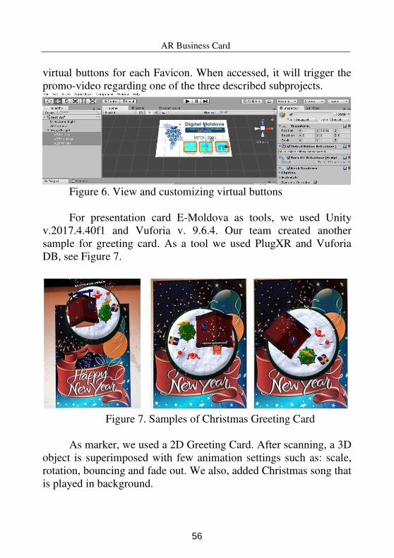
AR Business Card
virtual buttons for each Favicon. When accessed, it will trigger the
promo-video regarding one of the three described subprojects.
Figure 6. View and customizing virtual buttons
For presentation card E-Moldova as tools, we used Unity
v.2017.4.40f1 and Vuforia v. 9.6.4. Our team created another
sample for greeting card. As a tool we used PlugXR and Vuforia
DB, see Figure 7.
Figure 7. Samples of Christmas Greeting Card
As marker, we used a 2D Greeting Card. After scanning, a 3D
object is superimposed with few animation settings such as: scale,
rotation, bouncing and fade out. We also, added Christmas song that
is played in background.
56
Olesea Caftanatov, et al.
7 Importance and creativity of business cards
Business cards are multifunctional tools that fulfill many
professional missions: advertising, brand recognition, and of course,
communicating contact details. When designed correctly, these mini
billboards can have a large and long-lasting impact, turning
occasional meetings into loyal customers. The business card is a
good tool to make you known. It is an essential communication tool
if you want to make yourself known and expand your professional
network. Indeed, the competition in the professional world is so
fierce that we must give ourselves every opportunity to increase our
visibility and attract new clients. During a meeting, the business
card is effective for conveying contact details as well as essential
information about your professional activities or company. It is a
small window that opens to the professional world.
This is why the content of a business card must be carefully
crafted to be as attractive as possible. So when we introduce
ourselves to potential customers, it's the right time to take out the
business card. In this way we capture the interlocutor's attention, we
do not force him to ask for all the information about us and more
importantly, we give an impression of solidity and professionalism.
It is a bit of the same concept that underlies uniforms and
identification badges: business cards, if presented correctly, certify
a role and authority in a particular field.
Regarding business card for our teammates, we created a
sample that includes in hidden layout such digital elements as: text,
buttons (that link to social media), video, avatar, 3D object. As a
marker, we used template, as it is shown in Figure 8-A. The result,
can be seen in Figure 8-B.
57
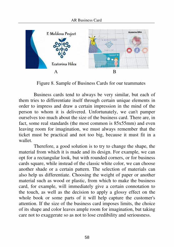
AR Business Card
A B
Figure 8. Sample of Business Cards for our teammates
Business cards tend to always be very similar, but each of
them tries to differentiate itself through certain unique elements in
order to impress and draw a certain impression in the mind of the
person to whom it is delivered. Unfortunately, we can't pamper
ourselves too much about the size of the business card. There are, in
fact, some real standards (the most common is 85x55mm) and even
leaving room for imagination, we must always remember that the
ticket must be practical and not too big, because it must fit in a
wallet.
Therefore, a good solution is to try to change the shape, the
material from which it is made and its design. For example, we can
opt for a rectangular look, but with rounded corners, or for business
cards square, while instead of the classic white color, we can choose
another shade or a certain pattern. The selection of materials can
also help us differentiate. Choosing the weight of paper or another
material such as wood or plastic, from which to make the business
card, for example, will immediately give a certain connotation to
the touch, as well as the decision to apply a glossy effect on the
whole book or some parts of it will help capture the customer's
attention. If the size of the business card imposes limits, the choice
of its shape and color leaves ample room for imagination, but taking
care not to exaggerate so as not to lose credibility and seriousness.
58
Olesea Caftanatov, et al.
Business cards can also be an extremely useful virtual thing
if we consider the situation we are all in at the moment. A large part
of conferences, seminars and business meetings take place online
which limits physical contact, and at this time a printed business
card is losing ground to a virtual business card.
8 Conclusion
Along our study, we observed that people can be very creative
in creating their business cards. They can use various types of
material, such as: wood, plastic, metals, papers, applications etc.
Due to new progress in technologies, it is possible to bring new
approaches in creating various types of cards (business cards,
invited cards, greeting cards, presentation cards etc.). For now, we
consider that using augmented reality in integrating digital content
on printing content became a novelty that should be explored. Since
a well-designed and crafted business card will make all the
difference, so it will make a good impression on receiver.
Acknowledgments
We would like to express our sincere gratitude to our
coordinator Dr. Ioachim Druguș for the continuous support and for
giving us the opportunity to study and research the possibility of
interaction between printed and digital media. By exploring
augmented reality in designing business cards we came to know
about many new and interesting things, so we are really thankful for
this. In addition, this work was supported by project “Intelligent information systems for solving ill-structured problems, processing
knowledge and big data”.
59
AR Business Card
References
[1] Cambridge Dictionary Website, Business Card. Accessed on December 12,
2020. https://dictionary.cambridge.org/dictionary/english/business-card
[2] Wikipedia Website, Business Card. Accessed on December 12, 2020.
https://en.wikipedia.org/wiki/Business_card
[3] Entrepreneur Encyclopedia Website, Business Card. Accessed on December
12, 2020. https://www.entrepreneur.com/encyclopedia/business-card
[4] Collins Dictionary Website. Business Card. Accessed on December 12,
2020. https://www.collinsdictionary.com/dictionary/english/business-card
[5] J.J. O’Donoghue. Calling card: the evolution of business card in Japan.
Japan Times Journal. May 6, 2017. Journal Website:
https://www.japantimes.co.jp/life/2017/05/06/lifestyle/calling-card-
evolution-business-cards-japan/
[6] Digita Exposition. Meisi and Paper Products in Sumida-ku Museum.
Museum website: https://whereintokyo.com/venues/25717.html
[7] History Website. Printing Press. Accessed on December 20, 2020.
https://www.history.com/topics/inventions/printing-press
[8] H.E. Lehmann-Haupt. Johannes Gutenberg, German printer. Published on
Britannica Encyclopedia Website. Accessed on January 4, 2021.
https://www.britannica.com/biography/Johannes-Gutenberg
[9] General History Website. The Hostory of Business Cards. Accessed on
January 3, 2021. https://general-history.com/the-history-of-business-cards/
[10] A. Cantrell. This is a Mostly True Story About… Business Cards. Published
on Institutional Investor Website. August 10, 2020.
https://www.institutionalinvestor.com/article/b1mwcw55h6c8p8/This-Is-a-
Mostly-True-Story-About-Business-Cards
[11] C. Dempsey. The History of the Calling Card. Published on E18HTEEN
SE7ENTY EI8HT Website. Accessed on Noveber 27, 2020.
https://eighteenseventyeight.com/2016/08/11/the-history-of-the-calling-card-
2/
[12] Cornell University Library Website. Trade Cards. An Illustrated History.
Highlights from the Waxman Collection. Accessed on January 5, 2021.
https://rmc.library.cornell.edu/tradecards/exhibition/history/index.html#moda
lClosed
[13] P. Hubbard. Trade Cards in 18th – Century Consumer Culture: Circulation,
and Exchange in Commercial and Collecting Spaces. Published in Digital
60
Olesea Caftanatov, et al.
Journal, UNB Libraries. Website was accessed on January 5, 2021.
https://journals.lib.unb.ca/index.php/mcr/article/view/20447/23603
[14] Britannica Encyclopedia Website. André-Adolphe-Eugène Disdéri. French photographer. Accessed on January 7, 2021.
https://www.britannica.com/biography/Andre-Adolphe-Eugene-Disderi
[15] Band CDS Company Website. How do CD business cards work. Accessed
on January 3, 2021. https://www.bandcds.co.uk/faqs/cd-business-cards-work/
[16] Business Cards Tech-IT Company Website. Share your data with 2D
Barcodes. Accessed on January 3, 2021. https://businesscards.tec-it.com/en
[17] Wikipedia. vCard. Accessed on January 4, 2021.
https://en.wikipedia.org/wiki/VCard
[18] Digital Moldova Projects Official Websites. https://emoldova.org/
Olesea Caftanatov1, Daniela Caganovschi2, Lucia Erhan3, Ecaterina Hilea4
1Vladimir Andrunachievici Institute of Mathematics and Computer Science; SRL
EST Computer
E-mail: [email protected]
2State University of Moldova; SRL EST Computer
E-mail: [email protected]
3SRL EST Computer
E-mail: [email protected]
4State University of Moldova; SRL EST Computer
E-mail: [email protected]
61
Proceedings of the Conference on Mathematical Foundations of Informatics
MFOI’2020, January 12-16, 2021, Kyiv, Ukraine
© 2021 by Irina Cercel, Adrian Iftene
Planetarium - An Augmented
Reality Application
Irina Cercel, Adrian Iftene
Abstract
In a short period of time, technology has exploded on the
market, growing not only in IT but also in areas such as health,
education, or astronomy. Although the future is unknown, digital
progress continues to shape the world in ways that encourage people
to form new habits and learn something new every day. The
Planetarium application is intended for any user who wants to know
information about the celestial bodies of our solar system. It can
visualise the 8 planets (Mercury, Venus, Earth, Mars, Jupiter, Saturn,
Uranus, and Neptune) and the dwarf planet Pluto, orbiting the Sun,
but also the Moon, in their real positions when using the application,
with the help of augmented reality (AR). The user can interact with
the 3D object to find out brief information about it.
Keywords: solar system, augmented reality, mobile app.
1 Introduction
The field of mobile phones has also developed a major change in recent
years, smartphones making their appearance. They make people’s lives much easier through various possibilities to communicate remotely (chat,
telephony), through different applications that help them organize their
daily activities (e-mail, calendar, text editing and spreadsheets), games, but
also through applications that help them learn something new (as is the case
of this application).
The evolution of mobile phones has allowed the inclusion and use of
augmented reality (AR), which has opened the way to another world, one
in which reality merges with fiction. AR is not only used for entertainment,
in the field of games, but also for education. It arouses the curiosity of both
children and adults through the innovations it brings to the learning system.
62
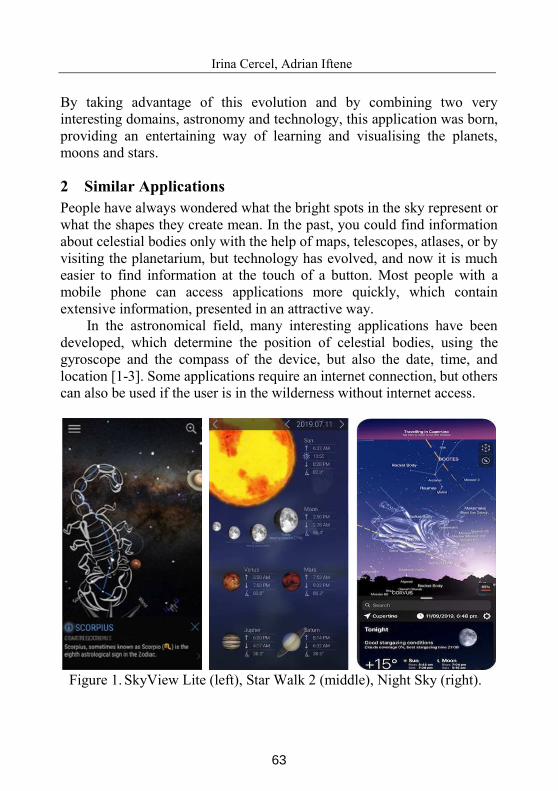
Irina Cercel, Adrian Iftene
By taking advantage of this evolution and by combining two very
interesting domains, astronomy and technology, this application was born,
providing an entertaining way of learning and visualising the planets,
moons and stars.
2 Similar Applications
People have always wondered what the bright spots in the sky represent or
what the shapes they create mean. In the past, you could find information
about celestial bodies only with the help of maps, telescopes, atlases, or by
visiting the planetarium, but technology has evolved, and now it is much
easier to find information at the touch of a button. Most people with a
mobile phone can access applications more quickly, which contain
extensive information, presented in an attractive way.
In the astronomical field, many interesting applications have been
developed, which determine the position of celestial bodies, using the
gyroscope and the compass of the device, but also the date, time, and
location [1-3]. Some applications require an internet connection, but others
can also be used if the user is in the wilderness without internet access.
Figure 1. SkyView Lite (left), Star Walk 2 (middle), Night Sky (right).
63
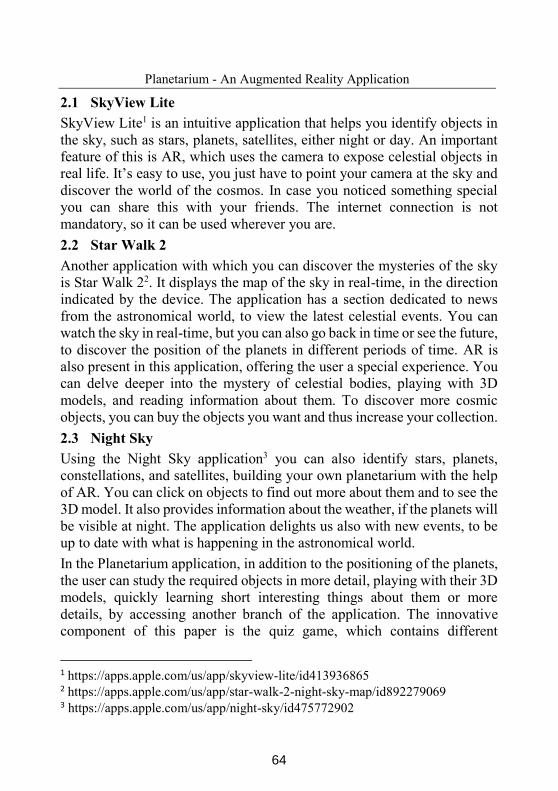
Planetarium - An Augmented Reality Application
2.1 SkyView Lite
SkyView Lite1 is an intuitive application that helps you identify objects in
the sky, such as stars, planets, satellites, either night or day. An important
feature of this is AR, which uses the camera to expose celestial objects in
real life. It’s easy to use, you just have to point your camera at the sky and
discover the world of the cosmos. In case you noticed something special
you can share this with your friends. The internet connection is not
mandatory, so it can be used wherever you are.
2.2 Star Walk 2
Another application with which you can discover the mysteries of the sky
is Star Walk 22. It displays the map of the sky in real-time, in the direction
indicated by the device. The application has a section dedicated to news
from the astronomical world, to view the latest celestial events. You can
watch the sky in real-time, but you can also go back in time or see the future,
to discover the position of the planets in different periods of time. AR is
also present in this application, offering the user a special experience. You
can delve deeper into the mystery of celestial bodies, playing with 3D
models, and reading information about them. To discover more cosmic
objects, you can buy the objects you want and thus increase your collection.
2.3 Night Sky
Using the Night Sky application3 you can also identify stars, planets,
constellations, and satellites, building your own planetarium with the help
of AR. You can click on objects to find out more about them and to see the
3D model. It also provides information about the weather, if the planets will
be visible at night. The application delights us also with new events, to be
up to date with what is happening in the astronomical world.
In the Planetarium application, in addition to the positioning of the planets,
the user can study the required objects in more detail, playing with their 3D
models, quickly learning short interesting things about them or more
details, by accessing another branch of the application. The innovative
component of this paper is the quiz game, which contains different
1 https://apps.apple.com/us/app/skyview-lite/id413936865
2 https://apps.apple.com/us/app/star-walk-2-night-sky-map/id892279069
3 https://apps.apple.com/us/app/night-sky/id475772902
64
Irina Cercel, Adrian Iftene
questions related to the information presented in the other components of
the application, and through which the user can test his knowledge, but
more about this will be presented in the future chapters.
3 Proposed System
Planetarium is intended for all people who want to learn about our solar
system, the application combining the virtual world with the real world
through AR, providing information about its celestial bodies, but also
offering the user the opportunity to test his knowledge through a game with
multiple questions. The application has 3 main components, these being AR
Experience, Almanac, and Trivia Game. For its development we used
Xcode4 and the Swift5 programming language.
Figure 2. Application architecture
4 https://developer.apple.com/xcode/ 5 https://developer.apple.com/swift/
65
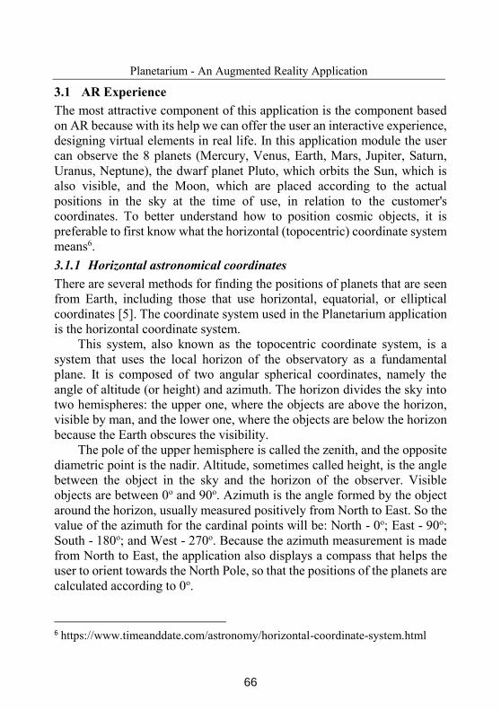
Planetarium - An Augmented Reality Application
3.1 AR Experience
The most attractive component of this application is the component based
on AR because with its help we can offer the user an interactive experience,
designing virtual elements in real life. In this application module the user
can observe the 8 planets (Mercury, Venus, Earth, Mars, Jupiter, Saturn,
Uranus, Neptune), the dwarf planet Pluto, which orbits the Sun, which is
also visible, and the Moon, which are placed according to the actual
positions in the sky at the time of use, in relation to the customer's
coordinates. To better understand how to position cosmic objects, it is
preferable to first know what the horizontal (topocentric) coordinate system
means6.
3.1.1 Horizontal astronomical coordinates
There are several methods for finding the positions of planets that are seen
from Earth, including those that use horizontal, equatorial, or elliptical
coordinates [5]. The coordinate system used in the Planetarium application
is the horizontal coordinate system.
This system, also known as the topocentric coordinate system, is a
system that uses the local horizon of the observatory as a fundamental
plane. It is composed of two angular spherical coordinates, namely the
angle of altitude (or height) and azimuth. The horizon divides the sky into
two hemispheres: the upper one, where the objects are above the horizon,
visible by man, and the lower one, where the objects are below the horizon
because the Earth obscures the visibility.
The pole of the upper hemisphere is called the zenith, and the opposite
diametric point is the nadir. Altitude, sometimes called height, is the angle
between the object in the sky and the horizon of the observer. Visible
objects are between 0o and 90o. Azimuth is the angle formed by the object
around the horizon, usually measured positively from North to East. So the
value of the azimuth for the cardinal points will be: North - 0o; East - 90o;
South - 180o; and West - 270o. Because the azimuth measurement is made
from North to East, the application also displays a compass that helps the
user to orient towards the North Pole, so that the positions of the planets are
calculated according to 0o.
6 https://www.timeanddate.com/astronomy/horizontal-coordinate-system.html
66
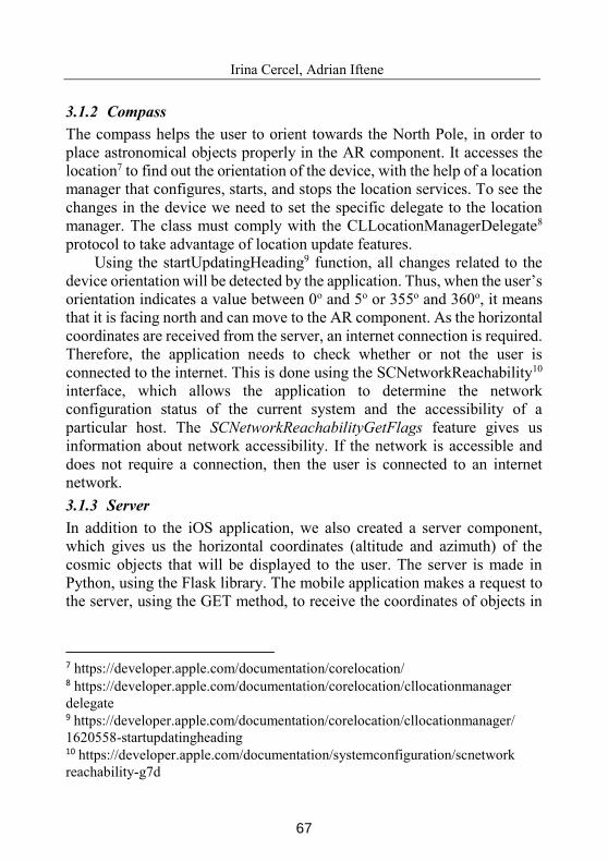
Irina Cercel, Adrian Iftene
3.1.2 Compass
The compass helps the user to orient towards the North Pole, in order to
place astronomical objects properly in the AR component. It accesses the
location7 to find out the orientation of the device, with the help of a location
manager that configures, starts, and stops the location services. To see the
changes in the device we need to set the specific delegate to the location
manager. The class must comply with the CLLocationManagerDelegate8
protocol to take advantage of location update features.
Using the startUpdatingHeading9 function, all changes related to the
device orientation will be detected by the application. Thus, when the user’s orientation indicates a value between 0o and 5o or 355o and 360o, it means
that it is facing north and can move to the AR component. As the horizontal
coordinates are received from the server, an internet connection is required.
Therefore, the application needs to check whether or not the user is
connected to the internet. This is done using the SCNetworkReachability10
interface, which allows the application to determine the network
configuration status of the current system and the accessibility of a
particular host. The SCNetworkReachabilityGetFlags feature gives us
information about network accessibility. If the network is accessible and
does not require a connection, then the user is connected to an internet
network.
3.1.3 Server
In addition to the iOS application, we also created a server component,
which gives us the horizontal coordinates (altitude and azimuth) of the
cosmic objects that will be displayed to the user. The server is made in
Python, using the Flask library. The mobile application makes a request to
the server, using the GET method, to receive the coordinates of objects in
7 https://developer.apple.com/documentation/corelocation/ 8 https://developer.apple.com/documentation/corelocation/cllocationmanager
delegate 9 https://developer.apple.com/documentation/corelocation/cllocationmanager/
1620558-startupdatingheading 10
https://developer.apple.com/documentation/systemconfiguration/scnetwork
reachability-g7d
67
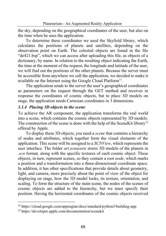
Planetarium - An Augmented Reality Application
the sky, depending on the geographical coordinates of the user, but also on
the time when he uses the application.
To determine these coordinates we used the Skyfield library, which
calculates the positions of planets and satellites, depending on the
observation point on Earth. The celestial objects are found in the file
“de421.bsp”, which we can access after uploading this file, as objects of a
dictionary, by name. In relation to the resulting object indicating the Earth,
the time at the moment of the request, the longitude and latitude of the user,
we will find out the positions of the other planets. Because the server must
be accessible from anywhere we call the application, we decided to make it
available on the Internet using the Google Cloud Platform11.
The application sends to the server the user’s geographical coordinates as parameters on the request through the GET method and receives in
response the coordinates of cosmic objects, but to place 3D models on
stage, the application needs Cartesian coordinates in 3 dimensions.
3.1.4 Placing 3D objects in the scene
To achieve the AR component, the application transforms the real world
into a scene, which contains the cosmic objects represented by 3D models.
The construction of the scene is done with the help of the SceneKit library12
offered by Apple.
To display these 3D objects, you need a scene that contains a hierarchy
of nodes and attributes, which together form the visual elements of the
application. This scene will be assigned to a SCNView, which represents the
user interface. The folder art.scnassets stores 3D models of the planets in
.scn format, along with the specific textures of each cosmic object. These
objects, in turn, represent scenes, so they contain a root node, which marks
a position and a transformation into a three-dimensional coordinate space.
In addition, it has other specifications that provide details about geometry,
light, and camera, more precisely about the point of view of the object for
displaying on stage, how the 3D model looks, its texture, orientation, and
scaling. To form the structure of the main scene, the nodes of the scenes of
cosmic objects are added to the hierarchy, but we must specify their
position. Having the horizontal coordinates of the cosmic objects received
11 https://cloud.google.com/appengine/docs/standard/python3/building-app
12 https://developer.apple.com/documentation/scenekit
68
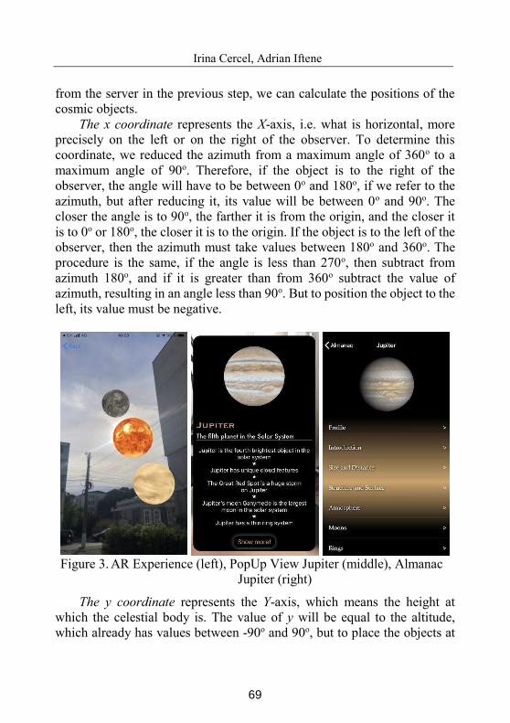
Irina Cercel, Adrian Iftene
from the server in the previous step, we can calculate the positions of the
cosmic objects.
The x coordinate represents the X-axis, i.e. what is horizontal, more
precisely on the left or on the right of the observer. To determine this
coordinate, we reduced the azimuth from a maximum angle of 360o to a
maximum angle of 90o. Therefore, if the object is to the right of the
observer, the angle will have to be between 0o and 180o, if we refer to the
azimuth, but after reducing it, its value will be between 0o and 90o. The
closer the angle is to 90o, the farther it is from the origin, and the closer it
is to 0o or 180o, the closer it is to the origin. If the object is to the left of the
observer, then the azimuth must take values between 180o and 360o. The
procedure is the same, if the angle is less than 270o, then subtract from
azimuth 180o, and if it is greater than from 360o subtract the value of
azimuth, resulting in an angle less than 90o. But to position the object to the
left, its value must be negative.
Figure 3. AR Experience (left), PopUp View Jupiter (middle), Almanac
Jupiter (right)
The y coordinate represents the Y-axis, which means the height at
which the celestial body is. The value of y will be equal to the altitude,
which already has values between -90o and 90o, but to place the objects at
69
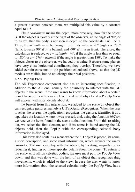
Planetarium - An Augmented Reality Application
a greater distance between them, we multiplied this value by a constant
equal to 1.5.
The z coordinate means the depth, more precisely, how far the object
is. If the object is exactly at the right of the observer, at the angle of 90o, or
to its left, then the body is not seen in depth, so the coordinate z will be 0.
Thus, the azimuth must be brought to 0 if its value is 90o (right) or 270o
(left), towards 90o if it is behind, and -90o if it is in front. Therefore, the
calculation is reduced to z = azimuth - 90o, if the angle is less than or equal
to 180o, or z = 270o - azimuth if the angle is greater than 180o. To make the
objects closer to the observer, we halved this value. Because some planets
have very close horizontal coordinates, they overlap. Therefore, we have
added certain constants to the positions calculated above, so that the 3D
models are visible, but do not change their real positions.
3.1.5 PopUp View
The AR Experience component also has an interesting specification, in
addition to the AR one, namely the possibility to interact with the 3D
objects in the scene. If the user wants to know information about a certain
planet he sees, then he can click on the desired object and a PopUp View
will appear, with short details about it.
To benefit from this interaction, we added to the scene an object that
can recognize gestures, namely a UITapGestureRecognizer. When the user
touches the screen, the application recognizes the gesture, identifies it as a
tap, takes the location where it was pressed, and, using the function hitTest,
we receive the items found in the scene at that location. From this resulting
list, we select the first element, and if its name is found among the 3D
objects held, then the PopUp with the corresponding celestial body
information is displayed.
This view also contains a scene where the 3D object is placed, its name,
a short description, and some short information, which arouses the user’s curiosity. The user can play with the object, by rotating, magnifying, or
reducing it, finding out more specific details about the planet. To return to
the scene with all the celestial bodies, the user must pull the PopUp View
down, and this was done with the help of an object that recognizes drag
movements, which is added to the view. In case the user wants to know
more information about the selected celestial body, the PopUp View has a
70
Irina Cercel, Adrian Iftene
button, which sends it to the corresponding cosmic object in the next
component, Almanac.
3.2 Almanac
The almanac holds all the celestial bodies in the database and information
about them. The application uses a collection of data, this data is
represented by custom cells. In order to display them, the collection must
have a source object, from which it obtains its data, and this is done by
adopting the UICollectionViewDataSource protocol. The data source
provides both the content for the elements and the interfaces for each one.
When the collection loads its contents, it asks the data source to provide an
interface for each visible element. The collection also maintains a list of
visual objects, which are marked by the data source for reuse. Instead of
creating a new view for each item, reuse one that needs to be removed
because it is no longer visible.
In addition to displaying cells, the collection also manages selected
items using the delegated object. To make it easier to search for a cosmic
object, the application also benefits from a search controller, built into the
navigation bar. Behind the cells in the collection is hidden more information
about cosmic objects, so by pressing one of them, the application sends the
user to the screen containing the data about the selected celestial body.
3.3 Database
After we talked about how information about cosmic objects is displayed,
this chapter is for the database that holds this information. To save all the
data about the celestial bodies we used the RealmSwift database13. It is
intended for mobile devices with iOS operating systems. The data is
represented by an object-oriented data model, being flexible, and easy to
use. Realm runs directly on devices, accessing objects using the Swift
language, making the process of storing, updating and accessing data much
easier. Being a local database, the internet connection is not mandatory,
users having the opportunity to learn anywhere.
It contains the following properties: name = name of the cosmic object;
shortDescription = optional property, specific only to objects that appear
in the AR Experience component, indicating a short description of that
object, displayed in PopUp View; profiles = Realm object, which means
13 https://docs.mongodb.com/realm-legacy/docs/swift/latest/
71
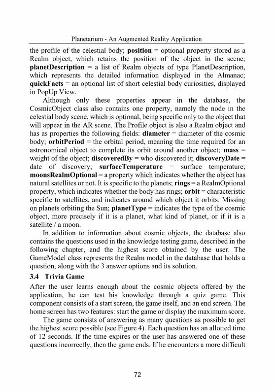
Planetarium - An Augmented Reality Application
the profile of the celestial body; position = optional property stored as a
Realm object, which retains the position of the object in the scene;
planetDescription = a list of Realm objects of type PlanetDescription,
which represents the detailed information displayed in the Almanac;
quickFacts = an optional list of short celestial body curiosities, displayed
in PopUp View.
Although only these properties appear in the database, the
CosmicObject class also contains one property, namely the node in the
celestial body scene, which is optional, being specific only to the object that
will appear in the AR scene. The Profile object is also a Realm object and
has as properties the following fields: diameter = diameter of the cosmic
body; orbitPeriod = the orbital period, meaning the time required for an
astronomical object to complete its orbit around another object; mass =
weight of the object; discoveredBy = who discovered it; discoveryDate =
date of discovery; surfaceTemperature = surface temperature;
moonsRealmOptional = a property which indicates whether the object has
natural satellites or not. It is specific to the planets; rings = a RealmOptional
property, which indicates whether the body has rings; orbit = characteristic
specific to satellites, and indicates around which object it orbits. Missing
on planets orbiting the Sun; planetType = indicates the type of the cosmic
object, more precisely if it is a planet, what kind of planet, or if it is a
satellite / a moon.
In addition to information about cosmic objects, the database also
contains the questions used in the knowledge testing game, described in the
following chapter, and the highest score obtained by the user. The
GameModel class represents the Realm model in the database that holds a
question, along with the 3 answer options and its solution.
3.4 Trivia Game
After the user learns enough about the cosmic objects offered by the
application, he can test his knowledge through a quiz game. This
component consists of a start screen, the game itself, and an end screen. The
home screen has two features: start the game or display the maximum score.
The game consists of answering as many questions as possible to get
the highest score possible (see Figure 4). Each question has an allotted time
of 12 seconds. If the time expires or the user has answered one of these
questions incorrectly, then the game ends. If he encounters a more difficult
72
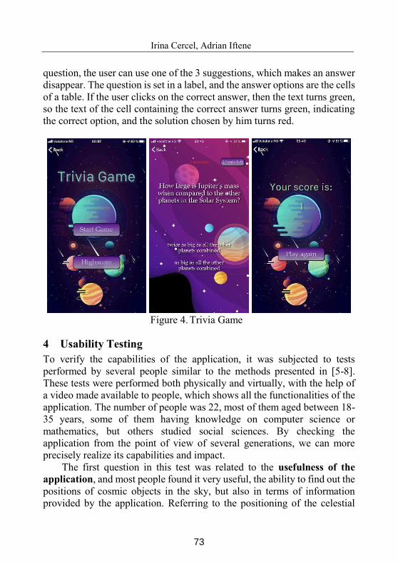
Irina Cercel, Adrian Iftene
question, the user can use one of the 3 suggestions, which makes an answer
disappear. The question is set in a label, and the answer options are the cells
of a table. If the user clicks on the correct answer, then the text turns green,
so the text of the cell containing the correct answer turns green, indicating
the correct option, and the solution chosen by him turns red.
Figure 4. Trivia Game
4 Usability Testing
To verify the capabilities of the application, it was subjected to tests
performed by several people similar to the methods presented in [5-8].
These tests were performed both physically and virtually, with the help of
a video made available to people, which shows all the functionalities of the
application. The number of people was 22, most of them aged between 18-
35 years, some of them having knowledge on computer science or
mathematics, but others studied social sciences. By checking the
application from the point of view of several generations, we can more
precisely realize its capabilities and impact.
The first question in this test was related to the usefulness of the
application, and most people found it very useful, the ability to find out the
positions of cosmic objects in the sky, but also in terms of information
provided by the application. Referring to the positioning of the celestial
73
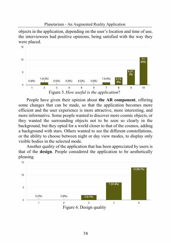
Planetarium - An Augmented Reality Application
objects in the application, depending on the user’s location and time of use, the interviewees had positive opinions, being satisfied with the way they
were placed.
Figure 5. How useful is the application?
People have given their opinion about the AR component, offering
some changes that can be made, so that the application becomes more
efficient and the user experience is more attractive, more interesting, and
more informative. Some people wanted to discover more cosmic objects, or
they wanted the surrounding objects not to be seen so clearly in the
background, but they opted for a world closer to that of the cosmos, adding
a background with stars. Others wanted to see the different constellations,
or the ability to choose between night or day view modes, to display only
visible bodies in the selected mode.
Another quality of the application that has been appreciated by users is
that of the design. People considered the application to be aesthetically
pleasing.
Figure 6. Design quality
74
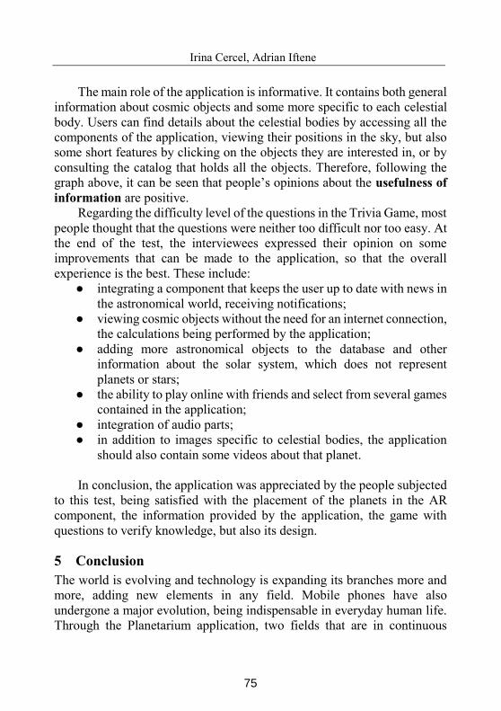
Irina Cercel, Adrian Iftene
The main role of the application is informative. It contains both general
information about cosmic objects and some more specific to each celestial
body. Users can find details about the celestial bodies by accessing all the
components of the application, viewing their positions in the sky, but also
some short features by clicking on the objects they are interested in, or by
consulting the catalog that holds all the objects. Therefore, following the
graph above, it can be seen that people’s opinions about the usefulness of
information are positive.
Regarding the difficulty level of the questions in the Trivia Game, most
people thought that the questions were neither too difficult nor too easy. At
the end of the test, the interviewees expressed their opinion on some
improvements that can be made to the application, so that the overall
experience is the best. These include:
integrating a component that keeps the user up to date with news in
the astronomical world, receiving notifications;
viewing cosmic objects without the need for an internet connection,
the calculations being performed by the application;
adding more astronomical objects to the database and other
information about the solar system, which does not represent
planets or stars;
the ability to play online with friends and select from several games
contained in the application;
integration of audio parts;
in addition to images specific to celestial bodies, the application
should also contain some videos about that planet.
In conclusion, the application was appreciated by the people subjected
to this test, being satisfied with the placement of the planets in the AR
component, the information provided by the application, the game with
questions to verify knowledge, but also its design.
5 Conclusion
The world is evolving and technology is expanding its branches more and
more, adding new elements in any field. Mobile phones have also
undergone a major evolution, being indispensable in everyday human life.
Through the Planetarium application, two fields that are in continuous
75
Planetarium - An Augmented Reality Application
development have been combined, namely the IT field and the astronomical
field. The cosmos, being full of mysteries, arouses the curiosity of any
person.
The application uses AR so that the user can view and interact with
celestial objects, without distinguishing between the virtual and the real
world. The planets are arranged in such a way as to coincide with their
actual positions, calculated from the user’s point of view when using the application. This was done with the help of a server, which provides the
client with the horizontal coordinates specific to the planets displayed in the
application. The application is a learning point for people of any generation,
providing detailed information about different bodies in the solar system.
Acknowledgments. This work was supported by project REVERT
(taRgeted thErapy for adVanced colorEctal canceR paTients), Grant
Agreement number: 848098, H2020-SC1-BHC-2018-2020 / H2020-SC1-
2019-Two-Stage-RTD.
References
[1] G. Shchur, N. Shakhovska. Smartphone app with usage of AR technologies -
SolAR System. Econtechmod. An International Quarterly Journal, vol 07, no.
3, (2018), pp. 63-68.
[2] A. Fraknoi. Astronomy Apps for Mobile Devices, A First Catalog. Astronomy
Education Review, vol 10, no. 1 (2011) dx.doi.org/10.3847/AER2011036
[3] D.E. Gușă, A. Iftene, D. Gîfu. Solar System Explorer. In 5th Proceedings of
the Conference on Mathematical Foundations of Informatics. 3-6 July 2019,
Iasi, Romania (2019), pp. 295-304.
[4] P. Schlyter. How to compute planetary positions. (Accessed last time in
November 2020) http://www.stjarnhimlen.se/comp/ppcomp.html
[5] A. Iftene, D. Trandabăț, V. Rădulescu. Eye and Voice Control for an
Augmented Reality Cooking Experience. In the 24rd International Conference
on Knowledge-Based and Intelligent Information & Engineering Systems. 16-
18 September. Procedia Computer Science, vol 176, (2020), pp.1469-1478.
[6] C. Macariu, A. Iftene, D. Gîfu. Learn Chemistry with Augmented Reality. In
the 24rd International Conference on Knowledge-Based and Intelligent
Information & Engineering Systems. 16-18 September. Procedia Computer
Science, vol 176, (2020), pp. 2133-2142.
76
Irina Cercel, Adrian Iftene
[7] M.N. Pinzariu, A. Iftene. Sphero - Multiplayer Augmented Game (SMAUG).
In International Conference on Human-Computer Interaction, 8-9 September
2016, Iasi, Romania, (2016), pp. 46-49.
[8] M. Chitaniuc, A. Iftene. GeoAR-An Augmented Reality Application to Learn
Geography. In Romanian Journal of Human-Computer Interaction, vol. 11,
issue 2, (2018), pp. 93-108.
Irina Cercel, Adrian Iftene
“Alexandru Ioan Cuza University” of Iasi, Faculty of Computer Science
E-mail: [email protected], [email protected]
77
Proceedings of the Conference on Mathematical Foundations of Informatics
MFOI’2020, January 12-16, 2021, Kyiv, Ukraine
© 2021 by Bianca Chirica, Adrian Iftene
Enhancing the Visit of the
Botanical Garden of Iasi with the
Help of Smart Devices and
Augmented Reality
Demetra-Bianca Chirica, Adrian Iftene
Abstract
Nowadays, both children and adults are more and more
connected to the mobile devices they have and the applications on
them, where they socialize, read the news or play games. Although
it may not sound like a bad thing, this has the effect of making them
allocate less and less time to go outside or to activities that take place
in nature. The application presented in this paper GB-Play, wants to
offer its users the opportunity to spend more time in the botanical
garden of Iasi, where through the available games they can engage
in various outdoor physical activities.
Keywords: applications for smart devices, augmented reality,
games, usability testing.
1 Introduction
This project comes as a modern solution to promote the beauty of the
Botanical Garden of Iasi, to motivate the teenagers to do more sport
outdoors and to provide an attractive method for children to learn about
nature. In 1870, the founder of the first botanical garden of Iași, Anastasie Fătu, writes: “By founding this garden, I set out to improve the sanitation
of the city of Iasi, to urge the studious youth to learn botany and to provide
lovers of natural sciences the opportunity to contemplate the beauties of
78
Bianca Chirica, Adrian Iftene
nature in their moments of rest”1. The application consists of two games,
one for learning different common plants in the form of a “quiz”, and the other is based on the “treasure hunt” model, where users need to find a target using three types of clues. To build these clues, we chose to use
augmented reality as a modern approach that will attract the children’s curiosity. Among the functionalities of the application, we mention
positioning the plants on the map and the calculation of the distance from
the player to the objective, facilities that make the game appreciated by its
users.
Further, Chapter 2 of this paper contains some details about existing
applications similar to the proposed application. Chapter 3 contains details
about the architecture and the most important modules, and Chapter 4
contains usability tests performed with the help of volunteers. The paper
ends with conclusions and bibliography.
2 Similar Applications
Existing applications for botanical gardens aim to introduce visitors to flora
and fauna and help them find certain areas identified with GIS [1-3].
2.1 Botanical Quiz about Beautiful Plants
This application allows the user to learn the names of plants through a
simple game: choosing the correct image from the presented variants (see
Figure 1 left).
2.2 Treasure Hunt
In this application, the user must find the hidden “treasure” based on some clues (description, direction to go, distance and position on the map) (see
Figure 1 in middle). After arriving at the right place, the user must scan a
QR code to move to the next level.
2.3 Google Maps AR
In 2019, Google launches “Live view”, a feature for the Google Maps
application that provides guidance through augmented reality. This feature
shows with the help of arrows the direction in which the user must go to
reach the destination, but also by the classic map with which users of the
application are accustomed (see Figure 1 in right).
1 http://botanica.uaic.ro/istoric.htm
79
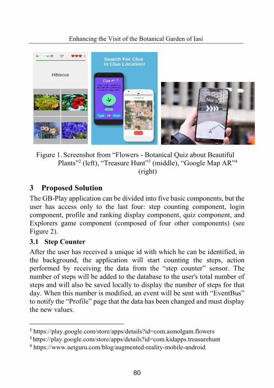
Enhancing the Visit of the Botanical Garden of Iasi
Figure 1. Screenshot from “Flowers - Botanical Quiz about Beautiful
Plants”2 (left), “Treasure Hunt”3 (middle), “Google Map AR”4
(right)
3 Proposed Solution
The GB-Play application can be divided into five basic components, but the
user has access only to the last four: step counting component, login
component, profile and ranking display component, quiz component, and
Explorers game component (composed of four other components) (see
Figure 2).
3.1 Step Counter
After the user has received a unique id with which he can be identified, in
the background, the application will start counting the steps, action
performed by receiving the data from the “step counter” sensor. The
number of steps will be added to the database to the user's total number of
steps and will also be saved locally to display the number of steps for that
day. When this number is modified, an event will be sent with “EventBus” to notify the “Profile” page that the data has been changed and must display the new values.
2 https://play.google.com/store/apps/details?id=com.asmolgam.flowers 3 https://play.google.com/store/apps/details?id=com.kidapps.treasurehunt
4 https://www.netguru.com/blog/augmented-reality-mobile-android
80
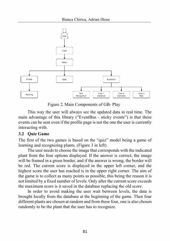
Bianca Chirica, Adrian Iftene
Figure 2. Main Components of GB- Play
This way the user will always see the updated data in real time. The
main advantage of this library (“EventBus - sticky events”) is that these events can be sent even if the profile page is not the one the user is currently
interacting with.
3.2 Quiz Game
The first of the two games is based on the “quiz” model being a game of learning and recognizing plants. (Figure 3 in left).
The user needs to choose the image that corresponds with the indicated
plant from the four options displayed. If the answer is correct, the image
will be framed in a green border, and if the answer is wrong, the border will
be red. The current score is displayed in the upper left corner, and the
highest score the user has reached is in the upper right corner. The aim of
the game is to collect as many points as possible, this being the reason it is
not limited by a fixed number of levels. Only after the current score exceeds
the maximum score is it saved in the database replacing the old score.
In order to avoid making the user wait between levels, the data is
brought locally from the database at the beginning of the game. Then four
different plants are chosen at random and from these four, one is also chosen
randomly to be the plant that the user has to recognize.
81
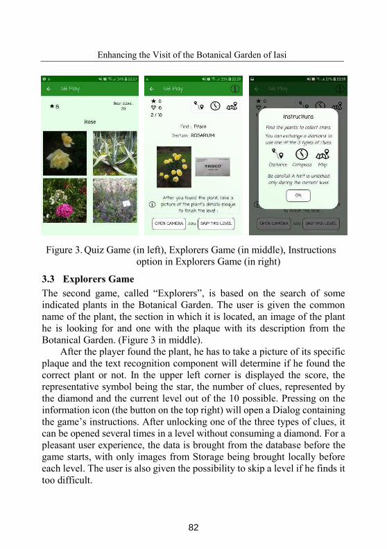
Enhancing the Visit of the Botanical Garden of Iasi
Figure 3. Quiz Game (in left), Explorers Game (in middle), Instructions
option in Explorers Game (in right)
3.3 Explorers Game
The second game, called “Explorers”, is based on the search of some indicated plants in the Botanical Garden. The user is given the common
name of the plant, the section in which it is located, an image of the plant
he is looking for and one with the plaque with its description from the
Botanical Garden. (Figure 3 in middle).
After the player found the plant, he has to take a picture of its specific
plaque and the text recognition component will determine if he found the
correct plant or not. In the upper left corner is displayed the score, the
representative symbol being the star, the number of clues, represented by
the diamond and the current level out of the 10 possible. Pressing on the
information icon (the button on the top right) will open a Dialog containing
the game’s instructions. After unlocking one of the three types of clues, it can be opened several times in a level without consuming a diamond. For a
pleasant user experience, the data is brought from the database before the
game starts, with only images from Storage being brought locally before
each level. The user is also given the possibility to skip a level if he finds it
too difficult.
82
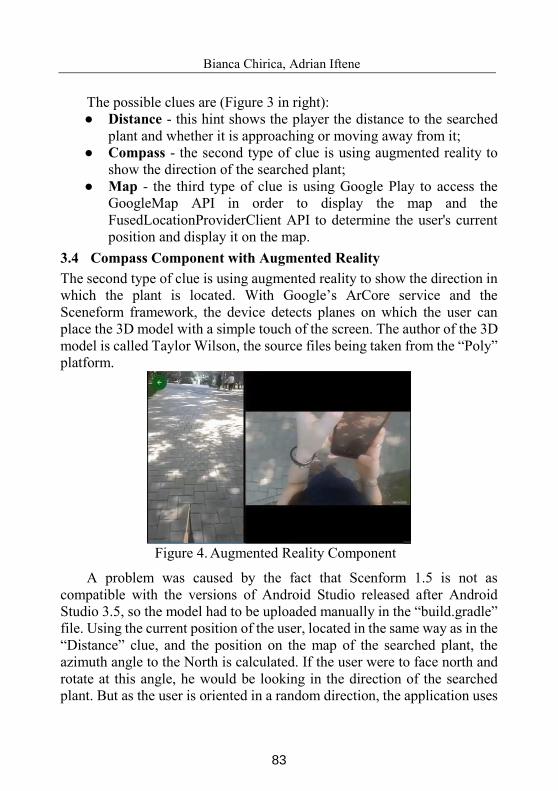
Bianca Chirica, Adrian Iftene
The possible clues are (Figure 3 in right):
Distance - this hint shows the player the distance to the searched
plant and whether it is approaching or moving away from it;
Compass - the second type of clue is using augmented reality to
show the direction of the searched plant;
Map - the third type of clue is using Google Play to access the
GoogleMap API in order to display the map and the
FusedLocationProviderClient API to determine the user's current
position and display it on the map.
3.4 Compass Component with Augmented Reality
The second type of clue is using augmented reality to show the direction in
which the plant is located. With Google’s ArCore service and the Sceneform framework, the device detects planes on which the user can
place the 3D model with a simple touch of the screen. The author of the 3D
model is called Taylor Wilson, the source files being taken from the “Poly” platform.
Figure 4. Augmented Reality Component
A problem was caused by the fact that Scenform 1.5 is not as
compatible with the versions of Android Studio released after Android
Studio 3.5, so the model had to be uploaded manually in the “build.gradle” file. Using the current position of the user, located in the same way as in the
“Distance” clue, and the position on the map of the searched plant, the azimuth angle to the North is calculated. If the user were to face north and
rotate at this angle, he would be looking in the direction of the searched
plant. But as the user is oriented in a random direction, the application uses
83
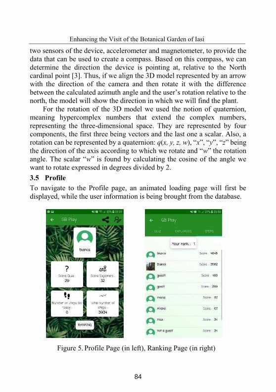
Enhancing the Visit of the Botanical Garden of Iasi
two sensors of the device, accelerometer and magnetometer, to provide the
data that can be used to create a compass. Based on this compass, we can
determine the direction the device is pointing at, relative to the North
cardinal point [3]. Thus, if we align the 3D model represented by an arrow
with the direction of the camera and then rotate it with the difference
between the calculated azimuth angle and the user’s rotation relative to the north, the model will show the direction in which we will find the plant.
For the rotation of the 3D model we used the notion of quaternion,
meaning hypercomplex numbers that extend the complex numbers,
representing the three-dimensional space. They are represented by four
components, the first three being vectors and the last one a scalar. Also, a
rotation can be represented by a quaternion: q(x, y, z, w), “x”, “y”, “z” being the direction of the axis according to which we rotate and “w” the rotation angle. The scalar “w” is found by calculating the cosine of the angle we
want to rotate expressed in degrees divided by 2.
3.5 Profile
To navigate to the Profile page, an animated loading page will first be
displayed, while the user information is being brought from the database.
Figure 5. Profile Page (in left), Ranking Page (in right)
84
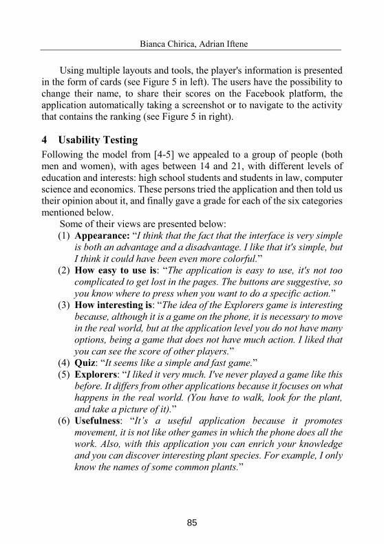
Bianca Chirica, Adrian Iftene
Using multiple layouts and tools, the player's information is presented
in the form of cards (see Figure 5 in left). The users have the possibility to
change their name, to share their scores on the Facebook platform, the
application automatically taking a screenshot or to navigate to the activity
that contains the ranking (see Figure 5 in right).
4 Usability Testing
Following the model from [4-5] we appealed to a group of people (both
men and women), with ages between 14 and 21, with different levels of
education and interests: high school students and students in law, computer
science and economics. These persons tried the application and then told us
their opinion about it, and finally gave a grade for each of the six categories
mentioned below.
Some of their views are presented below:
(1) Appearance: “I think that the fact that the interface is very simple
is both an advantage and a disadvantage. I like that it's simple, but
I think it could have been even more colorful.”
(2) How easy to use is: “The application is easy to use, it's not too
complicated to get lost in the pages. The buttons are suggestive, so
you know where to press when you want to do a specific action.”
(3) How interesting is: “The idea of the Explorers game is interesting
because, although it is a game on the phone, it is necessary to move
in the real world, but at the application level you do not have many
options, being a game that does not have much action. I liked that
you can see the score of other players.”
(4) Quiz: “It seems like a simple and fast game.”
(5) Explorers: “I liked it very much. I've never played a game like this
before. It differs from other applications because it focuses on what
happens in the real world. (You have to walk, look for the plant,
and take a picture of it).”
(6) Usefulness: “It’s a useful application because it promotes movement, it is not like other games in which the phone does all the
work. Also, with this application you can enrich your knowledge
and you can discover interesting plant species. For example, I only
know the names of some common plants.”
85
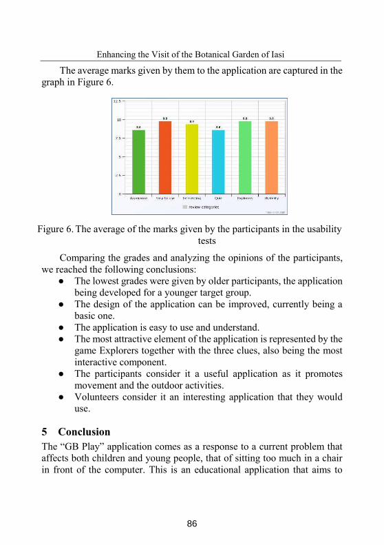
Enhancing the Visit of the Botanical Garden of Iasi
The average marks given by them to the application are captured in the
graph in Figure 6.
Figure 6. The average of the marks given by the participants in the usability
tests
Comparing the grades and analyzing the opinions of the participants,
we reached the following conclusions:
The lowest grades were given by older participants, the application
being developed for a younger target group.
The design of the application can be improved, currently being a
basic one.
The application is easy to use and understand.
The most attractive element of the application is represented by the
game Explorers together with the three clues, also being the most
interactive component.
The participants consider it a useful application as it promotes
movement and the outdoor activities.
Volunteers consider it an interesting application that they would
use.
5 Conclusion
The “GB Play” application comes as a response to a current problem that affects both children and young people, that of sitting too much in a chair
in front of the computer. This is an educational application that aims to
86
Bianca Chirica, Adrian Iftene
promote sport and attract children and users of all ages through the
presentation in the form of a game.
From comparing other applications similar in idea or technology and
based on feedback from users, we can conclude that it is an interesting
application that can attract users of all ages.
In the future, we aim to generate routes that the user can follow and
discover certain interesting places in the Botanical Garden, receiving
information about them after they arrive at the indicated locations.
Acknowledgments. This work was supported by project REVERT
(taRgeted thErapy for adVanced colorEctal canceR paTients), Grant
Agreement number: 848098, H2020-SC1-BHC-2018-2020/H2020-SC1-
2019-Two-Stage-RTD.
References
[1] J. Gregson, R. de Kok, J. Moat, S. Bachman. Application of GIS to
conservation assessments at the Royal Botanic Gardens, Kew. In book: Status
of Biological Diversity in Malaysia and Threat Assessment of Plant Species in
Malaysia, Edition 1, (2007), pp. 245-256.
[2] T. Borsch, C. Löhne. Botanic gardens for the future: Integrating research,
conservation, environmental education and public recreation. In Official
Journal of the Biological Society of Ethiopia, vol. 15, (2014), pp. 115-133.
[3] C.I. Irimia, M. Matei, A. Iftene, S.C. Romanescu, M.R. Lipan, M.
Costandache. Discover the Wonderful World of Plants with the Help of Smart
Devices. In Proceedings of the 17th International Conference on Human-
Computer Interaction RoCHI 2020, 22-23 October, (2020).
[4] M.N. Pinzariu, A. Iftene. Sphero - Multiplayer Augmented Game (SMAUG).
In International Conference on Human-Computer Interaction, 8-9 September,
Iasi, Romania (2016), pp. 46-49.
[5] M. Chițaniuc, A. Iftene. GeoAR-An Augmented Reality Application to Learn
Geography. In Romanian Journal of Human-Computer Interaction, vol. 11,
issue 2, (2018), pp. 93-108.
Demetra Bianca Chirica, Adrian Iftene
“Alexandru Ioan Cuza University” of Iasi, Faculty of Computer Science
E-mail: [email protected], [email protected]
87
Proceedings of the Conference on Mathematical Foundations of Informatics MFOI’2020, January 12-16, 2021, Kyiv, Ukraine
Recognition of Guitar Chords
using the Discrete Fourier
Transform
Matei-Alexandru Cioată, Adrian Iftene
Abstract
Mastering a musical instrument is a task that requires very much time, patience and motivation. Many people discover their passion for music late. Even though they begin to follow a path to become great musicians or they just search for the perfect hobby, it is hard to maintain the desire to learn this skill due to the low amount of free time. Interactivity is a very important element when learning music and therefore, this paper presents a method to help new guitarists who don’t have the possibility to search for music teachers.
Keywords : chord recognition, note recognition, discrete Fourier transform, frequency, Hamming window.
1 Introduction Technology is evolving very fast and the number of people who use it as a helping hand is increasing. These days, many different domains use software in order to automate tasks and music is not an exception. Tools for beginner, intermediate and advanced musicians are getting developed everyday: learning applications, games, virtual tuners, metronomes, etc.. The ease of use, the saved time and the low price are just some of the advantages obtained while using virtual tools. A simple application cannot replace a music teacher. The goal is to become as close as possible and therefore, interactivity is a must. It is very important to have this integrated into music projects because the users can receive feedback which they can use in order to improve. The learning process is entertaining and the
© 2021 by Matei-Alexandru Cioată, Adrian Iftene
88
Guitar Chord Recognition
motivation is maintained. Skills like dexterity, music theory and recognition by ear can be trained by this type of application.
2 Guitar Note and Chord Recognition An interesting way to bring interactivity into music projects is to implement a method of note recognition. Thus, the device which runs the app has the capacity to listen and process the sound produced by the user’s instrument [1].
There are multiple ways to develop such a functionality, but the first one that comes to mind is a method that involves artificial intelligence and neural networks. However, it is not practical because of the difficulty to find enough good quality data. There are many types of guitars in the world, each one with its specific tonality. Also, sound is propagated differently depending on the environment (room size, guitarist position, microphone quality, background noise, etc..). It would be almost impossible for a person to record a single note thousands of times, with hundreds of different guitars in hundreds of different environments.
At the same time, a huge amount of computational power is necessary in order to train a neural network of this complexity. Therefore, the Fourier Transform is the preferable solution to this problem.
3 Similar Work A considerable amount of popular applications that use a method of signal processing can be found online [1-4]. At the moment, a note recognition algorithm that ensures 100% accuracy doesn’t exist because, most of the time, background noise is present or the quality of the microphone is weak. One way to counter this problem is to capture unchanged signals directly from the instrument (for example, by connecting an electric guitar to a computer, no microphone is involved).
Rocksmith 1 is a video game developed by Ubisoft (available only on PC and consoles) which can teach the users to play a vast collection of rock, reggae and metal songs and it uses the method described above. Even though the accuracy is still not 100%, it comes close. The only problem with this signal capturing method is that it is not practical on mobile devices.
1 https://rocksmith.ubisoft.com/rocksmith/en-us/home/
89
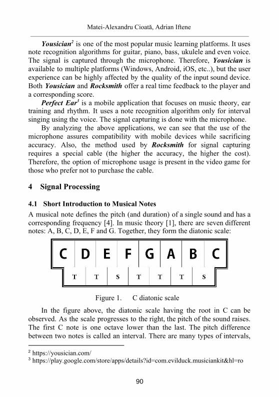
Matei-Alexandru Cioată, Adrian Iftene
Yousician 2 is one of the most popular music learning platforms. It uses note recognition algorithms for guitar, piano, bass, ukulele and even voice. The signal is captured through the microphone. Therefore, Yousician is available to multiple platforms (Windows, Android, iOS, etc..), but the user experience can be highly affected by the quality of the input sound device. Both Yousician and Rocksmith offer a real time feedback to the player and a corresponding score.
Perfect Ear 3 is a mobile application that focuses on music theory, ear training and rhythm. It uses a note recognition algorithm only for interval singing using the voice. The signal capturing is done with the microphone.
By analyzing the above applications, we can see that the use of the microphone assures compatibility with mobile devices while sacrificing accuracy. Also, the method used by Rocksmith for signal capturing requires a special cable (the higher the accuracy, the higher the cost). Therefore, the option of microphone usage is present in the video game for those who prefer not to purchase the cable.
4 Signal Processing
4.1 Short Introduction to Musical Notes A musical note defines the pitch (and duration) of a single sound and has a corresponding frequency [4]. In music theory [1], there are seven different notes: A, B, C, D, E, F and G. Together, they form the diatonic scale:
Figure 1. C diatonic scale
In the figure above, the diatonic scale having the root in C can be observed. As the scale progresses to the right, the pitch of the sound raises. The first C note is one octave lower than the last. The pitch difference between two notes is called an interval. There are many types of intervals,
2 https://yousician.com/ 3 https://play.google.com/store/apps/details?id=com.evilduck.musiciankit&hl=ro
90
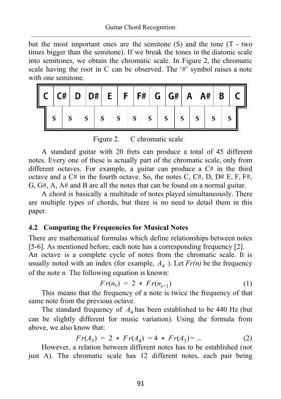
Guitar Chord Recognition
but the most important ones are the semitone (S) and the tone (T - two times bigger than the semitone). If we break the tones in the diatonic scale into semitones, we obtain the chromatic scale. In Figure 2, the chromatic scale having the root in C can be observed. The ‘#’ symbol raises a note with one semitone.
Figure 2. C chromatic scale
A standard guitar with 20 frets can produce a total of 45 different notes. Every one of these is actually part of the chromatic scale, only from different octaves. For example, a guitar can produce a C# in the third octave and a C# in the fourth octave. So, the notes C, C#, D, D# E, F, F#, G, G#, A, A# and B are all the notes that can be found on a normal guitar.
A chord is basically a multitude of notes played simultaneously. There are multiple types of chords, but there is no need to detail them in this paper.
4.2 Computing the Frequencies for Musical Notes There are mathematical formulas which define relationships between notes [5-6]. As mentioned before, each note has a corresponding frequency [2]. An octave is a complete cycle of notes from the chromatic scale. It is usually noted with an index (for example, ). Let Fr(n) be the frequency A4 of the note n. The following equation is known:
r(n ) 2 F r(n )F x = * x−1 (1) This means that the frequency of a note is twice the frequency of that
same note from the previous octave. The standard frequency of has been established to be 440 Hz (but A4
can be slightly different for music variation). Using the formula from above, we also know that:
= ...r(A ) 2 F r(A ) F r(A )F 5 = * 4 = 4 * 3 (2) However, a relation between different notes has to be established (not
just A). The chromatic scale has 12 different notes, each pair being
91
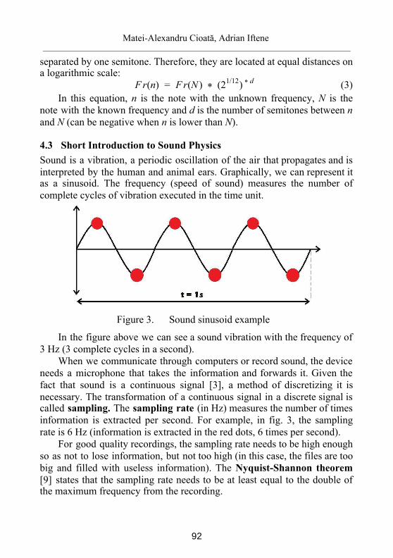
Matei-Alexandru Cioată, Adrian Iftene
separated by one semitone. Therefore, they are located at equal distances on a logarithmic scale:
r(n) F r(N ) (2 ) F = * 1/12 d* (3) In this equation, n is the note with the unknown frequency, N is the
note with the known frequency and d is the number of semitones between n and N (can be negative when n is lower than N). 4.3 Short Introduction to Sound Physics Sound is a vibration, a periodic oscillation of the air that propagates and is interpreted by the human and animal ears. Graphically, we can represent it as a sinusoid. The frequency (speed of sound) measures the number of complete cycles of vibration executed in the time unit.
Figure 3. Sound sinusoid example
In the figure above we can see a sound vibration with the frequency of 3 Hz (3 complete cycles in a second).
When we communicate through computers or record sound, the device needs a microphone that takes the information and forwards it. Given the fact that sound is a continuous signal [3], a method of discretizing it is necessary. The transformation of a continuous signal in a discrete signal is called sampling. The sampling rate (in Hz) measures the number of times information is extracted per second. For example, in fig. 3, the sampling rate is 6 Hz (information is extracted in the red dots, 6 times per second).
For good quality recordings, the sampling rate needs to be high enough so as not to lose information, but not too high (in this case, the files are too big and filled with useless information). The Nyquist-Shannon theorem [9] states that the sampling rate needs to be at least equal to the double of the maximum frequency from the recording.
92
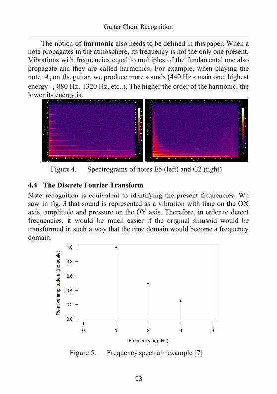
Guitar Chord Recognition
The notion of harmonic also needs to be defined in this paper. When a note propagates in the atmosphere, its frequency is not the only one present. Vibrations with frequencies equal to multiples of the fundamental one also propagate and they are called harmonics. For example, when playing the note on the guitar, we produce more sounds (440 Hz - main one, highest A4 energy -, 880 Hz, 1320 Hz, etc..). The higher the order of the harmonic, the lower its energy is.
Figure 4. Spectrograms of notes E5 (left) and G2 (right)
4.4 The Discrete Fourier Transform Note recognition is equivalent to identifying the present frequencies. We saw in fig. 3 that sound is represented as a vibration with time on the OX axis, amplitude and pressure on the OY axis. Therefore, in order to detect frequencies, it would be much easier if the original sinusoid would be transformed in such a way that the time domain would become a frequency domain.
Figure 5. Frequency spectrum example [7]
93
Matei-Alexandru Cioată, Adrian Iftene
In fig. 5, we can see that the frequency of 1 KHz is present and dominant (has the biggest amplitude). Also, its harmonics (2 KHz and 3 Khz) are also detected, but with a lower amplitude like described in section 4.3. The existence of these harmonics ensures that the fundamental 1 KHz vibration is indeed present.
This transformation of the domain from time to frequency is called Fourier Transform. In the previous section, the fact that the signal has to be discretized has been mentioned. Therefore the method that needs to be used is called Discrete Fourier Transform. Definition 1 [5]. Let x be a signal (sound signal in the case of this paper). Its Discrete Fourier Transform is defined as such:
(ω ) (t ) e , k 0, 1, 2, ..., N 1X k = ∑N−1
n=0x n * −i ω t* k * n = − (4)
where:
N - total number of samples; x( - amplitude of the initial signal at time ;)tn tn - the time when the n-th sample is found in the recording (equaltn
with n * T); T - the time interval at which sampling takes place; - the sampling rate of the recording (equal to 1/T);f s i - the imaginary unit ( ); i2 = − 1 - the frequency (angular, measured in rad/second instead of Hz)ωk
for which the amplitude is calculated (equal to , whereΠ F2 * k is the frequency in Hz); F k
- the spectrum [8] of signal x at frequency ; it is a(ω ) X k ωk complex number. To find the amplitude, the complex number module has to be calculated ( ).√a b2 + 2
Given the fact that the recording has N samples, a maximum of N frequencies can be detected. This is the reason why k has values between 0 and N-1. If the frequencies for which amplitudes need to be calculated are not known, they must be sampled too. However, in this paper, a simpler formula for the Discrete Fourier Transform will be used because at every moment, the frequencies, the time, and the total number of samples are known:
94
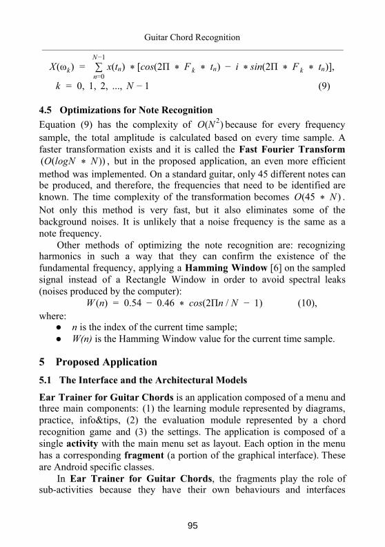
Guitar Chord Recognition
(ω ) (t ) cos(2Π F t ) i in(2Π F t )],X k = ∑N−1
n=0x n * [ * k * n − * s * k * n
0, 1, 2, ..., Nk = − 1 (9)
4.5 Optimizations for Note Recognition Equation (9) has the complexity of because for every frequency (N )O 2 sample, the total amplitude is calculated based on every time sample. A faster transformation exists and it is called the Fast Fourier Transform
, but in the proposed application, an even more efficientO(logN N ))( * method was implemented. On a standard guitar, only 45 different notes can be produced, and therefore, the frequencies that need to be identified are known. The time complexity of the transformation becomes . (45 N )O * Not only this method is very fast, but it also eliminates some of the background noises. It is unlikely that a noise frequency is the same as a note frequency.
Other methods of optimizing the note recognition are: recognizing harmonics in such a way that they can confirm the existence of the fundamental frequency, applying a Hamming Window [6] on the sampled signal instead of a Rectangle Window in order to avoid spectral leaks (noises produced by the computer):
(n) 0.54 0.46 cos(2Πn / N 1)W = − * − (10), where:
n is the index of the current time sample; W(n) is the Hamming Window value for the current time sample.
5 Proposed Application 5.1 The Interface and the Architectural Models
Ear Trainer for Guitar Chords is an application composed of a menu and three main components: (1) the learning module represented by diagrams, practice, info&tips, (2) the evaluation module represented by a chord recognition game and (3) the settings. The application is composed of a single activity with the main menu set as layout. Each option in the menu has a corresponding fragment (a portion of the graphical interface). These are Android specific classes.
In Ear Trainer for Guitar Chords , the fragments play the role of sub-activities because they have their own behaviours and interfaces
95
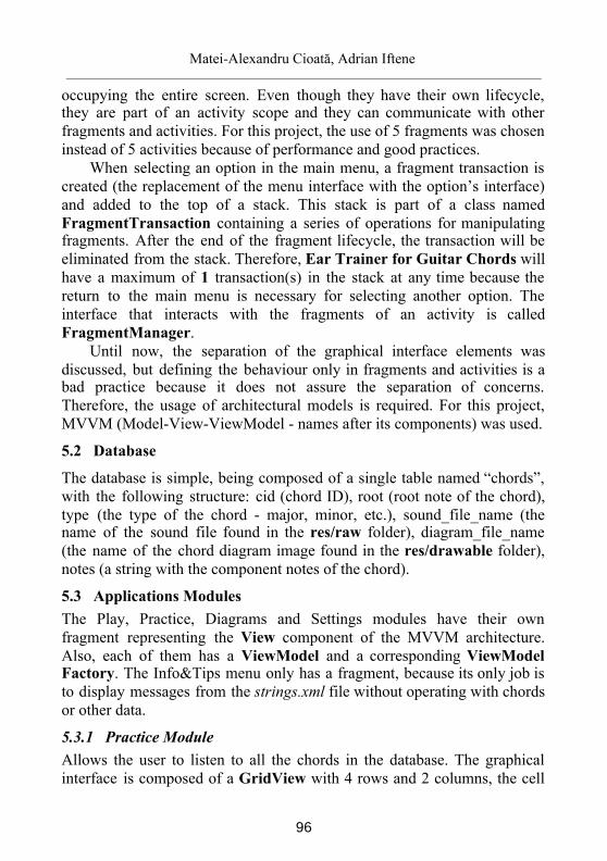
Matei-Alexandru Cioată, Adrian Iftene
occupying the entire screen. Even though they have their own lifecycle, they are part of an activity scope and they can communicate with other fragments and activities. For this project, the use of 5 fragments was chosen instead of 5 activities because of performance and good practices.
When selecting an option in the main menu, a fragment transaction is created (the replacement of the menu interface with the option’s interface) and added to the top of a stack. This stack is part of a class named FragmentTransaction containing a series of operations for manipulating fragments. After the end of the fragment lifecycle, the transaction will be eliminated from the stack. Therefore, Ear Trainer for Guitar Chords will have a maximum of 1 transaction(s) in the stack at any time because the return to the main menu is necessary for selecting another option. The interface that interacts with the fragments of an activity is called FragmentManager.
Until now, the separation of the graphical interface elements was discussed, but defining the behaviour only in fragments and activities is a bad practice because it does not assure the separation of concerns. Therefore, the usage of architectural models is required. For this project, MVVM (Model-View-ViewModel - names after its components) was used.
5.2 Database
The database is simple, being composed of a single table named “chords”, with the following structure: cid (chord ID), root (root note of the chord), type (the type of the chord - major, minor, etc.), sound_file_name (the name of the sound file found in the res/raw folder), diagram_file_name (the name of the chord diagram image found in the res/drawable folder), notes (a string with the component notes of the chord).
5.3 Applications Modules The Play, Practice, Diagrams and Settings modules have their own fragment representing the View component of the MVVM architecture. Also, each of them has a ViewModel and a corresponding ViewModel Factory. The Info&Tips menu only has a fragment, because its only job is to display messages from the strings.xml file without operating with chords or other data.
5.3.1 Practice Module Allows the user to listen to all the chords in the database. The graphical interface is composed of a GridView with 4 rows and 2 columns, the cell
96
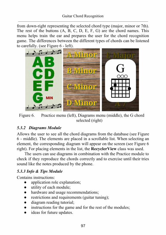
Guitar Chord Recognition
from down-right representing the selected chord type (major, minor or 7th). The rest of the buttons (A, B, C, D, E, F, G) are the chord names. This menu helps train the ear and prepares the user for the chord recognition game. The differences between the different types of chords can be listened to carefully. (see Figure 6 - left).
Figure 6. Practice menu (left), Diagrams menu (middle), the G chord
selected (right)
5.3.2 Diagrams Module Allows the user to see all the chord diagrams from the database (see Figure 6 - middle). The elements are placed in a scrollable list. When selecting an element, the corresponding diagram will appear on the screen (see Figure 6 right). For placing elements in the list, the RecyclerView class was used.
The users can use diagrams in combination with the Practice module to check if they reproduce the chords correctly and to exercise until their tries sound like the notes produced by the phone.
5.3.3 Info & Tips Module Contains instructions:
application role explanation; utility of each module; hardware and usage recommendations; restrictions and requirements (guitar tuning); diagram reading tutorial; instructions for the game and for the rest of the modules; ideas for future updates.
97
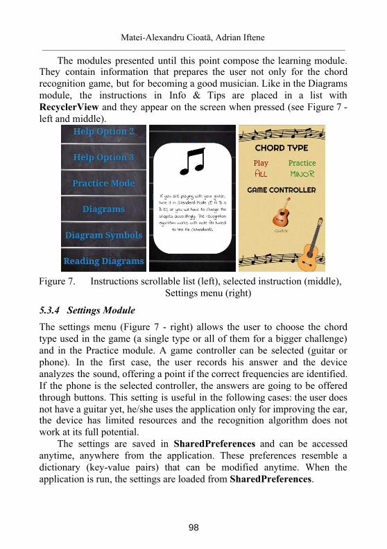
Matei-Alexandru Cioată, Adrian Iftene
The modules presented until this point compose the learning module. They contain information that prepares the user not only for the chord recognition game, but for becoming a good musician. Like in the Diagrams module, the instructions in Info & Tips are placed in a list with RecyclerView and they appear on the screen when pressed (see Figure 7 - left and middle).
Figure 7. Instructions scrollable list (left), selected instruction (middle),
Settings menu (right)
5.3.4 Settings Module The settings menu (Figure 7 - right) allows the user to choose the chord type used in the game (a single type or all of them for a bigger challenge) and in the Practice module. A game controller can be selected (guitar or phone). In the first case, the user records his answer and the device analyzes the sound, offering a point if the correct frequencies are identified. If the phone is the selected controller, the answers are going to be offered through buttons. This setting is useful in the following cases: the user does not have a guitar yet, he/she uses the application only for improving the ear, the device has limited resources and the recognition algorithm does not work at its full potential.
The settings are saved in SharedPreferences and can be accessed anytime, anywhere from the application. These preferences resemble a dictionary (key-value pairs) that can be modified anytime. When the application is run, the settings are loaded from SharedPreferences .
98
Guitar Chord Recognition
5.3.5 The Chord Recognition Game Represents the evaluation module. It is composed of more rounds and it lasts until the user makes a mistake. At the beginning of each round, a random chord is chosen (with the type selected in settings) (see Figure 8 - left). The player has the right to listen to that chord 3 times per round, to see 7 hints generated on the screen and to use 3 helpers (once used, they are not available in the corresponding game).
Figure 8. Chord recognition game (left), Thread communication for sound
recording and analysis (right) Button roles are explained in the Info & Tips menu. If the phone is
selected as a controller, the 7 hints are pressable (used to answer). The right answer will always be one of those. If the guitar is selected, the answer is recorded by pressing the red button from up-right. At the start of the recording, 3 threads begin their execution besides the main one (see Figure 8 - right):
the first one handles the sound recording in bytes form; it transfers the information further;
the second one is responsible for analyzing the information received from the previous thread. The chosen chord for the current round is known, therefore the identified notes will be compared with the ones from the database (table “chords”, column “notes”). When the chord is identified, a notification is sent to the main thread and the player receives a point. The round ends instantly;
99
Matei-Alexandru Cioată, Adrian Iftene
the third one is a timer of 5 seconds which stops the first two threads at the end and notifies the main thread that the game is over. At that moment, the score and the right answer are displayed;
the main thread displays elements to the screen, listens to buttons and responds to the notifications correspondingly.
A score is saved in SharedPreferences . Although the classes that handle sound recording and analysis are used just by the chord recognition game, they are part of the Model component of the MVVM architecture because they contain business logic. When the application is run, an initialization algorithm which calculates all guitar note frequencies executes. A MutableMap is obtained (key-value map, with the key being the name of the note, and the value being the frequency of the note). This algorithm helps with the identification of the chords.
For this project, royalty free images from Pixabay4 (backgrounds for menu, settings, practice, diagrams, info&tips and for the game) were used. The diagrams for chords were downloaded from this page5. The used fonts in the application are Indie Flower6 and Righteous 7 from Google Fonts.
6 Feedback and Usability Tests The best method for testing such an application is to offer it to users in order to receive feedback. This way, the potential impact in the music world can be observed. In order to write this chapter, a Google Form was made for 9 volunteers to answer some questions about their personal opinion on Ear Trainer For Guitar Chords . The guitarists that offered to help with the experiment (ages between 18 and 23 years old) have different experiences in music and different opinions about the usefulness of this application. Two volunteers have no guitar experience while the others have between 10 months and 10 years of experience.
A summary with all the opinions of the volunteers and statistics regarding different application components can be found below.
The form begins by asking some questions about the learning modules, especially helpful for beginners.
4 https://pixabay.com/ro/ 5 https://midnightmusic.com.au/2013/08/free-guitar-chord-image-library/ 6 https://fonts.google.com/specimen/Indie+Flower 7 https://fonts.google.com/specimen/Righteous
100
Guitar Chord Recognition
Question 1: How do you think that the learning module helps beginners? If you are part of this category, do you think that it can support your evolution?
“It’s very useful to have all the chords in the same place when you want to learn and to monitor the progress. If you learn a chord wrongly you can remember it like this (for example, an E7 instead of an E), and the Practice module helps you notice.” (10 years experience);
“I consider that this module helps a lot, especially beginners: they can learn chords by having the diagrams in front of them and comparing their sounds with the ones in the database.” (1 year experience);
“Beginners can learn fundamental chords, but the application does not offer real photos or videos of each chord. They can be easily misled.“ (7 years experience);
“I like that the application helps me to learn to read a diagram. Also, I found out how correct chords sound. The Info&Tips module helps me understand how the application works and how to use the other modules to my advantage.” (no experience).
Question 2 : Just for intermediates and advanced: do you consider that the learning module can help you at this level? If yes, how?
“Personally, it helps me with the listening part and to advance in a chord type that I don’t know very well yet.” (2 years experience);
“Just the diagrams, because I don’t know all the chords by heart.” (10 years experience);
“I consider that it is useful even for advanced guitarists because it helps to maintain the musical ear. The constant exercise is mandatory, no matter the level of experience.” (6 years experience).
Question 3: In your opinion, what is the most helpful learning module? There were different opinions at this question between the “Diagrams” and the “Practice” modules. The volunteers that already know the chords tend to choose “Practice” because it helps them with ear training, while the others prefer the diagrams. Question 4: In your opinion, are there useless functionalities in the learning module?
The only problem reported here was that some instructions from “Info & Tips” are hard to follow.
101
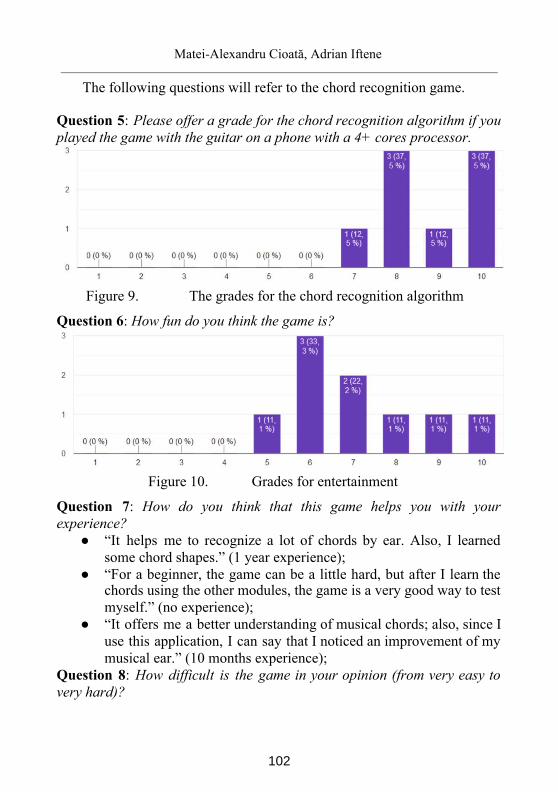
Matei-Alexandru Cioată, Adrian Iftene
The following questions will refer to the chord recognition game.
Question 5: Please offer a grade for the chord recognition algorithm if you played the game with the guitar on a phone with a 4+ cores processor.
Figure 9. The grades for the chord recognition algorithm
Question 6: How fun do you think the game is?
Figure 10. Grades for entertainment
Question 7: How do you think that this game helps you with your experience?
“It helps me to recognize a lot of chords by ear. Also, I learned some chord shapes.” (1 year experience);
“For a beginner, the game can be a little hard, but after I learn the chords using the other modules, the game is a very good way to test myself.” (no experience);
“It offers me a better understanding of musical chords; also, since I use this application, I can say that I noticed an improvement of my musical ear.” (10 months experience);
Question 8: How difficult is the game in your opinion (from very easy to very hard)?
102
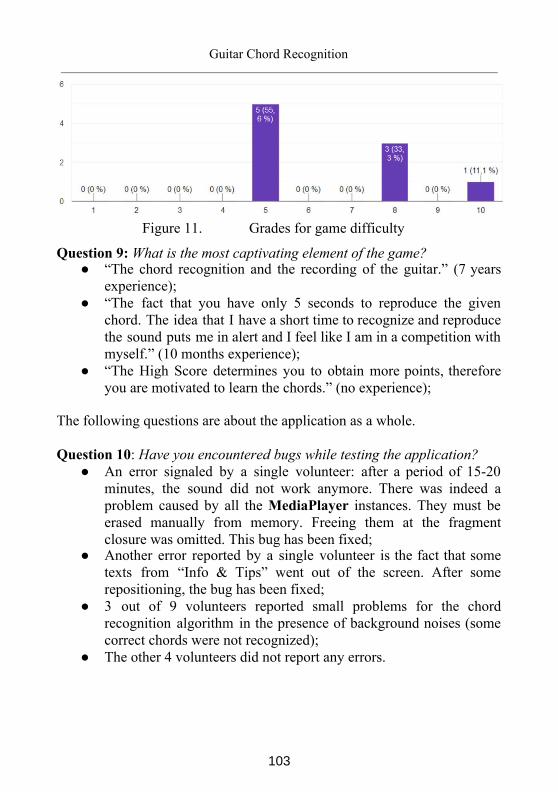
Guitar Chord Recognition
Figure 11. Grades for game difficulty
Question 9: What is the most captivating element of the game? “The chord recognition and the recording of the guitar.” (7 years
experience); “The fact that you have only 5 seconds to reproduce the given
chord. The idea that I have a short time to recognize and reproduce the sound puts me in alert and I feel like I am in a competition with myself.” (10 months experience);
“The High Score determines you to obtain more points, therefore you are motivated to learn the chords.” (no experience);
The following questions are about the application as a whole. Question 10: Have you encountered bugs while testing the application?
An error signaled by a single volunteer: after a period of 15-20 minutes, the sound did not work anymore. There was indeed a problem caused by all the MediaPlayer instances. They must be erased manually from memory. Freeing them at the fragment closure was omitted. This bug has been fixed;
Another error reported by a single volunteer is the fact that some texts from “Info & Tips” went out of the screen. After some repositioning, the bug has been fixed;
3 out of 9 volunteers reported small problems for the chord recognition algorithm in the presence of background noises (some correct chords were not recognized);
The other 4 volunteers did not report any errors.
103
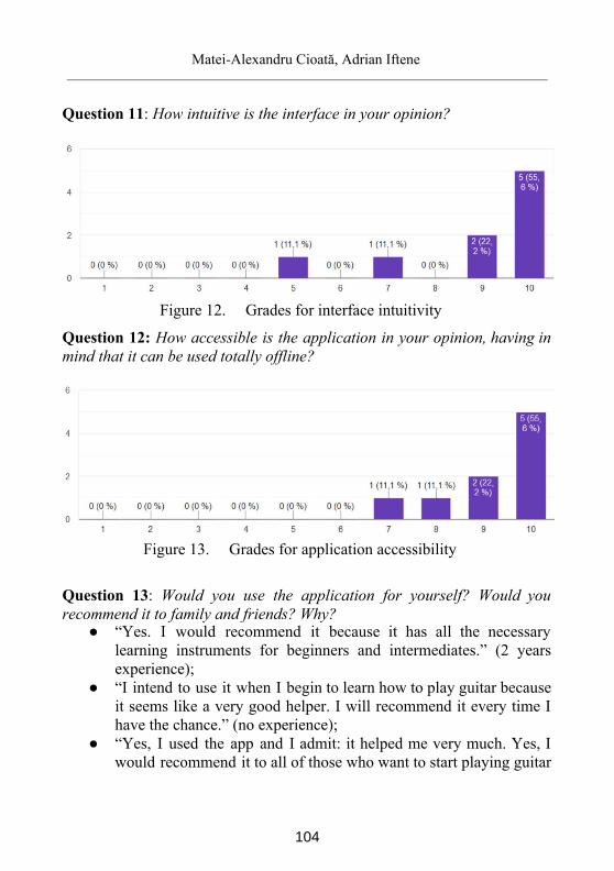
Matei-Alexandru Cioată, Adrian Iftene
Question 11: How intuitive is the interface in your opinion?
Figure 12. Grades for interface intuitivity
Question 12: How accessible is the application in your opinion, having in mind that it can be used totally offline?
Figure 13. Grades for application accessibility
Question 13: Would you use the application for yourself? Would you recommend it to family and friends? Why?
“Yes. I would recommend it because it has all the necessary learning instruments for beginners and intermediates.” (2 years experience);
“I intend to use it when I begin to learn how to play guitar because it seems like a very good helper. I will recommend it every time I have the chance.” (no experience);
“Yes, I used the app and I admit: it helped me very much. Yes, I would recommend it to all of those who want to start playing guitar
104
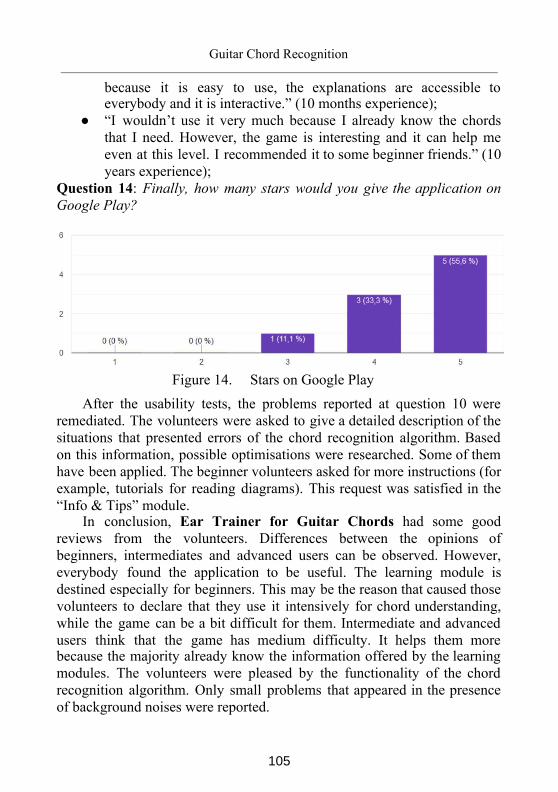
Guitar Chord Recognition
because it is easy to use, the explanations are accessible to everybody and it is interactive.” (10 months experience);
“I wouldn’t use it very much because I already know the chords that I need. However, the game is interesting and it can help me even at this level. I recommended it to some beginner friends.” (10 years experience);
Question 14: Finally, how many stars would you give the application on Google Play?
Figure 14. Stars on Google Play
After the usability tests, the problems reported at question 10 were remediated. The volunteers were asked to give a detailed description of the situations that presented errors of the chord recognition algorithm. Based on this information, possible optimisations were researched. Some of them have been applied. The beginner volunteers asked for more instructions (for example, tutorials for reading diagrams). This request was satisfied in the “Info & Tips” module.
In conclusion, Ear Trainer for Guitar Chords had some good reviews from the volunteers. Differences between the opinions of beginners, intermediates and advanced users can be observed. However, everybody found the application to be useful. The learning module is destined especially for beginners. This may be the reason that caused those volunteers to declare that they use it intensively for chord understanding, while the game can be a bit difficult for them. Intermediate and advanced users think that the game has medium difficulty. It helps them more because the majority already know the information offered by the learning modules. The volunteers were pleased by the functionality of the chord recognition algorithm. Only small problems that appeared in the presence of background noises were reported.
105
Matei-Alexandru Cioată, Adrian Iftene
7 Conclusions Electrical devices are very important instruments used in learning processes. Music is a difficult and wide domain that requires a lot of time and devotion. This is why the advantages of electrical devices are very important, since they bring extra convenience, time and diversity of learning resources. In our opinion, there are many quality resources, free and paid, that develop musical skills and can be found online. Personally, I evolved only with such resources in the last 4 years and I can say that I got to a pretty high point compared to what I imagined at the beginning of this experience. However, there were some shortcomings that made me come up with the idea of Ear Trainer for Guitar Chords .
In the first year of my experience with the guitar, I have been discouraged by chords, because they seemed very difficult and I couldn’t find a platform to help me. My wish was to play my favourite songs, an impossible thing to achieve without chord knowledge. We consider that Ear Trainer for Guitar Chords offers this kind of help to beginners in an interactive and easy to understand way. Even if intermediate and advanced guitarists already know the chords, they can always test their musical ear with the chord recognition game, evolving even more. This is why we believe that the application could represent an impact for all the guitarists.
Ear Trainer for Guitar Chords is at the beginning of its life. Lots of improvements and functionalities of different complexities destined to all kinds of musicians can be implemented. After some discussions with Mr. Adrian Iftene (my coordinating teacher) and the volunteers who tested the application, we came up with a list of improvements: (1) the first priority is to add some theory elements. Beginners wish to understand the definition, structure of chords and of other musical elements (for example, scales); (2) there are ideas of improving some graphical elements: reorganizations of the “Diagrams” menu and putting the elements in a table instead of a list, deleting some instructions and adding others, etc.; (3) support for vocal commands, since the pressing of buttons with the guitar in the hand is uncomfortable. There were attempts to solve this problem with offline libraries, but without success. I consider that the lack of necessity to connect to the internet is a defining feature of Ear Trainer for Guitar Chords . Therefore, in a future update, users will be able to decide if they want to use an online Speech to Text service or if they want to remain offline; (4) new types of chords; (5) images and videos containing
106
Guitar Chord Recognition
instructions of hand positions for every chord; (6) other interactive games with other musical elements (for example, recognition of pentatonic scales).
Acknowledgments. This work was supported by project REVERT (taRgeted thErapy for adVanced colorEctal canceR paTients), Grant Agreement number: 848098, H2020-SC1-BHC-2018-2020 / H2020-SC1- 2019-Two-Stage-RTD.
References [1] M. Pilhofer, H. Day. Music Theory for Dummies . In Wiley Publishing, Inc.,
Part II & Part III, (2007). [2] B. H. Suits. Physics of music - notes . (1998). https://pages.mtu.edu/
suits/Physicsofmusic.html [3] K. Deergha Rao. Signals and Systems . In Springer International Publishing,
(2018) pp. 271-320. [4] D. Santo Pietro. Introduction to sound. Khan Academy (2020)
https://www.khanacademy.org/science/apphysics-1/ap-mechanical-waves-and-sound/introduction-to-sound-waves-ap
[5] J.O. Smith. Mathematics of the Discrete Fourier Transform (DFT) with Audio Applications . Second Edition, (2007) http://ccrma.stanford.edu/ jos/mdft/
[6] F. J. Harris. On the Use of Windows for Harmonic Analysis with the Discrete Fourier Transform . In Proceedings of the IEEE, vol. 66, No. 1, (1978) http://web.mit.edu/xiphmont/Public/windows.pdf
[7] J. Sueur. A very short introduction to sound analysis for those who like elephant trumpet calls or other wildlife sound. (2020) https://cran.r-project.org/web/packages/seewave/vignettes/seewaveanalysis.pdf
[8] J. Wolfe. What is a Sound Spectrum? (2005) https://newt.phys.unsw.edu.au/jw/sound.spectrum.html
[9] L. N. Pintilie. Teorema lui Nyquist – Shannon - Demonstratie; Evidentierea conceptului de ”timp de esantionare” sau ”frecventa de esantionare” . https://epe.utcluj.ro/SCTR/Indicatii/Teorema lui Nyquist Shannon.pdf
Matei-Alexandru Cioată, Adrian Iftene
“Alexandru Ioan Cuza University” of Iasi, Faculty of Computer Science E-mail: [email protected], [email protected]
107
Proceedings of the Conference on Mathematical Foundations of Informatics
MFOI2020, January 12-16, 2021, Kyiv, Ukraine
Development of a platform for processing
heterogeneous printed documents
Alexandru Colesnicov, Ludmila Malahov,
Svetlana Cojocaru, Lyudmila Burtseva
Abstract
Most written documents (both historical and contemporary,printed or handwritten) contain non-textual elements, whichgives them a heterogeneous character. General optical charac-ter recognition systems can process only an extremely limitednumber of such elements. There are some dispersed approaches,oriented on specific types of content, which do not propose auniversal solution. The article presents the architecture of aplatform, which in semi-automatic mode integrates the necessarycomponents for the processing of heterogeneous documents.
For implementation, a convergent technology for assemblingcomplex software systems from ready-made heterogeneous mod-ules on a single platform is used, each of which performs a smallpart of the task using a container system. The possibility of usingthis approach is illustrated with specific examples.
Keywords: heterogeneous content recognition, content typedetection, convergent software platform, virtualization.
1 Introduction
Heterogeneous content digitization problem arose together with BigData archives, when the storing of document scans as the images beganto take irrational amount of resources.
For an informal introduction in the problem, let’s show some com-plicated samples of heterogeneous content taken from Internet (Fig. 1).
c©2020 by A. Colesnicov, L. Malahov, S. Cojocaru, L. Burtseva
108
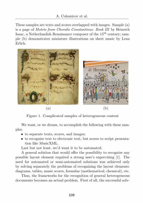
A. Colesnicov et al.
These samples are texts and scores overlapped with images. Sample (a)is a page of Motets from Choralis Constantinus: Book III by HeinrichIsaac, a Netherlandish Renaissance composer of the 15th century; sam-ple (b) demonstrates miniature illustrations on sheet music by LenaErlich.
(a) (b)
Figure 1. Complicated samples of heterogeneous content
We want, or we dream, to accomplish the following with these sam-ples:
• to separate texts, scores, and images;• to recognize text to electronic text, but scores to script presenta-tion like MusicXML.
Last but not least, we’d want it to be automated.A general solution that would offer the possibility to recognize any
possible layout element required a strong user’s supervising [1]. Theneed for automated or semi-automated solutions was achieved onlyby solving separately the problems of recognizing the layout elements:diagrams, tables, music scores, formulas (mathematical, chemical), etc.
Thus, the frameworks for the recognition of general heterogeneousdocuments becomes an actual problem. First of all, the successful solv-
109
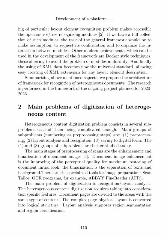
Development of a platform. . .
ing of particular layout element recognition problem makes accessiblethe open source/free recognizing modules [2]. If we have a full collec-tion of such modules, the task of the general framework would be tomake assumption, to request its confirmation and to organize the in-teraction between modules. Other modern achievements, which can beused in the development of the framework are Docker style techniques,these allowing to avoid the problem of modules uniformity. And finallythe using of XML data becomes now the universal standard, allowingeasy creating of XML extensions for any layout element description.
Summarizing above mentioned aspects, we propose the architectureof framework for recognition of heterogeneous documents. The researchis performed in the framework of the ongoing project planned for 2020-2023.
2 Main problems of digitization of heteroge-neous content
Heterogeneous content digitization problem consists in several sub-problems each of them being complicated enough. Main groups ofsubproblems (numbering as preprocessing steps) are: (1) preprocess-ing; (2) layout analysis and recognition; (3) saving to digital form. The(1) and (3) groups of subproblems are better studied today.
The main stages of preprocessing of scans are the enhancement andbinarization of document images [3]. Document image enhancementis the improving of the perceptual quality for maximum restoring ofdocument initial look, the binarization is the separation of texts andbackground.There are the specialized tools for image preparation: ScanTailor, OCR programs, for example, ABBYY FineReader (AFR).
The main problem of digitization is recognition/layout analysis.The heterogeneous content digitization requires taking into considera-tion specific features. Document pages are divided to the areas with thesame type of content. The complex page physical layout is convertedinto logical structure. Layout analysis supposes region segmentationand region classification.
110
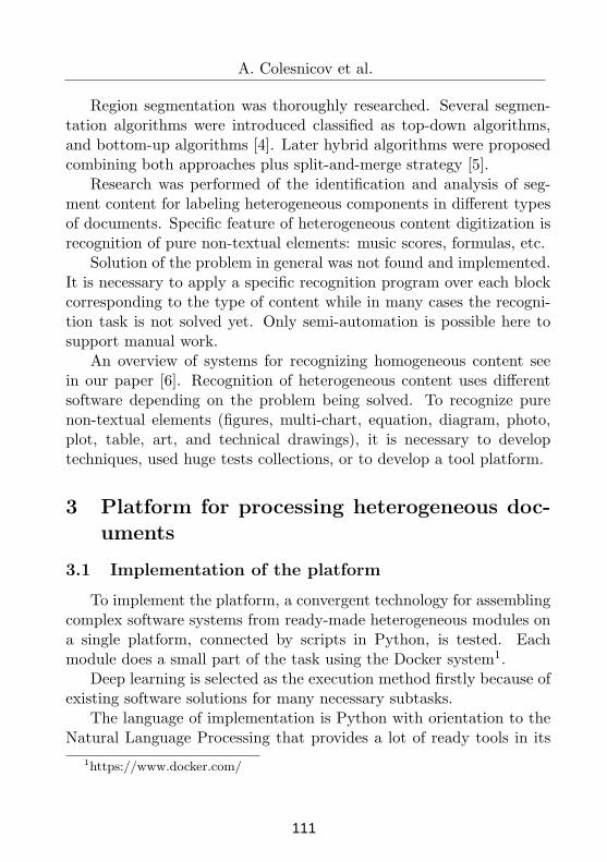
A. Colesnicov et al.
Region segmentation was thoroughly researched. Several segmen-tation algorithms were introduced classified as top-down algorithms,and bottom-up algorithms [4]. Later hybrid algorithms were proposedcombining both approaches plus split-and-merge strategy [5].
Research was performed of the identification and analysis of seg-ment content for labeling heterogeneous components in different typesof documents. Specific feature of heterogeneous content digitization isrecognition of pure non-textual elements: music scores, formulas, etc.
Solution of the problem in general was not found and implemented.It is necessary to apply a specific recognition program over each blockcorresponding to the type of content while in many cases the recogni-tion task is not solved yet. Only semi-automation is possible here tosupport manual work.
An overview of systems for recognizing homogeneous content seein our paper [6]. Recognition of heterogeneous content uses differentsoftware depending on the problem being solved. To recognize purenon-textual elements (figures, multi-chart, equation, diagram, photo,plot, table, art, and technical drawings), it is necessary to developtechniques, used huge tests collections, or to develop a tool platform.
3 Platform for processing heterogeneous doc-uments
3.1 Implementation of the platform
To implement the platform, a convergent technology for assemblingcomplex software systems from ready-made heterogeneous modules ona single platform, connected by scripts in Python, is tested. Eachmodule does a small part of the task using the Docker system1.
Deep learning is selected as the execution method firstly because ofexisting software solutions for many necessary subtasks.
The language of implementation is Python with orientation to theNatural Language Processing that provides a lot of ready tools in its
1https://www.docker.com/
111
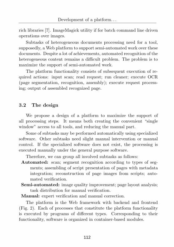
Development of a platform. . .
rich libraries [7]. ImageMagick utility if for batch command line drivenoperations over images.
Subtasks of heterogeneous documents processing need for a tool,supposedly, a Web platform to support semi-automated work over thesedocuments. Despite a lot of achievements, automated recognition of theheterogeneous content remains a difficult problem. The problem is tomaximize the support of semi-automated work.
The platform functionality consists of subsequent execution of re-quired actions: input scan; read request; run cleaner; execute OCR(page segmentation, recognition, assembly); execute request process-ing; output of assembled recognized page.
3.2 The design
We propose a design of a platform to maximize the support ofall processing steps. It means both creating the convenient “singlewindow” access to all tools, and reducing the manual part.
Some of subtasks may be performed automatically using specializedsoftware. Other subtasks need slight manual intervention or manualcontrol. If the specialized software does not exist, the processing isexecuted manually under the general purpose software.
Therefore, we can group all involved subtasks as follows:Automated: scan; segment recognition according to types of seg-
ments; assembling of script presentation of pages with metadataintegration; reconstruction of page images from scripts; auto-mated verification.
Semi-automated: image quality improvement; page layout analysis;task distribution for manual verification.
Manual: expert verification and manual correction.
The platform is the Web framework with backend and frontend(Fig. 2). Each of processes that constitute the platform functionalityis executed by programs of different types. Corresponding to theirfunctionality, software is organized in container-based modules.
112
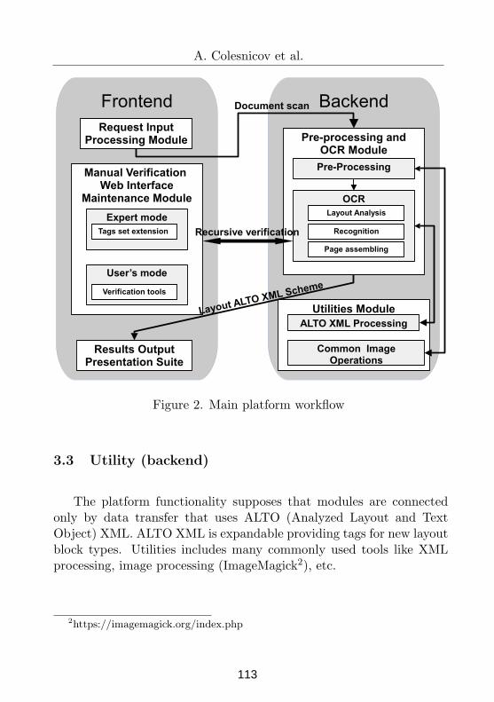
A. Colesnicov et al.
!! !
"
"
#$!
%!
& &
'' $
( !
&
)!
!
Figure 2. Main platform workflow
3.3 Utility (backend)
The platform functionality supposes that modules are connectedonly by data transfer that uses ALTO (Analyzed Layout and TextObject) XML. ALTO XML is expandable providing tags for new layoutblock types. Utilities includes many commonly used tools like XMLprocessing, image processing (ImageMagick2), etc.
2https://imagemagick.org/index.php
113
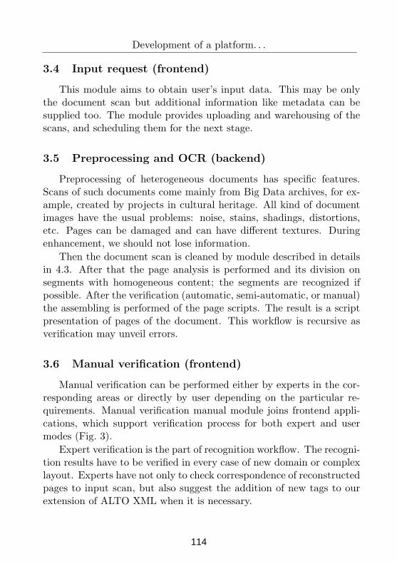
Development of a platform. . .
3.4 Input request (frontend)
This module aims to obtain user’s input data. This may be onlythe document scan but additional information like metadata can besupplied too. The module provides uploading and warehousing of thescans, and scheduling them for the next stage.
3.5 Preprocessing and OCR (backend)
Preprocessing of heterogeneous documents has specific features.Scans of such documents come mainly from Big Data archives, for ex-ample, created by projects in cultural heritage. All kind of documentimages have the usual problems: noise, stains, shadings, distortions,etc. Pages can be damaged and can have different textures. Duringenhancement, we should not lose information.
Then the document scan is cleaned by module described in detailsin 4.3. After that the page analysis is performed and its division onsegments with homogeneous content; the segments are recognized ifpossible. After the verification (automatic, semi-automatic, or manual)the assembling is performed of the page scripts. The result is a scriptpresentation of pages of the document. This workflow is recursive asverification may unveil errors.
3.6 Manual verification (frontend)
Manual verification can be performed either by experts in the cor-responding areas or directly by user depending on the particular re-quirements. Manual verification manual module joins frontend appli-cations, which support verification process for both expert and usermodes (Fig. 3).
Expert verification is the part of recognition workflow. The recogni-tion results have to be verified in every case of new domain or complexlayout. Experts have not only to check correspondence of reconstructedpages to input scan, but also suggest the addition of new tags to ourextension of ALTO XML when it is necessary.
114
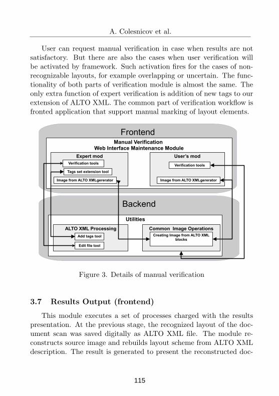
A. Colesnicov et al.
User can request manual verification in case when results are notsatisfactory. But there are also the cases when user verification willbe activated by framework. Such activation fires for the cases of non-recognizable layouts, for example overlapping or uncertain. The func-tionality of both parts of verification module is almost the same. Theonly extra function of expert verification is addition of new tags to ourextension of ALTO XML. The common part of verification workflow isfronted application that support manual marking of layout elements.
!
"
Figure 3. Details of manual verification
3.7 Results Output (frontend)
This module executes a set of processes charged with the resultspresentation. At the previous stage, the recognized layout of the doc-ument scan was saved digitally as ALTO XML file. The module re-constructs source image and rebuilds layout scheme from ALTO XMLdescription. The result is generated to present the reconstructed doc-
115
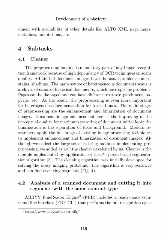
Development of a platform. . .
ument with availability of other details like ALTO XML page maps,metadata, annotations, etc.
4 Subtasks
4.1 Cleaner
The preprocessing module is mandatory part of any image recogni-tion framework because of high dependency of OCR techniques on scansquality. All kind of document images have the usual problems: noise,stains, shadings. The main source of heterogeneous documents scans isarchives of scans of historical documents, which have specific problems.Pages can be damaged and can have different textures: parchment, pa-pyrus, etc. As the result, the preprocessing is even more importantfor heterogeneous documents than for textual ones. The main stagesof preprocessing are the enhancement and binarization of documentimages. Document image enhancement here is the improving of theperceptual quality for maximum restoring of document initial look; thebinarization is the separation of texts and background. Modern re-searchers apply the full range of existing image processing techniquesto implement enhancement and binarization of document images. Al-though we collect the large set of existing modules implementing pre-processing, we added as well the cleaner developed by us. Cleaner is themodule implemented by application of the P system-based segmenta-tion algorithm [8]. The cleaning algorithm was initially developed forsolving the noisy imaging problems. The algorithm is very sensitiveand can find even tiny segments (Fig. 4).
4.2 Analysis of a scanned document and cutting it intosegments with the same content type
ABBYY FineReader Engine3 (FRE) includes a ready-made com-mand line interface (FRE CLI) that performs the full recognition cycle
3https://www.abbyy.com/ocr-sdk/
116
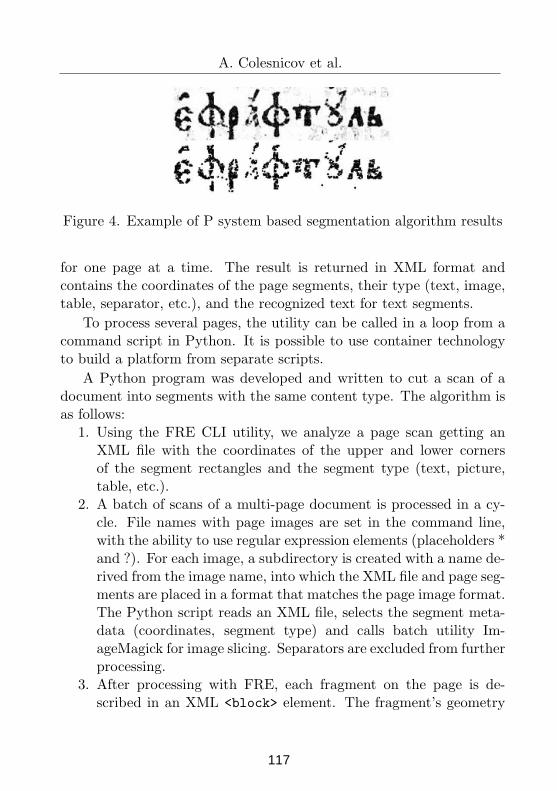
A. Colesnicov et al.
Figure 4. Example of P system based segmentation algorithm results
for one page at a time. The result is returned in XML format andcontains the coordinates of the page segments, their type (text, image,table, separator, etc.), and the recognized text for text segments.
To process several pages, the utility can be called in a loop from acommand script in Python. It is possible to use container technologyto build a platform from separate scripts.
A Python program was developed and written to cut a scan of adocument into segments with the same content type. The algorithm isas follows:
1. Using the FRE CLI utility, we analyze a page scan getting anXML file with the coordinates of the upper and lower cornersof the segment rectangles and the segment type (text, picture,table, etc.).
2. A batch of scans of a multi-page document is processed in a cy-cle. File names with page images are set in the command line,with the ability to use regular expression elements (placeholders *and ?). For each image, a subdirectory is created with a name de-rived from the image name, into which the XML file and page seg-ments are placed in a format that matches the page image format.The Python script reads an XML file, selects the segment meta-data (coordinates, segment type) and calls batch utility Im-ageMagick for image slicing. Separators are excluded from furtherprocessing.
3. After processing with FRE, each fragment on the page is de-scribed in an XML <block> element. The fragment’s geometry
117
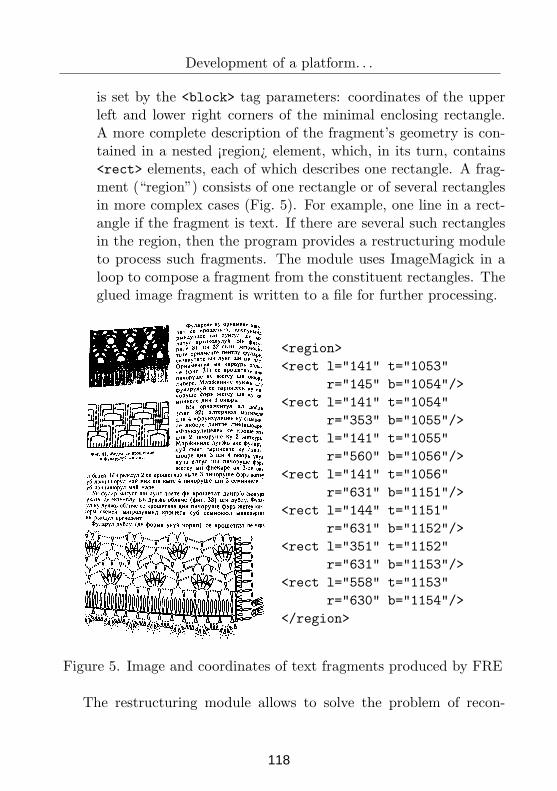
Development of a platform. . .
is set by the <block> tag parameters: coordinates of the upperleft and lower right corners of the minimal enclosing rectangle.A more complete description of the fragment’s geometry is con-tained in a nested ¡region¿ element, which, in its turn, contains<rect> elements, each of which describes one rectangle. A frag-ment (“region”) consists of one rectangle or of several rectanglesin more complex cases (Fig. 5). For example, one line in a rect-angle if the fragment is text. If there are several such rectanglesin the region, then the program provides a restructuring moduleto process such fragments. The module uses ImageMagick in aloop to compose a fragment from the constituent rectangles. Theglued image fragment is written to a file for further processing.
<region>
<rect l="141" t="1053"
r="145" b="1054"/>
<rect l="141" t="1054"
r="353" b="1055"/>
<rect l="141" t="1055"
r="560" b="1056"/>
<rect l="141" t="1056"
r="631" b="1151"/>
<rect l="144" t="1151"
r="631" b="1152"/>
<rect l="351" t="1152"
r="631" b="1153"/>
<rect l="558" t="1153"
r="630" b="1154"/>
</region>
Figure 5. Image and coordinates of text fragments produced by FRE
The restructuring module allows to solve the problem of recon-
118
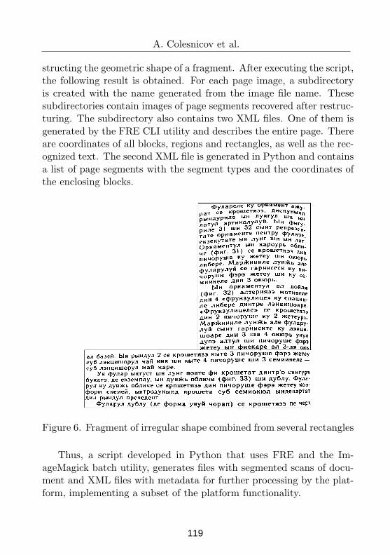
A. Colesnicov et al.
structing the geometric shape of a fragment. After executing the script,the following result is obtained. For each page image, a subdirectoryis created with the name generated from the image file name. Thesesubdirectories contain images of page segments recovered after restruc-turing. The subdirectory also contains two XML files. One of them isgenerated by the FRE CLI utility and describes the entire page. Thereare coordinates of all blocks, regions and rectangles, as well as the rec-ognized text. The second XML file is generated in Python and containsa list of page segments with the segment types and the coordinates ofthe enclosing blocks.
Figure 6. Fragment of irregular shape combined from several rectangles
Thus, a script developed in Python that uses FRE and the Im-ageMagick batch utility, generates files with segmented scans of docu-ment and XML files with metadata for further processing by the plat-form, implementing a subset of the platform functionality.
119
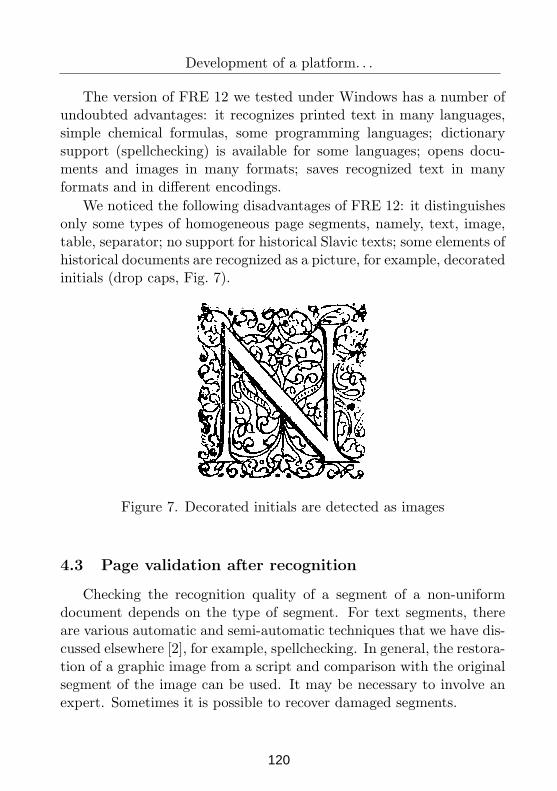
Development of a platform. . .
The version of FRE 12 we tested under Windows has a number ofundoubted advantages: it recognizes printed text in many languages,simple chemical formulas, some programming languages; dictionarysupport (spellchecking) is available for some languages; opens docu-ments and images in many formats; saves recognized text in manyformats and in different encodings.
We noticed the following disadvantages of FRE 12: it distinguishesonly some types of homogeneous page segments, namely, text, image,table, separator; no support for historical Slavic texts; some elements ofhistorical documents are recognized as a picture, for example, decoratedinitials (drop caps, Fig. 7).
Figure 7. Decorated initials are detected as images
4.3 Page validation after recognition
Checking the recognition quality of a segment of a non-uniformdocument depends on the type of segment. For text segments, thereare various automatic and semi-automatic techniques that we have dis-cussed elsewhere [2], for example, spellchecking. In general, the restora-tion of a graphic image from a script and comparison with the originalsegment of the image can be used. It may be necessary to involve anexpert. Sometimes it is possible to recover damaged segments.
120
A. Colesnicov et al.
5 Conclusions and further development
Automated recognition of the heterogeneous content remains a dif-ficult problem. We proposed a design of Web platform to maximizethe support of semi-automated work at this process.
In implementation, a convergent technology for assembling complexsoftware systems from ready-made heterogeneous modules on a singleplatform is used. Each of modules performs a small part of the taskusing inside a container.
The module for partitioning and mapping of heterogeneous docu-ments into homogeneous segments with different shapes was developedusing ABBYY FRE, ImageMagick and Python. Scans with text, mu-sic, images, etc. were analyzed. It is necessary to develop scripts thatdistinguish type of page fragments that is possible using deep learning.
The problem of complete detection for types of heterogeneous con-tent isn’t solved being the next stage of our work.
The other problem is the absence of old languages in FRE. It shouldbe trained over old texts printed in the Cyrillic fonts, using previouslyobtained resources.
Acknowledgement. This paper was written as part of the re-search project 20.80009.5007.22 “Intelligent information systems forsolving ill-structured problems, processing knowledge and big data”.
References
[1] D. Barbara, C. Domeniconi, Ning Kang. Mining relevant text
from unlabelled documents. Third IEEE International Conferenceon Data Mining, Melbourne, FL, USA, 2003, pp. 489-492, doi:10.1109/ICDM.2003.1250959.
[2] A. Colesnicov, S. Cojocaru, L. Malahov, L. Burtseva. On text pro-
cessing after OCR. Proceedings of 13-th International Conferenceon Linguistic Resources and Tools for Processing Romanian Lan-guage, Iasi, 22 – 23 November, 2018, pp. 53-60. ISSN: 1843-911X.
121
Development of a platform. . .
[3] I.V. Safonov, I.V. Kurilin, M.N. Rychagov, E.V. Tolstaya.Document Image Processing for Scanning and Printing. Springer,2019, 314 p.
[4] A.M. Namboodiri, A.K. Jain. Document structure and layout
analysis. Digital Document Processing, Springer, 2007, pp. 29–48.[5] Yu.A. Bolotova, V.G. Spitsyn, P.M. Osina. A Review of Algo-
rithms for Text Detection in Images and Videos. îìïüþòåðíàÿîïòèêà òîì ➑ pp.441-452.
[6] A. Colesnicov, L. Malahov, S. Cojocaru, L. Burtseva. Semi-
automated workflow for recognition of printed documents with
heterogeneous content. Computer Science Journal of Moldova,vol. 28, Nr. 3(84), 2020, pp. 223-240.
[7] H. Lane, H. Hapke, C. Howard. Natural Language Processing
in Action: Understanding, Analysing and Generating Text with
Python. March 2019, 544 p. ISBN: 9781617294631.[8] L. Burtseva. Enhancement of Historical Documents Scans by P
System Based Image Processing Techniques. Proceedings of theFifth Conference of Mathematical Society of Moldova IMCS-55,September 28 – October 1, 2019, Chisinau, Republic of Moldova,pp. 301-305.
A. Colesnicov1,2, L. Malahov1,3, S. Cojocaru1,4, L. Burtseva1,5,1“Vladimir Andrunachievici” Institute of Mathematics and Computer Science
5 Academiei str., MD-2028, ChisinauRepublic of Moldova
2E–mail: [email protected]–mail: [email protected]–mail: [email protected]–mail: [email protected]
122
Proceedings of the Conference on Mathematical Foundations of Informatics
MFOI2020, January 12-16, 2021, Kyiv, Ukraine
Towards a Non-associative Model of Language
Ioachim Drugus
Abstract
The currently widespread approaches to modeling natural lan-guages proceed from considering words as strings of charactersand phrases as strings of words. Accordingly, formal languageswhich emerged as an apparatus to model both natural languagesand computation phenomena, are sets of strings. Since stringscan be regarded as built by multiple applications of concatena-tion, an associative operation, these approaches are treated hereas pertaining to “associative paradigm” – a paradigm originat-ing in formal languages put in the basis of modeling the syntaxof natural languages. The models built per this paradigm uti-lize semigroups as main tool for rigorous treatment of the syn-tax. However, grouping of words into a constituent is essentialfor semantics and the associative paradigm ignores grouping ex-actly due to associativity of concatenation. A complementary ap-proach is introduced in this paper – an approach pivoted arounda non-associative operation. The paradigm resulting from the useof this operation employs the “imbrication algebras” earlier in-troduced by the author, rather than semigroups, and is expectedto be better suited for modeling the natural languages.
Keywords: semigroup, non-associative operation, imbrica-tion algebra, constituent structure.
1 Introduction
A discourse, oral or written, is a string of basic sounds (phonemes) ora string of characters, respectively. The constituents of a discourse –words, phrases, sentences – are treated by the linguists also as strings.
2020 by Ioachim Drugus
123
Ioachim Drugus
The algebraic operation over strings named concatenation is central tothis approach focused on strings since by multiple application of thisoperation one can build strings out of atomic constituents. Concate-nation is a binary operation with an infix operator – the symbol ‘|’in theoretical research, the sign ‘+’ in some programming languages,or most frequently, the “empty operator” – the space character usedbetween the arguments.
Since the beginning of rigorous modeling of languages in the middleof 20th century up today, a semigroup with concatenation as its singleoperation has been the unique algebraic structure used for explicationof linguistic phenomena. Since this operation is associative, one can de-scribe the paradigm which currently governs practically all approachesto modeling linguistic phenomena as the ‘associative paradigm’. Allcurrently existing approaches to modeling languages, which operatewith strings, can be certainly attributed to this paradigm. These ap-proaches deal with texts, not with the ideas encrypted in texts, andthus, can be described as specific either to non-interpreted languages,like the formal languages, or to the syntax of interpreted languages.
The term ‘interpreted language’ used in previous paragraph hasthe precise meaning defined in mathematical logic and not the mean-ing used in computer science which is opposed to ‘compiled language’(a distinction which has to do more with computing than linguistics).The term ‘interpreted language” is used in this paper to refer to a lan-guage L for which there exists an interpretation (a function) of the setof atomary expressions into a set of things outside language (‘rangeof interpretation’). Examples of interpreted languages are natural lan-guages or symbolic systems like the language of predicate logic. Ex-amples of non-interpreted languages are formal languages, which aresets of strings used for the purpose of computation; such strings arenot interpreted – on the contrary, these strings can serve as values ofinterpreting something else. The associative paradigm is of most usefor formal languages which are nothing else but sets of strings. It isnot clear if there are non-interpreted languages other than formal lan-guages, and going forward the expressions ‘interpreted languages’ and
124
Towards a Non-associative Model of Language
‘formal languages’ will be used for these two opposite meanings.
2 Linguistic phenomena which do not comply
with the associative paradigm
There are many phenomena which cannot be modeled by using theassociative paradigm methods. Here, only two examples of such phe-nomena are given.
A constituent is a word or a group of words that functions in lan-guage as a single unit within a hierarchical structure. Among the mostknown constituents are Noun Phrase (NP), Verb Phrase (VP), Prepo-sitional Phrase (PF). The constituent analysis of a sentence is buildinga hierarchy of its constituents in a way or another. An example of aconstituent structure of a sentence is indicated like this:
[[my cat][eats [at [[really fancy] restaurants]]]]
taken from [[6]]. Here and below the period sign is not indicated atthe end of a sentence to avoid cluttering the expression. Also, noticethat one should not drop the “external” brackets, since this pair cor-responds to one element in the hierarchy, which is diagrammaticallyrepresented as a node, the root of the tree representing the hierarchy.The structure of a sentence is a hierarchy which can be serialized bya bracketed expression like the above one. If the analyzed sentenceis considered as an expression in the language of concatenation semi-group, given that concatenation is associative, all the brackets can beelimininated, which brings to a “flat” structure of the expression. Thus,the associative paradigm is of little use to handle the constituency. Inorder to algebraically model the constituent analysis, a non-associativebinary operation is required.
Another linguistic phenomenon which defies the associative paradigmis structural ambiguity, and this phenomenon can hardly have an as-sociative paradigm model. Consider the following sentence:
He saw a man on the mountain with a telescope (1)
125
Ioachim Drugus
This sentence is ambiguous. It can be interpreted as “He saw a manon the mountain, who used a telescope”, or “He saw a man on themountain by using a telescope”.
One can use parentheses to show different manners of interpretingthe sentence (1) like this:
[He saw [a man on the mountain with a telescope] (2)[He saw a man on the mountain] with a telescope] (3)
A manner of disambiguation of a sentence is called here “a reading (ofthe sentence)”. Due to ambiguity, there are many readings of a sen-tence. Structurally, a reading can be regarded as “partial” constituentanalysis of the sentence – “partial” because only some pairs of bracketsare indicated. Due to reasons similar to those for constituent analysismentioned above, it becomes clear that it is hardly possibly to find adisambiguation mechanism within the realm of associative paradigm.
3 Towards a non-associative paradigm
In this paper, a non-associative paradigm in modeling languages is in-troduced, which is specific to semantics of interpreted languages whereit seem to originate. This paradigm is also applicable to the syntax ofinterpreted languages, where it can be used for the purpose of disam-biguation of discourse and for explication of constitutent analysis. Thenew paradigm is pivoted around a non-associative operation named“association operation”. The term “association” used in the name ofthis operation comes from the English philosopher John Locke’s “the-ory of ideas” ([1]), where this word was used as the name of the mainoperation over ideas done by human mind – the operation of associatingone idea with another.
4 Ideas as content of language expressions
According to some views, what is carried by the discourse in a lan-guage is information, and according the other views, a discourse can
126
Towards a Non-associative Model of Language
also carry ‘fascination’ (something different from information). Butwhat is carried by a short phrase like ‘white house’ - information orfascination? Whereas an affirmative sentence may carry information,what does an interrogative sentence carry? To avoid such questions, adifferent approach to semantics is taken here and instead of involvinginterpretations for specifying the semantics, which are usually treatedwithin the realm of semantics, the ideas which are expressed by phrasesor sentences are here employed.
In the grammar of English, but also of other languages, the notionof sentence is defined by the following statement: a sentence expresses
a complete thought. Other authors use for this purpose another state-ment: a sentence expresses a complete idea, and this manner theyshow that for the purpose of this definition, ‘thought’ and ‘idea’ canbe treated as synonyms. With further explanations of such definitionsgiven by their authors, it turns out that these formulations were givenfor the sake of shortness, and actually these have been definitions of a‘simple sentence’ or a ‘clause’ (the difference between these two gram-matical forms is that the former is a sentence, and the latter is a properpart of a sentence – a proper part which has both a subject and a pred-icate).
Proceeding from this terminology, in this paper the content of anyword, expression or sentence, is said to express an ‘idea’, and amongideas, the idea expressed by a simple sentence or a clause is said tobe a “complete thought”. Accordingly, an “incomplete thought” is anidea expressed by a proper part of a simple sentence or a clause, like acompound nominal predicate, circumstantial complement, or just one-word subject, predicate, modifier, etc.
The word ‘idea’ is chosen here to be used as the generic term forthe words ‘thought’ and ‘idea’, which make ‘thought’ to be a partialcase of ‘idea’, and refer as ‘idea’ to what formerly the linguists usedto refer as ‘content’ of an expression or sentence. An idea is said hereto be expressed by a word, expression, or sentence, and this calls forconsidering the word ‘expression’ as a generic for ‘word”, ‘expression’,‘phrase’, or ‘sentence’ as well as any other types of written or spo-
127
Ioachim Drugus
ken discourse which carries an idea. Thus, one can limit to the twoterms, ‘idea’ and ‘expression’, in discussions concerning the correlationbetween mind and language.
5 Ideas as objects of brain informatics
Since ideas are regarded here as objects of semantics the question whatis an idea naturally comes up. An idea is treated here as a pieceof content of mind and it must be encrypted into an expression, anobject of linguistics, in order that it can be communicated. Thus,ideas make the object of a science different from linguistics. Whereasthe Locke’s ‘theory of ideas’ is regarded as a subject of philosophy,the treatment of ideas by using the mathematical apparatus must bea domain different from philosophy. A good name for this area ofresearch would be ‘mind science’ (similar to ‘computer science’), butthis term is not widely used; a widely accepted term which could namethis domain is ‘brain informatics’. Thus, the notion of idea used in ourtreatment of semantics links language with mind.
What kind of content of mind might be an idea? The mind is acomplex mechanism, comprising intuition, premonition, other manifes-tations of intelligence, and one cannot be aware of all its workings. Itsounds hardly appropriate to refer as ‘idea’ to the hidden workings ofmind. This is why an idea is treated here as a piece of mental realitywhich is somehow “visible” – an idea is what one can see with the “eyeof the mind”. This treatment is justified by etymology. Namely, inGreek, the verb ‘idein’ means ‘to see’, and from this verb comes theGreek word ‘idea’, which means ‘form’ or ‘pattern’. In order for themind to think about an object, it must create an idea ‘of’ or ‘about’that object. Sometimes they refer as ‘aboutness’ or ‘intentionality’ tothe relation between ideas and things in the universe.
128
Towards a Non-associative Model of Language
6 The association operation explicated in math-
ematical terms
It is customary to say that an idea I is associated with an idea J , ifthe emergence in mind of the idea I causes also the idea J to emerge -an action which sounds appropriate to be referenced as “invocation ofone idea by another idea”. Here, the wording “is associated with” isused to link two terms of a binary relation which sounds convenient tobe named “association relation”. Whether or not two ideas are in thisrelation depends on individual minds - an idea may be associated withanother idea for one mind, and this fact may not be true for anothermind. Going forward, throughout this paper, by ‘mind’ one shouldunderstand one mind – his or her own mind, or the mind of somebodyelse - in order to eliminate the relativity of the fact that a certain ideaI is associated with another idea J .
In order that an idea I becomes associated with another idea J ,the mind must do an action over these two ideas, like the action ofcreating a directed link; let us name “association link” this directedlink. Most probably, this action is unconscious and the associationlink emerges after a large number cases when one idea is immediatelyfollowed by another, as a pattern. Possibly, numerical and/or fuzzyanalysis methods are most appropriate to model this process. However,for the aspect researched in this paper, only the fact that an associationlink emerged matters, whereas the process through which the mindtransitioned does not matter.
This unconscious action can be modeled as a binary operation overideas I and J , the result of application of which is denoted as (I, J).It is this mathematical operation that is named here ‘association op-eration’ and considered as an explication of the mental operation ofassociating ideas. The expression (I, J) is used in mathematics to referto an orderd pair, and our action of denoting the result of applicationof the association operation with this expression is intentional – thisunconsciously done operation is intended here to be modeled by theapparatus of ordered pairs.
129
Ioachim Drugus
Notice, that neither the operation of forming the ordered pair northe operation of forming the unordered pair obtained a name in settheory during over one century of history of this discipline. This is dueto the fact that only in late 20th century an algebraic set theory wasintroduced to bring the operations into the focus. In this paper, theoperation of forming the ordered pair is called ‘association operation’.The association operation is fundamental for set theory, since in anyaxiomatization of set theory this operation is used for representingfundamental notions (like that of relation or function), and without it,this would not be possible. Therefore, this operation is either declaredas a primitive operation of set theory (like in [2]), or is expressed,e.g. by using the Kuratowski’s definition of ordered pair, through theoperation of forming the unordered pair.
Notice, that the operation of forming the unordered pair is also afundamental operation of set theory. This total (everywhere defined)operation exists due to an axiom of ZF set theory sometimes refer-enced “axiom of pairing”. The main statement of this paper is thatthe association operation is same fundamental for mathematics as theoperation of pairing.
Suppose, that for three ideas, I, J ,K, it is true that if I is associatedwith J , and J is associated with K. Would it be correct to state thatthe idea I is associated with the idea K? To put it in other words, isthe association relation transitive? To answer this question, one has torecall that the association relation is treated in this paper in terms ofinvocation, and if an idea I invokes an idea J , and the idea J invokesthe idea K, this does not mean that the idea J invokes the idea K. Onecan follow the association link between I to J , then the association linkbetween J to K, to get from I to K, but this traversal does not meanthat I invokes K. Traversal and invocation are totally different actions:traversal is done by the mind, and the invocation is done by an idea(the idea which invokes the other idea). Thus, since the associationoperation is defined in terms of invocation, this operation should betreated as non-associative.
To name ‘association operation’ a non-associative operation may
130
Towards a Non-associative Model of Language
sound uncommon, but this impression immediately disappears whenone recalls that expressions like ((a · b) · c) · d and a · (b · (c · d)), where‘·’ is a symbol of an operation, are commonly said to be ‘associations’– the first expression is ‘left association’, and the second expression is‘right association’. This widely accepted terminology permits to referas ‘association’ also to expressions with other distribution of brackets,like a · ((b · c) · d) or (a · (b · c)) · d. A distribution of brackets representsan ‘association pattern: the right association or left association areassociation patterns.
In mathematics, the brackets are generally used as a device for dis-ambiguation of expressions and this was their use in the paragraphabove. However, there is nothing preventing their use for disambigua-tion also in natural languages as this was proposed in [3]. In this paper,like in [3], the parentheses will be used as a tool for disambiguation pur-poses because it is parentheses that are also used in ordered pairs in settheory, and the apparatus of ordered pairs serves as explication of oneaspect of natural language – associating the ideas expressed in naturallanguage. The only difference in denoting an association from denotingan ordered pair is that the separators different from comma (like blankspace, colon, or semicolon) are also allowed.
We complete current section by emphasizing this fact: ambiguitycan occur only at the level of syntax of natural languages – the levelof the associative model of language. An idea cannot be “ambiguous”;ambiguity makes no sense for ideas, since it is exactly due to disam-biguation of a text that “a reading of the text” is found to carry the oneencrypted idea intended by the author. The ideas equipped with theassociation operation are on the level of semantics – the level explicatedby the non-associative model of language.
7 Imbrication algebras as an algebraic appara-
tus for non-associative linguistics
The set theories, in their widespread formulations, do not have theoperation of formation of the ordered pair, but define this operation
131
Ioachim Drugus
through the operation of formation of an unordered pair. Is there atheory of ordered pairs which do not use the notion of set? It is con-tended in [4] that this is the theory of imbrication algebras. Next, anumber of results from [4] will be recapitulated after these have beenreformulated in the terminology of this paper. In order that the asso-ciation operation is considered as one of the operations of a universalalgebra, one has to admit the following practices:
1. The symbol of an operation can be “empty”, that is it may notbe used (as in the case of the “association operation”),
2. The signature of a universal algebra can contain an empty symbolof operation.
Definition 1. An imbrication algebra is a universal algebra with a
single symbol of a binary operation in its signature, which is the empty
symbol, and with the universal closure of the formula below as its single
axiom:
(x, y) = (x′, y′) → x = x′ & y = y′
The axiom of the imbrication algebras is the property owned byordered pairs defined in one set theory or another. No matter howthe ordered pairs are defined, this property is referenced in set theoryas “characteristic property of the ordered pairs”. In the theory ofimbrication algebras, this will be referenced as “association axiom”.
The first example of an imbrication algebra given in this paper isthe universe of ZF set theory equipped with the association operationto form a universal algebra. This imbrication algebra has a properclass as its support, and thus, this is a “large algebra”. There aremany large imbrication algebras – such are the universes of various settheories equipped with the association operation.
A quasi-variety is a class of universal algebras with the same sig-nature, all of which satisfy a set of quasi-identities. A quai-identity isan implication, the antecedent of which is a conjunction of equations,and the consequent of which is one equation.
132
Towards a Non-associative Model of Language
The class of imbrication algebras is a quasi-variety, since the asso-ciation axiom is equivalent to the conjunction of the universal closuresof the following two formulas:
(x, y) = (x′, y) → x = x′,
(x, y) = (x, y′) → y = y′.
Unlike the association axiom, these two formulas are quasi-identities,and thus, the class of imbrication algebras is a quasi-variety.
According to [5], p. 219, any quasi-variety is closed under iso-morphisms, subalgebras and reduced products. From other sources,a quasi-variety is also known to be closed under products, sub-directproducts, and ultra-filter products. This is a large palette of operationsover algebras for constructing new algebras. Since imbrication algebrasmake up a quasi-identity, proceeding from a number of such algebras,regarded as a “generating basis”, one can construct other algebras byapplying the operations mentioned above.
8 Conclusions and future research
Semigroups, which are pivoted around an associative operation, offer aconvenient apparatus for modeling a text and its parts. This apparatusserved as the core of the associative paradigm. However, the syntaxof natural languages uses also hierarchic constituent structures, andthese structures cannot be conveniently handled within the scope ofthe associative paradigm.
The imbrication algebras, which are pivoted around a non-associativeoperation - association, the operation of formation of ordered pair – andit can offer an alternative and complementary apparatus for modelingthe semantics of natural languages. However, this apparatus is at thefoundation of mathematics level (level of set-theoretic ordered pair),and it can be used in different manners to explicate various linguisticphenomena. Therefore, a new model of interpreted languages can beproposed only after thorough consideration of the basic notions.
133
Ioachim Drugus
The basic notions of constituent analysis - a domain of linguisticswhich extensively use hierarchic structures - look most amenable toexplication in the language of imbrication algebras. The first researchwithin the non-associative paradigm outlined is this paper is planned tobe explication in mathematical terms of the basic notions constituentanalysis, which might serve as a formalization of this domain.
References
[1] J. Locke, An Essay Concerning Human Understanding. ThomasBasset. London. 1690.
[2] N. Bourbaki, Theory of Sets. In: Theory of Sets. Springer, Berlin,Heidelberg, 2004.
[3] I. Drugus, PML: A Punctuation Symbolism for Semantic Markup.11th International Conference Linguistic Resources and Toolsfor Processing The Romanian Language, ConsILR-2015, 26-27November 2015, Iasi, Romania. (2015), pp. 79-92.
[4] I. Drugus, V. Skobelev, Imbrication algebras – algebraic structures
of nesting order. Computer Science Journal of Moldova, vol.26,no.3 (78), 2018, pp. 233-249.
[5] S. Burris and H. P. Sankappanavar, A course in universal alge-
bra (Graduate Texts in Mathematics, vol. 78), 1st ed., New-York,Heidelberg, Berlin: Springer-Verlag, 1981, 276 p. ISBN: 0-387-90578-2.
[6] A. Carnie. Constituent structure, Oxford. 2008.
Ioachim Drugus1
Institute of Mathematics and Computer Science
5 Academiei str., MD-2028, Chisinau, Republic of Moldova
Phone: +373 699 79 938
Email: [email protected]
134
Proceedings of the Conference on Mathematical Foundations of Informatics
MFOI’2020, January 12-16, 2021, Kyiv, Ukraine
© 2021 by Daniela Gîfu
Tracing Economic Crisis
Prediction
Daniela Gîfu
Abstract
One of the main challenges in managing economic crises is the
ability to determine in real time the triggers of the global financial
fiasco and how deep they will be. The article proposes an analysis
method of the stressful events which the international economy
have confronted more than a decade ago. Moreover, this approach
contrasts the current situation with a potential financial crisis. The
goal of this paper is to implement a system, economicRoTOOL,
able to provide a set of valid information about the next economic
crisis, using a dataset of financial and economic topics.
Keywords: economic crisis, financial stress, NLP Tech for
prediction, sentiment analysis, deep learning
1 Introduction
In the attempt to divulge ante-factum crises in public discourse (e.g.
political crisis [1]), primarily the messages of the experts of significant
publications must be analysed. The main idea of this survey is sustained
by the fact that the public discourses can be characterized from a
sentiment analysis perspective [2; 3] depending on the specific triggers of
the global crisis. As a target domain, the economy, along with basic
understandings of finance and business, have been analysed using five
types of deep learning algorithms, which are described below. Let's do not
forget the financial crisis [4] started in the United States in 2007 and
rapidly extended globally! It has affected the economies of all countries,
causing recessions, banking and financial crises, and a global credit
crunch [5; 6]!
135
Daniela Gîfu
In general, an economic crisis expresses the difficulty of a state to
manage its economic activity. The legitimate question of this paper is:
Can a state prevent an economic crisis by evaluating public discourses on
economic and financial issues?
Applying methods of automatic processing and learning over an
important newspapers collection has reached the development of an
application called economicRoTOOL. It is a promising application that
aims to predict the next economic crisis (here, Romania case) by
exploiting some methods of detecting triggers of a global financial fiasco.
The paper is structured as follow: Section 2 presents a short
overview of approaches to predict the economic crisis, while Section 3,
being the essence of this survey, presents the new system, highlighting the
dataset and the method based on neural networks, useful to predict the
next global economic crisis. Section 4 briefly discusses the final results
and the evaluation of this system, before drawing some conclusions in the
last section.
2 Background
Chronologically speaking, discriminate analysis (a type of statistical
technique) has been the most frequently used method before 1980s [7; 8]
for prediction of business failure. Even if this method has been criticized
for its unrealistic assumptions, by combining it with other algorithms
(e.g., logistic regression), the failure prediction accuracy increased over
90% [9; 10; 11]. Actually, logistic regression is widely used to predict the
probability of financial distress [12; 13; 14; 15]. As Ecer states, real world
financial data have often been nonlinear recently [16].
Bell et al. employed Back Propagation Neural network (BPN)
Classifier by using eleven predictor variables to classify whether selected
banks are bankrupt or not [17]. Also, Brockett et al. utilized BPN
technique and multivariate discriminant analysis to identify warning
signals of economic crisis [18].
Moreover, statistic label (ST) has been used as the symbol of
financial crisis in several studies related to China [19; 20; 21] with
significant results.
136
Tracing Economic Crisis Prediction
Automatic stabilizers are other methods used in prediction of
economic crisis, usually defined as those elements of fiscal policy which
mitigate output fluctuations without discretionary government action [22].
Since the 1990s, machine learning (ML) and deep learning (DL)
techniques, including decision trees, hybrid and ensemble classifiers, have
been studied extensively as tools for economic crisis prediction.
In order to provide the answer to the research question of this study,
five methods were used, such as: Exchange Rate Processing, Logistic
Regression, Linear Regression, Recurrent Neural Network, and Sentiment
Analysis.
3 Dataset and Method
This section describes a method with combined algorithms trained on a
collection of journalistic texts in order to detect a set of triggers used to
anticipate the next economic crisis.
3.1 Data set
This dataset, called RoNews (Romanian News), contains a set of 9.000
newspaper articles, chronologically ordered from 2008 to 2018, using an
external collector server.
First, RoNews was divided into two parent classes: economic
(trustworthy news from a well-known publication in the economic
environment) and non-economic (blog articles). Each of these two
categories was in turn divided into three child classes (see Figure 1):
- Exchange rate: all articles referring to an event involving a
discussion on the currency situation in Romania or abroad.
- Capital market (budget): this category included all the news from
which reference data can be extracted from the Romanian stock market.
The main areas of interest are: bank credits, the real estate market and the
IT industry, resulting from another division of the corpus.
- Leftovers: all items that could not fit in one of the above categories.
137
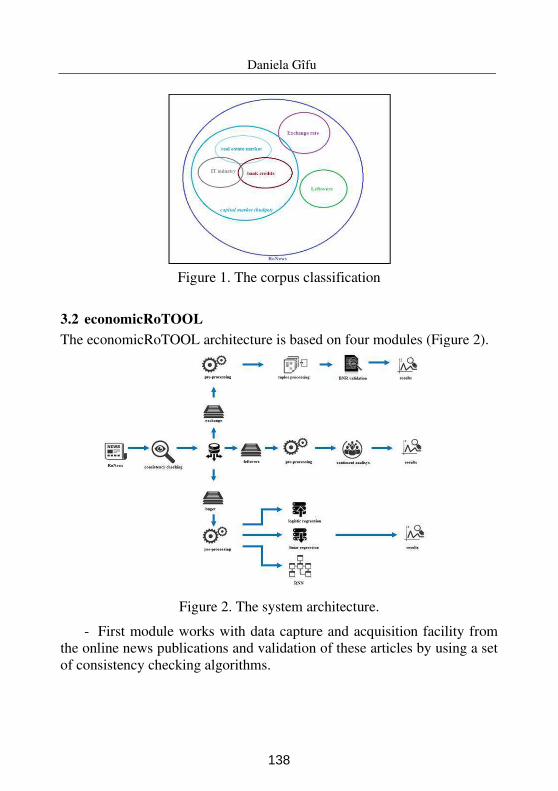
Daniela Gîfu
Figure 1. The corpus classification
3.2 economicRoTOOL
The economicRoTOOL architecture is based on four modules (Figure 2).
Figure 2. The system architecture.
- First module works with data capture and acquisition facility from
the online news publications and validation of these articles by using a set
of consistency checking algorithms.
138
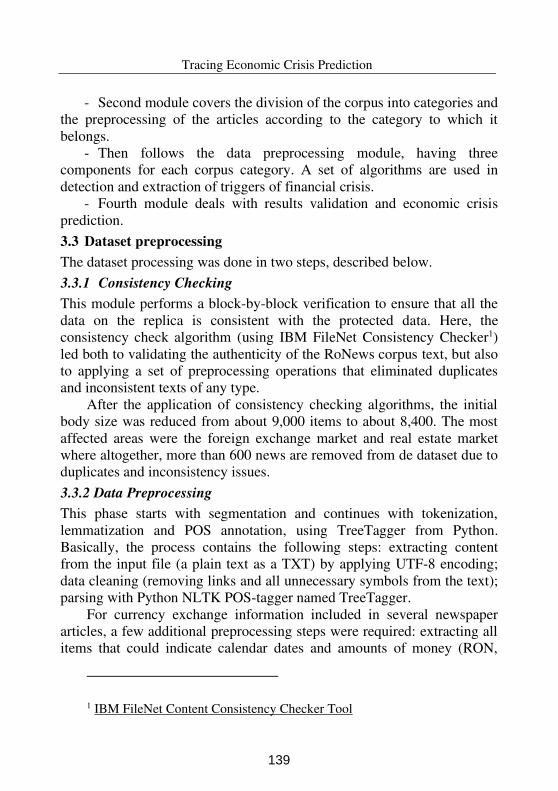
Tracing Economic Crisis Prediction
- Second module covers the division of the corpus into categories and
the preprocessing of the articles according to the category to which it
belongs.
- Then follows the data preprocessing module, having three
components for each corpus category. A set of algorithms are used in
detection and extraction of triggers of financial crisis.
- Fourth module deals with results validation and economic crisis
prediction.
3.3 Dataset preprocessing
The dataset processing was done in two steps, described below.
3.3.1 Consistency Checking
This module performs a block-by-block verification to ensure that all the
data on the replica is consistent with the protected data. Here, the
consistency check algorithm (using IBM FileNet Consistency Checker1)
led both to validating the authenticity of the RoNews corpus text, but also
to applying a set of preprocessing operations that eliminated duplicates
and inconsistent texts of any type.
After the application of consistency checking algorithms, the initial
body size was reduced from about 9,000 items to about 8,400. The most
affected areas were the foreign exchange market and real estate market
where altogether, more than 600 news are removed from de dataset due to
duplicates and inconsistency issues.
3.3.2 Data Preprocessing
This phase starts with segmentation and continues with tokenization,
lemmatization and POS annotation, using TreeTagger from Python.
Basically, the process contains the following steps: extracting content
from the input file (a plain text as a TXT) by applying UTF-8 encoding;
data cleaning (removing links and all unnecessary symbols from the text);
parsing with Python NLTK POS-tagger named TreeTagger.
For currency exchange information included in several newspaper
articles, a few additional preprocessing steps were required: extracting all
items that could indicate calendar dates and amounts of money (RON,
1 IBM FileNet Content Consistency Checker Tool
139
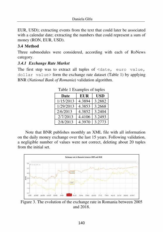
Daniela Gîfu
EUR, USD); extracting events from the text that could later be associated
with a calendar date; extracting the numbers that could represent a sum of
money (RON, EUR, USD).
3.4 Method
Three submodules were considered, according with each of RoNews
category.
3.4.1 Exchange Rate Market
The first step was to extract all tuples of <date, euro value,
dollar value> form the exchange rate dataset (Table 1) by applying
BNR (National Bank of Romania) validation algorithm.
Table 1 Examples of tuples
Date EUR USD
1/15/2013 4.3894 3.2882
1/29/2013 4.3853 3.2668
2/6/2013 4.3852 3.2404
2/7/2013 4.4106 3.2493
2/8/2013 4.3970 3.2773
Note that BNR publishes monthly an XML file with all information
on the daily money exchange over the last 15 years. Following validation,
a negligible number of values were not correct, deleting about 20 tuples
from the initial set.
Figure 3. The evolution of the exchange rate in Romania between 2005
and 2018.
140
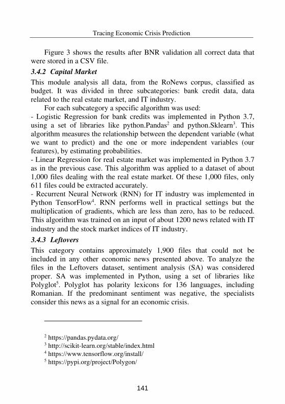
Tracing Economic Crisis Prediction
Figure 3 shows the results after BNR validation all correct data that
were stored in a CSV file.
3.4.2 Capital Market
This module analysis all data, from the RoNews corpus, classified as
budget. It was divided in three subcategories: bank credit data, data
related to the real estate market, and IT industry.
For each subcategory a specific algorithm was used:
- Logistic Regression for bank credits was implemented in Python 3.7,
using a set of libraries like python.Pandas2 and python.Sklearn3. This
algorithm measures the relationship between the dependent variable (what
we want to predict) and the one or more independent variables (our
features), by estimating probabilities.
- Linear Regression for real estate market was implemented in Python 3.7
as in the previous case. This algorithm was applied to a dataset of about
1,000 files dealing with the real estate market. Of these 1,000 files, only
611 files could be extracted accurately.
- Recurrent Neural Network (RNN) for IT industry was implemented in
Python TensorFlow4. RNN performs well in practical settings but the
multiplication of gradients, which are less than zero, has to be reduced.
This algorithm was trained on an input of about 1200 news related with IT
industry and the stock market indices of IT industry.
3.4.3 Leftovers
This category contains approximately 1,900 files that could not be
included in any other economic news presented above. To analyze the
files in the Leftovers dataset, sentiment analysis (SA) was considered
proper. SA was implemented in Python, using a set of libraries like
Polyglot5. Polyglot has polarity lexicons for 136 languages, including
Romanian. If the predominant sentiment was negative, the specialists
consider this news as a signal for an economic crisis.
2 https://pandas.pydata.org/ 3 http://scikit-learn.org/stable/index.html 4 https://www.tensorflow.org/install/ 5 https://pypi.org/project/Polygon/
141
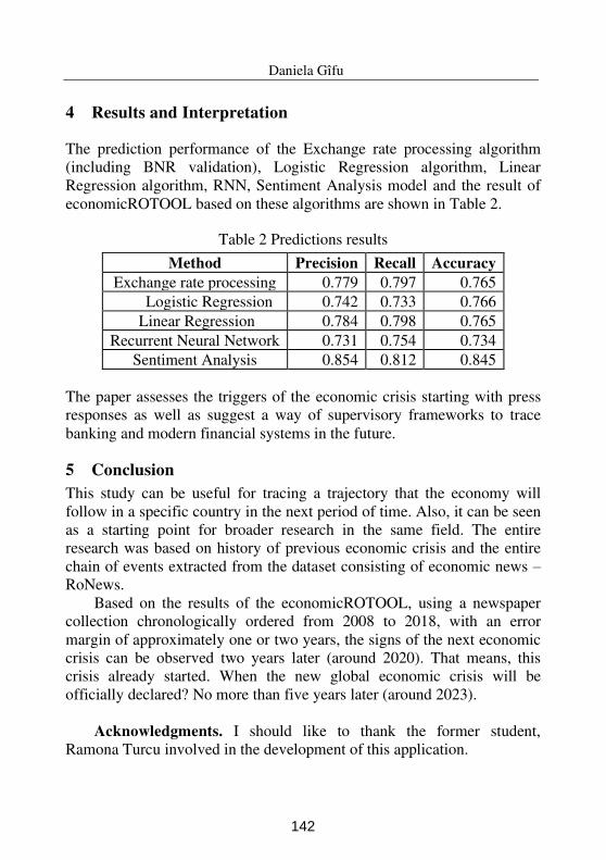
Daniela Gîfu
4 Results and Interpretation
The prediction performance of the Exchange rate processing algorithm
(including BNR validation), Logistic Regression algorithm, Linear
Regression algorithm, RNN, Sentiment Analysis model and the result of
economicROTOOL based on these algorithms are shown in Table 2.
Table 2 Predictions results
Method Precision Recall Accuracy
Exchange rate processing 0.779 0.797 0.765
Logistic Regression 0.742 0.733 0.766
Linear Regression 0.784 0.798 0.765
Recurrent Neural Network 0.731 0.754 0.734
Sentiment Analysis 0.854 0.812 0.845
The paper assesses the triggers of the economic crisis starting with press
responses as well as suggest a way of supervisory frameworks to trace
banking and modern financial systems in the future.
5 Conclusion
This study can be useful for tracing a trajectory that the economy will
follow in a specific country in the next period of time. Also, it can be seen
as a starting point for broader research in the same field. The entire
research was based on history of previous economic crisis and the entire
chain of events extracted from the dataset consisting of economic news –
RoNews.
Based on the results of the economicROTOOL, using a newspaper
collection chronologically ordered from 2008 to 2018, with an error
margin of approximately one or two years, the signs of the next economic
crisis can be observed two years later (around 2020). That means, this
crisis already started. When the new global economic crisis will be
officially declared? No more than five years later (around 2023).
Acknowledgments. I should like to thank the former student,
Ramona Turcu involved in the development of this application.
142
Tracing Economic Crisis Prediction
References
[1] D. Gîfu. Discursul presei scrise și violența simbolică. Analiza unei campanii
electorale, PhD Thesis, „Alexandru Ioan Cuza” University of Iaşi (2010)
[2] R. Delmonte, R. Tripodi, D. Gîfu. Opinion and Factivity Analysis of Italian
Political Discourse. Proceedings of the 4th edition of the Italian Information
Retrieval Workshop (IIR 2013), CEUR-WS on-line proceedings series, pp.
88-99 (2013)
[3] D. Gîfu and M. Cioca. Detecting Emotions in Comments on Forums. In:
International Journal of Computers Communications and Control, I. Dzitac,
F.G. Filip, M.-J. Manolescu (eds.), Vol. 9, no. 6, Agora University Editing
House, pp. 694-702 (2014)
[4] M. P. Bach, Z. Krstić, S. Seljan, L. Turulja. Text Mining for Big Data
Analysis in Financial Sector: A Literature Review. Sustainability, vol. 12
(2020)
[5] C. Guotai, M. Abedin and F–E Moula. Modeling Credit Approval Data with
Neural Networks: an Experimental Investigation and Optimization, Journal
of Business Economics and Management (2017)
[6] F-J Hsu, M-Y Chen and Y-C Chen. The Human-Like Intelligence with Bio-
inspired Computing Approach for Credit Ratings
Prediction, Neurocomputing (2018)
[7] W. Beaver. Financial Ratios as Predictors of Failures. In Empirical
Research in Accounting, selected studies supplement to the Journal of
Accounting research, 1(4): 71-127 (1966).
[8] E. I. Altman. Financial Ratios, Discriminant Analysis and the Prediction of
Corporate Bankruptcy. Journal of Finance, 23(4), 589-609 (1968).
[9] S. Cho, H. Hong, and B.-C. Ha. A Hybrid Approach Based on the
Combination of Variable Selection Using Decision Trees and Case-Based
Reasoning Using the Mahala Nobis Distance: for Bankruptcy Prediction,
Expert Syst. Appl., vol. 37 (2010)
[10] V. Arora and V. Ravi. Data Mining Using Advanced Ant Colony
Optimization Algorithm and Application to Bankruptcy Prediction, Banking,
Finance, and Accounting (2015)
[11] L. Svaboda, L. Michalkova, M. Durica, E. Nica. Business Failure Prediction
for Slovak Small and Medium-Sized Companies. Sustainability, vol. 11
(2020)
[12] Z. Xiao, X. Yang, Y. Pang and X. Dang. The Prediction for Listed
Companies’ Financial Distress by Using Multiple Prediction Methods with
143
Daniela Gîfu
Rough Set and Dempster–Shafer Evidence Theory. In Knowledge-Based
Systems 26: 196-506 (2012)
[13] Z. Li, J. Crook, G. Andreeva. Dynamic prediction of financial distress using
Malmquist DEA. In Expert Systems with Applications 80 (2017)
[14] I. Onur Oz and T. Yelkenci. A Theoretical Approach to Financial Distress
Prediction Modeling, Managerial Finance (2017)
[15] K. Ashraf, E. Félix, Z. Serrasqueiro, A-Score. Distress Prediction Model with
Earning Response during the Financial Crisis: Evidence from Emerging
Market, World Academy of Science (2018)
[16] F. Ecer. Comparing the Bank Failure Prediction Performance of Neural
Networks and Support Vector Machines: The Turkish Case. Ekonomska
Istraživanja / Economic Research 26(3):81-98 (2013)
[17] T. B. Bell, G. S. Ribar, J. Verchio. Neural Nets versus Logistic Regression: A
Comparison of Each Model’s Ability to Predict Commercial Bank Failures.
In Srivatsava, R.P. (Ed.), Proceedings of the 1990 Deloitte and
Touch/University of Kansas Symposium of Auditing Problems, 29-58
(1990).
[18] P. L. Brockett, W. W. Cooper, L. L. Golden, U. Pitaktong, U. A Neural
Network Method for Obtaining an Early Warning of Insure Insolvency. In the
Journal of Risk and Insurance, 61(3), 402-424 (1994).
[19] E. I. Altman, L. Zhang, J. Yen. Corporate Financial Distress Diagnosis in
China. New York University Salomon Center (2007).
[20] J. Sun, H. Li. Data mining method for listed companies’ financial distress prediction. In Knowledge-Based Systems 21(1):1-5 (2008).
[21] W. Bailey, W. Huang, Z. Yang. Bank Loans with Chinese Characteristics:
Some Evidence on Inside Debt in a State-Controlled Banking System. In
Journal of Financial and Quantitative Analysis, Volume 46, Issue 6, 1795-
1830 (2011).
[22] J. Eaton, H. S. Rosen. Optimal Redistributive Taxation and Uncertainty. In
Quarterly Journal of Economics 95(2):357-64 (1980).
Daniela Gîfu1,2
1Faculty of Computer Science, “Alexandru Ioan Cuza” University of Iasi, Romania 2 Institute of Computer Science, Romanian Academy, Iasi branch
E-mail: [email protected]
144
Proceedings of the Conference on Mathematical Foundations of Informatics MFOI’2020, January 12-16, 2021, Kyiv, Ukraine
© 2021 by Adrian Gotcă, Adrian Iftene
ECG Biometrics: Experiments
with SVM
Adrian Gotcă, Adrian Iftene
Abstract
We live in a complex society, maybe the most complex in the history of humanity, and the tech industry has evolved so much that from biometric recognition only in the most secured spots on the planet, we now have it even in the cheapest devices, including here laptops, smartphones, intelligent speakers, and so, on the list is quite long. The current paper presents a way to identify persons by the morphology of the electrocardiogram, identification based on differentiated characteristics.
Keywords: ECG, SVM, clustering, classification.
1 Introduction The ways of identifying a person with biometric characteristics are more diverse each year: from the fingerprint to iris, voice, face, cerebral waves, moving pattern, typing pattern, etc. [1]. We consider that the way presented in the current paper is more secure than other methods of biometric identification, being based on something that’s not easily falsified. We won’t say it cannot be falsified at all, because in our world so tech oriented as the one we live in you cannot be 100% sure of that. So the method we are going to present is based on some unique characteristics per individual, regarding the heart and more precisely the electrocardiogram that furthermore we will see other similar approaches of this subject as well as present our own approach and the results obtained during the experiments we have performed. For unique identification based on the EKG, we used a dedicated database, PTB Diagnostic ECG Database1, a component part of Physionet, a collection of databases in the medical field publicly listed by https://physionet.org/content/ptbdb/1.0.0/
145
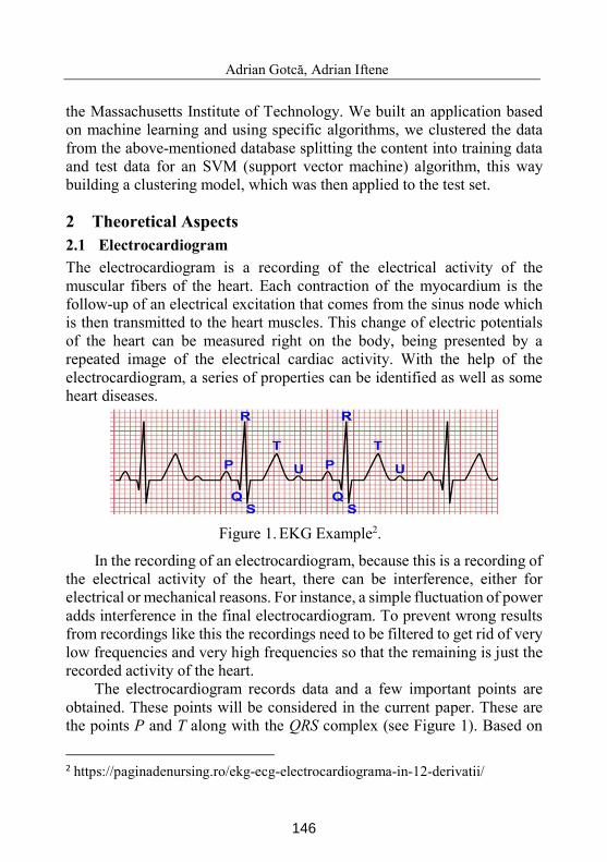
Adrian Gotcă, Adrian Iftene
the Massachusetts Institute of Technology. We built an application based on machine learning and using specific algorithms, we clustered the data from the above-mentioned database splitting the content into training data and test data for an SVM (support vector machine) algorithm, this way building a clustering model, which was then applied to the test set.
2 Theoretical Aspects 2.1 Electrocardiogram The electrocardiogram is a recording of the electrical activity of the muscular fibers of the heart. Each contraction of the myocardium is the follow-up of an electrical excitation that comes from the sinus node which is then transmitted to the heart muscles. This change of electric potentials of the heart can be measured right on the body, being presented by a repeated image of the electrical cardiac activity. With the help of the electrocardiogram, a series of properties can be identified as well as some heart diseases.
Figure 1. EKG Example2.
In the recording of an electrocardiogram, because this is a recording of the electrical activity of the heart, there can be interference, either for electrical or mechanical reasons. For instance, a simple fluctuation of power adds interference in the final electrocardiogram. To prevent wrong results from recordings like this the recordings need to be filtered to get rid of very low frequencies and very high frequencies so that the remaining is just the recorded activity of the heart.
The electrocardiogram records data and a few important points are obtained. These points will be considered in the current paper. These are the points P and T along with the QRS complex (see Figure 1). Based on
https://paginadenursing.ro/ekg-ecg-electrocardiograma-in-12-derivatii/
146
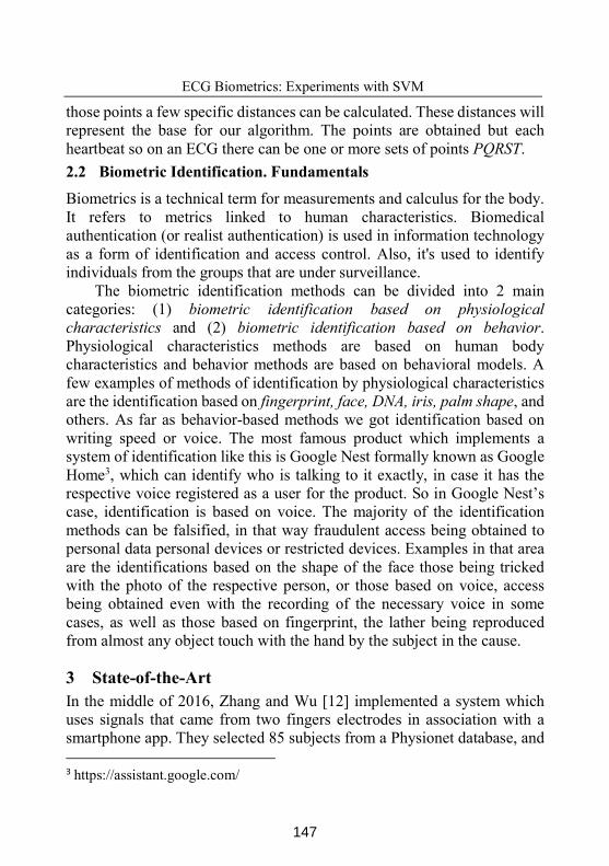
ECG Biometrics: Experiments with SVM
those points a few specific distances can be calculated. These distances will represent the base for our algorithm. The points are obtained but each heartbeat so on an ECG there can be one or more sets of points PQRST. 2.2 Biometric Identification. Fundamentals
Biometrics is a technical term for measurements and calculus for the body. It refers to metrics linked to human characteristics. Biomedical authentication (or realist authentication) is used in information technology as a form of identification and access control. Also, it's used to identify individuals from the groups that are under surveillance.
The biometric identification methods can be divided into 2 main categories: (1) biometric identification based on physiological characteristics and (2) biometric identification based on behavior. Physiological characteristics methods are based on human body characteristics and behavior methods are based on behavioral models. A few examples of methods of identification by physiological characteristics are the identification based on fingerprint, face, DNA, iris, palm shape, and others. As far as behavior-based methods we got identification based on writing speed or voice. The most famous product which implements a system of identification like this is Google Nest formally known as Google Home3, which can identify who is talking to it exactly, in case it has the respective voice registered as a user for the product. So in Google Nest’s case, identification is based on voice. The majority of the identification methods can be falsified, in that way fraudulent access being obtained to personal data personal devices or restricted devices. Examples in that area are the identifications based on the shape of the face those being tricked with the photo of the respective person, or those based on voice, access being obtained even with the recording of the necessary voice in some cases, as well as those based on fingerprint, the lather being reproduced from almost any object touch with the hand by the subject in the cause.
3 State-of-the-Art In the middle of 2016, Zhang and Wu [12] implemented a system which uses signals that came from two fingers electrodes in association with a smartphone app. They selected 85 subjects from a Physionet database, and https://assistant.google.com/
147
Adrian Gotcă, Adrian Iftene
used them for identification with Support Vector Machines and Neural Networks. They achieved an accuracy of 97.55% and a time for authentication of 4s. In the middle of 2017, a study that tried to show the efficacy of this type of biometrical identification in comparison with the other methods of identification being widely used in the industry was published. So in [2], the authors presented the efficacy of an approach that is dependent on the heartbeats in comparison with approaches like identification with the fingerprint, with the iris, or with the face, among others. The paper presents the process of feature extraction from the electrocardiogram waves, the process of training a machine-learning algorithm, and the results on data obtained from the same source as the current paper. At the end of 2017, the paper [3] which studied different ways of training a neural network, as well as a support vector machine to successfully identify persons from a finite universe was published. The solution presented in this paper is based on the support vector machine approach. The authors worked with a large set of features to define ECGs and then to recognize other samples of the same person. The two authors extracted features depending on distances, time, amplitude, or angles, this way extracting 72 features call Mom used them to build models of an artificial neural network, a support vector machine, and the k-nearest neighbor’s algorithm, established by a few statistics that the support vector machine is behaving best for this problem.
In September 2018, in [12], authors focused primarily on combining fiducial and non-fiducial points to achieve a better accuracy for authenticating many users. This work considered the PQRST complex, as well as PQ, QR, RS and ST duration ot PQ, PT or SQ amplitudes determined by wavelet transforms. For non-fiducial-based features, they defined the ECG signal as a matrix (M), obtained the Gramian matrix multiplying MTM, and finally obtained the features from the eigenvalues and eigenvectors from the Gramian matrix. They improve efficiency by increasing the number of features, but leading to increased computational effort. In [13], authors focused on Continuous Authentication (CA) using ECG, where the user needs to authenticate every period of time, ensuring the continued presence of the user. The samples are classified using the Decision Trees, Support Vector Machines, and other Machine Learning algorithms. They achieved accuracy ranging from 97.4% to 97.9%,
148
ECG Biometrics: Experiments with SVM
depending on some parameters by using recordings from 10 individuals from the MIT-BIH Normal Sinus Rhythm DataBase, taken also from Physionet. In [14], authors introduced a new multi-resolution convolutional neural network approach (MCNN) for ECG biometric identification, which considers 220 people. The achieved an identification rate of 96.5% for typical data sets, 90.5% for abnormal, and 93.5% for all data sets. They used a technique of getting random windows from ECG segments to increase data representation to cope with a data set with a small number of samples. In [15], the authors uses simple statistics for feature extraction, including the mean, standard deviation, median, maximum value, minimum value, range, interquartile range, interquartile first quarter (Q1), interquartile third quarter (Q3), kurtosis, and skewness of the ECG signal. The dataset used was the PTB ECG database again. The authors achieved an average accuracy of 99.61% using their band-based approach from single limb lead using Random Forest Classifier. They used a data segment length of 7 s, which guarantee a good number of heartbeat but takes too long to be acquired and can bother the user.
4 Proposed Solution Following will present the steps we followed for the classification algorithm of the AKG segments for each patient extracted from the database, as well as the external modules used for the algorithm. The algorithm is based on two important external modules: TensorFlow4 and WFDB (waveform database). 4.1 Libraries The application was coded using Python 3.7.85 and uses a few modules, some of them externals, which require installation before, some of them from the python standard library. The used modules are NumPy, Scikit-Learn, Matplotlib, SciPy, and WFDB (WaveForm Database). In this subchapter, we will provide details about the usage of Scikit-learn, SciPy, and WFDB for the presented solution. Waveform database6 was used to extract the data from the database, as well as to find the PQRST points for https://www.tensorflow.org/ https://www.python.org/downloads/ https://physionet.org/content/mimic3wdb/1.0/
149
Adrian Gotcă, Adrian Iftene
a record, the library has implemented a filtering type during the QRS complex calculation, which eased up the work further away.
SciPy module7 is dealing with specific digital signs processing, like specific filters applied to those. Scikit-learn module8 is dealing with the entire processing linked to the machine learning algorithm, which is the process of training and testing for the SVMs the algorithm is building. Numpy9 is a module specialized in complex mathematics operations on vectors and matrices and more. We used the module to build the vectors sent to Scikit-learn for training and testing. Matplotlib10 is a module specialized in making graphics and representative drawings for a certain function or for certain points in the plan. We used this module to extract graphics relevant to this paper. Imblearn11 is a module that deals with rebalancing data sets. It contains both methods for oversampling and undersampling strategies, so that in the end the resulting data set is a balanced one, with an equal number of entries for each class. 4.2 Main Modules The main modules of the application are: (1) the module designed for extracting the eligible patients’ data from the database, (2) the module for processing the data from the respective patients so that in the end we will have all relevant points of an EKG used in the current paper and (3) the module that handles the training and testing of a support vector machine for each patient. In the following, we will present the details of each module. 4.2.1 Patient Database The database we used was PTB Diagnostic ECG Database v1.0.0, and it consists of 549 records from 290 patients, with ages between 17 and 87 years, the average age being 57.2 years; 209 subjects are male, with the average age of 55.5 years, while the rest of 81 subjects are female, with an average age of 61.6 years. Also, the age was not recorded for 15 subjects, one female and 14 male. For each subject, there are up to 5 records. The records consist of ECG signals from 12 leads, these being i, ii, iii, avr, avl, https://www.scipy.org/ https://scikit-learn.org/ https://numpy.org/ https://matplotlib.org/ https://pypi.org/project/imblearn/
150
ECG Biometrics: Experiments with SVM
avf, v1, v2, v3, v4, v5, v6 plus 3 Frank leads, vx, vy and vz. The signal was digitized to 1,000 samples per second. In the header files, used for the current paper in the patients’ data extraction module, is present, along with the essential information, a detailed clinical history, including data about age, gender, diagnosis and, where applicable, data regarding medical history, medications and interventions, coronary arteries pathology, ventriculography, echocardiography, and hemodynamical data. This clinical summary is unavailable for 22 patients. 4.2.2 Patients’ Data Extraction Module This module is handling the eligible patients’ data extraction from the multitude of patients from the database. Therefore, this module will extract 10 randomly chosen patients from the ones that have at least an ECG record labeled with the “Healthy control” flag in the header file. As output, the module will return a list of 10 paths, each one pointing to a record of a single patient. The module will not return multiple records for a specific patient. This module uses standard functions of the Python language, like Random or the os modules. To correctly calculate this list, we’ll do the following: we’ll search the path where a copy of the database is stored to go through every patient stored there. So, every path from the list given as input which would be a file, not a directory, will be one of two types, either header file, with the extension .hea, containing specific metadata for the respective record, either data file, containing actual data, with the extension .dat. The header file can contain diverse data, from naming of the recorded leads to patient data. For this paper, we will use only the status of the patient and will search for a certain phrase present in all healthy patients. We will compute in that manner a list of all healthy patients from which will then extract 10 paths without extension to return them. We chose to return the paths without extension for easier processing at the next steps, well we need to process both files, the header one and the data one.
For this paper, the module chose the following patients: patient248 with record s0481, patient266 with record s0502, patient242 with record s0471, patient233 with record s0457, patient239 with record s0467, patient229 with record s0453, patient263 with record s0499, patient247 with record s0479, patient238 with record s0466 and patient246 with record s0478. These were the data used for the runs presented in the Experiments section, and the results are relative only to those 10 extracted patients.
151
Adrian Gotcă, Adrian Iftene
4.2.3 Data Processing Module This module will receive as input the returned list from the previously discussed module and will return as output a list with processed data of each patient with the designated record from the input list. In this manner, for each path from the input list, we will access the data file and will extract and process the data found in the file. This module has itself to big submodules: one for processing one subject and one for processing a 10 seconds segment. We will present each submodule in the following sections. 4.2.4 The 10-Second Segment Processing Submodule This submodule will receive an input vector consisting of the signal produced on the extracted lead, for a 10-second duration. As output, it will return for lists, consisting of indices where the important points are found including points from the QRS complex as well as the T point. These will be then used in the computing of the feature vectors used in the training and testing module. Well now present the procedure for localization of Q, R, S, and T points mentioned above.
For the R points the integrated QRS detector from WFDB was used, with slight modifications for the positions where applicable. This thing was necessary because the signal was not filtered, captured at 1,000 Hz, capturing some noise reflected in the transmitted signal, this one is a bit corrupted. This modification was realized with the following method: on the signal came to 1,000 Hz we applied a Butterworth lowpass12 second order filter with the resulted frequency of 10Hz, followed by a search of the closest extreme point for the point the QRS detector determined. This extreme point can be determined mathematically quite easily. Each EKG can be considered a function graph, then performing the first derivative and looking for the nearest point where the first derivative is equal to 0, or in this case, is very close to 0, we find the R point sought. Based on the R point and the first derivative, the other points are determined as follows: point Q, being a local minimum point, will be the first point less than R for which the first derivative is very close to 0, within 100 units. So, it is enough to look for the point between R-100 and R. For point S, we will look in the next 100 points relative to R on the first at which the sign of the derivative changes from negative to positive. In the case of point T, we will need to look in the next 300 points relative to S for the one at which the sign of the
152
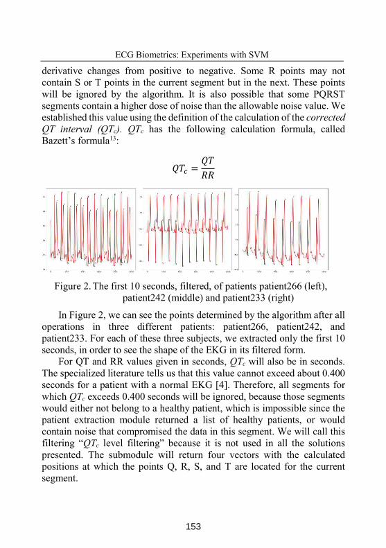
ECG Biometrics: Experiments with SVM
derivative changes from positive to negative. Some R points may not contain S or T points in the current segment but in the next. These points will be ignored by the algorithm. It is also possible that some PQRST segments contain a higher dose of noise than the allowable noise value. We established this value using the definition of the calculation of the corrected QT interval (QTc). QTc has the following calculation formula, called Bazett’s formula13: =
Figure 2. The first 10 seconds, filtered, of patients patient266 (left),
patient242 (middle) and patient233 (right)
In Figure 2, we can see the points determined by the algorithm after all operations in three different patients: patient266, patient242, and patient233. For each of these three subjects, we extracted only the first 10 seconds, in order to see the shape of the EKG in its filtered form.
For QT and RR values given in seconds, QTc will also be in seconds. The specialized literature tells us that this value cannot exceed about 0.400 seconds for a patient with a normal EKG [4]. Therefore, all segments for which QTc exceeds 0.400 seconds will be ignored, because those segments would either not belong to a healthy patient, which is impossible since the patient extraction module returned a list of healthy patients, or would contain noise that compromised the data in this segment. We will call this filtering “QTc level filtering” because it is not used in all the solutions presented. The submodule will return four vectors with the calculated positions at which the points Q, R, S, and T are located for the current segment.
153
Adrian Gotcă, Adrian Iftene
4.2.5 The sub-module for processing a subject This submodule will receive as input a path to the memory location of the data files for a patient. We know that the recording times are 120 seconds, so here we will also divide it into 10-second segments. In this submodule, each 10-second segment will be processed by obtaining the results of its processing in the processing submodule of a segment. Thus, at the output, there will be a vector representing all the results in each segment. 4.2.6 SVM training and testing module This module will take as input the list from the processing module and will return a list of 10 support vector machines, one for each patient involved in this paper. Thus, as can be seen, we chose to apply specific machine learning algorithms to train and test a support vector machine. Each patient will represent a class, and the characteristics identified for each QRS complex, together with a T wave, are the temporal distances between Q and T, hereinafter referred to as QT, R and T, called RT, respectively S and T, called ST. For a classification independent of the patient's pulse, a normalization on the training set is required. This normalization will be done in several ways.
This module was implemented in 5 different solutions, each with some differences from the others. The steps explained up to this point are not different from one solution to another, the testing data being the same and the steps performed up to this point, i.e. extracting patients from the database and processing them, except for QTc filtering, which is present only in some approaches, being also the same. We will specify in each approach whether or not this filtering has been performed. Thus we will detail, in this order, the following solutions for this module: Solution 1: Binary SVM, with data normalization relative to the
average RR distances of the subjects being trained, without performing QTc level filtering;
Solution 2: Binary SVM, with data normalization relative to the average RR distances of the subjects with which training is performed, with the QTc level filtering;
Solution 3: Multi-class SVM, with data normalization relative to the average RR distances of the subjects with which training is performed, with QTc level filtering;
154
ECG Biometrics: Experiments with SVM
Solution 4: Binary SVM, with data normalization using sklearn, with unbalanced classes, using tools provided by sklearn for balancing inside SVM, without altering the data set;
Solution 5: Binary SVM, with data normalization using sklearn, with balanced classes using the SMOTE14 technique for balancing classes, with the generation of new test or training instances.
5 Experiments 5.1 Solution 1 As described above, this solution consists of a binary SVM, with normalization of data relative to the average RR distances of the subjects being trained, without performing QTc filtering. We will detail below the performance calculation, how to build the training and test data set, how the training procedure goes, and what results we have obtained.
The classification performance made by the SVM-based classifier can be maximized by optimizing two general parameters that define SVM: hyperparameter C, which controls the trade-off between margin maximization and error minimization, and the core parameter, which controls drive data mapping in a multidimensional space when data are non-linearly independent. There are several core functions, including the basic radial function, which is the most widely used and is generally considered to be more suitable for working with biological features, according to several past studies that have worked with EKG signals or similar [5-9]. The use of the radial base function in the SVM requires the optimization of a third parameter, σ, i.e. the dispersion of the Gaussian function. The best parameters C and σ can be searched using an exhaustive search. Once you find the parameters, the classifier can be built with them and then trained, and finally tested. The two parameters were searched in the set 0.001, 0.01, 0.1, 1, 5, 10, 100.The characteristics were normalized using the average of the RR distances on each sample. The RR distance is the distance between 2 consecutive R points within the same segment. Since SVM is binary and the present problem is a multi-class one, a few more operations are needed. First, we will build an SVM for each patient. Second, for each SVM thus constructed, we will have two classes: one that would mean that the sample belonged to the EKG of the patient in question, and one that would mean the opposite. Thus, we will classify the samples belonging to the current
155
Adrian Gotcă, Adrian Iftene
patient with 1, and with 0 we will classify the samples of the other patients. We will divide this set into two disjoint subsets, one for training and one for testing. Thus, on the training set will go all the samples classified with 0, plus the samples from 10 of the 12 segments of the current patient, following that the 2 remaining segments will go on the test set. Thus, we can calculate the accuracy of the SVM by extracting each possible combination of 2 segments, obtaining 66 runs, and evaluating each run in turn, thus obtaining the average for all runs for each patient.
For each run, the best parameters C and σ were calculated using 5-fold cross-validation, this being the standard of the libraries used. Then, during the testing stage, each tuple QT, RT, ST was mapped in the space generated by the training stage, normalizing the values with the same average RR value found during the training stage. Regarding the average RR value, it was calculated relative to all samples in the training set, and not only relative to those of the patient in question, because the role of this normalization is to design a new entry in the search space of all subjects, regardless of the subject from which this new entry was chosen.
This approach has proven to be a failure, for the following reasons: inefficient normalization, unbalanced classes, and the presence of “noisy” data, data that can confuse training in giving poor results. The average accuracy for 10 patients was 50%. 5.2 Solution 2 As described above, this solution consists of a binary SVM, with normalization of data relative to the average RR distances of the subjects being trained, but compared to the previous solution it is also used to perform QTc filtering. Otherwise, the training and testing procedure is unchanged. We also consider this approach a failure, the results being mixed again, some being acceptable, in the sense that they are around 65-70%, others being below 50%. The average accuracy for the same 10 patients was 54%. 5.3 Solution 3 As described in the presentation of the SVM training and testing module, the third solution presented in this paper is based on a multi-class SVM, with data normalization relative to the average RR distances of the subjects being trained and with QTc level filtering. SVM is a binary classifier concept but within the sklearn.svm module there is a class dedicated to
156
ECG Biometrics: Experiments with SVM
multiclass classification, namely LinearSVC. It uses a linear kernel function and constructs N binary models, where N represents the number of classes. In the problem addressed by this paper, N is equal to 10, with 10 patients, each representing a class. Therefore, this variant is equivalent to using the SVC class within the sklearn.svm module with the appropriate parameters for multiclass classification. Here we noticed the importance of choosing the right core function in the construction of a model based on SVMs, in this case using a linear function, and not a radial base one, as is the case for the other solutions.
In this case, two sets X and Y were constructed, X containing tuples of the form [QT, RT, ST] before normalization, and Y containing a number from 0 to 9, representing the patient corresponding to this record. These two sets were divided proportionally so that 80% of each patient's samples were intended for training, and the remaining 20% remained for testing. Thus, the phenomenon of overfitting and/or under fitting was avoided by the presence of 80% of each class in the training subset. This procedure was repeated 100 times so as to obtain relevant results. Unfortunately, this method does not give any results, because the choice of the linear function for the construction of the SVM makes the SVM unable to finish the training. Also, the class used is limited to a number of iterations, but these are not the problem but the fact that the data are not suitable for such an approach. Therefore, the algorithm did not produce results, each run returning a ConvergenceWarning type warning. 5.4 Solution 4 This solution consists of a binary SVM, with data normalization using sklearn, with unbalanced classes, using tools provided by sklearn for balancing inside the SVM. This involves building a pipeline, in which the first step is to perform normalization using the Normalizer class within the sklearn.preprocessing module, and then to train the SVM model with the training data, composed of 80% of the data classified with 1 and 80% of the data classified with 0, and the remaining 20% of those with 1 and 20% of those with 0 to be in the subset for testing. This variant will make a binary SVM with balanced classes inside the SVM. This can be done by setting a parameter at the SVM instantiation, before training, which tells the kernel to handle balancing the data set, otherwise working with the same C parameter. By setting this parameter, the library will work with a variable
157
Adrian Gotcă, Adrian Iftene
C, depending on how many samples there are for that class. Thus we try to give more importance to the class represented by the samples classified with 1, these being significantly less, coming from a single patient, compared to those classified with 0, which come from several patients. The above-mentioned process was also run 100 times to obtain scientifically relevant data. The results obtained with this variant of the module are significantly better than with the other solutions, being over 80% on all runs. The average accuracy for the same 10 patients was 90%. 5.5 Solution 5 This solution is based on a binary SVM, also with normalization offered by sklearn, but this time with the generation of new samples by the synthetic minority oversampling technique [10]. This technique is recognized as effective enough to solve the problem of balancing data sets. So, once the data set is balanced, we can divide it into two disjoint subsets, one to be used for training and the other for testing. We chose the same ratio as in a previous solution, 80% for training, and 20% for testing. We did not need to make sure that we had samples from both classes, the data set is balanced. The average accuracy for the same 10 patients was 95%.
6 Conclusion From the results presented in the Experiments section, we can draw the following conclusions: QTc level filtering improved the algorithm to some extent, so it was a
good decision to use it, even if the difference was not significant, solutions 1 and 2 having only this different aspect, the results being differences of a maximum of 5% both on the minimum as well as on the maximum, respectively the average accuracy.
Normalization played a crucial role in achieving the accuracy of solutions 4 and 5. With the normalization offered by the sklearn package, we managed to obtain a correct mapping in the multidimensional space described by the available data, mapping that could further provide the accuracy obtained in the two solutions.
An SVM with unbalanced classes works in some cases better than an SVM with artificially balanced classes by oversampling. One possible cause would be that the artificial oversampling of the data set causes some samples to be classified as being of the oversampled class, due to
158
ECG Biometrics: Experiments with SVM
the proximity in the space described by the characteristics of the above-mentioned samples to some artificial samples generated for oversampling. Thus, for some patients SVMs without oversampling performed better than those with oversampling.
An SVM with unbalanced classes can face real problems for some patients. At the same time, SVM with balanced classes gives satisfactory results, of over 80% in the case of these patients, even if in the case of others the results are not as good as in the case of SVM with unbalanced classes. The latter results remain satisfactory, with over 90% accuracy.
The SVM that uses normalization at the level of average RR behaves very poorly, with a standard deviation approaching in some cases to 50%. This tells us that this solution, even if it gives classifications, they are much too diverse, and do not help too much.
The problem is not suitable for a multi-class SVM. The latter SVM, which is based on a linear function and not on a radial basis, fails to complete the algorithm because the data are not linearly separable. So we need to do binary SVMs, based on radial base functions.
References [1] C. R. Cazuc, A. Iftene. User Recognition Based on Keystroke Dynamics. In
5th Proceedings of the Conference on Mathematical Foundations of Informatics. 3-6 July 2019, Iasi, Romania, (2019), pp. 343-350.
[2] S.J. Paiva, D. Dias, J. P. Cunha, S., Gao. Beat-ID: Towards a computationally low-cost single heartbeat biometric identity check system based on electrocardiogram wave morphology. In the US National Library of Medicine, 18 July (2017).
[3] K.K. Patro, P. R. Kumar. Machine Learning Classification Approaches for Biometric Recognition System using ECG Signals. In Journal of Engineering Science and Technology Review 10, 7 December (2017).
[4] M. Shenasa, N. A. Mark Estes II, G. F. Tomaselli. Contemporary Challenges in Sudden Cardiac Death, An Issue of Cardiac Electrophysiology Clinics, 1st Edition. January (2018), pp. 608.
[5] Y. Liu, Y. F. Zheng. FS_SFS: A novel feature selection method for support vector machines. In ScienceDirect Journal, vol. 39, issue 7. 21 November (2005), pp. 1333-1345.
159
Adrian Gotcă, Adrian Iftene
[6] H. Li, H. Liang, C. Miao. et al. Novel ECG Signal Classification Based on KICA Nonlinear Feature Extraction. In Circuits Syst Signal Process 35, (2016), pp. 1187–1197. https://doi.org/10.1007/s00034-015-0108-3
[7] M. Korürek, B. Doğan. ECG beat classification using particle swarm optimization and radial basis function neural network. In Expert systems with Applications, vol. 37, Issue 12. 7 May (2010), pp. 7563-7569.
[8] O. Boumbarov, Y. Velchev, S. Sokolov. ECG personal identification in subspaces using radial basis neural networks. In Intelligent Data Acquisition and Advanced Computing Systems: Technology and Applications, IDAACS 2009. IEEE International Workshop on. IEEE (2009), pp. 446-451.
[9] N. Maglaveras, T. Stamkopoulos, K. Diamantaras, C. Pappas, M. Strintzis. ECG pattern recognition and classification using non-linear transformations and neural networks: a review. In International journal of medical informatics. (1998) pp. 191-208.
[10] N.V. Chawla, K.W. Bowyer, L.O. Hall, W.P. Kegelmeyer. SMOTE: Synthetic Minority Over-sampling Technique. In Journal of Artificial Intelligence 16. 6 February (2002), pp. 321-357.
[11] Zhang Y., Wu J. Practical human authentication method based on piecewise corrected Electrocardiogram; In Proceedings of the 7th IEEE International Conference on Software Engineering and Service Science (ICSESS); Beijing, China. 26–28 August (2016); pp. 300–303.
[12] Zhang Y., Gravina R., Lu H., Villari M., Fortino G. PEA: Parallel electrocardiogram-based authentication for smart healthcare systems. J. Netw. Comput. Appl., vol. 117 (2018); pp. 10–16
[13] Camara C., Peris-Lopez P., Gonzalez-Manzano L., Tapiador J. Real-Time Electrocardiogram Streams for Continuous Authentication. Appl. Soft Comput. J., vol. 68 (2018); pp. 784–794.
[14] Zhang Q., Zhou D., Zeng X. HeartID: A Multiresolution Convolutional Neural Network for ECG-Based Biometric Human Identification in Smart Health Applications. IEEE Access. , vol. 5 (2017): pp. 11805–11816.
[15] Palma A.J., Alotaiby T.N., Alrshoud S.R., Alshebeili S.A., Aljafar L.M. ECG-Based Subject Identification Using Statistical Features and Random Forest. J. Sens. vol 2019 (2019): id 6751932
Adrian Gotcă, Adrian Iftene
Alexandru Ioan Cuza University of Iasi, Faculty of Computer Science E-mail: [email protected], [email protected]
160
Proceedings of the Conference on Mathematical Foundations of Informatics
MFOI-2020, January 12-16, 2021, Kyiv, Ukraine
Using Artificial Intelligence in
Medicine
Adrian Iftene
Abstract
The field of artificial intelligence has evolved a lot in recent
years, reaching very good results in the area of text and voice
processing, image and video processing, clustering and
classification, prediction, etc. The medical field is one of the fields
that can benefit a lot from this evolution, we refer here to the
automatic analysis of images, radiographs and ECGs, predictions of
disease evolution and the identification of best treatment for patients,
etc. The Faculty of Computer Science from Iasi has several projects
related to the application of artificial intelligence in medicine: (1)
participation in CLEF competitions related to image processing with
radiographs of tuberculosis patients, kaggle competitions related to
the use of RSNA medical collections IHD, iris, etc., (2) projects
started from collaborations with doctors from the University of
Medicine in Iasi: identification of atrial fibrillation, identification of
strokes, classification of teeth, etc. (3) projects started at the level of
the ImagoMol Medical Imaging Cluster: REVERT - an H2020
project, which aims to predict the best treatments for colorectal
cancer patients, etc. This presentation aims to present these research
projects, the results obtained and the plans we have for the future.
Keywords: artificial intelligence, image processing, prediction.
161
Proceedings of the Conference on Mathematical Foundations of Informatics
MFOI2020, January 12-16, 2021, Kyiv, Ukraine
On Generalizations of Real Induction
Ievgen Ivanov
Abstract
We propose a generalization of the real induction principle toan induction principle for partial orders of a special class. The ob-tained results may be useful for verification of systems describedby discrete-continuous models and other related applications.
Keywords: induction, real induction, partial order, formalmethods.
1 Introduction
Mathematical induction by a natural number parameter and its gener-alizations have many applications in computer science. They appear infoundations of formal methods which deal with modeling and verifica-tion of hardware and software systems. Besides, formalizations in proofassistants such as Isabelle and Coq frequently involve applications ofsuch principles.
Although inductive proofs by a parameter which takes discrete val-ues are the most widely known, in the literature one can find principlesof induction over a continuous parameter. An overview of such princi-ples, usually called real or continuous induction principle, can be foundin [1, 2, 3].
Recently, real induction has been used as a rule in logics intendedfor specification and verification of cyber-physical systems [4, 5]. In thiswork we consider the problem of its generalization to certain types ofpartial orders. Such generalizations may be useful for proving proper-ties of nondeterministic discrete-continuous models as a part of formalverification.
c©2020 by Ievgen Ivanov
162
On Generalizations of Real Induction
More specifically, we propose an answer to a question posed in[6] about an induction principle for posets of a special class (posetswith infima). Examples of such posets include the poset of partialtrajectories of a nondeterministic dynamical system defined on timeintervals of the forms [0, t), [0, t] with an order given by the extensionrelation, i.e. s1 ≤ s2, if s2 extends s1.
2 Preliminaries
Let us describe the terminology from [6].Let (X,≤) be a totally ordered set which has a least element. Then
X has infima [6], if every nonempty S ⊆ X has an infimum.A set S ⊆ X is an inductive subset [6], if the following conditions
hold, where 0 denotes the least element of X:
POI1([6]) 0 ∈ S.
POI2([6]) For all x ∈ S, if there exists z ∈ X such that x < z, thenthere exists y > x such that [x, y] is contained in S.
POI3 [6] For all x ∈ X, if [0, x) ⊆ S, then x ∈ S.
Note that, formally, POI1 follows from POI3, but it makes sense toinclude it as a separate condition to make the base case clear.
It can be proven [6] that X has infima if and only if the only in-ductive subset of X is X, which generalizes one of the variants of thereal induction principle. The question in [6], basically, asks for a gen-eralization of this result to the case of partially ordered sets.
The proposed answers include a theorem which gives an inductionprinciple for complete lattices and characterizes them in terms of thisprinciple, and a theorem which implies that for a poset X in whichnonempty sets have infima, and a suitably modified notion of an induc-tive subset, the only inductive subset of X is X (however, the conversestatement does not hold, which is dissimilar to the situation with theabove mentioned induction for total orders with infima).
163
On Generalizations of Real Induction
Similarly to the above, let us say that a poset (X,≤) has infima, ifevery nonempty subset of X has an infimum.
Although a poset with infima without top element may be com-pleted to a complete lattice by adding a top element, this is not alwaysuseful, if the goal is to prove some property by induction, as the induc-tion principle becomes trivial in a certain sense.
Below we propose an induction principle for posets with infimawhich does not rely on such a completion.
3 Main Result
Definition 1.Let (X,≤) be a poset with a least element.A subset S ⊆ X is infima-inductive in (X,≤), if the following
conditions (II1, II2, II3) hold:
II1: 0≤ ∈ S;
II2: for every x ∈ S and z ∈ X such that x < z, and every sat-urated chain C in (X,≤) such that x, z ⊆ C ⊆ [x, z]≤ andinf≤(C\x) = x, there exists y ∈ C such that x < y and foreach t ∈ [x, y]≤ ∩ C, if inf≤t, s exists for all s ∈ X, then t ∈ S;
II3: for every x ∈ X, if [0≤, x)≤ ⊆ S holds, and the infimum inf≤x, yexists for each y ∈ X, then x ∈ S.
Note that in the case of total orders, if a saturated chain satisfiesx, z ⊆ C ⊆ [x, z]≤, then C = [x, z]≤, and, besides, 2-meets (infimaof pairs of elements) exist, so the conditions II1-II3 can be simplifiedaccordingly.
Definition 2. A poset with a least element (X,≤) satisfies theinfima induction principle, if for each S ⊆ X,
if S is infima-inductive, then S = X.We will also say that a subset S ⊆ X in a poset (X,≤) is
Noetherian-inductive, if
∀x ∈ X (∀y ∈ X (x < y ⇒ y ∈ S) ⇒ x ∈ S) .
164
On Generalizations of Real Induction
Theorem 1. A poset with a least element has infima if and only if it
satisfies the infima induction principle.
Proof. “If”. Let (X,≤) be a poset with a least element which satisfiesthe infima induction principle, i.e. for each S ⊆ X, if S satisfies II1,II2, II3, then S = X. Let us show that (X,≤) has infima.
Let S0 be the set of all x ∈ X such that inf≤x, y exists for ally ∈ X. Then S0 satisfies the condition II1.
Let x ∈ S0, z ∈ X, x < z, and C be a saturated chain such thatx, z ⊆ C ⊆ [x, z]≤. Let y = z. Then y ∈ C, x < y, and for eacht ∈ [x, y]≤ ∩ C, if inf≤t, s exists for all s ∈ X, then t ∈ S0. Thus S0
satisfies the condition II2.Let x ∈ X and [0≤, x)≤ ⊆ S0. If inf≤x, y exists for each y ∈ X,
then x ∈ S0. Thus S0 satisfies the condition II3.Since (X,≤) satisfies the infima induction principle, we have S0 =
X, whence (X,≤) has 2-meets.Let us show that (X,≤−1) satisfies Raoult’s open induction prin-
ciple [8], i.e. if a subset is directed open (d-open) and Noetherian-inductive, then it is X. Let S be a d-open, Noetherian-inductive subsetin (X,≤−1). Since S is Noetherian-inductive in (X,≤−1), the condi-tions II1 and II3 hold for S.
Let us show that the condition II2 holds for S. Let x ∈ S, z ∈ X,x < z, C be a saturated chain in (X,≤) such that x, z ⊆ C ⊆ [x, z]≤and x = inf≤(C\x).
Suppose that there is no y ∈ C such that x < y and [x, y]≤∩C ⊆ S.Then for each y ∈ C\x, there exists y′ ∈ C\S such that y′ ≤ y. Then,since x ∈ S, C\S is a coinitial subset of C\x. Moreover, C\S 6= ∅,because x < z and z ∈ C\x. Then inf≤(C\S) = x ∈ S. Thiscontradicts the assumption that S is d-open in (X,≤−1). Thus II2holds for S.
Since (X,≤) satisfies the infima induction principle, we have S = X.We conclude that (X,≤−1) satisfies Raoult’s open induction principle.By [7, Theorem 1], (X,≤−1) is a dcpo. Then (X,≤) is a fcpo whichhas 2-meets. Then (X,≤) has infima.
165
On Generalizations of Real Induction
“Only if”. Let (X,≤) be a poset with a least element. Assumethat (X,≤) has infima. Let us show that (X,≤) satisfies the infimainduction principle. Let S ⊆ X be an infima-inductive subset. Letus show that S is filtered-open (f-open) in (X,≤). Let C0 ⊆ X be anonempty ≤-chain and inf≤C0 = x ∈ S. If x ∈ C0, then C0 ∩ S 6= ∅.
Assume that x /∈ C0. Then there exists z ∈ C0 such that x < z.Note that C0 ∪ x is a ≤-chain. Let C ′ be a saturated ≤-chain suchthat C0∪x ⊆ C ′ and C = C ′∩[x, z]≤. Then C is a saturated ≤-chainand x, z ⊆ C ⊆ [x, z]≤.
Let us show that C0 and C\x are coinitial subsets of X. If y1 ∈C0, then there exists y2 = inf≤y1, z ∈ C0 ∩ (x, z]≤ ⊆ C\x andy2 ≤ y1. Let y1 ∈ C\x. Then x < y1. Moreover, y1 ≤ y2 cannothold for all y2 ∈ C0, since otherwise, y1 ≤ x = inf≤C0. Then y1 ≤ y2does not hold for some y2 ∈ C0. Then y2 ≤ y1, since y1, y2 ∈ C ′, andso are ≤-comparable. We conclude that C0 and C\x are coinitial, soinf≤(C\x) = x.
Since S is infima-inductive and (X,≤) has infima, the condition II2implies that there exists y′ ∈ C such that x < y′ and [x, y′]≤ ∩ C ⊆S. Then y′ ∈ C\x. Since C0 and C\x are coinitial, there existsy ∈ C0 ⊆ C ′ such that y ≤ y′ ≤ z. Then y ∈ [x, y′]≤ ∩ C ⊆ S. ThusC0 ∩ S 6= ∅.
We conclude that S is f-open in (X,≤). Then S is a d-open subsetof X in the opposite poset (X,≤−1). Since (X,≤) has infima, thecondition II3 implies that S is a Noetherian-inductive subset of X in(X,≤−1). Moreover, (X,≤) is a fcpo, so (X,≤−1) satisfies Raoult’sopen induction principle. Then S = X.
We conclude that (X,≤) satisfies the infima induction principle.
4 Conclusions
We have proposed a generalization of real induction to a class of posetsrelevant for formal methods (formal verification of discrete-continuoussystems). Further work may include formalization of this principle inproof assistants such as Isabelle and Coq.
166
On Generalizations of Real Induction
References
[1] P. Clark. The Instructor’s Guide to Real Induction. MathematicsMagazine, vol. 92, 2019, pp. 136–150.
[2] P. Clark. The Instructor’s Guide to Real Induction, 2012. Availableat: http://arxiv.org/abs/1208.0973
[3] I. Kalantari. Induction over the Continuum. In M. Friend, N.B.Goethe and V.S. Harizanov (eds.), Induction, Algorithmic Learn-ing Theory, and Philosophy, pp. 145–154, Springer, 2007.
[4] A. Platzer, Yong Kiam Tan. Differential Equation Axiomatization:
The Impressive Power of Differential Ghosts. In Proc. of LICS’18,pp. 819–828, 2018.
[5] A. Platzer, Yong Kiam Tan. Differential Equation Invariance Ax-
iomatization, 2019. Available at: http://arxiv.org/abs/1905.13429
[6] A principle of mathematical induction for partially ordered sets
with infima. –Web page: https://mathoverflow.net/questions/38238
[7] I. Ivanov. On Induction for Diamond-Free Directed Complete Par-
tial Orders. Proc. of the 16th International Conference on ICT inEducation, Research and Industrial Applications. ICTERI 2020,CEUR-WS.org, vol. 2732 (2020)
[8] J.-C. Raoult. Proving open properties by induction. InformationProcessing Letters, vol. 29 (1988) pp. 19-23
Ievgen Ivanov
Taras Shevchenko National University of Kyiv
Email: [email protected]
167
Proceedings of the Conference on Mathematical Foundations of Informatics
MFOI2020, January 12-16, 2021, Kyiv, Ukraine
Dynamic Time Warping for uncovering
dissimilarity of regional wages in Ukraine
Dmytro Krukovets
Abstract
The work shows how advanced Data Science and Time Series
algorithms such as Dynamic Time Warping with some clustering
techniques might be used over real-life data and which results will
they give. As a real-life example, the regional wages in Ukraine
were chosen. Overall, algorithms have shown satisfying perfor-
mance and have been able to give meaningful results that can be
used further in the hypothesis formulation and economic analysis.
Keywords: Computer Science, Data Science, Time-series
Analysis, Dynamic Time Warping, Clustering, Regional Wages.
1 Introduction
In the world of the data transformation, we’re living with a constantlygrowing amount of it in all the possible fields. To make this datawork, we’ve got to bring appropriate algorithms to analyze it. Theirappearance is mostly shown by two major cases: the first is aboutdeveloping unique techniques and the other is about the usage of theold ones, but in an unusual manner or with some adjustments.
The purpose of the paper is to try several algorithms that are tradi-tional for Computer Science and Data Science and do it in the case ofthe real-life data i.e. economic data in this particular paper. Moreover,these results might give applicable analysis and unusual conclusions,which might support other researches in the area.
Nowadays, Data Science enhances its popularity in many areas in-cluding Economics. In the overview by Dmytro Krukovets, 2020[6], it
©2020 by Dmytro Krukovets
168
Dmytro Krukovets
is shown how Data Science might be used to solve different economicissues, improve the performance of existing models and add new waysto solve old problems. Thus, the topic of usage Data Science techniquesin economics is hot and requires a lot of work and research to do.
The paper is dedicated to the measuring of time series similarity viaa set of algorithms and then a grouping of these series by their similaritywith clustering techniques. The data is represented by average salariesin Ukrainian regions. The problem is interesting for analysis as longas there is brightly determined heterogeneity in wages for regions, forexample, it is way higher in Kyiv throughout the whole history. More-over, during the beginning of the war in the east of Ukraine, the mostharmed regions were Donetska and Luhanska, that must have been seenin the data. These obvious discourses give fundamentals for evaluatingthe model quality and ability to believe in other results because thereis no clear opportunity to evaluate this model quality.
The model itself consists of some way to measure distances betweentime series, then it builds a matrix of these distances and converts thismatrix to the points on a 2D plane. These points will be groupedfurther in a way that similar series will appear in the same cluster.
The paper is structured as follows: section 2 will show the dataand give some basic analysis of it; section 3 explain used algorithmsand distance types; section 4 will present the results; and section 5 willcontain a conclusion with a few words about future work.
2 Data
The dataset is pretty simple. There are twenty-six monthly series from2008m1 to 2020m9. They are provided by the State Statistical Ser-
169
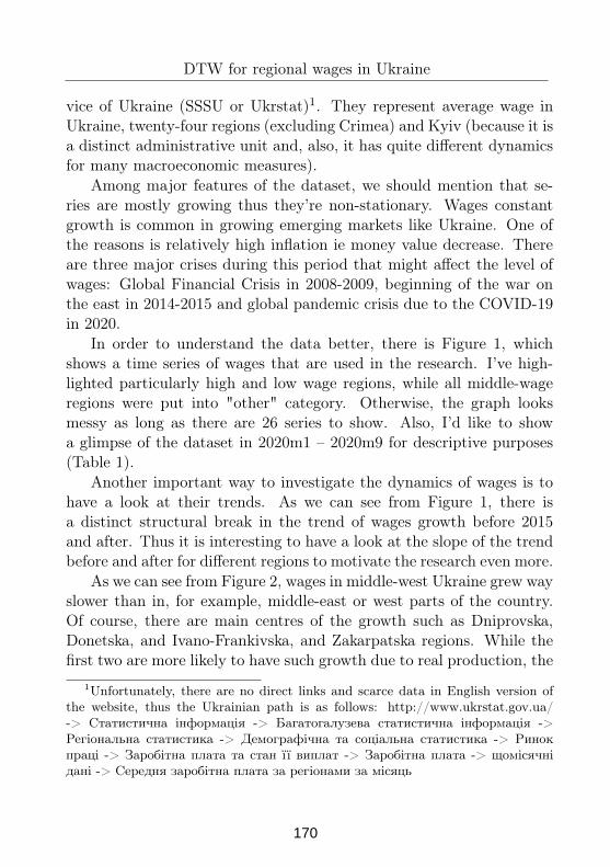
DTW for regional wages in Ukraine
vice of Ukraine (SSSU or Ukrstat)1. They represent average wage inUkraine, twenty-four regions (excluding Crimea) and Kyiv (because it isa distinct administrative unit and, also, it has quite different dynamicsfor many macroeconomic measures).
Among major features of the dataset, we should mention that se-ries are mostly growing thus they’re non-stationary. Wages constantgrowth is common in growing emerging markets like Ukraine. One ofthe reasons is relatively high inflation ie money value decrease. Thereare three major crises during this period that might affect the level ofwages: Global Financial Crisis in 2008-2009, beginning of the war onthe east in 2014-2015 and global pandemic crisis due to the COVID-19in 2020.
In order to understand the data better, there is Figure 1, whichshows a time series of wages that are used in the research. I’ve high-lighted particularly high and low wage regions, while all middle-wageregions were put into "other" category. Otherwise, the graph looksmessy as long as there are 26 series to show. Also, I’d like to showa glimpse of the dataset in 2020m1 – 2020m9 for descriptive purposes(Table 1).
Another important way to investigate the dynamics of wages is tohave a look at their trends. As we can see from Figure 1, there isa distinct structural break in the trend of wages growth before 2015and after. Thus it is interesting to have a look at the slope of the trendbefore and after for different regions to motivate the research even more.
As we can see from Figure 2, wages in middle-west Ukraine grew wayslower than in, for example, middle-east or west parts of the country.Of course, there are main centres of the growth such as Dniprovska,Donetska, and Ivano-Frankivska, and Zakarpatska regions. While thefirst two are more likely to have such growth due to real production, the
1Unfortunately, there are no direct links and scarce data in English version ofthe website, thus the Ukrainian path is as follows: http://www.ukrstat.gov.ua/-> Статистична iнформацiя -> Багатогалузева статистична iнформацiя ->Регiональна статистика -> Демографiчна та соцiальна статистика -> Ринокпрацi -> Заробiтна плата та стан її виплат -> Заробiтна плата -> щомiсячнiданi -> Середня заробiтна плата за регiонами за мiсяць
170
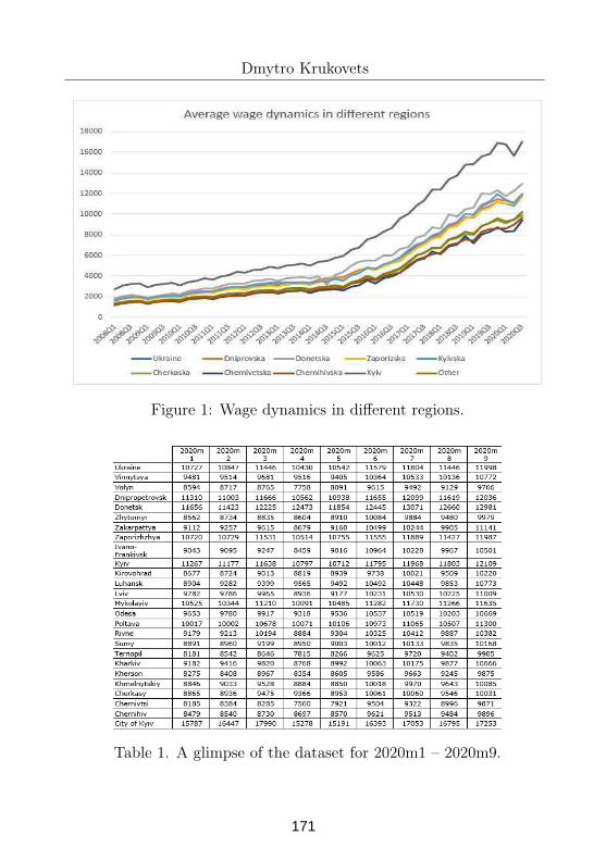
Dmytro Krukovets
Figure 1: Wage dynamics in different regions.
Table 1. A glimpse of the dataset for 2020m1 – 2020m9.
171
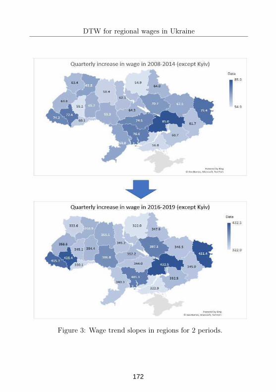
DTW for regional wages in Ukraine
Figure 3: Wage trend slopes in regions for 2 periods.
172
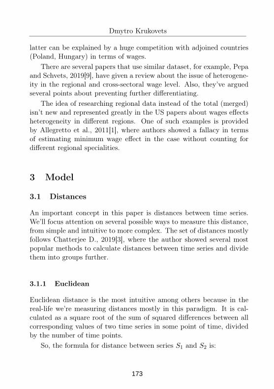
Dmytro Krukovets
latter can be explained by a huge competition with adjoined countries(Poland, Hungary) in terms of wages.
There are several papers that use similar dataset, for example, Pepaand Schvets, 2019[9], have given a review about the issue of heterogene-ity in the regional and cross-sectoral wage level. Also, they’ve arguedseveral points about preventing further differentiating.
The idea of researching regional data instead of the total (merged)isn’t new and represented greatly in the US papers about wages effectsheterogeneity in different regions. One of such examples is providedby Allegretto et al., 2011[1], where authors showed a fallacy in termsof estimating minimum wage effect in the case without counting fordifferent regional specialities.
3 Model
3.1 Distances
An important concept in this paper is distances between time series.We’ll focus attention on several possible ways to measure this distance,from simple and intuitive to more complex. The set of distances mostlyfollows Chatterjee D., 2019[3], where the author showed several mostpopular methods to calculate distances between time series and dividethem into groups further.
3.1.1 Euclidean
Euclidean distance is the most intuitive among others because in thereal-life we’re measuring distances mostly in this paradigm. It is cal-culated as a square root of the sum of squared differences between allcorresponding values of two time series in some point of time, dividedby the number of time points.
So, the formula for distance between series S1 and S2 is:
173
DTW for regional wages in Ukraine
dist(S1, S2) =
√
n∑
t=1(pt − qt)2
n(1)
Where t is the time point, n is a total series length, pt and qt arevalues of abovementioned series in corresponding time point.
3.1.2 Euclidean Scaled
A simple Euclidean distance suffers from a difference in levels, which inthe case of the current dataset is crucial because there are regions likeKyiv with a relatively higher income than in any other region. We’dlike to compare the real dynamics of the series.
One possible solution for this problem is to standardize data beforeproceeding with the distance calculation and other parts of the model.It will help to put a series on the same scale, especially if the level ofgrowth is similar. The formula for series S transformation is given by:
St =(St −mean(S))
stdev(S)(2)
3.1.3 Correlation-based
Next approach is also simple, it is given by the formula:
dist(S1, S2) = 1− |corr(S1, S2)| (3)
As long as we determine the distance as a measure of similarityand close series are similar, then high correlation should give a smalldistance, which is the case in the formula.
3.1.4 Dynamic Time Warping
Dynamic Time Warping procedure allows counting for shifts, stretches,lags etc, because its architecture is based on finding shortest distancesbetween time points not necessarily in the same moment and minimize
174
Dmytro Krukovets
the sum of these distances with a condition that correspondences cannot intersect.
These properties are extremely useful in the case of economic seriesas long as relationship between series might be non-linear and shifteddue to non-similar reaction in terms of time for distinct shocks.
The algorithm, in simple words, is to find distances between everypair of points, then build a corresponding matrix and find minimum apath through this matrix if we can go only up, right and up-right.
The algorithm first appears in Berndt D., Clifford J., 1994[2], butwas strongly improved in forthcoming papers, where one of the mostimportant is written by Salvador S., Chan P., 2004[10]. It’s aboutFastDTW extension that reworks slightly the algorithm and decreasesits complexity substantially, which is extremely important in the caseof large time series as long as it works with an n by n matrices.
3.2 Distance matrix
After deciding over the type of distance, it is necessary to take the nextstep and create a distance matrix. It is built in a way that distancebetween series i and j put into the cell on the intersection of column iand row j. Thus, the matrix has zero main diagonal because distanceof series i with itself is 0and its symmetric, because d(i,j) = d(j ,i).
An important paper in this topic is written by Dokmanic et al.,2015[4]. Authors provide with an algorithm that makes necessary alge-braic transformation of the distance matrix in order to obtain approx-imation of the necessary two-dimensional plane with points. They’vealso given a proof of major theorems in the topic such as uniquenessof this transformation (up to some affine transformation that saves dis-tances ie rotation).
3.3 Clustering
After creating a plane, there are several points that might be treatedas a set for which we can perform some clustering algorithm. The idea
175
DTW for regional wages in Ukraine
of clustering techniques is based on grouping by some similar features.In the case of the set of points, the ones which are close to each otherwill be treated as points from the same cluster.
There is a great variety of clustering algorithms that are divided onseveral major categories: centroid-based; density-based; connectivity-based; distribution-based and grid-based. All these types of cluster-ings differs by the fundamental approach of treatment clusters: whilecentroid-based are mostly about the idea that there is exist some cen-ter for particular cluster that minimizes total distance of elements tothis center, density-based algorithms are define sets of close enoughpoints as clusters, ignoring sparse parts of the total point set. Theseapproaches are fundamentally different, thus in the paper will be usedmost popular algorithms from distinct types.
3.3.1 K-Means
The first example of the clustering algorithms will be a K-Means. Itwas firstly described by MacQueen J., 1967[7], and its core idea is toiteratively find clusters with a minimum sum of in-group variation.Thus, the problem might be described as follows:
argminS
k∑
i=1
∑
x∈Si
‖x− µi‖2 (4)
It is done by iterative recalculation of the centroid for each clusterand then reassigning the closest points to this cluster.
3.3.2 DBSCAN
Another way to build a clusterization is represented by density-basedalgorithms and the simplest among them – DBSCAN. The general ideaof the algorithm is firstly described by Ester et al.,1996[5]. It works ina way to find tight clouds of points, where we exogenously determinehyperparameters such as the number of points that should be in rangeto the one or the size of this range.
176
Dmytro Krukovets
3.3.3 Hierarchical Clustering
The last but not least is a Hierarchical clustering. It is based on an ideaof building some hierarchical structure (tree) that has a different levelof clustering on each level, starting from n clusters with a single elementand finishing with a single cluster with all elements. The algorithm iswell described by Mullner, 2011[8], with a deep dive into sub-types andtheir features such as complexity.
4 Results
After performing abovementioned sequence of action (find distancesbetween series, build a distance matrix, create a 2-dimensional planethat corresponds to the matrix) for all distance types (ie the algorithmdivides in the first step, then it is similar), we have obtained two-dimensional sets of points, that are depicted in Figure 3 – Figure 6(every Figure correspond to the distance type, used in the first step).Each point represents a time series of wages and distances between thesepoints are equal to those, that are found by corresponding distance met-rics (Euclidean, Correlation-based, DTW). The scaling doesn’t matteras long as we’re looking on the relative distance between series.
In all these figures (except, maybe, the Euclidean Scaled case) it isabsolutely clear that Kyiv has different dynamics in comparison withother regions. It comes from the fact that point that correspond to theKyiv is not relatively close to other points. Also we should emphasizean attention on the fact that most of the models, presented in thepaper, control for the level of wages (which is higher in Kyiv), thus theconclusion is that there is a real structural difference in dynamics. It isparticularly important as a motivation for further economic analysis ofthese processes.
In all cases except DTW, we can see that dynamics of Donetskaand Luhanska regions are also different in comparison with other, whichcorrespond to the common logic as long as their reaction for the crisisin 2015 is of another nature as for other regions, but they’re not that
177

DTW for regional wages in Ukraine
close to each other as they should be. Moreover, the Donbass region istraditionally more dependent on world fossil fuel prices (oil, gas, coal)than any other region in Ukraine, particularly in terms of wages. Thus,it should have somehow different dynamics.
In most cases Kyivska region and Ukraine are pretty close to eachother, so as "richer regions" like Dniprovska, Odeska, Kharkivska,Lvivska that are also close to each other. Also, in several figures, thereis a higher chance of west regions to be closer to each other.
Figure 4: Euclidean.
In Figure 7 – Figure 9 we can observe how different clustering algo-rithms perform with a DTW-based distance. This type of distance waschosen as the main as long as the main focus of the paper lying on it.Also, by construction, it should give more robust to shocks and season-ality results. In abovementioned figures, you’ll see the same location ofpoints as in Figure 5, but they’ll be coloured according to groups thatare found using corresponding clustering algorithms.
K-Means gives rather predictable results, when Kyiv is single, so
178
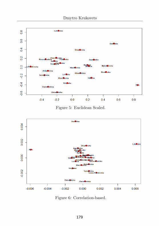
Dmytro Krukovets
Figure 5: Euclidean Scaled.
Figure 6: Correlation-based.
179
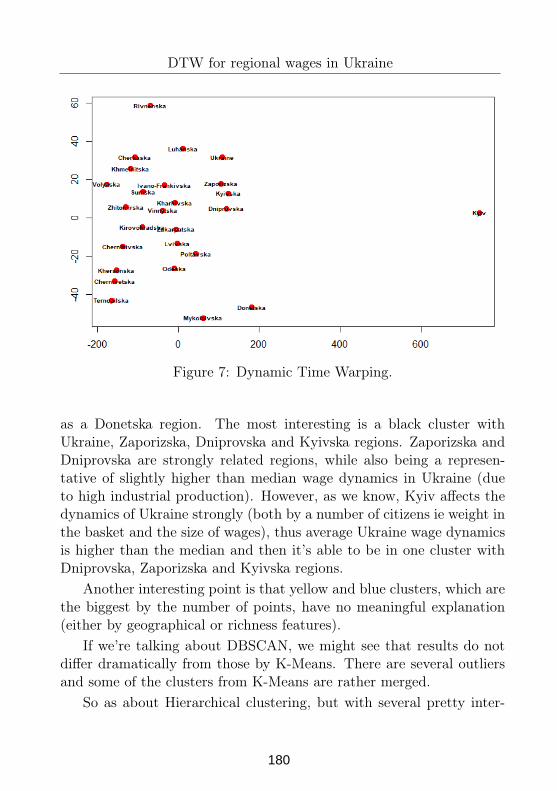
DTW for regional wages in Ukraine
Figure 7: Dynamic Time Warping.
as a Donetska region. The most interesting is a black cluster withUkraine, Zaporizska, Dniprovska and Kyivska regions. Zaporizska andDniprovska are strongly related regions, while also being a represen-tative of slightly higher than median wage dynamics in Ukraine (dueto high industrial production). However, as we know, Kyiv affects thedynamics of Ukraine strongly (both by a number of citizens ie weight inthe basket and the size of wages), thus average Ukraine wage dynamicsis higher than the median and then it’s able to be in one cluster withDniprovska, Zaporizska and Kyivska regions.
Another interesting point is that yellow and blue clusters, which arethe biggest by the number of points, have no meaningful explanation(either by geographical or richness features).
If we’re talking about DBSCAN, we might see that results do notdiffer dramatically from those by K-Means. There are several outliersand some of the clusters from K-Means are rather merged.
So as about Hierarchical clustering, but with several pretty inter-
180
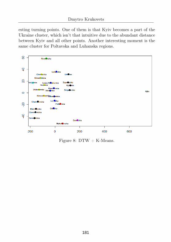
Dmytro Krukovets
esting turning points. One of them is that Kyiv becomes a part of theUkraine cluster, which isn’t that intuitive due to the abundant distancebetween Kyiv and all other points. Another interesting moment is thesame cluster for Poltavska and Luhanska regions.
Figure 8: DTW + K-Means.
181
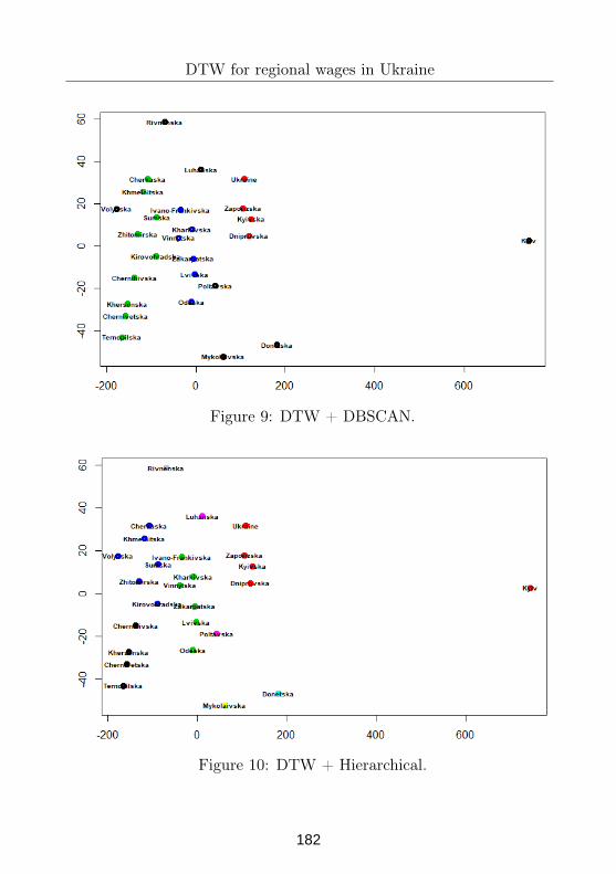
DTW for regional wages in Ukraine
Figure 9: DTW + DBSCAN.
Figure 10: DTW + Hierarchical.
182
Dmytro Krukovets
5 Conclusion
In this paper, I’m using the dataset of wages in twenty-five regions ofUkraine (including Kyiv) and Ukraine itself. I’m using the next routineto find similarity between series: find distances in one over four differentmetrics, build a distance matrix, transform it into a two-dimensionalplane with points and, finally, perform several clustering algorithms.Special attention is given to Dynamic Time Warping as one of the mostpromising algorithms by construction in terms of economic data.
Results give several important and rational points, that satisfy com-mon economic logic and let the experiment to be called successful.These conclusions can be squeezed from the figures, such as absoluteconfidence that dynamics in Kyiv wages are different from those inregions, so as dynamics of wages in Donetska and Luhanska regions.
For the former, it is given by K-Means (Figure 7) and graphicalanalysis of Figures 3-6. For the latter two, it is seen mostly in Figures 3-5 and Hierarchical clustering (Figure 9). Partially, for Donetska region,it’s seen in Figure 7 and Figure 6.
These results are crucial to show that Data Science algorithms areable to work adequately in such unusual domain as economic data andthey can be used as a main or supportive tool to draw economic conclu-sions and reinforce economic analysis. Thus, the paper sheds the lighton the initial question and manages to answer that the area worth tobe researched further.
As for further progress, we should go away from the focus on techni-cal (computer science) part of the paper and do major economic analysisexercise. Moreover, there is a room to advances in computer science partsuch as a change in the algorithmic routine with performing clusteringalgorithms right for the time series rather than for a two-dimensionalset of points. Also, it is quite interesting to compare these results withresults from common dimensionality reduction algorithms such as PCA,t-SNE or UMAP.
183
DTW for regional wages in Ukraine
References
[1] Allegretto S., Dube A., Reich M., 2011. Do Minimum
Wages Really Reduce Teen Employment? Accounting for
Heterogeneity and Selectivity in State Panel Data. Avail-able at: https://onlinelibrary.wiley.com/doi/abs/10.1111/j.1468-232X.2011.00634.x
[2] Berndt D., Clifford J., 1994. Using Dynamic Time Warping to Find
Patterns in Time Series. AAAI Technical Report WS-94-03. Avail-able at: https://www.aaai.org/Papers/Workshops/1994/WS-94-03/WS94-03-031.pdf
[3] Chatterjee D., 2019. Log Book – Guide to Distance Mea-
suring Approaches for K-Means Clustering. Available at:https://towardsdatascience.com/log-book-guide-to-distance-measuring-approaches-for-k-means-clustering-f137807e8e21
[4] Dokmanic I., Parhizkar R., Ranieri J., Vetterli M., 2015. Euclidean
Distance Matrices. Essential Theory, Algorithms and Applications.
Available at: https://arxiv.org/pdf/1502.07541.pdf
[5] Ester M., Kriegel H., Sander J., Xu X., 1996. A Density-
Based Algorithm for Discovering Clusters in Large Spatial
Databases with Noise. Available at: http://www2.cs.uh.edu/ ce-ick/7363/Papers/dbscan.pdf
[6] Krukovets D., 2020. Data Science Opportunities at Central Banks:
Overview. Visnyk of the National Bank of Ukraine, 249, 13-24.Available at: https://doi.org/10.26531/vnbu2020.249.02
[7] MacQueen J., 1967. Some methods for classification
and analysis of multivariate observations. Available at:https://projecteuclid.org/euclid.bsmsp/1200512992
[8] Muller D., 2011. Modern Hierarchical, Agglomerative Clustering
Algorithms. Available at: https://arxiv.org/pdf/1109.2378.pdf
184
Dmytro Krukovets
[9] Pepa T., Shvets P., 2019. Different Levels of Salaries in Ukraine:
Reasons, Implications and Relevant Regulatory Tools. Available at:https://ibn.idsi.md/sites/default/files/imagf ile/49− 581.pdf
[10] Salvador S., Chan P., 2004. FastDTW: Toward Accurate Dy-
namic Time Warping in Linear Time and Space. Availableat: https://www.semanticscholar.org/paper/FastDTW%3A-Toward-Accurate-Dynamic-Time-Warping-in-Salvador-Chan/05a20cde15e172fc82f32774dd0cf4fe5827cad2
Dmytro Krukovets1
1Taras Shevchenko National University of KyivEmail: [email protected]
185
Proceedings of the Conference on Mathematical Foundations of Informatics
MFOI2020, January 12-16, 2021, Kyiv, Ukraine
Algebra, informatics, programming
Sergii Kryvyi
Abstract
This is a review of some classical algebra applications in com-puter science and programming, their influence on informatics,programming and other areas.
Key words: algebras, informatics, programming, applica-tions.
1 Introduction
The material given in this work is considered there due to the factthat last time the idea that science has exhausted itself and its role isdecreasing every day, appears in the media and among specialists. Thissituation is especially surprising when a person who graduated fromsome University has access to the Internet, believes that everything heneeds is in the Internet and there is no need for scientific research.
Various pandemics demonstrates us the absurdity of such a thought.It is obvious that the progress in virology is absolutely important andnecessary. But achievement in other areas of science, in particular incomputer science, is very important also (may be less obvious). Therelationship between algebra, computer science and programming isconsiders in this work; moreover we made an attempt to describe acertain influence of algebra on computer science and on the contrarycomputer science on algebra and other fields.
We do not pretend on completeness of the material, however it isalmost impossible to give a full description of algebra applications incomputer science and programming.
c⃝2020 Sergii Kryvyi
186
Sergii Kryvyi
2 Classical algebras
Consider a number of algebras
G1 ⊃ G2 ⊃ G3 ⊃ G4 ⊃ G5 ⊃ G6 ⊃ G7, G71, G8 ⊃ G9, (1)
whose theory have already been created. Algebras of this kind areinteresting for their applications in computer science and programming,both in theoretical and applied terms.
Recall that a universal algebra is a triple G = (X,Ω, E), where Xis the basic set (carrier) of the algebra on which are defined fixed arityoperations from the set Ω (algebra signature) and these operationssatisfy identical relations from the set E. The concretization ofthe set E defines some family of algebras (semigroups, groups, rings,lattices, etc.) [12, 13].
The first algebra in the series (1) is the algebra of the form G1 = (X,Ω,Ø), which is called the algebra of terms over the alphabet X of thesignature Ω with empty set of identical relations. The emptiness of theidentical relations means that every element in this algebra identicalonly to himself.
The algebra of terms is also called Ω-algebra or absolutely free al-gebra of the signature Ω.
The second family of algebras in the series (1) is semigroups
G2 = (X,Ω = ∗, E = x ∗ (y ∗ z) = (x ∗ y) ∗ z
– algebras of terms over the alphabet X, signature which includes asingle binary multiplication operation that satisfies the law of asso-ciativity. A special case of semigroups is monoids – semigroups withunit.
Next in series: G3 – groups, G4 – Abelian groups, G5 – rings, G6
– solid, G7 – fields, G71 – vector spaces, G8 – lattices, G9 – Booleanalgebras.
187
Algebra, informatics, programming
3 Algebras in Computer Science and Program-
ming
Consider the application and role of these algebras in computer scienceand programming.
3.1 Algebra of terms
The formal definition of the algebra G1 has the form. Alphabet Xalgebras G1 are symbols divided into three groups: T0, Ω and (, ).Symbols a, b, x, y, . . . from T0 are called subject variables and constants,the symbols w3
2, w52, w5, . . . of Ω are called functional (top the index
indicates the arity of the symbol wni – ar(wn
i ) = n) the third group –left, right brackets and comma.
Definition 1.Terms are words in the alphabet X, built on the followingrules:
1) all characters from T0 are terms ;2) if t1, . . . , tn are terms, then the word is of the form wn(t1, . . . , tn)
is term (wn ∈ Ω, n ≥ 1);3) terms are those and only those words that are built according to
rules 1), 2).The algebra of all terms in the alphabet X of the signature Ω is
denoted T (Ω, X).
If t = ω(t1, . . . , tn) ∈ T (Ω, X), the terms t1, . . . , tn are called directsubterms of the term t. Transitive closure of the relationship “directsubterm” is called the relation “subterm of term”.
Algebra of terms T (Ω, X) can be considered as universal Ω-algebra,if we determine the operations of zero arity, since when definition ofT (Ω, X) it was assumed that ar(ω) ≥ 1 for arbitrary operation ω ∈ Ω.This is achieved by expansion alphabet X algebra terms with zerocharacters operations Ω0 and consideration of the algebra T (Ω′, X ′),where Ω′ = Ω \ Ω0, X
′ = X ∪ Ω0. Received thus universal algebra willbe denoted as before, T (Ω, X) = G1, having on mean the transitiondescribed, and call its term algebra.
188
Sergii Kryvyi
Let be an arbitrary algebra G = (A,Ω) and an algebra T (Ω, X).If Ω0 = ∅, then let a(w) mean the element with A, which correspondsto the operation w of Ω0. Consider mapping φ : T0 → A such thatφ(w) = a(w) for w ∈ Ω0. You can continue to display φ on all algebraT (Ω, X), if for p1, p2, . . . , pn ∈ T (Ω, X) and wn ∈ Ω (n ≥ 1) putφ(w(p1, . . . , pn)) = w(φ(p1), . . . , φ(pn)).
The mapping φ is called the interpretation of the algebra T (Ω, X)in the algebra G.
It is said that in the algebra G the identical relation holds (or justidentity) p1 = p2 when φ(p1) = φ(p2) in G with an arbitrary inter-pretation of φ.
If given the set of identities E, then set of all algebras of signatureΩ, in which all identities from E are hold, is a class of algebras thatwill be denoted by K(Ω, E).
Let p1 = p2 ∈ E, p, q ∈ T (Ω, X) and the term p obtained from theterm q in the result of substituting p1 instead some occurrence of theterm p2 in the term q. In this case, we say that the term p directly isderived from the term q using identical relation p1 = p2 with E. Thetransition closure of relationship of direct derivation is simply calledderivation. The terms q1 and q2 are said to be equivalent with respectto E if one of them is derived from another (q1 ≡E q2). It is well knowthat the relation ≡E is congruence.
Definition 2. Let T (Ω, X,E) be the quotient algebra T (Ω, X)/ ≡E
in relation to ≡E. The algebra T (Ω, X,E) is called free algebra ofclass K(Ω, E), and the set X is its system of free generators (ba-sis). The algebra T (Ω, X,E) is called hereditary free, if its arbitrarysubalgebra is also a free algebra.
From the definition of T (Ω, X,E) it follows that T (Ω, X,E) ∈K(Ω, E). The importance of the concept of free algebra shows
Theorem 1. An arbitrary algebra G of class K(Ω, E) is homomorphicimage of the free algebra T (Ω, X,E) of this class [12].
Algebra of terms, despite its ”poor” identity set, is included in al-most every programming language. This inclusion is based on the fact,
189
Algebra, informatics, programming
that concretization of the X alphabet of the programming languageand signature operations, gives us absolutely free algebra. Indeed, wefix the signature of operations
Ω = +,−, ∗, /,∧,∨, <<,>>,÷,¬, 0(false), 1(true),
where the first eight operations: addition, subtraction, multiplication,division, conjunctions, disjunctions, left and right shifts – binary, minus÷ and negation ¬ – unary operations, and 0 and 1 – zero operations.Then this algebra is described by the following grammar:
< exp >::=< var > | < opu >< exp > | < exp >< bop >< exp >
< opu >::= ¬|÷
< bop >::= +| - | ∗ |/| << | >> | ∨ |∧
< var >::=< ident >:< type >
< type >::= int|real|char|bin|bin float|bin fixed
< ident >::=< symbol > | < ident >< cypher > | < ident >< symb >
< cypher >::= 0|1|2|3|4|5|6|7|8| 9,
where symbol means an element of the alphabet X of the program-ming language, which includes zero operations 0 (false) and 1 (true)(the alphabet usually fixed for a given language).
All other algebras of the series (1), starting with the algebra G1,have their own peculiarities, which vary from algebra to algebra, andtherefore it is generally impossible to describe them using a formalgrammar. These features need to be programmed.
3.2 Semigroups
Semigroups and monoids are a particularly important family of alge-bras, which plays a key role in both algebra and programming. Oneof the most used algorithmic ones is built on these algebras systems– a system of normal Markov algorithms [9]. At one time the occur-rence of this system played an important role in the formation of thetheory of algorithms and the solution of some problems in algebra andmathematical logic.
190
Sergii Kryvyi
In programming based on this algorithmic system, the conditionsfor algorithmic completeness of functional programming languages [5,17] and substantiation of their semantics were found.
Semigroups and monoids play an important role in coding theory,theory of formal languages and signal processing. In particular, thecodes are considered as submonoids of free monoid and on their basisclassification is entered formal languages. It is built on the basis of finitefree monoids algebraic theory of automata (Crohn-Rhodes theory) [1].
Semigroups play a key role in general algebras, because they accu-mulate the properties of most algebras from series (1). From this itfollows, that everything that is studied in general algebra ultimatelyfinds its way into semigroup theory. This is based on the followingconsiderations.
Let there be given a semigroup P = (A, ·). Let’s fix in it elementa, a natural number n and consider the word x1x2 . . . xna, where thecharacters x1, x2, . . . , xn are unknown. An arbitrary system of valuesb1, b2, . . . , bn ∈ P unknown x1, x2, . . . , xn we correspond to an unam-biguously defined element b1b2 . . . bna semigroup P , that is defining onP n-arity operation.
If the signature Ω is set, we will put it in accordance every n-arityoperation ω ∈ Ω (n ≥ 1) some element aω semigroup P (these elementsare optional different for different ω). Define on set P the operation ωby using the words x1, x2, . . . , xnaω, and for all zero operations with Ωwe will fix elements aω in P . After that, on the semigroup P , an algebraof signatures Ω will be defined. This algebra is called special derivativealgebra signatures Ω on the semigroup P . This algebra, as follows fromthe construction, is determined by the choice of the elements aω forω ∈ Ω.
Definition 3. It is said that the algebra G of the signature Ω has aspecial exact image in semigroup P if it is isomorphically embedded insome special derivative of the signature algebra Ω on the semigroup P.
Hens the following is true
191
Algebra, informatics, programming
Theorem 2 (Kohn, Rebane). An arbitrary algebra G of the signatureΩ has a special exact image on some semigroup P [10, 12].
4 Information security, computer geometry and
algebra
Groups, rings, fields, vector spaces and other algebras have wide ap-plications not only in computer science, but also in other fieds scienceand technology. In particular, they find their applications in crystal-lography, nuclear physics, optics, astronomy, instrumentation etc.
4.1 Information security
One of the widely used algebra application is protection systems in-formation and construction of cryptographic algorithms. In particular,groups substitutions were and are one of the main sources of construc-tion reliable encryption algorithms and information exchange. Basedon groups, the most commonly used key exchange algorithms (algo-rithms Diffie-Hellman, El Gamal, Shamir).
Here is an algorithm for an example Diffie-Hellman key exchange.
Let p be a large prime number, and let g be some number from theinterval 1 < g < p − 1 such that all numbers from sets 1, 2, . . . , p −1 can be given in different degrees numbers g modulo p (about themethod selection of such numbers is given below):
g mod p, g2 mod p, . . ., gp−1 mod p.
The numbers p and g are known to all subscribers.
DIFFY-HELLMAN KEY EXCHANGE PROTOCOL
Input: (p, g), where p is a large prime number, g – generating element of themultiplicative group of the field Fp.
Exit: The group element k to exchange subscribers A and B.
1. A generates the element a ∈ (1, p− 1), calculates the number ga = ga mod pand sends it to the subscriber B.
192
Sergii Kryvyi
2. B generates the element b ∈ (1, p− 1), calculates the number gb = gb mod pand sends it to the subscriber A.
3. A calculates the number k = gab mod p.
4. B calculates the number k = gba mod p.
Thus, the exchange of the key k between subscribers A and B hasfulfilled.
The foundation for this method follows from such a simple state-ment.
Theorem 3. ZAB = ZBA.
Basic properties of the protocol Diffie-Hellman are as follows:– A and B received the same number Z = ZAB = ZBA;– person unwanted number XA and XB unknown and it does not
have the ability to calculate the number Z (at least for a reasonableperiod of time).
Select number g. Stability protocol Diffie-Hellman to break isbased on the complexity of the function discrete logarithm. In orderfor such stability to be high, it is necessary choose the number p asfollows:
p = 2r + 1 or p− 1 = 2r.
where r is also a prime number. If the number p is selected as then theelement g can be an arbitrary satisfying element inequality: 1 < g <p− 1 and gr mod p = 1.
4.2 Computer geometry
The second area of application of group theory, fieds and vector spacesis computer geometry. Based on group properties of vector transfor-mations spaces systems of transformations that preserve distances werebuilt and they are classified according to these group properties (groupparallel transfers, turns, different types of symmetries etc.) [15].
Next, to illustrate the use of groups, a two-dimensional space L2
is considered, which is called the plane. But if the definition or the
193
Algebra, informatics, programming
statement is also valid for the dimension n ≥ 2, then the notation Ln
is used.Moving space Ln is the mapping F : Ln → Ln that preserved the
distance between the points, that is if F is a moving space and A,B arearbitrary points from Ln, then |AB| = |A′B′|, where A′ = F (A), B′ == F (B), and |AB| is the distance between the points A and B.
Examples of plane displacements are well known:– parallel transfer to vector r – Tr;– rotation around point O at angle θ – TRθ;– symmetry with respect to the line l – Sl;– sliding symmetry – Sr
l .Consider each of these transformations separately.The mapping Tr : Ln → Ln is called parallel transfer, if Tr(v) =
= v+ r, where r is some fixed vector, and v is an arbitrary vector withLn. In coordinate form this transformation is written as: Tr(v) = v++r = (x+ x0, . . . , z + z0), where v = (x, y, . . . , z), r = (x0, y0, . . . , z0).
The following properties follow directly from the definition of Tr.B1. The transformation Tr is nonlinear.B2. Tr ∗ Tr′ = Tr+r′ , where * is mapping product operation.
Theorem 4. The set of all parallel transfers is an Abelian group withrespect to mapping product operations.
The group of all parallel transfers Ln is denoted by T (n).Rotate the plane relative to some point O by the angle θ is called
display TRθ : L2 → L2, which transforms the point A(x, y) to the pointA′(x′, y′) by rotating L2 relative to the point O at the angle θ.
The rotation transformation is linear, and its matrix in L2 has likethis:
TRθ =
[
cos θ − sin θsin θ cos θ
]
.
Using the rotation matrix, it is easy to set such properties.RP1. The rotation transformation is orthogonal.From this property and the fact that the determinant of the rotation
matrix is equal to units, it follows: there is an inverse transformation
194
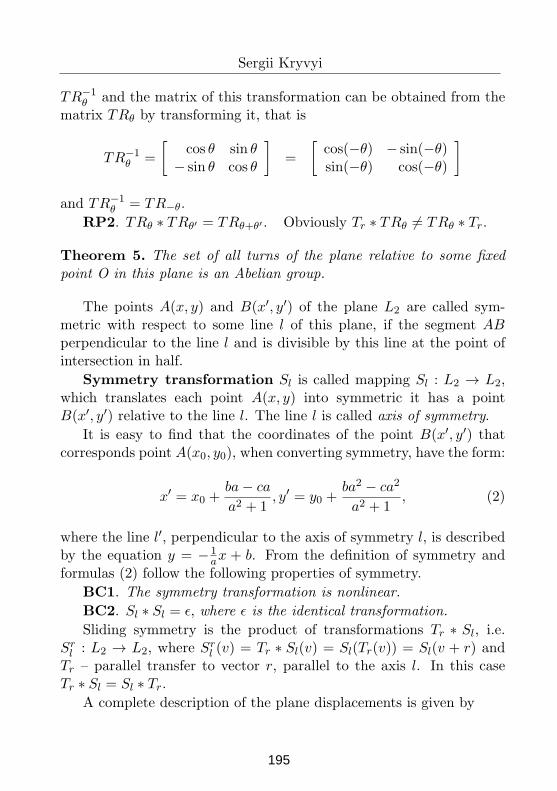
Sergii Kryvyi
TR−1θ and the matrix of this transformation can be obtained from the
matrix TRθ by transforming it, that is
TR−1θ =
[
cos θ sin θ− sin θ cos θ
]
=
[
cos(−θ) − sin(−θ)sin(−θ) cos(−θ)
]
and TR−1θ = TR−θ.
RP2. TRθ ∗ TRθ′ = TRθ+θ′ . Obviously Tr ∗ TRθ = TRθ ∗ Tr.
Theorem 5. The set of all turns of the plane relative to some fixedpoint O in this plane is an Abelian group.
The points A(x, y) and B(x′, y′) of the plane L2 are called sym-metric with respect to some line l of this plane, if the segment ABperpendicular to the line l and is divisible by this line at the point ofintersection in half.
Symmetry transformation Sl is called mapping Sl : L2 → L2,which translates each point A(x, y) into symmetric it has a pointB(x′, y′) relative to the line l. The line l is called axis of symmetry.
It is easy to find that the coordinates of the point B(x′, y′) thatcorresponds point A(x0, y0), when converting symmetry, have the form:
x′ = x0 +ba− ca
a2 + 1, y′ = y0 +
ba2 − ca2
a2 + 1, (2)
where the line l′, perpendicular to the axis of symmetry l, is describedby the equation y = − 1
ax + b. From the definition of symmetry and
formulas (2) follow the following properties of symmetry.
BC1. The symmetry transformation is nonlinear.
BC2. Sl ∗ Sl = ϵ, where ϵ is the identical transformation.
Sliding symmetry is the product of transformations Tr ∗ Sl, i.e.Srl : L2 → L2, where Sr
l (v) = Tr ∗ Sl(v) = Sl(Tr(v)) = Sl(v + r) andTr – parallel transfer to vector r, parallel to the axis l. In this caseTr ∗ Sl = Sl ∗ Tr.
A complete description of the plane displacements is given by
195
Algebra, informatics, programming
Theorem 6 (Chasles). Arbitrary plane displacement is one of threetransformations:
1) parallel transfer;
2) rotation;
3) sliding symmetry (and when r = 0 is symmetry).
Plane Moving Groups. The displacements of the plane are bro-ken into two subgroups – the movement of the first kind, to which theybelong parallel transfer and rotation, and movement of the second kind,to which belong symmetry and sliding symmetry.
Proposition 1. The product of two displacements of the first kind is adisplacement of the first kind, the product of displacements of the firstand second kind is the displacement of the second kind and the productof displacements of the second kind is a displacement of the first kind.
Arbitrary movement of the first kind can be unambiguously rep-resented in the form of the product of the transformation of paralleltransfer and rotation around a fixed point.
Arbitrary movement of the first kind is uniquely decomposed intoproduct of rotation around a fixed point of the plane and parallel trans-fer.
Theorem 7. The set of all plane displacements in L2 is a group withrespect to mapping product operations.
This subgroup is denoted by E(2). Group E(2) has an infinitenumber of subgroups. Indeed, according to the proposition 1 subgroupwill be all movements of the first kind. This the subgroup is denotedby E0(2). If F is a movement of the first kind, and G is a movementof the second kind, then according to the proposition 1 the movementG∗F ∗G−1 is a movement of the first kind, that is, the subgroup E0(2)is a invariant subgroup of E(2). Thus, there are only two classes in thissubgroup: she herself and the class of movements of the second kind.Then E0(2) has an index 2 in the group E(2) and the quotient groupE(2)/E0(2) is a finite cyclic second-order group.
196
Sergii Kryvyi
The group E0(2) has an infinite number of subgroups of rotations:the set of all rotations relative to any fixed point of the plane is asubgroup. All these subgroups are commutative.
The set of all rotations will not be a subgroup. Really, a rotationaround the point O at the angle α, and then rotation around the pointO′ the angle 2π − α will be a parallel transfer.
Theorem 8.The set of all parallel transfers will be a subgroup of E0(2).
Since any transfer is uniquely characterized by the length and thedirection of the transfer vector, the group of all parallel transfers rela-tive to the line l (they are transfers whose vectors are parallel to the linel) will be an isomorphic group of all real numbers relative to ordinaryadd operations. This group is denoted by T (2).
Theorem 9. The group T (2) is the invariant subgroup of the groupE0(2).
The importance of these statements is that on their basis it is possi-ble simplify the sequence of transformations, for example, by replacingproducts displacements of the second kind by displacements of the firstkind having more effective implementation.
The properties of space displacement are determined and investi-gated in a similar way.
4.3 Computer algebra
Widespread use of classical algebras (semigroups, groups and theirgeneralizations of so-called associative-commutative algebras, rings,Boolean algebras) obtained in systems of automating reasoningby using resolution rule in first-order theories.
In the process of applying resolution rule, it becomes necessaryto develop algorithms for unification and matching of predicate argu-ments. Unification and its special case matching are the problem ofsolving equations of the form t = t′ in a given algebra T (X,Ω, E),where t, t′ ∈ T (Ω, X,E). Solve the equation t = t′ in a given algebra
197
Algebra, informatics, programming
means to find such a substitution σ that σ(t) = σ(t′). Matching oper-ation for a given two of the terms s and t finds a substitution σ suchthat σ(s) = t.
The solution of the unification problem stimulated the developmentof algorithmic and complex research of classical algebras, as well as theextension of the results obtained for these algebras to many sortedalgebras [18].
Unification theory development led to the development of computeralgebra, systems of rewriting terms and the emergence of algebraicsystems programming [8]. Let’s briefly consider the basic concepts ofthis type of systems.
As mentioned above, with each algebra G = (X,Ω, E) is associatedwith a congruence relation ≡E induced by the set of identity relationsE.
The elements of the set E are pairs s = s′, the application of whichto a given term t is running by finding the occurrence of the term s in tand substitution instead of s term s′. Because the identity relationshipreflexive, symmetrical and transitive, then such substitutions can beperformed and in the opposite direction (substitution instead of s′ terms).
Definition 4. The binary relation t(s) → t(s′) means the reduction ofthe term t(s) to the term t(s′), that is substitution instead of enteringthe term s in t term s′. This relation is called the reduction relanion.
The term t(s) is reducible ⇔ there is a t(s′), such that t(s) → t(s′).
The term t is in the normal form (irredusible) ⇔ if it is not re-ducible.
The term t′ is a normal form of t ⇔ t∗→ t′ and t′ is in normal form,
where∗→ – reflexive, symmetrical and transitive reduction relation →.
If a term has a uniquely determined normal form, then such a form iscalled the canonical form of this term.
Term t′ direct subterm (successor) of t ⇔ t → t′.
The terms t and t′ joinable ⇔ there is a term z such that t∗→ z
and t′∗→ z (notation t ↓ t′).
198
Sergii Kryvyi
The main task of reductions is to build a normal form of terms in agiven algebra. But the normal form, and even more canonical the formof a term does not always exists. In order for such forms to exist it isnecessary that the rules of reductions satisfy certain conditions.
Definition 5. The reduction relation → is called• Church-Rosser ⇔ t
∗→ t′ ⇒ t ↓ t′;
• confluent ⇔ from t∗→ z and z
∗→ t′ ⇒ t ↓ t′; the relation is called
semi-confluent ⇔ from z → t and z∗→ t′ follows t ↓ t′;
• terminating ⇔ there is no infinite descending chain t → t1 →→ t2 → . . .;
• normalizing ⇔ every element has a normal form;• convergent ⇔ it is both confluent and terminating.
Suppose we have two rules for rewriting l → r and l1[u] → r1,where u is not a variable. If there is a unifier σ such that σ(l) = σ(u),then a pair (σ(l1[r]), σ(r1)) is called the critical pair for rules l → rand l1[u] → r1. The critical pair is called divergent, if (σ(l1[r])
∗ == (σ(r1))
∗, where t[u] means u is subterm of term t, and t∗ means thatterm t is not reducible.
Theorem 10. The following conditions are equivalent:1) the relation → is the Church-Rosser relation;2) the relation → is confluent;3) the relation → is semi-confluent.
The following consequences follow from this theorem.
Corollary 1. If the relation → is confluent and t∗↔ t′, then
a) t∗→ t′, if t’ has a normal form;
b) t = t′, if both t and t’ are in normal form;c) if → is confluent, then element has at most one normal form;d) if → is normalizing and confluent, then every element has unique
normal form.
The terminating relations are often called (well founded) orNoethe-rian.
199
Algebra, informatics, programming
Therefore, from the above consequences it follows that the relationt ↓ is well founded and from here we get such an important theorem.
Theorem 11. If the relation → is confluent and terminal, then t∗↔ t′
iff t ↓= t′ ↓.
An important rule is structural induction (CI) on arbitrary ter-minal system of reductions (A,>), which generalizes the usual induc-tion on the set (N,>). Formally, this rule is written as follows:
∀x∈A(∀y∈A x+→y ⇒P (y))⇒P (x)
∀x∈A P (x) (CI),
where P is some property of elements of A and x+→ y means transitive
and symmetric closure of →.The relationship between → and CI follows from such theorems.
Theorem 12. If → is terminal, then the CI rule is valid. If the CIrule is valid, then → is terminal.
For a given algebra G = (X,Ω, E) there is the set of its ordered andoriented identical relations. Orientation of relations occurs, as a rule,from left to right, that is identity t ≡E t′ is written as t → t′ relativereduction →.
Definition 6.The rewriting rule is called the identity t ≡E t′ such thatt is not a variable and V ar(t) ⊇ V ar(t′), where V ar(s) is the set ofvariables of the term s. In this case we get the rewriting rule t → t′.
The term rewriting system (TRS) is called the set of rewriting rulesR. The expression that is reduced (redex expression), is the expressionto which the rewrite rules are applied. In the rewriting rule t → t′ theterm t is the left side and is denoted by lhs, and the right part is theterm t’, is denoted rhs.
The reduction (rewriting) →E⊆ T (X,Ω, E) × T (X,Ω, E) is calleda relation
s →E t ⇔ ∃(l ≡ r) ∈ E, p ∈ Pos(s), σ ∈ Sub, s|p = σ(l) andt = s[σ(r)]p,
200
Sergii Kryvyi
where Pos(s) is the set of occurrences of the term l in the term s, Subis the set of substitutions, s|p p is the occurrence of the term in s.
Theorem 13. If E is the set of identities of the algebra G(X,Ω, E),then the reduction ≡E is closed with respect to substitutions and Ω-operations.
The relation∗↔E is the smallest the equivalence relation on T (X,Ω),
which includes E and closed with respect to substitutions and Ω-operations.
It follows from the theorem 11 that the relation∗↔E is algorithmi-
cally solved if it is confluent. Therefore, you can effectively build ↓E ,that is, you can find out: whether one term can be reduced to anotherterm. An important property of the relation →E gives
Theorem 14. If E is a finite set of identities and relations →E con-vergent, then the relation ≡E is solvable.
Hence we get the following property: if R is a finite convergentrewriting system and the relation ≡R is solvable, then s ≡R t iff s ↓R== t ↓R.
There is a general statement [24].
Theorem 15 (Knut-Bendix). The terminal system of rules for rewrit-ing R is confluent iff there is no divergent critical pair for this systemof rules.
It follows from what has been said that in systems of rewritingterms, the important operations are unifications and its special casesare matching (unification with sample) and substitution.
The main properties of these operations are described in many ar-ticles and monographs (see [18]), which confirms the influence of com-puter science on algebra.
4.3.1 Algebraic programming
One of the areas of further influence of programming on the develop-ment of algebra was the algebraic programming paradigm. Data
201
Algebra, informatics, programming
are represented by terms or labeled graphs, and algorithms representedas systems of rewriting rules (oriented equations or conditional equa-tions, relations of data algebra). The object, which is determined by thesystem of equalities, expressed by the rewriting rules, is a congruencerelation on the term algebra generated by constants. This relation-ship is defined as a congruent closure of rewriting relations, which areconsidered as identities of term algebra.
The elementary step of calculations in the algebraic paradigm ismatching, checking of conditions and substitution. The rewriting strat-egy determines the order in which they are applied rules of rewritingand subterm (subexpression) of the current term for comparison withthe left parts of the relationship. For the canonical systems rules ofrewriting the result does not depend on the strategy. If the systemof rules is not canonical, then the strategy determines not only timerewriting, but also the result. In any case the result of rewriting, sub-ject to the end of the calculations, is term, which equivalent to theinitial term in relation congruence, which is determined by the systemof rules of rewriting. That is, the strategy chooses result in the classof congruent terms.
The corresponding algebraic program for calculating GCD is givenbelow.
RS(x, y) (
(x, x) = x,
(x > y) → ((x, y) = (x− y, y)),
(x < y) → ((x, y) = (x, y − x))
).
4.3.2 Calculation methods
Rings, fields and their varieties are the basis of the algebra of computersystems, because computer algebra systems include rings of polynomi-als necessarily. This is due to the fact that polynomials used for ap-proximation various functions. The simplest example of such approxi-mation is represtntation of functions in the form of Taylor series. Forexample, the calculations of the exponential function ex or trigonomet-
202
Sergii Kryvyi
ric functions sin(x) and cos(x) are performed using the Taylor seriesexpansion:
ex = 1 + x
1!+ x2
2!+ . . . xn
n!+Rn+1(x);
sinx = x− x3
3!+ x5
5!− x7
7!+ . . .+ (−1)
n−1
2xn
n!+Rn+2(x);
cosx = 1− x2
2!+ x4
4!− x6
6!+ . . .+ (−1)
n2
xn
n!+Rn+2(x),
where Rn+1(x) and Rn+2(x) are residual members of decompositions.For example, programs for calculating functions ex end sin(x) with agiven accuracy ε are constructed as follows.
The partial sums of decomposition of these functions in the Taylorseries are the recurrence relations for ex:
t0 = 1, tj = tj−1 ·x
jfor j > 0
and for sin(x):
t0 = x; k0 = 1; tj = −tj−1 ·x2
kj(kj−1); kj = kj−1 + 2 for j > 0.
Based on these ratios, we obtain a calculation program for functions ex
proc : exp(x, ε);
s, t : real, k : integer;
begin
t := 1; k := 0; s := t;
until t > ε do
(k := k + 1; t := t · x
k; s := s+ t)
end
end exp
and for functions sin(x):proc : sinus(x, ε);
s, t : real, k : integer;
begin
t := x; k := 1; s := t;
until mod(t) > ε ·mod(s) do
(k := k + 2; t := −t · sqr(x)/(k · (k − 1)); s := s+ t)
end
end sinus
Note, that in this computational program of sin(x), the number ofmembers in the series and the number of iterations are not easy todetermine. These numbers depend on the value of ε and the rate ofconvergence of the series. Therefore, the use of this type of recurrence
203
Algebra, informatics, programming
relations requires caution, despite the guarantees of mathematical anal-ysis, since fast convergence is important in practice.
For example, the partial sum of the variable series for the sin(x)function converges quickly only for small values of x.
Therefore, the application is recommended to use the followingidentifiers for large values of x:
sin(x) = sin(x− 2πn), if 2πn ≤ |x| < 2π(n+ 1),
sin(x) = −sin(x− π), if π ≤ |x| < 2π,
sin(x) = sin(π − x), if π2 ≤ |x| < π,
sin(x) = cos(π2 − x), if π4 < |x| < π
2 ,
sin(x) = −sin(−x), if x < 0.
Thanks to these formulas, in the sin(x) calculation program, we canassume that 0 ≤ |x| < π
4 . And in this interval, the convergence rateof the series is good from a practical point of view, and the numberof members of the series is relatively small, and the accuracy error iswithin acceptable limits.
Programs such as sinus is included in almost all programming lan-guages. This also applies to other functions (for example, ex, tg(x), lnx,sh(x), ch(x), th(x), cth(x) and inverse functions).
The ability to calculate trigonometric functions allows us to calcu-late Fourier series and expressions that include these functions. Thesituation is similar with inverse trigonometric functions.
Fields are used in informatics in connection with systems in whichyou need to work with complex numbers. In particular, such work re-quires theory of complex variable functions. Calculating the values offunctions of complex variable is close to calculating functions of a realvariable, because often it is possible to separate the real and imagi-nary part of a complex function and calculate each of them separately.Example, exponential function ez, where z = x + iy complex num-ber, calculated on the basis of the calculations of the above functionsex, sin(x) and cos(x), because
ez = ex+iy = ex · eiy = ex(cos(y) + isin(y)).
204
Sergii Kryvyi
4.4 Lattices
An important property of a lattice as a universal algebra is: it carrieris a partially ordered set. This order is important for proving the ter-minality (termination) of algorithm work in a finite time; and the orderis related to the height (depth) of the lattice, the elements of which areprocessed by algorithm. From theoretical point of view, an importantproperty of lattices is the equivalence of these three conditions.
Theorem 16. In the lattice the following conditions are equivalent:a) the ascending (descending) chain condition;b) the condition of the existence of minimal elements in the lattice;c) condition of inductance (applicable method of transfinite induc-
tion).
There are algebras that are not universal algebras in the sense inwhich they were defined above.
Many algebras have properties: intersection, union and sum, de-fined in algebras not only for two number of elements and, therefore,for an arbitrary finite number of elements, moreover, even for an in-finite countable number of elements, which is based on the law of as-sociativity. This type of algebra includes complete lattices. Thesealgebras play an important role in the software verification process andsubstantiating the semantics of programming languages.
Definition 7.Let A be a partially ordered set by using the order ≤. The set A
is called complete lattice if for any nonempty subsets B of the set Ain the set A there are such elements c and d for which the followingconditions are hold:
(i) for all elements of a ∈ B c ≤ a and if there is some element c′,such that c′ ≤ a, then c′ ≤ c,
(ii) for all elements a ∈ B d ≥ a, and if there is some element d′,such that d′ ≥ a, then d′ ≥ d.
Unambiguously determined elements c and d are called the inter-section and union elements of the subset B, respectively, and they are
205
Algebra, informatics, programming
written as c =∩
B (or c =∩
a∈Ba or c =
∩
i∈Iai if ai runs all elements of
the set B), d =∪
B (or d =∪
a∈Ba or d =
∪
i∈Iai).
Obviously, an infinite complete lattice is not a universal algebra, butit is clear that it will be a lattice. It is also obvious that the completelattice has zero and unit: these will be the elements, respectively
∩
Aand
∪
A.
Theorem 17. If a partially ordered set A has a unit and exists aintersection for arbitrary nonempty subsets, then A is a complete lattice[10, 16].
Let A and A′ be partially ordered sets by partial order ≤ and φ :A → A′ be a mapping the set A into the set A′.
Recall that the mapping φ : A → A is called isotonic, if a ≤ bimplies φ(a) ≤ φ(b) and inversely isotonic, if from a ≤ b, followsφ(a) ≥ φ(b).
An important property of complete lattices is the existence of fixedpoints in such algebras.
Definition 8.. Element a ∈ A is called a fixed point of isotonic map-ping φ of a set A into itself, if φ(a) = a.
Theorem 18 (about a fixed point). If φ is an isotonic mapping com-plete lattice A into itself, then φ(a) = a for some element a from A.
The theorem inverse to the fixed point theorem is not true.The set of fixed points of isotonic mapping also forms a complete
lattice. This follows from the following statement [27].
Theorem 19 (Tarski). If φ is an isotonic mapping of a complete lattice(A,≤) into itself, then the set of fixed points of φ is a complete latticewith respect to the same relation of partial order ≤.
The given properties of lattices are applied at a substantiation se-mantics of programming languages [17] as well as in data flow analysissystems and search of invariant assertions in the states of programs.
206
Sergii Kryvyi
4.4.1 Invariants in program states
Let A be the U -Y -schema of a program over the memory R [2], whichis interpreted on the data domain D (U -Y -program), and L is thelanguage in which statements about the properties of information en-vironment B are described. Regarding L we will assume that arbi-trary condition can be expressed by the formula F (r) of the predi-cate language of the first order, including free variables from the tupler =< r1, . . . , rm > and interpreted on the data area D, where the op-erations of signature Ω and predicate of signatures Π are defined. Letu(r) be some condition of L.
Definition 9. The condition F (r) ∈ L is called the invariant of thestate a U -Y -program A with respect to condition u(r), if it is true ateach pass state a during program execution A for those and only thoseinitial memory states with B, on which the condition u(r) is true. Con-dition u(r) is called the initial. If it is identically true on D, then F(r)we will simply call the invariant of state a.
The construction of invariants of the program is performed by thegenerator of invariants in L. The concept of generator includes threecomponents:
– function ef : L× U × Y → L is “operator effect”;
– lattice structure on the set of conditions with L;
– iterative algorithm.
The function ef under the conditions u′ and u with L, true beforeexecution operator y ∈ Y , constructs the condition ef(u′, u, y), whichis true on the state of memory converted by the y operator. Sometimesa simpler version of the ef function is considered when there is nocondition among its arguments u, which causes the transition u/y.The definition of function ef implies the property of its monotonicityin the first argument, that is from the fact that the set of conditionsN is a logical consequence of the set of conditions N ′, it follows thatef(N,u, y) is a logical consequence ef(N ′, u, y). Indeed, ef(N,u, y) isexecuted on the sequence y(b) if and only ifN and u are executed on the
207
Algebra, informatics, programming
sequence b from B. But then ef(N ′, u, y) is executed on any sequencey(b) on which ef(N, u, y) is executed, since N is a consequence N ′.
4.4.2 Search Methods of program invariants
Since N and ef(N,u, y) are some predicates on the set D, then theycan be considered as relations on D, which are determined by thesepredicates. Then it is convenient to consider the boolean B(L) as alattice with respect to operations intersection and union, which includeszero ∅ and unit L. The expressions ef(N,u, y)∩(∪)ef(N ′, u′, y′) in thiscase is considered as the intersection (union) of the relevant relations onD, and the set ef(N, u, y) is a logical consequence of the set formulasof the sets ef(N ′, u, y) as a set-theoretic inclusion of ef(N, u, y) ⊆⊆ ef(N ′, u, y). We will use these designations below.
The number of different possible paths in the program (including atleast one cycle) can be infinite, and then the process constructing thestate condition a can also become infinite. Despite this, let a1, . . . , akbe all states of the U -Y -program A, and they are connected by tran-sitions (ai, ui, yi, a) with state a, and Ni is the set of invariants of thestate ai with respect to some condition. Then it is obviously, thatk∩
i=1ef(Ni, ui, yi) will be an invariant state a relative to the same initial
condition. This is a simple fact that can serve as a starting point forconstructing invariants of two iterative generation methods [2].
In the first of them, called by the method of lower approxima-tion (MLA), the iterative process is given by a recurrent relation
N (n)a =
∩
(a′,u,y,a)∈S
ef(N(n−1)a′ , u, y), n > 0, a, a′ ∈ A, (3)
and the initial approximation N(0)a are equations N
(0)a0 = u and
N(0)a = ∅ for a = a0. From the property of monotonicity of the function
ef it follows that
N(0)a ⊆ N
(1)a ⊆ . . . N
(m)a ⊆ . . .
208
Sergii Kryvyi
independent on the state of a.The described iterative process can be completed in a finite num-
ber of steps due to stabilization of the sequence N (n) for all a ∈ A,or continue a infinitely long. But the advantage of this method isthat, without waiting for stabilization of the computational process,
they can be interrupted because each set N(n)a is included in the set
of invariants of the state a. In the second method method of upperapproximation (MUA), the iterative process is given by a recurrentrelation
N (n)a = N (n−1)
a ∩ (∩
(a′,u,y,a)∈S
ef(N(n−1)a′ , u, y), n > 0, a, a′ ∈ A, (4)
and the initial approximation is determined by the equationN(0)a0 = u
and some a set of simple paths that cover the whole set of states U -Y -program A.
The calculation of the initial approximation is performed for all
such paths, starting with N(0)a0 , if for some a′ ∈ A already known N
(0)a′ ,
transition (a′, u, y, a) belongs to one of the paths of a given system, and
N(0)a is still unknown, then we assume N
(0)a = ef(Na′ , u, y). From the
relation (4) it follows that for an arbitrary a ∈ A next inclusions arehold
N(0)a ⊇ N
(1)a ⊇ . . . N
(m)a ⊇ . . .
and, therefore, the desired set of invariants can be obtained only afterstabilization of the iterative process. Because the process of searchingfor invariants can be infinite, then it is a weakness of the MUA method,which in the case it generates more complete systems of invariants thanthe MLA method.
4.4.3 Equality language. Basic tasks
Let A be some U -Y -program with the set of variables R = r1, . . . , rm,which is considered over data algebra (D,Ω), where K(Ω, E) is a classof algebras that includes an algebra (D,Ω) and is determined by the
209
Algebra, informatics, programming
set of identities E, a TD(R) means the free algebra of signature Ω overthe alphabet R in the class of algebras K(Ω, E).
Consider the problem of finding invariants for language L, which in-cludes conditions of the type of equality g(r) = h(r), where g(r), h(r) ∈∈ TD(R), r = (r1, . . . , rm) (that is language L not takes into accountthe conditions of the set U).
Let M be some set of equalities. Every equality is considered asa pair of terms, and the set M as binary relation on the set of termsTD(R).
An algebraic closure of the set M with respect to E is called thesmallest set C(M), which includes reflexive, symmetric and transitiveclosure M , all identities with E and for arbitrary n-arity operationω ∈ Ω together with pairs (g1(r), q1(r)), . . . , (gn(r), qn(r)) includes thepair (ω(g1(r), . . . , gn(r)), ω(q1(r), . . . , qn(r))). The set M is called al-gebraically closed if C(M) = M .
Theorem 20. C(M) = M ⇔ M is congruence on TD(R).
The subset P of an algebraically closed set M is called algebraicbasis M , if C(P ) = M .
Let M be an algebraically closed set of equalities. Appropriatefactor algebra will be denoted by TD(R)/M , its elements throught(mod M), t ∈ TD(R), and the equality of terms in the form t =t′ (modM). With each assignment operator y = (r1 := t1(r), . . . , rm :=tm(r))(ti ∈ TD(R)) and algebraically closed set M we connect the ho-momorphism hy : TD(R) → TD(R)/M , assuming hy(ri) = ti (mod M).
The congruence of M on TD(R) is called normal if it is the core ofthe endomorphism of the algebra TD(R), that is TD(R)/M isomorphicsubalgebra of the algebra TD(R).
Let ef(M, y) (narrowing ef(M,u, y)) mean the set equations of theform t(r) = t′(r) such that t(t1, . . . , tm) = t′(t1, . . . tm) ∈ M . It isobvious that ef(M, y) is a congruence and ef(M, y) = ker(hy), wherehy : TD(R) → TD(R)/M is some homomorphism.
Lemma 1. ef(ef(M, y), y′) = ef(M,yy′).
210
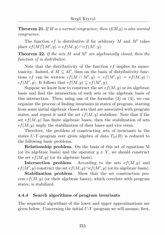
Sergii Kryvyi
Theorem 21. If M is a normal congruence, then ef(M,y) is also normalcongruence.
The function ef is distributive if for arbitrary M and M ′ takesplace ef(M
∩
M ′, y) = ef(M,y) ∩ ef(M ′, y)
Theorem 22. If the sets M and M ′ are algebraically closed, then thefunction ef is distributive.
Note that the distributivity of the function ef implies its mono-tonicity. Indeed, if M ⊆ M ′, then on the basis of distributivity func-tions ef can be written ef(M ∩ M ′, y) = ef(M ′, y) = ef(M, y) ∩ef(M ′, y). It follows that ef(M,y) ⊆ ef(M ′, y).
Suppose we know how to construct the set ef(M,y) or its algebraicbasis and find the intersection of such sets or the algebraic basis ofthis intersection. Then, using one of the formulas (3) or (4), we canorganize the process of finding invariants in states of program, startingfrom some initial algebraic closed sets that are associated with programstates, and repeat it until the set ef(M, y) stabilizes. Note that if theset ef(M, y) has finite algebraic bases, then the stabilization of setsef(M,y) imply the stabilization of their bases and vice versa.
Therefore, the problem of constructing sets of invariants in thestates U -Y -program over given algebra of data TD(R) is reduced tothe following basic problems.
Relationship problem. On the basis of this set of equations M(or its algebraic basis) and the operator y ∈ Y , we should constructthe set ef(M,y) (or its algebraic basis).
Intersection problem. According to the sets ef(M,y) andef(M ′, y) construct the set ef(M, y)∩ef(M ′, y) (or its algebraic basis).
Stabilization problem. Show that the set construction pro-cess ef(M,y) (or their algebraic bases), which correlate with programstates, is stabilized.
4.4.4 Search algorithms of program invariants
The sequential algorithms of the lower and upper approximations aregiven below. Concerning the initial U -Y -program we will assume, first,
211
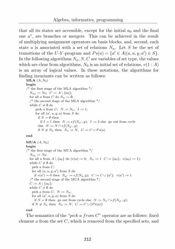
Algebra, informatics, programming
that all its states are accessible, except for the initial a0 and the finalone a∗, are branches or mergers. This can be achieved in the resultof multiplying assignment operators on basis blocks, and, second, eachstate a is associated with a set of relations Na. Let S be the set oftransitions of the U -Y -program and Ps(a) = a′ ∈ A|(a, u, y, a′) ∈ S.In the following algorithmsNa, N,C are variables of set type, the valueswhich are clear from algorithms, N0 is an initial set of relations, v(1 : A)is an array of logical values. In these notations, the algorithms forfinding invariants can be written as follows:
MLA (A,N0)begin
/* the first stage of the MLA algorithm */Na0
:= N0; C := A \ a0;for all a from C do Na := ∅;/* the second stage of the MLA algorithm */while C = ∅ do
pick a from C; N := Na; I := 1;for all (a′, u, y, a) from S doif N = ∅ thenif I = 1 then N := ef(Na′ , y); I := 2 else go out from cycle
else N := N ∩ ef(Na′ , y)if N = Na then Na := N ; C := C ∪ Ps(a)
end
MUA (A,N0)begin
/* the first stage of the MUA algorithm */Na0
:= N0;for all a from A \ a0 do (v(a) := 0; Na := 1 C := a0; v(a0) := 1);while C = ∅ dopick a from C;for all (a, u, y, a′) from S doif v(a′) = 0 then Na′ := ef(Na, y); C := C ∪ a′; v(a′) := 1
/* the second stage of the MUA algorithm */C := A \ a0;while C = ∅ dopick a from C; N := Na;for all (a′, u, y, a) from S doif N = ∅ then go out from cycle else N := Na ∩ ef(Na′ , y);
if N = Na then Na := N ; C := C ∪ Ps(a)
end
The semantics of the “pick a from C” operator are as follows: fixedelement a from the set C, which is removed from the specified sets, and
212
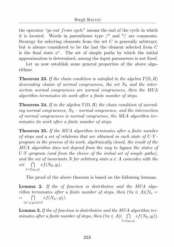
Sergii Kryvyi
the operator “go out from cycle” means the end of the cycle in whichit is located. Words in parentheses type /* and */ are comments.Strategy for selecting elements from the set C is generally arbitrary,but is always considered to be the last the element selected from Cis the final state a∗. The set of simple paths by which the initialapproximation is determined, among the input parameters is not fixed.
Let us now establish some general properties of the above algo-rithms.
Theorem 23. If the chain condition is satisfied in the algebra T (Ω, R)descending chains of normal congruences, the set N0 and the inter-section normal congruences are normal congruences, then the MUAalgorithm terminates its work after a finite number of steps.
Theorem 24. If in the algebra T (Ω, R) the chain condition of ascend-ing normal congruences, N0 – normal congruence, and the intersectionof normal congruences is normal congruence, the MLA algorithm ter-minates its work after a finite number of steps.
Theorem 25. If the MUA algorithm terminates after a finite numberof steps and a set of relations that are obtained in each state of U -Y -program in the process of its work, algebraically closed, the result of theMUA algorithm does not depend from the way to bypass the states ofU -Y -program (and from the choice of the initial set of simple paths),and the set of invariants N for arbitrary state a ∈ A coincides with theset
∩
l=l(a0,a)
ef(N0, yl).
The proof of the above theorem is based on the following lemmas.
Lemma 2. If the ef function is distributive and the MUA algo-rithm terminates after a finite number of steps, then (∀a ∈ A)(Na ==
∩
(a′,u,y,a)∈S
ef(Na′ , y)).
Lemma 3. If the ef function is distributive and the MUA algorithm ter-minates after a finite number of steps, then (∀a ∈ A)(
∩
l=(a0,a)
ef(N0, yl)).
213
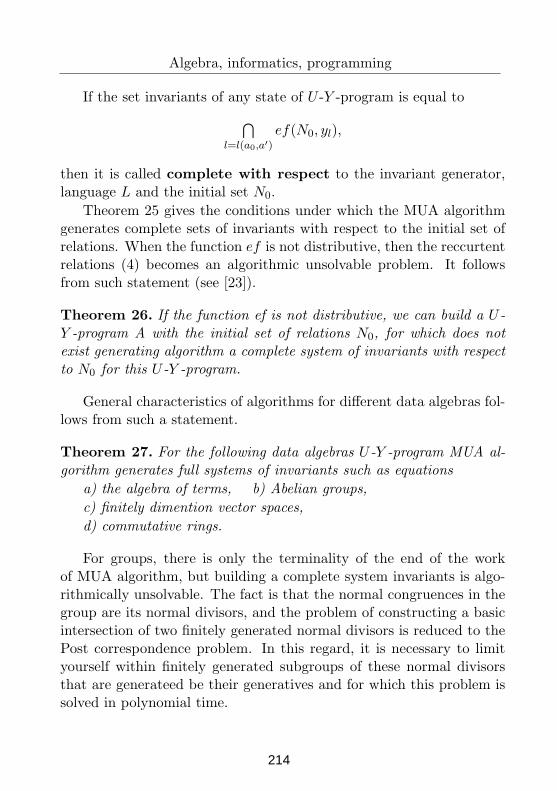
Algebra, informatics, programming
If the set invariants of any state of U -Y -program is equal to
∩
l=l(a0,a′)
ef(N0, yl),
then it is called complete with respect to the invariant generator,language L and the initial set N0.
Theorem 25 gives the conditions under which the MUA algorithmgenerates complete sets of invariants with respect to the initial set ofrelations. When the function ef is not distributive, then the reccurtentrelations (4) becomes an algorithmic unsolvable problem. It followsfrom such statement (see [23]).
Theorem 26. If the function ef is not distributive, we can build a U -Y -program A with the initial set of relations N0, for which does notexist generating algorithm a complete system of invariants with respectto N0 for this U -Y -program.
General characteristics of algorithms for different data algebras fol-lows from such a statement.
Theorem 27. For the following data algebras U -Y -program MUA al-gorithm generates full systems of invariants such as equations
a) the algebra of terms, b) Abelian groups,
c) finitely dimention vector spaces,
d) commutative rings.
For groups, there is only the terminality of the end of the workof MUA algorithm, but building a complete system invariants is algo-rithmically unsolvable. The fact is that the normal congruences in thegroup are its normal divisors, and the problem of constructing a basicintersection of two finitely generated normal divisors is reduced to thePost correspondence problem. In this regard, it is necessary to limityourself within finitely generated subgroups of these normal divisorsthat are generateed be their generatives and for which this problem issolved in polynomial time.
214
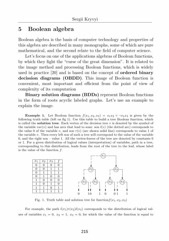
Sergii Kryvyi
5 Boolean algebra
Boolean algebra is the basis of computer technology and properties ofthis algebra are described in many monographs, some of which are puremathematical, and the second relate to the field of computer science.
Let’s focus on one of the applications algebras of Boolean functions,by which they fight the “curse of the great dimension”. It is related tothe image method and processing Boolean functions, which is widelyused in practice [20] and is based on the concept of ordered binarydecission diagrams (OBDD). This image of Boolean function isconvenient, most important and efficient from the point of view ofcomplexity of its computation
Binary solution diagrams (BDDs) represent Boolean functionsin the form of roots acyclic labeled graphs. Let’s use an example toexplain the image.
Example 1. Let Boolean function f(x1, x2, x3) = x1x2 ∨ ¬x1x3 is given by thefollowing truth table (left on fig 1). Use this table to build a tree Boolean function, whichis called the solution tree. Each vertex of the decision tree v is denoted by the symbol ofthe variable var(v) and has arcs that lead to sons: son l(v) (the dotted arc) corresponds tothe value 0 of the variable v, and son r(v) (arc shown solid line) corresponds to value 1 ofthe variable v. Then every left son of such a tree will correspond to the value of the variable0, and the right son – value 1. All the vertex-leaves of the tree are denoted by constants 0or 1. For a given distribution of logical values (interpretation) of variables, path in a tree,corresponding to this distribution, leads from the root of the tree to the leaf, whose labelis the value of the function f .
x1 x2 x3
1 1 1011
1 0 11 0 0
0 0 0100
0 1 1010
x1
x2
Fig. 1. Truth table and solution tree for functionf(x1, x2, x3)
x2
x3 x3 x3 x3
1100
f
0110
0 10 1 0 0 1 1
For example, the path l(x1)r(x2)l(x3) corresponds to the distribution of logical val-
ues of variables x1 = 0, x2 = 1, x3 = 0, for which the value of the function is equal to
215
Algebra, informatics, programming
0, and the path r(x1)r(x2)l(x3) corresponds to the distribution logical values of variables
x1 = 1, x2 = 1, x3 = 0, for whose value of the function is 1. ♠
Ordering and reduction of BDD. From this example, we cansee that the variables of the Boolean function are done in the followingorder: if u is some inner vertex of the decision tree, and v its descen-dant, then var(u) < var(v).
In the tree shown in Fig. 1, the variables are arranged as follows:x1 < x2 < x3. BDD with a given order of variables is called orderedBDD. In general, the order of the variables can be arbitrary and algo-rithms for processing such OBDD will be correct, but in practice thechoice of the appropriate order is significant, as the size of OBDD andefficiency depend on this order manipulations with them. The choice oforder will be considered in the following subdivisions, and now considerthe transformations by which reduction of a tree of decisions to OBDDis carried out. There are three such transformations:
(1) Gluing duplicate leaves (GDL): remove all the leaves of thesolution tree, except one, the leaves that are marked with the sameconstant, and reorient all input arcs of the removed vertices to theremaining vertex-leaf.
(2) Gluing of internal vertices of duplicates (GIV): if theinner vertices of the u and v solution trees are such that var(u) =var(v), l(u) = l(v) and r(u) = r(v), then remove one of those verticesand reorient all its input arcs to the remaining second vertex.
(3) Removal of redundant tests (RRT): if the internal vertexv is such that l(v) = r(v), then we remove the vertex v and reorient allits input arcs to the vertex l(v).
If the first transformation is not in doubt, but the correctness oftransformations GIV and RRT need to be proven. The proof of thiscorrectness for both transformations is based on the concept of restric-tion of a Boolean function and the well-known Shannon decompositionformula.
Boolean function obtained as a result assigning a fixed value k ∈∈ 0, 1 to some of its arguments x, is called decomposition of the
216
Sergii Kryvyi
Boolean function f relative to the variable x and is denoted by f|x←k.
If two restrictions of the function f with respect to the variable x aregiven, then for the function f the following identity holds (Shannon’sformula):
f = ¬x · f|x←0+ x · f|x←1
. (5)
Example 2. Suppose that the function is f(x1, x2, x3) = x1 · x2 + ¬x2 · x3. For thisfunction we have
f|x1←0= f1(x2, x3) = ¬x2 · x3 and f|x1←1
= f2(x2, x3) = x2 + ¬x2 · x3.
Then,
f(x1, x2, x3) = ¬x1 · f1(x2, x3) + x1 · f2(x2, x3) =
= ¬x1 · (¬x2 · x3) + (x1 · (x2 + ¬x2 · x3)) = x1 · x2 + ¬x2 · x3. ♠
Justification of correctness for GIV follows from conditions of applica-tion of this reduction (var(u) = var(v), l(u) = l(v) and r(u) = r(v))and Shannon’s formula. Really
fu = xf|x←l(u)∨ ¬xf|x←r(u)
= xf|x←l(v)∨ ¬xf|x←r(v)
= fv,
where fu, fv denote functions whose OBDDs have vertex roots u andv respectively.
Justification of correctness for RRT is performed similarly. Indeed,in terms of application of this reduction (l(v) = r(v)) and Shannon’sformula we get:
fv = xf|x←l(v)∨ ¬xf|x←r(v)
= (x ∨ ¬x)f|x←l(v)= f|x←l(v)
.
Starting from some solution tree, the variables of which are orderedrelatively to a certain order, and applying the transformation of GDL,GIV and RRT, you can always reduce this tree to OBDD. For example,a solution tree, shown in Fig. 1, is reduced to the following OBDD:
217
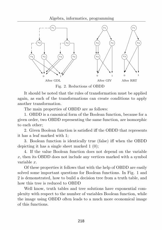
Algebra, informatics, programming
♠
♠
x1
x2♠x2
♠♠♠♠
x3 x3 x3 x3
10
After GDL
♠x1
♠ ♠
❯
x2 x2
♠x3
After GIV After RRT
Fig. 2. Reductions of OBDD
s
0 1
♠x1
♠
x3
♠x2
❯
0
1
It should be noted that the rules of transformation must be appliedagain, as each of the transformations can create conditions to applyanother transformation.
The main properties of OBDD are as follows:
1. OBDD is a canonical form of the Boolean function, because for agiven order, two OBDD representing the same function, are isomorphicto each other;
2. Given Boolean function is satisfied iff the OBDD that representsit has a leaf marked with 1;
3. Boolean function is identically true (false) iff when the OBDDdepicting it has a single sheet marked 1 (0);
4. If the value Boolean function does not depend on the variablex, then its OBDD does not include any vertices marked with a symbolvariable x.
Of these properties it follows that with the help of OBDD are easilysolved some important questions for Boolean functions. In Fig. 1 and2 is demonstrated, how to build a decision tree from a truth table, andhow this tree is reduced to OBDD
Well know, truth tables and tree solutions have exponential com-plexity with respect to the number of variables Boolean function, whilethe image using OBDD often leads to a much more economical imageof this functions.
218
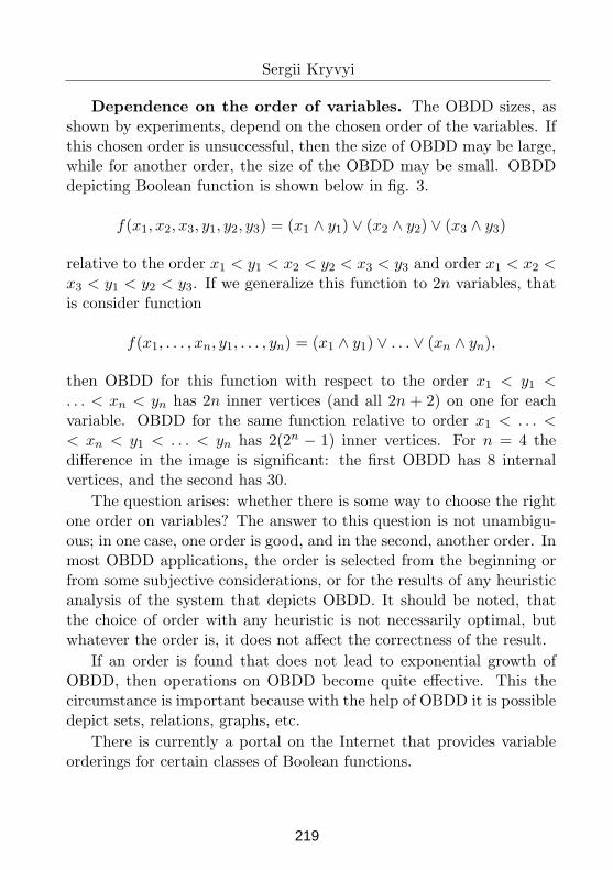
Sergii Kryvyi
Dependence on the order of variables. The OBDD sizes, asshown by experiments, depend on the chosen order of the variables. Ifthis chosen order is unsuccessful, then the size of OBDD may be large,while for another order, the size of the OBDD may be small. OBDDdepicting Boolean function is shown below in fig. 3.
f(x1, x2, x3, y1, y2, y3) = (x1 ∧ y1) ∨ (x2 ∧ y2) ∨ (x3 ∧ y3)
relative to the order x1 < y1 < x2 < y2 < x3 < y3 and order x1 < x2 <x3 < y1 < y2 < y3. If we generalize this function to 2n variables, thatis consider function
f(x1, . . . , xn, y1, . . . , yn) = (x1 ∧ y1) ∨ . . . ∨ (xn ∧ yn),
then OBDD for this function with respect to the order x1 < y1 <. . . < xn < yn has 2n inner vertices (and all 2n + 2) on one for eachvariable. OBDD for the same function relative to order x1 < . . . << xn < y1 < . . . < yn has 2(2n − 1) inner vertices. For n = 4 thedifference in the image is significant: the first OBDD has 8 internalvertices, and the second has 30.
The question arises: whether there is some way to choose the rightone order on variables? The answer to this question is not unambigu-ous; in one case, one order is good, and in the second, another order. Inmost OBDD applications, the order is selected from the beginning orfrom some subjective considerations, or for the results of any heuristicanalysis of the system that depicts OBDD. It should be noted, thatthe choice of order with any heuristic is not necessarily optimal, butwhatever the order is, it does not affect the correctness of the result.
If an order is found that does not lead to exponential growth ofOBDD, then operations on OBDD become quite effective. This thecircumstance is important because with the help of OBDD it is possibledepict sets, relations, graphs, etc.
There is currently a portal on the Internet that provides variableorderings for certain classes of Boolean functions.
219
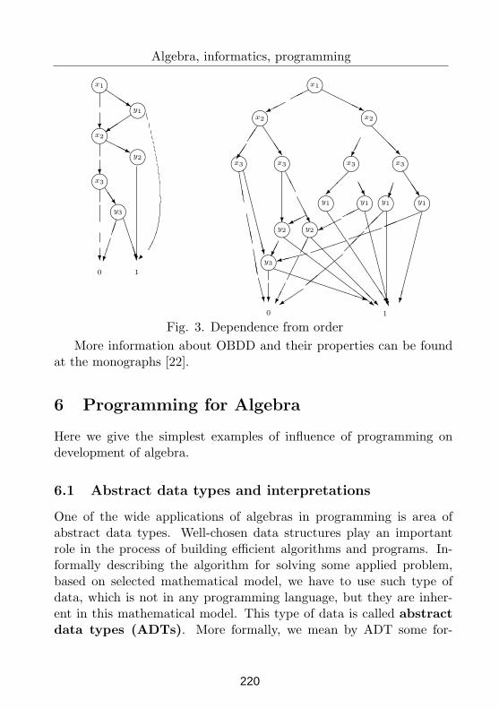
Algebra, informatics, programming
x1
x2
y1s
x3
❫y3
y2
x1
x2x2
❫
x3 x3
x3 x3
❫
y1 y1y1y1
y2 y2
y3
0
❲
❫
❩❩
❩❩❩❩
❩❩⑦
PPPPPPPPq1
Fig. 3. Dependence from order
❯
❲
❯❲
0 1
More information about OBDD and their properties can be foundat the monographs [22].
6 Programming for Algebra
Here we give the simplest examples of influence of programming ondevelopment of algebra.
6.1 Abstract data types and interpretations
One of the wide applications of algebras in programming is area ofabstract data types. Well-chosen data structures play an importantrole in the process of building efficient algorithms and programs. In-formally describing the algorithm for solving some applied problem,based on selected mathematical model, we have to use such type ofdata, which is not in any programming language, but they are inher-ent in this mathematical model. This type of data is called abstractdata types (ADTs). More formally, we mean by ADT some for-
220
Sergii Kryvyi
mal mathematical model together with operations or operators definedon this model. Simple example of this type of data is a set togetherwith union, intersection and difference operations. In the ADT model,operators can have operands not only as data, defined by this ADT,but also as programming language operands and operands defined byanother ADT. The result of execution of operator can also be a datatype, which is not defined in the model of ADT.
But within this ATD it is assumed that at least one operand or theresult of an arbitrary operator has a data type defined in this model ofATD.
ATD are defined, as a rule, using axioms, and they differ from datastructures implemented in programming languages, in that, when con-sidering the properties of ATD, they abstract from the way of theirimplementation and take into account only the algebraic propertiesarising from the axioms [15]. The use of ATD gives possibility designalgorithms and programs based on properties of their operations andpredicates with subsequent selection of the most effective way of themimplementation. When developing software providing abstraction fromthe method of implementation of ADT has certain benefits. This ab-straction gives possibility
– group ADT processing operators in one place of the program thatsignificantly facilitates its debugging;
– quickly modify software product in case of method change imple-mentation of ADT;
– minimize the number of changes in the main software modulesproduct used by the processing operators of this ATD [6].
For example, if you need to build an ADT for processing polyno-mials, then one of the main operations on polynomials is the operationadd(p, q) adding polynomials p and q. To implement this operation,there are several ways to represent polynomials in computer memory,but regardless of the choice of such an image, the meaning of the ad-dition operation does not change.
The ADT theory, in turn, influenced the development of algebra inthe sense that it stimulated the development of research in the algebras
221
Algebra, informatics, programming
of multi-sorted sets and relations [26].
6.2 Algebraic specifications in programming
The needs of programming and, in particular, ATD cause the appear-ance of a separate section of modern algebra in the form of algebraicspecifications and specification languages, which form the basis of soft-ware development and validation methods [25, 26].
The main idea of using an algebraic approach to software develop-ment and justification is to use the properties of data structures thatare selected during software development, as well as the operations andoperators that are performed on this data. Based on these properties,algebraic specification languages are developed, which describe one ormore data types together with all their properties of operations andoperators.
There are three main types of algebras and approaches in this di-rection to develop algebraic specifications that based on these algebra:
– initial algebras,
– terminal algebras,
– free algebras of specifications.
The first of these algebras describes those properties that followdirectly from the axiomatics of this type of data. In this algebra weconsider the equivalences between different data types.
The second algebras describes those properties that are fundamen-tally different for selected data types.
The third algebras deals with properties of data models that areconsidered as separate incompatible parts.
Details related to algebraic specifications, you can find in the aboveworks [25, 26].
6.3 Programming and Graph theory
Development of computer systems and programming, which in theirown way nature are discrete, most influenced by graph theory since
222
Sergii Kryvyi
graphs is a convenient and visual way images of discrete processes andevents that take place in them.
The pioneers in the use of graphs in programming were the works ofA.P. Ershov and Karp R. about organization of calculations arithmeticexpressions, the optimal distribution of registers for such calculationsand optimal use of RAM.
In these works, theoretical graphic model of programs in the formof transition graph was introduced in practice, which became classicalin solving translation problems. Then graphs of procedure call, datadependency graphs, syntax sort trees, nesting trees came, and so on.
These tasks, in turn, contributed to the development of research inthe field of graph theory related to the search for efficient graph naviga-tion algorithms (traversing the graph in depth and width), finding thepath in the graph of minimum length, transitive closure the relation ofthe reach of the vertices of the graph, checking the graph for planarity,checking the isomorphism of graphs, decomposition graphs, informa-tion storage etc. The development of data structures for displayinggraphical objects became relevant for these tasks. In particular, treesform the basis of data structures for the image of objects, which inthe process of working with them can change their structure (dynamicobjects). This type of data structure is required databases, knowledgebases, computational optimization, etc.
In particular, semantics of procedural type programming languagesare based on graph theory, the style of structural programming is sub-stantiated (programming without “goto” operator), data flow analysis[3], optimization transformation of software code [4], composition ofprograms, etc.
7 Epilogue
In conclusion, we give several examples in which the implementationof algorithms for solving specific problems is required. These examplesrequire a thorough knowledge of the subject area to which they relate.Without the knowledge, it is impossible to build such algorithms.
223
Algebra, informatics, programming
Problem 1. Implement the Babay algorithm for checking graphisomorphism [19].
Task 2. Develop an efficient (polynomial) algorithm for construc-tion of the basis of the set of solutions of the system of linear inequalitiesin the field of real numbers.
Task 3. Implement the Safra determination algorithm for Mullerautomata [7].
I thank doctor Protasova K.D. for discussion on content of thiswork and for professional profreading of an early version of this work.
References
[1] Glushkov. V. M, Letichevsky A.A, Godlevsky A.B. The Methods ofsynthesis disscrete models of biological systems (in russian). – Kiev:High Scool. – 1983. – 262 p.
[2] Godlevsky A.B, Kapitonova J.V, Kryvyi S.L, Letichevsky A.A. Iterativemethods of analysis of programs (in russian). Journ. Cybernetics. –1989. – N 2. – PP. 9 – 19.
[3] Evstigneev V.A. Application of graph theory in programming (in rus-sian). M.: Nauka. - 1985. - 351 p.
[4] Kas’yanov V.N. Optimizing program transformations (in russian). M.:Nauka. – 1988. – 334 p.
[5] Kryvyi S.L. Discrete mathematics (in ukrainian). Chernivtsi-Kyiv:“Bukrek”. – 2017. – 576 p.
[6] Kryvyi S.L. Introduction to software creation methods (in ukrainian).Kyiv: NaUKMA. – 2018. – 449 p.
[7] Kryvyi S.L. Finite automata: theory, algorithms, complexity (inukrainian). Chernivtsi-Kyiv:“Bukrek”. – 2020. – 427 p.
[8] Kapitonova J. V., Letichevsky A.A. About basic programmingparadigms (in russian). Journ. Cybernetics and syst. analysis. – 1994 –N 6. – PP. 3–20.
[9] Markov A.A., Nagorny N.M. Algorithm theory (in russian). –M.:FAZIST. – 1996. – 448 p.
224
Sergii Kryvyi
[10] Kohn P.M. Universal algebra. – M.: Mir. – 1968. – 351 p.
[11] Cooke D.J., Bez H.E. Computer mathematics. – Cambridge UniversityPress. – 1984. – 303 p.
[12] Kurosh A.G. Lectures on general algebra (in russian). – M.: Nauka. –1973. – 399 p.
[13] Kurosh A.G. General algebra. Lectures 1969-70 (in russian). – M.:Nauka. – 1974. – 158 p.
[14] Plotkin B.I. Universal algebra, algebraic logics and data bases (in rus-sian). – M.: Nauka. – 1991. – 446 p.
[15] Sergienko I.V., Kryvy S.L., Provotar O.I. Algebraic aspects of infor-mational technologies (in ukrainian). – Kyiv:Interservice.–2018.–410 p.
[16] Skornyakov L.A. Elements of structure theory (in russian). – M.:Nauka. – 1982. – 158 p.
[17] Field A., Harrison P. Functional programming. – M.: Mir. – 1993. –638 p.
[18] Baader F., Ziekmann J. Unification theory. – In Handbook of Logicin Artificial Intelligence and Logic Programming. – Oxford UniversityPress. – 1994. – P. 1–85.
[19] Babai L. Graph Isomoirfism in Quasipolinomial Time. – 2nd prelim.version (January 19). – 2016. – 89 p.
[20] Bryant R.E. Symbolic Boolean Manipulation with Ordered Binary De-cision Diagrams. – Scool of Comp. Science, Carnegi Mellon University,Pittsburg. – 1992 (june). – 34 p.
[21] Bryant R.E. Graph-based algorithms for Boolean function manipula-tion. – IEEE Trans. on Comp. – 1986. – v. 40. – P. 677 – 691.
[22] Ebendt R., Fey G., Drechsler R. Advanced BDD Optimization. –Springer. – 2005. – 222 p.
[23] Kam J.B., Ullman D.J. Monotone data flow analysis frame works. ActaInform. – 1978. – N 3. – P. 305–318.
[24] Knut D. E., Bendix P. B. Simple word problem in universal algebras.– In J. Leech, editor, Computational Problems in Abstract Algebra,Pergamon Press. – Oxford. – 1970.
225

Algebra, informatics, programming
[25] Wirsing M. Algebraic Specification. – Edites by J. van Leeuwen ElsevierPublishers B.V. – 1990. – PP. 677 – 788.
[26] Sannella D., Tarlecki A. Foundations of Algebraic Specification andFormal Software Development. – Springer-Verlag Berlin Heidelberg. –2012. – 581 p.
[27] Tarski A. A Lattice Theoretical Fixed Point Theorem and Its Applica-tions. – Pac. Journ. Math. – 1955. – v. 5. – N 2. – P. 285–309.
Sergii Kryvyi1
1Taras Shevchenko National University of KyivEmail: [email protected]
226
Proceedings of the Conference on Mathematical Foundations of Informatics
MFOI-2020, January 12-16, 2021, Kyiv, Ukraine
One Approach to Formal
Verification of Distributed Ledger
Technologies on the Blockchain
Technologies Example
Oleksandr Letychevskyi, Volodymyr Peschanenko, Maksym
Poltoratskyi, Serhii Horbatiuk, Viktor Horbatiuk and YuliiaTarasich
Abstract
In the article, the approach to formal verification of distributed
ledger technologies on the blockchain technologies example is
considered. Behavior algebra specifications are used as the modeling
language.
Thus, this article provides a brief description of the technology
and the methods and tools developed by the authors for blockchain
technologies modeling and for the analysis and study of its
properties. The article also describes the formalization of the
examples of the DAO for Smart Contracts and the Double Spend
attack. The formalization and properties analysis is considered with
the usage of the insertion modeling platform.
Keywords: formal verification, blockchain technologies,
insertion modeling, Smart Contracts, algebraic behavior.
1 Introduction
Distributed ledger technology is information storage technology, the keyfeatures of which are the sharing and synchronization of digital data
according to the consensus algorithm, the geographical distribution ofequivalent copies at different points around the world, the absence of a
central administrator. We are talking about immutable transactions,
© 2021 by Oleksandr Letychevskyi, Volodymyr Peschanenko, Maksym
Poltoratskyi, Serhii Horbatiuk, Viktor Horbatiuk and Yuliia Tarasich
227
Oleksandr Letychevskyi, Volodymyr Peschanenko, et al.
preventing of data loss, the ability to track the digital assets, cryptographic
security, consensus algorithms, joint verification of transactions byuntrusted participants. All processes are carried out in the cloud and meet to
the principles of distribution and joint sharing [1].Today, there are many DLT implementations that are made by different
developers, but there is no information that can be used to create universalframeworks. Thus, the main difficulties are
- the need to analyze different types of systems,- different sets of rules on which a DLT system should work,
- different types of protocol updates and their management(management takes many forms, that are often unclear),
- different transaction processing, etc.Based on this, we can already say that the development of systems
requires a special approach to its verification at the design stage.Accordingly, like any new technology, blockchain has its
vulnerabilities. Thus, all algorithms that are used require careful analysisand verification, namely, checking the stability of the system against
various attacks, such as Double spending attacks, Grinding attacks,Transaction denial attacks, Desynchronization attacks, 51% attacks,
Selfish-mining, etc. Thus, special attention also must be paid to smartcontracts. The most known language of smart contract specification is the
Solidity language created by Etherium [2]. The increasing popularityentailed that smart contracts became an object of numerous attacks bringing
the money loses and falsification of results generated by the decentralizedsystem. Many tools intended for the verification of smart contracts have
been developed and security policies are established [3-6]. Anyway theproblem of vulnerability of smart contract still remain actual.
The usage of formal methods has become one of the advancedtechnologies and different theories are used for the implementation of
cybersecurity defense and verification systems. Thus we consider thebehavior algebra and insertion modeling for the creation of methods of
vulnerability detection in the smart contracts.
2 Our Contribution
Successful implementation of behavior algebra specification for detection
of vulnerabilities in binary code [7], proving of consensus protocolproperties [8], studying of token economy issues [9-11] spawned the idea
of the usage of these results in smart contract verification. We are following
228
One Approach to Formal Verification of Distributed Ledger Technologies on the
Blockchain Technologies Example
the way when some object shall be presented as algebraic specifications
and the methods and properties of the algebraic theory are applicable. Inthe research, we consider smart contracts as the objects that interact with
users and each other. The formal language of smart contract presentation,especially Solidity, has the well-defined semantics that can be expressed in
some formal theory which is the behavior algebra. It gives the possibility toconvert smart contracts in Solidity to behavior algebra automatically.
We created the methods and tools for smart contract vulnerabilitydetection. It translates the smart contract to the behavior algebra
specifications that are the input for algebraic processing. From the otherside, we developed the technique of formalization of attacks that are
possible in smart contracts. The attacks can be formalized as patterns inbehavior algebra expressions. Algebraic processing anticipates algebraic
matching of given patterns of attacks with converted smart contracts. Ituses our algorithms of symbolic modeling, algebraic matching, and
resolving of behavior algebra expressions.
3 Insertion Modeling and Behavior Algebra
In 1997, Gilbert and Letichevsky introduced the notion of behavior algebra
[12]. It was realized in the scope of the IMS [13]. Behavior algebra is atwo-sorted universal algebra. The main sort is a set of behaviors and the
second sort is a set of actions. This algebra has two operations, threeterminal constants, and an approximation relation. The operations are the
prefixing a.u (where a is an action and u is a behavior) andnondeterministic choice of behaviors u + v. The terminal constants are
successful termination ∆, deadlock 0, and divergent behavior . The⊥
approximation relation is a partial order on the set of behaviors with the⊑
minimal element . The behavior algebra is also enriched by two⊥
operations: parallel (||) and sequential (;) compositions of behaviors.
The action language is built over some attribute environment in whichall agents interact with one another. Every agent is defined by a set of
attributes. An agent changes its state under some conditions formed byvalues of attributes. Every agent’s actions are represented by the triple B =
<P, A, S>, where P is a precondition of the action presented as a formula insome basic logic language; S, a postcondition; and A, a process that
illustrates the agent transition. As a basic logical language, we consider theset of formulas of first-order logic over polynomial arithmetic. As a whole,
229
Oleksandr Letychevskyi, Volodymyr Peschanenko, et al.
the semantic of action means that the agent could change its state if the
precondition is true and the state will change correspondingly to thepostcondition, which is also a formula of first-order logic. The
postcondition could also contain an assignment statement. The initial state of agents can be represented by an initial formula.
Starting from the initial formula, we can apply the action corresponding tothe behavior algebra expression. The action is applicable if its precondition
is satisfiable and consistent with the current state. Starting from the formulaof the initial state S0 and the initial behavior B0, we select the action and
move to the next behavior. In the first step, we check the satisfiability of theconjunction
S0 /\ Pa1if B0 = a1.B1, and Pa1 is a precondition of a1. The next state of the
environment is obtained by means of the predicate transformer, that is, thefunction over the current agent state, precondition, and postcondition.
PT(Si, Pai, Qai) = Si+1By applying the predicate transformer function to different agent
states, we can obtain the sequence S0, S1,… of formulas that express theagent states changing from the initial state. We present the trace by the
sequence of processes of actions a1, a2,… Every agent state covers the setof concrete agent values, and the process of generating such traces is called
symbolic modeling. The predicate transformer has to be defined for thecorresponding theory.
4 Formal Verification of Distributed Ledger Technologies onthe Blockchain Technologies Example
4.1 Insertion Semantics of blockchain system
In general, the blockchain algorithm can be considered as the interaction of
nodes of some network. Each node can act as a block generator, whichcreates and sends blocks to all other nodes according to the consensus
algorithm. On the other hand, the node may also receive blocks and othernecessary information from other nodes to build the blockchain.
The model of the blockchain platform can be seen as the interaction ofsome number of agents in the environment in which they exchange
notifications. Notifications contain information that is necessary to build ablockchain.
230
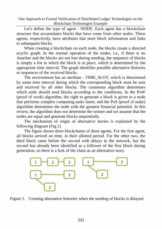
One Approach to Formal Verification of Distributed Ledger Technologies on the
Blockchain Technologies Example
Let's define the type of agent - NODE. Each agent has a blockchain
structure that accumulates blocks that have come from other nodes. Theseagents, respectively, have attributes that store block information and links
to subsequent blocks.When creating a blockchain on each node, the blocks create a directed
acyclic graph. In the normal operation of the nodes, i.e., if there is noAttacker and the blocks are not lost during sending, the sequence of blocks
is simply a list in which the block is in place, which is determined by theappropriate time interval. The graph identifies possible alternative histories
or sequences of the received blocks.The environment has an attribute - TIME_SLOT, which is determined
by some time interval during which the corresponding block must be sentand received by all other blocks. The consensus algorithm determines
which node should send blocks according to the conditions. In the PoW(proof of work) algorithm, the right to generate a block is given to a node
that performs complex computing tasks faster, and the PoS (proof of stake)algorithm determines the node with the greatest financial potential. In this
review, the algorithm does not determine the winner and we assume that thenodes are equal and generate blocks sequentially.
The mechanism of origin of alternative stories is explained by thefollowing diagram (Fig.1).
The figure shows three blockchains of three agents. For the first agent,all blocks arrived on time, in their allotted period. For the other two, the
third block came before the second with delays in the network, but thesecond has already been identified as a follower of the first block during
generation, so there is a fork of the chain as an alternative story.
Figure 1. Creating alternative histories when the sending of blocks is delayed.
1 2 3
1
2
3
1
2
3
231
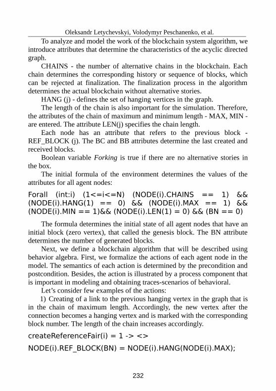
Oleksandr Letychevskyi, Volodymyr Peschanenko, et al.
To analyze and model the work of the blockchain system algorithm, we
introduce attributes that determine the characteristics of the acyclic directedgraph.
CHAINS - the number of alternative chains in the blockchain. Eachchain determines the corresponding history or sequence of blocks, which
can be rejected at finalization. The finalization process in the algorithmdetermines the actual blockchain without alternative stories.
HANG (j) - defines the set of hanging vertices in the graph.The length of the chain is also important for the simulation. Therefore,
the attributes of the chain of maximum and minimum length - MAX, MIN -are entered. The attribute LEN(j) specifies the chain length.
Each node has an attribute that refers to the previous block -REF_BLOCK (j). The BC and BB attributes determine the last created and
received blocks.Boolean variable Forking is true if there are no alternative stories in
the box.The initial formula of the environment determines the values of the
attributes for all agent nodes:
Forall (int:i) (1<=i<=N) (NODE(i).CHAINS == 1) &&(NODE(i).HANG(1) == 0) && (NODE(i).MAX == 1) &&(NODE(i).MIN == 1)&& (NODE(i).LEN(1) = 0) && (BN == 0)
The formula determines the initial state of all agent nodes that have an
initial block (zero vertex), that called the genesis block. The BN attributedetermines the number of generated blocks.
Next, we define a blockchain algorithm that will be described usingbehavior algebra. First, we formalize the actions of each agent node in the
model. The semantics of each action is determined by the precondition andpostcondition. Besides, the action is illustrated by a process component that
is important in modeling and obtaining traces-scenarios of behavioral.Let’s consider few examples of the actions:
1) Creating of a link to the previous hanging vertex in the graph that isin the chain of maximum length. Accordingly, the new vertex after the
connection becomes a hanging vertex and is marked with the correspondingblock number. The length of the chain increases accordingly.
createReferenceFair(i) = 1 -> <>
NODE(i).REF_BLOCK(BN) = NODE(i).HANG(NODE(i).MAX);
232
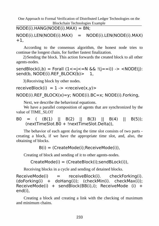
One Approach to Formal Verification of Distributed Ledger Technologies on the
Blockchain Technologies Example
NODE(i).HANG(NODE(i).MAX) = BN;
NODE(i).LEN(NODE(i).MAX) = NODE(i).LEN(NODE(i).MAX)+1,
According to the consensus algorithm, the honest node tries to
continue the longest chain, for further fastest finalization.2)Sending the block. This action forwards the created block to all other
agents-nodes.
sendBlock(i,b) = Forall (1<=j<=N && !(j==i)) -> <NODE(j):send(b, NODE(i).REF_BLOCK(b)> 1,
3)Receiving block by other nodes.
receiveBlock(i) = 1 -> <receive(x,y)>
NODE(i).REF_BLOCK(x)=y; NODE(i).BC=x; NODE(i).Forking,
Next, we describe the behavioral equations.We have a parallel composition of agents that are synchronized by the
value of TIME_SLOT
B0 = ( (B(1) || B(2) || B(3) || B(4) || B(5)); (nextTimeSlot.B0 + !nextTimeSlot.Delta)),
The behavior of each agent during the time slot consists of two parts -
creating a block, if we have the appropriate time slot, and, also, theobtaining of blocks.
B(i) = (CreateMode(i);ReceiveMode(i)),
Creating of block and sending of it to other agents-nodes.
CreateMode(i) = (CreateBlock(i);sendBLock(i)),
Receiving blocks in a cycle and sending of detained blocks.
ReceiveMode(i) = receiveBlock(i). checkForking(i).(doForking(i) + doHang(i)); (checkMin(i). checkMax(i));ReceiveMode(i) + sendBlock(BB(i),i); ReceiveMode (i) +end(i),
Creating a block and creating a link with the checking of maximumand minimum chains.
233
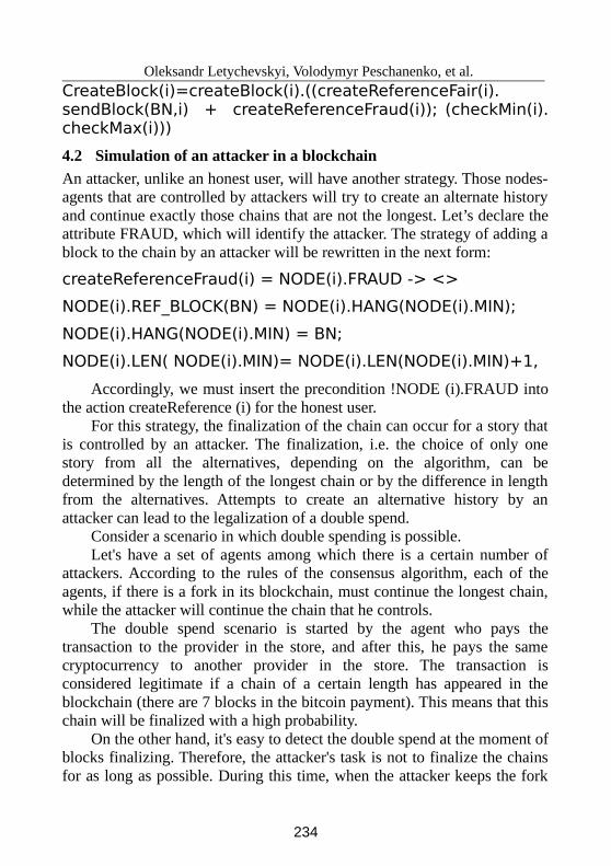
Oleksandr Letychevskyi, Volodymyr Peschanenko, et al.
CreateBlock(i)=createBlock(i).((createReferenceFair(i).sendBlock(BN,i) + createReferenceFraud(i)); (checkMin(i).checkMax(i)))
4.2 Simulation of an attacker in a blockchain
An attacker, unlike an honest user, will have another strategy. Those nodes-agents that are controlled by attackers will try to create an alternate history
and continue exactly those chains that are not the longest. Let’s declare theattribute FRAUD, which will identify the attacker. The strategy of adding a
block to the chain by an attacker will be rewritten in the next form:
createReferenceFraud(i) = NODE(i).FRAUD -> <>
NODE(i).REF_BLOCK(BN) = NODE(i).HANG(NODE(i).MIN);
NODE(i).HANG(NODE(i).MIN) = BN;
NODE(i).LEN( NODE(i).MIN)= NODE(i).LEN(NODE(i).MIN)+1,
Accordingly, we must insert the precondition !NODE (i).FRAUD into
the action createReference (i) for the honest user. For this strategy, the finalization of the chain can occur for a story that
is controlled by an attacker. The finalization, i.e. the choice of only onestory from all the alternatives, depending on the algorithm, can be
determined by the length of the longest chain or by the difference in lengthfrom the alternatives. Attempts to create an alternative history by an
attacker can lead to the legalization of a double spend.Consider a scenario in which double spending is possible.
Let's have a set of agents among which there is a certain number ofattackers. According to the rules of the consensus algorithm, each of the
agents, if there is a fork in its blockchain, must continue the longest chain,while the attacker will continue the chain that he controls.
The double spend scenario is started by the agent who pays thetransaction to the provider in the store, and after this, he pays the same
cryptocurrency to another provider in the store. The transaction isconsidered legitimate if a chain of a certain length has appeared in the
blockchain (there are 7 blocks in the bitcoin payment). This means that thischain will be finalized with a high probability.
On the other hand, it's easy to detect the double spend at the moment ofblocks finalizing. Therefore, the attacker's task is not to finalize the chains
for as long as possible. During this time, when the attacker keeps the fork
234
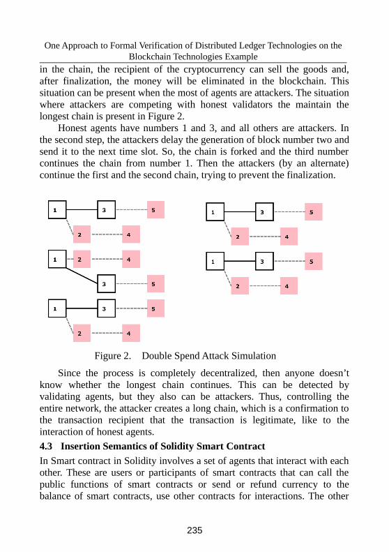
One Approach to Formal Verification of Distributed Ledger Technologies on the
Blockchain Technologies Example
in the chain, the recipient of the cryptocurrency can sell the goods and,
after finalization, the money will be eliminated in the blockchain. Thissituation can be present when the most of agents are attackers. The situation
where attackers are competing with honest validators the maintain thelongest chain is present in Figure 2.
Honest agents have numbers 1 and 3, and all others are attackers. Inthe second step, the attackers delay the generation of block number two and
send it to the next time slot. So, the chain is forked and the third numbercontinues the chain from number 1. Then the attackers (by an alternate)
continue the first and the second chain, trying to prevent the finalization.
Figure 2. Double Spend Attack Simulation
Since the process is completely decentralized, then anyone doesn’t
know whether the longest chain continues. This can be detected byvalidating agents, but they also can be attackers. Thus, controlling the
entire network, the attacker creates a long chain, which is a confirmation tothe transaction recipient that the transaction is legitimate, like to the
interaction of honest agents.
4.3 Insertion Semantics of Solidity Smart Contract
In Smart contract in Solidity involves a set of agents that interact with eachother. These are users or participants of smart contracts that can call the
public functions of smart contracts or send or refund currency to thebalance of smart contracts, use other contracts for interactions. The other
235
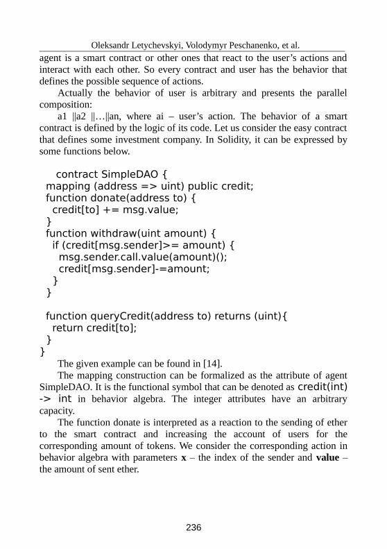
Oleksandr Letychevskyi, Volodymyr Peschanenko, et al.
agent is a smart contract or other ones that react to the user’s actions and
interact with each other. So every contract and user has the behavior thatdefines the possible sequence of actions.
Actually the behavior of user is arbitrary and presents the parallelcomposition:
a1 ||a2 ||…||an, where ai – user’s action. The behavior of a smartcontract is defined by the logic of its code. Let us consider the easy contract
that defines some investment company. In Solidity, it can be expressed bysome functions below.
contract SimpleDAO mapping (address => uint) public credit; function donate(address to) credit[to] += msg.value; function withdraw(uint amount) if (credit[msg.sender]>= amount) msg.sender.call.value(amount)(); credit[msg.sender]-=amount;
function queryCredit(address to) returns (uint) return credit[to];
The given example can be found in [14].
The mapping construction can be formalized as the attribute of agentSimpleDAO. It is the functional symbol that can be denoted as credit(int)-> int in behavior algebra. The integer attributes have an arbitrary
capacity.
The function donate is interpreted as a reaction to the sending of etherto the smart contract and increasing the account of users for the
corresponding amount of tokens. We consider the corresponding action inbehavior algebra with parameters x – the index of the sender and value –
the amount of sent ether.
236
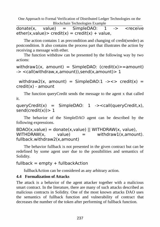
One Approach to Formal Verification of Distributed Ledger Technologies on the
Blockchain Technologies Example
donate(x, value) = SimpleDAO: 1 -> <receiveether(x,value)> credit(x) = credit(x) + value,
The action contains 1 as precondition and changing of credit(sender) as
postcondition. It also contains the process part that illustrates the action byreceiving a message with ether.
The function withdraw can be presented by the following way by twoactions:
withdraw1(x, amount) = SimpleDAO: (credit(x)>=amount)-> <call(withdraw,x,amount)),send(x,amount)> 1
withdraw2(x, amount) = SimpleDAO:1 -><> credit(x) =credit(x) - amount
The function queryCredit sends the message to the agent x that calledit.
queryCredit(x) = SimpleDAO: 1 -><call(queryCredit,x),send(credit(x))> 1
The behavior of the SimpleDAO agent can be described by thefollowing expressions.
BDAO(x,value) = donate(x,value) || WITHDRAW(x, value),WITHDRAW(x, value) = withdraw1(x,amount).fullback.withdraw2(x,amount)
The behavior fullback is not presented in the given contract but can beredefined by some agent user due to the possibilities and semantics of
Solidity.
fullback = empty + fullbackAction
fullbackAction can be considered as any arbitrary action.
4.4 Formalization of Attacks
The attack is a behavior of the agent attacker together with a malicious
smart contract. In the literature, there are many of such attacks described asmalicious contracts in Solidity. One of the most known attacks DAO uses
the semantics of fullback function and vulnerability of contract thatdecreases the number of the token after performing of fullback function.
237
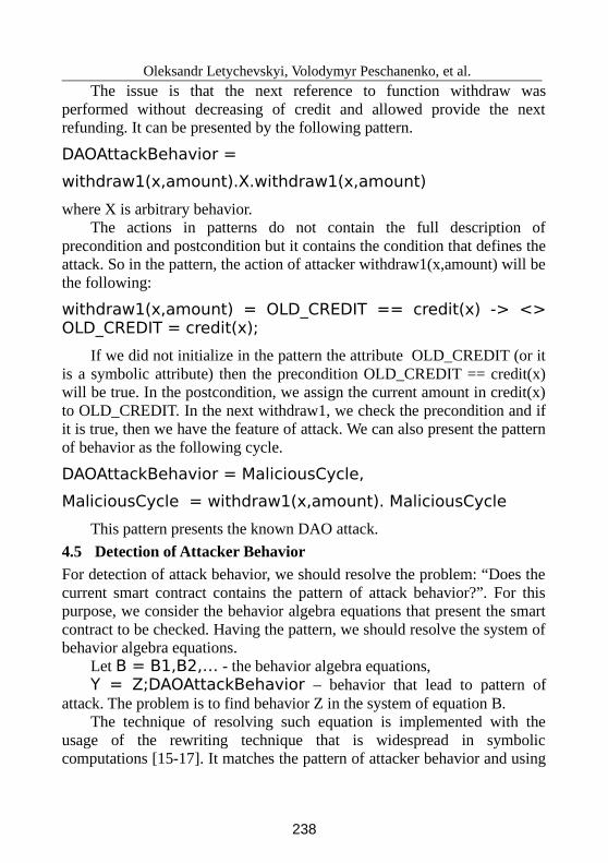
Oleksandr Letychevskyi, Volodymyr Peschanenko, et al.
The issue is that the next reference to function withdraw was
performed without decreasing of credit and allowed provide the nextrefunding. It can be presented by the following pattern.
DAOAttackBehavior =
withdraw1(x,amount).X.withdraw1(x,amount)
where X is arbitrary behavior. The actions in patterns do not contain the full description of
precondition and postcondition but it contains the condition that defines theattack. So in the pattern, the action of attacker withdraw1(x,amount) will be
the following:
withdraw1(x,amount) = OLD_CREDIT == credit(x) -> <>OLD_CREDIT = credit(x);
If we did not initialize in the pattern the attribute OLD_CREDIT (or it
is a symbolic attribute) then the precondition OLD_CREDIT == credit(x)will be true. In the postcondition, we assign the current amount in credit(x)
to OLD_CREDIT. In the next withdraw1, we check the precondition and ifit is true, then we have the feature of attack. We can also present the pattern
of behavior as the following cycle.
DAOAttackBehavior = MaliciousCycle,
MaliciousCycle = withdraw1(x,amount). MaliciousCycle
This pattern presents the known DAO attack.
4.5 Detection of Attacker Behavior
For detection of attack behavior, we should resolve the problem: “Does the
current smart contract contains the pattern of attack behavior?”. For thispurpose, we consider the behavior algebra equations that present the smart
contract to be checked. Having the pattern, we should resolve the system ofbehavior algebra equations.
Let B = B1,B2,… - the behavior algebra equations,
Y = Z;DAOAttackBehavior – behavior that lead to pattern of
attack. The problem is to find behavior Z in the system of equation B.The technique of resolving such equation is implemented with the
usage of the rewriting technique that is widespread in symboliccomputations [15-17]. It matches the pattern of attacker behavior and using
238
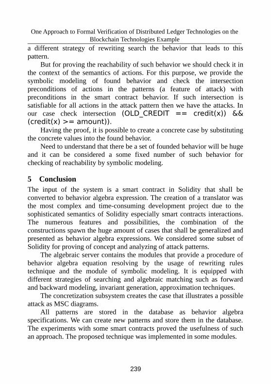
One Approach to Formal Verification of Distributed Ledger Technologies on the
Blockchain Technologies Example
a different strategy of rewriting search the behavior that leads to this
pattern.But for proving the reachability of such behavior we should check it in
the context of the semantics of actions. For this purpose, we provide thesymbolic modeling of found behavior and check the intersection
preconditions of actions in the patterns (a feature of attack) withpreconditions in the smart contract behavior. If such intersection is
satisfiable for all actions in the attack pattern then we have the attacks. Inour case check intersection (OLD_CREDIT == credit(x)) &&(credit(x) >= amount)).
Having the proof, it is possible to create a concrete case by substitutingthe concrete values into the found behavior.
Need to understand that there be a set of founded behavior will be hugeand it can be considered a some fixed number of such behavior for
checking of reachability by symbolic modeling.
5 Conclusion
The input of the system is a smart contract in Solidity that shall be
converted to behavior algebra expression. The creation of a translator wasthe most complex and time-consuming development project due to the
sophisticated semantics of Solidity especially smart contracts interactions.The numerous features and possibilities, the combination of the
constructions spawn the huge amount of cases that shall be generalized andpresented as behavior algebra expressions. We considered some subset of
Solidity for proving of concept and analyzing of attack patterns.The algebraic server contains the modules that provide a procedure of
behavior algebra equation resolving by the usage of rewriting rulestechnique and the module of symbolic modeling. It is equipped with
different strategies of searching and algebraic matching such as forwardand backward modeling, invariant generation, approximation techniques.
The concretization subsystem creates the case that illustrates a possibleattack as MSC diagrams.
All patterns are stored in the database as behavior algebraspecifications. We can create new patterns and store them in the database.
The experiments with some smart contracts proved the usefulness of suchan approach. The proposed technique was implemented in some modules.
239
Oleksandr Letychevskyi, Volodymyr Peschanenko, et al.
Acknowledgments. We would like to thank the company LitSoft
Enterprise R&D [18] for the opportunity to work with the platform formodeling algebraic behavior for our research and experiments in the
modeling area. We are also grateful to the Glushkov Institute of Cybernetics of NAS
of Ukraine for the theoretical and practical results in the field ofverification that were used as a basis for our studies of formalization and
algebraic modeling in the Blockchain Technologies area and to the KhersonState University for the active supporting of Insertion Modeling System.
References
[1] R. Maull, et al. Distributed ledger technology: Applications and implications.
Strategic Change, vol. 26, no 5 (2017), pp. 481-489.
[2] Etherium, https://ethereum.org/en/
[3] S. Kalra et al. ZEUS: Analyzing Safety of Smart Contracts. Network and
Distributed Systems Security (NDSS) Symposium 2018, San Diego, CA, USA
(2018).
[4] S. Tikhomirov et al. Smartcheck: Static analysis of ethereum smart contracts.
Proceedings of the 1st International Workshop on Emerging Trends in
Software Engineering for Blockchain, ( 2018), pp. 9-16.
[5] K. Bhargavan et al. Short paper: Formal verification of smart contracts.
Proceedings of the 11th ACM Workshop on Programming Languages and
Analysis for Security (PLAS), in conjunction with ACM CCS, (2016), pp.91-
96.
[6] P. Praitheeshan et al. Security analysis methods on Ethereum smart contract
vulnerabilities: a survey. arXiv preprint arXiv:1908.08605. (2019).
[7] O. Letychevskyi, et al. Algebraic Patterns of Vulnerabilities in Binary Code.
In 2019 10th International Conference on Dependable Systems, Services and
Technologies (DESSERT), (2019), pp. 70-73
[8] A. Sobol, V. G. Skobelev, J. Konchunas, V. Radchenko, S. Sachtachtinskagia,
O. A. Letychevskyi,... & M. Orlovsky Random Re-Ordering of the Parties in
the Consensus Protocol. In ICTERI Workshops, (2019), pp. 694-703
[9] O. Letychevskyi, V. Peschanenko, M. Poltoratskyi, Y. Tarasich, Our Approach
to Formal Verification of Token Economy Models. Communications in
Computer and Information Science, 1175 CCIS, (2020), pp. 348–363
[10]O. Letychevsky, V. Peschanenko, V. Radchenko,... P. Kovalenko, S. Mogylko,
Formal verification of token economy models. ICBC 2019 - IEEE International
Conference on Blockchain and Cryptocurrency, (2019), pp. 201–204.
240
One Approach to Formal Verification of Distributed Ledger Technologies on the
Blockchain Technologies Example
[11] O. Letychevskyi, V. Peschanenko, V. Radchenko, M. Poltoratskyi, Y. Tarasich,
Formalization and algebraic modeling of tokenomics projects. CEUR
Workshop Proceedings, (2019), pp. 577–584
[12]A.A. Letichevsky and D.R. Gilber A general theory of action languages.
Technical report Department of Computer Science. City University, London,
UK, vol. 34, no 1, (1998), pp.12-30.
[13]A. Letichevsky, O. Letychevskyi, V. Peschanenko Insertion Modeling and Its
Applications. Computer Science Journal of Moldova, vol. 24, no 3, (2016), pp.
357-370
[14]A Survey of Attacks on Ethereum Smart Contracts,
https://blockchain.unica.it/projects/ethereum-survey/attacks.html
[15]A. Letichevsky, O. Letychevskyi, V. Peschanenko The Non-Deterministic
Strategy of Rewriting. Control Systems and Computers, vol. 6, (2013), pp. 53–
58.
[16]A. Letichevsky, V.Peschanenko Simple Non-Deterministic Rewriting in
Verification. Programming Problems. no. 2-3, (2010), pp. 97-101
[17]A. Letichevsky, A. Letichevsky jr, V. Peschanenko Optimization of Rewriting
Machine of Algebraic Programming System APS. Bulletin of Kharkiv National
University VN Karazin. no. 847, (2009), pp.213-220 (series, "Mathematical
modeling. Information Technology. Automatic Control Systems)(in russian)
[18]LitSoft Enterprise R&D, http://litsoft.com.ua/
Oleksandr Letychevskyi1,Volodymyr Peschanenko2, Maksym Poltoratskyi3, Serhii
Horbatiuk4, Viktor Horbatiuk5 and Yuliia Tarasich6
1V.M.Glushkov Institute of Cybernetics of the NAS of Ukraine,
E-mail: [email protected]
2Kherson State University, Universytets’ka St. 27, 73000, Kherson, Ukraine,
E-mail: [email protected]
3Kherson State University, Universytets’ka St. 27, 73000, Kherson, Ukraine,
E-mail: [email protected]
4V.M.Glushkov Institute of Cybernetics of the NAS of Ukraine,
E-mail: [email protected]
5V.M.Glushkov Institute of Cybernetics of the NAS of Ukraine,
E-mail: [email protected]
241

Oleksandr Letychevskyi, Volodymyr Peschanenko, et al.
6Kherson State University, Universytets’ka St. 27, 73000, Kherson, Ukraine,
E-mail: [email protected]
242
Proceedings of the Conference on Mathematical Foundations of Informatics
MFOI2020, January 12-16, 2021, Kyiv, Ukraine
Ias, i Botanic Garden App
Radu-Matei Lipan, Adrian Iftene
Abstract
The ”Ias,i Botanical Garden App” is an attempt at modernizing
the way in which the average visitor of the ”Anastasie Fatu”Botanical Garden interacts with and accesses the informationoffered by the garden’s staff. The three main targets of thisproject were to expand the educational potential of visiting sucha garden, to provide an easy way to add and modify modules andfunctionalities of the app in and to follow precisely the location ofthe user in order to give an intuitive and easy to follow navigationsystem. For newer smartphones, this navigation system can alsobe extended in order to give a more unique experience with thehelp of AR.
Keywords: Android, MVVM architecture, QR, Maptiler,AR navigation.
1 Introduction
This project was born from the desire to transform the action of visitingthe local botanic garden into a better educational experience. Eventhough the garden has a lot of recorded information about the speciesthat it has under its surveillance there isn’t currently any way of makingthat information easily accessible for the tourists. Also, they oftenmiss a lot of interesting flora displayed because they use to visit thesame areas every time, not knowing how to locate the more remotesections of the garden. In order to solve this we thought of developinga smartphone application that will quickly bring information about thenearby plants to the user and offer a state of the art navigation systemthat takes into account the garden’s particularities.
©2021 by Radu-Matei Lipan, Adrian Iftene
243
Radu-Matei Lipan, Adrian Iftene
2 Similar Solutions
We began by analysing the solutions offered by other botanic gardensaround the globe, like Chicago’s GardenGuide [1], Sydney’s RoyalBotanic Garden app [2] and Canberra’s National Arboretum app [3].The keynotes obtained from this were that:
1. We need a very intuitive user interface like the one from Chicago’sGardenGuide that prioritizes the quick access to informationabout plants. Apart from that, as an improvement over Chicago’sGardenGuide, we also need a way to offer that information to theuser even when he isn’t connected to the network.
2. A powerful and interactive navigation system, like the one presentin Sydney’s Royal Botanic Garden app could be found as beingvery useful by new visitors. Also, we have to think of a solutionfor making the app work without latency in nature, where a stablenetwork connection isn’t always assured.
3. Canberra’s National Arboretum app shows us that we couldimprove the experience of using the app for both children andadults by adding AR functionalities like: AR informative videos,3D objects representing the garden’s exhibits and history or anAR navigation system.
The solution presented by this paper tries to capture in one packageall the advantages of the similar applications presented above. Thereis definitely still place for improvement but, for now, our applicationoffers the possibility of using it offline (improvement over GardenGuideand Sydney’s Royal Botanic Garden), a more cost efficient solution formaking the app work without latency in nature (where a stable networkconnection isn’t always assured) by the use of caching (compared toSydney’s Royal Botanic Garden’s solution of installing a large numberof wifi routers on the on most of the garden’s light poles) and anavigation sistem that combines the one from Sydney with the ARtechnologies presented by Canberra’s application.
244
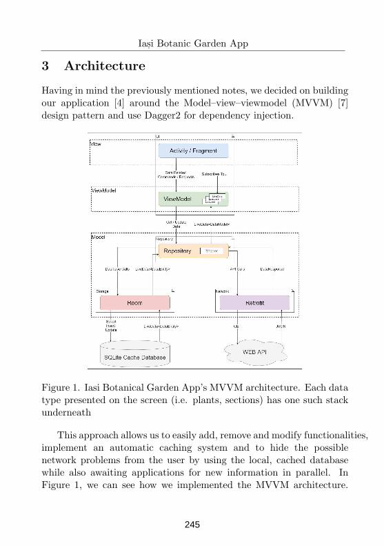
Ias,i Botanic Garden App
3 Architecture
Having in mind the previously mentioned notes, we decided on buildingour application [4] around the Model–view–viewmodel (MVVM) [7]design pattern and use Dagger2 for dependency injection.
Figure 1. Iasi Botanical Garden App’s MVVM architecture. Each datatype presented on the screen (i.e. plants, sections) has one such stackunderneath
This approach allows us to easily add, remove and modify functionalities,implement an automatic caching system and to hide the possiblenetwork problems from the user by using the local, cached databasewhile also awaiting applications for new information in parallel. InFigure 1, we can see how we implemented the MVVM architecture.
245
Radu-Matei Lipan, Adrian Iftene
The whole app is composed of multiple model, view, view-model stackslike this one. There is a stack for each data type we have inside theapplication (plants, sections, etc.).
On the View level we have all the classes responsible for renderingthe information on the screen. These classes request the informationthey need from the ViewModel level. The ViewModels keep theinformation for multiple views at a time. This way we don’t haveto make a new query each time we switch pages. When a ViewModelreceives a request for some data it doesn’t currently have, it will askthe Repository for it. At the Repository level is where the automaticcaching also takes place. The Repository will retrieve the requesteddata from the local database, wrapped as LiveData and will pass itback to the ViewModel. While doing so, it will also take a look to seehow old the data is and if it exceeds a certain threshold it will alsomake a request to the server, on a different thread, to get it updated.
It is important to mention that LiveData is a special wrapperthat implements the Observer design pattern. More than that, it willobserve directly on the database entries. Because of that, once wereceive the updated information from the server and add it to ourdatabase, the View will get updated seamlessly. Almost no loadingtime even on a poor network connection.
4 Information about Plants
We don’t want the visitors to look too much on their screens insteadof admiring the nature. This is why we needed a way to quickly offerinformation about the plants near the user immediately after openingthe app. For this we decided to make use of the panels that are alreadyput next to each plant inside the garden. They usually contain thescientific and popular names of the plant.
At first, we thought of using an OCR (optical character recognition)solution in order to make the phone read the name of the plant. Itwasn’t very successful as the accuracy was pretty low because the panelwas either too far away for it to be read or the plant’s leafs were covering
246
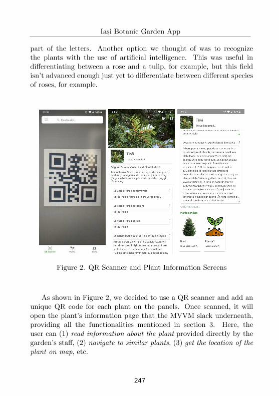
Ias,i Botanic Garden App
part of the letters. Another option we thought of was to recognizethe plants with the use of artificial intelligence. This was useful indifferentiating between a rose and a tulip, for example, but this fieldisn’t advanced enough just yet to differentiate between different speciesof roses, for example.
Figure 2. QR Scanner and Plant Information Screens
As shown in Figure 2, we decided to use a QR scanner and add anunique QR code for each plant on the panels. Once scanned, it willopen the plant’s information page that the MVVM slack underneath,providing all the functionalities mentioned in section 3. Here, theuser can (1) read information about the plant provided directly by thegarden’s staff, (2) navigate to similar plants, (3) get the location of theplant on map, etc.
247
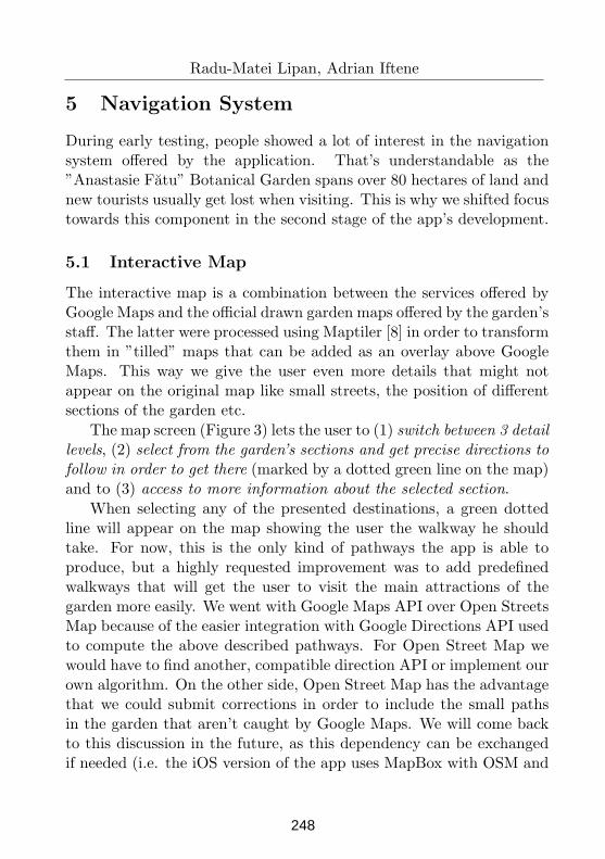
Radu-Matei Lipan, Adrian Iftene
5 Navigation System
During early testing, people showed a lot of interest in the navigationsystem offered by the application. That’s understandable as the”Anastasie Fatu” Botanical Garden spans over 80 hectares of land andnew tourists usually get lost when visiting. This is why we shifted focustowards this component in the second stage of the app’s development.
5.1 Interactive Map
The interactive map is a combination between the services offered byGoogle Maps and the official drawn garden maps offered by the garden’sstaff. The latter were processed using Maptiler [8] in order to transformthem in ”tilled” maps that can be added as an overlay above GoogleMaps. This way we give the user even more details that might notappear on the original map like small streets, the position of differentsections of the garden etc.
The map screen (Figure 3) lets the user to (1) switch between 3 detaillevels, (2) select from the garden’s sections and get precise directions tofollow in order to get there (marked by a dotted green line on the map)and to (3) access to more information about the selected section.
When selecting any of the presented destinations, a green dottedline will appear on the map showing the user the walkway he shouldtake. For now, this is the only kind of pathways the app is able toproduce, but a highly requested improvement was to add predefinedwalkways that will get the user to visit the main attractions of thegarden more easily. We went with Google Maps API over Open StreetsMap because of the easier integration with Google Directions API usedto compute the above described pathways. For Open Street Map wewould have to find another, compatible direction API or implement ourown algorithm. On the other side, Open Street Map has the advantagethat we could submit corrections in order to include the small pathsin the garden that aren’t caught by Google Maps. We will come backto this discussion in the future, as this dependency can be exchangedif needed (i.e. the iOS version of the app uses MapBox with OSM and
248
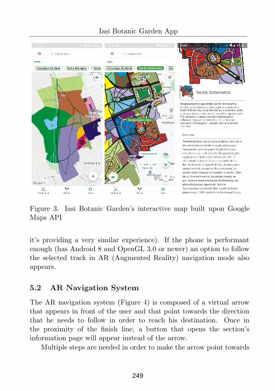
Ias,i Botanic Garden App
Figure 3. Iasi Botanic Garden’s interactive map built upon GoogleMaps API
it’s providing a very similar experience). If the phone is performantenough (has Android 8 and OpenGL 3.0 or newer) an option to followthe selected track in AR (Augmented Reality) navigation mode alsoappears.
5.2 AR Navigation System
The AR navigation system (Figure 4) is composed of a virtual arrowthat appears in front of the user and that point towards the directionthat he needs to follow in order to reach his destination. Once inthe proximity of the finish line, a button that opens the section’sinformation page will appear instead of the arrow.
Multiple steps are needed in order to make the arrow point towards
249
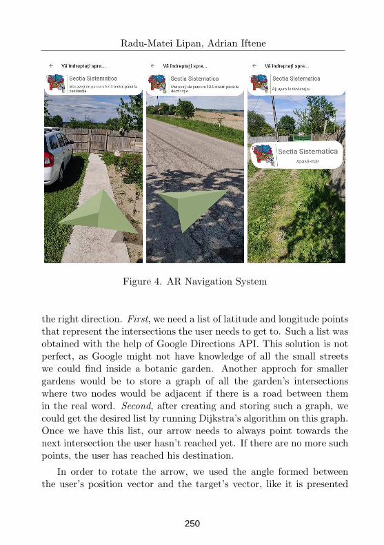
Radu-Matei Lipan, Adrian Iftene
Figure 4. AR Navigation System
the right direction. First, we need a list of latitude and longitude pointsthat represent the intersections the user needs to get to. Such a list wasobtained with the help of Google Directions API. This solution is notperfect, as Google might not have knowledge of all the small streetswe could find inside a botanic garden. Another approch for smallergardens would be to store a graph of all the garden’s intersectionswhere two nodes would be adjacent if there is a road between themin the real word. Second, after creating and storing such a graph, wecould get the desired list by running Dijkstra’s algorithm on this graph.Once we have this list, our arrow needs to always point towards thenext intersection the user hasn’t reached yet. If there are no more suchpoints, the user has reached his destination.
In order to rotate the arrow, we used the angle formed betweenthe user’s position vector and the target’s vector, like it is presented
250
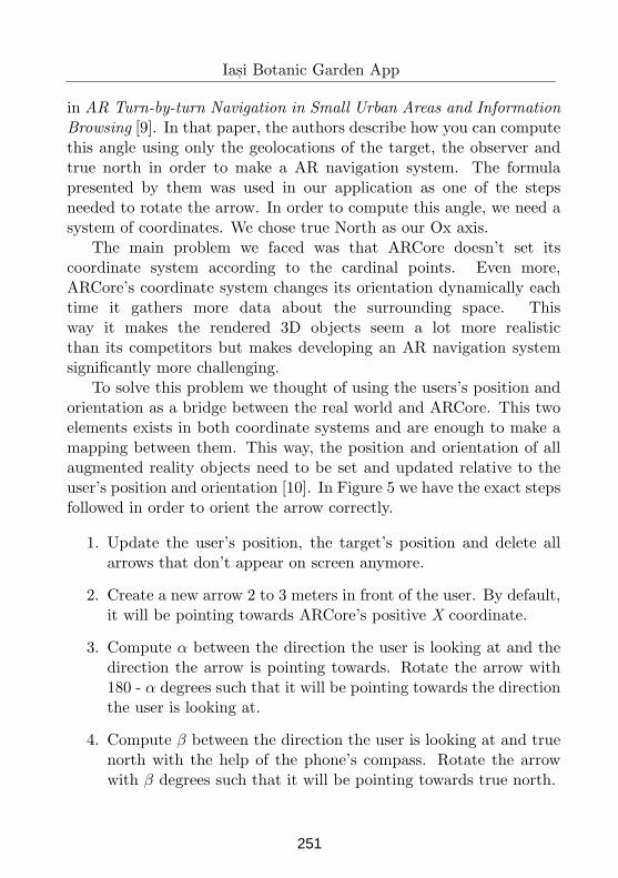
Ias,i Botanic Garden App
in AR Turn-by-turn Navigation in Small Urban Areas and InformationBrowsing [9]. In that paper, the authors describe how you can computethis angle using only the geolocations of the target, the observer andtrue north in order to make a AR navigation system. The formulapresented by them was used in our application as one of the stepsneeded to rotate the arrow. In order to compute this angle, we need asystem of coordinates. We chose true North as our Ox axis.
The main problem we faced was that ARCore doesn’t set itscoordinate system according to the cardinal points. Even more,ARCore’s coordinate system changes its orientation dynamically eachtime it gathers more data about the surrounding space. Thisway it makes the rendered 3D objects seem a lot more realisticthan its competitors but makes developing an AR navigation systemsignificantly more challenging.
To solve this problem we thought of using the users’s position andorientation as a bridge between the real world and ARCore. This twoelements exists in both coordinate systems and are enough to make amapping between them. This way, the position and orientation of allaugmented reality objects need to be set and updated relative to theuser’s position and orientation [10]. In Figure 5 we have the exact stepsfollowed in order to orient the arrow correctly.
1. Update the user’s position, the target’s position and delete allarrows that don’t appear on screen anymore.
2. Create a new arrow 2 to 3 meters in front of the user. By default,it will be pointing towards ARCore’s positive X coordinate.
3. Compute α between the direction the user is looking at and thedirection the arrow is pointing towards. Rotate the arrow with180 - α degrees such that it will be pointing towards the directionthe user is looking at.
4. Compute β between the direction the user is looking at and truenorth with the help of the phone’s compass. Rotate the arrowwith β degrees such that it will be pointing towards true north.
251
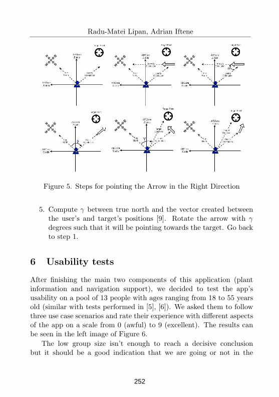
Radu-Matei Lipan, Adrian Iftene
Figure 5. Steps for pointing the Arrow in the Right Direction
5. Compute γ between true north and the vector created betweenthe user’s and target’s positions [9]. Rotate the arrow with γ
degrees such that it will be pointing towards the target. Go backto step 1.
6 Usability tests
After finishing the main two components of this application (plantinformation and navigation support), we decided to test the app’susability on a pool of 13 people with ages ranging from 18 to 55 yearsold (similar with tests performed in [5], [6]). We asked them to followthree use case scenarios and rate their experience with different aspectsof the app on a scale from 0 (awful) to 9 (excellent). The results canbe seen in the left image of Figure 6.
The low group size isn’t enough to reach a decisive conclusionbut it should be a good indication that we are going or not in the
252
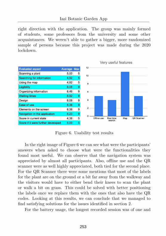
Ias,i Botanic Garden App
right direction with the application. The group was mainly formedof students, some professors from the university and some otheracquaintances. We weren’t able to gather a bigger, more randomizedsample of persons because this project was made during the 2020lockdown.
Figure 6. Usability test results
In the right image of Figure 6 we can see what were the participants’answers when asked to choose what were the functionalities theyfound most useful. We can observe that the navigation system wasappreciated by almost all participants. Also, offline use and the QRscanner were as well highly appreciated, both tied for the second place.For the QR Scanner there were some mentions that most of the labelsfor the plant are on the ground or a bit far away from the walkway andthe visitors would have to either bend their knees to scan the plantor walk a bit on grass. This could be solved with better positioningthe labels once we replace them with the ones that also have the QRcodes. Looking at this results, we can conclude that we managed tofind satisfying solutions for the issues identified in section 2.
For the battery usage, the longest recorded session was of one and
253
Radu-Matei Lipan, Adrian Iftene
a half hours of continuous use on a OnePlus 6 (with 4000 mah batteryand Android 10). The app was used normally (a mix of AR and non-ARusage) while connected to the network. The battery level declined by20% in this period and the network usage was under 5MB of datatransferred.
7 Conclusion
This paper presents our work on an application for the ”AnastasieFatu” Botanical Garden which has the aim to improve the educationalaspect of visiting such a garden while also improving the overallexperience of the visit. Even though incomplete, it is a very goodstarting point that helped us identify the requirements we must focuson and also let us experiment with adding more advanced componentslike the AR navigation.
Looking forward, there are a lot of functionalities heavily desired bythe visitors, like a notification system for the events that will take placein the garden, an In bloom list, predefined visit tracks with audio andvideo guides, a button to preload all data (instead of having to scrollthe plant list at home in order to cache all the plants if you want to usethe app 100% offline) and an iOS version (currently in developmentby S.C. Romanescu [4]. Currently it includes everything minus thenavigation functionalities: both AR and non-AR).
Acknowledgments. This work was supported by project REVERT(taRgeted thErapy for adVanced colorEctal canceR paTients), GrantAgreement number: 848098, H2020-SC1-BHC-2018-2020/H2020-SC1-2019-Two-Stage-RTD.
References
[1] Chicago Botanic Garden: GardenGuide, URL:https://play.google.com/store/apps/details?id=org.chicagobotanic.
GardenGuide, https://www.chicagobotanic.org/app
254
Ias,i Botanic Garden App
[2] The Royal Botanic Garden of Sydney: Royal BotanicGarden Sydney, URL: https://play.google.com/store/apps/details?id=com.specialistapps.rbgs, https://www.rbgsyd.nsw.gov.au/Stories/2018/Connect-with-the-Garden
[3] APositive: National Arboretum Canberra, URL:https://play.google.com/store/apps/details?id=au.com.
apositive.NationalArboretumCanberra&hl=en
[4] C.I. Irimia, M. Matei, A. Iftene, S.C. Romanescu, M.R., Lipan,M. Costandache. Discover the Wonderful World of Plants with theHelp of Smart Devices. In Proceedings of the 17th InternationalConference on Human-Computer Interaction RoCHI 2020, 22-23October, (2020).
[5] M.N. Pinzariu, A. Iftene. Sphero - Multiplayer Augmented Game(SMAUG). In International Conference on Human-ComputerInteraction, 8-9 September 2016, Iasi, Romania, (2016), pp. 46-49.
[6] M. Chitaniuc, A. Iftene. GeoAR-An Augmented RealityApplication to Learn Geography. In Romanian Journal ofHuman-Computer Interaction, vol. 11, issue 2, (2018), pp. 93-108.
[7] Google: Guide to app architecture, URL:https://developer.android.com/jetpack/docs/guide
[8] Maptiler: Maptile manual, URL:https://manual.maptiler.com/en/stable/
[9] G. Cherchi, F. Sorrentino, R. Scateni. AR Turn-by-turnNavigation in Small Urban Areas and InformationBrowsing, STAG: Smart Tools & Apps for Graphics(2014), URL:https://pdfs.semanticscholar.org/49be/3915dea4530664b5312b2e6c23d5035c33b0.pdf?_ga=2.
81427155.595398977.1590476070-644948595.1590476070
255
Radu-Matei Lipan, Adrian Iftene
[10] J. Hardy. Creating an ARCore powered indoor navigationapplication in Unity, Raccoons, (2019), URL: https://blog.
raccoons.be/arcore-powered-indoor-navigation-unity
*All the links were last accessed in November 2020.
*The code for this project can be found on Githubunder the MIT license (the Android app only):https://github.com/Matei-L/Iasi-Botanical-Garden-Mobile-App-Public-Repo
Radu-Matei Lipan, Adrian Iftene
Faculty of Computer Science, “Alexandru Ioan Cuza” University of Ias,i, Romania
Email: radu.lipan1, [email protected]
256
Proceedings of the Conference on Mathematical Foundations of Informatics
MFOI2020, January 12-16, 2021, Kyiv, Ukraine
Evidence Algorithm: 50 Years of Development
Alexander Lyaletski
Abstract
The work is devoted to the Evidence Algorithm programme onautomated theorem proving initiated by Academician Glushkov50 yeas ago as well as to the Russian-language and English-language SAD systems implemented in the framework of thisprogramme and intended for automated deduction. Character-istic peculiarities, features, and differences between the systemsare described. Possible ways of the further development of theEnglish-language SAD system are presented.
Keywords: Evidence Algorithm, SAD system, automateddeduction, automated theorem proving.
1 Introduction
In 1970, Academician V.M. Glushkov published a paper [1], in whichhe, along with a discussion of some problems of artificial intelligence,formulated a research programme called Evidence Algorithm (EA), inwhich he described his vision of a solution of the problem of automatedtheorem proving in mathematics.
In [1], V.M. Glushkov proposed to focus attention on the construc-tion of an automated theorem-proving system by performing simultane-ous investigations in: (1) creating formal natural languages for writingmathematical texts in a form accustomed to a human, (2) constructinga procedure for a proof search based on the evolutionary developing ofthe machine notion of an evidence of a computer-made proof step, (3)using the knowledge gained by the system during its operation, and(4) providing a user with the opportunity to assist to the system in
c©2020 by Alexander Lyaletski
257
Alexander Lyaletski
its proof search process. (A full description of the chronology of allUkrainian research on this subject can be found in [2], as well as in [3]containing an exhaustive list of relevant publications before 1998.)
Two attempts have been made in order to implement this pro-gramme. The first led to the appearance in 1978 of the Russian-language automated theorem-proving system denoted by Russian SADfurther and the second – to the appearance in 2002 of the English-language system for automated deduction denoted by English SAD inwhat follows. And if the development and trial operation of RussianSAD were stopped in 1992 after the output from the operating of theES-line computers, the English-language system, after its placement onthe site “nevidal.org”, is still online available now. As a result, thereexists the ability to carry out various experiments with it and solve avariety of tasks requiring rigorous mathematical reasonings.
This work is devoted to a chronological description of studies on theimplementation of the EA program for the entire period of its existenceand to the highlighting of peculiarities of both the systems, as well asof their common features and distinguishes.
2 Beginning of research on automated theorem
proving
The first publications devoted to the possibility of using computers formaking logical constructions, relate to the late 1950’s - early 1960’s (see,for example, [4] and [5]), when there were appeared computers of sucha performance, memory capacity, and informational flexibility that theprogramming of complex intelligent processes has become possible. Anearly history of the development of this branch of computer sciencein Western countries can be found in [6]. As for the USSR and thecountries of Eastern Europe, two schools of automated theorem provingappeared in the USSR almost simultaneously in the 1960s: one createdby Academician V.M. Glushkov in 1962, a brief description of whichis given below, appeared in Kyiv, and the other in Leningrad, for thedescription of which we refer to [7] (see also [8]).
258
Evidence Algorithm: 50 Years of Development
Much later, after 1975, several groups that specialized in findingsolutions of mathematical problems relating to special classes appearedin the USSR. One such an example is V.M. Matrosov’s group, whichin 1976 began its work on the machine search for proofs of theoremson the dynamic properties of the Lyapunov vector functions in Kazanand after 1980, it continued its work in Irkutsk. Another example isthe laboratory of A. Voronkov in Novosibirsk (in late 1980s), whereautomated reasoning methods were used to study and find solutionsof various problems of logical programming. However, the collapse ofthe USSR in 1991 led to the discontinuance of all such investigations.This also affected the Kyiv school and the revival of its research becamepossible only in 1998 due to the involvement of some its representativesin the participation in one of the INTAS projects.
Let us list the main stages of research on automated reasoning inKyiv and give them a brief description in chronological order.
3 Research on EA in 1962-1970
Research on automated reasoning began in Ukraine (Ukrainian SovietSocialist Republic) since the formation in the Institute of Cyberneticsin 1962 of the first group of researchers, who began to deal with theproblem of automated theorem proving in mathematics. Their researchfocused mainly on solutions of (1) and (2) on the basis of the analysis ofmathematical texts on group theory. As a result, first-order languagesignatures were enriched with a symbol to indicate the predicate of theelement belonging to a set and corresponding set-theoretical construc-tions. Besides, from the analysis of proofs in group theory, an originalprocedure (called PVC) was “extracted”. It admits its interpretationas a special, correct and complete, sequent calculus, the peculiarity ofwhich are a goal-orientedness (that is, at each moment of time, thesuccedent of any sequence always contained exactly one formula-goal),the separation of equation handling deduction, and a special work withquantifiers.
As for the issues of a practical realization on a computer of the
259
Alexander Lyaletski
research results available at that time, no serious work in this directionwas carried out in the late. Perhaps, we should remind here the latestimplementation of the propositional part of the above-mentioned PVCprocedure on a BESM-2 computer, which belongs to the late 1969 –early 1970s.
4 Research on EA in 1971-1992
This period can be divided into three time slots, each of which coversa certain range of research and implementations.
1970-1976. In 1970, the EA program was published. Its appear-ance has caused performing research on automated theorem proving ata new level of investigations.
To solve the language problem (1), a formal version of a fragment ofRussian with the abbreviation TL (Theory Language) was proposed in[9]. This language makes it possible to write mathematical texts thathas a usual form for a person and is correct from a mathematical pointof view. In addition, TL admits to make its translations into first-orderlanguage, which is an important property, as it is possible to proversfor establishing deducibility in classical first-order logics.
As for (2), a number of investigations have been performed inthe direction of the development of both a resolution approach anda machine-oriented sequent formalism.
In the field of resolution methods, the unification algorithm hasbeen carefully studied and new strategies have been developed for the”resolution + paramodulation” system.
For sequent methods, an approach based on the original notion ofan admissible substitution distinguished from its Genzen and Kangeranalogues was proposed, which permits to determine whether it is pos-sible to choose the order of a quantifier rules application, which leads tosuccess, relying only on the quantifier structure a sequent under consid-eration and selected substitution of terms instead of certain variables(see, for example, [10]). This notion was “incorporated” into the PVCprocedure, which allowed to build an efficient enough sequent calcu-
260
Evidence Algorithm: 50 Years of Development
lus, which was later “embedded” in the logical “engine” of the RussianSAD system.
A number of experiments were performed on ES-line computers inorder to identify those basic programming units of the PL/1 program-ming language that could be used to create an effective toolkit for theconstruction of an automated theorem-proving system and this toolkitwas used for implementation purposes in the next stage.
1977-1982. In the period from 1977 to the first half of 1978,a Russian-language automated theorem-proving system was designed,implemented, and tested on the ES-line computer [11]. (Later, V.M.Glushkov gave it the name SAD [12] called Russian SAD here.) Itcan be considered as the first software “embodiment” of EA. It wasfocused on automated theorem proving and, in the case of using itssequent prover, it admitted an interactive mode of operation takinginto account that the sequent search was performed by the prover fromtop to bottom from and left to right. The Russian SAD system in-cluded: linguistic tools for the structural, syntactic and grammaticalprocessing of mathematical texts, tools for the construction of a proofenvironment, tools for theorem proving, and tools for a communica-tion with the user. The language TL was taken as an input languageof English SAD; its sentences were translated into first-order languageformulas, which were transmitted to the logical “engine” of the system.
The Russian SAD logical module consisted of two “engines” – reso-lution and sequent ones, each of which could be used independently andwas a correct and complete prover for establishing of the deducibilityof first-order language formulas with functional symbols and equality.The realization of these two “engines” revealed the strengths and weak-nesses of the resolution and sequent approaches, and it turned out thatdespite the higher efficiency of resolution methods compared to sequentones, the latter have a number of advantages associated with flexibilityin the management of passing through a search space and organiza-tion of a friendly interface, transparent enough for an unqualified user.In addition, a certain modification of sequent logical tools was made,which permitted to generate statements sufficient to prove the propo-
261
Alexander Lyaletski
sition in question, and to obtain the consequences of a given set ofpremises.
1983-1992. After 1982, the Russian SAD system had been devel-oping only in the resolution direction focused mainly on improving thedeductive capabilities of the system by ”embedding” a natural prooftechnique used by mathematicians in proving theorems (see details in[2]). A modification of one of the resolution strategies for statementswith bounded quantifiers was proposed for proving theorems in mul-tisorted theories. It used the transformation of sets of clauses, whichcan be considered as a mixed calculation in a proof search.
A number of experiments were performed with an improved modifi-cation of Russian SAD. The most interesting of them is the theorem ”Aclosed subset of a compact set is compact”. Statistics gathered duringthe processing of this proposition showed that a relatively small num-ber of redundant clauses were generated, memory was used efficiently,and a proof search space was available for evaluation.
Research on EA and Russian SAD was stopped in 1992, when theES-line computers were decommissioned.
5 Research on EA in 1998 - present time
Research on EA was resumed in 1998, when some of the developers ofthe Russian SAD system were included in the list of executors of theIntas project ”Rewriting techniques and efficient theorem proving”.
1998-2002. During the Intas project, an English version of theTL language called ForTheL (Formal Theory Language) was devel-oped [13] and the PVC procedure in the form of a sequent calculus wassignificantly improved [14]. This calculus was constructed on the basisof the requirements for deduction in the EA-style: syntactic form ofthe original problem should be preserved; search for a proof should begoal-oriented; deductive transformations should be carried out effec-tively in the signature of an original theory (i.e. Skolemization shouldnot be obligatory); equation processing/equation solutions should beseparated from a deductive process.
262
Evidence Algorithm: 50 Years of Development
Certain modifications of the calculus from [14] were proposed in[15], one of which formed the basis of the logical “engine” of the above-mentioned English SAD system (System for Automated Deduction)with ForTheL as its input language. The first report on the appearanceof the English version of SAD was made in 2002 [16], which, as in thecase of the Russian SAD system, had a two-level structure at that time.
Pay your attention to the fact that only sequent methods for aninference search were developed for English SAD, while numerousresolution-type methods and strategies that were presented in the Rus-sian SAD system, were not implemented in it at all. This decision wasmade on the basis that by that time, there were a large number of high-performance well-known resolution provers, such as SPASS, Vampire,Otter, and so on, which could be used directly in English SAD. And itwas done.
Another difference was in that while the Russian-language SAD sys-tem was entirely focused on automated theorem proving, its English-language “modification” (English SAD) was initially designed to beused mainly as a verifier of a proof provided by the user to the EnglishSAD system for verification. Therefore, English SAD had to have lin-guistic tools for writing theorem proofs and such tools were includedin the ForTheL language a little later.
2003-2007. The just-mentioned modification of linguistic toolsled to the reconstruction of English SAD into a mathematical assis-tant having the third (reasoner) level that was “built-in” between thelinguistic and deductive ones. It was introduced to give the systemthe possibility to perform a verification of texts containing heuristictechniques used by a human in his daily practice.
This “enriched” three-level version of English SAD system was pre-sented at the 21st CADE’21 Automated Deduction Conference (Bre-men, Germany) in 2007 [17]. It is currently available on the site “nevi-dal.org” and there exists an online access to it, which allows any user toinitiate one of the following sessions: (1) establishing the deducibilityof a formula/sequent in the classical first-order logic, (2) search for aproof of a theorem in a ForTheL environment, and (3) verification of a
263
Alexander Lyaletski
given ForTheL-text.
A number of experiments on automated theorem proving and proofverification were carried out with the English SAD system. The mostinteresting on verifications include, for example: the finite and infi-nite Ramsey theorems, the Cauchy-Bunyakovsky inequality, the Nu-man lemma, and Tarsky’s fixed point theorem (see, for example, anappropriate page on the site “nevidal.org”).
2008-present. Throughout the existence of the Evidence Algo-rithm, all work on the English SAD systems was accompanied by thestudy of the possibilities of constructing sequent methods for inferencesearch in the EA style.
One of the EA-style requirements is the rejection of obligatorySkolemization without significant loss of efficiency of the process of in-ference search, which allows performing the process machine deductionprocess only in the signature of an original theory. Such considerationsbecome even more important also because Skolemization is always acorrect operation only for classical logic; for the rest of first-order log-ics, its application leads to the correctness of this transformation onlyin special cases.
Inference search without Skolemization requires the application ofquantifier rules with certain restrictions on terms that are substitutedfor certain (negative) variables. For the purposes of the proof theory (inthe classical sense), Genzens notion of admissibility of a substitutionof terms instead of variables is convenient (and sufficient). However,it is completely useless in terms of efficiency in the case of its machineimplementation, as an additional step-by-step examination is appearedw.r.t. different orders of quantifier rule applications. S. Kanger suc-ceeded to “improve” this situation by introducing his (Kanger’s) notionof an admissible substitution. However, its use still continues to leadto an additional (compared to the case of Skolemization) examinationfor different orders of quantifier rule applications.
For classical first-order logic, this situation was corrected by intro-ducing into sequent calculi the new, already mentioned above, notion ofadmissibility of a substitution (see, e.g., [14]). As for the intuitionistic
264
Evidence Algorithm: 50 Years of Development
case, it turned out that this new notion should be used only in coopera-tion with a developed notion of the compatibility of a so-called inferencetree with a generated substitution. Thus, these notions proved to besufficient to construct a sound and complete tableau calculus for intu-itionistic logic [18]. Later, the results were obtained on the soundnessand completeness of a number of classical and intuitionistic modal se-quent calculi, which have the subformula property and use the notionsof admissibility and compatibility [19]. In this connection, note thatthese studies are more fully reflected in [20] and [21].
6 Conclusion
The above-said demonstrates that the ideas, laid down by V.M.Glushkov in the Evidence Algorithm programme, are well in line withmodern trends and approaches to the intelligent processing of formal-ized (not necessarily mathematical) knowledge and that the experiencegained during the development and implementation of the Russian SADand English SAD systems may be useful to developers of modern com-puter services possessing the possibility to make numerical calculationsand/or symbolic transformations and/or deductive constructions in theenvironment of a formal natural language. As for the current EnglishSAD system, it seems reasonable to construct Ukrainian and Russianversions of ForTheL for it and implement a set of tools that will allowthe system to make efficient deduction in various non-classical logics,especially in intuitionist logic.
In the long run, Evidence Algorithm and the Russian SAD andEnglish SAD systems can give a good basis for creating a broad in-frastructure intended for the intelligent processing of various computerknowledge used by a human in his daily and scientific activities.
References
[1] V.M. Glushkov. Some problems in the theories of automata and artificialintelligence. Cybernetics and System Analysis, 6(2) (1970), pp. 17-27.
265
Alexander Lyaletski
[2] A. Lyaletski, M.Morokhovets, A.Paskevich. Kyiv school of automatedtheorem proving: a historical chronicle. Logic in Central and EasternEurope: History, Science, and Discourse, University Press of America(2012), pp. 376-415.
[3] A. Lyaletski, K. Verchinine. Evidence Algorithm and System for Auto-mated Deduction: a retrospective view. Intelligent Computer Mathemat-ics, LNAI, Vol. 6167 (2010), pp. 411-426.
[4] P.C. Gilmore. A program for the production of proofs for theorems deriv-able within the first-order predicate calculus from axioms. Proceedings ofthe International Conference on Information Processing, Unesco, Paris(1959), pp. 265-273.
[5] Hao Wang. Towards mechanical mathematics. IBM Journal of Researchand Development, Vol. 4 (1960), pp. 2-22.
[6] J.A. Robinson and A. Voronkov. Handbook of Automated Reasoning (in2 volumes). Elsevier and MIT Press (2001), 2122 pp.
[7] V. Lifschitz. Mechanical theorem proving in the USSR: The Leningradschool. Delphic Associates Inc. (1986), 206 pp.
[8] G. Mints. Proof theory in the USSR (1925-1970). Journal of SymbolicLogic, Vol. 56, No. 2 (1991), pp. 385-422.
[9] V.M. Glushkov, Yu.V. Kapitonova, A.A Letichevskii, K.P. Vershinin,N.P. Malevanyi. Construction of a practical formal language for math-ematical theories. Cybernetics and Systems Analysis, 8(5) (1972), pp.730-739.
[10] A.V. Lyaletski. Machine methods for proof search in first-order predicatecalculus. PhD thesis, GIC, AS of UkrSSR, Kyiv (1982), 15 pp.
[11] Yu.V. Kapitonova, K.P. Vershinin, A.I. Degtyarev, A.P. Zhezherun,A.V. Lyaletski. System for processing mathematical texts, Cyberneticsand System Analysis, 15(2) (1979), pp. 209-210.
[12] V. M. Glushkov. System for automatic theorem proving (SAD) (abrief informal description). Computer-aided Processing of Mathemati-cal Texts, GIC, AS of UkrSSR, Kiev (1980), pp. 3-30 (in Russian).
266
Evidence Algorithm: 50 Years of Development
[13] K. Vershinin, A. Paskevich. ForTheL - the language of formal theories.International Journal of Information Theories and Applications, Vol.7(3) (2000), pp. 120-126.
[14] A. Degtyarev, A. Lyaletski, M. Morokhovets. Evidence Algorithm andsequent logical inference search. Lecture Notes in Computer Science,Vol.1705 (1999), pp. 44-61.
[15] A. Lyaletski, A. Paskevich.Goal-driven inference search in classicalpropositional logic. Proceedings of the International Workshop STRATE-GIES’2001, Siena, Italy (2001), pp. 65-74.
[16] Lyaletski, K. Verchinine, A. Degtyarev, A. Paskevich. System for Au-tomated Deduction (SAD): Linguistic and deductive peculiarities. Ad-vances in Intelligent and Soft Computing (the 11th International Sym-posium IIS 2002), Physica-Verlag (2002), pp. 413-422.
[17] K. Verchinine, A. Lyaletski, A. Paskevich. System for Automated Deduc-tion (SAD): a tool for proof verification. Lecture Notes in Computer Sci-ence (Proceedings of the Conference on Automated Deduction (CADE-21), July 2007, Bremen), Vol. 4603 (2007), pp. 398-403.
[18] B. Konev, A. Lyaletski. Tableau proof search with admissible substitu-tions. Proceedings of the International Workshop on First-order Theo-rem Proving, September 2005, Koblenz, Germany (2005). pp. 35-50.
[19] A. Lyaletski. On some problems of efficient inference search in first-order cut-free modal sequent calculi. Proceedings of the 10th Interna-tional Symposium on Symbolic and Numeric Algorithms for ScientificComputing, September 2008, Timisoara, Romania (2008). pp. 39-46.
[20] A. Lyaletski. Evidence Algorithm and inference search in first-order log-ics. Journal of Automated Reasoning, Vol. 55 (2015), No. 3. pp. 269-284.
[21] A. Lyaletski. Mathematical text processing in EA-style: a sequent aspect,
Journal of Formalized Reasoning. Vol. 9, No. 1 (2016), pp. 235-264.
Alexander Lyaletski
National University of Life and Environmental Sciences of Ukraine
Email: [email protected]
267

Proceedings of the Conference on Mathematical Foundations of Informatics
MFOI2020, January 12-16, 2021, Kyiv, Ukraine
Quick Recursive QR Decomposition
Gennadi Malaschonok, Andriy Ivashkevich
Abstract
A description of a recursive algorithm for QR-decompositionof a matrix based on Givens rotation matrices is given. Anotherversion of the block-recursive algorithm is obtained by replacingGivens rotations with the Householder transform. These block-recursive algorithms have the same complexity as the matrix mul-tiplication algorithm.
Keywords: recursive QR decomposition, block-recursivematrix algorithms, factorization of matrices, Givens rotation,Householder transformation.
1 Introduction
In connection with the new concept of creating recursive parallel algo-rithms with dynamic control (see [1]-[3]), we began to look for a recur-sive algorithm for QR decomposition. When did we get the algebraicequations of such an algorithm, thanks to the personal communicationof Prof. Alexandr Tiskin and his publication [3], we found A. Schonhagepaper [4] in German, which suggested a similar algorithm, and whichwas quoted very little in recent years. This convinced us of the correct-ness of this approach and the whole concept of revising and searchingfor recursive matrix algorithms.
To simplify the description of the algorithm, we restrict ourselvesto the decomposition of matrices over real numbers. At the same time,we note that these matrix factorization algorithms are closed in thesets of algebraic, real and complex numbers and are not closed in theset of rational numbers.
c©2020 by Gennadi Malaschonok, Andriy Ivashkevich
268
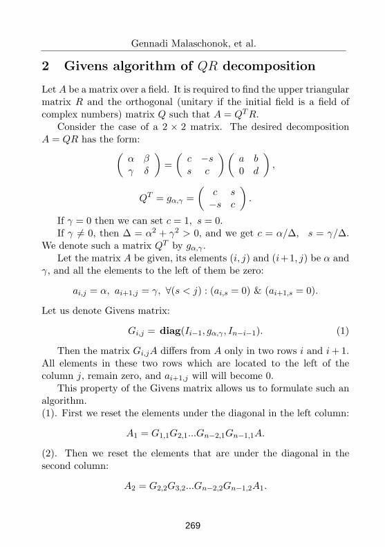
Gennadi Malaschonok, et al.
2 Givens algorithm of QR decomposition
Let A be a matrix over a field. It is required to find the upper triangularmatrix R and the orthogonal (unitary if the initial field is a field ofcomplex numbers) matrix Q such that A = QTR.
Consider the case of a 2 × 2 matrix. The desired decompositionA = QR has the form:
(
α βγ δ
)
=
(
c −ss c
)(
a b0 d
)
,
QT = gα,γ =
(
c s−s c
)
.
If γ = 0 then we can set c = 1, s = 0.If γ 6= 0, then ∆ = α2 + γ2 > 0, and we get c = α/∆, s = γ/∆.
We denote such a matrix QT by gα,γ .Let the matrix A be given, its elements (i, j) and (i+1, j) be α and
γ, and all the elements to the left of them be zero:
ai,j = α, ai+1,j = γ, ∀(s < j) : (ai,s = 0) & (ai+1,s = 0).
Let us denote Givens matrix:
Gi,j = diag(Ii−1, gα,γ , In−i−1). (1)
Then the matrix Gi,jA differs from A only in two rows i and i+ 1.All elements in these two rows which are located to the left of thecolumn j, remain zero, and ai+1,j will will become 0.
This property of the Givens matrix allows us to formulate such analgorithm.(1). First we reset the elements under the diagonal in the left column:
A1 = G1,1G2,1...Gn−2,1Gn−1,1A.
(2). Then we reset the elements that are under the diagonal in thesecond column:
A2 = G2,2G3,2...Gn−2,2Gn−1,2A1.
269
Quick Recursive QR Decomposition
(k). Denote
G(k) = Gk,kGk−1,k...Gn−2,kGn−1,k, (2)
for k = 1, 2, .., n−1. Then, to calculate the elements of the k-th column,we need to obtain the product of matrices
Ak = G(k)Ak−1.
(n-1). At the end of the calculation, the element in the n − 1 columnwill be reseted: An−1 = G(n−1)An−2 = Gn−1,n−1An−2.
Let’s find the number of operations in this algorithm.
It is necessary to calculate the (n2 − n)/2 Givens matrices and foreach of them 6 operations must be performed. When calculating A1 in(1), the number of multiplications of the Givens matrices into columnsof two elements (4 multiplications and 2 additions) is (n− 1)2. Whencalculating A2 in (2), the number of such multiplications is (n − 2)2,and so on. As a result, we get
6(n2 − n)/2 + 6∑
i=1..n−1
i2 = 3n2 − 3n+ 6(n− 1)(2n− 1)n/6 ≈ 2n3
Here we count the number of all arithmetic operations and the opera-tions of extracting the square root.
3 Recursive QR decomposition
We will change the order of actions in the algorithm so that it becomesa recursive algorithm, which contains another recursive algorithm (QPalgorithm).
Let a matrix M of size 2n× 2n be divided into four equal blocks:
M =
(
A BC D
)
.
270
Gennadi Malaschonok, et al.
3.1 Recursive QR decomposition algorithm.
There are three steps in this algorithm.(1). The first step is the QR decomposition of the C block: Q1C = CU
M1 =
(
I 00 Q1
)(
A BC D
)
=
(
A BCU D1
)
, D1 = Q1D. (3)
(2). The second step is the decomposition of a “parallelogram”, whichis consist of two triangular blocks: the lower triangular part of theblock A and the upper triangular part of the block CU :
M2 = Q2
(
A BCU D1
)
=
(
AU B1
0 D2
)
. (4)
(3). The third step is the QR decomposition of the D2 block: Q3D3 =DU .
R =
(
I 00 Q3
)(
AU B1
0 D2
)
=
(
AU B1
0 DU
)
. (5)
As a result, we get:
M = QR, Q = diag(I,Q3)Q2 diag(I,Q1). (6)
Since the first and third steps are recursive calls of the QR proce-dures, it remains to describe the procedure for decomposing a “paral-lelogram”. We will call it QP-decomposition.
3.2 Recursive QP-decomposition.
We are looking for the decomposition of the matrix P :
Q2P = PU , QT2 = Q−1
2 , P = QT2 P
U .
The matrix P =
(
ACU
)
is the left half of the matrix M1 (3). We
divided each of the two blocks that make up matrix P (of size 2n× n)into four equal parts. We got 8 blocks, including one zero block andtwo upper triangular blocks: fU and hU (7).
271
Quick Recursive QR Decomposition
It is required to annul all elements between the upper and lowerdiagonals of the P matrix, including the lower diagonal. We are inter-ested in a block procedure. Since n is even, we can split the parallelo-gram formed by the diagonals into 4 parts using its two middle lines.We get 4 equal parallelograms. To decompose each of them, we simplycall the QP-procedure 4 times. We will decompose each of them in thefollowing order: lower left (Pll), then simultaneously cancel the upperleft (Pul) and the lower right (Plr) and the last we decompose parallel-ogram in the upper right corner (Pur). The corresponding orthogonalmatrices of size n× n are denoted as Qll. Qul. Qlr and Qur
P =
(
ACU
)
=
a cb dfU g0 hU
, PU =
(
AU
0
)
=
aU c10 dU
0 00 0
.
(7)
Pll = Qll
(
b dfU g
)
=
(
bU d10 g1
)
, (8)
Pul = Qul
(
a cbU d1
)
=
(
aU c10 d2
)
,
Plr = Qlr
(
0 g10 hU
)
=
(
0 gU
0 0
)
, (9)
Pur = Qur
(
0 d20 gU
)
=
(
0 dU
0 0
)
. (10)
As result, we get matrices Q2 (4) and PU (7):
Q2 = QurQ2Qll, Q2P = PU , (11)
with such factors:
Qur = diag(In2
, Qur, In2
), Q2 = diag(Qul, Qlr), Qll = diag(In2
, Qll, In2
)
272
Gennadi Malaschonok, et al.
3.3 Complexity of QP decomposition algorithm
The total number of multiplications of matrix blocks of size n/2× n/2is 28: 8 multiplications is necessary for the matrices Pll (8) and Pul (9)and 20 multiplications is necessary for the matrix Q2 (11).
Hence the total number of operations: Cp(2n) = 4Cp(n) +24M(n/2). Suppose that for multiplication of two matrices of sizen× n you need γnβ operations and n = 2k, then we get:
Cp(2k+1) = 4Cp(2k) + 28M(2k−1) = 4kCp(21) + 28γk−1∑
i=0
4k−i−12iβ =
28γ(n2/4)2k(β−2) − 1
2(β−2) − 1+ 6n2 = 7γ
nβ − n2
2β − 4+ 6n2
Cp(n) =7γnβ
2β(2β − 4)+
n2
2(3−
7γ
2β+1 − 8). (12)
4 The complexity of QR decomposition algo-
rithm
Let us estimate the number of operations C(n) in this block-recursiveQR-decomposition algorithm, assuming that the complexity of the ma-trix multiplication isM(n) = γnβ , the complexity of QP-decompositionis Cp(n) = αnβ , where α, β, γ are constants, α = 7γ
2β(2β−4)and n = 2k:
C(n) = 2C(n/2)+Cp(n)+6M(n/2) = 2C(2k−1)+Cp(2k)+6M(2k−1) =
C(20)2k +
k∑
i=0
2k−iCp(2i) + 6
k∑
i=0
2k−iM(2i−1) =
α
k∑
i=0
2k−i2iβ + 6γ
k∑
i=0
2k−i2(i−1)β =
273
Quick Recursive QR Decomposition
(α2k + 6γ2k−β)k
∑
i=0
2i(β−1) =
(α+ 6γ2−β)2βnβ − 2n
2β − 2=
γ(2β6− 17)(nβ − 2n2β)
(2β − 4)(2β − 2)
For the case of β = 3, γ = 1, we get C(n) = (31/24)(n3 − n/4).For the case of β = log2 7, γ = 1, we get C(n) = (5/3)(nβ − 2n/7).
5 Conclusion
We have presented a recursive algorithm for computing the QR-factorization of a matrix, which is based on Givens rotations and hasthe complexity of matrix multiplication. It is not difficult to see thatGivens rotations can be replaced by Householder transformation [6].For this, it is necessary to use matrices
Hk = I −2
||uk||22
ukuTk
(with Householder vector uk) insted of G(k) (2). All other steps ofthe recursive algorithm can be left unchanged. An experimental com-parison of these two variants of QR-decomposition is of interest. Ofparticular interest is the implementation of these algorithms for a dis-tributed memory cluster.
References
[1] G. Malaschonok and E. Ilchenko. Recursive Matrix Algorithms in
Commutative Domain for Cluster with Distributed Memory.2018Ivannikov Memorial Workshop (IVMEM), Yerevan, Armenia,(2018), pp. 40–46. doi: 10.1109/IVMEM.2018.00015.
[2] G.I. Malaschonok. Fast Generalized Bruhat Decomposition. 12th In-ternational Workshop on Computer Algebra in Scientific Comput-ing (CASC 2010), LNCS, vol. 6244 (2010), pp. 194–202.
274
Gennadi Malaschonok, et al.
[3] G. Malaschonok. Generalized Bruhat decomposition in commutative
domains. Computer Algebra in Scientific Computing, CASC2013,LNCS, vol. 8136 (2013), pp. 231–242.
[4] A. Tiskin. Communication-efficient parallel generic pairwise elimi-
nation. Future Generation Computer Systems, vol. 23, no. 2 (2007),pp. 179–188. doi:10.1016/j.future.2006.04.017
[5] A. Schonhage. Unitre Transformationen groer Matrizen. Nu-merische Mathematik 20, (1973), pp. 409–417
[6] A. S. Householder. Unitary Triangularization of a Nonsymmetric
Matrix. Journal of the ACM, vol. 5, no. 4, (1958), pp. 339–342.doi:10.1145/320941.320947. MR 0111128.
Gennadi Malaschonok1, Andriy Ivashkevich2
1 National University of Kyiv-Mohyla Academy, 2 Skovorodi str., Kiev 04070,
Ukraine
Email:[email protected]
2Kyiv Academic University, 36 Vernadsky blvd., Kyiv 03142, Ukraine
Email:[email protected]
275
Proceedings of the Conference on Mathematical Foundations of Informatics
MFOI2020, January 12-16, 2021, Kyiv, Ukraine
Speech Recognition in the Medical Domain with
Application in Patient Monitoring
Camelia-Maria Milut
Abstract
In recent times, we observe more and more the importance ofeasy access to medical services, and what can be easier to accessthan our own devices in the comfort of our homes. As developers,one important thing we have to consider while developing appli-cations for this domain is the fact that our end user might not bea typical one, and might have some special needs that we have toaccommodate. The main stakeholders for these applications areelderly and disabled people who might find it harder to interactwith a traditional application, meaning that they have difficul-ties on seeing the contents displayed on a screen or inputtinginformation into a smartphone or a laptop. This paper proposesan easy integrable accessibility interface component that can beused together with medical software, in order to be easier to useby people with special needs.
Keywords: accessibility, visual impairment, speech to text,serverless
1 Motivation
Latterly, creating applications that use voice interaction has becomecommonplace for mobile phone users [6], [8]. Creating an easy to usecommunication platform between the elderly, ill, disabled people anddoctors will efficientize the monitoring process by having a constantstatus update of the patient, totally remote. In order to gain adoptionfor this kind of application we have to put the user first, and think
©2021 by Camelia-Maria Milut
276
Camelia-Maria Milut
about how we, as developers can make their life easier, here comes indiscussion: possibility of using a smartphone, voice recognition for lim-iting the screen usage, variety of languages, speech input and output.
The main research question proposed by this paper is How canwe improve patient-doctor communication and non specialised moni-torisation in the context of the elderly ill persons with existing healthconditions in an easy and accessible way?In the following sections, the paper presents related research, anoverview of the proposed solution followed by an in detail architecturedescription and next steps.
2 Domain Overview
Only a few decades ago, speech recognition by machine would seem tobe something from the Sci-Fi domain. Currently, it is used in manyareas, making day to day life easier. Focusing on the medical domain,we can see a few areas that benefit from usage of speech recognition,as follows:
In the paper Using voice to create hospital progress notes: Descrip-tion of a mobile application and supporting system integrated with acommercial electronic health record [1] we can see how voice recognitionimplemented within an Android application meant to create ElectronicHealth Records. The application resolves the problem of recordingmedical notes on patient visits for progress monitoring by using voicecommands and formats the medical notes. By using the vocal com-mands, the medical visit can be more focused on the patient and lesson the paperwork.
The importance of accessibility and impact of voice recognition sys-tems in patient care is described in the study Capturing at-home healthand care information for children with medical complexity using voiceinteractive technologies: Multi-stakeholder viewpoint [2] in the contextof children with medical complexities. In this study we can see thatvoice recognition devices, like Amazon Alexa, can come in help of thecaregivers and doctors to keep up with medication diaries and health
277
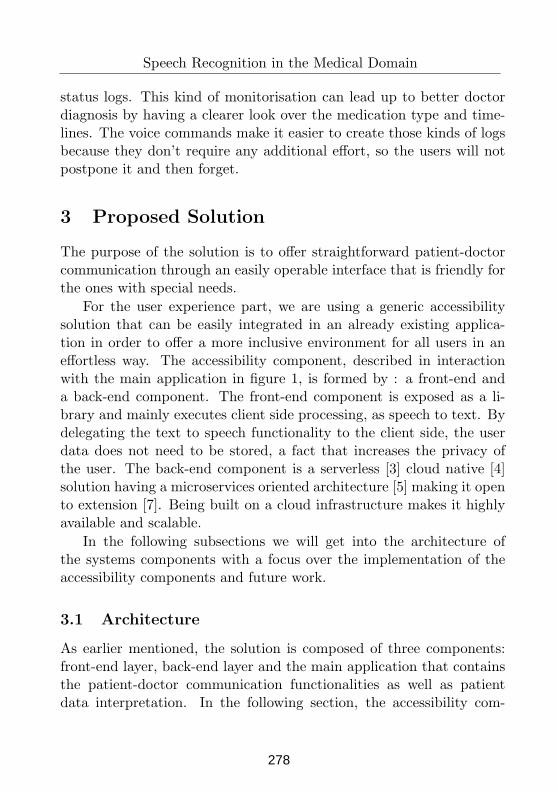
Speech Recognition in the Medical Domain
status logs. This kind of monitorisation can lead up to better doctordiagnosis by having a clearer look over the medication type and time-lines. The voice commands make it easier to create those kinds of logsbecause they don’t require any additional effort, so the users will notpostpone it and then forget.
3 Proposed Solution
The purpose of the solution is to offer straightforward patient-doctorcommunication through an easily operable interface that is friendly forthe ones with special needs.
For the user experience part, we are using a generic accessibilitysolution that can be easily integrated in an already existing applica-tion in order to offer a more inclusive environment for all users in aneffortless way. The accessibility component, described in interactionwith the main application in figure 1, is formed by : a front-end anda back-end component. The front-end component is exposed as a li-brary and mainly executes client side processing, as speech to text. Bydelegating the text to speech functionality to the client side, the userdata does not need to be stored, a fact that increases the privacy ofthe user. The back-end component is a serverless [3] cloud native [4]solution having a microservices oriented architecture [5] making it opento extension [7]. Being built on a cloud infrastructure makes it highlyavailable and scalable.
In the following subsections we will get into the architecture ofthe systems components with a focus over the implementation of theaccessibility components and future work.
3.1 Architecture
As earlier mentioned, the solution is composed of three components:front-end layer, back-end layer and the main application that containsthe patient-doctor communication functionalities as well as patientdata interpretation. In the following section, the accessibility com-
278
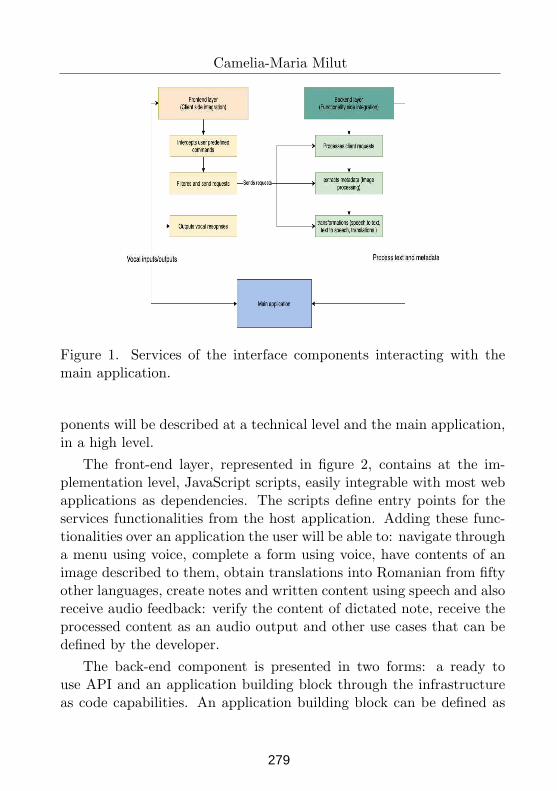
Camelia-Maria Milut
Figure 1. Services of the interface components interacting with themain application.
ponents will be described at a technical level and the main application,in a high level.
The front-end layer, represented in figure 2, contains at the im-plementation level, JavaScript scripts, easily integrable with most webapplications as dependencies. The scripts define entry points for theservices functionalities from the host application. Adding these func-tionalities over an application the user will be able to: navigate througha menu using voice, complete a form using voice, have contents of animage described to them, obtain translations into Romanian from fiftyother languages, create notes and written content using speech and alsoreceive audio feedback: verify the content of dictated note, receive theprocessed content as an audio output and other use cases that can bedefined by the developer.
The back-end component is presented in two forms: a ready touse API and an application building block through the infrastructureas code capabilities. An application building block can be defined as
279
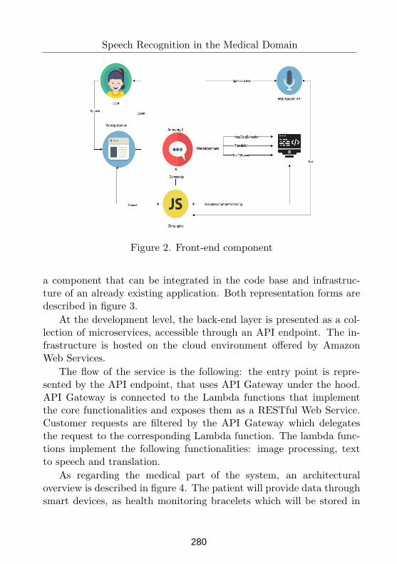
Speech Recognition in the Medical Domain
Figure 2. Front-end component
a component that can be integrated in the code base and infrastruc-ture of an already existing application. Both representation forms aredescribed in figure 3.
At the development level, the back-end layer is presented as a col-lection of microservices, accessible through an API endpoint. The in-frastructure is hosted on the cloud environment offered by AmazonWeb Services.
The flow of the service is the following: the entry point is repre-sented by the API endpoint, that uses API Gateway under the hood.API Gateway is connected to the Lambda functions that implementthe core functionalities and exposes them as a RESTful Web Service.Customer requests are filtered by the API Gateway which delegatesthe request to the corresponding Lambda function. The lambda func-tions implement the following functionalities: image processing, textto speech and translation.
As regarding the medical part of the system, an architecturaloverview is described in figure 4. The patient will provide data throughsmart devices, as health monitoring bracelets which will be stored in
280
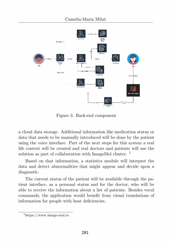
Camelia-Maria Milut
Figure 3. Back-end component
a cloud data storage. Additional information like medication status ordata that needs to be manually introduced will be done by the patientusing the voice interface. Part of the next steps for this system a reallife context will be created and real doctors and patients will use thesolution as part of collaboration with ImagoMol cluster. 1
Based on that information, a statistics module will interpret thedata and detect abnormalities that might appear and decide upon adiagnostic.
The current status of the patient will be available through the pa-tient interface, as a personal status and for the doctor, who will beable to receive the information about a list of patients. Besides vocalcommands, the application would benefit from visual translations ofinformation for people with hear deficiencies.
1https://www.imago-mol.ro
281
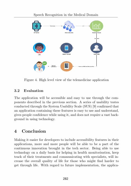
Speech Recognition in the Medical Domain
Figure 4. High level view of the telemedicine application
3.2 Evaluation
The application will be accessible and easy to use through the com-ponents described in the previous section. A series of usability testesconducted through the System Usability Scale (SUS) [9] confirmed thatan application containing these features is easy to use and understand,gives people confidence while using it, and does not require a vast back-ground in using technology.
4 Conclusion
Making it easier for developers to include accessibility features in theirapplications, more and more people will be able to be a part of thecontinuous innovation brought in the tech sector. Being able to usetechnology on a daily basis for helping in health monitorisation, keeptrack of their treatments and communicating with specialists, will in-crease the overall quality of life for those who might find harder toget through life. With regard to future implementation, the applica-
282
Camelia-Maria Milut
tion will be enhanced with more features resulting from analysing thestakeholders reviews.Important things that will be taking into consideration regarding thenext steps are: exploring more data gathering methods, apply algo-rithms for diagnosis and use medical data storage standards like FastHealthcare Interoperability Resources (FHIR) 2 and European Elec-tronic Health Record format. 3
References
[1] H. T. Payne, J. D. Alonso, A. Markiel, K. Lybarger, A. White. Us-ing voice to create hospital progress notes: Description of a mobileapplication and supporting system integrated with a commercialelectronic health record, Journal of Biomedical Informatics, ISSN1532-046, vol. 77, (2018), pp. 91-96.
[2] E. Sezgin, G. Noritz, A. Elek, K. Conkol, S. Rust, M. Bai-ley, R. Strouse, A. Chandawarkar, V. von Sadovszky, S. Lin,Y. Huang. Capturing At-Home Health and Care Informationfor Children With Medical Complexity Using Voice Interac-tive Technologies: Multi-Stakeholder Viewpoint, Journal Med-ical Internet Resources 2020; vol.22, issue 2:e14202, URL:https://www.jmir.org/2020/2/e14202, (2020).
[3] G. C. Fox, V. Ishakian, V. Muthusamy, A. Slominski. Status ofServerless Computing and Function-as-a-Service (FaaS). In Indus-try and Research. CoRR, abs/1708.08028, (2017).
[4] D. Gannon, R. Barga, N. Sundaresan. Cloud-Native Ap-plications. IEEE Cloud Computing, vol. 4, issue 5,https://doi.org/10.1109/MCC.2017.4250939, (2017), pp.16-21.
2https://www.hl7.org/fhir/overview.html3https://ec.europa.eu/digital-single-market/en/news/recommendation-
european-electronic-health- record-exchange-format
283
Speech Recognition in the Medical Domain
[5] L. Bao, C. Wu, X. Bu, N. Ren, M. Shen. Performance mod-eling and workflow scheduling of microservice-based applicationsin clouds. IEEE Transactions on Parallel and Distributed Sys-tems, vol.30, issue 9, https://doi.org/10.1109/TPDS.2019.2901467(2019), pp.2101-2116.
[6] C. Milut, A. Iftene, D. Gıfu. Iasi City Explorer - Alexa, what wecan do today? In Proceedings of the 16th International Confer-ence on Human-Computer Interaction RoCHI 2019, ISSN 2501-9422, ISSN-L 2501-9422, 17-18 October, Politehnica University ofBucharest, Romania, (2019), pp. 139-144.
[7] C.G. Calancea, C. Milut, L. Alboaie, A. Iftene. iAssistMe - Adapt-able Assistant for Persons with Eye Disabilities. In 23rd Interna-tional Conference on Knowledge-Based and Intelligent Information& Engineering Systems. Procedia Computer Science, vol. 159, 4-6September, Budapest, Hungary, (2019), pp. 145-154.
[8] C. M. Milut, A. Iftene. Accessibility Solution for Poor Sighted Peo-ple and Elderly as an End-To-End Service for Applications. Roma-nian Approach. In Proceedings of the 15th International Confer-ence on Linguistic Resources and Tools for Processing the NaturalLanguage, 14-16 December, Bucharest, Romania, (2020).
[9] J. Brooke. SUS: a ”quick and dirty” usability scale”. In P. W. Jor-dan; B. Thomas; B. A. Weerdmeester; A. L. McClelland (eds.).Usability Evaluation in Industry. London: Taylor and Francis,(1986).
Camelia-Maria Milut
”Alexandru Ioan Cuza” University of Iasi, Faculty of Computer ScienceEmail: [email protected]
284
Proceedings of the Conference on Mathematical Foundations of Informatics
MFOI’2021, January 12-16, 2021, Kyiv, Ukraine
© 2021 by Ioan-Alexandru Mititelu, Adrian Iftene
Thread up - Application for
Analysis of the Trending
Phenomenon
Ioan-Alexandru Mititelu, Adrian Iftene
Abstract
As access to the internet is part of our day to day lives
nowadays, the volume of data has raised exponentially from a
quantitative perspective. This led to the need of differentiating
content by several metrics such as relevance and popularity, having
an influence over both the activity of content creators and
consumers. In this paper, we will present the concept of “Trending”
on several platforms, several trending techniques, and a study that
shows the factors which can have an impact on the classification
mechanism of YouTube content (trending or non-trending).
Furthermore, we will present a solution from a software engineering
perspective that can help with understanding this concept and with
monitoring the evolution of it in regards to the YouTube content.
Keywords: trending, YouTube.
1 Introduction
By analyzing several data streams on different social platforms (YouTube,
Twitter, Instagram, Reddit, etc.), we can see that they share a common
concept but they promote it in different ways. Each platform has a key
feature that describes the idea of “popularity” among the content displayed.
Furthermore, we can see that it would be useful for content creators or
content administrators to have the possibility to follow these data streams
in a more granular way, especially when it comes to the evolution of metrics
that altogether consist of user’s engagement (number of visits, number of
likes, number of dislikes, etc.). Eventually, these metrics could be presented
285
Ioan-Alexandru Mititelu, Adrian Iftene
as reports showing their impact over the actively involved audience (that
actively contributes to this data flow by commenting, for example) [1]. This
way, by using a sentiment analysis algorithm over the comments in a data
stream we can get the evolution of more complex metadata such as the
transmitted emotions [2-3].
The current project has two parts. The first one is an analysis of the
“trending” phenomena, explaining what is it, which methods are most used
and which are the alternatives, and, also, which is the impact that this
feature has over the platforms and over their users, especially when the
consumers have different backgrounds (e.g. different countries).
The second part presents the proposed solution for the application
itself, with more details regarding technologies used, architecture, services,
and how the data has been used during the monitoring of these data streams.
As a proof of concept, we highlighted YouTube entities, especially because
it’s a universe less explored in general when it comes to data analysis
(usually studies are based on data from data streams coming from social
media platforms, e.g. twitter).
2 Trending
We will continue by explaining the concept of “trending” and which the
benefits of it in software applications are. As a concrete case of study, we
will discuss some well-known applications that have this feature, such as
YouTube, Twitter, and Instagram.
Definition: trending is a reference to widely mentioned or discussed on
the internet, especially on social media websites1.
Even if all the above-mentioned applications have the same goal, to
offer the most popular content from the application to as many users as
possible, each application has a different approach when it comes to
promoting this content and marking it as being really popular.
1https://www.dictionary.com/browse/trending
286
Thread Up - an Analysis of the Trending Phenomenon
2.1 YouTube - Trending2
YouTube has defined trending as a section in their platform where users
can see which are the most popular videos at that time. From a content
perspective, this section includes 30 videos that have been selected and the
goal of this selection (or at least a subset of it) is to be relevant for as many
users as possible. Another important aspect is that the content mentioned
above differs from country to country as the content (or part of it) will be
relevant for people with a specific given context (that can be influenced by
socio-economic factors). On a general note, some of the content selected
and marked as trending is predictable (e.g. a trailer for a new movie that is
very popular already, a song of a professional artist). Although, there are
selections that have a flavor of new regarding that content and usually it
happens for videos that became viral (a very high amount of users have
watched/shared/liked the content in a very short amount of time).
By analysing YouTube’s documentation, we found some factors that
are possible to be significant in terms of the chances of a video to be
included in the trending section: (1) to be relevant for a very high amount
of users, (2) to be clear and leave no room for interpretation, (3) to show
something new and diverse.
More exactly, there is a correlation between the number of views and
how fast the video generates views. This concept is called “temperature”
and the idea is that a video that is accessed by many people in a short time
will be a hot area (red area) in terms of both content interest and
computational aspects. Another aspect taken into consideration is the origin
of these requests for accessing some videos, therefore the diversity of the
users’ locations might be important as well, but we don’t know how
granular. Besides the diversity between users, given the goal to reach a
broad audience, it’s very important to have diversified content as trending.
And when it comes to YouTube’s diversity we have 4 main categories:
music, games, news, and movies.
Another key aspect for YouTube’s trending is that in the US and other
geographical areas, besides the selection made automatically via filters and
algorithms, there is a manual verification of the content for security reasons.
2https://www.youtube.com/feed/trending?gl=RO
287
Ioan-Alexandru Mititelu, Adrian Iftene
2.2 Twitter - What’s happening3
On Twitter, this feature is called trending as well, in the “Explore” section.
Being in sync with their popular motto, “What’s happening”, the Explore
section has several categories where the most popular content is displayed.
Sometimes it’s about breaking news and live events while sometimes it’s
about random content that got very popular. But the main idea is the same,
to have a place in the application which will encapsulate the most relevant
content and the most discussed things at the current time in a specific
country or region, no matter if it’s a sporting event or a hazard, or anything
else that got a lot of interest overnight. On Twitter this content is updated
in real-time, being in sync with users’ activity.
2.3 Instagram - Explore4
On Instagram, the trending section is called as well “Explore” and it
displays the most popular/relevant content for the logged in user. The
content displayed there is a mix of posts that are related to the user’s activity
or to the user’s Instagram network. It’s less obvious and complex compared
to the other two platforms mentioned above, but its goal remains the same
- to encourage users to find new content that might be interesting for them.
2.4 Existing platforms
Viralstat5 - is a platform that gives users the possibility to analyze videos
and channels on YouTube, Instagram, and Facebook. It enables metrics
regarding the number of views, the number of likes and dislikes, comments,
and, additionally, a rate of engagement.
Google Trends6 – enables the possibility to explore the most searched
topics (by enabling different timeframes, filters for the category of interest,
and the origin of the search - YouTube/Google/Google Images.
YouTube Analytics7 – is an internal dashboard, available only to the
content creator, which shows how the metrics have evolved over time (e.g.
3https://twitter.com/explore 4https://www.instagram.com/explore 5https://viralstat.com/ 6https://trends.google.com/trends/explore 7https://www.youtube.com/analytics
288
Thread Up - an Analysis of the Trending Phenomenon
number of views). Besides this, it also displays some information about the
audience (if they are subscribers or not, their location, where the traffic
comes from, etc.)
2.5 Research Activity
In the paper Trending Topics Detection using Machine Learning Approach
[4], the authors described their approach on “text mining and analysis”,
identifying the topics of interest from blog-like data. More exactly, they
worked with data from Twitter. After preprocessing the data (eliminating
noise and refining the data), they extracted metadata such as the size of the
text, the frequency of terms, and the probability of formation of a phrase.
By using the new data along with the features obtained after the
preprocessing step, they clustered the data using the FCM algorithm - Fuzzy
C Means8 [5], which is considered to have a higher efficiency rate compared
to k-means. After clustering of data has been done, by using Bayesian
probability [6], they identified the topic of each cluster. Finally, the authors
demonstrated that this approach of analysis and clustering on the text in
order to get the topics of interest is one of the most efficient with a good
level of accuracy.
In the paper Trending Videos: Measurement and Analysis [7], the
authors have described an analysis of the concept of trending on YouTube,
by highlighting the videos which get a lot of attention in a short amount of
time, having therefore potential to become popular. The study is based on
collecting and monitoring 8,000 videos on YouTube for over 9 months.
Also, the profiles of content creators have been analysed as well, especially
for those who posted the content that became at some point viral. The goal
was to see if some key aspects from profiles would have any influence or
not over the possibility of that video to be included in trending.
Moreover, the authors took into consideration the category of the
content as well. They noticed that the content marked as trending is
different from the others, from a statistical point of view. When it comes to
results, these show an asymmetric directional relationship between
different categories of trending. The directional analysis uncovers a clear
pattern for some categories, and how the content gets marked as trending,
while other categories tend to be isolated from this point of view. One of
8 https://en.wikipedia.org/wiki/Fuzzy_clustering
289
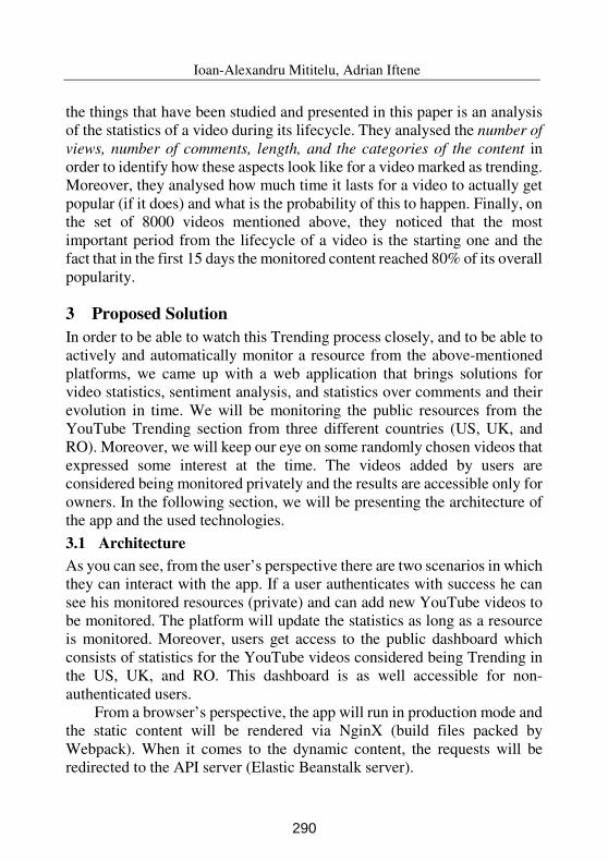
Ioan-Alexandru Mititelu, Adrian Iftene
the things that have been studied and presented in this paper is an analysis
of the statistics of a video during its lifecycle. They analysed the number of
views, number of comments, length, and the categories of the content in
order to identify how these aspects look like for a video marked as trending.
Moreover, they analysed how much time it lasts for a video to actually get
popular (if it does) and what is the probability of this to happen. Finally, on
the set of 8000 videos mentioned above, they noticed that the most
important period from the lifecycle of a video is the starting one and the
fact that in the first 15 days the monitored content reached 80% of its overall
popularity.
3 Proposed Solution
In order to be able to watch this Trending process closely, and to be able to
actively and automatically monitor a resource from the above-mentioned
platforms, we came up with a web application that brings solutions for
video statistics, sentiment analysis, and statistics over comments and their
evolution in time. We will be monitoring the public resources from the
YouTube Trending section from three different countries (US, UK, and
RO). Moreover, we will keep our eye on some randomly chosen videos that
expressed some interest at the time. The videos added by users are
considered being monitored privately and the results are accessible only for
owners. In the following section, we will be presenting the architecture of
the app and the used technologies.
3.1 Architecture
As you can see, from the user’s perspective there are two scenarios in which
they can interact with the app. If a user authenticates with success he can
see his monitored resources (private) and can add new YouTube videos to
be monitored. The platform will update the statistics as long as a resource
is monitored. Moreover, users get access to the public dashboard which
consists of statistics for the YouTube videos considered being Trending in
the US, UK, and RO. This dashboard is as well accessible for non-
authenticated users.
From a browser’s perspective, the app will run in production mode and
the static content will be rendered via NginX (build files packed by
Webpack). When it comes to the dynamic content, the requests will be
redirected to the API server (Elastic Beanstalk server).
290
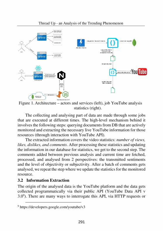
Thread Up - an Analysis of the Trending Phenomenon
Figure 1. Architecture – actors and services (left), job YouTube analysis
statistics (right).
The collecting and analysing part of data are made through some jobs
that are executed at different times. The high-level mechanism behind it
involves the following steps: querying documents from DB that are actively
monitored and extracting the necessary live YouTube information for those
resources (through interaction with YouTube API).
The extracted information covers the video statistics: number of views,
likes, dislikes, and comments. After processing these statistics and updating
the information in our database for statistics, we get to the second step. The
comments added between previous analysis and current time are fetched,
processed, and analysed from 2 perspectives: the transmitted sentiments
and the level of objectivity or subjectivity. After a batch of comments gets
analysed, we repeat the step where we update the statistics for the monitored
resource.
3.2 Information Extraction
The origin of the analysed data is the YouTube platform and the data gets
collected programmatically via their public API (YouTube Data API v
3.09). There are many ways to interrogate this API, via HTTP requests or
9 https://developers.google.com/youtube/v3
291
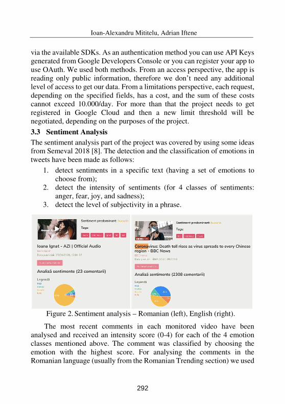
Ioan-Alexandru Mititelu, Adrian Iftene
via the available SDKs. As an authentication method you can use API Keys
generated from Google Developers Console or you can register your app to
use OAuth. We used both methods. From an access perspective, the app is
reading only public information, therefore we don’t need any additional
level of access to get our data. From a limitations perspective, each request,
depending on the specified fields, has a cost, and the sum of these costs
cannot exceed 10.000/day. For more than that the project needs to get
registered in Google Cloud and then a new limit threshold will be
negotiated, depending on the purposes of the project.
3.3 Sentiment Analysis
The sentiment analysis part of the project was covered by using some ideas
from Semeval 2018 [8]. The detection and the classification of emotions in
tweets have been made as follows:
1. detect sentiments in a specific text (having a set of emotions to
choose from);
2. detect the intensity of sentiments (for 4 classes of sentiments:
anger, fear, joy, and sadness);
3. detect the level of subjectivity in a phrase.
Figure 2. Sentiment analysis – Romanian (left), English (right).
The most recent comments in each monitored video have been
analysed and received an intensity score (0-4) for each of the 4 emotion
classes mentioned above. The comment was classified by choosing the
emotion with the highest score. For analysing the comments in the
Romanian language (usually from the Romanian Trending section) we used
292
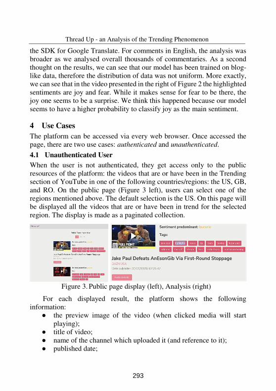
Thread Up - an Analysis of the Trending Phenomenon
the SDK for Google Translate. For comments in English, the analysis was
broader as we analysed overall thousands of commentaries. As a second
thought on the results, we can see that our model has been trained on blog-
like data, therefore the distribution of data was not uniform. More exactly,
we can see that in the video presented in the right of Figure 2 the highlighted
sentiments are joy and fear. While it makes sense for fear to be there, the
joy one seems to be a surprise. We think this happened because our model
seems to have a higher probability to classify joy as the main sentiment.
4 Use Cases
The platform can be accessed via every web browser. Once accessed the
page, there are two use cases: authenticated and unauthenticated.
4.1 Unauthenticated User
When the user is not authenticated, they get access only to the public
resources of the platform: the videos that are or have been in the Trending
section of YouTube in one of the following countries/regions: the US, GB,
and RO. On the public page (Figure 3 left), users can select one of the
regions mentioned above. The default selection is the US. On this page will
be displayed all the videos that are or have been in trend for the selected
region. The display is made as a paginated collection.
Figure 3. Public page display (left), Analysis (right)
For each displayed result, the platform shows the following
information:
the preview image of the video (when clicked media will start
playing);
title of video;
name of the channel which uploaded it (and reference to it);
published date;
293
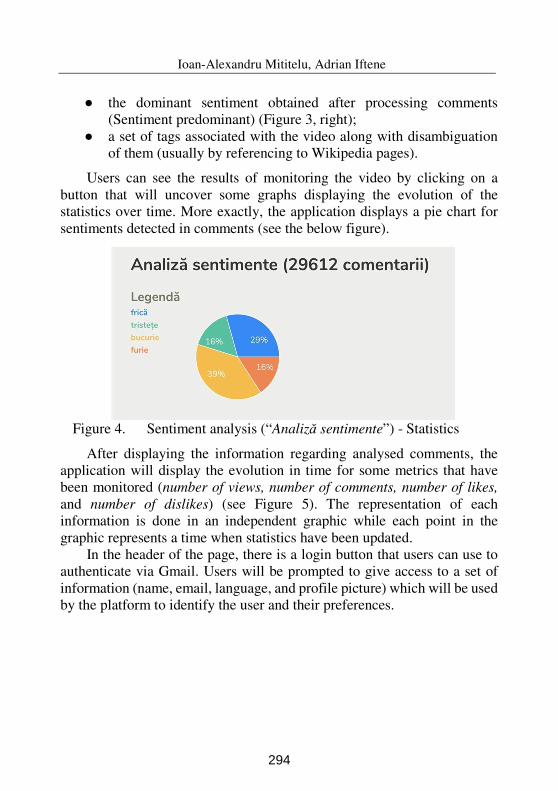
Ioan-Alexandru Mititelu, Adrian Iftene
the dominant sentiment obtained after processing comments
(Sentiment predominant) (Figure 3, right);
a set of tags associated with the video along with disambiguation
of them (usually by referencing to Wikipedia pages).
Users can see the results of monitoring the video by clicking on a
button that will uncover some graphs displaying the evolution of the
statistics over time. More exactly, the application displays a pie chart for
sentiments detected in comments (see the below figure).
Figure 4. Sentiment analysis (“Analiză sentimente”) - Statistics
After displaying the information regarding analysed comments, the
application will display the evolution in time for some metrics that have
been monitored (number of views, number of comments, number of likes,
and number of dislikes) (see Figure 5). The representation of each
information is done in an independent graphic while each point in the
graphic represents a time when statistics have been updated.
In the header of the page, there is a login button that users can use to
authenticate via Gmail. Users will be prompted to give access to a set of
information (name, email, language, and profile picture) which will be used
by the platform to identify the user and their preferences.
294
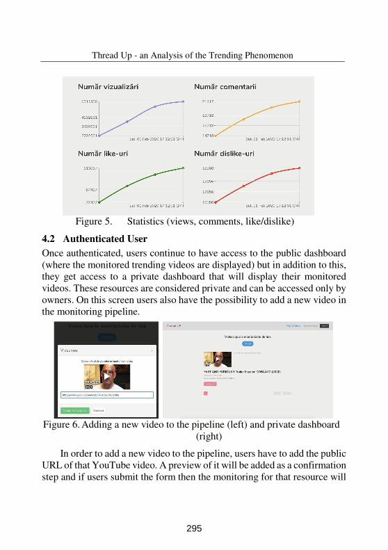
Thread Up - an Analysis of the Trending Phenomenon
Figure 5. Statistics (views, comments, like/dislike)
4.2 Authenticated User
Once authenticated, users continue to have access to the public dashboard
(where the monitored trending videos are displayed) but in addition to this,
they get access to a private dashboard that will display their monitored
videos. These resources are considered private and can be accessed only by
owners. On this screen users also have the possibility to add a new video in
the monitoring pipeline.
Figure 6. Adding a new video to the pipeline (left) and private dashboard
(right)
In order to add a new video to the pipeline, users have to add the public
URL of that YouTube video. A preview of it will be added as a confirmation
step and if users submit the form then the monitoring for that resource will
295
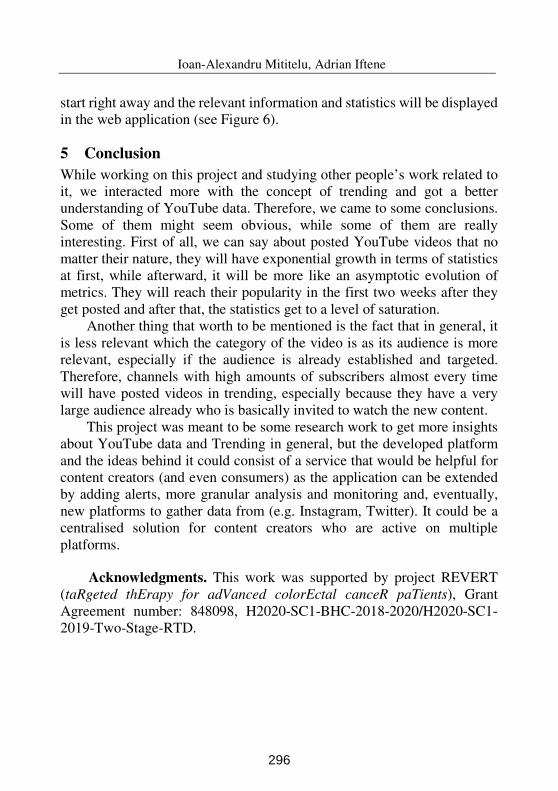
Ioan-Alexandru Mititelu, Adrian Iftene
start right away and the relevant information and statistics will be displayed
in the web application (see Figure 6).
5 Conclusion
While working on this project and studying other people’s work related to
it, we interacted more with the concept of trending and got a better
understanding of YouTube data. Therefore, we came to some conclusions.
Some of them might seem obvious, while some of them are really
interesting. First of all, we can say about posted YouTube videos that no
matter their nature, they will have exponential growth in terms of statistics
at first, while afterward, it will be more like an asymptotic evolution of
metrics. They will reach their popularity in the first two weeks after they
get posted and after that, the statistics get to a level of saturation.
Another thing that worth to be mentioned is the fact that in general, it
is less relevant which the category of the video is as its audience is more
relevant, especially if the audience is already established and targeted.
Therefore, channels with high amounts of subscribers almost every time
will have posted videos in trending, especially because they have a very
large audience already who is basically invited to watch the new content.
This project was meant to be some research work to get more insights
about YouTube data and Trending in general, but the developed platform
and the ideas behind it could consist of a service that would be helpful for
content creators (and even consumers) as the application can be extended
by adding alerts, more granular analysis and monitoring and, eventually,
new platforms to gather data from (e.g. Instagram, Twitter). It could be a
centralised solution for content creators who are active on multiple
platforms.
Acknowledgments. This work was supported by project REVERT
(taRgeted thErapy for adVanced colorEctal canceR paTients), Grant
Agreement number: 848098, H2020-SC1-BHC-2018-2020/H2020-SC1-
2019-Two-Stage-RTD.
296
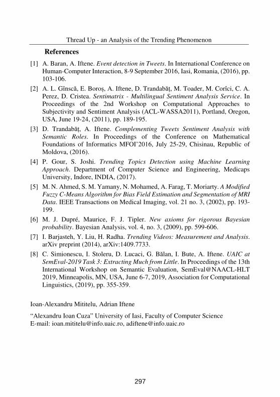
Thread Up - an Analysis of the Trending Phenomenon
References
[1] A. Baran, A. Iftene. Event detection in Tweets. In International Conference on
Human-Computer Interaction, 8-9 September 2016, Iasi, Romania, (2016), pp.
103-106.
[2] A. L. Gînscă, E. Boroș, A. Iftene, D. Trandabăț, M. Toader, M. Corîci, C. A.
Perez, D. Cristea. Sentimatrix - Multilingual Sentiment Analysis Service. In
Proceedings of the 2nd Workshop on Computational Approaches to
Subjectivity and Sentiment Analysis (ACL-WASSA2011), Portland, Oregon,
USA, June 19-24, (2011), pp. 189-195.
[3] D. Trandabăț, A. Iftene. Complementing Tweets Sentiment Analysis with
Semantic Roles. In Proceedings of the Conference on Mathematical
Foundations of Informatics MFOI’2016, July 25-29, Chisinau, Republic of
Moldova, (2016).
[4] P. Gour, S. Joshi. Trending Topics Detection using Machine Learning
Approach. Department of Computer Science and Engineering, Medicaps
University, Indore, INDIA, (2017).
[5] M. N. Ahmed, S. M. Yamany, N. Mohamed, A. Farag, T. Moriarty. A Modified
Fuzzy C-Means Algorithm for Bias Field Estimation and Segmentation of MRI
Data. IEEE Transactions on Medical Imaging, vol. 21 no. 3, (2002), pp. 193-
199.
[6] M. J. Dupré, Maurice, F. J. Tipler. New axioms for rigorous Bayesian
probability. Bayesian Analysis, vol. 4, no. 3, (2009), pp. 599-606.
[7] I. Barjasteh, Y. Liu, H. Radha. Trending Videos: Measurement and Analysis.
arXiv preprint (2014), arXiv:1409.7733.
[8] C. Simionescu, I. Stoleru, D. Lucaci, G. Bălan, I. Bute, A. Iftene. UAIC at
SemEval-2019 Task 3: Extracting Much from Little. In Proceedings of the 13th
International Workshop on Semantic Evaluation, SemEval@NAACL-HLT
2019, Minneapolis, MN, USA, June 6-7, 2019, Association for Computational
Linguistics, (2019), pp. 355-359.
Ioan-Alexandru Mititelu, Adrian Iftene
“Alexandru Ioan Cuza” University of Iasi, Faculty of Computer Science
E-mail: [email protected], [email protected]
297
Proceedings of the Conference on Mathematical Foundations of Informatics
MFOI-2020, January 12-16, 2021, Kyiv, Ukraine
Remarks On Nonmonotonic Consequence
Relations
Alexei Muravitsky
Abstract
We discuss nonmonotonic reasoning in terms of consequence re-lations and corresponding operators. Based on the matrix con-sequence that gives the monotonic case, we define a restrictedmatrix consequence that illustrates the nonmonotonic case. Thelatter is a generalization of the relation of friendliness introducedby D. Makinson. We prove that any restricted single matrixconsequence is strongly finitary. Further, by modifying the def-inition of friendliness relation formulated specifically in proof-theoretic manner, we show a possibility to obtain other non-monotonic strongly finitary relations. This leads to numerousquestions about nonmonotonic finitary consequence relations inthe segment between the monotonic consequence relation basedon intuitionistic propositional logic and friendliness.Keywords: matrix consequence, logical friendliness, intermedi-
ate logics, satisfiable formulas.
Mathematical Subject Classification (2000). Primary03B05; Secondary 03B99, 03F99.
1 Nonmonotonic reasoning in terms of conse-
quence relations
In this paper,1 we explore the possibilities of abandoning the mono-tonicity property of the “classical” (that is, Tarskian) consequence re-
c©2021 by Alexei Muravitsky1This is a shortened version of a longer paper. I have omitted all but a few of
the proofs from the current version.
298
Alexei Muravitsky
lation. Among several approaches to analyzing the phenomenon ofnon-monotonicity, we will focus on how non-monotonicity can be re-alized in terms of consequence relations, widely understood, and thecorresponding consequence operators.
We investigate possibilities of defining reflexive nonmonotonic fini-tary consequence relations. The investigations involving the notion ofa consequence operator have been undertaken in the past; cf. for ex-ample, a comprehensive account in [6]. Our approach outlined in thispaper is different. On the one hand, in Section 4, we explore a possi-bility of defining nonmonotonic consequence relations through logicalmatrices for an arbitrary propositional language; and on the other, weinvestigate the possibility of certain nonmonotonic consequence rela-tions in the framework of proof-theoretic deduction. The presentedresults in the framework of matrix consequence stem from the notionof logical friendliness which was introduced by D. Makinson in [7];this nonmonotonic consequence relation is coincident with our relation|=r
B2.
With regard to the possibility of considering non-monotonicitywithin a proof-theoretic framework, some researchers express rathera skeptical point of view. In particular, we read:
The paradise of classical logical reasoning in which seman-tic notion of validity is equivalent to syntactic notions ofproofs and derivation is hardy achievable for nonmonotonicreasoning. — [2], Introduction
As for the monotonic consequence relations, there is a wealth ofmaterial on the definition of these relations using inference rules.2 InSection 5, we use monotonic consequence relations based on proposi-tional intermediate logics. The situation is different for nonmonotonicconsequence. The term nonmonotonic consequence itself has not yetbecome common. The reason for this, perhaps, is that it is not clearwhat properties the nonmonotonic operators must satisfy in order tobe considered as consequence operators.
2See, e.g., [4], Section 4.3.5, and references there.
299
Remarks On Nonmonotonic Consequence Operators
We will challenge the aforementioned skeptical view in Section 5,by showing how to formulate |=r
B2syntactically, that is, we define a
sequential calculus adequate to this relation. Using that definition asa pattern, we show a systematic way of defining nonmonotonic conse-quence relations in a proof-theoretic fashion.
2 Monotonicity vs. nonmonotonicity expressed
formally
Our formal language will be propositional. Starting with Section 4.2,we use only Boolean connectives, but for now, we don’t need any re-strictions.
A language L consists of the following categories of symbols:
• a denumerable set VL of propositional variables; unspecifiedvariables are denoted by letters p, q, r, . . ., perhaps with sub-scripts; any V ′ ⊂ VL is called a restriction of VL;
• a nonempty set FL of symbols of logical connectives; to eachF ∈ FL, a nonnegative number #(F ) is assigned, which is calledthe arity of F ; logical constants, if any, are the connectives ofthe arity 0.
Formulas of the language L, or L-formulas, are defined induc-tively according to usual clauses:
(a) every variable from VL is an L-formula;
(b) if α1, . . . , αn are L-formulas and F ∈ FL with #(F ) = n, thenFα1, . . . , αn is an L-formula;
(c) L-formulas are only those formal object that are constructed ac-cording to (a) and (b).
Unspecified L-formulas are denoted by letters α, β, . . ., perhaps withsubscripts, and sets of formulas by X,Y, Z, etc. The set of all L-formulas is denoted by FmL. The set of L-formulas built up from a
300
Alexei Muravitsky
restriction V ′ is denoted by FmL[V ′]. If X ⊆ FmL, we denote by V(X)the set of variables that occur in the formulas of X; in particular, V(α)is the set of all variables occurring in a formula α. So, we just have:
V(X) =⋃
p ∈ V(α) | α ∈ X.
Comparing two sets of L-formulas, X and Y , we write
X ⋐ Y
if X is a finite subset of Y .
What is important is that FmL together with FL form an algebraof similarity type L, which we call the formula algebra of type L.We denote this algebra by FL, that is,
FL := 〈FmL,FL〉.
This opens the door to the application of algebraic concepts.
We call any homomorphism σ : FL −→ FL a substitution.
Further, denoting by P(FmL) the power set of FmL, we call anybinary relation
⊢⊆ P(FmL) × FmL
a (monotonic) consequence relation if it satisfies the followingproperties:
(a) α ∈ X implies X ⊢ α; (reflexivity)(b) X ⊢ α and X ⊆ Y imply Y ⊢ α; (monotonicity)(c) if X ⊢ β, for all β ∈ Y , and Y, Z ⊢ α, then X,Z ⊢ α, (transitivity)
for any sets X, Y and Z of L-formulas.
A relation ⊢ is trivial if ⊢= P(FmL)×FmL; otherwise ⊢ is non-
trivial.
Further, we denote
C(X) := α | X ⊢ α. (1)
301
Remarks On Nonmonotonic Consequence Operators
The function C thus defined is called a consequence operator.The characteristic properties of consequence operators are parallel tothe items (a)–(c) above. Reformulating (a)–(c) in terms of C, we ob-tain the following properties of this operator (defined through (1)),providing that ⊢ satisfies the properties (a)–(c):
(a†) X ⊆ C(X); (reflexivity)
(b†) X ⊆ Y implies C(X) ⊆ C(Y ); (monotonicity)(c†) C(C(X)) ⊆ C(X), (closedness)
for any sets X and Y of L-formulas.
The operator C is said to be trivial if C(∅) = FmL and nontriv-
ial otherwise.
In a sense, a relation ⊢ satisfying (a)–(c) and the operator definedvia (1) describe the same phenomenon in two different metalanguages.For convenience, we introduce a unifying notion, an abstract logic,which will allow us to speak of properties of such a logic, say S, eitherin terms of ⊢S or in terms of CS . Thus, referring to S, we mean that
X ⊢S α ⇐⇒ α ∈ CS(X). (2)
The key question is: If we want to challenge the monotonicity prop-erty, what properties would we like to retain? However, the followingnotation must first be agreed upon. If an operator C : P(FmL) −→P(FmL) satisfies all the properties (a)–(c) we will denote it by Cn (orby CnS , relating it to an abstract logic S) and call it a monotonic
consequence operator. For general consideration, we reserve nota-tion C; also, we will use C with a subscript, something like CS , if anabstract logic S does not satisfy all the properties (a)–(c) or, respec-tively, all the properties (a†)–(c†). Now we return to our question.
Perhaps, the most important is the following property:
(d†) C(X) ⊆⋃
C(Y ) | Y ⋐ X. (finitariness or compactness)
Here are other properties of logical consequence which have at-
302
Alexei Muravitsky
tracted attention in the literature.3
(e†) X ⊆ C(Y ) implies C(X) ⊆ C(Y ); (comulative transitivity)
(f†) X ⊆ C(Y ) implies C(X ∪ Y ) ⊆ C(Y ); (strong comulative transitivity)(g†) X ⊆ Y ⊆ C(X) implies C(Y ) ⊆ C(X); (weak comulative transitivity)
(h†)⋃
C(Y ) | Y ⋐ X ⊆ C(X); (finitary inclusion)
(i†) if X 6= ∅, then C(X) ⊆⋃
C(Y ) | Y 6= ∅ and Y ⋐ X;(strong finitariness)
(j†) if α /∈ C(X), then there is a maximal X∗ such that X ⊆ X∗
and α /∈ C(X∗). (maximalizability)
A quick look at how these properties relate to each other revealsthe following.
Proposition 2.1 ([4], Proposition 4.2.5). Let C be a map from
P(FmL) into P(FmL), Then the following implications hold:
i) (a†) and (g†) imply (c†);
ii) (b†) and (c†) imply (e†);iii) (e†) implies (g†);
iv) (f†) implies (g†);
v) (a†) and (g†) imply (f†);
vi) (a†) and (f†) imply (c†);
vii) (a†) and (b†) and (c†) imply (f†);
viii) (i†) implies (d†);
ix) (b†) and (d†) imply (i†);
x) (b†) implies (h†);
xi) (b†) and (d†) imply (j†);
xii) (d†) and (h†) imply (b†).
Except for properties (a†) and (b†), the remaining properties canbe divided into three groups: 1) transitivity properties, that is, (c†)and (e†)–(g†), 2) finitariness properties, that is, (d†), (h†) and (i†), and
3See, e.g., [6].
303
Remarks On Nonmonotonic Consequence Operators
3) maximalizability property (j†).4
Interactions between the properties of the groups (1) and (2) arerare, but two of them are essential; namely, the statements (x) and(xii) of Proposition 2.1.
We see that (h†) is closely connected to (b†), while (d†), as far aswe currently know, is not. On the other hand, if we want to challenge(b†), we have to choose between (d†) and (h†). In fact, (d†) is moreimportant for theory of logical consequence; cf. [4]. This determinesour choice. Thus, we will be focusing on (d†) rather than (h†).
Before moving on to a further investigation of consequence rela-tions or operators, monotone or otherwise, we introduce the followingrelation.
Let C and C′ be two operators understood as maps from P(FmL)to P(FmL), We define:
C ≤ C′ df⇐⇒ C(X) ⊆ C′(X) for any X ⊆ FmL. (3)
It should be obvious that the relation ≤ is a partial ordering onthe set of all maps from P(FmL) to itself. We use this fact withoutreference.
3 Realizations of monotonicity and nonmono-
tonicity
There are two main frameworks to express logical consequence — se-mantic and syntactic, that is, proof-theoretic, approaches. Althoughthe latter appeared historically first, we begin with the former.
Definition 3.1 (algebra of type L). An algebra of type L (or an L-algebra or simply an algebra when a type is specified ahead and con-
fusion is unlikely) is a structure A = 〈A;FL〉, where A is a nonempty
4The property (j†) appears only as a conclusion in (xi). Thus, if we challenge(b†), we can possibly have (j†) only in some exotic situations. Therefore, we willnot be considering it.
304
Alexei Muravitsky
set called the carrier (or universe) of A; FL, which in the notion
of L-formulas represents logical connectives, now represents the set of
finitary operations on A of the corresponding arities; it is assumed that
each F of FL is closed on A. As is customary, we use the notation
|A| = A. The part 〈FL〉 of the structure A is called its signature.
Referring to an algebra A of type L, we also say that it is an algebra
of signature 〈FL〉. A matrix M is called finite if the corresponding
algebra A is finite.
Definition 3.2 (valuation, value of a formula in an algebra). Let A be
an algebra of type L. Then any map v : VL −→ |A| is called a valu-
ation (or an assignment) in the algebra A. Then, given a valuation
v, the value of an L-formula α with respect to v, in symbols v[α], is
defined inductively as follows :
(a) v[p] = v(p), for any p ∈ VL;(b) v[c] is the value of the nullary operation of A corresponding to
the constant c of FL;(c) v[α] = Fv[α1] . . . v[αn] if α = Fα1 . . . αn.
If V ′ ⊂ VL, then a map v : V ′ −→ |A| is called a V ′-valuation, or a
valuation restricted to V ′.
If v is a valuation (in some algebra) we denote by dom(v) thedomain of v.
It should be clear that an arbitrary valuation v in an algebra A isa homomorphism v : FL −→ A, and vice versa.
Give a valuation v : FL −→ A and X ⊆ FmL, we denote:
v[X] := v[α] | α ∈ X.
Definition 3.3 (logical matrix of type L). A logical matrix (or sim-
ply a matrix) of type L is a structure M = 〈A, D(x)〉, where A is an
algebra of type L, which, if considered as part of M, is called an M-
algebra, and D(x) is a predicate on |A|. The matrix M is nontrivial
if the algebra A is nontrivial, and trivial otherwise. We also denote
305
Remarks On Nonmonotonic Consequence Operators
a matrix by 〈A, D〉 or by 〈A;F , D〉, where D ⊆ |A|; in this case, D is
called the set of designated elements or a logical filter (or simply a
filter) in (or of) M. A valuation (or assignment) in M is the same
as a valuation in A, where the latter is an algebraic component of M.
If v[α] ∈ D, we say that a valuation v validates a formula α in a
matrix M; v validates a set X of formulas in M whenever v[X] ⊆ D.
The next definition will be used later.
Definition 3.4. Given a logical matrix M = 〈A, D〉 and a set X ⊆FmL, X is consistent in M if X = ∅ or, if X 6= ∅, there is a
valuation v such that v[X] ⊆ D. Otherwise, X is inconsistent in M.
Given a (logical) matrix M = 〈A, D〉, we define a relation |=M onP(FmL) × FmL as follows:
X |=M αdf
⇐⇒ (v[X] ⊆ D ⇒ v[α] ∈ D, for any valuation v in A). (4)
Given a matrix M, the relation |=M is called matrix consequence
or M-consequence if we know the matrix M.The following proposition is well known.
Proposition 3.1 (cf. [5]). Any matrix consequence is a monotonic
consequence relation.
In the light of Proposition 3.1, let us look at the definition (4)closely.
Suppose X |=M α and assume that V(α) 6⊆ V(X). First, we noticethat in order to evaluate the right-hand side of (4), we need to useonly the variables of the set V(X ∪ α), and even for this, we canfirst use a restricted valuation v : V(X) −→ A and then an extensionv′ : V(X∪α) −→ A of v, that is, when for each p ∈ V(X), v[p] = v′[p].
Thus, in terms of restricted valuations, the right-hand side of (4)can be reformulated as follows:
For any restricted valuation v : V(X) −→ A, if v[X] ⊆ D,then for any extension v′ : V(X ∪ α) −→ A, v′[α] ∈ D.
306
Alexei Muravitsky
We call the above type of matrix consequence (which is monotonic)∀∀-type. Now we modify the last definition to the following, calling it∀∃-type :
For any restricted valuation v : V(X) −→ A, if v[X] ⊆ D,
then there exists an extension v′ : V(X ∪ α) −→ A of vsuch that v′[α] ∈ D.
(5)
Now we define:
X |=rM α
df⇐⇒ (5) holds; (6)
and then
X |=rM α
df⇐⇒ (X |=r
M α, for all M ∈ M). (7)
We call the relation defined by (6) and (7) M-r-consequence andM-r-consequence, respectively. If X |=r
Mα, we say that X restric-
tively implies α relative to M, and we use a similar formulation forX |=r
M α.5
We accept by default that
∅ |=rMα means that there is a restricted valuation
v : V(α) −→ A such that v[α] ∈ D.(8)
For future references, we state a quite obvious proposition.
Proposition 3.2. Let M = 〈A, D〉 be a logical matrix. Then:
(a) if X is inconsistent in M, then X |=rMα;
(b) if α is inconsistent in M, then X |=rMα if, and only if, X is
inconsistent in M.
5The idea of obtaining non-monotonicity by passing from ∀∀-type to ∀∃-typebelongs to D. Makinson; see [7].
307
Remarks On Nonmonotonic Consequence Operators
Now we observe the following.
Proposition 3.3. Given a set M of logical matrices, the M-r-
consequence satisfies the property (a) but in general fails to satisfy the
monotonicity property (b) and the transitivity property (c).
In the proof of the last proposition we use the logical matrix
B2 := 〈A2, 1〉, (9)
where A2 := 〈0,1;∧,∨,¬,1〉 is a 2-element Boolean algebra.
In the next section, we will explain why the relation |=rM
is inter-esting, at least when M is finite.
4 Finite case of M-r-consequence
4.1 Finite case in general
In this subsection, we fix a logical matrix M and assume that M isfinite. Accordingly, all restricted valuations are valuations in M.
It will be convenient to use the following notation.
• Given a nonempty V0 ⊆ VL, we mean by vV0an M-valuation
with dom(vV0) = V0.
• v α means that a (restricted) valuation v can be extended tovalidate a formula α.
• v X means that v α for each α ∈ X.
Given a set X ∪ α ⊆ FmL, denoting V0 := V(X) ∩ V(α), weobserve:
X |=rM α ⇐⇒ (vV0
X =⇒ vV0 α, for any vV0
). (10)
We use (10) to prove the following proposition.
308
Alexei Muravitsky
Proposition 4.1. Given a finite matrix M, if X |=rMα and X 6= ∅,
then there is a nonempty Y ⋐ X with V(Y )∩V(α) ⊆ V(X)∩V(α) suchthat Y |=r
Mα. Further, for any set Z with Y ⊆ Z and V(Z) ∩ V(α) ⊆
V(X) ∩ V(α), Z |=rMα.
Proposition 4.1 induces the following definition.
Definition 4.1. An relation ⊢⊆ P(FmL)×FmL, or the corresponding
to it operator C : P(FmL) −→ P(FmL) (in the sense of (2)), is
strongly finitary plus if for any nonempty set X, if X ⊢ α, then
there is a nonempty Y ⋐ X such that Y ⊢ α and for every Z with
Y ⊆ Z and V(Z) ∩ V(α) ⊆ V(X) ∩ V(α), Z ⊢ α.
Proposition 4.1 leads to the following question.
Problem 1. Let M0 be an arbitrary nonempty class of finite logical
matrices. Is it true that M0-r-consequence is (at least) finitary or
strongly finitary?
4.2 Friendliness
The relation |=rB2
, where B2 is defined in (9), was introduce by D.Makinson in [7]; he called this relation friendliness. We denote therelation of friendliness by |=F , while keeping the notation |=r
B2as well.
First of all, we specify the propositional language suitable for |=F ,denoting this language by L. The propositional variables of L arethe same as those of L, that is, VL = VL; we continue using the latternotation. The logical connectives are ∧ (conjunction), ∨ (disjunction),→ (implication), ¬ (negation), and ⊤ (propositional constant true).The formulas are built in a usual way and are called L-formulas;we denote them by uppercase letters A,B, . . ., perhaps with subscriptsand other marks, and sets of L-formulas by Γ,∆ and so on, perhapswith subscripts; the set of all L-formulas is denoted by FmL .
In this section, referring to consistency of a set, we mean consistencyin B2.
309
Remarks On Nonmonotonic Consequence Operators
By definition, we count that any valuation v in the matrix B2 sat-isfies the condition:
v[⊤] = 1.
The next proposition is obviously a refinement of Proposition 4.1.
Proposition 4.2 (comp. [7], section 1.6). The relation |=F is strongly
finitary plus. That is, for any Γ ∪ A ⊆ FmL , where Γ 6= ∅, if
Γ |=F A, then there is a nonempty set ∆ ⋐ Γ with V(∆) ∩ V(A) ⊆V(Γ) ∩ V(A) such that ∆ |=F A, and for any set Λ with ∆ ⊆ Λ and
V(Λ) ∩ V(A) ⊆ V(Γ) ∩ V(A), Λ |=F A.6
In Section 7, we consider a possibility of defining a nonmonotonicoperator Cϕ such that Cϕ < CF ; and in Section 5, we give a systematicway of defining nonmonotonic consequence operators less than or equalto CF in a proof-theoretic manner.
5 Syntactic treatment of nonmonotonicity
We start with generalizing the proof-theoretic treatment of the friend-liness relation presented in [8].
The notions of a classical tautology and of an intuitionistic tautol-ogy can be found in [10] or in [4]; we denote the set of all classicaltautologies by Cl and the set of all intuitionistic tautologies by Int. Aset L of L-formulas, which is closed under substitution and modusponens, is called an intermediate logic if Int ⊆ L ⊆ Cl. The set ofall intermediate logics is denoted by ExtInt. It is clear that ExtInt is apartially ordered set with respect to ⊆.
As we will se below, each intermediate logic L leads to two conse-quence relations, a monotonic relation ⊢L and a nonmonotonic relation L.
6Makinson proved the strong finitariness of friendliness in a stronger form, how-ever, weaker than the one exposed in this proposition. The condition imposed on Λin Makinson’s version is ∆ ⊆ Λ ⊆ Γ.
310
Alexei Muravitsky
Given a set Γ ∪ A ⊆ FmL , we say that Γ derives A relative
to L, symbolically Γ ⊢L A, if there is a finite list of formulas
A1, . . . , Ai, . . . , An,
where the last formula An = A and each formula Ai of this list eitherbelongs to the set L∪Γ or can be obtained from preceding formulas Ajand Aj → Ai by modus ponens. Since each L is closed under modusponens, it follows from this definition that for any A,
∅ ⊢L A ⇐⇒ A ∈ L.
Given L ∈ ExtInt, the monotonic consequence operator that corre-sponds to ⊢L in the sense of (2) is denoted by CnL.
For future reference, we note that each consequence relation ⊢Lsatisfies the deduction property:
Γ ∪ A ⊢L B ⇐⇒ Γ ⊢L A→ B. (11)
Another feature of each consequence relation ⊢L is that it is finitary,and since each ⊢L is monotonic, it is even strongly finitary.
We now aim to consider non-monotonicity using two deductive sys-tems. The first system axiomatically defines a unary predicate ⊲L A,and the second, using the first predicate, defines a binary predicateΓ L A. As we will see below (Proposition 5.1), the interconnectionbetween the predicates is the following:
⊲L A ⇐⇒ ∅ L A. (12)
⊲L-Axioms:
axiom 1: ⊲L p. for any p ∈ VL;
axiom 2: ⊲L ⊤.
⊲L-Rules:
311
Remarks On Nonmonotonic Consequence Operators
rule 1:⊲L A, ∅ ⊢L A→ B
⊲L B; (Soundness w.r.t. ⊢L)
rule 2:⊲L σ(A)
⊲L A, (Reverse substitution)
where σ is an L-substitution, that is a homomorphism of FL toFL .
L-Axioms:
axiom 1: Γ L ⊤;
axiom 2: Γ L A, providing that V(Γ) ∩ V(A) = ∅ and ⊲L A;
axiom 3: Γ L∧
∆ if ∆ ⋐ Γ (∧
∆ := ⊤ if ∆ = ∅);
axiom 4: Γ L A whenever Γ ⊢L A.
L-Rules:
rule 1:Γ, A L C and ∆, B L C
Γ ∪ ∆, A ∨B L C,
providing that V(Γ ∪ A) = V(∆ ∪ B);
rule 2:Γ L σ(A)
Γ L A, (Reverse substitution)
providing that the following conditions are satisfied: σ(A) =A[pi1\B1, . . . , pin\Bn] and V(Γ) ∩ pi1 , . . . , pin = ∅, where σis an L-substitution;
rule 3:Γ L A, and A L B
Γ L B, (Cut 1)
providing that either V(Γ) ⊆ V(A) or V(Γ) ∩ V(B) ⊆ V(A) ⊆V(Γ);
312
Alexei Muravitsky
rule 4:Γ L A and A ⊢L B
Γ L B; (Cut 2)
rule 5:Γ, A L B and C L A
Γ, C L B,
(Deductive replacement in antecedent)providing that V(C) ⊆ V(Γ ∪ A).
We call each expression of the form ⊲L A a ⊲L-sequent and that ofthe form Γ L A a L-sequent.
We say that ⊲L A holds (or is true) if there is a finite list of ⊲L-sequents, called a ⊲L-derivation, such that the last sequent of thislist is ⊲L A and each sequent in this list is either a ⊲L-axiom or can beobtained from one or two preceding sequents by one of the ⊲L-rules.
Further, we say that a sequent Γ L A holds (or is true) if there isa list of⊲L-sequents and L-sequents, where the last sequent is Γ L A,and such that each L-sequent is either a L-axiom or obtained frompreceding sequents by one of the L-rules.
We note that the presence of each ⊲L-sequent in the definition ofa L-derivation is justified, on the one hand, by a ⊲L-derivation of itand, on the other hand, by its participation in an application of theaxiom 2.
Lemma 5.1. For any L ∈ ExtInt and Γ ∪ A ⊆ FmL , the following
properties hold:
(a) ∅ ⊢L A =⇒ ⊲L A;(b) Γ ⊢L A =⇒ Γ L A.
Proposition 5.1. The equivalence (12) holds.
We recall the two completeness results from our previous research.
Proposition 5.2 ([8], theorems 3.2 and 3.4). For any FmL-formula
A, ⊲Cl A if, and only if, A is satisfiable in B2, or, in other words,
∅ |=F A.
313
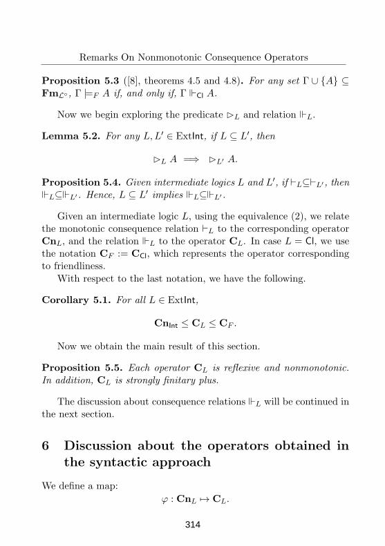
Remarks On Nonmonotonic Consequence Operators
Proposition 5.3 ([8], theorems 4.5 and 4.8). For any set Γ ∪ A ⊆FmL , Γ |=F A if, and only if, Γ Cl A.
Now we begin exploring the predicate ⊲L and relation L.
Lemma 5.2. For any L,L′ ∈ ExtInt, if L ⊆ L′, then
⊲L A =⇒ ⊲L′ A.
Proposition 5.4. Given intermediate logics L and L′, if ⊢L⊆⊢L′, then
L⊆ L′. Hence, L ⊆ L′ implies L⊆ L′.
Given an intermediate logic L, using the equivalence (2), we relatethe monotonic consequence relation ⊢L to the corresponding operatorCnL, and the relation L to the operator CL. In case L = Cl, we usethe notation CF := CCl, which represents the operator correspondingto friendliness.
With respect to the last notation, we have the following.
Corollary 5.1. For all L ∈ ExtInt,
CnInt ≤ CL ≤ CF .
Now we obtain the main result of this section.
Proposition 5.5. Each operator CL is reflexive and nonmonotonic.
In addition, CL is strongly finitary plus.
The discussion about consequence relations L will be continued inthe next section.
6 Discussion about the operators obtained in
the syntactic approach
We define a map:
ϕ : CnL 7→ CL.
314
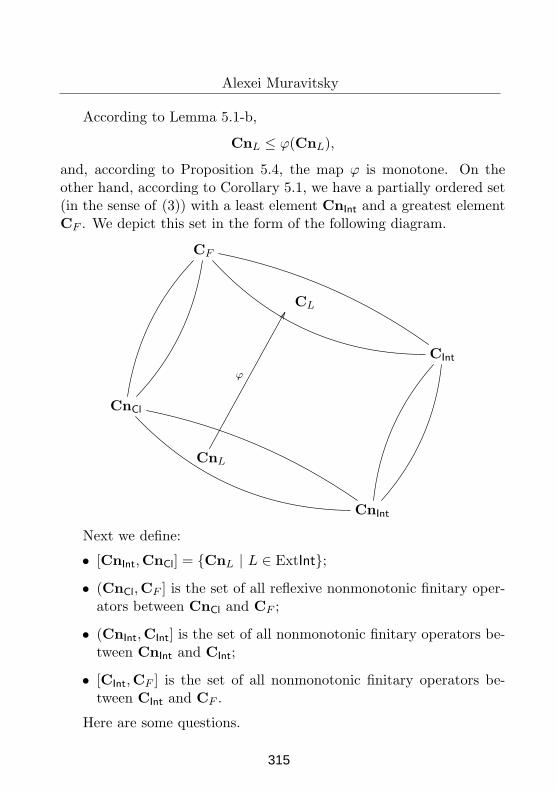
Alexei Muravitsky
According to Lemma 5.1-b,
CnL ≤ ϕ(CnL),
and, according to Proposition 5.4, the map ϕ is monotone. On theother hand, according to Corollary 5.1, we have a partially ordered set(in the sense of (3)) with a least element CnInt and a greatest elementCF . We depict this set in the form of the following diagram.
CF
CL
CInt
CnCl
CnL
ϕ
FF
CnInt
Next we define:
• [CnInt,CnCl] = CnL | L ∈ ExtInt;
• (CnCl,CF ] is the set of all reflexive nonmonotonic finitary oper-ators between CnCl and CF ;
• (CnInt,CInt] is the set of all nonmonotonic finitary operators be-tween CnInt and CInt;
• [CInt,CF ] is the set of all nonmonotonic finitary operators be-tween CInt and CF .
Here are some questions.
315
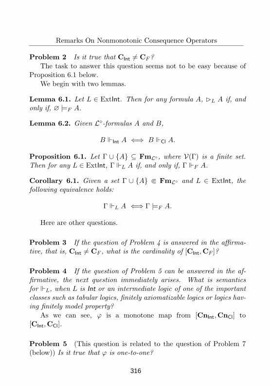
Remarks On Nonmonotonic Consequence Operators
Problem 2 Is it true that CInt 6= CF ?
The task to answer this question seems not to be easy because ofProposition 6.1 below.
We begin with two lemmas.
Lemma 6.1. Let L ∈ ExtInt. Then for any formula A, ⊲L A if, and
only if, ∅ |=F A.
Lemma 6.2. Given L-formulas A and B,
B Int A ⇐⇒ B Cl A.
Proposition 6.1. Let Γ ∪ A ⊆ FmL, where V(Γ) is a finite set.
Then for any L ∈ ExtInt, Γ L A if, and only if, Γ F A.
Corollary 6.1. Given a set Γ ∪ A ⋐ FmL and L ∈ ExtInt, the
following equivalence holds:
Γ L A ⇐⇒ Γ |=F A.
Here are other questions.
Problem 3 If the question of Problem 4 is answered in the affirma-
tive, that is, CInt 6= CF , what is the cardinality of [CInt,CF ]?
Problem 4 If the question of Problem 5 can be answered in the af-
firmative, the next question immediately arises. What is semantics
for L, when L is Int or an intermediate logic of one of the important
classes such as tabular logics, finitely axiomatizable logics or logics hav-
ing finitely model property?
As we can see, ϕ is a monotone map from [CnInt,CnCl] to[CInt,CCl].
Problem 5 (This question is related to the question of Problem 7(below)) Is it true that ϕ is one-to-one?
316
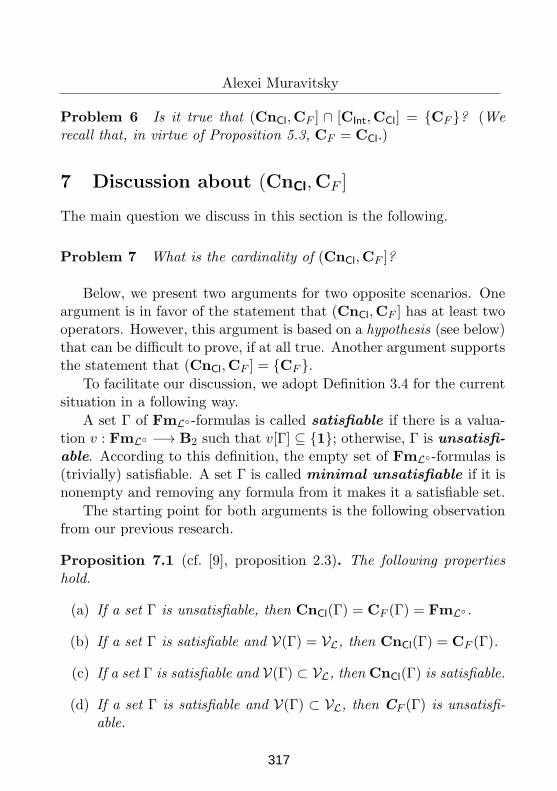
Alexei Muravitsky
Problem 6 Is it true that (CnCl,CF ] ∩ [CInt,CCl] = CF ? (We
recall that, in virtue of Proposition 5.3, CF = CCl.)
7 Discussion about (CnCl,CF ]
The main question we discuss in this section is the following.
Problem 7 What is the cardinality of (CnCl,CF ]?
Below, we present two arguments for two opposite scenarios. Oneargument is in favor of the statement that (CnCl,CF ] has at least twooperators. However, this argument is based on a hypothesis (see below)that can be difficult to prove, if at all true. Another argument supportsthe statement that (CnCl,CF ] = CF .
To facilitate our discussion, we adopt Definition 3.4 for the currentsituation in a following way.
A set Γ of FmL-formulas is called satisfiable if there is a valua-tion v : FmL −→ B2 such that v[Γ] ⊆ 1; otherwise, Γ is unsatisfi-
able. According to this definition, the empty set of FmL-formulas is(trivially) satisfiable. A set Γ is called minimal unsatisfiable if it isnonempty and removing any formula from it makes it a satisfiable set.
The starting point for both arguments is the following observationfrom our previous research.
Proposition 7.1 (cf. [9], proposition 2.3). The following properties
hold.
(a) If a set Γ is unsatisfiable, then CnCl(Γ) = CF (Γ) = FmL.
(b) If a set Γ is satisfiable and V(Γ) = VL, then CnCl(Γ) = CF (Γ).
(c) If a set Γ is satisfiable and V(Γ) ⊂ VL, then CnCl(Γ) is satisfiable.
(d) If a set Γ is satisfiable and V(Γ) ⊂ VL, then CF (Γ) is unsatisfi-
able.
317
Remarks On Nonmonotonic Consequence Operators
Reviewing the last proposition, we observe that if we want to definea reflexive nonmonotonic operator C such that CnCl < C < CF , inits definition for any satisfiable set Γ with V(Γ) ⊂ VL, we have to addto CnCl(Γ) an unsatisfiable set, because for any such a set Γ, the setCnCl(Γ) is satisfiable but CF (Γ), which includes CnCl(Γ), is not. Andif CF (Γ) is unsatisfiable, then, in view of compactness theorem forpropositional classical logic,7 we know that there is a finite minimalunsatisfiable subset of CF (Γ).
Now we have two choices: either to add to CnCl(Γ) all finite minimalunsatisfiable subsets of CF (Γ) or only some of them.
This is an example of a minimal finite unsatisfiable set of satisfiableformulas. (We will use it in the sequel.) We note that if Λ is a minimalfinite unsatisfiable subset of CF (Γ), where Γ is a satisfiable set withV(Γ) ⊂ VL, Λ contains more than 1 formula.
Example 7.1. Consider the following formulas:
A∗ := (¬p ∧ ¬q ∧ r) ∨ (p ∧ q ∧ ¬r),B∗ := (¬p ∧ ¬q ∧ ¬r) ∨ (p ∧ q ∧ r),C∗ := (¬p ∧ ¬q) ∨ (p ∧ q).
We observe the following properties:
• The set C∗ is satisfiable and V(C∗) ⊂ VL;
• A∗, B∗ ⊆ CF (C∗);
• The set A∗, B∗ is a minimal unsatisfiable set;
• A∗ /∈ CF (C∗, B∗).
We discuss the second option first.
It will be convenient to use the following notation:
U(Σ) is the set of all finite minimal unsatisfiable subsets of Σ.
7See, e.g., [1], theorem 2.4, or [3], theorem 1.3.22.
318
Alexei Muravitsky
Let ψ be a choice function that for each satisfiable set Γ with V(Γ) ⊂VL, maps it to a set ψ(Γ) ∈ U(CF (Γ)).
We have prepared everything to implement the first choice.
We define:
Cψ(Γ) =
CnCl(Γ) if CF (Γ) is satisfiable;
CnCl(Γ) ∪ B | there is C ∈ ψ(Γ) such that C ⊢Cl B
if CF (Γ) is unsatisfiable.
Now, the following properties are under question:
(a) Cψ is reflexive;
(b) CnCl < Cψ < CF ;
(c) Cψ is nonmonotonic;
(d) Cψ is finitary.
The reflexivity of Cψ follows from the observations that Γ ⊆CnCl(Γ) and CnCl ≤ Cψ. (The latter is obvious.)
The inequality Cψ ≤ CF is obvious. Thus we have:
CnCl ≤ Cψ ≤ CF . (∗)
To prove CnCl < Cψ, we take Γ = p → p. It is clear thatCnCl(Γ) is the set of classical tautologies and, hence, is a satisfiableset. On the other hand, in virtue of Proposition 7.1-d, the set CF (Γ) isunsatisfiable. Then, by definition, Cψ(Γ) is unsatisfiable. This impliesthat CnCl(Γ) ⊂ Cψ(Γ).
To prove Cψ < CF , we have to play with that in the definitionof Cψ, we used possibly not all unsatisfiable subsets of CF (Γ), whenΓ is satisfiable and V(Γ) ⊂ VL. Although our proof of the desirableinequality is incomplete, the idea just mentioned is likely to be realized.
To prove (c), we return to Example 7.1. Let us take a choice func-tion with ψ(C) = A,B. It is clear that A ∈ Cψ(C). If Cψ were
319
Remarks On Nonmonotonic Consequence Operators
monotonic, then we would have that A ∈ Cψ(C,B) and hence, invirtue of (∗), A ∈ CF (C,B), which is not true.
Thus for any 1-element satisfiable set Γ, we have to be more specificabout a choice function ψ.
As expected the property (d) is the most difficult to prove. Andalso, as expected, the finitariness of CF has to be employed in theproof.
Our argument is based on the following hypothesis.
Hypothesis: There is a choice function ψ defined onnonempty satisfiable sets Γ with V(Γ) ⊂ VL such that forany nonempty ∆ ⋐ Γ with ψ(Γ) ⊆ CF (∆), ψ(∆) = ψ(Γ).
We show that the hypothesis implies that Cψ is finitary.
Assume that A ∈ Cψ(Γ). It will be convenient to use the notation:
V0 := V(Γ) ∩ V(A).
Note that if A ∈ CnCl(Γ), then, in virtue of the finitariness of CnCl,we receive that A ∈ CnCl(∆) for some ∆ ⋐ Γ. (The monotonicity ofCnCl guarantees that ∆ 6= ∅.) This, according to (∗), implies thatA ∈ Cψ(∆).
In the cases considered below, we assume that A /∈ CnCl(Γ) andΓ 6= ∅.
It follows from the main premise that if V0 = ∅, then one can takeany nonempty ∆ ⋐ Γ. Then if ∆ ⊆ Λ and V(Λ) ∩ V(A) = ∅, thenΛ |=F A.
Now we assume that V0 6= ∅. In the view of the assumption thatA /∈ CnCl(Γ), Proposition 7.1 and (∗), the set Γ must be satisfiableand V(Γ) ⊂ VL. Applying the choice function ψ to Γ, we have:
ψ(Γ) = B1, . . . , Bn,
320
Alexei Muravitsky
where n ≥ 2. In addition, by definition, there is B ∈ ψ(Γ) such thatB ⊢Cl A.
Further, in virtue of Proposition 4.2, for each Bi, there is anonempty ∆i ⋐ Γ such that Bi ∈ CF (∆i).
We then define:∆ := ∆1 ∪ . . . ∪ ∆n.
Since for each Bi, V(∆) ∩ V(Bi) ⊆ V(Γ) ∩ V(Bi), applying Propo-sition 4.2, we obtain that each B1, . . . , Bn ⊆ CF (∆) and hence, .This implies that B1, . . . , Bn ∈ U(CF (∆)). Then, in virtue of thehypothesis, ψ(∆) = B1, . . . , Bn. This implies that A ∈ Cψ(∆).
Our second choice also uses addition of minimal finite unsatisfiablesets to CnCl(Γ), but we add all 2-element such sets which are includedin CF (Γ). More exactly, our definition goes as follows.
C⋆(Γ) =
CnCl(Γ) if CF (Γ) is satisfiable;
CnCl(Γ) ∪ B | there is C with V(C) ⊆ V(B) such that
B,C ∈ U(CF (Γ) if CF (Γ) is unsatisfiable.
It is clear thatCnCl ≤ C⋆ ≤ CF .
In the rest of this section, we aim to outline the idea of proving thatCF ≤ C⋆ and, hence, CF = C⋆. Indeed, the last inequality followsfrom the following lemma.
Lemma 7.1. Given satisfiable set Γ with V(Γ) ⊂ VL, for any formula
A ∈ CF (Γ) \ CnCl(∅), there is a formula B with V(B) = V(A) such
that A,B ∈ U(CF (Γ)).
References
[1] J. Barwise. An introduction to first-order logic. In Handbook of
mathematical logic, volume 90 of Stud. Logic Found. Math., pages5–46. North-Holland, Amsterdam, 1977.
321
Remarks On Nonmonotonic Consequence Operators
[2] A. Bochman. A logical theory of nonmonotonic inference and belief
change. Artificial Intelligence. Springer-Verlag, Berlin, 2001.
[3] C.C. Chang and H.J. Keisler. Model theory, volume 73 of Stud-
ies in Logic and the Foundations of Mathematics. North-HollandPublishing Co., Amsterdam, third edition, 1990.
[4] A. Citkin and A. Muravitsky. Consequence Relations: An In-
troduction to the Tarski-Lindenbaum Method. Oxford UniversityPress, Oxford, UK, 2021. (to appear)
[5] J. Lukasiewicz and A. Tarski. Untersuchungen uber den Aus-sagenkalkul (German). Comptes rendus des seances de la Societe
des Sciences et des Lettres de Varsovie, CI III, 23:30–50, 1930.English translation: Investigations into the sentential calculus,in: [11], pp. 38–59; also in: [12], pp. 38–59.
[6] D. Makinson. Bridges from classical to nonmonotonic logic, vol-ume 5 of Texts in Computing. King’s College Publications, Lon-don, 2005.
[7] D. Makinson. Logical friendliness and sympathy. In Logica uni-
versalis, pages 191–205. Birkhauser, Basel, 2005.
[8] A. Y. Muravitsky. Satisfaction and friendliness relations withinclassical logic: Proof-theoretic approach. In Peter Bosch, DavidGabelaia, and Jerome Lang, editors, Logic, Language, and Compu-
tation, 7th International Tbilisi Symposium on Logic, Language,
and Computation, TbiLLC 2007, Tbilisi, Georgia, October 1-5,
2007. Revised Selected Papers, volume 5422 of Lecture Notes in
Computer Science, pages 180–192. Springer, 2007.
[9] A. Y. Muravitsky. Consequence operators related to logical friend-liness. In C. Gaindric and S Cojocaru, editors, Proceedings IIS,
International Conference on Intelligent Information Systems, Au-
gust 20—23, 2013,Chisinau, Moldova, pages 126–132. Institute ofMathematics and Computer Science, 2013.
322
Alexei Muravitsky
[10] H. Rasiowa and R. Sikorski. The mathematics of metamathemat-
ics. PWN—Polish Scientific Publishers, Warsaw, third edition,1970. Monografie Matematyczne, Tom 41.
[11] A. Tarski. Logic, Semantics, Metamathematics. Papers from 1923
to 1938. Oxford at the Clarendon Press, 1956. Translated by J.H. Woodger.
[12] A. Tarski. Logic, Semantics, Metamathematics. Hackett Pub-lishing Co., Indianapolis, IN, second edition, 1983. Papers from1923 to 1938, Translated by J. H. Woodger, Edited and with anintroduction by John Corcoran.
323
Proceedings of the Conference on Mathematical Foundations of Informatics
MFOI-2020, January 12-16, 2021, Kyiv, Ukraine
© 2020 by Mykola Nikitchenko
Towards Defining Program Logics via Three-level
Scheme
Mykola Nikitchenko
Abstract
In previous papers we advocated usage of three-level
(philosophical, scientific, and mathematical) approach to
foundations of Informatics. In this paper we specify this approach
for program logic definition. We enhance the approach by
identifying philosophical categories and their logic-oriented
finitizations (projections) that lead to formal definitions of program
logics. Obtained results can be useful for integration of logics of
various levels, in particular, for development of program logics for
software verification.
Keywords: program logic, predicate logic, partial algebra,
compositionality, nominativity, Hoare triple.
1 Introduction
The idea of presenting knowledge at different levels is widely accepted in
science in general and in computing in particular. For example, we can see
clear formulation of this idea in structuring of computer systems, in
object-oriented programming, in abstract data types etc. We can say even
more: any complex system is to be considered at different levels of
abstraction and generality. Such consideration is a means of overcoming
system complexity. Going further, we can distinguish methodological
(philosophical) and professional (scientific) levels which represent
universal and particular knowledge respectively. For Informatics
(Computer Science) it is reasonable to introduce one more level – formal
(mathematical) level [1]. This level gives not only precise definitions of
324
Towards Defining Program Logics via Three-level Scheme
considered notions but also permits to automatize solutions of problems
that have formal descriptions. In this paper we specify this approach for program logic definition. It
means that we describe at three mentioned levels (philosophical, scientific,
and mathematical) the main notions on which program logics are based.
Here we treat the term “notion” as generic one applied to all three levels. In the sequel notions of the philosophical level will be also named
categories, notions of the scientific level will be also named professional
notions, and notions of mathematical levels will be also named formal
notions.
The paper is structured in the following way: Sections 2–4 are
devoted to a brief description of principles and notions related to program
logics at philosophical, scientific, and mathematical levels respectively.
Section 5 summarizes the main ideas of the proposed approach.
2 Philosophical Level of Logic Definition
At philosophical (methodologic) level we adopt the scheme proposed by
G.W.F. Hegel and his followers [2, 3]. We identify the following
principles [1].
Principle of development from abstract to concrete: development is
definitely oriented change of the notion from abstract to concrete (from
simple to complex, from a lower level to a higher one, from the old to the
new).
Triadic principle of development: one of the main schemes of
development is specified as a development triad: thesis – antithesis –
synthesis.
Principle of unity of theory and practice: theory and practice should
be considered as influencing each other. This principle substantiates
development of notions in praxeological perspective, i.e. this
development should be based on analysis of human action over objects.
The praxeological aspect is one of the main philosophical aspects relating
categories of subject and object. We can say that this aspect is a basic one
on which ontological, gnoseological, and axiological aspects are
developed.
Integrity principle in notion definition: notions should be defined in
integrity of their three moments: universal, particular, and individual.
325
Towards Defining Program Logics via Three-level Scheme
Here universal moment is a leading one, particular and individual
moments are subordinated to it. As a consequence it is required that the
main attention should be paid to revealing universal moments of notions
and formulating clear distinctions between these three moments.
Based on these principles we can now identify notions (categories)
related to program logic at the philosophical level. To do this we first
consider the main notions of logic, then the main notions of programs, and
at last, we specify the main notions of program logics.
We start with the anthropological approach. This means that we
focus on a man (a human being) as an initial point of our investigations.
The natural question arises: what is the most important characteristic of a
man? Analysis of various aspects of a human being permits to say that the
most important thing for appraising a man is his activity. This statement is
confirmed in various situations and is formulated by many authors.
Especially, for Kojève, as for Hegel, “the true being of man is his action” [4].
This thesis presupposes the following three moments: 1) a man should be
active, 2) his activity should be thoughtful (rational, reasonable,
meaningful, comprehended, sensible), and 3) man’s activity should be
fruitful (logical, productive, efficient) in the sense that it gives the desired
results.
Thus, we identified three categories: ACTIVITY, THINKING, and
LOGIC. How they are related? We can say that THINKING is sublated
ACTIVITY and LOGIC is sublated THINKING. Even more, these three
categories constitute the logic development triad in which ACTIVITY is
thesis, THINKING is antithesis, and LOGIC is synthesis. Therefore
LOGIC specifies integrity of ACTIVITY and THINKING. The measure
of their integrity is called TRUTH relation.
The logic development triad presents the initial definition of logic.
But in this triad the category ACTIVITY is not specified. We do this by
triad SUBJECT – OBJECT – ACTIVITY. This means that ACTIVITY
integrates SUBJECT and OBJECT.
Summarizing, we specify logic development pentad:
SUBJECT – OBJECT – ACTIVITY – THINKING – LOGIC.
In this pentad the category of ACTIVITY plays the central role.
Therefore, the proposed approach to logic definition may be called
activity-oriented. Further explication of the above-mentioned categories
leads to logic definition on scientific and mathematical levels.
326
Towards Defining Program Logics via Three-level Scheme
3 Scientific Level of Logic Definition
Transitions from philosophical to scientific level may be treated as
projections of infinite philosophical categories to finite scientific notions.
Therefore we call such transitions as finitizations. They should be oriented
on applied domain studied at the chosen scientific level.
We start with categories UNIVERSAL, PARTICULAR, and
INDIVIDUAL. Their finitizations are called intension, particular
intension, and extension respectively. This terminology is induced by
extensionality approach in set theory. Reformulating the integrity
principle of philosophical level we obtain
Integrity principle in notion definition at scientific level: scientific
notions should be defined in integrity of their three moments: intension,
particular intension, and extension that reflect the specifics of a subject
domain.
Now the following question arises: what finitization of the category
ACTIVITY is to be proposed? Taking into account that such finitization
should be logic-oriented we suggest that this is activity on
selection/classification of objects. Looking ahead it worth noting that
selection will lead to bivalent logics while classification will lead to
many-valued logics. Still, further clarification of the formulated activity is
required.
We do such clarification with respect to levels of objects
consideration. According to the scheme proposed by Hegel we can
consider objects (being) at different levels, in particular, with respect to
logic, we are interested of the levels of determinate, real, and actual being
[2, 3].
At the level of determinate being we focus on the category
QUALITY; at the level of real being we concentrates on categories
THING and PROPERTY, PART and WHOLE; and at the level of actual
being we identify categories ACTION and REACTION, CAUSE and
EFFECT.
Finitization of the above-written categories leads to three types of
objects models [1]. Further clarification gives three types of logics:
propositional, predicate, and program logic respectively. It is important to
admit that in this case we indicated direct correspondence of these logics
with levels of being.
327
Towards Defining Program Logics via Three-level Scheme
4 Mathematical Level of Program Logic Definition
Traditionally, the main notions of Logic and Computer Science are
formalized on the basis of set-theoretic approach. This approach provides
many advantages in formalizing and studying of such notions. Its main
feature is orientation on extensional aspects of notions that is determined
by the extensionality axiom of set theory. But further development of
Logic and Computer Science demands involvement of intensional aspects.
Besides, the numerous aspects of programs have clear functional
characteristics that are difficult to formalize on the basis of set-theoretic
approach. Therefore we advocate the principle of function-theoretic
formalization of the main notions of Logic and Computer Science. Of
course, in this case we treat the notion of function in integrity of its
intensional and extensional aspects. As to the notion of set, it also should
be considered in such integrity; therefore the notions of function and set
are not reducible to each other but sooner are complementary.
We formalize the notion of function using principles of nominativity
and compositionality.
Nominativity principle emphasizes the importance of naming
relations in construction of object models. Compositionality principle
asserts that properties of complex systems (program models) are specified
by properties of their components and systems structure. Nominativity is
derived as finitization of categories THING, FORM and CONTENT while
compositionality is derived as finitization of categories PART and
WHOLE. In this case category THING is modelled by nominative data
and category ACTION is modelled by nominative functions [1]. Thus,
programs can be formalized by two partial algebras: data algebra and
function algebra [1–5].
The proposed program formal models (as finitization of the category
ACTION) can now be extended to formal program logic. Treating
programs as data transformations, we present initial and final data as
nominative data (finitization of the categories THING, PART and
WHOLE). Presenting classes of data by predicates, we obtain Hoare-like
triple: precondition, program, and postcondition. Obtained logics are
called composition-nominative program logics. Their formal definitions
are presented in [5, 6].
328
Towards Defining Program Logics via Three-level Scheme
5 Conclusion
In our previous papers we proposed three-level approach to foundations of
Informatics. In this paper we have enhanced this approach for program
logics. Also, we have establishing connections between levels. We have
identified philosophical categories and demonstrated how their logic-
oriented finitizations can lead to formal definitions of program logics.
Obtained results can be useful for integration of logics of various levels of
abstraction and generality, in particular, for development of program
logics for software verification.
References
[1] M. Nikitchenko. Gnoseology-based Approach to Foundations of Informatics.
In Proceedings of the ICTERI-2011, CEUR Workshop Proceedings, vol. 716,
(2011), pp. 27–40.
[2] G.W.F. Hegel. Hegel's Science of Logic / translated by A.V. Miller; foreword
by J.N. Findlay, G. Allen & Unwin, London, 1969.
[3] V. Gavryluk. Theory of Development, Publishing House of European
university, Kyiv, in 3 volumes (2009–2013), in Russian.
[4] M. Filoni. “Man is action, not being” Hegel contra Heidegger in an unpublished essay by Kojève. Philosophical Inquiries, vol. 8, No. 2 (2020),
pp. 203–208.
[5] M. Nikitchenko, S. Shkilniak, Applied Logic, Publishing house of Taras
Shevchenko National University of Kyiv, Kyiv (2013), 278 p., in Ukrainian.
[6] M. Nikitchenko, I. Ivanov, A. Korniłowicz, A. Kryvolap. Extended Floyd–Hoare logic over relational nominative data. CCIS, vol. 826. Springer
International Publishing, Cham (2018), pp. 41–64.
Mykola Nikitchenko
Taras Shevchenko National University of Kyiv, Ukraine
E-mail: [email protected]
329
Proceedings of the Conference on Mathematical Foundations of Informatics
MFOI2020, January 12-16, 2021, Kyiv, Ukraine
Detection of Geographical Areas where there are
Discussions about Epidemics Based on Twitter
Cristian Ninicu, Adrian Iftene
Abstract
Social media and micro-blogging applications became moreused in the era of unstoppable technological evolution. Thus,these are seen as one of the most important sources of informa-tion retrieval about, and for people, but also for applications andsystems which consume this type of data in order to process, clas-sify, detect and prevent patterns in it. Using data from Twitter,this paperwork presents a way to monitor and detect events thatare mainly about health problems like disease, epidemics, anddysfunctional issues. Processed and analyzed data are shown onmaps in addition to other useful highlights in order to help thosewho plan to trip to a specific area.
Keywords: epidemic, Twitter, clustering.
1 Introduction
Twitter1 is a social network were millions of people share their ideas,aspirations and other daily thoughts. Even if there are special orga-nizations which are working on monitoring our environment and ourhabitual patterns in order to extract data and analyze it, the idea ofgiving to developers social media APIs which have a lot of data, anda lot of data does mean more accuracy, people are more likely to beinterested in developing systems which monitors and analyze it. If inthe past there were special experts who were monitoring these aspects,now there are special fields in Computer Science which uses Artificial
©2021 by Cristian Ninicu, Adrian Iftene1https://twitter.com/
330
Cristian Ninicu, Adrian Iftene
Intelligence and Machine Learning [1]. Additionally, we would say thatif we use the computational power we have today, with help of AI andML fields, it surely will overtake the powers of human abilities, also ifan event is detected earlier you can take action earlier and prevent theunwanted consequences [2-3].
2 Basic Concepts
The growth of social media services in the last few years have as a con-sequence the appearance of the numerous sources of social data. Eventdetection based on social media became a complex subject, especiallywhen we are talking about event detection in a real time stream of data.[4]. People have done before different researches which were mainlybased on Machine Learning approaches for anomaly and event detec-tion in social behavior [5-6]. Although, the issue even now remainsopen for research and possible improvements because the additionalreal time processing and detection adds up one layer of complexity tothe problem of event detection. One thing is for sure, the interest foranalyzing these types of data has grown in the last few years, fromacademic to industrial scale. Twitter2 is one of the most popular so-cial media, even if it is mainly used in United States, Europe, UnitedKingdom or Russia. Millions of people are using it daily, in such waythey are staying connected to beloved ones and share their daily newsabout family, work and life in general.
2.1 Twitter’s Streaming API
Twitter gives developers a set of APIs3 with which we can extracttweets in two ways. The first way is a querying mode, in this case, theresults are not necessarily chronologically ordered or the latest ones,the second way is a streaming mode, were you are given a bit of theirposted tweets on twitter. Twitter has a freemium model and you can
2https://twitter.com/3https://developer.twitter.com/en/docs
331
Detection of Geographical Areas where are Epidemics Based on Twitter
use their free version of the API with some restrictions, you are onlygiven a small set of data instead of full data in the free version, but youcan opt for a enterprise version too, named Twitter Firehose4, we wouldsay it would be more suitable for the main scope of this project and itwould allow us to make some better decisions in our event detection,which would result, obviously, in having a better accuracy.
2.2 Forward Geo-Coding
An important step here is to find out the exact location of the tweet.This information could be used later in the visualisation step by group-ing data points by their density. If a tweet has coordinates, we don’thave to go further with this step, we only need to save the tweet ina database to use it later. If the tweet hasn’t coordinates, the secondstep is to find out if it has the ”place” attribute, which represents thelocation of the user, not in the coordinate system, but as a plain lo-cation. With all these, this is not 100% for sure that the tweet wasposted from that location, because the ”place” attribute may only beassociated with that specific location but not necessarily posted fromthat location. Our last chance to find out the location, if the tweethasn’t the ”place” attribute, is to verify profile settings of the author,on which we have access from returned object for that tweet. In thelast two cases we have only the location name, so in order to have anormalised data and all represented in coordinate system we used apython library named Geocoder5 for extracting latitude and longitudeusing plain location names, i.e. Forward Geocoding.
2.3 Sentiment Analysis
Sentiment analysis is the process of determining in a computationalway the feeling, the emotion from a text, in our case, the emotion froma tweet [7]. Like event detection, sentiment analysis is a complex NLP
4https://developer.twitter.com/en/docs/tweets/compliance/api-reference/compliance-firehose
5https://geocoder.readthedocs.io/
332
Cristian Ninicu, Adrian Iftene
field. The biggest problem is that things like sarcasm, irony and theabsence of writing correctness makes it harder to analyse expressedsentiments. Other complex issues is voice dynamic and the context inwhich a specific phrase is said, usually on twitter we have only textualmessages, thus, it’s hard to find out in which way that phrase could besaid, or what is the appropriate context for it, because of this, sentimentidentification may result in a good interpretation, but not necessarilyto the optimal or let’s say to the most suitable one.
For sentiment analysis of tweets we used TextBlob6, a python li-brary which has a various NLP tools for manipulating and workingwith text. For extracting the sentiment, the first step is to computethe polarity and subjectivity for each tweet and then find out based onthese two metrics if our tweet is neutral, negative or a positive one.
2.4 Clustering
After all of these pre-processing steps, one of next important step isto find out a method for clustering data points by their density, andthen to use it to analyse grouped clusters and to detect anomalies intheir time evolution, starting from a local stage and expanding it. Inthe experiments we undertook we used the following algorithms:
• K-means - [8] is a simple and common algorithm for clustering,but it is not necessarily appropriate in the current context asit begins by randomly selecting K points, by computing meansusing all points, i.e. centroids, after which, at each iteration,these K points change (or not) depending on the positioning ofthe points in the cluster for each centroid. The algorithm stopswhen these K points remain unchanged, resulting in a set of Kclusters formed around these centroids.
• DBSCAN - This algorithm is different compared to K-means, isbetter for the current case and solves the problems stated in thedescription of the K-means algorithm. DBSCAN (Density-based
6https://textblob.readthedocs.io/en/dev/
333
Detection of Geographical Areas where are Epidemics Based on Twitter
spatial clustering of applications with noise) generates clustersby traversing each point and adding it to the current cluster ifthe point is at a distance less than a epsilon preset by us [9].DBSCAN solves the problems of the K-means algorithm becauseit is better at ignoring redundant points (noise) and does notrequire presetting the number of clusters. However, DBSCANdoes not fit well with different density clusters and it is quitedifficult to find a value for the corresponding epsilon.
• HDBSCAN - HDBSCAN [10] is a redefinition of the DBSCANalgorithm, which seems to behave better when our data set in-cludes clusters that have significantly different densities. In addi-tion to the fact that the HDBSCAN algorithm handles groupingclusters of different densities better, it is faster than the classicalDBSCAN. Compared to DBSCAN, HDBSCAN receives as inputparameters only the minimum number of points that should forma cluster. It’s more intuitive than the value ǫ required by DB-SCAN and we probably don’t know exactly how to calculate itbecause we don’t know what size and density the clusters we’relooking for are.
2.5 Event detection
The next step after obtaining clustering result is to detect anomalies ineach cluster [11]. Thus to see if at a specific point in time, the discus-sion frequency is greater than usual. From the clustering result, 3 ofthe largest formed clusters are chosen and grouped by their frequency,by hours, for the current day. 3 of them were selected just for keepingthe most dense ones and to not process all of them every time, if ananomaly starts in some of the others, through evolution, they will grow,thus, there’s a high chance it will be selected in one of next iteration.The limit denoting an anomaly in the discussion frequencies is 2 times
standard deviation, if the distribution is represented by the Gaussiancurve (normal distribution), the arithmetic mean and the median havethe same values. After detecting anomalies in the frequency of discus-
334
Cristian Ninicu, Adrian Iftene
sions, we extract the tweets from that time interval, which belong tothat cluster.
2.6 Topic detection
The topic detection of a tweet is implemented using LSA (Latent Se-mantic Analysis), which is based on distributional hypothesis [12]: theword and expressions which appear in equivalent texts, will have equiv-alent characteristics. The algorithm is based on the frequency of wordsfrom our data set. The general idea is to group sentences that containhigh frequencies of the same words. The frequency is calculated sim-ply, if a word appears 5 times in a text, it has a frequency of 5. Thisapproach may be a bit limited, for this reason, usually tf-idf7 (termfrequency and inverse document frequency) is used in such cases.
Tf-idf takes into account the frequency of a word in the whole dataset and the frequency of the same word in a given text, so the mostcommon words are better marked, being considered a better represen-tation because they appear more often, and not more. For each wordTF and IDF are calculated, their product W is also called the weightof the term. TF is the frequency of terms (words) in a given text. TheIDF of a word represents its importance in the whole set of texts. Thelarger W, the rarer the term, the smaller W, the more common theterm.
3 Our Solution
3.1 System Architecture
The general architecture of the system can be viewed in Fig. 1. Bothmodules DATA COLLECTOR and DATA PROCESSOR wereimplemented in python, the graphical part was implemented usingDash8 framework and the ML algorithms used were from scikit-learn9
7http://www.tfidf.com/8https://plot.ly/dash/9https://scikit-learn.org/stable/
335
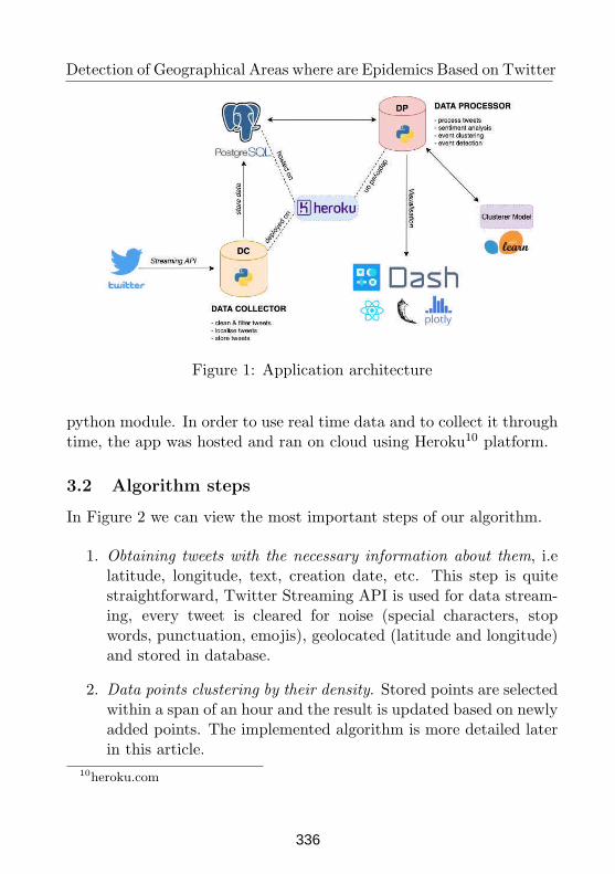
Detection of Geographical Areas where are Epidemics Based on Twitter
Figure 1: Application architecture
python module. In order to use real time data and to collect it throughtime, the app was hosted and ran on cloud using Heroku10 platform.
3.2 Algorithm steps
In Figure 2 we can view the most important steps of our algorithm.
1. Obtaining tweets with the necessary information about them, i.elatitude, longitude, text, creation date, etc. This step is quitestraightforward, Twitter Streaming API is used for data stream-ing, every tweet is cleared for noise (special characters, stopwords, punctuation, emojis), geolocated (latitude and longitude)and stored in database.
2. Data points clustering by their density. Stored points are selectedwithin a span of an hour and the result is updated based on newlyadded points. The implemented algorithm is more detailed laterin this article.
10heroku.com
336
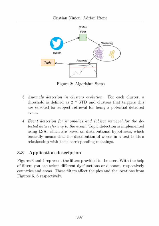
Cristian Ninicu, Adrian Iftene
Figure 2: Algorithm Steps
3. Anomaly detection in clusters evolution. For each cluster, athreshold is defined as 2 * STD and clusters that triggers thisare selected for subject retrieval for being a potential detectedevent.
4. Event detection for anomalies and subject retrieval for the de-
tected data referring to the event. Topic detection is implementedusing LSA, which are based on distributional hypothesis, whichbasically means that the distribution of words in a text holds arelationship with their corresponding meanings.
3.3 Application description
Figures 3 and 4 represent the filters provided to the user. With the helpof filters you can select different dysfunctions or diseases, respectivelycountries and areas. These filters affect the pies and the locations fromFigures 5, 6 respectively.
337
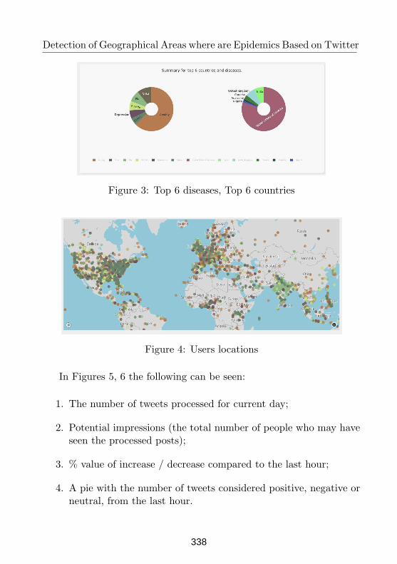
Detection of Geographical Areas where are Epidemics Based on Twitter
Figure 3: Top 6 diseases, Top 6 countries
Figure 4: Users locations
In Figures 5, 6 the following can be seen:
1. The number of tweets processed for current day;
2. Potential impressions (the total number of people who may haveseen the processed posts);
3. % value of increase / decrease compared to the last hour;
4. A pie with the number of tweets considered positive, negative orneutral, from the last hour.
338
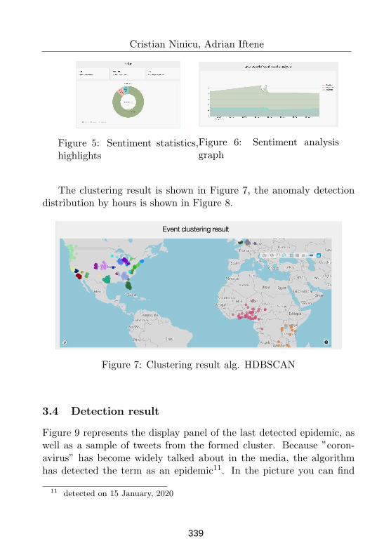
Cristian Ninicu, Adrian Iftene
Figure 5: Sentiment statistics,highlights
Figure 6: Sentiment analysisgraph
The clustering result is shown in Figure 7, the anomaly detectiondistribution by hours is shown in Figure 8.
Figure 7: Clustering result alg. HDBSCAN
3.4 Detection result
Figure 9 represents the display panel of the last detected epidemic, aswell as a sample of tweets from the formed cluster. Because ”coron-avirus” has become widely talked about in the media, the algorithmhas detected the term as an epidemic11. In the picture you can find
11 detected on 15 January, 2020
339
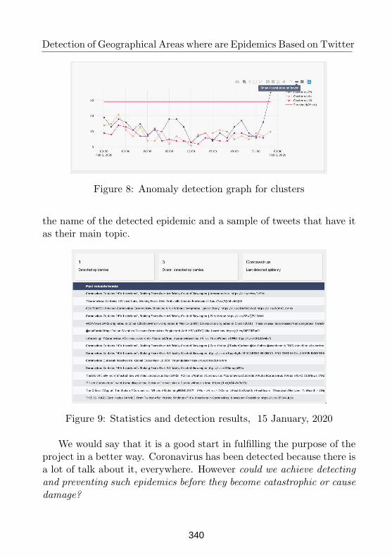
Detection of Geographical Areas where are Epidemics Based on Twitter
Figure 8: Anomaly detection graph for clusters
the name of the detected epidemic and a sample of tweets that have itas their main topic.
Figure 9: Statistics and detection results, 15 January, 2020
We would say that it is a good start in fulfilling the purpose of theproject in a better way. Coronavirus has been detected because there isa lot of talk about it, everywhere. However could we achieve detecting
and preventing such epidemics before they become catastrophic or cause
damage?
340
Cristian Ninicu, Adrian Iftene
4 Other similar works
The overwhelming amount of health related conversations on Twitterhas been a goldmine for the field of epidemiology in that people areoften very open and candid about their health issues in Tweets. Theearliest innovators in this field understood this early and started towork on solutions that consumes this real time stream of data, notonly with main scope being find out health related problems, but alsoother social activities and problems such as terrorism, distribution offake news or local and global trendings in different areas of world’sconsumers.
For example, Commonwealth Scientific and Industrial Research Or-ganisation understood that social media posts such as tweets can beused as input to monitoring or detection algorithm for a more accurateresult and better prevention time. Their proposal solution is using afour step architecture for the early detection of the acute disease events,using social media. The first three steps of the algorithm ensure therelevance of the tweets and the last one is a monitoring algorithm basedon time between tweets. Algorithm steps:
1. Initial Selection. The input to this step was a set of filteringparameters applied to a database of tweets. The output of thisstep was a dataset of tweets where each tweet contains the text,timestamp, and the username of the author on Twitter.
2. Personal Health Mention Classification. Tweets containing wordsindicating disease or symptoms may not necessarily be reports ofthe disease or symptom. Therefore, one important step in theirselection was a personal health mention classification with inputbeing output from step 1 and output shows predicted tweets thatare classified as personal health related. Their implementationcombines a heuristic and statistical classification algorithm in or-der to achieve this.
3. Duplication removal. Epidemic intelligence using hospital recordsconsiders a hospital presentation or a hospital admission as an
341
Detection of Geographical Areas where are Epidemics Based on Twitter
event. We observe that social media poses peculiar challengeswhen tweets are used. While a person presenting themselves to ahospital got counted as one event, a person reporting their healthcondition in multiple tweets or replying to the comments on theirtweet(s) results in multiple events. Similarly, the person couldalso retweet related tweets. As a result, a tweet by itself couldbe regarded as an event.
4. Time between events - based monitoring algorithm. The algo-rithm is summarised as follows: the timestamps of all eventswere converted to integers using the Julian12 value of the ear-liest timestamp as the starting point. The time-between-eventsvalues were computed as the difference between timestamps ofconsecutive events. They then fitted a Weibull distribution 13
for the time-between-events values. After that, for every event,we computed the adapted exponentially weighted moving aver-age as a function of time between events, false discovery rate,and the scale and shape parameters obtained from the Weibulldistribution. The false discovery rate refers to the flagging of anoutbreak when no outbreak has occurred, thus triggering a falsealarm. We experimented with two values of the false discoveryrate: 1 in 1,000 and 1 in 2,000 events. Step 13 in the algorithmwas different from the original article: the algorithm signalled analert when at least P consecutive tweets have an adapted movingaverage lower than 1. The significance of using these consecutivealerts was described in the their paper14. In the case of 1 in 1,000,the algorithm looked for four alerts in a sequence. On the otherhand, in the case of 1 in 2,000, the algorithm looked for two alertsin a sequence. We used R to implement the algorithm, and theGAMLSS model15 to fit the Weibull distribution.
12https://en.wikipedia.org/wiki/Julian day13https://en.wikipedia.org/wiki/Weibull distribution14http://links.lww.com/EDE/B60915https://cran.r-project.org/web/packages/gamlss/index.html
342
Cristian Ninicu, Adrian Iftene
Their results shows a good improvement in detecting and prevent-ing the outbreaks, out of 18 experiment combination, three detectedthe thunderstorm asthma up to 9 hours before the time it was officiallydetected. Their experiments were made on datasets of tweets posted inMelbourne from 2014 to 2016 and the main focus was on the thunder-storm asthma outbreak in Melbourne in November 2016. Comparedto our solution, their proposal was mainly used for discovering localoutbreaks, mainly referring to asthma.
5 Conclusion
With motivation of trying to find out why and how we should processsocial media data, the main goal of this project was to detect andprevent anomalies in health-related topics from Twitter.
The problem still remains open for research and improvements.There’re still space for improving it when talking about aspects suchas NLP or cognitive computational skills, as the computer unit haven’tthe same ability to detect sarcasm, humor, irony, sadness from non-verbal ways of data transmissions, even if this paper was mainly abouttext-related processing, a lot of valuable information could be gainedon cognitive parts when speaking about human intercommunication.The fields of ML and AI are increasing their importance in academicand industrial environment, and this contributes to their integrationinto many projects or industries that previously did not use AI andML for making decision or preventing events, so it looks like the jour-ney for these fields has only started and will grow a lot more in thefuture, also, in combination with other technological progresses suchas 5G, this could lead to even more ways of detecting and analysingbehaviours.
Acknowledgments. This work was supported by project REVERT(taRgeted thErapy for adVanced colorEctal canceR paTients), GrantAgreement number: 848098, H2020-SC1-BHC-2018-2020/H2020-SC1-2019-Two-Stage-RTD.
343
Detection of Geographical Areas where are Epidemics Based on Twitter
References
[1] I. Minea, A. Iftene. News on Twitter. In Proceedings CMSM4(The Fourth Conference of Mathematical Society of the Repub-lic of Moldova), June 25 - July 2, Chisinau, Republic of Moldova,(2017), pp. 535–538.
[2] A. Iftene, A. L. Gınsca. Using Opinion Mining Techniques for
Early Crisis Detection. In International Journal of Computers,Communications & Control. With Emphasis on the Integration ofThree Technologies IJCCC. Workshop on Intelligent Decision Sup-port Systems for Crisis Management (ICCCC2012). Agora Uni-versity Editing House, Oradea, 8-12 May, vol.7, no. 5, (2012), pp.844–851.
[3] A. Iftene, M. S. Dudu, A. R., Miron. Scalable system for opinion
mining on Twitter data. Dynamic visualization for data related to
refugees’ crisis and to terrorist attacks. In 26th International Con-ference on Information Systems Development, Larnaca, Cyprus,September 6-8, (2017).
[4] A. Iftene, D. Gıfu, A.R. Miron, M. S. Dudu. A Real-Time Sys-
tem for Credibility on Twitter. In Proceedings of The 12th Lan-guage Resources and Evaluation Conference (LREC 2020), Mar-seille, France, May 2020, (2020), pp. 6168–6175.
[5] C. S. Atodiresei, A. Tanaselea, A. Iftene. Identifying Fake News
and Fake Users on Twitter. In Proceedings of International Con-ference on Knowledge Based and Intelligent Information and Engi-neering Systems, KES2018, 3-5 September 2018, Belgrade, Serbia.Procedia Computer Science vol. 126, (2018), pp. 451–461.
[6] C. G. Cus,muliuc, L. G. Coca, A. Iftene. Identifying Fake News on
Twitter using Naive Bayes, SVM and Random Forest Distributed
Algorithms. Proceedings of The 13th Edition of the InternationalConference on Linguistic Resources and Tools for Processing Ro-manian Language (ConsILR-2018), (2018), pp. 177–188.
344
Cristian Ninicu, Adrian Iftene
[7] A. L. Gınsca, E. Boros, , A. Iftene, D. Trandabat, , M. Toader, M.Corıci, C. A. Perez, D. Cristea. Sentimatrix - Multilingual Sen-
timent Analysis Service. In Proceedings of the 2nd Workshop onComputational Approaches to Subjectivity and Sentiment Analy-sis (ACL-WASSA2011). ISBN-13 9781937284060, Portland, Ore-gon, USA, June 19-24, (2011), pp. 189–195.
[8] J.A. Hartigan, M. A. Wong. Algorithm AS 136: A k-Means Clus-
tering Algorithm. Journal of the Royal Statistical Society, SeriesC. vol. 28, no. 1, (1979), pp. 100—108.
[9] M. Ester, H.P. Kriegel, J. Sander, X. Xu. A density-based algo-
rithm for discovering clusters in large spatial databases with noise.Proceedings of the Second International Conference on KnowledgeDiscovery and Data Mining (KDD-96). AAAI Press. (1996), pp.226—231.
[10] R.J.G.B. Campello, D. Moulavi, J. Sander. Density-Based Clus-
tering Based on Hierarchical Density Estimates. In: Pei J., TsengV.S., Cao L., Motoda H., Xu G. (eds) Advances in KnowledgeDiscovery and Data Mining. PAKDD 2013. Lecture Notes in Com-puter Science, vol 7819. Springer, Berlin, Heidelberg, (2013).
[11] A. Baran, A. Iftene. Event detection in Tweets. In InternationalConference on Human-Computer Interaction. 8-9 September 2016,Iasi, Romania, (2016), pp. 103–106.
[12] Z. Harris. Distributional structure. Word. vol. 10, no. 23, (1954),pp. 146–162. doi:10.1080/00437956.1954.11659520
[13] https://journals.lww.com/epidem/fulltext/2020/01000/harnessing tweets for early detection of an acute.10.aspx
Cristian Ninicu, Adrian Iftene
”Alexandru Ioan Cuza” University of Iasi, Faculty of Computer ScienceEmail: [email protected], [email protected]
345
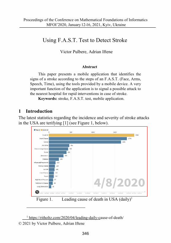
Proceedings of the Conference on Mathematical Foundations of Informatics
MFOI’2020, January 12-16, 2021, Kyiv, Ukraine
© 2021 by Victor Pulbere, Adrian Iftene
Using F.A.S.T. Test to Detect Stroke
Victor Pulbere, Adrian Iftene
Abstract
This paper presents a mobile application that identifies the
signs of a stroke according to the steps of an F.A.S.T. (Face, Arms,
Speech, Time), using the tools provided by a mobile device. A very
important function of the application is to signal a possible attack to
the nearest hospital for rapid interventions in case of stroke.
Keywords: stroke, F.A.S.T. test, mobile application.
1 Introduction
The latest statistics regarding the incidence and severity of stroke attacks
in the USA are terifying [1] (see Figure 1, below).
Figure 1. Leading cause of death in USA (daily)1
1 https://ritholtz.com/2020/04/leading-daily-cause-of-death/
346
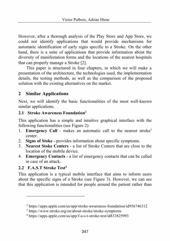
Victor Pulbere, Adrian Iftene
However, after a thorough analysis of the Play Store and App Store, we
could not identify applications that would provide mechanisms for
automatic identification of early signs specific to a Stroke. On the other
hand, there is a suite of applications that provide information about the
diversity of manifestation forms and the locations of the nearest hospitals
that can properly manage a Stroke [2]. This paper is structured in four chapters, in which we will make a
presentation of the architecture, the technologies used, the implementation
details, the testing methods, as well as the comparison of the proposed
solution with the existing alternatives on the market.
2 Similar Applications
Next, we will identify the basic functionalities of the most well-known
similar applications.
2.1 Stroke Awareness Foundation2
This application has a simple and intuitive graphical interface with the
following functionalities (see Figure 2):
1. Emergency Call - makes an automatic call to the nearest stroke3
center.
2. Signs of Stoke - provides information about specific symptoms.
3. Nearest Stoke Centers - a list of Stroke Centers that are close to the
location of the mobile device.
4. Emergency Contacts - a list of emergency contacts that can be called
in case of an attack.
2.2 F.A.S.T Stroke Test4
This application is a typical mobile interface that aims to inform users
about the specific signs of a Stroke (see Figure 3). However, we can see
that this application is intended for people around the patient rather than
2 https://apps.apple.com/us/app/stroke-awareness-foundation/id956746312 3 https://www.stroke.org/en/about-stroke/stroke-symptoms 4 https://apps.apple.com/us/app/f-a-s-t-stroke-test/id833825993
347
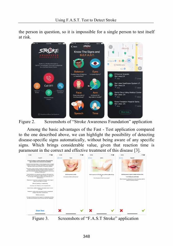
Using F.A.S.T. Test to Detect Stroke
the person in question, so it is impossible for a single person to test itself
at risk.
Figure 2. Screenshots of “Stroke Awareness Foundation” application
Among the basic advantages of the Fast - Test application compared
to the one described above, we can highlight the possibility of detecting
disease-specific signs automatically, without being aware of any specific
signs. Which brings considerable value, given that reaction time is
paramount in the correct and effective treatment of this disease [3].
Figure 3. Screenshots of “F.A.S.T Stroke” application
348
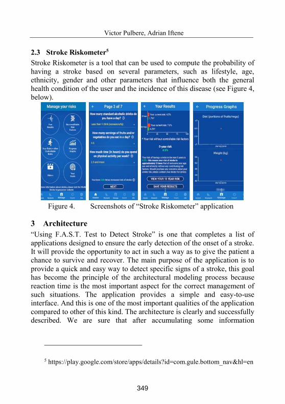
Victor Pulbere, Adrian Iftene
2.3 Stroke Riskometer5
Stroke Riskometer is a tool that can be used to compute the probability of
having a stroke based on several parameters, such as lifestyle, age,
ethnicity, gender and other parameters that influence both the general
health condition of the user and the incidence of this disease (see Figure 4,
below).
Figure 4. Screenshots of “Stroke Riskometer” application
3 Architecture
“Using F.A.S.T. Test to Detect Stroke” is one that completes a list of applications designed to ensure the early detection of the onset of a stroke.
It will provide the opportunity to act in such a way as to give the patient a
chance to survive and recover. The main purpose of the application is to
provide a quick and easy way to detect specific signs of a stroke, this goal
has become the principle of the architectural modeling process because
reaction time is the most important aspect for the correct management of
such situations. The application provides a simple and easy-to-use
interface. And this is one of the most important qualities of the application
compared to other of this kind. The architecture is clearly and successfully
described. We are sure that after accumulating some information
5 https://play.google.com/store/apps/details?id=com.gule.bottom_nav&hl=en
349
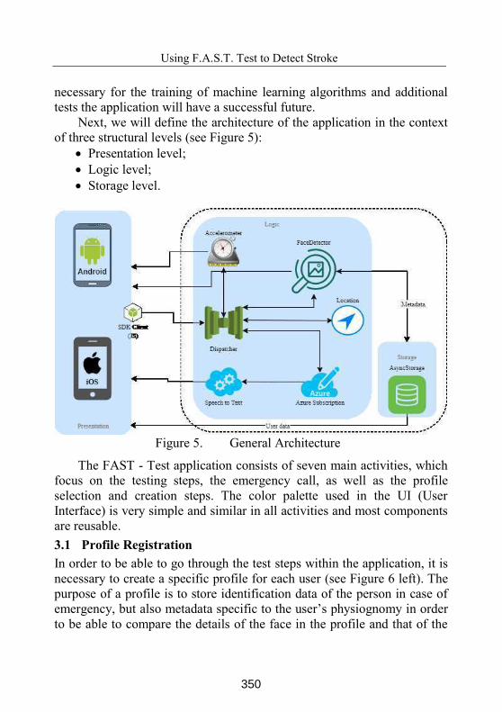
Using F.A.S.T. Test to Detect Stroke
necessary for the training of machine learning algorithms and additional
tests the application will have a successful future.
Next, we will define the architecture of the application in the context
of three structural levels (see Figure 5):
Presentation level;
Logic level;
Storage level.
Figure 5. General Architecture
The FAST - Test application consists of seven main activities, which
focus on the testing steps, the emergency call, as well as the profile
selection and creation steps. The color palette used in the UI (User
Interface) is very simple and similar in all activities and most components
are reusable.
3.1 Profile Registration
In order to be able to go through the test steps within the application, it is
necessary to create a specific profile for each user (see Figure 6 left). The
purpose of a profile is to store identification data of the person in case of
emergency, but also metadata specific to the user’s physiognomy in order
to be able to compare the details of the face in the profile and that of the
350
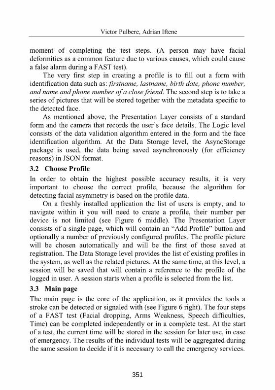
Victor Pulbere, Adrian Iftene
moment of completing the test steps. (A person may have facial
deformities as a common feature due to various causes, which could cause
a false alarm during a FAST test).
The very first step in creating a profile is to fill out a form with
identification data such as: firstname, lastname, birth date, phone number,
and name and phone number of a close friend. The second step is to take a
series of pictures that will be stored together with the metadata specific to
the detected face.
As mentioned above, the Presentation Layer consists of a standard
form and the camera that records the user’s face details. The Logic level
consists of the data validation algorithm entered in the form and the face
identification algorithm. At the Data Storage level, the AsyncStorage
package is used, the data being saved asynchronously (for efficiency
reasons) in JSON format.
3.2 Choose Profile
In order to obtain the highest possible accuracy results, it is very
important to choose the correct profile, because the algorithm for
detecting facial asymmetry is based on the profile data.
On a freshly installed application the list of users is empty, and to
navigate within it you will need to create a profile, their number per
device is not limited (see Figure 6 middle). The Presentation Layer
consists of a single page, which will contain an “Add Profile” button and
optionally a number of previously configured profiles. The profile picture
will be chosen automatically and will be the first of those saved at
registration. The Data Storage level provides the list of existing profiles in
the system, as well as the related pictures. At the same time, at this level, a
session will be saved that will contain a reference to the profile of the
logged in user. A session starts when a profile is selected from the list.
3.3 Main page
The main page is the core of the application, as it provides the tools a
stroke can be detected or signaled with (see Figure 6 right). The four steps
of a FAST test (Facial dropping, Arms Weakness, Speech difficulties,
Time) can be completed independently or in a complete test. At the start
of a test, the current time will be stored in the session for later use, in case
of emergency. The results of the individual tests will be aggregated during
the same session to decide if it is necessary to call the emergency services.
351
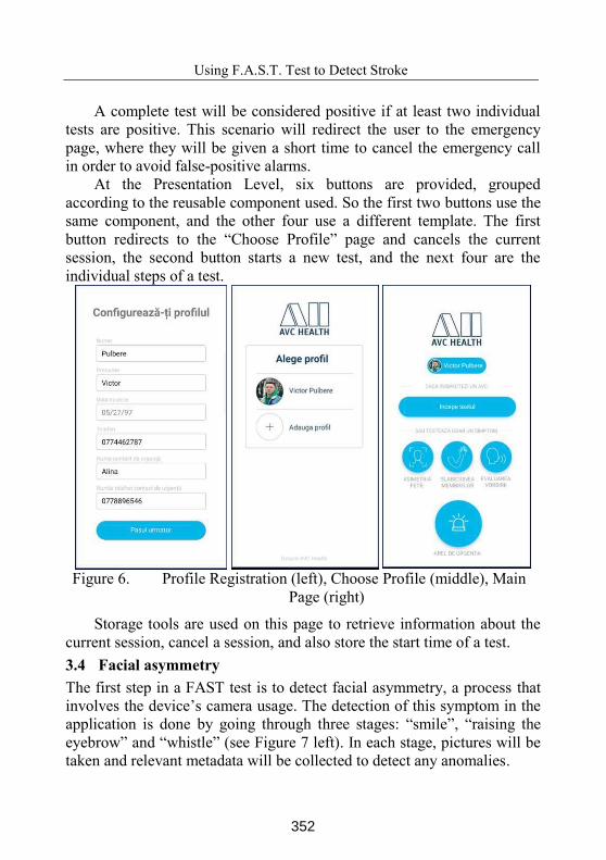
Using F.A.S.T. Test to Detect Stroke
A complete test will be considered positive if at least two individual
tests are positive. This scenario will redirect the user to the emergency
page, where they will be given a short time to cancel the emergency call
in order to avoid false-positive alarms.
At the Presentation Level, six buttons are provided, grouped
according to the reusable component used. So the first two buttons use the
same component, and the other four use a different template. The first
button redirects to the “Choose Profile” page and cancels the current session, the second button starts a new test, and the next four are the
individual steps of a test.
Figure 6. Profile Registration (left), Choose Profile (middle), Main
Page (right)
Storage tools are used on this page to retrieve information about the
current session, cancel a session, and also store the start time of a test.
3.4 Facial asymmetry
The first step in a FAST test is to detect facial asymmetry, a process that
involves the device’s camera usage. The detection of this symptom in the
application is done by going through three stages: “smile”, “raising the
eyebrow” and “whistle” (see Figure 7 left). In each stage, pictures will be
taken and relevant metadata will be collected to detect any anomalies.
352
Victor Pulbere, Adrian Iftene
Figure 7. Facial asymmetry (left), Arms weakness (right)
The current page consists of the key element: the camera, as well as
some secondary details, such as the template for the correct positioning of
the face in the center and at an angle of 0, the frame indicating the
position and size of the face detected in relation to the template and at the
bottom a bar describing the current stage and the action to be taken. When
the detected face falls within the parameters set by the template and the
malformation detection algorithm is completed, a green checkmark or a
red X will appear at the bottom of the page, indicating a visible
malformation.
A very important landmark in establishing the facial asymmetry can
be considered the mouth positioning because at this level the most visible
and implicitly most important anomalies can appear. As assumed
mentioned above, the facial asymmetry can be reduced to the mouth
position analysis in Cartesian coordinates. Each step will result in the
evaluation of the probability of a Stroke according to an established
heuristic computed from the analysis of a data set related to the
differences in the mouth positioning at the time of an attack in contrast to
the usual condition (the one in profile). Therefore, the heuristic is based
on the following sequence of actions:
353
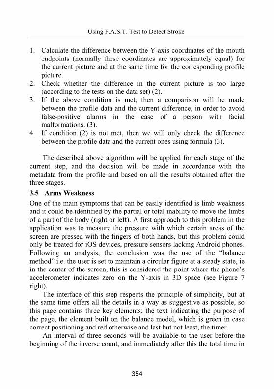
Using F.A.S.T. Test to Detect Stroke
1. Calculate the difference between the Y-axis coordinates of the mouth
endpoints (normally these coordinates are approximately equal) for
the current picture and at the same time for the corresponding profile
picture.
2. Check whether the difference in the current picture is too large
(according to the tests on the data set) (2).
3. If the above condition is met, then a comparison will be made
between the profile data and the current difference, in order to avoid
false-positive alarms in the case of a person with facial
malformations. (3).
4. If condition (2) is not met, then we will only check the difference
between the profile data and the current ones using formula (3).
The described above algorithm will be applied for each stage of the
current step, and the decision will be made in accordance with the
metadata from the profile and based on all the results obtained after the
three stages.
3.5 Arms Weakness
One of the main symptoms that can be easily identified is limb weakness
and it could be identified by the partial or total inability to move the limbs
of a part of the body (right or left). A first approach to this problem in the
application was to measure the pressure with which certain areas of the
screen are pressed with the fingers of both hands, but this problem could
only be treated for iOS devices, pressure sensors lacking Android phones.
Following an analysis, the conclusion was the use of the “balance
method” i.e. the user is set to maintain a circular figure at a steady state, ie
in the center of the screen, this is considered the point where the phone’s
accelerometer indicates zero on the Y-axis in 3D space (see Figure 7
right).
The interface of this step respects the principle of simplicity, but at
the same time offers all the details in a way as suggestive as possible, so
this page contains three key elements: the text indicating the purpose of
the page, the element built on the balance model, which is green in case
correct positioning and red otherwise and last but not least, the timer.
An interval of three seconds will be available to the user before the
beginning of the inverse count, and immediately after this the total time in
354
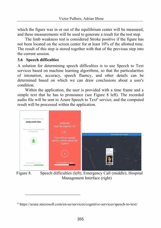
Victor Pulbere, Adrian Iftene
which the figure was in or out of the equilibrium center will be measured,
and these measurements will be used to generate a result for the test step.
The limb weakness test is considered Stroke positive if the figure has
not been located on the screen center for at least 10% of the allotted time.
The result of this step is stored together with that of the previous step into
the current session.
3.6 Speech difficulties
A solution for determining speech difficulties is to use Speech to Text
services based on machine learning algorithms, so that the particularities
of intonation, accuracy, speech fluency, and other details can be
determined based on which we can draw conclusions about a user's
condition.
Within the application, the user is provided with a time frame and a
simple text that he has to pronounce (see Figure 8 left). The recorded
audio file will be sent to Azure Speech to Text6 service, and the computed
result will be processed within the application.
Figure 8. Speech difficulties (left), Emergency Call (middle), Hospital
Management Interface (right)
6 https://azure.microsoft.com/en-us/services/cognitive-services/speech-to-text/
355
Using F.A.S.T. Test to Detect Stroke
At the presentation level, this step consists of a single page, which
includes details about the actions to be taken, a button that starts the audio
recording, and a stopwatch at the bottom, which represents the time
remaining from the one initially allocated for this step.
Information obtained from the Cloud service is being processed
within the application.
3.7 Emergency Call
The emergency call is actually the last step in a FAST test, and its purpose
is to report a stroke to a specialized unit (see Figure 8 middle). Within the
application, the emergency call represents the moment when the patient’s
identification and location data will be sent to the nearest hospital.
In order to avoid false-positive alarms, the emergency call can be
canceled by the user. The cancellation mechanism is very simple, but it
still has a level of security in that the button must be held down for it to be
fulfilled and the user will be redirected to the home page, so a simple click
will be ignored. When the allotted time expires, a WebSocket connection
is initiated with the server and the device location services start. The first
message sent to the server contains a unique identifier generated at startup
and user profile information, along with a session photo that was rated as
Stroke Positive. Location and speed variations are iteratively tracked
within the Hospital Management Interface.
3.8 Hospital Management Interface
For efficient management of emergencies, it has become necessary to
introduce a separate component for the hospital, which aims to view the
requests initiated by the application in real-time. Currently, the hospital
interface is an interactive map that provides two types of graphical
elements: a blue pin indicating the location of the concerned hospital and
the red dots, illustrating the location of devices that initiated emergency
calls. Each red dot will generate a short report on the profile of the person
at risk, this report will contain the information stored in the user's profile.
The profile data and the photo sent by the application can be used by the
medical staff to decide on a possible false alarm, or to identify the
predisposition to a certain type of disease in advance: ischemic or
hemorrhagic [4].
356
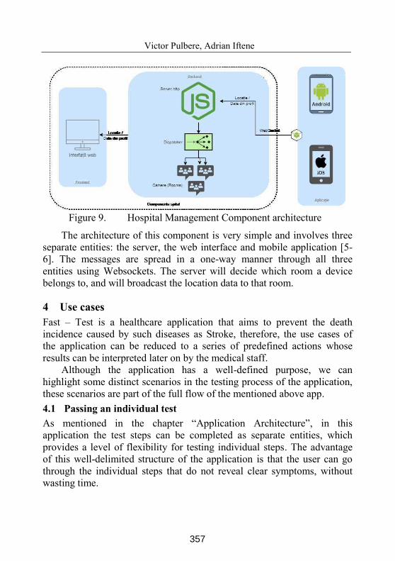
Victor Pulbere, Adrian Iftene
Figure 9. Hospital Management Component architecture
The architecture of this component is very simple and involves three
separate entities: the server, the web interface and mobile application [5-
6]. The messages are spread in a one-way manner through all three
entities using Websockets. The server will decide which room a device
belongs to, and will broadcast the location data to that room.
4 Use cases
Fast – Test is a healthcare application that aims to prevent the death
incidence caused by such diseases as Stroke, therefore, the use cases of
the application can be reduced to a series of predefined actions whose
results can be interpreted later on by the medical staff.
Although the application has a well-defined purpose, we can
highlight some distinct scenarios in the testing process of the application,
these scenarios are part of the full flow of the mentioned above app.
4.1 Passing an individual test
As mentioned in the chapter “Application Architecture”, in this
application the test steps can be completed as separate entities, which
provides a level of flexibility for testing individual steps. The advantage
of this well-delimited structure of the application is that the user can go
through the individual steps that do not reveal clear symptoms, without
wasting time.
357
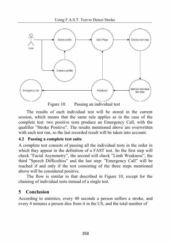
Using F.A.S.T. Test to Detect Stroke
Figure 10. Passing an individual test
The results of each individual test will be stored in the current
session, which means that the same rule applies as in the case of the
complete test: two positive tests produce an Emergency Call, with the
qualifier ”Stroke Positive”. The results mentioned above are overwritten
with each test run, so the last recorded result will be taken into account.
4.2 Passing a complete test suite
A complete test consists of passing all the individual tests in the order in
which they appear in the definition of a FAST test. So the first step will
check ”Facial Asymmetry”, the second will check ”Limb Weakness”, the third ”Speech Difficulties” and the last step: ”Emergency Call” will be
reached if and only if the test consisting of the three steps mentioned
above will be considered positive.
The flow is similar to that described in Figure 10, except for the
chaining of individual tests instead of a single test.
5 Conclusion
According to statistics, every 40 seconds a person suffers a stroke, and
every 4 minutes a person dies from it in the US, and the total number of
358
Victor Pulbere, Adrian Iftene
deaths rises to 140,000 in one year7. The age of technology could provide
a way of saving thousands of lives and this has been highlighted in the
context of the current pandemic (COVID-19). The health sector needs a
continuous collaboration with that of Information Technologies, both in
terms of preventing risk factors and in the effective treatment of their
patients.
The Fast - Test application started with a well-defined purpose:
“reporting of stroke-specific symptoms in a short time” - a very important
aspect in the context of this disease, moreover, we can say that the
measure of time is inversely proportional to a patient’s chance of life.
Future work envisages a substantial improvement through the use of
machine learning algorithms to detect facial asymmetry, which is
impossible at this stage due to lack of training data. This application could
be used to collect this data by storing images during the tests with the
consent of the users.
Another improvement could be the usage of a more complex test,
such as NEWFAST (nausea, eyes, walking, facial dropping, arm
weakness, speech, terrible headache) or BE-FAST (balance, eyes, face,
arms, speech, time), but in this case, the time and complexity of the test
should be taken into consideration.
Acknowledgments. This work was supported by project REVERT
(taRgeted thErapy for adVanced colorEctal canceR paTients), Grant
Agreement number: 848098, H2020-SC1-BHC-2018-2020/H2020-SC1-
2019-Two-Stage-RTD.
References
[1] J. D. Guzman, J. A. Egido, C. F. Pérez, B. Fuentes, G. Barberá-Comes, R.
Gabriel-Sánchez. Stroke and transient ischemic attack incidence rate in
Spain: The IBERICTUS study. Cerebrovascular Diseases vol. 34, issue 4,
(2012), pp. 272-281.
[2] M. Rezmerita, I. Cercel, A. Iftene. Stroke Detector - An Application that
applies the F.A.S.T. Test to Identify Stroke. In Proceedings of the 17th
7 https://www.cdc.gov/stroke/facts.htm
359
Using F.A.S.T. Test to Detect Stroke
International Conference on Human-Computer Interaction RoCHI 2020, 22-
23 October, (2020).
[3] C. E.Weber. Stroke: Brain Attack, Time to React. AACN Clinical Issues
Advanced Practice in Acute and Critical Care, vol. 6, issue 4, (1995), pp.
562-75.
[4] T. Sorenson, E. Giordan, G. Lanzino. Neurosurgery for Ischemic and
Hemorrhagic Stroke. In book “Fundamentals of Neurosurgery” 10.1007/978-
3-030-17649-5_9 (2019).
[5] C. Damian, L. Alboaie, A. Iftene. Using WSN and Mobile Apps for Home
and Office Ambient Monitoring and Control. In International Conference on
Human-Computer Interaction, 8-9 September, Iasi, Romania, (2016), pp. 42-
45.
[6] C. I. Irimia, A. Iftene. Mobile Application for UAIC Home. In Proceedings of
the 16th International Conference on Human-Computer Interaction RoCHI
2019, 17-18 October, Politehnica University of Bucharest, Romania (2019),
pp. 102-109.
Victor Pulbere, Adrian Iftene
“Alexandru Ioan Cuza” University of Iasi, Faculty of Computer Science
E-mail: [email protected], [email protected]
360
Proceedings of the Conference on Mathematical Foundations of Informatics
MFOI2020, January 12-16, 2021, Kyiv, Ukraine
A Disambiguation Model for Natural Language
Processing
Stefan Stratulat, Dumitru Prijilevschi
Gheorghe Morari, Tudor Bumbu
Abstract
This article describes the implementation of a method fornatural language disambiguation. It includes the encounteredproblems, their description and proposed solutions. The paperemphasizes the principal Natural Language Processing problemsfrom Artificial Intelligence domain: the processing of semantics,structure, linguistics, and pragmatics.
Keywords: disambiguation, punctuation markup language,natural language processing
1 Motivation
The primary problems of the Natural Language Processing (NLP)domain have a factorial complexity which can only be solved with con-nectionism models, which at the moment cannot be widely used. Away to resolve the primary problems is to define new models that canbetter describe the Natural Language.
NLP is a subdomain of AI. This means that AI can be used inall fields where human interaction exists, e.g.: medical, military, eco-nomics, education, etc.
The development of the AI and NLP systems are propelled by theresults these domains offer, making big economic changes in the world.
The primary problems of the NLP domain described in this arti-cle are: semantic problem, structural problem, inter-sentence problem,inter-textual problem, linguistic problem, contextual problem.
©2020 by Stefan Stratulat et al.
361
Stefan Stratulat et al.
2 Notions
• Ambiguous - open to more than one interpretation; not havingone obvious meaning;
• Disambiguation - the process of removing ambiguity by identify-ing all interpretations;
• Token - an entity of the textual structure;
• Tokenisation - the process of conversion of a text into tokens;
• ’B’ Structure - implicit structure that represents multiple ele-ments from its substructure (words). The structure is boundedby ’,’ or ’.’ characters see figure 8 (page 18);
• Atom - smallest unit that cannot be divided;
• Atomification - the process of grouping two or more textual en-tities into one atomic textual entity;
• Structural Atomification - the process of grouping two or moretextual structures into one atomic textual structure;
• Semantic Reduction - process applied to texts, that results inthe minimisation or reduction of semantics from the source text,while maintaining its structure.
3 Introduction
The AI domain at the moment is characterised by three develop-ment periods. The most fitting historic period for this article is the sec-ond period called the “Romantic” period, which lasted through 1965-1975 and is characterised by the effort to understand natural languages[1]. In these trials of language understanding appear such systemsas ELIZA (1965) and PARRY (1972), which tried to simulate human
362
A Disambiguation Model for NLP
behaviour. All the activities of the past, helped at creation of NLPdomain.
To this day NLP remains a science from the AI domain. It is usedto analyze NLP problems and with the help of natural language modelsand structures, it can be used to create human-computer interactionapplications.
With greater understanding of the natural languages, there ap-peared multiple problems of varying complexities, which were cate-gorised into structural and semantic problems. Structural problemstackled the understanding and the computational processing of dif-ferent forms of expressions of natural languages. Semantic problemstackle the understanding and the processing of meaning. Most of theunresolved problems are semantic problems. The solutions for the un-resolved natural language semantic problems can influence directly thesolving of unresolved structural problems.
The structural and semantic problems, which are not solved yet,can be described in one word: ambiguities. In the NLP domain am-biguities are considered to be the uncertainty of the meaning a text,the uncertainty of its entities’ meaning, or the variety of structuralrepresentations that can represent the same meaning. Ambiguities ofmeaning and structure induce an uncertainty for the representationof natural languages or its understanding, because it is unclear whichvariation to use when in the processing of a text.
The processing of natural language, represents computations of highcomplexity, which cannot be realised only with human implication. Theprogress in the computer computation domain offered the possibility tocompute the most complex formulas in a fraction of the time, comparedto human computation.
A textual disambiguation system is a computational model thatuses component interaction to solve the natural language semantic andstructural ambiguities.
363
Stefan Stratulat et al.
4 Similar works
The problems addressed in this article are actual for several years,where many people are currently trying to solve today’s problems,many researchers have partial results for the subproblems of the dis-ambiguation problem. Many papers in this field are published annu-ally, and the models and ideas described in these articles have led tothe emergence of many subdomains of the AI field, such as: MachineTranslation, Question Answering, Natural Language Disambiguation,etc. Some more recent works, which have a tangent to the given articleand propose an approach that is of interest.
4.1 Sequential Contextual Similarity Matrix Multiplica-
tion
SCSMM (Sequential Contextual Similarity Matrix Multiplication)represents a novel knowledge-based word sense disambiguation algo-rithm witch combines semantic similarity, heuristic knowledge, anddocument context to respectively exploit the merits of local contextbetween consecutive terms, human knowledge about terms, and a doc-ument’s main topic in disambiguating terms. The SCSMM article de-scribes in detail the proposed algorithm, the positive parts, the negativeparts and the comparison with other algorithms. In addition, the arti-cle discusses the impact of the level of division (granularity), ambiguityrate, sentence size, and part of speech distribution on the performanceof the proposed algorithm [3].
4.2 Learning to Disambiguate Natural Language Using
World Knowledge
This paper presents a framework and a learning algorithm on theproblem of concept labeling, what means that each word in a given sen-tence has to be tagged with the unique physical entity (e.g. person, ob-ject or location) or abstract concept it refers to. The method describedin article allows both world knowledge and linguistic information to
364
A Disambiguation Model for NLP
be used during learning and prediction. Was showed experimentallythat the model can handle natural language and learn to use worldknowledge to resolve ambiguities in language, such as word senses orcoreference, without the use of hand-crafted rules or features [4].
4.3 On Conceptual Labeling of a Bag of Words
This paper represents an introduction to the idea of annotation(conceptual labeling), which aims at generating a minimum set of con-ceptual labels that best summarize a bag of words. To achieve the goal,was used an information theoretic approach to trade-off the semanticcoverage of a bag of words against the minimally of the output labels.The experimental results in this article demonstrate the effectiveness oftheir approach in representing the explicit semantics of a bag of words[5].
4.4 Zero-shot Word Sense Disambiguation using Sense
Definition Embeddings
This article proposes Extended WSD (Word Sense Disambiguation)Incorporating Sense Embeddings, a supervised model to perform WSDby predicting over a continuous sense embedding space as opposed toa discrete label space. This allows EWISE to generalize over bothseen and unseen senses, thus achieving generalized zero-shot learning.To obtain target sense embeddings, EWISE utilizes sense definitions.EWISE learns a novel sentence encoder forsense definitions by usingWordNet relations. In this article also was compared EWISE againstother sentence encoders pretrained on large corpora to generate defini-tion embeddings [6].
5 Problems
The human activity is always trying to answer the questions andsolve the problems the society has, with the use of their intellectual
365
Stefan Stratulat et al.
capacity. The questions that don’t have answers, are the basis of re-search of their respective domains. A part of the problems associatedwith the understanding of meaning and language processing are partof the NLP domain.
The developed systems that use AI can be classified in two types,the first type is weak AI, and the second type is strong AI. StrongAI implies an intelligent system with the capacity to obtain humanbehaviour characteristics. Weak AI is used to tackle problems one byone, generally considered as easy tasks for a human. The developmentof strong AI relies on new discoveries of the 21st century, which de-fine the primary problems of AI, and NLP, that are currently widelyresearched.
The nature of the primary problems of the AI domain is computa-tional and theoretic expression of human ideas in origin, The primaryproblems of the AI domain are closely linked with computational prob-lems, and linguistic problems. The linguistic problem contains multiplesub-problems which all have the understanding of the natural languageas the base problem. The computational problems are characterisedmostly by the limits of the current technology, at this time we have anunbelievable amount of computational power, yet it’s not enough forsome type of workloads.
The most important problems are:
• linguistic - different languages use different structural entities toconvey the same semantic entities;
• contextual - same structural entities can represent different se-mantic entities based on the context;
• inter-sentence - ambiguity is present inside sentences;
• inter-textual - ambiguity is present inside texts;
• data scarcity - scarcity of the useful data, for the needed lan-guages;
• data quality - poor quality of useful information.
366
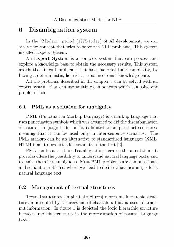
A Disambiguation Model for NLP
6 Disambiguation system
In the “Modern” period (1975-today) of AI development, we cansee a new concept that tries to solve the NLP problems. This systemis called Expert System.
An Expert System is a complex system that can process andexplore a knowledge base to obtain the necessary results. This systemavoids the difficult problems that have factorial time complexity, byhaving a deterministic, heuristic, or connectionist knowledge base.
All the problems described in the chapter 5 can be solved with anexpert system, that can use multiple components which can solve oneproblem each.
6.1 PML as a solution for ambiguity
PML (Punctuation Markup Language) is a markup language thatuses punctuation symbols which was designed to aid the disambiguationof natural language texts, but it is limited to simple short sentences,meaning that it can be used only in inter-sentence scenarios. ThePML markup can be an alternative to standardised languages (XML,HTML), as it does not add metadata to the text [2].
PML can be a used for disambiguation because the annotations itprovides offers the possibility to understand natural language texts, andto make them less ambiguous. Most PML problems are computationaland semantic problems, where we need to define what meaning is for anatural language text.
6.2 Management of textual structures
Textual structures (Implicit structures) represents hierarchic struc-tures represented by a succession of characters that is used to trans-mit information. In figure 1 is depicted the logic hierarchic structurebetween implicit structures in the representation of natural languagetexts.
367
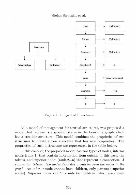
Stefan Stratulat et al.
Figure 1. Integrated Structures.
As a model of management for textual structures, was proposed amodel that represents a space of states in the form of a graph whichhas a tree-like structure. This model combines the proprieties of twostructures to create a new structure that has new proprieties. Theproprieties of such a structure are represented in the table below.
In this context, the proposed model has two types of nodes, inferiornodes (rank 1) that contain information from outside in this case, thetokens, and superior nodes (rank 2...n) that represent a connection. Aconnection between two nodes describes a path between the nodes in the
graph. An inferior node cannot have children, only parents (superiornodes). Superior nodes can have only two children, which are chosen
368
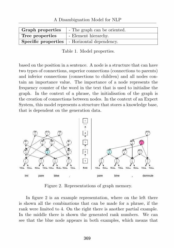
A Disambiguation Model for NLP
Graph properties - The graph can be oriented.
Tree properties - Element hierarchy.
Specific properties - Horizontal dependency.
Table 1. Model properties.
based on the position in a sentence. A node is a structure that can havetwo types of connections, superior connections (connections to parents)and inferior connections (connections to children) and all nodes con-tain an importance value. The importance of a node represents thefrequency counter of the word in the text that is used to initialise thegraph. In the context of a phrase, the initialisation of the graph isthe creation of connections between nodes. In the context of an ExpertSystem, this model represents a structure that stores a knowledge base,that is dependent on the generation data.
Figure 2. Representations of graph memory.
In figure 2 is an example representation, where on the left thereis shown all the combinations that can be made for a phrase, if therank were limited to 4. On the right there is another partial example.In the middle there is shown the generated rank numbers. We cansee that the blue node appears in both examples, which means that
369
Stefan Stratulat et al.
this particular node will have a higher importance, when comparedto others. Each node has an index and a frequency of occurrence inthe text. Nodes that have NULL terminals, their index correspondsto the words in the text. Nodes that do not have NULL terminalsrepresent different hierarchies of binary associations. In the figure 2the nodes marked with the identifiers M1-M15 represent a hierarchy ofbinary associations. The rank of the hierarchy represents the numberof association ranks, where rank 1 is the nodes that have null children(rank 1 represent tokens in the text), the rank from 2 to N representscomplex associations with the number M of association levels, where Mis from 1 to the N-1. To evaluate the annotation efficiency of the givenmodel, the annotation of this model was compared with the manualannotation.
Manual annotation:
1. ((In ziua) urmatoare), (((vei merge) (la lucru)) (fara servieta)).
2. (Daca ((nu sunt) eu)),(((ıt, i da) (servitorul meu)) dict, ionarul).
3. ((((La schemele) (cu (trei arbori))) ((este (foarte dificila))(coordonarea lor))) (s, i (((foarte put, ini) (producatori (din lume)))((dispun ((de tehnologia) necesara)) (ın (acest caz)))))).
Model annotation:
1. (In ziua urmatoare),((vei merge la lucru) fara servieta).
2. (Daca nu sunt eu),((ıt, i da servitorul meu) dict, ionarul).
3. (((La schemele cu trei arbori) (este foarte dificilacoordonarea lor)) (s, i ((foarte put, ini producatori din lume) ((dis-pun (de tehnologia necesara)) ın acest caz)))).
The manual annotation represent the ground truth, because theresults are so close to the ground truth, we consider that the modelhas achieved its performance targets.
370
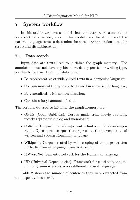
A Disambiguation Model for NLP
7 System workflow
In this article we have a model that annotates word associationsfor structural disambiguation. This model uses the structure of thenatural language texts to determine the necessary annotations used forstructural disambiguation.
7.1 Data search
Input data are texts used to initialize the graph memory. Theannotation must not have any bias towards any particular writing type,for this to be true, the input data must:
• Be representative of widely used texts in a particular language;
• Contain most of the types of texts used in a particular language;
• Be generalised, with no specialisation;
• Contain a large amount of texts.
The corpora we used to initialise the graph memory are:
• OPUS (Open Subtitles), Corpus made from movie captions,mostly represents dialog and monologue;
• CoRoLa (Corpusul de referint, a pentru limba romana contempo-rana), Open access corpus that represents the current state ofwritten and spoken Romanian language;
• Wikipedia, Corpus created by web-scraping of the pages writtenin the Romanian language from Wikipedia;
• RoWordNet, Semantic network for the Romanian language;
• UD (Universal Dependencies), Framework for consistent annota-tion of grammar across across different natural languages.
Table 2 shows the number of sentences that were extracted fromthe respective resources.
371
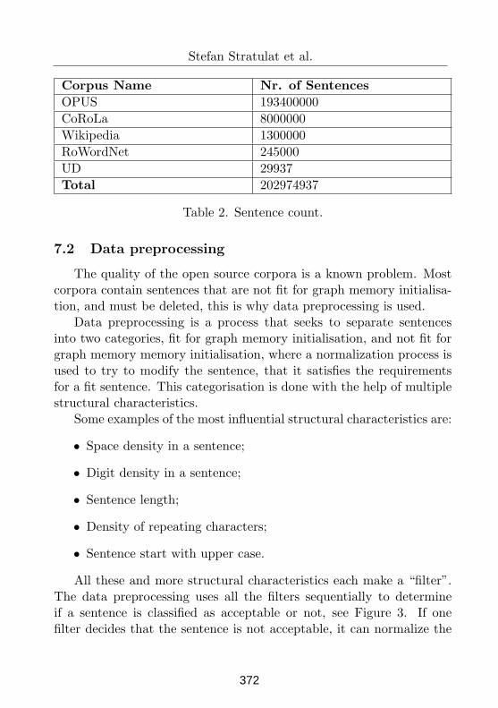
Stefan Stratulat et al.
Corpus Name Nr. of Sentences
OPUS 193400000
CoRoLa 8000000
Wikipedia 1300000
RoWordNet 245000
UD 29937
Total 202974937
Table 2. Sentence count.
7.2 Data preprocessing
The quality of the open source corpora is a known problem. Mostcorpora contain sentences that are not fit for graph memory initialisa-tion, and must be deleted, this is why data preprocessing is used.
Data preprocessing is a process that seeks to separate sentencesinto two categories, fit for graph memory initialisation, and not fit forgraph memory memory initialisation, where a normalization process isused to try to modify the sentence, that it satisfies the requirementsfor a fit sentence. This categorisation is done with the help of multiplestructural characteristics.
Some examples of the most influential structural characteristics are:
• Space density in a sentence;
• Digit density in a sentence;
• Sentence length;
• Density of repeating characters;
• Sentence start with upper case.
All these and more structural characteristics each make a “filter”.The data preprocessing uses all the filters sequentially to determineif a sentence is classified as acceptable or not, see Figure 3. If onefilter decides that the sentence is not acceptable, it can normalize the
372
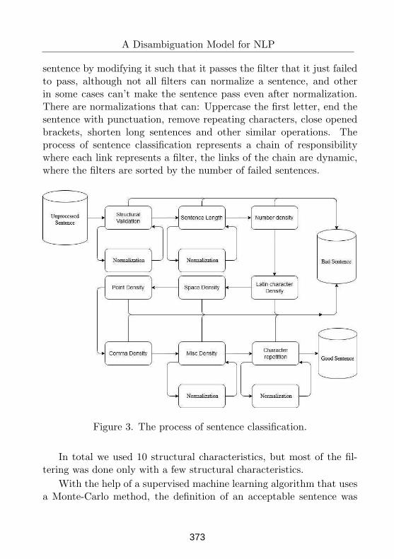
A Disambiguation Model for NLP
sentence by modifying it such that it passes the filter that it just failedto pass, although not all filters can normalize a sentence, and otherin some cases can’t make the sentence pass even after normalization.There are normalizations that can: Uppercase the first letter, end thesentence with punctuation, remove repeating characters, close openedbrackets, shorten long sentences and other similar operations. Theprocess of sentence classification represents a chain of responsibilitywhere each link represents a filter, the links of the chain are dynamic,where the filters are sorted by the number of failed sentences.
Figure 3. The process of sentence classification.
In total we used 10 structural characteristics, but most of the fil-tering was done only with a few structural characteristics.
With the help of a supervised machine learning algorithm that usesa Monte-Carlo method, the definition of an acceptable sentence was
373
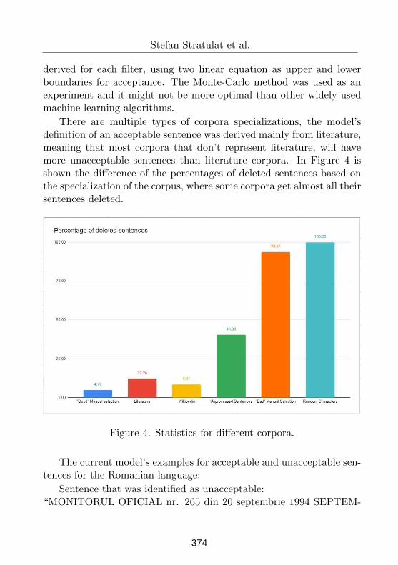
Stefan Stratulat et al.
derived for each filter, using two linear equation as upper and lowerboundaries for acceptance. The Monte-Carlo method was used as anexperiment and it might not be more optimal than other widely usedmachine learning algorithms.
There are multiple types of corpora specializations, the model’sdefinition of an acceptable sentence was derived mainly from literature,meaning that most corpora that don’t represent literature, will havemore unacceptable sentences than literature corpora. In Figure 4 isshown the difference of the percentages of deleted sentences based onthe specialization of the corpus, where some corpora get almost all theirsentences deleted.
Figure 4. Statistics for different corpora.
The current model’s examples for acceptable and unacceptable sen-tences for the Romanian language:
Sentence that was identified as unacceptable:“MONITORUL OFICIAL nr. 265 din 20 septembrie 1994 SEPTEM-
374
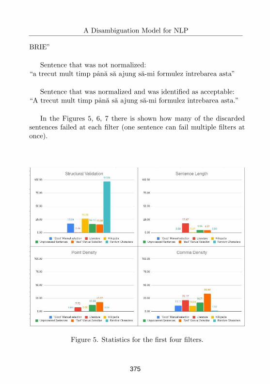
A Disambiguation Model for NLP
BRIE”
Sentence that was not normalized:“a trecut mult timp pana sa ajung sa-mi formulez ıntrebarea asta”
Sentence that was normalized and was identified as acceptable:“A trecut mult timp pana sa ajung sa-mi formulez ıntrebarea asta.”
In the Figures 5, 6, 7 there is shown how many of the discardedsentences failed at each filter (one sentence can fail multiple filters atonce).
Figure 5. Statistics for the first four filters.
375
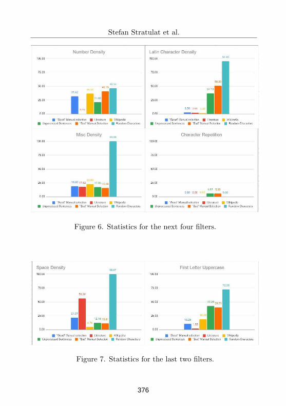
Stefan Stratulat et al.
Figure 6. Statistics for the next four filters.
Figure 7. Statistics for the last two filters.
376
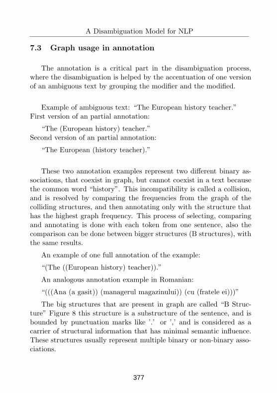
A Disambiguation Model for NLP
7.3 Graph usage in annotation
The annotation is a critical part in the disambiguation process,where the disambiguation is helped by the accentuation of one versionof an ambiguous text by grouping the modifier and the modified.
Example of ambiguous text: “The European history teacher.”First version of an partial annotation:
“The (European history) teacher.”Second version of an partial annotation:
“The European (history teacher).”
These two annotation examples represent two different binary as-sociations, that coexist in graph, but cannot coexist in a text becausethe common word “history”. This incompatibility is called a collision,and is resolved by comparing the frequencies from the graph of thecolliding structures, and then annotating only with the structure thathas the highest graph frequency. This process of selecting, comparingand annotating is done with each token from one sentence, also thecomparison can be done between bigger structures (B structures), withthe same results.
An example of one full annotation of the example:
“(The ((European history) teacher)).”
An analogous annotation example in Romanian:
“(((Ana (a gasit)) (managerul magazinului)) (cu (fratele ei)))”
The big structures that are present in graph are called “B Struc-ture” Figure 8 this structure is a substructure of the sentence, and isbounded by punctuation marks like ’.’ or ’,’ and is considered as acarrier of structural information that has minimal semantic influence.These structures usually represent multiple binary or non-binary asso-ciations.
377
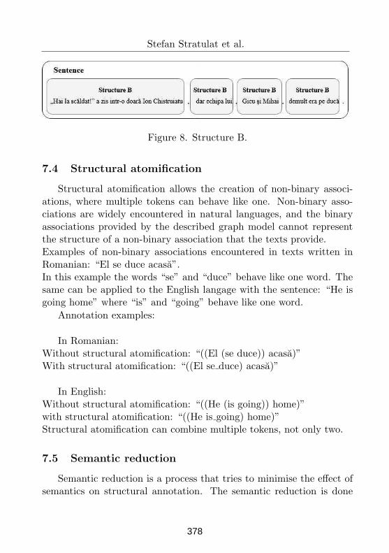
Stefan Stratulat et al.
Figure 8. Structure B.
7.4 Structural atomification
Structural atomification allows the creation of non-binary associ-ations, where multiple tokens can behave like one. Non-binary asso-ciations are widely encountered in natural languages, and the binaryassociations provided by the described graph model cannot representthe structure of a non-binary association that the texts provide.Examples of non-binary associations encountered in texts written inRomanian: “El se duce acasa”.In this example the words “se” and “duce” behave like one word. Thesame can be applied to the English langage with the sentence: “He isgoing home” where “is” and “going” behave like one word.
Annotation examples:
In Romanian:Without structural atomification: “((El (se duce)) acasa)”With structural atomification: “((El se duce) acasa)”
In English:Without structural atomification: “((He (is going)) home)”with structural atomification: “((He is going) home)”Structural atomification can combine multiple tokens, not only two.
7.5 Semantic reduction
Semantic reduction is a process that tries to minimise the effect ofsemantics on structural annotation. The semantic reduction is done
378
A Disambiguation Model for NLP
with the replacement of words with the respective class that a word ispart of (example can be part of speech), as a result highlighting thestructure of the text.Annotation examples:Without semantic reduction: (El ((se duce) acasa))With semantic reduction: ((pron (aux verb)) adv)
The pros of this process are: reduction of graph size, higher an-notation consistency. The cons of this process are: dependency onan external classification process, word semantic specific annotationscannot be accounted for, and thus cannot be annotated properly.
8 Conclusion
The advancements in the NLP and computer technology domainshelp the finding of new solutions for old problems which still aren’tenough to cover all principal problems related to this domain. Someprimary problems that still persist are: structural ambiguity, definitionof meaning, absence of a general structural or semantical processingmodel. The current attempts at solving these problems are based onstochastic or heuristic methods. The stochastic methods used todayare too complex to be used in an acceptable time frame, just like in thepast when complex computations were done by people with pen andpaper.
The system described in this article is an attempt to implement asolution for some structural problems found in the NLP domain, usingmethods that theoretically solve semantic problems. This system isshowing adequate results, meaning that the work done on this modelis not in vain, but it still needs work and study to become a generalmodel. In the future works we will try to measure the disambiguationaccuracy of sentences.
One key feature of this model is the management of textual struc-tures, that can be directly used for different languages other than En-glish or Romanian, which is a huge help in trying to generalise the
379
Stefan Stratulat et al.
model by generalising structural relations to identify and describe tex-tual structures from different natural languages.
References
[1] V. Cotelea. Procesarea limbajului natural. Artificial Intelligencecourse materials, Master program, Technical University of Moldova.
[2] I. Drugus. PML: A Punctuation Symbolism for Semantic Markup.
Proc. of 11th International Conf. “Linguistic Resources and Toolsfor Processing the Romanian Language”, 26-27 November 2015, pp.79 - 92.
[3] M. AlMousa, R. Benlamri, R. Khoury. A Novel Word
Sense Disambiguation Approach Using WordNet Knowl-
edge Graph, Lakehead University, Universite Laval, Canada.https://arxiv.org/pdf/2101.02875.pdf.
[4] A. Bordes, N. Usunier, J. Weston, R. Collobert, Learning to
Disambiguate Natural Language UsingWorld Knowledge, Uni-versite Paris 6, Paris, France, NEC Labs, Princeton, USA.https://bit.ly/3upb0Ky.
[5] X. Sun, Y. Xiao, H. Wang, W. Wang, On Con-
ceptual Labeling of a Bag of Words, Fudan Uni-versity, Shanghai, China, Google Research, USA.https://www.ijcai.org/Proceedings/15/Papers/191.pdf
[6] Kumar, Sawan, Sharmistha Jat, Karan Saxena and Partha Taluk-dar. Zero-shot word sense disambiguation using sense definition
embeddings. In Proceedings of the 57th Annual Meeting of theAssociation for Computational Linguistics, pp. 5670-5681. 2019.https://www.aclweb.org/anthology/P19-1568.pdf
380

A Disambiguation Model for NLP
Stefan Stratulat1, Gheorghe Morari2, Dumitru Prijilevschi3, Tudor Bumbu4
1Technical University of Moldova
Email: [email protected]
2Technical University of Moldova
Email: [email protected]
3Technical University of Moldova
Email: [email protected]
4Technical University of Moldova
Email: [email protected]
381
Proceedings of the Conference on Mathematical Foundations of Informatics
MFOI2020, January 12-16, Kyiv, Ukraine
A practical implementation of Natural
Deduction in Propositional Logic
S, tefan-Claudiu Susan
Abstract
Propositional logic is a type of logic frequently used even to-day, its simplicity and efficiency make it the foundation for manyalgorithms used in domains such as Artificial Intelligence. Evenstill, natural deduction is a pretty hard subject to be tackled by acomputer given its roots in human thinking. This paper presentsa way of implementing a deductive system for Propositional Logicthat contains functionalities for building proofs and for checkingalready existing proofs.
Keywords: Propositional Logic, Natural Deduction, Deduc-tive System, Object-Oriented Programming, Proof Checking.
1 Introduction
This paper presents a simple and efficient implementation of naturaldeduction for Propositional Logic. This implementation allows users todevelop and build formal proofs than can be checked mechanically bythe computer. The proposed implementation is modeled in an object-oriented format, but the ideas can be applied to other programmingparadigms too. It was successfully used for the Natural Deductioncomponent of Logic E-Learning Assistant, a tool designed to help inthe study of logic that was developed using Java1 for my bachelor thesis.This tool will be used in Chapter 4 to exemplify the use of a deductivesystem built this way.
©2021 by S,tefan-Claudiu Susan
1The complete implementation is available at https://github.com/CDU55/Logic-E-Learning-Assistant
382
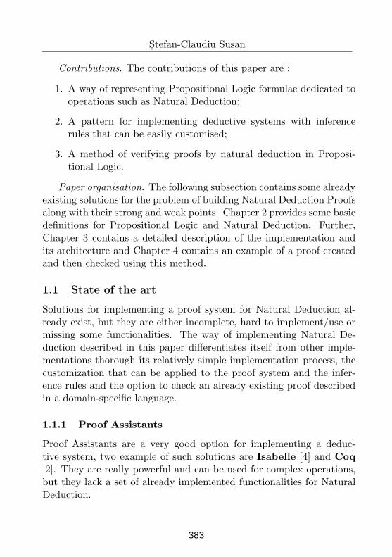
S, tefan-Claudiu Susan
Contributions. The contributions of this paper are :
1. A way of representing Propositional Logic formulae dedicated tooperations such as Natural Deduction;
2. A pattern for implementing deductive systems with inferencerules that can be easily customised;
3. A method of verifying proofs by natural deduction in Proposi-tional Logic.
Paper organisation. The following subsection contains some alreadyexisting solutions for the problem of building Natural Deduction Proofsalong with their strong and weak points. Chapter 2 provides some basicdefinitions for Propositional Logic and Natural Deduction. Further,Chapter 3 contains a detailed description of the implementation andits architecture and Chapter 4 contains an example of a proof createdand then checked using this method.
1.1 State of the art
Solutions for implementing a proof system for Natural Deduction al-ready exist, but they are either incomplete, hard to implement/use ormissing some functionalities. The way of implementing Natural De-duction described in this paper differentiates itself from other imple-mentations thorough its relatively simple implementation process, thecustomization that can be applied to the proof system and the infer-ence rules and the option to check an already existing proof describedin a domain-specific language.
1.1.1 Proof Assistants
Proof Assistants are a very good option for implementing a deduc-tive system, two example of such solutions are Isabelle [4] and Coq
[2]. They are really powerful and can be used for complex operations,but they lack a set of already implemented functionalities for NaturalDeduction.
383
A practical implementation of Natural Deduction in Propositional Logic
Figure 1. Proof generated by natural deduction for ¬p∧¬q|−¬(p∨q)
1.1.2 Natural Deduction
Natural Deduction [9] is a tool used for building proofs in Proposi-tional Logic. The proofs are automatically generated and they are clearand easy to understand. The automatical generation (Figure 1) is astrong point of this implementations, but it also has some weak pointsthat must be taken into consideration. These weak points inlcude thesyntax used, it is different from the one usually used in PropositionalLogic, and the fact that it does not support all inference rules, so it isnot a complete proof system. Also, it does not feature a componentthat allows the user to check an already existing proof.
2 Propositional Logic and Natural Deduction
2.1 Propositional Logic
Propositional Logic. Propositional logic is concerned with propositionsand the relationships between them, as described in [1]. A propositionis an affirmation that is either true or false. To represent these con-ditions we use propositional variables. Sentences can be simple, a sin-
384
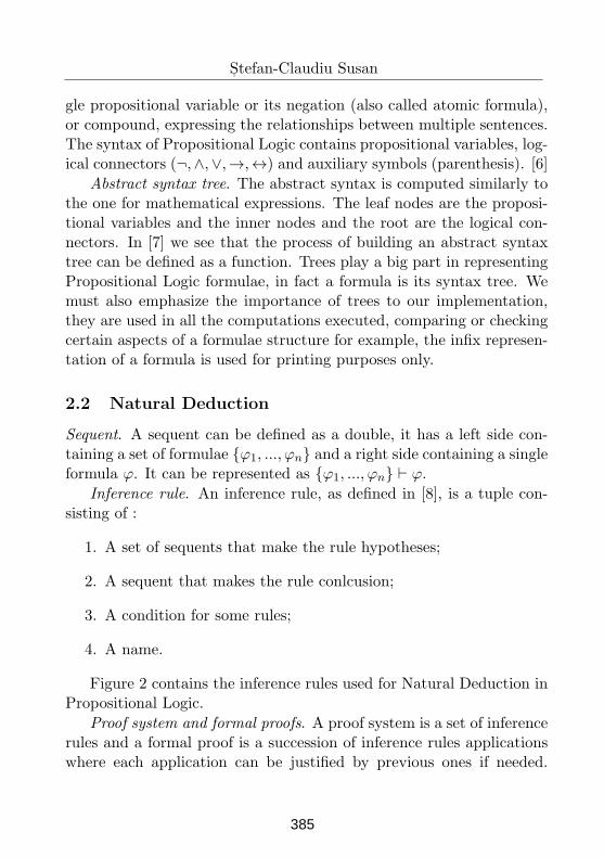
S, tefan-Claudiu Susan
gle propositional variable or its negation (also called atomic formula),or compound, expressing the relationships between multiple sentences.The syntax of Propositional Logic contains propositional variables, log-ical connectors (¬,∧,∨,→,↔) and auxiliary symbols (parenthesis). [6]
Abstract syntax tree. The abstract syntax is computed similarly tothe one for mathematical expressions. The leaf nodes are the proposi-tional variables and the inner nodes and the root are the logical con-nectors. In [7] we see that the process of building an abstract syntaxtree can be defined as a function. Trees play a big part in representingPropositional Logic formulae, in fact a formula is its syntax tree. Wemust also emphasize the importance of trees to our implementation,they are used in all the computations executed, comparing or checkingcertain aspects of a formulae structure for example, the infix represen-tation of a formula is used for printing purposes only.
2.2 Natural Deduction
Sequent. A sequent can be defined as a double, it has a left side con-taining a set of formulae ϕ1, ..., ϕn and a right side containing a singleformula ϕ. It can be represented as ϕ1, ..., ϕn ⊢ ϕ.
Inference rule. An inference rule, as defined in [8], is a tuple con-sisting of :
1. A set of sequents that make the rule hypotheses;
2. A sequent that makes the rule conlcusion;
3. A condition for some rules;
4. A name.
Figure 2 contains the inference rules used for Natural Deduction inPropositional Logic.
Proof system and formal proofs. A proof system is a set of inferencerules and a formal proof is a succession of inference rules applicationswhere each application can be justified by previous ones if needed.
385
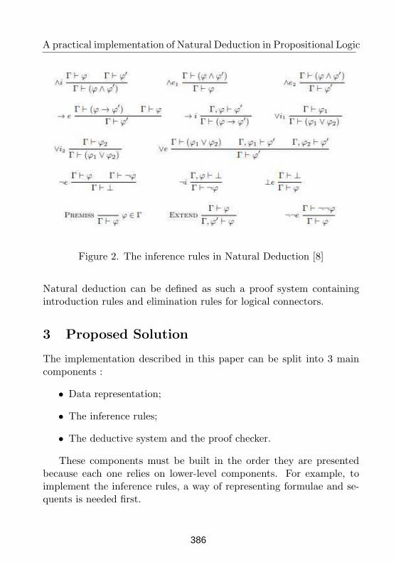
A practical implementation of Natural Deduction in Propositional Logic
Figure 2. The inference rules in Natural Deduction [8]
Natural deduction can be defined as such a proof system containingintroduction rules and elimination rules for logical connectors.
3 Proposed Solution
The implementation described in this paper can be split into 3 maincomponents :
• Data representation;
• The inference rules;
• The deductive system and the proof checker.
These components must be built in the order they are presentedbecause each one relies on lower-level components. For example, toimplement the inference rules, a way of representing formulae and se-quents is needed first.
386
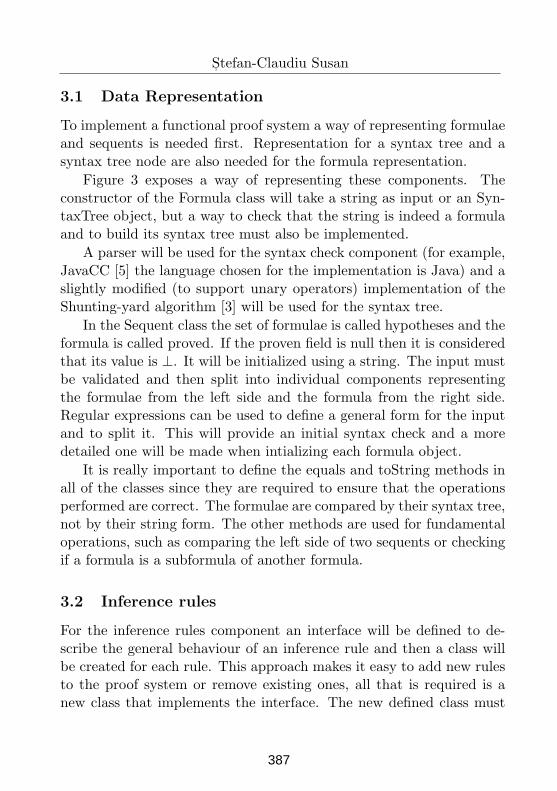
S, tefan-Claudiu Susan
3.1 Data Representation
To implement a functional proof system a way of representing formulaeand sequents is needed first. Representation for a syntax tree and asyntax tree node are also needed for the formula representation.
Figure 3 exposes a way of representing these components. Theconstructor of the Formula class will take a string as input or an Syn-taxTree object, but a way to check that the string is indeed a formulaand to build its syntax tree must also be implemented.
A parser will be used for the syntax check component (for example,JavaCC [5] the language chosen for the implementation is Java) and aslightly modified (to support unary operators) implementation of theShunting-yard algorithm [3] will be used for the syntax tree.
In the Sequent class the set of formulae is called hypotheses and theformula is called proved. If the proven field is null then it is consideredthat its value is ⊥. It will be initialized using a string. The input mustbe validated and then split into individual components representingthe formulae from the left side and the formula from the right side.Regular expressions can be used to define a general form for the inputand to split it. This will provide an initial syntax check and a moredetailed one will be made when intializing each formula object.
It is really important to define the equals and toString methods inall of the classes since they are required to ensure that the operationsperformed are correct. The formulae are compared by their syntax tree,not by their string form. The other methods are used for fundamentaloperations, such as comparing the left side of two sequents or checkingif a formula is a subformula of another formula.
3.2 Inference rules
For the inference rules component an interface will be defined to de-scribe the general behaviour of an inference rule and then a class willbe created for each rule. This approach makes it easy to add new rulesto the proof system or remove existing ones, all that is required is anew class that implements the interface. The new defined class must
387
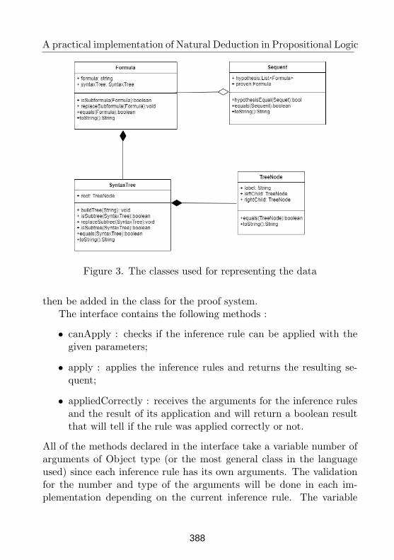
A practical implementation of Natural Deduction in Propositional Logic
Figure 3. The classes used for representing the data
then be added in the class for the proof system.The interface contains the following methods :
• canApply : checks if the inference rule can be applied with thegiven parameters;
• apply : applies the inference rules and returns the resulting se-quent;
• appliedCorrectly : receives the arguments for the inference rulesand the result of its application and will return a boolean resultthat will tell if the rule was applied correctly or not.
All of the methods declared in the interface take a variable number ofarguments of Object type (or the most general class in the languageused) since each inference rule has its own arguments. The validationfor the number and type of the arguments will be done in each im-plementation depending on the current inference rule. The variable
388
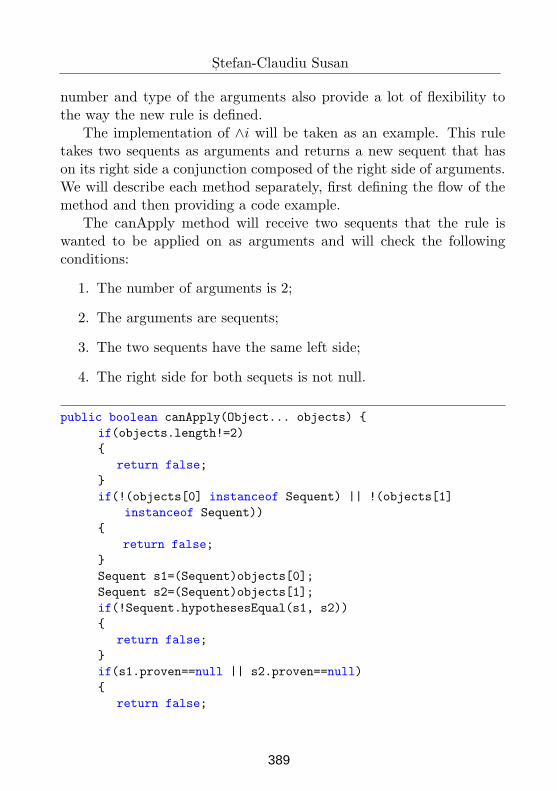
S, tefan-Claudiu Susan
number and type of the arguments also provide a lot of flexibility tothe way the new rule is defined.
The implementation of ∧i will be taken as an example. This ruletakes two sequents as arguments and returns a new sequent that hason its right side a conjunction composed of the right side of arguments.We will describe each method separately, first defining the flow of themethod and then providing a code example.
The canApply method will receive two sequents that the rule iswanted to be applied on as arguments and will check the followingconditions:
1. The number of arguments is 2;
2. The arguments are sequents;
3. The two sequents have the same left side;
4. The right side for both sequets is not null.
public boolean canApply(Object... objects)
if(objects.length!=2)
return false;
if(!(objects[0] instanceof Sequent) || !(objects[1]
instanceof Sequent))
return false;
Sequent s1=(Sequent)objects[0];
Sequent s2=(Sequent)objects[1];
if(!Sequent.hypothesesEqual(s1, s2))
return false;
if(s1.proven==null || s2.proven==null)
return false;
389
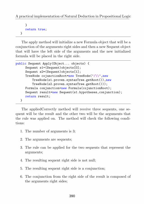
A practical implementation of Natural Deduction in Propositional Logic
return true;
The apply method will initialize a new Formula object that will be aconjunction of the arguments right sides and then a new Sequent objectthat will have the left side of the arguments and the new initializedformula will be placed in the right side.
public Sequent Apply(Object... objects)
Sequent s1=(Sequent)objects[0];
Sequent s2=(Sequent)objects[1];
TreeNode cojunctionRoot=new TreeNode("/\\",new
TreeNode(s1.proven.syntaxTree.getRoot()),new
TreeNode(s2.proven.syntaxTree.getRoot()));
Formula conjunction=new Formula(cojunctionRoot);
Sequent result=new Sequent(s1.hypotheses,conjunction);
return result;
The appliedCorrectly method will receive three sequents, one se-quent will be the result and the other two will be the arguments thatthe rule was applied on. The method will check the following condi-tions:
1. The number of arguments is 3;
2. The arguments are sequents;
3. The rule can be applied for the two sequents that represent thearguments;
4. The resulting sequent right side is not null;
5. The resulting sequent right side is a conjunction;
6. The conjunction from the right side of the result is composed ofthe arguments right sides;
390
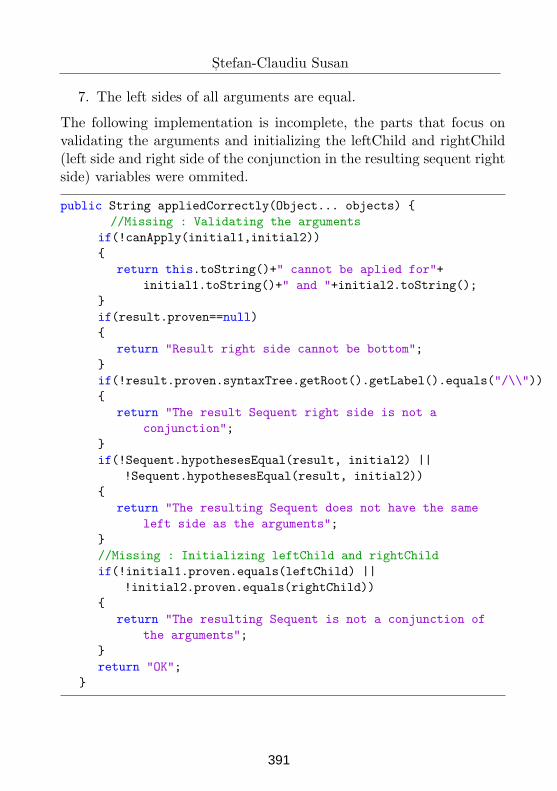
S, tefan-Claudiu Susan
7. The left sides of all arguments are equal.
The following implementation is incomplete, the parts that focus onvalidating the arguments and initializing the leftChild and rightChild(left side and right side of the conjunction in the resulting sequent rightside) variables were ommited.
public String appliedCorrectly(Object... objects)
//Missing : Validating the arguments
if(!canApply(initial1,initial2))
return this.toString()+" cannot be aplied for"+
initial1.toString()+" and "+initial2.toString();
if(result.proven==null)
return "Result right side cannot be bottom";
if(!result.proven.syntaxTree.getRoot().getLabel().equals("/\\"))
return "The result Sequent right side is not a
conjunction";
if(!Sequent.hypothesesEqual(result, initial2) ||
!Sequent.hypothesesEqual(result, initial2))
return "The resulting Sequent does not have the same
left side as the arguments";
//Missing : Initializing leftChild and rightChild
if(!initial1.proven.equals(leftChild) ||
!initial2.proven.equals(rightChild))
return "The resulting Sequent is not a conjunction of
the arguments";
return "OK";
391
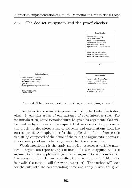
A practical implementation of Natural Deduction in Propositional Logic
3.3 The deductive system and the proof checker
Figure 4. The classes used for building and verifying a proof
The deductive system is implemented using the DeductiveSystemclass. It contains a list of one instance of each inference rule. Forits initialization, some formulae must be given as arguments that willbe used as hypotheses and a sequent that represents the purpose ofthe proof. It also stores a list of sequents and explanations from thecurrent proof. An explanation for the application of an inference ruleis a string composed of the name of the rule, the arguments indexes inthe current proof and other arguments that the rule requires.
Worth mentioning is the apply method, it receives a variable num-ber of arguments representing the name of the rule applied and thearguments for its application (numerical arguments are transformedinto sequents from the corresponding index in the proof, if this indexis invalid the method will throw an exception). The method will lookfor the rule with the corresponding name and apply it with the given
392
S, tefan-Claudiu Susan
arguments after which it will store the result in the current proof andthe name of the rule along with the application parameters in the jus-tification for the newly added sequent. If an error is encountered infinding the rule or the way it is applied is invalid then an exceptionwill be thrown.
To be evaluated, a proof must be written in text format. Verifica-tion of a proof is done using the classes ProofChecker and ProofReader.
The ProofChecker class contains a list with one instance of eachinference rule. It also contains two lists where the sequents and theirjustifications will be added. Semantic verification is done using thecheckProof method in this class; to test the validity of applying a rulethe appliedCorrectly method of that rule will be used. In order to de-termine the arguments with which this method will be called, but alsothe rule from which we will call it, the pair formed from the currentsequent and its justification will be analyzed. If the evaluation is posi-tive, the message ”OK” will be returned, otherwise the error messageprovided by appliedCorrectly followed by the corresponding line willbe returned. This class tries to build the proof from the beginningby checking each rule application line by line. If this reconstructionsucceeded, the proof is considered valid.
The ProofReader class reads the proof from the text file and checksit syntactically. The proof is red line by line and each is checked ata syntactic level; if everything is fine it will be separated into the se-quent and justification and these 2 will be added to an object of typeProofChecker. If the entire proof has been red without reporting syn-tactic errors, the checkProof method in ProofChecker will be called tomake the semantic evaluation of the proof.
4 Usability
For this section we will use as an example the Natural Deduction com-ponent from Logic E-Learning Assistant since it was implemented usingthe method described in this paper. The proof in Figure 5 was selectedto be built using the application and then copied in text format to
393
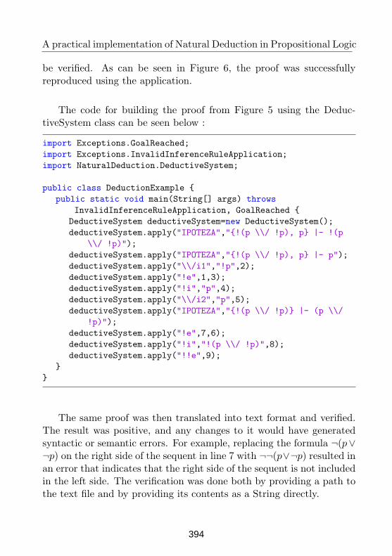
A practical implementation of Natural Deduction in Propositional Logic
be verified. As can be seen in Figure 6, the proof was successfullyreproduced using the application.
The code for building the proof from Figure 5 using the Deduc-tiveSystem class can be seen below :
import Exceptions.GoalReached;
import Exceptions.InvalidInferenceRuleApplication;
import NaturalDeduction.DeductiveSystem;
public class DeductionExample
public static void main(String[] args) throws
InvalidInferenceRuleApplication, GoalReached
DeductiveSystem deductiveSystem=new DeductiveSystem();
deductiveSystem.apply("IPOTEZA","!(p \\/ !p), p |- !(p
\\/ !p)");
deductiveSystem.apply("IPOTEZA","!(p \\/ !p), p |- p");
deductiveSystem.apply("\\/i1","!p",2);
deductiveSystem.apply("!e",1,3);
deductiveSystem.apply("!i","p",4);
deductiveSystem.apply("\\/i2","p",5);
deductiveSystem.apply("IPOTEZA","!(p \\/ !p) |- (p \\/
!p)");
deductiveSystem.apply("!e",7,6);
deductiveSystem.apply("!i","!(p \\/ !p)",8);
deductiveSystem.apply("!!e",9);
The same proof was then translated into text format and verified.The result was positive, and any changes to it would have generatedsyntactic or semantic errors. For example, replacing the formula ¬(p∨¬p) on the right side of the sequent in line 7 with ¬¬(p∨¬p) resulted inan error that indicates that the right side of the sequent is not includedin the left side. The verification was done both by providing a path tothe text file and by providing its contents as a String directly.
394
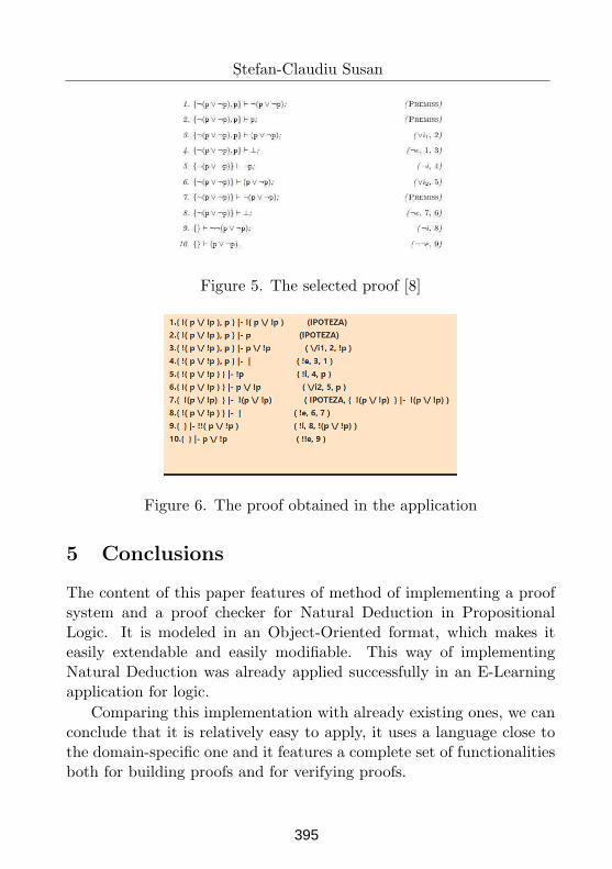
S, tefan-Claudiu Susan
Figure 5. The selected proof [8]
Figure 6. The proof obtained in the application
5 Conclusions
The content of this paper features of method of implementing a proofsystem and a proof checker for Natural Deduction in PropositionalLogic. It is modeled in an Object-Oriented format, which makes iteasily extendable and easily modifiable. This way of implementingNatural Deduction was already applied successfully in an E-Learningapplication for logic.
Comparing this implementation with already existing ones, we canconclude that it is relatively easy to apply, it uses a language close tothe domain-specific one and it features a complete set of functionalitiesboth for building proofs and for verifying proofs.
395
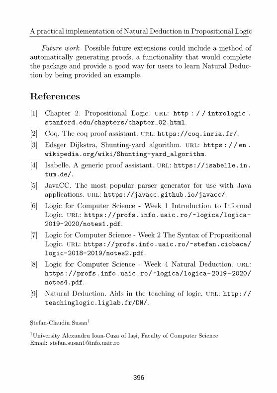
A practical implementation of Natural Deduction in Propositional Logic
Future work. Possible future extensions could include a method ofautomatically generating proofs, a functionality that would completethe package and provide a good way for users to learn Natural Deduc-tion by being provided an example.
References
[1] Chapter 2. Propositional Logic. url: http : / / intrologic .
stanford.edu/chapters/chapter_02.html.
[2] Coq. The coq proof assistant. url: https://coq.inria.fr/.
[3] Edsger Dijkstra, Shunting-yard algorithm. url: https : / / en .wikipedia.org/wiki/Shunting-yard_algorithm.
[4] Isabelle. A generic proof assistant. url: https://isabelle.in.tum.de/.
[5] JavaCC. The most popular parser generator for use with Javaapplications. url: https://javacc.github.io/javacc/.
[6] Logic for Computer Science - Week 1 Introduction to InformalLogic. url: https://profs.info.uaic.ro/~logica/logica-2019-2020/notes1.pdf.
[7] Logic for Computer Science - Week 2 The Syntax of PropositionalLogic. url: https://profs.info.uaic.ro/~stefan.ciobaca/logic-2018-2019/notes2.pdf.
[8] Logic for Computer Science - Week 4 Natural Deduction. url:https://profs.info.uaic.ro/~logica/logica-2019-2020/
notes4.pdf.
[9] Natural Deduction. Aids in the teaching of logic. url: http://teachinglogic.liglab.fr/DN/.
S,tefan-Claudiu Susan1
1University Alexandru Ioan-Cuza of Ias,i, Faculty of Computer Science
Email: [email protected]
396
Proceedings of the Conference on Mathematical Foundations of Informatics
MFOI’2020, January 12 -16 , 2021, Kyiv, Ukraine
On the implementations of new multivariate public
keys based on transformations of linear degree
Vasyl Ustimenko, Oleksandr Pustovit
Abstract
Multivariate Cryptography (MC) is important direction of Post Quantum
Cryptography. Two algorithms of MC were presented for the second round of
competition supervised by National Institute of Standardisation Technology (NIST,
USA, announcement of March of 2019). One of these algorithms named
‘’Rainbow like Unbalanced Oil and Vinegar digital signatures” was taken for the
Third Round of competition. Noteworthy that this algorithm is based on
noninjective transformations of finite vector space. So it is usage for the message
exchange is impossible. We suggest new postquantum public key cryptosystems
based on injective transformation i. They are rather closed to bijective maps and
can be used for information exchange tasks. In difference to classical multivariate
cryptosystem we use maps with degree dependable from the dimension of vector
space.
Keywords: Multivariate Cryptography, affine Cremona semigroup, stable
families of transformations, maps with the density gap, public key.
.
1 Introduction
One of the fifth directions of Postquantum Public key Cryptography is
a construction of multivariate public keys. It was started from constructionsof quadratic bijective maps F and private algorithms of finding the reimage
for b=F(a) (see [1], [2] and [16] and further references). Later somenonbijective maps of bounded degree were used in multivariate
cryptography (see [17], [18], [19]).Recently some attempts to construct public keys with encryption maps
of unbounded degree and polynomial density were suggested (see forexample [12]).
© 2021 by Vasyl Ustimenko, Oleksandr Pustovit
397
Vasyl Ustimenko, Oleksandr Pustovit
Multivariate public keys can be found among candidates selected forNIST standartisation. Recall that In March 2019 NIST published a list of
candidates qualified to the second round of the PQC process (see [20],[21]and further references). Nowadays hardware performance of some second
round candidates was already reported. Current candidates different frommultivariate cryptosystems are developed within following directions of
PQC: lattice based systems, code based cryptosystems, multivariatecryptography, hash based Cryptography, studies of isogenies for
superelliptic curves.Some researchers are study possibilities different from multivariate
cryptography possibilities of cryptosystems defined via algebraic objects,this direction is known asconnected with recent development of
Noncommutative Cryptography (see [22]-[38]). It is important thatcryptoapplication of Algebra are supported by recent cryptanalitical
studies( [39]-[48]).
2. On affine Cremona semigroup.Let K be a commutative ring. Let us consider the totality of all rules f
of kind x1 → f1(x1, x2 , …, xn ), x2 → f2 (x1, x2 , …, xn ), ..., xn → fn(x1, x2 , …,xn ), for given parameter n and a chosen commutative ring K with natural
operation of composition. We assume that each rule is written in itsstandard form, i. e. each polynomial fi is given by the list of its monomial
written in chosen order. We refer to this semigroup as semigroup of formaltransformations SFn(K) of free module Kn. In fact it is a totality of all
endomorphisms of ring K[x1, x2 , …, xn] with the operations of theirsuperposition. Each rule f from SFn(K) induces transformation t( f) which
sends tuple (p1, p2 , …, pn) into ( f1(p1, p2 , …,pn ), f2 (p1, p2 , …,pn ), .,. , fn(p1,
p2 , …, pn ). Affine Cremona semigroup S(Kn) is a totality of all
transformations of kind t( f) (see historicalsurvey [50]. The canonical homomorphism h: f → t(f) maps infinite
semigroup SFn(K) onto a finite semigroup S(Kn), in the case of finitecommutative ring K. We refer to pair (f, f ’) of elements SFn(K) such that
f, f’ and f ’ f are two copies of identical rule x1 → x1, x2→ x2, ..., xn → xn asa pair of invertible elements. If (f, f’) is such a pair, then product t( f) t( f ’)
is an identity map. Let us consider the subgroup CFn(K) of all invertibleelements of SFn(K) (group of formal maps). It is clear that the image of a
398
On the implementations of new multivariate public keys based on transformations
of linear degree
restriction of h on CFn(K) is affine Cremona group C(Kn) of all
transformations of Kn onto Kn for which there exists a polynomial inverse.
Semigroup SFn(K) is an important object of theory of symbolic
computation or so-called Computer Algebra (see [1]), which is a powerfulinstrument of Multivariate Cryptography ([2], [3]). We will assume that
each element f of this semigroup are written in the same basis in itsstandard form. A degree deg(f) is the maximal degree of polynomials fi,
i=1,2, ..., n. The density den(f) of f is the maximal number of monomialterms in fi(x1, x2 , …, xn ).
We say that a family of subsemigroups Sn of SFn(K) (or S(Kn)) isstable of degree d if maximal degree of elements from Sn is an
independent constant d, d > 2. If K is a finite commutative ring, then thestable semigroup has to be a finite set. The brief observation of known
families of stable groups and their cryptographical applications can befound in [4].
Let f(n) be a family of nonlinear maps from SFn(K) of a degreebounded by the constant d . We say that f(n) form a tame family if, in
SFn(K , there is a family g(n) from SFn(K ) of degree bounded by constantd ' such that f(n)g(n) = g(n)f(n) is an identity map. Let T1(n) and T2(n) be
two families of elements from the group AGLn(K) of all affine bijectivetransformations, i. e., elements of affine Cremona group of degree 1. Then
we refer to f‘(n)= T1 (n)f(n) T2(n) as a linear deformation of f(n). Obviouslyf ‘(n) is also tame family of transformations, and the degrees of maps from
this family are also bounded by d . The degrees of the inverses for f ’(n)are bounded by d '.
Let Gn< CFn(K) be a stable family of subgroups of degree d , d > 1,then the nonlinear representatives f(n) of Gn form a tame family of maps. It
is easy to see that the densities of f(n) and its linear deformation f‘(n) canbe very different. We refer to a pair of mutually invertible elements f(n) ,
f(n) -1 from CFn(K) as a pair with a density gap, if the density of f(n) is apolynomial expression in variable n and the density of f(n) -1 is bounded
below by exponential function an with base a>1.Similarly we refer to a pair of mutually invertible elements f(n), f(n)
-1from CFn(K) as a pair with a degree, if the degree of f(n) is a polynomialexpression in variable n, and a degree of f(n) -1 is bounded below by
exponential function an with base a>1.
399
Vasyl Ustimenko, Oleksandr Pustovit
3. On explicit construction of stable maps of prescribed degreeand large order.
We define Double Schubert Graph DS(k,K) over commutative ring Kas incidence structure defined as disjoint union of partition sets PS=K k(k+
1) consisting of points which are tuples of kind x =(x1 , x2, … , xk, x11 , x12, …, xkk ) and LS=K k(k+1) consisting of lines which are tuples of kind y =[y1 ,y2,
… ,yk, y11 ,y12, … ,ykk ], where x is incident to y , if and only if xij - yij =xi yj
for i=1, 2,..., k and j=1, 2,..., k. It is convenient to assume that the indices
of kind i,j are placed for tuples tuples of K k(k+1) in the lexicographical order.Remark. The term Double Schubert Graph is chosen, because points
and lines of DS(k, Fq) can be treated as subspaces of Fq (2k+1) of dimensions
k+1 and k, which form two largest Schubert cells. Recall that the largest
Schubert cell is the largest orbit of group of unitriangular matrices actingon the variety of subsets of given dimensions (see [5] and references
therein or [6]).We define the colour of point x =(x1 , x2, … , xk, x11 , x12, … , xkk ) from
PS as tuple (x1 , x2, … , xk, ) and the colour of a line y =[y1 ,y2, … ,yk, y11 ,y12,… ,ykk ] as the tuple (y1 ,y2, … ,yk ). For each vertex v of DS(k, K), there is
the unique neighbour y= Na (v) of a given colour a=(a1 a2, … ,ak).The symbolic colour g from K[x1 , x2, … , xk,]
k of v of kind ( f1(x1 , x2,
… , xk,), f2(x1 , x2, … , xk,), … , fk (x1 , x2, … , xk,)), where fi are polynomialsfrom K[x1 , x2, … , xk,]
defines the neighbouring line of the general point
x =(x1 , x2, … , xk, x11 , x12, … , xkk ) with colour kind ( f1(x1,x2, …,xk), f2 (x1,x2, …, xk),… fk(x1,x2, …, xk)). Similarly, we can compute the
neigbouring point of general line [x] =[x1 , x2, … , xk, x11 , x12, … , xkk ] ofcolour g.
Let us consider a tuple of symbolic colours g 1, g 2, … , g2t from( K[x1 , x2, … , xk,]
k )2t and the map f of PS to itself, which sends the point
x =(x1 , x2, … , xk, x11 , x12, … , xkk ) to the end v2t, of the chain v0 , v1, v2,,… ,v2t, where x= v0, vi I vi+1, i=0,1, 2,...,2t-1 and the colour of vi is the tuple gi,
of elements from K[ x1 , x2, … , xk,]. We refer to f as the map of closedpoint-to-point computation with the symbolic key g 1, g 2, … , g2t or simply
the symbolic computation. As it follows from the definitions, f = f g 1, g 2,… , g2t is a multivariate map of K k(k+ 1) to itself. When the symbolic key is
given, f can be computed in the standard form via the elementaryoperations of addition and multiplication of the ring K[ x1 , x2, … , xk, x11 ,
x12, … , xkk]. Recall that (x1 , x2, … , xk, x11 , x12, … , xkk) is our symbolic point
400
On the implementations of new multivariate public keys based on transformations
of linear degree
of the graph. We refer to expression f g 1, g 2, … , g2t as automaton
presentation of f with a symbolic key g 1, g 2, … , g2t . Note that if t( g2t ) isan element of the affine Cremona group C(Kk) then f g 1, g 2, … , g2 t is
invertible and automaton presentation of its inverse has a symbolic key g-
2t g 2t-1, g-2t g 2t-2, g
-2t g 2t-3 , …, g-2t g 1, g-2t , where g-2t is the inverse of the
element g2t . The restrictions on degrees and densities of multivariate mapst(ggi) of Kk to Kk and the size of parameter t
allow us to define a polynomial map f with polynomial degree and density.Let g i = (h1
i, h2 i, … , hk
i) , i=1, 2,..., 2t be the symbolic key of the
closed point to point computation f= f(n) of the symbolic automatonDS(k,K)). We refer to elements g i as the governing functions of the
symbolic key. We set that g 0 = (h1 0, h2
0, … , hk0) =(x1 , x2, … , xk,) . Then f
is a transformation of kind
x1 → h1 2t(x1, x2, …, xk), x2→ h2
2t(x1, x2, …, xk), ..., xk→ hn 2t (x1, x2, …,
xk),
x11 → x11 - h11 x1 + h1
1 h12- h1
2 h13+ h1
3 h14 + ...+h1
2t-1 h12t
x12 → x12 - h11 x2 + h1
1 h22- h2.
2h13+ h1
3 h24 + ...+h2
2t-1 h12t
…
xkk → xkk - hk
1 xk + hk1 hk
2- hk2hk
3+ hk3 hk
4 + ...+hk2t-1 hk
2t
We say that the map f of closed point-to-point computation is affine, if
all elements g i of the symbolic key are elements of degree < 2 . We referto a subsemigroup G in S(Kn) as semigroup of degree d, if the maximal
degree for representative g equals d. Let AGLn(K) be the group of affinetransformations of Kn, i. e., the group of all bijective transformations of
degree 1. Let us consider a semigroup Ek(K) introduced in [7], which consists of
all transformations f h 1, h 2, … , hl , g , where degrees of hi for i=1, 2,...,l and g are bounded by 1, and l is odd number. It is clear that Ek(K) is a
stable subsemigroup of degree 2.The group GLn(Fq) contains Singer cycles, i. e., elements of order qn
-1 (see [8,9]).
401
Vasyl Ustimenko, Oleksandr Pustovit
Lemma 1. Let K=Fq , let f be the map of closed point-to-pointcomputation h 1, h 2, … , hl , h and h defines a Singer Cycle from
GLk(Fq) . Then the order of f is at least qk -1.Lemma 2. Let K=Fq and f h 1, h 2, … , hl , h is an element of
semigroup Ek(K) such that h defines the map from GLk(Fq), which has aninvariant subspace W of dimension m, and the restriction of h onto W
defines a Singer cycle. Then the stable semigroup <f > generated by fcontains at least qm -1 elements.
We consider two symbolic computations 1C and 2C with governingfunctions f 1, f 2, … ,f t and g 1, g 2, … , gs and corresponding maps m1 =
m(1C) and m2 = m(2C) .We refer to the symbolic computation 1C withgoverning functions f 1, f 2, … ,f t and g 1(f t), g 2(f t), … , gs(f t) as
concatenation of 1C and 2C. It is easy to see that the map corresponding toC is m2(m1). So, C→ m(C) is homomorphism of two monoids.
Let us consider the totality PL = PL(k,K) of all point-to-pointcomputations C with governing functions f 1, f 2, … , f t with the last, ,f t
from K(x1, x2, …, xk]k of kind ( l1 (x1, x2, …, xk ), l2(x1, x2, …, xk ), … , lk(x1,
x2, …, xk )) , where all expressions li are of degree 1. It is easy to see that
PL is a closed set with the respect to the concatenation operation. We addthe empty computation as a formal neutral element. This means that the
maps of kind m(C) from PL form a subsemigroup S\PL of the affineCremona semigroup S(Kk(k+1)).
Note that a map m (C) induced by a point-to-point computation C withgoverning functions f 1, f 2, … , f t , where f t has coordinates ,f t
1 (x1, x2, …,
xk ), f t2 (x1, x2, …, xk ) , …, f t
k (x1, x2, …, xk ), is an invertibletransformation of Kk(k+1), if and only if the map x1 → f1
t(x1, x2, …, xk ) , x1→
f2t(x1, x2, …, xk ) , ..., xk→ fk
t(x1, x2, …, xk ), , is a bijection. It is clear thatm(C) -1 of invertible map from SPL is also an element of SPL.
Let GPL be the group of all invertible elements from PL. We define adegree of governing function f i , given by a tuple with coordinates f i
1 (x1 ,
x2, … , xk ) , f i2 (x1 , x2, … , xk ), … , f i
k (x1 , x2, … , xk ) as the maximaldegree of f i
j for various i and j . Notice that m(C) from GPL can be an
element with very large order. In fact, in the case of K=Fq and an arbitrarylist of governing functionsf 1, f 2, … ,f t-1 and f t for the given bilinear map
x1→ f1 t(x1 , x2, … , xk ), x2→f2
t (x1 , x2, … , xk ) , ..., xk→ fkt (x1 , x2, … , xk ) ,
which is a Singer cycle, i. e., its order is at least qk -1, the order of m( C) is
also bounded below by qk –1.
402
On the implementations of new multivariate public keys based on transformations
of linear degree
We can easily construct non bijective maps of kind m( C) from SPL
such that the subgroup generated by this element consists of more than qk-c
elements for some constant c>1. In fact, one can take f t with the invariant
subspace W of dimension k-c , such that the restriction of f t on W is aSinger cycle. It is convenient for us to consider the tuple (x1 , x2, … , xk ) as
governing function f 0 of the symbolic computation C. For polynomials f 2i
, i=1, 2,..., t/2 which are colours of the points from DS(k,K[x1, x2, …, xk]) ,
we consider their maximal degree de. Let do be the maximal degree of f 2i+1, i=1, 2,..., t/2 . Note that the degree of the polynomial map m( C) is
bounded from above by de+do . In fact, the degree of this map is themaximum of products of coordinates of f i and f i+1, i=1, 2,..., t-1 .
Let us consider the totality Srs(PL) of maps m(C) for the symboliccomputations with de equals at most r and do equals at most s.
Theorem. The totality Srs(PL(k,K)) is a stable subsemigroup of theaffine Cremona semigroup S(Kk(k+1)) of degree r +s.
It is clear that the intersection Grs(PL(k,K)) of G(PL) and Srs(PL(k,K))is a stable subgroup of C(Kk(k+1)) of degree r +s. Notice that Ek(K)
presented in [7] coincides with S11( PL (k, K)).
4. On pairs of transformations with the density gap andcorresponding public key.
Let us consider a point to point computation of the Schubert symbolic
automaton from the semigroup Sm1(PL (n,K)) with m=d(n) of kind an=b,a>1 corresponding to symbolic key f 1, f 2, … , f t for some even parameter
t with elements f i , i is odd, of linearly increasing in variable n degree andfinite density.
Then the corresponding transformation F will be of degree O(n) andlinear density. Let us assume that f t is a bijective map. Then, in majority
cases, the inverse map F -1 given by the symbolic key formed by elementsf t-1 ( f –t), f t-2 ( f –t) , … , f 1( f –t) , f -t , where f –t is the inverse for f t will be
of density O(nn ). So, the pair F , F -1 be the pair with the density gap.We propose the following public key algorithm. Alice chooses a finite
commutative ring K, positive integer n and a linear expression m=d(n).She works with the Double Schubert graph DS(n, K) and related symbolic
automaton. Alice selects odd parameter t and a symbolic key f 1, f 2, … , f t
for an invertible element of Sm1(PL (n, K)).
403
Vasyl Ustimenko, Oleksandr Pustovit
She generates the polynomial map F corresponding to the computationwith a chosen symbolic key. The standard form of this transformation can
be computed with O(n4 ) elementary operations (quadratic in the number ofvariables).
Alice selects the bijective monomial transformation T ofV=Kn(n+1)given by a monomial matrix of size n(n+1) times n(n+1) with
n(n+1) nonzero regular entries from K* (each column and each rowcontains exactly one nonzero element). She takes the affine bijective
transformation T’ of V and forms G=TFT’. For the construction of GAlice has to compute n2 linear combinations of polynomial expression of
n2 multivariate polynomials of density and degree O(n ). So, the total costto form G is O(n6 ) (cubic in the number of variables).
Alice sends the standard form of G to Bob. Note that G has degreeO(n ) and density O(n3 ). Bob writes his plaintext p from V and computes
the ciphertext c=G(p) in time O(n4 ) (quadratic time in the number ofvariables).
Decryption process. Assume that Alice keeps the already computedtransformation T1=T’ -1 and T2=T -1. Firstly, she computes T1(c )=b. It take
her O(n4 ) elementary operations.Now, she has the colour t=(b1 , b2, … , bn ) of point (b). Alice is looking
for an intermediate vector v formed by the coordinates of a point (v) suchthat F(v)=c. Let (r)= (v1 ,v2, … , vn ) be the colour of point (v ). Alice has
the inverse f –t of the bijective affine map f t. So, she computes (r)= f –t (r)in time O(n2 ). Now, Alice can compute values of f 1, f 2, … , f t-1 on the
tuple (r). This costs O(n) operations. After that, she computes v as the finalelement of the walk of the length t with starting point (b) and the prescribed
colours of vertices. This costs O(n2 ) elementary operations to Alice.Finally she gets the plaintext via application T2=T -1 also in the time
O(n2 ).Other ideas of usage algebraic graphs for the construction of
multivariate cryptosystems can be found in [13], [14] and [15].
5. On Eulerian transformations and their cryptographic
applications.
One can look for encryption tools from the following subsemigroup ESn(K)of SFn(K) of formal rules G of kind
404
On the implementations of new multivariate public keys based on transformations
of linear degree
x 1 →T1 (x 1 , x 2 , … , x n),
x 2 →T 2 (x 1 , x 2 , … , x n), (1) …
xn →Tn(x 1 , x 2 , … , x n)
where Ti are monomial term from K[x1 , x2 ,… , xn] with regular coefficient
K*. Such a transformation preserves (K*)n. We refer to such G as Euleriantransformation. Let EGn (K) be a totality of elements from ESn(K) which
act bijectively on K*. Let us assume that K is finite and consider several Jordan - Gauss
transformations J1 , J2, …, Js from EGn(K) i.e. transformations of kindx1 → b1x1
a(1,1)
x2 → b2x1a(2,1)x2
a(2,2)
...xn →bnx1
a(n,1)x2 a(n,2) … xn
a(n,n),
where a(i, j) Zϵ m, m=|K*|, (a(i,i), m)=1.
We can select s+1 monomial affine transformations 1T, 2T, ..., s+1 Tfrom AGLn(K) and use
G=1T J1 2T J2
3T J3 … sT Js
s+1T (2)Noteworthy that the knowledge of decomposition (2) allows us to find
the inverse of G via straightforward algorithms of computing inverses of Ji
and jT.
We say that of kind (2) is computationally tame Eulerian element
from EGn(K). It is clear that sends variable xi to a certain monomial
term. The decomposition of into product of Jordan - Gauss
transformations allows us to find the solution of equations bx )( for x
from (K*)n.
We refer to nES(K) as Eulerian semigroup of formal Cremona
semigroup SFn(K). Assume that the order of K is constant. As it follows
from definition the computation of the value of element from nES(K) on the
given element of Kn is estimated by O(n2). The product of two
multiplicative Cremona elements can be computed in time O(n4).
405
Vasyl Ustimenko, Oleksandr Pustovit
We are not discussing here the complexity of computing the inverse for
general element gϵ n
EG(K) on Turing machine or Quantum computer and
problem finding the inverse for tame Eulerian elements.
Remark. Let G be a subgroup of nEG(K) , K Zϵ m, Fq generated by
Jordan-Gauss elements g1, g2, …, , gt. The word problem of finding the
decomposition of g G ϵ into product of generator gi is difficult, i. e.
polynomial algorithms to solve it with Turing machine or Quantum
Computer are unknown. If word problem is solved and the inverses of gi is
computable then the inverse of g is determined. Notice that if n=1, K=Zm,
, m=pq where p and q are large primes and G is generated by g1=ϻg1a the
problem is unsolvable with Turing machine but it can be solved with
Quantum Computer.So Alice can announce that standard form (1) of G is a public rule.
Correspondents work with the plainspace (K*)n which coincided with the
cipherspace. Bob uses G for the encryption. Alice uses her knowledge onthe decomposition (2) for the decryption.
The polynomial algorithm to invert G in the form (1) is unknown.
6. On combined public keys.
Recall that the density of element F from SFn(K) given by the standard
form xi →fi(x1, x2, …, xn) , i=1,2,…,n is a total number den(F) of monomial
terms in all polynomials fi. For studies of t(H) ϵnES(K) without loss of
generality we may assume that deg(H) is O(n).
Let us consider a composition F of element H from nEG(K) and
element G from SFn(K) of density O(nt) and degree O(n
r) where t and r are
some constants. Then F has the same density with H and degree of size
O(nr+1
).
Let us assume that restriction of G on (K*)n is injective. Notice that the
map G’ ϵ SFn(K) such that GG’ fixes each x from (K*)n may exist but be
with non-polynomial density.Let us consider the following type of multivariate public keys. Alice
chooses H ϵ n
EG(K) with known decomposition of kind (2) for this map
and G on (K*)n as above Assume that she has private key algorithm to
406
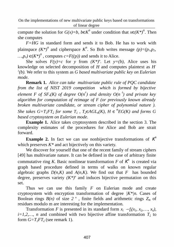
On the implementations of new multivariate public keys based on transformations
of linear degree
compute the solution for G(x)=b, b Kϵn under condition that xϵ(K*)
n. Then
she computes
F=HG in standard form and sends it to Bob. He has to work with
plainspace (K*)n and cipherspace K
n. So Bob writes message (p)=(p1,p2,
…,pn) (ϵ K*)n , computes c=F((p)) and sends it to Alice.
She solves F(y)=c for y from (K*)n. Let y=(b), Alice uses his
knowledge on selected decomposition of H and computes plaintext as H-
1(b). We refer to this system as G based multivariate public key on Eulerian
mode.Remark 1. Alice can take multivariate public rule of PQC candidate
from the list of NIST 2019 competition which is formed by bijective
element F of SFn(K) of degree O(nr) and density O(n
t) and private key
algorithm for computation of reimage of F (or previously known already
broken multivariate candidate, or stream cipher of polynomial nature ).
She takes G=T1FT2 for some T1 , T2 AGLϵ n(K), H ϵ n
EG(K) and forms G
based cryptosystem on Eulerian mode.
Example 1. Alice takes cryptosystem described in the section 3. Thecomplexity estimates of the procedures for Alice and Bob are strait
forward.
Example 2. In fact we can use nonbijective transformations of Kn
which preserves K* and act bijectively on this variety.
We discover for yourself that one of the recent family of stream ciphers[49] has multivariate nature. It can be defined in the case of arbitrary finite
commutative ring K. Basic nonlinear transformation F of Kn is created via
graph based procedure defined in terms of walks on known regularalgebraic graphs D(n,K) and A(n,K). We find out that F has bounded
degree, preserves variety (K*)n and induces bijective permutation on thisset.
Thus we can use this family F on Eulerian mode and createcryptosystem with encryption transformation of degree |K*|n. Cases of
Boolean rings B(n) of size 2 n , finite fields and arithmetic rings Zm ofresidues modulo m are interesting for the implementation.
Transformation F is presented in its standard form xi →fi(x1, x2,…, xn),i=1,2,…, n and combined with two bijective affine transformation T1 to
form G=T1FT2 (see remark 1).
407
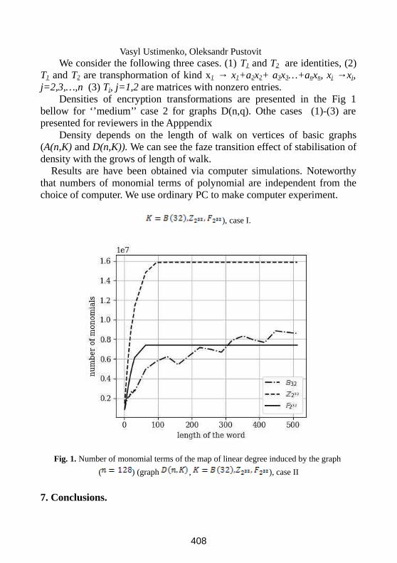
Vasyl Ustimenko, Oleksandr Pustovit
We consider the following three cases. (1) T1 and T2 are identities, (2)T1 and T2 are transphormation of kind x1 → x1+a2x2+ a3x3…+anxn, xj →xj,
j=2,3,…,n (3) Tj, j=1,2 are matrices with nonzero entries.Densities of encryption transformations are presented in the Fig 1
bellow for ‘’medium’’ case 2 for graphs D(n,q). Othe cases (1)-(3) arepresented for reviewers in the Apppendix
Density depends on the length of walk on vertices of basic graphs(A(n,K) and D(n,K)). We can see the faze transition effect of stabilisation of
density with the grows of length of walk.Results are have been obtained via computer simulations. Noteworthy
that numbers of monomial terms of polynomial are independent from thechoice of computer. We use ordinary PC to make computer experiment.
), case I.
Fig. 1. Number of monomial terms of the map of linear degree induced by the graph
( ) (graph , ), case II
7. Conclusions.
408
On the implementations of new multivariate public keys based on transformations
of linear degree
We propose an algorithm of generation of stable groups G of
bijective polynomial maps f(n) of n-dimensional affine space overcommutative ring K, i. e. groups of elements of bounded degree. All maps
are given in a standard basis in which the degrees and densities arecounted. The method allows to generate transformations f(n) of linear
density with degree given by the prescribed linear function d(n) withexponential density for f(n)-1 . In case of K=Fq we can select f(n) of
exponential order. The scheme of generation of public key f(n) ofmultivariate cryptography of kind g(n)=T1 f(n)T2, where T1 is a monomial
linear transformation of Kn and degree of T2 is one, is proposed.Complexity estimates show that time of execution of encryption rule with
high degree coincides with the time of computation of value of quadraticmultivariate map. Decryption procedure based on the knowledge of
generation algorithm is even faster. The security rests on the idea of lack ofresources for adversary to restore the inversemap of exponential densityand
linear degree and absence of known general polynomial algorithms to solvethis task.
We combined Eulerian transformation which sends each variable intomonomial term with the proposed multivariate ring to construct another
public key of non-bijective nature which use plainspace (K*)n.
References. [1] Machi, A. (2012). Algebra for Symbolic Computation. Springer.
[2] Ding, J., J. E. Gower, J. E.& Schmidt, D. S. (2006). Multivariate Public Key
Cryptosystems. Advances in Information Security, V. 25.Springer.
[3] Goubin, L., Patarin, J., Yang Bo Yin.(2011). Multivariate Cryptography. In
Encyclopedia of Cryptography and Security. 2nd Ed. (pp. 824-828). Springer.
[4] Ustimenko, V (2017). On the families of stable transformations of large order
ane their cryptographical applications. Tatra Mt. Math. Publ., 70, pp. 107-117.
[5] Ustimenko V. (2015). On Schubert cells in grassmanians and new algorithm of
multivariate cryptography.Tr. Inst. Mat., 23, No. 2, pp 137-148.
[6] Ustimenko, V. A. (1998). On the varieties of parabolic subgroups, their
generalizations and combinatorial applications. Acta Appl. Math., 52,pp. 223-238.
[7] Ustimenko, V. (2017). On desynchronised multivariate El Gamal algorithm.
Retrieved from https// eprint.iacr.org/2017/712.pdf
[8] Cossidente A. &de Ressmine M. J. (2004). Remarks on Singer Cycle Groups
and their Normalizers. Designs Codes Cryptogr., 32, pp. 97-102.
409
Vasyl Ustimenko, Oleksandr Pustovit
[9] Kantor W. (1982), Linear groups containing a Singer cycle. J. Algebra, 62, pp.
232-234.
[10] Ustimenko, V. (2015). On algebraic graph theory and non–bijective maps in
cryptography.Algebra Discrete Math., 20, No 1, pp. 152–170.
[11] Ustimenko, V. (2017). On new multivariate cryptosystems with nonlinearity
gap. Algebra and Discrete Math., 23, No 2, pp. 331–348.
[12] Ustimenko, V. (2017). On new multivariate cryptosystems based on hidden
Eulerian equations, Dopov. Nac. Akad.nauk Ukr., No. 5, pp. 17-24.
doi:https;//doi.org/10.15407/dopovidi2017.05.017
[13] Romańczuk-Polubiec, U. & Ustimenko, V. (2015). On two windows
multivariate cryptosystem depending on random parameters // Algebra and
Discrete Math., 19, No. 1, pp. 101-129.
[14] Ustimenko V. &Romanczuk, U. (2013). On dynamical systems of large girth
or cycle indicator and their applications to multivariate cryptography. In Artificial
Intelligence, Evolutionary Computing and Metaheuristics (pp. 257-285). Berlin:
Springer.
[15] Polak, M., Romańczuk, U., Ustimenko, V.&V.Wróblewska, A. (2013). On the
applications of extremal graph theory to coding theory and cryptography.
Electron.Notes Discrete Math., 43, pp. 329-342.
[16] N. Koblitz, Algebraic aspects of cryptography, Springer (1998)., 206 P.[17] Patarin J., The Oil and Vinegar digital signatures, Dagstuhl Workshopon Cryptography, 1997.[18] Kipnis A., Shamir A., Cryptanalisis of the Oil and Vinegar Signature Scheme , Advances in Cryptology- Crypto 96, Lecture Notes in Computer Science, Vol. 1462, 1996, pp 257-266.[19] Bulygin S., Petzoldt A. and Buchmann J., Towards provable security of the unbalanced oil and vinegar signature scheme under direct attacks, In Guang Gong and Kishan Chand Gupta, editors, "Progress in Cryptology - INDOCRYPT", Lecture notes in Computer Science, Vol. 6498, 2010. pp. 1732.[20] Post-Quantum Cryptography: Call for Proposals:https://csrc.nist.gov/Project;
Post-Quantum-Cryptography-Standardization/Call-for-Proposals, Post-Quantum
Cryptography: Round 2 Submissions.
[21] M. Andrzejczak , The Low –Area FPGA Desighn for the Post – Quantum
Cryptography Proposal Round 5, Proceedings of the Federated Conference on
Computer Science and Information Systems (FedCSIS), Cryptography and
Security Systems, Leipzig, September, 2019.
[22] D. N. Moldovyan, N. A. Moldovyan, A New Hard Problem over Non-
commutative Finite Groups for Cryptographic Protocols, International Conference
on Mathematical Methods, Models, and Architectures for Computer Network
Security, MMM-ACNS 2010: Computer Network Security pp 183-194.
410
On the implementations of new multivariate public keys based on transformations
of linear degree
[23] L. Sakalauskas., P. Tvarijonas , A. Raulynaitis, Key Agreement Protocol
(KAP) Using Conjugacy and Discrete Logarithm Problema in Group
Representation Level, INFORMATICA, 2007, vol. !8, No 1, 115-124.
[24] V. Shpilrain, A. Ushakov,The conjugacy search problem in public key
cryptography: unnecessary and insufficient,Applicable Algebra in Engineering,
Communication and Computing, August 2006, Volume 17, Issue 3–4, pp 285–289.
[25] Delaram Kahrobaei, Bilal Khan, A non-commutative generalization of
ElGamal key exchange using polycyclic groups, In IEEE GLOBECOM 2006 -
2006 Global Telecommunications Conference [4150920] DOI:
10.1109/GLOCOM.2006.
[26] Alexei Myasnikov; Vladimir Shpilrain; Alexander Ushakov (2008). Group-
based Cryptography. Berlin: Birkhäuser Verlag.
[27] Zhenfu Cao (2012). New Directions of Modern Cryptography. Boca Raton:
CRC Press, Taylor & Francis Group. ISBN 978-1-4665-0140-9.
[28] Benjamin Fine, et. al. "Aspects of Non abelian Group Based Cryptography: A
Survey and Open Problems". arXiv:1103.4093.
[29] Alexei G. Myasnikov; Vladimir Shpilrain; Alexander Ushakov (2011). Non-
commutative Cryptography and Complexity of Group-theoretic Problems.
American Mathematical Society.
[30] Anshel, I., Anshel, M., Goldfeld, D.: An algebraic method for public-key
cryptography. Math. Res.Lett. 6(3–4), 287–291 (1999).
[31] Blackburn, S.R., Galbraith, S.D.: Cryptanalysis of two cryptosystems based
on group actions. In: Advances in Cryptology—ASIACRYPT ’99. Lecture Notes
in Computer Science, vol. 1716, pp. 52–61. Springer, Berlin (1999).
[32] C Ko, K.H., Lee, S.J., Cheon, J.H., Han, J.W., Kang, J.S., Park, C.: New
public-key cryptosystem using braid groups. In: Advances in Cryptology—
CRYPTO 2000, Santa Barbara, CA. Lecture Notes in Computer Science, vol.
1880, pp. 166–183. Springer, Berlin (2000)
[33] Maze, G., Monico, C., Rosenthal, J.: Public key cryptography based on
semigroup actions. Adv.Math. Commun. 1(4), 489–507 (2007)
[34] P.H. Kropholler, S.J. Pride , W.A.M. Othman K.B. Wong, P.C. Wong,
Properties of certain semigroups and their potential as platforms for cryptosystems,
Semigroup Forum (2010) 81: 172–186
[35] J. A. Lopez Ramos, J. Rosenthal, D. Schipani, R. Schnyder, Group key
management based on semigroup actions, Journal of Algebra and its applications,
2019, vol.16.
[36] Gautam Kumar and Hemraj Saini, Novel Noncommutative Cryptography
Scheme Using Extra Special Group, Security and Communication Networks
,Volume 2017, Article ID 9036382, 21 pages,
https://doi.org/10.1155/2017/9036382
411
Vasyl Ustimenko, Oleksandr Pustovit
[37] V. Ustimenko, On semigroups of multiplicative Cremona transformations and
new solutions of Post Quantum Cryptography, Cryptology ePrint Archive, 133,
2019.
[38] R. Wagner, M. R. Magyarik, A Public-Key Cryptosystem Based on the
Word N Problem, Advances in Cryptology, Proceedings of CRYPTO '84, Santa
Barbara, California, USA, August 19-22, 1984. [39] A. G. Myasnikov, A. Roman'kov, A linear decomposition attack, Groups
Complex. Cryptol. 7, No. 1 (2015), 81-94.
[40] V. A. Roman'kov. Algebraic cryptography. Omsk State University, Omsk,
2013, 136 p..
[41] V. A. Roman'kov, Cryptanalysis of some schemes applying automorphisms.
Prikladnaya Discretnaya Matematika. 3 (2013), 35-51.
[42] V. A. Roman'kov, Essays in algebra and cryptology: Algebraic cryptanalysis.
Omsk State University, Omsk, 2018, 207 p.
[43] V. A. Roman'kov, A nonlinear decomposition attack, Groups Complex.
Cryptol. 8, No. 2 (2016), 197-207.
[44] V. Roman'kov, An improved version of the AAG cryptographic protocol,
Groups, Complex., Cryptol, 11, No. 1 (2019), 35-42.
[45] V. A. Roman'kov, Efficient methods of algebraic cryptanalysis and protection
against them , Prykladnaya Discretnaya Matematika, Prilojenie, 12 (2019), 117-
125.
[46] V. A. Roman'kov, Efficient methods of algebraic cryptanalysis and protection
against them , Prykladnaya Discretnaya Matematika, Prilojenie, 12 (2019), 117-
125.
[47] A. Ben-Zvi, A. Kalka and B. Tsaban, Cryptanalysis via algebraic span, In:
Shacham H. and Boldyreva A. (eds.) Advances in Cryptology - CRYPTO 2018 -
38th Annual International Cryptology Conference, Santa Barbara, CA, USA,
August 19-23, 2018, Proceedings, Part I, Vol. 10991, 255274, Springer, Cham
(2018).
[48] B. Tsaban, Polynomial-time solutions of computational problems in
noncommutative-algebraic cryptography, J. Cryptol. 28, No. 3 (2015), 601-622.
[49] V. Ustimenko, U. Romanczuk-Polubiec, A. Wroblewska, M. Polak, E. Zhupa,
On the constructions of new symmetric ciphers based on non-bijective multivariate
maps of prescribed degree,Security and Communication Networks, Volume 2019,
Article ID 213756.
[50] Max Noether, Luigi Cremona, MathematischeAnnalen 59, 1904, p. 1–19.
Ustimenko Vasyl1, Pustovit Оleksandr2
1Ustimenko Vasyl – Doctor of Sciences (Physics and Mathematics), Professor,
Head of the department of ontological systems and applied algebraic combinatorics
of the Institute of Telecommunications and the Global Information Space of the
412
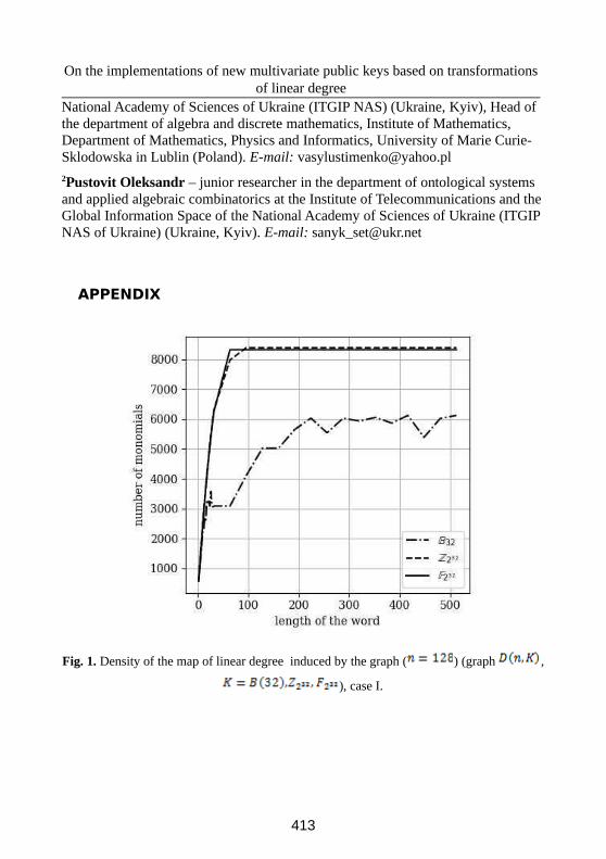
On the implementations of new multivariate public keys based on transformations
of linear degree
National Academy of Sciences of Ukraine (ITGIP NAS) (Ukraine, Kyiv), Head of
the department of algebra and discrete mathematics, Institute of Mathematics,
Department of Mathematics, Physics and Informatics, University of Marie Curie-
Sklodowska in Lublin (Poland). E-mail: [email protected]
2Pustovit Оleksandr – junior researcher in the department of ontological systems
and applied algebraic combinatorics at the Institute of Telecommunications and the
Global Information Space of the National Academy of Sciences of Ukraine (ITGIP
NAS of Ukraine) (Ukraine, Kyiv). E-mail: [email protected]
APPENDIX
Fig. 1. Density of the map of linear degree induced by the graph ( ) (graph ,
), case I.
413
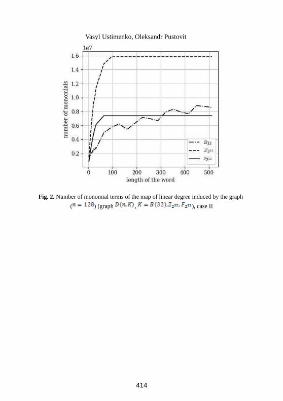
Vasyl Ustimenko, Oleksandr Pustovit
Fig. 2. Number of monomial terms of the map of linear degree induced by the graph
( ) (graph , ), case II
414
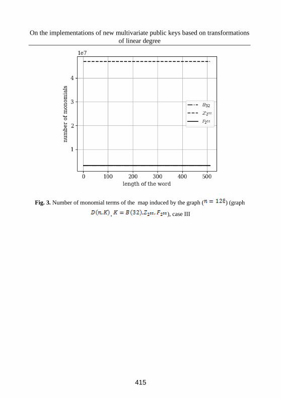
On the implementations of new multivariate public keys based on transformations
of linear degree
Fig. 3. Number of monomial terms of the map induced by the graph ( ) (graph
, ), case III
415
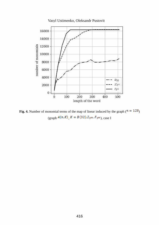
Vasyl Ustimenko, Oleksandr Pustovit
Fig. 4. Number of monomial terms of the map of linear induced by the graph ( )
(graph , ), case I
416
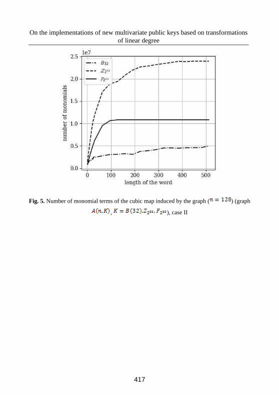
On the implementations of new multivariate public keys based on transformations
of linear degree
Fig. 5. Number of monomial terms of the cubic map induced by the graph ( ) (graph
, ), case II
417
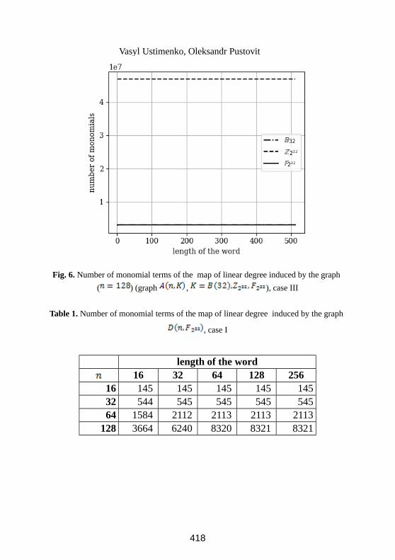
Vasyl Ustimenko, Oleksandr Pustovit
Fig. 6. Number of monomial terms of the map of linear degree induced by the graph
( ) (graph , ), case III
Table 1. Number of monomial terms of the map of linear degree induced by the graph
, case I
length of the word
16 32 64 128 256
16 145 145 145 145 145
32 544 545 545 545 545
64 1584 2112 2113 2113 2113
128 3664 6240 8320 8321 8321
418
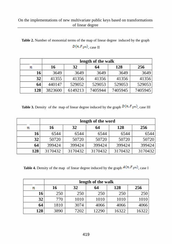
On the implementations of new multivariate public keys based on transformations
of linear degree
Table 2. Number of monomial terms of the map of linear degree induced by the graph
, case II
length of the walk
16 32 64 128 256
16 3649 3649 3649 3649 3649
32 41355 41356 41356 41356 41356
64 440147 529052 529053 529053 529053
128 3823600 6149213 7405944 7405945 7405945
Table 3. Density of the map of linear degree induced by the graph , case III
length of the word
16 32 64 128 256
16 6544 6544 6544 6544 6544
32 50720 50720 50720 50720 50720
64 399424 399424 399424 399424 399424
128 3170432 3170432 3170432 3170432 3170432
Table 4. Density of the map of linear degree induced by the graph , case I
length of the walk
16 32 64 128 256
16 250 250 250 250 250
32 770 1010 1010 1010 1010
64 1810 3074 4066 4066 4066
128 3890 7202 12290 16322 16322
419
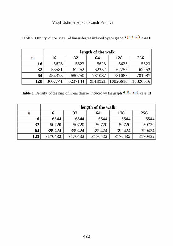
Vasyl Ustimenko, Oleksandr Pustovit
Table 5. Density of the map of linear degree induced by the graph , case II
length of the walk
16 32 64 128 256
16 5623 5623 5623 5623 5623
32 53581 62252 62252 62252 62252
64 454375 680750 781087 781087 781087
128 3607741 6237144 9519921 10826616 10826616
Table 6. Density of the map of linear degree induced by the graph , case III
length of the walk
16 32 64 128 256
16 6544 6544 6544 6544 6544
32 50720 50720 50720 50720 50720
64 399424 399424 399424 399424 399424
128 3170432 3170432 3170432 3170432 3170432
420
Proceedings of the Conference on Mathematical Foundations of Informatics
MFOI’2020, January 12-16, 2020, Kyiv, Ukraine
© 2021 by Cristian Vararu, Adrian Iftene
Methods of Recognizing the
Hand and Gestures
Cristian Vararu, Adrian Iftene
Abstract
Even though these days more and more devices can be
controlled remotely by remote controls or in some cases by voice
commands, there are times when we do not have the remote control
at hand or we cannot make noise. In these situations it would be
useful to be able to control these devices through other procedures
such as human gestures. In this paper will be presented three methods
of hand processing and a method by which starting from the
processed images we can recognize a static or dynamic gesture. A
study was also conducted to determine the accuracy of the methods
explained in this paper.
Keywords: hand recognition, gesture recognition, Haar
characteristics, Bayes Naive.
1 Introduction
With each passing day, we become more and more surrounded by devices.
In addition to a laptop, a TV, a mobile phone, many people have more and
more devices in the house such as a coffee maker, a music player, a home
cinema, electric windows or even smart light bulbs. Many of these devices
are controlled by a remote control, but these small devices can be lost,
damaged or run out of battery. Also, each device that is controlled by a
remote control requires exactly its own remote control, thus gathering more
and more small devices that take up unnecessary space.
Nowadays there are several solutions for replacing the remote controls.
More and more devices can be controlled by voice using google assistance,
Amazon Alexa, Apple Siri, etc. Although this technology solves most of
the problems created by remote controls, it adds new ones such as the
knowledge of one of the supported languages, with all voice assistants
421
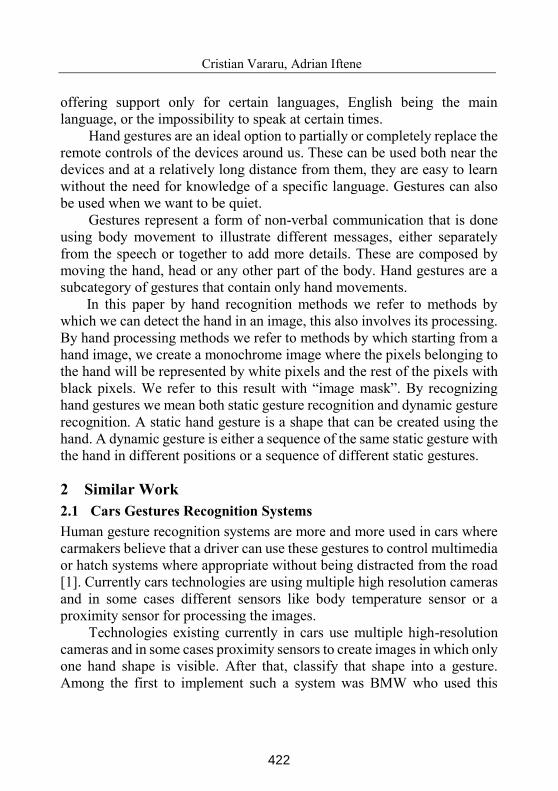
Cristian Vararu, Adrian Iftene
offering support only for certain languages, English being the main
language, or the impossibility to speak at certain times.
Hand gestures are an ideal option to partially or completely replace the
remote controls of the devices around us. These can be used both near the
devices and at a relatively long distance from them, they are easy to learn
without the need for knowledge of a specific language. Gestures can also
be used when we want to be quiet.
Gestures represent a form of non-verbal communication that is done
using body movement to illustrate different messages, either separately
from the speech or together to add more details. These are composed by
moving the hand, head or any other part of the body. Hand gestures are a
subcategory of gestures that contain only hand movements.
In this paper by hand recognition methods we refer to methods by
which we can detect the hand in an image, this also involves its processing.
By hand processing methods we refer to methods by which starting from a
hand image, we create a monochrome image where the pixels belonging to
the hand will be represented by white pixels and the rest of the pixels with
black pixels. We refer to this result with “image mask”. By recognizing hand gestures we mean both static gesture recognition and dynamic gesture
recognition. A static hand gesture is a shape that can be created using the
hand. A dynamic gesture is either a sequence of the same static gesture with
the hand in different positions or a sequence of different static gestures.
2 Similar Work
2.1 Cars Gestures Recognition Systems
Human gesture recognition systems are more and more used in cars where
carmakers believe that a driver can use these gestures to control multimedia
or hatch systems where appropriate without being distracted from the road
[1]. Currently cars technologies are using multiple high resolution cameras
and in some cases different sensors like body temperature sensor or a
proximity sensor for processing the images.
Technologies existing currently in cars use multiple high-resolution
cameras and in some cases proximity sensors to create images in which only
one hand shape is visible. After that, classify that shape into a gesture.
Among the first to implement such a system was BMW who used this
422
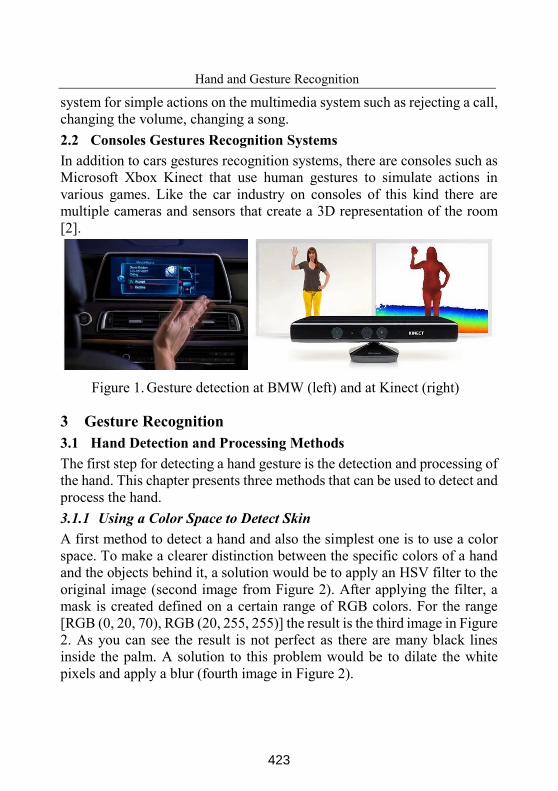
Hand and Gesture Recognition
system for simple actions on the multimedia system such as rejecting a call,
changing the volume, changing a song.
2.2 Consoles Gestures Recognition Systems
In addition to cars gestures recognition systems, there are consoles such as
Microsoft Xbox Kinect that use human gestures to simulate actions in
various games. Like the car industry on consoles of this kind there are
multiple cameras and sensors that create a 3D representation of the room
[2].
Figure 1. Gesture detection at BMW (left) and at Kinect (right)
3 Gesture Recognition
3.1 Hand Detection and Processing Methods
The first step for detecting a hand gesture is the detection and processing of
the hand. This chapter presents three methods that can be used to detect and
process the hand.
3.1.1 Using a Color Space to Detect Skin
A first method to detect a hand and also the simplest one is to use a color
space. To make a clearer distinction between the specific colors of a hand
and the objects behind it, a solution would be to apply an HSV filter to the
original image (second image from Figure 2). After applying the filter, a
mask is created defined on a certain range of RGB colors. For the range
[RGB (0, 20, 70), RGB (20, 255, 255)] the result is the third image in Figure
2. As you can see the result is not perfect as there are many black lines
inside the palm. A solution to this problem would be to dilate the white
pixels and apply a blur (fourth image in Figure 2).
423
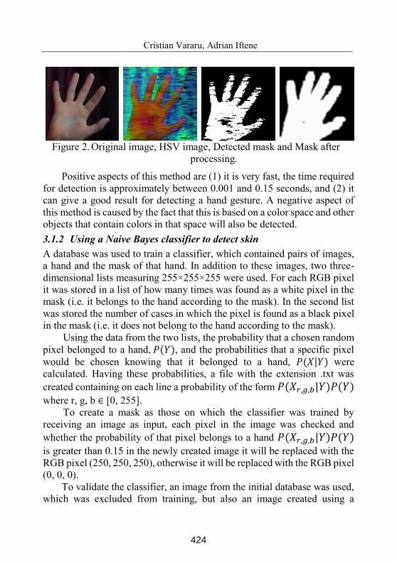
Cristian Vararu, Adrian Iftene
Figure 2. Original image, HSV image, Detected mask and Mask after
processing.
Positive aspects of this method are (1) it is very fast, the time required
for detection is approximately between 0.001 and 0.15 seconds, and (2) it
can give a good result for detecting a hand gesture. A negative aspect of
this method is caused by the fact that this is based on a color space and other
objects that contain colors in that space will also be detected.
3.1.2 Using a Naive Bayes classifier to detect skin
A database was used to train a classifier, which contained pairs of images,
a hand and the mask of that hand. In addition to these images, two three-
dimensional lists measuring 255×255×255 were used. For each RGB pixel
it was stored in a list of how many times was found as a white pixel in the
mask (i.e. it belongs to the hand according to the mask). In the second list
was stored the number of cases in which the pixel is found as a black pixel
in the mask (i.e. it does not belong to the hand according to the mask).
Using the data from the two lists, the probability that a chosen random
pixel belonged to a hand, , and the probabilities that a specific pixel
would be chosen knowing that it belonged to a hand, | were
calculated. Having these probabilities, a file with the extension .txt was
created containing on each line a probability of the form ,,|
where r, g, b ∈ [0, 255].
To create a mask as those on which the classifier was trained by
receiving an image as input, each pixel in the image was checked and
whether the probability of that pixel belongs to a hand ,,|
is greater than 0.15 in the newly created image it will be replaced with the
RGB pixel (250, 250, 250), otherwise it will be replaced with the RGB pixel
(0, 0, 0).
To validate the classifier, an image from the initial database was used,
which was excluded from training, but also an image created using a
424
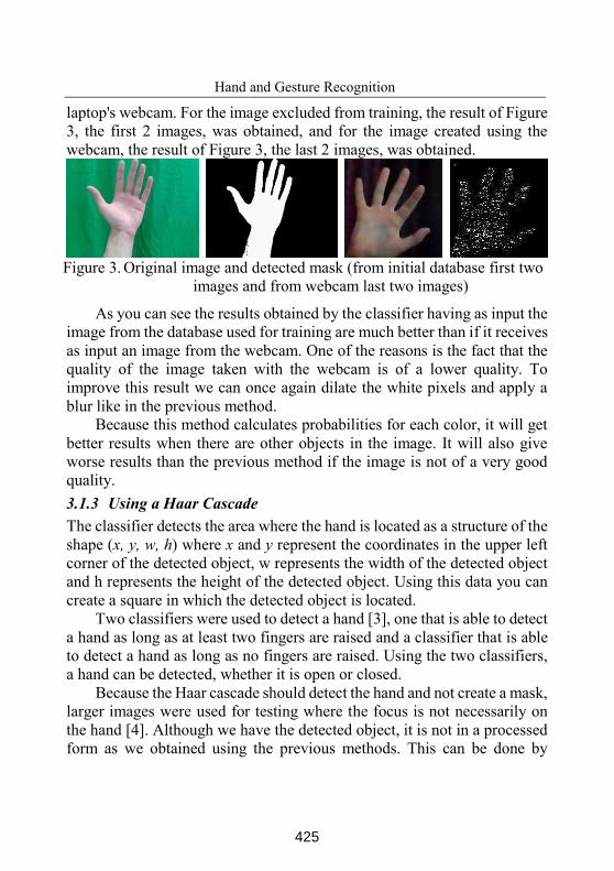
Hand and Gesture Recognition
laptop's webcam. For the image excluded from training, the result of Figure
3, the first 2 images, was obtained, and for the image created using the
webcam, the result of Figure 3, the last 2 images, was obtained.
Figure 3. Original image and detected mask (from initial database first two
images and from webcam last two images)
As you can see the results obtained by the classifier having as input the
image from the database used for training are much better than if it receives
as input an image from the webcam. One of the reasons is the fact that the
quality of the image taken with the webcam is of a lower quality. To
improve this result we can once again dilate the white pixels and apply a
blur like in the previous method.
Because this method calculates probabilities for each color, it will get
better results when there are other objects in the image. It will also give
worse results than the previous method if the image is not of a very good
quality.
3.1.3 Using a Haar Cascade
The classifier detects the area where the hand is located as a structure of the
shape (x, y, w, h) where x and y represent the coordinates in the upper left
corner of the detected object, w represents the width of the detected object
and h represents the height of the detected object. Using this data you can
create a square in which the detected object is located.
Two classifiers were used to detect a hand [3], one that is able to detect
a hand as long as at least two fingers are raised and a classifier that is able
to detect a hand as long as no fingers are raised. Using the two classifiers,
a hand can be detected, whether it is open or closed.
Because the Haar cascade should detect the hand and not create a mask,
larger images were used for testing where the focus is not necessarily on
the hand [4]. Although we have the detected object, it is not in a processed
form as we obtained using the previous methods. This can be done by
425
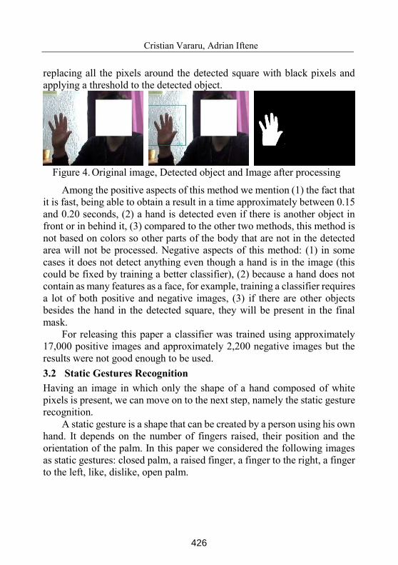
Cristian Vararu, Adrian Iftene
replacing all the pixels around the detected square with black pixels and
applying a threshold to the detected object.
Figure 4. Original image, Detected object and Image after processing
Among the positive aspects of this method we mention (1) the fact that
it is fast, being able to obtain a result in a time approximately between 0.15
and 0.20 seconds, (2) a hand is detected even if there is another object in
front or in behind it, (3) compared to the other two methods, this method is
not based on colors so other parts of the body that are not in the detected
area will not be processed. Negative aspects of this method: (1) in some
cases it does not detect anything even though a hand is in the image (this
could be fixed by training a better classifier), (2) because a hand does not
contain as many features as a face, for example, training a classifier requires
a lot of both positive and negative images, (3) if there are other objects
besides the hand in the detected square, they will be present in the final
mask.
For releasing this paper a classifier was trained using approximately
17,000 positive images and approximately 2,200 negative images but the
results were not good enough to be used.
3.2 Static Gestures Recognition
Having an image in which only the shape of a hand composed of white
pixels is present, we can move on to the next step, namely the static gesture
recognition.
A static gesture is a shape that can be created by a person using his own
hand. It depends on the number of fingers raised, their position and the
orientation of the palm. In this paper we considered the following images
as static gestures: closed palm, a raised finger, a finger to the right, a finger
to the left, like, dislike, open palm.
426
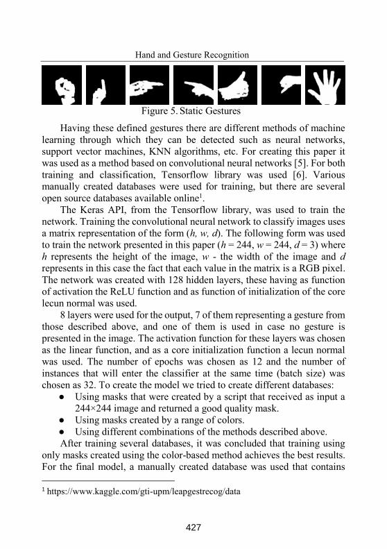
Hand and Gesture Recognition
Figure 5. Static Gestures
Having these defined gestures there are different methods of machine
learning through which they can be detected such as neural networks,
support vector machines, KNN algorithms, etc. For creating this paper it
was used as a method based on convolutional neural networks [5]. For both
training and classification, Tensorflow library was used [6]. Various
manually created databases were used for training, but there are several
open source databases available online1.
The Keras API, from the Tensorflow library, was used to train the
network. Training the convolutional neural network to classify images uses
a matrix representation of the form (h, w, d). The following form was used
to train the network presented in this paper (h = 244, w = 244, d = 3) where
h represents the height of the image, w - the width of the image and d
represents in this case the fact that each value in the matrix is a RGB pixel.
The network was created with 128 hidden layers, these having as function
of activation the ReLU function and as function of initialization of the core
lecun normal was used.
8 layers were used for the output, 7 of them representing a gesture from
those described above, and one of them is used in case no gesture is
presented in the image. The activation function for these layers was chosen
as the linear function, and as a core initialization function a lecun normal
was used. The number of epochs was chosen as 12 and the number of
instances that will enter the classifier at the same time (batch size) was
chosen as 32. To create the model we tried to create different databases:
Using masks that were created by a script that received as input a
244×244 image and returned a good quality mask.
Using masks created by a range of colors.
Using different combinations of the methods described above.
After training several databases, it was concluded that training using
only masks created using the color-based method achieves the best results.
For the final model, a manually created database was used that contains
1 https://www.kaggle.com/gti-upm/leapgestrecog/data
427
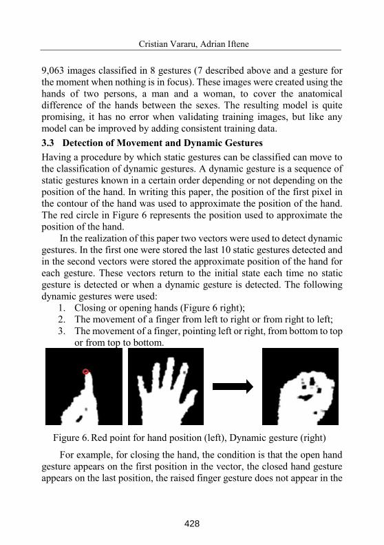
Cristian Vararu, Adrian Iftene
9,063 images classified in 8 gestures (7 described above and a gesture for
the moment when nothing is in focus). These images were created using the
hands of two persons, a man and a woman, to cover the anatomical
difference of the hands between the sexes. The resulting model is quite
promising, it has no error when validating training images, but like any
model can be improved by adding consistent training data.
3.3 Detection of Movement and Dynamic Gestures
Having a procedure by which static gestures can be classified can move to
the classification of dynamic gestures. A dynamic gesture is a sequence of
static gestures known in a certain order depending or not depending on the
position of the hand. In writing this paper, the position of the first pixel in
the contour of the hand was used to approximate the position of the hand.
The red circle in Figure 6 represents the position used to approximate the
position of the hand.
In the realization of this paper two vectors were used to detect dynamic
gestures. In the first one were stored the last 10 static gestures detected and
in the second vectors were stored the approximate position of the hand for
each gesture. These vectors return to the initial state each time no static
gesture is detected or when a dynamic gesture is detected. The following
dynamic gestures were used:
1. Closing or opening hands (Figure 6 right);
2. The movement of a finger from left to right or from right to left;
3. The movement of a finger, pointing left or right, from bottom to top
or from top to bottom.
Figure 6. Red point for hand position (left), Dynamic gesture (right)
For example, for closing the hand, the condition is that the open hand
gesture appears on the first position in the vector, the closed hand gesture
appears on the last position, the raised finger gesture does not appear in the
428
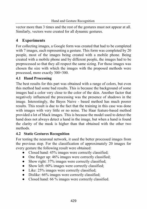
Hand and Gesture Recognition
vector more than 3 times and the rest of the gestures must not appear at all.
Similarly, vectors were created for all dynamic gestures.
4 Experiments
For collecting images, a Google form was created that had to be completed
with 7 images, each representing a gesture. This form was completed by 20
people, most of the images being created with a mobile phone. Being
created with a mobile phone and by different people, the images had to be
preprocessed so that they all respect the same sizing. For those images was
chosen the size with which the images with the proposed methods were
processed, more exactly 300×300. 4.1 Hand Processing
The best results for this part was obtained with a range of colors, but even
this method had some bad results. This is because the background of some
images had a color very close to the color of the skin. Another factor that
negatively influenced the processing was the presence of shadows in the
image. Interestingly, the Bayes Naive - based method has much poorer
results. This result is due to the fact that the training in this case was done
with images with very little or no noise. The Haar feature-based method
provided a lot of black images. This is because the model used to detect the
hand does not always detect a hand in the image, but when a hand is found
the clarity of the mask is higher than that obtained with the other two
methods.
4.2 Static Gestures Recognition
For testing the neuronal network, it used the better processed images from
the previous step. For the classification of approximately 20 images for
every gesture the following result were obtained:
Closed hand: 45% images were correctly classified;
One finger up: 46% images were correctly classified;
Show right: 37% images were correctly classified;
Show left: 60% images were correctly classified;
Like: 25% images were correctly classified;
Dislike: 66% images were correctly classified;
Closed hand: 66 % images were correctly classified.
429
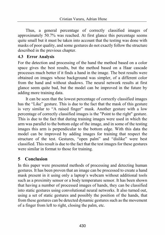
Cristian Vararu, Adrian Iftene
Thus, a general percentage of correctly classified images of
approximately 50.7% was reached. At first glance this percentage seems
quite small but it must be taken into account that the testing was done with
masks of poor quality, and some gestures do not exactly follow the structure
described in the previous chapter.
4.3 Error Analysis
For the detection and processing of the hand the method based on a color
space gives the best results, but the method based on a Haar cascade
processes much better if it finds a hand in the image. The best results were
obtained on images whose background was simpler, of a different color
from the hand and without shadows. The neural network results at first
glance seem quite bad, but the model can be improved in the future by
adding more training data.
It can be seen that the lowest percentage of correctly classified images
has the “Like” gesture. This is due to the fact that the mask of this gesture
is very similar to “A raised finger” mask. Another gesture with a low
percentage of correctly classified images is the "Point to the right" gesture.
This is due to the fact that during training images were used in which the
arm was parallel to the bottom edge of the image, and in some of the testing
images this arm is perpendicular to the bottom edge. With this data the
model can be improved by adding images for training that respect the
structure of the test. Gestures, “open palm” and “dislike” were best classified. This result is due to the fact that the test images for these gestures
were similar in format to those for training.
5 Conclusion
In this paper were presented methods of processing and detecting human
gestures. It has been proven that an image can be processed to create a hand
mask present in it using only a laptop’s webcam without additional tools such as a proximity sensor or a body temperature sensor. It has been shown
that having a number of processed images of hands, they can be classified
into static gestures using convolutional neural networks. It also turned out,
using a set of static gestures and possibly the position of the hands, that
from these gestures can be detected dynamic gestures such as the movement
of a finger from left to right, closing the palm, etc.
430
Hand and Gesture Recognition
For processing images, 3 methods were used based on: a color space,
a Bayes Naive classifier, or a Haar classifier. Thus it was proved that
although the method based on a color space seems the simplest, in this
paper, it gave the best results, the other methods needing some
improvements. However, it can be seen that the Haar cascade classifier
would have a good chance of being improved, as it needs a larger and more
carefully chosen dataset of images.
A convolutional neural network was used to detect static gestures,
which proved to be a fairly efficient and accurate method to detect such
gestures. However, this network could also be improved by using a larger
training database. More than two people would be needed to create this
database, thus covering more types of hands. For the detection of dynamic
gestures, models of 10 static gestures and the positions of the hands present
in these gestures were created. The central pixel of the hand was not used
for the position, as it was difficult to find and possibly inefficient. Instead
of the central pixel of the hand, the first white pixel present in the mask was
used. To detect motion on both the X and Y axes, it was checked whether
the position of this pixel increased in relation to X or Y.
As a first possible improvement in the future would be to create a fairly
well-balanced database so as to increase the percentage for which the Haar
classifier finds a hand in the image. This would allow us to get better
processed images. Another improvement that we will consider in the future
would be the addition of hardware that could facilitate image processing.
For example, a proximity sensor could be used to detect the nearest object.
Acknowledgments. This work was supported by project REVERT
(taRgeted thErapy for adVanced colorEctal canceR paTients), Grant
Agreement number: 848098, H2020-SC1-BHC-2018-2020/H2020-SC1-
2019-Two-Stage-RTD.
References
[1] F. Parada-Loira, E., González-Agulla, J. L. Alba-Castro. Hand Gestures to
Control Infotainment Equipment in Cars. In IEEE Intelligent Vehicles
Symposium Proceedings (2014), pp. 1-6.
431
Cristian Vararu, Adrian Iftene
[2] X. Ma, J. Peng. Kinect Sensor-Based Long-Distance Hand Gesture
Recognition and Fingertip Detection with Depth Information. In Journal of
Sensors (2018) https://www.hindawi.com/journals/js/2018/5809769/
[3] W. Berger. Deep Learning Haar Cascade Explained.
http://www.willberger.org/cascade-haar-explained/. Accessed 11 Nov 2020
[4] P. Viola, M. Jones. Rapid Object Detection using a Boosted Cascade of
Simple Features. In Proceedings of the 2001 IEEE Computer Society
Conference on Computer Vision and Pattern Recognition. CVPR (2001)
https://ieeexplore.ieee.org/document/990517
[5] S. Indolia, A. Kumar Goswami, S. P. Mishra, P. Asopa. Conceptual
Understanding of Convolutional Neural Network - A Deep Learning
Approach. In Procedia Computer Science vol 132, (2018), pp. 679-688.
[6] A. Géron. Machine Learning with Scikit-Learn & TensorFlow. In O'Reilly
Media, Inc. (2019)
Cristian Vararu, Adrian Iftene
“Alexandru Ioan Cuza” University of Iasi, Faculty of Computer Science
E-mail: [email protected], [email protected]
432
Proceedings of the Conference on Mathematical Foundations of Informatics
MFOI2020, January 12-16, 2021, Kyiv, Ukraine
Discrete System Modelling: Dialgebraic
Approach
Grygoriy Zholtkevych, Maksym Labzhaniia
Abstract
The article is devoted to the problem of constructing a math-ematical formalism that allows one to specify both the structureand behaviour of an abstract discrete system using a commonframework. The importance of abstract discrete systems is as-sociated with the fact that they are adequate models of cyber-physical systems, which leads to the need to develop formal mod-els and rigorous methods for their analysis. There are currentlytwo approaches to solving the problem. These approaches focusedon various aspects of systems, namely structural and behaviouralone, which are provided by two formalisms of universal algebrasand universal coalgebras, respectively. The combination of thesetwo views leads to the concept of dialgebras. The article presentsand proved some facts about dialgebras. Also in the paper, theinformal interpretation of the presented facts.
Keywords: discrete system, system structure, system be-haviour, initial semantics, final semantics.
1 Motivation
At present, it is generally accepted that abstract discrete systems ofvarious types give adequate mathematical tools for studying big com-plexes that combine physical and digital components. Taking into ac-count that such complexes (often called cyber-physical systems) deter-mine one of main directions of developing technology, it can be agreedthat researching methods for the specification and analysis of discrete
c©2020 by Grygoriy Zholtkevych, Maksym Labzhaniia
433
Grygoriy Zholtkevych, et al.
systems is a highly topical issue for modern system and software engi-neering. It should be noted that a desirable property of the theory ofabstract discrete systems is a generality, which would provide a unifiedapproach to the analysis of systems of a quite different nature, based ondifferent types of logic systems. The need for the property of generalityis explained by the fact that, for example, the physical components of acyber-physical system operate in accordance with models based on theclassical logic, and cyber-components operate in accordance with mod-els based on the constructive logic. The almost evident approach forensuring the generality property is to replace the set-theoretic frame-work of the theory being created with the category-theoretic one. Thisapproach was introduced in the works of M.A. Arbib and E.G. Manes(the brief survey can be found in [1]). The particularity of the Arbib–Manes’s approach is that authors consider the concept of a universalalgebra in a category as the principal tool for studying discrete a sys-tem. In other words, this approach is structurally (or syntactically)oriented.
In contrast, in works of J. Rutten, J. Adamek , and B. Jacobs [2, 3,4, 5] the dual approach based on the concept of a universal coalgebrain a category is proposed and studied. This approach is focused onstudying the behaviour of discrete systems rather than their structure.
But to study a real technical complex, we need both structural andbehavioural approaches to its modelling. The corresponding concept isthe concept of a universal dialgebra, which combine as structural andbehavioural approaches. There are works (for example, see [6, 7, 8]),which study semantic properties of software systems in the terms ofdialgebras.
2 Preliminaries and Notation
In the paper, we use widely category theory and the correspondingconcepts, definitions, and statements, which can be found in [9, 10, 11].They are also presented at nLab site [12].
Let C be a category then for referring to the next facts, we use the
434
Dialgebraic Discrete System Modelling
notation
Cop means the opposite category for C;
X : C means X is an object of C;f : X → Y means f is a morphism in C from X into Y .
An important notion for our consideration is bifunctor
HomC : Cop × C → Set
defined for a locally small category C [12, see here1] as follows
HomC〈X,Y 〉 = Hom(X, Y ) where X,Y : C
HomC〈fop, g〉 = λh : X ′ → Y ′ . ghf where fop : X ′ → X ′′ and
g : Y ′ → Y ′′.
The next principal concept is the concept of adjoint functors [12,see here2]. Taking into account the importance of the concept for ourstudy, we will give one of a series of equivalent definitions.Let B and C be locally small categories and S : B C : B befunctors then S is the left adjoint functor of B (or, equivalently, Bis the right adjoint functor of S) if there exists a natural isomor-phism Ψ : HomC(S × IC) ∼= HomB(IB × B) or, in other words, forany f : X ′′ → X ′, g : Y ′ → Y ′′, and h : SX ′ → Y ′, the equation
ΨX′′,Y ′′(gh(Sf)) = (Bg)(ΨX′,Y ′h)f (1)
holds where
Ψ = 〈ΨX,Y : HomC(SX, Y ) ∼= HomB(X, BY ) | X : B, Y : C〉.
Taking h′ : X ′ → BY ′, h = Ψ−1X′,Y ′h
′ : SX ′ → Y ′ and replacing h in(1), one can obtain
g(Ψ−1X′,Y ′h
′)(Sf) = Ψ−1X′′,Y ′′((Bg)h
′f). (2)
1https://ncatlab.org/nlab/show/locally+small+category2https://ncatlab.org/nlab/show/adjoint+functor
435
Grygoriy Zholtkevych, et al.
Thus, it is evident that (2) and (1) are equivalent equations.A detailed discussing other definitions of the concept can be found
in [9, Ch. IV] or [11, Ch. 9].
Note 1 (about notation). The denotation S ⊣ B is used for referring tofact that S is a left adjoint functor of B or, equivalently, B is a rightadjoint functor of S.
3 Dialgebra and Related Concepts
In the section, we assume that some locally small category C and someendofunctors S and B of C are given.
Definition 1. A pair a = (X, op) is called a dialgebra if X is anobject of C, and op : SX → BX is a morphism.The pair (S,B) is called the type of a.The object X is called the carrier of a and the morphism op is calledthe operation of a.
Note 2. Everywhere below we denote the carrier of dialgebra a by a,and its operation by opa.
Here, we need to stress that in the definition of a dialgebra endo-functor S ensures the structural specification of the system being mod-elled, and endofunctor B ensures its behavioural specification.
Definition 2. A dialgebraic morphism from dialgebra a into di-algebra b is a morphism f : a → b ensuring commutativity of thediagram
SaSf
−−−−→ Sb
opa
y
y
opb
BaBf
−−−−→ Bb
(3a)
i.e. holding the equation
(Bf) opa = opb(Sf) . (3b)
436
Dialgebraic Discrete System Modelling
The next statement is evident.
Proposition 1. The class of dialgebras equipped with dialgebraic mor-phisms is a category.
This category is denoted by DialgSB (or DialgS
B(C) if it needs re-ferring explicitly to category C) and called the category of dialgebrasof type (S,B) over category C.
Note 3. CategoryDialgSIC
has an own name and denotation. It is called
the category of S-algebras and denoted by AlgS .Similarly, category Dialg
ICS
is called the category of S-coalgebras anddenoted by CoalgS .
In this sense, the theory of dialgebras is a generalization of both thetheory of algebras and the theory of coalgebras. In some cases, one canreduce studying a dialgebra for studying either algebra or coalgebra.The following Theorems 1 and 2 describe some classes of the cases.
Theorem 1. If B# ⊣ B then category DialgSB is isomorphic to category
AlgB#S .
Proof. Let Ψ refers to the natural isomorphism defined by the conditionB# ⊣ B.Using Ψ, one can define a functor Alg : DialgS
B → AlgB#S as follows
for any (S,B)-dialgebra a,
Alg a = a and
opAlga = Ψ−1Sa,a opa;
for any dialgebraic morphism f : a → b,
Alg f = f.
By construction, Alg sends an (S,B)-dialgebra to a B#S-algebra.Now we need to make sure that Alg sends a dialgebraic morphism
437
Grygoriy Zholtkevych, et al.
to algebraic morphism. In other words, we need to check that anydialgebraic morphism is algebraic too.If f : a → b is a dialgebraic morphism then
opb(Sf) = (Bf) opa .
We need to prove that
opAlgb((B#S)f) = f(Alg opa)
or, equivalently,
(Ψ−1Sb,b opb)(B
#(Sf)) = f(Ψ−1Sa,a opa).
Indeed,
(Ψ−1Sb,b opb)(B
#(Sf)) = Ψ−1Sa,b(opb(Sf)) due to (2)
= Ψ−1Sa,b((Bf) opa) as dialgebraic morphism
= f(Ψ−1Sa,a opa) due to (2).
Thus, Alg is really a functor.Now let us define a functor DiAlg : AlgB#S → DialgS
B as follows
for any B#S-algebra a,
DiAlg a = a and
opDiAlga = ΨSa,a opa;
for any dialgebraic morphism f : a → b,
DiAlg f = f.
The reasoning for proving DiAlg is indeed a functor is quite similar tothe argument that Alg is a functor so omitting it is sound.It is evident by construction that functors Alg and DiAlg are mutuallyinverse. Thus, categories DialgS
B and AlgB#S are isomorphic.
438
Dialgebraic Discrete System Modelling
The next theorem is a dual statement to Theorem 1.
Theorem 2. If S ⊣ S# then category DialgSB is isomorphic to category
CoalgS#B.
Theorems 1 and 2 can be interpreted as follows: there are condi-tions under which the behaviour of a discrete system is determinedby its structure, or, conversely, its structure is determined by its be-haviour. It is beyond any doubt these theorems state very importantfacts. Therefore, we need more clear criteria for checking hypothesesof these theorems i.e. we need in answers to the next problem.
Problem 1. Are inverse statements to Theorems 1 and 2 true? Es-tablish additional conditions on functors S and B when such inversionsare true?
4 Forgetful Functor
As you know, the initial algebra and catamorphisms, as well as the finalcoalgebra and anamorphisms, are principle tools for studying proper-ties of the corresponding categories. Unfortunately, when we studydialgebras, it is not clear whether such constructions exist and how toconstruct them, if they exist. In this section, we propose some con-structs that can help bridge this gap.
In the section, we assume that some locally small category C andsome endofunctors S and B of C are given.
Let us consider the following functor U : DialgSB(C) → C
Ua = a for any dialgebra a ; (4a)
Uf = f for any dialgebraic morphism f . (4b)
Checking that U is really a functor is trivial.The following proposition is simple but important.
Proposition 2. If there exists the left adjoint functor U# of forgetfulfunctor U then existence of an initial object 0 in C ensures that there
439
Grygoriy Zholtkevych, et al.
exists an initial (S,B)-dialgebra namely this dialgebra is U# 0 and thecatamorphism family is U# !a | a : DialgS
B(C) where !X : 0 → X is aunique morphism from the definition of an initial object.Similarly, if there exists the right adjoint functor U# of forgetful functorU then existence of a final object 1 in C ensures that there exists a final(S,B)-dialgebra namely this dialgebra is U# 1 and the anamorphismfamily is U# !a | a : DialgS
B(C) where !X : X → 1 is a uniquemorphism from the definition of a final object.
Proof. Taking into account that
Ψ0,a : HomSet(0, Ua) ∼= HomDialgS
B
(U# 0, a)
is a bijection, one can conclude that for any a : DialgSB , HomSet(0, Ua)
is a singleton and, therefore, HomDialgS
B
(U# 0, a) is a singleton. It
means that U# 0 is an initial dialgebra and U# !a is a catamorphismcorresponding to a. The argumentation for proving the second part ofthe proposition is quite similar to the previous reasoning.
In fact, the existence of left (right) adjoint to U gives more than justthe existence of an initial (final) dialgebra. It gives the constructionof a universal (co-universal) wrap-around of an object of the originalcategory to lift one up to a dialgebra. So, we are interested in an answerto the next problem.
Problem 2. What properties of dialgebras related to the existence ofthe left or right adjoint of the forgetful functor?
In the situation whenever the forgetful functor has both the left andright adjoint functors then in the corresponding category of dialgebrasthere exist both initial and final dialgebras. In the situation, the initialand final dialgebra connected by the unique morphism. This fact canbe interpreted as the fact that the initial semantic model does notcontradict to the final semantic model. Thus, the existence of adjointfunctors of the forgetful functor is a very important property. Thus,we come to the next problem.
440
Dialgebraic Discrete System Modelling
Problem 3. Can the existence of conjugate functors of the forgetfulfunctor be expressed in terms of structural and behavioural endofunc-tors?
5 Conclusion
Summing up, we can express confidence that dialgebras are a promis-ing tool for the formal specification of discrete systems and rigorousmethods for their analysis. Answers to the Problems 1-3 posed in thepaper will justify or will invalidate this promising.
References
[1] M.A. Arbib, E.G. Manes. Machines in a Category. Journal of Pureand Applied Algebra, vol. 19 (1980), pp. 9–20.
[2] J.J.M.M. Rutten, Universal coalgebra: a theory of systems. Theo-retical Computer Science, vol. 249, no. 1 (2000), pp. 3–80.
[3] B. Jacobs and J.J.M.M. Rutten. An introduction to (co)algebrasand (co)induction. In: D. Sangiorgi, J. Rutten (eds). Advancedtopics in bisimulation and coinduction. Cambridge Tracts in The-oretical Computer Science, vol. 52 (2011), Cambridge UniversityPress, pp. 38–99.
[4] J. Adamek, V. Koubek. On the greatest fixed point of a functor.Theor. Comp. Science, vol. 150 (1995), pp. 57-75
[5] B. Jacobs. Introduction to Coalgebra: Towards Mathematics ofStates and Observation (Cambridge Tracts in Theoretical Com-puter Science) Cambridge University Press, 2016.
[6] T. Hagino. A typed lambda calculus with categorical type construc-tors. In: Pitt D.H., Poign A., Rydeheard D.E. (eds) CategoryTheory and Computer Science. LNCS, vol 283 (1987), pp. 140–157.
441
Grygoriy Zholtkevych, et al.
[7] T. Altenkirch T. et al. A Categorical Semantics for Inductive-Inductive Definitions. In: Corradini A., Klin B., Crstea C.(eds) Algebra and Coalgebra in Computer Science. CALCO 2011.LNCS, vol 6859 (2011), pp. 70–84.
[8] V. Ciancia. Interaction and Observation: Categorical Semanticsof Reactive Systems Trough Dialgebras. In: Heckel R., Milius S.(eds) Algebra and Coalgebra in Computer Science. CALCO 2013.LNCS, vol 8089 (2013), pp 110–125.
[9] S. Mac Lane. Categories for the Working Mathematician.Springer-Verlag New York, 1978.
[10] J. Adamek, H. Herrlich, G.E. Strecker. Abstract and Concrete Ca-tegories, John Wiley & Sons, 1990
[11] S. Awodey. Category Theory, 2nd edition, Oxford University Press,2010.
[12] nLab authors. Category Theory, 2020.http://ncatlab.org/nlab/show/category%20theory.
Grygoriy Zholtkevych1, Maksym Labzhaniia2
1V.N. Karazin Kharkiv National University, Kharkiv, UkraineEmail: [email protected]
2V.N. Karazin Kharkiv National University, Kharkiv, UkraineEmail: [email protected]
442
Proceedings of the Conference on Mathematical Foundations of Informatics
MFOI-2020, January 12-16, 2021, Kyiv, Ukraine
Table of Contents
Preface 3
Andrei Alexandru, Gabriel Ciobanu
Properties of Finitely Supported Binary Relations between Atomic Sets 5
Andrei Alexandru
Finitely Supported Mappings Defined on the Finite Powerset of Atoms in FSM 20
Andrei Arusoaie
Certification in Matching Logic 34
Tudor Bumbu, Iulian CerneiEnsuring Access to the Moldovan Legacy using Elements of
Artificial Intelligence 35
Olesea Caftanatov, Daniela Caganovschi, Lucia Erhan, Ecaterina Hilea
State of the Art: Augmented reality Business Cards 46
Irina Cercel, Adrian IftenePlanetarium - An Augmented Reality Application 62
Demetra-Bianca Chirica, Adrian Iftene
Enhancing the Visit of the Botanical Garden of Iasi with the Helpof Smart Devices and Augmented Reality 78
Matei-Alexandru Cioata, Adrian Iftene
Recognition of Guitar Chords using the Discrete Fourier Transform 88
Alexandru Colesnicov, Ludmila Malahov, Svetlana Cojocaru, Lyudmila Burtseva
Development of a platform for processing heterogeneousprinted documents 108
443
Proceedings of the Conference on Mathematical Foundations of Informatics
MFOI-2020, January 12-16, 2021, Kyiv, Ukraine
Ioachim Drugus
Towards a Non-associative Model of Language 123
Daniela GifuTracing Economic Crisis Prediction 135
Adrian Gotca, Adrian Iftene
ECG Biometrics: Experiments with SVM 145
Adrian IfteneUsing Artificial Intelligence in Medicine 161
Ievgen Ivanov
On Generalizations of Real Induction 162
Dmytro KrukovetsDynamic Time Warping for uncovering dissimilarity
of regional wages in Ukraine 168
Sergii KryvyiAlgebra, informatics, programming 186
Oleksandr Letychevskyi, Volodymyr Peschanenko,
Maksym Poltoratskyi, Serhii Horbatiuk, Viktor Horbatiuk, Yuliia Tarasich
One Approach to Formal Verification of Distributed Ledger Technologies on the Blockchain Technologies Example 227
Radu-Matei Lipan, Adrian Iftene
Iasi Botanic Garden App 243
Alexander LyaletskiEvidence Algorithm: 50 Years of Development 257
Gennadi Malaschonok, Andriy Ivashkevich
Quick Recursive QR Decomposition 268
444
Proceedings of the Conference on Mathematical Foundations of Informatics
MFOI-2020, January 12-16, 2021, Kyiv, Ukraine
Camelia-Maria Milut
Speech Recognition in the Medical Domain with Application in Patient Monitoring 276
Ioan-Alexandru Mititelu, Adrian Iftene
Thread Up - Application for Analysis of the Trending Phenomenon 285
Alexei MuravitskyRemarks On Nonmonotonic Consequence Relations 298
Mykola Nikitchenko
Towards Defining Program Logics via Three-level Scheme 324
Cristian Ninicu, Adrian IfteneDetection of Geographical Areas where there are
Discussions about Epidemics Based on Twitter 330
Victor Pulbere, Adrian IfteneUsing F.A.S.T. Test to Detect Stroke 346
Stefan Stratulat, Dumitru Prijilevschi, Gheorghe Morari, Tudor Bumbu
A Disambiguation Model for Natural Language Processing 361
Stefan-Claudiu SusanA practical implementation of Natural Deduction in
Propositional Logic 382
Vasyl Ustimenko, Oleksandr PustovitOn the implementations of new multivariate public keys
based on transformations of linear degree 397
Cristian Vararu, Adrian IfteneMethods of Recognizing the Hand and Gestures 421
Grygoriy Zholtkevych, Maksym Labzhaniia
Discrete System Modelling: Dialgebraic Approach 433
445

Наукове видання
Конференція з математичних основ інформатикиMFOI-2020: Праці; 12-16 січня 2021
(англійською мовою)
ФАКУЛЬТЕТ КОМП’ЮТЕРНИХ НАУК ТА КІБЕРНЕТИКИКИЇВСЬКОГО НАЦІОНАЛЬНОГО УНІВЕРСИТЕТУ
ІМЕНІ ТАРАСА ШЕВЧЕНКА,64/13, вул. Володимирська, 01601, Київ, Україна
ІНСТИТУТ МАТЕМАТИКИ ТА КОМП'ЮТЕРНОЇ НАУКИ ІМЕНІВОЛОДИМИРА АНДРУНАКІЄВИЧА
Вулиця Академічна, 5, Кишинів, Республіка Молдова, MD 2028
Редактори: проф. Микола Нікітченко, проф. Світлана Кожокару,проф. Адріан Іфтене, проф. Іоахім Другус
Автори несуть повну відповідальність за зміст своїх робіт.
Підписано до друку 15.02.2021 р.Формат 60х84/16. Друк офсетний
Гарнітура TimesNewRoman. Умов. друк. арк.: 25.9Наклад прим.: 300. Замовлення 2212/17
Видавець: ТОВ «НВП «Інтерсервіс»м. Київ, вул. Бориспільська, 9
Свідоцтво: серія ДК 3534 від 24.07.2009 р.
Виготовлювач: СПД Андрієвська Л. В.м. Київ, вул. Бориспільська, 9
Свідоцтво: серія В03 919546 від 19.09.2004 р.
Related Documents